to study or to work?

49

Eastern European Economics, vol. 50, no. 3, May–June 2012, pp. 49–78.© 2012 M.E. Sharpe, Inc. All rights reserved. Permissions: www.copyright.comISSN 0012-8775 (print) / ISSN 1557-9298 (online)DOI: 10.2753/EEE0012-8775500303

Francesco Pastore

To Study or to Work? Education and Labor-Market Participation of Young People in Poland

ABSTRACT: This paper proposes Heckman probit (Heckprobit) estimates of the determinants of success in finding a job in a sample of young (age 15–30) Poles, controlling for the possible selection bias caused by excluding those in school. There is evidence of sample selection bias in the case of young men, suggesting that they use economic factors to make their educational choices more than women do. Education is an important determinant of success in the labor market. The instrumental variables used in the selection equation—the local unemployment rate, expected lifetime earnings and the opportunity cost of education—have a statistically significant impact on the probability of pursuing an education. In contrast to several previous studies relative to mature market economies, ours found that in high unemployment areas, young people prefer to seek a job rather than study. This in fact contributes to the persistence of regional unemployment.

Francesco Pastore is an assistant professor of economics, Seconda Università di Napoli Palazzo Melzi, Santa Maria Capua Vetere (Caserta), Italy. This research was financed in part by a grant from the Center for Economic Research and Graduate Education-Economics Institute (CERGE-EI) under a program of the Global Development Network. Through the Wiener Institute für Internationale Wirtschaftsvergleiche (WIIW), Vienna, the Austrian government provided additional funds to grantees in the Balkan countries. All opinions expressed are those of the author and have not been endorsed by CERGE-EI, WIIW, or the Global Development Network. An earlier version of this paper was presented at a CERGE-EI Conference in Prague (2004) and at the IZA/World Bank Conference, Bonn (2007). A longer version of this paper has been circulated as IZA Discussion Paper no. 1793. The author thanks Ira Gang, Daniel Munich, Mietek Socha, and two anonymous referees for useful comments, and Alina Verashchagina for excellent research assistance. The usual disclaimer applies.

50 EasTErn EuroPEan EconomIcs

Youth unemployment is a dramatic outcome of economic transition, becoming increasingly problematic as time passes. Most of the new members of the European Union (EU) are experiencing a ratio of the youth to the adult unemployment rate higher than the EU average of 1.9. In posttransition Poland, it has always been above 2.5. With few exceptions, however (Beleva et al. 2001; Domadenik and Pastore 2006; Micklewright 1999; O’Higgins 2004; Pastore 2010), youth unemployment in transition countries remains a neglected issue.

This research aims to contribute to the debate on the design of better education and employment policies in transition countries. Since the transition began, the market for human capital has been subject to tremendous tension during the reform period. Several demand- and supply-side factors are at work. On the demand side, a rapid rate of technical change, sometimes adopted defensively to meet the competition from mature market economies, has dramatically increased the demand for skilled labor. On the supply side, two opposite phenomena have been at work. On the one hand, the relatively high human capital inherited from the previous regime has been partly displaced by market mechanisms (see, e.g., Boeri 2000; Ferragina and Pastore 2005, and the references therein), owing perhaps to the high number of workers holding a vocational diploma (Boeri et al. 1997). On the other hand, the investment in general secondary and tertiary education has also dramatically increased, as a consequence of the increased payoff for skills. According to anecdotal evidence, highly skilled young people are among the winners in this transformation.

The case of Poland is typical of these changes. The country has experienced the highest degree of structural change and the highest unemployment rate in the area. Over the years, the number of individuals who have achieved a high level of educa-tion has dramatically increased, whereas that of people with vocational secondary degrees has shrunk (Boeri 2000). Domadenik and Pastore (2006, tables 5 and A5) find that from 1997 to 2002, the percentage of teenagers (ages 15–19) in school increased from about 84 percent to 88 percent, whereas that of young adults (ages 20–24) increased from 20 percent to 31 percent. The corresponding figures for the early 1990s were 45 percent and 13 percent, respectively. In both cases, Poland is close to the targets set in the Lisbon strategy.

These figures raise two important issues, however. First is the contrast between increasing levels of education and the difficulty in bringing unemployment down. Will the already high number of young people with a high school diploma and/or a university degree increase further, or will it decrease? If the unemployment rate decreases, will the number of young people pursuing an education shrink? Is an increase in the average level of education sufficient per se to increase youth employment?

The second issue is the dramatic and persistent regional differences in unem-ployment rates, which according to some authors depend on, and are also fostered by, dramatic differences in the human capital endowment of voivodships (World Bank 2004, pp. 29–31).1 Moreover, complementarities between high-technology industries and human capital generate persistent unemployment differentials with

may–JunE 2012 51

respect to rural, depressed areas (Ferragina and Pastore 2008). Migration flows tend to reinforce this result (Fidrmuc 2004).

This is the first study attempting to explore these questions. It does so by focusing on the determinants of success in the labor market versus the pursuit of education by young Poles. Of course, increasing a young person’s chances of finding gainful employment is the final aim of accumulating human capital. Starting work early in life might be a poor choice, however, especially in a period of dramatic structural change.

To compare the individual determinants of the decision to continue education (or drop out), this study proposes a Heckman probit (Heckprobit) model. This is similar to the error correction procedure commonly used to control for sample selection bias in Mincerian-type earnings equations, which is known as Heckit (see Heck-man 1979). In the latter model, a selectivity term is used to correct the estimates of coefficients in the earnings equations relative to employed workers for the existence of jobless people—unemployed or inactive—with different characteristics. By tak-ing into account only jobless people, it is possible to assess the true impact of, say, education on earnings.

In the Heckprobit model, the dependent variable of the so-called main equation is a dummy variable, which in this study takes a value of one if the individual is employed and zero if he or she is jobless (either unemployed or inactive). To con-trol for the possible selectivity implied by excluding those in school, the estimates are corrected by a term simultaneously estimated by maximum likelihood using a selection equation. The dependent variable of the selection equation takes a value of one if the individual is participating in the labor market and zero if he or she is in school full time.

The study is based on the November 1997 Polish labor force survey (LFS). This was the year the Polish economy experienced one of the lowest unemployment rates in its recent history. The analysis considers a sample of individuals aged fifteen to thirty, comprising hence not only teenagers (ages 15–19) and young adults (ages 20–24), but also an older age group (25- to 30-year-olds), to take into account the high proportion of long-term unemployed. Only a few find employment shortly after obtaining their degree.

A special focus of the analysis is on ascertaining the role of expected lifetime earnings and local labor market conditions on the decision to invest in further educa-tion. Whereas the coefficient of the former is expected to be positive, the theory and evidence on the impact of the unemployment rate are mixed. Some authors (Giannelli and Monfardini 2000, 2003; Rice 1987, 1999) argue that high unemployment re-duces the opportunity cost of education and increases the probability of studying rather than searching for a job. Conversely, Micklewright (1990) finds no significant positive effect of unemployment on education, but rather the opposite.

This paper adds to the existing literature in at least two ways. First, this is the first study to analyze the determinants of the educational choices of young people in transition countries and assess the impact of local labor-market conditions and


expected lifetime earnings. Second, from a methodological point of view, the use of a Heckprobit model is a novelty compared with the existing literature on mature market economies, which generally adopts either multinomial logit (MNL; see, e.g., Domadenik and Pastore 2006; Rice 1999) or multinomial probit (MNP) (see, e.g., Giannelli and Monfardini 2003) models. The former, suffers from a serious shortcoming when analyzing the youth labor market: it assumes independence of irrelevant alternatives (IIA). This would imply that labor market choices are inde-pendent of education, which is hardly the case. The MNP model does not need the IIA assumption, but still does not allow one to control for the fact that the labor market outcome (employed versus unemployed/inactive) depends on decisions whether to study instead of seeking work.

The rest of this paper is structured as follows. The first section gives an overview of the main features of youth unemployment in transition countries and especially in Poland. The second describes the methodology and data. A short survey of the literature precedes discussion of the Heckprobit model and the a priori impact of independent variables. The third section presents the results and is followed by a conclusion.

Youth Unemployment During Transition

Economic transition is a system change involving dramatic shifts in labor demand across and within sectors. It requires an important effort from the labor supply, especially the youngest segment, to upgrade skills to meet the needs of a market economy. This means not only learning new technical notions, but, perhaps more importantly, facing a period of cultural change. In a way, the success of the reforms depends on the ability of the youngest generation to face these challenges. Such ability depends not only on individual skills, but also on the system of incentives the economic environment is able to provide and the effectiveness of the education and training systems in furnishing opportunities for all.

In most transition countries, unemployment rates for the under-25s are at least twice as high as the national average. O’Higgins (2004, figure 5) reports that in 2001, the ratio of the youth- to adult-unemployment rate in transition countries was 2.2, which was slightly higher than in the fifteen member states of the European Union, where it averaged 1.9. If one excludes the Mediterranean member states, where this ratio is traditionally very high, the difference is remarkable. Poland is one of the transition countries with the highest ratio, about 2.7, just below Slovenia (3.7), Romania (3.6), and Croatia (3). In Poland, however, the youth unemploy-ment rate equals 42 percent and is higher than in Croatia (37 percent), Slovenia (17 percent), and Romania (17 percent).

Domadenik and Pastore (2006) found that, unlike in other transition countries, in the late 1990s and early 2000s the Polish unemployment rate declined and later increased only for 25- to 34-year-olds, whereas it increased dramatically for 35- to 54-year-olds, then declined again slightly for the over-55s. This pecu-

may–JunE 2012 53

liar U-shaped distribution of the unemployment rate by age is probably due to the high degree of restructuring that the Polish economy underwent in the late 1990s, when the veto power of unions on the decision to close down the remain-ing state-owned and commercialized enterprises was abolished. This gave rise to conspicuous mass dismissals, which involved numerous workers in their prime (World Bank 2001).

Newell and Pastore (1999) estimate Cox models of the probability of job loss separately for the highest and the lowest unemployment regions in 1994, a period of dramatic structural change. They allowed a spline in age with slope changes at 25, 35, and 45 years. One of the most important differences between the counties with low and high unemployment was that middle-aged workers in counties with high unemployment had almost no greater job security than young workers. This is in clear contrast to the situation in counties with low unemployment regions, where young workers are much more likely to be unemployed than their older colleagues are. Thus, in counties with high unemployment, the risk of unemploy-ment does not diminish with age, as is normally the case in Western economies (see Arulampalam and Stewart 1995).

The picture was slightly different in 1997. Before the recent surge in unem-ployment, young teenagers had double the unemployment rate of young adults, and more than three times the average unemployment rate. Moreover, in 1997, the distribution of the unemployment rate by age was similar to that in other transition countries: It decreased as age increased, except for people over age fifty-five, for whom it increased.

About 9.6 percent of workers are employed on a temporary basis. This percent-age is similar to that in other transition countries. In 1997, it was only 4.3 percent, which is suggestive of an increasing degree of flexibility of the Polish labor market in this respect.

Methodology and Data

The State of the Art

Blinder and Weiss (1976) and Heckman (1976) are seminal contributors in terms of school-to-work transitions. They assume that education increases not only earn-ings but also employment opportunities. With the availability of longitudinal data sets, some authors, such as Keane and Wolpin (1997), have attempted to simulate the initial career of a sample of young men provided that they maximize utility deriving from different states: attending school, working, and choosing a given occupation.

When only cross-sectional data are available, however, two alternative approach-es dominate research in the field. Caroleo and Pastore (2003), Denny and Harmon (2000), Nguyen and Taylor (2003), and Rice (1999) use an MNL framework to study the probabilities of being employed rather than unemployed, inactive, or in


school. This approach requires the extreme assumption that the alternatives faced by young people are mutually exclusive: the IIA assumption.

Giannelli and Monfardini (2000, 2003) take the other approach: eliminating the IIA assumption implicit in an MNL model by adopting an MNP approach.2 In particular, Giannelli and Monfardini (2003) study the decisions of Italian young adults (ages 18–30) regarding pursuing education versus working, and regarding remaining in the parental home. They focus on the effects of labor market condi-tions (affecting income and employment expectations) and family background characteristics, as well as housing costs. Davia (2004) adopts a multivariate probit, which eliminates the IIA assumption and also allows for decisions to be taken simultaneously instead of alternatively or sequentially.

Domadenik and Pastore (2006) apply MNL analysis to the study of the determi-nants of labor market participation and education of young people in Poland and Slovenia in 1997 and 2002. They consider six choices: permanent employment, temporary employment, self-employment, unemployment, education, training, and inactivity. Their findings point to tertiary education as an important buffer against the risk of unemployment. Participation in training programs reduces the risk of being unemployed, but not of being inactive. Gender differences had a strong effect on young people’s probability of being employed on a permanent basis in Poland, but this effect has tended to abate in recent years. Finally, family break-ups lower the probability of finding employment in both countries.

The Heckman Probit Model

The assumption of the modeling strategy pursued here is that the primary decision of young people is whether or not to study. Only at a later stage, once he or she has decided to leave school, will the young person seek permanent employment. This would suggest rejecting both an MNL and an MNP model.3 The best alternative would be to have longitudinal data covering long periods of time, but since only short panels of individuals are available in the Labor Force Survey (Pastore and Socha 2006), this study opts for a Heckman correction procedure, the Heckprobit. Introduced for the first time by Van de Ven and Van Pragg (1981), the Heckprobit allows estimation of probit models with tests and controls for sample selection bias. From an analytical perspective, the Heckprobit model assumes the existence of an underlying relationship, also known as a latent equation:

yj* = Xj β + u1j

such that the binary outcome is observed, which is mirrored by a probit (main) equation:

yjprobit = (yj* > 0).

In this paper, this binary outcome takes a value of 1 for employment and 0 for joblessness. The unemployed and the inactive are pooled together because they are

may–JunE 2012 55

similar in the case of young people. Clark and Summers (1990) noted that young people experience a high degree of labor turnover: In their study, there were as many transitions from unemployment to employment as from inactivity to employment, and a high number of transitions from unemployment to inactivity as well. Poterba and Summers (1995) also found there to be little difference between unemployment and inactivity, which caused dramatic classification errors, especially among the youngest study participants.4

The dependent variable, however, is not always observed. In the case under scrutiny, if the sample of individuals participating in the labor market is system-atically different from that of those who are in school, the coefficients of the determinants of success in finding employment may be biased. To capture the relevant effect on the standard probit results, the corresponding selection equa-tion is introduced:

zjγ + u

2j >0

such that

yjselect = (z

jγ + u

2j > 0)

u1 ~ n(0,1)

u2 ~ n(0,1)

corr(u1u

2) = ρ,

where yjselect is a binary variable taking a value of 1 for individuals participating in

the labor market and 0 for those involved in full-time education. When ρ ≠ 0, that is, when there is correlation between the error terms of the main and participation equations, the standard probit model will produce biased results. The Heckprobit procedure is intended to correct for selection bias and to provide consistent, as-ymptotically efficient estimates for all the parameters in the model.

Data and Variables

The estimates are based on the November 1997 Polish LFS. From the point of view of this study, the main shortcoming of the LFS data is the lack of information on family background, which is usually found to be an important determinant of the educational choices of young people.

Table 1 provides a detailed description of the variables used in the estimates. The sample includes about 16,000 young people aged fifteen to thirty, grouped as employed, jobless, and in school.5 These states are treated as mutually exclusive. As per the International Labor Organization (ILO) definitions, the employed have been identified as all those declaring some type of paid work during the reference week, independent of whether or not they are also students.6 A specific question allows us to identify whether the individual is a student. The rest are considered


Table 1. Definition of Independent Variables

Variables Definition

Educational variables Baseline—primary education or below (years of education = 5 or below)

University education University degree (19) or above (Ph.D. 22)Post-secondary degree Post-secondary degree (17)General high school General high school diploma (13)Middle school Lower secondary level (8)

Counties with low, medium, and high unemployment. Counties were ranked according to their unemployment rate. Subsequently, they were divided into three groups, each rep-resenting one-third of the sample. In the Heckprobit estimates, the same procedure was applied, using the unemployment rate of people aged 15 to 30.Ureg30 The county unemployment rate for youth (ages 15–30)U30(1)_1 Counties included (the youth [15–30] unemployment rate is

between brackets): 3 [8.6], 19 [9.7], 41 [7.8], 55 [10.0], 63 [8.0], 75 [8.7]

U30(1)_2 1 [12.6], 7 [12.8], 35 [13.3], 95 [13.4]U30(1)_3 11 [14.3], 25 [14.8], 27 [14.7], 59 [14.7], 71 [14.5] U30(1)_4 13 [17.8], 29 [17.6], 45 [15.6], 53 [17.3], 93 [15.6] U30(1)_5 9 [18.7], 43 [18.0], 61 [19.1], 83 [19.3], 85 [19.5], 87 [18.4]U30(1)_6 5 [20.7], 21 [21.9], 31 [22.0], 39 [21.8], 47 [20.5], 57 [22.4], 73

[20.4], 97 [22.4] U30(1)_7 15 [23.8], 17 [24.2], 49 [24.1], 67 [24.6], 81 [24.8], 89 [24.4]U30(1)_8 23 [26.1], 33 [26.7], 37 [27.0], 51 [26.3], 65 [27.2], 69 [28.4],

77 [28.3], 79 [28.3], 91 [29.9] U30(2)_1 Counties included: Men: 3, 11, 19, 27, 41, 55, 63, 75; Women:

3, 7, 19, 35, 41, 45, 55, 63, 75, 95.U30(2)_2 Men: 1, 7, 35, 53, 57, 59 and 71; Women: 1, 25, 47, 59, 61,

71, 83 and 93.U30(2)_3 Men: 9, 13, 25, 29, 43, 85, 93, 95, 97; Women: 5, 11, 21, 27,

29, 43 and 87.U30(2)_4 Men: 5, 15, 31, 37, 39, 45, 61, 73, 77, 79, 81, 87 and 89;

Women: 9, 13, 17, 31, 39, 49, 53, 67, 73, 85 and 89.U30(2)_5 Men: 17, 21, 23, 33, 47, 49, 51, 65, 67, 69, 83 and 91;

Women: 15, 23, 33, 37, 51, 57, 65, 69, 77, 79, 81, 91, and 97.

Expected lifetime earnings for university degree

Expected lifetime earnings were computed for individuals aiming to attain a university degree or a high school diploma. Separate out-of-sample earnings equations were estimated considering only the sample of individuals holding a university degree and individuals holding a high school diploma aged 31 to 60 if women, and 31 to 65 if men (see Table 2). Based on the results of these estimates, the expected lifetime earnings (ELE) were computed for these two groups, as follows:

ELEEE

r

EE

ri

i i=( )

−( )+ +

( )−( )− −

31

1

65

131 65age age

… ,

may–JunE 2012 57

Variables Definition

where i = 1 (university degree) and 2 (high school diploma). ELE are calculated by discounting the expected earnings (EE) for certain ages by the interest rate. Expected earnings are attained using means of the predicted value of earnings for certain ages within the Heckit specifications. In turn, the average annual interest rate, declared by the Warsaw Stock Exchange for 1997, is used as a discount factor.

Expected lifetime earnings for high school diploma

See the preceding explanation.

Opportunity cost of studying

The product of the average hourly wage and the probability of finding employment by age, defined for each individual according to his or her age.

jobless (unemployed and inactive), except for a small number who declared that they are unable to work. These individuals were dropped from the sample.

The independent variables in the main and the selection equations include differ-ent levels of education, age (as a proxy for work experience) and its squared value, gender, civil status, relation to the head of household, main source of income of the household, and size of the town where the participant lives. The expectation is that the chances of successfully finding a job depend on education and work experience, which, according to the model of investment in human capital, are factors able to affect the productivity of individuals, controlling for the other available variables, such as the main source of income of the household. Married men age fifteen to thirty who obtained a primary education or below live with their parents in rural areas and have household income from private farming are the reference group in the main equation.7

Similarly to the Heckit, the selection equation should include the same inde-pendent variables that are in the main equation (provided that they are also defined for the selection equation), plus some additional instrumental variables, which are intended to affect the dependent variable of the selection equation (pursuit of education), but not that of the main equation (success in the labor market). The instruments include expected lifetime earnings from further education, the local unemployment rate, and the opportunity cost of studying.

Expected lifetime earnings are measured for holding a high school diploma or a university degree (see, e.g., Giannelli and Monfardini 2003). In other words, two different out-of-sample Heckit earnings equations were estimated for university and high school graduates using a sample of women age thirty-one to sixty (the retirement age) and men age thirty-one to sixty-five. Table 1 contains a more de-tailed description of the procedure adopted to construct these variables, whereas Table 2 reports the results of the Heckit estimates. The interpretation of the impact of expected earnings on participation in further education is straightforward. The expected sign in the selection equation is negative because the higher the expected


Tabl

e 2.

Hec

kit

Est

imat

es o

f E

arn

ing

s E

qu

atio

ns

(wom

en 3

1–60

; men

31–

65)

Uni

vers

ity g

radu

ates

Hig

h sc

hool

gra

duat

es

Var

iabl

esC

oeffi

cien

t

Rob

ust

stan

dard

er

rors

Coe

ffici

ent

Rob

ust

stan

dard

er

rors

Wor

k ex

perie

nce

–0.0

107

0.00

77–0

.000

70.

005

Wor

k ex

perie

nce

squa

red

0.00

04**

0.00

020.

0001

0.00

01Jo

b te

nure

0.00

020.

0001

0.00

04**

*0.

0001

Mar

ital s

tatu

s (r

efer

ence

cat

egor

y: m

arrie

d):

Sin

gle

–0.0

834*

0.04

59–0

.066

8*0.

0268

Div

orce

d or

sep

arat

ed–0

.069

70.

0666

–0.0

057

0.03

01W

idow

ed–0

.046

90.

0799

0.04

410.

0323

Trai

ning

in th

e pa

st th

ree

mon

ths

0.06

70.

074

0.14

27**

*0.

0384

Tem

pora

ry c

ontr

act

–0.2

154

0.22

93–0

.270

2***

0.04

98F

irm

’s o

wne

rshi

p (s

tate

sec

tor)

Loca

l aut

horit

y0.

0915

***

0.03

060.

1285

***

0.02

63C

oope

rativ

e or

gani

zatio

n0.

0193

0.08

55–0

.095

4**

0.03

07P

rivat

e fir

m0.

2144

***

0.05

52–0

.011

40.

0201

Less

than

5 e

mpl

oyee

s–0

.178

8***

0.06

68–0

.071

9***

0.02

916–

20 e

mpl

oyee

s–0

.081

3**

0.03

89–0

.032

20.

0199

21–5

0 em

ploy

ees

–0.0

254

0.04

08–0

.011

0.01

8650

–100

em

ploy

ees

–0.0

343

0.03

64–0

.017

10.

0212

Doe

s no

t kno

w th

e si

ze o

f the

firm

–0.0

105

0.08

62–0

.008

50.

0563

may–JunE 2012 59

Indu

stry

(st

ate

serv

ices

)P

rivat

e fa

rms

–0.0

362

0.08

290.

0215

0.03

94C

oope

rativ

e fa

rms

0.43

13**

*0.

0338

Min

ing

and

quar

ryin

g0.

1549

0.10

320.

1893

***

0.03

Man

ufac

turin

g–0

.072

40.

0529

–0.0

230.

022

Ele

ctric

ity, g

as, a

nd w

ater

sup

ply

0.17

02*

0.09

580.

1513

***

0.03

46C

onst

ruct

ion

–0.1

222

0.09

850.

0147

0.03

62Tr

ade

and

repa

ir–0

.227

2***

0.06

97–0

.086

2***

0.02

85H

otel

s an

d re

stau

rant

s–0

.311

0***

0.09

41–0

.000

60.

0842

Tran

spor

t, st

orag

e, a

nd c

omm

unic

atio

n0.

1044

0.09

17–0

.056

7**

0.02

33F

inan

cial

ser

vice

s0.

0015

0.05

130.

0842

**0.

0257

Oth

er s

ervi

ces

–0.2

127*

**0.

0779

0.02

020.

0341

Reg

ion

(cou

ntie

s w

ith lo

w u

nem

ploy

men

t)C

ount

ies

with

med

ium

une

mpl

oym

ent

–0.0

756*

*0.

0359

–0.0

801*

**0.

0163

Cou

ntie

s w

ith h

igh

unem

ploy

men

t–0

.045

90.

0341

–0.0

605*

**0.

0158

Con

stan

t2.

0119

***

0.08

821.

5486

***

0.06

3 (con

tinu

es)


Uni

vers

ity g

radu

ates

Hig

h sc

hool

gra

duat

es

Var

iabl

esC

oeffi

cien

t

Rob

ust

stan

dard

er

rors

Coe

ffici

ent

Rob

ust

stan

dard

er

rors

Sel

ectio

n eq

uatio

nW

ork

expe

rienc

e0.

0254

0.01

580.

0831

***

0.01

08W

ork

expe

rienc

e sq

uare

d–0

.001

0***

0.00

04–0

.001

9***

0.00

02M

arita

l sta

tus

(ref

eren

ce c

ateg

ory:

mar

ried)

: S

ingl

e–0

.28*

0.14

940.

2347

***

0.09

3D

ivor

ced

0.15

830.

1394

–0.1

363*

0.07

71W

idow

ed–0

.049

80.

1712

–0.1

455*

0.08

41Tr

aini

ng in

the

past

thre

e m

onth

s0.

4032

**0.

1869

0.07

90.

1333

Cou

ntie

s w

ith h

igh

unem

ploy

men

t0.

2595

***

0.06

660.

1094

***

0.03

8R

elat

ion

to th

e he

ad o

f hou

seho

ld (

wife

/hus

band

)H

ead

of h

ouse

hold

(no

nsin

gle

wom

an)

–0.2

236*

*0.

0966

0.23

11**

*0.

0501

Oth

er ty

pe o

f rel

atio

n (s

on/d

augh

ter,

aunt

/unc

le,

gran

dchi

ld)

0.27

7*0.

1483

0.18

48**

*0.

0738

Livi

ng in

rur

al a

reas

–0.0

716

0.07

54–0

.292

1***

0.03

68M

ain

sour

ce o

f inc

ome

of th

e ho

useh

old

(labo

r in

com

e)D

isab

ility

pen

sion

–1.0

105*

**0.

1085

–0.8

216*

**0.

054

Une

mpl

oym

ent b

enefi

ts–1

.181

2**

0.55

7–1

.474

8***

0.26

57U

near

ned

inco

me

–7.1

918*

**0.

1863

–1.6

844*

**0.

26S

elf-

empl

oym

ent

–1.1

166*

**0.

0902

–1.2

44**

*0.

059

Tabl

e 2.

(C

ontin

ued)

may–JunE 2012 61

Con

stan

t–0

.390

7**

0.18

75–1

.143

2***

0.14

8A

thrh

o–0

.144

80.

087

–0.2

585*

**0.

0445

Ln s

igm

a–0

.830

4***

0.03

52–1

.029

7***

0.02

77R

ho–0

.143

80.

0852

–0.2

529

0.04

16S

igm

a0.

4359

0.01

530.

3571

0.00

99La

mbd

a–0

.062

70.

0375

–0.0

903

0.01

55

Num

ber

of o

bser

vatio

ns2,

773

8,31

0C

enso

red

num

ber

of o

bser

vatio

ns1,

523

4,95

2U

ncen

sore

d nu

mbe

r of

obs

erva

tions

1,25

03,

358

Wal

d te

st (

inde

pend

ent e

quat

ions

) (r

ho =

0):

c2 (1)

=2.

77(P

r =

0.0

96)

33.7

7(P

r =

0.0

)W

ald

c2 (29

)12

7.13

0.00

Log

pseu

do-li

kelih

ood

–2,3

88.3

6–6

,186

.59

sour

ce:

Polis

h la

bor

forc

e su

rvey

.

not

es:

Max

imum

like

lihoo

d sa

mpl

e se

lect

ion

proc

edur

e (H

ecki

t). M

odel

1 in

clud

es in

divi

dual

s ho

ldin

g a

univ

ersi

ty d

egre

e; m

odel

2

indi

vidu

als

hold

ing

a hi

gh s

choo

l dip

lom

a. T

he s

ampl

e in

clud

es m

en a

ge th

irty

-one

thro

ugh

sixt

y-fiv

e an

d w

omen

age

thir

ty-o

ne

thro

ugh

sixt

y. T

he d

epen

dent

var

iabl

e is

the

log

of h

ourl

y w

ages

(m

onth

ly w

ages

div

ided

by

wee

kly

hour

s of

wor

k ×

4.3)

. For

the

defin

ition

of

the

inde

pend

ent v

aria

bles

, see

Tab

le 1

. The

ref

eren

ce g

roup

in th

e m

ain

equa

tion

is c

onst

itute

d of

mar

ried

men

with

a

perm

anen

t lab

or c

ontr

act i

n a

larg

e or

gani

zatio

n (m

ore

than

100

em

ploy

ees)

in th

e st

ate

serv

ice

sect

or, l

ivin

g in

a c

ount

y w

ith h

igh

unem

ploy

men

t. T

he r

efer

ence

gro

up in

the

sele

ctio

n eq

uatio

n is

mad

e up

of

mar

ried

men

livi

ng in

a c

ount

y w

ith h

igh

unem

ploy

men

t w

ho a

re n

ot h

ouse

hold

hea

ds a

nd w

hose

mai

n so

urce

of

inco

me

is n

ot a

dis

abili

ty p

ensi

on o

r un

empl

oym

ent b

enefi

ts. T

he H

uber

/W

hite

/san

dwic

h es

timat

or o

f va

rian

ce a

nd c

lust

erin

g by

hou

seho

ld is

use

d to

cor

rect

for

het

eros

keda

stic

ity. *

p <

0.1

; **

p <

0.0

5;

***

p <

0.0

1.


earnings from further education, the higher the probability that a young person will prefer to attend school rather than drop out.

The literature is ambiguous as to the impact of local unemployment on pursuing education. Some authors find that the proportion of the age cohort that remains in full-time education after completion of compulsory schooling is countercyclical and therefore positively correlated with the unemployment rate (see McVicar and Rice 2001; Pissarides 1981; Whitfield and Wilson 1991). The argument is that the higher the local unemployment rate, taken as a proxy of local labor market conditions, the lower the opportunity cost of investing in education because the lower cost also represents the chance to find employment if one is not in school. As a consequence, one would expect counties with high unemployment to have a larger number of people enrolled in school, all other things being equal. This is sometimes called the “parking theory,” since it implies that young people “park” at the university while waiting for a job offer. Nonetheless, the evidence is mixed: Although some authors (Giannelli and Monfardini 2000, 2003; Rice 1987, 1999) confirm the results of studies based on aggregate data, others (see, e.g., Micklewright 1990) find either no significant effect or a negative relationship. One reason that the local unemployment rate may correlate with a smaller rather than a larger number of people enrolled in higher education might be the lower expected earnings of postcompulsory education in counties with high unemployment. In fact, assuming that capital and skills are complementary, if such counties are also backward, it is likely that the demand for skilled labor is lower than in counties with low unem-ployment. As a consequence, counties with low unemployment may provide not only a lower opportunity cost, but also a lower expected benefit from investment in further education. Moreover, backward counties with high unemployment might also have a lower supply of educational opportunities—often of lower quality (Card and Krueger 1992)—that might increase the cost of education.

To sum up the preceding paragraph, according to one hypothesis, local unemploy-ment increases the chances of being in school because it reduces the opportunity cost of pursuing education. Considering the values that the dependent variable in the selection equation takes, the expected sign of local unemployment should be negative. But according to another hypothesis, local unemployment should reduce the chances of being in school because it reduces the return to school. The expected sign in the selection equation should then be positive. Which hypothesis will prevail cannot be predicted ex ante.

The unemployment rate has been used either as a continuous variable—the 1997 county unemployment rate by gender for those age thirty or below—or as a set of dummy variables that each represents about one-third of the sample population (see Table 3 for details). As Figure 1 shows, no clear geographic pattern emerges from the data. More detailed classifications have also been used. The preferred one is constructed by dividing counties into five groups, each of which represents about 20 percent of the sample.

may–JunE 2012 63

Table 3. Descriptive Statistics (ages 15–30)

Variable All Women Men

Employed/jobless, of whom: 61.8 61.0 62.5Employed 71.3 60.3 81.2Jobless 28.7 39.7 18.1Students 38.2 39.0 37.5

Educational level attainedUniversity degree 3.9 4.7 3.1Post-secondary school diploma1 2.4 3.8 1.0General high school 17.4 18.8 15.9Middle school 28.3 22.1 34.4Primary school 37.7 36.9 38.4Below primary 1.4 1.1 1.6

Age 21.7 21.7 21.7Age squared 491.6 492.9 490.2Training in the past three months 1.2 1.3 1.2Marital status

Single 69.3 62.9 75.7Married 30.0 36.0 24.1Divorced or separated 0.6 0.9 0.2Widowed 0.1 0.2 0.0

Disabled 1.0 0.8 1.1Relation to the head of household

Head of household, man 8.6 — 17.1Head of household, single woman 0.8 1.7 —Head of household, nonsingle woman 1.9 3.8 —Wife/husband 12.3 22.6 2.0Son/daughter, living with parents 68.9 64.4 73.3Son-in-law 3.6 3.7 3.4Other members of the household 4.0 3.8 4.2

Main source of income of the householdLabor income 63.9 65.2 62.5Disability pension 15.0 13.8 16.2Unemployment benefits 1.1 1.3 0.9Unearned income 2.1 2.5 1.7Private farm 11.3 11.0 11.5Self-employment 6.7 6.2 7.1

Size of the place of residenceMore than 100,000 inhabitants 25.9 26.3 25.550,000–99,000 inhabitants 9.4 9.6 9.220,000–49,000 inhabitants 11.2 11.2 11.210,000–19,000 inhabitants 6.7 6.9 6.55,000–9,000 inhabitants 3.5 3.4 3.5Less than 4,000 inhabitants 2.3 2.2 2.4

(continues)



Living in rural areas 41.1 40.3 41.8County with low unemployment2 11.2 13.6 8.7County with medium unemployment2 17.9 21.4 14.5County with high unemployment2 26.3 31.3 21.3Ureg302 19.2 22.1 15.2U30(1)_12 8.7U30(1)_22 13.0U30(1)_32 14.6U30(1)_42 16.8U30(1)_52 18.8U30(1)_62 21.5U30(1)_72 24.3U30(1)_82 27.6U30(2)_12 12.5 7.5U30(2)_22 17.3 11.8U30(2)_32 21.4 14.5U30(2)_42 25.6 18.1U30(2)_52 34.5 23.0Expected lifetime earnings for university

degree5.2 6.3 4.1

Expected lifetime earnings for high school diploma

4.0 3.2 4.9

Opportunity cost of studying 1.2 1.2 1.2

Number of observations 16,018 7,956 8,062

1 In Poland, vocational high school is a type of secondary school alternative to the general secondary school.2 The figures represent the unemployment rate.

Finally, the product of the average hourly wage and the probability of finding employment by age measures the opportunity cost of studying. The expected sign in the selection equation is positive because the higher the opportunity cost of studying, the higher the probability of dropping out (and seeking work).

Results

Table 3 reports descriptive statistics. Slightly more than 60 percent of the sample are employed or jobless, whereas the rest are students. Of the 28.7 percent of the sample who are jobless, 19.2 percent are unemployed. Whereas the percentage of women who are studying is slightly higher than that of men, the latter are more successful than the former in finding a job. About 40 percent of the women who are not studying remain jobless; the corresponding figure for men is only 18.1 percent.

Table 3. (Continued)

may–JunE 2012 65

Figure 1. The Spatial Pattern of Youth Unemployment

No. County No. County No. County

1 Warszawskie 35 Krakovskie 67 Radomskie3 Bialskopodlaskie 37 Krosnienskie 69 Rzeszowskie5 Bialostockie 39 Legnickie 71 Siedleckie7 Bielskie 41 Lesczynskie 73 Sieradskie9 Bydgoskie 43 Lubelskie 75 Skiernewickie11 Chelmskie 45 Lomzynskie 77 Slupskie13 Ciechanowskie 47 Lódzskie 79 Suwalskie15 Czestochowskie 49 Nowosadeckie 81 Szczecinskie17 Elblaskie 51 Olsztynskie 83 Tarnobrzeskie19 Gdanskie 53 Opolskie 85 Tarnowskie21 Gorzowskie 55 Ostroleckie 87 Torunskie23 Jelenogorskie 57 Pilskie 89 Walbrzyskie25 Kaliskie 59 Piotrkówskie 91 Wloclawskie27 Katowickie 61 Plockie 93 Wroclavskie29 Kieleckie 63 Poznanskie 95 Zamojskie31 Koninskie 65 Przemiskie 97 Zielonogorskie33 Koszalinskie

source: Polish labor force survey.

notes: LUV, MUV, and HUV: counties (wojewodstwa) with low, medium, and high un-employment, respectively. Until 1998, Poland was divided into 49 counties.


In addition, the unemployment rate for women (22.1 percent) is much higher than that for men (15.2 percent). This fact is probably related to women’s reproductive activities. In fact, the number of married women in the sample is much greater than that of men.

As in several south European countries (Hammer 2003), in Roman Catholic Poland, a large number of young people (68.9 percent) live with their parents up to the age of thirty. This is especially the case for men (73.3 percent). These per-centages cannot be fully explained by attendance in university programs, as is the case of Italy, for instance. In Poland, four to five years on average are sufficient to obtain a university degree, college attendance is not at its highest, and the number of dropouts is relatively low. The high proportion of the population living in rural areas where the extended family is still the norm, as well as the high cost of housing in urban areas, help to explain the phenomenon under discussion.

Table 4 reports the results of estimates relative to the entire sample, to men, and to women. The main equation precedes the selection equation, whereas auxiliary information and the main statistical tests are reported in the last rows.

Overall Fit of the Model and Sample Selection Hypothesis

The significance level of the coefficient of the athrho and the Wald test of indepen-dent equations concur to suggest that the null hypothesis of no correlation between error terms of the main (participation) and selection (education) equation is rejected for the entire sample and for men, but not for women. This is not particularly sur-prising. In fact, the economic factors that women consider when deciding about their labor market participation are more complex than those of men (see also Rice 1987). Some important determinants of the youth labor market decisions, such as when to give birth, are also not fully controlled for in the data available.8

Main Equation

Education is an important determinant of success in the labor market. All the coef-ficients are statistically significant, with the only exception being vocational school for men. University education is more important than other types of education. In addition, there are statistically significant differences between those with a high school diploma and those with a middle school diploma.

The return to education is higher for women, despite sizable conditional gen-der gaps confirming a well-known finding of the literature on the determinants of earning differentials by gender (Psacharopoulos 1994). One possible explanation of this finding is the higher motivation of women with a high level of education as compared with their male counterparts.

Age is an important determinant of the probability of being employed for men but not for women. The profile is concave, as shown by the negative coefficient of the squared term.

may–JunE 2012 67

Table 4. Heckman Probit Estimates of Labor Force Participation (ages 15–30)


Main equationEducation (reference category: primary or below)University degree or above 1.1074***

(0.089)1.0999***

(0.1082)0.9157***

(0.1664)Post-secondary diploma 0.6578***

(0.0859)0.6784***

(0.1035)0.1931

(0.1712)General high school 0.48***

(0.0531)0.4826***

(0.0733)0.351***

(0.0766)Vocational school 0.252*** 0.3435*** –0.0476Middle school 0.34***

(0.0516)0.2148***

(0.0738)0.4075***

(0.0917)Age 0.2006***

(0.0687)0.0298

(0.0974)0.3575***

(0.1304)Age squared –0.0028**

(0.0014)0.0006

(0.0019)–0.0059**(0.0026)

Training in the past three months 0.1088(0.1091)

0.0434(0.1487)

0.1278(0.1754)

Women –0.5293***(0.0334)

— —

Marital statusSingle 0.3126***

(0.0398)0.6275***

(0.054)–0.2847***(0.0701)

Divorced or separated 0.0673(0.1493)

0.1071(0.1691)

–0.2882(0.3239)

Widowed –0.0367(0.3717)

0.1547(0.4049)

–0.8777(0.5723)

Disabled –0.3943***(0.133)

–0.5855***(0.1957)

–0.2644(0.1877)

Relation to the head of household (living with parents)

Head of household, single man

–0.0081(0.1604)

— 0.1972(0.168)

Head of household, nonsingle man 0.3093***(0.0918)

— –0.0433(0.123)

Head of household, single woman

–0.5653***(0.1446)

–0.4517***(0.105)

—

Head of household, nonsingle woman

–0.4363***(0.0949)

–0.8746***(0.1548)

—

(continues)



Main source of income of the household when the individual is not head of household (private farm)

Labor income –0.663***(0.0596)

–0.7613***(0.0752)

–0.5322***(0.0951)

Disability pension –0.8418***(0.0662)

–0.8986***(0.0874)

–0.8079***(0.0978)

Unemployment benefits –1.6599***(0.1627)

–1.7632***(0.2295)

–1.5173***(0.2601)

Unearned income –1.636***(0.1432)

–1.7674***(0.1888)

–1.5315***(0.2001)

Self-employment –0.7361***(0.0863)

–0.8699***(0.1103)

–0.5468***(0.1361)

Population of place of residence (in rural areas)

More than 100,000 inhabitants –0.0219(0.0404)

0.0815(0.054)

–0.1402**(0.0641)

50,000–99,000 inhabitants –0.1193**(0.0548)

–0.1003(0.0689)

–0.152*(0.0862)

20,000–49,000 inhabitants –0.1348***(0.0502)

–0.0139(0.0669)

–0.2744***(0.0773)

10,000–19,000 inhabitants –0.0905(0.0611)

–0.0581(0.0795)

–0.1228(0.0939)

5,000–9,000 inhabitants –0.2326***(0.0813)

–0.1122(0.1068)

–0.3458***(0.1203)

Less than 5,000 inhabitants –0.2574**(0.1042)

–0.1133(0.1425)

–0.4123***(0.1338)

Constant –2.2891***(0.8528)

–0.6943(1.2208)

–3.8387**(1.6618)

Selection equationEducation (reference category: primary or below)

Post-secondary degree or above 1.8147***(0.4483)

1.8127***(0.4093)

1.698*(0.9377)

General high school 1.7796***(0.4049)

1.8435***(0.3703)

1.8754**(0.8434)

Vocational school 0.7619* 0.6389* 0.9157Middle school 2.116***

(0.3535)2.0692***

(0.5709)2.6014***

(0.5656)Age 0.7217***

(0.1035)0.7908***

(0.1203)0.5565***

(0.1998)Age squared –0.0092***

(0.0027)–0.0118***(0.0029)

–0.004(0.0054)

Training in the past three months 1.3483***(0.217)

1.3122***(0.3145)

1.392***(0.3133)


may–JunE 2012 69


Women –0.0566(0.0366)

— —

Marital statusSingle –1.1557***

(0.08)–1.2508***(0.0895)

–0.7909***(0.1865)

Widowed –1.1117*(0.6472)

–1.0233(0.704)

—

Disabled 0.5998***0.1678

0.4197*0.2467

0.7348***0.2164

Relation to the head of household (living with parents)

Head of household, single man 0.0159(0.1708)

— –0.0721(0.1766)

Head of household, nonsingle man –0.0036(0.2464)

— 0.2055(0.3117)

Head of household, single woman 0.3297(0.2063)

0.4376**(0.2139)

—

Head of household, nonsingle woman

–0.0046(0.3619)

0.0718(0.3904)

—

Main source of income of the household when the individual is not the head of household (private farm)

Labor income –0.4058***(0.066)

–0.2552***(0.0906)

–0.5169***(0.0923)

Disability pension –0.2953***(0.0749)

–0.1389(0.1055)

–0.4041***(0.1023)

Unemployment benefit 0.0058(0.2155)

0.1037(0.2602)

0.018(0.3452)

Unearned income –0.2214(0.1612)

–0.2606(0.2278)

–0.1124(0.2126)

Self-employment –0.4926***(0.0917)

–0.305**(0.1267)

–0.6113***(0.1236)

Size of the place of residence (living in rural areas)

More than 100,000 inhabitants –0.4979***(0.0497)

–0.4253***(0.0703)

–0.5164***(0.0669)

50–99,000 inhabitants –0.2532***(0.0641)

–0.1766(0.0909)

–0.2949***(0.0885)

20–49,000 inhabitants –0.4036***(0.059)

–0.3184(0.0825)

–0.4279***(0.0799)

10–19,000 inhabitants –0.2946***(0.0741)

–0.2974(0.1056)

–0.2414**(0.103)

5–9,000 inhabitants –0.2856***(0.0996)

–0.3835(0.1249)

–0.2131(0.1362)

Less than 5,000 inhabitants –0.2187*(0.1133)

–0.1222(0.1371)

–0.2944*(0.1763)

(continues)



Regional unemployment of the under-30 (group U30(2)_1)

U30(2)_2 0.0431(0.0568)

0.0636(0.0812)

0.0257(0.0791)

U30(2)_3 0.1279**(0.0547)

0.0186(0.08)

0.1739**(0.0746)

U30(2)_4 0.1724***(0.0566)

0.1605*(0.0827)

0.1636**(0.0803)

U30(2)_5 0.1197**(0.0585)

0.1045(0.0811)

0.0956(0.0901)

Expected lifetime earnings, university degree

–0.0852***(0.0274)

–0.0582**(0.0246)

–0.1193**(0.0579)

Expected lifetime earnings, high school –0.0523(0.0328)

–0.0246(0.0535)

–0.1137**(0.0534)

Constant –9.3367***(1.0108)

–9.987***(1.2487)

–8.2222***(1.843)

Athrho 0.2111***(0.0741)

–0.0817(0.1046)

0.4241***(0.1889)

Rho 0.2081(0.0709)

–0.0816(0.1039)

0.4004(0.1586)

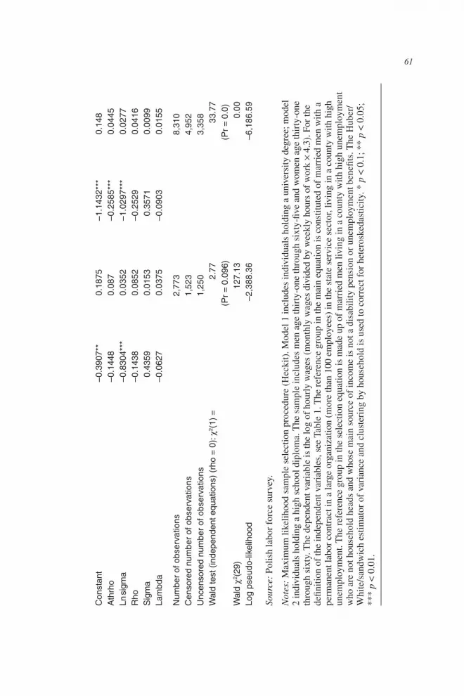
Number of observations 16,018 7,956 8,062Censored number of observations 6,122 3,100 3,022Uncensored number of observations 9,896 4,856 5,040Wald test (independent equations)

(rho = 0): c2(1) =8.13***

(Pr = 0.00)0.61

(Pr = 0.4346)5.04**

(Pr = 0.02)Wald c2 1,295.75

Pr(0.00)553.37Pr(0.00)

420.88Pr(0.00)

Log pseudo-likelihood –8,708.00 –4,599.00 –3,967.00

source: Polish labor force survey.

notes: Standard errors are in parentheses. The sample includes young people age fifteen to thirty. The dependent variable of the main equation takes a value of 1 for employment and 0 for joblessness (unemployment and inactivity). It is omitted if the respondent is in school. The dependent variable of the selection equation takes a value of1 for selection in the main equation and 0 for participation into education. For the definition of independent variables, see Table 1. The reference group in the main equation comprises married men age fifteen to thirty, with primary education or below, living with their parents in rural counties, in households living on labor income. The Huber/White/sandwich estimator of variance and clustering by household are used to correct for heteroskedasticity. * p < 0.1; ** p < 0.05; *** p < 0.01.


may–JunE 2012 71

Participation in training in the past three months is not a statistically significant determinant of success in finding employment but of participating in the labor market, as the coefficient in the selection equation shows.

Women are worse off, which confirms a finding of Domadenik and Pastore (2006). Poland is one of the countries where women experience a disadvantage early in their working career, which is common in south European countries, but not in Nordic or other East European countries (O’Higgins 2004).

All other things being equal, single women have a higher probability of finding employment than married (divorced or widowed) women, but for men the opposite holds true. Single men are less likely than other men to be working. It should be recalled that people marry as early as their early twenties in Poland and soon have children. Nonetheless, the average age at marriage and the age when people have children is gradually increasing, which is likely to reduce the impact of choices regarding family life on labor market participation.

For similar reasons, being the head of household reduces the reservation wage and increases the probability of employment for men but not for women. Women who are heads of households are less likely to find jobs than those living with parents, especially if they are not single. This is probably related to the presence of children.

Interestingly, the most successful job seekers are those young people whose household income comes from private farming. Private agriculture, often constituted of small land plots, has always existed in Poland (even during the communist era) and constitutes an important reservoir of employment in the posttransition high unemployment period. This finding is also confirmed by the set of variables relative to the city of residence. The smaller the population size of the city of residence, the lower the probability of finding employment. In urban areas, however, it is generally less easy for a young person to find employment than in rural areas. According to the literature on regional unemployment in Poland and other transition countries, big cities and rural areas offer much greater chances to find employment than small towns. In fact, the group of counties with low unemployment traditionally includes both urban and rural counties (for a survey, see Ferragina and Pastore 2008).

Selection Equation

Generally speaking, the higher the educational degree obtained, the higher the probability one will participate in the labor market. Obtaining vocational training seems to reduce the probability of participating in the labor market and to increase that of investing in further education. This finding might mirror the hardship these people are experiencing in the posttransition period.

The age profile of labor market participation is steep, but still concave for women, since with time, young people tend to finish their studies. As already noted, gender differences in educational choices are less important than those in terms of the probability of success in the labor market. As the gender coefficient shows, all


things being equal, the probability that a young man will remain in school is not statistically different from the probability that a woman will.

Single individuals prefer to continue to invest in education rather than search for a job. This result is symmetrical to that found when we look at the main equation and is obviously associated with the fact that the decision to work and the decision to establish a new household are strongly related. Conversely, heads of households tend to seek work rather than invest in education.

Households with private farms provide a smaller incentive to study and easier access to gainful employment. Similarly, living in urban areas significantly increases the probability of investing in further education. This might be due not only to a demand-side but also to a supply-side effect.

The Instrumental Variables

The instrumental variables have the expected sign and are generally statistically significant. Experiments with variables9 suggest that the estimated coefficients are robust to changes in the specification adopted.

Expected lifetime earnings from university education have a statistically signifi-cant impact on the probability of pursuing such an education. Earnings expected from successfully completing high school, however, are statistically significant only in the case of men (though always with the right sign).10

Overall, these results confirm that, similarly to that of other new EU members, the Polish economy provides strong economic incentives to invest in postcompul-sory education, which, in turn, helps to explain the recent increase in the level of education obtained. Nonetheless, the impact of expected earnings on investment in education is smaller in the case of women. This finding is in line with the previous observation that the system of incentives is different for women.

Furthermore, although not always highly significant, all things being equal, unemployment has a consistently negative, rather than positive, affect on pursu-ing education.11 A high local unemployment rate does not represent an incentive to invest in further education, but rather the opposite. In other words, the impact of unemployment in terms of lower return outweighs that in terms of a lower op-portunity cost.

Such an impact is inverse-U-shaped: with unemployment increasing, pursuit of education first increases, then decreases. This interesting result is confirmed in all the estimates. To investigate this finding further, Table 5 presents several estimates based on two sets of unemployment dummies. The former set uses the average youth unemployment rates, whereas the latter uses different youth unemployment rates for men and women. These regressors are used in two types of models. Model (1) is the same as in Table 3, whereas dummies measuring the population size of the place of residence are dropped from Model (2). The table clearly shows that non-linearity is especially strong in the case of women and, as Model (2) shows, seems to depend only in part on interaction with the place of residence. Wald tests were

may–JunE 2012 73

Tabl

e 5.

Lo

cal U

nem

plo

ymen

t an

d P

urs

uit

of

Ed

uca

tio

n

Mod

el (

1)M

odel

(2)

Var

iabl

eA

llW

omen

Men

All

Wom

enM

en

U30

(1)_

20.

0445

0.02

840.

0488

0.01

270.

0040

0.01

20U

30(1

)_3

0.04

530.

0419

0.01

290.

0331

0.03

70–0

.005

4U

30(1

)_4

0.09

420.

0297

0.13

260.

0990

0.03

390.

1376

U30

(1)_

50.

1233

*0.

1204

0.10

330.

1300

*0.

1262

0.11

10U

30(1

)_6

0.13

96*

0.12

660.

1399

0.12

39*

0.10

900.

1278

U30

(1)_

70.

1663

**0.

1593

0.14

190.

1755

**0.

1529

0.15

97U

30(1

)_8

0.05

330.

1445

–0.0

669

0.10

700.

1858

–0.0

091

U30

(2)_

20.

0434

0.06

930.

0208

0.05

640.

0651

0.05

41U

30(2

)_3

0.12

40**

0.01

860.

1735

**0.

1253

**–0

.011

50.

2173

***

U30

(2)_

40.

1734

***

0.16

30**

0.16

24**

0.21

24**

*0.

1758

**0.

2227

***

U30

(2)_

50.

1183

**0.

1083

0.08

320.

1595

***

0.13

090.

1365

sour

ce:

Polis

h la

bor

forc

e su

rvey

.

not

es:

The

coe

ffici

ents

hav

e be

en o

btai

ned

usin

g th

e sa

me

estim

atio

n m

etho

d as

in T

able

3 (

see

sele

ctio

n eq

uatio

n). M

odel

(1)

has

the

sam

e sp

ecifi

catio

n as

in T

able

3, w

here

as th

e se

t of

dum

mie

s re

lativ

e to

the

city

of

resi

denc

e is

dro

pped

fro

m M

odel

(2)

. Not

e th

at f

or th

e fir

st s

et

of d

umm

ies,

the

yout

h (a

ges

15–3

0) u

nem

ploy

men

t rat

e is

the

sam

e fo

r m

en a

nd w

omen

, whe

reas

in th

e se

cond

set

of

estim

ates

, the

you

th

unem

ploy

men

t rat

e is

dif

fere

nt f

or m

en a

nd w

omen

. For

a d

etai

led

defin

ition

of

the

two

sets

of

dum

mie

s, s

ee T

able

1. *

p <

0.1

; **

p <

0.0

5;

***

p <

0.0

1.


used to verify the statistical significance of coefficients’ differences. They cannot always reject the hypothesis that differences are significant, but in some cases they do. In the estimates relative to the entire sample, differences are statistically sig-nificant between U30(2)_2 and U30(2)_4 only. For women, the statistics reject the hypothesis that the coefficients of U30(2)_2 and U30(2)_3 are equal. For men, the tests cannot reject the hypothesis that the coefficients of U30(2)_3 and U30(2)_4 are equal and those of U30(2)_2 and U30(2)_5 are equal, but reject the hypothesis that these two pairs are equal.

In other words, in counties with high youth unemployment, the probability of a young person being in school is lower than in counties with low youth unemploy-ment, suggesting that unemployment causes a greater reduction in the benefit of education than in the opportunity cost of education.

Let us consider again the interaction between local unemployment and the urban/rural divide. High unemployment areas are often also rural counties, but neverthe-less the coefficient of high local unemployment is still statistically significant even after controlling for the place of residence. Therefore, the incentive to invest in education is the lowest in rural counties with high unemployment. This is likely to contribute to an increase in the spatial unemployment gap if the level of human capital endowment is to be taken as an important factor of economic growth. This is a major cause for concern: without interventions aimed at bridging the educational divide between rural counties with high unemployment and urban counties with low unemployment, pursuit of the Lisbon strategy is bound to reinforce the already dramatically persistent regional unemployment pattern.

Finally, in unreported estimates, the coefficient of the opportunity cost of edu-cation is positive in the selection equation, as expected. It is highly significant in the entire sample (with a coefficient of 0.52) and for women (0.56), but significant only at 10 percent for men (0.38). This variable is not included in the preferred specification of Table 4, however, because of suspected collinearity with the un-employment rate.

Concluding Remarks

This paper aims to contribute to the work on determining how hard it is for young people in Poland to choose between working and studying. To that end, the paper proposes Heckprobit estimates of the probability of finding employment rather than being jobless in a sample of young Poles (ages fifteen to thirty), controlling for the possible sample selection bias caused by the presence of people involved in further education. There is evidence of sample selection bias in the case of young men (but not of women), confirming the a priori expectation that the two choices, namely employment/joblessness and investment in education, are not independent. This suggests that policymakers might target economic incentives to increase the level of male education.

may–JunE 2012 75

Indirectly, the analysis contributes to the problem of identifying subgroups of young people with a high probability of leaving school, therefore reducing their chances of finding gainful employment in the long run. Precise targeting of edu-cational reforms and active labor market policy on these specific groups would enhance their effectiveness at a time of tight state budget constraints.

The results confirm the role of education in explaining the success in the labor market of young people. Also, factors that reduce (increase) the reservation wage tend to increase (reduce) the probability of employment. Being a head of house-hold, for instance, increases the chances of being employed for a man. Women are more likely to continue education and less likely to find a job thereafter. It should be important for policymakers to provide women with incentives and support in finding jobs. This probably requires reinforcement of the existing instruments to help women reconcile family and work: This would require easier access to stable jobs as well as to jobs with reduced or flexible working hours, and the availability of child-care facilities.

The instrumental variables used in the selection equation—the local unemploy-ment rate, expected lifetime earnings, and the opportunity cost of education—have a statistically significant impact on the probability of being in school. The positive impact on the decision to invest in further education provided by expected lifetime earnings is unsurprising. Conversely, in contrast to what several previous studies relative to mature market economies found, our study found that, all things being equal, counties with high unemployment provide a disincentive to further educa-tion. Overall, the analysis confirms that rural areas with high unemployment have contributed the least to the recent increase in educational levels in Poland. In turn, this contributes to making regional unemployment persistent. Policymakers, at the EU level as well, should target rural areas when trying to increase the local supply of education.

Future research will need to calculate comparable results relative to more recent years, when the unemployment rate dramatically increased, and consider different age groups and the decision to reside with parents.

Notes

1. Wojewòdztwo (voivodship) is the Polish equivalent to “region.” In fact, rather than regions, voivodships resemble English counties (NUTS3 level), considering that their number (49) is rather large compared with the country’s population (38 million). A reform approved in 1998 reduced the number of these administrative units to sixteen. The new larger units do not overlap the old ones, making any comparison between the pre- and postreform administrative structure impossible.

2. One reason the MNP is less frequently used is its computational difficulty.3. Other natural alternatives would be a conditional logit model (which requires

detailed longitudinal data that can individualize the time of exit from school) and a bivari-ate probit model (which is generally used for evaluation of the gross impact of proactive schemes).


4. Those who declared they did not work because they were unable to were excluded from the analysis, whereas the disabled who did not declare they were unable to work were included in the analysis.

5. Eight graduate students were included among those in education.6. The study thus includes 237 individuals who study and work, and 51 who study and

are jobless.7. The discussion paper version contains a summary description of the educational

system.8. Only women on maternity leave can be identified. No information is provided on

the number of children.9. Results of such experiments are available on request.

10. Wald tests cannot reject the null hypothesis that the two coefficients relative to dif-ferent education levels are equal.

11. The use of different unemployment measures confirms this finding. In omitted esti-mates, the county unemployment rate gives a coefficient of 0.49 for the entire sample, 0.95 for women, and 0.11 for men. It is highly significant only in the case of women.

References

Arulampalan, W., and M.B. Stewart. 1995. “The Determinants of Individual Unemploy-ment Durations in an Era of High Unemployment.” Economic Journal 105, no. 405: 321–332.

Beleva, I.; Ivanov, A.; O’Higgins, N.; and Pastore, F. 2001. “Targeting Youth Employment Policy in Bulgaria.” Economic and Business review 3, no. 2: 113–135.

Blinder, A.S., and Y. Weiss. 1976. “Human Capital and Labour Supply: A Synthesis.” Journal of Political Economy 84, no. 3: 449–472.

Boeri, T. 2000. structural change, Welfare systems, and Labour reallocation. Oxford: Oxford University Press.

Boeri, T.; J. Köllo; and M. Burda. 1997. “Labour Market in Central Europe and the EU Enlargement.” Paper presented at the Centre for Economic Policy Research Conference, Portoroz, June 13–15.

Card, D., and A. Krueger. 1992. “Does School Quality Matter? Returns to Education and the Characteristics of Public Schools in the United States.” Journal of Political Economy 100, no. 1: 1–40.

Caroleo, F.E., and F. Pastore. 2003. “Youth Participation in the Labour Market in Germany, Spain and Sweden.” In youth unemployment and social Exclusion, ed. T. Hammer, 115–141. Bristol, UK: Policy Press.

Clark, K.B., and L.H. Summers. 1990. “The Dynamics of Youth Unemployment.” In under-standing unemployment, ed. L.H. Summers, 48–85. Cambridge: MIT Press.

Davia, M.A. 2004. “Tackling Multiple Choices: A Joint Determination of Transitions out of Education and into the Labour Market Across the European Union.” Discussion Paper no. 22, Institute for Social and Economic Research, Colchester, UK.

Denny, K., and C. Harmon. 2000. “The Impact of Education and Training on the Labour Market Experiences of Young Adults.” Working Paper no. 00/08, Institute for Fiscal Studies, London.

Domadenik, P., and F. Pastore. 2006. “Influence of Education and Training Systems on Participation of Young People in Labour Market of CEE Economies: A Comparison of Poland and Slovenia.” International Journal of Entrepreneurship and small Business 3, no. 5: 640–666.

may–JunE 2012 77

Ferragina, A., and F. Pastore. 2005. “Factor Endowment and Market Size in EU-CEE Trade. Would Human Capital Change the Actual Quality Trade Patterns?” Eastern European Economics 43, no. 1 (January–February): 5–33.

———. 2008. “Mind the Gap. Unemployment in the New EU Regions” Journal of Economic surveys 22, no. 1: 77–113.

Fidrmuc, J. 2004. “Migration and Regional Adjustment to Asymmetric Shocks in Transition Economies.” Journal of comparative Economics 32, no. 2: 230–247.

Giannelli, G.C., and Monfardini, C. 2000. “A Nest or a Golden Cage? Family Co-Residence and Human Capital Investment Decisions of Young Adults.” International Journal of manpower 21, nos. 3–4: 227–245.

———. 2003. “Joint Decisions on Household Membership and Human Capital Accumulation of Youths. The Role of Expected Earnings and Local Markets.” Journal of Population Economics 16, no. 2: 265–286.

Hammer, T. 2003. youth unemployment and social Exclusion. Bristol, UK: Policy Press.Heckman, J.J. 1976. “A Life-Cycle Model of Earnings, Learning and Consumption.” Journal

of Political Economy 84, no. 4, S11–S44.———. 1979. “Sample Selection as a Specification Error.” Econometrica 47, no. 1:

131–161.Keane, M.P., and K.I. Wolpin. 1997. “The Career Decisions of Young Men.” Journal of

Political Economy 105, no. 3: 473–522.McVicar, D., and P.G. Rice. 2001. “Participation in Further Education in England and Wales:

An Analysis of Post-War Trends.” oxford Economic Papers 53, no. 1: 47–66.Micklewright, J. 1990. “Unemployment and Early School Leaving.” Economic Journal

100, no. 400: 163–169.———. 1999. “Education, Inequality and Transition.” Innocenti Working Papers, Economic

and Social Policy series no. 74, UNICEF Innocenti Research Centre, Florence.Newell, A., and F. Pastore. 1999. “Structural Change and Structural Unemployment in

Poland.” studi Economici 69, no. 3: 81–100.Nguyen, A.N., and J. Taylor. 2003. “Post-High School Choices: New Evidence from a Mul-

tinomial Logit Model.” Journal of Population Economics 16, no. 2: 287–306.O’Higgins, N. 2004. “Recent Trends in Youth Labour Markets and Youth Employment Policy

in Europe and Central Asia.” Discussion Paper no. 85, Centro di Economia del Lavoro e Politica Economica, Salerno, Italy.

Pastore, F. 2010. “The Gender Gap in Early Career in Mongolia.” International Journal of manpower 31, no. 2: 188–207.

Pastore, F., and M. Socha. 2006. “The Polish LFS: A Rotating Panel with Attrition,” Eko-nomia Journal 15, no. 3: 3–24.

Pissarides, C.A. 1981. “Staying on at School in England and Wales.” Economica 48, no. 192: 345–363.

Poterba, J.M., and L.H. Summers. 1995. “Unemployment Benefits and Labour Market Tran-sitions: A Multinomial Logit Model with Errors in Classification.” review of Economics and statistics 77, no. 2: 207–216.

Psacharopoulos, G. 1994. “Returns to Investment in Education: A Global Update.” World Development 22, no. 9: 1325–1343.

Rice, P.G. 1987. “The Demand for Post-Compulsory Education in the UK and the Effects of Educational Maintenance Allowances.” Economica 54, no. 216: 465–475.

———. 1999. “The Impact of Local Labour Markets on Investment in Further Education: Evidence from the England and Wales Cohort Studies.” Journal of Population Econom-ics 12, no. 2: 287–312.


Van de Ven, W.P.M.M., and B.M.S. Van Pragg. 1981. “The Demand for Deductibles in Pri-vate Health Insurance: A Probit Model with Sample Selection.” Journal of Econometrics 17, no. 2: 229–252.

Whitfield, K., and R.A. Wilson. 1991. “Staying-On in Full-Time Education: The Educational Participation Rate of 16-Year-Olds.” Economica 58, no. 231: 391–404.

World Bank. 2001. Poland-Labor market study: The challenge of Job creation. World Bank Country Study, March. Washington, DC.

———. 2004. Poland: Growth, Employment and Living standards in Pre-accession Poland. Report no. 28233, Washington, DC.

To order reprints, call 1-800-352-2210; outside the united states, call 717-632-3535.

to study or to work?

Documents