1

To Give a Surprise Exam, Use Game Theory

Elliott Sober*

Philosophy Department

University of Wisconsin, Madison 53706

Abstract: This paper proposes a game-theoretic solution to the surprise examination problem. It is

argued that the game of “matching pennies” provides a useful model for the interaction of a teacher

who wants her exam to be surprising and students who want to avoid being surprised. A distinction is

drawn between prudential and evidential versions of the problem. In both, the teacher should not

assign a probability of zero to giving the exam on the last day. This representation of the problem

provides a diagnosis of where the backwards induction argument, which “proves” that no surprise exam

is possible, is mistaken.

1. The Problem and its Game-Theoretic Setting

Before the semester begins, a teacher announces to her class that she will give exactly one

exam during the semester and that the exam will come as a surprise to the students when it occurs.

One of the students in the class reasons as follows:

If the teacher wants to give a surprise exam, she won't wait until the last day of the semester to

give the exam, because the students will be expecting an exam then, if none has been given

earlier. So the teacher won’t give the exam on the last day. But if the last day is ruled out, the

2

same reasoning also eliminates the next to last day. After all, if the teacher waits until the next

to last day, she will have to give the exam then, since

the day after that has been ruled out. But this allows the students to predict an exam

on the next to last day, if the teacher fails to give one before then. So no suprise exam on

the next to last day is possible either. By a "backwards induction," each day is ruled out

and thus there is no day on which a surprise exam can be given.

The surprise examination problem is to figure out what is wrong with this bit of reasoning. There must

be a mistake somewhere; after all, we all know that it is possible to give a surprise exam, even when the

students are told at the beginning of the semester that one will occur.

Previous treatments of the problem (reviewed briefly in Sainsbury 1988 and in more detail in

Sorensen 1988) have taken pains to analyze the student's reasoning, but have spent less time assessing

what the teacher must do to give a surprise exam and how the students should respond to the teacher's

chosen strategy. My approach is the reverse; I want to consider carefully what the teacher and

students should do and then, in the light of this, I'll try to determine where the student's reasoning goes

wrong.

I propose to consider this problem from the point of view of game theory. The teacher's goal is

to give an exam that will surprise the students; the student's goal is to predict the exam before it occurs,

thus frustrating the teacher's intention. More specifically, I will attempt to identify the best strategy that

the teacher can use to decide the day on which the exam will be given and the best strategy for the

3

students to use in predicting when the exam will occur. This is a problem in game theory because which

behavior is best for one player depends on what the other player does.1

The usual assumption in discussions of this problem is that the players are ideal rational agents;

they make no logical errors and moreover do not fail to notice implications of what they believe that are

pertinent -- they are "logically omniscient." In addition, each player knows that the other is an ideal

rational agent. For example, if it would be rational for the teacher to avoid the last day of the semester

as an exam date, she will do so and the students will know that she will do so. Rationality is "common

knowledge." This means that if there is a strategy that is most rational for the teacher to follow, given

her goal of surprising the students, the teacher will follow that strategy and the students will know that

she is doing so.

In addition to diagnosing where the student's reasoning goes wrong, there is a second feature of

the surprise exam problem that needs to be elucidated. There is a peculiar deliberational instability that

both the teacher and the student seem to experience. Typically, when a person deliberates, the

deliberation process terminates in a decision, which further reflection on the information at hand would

not displace. However, when teacher and students each make a decision about what they'll do, their

decisions seem to constantly shift because each can calculate what the other is planning to do. For

example, if the teacher decides to perform action a and the students think she will perform action b, the

students apparently have an incentive to trade their false belief for a true one. However, if the teacher

plans to perform a and the students expect this to happen, the teacher seems to have an incentive to

4

shift to a new plan -- to perform action c. No matter which pair of decisions the teacher and the

students select, one or the other seems to have a reason to change. A game-theoretic analysis should

explain whether this appearance of instability is in fact correct.

I will represent the ideas of rationality and common knowledge within a Bayesian framework.

Before the semester begins, the teacher and the students are in a state of uncertainty as to when the

exam will be; then, by reflection on their own situation and goals as well as on the situation and goals of

the other player, they each reach a decision about when the exam will take place. The teacher begins

with a probability distribution p1, p2, ..., pn over the n days of the semester, which deliberation may lead

her to modify; the students likewise begin with a distribution q1, q2, ...,qn, which they may change in the

light of reflection. After each player selects a probability distribution for the semester that lies before

them, the first day of the semester takes place. If an exam occurs on that day, we can see how

surprised the students are and the game is over. If no exam occurs, the teacher and the students must

choose new distributions for the n-1 remaining days by taking account of their knowledge of what

transpired on the semester's first day. If the exam occurs on the second day, we again can see how

surprised the students are and the game is over. If no exam occurs, the two players construct

distributions for the n-2 remaining days. And so on. Our task is to determine what distribution the

teacher should choose at each step, given her goal of surprising the students; we also need to see what

distribution the students should choose at each step, given their goal of not being taken by surprise by

the exam when it occurs. A full solution of this problem will identify n pairs of distributions, one pair for

each day.

5

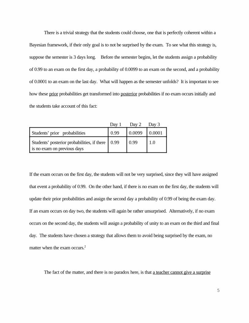
There is a trivial strategy that the students could choose, one that is perfectly coherent within a

Bayesian framework, if their only goal is to not be surprised by the exam. To see what this strategy is,

suppose the semester is 3 days long. Before the semester begins, let the students assign a probability

of 0.99 to an exam on the first day, a probability of 0.0099 to an exam on the second, and a probability

of 0.0001 to an exam on the last day. What will happen as the semester unfolds? It is important to see

how these prior probabilities get transformed into posterior probabilities if no exam occurs initially and

the students take account of this fact:

Day 1 Day 2 Day 3

Students’ prior probabilities 0.99 0.0099 0.0001

Students’ posterior probabilities, if thereis no exam on previous days

0.99 0.99 1.0

If the exam occurs on the first day, the students will not be very surprised, since they will have assigned

that event a probability of 0.99. On the other hand, if there is no exam on the first day, the students will

update their prior probabilities and assign the second day a probability of 0.99 of being the exam day.

If an exam occurs on day two, the students will again be rather unsurprised. Alternatively, if no exam

occurs on the second day, the students will assign a probability of unity to an exam on the third and final

day. The students have chosen a strategy that allows them to avoid being surprised by the exam, no

matter when the exam occurs.2

The fact of the matter, and there is no paradox here, is that a teacher cannot give a surprise

6

exam to students like this. This means that our confidence that surprise exams are possible in the real

world assumes that real world students are different. How so? Surely the answer is not that real

students are being irrational when they fail to adopt the distribution just described. Real students don't

want to be surprised by exams, but they also don't want to predict exams that fail to occur. If

predicting an exam has the behavioral consequence that the students spend time preparing for the exam,

it is easy to see why they associate a cost with false prediction.

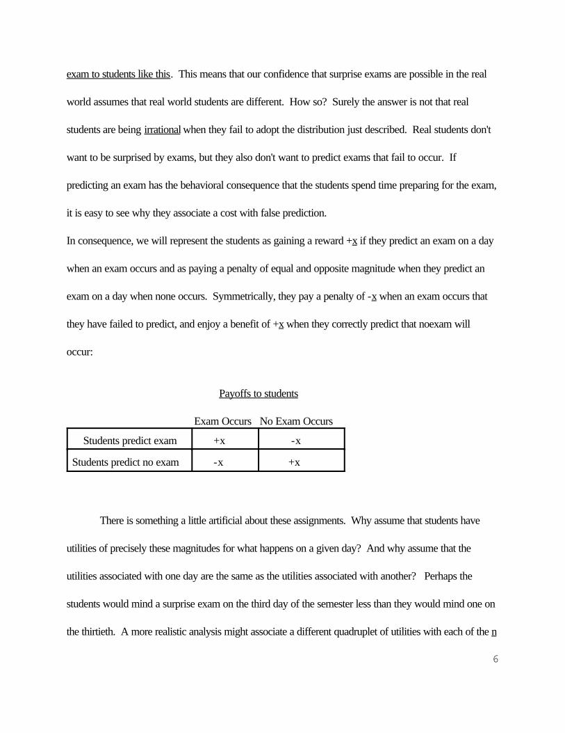
In consequence, we will represent the students as gaining a reward +x if they predict an exam on a day

when an exam occurs and as paying a penalty of equal and opposite magnitude when they predict an

exam on a day when none occurs. Symmetrically, they pay a penalty of -x when an exam occurs that

they have failed to predict, and enjoy a benefit of +x when they correctly predict that noexam will

occur:

Payoffs to students

Exam Occurs No Exam Occurs

Students predict exam +x -x

Students predict no exam -x +x

There is something a little artificial about these assignments. Why assume that students have

utilities of precisely these magnitudes for what happens on a given day? And why assume that the

utilities associated with one day are the same as the utilities associated with another? Perhaps the

students would mind a surprise exam on the third day of the semester less than they would mind one on

the thirtieth. A more realistic analysis might associate a different quadruplet of utilities with each of the n

7

days in the semester. Fortunately, our simplifying assumptions about payoffs will not affect the

diagnosis concerning where the students go wrong in their backwards induction argument.

Having specified what the students like and dislike, what are we to say of the teacher? To keep

things simple, we will assume that she is the mirror image of her students. If she succeeds in giving a

surprise exam, she gains a benefit whose magnitude is +x; if she gives an exam that the students have

predicted, her utility is -x; and so on. This simplification also will not affect the points of importance.

2. Matching Pennies

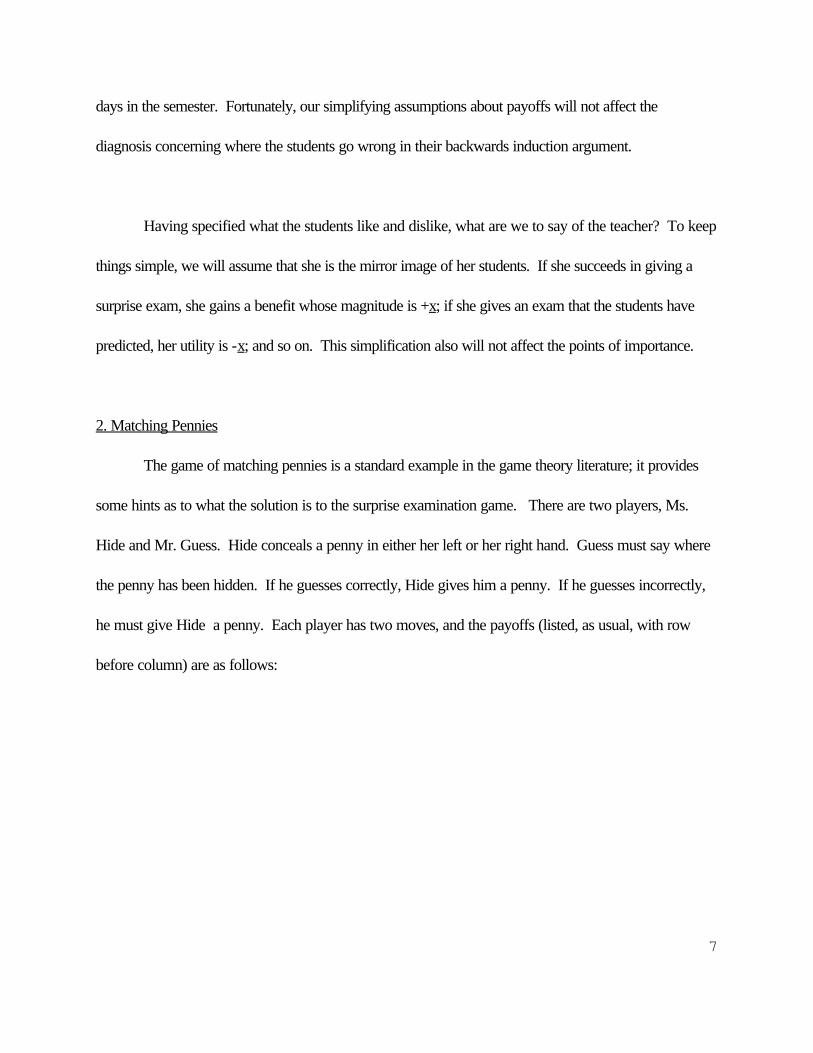
The game of matching pennies is a standard example in the game theory literature; it provides

some hints as to what the solution is to the surprise examination game. There are two players, Ms.

Hide and Mr. Guess. Hide conceals a penny in either her left or her right hand. Guess must say where

the penny has been hidden. If he guesses correctly, Hide gives him a penny. If he guesses incorrectly,

he must give Hide a penny. Each player has two moves, and the payoffs (listed, as usual, with row

before column) are as follows:

8

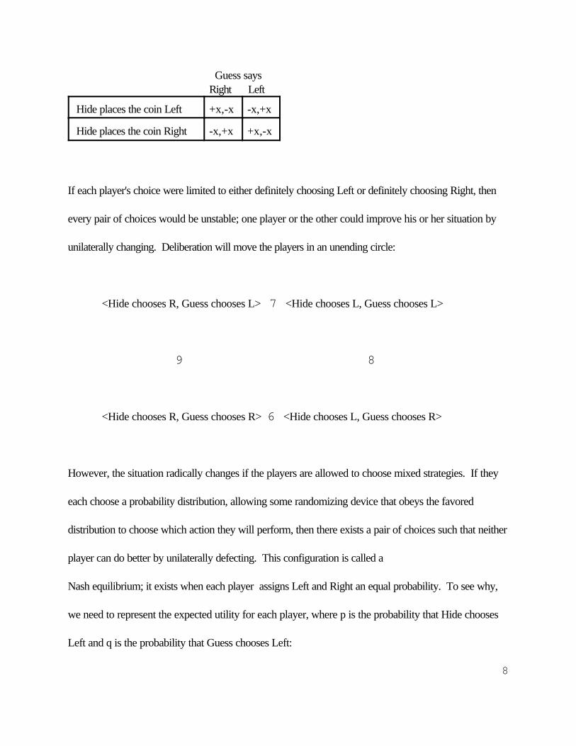
Guess says Right Left

Hide places the coin Left +x,-x -x,+x

Hide places the coin Right -x,+x +x,-x

If each player's choice were limited to either definitely choosing Left or definitely choosing Right, then

every pair of choices would be unstable; one player or the other could improve his or her situation by

unilaterally changing. Deliberation will move the players in an unending circle:

<Hide chooses R, Guess chooses L> 7 <Hide chooses L, Guess chooses L>

9 8

<Hide chooses R, Guess chooses R> 6 <Hide chooses L, Guess chooses R>

However, the situation radically changes if the players are allowed to choose mixed strategies. If they

each choose a probability distribution, allowing some randomizing device that obeys the favored

distribution to choose which action they will perform, then there exists a pair of choices such that neither

player can do better by unilaterally defecting. This configuration is called a

Nash equilibrium; it exists when each player assigns Left and Right an equal probability. To see why,

we need to represent the expected utility for each player, where p is the probability that Hide chooses

Left and q is the probability that Guess chooses Left:

9

E(Hide) = -pqx - (1-p)(1-q)x + p(1-q)x + (1-p)qx.

E(Guess) = +pqx + (1-p)(1-q)x - p(1-q)x - (1-p)qx.

Notice that if Hide sets p=0.5, then Guess has the same expected utility no matter what value he assigns

to q. And if Guess sets q=0.5, then Hide has the same expected utility no matter what value she assigns

to p. There is a Nash equilibrium at <Hide sets p=0.5, Guess sets q=0.5>; no other pair of

distributions has this property.

If we assume that players change their distributions if and only if the change would improve their

expected utilities, then the <p=0.5, q=0.5> configuration is stable; this means that if the players each

choose a flat distribution, they will never depart from that choice. However, a separate question may

be raised about this equilibrium's accessibility. If the players begin deliberation with some other pair of

distributions, will deliberation lead them to change what they think is best and eventually converge on

the Nash equilibrium? Part of the answer to this question is suggested by considering the direction of

change that occurs if the players' assignments are located in each of the four quadrants depicted in

Figure 1.3

FIGURE 1

If the players assign low values to p and q, then Hide will shift to a high value for p. If Hide

assigns a high value to p, then Guess will want to assign a high value to q as well. And so on. We have

10

here the makings of a more-or-less circular flow. But what can be said that is more specific? Will the

players circle endlessly, will they spiral into the center, or will they spiral out to the edges?

We now need to consider the specific rules that rational players use to revise their choice of

distributions in the light of common knowledge; these rules constitute the dynamics of the process of

rational deliberation. Skyrms (1990) considers a family of dynamical rules under which agents adjust

their probability assignments by making repeated small changes in the direction that improves their

expected utility. In the dynamics that Skyrms favors, the Nash equilibrium is a global attractor in the

game of matching pennies (Skyrms 1990, p. 64, p. 176). However, in other dynamics, this fails to be

true, as Skyrms notes; deliberation can move in endless ellipses centered on the Nash equilibrium, and

it can spiral out to the edges. I don’t want to address here the substantive question of which of these

dynamical rules is most realistic. Rather, for purposes of the problem at hand, I’ll assume a dynamics

in which deliberation spirals into the center of the unit square in Figure 2, regardless of where the

players begin in their deliberation. Perhaps we should expect rational agents to settle down to the

50/50 strategy when playing this game. If so, we should adopt the dynamical assumptions that yield this

result.

FIGURE 2

3. The Surprise Examination as a Game of Iterated Matching Pennies

I suggest that the surprise examination problem is an iterated game of matching pennies. Before

11

each day of the semester, the teacher and the students must assign probabilities to the r remaining days.

The first step in this game is for them to choose a pair of distributions over n days, the second is to

construct distributions over n-1 days that take account of what happened on the previous day, and so

on. Thus, at each stage the players select values for p1, p2,...,pr and q1, q2,..., qr respectively, with each

attempting to maximize expected utility.4

The fact that this game comes in temporal stages, with new probabilities replacing old ones as

the semester unfolds, complicates this problem a bit, and leads to a solution that fails to resemble

exactly what matching pennies might lead one to expect. To see how the problem is to be analyzed,

let's assume that the semester is just two days long. Before the semester begins, the teacher's

probability of giving an exam on day one is p and her probability of giving an exam on day two is (1-p).

Likewise, the students' prior probabilities are q and (1-q), respectively. If no exam occurs on the first

day, the probability of an exam on the second day then becomes unity. The expected utilities for the

two players are as follows:

E(Teacher) = p(1-q)x + (1-p)qx - pqx - (1-p)(1-q)x - (1-p)x

E(Student) = -p(1-q)x - (1-p)qx + pqx + (1-p)(1-q)x + (1-p)x.

Each of these expectations has five addends. The first four describe the four possible events that might

happen on day 1; the teacher either gives an exam or fails to do so, and the students either predict an

exam for that day or fail to do so. The fifth addend takes account of what will happen if the game

12

continues into the second day; this has a probability of (1-p) of occurring, and entails a loss of x for the

teacher and a gain of x for the student. Without this fifth addend, the expressions for E(Teacher) and

E(Student) are none other than the expressions for E(Hide) and E(Guess); it is the fifth addend that

makes the surprise exam problem different from the game of matching pennies.

The two expressions just given simplify to:

E(Teacher) = px(1-2q) + (1-p)x(2q-2)

E(Student) = px(2q-1) + (1-p)x(2-2q).

If the teacher assigns p = (1-p) = 0.5, then the student's expected utility is (0.5)x, a quantity that does

not depend on what value the students assign to q. Similarly, if the students choose a value for q such

that (1-2q) = (2q-2) (i.e., q = 0.75), then the teacher's expectation is -(0.5)x, which is independent of

the value that she assigns to p. This means that the pair <Teacher assigns p=0.5, Students assign

q=0.75> forms a Nash equilibrium.

We saw earlier that deliberation in matching pennies is perpetually unstable when the players

are limited to considering pure strategies, but stabilizes when the players get to use mixed strategies.

The same point holds for the surprise examination problem. The players do not perpetually shift their

decisions about what to do; rather, each settles down to a specific probabilistic strategy.

13

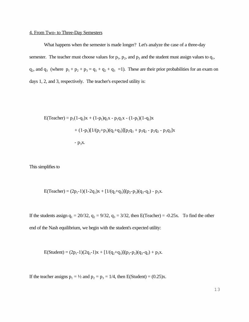
4. From Two- to Three-Day Semesters

What happens when the semester is made longer? Let's analyze the case of a three-day

semester. The teacher must choose values for p1, p2, and p3 and the student must assign values to q1,

q2, and q3 (where p1 + p2 + p3 = q1 + q2 + q3 =1). These are their prior probabilities for an exam on

days 1, 2, and 3, respectively. The teacher's expected utility is:

E(Teacher) = p1(1-q1)x + (1-p1)q1x - p1q1x - (1-p1)(1-q1)x

+ (1-p1)[1/(p2+p3)(q2+q3)][p2q3 + p3q2 - p2q2 - p3q3]x

- p3x.

This simplifies to

E(Teacher) = (2p1-1)(1-2q1)x + [1/(q2+q3)](p2-p3)(q3-q2) - p3x.

If the students assign q1 = 20/32, q2 = 9/32, q3 = 3/32, then E(Teacher) = -0.25x. To find the other

end of the Nash equilibrium, we begin with the student's expected utility:

E(Student) = (2p1-1)(2q1-1)x + [1/(q2+q3)](p3-p2)(q3-q2) + p3x.

If the teacher assigns p1 = ½ and p2 = p3 = 1/4, then E(Student) = (0.25)x.

14

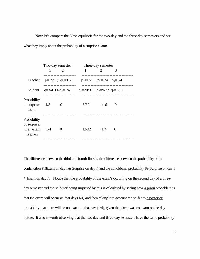
Now let's compare the Nash equilibria for the two-day and the three-day semesters and see

what they imply about the probability of a surprise exam:

Two-day semester Three-day semester 1 2 1 2 3

---------------------- ----------------------------------- Teacher p=1/2 (1-p)=1/2 p1=1/2 p2=1/4 p3=1/4 ---------------------- ----------------------------------- Student q=3/4 (1-q)=1/4 q1=20/32 q2=9/32 q3=3/32 ---------------------- ----------------------------------- Probabilityof surprise 1/8 0 6/32 1/16 0 exam ---------------------- ----------------------------------- Probabilityof surprise, if an exam 1/4 0 12/32 1/4 0 is given

---------------------- -----------------------------------

The difference between the third and fourth lines is the difference between the probability of the

conjunction Pr(Exam on day i & Surprise on day i) and the conditional probability Pr(Surprise on day i

* Exam on day i). Notice that the probability of the exam's occurring on the second day of a three-

day semester and the students' being surprised by this is calculated by seeing how a priori probable it is

that the exam will occur on that day (1/4) and then taking into account the student's a posteriori

probability that there will be no exam on that day (1/4), given that there was no exam on the day

before. It also is worth observing that the two-day and three-day semesters have the same probability

15

(1/4) of the students’ being surprised, if the exam occurs on the next to last day. However, the

semesters have different probabilities that the surprise exam occurs on the next to last day.

The trends suggested by these two examples are quite intuitive. In any semester, the probability

of a surprise exam declines as the semester unfolds. In addition, the longer the semester, the higher the

probability that there will be a surprise exam. Quite obviously, a surprise examination is not impossible.

Note also that neither player assigns a probability of zero to an exam's occurring on the last day. If the

teacher wants to give a surprise exam, her best strategy is to use a distribution in which there is some

chance that the exam will be completely unsurprising; more on this later. 5

5. Prudential versus Evidential Prediction

In the analysis of the two-day and the three-day problem just described, the students choose a

distribution that differs from the one that the teacher selects, even though the students know that the

teacher controls when the exam will occur and also know which distribution the teacher will select.

This may seem paradoxical, but in fact it is not, once we recognize that the students' predicting an exam

is here conceptualized as an action, not as a belief driven purely by the evidence at hand. It isn't

counter-intuitive that students who are extremely averse to surprise exams, but who don't mind studying

when there is no exam, should "predict" an exam even when they think that the probability of an exam is

low. They prepare for an exam because they would rather be safe than sorry. The present analysis has

a similar consequence, except that we have assumed that the students mind surprise exams exactly as

much as they mind preparing when no exam is given. We have viewed prediction as an action that is

16

properly regulated by both evidential and prudential considerations.6

If one wishes to view the surprise examination problem in terms of a purely evidential rather

than a prudential concept of prediction, a different analysis is needed. Suppose we interpret the

common knowledge assumption as forcing the students to believe whatever distribution the teacher

selects. The teacher knows that whatever distribution she selects, the students will select the same one.

In deliberating, she will not move from distribution a to distribution b because she sees that she does

better under <Teacher chooses b, Students choose a> than she does under <Teacher chooses a,

Students choose a>; rather, if she moves from a to b, this will be because she sees that her expected

payoff under <Teacher chooses b, Students choose b> exceeds what she would receive under

<Teacher chooses a, Students choose a>.

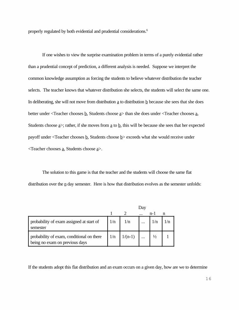
The solution to this game is that the teacher and the students will choose the same flat

distribution over the n day semester. Here is how that distribution evolves as the semester unfolds:

Day 1 2 ... n-1 n

probability of exam assigned at start ofsemester

1/n 1/n ... 1/n 1/n

probability of exam, conditional on therebeing no exam on previous days

1/n 1/(n-1) ... ½ 1

If the students adopt this flat distribution and an exam occurs on a given day, how are we to determine

17

whether the students have been "surprised?" Since we now are viewing the students as adopting a

probability distribution, not as performing a behavior, this question requires that a dichotomous

category be imposed on a continuous underlying reality. Perhaps we should say that an event

"surprises" an agent when the agent assigned that event a probability of 0.5 or less. This would have

the intuitive implication that an exam on any day but the last will surprise the students. However, in

other circumstances, this proposal has peculiar consequences. Suppose three events occur to which an

agent had assigned probabilities of 0.50, 0.51, and 0.99, respectively. According to the proposal, the

first is surprising, but the second and third are not. This is an odd grouping; surely the first two events

resemble each other more than either resembles the third, in terms of how surprising they are. Thus

does the paradox of the heap intrude into the surprise examination problem.

Let me note, however, that if surprise is defined in terms of a threshold of 0.5, then the

probability of a surprise exam during the semester is (n-1)/n; other cut-offs would have other

implications. Regardless of which threshold one adopts, the probability of a surprise exam approaches

unity as the semester is lengthened.

There is no need to choose between the prudential and the evidential interpretations of the

surprise examination problem. The relevant features of the analysis are the same. In both cases, exams

that occur earlier in the semester are more surprising than ones that occur later. And if the semester is

long enough, exams given early are apt to be very surprising indeed.

18

6. The Last Day

In both the prudential and the purely evidential formulation of the problem, the teacher does

best by choosing a distribution under which there is a positive probability that the exam will occur on

the last day. Given that the teacher's goal is to have the exam surprise the students, how can this choice

make sense, since an exam on the last day has no chance of surprising the students? The direct answer

to this question is that the teacher’s choice is a consequence of the game-theoretic analysis. Still, some

explanation is needed for why this choice seems so counter-intuitive.

I suggest that the optimal distribution seems wrong-headed because it apparently violates the

following principle about rational action:

(R) Suppose your only ultimate goal is to bring about S and you have to decide whether to

perform action A. Then, you should perform A, if you can bring about N by doing A and N will

increase the probability of S.

Principle (R) applies to the decision problem that the teacher faces as follows:

19

---------------------- ----------------- -------------- A: assign exam N: S:

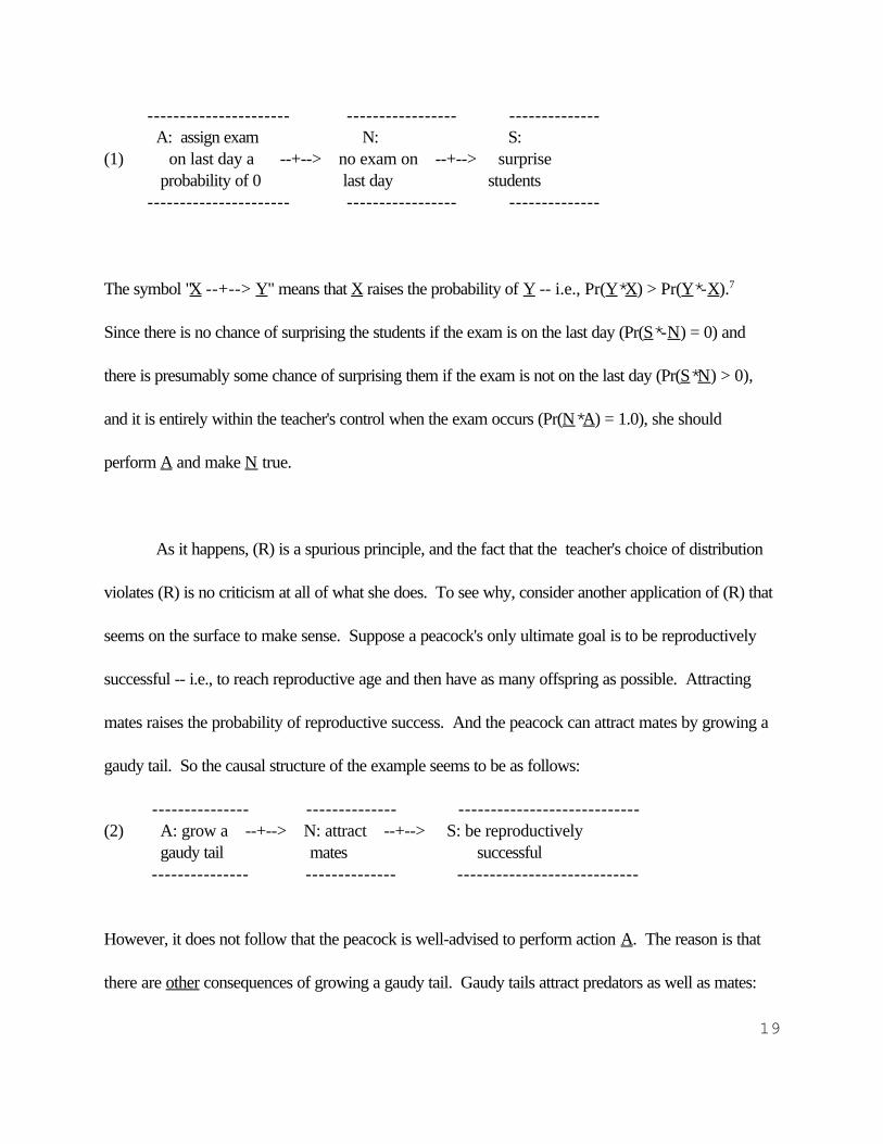
(1) on last day a --+--> no exam on --+--> surprise probability of 0 last day students ---------------------- ----------------- --------------

The symbol "X --+--> Y" means that X raises the probability of Y -- i.e., Pr(Y*X) > Pr(Y*-X).7

Since there is no chance of surprising the students if the exam is on the last day (Pr(S*-N) = 0) and

there is presumably some chance of surprising them if the exam is not on the last day (Pr(S*N) > 0),

and it is entirely within the teacher's control when the exam occurs (Pr(N*A) = 1.0), she should

perform A and make N true.

As it happens, (R) is a spurious principle, and the fact that the teacher's choice of distribution

violates (R) is no criticism at all of what she does. To see why, consider another application of (R) that

seems on the surface to make sense. Suppose a peacock's only ultimate goal is to be reproductively

successful -- i.e., to reach reproductive age and then have as many offspring as possible. Attracting

mates raises the probability of reproductive success. And the peacock can attract mates by growing a

gaudy tail. So the causal structure of the example seems to be as follows:

--------------- -------------- ---------------------------- (2) A: grow a --+--> N: attract --+--> S: be reproductively gaudy tail mates successful --------------- -------------- ----------------------------

However, it does not follow that the peacock is well-advised to perform action A. The reason is that

there are other consequences of growing a gaudy tail. Gaudy tails attract predators as well as mates:

20

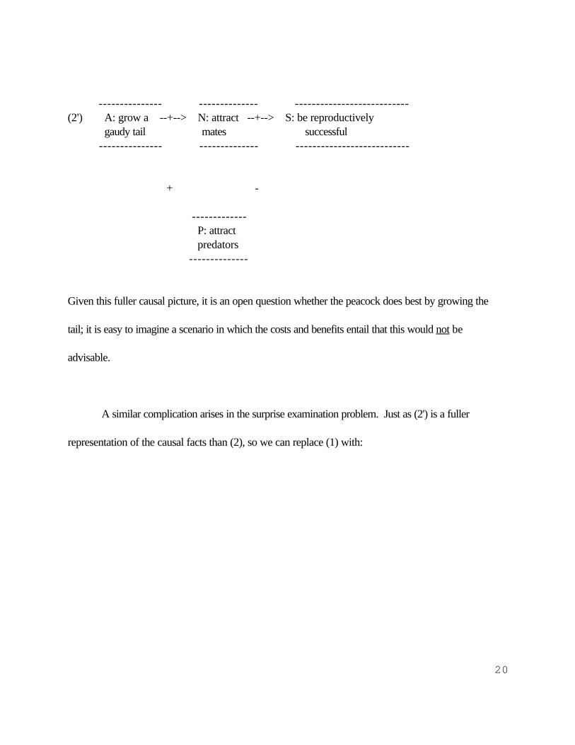
--------------- -------------- ---------------------------(2') A: grow a --+--> N: attract --+--> S: be reproductively gaudy tail mates successful --------------- -------------- ---------------------------

+ -

------------- P: attract predators

--------------

Given this fuller causal picture, it is an open question whether the peacock does best by growing the

tail; it is easy to imagine a scenario in which the costs and benefits entail that this would not be

advisable.

A similar complication arises in the surprise examination problem. Just as (2') is a fuller

representation of the causal facts than (2), so we can replace (1) with:

21

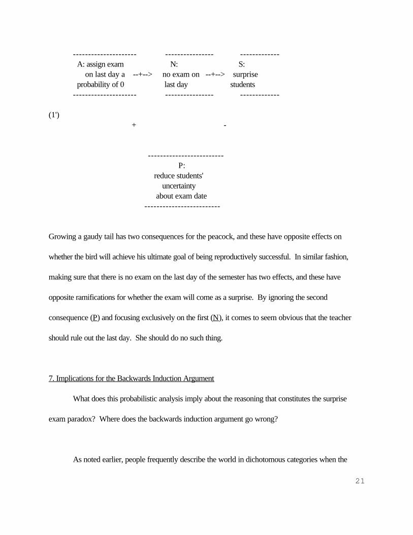
--------------------- ---------------- ------------- A: assign exam N: S:

on last day a --+--> no exam on --+--> surprise probability of 0 last day students --------------------- ---------------- -------------

(1') + -

------------------------- P:

reduce students' uncertainty about exam date

-------------------------

Growing a gaudy tail has two consequences for the peacock, and these have opposite effects on

whether the bird will achieve his ultimate goal of being reproductively successful. In similar fashion,

making sure that there is no exam on the last day of the semester has two effects, and these have

opposite ramifications for whether the exam will come as a surprise. By ignoring the second

consequence (P) and focusing exclusively on the first (N), it comes to seem obvious that the teacher

should rule out the last day. She should do no such thing.

7. Implications for the Backwards Induction Argument

What does this probabilistic analysis imply about the reasoning that constitutes the surprise

exam paradox? Where does the backwards induction argument go wrong?

As noted earlier, people frequently describe the world in dichotomous categories when the

22

underlying reality is continuous. We talk of believing propositions and of events being surprising, when

the fact of the matter is that we have degrees of belief and find events surprising to a certain extent. To

be sure, it is often overly fastidious to describe the probabilities that we take propositions to have;

frequently, we find it entirely natural simply to assert those propositions outright. When we leave our

places of work for the day, we turn to our fellow workers and say "see you tomorrow." It would raise

eyebrows to say "the probability that I will see you tomorrow is 0.999." A teacher who plans to give a

surprise exam in a semester that is, say, fifteen weeks long, is following the same convention when she

says "there will be a surprise exam this semester." The chances of her being wrong are small, so why

should she bother to be more precise?

The surprise examination problem shows that there are contexts in which departing from a more

precise quantitative formulation can lead one astray. To see why, let's first represent the student's

argument in terms of dichotomous categories; then, I'll correct that argument by describing the

underlying quantitative reality. Here is how the student reasons in his effort to show that no surprise

exam will occur:

(O) The teacher wants to give just one exam and she wants it to be surprising.

(1) If the teacher gives the exam on the last day, it will not be surprising.

(2) Hence, the teacher will not give the exam on the last day.

(3) If the teacher gives the exam on the next to the last day, it will not be surprising.

(4) Hence, the teacher will not give the exam on the next to the last day.

23

And so on. Formulated in this way, the student’s reasoning goes wrong at the first step. Premisses (0)

and (1) are true, but (2) does not follow. As we have seen, a rational teacher who wants to give a

surprise exam will not assign a probability of 0 to giving the exam on the last day. True, she will make

this the least probable exam day, and if the semester is sufficiently long, an exam on the last day will be

very improbable. But (2) overstates what follows from the preceding premisses. The next step in the

argument goes wrong as well, but in a more egregious fashion. An exam on the next to last day will be

more surprising than an exam on the last day. And a rational teacher will assign to the next to last day a

higher probability of being the exam day than she assigns to the last day of the semester. The

backwards induction argument gets worse and worse. Early steps involve fairly modest departures

from the underlying probabilistic reality; later steps involve more extreme departures.

We see here an affinity between the surprise exam problem and Kyburg's (1961) lottery

paradox.8 Suppose you know that a lottery in which there are 10,000 tickets is fair; one ticket will

win and each has the same chance of winning. Each proposition of the form "ticket i will not win" has a

probability of 0.9999. If you accept a proposition precisely when its probability exceeds some

threshold (0.99, for example), then you should accept each such proposition. However, the

conjunction of these propositions contradicts the starting assumption that some ticket will win.

Whatever solution one favors for this problem, it seems clear that "acceptance" is a problematic

concept. We assign probabilities to propositions that describe the outcomes of chance processes; if, in

addition, we either accept or reject those propositions, what does this mean? If it means anything, the

24

rules for acceptance and rejection must be more subtle than the threshold criterion just described. This

is not to deny that it is often good enough to talk about the propositions that we "accept." However,

we must recognize that this coarse-grained dichotomous description can get us into trouble. The lottery

paradox and the surprise examination problem describe two contexts in which this can happen.

8. Concluding Remarks

It might be suggested that I have used a cannon to kill a flea. The game-theoretic analysis

shows that if the semester is long enough, it is highly probable, but not certain, that the exam will

surprise the students. However, it doesn't take game theory to see that the backwards induction is

unsound if a surprise exam is merely probable.

In reply, let me say that game theory explains why the assumption that the players are rational

(and that this is common knowledge) is incompatible with the announcement that the teacher makes if

that announcement is interpreted as saying what will happen, not just what will probably happen. It

might appear that the teacher can ensure that her exam will be surprising, just as she can simply choose

the day on which the exam occurs. However, the assumptions of rationality and common knowledge

entail that she can ensure nothing of the kind. The best the teacher can do is something more modest.

Not only does a probabilistic representation of the problem explain what is wrong with the

teacher's announcement; it also explains why the teacher's announcement seems so unexceptionable. It

is something like a convention of conversation to omit probabilistic qualifications of statements that are

25

overwhelmingly probable. We are used to this simplification's not getting us into trouble, and so there

seems to be nothing suspicious about the teacher's announcement.

The game-theoretic approach provides several further benefits. It provides a precise diagnosis

of what goes wrong in the student's backwards induction argument. By identifying the distributions that

the two players will use, we can see how the backwards induction argument degenerates as the steps

are iterated. A probabilistic framework also explains why the teacher should not absolutely rule out

giving the exam on the last day, even though she knows that an exam on that day will be completely

unsurprising. In addition, this approach elucidates the difference between prudential and evidential

versions of the problem. And finally, the game-theoretic formulation provides a model of the

deliberation process itself, one that undercuts the impression that rational players must be trapped in a

chain of reasoning that is perpetually shifting. This is true if the players consider only pure strategies;

however, if they help themselves to probabilities, deliberation can stabilize, just as in the game of

matching pennies.

References

Cargile, J. (1967): "The Surprise Test Paradox." Journal of Philosophy 64: 550-563.

Eells, E. (1991): Probabilistic Causality. Cambridge: Cambridge University Press.

Kyburg, H. (1961): Probability and the Logic of Rational Belief. Middletown, Connecticut:

Wesleyan University Press.

Mougin, G. and Sober, E. (1994): "Betting Against Pascal's Wager." Nous 28: 382-395.

26

1. Cargile (1967) also describes the surprise examination problem in game-theoretic terms. However,

he rejects the idea that the teacher should use probabilities to choose an exam date (p. 559, p.561);

also, his proposed solution to the problem appeals to the idea that knowledge claims demand different

standards of evidence in different contexts (pp. 562-563). Neither of these elements will be present in

the analysis I propose.

2. There is nothing special about 0.99 in this argument. It is possible for the students to be as certain as

you please of an exam on each day; let their posterior probability of an exam on day i, given that no

exam occurred previously, be 1-e, for arbitrarily small e. Since Bayesian updating by conditionalization

is impossible if agents assign probabilities of 1's and 0's, we assume that e =/ 0.

Olin, D. (1983): "The Prediction Paradox Resolved." Philosophical Studies 44: 225-233.

Sainsbury, M. (1988): Paradoxes. Cambridge: Cambridge University Press.

Skyrms, B. (1990): The Dynamics of Rational Deliberation. Cambridge, MA: Harvard

University Press.

Sober, E. (1994): "The Primacy of Truth-Telling and the Evolution of Lying." In From a

Biological Point of View. Cambridge: Cambridge University Press.

Sorensen, T. (1988): Blindspots. Oxford: Oxford University Press.

Notes

*. I thank Martin Barrett, Ellery Eells, Branden Fitelson, Daniel Hausman, Don Moskowitz, Greg

Mougin, Larry Samuelson, Alan Sidelle, Brian Skyrms, Samuel Sober, Roy Sorensen, and the

anonymous referees of this journal for comments.

27

3. The circular flow depicted in Figure 1 also characterizes the dynamics of an evolutionary model that

describes how lying and truth-telling coevolve with a policy concerning credulity and skepticism; see

Sober (1994).

4. The assumption of Bayesian rationality entails that the first distribution over n days determines what

the subsequent distributions will be.

5.There are variations on the surprise examination problem, as just construed, that have slightly

different solutions. For example, let the payoffs be as described, except that neither player gains or

loses on a day when there is no exam and the students have not predicted one. Here the Nash

equilibrium when the semester is two days long is <Teacher chooses p=0.33, Students choose

q=0.67>. Alternatively, suppose the students get to say just once in the entire semester when they

think the exam will be. Now the surprise examination problem and the game of matching pennies are

identical; days in the first problem correspond to fists in the second.

6. Pascal's wager is perhaps the most famous problem in which prudential and evidential criteria for

belief come into conflict. Mougin and Sober (1994) consider the wager in connection with the issue of

deliberational instability.

7. More precisely, "X --+--> Y" means that X raises the probability of Y, when other causal factors

are held fixed. X is a positive causal factor for Y in the sense discussed in the literature on probabilistic

causality. See, for example, Eells (1991).

8. Olin (1983) also argues that the surprise examination problem and the lottery paradox are

connected, but for different reasons.