1

Timing of innovation policies when carbon emissions are

restricted: an applied general equilibrium analysis

Tom-Reiel Heggedal1 and Karl Jacobsen

Research Department, Statistics Norway, Oslo, Norway

Abstract:

This paper studies the timing of subsidies for environmental research and development (R&D) and how innovation policy is influenced by the costs of emissions. We use a dynamic computable general equilibrium (CGE) model with both general R&D and specific environmental R&D. We find two results that are important when subsidizing environmental R&D in order to target inefficiencies in the research markets. Firstly, the welfare gain from subsidies is larger when the costs of emissions are higher. This is because a high carbon tax increases the social (efficient) investment in environmental R&D, in excess of the private investment in R&D. Secondly, the welfare gain is greater when there is a falling time profile of the rate of subsidies for environmental R&D, rather than a constant or increasing profile. The reason is that the innovation externalities are larger in early periods. JEL codes: E62, H31, O38, Q55

Keywords: Applied general equilibrium, endogenous growth, research and development, carbon emissions.

Acknowledgments: The authors would like to thank Birger Strøm for excellent computer assistance in coding and calibrating the model. We would also like to thank Geir H. Bjertnæs, Brita Bye, Taran Fæhn, Snorre Kverndokk, and Knut-Einar Rosendahl for useful comments. Finally, we gratefully acknowledge financial support from the Norwegian Research Council programs SAMSTEMT and RENERGI.

1 Corresponding author: tom@ssb.no

2

1. Introduction In the coming decades, industrialized countries will have to face large reductions in emissions of greenhouse gases (GHGs) to curb anthropogenic interference with the global climate system. This may be through restrictions stipulated in international agreements under the United Nations Framework Convention on Climate Change or through aspirational goals and voluntary reductions of individual countries. Norway is at the forefront of planning unilateral GHG reductions, with a goal of being “carbon neutral” by 2030. The EU has implemented legislative measures to cut emissions by 20 percent from 1990 levels by 2020; this reduction will increase to 30 percent if other industrialized countries follow. In the US and Canada, several states are involved in regional cap-and-trade programs, such as the Western Climate Initiative and the Regional Greenhouse Gas Initiative. California has taken a leadership role, with a goal of reducing GHG emissions by 80 percent by 2050, compared with 1990 levels.

One expects that a variety of policy measures will be needed to achieve the cuts in GHGs. Most likely these will include a cap-and-trade system that gives a price to carbon emissions, like the European Trading Scheme, and a policy to improve clean energy technology like power production with carbon capture and storage (CCS). The most cost-efficient single policy to reduce emissions is an environmental policy that directly targets emissions, such as a tax or cap-and-trade system.2 However, in the presence of induced technological change and market failures in R&D, a combination of environmental and innovation policies may be more cost effective.3 Jaffe et al. (2005) argue that market failures associated with environmental pollution interact with market failures associated with the innovation and diffusion of new technologies. These combined market failures provide a strong rationale for a portfolio of public policies to foster emissions reductions as well as the development and adoption of environmentally beneficial technology.

Key arguments for subsidizing innovation activities are external spillovers from previous R&D and love of capital variety in demand, combined with inefficiencies arising from imperfect competition in the capital variety market.4 The market inefficiencies imply that the private returns from environmental R&D are lower than the social returns, which leads to underinvestment in environmental R&D. This underinvestment is the rationale for subsidizing R&D activity. Several environmental economics R&D models include specific policies to target inefficiencies in innovation markets. A typical policy is providing a constant subsidy for R&D.5 However, the optimal subsidy rate would not necessarily be constant over time. Hart (2008) finds that the gap between social and private returns from R&D investments may vary across time along a transition path. He implements optimal second-best carbon taxes, which may be higher than the Pigouvian level outside the balanced growth path in order to encourage investment in emissions-saving technology at the expense of ordinary production technology. Hart (2008) does not study the implication this has for first-best environmental R&D subsidies.

This paper adds to the literature by studying the timing and impact of environmental R&D subsidies when future emissions are limited, e.g., by a binding international agreement implemented via a carbon tax. In our model, emissions are reduced through a carbon tax that represents the marginal costs of emissions. This means that the R&D policy only targets

2 See Schneider and Goulder (1997), Popp (2006), Parry et al. (2003). 3 See Schneider and Goulder (1997), Goulder and Schneider (1999), Rosendahl (2004), Fischer and Newell (2008),

Otto et al. (2006). 4 See Jones and Williams (2000). 5 See Gillingham et al. (2007) for a survey of induced technological change in climate policy modeling.

3

innovation externalities, and not environmental externalities. We ask two questions. Firstly, we ask whether the welfare gains from environmental R&D subsidies are larger when the future costs of emissions are higher. Raising the costs of emissions causes an increase in the social value of R&D in environmental technologies. This may only partly be captured by private firms and thus change the welfare gains from subsidizing R&D. Secondly, we ask if welfare gains are influenced by how environmental R&D subsidies are distributed across time. This timing problem of R&D subsidies has not received much attention in the literature, to our knowledge.

Rather than studying optimal policy directly, we focus on market responses to a set of policies. We study the welfare gains from subsidizing environmental R&D when emissions are reduced through a given set of carbon taxes. We find two results that are important when subsidizing environmental R&D in order to target inefficiencies in the research markets.

Firstly, the welfare gains from R&D subsidies are larger when the costs of emissions are higher. This is because a higher carbon tax increases the underinvestment in environmental R&D. When the underinvestment increases a subsidy to R&D gives more welfare. This result indicates that there is an interaction between the costs of emissions and the gains from subsidizing environmental R&D. This is not opposed to the conventional wisdom of de-linking climate policy from R&D policy, i.e., that in a first-best world, there should be a carbon tax to target the environmental externality and an R&D subsidy to correct for innovation externalities.6 Rather, the result means that optimal innovation policy is influenced by the carbon tax, since the tax influences the innovation externalities. Greaker and Rosendahl (2006) find a similar result in a three-stage game between the government, polluting industries, and suppliers of abatement technology. They find that an R&D subsidy is a strategic complement to a stringent environmental policy. The reason is that when environmental policy is more stringent, there is an increase in inefficiencies arising from imperfect competition in the supply of abatement technology. However, they do not take into account intertemporal inefficiencies, e.g., knowledge spillovers.

Secondly, we find that the welfare gains are greater when there is a falling time profile for the subsidy rate for environmental R&D, rather than a constant or increasing rate, when the economy is subject to emissions restrictions. This means that, when facing increased carbon prices, it is better policy to subsidize environmental R&D more heavily initially than to distribute policy incentives evenly across time. The reason for this is that underinvestment is greatest in early periods. Gerlagh et al. (2008) also study the optimal timing of R&D subsidies; however, they study inefficiencies in the R&D market related to limited patent lifetime. In our model, patent lifetime is infinite and not the source of underinvestment in R&D. Externalities from knowledge spillovers—which are included in this paper—are not included in their study. They find that the externality related to finite patent lifetime makes the optimal R&D subsidy fall over time. The reason is that the value of abatement increases rapidly in the beginning as the carbon tax increases. The early innovators get a smaller share of the benefits from this increase than late innovators, since patent lifetime is finite. In another study, Kverndokk and Rosendahl (2007) find that optimal technology subsidies also decrease over time, since newly adopted technologies have higher spillovers than older technologies. Their technology externalities, however, come from learning effects, as opposed to R&D externalities in our paper. When learning effects are present, the technology has to be implemented in order to reduce the future cost of the technology. This is not the case in R&D- 6 In a second-best situation where, e.g., only environmental policy, and not innovation policy, is set optimally, the de-linking

breaks down. In this case, the innovation externalities call for an environmental tax that exceeds the Pigouvian level. See Parry (1995), Nordhaus (2002), and Hart (2007).

4

driven models, as the development of the technology can be separated from implementation. In such models, it is efficient to conduct R&D in early periods and implement the technology later, when costs are driven down. Goulder and Mathai (2000) show that the presence of R&D is an argument for delaying the implementation of abatement technology; the presence of “learning by doing”, on the other hand, may be an argument for immediate abatement action.

In order to study quantitatively how future emissions reductions will influence the gains from subsidizing environmental R&D, we develop a dynamic CGE model with both general and specific environmental R&D. The model is theoretically founded in the product-variety model by Romer (1990), in which technological change happens as a result of patents by profit-maximizing R&D firms. In addition, we take into consideration the high reliance of small, open economies on externally set international prices, competition, and growth. The case of a small, internationally exposed economy is exemplified by the Norwegian economy.

Section 2 describes the CGE model and the simulation and calibration procedures. The policy effects and sensitivity tests are presented and discussed in Section 3. Section 4 concludes.

2. The model

2.1 General features The CGE model is a dynamic growth model with intertemporally optimizing firms and households. The model replicates a detailed industry structure with two R&D industries, two variety-capital industries (Romer’s intermediates industries) and 15 final goods industries7 (see Appendix A for a list). The final goods industries deliver goods to each other according to the empirical input–output structure. Growth is perpetuated through dynamic spillovers from the accumulated knowledge stemming from R&D production, though with decreasing returns, as in Jones (1995). R&D production creates new patents. The patent production takes place in two industries, one directed toward general technology, and the other toward environmental technology. The patents are bought by firms in the two variety-capital industries. Each patent represents a fixed entry cost for a capital variety firm, and gives that firm a monopoly on the production of a separate capital variety. Due to love of capital variety, the productivity of variety capital within final goods industries increases with the number of capital variety firms.

The model presented in this paper is an extension of that of Bye et al. (2007) in three dimensions. Firstly, GHG emissions are included. Emissions from both consumers and producers are subjected to a carbon tax that is set in accordance with an emissions-reduction target. Secondly, we develop a detailed electricity market with several power-producing industries. Finally, we include environmental R&D directed at improving the technology for clean power production. This environmental technology develops separately from general technology used by the other industries in the economy.8

The model fits a small, open economy and is applied to Norway. It gives a detailed description of the empirical tax, production, and final consumption structures. Labor is perfectly mobile within the country, but immobile internationally. Other inputs, including investment goods, are internationally traded at given world-market prices. Imports are

7 The following industries are treated exogenously: the government sector, offshore production of oil and gas, pipeline

transport, and ocean transport. 8 Otto and Reilly (2006) develop a similar model but study different policy questions to ours.

5

modeled as imperfect substitutes for domestically produced goods (Armington function), and export deliveries as imperfect substitutes for home-market deliveries (constant elasticity of transformation—CET—technology). Both assumptions imply that the trade volumes are determined by the ratio of domestic to world-market prices. The world-market prices are exogenous, while domestic prices are determined by the respective market equilibriums. The interest rate is also externally given. Financial savings are endogenously determined, subject to a non-Ponzi game restriction that prevents foreign net wealth from exploding in the very long run.

In the following, we broadly present key elements of the model structure, with functions and equations listed in Appendix B. See Bye et al. (2008) for a detailed description of the model.

2.2 Industries

Final goods industries We assume that all firms within the final goods industries are identical and take prices as given by the factor and goods markets, domestically and abroad. The technology of production is given by constant elasticity of substitution (CES) functions. The entire nested input factor tree of CES aggregates is presented in Appendix C. Each firm has perfect foresight and maximizes the present value of after-tax cash flow. This gives first-order conditions that equate prices with marginal costs for deliveries to the respective markets. Productivity changes in the final goods industries come from two sources, one foreign and one domestic. There is an exogenously driven factor-productivity change from abroad, which represents the adoption of international technological change. This is assumed to be neutral across factors and industries and to increase the efficient input of each factor. The domestic source of productivity change is the capital varieties used in production. The input of capital varieties is represented by so-called Spence-Dixit-Stiglitz (love-of-variety) preferences for variety. This means that the variety-capital productivity within final goods industries increases with the number of inputted varieties.

Production of R&D services There are two R&D industries, one general and one environmental. The environmental technology in this study is exemplified by gas power production with CCS. This technology enables power production with low GHG emissions. More low-emissions technologies could have been included, but this is unnecessary for analyzing how the costs of emissions influence the impact and optimal timing of environmental R&D subsidies. Moreover, gas power production with CCS is a ‘hot’ technology in Norway, and plants with full-scale carbon extraction are close to realization.

The general R&D industry delivers new patents to domestic firms that wish to enter the general variety-capital industry, while the environmental R&D industry delivers new patents to domestic firms that wish to enter the CCS variety-capital industry. The firms in the R&D industries have the same nested CES production technology as the final goods industries, except that the R&D industries do not use the differentiated capital varieties.9 As for final goods production, the exogenous change in factor productivity captures the adoption of international technological change. In addition, productivity is enhanced by endogenous domestic spillovers that are freely accessible by all incumbent and potential patent producers. These originate from the accumulated stock of knowledge. This stock of knowledge grows 9 This choice is made to avoid cumulative multipliers of the love-of-variety effect.

6

with the production of new patents. However, the elasticity of scale related to previous knowledge means that the spillover effects of the knowledge base decrease with time. This means that the productivity gain for future R&D from a new patent is declining as the knowledge stock grows. There are no spillovers in knowledge between general and environmental R&D.

All firms in the two R&D industries are identical and take prices as given in factor and output markets. Each firm has perfect foresight and maximizes the present value of the after-tax cash flow. This gives first-order conditions that equate domestic prices with marginal costs.

Production of capital varieties As for the R&D industries, there are two capital-variety industries, general and environmental. Each firm producing capital variety buys one patent from one of the R&D industries as a fixed establishment cost, and produces one capital variety that is based on the patent. The general industry delivers capital varieties to all final goods industries except the gas power industry with CCS. The directed environmental industry delivers only to the gas power industry with CCS. We assume that the cost structure is identical for all the firms within the industries. As for the R&D industries, we exclude variety capital as a production factor. Technological change from abroad is accounted for through the exogenous productivity change, therefore we do not allow for additional productivity growth through the import of capital varieties.

The capital-variety firms have market power in the domestic market. This gives a monopoly-pricing rule that is a markup factor above marginal costs. The firms exhibit no market power in the export market, where prices are externally given. This is a reasonable assumption for a small, open economy. Each firm has perfect foresight and maximizes the present value of after-tax cash flow.

The patent price in each period (establishment cost) is determined from the free-entry condition in the capital-variety markets. Firms enter their respective capital-variety industry until the representative firm’s total discounted net profit equals the entry cost. In each period, new patents are produced and new firms will enter the variety-capital industries.

Production of electricity There are three power-producing industries: hydropower, gas power without CCS, and gas power with CCS. These three industries are modeled like the other final goods industries, with three exceptions. Firstly, they produce the same good, namely electricity, with a homogenous price. Sale of electricity to demanders is organized by the distribution industry. This industry charges distribution and transmission costs that may vary between demanders. Secondly, the net export of electricity is exogenous. This means that the price of electricity is set in the domestic market. Thirdly, the production of hydropower is exogenous. Since the unit cost of production in hydropower is relatively low, this industry earns high profits, which are to be understood as a natural resource rent that is committed to taxation.

The gas power industries adjust their production according to normal optimization. To avoid zero production in one of these industries—arising from unequal production costs—we assume that gas power with and without CCS are close but imperfect substitutes.10 The total supply of electricity from gas power production is a CES aggregate of gas power with and without CCS. 10 This is technically motivated: it is to avoid problems connected with zero production when solving the model.

7

2.3 Emissions Emissions of GHGs11 are based on factor inputs to consumer activities and production in all industries. The use of factor inputs is converted into emissions according to activity- and industry-specific technical parameters, see Bye et al. (2008). Emissions are converted into CO2 equivalents, and a uniform tax is imposed on them. This carbon tax can be seen as either a direct tax or a quota price in a well functioning market. Either way, the tax can be thought of as representing the marginal costs of emissions for the economy, where the costs may result from international agreements or domestic targets. The environmental impacts of emissions are not included in the model.

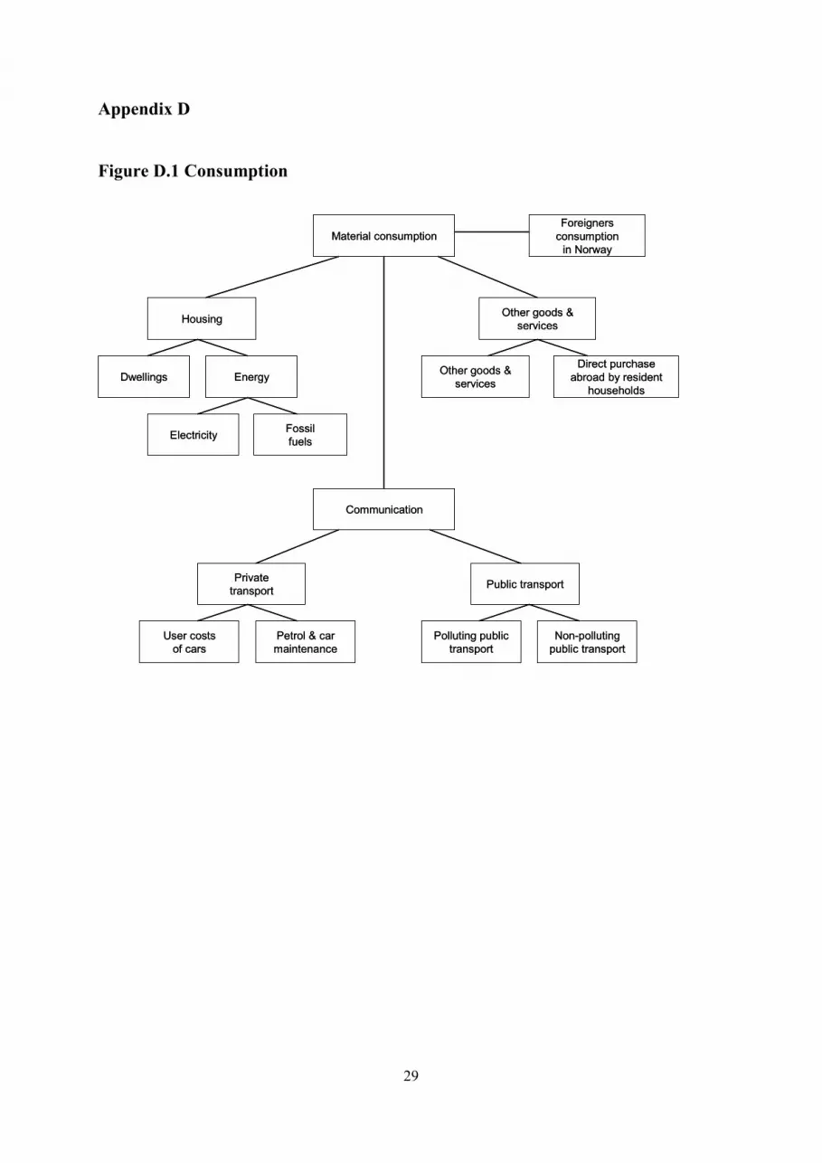
2.4 Consumer behavior Consumption and saving result from the decisions of a representative consumer with an infinite lifetime who maximizes intertemporal utility with perfect foresight. The consumer chooses a consumption path subject to an intertemporal budget constraint that requires the present value of consumption not to exceed total wealth (present non-human wealth plus the present value of labor income and net transfers). The labor supply is exogenous. We assume that the consumer’s rate of time preference equals the exogenously given nominal interest rate for the entire time path. Total consumption is allocated across 10 different goods and services according to a nested CES structure. The structure is given in Figure D.1, Appendix D.

2.5 Equilibrium conditions The model is characterized by equilibrium in each period in all product markets and the labor market. It also incorporates a detailed account of the revenues and expenditures of the government. The government produces services and purchases intermediates from the industries and abroad. Changes in government budgets are neutralized by lump-sum transfers.

Intertemporal equilibrium requires fulfillment of two transversality conditions: the limits of the total discounted values of net foreign debt and real capital must both be zero. The model is characterized by a path-dependent balanced growth path solution (or steady-state solution). This implies that both the path and the long-run stationary solution differ between simulated scenarios.

2.6 Data and parameters The model is calibrated to the 2002 Norwegian National Accounts. The elasticity of substitution between the different capital varieties is assumed to be 5.0, giving a markup factor of 1.25 for the domestic price of capital varieties.12 The elasticity of scale related to previous knowledge is equal to 0.4, in order to ensure decreasing spillover effects of the knowledge base, supported by both theoretical and empirical findings (see Jones, 1995 and 1999; Leahy and Neary, 1999). See Appendix B.6 for an overview of elasticities of substitution and other parameter values.

11 The GHGs included in the model are: carbon dioxide, methane, nitrous oxide, sulfur hexafluoride, hydrofluorocarbons,

and perfluorocarbons. 12 This is in line with the Jones and Williams (2000) computations, which exclude creative destruction, similar to our model.

Numerical specifications of Romer’s Cobb–Douglas production functions, as in Diao et al. (1999) and Lin and Russo (2002), result in far larger markups. Markup factors of 1.25 are nevertheless in the upper bound of econometric estimates (Norrbin, 1993; Basu, 1996). Our motivation for staying in the upper bound area is the fact that the capital varieties represent a small share of machinery capital and, thus, of total inputs. This, in isolation, drives up the markups required to calibrate the model.

8

The technical parameters that calculate emissions from factor inputs and consumer activities are taken from Strøm (2007). Emissions are spread over industries and consumers in line with Strøm (2007), which gives total emissions from the Norwegian economy in 2002 corresponding to 56.1 million tonnes of CO2 equivalents.

In 2008, there is one gas power plant in operation and one under construction in the Norwegian economy.13 Several other plants are planned. Not one of these plants will initially incorporate CCS technology. However, the political majority in Norway have aspirational goals of gas power production with low GHG emissions. Therefore, the plants have timetables for the eventual full-scale extraction of CO2 14. These plans to implement CCS technology are joint projects with the government, energy producers, and potential suppliers of CCS technology. It is unclear how the costs of implementing and developing the technology will be shared between the parties.

To roughly reflect the Norwegian situation, the model is calibrated to include two 860 megawatt gas power plants, one with CCS and one without CCS. The production costs of gas power in our calibration are based on Statoil (2005).15 Basically, capital and operating costs are doubled for a CCS plant compared with a non-CCS plant, and the required gas input is about 20 percent larger for a CCS plant. See Appendix E for more information on costs and prices in the gas power industry.

The Norwegian National Accounts lack a good exposition of R&D costs and production, so we use specific R&D statistics. See Bye et al. (2008) for more details. The share of R&D targeting CCS technology is set to match the share of variant capital used by the gas power industry with CCS relative to the total production of capital variants in the economy.16

2.7 Business-as-usual path and balanced growth Along the business-as-usual path (BAU), the exogenous growth factors are assumed to grow at a constant rate. In most cases, rates are set in accordance with the average annual growth estimates in the baseline scenario of Norwegian Ministry of Finance (2004), which reports the government’s economic predictions until 2050. In the government’s evaluation, total factor productivity growth is entirely exogenous and valued at, on average, 1.0 percent annually. Our model distinguishes between exogenous and endogenous factor productivity components. In line with empirical findings (see, e.g., Coe and Helpman, 1995; Keller, 2004), we ascribe 90 percent of domestic total factor productivity growth to the exogenous diffusion of international technological change; the remaining 10 percent is the result of domestic R&D.17 The latter forms a basis for calibrating the 2002 level of knowledge,18 which, together with the 13 The plant in operation is at the Kårstø industrial facility; the one under construction is at Mongstad. In addition, gas power

is used in specific industries offshore and in processing. This power is geared toward processes in the industries, not the electricity market. In the model, this power production is not separated from the user industries.

14 CCS technology is planned to be operational by 2011 at Kårstø and 2014 at Mongstad. 15 Statoil (2005) bases costs on combined-cycle power plants with amine-based post-combustion separation of CO2. Reduced

energy efficiency, pipeline transport, and storage in geographic formations are included in the costs. 16 This R&D production, from the environmental R&D industry, is quite low in the base year, about US$35 million, and is in

line with information obtained from the Norwegian Research Council. 17 Ten percent from domestic R&D is in the lower bound of estimates for small, open countries like Norway. We have

chosen this lower-bound estimate because several mechanisms believed to drive domestic innovations are excluded from the model, like basic government research, endogenous education, learning-by-doing, and an extension of the direct absorptive capacity related to R&D.

18 The environmental knowledge stock is set so that it grows at the same rate as the general knowledge stock when the two gas power industries demand equal amounts of capital varieties. Since both knowledge stocks are indexed to unity in the base year, this means that an equal growth in the knowledge stocks gives the same productivity increase in the use of general and environmental capital variants. See Bye et al. (2008) for more details.

9

remaining parameters of the model, determines the productivity growth from domestic knowledge accumulation. The international nominal interest rate is 4 percent. All policy variables are constant in real terms at their 2002 levels.

In the long run, i.e., 60–70 years from now, the economy reaches stationary growth rates. The GDP grows by 1.5 percent annually; consumption grows 0.5 percentage points lower, as net exports are increasing more in this period. The 10 percent contribution from the endogenous productivity impact of domestic innovations requires a relatively strong growth in general R&D production and the generation of new general varieties: both grow about 3 percent annually.19

In the period up to 2070, the demand for electricity increases substantially. Most of this is covered by gas power without CCS. Gas power with CCS does not grow, as the production costs are relatively high when the carbon tax faced by the gas power industry without CCS is low. This leads to low demand for the environmental capital varieties, which again leads to low production in the environmental R&D industry. The low level of investment in environmental R&D yields poor productivity growth in the gas power industry with CCS, and increases the cost difference between power production with and without CCS. Note that gas power without CCS experiences the general productivity growth from general R&D, and that there is no spillover between general and environmental R&D in the model.

The uniform carbon tax replaces a variety of taxes on GHGs in the Norwegian economy. It is set at about US$16 per tonne of CO2 equivalents (US$16/tCO2) to replicate baseline emissions in 2002 of 56.1 million tonnes of CO2 equivalents. Emissions rise substantially through the period to 92.0 million tonnes in 2050 and 120.5 million tonnes in 2070. About 16 percent of the increase in emissions comes from the gas power industry.

3. Policy analyses and numerical results We explore how innovation incentives should be designed when future emissions are limited. The reason for subsidizing R&D comes from two distortions in the innovation markets. Firstly, there are knowledge spillovers in the production of patents. The production of patents contributes to the knowledge stock, which lowers the cost of future R&D. These knowledge spillovers are freely accessible to all R&D firms. Secondly, the capital variety producers engage in monopolistic competition, giving rise to the surplus appropriability problem. The capital variety firms are unable to appropriate the entire “consumer surplus” from the goods they sell. Thus, the price of patents facing the R&D firms is lower than the socially optimal price, since the former price is equal to the present discounted value of a capital variety firm holding a patent. 20

Rather than studying optimal policy directly, we focus on market responses to a set of policies. In particular, we study the timing and welfare impact of environmental R&D subsidies when the future price of carbon is high. To do that, we establish two carbon reduction regimes, one high and one low. The two regimes represent different carbon costs facing the economy through the carbon tax. We simulate several distinct innovation policy alternatives on the two reduction regimes. The focus is on the welfare gain from subsidies to 19 Eventually, in the distant future (after about 90 years), all exogenous and endogenous growth mechanisms are cut off. This

is technically motivated, in order to ensure that the economy is on a balanced growth path (steady state) and that this growth path satisfies the transversality conditions described in Section 2.5. The relative effects of the different policy analyses are independent of this assumption.

20 See Jones and Williams (2000).

10

the environmental R&D industry. The policy alternatives are constant innovation policy, falling innovation policy, and increasing innovation policy. In the simulations, all the policy alternatives are implemented through ad valorem subsidy rates to the R&D industry. To make the distinct policy alternatives comparable, the subsidy rates are dimensioned so that the present discounted values of the subsidies are equal. The public revenue annuity is approximately US$9 million, which is about one-fourth of the total environmental R&D effort by the R&D industry in 2002.

3.1 The carbon reduction regimes The carbon reduction regimes give two different paths for the costs of emissions. In the high carbon reduction regime, we impose a carbon tax that corresponds to a 25 percent reduction in national GHG emissions by 2050, compared with BAU. In the low carbon reduction regime, the carbon tax is lower and corresponds to a 15 percent reduction. We implement this by a linear increase of the carbon tax until it reaches a stable level in 2050. The carbon tax starts at the BAU level in 2002, i.e., US$16/tCO2, and increases to about US$140/tCO2 in 2050 in the high carbon reduction regime, and about US$68/tCO2 in the low carbon reduction regime. For the rest of the simulated period, the tax is kept constant. The carbon tax is a first-best policy instrument to achieve the emissions reductions, i.e., it does not target any other market failures. The carbon tax is not under the influence of policy makers when innovation policy is decided; underinvestment in R&D is addressed solely through the R&D subsidies. All other exogenous inputs are the same as in BAU.

Domestic emissions reductions can be achieved through factor substitution, emission abatement in gas power production (by CCS), or by general factor productivity growth. CCS is the only abatement technology available in the power market in this study, and we do not include other specific energy-saving technological changes, such as low-emissions vehicles or increased energy efficiency in buildings.

The long-run effects of the carbon reduction regimes, measured as percentage deviations from BAU, are given in Table 1.

11

Table 1: Long-run effects of the carbon reduction regimes, given as percentage deviations from the BAU path in 2070.

Carbon reduction regime → High carbon reduction regime

Low carbon reduction regime

Emissions reduction in 2050 25 15

GHG emissions in 2050 in actual millions of tonnes of CO2 equivalents

69.0* 78.2*

Production of general patents 16.2 7.3

Production of environmental patents 84.6 54.5

General knowledge stock 6.9 3.1

Environmental knowledge stock 22.0 15.0

Production of general capital varieties 6.41 2.8

Production of environmental capital varieties

36.6 25.8

Production of gas power without CCS –99.3 –74.3

Production of gas power with CCS 53.3 46.2

Production of main final goods –0.207 –0.035

Production of power-intensive goods –37.6 –19.8

Nominal wage rate –1.6 –0.8

Gross domestic product (GDP)21 –0.095 –0.077

Welfare22 –0.058 –0.015

CO2 tax, actual value in US$/tCO2 140† 68†

*Millions of tonnes of CO2 equivalents; †Value in US$/tCO2.

21 This includes returns from the factors labor, capital, and knowledge, and excludes exogenous, offshore petroleum

production. 22 Welfare is measured as the present value of utility in the period 2002–2070.

12

As the carbon tax increases, gas power production uses more CCS technology. The demand for environmental R&D investment increases, improving the productivity growth in the CCS power industry. However, the total costs of electricity production increase since the carbon tax increases costs for gas power production without CCS. This leads to a reduction in the production of electricity. The carbon tax paid on emissions combined with the increased price of electricity induces a fall in the power-intensive sector. This frees resources in the economy like labor and capital goods, and so labor costs decrease. The total effect of the higher carbon tax and changed input costs differs between industries, depending on their carbon and energy intensities. Both R&D industries and capital variety industries experience reduced costs, and the production of patents and capital varieties increase. This yields productivity gains through an increased level of technology and contributes to offset some of the overall costs of the carbon tax. Production in the main final goods industry is almost unchanged from BAU. Both the welfare and GDP reductions from the emissions reductions are modest.

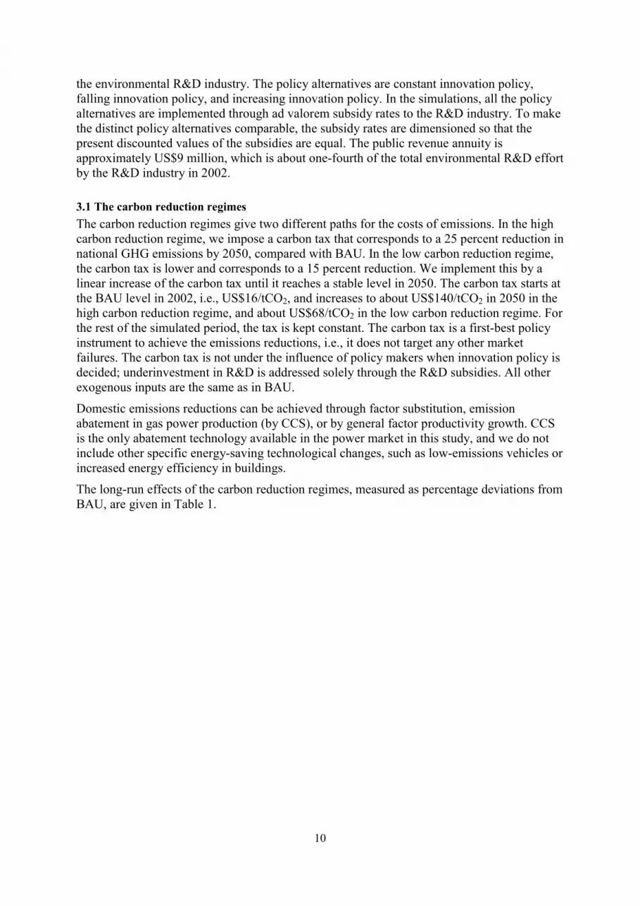
3.2 The innovation policy alternatives We implement three different innovation policy alternatives for each of the carbon reduction regimes. The alternatives are all subsidies for environmental R&D, but with constant, falling, or increasing time profiles on the subsidy rates. The carbon tax does not change between the subsidy alternatives. We do this in order to analyze the effect of different subsidy policies given a set carbon price, e.g., determined in an international carbon market.23 The long-run effects, measured as percentage changes caused by the innovation policies in the high and low carbon reduction regimes, are given in Table 2.

23 In the results reported, the carbon tax is not changed when environmental R&D is subsidized. This leads to a change in the

carbon emissions when the policy alternatives are implemented. We have done similar simulations where we keep emissions constant so that the carbon tax changes when the innovation policy alternatives are implemented. This does not change any of our results. See Appendix F, Table F.2.

13

Table 2: Long-run effects of different time profiles for environmental R&D subsidy rates, given as percentage changes for each carbon reduction regime in 2070.

Innovation policy Constant Falling Increasing

Carbon reduction regime → High Low High Low High Low

Production of general patents –0.8 –0.8 –0.7 –0.7 –0.8 –0.8

Production of environmental patents 188.5 202.1 166.3 160.8 174.0 190.0

General knowledge stock –0.3 –0.3 –0.3 –0.3 –0.2 –0.2

Environmental knowledge stock 61.4 63.7 71.0 69.0 43.8 47.1

Production of general capital varieties –0.3 –0.3 –0.3 –0.3 –0.3 –0.3

Production of environmental capital varieties

58.6 60.9 66.1 64.3 43.3 46.7

Production of gas power without CCS –9.6 –4.2 –10.9 –4.6 –7.1 –3.2

Production of gas power with CCS 5.8 6.6 6.6 7.2 4.2 5.0

Production of main final goods –0.02 –0.02 –0.02 –0.02 –0.02 –0.02

Production of power-intensive goods 0.27 0.21 0.32 0.24 0.20 0.15

Nominal wage rate 0.04 0.03 0.04 0.03 0.03 0.03

Electricity price –1.01 –0.77 –1.15 –0.84 –0.74 –0.59

GDP 0.057 0.053 0.064 0.055 0.041 0.040

Welfare 0.0303 0.0266 0.0327 0.0273 0.0242 0.0218

14

3.2.1 The constant innovation policy We first consider the case with a constant subsidy rate.24 The reported results are for the long run and relative to the two carbon reduction regimes without subsidies for environmental R&D.

Effects on production The subsidy given to producers of new patents in the environmental R&D industry pushes down the marginal costs of environmental R&D production. For a given patent price, supply increases, and for the environmental capital-variety industry to be able to absorb more patents, the price of patents must fall. The marginal willingness to pay for patents is determined by the discounted profit for the last new firm entering the capital industry. More patents in the industry means more firms. As a result, production by each firm falls as a proportion of the given total industry production, and thus individual firm profits fall. The marginal costs of the environmental R&D firms will be further shifted downward because of dynamic, positive spillover effects from the accumulated environmental knowledge stock, and this reinforces the partial market dynamics. In the long-run equilibrium, the environmental R&D production more or less triples. The number of patents, and thus the environmental knowledge stock, also increases considerably.

In the market for CCS variety-capital, the demand faced by each variety firm shifts downward as the number of varieties increases. This reduces both the markup price and the domestic production of each variety. The increased number of patents for CCS technology will increase the efficiency of using the capital composite. This love of capital variety in the gas power industry with CCS, combined with the price effect, increases the overall demand for environmental capital varieties.

Improvement in CCS technology decreases the costs of gas power production with CCS, and the production increases. Gas power production without CCS decreases from the already-low level because of the carbon tax. The total effect is that overall gas power production increases, and the electricity price falls.

Reallocation and welfare The results reported above are influenced by indirect changes in all factor markets. The R&D subsidy increases demand in both the environmental R&D industry and the environmental variety-capital industry for other inputs, like labor, intermediates, and other investment goods. Combined with higher final consumption, this contributes to a rise in all factor prices except variety capital and electricity. The power-intensive industry benefits strongly from a decrease in the costs of power production and increases its production. For most of the remaining industries, the unit costs of production increase, and production falls in both the short and long run. This includes the general R&D industry, since production here uses the same factor inputs as the subsidized environmental R&D industry. Thus, general R&D is affected worse than other industries by the expansion of environmental R&D. In both carbon reduction regimes, general R&D falls by 0.8 percent, while the large main final goods industry falls only marginally. General capital variety production is also reduced and the general knowledge stock is lowered. The total effect on the economy is a GDP increase of 0.05–0.06 percent.

Welfare increases by 0.030 and 0.027 percent in the high and low carbon reduction regimes, respectively. Welfare increases because the subsidy for environmental R&D targets

24 All subsidies are phased out in 2090, at the same time the endogenous growth mechanism is turned off.

15

externalities connected to knowledge spillovers and the surplus appropriability problem. The main contributions to welfare gain in our model come from increased environmental R&D and environmental variety-capital production through two channels: the positive spillover effect in patent production of a larger environmental knowledge stock, and the positive love-of-variety effect in the demand for variety capital as the number of capital varieties increases. These are counteracted by two negative effects: the welfare loss through lower production within each monopoly firm producing capital varieties, and the negative contribution from higher overall fixed entry costs in terms of patent expenditures.

The welfare increase is larger in the high carbon reduction regime than in the low one. This indicates that higher costs of emissions, through a higher carbon tax, lead to larger innovation externalities. Larger externalities imply that the underinvestment in environmental R&D increases, and so the subsidy for environmental R&D gives a greater welfare gain (see the discussion in Section 3.3).

3.2.2 The falling innovation policy To analyze the effect of the time profile of subsidies, we next consider a falling subsidy for environmental R&D production in the two carbon reduction regimes. The subsidy rate is high in the first years and decreases linearly until it ceases in 2090. The present value of government spending on innovation policy is the same in all the three innovation policy alternatives.

The subsidy increases long-run environmental R&D production considerably, but not as much as in the constant innovation policy alternative. The reason is that in the latter, the long-run subsidy rate for environmental R&D is considerably higher. Halfway through the study period, however, the increase in environmental R&D production is larger under the falling innovation policy than the constant innovation policy, so the environmental knowledge stock is developed earlier. Under the falling innovation policy, the long-run environmental knowledge stock increases by about 70 percent in both carbon reduction regimes. The production of environmental capital varieties increases by about 65 percent. Both these increases are larger than those under the constant innovation policy. By having larger subsidies early on, the technology is more rapidly developed and the costs of producing patents in later periods are more greatly reduced through the spillover effect.

The total effect on the economy is a GDP increase of about 0.06 percent. Welfare increases by 0.033 and 0.027 percent in the high and low carbon reduction regimes, respectively. Both GDP and welfare increase slightly more with falling subsidies than with constant subsidies for a given carbon reduction regime. The reason for this is that the innovation externalities are large in early periods. This means that underinvestment in environmental R&D is larger in early periods (see the discussion in Section 3.3).

3.2.3 The increasing innovation policy Finally, we consider an increasing time profile for environmental R&D subsidies in the two carbon reduction regimes. The subsidy rate is low in the early years and then increases linearly throughout time. As with the other innovation policies, the subsidy ceases in 2090.

The long-run increase in environmental R&D production lies between the increases for the constant innovation and falling innovation policies. The environmental knowledge stock, however, is lowest for the increasing innovation policy, with an increase of less than 50 percent. Because of a slower start, the environmental knowledge stock is not as rapidly developed, and the costs of environmental R&D production stay higher throughout the study

16

period. Smaller spillovers lead to slower accumulation of patents and higher costs for power production with CCS technology.

The total effect on the economy is a GDP increase of about 0.04 percent. Welfare increases by 0.024 and 0.022 percent in the high and low carbon reduction regimes, respectively. Both GDP and welfare increase less with increasing subsidies than with falling or constant subsidies. The reason for this is that an increasing subsidy rate fails to correct for the underinvestment in environmental R&D in early periods.

3.3 Comparison of the policy alternatives in the different emissions reduction regimes An R&D subsidy to increase innovations is intended to correct for underinvestment in R&D originating from innovation externalities.25 A carbon tax above the marginal costs of emissions could also target underinvestment in R&D. This is not the case in our study, as the carbon tax only represents the marginal costs of emissions for the economy and does not target innovation externalities. The carbon tax may, however, influence the underinvestment in environmental R&D through its effect on the demand for clean gas power technology. The level of welfare gain from R&D subsidies is not the same for the two emissions reduction regimes. This indicates that underinvestment in R&D does not stay the same for different carbon tax levels.

R&D induced by a subsidy gives a higher welfare gain for the economy when the initial underinvestment in R&D is large. In stating this, we have implicitly assumed that the economy gets more welfare out of correcting for the first dollar of a large underinvestment than from the first dollar of a small underinvestment. In other words, the marginal social returns from R&D investments increase with the level of underinvestment. The welfare gains from the innovation policy alternatives in the two carbon reduction regimes are given in Figure 1.

Figure 1: Welfare effects of innovation policy alternatives, measured as percentage changes for each carbon reduction regime.

0

0,005

0,01

0,015

0,02

0,025

0,03

0,035

High reductionregime

Low reductionregime

Falling innovationpolicyConstant innovationpolicyIncreasing innovationpolicy

25 When the social (welfare) optimal level of investment is greater than the actual private investment, the difference is called

“underinvestment”. In this context, we mean by investment the actual dollars invested (or not) in a particular year of the

17

We see that the welfare changes are larger in the high carbon reduction regime than in the low carbon reduction regime for a given innovation policy. The differences in welfare gain from introducing the subsidies stem from differences in underinvestment in environmental R&D. This means that it is more important to subsidize the environmental R&D industry when the costs of emissions, through the carbon tax, are higher. This leads to the first result:

Result 1: The welfare gain from subsidizing environmental R&D increases with the costs of emissions, since the level of underinvestment increases with the carbon tax. The underinvestment increases because a higher carbon tax means larger returns from carbon-saving technology that are not internalized fully by the private R&D firms. One of the reasons for the underinvestment is knowledge spillovers from environmental R&D. When the carbon tax is higher, the value of gas power production with CCS goes up relative to production in other sectors. This increases demand for CCS technology, which again increases demand for environmental R&D. The individual R&D firms do not take into account that their activity reduces the costs of future R&D. Thus, the increased investment in R&D under a high carbon tax because of stronger demand is lower than the increase in the social optimal investment level.

Another reason for the underinvestment is that the environmental capital varieties producing firms do not take into account the full value of the carbon-saving technology for the gas power industry. Since the environmental capital varieties producers cannot reap the full benefit from the increasing number of varieties through the love-of-variety effect in the CCS gas power industry, the price of patents does not reflect the full value of ideas. This surplus appropriability problem is larger when the carbon tax is higher, since a higher tax increases the value of abatement technology. The effects from both the surplus appropriability and the knowledge spillovers mean that the higher carbon tax results in increased social returns from environmental R&D. These are not fully covered by an increase in the private returns from R&D. Thus, the underinvestment in environmental R&D increases.

In both carbon reduction regimes, the level of welfare is higher for the falling innovation policy than for the other policies. This indicates that the underinvestment in environmental R&D decreases over time, since a subsidy gives a larger welfare gain when the underinvestment is larger. This leads to the second result:

Result 2: There is a greater welfare gain from a falling time profile of subsidy rates for environmental R&D than from constant or increasing time profiles when the economy faces increased emissions costs. This is because the level of underinvestment is larger in the beginning of the period than the end. The reason for this time difference in underinvestment is that the knowledge externalities from R&D are largest in early periods. There are two explanations for this. Firstly, early R&D investments contribute over a longer time period. In other words, knowledge generated early spills over to a larger number of later periods, compared with knowledge generated later. These spillovers are ignored by the private firms, and therefore the underinvestment is larger in early time periods. Secondly, there is a declining increase in the benefit from new ideas (i.e., concave curves) in both the R&D production function and the love-of-variety component. This means that R&D activity has a larger impact on the economy when the knowledge stock is small. As the knowledge stock grows over time, there are fewer spillovers

model. The social and private levels of investment in a year depend on the rates of return on the investment. In this study, we do not measure relative rates of return, only the absolute levels of underinvestment.

18

and productivity gains from new ideas. Thus, the innovation externalities are smaller in the later periods and the underinvestment is falling over time.

However, the welfare gain from a falling time profile of subsidies compared with constant subsidies is larger in the high carbon reduction regime than in the low carbon reduction regime. Combining results 1 and 2 explains this. Result 1 implies that the value of spillovers from investments in all periods increases with the carbon tax level. Result 2 implies that early investments yield spillovers over more periods than later investments do, and therefore the total value of spillovers from early investments increases more compared with that from later investments when the carbon tax increases. This is why the time difference in underinvestment is larger when the carbon tax is higher.

3.5 Sensitivity analyses In the carbon reduction regimes, the emissions are restricted through a carbon tax that increases over time. To analyze whether this is a driving mechanism for our result regarding the timing of subsidies for environmental R&D, we construct a carbon tax regime with a constant carbon tax. The carbon tax is imposed on the BAU path in the first year of simulation and kept constant throughout the simulation period. The constant carbon tax is the same as the average tax in the high carbon reduction regime and gives approximately the same accumulated emissions reduction. The welfare gain from environmental R&D subsidies are 0.030 percent for the constant innovation policy, 0.032 percent for the falling innovation policy, and 0.024 percent for the increasing innovation policy. The ranking of the innovation policy alternatives does not change when the carbon tax is constant. Hence, we conclude that it is the overall carbon tax level and not the time profile of the tax that is the driving mechanism for our results.26

4. Concluding remarks Facing higher costs of GHG emissions, an important policy question is how to stimulate innovation in environmental R&D. Stimulation of innovation gives welfare gains, since private firms do not reap the full benefits of their R&D activities. An appropriate policy instrument to correct for the externalities in innovation is an R&D subsidy. We ask whether the benefits of such a subsidy are influenced by the costs of emissions, and whether environmental R&D should be subsidized more heavily in early periods. We find two results that point toward a specific policy on environmental R&D. Firstly, the welfare gain from subsidizing environmental R&D increases with the costs of emissions. This means that when the price of carbon increases, e.g., through international carbon markets or domestic reduction programs, it is more important to have an active innovation policy to promote environmental R&D. The reason for this is that the carbon tax increase raises the social (efficient) investment level in environmental R&D that is not fully covered by an increase in private investment in R&D because of externalities in the innovation process. Secondly, the welfare gain is greatest from a falling time profile of subsidy rates for environmental R&D, rather than a constant or increasing profile, when the economy faces increased emissions costs. This means that when faced with a future price on carbon, it is a better policy to take R&D action now than to distribute policy incentives evenly across time. The reason for this is that the innovation externalities are larger in early periods.

26 See Appendix F, Table F.1.

19

Further research is needed to analyze the mechanisms that influence the interaction between the carbon tax and underinvestment in environmental R&D, both theoretical and empirical. Specifically, it may be fruitful to research optimal subsidy profiles in theoretical models under different carbon tax scenarios, with a focus on the development of social and private rates of return from R&D. The maturity of different technologies may also be interesting to explore. It may be that new technologies have larger knowledge spillovers than older technologies, where most advances have already been exploited. This would give another argument for an active R&D policy toward new environmental technologies.

There is potential to add to the model many new features that are empirically significant and relevant to the effects of innovation policies. First of all, the modeling of knowledge spillovers may be made richer. Including spillovers between general technological development and the specific environmental technological development could diminish the gains from early subsidies to environmental R&D, as the technology would benefit from early increases in the general knowledge stock. Linking domestic R&D to the absorption capacity for international knowledge spillovers could increase the gains from R&D and amplify the effects of the subsidy alternatives. On the other hand, the foreign technological change in environmental technology may be as large as, or larger than, the domestic, which would offset some of the gain from engaging in domestic environmental R&D early. Further, the assumptions about labor supply have crucial implications for innovation policies. The present model assumes one national labor market with exogenous, unaltered labor supply across all the policy alternatives. The welfare potential of innovation policy is restricted by limited resources, in particular the inflexible labor resources. Expansion of the R&D industries is likely to attract mainly high-skilled labor. In reality, therefore, the allocation effect of increasing innovation in one R&D industry would be to crowd out the other R&D industries even more than in the present framework.

References Basu, S. (1996): Procyclical Productivity: Increasing Returns to Cyclical Utilization? Quarterly Journal of Economics, 111, 709–751.

Bye, B., Fæhn, T. and Heggedal, T.R. (2007): Welfare and growth impacts of innovation policies in a small, open economy: An applied general equilibrium analysis, Discussion Paper 510, Statistics Norway.

Bye, B., Heggedal, T.R, Jacobsen, K., Fæhn, T. and Strøm, B. (2008): A CGE model of directed technological change and carbon emissions: A detailed model description, Documents 2008/xx, Statistics Norway.

Coe, D.T. and Helpman, E. (1995): International R&D spillovers, European Economic Review, 39, 859–887.

Diao, X., Roe, T. and Yeldan, E. (1999): Strategic policies and growth: An applied model of R&D-driven endogenous growth, Journal of Development Economics, 60, 343–380.

Fischer, C. and Newell, R.G. (2008): Environmental and Technology Policies for Climate Mitigation, Journal of Environmental Economics and Management, 55, 142–162.

Gerlagh, R., Kverndokk, S. and Rosendahl, K.E. (2008): Linking Environmental and Innovation Policy? Presented at the Norwegian Annual Economist Meeting – January 2008.

20

Gillingham, K., Newell, R.G. and Pizer, W.A. (2007): Modeling Endogenous Technological Change for Climate Policy Analysis, Discussion Paper 07-14, Resources for the Future, Washington D.C.

Goulder, L.H. and Mathai, K. (2000): Optimal CO2 Abatement in the Presence of Induced Technological Change, Journal of Environmental Economics and Management, 39, 1–38.

Goulder, L.H. and Schneider, S.H. (1999): Induced technological change and the attractiveness of CO2 abatement policies, Resource and Energy Economics, 21, 211–253.

Greaker, M. and Rosendahl, K.E. (2006): Strategic Climate Policy in Small, Open Economies, Discussion Paper 448, Statistics Norway.

Hart, R. (2008): The timing of taxes on CO2 emissions when technological change is endogenous, Journal of Environmental Economics and Management, 55, 194–212.

Jaffe, A.B., Newell, R.G. and Stavins, R.N. (2005): A Tale of Two Market Failures: Technology and Environmental Policy, Ecological Economics, 54, 164–174.

Jones, C.I. (1995): R&D-based models of economic growth, Journal of Political Economy 193, 759–84.

Jones, C.I. (1999): Growth: With or Without Scale Effects, The American Economic Review, 89, 139–144.

Jones, C. I. and Williams, J.C. (2000): Too Much of a Good Thing? The Economics of Investment in R&D, Journal of Economic Growth, 5, 65–85.

Keller, W. (2004): International Technology Diffusion, Journal of Economic Literature, XLII, 752–782.

Kverndokk, S. and Rosendahl, K.E. (2007): Climate policies and learning by doing: Impacts and timing of technology subsidies, Resource and Energy Economics, 29, 58–82.

Leahy, D. and Neary, J.P. (1999): R&D spillovers and the case for industrial policy in an open economy, Oxford Economic Papers, 51, 40–59.

Lin, H.C. and Russo, B. (2002): Growth Effects of Capital Income Taxes: How much does Endogenous Innovation Matter? Journal of Public Economic Theory, 4, 613–640.

Nordhaus, W.D. (2002): Modeling induced innovation in climate-change policy, in Technological Change and the Environment, Narkicenovic, N. Grubler, A. and Nordhaus, W.D. (Eds.), Washington, Resources for the Future.

Norrbin, S.C. (1993): The Relationship Between Price and Marginal Cost in U.S. Industry: A Contradiction, Journal of Political Economy, 101, 1149–1164.

Norwegian Ministry of Finance (2004): Perspektivmeldingen 2004 – utfordringer og valgmuligheter for norsk økonomi (Perspectives 2004 – challenges and options for the Norwegian economy), Stortingsmelding. no. 8. Otto, V.M., Löschel, A. and Reilly, J. (2006): Directed Technical Change and Climate Policy, FEEM Nota Di Lavoro 81 – 2006.

Otto, V.M. and Reilly, J. (2006): Directed Technical Change and the Adoption of CO2 Abatement Technology, MIT Joint Program on the Science and Policy of Global Change, Report No 139 – 2006.

21

Parry, I.W.H. (1995): Optimal Pollution Taxes and Endogenous Technological Progress, Resource and Energy Economics, 17, 69–85.

Parry, I.W.H., Pizer, W.A. and Fischer, C. (2003): How Important is Technological Innovation in Protecting the Environment? Journal of Regulatory Economics, 23, 237–255.

Popp, D. (2006): R&D Subsidies and Climate Policy: Is There a ‘Free Lunch’? Climatic Change, 77, 311-341.

Romer, P. (1990): Endogenous Technological Change, Journal of Political Economy, 94, 1002–1037.

Rosendahl, K.E. (2004): Cost-effective environmental policy: implications of induced technological change, Journal of Environmental Economics and Management, 48, 1099–1121.

Schneider, S.H. and Goulder, L.H. (1997): Achieving low-cost emissions targets, Nature, 389, 13–14.

Statoil (2005): Tillegg til konsekvensutredning for utvidelse av metanolfabrikk og bygging av gasskraftverk på Tjeldbergodden (Addition to report on expansion of methanol factory and construction of gas power plant on Tjeldbergrodden), www.nve.no/admin/FileArchive/311/200401582_36.pdf. Strøm, B. (2007): Utslippsregnskap 1990–2004: Etablering av datagrunnlag for likevektsmodeller (Emissions account 1990–2004: Establishment of data for general equilibrium models), Teknisk dokumentasjon, Notater 2007/13, Statistics Norway.

22

Appendix A

Table A.1: Production sectors in the model ITC Code Production Sectors

20 Other commodities and services 30 Power-intensive industry 32 Polluting transport 33 Non-polluting transport

38G General research and development (R&D) 38E Energy research and development (R&D) 40 Refining

46G General machinery varieties 46E Energy machinery varieties 47 Other machinery 50 Ships, oil rigs, and oil-production platforms 55 Construction, excl. oil-well drilling 60 Ocean transport, and oil and gas exploration and drilling

701 Electricity from hydropower 704 Electricity from gas power without CCS 705 Electricity from gas power with CCS 74 Transmission and distribution of electricity 83 Building services 90 Central and local government

23

Appendix B

The model structure of firm and household behavior

When firm notation i is suppressed, all variables in the equation apply to firm i. Subscripts denoting industry are also suppressed for most variables. Subscripts 0, -1, or t denote periods. When period specification is absent, all variables apply to the same period. In consumption, i denotes good i, and j denotes CES composite j.

B.1 Production of final goods

(B.1) ( ) ( ) 000

0 KPdtKPedtJPePV Jtt

Ktt

rtt

Jtt

rt +−=−= ∫∫∞

−∞

− ππ

(B.2) wLXPXP WWHH −+=π

(B.3) ( ) ( )[ ] ( )[ ]sWH KLfXX ττθθθ ,1

=+

(B.4) ( ) ( ) ⎥⎦

⎤⎢⎣

⎡+= sHsW XXcC

11

(B.5) ( ) ( ) sWWWsHHH XcXPXcXP11

' −+−=π

(B.6) ( ) ss

HH XscP

−

=1

(B.7) ( ) ss

WW XscP

−

=1

(B.8) θ/1=s

(B.9) ( ) ( )

( ) ( )⎟⎠⎞⎜

⎝⎛

−⎟⎠⎞⎜

⎝⎛ −⎟

⎠⎞⎜

⎝⎛ −

⎥⎥⎥

⎦

⎤

⎢⎢⎢

⎣

⎡

⎟⎟⎠

⎞⎜⎜⎝

⎛−

−+⎟⎟⎠

⎞⎜⎜⎝

⎛=

11)1(

11

kk

kk

kM

VkM

kk

kM

MkM

KKK

σσ

σσ

σσ

δδ

δδ

(B.10) ( )( ) ( )1

1

1 −

=

−

⎥⎦

⎤⎢⎣

⎡= ∫

kvkv

kvkv

R

iViV diKK

σσ

σσ

B.2 Production of ideas The two R&D industries, general and environmental, are not separated in this exposition. This is because the two industries work the same way. The same applies to the variety-capital industries below. Equations (B.1) and (B.8) apply to firms within the R&D industries. In addition, the following structure describes the industries: (B.2') wLXP H

RHR −=π

(B.3') [ ] ( )[ ]sM

sHR KLfRX ττ ,1=

(B.4') [ ] sHR

ss X

R

cC /1

1

)(=

24

(B.11) HRXRR += −1

(B.5') ( ) sHR

ss

HR

HR X

R

cXP1

1

)(' −=π

(B.6') ( ) ss

HR

ss

HR X

Rs

cP−

=1

1

)(

B.3 Production of capital varieties For firms producing capital varieties, Eq. (B.2) applies, in addition to the following:

(B.1'') ( ) 0000

0 iJH

RitK

titrt

i KPPdtKPePV +−−= ∫∞

− π

(B.3'') ( ) ( )[ ] ( )[ ]sMii

Wki

Hki KLfXX ττθθθ ,

1

=+

(B.4'') ( ) ( ) ⎥⎦

⎤⎢⎣

⎡+= sH

kisW

kii XXcC11

(B.5'') ( ) ( ) ( ) sWki

Wki

Wk

sHki

Hki

Hki

Hkii XcXPXcXXP

11' −+−=π

(B.6'') ( ) ss

Hkiki

Hki X

scmP

−

=1

(B.12) Hki

Hki

Hki

Hki

ki XP

PX

∂

∂−=ε

(B.13) 11 −

=−

=kv

kv

ki

kikim

σσ

εε

(B.7'') ( ) ss

Wki

Wk X

scP

−

=1

(B.14) ( )( )( )kv

kv diPPR

ikvikv

σσ

−

=

−⎥⎦

⎤⎢⎣

⎡= ∫

11

1

1

(B.15) ( )dteP itrtH

R ∫∞

−=0

0 'π

B.4 Consumer behavior

(B.16) ( ) dteduU tt

ρ−∞

∫=0

0

(B.17) ⎟⎟⎠

⎞⎜⎜⎝

⎛ −

−= d

d

ddud

dt

σσ

σσ

1

1)(

(B.18) dtedPDW rttt

−∞

∫=0

0

(B.19) [ ] dtt PDd σλ −⋅=

25

(B.20) ttt ndD )1( +=

(B.21) jt

jtj

it

jtiit PD

VDPDPD

Dσ

ω ⎟⎟⎠

⎞⎜⎜⎝

⎛= 0.

(B.22) ( )( )s

t

t gnD

D++=+ 111

B.5 Variable list 0PV The present value of the representative firm

π Operating profit JP Price index of the investment good composite

J Gross investment KP User cost index of capital composite

K Capital composite XH Output of final good firm delivered to the domestic market XW Output of final good firm delivered to the export market PH Domestic market price index of final good PW World market price index of final good W Wage rate L Labor

VK Variety capital MK Other ordinary capital

C The variable cost function c Price index of the CES-aggregate of production factors

'π Modified profit kMδ Share of other ordinary capital in the capital composite

R Accumulated number of capital varieties (and of firms and patents) HRX Production of new ideas ViK Capital variety i

kviP User cost index of capital variety i H

RP Price index of the patent HkiX Output of variety firm i delivered to the domestic market WkiX Output of variety firm i delivered to the export market H

kiP Domestic market price index of variety i WkP World market price index of varieties

Pkv User cost index of the variety-capital composite 0U Discounted period utilities of a representative consumer

d Consumption of a representative consumer PD Consumer price index W0 Consumer’s current non-human wealth + present value of labor income + net transfers λ Marginal utility of wealth D Aggregate consumption n Annual population growth rate Di Demand for consumer good i VDj Aggregate expenditure on CES aggregate j

0.iω Budget share of good i in CES aggregate j in period 0 gs Growth rate

26

B.6 Parameter list τ =0.009 Factor productivity change through international spillovers s=0.83 Scale elasticity θ=1.2 Transformation parameter between deliveries to the domestic and the foreign market σc=1.5 Elasticity of substitution between variety-capital and other ordinary capital σkv=5 Uniform elasticity of substitution applying to all pairs of capital varieties s1=0.4 Elasticity of domestic spillovers, j=G, E

kim =1.25 Markup factor for variety firm i ρ=0.04 Consumer’s rate of time preferences σd=0.3 Intertemporal elasticity of substitution σ=0.5 Elasticity of substitution between the two consumer goods

27

Appendix C

Figure C.1: The nested structure of the production technologies

GrossProduction

(X)

VariableInput(VF)

OtherInput(S)

Buildingsand Constructions

(KB)

Various MaterialInputs

(V)

Modified RealValue Added

(RT)

Labour and Machinery Serv.

(R)

TransportServices

(T)

PollutingTransport

(P)

Non-PollutingTransport

(TN)

MachineryServices

(N)

Labour(L)

PollutingCommercial

Transport (TP)

OwnTransport

(O)

Machinery(K)

Energy(U)

Electricity(E)

FossilFuels(F)

Transport Oiland Gasoline

(FT)

TransportEquipment

(KT)

CapitalVarieties

(KV)

OtherMachinery

(KO)

Varieties(KV1, ..., KvR)

28

Figure C.2: The nested structure of the production technologies for the gas power sectors

GrossProduction

(X)

VariableInput(VF)

OtherInput(S)

Buildingsand Constructions

(KB)

Various MaterialInputs

(V)

Modified RealValue Added

(RT)

Labor and Machinery Serv.

(R)

TransportServices

(T)

PollutingTransport

(P)

Non-PollutingTransport

(TN)

MachineryServices

(N)

Labor(L)

PollutingCommercial

Transport (TP)

OwnTransport

(O)

CapitalGas(KG)

Energy(U)

Electricity(E)

FossilFuels

(F)

Transport Oiland Gasoline

(FT)

TransportEquipment

(KT)

Gas Pipes(GP)

Gas Transport

(TG)

Varieties(KV1, ..., KvR)

NaturalGas (NG)

Machinery(KM)

CapitalVarieties(KMV)

OtherMachinery

(KMO)

29

Appendix D

Figure D.1 Consumption

Material consumption

Communication

Housing

Dwellings Energy

Electricity Fossilfuels

Other goods & services

Other goods & services

Direct purchaseabroad by resident

households

Privatetransport

User costsof cars

Petrol & carmaintenance

Public transport

Polluting publictransport

Non-polluting public transport

Foreigners consumption

in NorwayMaterial consumption

Communication

Housing

Dwellings Energy

Electricity Fossilfuels

Other goods & services

Other goods & services

Direct purchaseabroad by resident

households

Privatetransport

User costsof cars

Petrol & carmaintenance

Public transport

Polluting publictransport

Non-polluting public transport

Foreigners consumption

in Norway

30

Appendix E

The price of electricity from the gas power producers The cost structure in the model gives a producer price of electricity delivered from the CCS gas power industry of US$0.075/kWh in 2002. From the gas power industry without CCS the price is US$0.047/kWh. The producer base price of electricity delivered to the market in the calibrated year is US$0.03/kWh. So to keep production levels in the gas power industries at the calibrated level, their producer prices are subsidized in 2002 with US$0.045/kWh and US$0.017/kWh for production with and without CCS, respectively. These subsidies are phased out during the first 10 years. As the demand for electricity increases in this period, the gas power industries manage to produce without subsidies at the end of the period.

The costs presented here are sensitive to the price of gas. The model is calibrated to a gas price of US$0.15/m3 in 2002. For a higher gas price, both gas power industries face higher costs; however, the cost difference between the industries is smaller for a higher gas price, since the gas factor input share is smaller for the CCS plants.

31

Appendix F

Table F.1 Constant carbon tax regime Table F.1: Long-run effects of different time profiles of subsidies for environmental R&D, given as percentage changes from the constant carbon tax regime in 2070:

Innovation policy Constant Falling Increasing

Production of general patents –0.8 –0.7 –0.8

Production of environmental patents 187.6 164.8 173.6

General knowledge stock –0.3 –0.3 –0.2

Environmental knowledge stock 38.4 70.5 43.7

Production of general capital varieties –0.3 –0.3 –0.3

Production of environmental capital varieties

58.4 65.6 43.2

Production of gas power without CCS –9.5 –10.8 –7.1

Production of gas power with CCS 5.8 6.6 4.2

Production of main final goods –0.02 –0.02 –0.02

Production of power-intensive goods 0.27 0.45 0.20

Nominal wage rate 0.04 0.04 0.03

Electricity price –1.00 –1.15 –0.74

GDP 0.056 0.063 0.041

Welfare 0.0300 0.0322 0.0240

32

Table F.2 Policy analysis with exogenous emissions and endogenous carbon taxes Table F.2: Long-run effects of different time profiles of subsidies for environmental R&D, given as percentage changes in the emissions regimes in 2070:

Innovation policy Constant Falling Increasing

Carbon reduction regime → High Low High Low High Low

Production of general patents –0.8 –0.8 –0.7 –0.7 –0.8 –0.8

Production of environmental patents 188.4 200.8 166.3 159.3 174.0 198.3

General knowledge stock –0.3 –0.3 –0.3 –0.3 –0.2 –0.2

Environmental knowledge stock 61.3 63.5 71.0 68.7 43.8 47.0

Production of general capital varieties –0.3 –0.3 –0.3 –0.3 –0.2 –0.3

Production of environmental capital varieties

58.6 60.6 66.0 63.9 43.3 46.5

Production of gas power without CCS –10.4 –2.7 –12.0 –3.0 –7.7 –2.1

Production of gas power with CCS 5.7 6.5 6.6 7.0 4.2 4.9

Production of main final goods –0.02 –0.02 –0.02 –0.02 –0.02 –0.02

Production of power-intensive goods 0.23 0.38 0.27 0.42 0.17 0.28

Nominal wage rate 0.04 0.04 0.04 0.04 0.03 0.03

Electricity price –1.01 –0.82 –1.16 –0.89 –0.74 –0.62

GDP 0.057 0.054 0.064 0.056 0.041 0.041

Welfare 0.0302 0.0270 0.0326 0.0276 0.0241 0.0224