time granularity in temporal data mining

Time Granularity in Temporal Data Mining

Paul Cotofrei1 and Kilian Stoffel2

1 Information Management Institute, University of Neuchatel, Pierre-a-Mazel, 7,2000, Neuchatel, Switzerland, [email protected]

2 Information Management Institute, University of Neuchatel, Pierre-a-Mazel, 7,2000, Neuchatel, Switzerland, [email protected]

Summary. In this chapter, a formalism for a specific temporal data mining task(the discovery of rules, inferred from databases of events having a temporal dimen-sion), is defined. The proposed theoretical framework, based on first-order temporallogic, allows the definition of the main notions (event, temporal rule, confidence) ina formal way. This formalism is then extended to include the notion of temporalgranularity and a detailed study is made to investigate the formal relationships be-tween the support measures of the same event in linear time structures with differentgranularities. Finally, based on the concept of consistency, a strong result concern-ing the independence of the confidence measure for a temporal rule, over the worldswith different granularities, is proved.

1 Introduction

The domain of temporal data mining focuses on the discovery of causal rela-tionships among events that are ordered in time and may be causally related.The contributions in this domain encompass the discovery of temporal rule,of sequences and of patterns. However, in many respects this is just a termi-nological heterogeneity among researchers that are, nevertheless, addressingthe same problem, albeit from different starting points and domains.

Although there is a rich bibliography concerning the formalism for tem-poral databases, there are very few articles on this topic for temporal datamining. In [1, 5, 21] general frameworks for temporal mining are proposed,but usually the researches on causal and temporal rules are more concentratedon the methodological/algorithmic aspect, and less on the theoretical aspect.Based on a methodology for temporal rule extraction, described in [9], weproposed in [10, 11] an innovative formalism based on first-order temporallogic, which permits an abstract view on temporal rules. An important con-cept defined in this formalism is the property of consistency, which guaranteesthe preserving over time of the confidence/support of a temporal rule. Theformalism is developed around a time model for which the events are thosethat describe system evolution (event-based temporal logic). Each formula

2 Paul Cotofrei and Kilian Stoffel

expresses what the system does at each event, events are referring to otherevents, and so on: this results in specifying relationships of precedence andcause-effect among events. But the real systems are systems whose compo-nents (events) have dynamic behavior regulated by very different – even byorders of magnitude – time granularities. Analyzing such systems (hereinaftergranular systems) means to approach theories, methodologies, techniques andtools that make use of granules (or groups, classes, clusters of a universe) inthe process of problem solving. Granular computing (the label which coversthis approach) is a way of thinking that relies on our ability to perceive the realworld under various grain sizes, to abstract and to consider only those thingsthat serve our present interest, and to switch among different granularities.By focusing on different levels of granularities, one can obtain various levelsof knowledge, as well as inherent knowledge structure. Granular computing isessential to human problem solving, and hence has a very significant impacton the design and implementation of intelligent systems [28, 27, 29, 20].

2 State of Art

The notions of granularity and abstraction are used in many subfields of artifi-cial intelligence. The granulation of time and space leads naturally to temporaland spatial granularities. They play an important role in temporal and spatialreasoning [13, 18, 26]. Based on granularity and abstraction, many authorsstudied some fundamental topics of artificial intelligence, such as knowledgerepresentation [30], theorem proving [15], search [31], planning [19], naturallanguage understanding [22], intelligent tutoring systems [23], machine learn-ing [25], and data mining [16].

Despite the widespread recognition of its relevance in the fields of formalspecifications, knowledge representation and temporal databases, there is alack of a systematic framework for time granularity. Hobbs [17] proposeda formal characterization of the general notion of granularity, but gives nospecial attention to time granularity. Clifford et al. [8] provide a set-theoreticformalization of time granularity, but they do not attempt to relate the truthvalue of assertions to time granularity. Extensions to existing languages forformal specifications, knowledge representation and temporal databases thatsupport a limited concept of time granularity are proposed in [24, 14, 7].Finally, Bettini et al. [2, 4] provide a formal framework for expressing datamining tasks involving time granularities, investigate the formal relationshipsamong event structures that have temporal constraints, define the pattern-discovery problem with these structures and study effective algorithms tosolve it.

The purpose of this chapter is to extend our formalism to include theconcept of time granularity. We define the process by which a given structureof time granules µ (called temporal type) induces a first-order linear timestructure Mµ (called granular world) on the basic (or absolute) linear time

Time Granularity in Temporal Data Mining 3

structure M . The major change for the temporal logic based on Mµ is at thesemantic level: for a formula p, the interpretation does not assign a meaningof truth (one of the values {true, false}), but a degree of truth (a real valuefrom [0, 1]). Consequently, we can give an answer to the following question: ifthe temporal type µ is finer than temporal type ν, what is the relationshipbetween the support of the same temporal rule Tp in the linear time structuresMµ andMν . We also study the variation process for the set of satisfiable events(degree of truth equal one) during the transition between two time structureswith different granularity. By an extension at the syntactic and semantic levelwe are able to define an aggregation mechanism for events, reflecting thefollowing intuitive phenomenon: in a coarser world, not all events inheritedfrom a finer world are satisfied, but in exchange there are new events whichbecome satisfiable. Finally, using an extension of the concept of consistencyfor a granular time structure Mµ, we prove a strong result concerning theinvariance of the confidence measure for a temporal rule during the processof information transfer between worlds with different granularities.

The rest of the chapter is structured as follows. In the next section, thefirst-order temporal logic formalism is extensively described (the main termsand concepts). The definitions and theorems concerning the extension of theformalism towards a temporal granular logic are presented in Sect. 4. Finally,the last section summarizes our work, followed by an appendix containing theproofs of the theorems in the chapter.

3 Formalism of Temporal Rules

Time is ubiquitous in information systems, but the mode of representa-tion/perception varies in function of the purpose of the analysis [6, 12]. Firstly,there is a choice of a temporal ontology, which can be based either on timepoints (instants) or on intervals (periods). Secondly, time may have a discreteor a continuous structure. Finally, there is a choice of linear vs. nonlinear time(e.g. acyclic graph). Our selection, imposed by the discrete representation ofall databases, is a temporal domain represented by linearly ordered discreteinstants.

Databases being first-order structures, the first-order logic represents anatural formalism for their description. Consequently, the first-order tempo-ral logic expresses the formalism of temporal databases. For the purpose of ourapproach we consider a restricted first-order temporal language L which con-tains only constant symbols {c, d, ..}, n-ary (n ≥ 1) function symbols {f, g, ..},variable symbols {y1, y2, ...}, n-ary predicate symbols (n ≥ 1, so no propositionsymbols), the set of relational symbols {=, <,≤, >,≥}, the logical connective∧ and a temporal connective of the form ∇k, k ∈ Z, where k strictly positivemeans after k time instants, k strictly negative means before k time instantand k = 0 means now.


The syntax of L defines terms, atomic formulae and compound formulae.The terms of L are defined inductively by the following rules:

T1. Each constant is a term.T2. Each variable is a term.T3. If t1, t2, . . . , tn are terms and f is an n-ary function symbol then f(t1, . . . , tn)

is a term.

The atomic formulae (or atoms) of L are defined by the following rules:

A1. If t1, . . . , tn are terms and P is an n-ary predicate symbol then P (t1, . . . , tn)is an atom.

A2. If t1, t2 are terms and ρ is a relational symbol then t1ρ t2 is an atom (alsocalled relational atom).

Finally, the (compound) formulae of L are defined inductively as follow:

F1. Each atomic formula is a formula.F2. If p, q are formulae then (p ∧ q), ∇kp are formulae.

A Horn clause is a formula of the form B1 ∧ · · · ∧ Bm → Bm+1 whereeach Bi is a positive (non-negated) atom. The atoms Bi, i = 1, . . . ,m arecalled implication clauses, whereas Bm+1 is known as the implicated clause.Syntactically, we cannot express Horn clauses in our language L because thelogical connective→ is not included. However, to allow the description of rules,which formally look like a Horn clause, we introduce a new logical connective,7→, representing practically a rewrite of the connective ∧. Therefore, a formulain L of the form p 7→ q is syntactically equivalent to the formula p ∧ q. Whenand under what conditions we may use the new connective, is explained inthe next definitions.

Definition 1. An event (or temporal atom) is an atom formed by the predicatesymbol E followed by a bracketed n-tuple of terms (n ≥ 1) E(t1, t2, . . . , tn).The first term of the tuple, t1, is a constant symbol representing the nameof the event and all others terms are expressed according to the rule ti =f(ti1, . . . , tiki). A short temporal atom (or the event’s head) is the atom E(t1).

Definition 2. A constraint formula for the event E(t1, t2, . . . tn) is a con-junctive compound formula, E(t1, t2, . . . tn) ∧ C1 ∧ C2 ∧ · · · ∧ Ck. Each Cj isa relational atom tρ c, where the first term t is one of the terms ti, i = 1 . . . nand the second term is a constant symbol.

For a short temporal atom E(t1), the only constraint formula that is permittedis E(t1) ∧ (t1 = c). We denote such constraint formula as short constraintformula.

Definition 3. A temporal rule is a formula of the form H1 ∧ · · · ∧ Hm 7→Hm+1, where Hm+1 is a short constraint formula and Hi, i = 1..m are con-straint formulae, prefixed by the temporal connectives ∇−k, k ≥ 0. The max-imum value of the index k is called the time window of the temporal rule.


Remark. The reason for which we did not permit the expression of theimplication connective in our language is related to the truth table for aformula p→ q: even if p is false, the formula is still true, which is unacceptablefor a temporal rationing of the form cause→ effect.

If we change in Definition 1 the conditions imposed on the terms ti, i =1 . . . n, into ”each term ti is a variable symbol”, we obtain the definitionof a temporal atom template. We denote such a template as E(y1, . . . , yn).Following the same rationing, a constraint formula template for E(y1, . . . , yn)is defined as a conjunctive compound formula, C1 ∧ C2 ∧ · · · ∧ Ck, where thefirst term of each relational atom Cj is one of the variables yi, i = 1 . . . n.Consequently, a short constraint formula template is the relational atom y1 =c. Finally, by replacing in Definition 3 the notion “constraint formula” with“constraint formula template” we obtain the definition of a temporal ruletemplate. Practically, the only formulae constructed in L are temporal atoms,constraint formulae, temporal rules and the corresponding templates.

The semantics of L is provided by an interpretation I over a domain D(in our formalism, D is always a linearly ordered domain). The interpretationassigns an appropriate meaning over D to the (non-logical) symbols of L.Usually, the domain D is imposed during the discretisation phase, which is apre-processing phase used in almost all knowledge extraction methodologies.Based on Definition 1, an event can be seen as a labelled (constant symbol t1)sequence of points extracted from raw data and characterized by a finite set offeatures (terms t2, · · · , tn). Consequently, the domain D is the union De∪Df ,where the set De contains all the strings used as event names and the set Df

represents the union of all domains corresponding to chosen features.

Example 1. Consider a database containing daily price variations of a givenstock. Suppose that a particular methodology for event detection was ap-plied, which revealed three types of events (shape patterns in this case),potentially useful for a final user. Each event is labelled with one of thestrings from the set {peak, flat, valley} and is characterized by two fea-tures, f1 and f2, representing the output of the statistical functions meanand standard error. These statistics are calculated using daily prices, sup-posed to be subsequences of length w = 12. In the frame of our formalismthe language L will include a 3-ary predicate symbol E, three variable sym-bols yi, i = 1..3, two 12-ary function symbols f and g, two sets of constantsymbols – {d1, . . . , d3} and {c1, . . . , cn} – and the usual set of relational sym-bols and logical(temporal) connectives. Consequently, a temporal atom inL is defined as E(di, f(cj1 , . . . , cj12), g(ck1 , . . . , ck12)), whereas an event tem-plate is defined as E(y1, y2, y3). Finally, the domain D is the union of the setDe = {peak, flat, valley} and of the set Df = <+ (as the stock prices arepositives real numbers and the features are statistical functions).

To define a first-order linear temporal logic based on L, we need a structurehaving a temporal dimension and capable to capture the relationship betweena time moment and the interpretation I at this moment.


Definition 4. Given L and a domain D, a (first order) linear time structureis a triple M = (S, x, I), where S is a set of states, x : N → S is an infinitesequence of states (s1, s2, . . . , sn, . . .) and I is a function that associates witheach state s an interpretation Is of all symbols from L.

In the framework of linear temporal logic, the set of symbols is dividedinto two classes, the class of global symbols and the class of local symbols.Intuitively, a global symbol w has the same interpretation in each state, i.e.Is(w) = Is′(w) = I(w), for all s, s′ ∈ S; the interpretation of a local symbolmay vary, depending on the state at which is evaluated. The formalism oftemporal rules assumes that all function symbols (including constants) andall relational symbols are global, whereas the predicate symbols and variablesymbols are local. Consequently, as the temporal atoms, constraint formulae,temporal rules and the corresponding templates are expressed using the pred-icate symbol E or the variable symbols yi, the meaning of truth for theseformulae depend on the state at which they are evaluated. Given a first ordertime structure M and a formula p, we denote the instant i (or equivalently, thestate si) for which Isi(p) = true by i |= p, i.e. at time instant i the formulap is true. Therefore, i |= E(t1, . . . , tn) means that at time i an event with thename I(t1) and characterized by the global features I(t2), . . . , I(tn) occurs.Concerning the event template E(y1, . . . , yn), the interpretation of the vari-able symbols yj at the state si, Isi(yj), is chosen such that i |= E(y1, . . . , yn)for each time moment i. Because

• i |= p ∧ q if and only if i |= q and i |= q, and• i |= ∇kp if and only if i+ k |= p,

a constraint formula (template) is true at time i if and only if all relationalatoms are true at time i and i |= E(t1, . . . , tn), whereas a temporal rule(template) is true at time i if and only if i |= Hm+1 and i |= (H1 ∧ · · · ∧Hm).

Remark. The fact that the symbols of language L are divided into twosets (local and global), according to the persistence of their interpretationalong the infinite sequence of states s1, s2, . . ., is the main reason for theintroduction of the notion of template. Consider, as example, the temporalatom E(t1, t2, t3) and its corresponding template E(y1, y2, y3). In our vision,the event template is a kind of event pattern and because there is a realevent which matches the pattern (an event with name I(t1) and features I(t2)and I(t3)), the interpretation of the template must be true at each moment.For this reason we imposed the condition that the interpretation of variablesymbols must be chosen such that i |= E(y1, y2, y3) for each time moment i.On the other hand, we expect that in the real word, an event occurs only atcertain moments, i.e. the interpretation of the event is evaluated true only atthese moments. Because the terms ti, i = 1..3 are global symbols (as constantsymbols and function symbols) and I(E(t1, t2, t3)) = I(E)(I(t1), I(t2), I(t3)),the only way to achieve the variability in time for the event interpretation isto include the predicate symbol E in the set of local symbols.


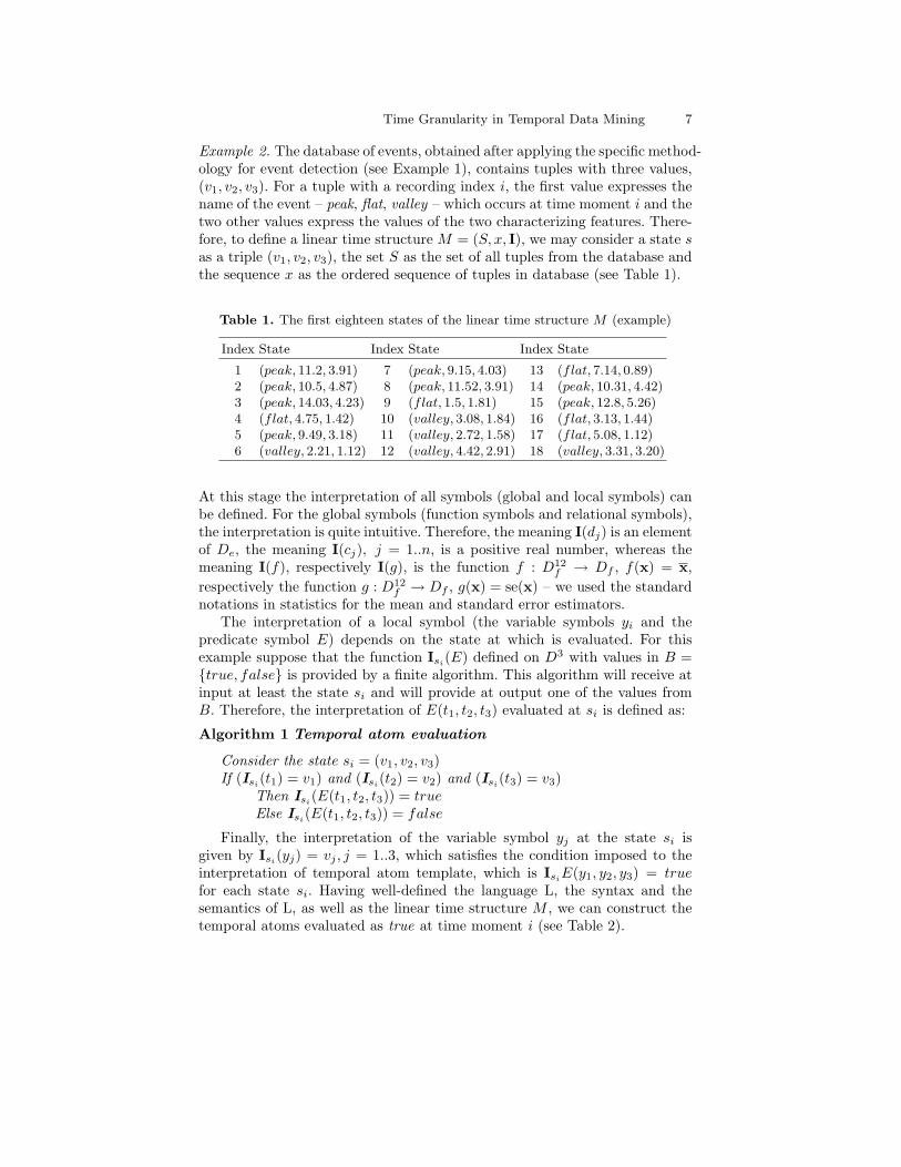
Example 2. The database of events, obtained after applying the specific method-ology for event detection (see Example 1), contains tuples with three values,(v1, v2, v3). For a tuple with a recording index i, the first value expresses thename of the event – peak, flat, valley – which occurs at time moment i and thetwo other values express the values of the two characterizing features. There-fore, to define a linear time structure M = (S, x, I), we may consider a state sas a triple (v1, v2, v3), the set S as the set of all tuples from the database andthe sequence x as the ordered sequence of tuples in database (see Table 1).

Table 1. The first eighteen states of the linear time structure M (example)

Index State Index State Index State

1 (peak, 11.2, 3.91) 7 (peak, 9.15, 4.03) 13 (flat, 7.14, 0.89)2 (peak, 10.5, 4.87) 8 (peak, 11.52, 3.91) 14 (peak, 10.31, 4.42)3 (peak, 14.03, 4.23) 9 (flat, 1.5, 1.81) 15 (peak, 12.8, 5.26)4 (flat, 4.75, 1.42) 10 (valley, 3.08, 1.84) 16 (flat, 3.13, 1.44)5 (peak, 9.49, 3.18) 11 (valley, 2.72, 1.58) 17 (flat, 5.08, 1.12)6 (valley, 2.21, 1.12) 12 (valley, 4.42, 2.91) 18 (valley, 3.31, 3.20)

At this stage the interpretation of all symbols (global and local symbols) canbe defined. For the global symbols (function symbols and relational symbols),the interpretation is quite intuitive. Therefore, the meaning I(dj) is an elementof De, the meaning I(cj), j = 1..n, is a positive real number, whereas themeaning I(f), respectively I(g), is the function f : D12

f → Df , f(x) = x,respectively the function g : D12

f → Df , g(x) = se(x) – we used the standardnotations in statistics for the mean and standard error estimators.

The interpretation of a local symbol (the variable symbols yi and thepredicate symbol E) depends on the state at which is evaluated. For thisexample suppose that the function Isi(E) defined on D3 with values in B ={true, false} is provided by a finite algorithm. This algorithm will receive atinput at least the state si and will provide at output one of the values fromB. Therefore, the interpretation of E(t1, t2, t3) evaluated at si is defined as:

Algorithm 1 Temporal atom evaluation

Consider the state si = (v1, v2, v3)If (Isi(t1) = v1) and (Isi(t2) = v2) and (Isi(t3) = v3)

Then Isi(E(t1, t2, t3)) = trueElse Isi(E(t1, t2, t3)) = false

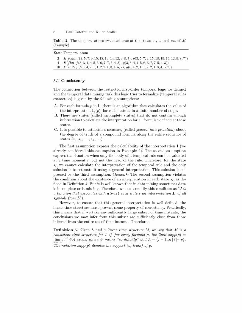
Finally, the interpretation of the variable symbol yj at the state si isgiven by Isi(yj) = vj , j = 1..3, which satisfies the condition imposed to theinterpretation of temporal atom template, which is IsiE(y1, y2, y3) = truefor each state si. Having well-defined the language L, the syntax and thesemantics of L, as well as the linear time structure M , we can construct thetemporal atoms evaluated as true at time moment i (see Table 2).


Table 2. The temporal atoms evaluated true at the states s2, s4 and s10 of M(example)

State Temporal atom

2 E(peak, f(3, 5, 7, 9, 15, 18, 19, 14, 12, 9, 8, 7), g(3, 5, 7, 9, 15, 18, 19, 14, 12, 9, 8, 7))4 E(flat, f(3, 3, 4, 4, 5, 6, 6, 7, 7, 5, 4, 3), g(3, 3, 4, 4, 5, 6, 6, 7, 7, 5, 4, 3))10 E(valley, f(5, 4, 2, 1, 1, 2, 2, 1, 3, 4, 5, 7), g(5, 4, 2, 1, 1, 2, 2, 1, 3, 4, 5, 7))

3.1 Consistency

The connection between the restricted first-order temporal logic we definedand the temporal data mining task this logic tries to formalize (temporal rulesextraction) is given by the following assumptions:

A. For each formula p in L, there is an algorithm that calculates the value ofthe interpretation Is(p), for each state s, in a finite number of steps.

B. There are states (called incomplete states) that do not contain enoughinformation to calculate the interpretation for all formulae defined at thesestates.

C. It is possible to establish a measure, (called general interpretation) aboutthe degree of truth of a compound formula along the entire sequence ofstates (s0, s1, . . . , sn, . . .).

The first assumption express the calculability of the interpretation I (wealready considered this assumption in Example 2). The second assumptionexpress the situation when only the body of a temporal rule can be evaluatedat a time moment i, but not the head of the rule. Therefore, for the statesi, we cannot calculate the interpretation of the temporal rule and the onlysolution is to estimate it using a general interpretation. This solution is ex-pressed by the third assumption. (Remark: The second assumption violatesthe condition about the existence of an interpretation in each state si, as de-fined in Definition 4. But it is well known that in data mining sometimes datais incomplete or is missing. Therefore, we must modify this condition as ”I isa function that associates with almost each state s an interpretation Is of allsymbols from L”).

However, to ensure that this general interpretation is well defined, thelinear time structure must present some property of consistency. Practically,this means that if we take any sufficiently large subset of time instants, theconclusions we may infer from this subset are sufficiently close from thoseinferred from the entire set of time instants. Therefore,

Definition 5. Given L and a linear time structure M, we say that M is aconsistent time structure for L if, for every formula p, the limit supp(p) =limn→∞

n−1#A exists, where # means ”cardinality” and A = {i = 1..n | i |= p}.The notation supp(p) denotes the support (of truth) of p.


Now we define the general interpretation for an n-ary predicate symbol P as:

Definition 6. Given L and a consistent linear time structure M for L, thegeneral interpretation IG for an n-ary predicate P is a function Dn →[0, 1], such that, for each n-tuple of terms {t1, . . . , tn}, IG(P (t1, . . . , tn)) =supp(P (t1, . . . , tn)).

The general interpretation is naturally extended to constraint formulae, tem-poral rules and the corresponding templates. There is another useful measure,called confidence, but available only for temporal rules (templates). This mea-sure is calculated as a limit ratio between the number of certain applications(time instants where both the body and the head of the rule are true) andthe number of potential applications (time instants where only the body ofthe rule is true).

Definition 7. The confidence of a temporal rule (template) H1 ∧ · · · ∧Hm 7→Hm+1 is the limit lim

n→∞(#B)−1#A, where A = {i = 1 . . . n | i |= H1 ∧ · · · ∧

Hm ∧Hm+1} and B = {i = 1 . . . n|i |= H1 ∧ · · · ∧Hm}.

The relation between the property of consistency and the existence of theconfidence for a temporal rule is expressed in the following lemma.

Lemma 1. If M is a consistent linear time structure for L then every temporalrule (template) H1 ∧ · · · ∧Hm 7→ Hm+1 for which supp(H1 ∧ · · · ∧Hm) 6= 0has a well-defined confidence.

For different reasons, (the user has not access to the entire sequence ofstates, or the states he has access to are incomplete), the general interpretationcannot be calculated. A solution is to estimate IG using a finite linear timestructure, i.e. a model.

Definition 8. Given L and a consistent time structure M = (S, x, I), amodel for M is a structure M = (T , x) where T is a finite temporal domain{i1, . . . , in}, x is the subsequence of states {xi1 , . . . , xin} (the restriction of xto the temporal domain T ) and for each ij , j = 1, . . . , n, the state xij is acomplete state.

Now we may define the estimator for a general interpretation:

Definition 9. Given L and a model M for M, an estimator of the generalinterpretation for an n-ary predicate P, IG(M)(P ), is a function Dn → [0, 1],assigning to each atomic formula p = P (t1, . . . , tn) the value defined as the

ratio#A#T

, where A = {i ∈ T | i |= p}. The notation supp(p, M) will denote

the estimated support of p, given M.


The extension of this definition to the other types of formulae in L demands adeeper analysis. Consider, as example, the model M induced by the sequenceof n > 1 states x = x1, . . . , xn. The interpretation of a formula ∇1p at thestate xn can not be calculated, because n |= ∇1p if (n+1) |= p, but xn+1 6∈ x.Therefore, the cardinality of the set A = {i ≤ n | i |= ∇1p} is strictly smallerthan n, which means that, for p a global formula having the meaning of truthtrue, the estimated support is

supp(∇1p, M) = (n− 1)/n 6= 1 = supp(∇1p). (1)

The fact that the support estimator is biased seems at first glance withoutimportance, especially when, as in this case, the bias (n−1) tends to zerofor n ↑ ∞. But considering a formula of type ∇np, it is evidently that theinterpretation can not be calculated at none of the states from x, and so thesupport estimator is not even defined. Before indicating how the expression#A

#Tmust be adjusted to avoid this kind of problem, we start by defining the

standard form of a formula in L.

Definition 10. A formula ∇k1p1 ∧∇k2p2 ∧ . . . ∧∇knpn, where n ≥ 1 and piare atoms of L, is in standard form if exists i0 ∈ {1, . . . , n} such that ki0 = 0and for all i = 1..n, ki ≤ 0.

For an atomic formula p, it is clearly that its standard form is∇0p. Anotherexample of formula in standard form is a temporal rule (template), wherethe head of the rule is prefixed by ∇0 and all other constraint formulae areprefixed by ∇−k, k ≥ 0. It is obviously that, for M a consistent time structure,the support of a formula does not change if it is prefixed with a temporalconnective ∇k, k ∈ Z. Therefore, to each formula p in L corresponds anequivalent formula (under the measure supp) having a standard form (denotedF(p)). Based on this concept, we can now give a non equivocal definition fortime windows:

Definition 11. Let be p a formula in L having the standard form ∇k1p1 ∧∇k2p2 ∧ . . . ∧ ∇knpn. The time window of p – denoted w(p) – is defined asmax{ | ki | : i = 1..n}

In the following, a formula having a time window equal zero will be calledtemporal free formula, whereas a formula with a strictly positive time windowwill be called a temporal formula. The concept of time window allows us todefine a non biased estimator for the support measure.

Definition 12. Given L and a model M for M, the estimator of the supportfor a formula p in L and having w(p) < #T = m, denoted supp(p, M), is theratio

#Am− w(p)

, where A = {i ∈ T | i |= F(p)}. (2)


According to this definition, if w(p) ≥ m then the estimator supp(p, M)is not defined. The use of the standard form of a formula, in the constructionof the set A, eliminates the interpretation problem for a formula of type ∇kp,k ≥ m. Moreover, it is easy to see that supp(∇kp, M) = supp(p, M), for allk ∈ Z.

Definition 13. Given L and a model M for M, an estimate of the generalinterpretation for a formula p is given by

IG(M)(p) =

{supp(p, M), if w(p) < #T ,0 if w(p) ≥ #T

(3)

Once again, the estimation of the confidence for a temporal rule (template)is defined as:

Definition 14. Given a model M = (T , x) for M, the estimation of the con-fidence for the temporal rule (template) H1 ∧ · · · ∧Hm 7→ Hm+1 is the ratio#A#B

, where A = {i ∈ T | i |= H1 ∧ · · · ∧ Hm ∧ Hm+1} and B = {i ∈ T | i |=

H1∧· · ·∧Hm}. The notation conf(H, M) will denote the estimated confidenceof the temporal rule (template) H given M .

According to the same arguments used in the definition of a correct supportestimator, the existence of a confidence estimator for a temporal rule H isguaranteed only for models having a number of states greater than the timewindow of the rule. Moreover, if ˜T is the set obtained from T by deleting thefirst w(H1 ∧ . . .∧Hm+1)−w(H1 ∧ . . .∧Hm) states, then we can obtain a nonbiased confidence estimator if in the expression of the set B = {i ∈ T | i |=H1 ∧ · · · ∧Hm} the set T is replaced with ˜T .

Example 3. Consider the following temporal rule template T (for the momentwe are not concerned on how it was discovered):

∇−2(y1 = peak)∧∇−2(y2 < 11)∧∇−1(y1 = peak)∧∇−1(y3 > 3) 7→ ∇0(y1 =flat)

which may be ”translated” in a natural language as:

IF at time t− 2 an event ”peak” occurred with a mean less than 11 AND attime t − 1 another event ”peak” occurred with a standard error greater than 3THEN at time t an event type ”flat” occurs.

If M is a consistent linear time structure for the temporal language Ldefined in Example 1, then the model M given by the sequence of states{s1, . . . , s18} (see Table 1) can be used to estimate the confidence of the tem-poral rule T . If the local support for the rule is 0.125 (true at states 2 and 14,among 17 states) and the local support for the body of the rule is 0.176 (trueat states 2, 7 and 14, among 16 states) then the estimated confidence for the


rule, based on model M , is 0.125/0.176 = 0.71. And, due to the consistencyproperty, this estimation is a reliable information about the success rate forthis rule when applied on future data.

4 The Granularity Model

We start with the concept of a temporal type to formalize the notion of timegranularities, as described in [3].

Definition 15. Let (T , <) (index) be a linearly ordered temporal domain iso-morphic to a subset of integers with the usual order relation, and let (A, <)(absolute time) be a linearly ordered set. Then, a temporal type on (T ,A) isa mapping µ from T to 2A such that

1. µ(i) 6= ∅ and µ(j) 6= ∅, where i < j, imply that each element in µ(i) isless than all the elements in µ(j), and

2. for all i < j, if µ(i) 6= ∅ and µ(j) 6= ∅, then ∀k , i < k < j impliesµ(k) 6= ∅.

Each set µ(i), if non-empty, is called a granule of µ. Property (1) says thatgranules do not overlap and that the order on indexes follows the order on thecorresponding granules. Property (2) disallows an empty set to be the valueof a mapping for a certain index value if a lower index and a higher index aremapped to non-empty sets.

When considering a particular application or formal context, we can spe-cialize this very general model along the following dimensions:

• choice of the index set T ,• choice of the absolute time set A,• restrictions on the structure of granules,• restrictions on the temporal types by using relationships.

We call the resulting formalization a temporal type system. Consider somepossibilities for each of the above four dimensions. Convenient choices for theindex set are natural numbers, integers, and any finite subset of them. Thechoice for absolute time is typically between dense and discrete. In general, ifthe application imposes a fixed basic granularity, then a discrete absolute timein terms of the basic granularity is probably the appropriate choice. However,if one is interested in being able to represent arbitrary finer temporal types,a dense absolute time is required. In both cases, specific applications couldimpose left/right boundedness on the absolute time set. The structure of tickscould be restricted in several ways:

(1) disallow types with gaps in a granule,(2) disallow types with non-contiguous granules,(3) disallow types whose granules do not cover all the absolute time, or(4) disallow types with nonuniform granules (only types with granules having

the same size are allowed).


4.1 Relationships and formal properties

Following Bettini et al. [3], we define a number of interesting relationshipsamong temporal types.

Definition 16. Let be µ and ν be temporal types on (T ,A).

• Finer-than: µ is said to be finer than ν, denoted µ 4 ν, if for each i ∈ T ,there exists j ∈ T such that µ(i) ⊆ ν(j).

• Groups-into: µ is said to group into ν, denoted µ E ν, if for each non-empty granule ν(j), there is a subset S of T such that ν(j) =

⋃i∈S µ(i).

• Subtype: µ is said to be a subtype of ν, denoted µ v ν, if for each i ∈ T ,there exists j ∈ T such that µ(i) = ν(j).

• Shifting: µ and ν are said to be shifting equivalent, denoted µ1 µ2, ifµ v ν and ν v µ.

When a temporal type µ is finer than a temporal type ν, we also say that νis coarser than µ. The finer-than relationship formalizes the notion of finerpartitions of the absolute time. By definition, this relation is reflexive, i.e. µ 4µ for each temporal type µ. Furthermore, the finer-than relation is obviouslytransitive. However, if no restrictions are given, it is not antisymmetric, andhence it is not a partial order. Indeed, µ 4 ν and ν 4 µ do not imply µ = ν,but only µ ν. Considering the groups-into relation, µ E ν ensures thatfor each granule of µ there exists a set of granules of ν covering exactly thesame span of time. The relation is useful, for example, in applications whereattribute values are associated with time granules; sometimes it is possibleto obtain the value associated with a granule of ν from the values associatedwith the granules of µ whose union covers the same time. The groups-intorelation has the same two properties as the finer-than relation, but generallyµ 4 ν does not imply µ E ν or viceversa. The subtype relation intuitivelyidentifies a type corresponding to subsets of granules of another type. Similarto the two previous relations, subtype is reflexive and transitive, and satisfiesµ v ν ⇒ µ 4 ν. Finally, shifting is clearly an equivalence relation. Concerningthis last relation, an equivalent, more useful and practical definition, is:

Definition 17. Two temporal types µ1 and µ2 are said to be shifting equiv-alent (denoted µ1 µ2) if there is a bijective function h : T → T such thatµ1(i) = µ2(h(i)), for all i ∈ T .

In the following we will consider only temporal type systems which satisfythe restriction that no pair of different types can be shifting equivalent, i.e.

µ1 µ2 ⇒ µ1 = µ2. (4)

For this class of systems, the three relationships 4 ,E and v are reflexive,transitive and antisymmetric and, hence, each relationship is a partial order.Therefore, for the relation we are particulary interested in, finer-than, thereexists a unique least upper bound of the set of all temporal types, denoted by


µ>, and a unique greatest lower bound, denoted by µ⊥. These top and bottomelements are defined as follows: µ>(i) = A for some i ∈ T and µ>(j) = ∅for each j 6= i, and µ⊥(i) = ∅ for each i ∈ T . Moreover, for each pair oftemporal types µ1, µ2, there exist a unique least upper bound (µ1, µ2) and aunique greatest lower bound (µ1, µ2) of the two types, with respect to 4. Weformalize this result in the following theorem, proved by Bettini et al. [3]:

Theorem 1. Any temporal type system having an infinite index, and satisfy-ing (4), is a lattice with respect to the finer-than relationship.

Let denote G0 the set of temporal types for which the index set and theabsolute time set are isomorphic with the set of positive natural numbers, i.e.A = T = N. Consider now the following particular subsets of G0, representedby temporal types with a) non-empty granules, b) with granules covering allthe absolute time and c) with constant size granules:

G1 = {µ ∈ G0 | ∀i ∈ N, 0 < #µ(i)} (5)

G2 = {µ ∈ G1 | ∀i ∈ N, µ(i)−1 6= 0} (6)G3 = {µ ∈ G2 | ∀i ∈ N, µ(i) = cµ} (7)

The membership of a temporal type defined by one of these subsets impliesvery useful properties, a first result being expressed in the following lemma.

Lemma 2. If µ1, µ2 are temporal types from G1, then µ1 µ2 ⇒ µ1 = µ2.

Therefore, the set G1 of temporal types is a lattice with respect to the finer-than relationship. The temporal type system G1 is not closed, because (µ1, µ2)is not always in G1. In exchange it can be shown that the temporal typesystem G2 (given by (6), where µ−1(i) = {j ∈ N : i ∈ µ(j)}) is a closed systemhaving a unique greatest lower bound, µ⊥(i) = i, ∀i ∈ N, but no least upperbound µ>. Furthermore, the membership of G2 is a sufficient condition for theequivalence of the relationships finer-than and groups-into, according to thefollowing lemma:

Lemma 3. If µ and ν are temporal types from G2, then µ 4 ν ⇔ µ E ν.

4.2 Linear Granular Time Structure

If M = (S, x, I) is a first-order linear time structure, then let the absolutetime A be given by the sequence x, by identifying the time moment i with thestate s(i) (on the ith position in the sequence). If µ is a temporal type fromG2, then the temporal granule µ(i) may be identified with the set {sj ∈ S | j ∈µ(i)}. Therefore, the temporal type µ induces a new sequence, xµ, defined asxµ : N → 2S , xµ(i) = µ(i). (Remark : In the following the set µ(i) will beconsidered, depending of the context, either as a set of states or as a set ofnatural numbers, the indexes of these states).


Consider now the linear time structure derived from M , Mµ = (2S , xµ, Iµ).To be well defined, we must give the interpretation Iµµ(i), for each i ∈ N.Because for a fixed i the set µ(i) is a finite sequence of states, it defines (if allthe states are complete states) a model Mµ(i) for M . Therefore the estimatedgeneral interpretation IG(Mµ(i))

is well defined and we consider, by definition,that for a temporal free formula (e.g. a temporal atom) p in L,

Iµµ(i)(p) = IG(Mµ(i))(p) = supp(p, Mµ(i)) (8)

This interpretation is extended to any temporal formula in L according to therule:

Iµµ(i)(∇k1p1 ∧ . . . ∧∇knpn) =1n

n∑j=1

Iµµ(i+kj)(pj) (9)

where pi are temporal free formulae and ki ∈ Z, i = 1 . . . n.

Definition 18. If M = (S, x, I) is a first-order linear time structure and µis a temporal type from G2, then the linear granular time structure inducedby µ on M is the triple Mµ = (2S , xµ, Iµ), where xµ : N → 2S, xµ(i) = µ(i)and Iµ is a function that associates with almost each set of states µ(i) aninterpretation Iµµ(i) according to the rules (8) and (9).

Of a particular interest is the linear granular time structure induced by thegreatest lower bound temporal type of the lattice G2, µ⊥(i) = i. In this case,Mµ⊥ = (S, x, Iµ⊥), where the only difference from the initial time structureM is at the interpretation level: for p = P (t1, . . . , tn) a formula in L, if theinterpretation Is(p) is a function defined on Dn with values in {true, false} –giving so the meaning of truth – the interpretation Iµ⊥s (p) is a function definedon Dn with values in [0, 1] – giving so the degree of truth. The relation linkingthe two interpretations is given by Is(p) = true if and only if Iµ⊥s (p) = 1.Indeed, supposing the state s(i) is a complete state, it defines the model Mi =(i, s(i)) and we have, for p a temporal free formula,

Iµ⊥µ⊥(i)(p) = supp(p, Mi) =

{1, if Is(i)(p) = true,

0, if Is(i)(p) = false(10)

For a formula π = ∇k1p1 ∧ . . . ∧ ∇knpn, we have Isi(π) = true iff ∀j ∈{1 . . . n}, i+ kj |= pj , which is equivalent with

supp(p1, Mi+k1) = · · · = supp(pn, Mi+kn) = 1

⇔ 1n

n∑j=1

Iµ⊥µ⊥(i+kj)(pj) = Iµ⊥µ⊥(i)(π) = 1. (11)

Consequently, the linear granular time structure Mµ⊥ can be seen as an ex-tension, at the interpretation level, of the classical linear time structure M .


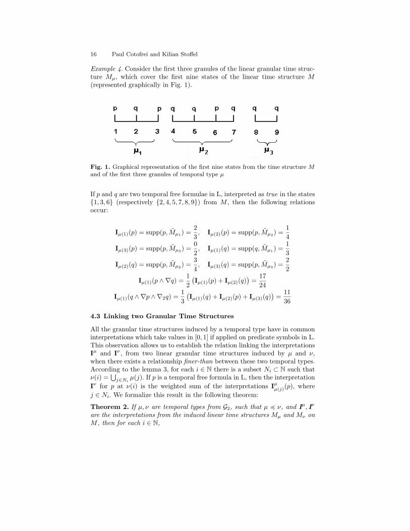
Example 4. Consider the first three granules of the linear granular time struc-ture Mµ, which cover the first nine states of the linear time structure M(represented graphically in Fig. 1).

Fig. 1. Graphical representation of the first nine states from the time structure Mand of the first three granules of temporal type µ

If p and q are two temporal free formulae in L, interpreted as true in the states{1, 3, 6} (respectively {2, 4, 5, 7, 8, 9}) from M , then the following relationsoccur:

Iµ(1)(p) = supp(p, Mµ1) =23, Iµ(2)(p) = supp(p, Mµ2) =

14

Iµ(3)(p) = supp(p, Mµ3) =02, Iµ(1)(q) = supp(q, Mµ1) =

13

Iµ(2)(q) = supp(p, Mµ2) =34, Iµ(3)(q) = supp(p, Mµ3) =

22

Iµ(1)(p ∧∇q) =12(Iµ(1)(p) + Iµ(2)(q)

)=

1724

Iµ(1)(q ∧∇p ∧∇2q) =13(Iµ(1)(q) + Iµ(2)(p) + Iµ(3)(q)

)=

1136

4.3 Linking two Granular Time Structures

All the granular time structures induced by a temporal type have in commoninterpretations which take values in [0, 1] if applied on predicate symbols in L.This observation allows us to establish the relation linking the interpretationsIµ and Iν , from two linear granular time structures induced by µ and ν,when there exists a relationship finer-than between these two temporal types.According to the lemma 3, for each i ∈ N there is a subset Ni ⊂ N such thatν(i) =

⋃j∈Ni µ(j). If p is a temporal free formula in L, then the interpretation

Iν for p at ν(i) is the weighted sum of the interpretations Iµµ(j)(p), wherej ∈ Ni. We formalize this result in the following theorem:

Theorem 2. If µ, ν are temporal types from G2, such that µ 4 ν, and Iµ, Iν

are the interpretations from the induced linear time structures Mµ and Mν onM , then for each i ∈ N,


Iνν(i)(p) =1

#ν(i)

∑j∈Ni

#µ(j)Iµµ(j)(p), (12)

where Ni is the subset of N which satisfies ν(i) =⋃j∈Ni µ(j) and p is a

temporal free formula in L.

If we consider µ = µ⊥ 4 ν then #µ(j) = 1, for all j ∈ N and Iµµ(j)(p) =

supp(p, Mj). Therefore,

Iνν(i)(p) =1

#ν(i)

∑j∈ν(i)

supp(p, Mj)

=1

#ν(i)#{j ∈ ν(i) | j |= p} = supp(p, Mν(i)) = IG(Mν(i))

(p) (13)

result which is consistent with Definition 18. But the significance of the the-orem 2 is revealed in a particular context. If µ, ν ∈ G3 and µ 4 ν, it can beshown that #Ni = cν

cµ,∀i ∈ N and so the relation (12) becomes

Iνν(i)(p) =1

#Ni

∑j∈Ni

Iµµ(j)(p). (14)

Generally speaking, consider three worlds, W1,W2 and W3 – defined as setsof granules of information – where W1 is finer than W2 which is finer thanW3. Suppose also that the conversion between granules from two differentworlds is given by a constant factor. If the independent part of informationin each granule is transferred from W1 to W2 and then the world W1 is ”lost”,the theorem 2 under the form (14) affirms that it is possible to transfer theindependent information from W2 to W3 and to obtain the same result as forthe transfer from W1 to W3.

Example 5. : Consider a linear time structure M (here, the world W1) and atemporal free formula p such that, for the first six time moments, we have i |= pfor i ∈ {1, 3, 5, 6}. The concept of independence, in this example, means thatthe interpretation of p in the state si does not depend on the interpretationof p in the state sj . Let be µ, ν ∈ G3, µ 4 ν, with µ(i) = {2i − 1, 2i} andν(i) = {6i− 5, . . . , 6i}. Therefore, ν(1) = µ(1)∪µ(2)∪µ(3). According to thedefinition 18, Iµµ(1)(p) = supp(p, {1, 2}) = 0.5, Iµµ(2)(p) = supp(p, {3, 4}) = 0.5,Iµµ(3)(p) = supp(p, {5, 6}) = 1, whereas Iνν(1)(p) = supp(p, {1, .., 6}) = 0.66. Ifthe linear time structure M is ”lost”, the temporal types µ and ν are ”lost”too (we don’t know the absolute time A given by M). But if we know theinduced time structure Mµ (world W2) and the relation between µ and ν

ν(k) = µ(3k − 2) ∪ µ(3k − 1) ∪ µ(3k), ∀k ∈ N

then we can completely deduce the time structure Mν (world W3). As ex-ample, according to (14), Iνν(1)(p) = 1

3

∑3i=1 Iµµ(i)(p) = 0.66. The condition


about a constant conversion factor between granules is necessary because theinformation about the size of granules, as it appears in expression 12, is ”lost”when the time structure M is ”lost”

The theorem 2 is not effective for temporal formulae (which can be seen asthe dependent part of the information of a temporal granule). In this case wecan prove that the interpretation, in the coarser world, of a temporal formulawith a given time window is linked with the interpretation, in the finer world,of a similar formula but having a larger time window.

Theorem 3. If µ and ν are temporal types from G3 such that µ 4 ν and Iµ, Iν

are the interpretations from the induced linear time structures Mµ and Mν onM , then for each i ∈ N,

Iνν(i)(p ∧∇q) =1k

∑j∈Ni

Iµµ(j)(p ∧∇kq) (15)

where k = cν/cµ, ν(i) =⋃j∈Ni µ(j) and p, q are temporal free formulae in L.

If we define the operator zoomk over the set of formulae in L as

zoomk(∇k1p1 ∧ . . . ∧∇knpn) = ∇k·k1p1 ∧ . . . ∧∇k·knpn

then an obvious corollary of this theorem is

Corollary 1. If µ and ν are temporal types from G3 such that µ 4 ν andIµ, Iν are the interpretations from the induced linear time structures Mµ andMν on M , then for each i ∈ N,

Iνν(i)(∇k1p1 ∧ . . .∧∇knpn) =1k

∑j∈Ni

Iµµ(j)(zoomk(∇k1p1 ∧ . . .∧∇knpn)) (16)

where k = cν/cµ, ν(i) =⋃j∈Ni µ(j), ki ∈ N and pi, i = 1..n are temporal free

formulae in L.

According to this corollary, if we know the degree of truth of a temporalrule (template) in the world W1, we can say nothing about the degree of truthof the same rule in the world W2, coarser than W1. The information is onlytransferred from the temporal rule zoomk(H) in W1 (which has a time windowgreater than k−1) to the temporal rule H in W2, where k is the coefficient ofconversion between the two worlds. Consequently, all the information relatedto temporal formulae having a time window less than k is lost during thetransition to the coarser world W2.

4.4 The Consistency Problem

The importance of the concepts of consistency, support and confidence, (seeSubsect. 3.1), for the process of information transfer between worlds with dif-ferent granularity may be highlighted by analyzing the analogous expressionsfor a linear granular time structure Mµ.


Definition 19. Given L and a linear granular time structure Mµ on M , wesay that Mµ is a consistent granular time structure for L if, for every formulap, the limit

supp(p,Mµ) = limn→∞

∑ni=1 Iµµ(i)(p)

n(17)

exists. The notation supp(p,Mµ) denotes the support (degree of truth) of punder Mµ.

A natural question concern the inheritance of the consistency propertyfrom the basic linear time structure M by the induced time structure Mµ.The answer is formalized in the following theorem.

Theorem 4. If M is a consistent linear time structure and µ ∈ G3 then thegranular time structure Mµ is also consistent.

The proof of the theorem (see Appendix 6) is based on the relation betweenthe support of a formula p in M , respectively in Mµ, which is:

supp(p,Mµ) = supp(p,M) (18)

supp(∇k1p1 ∧ . . . ∧∇kmpm,Mµ) =1m

m∑j=1

supp(pj ,M) (19)

The implications of Theorem 4 are extremely important. It is easy to show,starting from Definition 14, that the confidence of a temporal rule (template)may be expressed using only the support measure if the linear time structureM is consistent. Therefore, considering that by definition the confidence ofa temporal rule (template) H, H1 ∧ . . . ∧ Hm 7→ Hm+1, giving a consistentgranular time structure Mµ, is

conf(H,Mµ) =

{supp(H1∧...∧Hm∧Hm+1,Mµ)

supp(H1∧...∧Hm,Mµ) if supp(H1 ∧ . . . ∧Hm,Mµ) > 0,

0 if not(20)

we can deduce, by applying Theorem 4 and the relations (18) and (19), thatthe confidence of H, for a granular time structure Mµ induced on a consistenttime structure M by a temporal type µ ∈ G3, is independent of µ. In otherwords,

”The property of consistency is a sufficient condition for the independenceof the measure of support/confidence, during the process of information trans-fer between worlds with different granularities, all derived from an absoluteworld using constant conversion factors. In practice, this means that even weare not able to find, for a given world Mµ, the granules where a temporal ruleH apply (according to Theorem 3), we are sure that the confidence of H is thesame in each world Mµ,∀µ ∈ G3.”


4.5 Event Aggregation

All the deduction processes made until now were conducted to obtain ananswer to the following question: how is changing the degree of truth of aformula p if we pass from a linear time structure with a given granularityto a coarser one. And we proved that we can give a proper expression ifwe impose some restrictions on the temporal types which induce these timestructures. But there is another phenomenon which follows the process oftransition between two real worlds with different time granularities: new kindsof events appear, some kinds of events disappear.

Definition 20. An event type (denoted E[t]) is the set of all temporal atomsfrom L having the same name (or head).

All the temporal atoms of a given type E[t] are constructed using the samesymbol predicate and we denote by N [t] the arity of this symbol. ConsiderE(t, t2, . . . , tn) ∈ E[t] (where n = N [t]). According to Definition 1, a termti, i ∈ {2, .., n} has the form ti = f(ti1, . . . , tiki). Suppose now that for eachindex i the function symbol f from the expression of ti belongs to a familyof function symbols with different arities, denoted Fi[t] (so different sets fordifferent event types E[t] and different index i). This family has the propertythat the interpretation for each of its member is given by a real functionswhich

• is applied on a variable number of arguments, and• is invariant in the order of the arguments.

A good example of a such real function is a statistical function, e.g. mean(x1, .., xn).Based on the set Fi[t] we consider the set of terms expressed as fk(c1, . . . , ck),where fk is a k−ary function symbol from Fi[t] and ci, i = 1..k are constantsymbols. We denote such a set as Ti[t]. Consider now the operator ⊕ definedon Ti[t]× Ti[t]→ Ti[t] such that

fn(c1, .., cn)⊕ fm(d1, .., dm) = fn+m(c1, .., cn, d1, .., dm)

Of course, because the interpretation of any function symbol from Fi[t] isinvariant in the order of arguments, we have

fn(c1, . . . , cn)⊕ fm(d1, . . . , dm) = fn(cσ(1), . . . , cσ(n))⊕ fm(dϕ(1), . . . , cϕ(n))

where σ (respectively ϕ) is a permutation of the set {1, . . . , n} (respectively{1, . . . ,m}). Furthermore, it is evident that the operator ⊕ is commutativeand associative.

We introduce now a new operator (denoted �) defined on E[t] × E[t] →E[t], such that, for E(t, t2, .., ti, .., tn) ∈ E[t], E(t, t′2, .., t

′i, .., t

′n) ∈ E[t] we

have:

E(t, t2, . . . , tn)� E(t, t′2, . . . , t′n) = E(t, t2 ⊕ t′2, . . . , tn ⊕ t′n) (21)


Once again, it is obviously that the operator� is commutative and associative.Therefore, we can apply this operator on a subset E of temporal atoms fromE[t] and we denote the result as �

ei∈Eei.

By definition, a formula p is satisfied by a linear time structure M =(S, x, I) (respectively by a model M = (T , x) of M) if there is at least a statesi ∈ x (respectively si ∈ x) such that Isi(p) = true. Therefore, the set ofevents of type t satisfied by M (respectively M) is given by:

E[t]M = {e ∈ E[t] | ∃si ∈ x such that Isi(e) = true} (22)

respectively by:

E[t]M = {e ∈ E[t] | ∃si ∈ x such that Isi(e) = true} (23)

If we consider now Mµ, the linear time structure induced by the temporaltype µ on M , the definition of E[t]Mµ

is derived from (22) by changing thecondition Isi(e) = true with Iµµ(i)(e) = 1. Of course, only for µ = µ⊥ we haveE[t]M = E[t]Mµ (we proved that Isi(p) = true ⇔ Iµ⊥µ⊥(i)(p) = 1). GenerallyE[t]M ⊃ E[t]Mµ

⊃ E[t]Mν, for µ 4 ν, which is a consequence of the fact that

a coarser world satisfies less temporal events than a finer one.

Example 6. : If M is a linear time structure such that for the event e ∈ E[t]we have i |= e if and only if i is odd, and µ is a temporal type given byµ(i) = {2i− 1, 2i}, then it is obviously that e ∈ E[t]M but e 6∈ E[t]Mµ

(for alli ∈ N, Iµµ(i)(e) = supp(e, {2i− 1, 2i}) = 0.5).

In the same time a coarser world may satisfies new events, representing a kindof aggregation of local, ”finer” events.

Definition 21. If µ is a temporal type from G2, we call the aggregate eventof type t induced by the granule µ(i) (denoted e[t]µ(i)) the event obtained byapplying the operator � on the set of events of type t which are satisfied bythe model Mµ(i), i.e.

e[t]µ(i) = �ei∈E[t]Mµ(i)

ei (24)

According to (8), the interpretation of an event e in any world Mµ dependson the interpretation of the same event in M . Therefore, if e is not satisfied byM it is obvious that Iµµ(i)(e) = 0, for all µ and all i ∈ N. Because an aggregateevent (conceived of a new, ”federative” event), usually is not satisfied by M ,the relation (8) is not appropriate to give the degree of truth for e[t]µ(i). Butbefore to give the rule expressing the interpretation for an aggregate temporalatom, we must impose on M the following restriction: two different events oftype t can not be evaluated as true at the same state s ∈ S, or:

∃h : E[t]M → S, h injective, such that h(e) = s where Is(e) = true (25)


Definition 22. If Mν is a linear granular time structure and e[t]µ(i0) is anaggregate event induced by the granule µi0 (µ, ν ∈ G2), then the interpretationof e[t]µ(i0) in the state ν(i) is defined as:

Iνν(i)(e[t]µ(i0)) =#(Ei ∩ E)

#E∑ej∈E

Iνν(i)(ej) (26)

where E = E[t]Mµ(i0), Ei = E[t]Mν(i)

.

The restriction (25) is given to assure that∑ej∈E Iνν(i)(ej) ≤ 1, for all i, i0 ∈ N.

Indeed, let be e1, . . . , en the events from E . If h(ej) = sj , j = 1..n, thenconsider the sets Aj = {k ∈ ν(i) | k |= ej} = {s ∈ ν(i) | s = sj}. The functionh being injective, the sets Aj are disjoint and therefore

∑nj=1 #Aj ≤ #ν(i).

Consequently, we have

n∑j=1

Iνν(i)(ej) =n∑j=1

supp(ej ,Mν(i)) =1

#ν(i)

n∑j=1

#Aj ≤#ν(i)#ν(i)

= 1. (27)

The relation (27) and the fact that the coefficient #(Ei∩E)#E is less or equal one

guarantee that the interpretation of an aggregate event is well-defined, i.e.Iνν(i)(e[t]µ(i0)) ≤ 1. Furthermore, the interpretation is equal one if and only if:

(i)#(Ei ∩ E)

#E= 1⇔ E = Ei (28)

meaning that all the events of type t satisfied by Mµi0are also satisfied by

Mνi , and

(ii)n∑j=1

Iνν(i)(ej) = 1⇔ 1#ν(i)

n∑j=1

#Aj = 1⇔n∑j=1

#Aj = #ν(i) (29)

meaning that the sets Aj form a partition of ν(i) (or equivalently h−1(ν(i)) =E).

Example 7. Let be M a linear time structure, e1, e2, e3 ∈ E[t] such that (seeFig. 2)

1 |= e1, 4 |= e1 and i |= e1 for i ∈ {6k − 2, 6k − 1, 6k | k ≥ 2}3 |= e2, 5 |= e2 and i |= e2 for i ∈ {6k + 1, 6k + 2, 6k + 3 | k ≥ 1}6 |= e3

Consider two temporal types µ, ν ∈ G3 such that µ(i) = {3i− 2, 3i− 1, 3i | i ≥1} and ν(i) = {6i − 5, . . . , 6i | i ≥ 1}. The different aggregate events inducedby granules of temporal type µ and ν are:


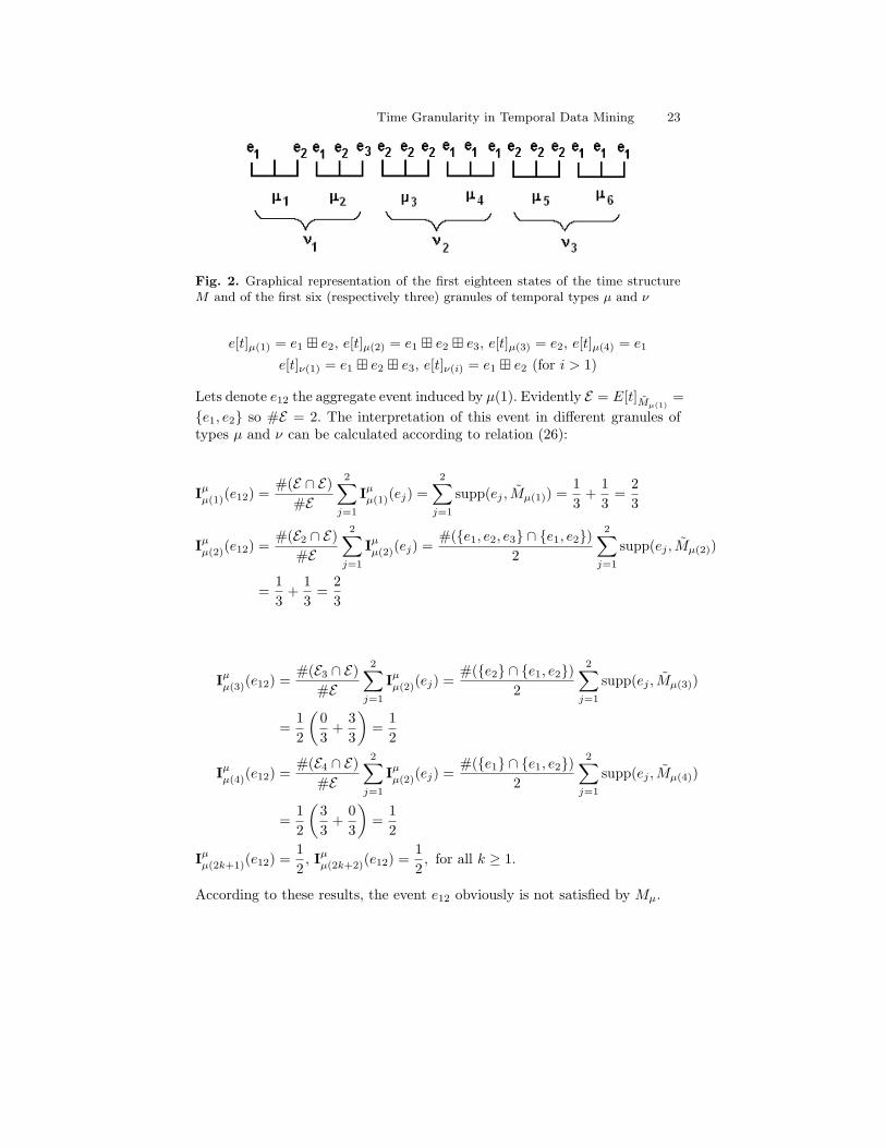
Fig. 2. Graphical representation of the first eighteen states of the time structureM and of the first six (respectively three) granules of temporal types µ and ν

e[t]µ(1) = e1 � e2, e[t]µ(2) = e1 � e2 � e3, e[t]µ(3) = e2, e[t]µ(4) = e1

e[t]ν(1) = e1 � e2 � e3, e[t]ν(i) = e1 � e2 (for i > 1)

Lets denote e12 the aggregate event induced by µ(1). Evidently E = E[t]Mµ(1)=

{e1, e2} so #E = 2. The interpretation of this event in different granules oftypes µ and ν can be calculated according to relation (26):

Iµµ(1)(e12) =#(E ∩ E)

#E

2∑j=1

Iµµ(1)(ej) =2∑j=1

supp(ej , Mµ(1)) =13

+13

=23

Iµµ(2)(e12) =#(E2 ∩ E)

#E

2∑j=1

Iµµ(2)(ej) =#({e1, e2, e3} ∩ {e1, e2})

2

2∑j=1

supp(ej , Mµ(2))

=13

+13

=23

Iµµ(3)(e12) =#(E3 ∩ E)

#E

2∑j=1

Iµµ(2)(ej) =#({e2} ∩ {e1, e2})

2

2∑j=1

supp(ej , Mµ(3))

=12

(03

+33

)=

12

Iµµ(4)(e12) =#(E4 ∩ E)

#E

2∑j=1

Iµµ(2)(ej) =#({e1} ∩ {e1, e2})

2

2∑j=1

supp(ej , Mµ(4))

=12

(33

+03

)=

12

Iµµ(2k+1)(e12) =12, Iµµ(2k+2)(e12) =

12, for all k ≥ 1.

According to these results, the event e12 obviously is not satisfied by Mµ.


Iνν(1)(e12) =#(E1 ∩ E)

#E

2∑j=1

Iνν(1)(ej) =#({e1, e2, e3} ∩ {e1, e2})

2

2∑j=1

supp(ej , Mν(1))

=26

+26

=23

Iνν(2)(e12) =#(E2 ∩ E)

#E

2∑j=1

Iνν(2)(ej) =#({e1, e2} ∩ {e1, e2})

2

2∑j=1

supp(ej , Mν(2))

=36

+36

= 1

Iνν(k)(e12) = 1 for all k ≥ 1,

which means that e12 is satisfied by Mν , a coarser world than Mµ. As a generalrule, the degree of truth for an aggregate event e is equal one in a given granuleµ(i) if all individual events composing e (and only these events) are satisfiedby µ(i).

5 Conclusions

In this article we developed a formalism for a specific temporal data miningtask: the discovery of knowledge, represented in the form of general Hornclauses, inferred from databases with a temporal dimension. The theoreticalframework we proposed, based on first-order temporal logic, permits to definethe main notions (event, temporal rule, constraint) in a formal way. The con-cept of a consistent linear time structure allows us to introduce the notionsof general interpretation, of support and of confidence, the lasts two measurebeing the expression of the two similar concepts used in data mining.

Starting from the inherent behavior of temporal systems – the perceptionof events and of their interactions is determined, in a large measure, by thetemporal scale – we extended the capability of our formalism to ”capture” theconcept of time granularity. To keep an unitary viewpoint on the meaning ofthe same formula at different scales of time, we changed the usual definitionof the interpretation Iµ for a formula in the frame of a first-order temporalgranular logic: it return the degree of truth (a real value between zero andone) and not only the meaning of truth (true or false).

The consequence of the definition for Iµ is formalized in Theorem 2 :only the independent information (here, the degree of truth for a temporalfree formula) may be transferred without loss between worlds with differentgranularities. Concerning the temporal rules (scale dependent information),we proved that the interpretation of a rule in a coarser world is linked withthe interpretation of a similar rule in a finer world, rule obtained by applyingthe operator zoomk on the initial temporal rule.

By defining a similar concept of consistency for a granular time structureMµ, we could proved that this property is inherited from the basic time struc-ture M if the temporal type µ is of type G2 (granules with constant size). The


major consequence of Theorem 4 is that the confidence of a temporal rule(template) is preserved in all granular time structures derived from the sameconsistent time structure.

We defined also a mechanism to aggregate events of the same type, thatreflects the following intuitive phenomenon: in a coarser world, not all eventsinherited from a finer world are satisfied, but in exchange there are new eventswhich become satisfiable. To achieve this we extended the syntax and thesemantics of L by allowing ”family” of function symbols and by adding twonew operators.

In our opinion, the logical next step in our work consists in adding aprobabilistic dimension to the formalism. Preliminary results (see [11]) confirmthat this approach allows a unified framework including the logical formalismand its granular extension, framework in which the property of consistencybecomes a consequence of the capacity of a particular stochastic process toobey the strong law of large numbers.

6 Appendix. Proofs

Proof (of Lemma 2).Before we start, we introduce the following notation: given two non-empty

sets S1 and S2 of elements in A, S1 � S2 holds if each number in S1 is strictlyless than each number in S2 (formally, S1 � S2 if ∀x ∈ S1 ∀y ∈ S2 (x < y)).Moreover, we say that a set S of non-empty sets of elements in A is monotonicif for each pair of sets S1 and S2 in S either S1 � S2 or S2 � S1.

The relation µ1 µ2 is equivalent with the existence of a bijection func-tion h : N→ N such that µ1(i) = µ2(h(i)), for all i. We will prove by inductionthat h(i) = i, which is equivalent with µ1 = µ2.

• i = 1: suppose that h(1) > 1. If a = min(µ1(1)) – the existence of a isensured by the condition (5) – then µ1(1) = µ2(h(1)) ⇒ a ∈ µ2(h(1)).Because 1 < h(1) we have µ2(1) � µ2(h(1)) (according to Definition 15)and so there is b ∈ µ2(1) such that b < a. The inequality 1 < h(1) impliesh−1(1) > 1, and so µ2(1) = µ1(h−1(1)) � µ1(1). But the last inequality(�) is contradicted by the existence of b ∈ µ1(h−1(1)) which is smallerthan a ∈ µ1(1). In conclusion, h(1) = 1.

• i = n + 1: from the induction hypothesis we have h(i) = i,∀i ≤ n. Sup-posing that h(n+ 1) 6= n+ 1, then the only possibility is h(n+ 1) > n+ 1.This last relation implies also h−1(n+1) > n+1. Using a similar rationingas in the previous case (it’s sufficient to replace 1 with n+ 1), we obtain

µ1(n+ 1)� µ1(h−1(n+ 1)) = µ2(n+ 1)� µ2(h(n+ 1)) = µ1(n+ 1)

where each of the set from this relation are non-empty, according to (5).The contradiction of the hypothesis, in this case, means that h(n + 1) =n+ 1 and, by induction principle, that h(i) = i,∀i ∈ N. �


Proof (of Lemma 3).Let be µ ∈ G2, ν ∈ G2.

• µ 4 ν : let j0 ∈ N. The relation (6) means that for all k ∈ ν(j0), µ−1(k) 6= ∅and so S =

⋃k∈ν(j0){µ

−1(k)} 6= ∅. It is obviously, according to Definition15, that the relation finer-than implies that for each i ∈ N there is aunique j ∈ N such that µ(i) ⊆ ν(j). Consequently, if µ 4 ν and µ(i) ∩ν(j) 6= ∅ then µ(i) ⊆ ν(j). Therefore, for all i ∈ S, µ(i) ⊂ ν(j0) whichimplies

⋃i∈S µ(i) ⊂ ν(j0) (a). At the same time, ∀k ∈ ν(j0) we have

k ∈ µ(µ−1(k)

)which implies ν(j0) ⊆

⋃i∈S µ(i) (b). From (a) and (b) we

have ν(j0) =⋃i∈S µ(i), which implies µ E ν.

• µ E ν: let i0 ∈ N and let k ∈ µ(i0). According to (6), there exists j =ν−1(k). Because µ E ν there is a set S such that ν(j) =

⋃i∈S µ(i). Because

the sets µ(i), i ∈ S are disjunct and k ∈ ν(j) ∩ µ(i0) we have i0 ∈ S.Therefore, for each i0 there is j ∈ N such that µ(i0) ⊆ ν(j), which impliesµ 4 ν. �

Proof (of Theorem 2).The formula p being a temporal free formula, we have w(p) = 0. According

to Definition 18 and Definition 12, we have

Iνν(i)(p) = supp(p, Mν(i)) =#{j ∈ ν(i) | j |= p}

#ν(i)(30)

On the other hand, because ν(i) =⋃j∈Ni µ(j), we have also

1#ν(i)

∑j∈Ni

#µ(j)Iµµ(j)(p) =1

#ν(i)

∑j∈Ni

#µ(j)supp(p, Mµ(j))

=1

#ν(i)

∑j∈Ni

#{k ∈ µ(j) | k |= p} =#{j ∈ ν(i) | j |= p}

#ν(i)(31)

From (30) and (31) we obtain (12). �

Proof (of Theorem 3).If µ, ν ∈ G3 such that #µ(i) = cµ and #ν(i) = cν , for all i ∈ N, it

is easy to show that the sets Ni satisfying ν(i) =⋃j∈Ni µ(j) have all the

same cardinality, #Ni = cν/cµ = k and contain successive natural numbers,Ni = {ji, ji + 1, . . . , ji + k − 1}. From the relations (9) and (14) we have:


Iνν(i)(p ∧∇q) =12

(Iνν(i)(p) + Iνν(i+1)(q)

)=

12

1#Ni

∑j∈Ni

Iµµ(j)(p) +1

#Ni+1

∑j∈Ni+1

Iµµ(j)(q)

=

12

1k

ji+k−1∑j=ji

Iµµ(j)(p) +1k

ji+2k−1∑j=ji+k

Iµµ(j)(q)

=

12k

ji+k−1∑j=ji

(Iµµ(j)(p) + Iµµ(j+k)(q)

)=

12k

ji+k−1∑j=ji

2Iµµ(j)(p ∧∇kq)

=1k

∑j∈Ni

Iµµ(j)(p ∧∇kq) �.

Proof (of Theorem 4).M being a consistent time structure, for each formula p in L the sequencex(p)n = n−1#{i ≤ n | i |= p} has a limit and lim

n→∞x(p)n = supp(p,M). In the

same time, µ ∈ G3 implies #µ(i) = k for all i ∈ N and µ(i) = {k(i − 1) +1, k(i− 1) + 2, . . . , ki}. Consider the following two cases:

• p temporal free formula : We have∑ni=1 Iµµ(i)(p)

n=∑ni=1 supp(p,Mµ(i))

n

=

∑ni=1

#{j∈µ(i) | j|=p}#µ(i)

n=∑ni=1 #{j ∈ µ(i) | j |= p}

kn

=#{i ∈

⋃ni=1 µ(i) | i |= p}kn

=#{i ≤ kn | i |= p}

kn= x(p)kn

Therefore, there exists the limit limn→∞

∑ni=1 Iµµ(i)(p)

n= limn→∞

x(p)kn and wehave

supp(p,Mµ) = supp(p,M) for p temporal free formula (32)

• temporal formula π = ∇k1p1 ∧ . . . ∧∇kmpm: We have

28 Paul Cotofrei and Kilian Stoffel∑ni=1 Iµµ(i)(∇k1p1 ∧ . . . ∧∇kmpm)

n=

∑ni=1

(m−1

∑mj=1 Iµµ(i+kj)

(pj))

n

=1m

∑ni=1

∑mj=1 supp(pj ,Mµ(i+kj))

n=

1mn

m∑j=1

n∑i=1

supp(pj ,Mµ(i+kj))

=1mn

m∑j=1

n∑i=1

#{h ∈ µ(kj + i) |h |= pj}k

=1mn

m∑j=1

#{h ∈⋃ni=1 µ(kj + i) |h |= pj}

k

=1

mnk

m∑j=1

(#{h ≤ k(kj + n) |h |= pj} −#{h ≤ kkj |h |= pj})

=1

mnk

m∑j=1

(k(kj + n)x(pj)k(kj+n) − kkjx(pj)kkj

)=

1m

m∑j=1

kj + n

nx(pj)k(kj+n) −

1m

m∑j=1

kjnx(pj)kkj (33)

By tacking n→∞ in (33), we obtain

limn→∞

∑ni=1 Iµµ(i)(∇k1p1 ∧ . . . ∧∇kmpm)

n

= limn→∞

1m

m∑j=1

kj + n

nx(pj)k(kj+n) −

1m

m∑j=1

kjnx(pj)kkj

=

1m

m∑j=1

limn→∞

kj + n

nx(pj)k(kj+n) −

1m

m∑j=1

limn→∞

kjnx(pj)kkj

=1m

m∑j=1

limn→∞

x(pj)k(kj+n) =1m

m∑j=1

supp(pj ,M) (34)

and so we have

supp(∇k1p1 ∧ . . . ∧∇kmpm,Mµ) =1m

m∑j=1

supp(pj ,M) (35)

From (6) and (35) results the conclusion of the theorem �.

References

[1] S. Al-Naemi. A theoretical framework for temporal knowledge discovery.In Proceedings of International Workshop on Spatio-Temporal Databases,pages 23–33, Spain, 1994.


[2] C. Bettini, X. S. Wang, and S. Jajodia. Mining temporal relationshipswith multiple granularities in time sequences. Data Engineering Bulletin,21(1):32–38, 1998.

[3] C. Bettini, X. S. Wang, and S. Jajodia. A general framework for timegranularity and its application to temporal reasoning. Ann. Math. Artif.Intell., 22(1-2):29–58, 1998.

[4] C. Bettini, X. S. Wang, S. Jajodia, and J.-L. Lin. Discovering frequentevent patterns with multiple granularities in time sequences. IEEE Trans.Knowl. Data Eng., 10(2):222–237, 1998.

[5] X. Chen and I. Petrounias. A Framework for Temporal Data Mining.Lecture Notes in Computer Science, 1460:796–805, 1998.

[6] J. Chomicki and D. Toman. Temporal Logic in Information Systems.BRICS Lecture Series, LS-97-1:1–42, 1997.

[7] E. Ciapessoni, E. Corsetti, A. Montanari, and P. S. Pietro. Embeddingtime granularity in a logical specification language for synchronous real-time systems. Sci. Comput. Program., 20(1-2):141–171, 1993.

[8] J. Clifford and A. Rao. A simple general structure for temporal domains.In Temporal Aspects of Information Systems. Elsevier Science, 1988.

[9] P. Cotofrei and K. Stoffel. Classification Rules + Time = TemporalRules. In Lecture Notes in Computer Science, vol 2329, pages 572–581.Springer Verlang, 2002.

[10] P. Cotofrei and K. Stoffel. From temporal rules to temporal meta-rules.In Procedings of 6th International Conference Data Warehousing andKnowledge Discovery, DaWaK 2004, Lecture Notes in Computer Science,vol. 3181, pages 169–178, Zaragoza, Spain, 2004.

[11] P. Cotofrei and K. Stoffel. Stochastic processes and temporal data min-ing. In Proceedings of the 13th ACM SIGKDD International Confer-ence on Knowledge Discovery and Data Mining, pages 183–190, San Jose,USA, August 2007.

[12] E. A. Emerson. Temporal and Modal Logic. Handbook of TheoreticalComputer Science, pages 995–1072, 1990.

[13] J. Euzenat. An algebraic approach to granularity in qualitative time andspace representation. In IJCAI (1), pages 894–900, 1995.

[14] C. Evans. The macro-event calculus: representing temporal granularity.In Proceedings of PRICAI, Japan, 1990.

[15] F. Giunchglia and T. Walsh. A theory of abstraction. Artificial Intelli-gence, 56:323–390, 1992.

[16] J. Han, Y. Cai, and N. Cercone. Data-driven discovery of quantitativerules in databases. IEEE Transactions on Knowledge and Data Engi-neering, 5:29–40, 1993.

[17] J. Hobbs. Granularity. In Proceedings of the IJCAI-85, pages 432 – 435,1985.

[18] K. Hornsby. Temporal zooming. Transactions in GIS, 5:255–272, 2001.


[19] C. Knoblock. Generating Abstraction Hierarchies: an Automated Ap-proach to Reducing Search in Planning. Kluwer Academic Publishers,1993.

[20] T. Y. Lin and E. Louie. Data mining using granular computing: fastalgorithms for finding association rules. Data mining, rough sets andgranular computing, pages 23–45, 2002.

[21] D. Malerba, F. Esposito, and F. Lisi. A logical framework for frequentpattern discovery in spatial data. In Proceedings of 5th ConferenceKnowledge Discovery in Data, 2001.

[22] I. Mani. A theory of granularity and its application to problems of pol-ysemy and underspecification of meaning. In Proceedings of the SixthInternational Conference Principles of Knowledge Representation andReasoning, pages 245–255, 1998.

[23] G. McCalla, J. Greer, J. Barrie, and P. Pospisil. Granularity hierarchies.Computers and Mathematics with Applications, 23:363–375, 1992.

[24] G.-C. Roman. Formal specification of geographic data processing require-ments. IEEE Trans. Knowl. Data Eng., 2(4):370–380, 1990.

[25] L. Saitta and J.-D. Zucker. Semantic abstraction for concept represen-tation and learning. In Proceedings of the Symposium on Abstraction,Reformulation and Approximation, pages 103–120, 1998.

[26] J. Stell and M. Worboys. Stratified map spaces: a formal basis for multi-resolution spatial databases. In Proceedings of the 8th International Sym-posium on Spatial Data Handling, pages 180–189, 1998.

[27] Y. Yao. Granular computing: basic issues and possible solutions. InP. Wang, editor, Proceedings of the 5th Joint Conference on InformationSciences, pages 186–189, Atlantic City, New Jersey, USA, 2000.

[28] Y. Yao and N. Zhong. Potential applications of granular computingin knowledge discovery and data mining. In M. Torres, B. Sanchez,and J. Aguilar, editors, Proceedings of World Multiconference on Sys-temics, Cybernetics and Informatics, pages 573–580, Orlando, Florida,USA, 1999. International Institute of Informatics and Systematics.

[29] L. A. Zadeh. Information granulation and its centrality in human andmachine intelligence. In Rough Sets and Current Trends in Computing,pages 35–36, 1998.

[30] B. Zhang and L. Zhang. Theory and Applications of Problem Solving,.North-Holland, Amsterdam, 1992.

[31] L. Zhang and B. Zhang. The quotient space theory of problem solving. InProceedings of International Conference on Rough Sets, Fuzzy Set, DataMining and Granular Computing, pages 11–15, 2003.

time granularity in temporal data mining

Documents