Threshold Behaviour of WalkSAT and Focused

Metropolis Search on Random 3-Satisfiability?

Sakari Seitz1,2, Mikko Alava2, and Pekka Orponen1

1 Laboratory for Theoret. Computer Science, P.O.B. 54002 Laboratory of Physics, P.O.B. 1100

Helsinki University of TechnologyFI-02015 TKK, Finland

E-mail: firstname.lastname@tkk.fi

Abstract. An important heuristic in local search algorithms for Satisfi-ability is focusing, i.e. restricting the selection of flipped variables to thoseappearing in presently unsatisfied clauses. We consider the behaviour onlarge randomly generated 3-SAT instances of two focused solution meth-ods: the well-known WalkSAT algorithm, and the straightforward algo-rithm obtained by imposing the focusing constraint on basic Metropolisdynamics. We observe that both WalkSAT and our Focused MetropolisSearch method are quite sensitive to the proper choice of their “noise”and “temperature” parameters, and attempt to estimate ideal values forthese, such that the algorithms exhibit generically linear solution timesas close to the satisfiability transition threshold αc ≈ 4.267 as possible.With an appropriate choice of parameters, the linear time regime of bothalgorithms seems to extend well into clauses-to-variables ratios α > 4.2,which is much further than has generally been assumed in the literature.

1 Introduction

An instance of the 3-satisfiability (3-SAT) problem is a formula consisting ofM clauses, each of which is a set of three literals, i.e. Boolean variables ortheir negations. The goal is to find a solution consisting of a satisfying truthassignment to the N variables, such that each clause contains at least one literalevaluating to ’true’, provided such an assignment exists. In a random 3-SATinstance, the literals comprising each clause are chosen uniformly at random.

It was observed in [15] that random 3-SAT instances change from being gener-ically satisfiable to being generically unsatisfiable when the clauses-to-variablesratio α = M/N exceeds a critical threshold αc. Current numerical estimates [4]suggest that this satisfiability threshold is located approximately at αc ≈ 4.267.For a general introduction to aspects of the satisfiability problem see [6].

Two questions are often asked in this context: how to solve random 3-SATinstances effectively close to the threshold αc, and what can be said of the point

? Research supported by the Academy of Finland, by grants 206235 (S. Seitz) and204156 (P. Orponen), and by the Center of Excellence program (M. Alava).

at which various types of algorithms begin to falter. Recently progress has beenmade by the survey propagation method [4, 5, 14] that essentially iterates a guessabout the state of each variable, in the course of fixing an ever larger proportionof the variables to their “best guess” values. In this paper we argue that alsosimple local search methods, i.e. algorithms that try to find a solution by flippingthe value of one variable at a time, can achieve comparable performance levelson random 3-SAT instances.1

When the variables to be flipped are chosen only from the unsatisfied (un-sat) clauses, a local search algorithm is called focusing. A well-known exampleof a focused local search algorithm for 3-SAT is WalkSAT [23], which makesgreedy and random flips with a fixed probability. Many variants of this andother local search algorithms with different heuristics have been developed; fora general overview of the techniques see [1]. We shall contrast the WalkSATalgorithm with a focused variant of the standard Metropolis dynamics [12] ofspin systems, which is also the base for the well-known simulated annealing op-timisation method. When applied to the 3-SAT problem, we call this dynamicsthe Focused Metropolis Search (FMS) algorithm.

The space of solutions to 3-SAT instances slightly below αc is known to de-velop structure. Physics-based methods from mean-field -like spin glasses implythrough replica methods that the solutions become “clustered”, with a thresh-old of α ≈ 3.92 [14]. Clustering implies that solutions belonging to the samecluster are close to each other in terms of, e.g., Hamming distance. A possibleconsequence of this is the existence of cluster “backbones”, which means thatin a cluster a certain fraction of the variables is fixed, while the others can bevaried subject to some constraints. The stability of the replica ansatz becomescrucial for higher α, and it has been suggested that this might become importantat α ≈ 4.15 [16]. The energy landscape in which the local algorithms move ishowever a finite-temperature version. The question is how close to αc one can getby moving around by local moves (spin flips) and focusing on the unsat clauses.

Our results concern the optimality of this strategy for various algorithmsand clauses-to-variables ratios α. First, we demonstrate that WalkSAT worksin the “critical” region up to α > 4.2 with the optimal noise parameter p ≈0.57. Then we concentrate on the numerical performance of the FMS method.In this case, the solution time is found to be linear in N within a parameterwindow ηmin ≤ η ≤ ηmax, where η is essentially the Metropolis temperatureof the FMS dynamics. More precisely, we observe that within this window, themedian and all other quantiles of the solution times normalised by N seem toapproach a constant value as N increases. A stronger condition would be that thedistributions of the solution times be concentrated in the sense that the ratio ofthe standard deviation and the average solution time decreases with increasingN . While numerical studies of the distributions do not indicate heavy tails thatwould contradict this condition, we can of course not at present prove that this

1 Anecdotal evidence suggests that local search methods may also be more robustthan survey propagation on structured SAT instances, but we have at present nosystematical data to support this conjecture.

is rigorously true. The existence of the η window implies that for too large ηthe algorithm becomes entropic, while for too small η it is too greedy, leadingto freezing of degrees of freedom (variables) in that case.

The optimal η = ηopt(α), i.e. that η for which the solution time median islowest, seems to increase with increasing α. We have tried to extrapolate thisbehaviour towards αc and consider it possible that the algorithm works, in themedian sense, linearly in N all the way up to αc. This is in contradiction withsome earlier conjectures. All in all we postulate a phase diagram for the FMSalgorithm based on two phase boundaries following from too little or too muchgreed. Of this picture, one particular phase space point has been consideredbefore [3, 25], since it happens to be the case that for η = 1 the FMS coincideswith the so called Random Walk method [17], which is known to suffer frommetastability at α ≈ 2.7 [3, 25].

The structure of this paper is as follows: In Section 2 we present the WalkSATalgorithm, list some of the known results concerning the random 3-SAT problem,and report on our experiments on the behaviour of WalkSAT for varying p andα values. In Section 3 we outline the FMS algorithm, report on the correspond-ing numerical simulations with it, and present some analysis of what the dataindicates about this algorithm’s threshold behaviour. Section 4 summarises ourresults. An extended version of this paper, available as a technical report [22],contains some further experiments covering also the so called Focused Record-to-Record Travel (FRRT) algorithm [7, 21], as well as a discussion on how thenotion of whitening [18] might shed some light on the dynamics of focused localsearch.

2 Local Search for Satisfiability

It is natural to view the satisfiability problem as a combinatorial optimisationtask, where the goal for a given formula F is to minimise the objective functionE = EF (s) = the number of unsatisfied clauses in formula F under truth as-signment s. The use of local search heuristics in this context was promoted e.g.by Selman et al. in [24] and by Gu in [8]. Viewed as a spin glass model, E canbe taken to be the energy of the system.

Selman et al. introduced in [24] the simple greedy GSAT algorithm, wherebyat each step the variable to be flipped is determined by which flip yields thelargest decrease in E, or if no decrease is possible, then smallest increase. Thismethod was improved in [23] by augmenting the simple greedy steps with anadjustable fraction p of pure random walk moves, leading to the algorithmNoisyGSAT.

In a different line of work, Papadimitriou [17] introduced the very importantidea of focusing the search to consider at each step only those variables thatappear in the presently unsatisfied clauses. Applying this modification to theNoisyGSAT method leads to the WalkSAT [23] algorithm (Figure 1), which isarguably the currently most popular local search method for satisfiability.

WalkSAT(F,p):

s = random initial truth assignment;

while flips < max_flips do

if s satisfies F then output s & halt, else:

- pick a random unsatisfied clause C in F;

- if some variables in C can be flipped without

breaking any presently satisfied clauses,

then pick one such variable x at random; else:

- with probability p, pick a variable x

in C at random;

- with probability (1-p), pick some x in C

that breaks a minimal number of presently

satisfied clauses;

- flip x.

Fig. 1. The WalkSAT algorithm.

In [23], Selman et al. presented some comparisons among their new NoisyGSATand WalkSAT algorithms, together with some other methods. These experi-ments were based on a somewhat unsystematic set of benchmark formulas withN ≤ 2000 at α ≈ αc, but nevertheless illustrated the significance of the focus-ing idea, since in the results reported, WalkSAT outperformed NoisyGSAT byseveral orders of magnitude.

More recently, Barthel et al. [3] performed systematic numerical experi-ments with Papadimitriou’s original Random Walk method at N = 50, 000,α = 2.0 . . . 4.0. They also gave an analytical explanation for a transition in thedynamics of this algorithm at αdyn ≈ 2.7, already observed by Parkes [20]. Whenα < αdyn, satisfying assignments are generically found in time that is linear inthe number of variables, whereas when α > αdyn exponential time is required.(Similar results were obtained by Semerjian and Monasson in [25], though withsmaller experiments (N = 500).) The reason for this dynamical threshold phe-nomenon seems to be that at α > αdyn the search equilibrates at a nonzeroenergy level, and can only escape to a ground state through a large enough ran-dom fluctuation. A rate-equation analysis of the method [3] yields a very wellmatching approximation of αdyn ≈ 2.71.2 See also [26] for further analyses ofthe Random Walk method on random 3-SAT.

WalkSAT is more powerful than the simple Random Walk, because in itfocusing is accompanied by other heuristics. However, it is known that the be-haviour of WalkSAT is quite sensitive to the choice of the noise parameter p.E.g. Parkes [19] experimented with the algorithm using a noise value p = 0.3 andconcluded that with this setting the algorithm works in linear time at least up toα = 3.8. Even this result is not the best possible, since it has been estimated [9,10, 27] that for random 3-SAT close to the satisfiability transition the optimal

2 Our numerical experiments with the Random Walk algorithm suggest that its dy-namical threshold is actually somewhat lower, αdyn ≈ 2.67.

noise setting for WalkSAT is p ≈ 0.55. (Actually our numerical experiments,reported below, suggest that the ideal value is closer to p ≈ 0.57.)

These positive results notwithstanding, it has been generally conjectured(e.g. in [4]) that no local search algorithm can work in linear time beyond theclustering transition at αd ≈ 3.92. In a series of recent experiments, however,Aurell et al. [2] concluded that with a proper choice of parameters, the mediansolution time of WalkSAT remains linear in N up to at least α = 4.15, theonset of 1-RSB symmetry breaking. Our experiments, reported below, indicatethat the median time in fact remains linear even beyond that, in line with ourprevious results [21].

1

10

100

1000

10000

100000

3.8 3.9 4 4.1 4.2 4.3

flips

/N

alpha

WalkSAT (N = 10^5)

p = 0.45p = 0.55p = 0.57p = 0.65

(a) Complete data

1

10

100

1000

10000

100000

3.8 3.9 4 4.1 4.2 4.3

flips

/N

alpha

WalkSAT (N = 10^5)

p = 0.45p = 0.55p = 0.57p = 0.65

(b) Medians and quartiles

Fig. 2. Normalised solution times for WalkSAT, α = 3.8 . . . 4.3.

Figure 2 illustrates our experiments with the WalkSAT algorithm3 on ran-domly generated formulas of size N = 105, various values of the noise parameterp, and values of α starting from 3.8 and increasing at increments of 0.2 up to4.22. For each (p, α)-combination, 21 formulas were generated, and for each ofthese the algorithm was run until either a satisfying solution was found or atime limit of 80000×N flips was exceeded. Figure 2(a) shows the solution timestsol, measured in number of flips normalised by N , for each generated formula.Figure 2(b) gives the medians and quartiles of the data for each value of α.

As can be seen from the figures, for value p = 0.45 of the noise parameterWalkSAT finds satisfying assignments in roughly time linear in N , with the co-efficient of linearity increasing gradually with increasing α, up to approximatelyα = 4.1 beyond which the distribution of solution times for the algorithm di-verges. For p = 0.55, this linear regime extends further, up to at least α = 4.18,but for p = 0.65 it seems to end already before α = 3.9. For the best value of

3 Version 43, downloaded from the Walksat Home Page athttp://www.cs.washington.edu/homes/kautz/walksat/, with its default heuris-tics.

p we have been able to experimentally determine, p = 0.57, the linear regimeseems to extend up to even beyond α = 4.2.

0

20

40

60

80

100

1 10 100 1000 10000

cum

.freq

.

flips/N

WalkSAT (p = 0.55, alpha = 4.15)

N = 10^4N = 3*10^4

N = 10^5N = 3*10^5

N = 10^6

(a) α = 4.15

0

20

40

60

80

100

1 10 100 1000 10000

cum

.freq

.

flips/N

WalkSAT (p = 0.55, alpha = 4.20)

N = 10^4N = 3*10^4

(b) α = 4.20

Fig. 3. Cumulative solution time distributions for WalkSAT with p = 0.55.

To investigate the convergence of the solution time distributions, we testedthe WalkSAT algorithm with p = 0.55 at α = 4.15 and α = 4.20, in both caseswith randomly generated sets of 100 formulas of sizes N = 104, 3×104, 105, 3×105

and 106. Figure 3 shows the cumulative distributions of the solution times nor-malised by N achieved in these tests. As can be seen, for α = 4.15 the distribu-tions are well-defined, with normalised medians and all other quantiles converg-ing to a finite value for increasing N . However, for α = 4.20, the distributionsseem to diverge, with median values increasing with increasing N .4

1

10

100

1000

10000

100000

0.5 0.51 0.52 0.53 0.54 0.55 0.56 0.57 0.58 0.59 0.6

flips

/N

p

WalkSAT (N = 10^5)

alpha = 4.10alpha = 4.12alpha = 4.14alpha = 4.16alpha = 4.18alpha = 4.20alpha = 4.22

Fig. 4. Normalised solution times for WalkSAT with α = 4.10 . . . 4.22, p = 0.50 . . . 0.60.

4 For α = 4.20, the tests for N = 105 and larger were not completed, because thesolution times consistently overran the time limit of 80000×N flips, and consequentlythe test runs were exceedingly long yet uninformative.

0

20

40

60

80

100

1 10 100 1000 10000

cum

.freq

.

flips/N

WalkSAT (p = 0.57, alpha = 4.20)

N = 10^4N = 3*10^4

N = 10^5N = 3*10^5

N = 10^6

Fig. 5. Cumulative solution time distributions for WalkSAT with p = 0.57, α = 4.20.

In order to estimate the optimal value of the WalkSAT noise parameter, i.e.that value of p for which the linear time regime extends to the biggest value ofα, we generated test sets consisting of 21 formulas, each of size N = 105, for αvalues ranging from 4.10 to 4.22 at increments of 0.02, and for each α for p valuesranging from 0.50 to 0.60 at increments of 0.01. WalkSAT was then run on eachresulting (α, p) test set; the medians and quartiles of the observed solution timedistributions are shown in Figure 4. The data suggest that the optimal valueof the noise parameter is approximately p = 0.57. Figure 5 shows the empiricalsolution time distributions at α = 4.20 for p = 0.57. In contrast to Figure 3(b),now the quantiles seem again to converge to a finite value for increasing N ,albeit more slowly than in the case of the simpler α = 4.15 formulas presentedin Figure 3(a).

3 Focused Metropolis Search

From an analytical point of view, the WalkSAT algorithm is rather complicated,with its interleaved greedy and randomised moves. Thus, it is of interest toinvestigate the behaviour of the simpler algorithm obtained by imposing thefocusing heuristic on a basic Metropolis dynamics [12].

FMS(F,eta):

s = random initial truth assignment;

while flips < max_flips do

if s satisfies F then output s & halt, else:

pick a random unsatisfied clause C in F;

pick a variable x in C at random;

let x’ = flip(x), s’ = s[x’/x];

if E(s’) <= E(s) then flip x, else:

flip x with prob. eta^(E(s’)-E(s)).

Fig. 6. The Focused Metropolis Search algorithm.

We call the resulting algorithm, outlined in Figure 6, the Focused Metropolis

Search (FMS) method. The algorithm is parameterised by a number η, 0 ≤ η ≤ 1,which determines the probability of accepting a candidate variable flip thatwould lead to a unit increase in the objective function E. (Thus in customaryMetropolis dynamics terms, η = e1/T , where T is the chosen computationaltemperature. Note, however, that detailed balance does not hold with focusing.)

1

10

100

1000

10000

100000

3.8 3.9 4 4.1 4.2 4.3

flips

/N

alpha

Focused Metropolis Search (N = 10^5)

eta = 0.2eta = 0.3

eta = 0.36eta = 0.4

(a) Complete data

1

10

100

1000

10000

100000

3.8 3.9 4 4.1 4.2 4.3

flips

/N

alpha

Focused Metropolis Search (N = 10^5)

eta = 0.2eta = 0.3

eta = 0.36eta = 0.4

(b) Medians and quartiles

Fig. 7. Normalised solution times for FMS, α = 3.8 . . . 4.3.

We repeated the data collection procedure of Figure 2 for the FMS algorithmwith various parameter values. The results for η = 0.2, 0.3, 0.4 and η = 0.36 (thebest value we were able to find) are shown in Figure 7; note that also rejectedflips are here included in the flip counts. As can be seen, the behaviour of thealgorithm is qualitatively quite similar to WalkSAT. For parameter value η = 0.2,the linear time regime seems to extend up to roughly α = 4.06, for η = 0.3 up toat least α = 4.14, and for η = 0.36 even beyond α = 4.20; however for η = 0.4again only up to maybe α = 4.08. To test the convergence of distributions, wedetermined the empirical cumulative distributions of FMS solution times forη = 0.3 at α = 4.0 and α = 4.1, in a similar manner as in Figure 3. The resultsare shown in Figure 8.

To determine the optimal value of the η parameter we proceeded as in Fig-ure 4, mapping out systematically the solution time distributions of the FMSalgorithm for α increasing from 4.10 to 4.22 and η ranging from 0.28 to 0.38.The results, shown in Figure 9, suggest that the optimal value of the parameteris approximately η = 0.36.

In order to investigate the algorithm’s behaviour at this extreme of its pa-rameter range, we determined the empirical cumulative distributions of the FMSsolution times for η = 0.36 at α = 4.20. The results, shown in Figure 10, suggestthat even for this high value of α, the FMS solution times are linear in N , withall quantiles converging to a finite value as N increases.

0

20

40

60

80

100

1 10 100 1000 10000

cum

.freq

.

flips/N

Focused Metropolis Search (eta = 0.3, alpha = 4.00)

N = 10^4N = 3*10^4

N = 10^5N = 3*10^5

N = 10^6

(a) α = 4.00

0

20

40

60

80

100

1 10 100 1000 10000

cum

.freq

.

flips/N

Focused Metropolis Search (eta = 0.3, alpha = 4.10)

N = 10^4N = 3*10^4

N = 10^5N = 3*10^5

N = 10^6

(b) α = 4.10

Fig. 8. Cumulative solution time distributions for FMS with η = 0.3.

1

10

100

1000

10000

100000

0.28 0.29 0.3 0.31 0.32 0.33 0.34 0.35 0.36 0.37 0.38

flips

/N

eta

Focused Metropolis Search (N = 10^5)

alpha = 4.10alpha = 4.12alpha = 4.14alpha = 4.16alpha = 4.18alpha = 4.20alpha = 4.22

Fig. 9. Normalised solution times for FMS with η = 0.28 . . . 0.38, α = 4.10 . . . 4.22.

0

20

40

60

80

100

1 10 100 1000 10000

cum

.freq

.

flips/N

Focused Metropolis Search (eta = 0.36, alpha = 4.20)

N = 10^4N = 3*10^4

N = 10^5N = 3*10^5

Fig. 10. Cumulative solution time distributions for FMS with η = 0.36, α = 4.20.

0e+00 2e−05 4e−05 6e−05 8e−05 1e−04

1/N

300

350

400

450

500

flip

s/N

α = 4.1, η = 0.3average solution time

10

100

1000

1e-06 1e-05 0.0001

diffe

renc

e of

upp

er/lo

wer

qua

rtile

s

1/N

Fig. 11. (a) The N-dependence of the average solution time for α = 4.1 and η = 0.3. (b)The difference of the upper and lower quartiles in tsol vs. N for the same parameters.The line shows 1/

√N -behaviour as a guide for the eye.

The linearity of FMS can fail due to the formation of heavy tails. This, witha given α and a not too optimal, large η would imply that the solution time tsol

has at least a divergent mean (first moment) and perhaps a divergent median aswell. This can be deliberated upon by considering the ”scaling ansatz”

P (tsol) ∼ (tsol)−af(tsol/N

b) (1)

where f(x) = const for x small, and f → 0 rapidly for x ≥ 1. This simply statesthat for a fixed N there has to be a maximal solution time (even exponentiallyrare) since the FMS is generically “ergodic” or able to get out of local minima.The condition that 〈tsol〉 ∼ N b(2−a) be divergent with N would then set a rela-tion for the exponents a and b. Our experiments in the linear regime have notyielded any evidence for a distribution following such an ansatz, and moreoverwe have not explored systematically the non-linear parameter region, where suchbehaviour might make considering scalings as Eq. (1) interesting. The averagesolution time, in terms of flips per spin, is shown in Figure 11(a) for α = 4.1.Together with Figure 11(b), showing the tendency for the width of the distribu-tion to diminish as 1/

√N , this 1/N -behaviour implies rather trivial finite size

corrections to P (tsol). In the Figure we depict the width of the distribution Pmeasured by quantiles instead of the standard deviation, since this is the mostsensible measure given the nature of the data.

We also tried to extract the best possible performance of the algorithm asa function of α. Using the data for varying η allows one to extract roughly theoptimal values ηopt(α) which are demonstrated in Figure 12. As can be seen,the data indicate a roughly linear increase of the optimal η with in particularno notice of the approach to αc or to an algorithm-dependent maximum valueαmax. The same data can be also utilised to plot, for a fixed N (recall the FMSruns linearly in this regime) the solution time at the optimal noise parameter η.Figure 13 shows that this as expected diverges. Attempts to extract the value

4 4.05 4.1 4.15 4.2 4.25 4.3

α0.3

0.31

0.32

0.33

0.34

0.35

0.36

0.37

0.38

0.39

0.4

η op

t

Fig. 12. Optimal η vs. α, for N = 105.

4.05 4.10 4.15 4.20 4.25

α100

1000

10000

flip

s/N

, at

η op

t

Fig. 13. Solution time at ηopt vs. α.

10−2

10−1

100

αmax

− α10

−5

10−4

10−3

10−2

flip

s/N

, at

η opt

fit, ∆α−2.6

data, inc. α = 4.22

Fig. 14. Solution time tsol at η = ηopt(α) for N = 105: possible divergence.

αmax limiting the linear regime by fitting to various divergences of the kindtsol ∼ (αmax − α)−b do not allow one to make a statistically reliable conclusionas to whether αmax < αc, though . The reason for this is, as far as the datais concerned, the distance of the α studied to any plausible value of αmax. SeeFigure 14.

4 Conclusions

In this paper we have elucidated the behaviour of two focused local search algo-rithms for the random 3-SAT problem. An expected conclusion is that they canbe tuned so as to extend the regime of good, linear-in-N behaviour closer to αc.

0 1 2 3 4 5 6

α0

0.2

0.4

0.6

0.8

1

η

whitening, α > αc

ηU, ergodicity

ηL, whitening

αc

this part of

phase boundary?

α(ηL=0)=4.10?

Linear phase

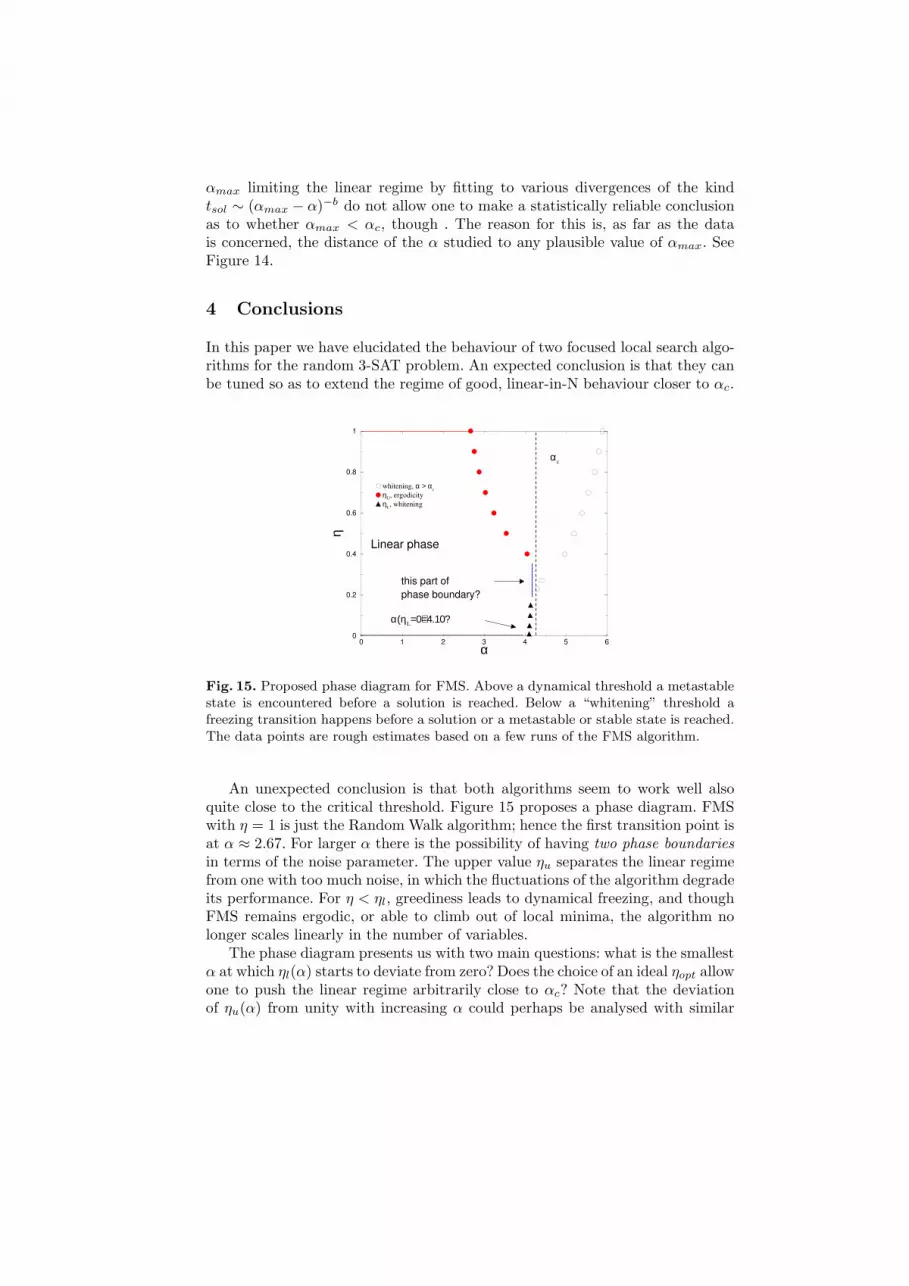
Fig. 15. Proposed phase diagram for FMS. Above a dynamical threshold a metastablestate is encountered before a solution is reached. Below a “whitening” threshold afreezing transition happens before a solution or a metastable or stable state is reached.The data points are rough estimates based on a few runs of the FMS algorithm.

An unexpected conclusion is that both algorithms seem to work well alsoquite close to the critical threshold. Figure 15 proposes a phase diagram. FMSwith η = 1 is just the Random Walk algorithm; hence the first transition point isat α ≈ 2.67. For larger α there is the possibility of having two phase boundaries

in terms of the noise parameter. The upper value ηu separates the linear regimefrom one with too much noise, in which the fluctuations of the algorithm degradeits performance. For η < ηl, greediness leads to dynamical freezing, and thoughFMS remains ergodic, or able to climb out of local minima, the algorithm nolonger scales linearly in the number of variables.

The phase diagram presents us with two main questions: what is the smallestα at which ηl(α) starts to deviate from zero? Does the choice of an ideal ηopt allowone to push the linear regime arbitrarily close to αc? Note that the deviationof ηu(α) from unity with increasing α could perhaps be analysed with similar

techniques as the methods in refs. [3, 25]. The essential idea there is to constructrate equations for densities of variables or clauses while ignoring correlations ofneighboring ones. Such analysis, while illuminating, would of course not resolvethe above two main questions.

The resolution of these questions will depend on our understanding the per-formance of FMS or other local search methods in the presence of the clusteringof solutions. The range of the algorithm presents us with a fundamental dilemma:though replica methods have revealed the presence of clustering in the solutionspace starting from α ≈ 3.92, the FMS works for much higher α’s still. The clus-tered solutions should have an extensive core of frozen variables, and thereforebe hard to find. Thus, the ability of FMS to perform well even in this regime,given the right choice of η, tells us that there are features in the solution spaceand energy landscape that are not yet well understood.

Our numerical experiments also indicate that in the linear scaling regimethe solution time probability distributions become sharper (“concentrate”) asN increases, implying indeed that the median solution time scales linearly. Wecannot establish numerically that this holds also for the average behaviour, butwould like to note that our empirical observations from the distributions do notindicate such heavy tails that would contradict this possibility.

Acknowledgements: We are most grateful to Dr. Supriya Krishnamurthyfor useful comments and discussions.

References

1. E. Aarts and J. K. Lenstra (Eds.), Local Search for Combinatorial Optimization.J. Wiley & Sons, New York NY, 1997.

2. E. Aurell, U. Gordon and S. Kirkpatrick, Comparing beliefs, surveys and randomwalks. 18th Annual Conference on Neural Information Processing Systems (NIPS2004). Technical report cond-mat/0406217, arXiv.org (June 2004).

3. W. Barthel, A. K. Hartmann and M. Weigt, Solving satisfiability problems byfluctuations: The dynamics of stochastic local search algorithms. Phys. Rev. E 67(2003), 066104.

4. A. Braunstein, M. Mezard and R. Zecchina, Survey propagation: an algorithm forsatisfiability. Technical report cs.CC/0212002, arXiv.org (Dec. 2002).

5. A. Braunstein and R. Zecchina, Survey propagation as local equilibrium equations,Technical report cond-mat/0312483, arXiv.org (Dec. 2003).

6. D. Du, J. Gu, P. Pardalos (Eds.), Satisfiability Problem: Theory and Applications.DIMACS Series in Discr. Math. and Theoret. Comput. Sci. 35, American Math.Soc., Providence RI, 1997.

7. G. Dueck, New optimization heuristics: the great deluge algorithm and the record-to-record travel. J. Comput. Phys. 104 (1993), 86–92.

8. J. Gu, Efficient local search for very large-scale satisfiability problems. SIGARTBulletin 3:1 (1992), 8–12.

9. H. H. Hoos, An adaptive noise mechanism for WalkSAT. Proc. 18th Natl. Conf.on Artificial Intelligence (AAAI-02), 655–660. AAAI Press, San Jose Ca, 2002.

10. H. H. Hoos and T. Stutzle, Towards a characterisation of the behaviour of stochas-tic local search algorithms for SAT. Artificial Intelligence 112 (1999), 213–232.

11. E. Maneva, E. Mossel and M. J. Wainwright, A new look at survey propagationand its generalizations. Technical report cs.CC/0409012, arXiv.org (April 2004).

12. N. Metropolis, A. Rosenbluth, M. Rosenbluth, A. Teller and E. Teller, Equationsof state calculations by fast computing machines, J. Chem. Phys. 21 (1953), 1087–1092.

13. M. Mezard, F. Ricci-Tersenghi, and R. Zecchina, Alternative solutions to dilutedp-spin models and XORSAT problems. J. Stat. Phys. 111 (2003), 505–533.

14. M. Mezard and R. Zecchina, Random K-satisfiability problem: From an analyticsolution to an efficient algorithm. Phys. Rev. E 66 (2002), 056126.

15. D. Mitchell, B. Selman and H. Levesque, Hard and easy distributions of SATproblems. Proc. 10th Natl. Conf. on Artificial Intelligence (AAAI-92), 459–465.AAAI Press, San Jose CA, 1992.

16. A. Montanari, G. Parisi and F. Ricci-Tersenghi, Instability of one-step replica-symmetry-broken phase in satisfiability problems. J. Phys. A 37 (2004), 2073–2091.

17. C.H. Papadimitriou, On selecting a satisfying truth assignment. Proc. 32nd IEEESymposium on the Foundations of Computer Science (FOCS-91), 163–169. IEEEComputer Society, New York NY, 1991.

18. G. Parisi, On local equilibrium equations for clustering states. Technical reportcs.CC/0212047, arXiv.org (Feb 2002).

19. A. J. Parkes, Distributed local search, phase transitions, and polylog time. Proc.Workshop on Stochastic Search Algorithms, 17th International Joint Conferenceon Artificial Intelligence (IJCAI-01). 2001.

20. A. J. Parkes, Scaling properties of pure random walk on random 3-SAT. Proc.8th Intl. Conf. on Principles and Practice of Constraint Programming (CP 2002),708–713. Lecture Notes in Computer Science 2470. Springer-Verlag, Berlin 2002.

21. S. Seitz and P. Orponen, An efficient local search method for random 3-satisfiability. Proc. IEEE LICS’03 Workshop on Typical Case Complexity andPhase Transitions. Electronic Notes in Discrete Mathematics 16, Elsevier, Am-sterdam 2003.

22. S. Seitz, M. Alava and P. Orponen, Focused local search for random 3-satisfiability.Technical report cond-mat/0501707, arXiv.org (Jan 2005).

23. B. Selman, H. Kautz, B. Cohen, Local search strategies for satisfiability testing.In: D. S. Johnson and M. A. Trick (Eds.), Cliques, Coloring, and Satisfiability,521–532. DIMACS Series in Discr. Math. and Theoret. Comput. Sci. 26, AmericanMath. Soc., Providence RI, 1996.

24. B. Selman, H. J. Levesque and D. G. Mitchell, A new method for solving hardsatisfiability problems. Proc. 10th Natl. Conf. on Artificial Intelligence (AAAI-92), 440–446. AAAI Press, San Jose CA, 1992.

25. G. Semerjian and R. Monasson, Relaxation and metastability in a local searchprocedure for the random satisfiability problem. Phys. Rev. E 67 (2003), 066103.

26. G. Semerjian and R. Monasson, A study of Pure Random Walk on random satis-fiability problems with “physical” methods. Proc. 6th Intl. Conf. on Theory andApplications of Satisfiability Testing (SAT 2003), 120–134. Lecture Notes in Com-puter Science 2919. Springer-Verlag, Berlin 2004.

27. W. Wei and B. Selman, Accelerating random walks. Proc. 8th Intl. Conf. on Prin-ciples and Practice of Constraint Programming (CP 2002), 216–232. Lecture Notesin Computer Science 2470. Springer-Verlag, Berlin 2002.