thesis_ebe_2019_naik_linus.pdf - university of cape town
TRANSCRIPT
ENVIRONMENTAL & PROCESS SYSTEMS ENGINEERING RESEARCH GROUP DEPARTMENT OF CHEMICAL ENGINEERING
UNIVERSITY OF CAPE TOWN
An investigation of the potential and the limitations of small-scale biogas in urban
Africa A revised dissertation submitted for the degree
of Philosophiae Doctor
by
Linus Naik
Supervisor
Prof. Harro von Blottnitz
Univers
ity of
Cap
e Tow
n
The copyright of this thesis vests in the author. No quotation from it or information derived from it is to be published without full acknowledgement of the source. The thesis is to be used for private study or non-commercial research purposes only.
Published by the University of Cape Town (UCT) in terms of the non-exclusive license granted to UCT by the author.
Univers
ity of
Cap
e Tow
n

Dedication
i
Dedication
For my father,
who willingly gave up so much to give me an opportunity.
Thank you for teaching me to be a scientist.
Declaration
ii
Declaration
I, Linus Naik, hereby declare that the work on which this thesis is based is my original work (except where acknowledgements indicate otherwise) and that neither the whole work nor any part of it has been, is being, or is to be submitted for another degree in this or any other university. I authorise the University of Cape Town to reproduce for the purpose of research either the whole or any portion of the contents in any manner whatsoever.
23rd October, 2019
Linus Naik
Synopsis
iii
Synopsis
Continuing urbanisation in Sub-Saharan Africa provides many development challenges
including; energy provision, waste management and sanitation. On-site biogas has the
potential to provide renewable energy to meet energy needs, whilst also addressing waste
management and possibly sanitation. In urban settings, up to 50% of the municipal waste in
urban can comprise organic waste which typically remains an untapped energy source, while
the total waste volume continually increases with population growth. Whilst some countries
(including Ethiopia and Uganda) have support via national government and/or foreign
investment for biogas deployment, their focus is on rural biogas for agricultural waste, not
urban biogas for municipal waste. This thesis investigates the case for small-scale biogas as a
technology to assist sustainable urban development through understanding factors which will
ensure operational success to safeguard investment. The factors investigated were
productivity, stability and the need for remote monitoring. The research was divided into
three distinct phases which occurred chronologically.
The first phase was observational and developmental, in which one biogas unit in a
semi-controlled environment was monitored. Some initial insight into the factors which
caused instability (in this case, the addition of simple carbohydrates) as well as two methods
of mitigation of instability (namely addition of lime and a cessation of feed) were noted for
future investigation. Also, in this phase, a mobile phone application, called the “Biogas
Monitoring Tool” was developed and refined, accompanied by a monitoring methodology to
collect information on measured variables which were considered to inform productivity and
stability of small-scale biogas units. Of the variables mentioned, the laboratory method of
evaluation of two in particular (pH and temperature) was replaced with more practical and
rudimental measuring techniques. The appropriateness of the replacements was statistically
analysed, evaluated and found to be acceptable for the intended purposes.
Synopsis
iv
The second phase of research involved the widespread rollout of the Biogas
Monitoring Tool developed in the first phase. The platform was used to gather data from ten
small-scale biogas units across southern Africa to further investigate and analyse the factors
which affected the productivity and stability of small-scale biogas units. Readings of pH, burn
time, pressure, mass and type of feed were captured through the Biogas Monitoring Tool over
twelve months. The analysis showed episodes of instability of biogas units linked to changing
feeding regimes of simple carbohydrates, organic loading rates as well as changes in feed
ratios and frequency. In terms of productivity of the biogas units, seasonal fluctuations in the
five units which were monitored over the winter months was evident, as well as potential
underutilization of biogas produced. Furthermore, it was noted that there was better
utilisation of gas for institutional installations compared to domestic installations. It was also
shown that in five of the biogas units, the stability of the unit had an influence on the quality
of gas produced, and it was indicative that it had an influence on the quantity of gas produced.
For the third and final phase of research, theories developed from insight gleaned in
the second phase were tested on one biogas unit in a controlled environment. There were
three sets of experiments conducted on this unit which had a pre-determined feeding regime.
Also, the biogas stove was burned daily until the biogas ran out, to quantify the productivity
of the biogas unit. Firstly, a stepwise addition of the organic fraction of municipal solid waste
was introduced into the feeding regime. In this case, it was demonstrated that the organic
fraction of municipal solid waste can in fact be the sole feed-stock for biogas unit, with the
proviso that there was appropriate knowledge support which includes quick mitigation
strategies for periods of instability. Secondly, the effect of pre-treatment of the organic
fraction of municipal solid waste was investigated. It was found here that the pre-treatment
did appear to improve the stability of the biogas unit, a consideration which may be significant
for potential widespread adoption of the technology. Finally, the effect of temperature on
gas production was confirmed and quantified, with higher average temperatures showing
higher gas production.
Synopsis
v
In conclusion, it was found that all the small-scale units which formed part of this
research showed episodes of instability. When considering this technology for energy
provision for urban development, there are important considerations around feedstock
variability by way of feed type, volume, and frequency affecting the stability of these units.
With reference to productivity, it was shown, not only that temperature naturally does affect
gas production, but also that the productivity is linked to the stability. Furthermore, it was
deemed that the type of setting (institutional versus domestic) was in fact more significant
than the ambient temperature or the feeding regime when considering gas use and gas
utilisation as indicators of productivity. Finally, with regard to knowledge support via remote
monitoring, it was shown that simple and practical measurements were able to provide
insight into factors which affected productivity and stability of small-scale biogas units. The
final phase further utilised the remote monitoring tool to actively manage the operation of
the biogas unit and quickly mitigate instability.
Thus, small-scale biogas has the potential to be adopted as technology for energy
provision in urban development. The limitations of the application are that waste-based
biogas would meet only an portion of the total energy requirement in any particular urban
area and that based on the findings of this research, all units are subject to periods of
instability. There are various mitigation strategies for instability, some of which involve active
management, which may be supplied remotely.

Acknowledgements
vi
Acknowledgements
In this re-submission, I would like to thank the Environmental & Process Systems
Engineering Research group for financial support, with special mention to Mrs. Carol Carr in
the group for administrative support.
I would like to thank my wife, Celeste, for her support through this, as in all aspects of
life.
Lastly and most importantly, I would like to acknowledge my supervisor, Prof. von
Blottnitz for his guidance, patience and invaluable contribution in the supervision of this
thesis.
Foreword
vii
Foreword
In my initial foreword, I had highlighted the advent of commercial biogas technology
in Southern Africa. In this regard, there was mention of some organisations promoting the
adoption of waste to energy, (particularly biogas) and my own involvement in some of them.
These are now quite dated as the examination of the original thesis took just over fifteen
months, meaning that two years have passed between the original thesis and this revised
submission. Therefore, in line with the revisions made to the body of the thesis, I have
replaced the original foreword with a revised one. With reference to the thesis itself, I have
gone into detail on the changes made and reasons for them in a separate document. Here,
however, I would like the take the opportunity here to make a few relevant comments on
some developments in the biogas and energy space over the last two years.
In March 2017, at the time of the original submission, the New Horizons Energy plant
was being commissioned in Cape Town. It was to become the second large-scale commercial
biogas plant and the first commercial urban biogas plant in South Africa. It was also the first
plant to have the organic fraction of municipal solid waste as an anchor feedstock. The plant
opened in late 2017 but has since closed its doors in mid-2018. However, in late 2018, a small-
scale unit was commissioned at a shopping centre in Cape Town – N1 City. This unit is
monitored remotely (an aspect explored in this thesis) from the Netherlands. In my initial
foreword, I had concluded with note for a case to be made for smaller decentralised facilities,
and the N1 City unit, while still a demonstration plant, it is an interesting application at an
institutional level.
In 2017, it was envisioned that the energy climate in South Africa would start changing
to accommodate more renewables into the energy mix. However, the country still has a heavy
reliance on coal and the crunch has started to yet again become felt. This thesis should
provide an insight into the potential and limitations of small-scale biogas to meet such energy
needs in urban Africa.
– Linus Naik, June 2019
Table of Contents
viii
Table of Contents
Dedication ....................................................................................................................... i
Declaration ..................................................................................................................... ii
Synopsis......................................................................................................................... iii
Acknowledgements....................................................................................................... vi
Foreword ...................................................................................................................... vii
Table of Contents ........................................................................................................ viii
List of figures ............................................................................................................... xiii
List of tables ................................................................................................................ xvi
List of abbreviations ................................................................................................... xvii
List of symbols ........................................................................................................... xviii
Chapter 1: Introduction ................................................................................................. 1
1.1. Urbanisation in Africa and the need for technologies ................................. 1
1.2. A case for biogas as the technology of choice ............................................. 4
1.3. Problem statement ....................................................................................... 6
1.4. Research objectives ...................................................................................... 6
1.5. Thesis outline ................................................................................................ 7
Chapter 2: Literature Review ......................................................................................... 9
2.1. Biogas compared to other technologies ...................................................... 9
2.2. A further look at biogas as the technology of choice ................................. 10
2.3. Current energy and waste management practices in urban Africa ........... 12
2.4. The economics of small-scale biogas operation ......................................... 14
2.5. Factors governing the operation of small-scale biogas .............................. 15
2.6. Considerations for urban biogas installations ............................................ 19
Table of Contents
ix
2.7. Synthesis & Contextualisation .................................................................... 21
2.7.1. Small-scale biogas in Africa and the role of monitoring............................. 22
2.7.2. Operational challenges in the urban setting .............................................. 23
2.8. Summary ..................................................................................................... 24
Chapter 3: Methodology .............................................................................................. 25
4.1. Hypotheses ................................................................................................. 25
4.2. Approach .................................................................................................... 26
4.2.1. Biogas units monitored............................................................................... 29
4.2.2. Development of the mobile phone application for remote monitoring .... 32
4.2.3. Measurement of specific parameters ........................................................ 36
4.2.3.1. Measurement of pH ................................................................................. 36
4.2.3.2. Measurement of temperature ................................................................ 37
4.2.3.3. Weighing of feedstock ............................................................................. 38
4.2.3.4. Observation of pressure .......................................................................... 38
4.2.3.5. Recording of ‘burning time’ ..................................................................... 38
4.3. Operation, monitoring and measurement methodology .......................... 39
4.3.1. Operation and monitoring in Phase 1 ........................................................ 39
4.3.2. Operation and monitoring in Phase 2 ........................................................ 40
4.3.3. Operation and monitoring in Phase 3 ........................................................ 43
4.3.3.1. Migration to OFMSW ............................................................................... 44
4.3.3.2. Experimentation with Bokashi treated waste ......................................... 44
4.3.3.3. Experimentation with simple carbohydrates .......................................... 45
4.4. Calculation methodology............................................................................ 45
4.4.1. Confirmation of stove rating and calculation of gas utilisation ................. 46
4.4.2. Calculation of maximum theoretical biogas ............................................... 48
4.4.3. Error analysis .............................................................................................. 49
Table of Contents
x
4.5. Research ethics ........................................................................................... 50
4.6. Outlook ....................................................................................................... 51
Chapter 4: Initial Field Observation ............................................................................. 52
4.1 Observations on unit stability, pH and feeding regime ................................. 52
4.1.1 The effect of feed regime effect on stability .............................................. 55
4.1.2 Observations of temperature ..................................................................... 56
4.1.3 Gas utilisation and productivity .................................................................. 58
4.2 Evaluation of monitoring techniques ............................................................. 60
4.2.1 Evaluation of pH monitoring methods ....................................................... 60
4.2.2 Evaluation of temperature monitoring methods ....................................... 64
4.2.3 Other monitoring methods ........................................................................ 66
4.3 Refinement of the Biogas Monitoring Tool application ................................. 66
4.4 Final discussions and conclusions .................................................................. 68
Chapter 5: Remote Monitoring Studies ....................................................................... 69
5.1 Stability of biogas units .................................................................................. 69
5.1.1 Biogas unit pH vs time series ...................................................................... 70
5.1.1.1. Individual pH profiles of all units ............................................................. 70
5.1.1.2. Summary of observations in acidity profiles ........................................... 80
5.1.2 The effect of organic loading rate on stability ........................................... 81
5.2 The effect of instability on biogas production/utilisation ............................. 83
5.3 Productivity of Biogas units ............................................................................ 87
5.3.1 Gas utilisation of the biogas units .............................................................. 88
5.3.2 Normalised gas use by month .................................................................... 89
5.3.3 The effect of feedstock on productivity ..................................................... 91
5.3.4 The effect of climate on productivity ......................................................... 92
5.4 Summary of findings and conclusions ............................................................ 93
Table of Contents
xi
Chapter 6: Field Experimentation ................................................................................ 95
6.1 Performance on structured feeding regime .................................................. 96
6.1.1 Migration to OFMSW from manure ........................................................... 96
6.1.2 Gas utilisation ............................................................................................. 97
6.2 Performance on Bokashi treated food waste .............................................. 100
6.3 Experimentation with simple carbohydrates ............................................... 101
6.4 Summary and conclusions ............................................................................ 103
Chapter 7: Conclusions .............................................................................................. 104
7.1 Synthesis of findings ..................................................................................... 104
7.2 Conclusions................................................................................................... 106
7.3 Recommendations ....................................................................................... 109
7.3.1 Recommendations for further research ................................................... 109
7.3.2 Recommendations for practice ................................................................ 110
7.4 Outlook ......................................................................................................... 111
References ................................................................................................................. 112
Appendices ...................................................................................................................... I
Appendix A: The sustainable development goals (UN, 2016) .................................. II
Appendix B: Glossary of terms .................................................................................. III
Appendix C: The IPAT equation illustrated ...............................................................IV
Appendix D: The potential impact for biogas in the City of Cape Town....................V
Appendix E: Ethics Clearance ....................................................................................VI
Appendix F: Associated projects ..............................................................................VII
F1: The UCT residence biogas project brief .........................................................VII
F2: The Abalimi biogas project brief ..................................................................... IX
F3: Aquatest: Remote Water Quality Monitoring (UCTCivEng, 2011).................. IX
Appendix G: Abstracts from relevant conference papers ........................................ XI
Table of Contents
xii
G1. WasteCon 2012 (Naik, et al., 2012) ................................................................ XI
G2. WasteCon 2016 (Naik, 2016) ......................................................................... XII
Appendix H: Sample Data ....................................................................................... XIII
H1. Raw data sample from UCT biogas unit for Phase 1 .................................... XIII
H2. Sample of data from Remote Monitoring Study for Phase 2 ...................... XIV
H3. Data sample from LCF biogas unit showing introduction of simple
carbohydrates for Stage 3 of Phase 3 ............................................................................. XV
ANNEXURE: The Energisation Study .......................................................................... A-1
Introduction ........................................................................................................... A-1
Methodology .......................................................................................................... A-3
Application of the Toolkit ...................................................................................... A-7
Application A: Small-scale biogas vs alternative technologies .......................... A-7
Application A: Summary and discussions ........................................................ A-12
Application B: Context of two small-scale biogas units ................................... A-15
Conclusions .......................................................................................................... A-16
References ........................................................................................................... A-17
Definitions ............................................................................................................ A-18
The definition of “Energisation” ...................................................................... A-18
The definitions of the “Aspects” ...................................................................... A-20
An example of an “Application”....................................................................... A-26
List of figures
xiii
List of figures Figure 1. Schematic representation of the anaerobic digestion process (Divya, et al.,
2015). ....................................................................................................................................... 16
Figure 2. Schematic summary of the approach taken in Phases 1, 2 and 3 with a
description of each phase ( - - ) and their interrelation ( � ) as well as the information flow (
� ) to address the objectives. ................................................................................................... 27
Figure 3. Picture of the welcome "splash" screen for the Biogas Monitoring Tool
application used for the remote monitoring study from Phase 2 onwards. ........................... 32
Figure 4. Screen from the user interface of the Biogas Monitoring Tool application as
displayed on an emulator for a Nokia C2-00. .......................................................................... 34
Figure 5. Illustration of the User Interface of captured data for a monitored site. .... 35
Figure 6. pH indicator strip used to measure pH of biogas digesters (Distillique, 2016).
.................................................................................................................................................. 37
Figure 7. Location map of the biogas units monitored across southern Africa for Phase
2................................................................................................................................................ 40
Figure 8. Letter sent to biogas operators at the onset of Phase 2. ............................. 41
Figure 9. Example of the monthly newsletter distributed to operators in the Biogas
Monitoring Tool study in Phase 2. ........................................................................................... 42
Figure 10. Trends in pH (•) for the UCT biogas unit in Phase 1, between March 2011
and April 2012 .......................................................................................................................... 53
Figure 11. Trends in food mass (•) and water volume (•) fed to UCT biogas unit in Phase
1, between March 2011 and April 2012 .................................................................................. 54
Figure 12. Temperature measurement (•) of the UCT biogas unit in Phase 1, between
March 2011 and April 2012 ..................................................................................................... 57
Figure 13. Parity plot of pH measured by indicator strip vs probe for the UCT biogas
unit (•), the Eastern Cape biogas unit (•) and the N1 City Shopping Mall biogas unit (•). ..... 61
Figure 14. Comparison of reported and measured temperature readings for the UCT
digester. ................................................................................................................................... 64
Figure 15. Reported (•) and measured (•) temperature readings for the UCT digester
over a 92 day period. ............................................................................................................... 65
List of figures
xiv
Figure 16. pH vs time series for 1.(WC).6.[O].[I] (•) with trendlines marking a pH of 6.5
(- -) and a pH of 6.0 (- -)............................................................................................................ 70
Figure 17. pH vs time series for 2.(WC).10.[O].[I] (•) with trendlines marking a pH of
6.5 (- -) and a pH of 6.0 (- -)...................................................................................................... 72
Figure 18. pH vs time series for 3.(WC).6.[O][S].[D] (•) with trendlines marking a pH of
6.5 (- -) and a pH of 6.0 (- -)...................................................................................................... 73
Figure 19. pH vs time series for 4.(EC).6.[O][S].[D] (•) with trendlines marking a pH of
6.5 (- -) and a pH of 6.0 (- -)...................................................................................................... 74
Figure 20. pH vs time series for 5.(SWZ).6.[O][S].[D] (•) with trendlines marking a pH
of 6.5 (- -) and a pH of 6.0 (- -). ................................................................................................ 75
Figure 21. pH vs time series for 6.(WC).20.[O][S].[I] (•) with trendlines marking a pH of
6.5 (- -) and a pH of 6.0 (- -)...................................................................................................... 76
Figure 22. pH vs time series for 7.(LIM).8.[A][M].[D] (•) with trendlines marking a pH
of 6.5 (- -) and a pH of 6.0 (- -). ................................................................................................ 77
Figure 23. pH vs time series for 8.(KZN).8.[A][M].[D] (•) with trendlines marking a pH
of 6.5 (- -) and a pH of 6.0 (- -). ................................................................................................ 78
Figure 24. pH vs time series for 9.(WC).10.[A][M].[I] (•) with trendlines marking a pH
of 6.5 (- -) and a pH of 6.0 (- -). ................................................................................................ 78
Figure 25. pH vs time series for 10.(WC).6.[M][S].[I] (•) with trendlines marking a pH
of 6.5 (- -) and a pH of 6.0 (- -). ................................................................................................ 79
Figure 26. Average weekly pH vs weekly OLR for 1.(WC).6.[O].[I] (x); 2.(WC).10.[O].[I]
(x); 3.(WC).6.[O][S].[D] (x); 5.(SWZ).6.[O][S].[D] (x); 6.(WC).20.[O][S].[D] (x);
8.(KZN).8.[A][M].[D] (x); 9.(WC).10.[A][M].[I] (x) and 10.(WC).6.[M][S].[I] (x). ...................... 82
Figure 27. Burning times around episodes of low pH for 1.(WC).6.[O].[I]. ................. 83
Figure 28. Burning times around episodes of low pH for 2.(WC).10.[O].[I]. ............... 84
Figure 29. Burning times around episodes of low pH for 3.(WC).6.[O][S].[D]. ........... 85
Figure 30. Burning times around episodes of low pH for 6.(WC).20.[O][S].[I]. ........... 86
Figure 31. Burning times around episodes of low pH for 9.(WC).10.[A][M].[I]. .......... 86
Figure 32. Average daily normalised gas use by month (primary axis) and average
annual gas utilisation (secondary axis) for all units over Phase 2, from February 2012 to
January 2013. ........................................................................................................................... 90
Figure 33. Mass of OFMSW (•) fed to the LCF unit from Mar 2014 to Aug 2015. ...... 96
List of figures
xv
Figure 34. Temperature (•) and gas utilisation (•) of the LCF biogas unit from Mar 2014
to Aug 2015. ............................................................................................................................. 98
Figure 35. Normalised gas use vs temperature plot (•) with linear trendline (- -) for LCF
biogas unit from Nov 2014 to Aug 2015 .................................................................................. 99
Figure 36. Time series profiles of total weight of OFMSW (•), weight of simple
carbohydrate (•) on the primary axis, and pH (•) on the secondary axis for LCF biogas unit
from January to July 2015 ...................................................................................................... 102
List of tables
xvi
List of tables Table 1. Comparison between the University of Cape Town (UCT) and Local
Composting Facility (LCF) Biogas Units used in Phases 1 and 3 respectively. ......................... 29
Table 2. Description of the properties of biogas units monitored in Phase 2. ............ 30
Table 3. Properties of biogas stoves used in the study (Puxin, 2019). ........................ 31
Table 4. Parameters reported through the Biogas Monitoring Tool application in Phase
2................................................................................................................................................ 33
Table 5. Summary of changes in monitoring techniques of the parameters measured
at the UCT biogas unit between March 2011 and April 2012. ................................................ 39
Table 6. Parameters monitored via Biogas Monitoring Tool application for the LCF
biogas unit in Phase 3. ............................................................................................................. 43
Table 7. Biochemical methane potentials used for calculation of maximum theoretical
biogas ....................................................................................................................................... 48
Table 8. Burning times over five weeks in Period 2 for the stove connected to the UCT
biogas unit in Phase 1 .............................................................................................................. 58
Table 9. Burning time over ten weeks in Period 4 for the stove connected to the UCT
biogas unit in Phase 1. ............................................................................................................. 59
Table 10. Analysis of absolute mean and standard deviations over the pH ranges for
pH indicator strip vs. pH probe measurements. ...................................................................... 62
Table 11. Results of t-test analysis of pH data measurements by indicator strip vs. pH
probe. ....................................................................................................................................... 62
Table 13. Extraction of data recordings of feeding regime of 1.(WC).6.[O].[I] before
instances of a decline in pH. .................................................................................................... 71
Table 14. Observations of low acidity in all biogas units across remote monitoring
study. ........................................................................................................................................ 80
Table 15. Average gas utilisation of the remote monitoring users from Feb 2012 to Jan
2013 ......................................................................................................................................... 88
Table 16. Frequency of lime treatments in different period of operation of the LCF
biogas unit. ............................................................................................................................... 97
List of abbreviations
xvii
List of abbreviations AW Agricultural Wastes
BMP Biochemical Methane Potential
CoCT City of Cape Town
E&PSE Environmental & Process Systems Engineering
EC Eastern Cape
EM Effective Microbes
GDP Gross Domestic Profit
KZN KwaZulu-Natal
LCF Local Composting Facility
LIM Limpopo Province
LPG Liquefied Petroleum Gas
min minute
MDGs Millennium Development Goals
MSW Municipal Solid Waste
OFMSW Organic Fraction of Municipal Solid Waste
S Sewage
SDGs Sustainable Development Goals
SWZ Swaziland
UCT University of Cape Town
UN United Nations
WC Western Cape
List of symbols
xviii
List of symbols
°C degrees Celsius
Ca(OH)2 calcium hydroxide a.k.a. lime
CH4 methane
C:N carbon to nitrogen mass ratio
CO2 carbon dioxide
e energy rating
H2 hydrogen
hr hour(s)
J Joules
K Kelvin
kg kilograms
kJ kiloJoule
kPa kiloPascal
kW kiloWatt
m3 cubic metres
mol mole(s)
n number of moles
ñ molar flow rate
mV millliVolts
P pressure
PJ petaJoule
R rate constant for ideal gases
sec second(s)
T temperature
V volume
Chapter 1: Introduction
1
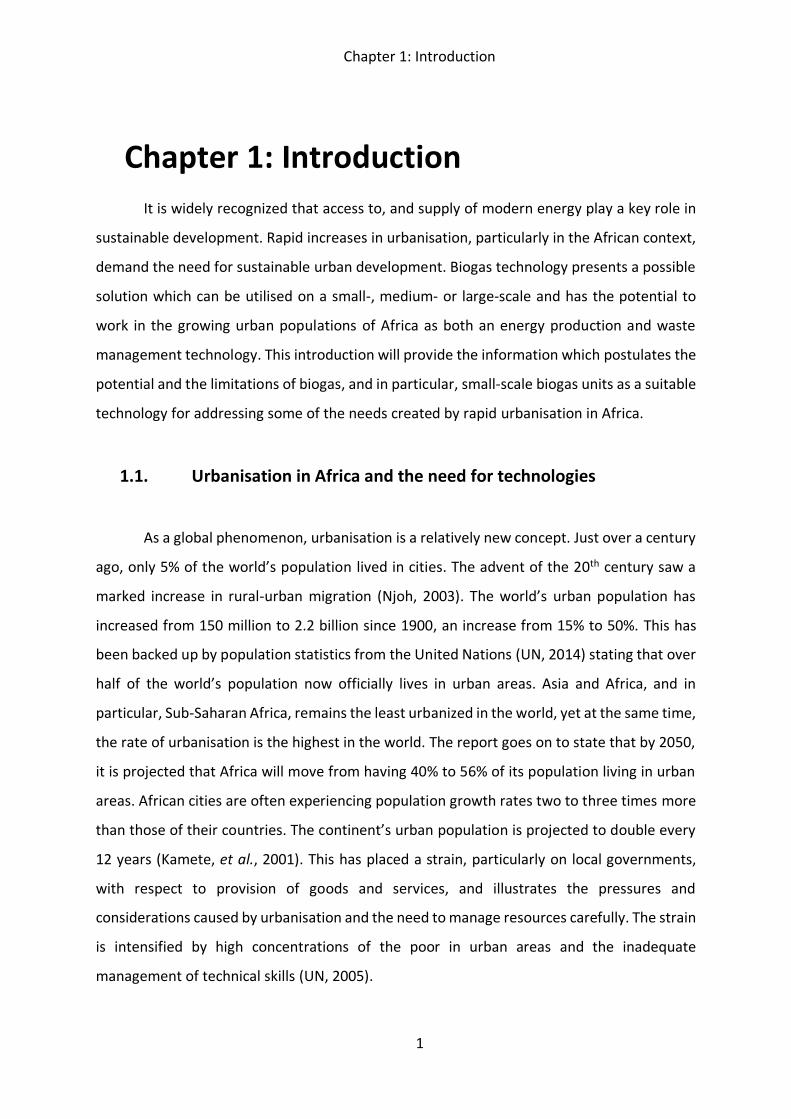
Chapter 1: Introduction It is widely recognized that access to, and supply of modern energy play a key role in
sustainable development. Rapid increases in urbanisation, particularly in the African context,
demand the need for sustainable urban development. Biogas technology presents a possible
solution which can be utilised on a small-, medium- or large-scale and has the potential to
work in the growing urban populations of Africa as both an energy production and waste
management technology. This introduction will provide the information which postulates the
potential and the limitations of biogas, and in particular, small-scale biogas units as a suitable
technology for addressing some of the needs created by rapid urbanisation in Africa.
1.1. Urbanisation in Africa and the need for technologies
As a global phenomenon, urbanisation is a relatively new concept. Just over a century
ago, only 5% of the world’s population lived in cities. The advent of the 20th century saw a
marked increase in rural-urban migration (Njoh, 2003). The world’s urban population has
increased from 150 million to 2.2 billion since 1900, an increase from 15% to 50%. This has
been backed up by population statistics from the United Nations (UN, 2014) stating that over
half of the world’s population now officially lives in urban areas. Asia and Africa, and in
particular, Sub-Saharan Africa, remains the least urbanized in the world, yet at the same time,
the rate of urbanisation is the highest in the world. The report goes on to state that by 2050,
it is projected that Africa will move from having 40% to 56% of its population living in urban
areas. African cities are often experiencing population growth rates two to three times more
than those of their countries. The continent’s urban population is projected to double every
12 years (Kamete, et al., 2001). This has placed a strain, particularly on local governments,
with respect to provision of goods and services, and illustrates the pressures and
considerations caused by urbanisation and the need to manage resources carefully. The strain
is intensified by high concentrations of the poor in urban areas and the inadequate
management of technical skills (UN, 2005).
Chapter 1: Introduction
2
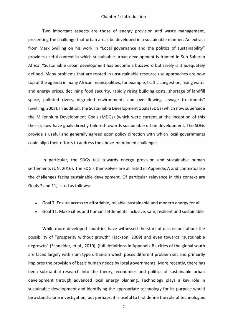
Two important aspects are those of energy provision and waste management,
presenting the challenge that urban areas be developed in a sustainable manner. An extract
from Mark Swilling on his work in “Local governance and the politics of sustainability”
provides useful context in which sustainable urban development is framed in Sub-Saharan
Africa: “Sustainable urban development has become a buzzword but rarely is it adequately
defined. Many problems that are rooted in unsustainable resource use approaches are now
top of the agenda in many African municipalities, for example, traffic congestion, rising water
and energy prices, declining food security, rapidly rising building costs, shortage of landfill
space, polluted rivers, degraded environments and over-flowing sewage treatments”
(Swilling, 2008). In addition, the Sustainable Development Goals (SDGs) which now supersede
the Millennium Development Goals (MDGs) (which were current at the inception of this
thesis), now have goals directly tailored towards sustainable urban development. The SDGs
provide a useful and generally agreed upon policy direction with which local governments
could align their efforts to address the above-mentioned challenges.
In particular, the SDGs talk towards energy provision and sustainable human
settlements (UN, 2016). The SDG’s themselves are all listed in Appendix A and contextualise
the challenges facing sustainable development. Of particular relevance in this context are
Goals 7 and 11, listed as follows:
x Goal 7. Ensure access to affordable, reliable, sustainable and modern energy for all
x Goal 11. Make cities and human settlements inclusive, safe, resilient and sustainable
While more developed countries have witnessed the start of discussions about the
possibility of “prosperity without growth” (Jackson, 2009) and even towards “sustainable
degrowth” (Schneider, et al., 2010) (full definitions in Appendix B), cities of the global south
are faced largely with slum type urbanism which poses different problem set and primarily
implores the provision of basic human needs by local governments. More recently, there has
been substantial research into the theory, economies and politics of sustainable urban
development through advanced local energy planning. Technology plays a key role in
sustainable development and identifying the appropriate technology for its purpose would
be a stand-alone investigation, but perhaps, it is useful to first define the role of technologies
Chapter 1: Introduction
3
in sustainable development. This is illustrated using the well-known IPAT equation (Ehrlich &
Holdren, 1971) shown as follows: Impact = Population x Affluence x Technology.
Using the example of carbon emissions, it is apparent that if population and affluence
keep increasing, then in order to stabilise the impacts, the technology must counteract
(example presented in Appendix C). From an energy perspective, renewable energy and
energy efficiency address the role of technology through:
x dematerialisation – using less resources to produce the same energy service
x substitution – using renewable energy instead of carbon intensive ones (Robert, et al.,
2002)
In Europe, the installed power production capacity in 2008 based on several sources
was as follows: natural gas (18%), oil (6%), coal (26%), nuclear (33%), hydro (12%) and other
renewable (3%). The current trends in power production point to an increased use of natural
gas and renewables, slight increase in nuclear and decrease in coal and oil consumption
(Afgan & Carvallo, 2008). Two factors were expected to influence future trends in the
European energy sector (Hemmes, et al., 2007): the need to meet the Kyoto commitments
and the issue of security of energy supply, reflected in the green paper: “Towards a European
Strategy for the Security of Energy Supply”. The authors go on to stress the importance of
multi-source, multi-product energy technologies; their work is a prominent example of how
the European Union is trying to meet its challenges by innovating its way out of dirty energy
(Jacobsson & Bergek, 2004); investing heavily in research and innovation since the 1980s
(Suurs & Hekkert, 2009). Since 2010, however, it has been proposed that working with
technologies in the African setting may be significantly different to working with technologies
in the European Union (Sovacool, et al., 2015). One of the attributed reasons for this is the
that there is now an extensive inventory of available developed technologies, yet a dearth of
application. Thus, it has been argued that the African focus should be on developing the ability
to choose and deploy suitable technologies rather than on developing new ones (von Blottnitz
& Chakraborty, 2006).
Chapter 1: Introduction
4
1.2. A case for biogas as the technology of choice
In the last few decades, there has been a significant non-sustainable use of fossil fuels
which has necessitated research into renewable energy sources and technologies. This, in
part, has led to increased awareness into the availability and accessibility of such
technologies, significantly since the 1970s oil crisis (EOCD, 1985). Biogas is a renewable energy
source which has been practiced for centuries and represents a potentially viable option for
the future. It is produced via anaerobic digestion in biogas units with two main outputs, a
methane rich gas (which is an energy source) and a digestate (which is a nutrient source).
Biogas units may be used as a treatment for many organic products and waste streams, from
food crops (such as maize) (Dutt, 1992), to organic fraction of municipal solid waste, animal
manure (Balasubramanian & Bai, 1992) and even wastewater (where it was commonly used
as a method of reducing the organic loading) (Elango, et al., 2007). Thus, biogas units have a
variety of designs and applications, ranging from small to large-scale operations, and even
one- and two-stage processes (Aslanzadeh, et al., 2014). In this thesis, small-scale is defined
as units at a household or institutional level, having no more than 20 m3 total capacity.
Biogas production via anaerobic digestion has been noted to have been practiced for
centuries, so in a sense it is not a new technology, but has more recently been identified as
an important renewable energy source (Surendra et al., 2014). Thus, the technology itself and
the factors which affect its effectiveness have been well researched. For example, the impacts
temperature, pH, organic loading rate, carbon-to-nitrogen ratios, microbial populations and
hydraulic retention time have all been identified to have an effect on biogas operation (these
are all discussed further in Chapter 2). Large-scale units would naturally be centralised and
need to be commercially viable and ensure operational success to attract investment. In
Europe and Asia, there has also been widespread rollout of small-scale biogas systems, which
would be decentralised and have the added advantages of energy generation on site – with a
concomitant saving on transport (and associated carbon emissions). Thus, biogas may be seen
as a multi-purpose solution, as it provides a renewable energy source with a waste
management (and possibly a sanitation) solution and may be used to address some of the
issues facing the growing urban population of the developing world (Surendra et al., 2014).
Chapter 1: Introduction
5
The following has been taken as a summary from a review paper on small-scale biogas.
“As a technology, it possesses highly attractive attributes, particularly when considering
renewable energy options.
x It is a renewable energy technology that produces a multi-purpose fuel that can be used
to produce domestic or industrial heat, electricity or stationery and motive power (e.g.
for water pumps and transportation).
x It can often replace fossil fuels in provision of energy, thereby reducing greenhouse gas
emissions
x It has the potential to address a portion of municipal solid waste problems which include
landfilling and its associated land availability issues and concomitant greenhouse gas
emissions
x A by-product of the process is the digestate/effluent, which contains liberated nutrients,
specifically nitrogen and phosphorus, which make it potentially useful for soil application
as a fertilizer.” (Naik, et al., 2014)
However, as mentioned, much of the research and rollout of small-scale biogas has
been in done in Europe and Asia, both of which now boast millions of small- to medium-scale
installations (Deng, et al., 2017). In Africa, where there is a definite need of on-site energy
generation has not experienced the same level of deployment. In a few countries (initially
Kenya, Uganda, Ethiopia at the onset of this thesis, and since then Tanzania, Rwanda,
Cameroon, Burkina Faso and Benin (Roopanarain & Adekele, 2017)) there are partnerships
with governmental departments and technology companies in European countries (usually
German or Dutch) to facilitate the deployment of the technology in appropriate rural settings
via micro-financing and government grants/support. However, the operational knowledge
around the productivity and the stability of such installations does not appear to be retained
by the local governments or translated into wide-spread roll-out of the technology.
Thus, it appears that biogas, and in particular, small-scale biogas is a technology which
is fit for purpose (Balat & Balat, 2009) but lacks understanding and knowledge support which
would facilitate wide-spread deployment, particularly in urban Africa where the energy is
needed.
Chapter 1: Introduction
6
1.3. Problem statement
Primarily, in response to the observation that access to energy services plays a pivotal
role in sustainable urban development, it is noted that decentralised, small-scale biogas
installations represent a technological intervention. However, such installations may come
with their own set of challenges by way of ensuring productivity and stability.
Therefore, it is necessary to understand the factors which influence the operation of
small-scale biogas units, and to provide appropriate knowledge support for the system to
ensure operational success and safeguard any potential investments. This presents two
unique challenges. The first would be to understand factors which specifically affect small-
scale units which are currently in operation. The second would be to see whether there are
any differences when these units are operated with typical feedstocks from an urban setting.
Both these would tie in to providing the necessary knowledge support, and possibly informing
an effective monitoring system.
1.4. Research objectives
The overarching objective of this thesis is therefore to develop new knowledge to
inform the potential for, and limitations of small-scale biogas, as a technology for deployment
in urban Africa, specifically:
1. To advance the understanding of operational stability, the factors which
influence it and potentially how to mitigate instability.
2. To quantify the gas production from substrates and determine initially
whether it is dependent on the stability of the biogas unit, and secondly,
determine the factors which influence it.
3. To develop and test the appropriateness of knowledge support systems for
small-scale biogas units deployed in an African setting.
Chapter 1: Introduction
7
1.5. Thesis outline
Following on from this introductory chapter, this thesis goes on to review relevant
literature from the academic sphere in Chapter 2. Since anaerobic digestion itself is an old
technology, there is significant relevant literature on biogas and anaerobic digestion, so it is
important to only highlight information, which is pertinent to this study, and to be concise
with peripheral, but applicable topics. Given the objectives, the first task in the literature
review is to understand biogas as a technology in the context of establish its intended
applications. The scope is first narrowed to an African context, and then furthermore to an
urban context in Africa, focusing on its unique set of challenges. There is, then, a detailed
discussion and analysis of the factors which have been identified to affect the productivity
and stability of small-scale systems, as well as a venture into the required knowledge support
which may be required to sustain the widespread deployment of such systems. The summary
of the current state of knowledge is distilled through the objectives to formulate hypotheses
and develop a methodology, in that the findings from Chapter 2 are used in Chapter 3 for
research formulation.
Chapters 4, 5 and 6 are results chapters in which various aspects of the thesis have
been completed, analysed and discussed in context relevant to the research objectives in this
introductory chapter, and the hypotheses in Chapter 3. Chapter 4 is the initial field
investigation conducted on the UCT biogas unit. This study ventures initial learnings on
productivity and stability of one small-scale system, noting potential mitigation strategies for
instability. At the same time, the remote monitoring methodology is developed, refined and
analysed by way of comparisons of various monitoring techniques. Chapter 5 is a remote
monitoring study, which uses the new developed and refined monitoring methodology on a
widespread application, to collect and analyse real data from ten small-scale biogas systems
around Southern Africa. The purpose of using the monitoring methodology was two-fold;
firstly, to gain insights into productivity and stability of small-scale biogas units through
reported parameters; and secondly, to test the effectiveness of the remote monitoring
methodology. In Chapter 6, one small-scale unit, installed at a composting facility was actively
managed to run test work to further inform theories on stability and productivity which had
Chapter 1: Introduction
8
been developed after the monitoring study in Chapter 5. Key outcomes of the results chapters
are consolidated and synthesised in Chapter 7, to re-address the research objectives, the
problem statement and the hypotheses. Some recommendations are then made for future
work with an outlook on the scene for small-scale biogas in urban Africa.
The intention of this thesis was to propose contexts for where small-scale biogas units
could be successful as a technology in urban Africa, and to identify the knowledge support
needed to safeguard new infrastructure investment. Firstly, observational analysis was used
to gain initial insight and then build and deploy a monitoring methodology. This is then
deployed and used to gather data on a wide-scale to further inform operational productivity
and stability. Lastly, theories generated from the insights are tested on one final biogas unit
to reach more confident conclusions. Two unique contributions are attempted in this work.
The first is using monitoring and operational experience to propose a knowledge support
system which could safeguard investments into such a technology. The second, is the various
mitigation techniques for instability to ensure operational success of small-scale biogas units.
Chapter 2: Literature Review
9
Chapter 2: Literature Review This chapter unpacks the current body of knowledge around relevant aspects of this
thesis. From Chapter 1, the need for technologies to meet the growing energy demands of
urban Africa. In this light, the first section broadly contrasts biogas against other technologies
fit for the same purpose. From here, small-scale biogas is reviewed from an economic and
then from an operational standpoint, before looking at the current waste management
practices in urban Africa and the finally the unique challenges which may affect urban biogas
installations. Findings from all these are discussed and summarised from the standpoint of
the potential and limitations of small-scale biogas in urban Africa. The findings are then
distilled through the objectives to inform the methodology for research in Chapter 3.
2.1. Biogas compared to other technologies
In this context, particularly on the small-scale, biogas would be used to meet primary
energy needs; namely cooking, and then heating and/or lighting. Other renewable
competitive technologies in the same context would be solar cookers and efficient wood-
stoves for cooking; and then solar heaters and possibly photovoltaic cells for heating and
lighting. Efficient wood-stoves would use the same fuel, namely wood, just less of it. Therein
lies both the advantage (in that it would be market compliant as it uses the same fuel) but
also the drawback (in that that using the same fuel means that any problems associated with
burning wood will still be there – in this case, health issues associated with burning wood)
would still be there, just less pronounced). For solar cookers, the advantage is that it is the
cleanest of the technologies. However, the drawback, and the issue which may be a critical
flaw to using the technology, is that it depends largely on an energy source which cannot be
ensured. If being used to meet primary energy needs (as it indeed is in this context) then the
cooker may simply not work on overcast days and can therefore not be used to replace
traditional wood stoves. Additionally, the meal cooking efficiency is typically less than other
technologies.
Chapter 2: Literature Review
10
Biogas is certainly a more complex technology and comes with its own set of
challenges and concerns when considering the context of meeting primary energy needs in
urban Africa. More complex technologies are not necessarily more appropriate. Indeed, it has
the added advantage of addressing a waste management challenge, something that the other
two technologies do not offer. However, the complexity may arise through the need for
knowledge support and skill in the operation and handling of the gas. Also, although it may
have been an old technology on the whole, it is a relatively “new” technology in the proposed
application, meaning that there are cultural and market compliance concerns. Finally, the high
capital cost of a biogas unit is a major drawback of the technology. Skills or knowledge
support may be needed to manage operations and health and safety concerns would need to
be addressed to ensure operational success. Additionally, there are high capital costs
associated with the technology and a need for existing infrastructure, so deployment in the
informal sector may be less feasible. These details of these considerations are out of the scope
of this thesis. However, they are explored in detail in the energisation study, presented as a
stand-alone annexure to this thesis.
2.2. A further look at biogas as the technology of choice
It was mentioned in Chapter 1 that biogas has been well established in parts of Europe,
especially Germany (Negro & Hekkert, 2009) and Asia (Rees, 2005), especially China (Deng, et
al., 2017), where small- to medium-scale installations exist in the millions (Polpraset, 2007).
However, as a technology, it has seen very limited deployment on any scale in Africa. At the
start of this thesis, in 2011, there were only about 40 installations in South Africa (Boyd, 2010),
the majority of which are rural, small- to medium-scale operations. Over the last five to six
years, this has increased to just under 400 (Roopanarain & Adekele, 2017), two of which are
commercial scale, with the balance being largely rural and small- to medium-scale.
The differences between urban and rural biogas units are investigated in detail later
in Section 2.6, but at this stage attention must be drawn to the potential difference in
feedstock between urban and rural biogas units in Africa, and indeed in commercial and
personal application in places where biogas deployment is abundant. In Europe, biogas
Chapter 2: Literature Review
11
production has been incentivised and food-crops are often used as feed because they have
very high biogas yields. In developing countries, this is typically not supported, for example,
the Department of Energy in South Africa will only support water efficient and non-food-
based crops since the country has limited arable land and is water scarce (ENS Africa, 2015),
so the majority of biogas is waste based. From an energisation angle, this is advantageous, as
it allows the technology to not only meet energisation needs, but also those of waste
management, and possibly sanitation. Particularly in the context of municipal solid waste
management, organic waste constitutes 40 – 85% of total domestic waste and is currently
insufficiently utilised as an energy resource (Abraham, et al., 2007). At the start of this thesis,
the example was taken of the City of Cape Town (CoCT) in 2011, where the OFMSW has a high
moisture content (40-80%) (Munganga, et al., 2010) rendering technologies such as mass
burn incineration unsuitable. Upon analysis in 2011, the waste generation to landfill in the
CoCT had peaked at 2.8 million tonnes per annum in 2007/8, and although it had previously
declined to some 1.8 million tonnes per annum in 2008/9 (CoCT, 2010), there remains a
shortage of landfill space (Engledow, 2007). Given the current organic fraction of municipal
solid waste (≈50%) produced in the CoCT, biogas was calculated to have the potential to meet
between 4% and 5% of the energy needs of the city (based on a simple calculation presented
in Appendix D) while at the same time reducing waste to landfill by 50% through using
centralised biogas from waste generation. Anaerobic digestion was therefore postulated as
the priority treatment option for the organic fraction of municipal solid waste (OFMSW) due
to the advantages stated above, and indeed, this was attempted to prove itself true (at least
on the large-scale) with the initial commissioning of the New Horizons Energy biogas plant
which can process 500 tonnes per day of MSW (EngineeringNews, 2017). This plant has since
closed as it ran out of capital before all parts could be fully commissioned.
The example given is for a large centralised facility. If a large-scale plant can only meet
5% of the energy demand of the city, the question arises as to how much of the energy
demand of a household that small-scale biogas would meet. This would depend on the
amount of waste that the household produced, and so the question then becomes whether
or not a household produces enough waste to potentially meet its own energy demand
through biogas production.
Chapter 2: Literature Review
12
2.3. Current energy and waste management practices in urban Africa
Urban areas in Sub-Saharan Africa are faced with the challenges of appropriately
accessing energy and managing their organic waste. Traditional fuels for energy (i.e. coal,
paraffin and biomass) have associated health, safety and environmental impacts, as does the
improper management of waste (in particular, organic waste). The demands of the urban
areas and the associated waste are also markedly different to those in rural areas. The key
feature is that the vast majority of the organic fraction of municipal solid waste (OFMSW)
produced or generated in urban areas throughout Africa is disposed of in landfills or dumps
and not further utilised aerobically nor anaerobically (Kasozi, et al., 2010). In landfills, the
OFMSW will degrade anaerobically to produce methane gas which is not extracted and is
emitted straight into the atmosphere. In the last ten years, there have been urban composting
initiatives in Kenya, Malawi and South Africa (Scheinberg, et al., 2011) while in the rural
setting, there has been anaerobic treatment of agricultural waste on a large scale. The
government programmes for anaerobic digestion, (usually with a European sponsor) have
been mentioned in Section 1.2. These programmes followed widespread rollout in Asia,
particularly China, India and Nepal which have over a hundred million units between them,
deployed over the last 30 years (De Clercq, et al., 2017). This makes the case that there is
space for widespread rollout in Africa and that, with government local energy planning, there
can be structured rollout of biogas in urban Africa if the technology is proven to be fit-for-
purpose.
A further look into the potential valorisation of OFMSW is discussed as follows. If
valorised, biological treatment the predominant option due to the nature of the waste.
Biological treatment can be classified into aerobic and anaerobic. Aerobic valorisation is
usually composting, while anaerobic would be microbial fermentation in a biogas unit, or
alternatively with effective microbes, now commercially found in Bokashi to produce a pre-
compost which can either be applied directly to soil, or used as a pre-compost (Swilling, et al.,
2015). Bokashi treatment has been used in a pilot study in informal settlements (von der
Heyde, et al., 2014), as an organic waste management tool.
Chapter 2: Literature Review
13
Bokashi is the term given to the Bokashi bran, as well as the treatment procedure. The
treatment involves the layering of organic waste with Bokashi bran (which is wheat or oat
bran sprayed with effective microbes). On a small-scale, this would be done in five or ten litre
plastic drums, and on the commercial scale, it would be performed in 210 dm3 drums. In all
cases, the container would be sealed for ten to fourteen days to allow the fermentation to
occur (Earth Probiotic, 2018). The resulting mixture is a valuable pre-compost. In the case of
the study at the informal settlement, the treatment was found to be effective, with the
observation of rodent and fly reduction, but was not cost effective due to the cost of the
Bokashi Bran. The resulting Bokashi treated waste was not utilised further (e.g. in
composting), but rather collected and disposed of as the intended purpose was for hygiene
and sanitation.
Comparisons have been done between these treatment methods under the factors of
cost, energy and greenhouse gas emissions. It was found that anaerobic treatment typically
requires a larger investment (Mata-Alvarez, 1999), while from an energy balance standpoint,
it was found that anaerobic treatment has a better energy balance as well as lower associated
carbon footprint (Edelman, et al., 2005). The latter went on to propose that in some cases,
the two are combined for optimal results, in the fashion of anaerobic digestion followed by
aerobic composting of the digestate. In Sub-Saharan Africa, OFMSW and agricultural wastes
have been treated aerobically to produce compost which has been used mainly in the rural
setting, but also in some urban farms (Scheinberg, et al., 2011) Some examples of urban
composting are in Nairobi, Kenya where a food delivery company used reverse logistics to
collect OFMSW for composting, and in Lilongwe, Malawi, where a community driven project
collected OFMSW for an urban farming application. However, despite seeming to be simple
and cost effective, aerobic treatment is not used widely in Sub-Saharan Africa (Vogel &
Zurbrugg, 2008).
Anaerobic digestion on the small-scale is becoming increasingly popular in rural Africa
(Bond & Templeton, 2011), but not so much in urban areas. The impact of the technology
could be considerable, depending on the size of the urban area and the availability of
separated organic waste as a feedstock.
Chapter 2: Literature Review
14
2.4. The economics of small-scale biogas operation
The first aspect of economies is that of a large-scale operation compared to a small-
scale operation, which naturally requires an economic analysis. There have been many studies
which have tried to make or contest the economic case for small-scale biogas. However, this
was again largely concerned with rural biogas units or large-scale commercial operations. It
has been argued that the advantage of decentralising removes the necessity to transport a
waste fraction to a centralised treatment facility (Lijo, et al., 2017), and thereby saving
transportation costs and the concomitant carbon emissions. Additionally, other factors have
been modelled, to show that the landfill fee, as well as the operational expenses, both play
crucial roles in determining the optimal size and location of a proposed biogas unit
(Rajendran, et al., 2014) and make a case for small-scale energy generation on site, at least
for biogas from OFMSW. However, for large-scale commercial plants, it has been argued that
the economies of scale for the centralised plants outweigh the diseconomies of scale for the
transport (Skovsgaard & Jacobsen, 2017). On the household level, the focus is somewhat
different, in that the technology must show a saving to the household in their cost of primary
energy needs, and in this regard, biogas has proven itself (Yasar, et al., 2017) showing a six
year return on investment. In fact, there have been attempts to improve the economics by
modifying the biogas operation (Renda, et al., 2016) to improve the return on investment.
The second aspect of economics would be that of widespread rollout of small-scale
biogas units. It has been mentioned that China, India, Pakistan and Nepal both boast
widespread rollout of small-scale biogas units (De Clercq, et al., 2017) with Nepal boasting
the highest number of biogas units per capita. In Africa, there have been programmes from
Dutch government in Ethiopia via Dutch support, and by the German government in Uganda
via German support. These models work by a partial loan and a micro-financing opportunity
to install small-scale biogas units in the rural setting meaning that they are not viable without
a portion of grant funding. In effect, policies have been put in place for such programmes. In
2015, a group attempted a pilot study on scaling and commercialisation of small-scale biogas
units (Sovacool, et al., 2015). The findings confirmed the notion that while the technology had
potential, policies were required to support the widespread rollout.
Chapter 2: Literature Review
15
2.5. Factors governing the operation of small-scale biogas
Before reviewing the factors that affect the operation of biogas units, it is imperative
to understand the process of biogas production. The production of biogas itself is carried out
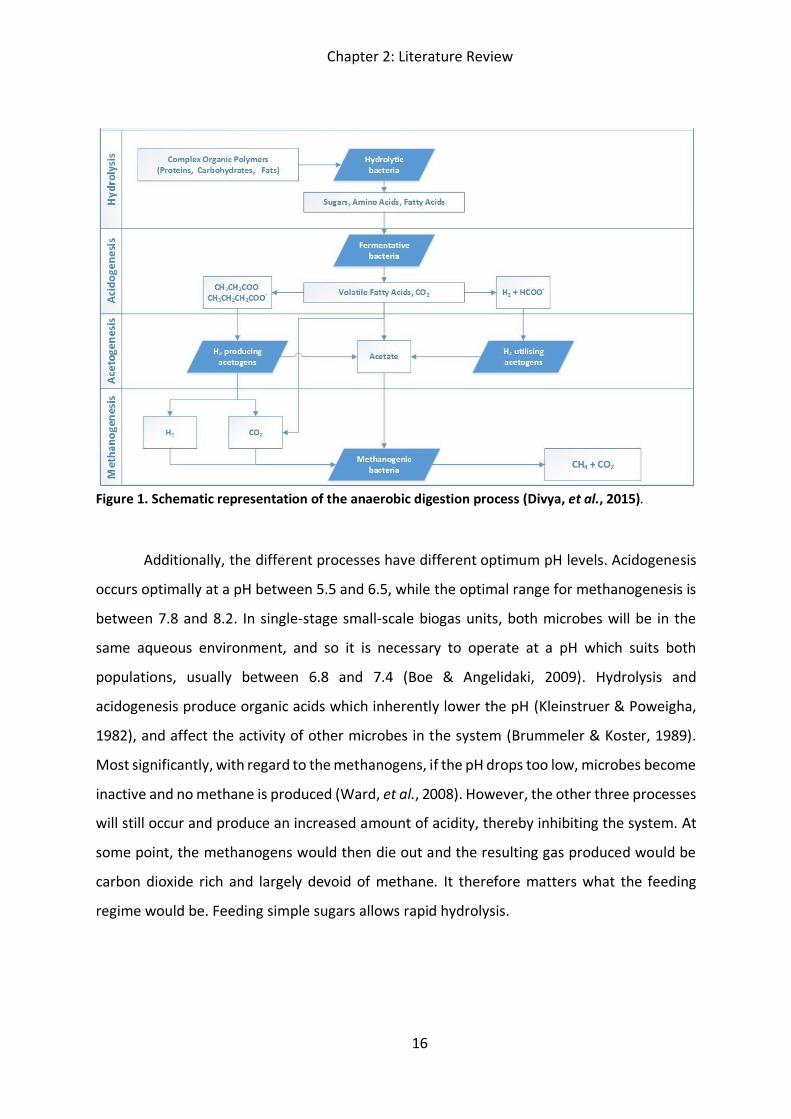
by four main groups of microbes as depicted in Figure 1, which shows the four main stages in
anaerobic digestion (Chynoweth & Isaacson, 1987). The first, hydrolysis, is the breakdown of
large polymers into the simple substrates. The second, acidogenesis, carried out by
fermentative bacteria, produces volatile fatty acids and some carbon dioxide. These volatile
fatty acids are then converted to acetate by a process called acetogenesis. Lastly,
methanogenic bacteria produce methane and carbon dioxide from the acetate, hydrogen and
carbon dioxide (Grebben, et al., 2008). Each of the main four subsets of microbes operate in
their own niche conditions (Cheng, et al., 1987) and each of these microbes have different
resilience and activities (Wang, et al., 2004). The microbial population is typically introduced
in the start-up phase of operation. Where the feedstock is cow-manure, the microbes will all
be naturally occurring. However, if the feedstock is OFMSW, then inoculation (typically with
cow manure) will be needed and the population will need to be maintained throughout the
operation of the biogas system (Monnet, 2003). If conditions are not favourable, certain
populations may die out and re-inoculation will be needed. The inoculation is a biological
process, and is the period needed to get to optimal operation, so there have been studies on
how to reduce this time (Adl, et al., 2012).
Chapter 2: Literature Review
16
Figure 1. Schematic representation of the anaerobic digestion process (Divya, et al., 2015).
Additionally, the different processes have different optimum pH levels. Acidogenesis
occurs optimally at a pH between 5.5 and 6.5, while the optimal range for methanogenesis is
between 7.8 and 8.2. In single-stage small-scale biogas units, both microbes will be in the
same aqueous environment, and so it is necessary to operate at a pH which suits both
populations, usually between 6.8 and 7.4 (Boe & Angelidaki, 2009). Hydrolysis and
acidogenesis produce organic acids which inherently lower the pH (Kleinstruer & Poweigha,
1982), and affect the activity of other microbes in the system (Brummeler & Koster, 1989).
Most significantly, with regard to the methanogens, if the pH drops too low, microbes become
inactive and no methane is produced (Ward, et al., 2008). However, the other three processes
will still occur and produce an increased amount of acidity, thereby inhibiting the system. At
some point, the methanogens would then die out and the resulting gas produced would be
carbon dioxide rich and largely devoid of methane. It therefore matters what the feeding
regime would be. Feeding simple sugars allows rapid hydrolysis.
Chapter 2: Literature Review
17
With regard to the composition of feed, much importance has been attributed to the
carbon to nitrogen (C:N) mass ratio (Cuetos, et al., 2008). This is the amount of carbon over
the amount of nitrogen present in the feed by mass ratio (Bernal, et al., 2009). The optimum
C:N is 20 - 30 (Gomez, et al., 2006). Although discussed later in Section 2.6, it is worthwhile
mentioning that one of the main differences between urban and rural biogas units is the
nature of the feedstock. In rural settings, the feedstock is largely homogenous, while this is
certainly not the case with OFMSW (Resch, et al., 2010). In this regard, the C:N becomes very
important when attempting to optimise the performance of a biogas unit (Sisnowski &
Wieczorsk, 2003), as there may be high breakdown of feedstock with low methane
production, and vice versa (Forster-Cerneiro, et al., 2008). Also, with regard to the feed, the
particle size would be important, because of the increased surface area to volume ratio with
smaller particles (Agwunwamba, 2001).
Practically, for small-scale operations, this may involve mechanical processing of
larger particles, and is a notable form of pre-treatment. The amount of water, or conversely,
the quantity of solids also has an effect on the operation of the biogas unit. Low total solids
systems range from 1-5% mass fraction of solids, whereas high total solids systems range from
11-15% mass fraction of solids (Kaltwassar, 1980). The amount of water and solids naturally
influence the organic loading rate, which is the rate of organics fed to the system per unit of
reactor volume. Furthermore, the amount of water crucially affects the hydraulic residence
time inside the system. There are therefore optimal organic loading rates which are
dependent on temperature, type and quantity of feed (Fang, 2010). In that study, they were
noted to be optimum between 0.5 and 0.6 kg.m-3.day-1, while other studies which have aimed
to reduce acidogenesis have reported acidosis occurring above 3.0 kg.m-3.day-1 (Goux et al.,
2015). In cases where the aim is to produce volatile fatty acids, the organic loading rate can
be increased to 20 to 30 kg.m-3.day-1. kg.m-3.day-1 (Demirer & Chen, 2004). Crucially, since all
the reactions all occur in an aqueous environment, the production of biogas is significantly
reduced when there is above 80% mass fraction of solids (Rajeshwari, et al., 2001).
Besides the feeding regime, external factors are also important, and most important,
considering that this is a biological process, would be temperature. Similar to acidity, each
microbe would have an optimum temperature. However, given that in most cases, all
Chapter 2: Literature Review
18
microbes would be at the same temperature, the microbes would typically function optimally
at either mesophilic or thermophilic temperatures (Igoni, et al., 2008). Below 65 °C there
would be a linear relationship, whereby an increase in temperature would increase microbial
activity, and therefore biogas production (Karangiannidis & Perkoulidis, 2009). Above 65 °C,
the microbial populations would die off and the rate of production would drastically decline.
Large-scale biogas units can be tuned to operate in the mesophilic or thermophilic ranges.
Mesophilic are the more predominant (Tchobanogolous & Burton, 1981) with many kinetic
studies being carried out in that range (Veissmen & Hammer, 1993). Thermophilic operations
are generally considered to be more productive but subject to instabilities (Kiely, et al., 1997).
Without temperature control, small-scale biogas units would operate at ground temperature
(if underground) or ambient temperature (if above ground). This would largely depend on the
climate, but is almost always below the mesophilic range of 35 °C to 45 °C.
The reactor configuration has also been identified as important. It is known that the
productivity is a function of the geometry of the biogas unit (Khanal, 2008). Two-stage
digestion, with hydrolysis, acidogenesis and acetogenesis in one stage and then
methanogenesis in the next has been shown to improve biogas production in certain cases
(Liu, et al., 2006), which in turn improves the economic viability (Renda, et al., 2016). The
hydraulic retention time is vital in continuous systems. Production usually increases to a point
of “washout”, where the microbes leave the system before they can reproduce (Deublin &
Stenhouser, 2008).
It is also known that methanogens, being anaerobic bacteria (Mudrack & Kunst, 1991)
may be inhibited by the presence of increased oxygen (Hungate, 1996). Biogas systems on
the whole are tolerant to limited amounts of oxygen (Morris, 1975). The redox potential can
be used as an indication of methanogenesis (Archer & Harris, 1986), where the redox
potential for anaerobes is known to be between -200 mV and -400 mV (Hungate, 1967).
Oxygen inhibition Is only one of the forms of inhibition. The C:N ratio mentioned previously
is significant because a high nitrogen content results in the production of ammonia which is
also inhibitory to methanogens. Other inhibitory by-products include volatile fatty acids and
sulphides (Konzeli-Katsiri & Kartsonas, 1986). Some investigations on the adaptation and
resistance of the microbes under acidic conditions and high organic loading rates has been
Chapter 2: Literature Review
19
done on the laboratory scale (Goux et al., 2015). These investigations showed that some of
the microbes were able to survive the highly acidic conditions and recover from such
episodes, returning to normal biogas production after a few days. This may be an indication
of resilience or adaption on the part of the microbes.
Thus, it is observed that many detailed studies have been carried out to determine the
factors which affect biogas operation. There is a need to isolate those which are most crucial
to the operation of small-scale biogas units. It is apparent that the feeding regime appears to
play a key role in the operation of the biogas units and is the primary parameter which can be
controlled. Based on these learnings, a focus is now taken on urban biogas installations,
considering which of the factors might be of most significance.
2.6. Considerations for urban biogas installations
It has been identified in Section 2.3 that there has been extensive roll-out of biogas
units in some developing countries (mostly Asia). These apply largely to rural settings, and not
urban ones. Before identifying the challenges facing urban biogas units, it is important to
understand how they are different from rural ones.
When considering the size of the biogas unit, rural units would be on a household
scale (Akinbami, et al., 2001), or an institutional scale (Arthur & Baidoo, 2011). For urban
systems, there has been a particularly noteworthy attempt for the rollout of biogas and the
twenty one units were installed at institutional levels, e.g. a prison (Barry, et al., 2011).
However, if the intended application is the informal sector, there are two major challenges
around infrastructure. The first consideration would be where the unit would be installed,
and the second would be around ownership of the biogas unit, as well of the gas produced.
It was also mentioned that when considering waste-based biogas, the rural units
would typically have a more homogenous feed, by way of animal manure and agricultural
waste. Agricultural waste may be seasonal, but still consistent. In rural settings, OFMSW
would typically only make up a small fraction of the waste stream (Ghimere, 2013). However,
Chapter 2: Literature Review
20
in urban settings, OFMSW would be the main feedstock. Challenges in this regard may arise
around the purity of the organic waste, as common practice is not source separation. On the
large-scale, urban biogas in an industrial setting could have a homogenous feedstock, e.g.
abattoir, brewing, feedlot. However, on the small-scale application, the feedstock would be
heterogenous due to the nature of OFMSW.
Considering the outputs from the biogas unit, the first is naturally the biogas. For all
small-scale biogas units, the gas is used to meet primary energy needs, which is usually
cooking, but has been used for lighting and sometimes heating (Tumwesige, et al., 2014),
whereas, on the large-scale, it may be used for power generation and to supplement process-
heat requirements to improve efficiencies (Gebreegziabher, et al., 2014). The other output is
the digestate. Smith et al. (Smith, et al., 2014), in their review, found numerous studies which
show the advantages of the nutrient value from composting the digestate. On the whole, in
the rural setting, biogas has been shown to improve rural livelihood by meeting primary
energy demands and improving soil quality (Smith & Avery, 2014). For urban units, it is normal
for large-scale operations to compost the digestate or sell it on to a composting facility which
will do the same. However, on the small-scale, and depending on the location, the digestate
itself may prove to be a challenge in the urban setting. Furthermore, the inability to valorise
the digestate may affect the economic case of the technology.
Chapter 2: Literature Review
21
2.7. Synthesis & Contextualisation
This section will bring together the key points of the review under the headings of
“stability”, “productivity”, and “remote monitoring”. Each section will discuss key outcomes
from the literature reviewed and how it may be relevant to the objectives of this thesis from
Section 1.4. The objectives are re-stated here, now reinforced with relevant literature as
follows:
1. Various studies have indicated that the feedstock variability will have an effect
on the stability of the biogas system. Given the complex chain of reactions
which occur, from acidogenesis through to methanogenesis, and the different
rates of these reactions, the feeding regime (including possible pre-treatment)
is likely to be a key factor in the stability of the system as a whole, particularly
on the small-scale. Quantifying and qualifying the effect would prove useful in
the successful operation of small-scale biogas units.
2. Since biogas units are biological systems, operating temperature would affect
the biogas yield. As per point 1, understanding and qualifying this effect would
prove useful in the successful operation of small-scale biogas units.
3. Lastly, since biogas is a complex technology requiring some expertise to
operate successfully, there would be a necessity for knowledge support for
successful operation and to safeguard investment.
Chapter 2: Literature Review
22
2.7.1. Small-scale biogas in Africa and the role of monitoring
Addressing the first and second objectives, there needs to be a definition of the
system, and then a definition of productivity and stability. The system may be defined as the
whole biogas unit, from the feed inlet, and including the end-user device. Productivity can be
defined as the amount of biogas produced per unit mass of feed (if necessary, normalised to
reactor volume). The stability of the system is defined as the sensitivity of the system to
changes in operation.
Many parameters have been identified which affect the operation of the biogas units,
and thereby the productivity and stability of the operations. Furthermore, many of the
parameters are linked, and dynamically inter-dependant. The inter-dependency is important
because it allows certain parameters to be measured and even inferred from others. For
example, volatile fatty acid concentration and pH, where the volatile fatty acid concentration
(a typically technology intensive measurement) can be inferred from the pH (a typically low-
tech measurement) (Lahav, et al., 2002). The pH would primarily be influenced by the feeding
regime. This would be the same case for C:N ratio (which impacts inhibition), the hydraulic
residence time (which may influence washout) and the particle size (which would affect
productivity). The feeding regime therefore appears to be of paramount importance when
considering operational success. Furthermore, pH can be monitored as a linked parameter as
an indication of operational stability. Another low-tech measurement is flame quality, in the
instances noted above where there would be high acidity and therefore production of carbon
dioxide over methane, the flame would burn yellow as opposed to blue. Monitoring of
parameters to ensure productivity and stability may be crucial in itself to safeguard
investment.
Chapter 2: Literature Review
23
The design of the unit, and the context of its installation may also govern the success
of the unit. There are different designs, but more complex often means more expensive,
which works against affordability in the context of energisation. Lastly, although it is
recognised that anaerobic digestion is a biological process, there is no control over the actual
microbes responsible for the process, apart from the initial inoculation. That being said, it is
observed that the microbes are sensitive to temperature. Again, for simple systems, there
would not be any temperature control, so this would largely be a function of the climate of
the location where the biogas unit is installed.
2.7.2. Operational challenges in the urban setting
Having understood the differences between urban and rural systems, the challenges
which may face urban biogas rollout can be considered from the angle of feasibility. The
economics of small- versus large- scale has already been debated in Section 2.4, so in this
section, the discussions will only be relevant to small-scale urban biogas units.
In addition to the operational concerns around productivity and stability, it appears
that there may be two more concerns when dealing with small-scale urban biogas units.
Section 2.7.1. draws attention to the fact that feeding regime has a significant effect on the
operational stability and that the nature of the intended feedstock (OFMSW) is heterogenous,
this may prove to be a significant challenge to urban biogas units. Stability and productivity
of the system may be further impacted by inconsistencies in feedstock.
While the digestate is seen as a valuable by-product in rural cases, the digestate,
without a use, in the urban setting may prove to be a challenge. It may also detract from the
feasibility of small-scale urban biogas units as a whole.
Chapter 2: Literature Review
24
2.8. Summary
The success of small-scale operations will depend largely on the ability to maintain
stability and high productivity of these units and may beg the need for monitoring and control
of important parameters in a cost-effective manner. The technology itself comes with
operational concerns, which themselves are exacerbated in small-scale units, where small
reaction volumes are more susceptible to minor perturbations. The feeding regime has been
identified as critical for reliable production of biogas, which may necessitate monitoring (and
in indeed smart-monitoring when considering widespread rollout) to safeguard investments.
There has been widespread rollout in Europe and Asia which have preceded some
European initiatives in some African countries to promote small-scale biogas units in rural
settings. However, apart from a few institutional units, there have not been any attempts to
promote small-scale biogas in the urban setting. The urban setting itself brings with it its own
set of challenges. The two main challenges identified are the heterogeneity of OFMSW which
may impact operational stability of the biogas unit, and the effective use of the nutrient rich
digestate. The use of the digestate also has an economic impact, as the nutrients have value
and impact on the financial case for the technology.
These concepts are central to the potential success and understanding the limitations
of small-scale biogas in urban Africa.
Chapter 3: Methodology
25
Chapter 3: Methodology Based on the literature reviewed, the problem statement from Section 1.3 is now built
upon. The problem statement outlined that access to energy services had been identified to
play a pivotal role in sustainable urban development, particularly in the fast-developing cities
of the global south. Now, based on the literature reviewed, it is apparent that decentralised,
small-scale biogas units characterise a technological intervention that would potentially fit
well into this context as a solution to energy demands, with additional waste management
and sanitation benefits. Although the technology has been well researched, with a large
scientific body of literature (making it principally ready to deploy), there is a dearth of
application in urban Africa. There is a need to understand the important parameters which
would control the productivity and stability of small-scale systems particularly in urban Africa
(given that the intended feedstock would be the organic fraction of municipal solid waste),
and to identify the support infrastructure needed to maintain the successful operation of such
installations.
4.1. Hypotheses
There are three hypotheses which have been formulated through the analysis of
relevant literature. These are as follows:
Hypothesis 1: Feedstock variability is a key factor affecting the stability of small-
scale biogas units; it is further hypothesised that pre-treatment of the organic waste can
improve stability of biogas units.
Anaerobic digestion is a staged process, the first of which is a hydrolysis phase which
can occur very quickly with simple carbohydrates and can lower the pH of the system,
adversely affecting the balance of biological agents. In small-scale systems, such
perturbations would be more significant. Pre-treatment of the organic waste may produce a
more homogenous feedstock and therefore improve the stability of small-scale anaerobic
digesters.
Chapter 3: Methodology
26
Hypothesis 2: Ambient temperature is the other determining factor of productivity
of small-scale anaerobic digesters to the point that it significantly affects biogas yield of
installed digesters across seasons and across locations.
Biochemical reactions increase with temperature as they are based on microbial
activity. It is widely accepted that the microbial activity is a function of temperature up to a
point where the microbes die when the temperature is too high. Thus, the biogas yield should
be higher in warmer climates.
Hypothesis 3: Smart monitoring of key parameters will improve stability and thus
productivity of small-scale biogas units.
Given the complex nature of the technology, smart monitoring would be needed to
provide knowledge support, to safeguard the success of the technology if it were indeed to
be adopted in a widespread rollout.
4.2. Approach
To gather evidence in support of the hypotheses, the proposed approach was, of
necessity, located more in the field than in the laboratory. The framework of the
investigations undertaken were formulated around opportunities and projects which arose
organically over the development of the research project. Overall, the application of research
undertook the following phases:
x Phase 1: Initial Field Observation. This was the study of one particular unit, to
understand factors which affected productivity and stability in a controlled
environment. This unit was also used to test and hone the remote monitoring
parameters and methodology for the next phase.
x Phase 2: Remote Monitoring. This was the widespread application of the parameter
monitoring procedure informed by Phase 1 presenting a large amount of data for
analysis of key trends and providing insights to test hypotheses.
x Phase 3: Field Experimentation. This was taking some of the learnings from Phases 1
& 2 to set up experiments in another controlled environment.
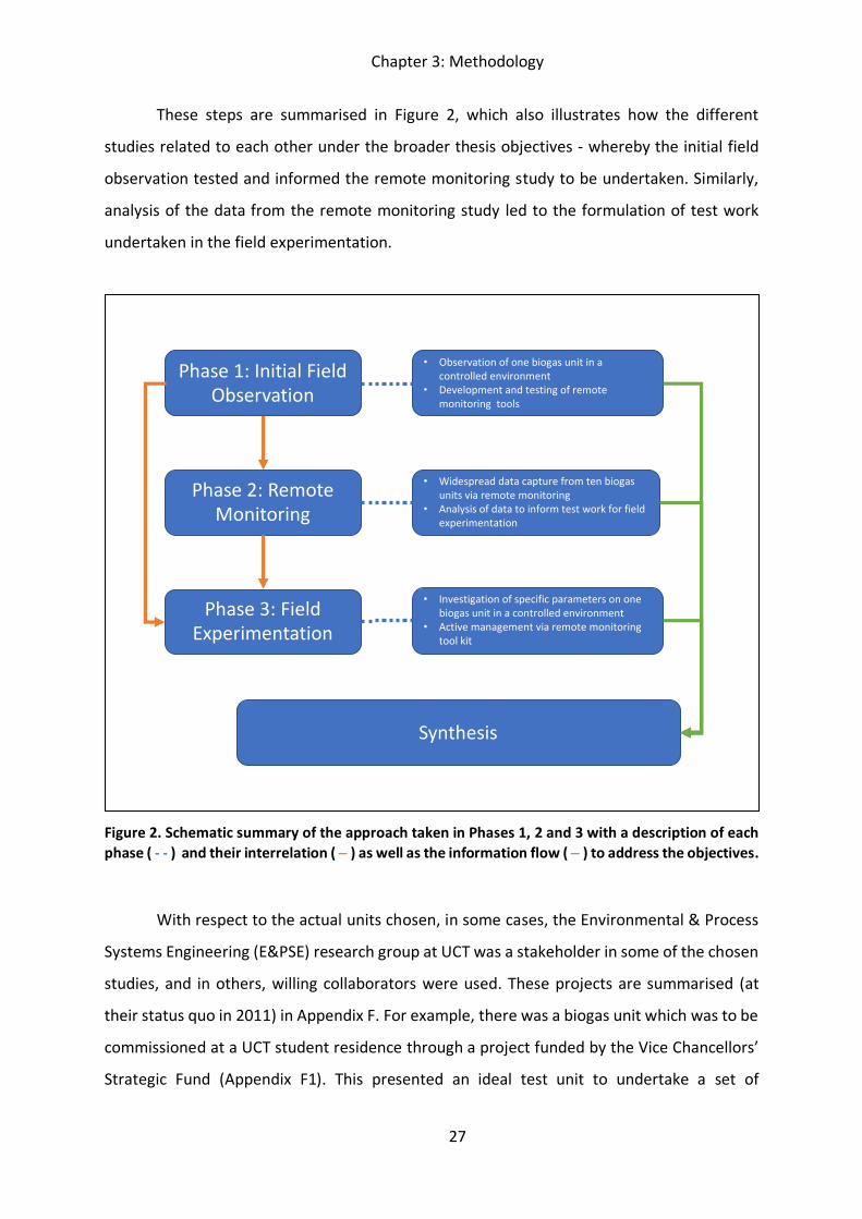
Chapter 3: Methodology
27
These steps are summarised in Figure 2, which also illustrates how the different
studies related to each other under the broader thesis objectives - whereby the initial field
observation tested and informed the remote monitoring study to be undertaken. Similarly,
analysis of the data from the remote monitoring study led to the formulation of test work
undertaken in the field experimentation.
Figure 2. Schematic summary of the approach taken in Phases 1, 2 and 3 with a description of each phase ( - - ) and their interrelation ( � ) as well as the information flow ( � ) to address the objectives.
With respect to the actual units chosen, in some cases, the Environmental & Process
Systems Engineering (E&PSE) research group at UCT was a stakeholder in some of the chosen
studies, and in others, willing collaborators were used. These projects are summarised (at
their status quo in 2011) in Appendix F. For example, there was a biogas unit which was to be
commissioned at a UCT student residence through a project funded by the Vice Chancellors’
Strategic Fund (Appendix F1). This presented an ideal test unit to undertake a set of
Phase 1: Initial Field Observation
Phase 2: Remote Monitoring
Phase 3: Field Experimentation
• Observation of one biogas unit in a controlled environment
• Development and testing of remote monitoring tools
• Widespread data capture from ten biogas units via remote monitoring
• Analysis of data to inform test work for field experimentation
• Investigation of specific parameters on one biogas unit in a controlled environment
• Active management via remote monitoring tool kit
Synthesis
Chapter 3: Methodology
28
investigations for the initial field observation to start addressing Hypotheses 1 & 2. The unit
was also used for the development of the remote monitoring methodology, identifying which
parameters could be monitored and then trial analytical methods. This culminated in a smart
phone application and monitoring toolkit, the methodology for which is further discussed
later in Section 4.2.2.
For Phase 2, the manufacturer/supplier of the initial unit was able to provide contact
details of other small-scale biogas units in the region, all of whom were contacted to find
some willing collaborators to use the now-built mobile phone application. Once the
monitoring methodology was finalised, the application was rolled out and sent to ten test
units across southern Africa over 2012 and 2013. The biogas unit at the university residence
was one of the units in the monitoring study, and as some contacts were sourced through the
supplier four other biogas units were the same model as the biogas unit in Phase 1, allowing
for comparisons. The aim was to generate a wealth of data from biogas units in urban settings
with different feedstocks and in different climates to further address Hypotheses 1 & 2
respectively. Furthermore, there existed a smart monitoring service as this data was being
collected via smart phone application. There was also a level of interaction and support with
the biogas operators.
In 2014, an opportunity arose to undertake further investigations on another biogas
unit with the owner wanting to prove the case of using the organic fraction of municipal solid
waste as the sole feedstock for an urban biogas unit. Based on learnings and experiences from
Phase 2, key parameters were chosen to carry out a tailored investigation on this unit which
became Phase 3, starting in 2014. The pre-treatment of feedstock as well as staggered
introduction of simple carbohydrate feed was investigated to specifically speak to Hypothesis
1, while the now standardised remote monitoring from Phase 2 was used to further speak
towards Hypothesis 2.
All three phases of research involved remote monitoring. Phase 1 involved the
development of the monitoring methodology. Phase 2 used the tool to gather data and
interact with some of the users. Phase 3 actively used the tool to manage a biogas unit
remotely. Thus, all three phases provided learnings which addressed Hypothesis 3.
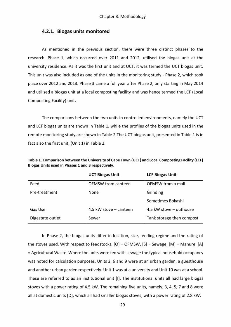
Chapter 3: Methodology
29
4.2.1. Biogas units monitored
As mentioned in the previous section, there were three distinct phases to the
research. Phase 1, which occurred over 2011 and 2012, utilised the biogas unit at the
university residence. As it was the first unit and at UCT, it was termed the UCT biogas unit.
This unit was also included as one of the units in the monitoring study - Phase 2, which took
place over 2012 and 2013. Phase 3 came a full year after Phase 2, only starting in May 2014
and utilised a biogas unit at a local composting facility and was hence termed the LCF (Local
Composting Facility) unit.
The comparisons between the two units in controlled environments, namely the UCT
and LCF biogas units are shown in Table 1, while the profiles of the biogas units used in the
remote monitoring study are shown in Table 2.The UCT biogas unit, presented in Table 1 is in
fact also the first unit, (Unit 1) in Table 2.
Table 1. Comparison between the University of Cape Town (UCT) and Local Composting Facility (LCF) Biogas Units used in Phases 1 and 3 respectively.
UCT Biogas Unit LCF Biogas Unit
Feed OFMSW from canteen OFMSW from a mall
Pre-treatment None Grinding
Sometimes Bokashi
Gas Use 4.5 kW stove – canteen 4.5 kW stove – outhouse
Digestate outlet Sewer Tank storage then compost
In Phase 2, the biogas units differ in location, size, feeding regime and the rating of
the stoves used. With respect to feedstocks, [O] = OFMSW, [S] = Sewage, [M] = Manure, [A]
= Agricultural Waste. Where the units were fed with sewage the typical household occupancy
was noted for calculation purposes. Units 2, 6 and 9 were at an urban garden, a guesthouse
and another urban garden respectively. Unit 1 was at a university and Unit 10 was at a school.
These are referred to as an institutional unit [I]. The institutional units all had large biogas
stoves with a power rating of 4.5 kW. The remaining five units, namely; 3, 4, 5, 7 and 8 were
all at domestic units [D], which all had smaller biogas stoves, with a power rating of 2.8 kW.
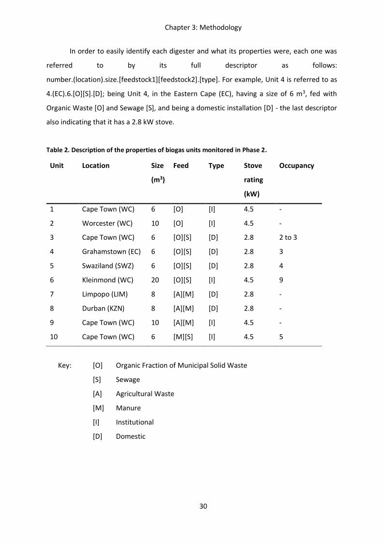
Chapter 3: Methodology
30
In order to easily identify each digester and what its properties were, each one was
referred to by its full descriptor as follows:
number.(location).size.[feedstock1][feedstock2].[type]. For example, Unit 4 is referred to as
4.(EC).6.[O][S].[D]; being Unit 4, in the Eastern Cape (EC), having a size of 6 m3, fed with
Organic Waste [O] and Sewage [S], and being a domestic installation [D] - the last descriptor
also indicating that it has a 2.8 kW stove.
Table 2. Description of the properties of biogas units monitored in Phase 2.
Unit Location Size
(m3)
Feed Type Stove
rating
(kW)
Occupancy
1 Cape Town (WC) 6 [O] [I] 4.5 -
2 Worcester (WC) 10 [O] [I] 4.5 -
3 Cape Town (WC) 6 [O][S] [D] 2.8 2 to 3
4 Grahamstown (EC) 6 [O][S] [D] 2.8 3
5 Swaziland (SWZ) 6 [O][S] [D] 2.8 4
6 Kleinmond (WC) 20 [O][S] [I] 4.5 9
7 Limpopo (LIM) 8 [A][M] [D] 2.8 -
8 Durban (KZN) 8 [A][M] [D] 2.8 -
9 Cape Town (WC) 10 [A][M] [I] 4.5 -
10 Cape Town (WC) 6 [M][S] [I] 4.5 5
Key: [O] Organic Fraction of Municipal Solid Waste
[S] Sewage
[A] Agricultural Waste
[M] Manure
[I] Institutional
[D] Domestic
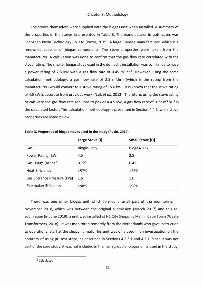
Chapter 3: Methodology
31
The stoves themselves were supplied with the biogas unit when installed. A summary of
the properties of the stoves in presented in Table 3. The manufacturer in both cases was
Shenzhen Puxin Technology Co. Ltd (Puxin, 2019), a large Chinese manufacturer, which is a
renowned supplier of biogas components. The stove properties were taken from the
manufacturer. A calculation was done to confirm that the gas flow rate correlated with the
stove rating. The smaller biogas stove used in the domestic installation was confirmed to have
a power rating of 2.8 kW with a gas flow rate of 0.45 m3.hr-1. However, using the same
calculation methodology, a gas flow rate of 2.5 m3.hr-1 (which is the rating from the
manufacturer) would convert to a stove rating of 15.6 kW. It is known that the stove rating
of 4.5 kW is accurate from previous work (Naik et al., 2012). Therefore, using the stove rating
to calculate the gas flow rate required to power a 4.5 kW, a gas flow rate of 0.72 m3.hr-1 is
the calculated factor. This calculation methodology is presented in Section 4.4.1, while stove
properties are listed below.
Table 3. Properties of biogas stoves used in the study (Puxin, 2019).
Large Stove [I] Small Stove [D]
Gas Biogas Only Biogas/LPG
Power Rating (kW) 4.5 2.8
Gas Usage (m3.hr-1) 0.721 0.45
Heat Efficiency !57% !57%
Gas Entrance Pressure (kPa) 1.6 1.6
Fire maker Efficiency !98% !98%
There was one other biogas unit which formed a small part of the monitoring. In
November 2018, which was between the original submission (March 2017) and this re-
submission (in June 2019), a unit was installed at N1 City Shopping Mall in Cape Town (Waste
Transformers, 2018). It was monitored remotely from the Netherlands who gave instruction
to operational staff at the shopping mall. This unit was only used in an investigation on the
accuracy of using pH test strips, as described in Sections 4.2.3.1 and 4.2.1. Since it was not
part of the core study, it was not included in the main group of biogas units used in the study.
1 Calculated
Chapter 3: Methodology
32
4.2.2. Development of the mobile phone application for remote
monitoring
In early 2012, a smartphone application was developed to assist with the remote
capture of data. The application which was inspired by the Aquatest App (Appendix F3) and
consisted of two components. The first component was a digital form, completed by the user,
by filling out sections in various fields when prompted. The second component was a photo
assessment, whereby a photo of a water-quality sampling test-kit would be evaluated by
software and a reading returned. The logic for the first component was adopted for the biogas
monitoring toolkit, initially using the digital form completed by the users in remote location
and submitted to a central database. The second component, i.e. the photo application was
to be a future development if necessary. The form itself was coded into a JAVA application
and loaded onto a Nokia C2-00. The development of the application was commissioned to the
Spatial Data Research Group in the Department of Civil Engineering at UCT. This is the
research group which built the Aquatest App (UCTCivEng, 2011) and deployed it in the same
way (onto Nokia C2-00 smartphones to be used in the field). The welcome screen for the
mobile phone application is shown below in Figure 3.
Figure 3. Picture of the welcome "splash" screen for the Biogas Monitoring Tool application used for the remote monitoring study from Phase 2 onwards.
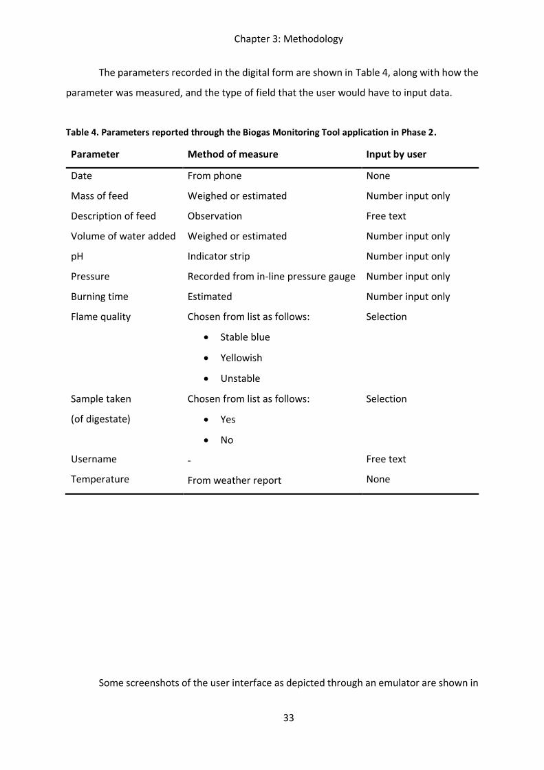
Chapter 3: Methodology
33
The parameters recorded in the digital form are shown in Table 4, along with how the
parameter was measured, and the type of field that the user would have to input data.
Table 4. Parameters reported through the Biogas Monitoring Tool application in Phase 2.
Parameter Method of measure Input by user
Date
Mass of feed
From phone
Weighed or estimated
None
Number input only
Description of feed Observation Free text
Volume of water added Weighed or estimated Number input only
pH Indicator strip Number input only
Pressure Recorded from in-line pressure gauge Number input only
Burning time Estimated Number input only
Flame quality Chosen from list as follows:
x Stable blue
x Yellowish
x Unstable
Selection
Sample taken
(of digestate)
Username
Temperature
Chosen from list as follows:
x Yes
x No
-
From weather report
Selection
Free text
None
Some screenshots of the user interface as depicted through an emulator are shown in
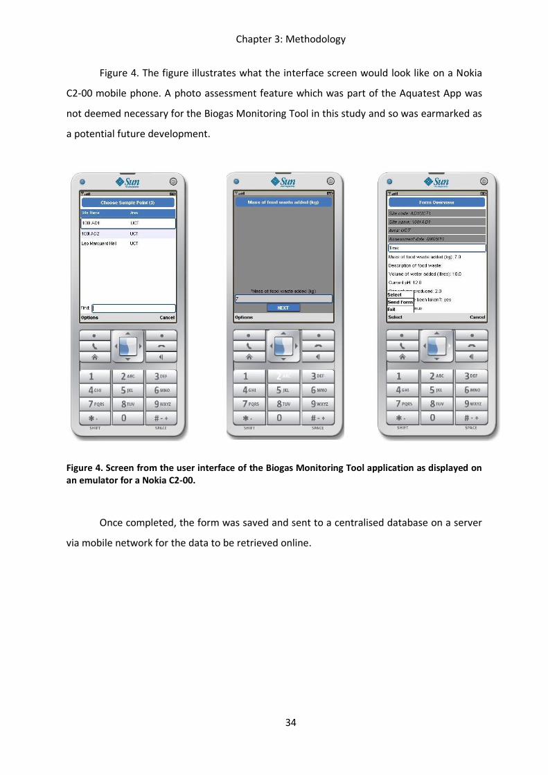
Chapter 3: Methodology
34
Figure 4. The figure illustrates what the interface screen would look like on a Nokia
C2-00 mobile phone. A photo assessment feature which was part of the Aquatest App was
not deemed necessary for the Biogas Monitoring Tool in this study and so was earmarked as
a potential future development.
Figure 4. Screen from the user interface of the Biogas Monitoring Tool application as displayed on an emulator for a Nokia C2-00.
Once completed, the form was saved and sent to a centralised database on a server
via mobile network for the data to be retrieved online.
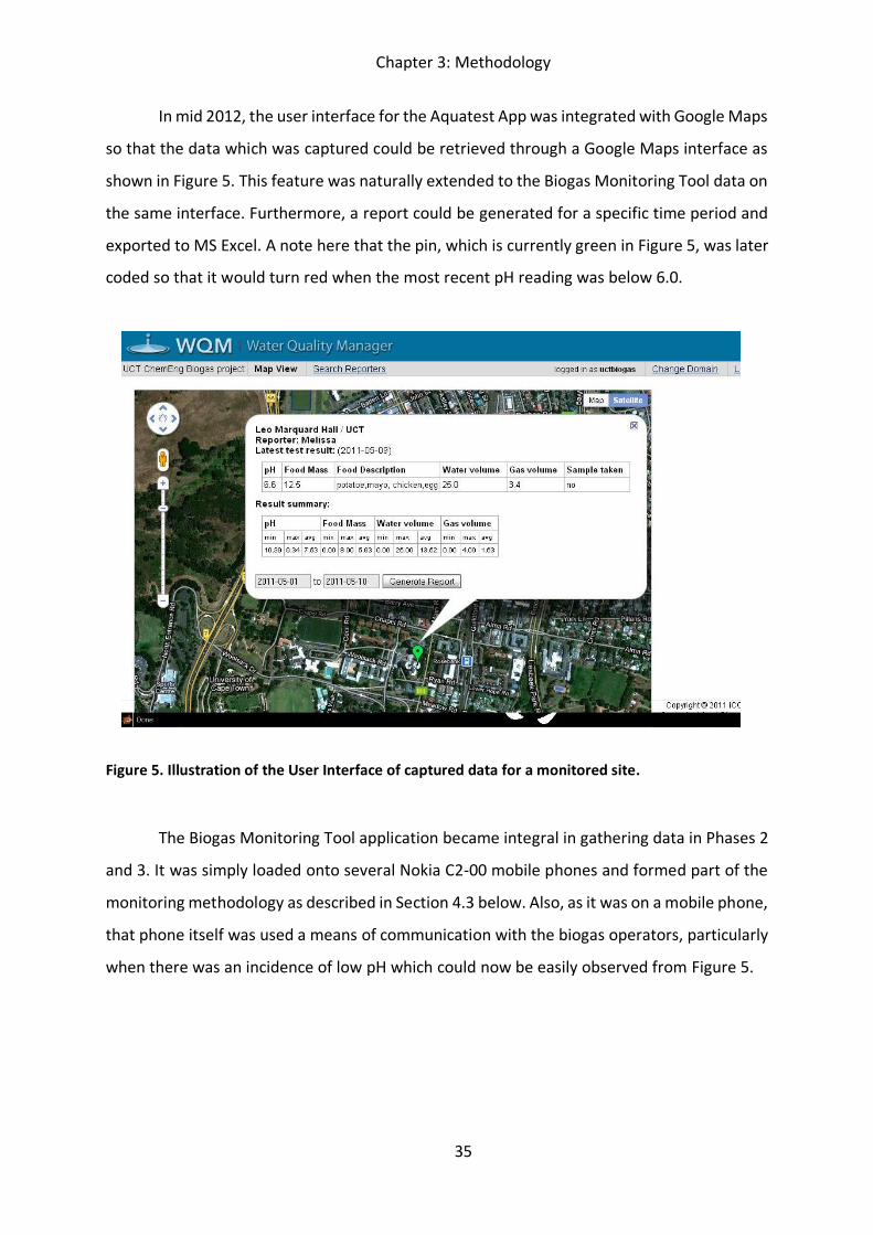
Chapter 3: Methodology
35
In mid 2012, the user interface for the Aquatest App was integrated with Google Maps
so that the data which was captured could be retrieved through a Google Maps interface as
shown in Figure 5. This feature was naturally extended to the Biogas Monitoring Tool data on
the same interface. Furthermore, a report could be generated for a specific time period and
exported to MS Excel. A note here that the pin, which is currently green in Figure 5, was later
coded so that it would turn red when the most recent pH reading was below 6.0.
Figure 5. Illustration of the User Interface of captured data for a monitored site.
The Biogas Monitoring Tool application became integral in gathering data in Phases 2
and 3. It was simply loaded onto several Nokia C2-00 mobile phones and formed part of the
monitoring methodology as described in Section 4.3 below. Also, as it was on a mobile phone,
that phone itself was used a means of communication with the biogas operators, particularly
when there was an incidence of low pH which could now be easily observed from Figure 5.
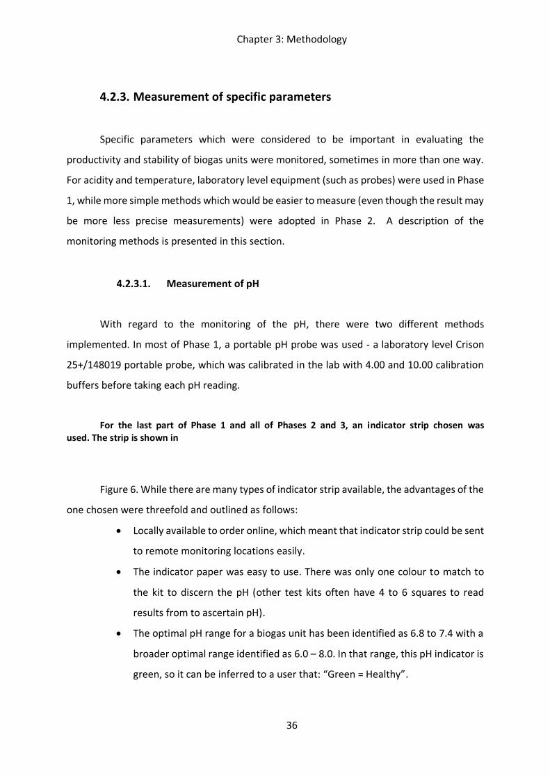
Chapter 3: Methodology
36
4.2.3. Measurement of specific parameters
Specific parameters which were considered to be important in evaluating the
productivity and stability of biogas units were monitored, sometimes in more than one way.
For acidity and temperature, laboratory level equipment (such as probes) were used in Phase
1, while more simple methods which would be easier to measure (even though the result may
be more less precise measurements) were adopted in Phase 2. A description of the
monitoring methods is presented in this section.
4.2.3.1. Measurement of pH
With regard to the monitoring of the pH, there were two different methods
implemented. In most of Phase 1, a portable pH probe was used - a laboratory level Crison
25+/148019 portable probe, which was calibrated in the lab with 4.00 and 10.00 calibration
buffers before taking each pH reading.
For the last part of Phase 1 and all of Phases 2 and 3, an indicator strip chosen was used. The strip is shown in
Figure 6. While there are many types of indicator strip available, the advantages of the
one chosen were threefold and outlined as follows:
x Locally available to order online, which meant that indicator strip could be sent
to remote monitoring locations easily.
x The indicator paper was easy to use. There was only one colour to match to
the kit to discern the pH (other test kits often have 4 to 6 squares to read
results from to ascertain pH).
x The optimal pH range for a biogas unit has been identified as 6.8 to 7.4 with a
broader optimal range identified as 6.0 – 8.0. In that range, this pH indicator is
green, so it can be inferred to a user that: “Green = Healthy”.
Chapter 3: Methodology
37
Figure 6. pH indicator strip used to measure pH of biogas digesters (Distillique, 2016).
Comparison of the different sampling methods for pH was done in three different
studies. Firstly, for a period during Phase 1, both the pH probe and the indicator strip were
used to take readings at the same time to evaluate the suitability of using the indicator strip.
Secondly, Unit 4 in Phase 2 was operated by a user who had access to a calibrated pH probe,
so there was additional comparative data available from that unit. Thirdly, the unit installed
at N1 City Shopping Mall mentioned in Section 4.2.1. was monitored remotely from the
Netherlands, including the parameters of temperature and pH. Therefore, it was possible to
take readings with the indicator strip and compare them to the recorded data with the pH
probe. This comparison is presented in Chapter 4.
4.2.3.2. Measurement of temperature
Temperature monitoring was also carried out in two ways. The first (for the greater
part of Phase 1) was using a temperature probe, the same Crison 25+/148019 probe which
measured pH to obtain the temperature inside the unit. The second was by referring to online
weather reports (AccuWeather, 2012) and recording ambient temperature. Comparisons
between these two methods are also presented in Chapter 4.
Chapter 3: Methodology
38
4.2.3.3. Weighing of feedstock
The mass of food was weighed by picking up a bucket (which had previously been
weighed to tare) with an analogue hanging scale. The tare weight was then subtracted from
the weight of the bucket mentally and the resulting weight recorded. Where water was
added, the volume of the bucket was used to estimate the volume and recorded in the
relevant field on the digital form.
4.2.3.4. Observation of pressure
Most biogas units (certainly all the ones in this study) were installed with a pressure
gauge. In some cases, as in the initial field observational study, the pressure gauge reading
was recorded as a cross check for the gas utilisation. If gas was utilised, the pressure reading
should be lower. Thus, the decrease in pressure over a period of gas use, i.e. recording the
pressure before and after cooking would be the only way of recording meaningful data. A
daily reading of pressure would not be useful as gas was continuously produced. A study
which recorded the decrease in pressure over a period of cooking was carried out over ten
weeks in Phase 1 – the initial field observation. The actual recording of the pressure through
the digital form was later excluded as a measurement parameter in the monitoring study for
the reason that there was typically only one daily recording from users and this parameter
was no longer deemed useful to measure.
4.2.3.5. Recording of ‘burning time’
Time of flame burning, or the “burning time” was estimated to the nearest five minutes by
the user and recorded as a field in the Biogas Monitoring Tool application data form.
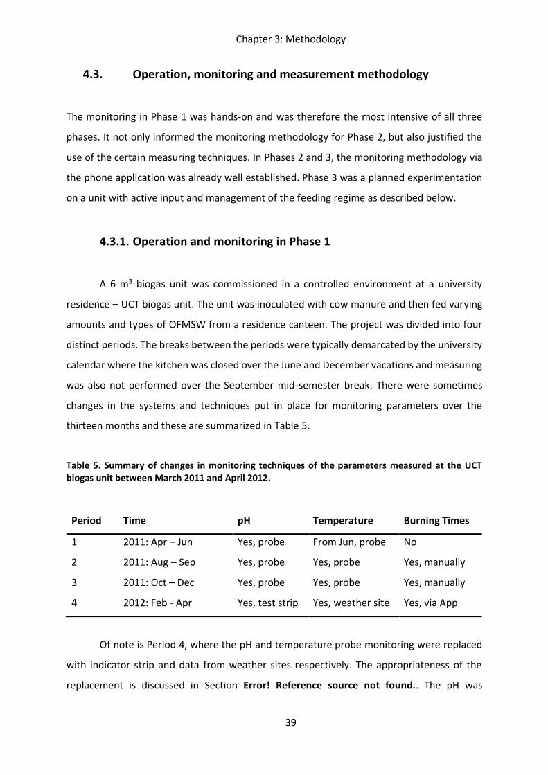
Chapter 3: Methodology
39
4.3. Operation, monitoring and measurement methodology
The monitoring in Phase 1 was hands-on and was therefore the most intensive of all three
phases. It not only informed the monitoring methodology for Phase 2, but also justified the
use of the certain measuring techniques. In Phases 2 and 3, the monitoring methodology via
the phone application was already well established. Phase 3 was a planned experimentation
on a unit with active input and management of the feeding regime as described below.
4.3.1. Operation and monitoring in Phase 1
A 6 m3 biogas unit was commissioned in a controlled environment at a university
residence – UCT biogas unit. The unit was inoculated with cow manure and then fed varying
amounts and types of OFMSW from a residence canteen. The project was divided into four
distinct periods. The breaks between the periods were typically demarcated by the university
calendar where the kitchen was closed over the June and December vacations and measuring
was also not performed over the September mid-semester break. There were sometimes
changes in the systems and techniques put in place for monitoring parameters over the
thirteen months and these are summarized in Table 5.
Table 5. Summary of changes in monitoring techniques of the parameters measured at the UCT biogas unit between March 2011 and April 2012.
Period Time pH Temperature Burning Times
1 2011: Apr – Jun Yes, probe From Jun, probe No
2 2011: Aug – Sep Yes, probe Yes, probe Yes, manually
3 2011: Oct – Dec Yes, probe Yes, probe Yes, manually
4 2012: Feb - Apr Yes, test strip Yes, weather site Yes, via App
Of note is Period 4, where the pH and temperature probe monitoring were replaced
with indicator strip and data from weather sites respectively. The appropriateness of the
replacement is discussed in Section Error! Reference source not found.. The pH was
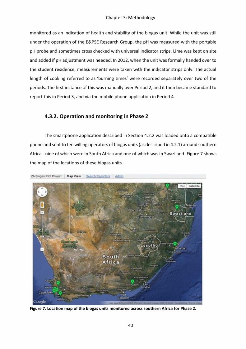
Chapter 3: Methodology
40
monitored as an indication of health and stability of the biogas unit. While the unit was still
under the operation of the E&PSE Research Group, the pH was measured with the portable
pH probe and sometimes cross checked with universal indicator strips. Lime was kept on site
and added if pH adjustment was needed. In 2012, when the unit was formally handed over to
the student residence, measurements were taken with the indicator strips only. The actual
length of cooking referred to as ‘burning times’ were recorded separately over two of the
periods. The first instance of this was manually over Period 2, and it then became standard to
report this in Period 3, and via the mobile phone application in Period 4.
4.3.2. Operation and monitoring in Phase 2
The smartphone application described in Section 4.2.2 was loaded onto a compatible
phone and sent to ten willing operators of biogas units (as described in 4.2.1) around southern
Africa - nine of which were in South Africa and one of which was in Swaziland. Figure 7 shows
the map of the locations of these biogas units.
Figure 7. Location map of the biogas units monitored across southern Africa for Phase 2.
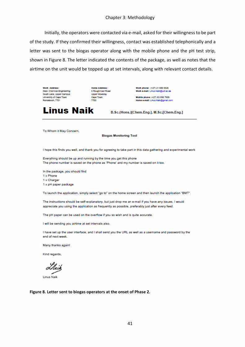
Chapter 3: Methodology
41
Initially, the operators were contacted via e-mail, asked for their willingness to be part
of the study. If they confirmed their willingness, contact was established telephonically and a
letter was sent to the biogas operator along with the mobile phone and the pH test strip,
shown in Figure 8. The letter indicated the contents of the package, as well as notes that the
airtime on the unit would be topped up at set intervals, along with relevant contact details.
Figure 8. Letter sent to biogas operators at the onset of Phase 2.
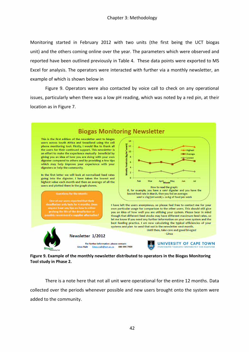
Chapter 3: Methodology
42
Monitoring started in February 2012 with two units (the first being the UCT biogas
unit) and the others coming online over the year. The parameters which were observed and
reported have been outlined previously in Table 4. These data points were exported to MS
Excel for analysis. The operators were interacted with further via a monthly newsletter, an
example of which is shown below in
Figure 9. Operators were also contacted by voice call to check on any operational
issues, particularly when there was a low pH reading, which was noted by a red pin, at their
location as in Figure 7.
Figure 9. Example of the monthly newsletter distributed to operators in the Biogas Monitoring Tool study in Phase 2.
There is a note here that not all unit were operational for the entire 12 months. Data
collected over the periods whenever possible and new users brought onto the system were
added to the community.
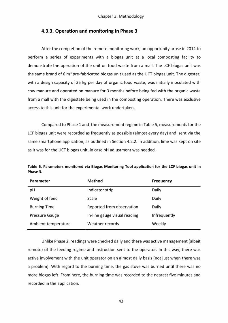
Chapter 3: Methodology
43
4.3.3. Operation and monitoring in Phase 3
After the completion of the remote monitoring work, an opportunity arose in 2014 to
perform a series of experiments with a biogas unit at a local composting facility to
demonstrate the operation of the unit on food waste from a mall. The LCF biogas unit was
the same brand of 6 m3 pre-fabricated biogas unit used as the UCT biogas unit. The digester,
with a design capacity of 35 kg per day of organic food waste, was initially inoculated with
cow manure and operated on manure for 3 months before being fed with the organic waste
from a mall with the digestate being used in the composting operation. There was exclusive
access to this unit for the experimental work undertaken.
Compared to Phase 1 and the measurement regime in Table 5, measurements for the
LCF biogas unit were recorded as frequently as possible (almost every day) and sent via the
same smartphone application, as outlined in Section 4.2.2. In addition, lime was kept on site
as it was for the UCT biogas unit, in case pH adjustment was needed.
Table 6. Parameters monitored via Biogas Monitoring Tool application for the LCF biogas unit in Phase 3.
Parameter Method Frequency
pH Indicator strip Daily
Weight of feed Scale Daily
Burning Time Reported from observation Daily
Pressure Gauge In-line gauge visual reading Infrequently
Ambient temperature Weather records Weekly
Unlike Phase 2, readings were checked daily and there was active management (albeit
remote) of the feeding regime and instruction sent to the operator. In this way, there was
active involvement with the unit operator on an almost daily basis (not just when there was
a problem). With regard to the burning time, the gas stove was burned until there was no
more biogas left. From here, the burning time was recorded to the nearest five minutes and
recorded in the application.
Chapter 3: Methodology
44
4.3.3.1. Migration to OFMSW
Based on findings from Phase 2, testing on purposive disruptions and stepwise
increase of simple carbohydrates was undertaken, along with another investigation on pre-
treatment with Bokashi treated waste. As mentioned, the unit was initially primed with cow
manure and run solely on cow manure for 3 months (April to June 2014). The biogas unit was
first brought to operation on food waste by the stepwise addition of food waste.
OFMSW was fed in fixed incremental amounts of 2 kg every second day, until the
weight fed every second day was 20 kg. From thereon, 10 kg was fed daily and increased
stepwise until it was operating at 35 kg per day by 1 October 2014. This process took 3 months
from 1 July 2014 and the food waste was supplemented by cow manure. At this stage, the
contents of one 120 dm3 wheelie bin (weight varying between 10 kg and 65 kg) was processed
through the food waste disposal unit and fed into the unit. The weight of each bin was
recorded. When simple carbohydrates were needed, the staff at the mall were instructed to
only keep aside simple carbohydrates which were then delivered to the local composting
facility.
4.3.3.2. Experimentation with Bokashi treated waste
Four months after the completion of the experiment described above, (September to
December 2015), the biogas unit was fed with Bokashi treated waste instead of fresh food
waste. The mall was also treating food waste with Bokashi, layered with Bokashi bran and
stored in 210 dm3 Bokashi drums which were then sealed and stored for two weeks before
being delivered to the composting facility to be composted in windrows. When Bokashi waste
was used as a feed for the biogas unit, it was taken from the Bokashi drums which were
delivered to the composting facility.
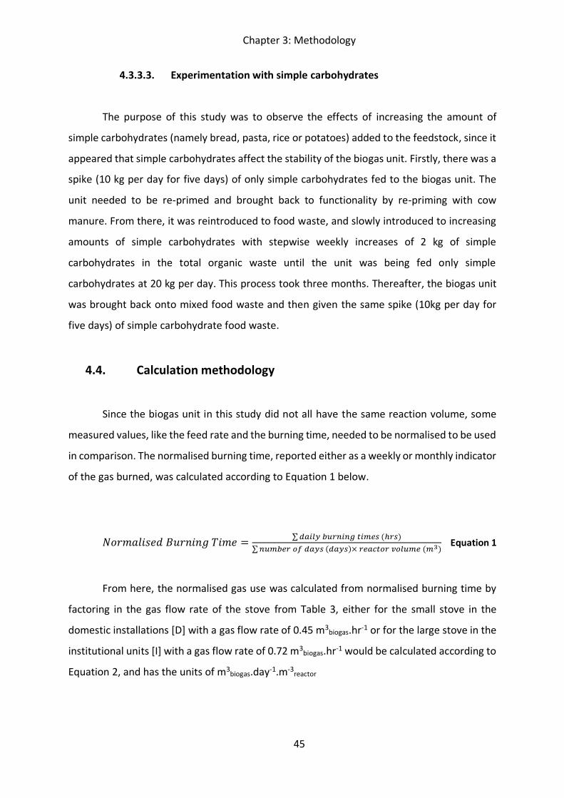
Chapter 3: Methodology
45
4.3.3.3. Experimentation with simple carbohydrates
The purpose of this study was to observe the effects of increasing the amount of
simple carbohydrates (namely bread, pasta, rice or potatoes) added to the feedstock, since it
appeared that simple carbohydrates affect the stability of the biogas unit. Firstly, there was a
spike (10 kg per day for five days) of only simple carbohydrates fed to the biogas unit. The
unit needed to be re-primed and brought back to functionality by re-priming with cow
manure. From there, it was reintroduced to food waste, and slowly introduced to increasing
amounts of simple carbohydrates with stepwise weekly increases of 2 kg of simple
carbohydrates in the total organic waste until the unit was being fed only simple
carbohydrates at 20 kg per day. This process took three months. Thereafter, the biogas unit
was brought back onto mixed food waste and then given the same spike (10kg per day for
five days) of simple carbohydrate food waste.
4.4. Calculation methodology
Since the biogas unit in this study did not all have the same reaction volume, some
measured values, like the feed rate and the burning time, needed to be normalised to be used
in comparison. The normalised burning time, reported either as a weekly or monthly indicator
of the gas burned, was calculated according to Equation 1 below.
𝑁𝑜𝑟𝑚𝑎𝑙𝑖𝑠𝑒𝑑 𝐵𝑢𝑟𝑛𝑖𝑛𝑔 𝑇𝑖𝑚𝑒 = ∑ 𝑑𝑎𝑖𝑙𝑦 𝑏𝑢𝑟𝑛𝑖𝑛𝑔 𝑡𝑖𝑚𝑒𝑠 (ℎ𝑟𝑠)∑ 𝑛𝑢𝑚𝑏𝑒𝑟 𝑜𝑓 𝑑𝑎𝑦𝑠 (𝑑𝑎𝑦𝑠)× 𝑟𝑒𝑎𝑐𝑡𝑜𝑟 𝑜𝑙𝑢𝑚𝑒 (𝑚3)
Equation 1
From here, the normalised gas use was calculated from normalised burning time by
factoring in the gas flow rate of the stove from Table 3, either for the small stove in the
domestic installations [D] with a gas flow rate of 0.45 m3biogas.hr-1 or for the large stove in the
institutional units [I] with a gas flow rate of 0.72 m3biogas.hr-1 would be calculated according to
Equation 2, and has the units of m3biogas.day-1.m-3reactor
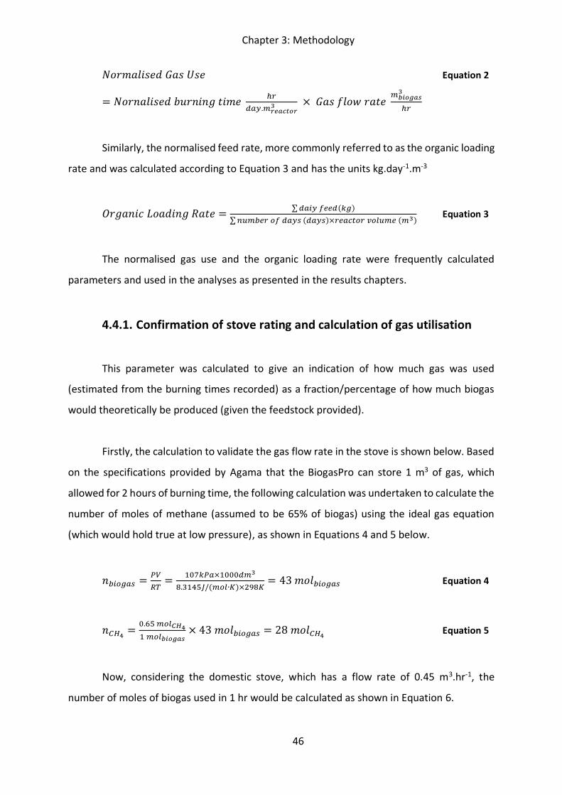
Chapter 3: Methodology
46
𝑁𝑜𝑟𝑚𝑎𝑙𝑖𝑠𝑒𝑑 𝐺𝑎𝑠 𝑈𝑠𝑒 Equation 2
= 𝑁𝑜𝑟𝑛𝑎𝑙𝑖𝑠𝑒𝑑 𝑏𝑢𝑟𝑛𝑖𝑛𝑔 𝑡𝑖𝑚𝑒 ℎ𝑟𝑑𝑎𝑦.𝑚𝑟𝑒𝑎𝑐𝑡𝑜𝑟
3 × 𝐺𝑎𝑠 𝑓𝑙𝑜𝑤 𝑟𝑎𝑡𝑒 𝑚𝑏𝑖𝑜𝑔𝑎𝑠
3
ℎ𝑟
Similarly, the normalised feed rate, more commonly referred to as the organic loading
rate and was calculated according to Equation 3 and has the units kg.day-1.m-3
𝑂𝑟𝑔𝑎𝑛𝑖𝑐 𝐿𝑜𝑎𝑑𝑖𝑛𝑔 𝑅𝑎𝑡𝑒 = ∑ 𝑑𝑎𝑖𝑦 𝑓𝑒𝑒𝑑(𝑘𝑔)∑ 𝑛𝑢𝑚𝑏𝑒𝑟 𝑜𝑓 𝑑𝑎𝑦𝑠 (𝑑𝑎𝑦𝑠)×𝑟𝑒𝑎𝑐𝑡𝑜𝑟 𝑜𝑙𝑢𝑚𝑒 (𝑚3)
Equation 3
The normalised gas use and the organic loading rate were frequently calculated
parameters and used in the analyses as presented in the results chapters.
4.4.1. Confirmation of stove rating and calculation of gas utilisation
This parameter was calculated to give an indication of how much gas was used
(estimated from the burning times recorded) as a fraction/percentage of how much biogas
would theoretically be produced (given the feedstock provided).
Firstly, the calculation to validate the gas flow rate in the stove is shown below. Based
on the specifications provided by Agama that the BiogasPro can store 1 m3 of gas, which
allowed for 2 hours of burning time, the following calculation was undertaken to calculate the
number of moles of methane (assumed to be 65% of biogas) using the ideal gas equation
(which would hold true at low pressure), as shown in Equations 4 and 5 below.
𝑛𝑏𝑖𝑜𝑔𝑎𝑠 = 𝑃𝑉𝑅𝑇
= 10 𝑘𝑃𝑎×1000𝑑𝑚3
8.3145𝐽/(𝑚𝑜𝑙∙ )×298= 43 𝑚𝑜𝑙𝑏𝑖𝑜𝑔𝑎𝑠 Equation 4
𝑛 4 = 0.65 𝑚𝑜𝑙 41 𝑚𝑜𝑙𝑏𝑖𝑜𝑔𝑎𝑠
× 43 𝑚𝑜𝑙𝑏𝑖𝑜𝑔𝑎𝑠 = 28 𝑚𝑜𝑙 4 Equation 5
Now, considering the domestic stove, which has a flow rate of 0.45 m3.hr-1, the
number of moles of biogas used in 1 hr would be calculated as shown in Equation 6.
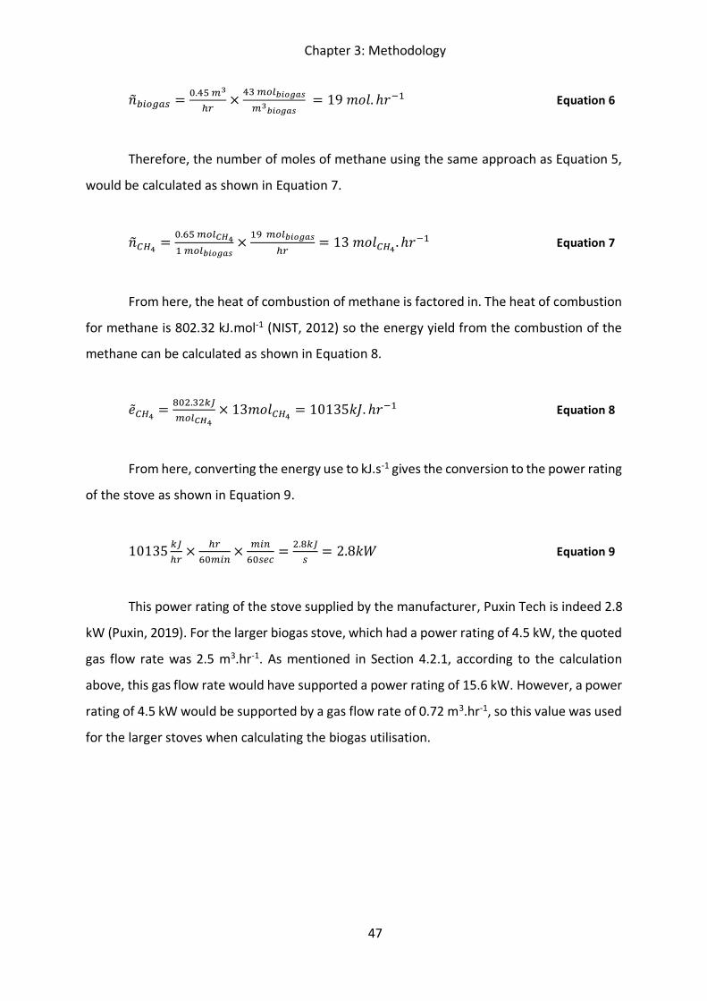
Chapter 3: Methodology
47
𝑛𝑏𝑖𝑜𝑔𝑎𝑠 = 0.45 𝑚3
ℎ𝑟× 43 𝑚𝑜𝑙𝑏𝑖𝑜𝑔𝑎𝑠
𝑚3𝑏𝑖𝑜𝑔𝑎𝑠 = 19 𝑚𝑜𝑙. ℎ𝑟 1 Equation 6
Therefore, the number of moles of methane using the same approach as Equation 5,
would be calculated as shown in Equation 7.
𝑛 4 = 0.65 𝑚𝑜𝑙 41 𝑚𝑜𝑙𝑏𝑖𝑜𝑔𝑎𝑠
× 19 𝑚𝑜𝑙𝑏𝑖𝑜𝑔𝑎𝑠
ℎ𝑟= 13 𝑚𝑜𝑙 4. ℎ𝑟 1 Equation 7
From here, the heat of combustion of methane is factored in. The heat of combustion
for methane is 802.32 kJ.mol-1 (NIST, 2012) so the energy yield from the combustion of the
methane can be calculated as shown in Equation 8.
�̃� 4 = 802.32𝑘𝐽𝑚𝑜𝑙 4
× 13𝑚𝑜𝑙 4 = 10135𝑘𝐽. ℎ𝑟 1 Equation 8
From here, converting the energy use to kJ.s-1 gives the conversion to the power rating
of the stove as shown in Equation 9.
10135 𝑘𝐽ℎ𝑟
× ℎ𝑟60𝑚𝑖𝑛
× 𝑚𝑖𝑛60𝑠𝑒𝑐
= 2.8𝑘𝐽𝑠
= 2.8𝑘𝑊 Equation 9
This power rating of the stove supplied by the manufacturer, Puxin Tech is indeed 2.8
kW (Puxin, 2019). For the larger biogas stove, which had a power rating of 4.5 kW, the quoted
gas flow rate was 2.5 m3.hr-1. As mentioned in Section 4.2.1, according to the calculation
above, this gas flow rate would have supported a power rating of 15.6 kW. However, a power
rating of 4.5 kW would be supported by a gas flow rate of 0.72 m3.hr-1, so this value was used
for the larger stoves when calculating the biogas utilisation.
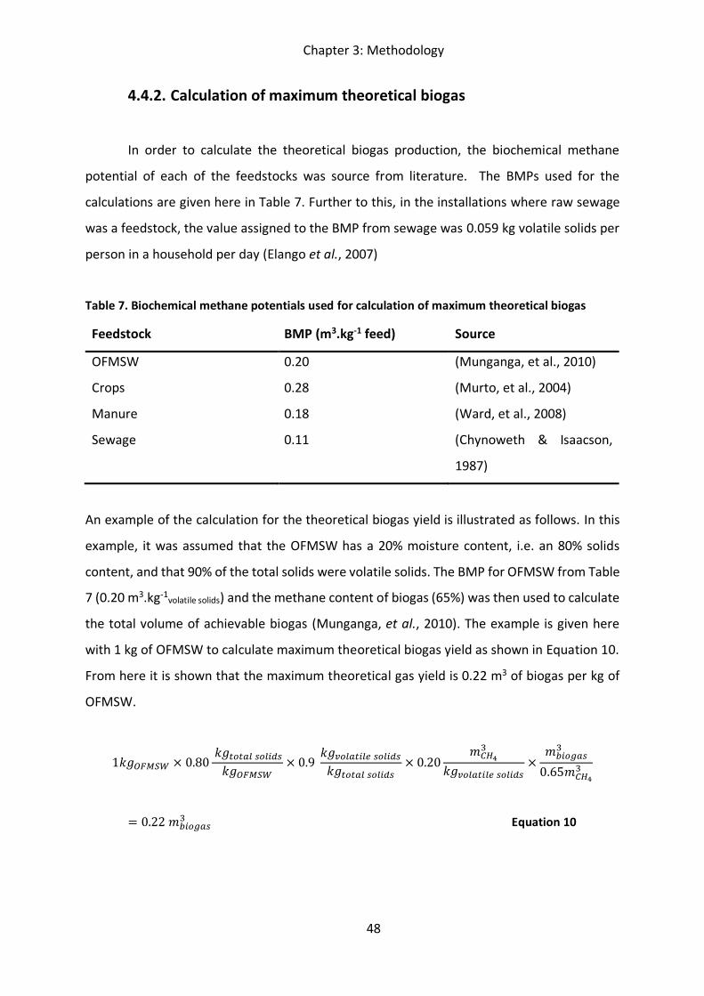
Chapter 3: Methodology
48
4.4.2. Calculation of maximum theoretical biogas
In order to calculate the theoretical biogas production, the biochemical methane
potential of each of the feedstocks was source from literature. The BMPs used for the
calculations are given here in Table 7. Further to this, in the installations where raw sewage
was a feedstock, the value assigned to the BMP from sewage was 0.059 kg volatile solids per
person in a household per day (Elango et al., 2007)
Table 7. Biochemical methane potentials used for calculation of maximum theoretical biogas
Feedstock BMP (m3.kg-1 feed) Source
OFMSW 0.20 (Munganga, et al., 2010)
Crops 0.28 (Murto, et al., 2004)
Manure 0.18 (Ward, et al., 2008)
Sewage 0.11 (Chynoweth & Isaacson,
1987)
An example of the calculation for the theoretical biogas yield is illustrated as follows. In this
example, it was assumed that the OFMSW has a 20% moisture content, i.e. an 80% solids
content, and that 90% of the total solids were volatile solids. The BMP for OFMSW from Table
7 (0.20 m3.kg-1volatile solids) and the methane content of biogas (65%) was then used to calculate
the total volume of achievable biogas (Munganga, et al., 2010). The example is given here
with 1 kg of OFMSW to calculate maximum theoretical biogas yield as shown in Equation 10.
From here it is shown that the maximum theoretical gas yield is 0.22 m3 of biogas per kg of
OFMSW.
1𝑘𝑔𝑂 𝑀𝑆𝑊 × 0.80 𝑘𝑔𝑡𝑜𝑡𝑎𝑙 𝑠𝑜𝑙𝑖𝑑𝑠
𝑘𝑔𝑂 𝑀𝑆𝑊× 0.9
𝑘𝑔 𝑜𝑙𝑎𝑡𝑖𝑙𝑒 𝑠𝑜𝑙𝑖𝑑𝑠𝑘𝑔𝑡𝑜𝑡𝑎𝑙 𝑠𝑜𝑙𝑖𝑑𝑠
× 0.20𝑚 4
3
𝑘𝑔 𝑜𝑙𝑎𝑡𝑖𝑙𝑒 𝑠𝑜𝑙𝑖𝑑𝑠×
𝑚𝑏𝑖𝑜𝑔𝑎𝑠3
0.65𝑚4
3
= 0.22 𝑚𝑏𝑖𝑜𝑔𝑎𝑠3 Equation 10
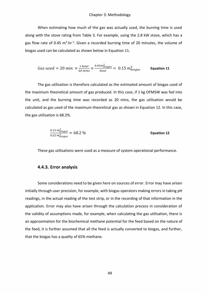
Chapter 3: Methodology
49
When estimating how much of the gas was actually used, the burning time is used
along with the stove rating from Table 3. For example, using the 2.8 kW stove, which has a
gas flow rate of 0.45 m3.hr-1. Given a recorded burning time of 20 minutes, the volume of
biogas used can be calculated as shown below in Equation 11.
𝐺𝑎𝑠 𝑢𝑠𝑒𝑑 = 20 𝑚𝑖𝑛 × 1 ℎ𝑜𝑢𝑟60 𝑚𝑖𝑛𝑠
×0.45𝑚𝑏𝑖𝑜𝑔𝑎𝑠
3
ℎ𝑜𝑢𝑟= 0.15 𝑚𝑏𝑖𝑜𝑔𝑎𝑠
3 Equation 11
The gas utilisation is therefore calculated as the estimated amount of biogas used of
the maximum theoretical amount of gas produced. In this case, if 1 kg OFMSW was fed into
the unit, and the burning time was recorded as 20 mins, the gas utilisation would be
calculated as gas used of the maximum theoretical gas as shown in Equation 12. In this case,
the gas utilisation is 68.2%.
0.15 𝑚𝑏𝑖𝑜𝑔𝑎𝑠3
0.22 𝑚𝑏𝑖𝑜𝑔𝑎𝑠3 = 68.2 % Equation 12
These gas utilisations were used as a measure of system operational performance.
4.4.3. Error analysis
Some considerations need to be given here on sources of error. Error may have arisen
initially through user precision, for example, with biogas operators making errors in taking pH
readings, in the actual reading of the test strip, or in the recording of that information in the
application. Error may also have arisen through the calculation process in consideration of
the validity of assumptions made, for example, when calculating the gas utilisation, there is
an approximation for the biochemical methane potential for the feed based on the nature of
the feed, it is further assumed that all the feed is actually converted to biogas, and further,
that the biogas has a quality of 65% methane.
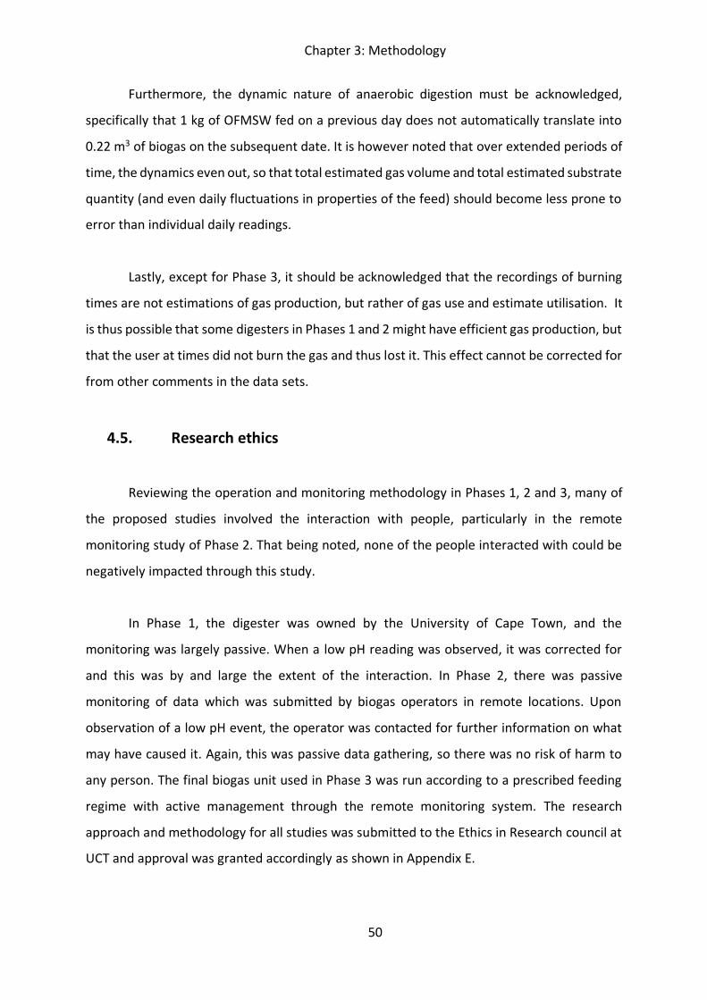
Chapter 3: Methodology
50
Furthermore, the dynamic nature of anaerobic digestion must be acknowledged,
specifically that 1 kg of OFMSW fed on a previous day does not automatically translate into
0.22 m3 of biogas on the subsequent date. It is however noted that over extended periods of
time, the dynamics even out, so that total estimated gas volume and total estimated substrate
quantity (and even daily fluctuations in properties of the feed) should become less prone to
error than individual daily readings.
Lastly, except for Phase 3, it should be acknowledged that the recordings of burning
times are not estimations of gas production, but rather of gas use and estimate utilisation. It
is thus possible that some digesters in Phases 1 and 2 might have efficient gas production, but
that the user at times did not burn the gas and thus lost it. This effect cannot be corrected for
from other comments in the data sets.
4.5. Research ethics
Reviewing the operation and monitoring methodology in Phases 1, 2 and 3, many of
the proposed studies involved the interaction with people, particularly in the remote
monitoring study of Phase 2. That being noted, none of the people interacted with could be
negatively impacted through this study.
In Phase 1, the digester was owned by the University of Cape Town, and the
monitoring was largely passive. When a low pH reading was observed, it was corrected for
and this was by and large the extent of the interaction. In Phase 2, there was passive
monitoring of data which was submitted by biogas operators in remote locations. Upon
observation of a low pH event, the operator was contacted for further information on what
may have caused it. Again, this was passive data gathering, so there was no risk of harm to
any person. The final biogas unit used in Phase 3 was run according to a prescribed feeding
regime with active management through the remote monitoring system. The research
approach and methodology for all studies was submitted to the Ethics in Research council at
UCT and approval was granted accordingly as shown in Appendix E.
Chapter 3: Methodology
51
4.6. Outlook
The methodology proposed takes the following approach. Firstly, observational
research on one biogas unit to inform initial learnings around productivity and stability, and
to develop a remote monitoring toolkit to capture data from small-scale biogas units in urban
settings. The method for measuring parameters to infer operational data (to inform
productivity and stability) is evaluated. These form the body of Phase 1 and the results and
discussions around this are presented in Chapter 4. This toolkit is then used to gather data
from ten biogas units across southern Africa. This remote monitoring work is Phase 2 and is
presented in Chapter 5. After the analysis of this data, theories are generated and specific
experimentation to inform these theories is undertaken on one biogas unit in a controlled
environment. These sets of experiments are Phase 3 and are presented in Chapter 6.
Thus, the approach across the phases will broadly and specifically speak to the
potential and limitations of small-scale biogas operations in urban Africa. The hypotheses
generated speak to the stability and the productivity of such small-scale biogas units, as well
the potential need for remote monitoring as knowledge support to safeguard investment.
Chapter 4: Initial Field Observation
52
Chapter 4: Initial Field Observation
The UCT biogas unit, a 6 m3 Agama BiogasPro (Agama, 2010) was commissioned in
February 2011. The first set of observations on this small-scale biogas unit was carried out
from March 2011 to February 2012. The UCT biogas unit was also used to inform the
development of the mobile phone application for Phase 2, the remote monitoring study
presented in Chapter 5. The operation of the unit followed the methodology outlined in
Section 4.3.1. Aspects of this study were presented at WasteCon 2012 (Naik, et al., 2012) with
abstracts in Appendix G1. The full operational experience of this biogas unit is presented here
in Section 4.1. Section 4.2 presents evaluation of the different sampling methods used, while
Section 4.3 describes the refinement of the Biogas Monitoring Tool application which was
piloted on the UCT biogas unit for use in Phase 2. A summary of the findings and discussion
on how these findings speak to the first and second hypotheses presented in the previous
chapter are presented in Section 4.4.
4.1 Observations on unit stability, pH and feeding regime
Referring back to Table 5 in Section 4.3.1, reproduced below for ease of reference, the
first three months (Period 1), involved the start-up phase and the stabilising of the system.
In this time, the lime buffer was used three times when the pH was detected to be below 6.0
as shown in Figure 10. These points were recorded along with the other normal readings. In
this period, the mass of food waste fed to the reactor was also reduced if the pH crossed
below the 6.0 value.
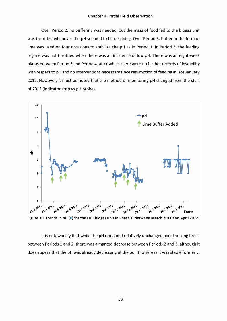
Chapter 4: Initial Field Observation
53
Over Period 2, no buffering was needed, but the mass of food fed to the biogas unit
was throttled whenever the pH seemed to be declining. Over Period 3, buffer in the form of
lime was used on four occasions to stabilize the pH as in Period 1. In Period 3, the feeding
regime was not throttled when there was an incidence of low pH. There was an eight-week
hiatus between Period 3 and Period 4, after which there were no further records of instability
with respect to pH and no interventions necessary since resumption of feeding in late January
2012. However, it must be noted that the method of monitoring pH changed from the start
of 2012 (indicator strip vs pH probe).
Figure 10. Trends in pH (•) for the UCT biogas unit in Phase 1, between March 2011 and April 2012
It is noteworthy that while the pH remained relatively unchanged over the long break
between Periods 1 and 2, there was a marked decrease between Periods 2 and 3, although it
does appear that the pH was already decreasing at the point, whereas it was stable formerly.
4
5
6
7
8
9
10
11
28-3-2011
28-4-2011
28-5-2011
28-6-2011
28-7-2011
28-8-2011
28-9-2011
28-10-2011
28-11-2011
28-12-2011
28-1-2012
28-2-2012
28-3-2012
pH
Date
pH
Lime Buffer Added
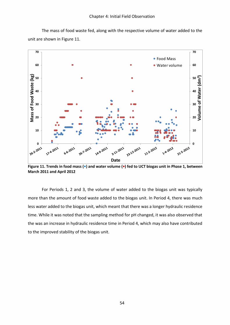
Chapter 4: Initial Field Observation
54
The mass of food waste fed, along with the respective volume of water added to the
unit are shown in Figure 11.
Figure 11. Trends in food mass (•) and water volume (•) fed to UCT biogas unit in Phase 1, between March 2011 and April 2012
For Periods 1, 2 and 3, the volume of water added to the biogas unit was typically
more than the amount of food waste added to the biogas unit. In Period 4, there was much
less water added to the biogas unit, which meant that there was a longer hydraulic residence
time. While it was noted that the sampling method for pH changed, it was also observed that
the was an increase in hydraulic residence time in Period 4, which may also have contributed
to the improved stability of the biogas unit.
0
10
20
30
40
50
60
70
0
10
20
30
40
50
60
70
26-2-2011
17-4-2011
6-6-2011
26-7-2011
14-9-2011
3-11-2011
23-12-2011
11-2-2012
1-4-2012
21-5-2012
Volu
me
of W
ater
(dm
3 )
Mas
s of F
ood
Was
te (k
g)
Date
Food MassWater volume
Chapter 4: Initial Field Observation
55
4.1.1 The effect of feed regime effect on stability
In this initial work, the pH was used as an indicator of the stability of the biogas unit,
considering it as a whole system. Between Figure 10 and Figure 11 and 2, it is noted that the
initial decline in pH at the beginning of Period 1 occurred even while the feed rate was very
low. However, after the system was buffered, it stabilized until June with the constant feed
rate of 12 kg per day. Granted, there were two further occasions when lime was added as a
buffer, but on the whole, the system was relatively pH stable. Over Period 2, the amount of
feed added to the reactor was decided based on the current feeding regime and the pH of
the system. If the pH was decreasing to 6.0 and addition of lime seemed imminent, less food
was added to the biogas unit. In other words, the organic loading rate was reduced when
there were observed drop in pH. Therefore, with close monitoring of the operating conditions
of the reactor, relatively stable operation was achievable. Over Period 3, the system was only
buffered when the pH dropped below 5.5. Pseudo-stable operation was achieved at a lower
operating pH, but this time with the addition of lime at key points. The slightly higher masses
of food added in this period (often close to 20 kg) was likely to have been the factor that
caused this drop in pH. Over Period 4, there was stable operation in the optimum range
between 6.5 and 7.5. On the four occasions when the pH did drop below 6.5, it was noted
that two days before these episodes, the feedstock was always typically high in simple
carbohydrates and often only contained simple carbohydrates, namely; “rice & pasta”, “pasta
& vegetables”, “bread & pasta” and “rice & bread” respectively. Over Period 4, the decrease
in the volume of water fed to the digester would have significantly affected the hydraulic
residence time of the food waste in the digester. The increase in hydraulic residence time, as
a direct result of lower amounts of water fed to the digester could be the reason for the
improved stability of the biogas unit.
Thus, attention needs to be paid to the effect of the type of food waste on the pH.
This is why the type of food waste fed to the unit was recorded. The reason for this, is that
prior to the study, the reactor was fed with waste from the breakfast meal, which consisted
largely of discarded bread. The pH was seen to plummet and the unit needed re-inoculation
with cow manure before this study was carried out. Also, the OFMSW was switched to
Chapter 4: Initial Field Observation
56
canteen waste from the lunch meal as opposed to the breakfast meal. Furthermore, it was
attempted to ensure that there was a fair amount of protein to reach a C:N ratio of between
20 to 30 wherever possible. This was not always achievable and sometimes only a carbon
source was added. If the carbon source was all simple carbohydrates, then the above
described reduction of pH was noticed. Typical feedstock over the entire period was often a
mixture of rice or bread with chicken, beef or eggs and often some salad or other vegetables.
It should further be noted that towards the end of Period 3, the feed was sporadic and
typically a small amount of almost entirely vegetables most often accompanied by some form
of carbohydrate. Over these times, there was noted decrease in the amount of gas produced
and this is why the burning time measurements were not performed over Period 3.
4.1.2 Observations of temperature
The temperature over the entire Periods 1, 2 and 3 fluctuated between 15 and 20 °C.
The temperature is not seen to influence the stability of the system, but it may very well have
an effect on the system’s productivity, i.e. the volume of biogas produced. The Biogas
Monitoring Tool application was refined to include burning time as discussed in Section 4.3 in
order to quantify productivity and determine this effect. Further discussions on productivity,
however, are presented in Section 4.1.3.
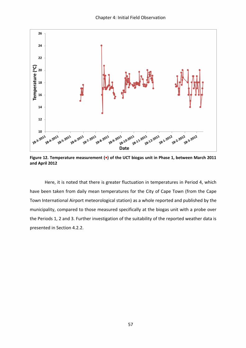
Chapter 4: Initial Field Observation
57
Figure 12. Temperature measurement (•) of the UCT biogas unit in Phase 1, between March 2011 and April 2012
Here, it is noted that there is greater fluctuation in temperatures in Period 4, which
have been taken from daily mean temperatures for the City of Cape Town (from the Cape
Town International Airport meteorological station) as a whole reported and published by the
municipality, compared to those measured specifically at the biogas unit with a probe over
the Periods 1, 2 and 3. Further investigation of the suitability of the reported weather data is
presented in Section 4.2.2.
10
12
14
16
18
20
22
24
26
28-3-2011
28-4-2011
28-5-2011
28-6-2011
28-7-2011
28-8-2011
28-9-2011
28-10-2011
28-11-2011
28-12-2011
28-1-2012
28-2-2012
28-3-2012
Tem
pera
ture
(o C)
Date
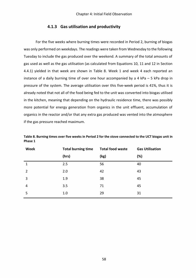
Chapter 4: Initial Field Observation
58
4.1.3 Gas utilisation and productivity
For the five weeks where burning times were recorded in Period 2, burning of biogas
was only performed on weekdays. The readings were taken from Wednesday to the following
Tuesday to include the gas produced over the weekend. A summary of the total amounts of
gas used as well as the gas utilisation (as calculated from Equations 10, 11 and 12 in Section
4.4.1) yielded in that week are shown in Table 8. Week 1 and week 4 each reported an
instance of a daily burning time of over one hour accompanied by a 4 kPa – 5 kPa drop in
pressure of the system. The average utilisation over this five-week period is 41%, thus it is
already noted that not all of the food being fed to the unit was converted into biogas utilised
in the kitchen, meaning that depending on the hydraulic residence time, there was possibly
more potential for energy generation from organics in the unit effluent, accumulation of
organics in the reactor and/or that any extra gas produced was vented into the atmosphere
if the gas pressure reached maximum.
Table 8. Burning times over five weeks in Period 2 for the stove connected to the UCT biogas unit in Phase 1
Week Total burning time
(hrs)
Total food waste
(kg)
Gas Utilisation
(%)
1 2.5 56 40
2 2.0 42 43
3 1.9 38 45
4 3.5 71 45
5 1.0 29 31
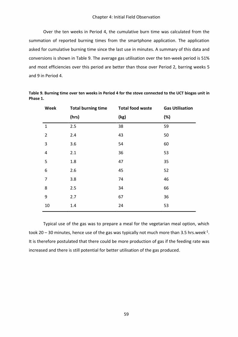
Chapter 4: Initial Field Observation
59
Over the ten weeks in Period 4, the cumulative burn time was calculated from the
summation of reported burning times from the smartphone application. The application
asked for cumulative burning time since the last use in minutes. A summary of this data and
conversions is shown in Table 9. The average gas utilisation over the ten-week period is 51%
and most efficiencies over this period are better than those over Period 2, barring weeks 5
and 9 in Period 4.
Table 9. Burning time over ten weeks in Period 4 for the stove connected to the UCT biogas unit in Phase 1.
Week Total burning time
(hrs)
Total food waste
(kg)
Gas Utilisation
(%)
1 2.5 38 59
2 2.4 43 50
3 3.6 54 60
4 2.1 36 53
5 1.8 47 35
6 2.6 45 52
7 3.8 74 46
8 2.5 34 66
9 2.7 67 36
10 1.4 24 53
Typical use of the gas was to prepare a meal for the vegetarian meal option, which
took 20 – 30 minutes, hence use of the gas was typically not much more than 3.5 hrs.week-1.
It is therefore postulated that there could be more production of gas if the feeding rate was
increased and there is still potential for better utilisation of the gas produced.
Chapter 4: Initial Field Observation
60
4.2 Evaluation of monitoring techniques
The UCT biogas unit was also the test unit for which the remote monitoring
methodology was trialled. There were two key aspects to this. The first, was an evaluation of
the monitoring techniques, specifically for acidity and temperature, to determine whether
more simple and crude measurement techniques would be suitable as replacements for the
refined laboratory level techniques. These are presented in Section 4.2.1 and 4.2.2
respectively. The second, was the development and then the refinement of the smartphone
application to collect the data from the various biogas units. This is presented in Section 4.3.
4.2.1 Evaluation of pH monitoring methods
Data was gathered from three separate units at separate timeframes. The UCT data
was gathered from October to December 2011. Data was gathered by one of the remote
monitoring users (Unit 4) from the Eastern Cape (EC) during 2014. As there was a concern
that these data sets, were somewhat limited to conclude that pH strip measurement was
sufficiently robust, a final set of data was gathered over April and May 2019 from the digester
at N1 City Shopping Mall (N1). In each case, a user submitted recorded pH readings from
indicator strip, and this was compared to the measured pH by the probe. In the last case, the
data from the probe was obtained from The Waste Transformers (Waste Transformers, 2018)
office in the Netherlands. This data is presented in Figure 13.
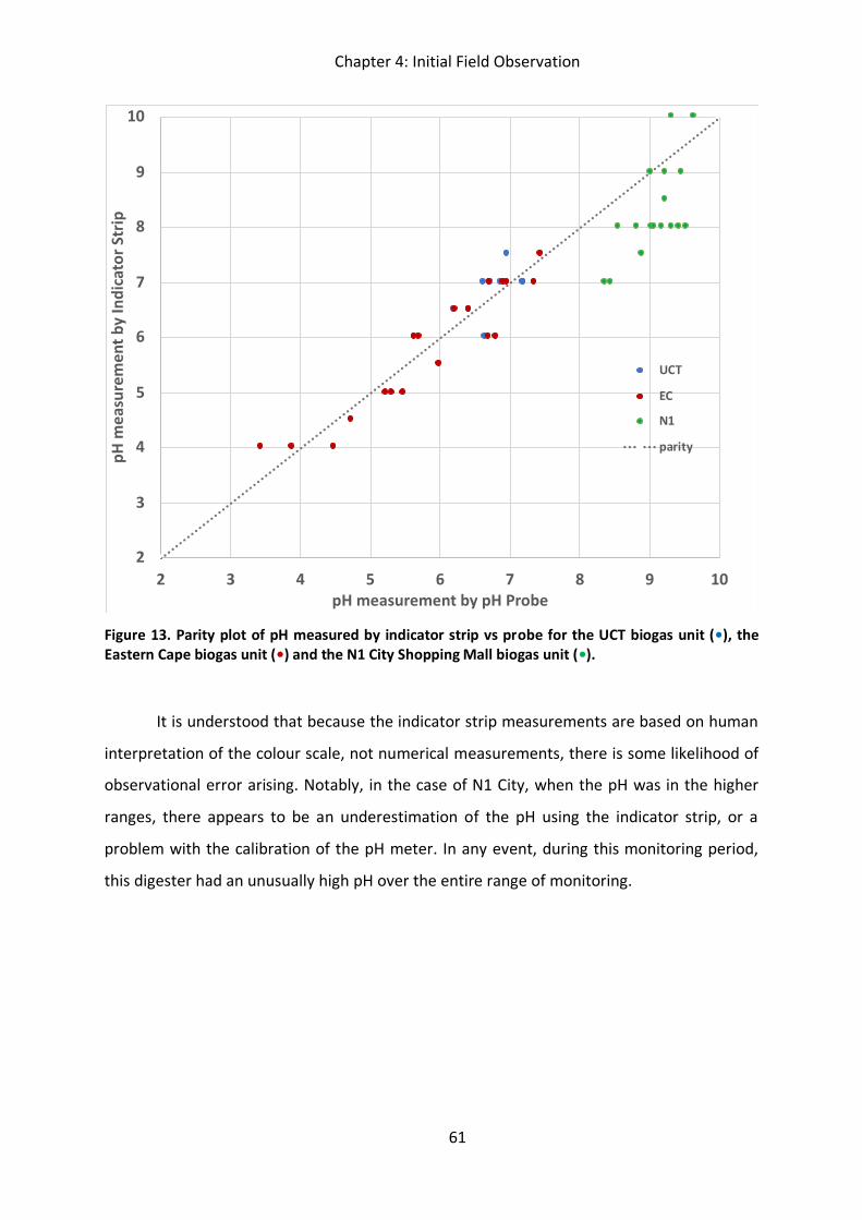
Chapter 4: Initial Field Observation
61
Figure 13. Parity plot of pH measured by indicator strip vs probe for the UCT biogas unit (•), the Eastern Cape biogas unit (•) and the N1 City Shopping Mall biogas unit (•).
It is understood that because the indicator strip measurements are based on human
interpretation of the colour scale, not numerical measurements, there is some likelihood of
observational error arising. Notably, in the case of N1 City, when the pH was in the higher
ranges, there appears to be an underestimation of the pH using the indicator strip, or a
problem with the calibration of the pH meter. In any event, during this monitoring period,
this digester had an unusually high pH over the entire range of monitoring.
2
3
4
5
6
7
8
9
10
2 3 4 5 6 7 8 9 10
pH m
easu
rem
ent b
y In
dica
tor S
trip
pH measurement by pH Probe
UCT
EC
N1
parity
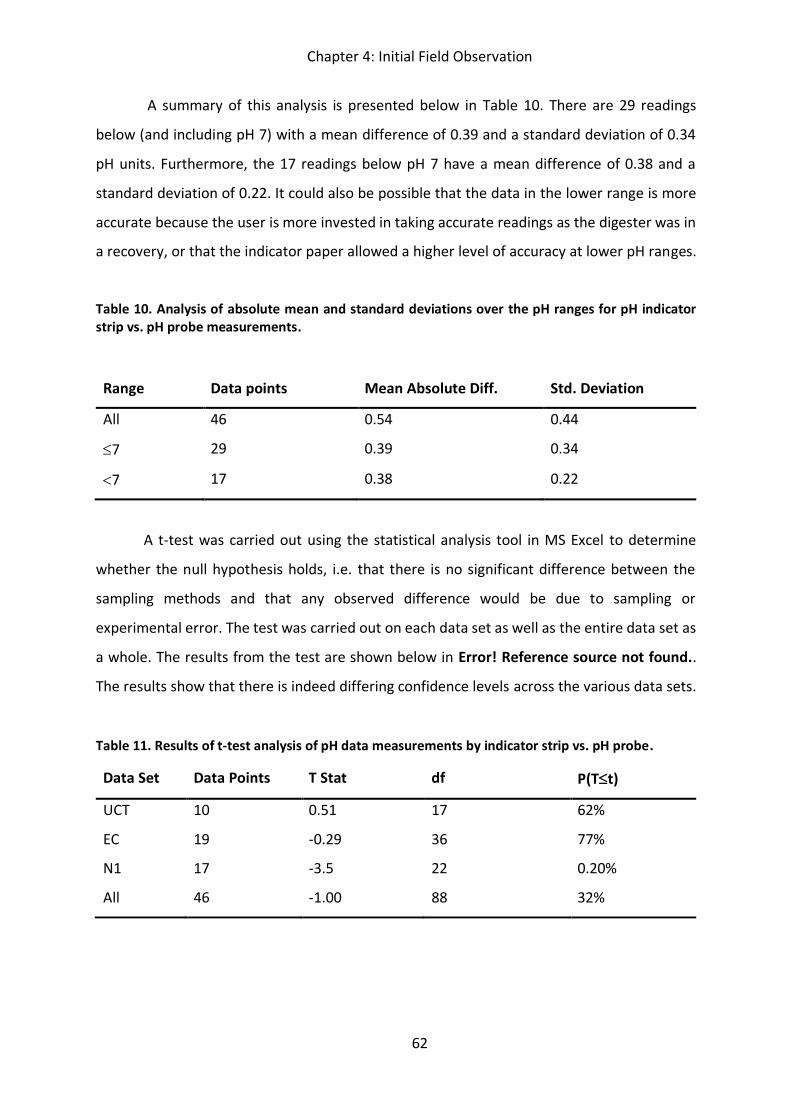
Chapter 4: Initial Field Observation
62
A summary of this analysis is presented below in Table 10. There are 29 readings
below (and including pH 7) with a mean difference of 0.39 and a standard deviation of 0.34
pH units. Furthermore, the 17 readings below pH 7 have a mean difference of 0.38 and a
standard deviation of 0.22. It could also be possible that the data in the lower range is more
accurate because the user is more invested in taking accurate readings as the digester was in
a recovery, or that the indicator paper allowed a higher level of accuracy at lower pH ranges.
Table 10. Analysis of absolute mean and standard deviations over the pH ranges for pH indicator strip vs. pH probe measurements.
Range Data points Mean Absolute Diff. Std. Deviation
All 46 0.54 0.44
d7 29 0.39 0.34
�7 17 0.38 0.22
A t-test was carried out using the statistical analysis tool in MS Excel to determine
whether the null hypothesis holds, i.e. that there is no significant difference between the
sampling methods and that any observed difference would be due to sampling or
experimental error. The test was carried out on each data set as well as the entire data set as
a whole. The results from the test are shown below in Error! Reference source not found..
The results show that there is indeed differing confidence levels across the various data sets.
Table 11. Results of t-test analysis of pH data measurements by indicator strip vs. pH probe.
Data Set Data Points T Stat df P(Tdt)
UCT 10 0.51 17 62%
EC 19 -0.29 36 77%
N1 17 -3.5 22 0.20%
All 46 -1.00 88 32%
Chapter 4: Initial Field Observation
63
Results from the t-test show that there is the most confidence in the data from the EC
biogas unit, as suspected from the higher accuracy in observations. Notably, these were at
lower pH readings. There is the least confidence in the data from the N1 City Shopping Centre
biogas unit. This unit was not part of the original study as it was only installed in late 2018.
The reason for using this unit was to generate more confidence in the use of pH indicator strip
in lieu of the pH probe, but it appears that the results from this set of data have done the
opposite. This digester was suffering from a high alkalinity at the time of observation. While
this was useful to obtain a full range of data (as there were no data points above a pH of 7.5
until this data set was introduced) it showed high levels of inaccuracy at higher pH levels. This
unit is unique in that it is monitored remotely from the Netherlands and also that the pH
indicator strip readings were taken by a commercial relationship manager, rather than a
biogas unit operator, as they were for the other studies. The reasons for the higher levels of
inaccuracy could be attributed to the user; to a shortcoming of testing method (i.e. the
indicator strip not allowing for differentiation at higher pH readings); to an uncalibrated pH
probe; or in part to some or all of the factors mentioned.
For the purpose of this study, since all the pH readings of the biogas units monitored
were at 8.0 or below, the data from the N1 City digester was disregarded. Looking at the UCT
and the EC biogas units, the probability that the measured value from the indicator strip
would be within 1 standard deviation of the value measured by the pH probe was at 62% and
77% respectively, with those for a digester in distress being higher than for one operating
under good conditions. It was decided that this level of precision was acceptable for the
purpose of this study and the pH measurement via indicator strip was used in the monitoring
study in Chapter 5.
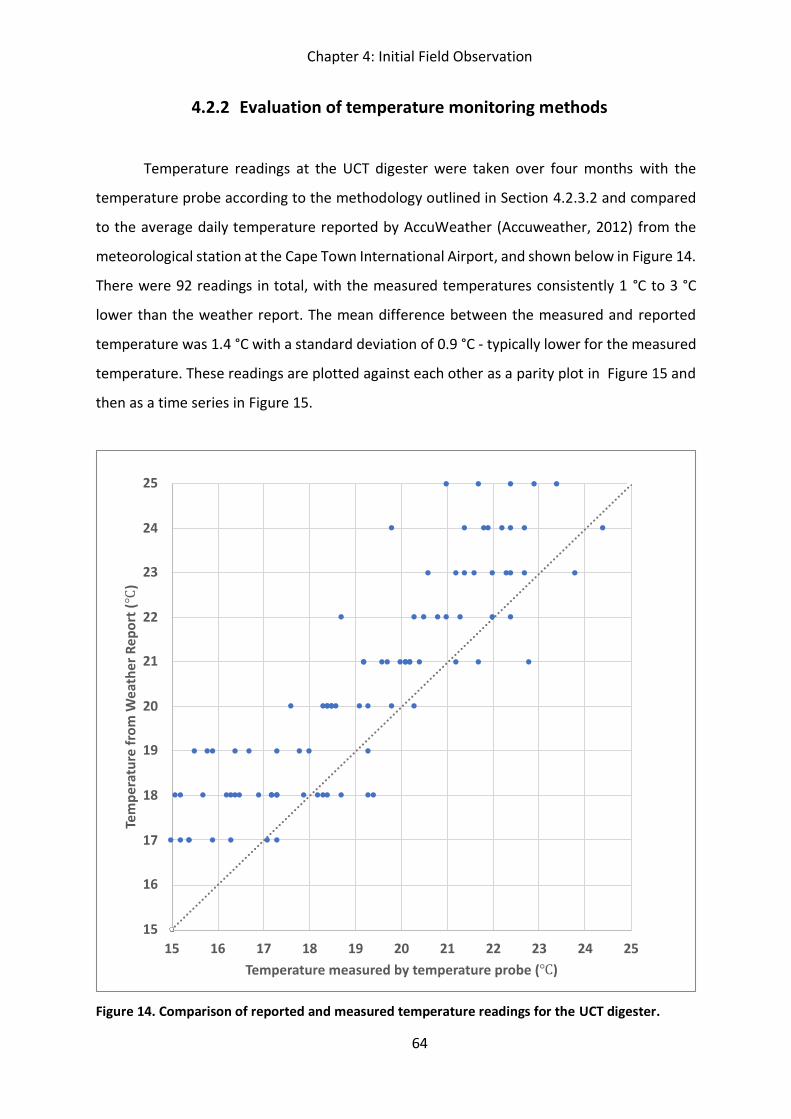
Chapter 4: Initial Field Observation
64
4.2.2 Evaluation of temperature monitoring methods
Temperature readings at the UCT digester were taken over four months with the
temperature probe according to the methodology outlined in Section 4.2.3.2 and compared
to the average daily temperature reported by AccuWeather (Accuweather, 2012) from the
meteorological station at the Cape Town International Airport, and shown below in Figure 14.
There were 92 readings in total, with the measured temperatures consistently 1 °C to 3 °C
lower than the weather report. The mean difference between the measured and reported
temperature was 1.4 °C with a standard deviation of 0.9 °C - typically lower for the measured
temperature. These readings are plotted against each other as a parity plot in Figure 15 and
then as a time series in Figure 15.
Figure 14. Comparison of reported and measured temperature readings for the UCT digester.
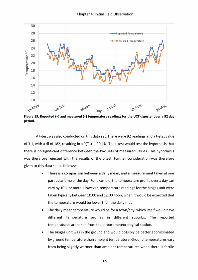
Chapter 4: Initial Field Observation
65
Figure 15. Reported (•) and measured (•) temperature readings for the UCT digester over a 92 day period.
A t-test was also conducted on this data set. There were 92 readings and a t-stat value
of 3.1, with a df of 182, resulting in a P(Tdt) of 0.1%. The t-test would test the hypothesis that
there is no significant difference between the two sets of measured values. This hypothesis
was therefore rejected with the results of the t-test. Further consideration was therefore
given to this data set as follows:
x There is a comparison between a daily mean, and a measurement taken at one
particular time of the day. For example, the temperature profile over a day can
vary by 10°C or more. However, temperature readings for the biogas unit were
taken typically between 10:00 and 12:00 noon, when it would be expected that
the temperature would be lower than the daily mean.
x The daily mean temperature would be for a town/city, which itself would have
different temperature profiles in different suburbs. The reported
temperatures are taken from the airport meteorological station.
x The biogas unit was in the ground and would possibly be better approximated
by ground temperature than ambient temperature. Ground temperatures vary
from being slightly warmer than ambient temperatures when there is fertile
Chapter 4: Initial Field Observation
66
soil with an active microbial population, to being slightly colder for less fertile
soils. (Bharadwaj & Bansal, 1981; Mann & Schmidt, 2003)
x The biogas unit could be in the sun or the shade, which would have an
influence on ambient temperature, and on the temperature of the biogas unit.
x The sampling point in the digester was close to the surface of the unit, not in
the centre of it.
With the above in consideration, while factoring in the offset of 1.4 °C , and noting
from Figure 15 that the reported temperature does track the measured temperature over the
entire date range as the temperature fluctuates, reported weather data was taken as an
acceptable measurement for the approximate digester temperature.
4.2.3 Other monitoring methods
Weights of food and water were recorded as described in Section 4.2.3.3 and the
burning time was occasionally recorded to estimate the gas utilisation. The burning time was
not originally included in the first build of the application but was done so from January 2012
to allow utilisation efficiency calculations to be included.
4.3 Refinement of the Biogas Monitoring Tool application
The mobile phone application used, was developed as described in Section 4.2.2. The
final digital form presented in that section was the result of an iterative process based on
learnings with the UCT biogas unit. Initially, the digital form was created to allow individual
users to submit data obtained. In the first build, there were 5 input options, all as free text
and listed as follows:
x Date
x pH
x Temperature (qC)
x Mass of food fed (kg)
x Pressure (kPa)
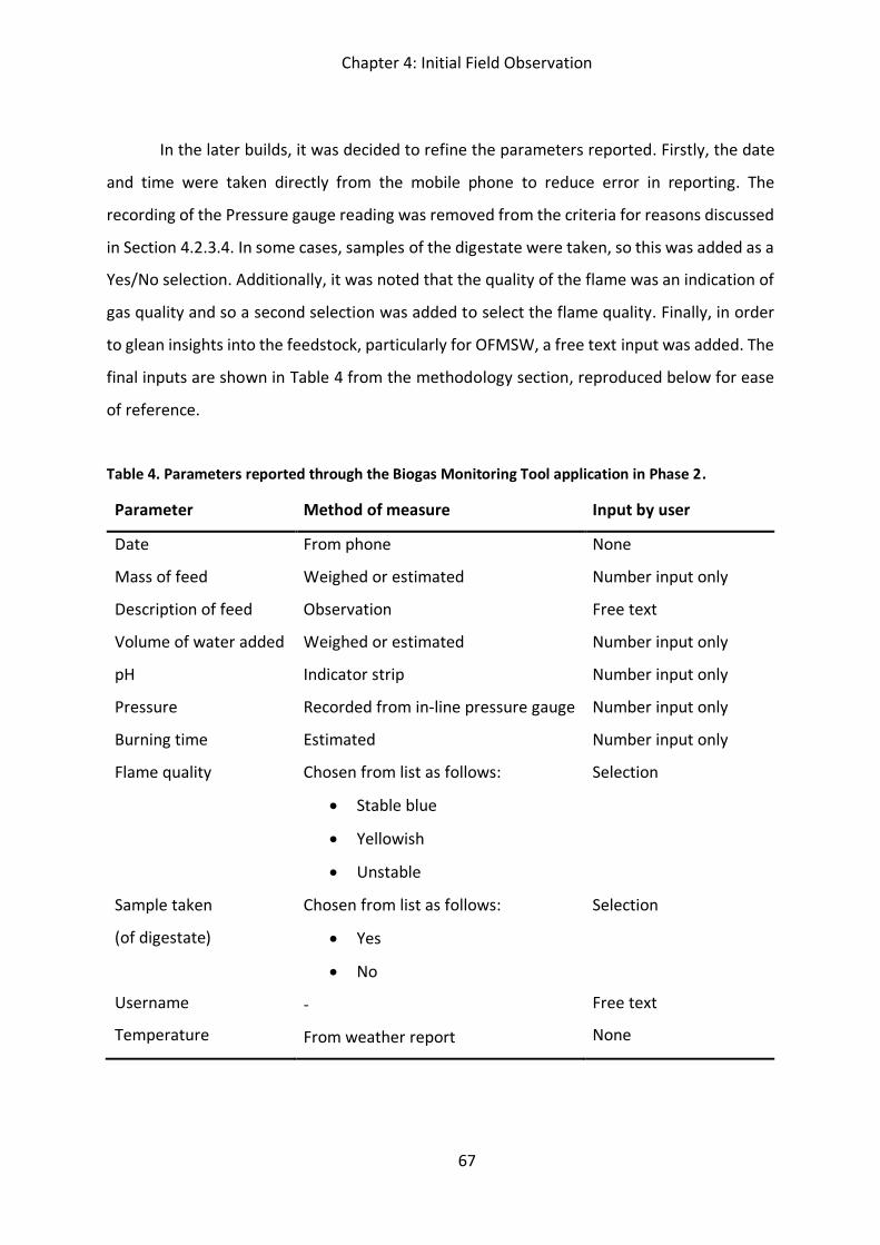
Chapter 4: Initial Field Observation
67
In the later builds, it was decided to refine the parameters reported. Firstly, the date
and time were taken directly from the mobile phone to reduce error in reporting. The
recording of the Pressure gauge reading was removed from the criteria for reasons discussed
in Section 4.2.3.4. In some cases, samples of the digestate were taken, so this was added as a
Yes/No selection. Additionally, it was noted that the quality of the flame was an indication of
gas quality and so a second selection was added to select the flame quality. Finally, in order
to glean insights into the feedstock, particularly for OFMSW, a free text input was added. The
final inputs are shown in Table 4 from the methodology section, reproduced below for ease
of reference.
Table 4. Parameters reported through the Biogas Monitoring Tool application in Phase 2.
Parameter Method of measure Input by user
Date
Mass of feed
From phone
Weighed or estimated
None
Number input only
Description of feed Observation Free text
Volume of water added Weighed or estimated Number input only
pH Indicator strip Number input only
Pressure Recorded from in-line pressure gauge Number input only
Burning time Estimated Number input only
Flame quality Chosen from list as follows:
x Stable blue
x Yellowish
x Unstable
Selection
Sample taken
(of digestate)
Username
Temperature
Chosen from list as follows:
x Yes
x No
-
From weather report
Selection
Free text
None
Chapter 4: Initial Field Observation
68
4.4 Final discussions and conclusions
Instability of the biogas unit was observed in all four periods. The mitigation technique
adopted in Periods 1 and 3 was the addition of lime. However, close monitoring of the pH and
adjustment of the organic loading rate proved to be effective as well, avoiding the need for
lime in Period 2. Finally, a hiatus in feed before Period 4 appeared to improve the stability of
the unit which did not need buffering or strict control of the organic loading rate in Period 4.
This is with the note that two variables were different in Period 4, namely that the volume of
water fed to the unit was significantly lower than previous Periods, and that the method of
monitoring pH (i.e. stability) was less precise as it was with indicator strip rather than pH
probe.
Temperature was merely observed in this study and not linked to gas production or
utilisation. Gas utilisations were conducted over two separate periods, namely over five
weeks in Period 2 and over ten weeks in Period 4. The utilisation was on average 10% higher
in Period 4 (which was in summer) than in Period 2 (which was in winter). This is not conclusive
of higher gas production just utilisation. Low utilisations are an indication that there is more
gas available than is being used and the hydraulic residence time would need to be factored
in to conclude on this.
The use of a mobile phone application to report data was trialled in Period 4. The initial
parameters chosen for monitoring were refined over the course of the development, for
example, pressure gauge readings were not deemed to be useful indicators, while flame
quality was added to the list as a measure of gas quality. Considering that the laboratory
measurement of pH and temperature were taken at sampling points of less than a metre in
the inlet pipe (not in the centre of a mixed reactor), acceptable confidence was bestowed to
the substitution of laboratory measuring techniques for pH and temperature with indicator
strips and reported weather data respectively. In this study, the remote monitoring
methodology was able to generate data sets through more simple measurement techniques.
Whether the data sets are still useful remains to be determined.
Chapter 5: Remote Monitoring Studies
69
Chapter 5: Remote Monitoring Studies
The key engineering contribution of this thesis lies in the attempt to develop a remote
monitoring and knowledge support tool for the operation of small-scale biogas units. The tool
was developed as described in Section 3.2.2 and used in this study in an attempt to address
Hypotheses 1 & 2; which were around biogas unit stability being affected by the feedstock,
and the productivity being affected by the temperature respectively. The study was
undertaken to gain an understanding of actual performance of installed units in various
locations, and specifically to understand factors which affect their productivity and stability.
This facilitated the refinement of the monitoring techniques and gave confidence in the
methods chosen. The second study took these smart monitoring learnings and applied them
to ten units around southern Africa, as described in Table 2, Chapter 3.
5.1 Stability of biogas units
The stability of biogas units was analysed on a case by case basis. It was noted that
whenever the pH gave a reading below 6.0, the user was contacted to ascertain whether any
assistance could be offered in the feeding regime. This was facilitated by an update to the
user interface mentioned in Section 4.2.2 which turned location markers in Figure 7 from
“green” to “red” if the last pH data point sent through was less than 6.0. Typically, the user
was contacted at that time and questioned about any changes to the feeding regime of the
biogas unit. The feeding regime of the previous two weeks was also analysed to determine
possible causes for the instability in order to inform Hypothesis 1, which postulated that the
feeding regime would be significant in the stability of small-scale biogas units.
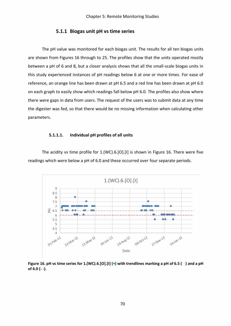
Chapter 5: Remote Monitoring Studies
70
5.1.1 Biogas unit pH vs time series
The pH value was monitored for each biogas unit. The results for all ten biogas units
are shown from Figures 16 through to 25. The profiles show that the units operated mostly
between a pH of 6 and 8, but a closer analysis shows that all the small-scale biogas units in
this study experienced instances of pH readings below 6 at one or more times. For ease of
reference, an orange line has been drawn at pH 6.5 and a red line has been drawn at pH 6.0
on each graph to easily show which readings fall below pH 6.0. The profiles also show where
there were gaps in data from users. The request of the users was to submit data at any time
the digester was fed, so that there would be no missing information when calculating other
parameters.
5.1.1.1. Individual pH profiles of all units
The acidity vs time profile for 1.(WC).6.[O].[I] is shown in Figure 16. There were five
readings which were below a pH of 6.0 and these occurred over four separate periods.
Figure 16. pH vs time series for 1.(WC).6.[O].[I] (•) with trendlines marking a pH of 6.5 (- -) and a pH of 6.0 (- -).
44.5
55.5
66.5
77.5
88.5
9
01-Feb-12
22-Mar-12
11-May-12
30-Jun-12
19-Aug-12
08-Oct-12
27-Nov-12
16-Jan-13
PH
Date
1.(WC).6.[O].[I]
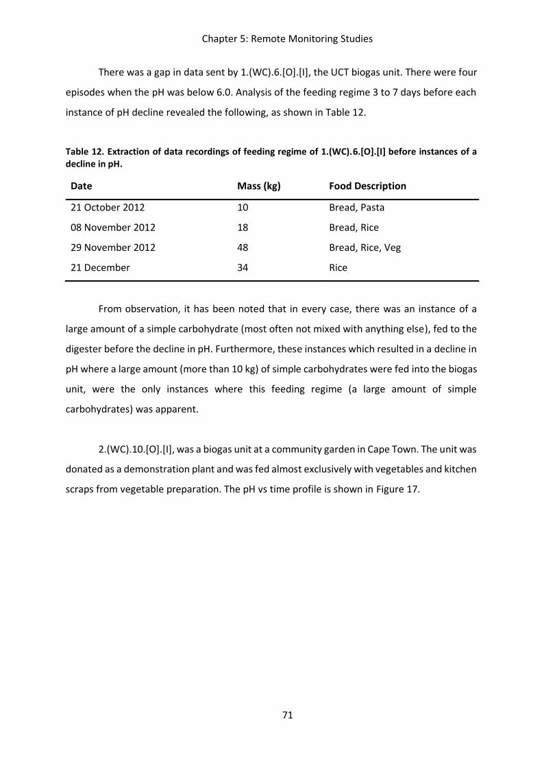
Chapter 5: Remote Monitoring Studies
71
There was a gap in data sent by 1.(WC).6.[O].[I], the UCT biogas unit. There were four
episodes when the pH was below 6.0. Analysis of the feeding regime 3 to 7 days before each
instance of pH decline revealed the following, as shown in Table 12.
Table 12. Extraction of data recordings of feeding regime of 1.(WC).6.[O].[I] before instances of a decline in pH.
Date Mass (kg) Food Description
21 October 2012 10 Bread, Pasta
08 November 2012 18 Bread, Rice
29 November 2012 48 Bread, Rice, Veg
21 December 34 Rice
From observation, it has been noted that in every case, there was an instance of a
large amount of a simple carbohydrate (most often not mixed with anything else), fed to the
digester before the decline in pH. Furthermore, these instances which resulted in a decline in
pH where a large amount (more than 10 kg) of simple carbohydrates were fed into the biogas
unit, were the only instances where this feeding regime (a large amount of simple
carbohydrates) was apparent.
2.(WC).10.[O].[I], was a biogas unit at a community garden in Cape Town. The unit was
donated as a demonstration plant and was fed almost exclusively with vegetables and kitchen
scraps from vegetable preparation. The pH vs time profile is shown in Figure 17.
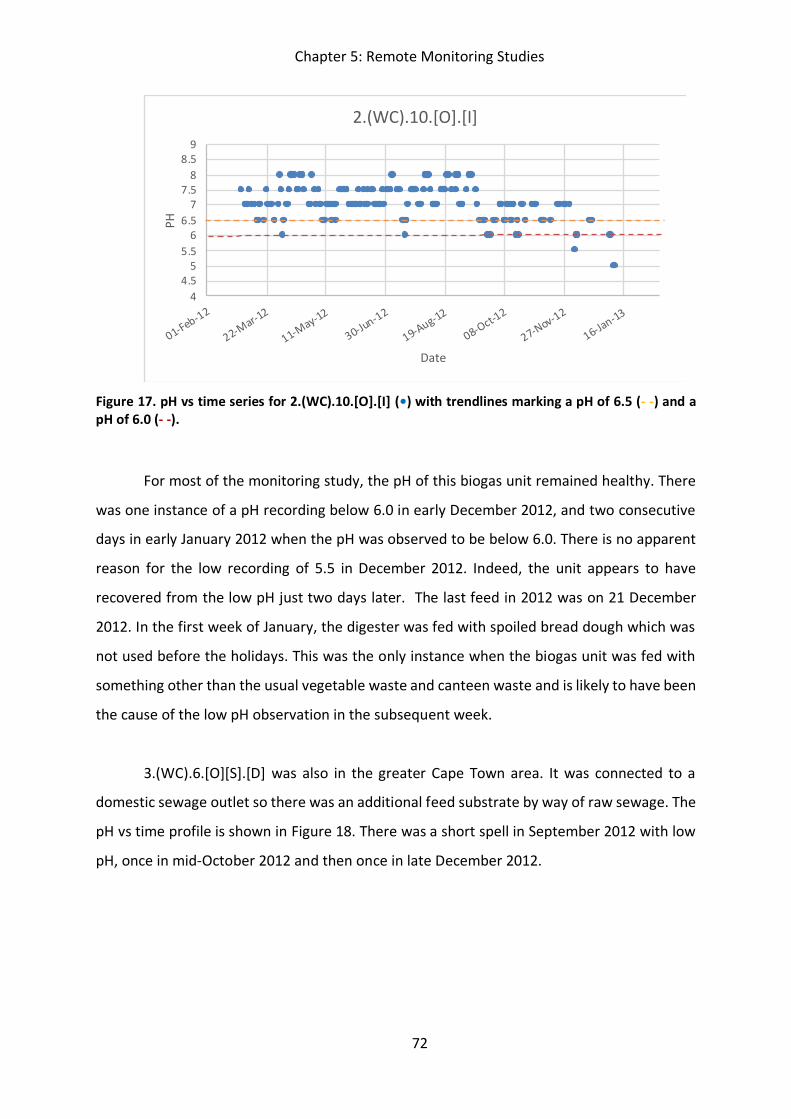
Chapter 5: Remote Monitoring Studies
72
Figure 17. pH vs time series for 2.(WC).10.[O].[I] (•) with trendlines marking a pH of 6.5 (- -) and a pH of 6.0 (- -).
For most of the monitoring study, the pH of this biogas unit remained healthy. There
was one instance of a pH recording below 6.0 in early December 2012, and two consecutive
days in early January 2012 when the pH was observed to be below 6.0. There is no apparent
reason for the low recording of 5.5 in December 2012. Indeed, the unit appears to have
recovered from the low pH just two days later. The last feed in 2012 was on 21 December
2012. In the first week of January, the digester was fed with spoiled bread dough which was
not used before the holidays. This was the only instance when the biogas unit was fed with
something other than the usual vegetable waste and canteen waste and is likely to have been
the cause of the low pH observation in the subsequent week.
3.(WC).6.[O][S].[D] was also in the greater Cape Town area. It was connected to a
domestic sewage outlet so there was an additional feed substrate by way of raw sewage. The
pH vs time profile is shown in Figure 18. There was a short spell in September 2012 with low
pH, once in mid-October 2012 and then once in late December 2012.
44.5
55.5
66.5
77.5
88.5
9
01-Feb-12
22-Mar-12
11-May-12
30-Jun-12
19-Aug-12
08-Oct-12
27-Nov-12
16-Jan-13
PH
Date
2.(WC).10.[O].[I]
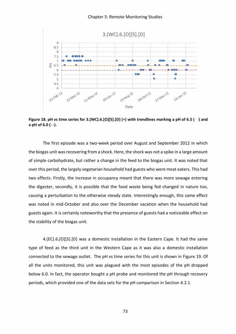
Chapter 5: Remote Monitoring Studies
73
Figure 18. pH vs time series for 3.(WC).6.[O][S].[D] (•) with trendlines marking a pH of 6.5 (- -) and a pH of 6.0 (- -).
The first episode was a two-week period over August and September 2012 in which
the biogas unit was recovering from a shock. Here, the shock was not a spike in a large amount
of simple carbohydrate, but rather a change in the feed to the biogas unit. It was noted that
over this period, the largely vegetarian household had guests who were meat eaters. This had
two effects. Firstly, the increase in occupancy meant that there was more sewage entering
the digester, secondly, it is possible that the food waste being fed changed in nature too,
causing a perturbation to the otherwise steady state. Interestingly enough, this same effect
was noted in mid-October and also over the December vacation when the household had
guests again. It is certainly noteworthy that the presence of guests had a noticeable effect on
the stability of the biogas unit.
4.(EC).6.[O][S].[D] was a domestic installation in the Eastern Cape. It had the same
type of feed as the third unit in the Western Cape as it was also a domestic installation
connected to the sewage outlet. The pH vs time series for this unit is shown in Figure 19. Of
all the units monitored, this unit was plagued with the most episodes of the pH dropped
below 6.0. In fact, the operator bought a pH probe and monitored the pH through recovery
periods, which provided one of the data sets for the pH comparison in Section 4.2.1.
44.5
55.5
66.5
77.5
88.5
9
01-Feb-12
22-Mar-12
11-May-12
30-Jun-12
19-Aug-12
08-Oct-12
27-Nov-12
16-Jan-13
PH
Date
3.(WC).6.[O][S].[D]
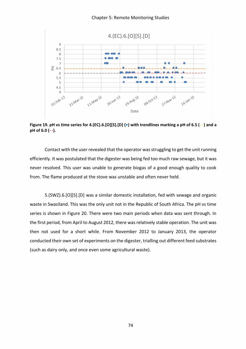
Chapter 5: Remote Monitoring Studies
74
Figure 19. pH vs time series for 4.(EC).6.[O][S].[D] (•) with trendlines marking a pH of 6.5 (- -) and a pH of 6.0 (- -).
Contact with the user revealed that the operator was struggling to get the unit running
efficiently. It was postulated that the digester was being fed too much raw sewage, but it was
never resolved. This user was unable to generate biogas of a good enough quality to cook
from. The flame produced at the stove was unstable and often never held.
5.(SWZ).6.[O][S].[D] was a similar domestic installation, fed with sewage and organic
waste in Swaziland. This was the only unit not in the Republic of South Africa. The pH vs time
series is shown in Figure 20. There were two main periods when data was sent through. In
the first period, from April to August 2012, there was relatively stable operation. The unit was
then not used for a short while. From November 2012 to January 2013, the operator
conducted their own set of experiments on the digester, trialling out different feed substrates
(such as dairy only, and once even some agricultural waste).
44.5
55.5
66.5
77.5
88.5
9
01-Feb-12
22-Mar-12
11-May-12
30-Jun-12
19-Aug-12
08-Oct-12
27-Nov-12
16-Jan-13
PH
Date
4.(EC).6.[O][S].[D]
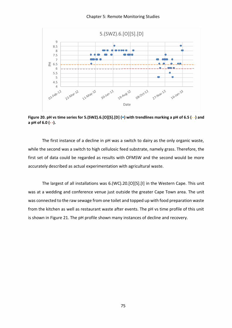
Chapter 5: Remote Monitoring Studies
75
Figure 20. pH vs time series for 5.(SWZ).6.[O][S].[D] (•) with trendlines marking a pH of 6.5 (- -) and a pH of 6.0 (- -).
The first instance of a decline in pH was a switch to dairy as the only organic waste,
while the second was a switch to high cellulosic feed substrate, namely grass. Therefore, the
first set of data could be regarded as results with OFMSW and the second would be more
accurately described as actual experimentation with agricultural waste.
The largest of all installations was 6.(WC).20.[O][S].[I] in the Western Cape. This unit
was at a wedding and conference venue just outside the greater Cape Town area. The unit
was connected to the raw sewage from one toilet and topped up with food preparation waste
from the kitchen as well as restaurant waste after events. The pH vs time profile of this unit
is shown in Figure 21. The pH profile shown many instances of decline and recovery.
44.5
55.5
66.5
77.5
88.5
9
01-Feb-12
22-Mar-12
11-May-12
30-Jun-12
19-Aug-12
08-Oct-12
27-Nov-12
16-Jan-13
PH
Date
5.(SWZ).6.[O][S].[D]

Chapter 5: Remote Monitoring Studies
76
Figure 21. pH vs time series for 6.(WC).20.[O][S].[I] (•) with trendlines marking a pH of 6.5 (- -) and a pH of 6.0 (- -).
Declines in pH were noted after events, i.e. whenever there would have been a sharp
increase in the amount of organic waste and also when the amount of raw sewage would
probably have increased as well. The time of the highest instability was between November
and mid-January, when the venue was full every week, their peak season.
7.(LIM).8.[A][M].[D] was only monitored for 3 months. It was a small-scale unit in the
Limpopo province. It was donated as a demonstration unit to show how biogas could be
harnessed from manure and agricultural waste. The pH vs time series for this unit is shown in
Figure 22.
44.5
55.5
66.5
77.5
88.5
9
01-Feb-12
22-Mar-12
11-May-12
30-Jun-12
19-Aug-12
08-Oct-12
27-Nov-12
16-Jan-13
PH
Date
6.(WC).20.[O][S].[I]
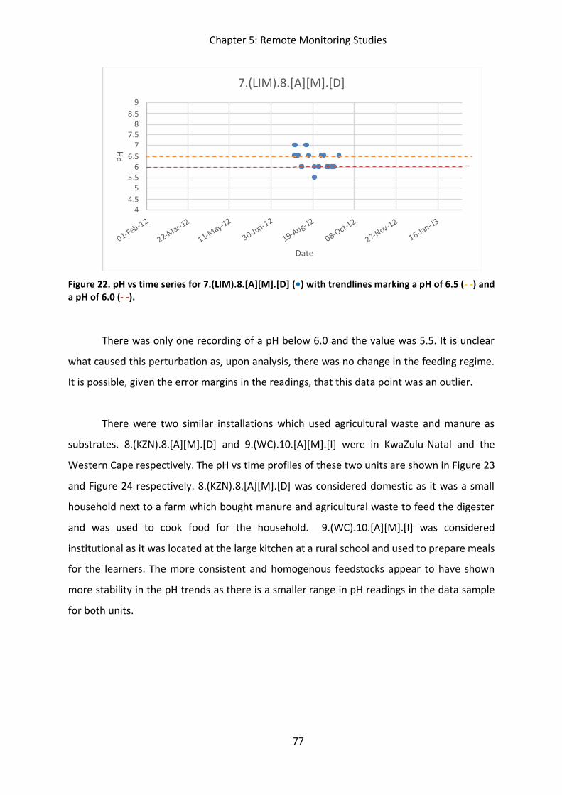
Chapter 5: Remote Monitoring Studies
77
Figure 22. pH vs time series for 7.(LIM).8.[A][M].[D] (•) with trendlines marking a pH of 6.5 (- -) and a pH of 6.0 (- -).
There was only one recording of a pH below 6.0 and the value was 5.5. It is unclear
what caused this perturbation as, upon analysis, there was no change in the feeding regime.
It is possible, given the error margins in the readings, that this data point was an outlier.
There were two similar installations which used agricultural waste and manure as
substrates. 8.(KZN).8.[A][M].[D] and 9.(WC).10.[A][M].[I] were in KwaZulu-Natal and the
Western Cape respectively. The pH vs time profiles of these two units are shown in Figure 23
and Figure 24 respectively. 8.(KZN).8.[A][M].[D] was considered domestic as it was a small
household next to a farm which bought manure and agricultural waste to feed the digester
and was used to cook food for the household. 9.(WC).10.[A][M].[I] was considered
institutional as it was located at the large kitchen at a rural school and used to prepare meals
for the learners. The more consistent and homogenous feedstocks appear to have shown
more stability in the pH trends as there is a smaller range in pH readings in the data sample
for both units.
44.5
55.5
66.5
77.5
88.5
9
01-Feb-12
22-Mar-12
11-May-12
30-Jun-12
19-Aug-12
08-Oct-12
27-Nov-12
16-Jan-13
PH
Date
7.(LIM).8.[A][M].[D]
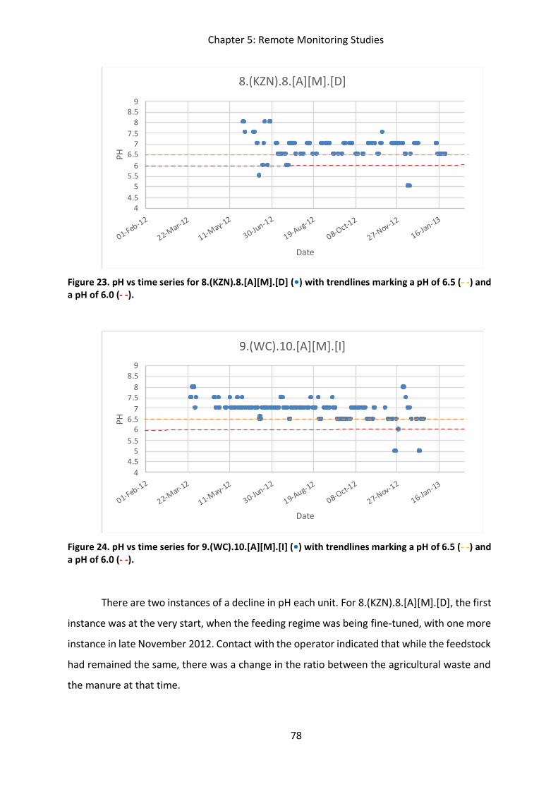
Chapter 5: Remote Monitoring Studies
78
Figure 23. pH vs time series for 8.(KZN).8.[A][M].[D] (•) with trendlines marking a pH of 6.5 (- -) and a pH of 6.0 (- -).
Figure 24. pH vs time series for 9.(WC).10.[A][M].[I] (•) with trendlines marking a pH of 6.5 (- -) and a pH of 6.0 (- -).
There are two instances of a decline in pH each unit. For 8.(KZN).8.[A][M].[D], the first
instance was at the very start, when the feeding regime was being fine-tuned, with one more
instance in late November 2012. Contact with the operator indicated that while the feedstock
had remained the same, there was a change in the ratio between the agricultural waste and
the manure at that time.
44.5
55.5
66.5
77.5
88.5
9
01-Feb-12
22-Mar-12
11-May-12
30-Jun-12
19-Aug-12
08-Oct-12
27-Nov-12
16-Jan-13
PH
Date
8.(KZN).8.[A][M].[D]
44.5
55.5
66.5
77.5
88.5
9
01-Feb-12
22-Mar-12
11-May-12
30-Jun-12
19-Aug-12
08-Oct-12
27-Nov-12
16-Jan-13
PH
Date
9.(WC).10.[A][M].[I]
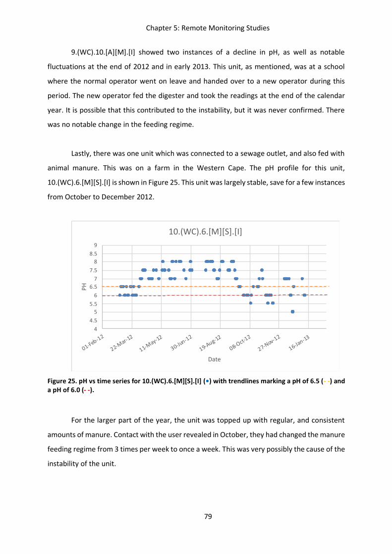
Chapter 5: Remote Monitoring Studies
79
9.(WC).10.[A][M].[I] showed two instances of a decline in pH, as well as notable
fluctuations at the end of 2012 and in early 2013. This unit, as mentioned, was at a school
where the normal operator went on leave and handed over to a new operator during this
period. The new operator fed the digester and took the readings at the end of the calendar
year. It is possible that this contributed to the instability, but it was never confirmed. There
was no notable change in the feeding regime.
Lastly, there was one unit which was connected to a sewage outlet, and also fed with
animal manure. This was on a farm in the Western Cape. The pH profile for this unit,
10.(WC).6.[M][S].[I] is shown in Figure 25. This unit was largely stable, save for a few instances
from October to December 2012.
Figure 25. pH vs time series for 10.(WC).6.[M][S].[I] (•) with trendlines marking a pH of 6.5 (- -) and a pH of 6.0 (- -).
For the larger part of the year, the unit was topped up with regular, and consistent
amounts of manure. Contact with the user revealed in October, they had changed the manure
feeding regime from 3 times per week to once a week. This was very possibly the cause of the
instability of the unit.
44.5
55.5
66.5
77.5
88.5
9
01-Feb-12
22-Mar-12
11-May-12
30-Jun-12
19-Aug-12
08-Oct-12
27-Nov-12
16-Jan-13
PH
Date
10.(WC).6.[M][S].[I]
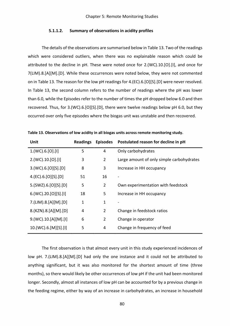
Chapter 5: Remote Monitoring Studies
80
5.1.1.2. Summary of observations in acidity profiles
The details of the observations are summarised below in Table 13. Two of the readings
which were considered outliers, when there was no explainable reason which could be
attributed to the decline in pH. These were noted once for 2.(WC).10.[O].[I], and once for
7(LIM).8.[A][M].[D]. While these occurrences were noted below, they were not commented
on in Table 13. The reason for the low pH readings for 4.(EC).6.[O][S].[D] were never resolved.
In Table 13, the second column refers to the number of readings where the pH was lower
than 6.0, while the Episodes refer to the number of times the pH dropped below 6.0 and then
recovered. Thus, for 3.(WC).6.[O][S].[D], there were twelve readings below pH 6.0, but they
occurred over only five episodes where the biogas unit was unstable and then recovered.
Table 13. Observations of low acidity in all biogas units across remote monitoring study.
Unit Readings Episodes Postulated reason for decline in pH
1.(WC).6.[O].[I] 5 4 Only carbohydrates
2.(WC).10.[O].[I] 3 2 Large amount of only simple carbohydrates
3.(WC).6.[O][S].[D] 8 3 Increase in HH occupancy
4.(EC).6.[O][S].[D] 51 16 -
5.(SWZ).6.[O][S].[D] 5 2 Own experimentation with feedstock
6.(WC).20.[O][S].[I] 18 5 Increase in HH occupancy
7.(LIM).8.[A][M].[D] 1 1 -
8.(KZN).8.[A][M].[D] 4 2 Change in feedstock ratios
9.(WC).10.[A][M].[I] 6 2 Change in operator
10.(WC).6.[M][S].[I] 5 4 Change in frequency of feed
The first observation is that almost every unit in this study experienced incidences of
low pH. 7.(LIM).8.[A][M].[D] had only the one instance and it could not be attributed to
anything significant, but it was also monitored for the shortest amount of time (three
months), so there would likely be other occurrences of low pH if the unit had been monitored
longer. Secondly, almost all instances of low pH can be accounted for by a previous change in
the feeding regime, either by way of an increase in carbohydrates, an increase in household
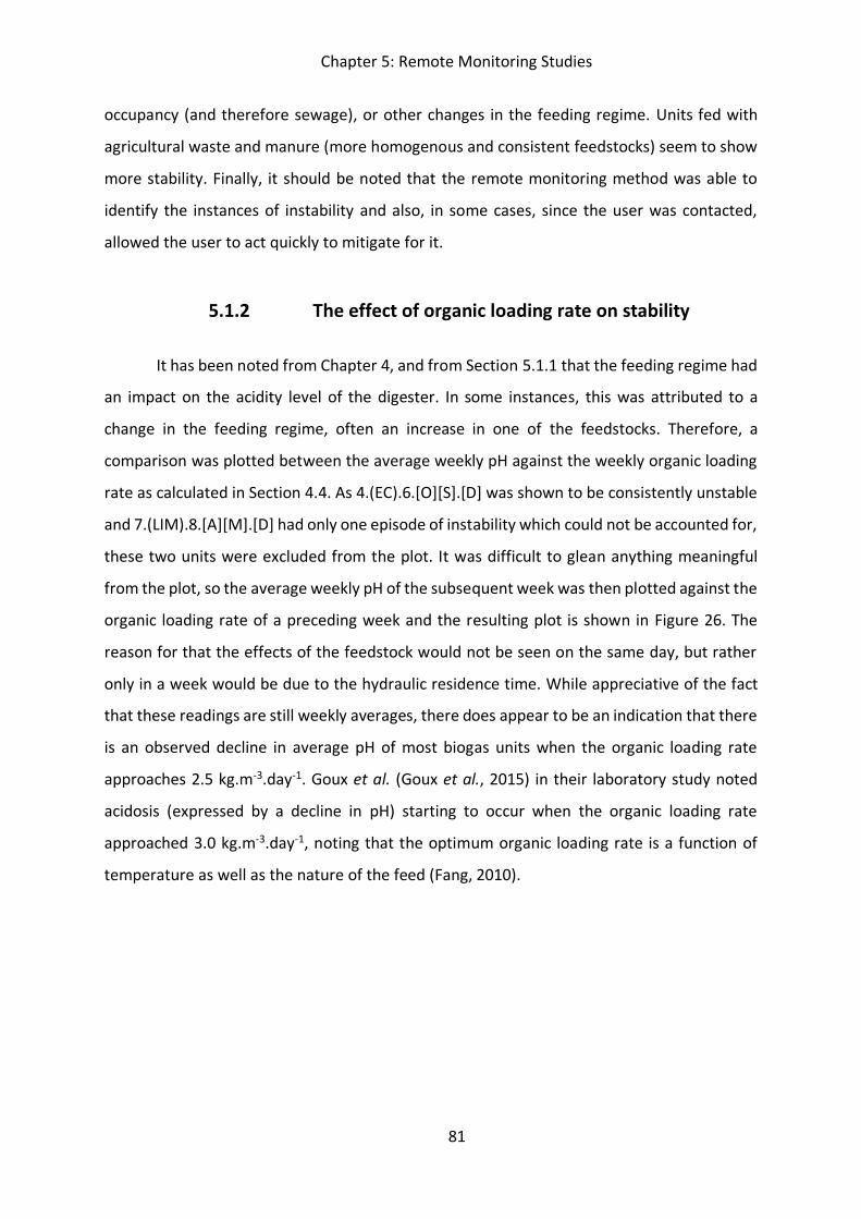
Chapter 5: Remote Monitoring Studies
81
occupancy (and therefore sewage), or other changes in the feeding regime. Units fed with
agricultural waste and manure (more homogenous and consistent feedstocks) seem to show
more stability. Finally, it should be noted that the remote monitoring method was able to
identify the instances of instability and also, in some cases, since the user was contacted,
allowed the user to act quickly to mitigate for it.
5.1.2 The effect of organic loading rate on stability
It has been noted from Chapter 4, and from Section 5.1.1 that the feeding regime had
an impact on the acidity level of the digester. In some instances, this was attributed to a
change in the feeding regime, often an increase in one of the feedstocks. Therefore, a
comparison was plotted between the average weekly pH against the weekly organic loading
rate as calculated in Section 4.4. As 4.(EC).6.[O][S].[D] was shown to be consistently unstable
and 7.(LIM).8.[A][M].[D] had only one episode of instability which could not be accounted for,
these two units were excluded from the plot. It was difficult to glean anything meaningful
from the plot, so the average weekly pH of the subsequent week was then plotted against the
organic loading rate of a preceding week and the resulting plot is shown in Figure 26. The
reason for that the effects of the feedstock would not be seen on the same day, but rather
only in a week would be due to the hydraulic residence time. While appreciative of the fact
that these readings are still weekly averages, there does appear to be an indication that there
is an observed decline in average pH of most biogas units when the organic loading rate
approaches 2.5 kg.m-3.day-1. Goux et al. (Goux et al., 2015) in their laboratory study noted
acidosis (expressed by a decline in pH) starting to occur when the organic loading rate
approached 3.0 kg.m-3.day-1, noting that the optimum organic loading rate is a function of
temperature as well as the nature of the feed (Fang, 2010).
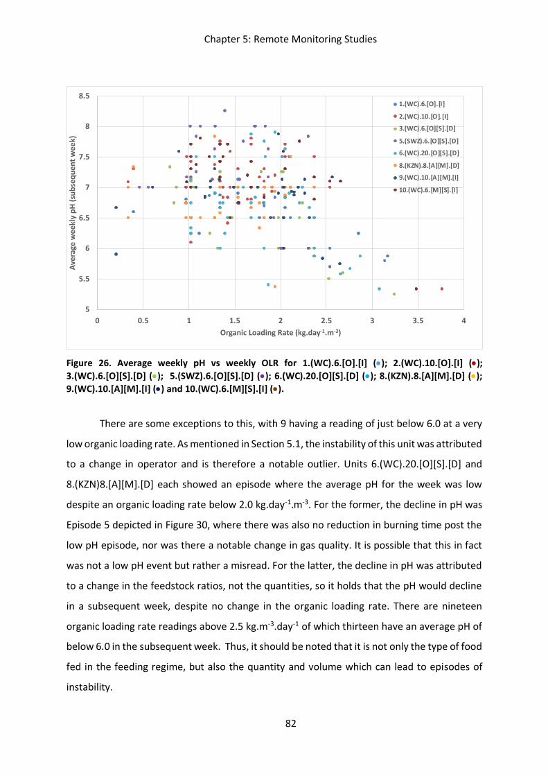
Chapter 5: Remote Monitoring Studies
82
Figure 26. Average weekly pH vs weekly OLR for 1.(WC).6.[O].[I] (x); 2.(WC).10.[O].[I] (x); 3.(WC).6.[O][S].[D] (x); 5.(SWZ).6.[O][S].[D] (x); 6.(WC).20.[O][S].[D] (x); 8.(KZN).8.[A][M].[D] (x); 9.(WC).10.[A][M].[I] (x) and 10.(WC).6.[M][S].[I] (x).
There are some exceptions to this, with 9 having a reading of just below 6.0 at a very
low organic loading rate. As mentioned in Section 5.1, the instability of this unit was attributed
to a change in operator and is therefore a notable outlier. Units 6.(WC).20.[O][S].[D] and
8.(KZN)8.[A][M].[D] each showed an episode where the average pH for the week was low
despite an organic loading rate below 2.0 kg.day-1.m-3. For the former, the decline in pH was
Episode 5 depicted in Figure 30, where there was also no reduction in burning time post the
low pH episode, nor was there a notable change in gas quality. It is possible that this in fact
was not a low pH event but rather a misread. For the latter, the decline in pH was attributed
to a change in the feedstock ratios, not the quantities, so it holds that the pH would decline
in a subsequent week, despite no change in the organic loading rate. There are nineteen
organic loading rate readings above 2.5 kg.m-3.day-1 of which thirteen have an average pH of
below 6.0 in the subsequent week. Thus, it should be noted that it is not only the type of food
fed in the feeding regime, but also the quantity and volume which can lead to episodes of
instability.
5
5.5
6
6.5
7
7.5
8
8.5
0 0.5 1 1.5 2 2.5 3 3.5 4
Aver
age
wee
kly
pH (s
ubse
quen
t wee
k)
Organic Loading Rate (kg.day-1.m-3)
1.(WC).6.[O].[I]
2.(WC).10.[O].[I]
3.(WC).6.[O][S].[D]
5.(SWZ).6.[O][S].[D]
6.(WC).20.[O][S].[D]
8.(KZN).8.[A][M].[D]
9.(WC).10.[A][M].[I]
10.(WC).6.[M][S].[I]
Chapter 5: Remote Monitoring Studies
83
5.2 The effect of instability on biogas production/utilisation
The important impact to the user would be whether or not the incidence of low acidity
affected their gas production, either by the quantity or the quality of gas produced. Again,
notes made that the burning time was an indication of gas used, rather than the gas produced.
Still, the time series is plotted a week before and a week after the incidence of low pH. For
1.(WC).6.[O].[I], this occurred 4 times, and the burning time series is plotted against this
series, with day 0, as the first day of low pH and the start of the episode, shown in Figure 27.
The total burning time of the stove is seen to decline in all episodes in days following a low
pH reading. Further investigation into reported data, shows that in three of the four cases,
there was also a note from the user that the flame quality had been compromised, a change
in reading from “Blue” to “Yellow(unstable)”. These three episodes of poor flame quality were
around the incidences of low pH and also the only instances of poor flame quality reported in
the data set.
Figure 27. Burning times around episodes of low pH for 1.(WC).6.[O].[I].
0
20
40
60
80
100
120
140
-7 -6 -5 -4 -3 -2 -1 0 1 2 3 4 5 6 7
Burn
ing
time
(min
s)
Days surrounding low pH event
Episode 1
Episode 2
Episode 3
Episode 4
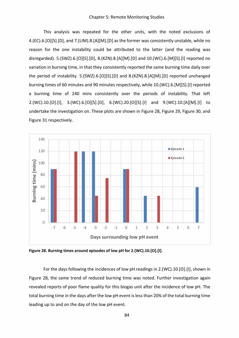
Chapter 5: Remote Monitoring Studies
84
This analysis was repeated for the other units, with the noted exclusions of
4.(EC).6.[O][S].[D], and 7.(LIM).8.[A][M].[D] as the former was consistently unstable, while no
reason for the one instability could be attributed to the latter (and the reading was
disregarded). 5.(SWZ).6.[O][S].[D], 8.(KZN).8.[A][M].[D] and 10.(WC).6.[M][S].[I] reported no
variation in burning time, in that they consistently reported the same burning time daily over
the period of instability. 5.(SWZ).6.[O][S].[D] and 8.(KZN).8.[A][M].[D] reported unchanged
burning times of 60 minutes and 90 minutes respectively, while 10.(WC).6.[M][S].[I] reported
a burning time of 240 mins consistently over the periods of instability. That left
2.(WC).10.[O].[I], 3.(WC).6.[O][S].[D], 6.(WC).20.[O][S].[I] and 9.(WC).10.[A][M].[I] to
undertake the investigation on. These plots are shown in Figure 28, Figure 29, Figure 30, and
Figure 31 respectively.
Figure 28. Burning times around episodes of low pH for 2.(WC).10.[O].[I].
For the days following the incidences of low pH readings in 2.(WC).10.[O].[I], shown in
Figure 28, the same trend of reduced burning time was noted. Further investigation again
revealed reports of poor flame quality for this biogas unit after the incidence of low pH. The
total burning time in the days after the low pH event is less than 20% of the total burning time
leading up to and on the day of the low pH event.
0
20
40
60
80
100
120
140
-7 -6 -5 -4 -3 -2 -1 0 1 2 3 4 5 6 7
Burn
ing
time
(min
s)
Days surrounding low pH event
Episode 1
Episode 2
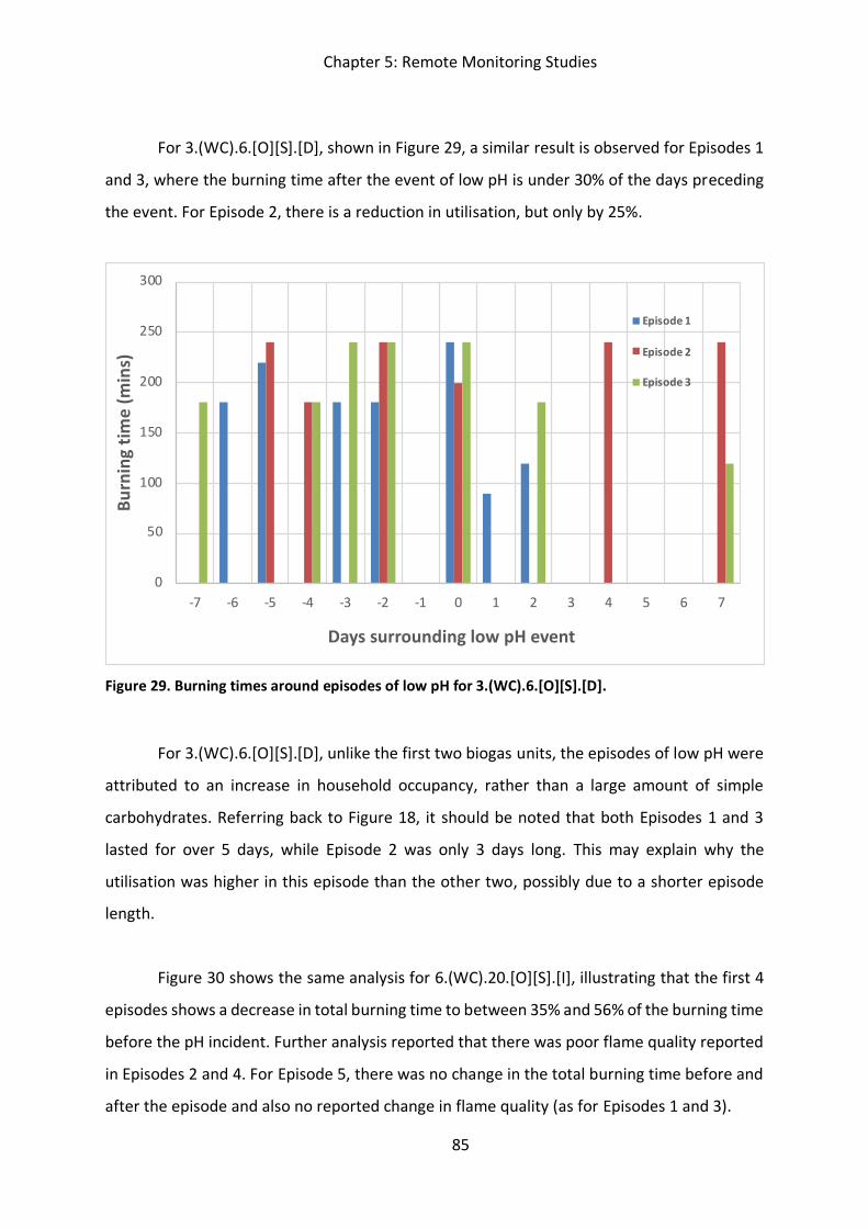
Chapter 5: Remote Monitoring Studies
85
For 3.(WC).6.[O][S].[D], shown in Figure 29, a similar result is observed for Episodes 1
and 3, where the burning time after the event of low pH is under 30% of the days preceding
the event. For Episode 2, there is a reduction in utilisation, but only by 25%.
Figure 29. Burning times around episodes of low pH for 3.(WC).6.[O][S].[D].
For 3.(WC).6.[O][S].[D], unlike the first two biogas units, the episodes of low pH were
attributed to an increase in household occupancy, rather than a large amount of simple
carbohydrates. Referring back to Figure 18, it should be noted that both Episodes 1 and 3
lasted for over 5 days, while Episode 2 was only 3 days long. This may explain why the
utilisation was higher in this episode than the other two, possibly due to a shorter episode
length.
Figure 30 shows the same analysis for 6.(WC).20.[O][S].[I], illustrating that the first 4
episodes shows a decrease in total burning time to between 35% and 56% of the burning time
before the pH incident. Further analysis reported that there was poor flame quality reported
in Episodes 2 and 4. For Episode 5, there was no change in the total burning time before and
after the episode and also no reported change in flame quality (as for Episodes 1 and 3).
0
50
100
150
200
250
300
-7 -6 -5 -4 -3 -2 -1 0 1 2 3 4 5 6 7
Burn
ing
time
(min
s)
Days surrounding low pH event
Episode 1
Episode 2
Episode 3
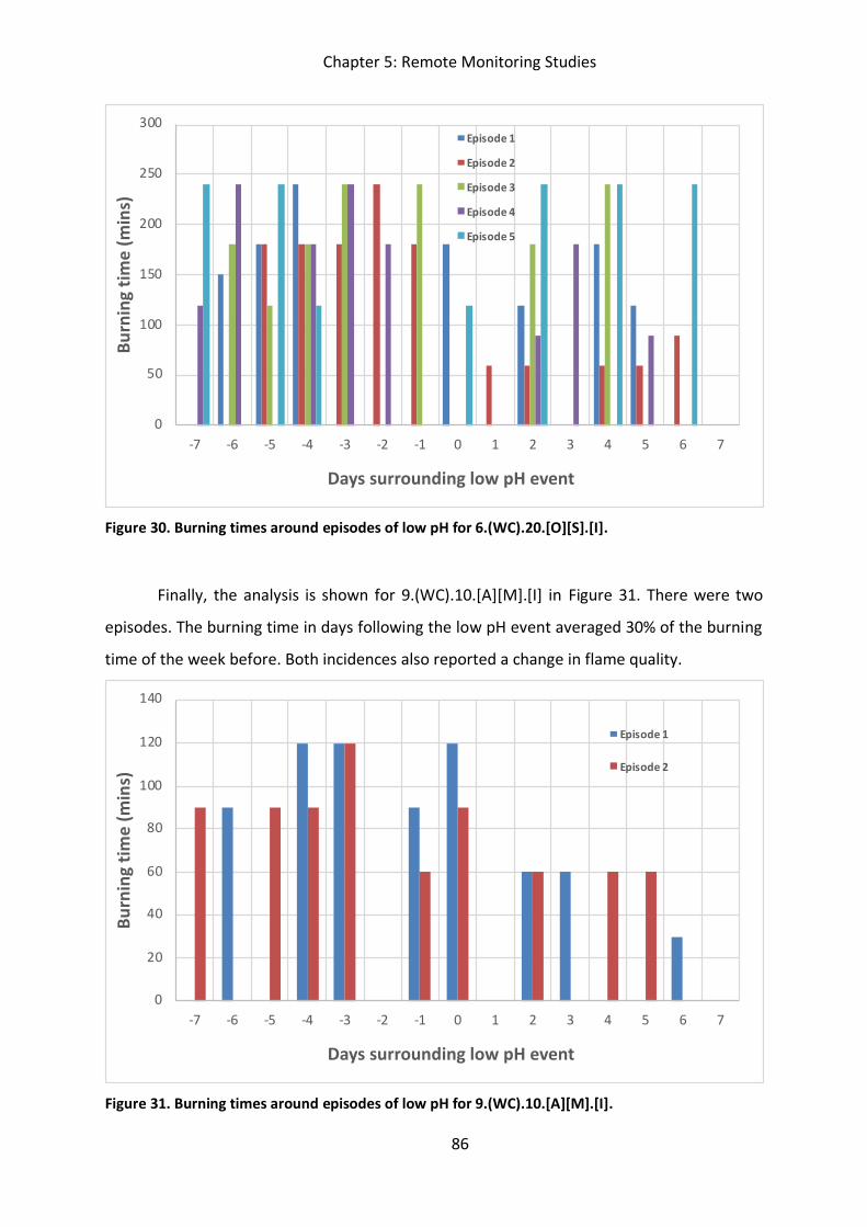
Chapter 5: Remote Monitoring Studies
86
Figure 30. Burning times around episodes of low pH for 6.(WC).20.[O][S].[I].
Finally, the analysis is shown for 9.(WC).10.[A][M].[I] in Figure 31. There were two
episodes. The burning time in days following the low pH event averaged 30% of the burning
time of the week before. Both incidences also reported a change in flame quality.
Figure 31. Burning times around episodes of low pH for 9.(WC).10.[A][M].[I].
0
50
100
150
200
250
300
-7 -6 -5 -4 -3 -2 -1 0 1 2 3 4 5 6 7
Burn
ing
time
(min
s)
Days surrounding low pH event
Episode 1
Episode 2
Episode 3
Episode 4
Episode 5
0
20
40
60
80
100
120
140
-7 -6 -5 -4 -3 -2 -1 0 1 2 3 4 5 6 7
Burn
ing
time
(min
s)
Days surrounding low pH event
Episode 1
Episode 2
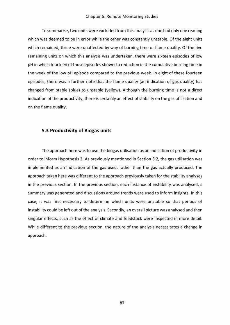
Chapter 5: Remote Monitoring Studies
87
To summarise, two units were excluded from this analysis as one had only one reading
which was deemed to be in error while the other was constantly unstable. Of the eight units
which remained, three were unaffected by way of burning time or flame quality. Of the five
remaining units on which this analysis was undertaken, there were sixteen episodes of low
pH in which fourteen of those episodes showed a reduction in the cumulative burning time in
the week of the low pH episode compared to the previous week. In eight of these fourteen
episodes, there was a further note that the flame quality (an indication of gas quality) has
changed from stable (blue) to unstable (yellow). Although the burning time is not a direct
indication of the productivity, there is certainly an effect of stability on the gas utilisation and
on the flame quality.
5.3 Productivity of Biogas units
The approach here was to use the biogas utilisation as an indication of productivity in
order to inform Hypothesis 2. As previously mentioned in Section 5.2, the gas utilisation was
implemented as an indication of the gas used, rather than the gas actually produced. The
approach taken here was different to the approach previously taken for the stability analyses
in the previous section. In the previous section, each instance of instability was analysed, a
summary was generated and discussions around trends were used to inform insights. In this
case, it was first necessary to determine which units were unstable so that periods of
instability could be left out of the analysis. Secondly, an overall picture was analysed and then
singular effects, such as the effect of climate and feedstock were inspected in more detail.
While different to the previous section, the nature of the analysis necessitates a change in
approach.
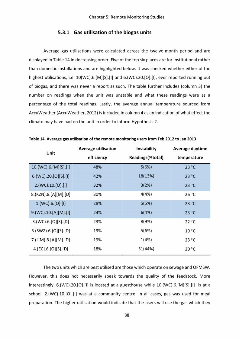
Chapter 5: Remote Monitoring Studies
88
5.3.1 Gas utilisation of the biogas units
Average gas utilisations were calculated across the twelve-month period and are
displayed in Table 14 in decreasing order. Five of the top six places are for institutional rather
than domestic installations and are highlighted below. It was checked whether either of the
highest utilisations, i.e. 10(WC).6.[M][S].[I] and 6.(WC).20.[O].[I], ever reported running out
of biogas, and there was never a report as such. The table further includes (column 3) the
number on readings when the unit was unstable and what these readings were as a
percentage of the total readings. Lastly, the average annual temperature sourced from
AccuWeather (AccuWeather, 2012) is included in column 4 as an indication of what effect the
climate may have had on the unit in order to inform Hypothesis 2.
Table 14. Average gas utilisation of the remote monitoring users from Feb 2012 to Jan 2013
Unit Average utilisation
efficiency
Instability
Readings(%total)
Average daytime
temperature
10.(WC).6.[M][S].[I] 48% 5(6%) 23 qC
6.(WC).20.[O][S].[I] 42% 18(13%) 23 qC
2.(WC).10.[O].[I] 32% 3(2%) 23 qC
8.(KZN).8.[A][M].[D] 30% 4(4%) 26 qC
1.(WC).6.[O].[I] 28% 5(5%) 23 qC
9.(WC).10.[A][M].[I] 24% 6(4%) 23 qC
3.(WC).6.[O][S].[D] 23% 8(9%) 22 qC
5.(SWZ).6.[O][S].[D] 19% 5(6%) 19 qC
7.(LIM).8.[A][M].[D] 19% 1(4%) 23 qC
4.[EC].6.[O][S].[D] 18% 51(44%) 20 qC
The two units which are best utilised are those which operate on sewage and OFMSW.
However, this does not necessarily speak towards the quality of the feedstock. More
interestingly, 6.(WC).20.[O].[I] is located at a guesthouse while 10.(WC).6.[M][S].[I] is at a
school. 2.(WC).10.[O].[I] was at a community centre. In all cases, gas was used for meal
preparation. The higher utilisation would indicate that the users will use the gas which they
Chapter 5: Remote Monitoring Studies
89
need, rather than the total gas available. Whether or not this was indeed the case, the
hydraulic residence time would need to be considered. If the hydraulic residence time was
high, then indeed, almost all the substrate would be converted to biogas and the calculated
utilisations would be correct. However, if the hydraulic residence time was low, then not all
the substrate may have been converted to gas, and the utilisation may in fact be higher. For
example, in 6.(WC).20.[O][S].[I], where the unit was connected to the sewage outlet. When
there was an increase in occupancy, the hydraulic residence time would have decreased with
the increasing water being flushed through, meaning that the utilisation calculated may in
fact be higher. This is noted as a further limitation of the methodology used to investigate
Hypothesis 2, which is around productivity of small-scale biogas units.
5.3.2 Normalised gas use by month
The normalised burning time was calculated and converted to normalised gas use per
month calculated from Section 4.4.1 and shown by month in Figure 32, with the average
annual gas utilisations for the same units taken from Table 14 plotted against a secondary y-
axis. Based on the gas utilisation calculation, it could be seen that even 10.(WC).6.[M][S].[I]
which is the unit with the highest normalised gas use, still has an average gas utilisation of
less than 50%. The graph naturally only depicts average monthly normalised burning times
for the months where there was data, e.g. 7.(LIM).8.[A][M].[D], where data was only captured
over three months, there are only three records for July, August and September.
The first observation was around the gas utilisation, where calculations appeared to
show that it was possible that all the gas produced was not used, and further, that it is possible
that the units are also not being fed a maximum design capacity. The reason why these
observations were not firm, is due to notes from previous discussions that utilisation were
not a definitive indication of productivity, and the limitations in calculation of full gas
utilisations. However, the first theory stating that not all the gas produced was used, was
supported by the fact that no units ever reported running out of gas. The impact on gas
production was further explored under the headings of feedstock and climate in Sections
5.3.3 and 5.3.4.
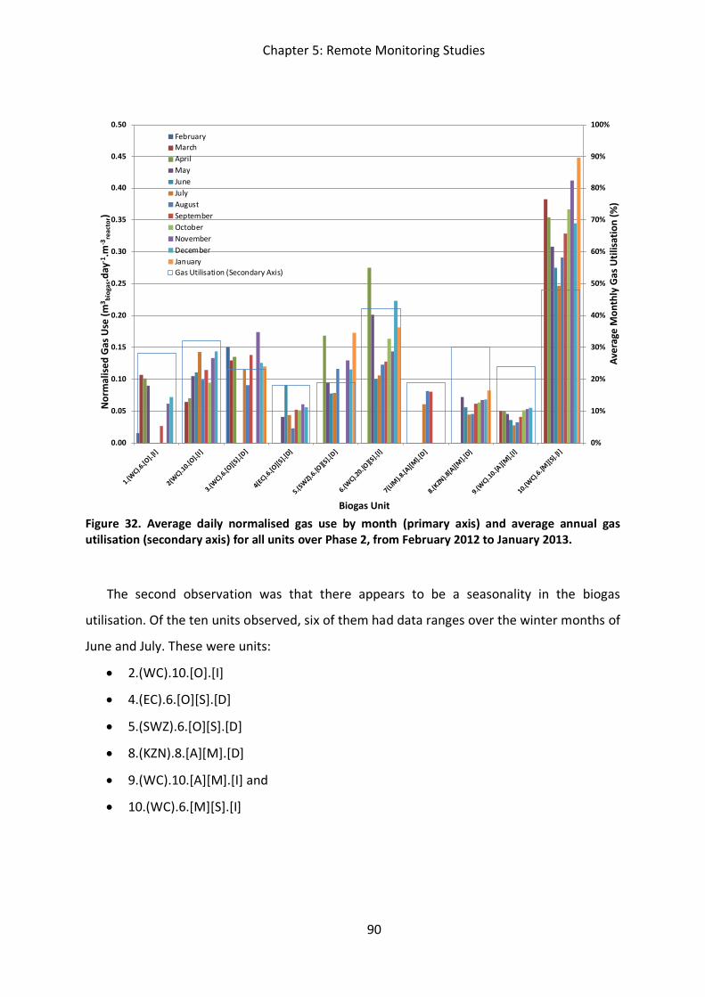
Chapter 5: Remote Monitoring Studies
90
Figure 32. Average daily normalised gas use by month (primary axis) and average annual gas utilisation (secondary axis) for all units over Phase 2, from February 2012 to January 2013.
The second observation was that there appears to be a seasonality in the biogas
utilisation. Of the ten units observed, six of them had data ranges over the winter months of
June and July. These were units:
x 2.(WC).10.[O].[I]
x 4.(EC).6.[O][S].[D]
x 5.(SWZ).6.[O][S].[D]
x 8.(KZN).8.[A][M].[D]
x 9.(WC).10.[A][M].[I] and
x 10.(WC).6.[M][S].[I]
0%
10%
20%
30%
40%
50%
60%
70%
80%
90%
100%
0.00
0.05
0.10
0.15
0.20
0.25
0.30
0.35
0.40
0.45
0.50
1.(WC).6
.[O].[
I]
2(WC).1
0.[O].[
I]
3.(WC).6
.[O][S
].[D]
4(EC).6.[O
][S].[
D]
5.(SW
Z).6.[O
][S].[
D]
6.(WC).2
0.[O][S
].[I]
7(LIM
).8.[A
][M].[
D]
8.(KZN
).8[A
][M].[
D]
9.(WC).1
0.[A][M
].[I]
10.(WC).6
.[M][S
].[I]
Aver
age
Mon
thly
Gas
Util
isat
ion
(%)
Nor
mal
ised
Gas
Use
(m3 bi
ogas
.day
-1.m
-3re
acto
r)
Biogas Unit
FebruaryMarchAprilMayJuneJulyAugustSeptemberOctoberNovemberDecemberJanuaryGas Utilisation (Secondary Axis)
Chapter 5: Remote Monitoring Studies
91
All the above units, except for 5.(SWZ).6.[O][S].[D] showed a decrease in normalised
monthly gas use after May followed by an increase after August, giving a strong indication of
seasonality (through ambient temperature) being linked to gas usage.
5.3.3 The effect of feedstock on productivity
The following four units were chosen for the investigation of the effect of feedstock
on productivity:
x 1.(WC).6.[O].[I] - feedstock OFMSW
x 6.(WC).20.[O][S].[I] - feedstock OFMSW and sewage
x 9.(WC).10.[A][M].[I] - feedstock agricultural waste and manure
x 10.(WC).6.[M][S].[I] - feedstock manure and sewage
While there is a difference in size of the biogas units, all units were based in the Western
Cape, all are at institutions and therefore have the same stove, and it is only the feedstock
which varies between them. Firstly, reflecting back to Table 14, it is observed that all these
units shown, are in the higher gas utilisation, which has been attributed to the demand for
gas at an institutional level more than anything else. Notably, 6.(WC).20.[O][S].[I], is second
highest on gas utilisation, but also second highest in readings and % of instability. This would
imply that a biogas unit can be unstable, but also productive.
Normalised gas use shows the best use being for 10.(WC).6.[M][S].[I] which has
manure and sewage, followed by 6.(WC).20.[O][S].[I] being OFMSW and sewage, followed by
1.(WC).6.[O].[I] and finally 9.(WC).10.[A][M].[I]. This would imply that having the sewage
outlet connected to the biogas unit is beneficial for gas utilisation, possible since the
feedstock (human sewage) is more readily degradable. In this case, the members of the
household would essentially have been pre-treating the feedstock.
Chapter 5: Remote Monitoring Studies
92
5.3.4 The effect of climate on productivity
The first comparison undertaken to investigate the effect of climate is on the following
units which all have OFMSW and sewage as the feed, but are based in different climates:
x 3.(WC).6.[O][S].[D] - based in the Western Cape, daytime mean of 22 qC
x 4.(EC).6.[O][S].[D] - based in the Eastern Cape, daytime mean of 20 qC
x 5.(SWZ).6.[O][S].[D] - based in Swaziland, daytime mean of 19 qC
x 6.(WC).20.[O][S].[I] - based in the Western Cape, daytime mean of 23 qC
In this case, 4.(EC).6.[O][S].[D] was excluded from the data set as it was plagued with
instability. The two units in the Western Cape were in different parts of the Western Cape,
hence the difference in reported temperature. However, these units, 3.(WC).6.[O][S].[D] and
6.(WC).20.[O][S].[I], showed similar normalised gas use, typically ranging between 0.1 and 0.2
m3biogas.day-1.m-3reactor. Between them, 6.(WC).20.[O][S].[I] showed a higher gas utilisation,
explained by the fact that it was at an institutional level. Comparing these two to the unit in
Swaziland which was at a lower temperature, there was no observable difference between
its performance by way of the gas utilisation, nor the normalised gas use.
The second comparison undertaken to investigate the effect of climate is on the
following units which all have agricultural waste and manure as the feedstock, but are based
in different climates:
x 7.(LIM).8.[A][M].[D] - based in the Limpopo Province, daytime mean of 23 qC
x 8.(KZN).8.[A][M].[D] - based in Kwa-Zulu Natal, daytime mean of 26 qC
x 9.(WC).10.[A][M].[I] - based in the Western Cape, daytime mean of 23 qC
Limited data was available for the unit in Limpopo as it was only monitored for three
months. The unit in KwaZulu-Natal displayed a higher normalised gas use than the unit in the
cooler climate, in the Western Cape, 0.06 vs 0.04 m3biogas.day-1.m-3reactor, with only a slightly
higher gas utilisation 30% vs 24%. Again, no conclusive impact of climate can be drawn from
this, other than that it appears that temperature may possibly have an effect on productivity.
Chapter 5: Remote Monitoring Studies
93
5.4 Summary of findings and conclusions
From this study, it was established that the smart monitoring via smartphone app with
very basic measurement of parameters was able to provide some insight into the operations
of small-scale biogas units. The pH detection system via the website provided enough
information to detect an instability and in cases, contact the operator and make correction
for it. The corrections made were the addition of lime (if available) or a brief cessation in feed.
Both techniques were learned from the observational study in Chapter 4. The flame quality
selection was also able to provide insights into the gas quality.
The heterogeneity of food waste appears to be responsible for the instability observed
by pH readings. Moreover, upon further investigations, it is the addition of simple
carbohydrates which appears to cause a decrease in pH for units which have OFMSW in the
feedstock. In other cases, it was an increase in the household members which lead to an
increase in organic loading rate which was attributed to be responsible for the instability.
Finally, a change in the frequency and ratios is also seen to have an effect on stability. In five
of the ten units, there was no reported effect of low pH on gas production or quality. In the
other five, there were sixteen episodes of a low pH, of which fourteen of those episodes
showed a reduction in the cumulative burning time in the week of the low pH episode,
compared to the week before. In eight of these fourteen episodes, there was a further note
that the flame quality (an indication of gas quality) had changed from stable (blue) to unstable
(yellow). These are important findings when considering small-scale biogas for urban Africa,
where the feedstock will be predominantly OFMSW. If small-scale biogas is being utilised to
meet primary energy needs, low gas quality may have drastic impacts on the success of the
technology. Hypothesis 1 is addressed here as the feeding regime and in particular, the effect
of simple carbohydrates is noted.
Chapter 5: Remote Monitoring Studies
94
While it is postulated that the climate or ambient temperature would have an effect
on gas production, it appears that the type of installation is more significant than the climate.
For example, on the whole, units installed at institutions displayed higher gas utilisations than
domestic ones. That being said, some seasonality is still observed in five of the six units which
were monitored over winter months. As there were limitations in the sampling method, as
well as in the ability to measure some of the parameters, much of the analysis on productivity
was inconclusive and warrants further investigation to more confidently make the link
between temperature and productivity and to fully address Hypothesis 2.
Reflecting on remote monitoring, it has been shown that the tool was able to detect
instances of instability and even able to detect changes in gas quality as such times. The tool
was unable to predict future instability, but by contact with the users, it was valuable in
correcting incidences of instability. Therefore, in light of Hypothesis 3, remote monitoring has
proved useful, supporting the effective operation of biogas units. However, there are some
limitations to what it can monitor and infer notably, that it also relies on a person checking
the data frequently and engaging with the biogas operator.
.
Chapter 6: Field Experimentation
95
Chapter 6: Field Experimentation
After the conclusion of the remote monitoring study, and given the emerging
observations on productivity and stability, particularly around organic waste, there emerged
further theories around organic waste and unvalidated techniques for mitigation against
instability. From Chapter 5, it was observed that the feeding regime did affect the stability of
the biogas unit. Of the three factors (high amount of simple carbohydrate, increases in the
organic loading rate and changes in feed ratio/frequency), it was surmised that there may be
ways to mitigate for some of these factors (particularly the simple carbohydrates). In 2014,
the opportunity arose to conduct experiments on another small-scale biogas unit places at a
local composting facility (LCF). Experiments were conducted as described in Section 4.3.3 to
advance the understandings of operational stability and productivity, of a biogas unit with a
feedstock of OFMSW and further address Hypotheses 1 and 2. Monitoring of this unit was
with the now established remote monitoring method using the mobile phone application and
pH indicator strip. Instead of taking passive readings, there was a daily active involvement
with the biogas unit operator via the mobile phone to further inform Hypothesis 3.
Unlike the UCT biogas unit in Chapter 4, or the remote monitoring biogas units in
Chapter 5, the feedstock for the LCF unit was fed a pre-determined regime as described in
Section 4.3.3. Initially, there was a stepwise introduction to organic waste from the initial
inoculum of cow manure. Then an experiment was done with waste pre-treated with Bokashi.
Bokashi treatment involves the layering of organic waste with Bokashi bran followed by a
fourteen-day fermentation in an airtight drum. This pre-treated organic waste is then fed to
the biogas unit. Finally, there was purposeful introduction of simple carbohydrates in pre-
determined quantities. Monitoring was also more active, with daily checking of the data sent
through and interaction with the operation via the mobile phone on which the Biogas
Monitoring Tool application was loaded.
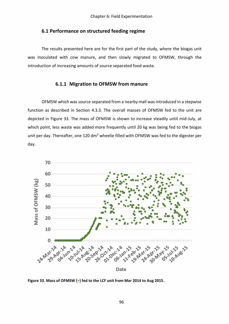
Chapter 6: Field Experimentation
96
6.1 Performance on structured feeding regime
The results presented here are for the first part of the study, where the biogas unit
was inoculated with cow manure, and then slowly migrated to OFMSW, through the
introduction of increasing amounts of source separated food waste.
6.1.1 Migration to OFMSW from manure
OFMSW which was source separated from a nearby mall was introduced in a stepwise
function as described in Section 4.3.3. The overall masses of OFMSW fed to the unit are
depicted in Figure 33. The mass of OFMSW is shown to increase steadily until mid-July, at
which point, less waste was added more frequently until 20 kg was being fed to the biogas
unit per day. Thereafter, one 120 dm3 wheelie filled with OFMSW was fed to the digester per
day.
Figure 33. Mass of OFMSW (•) fed to the LCF unit from Mar 2014 to Aug 2015.
0
10
20
30
40
50
60
70
24-Mar-1
4
29-Apr-14
04-Jun-14
10-Jul-1
4
15-Aug-14
20-Sep-14
26-Oct-
14
01-Dec-14
06-Jan-15
11-Feb-15
19-Mar-1
5
24-Apr-15
30-May-1
5
05-Jul-1
5
10-Aug-15
Mas
s of O
FMSW
(kg)
Date
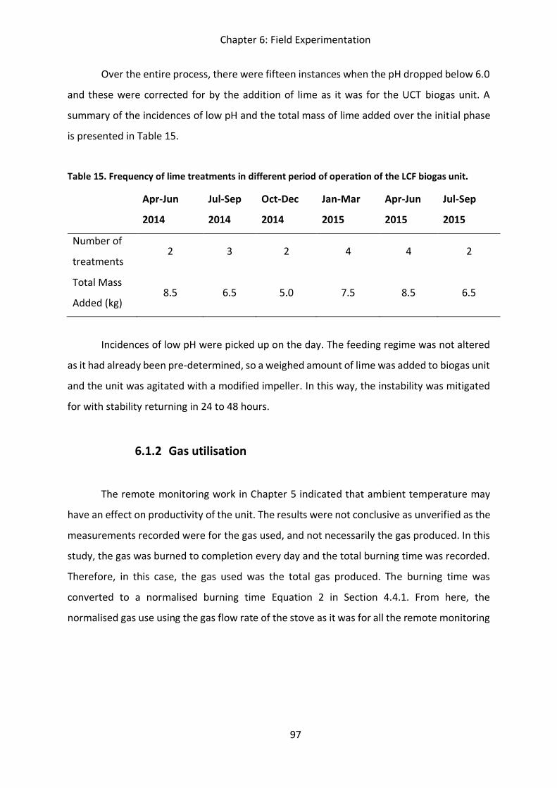
Chapter 6: Field Experimentation
97
Over the entire process, there were fifteen instances when the pH dropped below 6.0
and these were corrected for by the addition of lime as it was for the UCT biogas unit. A
summary of the incidences of low pH and the total mass of lime added over the initial phase
is presented in Table 15.
Table 15. Frequency of lime treatments in different period of operation of the LCF biogas unit.
Apr-Jun
2014
Jul-Sep
2014
Oct-Dec
2014
Jan-Mar
2015
Apr-Jun
2015
Jul-Sep
2015
Number of
treatments 2 3 2 4 4 2
Total Mass
Added (kg) 8.5 6.5 5.0 7.5 8.5 6.5
Incidences of low pH were picked up on the day. The feeding regime was not altered
as it had already been pre-determined, so a weighed amount of lime was added to biogas unit
and the unit was agitated with a modified impeller. In this way, the instability was mitigated
for with stability returning in 24 to 48 hours.
6.1.2 Gas utilisation
The remote monitoring work in Chapter 5 indicated that ambient temperature may
have an effect on productivity of the unit. The results were not conclusive as unverified as the
measurements recorded were for the gas used, and not necessarily the gas produced. In this
study, the gas was burned to completion every day and the total burning time was recorded.
Therefore, in this case, the gas used was the total gas produced. The burning time was
converted to a normalised burning time Equation 2 in Section 4.4.1. From here, the
normalised gas use using the gas flow rate of the stove as it was for all the remote monitoring
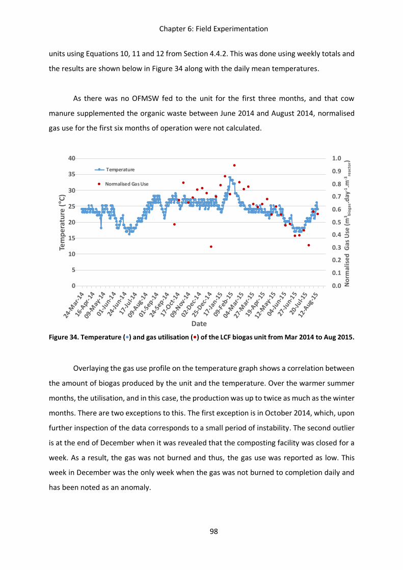
Chapter 6: Field Experimentation
98
units using Equations 10, 11 and 12 from Section 4.4.2. This was done using weekly totals and
the results are shown below in Figure 34 along with the daily mean temperatures.
As there was no OFMSW fed to the unit for the first three months, and that cow
manure supplemented the organic waste between June 2014 and August 2014, normalised
gas use for the first six months of operation were not calculated.
Figure 34. Temperature (•) and gas utilisation (•) of the LCF biogas unit from Mar 2014 to Aug 2015.
Overlaying the gas use profile on the temperature graph shows a correlation between
the amount of biogas produced by the unit and the temperature. Over the warmer summer
months, the utilisation, and in this case, the production was up to twice as much as the winter
months. There are two exceptions to this. The first exception is in October 2014, which, upon
further inspection of the data corresponds to a small period of instability. The second outlier
is at the end of December when it was revealed that the composting facility was closed for a
week. As a result, the gas was not burned and thus, the gas use was reported as low. This
week in December was the only week when the gas was not burned to completion daily and
has been noted as an anomaly.
0.0
0.1
0.2
0.3
0.4
0.5
0.6
0.7
0.8
0.9
1.0
0
5
10
15
20
25
30
35
40
24-M
ar-1
416
-Apr
-14
09-M
ay-1
401
-Jun-
1424
-Jun-
1417
-Jul-1
409
-Aug
-14
01-S
ep-1
424
-Sep
-14
17-O
ct-1
409
-Nov
-14
02-D
ec-1
425
-Dec
-14
17-Ja
n-15
09-F
eb-1
504
-Mar
-15
27-M
ar-1
519
-Apr
-15
12-M
ay-1
504
-Jun-
1527
-Jun-
1520
-Jul-1
512
-Aug
-15
Nor
mal
ised
Gas
Use
(m3 bi
ogas
.day
-1.m
-3re
acto
r)
Tem
pera
ture
(°C)
Date
Temperature
Normalised Gas Use
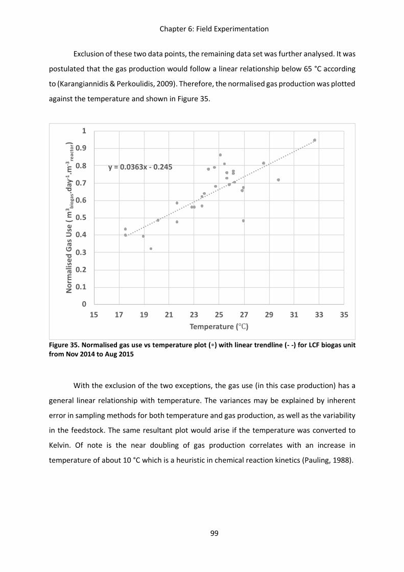
Chapter 6: Field Experimentation
99
Exclusion of these two data points, the remaining data set was further analysed. It was
postulated that the gas production would follow a linear relationship below 65 °C according
to (Karangiannidis & Perkoulidis, 2009). Therefore, the normalised gas production was plotted
against the temperature and shown in Figure 35.
Figure 35. Normalised gas use vs temperature plot (•) with linear trendline (- -) for LCF biogas unit from Nov 2014 to Aug 2015
With the exclusion of the two exceptions, the gas use (in this case production) has a
general linear relationship with temperature. The variances may be explained by inherent
error in sampling methods for both temperature and gas production, as well as the variability
in the feedstock. The same resultant plot would arise if the temperature was converted to
Kelvin. Of note is the near doubling of gas production correlates with an increase in
temperature of about 10 °C which is a heuristic in chemical reaction kinetics (Pauling, 1988).
Chapter 6: Field Experimentation
100
6.2 Performance on Bokashi treated food waste
Four months (September 2015 up to and including December 2015) after the
completion of the experiments described in Section 6.1, the biogas unit was fed with Bokashi
treated waste instead of fresh food waste. During this period, there appeared to be no direct
effect of the Bokashi on the gas production/utilisation, there was one notable observation
and it was around instability. Referring back to Table 15, it was noted that there were
seventeen instances of instability over the eighteen month period with a total of 43 kg of lime
added for the purpose of rectifying instability. On average, that amounts to one episode of
instability per month with just under 2.4 kg of lime added per month. Over the four months
while the unit was fed with Bokashi treated organic waste, there was only one instance of
instability, and the total amount of lime added to correct the acidity was 1.5 kg. Thus, it
appears that Bokashi pre-treatment has a stabilising effect on the operation of the biogas
unit, at least when using OFMSW as a feedstock food waste. The method of action of Bokashi
is essentially a pre-fermentation and stabilisation of food waste for composting application.
According to Liu et al. (Liu et al., 2006), two-stage anaerobic digestion allows for
hydrolysis to occur at optimum conditions in the first stage, followed by methanogenesis at
optimum conditions in the second stage, improving overall operational efficiency. It is
postulated that the pre-treatment with Bokashi has essentially simulated a two-stage AD
process, by which the hydrolysis occurs in its peak environment in the Bokashi bin, and the
methanogenesis can occur at the methanogens peak condition in the biogas unit.
Chapter 6: Field Experimentation
101
6.3 Experimentation with simple carbohydrates
From both Chapter 4 and 5, there was an indication that the feeding regime affected
the stability of the biogas units. After the trial on Bokashi described in 6.2, there was then a
further study to observe the effects of an increase in the amount of simple carbohydrates. Of
the three types of feeding regime, namely simple carbohydrates, increases in household
occupancy and changes in frequency/ratio, the first appeared as the simplest to mitigate for.
While pre-treatment with Bokashi appeared to offer one solution, there remained a further
theory to be tested. In Chapter 4, there was a long hiatus over the December vacation when
the UCT biogas unit remained dormant, after which there appeared to be no issues of
instability. Granted, the sampling method of measuring the pH changed as well, but the
theory was that the microbes given the chance could adapt to a high carbohydrate feed, in
the same way that they adapt to an OFMSW feed from cow manure. In order to investigate
this further, there operational procedure described in Section 4.3.3.3 was undertaken. It
involved a sharp spike in simple carbohydrate feedstocks, before and after a stepwise
increase of the amount of simple carbohydrates. The total amounts of food waste, the specific
amount of simple carbohydrates and the relative pH are shown in Figure 36.
Stage 1 was the initial shock treatment with 10 kg per day of simple carbohydrate
OFSMW for five days. This caused the pH to drop irreversibly and the biogas unit was re-
primed with cow manure and brought back to functional operation in Stage 2. From there,
the biogas unit was reintroduced to OFMSW in the same way that is was migrated to OFMSW
in Section 6.1.1. This time however, the portion of OFMSW which was simple carbohydrates
was tracked and increased until the biogas unit was running completely on simple
carbohydrates by the end of Stage 3. For two weeks after, the biogas unit fed varying
amounts of mixed OFMSW – Stage 4. The shock of simple carbohydrates was then repeated
in Stage 5 as it was done in Stage 1.
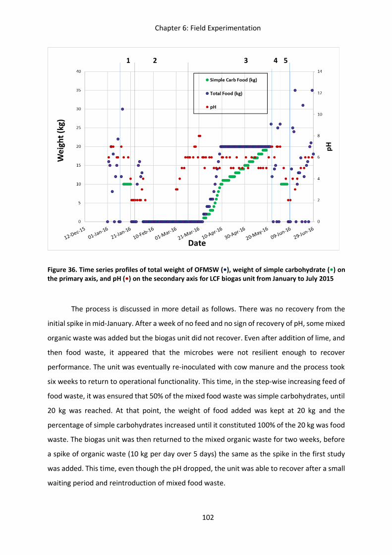
Chapter 6: Field Experimentation
102
Figure 36. Time series profiles of total weight of OFMSW (•), weight of simple carbohydrate (•) on the primary axis, and pH (•) on the secondary axis for LCF biogas unit from January to July 2015
The process is discussed in more detail as follows. There was no recovery from the
initial spike in mid-January. After a week of no feed and no sign of recovery of pH, some mixed
organic waste was added but the biogas unit did not recover. Even after addition of lime, and
then food waste, it appeared that the microbes were not resilient enough to recover
performance. The unit was eventually re-inoculated with cow manure and the process took
six weeks to return to operational functionality. This time, in the step-wise increasing feed of
food waste, it was ensured that 50% of the mixed food waste was simple carbohydrates, until
20 kg was reached. At that point, the weight of food added was kept at 20 kg and the
percentage of simple carbohydrates increased until it constituted 100% of the 20 kg was food
waste. The biogas unit was then returned to the mixed organic waste for two weeks, before
a spike of organic waste (10 kg per day over 5 days) the same as the spike in the first study
was added. This time, even though the pH dropped, the unit was able to recover after a small
waiting period and reintroduction of mixed food waste.
1 2 4 3 5
Chapter 6: Field Experimentation
103
6.4 Summary and conclusions
Firstly, operational experience demonstrated that OFMSW can be the sole feedstock
for an urban biogas system. Simple carbohydrates have been shown to cause the pH of the
unit to drop and have an effect on the flame quality. If the load of simple carbohydrates is too
high, it may permanently halt the production of biogas (i.e. the methanogenic population dies
out). Mitigation for operational instability has been attempted in a few ways. Firstly, lime can
be added to adjust the pH and has been proven to be successful even if it is the only method
of correction for acidity. Secondly, pre-treatment of the OFMSW, simulating a two-stage
reaction improves the operational stability. Lastly, it was investigated as to whether the
microbes could adapt to the different feedstock by succession so that more resilient strains
may be present to mitigate changes. This investigation had some success. Before the stepwise
increase, the LCF biogas unit was unable to recover from a spike in simple carbohydrates.
However, after an adaption phase it was able to recover after a similar spike in simple
carbohydrates. Notably, there was a short hiatus needed for the recovery of the unit, which
is another potential method to mitigate instability. Thus, the feeding regime has again been
shown to influence the stability of small-scale biogas units in line with Hypothesis 2.
With regard to temperature, a correlation between temperature and productivity has
finally been established. Since the gas used was the total gas produced, a direct correlation
could be drawn between the increase in temperature and the increase in gas used/produced.
Notably, the fluctuation of 10 qC was met with an almost doubling of biogas production, which
is in line with the chemical reaction heuristic. Higher temperatures have allowed for higher
use/production and in line with Hypothesis 2, temperature has been shown to have an effect
on the productivity of small-scale biogas units
Lastly, reflecting on Hypothesis 3, the LCF unit, even though it used the same
application, had active management and an operator on site who used the application daily
and was contacted daily on the mobile device. Expanding on this, it may be safe to say that
the tool was better and more frequently utilised because the with more active management
via the application.
Chapter 7: Conclusions
104
Chapter 7: Conclusions
This thesis set out to investigate a particular version of biogas technology, viz. small
decentralised installations, as a contributor to achieving sustainable urban development in
Africa’s cities, through investigations into the potential and limitations of the technology in
various situations. The investigation was structured into three parts, covered in Chapters 4, 5
and 6. This final chapter of the thesis first synthesises the findings from the three results
chapters, then proceeds to draw conclusions by revisiting the hypotheses posed in Chapter 3,
and finally presents recommendations, both for further research and for practise.
7.1 Synthesis of findings
In this section, the findings of the various chapters are synthesised. The first objective
of this thesis addressed through all the results chapters, was to understand how stable small-
scale urban biogas units can be operated. This was largely inferred from changes in pH and
flame quality, supported by analyses of gas burn times. In the first study with the UCT biogas
unit, it was shown that the instability, as reflected by a decrease in pH occurred after a large
amount of simple carbohydrates had previously been fed to the biogas unit. In the second
study, it was shown that all small-scale units were prone to episodes of instability. These
instances were often investigated through a monitoring system to determine a cause, which
were typically linked to the feeding regime, specifically the amount of simple carbohydrates
fed to the unit, the organic loading rate or simply a change in the ratio/frequency of the feed.
Learnings from these two chapters led to the formulation of an investigation of a final biogas
unit at a local composting facility. This unit was slowly migrated onto OFMSW initially by
stepwise increase and the feeding regime was manipulated. Furthermore, after an initial
shock of simple carbohydrates caused permanent souring, resilience was shown to improve
after the same shock was conducted, but after a slow stepwise adaption to simple
carbohydrate over 3 months. Mitigation techniques in the first study included addition of
lime, while a long hiatus was also shown to contribute to a more stable biogas unit in later
periods. In the second study, a small break in feeding was recommended to the biogas
Chapter 7: Conclusions
105
operators and it showed some success. In the final study, lime was used very actively with
noted success, but more notably, the unit demonstrated improved stability after the
feedstock of OFMSW was pre-treated with Bokashi, needing a lime buffer only once over the
four months of operation on Bokashi treated waste (c.f. approximately one a month in normal
operation on untreated OFMSW).
The second objective was to advance the understandings of operational productivity
of small-scale biogas units. Normalised gas use, and gas utilisations were used as indications
of productivity in the first two studies, in which regard, the learnings were limited, as those
calculated variables are a function of the gas used, rather than the gas produced. The
maximum theoretical biogas would be a function of the hydraulic residence time, which was
not measured, as it was assumed that all the volatile solids in the substrate were converted
to biogas, which may have not been the case. Secondly, gas utilisation is a measure of gas
used, not necessarily gas produced. Even in the cases with the highest gas utilisation, there
was never an instance when the gas supply was completely exhausted, indicating that the
users used what only what they needed, and not what they produced. The latter is, however,
an indication that many installations were under-utilised.
That being noted, the first study showed an improved gas utilisation over ten weeks
in the summer months compared to five weeks in the winter months. In the second study,
five of the six digesters which were operational over the winter months showed a lower gas
utilisation in those months. In the final study, gas was burned until it was completely finished,
meaning that the gas used was the actual gas produced. In this study, the gas utilisation
tracked the temperature profile, showing almost a doubling in normalised gas utilisation in
summer months, which had an average daytime temperature which was 10 qC higher than
winter months. Furthermore, it is noted that productivity is linked to stability. From the
second study, it is noted that the unit in the Eastern Cape which was plagued by instability
was the least productive and suffered from poor gas quality. In five of the units in the remote
monitoring study there was no noted decline in gas utilisation, but in the other five, where a
decline in utilisation was observed, the majority of incidences also reported a decline in gas
quality in the episode of instability.
Chapter 7: Conclusions
106
Lastly, with regard to the final objective, the remote monitoring work was an attempt
to monitor and then build an early detection system as part of operational knowledge
support. The results from the second and third study showed that this was successful to a
degree. In the second study, the monitoring system was successful at detecting incidences of
instability and the recorded data, coupled with contact with the user was able to determine
the cause of such. In the third study, with more active management and use of the system,
instances of instability were mitigated quickly and the digester itself was operated within a
set of guidelines. This shows that the system would be most significant with engaged users.
7.2 Conclusions
The first major conclusion is around the stability of the biogas units. It was
hypothesised that feedstock variability would be the key factor affecting the stability of such
small-scale systems. As per the synthesis above, an increase in the simple carbohydrates in
the feeding regime (most often observed when the feedstock was OFMSW) was responsible
for a decline in the pH in three of the biogas units over eight different periods. In the LCF unit,
a large amount of simple carbohydrate caused permanent souring of the unit. In two units,
where the digesters were connected to the sewage outlet, it was an increase in the organic
loading rate, via an increase in household occupancy. For the two units fed with agricultural
waste it was a change in the feeding ratios/intervals which were attributed as the cause of
instability. These can be explained as follows. Firstly, anaerobic digestion is a staged process,
the first of which is a hydrolysis phase which can occur very quickly with simple
carbohydrates, possibly lowering the pH of the system, adversely affecting the balance of
biological agents. Increase in household occupancy (i.e. an increase in volume) and changes
in the feeding regime also caused instability. The various mitigation techniques, namely;
addition of lime; interaction with users; pre-treatment with Bokashi; cessation of feed and an
adaption for resilience, were shown to be effective in varying degrees at combatting
instability. Therefore, the hypothesis that the feeding regime would affect stability was
proved to be true, that feedstock variability, not just in terms of composition, but also in terms
of volume is the key factor affecting stability.
Chapter 7: Conclusions
107
The second part of the investigation focused on productivity of small-scale biogas and
the effect that climate (thereby ambient temperature) would have on the gas production. The
method of quantification proved limited in the first two studies, but a small tweak in the active
management of the last unit allowed the same measurements to infer gas produced, rather
than just the gas utilised. In the second study, it was shown that the units at institutions were
showed better utilisation than the units at domestic households, thus the efficiency of use is
more a factor of the demand for the gas. Despite the limitations the gas utilisation of
individual units do appear to follow a seasonal profile, noting that the actual percentages are
a function of hydraulic residence and therefore, while the trend is observed, the actual
numbers may not be accurate. The second study, despite providing some insight, remained
inconclusive. The final study did show a clear link between temperature and productivity. The
second hypothesis can therefore only partially be proven true. Under controlled conditions,
yes, the productivity is linked to the temperature. However, under uncontrolled conditions,
based on evidence here, when gas utilisation is not always at maximum the temperature
profile seems to be less important than the type biogas installation and the demand for gas.
Lastly, it was postulated that smart monitoring of key parameters would improve the
stability and productivity of small-scale biogas units. Firstly, two parameters which would
typically need laboratory equipment to measure, could be approximated by more crude
measuring techniques. Also, flame quality was a useful simple measurement of gas quality.
The monitoring of key parameters, even with crude techniques and limited information was
able to inform the stability and also productivity of small-scale units. Moreover, the system
allowed for some level of interaction and knowledge sharing to mitigate for instability. Thus,
speaking towards Hypothesis 3, not only was the monitoring of key parameters useful to
improve the stability and productivity of small-scale biogas units, but when strongly
championed, it could be used to gain insights into the factors which affect the stability and
productivity of the system, as well as further investigate mitigation techniques for instability.
Chapter 7: Conclusions
108
In summary, tying this back into the productivity and stability investigations in the
context of the actual deployment and operation of the technology, the parameters which
most greatly influence the stability and productivity of biogas units have been identified as
feeding regime, and then the installation type and the climate respectively. The monitoring
of these parameters can be done relatively easily with low tech innovations to provide
meaningful and useful data with which to inform a monitoring infrastructure, which is itself
able to pre-empt perturbations and 'rescue' a unit which is about to lose productivity or
stability. This knowledge support system mentioned above, needs a technician who
understands the process of anaerobic digestion on the other end of the smartphone to give
feedback to the champion. Thus, the third hypothesis, stating that remote monitoring would
be useful to safeguard investment, was proven true.
Overall, when considering small-scale biogas as a renewable energy option for urban
Africa, there are incidences of instability which arise frequently in all installations. These
incidences will impact on the productivity of the biogas unit. This work shows that it is possible
even with limited information and instrumentation to pick up these incidences, and
moreover, to mitigate for these, either through monitoring, or pre-treatment of
heterogenous feedstocks. The technology does, however, come with its own unique set of
challenges. Its application and reach are limited by feedstock and would still need to be part
of a group of technologies to meet all the energy demands (noting the capacity of 5% of
energy using waste-based feedstock only). Having stated that, the additional advantages of
waste management and sanitation need to be re-iterated. Thus, through the lenses of
productivity and stability, small-scale biogas may be an important technology, but comes with
limitations and operational challenges, the latter which can be mitigated by knowledge
support, possibly through smart monitoring.
Chapter 7: Conclusions
109
7.3 Recommendations
7.3.1 Recommendations for further research
One of the more interesting outcomes of this work is the synergistic effect of Bokashi
pre-treatment on the stability of a biogas unit run on heterogeneous food waste. In effect,
pre-treatment with Bokashi has simulated a two-stage digestion process, with the feed to the
second stage (the actual biogas plant) having been conditioned and stabilised. The function
of Bokashi is to stabilise organic waste, so it is not unexpected to have this outcome. Since
this part of the investigation was limited to one experiment under field conditions, it would
be useful to have laboratory scale and then pilot scale tests to confirm and quantify these
observations, inter alia to determine the exact quantities needed, and the necessary
fermentation times with different feedstocks. Pre-treatment was also only one of the
proposed mitigation techniques. Others included a hiatus (with a noted consequence of not
having a waste treatment option for some time) and direct pH adjustment with lime. The
relative effectiveness of these techniques along with an economic analysis, could be
quantified in a completely separate research study.
For the productivity investigation, it would be useful to glean further insights into the
real gas utilisation at institutional levels versus domestic ones, as it currently appears that
domestic (probably more affluent) users have lower gas utilisations than institutions which
would value the energy more. This would involve the refinement in the method of
quantification of productivity possibly with the involvement of the measurement of hydraulic
residence time to better inform the maximum theoretical biogas calculated. This could be
achieved through another monitoring study or a direct investigation.
Lastly, it is interesting to note that the entry point for biogas was from energy
provision, but the final investigations were carried out from a waste management angle. The
obvious link is waste-to-energy practices. It may be useful to assess this technology from a
waste treatment angle first with the added benefit of energy provision.
Chapter 7: Conclusions
110
7.3.2 Recommendations for practice
This research has initiated the case for the actual deployment of small-scale biogas to
be in urban Africa. A region with the correct climate, and a situation in which the
proactive/incentivised champions, armed with some knowledge, a smartphone and access to
technical support can be allocated to individual units, for a number of units to be deployed in
an urban setting. The context would also ideally utilise the digestate to make a stronger
economic case for the programme. Also, the current system had the technician logging in to
check each unit and go through data, while the overall system required, would need to be
more complex, at least on the side of the technician, who would need automatic alerts and
reports to be sent to them if there were potential issues on the horizon. What this means for
decentralised installations in Africa is as follows.
The mobile application for this work was built in JAVA to run on basic Nokia
Smartphones in 2011. Since then, iOS and Android have become the global standards. If this
work were to be continued, then a compatible application should be developed. Advances in
technology could allow the mobile application to have more functionality. One consideration
during this study was to include a camera function to read the colour of the pH test strip as
an additional feature to aid those suffering from red/green colour-blindness and/or to reduce
human error. Another option could be to more accurately understand the feedstock with a
photo. Also, the application was loaded onto a separate phone, and it is likely that if it were
installed on a personal device, it is much more likely that it will be used daily.
Finally, with reference to sustainable development goal around cities and
communities, I believe that given the right conditions, biogas can be an important
supplementary technology, and should be considered (in conjunction with other
technologies) when planning smarter, sustainable communities.
Chapter 7: Conclusions
111
7.4 Outlook
Over the time of this investigation, the first large-scale commercial waste-based
biogas plant in South Africa was commissioned in Bronkhorstspruit. At the time of the initial
submission, in 2017, the commissioning of the first biogas plant which will receive municipal
solid waste was underway. This project could however not be successfully commissioned as
it ran out of operating capital before all its components could be demonstrated to be working;
several were novel and never built at this scale before. Energetically, it is always more efficient
to have decentralised operations, but this research has also shown that small-scale
installations have very low overall efficiencies and are prone to instabilities. However, a new
biogas unit was commissioned in late 2018 at a shopping centre in Cape Town and
incorporated elements of remote monitoring. This deployment of many such medium-scale
units may be what is needed to address energy challenges of developing cities. In Africa,
therefore, decentralised may mean medium scale units at shopping centres, which could
justify investments and ensure operational success. Of note is that the source separated
organic waste for the LCF unit was sourced from a nearby shopping mall. Thus, as landfill
prices rise, there will be a need for waste management alternative (not just energy
alternative) and formerly costly alternatives become feasible. In that regard, biogas should
therefore not be too far in the future, at least at the optimal institutional level.
There has been some debate about whether we are in a new industrial revolution, or
whether we are just in a second phase of the previous, third industrial revolution. Either way,
the advent of the Internet of Things, means that there are now platforms and systems which
rely on trackers, sensors and devices, all online and working together. There is definitely an
opportunity for application for IoT in the rollout of small-scale biogas. Real-time data and
machine-to-machine communication would allow data to be pushed to alert the technician.
There are naturally concerns about job replacement, but if this were to be used on the right
scale, there would be enough employment created from the deployment of the technology
that monitoring could be left to smart sensors and the overall costs of knowledge support
would be cheaper, making small-scale biogas more feasible.
References
112
References Abraham, E., Ramchandran, S. & Ramalingam, V., 2007. Biogas: Can it be an
important source of energy?. Environmental Science and Pollution Research, 14(1), pp. 67-
71.
AccuWeather, 2012. Accuweather. [Online]
Available at: http://www.accuweather.com/, [Accessed 02 02 2012].
Adl, M., Sheng, K.C., Xia, Y.H., Gharibi, A. & Chen, X., 2012. Examining a hybrid plug-
flow pilot reactor for anaerobic digestion of farm-based biodegradable solids. International
Journal of Environmental Resources, 6, pp. 335-344.
Afgan, N. & Carvallo, M., 2008. Sustainability assessment of a hybrid energy system.
Energy Policy, 36(8), pp. 2903-2910.
Agama, 2010. BiogasPro. [Online]
Available at: http://www.biogaspro.com, [Accessed 1 11 2010].
Agwunwamba, J., 2001. Waste and engineering management tools. 1st ed. Nigeria:
Immaculate Publication Ltd.
Akinbami, J., Illori, M.O., Oyebisi, T.O., Akinwumi, I.O. & Adeoti, O., 2001. Biogas
energy use in Nigeria: current status, future prospects and policy implications. Renewable
and Sustainable Energy Reviews, 5(1), pp. 97-112.
Alcott, B., 2010. Impact Caps: Why population, affluence and technology strategies
should be abandoned. Journal of Cleaner Production, 18, pp. 552-560.
Archer, D. & Harris, J., 1986. Methanogenic bacteria and methane production in
various habitats. In: Barnes. M. & Mead. G., eds. Anaerobic bacteria in habitats other than
man. Boston: Blackwell Scientific Publications, pp. 185-223.
Arthur, R. & Baidoo, M. A. R., 2011. Biogas as a potential renewable energy source: A
Ghanaian case study. Renewable Energy, 36(5), p. 1510.
Aslanzadeh, A., Rajendran, K. & Therzadeh, M., 2014. A comparative study between
single- and two-stage anaerobic digestion processes; Effects of organic loading rate and
hydraulic retention time. International Biodeterioration and Biodegradation, 95(A), pp. 181-
188.
References
113
Balasubramanian, P. & Bai, R., 1992. Evaluation of nutrient recovery after anaerobic
digestion of cattle dung in family size biogas plant. Biomass and Bioenergy, 3, pp. 377-380.
Balat, M., & Balat, H., 2009., Biogas as a renewable energy source – A review. Energy
Sources, 31(14), pp 1280-1293.
Barry, M., Steyn, H. & Brent, A., 2011. Selection of renewable energy technologies
for Africa: 8 case studies in Rwanda, Tanzania and Malawi. Renewable Energy, 36(11), pp.
2845-2852.
Berkhout, P., Muskens, J. & Velthuijsen, J., 2000. Defining the rebound effect. Energy
Policy, 28(6-7), pp. 425-432.
Bernal, M., Alburquerque, J. & Moral, R., 2009. Composting of animal manures and
chemical criteria for compost maturity assessment: A review. Bioresource Technology, 100,
pp. 5444-5453.
Bharadwaj, S.S. & Bansal, N.K., 1981. Temperature distributions inside ground for
various surface conditions. Building and Environment, 16(3), pp 183-192.
Boe, K. & Angelidaki, I., 2009. Serial CSTR digester configuration for improving biogas
production from manure. Water Research, 43(1), pp. 166-172.
Bond, T. & Templeton, M., 2011. History and future of domestic biogas plants in the
developing world. Energy and Sustainable Development, 15, pp. 187-200.
Boyd, A., 2010. Informing proposed international UNFCCC technology mechanisms
from the ground up: Using biogas in South Africa as a case study, Cape Town: University of
Cape Town.
Brummeler, E. & Koster, I., 1989. The effect of several pH control chemicals on the
dry batch digestion of the organic fraction of municipal solid waste. Resources, Conservation
and Recycling, 3(1), pp. 19-32.
Cheng, T., Day, D. & Steinberg, M., 1987. Methane production from fresh versus dry
dairy manure. Biological Wastes, 24(4), pp. 297-306.
Chen, Y., Cheng, J. & Creamer, K., 2008. Inhibition of anaerobic digestion process: A
review. Bioresource Technology, 99, pp. 4044-4064.
Chynoweth, D. & Isaacson, R., 1987. Anaerobic digestion of biomass. 1st ed. London:
Elsevier Applied Science.
CoCT, 2010. City of Cape Town. [Online]
Available at: http://www.capetown.gov.za/en/SolidWaste, [Accessed 15 11 2010].
References
114
Cuetos, M., Xiomar, G., Otero, M. & Moran, A., 2008. Anaerobic treatment of solid
slaughterhouse waste (SHW) at a laboratory scale: Influence of co-digestion with the organic
fraction of municipal solid waste (MSW). Biochemical Engineering Journal, 40(1), pp. 99-106.
de Blij, H. & Muller, P., 2000. Regions 2000: Geography: realms, region and concepts.
1st ed. New York: John Wiley & Sons.
de Clercq, D., Wen, Z. & Fan, F., 2017. Performance evaluation of restaurant food
waste and biowaste to biogas pilot projets in China and implications for national policy.
Journal of Environmental Management, 189, pp. 115-124.
Demirer, G.N. & Chen, S., 2004. Effect of retention time and organic loading rate on
anaerobic acidification and biogasification of dairy manure. Journal of Chemical Technology
and Biotechnology, 79(12), pp 1381-1387.
Deng, L., Liu, Y., Zheng, D., Wang, L., Pu, X., Song, L., Wang, Z., Lei, Y., Chen, Z. &
Long, Y., 2017. Application and development of biogas technology for the treatment of
waste in China. Renewable and Sustainable Energy Resources, 70, pp. 845-851.
Deublin, D. & Stenhouser, A., 2008. Biogas from waste and renewable resources: An
introduction. 1st ed. Vancouver: Wiley.
Distillique, 2016. Distillique. [Online]
Available at: http://distillique.co.za/distilling_shop/phmeasurement/123-ph-test-strips-ph-
1-11-universal-200-strips-in-books-of-20.html, [Accessed 07 01 2016].
Divya, D., Gopinath, L. & Christy, P., 2015. A review on current aspects and diverse
prospects for enhancing biogas production in sustainable means. Renewable & Sustainable
Energy Reviews, 42, pp. 690-699.
Dutt, G., 1992. ‘Comparing alternative biogas technologies’, Workshop on Materials
Science and Physics of Non-Conventional Energy Sources, Buenos Aires, 1 March.
Earth Probiotic, 2018. Earth Probiotic Food Waste Solution [Online]
Available at: https://www.earthprobiotic.co.za, [Accessed 08 07 2018]
Edelman, W., Baier, U. & Engeli, H., 2005. Environmental aspects of the anaerobic
digestion of the organic fraction of municipal solid wastes and solid agricultural wastes.
Water Science Technology, 52(1-2), pp. 203-208.
Ehrlich, P. & Holdren, J., 1971. Impact of Population Growth. Science (New Series),
171(3977), pp. 1212-1217.
References
115
Elango, D., Pulikesi, M., Baskaralingam, P., Ramamurthi, V. & Sivanesan, S., 2007.
Production of biogas from municipal solid waste with domestic sewage. Journal of
Hazardous Materials, 141, pp. 301-304.
EngineeringNews, 2017. Engineering News. [Online]
Available at: http://www.engineeringnews.co.za/article/ground-breaking-waste-to-energy-
plant-opens-in-cape-town-2017-01-24/rep_id:4136, [Accessed 24 01 2017].
Engledow, S., 2007. Integrated analysis solid waste baseline report. Sustainable
Institute, pp. 46-49.
ENS Africa, 2015. ENS Africa. [Online]
Available at: https://ensafrica.com/biofuels-in-south-africa?id=1339, [Accessed 10 05 2015]
EOCD, 1985. Biomass for energy: Economic and policy issues. 1st ed. New Delhi:
Oxford and IBH publishing.
Eskom, 2011. Eskom. [Online]
Available at: http://financialresults.co.za/2011/eskom_ar2011/index.php, [Accessed 10 10
2011].
Fang, C., 2010. ‘Biogas production from food-processing industrial wastes by
anaerobic digestion’, PhD Thesis, Technical University of Denmark, Denmark
Forster-Cerneiro, T., Perez, M. & Romero, L., 2008. Thermophilic anaerobic digestion
of source-sorted organic fraction of municipal solid waste. Bioresource Technology, 99, pp.
6763-6770.
Gebreegziabher, Z., Naik, L., Melamu, R. & Balana, B., 2014. Propspects and
challenges fo urban application of biogas installations in Sub-Saharan Africa. Biomass and
Bioenergy, 70, pp. 130-140.
Ghimere, P., 2013. SNV supported domestic biogas programmes in Asia and Africa.
Renewable Energy, 49, pp. 90-94.
Gomez, X., Moran, A., Cuetos, M. & Sanchez, M., 2006. The production of hydrogen
by dark fermentation of municipal solid waste and slaughterhouse wastes: A two-phase
process. Journal of Power Sources, 157(2), pp. 727-732.
Goodland, R. & Daly, H., 1996. Environmental sustainability: Universal and non-
negotiable. Ecological Applications, 6(4), pp. 1002-1017.
Goux, X., Calusinska, M., Lemaigre, S., Marynowska, M., Klocke, M., Udelhoven, T.,
Benizri, E. & Delfosse, P., 2015. Microbial community dynamics in replicate anaerobic
References
116
digesters exposed sequentially to increasing organic loading rate, acidosis and process
recovery. Biotechnology for Biofuels, 8, pp 122-124
Grebben, H., Burke, L. & Szewczuk, S., 2008. Biogas as a renewable energy source
produced during the anaerobic digestion of waste. [Online]
Available at: http://hdl.handle.net/10204/3716, [Accessed 29 6 2009].
Hemmes, K., Zahariah-Wolf, J., Geild, M. & Anderson, G., 2007. Toward a multi-
source and multi-product energy system. International Journal of Hydrogen Energy, 33, pp.
1322-1338.
Hungate, R., 1967. A roll tube method for cultivation of strict anaerobes. In: J. Norris
& D. Ribbons, eds. Methods in Microbiology. New York: Academic Press, p. 117–132.
Hungate, R., 1996. The rumen and its microbes. New York: Academic New York.
IGAD, 2007. Biogas in Kenya. [Online]
Available at: http://igadrhep.energyprojects.net/Links/Profiles/Biogas/Kenya.htm,
[Accessed 27 02 2007].
Igoni, A., Abowei, M., Avotamuno, M. & CL, E., 2008. Effects of municipal solid waste
on the biogas produced in an anaerobic continuous digester. [Online]
Available at: http://www.cigrjournal.org/index.php/Ejounral/article/viewFile/1288/1144,
[Accessed 11 02 2013].
IPCCC, 2008. Changes in atmospheric constituents and in radioactive forcing. [Online]
Available at: http://www.ipcc-wg1.unibe.ch/publications/wg1-ar4/ar4-wg1-chapter2.pdf,
[Accessed 17 11 2010].
Jackson, T., 2009. Properity without growth? The transition to a sustainable
economy, London: The Sustainable Development Comission.
Jacobsson, S. & Bergek, A., 2004. Transforming the energy sector: The evolution of
technological systems in renewable energy technology. Industrial and Corporate Change,
13(5), pp. 815-849.
Johanssen, T., Kelly, H., Reddy, A. & Willians, R., 1993. Renewable energy sources for
fuels and electricity. 1st ed. Washington D.C.: Island Press.
Juarez-Hernandez, S. & Castro-Gonzalez, A., 2016. Assessing the impact of biogas on
the energy sustainability of an urban restaurant in Mexico. Ingeniera, invesigacion y
tecnologi, 17(1), pp. 61-71.
References
117
Kaltwassar, B., 1980. Regenerative energieerzeugung durch anaerobe fermentation
organischer abfälle in biogasanlagen. Berlin: Bauverlag GmbH Wiesbaden.
Kamete, A., Tostensen, A. & Tvedten, I., 2001. From global village to urban globe:
Urbanisation and poverty in Africa: Implications for a Norwegian Aid Policy, Copenhagen:
Chr. Michelsen Institute.
Karangiannidis, A. & Perkoulidis, G., 2009. A multicriteria ranking of different
technologies for anaerobic digestion for energy recovery from the organic fraction of
municipal solid wastes. Bioresource Technology, 100, pp. 2355-2360.
Kasozi, A., von Blottnitz, H., Ngau, P. & Kahui, N., 2010. ‘Using local knowledge
production and systems thinking approaches in the development of an Integrated Solid
Waste Management (ISWM) plan harnessing semi-informal systems: Lessons from Nairobi,
Kenya’, WasteCon 2010, Johannesburg, 4 -8 October
Khanal, S., 2008. Overview of anaerobic biotechnology: Anaerobic biotechnology for
bioenergy production: Principles and applications. Oxford: John Wiley & Sons.
Kiely, G., Tayfur, G., Dolan, C. & Tanji, K., 1997. Physical and mathemaical modelling
of anaerobic digestion of organic wastes. Water Research, 31, pp. 534-540.
Kleinstruer, C. & Poweigha, T., 1982. Dynamic simulator for anaerobic digestion
process. Biotechnology and Bioengineering, 24, pp. 1941-1951.
Konzeli-Katsiri, A. & Kartsonas, N., 1986. Inhibition of anaerobic digestion by heavy
metals. In: Bruce, A. Konzeli-Katsiri, A., & Newman, P., eds. Anaerobic Digestion of Sewage
Sludge and Organic Agricultural Wastes. London: Elsevier Applied Science, pp. 104-119.
Kuyasa, 2009. Kuyasa CDM. [Online]
Available at: http://www.kuyasacdm.co.za, [Accessed 07 09 2009].
Lahav, O., Morgan, B. & Loewenthal, R., 2002. Rapid, simple, and accurate method
for measurement of VFA and carbonate alkalinity in anaerobic reactors. Environmental
Science and Technology, pp. 2736-2741.
Lijó, L., Toja, Y.L., Gonzáles-Garcia, S., Bacenetti, J., Fiala, M. & Moreira, M.T., 2017.
Eco-efficiency assessment of farm-scale biogas. Bioresource Technology, 237, pp 146-155.
Liu, D., Zeng, R. & Angelidaki, I., 2006. Hydrogen and methane production from
household solid waste in the two-stage fermentation process. Water Resources, 40, pp.
2230-2236.
References
118
Malgavkar, P. & Panandiker, P., 1986. Impediments to rural technology. 1st ed.
Bombay: Oxford & IBH Publishing.
Mandal, T., Kiran, B. & Mandal, N., 1998. Determination of the quality of biogas by
flame temperature measurement. Energy Conservation and Management, 40, pp. 1225-
1228.
Mann, M.E. & Schmidt, G.A., 2003. Ground vs surface air temperature trends.
Geophysical research letters, 30(12), pp. 91-93.
Mata-Alvarez, J., 1999. Biomethanisation of the Organic Fraction of Municipal Solid
Wastes. 1st ed. London: s.n. publishing
Mechichi, T. & Sayadi, S., 2005. Evaluating process imbalance of anaerobic digestion
of olive mill wastewaters. Process Biochemistry, 40, pp. 139-145.
Monnet, F., 2003. An Introduction ot anaerobic digestion of organic wastes. [Online]
Available at: hrrp://www.biogasmax.co.uk/media/introanaerobicdigestions, [Accessed 12 05
2011].
Morris, J., 1975. The physiology of obligate anaerobiosis. Advanced Microbial
Physiology, 12, p. 169–246.
Mudrack, K. & Kunst, S., 1991. Biologie der Abwasserreinigung. Stuttgart: Gustav
Fischer.
Munganga, G., Melamu, R., von Blottnitz, H. & Haider, S., 2010. An assessment of the
bio-methane potential of seventeen types of organic fraction of the municipal solid waste
(OFMSW) in Cape Town, Cape Town: University of Cape Town.
Murto, M., Björnsson, L. & Mattiasson, B., 2004. Impact of food industrial waste on
anaerobic co-digestion of sewage sludge and pig manure. Journal of Environmental
Management, 70, pp. 101-107.
Mwirigi, J., Balana, B.B., Mugisha, J., Walekhwa, P., Melamu, R., Nakami, S. &
Makenzi, P., 2014. Socio-economic hurdles to widespread adoption of small-scale biogas
digesters in Sub-Saharan Africa: A review. Biomass and Bioenergy, 70, pp. 17-25.
Mwirigi, J., Makenzi, P. & Ocholoa, W., 2009. Socio-economic contraints to adoption
and sustainable use of biogas technology by farmers in Nakeru disctrics, Kenya. Energy for
Sustainable Development, 13, pp. 106-115.
References
119
Naik, L., 2016. ‘Operational experiences in treatment of organic waste from malls via
anaerobic digestion, bokashi fermentation and composting’, WasteCon 2016,
Johannesburg, 17 – 21 October.
Naik, L. et al., 2014. Fators affecting the stability and productivity of small scale
digesters. Biomass and bioenergy, 70, pp. 51-57.
Naik, L. & von Blottnitz, H., 2012. Poverty alleviation via energisation of unformal
urban Africa: a special role for small-scale biogas. Cape Town, UCT.
Naik, L., von Blottnitz, H. & Melamu, R., 2012. ‘Onsite food waste valorisation:
Experiences with an anaerobic digester at a university residence’, WasteCon 2012, East
London, 15 – 19 October.
Negro, S. & Hekkert, M., 2009. "Benchmarking" the functions of innovation systems:
the success story of the German biomass digestion innovation system, Utrecht: Utrecht
University.
NIST, 2012, NIST Chemistry WebBook [Online]
Available at: https://webbook.nist.gov/chemistry, [Accessed 28 08 2012]
Niyobuhungiro, R. & von Blottnitz, H., 2018. ‘Biogas production from blood and
rumen content of sheep slaughtering waste under ambient conditions’, in Godfrey, L.,
Görgens, J.F. & Roman, H. (eds.), Opportunities for waste biomass and organic waste
valorization; Finding alternative solutions to disposal, Routledge: Unisa Press, pp. 77-87.
Njoh, A., 2003. Urbanisation and development in sub-Saharan Afica. Cities, 20(3), pp.
167-174.
O’Reilly, J., Lee, C., Collins, G., Chinalia, F., Mahoney, T. & O’Flaherty, V., 2009.
Quantitative and qualitative analysis of methanogenic communities in mesophilically and
psychrophilically cultivated anaerobic granular biofilms. Water Resource, 43, pp. 3365-3374.
Pahl, O., Firth, A., McLead, I. & Baird, J., 2008. Anaerobic co-digestion of
mechanically biologically treated municipal waste with primary sewage sludge - a feasibility
study. Bioresource Technology, 99, pp. 3354-3364.
Parawira, A., 2009. Biogas technology in sub-Saharan Africa: Status, prospects and
constraints. Reviews in environmental science and biotechnology, 8, pp. 187-200.
Polese, M., 1997. Urbanisation and development (Canadian International
Development Agency CIDA). Development Express, 4, pp. 4-8.
References
120
Polpraset, C., 2007. Organic waste recycling: Technology and management. 3rd
edition. London: IWA Publishing.
Puxin, 2019. [Online]
Available at: http://en.puxintech.com/, [Accessed 27 02 2019]
Rajendran, K., Kankanala, H., Martinsson, R. & Taherzadeh, M., 2014. Uncertainty
over techno-economic potentials of biogas from municipal solid waste (MSW): A case study
on an industrial process. Applied energy, 125, pp. 84-92.
Rajeshwari, K., Lata, K., Pant, D. & Kishore, V., 2001. A novel process using enhanced
acidification and a UASB reactor for biomethanation of vegetable market waste. Waste
management resource, 19, pp. 292-300.
Rees, D., 2005. Recycling Organic Waste. [Online]
Available at:
http://practicalaction.org/docs/technical_information_service/recycling_organic_waste.pdf,
[Accessed 15 11 2010].
Renda, R., Gigli, E., Capelli, A., Simoni, S., Guerriero, E. & Romagnoli, F., 2016.
Economic feasibility study of a small-scale biogas plant using a two-stage process and fixed
biofilm reactor for a cost-effective production. Energy Procedia, pp. 385-392.
Resch, C., Wörl, A., Waltenberger, R., Braun, R. & Kirchmeyer, R., 2010.
Enhancements options for the uilisation of nitrogen rich animal by-products in anaerobic
digestion. Bioresource technology, 102(3), pp. 2503-2510.
Rincon, B., Borja, R. & Martin, M., 2009. Evaluation of the methanogenic step of a
two-stage anaerobic digestion process of acidified olive mill solid residue from a previous
hyrolytic-acidogenic step. Waste Management, 29(9), pp. 2566-2573.
Robèrt, K.H., Schmidt-Bleek, B., Aloisi de Larderel, J., Basile, G., Jansen, J.L., Kuehr, R.,
Price Thomas, P., Suzuki, M., Hawken, P. & Wackemagel. M., 2002. Strategic sustainable
development -- selection, design and synergies of applied tools. Journal of Cleaner
Production, 10, pp. 197-214.
Roopanarain, R. & Adekele, R., 2017. Current status, hurdles and future prospects of
biogas digestion technology in Africa. Renewable and Sustainable Energy Reviews, 67, pp.
1162-1179.
References
121
Roubik, H., Mazancova, J. & Banout, J. V. V., 2016. Addressing problems at small-
scale biogas plants: a case study from central Vietnam. Journal of Cleaner Production,
112(4), pp. 2784-2792.
Santosh, Y., Sreekrishnan, T., Kohli, S. & Rana, V., 2004. Enhancement of biogas
production from solid substrates using different techniques – a review. Bioresource
technology, 95, pp. 1-10.
Scheinberg, A., Spies, S., Simpson, M. & Mol, A., 2011. Assessing urban recycling in
low- and middle-income countries: Building on modernised mixtures. Habitat International,
35(2), pp. 188-198.
Schneider, F., Kallis, G. & Martinez-Alier, J., 2010. Crisis or oppprtunity? Economic
degrowth for social equity and ecological sustainability. Journal of Cleaner Production, 18,
pp. 511-518.
SEA, 2010. Energy scenarios for Cape Town, Cape Town: Sustainable Energy Africa &
University of Cape Town.
Shi, H., Pei, X., Zhu, H., Luo, Z., Wang, T., Rong, L. & Li, Y., 2009. How to compensate
the lost temperature of the digester in cold climate. Kobe, International Conference on
Power Engineering.
Sisnowski, P. & Wieczorsk, A. L. S., 2003. Anaerobic co-digestion of sewage sludge
and organic fraction of municipal solid waste. Advances in Environmental Research, 7(3), pp.
609-616.
Skovsgaard, L. & Jacobsen, H., 2017. Economies of scale in biogas production and the
significance of flexible regulation. Energy Policy, 101, pp. 77-89.
Smith, J., Abegaz, A., Matthews, R.B., Subedi, M., Orskov, E., Tumwesige, V. & Smith,
P., 2014. What is the potential for biogas digesters to improve soil fertility and crop
production in Sub-Saharan Africa?. Biomass and Bioenergy, 70, pp. 8-72.
Smith, J. & Avery, L., 2014. The potential for small-scale biogas digesters in Sub-
Saharan Africa to improve sustainable rural livelihoods. Biomass and Bioenergy, 70, pp. 1-3.
Sovacool, B., Kryman, M. & Smith, T., 2015. Scaling and commercialising mobile
biogas systems in Kenya; A quantitative pilot study. Renewable Energy, 76, pp. 115-125.
Sun, Y. & Cheng, J., 2002. Hydrolysis of ligno-cellulosic material for ethanol
prodction: A review. Bioresource Technology, 83, pp. 1-11.
References
122
Surendra, K.C., Takara, D., Hashimoto, A.G., Khanal, S.K., 2014, Biogas as a
sustainable energy source for developing countries: Opportunities and challenges.
Renewable and Sustainable Energy Reviews, 31, pp. 846-859.
Suurs, R. & Hekkert, M., 2009. Cumulative causation in the formation of a
technological innovation sysem: The case of biofuels in the Netherlands. Technological
Forecasting and Social Change, 76, pp. 1003-1020.
Swilling, M., 2008. Local governance and the politics of sustainability. In: M. van
Donk, M. Swilling, E. Pieterse & S. Parnell, eds. Consolidating developmental local
government; Lessons from the South African experience. Cape Town: University of Cape
Town Press.
Swilling, M., 2015. Mark Swilling. [Online]
Available at: http://markswilling.co.za/wp-content/uploads/2015/10/Swilling-et-al-2013-
Isandla-paper-first-draft.pdf, [Accessed 11 01 2017].
Tahlegani, G. & Kia, A., 2005. Technical-economical analysis of the Savch biogas
powerplant. Renewable Energy, 30, pp. 441-46.
Taylor, C., Hassan, M. & Ali, S., 2009. Integrated portable biogas systems for
managing organic waste. [Online]
Available at: http://www.wseas.us/e-library/conferences/2010/Tunisia/EPERES/EPERES-
21.pdf, [Accessed 11 12 2016].
Tchobanogolous, G. & Burton, F., 1981. Waste-water engineering: treatment,
disposal and reuse. 3rd ed. New York: McGraw-Hill.
Tumwesige, V., Fulford, D. & Davidson, G., 2014. Biogas appliances in Sub-Sahara
Africa. Biomass and Bioenergy, 70, pp. 40-50.
UCTCivEng, 2011. Spatial Data Management. [Online]
Available at: http://spatialdatamanagement.uct.ac.za/current-projects/aquatest-project/,
[Accessed 11 10 2011].
UN, 2005. Energising the millenium development goals - a guide to energy's role in
reducing poverty, New York: United Nations Development Programme.
UN, 2007. World urbanisation prospects - The 2007 revision. [Online]
Available at:
http://www.un.org/esa/population/publications/wup2007/2007WUP_ExecSum_web.pdf,
[Accessed 07 10 2010].
References
123
UN, 2010. United Nations Millenium Development Goals. [Online]
Available at: http://www.un.org/milleniumgoals, [Accessed 11 11 2010].
UN, 2014. Our urbanising world. [Online]
Available at:
http://www.un.org/en/development/desa/population/publications/pdf/popfacts/PopFacts
_2014-3.pdf, [Accessed 05 11 2016].
UN, 2015. United Nations. [Online]
Available at: http://www.un.org/ga/search/view_doc.asp?symbol=A/RES/70/1&Lang=E,
[Accessed 13 01 2017].
UN, 2016. Sustainable development goals. [Online]
Available at: http://www.un.org/sustainabledevelopment/sustainable-development-goals/,
[Accessed 11 08 2016].
Veissmen, W. J. & Hammer, M., 1993. Water supply and pollution control. 2nd ed.
New York: Harper Collins College Publishers.
Vogel, Y. & Zurbrugg, C., 2008. Biogas in cities - a new trend?, Dubendorf: Sandec.
von Blottnitz, H. & Chakraborty, A., 2006. ‘2nd generation bio-energy technology;
thought about getting the best new developments to work for Africa’, South African
Chemical Engineering Congress, Durban, 20 – 22 September.
von der Heyde, V., Haider, S., van der Merwe, R. & Mullat, M., 2014. ‘Towards a
sustainable Incremental Waste management System in Enkanini Informal Settlement’,
WasteCon 2014, Cape Town, 6 – 10 October.
Wang, J., Huang, Y. & Zhao, X., 2004. Performance and characterisation of an
anaerobic baffled reactor. Bioresource Technology, 93(2), pp. 205-208.
Waste Transformers, 2018. [Online}
Available at: http://www.thewastetransformers.com/projects-development/n1citymall/,
[Accessed: 16 12 2018]
Ward, A., Hobbs, P., Holliman, P. & Jones, D., 2008. Optimisation of the anaerobic
digestion of agricultural resources. Bioresource technology, 99, pp. 7928-7940.
Yasar, A., Nazir, S., Rasheed, R., Tabinda, A.B. & Nazar, M., 2017. Economic review of
different designs of biogas plants at household level in Pakistan. Renewable and Sustainable
Energy Reviews, 74, pp. 221-229.

I
Appendices
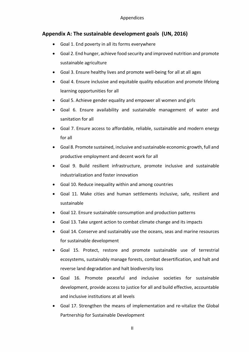
Appendices
II
Appendix A: The sustainable development goals (UN, 2016)
x Goal 1. End poverty in all its forms everywhere
x Goal 2. End hunger, achieve food security and improved nutrition and promote
sustainable agriculture
x Goal 3. Ensure healthy lives and promote well-being for all at all ages
x Goal 4. Ensure inclusive and equitable quality education and promote lifelong
learning opportunities for all
x Goal 5. Achieve gender equality and empower all women and girls
x Goal 6. Ensure availability and sustainable management of water and
sanitation for all
x Goal 7. Ensure access to affordable, reliable, sustainable and modern energy
for all
x Goal 8. Promote sustained, inclusive and sustainable economic growth, full and
productive employment and decent work for all
x Goal 9. Build resilient infrastructure, promote inclusive and sustainable
industrialization and foster innovation
x Goal 10. Reduce inequality within and among countries
x Goal 11. Make cities and human settlements inclusive, safe, resilient and
sustainable
x Goal 12. Ensure sustainable consumption and production patterns
x Goal 13. Take urgent action to combat climate change and its impacts
x Goal 14. Conserve and sustainably use the oceans, seas and marine resources
for sustainable development
x Goal 15. Protect, restore and promote sustainable use of terrestrial
ecosystems, sustainably manage forests, combat desertification, and halt and
reverse land degradation and halt biodiversity loss
x Goal 16. Promote peaceful and inclusive societies for sustainable
development, provide access to justice for all and build effective, accountable
and inclusive institutions at all levels
x Goal 17. Strengthen the means of implementation and re-vitalize the Global
Partnership for Sustainable Development
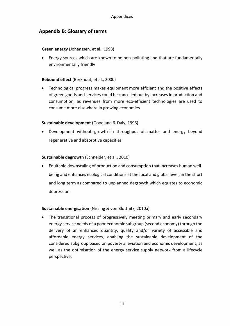
Appendices
III
Appendix B: Glossary of terms
Green energy (Johanssen, et al., 1993)
x Energy sources which are known to be non-polluting and that are fundamentally environmentally friendly
Rebound effect (Berkhout, et al., 2000)
x Technological progress makes equipment more efficient and the positive effects of green goods and services could be cancelled out by increases in production and consumption, as revenues from more eco-efficient technologies are used to consume more elsewhere in growing economies
Sustainable development (Goodland & Daly, 1996)
x Development without growth in throughput of matter and energy beyond
regenerative and absorptive capacities
Sustainable degrowth (Schneider, et al., 2010)
x Equitable downscaling of production and consumption that increases human well-
being and enhances ecological conditions at the local and global level, in the short
and long term as compared to unplanned degrowth which equates to economic
depression.
Sustainable energisation (Nissing & von Blottnitz, 2010a)
x The transitional process of progressively meeting primary and early secondary energy service needs of a poor economic subgroup (second economy) through the delivery of an enhanced quantity, quality and/or variety of accessible and affordable energy services, enabling the sustainable development of the considered subgroup based on poverty alleviation and economic development, as well as the optimisation of the energy service supply network from a lifecycle perspective.
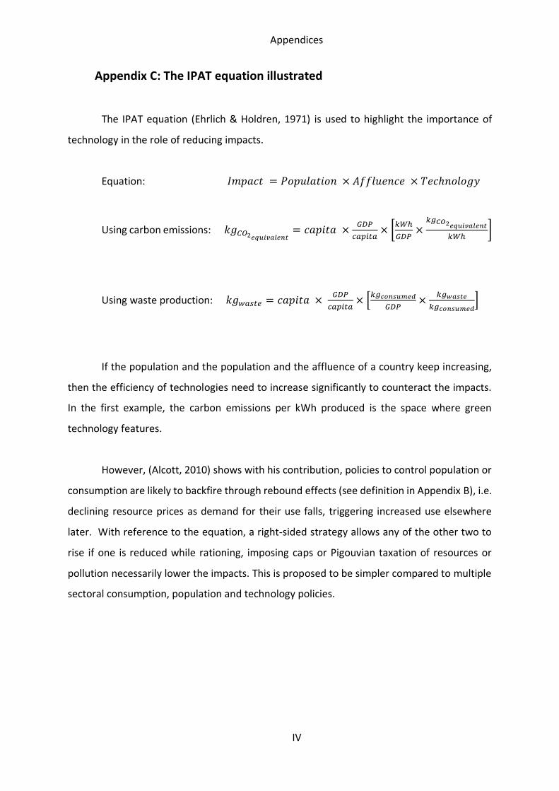
Appendices
IV
Appendix C: The IPAT equation illustrated
The IPAT equation (Ehrlich & Holdren, 1971) is used to highlight the importance of
technology in the role of reducing impacts.
Equation: 𝐼𝑚𝑝𝑎𝑐𝑡 = 𝑃𝑜𝑝𝑢𝑙𝑎𝑡𝑖𝑜𝑛 × 𝐴𝑓𝑓𝑙𝑢𝑒𝑛𝑐𝑒 × 𝑇𝑒𝑐ℎ𝑛𝑜𝑙𝑜𝑔𝑦
Using carbon emissions: 𝑘𝑔 𝑂2𝑒 𝑢𝑖 𝑎𝑙𝑒𝑛𝑡= 𝑐𝑎𝑝𝑖𝑡𝑎 × 𝐺𝐷𝑃
𝑐𝑎𝑝𝑖𝑡𝑎× 𝑘𝑊ℎ
𝐺𝐷𝑃×
𝑘𝑔 𝑂2𝑒 𝑢𝑖 𝑎𝑙𝑒𝑛𝑡
𝑘𝑊ℎ
Using waste production: 𝑘𝑔𝑤𝑎𝑠𝑡𝑒 = 𝑐𝑎𝑝𝑖𝑡𝑎 × 𝐺𝐷𝑃𝑐𝑎𝑝𝑖𝑡𝑎
× 𝑘𝑔𝑐𝑜𝑛𝑠𝑢𝑚𝑒𝑑𝐺𝐷𝑃
× 𝑘𝑔𝑤𝑎𝑠𝑡𝑒𝑘𝑔𝑐𝑜𝑛𝑠𝑢𝑚𝑒𝑑
If the population and the population and the affluence of a country keep increasing,
then the efficiency of technologies need to increase significantly to counteract the impacts.
In the first example, the carbon emissions per kWh produced is the space where green
technology features.
However, (Alcott, 2010) shows with his contribution, policies to control population or
consumption are likely to backfire through rebound effects (see definition in Appendix B), i.e.
declining resource prices as demand for their use falls, triggering increased use elsewhere
later. With reference to the equation, a right-sided strategy allows any of the other two to
rise if one is reduced while rationing, imposing caps or Pigouvian taxation of resources or
pollution necessarily lower the impacts. This is proposed to be simpler compared to multiple
sectoral consumption, population and technology policies.
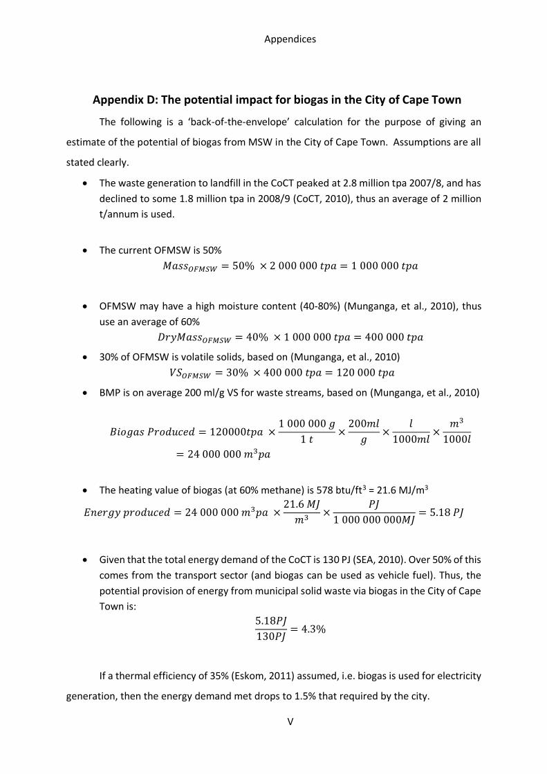
Appendices
V
Appendix D: The potential impact for biogas in the City of Cape Town
The following is a ‘back-of-the-envelope’ calculation for the purpose of giving an
estimate of the potential of biogas from MSW in the City of Cape Town. Assumptions are all
stated clearly.
x The waste generation to landfill in the CoCT peaked at 2.8 million tpa 2007/8, and has declined to some 1.8 million tpa in 2008/9 (CoCT, 2010), thus an average of 2 million t/annum is used.
x The current OFMSW is 50% 𝑀𝑎𝑠𝑠𝑂 𝑀𝑆𝑊 = 50% × 2 000 000 𝑡𝑝𝑎 = 1 000 000 𝑡𝑝𝑎
x OFMSW may have a high moisture content (40-80%) (Munganga, et al., 2010), thus use an average of 60%
𝐷𝑟𝑦𝑀𝑎𝑠𝑠𝑂 𝑀𝑆𝑊 = 40% × 1 000 000 𝑡𝑝𝑎 = 400 000 𝑡𝑝𝑎
x 30% of OFMSW is volatile solids, based on (Munganga, et al., 2010) 𝑉𝑆𝑂 𝑀𝑆𝑊 = 30% × 400 000 𝑡𝑝𝑎 = 120 000 𝑡𝑝𝑎
x BMP is on average 200 ml/g VS for waste streams, based on (Munganga, et al., 2010)
𝐵𝑖𝑜𝑔𝑎𝑠 𝑃𝑟𝑜𝑑𝑢𝑐𝑒𝑑 = 120000𝑡𝑝𝑎 ×1 000 000 𝑔
1 𝑡 ×200𝑚𝑙
𝑔 ×𝑙
1000𝑚𝑙 ×𝑚3
1000𝑙= 24 000 000 𝑚3𝑝𝑎
x The heating value of biogas (at 60% methane) is 578 btu/ft3 = 21.6 MJ/m3
𝐸𝑛𝑒𝑟𝑔𝑦 𝑝𝑟𝑜𝑑𝑢𝑐𝑒𝑑 = 24 000 000 𝑚3𝑝𝑎 ×21.6 𝑀𝐽
𝑚3 ×𝑃𝐽
1 000 000 000𝑀𝐽 = 5.18 𝑃𝐽
x Given that the total energy demand of the CoCT is 130 PJ (SEA, 2010). Over 50% of this comes from the transport sector (and biogas can be used as vehicle fuel). Thus, the potential provision of energy from municipal solid waste via biogas in the City of Cape Town is:
5.18𝑃𝐽130𝑃𝐽 = 4.3%
If a thermal efficiency of 35% (Eskom, 2011) assumed, i.e. biogas is used for electricity
generation, then the energy demand met drops to 1.5% that required by the city.
Appendices
VI
Appendix E: Ethics Clearance
Appendices
VII
Appendix F: Associated projects
F1: The UCT residence biogas project brief
Objectives and approaches
This project aims to demonstrate that it is technically feasible to produce methane gas
from source-separated wet waste on campus, and to use this gas for cooking purposes.
Beyond the potential wider application of this technology at UCT, it is important for several
current research projects to demonstrate that decentralised biogas technology can be
deployed in an urban setting; it is so far regarded to have mainly rural applications.
This project foresees bringing onto campus a 6 m3 pre-fabricated biogas unit, the
BiogasPro (Agama, 2010) if the residence kitchens where waste is already sorted into
recyclables and wet waste. The unit would take between 20 kg and 40 kg of organic waste
from the kitchen per day. The unit can be installed above-ground although a below-ground
installation is usually preferred. Treated effluent should go to sewer, and sludge will have to
be recovered and disposed of (or utilised for composting) from time to time.
Status of the project
Relevant stake-holders were consulted with regards to installing a biogas unit at one
of the university’s residences. Two of the university departments, Properties and Services
(P&S) and Student Housing and Residence Life, were identified as important stakeholders to
engage for a successful implementation of the project. After a general engagement of
stakeholders that was meant to introduce the idea to them, discussions on identifying a
suitable catering residence where the biogas unit would be installed were held between the
task team and stake-holder representatives. Leo Marquard Hall catering residence was
selected as a pilot site. Once the pilot site had been identified, a decision was taken to carry
out a formal monitoring and quantifying of food waste generated per meal. The monitoring
was done over five weeks, as much as 38 kg of food waste was generated per meal which is
sufficient waste for the pre-fabricated unit to be used.
Appendices
VIII
During the initial stakeholder engagements, several concerns were raised; these
included odours problems and probability of perpetuation of existing flies’ problem. A
consensus was reached for relevant stake-holder representatives to thus pay a site visit where
one of the biogas units installed by technology supplier is in operation. The chosen site was
Goedgedacht Trust farm in Riebeek Kasteel where both a pre-fabricated and concrete-
constructed unit are installed. The visit addressed the issues raised in the previous meeting
of odours, flies, maintenance and gas quality.
Implementation plan:
Consent from the Property and Services department to go ahead with the proposed
plan has already been granted. The technology providers (AGAMA Energy) are busy with the
detailed design phase after survey of the site. Detailed engineering design tailor-made for
Marquard Hall is to be approved either internally by P&S. Installation is estimated to happen
within the next six weeks.
Once installed, the unit would be operated on monitored diets for a period of 12
months, and its performance regularly evaluated by the E&PSE research assistants, with an
option of being shadowed by the kitchen staff to take over at a time that will be discussed at
a later stage. However, our team will continue to monitor the performance of the unit from
a research perspective However, after these 12 months there will be a better understanding
of the ongoing maintenance routing and cost, and this will be negotiated with the relevant
UCT departments.
Appendices
IX
F2: The Abalimi biogas project brief
Objectives and approaches
This project aims to provide biogas as an energy source in a community garden.
Abalimi Bezekhaya is a community garden located in Philippi in Cape Town. The site doubles
as a community kitchen and a crafts workshop. The land is owned by the municipality and
residents around the area are allowed to grow crops for subsistence and sale. An inflatable
bag biogas unit was donated by Silverlight energy and installed at the community garden to
provide energy for cooking. Technical support is provided by EwB who consulted E&PSE for
assistance. Construction was done by Silverlight in conjunction with EwB.
Status of the project
The unit was installed in October 2013. The gas produced is used in the kitchen to
prepare meals, and the digestate was used as an additive to composting.
F3: Aquatest: Remote Water Quality Monitoring (UCTCivEng, 2011)
Objectives and approaches
The Aquatest Research Programme is an international, multi-disciplinary consortium
led by the University of Bristol. The aim is to deliver a water test that can be used widely in
developing countries, with a sustainable basis for manufacturing, distributing and marketing
the Aquatest device. Close collaboration with researchers and potential users in South Africa
and India will help to develop a device that meets users' needs.
The Global Development Program of the Bill & Melinda Gates Foundation has
provided support to the this second phase of the Aquatest programme with a grant of US $13
million. The award has been made to the University of Bristol who will lead and coordinate
the consortium of participants. Other consortium members include the World Health
Organisation, University of California – Berkeley, University of Southampton, University of
Cape Town, PATH, Aquaya Institute, and the UK Health Protection Agency.

Appendices
X
Objectives relevant to South African field studies
x Develop a low-cost water test device that is highly portable, simple to operate and
gives a clear indication of water quality. The device will be designed for general use in
the field and will be developed to ensure reliable use in low resource settings
(University of Bristol)
x Design and development of a smartphone application that allows transfer of the water
quality results and observed aspects (risk assessment, sanitary inspection forms) into
a centralised database (University of Cape Town)
x Integration of water quality results into existing information systems (University of
Cape Town)
x Design and development of a feedback loop between communities and supporting
authorities, e.g. information regarding status of water quality, routine water quality
information, targeted requests (University of Cape Town)
x Assess the impact of water quality information flow over one to two years(University
of Cape Town, University of California - Berkeley, University of Bristol, WHO)
x Test the information flow system in India (Indian partner organisation)
x Develop an understanding of barriers to implement the water quality test kit and the
information management system (WHO)
x Develop techniques for combining routinely collected water quality data with other
spatial data sets to improve monitoring and targeting in the water sector (University
of Southampton)
These are the major objectives that will apply to South Africa. Since the AQUATEST
water quality test design is only expected to be finalised next year, the information system
backbone will be developed and tested using existing water quality test kits, such as H2S test.
For this study we will be targeting professional and semi-professional users working
in rural environments. This includes municipal officials as well as community water
committees, supply caretakers or dedicated community resource persons. The focus will be
at community management level and the information transfer of water quality status to
supporting/local authorities.
The study and the study area will be selected to be representative of a cross-section
of developing countries, not only of South Africa.
Appendices
XI
Appendix G: Abstracts from relevant conference papers
G1. WasteCon 2012 (Naik, et al., 2012)
Onsite anaerobic digestion of the organic fraction of municipal solid waste (OFMSW)
has the potential to address a waste management problem while at the same time providing
energy. To show that this can be done in urban settings, a household scale anaerobic digester
was installed at the Leo Marquard Hall residence of the University of Cape Town in early 2011.
Fed on kitchen and canteen wastes, the produced gas is used in the kitchen to supplement
cooking energy requirements.
This paper presents operating experiences for the first 13 months, focusing on the
productivity and stability of the 6m3 pre-fabricated digester. Among the parameters
monitored were pH, temperature, pressure, burning-time and the type of food fed to the unit.
Daily burning times of up to an hour on a 4.5 kW biogas stove have been achievable at times.
The type of food waste and its quantity were the primary factors which affected the pH of the
unit. High amounts of simple carbohydrate in the feed caused a drop in pH and at times, lime
was added to buffer the reactor back into operating range. The energetic efficiency of the
digester as operated was estimated as the ratio of energy in gas burnt to energy content of
the food input and found to have increased from 41% during a five-week winter period fairly
early on in the project to 51% during a ten week summer period later on.
The study has shown that small scale biogas production from the organic fraction of
municipal solid waste is feasible in an urban setting, as long as strategies are in place to
control the feed rate and for quick detection and action to ensure continued productivity after
process upsets
Appendices
XII
G2. WasteCon 2016 (Naik, 2016)
Organic waste typically comprises the largest fraction of non-recycled general waste
in South Africa. Anaerobic digestion, Bokashi treatment and composting are alternative
treatments for organic waste, which harness its energy and/or nutrient value.
This paper presents operational experiences at a composting facility, which has a 6m3
pre-fabricated anaerobic digester on site. A portion of the pre-sorted organic waste from a
mall was fed to the anaerobic digester to produce biogas (used on site) and digestate (added
to compost). Another portion was treated at the mall with Bokashi bran and transported to
the composter to be added to other compost heaps.
Anaerobic Digestion with use of the biogas on site as well as the composting of the
digestate had a normalised profit of R 0.67 per kg of organic waste processed compared to R
0.28 for Bokashi treatment with composting. However, anaerobic digestion required technical
expertise, had a high capital cost and was subject to efficiency fluctuations with temperature
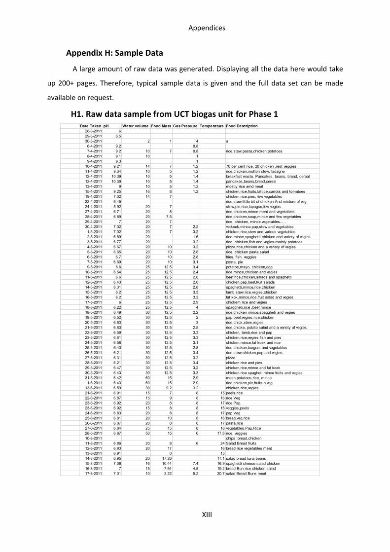
Appendices
XIII
Appendix H: Sample Data
A large amount of raw data was generated. Displaying all the data here would take
up 200+ pages. Therefore, typical sample data is given and the full data set can be made
available on request.
H1. Raw data sample from UCT biogas unit for Phase 1
Date Taken pH Water volume Food Mass Gas Pressure Temperature Food Description28-3-2011 629-3-2011 6.530-3-2011 2 1 4 a6-4-2011 9.2 0.87-4-2011 9.2 10 7 0.8 rice,stew,pasta,chicken,potatoes8-4-2011 9.1 10 19-4-2011 9.3 1
10-4-2011 9.21 14 7 1.2 70 per cent rice, 20 chicken ,rest veggies11-4-2011 9.34 10 5 1.2 rice,chicken,mutton stew, lasagne12-4-2011 10.39 10 5 1.4 breakfast waste. Pancakes, beans, bread, cereal12-4-2011 10.39 10 5 1.4 pancakes,beans,bread,cereal13-4-2011 9 10 5 1.2 mostly rice amd meat15-4-2011 9.25 16 8 1.2 chicken,rice,fruits,lattice,carrots and tomatoes19-4-2011 7.02 14 7 chicken rice.pies, few vegetables22-4-2011 6.45 rice,stew,little bit of chicken And mixture of veg24-4-2011 5.92 20 7 stew,pie,rice,lapagse,few vegies27-4-2011 6.71 20 8 rice,chicken,mince meat and vegetables28-4-2011 6.89 20 7.5 rice,chicken,soup,mince and few vegetables29-4-2011 7 20 7 rice, chicken, mince,vegetables.....30-4-2011 7.02 20 7 2.2 vetkoek,mince,pap,stew and vegetables1-5-2011 7.02 20 7 3.2 chicken,rice,stew and various vegetables2-5-2011 6.89 20 1.6 rice,mince,spaghetti,chicken and variety of vegies3-5-2011 6.77 20 3.2 rice, chicken,fish and vegies-mainly potatoes4-5-2011 6.67 20 10 3.2 pizza,rice,chicken and a variety of vegies5-5-2011 6.65 20 10 2.8 rice, chicken pasta salad6-5-2011 6.7 20 10 2.8 fries, fish, veggies7-5-2011 6.69 20 10 3.1 pasta, pie9-5-2011 6.6 25 12.5 3.4 potatoe,mayo, chicken,egg
10-5-2011 6.54 25 12.5 2.4 rice,mince,chicken and vegies11-5-2011 6.6 25 12.5 2.8 beef,rice,chicken,salads and spaghetti12-5-2011 6.43 25 12.5 2.8 chicken,pap,beef,fruit salads14-5-2011 6.31 25 12.5 2.8 spaghetti,mince,rice,chicken15-5-2011 6.2 25 12.5 3.3 lamb stew,rice,vegies,chicken16-5-2011 6.2 25 12.5 3.3 fat kok,mince,rice,fruit salad and vegies17-5-2011 6 25 12.5 2.9 chickem rice and vegies18-5-2011 6.22 25 12.5 4 spaggheti,rice ,beef,mince18-5-2011 6.49 30 12.5 2.2 rice,chicken mince,spaggheti and vegies19-5-2011 6.52 30 12.5 2 pap,beef,vegies,rice,chicken20-5-2011 6.63 30 12.5 3 rice,chick,stew,vegies21-5-2011 6.63 30 12.5 2.5 rice,chicke, potato salad and a variety of vegies22-5-2011 6.59 30 12.5 3.3 chicken, lamb,rice and pap23-5-2011 6.61 30 12.5 3.3 chicken,rice,vegies,fish and pies24-5-2011 6.58 30 12.5 3.1 chicken,mince,fat koek and rice25-5-2011 6.43 30 12.5 2.8 rice chicken,burgers and vegetables26-5-2011 6.21 30 12.5 3.4 rice,stew,chicken,pap and vegies27-5-2011 6.31 30 12.5 3.2 pizza28-5-2011 6.21 30 12.5 3.4 chicken rice and pies29-5-2011 6.47 30 12.5 3.2 chicken,rice,mince and fat koek30-5-2011 6.43 30 12.5 3.3 chicken,rice spagheti,mince fruits and vegies31-5-2011 6.42 60 15 2.9 mash potatoes,rice, mince1-6-2011 6.43 60 15 2.9 rice,chicken,pie,fruits n veg
13-6-2011 6.59 30 9.2 3.2 chicken,rice,vegies21-6-2011 6.91 15 7 8 15 peels,rice22-6-2011 6.87 15 9 8 16 rice.Veg23-6-2011 6.92 20 8 8 17 rice.Pap.23-6-2011 6.92 15 8 8 16 veggies,peels24-6-2011 6.83 20 8 8 17 pap.Veg25-6-2011 6.81 20 10 8 16 bread,veg,rice26-6-2011 6.87 20 8 8 17 pasta,rice27-6-2011 6.84 25 15 8 16 vegetables.Pap.Rice28-6-2011 6.87 50 15 6 17.6 rice, veggies10-8-2011 chips ,bread,chicken11-8-2011 6.86 20 8 6 24 Salad Bread fruits12-8-2011 6.93 20 17 16 bread rice vegetables meat13-8-2011 6.91 0 1314-8-2011 6.95 20 17.26 17.1 salad bread tuna beans15-8-2011 7.06 16 10.44 7.4 16.9 spaghetti cheese salad chicken16-8-2011 7 15 7.64 4.8 19.2 bread Bun rice chicken salad17-8-2011 7.01 10 3.22 5.2 20.7 salad Bread Buns meat
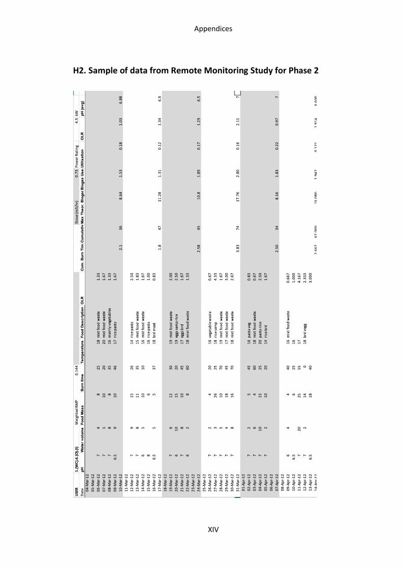
Appendices
XIV
H2. Sample of data from Remote Monitoring Study for Phase 2
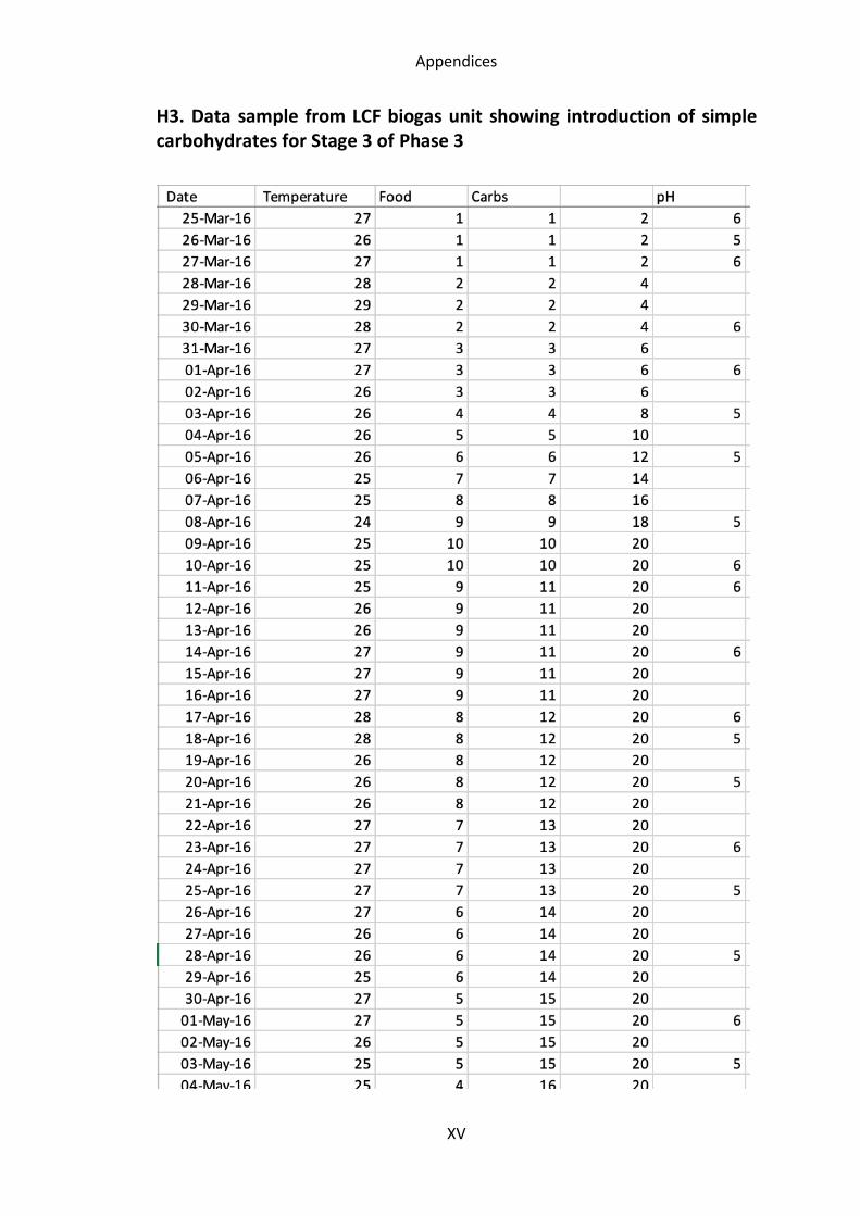
Appendices
XV
H3. Data sample from LCF biogas unit showing introduction of simple carbohydrates for Stage 3 of Phase 3
ANNEXURE: The Energisation Study
A-1
ANNEXURE: The Energisation Study A. A
This study was Chapter 4 in the original thesis. It has been removed in the revised
submission and is presented here as a standalone annexure. All references, apart from one
mention in the introduction, have been removed from the core dissertation. As such, this
annexure can be read independently.
Introduction
It was under the banner of “Renewable energy for sustainable urban development”
by which energisation was redefined in 2010 (Nissing & von Blottnitz, 2010a). With the
growing trend of urbanisation, this proved to be seminal work, collating all previous
definitions and taking three examples of perceived energisation in South Africa, to redefine
the term focusing on socio-economic needs. In this definition, “Sustainable Energisation is the
transitional process of progressively meeting primary and early secondary energy service
needs of a poor economic subgroup (secondary economy) through the delivery of an
enhanced quantity, quality and/or variety of accessible and affordable energy services,
enabling the sustainable development of the considered subgroup based on poverty
alleviation and economic development as well as the optimisation of the energy service
supply network from a lifecycle perspective” (Nissing & von Blottnitz, 2010a). Since this
definition, there has been only one actual application using the new definition to improve the
quantity, quality and variety of accessible and affordable energy services for a more
sustainable development in a rural setting, specifically when finding a replacement for
biomass as a cooking fuel (Mungwe et al., 2016). The definition would potentially suit the
evaluation of new technologies when evaluating their suitability for deployment in urban
settings.
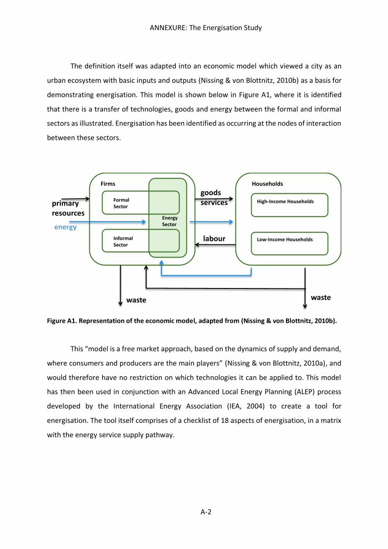
ANNEXURE: The Energisation Study
A-2
The definition itself was adapted into an economic model which viewed a city as an
urban ecosystem with basic inputs and outputs (Nissing & von Blottnitz, 2010b) as a basis for
demonstrating energisation. This model is shown below in Figure A1, where it is identified
that there is a transfer of technologies, goods and energy between the formal and informal
sectors as illustrated. Energisation has been identified as occurring at the nodes of interaction
between these sectors.
Figure A1. Representation of the economic model, adapted from (Nissing & von Blottnitz, 2010b).
This “model is a free market approach, based on the dynamics of supply and demand,
where consumers and producers are the main players” (Nissing & von Blottnitz, 2010a), and
would therefore have no restriction on which technologies it can be applied to. This model
has then been used in conjunction with an Advanced Local Energy Planning (ALEP) process
developed by the International Energy Association (IEA, 2004) to create a tool for
energisation. The tool itself comprises of a checklist of 18 aspects of energisation, in a matrix
with the energy service supply pathway.
Formal Sector
Informal Sector
Energy Sector
High-Income Households
Low-Income Households
Firms Households
waste waste
labour
goodsservicesprimary
resources
energy
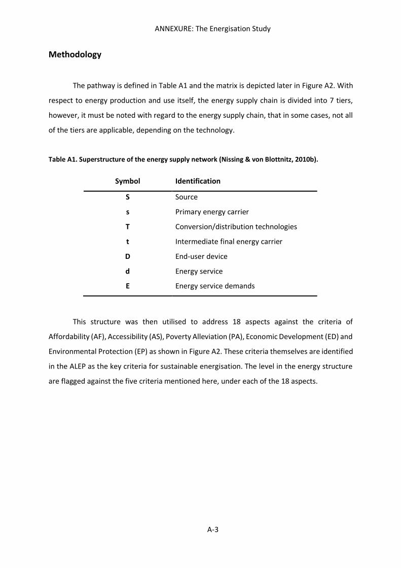
ANNEXURE: The Energisation Study
A-3
Methodology
The pathway is defined in Table A1 and the matrix is depicted later in Figure A2. With
respect to energy production and use itself, the energy supply chain is divided into 7 tiers,
however, it must be noted with regard to the energy supply chain, that in some cases, not all
of the tiers are applicable, depending on the technology.
Table A1. Superstructure of the energy supply network (Nissing & von Blottnitz, 2010b).
This structure was then utilised to address 18 aspects against the criteria of
Affordability (AF), Accessibility (AS), Poverty Alleviation (PA), Economic Development (ED) and
Environmental Protection (EP) as shown in Figure A2. These criteria themselves are identified
in the ALEP as the key criteria for sustainable energisation. The level in the energy structure
are flagged against the five criteria mentioned here, under each of the 18 aspects.
Symbol Identification
S Source
s Primary energy carrier
T Conversion/distribution technologies
t Intermediate final energy carrier
D End-user device
d Energy service
E Energy service demands
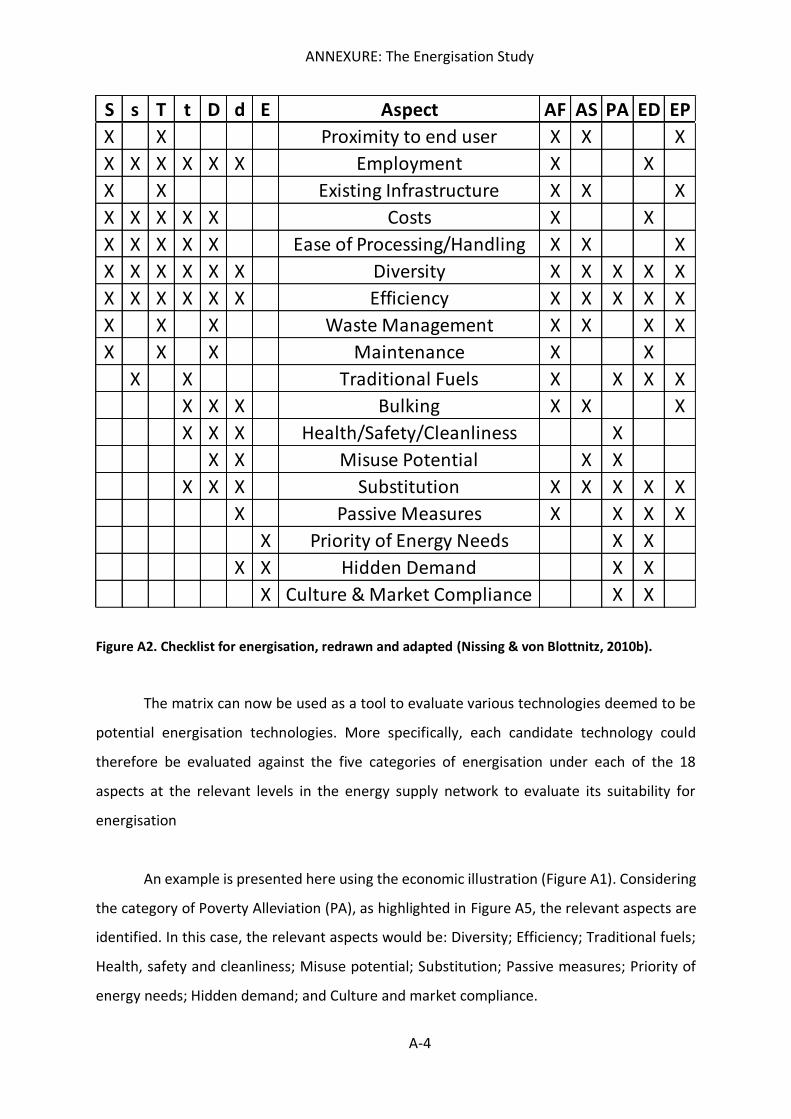
ANNEXURE: The Energisation Study
A-4
Figure A2. Checklist for energisation, redrawn and adapted (Nissing & von Blottnitz, 2010b).
The matrix can now be used as a tool to evaluate various technologies deemed to be
potential energisation technologies. More specifically, each candidate technology could
therefore be evaluated against the five categories of energisation under each of the 18
aspects at the relevant levels in the energy supply network to evaluate its suitability for
energisation
An example is presented here using the economic illustration (Figure A1). Considering
the category of Poverty Alleviation (PA), as highlighted in Figure A5, the relevant aspects are
identified. In this case, the relevant aspects would be: Diversity; Efficiency; Traditional fuels;
Health, safety and cleanliness; Misuse potential; Substitution; Passive measures; Priority of
energy needs; Hidden demand; and Culture and market compliance.
S s T t D d E Aspect AF AS PA ED EPX X Proximity to end user X X XX X X X X X Employment X XX X Existing Infrastructure X X XX X X X X Costs X XX X X X X Ease of Processing/Handling X X XX X X X X X Diversity X X X X XX X X X X X Efficiency X X X X XX X X Waste Management X X X XX X X Maintenance X X
X X Traditional Fuels X X X XX X X Bulking X X XX X X Health/Safety/Cleanliness X
X X Misuse Potential X XX X X Substitution X X X X X
X Passive Measures X X X XX Priority of Energy Needs X X
X X Hidden Demand X XX Culture & Market Compliance X X
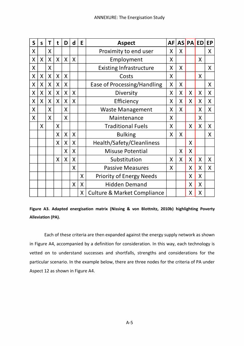
ANNEXURE: The Energisation Study
A-5
Figure A3. Adapted energisation matrix (Nissing & von Blottnitz, 2010b) highlighting Poverty
Alleviation (PA).
Each of these criteria are then expanded against the energy supply network as shown
in Figure A4, accompanied by a definition for consideration. In this way, each technology is
vetted on to understand successes and shortfalls, strengths and considerations for the
particular scenario. In the example below, there are three nodes for the criteria of PA under
Aspect 12 as shown in Figure A4.
S s T t D d E Aspect AF AS PA ED EPX X Proximity to end user X X XX X X X X X Employment X XX X Existing Infrastructure X X XX X X X X Costs X XX X X X X Ease of Processing/Handling X X XX X X X X X Diversity X X X X XX X X X X X Efficiency X X X X XX X X Waste Management X X X XX X X Maintenance X X
X X Traditional Fuels X X X XX X X Bulking X X XX X X Health/Safety/Cleanliness X
X X Misuse Potential X XX X X Substitution X X X X X
X Passive Measures X X X XX Priority of Energy Needs X X
X X Hidden Demand X XX Culture & Market Compliance X X
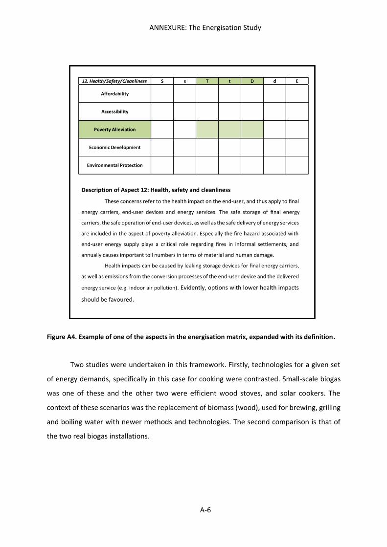
ANNEXURE: The Energisation Study
A-6
Figure A4. Example of one of the aspects in the energisation matrix, expanded with its definition.
Two studies were undertaken in this framework. Firstly, technologies for a given set
of energy demands, specifically in this case for cooking were contrasted. Small-scale biogas
was one of these and the other two were efficient wood stoves, and solar cookers. The
context of these scenarios was the replacement of biomass (wood), used for brewing, grilling
and boiling water with newer methods and technologies. The second comparison is that of
the two real biogas installations.
Description of Aspect 12: Health, safety and cleanliness
These concerns refer to the health impact on the end-user, and thus apply to final
energy carriers, end-user devices and energy services. The safe storage of final energy
carriers, the safe operation of end-user devices, as well as the safe delivery of energy services
are included in the aspect of poverty alleviation. Especially the fire hazard associated with
end-user energy supply plays a critical role regarding fires in informal settlements, and
annually causes important toll numbers in terms of material and human damage.
Health impacts can be caused by leaking storage devices for final energy carriers,
as well as emissions from the conversion processes of the end-user device and the delivered
energy service (e.g. indoor air pollution). Evidently, options with lower health impacts
should be favoured.
12. Health/Safety/Cleanliness S s T t D d E
Affordability
Accessibility
Poverty Alleviation
Economic Development
Environmental Protection
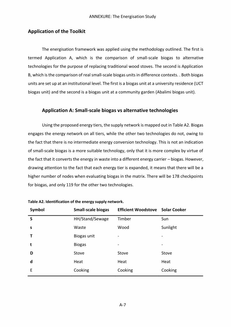
ANNEXURE: The Energisation Study
A-7
Application of the Toolkit
The energisation framework was applied using the methodology outlined. The first is
termed Application A, which is the comparison of small-scale biogas to alternative
technologies for the purpose of replacing traditional wood stoves. The second is Application
B, which is the comparison of real small-scale biogas units in difference contexts. . Both biogas
units are set up at an institutional level. The first is a biogas unit at a university residence (UCT
biogas unit) and the second is a biogas unit at a community garden (Abalimi biogas unit).
Application A: Small-scale biogas vs alternative technologies
Using the proposed energy tiers, the supply network is mapped out in Table A2. Biogas
engages the energy network on all tiers, while the other two technologies do not, owing to
the fact that there is no intermediate energy conversion technology. This is not an indication
of small-scale biogas is a more suitable technology, only that it is more complex by virtue of
the fact that it converts the energy in waste into a different energy carrier – biogas. However,
drawing attention to the fact that each energy tier is expanded, it means that there will be a
higher number of nodes when evaluating biogas in the matrix. There will be 178 checkpoints
for biogas, and only 119 for the other two technologies.
Table A2. Identification of the energy supply network.
Symbol Small-scale biogas Efficient Woodstove Solar Cooker
S HH/Stand/Sewage Timber Sun
s Waste Wood Sunlight
T Biogas unit - -
t Biogas - -
D Stove Stove Stove
d Heat Heat Heat
E Cooking Cooking Cooking
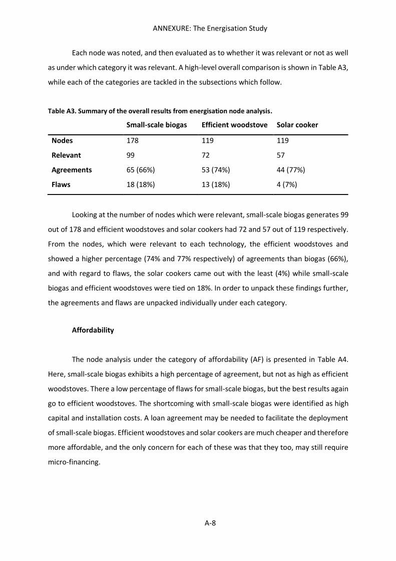
ANNEXURE: The Energisation Study
A-8
Each node was noted, and then evaluated as to whether it was relevant or not as well
as under which category it was relevant. A high-level overall comparison is shown in Table A3,
while each of the categories are tackled in the subsections which follow.
Table A3. Summary of the overall results from energisation node analysis.
Small-scale biogas Efficient woodstove Solar cooker
Nodes 178 119 119
Relevant 99 72 57
Agreements 65 (66%) 53 (74%) 44 (77%)
Flaws 18 (18%) 13 (18%) 4 (7%)
Looking at the number of nodes which were relevant, small-scale biogas generates 99
out of 178 and efficient woodstoves and solar cookers had 72 and 57 out of 119 respectively.
From the nodes, which were relevant to each technology, the efficient woodstoves and
showed a higher percentage (74% and 77% respectively) of agreements than biogas (66%),
and with regard to flaws, the solar cookers came out with the least (4%) while small-scale
biogas and efficient woodstoves were tied on 18%. In order to unpack these findings further,
the agreements and flaws are unpacked individually under each category.
Affordability
The node analysis under the category of affordability (AF) is presented in Table A4.
Here, small-scale biogas exhibits a high percentage of agreement, but not as high as efficient
woodstoves. There a low percentage of flaws for small-scale biogas, but the best results again
go to efficient woodstoves. The shortcoming with small-scale biogas were identified as high
capital and installation costs. A loan agreement may be needed to facilitate the deployment
of small-scale biogas. Efficient woodstoves and solar cookers are much cheaper and therefore
more affordable, and the only concern for each of these was that they too, may still require
micro-financing.
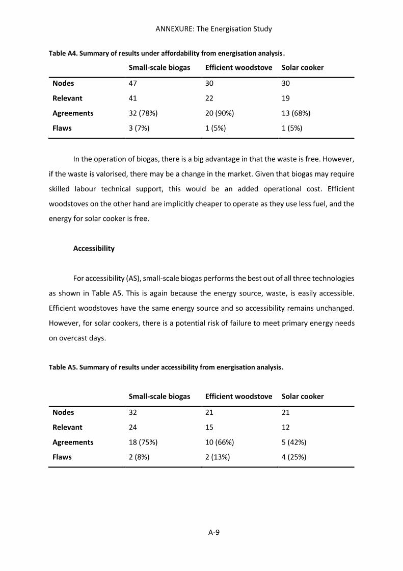
ANNEXURE: The Energisation Study
A-9
Table A4. Summary of results under affordability from energisation analysis.
Small-scale biogas Efficient woodstove Solar cooker
Nodes 47 30 30
Relevant 41 22 19
Agreements 32 (78%) 20 (90%) 13 (68%)
Flaws 3 (7%) 1 (5%) 1 (5%)
In the operation of biogas, there is a big advantage in that the waste is free. However,
if the waste is valorised, there may be a change in the market. Given that biogas may require
skilled labour technical support, this would be an added operational cost. Efficient
woodstoves on the other hand are implicitly cheaper to operate as they use less fuel, and the
energy for solar cooker is free.
Accessibility
For accessibility (AS), small-scale biogas performs the best out of all three technologies
as shown in Table A5. This is again because the energy source, waste, is easily accessible.
Efficient woodstoves have the same energy source and so accessibility remains unchanged.
However, for solar cookers, there is a potential risk of failure to meet primary energy needs
on overcast days.
Table A5. Summary of results under accessibility from energisation analysis.
Small-scale biogas Efficient woodstove Solar cooker
Nodes 32 21 21
Relevant 24 15 12
Agreements 18 (75%) 10 (66%) 5 (42%)
Flaws 2 (8%) 2 (13%) 4 (25%)
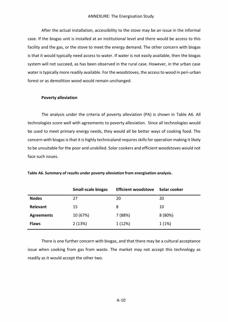
ANNEXURE: The Energisation Study
A-10
After the actual installation, accessibility to the stove may be an issue in the informal
case. If the biogas unit is installed at an institutional level and there would be access to this
facility and the gas, or the stove to meet the energy demand. The other concern with biogas
is that it would typically need access to water. If water is not easily available, then the biogas
system will not succeed, as has been observed in the rural case. However, in the urban case
water is typically more readily available. For the woodstoves, the access to wood in peri-urban
forest or as demolition wood would remain unchanged.
Poverty alleviation
The analysis under the criteria of poverty alleviation (PA) is shown in Table A6. All
technologies score well with agreements to poverty alleviation. Since all technologies would
be used to meet primary energy needs, they would all be better ways of cooking food. The
concern with biogas is that it is highly technicaland requires skills for operation making it likely
to be unsuitable for the poor and unskilled. Solar cookers and efficient woodstoves would not
face such issues.
Table A6. Summary of results under poverty alleviation from energisation analysis.
Small-scale biogas Efficient woodstove Solar cooker
Nodes 27 20 20
Relevant 15 8 10
Agreements 10 (67%) 7 (88%) 8 (80%)
Flaws 2 (13%) 1 (12%) 1 (1%)
There is one further concern with biogas, and that there may be a cultural acceptance
issue when cooking from gas from waste. The market may not accept this technology as
readily as it would accept the other two.
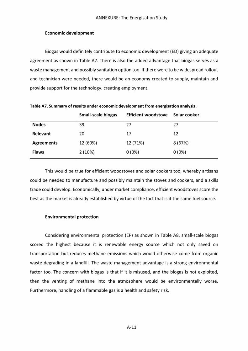
ANNEXURE: The Energisation Study
A-11
Economic development
Biogas would definitely contribute to economic development (ED) giving an adequate
agreement as shown in Table A7. There is also the added advantage that biogas serves as a
waste management and possibly sanitation option too. If there were to be widespread rollout
and technician were needed, there would be an economy created to supply, maintain and
provide support for the technology, creating employment.
Table A7. Summary of results under economic development from energisation analysis.
Small-scale biogas Efficient woodstove Solar cooker
Nodes 39 27 27
Relevant 20 17 12
Agreements 12 (60%) 12 (71%) 8 (67%)
Flaws 2 (10%) 0 (0%) 0 (0%)
This would be true for efficient woodstoves and solar cookers too, whereby artisans
could be needed to manufacture and possibly maintain the stoves and cookers, and a skills
trade could develop. Economically, under market compliance, efficient woodstoves score the
best as the market is already established by virtue of the fact that is it the same fuel source.
Environmental protection
Considering environmental protection (EP) as shown in Table A8, small-scale biogas
scored the highest because it is renewable energy source which not only saved on
transportation but reduces methane emissions which would otherwise come from organic
waste degrading in a landfill. The waste management advantage is a strong environmental
factor too. The concern with biogas is that if it is misused, and the biogas is not exploited,
then the venting of methane into the atmosphere would be environmentally worse.
Furthermore, handling of a flammable gas is a health and safety risk.
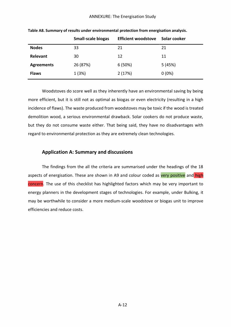
ANNEXURE: The Energisation Study
A-12
Table A8. Summary of results under environmental protection from energisation analysis.
Small-scale biogas Efficient woodstove Solar cooker
Nodes 33 21 21
Relevant 30 12 11
Agreements 26 (87%) 6 (50%) 5 (45%)
Flaws 1 (3%) 2 (17%) 0 (0%)
Woodstoves do score well as they inherently have an environmental saving by being
more efficient, but it is still not as optimal as biogas or even electricity (resulting in a high
incidence of flaws). The waste produced from woodstoves may be toxic if the wood is treated
demolition wood, a serious environmental drawback. Solar cookers do not produce waste,
but they do not consume waste either. That being said, they have no disadvantages with
regard to environmental protection as they are extremely clean technologies.
Application A: Summary and discussions
The findings from the all the criteria are summarised under the headings of the 18
aspects of energisation. These are shown in A9 and colour coded as very positive and high
concern. The use of this checklist has highlighted factors which may be very important to
energy planners in the development stages of technologies. For example, under Bulking, it
may be worthwhile to consider a more medium-scale woodstove or biogas unit to improve
efficiencies and reduce costs.
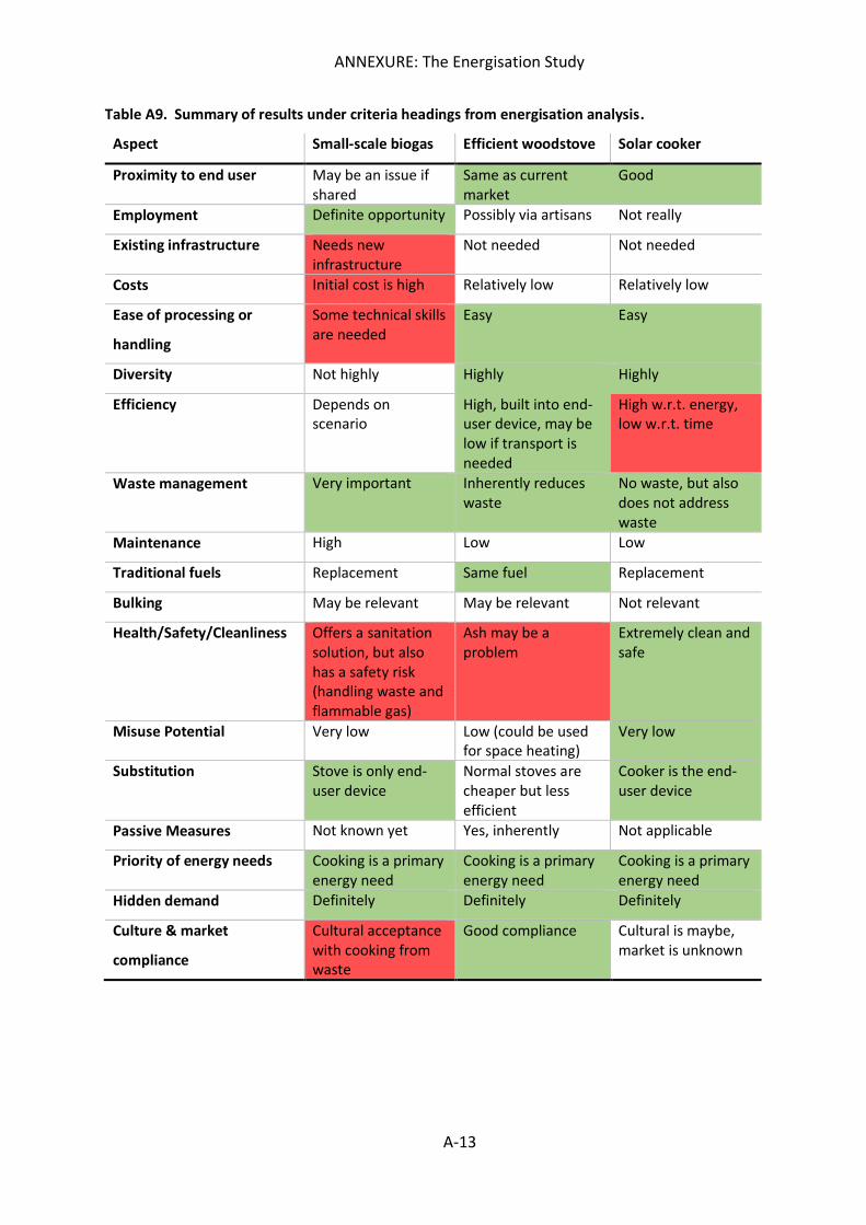
ANNEXURE: The Energisation Study
A-13
Table A9. Summary of results under criteria headings from energisation analysis.
Aspect Small-scale biogas Efficient woodstove Solar cooker
Proximity to end user May be an issue if shared
Same as current market
Good
Employment Definite opportunity Possibly via artisans Not really
Existing infrastructure Needs new infrastructure
Not needed Not needed
Costs Initial cost is high Relatively low Relatively low
Ease of processing or
handling
Some technical skills are needed
Easy Easy
Diversity Not highly Highly Highly
Efficiency Depends on scenario
High, built into end-user device, may be low if transport is needed
High w.r.t. energy, low w.r.t. time
Waste management Very important Inherently reduces waste
No waste, but also does not address waste
Maintenance High Low Low
Traditional fuels Replacement Same fuel Replacement
Bulking May be relevant May be relevant Not relevant
Health/Safety/Cleanliness Offers a sanitation solution, but also has a safety risk (handling waste and flammable gas)
Ash may be a problem
Extremely clean and safe
Misuse Potential Very low Low (could be used for space heating)
Very low
Substitution Stove is only end-user device
Normal stoves are cheaper but less efficient
Cooker is the end-user device
Passive Measures Not known yet Yes, inherently Not applicable
Priority of energy needs Cooking is a primary energy need
Cooking is a primary energy need
Cooking is a primary energy need
Hidden demand Definitely Definitely Definitely
Culture & market
compliance
Cultural acceptance with cooking from waste
Good compliance Cultural is maybe, market is unknown
ANNEXURE: The Energisation Study
A-14
Reflecting again on the node analyses, the fact that biogas engaged all the energy tiers
meant that it was a more complex technology. More complex technologies are not necessary
more appropriate. Indeed, it has the added advantage of addressing a waste management
challenge, something that the other two technologies do not offer, but the complexity comes
at the expense of needed knowledge support/skill in the operation and handling of the gas. It
is also a new technology, meaning that there are cultural and market compliance concerns.
Finally, the high capital cost of a biogas unit is a major drawback of the technology.
The biggest advantage with efficient woodstoves is that they use the same fuel source
giving it good market compliance. However, this is also its biggest drawback because not
having a fuel switch means that although there are efficiency savings, any problems
associated with the fuel source will still be there, just less pronounced. In this case, health
issues associated with burning wood will be reduced, but not removed.
For solar cookers, the cleanest of the technologies, the only issue, but the issue which
may be a critical flaw to using the technology, is that it depends largely on an energy source
which cannot be ensured. If being used to meet primary energy needs (as it indeed is in this
context) then the cooker may simply not work on overcast days and can therefore not be used
to replace traditional wood stoves. Additionally, the meal cooking time is typically longer than
other technologies. Upon further thought, it is useful to look at the evaluation process as
flagging relevance. In this way, the evaluation process evaluated the tool by marking how
many of the nodes were in fact relevant. There were indeed instances where the flagged node
was not applicable, but certainly no oversights (i.e. a node which should have been marked
but wasn’t) were encountered.
In summary, biogas is a more complex technology and comes with its own set of
challenges and concerns when considering the context of meeting primary energy needs in
urban Africa. Skills or knowledge support would be needed to manage operations and health
and safety concerns would need to be addressed to ensure operational success. Additionally,
there are high costs associated with the technology and a need for existing infrastructure, so
deployment in the informal sector may not be an option.
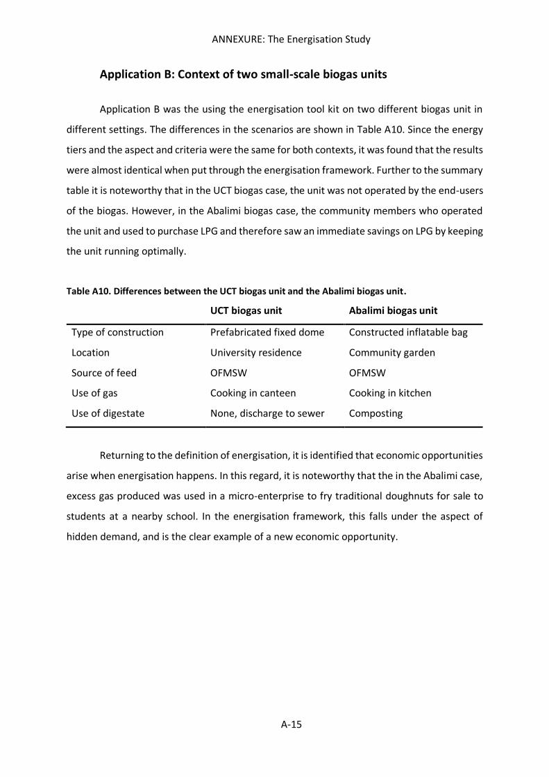
ANNEXURE: The Energisation Study
A-15
Application B: Context of two small-scale biogas units
Application B was the using the energisation tool kit on two different biogas unit in
different settings. The differences in the scenarios are shown in Table A10. Since the energy
tiers and the aspect and criteria were the same for both contexts, it was found that the results
were almost identical when put through the energisation framework. Further to the summary
table it is noteworthy that in the UCT biogas case, the unit was not operated by the end-users
of the biogas. However, in the Abalimi biogas case, the community members who operated
the unit and used to purchase LPG and therefore saw an immediate savings on LPG by keeping
the unit running optimally.
Table A10. Differences between the UCT biogas unit and the Abalimi biogas unit.
UCT biogas unit Abalimi biogas unit
Type of construction Prefabricated fixed dome Constructed inflatable bag
Location University residence Community garden
Source of feed OFMSW OFMSW
Use of gas Cooking in canteen Cooking in kitchen
Use of digestate None, discharge to sewer Composting
Returning to the definition of energisation, it is identified that economic opportunities
arise when energisation happens. In this regard, it is noteworthy that the in the Abalimi case,
excess gas produced was used in a micro-enterprise to fry traditional doughnuts for sale to
students at a nearby school. In the energisation framework, this falls under the aspect of
hidden demand, and is the clear example of a new economic opportunity.
ANNEXURE: The Energisation Study
A-16
Conclusions
In the considerations technologies for the energisation of urban Africa, the
energisation framework used provided a useful vetting system to flag potential concerns
which should be undertaken by energy planners in the concept design phase. From
Application A, and in the case of biogas in particular, the complexity of the technology allows
it to engage the energy supply network on all tiers, but also creates challenges in the health
and safety, cost and cultural acceptance aspects of energisation. It has also been identified
that the technical expertise needed to ensure operation is an economic concern, and that
there is a need for some formal infrastructure for the biogas unit, so it may not be applicable
in the informal African context. That being said, it performs extremely well on the
environmental protection category, because it is also a waste management solution, which is
one of the 18 aspects.
Efficient woodstoves and solar cookers provide a more direct comparison with each
other as they both engage the energy supply network on the same number of tiers. The
primary concern with efficient woodstoves is that there is no replacement of traditional fuel
with a renewable energy source, only an increase in efficiency, meaning that any
disadvantages of the fuel source are only reduced, and not eliminated. Solar cookers, the
cleanest of the technologies have one major drawback - the reliability of the energy source.
However, this is of high concern and may be a critical concern when considering widespread
rollout.
Reflecting on Comparison B, the energisation tool is not useful for comparing different
contexts of the same technology. However, observation of each context from the angle of
energisation reveals that there was in fact alignment with energisation theory, even though
it cannot be directly quantified
ANNEXURE: The Energisation Study
A-17
References
IEA, 2004. ‘Energy Policies of IEA Countries – 2004 review, International Energy
Agency, Paris, 2 – 4 December.
Mungwe, J., Bandeira, L., Accorona, D. & Colombo, E., 2016. Sustainable energisation
of rural areas of developing countries - a comprehensive planning approach. Energy
Procedia, 93, pp. 46-52.
Nissing, C. & von Blottnitz, H., 2010a. Renewable energy for sustainable urban
development: redefining the concept of energisation. Energy policy, Volume 38, pp. 2179-
2187.
Nissing, C. & von Blottnitz, H., 2010b. An economic model for energisation and its
interation into the urban energy planning process. Energy policy, Volume 38, pp. 2370-2378.
ANNEXURE: The Energisation Study
A-18
Definitions
The definition of “Energisation”
The following is the revised definition of energisation (Nissing & von Blottnitz, 2010b)
Sustainable Energisation is the transitional process (1) of progressively (2) meeting
primary and early secondary energy service needs (3) of a poor economic subgroup (second
economy) (4) through the delivery of an enhanced quantity, quality and/or variety (5) of
accessible and affordable energy services (6), enabling the sustainable development (7) of the
considered subgroup based on poverty alleviation and economic development (8), as well as
the optimisation of the energy service supply network from a lifecycle perspective (9).
Key:
(1) The adjective ‘transitional’ is used, as the described process focuses on the shift from
primary to early secondary energy service needs.
(2) The adverb ‘progressively’ is used in order to emphasise a defined chronological order
according to which energy needs have to be met. Although there might be overlaps
between primary and secondary energy service needs, it is assumed that generally,
primary energy needs will have to be satisfied before secondary energy service needs
can be met.
(3) The definition of the terms ‘primary and early secondary energy service needs’ has
been given.
(4) The definition of the target group ‘poor economic subgroup (second economy)’ is
given.
(5) Sustainable energisation takes place when the quantity, quality, and/or variety of
energy services delivered are enhanced. This means that at least one of the three
elements needs to be enhanced. It is emphasised though that the three elements will
never decrease under sustainable energisation. For instance, if the energy carriers fuel
wood and cow dung are entirely substituted by the energy carrier electricity, the
variety of energy carriers decreases from two to one. However, the variety of energy
ANNEXURE: The Energisation Study
A-19
services delivered (e.g. cooking and space heating) will remain equal or even increase
(e.g. additional refrigeration).
(6) Accessibility and affordability of modern energy carriers have been identified as
critical enablers of energisation. In analogy, it is assumed that the terms ‘accessibility’
and ‘affordability’ can be applied to the energy service as such, as the energy carrier
is integral part of the energy service supply network.
(7) The term ‘sustainable development’ has been described in the context of sustainable
energisation
(8) The terms ‘poverty alleviation’ and ‘economic development’ are defined
(9) The energy service supply network integrates as such the cradle-to-grave approach to
the energy service delivered, as it stretches up to the initial resource. However, the
lifecycle perspective emphasises that the optimisation of the energy service supply
network must account, next to the cradle-to- grave approach, for impacts on all
environmental media, as well as a timely component.
ANNEXURE: The Energisation Study
A-20
The definitions of the “Aspects”
The definitions of each of the aspects are needed to consider each technology in the
expanded framework.
Employment This aspect applies to all tiers of the energy service supply network except energy service demand, and focuses specifically on job opportunities for low skilled labour and venture opportunities for small and micro enterprises. For the source, employment can be created regarding the harnessing of the resource. For the primary, intermediate/final energy carriers, job and enterprise opportunities might be available regarding collection, transport, and retail of these commodities. For the conversion/distribution technologies, job and enterprise options might lie in the operation and maintenance sector. For the end-user devices, job and enterprise opportunities might lie in the transport and retail branche. In each case, existing job networks should be respected, and integrated where possible. It is suggested in connection with the existing infrastructure regarding LPG and paraffin, that retail activities could be borne by local Small Medium and Micro Enterprises (SMMEs) (Ward, 2002).
Existing Infrastructure The integration of existing infrastructure applies for the sources and the conversion/distribution technologies. In an urban area, service infrastructure such as sewage plants exist, which could be integrated as energy sources. Furthermore, existing electricity, gas and heat grids can be integrated for the distribution of intermediate/final energy carriers. For instance, the existing petrol station infrastructure could be used for the distribution of biofuels.
Proximity to end-user This aspect applies to the source, as well as to conversion and distribution technologies. It supports the reduction of transport distances between the different elements, as well as related costs and emissions. Thus, there is an improvement of AF, AS and EP. Note that a source in close proximity to the end-user is generally less prone to global market fluctuations, as it is the case for the fossil resources. Hence, an aspect of security of supply is included. Furthermore, the closer the source or the conversion/distribution technology is to the end-user, the more likely it is that local job/enterprise opportunities are created (see ‘Employment’).
ANNEXURE: The Energisation Study
A-21
Costs The cost factor is the key to the final Affordability (AF) of the energy service, and should thus be considered for every element of the energy network, except for the energy service itself and the final energy demand. Generally, low-cost energy service supply systems should be considered, where harnessing, conversion and distribution include low capital investment and operational costs, while operating with a high technical efficiency, i.a. reducing further costs. In the context of a developing country, cost estimation for the erection of plants and establishment of energy systems is difficult, as long-term investments are prone to risks (e.g. political stability - see Delany & Varga (2002) and Erb et al. (1996)), there are few cases of precedent, and cost estimations must happen based on proxy factors such as location factors (see e.g. Amigun et al., 2008). As a rule-of-thumb, it should be aimed at settling labour-intensive industries in developing countries, as a typical characteristic for developing countries is high (unskilled) labour availability and low investment capacity. However, this approach has the danger to oversimplify microeconomic reality. According to van de Ven & van Luijk (1986), labour-intensive industries can be advantageous in underdeveloped countries only if a number of rigorous conditions is satisfied, i.a. a minimum local labour productivity, and a high ratio of indirect/direct workers. Economic viability for investors is a further issue. While securing affordability for end-users, markets must remain attractive for investors. A means for achieving this goal is the creation of Public-Private Partnerships (PPPs), where financial support from the public side due to its responsibilities towards the population can attract private investment into unattractive markets. Furthermore, markets unattractive for formal business activity might still bear potentials for informal activities or micro and small enterprises. A conscious coupling of these two business spheres can lead to high synergistic effects. In this context, DME (2003) states that “In order to provide affordable access and to attract the market and banking sector to service communities with a package of energy services (photovoltaic systems, paraffin, LPG, and renewable alternatives such as gel fuel and solar cookers) sustainable, effective and efficient microcredit schemes and other financial support mechanisms have to be developed and implemented.”Furthermore, there are financing schemes and subsidies for the different tiers in the energy service supply system in order to render the realisation and implementation economically viable. In a non-Annexure A country under the Kyoto protocol (e.g. South Africa), the setup of energy service supply measures according to the requirements of the Clean Development Mechanism (CDM) qualifies for extra support based on the trade of Certified Emissions Reductions (CERs) (see e.g. Tyler, 2005). Note that it is more efficient to integrate such requirements in the planning phase of a project, than to upgrade existing projects to fit the requirements. In South Africa, further potential funding for sustainable/renewable energy options is available via Eskom’s Demand-Side Management (DSM) fund, or the DME’s Renewable Energy Finance and Subsidy Office (REFSO). Social tariffs for electricity might increase the affordability of electricity. However, a high misuse potential is given (see previous paper, Section 3.1). Microcredits for the purchase of energy supply technology might be a better option. Micro-fina nc i ng schemes for the start-up of micro-enterprises are believed to be the best solution regarding economic development from a long-term perspective, as they include the prospect of job creation in the local energy sector (see e.g. Kebir (2003) and E+Co (2004)).External costs regarding threat to human health and environment should also be considered. However, these issues are discussed elsewhere in this Section. http://www.dme.gov.za/energy/renew_finnace.stmThe 2006 Nobel Peace Prize was awarded to Dr. Muhammad Yunus and the Grameen Bank “for their efforts to create economic and social development from below” (Nobel Foundation, 2006). Yunus and his bank have meaningfully contributed to the development of the concepts of microcredit and microfinancing (see e.g. Yunus, 1999).
ANNEXURE: The Energisation Study
A-22
Ease of Processing/HandlingA low technical expenditure regarding the harnessing and processing of energy carriers reduces costs, improves efficiency, decreases health risks and environmental impacts. Moreover, according to the physical state and the harmfulness of the energy carrier, adequate technical measures must be taken regarding the means of transport. By focusing on easily transportable energy carriers, related capital expenditure and potential threats to human health and environment are kept low.
DiversityThe question of diversity applies to all tiers of the energy service supply network, except for the energy service demand. A diverse energy service supply network secures energy service supply firstly in terms of being less vulnerable to global market fluctuations esp. regarding fossil energy carriers, due to the systems capacity to balance instabilities regarding pricing and availability (Heinberg, 2003). Furthermore, a diverse energy supply network is a prerequisite for meeting the diversity of the end-user’s energy service demands. Finally, a diverse energy service supply network bears a higher variety of job and venture opportunities, esp. regarding low skilled labour and informal business activities. A threat is though that the system tends to become less efficient the more diverse it gets after passing a critical point. According to Figure 1 (adapted from Tainter, 1988), prior to point C1/B1, the system can gain efficiency by becoming more diverse. Between points B1/C1 and B2/C2, efficiency gain gradually decreases. After a system passes point B2/C2, efficiency gain becomes negative, and the system becomes vulnerable to collapse. The challenge for planners thus is to render a system as diverse as possible without passing the critical point. By focusing more specifically on conversion technologies and end-user devices, the option more diverse in its energy products (e.g. Combined heat and power (CHP), cooking stove) should be favoured and recognised as such
ANNEXURE: The Energisation Study
A-23
Efficiency From a technical point of view (e.g. thermal and electrical efficiency), sources should be easily harnessed, primary/intermediate energy carriers should be efficiently converted and distributed, and final energy carriers should efficiently be transformed into energy services. The reduction of related emissions, as well as the reduction and reuse of emerging by-product/waste streams contribute to the decrease of malign environmental impacts (see ‘Waste Management’). These considerations could be summarised under the concept of “Cleaner Production” (see e.g. Fijal, 2007). The ratio of Energy Returned On Energy Invested (EROEI) gives a good approach for measuring the efficiency of specific energy service supply pathways (see e.g. Heinberg, 2003). Effects are not only lower costs, but also a positive environmental impact. It should also be noted that EROEI does not necessarily remain constant over time, but might vary according to the level of depletion of finite sources, or improved conversion efficiency due to technological progress. As a rule-of-thumb, energy carriers with higher energy content and higher density should be favoured, as they are easier to transport, and allow higher efficiency rates for conversion processes
Waste Management By reducing/reusing by-products and waste, conversion pathways can be rendered even more efficient. Furthermore, waste and by-products can be used as sources for other energy service supply pathways (see e.g. von Blottnitz et al., 2006). In both cases, waste streams are being diverted from local landfill sites, and environmental impacts as well as related costs are being reduced. Note that here, meaningful business opportunities exist esp. for informal approaches, e.g. paper waste collectors (see Nissing & von Blottnitz, 2007). A good example of this is the success of Zablon Karingi Muthaka (Nairobi, Kenya) who won the Youth Business International Entrepreneur of the Year 2006. Williams (2006) says “Frustrated by the scarcity of official waste disposal sites and the accumulation of rubbish at every street corner of his city, Muthaka spotted a business opportunity and set up Beta Bins Waste Management, a domestic waste collection company. [...] [T]he business proved so successful that its remit has been expanded to include recycling plastics, cottons, paper, bones, metallic products, composite manure and food-stuffs.”
Maintenance This aspect applies to the source, conversion/distribution technologies, and end-user devices. The ease of maintenance is derived from the nature of the process technology/appliance as such, as well the availability of spare parts and personnel qualified for the task. A simple conversion process or end-user device is in general easier to maintain than a complex one, thus causing lower maintenance costs. On the other hand, the maintenance infrastructure necessary for more complex harnessing/processing technologies and devices bears job and enterprise potentials. These two aspects must be balanced.
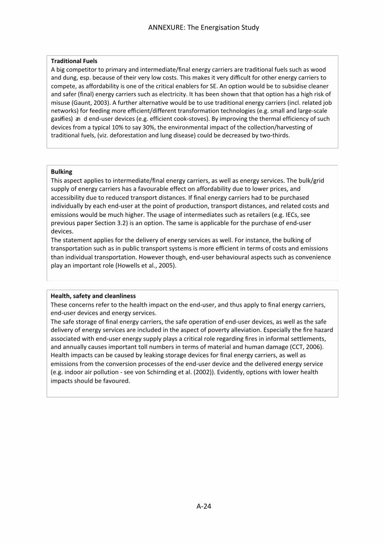
ANNEXURE: The Energisation Study
A-24
Traditional Fuels A big competitor to primary and intermediate/final energy carriers are traditional fuels such as wood and dung, esp. because of their very low costs. This makes it very difficult for other energy carriers to compete, as affordability is one of the critical enablers for SE. An option would be to subsidise cleaner and safer (final) energy carriers such as electricity. It has been shown that that option has a high risk of misuse (Gaunt, 2003). A further alternative would be to use traditional energy carriers (incl. related job networks) for feeding more efficient/different transformation technologies (e.g. small and large-scale gasifier s) an d end-user devices (e.g. efficient cook-stoves). By improving the thermal efficiency of such devices from a typical 10% to say 30%, the environmental impact of the collection/harvesting of traditional fuels, (viz. deforestation and lung disease) could be decreased by two-thirds.
Bulking This aspect applies to intermediate/final energy carriers, as well as energy services. The bulk/grid supply of energy carriers has a favourable effect on affordability due to lower prices, and accessibility due to reduced transport distances. If final energy carriers had to be purchased individually by each end-user at the point of production, transport distances, and related costs and emissions would be much higher. The usage of intermediates such as retailers (e.g. IECs, see previous paper Section 3.2) is an option. The same is applicable for the purchase of end-user devices. The statement applies for the delivery of energy services as well. For instance, the bulking of transportation such as in public transport systems is more efficient in terms of costs and emissions than individual transportation. However though, end-user behavioural aspects such as convenience play an important role (Howells et al., 2005).
Health, safety and cleanliness These concerns refer to the health impact on the end-user, and thus apply to final energy carriers, end-user devices and energy services. The safe storage of final energy carriers, the safe operation of end-user devices, as well as the safe delivery of energy services are included in the aspect of poverty alleviation. Especially the fire hazard associated with end-user energy supply plays a critical role regarding fires in informal settlements, and annually causes important toll numbers in terms of material and human damage (CCT, 2006). Health impacts can be caused by leaking storage devices for final energy carriers, as well as emissions from the conversion processes of the end-user device and the delivered energy service (e.g. indoor air pollution - see von Schirnding et al. (2002)). Evidently, options with lower health impacts should be favoured.
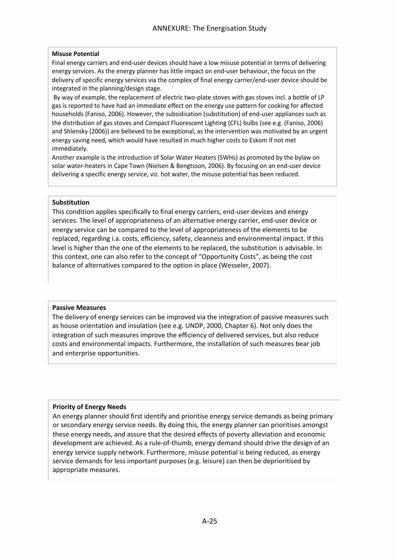
ANNEXURE: The Energisation Study
A-25
Misuse Potential Final energy carriers and end-user devices should have a low misuse potential in terms of delivering energy services. As the energy planner has little impact on end-user behaviour, the focus on the delivery of specific energy services via the complex of final energy carrier/end-user device should be integrated in the planning/design stage. By way of example, the replacement of electric two-plate stoves with gas stoves incl. a bottle of LP gas is reported to have had an immediate effect on the energy use pattern for cooking for affected households (Faniso, 2006). However, the subsidisation (substitution) of end-user appliances such as the distribution of gas stoves and Compact Fluorescent Lighting (CFL) bulbs (see e.g. (Faniso, 2006) and Shlensky (2006)) are believed to be exceptional, as the intervention was motivated by an urgent energy saving need, which would have resulted in much higher costs to Eskom if not met immediately. Another example is the introduction of Solar Water Heaters (SWHs) as promoted by the bylaw on solar water-heaters in Cape Town (Nielsen & Bengtsson, 2006). By focusing on an end-user device delivering a specific energy service, viz. hot water, the misuse potential has been reduced.
Substitution This condition applies specifically to final energy carriers, end-user devices and energy services. The level of appropriateness of an alternative energy carrier, end-user device or energy service can be compared to the level of appropriateness of the elements to be replaced, regarding i.a. costs, efficiency, safety, cleanness and environmental impact. If this level is higher than the one of the elements to be replaced, the substitution is advisable. In this context, one can also refer to the concept of “Opportunity Costs”, as being the cost balance of alternatives compared to the option in place (Wesseler, 2007).
Passive Measures The delivery of energy services can be improved via the integration of passive measures such as house orientation and insulation (see e.g. UNDP, 2000, Chapter 6). Not only does the integration of such measures improve the efficiency of delivered services, but also reduce costs and environmental impacts. Furthermore, the installation of such measures bear job and enterprise opportunities.
Priority of Energy Needs An energy planner should first identify and prioritise energy service demands as being primary or secondary energy service needs. By doing this, the energy planner can prioritises amongst these energy needs, and assure that the desired effects of poverty alleviation and economic development are achieved. As a rule-of-thumb, energy demand should drive the design of an energy service supply network. Furthermore, misuse potential is being reduced, as energy service demands for less important purposes (e.g. leisure) can then be deprioritised by appropriate measures.
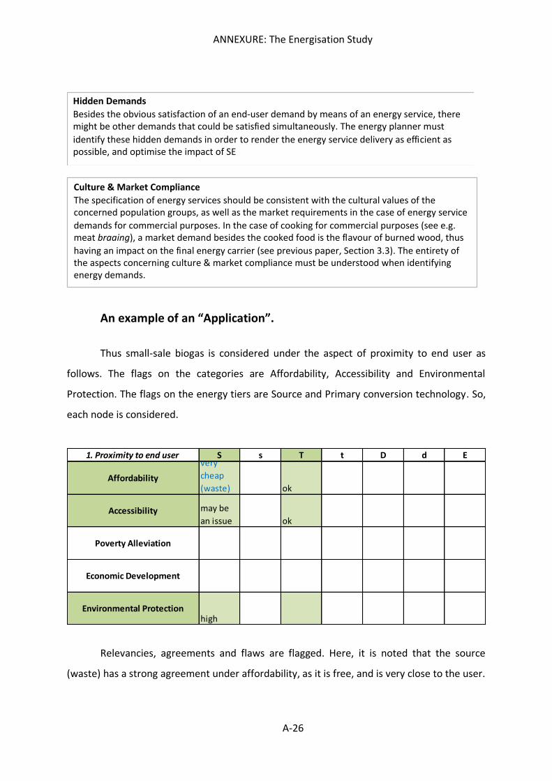
ANNEXURE: The Energisation Study
A-26
An example of an “Application”.
Thus small-sale biogas is considered under the aspect of proximity to end user as
follows. The flags on the categories are Affordability, Accessibility and Environmental
Protection. The flags on the energy tiers are Source and Primary conversion technology. So,
each node is considered.
Relevancies, agreements and flaws are flagged. Here, it is noted that the source
(waste) has a strong agreement under affordability, as it is free, and is very close to the user.
Hidden Demands Besides the obvious satisfaction of an end-user demand by means of an energy service, there might be other demands that could be satisfied simultaneously. The energy planner must identify these hidden demands in order to render the energy service delivery as efficient as possible, and optimise the impact of SE
Culture & Market Compliance The specification of energy services should be consistent with the cultural values of the concerned population groups, as well as the market requirements in the case of energy service demands for commercial purposes. In the case of cooking for commercial purposes (see e.g. meat braaing), a market demand besides the cooked food is the flavour of burned wood, thus having an impact on the final energy carrier (see previous paper, Section 3.3). The entirety of the aspects concerning culture & market compliance must be understood when identifying energy demands.
1. Proximity to end user S s T t D d E
Affordability
very cheap (waste) ok
Accessibility may be an issue ok
Poverty Alleviation
Economic Development
Environmental Protectionhigh