thesis supervisor libraries - dspace@mit
TRANSCRIPT
THREE-DIMENSIONAL MAGNETOTELLURIC
MODELLING AND INVERSION
by
Stephen Keith Park
B.S. University of California, Riverside (1978)
SUBMITTED TO THE DEPARTMENT OFEARTH, ATMOSPHERIC, AND PLANETARY SCIENCES
IN PARTIAL FULFILLMENTOF THE REQUIREMENTSFOR THE DEGREE OF
DOCTOR OF PHILOSOPHY
at the
MASSACHUSETTS INSTITUTE OF TECHNOLOGY
October 1983
( Massachusetts Institute of Technology 1983
Signature of Author
Department of Earth, Atmospheric, and Planetary SciencesOctober 27, 1983
Certified byTheodore R. MaddenThesis Supervisor
Accepted by,Theodore R. Madden
Chairman, Committee on Graduate Students
MASSACHUSETTS I TEOF TECHNOL4
LIBRARIES
THREE-DIMENSIONAL MAGNETOTELLURIC
MODELLING AND INVERSION
by
Stephen Keith Park
Submitted to the Department of Earth, Atmospheric,Planetary Sciences on October 27, 1983
in partial fulfillment of the requirementsfor the degree of Doctor of Philosophy
in Geophysics
ABSTRACT
Distortions of the magnetotelluric fields caused bythree-dimensional structures can be severe and are notpredictable using one-dimensional and two-dimensional models.While three-dimensional modelling methods have been availablefor five years (Hohmann and Ting, 1978), these are limitedto simple structures. We have developed a practical,efficient,three-dimensional modelling algorithm based on thedifferential form of Maxwell's equations. We use anextension of Ranganayaki's generalized thin sheet analysis(1978) which allows us to stack heterogeneous layers.
We use this modelling algorithm to examine what kinds ofdistortion occur near three-dimensional bodies. We haveidentified three major physical mechanisms governing thisdistortion: horizontal current gathering; vertical currentgathering; and local induction of current loops. We presentsimple procedures for estimating the order-of-magnitudecontribution from each mechanism, given rudimentary knowledgeof the structure. Each mechanism produces a differentspatial and frequency distortion in the background field, soidentification of the dominant mechanism is possible. Thisidentification aids in the qualitative interpretation offield data.
We then use two- and three-dimensional modelling todeduce the structure in the Beowawe Known GeothermalResource Area in Nevada from magnetotelluric data. Animportant result from this interpretation is that thetruncation along strike of a conductive, two-dimensional bodydoes not affect the electric fields significantly. Thisinsensitivity only occurs when the fields within theconductor are dominated by the local induction mechanism.Two-dimensionality in this case can mean ratios of length towidth of 2 or greater.
The theoretical basis for a practical three-dimensionalinversion is also presented here. The inversion method
replaces conductivity perturbations with equivalent sourcesand then applies Lanczos' generalized reciprocal theorem(1956) to derive the surface field sensitivity to aconductivity change at depth. We hope to use this method toexamine the question of uniqueness in three-dimensionalinversion.
We also present our attempts at solving the multiplescales problem. Ultimately, a practical modelling algorithmmust be able to simultaneously account for both regional andlocal structure. Multiple scales is a method by which manydifferent length scales are included in the same model. Wehave a better understanding of the problem now, and propose ausing a boundary value approach which may bypass thedifficulties we encountered. Much work is still needed,however.
Thesis Supervisor: Theodore R. Madden
Title: Professor of Geophysics
iii
ACKNOWLEDGEMENTS
This thesis has been written using the first person
plural deliberately. It does not represent just my work.
Ted Madden has contributed as much to this work as I have.
As I look through the chapters, I realize that virtually all
of the intuitive leaps have been his (or subtly suggested by
him). I have the greatest admiration for him, despite the
fact that it may not have seemed that way sometimes in our
interactions. I will greatly miss his friendship and
intellectual stimulation when I leave here.
My officemates, both past and present, have also
contributed to this thesis and my education. Rambabu
Ranganayaki, Adolfo Figueroa-Vinas, Olu Agunlowe, Ru Shan Wu,
John Williams, Fran Bagenal, Jia Dong Qian, Bob Davis, and
Brian Bennett are among those. A special note of thanks goes
to Earle Williams, Gerry LaTorraca, and Dale Morgan, who
are not only colleagues but dear friends also.
Gene Simmons, Kei Aki, and Peter Molnar were among
those outside of the Geoelectricity Group who provided help
along the way. I owe a great debt of gratitude to Renee
Zollinger, Ann Leifer, Ellen Brown, Scott Phillips, Darby
Dyar, Kaye Shedlock, Kathy Perkins, Wayne Hagman, Mary Reid,
and Tom Wissler for helping me through rough times while
here. The help from my good friends was appreciated. To all
the people who drank beer with me on Wednesdays and Fridays,
remember, that is a tradition that must not die!
iv
My parents, Harold and Joan Park, were probably the most
instrumental people in getting me here in the first place.
Their constant encouragement got me through all this school
nonsense to the point I am at now. How do you begin to say
thank you? I know of no adequate words.
Thanks go to Shawn Biehler, who sent me here, and Tien
Lee, who agreed with him. I still remember Shawn's comment
about MIT--"You'll get a damn fine education if you can stand
the climate.". I agree wholeheartedly.
I owe thanks to Judy Roos, Sharon Feldstein, Debby
Roecker, Jan Natier-Barbaro, Doug Pfeiffer, Jean Titilah, and
Ann Harlow for putting up with my unorthodox ways of dealing
with the MIT Administration. I am fully convinced MIT would
have had me arrested long ago for creative accounting in
field work if it had not been for the tolerance and
flexibility of these people.
The NSF, USGS, and the Department of Earth and Planetary
Sciences have provided financial aid for this work. Chevron
Oil Company has provided both the data set and money for some
of this work.
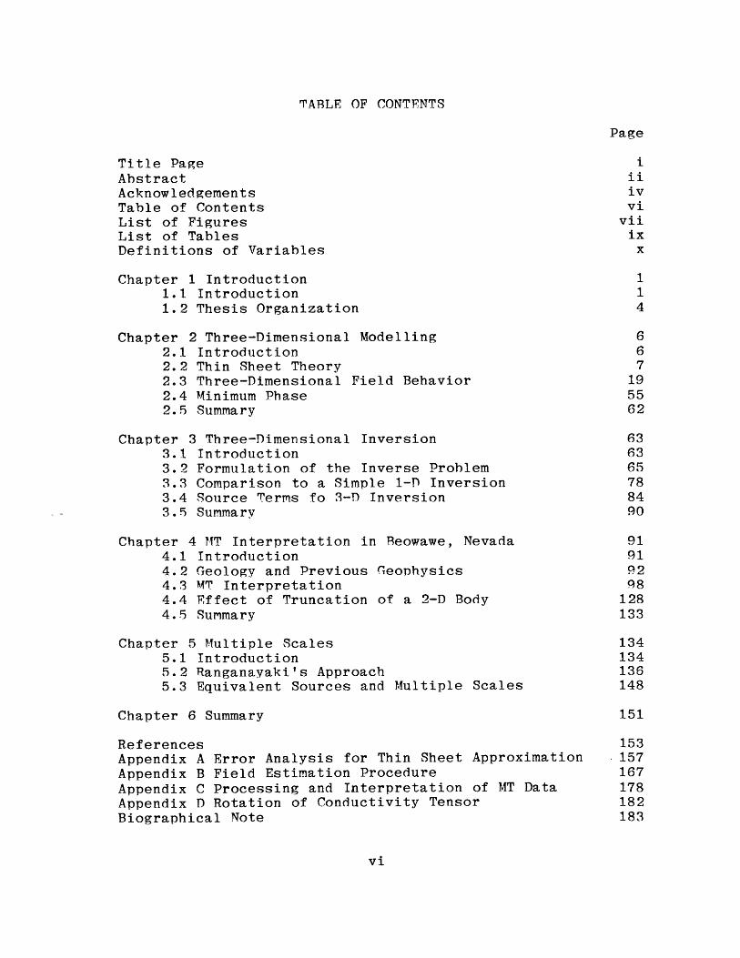
TABLE OF CONTENTS
Page
Title Page iAbstract iiAcknowledgements ivTable of Contents viList of Figures viiList of Tables ixDefinitions of Variables x
Chapter 1 Introduction 11.1 Introduction 11.2 Thesis Organization 4
Chapter 2 Three-Dimensional Modelling 62.1 Introduction 62.2 Thin Sheet Theory 72.3 Three-Dimensional Field Behavior 192.4 Minimum Phase 552.5 Summary 62
Chapter 3 Three-Dimensional Inversion 633.1 Introduction 633.2 Formulation of the Inverse Problem 653.3 Comparison to a Simple 1-P Inversion 783.4 Source Terms fo 3-D Inversion 843.5 Summary 90
Chapter 4 MT Interpretation in Beowawe, Nevada 914.1 Introduction 914.2 Geology and Previous Geophysics 924.3 MT Interpretation 984.4 Effect of Truncation of a 2-D Body 1284.5 Summary 133
Chapter 5 Multiple Scales 1345.1 Introduction 1345.2 Ranganayaki's Approach 1365.3 Equivalent Sources and Multiple Scales 148
Chapter 6 Summary 151
References 153Appendix A Error Analysis for Thin Sheet Approximation 157Appendix B Field Estimation Procedure 167Appendix C Processing and Interpretation of MT Data 178Appendix D Rotation of Conductivity Tensor 182Biographical Note 183
LIST OF FIGURES
Page
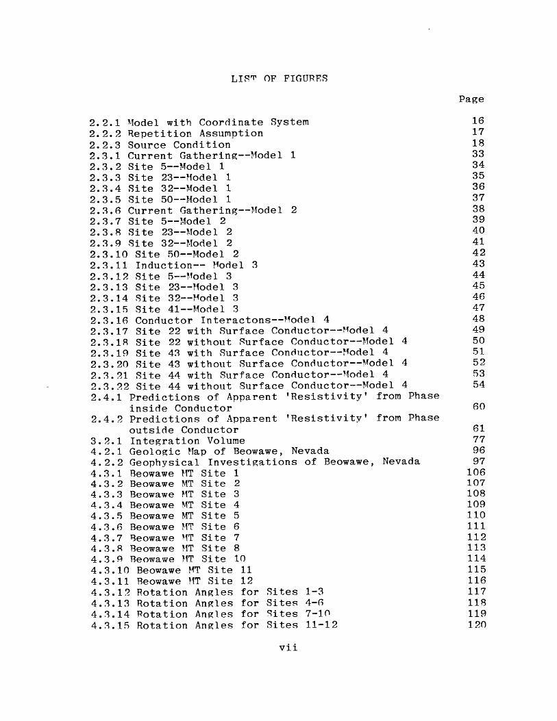
2.2.1 Model with Coordinate System 162.2.2 Repetition Assumption 172.2.3 Source Condition 182.3.1 Current Gathering--Model 1 332.3.2 Site 5--Model 1 342.3.3 Site 23--Hodel 1 352.3.4 Site 32--Model 1 362.3.5 Site 50--Model 1 372.3.6 Current Gathering--Model 2 382.3.7 Site 5--Model 2 392.3.8 Site 23--Model 2 402.3.9 Site 32--Model 2 412.3.10 Site 50--Model 2 422.3.11 Induction-- Model 3 432.3.12 Site 5--Model 3 442.3.13 Site 23--Model 3 452.3.14 Site 32--Model 3 462.3.15 Site 41--Model 3 472.3.16 Conductor Interactons--Model 4 482.3.17 Site 22 with Surface Conductor--Model 4 492.3.19 Site 22 without Surface Conductor--Miodel 4 502.3.19 Site 43 with Surface Conductor--Mfodel 4 512.3.20 Site 43 without Surface Conductor--'Model 4 522.3.21 Site 44 with Surface Conductor--Model 4 532.3.22 Site 44 without Surface Conductor--Model 4 542.4.1 Predictions of Apparent 'Resistivity' from Phase
inside Conductor 602.4.2 Predictions of Apparent 'Resistivity' from Phase
outside Conductor 613.2.1 Integration Volume 774.2.1 Geologic Map of Beowawe, Nevada 964.2.2 Geophysical Investigations of Beowawe, Nevada 974.3.1 Beowawe MT Site 1 1064.3.2 Beowawe MT Site 2 1074.3.3 Beowawe MT Site 3 1084.3.4 Beowawe MT Site 4 1094.3.5 Beowawe MT Site 5 1104.3.6 Beowawe MT Site 6 1114.3.7 Beowawe MT Site 7 1124.3.8 Beowawe MT Site 8 1134.3.9P Beowawe MT Site 10 1144.3.10 Beowawe MT Site 11 1154.3.11 Beowawe MTT Site 12 1164.3.12 Rotation Angles for Sites 1-3 1174.3.13 Rotation Angles for Sites 4-6 1184.3.14 Potation Angles for Sites 7-10 1194.3.15 Rotation Angles for Sites 11-12 120
vii
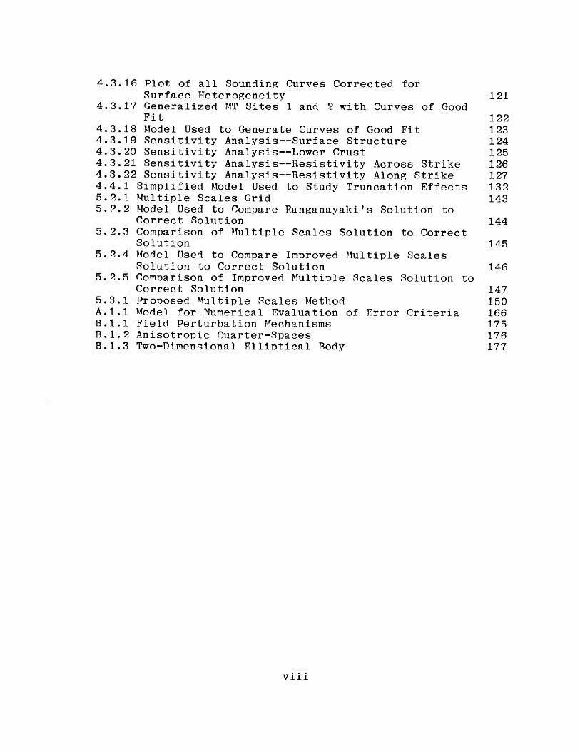
4.3.16 Plot of all Sounding Curves Corrected forSurface Heterogeneity 121
4.3.17 Generalized MT Sites 1 and 2 with Curves of GoodFit 122
4.3.18 Model Used to Generate Curves of Good Fit 1234.3.19 Sensitivity Analysis--Surface Structure 1244.3.20 Sensitivity Analysis--Lower Crust 1254.3.21 Sensitivity Analysis--Resistivity Across Strike 1264.3.22 Sensitivity Analysis--Resistivity Along Strike 1274.4.1 Simplified Model Used to Study Truncation Effects 1325.2.1 Multiple Scales Grid 1435.9.2 Model Used to Compare Ranganayaki's Solution to
Correct Solution 1445.2.3 Comparison of Multiple Scales Solution to Correct
Solution 1455.2.4 Model Used to Compare Improved Multiple Scales
Solution to Correct Solution 1465.2.5 Comparison of Improved Multiple Scales Solution to
Correct Solution 1475.3.1 Proposed Multiple Scales Method 150A.1.1 Model for Numerical Evaluation of Error Criteria 166B.1.1 Field Perturbation Mechanisms 175B.1.2 Anisotropic Quarter-Spaces 176B.1.3 Two-Dimensional Elliptical Body 177
viii
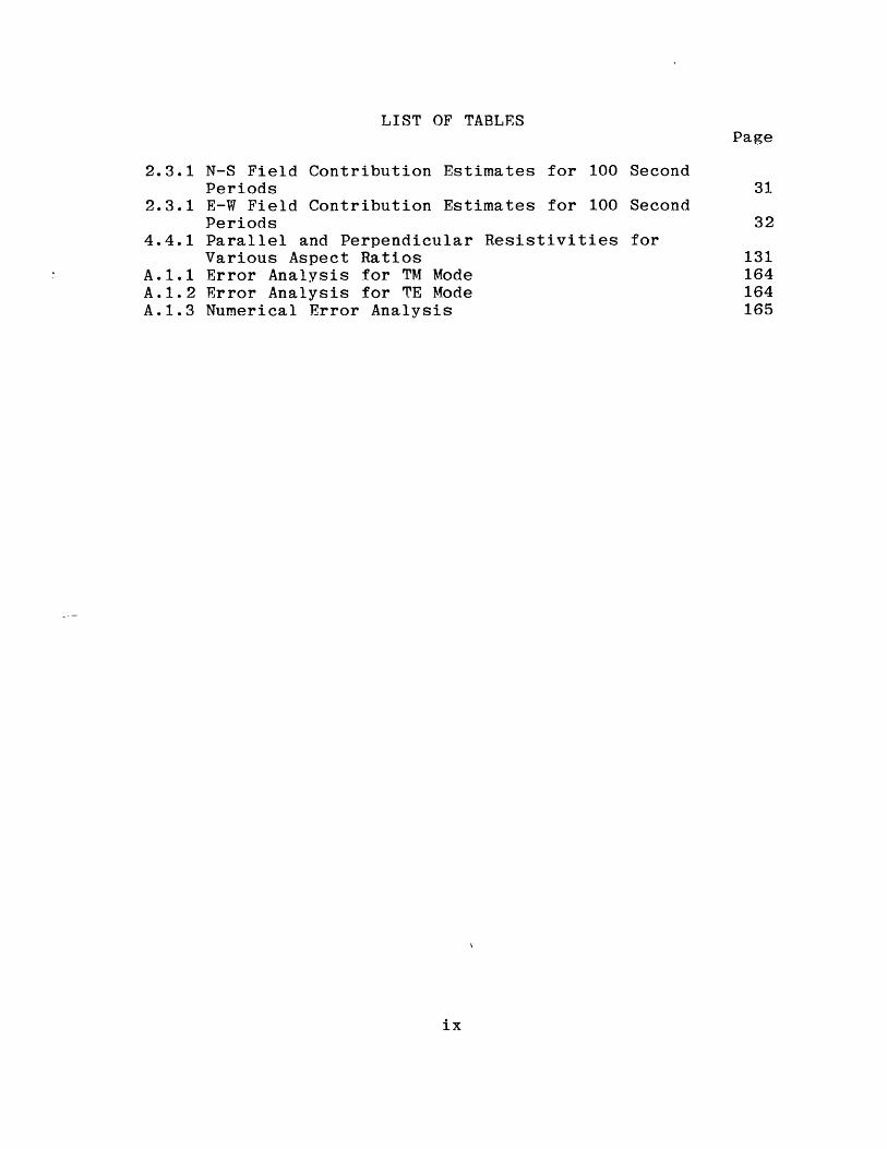
LIST OF TABLESPage
2.3.1 N-S Field Contribution Estimates for 100 SecondPeriods 31
2.3.1 E-W Field Contribution Estimates for 100 SecondPeriods 32
4.4.1 Parallel and Perpendicular Resistivities forVarious Aspect Ratios 131
A.1.1 Error Analysis for TM Mode 164A.1.2 Error Analysis for TE Mode 164A.1.3 Numerical Error Analysis 165
ix
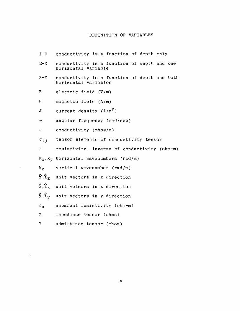
DEFINITION OF VAPIABLES
1-D conductivity is a function of depth only
2-D conductivity is a function of depth and onehorizontal variable
3-D conductivity is a function of depth and bothhorizontal variables
E electric field (V/m)
H- magnetic field (A/m)
J current density (A/m 2 )
w angular frequency (rad/sec)
a conductivity (mhos/m)
aij tensor elements of conductivity tensor
p resistivity, inverse of conductivity (ohm-m)
kxky horizontal wavenumbers (rad/m)
kz vertical wavenumber (rad/m)
Aiz uz,ix unit vectors in z direction
x~ unit vetcors in x direction
y,iy unit vectors in y direction
Pa apparent resistivity (ohm-m)
7 impedance tensor (ohms)
Y admittance tensor (mhos)
CHAPTER 1
1.1 Introduction
Low frequency electromagnetic waves generated by solar
wind-magnetosphere interactions induce currents in a
conductive earth (Jacobs, 1970). Fields produced by these
currents in turn modify the total fields. The
magnetotelluric (MT) method, first introduced by Cagniard
(1953), involves measurement of the total electric and
magnetic fields at the earth's surface. The total field
variation at the surface is influenced by the subsurface
conductivity. The MT method is used to man the conductivity
structure. This structure is then combined with knowledge
of the relationship between conductivity and geologic
materials to infer geologic structure.
The MT method has been used to determine sedimentary
basin structure (Vozoff, 1972), locate geothermal reservoirs
(Morrison, et.al., 197q), delineate mineral deposits
(Strangway, et.al., 1973), and study deep crustal structure
(Swift, 1967). The targets of these surveys have all been
three-dimensional bodies, while interpretation techniques
until recently have been limited by one-dimensional or two-
dimensional models (e.g. Swift, 1967, Laird and Bostick,
1970). Madden (1980) has shown that lower crustal resis-
tivity may be severely underestimated when data around 3-D
structures are interpreted using 1-D models. This problem
1
is especially prevalent in the Basin and Range Province of
the western United States (e.g., Stanley, et. al., 1977 or
Jiracek, et. al., 1979 for examples of such surveys).
Three-dimensional modelling poses severe computational
problems. Asymptotic approximation and series expansion of
the fields around 3-D structures were the two techniques
commonly used before the advent of high-speed computers in
the early 1970's. Kaufman and Keller (1981) provide an
excellent review of these analytic solution methods.
Many different mathematical techniques have been
applied to the numerical problem of modelling the electro-
magnetic response of 3-D structures. These techniques can
be broadly classed into two methods-- the integral equation
approach and the differential equation approach. Thin sheet
approximations are used by researchers with both classes of
methods.
The integral equation approach is the most common (e.g.
Weidelt, 1975; Hohmann and Ting, 1978; Dawson and Weaver,
1979). Variations in conductivity are treated as equivalent
current sources, and the fields are computed using dyadic
Green's functions for a simple earth model. The integral
equation methods have the advantage that they are
computationally efficient for simple structures (Hohmann and
Ting, 1978). This efficiency is lost, however, when
modelling complicated conductivity distributions (Reddy, et.
al., 1977).
The differential equation approach is the next most
common method. This approach can be applied to complex
structures , but most implementations are computationally
inefficient. Finite differencing has been used (Lines and
Jones, 1973), as has finite element modelling (Reddy,
et.al., 1977). Hermance (1982) has used finite differencing
modelling combined with approximating fields by their DC
limits to model the MT response at very low frequencies.
Ranganayaki and Madden (1980) use spectral methods (Orzag,
1972) applied to a thin, heterogeneous sheet. This approach
seems the most efficient because the step size can be equal
to the smallest scale length for conductivity variations.
Thin sheet approximations were introduced first by
Price (1949). The region containing conductivity variations
is thin compared to the electromagnetic skin depth in that
region. The media on either side of the heterogeneous sheet
may be homogeneous (Weidelt, 1975) or layered (Ranganayaki
and Madden, 1980). Weidelt (1975) and Dawson and Weaver
(1979) use thin layer approximations with their integral
equation modelling approaches.
Our work presented here is an extension of Ranganayaki
and Madden's (1980) generalized thin sheet approach. The
original formulation of the problem allowed only one
heterogeneous layer to be used. We have modified this
formulation to allow us to stack heterogeneous layers.
1.2 Thesis Organization
We will examine four different topics concerning field
behavior around 3-D structures. Chapter 2 contains the
modification of the generalized thin sheet approach to allow
stacking of heterogeneous layers. This is the forward
modelling problem. We present several models to illustrate
some key aspects of field behavior around 3-D structures.
we also discuss whether fields around complicated structures
obey the minimum phase assumption commonly used in data
processing (Boehl, et.al., 1977).
Chapter 3 establishes the theoretical groundwork for a
Dractical 3-D inversion scheme using the forward modelling
method of Chapter 2. We use the generalized reciprocity
theorem (Lanczos, 1956) to give us the field responses at
the surface due to conductivity perturbations at depth. We
show that our inversion scheme reduces to a linearized
inversion method when applied to a 1-D model.
Chapter 4 is an analysis of 4T data collected around a
geothermal area at Beowawe, Nevada. The data are fit well
with a ?-P structure. Considerations of possible 3-D
effects, however, suggests that the 2-D structure need not
be long in the strike direction.
Chapter 5 examines the problem of modelling effects
from regional structure and local structure simultaneously.
This problem has several different length scales--hence the
name multiple scale analysis (Ranganayaki, 1978). The
4
results here are all negative, but shed considerable insight
into the difficulties in the multiple scaling problem. We
suggest a method which may bypass these difficulties.
'Ten years ago, we thought we knew a lot more about MT
than we do today.'
M.G. Bloomquist
CHAPTER 2
2.1 Introduction
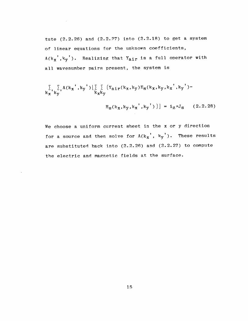
The 3-D modelling algorithm presented in this chapter
consists of stacking thin heterogeneous layers over homo-
geneous layers of arbitrary thickness. We will present the
extension of Ranganayaki's (1978) thin sheet analysis which
allows us to stack these heterogeneous layers.
Ranganayaki's work allowed the use of just one heterogeneous
layer. We also discuss some of the important features of
electromagnetic field behavior around 3-D bodies and show
several models to illustrate these features. Finally, we
show whether fields near 3-D bodies obey the minimum phase
criterion used by Boehl, et. al. (1977). This assumption is
important in data processing applications. Some of the
material in this chapter has been published in Madden and
Park (1982) and Park, et. al. (1983).
2.2 Thin Sheet Theory
Maxwell's equations, with a time dependence assumption
of exp(-jwt) in all fields, are
VxE=jwH (2.2.1)
VxH=aE-jwE (2.2.2)
Conductivities within the earth range from .00001 mhos/m to
1 mho/m, and the magnetotelluric method uses low frequencies
(f<100 Hertz). The displacement current term in (2.2.2) is
thus much smaller than the conduction current term and can
be neglected.
The conductivity in (2.2.2) is a tensor conductivity.
Its general form is
Kxx axy oxza= Gyx ayy ayz (2.2.3)
ozx azy Czz
We assume that one of the principal axes of the medium is
the z axis, but that the x and y axes are not necessarily
principal axes. The conductivity tensor thus reduces to
[xx axy 0
a= ayx ayy 0 (2.2.4)
0 0 azz
The coordinate system and the model are shown in Figure
2.2.1.
We rewrite Maxwell's equations using the conductivity
tensor in (2.2.4) so that we separate the horizontal and
vertical components of the electric and magnetic fields in
the curl operators. The new equations are
aEs/3z=-jWo(izxT"s) + Vs(Ez) (2.2.5)
aHs/3z=-izX(asEs) + Vs(Hz) (2.2.6)
Tz=(V sxs)'4 z/(joy) (2.2.7)
z=( VsXTs)'z/zz (2.2.8)
where Vs=(a/3x, 3/ay), Es=(Ex 'Ey), Hs=(HX, Hy),
(VsxFs)' 4 z= (aFy/9x -aFx/ay), and
4xx xy~
Cyx Cryy. *
We want to eliminate Ez and Hz from the set of equations
because we ultimately want only the horizontal fields. We
substitute (2.2.7) into (2.2.6) and (2.2.8) into (2.2.5) to
get
3Es/3z=-jly(izxHs)+Vs(pzz(VsXs)' z) (2.2.9)
aHs/az=-zx(asFs)+Vs((VsxEs)' z/(jow1)) (2.2.10)
where Pzz=l/Ozz. Equations (2.2.q) and (2.2.10) are the
equations which govern the behavior of fields within a
heterogeneous layer.
We have two types of derivatives in (2.2.9) and
(2.2.10) - horizontal derivatives and vertical ones. The
8
vertical derivatives are approximated by finite differences.
This approximation limits us to using small step sizes in
the vertical direction-- hence the term 'thin sheet'.
Both analytic and numerical error analyses indicate field
errors of 10% or less occur when using vertical step sizes
which are no larger than 20% of the horizontal step size
(See Appendix A). The thickness:skin depth ratio must also
be less than 0.5 for the fields to be accurate to within
10%.
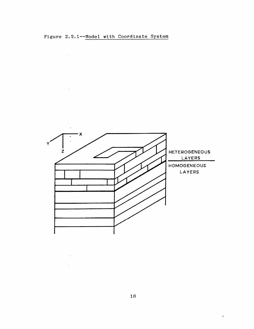
The horizontal derivatives must be handled differently
because we use a horizontal step size equal to the smallest
scale length for conductivity variations. We assume the
model repeats indefinitely in both the x and y directions.
This repetition is illustrated in Figure 2.2.2. The con-
ductivity variations, and thus the field variations, will
have a wavenumber structure involving a finite number of
wavenumbers. Forizontal derivatives are computed exactly
using multiplication by wavenumbers in the wavenumber
domain. Transformation between the space and wavenumber
domains is efficiently achieved through the use of a 2-D
fast Fourier transform (2-D because we have both x and y
directions).
We now approximate the vertical derivatives with
finite differences and derive upward continuation operators
relating the fields at the bottom of a heterogeneous layer
(TsEs~) with those at the top of the same layer (Hs+,Es+).
9
The approximations to the vertical derivatives are
3Es, Es -Ea (2.2.11)Az
and 3Hs Hs--Hs+ (2.2.12)bz Az
because we want an upward continuation operator, while the
z axis is positive downward. We substitute (2.2.11) and
(2.2.12) into (2.2.9) and (2.2.10), respectively, and
rearrange the equations to get
Es+ = Es- + Az[jop( zx sVs(Pzz(Vsx"s~)iz)]
(2.2.13)
s= s- + Az[z"X(CsFs~)~Vs((V xPs)*oz/(joj)) (2.2.14)
Note that we have approximated the fields within the layer
with those at the bottom of the layer. We use continuity of
tangential fields at the interfaces between layers. The
surface fields at the top of a layer are thus identically
equal to those at the bottom of the layer immediately above,
and we have a way to continue fields between layers.
We use a technique similar to the method of Fourier
analysis to solve for the fields at the surface of the
earth. We first find all possible solutions to our problem
(the stack of layers with (2.2.13) and (2.2.14) governing
the field behavior) and then apply boundarv and source
conditions at the surface of the earth. These conditions
allow us to combine our set of all possible solutions into a
single solution which satisfies our system of equations and
all boundary and source conditions. The set of all possible
solutions is finite because the fields anywhere can be
represented by a finite number of wavenumber pairs (kx, ky).
The next step is to determine the set of all possible
solutions. We assume the magnetic field at the bottom of
the stack of heterogeneous layers, HB, has the form of a
pure exponential, A-exp(jkx'x+jky'y), where A is an arbi-
trary scalar constant. We apply an impedance boundary
condition at the bottom of the stack of heterogeneous
layers, so we know EB = ZHB. This tensor impedance, Z,
is computed for each (kx', ky') wavenumber pair for the
stack of homogeneous layers. This method (Ranganayaki,
1978) yields the impedance for a 1-D model for arbitrary
horizontal wavenumbers. We then continue EB and HB up
through the stack of heterogeneous layers to the earth's
surface using (2.2.13) and (2.2.14). This continuation
process is done twice for each unique wavenumber pair--once
for
HR = (A,O)-exp(...)
and once for HB = (0,A')-exp(...).
The electric and magnetic fields at the surface of the model
will have a wavenumber structure reflecting: 1) the
composite wavenumber structure of the conductivity distri-
bution; and 2) the original wavenumber pair chosen for HB-
The source is a current sheet at the surface of the
earth (see Figure 2.2.3 for source configuration). A
current sheet is used because it allows for the possibility
of electromagnetic (EM) modelling and is necessary for the
inverse problem later. We apply an admittance boundary
condition to the fields above the current sheet to account
for fields radiated back into the atmosphere. The
relationship between the electric and magnetic fields in the
air is governed by
VxE = joyH (2.2.15)
VxHI = 0 (2.2.16)
because aair ~ 0. Equations (2.2.15) and (2.2.16) are com-
bined into a form Hs+ = yair'Es+ in the wavenumber domain
where
'-kxky kx 2
Yair = -ky kxkyl (2.2.17)
2 Us-k 2 k2W1iVl(j W I~sx k
The current sheet has zero thickness, so Es~ = Es+. The
magnetic field changes across the sheet, however. The
12
amount of change is given by
Ms+ - Hs z xsj (2.2.18)
We substitute in Ts + = Yair'Es+ and use the fact that
Es+ = Es~ to get our surface condition (which combines both
boundary and source conditions)
Yair*Es--Hs~ = 1zxJs (2.2.19)
We know that Es and Ts- are some linear combination of the
set of all possible solutions. The key is that the
coefficients for Es~ and Hs- are the same set of constants
we started with for HB- We assume some HB and an
impedance relation to EB, EB=ZBHB- If we scale HB by a
scalar, A, then E is scaled by the same A because ZB is
linear. Equations (2.2.13) and (2.2.14) can he rewritten
Es+ = Ps- + FHs-
Fs+ = Hs- + GES-
(2.2.20)
(2.2.21)
where F and G are the linear operators in (2.2.13) and
(2.2.14), respectively. Let us suppose we wish to continue
the fields (AEB,AHB) at the bottom of a heterogeneous layer
to the top (ET,HT). The fields at the top of the layer are
(2.2.22)ET = Fg + FHB
13
HT = HB + GEB
We substitute the scaled value of HB and the expression for
EB into (2.2.22) and (2.2.23)
ET = AZBHB + AFHB = A(EB + FHB) (2.2.24)
HT = AHB + AGZBTTB = A(HB + GEB) (2.2.25)
Notice that the fields at the top contain the same scalar
constant, A, as the fields at the bottom. This
This coefficient is carried up through the heterogeneous
structure without change because of the linearity of the
operators. There is a unique, but undetermined, coefficient
A(kx', ky ) for each trial value of HB. The fields just
below the current sheet can thus be written
s= , A(kx',ky')-Es(kkykx',ky') (2.2.26)kx ky
Hs- =kkA(kx',ky')-Hs(kkykx ?,kV) (2.2.27)k ky
We have used (kx', ky') to denote the original wavenumber
nair chosen for HB and (kx, ky) to denote the total
wavenumber structure in the fields in (2.2.26) and (2.2.27).
All wavenumber pairs will in general be present in the
fields Es(kxky,kx',ky') and Is(kx,ky,kx',ky'). We substi-
(2.2.23)
tute (2.2.26) and (2.2.P7) into (2.2.18) to get a system
of linear equations for the unknown coefficients,
A(kx?,ky'). Realizing that Yair is a full operator with
all wavenumber pairs present, the system is
fxA(kX',ky')[ X (Yair(kx~ky)Es(kxtkytkxfky')-kx ky kxky
Hs(kxky,kx',ky'))] = izxJs (2.2.28)
We choose a uniform current sheet in the x or y direction
for a source and then solve for A(kX', ky'). These results
are substituted back into (2.2.26) and (2.2.27) to compute
the electric and magnetic fields at the surface.
with Coordinate System
xY
z Z HETEROGENEOUSLAYERS
HOMOGENEOUS
LAYERS
16
Figure 2. 2.1--M,'odel
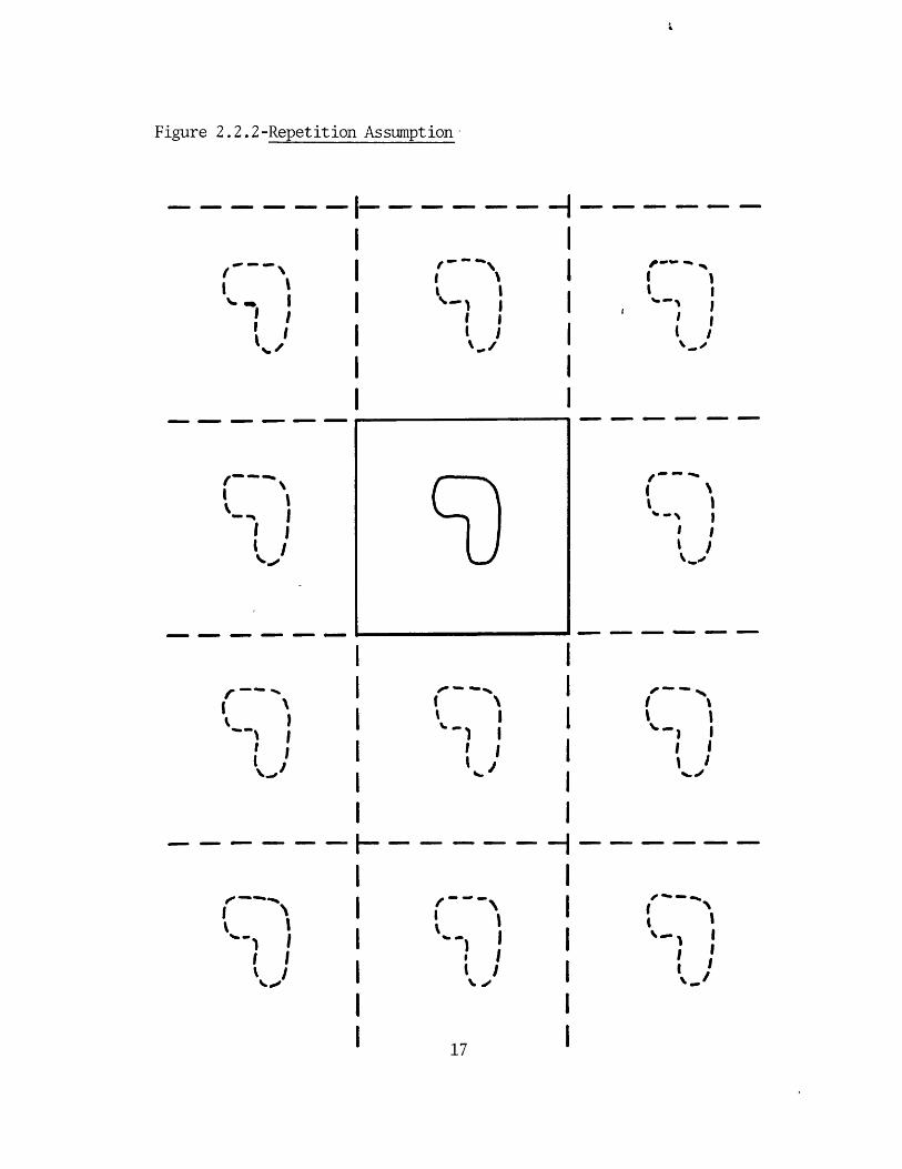
Figure 2.2.2-Repetition Assumption-
I- - - - - -
II
I I4%~~
I II I,
"U,,
II
I
I
I
-I
'**~) III
/
-- - -----
I I
II I
%-' Ie gI,%
I
I
-1
-U ~
I
'*'~) II II,
II I'- III ~
t I'-I
17
(I%mu. I
I,I,K -
(I~ I
IiI,
I
I
- I
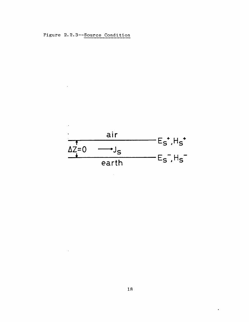
Figure 2. 2.3--Source
air
AZ=O --- s
earth
Es ,Hs+
Es , Hs
Condition
2.3 Three-Dimensional Field Behavior
We present "T sounding curves here for several 3-D
models. These models have been chosen to illustrate certain
asnects of field behavior around 3-D bodies. Large scale
induction is responsible for regional electric fields.
Mechanisms such as current gathering and local induction
perturb these background fields near heterogeneities. These
mechanisms produce different spatial and frequency behavior
in the perturbed fields, so identification of the dominant
effect is essential. Methods for estimating the contri-
hution from each mechanism are presented in Appendix B. We
use these methods to gain physical insight into why the
fields hehave the way they do. We also illustrate some
pitfalls in the interpretation of MT data.
Magnetotelluric impedance tensors from the modelling
program are rotated to their principal axes following the
procedure outlined in Appendix C. Maximum and minimum
apparent resistivities, phases, and rotation angles are
computed. The rotation angles presented are measured with
respect to the x axis (see Figure 2.3.1) and are positive in
the clockwise direction. The rotation angle is the
direction of maximum apparent resistivity. Three-
dimensional structural indicators, the skew and ellipticity
coefficients, are also presented. The skew and ellipticity
are
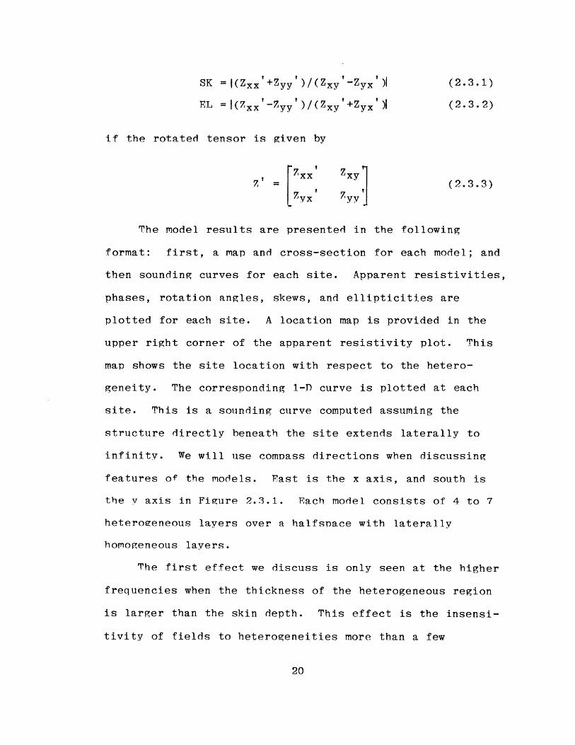
SK =|(Zxx'+Zyy')/(Zxy'-Zyx') (2.3.1)
EL =I(Zxx'-Zyy')/(Zxy'+Zyxt )| (2.3.2)
if the rotated tensor is given by
z = (2.3.3)zyx 7.yy
The model results are presented in the following
format: first, a map and cross-section for each model; and
then sounding curves for each site. Apparent resistivities,
phases, rotation angles, skews, and ellipticities are
plotted for each site. A location map is provided in the
upper right corner of the apparent resistivity plot. This
map shows the site location with respect to the hetero-
geneity. The corresponding 1-D curve is plotted at each
site. This is a sounding curve computed assuming the
structure directly beneath the site extends laterally to
infinity. We will use compass directions when discussing
features of the models. East is the x axis, and south is
the y axis in Figure 2.3.1. Each model consists of 4 to 7
heterogeneous layers over a halfspace with laterally
homogeneous layers.
The first effect we discuss is only seen at the higher
frequencies when the thickness of the heterogeneous region
is larger than the skin depth. This effect is the insensi-
tivity of fields to heterogeneities more than a few
electromagnetic skin depths away. This statement is not
strictly true if anisotropic material is present, and this
exception will be discussed later. The second effect is the
ability of the conductive heterogeneity to gather current
both laterally and vertically. A way of estimating vertical
and horizontal current gathering is discussed in Appendix B,
and is used here. The final effect we consider is local
induction. These last two effects are seen at low
frequencies where the skin depth is much larger that the
thickness of the heterogeneous region.
High Frequency Insensitivity to Distant Heterogeneities
The first effect is seen at all the sites in Figures
2.3.2-2.3.5. The MT sounding curves and the local 1-D
sounding curves merge at frequencies above 0.1 Hz in Figures
2.3.4 and 2.3.5. The skin depth within the heterogeneity
is 5 km at 0.1 Hz. The nearest boundary is 25 km, or 5
skin depths, from the MT sites (which lie at the centers of
the blocks). The secondary fields due to interactions with
the boundary have decayed to a negligible fraction of the
primary 1-D fields at these sites, so the structure 'sensed'
is essentially one-dimensional above 0.1 Hz. This same
effect can be seen in Figures 2.3.2 and 2.3.3 for sites
outside the heterogeneity, but the sounding curves merge
with the 1-D curves above 0.5 Hz. The skin depth at 0.5 Hz
outside the conductive feature is 14 km., so the nearest
boundary is about 1.5 skin depths away.
21
Current Gathering
Current gathering effects are seen below 0.01 Tiz at the
sites shown in Figures 2.3.2 - 2.3.5. Table 2.3.1
summarizes the relative contributions of the different
mechanisms at 0.01 Hz both inside and outside the hetero-
geneity in Figure 2.3.1. We see that vertical current flow
is the dominant mechanism within the conductor and equally
important to horizontal current flow without. Local
induction plays virtually no role in this first model.
Ranganayaki and Madden (1980) have shown that variations in
electric field strength due to vertical current flow are
frequency-independent when the thickness of the
heterogeneous region is much smaller than the skin depth.
The amount of variation is only a function of position at
low frequencies. The skin depths inside and outside the
heterogeneity at 0.01 Hz are 16 km and 100 km ,
respectively. The thickness of the conductive feature is
only 1 km, so variations in the apparent resistivity should
he frequency-independent below 0.01 Hz. The change in
electric field due to horizontal current gathering is also
assumed to be frequency-independent at these low
frequencies.
The current gathering effects seen at all sites
(Figures 2.3.2-2.3.5) appear as parallel offsets of the
sounding curves from the low frequency portions of the
corresponding 1-D curves. The variation of apparent
22
resistivity, proportional to (F/H) , is a direct result of
electric field strength variations. This correlation
occurs because the secondary magnetic field is only a few
percent of the source field. We have never seen a secondary
field strength of more than 30' of the primary field in any
of our test models.
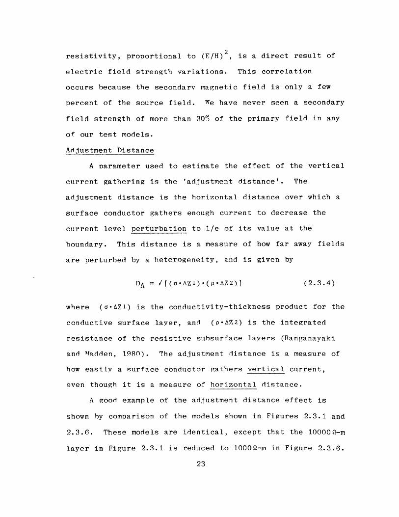
Adjustment Distance
A parameter used to estimate the effect of the vertical
current gathering is the 'adjustment distance'. The
adjustment distance is the horizontal distance over which a
surface conductor gathers enough current to decrease the
current level perturbation to 1/e of its value at the
boundary. This distance is a measure of how far away fields
are perturbed by a heterogeneity, and is given by
DA = I[(a-AZ1)-(p-AZ2)] (2.3.4)
where (a-AZ1) is the conductivity-thickness product for the
conductive surface layer, and (p-AZ2) is the integrated
resistance of the resistive subsurface layers (Ranganayaki
and Madden, 1980). The adjustment distance is a measure of
how easily a surface conductor gathers vertical current,
even though it is a measure of horizontal distance.
A good example of the adjustment distance effect is
shown by comparison of the models shown in Figures 2.3.1 and
2.3.6. These models are identical, except that the 1OOOOQ-m
layer in Figure 2.3.1 is reduced to 10000-m in Figure 2.3.6.
23
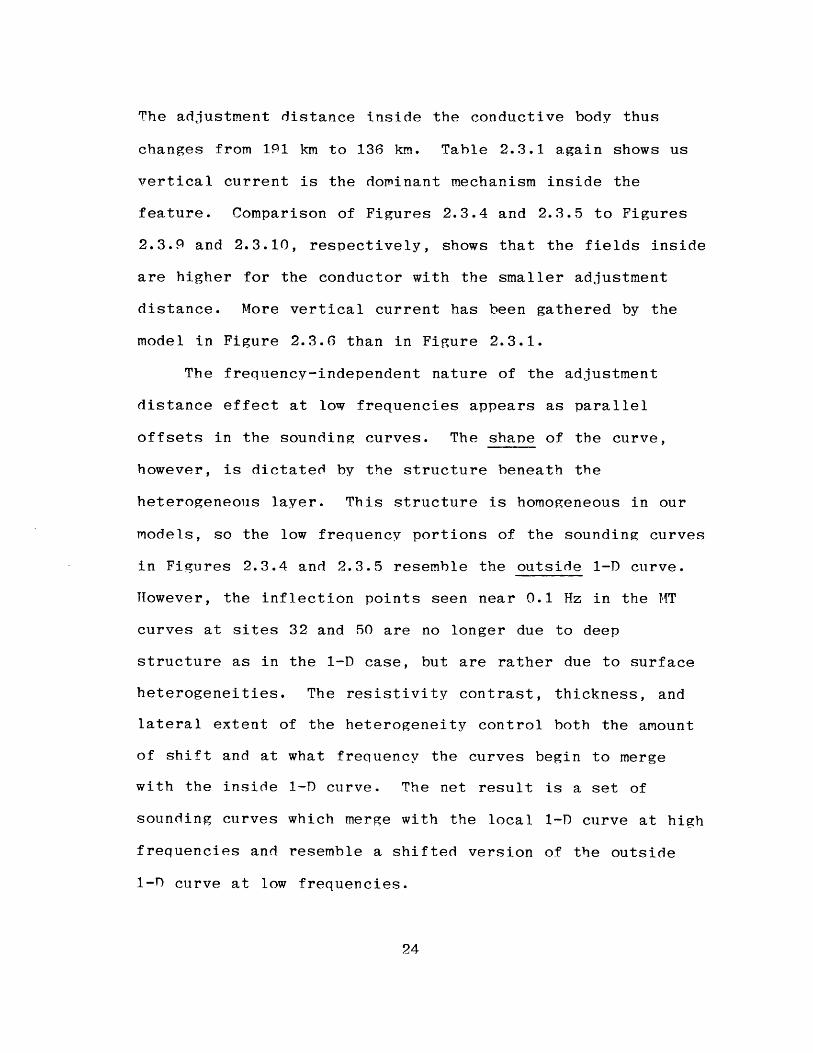
The adjustment distance inside the conductive body thus
changes from 191 km to 136 km. Table 2.3.1 again shows us
vertical current is the dominant mechanism inside the
feature. Comparison of Figures 2.3.4 and 2.3.5 to Figures
2.3.9 and 2.3.10, respectively, shows that the fields inside
are higher for the conductor with the smaller adjustment
distance. More vertical current has been gathered by the
model in Figure 2.3.6 than in Figure 2.3.1.
The frequency-independent nature of the adjustment
distance effect at low frequencies appears as parallel
offsets in the sounding curves. The shane of the curve,
however, is dictated by the structure beneath the
heterogeneous layer. This structure is homogeneous in our
models, so the low frequency portions of the sounding curves
in Figures 2.3.4 and 2.3.5 resemble the outside 1-D curve.
However, the inflection points seen near 0.1 Hz in the MT
curves at sites 32 and 50 are no longer due to deep
structure as in the 1-D case, but are rather due to surface
heterogeneities. The resistivity contrast, thickness, and
lateral extent of the heterogeneity control both the amount
of shift and at what frequency the curves begin to merge
with the inside 1-D curve. The net result is a set of
sounding curves which merge with the local 1-D curve at high
frequencies and resemble a shifted version of the outside
1-T) curve at low frequencies.
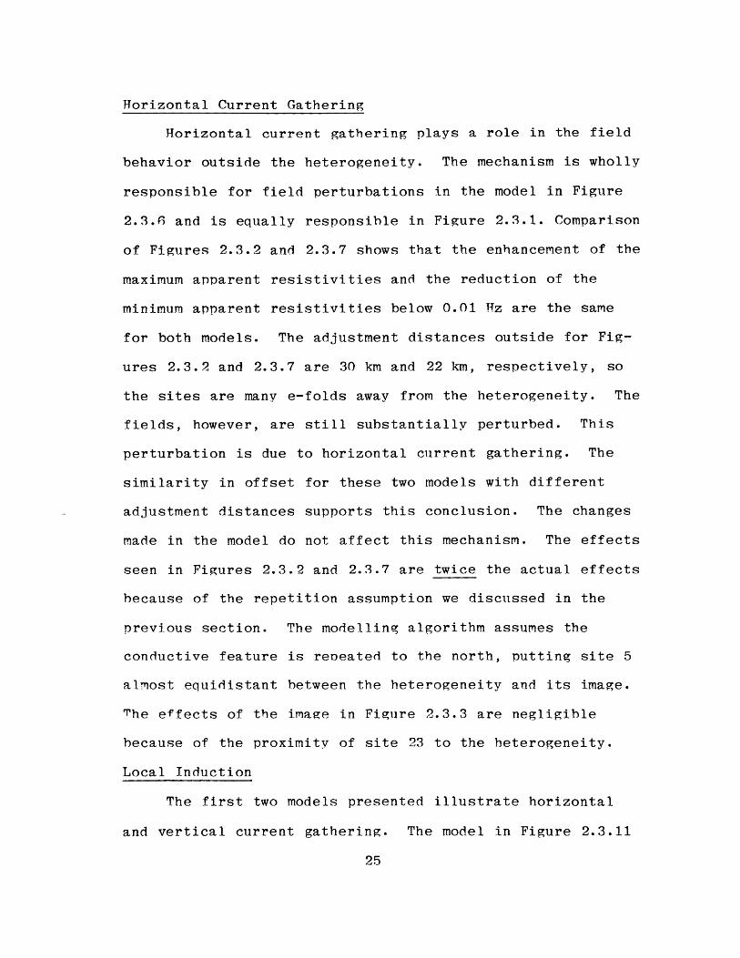
Horizontal Current Gathering
Horizontal current gathering plays a role in the field
behavior outside the heterogeneity. The mechanism is wholly
responsible for field perturbations in the model in Figure
2.3.6 and is equally responsible in Figure 2.3.1. Comparison
of Figures 2.3.2 and 2.3.7 shows that the enhancement of the
maximum apparent resistivities and the reduction of the
minimum apparent resistivities below 0.01 Hz are the same
for both models. The adjustment distances outside for Fig-
ures 2.3.2 and 2.3.7 are 30 km and 22 km, respectively, so
the sites are many e-folds away from the heterogeneity. The
fields, however, are still substantially perturbed. This
perturbation is due to horizontal current gathering. The
similarity in offset for these two models with different
adjustment distances supports this conclusion. The changes
made in the model do not affect this mechanism. The effects
seen in Figures 2.3.2 and 2.3.7 are twice the actual effects
because of the repetition assumption we discussed in the
previous section. The modelling algorithm assumes the
conductive feature is reneated to the north, putting site 5
almost equidistant between the heterogeneity and its image.
The effects of the image in Figure 2.3.3 are negligible
because of the proximity of site 23 to the heterogeneity.
Local Induction
The first two models presented illustrate horizontal
and vertical current gathering. The model in Figure 2.3.11
25
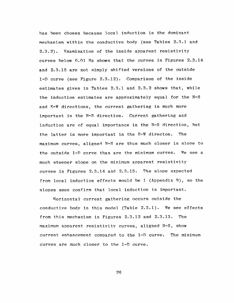
has been chosen because local induction is the dominant
mechanism within the conductive body (see Tables 2.3.1 and
2.3.2). Examination of the inside apparent resistivity
curves below 0.01 Hz shows that the curves in Figures 2.3.14
and 2.3.15 are not simply shifted versions of the outside
1-D curve (see Figure 2.3.12). Comparison of the inside
estimates given in Tables 2.3.1 and 2.3.2 shows that, while
the induction estimates are approximately equal for the N-S
and E-W directions, the current gathering is much more
important in the N-S direction. Current gathering and
induction are of equal importance in the N-S direction, but
the latter is more important in the E-W directon. The
maximum curves, aligned N-S are thus much closer in slope to
the outside 1-Dl curve than are the minimum curves. We see a
much steeper slope on the minimum apparent resistivity
curves in Figures 2.3.14 and 2.3.15. The slope expected
from local induction effects would be 1 (Appendix B), so the
slopes seen confirm that local induction is important.
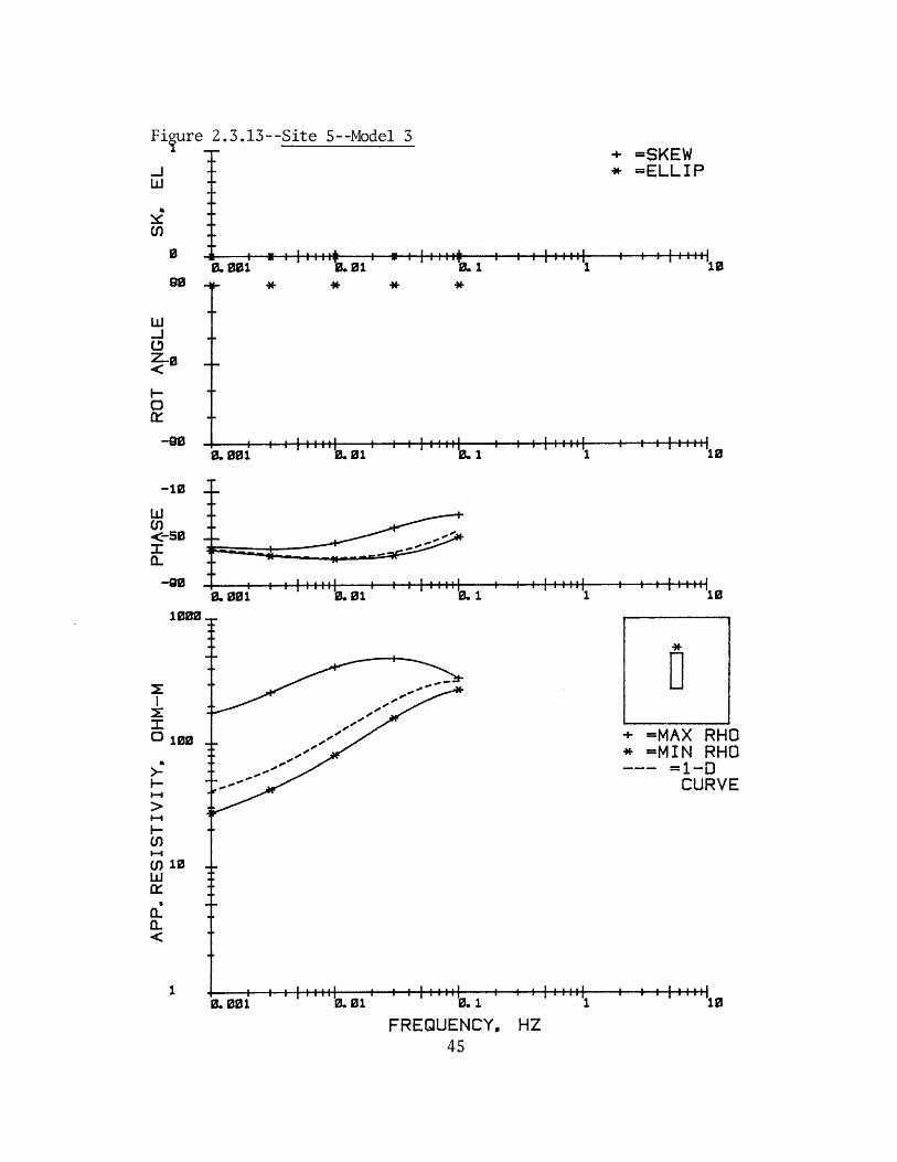
Horizontal current gathering occurs outside the
conductive body in this model (Table 2.3.1). We see effects
from this mechanism in Figures 2.3.12 and 2.3.13. The
maximum apparent resistivity curves, aligned N-S, show
current enhancement compared to the 1-D curve. The minimum
curves are much closer to the 1-D curve.
Apparent Isotropy
We infer from the almost isotropic character of the
sounding curves in Figures 2.3.4 and 2.3.9 that these sites
lie over a laterally homogeneous earth. The usual
interpretation approach would be to invert these data
assuming a 1-D model. Comparison of the local 1-D curves to
the sounding curves in these figures shows that the derived
resistivity structure would be quite erroneous in its
estimates of the intermediate and deep resistivity
structure. This problem arises because the sites in these
figures lie at points of approximate symmetry for the
heterogeneous structure. Isotropic-looking sounding curves
may not be free of 3-D structural effects.
Conductor Interactions
Figure 2.3.16 illustrates a model with a thin, surface
conductor and a deeper, thicker conductor. We present two
sets of curves for this model--one with the shallow
conductor and one without it. We use these curves to
discuss how surficial heterogeneity affects MT sounding
curves. We begin by computing the adjustment distance for
the surface conductor.
The adjustment distance must he calculated using only
the resistive layers between the feature and the nearest
current sources. The shallower conductor can attract
sufficient current from the deeper feature to raise current
levels at sites directly above the buried conductor. The
mantle thus plays no role in this case. The adjustment
distance for the shallow feature is determined using
only the resistive layers between the two heterogeneities,
and is 0.7 km. Every site over the deeper feature is thus
at least 18 e-folds away from the nearest boundary.
The insensitivity of fields to heterogeneities more
than a few skin depths away can be affected by anisotropic
material. The adjustment distance for the shallow conductor
is a good example of this. If the surface layers are highly
anisotropic, then the adjustment distance could be larger
than 0.7 km. The top layer is thin enough that the skin
depth is much larger than its thickness up to frequencies of
10 Hz (the skin depth is 0.5 km inside). The thin sheet
approximation, and its associated adjustment distance, is
therefore valid up to this frequency. All boundaries are
thus several skin depths away at these frequencies, but the
surface heterogeneity could still affect the sounding curves
if the adjustment distance was several kilometers long. This
example again shows the importance of the adjustment
distance.
Figures 2.3.17 and 2.3.18 show sounding curves for site
22 with and without the surface feature, respectively. These
curves are identical. The surface conductor exhibits no
influence upon the data at site 22. We infer from this
observation that both vertical and horizontal current
gathering mechanisms are negligible outside the shallow
conductor. Figures 2.3.19 and 2.3.20 are sounding curves
for site 43 with and without the surface feature,
respectively. The curves in Figure 2.3.19 are slightly
lower than those in Figure 2.3.20, but the change is only
3% in the electric fields. Enough current has been drawn
up from the deeper conductor to virtually compensate for the
shallow feature in this case.
Sites not over the deeper feature exhibit different
behavior, however. Figures 2.3.21 and 2.3.22 are used to
compare sounding curves for site 44 with and without the
surface conductor, respectively. The shallow feature
decreases the electric field strength by about 10% (20% for
apparent resistivities) at site 44. This decrease is
frequency-independent at low frequencies, suggesting
vertical current gathering. The adjustment distance here is
larger than the 0.7 km we derived for the body earlier. The
absence of the huried conductor beneath the site means
vertical current must be gathered from deeper structures.
The crust is conductive enough so that the conductance of
the upper 500m (500*.01=5 mhos) is equal to that of the top
layer (50*0.1=5 mhos). Hence, the body can gather current
vertically from the layers immediately beneath it.
Summary
We have presented some insights into field behavior
around 3-D structures in this section. The implications of
vertical versus horizontal current gathering, and local
induction must be considered when interpreting MT sounding
curves. Each mechanism influences the sounding curves
differently, and thus the dominant mechanism must be
identified. We have also presented some examples of pit-
falls in MT interpretation. Isotropic-looking sounding
curves are not always due to 1-D structure. Effects on MT
curves from variations in surficial conductivity are
dependent upon the structure beneath the surface layer.
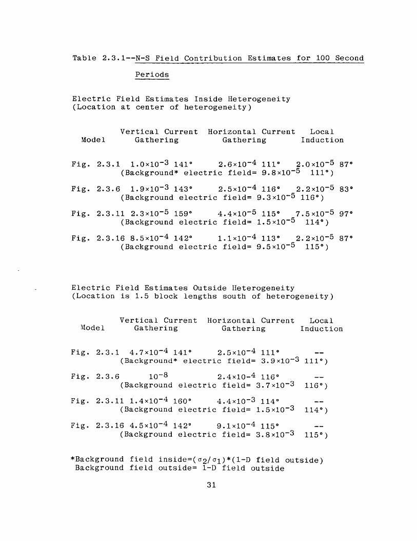
Table 2.3.1--N-S Field Contribution Estimates for 100 Second
Periods
Electric Field Estimates Inside Heterogeneity(Location at center of heterogeneity)
Vertical Current Horizontal CurrentGathering Gathering
LocalInduction
Fig. 2.3.1 1.0x10- 3 1410 2.6x10⁻⁴ 1110 2.0x10⁻⁵ 870(Background* electric field= 9.8x10⁻⁵ 1110)
Fig. 2.3.6 1.9x10⁻³ 143* 2.5x10~4 1160 2.2x10⁻⁵ 830(Background electric field= 9.3x10⁻⁵ 1160)
Fig. 2.3.11 2.3x10⁻⁵ 1590 4.4x10⁻⁵ 1150 7.5x10⁻⁵ 970(Background electric field= 1.5x10⁻⁵ 1140)
Fig. 2.3.16 8.5x10⁻⁴ 142* 1.1x10- 4 1130 2.2x10⁻⁵ 870(Background electric field= 9.5x10⁻⁵ 1150)
Electric Field Estimates Outside Heterogeneity(Location is 1.5 block lengths south of heterogeneity)
ModelVertical Current Horizontal Current
Gathering Gathering
Fig. 2.3.1 4.7x10⁻⁴ 141* 2.5x10-4 1110(Background* electric field= 3.9x10⁻³
Fig. 2.3.6 10-8 2.4x10⁻⁴ 1160(Background electric field= 3.7x10⁻³
Fig. 2.3.11 1.4x10⁻⁴ 1600 4.4x10⁻³ 1140(Background electric field= 1.5x10⁻³
Fig. 2.3.16 4.5x10⁻⁴ 142* 9.1x10~4 1150(Background electric field= 3.8x10⁻³
LocalInduction
1110)
1160)
1140)
1150)
*Background field inside=(a 2 /a1 )*(l-D field outside)Background field outside= 1-D field outside
Model
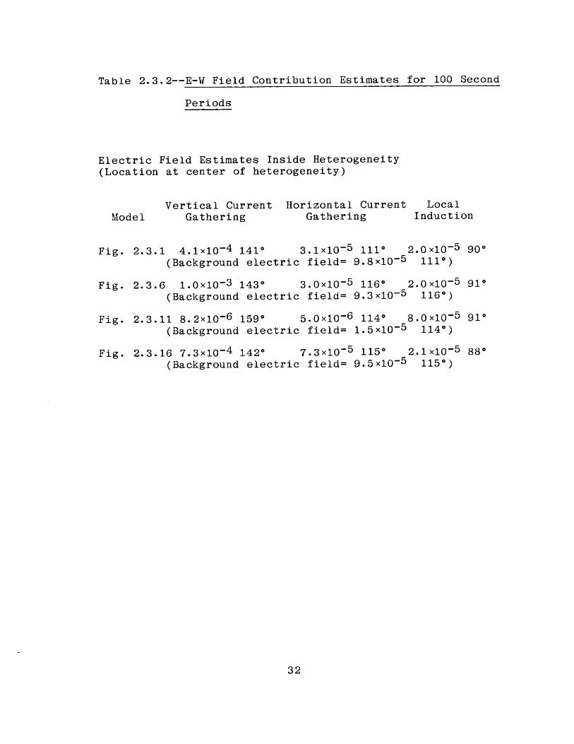
Table 2.3.2--E-W Field Contribution Estimates for 100 Second
Periods
Electric Field Estimates Inside Heterogeneity(Location at center of heterogeneity)
Vertical Current Horizontal Current LocalModel Gathering Gathering Induction
Fig. 2.3.1 4.1x10~4 141* 3.1x10-5 1110 2.0x10⁻⁵ 90*(Background electric field= 9.8x10⁻⁵ 1110)
Fig. 2.3.6 1.ox10-3 143* 3.0x10-5 1160 2.0x10⁻⁵ 910(Background electric field= 9.3x10⁻⁵ 1160)
Fig. 2.3.11 8.2x10⁻⁶ 159* 5.0x10-6 1140 8.0x10⁻⁵ 910(Background electric field= 1.5x10⁻⁵ 1140)
Fig. 2.3.16 7.3x10⁻⁴ 1420 7.3x10⁻⁵ 1150 2.1x1O-5 880(Background electric field= 9.5x10⁻⁵ 1150)
32
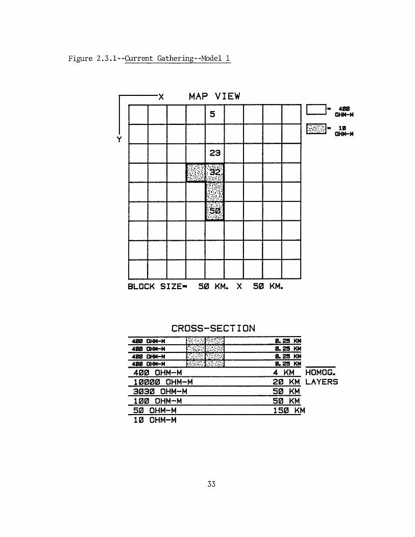
Figure 2.3.1--Current Gathering--Model 1
MAP VIEW
BLOCK SIZE-
- 400CHM-M
GHM-M
50 KM. X 50 KM.
CROSS-SECTION40 O-M :490 OHM-M400 OH-M .495 OHM-M400 OHM-M10000 OHM-M3030 OHM-M100 OHM-M50 OHM-M10 OHM-M
9.25 KM0.25 KM9.25 KM9.25 KM
4 KM20 KM50 KM50 KM150 KM
HOMOG.LAYERS
9. A:
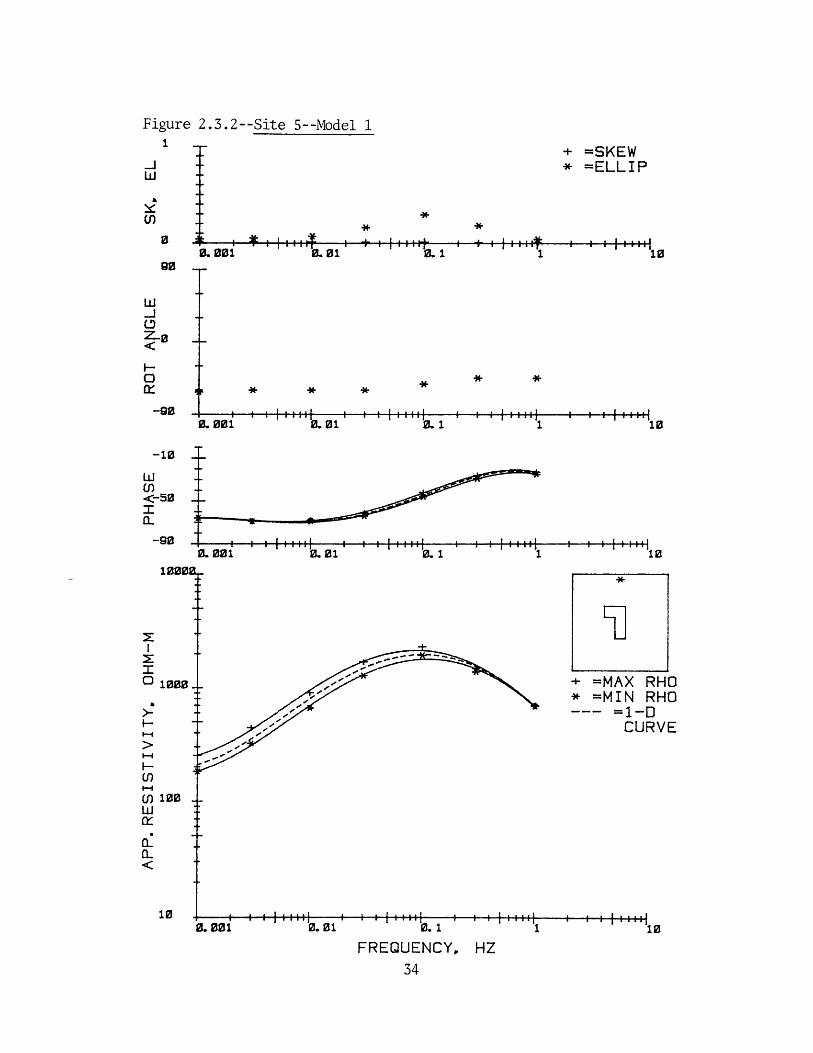
Figure 2.3.2--Site 5--Model 11
+ =SKEW* =ELLIP
........I
0.01 0. 1 1 10
* *F * * *
.I. 00i
0. 00i
I . . I
0.01 0.1
,* .01
I . ... I
10
.... ... ... ...
1, 10
+ =MAX RHO* =MIN RHO
=1-DCURVE
0.001
FREQUENCY, HZ
(I)
00. 00i
w
0
-10
wU)<-50I-0.
-90
1000
1-
I-
U)
(f) 100w
10
I . . . . Ia
I '. 1
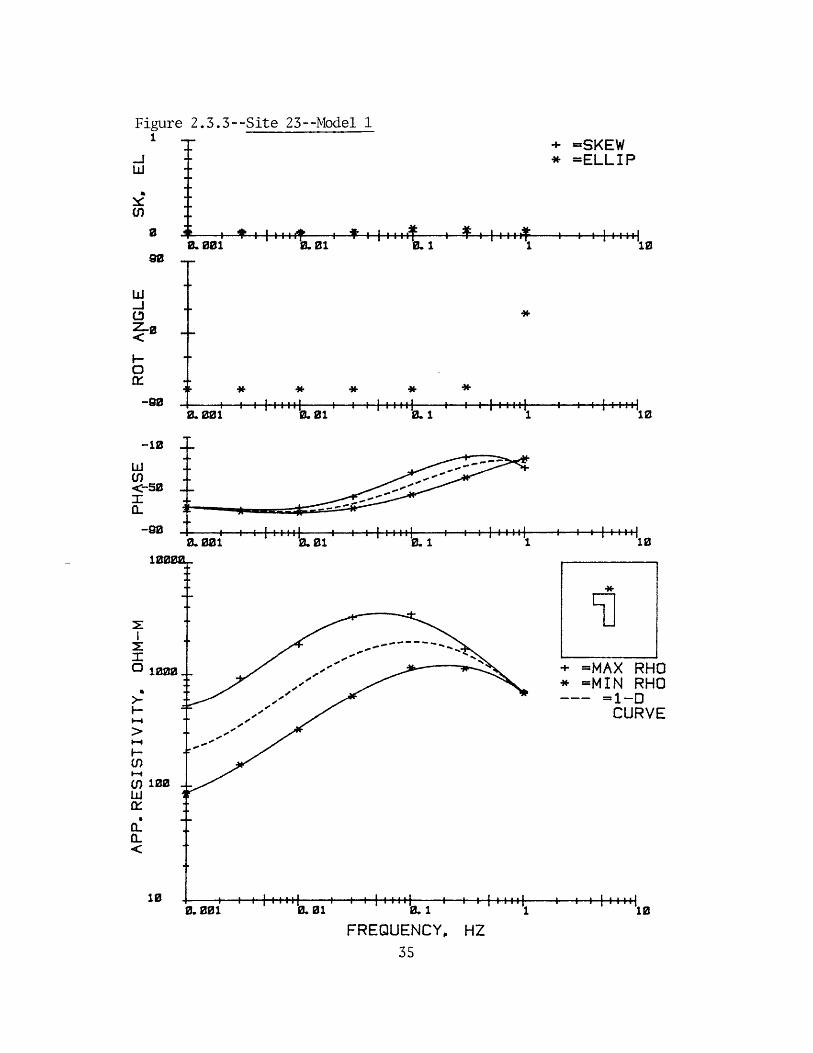
Figure 2.3.3--Site 23--Model 11 -
+ =SKEW* =ELL I P
.w 1 t ~~~ . . . . . . . . .... 1. . . I.4--64
1
I . ... I
1 0
I .... I
1
0
-90
-10
<-0
-90
-10:
1-00
Y.
CL
(1.
&.00i 01 0.1 1
10
.1......................................................................110
+ =MAX RHO* =MIN RHO
--1-CURVE
FREQUENCY, HZ
0. 00i 0. 01
*I....,
B. 001 0.01
.
Ah Ab. m - . - - - -:* - * - I - - - -*
... . . . I .-. .
! - - - I
, . 1 --&
1 10
0
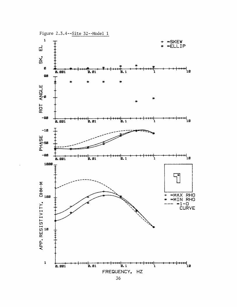
Figure 2.3.4--Site 32--Model 1
1 ___-
'0.01U.08i
+ =SKEW* =ELLIP
* *
k -----.-- **-. . . I,
* * *
B. 001 1. 01 1 10
- ~. =
I...., . . .
". 01 1 10
+ =MAX RHO* =MIN RHO
=1-DCURVE
FREQUENCY, HZ
.o
. 001
w.J
I0
0
-90
-10 .
w -
<-50 .I -
-90
1000
10
I-
Uf)
U) 10
0..
1
1 0. 1
; ; ; ;
..
.: : : :
0.01
I| : : : .: -
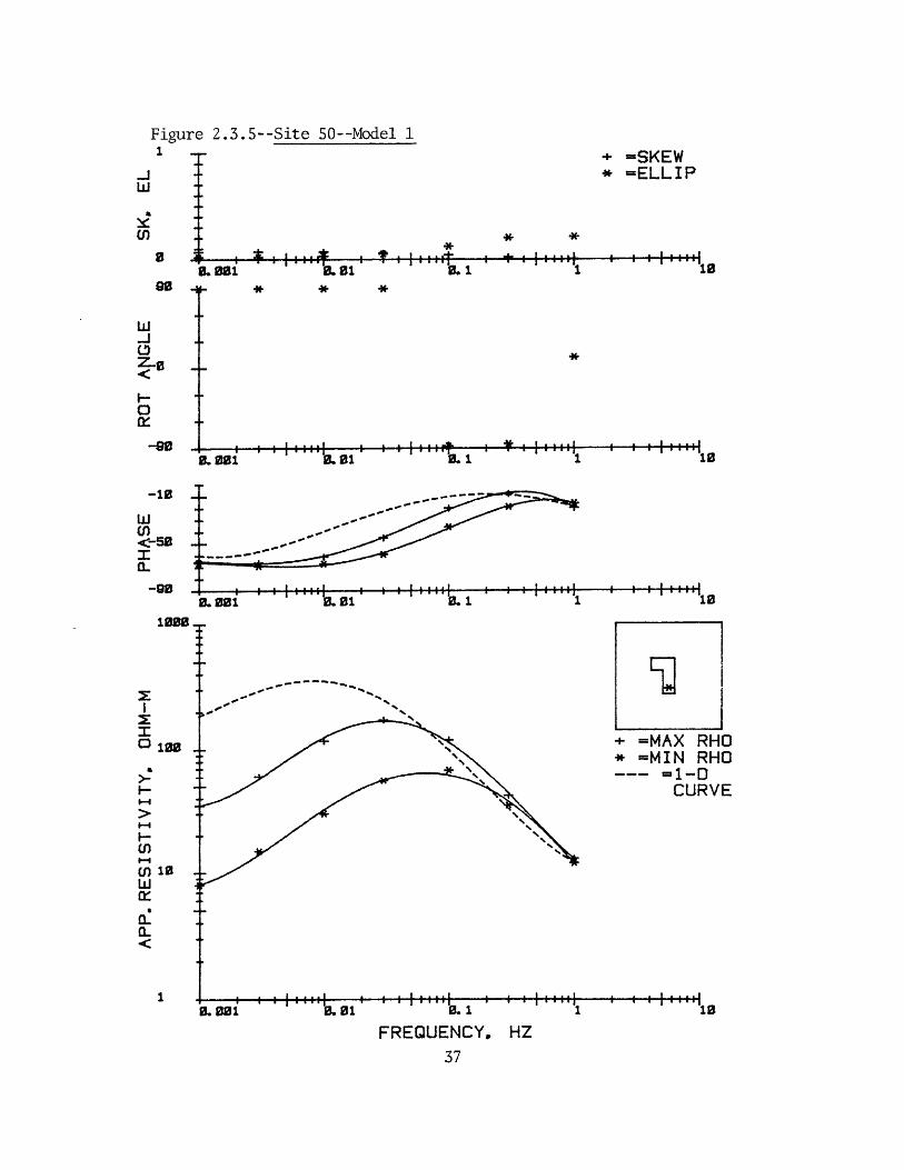
Figure 2.3.5--Site 50--Model 11
* **
~I~LkL~.±LEImLLLL.LA..L.
-J
.I
0. 00i 0.81
+ =SKEW* =ELLIP
1 10
* * *
L 001 1I . . .. I. a m t ir pa .0 . ai i i !
'0.01 0~.1' 1 '10
+ =MAX RHO- =M I N RHO
=1-DCURVE
0. 001
FREQUENCY, HZ
w
(n
as
w
z0
0wi
-410.
-90 .
-1000
w(I)<-52
-90.
1000
'- 122
I-'
(Is
w
1
"'. 1
I - - - - I
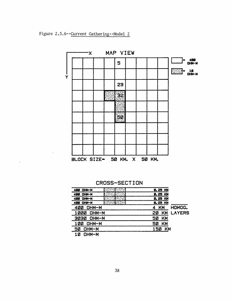
Figure 2.3.6--Current
x MAP VIEW
5
23
Le.
BLOCK SIZE- 50 KM. X 50 KM.
CROSS-SECTION408 WM-M .' 25 KM
430 OHM-M - .25 KM438 DHM-M :. 25 KM438 OHM-M400 OHM-M
E-
3.25 KM
4 KM HOMOG.1000 OHM-M 20 KM LAYERS3030 OHM-M 50 KM100 OHM-M 50 KM50 OHM-M 150 KM10 OHM-M
438OHM-M
*~*:.*m j5L~J OHM-H
Gathering--Model 2
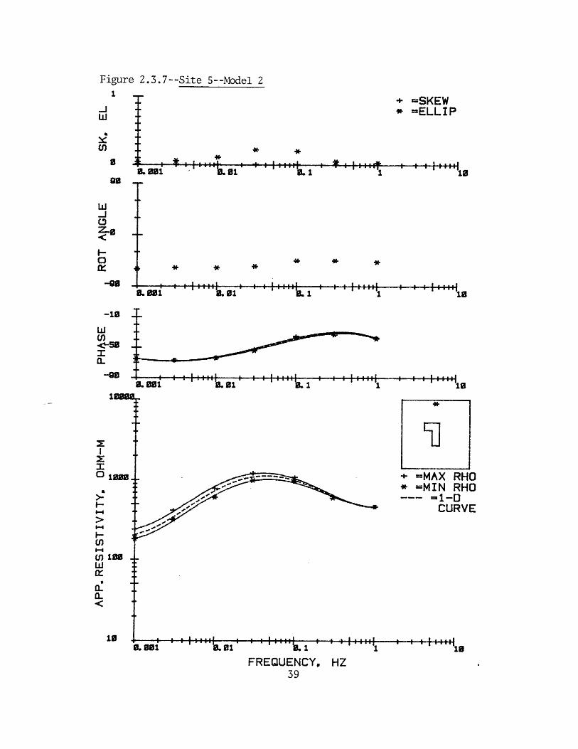
Figure 2.3.7--Site 5--Model 2
+ =SKEW* WELLIP
** *
.......................1iL 01go0
90
w
-J
20
_90
-10
-50
a-
I....,
' 10
* * *
-i .-. i :i:::ii I I Iiiti I i0. 001 I .01
i a i i a ! 1 . . .1 1 - - * .0.001 0. 01
1
1
'10
' ' '-'A"s.
+ =MAX RHO- =MIN RHO
V=1-DCURVE
r
1~..~..I
0. 01
FREQUENCY,39
i I
1
HZ1,
3. 001
* * *
LO 10.1
1C0
. 88. I . .I
-I&or 0 r i - I I I up I , I I I Pon
I
I gL i
I .* 1 i
j pjjjlllll
, .4 * *I I
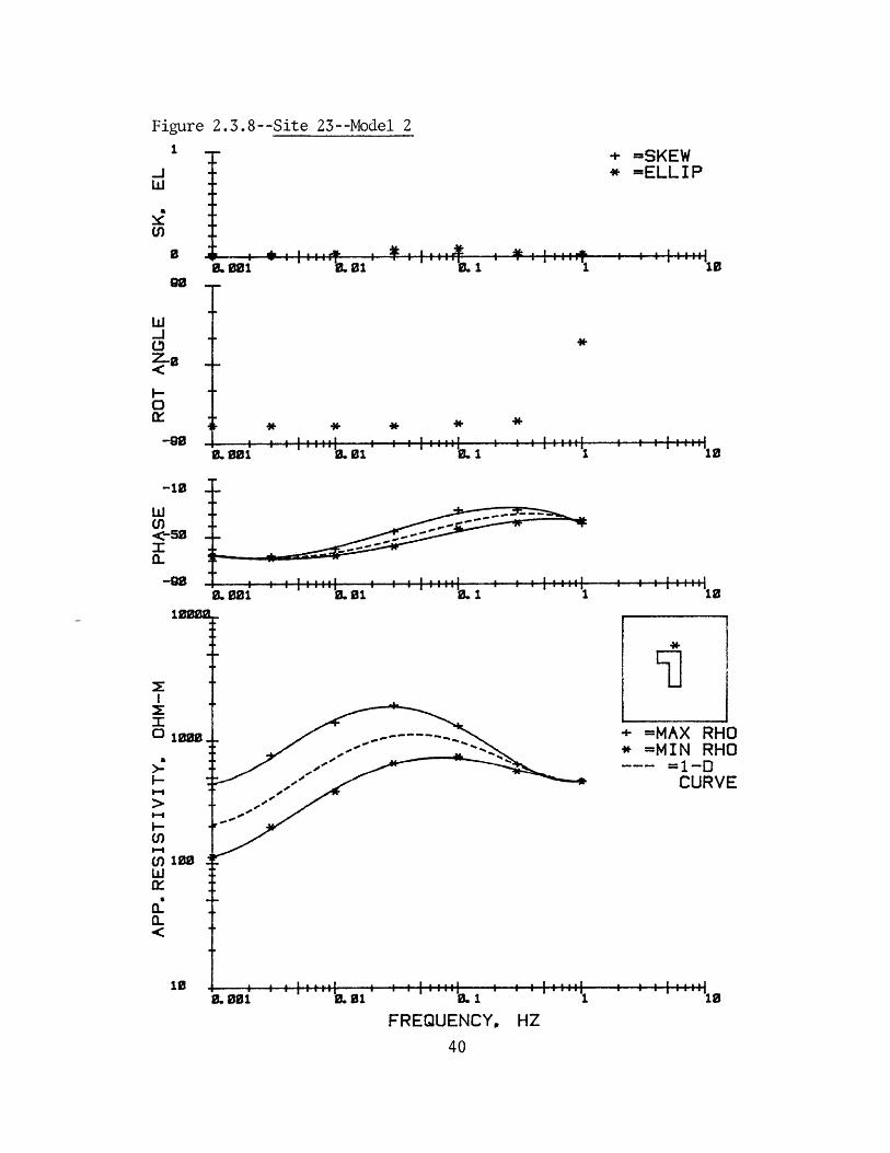
Figure 2.3.8--Site 23--Model 21 + =SVE+ =SKEW
*- -ELL I P
l~u~x ..
m ol IL1 1 10
U)
Z0
0
wz-0
-10
-4 t I 1111111 I I iitiii: :::....
0.0 1a 0.1 1 - '10
-4 I iiitiii I 11111111 I1
+ =MAX RHO- =M IN RHO
=1-DCURVE
FREQUENCY, HZ
0.-001
* ** * *
. 10i
L.001 - . 010.1
w(f)<-50
n.
-90
10001
o 1000
100a
(.
10
I - - - - I
I - - - I
- - - - I - . - - I
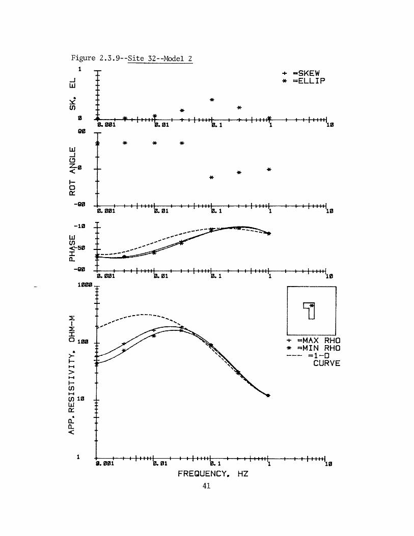
Figure 2.3.9--Site 32--Model 2
1 ~~~
-Jwj
w
z0
0
.0.01
+ =SKEW* =ELLIP
.I 1
i . I
10
1 * * *
. 001 0.01 0. 1 1
....1 ......... 110
+ =MAX RHO* =MIN RHO
=1-DCURVE
FREQUENCY, HZ
.. . . . . . . ... I .... I
.o
0. 001 .. 01
-10
w(f)<-50
-90
1000
100
ai
U,
w0I.
C..
i i
! t ! I I
AL . I . . . -*
, ., I
I
0. 1
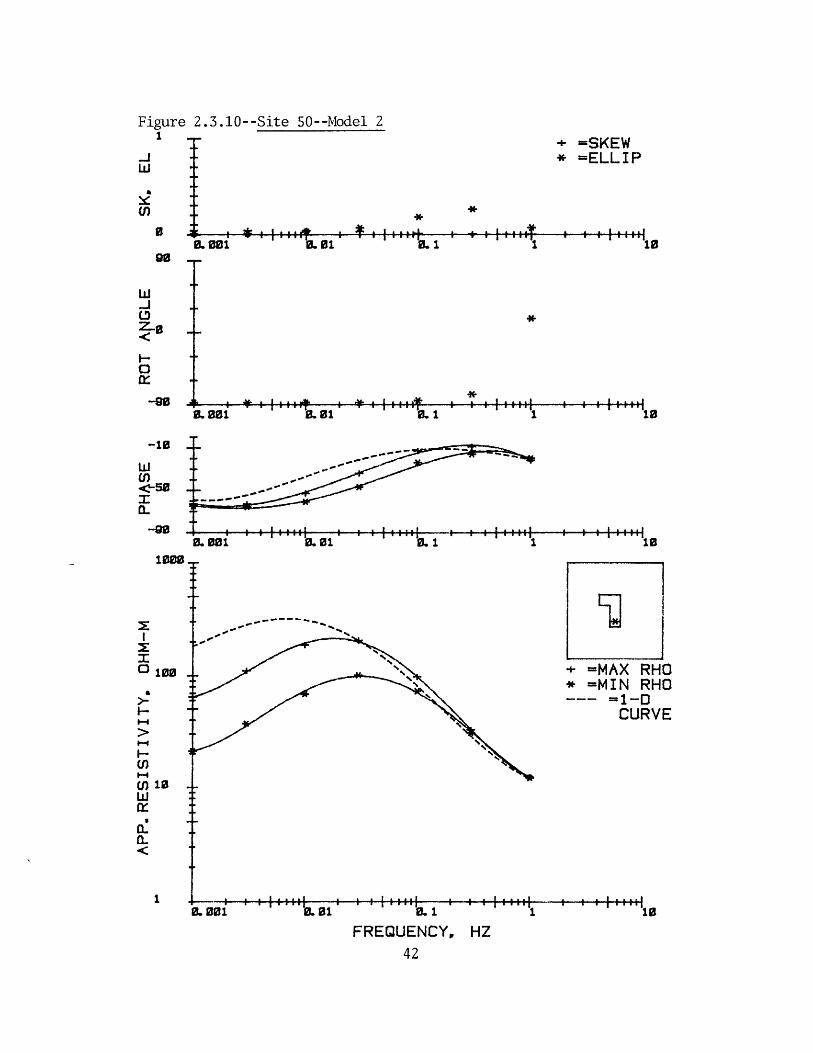
Figure 2.3.10--Site 50--Model 21 -
+. =SKEW* =ELL I P
A
.k 1 T I
.if. .
. 1 ,"1 10
(n)
0
go
w0
-w0
*
10
B. 00i I. 01SI .. ...
0. 1 1 10
+ =MAX RHO* =MIN RHO
=1-0CURVE
0.001
FREQUENCY, HZ
I. 001
0. 1. 001 0. 01
-10
wU)<-50
0.
-1m
1000
'100
I-
U) 10
0.
1
. .
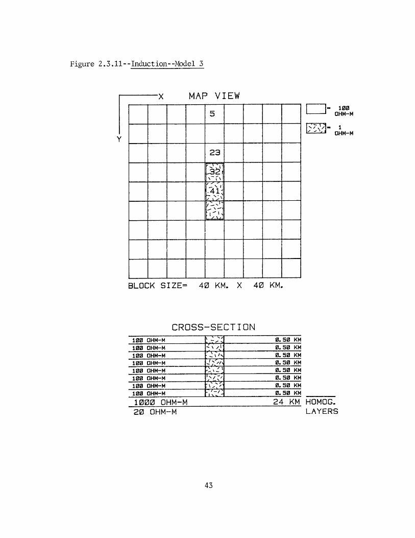
Figure 2.3.11--Induction--Model 3
x MAP VIEW
5
23
j*I
BLOCK SIZE= 40 KM. X 40 KM.
CROSS-SECTION
100 OHM-M 0. 50 KM100 OHM-M 0.50 KM100 OHM-M T0.50 KM100 OHM-M 0.50 KM100 OHM-M -_-_0.50 KM
100 oHM-M 0,.50 KM
100 OHM-M \ 0.50 KM
100 OHM-M 0.50 KM
1000 OHM-M 24 KM20 OHM-M
- 100OHM-M
OHM-M
HOMOG.LAYERS
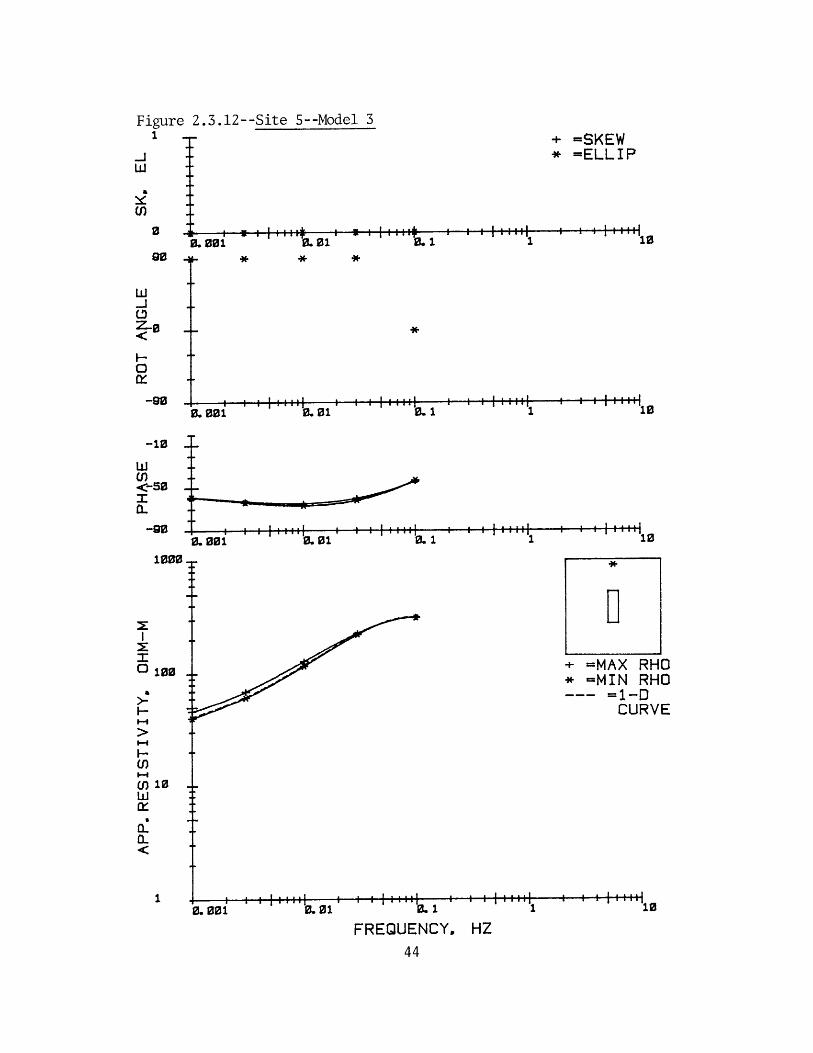
Figure 2.3.12--Site 5--Model 31 -E + =SKEW
* =ELLIP
90
.J00
w0Z-0
0
0.01 0.
I . .. .I*11 10
- - -- I ~ I........................ I
-I I illitill I 11111111 I IIiiti:i0.1
10
10
+ =MAX RHO* =MIN RHO
=1-DCURVE
FREQUENCY, HZ
&. 001i i ii a i i iR i m 1-1 .
0.001
-90
-10
U)<-50
-90
1000
L- 100
U)
U) 10
1
i 2 a i 2 4, a a I - - - - A i i a I . . . . I
IIL 01
I'0.01
Fivre 2.3.13--Site 5--Model 3-- + =SKEW
- =ELLIP
0.01 0. 1* * *
.
0. 01 0. 1
0
90
w-J
z7- 0
0
-90
-10
w(n<-50m(L
-90
1000
.I 1
I . -. .
1
I .. .. I
.1
10
I .. .. I
10
*1 10
+ =MAX RHO* =MIN RHO
=1-DCURVE
FREQUENCY. HZ
.;; 0::
0. 001I.
E. 001
. 001
100
a.
1-4
0
1d
.
' ' . I . . . . I
, , '' ' o'0. 1
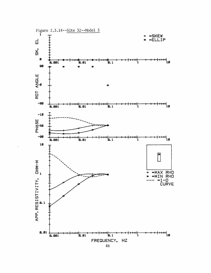
Figure 2.3.14--Site 32--Model 3
+ =SKEW- =ELLIP
.T.0 -- - ---- s a f
*"ro *lba 1
-I I 11111111 I iii:::::0.01 1.0. 1
- -. -
.1 ... I.......I
1
10
10
SI.......I
0.0 0". 1 1 10
w
00-
-90
-10
wU)<-50
0-90
10
U)
I-
() 0.1w
0.
0.01
FREQUENCY, HZ
0.001i
0. 001
0~.001
+ =MAX RHO- =MIN RHO
=1-0CURVE
I . . . . I
I - . - - I
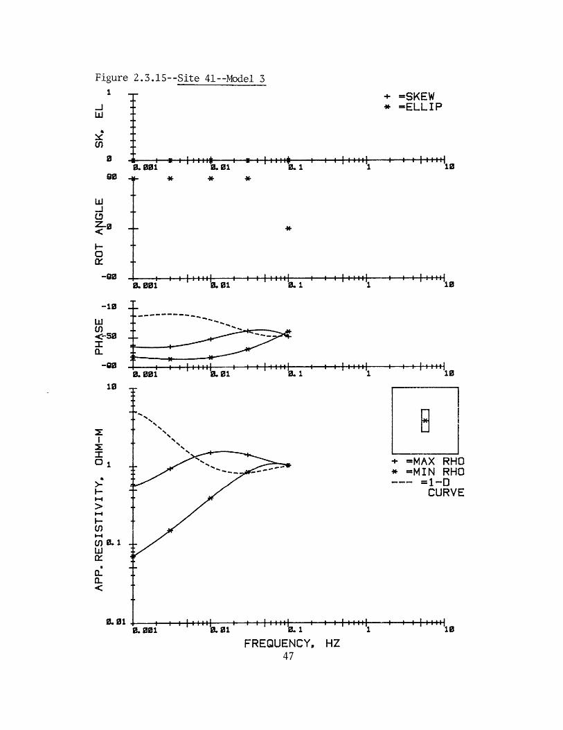
Figure 2.3.15--Site 41--Model 3
+ =SKEW* =ELLIP
0 1-+0. 001
-900.001
g.,.;J; ; 1 ; * ; , , ,
0. 01 0. 1
I .. . .I
0. 01
! a 6 o a I ii i1 10
I .... I..............I
.. 1 110
..................0.1 . 1 10
=MAX RHO*= MIN RHO
=1-DCURVE
FREQUENCY, HZ47
--------- .%. .
.-. . . .
0.001
-10
wU)<-50I(.
-90
10
U,)
0.1w
(-
0.01
I . . . A t . . . A.
A - - -1
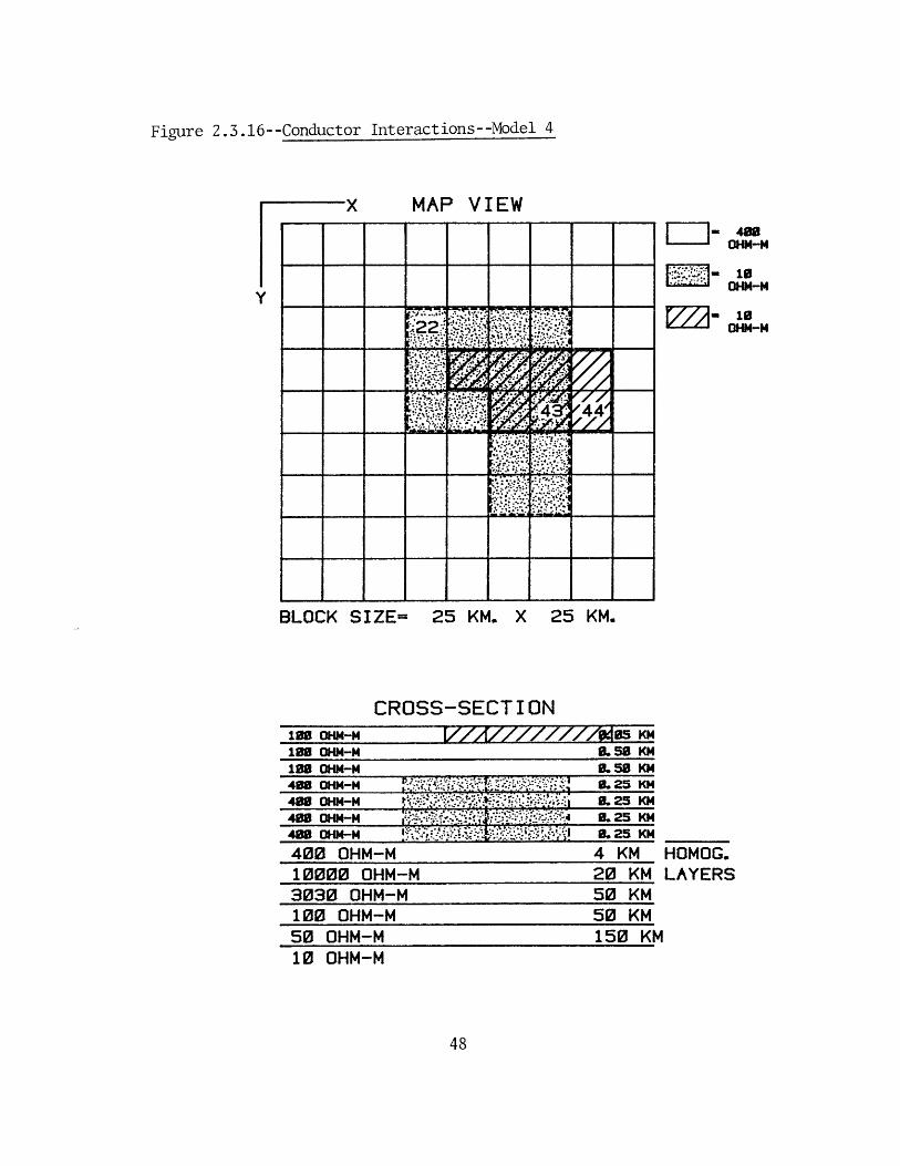
Figure 2.3.16--Conductor Interactions--Model 4
- 400OHM-M
.br-10....'OHM-M
= 10OHM-M
BLOCK SIZE= 25 KM. X 25 KM.
CROSS-SECTION
VJA/777ZI/i' 05 KM0.50 KM9.50 KM
I-:E:' ...: . . .'.*I8. 25 KM
-. ..-.... . -. i. 25KM
. -4 0.25 KMS0. 25 KM
400 OHM-M10000 OHM-M3030 OHM-M100 OHM-M50 OHM-M10 OHM-M
4 KM HOMOG.20 KM LAYERS50 KM50 KM150 KM
MAP VIEW
100 oHM-M100 GHM-M100 OHM-M408 OHM-M400 OHM-M400 OHM-M400 OHM-M
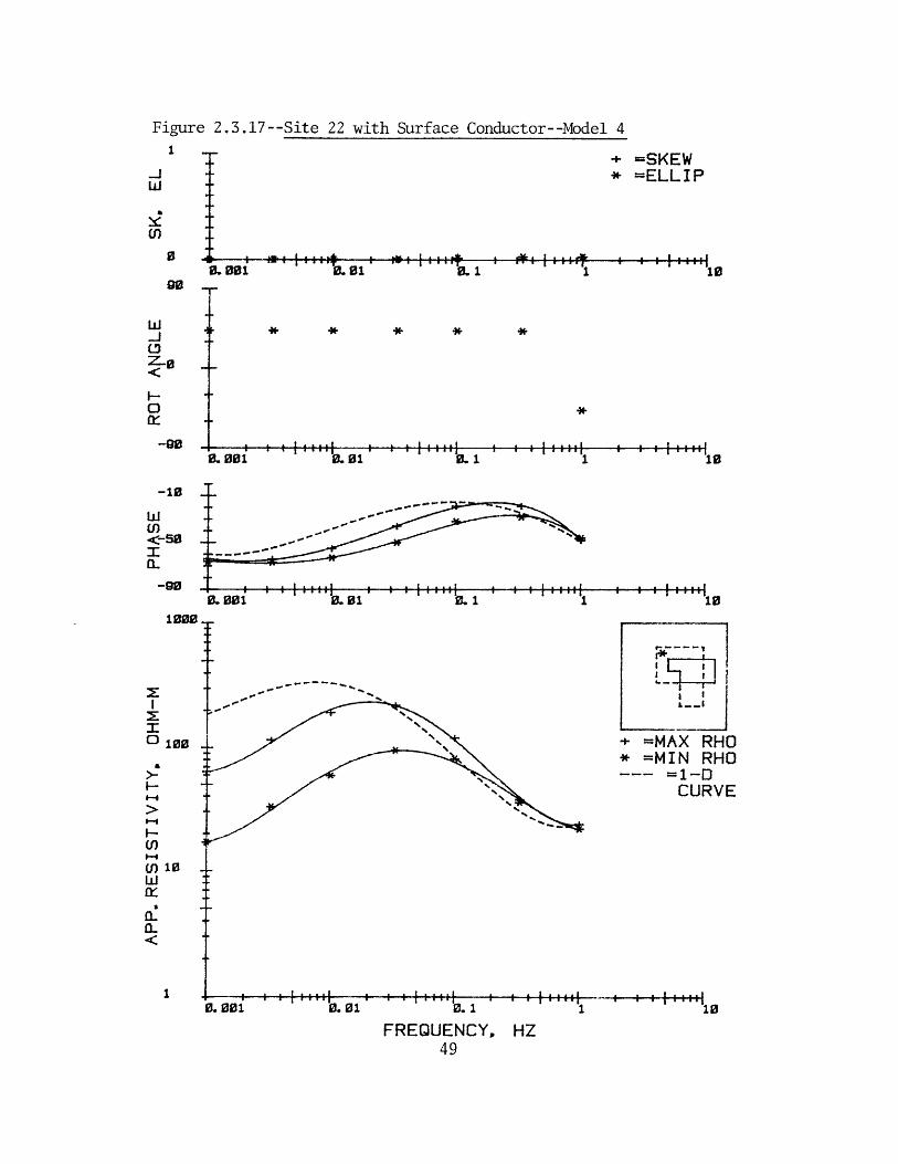
Figure 2.3.17--Site 22 with Surface Conductor--Model 4
+ =SKEW* =ELLIP
- - - TI - - --* 1. - - - - - --*.A0
1
UI)
90
.0-0
0
z-s1
-90
-10
w(I)<-so
fL-90
1000
I .. .. I I . -. -I
0.01 SI
I .. .. f
0.01 0. 1
10
I .. .. I
------------------'1 10
+ =MAX RHO* =MIN RHO
=1-DCURVE
0.001
FREQUENCY, HZ49
0. 001
I .. .. f
. 001 I
. .I
I. * * * * *
100
U10a
I-.
1)1
0. 00i
-W. -. v-.-. f .- . I - - - -I&
, - -' --.
I . . . I
0. 1m
I . . . . I
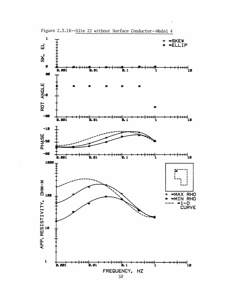
Figure 2.3.18--Site 22 without Surface Conductor--Model 4
+ -SKEW* -ELL IP
.bo a..-..... T
I. * * * * *
............ 1
10
I II I
a...
+ -MAX RHO* -MIN RHO
-1-0CURVE
FREQUENCY, HZ50
0.001 '12
I . . .. I
..01I .. .. I I .. .. I
.oui
0.001
I .. . .I
'10
t.. .5
w
7-0
..g
-10
wU)
-50
1000
o 100
I-
I-4
mi
a.(.)10
m i m A m s . . . . . . . A
i i i i i i i i i i - - - - - - -
. a " I I " 11
. - . . I
, .1 a. . . 6
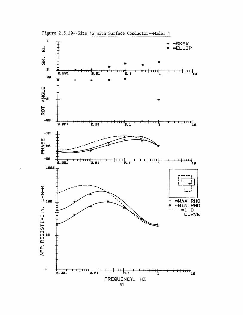
Figure 2.3.19--Site 43 with Surface Conductor--Model 4
1
-jw
U)
0
90
w
z- 0
F-0
-90
-10
wUI)<-50
-90
1000
+ =SKEW* =ELLIP
*. I 1 - a .... I
0. 01 'k.1 a......................1 's10
I-- - - - - - - - - 1,
. .. .. . ......-
'"10
10
+ =MAX RHO* -MIN RHO
=1-0CURVE
FREQUENCY, HZ
IL 00i
B. 001
0. 00i
0.01------------0.1-a * .. ;::;~ ::aa:ii a WIIIIIII i a aiaiaai
100
() 10
0..
1
0 - ---Ik. 01 g. 1
I . - - I.
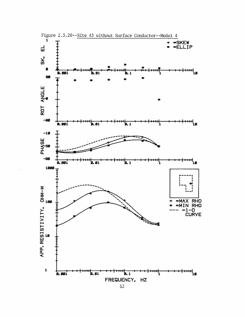
Figure 2.3.20--Site 43 without Surface Conductor--Model 4+ -SKEW* -ELLIP
*:~.
1L * *
esU)
0
0
---to
0.
-90
-113
wU)<-58XCL
I . -...
I.. .I.. . . . . . .1
................. I ......................... 3
.p 3
1 I
-
.~~.01........~~..........10. . .... . . . , .... I . . . , .... 'is
'10
I I I II II10I
+ -MAX RHO* -MIN RHO
=1-DCURVE
FREQUENCY, HZ
.1
1.30I........ "I1..........
LI isa
U)
Wa(Y.
1.
L 081
* - -+
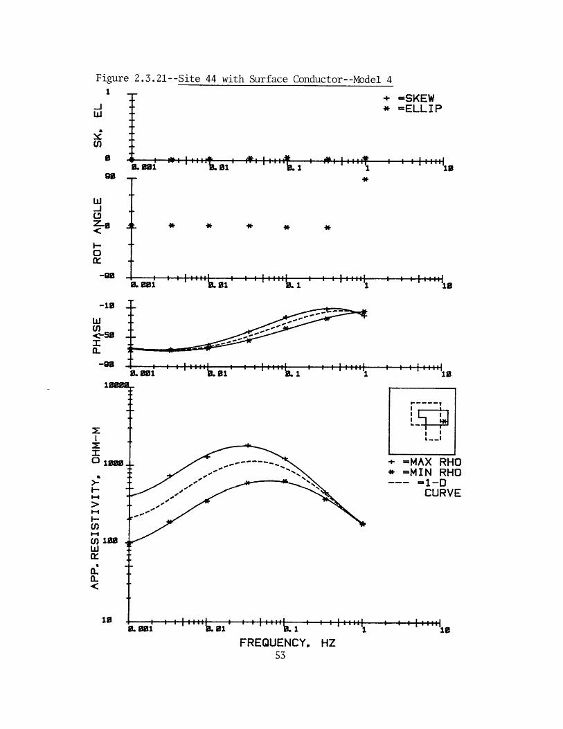
Figure 2.3.21--Site 44 with Surface Conductor--Model 41
8. 01
+ =SKEWS=ELLIP
Frii- I .milT- I I *-11111149 IL a a - I I1 .," 1
* * * * *
-.... I
B.081 .. 81
I ....
1 .1
I - ..
-.01
.A.A
1
1
- - -. I r
18
+ =MAX RHO* -MIN RHO
CURVE
FREQUENCY, HZ
w.J
z-8
0
-0
-1
ws)
<-58X(L
a-98
10881
W108
ix
01
is
1 - - - A
.1 " " I
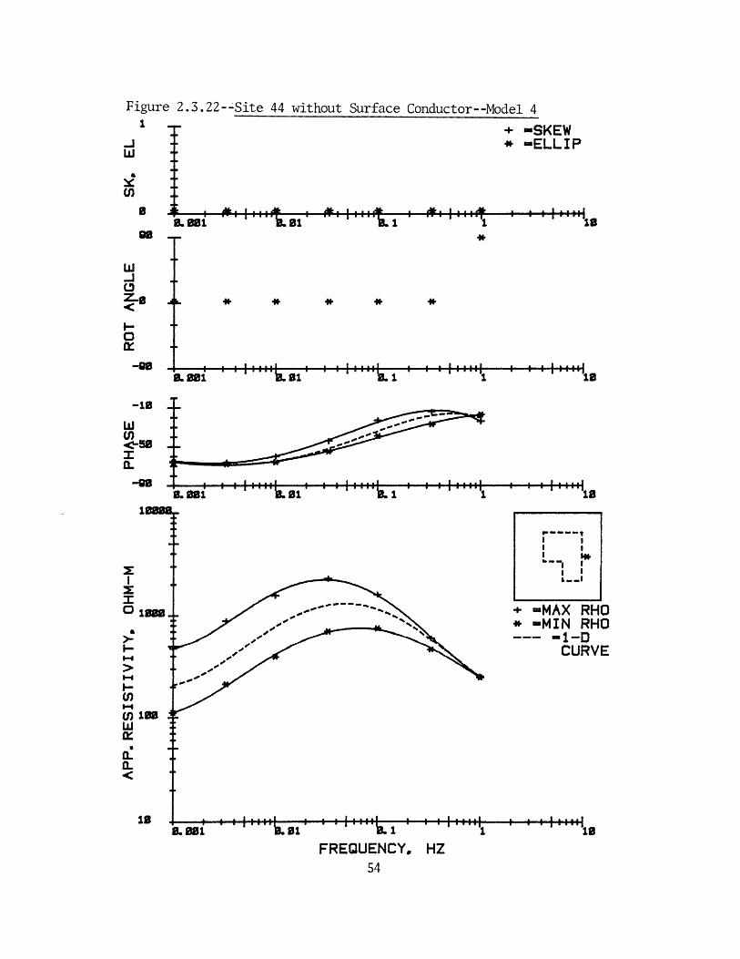
Figure 2.3.22--Site 44 without Surface Conductor--Model 41
+ -SKEWJ T * -ELLIP
.....................................I
------------------------------------------'1*
--------- * 1-- -- -'
10
10
- - - -
- a'* -
.............................. I . .. I.... I
" ' .................. is
w
-la
-ee
-.
C
-e
-10
(I)I
1.0
Q.
W
CL
FREQUENCY, HZ
L -i
* * * *
-t I 11111IT.0
(n0
+ -MAX RHO* -MIN RHO
-1-0CURVE
.- I
0.a001 -at. - v e we- - f 7 w
AIT. I . . .. A1T AAT. i . . A& Ade. i . . .. 41e
, T T Tl a , " .I 1
Tee ci IL al
' W.:
2.4 Minimum Phase
One of the questions that can be examined now is
whether MT responses from 3-D structures are minimum phase
responses. Minimum phase responses are those responses in
which the magnitude and phase are related. Given one, the
other can be derived from it. Boehl, et. al. (1977) have
discussed estimates of the MT tensor impedance using
electric and magnetic field measurements. They concluded
that the magnitudes of the tensor elements were susceptible
to measurement noise, but the chases were not. They
suggested using the phase estimates to smooth the magnitude
estimates and thus eliminate some of the noise problems.
Their work, however, was done under the assumption of 1-D or
2-D structures.
The Transverse Electric (TE) and Transverse Magnetic
(TM) modes decouple for 1-D and 2-D structures along the
principle axes of the medium, giving an impedance tensor
SZxy(o)0(x)= (2.4.1)
zyx(W) 0
It is thus sufficient to look at the minimum phase
properties of a scalar function, Zxy or Zyx (Boehl, et. al.,
1977). There is no set of principal axes along which this
decoupling occurs for general 3-D bodies. We will always
have a full tensor. It is therefore necessary to examine
the minimum phase properties of a tensor function, Z. If
we regard Z as a multichannel filter, then one property of a
minimum phase filter is that its inverse is stable (i.e.,
its Fourier transform exists) and causal (Robinson, 1966).
The inverse of Z(w) is
[yy -Zxy]
Z- 1()= -Zyx Zxx (2.4.2)
det Z
We assume that Z(w) is causal and stable, so Zxx, Zxy, Zyx,
and Zyy are also. The questions of stability and causality
for Z~ are thus dependent upon the properties of 1/det Z
(Robinson, 1966). We have now reduced the problem to the
examination of a scalar function, 1/det Z. We assume for
the moment that 1/det 7 is stable and causal. This function
is the inverse of a filter given hy det Z, hovever. Det Z
must be a minimum phase function for our assumption to be
true. If det Z is a minimum phase function, then Z(w) is
also.
The magnitude and phase of det Z will be related
through a Hilbert transform pair if the function is minimum
phase (Oppenheim and Shaefer, 1975). This transform pair
lnIdetZ(w)|I= 1f det Z (' dw'IT __ __ __ _
tdet Z (M) =1 f lnjdetZ(w')I dw'
T WdW
Boehl, et. al. (1977) show that these equations can be
modified to give the following relationship
d(lnldetZ|)
d(lnw) nw 0
2 2fd(lndetZ|) _d(lnldetZI)T2 d(lnw) lnwo d(inw) In
ln[coth ( lnw-lnwO )J]d(lnw)2
2- OdetZ(ln wO)
+
(2.4.5)
We will use
whether the
(2.4.5).
The mod
The results
2.4.2.
the method of Boehl, et. al.
phase and magnitude of det Z
el used for this test is sho
of the test are shown in Fig
(1977) to test
are related through
wn in Figure 2.3.16.
ures 2.4.1 and
57
(2.4.3)
(2.4.4)
An apparent 'resistivity' has been computed for plotting
purposes and is
' PA' =Idet Zl/(wu) (2.4.6)
The phase plotted is one-half of the phase of det Z. Figure
2.4.1 presents comparisons for two sites above the buried
conductor, and Figure 2.4.2 shows comparisons for two sites
outside. The phases shown in the top halves of Figures
2.4.1 and 2.4.2 are taken directly from the modelling
program. We predict the magnitude of det Z from these
phases using the Hilbert transform relation (equation
(2.4.5)). The apparent 'resistivities' in the lower halves
of the figures are the comparisons between the actual and
predicted values. The curves represent the predicted
values, while the symbols are the actual values. The
agreement between the predicted and actual values of |det ZI
is excellent. Many other sites were tested, and the maximum
RMS error in apparent 'resistivity' was 4.6% (Site 33,
Figure 2.4.2). A 1-D model was similarly tested, and the
RMS error was 2.11. Minimum phase responses were observed
all sites tested, within the limits of numerical accuracy.
The results of our test strongly suggest that the MT
response from 3-D structures is a minimum phase response,
although they do not conclusively prove it for all 3-D
58
bodies.
59
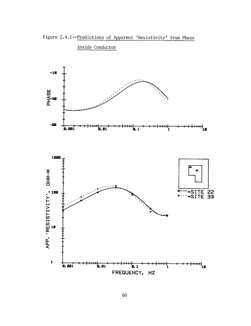
Figure 2.4.1--Predictions of Apparent 'Resistivity' from Phase
inside Conductor
1 : a - - Ia a - -m -- . . .m .. ,A
. I I *
4.
.4.
4.
.I .
"*=SITE 22+'' =SITE 33
I-. . . . . . . . . . . . . . .1a~a 1 1 ma0.081 FQ01 U.E I
FREQUENCY,.la
HZ
-11 ..
w
-90
0. 001
10a0..
O0
also
U)
W 13a:
0..
1
, "k. i
A . . . . I
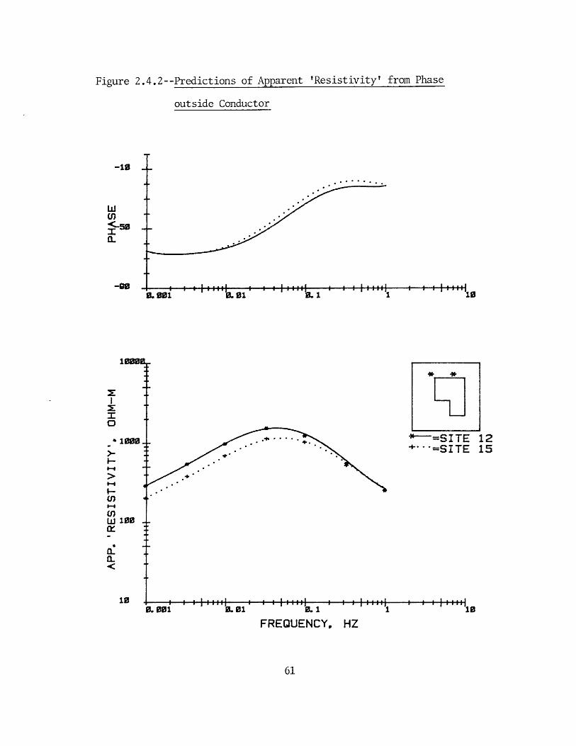
'Resistivity' from PhaseFigure 2.4.2--Predictions of Apparent
outside Conductor
0--'.01 "0.1 1 1
1215
*-=SITES=SI TE
. 01 .0. 1
FREQUENCY,
i.S1
HZ'10
IL 001-E~ ~~~ a 111 ~ iu
-10
w
-0~
-0
10000
- 1000
I--
W 100
0.001
1s
I - - - - I
2.5 Summary
We have developed a practical 3-D modelling algorithm
in this chapter and used it to gain insight into field
behavior around complicated structures. We extend
Ranganayaki's generalized thin sheet analysis (1978) to
allow us to stack heterogeneous thin layers. Methods of
Fourier analysis are used to formulate the solution, but
this restricts us to spatially repeating models.
Electric fields near complicated structures are locally
perturhed by three different mechanisms at low frequencies.
Horizontal and vertical current gathering are important for
heterogeneities with modest resistivity contrasts compared
to the surrounding medium. These mechanisms perturb fields
in a DC manner-- i.e., the effect has the same magnitude at
any low frequency. Induction of current loops is the
dominant mechanism in conductive heterogeneities (1 Q-m).
This mechanism is frequency-dependent, so it is an AC
effect. Each of these mechanisms has a different spatial
and frequency behavior so identification of the dominant
contribution is important. Appendix B outlines procedures
for this indentification.
We finally presented evidence, albeit empirical, that
the phase and magnitude of the impedance tensor are related
through a Hilhert transform pair. The earth response is
minimum phase even though the conductivity structure is
complicated.
62
'To stop at that which is beyond understanding is
indeed a high attainment.'
Ancient Chinese Philosopher
CHAPTER 3
3.1 Introduction
We outline a method for setting up the inverse problem
in this section. The inverse problem is derived for the
type of model in Chapter 2, which includes the repetition
assumption. We perform a perturbation analysis on the
'normal' problem (equations (2.2.9) and (2.2.10)) to get the
relationship between field changes and conductivity pertur-
bations. The conductivity perturbations appear as effective
'sources' for the normal problem. We can thus solve the
problem with 'sources' if we find the associated Green's
function. We want a Green's function relating field changes
at the surface to 'sources' at depth. This desired Green's
function for the normal problem (Dv=6) is related to the
Green's function for the adjoint problem (Du=y) through the
generalized reciprocal relation (Lanczos, 1956). The
reciprocity relation will be rederived here. Finally, we
show how to compute the Green's function numerically for our
problem.
This inverse problem was not programmed because of time
limitations, but we show how this method agrees with
linearized inverson theory for a 1-D model. Extensive work
63
is needed with this 3-D inversion and synthetic data to
answer the questions of uniqueness and resolution. These
tests must be performed before applying the inversion
actual data.
64
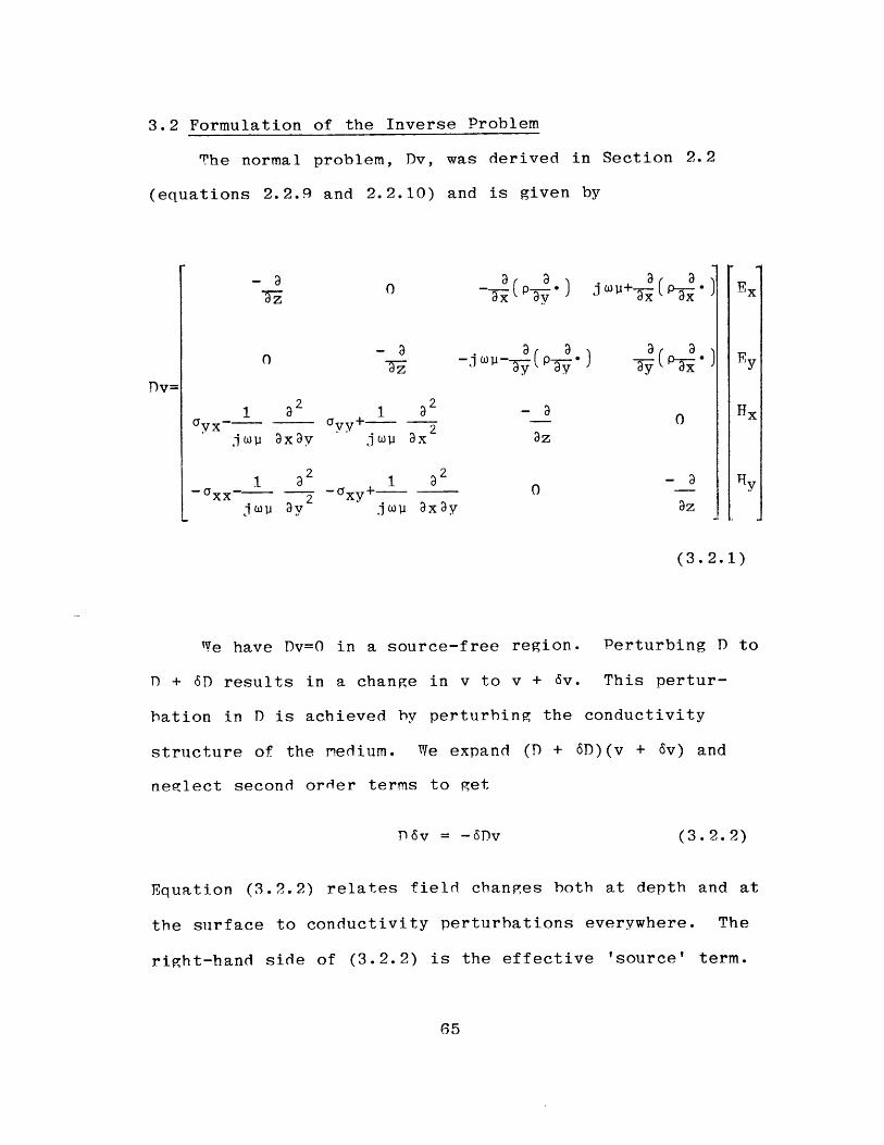
3.2 Formulation of the Inverse Problem
The normal problem, Dv, was derived in Section 2.2
(equations 2.2.9 and 2.2.10) and is given by
0 0~ 3j-(p 3.) W1 -
jo aay o x z
1 2 1 2 03a-a + 0jo ay joyj ax~y 2z
(3.2.1)
We have Dv=0 in a source-free region. Perturbing D to
D + 6D results in a change in v to v + Sv. This pertur-
bation in D is achieved by perturbing the conductivity
structure of the medium. We expand (D + 6D)(v + 6v) and
neglect second order terms to get
D6v = -6Dv (3.2.2)
Equation (3.2.2) relates field changes both at depth and at
the surface to conductivity perturbations everywhere. The
right-hand side of (3.2.2) is the effective 'source' term.
65
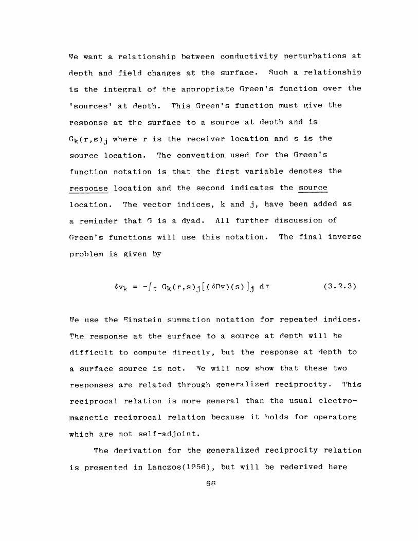
We want a relationship between conductivity perturbations at
depth and field changes at the surface. Such a relationship
is the integral of the appropriate Green's function over the
'sources' at depth. This Green's function must give the
response at the surface to a source at depth and is
Gk(r,s)j where r is the receiver location and s is the
source location. The convention used for the Green's
function notation is that the first variable denotes the
response location and the second indicates the source
location. The vector indices, k and j, have been added as
a reminder that G is a dyad. All further discussion of
Green's functions will use this notation. The final inverse
problem is given by
Svk = -fT Gk(r,s)j[(6Dv)(s)]j dT (3.2.3)
We use the Einstein summation notation for repeated indices.
The response at the surface to a source at depth will be
difficult to compute directly, but the response at depth to
a surface source is not. We will now show that these two
responses are related through generalized reciprocity. This
reciprocal relation is more general than the usual electro-
magnetic reciprocal relation because it holds for operators
which are not self-adjoint.
The derivation for the generalized reciprocity relation
is presented in Lanczos(1956), but will be rederived here
6r,
for completeness. The normal and adjoint problems are
Dvk(x)=6j(x) (3.2.4)
DUj(x)=Yk(x) (3.2.5)
where D is jxk and D is kxj. The tilde denotes the
Hermetian of D (complex conjugate transpose of D), following
Lanczos (1956). We know the solution to the normal problem
is given by
V
vk(r) = fs ) [Gk(rs)j-aj(s)] ds (3.2.6)j=1
where G is the solution to DG=6j, and the integration is
performed over all sources. We now derive an alternate ex-
pression for vk(r) through the bilinear identity. This
identity is
fT (u*Dv-v(Du) ) dT = 0 (3.2.7)
Introducing vector notation, (3.2.7) can be rewritten
fT i uj*(T)Dvk(T) dT = IT I Vk(T)[Dul(T)]* dT (3.2.8)j=1 k=1
becuase both D and D are square, 4x4 operators. We define
Gj(x,s)k to be the Green's function for the adjoint problem,
Djuj = 6k(x,s). G j(x,s)k is not related to Gj(r,s)k
through simple transpose and conjugation operations--it is a
separate operator in general. We substitute Dvk(T) = aj(T),
Duj(T) = Sk(T,s), and uj* (T) = G j(T,s)k into (3.2.8) and
get
4 4
f t T, T)] dT = fT vk(T) 6 *k(T,s) d T (3.2.)j1=1 k=1
We integrate (3.2.P) through the delta function and get
Vk(s) = f T [*j( T,s)kj( T) ] dTj=1
(3.2.10)
Making the variable substitutions sEr and TES into (3.2.10),
we get another expression for vk(s) in terms of the Green's
function for the adjoint problem
4
vk(r) = fs Gj(s,r)k0j(s) ds (3.2.11)j=1
We equate equations (3.2.6) and (3.2.11) term by term to get
the generalized reciprocal relation
Gk(r,s)j = *j(sr)k (3.2.12)
Let us put sources at depth and receivers at the
surface. This reciprocal relation says that the kth
response coefficient at the surface to the jth source
component at depth in the normal problem is related to the
jth response component at depth to the kth source component
at the surface for the adjoint problem. The next step is to
determine the Green's function for the adjoint problem. We
will show that G* is easily derived from the solution to the
normal problem through a change of variables.
We now derive the adjoint operator and the associated
boundary terms. The principle behind this exercise is to
make the left-hand side of the bilinear identity (3.2.7)
a perfect differential.
This perfect differential is
u*Dv-v(Du)* = 3Fi(u*,v)/ 3 xii=1
(3.2.13)
where D is the adjoint operator and the right-hand side is
the associated boundary term. Lanczos (1956) outlines the
procedure for computing D and the boundary term from D. We
have three types of terms in Dv:
I. No derivative - Av (A is a scalar)
u*Av-vAu* = 0 (3.2.14)
so D= A and 3Fi(u*,v)/axi = 0
3vII. First Derivative - A
(3.2.15)u*A av- (-v a (Au*)) = (u*Av)Txi 3xi 3xi
so = -3 -(A- ) and Fi(u*,v) = u*Av
23 vIII. Second Derivative - A xiax1
a2 2 a 2 (* av a 3ul*A 2v -v (Au*) = - (u*A-3v-_ 3 (v (Au*)
aXi3xj ax 1xj -xi axa (xu x
(3.2.16)
aa2so Dl* = a 1 x1 (A-
term is -
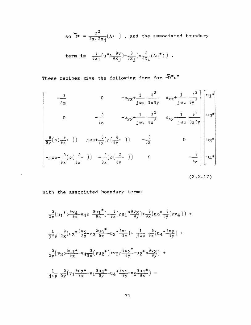
These recipes give
, and the associated boundary
Aa3xT.1
the following form for -D* *-D u
az
1 a2
-ayy+ 1 ajW ax3y
-~ C
13
1axx +
11
joy
ax-(p(ax 3y
a2
ay2
a2
ax ay
(3.2.17)
with the associated boundary terms
(u1*p A-v4P )-3ax 3 ax
1 (3 av 2 3U3
- v30' g-v4U-(PU2 )
(pu1i )+ (u2* (pv4)) +
*3vi 1 a(*av 2y)+ - (u4* g ) +
au* *Say -u2*
av3p ay
1 3uq u* au4*- *jopl Tay 13x +vi ' -- v2 as )
3z
0
ax
ul*
u2*
U3*
U4*ax 3z
3x- 3xt.i(Au)
3(u*v1+u2*v2 +u3 * 3 +u4*v4 ) (3. 2.18)
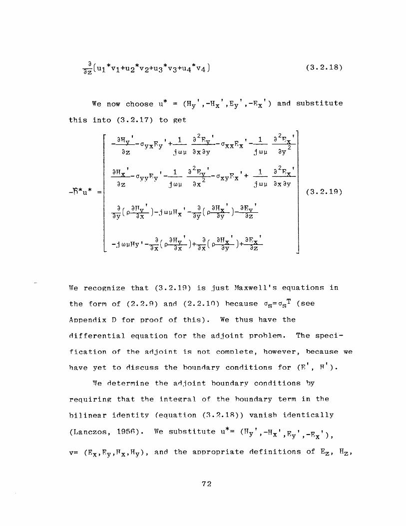
We now choose u* = (Hy , -H' , Ey , -Ex ' ) and substitute
this into (3.2.17) to get
- aY -yx y + a axxE - - a2x3z joy 3xay joy 3y2
S ' a 2 2_ t 1 2
X- -yy -__ Y -arxy +3z jW1 ax 2joy axay
u= (3.2.19)
(pa )-joy '-_ (p x I)_3~~PJj W I, TT (Pay >a z
3 a3H ' n @HX + 3EI-joyHy' -- ag(P ) )+ gz
We recognize that (3.2.19) is just Maxwell's equations in
the form of (2.2.9) and (2.2.10) because as=asT (see
Appendix D for proof of this). We thus have the
differential equation for the adjoint problem. The speci-
fication of the adjoint is not comnlete, however, because we
have yet to discuss the boundary conditions for (F', H).
We determine the adjoint boundary conditions by
requiring that the integral of the boundary term in the
bilinear identity (equation (3.2.19)) vanish identically
(Lanczos, 1956). We substitute u*= (Hy , Hx' ,Ey' , I ' ),
v= (Ex, Fy, x,Hy), and the appropriate definitions of Ez, Hz,
72
Fz', and Hzf into (3.2.18) to get
3
fT i 1 i i(u*,v) dT= f V-('xH-TxH' ) d T (3.2.21)
Our goal, then, will be to determine the boundary conditions
which force the integral in (3.2.21) to vanish. We also
choose these boundary conditions so that the form of the
adjoint problem is identical to that of the normal problem.
We then have the adjoint solution if we solve the normal
problem and reorder the normal solution vector (from v to
u*)u* ).
The volume integral in (3.2.21) can be transformed into
an integral over the surface enclosing the volume via
Gauss' law. The volume of interest encloses the current
sheet at the surface, the heterogeneous crust, and the
mantle structure beneath the crust. This volume is shown in
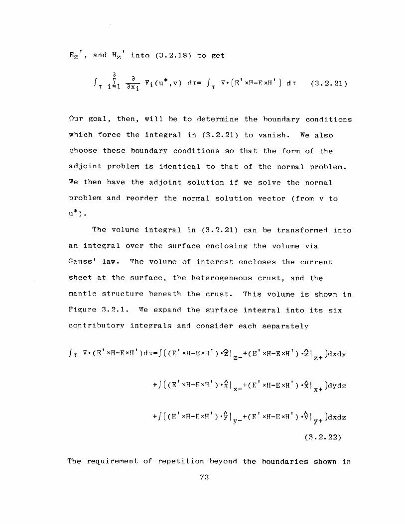
Figure 3.2.1. We expand the surface integral into its six
contributory integrals and consider each separately
fI V.(E'xH-ExH')dT=f(('xH-ExH')-z Iz-+(E'xH-ExH') -zz+)dxdy
+f((E'xH-Exu')-x| _+(E'xH-ExH')-x x+)dydz
+f(( 'xH-xH')9| +(E'xH-ExH')-yly+,)dxdz
(3.2.22)
The requirement of repetition beyond the boundaries shown in
73
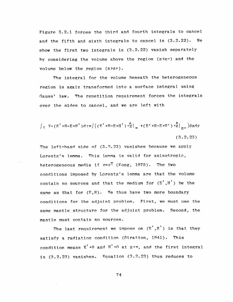
Figure 3.2.1 forces the third and fourth integrals to cancel
and the fifth and sixth integrals to cancel in (3.2.22). We
show the first two integrals in (3.2.22) vanish separately
by considering the volume above the region (z~z-) and the
volume below the region (z>z+).
The integral for the volume beneath the heterogeneous
region is again transformed into a surface integral using
Gauss' law. The repetition requirement forces the integrals
over the sides to cancel, and we are left with
f V-(F'xH-Ex')dTI=f((E'xH-ExH')z| +(E'xH-Ex')-zI z-)dxdv
(3.2.23)
The left-hand side of (3.2.23) vanishes because we apply
Lorentz's lemma. This lemma is valid for anisotropic,
heterogeneous media if a=aT (Kong, 1975). The two
conditions imposed by Lorentz's lemma are that the volume
contain no sources and that the medium for (E',H') be the
same as that for (F,H). We thus have two more boundary
conditions for the adjoint problem. First, we must use the
same mantle structure for the adjoint problem. Second, the
mantle must contain no sources.
The last requirement we impose on (E',H') is that they
satisfy a radiation condition (Stratton, 1941). This
condition means E'+0 and H'+0 at z+w, and the first integral
in (3.2.23) vanishes. Equation (3.2.23) thus reduces to
74
f (E'xrT-ExH')-lz-dxdy = 0
We can use the same arguments for the volume above the
heterogeneous region to show that
Af (E'xII-7x-x')-zz+ dxdy = 0 (3.2.25)
These arguments require that there he no sources in the air,
that the air have some conductivity (so that the radiation
condition is satisfied), and that the air for the adjoint
problem be identical to that for the normal problem. We
substitute (3.2.24) and (3.2.25) into (3.2.22) and get
f, V-(E'xH-EXH') dT = 0 (3.2.26)
as was desired.
We have derived the adjoint boundary conditions by
requiring that (3.2.22) vanish. The boundary conditions are
as follows: the media above and below the heterogeneous
region are the same as for the normal problem; the model
repeats itself; the only sources are within the
heterogeneous region; and that the adjoint solution satisfy
radiation conditions. We further require that the sources
be located in a current sheet at the surface. This last
(3.2.24)
specification completes the process of making the adjoint
problem identical to the normal one.
We have now shown that we can get the adjoint solution
from the normal solution merely by reordering the solution
terms. Our numerical method for solving Dv=8 generates
basis vectors from which all possible solutions may be
generated. We can put delta function sources at the surface
receiver points, solve for the surface fields, and downward
continue those fields to depth at the source (= conductivity
perturbation) locations. The Green's function for the
normal problem giving the response at depth due to a surface
point source is thus generated. We rearrange terms to get
the adjoint operator's Green's function for the response at
depth to a surface point source. This function is equal to
the Green's function for the normal problem giving the
response at the surface due to a source at depth by
generalized reciprocity. The desired Green's function for
the inverse problem can thus be derived.
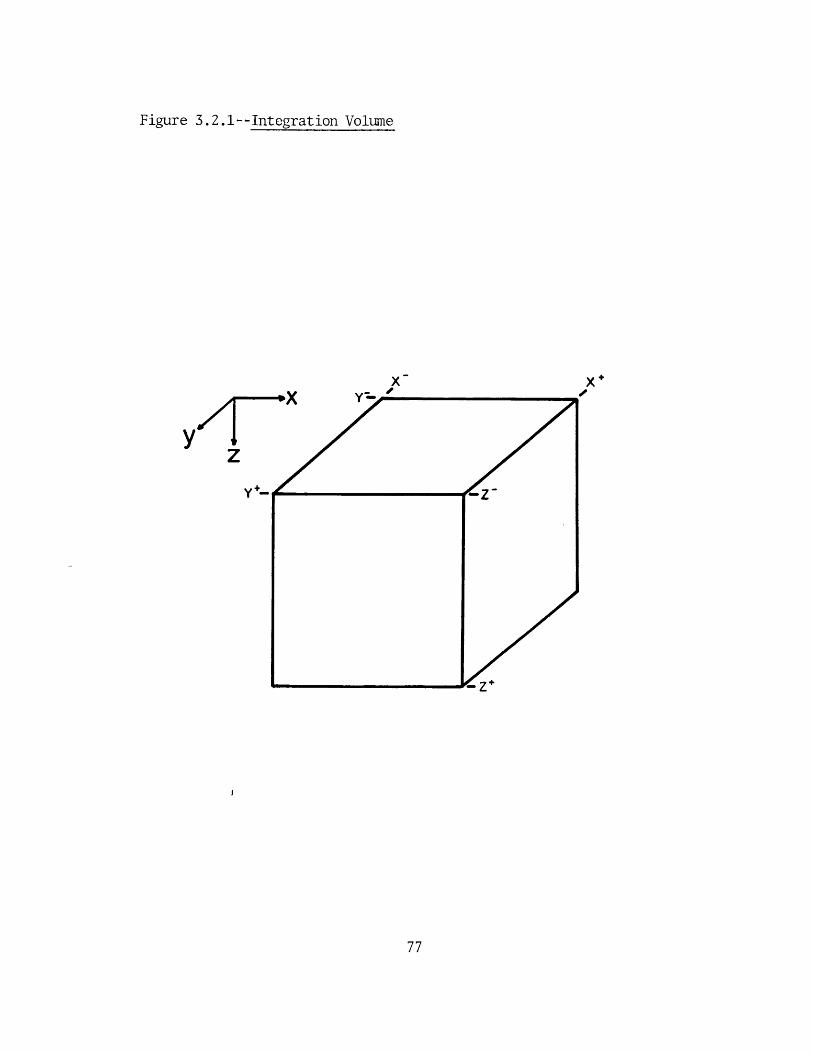
Figure 3.2.1--Integration Volume
xX Y~
Zzy
p-V.
2
3.3 Comparison to a Simple 1-D Inversion
We now apply this inverse technique to a simple nroblem
to show that it does indeed work. The problem is a 1-D
problem consisting of a layer over a halfspace (see Figure
3.3.1). We have chosen this example because we can compare
analytical results for the two different approaches to the
inverse problem and show that they are identical.
The two possible polarizations (Ex-Hy and Ey-Hx) de-
couple for the 1-D problem if we assume no x or y dependence
in the fields and use uniform current sheet sources. We
will work with just the Ey-THx polarization. The decoupled
1-D equations for Ey and Hx are
3z x (3.3.1)
3__ = -a (3.3.2)3z
We use the continuity of tangential fields at the interfaces
at z=O and z=d as a boundary condition, and our source at
the surface is a uniform current sheet in the y direction.
The source condition is thus Hx=Jy at z=0. The fields in
the layer and the halfspace are given by
Eyi(z) = -
Jy (1+k2 )exp (-jktd)cos(kiz)
jkl ksin(kid) - ,cos(kid)
+ Jyj exp(-jkiz)
(3.3.3)
Jy (1+k )jexp(-jkid)sin(kiz)
jsin(kid) - 2 cos(kd)kIcskd
- Jyexp(-jkiz)
(3.3.4)
Ey 2 (z) = -(1+F- )cos(kid)exp(-jkid-jk2d)
Jsin(kid) - !cos(kid)exp(jk 2 z)
+ Jyexp(jk2z-jkid-jk2d) (3.3.5)
T1X2(z) = (3.3.6)
where kj = (1+j)-/(wvaj/2) and k 2 = (1+j)-V(wIJo2 /2).
We are interested in the sensitivity of Ey at the
surface to changes in the halfspace conductivity, a2 -
Specifically, what is the change in Ev due to a change in
G2? We will first derive this sensitivity using our
generalized reciprocity approach in the previous section
and then compare it to the result from linearized inversion.
79
EYV2(z)
Dv and D*u* for this problem are
Dv =
Du =
0 0 jwy
0 -a -jwl 0
-
- a
0 a-
-3
0 joyiJ
-jWl
Perturbation analysis (equation
[ =FD)-
-3
-
0 -a
(3.2.2))
0
EY A a
EX Aac
gives
We now consider the bilinear identity
source for the adjoint problem. This
for DAv to give us the
identity is
Ex
Ey
Hy
(3.3.7)
(3.3.8)
(3.3.9)
f r [u*DAv - (Av)-(' 3u)*] dT = 0
We want to consider the surface AEy component of
(3.3.10)
Av only, so
('Du)* must be (0, -J 6 (z-0) 9 0, 0). Note that we choose the
same source as in the normal problem. The Green's function
for this problem is given
ff(-JyAEy)
by G j(r,0) 2 ,
dxdy = ffdxdyf
and (3.3.10)
G*j(r,0)2(DAv)
reduces
dz (3.3.11)
If we just equate the kernels of the surface integrals,
(3.3.11) hecomes
JyAEy = f G*j(r,0)2(DAv)
We know DAv from (3.3.9), so
JyAEy = f[Z'*3(r,0)2(Ey(z)aa(z))-Z*4 (rO)2 (Ex(z)
Ex(z) is zero if
ao(z) )]dz
(3.3.13)
the source is Jy because there is no
cross-coupling in the 1-D problem. Equation
thus
f C*3(r,0)2Ey(z)Aa(z)
then
(3.3.12)
(3.3.13)
-Jy AFy = dz (3.3.14)
G 3 (r,0)2 is the third response component at depth (r) to
the second source component at the surface. We know from
the previous section (equation (3.2.21)) that the third
response component is Ey, and the second source component
is a current sheet in the y direction at the surface. Thus,
G*3(r,0)2 = Ey(z). Substitution of this result into
(3.3.14) yields
-JyAEy = f Ey(z)Ey'(z)Aa(z) dz (3.3.15)
The source for Ey is the same source as for Ey for the 1-D
problem, so Ey'=Ey. We also only want the sensitivity of Ey
at the surface to changes in the halfspace conductivity, so
Aa(z) = Aa2UI(z-d), where U1 is the unit step function. The
sensitivity is thus given by
-JyAEy = Aa2 f Ey2 (z) dz (3.3.16)surface d
We substitute the expression for Ey2(z) given by (3.3.5)
into (3.3.16) and integrate to get
_ Jykgouj
2 a2k 12AEysurface (jsin(kd) - 2cos(kd) 2 Aa2 (3.3.17)
(Jsinkid) kicski)
82
We now derive the same result using linearized
inversion theory. This method assumes that
AEy '= ( ) (3.3.18)
where Ey/3a2 is the partial derivative of (3.3.3) with
respect to G2. This derivative is
_ Jyk 2w
_Ey 2a 2 ki
(CT2) z= 0 = (jsin(kid)- 2cos(k 2d) )2 (3.3.19)
We substitute (3.3.19) into (3.3.18) and compare this result
to (3.3.17). These two expressions are identical, thus
showing that the 3-D inversion scheme reduces to a known
result in the case of a 1-D structure.
- Aa2
3.4 Source Terms for 3-D Inversion
We show that conductivity perturbations are equivalent
to current sources at depth and perform the sensitivity
analysis here. The sensitivity derived in this section is
the surface electric field change due to a conductivity
perturbation at depth. Point sources must be used for 3-D
inversion because fields vary in both the x and y directions
at the surface. This situation is contrasted with that of
the 1-D inversion in the previous section in which uniform
current sheets were used. The analysis of the 3-D problem
cannot be compared to an analytic result because of the
Droblem's complexity, however.
We begin with the integral form of the bilinear
identity, as in the last section. We see that Du must be
(S 1 ,0,0,0) or (0,02,0,0) in order to analyze the changes in
surface electric fields ( because Av=(AExAEy,AHx, AHy)). We
expand D*u*= * into its component equations to determine
what kinds of sources are Si and 02- D*u*=8* is
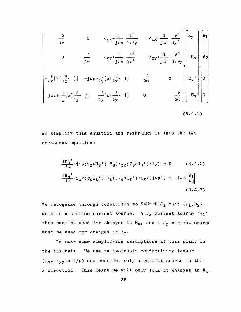
0 1 a2 1 2 H ' 1az joU axay j 1y
a 1 a2 1 320 - ayy+ 2 -Xy+ -Hx' 2
az jou ax j ou 3xay
aa a0E 0
- wi I(p( - l) -- (p( l- )) 0E' 0
jouJ+---(p(-- )) ---(p(--- )) 0 -- -Ex' 0ax ax ax ay az
(3.4.1)
We simplify this equation and rearrange it into the two
component equations
aEs ' +3s +jwl(izxHs')+Vs(pzz(VsxHs')'iz) =0 (3.4.2)
+izx(asEs')-Vs((sxEs')'iz/(j wi)) = i.zX i
(3.4.3)
We recognize through comparison to VxH=aE+Js that (al62)
acts as a surface current source. A Jx current source (f1)
thus must be used for changes in Ex, and a Jy current source
must be used for changes in Ey.
We make some simplifying assumptions at this point in
the analysis. We use an isotropic conductivity tensor
(axx=ayy=a=l/p) and consider only a current source in the
x direction. This means we will only look at changes in Ex.
85
fT u*PAv dT = fT (Av)a* dT
Given that a*= (a1,0,0,0) and Av=(AEx,AEy, AHXAJTy), equation
(3.4.4) reduces to
fT u*DAv dT = f T AEx81 dT (3.4.5)
We want the field change at one point at the surface,
at= Jx6(z)6(x-xo)6(y-yo). Equation (3.4.5) thus becomes
JXAFx(xo,YO,o) = fT u*DAv dT (3.4.6)
where u*=(y', -' , Ey ' , -F ) due to a point current source
at the surface in the x direction. The next step is to
compute DAv through the use of the identity, DAv=-ADv.
We use our assumption of conductivity isotropy and
equation (3.2.1) to Ret
0
0
a
6p -)
0
0
(
Ey
Hy]
3.4.7)
S83
ADv=
-a
(3.4.4)
We perform this matrix multiplication and make use of the
identity from Maxwell's equations that Ez =(V sxs)'z.
Equation (3.4.7) reduces, with these steps, to
PAv = - - a( 6 P apax(3.4.8)
We substitute this expression into (3.4.5) and make use of
the fact that u*= (Hy', -H ',Ey', -x') to arrive at the
change in a surface Ex due to a conductivity perturbation
at depth
JxAEX(xO,yO,0) = -fT [Hy' (6PaEz>-Ix' (SpaEz)] d T -
IT 6Ga (ExEx'+EyEy') dT (3.4.9)
The first integral in (3.4.9) is somewhat confusing, since
it involves derivatives of perturbations. We will thus
reduce this term to a recognizable quantity without any loss
of generality. We use the following identities
4y'-(6PEz) = (Hy'6PaEz) - p4.10a (3.4.10)
TTx'3(6PaEz) = '(Px'6pa~z) - 6payF 3v (3.4.11)
We substitute (3.4.10) and (3.4.11) into (3.4.9), and the
first integral in (3.4.9) becomes
fT [(Hy'6PaEz)~ (Hx'6paEz)) dT - fT6paEz( - ) d T
(3.4.12)
We expand the volume, T, to include an outer region where
there are no conductivity perturbations. The first integral
in (3.4.12) is an integral over the volume of perfect
differentials. This first term will reduce to a surface
integral over surfaces bounding the volume. The volume has
been expanded to include the outer region, however, so 6 p=0
on the surface bounding the volume. The first integral in
(3.4.12) is therefore zero. We again make use of the
Aidentity Ez = (VsxTs)'lz and simplify the second integral
of (3.4.12). Equation (3.4.9) thus reduces to
JxAEX(xO,yO,0) = -fT 60(ExEx'+EyEy' ) dT + fT 6pa 2EzEz' dT
(3.4.13)
We have one integral involving 6a and one involving 6p in
(3.4.13). The relationship between 6p and 6a can be
88
derived by expanding 1/(a+6a) and equating to p+ 6 p. This
procedure yields
6p ~ -6a/c 2 (3.4.14)
We substitute (3.4.14) into (3.4.13) to get the total change
in Ex due to conductivity perturbations
JXAEx(xo,yg,O) = -fT 6a(F-E') dT (3.4.15)
The sensitivity of Ex to a given conductivity perturbation
is
3Ex(xO,ygO) _ E(x,y,z)-E'(x,y,z) (3.4.16)
ao(x,y,z) Jx
Note that E' is the solution to the normal problem with a
delta function source in the x direction at (xo,y0,O), while
E is the solution to the normal problem with a uniform
current sheet.
We see a logical progression in the source complexity
as we move from the 1-D inversion to the 3-D inversion.
Fields vary as a function of depth only in the 1-D problem,
so sources were uniform current sheets. Fields vary as a
function of depth and one horizontal coordinate in the 2-P
problem, so line sources are needed. Point sources are
necessary in the 3-P case because fields are functions of
all three spatial coordinates.
3.5 Summary
We have presented the theoretical groundwork for the 3-D
inversion problem in this chapter. The inversion procedure
is based upon the method of forward modelling in Chapter 2.
We used the adjoint problem solution and generalized
reciprocity theorem (Lanczos, 1956) to determine the surface
field perturbation due to a conductivity change at some
point in the subsurface. We demonstrated that these
conductivity changes at depth in the normal problem are
equivalent to surface current sources for the adjoint
problem. Finally, we compared the 3-D inversion to an
analytic 1-D linearized inversion scheme and shown they are
equivalent.
'But do the data fit with our preconceived notion of
what is going on?'
Geophysics Field Teaching Assistant
CHAPTER 4
4.1 Introduction
We present in this section an interpretation of mag-
netotelluric data from a geothermal area. We use the
insights developed in Chapter 2 to guide our interpretation
of these data. We also use 3-D modelling to examine the
effect of truncating a 2-D body along its strike. We
finally make some recommendations regarding the planning of
an MT survey.
4.2 Geology and Previous Geophysics
The magnetotelluric data were collected in Whirlwind
Valley by Geotronics Corporation for Chevron Resources
Company. These data were released under a joint industry-
Department of Energy exploration program for geothermal
energy. Whirlwind Valley is located in north central
Nevada approximately 30 kilometers due east of Battle
Mountain. Whirlwind Valley is the site of the Beowawe Known
Geothermal Resource Area (KGRA).
Figure 4.2.1 is a generalized geologic map compiled
from Roberts, et. al. (1967) and from Stewart, et. al.
(1977). The following discussion of the geology is also
taken from these two references, unless otherwise indicated.
Nevada was the site of a north-south geosyncline during
the early Paleozoic era. Most of the rocks deposited in
central Nevada were carbonate rocks, while a siliceous and
volcanic assemblage was deposited in western Nevada. The
siliceous assemblage, which included chert, shale,
siltstone, and some volcanic beds, was thrust eastward over
the carbonate assemblage during the Antler orogeny in the
late Paleozoic era. Rocks forming the siliceous assemblage
are shown in Figure 4.2.1 as Paleozoic sediments. The
easternmost evidence of this thrust plate is about 50
kilometers east of Whilrwind Valley.
The next major geologic activity in this area occurred
in the Cenozoic era. The Basin and Range structure now
92
present began developing in the Miocene or Pliocene period.
Concurrently, a NNW trending rift zone developed in the area
(Stewart, et. al., 1975). The eastern edge of this rift
zone is the Dunphy Pass fault zone, which is the NNW
trending fault bisecting Whirlwind Valley (Smith, 1979).
The rift zone is characterized by numerous diabase dikes and
basaltic andesite flows (Stewart, et. al., 1975). The
andesite flows are shown in Figure 4.2.1 as Tertiary
volcanic rocks.
The andesite flows which crop out around Whirlwind
Valley thicken from west to east until the eastern edge of
the rift zone is reached (Smith, 1979). The flows thin
dramatically across the fault to about 100 meters thick
(Smith, 1979). Outcrops of the underlying Paleozoic
sediments can be seen along the southern edge of Whirlwind
Valley east of the Dunphy Pass fault zone. A well drilled
near MT Site 3 (Figure 4.2.2) shows 50 meters of valley fill
over 1.3 kilometers of volcanic rocks (Chevron Resources
Company, 1975). At least 1.5 kilometers of Paleozoic
sediments underly the volcanic flows. The-ENE trending
fault bounding Whirlwind Valley to the south forms the
Malpais rim scarp (Smith, 1979). The valley has been
dropped down relative to the outcrops south of Malpais rim.
Smith (1979) proposes that the Geysers (Figure 4.2.2) occur
near the intersection of the Malpais rim fault and the
Dunphy Pass fault zone because this intersection provides a
93
conduit for hot water to reach the surface.
The Beowawe KGRA has been the subject of many
geophysical investigations, so we will only discuss those
surveys relevant to our interpretation. Figure 4.2.2 is a
location map for two of these surveys. The gravity contours
are taken from Erwin (1974), and represent the complete
Bouguer anomaly. The resistivity lines are from Smith
(1979) and consist of dipole-dipole soundings using 600m
dipoles. The 11 MT sites shown comprise the survey we
interpret here.
The gravity data are needed to estimate the basin
depths in Boulder, Whirlwind, and Crescent Valleys. Erwin
(1974) estimates 500 meters of Cenozoic sediments are needed
to explain the gravity anomaly in Boulder Valley. This
assumes a density contrast of 0.4 g/cc. We estimate Whirl-
wind Valley has a maximum thickness of 150 meters of
Cenozoic sediments assuming this same density contrast, and
Crescent Valley has sediments 300-500 meters thick.
The resistivity data collected by Smith (1979) shows
several striking features. A 10-15 Q-m conductive body can
be seen at depths from 300 meters to 1500 meters which
follows the Malnais rim fault. This feature extends
eastward from the Dunphy Dass fault for 12 kilometers, and
is 2 kilometers wide. The background resistivity is 50-100
Q-m. Further, the resistivities of the sediments filling
Whirlwind Valley and the outcropping Tertiary volcanic
94
rocks are the same.
The final geophysical survey with applications to this
interpretation is an aeromagnetic survey of north central
Nevada. This map, presented by Stewart, et. al. (1975),
shows a very prominent magnetic anomaly with a NNW strike
direction. This feature is approximately 120 kilometers
long and is about 18 kilometers wide where it crosses
Whirlwind Valley. The anomaly's northeastern edge
corresponds with the Dunphy Pass fault zone. Stewart,
et. al. (1975) attribute this anomaly to highly magnetic,
vertically emplaced diabase dikes associated with the rift
zone and andesite flows.
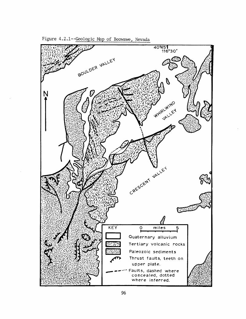
Figure 4.2.1--Geologic Map of Beowawe, Nevada
cd~
KEY
----
0 miles 5
Quaternary alluvium
Tertiary volcanic rocks
Paleozoic sediments
Thrust faults, teeth onupper plate.
Faults, dashed whereconcealed, dottedwhere inferred.
I?0
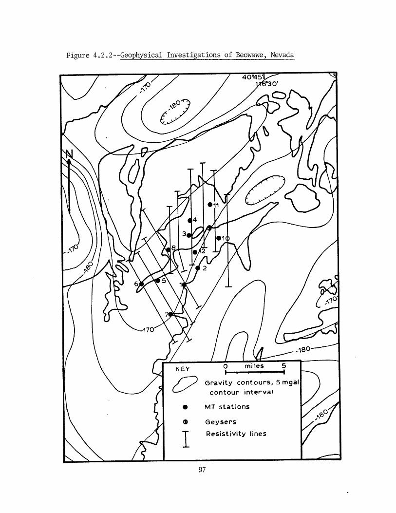
Figure 4.2.2--Geophysical Investigations of Beowawe, Nevada
0 miles 5t- II I-
Gravity contours, 5mgalcontour interval
0 MT 5tations
s Geysers
T Resistivity lines
KEY
4.3 MT Interpretation
The locations of the 11 MT sites in this survey are
shown in Figure 4.2.2. Site 9 was not used because of
errrors in the raw power spectra. Raw power spectra were
processed using the method in Appendix C to produce the
sounding curves for Sites 1 through 12 (Figures 4.3.1 to
4.3.11, respectively). Rotation angles for these sites are
presented in Figures 4.3.12 through 4.3.15. The rotation
angle is measured from north towards east, and all of the
sites show that the maximum apparent resistivities lie in
the NE direction. The data presented here are results from
reprocessing the survey. The original processing also
yielded tipper directions. The tipper direction is an
indicator of the regional current flow, and is derived from
measurements of the vertical magnetic field. The tipper
directions at these sites show a consistent NW trend for the
current flow. Maximum skews and ellipticities for these
sites are less than 0.3 (out of 1.0), and typical values are
0.1 or less. The variation in skews and ellipticities
appear to be a function of data quality rather than of
structure.
Proprietary MT data (Chevron Resources Company) in
Crescent Valley resemble our data quite closely. The
structure responsihle for the low frequency split in the
apparent resistivity curves thus appears to extend southeast
into Crescent Valley. We infer from this observation, the
98
aeromagnetic anomaly, and the low skews and ellipticities
that the structure beneath Whirlwind Valley is essentially
two-dimensional. We will later address the question of how
2-D the stucture must be. This conclusion, and the
following qualitative interpretation, was also reached by
Swift (1979).
We have an apparent contradiction presented by these
data. The tipper directions indicate the current flow is
NW-SE, but the maximum apparent resistivity is NE-SW. This
resistivity is really just a measure of electric field
strength, so the maximum resistivity direction usually
indicates the maximum current flow direction. These two
direction indicators thus should agree, if the body has
isotropic conductivity. We infer from this discrepancy in
directions that the body has anisotropic conductivity. The
observed behavior can be explained with a structure that is
conductive in the NW direction and resistive in the NE
direction. This anisotropy is not an intrinsic material
property-- it is a result of inhomogeneous structure on a
'fine' scale. Further, it is reasonable if we consider the
geologic structure at depth. We have vertically emplaced
resistive dikes intruding into conductive sediments. The
dike swarm has a NNW strike direction. Current flow along
strike would not be impeded because channels of conductive
sediment would exist. Across strike however, the structure
would appear resistive because the dikes would block
99
current flow.
Evidence of current entrapment in the upper crust is
also present in the data. The maximum apparent resistivity
increases as the frequency decreases at Sites 5, 6, 7, and
8 in the frequency range .01-1 Hertz. This increase is
approximately proportional to 1/f. The apparent resitivity
is
pa c ZI 2 /f (4.3.1)
We see immediately that this 1/f proportionality in Pa
implies IZI, or IF/HI, is roughly constant in this frequency
band. The current is not escaping into the mantle at the
lower frequencies, or the impedance would decrease. We
infer from this observation that the lower crust must he
resistive in order to trap the current in the upper crust.
This conclusion differs with that of Swift (1979) about the
lower crust.
Our model should qualitatively consist of a huried
sturcture with a NW to NNW strike direction underlain by a
resistive lower crust. The structure should be conductive
along strike and resistive across strike. All sites show
that the near-surface is resistive, but that a conductive
layer exists between the top layer and the anisotropic body.
This structure is indicated by the decrease of both maximum
and minimum apparent resistivities as frequency decreases in
the range 1-100 Hertz.
100
Several sites, such as Sites 1 and 2, show significant
anisotropy in the surface resistivity structure. This
anisotropy is indicated by the separation of the maximum
and minimum apparent resistivity curves at the highest
frequencies. This anisotropy is again not intrinsic, but
rather is due to heterogeneous structure. We know from the
results in Chapter 2 that variations in surface resistivity
produce parallel shifts of the whole sounding curve. We can
thus correct for these surface variations by shifting the
high frequency portions of the sounding curves to some
'standard' curve. This 'standard' curve was chosen using
Sites 3, 4, and 12. These sites show little to no surface
anisotropy and have very similar high frequency behavior.
This 'standard' curve represents the average structure at
the surface over the whole survey.
Figure 4.3.16 shows all the sounding curves after the
high frequency portions of the curves have been shifted to
the 'standard' curve. This has the effect of stripping off
the surface heterogeneities and allowing us to look at
variations at depth. We have plotted the sites together to
emphasize their similarities. Sites 5 and 7 have a
different surface resistivity structure--the surface
resistor is missing. These two sites thus could not be
shifted to the 'standard' curve.
Several features are visible in Figure 4.3.16. The
minimum apparent resistivity curves are all within a factor
101
of 3 of one another. Maximum apparent resistivity curves
for Sites 1, 2, 3, 4, 10, 11, and 12 all cluster within a
factor of 3 also. Maximum apparent resistivity curves for
Sites 5, 6, 7, and 8 are almost identical, although Sites 5
and 7 are suspect because of the different surface
structure. We see from Figure 4.2.2 that these two clusters
of sites lie in different geographic locations. Sites 1, 2,
3, 4, 10, 11, and 12 lie close to the Dunphy Pass fault
zone, while Sites 5, 6, 7, and 8 lie about 7 kilometers
southeast of the first group. We basically have just two
generalized KT sites in this survey because of the lack of
areal distribution. The first is located 3 kilometers from
the Dunphy Pass fault zone, and the second is about 10
kilometers from the zone. These two sites are shown in
Figure 4.3.17 and labelled Sites 1 and 2. These are the
sites we will interpret. The actual data sites will require
small perturbations in the structure derived from the
generalized sites.
We use both 2-D and 3-D modelling programs with a 2-D
structure to fit the generalized sites shown in Figure
4.3.17. The vertical resistivity in our dike model is
identical to the horizontal resistivity along strike. We
used the 2-P program to model the anisotropy simply by
assigning different resistivities for the parallel and
perpendicular polarization cases. This method unfortunately
varies the vertical resistivity for the two polarizations,
102
which is incorrect. The vertical resistivity is only
important at frequencies where current flow from the mantle
is significant, however. Prrors will only occur, then, at
the lower frequencies. We use the 3-D program at the lower
frequencies because it uses anisotropic conductivities. The
sounding curves from the 2-P program, valid at intermediate
to high frequencies, are merged with those from the 3-D
program at low frequencies. The fits to the data curves
shown in Figure 4.3.17 and Figures 4.3.19-4.3.21 have been
generated in this manner.
Figure 4.3.17 shows an example of a good fit. The
cross-section of the 2-D model used to produce this fit is
presented in Figure 4.3.18. We see all the essential
elements of our qualitative interpretation present in Figure
4.3.18. The resistivity of the body is highly anisotropic,
but this may he reasonable. The highest degree of
anisotropy is seen where the resistivity along strike is .3
Q-m and the resistivity across strike is 200 0-m. This
anisotropy can be produced by mixing dikes with an intrinsic
resistivity of 1000 Q-m with conductive sediments with an
intrinsic resistivity of .25 Q-m. The required mix consists
of 20% dikes and 80% sediments.
Figures 4.3.19-4.3.22 represent a crude sensitivity
analysis of the model shown in Figure 4.3.18. We observe
changes in the apparent resistivity curves as various
parameters in the model are perturbed. Figure 4.3.19
103
contains examples of perturbations in the near-surface
resistivity structure. None of these curves have the
inflection point at 5 Hertz that the data curves show,
although increasing the resistivity of the second layer to
20 Q-m is close. Overall, the response is very sensitive
to the surface resistivity structure, so that little
variation may occur.
Figure 4.3.20 shows how variations in the resistive
lower crust change the sounding curves. The most striking
change occurs when varying the thickness of the lower crust.
Thinning the crust by 30% shifts the inflection point on the
maximum apparent resistivity curve for Generalized Site 2 by
1/3 frequency decade. Thickening the lower crust by 30%
also shifts the inflection point, but by much less.
However, the level of the maximum curve at Generalized Site
2 is too low for the thicker crust. The thickness of 24
kilometers for the lower crust is thus probably good to
within 10%. Increasing the resistivity by one order of
magnitude has a negligible effect on the sounding curves.
We can only conclude that the lower crust is resistive
(greater than 1000 Q-m), but cannot say how resistive.
Figure 4.3.21 presents the effects of changing the
resistivities of the 2-D body across strike. Only the
maximum curves for the generalized sites are shown. We
again see the maximum sounding curves are relatively
104
sensitive to changes in these resistivities. Note that
varying the resistivity beneath generalized site 2 does not
greatly affect the maximum curve at generalized site 1, and
vice versa. These parameters are independent of one
another. We conclude that the 23 Q-m value is good to
within 50% and the 200 Q-m value is good to within 30%.
Figure 4.2.22 illustrates the effect of varying the
resistivity of the 2-D body along strike. Only the minimum
curves for the generalized sites are shown in this figure.
We conclude from Figure 4.2.22 that the resistivity along
strike is less than 1 Q-m in the most conductive portion of
the body.
105
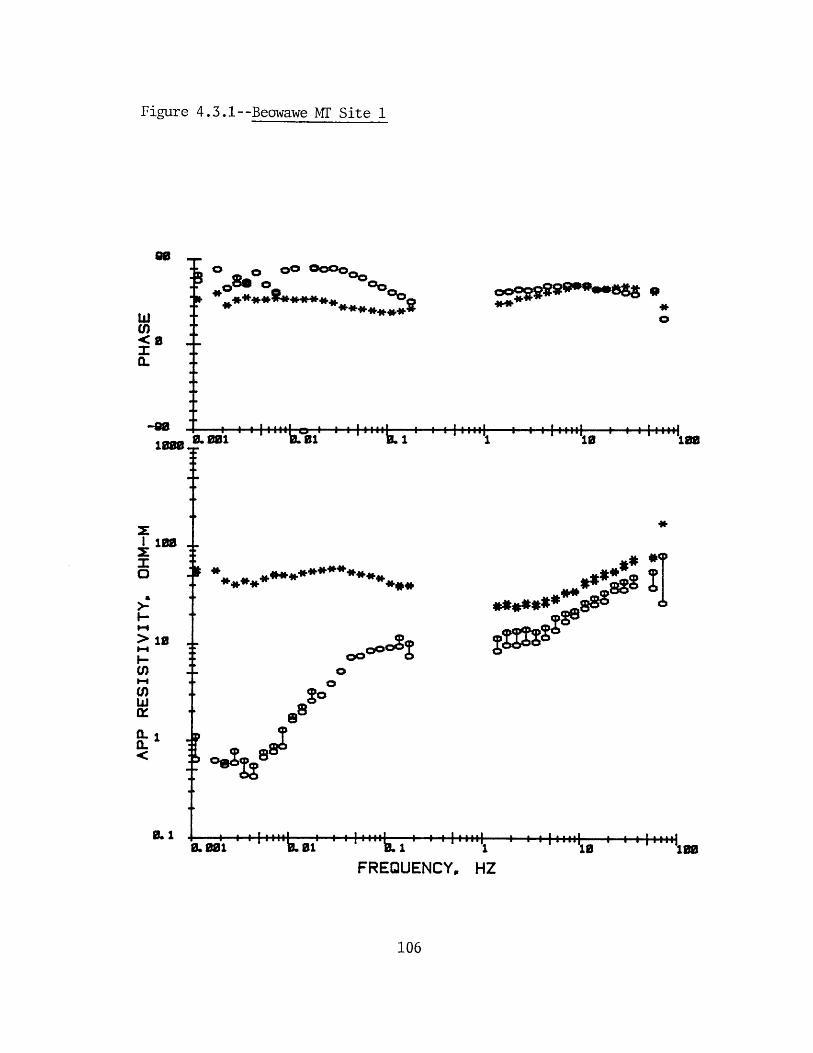
Figure 4.3.1--Beowawe MI' Site 1
90
wU)<0
0.
-M0100
I100
0
O
>10
I-wm~
0.1
o 0 00 cO0o
*8.
........ A
L.Oil
coo0OO0
018;
0.001.II....... .. A
9*0
I .. . A
a - -- -aI . .. I
-'10I~
I....'
'0
I .. . I
FREQUENCY, HZ*. -As .. 1 3-0
106
. . I . . . A I . . . 1
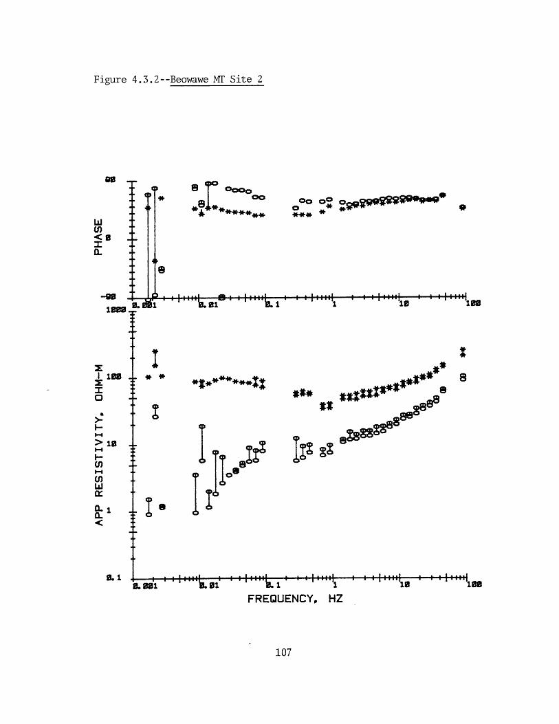
Figure 4.3.2--Beowawe MI' Site 2
8
wU)<0fI
8 0 coo
111111 fl i 111111 i I ,,iti I 1111111 10 10
* *
~I
0, B01
FREQUENCY,
I - - - -I
1
HZ
107
00 00o
I
**S
I100
O
I-
10
U)
w
.1
I. 1 ,i t I tiimi:I~.01a~g1 *10I .. . I I .. . A
10a - - - - A
, ... 01 ,. - , i I 1 10
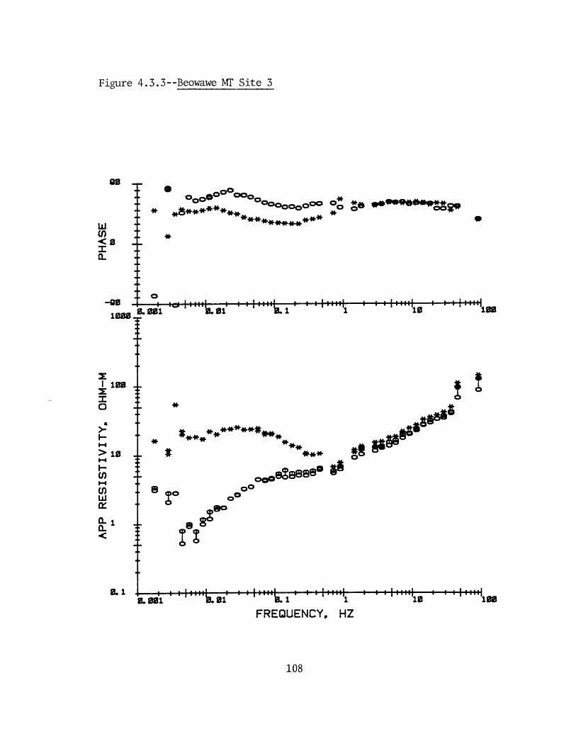
Figure 4.3.3--Beowawe MIF Site 3
0
w(1)<0
I.
*
-I ,.-i I :iail a i 111111 I I I iitii a a0. 001 .01 1 '10 100
00* **** ** **** * *
co8s8se8
, 1
'HZ
oc00
0. 001 IL 01
FREQUENCY
108
-1W10o0
-*
1 100
I
>10
w
.1
0-
-... I .... I
*10I ... I
lee
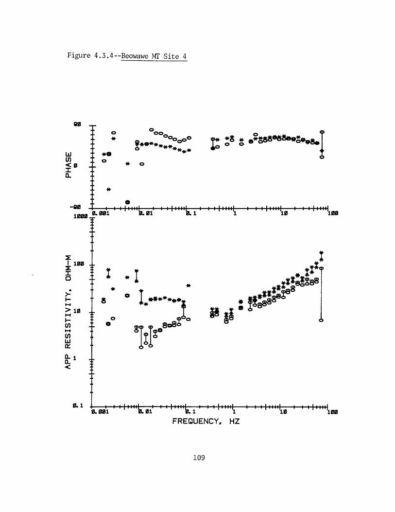
Figure 4.3.4--Beowawe MI' Site 4
90
wC,)<0r
-90
100w
100
*:
>-
>10
F-U)
C,)w
0o 0000 0 g
0
001
* 0
* 0
0
0 -
I . . .. I
- . 1
FREQUENCY,
I .. .. I
11
HZ
! .. t. .
10 100
109
.
10I .... I
100
0.1 I . ... I
0. 001
I . . . . I I . . . . I I . . .. II . . . . t
, .'I 016 1 . I
.I 01
Ala 6
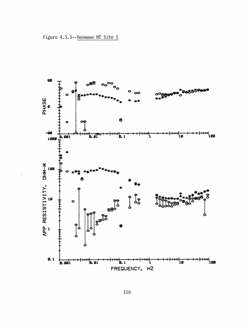
Figure 4.3.5--Beowawe MI' Site 5
C88 00c
g-****-....
***6839ee@0 c
. ., . .. . . . . . . . ...
' a 0 - aoe
90
w<0I -
-. -
1000
I
> o
I:0.-
> 10 ..
'--
'. -
0.1. I .. .. I
FREQUENCY,1
HZ
110
94
L 001
*
0 **'?*' "*
0.001I 11111::
I .. . .i
100
I--- - I
.L .f .... . .I .. L 1
I --. . II - - - - a
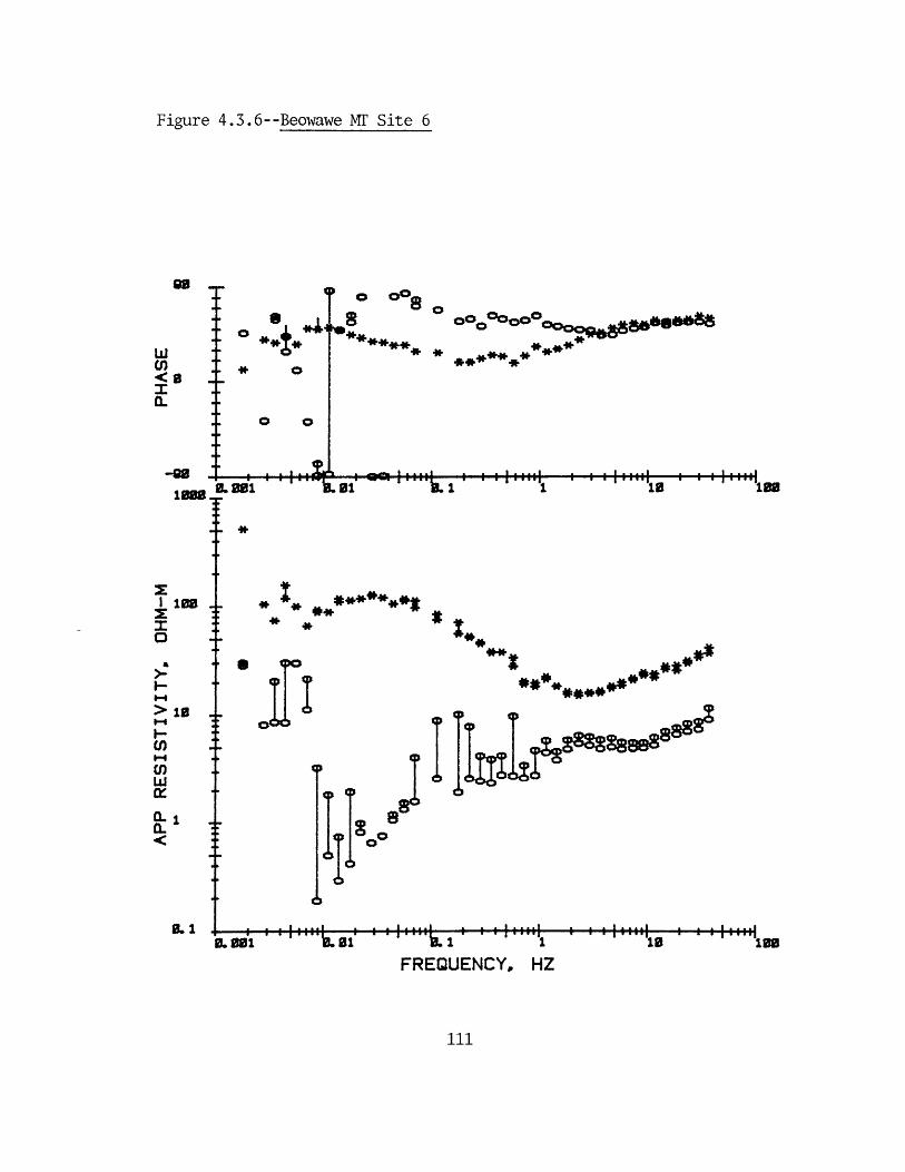
Figure 4.3.6--Beowawe Mr Site 6
* *
0 0
gel
0c 00
***
i I. ....
"13. of*
ococoo gee8 8
I. ... I a .. .
1 4 18
-*
* ** *********I:* *
T**
** * *
11:08
I -. . -I
0.001 .... .0i1 .1 *.
FREQUENCY,
111
98
w(n<0m0.
..1 W8
. I. ... I
198-io
I 19
0
'-
>is
inw
0-1CL
9.1 I .. . A I .. . a
1
HZ
.
.
1w s '198
. 66 iL I
I . . . -a a . -a
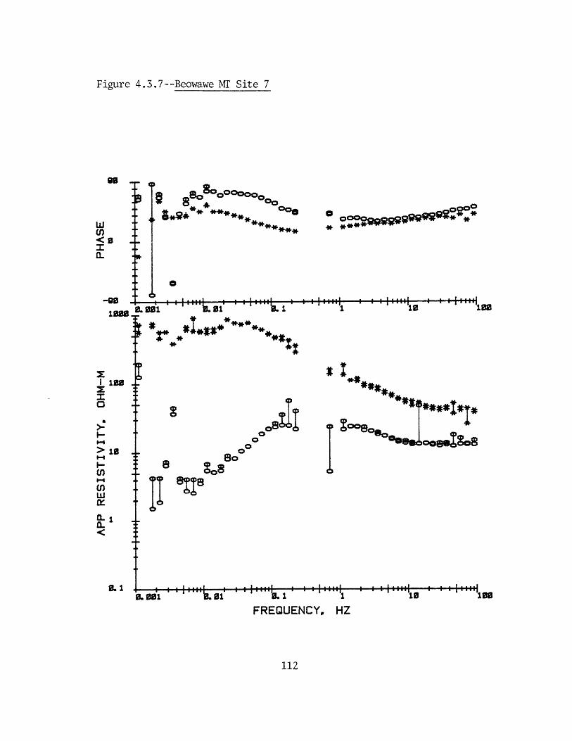
Figure 4.3.7--Beowawe Mr Site 7
I 000
00* ChD !
i I i:::i:: - .
0
9000t
SO SOc
- --- S......am ~ ~ * ~ b a a aA .,, -F U. E .FREQUENCY,
I .. .. I
100
HZ
112
081
es
wU)<0r0-
100 * -
100
i-
>10
Ul)
w
i.xt.
is ISO8
01,0.001
* %e "I
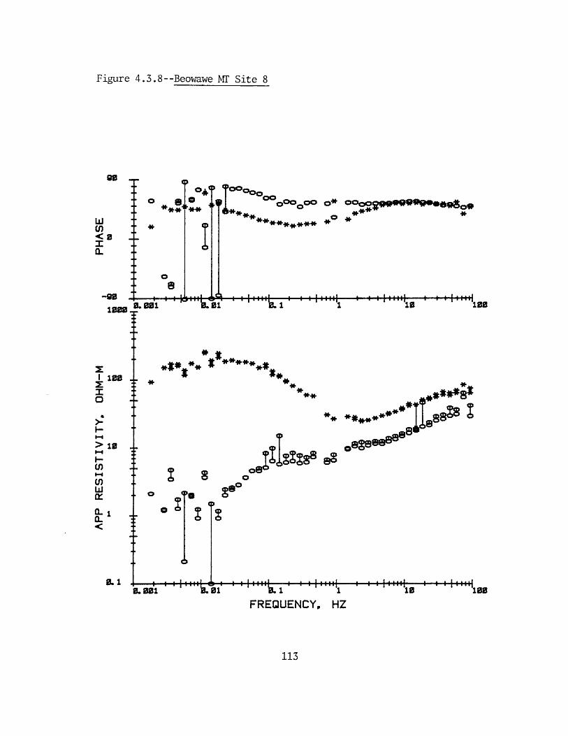
Figure 4.3.8--Beowawe MT Site 8
a **ip0
8-w0.
0001T
*
*:* ****
**
**
0 9~.
or.i '
FREQUENCY, HZ
113
I 100
0
> 1
(n
w
x~
0.1
so0
I . -. .1 I . .. .I
I
I....,
.a
I .. . .
'.a - - - - - - - - - - - - - - - - - - - - - - -64
's "- . I
fft- fft
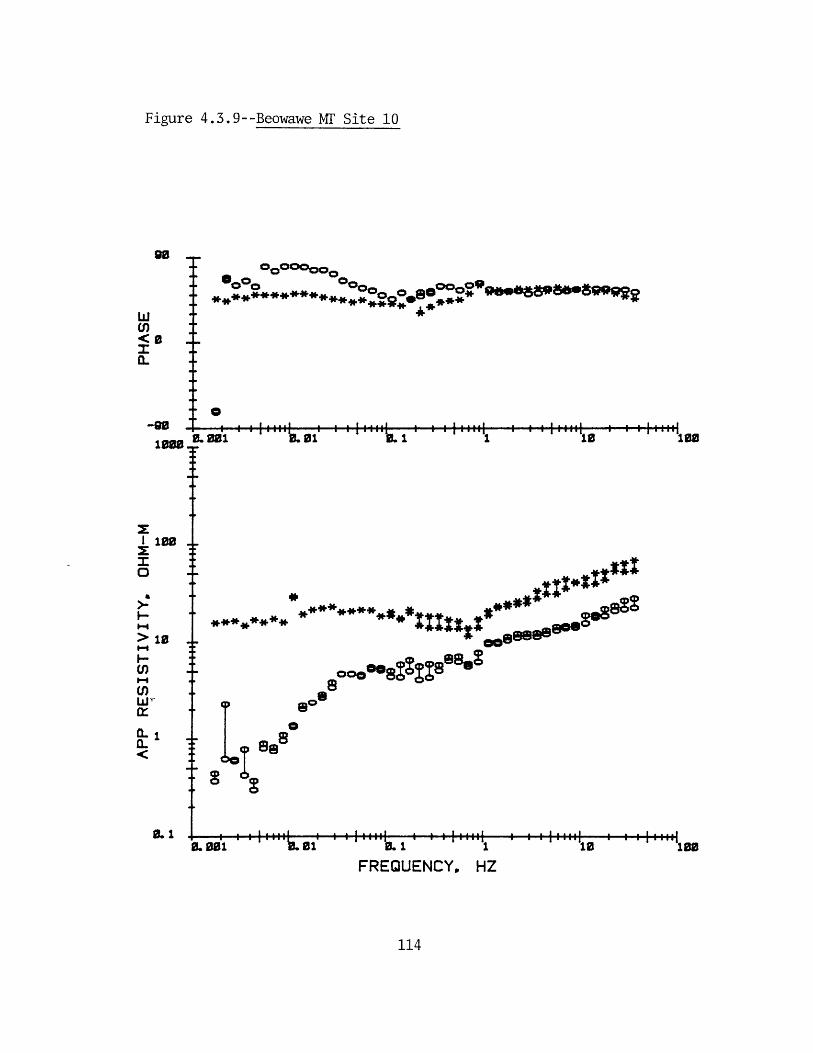
Figure 4.3.9--Beowawe MT Site 10
Doc 0 00o0oo
-x *******x 80 0
I .. .. i
00 1
0,
.go
wU)<0
-90.
1008
x0
> 10-4
( I0 .
a8068- f 8%
I .. .. A
0. 001
FREQUENCY,
114
I .. .. I
. I I 9
I .. . .I
10"'A
* **. * *
I .. .. III
I .... A I . . .I.p ..v
1I ... I
10
HZ100
I . . . . I
, ""' IL of * '"I , - - , "'loo
les
, ". of 1"." I
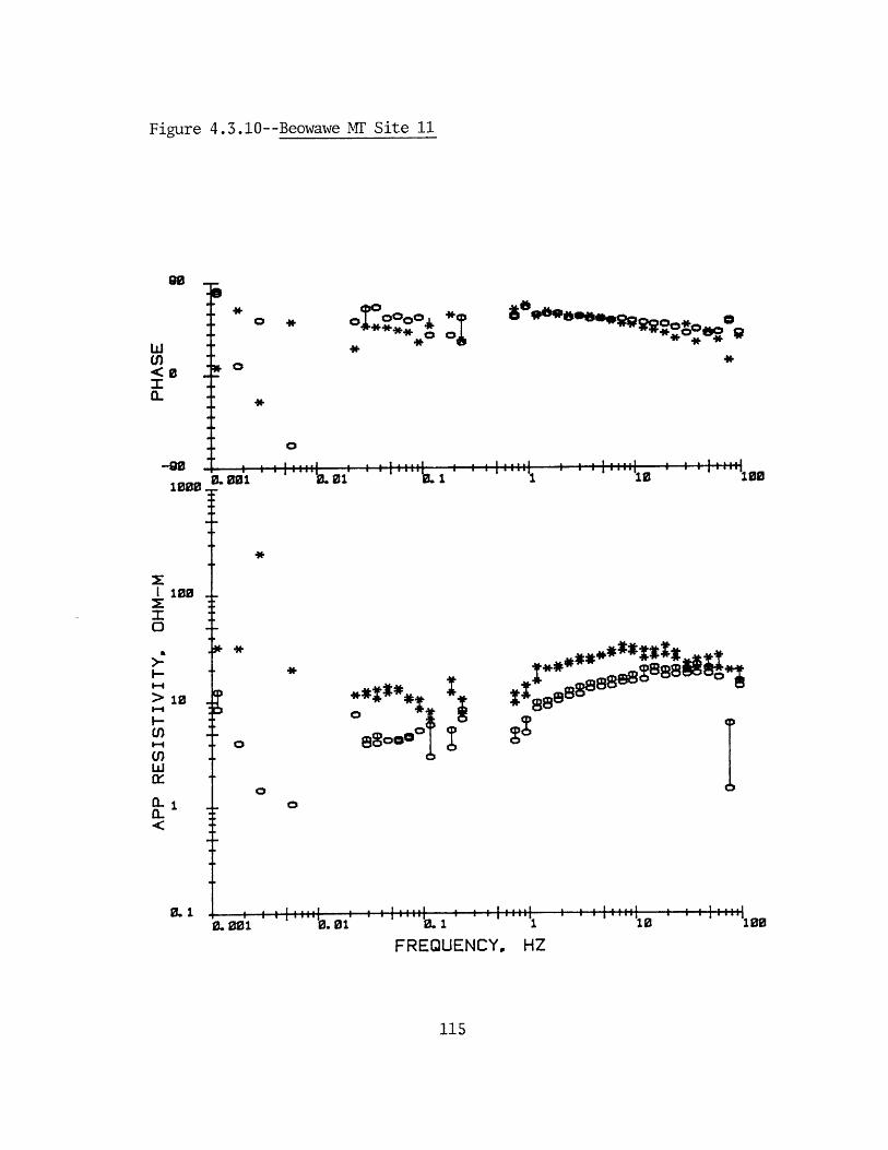
Figure 4.3.10--Beowawe M' Site 11
o * ~
*
*
,,iil a a aaaaaa ii:::::: .
I. 016 1
*
'0.01
FREQUENCY, HZ
115
so,...
*
B. 001 10
90 .
w(n<0
1(L
-90
1000
100
a
F-
> 10
U)I-4
w
(L
0.1
100
g.'10
100
I . ... II - - - I
. 1I I
I - . - - # I - - - - I
i '10
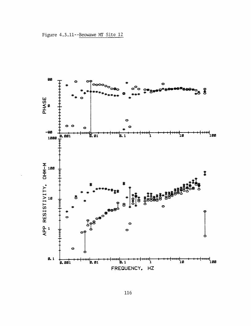
Figure 4.3.11--Beowawe MF Site 12
0
w -
G.
100..
* *~
**0
0 00
00000O000 o.~,.p*e9s~9Oepe
0 ****
*I .. *1 *10 100
SCSI0
0O
1 a a e 1 2 1 ! a : ! ! m'0.01 0. 1
FREQUENCY,
116
I .. . A
1
HZ
*
** *
*
100
oI
0
I- 1>010
I0.1
0.c*(
0
0.001
I .. . A
100
I . . . . I
'10 -100g. 1 'I'1
I . . . . II - --I'10 100
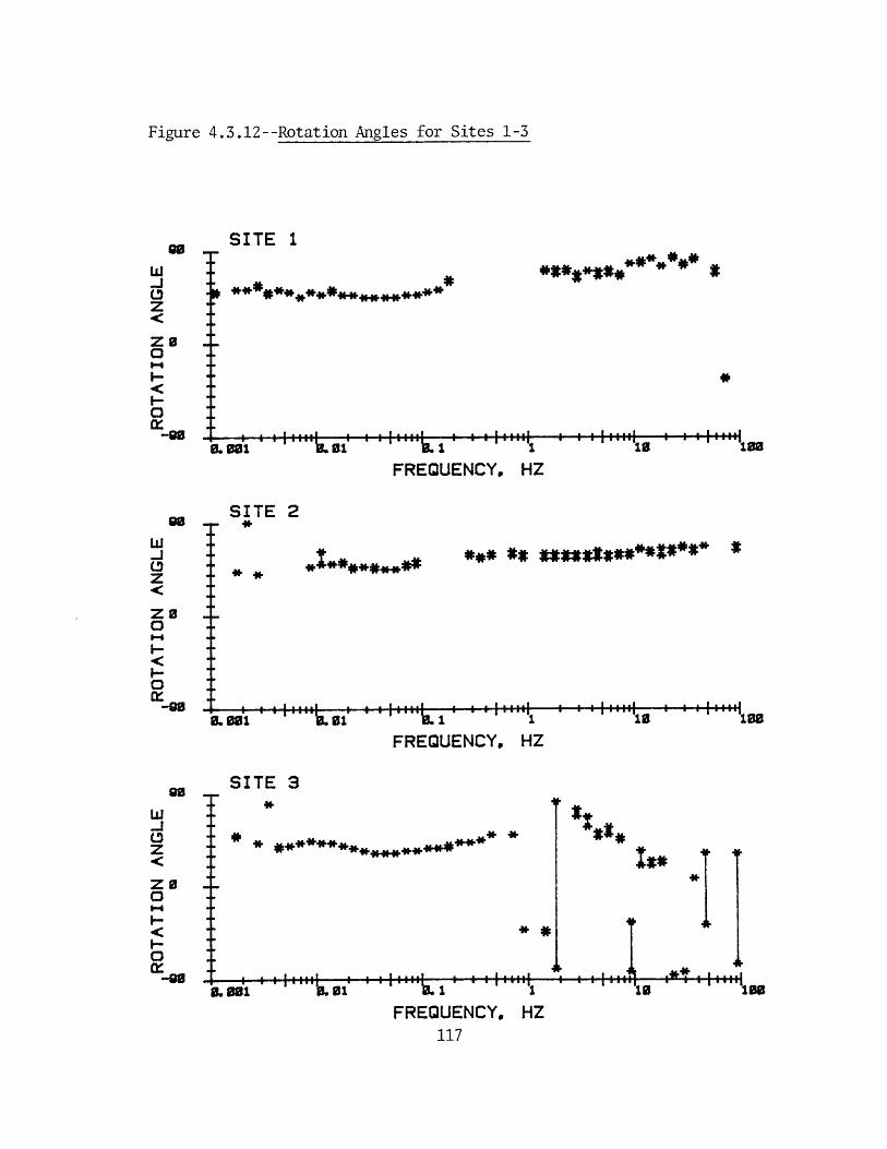
Figure 4.3.12--Rotation Angles for Sites 1-3
SITE 1** * ** ** * *
WI *********************
I - -.- *
. 1 1
FREQUENCY., HZ
I .. .. 2
10 '100
SITE 2.. *
*** ** **I******~**~*~ *- **
.v.01 10-I : .ittmi I 1111111 :::.::..
FREQUENCY, HZ
I....
loo
SITE 3
I*****
**
I .. .. I -p1 - -
. , " h . - - ,----,aaa'1
FREQUENCY, HZ117
*1a....'
0
w-
O
zo
-0.1 I i I 11111 I I I
0. 001
.J20
I-
z
zo0
& ail
s0
w-J.z
z0
0-
*14'.
-...
10 ---. 10
I . . -- l
1 '1131 v a a f iL 01
I . . .1
-. 0 *. ,,,,I 1
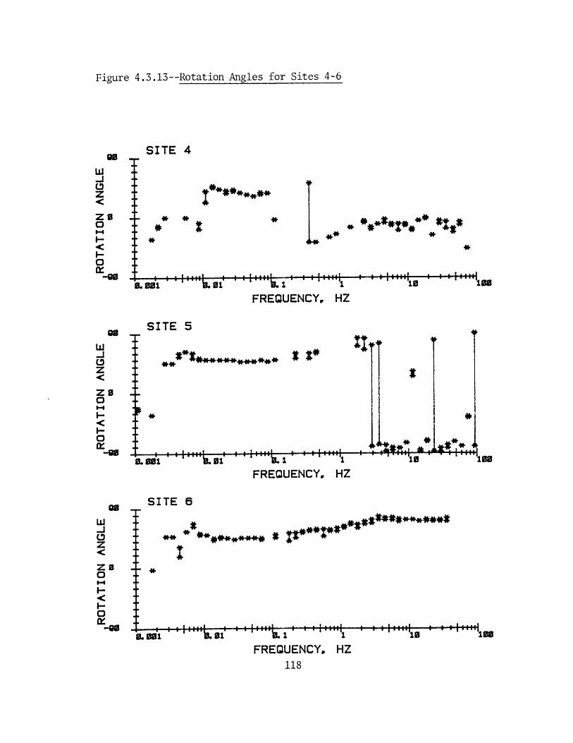
Figure 4.3.13--Rotation Angles for Sites 4-6
SITE 4
I****P
- * *-
T ~ * .. I
a . . .iL I . .1
* **4*:**** *: *
*
~W~L~L~JLd 10100
FREQUENCY, HZ
4& , 1111 I 111
FREQUENCY,- 10 10
HZ
SITE 6
** *******-ALI
# . ... I
FREQUENCY,118
I--.-, * .*10 100a a
HZ
w.Jz
-
SITE 5
* * ** ** * *** * ** ** *
0w.J
z
zo0
-=
L. 001
0w-j0
zO0
0Ir "
M.gel
T
IL 9d, "k Of I 'is
:11
-IIL i
*10 100IL ol I b. I 1 11
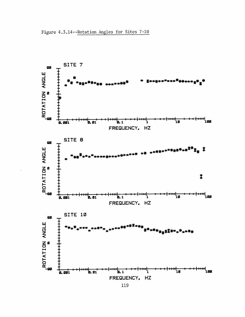
Figure 4.3.14--Rotation Angles for Sites 7-10
SITE 7
*** *
* ********* *******
*
t - -.. I
-. I 111111::1 - 10 1le
FREQUENCY, HZ
SITE 8
** *************R*~* :
.1 , '11111 I I 111111 I I I I 11111 I I ; ::::;I ' 'i 10
FREQUENCY, HZ- e1e
SITE 10
.i * 11111 I 111111 I.01
FREQUENCY, HZ119
w
z
0
O
O0
w.J0z
Z 00
0ix0G
0. 001
0w-JLoz
I-
0m-00
8. o01
I -
-is3
I . . . I
100-L I
L. 001 I. 01
I
1
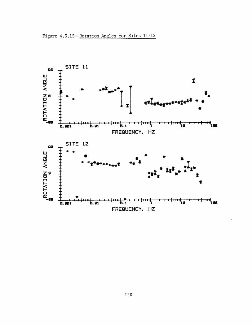
Figure 4.3.15--Rotation Angles for Sites 11-12
SITE 11
* *
I....' .1 ... I.... I
*
* ********
I....,......I
.. . . I.......1F 1 1 REUEY1FREQUENCY, HZ
h. I 1IFREQUENCY, HZ
120
**:
w.J
z
Za0m-
I-O
-90
w
zz
I-O-
. 001
SITE 12
***
*
a a
**
I A--
100
* *
#Ix *
I. 001 13 101 . 01
i 0 81
I - ---I I - ---I
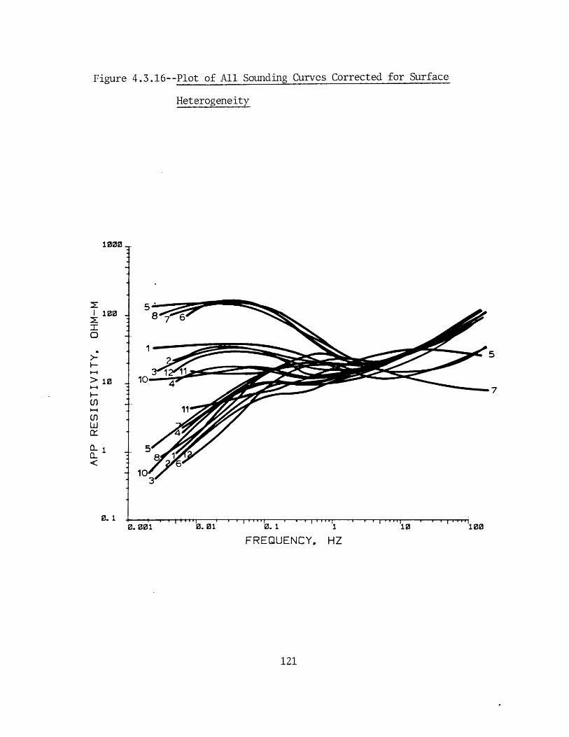
Figure 4.3.16--Plot of All Sounding Curves Corrected for Surface
Heterogeneity
10007.
I
5'100 876
7
1! 5
> 10 100
11
0- 1 5
-103
3. .00 i1 '0.01,- 0.1 110 100
FREQUENCY, HZ
121
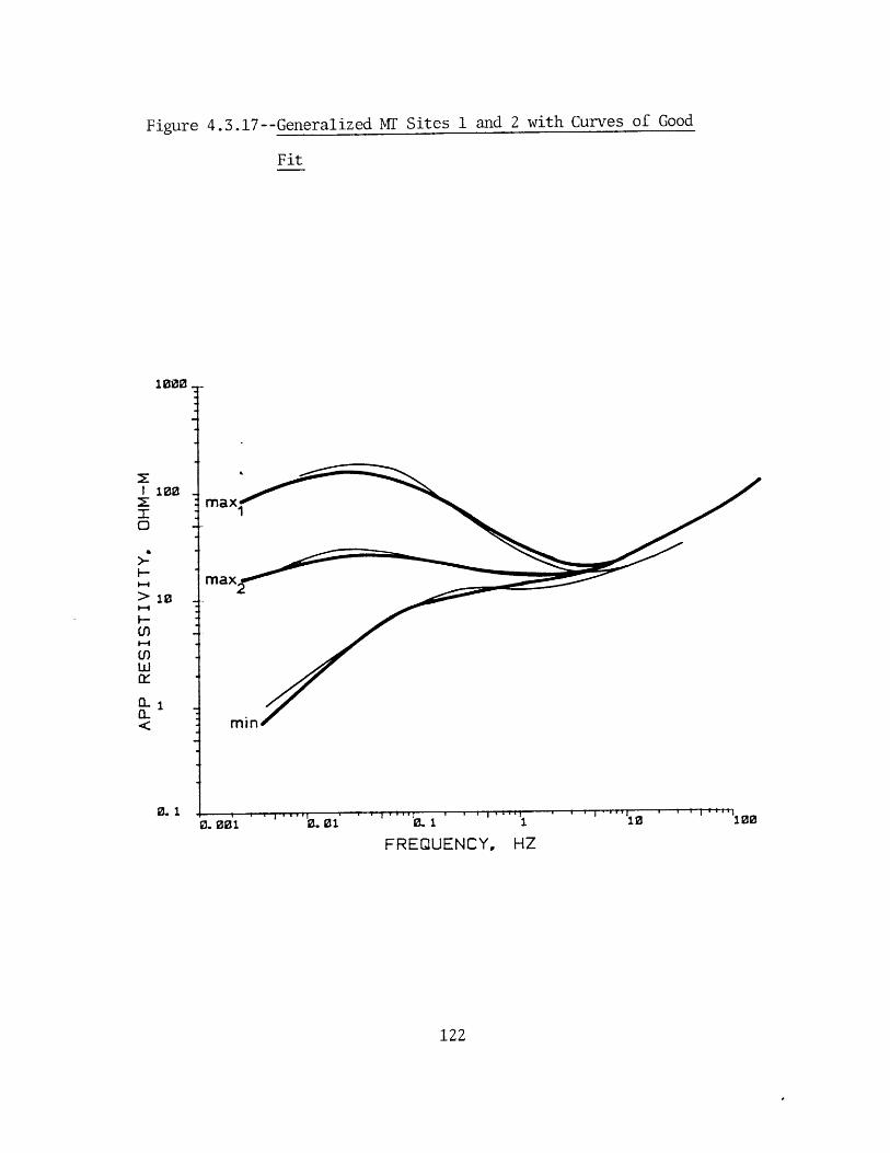
Figure 4.3.17--Generalized Mr Sites 1 and 2 with Curves of Good
Fit
ma.
'. oi1 '0.01 0.1
FREQUENCY.,10
HZ
122
100
O0
-1
> l0
U)
U)w
0
0. 1
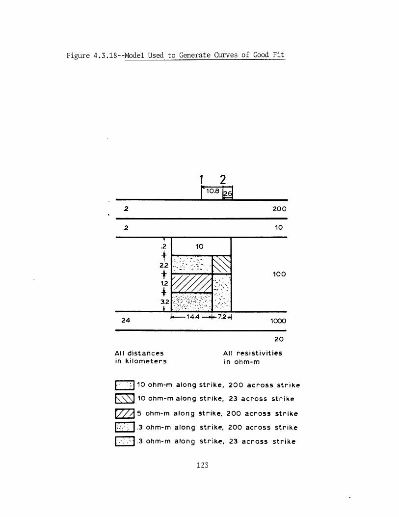
Figure 4.3.18--Model Used to Generate Curves of Good Fit
1 2
2 200
.2
22
1.2
3.2I ~ I
100
24 %14.4 - 7.2.4 1000
20
All distancesin kilometers
All resistivitiesin ohm-m
10 ohm-m along strike, 200 across strike
10 ohm-m along strike, 23 across strike
M 5 ohm-m along strike, 200 across strike
.3 ohm-m along strike, 200 across strike
.3 ohm-m along strike, 23 across strike
123
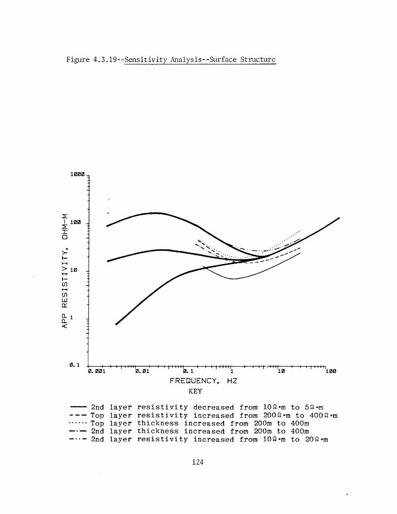
Figure 4.3.19--Sensitivity Analysis--Surface Structure
0.001 0.01 0. 1 1 10 100
FREQUENCY, HZKEY
2nd layer resistivity decreased from 1O-m to 50-m--- Top layer resistivity increased from 2000-m to 4002-m------ Top layer thickness increased from 200m to 400m---- 2nd layer thickness increased from 200m to 400m
2nd layer resistivity increased from 100-m to 20-m
124
100
0
0
- 1
> 10
U)
Ixi
0. 1
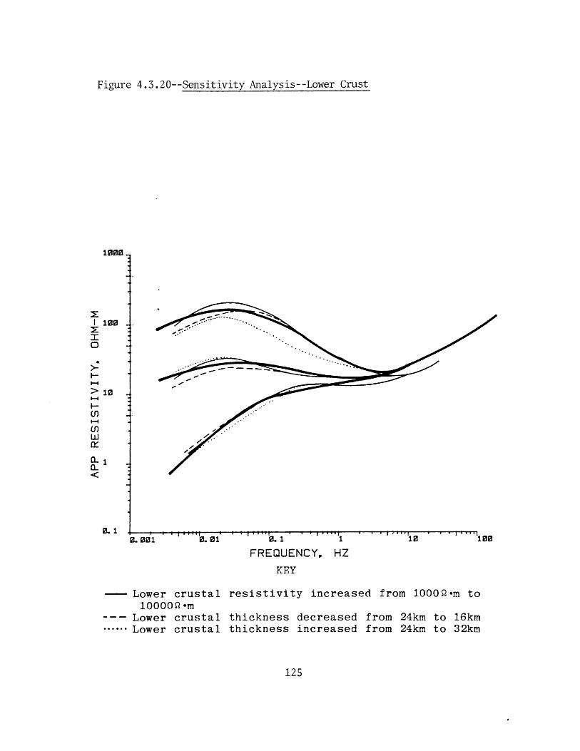
Figure 4.3.20--Sensitivity Analysis--Lower Crust
1000-
I100
> 10
'-4
xCL'-4
<)
0.10.1 1 10
FREQUENCY, HZKEY
-- Lower crustal resistivity increased from 10002-m to10000-m
--- Lower crustal thickness decreased from 24km to 16km------ Lower crustal thickness increased from 24km to 32km
125
100,
. . . . . ..... .
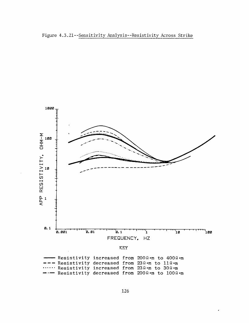
Figure 4.3.21--Sensitivity Analysis--Resistivity Across Strike
1000
I 100000-
> 1
U)
UI)
0.1 110 100
FREQUENCY, HZ
KEY
-Resistivity increased--- Resistivity decreased
.Resistivity increased- Resistivity decreased
from 200I-m to 40O-mfrom 23SI-m to 11Q-mfrom 23Q-m to 30-mfrom 200l-m to 100l-m
126
0. 001 0. 1 1
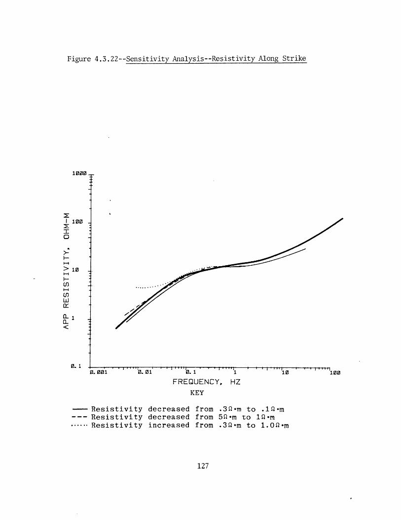
Figure 4.3.22--Sensitivity Analysis--Resistivity Along Strike
1000-
100
0
> 18
U)wd
(L
0. 10.001 0.01 0.1 1 10
FREQUENCY, HZKEY
-- Resistivity decreased from .30 -m to .1Q-m--- Resistivity decreased from 5Q-m to 1-m------ Resistivity increased from .3Q-m to 1.00-m
127
100
4.4 Effect of Truncation of a 2-D Body
The previous section produced a 2-D model which
exhibited all the essential characteristics of the observed
data. We answer here the question of whether this 2-D body
can be truncated along strike without significantly
affecting the fields. We simplify the model of Figure
4.3.18 to prevent confusion from factors such as anisotropy.
The simplified model is presented in Figure 4.4.1. We
examine the truncation effect at one frequency (.01 Hertz)
only. The essential behavior can be seen without
multi-frequency plots.
LaTorraca (1981) examined the change in the DC field
within a conductive ellipsoid buried in a homogeneous
half-space. The ellipsoid is prolate (cigar-shaped), so it
is a rough approximation to our rectangular conductive body.
The conductivity contrast in our model (Figure 4.4.1) is
100:1. LaTorraca (1981) predicts the apparent resistivity
along strike should be 0.7% of its 2-D value for an aspect
ratio of 3:1, and 11' for an aspect ratio of 10:1. These
changes assume the field behaves only in a resistive (i.e.,
DC) manner. The conductive feature draws current towards
itself, but is unable to attract enough because of its
finite dimensions along strike.
Table 4.4.1 summarizes the results of 3-D modelling
128
applied to the model in Figure 4.4.1 for various aspect
ratios. Included in this table is an evaluation of the
effect of the repetition assumption. The apparent
resistivities shown here are for a site above the symmetry
point of the conductive body. The effect of the repetition
assumption was tested by using rectangular blocks with
aspect ratios of 3:1. This change moved the image features
3 times further away along strike, making it 240 kilometers
away from the conductive body. The apparent resistivity
along strike changed by about 15% for the aspect ratio of
3:1. The effect of the image conductors are thus present
in the solutions, but it cannot explain the large deviations
observed from the expected DC behavior.
The most striking feature of Table 4.4.1 is that the
apparent resistivity along strike did not decrease by an
order of magnitude when we changed the aspect ratio from
to 7:1. The apparent resistivity actually increased by 20%,
but we believe this increase is due to interactions between
the conductive feature and its images. The resistivity
along strike decreases as we decrease the aspect ratio, but
the maximum change is only 20% for any aspect ratio above
3:1. The mechanism controlling the current in the conductor
is clearly not DC current flow.
We know from Section 2.3 that local induction plays an
important role in this model (The model in Figure 4.4.1 is
essentially the model in Figure 2.3.11). The induction
129
contribution is primarily dependent upon the body thickness
(See Appendix B), so varying the horizontal aspect ratio
should have little effect. We observe this in Table 4.4.1.
Hence, local induction is responsible for the lack of change
in apparent resistivities.
We conclude that the aspect ratio need not be very
large for the apparent resistivities along strike to be
within a few percent of the values for the 2-D model. The
conductive body is such a good conductor that local
induction dominates the electric field. Hence, varying the
aspect ratio does not affect the current level much. The
conductive 2-P body in Figure 4.3.18 is 18 kilometers wide,
so any length along strike greater than 60 kilometers is
allowable (based on a 3:1 aspect ratio). The length
inferred from the aeromagnetic survey is 120 kilometers, so
we have good agreement between the length estimates.
130
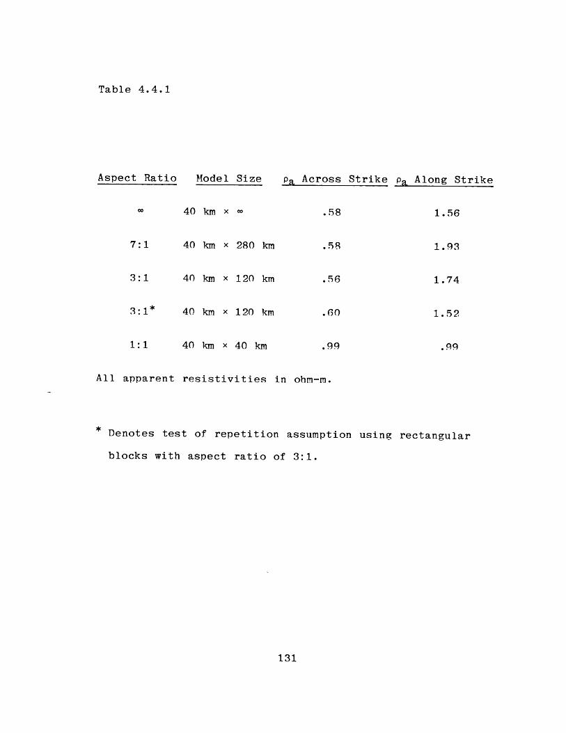
Table 4.4.1
Aspect Ratio Model Size Pp Across Strike Pa Along Strike
40 km x oo
40 km x 280 km
40 km x 120 km
40 km x 120 km
40 km x 40 km
All apparent resistivities in ohm-m.
Denotes test of repetition assumption using rectangular
blocks with aspect ratio of 3:1.
131
7:1
3:1
3:1*
1:1
.58
.58
.56
.60
.99
1.56
1.93
1.74
1.52
.99
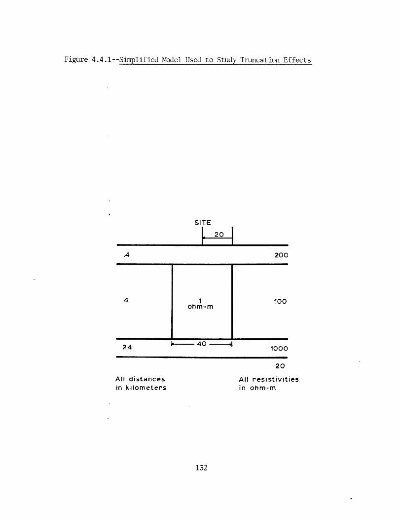
Figure 4.4.1--Simplified Model Used to Study Truncation Effects
SITE
.4 200
24
Iohm-m
40 -.
100
1000
20
All distancesin kilometers
All resistivitiesin ohm-m
132
4.5 Summary
The structure beneath the Beowawe, Nevada KGRA is an
anisotropic feature 20 mkm wide and 7 km thick. The body
has a NW strike and minimum length along strike of 60 km.
The conductivity anisotropy is due to a series of NNW
trending diabase dikes which make the structure conductive
along strike (1 Q-m) and resistive across strike (200 2-m).
The body is buried beneath a thin (400 m) veneer of
sediments and andesite flows. The lower crust beneath the
region is fairly resistive (1000 2-m) but not too thick (24
km). This interpretation is consistent with gravity,
resistivity, and aeromagnetic data for this region. Many of
the lateral structural constraints are based on these other
data, and the MT soundings are used to establish limits for
the conductivities and thicknesses.
133
'When in doubt, try something. It doesn't matter what.
Anything at all, but try something.'
Ken Bond
CHAPTER 5
5.1 Introduction
Structures several hundred kilometers from a measure-
ment site can influence the electric and magnetic fields at
that site. A good example of this is the field distortion
due to the ocean-continent boundary. This distortion has
been documented in data (e.g., Kasameyer, 1974) and has been
theoretically modelled (Ranganayaki and Madden, 1980). We
desire local structural information from an MT survey used
for exploration. The typical scale size for these local
structures is one kilometer. A practical, efficient
modelling algorithm must include both the local scale and
the regional scale. The technique presented in Chapter 2
uses just one scale, and is thus inadequate.
One method to incorporate many scales into the
modelling algorithm is the 'multiple scales' technique
proposed by Ranganayaki (1978). The fields are determined
on a regional scale, and these results are used as boundary
terms for the local scale. This method will theoretically
work for many scales, but was applied to just two scales by
Ranganayaki (1978). We will continue to use just two scales
in our work.
134
We review Ranganayaki's multiple scales approach and
illustrate its shortcomings in this chapter. We also
present our unsuccessful attempt to improve her multiple
scales method. Finally, we suggest a possible way to
successfully perform the multiple scale analysis. The
results presented in this chapter are all negative, but
provide considerable insight into the problem.
135
5.2 Ranganayaki's Approach
We review the multiple scales method in this section
and discuss its problems. We also present our attempt to
improve the method. Figure 5.2.1 illustrates the model we
use here. The heavy dotted lines are the coarse grid, or
regional scale. The thin solid lines are the fine grid, or
local scale. The unshaded region is the exterior region,
while the shaded region is the interior region (or region
of interest). We wish to determine the local scale fields
in the interior region without solving for the local fields
everywhere. We use the regional solution to estimate the
local fields in the exterior region, and assume that the
errors incurred using this approximation are small. We show
here that this assumption is not valid.
Ranganayaki (1978) begins with Maxwell's equations in
the form presented by equations (2.2.13) and (2.2.14).
These equations give the total field change across a thin
layer. The thin layer can be thought of as a laminate of a
conductive, heterogeneous layer and a resistive, homogeneous
layer. The electric field changes across the resistive
layer, but not the conductive layer. The magnetic field,
however, changes across the conductive layer, but not the
resistive layer. The resistive, homogeneous layer may be
incorporated into the layered half-space, while the
conductive, heterogeneous layer must be treated as a thin
sheet. There are thus no electric field changes across
136
the heterogeneous layer.
The equation governing the field changes across the
heterogeneous layer is
H = + AZ(1zF(sEs~) ~Vs((VsxEs~)'z)/(jyl)) (5.2.1)
Ranganayaki (1978) uses the following boundary conditions at
the top and bottom of the thin layer
s= earth * Es~ (5.2.2)
Hs+ = Hso + Yair * Es~ (5.2.3)
where Yearth is the admittance of the layered half-space,
Yair is the admittance of the air, and Hso is the source
magnetic field. We substitute (5.2.2) and (5.2.3) into
(5.2.1) to derive an equation for Fs~
HsO [Yearth* Y air* + AZ(zx(as-)~ Vs(( Vsx') z)/(jol))]Es
(5.2.4)
The operator in (5.2.4) is a full convolution operator in
the space domain. We rewrite this equation to simplify the
notation
Hs0 = Yt * Es~ (5.2.5)
137
where Y' is the operator shown in (5.2.4).
We set up and solve (5.2.5) at the regional scale in
the first step of the multiple scales process. This
procedure yields one electric field value per large block in
Figure 5.2.1. The fields in the exterior region are
approximated by the regional solution. The single regional
field is assigned to each of the 9 small blocks which make
up the large block. The local scale fields in the exterior
region are thus generated in this manner. Equation (5.2.5)
is reformulated using the fine grid, and Es~ is broken up
into the known values in the exterior region and the unknown
values in the interior region
us- = '* E sexterior + Y'* Es-interior (5.2.6)
We then transfer the known portion of the convolution to the
source side of (5.2.6) to get the final equation for the
interior region fields
s- Y* E sexterior = Y Esinterior (5.2.7)
Ranganayaki (1978) applied this multiple scales method
to the problem of resistive islands in a conductive ocean
and achieved good results. This success was possible
hecause the fields in the exterior region were much smaller
than in the interior region. Errors in the approximation
138
were much smaller than the interior fields. -ence, the
errors in the effective source term , Y* Es-exterior, were
negligible.
The problems with the approximation scheme surface when
the multiple scales method is applied to conductive bodies
(geothermal reservoirs or mineral bodies) in a resistive
medium. The fields in the exterior region are at least an
order of magnitude larger than those in the interior region.
Errors in approximation in the exterior region thus become
significant. The convolution process creates some
constructive interference of the errors, and source term
inaccuracies are frequently larger than the individual field
errors in the exterior region. Individual exterior region
field errors may be as much as 100%, and source term errors
are higher. The key is that these errors in estimation are
10 times the magnitude of the interior region fields, and
produce severe mistakes in the interior solution.
Figure 5.2.2 illustrates a model used for comparison of
the correct solution and the multiple scales solution. The
interior region for this comparison is the central large
block containing the conductive feature. Figure 5.2.3
presents the fields for this comparison. The correct
solution was comDuted using the fine grid and solving for
the fields in both the interior and exterior regions. The
fields are presented in units of apparent resistivity.
Comparison shows that the fields inside the conductive
139
feature are consistently overestimated, and the fields
outside are underestimated.
The multiple scales approach proposed by Ranganayaki is
a sound one in theory. The difficulty with the method lies
in the approximation scheme for the exterior region. None
of the field distribution information in the exterior region
is preserved. We accordingly attempt to improve this
estimation process. The frequencies in our problem are low
enough that the DC solution is a good approximation to the
fields in the exterior region. We first solve the DC
(resistivity) problem at the local scale and then use these
results to predict the current (and hence field)
distribution in the exterior region.
We use a network approximation to the DC problem
(Madden, 1972) and solve the equations
V'J=O (5.2.8)
VxE=O (5.2.9)
We get the x and y current densities at the local scale from
the DC solution and average the fine grid solution within
each coarse grid block. In this manner, we generate the
ratio of the local scale current to the average regional
scale current in the exterior region. We also compute the
average conductivity for each large block from the average
electric field and average current density for the DC
solution. We next compute the regional scale solution for
140
the electromagnetic (EM) problem, just as Ranganayaki does.
The local current density in the exterior region is
predicted from the regional current density
iexterior,local,EM = Jexterior,regional,EM. [ _local ]DCJregional
(5.2.10)
The electric fields for the exterior region are
Eexterior,local,EM =aregionalDC .[ local DC-Eregional,EMalocal Jregional
(5.2.11)
This estimation procedure yields exterior region fields
which are much closer to the correct solution, but errors
may still be 10-20%. These errors are still sufficient to
produce large errors in the interior region fields. Figure
5.2.4 shows a model used for comparison of the modified
multiple scales solution to the correct solution. Figure
5.2.5 presents the fields for this comparison. The multiple
scales solution is still erroneous, but it is much closer to
the correct solution than the results in Figure 5.2.3.
Two-dimensional symmetry is expected in the fields because
the model is two-dimensional. This symmetry is missing in
the multiple scales solution in Figure 5.2.5 because of the
field estimation process. The lack of symmetry indicates
141
that the multiple scales solution is erroneous. The
improved approximation scheme helps, but not enough.
The basic problem with this multiple scales method is
that it is too sensitive to errors in fields in the exterior
region. This sensitivity is a result of the convolution
operation--it amplifys errors. We now suggest an alternate
scheme which may bypass this problem.
142
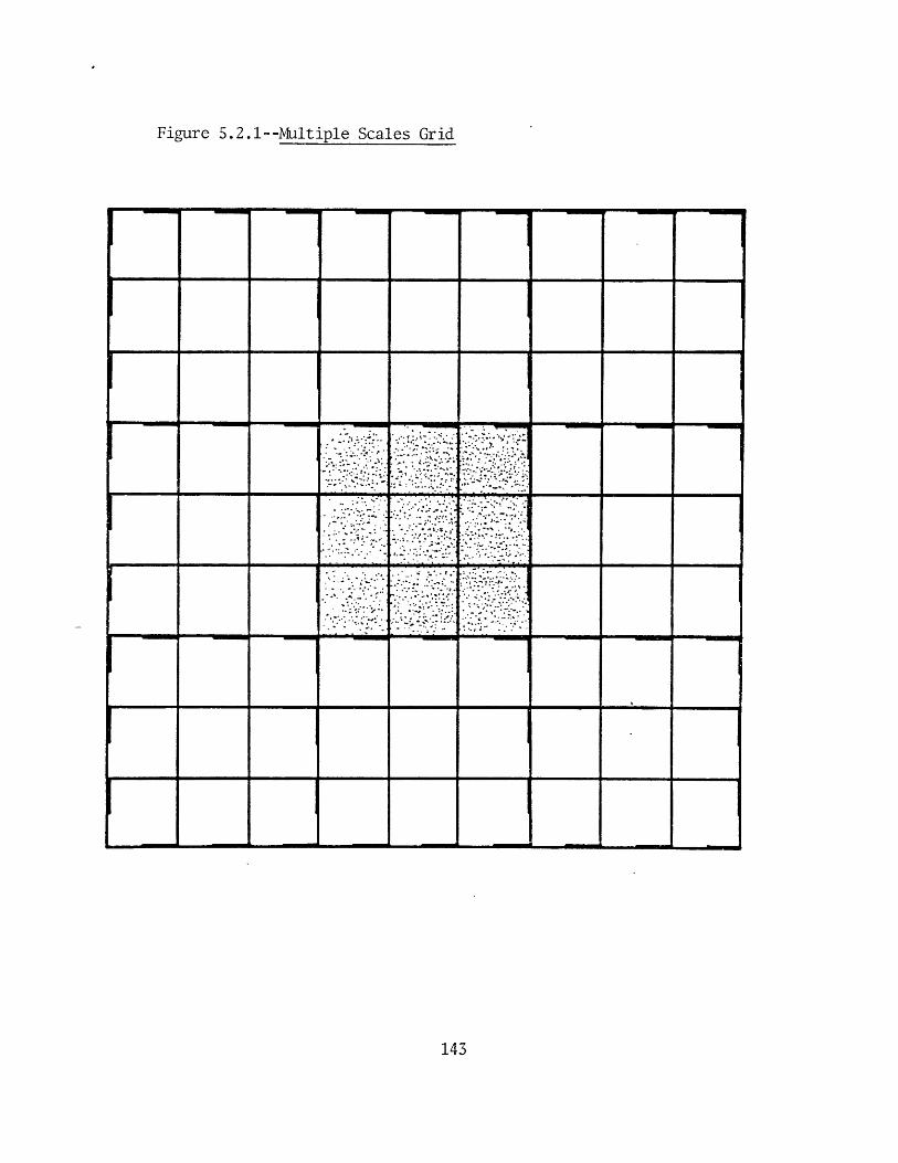
Figure 5.2.1--Multiple Scales Grid
- -* -- *- - - --
143
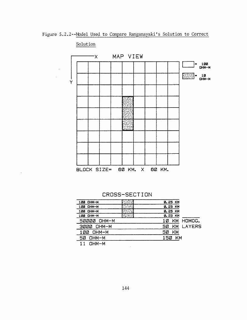
to Compare Ranganayaki's Solution to Correct
Solution
x MAP VIEW
BLOCK SIZE= 60 KM. X 60 KM.
CROSS-SECTION100 OHM-M 0. 25 KM100 OHM-M 0. 25 KM100 OHM-M 0. 25 KM100 OHM-M 0.25 KM
50000 OHM-M 10 KM3000 OHM-M 50 KM100 OHM-M 50 KM50 OHM-M 150 K11 OHM-M
- 100OHM-M
m10-- - HM-M
HOMOG.LAYERS
M
144
Figure 5.2.2--Model Used
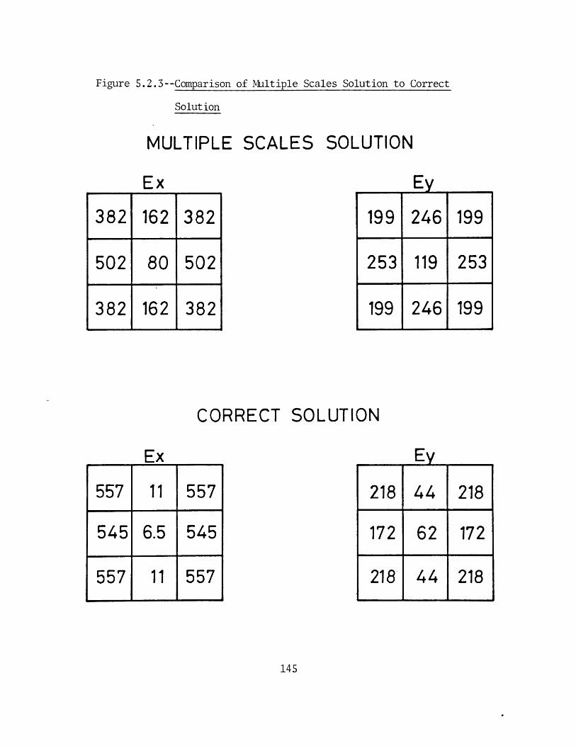
Figure 5.2.3--Comparison of Miltiple Scales Solution to Correct
Solution
MULTIPLE SCALES SOLUTION
Ex_
382 162 382
502 80 502
382 162 382
CORRECT
Ex
557 11 557
545 6.5 545
557 11 557
SOLUTION
145
.- 7
Ey
199 246 199
253 119 253
199 246 199
Ey
218 44 218
172 62 172
218 44 218
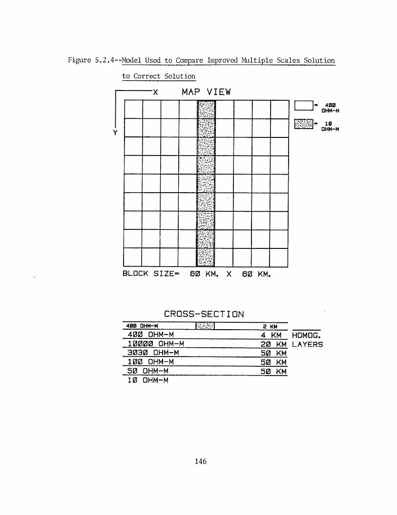
Figure 5.2.4--Model Used to Compare Improved Multiple Scales Solution
to Correct Solution
x MAP VIEW
BLOCK SIZE= 60 KM. X 60 KM.
CROSS-SECTION400 OHM-M 2 KM400 OHM-M 4 KM HOMOG.10000 OHM-M 20 KM LAYERS3030 OHM-M 50 KM100 OHM-M 50 KM50 OHM-M 50 KM10 OHM-M
146
- 400OHM-M
' 10OHM-M
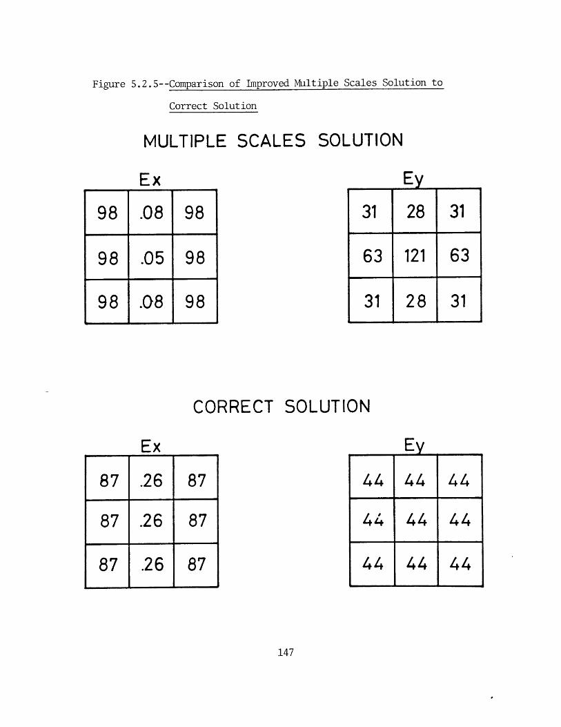
Figure 5.2.5--Comparison of Improved Multiple Scales Solution to
Correct Solution
MULTIPLE
Ex
98 .08 98
98 .05 98
98 .08 98
SCALES SOLUTION
SOLUTION
147
Ey
31 28 31
63 121 63
31 28 31
CORRECT
Ex
87 .26 87
87 .26 87
87 .26 87
Ey
44 44 44
44 44 44
44 44 44
5.3 Equivalent Sources and Multiple Scales
We propose an alternate approach to the multiple scales
problem in this section. This approach differs from the
previous one in that we replace the exterior region with
fields sources on the boundary of the interior region.
We use the average conductivity from the DC solution
and compute the regional solution as in the previous
section. We then get fields at the boundary between the
interior and exterior regions. Figure 5.3.1 is a graphic
representation of our proposed procedure. The heavy, solid
lines in the top sketch represent the boundary fields. The
second sketch in Figure 5.3.1 shows these fields on the
boundaries of the interior region.
The final step is to embed the interior region with its
sources in an infinite, repetitive medium of like cells.
This embedding is shown in the third sketch of Figure 5.3.1.
We can then use a modified form of the thin sheet solution
method presented in Chapter 2 to solve for fields at the
surface. The problem is complicated because the boundary
fields must be substituted for the exterior region at all
levels in the structure including the homogeneous, layered
half-space and the air above the surface.
This proposed method eliminates the need for the
convolution of the local scale Y' with the local scale
fields in the exterior region. Ranganayaki's multiple scale
approach (1978) essentially dealt with only one scale
148
because the boundary for model repetition did not change.
The total number of wavenumbers for the whole region
(interior and exterior) increased as finer subdivisions of
the grid were used. Our procedure retains the same number
of wavenumbers at each step, although the actual wavenumbers
are different. The local scale information in the exterior
region is not needed in the proposed procedure. All
necessary information is contained within the boundary
fields we use.
149
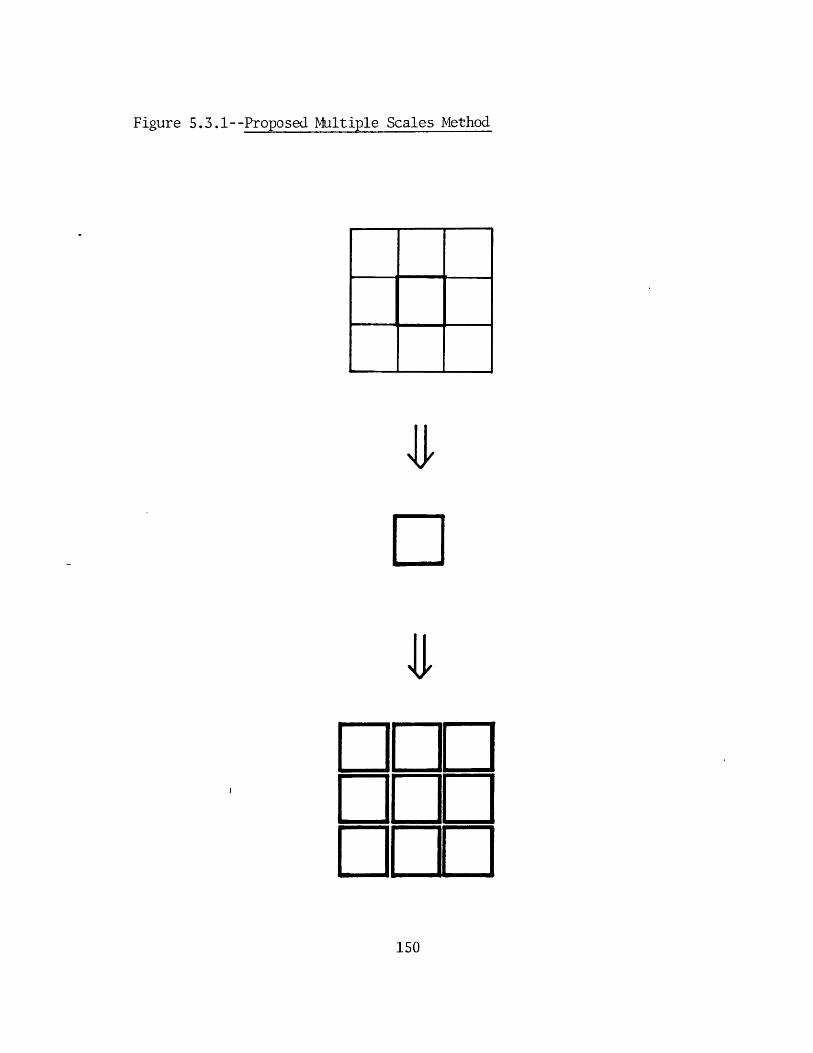
Figure 5.3.1--Proposed Multiple Scales Method
1k
D
lb
III
DI
DD
DEIJD
150
'What a long, strange trip it's been.'
Grateful Dead
CHAPTER 6
We have developed an efficient 3-D modelling alogorithm
in this thesis. This modelling procedure has been used to
extend our knowledge about interactions of MT fields with
complicated structures. We have used simple techniques to
identify which physical mechanism is controlling field
behavior. These mechanisms are horizontal current gathering,
vertical current gathering, and local induction. The
emphasis has been on understanding why the fields behave the
way they do, rather than generating a catalog of models. We
believe the estimation techniques can be applied to real data
to identify the dominant mechanism. This identification
will, in turn, lead to an accurate qualitative interpretation
of the data--the first step towards good quantitative
interpretation.
We have also outlined the theoretical groundwork for a
practical 3-T inversion based on the forward modelling scheme
of Chapter 2. We showed this complicated theory reduced to
known results when applied to a simple problem. We believe
this procedure will be the most efficient inversion method
for complicated structures. Practical application of this
theory has begun.
We applied the techniques and insights in Chapter 2 to
151
interpretation of MT data from Beowawe, Nevada. The most
important result from this interpretation is that, when local
induction dominates the electric field, horizontal dimensions
along the strike of a 2-D body are relatively unimportant.
We also showed that the 12 sites comprising this survey were
really only 2 unique sites. The rest were just duplicates
affected by surface heterogeneities. We see from this survey
that adequate areal coverage of the region, both on and off
the target, is essential for accurate interpretation. These
data would have been uninterpretable without independent
geologic and geophysical information.
We finally discussed our unsuccessful attempts at
solving the most critical, difficult, and interesting problem
in MT modelling--that of multiple scaling. We must be able
to effectively model both the local, fine structure and the
regional, gross structure simultaneously. We understand the
problem more thoroughly now, but a correct approach to its
solution eludes us. We suggest a possible method, but much
work is still needed.
152
REFERENCES
Boehl, J.E., F.X. Bostick, Jr., and H.W. Smith, 1977. AnApplication of the Hilbert Transform to the Magneto-telluric Method, Electrical Geophysics ResearchLaboratory Report, Univ. of Texas at Austin,98 pp.
Cagniard, L., 1953. "Basic Theory of the MagnetotelluricMethod of Prospecting", Geophys. 18, p. 605-635.
Chevron Resources Company, 1975. Well Summary Report forGinn #1-13 Well.
Dawson, T.W., and J.T. Weaver, 1979. "Three-dimensionalInduction in a Non-uniform Thin Sheet at the Surfaceof a Uniformly Conducting Earth", Geophys. Jour.R.A.S. 59, p. 445-462.
Erwin, J.W., 1974. Bouguer Gravity Map of Nevada,Winnemucca Sheet, Nev. Bur. of Mines and Geol. Map 47.
Hermance, J.F., 1982. "The Asymptotic Response of Three-dimensional Offsets to Magnetotelluric Fields at LongPeriods: The Effects of Current Channeling", Geophys.47, p. 1562-1573.
Hohmann, G.W., and S.C. Ting, 1978. Three-dimensionalMagnetotelluric Modelling, Dept. of Energy Rept.IDO-1601-4, Univ. of Utah Research Institute, 48pp.
Jacobs, J.A., 1970. Geomagnetic Micropulsations,Springer-Verlag, New York, 179 pp.
Jiracek, G.R., M.E.Anders, and H.T. Holcombe, 1979. "Mag-netotelluric Soundings of Crustal Conductive Zones inMajor Continental Rifts" in Rio Grande Rift: Tectonicsand Magmatism, AGU, p. 209-222.
Kasameyer, P.W., 1974. Low-frequency Magnetotelluric Surveyof New England, PhD Thesis, Massachusetts Institute ofTechnology, 204 pp.
Kaufman, A.A., and G.V. Keller, 1981. The MagnetotelluricSounding Method, Elsevier Scientific Publishing Co.,Holland, 595 pp.
153
Kong, J.A.,1975. Theory of Electromagnetic Waves, Wiley,New York, 339 pp.
Laird, E.E., and F.X.Bostick, Jr., 1970. One-dimensionalMagnetotelluric Modelling Techniques, ElectricalEngineering Research Laboratory, Tech. Rept. 101, Univ.of Texas at Austin.
Lanczos C., 1956. Linear Differential Operators, VanNostrand, New York, 564 pp.
LaTorraca, G.A., 1981. Differential Tellurics,PhD Thesis, Massachusetts Institute of Technology,182 pp.
Lines, L.R., and F.W. Jones, 1973. "The Perturbation ofAlternating Geomagnetic Fields by Three-dimensionalIsland Structures", Geophys. Jour. R.A.S. 32, p. 133-154.
Madden, T.R. ,1972. Transmission Systems and NetworkAnalogies to Geophysical Forward and Inverse Problems,ONR Rept. NOOO-14-67-A-0204-0045, 45 pp.
, 1980. "Lower Crustal Effects on MagnetotelluricInterpretations or Pulling the Mantle Up by Its Boot-straps" presented at Workshop on Research in Magneto-tellurics: Implications of Electrical Interpretationfor Geothermal Exploration.
, and S.K. Park, 1982. Magnetotellurics in a CrustalEnvironment, USGS Final Rept.
Morrison, H.F., K.H. Lee, G. Oppliger, and A. Dey, 1979.Magnetotelluric Studies in Grass Valley, Nevada,Lawrence Berkeley Laboratory Report LBL-8646, 50 pp.
Oppenheim, A.V., and R.W. Schafer, 1975. Digital SignalProcessing, Prentice Hall, New Jersey, P. 337-366.
Orzag, S.A., 1972. "Comparison of Pseudospectral andSpectral Approximation", Stud. Appl. Math. 51, p. 253-259.
Park, S.K., A.S. Orange, and T.R. Madden, 1983. "Effectsof Three-dimensional Structure in MagnetotelluricSounding Curves", Geophys. in press.
154
Ranganayaki, R.P., 1978. Generalized Thin SheetApproximation for Magnetotelluric Modelling, PhDThesis, Massachusetts Institute of Technology, 204 pp.
,. and T.R. Madden, 1980. "Generalized Thin Sheet
Analysis in Magnetotellurics: An Extension of Price'sAnalysis", Geophys. J. R.A.S. 60, p. 445-457.
Reddy, I.K., D. Rankin, and R.J. Phillips, 1977. "Three-dimensional modelling in Magnetotelluric and MagneticVariation Sounding", Geophys. J. R.A.S. 51, p. 313-325.
Roberts, R.J., K.M. Montgomery, and R.E. Lehner, 1967.Geology and Mineral Resources of Eureka County, Nevada,Nevada Bur. of Mines and Geol. Bull. 64 , 152 pp.
Robinson, E.A., 1966. "Multichannel Z-Transforms andMinimum Delay", Geophys. 31, p. 482-500.
Smith, C., 1979. Interpretation of Electrical Resistivityand Shallow Seismic Reflection Profiles, WhirlwindValley and Horse Heaven Areas, Beowawe KGRA, Nevada,Univ. of Utah Research Institute Rept. ESL-25, 43 pp.
Stanley, W.D., J.E. Boehl, F.X., Bostick, Jr., and H.W.Smith, 1977. "Geothermal Significance ofMagnetotelluric Sounding in the Eastern Snake RiverPlain--Yellowstone Region", J.G.R. 82, p. 2501-2514.
Stewart, J.H., G.W. Walker, and F.J. Kleinhampl, 1975."Oregon-Nevada Lineament", Geology 3, p. 265-268.
Stewart, J.H., E.H. McKee, and H.K. Stager, 1977. Geologyand Mineral Deposits of Lander County, Nevada, NevadaBur. of Mines and Geol. Bull. 88, 106 pp.
Strangway, D.W., C.M. Swift, Jr., and R.C. Holmer, 1973."The Application of Audio-frquency Magnetotellurics toMineral Exploration", Geophys. 38, p. 1159-1175.
Swift, C.M., Jr., 1967. A Magnetotelluric Investigation ofan Electrical Conductivity Anomaly in the SouthwesternUnited States, PhD Thesis, Massachusetts Institute ofTechnology, 211 pp.
155
, 1979. "Geophysical Data, Beowawe Geothermal Area,Nevada", Geothermal Resources Council Trans. 3, p. 701-703.
Weidelt, P., 1975. "Electromagnetic Induction in Three-dimensional Structures", J. Geophys. 41, p. 85-109.
Vozoff, K., 1972. "The Magnetotelluric Method in theExploration of Sedimentary Basins", Geophys. 37, p. 98-141.
156
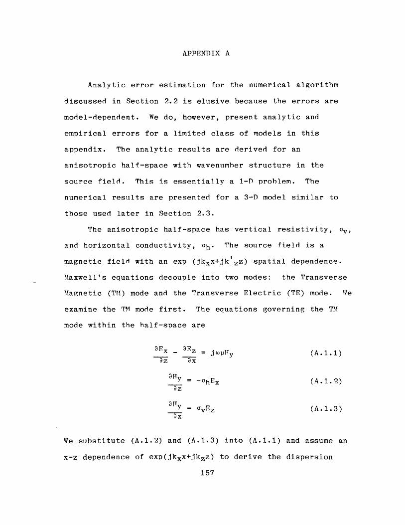
APPENDIX A
Analytic error estimation for the numerical algorithm
discussed in Section 2.2 is elusive because the errors are
model-dependent. We do, however, present analytic and
empirical errors for a limited class of models in this
appendix. The analytic results are derived for an
anisotropic half-space with wavenumber structure in the
source field. This is essentially a 1-P problem. The
numerical results are presented for a 3-D model similar to
those used later in Section 2.3.
The anisotropic half-space has vertical resistivity, av,
and horizontal conductivity, Gh. The source field is a
magnetic field with an exp (jkxx+jk'zz) spatial dependence.
Maxwell's equations decouple into two modes: the Transverse
Magnetic (TM) mode and the Transverse Electric (TE) mode. We
examine the TM mode first. The equations governing the TM
mode within the half-space are
X - -z (A.1.1)
3ZHa3Hy = -ghEx (A.1.2)
az
VTy = CYvEz (A.1.3)3x
We substitute (A.1.2) and (A.1.3) into (A.1.1) and assume an
x-z dependence of exp(jkxx+jkzz) to derive the dispersion
157
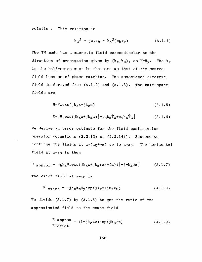
This relation is
9kz - jwah - kx 2 (ahPv) (A.1.4)
The TM mode has a magnetic field perpendicular to the
direction of propagation given by (kxkz), so H=Hy. The kx
in the half-space must be the same as that of the source
field because of phase matching. The associated electric
field is derived from (A.1.2) and (A.1.3). The half-space
fields are
H=Hyexp(jkxx+jkzz) (A.1.5)
E=jHyexp(jkxx+jkzz)[-phkzx+pvkxz] (A.1.6)
We derive an error estimate for the field continuation
operator (equations (2.2.13) or (2.2.14)). Suppose we
continue the fields at z=(z 0 +Az) up to z=zo. The horizontal
field at z=zO is then
F approx " Phkzyexp(jkxx+jkz(z+Az))[-j-kzAz] (A.1.7)
The exact field at z=zo is
F exact = -jPhkzHyexp(jkxx+jkzzo) (A.1.8)
We divide (A.1.7) by (A.1.8) to get the ratio of the
approximated field to the exact field
E approx = (1-jkzAz)exp(jkzAz) (A..9)E exact
158
relation.
Equation (A.1.4) gives the relation between kx, kz, and
a. We have two cases to examine: one in which kx dominates
kz; and one in which joiia dominates kz. The first is
important when source fields exhibit rapid horizontal
fluctuations. The vertical wavenumber then is jkx(ahPv)-
Notice that there is amplification of the error by the
anisotropy factor, ahPv, for the TM mode. We substitute this
expression for kz into (A.1.9) to get
E approx = (1+kx(ahPv)Az)exp(-kx(ahpv)Az) (A.1.10)E exact
Table A.1.1 contains estimates of this ratio for different
values of kxAz and anisotropy factor.
This first case is heuristically similar to small scale
conductivity heterogeneities in the presence of uniform
source fields. The repetition assumption in Section 2.2
limits the number of horizontal wavenumbers, and the spatial
Nyquist 'frequency' gives us the largest wavenumber. The
maximum wavenumber is k=Tr/AL, where AL is the horizontal
block length. We see for no anisotropy (Table A.1.1) that
kAz=.6 is the maximum value for which fields are accurate to
within 10%. This maximum value limits us to using Az no
greater than 20% of the horizontal block length.
The second case is the case of zero kx. The dispersion
relation then gives
kz = (1+j)V(w1ah/2)=(1+j)/6 (A.1.11)
159
where 6 is the electromagnetic skin depth. We substitute
(A.1.11) into (A.1.9) to get the error criterion
E approx = (1+(1+j)Az/6)exp(-(l-j)Az/6) (A.1.12)E exact
We now have both amplitude and phase errors. These errors
are tahulated in Table A.1.2 for several values of Az/6.
These limitations are much less restrictive than those of
Table A.1.1. We can use thicknesses up to 70% of the skin
depth in this case.
We now examine the TE mode. The equations governing
field behavior in the anisotropic half-space are
aux - -z = ahEy (A.1.13)3z ax
7 = -joyHx (A.1.14)3z
3EY = jWyTz (A.1.15)ax
The dispersion relation is derived as before by substituting
(A.1.14) and (A.1.15) into (A.1.13) and assuming an exp(jkxx+
jkzz) dependence in Ey. The dispersion relation is
kz2 = jwah - kx2 (A.1.16)
The anisotropy factor does not appear in the TE mode. The TE
mode is so named because the electric field is polarized
perpendicular to the direction of propagation. The electric
160
field is thus Eyexp(jkxx+jkzz). The associated magnetic
field is determined by substituting Ey into (A.1.14) and
(A.1.15). The TE mode fields are
E=Eyexp(jkxx+jkzz) (A.1.17)
H= Eyexp(jkxx+jkzz)[-kz x+kxizj/w (A.1.18)
We again use (2.2.13) to predict the approximated field and
divide by the exact field to get
F approx = (1-jzAz)exp(jkzAz) (A.1.19)E exact
The cases of large kx and zero kx are again considered. Com-
parison of (A.1.16) and (A.1.4) shows that the zero kx cases
for the TE and TM modes are identical. The large kx case for
the TE mode is identical to the same case for the TM mode
with no anisotropy (OhPv=l)' Hence, Tables A.1.1 and A.1.2
contain the errors for the TE mode also.
The previous analytic error criteria are strictly only
valid for an anisotropic half-space. This analysis can be
extended to layered, anisotropic media, but not to laterally
heterogeneous media. Lateral heterogeneity is always the
case for 3-D bodies. We must resort to empirical error
estimates for 3-D bodies. Figure A.1.1 illustrates a model
used to evaluate these errors. The heterogeneous region is
successively divided into more layers with smaller
thicknesses so that the total thickness is always 600 m. We
161
present errors for the cases of large k and zero k for a
frequency of 0.01 Hz. We have both kx and ky in this
problem, so the effective kz for large k is kxV2. The
largest horizontal wavenumber present in the solution is
kx=7r/AL, so kAz for our model is /TrAz/AL. We first present
errors for the large k case in Table A.1.3. Maximum errors
in apparent resistivity inside and outside the heterogeneity
are tabulated. The error shown is |1-Pa/Pa at 9% thicknessl*
100%. We see from these errors that we are limited to using
thicknesses less than 5% of the horizontal dimensions if we
want errors less than 10%.
The second case we evaluate is that of zero k. The
ratio of the thickness to the skin depth is now important, so
the model in Figure A.1.1 has been changed. Block sizes are
increased ten-fold, decreasing the maximum wavenumber by an
order of magnitude. The frequency is increased to 1 Hz so
that the minimum thickness used is now 10% of the skin depth.
We perform the same error analysis as before by varying the
individual layer thicknesses and the total number of layers.
The results of this analysis are presented in Table A.1.4.
We see that a thickness of half of the skin depth may be used
before 10% errors appear.
We have presented both analytic and empirical error
analyses in this appendix. These two types of analysis
qualitatively agree. The aspect ratio (Az/AL) is much more
restrictive than is the thickness:skin depth ratio. Field
162
errors of 10% or less occur for aspect ratios of less than
0.2. The thickness:skin depth ratio can be much larger--up
to 0.5 is the same 10% error level is sought. These errors
are model-dependent, however. The relative importance of
solutions with the large wavenumber behavior is dependent
upon the conductivity structure. Rapid spatial conductivity
variations will produce a solution with large wavenumber
structure.
163
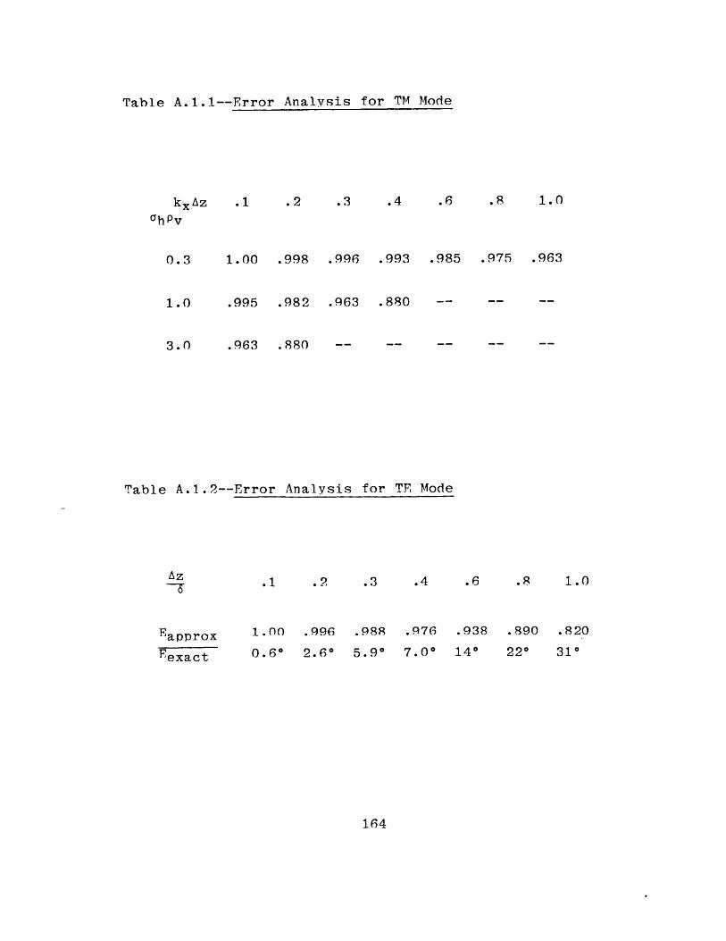
Table A.1.1--Error Analysis for
.2 .3 .4 .6 .8 1.0
1.00 .998 .996 .993 .985 .975 .963
.995 .982 .963 .880
.963 .880
Table A.1.2--Error Analysis for TE Mode
.1 .2 .3 .4 .6 .8 1.0
1.00 .996 .988 .976 .938 .890 .820
0.6* 2.6* 5.90 7.00 14* 220 310
164
kxAz
GhPv
0.3
1.0
3.0
Az
Eapprox
Eexact
TM Mode
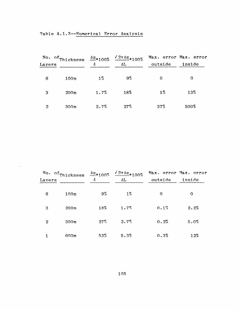
Table A.1.3--Numerical Error Analysis
No. of Thickness
Layers
loom
200m
300m
No. ofThickness
Layers
loom
200m
300m
600m
Az*100% / 2 AzO*100% Max. error Max. error
6 AL outside inside
1%
1.7%
2.7%
Az*100%6
9%
18%
27%
53%
9%
18%
27%
/2rAz
1%
37%
13%
500%
Max. error Max. error
AL outside inside
1%
1.7%
2.7%
5.3%
0
0.1%
0.2%
0.3%
0
2.2%
5.0%
12%
1 05
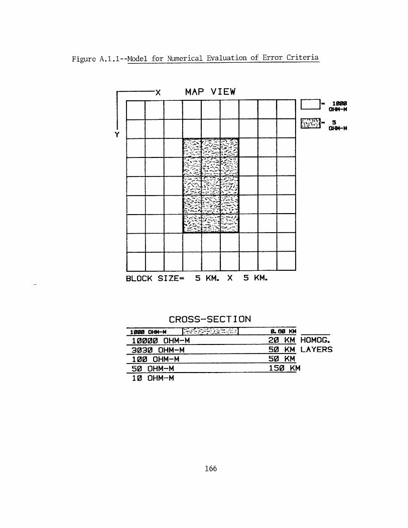
Figure A.1.1--Model for Numerical
MAP VIEW
BLOCK SIZE= 5 KM. X 5 KM.
CROSS-SECTION1993 OHM4-M
10000 OHM-3030 OHM-100 OHM-M50 OHM-M10 OHM-M
I. 80 KM
20 KM HOMOG.50 KM LAYERS50 KM150 KM
166
L ]- 1900OHM-M=lIowM-
Evaluation of Error Criteria
,
APPENDIX B
The AC magnetic field induces regional electric fields
which we treat as background fields in the following
analysis. These background fields are perturbed by local
conductivity heterogeneities. We recognize three different
mechanisms responsible for these perturbations at low
frequencies. Figure B.1.1 illustrates these mechanisms. The
first is vertical current gathering, and has been discussed
extensively by Ranganayaki and Madden (1980). The second is
horizontal current gathering. These first two mechanisms
have essentially DC behavior--their electric field magnitudes
are frequency-independent. The third is local induction.
The regional magnetic field creates local current cells in a
good conductor. This local induction is frequency-dependent.
Each mechanism has a different influence on the spatial
behavior of the local electric field, so the importance of
identifying the dominant contribution is clear. We present a
simple method of estimating each contribution to within an
order of magnitude. This estimation process is only valid
for frequencies at which the skin depth is much greater than
the thickness of the heterogeneous region.
We consider the vertical current mechanism first. We
esitmate the electric field change due to vertical current
gathering by a conductive body. Ranganayaki and Madden
(180) give the solution for the perpendicular electric
167
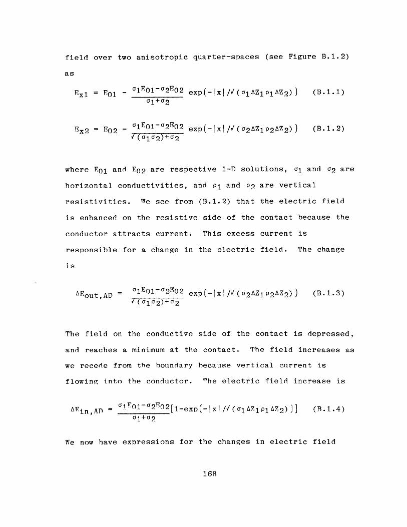
field over two anisotropic quarter-spaces (see Figure B.1.2)
as
Exi = -E a1_ 01 -G 2E0 2 exp(-Ix|/V(aiAZipiAZ2 )) (B.1.1)
Ex2 = E0 2 - alE0 1- 2 E0 2 exp(-IxI/V(a 2 AZ 1 P2 A72 )) (B.1.2)
V(G 1 a2 )+a2
where Ei and E0 2 are respective 1-D solutions, a1 and a2 are
horizontal conductivities, and Pi and p2 are vertical
resistivities. We see from (B.1.2) that the electric field
is enhanced on the resistive side of the contact because the
conductor attracts current. This excess current is
responsible for a change in the electric field. The change
is
AEout,AD = aiEOg-a2EO2 exp(-xl//(a 2 AZ1P 2 AZ2 )) (B.1.3)
V(a 1 a2 )+a2
The field on the conductive side of the contact is depressed,
and reaches a minimum at the contact. The field increases as
we recede from the boundary because vertical current is
flowing into the conductor. The electric field increase is
AEin,AD = a1E01~2E02[1.exp(_Ixl/V(clAZlPlAZ2))] (B.1.4)
01+02
We now have expressions for the changes in electric field
168
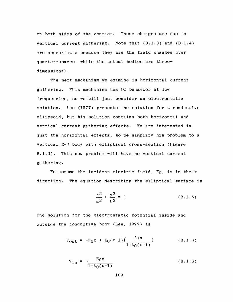
on both sides of the contact. These changes are due to
vertical current gathering. Note that (B.1.3) and (B.1.4)
are approximate because they are the field changes over
quarter-spaces, while the actual bodies are three-
dimensional.
The next mechanism we examine is horizontal current
gathering. This mechanism has DC behavior at low
frequencies, so we will just consider an electrostatic
solution. Lee (1977) presents the solution for a conductive
ellipsoid, but his solution contains both horizontal and
vertical current gathering effects. We are interested in
just the horizontal effects, so we simplify his problem to a
vertical 2-D body with elliptical cross-section (Figure
B.1.3). This new problem will have no vertical current
gathering.
We assume the incident electric field, EO, is in the x
direction. The equation describing the elliptical surface is
- - 1 (B.1.5)
a2 b2
The solution for the electrostatic potential inside and
outside the conductive body (Lee, 1977) is
Vout = -Eox + E0 (6-1)( Axx ) (B.1.6)1+A0 (s-i)
Vin = EOx (B.1.6)1+A0 (E-1)
169
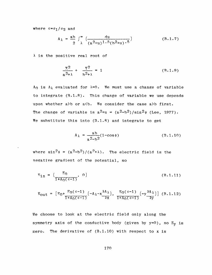
where E=a/a 2 and
A ab f 0 du (B.1.7)2 X (a2+u)1 5 (b2+u)'5
X is the positive real root of
X2 + y2+ =-1 (B3.1.9)a2+X b2+X
A0 is AX evaluated for X=0. We must use a change of variable
to integrate (B.1.8). This change of variable we use depends
upon whether a>b or a<b. We consider the case a>b first.
The change of variable is a2+u = (a2-b2 )/sin 2 * (Lee, 1977).
We substitute this into (B.1.8) and integrate to get
AX = ab (1-cos$) (B.1.10)a2-b2
where sin 2 $ = (a 2 -b 2 )/(a 2 +X). The electric field is the
negative gradient of the potential, so
Ein = ( 0 , 0) (B.1.11)1+A0 (s-1)
Eout = [T'0+ F0(E1) (-AX-x3AX), E0 (c-1) (.y3AX)] (B.1.12)1+AO(e-1) 3x 1+AO(E-1) ~3y
We choose to look at the electric field only along the
symmetry axis of the conductive body (given by y=0), so Ey is
zero. The derivative of (B.1.10) with respect to x is
170
3AX ab sint]- tan$ 2x x 2 v 2 1
ax a2-b 2 2(a 2 +X) a 2 +X (a2 +X)2 (h2+X) 2
(B.1.13)
We evaluate (B.1.13) along a line of y=O,and substitute this
and (B.1.10) into (B.1.12) to get
Rout = E0 +[ E0 (c-1) j[1-cosj[ ab (B.1.14)1+A0 (e-1) cos$ a2-b 2
We desire the change in the electric field due to the
presence of the conductor. The background field outside is
E0, so from (B.1.14)
Arout'h E(E-1) -cos[ ab j (.1.15)
1+A0 (c-1) cost a2 -h 2
The background field inside is not so simple. We want the
electric field change due to excess current gathered by the
conductor. The background current density is a2E0 . The
background field is that field that would be present is the
background current were flowing in a conductor with
conductivity al. The background field is thus (a2E0 )/a1 , and
the electric field change inside is
AEin,h = 0 - a2 E (B.1.16)
1+AT(d-1) ai
These field change estimates due to horizontal current
171
gathering are only valid for a>b. We now consider the case
a<b.
We must use the substitution a2 +u=(b 2 -a2 )/sin 2 * for b>a.
This results in the following expression for AX
AX = ab (b2+ )-i] (B.1.17)a2-b 2 a2+X
We go through the same manipulations that led to (B.1.15) and
derive an alternate expression for AEout,h
Fuh ~(s-1) ab V(b2-a 2 +x 2 ) abA~out,h =b ~ -1)-1+AO(6-1) b2-a 2 x xV(h 2 -a 2+x 2 )
(B.1.18)
The expression for A~inh is unchanged for b>a. All of the
electric field changes ((B.1.15), (B.1.16), and (B.1.18)) are
approximations because the elliptical body is
two-dimensional.
The last mechanism is local induction. The fluctuating
magnetic field induces current cells in the conductive body.
The magnetic field has a large constant component (80-90% of
the total field) within the body, and this component is
coupled to the fundamental mode (illustrated in Figure
B.1.1). We estimate the electric field due to this
fundamental mode by using Faraday's law
172
1 A
where A is the area encircled by the path 1. The area for
the fundamental mode is roughly the cross-section of the body
(AY long and AZ thick). We assume E is constant on the path
since the current is circulating in a loop, and that the
magnetic field threading the loop is constant. Equation
(B.1.19) reduces with these assumptions to
E(2AY+2AZ) = jwuTAYAZ (B.1.20)
Equation (P.1.20) simnlifies even further because AZ<<AY.
The final expression for E is
Einduct 2AZ (B.1.21)
Local induction effects also exist outside the
conductor. A rough approximation to these effects is the
field due to a horizontal magnetic dipole with moment
m=I*area. Stratton (1941) gives the far field electric field
as
-- 2 V- 1+ )Im sine (B.1.22)47T e R kR2
where E is the $ component in a spherical coordinate system
aligned along the axis of the horizontal dipole. The axis of
the conductor is perpendicular to the dipole axis, so the
173
f E-dl = joyf HT-da (B. 1. 19)
line y=0 has 6=90*. The $ vector is aligned parallel to the
z axis at the surface, so the electric field given by
(R.1.22) is all Ez. There is no horizontal electric field at
the surface due to the magnetic dipole to a first
approximation. Local induction effects can thus be neglected
outside the conductor in this analysis.
We have presented methods for determining the dominant
mechanism governing local electric field perturbation. The
mechanisms are local induction, horizontal current gathering,
and vertical current gathering. Each produces a different
spatial field behavior. The field separation procedure
outlined here is only approximate, but suffices for an
order-of-magnitude study. We will apply this method to the
models presented in Section 2.3 when discussing the MT
sounding curves.
174
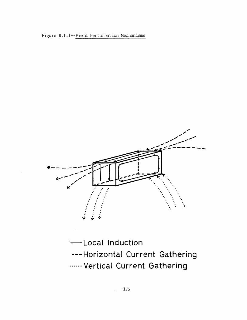
Figure B.1.1--Field Perturbation Mechanisms
- 0-
* ~ 0, so"--- .
-900-
-- Local Induction--- Horizontal Current Gathering
------- Vertical Current Gathering
175
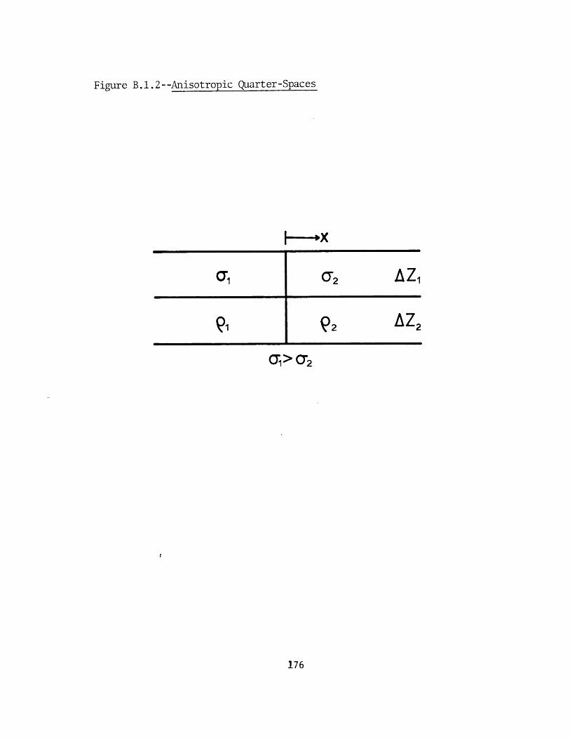
Figure B.1.2--Anisotropic Quarter-Spaces
a1 2 AZ1
91 92 AZ2
176
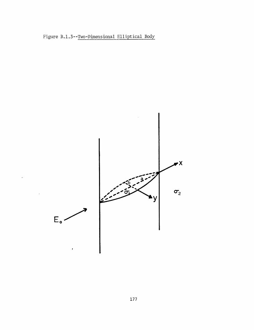
Figure B.1.3--Two-Dimensional Elliptical Body
E0
177
APPENDIX C
We present here the processing done on the raw power
spectra from Beowawe to produce the needed impedance tensor
estimates. Geotronics Corporation records time series which
are filtered to pass one frequency decade. The effective
passband of the system is about 3 decades, centered on the
single decade of interest. These time series are Fourier
transformed, and power estimates are computed between all
channels. These are the raw power spectra supplied by
Geotronics on computer tape. The data consist of 5
overlapping frequency bands (runs) which need to be
'stacked' to yield a single power estimate at any given
frequency. Each sounding curve in Chapter 4 is a
compilation of 5-10 data runs over different frequency
decades.
We use constant bandwidth averaging to achieve this
'stacking'. Each band is .1 frequency decade wide. All
power estimates within each band are weighted by the number
of spectral harmonics contributing to that estimate and then
summed. The sum is normalized by the total number of
spectral harmonics used to produce the sum. This procedure
yields a single average spectral estimate for each .1
frequency decade over the 5 decades for which we have data.
The next step in the process is to estimate impedance
tensors for each frequency band. We use two different
estimates called the E estimate and the H estimate. The
178
impedance tensor is slowly varying for a narrow frequency
band so
Ex(w) Zxx Zxy~ Hx(w)II I I j(C.3.1)
Ey(o) Zyx Zyy Hy(W)
We postmultiply by (T*)T, average over a narrow frequency
band, and invert HUT to yield the T estimate of the
impedance tensor
-1
[(Exi U*> <ExIT x <HxU*> <HxHy*>Zg1 = *] (0'.3.2)<EyTx > (EyTUy . .(HyH*> <HyHy*>
where < > is the average power estimate over .1 frequency
decade band. The E estimate can be similarly derived
-1
(E~*> (EYEy* yHEx*> <HyEy*>ZE <E * > <EXEy*>j <HXEX*> <HxEy*> (C.3.3)
Sims, et. al. (197P) show that the E estimate is biased up
by noise in the electric fields, and the H estimate is
biased downward by noise in the magnetic fields. These two
estimates should thus bracket the noise-free impedance
tensor estimate.
We also look at predicted F field coherencies as a
179
measure of noise. The predicted E field is calculated from
the tensor impedance
7i pred = ZixHx data + ZiyHy data (C.3.4)
We then compute the coherency between the predicted field
and the measured field
coh(Ei predEi data) - <Ei dataEi pred>V(<7i pred i pred><Ei dataEi" data>)
(C.3.5)
This coherency can be rewritten in terms of the measured
power spectra solely. Tensor estimates in the Beowawe data
set were rejected if either of the predicted E coherencies
was below 0.9. This corresponds to about 45% noise
(noise=/(1-coh )).
Swift (1967) demonstrates that the impedance tensor
reduces to two off-diagonal elements along symmetry axes for
a 2-D structure. This off-diagonalization also occurs for
tensors along symmetry axes of 3-P structures. W7e rotate
the tensor about the z axis to find these axes of symmetry.
The rotated tensor is
cos6 sinO[ Zxx Zxy' cose -sinf-sine cos6 Zyx Zyy sine cosOJ (C.3.6)
180
We minimize the magnitude of the sum of the diagonal
elements of the rotated tensor to choose the symmetry
directions. This sum is often non-zero after it has been
minimized however, because of data noise or the presence of
3-D structures. We use two further quantities, the skew and
ellipticity, as indicators of 3-D structure (or noise).
These quantities are defined in Section 3 of Chapter 2, so
need not be restated here. Apparent resitivities and phases
are computed from the off-diagonal elements of the rotated
tensor and plotted versus frequency.
LaTorraca (1981) has developed an alternate method of
tensor analysis based on eigenvalue decomposition which has
some advantages over the conventional method outlined above.
LaTorraca's procedure was used on the Beowawe data set, but
the high degree of two-dimensionality eliminated any
advantage the eigenanalysis had over the conventional
method.
181
APPFNDIX D
We prove that the off-diagonal terms in the conductivity
tensor are equal in this appendix. This proof assumes that
the z axis is one of the principal axes of the medium.
There is thus some set of orthogonal axes in the x-y plane
for which
410a = a2(D.1.1)
Rotation about the z axis to any set of x-y axes is
achieved through matrix multiplication
axx axy- cose sine' 'ai 0 'cose -sine
ayx ayy -sinG cosO 0 a2 -sine cosO
This equation reduces to
1 2 2axx axy _ acos 6+a9sin 2 sinocosO(al-a2)]
ayx ayy sinecosO(a1 -a 2 ) a1sin O+a2 cos 6
We see immediately from (D.1.3) that axy=ayx.
182
BIOGRAPHICAL NOTE
The author was conceived in Berkeley, California (which
explains a lot of things). He was born roughly 9 months
later on April 27, 1956 in a Quonset hut on Lackland Air
Force Base in San Antonio, Texas. His mother was
simultaneously experiencing two firsts--her first child and
her first thunderstorm. As she put it, 'Life with you as a
small child--I'm not sure if the thunderstorm ever ended'.
Birth in Texas, for those unfamiliar with Texan customs,
automatically confers membership in the Good Ole Boy Club.
Courtesy of the U.S. Air Force, the author was moved
many times until he got old enough to move himself. He spent
7 years in Waco, Texas, where he learned a game called "North
vs. South" in elementary school. In this game, all the
popular (or big) kids in school got together on one side
(they were the South) and knocked down everyone else (the
North). After living in El Cerrito, California (next to
Berkeley!), Wiesbaden, Germany, Escondido, California, and
Tucson, Arizona, the author was given the privilege of
attending high school in Biloxi, Mississippi. He learned
here from an American History teacher that "V.D. was God's
way of showing who the sinnners were". He moved to
Grandview, Missouri shortly after this pearl of wisdom and
finished high school in the 20th Century.
The author chose to attend college, but aside from
going to Berkeley, he was not sure what he wanted to do.
183
He found a short paragraph in a book on careers in physics
about the exciting field of geophysics. He had planned to
major in physics, but decided what the hell, why not
geophysics? He had always enjoyed collecting pretty rocks
anyway. The author ended up at the University of California
at Riverside after redirection from Berkeley and San Diego.
He learned about Beer Drinking, Volleyball, Water Polo,
Explosives Fun, and Geophysical Hell-Raising in the Desert
from 1974 to 1978 under the tutelage of Shawn Biehler and
Tien C. Lee. He decided at this time that field geophysics
was not a bad life after all.
The author began work with Ted Madden at the
Massachusetts Institute of Technology in 1978. He enjoyed
living on the East Coast so much that he promptly arranged so
that he could spend 6-8 months a year out West. He continued
his work in Water Polo, Volleyball, and Beer Drinking during
his rare visits to the East Coast. He also learned something
about being flexible from his advisor during this time. He
does not and never has played ice hockey, however!
The author quickly discovered the monetary and travel
benefits of summer employment with the oil companies. He has
had the opportunity to rape and pillage the environment in
such diverse places as the Michigan swamps, south Texas,
Arizona, Berkeley (there it is again!), and the San Juan
Mountains of Colorado while ostensibly employed by big oil.
His work with Ted Madden on earthquake prediction (sic) has
184
allowed him to sample the charms of the California towns of
Palmdale and Hollister.
The author has taken a position with Chevron Oil Field
Research Company in La Habra, California as one-half of
their non-seismic research group. He is a member in good
standing of the Sierra Club.
185