theoretical and numerical aspects of modelling geological
TRANSCRIPT
Theoretical and Numerical Aspects of Modelling
Geological Carbon Storage with Application to
Muographic Monitoring
Darren L. Lincoln
This thesis is submitted for partial consideration towards the degree
of Doctor of Philosophy at the
The Department of Civil and Structural Engineering
at the University of Sheffield
December 2015

No flow system is an island.
A. Bejan
Abstract
The storage of waste carbon dioxide (CO2) from fossil fuel combustion in deep geological forma-
tions is a strategy component for mitigating harmfully increasing atmospheric concentrations to
within safe limits. This is to help prolong the security of fossil fuel based energy systems while
cleaner and more sustainable technologies are developed. The work of this thesis is carried out
as part of a multi-disciplinary project advancing knowledge on the modelling and monitoring of
geological carbon storage/sequestration (GCS).
The underlying principles for mathematically describing the multi-physics of multiphase multi-
component behaviour in porous media are reviewed with particular interest on their application
to modelling GCS. A fully coupled non-isothermal multiphase Biot-type double-porosity formu-
lation is derived, where emphasis during derivation is on capturing the coupled hydro-thermo-
mechanical (HTM) processes for the purposes of study.
The formulated system of governing field equations is discretised in space by considering the
standard Galerkin finite element procedure and its spatial refinement in the context of capturing
coupled HTM processes within a GCS system. This presents a coupled set of nonlinear first-order
ordinary differential equations in time. The system is discretised temporally and solved using
an embedded finite difference method which is schemed with control theoretical techniques and
an accelerated fixed-point-type procedure.
The developed numerical model is employed to solve a sequence of benchmark problems of in-
creasing complexity in order to comprehensively study and highlight important coupled processes
within potential GCS systems. This includes fracture/matrix fluid displacement, formation de-
formation and Joule-Thomson cooling effects. The computational framework is also extended
to allow for the simulation of cosmic-ray muon radiography (muography) in order to assess the
extent to which detected changes in subsurface muon flux due to CO2 storage can be used to
monitor GCS. This study demonstrates promise for muography as a novel passive-continuous
monitoring aid for GCS.
i


Acknowledgements
I thank the University of Sheffield for granting resource to support my development to carry
out this work. I would especially like to thank Harm Askes, Colin Smith, Terry Bennett, John
Cripps and Vitaly Kudryavtsev for their vision, inspiration and guidance during my studies. I
would like to further express my gratitude for the technical and often philosophical discussions
which have coincided and entwined with the work of this thesis. This goes to everyone who
has known me from my vantage at the Department of Civil and Structural Engineering and the
Department of Physics and Astronomy at the University of Sheffield, to whom I am indebted.
Finally, I thank my friends and family, and not least, Petra, my parents and my brother, for
whom I will continue to achieve the best I can.
Darren Lincoln
December 2015
iii

Contents
Abstract i
Acknowledgements iii
List of Figures xi
List of Tables xiii
Nomenclature xv
1 Introduction 1
1.1 Energy . . . . . . . . . . . . . . . . . . . . . . . . . . . . . . . . . . . . . . . . . . 1
1.2 Fossil fuels and climate change . . . . . . . . . . . . . . . . . . . . . . . . . . . . 1
1.3 Carbon capture and storage . . . . . . . . . . . . . . . . . . . . . . . . . . . . . . 3
1.3.1 Principles of GCS . . . . . . . . . . . . . . . . . . . . . . . . . . . . . . . 3
1.4 Thesis aims, objectives and layout . . . . . . . . . . . . . . . . . . . . . . . . . . 5
2 Literature Review & Fundamentals 9
2.1 Porous media theory . . . . . . . . . . . . . . . . . . . . . . . . . . . . . . . . . . 9
2.1.1 Porosity . . . . . . . . . . . . . . . . . . . . . . . . . . . . . . . . . . . . . 10
2.1.2 Distribution functions and volume fractions . . . . . . . . . . . . . . . . . 10
2.1.3 Averaging functions/operators . . . . . . . . . . . . . . . . . . . . . . . . 12
2.2 Kinematics . . . . . . . . . . . . . . . . . . . . . . . . . . . . . . . . . . . . . . . 13
2.3 Identities . . . . . . . . . . . . . . . . . . . . . . . . . . . . . . . . . . . . . . . . 14
2.4 General microscopic balance equations . . . . . . . . . . . . . . . . . . . . . . . . 14
2.5 General mean macroscopic balance equations . . . . . . . . . . . . . . . . . . . . 16
2.6 Equations of state and constitutive relations . . . . . . . . . . . . . . . . . . . . . 18
2.6.1 Helmholtz free energy . . . . . . . . . . . . . . . . . . . . . . . . . . . . . 18
2.6.2 Entropy inequality . . . . . . . . . . . . . . . . . . . . . . . . . . . . . . . 19
v
Contents
2.6.3 Porous media stress partition . . . . . . . . . . . . . . . . . . . . . . . . . 19
2.6.4 Effective stress and strain/deformation . . . . . . . . . . . . . . . . . . . . 21
2.6.5 Fick’s law . . . . . . . . . . . . . . . . . . . . . . . . . . . . . . . . . . . . 22
2.6.6 Darcy’s law . . . . . . . . . . . . . . . . . . . . . . . . . . . . . . . . . . . 23
2.6.7 Fourier’s law . . . . . . . . . . . . . . . . . . . . . . . . . . . . . . . . . . 23
2.6.8 Fluid thermodynamic properties . . . . . . . . . . . . . . . . . . . . . . . 24
2.6.8.1 Density: CO2-brine mixture p-v-T-x relationship . . . . . . . . . 25
2.6.8.2 Heat capacity . . . . . . . . . . . . . . . . . . . . . . . . . . . . 27
2.6.8.3 Joule-Thomson coefficient and cooling . . . . . . . . . . . . . . . 28
2.6.9 Fluid transport properties . . . . . . . . . . . . . . . . . . . . . . . . . . . 29
2.6.9.1 Dynamic viscosity . . . . . . . . . . . . . . . . . . . . . . . . . . 29
2.6.9.2 Thermal conductivity . . . . . . . . . . . . . . . . . . . . . . . . 30
2.6.9.3 Surface tension and energy . . . . . . . . . . . . . . . . . . . . . 30
2.6.10 Compressibility & thermal expansion coefficients . . . . . . . . . . . . . . 31
2.6.10.1 Fluid density . . . . . . . . . . . . . . . . . . . . . . . . . . . . . 31
2.6.10.2 Solid density . . . . . . . . . . . . . . . . . . . . . . . . . . . . . 32
2.7 Capillarity . . . . . . . . . . . . . . . . . . . . . . . . . . . . . . . . . . . . . . . . 32
2.7.1 Capillary pressure-saturation relationship . . . . . . . . . . . . . . . . . . 33
2.7.2 Relative permeability-saturation relationship . . . . . . . . . . . . . . . . 34
2.7.3 Interface stability and phase mobility contrast . . . . . . . . . . . . . . . 35
2.8 Further HTMC Processes . . . . . . . . . . . . . . . . . . . . . . . . . . . . . . . 36
2.8.1 Dissolution (solubility and ionic) mechanisms . . . . . . . . . . . . . . . . 36
2.8.2 Mineral mechanisms . . . . . . . . . . . . . . . . . . . . . . . . . . . . . . 37
2.8.3 Adsorption mechanisms . . . . . . . . . . . . . . . . . . . . . . . . . . . . 37
2.8.4 Density convection mixing . . . . . . . . . . . . . . . . . . . . . . . . . . . 38
2.8.5 Porosity and permeability changes . . . . . . . . . . . . . . . . . . . . . . 38
2.9 Upscaling . . . . . . . . . . . . . . . . . . . . . . . . . . . . . . . . . . . . . . . . 38
2.10 Double-porosity transfer function . . . . . . . . . . . . . . . . . . . . . . . . . . . 39
2.11 Monitoring . . . . . . . . . . . . . . . . . . . . . . . . . . . . . . . . . . . . . . . 40
2.11.1 Electrokinetic monitoring . . . . . . . . . . . . . . . . . . . . . . . . . . . 41
2.11.2 Cosmic-ray muon tomographic monitoring . . . . . . . . . . . . . . . . . . 42
2.11.2.1 Muon scattering tomography imaging . . . . . . . . . . . . . . . 43
2.11.2.2 Muon transmission imaging . . . . . . . . . . . . . . . . . . . . . 43
vi
Contents
2.11.2.3 Particle transport simulation . . . . . . . . . . . . . . . . . . . . 44
2.12 Modelling . . . . . . . . . . . . . . . . . . . . . . . . . . . . . . . . . . . . . . . . 44
2.12.1 Modular Class: Sequential coupling of a flow simulator with other software 45
2.12.2 Fully Coupled Class: Fully coupled (simultaneous) behaviour . . . . . . . 45
2.13 Review on fractures/fracturing—initiation and propagation . . . . . . . . . . . . 46
2.14 Summary of key research needs . . . . . . . . . . . . . . . . . . . . . . . . . . . . 47
3 Model Formulations 49
3.1 Model description . . . . . . . . . . . . . . . . . . . . . . . . . . . . . . . . . . . . 49
3.2 Mass balance . . . . . . . . . . . . . . . . . . . . . . . . . . . . . . . . . . . . . . 51
3.2.1 Primary/state variables . . . . . . . . . . . . . . . . . . . . . . . . . . . . 51
3.2.2 Solid mass balance for a porous continuum . . . . . . . . . . . . . . . . . 52
3.2.3 Generic biphasic fluid and solid phase mass balance in a porous continuum 52
3.2.4 Wetting and nonwetting phase mass balance in the porous continuum . . 53
3.2.5 Wetting and nonwetting phase mass balance in the fracture continuum . . 55
3.2.6 Illustration: 1D axisymmetric mass balance solutions . . . . . . . . . . . . 57
3.3 Momentum balance . . . . . . . . . . . . . . . . . . . . . . . . . . . . . . . . . . . 64
3.4 Energy/enthalpy balance . . . . . . . . . . . . . . . . . . . . . . . . . . . . . . . . 65
3.5 Summary of governing field equations . . . . . . . . . . . . . . . . . . . . . . . . 70
4 Spatial Discretisation 73
4.1 Method of weighted residuals (Galerkin procedure) . . . . . . . . . . . . . . . . . 74
4.1.1 Momentum balance initial and boundary conditions . . . . . . . . . . . . 75
4.1.2 Momentum balance discretisation . . . . . . . . . . . . . . . . . . . . . . . 76
4.1.3 Mass balance initial and boundary conditions . . . . . . . . . . . . . . . . 76
4.1.4 Mass balance discretisation . . . . . . . . . . . . . . . . . . . . . . . . . . 77
4.1.5 Energy balance initial and boundary conditions . . . . . . . . . . . . . . . 78
4.1.6 Energy balance discretisation . . . . . . . . . . . . . . . . . . . . . . . . . 78
4.2 The spatially discretised system of equations . . . . . . . . . . . . . . . . . . . . 79
4.3 Shape functions & isoparametric finite elements . . . . . . . . . . . . . . . . . . . 81
4.3.1 2D Jacobian matrix and determinant . . . . . . . . . . . . . . . . . . . . . 84
4.3.2 Gauss-Legendre quadrature for axisymmetric numerical integration . . . . 85
4.4 General Finite Element Formulations . . . . . . . . . . . . . . . . . . . . . . . . . 86
4.4.1 Tangential stiffness element matrix . . . . . . . . . . . . . . . . . . . . . . 86
vii
Contents
4.4.2 Laplace element matrix . . . . . . . . . . . . . . . . . . . . . . . . . . . . 87
4.4.3 Mass element matrix . . . . . . . . . . . . . . . . . . . . . . . . . . . . . . 88
4.4.4 Advection element matrix . . . . . . . . . . . . . . . . . . . . . . . . . . . 89
4.4.5 Displacement and pressure coupling element matrices . . . . . . . . . . . 89
4.4.6 Body force/source element vectors . . . . . . . . . . . . . . . . . . . . . . 89
4.4.7 Surface force/flux element vectors . . . . . . . . . . . . . . . . . . . . . . 90
4.5 Global matrix assembly and programming aspects . . . . . . . . . . . . . . . . . 91
4.6 Meshing and mesh refinement . . . . . . . . . . . . . . . . . . . . . . . . . . . . . 92
5 Temporal Integration & Solution Control 93
5.1 Method 1: The θ-method . . . . . . . . . . . . . . . . . . . . . . . . . . . . . . . 95
5.2 Method 2: The Thomas-Gladwell method . . . . . . . . . . . . . . . . . . . . . . 96
5.3 Embedded backward-Euler/Thomas-Gladwell pair . . . . . . . . . . . . . . . . . 97
5.4 Nonlinear solver . . . . . . . . . . . . . . . . . . . . . . . . . . . . . . . . . . . . 98
5.4.1 Solver . . . . . . . . . . . . . . . . . . . . . . . . . . . . . . . . . . . . . . 99
5.4.2 Anderson acceleration and mixing . . . . . . . . . . . . . . . . . . . . . . 99
5.4.3 Tolerance . . . . . . . . . . . . . . . . . . . . . . . . . . . . . . . . . . . . 101
5.5 Control theory: Adaptive time-step size control . . . . . . . . . . . . . . . . . . . 101
5.5.1 Optimal error control for the integration procedure . . . . . . . . . . . . . 101
5.5.2 Optimal convergence control for an accelerated fixed-point iteration method103
5.5.3 Management of truncation error and convergence control . . . . . . . . . 104
5.6 Initial variable values and time-step size . . . . . . . . . . . . . . . . . . . . . . . 104
5.6.1 Initial derivative . . . . . . . . . . . . . . . . . . . . . . . . . . . . . . . . 104
5.6.2 Initial time-step size . . . . . . . . . . . . . . . . . . . . . . . . . . . . . . 104
5.6.3 Initial estimate for the nonlinear solver . . . . . . . . . . . . . . . . . . . 105
5.7 Conditioning spatial and temporal discretisation . . . . . . . . . . . . . . . . . . 105
5.8 Time discretisation algorithm . . . . . . . . . . . . . . . . . . . . . . . . . . . . . 106
5.9 Potential matrix partitioning and solution staggering . . . . . . . . . . . . . . . . 108
6 Model Results & Performance 111
6.1 Physical parameter base set . . . . . . . . . . . . . . . . . . . . . . . . . . . . . . 111
6.2 Numerical parameter base set . . . . . . . . . . . . . . . . . . . . . . . . . . . . . 114
6.3 Mesh design . . . . . . . . . . . . . . . . . . . . . . . . . . . . . . . . . . . . . . . 115
6.4 Full saturation to partial saturation flow transition . . . . . . . . . . . . . . . . . 116
viii
Contents
6.5 Stress recovery . . . . . . . . . . . . . . . . . . . . . . . . . . . . . . . . . . . . . 116
6.6 Visualisation and data management . . . . . . . . . . . . . . . . . . . . . . . . . 117
6.7 Model verification . . . . . . . . . . . . . . . . . . . . . . . . . . . . . . . . . . . 117
6.7.1 One fluid phase Hydro-Mechanical behaviour: (1H)M . . . . . . . . . . . 118
6.7.2 Two fluid phase Hydraulic behaviour: (2H) . . . . . . . . . . . . . . . . . 121
6.7.3 Two phase Hydro-Mechanical behaviour: (2H)M . . . . . . . . . . . . . . 126
6.7.4 Two phase double-porosity (fractured) Hydro-Mechancial behaviour: (4H)M131
6.7.4.1 Double-porosity effects on trapping mechanisms . . . . . . . . . 134
6.7.5 Two phase Hydro-Thermal behaviour: (2H)T . . . . . . . . . . . . . . . . 137
6.7.6 Two phase single and double-porosity Hydro-Thermo-Mechanical behaviour:
(2/4H)TM . . . . . . . . . . . . . . . . . . . . . . . . . . . . . . . . . . . 140
6.8 Algorithm performance . . . . . . . . . . . . . . . . . . . . . . . . . . . . . . . . 143
7 Muographic Modelling Applications 145
7.1 Modelling muon radiography for monitoring a GCS site . . . . . . . . . . . . . . 146
7.1.1 Modelling methodology . . . . . . . . . . . . . . . . . . . . . . . . . . . . 146
7.1.1.1 Boulby GCS test model . . . . . . . . . . . . . . . . . . . . . . . 147
7.1.1.2 Model integration . . . . . . . . . . . . . . . . . . . . . . . . . . 148
7.1.2 Simulation results and discussion . . . . . . . . . . . . . . . . . . . . . . . 149
7.2 Site screening of muon radiography for a real-world scenario . . . . . . . . . . . . 153
7.2.1 Real-world CO2 geo-storage model . . . . . . . . . . . . . . . . . . . . . . 154
7.2.2 Model screening results and discussion . . . . . . . . . . . . . . . . . . . . 156
7.3 Evaluation . . . . . . . . . . . . . . . . . . . . . . . . . . . . . . . . . . . . . . . . 158
8 Conclusions & Further Work 161
8.1 Conclusions . . . . . . . . . . . . . . . . . . . . . . . . . . . . . . . . . . . . . . . 161
8.2 Further work . . . . . . . . . . . . . . . . . . . . . . . . . . . . . . . . . . . . . . 165
ix

List of Figures
2.1 Microscopic to macroscopic averaging volume and the variation of an averaged
field variable . . . . . . . . . . . . . . . . . . . . . . . . . . . . . . . . . . . . . . 11
2.2 Illustration of porosity, saturation and volume fraction relations . . . . . . . . . . 12
2.3 Illustration of macroscopic overlapping continua . . . . . . . . . . . . . . . . . . . 12
2.4 Axisymmetric elementary volume depicting stress components . . . . . . . . . . . 22
2.5 CO2 and brine p-v-T-x relationships over applicable ranges . . . . . . . . . . . . 27
2.6 CO2 and brine viscosities as a function of pressure and temperature . . . . . . . 30
2.7 van Genuchten and relative permeability correlations . . . . . . . . . . . . . . . . 35
2.8 Illustration of the double-porosity concept . . . . . . . . . . . . . . . . . . . . . . 39
2.9 Double-porosity system compaction and dilation illustrated with respect to matrix
and fracture pressures . . . . . . . . . . . . . . . . . . . . . . . . . . . . . . . . . 40
2.10 Schematic illustrating muon transmission imaging . . . . . . . . . . . . . . . . . . 44
3.1 Schematic of a one-dimensional axisymmetric system illustrating a typical stable
CO2-Brine interface profile . . . . . . . . . . . . . . . . . . . . . . . . . . . . . . 57
3.2 Simplified problem axisymmetric control volume . . . . . . . . . . . . . . . . . . 57
3.3 Analytical and FD solutions for fluid interface and vertically averaged bulk density
profiles for varying permeability . . . . . . . . . . . . . . . . . . . . . . . . . . . . 63
3.4 Analytical and FD solutions for fluid interface and vertically averaged bulk density
profiles for varying rock compressibility . . . . . . . . . . . . . . . . . . . . . . . 63
4.1 Visualisation of domain and boundary for an arbitrary problem . . . . . . . . . . 74
4.2 Finite elements in global and natural coordinate systems . . . . . . . . . . . . . . 82
5.1 Illustration of primary variable approximations in the time domain for the θ-method
of time integration . . . . . . . . . . . . . . . . . . . . . . . . . . . . . . . . . . . 95
6.1 Model boundary conditions for a hydro-mechanical consolidation problem . . . . 119
xi
List of Figures
6.2 Fourier/Laplace transform and finite element/finite difference consolidation prob-
lem solutions . . . . . . . . . . . . . . . . . . . . . . . . . . . . . . . . . . . . . . 121
6.3 Final deformed shape and vertical effective stress profile after consolidation . . . 121
6.4 Model boundary condition schematic for multiphase hydraulic behaviour . . . . . 122
6.5 Example finite element mesh . . . . . . . . . . . . . . . . . . . . . . . . . . . . . 122
6.6 Shallow depth: cool and warm formation corresponding saturation and averaged
fluid pressure distributions . . . . . . . . . . . . . . . . . . . . . . . . . . . . . . . 125
6.7 Deep depth: cool and warm formation corresponding saturation and averaged
fluid pressure distributions . . . . . . . . . . . . . . . . . . . . . . . . . . . . . . . 125
6.8 Model boundary condition schematic for hydro-mechanical behaviour . . . . . . . 128
6.9 Shallow depth: cool and warm formation corresponding average fluid pressure
distributions and caprock uplift . . . . . . . . . . . . . . . . . . . . . . . . . . . . 129
6.10 Deep depth: cool and warm formation corresponding average fluid pressure dis-
tributions and caprock uplift . . . . . . . . . . . . . . . . . . . . . . . . . . . . . 129
6.11 Model boundary condition schematic for double-porosity hydro-mechanical be-
haviour . . . . . . . . . . . . . . . . . . . . . . . . . . . . . . . . . . . . . . . . . 131
6.12 Shallow depth cool fractured (double-porosity) formation corresponding satura-
tions, averaged fluid pressure distributions and caprock uplift . . . . . . . . . . . 133
6.13 Fluid saturation profiles within a double-porosity storage system . . . . . . . . . 135
6.14 Model boundary condition schematic for hydro-thermal behaviour . . . . . . . . 137
6.15 Low pressure (depleted) reservoir scenario highlighting Joule-Thomson cooling . 140
6.16 Model boundary condition schematic for the (fractured) hydro-thermo-mechanical
behaviour . . . . . . . . . . . . . . . . . . . . . . . . . . . . . . . . . . . . . . . . 141
6.17 Low pressure (depleted) reservoir scenario highlighting Joule-Thomson cooling
with coupled mechanical behaviour . . . . . . . . . . . . . . . . . . . . . . . . . . 142
6.18 Algorithm performance . . . . . . . . . . . . . . . . . . . . . . . . . . . . . . . . 143
7.1 Schematic of classes developed to embed the numerical code with the Geant4
framework . . . . . . . . . . . . . . . . . . . . . . . . . . . . . . . . . . . . . . . . 149
7.2 Quarter symmetric illustration of the bulk density of the storage system . . . . . 149
7.3 Change in column bulk mass density with the corresponding significance over
muon zenith and time . . . . . . . . . . . . . . . . . . . . . . . . . . . . . . . . . 151
7.4 Local significance of change in muon flux . . . . . . . . . . . . . . . . . . . . . . 152
7.5 Local geological model of the Utsira formation top layer involved in the Sleipner
project . . . . . . . . . . . . . . . . . . . . . . . . . . . . . . . . . . . . . . . . . . 155
7.6 Vertical plume thickness and extent with relative change in muon flux . . . . . . 157
xii
List of Tables
1.1 World greenhouse gas emission data . . . . . . . . . . . . . . . . . . . . . . . . . 2
1.2 Potential trapping mechanisms enabling CO2 sequestration in geological formations. 4
2.1 Porosity, saturation and volume fraction relationships . . . . . . . . . . . . . . . 12
2.2 Nomenclature for the general microscopic balance equation . . . . . . . . . . . . 15
2.3 Physical microscopic balance equation variables . . . . . . . . . . . . . . . . . . . 15
2.4 Description of physical microscopic balance equation variables . . . . . . . . . . . 15
2.5 Nomenclature for the general mean macroscopic balance equation . . . . . . . . . 17
2.6 Physical macroscopic balance equation variables . . . . . . . . . . . . . . . . . . 17
2.7 Description of the physical mean macroscopic balance equation variables . . . . . 17
2.8 Potential GCS monitoring techniques . . . . . . . . . . . . . . . . . . . . . . . . . 41
2.9 Numerical simulators developed/employed for modelling GCS scenarios . . . . . 46
3.1 Storage formation parameter sets for extreme brine aquifer scenarios . . . . . . . 62
4.1 1D 2 node quadrilateral finite element shape functions and derivatives . . . . . . 83
4.2 1D 3 node quadrilateral finite element shape functions and derivatives . . . . . . 83
4.3 2D 4 node quadrilateral finite element shape functions and derivatives . . . . . . 83
4.4 2D 9 node quadrilateral finite element shape functions and derivatives . . . . . . 83
5.1 Accelerated solution control algorithm . . . . . . . . . . . . . . . . . . . . . . . . 106
6.1 Storage formation HTM parameter sets for extreme brine aquifer scenarios . . . 113
6.2 Numerical control parameters . . . . . . . . . . . . . . . . . . . . . . . . . . . . . 114
6.3 Numerical acceleration parameters . . . . . . . . . . . . . . . . . . . . . . . . . . 114
6.4 Summary of the coupled multi-physics problems assessed . . . . . . . . . . . . . . 118
6.5 Consolidation problem numerical control parameters . . . . . . . . . . . . . . . . 120
6.6 Lower pressure (depleted) reservoir parameter set for Joule-Thomson cooling sce-
narios . . . . . . . . . . . . . . . . . . . . . . . . . . . . . . . . . . . . . . . . . . 138
xiii

List of Tables
7.1 Boulby test site storage formation parameter set . . . . . . . . . . . . . . . . . . 147
7.2 Muon ray-tracing statistics . . . . . . . . . . . . . . . . . . . . . . . . . . . . . . 158
xiv
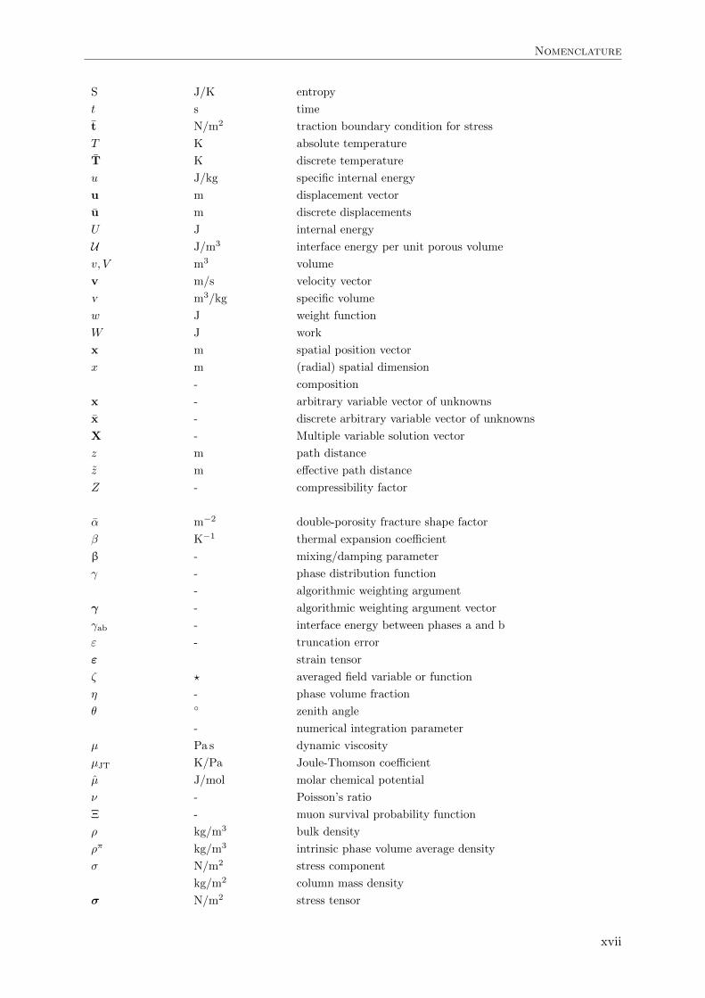
Nomenclature
The following is a generalised and non-exhaustive list of the symbols employed in this text,
incorporating those in particular which appear in multiple contexts. All symbols employed are
defined and described further throughout. The symbols are also additionally indexed where em-
ployed to further indicate to which phase/component and/or sub-domain the property is related.
Symbol Units Description
a m2 area
a m/s2 acceleration vector
A J Helmholtz free energy
Am m2 surface pixel area for path m
b - Biot coefficient
b m−1 Forchheimer coefficient
br - relative Forchheimer coefficient
c m2/s compressibility coefficient
cp J/(kgK) specific isobaric heat capacity
cv Pa−1 coefficient of consolidation
Cr - Courant number
C - capacity matrix
Dπ,κ m2/s effective dispersion tensor
DT - tangential stress/strain matrix
E Pa Young’s modulus
Eµ GeV muon energy
fmin - minimum control factor
fmax - maximum control factor
F - force/supply vector
gµ -/(m2 s srGeV) differential muon intensity
g m/s2 gravitational acceleration
g m/s2 external body force/supply of momentum
Gµ -/(m2 s sr) energy integrated muon flux
h J/kg specific enthalpy
m fluid interface height
H J enthalpy
m formation thickness/height
I - unit tensor
Jm -/(m2 s sr) detector muon flux arriving from path m
Jπ,κ kg/(m2 s) diffusive-dispersive mass flux vector
J - Jacobian matrix
xv
Nomenclature
k m2 permeability
kr - relative permeability
kr0 - phase end-point relative permeability
kI - integral gain control factor
kP - proportional gain control factor
k m2 permeability tensor
K Pa bulk modulus
K - conductivity matrix
lc m characteristic length
l m characteristic fracture spacing
L - displacement/strain differential operator
mk - wetting phase relative permeability exponent
mv Pa−1 coefficient of volume compressibility
mmax - maximum consecutive iterations to accelerate
mv - van Genuchten parameter
m - unit vector
M - mobility contrast
Mn kg/s nonwetting mass rate of injection
n - porosity
n - number of orthogonal fracture sets
nk - nonwetting phase relative permeability exponent
nv - van Genuchten parameter
n - unit normal vector
N mol number of moles
N - shape function array
p Pa pressure
- order of integration method
pc Pa capillary pressure
pv Pa van Genuchten reference pressure
p Pa discrete pressure
q kg/(m2 s) imposed boundary mass flux
qtrans s−1 double-porosity transfer function
q m/s fluid flux
q m/s Darcy flux vector
q J/(m2 s) flux vector of heat
Q J heat
r m wellbore radius
- growth rate
R m radius of curvature
R J/(kgK) specific gas constant
R - residual error vector
s - safety factor
s J/(kgK) specific entropy
m settlement
smax - maximum number of iterations
sstartA - acceleration starting iteration
S - fluid phase saturation
- statistical significance
xvi
Nomenclature
S J/K entropy
t s time
t N/m2 traction boundary condition for stress
T K absolute temperature
T K discrete temperature
u J/kg specific internal energy
u m displacement vector
u m discrete displacements
U J internal energy
U J/m3 interface energy per unit porous volume
v, V m3 volume
v m/s velocity vector
v m3/kg specific volume
w J weight function
W J work
x m spatial position vector
x m (radial) spatial dimension
- composition
x - arbitrary variable vector of unknowns
x - discrete arbitrary variable vector of unknowns
X - Multiple variable solution vector
z m path distance
z m effective path distance
Z - compressibility factor
α m−2 double-porosity fracture shape factor
β K−1 thermal expansion coefficient
β - mixing/damping parameter
γ - phase distribution function
- algorithmic weighting argument
γ - algorithmic weighting argument vector
γab - interface energy between phases a and b
ε - truncation error
ε strain tensor
ζ ? averaged field variable or function
η - phase volume fraction
θ zenith angle
- numerical integration parameter
µ Pa s dynamic viscosity
µJT K/Pa Joule-Thomson coefficient
µ J/mol molar chemical potential
ν - Poisson’s ratio
Ξ - muon survival probability function
ρ kg/m3 bulk density
ρπ kg/m3 intrinsic phase volume average density
σ N/m2 stress component
kg/m2 column mass density
σ N/m2 stress tensor
xvii

Nomenclature
τR - residual error tolerance
τT - truncation error tolerance
χ W/(mK) thermal conductivity
χ W/(mK) thermal conductivity tensor
φ - Lagrangian porosity
Φm -/(m2 s) muon flux arriving from path m with surface pixel area Am
ϕ1,2,3 - numerical integration parameters
ψ ? generic conserved thermodynamic property
Indices Type Description
i sub-domain generic sub-domain index
n phase nonwetting phase
n numerical time-step
s phase solid phase
s numerical iteration-step
w phase wetting phase
κ component generic component/species
π phase generic phase index
1 sub-domain primary matrix porosity
2 sub-domain secondary fracture network porosity
xviii

Chapter 1
Introduction
1.1 Energy
The United Nations Sustainable Development Goals (SDGs) agenda brings together its member
states and organisations in agreement to achieve criteria promoting sustainable socio-economic
development—that of a greater quality of life on Earth. Energy is fundamental to socio-economic
development, and it is centrally recognised by the UN High-level Political Forum (HLPF) on
Sustainable Development [134]. To holistically achieve these SDGs, energy must be universally
accessible, affordable, and clean.
Energy is a benefit which presently comes at a significant cost to our resources and environment,
its use must therefore be governed intelligently. The link, delivering an energy service compati-
ble with both our natural environment and developmental needs, is technology. Energy resource
extraction, conversion, transmission and waste management, as well as the infrastructure, pro-
duction processes and appliances which necessitate energy are all technologically based systems.
At all stages and levels these technologies can be addressed in order to bring about greater effi-
ciencies. However, in developing technologies and in choosing which to employ—ethical stances,
laws and regulations reflecting national capabilities, and social interests must also be respected.
This is particularly the case where waste management and storage is of concern [192].
1.2 Fossil fuels and climate change
Producing energy generates harmful by-products and waste, more so than any other industrial
process. For a global energy service, the main environmental challenge is preventing adverse
anthropogenic interference with the climate system. This interference is predominantly a result
of fossil fuel combustion, on which global primary energy demand is over 80% reliant [93, 192].
Greener technologies and end-use efficiencies require development and time to be phased into
existing infrastructure due to practicality and expense. Furthermore, given the current global
availability of fossil fuels they will continue to dominate as an energy source within the foreseeable
future. The world demand for energy cannot be supplied by any feasible growth in the existing
greener technologies alone; fossil fuels will continue to be used at a substantial rate.
1
Chapter 1. Introduction
Solar radiation, primarily of the ultraviolet, visible and infrared regions of the electromagnetic
spectrum, is absorbed and re-emitted by the Earth’s atmosphere and surface. Absorbed radia-
tion heats up the Earth, and by way of being converted into heat energy is partly radiated as
lower-energy longer-wave thermal infrared and near-infrared radiation back into the atmosphere
and space. It is this radiation that certain ‘greenhouse’ gas molecules within the atmosphere are
able to absorb and re-emit in all directions, thereby causing a greenhouse effect. This interac-
tion is due to the intramolecular vibrational properties of the greenhouse gases which correspond
with various frequencies in the infrared region of the electromagnetic radiation spectrum. This
input and output of radiation is an important process that controls the climate of the Earth.
The most influential greenhouse gases encountered in the Earth’s atmosphere are water vapour
(H2O), carbon dioxide (CO2), methane (CH4), nitrous oxide (N2O) and ozone (O3).
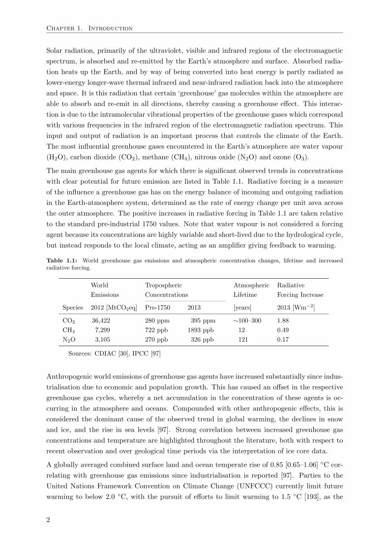
The main greenhouse gas agents for which there is significant observed trends in concentrations
with clear potential for future emission are listed in Table 1.1. Radiative forcing is a measure
of the influence a greenhouse gas has on the energy balance of incoming and outgoing radiation
in the Earth-atmosphere system, determined as the rate of energy change per unit area across
the outer atmosphere. The positive increases in radiative forcing in Table 1.1 are taken relative
to the standard pre-industrial 1750 values. Note that water vapour is not considered a forcing
agent because its concentrations are highly variable and short-lived due to the hydrological cycle,
but instead responds to the local climate, acting as an amplifier giving feedback to warming.
Table 1.1: World greenhouse gas emissions and atmospheric concentration changes, lifetime and increasedradiative forcing.
World Tropospheric Atmospheric Radiative
Emissions Concentrations Lifetime Forcing Increase
Species 2012 [MtCO2eq] Pre-1750 2013 [years] 2013 [Wm−2]
CO2 36,422 280 ppm 395 ppm ∼100–300 1.88
CH4 7,299 722 ppb 1893 ppb 12 0.49
N2O 3,105 270 ppb 326 ppb 121 0.17
Sources: CDIAC [30], IPCC [97]
Anthropogenic world emissions of greenhouse gas agents have increased substantially since indus-
trialisation due to economic and population growth. This has caused an offset in the respective
greenhouse gas cycles, whereby a net accumulation in the concentration of these agents is oc-
curring in the atmosphere and oceans. Compounded with other anthropogenic effects, this is
considered the dominant cause of the observed trend in global warming, the declines in snow
and ice, and the rise in sea levels [97]. Strong correlation between increased greenhouse gas
concentrations and temperature are highlighted throughout the literature, both with respect to
recent observation and over geological time periods via the interpretation of ice core data.
A globally averaged combined surface land and ocean temperate rise of 0.85 [0.65–1.06] C cor-
relating with greenhouse gas emissions since industrialisation is reported [97]. Parties to the
United Nations Framework Convention on Climate Change (UNFCCC) currently limit future
warming to below 2.0 C, with the pursuit of efforts to limit warming to 1.5 C [193], as the
2
1.3. Carbon capture and storage
threshold for dangerous interference. Maintaining temperatures below these levels is likely if at-
mospheric CO2-eq concentrations are stabilised below 450 ppm by 2100. The International Panel
on Climate Change (IPCC) outlines multiple strategic scenarios [97] for mitigating greenhouse
gas emissions to within acceptable limits while meeting global energy demands and while phasing
out the use of fossil fuels. These scenarios present major challenges involving a spectrum of socio-
economic-technological trajectories in order to stabilize atmospheric concentrations. Favourable
scenarios leading to 2100, predict an improved energy efficiency in technology in terms of gen-
eration and end-use, and predict energy supply from nuclear, renewables, and fossil fuels with
carbon dioxide capture and storage (CCS), and/or bioenergy with CCS (BECCS).
1.3 Carbon capture and storage
Carbon capture and storage/sequestration (CCS) is the process of capturing and sequestering
excessive anthropogenically produced carbon dioxide from point sources, as an alternative to
atmospheric disposal. It is an enabling technology that may allow for the continued safe use of
fossil fuels well into this century. The ambition is that the security and stability of the world’s
energy systems is maintained in the short- to medium-term while adverse climate change due to
the use of fossil fuels is mitigated. A key end-chain aspect to this initiative is the injection and
storage of the waste carbon dioxide, in a compressed state, in deep geological formations, thereby
returning the waste carbon to the subsurface. This is known as geological carbon storage/se-
questration (GCS). The primary subsets of geological storage settings are deep non-potable
saline sedimentary formations, depleted/declining hydrocarbon reservoirs, and unminable coal
seams/beds. The contribution of CCS emission reduction within this century is estimated to be
in the region of 20%, see [21, 96, 97], wherein global CO2 storage estimates are discussed. Basic
estimates of global storage capacity for the subsets are given respectively at 1,000–10,000 Gt,
675–900 Gt, and 3–200 Gt of CO2, with individual projects/sites proposed to have capacity up
to 10s of Gt. However, precise potential storage capacities, injection rates, leakage pathways,
and environment and ecological impacts of a CO2 containment breach appear to be unknown.
CCS projects are taking place on increasingly unprecedented scales, following previous successful
operations, and project information is being made widely available, see [22, 175] for important
pilot case studies. Furthermore, due to the lack of maturity of the technologies involved, it is
currently an energy intensive process in itself. To ensure the economic viability, cost competi-
tiveness and effectiveness of CCS, substantial research on development and deployment is still
required across the whole CCS chain [192], that is in general the capture, transport, storage and
monitoring of the carbon dioxide.
1.3.1 Principles of GCS
Foremost, a suitable geological storage scenario is at a depth greater than 800 m [21]. It is
beyond this approximate threshold that a CO2 phase will be in a supercritical state due to
the conditions of pressure and temperature, which generally increase along steady gradients
with depth. The CO2 density becomes high enough to efficiently utilise the pore space within
3
Chapter 1. Introduction
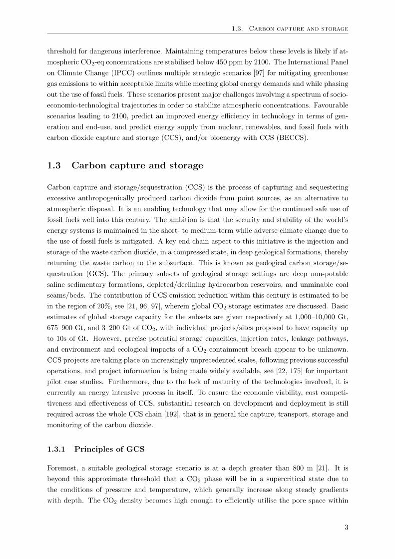
Table 1.2: Potential trapping mechanisms enabling CO2 sequestration in geological formations.
Trapping Mechanism Description
Physical Structural Fluid movement is impeded by low-permeability stratigraphic traps(caprocks) formed by geological depositional/diagenetic changes. Thesetraps are large and abundant, potentially covering horizontal areas of100s of square kilometres over more permeable trapped regions of 10sto 100s of metres in depth, and which naturally retain buoyancy drivenhydrocarbons if present.
Residual If a CO2 plume moves in the pore space in such a way that water is ablere-invade regions where it had been drained by CO2, then the CO2 canbecome disconnected and immobilised at a residual saturation within thepore space. This is due to capillary hysteresis phenomena between thephases (Section 2.7). In the wake of a CO2 plume large traced volumesof storage can be achieved without the need for structural trapping.
Hydrodynamic Trapping occurs due to the slow (∼mm–cm/y) migration of the fluidswithin the storage formation over large regional distances such that theCO2 would remain subsurface for geological periods, even without astructural trap, whereby the combination of residual, dissolution andmineral trapping mechanisms are able to take place [14, 22].
Chemical Dissolution Depending on the state variable mutual solubility and ionic behaviourof the phases (Section 2.8.1), CO2 partially dissolves becoming trappedwithin the water phase and thereby loses its free-phase behaviour. Assuch the affected water phase becomes denser and moves down fromthe fluid interface regions causing further dissolution with the replacingwater. This is a long-term effect, occurring over large time-scales of upto 100s of years, and also presents substantial trapping potential [192].
Mineral A weak carbonic acid is formed by CO2 dissolution, this may react withthe host rock matrix rich in Fe, Mg and Ca minerals and precipitate ascarbonates (Section 2.8.1). The contribution of this tapping mechanismoccurs substantially long-term over 100s of years to geological periods oftime.
Adsorption CO2 injected through fractures in coalbeds and shales diffuses into thesmall pore spaces where it is adsorbed onto the organic material.
the formation, and with respect to saline/brine formations, the buoyancy contrast becomes low
enough between the CO2 and in situ saline water (or brine) such that upwards CO2 migration
can potentially be managed. Note that under these conditions the CO2 and saline water are
largely immiscible. Maximum potential storage depths are dictated by geological and economic
considerations, noting that once the desired high density state is met the CO2 density does not
increase significantly with further depth.
Injection is achieved by pressurising the CO2 into a well, the section of the well injecting within
the storage region is either perforated or covered with a permeable screen to enable the CO2 to
enter the formation, generally of permeable sandstone or limestone. Injection rises the pressure
within the formation particularly near the well and the CO2 enters the pore space initially
occupied by the in situ fluids. Once the injection of CO2 has taken place in a geological formation,
undergoing various transport processes (Chapter 2), it displaces, dissolves, reacts and/or mixes
with the already present formation fluid(s) and rock.
At the appropriate depths, physical and chemical trapping mechanisms also occur preventing the
4
1.4. Thesis aims, objectives and layout
CO2 from migrating to the surface, these are itemised and described in Table 1.2 for reference. In
general, the main contribution to trapping at the early (injection) stages of storage comes from
the primary structural and/or hydrodynamic mechanisms. Over 10s of years the contribution
to trapping becomes shared with the secondary residual CO2 saturation and phase dissolution
mechanisms which take place progressively over time. Over 100s to 1000s of years the secondary
mechanisms contribute predominantly to trapping as the plume idles in movement after the
end of its injection. Further, over geological periods of time, mineralisation is anticipated to
contribute predominantly to storage. In effect, the security of the geological storage system
generally increases as the mechanisms contributing to trapping progress over time [21, 192].
The integrity of the storage site depends on its geological arrangement and physical properties.
For instance, at a sealing interface, the caprock should ideally be uniform in lithology, regionally
extensive and thick. Key storage site issues are existing faults/fractures, exiting/abandoned
wellbores and changes in site integrity and performance due to potential coupled hydro-thermo-
mechanical-chemical (HTMC) system behaviours, which are discussed further throughout Chap-
ter 2. For instance, a particular geomechanical focus is the maximum permissible ranges of
injection pressures sustainable for effective storage without the coupled fracturing and/or re-
opening of fractures within the storage and sealing rock, and any ensuing well damage and/or
seismic behaviour. A particular geothermal factor is the expansive cooling of the CO2 which
may inhibit the successful injection of CO2. Lastly, a particular geochemical factor is any po-
tential acidic CO2-rich water which may react with the rock and borehole cements and seals,
causing mineral dissolution breakdown and/or mineral precipitation pore blockage, depending
on the local system state, which may affect the performance of the storage system.
1.4 Thesis aims, objectives and layout
This work is part of a collaborative multi-disciplinary research project on advancing knowledge
on the modelling and monitoring of GCS in particular. The contribution of this thesis is on
the development of a computational framework for modelling the various multi-physics which
are relevant for predicting various important physical aspects of GCS. The emphasis of the
framework is on capturing the coupled HTM and muon radiographic processes of the storage
system for research purposes. This framework is to allow for the investigation and development of
both the physics modelled and the numerical procedures for discretising and solving the resulting
systems of equations. This is to cover the following two broad and interrelated research aims.
- Firstly, large scale GCS is a relatively new concept, and given the potentially complex
multi-physical nature of the problem, predictive models generally simplify the behaviour
and/or concentrate on certain relevant physical aspects. The aim of this thesis is to
develop an extended fully coupled non-isothermal multiphase Biot-type double-porosity
modelling approach, and then to apply this to realistic GCS scenarios for the first time.
This is aimed at the research need to further understand the system couplings and their
co-action in terms of storage system performance. Additionally, such models are compu-
tationally expensive, in view of the model application, research needs are also attended
5
Chapter 1. Introduction
to whereby alternative methods are developed and implemented in order to complement
existing numerical discretisation and solution procedures for coupled systems of governing
equations.
- Secondly, an existing CCS problem is how to cost-effectively/efficiently monitor the in-
accessible geo-stored CO2, ideally in a passive and continuous manner. A novel and
unconventional potential solution to this problem is the application of cosmic-ray muon
radiography. This has been successfully applied to other monitoring problems, though its
application for monitoring realistic GCS scenarios is unresearched. A key aim of this work
is to combine the modelling of GCS with the modelling of muon radiography for the first
time. The aforementioned computational framework is therefore an multi-disciplinary one
as it is to coordinate with the simulation of muon radiography in order to assess and effect
the development of such a monitoring system within this context.
These broad aims are also discussed and detailed further throughout the chapters of this thesis,
which are itemised below along with their key objectives.
- Chapter 2: The first objective is to give an in depth review of the underlying principles,
governing balance laws and constitutive relationships for building physics applications for
modelling multiphase multicomponent phenomena in heterogeneous porous media. The
second objective is to review the relevant subsurface modelling and monitoring technologies
and strategies. These reviews are carried out in the context of modelling and monitoring
GCS in particular, such that incentives are also highlighted for further research.
- Chapter 3: The work of Chapter 2 is adopted, linked and extended in order to develop
a system of fully coupled partial differential governing field equations for modelling mul-
tiphase fluid flow in fractured porous media. The research objective is to cover the key
hydro-thermal-mechanical coupled physical bases for the investigative modelling of GCS,
with particular emphasis on deriving a fully coupled double-porosity model formulation in
order to assess the HTM processes in a fractured storage formation.
- Chapter 4: The objective is to discretise the system of governing field equations in space.
Considerations on the standard Galerkin finite element procedure utilised, its spatial re-
finement and computational implementation are made and discussed given the derived
system of coupled equations and their application. The spatial discretisation process leads
to a coupled set of highly nonlinear first-order ordinary differential equations in time.
- Chapter 5: Given the complexity of the spatially discretised system of equations and
the computational expense required in order to bring about their solution using standard
procedures, the research objective is to devise an improved alternate solution strategy. To
achieve this objective, an embedded finite difference method is schemed with advantageous
control theoretical techniques and an accelerated fixed-point-type procedure.
- Chapter 6: A sequence of model verification and validation benchmark scenarios of in-
creasing complexity are carried out and discussed in detail. The objective is to assess
and discuss the performance of the numerical model against known simplified analytical
6
1.4. Thesis aims, objectives and layout
solutions to key problems and to highlight various coupled GCS phenomena in particular,
which result given the model formulation. The emphasis is on assessing and highlight-
ing coupled HTM processes in an isolated (or sealed) storage formation/system, thereby
neglecting the modelling of CO2 leakage from any sealing units (overburden) for later
study.
- Chapter 7: The research objective is to integrate the modelling of geology, subsurface fluid
flow phenomena and muon radiography in order to assess and develop the application of
muon radiography for monitoring GCS. To achieve this objective, computational strategies
are developed and implemented collaboratively. Presented and discussed are the first
realistic simulations of the application of muon radiography for detecting a migrating
body of CO2 in the subsurface.
- Chapter 8: Finally, conclusions are drawn from the work of this thesis along with recom-
mendations for future work.
The following conference and peer-reviewed work has also been carried out parallel to the work
of this thesis.
Conferences
GeoRepNet Technology Transfer, BGS Keyworth, UK, 2014.
8th Numerical Methods in Geotechnical Engineering, Delft, Netherlands, Oral presentation,
2014.
International Conference on Computational Mechanics, Durham, UK, 2013, Prize session oral
presentation for best paper (runner-up), 2013.
UKCCSC workshops, Nottingham & Liverpool, UK, Poster presentation, 2012.
Select publications & conference proceedings
Benton, C.J., Mitchell, C.N., Coleman, M., Paling, S.M., Lincoln, D.L., Thompson, L., Klinger, J.,
Telfer, S.J., Clark, S.J., Gluyas, J.G. (2015) Optimizing geophysical muon radiography using
information theory. Geophysical Journal International. In final preparation.
Klinger, J., Clarke, S.J., Coleman, M., Gluyas, J.G., Kudryavtsev, V.A., Lincoln, D.L., Pal, S.,
Paling, S.M, Spooner, N.J.C, Telfer, S., Thompson, L.F., Woodward, D. (2015) Simulation of
muon radiography for monitoring CO2 stored in a geological reservoir. International Journal. of
Greenhouse Gas Control, 42:644–654.
Lincoln, D.L., Askes, H., Smith, C.C., Cripps, J.C., Bennett, T. (2014) Coupled two-component
flow in deformable fractured porous media with application to modelling geological carbon stor-
age. Numerical Methods in Geotechnical Engineering, Hicks, Brinkgreve & Rohe (Eds) c© 2014
Taylor & Francis Group, London, 978-1-138-00146-6.
7

Chapter 2
Literature Review & Fundamentals
The principal engineering challenges for the geological disposal of carbon dioxide and radioac-
tive waste are set out in a broader enviro-socio-economic context in [72, 185, 192]. Therein
the disposal space defined is deep redundant geological void spaces, the essential characteristics
of which are capacity for storage and transmissibility, which are to demonstrate the necessary
structural/stratigraphic, residual, solubility and mineral trapping mechanisms for safe storage.
In this chapter a fundamental framework of the principles underlying these mechanisms is devel-
oped providing a basis from which to build appropriate applications to assess geological carbon
storage (GCS) in particular. This fundamental perspective also gives an effective vantage from
which to review the literature in the context of this emerging technology. It is envisioned that
this framework will also encompass principles necessary for research on other emerging tech-
nologies, for instance, on efficient building materials, enhanced environmental (bio)remediation,
geothermal energies, compressed air energy storage (CAES), and hydro-fracturing.
2.1 Porous media theory
The geological regions of interest for CO2 storage are essentially porous media, that is solid
phase materials containing an internal structure of open and closed pores forming intercon-
nected porous networks, potentially occupied by multiple miscible and immiscible fluid phases
of multiple components. Therefore, interacting multiphase multicomponent media are of inter-
est, which present different hydro-thermo-mechanical-chemical (HTMC) behaviour than would
their individual constituents alone. Such media are fundamental to many important processes
in nature and in engineering, and are widely encountered [48].
Naturally formed porous structures have discontinuous and complex geometry, which makes
descriptions at the microscopic scale difficult. Therefore, a representative macroscopic scale
model is ordinarily assumed for engineering purposes whereby the constituents occupy, in an
interpenetrable homogenised (or smeared) sense, portions of a control space via some volume
fractioning. Continuum mechanics may then be applied to the substitute continua. To date,
relevant descriptions of such systems are accomplished via this method broadly through the
following theories. Firstly, phenomenological theories are based mainly on Terzaghi’s work [189]
9
Chapter 2. Literature Review & Fundamentals
on the mechanics of soils, and further developed by Biot [26, 27]. Richards equation [158] and the
elaborations thereof form another important phenomenological set, and further thermodynamic
developments in this context are also made by Coussy [47, 48]. Secondly, modern thermodynamic
mixture theories, originating from classical gas mixture theory, utilise the constituent chemical
potentials extended with the use of volume fractioning. In this context incompressible and
compressible media are considered by Bowen [32, 33], with further consideration by de Boer
[54, 55]. Lastly, averaging theories employ the technique of local volume averaging, whereby
classical continuum balance laws governing the system at the microscopic scale are averaged
over a representative volume giving macroscopic equations and thermodynamic properties. A
thorough development in this context is given by Hassanizadeh & Gray [80, 81, 82, 83, 84].
The three theoretical approaches demonstrate equivalence under certain assumptions as demon-
strated in [48, 53, 120], from which similar macroscopic governing field equations may be derived.
This highlights their general accuracy and gives good scope for modelling strategies. During the
development of various numerical models, for instance [120, 131], a crossover of these theories
takes place when this is deemed appropriate during implementation. The modelling strategy
in this work is similar in that the averaging theories are introduced initially because they offer
the most in-depth and adaptive basis for advancement when considering a given application;
it is then to this basis that elements of the other macro-theories are applied depending on the
application and understanding required.
2.1.1 Porosity
Two types of porosity are distinguished because they exhibit distinct HTMC properties: primary
(matrix) porosity, referring to the collective void spaces due to sedimentation, and secondary
porosity, referring to fissures/fractures, vugs or other discontinuities due mainly to past cooling
and tectonic activities. Most sedimentary formations have both these porosities [192]. Geological
strata are widely characterised with continuous fracture networks through the porous rock mass.
The implication of fractures during injection/extraction processes affects reservoir performance
significantly, and models which conceptualise such strata as homogeneous can lead to conflicting
and/or inadequate results [120]. Furthermore, the change in bulk properties of the reservoir,
which are affected by the presence of multiple porosities, are key for statistically monitoring
reservoir performance [114]. For these reasons the porous medium is introduced and defined in
this section with a double(or dual)-porosity [3, 17, 201].
2.1.2 Distribution functions and volume fractions
The medium considered consists of fracture/rock-mass structures composed of porous matrix
void/grain structures occupied by CO2 and brine. That is, a system of solid, wetting and
nonwetting phases (Section 2.7).
On the microscopic level, inhomogeneities as defined at the grain and pore scale li, Figure 2.1(a),
require that any field variable for a particular phase be defined precisely at the points it occupies.
This level of detail is undesirable given the scales necessary for assessment and the extent of
10
2.1. Porous media theory
(a) (b)
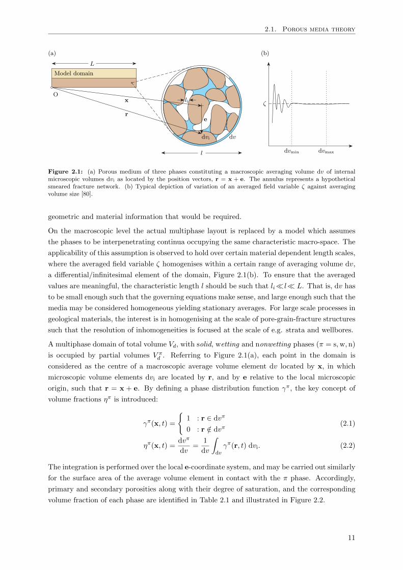
Figure 2.1: (a) Porous medium of three phases constituting a macroscopic averaging volume dv of internalmicroscopic volumes dvi as located by the position vectors, r = x + e. The annulus represents a hypotheticalsmeared fracture network. (b) Typical depiction of variation of an averaged field variable ζ against averagingvolume size [80].
geometric and material information that would be required.
On the macroscopic level the actual multiphase layout is replaced by a model which assumes
the phases to be interpenetrating continua occupying the same characteristic macro-space. The
applicability of this assumption is observed to hold over certain material dependent length scales,
where the averaged field variable ζ homogenises within a certain range of averaging volume dv,
a differential/infinitesimal element of the domain, Figure 2.1(b). To ensure that the averaged
values are meaningful, the characteristic length l should be such that li l L. That is, dv has
to be small enough such that the governing equations make sense, and large enough such that the
media may be considered homogeneous yielding stationary averages. For large scale processes in
geological materials, the interest is in homogenising at the scale of pore-grain-fracture structures
such that the resolution of inhomogeneities is focused at the scale of e.g. strata and wellbores.
A multiphase domain of total volume Vd, with solid, wetting and nonwetting phases (π = s,w,n)
is occupied by partial volumes V πd . Referring to Figure 2.1(a), each point in the domain is
considered as the centre of a macroscopic average volume element dv located by x, in which
microscopic volume elements dvi are located by r, and by e relative to the local microscopic
origin, such that r = x + e. By defining a phase distribution function γπ, the key concept of
volume fractions ηπ is introduced:
γπ(x, t) =
1 : r ∈ dvπ
0 : r /∈ dvπ(2.1)
ηπ(x, t) =dvπ
dv=
1
dv
∫dvγπ(r, t) dvi. (2.2)
The integration is performed over the local e-coordinate system, and may be carried out similarly
for the surface area of the average volume element in contact with the π phase. Accordingly,
primary and secondary porosities along with their degree of saturation, and the corresponding
volume fraction of each phase are identified in Table 2.1 and illustrated in Figure 2.2.
11
Chapter 2. Literature Review & Fundamentals
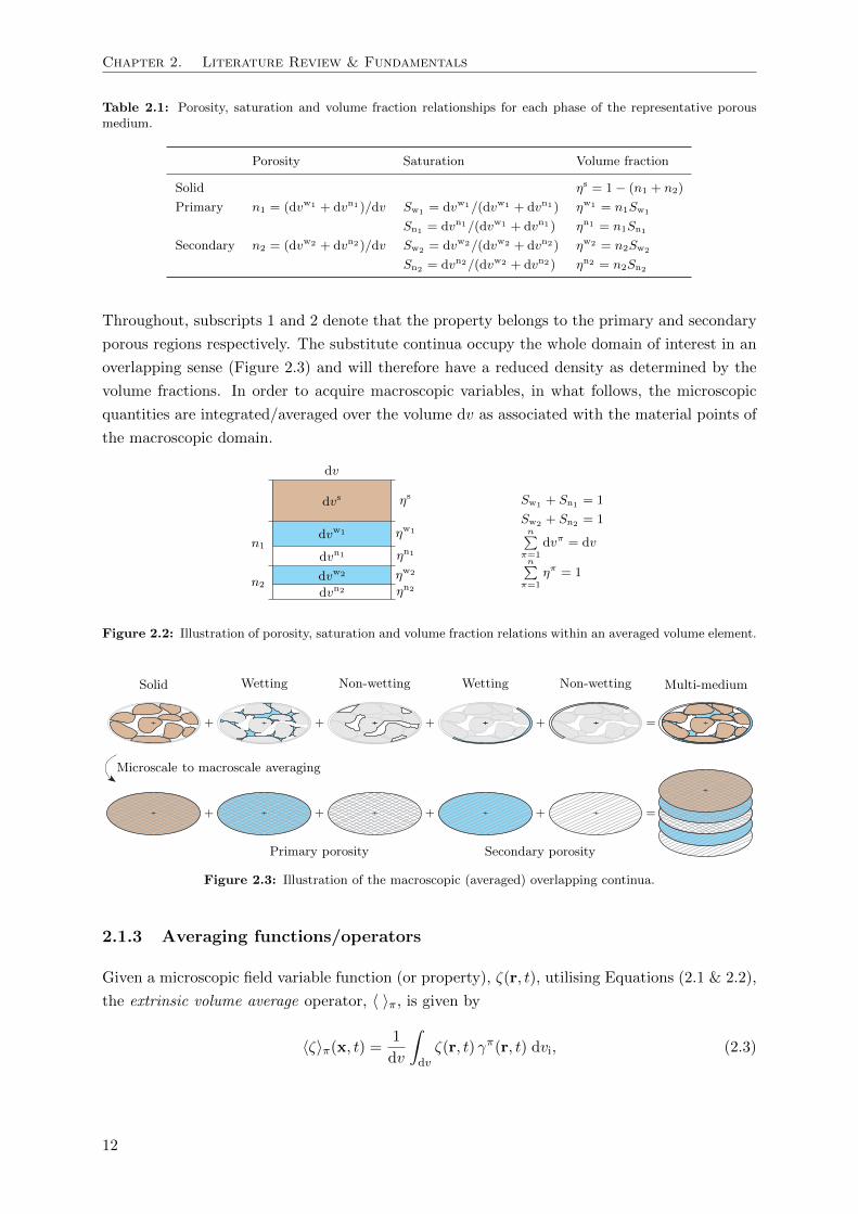
Table 2.1: Porosity, saturation and volume fraction relationships for each phase of the representative porousmedium.
Porosity Saturation Volume fraction
Solid ηs = 1− (n1 + n2)
Primary n1 = (dvw1 + dvn1)/dv Sw1 = dvw1/(dvw1 + dvn1) ηw1 = n1Sw1
Sn1 = dvn1/(dvw1 + dvn1) ηn1 = n1Sn1
Secondary n2 = (dvw2 + dvn2)/dv Sw2 = dvw2/(dvw2 + dvn2) ηw2 = n2Sw2
Sn2 = dvn2/(dvw2 + dvn2) ηn2 = n2Sn2
Throughout, subscripts 1 and 2 denote that the property belongs to the primary and secondary
porous regions respectively. The substitute continua occupy the whole domain of interest in an
overlapping sense (Figure 2.3) and will therefore have a reduced density as determined by the
volume fractions. In order to acquire macroscopic variables, in what follows, the microscopic
quantities are integrated/averaged over the volume dv as associated with the material points of
the macroscopic domain.
Sw1 + Sn1 = 1
Sw2 + Sn2 = 1n∑
π=1
dvπ = dv
n∑π=1
ηπ = 1
Figure 2.2: Illustration of porosity, saturation and volume fraction relations within an averaged volume element.
Figure 2.3: Illustration of the macroscopic (averaged) overlapping continua.
2.1.3 Averaging functions/operators
Given a microscopic field variable function (or property), ζ(r, t), utilising Equations (2.1 & 2.2),
the extrinsic volume average operator, 〈 〉π, is given by
〈ζ〉π(x, t) =1
dv
∫dvζ(r, t) γπ(r, t) dvi, (2.3)
12
2.2. Kinematics
and the intrinsic volume average operator, 〈 〉ππ, is given similarly by
〈ζ〉ππ(x, t) =1
dvπ
∫dvζ(r, t) γπ(r, t) dvi =
1
ηπ(x, t) dv
∫dvζ(r, t) γπ(r, t) dvi, (2.4)
with the relationship 〈ζ〉π(x, t) = ηπ(x, t)〈ζ〉ππ(x, t). The mass average operator, ζπ, is given by
ζπ(x, t) =
∫dv ρ(r, t)ζ(r, t) γ
π(r, t) dvi∫dv ρ(r, t) γ
π(r, t) dvi=
1
〈ρ〉π(x, t) dv
∫dvρ(r, t)ζ(r, t) γπ(r, t) dvi (2.5)
which uses the microscopic density as a weighting function with (2.3). Lastly, the area average
operator, ¯ζπ, is defined by
¯ζπ(x, t) =1
da
∫daζ(r, t) · nγπ(r, t) dai. (2.6)
It can be seen that volume and mass averages are the same if constant microscopic density is
present. Volume and area averages are the same if no anisotropic distribution of the phases is
present, in the sense that Delesse’s law is observed [55].
The mass and area averaging operators may be applied to a partial quantity relating to a
component within a phase, namely ζκ and ρκ. Utilising the operators in this fashion means that
partial values for each component would be given, which on summation would give the average
of the phase they constitute, as follows,
〈ζ〉ππ(x, t) =∑κ
〈ζκ〉ππ(x, t). (2.7)
An averaged representative 〈ζ〉 of the volume element dv is now given by the summations,
〈ζ〉(x, t) =∑π
〈ζ〉π(x, t) =∑π
ηπ〈ζ〉ππ(x, t), (2.8)
where the spatial variations of ζ for the individual phases within dv are now lost and an emer-
gent macroscopic alternative is presented. The averaged representative value of the property
ζ becomes important for building suitable macroscopic physics applications (Section 2.5) from
general principles.
2.2 Kinematics
The kinematics of the substitute continua of the multiphase medium may be examined inde-
pendently as follows. Firstly, the spatial positions of the material points of the continuum for
each phase xπ, at time t, are related to an original reference configuration xπ0 , by xπ = xπ(xπ
0 , t)
and inversely by xπ0 = xπ
0 (xπ, t), which present material (Lagrangian) and spatial (Eulerian)
descriptions of motion, respectively. That is xπ = xπ(xπ0 , t) = xπ
0 + uπ(xπ0 , t), where uπ may be
visualised as displacements of the π phase.
Considering a differentiable function in terms of spatial positions and time ζπ(x, t), the changes
of which experienced by a material point (Lagrangian description) are expressed in Eulerian
13
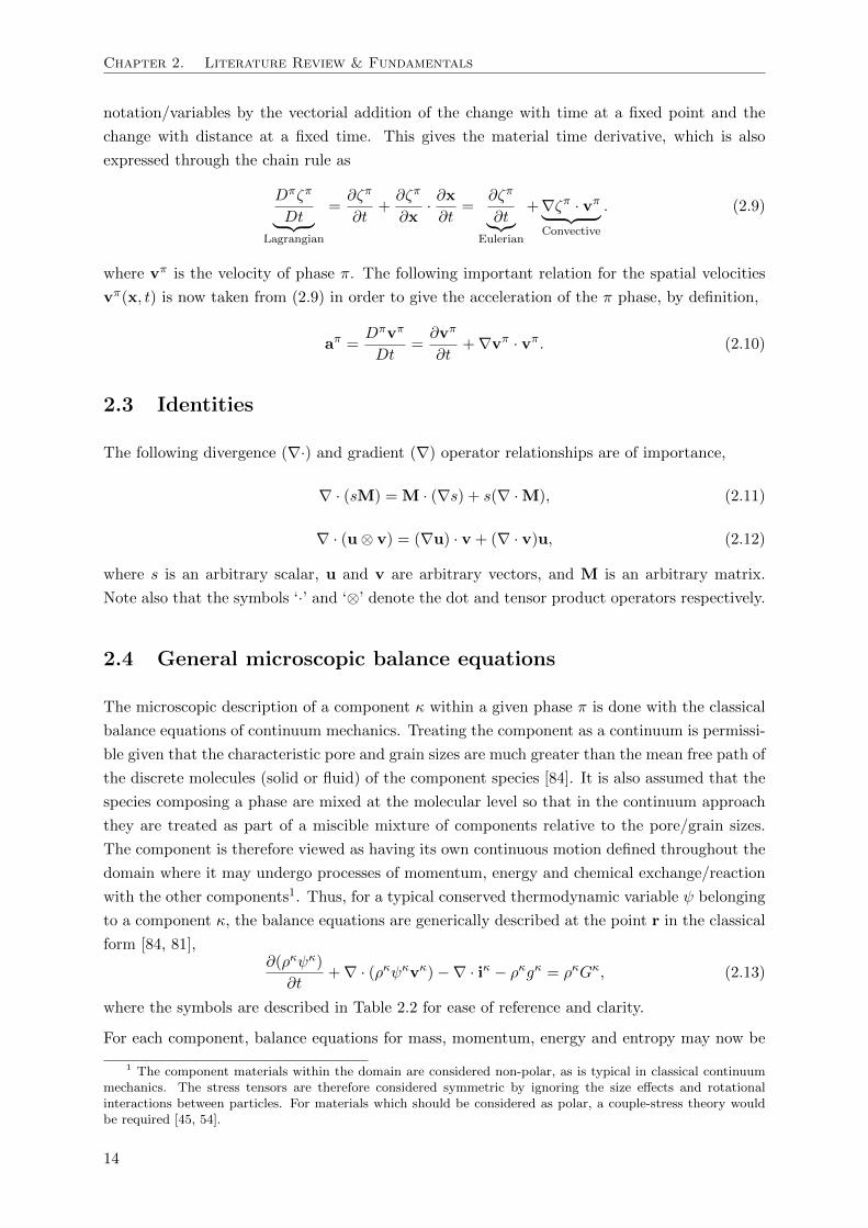
Chapter 2. Literature Review & Fundamentals
notation/variables by the vectorial addition of the change with time at a fixed point and the
change with distance at a fixed time. This gives the material time derivative, which is also
expressed through the chain rule as
Dπζπ
Dt︸ ︷︷ ︸Lagrangian
=∂ζπ
∂t+∂ζπ
∂x· ∂x∂t
=∂ζπ
∂t︸︷︷︸Eulerian
+∇ζπ · vπ︸ ︷︷ ︸Convective
. (2.9)
where vπ is the velocity of phase π. The following important relation for the spatial velocities
vπ(x, t) is now taken from (2.9) in order to give the acceleration of the π phase, by definition,
aπ =Dπvπ
Dt=∂vπ
∂t+∇vπ · vπ. (2.10)
2.3 Identities
The following divergence (∇·) and gradient (∇) operator relationships are of importance,
∇ · (sM) = M · (∇s) + s(∇ ·M), (2.11)
∇ · (u⊗ v) = (∇u) · v + (∇ · v)u, (2.12)
where s is an arbitrary scalar, u and v are arbitrary vectors, and M is an arbitrary matrix.
Note also that the symbols ‘·’ and ‘⊗’ denote the dot and tensor product operators respectively.
2.4 General microscopic balance equations
The microscopic description of a component κ within a given phase π is done with the classical
balance equations of continuum mechanics. Treating the component as a continuum is permissi-
ble given that the characteristic pore and grain sizes are much greater than the mean free path of
the discrete molecules (solid or fluid) of the component species [84]. It is also assumed that the
species composing a phase are mixed at the molecular level so that in the continuum approach
they are treated as part of a miscible mixture of components relative to the pore/grain sizes.
The component is therefore viewed as having its own continuous motion defined throughout the
domain where it may undergo processes of momentum, energy and chemical exchange/reaction
with the other components1. Thus, for a typical conserved thermodynamic variable ψ belonging
to a component κ, the balance equations are generically described at the point r in the classical
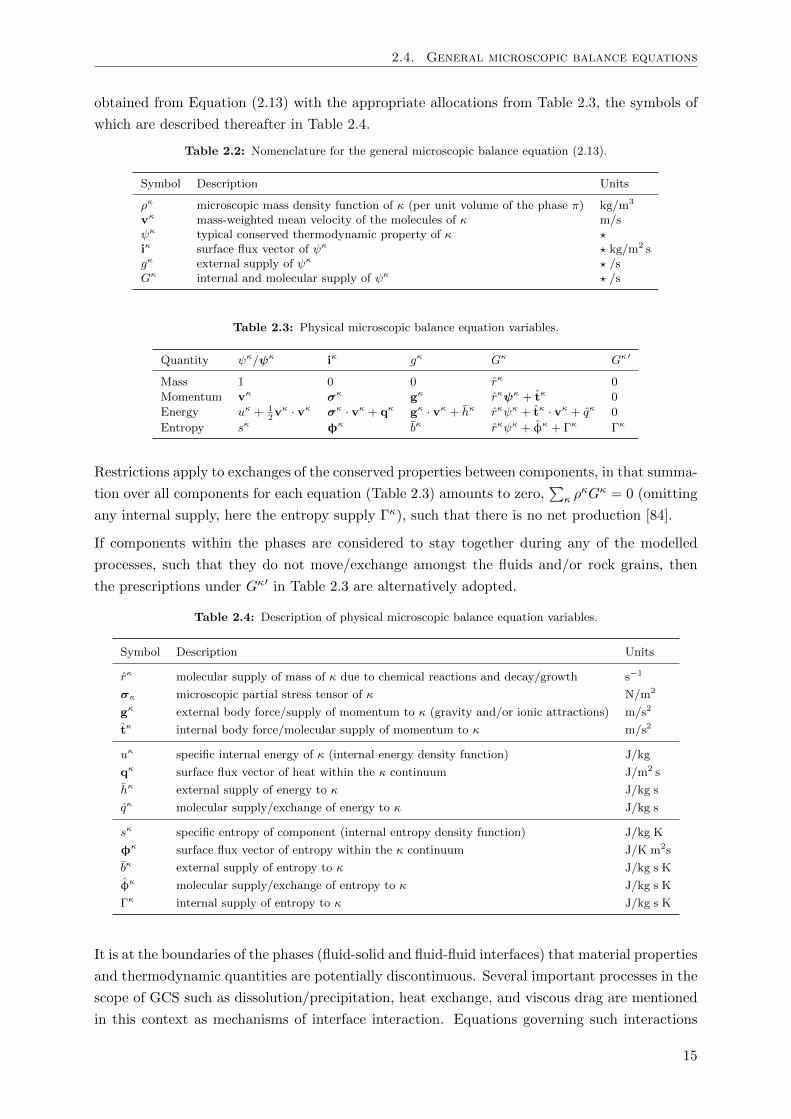
form [84, 81],∂(ρκψκ)
∂t+∇ · (ρκψκvκ)−∇ · iκ − ρκgκ = ρκGκ, (2.13)
where the symbols are described in Table 2.2 for ease of reference and clarity.
For each component, balance equations for mass, momentum, energy and entropy may now be
1 The component materials within the domain are considered non-polar, as is typical in classical continuummechanics. The stress tensors are therefore considered symmetric by ignoring the size effects and rotationalinteractions between particles. For materials which should be considered as polar, a couple-stress theory wouldbe required [45, 54].
14
2.4. General microscopic balance equations
obtained from Equation (2.13) with the appropriate allocations from Table 2.3, the symbols of
which are described thereafter in Table 2.4.
Table 2.2: Nomenclature for the general microscopic balance equation (2.13).
Symbol Description Units
ρκ microscopic mass density function of κ (per unit volume of the phase π) kg/m3
vκ mass-weighted mean velocity of the molecules of κ m/sψκ typical conserved thermodynamic property of κ ?iκ surface flux vector of ψκ ? kg/m2 sgκ external supply of ψκ ? /sGκ internal and molecular supply of ψκ ? /s
Table 2.3: Physical microscopic balance equation variables.
Quantity ψκ/ψκ iκ gκ Gκ Gκ′
Mass 1 0 0 rκ 0
Momentum vκ σκ gκ rκψκ + tκ 0
Energy uκ + 12vκ · vκ σκ · vκ + qκ gκ · vκ + hκ rκψκ + tκ · vκ + qκ 0
Entropy sκ φκ bκ rκψκ + φκ + Γκ Γκ
Restrictions apply to exchanges of the conserved properties between components, in that summa-
tion over all components for each equation (Table 2.3) amounts to zero,∑
κ ρκGκ = 0 (omitting
any internal supply, here the entropy supply Γκ), such that there is no net production [84].
If components within the phases are considered to stay together during any of the modelled
processes, such that they do not move/exchange amongst the fluids and/or rock grains, then
the prescriptions under Gκ′ in Table 2.3 are alternatively adopted.
Table 2.4: Description of physical microscopic balance equation variables.
Symbol Description Units
rκ molecular supply of mass of κ due to chemical reactions and decay/growth s−1
σκ microscopic partial stress tensor of κ N/m2
gκ external body force/supply of momentum to κ (gravity and/or ionic attractions) m/s2
tκ internal body force/molecular supply of momentum to κ m/s2
uκ specific internal energy of κ (internal energy density function) J/kg
qκ surface flux vector of heat within the κ continuum J/m2 s
hκ external supply of energy to κ J/kg s
qκ molecular supply/exchange of energy to κ J/kg s
sκ specific entropy of component (internal entropy density function) J/kg K
φκ surface flux vector of entropy within the κ continuum J/K m2s
bκ external supply of entropy to κ J/kg s K
φκ molecular supply/exchange of entropy to κ J/kg s K
Γκ internal supply of entropy to κ J/kg s K
It is at the boundaries of the phases (fluid-solid and fluid-fluid interfaces) that material properties
and thermodynamic quantities are potentially discontinuous. Several important processes in the
scope of GCS such as dissolution/precipitation, heat exchange, and viscous drag are mentioned
in this context as mechanisms of interface interaction. Equations governing such interactions
15
Chapter 2. Literature Review & Fundamentals
between adjacent phases are of the following form
[ρκψκ(w − vκ) + iκ]∣∣a· nab + [ρκψκ(w − vκ) + iκ]
∣∣b· nba = 0 (2.14)
where ab represents an interface between two different phases, n is the usual unit normal vector,
and w is the velocity of the interface. An inequality sign should be introduced, for the balance of
entropy, instead in (2.14) to allow for the potential production of entropy as a result of interface
processes. The equations so far have ignored the thermodynamic properties of the interfaces
themselves, such as interface tension and mass accumulation, for a more thorough consideration
of which in this general context references [80, 81, 82] and particularly [85] are given. For an
interface with surface properties, (2.14) will be non-zero. Interface behaviour is incorporated
indirectly in this work via appropriate constitutive relations, as introduced through Section 2.6.
2.5 General mean macroscopic balance equations
General balance equations for a macroscopic thermodynamic property are obtained by averaging
the microscopic balance equations by multiplying the general microscopic equations (2.13) and
their exchange restrictions with a distribution function and then integrating them over the
averaging volume. Additionally, the interface interaction (2.14) is integrated over the averaging
area of surfaces within the averaging volume. This is done such that the resulting equations
are localised as macroscopic point equations, with the averaging operators (2.3–2.6) defining the
macroscopic quantities. Equations are produced for each component κ in each phase π. This
averaging procedure is explored more thoroughly in the work referenced [83, 84, 131], wherein
considerations are also made on the linking in physical meaning between the respective micro-
and macroscopic quantities.
The next step is to produce convenient mean versions of these general balance equations for
each phase. This is done such that the mean thermodynamic property of a phase is primarily
described with the relative contributions of the separate components in respect of that mean.
Particularly, any partial densities may be summed to give an average intrinsic density of the
phase, as of (2.7),
ρπ = 〈ρ〉ππ =∑κ
〈ρκ〉ππ, (2.15)
and an average velocity of the phase may be produced,
vπ =∑κ
〈ρκ〉ππρπ
vκπ, (2.16)
where the density fraction represents a mass fraction or concentration of the component, and
vκπ is the velocity of the component. The difference between the mean and any value of a
component gives the diffusion-dispersive velocity, and the related mass flux of that component,
〈Jκ〉ππ = ηπ 〈ρκ〉ππ (vκπ − vπ). (2.17)
Finally, the general mean macroscopic balance equation for a macroscopic thermodynamic quan-
16
2.5. General mean macroscopic balance equations
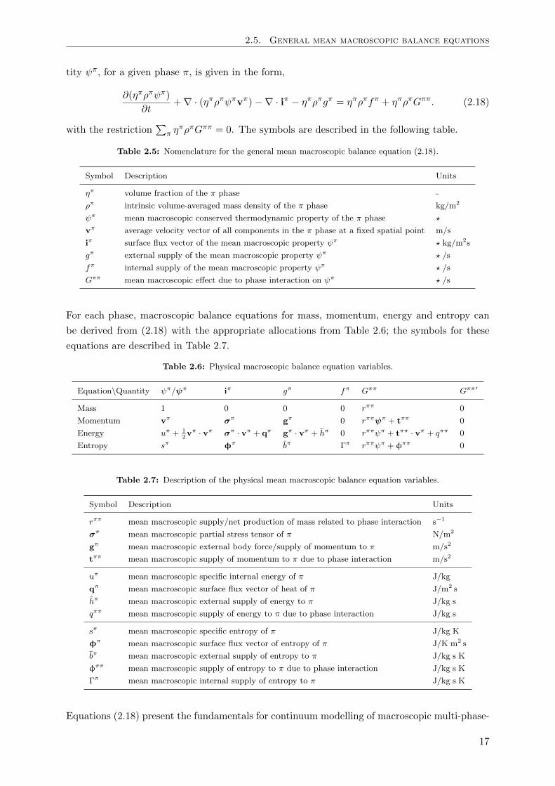
tity ψπ, for a given phase π, is given in the form,
∂(ηπρπψπ)
∂t+∇ · (ηπρπψπvπ)−∇ · iπ − ηπρπgπ = ηπρπfπ + ηπρπGππ. (2.18)
with the restriction∑
π ηπρπGππ = 0. The symbols are described in the following table.
Table 2.5: Nomenclature for the general mean macroscopic balance equation (2.18).
Symbol Description Units
ηπ volume fraction of the π phase -
ρπ intrinsic volume-averaged mass density of the π phase kg/m2
ψπ mean macroscopic conserved thermodynamic property of the π phase ?
vπ average velocity vector of all components in the π phase at a fixed spatial point m/s
iπ surface flux vector of the mean macroscopic property ψπ ? kg/m2s
gπ external supply of the mean macroscopic property ψπ ? /s
fπ internal supply of the mean macroscopic property ψπ ? /s
Gππ mean macroscopic effect due to phase interaction on ψπ ? /s
For each phase, macroscopic balance equations for mass, momentum, energy and entropy can
be derived from (2.18) with the appropriate allocations from Table 2.6; the symbols for these
equations are described in Table 2.7.
Table 2.6: Physical macroscopic balance equation variables.
Equation\Quantity ψπ/ψπ iπ gπ fπ Gππ Gππ ′
Mass 1 0 0 0 rππ 0
Momentum vπ σπ gπ 0 rππψπ + tππ 0
Energy uπ + 12vπ · vπ σπ · vπ + qπ gπ · vπ + hπ 0 rππψπ + tππ · vπ + qππ 0
Entropy sπ φπ bπ Γπ rππψπ + φππ 0
Table 2.7: Description of the physical mean macroscopic balance equation variables.
Symbol Description Units
rππ mean macroscopic supply/net production of mass related to phase interaction s−1
σπ mean macroscopic partial stress tensor of π N/m2
gπ mean macroscopic external body force/supply of momentum to π m/s2
tππ mean macroscopic supply of momentum to π due to phase interaction m/s2
uπ mean macroscopic specific internal energy of π J/kg
qπ mean macroscopic surface flux vector of heat of π J/m2 s
hπ mean macroscopic external supply of energy to π J/kg s
qππ mean macroscopic supply of energy to π due to phase interaction J/kg s
sπ mean macroscopic specific entropy of π J/kg K
φπ mean macroscopic surface flux vector of entropy of π J/K m2 s
bπ mean macroscopic external supply of entropy to π J/kg s K
φππ mean macroscopic supply of entropy to π due to phase interaction J/kg s K
Γπ mean macroscopic internal supply of entropy to π J/kg s K
Equations (2.18) present the fundamentals for continuum modelling of macroscopic multi-phase-
17
Chapter 2. Literature Review & Fundamentals
component porous media from which specific (coupled) applications can be built.
2.6 Equations of state and constitutive relations
To build appropriate physics applications (models) the generic balance laws are accompanied
by constitutive relationships in order that they facilitate workable parametrisation and produce
practical results. Essentially, constitution defines the specific materials being considered. This
section explores those relationships which are particular to multiphase flow in porous media
with specific reference to GCS where appropriate. An extensive review is made in this context
such that a thorough account of the fundamental phenomena involved is given with respect to
current state-of-the-art.
This thesis is application based and only that which is considered appropriate for now is taken
forward for modelling, as is discussed. This will however provide insight into the limitations of
any models developed and allow for a greater variety of potential geo-applications as well as for
the benchmarking of future work encompassing the more sophisticated constitutive theories.
2.6.1 Helmholtz free energy
The first and second laws of thermodynamics combine to state that the change in internal energy
U (microscopic potential and kinetic energies), for an amount of substance which undergoes a
change in volume V and a change in entropy S at temperature T and pressure p, is given by the
energy balance
dU = −p dV + T dS, (2.19)
which is a sum of the infinitesimal supply of mechanical work W and heat Q. By introducing
the Helmholtz free energy A = U −TS, which is the maximum energy available to produce work
in a thermodynamic system at a constant temperature, into (2.19), with an additional term to
account for the free energy supply due to a change in the number moles N of component κ with
the molar chemical potential µκ, gives,
dA = −p dV − SdT +∑κ
µκ dNκ. (2.20)
Assuming the system to be closed and isothermal, that is ignoring the last two terms in (2.20),
it is seen that the infinitesimal mechanical work is stored as free energy without its deterioration
or increase from the other terms.
Of importance, Coussy [47, 48] extends the general balance of free energy (2.20) for a thermo-
poroelastic solid phase only, with no molecular supply2,
das =∑f
pf dφf + (σ dε+ sij deij)− ss dT, (2.21)
2 The porosity n is Eulerian and may be related to a Lagrangian porosity φ with the relationship, φ dv0 = ndv,where dv0 is the initial volume [48].
18
2.6. Equations of state and constitutive relations
where as and ss are the Helmholtz free energy and the entropy of the porous solid per unit
initial volume, dv0. The first three terms on the r.h.s. sum to represent the infinitesimal strain
work per unit initial volume of the solid, where σ is mean/hydrostatic stress, ε is volumetric
dilation/strain, sij are deviatoric stress tensor components, and eij are deviatoric strain tensor
components. The first term on the r.h.s is the infinitesimal energy contributions from the
occupying immiscible fluid phases f, and may be expressed equivalently for the two fluid phase
system, f = w, n, given the saturation relationship φf = Sfφ, as∑f
pf dφf = (Swpw + Snp
n) dφ− φ(pn − pw) dSw = p dφ− φpc dSw, (2.22)
which identifies p defined as the macroscopic averaged fluid pressure and pc defined as the macro-
scopic capillary pressure which is exerted on the fluid-fluid interface. Practical interpretations
of (2.22) and its terms are given in Section 2.7.
2.6.2 Entropy inequality
One particular aspect on deriving constitutive relationships is the exploitation of the so called
entropy inequality (Clausius-Duhem inequality) [45, 120]. Derived in part from (2.13 & 2.18) it
gives a scientific and consistent thermodynamic description of macroscopic material behaviour.
As well as observing the balance laws, the inequality ensures that the second law of thermo-
dynamics is not violated, in that for an irreversible process net entropy production/increase
Γ is greater than zero (zero net entropy production/increase signifying a reversible process),∑π ρ
πΓπ ≥ 0 at all material points at all times. Elaborate analyses based on the systematic
consequences of this thermodynamic postulate have been carried out, including those in [85, 120],
from which the extent of validity has been assessed for notable relationships such as Darcy’s
law, Fick’s law and the effective stress principle, by its provision of more general theorems on
the phenomena thereof.
2.6.3 Porous media stress partition
Material stresses regulate constitutive behaviour and strength so it is essential to have them
well defined. For porous multi-phase-component continua the key concept is to decompose
the total stress into partial stresses carried by the solid and fluids. By exploring the entropy
inequality of the bulk system with volume averaging the following macroscopic relationships
are given, all forms of which presented here are simplified from their general form by ignoring
the stress contribution due to the relative motion of all components κ within the fluid phases
(f = w, n). Also, no fluid-solid dissipation is accounted for here; the dissipative part of the
fluid-solid momentum exchange due to local effects is treated in Section 2.6.6 and discussed in
more detail in [120].
Solid stresses are defined as tension-positive and fluid pressures as compression-positive. The
partial stress tensors of the fluid phases (force on the fluid phase per unit area of bulk medium)
are given by,
ηwσw = − ηwpwI and ηnσn = − ηnpnI (2.23)
19
Chapter 2. Literature Review & Fundamentals
where pf are the thermodynamic (macroscopic) pressures, and I is a unit tensor. Shear stresses
in the fluids are therefore negligible. However, for the solid phase the expression reads,
ηsσs = ηs(σs + psI)− ηspsI = σ′ − ηspsI (2.24)
where ps is the solid phase pressure and σ′ is the effective stress tensor, responsible for defor-
mation of the solid grain skeleton, assuming for now that the pressure on the matrix grains
does not cause them to deform, i.e. the effective stress here is a function of the grain structure
rearrangement.
At thermodynamic equilibrium, ignoring the contribution of the fluid interface energies, the solid
pressure is equal to the averaged fluid pressures as of (2.22),
psave = Swpw + Snp
n. (2.25)
The contribution however of the thermodynamic properties of the interfaces between the phases
may be taken into account directly but its implementation is impractical due to the complexity
of formulation [86, 131]. Alternatively, interface properties may be accounted indirectly with a
macroscopic poromechanical approach.
In Section 2.7 the experimental capillary pressure-saturation curve and the interface energy
U(Sw, T ) =∫ 1Swpc(Sw, T ) dSw are introduced after considering (2.21) and (2.22) further. Therein,
this interface energy can be identified as the area under the capillary pressure-saturation curve.
In [47], (2.25) is modified accordingly, leading to
pseqv = Swpw + Snp
n − U , (2.26)
which accounts for the additional tensile attributions of the surface stresses along the interfaces,
U being the macroscopic interface contribution to the solid pressure. The averaged fluid pressure
(2.25) is often employed as a convenient overall pore pressure instead of the equivalent pore
pressure (2.26) [47, 120] (equivalent because it acts the same as the pore pressure as of a fully
saturated scenario). This is acceptable if the fluid phases generally occupy separated pores such
that the phase contact is negligible, but evidence shows that this is not the case for clay or
cement-based materials in particular [47], where suction can cause shrinkage with significant
contribution from U .
For modelling GCS scenarios in particular, this aspect warrants further study in terms of its
applicability. In this work a total stress is given by a summation of all the partial stresses of
(2.23) and (2.24) while assuming (2.25),
σ = σ′ − Ips = σ′ − I(Swpw + Snp
n). (2.27)
This is also Bishop’s extended form of Terzaqhi’s effective stress principle for incompressible
grains. This assumption holds typically for soils as the matrix grains are relatively incompressible
compared to the grain skeleton; this is however not the case for concrete and rock materials.
In order to account for the effective stress σ′′ responsible for all deformation of the solid, both
20
2.6. Equations of state and constitutive relations
grain and skeleton, Biot’s coefficient b, is introduced,
b = 1− KT
Ks, (2.28)
which relates the bulk modulus (Section 2.6.10) of the solid macroscopic grain skeleton Ks
to the bulk modulus of the matrix grain solids Ks. Note that KT = E/3(1 − 2ν), assuming
the material to be elastic and isotropic, where E and ν are the usual experimental Young’s
modulus and Poisson’s ratio respectively (Section 2.6.4). Thorough physical and thermodynamic
understandings of this term are given in [27, 47, 48] and it is introduced in various interesting
contexts in [120]. Here the final form is presented,
σ = σ′′ − b Ips = σ′′ − b I(Swpw + Snp
n). (2.29)
If a comparably incompressible grain material is considered, 1/Ks = 0 and b = 1, meaning
that only rearrangement of the grains/compression of the voids/pores takes place (skeleton
compressibility), (2.29) reduces to the special case of (2.27).
Considering (2.29) in one dimension, for an incompressible grain porous medium, under constant
total stress conditions, a change in pore pressure causes an equal and opposite change in effective
stress (b = 1). That is, the pore space volume expands or contracts due to the pore pressure
changes, given the compressibility of the solid skeleton, while the grains remain undeformed.
Similarly, if the fluid is at constant pressure during deformation of the porous medium due to
changes in total stress, the fluid volume change entering or leaving the pore space is equal to
the total volume change. Alternatively, if the grains are compressible, these simplified effects
are inhibited. The coefficient b is essentially the ratio of pore to bulk compressibility, and
thus represents the ratio of fluid volume change to total volume change during deformation at
constant fluid pressure. Intuitively, introducing the coefficient (0 ≤ b < 1) in (2.29) thereby
accounts for the inhibited pore compression where the skeleton is relatively rigid or where the
skeleton and grain compressibilities are comparable.
2.6.4 Effective stress and strain/deformation
Key behaviour of a GCS system is determined by the rate at which it can accommodate the
fluid injection which induces various coupled phenomena, responding particularly in pressure
build-up, temperature change, and system deformation/fracturing (causing measured surface
uplift [29]). Various constitutive laws of deformation due to effective stress are given in the
general form,
dσ′′ = DT(σ′′, ε) dε, dε = Ldu, (2.30)
where DT is the tangential stress/strain matrix, which is a challenge to accurately characterise
for porous/geologic materials, ε is the overall strain tensor of the required components, L is the
appropriate differential operator, and u are the material displacements.
The simplest stress-strain constitutive relation is for a linear elastic isotropic material, where
the stress/strain matrix is constant (Del) and the stress/strain relationship linear. Equation
21
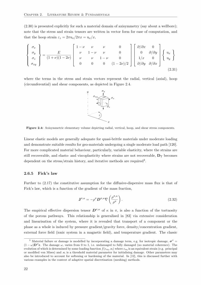
Chapter 2. Literature Review & Fundamentals
(2.30) is presented explicitly for such a material domain of axisymmetry (say about a wellbore);
note that the stress and strain tensors are written in vector form for ease of computation, and
that the hoop strain εz = 2πux/2πx = ux/x,σx
σy
σz
σxy
=E
(1 + ν)(1− 2ν)
1− ν ν ν 0
ν 1− ν ν 0
ν ν 1− ν 0
0 0 0 (1− 2ν)/2
∂/∂x 0
0 ∂/∂y
1/x 0
∂/∂y ∂/∂x
ux
uy
(2.31)
where the terms in the stress and strain vectors represent the radial, vertical (axial), hoop
(circumferential) and shear components, as depicted in Figure 2.4.
Figure 2.4: Axisymmetric elementary volume depicting radial, vertical, hoop, and shear stress components.
Linear elastic models are generally adequate for quasi-brittle materials under moderate loading
and demonstrate suitable results for geo-materials undergoing a single moderate load path [120].
For more complicated material behaviour, particularly, variable elasticity, where the strains are
still recoverable, and elasto- and viscoplasticity where strains are not recoverable, DT becomes
dependent on the stress/strain history, and iterative methods are required3.
2.6.5 Fick’s law
Further to (2.17) the constitutive assumption for the diffusive-dispersive mass flux is that of
Fick’s law, which is a function of the gradient of the mass fraction,
Jπ,κ = −ρπDπ,κ∇(ρπ,κ
ρπ
). (2.32)
The empirical effective dispersion tensor Dπ,κ of κ in π, is also a function of the tortuosity
of the porous pathways. This relationship is generalised in [83] via extensive consideration
and linearisation of the system, where it is revealed that transport of a component or the
phase as a whole is induced by pressure gradient/gravity force, density/concentration gradient,
external force field (ionic system in a magnetic field), and temperature gradient. The classic
3 Material failure or damage is modelled by incorporating a damage term, e.g. for isotropic damage, σ′′ =(1 − ω)Delε. The damage ω, varies from 0 to 1, i.e. undamaged to fully damaged (no material coherence). Theevolution of which is determined by some loading function f(εeq,κi) where εeq is an equivalent strain (e.g. principalor modified von Mises) and κi is a threshold material parameter for initialising damage. Other parameters mayalso be introduced to account for softening or hardening of the material. In [12], this is discussed further withvarious examples in the context of adaptive spatial discretisation (meshing) methods.
22
2.6. Equations of state and constitutive relations
form presented here is recovered by ignoring all but the density/concentration gradient term,
assuming it to be the most significant for most scenarios; this is explored and applied in more
detail in [83, 120].
2.6.6 Darcy’s law
Darcy flux is the discharge per unit area over a porous medium and is therefore a volume-
averaged relative velocity, determined by experimental work. This is equated with the actual
fluid pore velocity relative to the solid vfs via ηfvfs, which gives the typical extended multi-phase
relationship for Darcy flux,
ηfvfs =krfk
µf
[−∇pf + ρf
(g − as − afs
)]. (2.33)
where k is the empirical intrinsic permeability tensor of the porous medium, which may also be
considered as a function of porosity. Specific fluid properties are accounted for by the dynamic
viscosity µf and relative permeability krf , which are discussed in Sections 2.6.9.1 and 2.7.2
respectively. Darcy’s law is similarly generalised in [83, 82, 120], via the linearisation of the
fluid macroscopic momentum balance, where force, density gradient, and temperature gradient
terms, and coupling with the general form of (2.32) are also introduced, which warrant gauging
for given modelling scenarios. Particularly, it is shown that the dissipative part of the fluid-solid
and fluid-fluid momentum exchanges due to local effects is accounted for macroscopically via
the viscosity, permeability and relative permeability terms, which are dependent on the fluid
saturations. The movement of the fluid, as of (2.33), is governed by pressure gradient alone, and
gradients due to any accelerations other than gravity are generally assumed negligible and may
be further omitted. Darcy’s law is therefore valid as a first assumption for the slow flow of a
macroscopically inviscid fluid. It may also be arrived at without the inertial terms via reduction
of Navier-Stokes equation by assuming slow incompressible flow (low Reynolds number, Re 1,
Re = ρfvf lc/µf , ratio of inertial to viscous forces).
If velocities are however high enough the inertial effects start to have significance, the inclusion
of an inertial term representative of the kinetic energy of the fluid gives the Forchheimer form,
∇pf = − µf
kkrfqf − bbrfρ
fqf |qf | (2.34)
where qf is the Darcy fluid flux, and b and brf are the Forchheimer and relative Forchheimer
parameters, giving essentially the inertial permeability of the system, which are determined
experimentally.
2.6.7 Fourier’s law
Conduction is the process by which heat flows due to microscopic interactions of energetically
moving/vibrating particles with those less energetic within a temperature gradient. That is, heat
flows from a hotter to a colder region of substance without any net movement of the substance.
This occurs until thermal equilibrium is met, unless the system is externally driven. Other forms
23
Chapter 2. Literature Review & Fundamentals
of heat transfer are convection (due to net movements of the substance) and radiation.
The constitutive assumption for the flux of heat (supply of energy) and the temperature gradient
is given by a generalised form of Fourier’s law,
qπ = −χeff∇T (2.35)
where χeff is an effective thermal conductivity tensor, which is introduced for the fluids in a
thermodynamic context in Section 2.6.9.2, additional methods for its prediction are also given
in [120].
Noteworthy, interesting relationships in this context are given in the literature for the design of
various efficient (porous) building fabrics. Additionally, current additive manufacturing research
is also in pursuit of more representative thermal models which will give improved automated
control so that the build better matches the desired material properties and geometry. This is
particularly with respect to where the formed build and surrounding sintered powder exhibit
varying degrees of porosity which significantly affect the manufacturing and build performance.
2.6.8 Fluid thermodynamic properties
The thermodynamic properties of a fluid in the subsurface are dependent on the pressures and
temperatures present. Cubic equations of state (EoS) for real fluids, notably, van der Waals,
Redlich-Kwong and Peng-Robinson (of successive improvement), offer relatively simple and ac-
curate relationships for volume, pressure and temperature for a variety fluids. They represent
real fluids by incorporating terms which account, at the macroscopic, level for intermolecular
interactions operating at the microscopic level. If such behaviour is negligible as for when the
molecular sizes are small with respect to the mean distances between them, ideal gas behaviour
may be assumed [48].
More modern multiparameter equations of state can represent certain pure fluids and fluid
mixtures with high degrees of accuracy over the range of their states. These are typically
formulated in fundamental form explicit in terms of Helmholtz free energy, as a function of
density and temperature,
a(ρ, T )
RT=
ao(ρ, T ) + ar(ρ, T )
RT= α(δ, τ) = αo(δ, τ) + φr(δ, τ) (2.36)
where a is the specific Helmholtz energy, R is the specific gas constant, δ = ρ/ρc is reduced
density, and τ = T/Tc is reduced temperature. Subscripts c typically denote the fluids critical
point, α therefore being a reduced (nondimensionalized) form of the Helmholtz energy. The
equation is distinguished into a hypothetical ideal gas part, ao and a residual behaviour part,
ar. By defining all the thermodynamic properties, in relation to α and its partial derivatives
with respect to δ and τ , they may be determined algorithmically via weighting experimental
data, multi-property interpolation, and optimisation of the function form [20, 182]. For this
purpose, lists of the common thermodynamic properties are given in [182], in which the fun-
damental function form is used to derive EoS for important fluids and fluid mixtures. In [111]
comprehensive comparisons between the mentioned EoS are made along with their validity in
24
2.6. Equations of state and constitutive relations
the context of geo-applications.
Clearly, where appropriate and/or in view of avoiding computational expense, EoS simplifica-
tions can be made from which many practical methods may be developed. To begin, the most
robust case of EoS is used for accurate illustration of the following material properties, from
which it may also be assessed to what extent such simplifications can be made with respect to
modelling a GCS scenario.
In the following subsections, several thermodynamic properties of interest for CO2 and Brine,
namely, pressure, temperature, density (specific volume), composition and heat capacity are
assessed within the potential ranges of environmental conditions of interest (Section 1.3.1).
2.6.8.1 Density: CO2-brine mixture p-v-T-x relationship
Considering the pressure, volume, temperature and composition in mole fraction (p-v-T-x ) of
CO2-brine mixtures within the ranges of interest, that is at relatively low temperatures ranging
to approximately 100 C with relatively high pressures reaching several hundred atmospheres,
two distinct mutually soluble fluid phases coincide (a biphasic system). At equilibrium, the
following temperature and pressure dependent reactions and equilibrium constants Kf , may be
given,
CO2(aq) CO2(gl), KCO2 = fCO2(gl)/aCO2(aq)
, (2.37)
H2O(l) H2O(g), KH2O = fH2O(g)/aH2O(l)
, (2.38)
where f are the fugacities (effective pressures) and a are the activities (effective concentrations)
of the components from which their mole fractions can be ascertained [184].
The biphasic system is typically that of a CO2-rich supercritical phase and a H2O-rich liquid
phase, noting that pure CO2 is supercritical beyond its critical point [181] (Figure 2.5(a)):
Tc = 304.1282± 0.015 K (31.0 C ),
pc = 7.3773± 0.0030 MPa (72.8 atm),
ρc = 467.6± 0.6 kg/m3.
Although there is a degree of mutual solubility (partial miscibility), CO2-Brine displacement is
still essentially an immiscible process (primary drainage process) with phase interface tension
(Section 2.7) if the fluids are mutually saturated, as is further discussed in [24]. The problem
is therefore often simplified by treating the rich saturated fluids as immiscible by ignoring any
diffusive and/or reactive behaviour of the species involved, in particular the dissolution of CO2
and evaporation of H2O.
The role of partial miscibility is however important. Notably, it has been shown to reduce near-
wellbore pressures, which are of primary interest, after intermediate periods of injection. This
is due to the otherwise hypothetically trapped residual brine of lower compressibility evaporat-
ing whilst also giving up more permeable pathways for the more compressible CO2-rich phase.
Hence, the assumption of immiscibility keeps the brine at a minimum residual saturation which
overemphasises pressure build-up, as is quantified in [126]. This miscibility effect also leads to a
slightly reduced CO2-rich phase displacement as it is able to occupy more of the near-wellbore
25
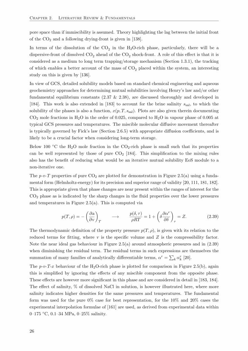
Chapter 2. Literature Review & Fundamentals
pore space than if immiscibility is assumed. Theory highlighting the lag between the initial front
of the CO2 and a following drying-front is given in [138].
In terms of the dissolution of the CO2 in the H2O-rich phase, particularly, there will be a
dispersive-front of dissolved CO2 ahead of the CO2 shock-front. A role of this effect is that it is
considered as a medium to long term trapping/storage mechanism (Section 1.3.1), the tracking
of which enables a better account of the mass of CO2 placed within the system, an interesting
study on this is given by [136].
In view of GCS, detailed solubility models based on standard chemical engineering and aqueous
geochemistry approaches for determining mutual solubilities involving Henry’s law and/or other
fundamental equilibrium constants (2.37 & 2.38), are discussed thoroughly and developed in
[184]. This work is also extended in [183] to account for the brine salinity ssal, to which the
solubility of the phases is also a function, x(p, T, ssal). Plots are also given therein documenting
CO2 mole fractions in H2O in the order of 0.025, compared to H2O in vapour phase of 0.005 at
typical GCS pressures and temperatures. The miscible molecular diffusive movement thereafter
is typically governed by Fick’s law (Section 2.6.5) with appropriate diffusion coefficients, and is
likely to be a crucial factor when considering long-term storage.
Below 100 C the H2O mole fraction in the CO2-rich phase is small such that its properties
can be well represented by those of pure CO2 [184]. This simplification to the mixing rules
also has the benefit of reducing what would be an iterative mutual solubility EoS module to a
non-iterative one.
The p-v-T properties of pure CO2 are plotted for demonstration in Figure 2.5(a) using a funda-
mental form (Helmholtz-energy) for its precision and superior range of validity [20, 111, 181, 182].
This is appropriate given that phase changes are near present within the ranges of interest for the
CO2 phase as is indicated by the sharp changes in the fluid properties over the lower pressures
and temperatures in Figure 2.5(a). This is computed via
p(T, ρ) = −(∂a
∂v
)T
−→ p(δ, τ)
ρRT= 1 +
(δ∂αr
∂δ
)τ
= Z. (2.39)
The thermodynamic definition of the property pressure p(T, ρ), is given with its relation to the
reduced terms for fitting, where v is the specific volume and Z is the compressibility factor.
Note the near ideal gas behaviour in Figure 2.5(a) around atmospheric pressures and in (2.39)
when diminishing the residual term. The residual terms in such expressions are themselves the
summation of many families of analytically differentiable terms, αr =∑
k αrk [20].
The p-v-T-x behaviour of the H2O-rich phase is plotted for comparison in Figure 2.5(b), again
this is simplified by ignoring the effects of any miscible component from the opposite phase.
These effects are however more significant in this phase and are considered in detail in [183, 184].
The effect of salinity, % of dissolved NaCl in solution, is however illustrated here, where more
salinity indicates higher densities for the same pressures and temperatures. The fundamental
form was used for the pure 0% case for best representation, for the 10% and 20% cases the
experimental interpolation formulae of [161] are used, as derived from experimental data within
0–175 C, 0.1–34 MPa, 0–25% salinity.
26
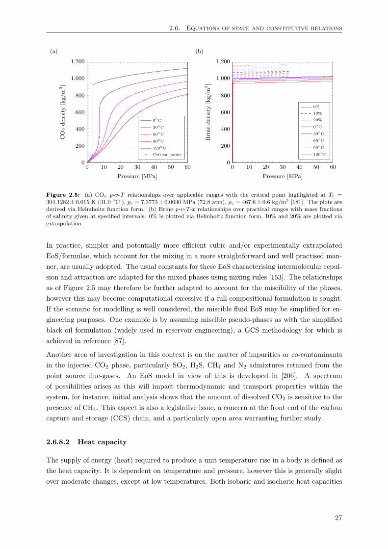
2.6. Equations of state and constitutive relations
(a)
0 10 20 30 40 50 600
200
400
600
800
1,000
1,200
Pressure [MPa]
CO
2den
sity
[kg/m
3]
0C
30C
60C
90C
120C
Critical point
(b)
0 10 20 30 40 50 600
200
400
600
800
1,000
1,200
Pressure [MPa]
Brineden
sity
[kg/m
3]
0%
10%
20%
0C
30C
60C
90C
120C
Figure 2.5: (a) CO2 p-v-T relationships over applicable ranges with the critical point highlighted at Tc =304.1282± 0.015 K (31.0 C ), pc = 7.3773± 0.0030 MPa (72.8 atm), ρc = 467.6± 0.6 kg/m3 [181]. The plots arederived via Helmholtz function form. (b) Brine p-v-T-x relationships over practical ranges with mass fractionsof salinity given at specified intervals: 0% is plotted via Helmholtz function form, 10% and 20% are plotted viaextrapolation.
In practice, simpler and potentially more efficient cubic and/or experimentally extrapolated
EoS/formulae, which account for the mixing in a more straightforward and well practised man-
ner, are usually adopted. The usual constants for these EoS characterising intermolecular repul-
sion and attraction are adapted for the mixed phases using mixing rules [153]. The relationships
as of Figure 2.5 may therefore be further adapted to account for the miscibility of the phases,
however this may become computational excessive if a full compositional formulation is sought.
If the scenario for modelling is well considered, the miscible fluid EoS may be simplified for en-
gineering purposes. One example is by assuming miscible pseudo-phases as with the simplified
black-oil formulation (widely used in reservoir engineering), a GCS methodology for which is
achieved in reference [87].
Another area of investigation in this context is on the matter of impurities or co-contaminants
in the injected CO2 phase, particularly SO2, H2S, CH4 and N2 admixtures retained from the
point source flue-gases. An EoS model in view of this is developed in [206]. A spectrum
of possibilities arises as this will impact thermodynamic and transport properties within the
system, for instance, initial analysis shows that the amount of dissolved CO2 is sensitive to the
presence of CH4. This aspect is also a legislative issue, a concern at the front end of the carbon
capture and storage (CCS) chain, and a particularly open area warranting further study.
2.6.8.2 Heat capacity
The supply of energy (heat) required to produce a unit temperature rise in a body is defined as
the heat capacity. It is dependent on temperature and pressure, however this is generally slight
over moderate changes, except at low temperatures. Both isobaric and isochoric heat capacities
27
Chapter 2. Literature Review & Fundamentals
are fundamentally defined,
Cp(T, p) =
(∂Q
∂T
)p
=
(∂H
∂T
)p
CV (T, ρ) =
(∂Q
∂T
)V
=
(∂U
∂T
)V
(2.40)
where H is the enthalpy (total energy content of system). These relationships can be derived
noting H = U + pV and observing the relationships of (2.19 & 2.20).
An effective macroscopic heat capacity may be given for a multiphase medium [120], in terms
of the specific isobaric heat capacities cπp , for the present phases, with reference to Table 2.1,
(ρcp)eff = (1− n)ρscsp + nSwρ
wcwp + nSnρncnp . (2.41)
Heat capacity is also fundamentally defined in Helmholtz energy explicit form for correlation
[182]. Variability of the heat capacities for CO2 and brine as a function of pressure and temper-
ature are illustrated in [111].
Note that the temperature front due to the subsurface injection of CO2 is behind the advection
front due to a retardation caused by the specific heat capacities of the in situ brine and rock
[125].
2.6.8.3 Joule-Thomson coefficient and cooling
The Joule-Thomson coefficient is described fundamentally as,
µJT =
(∂T
∂p
)H
, (2.42)
arising from the Joule-Thomson thermodynamic process which occurs along an insulated con-
stant/conserved enthalpy (isenthalpic) curve in the p-T plane, that is, a steady adiabatic process
with no exchange of heat with the surrounding environment. Along this curve an inversion point
occurs, where µJT = 0, due to a change in the dominant molecular interaction behaviour, which
all real gases have, µJT being always zero for an ideal gas. If the fluid is below the maximum
inversion temperature such that µJT > 0, then a reduction in pressure coincides with a reduction
in temperature, from (2.42).
This expansive cooling (known as throttling) is central to many thermal machines (refrigerators,
air conditioners, etc.) and is achieved by an insulated value or porous plug which causes the
fluid to pass from a high to lower pressure region and thus expand.
The process is a particular concern for GCS. Shallow reservoirs and particularly depleted oil
and gas reservoirs de-pressurised during exploitation are characterised by low pore pressures.
Injecting into a low pressured formations with high pressured CO2 will result in large pressure
gradients, from which significant Joule-Thomson cooling (JTC) may occur. It is believed that
the drop in pressure here would cause freezing of the pore fluids and form CO2 hydrates both
of which could cause significant loss of injectivity and reservoir performance. Cooling effects
are unlikely to pose a problem for initially moderately warm and permeable reservoirs at low
pressures (T0 > 40C , k > 10−14 m2, p0 > 2 MPa) [125, 141].
28
2.6. Equations of state and constitutive relations
The effects of JTC in the context of GCS are discussed further in [141], where the results of a
coupled non-linear hydro-thermal model capturing the transient behaviour of the problem are
assessed. Later [125, 129] produced good agreement with a simplified analytical assessment. This
is achieved by assuming constant and uniform material properties (in particularly µJT, which is
appropriate given that it is approximately constant for CO2 at the relatively low pressures of
interest), and steady-state behaviour, which are particularly conservative assumptions in that
they overestimate the spatial pressure gradient and cooling. The behaviour of a single fluid phase
is also assumed in the analytical assessment, which is appropriate given that the cooling front
lags within the CO2 phase behind the advection front. An objective of this thesis is therefore to
account for this hydro-thermal behaviour during the model formulation and to extend on this
work by additionally coupling mechanical deformation and a double-porosity network within the
formulation for assessment.
2.6.9 Fluid transport properties
Viscosity, thermal conductivity and surface energy are introduced here. The state-of-the-art is
less mature in predicting theses properties from the state variables, compared to the thermody-
namic properties of Section 2.6.8.
2.6.9.1 Dynamic viscosity
Fluid passing through a porous medium is generally slow such that non-turbulent or laminar
flow (low Reynolds number) is primarily considered. A proportionality exists for the shear stress
between laminar planes and the change in velocity between the planes with respect to their
distance apart, this is given by the dynamic (shear) viscosity, σzy = µ(∂v/∂z). This property
is therefore a measure of the fluid’s resistance to deformation by internal shear in overcoming
friction that is caused by intermolecular forces.
Dynamic viscosity is an important property when considering fluid flow through porous media
(Section 2.1.1) and interface stability/mobility (Section 2.7.3) when multiple phases are present.
Its variation for CO2 and brine with respect to pressure and temperature is given in Figures 2.6(a)
and 2.6(b). For CO2, with its near present critical point, at lower pressures and temperatures
sharp changes in viscosity are identified. Both phases demonstrate particular sensitivity to
temperature, with brine additionally becoming more viscous with increased salinity. For pure
CO2 and H2O the enhanced relationships discussed by [20] are used. For those of brine with
varying salinity the relationships of [105, 106] are used, as were derived therein with experimental
data within 20–150 C, 0.1–30 MPa, and 0–25% salinity. Note also the difference of an order of
magnitude between the two phases over the ranges of interest.
Correlation for the equations plotted takes the general form,
µ = µo(τ) + µr(τ, δ) + µc(τ, δ), (2.43)
where the three terms of summations capture, respectively, dependence on temperature at zero
density limits, residual dependence on temperature and density, and any dependence enhance-
29
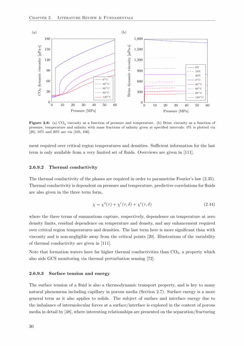
Chapter 2. Literature Review & Fundamentals
(a)
0 10 20 30 40 50 600
30
60
90
120
150
180
Pressure [MPa]
CO
2dynamic
viscosity
[µPa·s]
0C
30C
60C
90C
120C
(b)
0 10 20 30 40 50 600
300
600
900
1,200
1,500
1,800
Pressure [MPa]
Brinedynamic
viscosity
[µPa·s]
0%
10%
20%
0C
30C
60C
90C
120C
Figure 2.6: (a) CO2 viscosity as a function of pressure and temperature. (b) Brine viscosity as a function ofpressure, temperature and salinity with mass fractions of salinity given at specified intervals: 0% is plotted via[20], 10% and 20% are via [105, 106].
ment required over critical region temperatures and densities. Sufficient information for the last
term is only available from a very limited set of fluids. Overviews are given in [111].
2.6.9.2 Thermal conductivity
The thermal conductivity of the phases are required in order to parametrise Fourier’s law (2.35).
Thermal conductivity is dependent on pressure and temperature, predictive correlations for fluids
are also given in the three term form,
χ = χo(τ) + χr(τ, δ) + χc(τ, δ) (2.44)
where the three terms of summations capture, respectively, dependence on temperature at zero
density limits, residual dependence on temperature and density, and any enhancement required
over critical region temperatures and densities. The last term here is more significant than with
viscosity and is non-negligible away from the critical points [20]. Illustrations of the variability
of thermal conductivity are given in [111].
Note that formation waters have far higher thermal conductivities than CO2, a property which
also aids GCS monitoring via thermal perturbation sensing [72].
2.6.9.3 Surface tension and energy
The surface tension of a fluid is also a thermodynamic transport property, and is key to many
natural phenomena including capillary in porous media (Section 2.7). Surface energy is a more
general term as it also applies to solids. The subject of surface and interface energy due to
the imbalance of intermolecular forces at a surface/interface is explored in the context of porous
media in detail by [48], where interesting relationships are presented on the separation/fracturing
30
2.6. Equations of state and constitutive relations
energies for fluids and solids. An overview of the fundamental thermodynamic relations for
correlation with respect to fluids is given in [20]. Note that the surface tension and surface
energy density for a liquid are the same.
2.6.10 Compressibility & thermal expansion coefficients
For either solid or fluid, the compressibility coefficient c or its inverse bulk modulus K present a
measure of a material’s elasticity, relating relative volume change (volume strain) and pressure
(or mean stress) change at constant temperature,
c =1
K= − 1
V
(∂V
∂p
)T
=1
ρ
(∂ρ
∂p
)T
. (2.45)
Similarly, the thermal expansion coefficient presents a useful relationship for the relative volu-
metric change (volume strain) and change in temperature at constant pressure,
β =1
V
(∂V
∂T
)p
= −1
ρ
(∂ρ
∂T
)p
. (2.46)
As thermodynamic properties, these coefficients are dependent on pressure, temperature and
composition. The partial differentials are therefore to be taken within reasonable ranges de-
pending on the material’s behaviour if these coefficients are to be adopted as constant material
properties.
The isothermal compressibility (2.45) is the basis of all primary recovery mechanisms in hy-
drocarbon reservoirs [50]. This is seen by considering a reservoir initially overpressured with
trapped hydrocarbons, where a fall in fluid pressure, ∆p, due to drilling will cause the fluid
to expand, ∆V , to the surface manifesting as hydrocarbon production. The assumption of
isothermal behaviour in this context is also permissible given that the production process occurs
slow enough such that heat taken by convection within the produced fluids and so forth is re-
placed by conduction from the surrounding formation, thus keeping the reservoir at a constant
temperature.
2.6.10.1 Fluid density
By considering the conservation of mass in the form, D(ρV )/Dt = 0, and given that ρ(p, T ),
carrying out manipulation with the product rule and substituting (2.45) and (2.46) gives,
1
ρ
Dρ
Dt=
1
K
Dp
Dt− β
DT
Dt, (2.47)
which presents a useful first-order expansion or linear approximation of the real equation of state
for a given material at some reference point, Figures 2.5(a) and 2.5(b).
31
Chapter 2. Literature Review & Fundamentals
2.6.10.2 Solid density
For a porous solid, changes in volume of a unit mass are due to compression of the grains and/
or rearrangement of the grains. Again the conservation of mass in the from, D(ρV )/Dt = 0,
is considered, assuming the density of the solid phase to be a function of the solid pressure,
temperature, and the first invariant of effective stress. Following a similar procedure as for
(2.47), introducing the bulk modulus of the grains via the stress invariant, then applying (2.28),
reference [120] produces the following solid density material derivative function for a porous
solid with compressible skeleton and grains,
1
ρsDsρs
Dt=
1
1− n
[(b− n)
1
Ks
Dsps
Dt− βs(b− n)
DsT
Dt− (1− b)∇ · vs
], (2.48)
which reduces to the simple form of (2.47) when the grains are considered incompressible (b = 1).
This reduction is often assumed in petroleum engineering when the compressibility of the pore
volume is taken to represent that of the bulk medium, that is, dVs = 0, then dV = dVv.
2.7 Capillarity
Due to the action of surface energy (Section 2.6.9.3), a fluid (gas/liquid)-liquid interface is
potentially curved combining a difference in pressure pa− pb between the two phases. The work
produced by this pressure difference applying to some initial infinitesimal spherical segment
through an infinitesimal increase in curvature radius is (pa − pb) adR. Also, the change in
interface energy here due the change in surface area of the spherical segment is γab da. As two
surfaces of the same fluid would tend to merge losing their surface energies to an (original) state
of lower energy, two different surfaces equilibrate minimising the total potential energy of the
interface, that is the two previous terms should be equal [48]. This leads to the Young-Laplace
equation,
pa − pb =2γabR
, (2.49)
where γab is the interface energy (per unit area) for the fluids, assumed constant, and R is the
(mean) radius of interface curvature.
If a solid interface is also involved, a contact angle results at the point where all three phases meet
due the relative intermolecular interactions between them. The contact angle θ is a measure of
the relative wettability of the fluids with regard to the solid and is related by the Young-Dupre
equation, which is derived by similar considerations towards interfacial energy balances,
γsn = γsw + γnw cos θ. (2.50)
Assuming the spherically curved interface invades a cylindrical pore space with radius r, the
curvature R is related by r = R sin(π/2− θ). Combined with (2.49) this gives the specific form
pn − pw =2γnw cos θ
r. (2.51)
32
2.7. Capillarity
The capillary pressure is now defined as the difference in pressure between the nonwetting and
wetting phases, pc = pn − pw. Note that the capillary pressure behaviour is dependent on
the property specific relative wettability between the fluid phases and the solid present. For
CO2 and brine in the presence of one another in contact with rock, the wetting phase, which
preferentially wets the solid matrix, is generally brine, in which case the CO2 is therefore the
nonwetting phase. This phenomena is illustrated in Figure 2.1(a).
The free energy of a porous solid alone, through which a nonwetting phase invades displacing a
wetting phase, is considered after (2.21). Parametrising the first r.h.s. term to account for two
immiscible fluids (Equation (2.22)), while ignoring the other terms by assuming the system to
be undeformable and isothermal, reduces das to be the infinitesimal change in free energy of the
interface between the porous solid and the fluids [48],
das = pw(φ0 dSw) + pn(φ0 dSn) = −φ0 (pn − pw) dSw, (2.52)
where inside the first two brackets the changes in volume fraction are observed for each fluid
phase in relation to the free energy. If U = as/φ0 is introduced as the free energy of the interfaces
per unit porous volume then,
pn − pw = − dUdSw
. (2.53)
This result is also found by extending (2.51) by considering the energy balance of a moving
interface as it invades an isolated conical pore space [48]. The implication is that the capillary
pressure pc is a function of the saturation Sw and interface energy U associated with the specific
fluids and porous solid involved.
Equation (2.53) gives a fundamental interpretation of the prevalent experimental relationships
of pc(Sw) which give macroscopic functions (capillary pressure or retention curves) relating
specific fluids with porous media. An interpretation is also given on the microscale with regard
to (2.51). The function pc(Sw) is a maximum when the wetting saturation is zero and a minimum
until some entry pressure is breached. The entry pressure pentry, in accord with (2.51), is the
minimum pressure requisite for the nonwetting phase to enter pores of the largest radius, the
threshold at which Sw starts decreasing from 1. Essentially, by increasing pc the pore space is
invaded (desaturated) by the nonwetting phase. Conversely, imbibition or suction in the sense
of capillary rise takes place, of which the height of a capillary fringe or column above a phreatic
surface would be given by pentry/ρwg.
2.7.1 Capillary pressure-saturation relationship
A commonly used [120] capillary pressure curve is the Brooks-Corey model [34, 35], based
on the theory of [37], which proposes a convenient approximation of an effective saturation,
Se = (pentry/pc)λ, for pc ≥ pentry, where λ is a fitting parameter to the typical concave curve of pc
against Se, essentially characterising the pore-size distribution. A generally more representative
concave-convex curve (with a nonwetting regressive entry gradient, Figure 2.7(a)), which is more
challenging to implement numerically, is given by the van Genuchten model [194] based on the
33
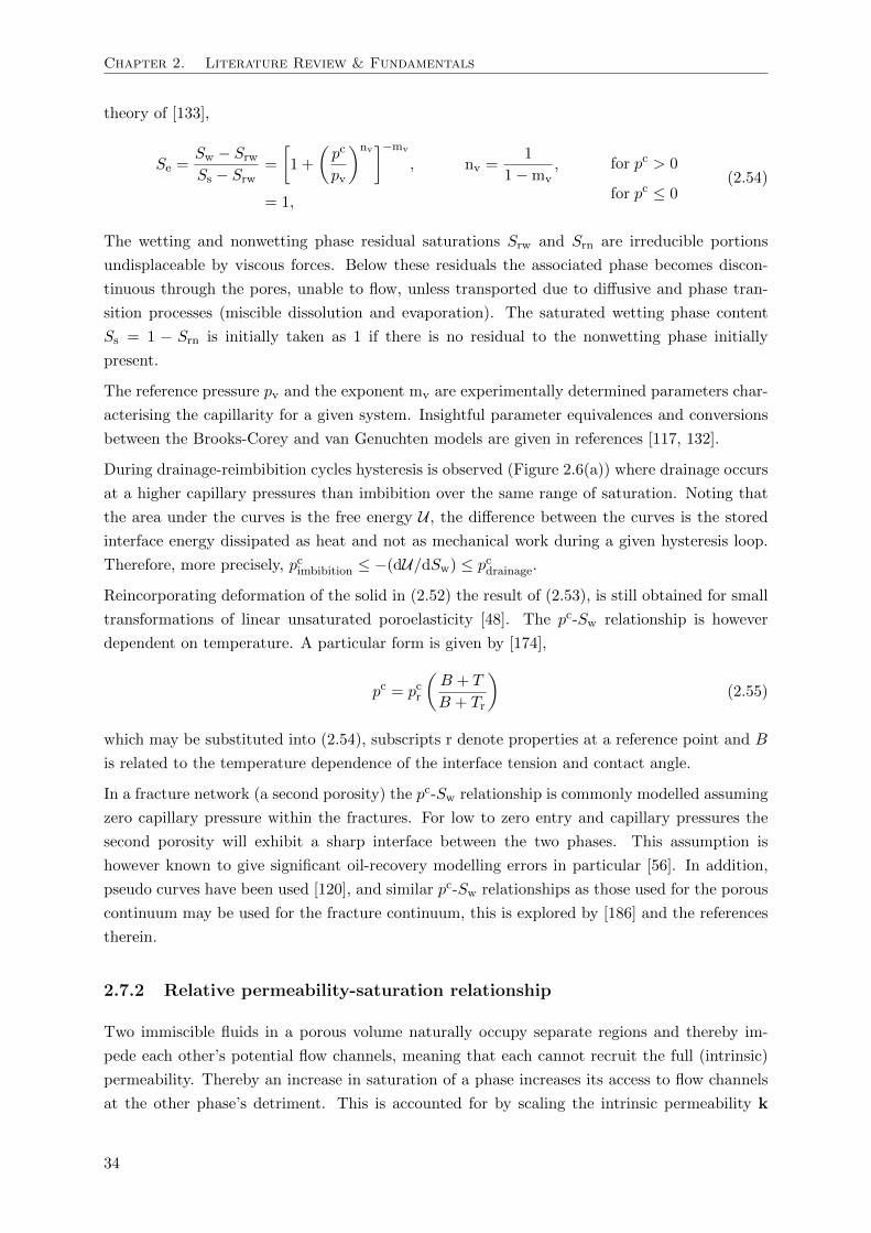
Chapter 2. Literature Review & Fundamentals
theory of [133],
Se =Sw − SrwSs − Srw
=
[1 +
(pc
pv
)nv]−mv
, nv =1
1−mv,
= 1,
for pc > 0
for pc ≤ 0(2.54)
The wetting and nonwetting phase residual saturations Srw and Srn are irreducible portions
undisplaceable by viscous forces. Below these residuals the associated phase becomes discon-
tinuous through the pores, unable to flow, unless transported due to diffusive and phase tran-
sition processes (miscible dissolution and evaporation). The saturated wetting phase content
Ss = 1 − Srn is initially taken as 1 if there is no residual to the nonwetting phase initially
present.
The reference pressure pv and the exponent mv are experimentally determined parameters char-
acterising the capillarity for a given system. Insightful parameter equivalences and conversions
between the Brooks-Corey and van Genuchten models are given in references [117, 132].
During drainage-reimbibition cycles hysteresis is observed (Figure 2.6(a)) where drainage occurs
at a higher capillary pressures than imbibition over the same range of saturation. Noting that
the area under the curves is the free energy U , the difference between the curves is the stored
interface energy dissipated as heat and not as mechanical work during a given hysteresis loop.
Therefore, more precisely, pcimbibition ≤ −(dU/dSw) ≤ pcdrainage.
Reincorporating deformation of the solid in (2.52) the result of (2.53), is still obtained for small
transformations of linear unsaturated poroelasticity [48]. The pc-Sw relationship is however
dependent on temperature. A particular form is given by [174],
pc = pcr
(B + T
B + Tr
)(2.55)
which may be substituted into (2.54), subscripts r denote properties at a reference point and B
is related to the temperature dependence of the interface tension and contact angle.
In a fracture network (a second porosity) the pc-Sw relationship is commonly modelled assuming
zero capillary pressure within the fractures. For low to zero entry and capillary pressures the
second porosity will exhibit a sharp interface between the two phases. This assumption is
however known to give significant oil-recovery modelling errors in particular [56]. In addition,
pseudo curves have been used [120], and similar pc-Sw relationships as those used for the porous
continuum may be used for the fracture continuum, this is explored by [186] and the references
therein.
2.7.2 Relative permeability-saturation relationship
Two immiscible fluids in a porous volume naturally occupy separate regions and thereby im-
pede each other’s potential flow channels, meaning that each cannot recruit the full (intrinsic)
permeability. Thereby an increase in saturation of a phase increases its access to flow channels
at the other phase’s detriment. This is accounted for by scaling the intrinsic permeability k
34
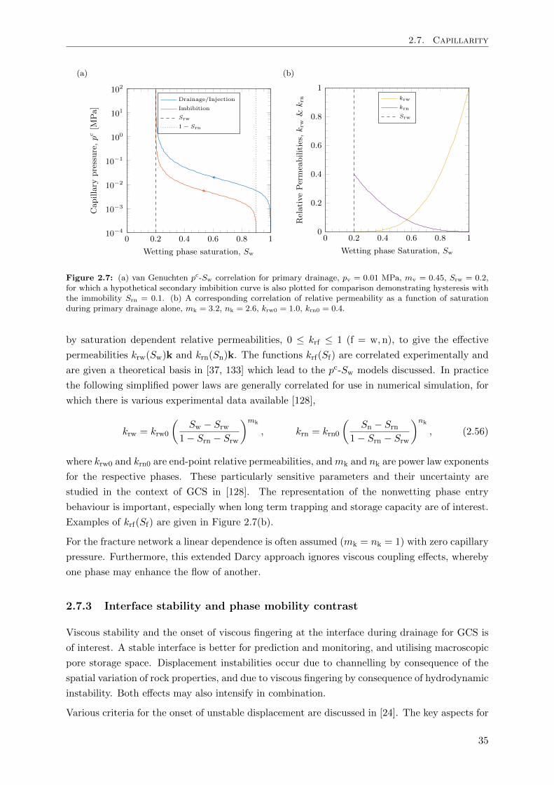
2.7. Capillarity
(a)
0 0.2 0.4 0.6 0.8 110−4
10−3
10−2
10−1
100
101
102
Wetting phase saturation, Sw
Capillary
pressure,pc[M
Pa]
Drainage/Injection
Imbibition
Srw
1 − Srn
(b)
0 0.2 0.4 0.6 0.8 10
0.2
0.4
0.6
0.8
1
Wetting phase Saturation, Sw
RelativePermeabilities,krw
&krn krw
krn
Srw
Figure 2.7: (a) van Genuchten pc-Sw correlation for primary drainage, pv = 0.01 MPa, mv = 0.45, Srw = 0.2,for which a hypothetical secondary imbibition curve is also plotted for comparison demonstrating hysteresis withthe immobility Srn = 0.1. (b) A corresponding correlation of relative permeability as a function of saturationduring primary drainage alone, mk = 3.2, nk = 2.6, krw0 = 1.0, krn0 = 0.4.
by saturation dependent relative permeabilities, 0 ≤ krf ≤ 1 (f = w,n), to give the effective
permeabilities krw(Sw)k and krn(Sn)k. The functions krf(Sf) are correlated experimentally and
are given a theoretical basis in [37, 133] which lead to the pc-Sw models discussed. In practice
the following simplified power laws are generally correlated for use in numerical simulation, for
which there is various experimental data available [128],
krw = krw0
(Sw − Srw
1− Srn − Srw
)mk
, krn = krn0
(Sn − Srn
1− Srn − Srw
)nk
, (2.56)
where krw0 and krn0 are end-point relative permeabilities, andmk and nk are power law exponents
for the respective phases. These particularly sensitive parameters and their uncertainty are
studied in the context of GCS in [128]. The representation of the nonwetting phase entry
behaviour is important, especially when long term trapping and storage capacity are of interest.
Examples of krf(Sf) are given in Figure 2.7(b).
For the fracture network a linear dependence is often assumed (mk = nk = 1) with zero capillary
pressure. Furthermore, this extended Darcy approach ignores viscous coupling effects, whereby
one phase may enhance the flow of another.
2.7.3 Interface stability and phase mobility contrast
Viscous stability and the onset of viscous fingering at the interface during drainage for GCS is
of interest. A stable interface is better for prediction and monitoring, and utilising macroscopic
pore storage space. Displacement instabilities occur due to channelling by consequence of the
spatial variation of rock properties, and due to viscous fingering by consequence of hydrodynamic
instability. Both effects may also intensify in combination.
Various criteria for the onset of unstable displacement are discussed in [24]. The key aspects for
35
Chapter 2. Literature Review & Fundamentals
perturbations in interface stability are the phase mobility krπ/µπ, capillary pressure pc, gravity
and length scale. Capillary pressure is known to stabilise immiscible displacement on shorter
length scales, however larger length scales are those practical for GCS. This stabilisation is
particularly a result of capillarity causing the shock-front (Section 3.2.6) to disperse; this acts to
decrease the mobility contrast and therefore suppresses instability, it also follows that capillarity
suppresses on the same length scale of this dispersion. It is the ratio of viscous to capillary forces
which determines the gradient or sharpness to the shock-front (Darcy macroscopic capillary
number), where low and high flow rates may be associated with capillary and viscous dominated
flows respectively.
A simple form of the shock-front mobility contrast ratio is given by the following, which is
discussed as an appropriate criterion for the onset of instability in [24],
M =krn(Sshock)/µ
n
krw(Sw = 1)/µw> 1, (2.57)
where instability occurs when the displacing phase is more mobile than the displaced phase
evaluated at the shock-front. In the context of GCS initial study shows the viscosity ratio µw/µn,
exponents nk and mk, and endpoints krw0 and krn0, to be the principal sensitive parameters.
Representative storage site data is therefore specifically required in order to assess stability in
a given system. Hypothetical stability maps are given in [25], which are based on (2.57) and
simple uncoupled simulations where finger nucleation/perturbation is caused by superimposed
random permeabilities. During the temporal and spatial discretion of the system a degree of
extra refinement is required to adequately capture this interface behaviour.
2.8 Further HTMC Processes
In Section 1.3.1 the trapping mechanisms for CO2 sequestration were outlined. So far the
key physical mechanisms have been reviewed for modelling. Static trapping (CO2 restricted by
structural/stratigraphic low-permeability barriers) by way of Section 2.6.6, and residual trapping
(CO2 restricted in pore spaces at irreducible saturation) by Section 2.7. These mechanisms
contribute the most to sequestration at the earlier stages of injection, however they offer the
least storage security. At the later stages the chemical mechanisms contribute more, potentially
offering more storage security.
2.8.1 Dissolution (solubility and ionic) mechanisms
As discussed in Section 2.6.8.1 the solubility of CO2 is a potential trapping mechanism, where
CO2 would be stored dissolved in solution as aqueous CO2 and carbonic acid, this solubility is
given by,
CO2(g) CO2(aq) and CO2(aq) +H2O H2CO3(aq). (2.58)
The amount of dissolution is state dependent (Section 2.6.8.1), future changes of which may
therefore cause the carbon to return back out of solution. The carbonic acid partially disasso-
36
2.8. Further HTMC Processes
ciates presenting an additional ionic form of trapping,
H2CO3(aq) +H2O HCO−3 (aq) +H3O
+. (2.59)
The extent of this dissociation determines the acidity of the solution and may be determined by a
state dependent acid dissociation constant, in terms of concentrations,Ka = [H+][HCO−3 ]/[H2CO3].
2.8.2 Mineral mechanisms
Further reactions with the host rock which is likely to be rich in Fe, Mg, and Ca minerals would
also affect the system performance, for instance the following typical reaction,
Ca2+ +HCO−3 (aq) +OH− Ca2+ +CO2−
3 (aq) +H2O CaCO3(s) +H2O, (2.60)
creates solid precipitates (carbonates). In addition to being a form of long-term storage, the
precipitate may block the pores impeding further sequestration. Conversely, as this reaction
is reversible, calcium carbonate already present in the host rock (particularly limestones and
shales in this case) may become dissolved, which could pose a problem if it is a constituent
of the sealing caprock, thus compromising the physical trapping mechanisms. It follows that
the extent and kinetic rates of such reactions in the subsurface should be considered in order
to account for the long-term fate and transport of the stored CO2. To do so the sink/source
terms for the individual species/components in the conservation equations must be attributed
to these chemical processes, giving rise to coupled diffusion-reaction equations accounting for
the CaCO3-H2O-CO2 compositions at the fluid-solid interfaces. Further study in this context is
given by [101] and with the incorporation of brine in [71].
2.8.3 Adsorption mechanisms
Adsorption becomes significant particularly in organic rocks, the sequestration of CO2 in disused
coalbeds on displacing host methane CH4 for instance, will alter the interface stresses, even if
the saturating fluid pressures are constant. CO2 replacing CH4 at the same fluid pressure still
causes an (additional) adsorption-induced deformation of the porous solid, and in this case the
adsorption of CO2 will cause the coalbed to swell as the interface energy is significantly less.
The change in interface stress is due to the difference in the dipolar nature of the fluids, the
macroscopic physics of which, following (2.21), and eventually incorporating fluid dependent
Langmuir’s adsorption isotherms is detailed for further study in [48].
In typical brine aquifer systems the brine remains adsorbed as the mineral-wetting phase; this
presents a thin water film coating the mineral grains which affects multiphase flow and mediates
reactions with the solid interfaces. A study in this context which demonstrates the sensitivity
of the thickness of residual water films is given by [191], which highlights the needed for further
detailed study of specific mineral-H2O-CO2 fate and transport behaviour.
37
Chapter 2. Literature Review & Fundamentals
2.8.4 Density convection mixing
The dissolution of CO2 in formation brine increases the nearby aqueous phase density, meaning
that it will sink while the less dense host brine will rise, resulting in convective mixing. This
results in a gravitational/density-driven instability and vertical fingering of dissolved CO2 which
present problems for numerical discretisation techniques. The onset of mixing is particularly
sensitive to permeability perturbations, heterogeneities, saturation, salinity, rock mineralogy,
and geochemistry [72].
2.8.5 Porosity and permeability changes
In addition to changes caused by mineral precipitation/dissolution and Joule-Thompson cooling,
there are porosity and permeability changes caused by stress/strain deformability within the
rock. This relationship is often determined by empirical (laboratory or field calibrated) models
describing changes in porosity and permeability as functions of the stress state within the host
rock [162]. Empirical relations for permeability as a function of theoretical changes in porosity
are also common and have been fitted for numerous rock types [72]. For the correction of
permeabilities within fractures, an exponential empirical model which is stress state dependent
has also been employed [72].
2.9 Upscaling
Upscaling or homogenising spatially detailed (measured) geological data so that it may be ap-
plied to spatially coarser numerical descriptions for computer simulation is motived primarily by
the demand for computational efficiency. That is, to date there is disparity between the scale of
measurement and the scale of discretisation over which numerical simulations can be performed
in practice. In basic, upscaling is achieved by analytical and numerical techniques which seek for
suitable effective descriptions for the coarse simulation grid such that the same gross behaviour
of interest is simulated. Techniques can be characterised as local or global, depending on the
spatial extent used to determined the coarse scale quantities, and include various heuristic, deter-
ministic and stochastic methods (for instance, averaging, inversion and Monte Carlo methods).
Detailed reviews and comparisons of the various techniques are made in [59, 63, 88, 157, 203]
and the references therein. The numerous techniques involved are demonstrated to have various
advantages and limitations in various modelling scenarios, and thus constitute an extensive re-
search area. In particular, upscaling for highly heterogeneous and fractured media are detailed
in [40, 49, 73, 115, 122], in which reference is made to dual-grid and dual-porosity/permeability
formulations (upscaling from discrete fracture characterisations) and CO2 sequestration. Em-
phasis is generally on the scaling of porosity and permeability/transmissibility parameterisations
for both porous matrix and fracture. For coupled fluid, heat and geomechanics modelling, the
upscaling of the deformability/moduli of the porous media is also considered in [100, 164].
38
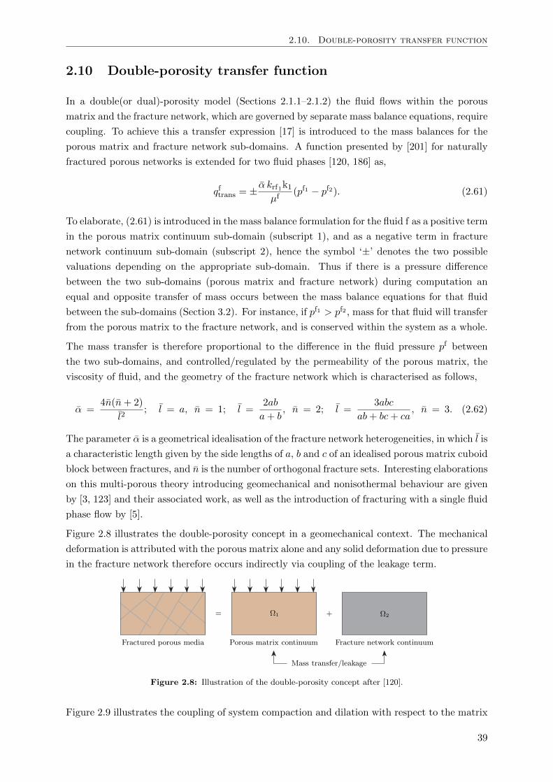
2.10. Double-porosity transfer function
2.10 Double-porosity transfer function
In a double(or dual)-porosity model (Sections 2.1.1–2.1.2) the fluid flows within the porous
matrix and the fracture network, which are governed by separate mass balance equations, require
coupling. To achieve this a transfer expression [17] is introduced to the mass balances for the
porous matrix and fracture network sub-domains. A function presented by [201] for naturally
fractured porous networks is extended for two fluid phases [120, 186] as,
qftrans = ± α krf1k1µf
(pf1 − pf2). (2.61)
To elaborate, (2.61) is introduced in the mass balance formulation for the fluid f as a positive term
in the porous matrix continuum sub-domain (subscript 1), and as a negative term in fracture
network continuum sub-domain (subscript 2), hence the symbol ‘±’ denotes the two possible
valuations depending on the appropriate sub-domain. Thus if there is a pressure difference
between the two sub-domains (porous matrix and fracture network) during computation an
equal and opposite transfer of mass occurs between the mass balance equations for that fluid
between the sub-domains (Section 3.2). For instance, if pf1 > pf2 , mass for that fluid will transfer
from the porous matrix to the fracture network, and is conserved within the system as a whole.
The mass transfer is therefore proportional to the difference in the fluid pressure pf between
the two sub-domains, and controlled/regulated by the permeability of the porous matrix, the
viscosity of fluid, and the geometry of the fracture network which is characterised as follows,
α =4n(n+ 2)
l2; l = a, n = 1; l =
2ab
a+ b, n = 2; l =
3abc
ab+ bc+ ca, n = 3. (2.62)
The parameter α is a geometrical idealisation of the fracture network heterogeneities, in which l is
a characteristic length given by the side lengths of a, b and c of an idealised porous matrix cuboid
block between fractures, and n is the number of orthogonal fracture sets. Interesting elaborations
on this multi-porous theory introducing geomechanical and nonisothermal behaviour are given
by [3, 123] and their associated work, as well as the introduction of fracturing with a single fluid
phase flow by [5].
Figure 2.8 illustrates the double-porosity concept in a geomechanical context. The mechanical
deformation is attributed with the porous matrix alone and any solid deformation due to pressure
in the fracture network therefore occurs indirectly via coupling of the leakage term.
Figure 2.8: Illustration of the double-porosity concept after [120].
Figure 2.9 illustrates the coupling of system compaction and dilation with respect to the matrix
39
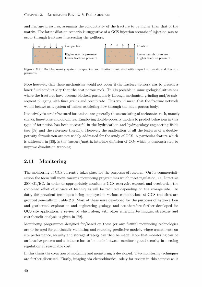
Chapter 2. Literature Review & Fundamentals
and fracture pressures, assuming the conductivity of the fracture to be higher than that of the
matrix. The latter dilation scenario is suggestive of a GCS injection scenario if injection was to
occur through fractures intersecting the wellbore.
Figure 2.9: Double-porosity system compaction and dilation illustrated with respect to matrix and fracturepressures.
Note however, that these mechanisms would not occur if the fracture network was to present a
lower fluid conductivity than the host porous rock. This is possible in some geological situations
where the fractures have become blocked, particularly through mechanical grinding and/or sub-
sequent plugging with finer grains and precipitate. This would mean that the fracture network
would behave as a system of baffles restricting flow through the main porous body.
Intensively fissured/fractured formations are generally those consisting of carbonates rock, namely
chalks, limestones and dolomites. Employing double-porosity models to predict behaviour in this
type of formation has been successful in the hydrocarbon and hydrogeology engineering fields
(see [38] and the reference therein). However, the application of all the features of a double-
porosity formulation are not widely addressed for the study of GCS. A particular feature which
is addressed in [38], is the fracture/matrix interface diffusion of CO2 which is demonstrated to
improve dissolution trapping.
2.11 Monitoring
The monitoring of GCS currently takes place for the purposes of research. On its commerciali-
sation the focus will move towards monitoring programmes which meet regulation, i.e. Directive
2009/31/EC. In order to appropriately monitor a GCS reservoir, caprock and overburden the
combined effort of subsets of techniques will be required depending on the storage site. To
date, the prevalent techniques being employed in various combinations at GCS test sites are
grouped generally in Table 2.8. Most of these were developed for the purposes of hydrocarbon
and geothermal exploration and engineering geology, and are therefore further developed for
GCS site application, a review of which along with other emerging techniques, strategies and
cost/benefit analysis is given in [72].
Monitoring programmes designed for/based on these (or any future) monitoring technologies
are to be used for continually validating and retooling predictive models, where assessments on
site performance, security and storage strategy can then be made. Note that monitoring can be
an invasive process and a balance has to be made between monitoring and security in meeting
regulation at reasonable cost.
In this thesis the co-action of modelling and monitoring is developed. Two monitoring techniques
are further discussed. Firstly, imaging via electrokinetics, solely for review in this context as it
40
2.11. Monitoring
Table 2.8: Potential GCS monitoring techniques, after [72].
Technique Description
2/3/4D seismic surveys On surface or across boreholes—assessing the reflections and refractionsof induced mechanical perturbations caused by contrasts in acousticimpedance within the subsurface.
Micro-seismicity Passive reading of CO2 injection induced seismic events.Surface gravity Measurements of the gravimetric effects of the injected CO2.Satellite interferometry (InSAR) Monitors surface subsistence and uplift (GCS in the order of mm/year)
[29], subsurface CO2 plume reconstruction via coupled geomechanicalmodels [195].
Pressure and temperature gauges Measuring hydraulic and thermal changes and connectivities between andalong wells and strata.
Electrokinetics (ERT) Assessing the changes in electrical potential between wells and strata.Chemical & biological analyses Various assurance monitoring and sampling techniques for determining
the extent of specific chemical leakages at key locations.
demonstrates an interesting coupling with the usual governing equations for reservoir modelling.
Secondly, imaging via muon tomography, which is a novel approach in the context of geological
reservoirs, showing promise for GCS in particular, given the geophysical changes induced by the
storage of CO2, is to be assessed in this thesis.
2.11.1 Electrokinetic monitoring
Fluid flow through porous media due to a pressure gradient is also accompanied by a restraining
effect due to electrical resistance. This is caused by the motion of the fluid dragging excess
charge in the electric boundary layer at the fluid-solid/mineral interfaces, which may result in an
electrical potential (electrokinetic streaming potential) [165]. Coupling these effects incorporates
various electrokinetic phenomena, such as the self-potential. The electrokinetic flow is the
natural movement of ions along the porous mediums electric layer, and if there is no source, the
charge conservation is given by,∂ρQ∂t
+∇ · j = 0 (2.63)
where ρQ is the charge density and j is the total electric current density. As highlighted in
Sections 2.6.5 and 2.6.6, the fluid flow may be coupled with other effects. Darcy’s law is coupled
with electric flow (Ohm’s law), after [165, 187], by
qf = L11(−∇pf + ρfg)− L12∇V (2.64)
j = L21(−∇pf + ρfg)− L22∇V (2.65)
where V is electric potential. The coefficient L11 represents the hydraulic conductivity, L22 the
electric conductivity, and L12 = L21 are cross coupling coefficients dependent on fluid saturation
and the usual state variables, as explored by [165, 187] and the references therein. Assuming a
quasi-steady state for (2.63) and substituting (2.65) presents a field continuity equation which
can be additionally solved along with the usual system of coupled field equations for further
investigation into subsurface flow phenomena. This is important given that electrokinetics is
employed as a ground improvement and monitoring technique for various applications.
Measuring the self-potential via arrays of installed electrodes has been used as a monitoring
41
Chapter 2. Literature Review & Fundamentals
technique for various subsurface problems. The first coupled numerical study of electrokinetics
for GCS has been given recently in [186, 187], for both single- and double-porosity mechanically
coupled geological systems. The coupled effect of thermal, miscible and/or chemical behaviour
is however ignored therein for study purposes. The main premise is that the brine is significantly
more conductive than the CO2 and during the displacing flow the fluids can be tracked by the
ensuing changes in the horizontal streaming potentials, where an electric potential peak in the
horizontal profile is indicative of the fluid interface. This monitoring approach is however limited
by the practicality in positioning the required electrodes.
2.11.2 Cosmic-ray muon tomographic monitoring
Muons are relatively unstable charged elementary particles belonging to the Standard Model
of particle physics. They occur naturally and abundantly on Earth, mainly as a result of
cosmic-rays (high-energy protons and nuclei) arriving from deep space colliding with atoms in
the upper atmosphere (particularly nitrogen and oxygen). Muons are a preferred decay product
of this collision, which continue at relativistic speeds able to penetrate the Earth’s surface during
a mean lifetime of 2.2 µs. Penetrations have been monitored at over 1× 10⁴ m w.e. (metres of
water equivalent, the product of density and depth, 1 m w.e. = 100 g/cm2) as determined in the
deep underground sciences [36], that is 4 km through a subsurface bulk density of 2.5 g/cm2.
Cosmic radiation enters the atmosphere such that it gives a near constant (at a given elevation)
muon flux, at sea-level of approximately 1 muon per cm2 per minute, the small variations of
which are well understood [114].
The muon flux at the Earth’s surface is typically given by the standard Gaisser parametrisation
[66]. This is a semi-empirical relationship for high energy muons, giving the differential muon
intensity gµ as the mean muon surface-level arrival rate per unit area, per unit solid angle per
unit energy,
gµ(Eµ, θ) =1400
m2 s sr GeV
(Eµ
GeV
)−2.7
F (Eµ, θ) (2.66)
which is essentially a power law related to the muon energy spectrum, where Eµ is the muon
energy, θ is zenith angle and F is the muon flux contribution due to other particle production.
A depth-intensity relation (DIR) in flux below surface level requires certain degrees of sophis-
tication [36], the attenuation in flux with depth, while propagating through matter, is due to
the wide differences in starting muon energies (0.1 to 10 GeV) and loss thereof due to a series
of fundamental physical processes [113]. Particularly, as charged particles they are subject to
electromagnetic (Coulomb) interactions and inelastically scatter deflecting as they pass through
a material deviating from their originally trajectory.
Muons are therefore an abundant and naturally occurring form of background radiation, which
on detection after having passed though the medium of interest may be used as a passive form of
material detection, as is outlined in the following subsections. Muon detection occurs passively
via scintillation, offering potential benefits over more active monitoring approaches (Table 2.8).
In the literature monitoring studies of tunnels, pyramid vaults, volcanoes, nuclear waste storage,
as well as the scanning of nuclear threats have all been reported in light of muon radiography
42
2.11. Monitoring
[150, 154, 171, 170].
2.11.2.1 Muon scattering tomography imaging
Muon Scattering Tomography (MST) is an advanced technique that uses the Multiple Coulomb
Scattering (MCS) of muon radiation through material in order to detect its composition. This
becomes possible when the number of interactions within the medium become high such that
the angular dispersion, measured as a projected deviation angle, ϑ, may be approximated as
a Gaussian distribution with a zero mean value, where the standard deviation ϑ0 (and rms in
this case) is the spread in overall scattering of many muon interactions through a given material
volume. The material composition giving rise to a certain scattering is related with the following
well-known formulae,
ϑ0 =13.6 (MeV)
pβc
√L
L0
[1 + 0.0038 ln
(L
L0
)]≈ 13.6 (MeV)
pβc
√L
L0(2.67)
L0 =716.4 (g/cm2)
ρ
A
Z(Z + 1) ln(287/√Z)
(2.68)
which shows the particle scattering proportional to the material depth L over its radiation
length L0 and inversely to the particle momentum p and relativistic velocity βc. Importantly,
the radiation length L0 is a function of the material’s mass number A, atomic number Z and
density ρ. It is demonstrated that a material of higher density will more readily scatter and/or
attenuate particles. This phenomenon can be exploited for imaging via statistical reconstruction,
whereby regions causing larger particle deflections indicate the presence of denser material.
2.11.2.2 Muon transmission imaging
The probability of muon survival over a given distance is increased primarily if less material is
encountered, or similarly if material of a lower density integrated over the distance travelled is
encountered. The muon flux from a given direction is thus dependent primarily on the column
composition and density through which it passes. Therefore, changes in baseline flux readings
due to the interference of another material entering a region of interest, causing changes in
column composition and density, can be interpreted to detect the entering material.
A primary study on using this technique for monitoring GCS has recently been given in [114],
wherein a basic scenario is modelled where hypothetical changes in bulk density of a geological
body due to CO2 storage are linked with statistically significant changes in simulated muon flux.
It is an aim of this thesis to extend this work by facilitating the simulation of muon radiography
through realistic GCS flow scenarios. This is done in order to better assess the sensitivity of the
technique for monitoring bulk density changes over time in storage layers which are indicative of
the presence and migration of CO2. This may also help to design and understand the detector
arrangements, locations, and responses for given injection/geological scenarios. Note that the
primary limitation on employing this technique for GCS is due to the substantial storage depths,
where the muon flux may become low for which the size of detector, required in order to capture
43
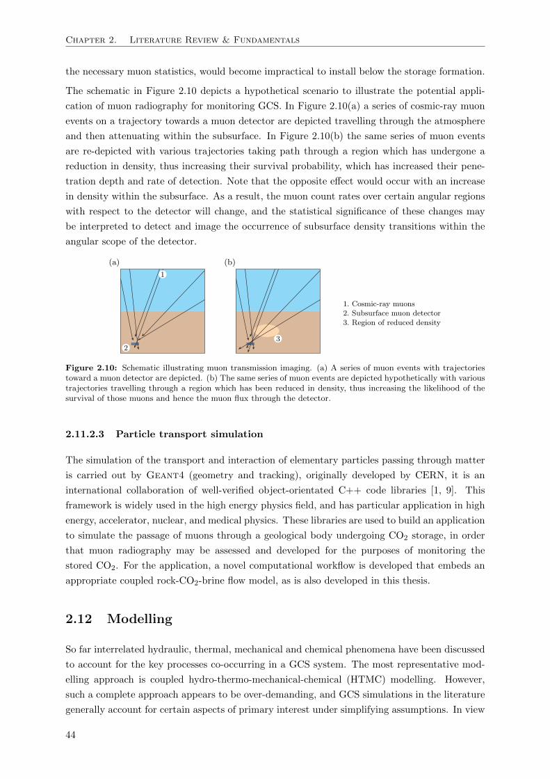
Chapter 2. Literature Review & Fundamentals
the necessary muon statistics, would become impractical to install below the storage formation.
The schematic in Figure 2.10 depicts a hypothetical scenario to illustrate the potential appli-
cation of muon radiography for monitoring GCS. In Figure 2.10(a) a series of cosmic-ray muon
events on a trajectory towards a muon detector are depicted travelling through the atmosphere
and then attenuating within the subsurface. In Figure 2.10(b) the same series of muon events
are re-depicted with various trajectories taking path through a region which has undergone a
reduction in density, thus increasing their survival probability, which has increased their pene-
tration depth and rate of detection. Note that the opposite effect would occur with an increase
in density within the subsurface. As a result, the muon count rates over certain angular regions
with respect to the detector will change, and the statistical significance of these changes may
be interpreted to detect and image the occurrence of subsurface density transitions within the
angular scope of the detector.
Figure 2.10: Schematic illustrating muon transmission imaging. (a) A series of muon events with trajectoriestoward a muon detector are depicted. (b) The same series of muon events are depicted hypothetically with varioustrajectories travelling through a region which has been reduced in density, thus increasing the likelihood of thesurvival of those muons and hence the muon flux through the detector.
2.11.2.3 Particle transport simulation
The simulation of the transport and interaction of elementary particles passing through matter
is carried out by Geant4 (geometry and tracking), originally developed by CERN, it is an
international collaboration of well-verified object-orientated C++ code libraries [1, 9]. This
framework is widely used in the high energy physics field, and has particular application in high
energy, accelerator, nuclear, and medical physics. These libraries are used to build an application
to simulate the passage of muons through a geological body undergoing CO2 storage, in order
that muon radiography may be assessed and developed for the purposes of monitoring the
stored CO2. For the application, a novel computational workflow is developed that embeds an
appropriate coupled rock-CO2-brine flow model, as is also developed in this thesis.
2.12 Modelling
So far interrelated hydraulic, thermal, mechanical and chemical phenomena have been discussed
to account for the key processes co-occurring in a GCS system. The most representative mod-
elling approach is coupled hydro-thermo-mechanical-chemical (HTMC) modelling. However,
such a complete approach appears to be over-demanding, and GCS simulations in the literature
generally account for certain aspects of primary interest under simplifying assumptions. In view
44
2.12. Modelling
of the interrelated and interdisciplinary nature, and given that GCS is to occur on evermore
unprecedented scales of inherent unpredictability, a staged learn-as-you-go approach is emerging
in the CCS industry.
Analytical, semi-analytical and numerical models form part of the framework for the risk analysis
of GCS. Essentially, they are to account for the migration and storage capacity of the injected
fluid, which involves modelling, in particular: physical, dissolution, residual, precipitation and
sorption trapping mechanisms; pore pressure breaching and fracturing of the seals; density
convection mixing; CO2 impurities; changes in formation porosity and permeability; and any
additional vertical leakage risks (e.g. abandoned boreholes and faults).
Analytical and semi-analytical codes employ various simplify assumptions (Chapter 3) and are
computationally inexpensive. They are used for primary/first order site assessments and are
therefore useful for screening sites and form a valuable component of risk assessment. They may
also be used for benchmarking special cases of more elaborate numerical codes.
The forefront numerical simulators currently employed for modelling GCS scenarios based on
various coupled HTMC approaches are summarised in Table 2.9. Additionally, the simulators as
listed generally employ implicit time integration and Newton-type methods for linearisation. A
more extensive review is given in the respective references and comparatively by [42, 72], where
the scenarios to which they have been applied (and compared) are also discussed.
In most subsurface flow modelling, the geochemical and geomechanical effects are often not
taken into account, due to the matter of significance for engineering purposes, as the calcula-
tions are complex, computationally expensive, and the necessary theoretical and empirical/field
information is limited [72]. However, for the injection of CO2 it is anticipated that there will be
important chemical mechanisms and significant increases in system pressure inducing site de-
formation. As a result there is a research interest growing for coupling these effects (Table 2.9).
There are two main classes of numerical codes that couple HTMC behaviour:
2.12.1 Modular Class: Sequential coupling of a flow simulator with other
software
This class consists mainly of general purpose simulators developed primarily for industrial oil
and gas reservoir engineering purposes. Essentially incorporating multiple (modular) software
programs via sequential coupling [172, 163]. The main benefit is that existing sophisticated
models, being developed and verified within their disciplines can be incorporated cost-effectively.
2.12.2 Fully Coupled Class: Fully coupled (simultaneous) behaviour
Full coupling takes place through a simultaneous (monolithic) solution of the system of governing
equations. However, if certain weak partial system couplings are present, they may be parti-
tioned and solved in a staggered form for improving computational performance [120]. These
models appear to be developed mainly for research purposes on specific HTMC problems. Those
which are researchable have been developed and applied mainly to geotechnical (consolidation
and settlement) and to geological nuclear waste repository problems. Notably for GCS, the
45
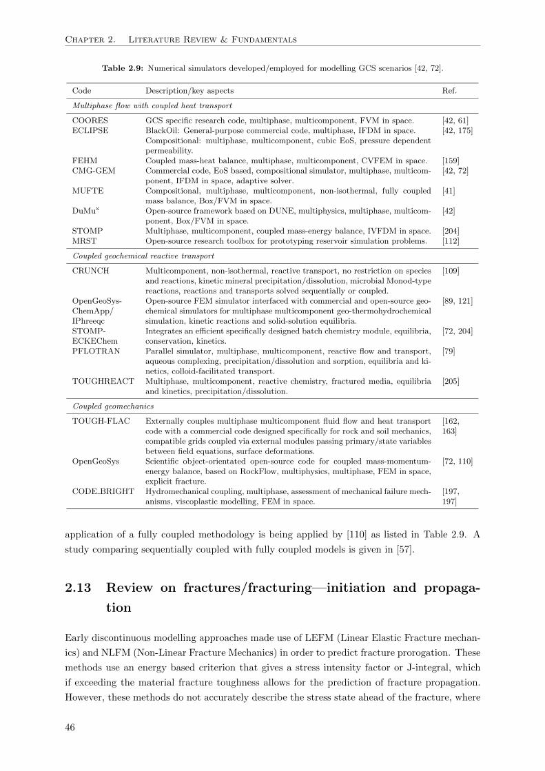
Chapter 2. Literature Review & Fundamentals
Table 2.9: Numerical simulators developed/employed for modelling GCS scenarios [42, 72].
Code Description/key aspects Ref.
Multiphase flow with coupled heat transport
COORES GCS specific research code, multiphase, multicomponent, FVM in space. [42, 61]ECLIPSE BlackOil: General-purpose commercial code, multiphase, IFDM in space. [42, 175]
Compositional: multiphase, multicomponent, cubic EoS, pressure dependentpermeability.
FEHM Coupled mass-heat balance, multiphase, multicomponent, CVFEM in space. [159]CMG-GEM Commercial code, EoS based, compositional simulator, multiphase, multicom-
ponent, IFDM in space, adaptive solver.[42, 72]
MUFTE Compositional, multiphase, multicomponent, non-isothermal, fully coupledmass balance, Box/FVM in space.
[41]
DuMux Open-source framework based on DUNE, multiphysics, multiphase, multicom-ponent, Box/FVM in space.
[42]
STOMP Multiphase, multicomponent, coupled mass-energy balance, IVFDM in space. [204]MRST Open-source research toolbox for prototyping reservoir simulation problems. [112]
Coupled geochemical reactive transport
CRUNCH Multicomponent, non-isothermal, reactive transport, no restriction on speciesand reactions, kinetic mineral precipitation/dissolution, microbial Monod-typereactions, reactions and transports solved sequentially or coupled.
[109]
OpenGeoSys-ChemApp/IPhreeqc
Open-source FEM simulator interfaced with commercial and open-source geo-chemical simulators for multiphase multicomponent geo-thermohydrochemicalsimulation, kinetic reactions and solid-solution equilibria.
[89, 121]
STOMP-ECKEChem
Integrates an efficient specifically designed batch chemistry module, equilibria,conservation, kinetics.
[72, 204]
PFLOTRAN Parallel simulator, multiphase, multicomponent, reactive flow and transport,aqueous complexing, precipitation/dissolution and sorption, equilibria and ki-netics, colloid-facilitated transport.
[79]
TOUGHREACT Multiphase, multicomponent, reactive chemistry, fractured media, equilibriaand kinetics, precipitation/dissolution.
[205]
Coupled geomechanics
TOUGH-FLAC Externally couples multiphase multicomponent fluid flow and heat transportcode with a commercial code designed specifically for rock and soil mechanics,compatible grids coupled via external modules passing primary/state variablesbetween field equations, surface deformations.
[162,163]
OpenGeoSys Scientific object-orientated open-source code for coupled mass-momentum-energy balance, based on RockFlow, multiphysics, multiphase, FEM in space,explicit fracture.
[72, 110]
CODE BRIGHT Hydromechanical coupling, multiphase, assessment of mechanical failure mech-anisms, viscoplastic modelling, FEM in space.
[197,197]
application of a fully coupled methodology is being applied by [110] as listed in Table 2.9. A
study comparing sequentially coupled with fully coupled models is given in [57].
2.13 Review on fractures/fracturing—initiation and propaga-
tion
Early discontinuous modelling approaches made use of LEFM (Linear Elastic Fracture mechan-
ics) and NLFM (Non-Linear Fracture Mechanics) in order to predict fracture prorogation. These
methods use an energy based criterion that gives a stress intensity factor or J-integral, which
if exceeding the material fracture toughness allows for the prediction of fracture propagation.
However, these methods do not accurately describe the stress state ahead of the fracture, where
46
2.14. Summary of key research needs
singularities occur at the fracture tip. To overcome this, the notion of replacing this inelastic
region with cohesive traction forces was introduced [16]. This is done with a discrete model
and has brought about the concept of fracture energy and cohesive fracture growth. Mainly,
the strategies for numerically modelling this have been developed within the finite element
method framework. One strategy involves incorporating interface elements, which initially have
no thickness, between the usual finite elements. In this instance fracturing will be highly mesh
dependent (occurring along element boundaries) and the interface elements initially have fake
stiffness which could also cause computational issues [131].
In order to better predict arbitrary fracture propagation, work was extended to this field by
reference [142]. As a result, embedded discontinuities in the way of strain jumps in the for-
mulations meant that the effect of the discontinuity can be accounted for without modelling
it. Work was then incorporated using special shape functions for certain situations, following
this the Partition of Unity Finite Element Method (PU-FEM) was developed [130]. Use of
this theory with discontinuous approximations has been termed the Extended Finite Element
Method (X-FEM) where the quadrature rule is altered for elements intersected by discontinu-
ities. This theory has been incorporated with cohesive traction laws by reference [202], in order
that a traction-separation model governing the non-linear behaviour in the fracture region is
given with an elastic continuum.
In [5] the double-porosity numerical technique has been incorporated with the partition of unity
method [130] in order to account for the fracturing process of a porous medium. It is essentially
the partition of unity that describes the fracturing, and the double-porosity model is used to
describe the resulting fluid flow. This approach, by coupling the two independent techniques,
provides means for better simulations of the complex processes involved. However, this work
covers for only a single fluid phase. This theoretical point of view has also be used to track fluid
interfaces [187].
Additionally, [131] gives a review on fracturing in porous media that concludes on the lack of ma-
turity in this field with regards to a global framework for continuous (unfractured)-discontinuous
(fractured)-transition (fracturing)-strategies. Therein modelling approaches utilising damage
mechanics, as developed in [142, 143, 144, 202], are also incorporated with the existing method-
ologies as outlined.
2.14 Summary of key research needs
This literature review has been carried out from various fundamental perspectives, and it is
hoped that it may also be applied where applicable for developing physics applications beyond
the scope of this thesis. The following research needs are identified in order to highlight the
innovative aspects and findings of this work. These needs are also to be addressed during further
in depth review within the respective chapters.
A comprehensive fully-coupled hydro-thermo-mechanical two-phase double-porosity Biot-type
formulation is to be devised in order to complement existing industry and research formula-
tions in the context of CGS. This is to be developed from first principles and is thus to form
47
Chapter 2. Literature Review & Fundamentals
an extensive basis from which to capture and study various coupled phenomena which are of
particular concern with respect to CO2 sequestration, as have been reviewed. In particular,
CO2-brine displacement, solid deformation, porous matrix/fracture and Joule-Thomson cooling
(JTC) effects.
The formulation of this work will present a highly nonlinear coupled system of governing equa-
tions. The numerical solution of such subsurface formulations over realistic domains are com-
putationally intensive. Effort is therefore to be made on the study and development of the
numerical methods employed in order to provide an effective means of solving the system of
governing equations. The finite element method is to be employed in space and assessed in
terms of its refinement for the various coupled physics involved. The finite difference method is
to be employed in time, for which adaptive control theoretical and acceleration techniques are
to be explored and adopted.
The various monitoring technologies leave scope for the innovation of an efficient, passive and
continuous monitoring system for the purposes of CCS. Muon radiography has been reviewed as
potential technology for this. In order to further assess the feasibility of employing this technol-
ogy in the context of CCS, the realistic modelling of CO2 sequestration and muon radiography
are to be incorporated into a single computational framework for simulation.
48
Chapter 3
Model Formulations
A system of governing field equations for modelling fully coupled hydro-thermal-mechanical
behaviour within a double-porosity (porous matrix and natural fracture/fissure network) mul-
tiphase (solid, wetting and nonwetting) medium is developed. This occurs following the funda-
mental principles introduced in Chapter 2, with particular reference to modelling a GCS system.
This is done from general principles so that the assumptions in developing such a model, from
the theoretical standpoint of this work, for describing a GCS system are highlighted compre-
hensively. The general approach given also allows for further development and application.
The development is a first attempt at accounting for such a system, the primary aim of which
is to cover the hydro-thermal-mechanical-chemical bases in the coupled sense, and present a
framework for study and further development. This work utilises and extends upon the following
notable formulations and explores their application for modelling a GCS system. In [120] a fully
coupled system accounting for miscible water and air flow within a deformable single porous
geological medium is thoroughly developed. This approach is also extended for a multiphase
water, gas and oil double-porosity system in [70, 120, 118], which neglect phase miscibility,
fracture network deformability, and any thermal effects. Later, in [119, 146] the fracture network
deformability is addressed. The thermal behaviour within a double-porosity system is also
addressed for a single fluid phase in [123] neglecting fracture network deformability. These fully
coupled formulation approaches which place particular emphasis on the mechanical behaviour
of the system, have been extended in order to model a GCS system, particularly in [110], which
accounts for thermal behaviour in a single porosity system, and [186] which accounts for a
double-porosity system without thermal behaviour.
3.1 Model description
In this work, the following chief formulation aspects are itemised with their consequences and
limitations. These aspects are detailed further during the derivation of the coupled governing
field equations.
- The porous medium is described with a double-porosity model consisting of two distinct
overlapping sub-domains, representing an interconnected porous matrix and fracture net-
49
Chapter 3. Model Formulations
work. The physical properties of each sub-domain are considered independently and any
coupling is controlled via the mass transfer/leakage function.
- The volume of fractures is considered to occupy a relatively small fraction of the total
volume of the system. It can therefore be assumed that the fracture compressibility does
not substantially alter the compressibility of the system as a whole [120], and only the
solid deformation of the porous matrix and the multiphase fluid flows are directly coupled.
The porous matrix sub-domain alone therefore carries the boundary and body forces.
- As the fracture compressibility is neglected, the intrinsic (or absolute) fracture network
permeability, which is related to its compressibility through its geometry, does not change.
Note that the modelling approach assumes a smeared fracture network of small volume
relative to the total void space, and thus any prescribed intrinsic permeability may be
viewed as an effective or averaged value of its actual performance. This is appropriate
given the vast extent of typical geological reservoir models and that the fracture/geology
is largely unknown for determining the actual effects of changes in stress state. It is
however a point for further research to comment further on the scope of sensitivity of
this behaviour, as well as for that of the porous matrix, within this context [118]. This
aspect would be more prevalent for large distinct opening and closing geological fractures
(or faults) which would however require that the faults be modelled explicitly.
- The solid deformation behaviour is assumed to undergo only small displacements which
are linear elastic. Other constitutive material models may however be employed.
- The processes involved are considered to happen slow enough such that the inertial effects
may be ignored.
- The two sub-domains are assumed to be fully saturated with a wetting and nonwetting
phase.
- The phase components do not interact, transfer between the phases (condensation evap-
oration and dissolution) or undergo chemical reactions. The thermophysical behaviour of
the phases may however be parametrised accurately given a physical state and composition
for each phase.
- A single thermodynamic continuum (energy balance) is assumed appropriate for describing
the temperature evolution over both sub-domains and the phases they constitute. There-
fore, all the phases of both sub-domains are considered to be in local thermodynamic
equilibrium at any point in the system domain. This means that the system temperature
varies in space and time, but all the overlapping continua coexisting at a point are at the
same temperature. This is generally acceptable given the interconnectedness of the dis-
tinct fluids and grains such that heat may diffuse by conduction instantly on the local scale
relative to the space and time scales of geological interest [137]. A double temperature
approach may be advocated between the porous matrix and fracture network continua,
however the supply and transfer terms are extremely difficult to formulate and parame-
terise. For engineering purposes the single temperature approach after [123] is considered
here.
- An effective saturation dependent bulk conductivity tensor is assumed appropriate. The
convective heat fluxes over both sub-domains are however considered separately due to
the potential difference in fluid velocities between the sub-domains. The notion of energy
50

3.2. Mass balance
transfer between the sub-domains is untreated as a single representative energy balance is
assumed; this transfer is absorbed in the effective conductive and convective terms.
In what follows, a consistent formulation for the system mass, momentum and energy balance
is given for a double-porosity multiphase deformable nonisothermal system. Firstly, two mass
balance equations are derived for the two fluids phases for each sub-domain. As an intermezzo,
a simplified single mass balance equation is solved for several GCS scenarios in order to present
some useful benchmarks and relationships. Afterwards, single multiphase momentum and energy
balance equations are derived.
3.2 Mass balance
The multiphase medium is described via the superposition of all the π phases in both sub-
domains. An accurate kinematic description of relative motion is obtained by taking the mate-
rial time derivative for the fluid phase f moving with the solid phase s, after the manipulation
of (2.9) that is,Dsζ f
Dt=∂ζ f
∂t+∇ζ f · vs. (3.1)
For practicality the convective component of this derivative is typically neglected for geome-
chanical applications, given that the solid displacements are usually small, hence,
∇ζπ · vs ∂ζπ
∂t∴Dsζπ
Dt≈ ∂ζπ
∂t. (3.2)
This simplifying approach is adopted prior to derivation, however material derivatives are easily
reintroduced.
3.2.1 Primary/state variables
The following relationship involving the specific moisture content/fluid saturation capacity (Sec-
tion 2.7.1),∂Sw∂t
=∂Sw∂pc
∂pc
∂t+∂Sw∂T
∂T
∂t=∂Sw∂pc
(∂pn
∂t− ∂pw
∂t
)+∂Sw∂T
∂T
∂t, (3.3)
is employed in order to bring about different sequences of primary variables, from primarily
u, pw, pn, pc, Sw, Sn, and T for each sub-domain. In this work it is employed in order to
derive a u-pw1-pn1-pw2-pn2-T (solid displacement-fluid pressure-temperature) primary variable
set, directing the others as secondary variables within the final system of equations. Note that
subscripts 1 and 2 refer to the matrix and fracture sub-domains respectively. Different variable
sets will present different numerical properties [120, 167, 168] and warrant further study. In the
context of modelling GCS some other interesting variable sets and elaborations are explored in
[110, 187].
51
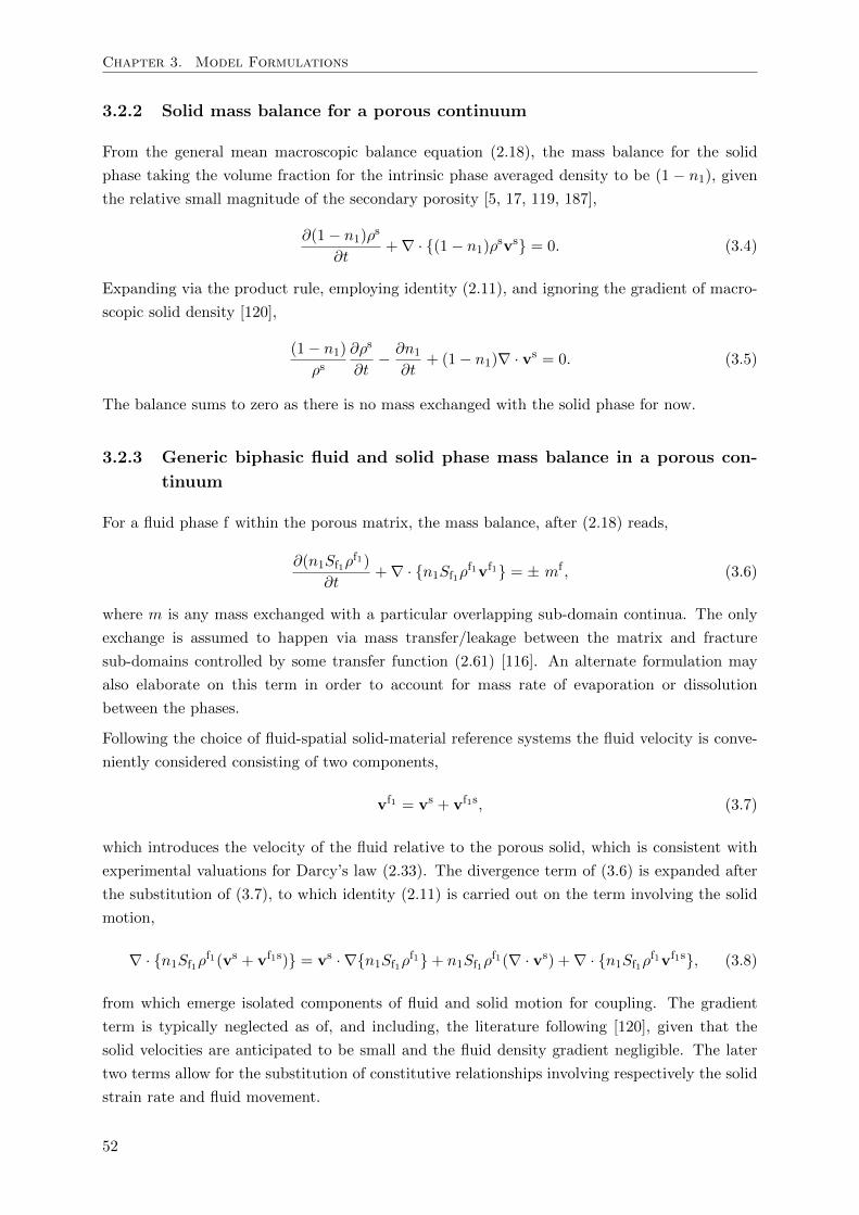
Chapter 3. Model Formulations
3.2.2 Solid mass balance for a porous continuum
From the general mean macroscopic balance equation (2.18), the mass balance for the solid
phase taking the volume fraction for the intrinsic phase averaged density to be (1 − n1), given
the relative small magnitude of the secondary porosity [5, 17, 119, 187],
∂(1− n1)ρs
∂t+∇ · (1− n1)ρ
svs = 0. (3.4)
Expanding via the product rule, employing identity (2.11), and ignoring the gradient of macro-
scopic solid density [120],
(1− n1)
ρs∂ρs
∂t− ∂n1
∂t+ (1− n1)∇ · vs = 0. (3.5)
The balance sums to zero as there is no mass exchanged with the solid phase for now.
3.2.3 Generic biphasic fluid and solid phase mass balance in a porous con-
tinuum
For a fluid phase f within the porous matrix, the mass balance, after (2.18) reads,
∂(n1Sf1ρf1)
∂t+∇ · n1Sf1ρf1vf1 = ± mf , (3.6)
where m is any mass exchanged with a particular overlapping sub-domain continua. The only
exchange is assumed to happen via mass transfer/leakage between the matrix and fracture
sub-domains controlled by some transfer function (2.61) [116]. An alternate formulation may
also elaborate on this term in order to account for mass rate of evaporation or dissolution
between the phases.
Following the choice of fluid-spatial solid-material reference systems the fluid velocity is conve-
niently considered consisting of two components,
vf1 = vs + vf1s, (3.7)
which introduces the velocity of the fluid relative to the porous solid, which is consistent with
experimental valuations for Darcy’s law (2.33). The divergence term of (3.6) is expanded after
the substitution of (3.7), to which identity (2.11) is carried out on the term involving the solid
motion,
∇ · n1Sf1ρf1(vs + vf1s) = vs · ∇n1Sf1ρf1+ n1Sf1ρf1(∇ · vs) +∇ · n1Sf1ρf1vf1s, (3.8)
from which emerge isolated components of fluid and solid motion for coupling. The gradient
term is typically neglected as of, and including, the literature following [120], given that the
solid velocities are anticipated to be small and the fluid density gradient negligible. The later
two terms allow for the substitution of constitutive relationships involving respectively the solid
strain rate and fluid movement.
52
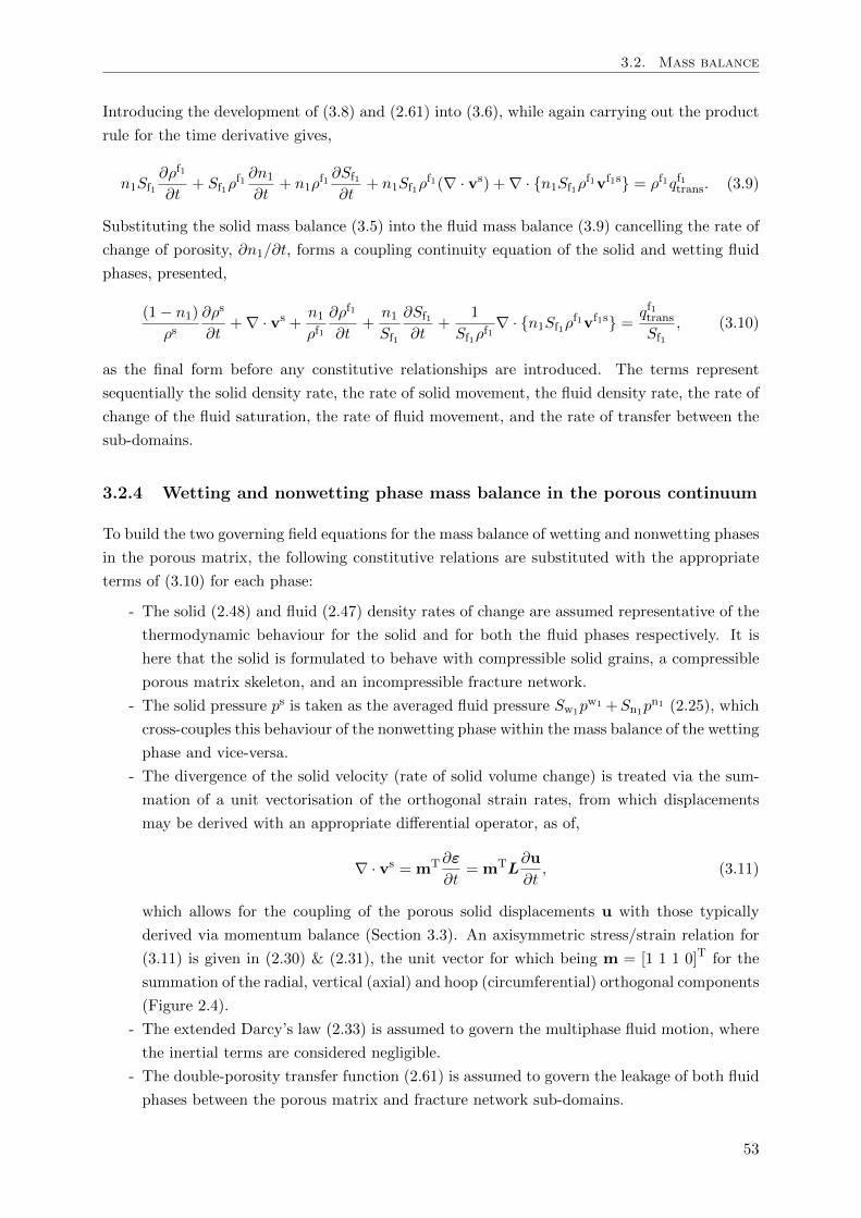
3.2. Mass balance
Introducing the development of (3.8) and (2.61) into (3.6), while again carrying out the product
rule for the time derivative gives,
n1Sf1∂ρf1
∂t+ Sf1ρ
f1 ∂n1∂t
+ n1ρf1 ∂Sf1∂t
+ n1Sf1ρf1(∇ · vs) +∇ · n1Sf1ρf1vf1s = ρf1qf1trans. (3.9)
Substituting the solid mass balance (3.5) into the fluid mass balance (3.9) cancelling the rate of
change of porosity, ∂n1/∂t, forms a coupling continuity equation of the solid and wetting fluid
phases, presented,
(1− n1)
ρs∂ρs
∂t+∇ · vs +
n1ρf1
∂ρf1
∂t+n1Sf1
∂Sf1∂t
+1
Sf1ρf1∇ · n1Sf1ρf1vf1s =
qf1transSf1
, (3.10)
as the final form before any constitutive relationships are introduced. The terms represent
sequentially the solid density rate, the rate of solid movement, the fluid density rate, the rate of
change of the fluid saturation, the rate of fluid movement, and the rate of transfer between the
sub-domains.
3.2.4 Wetting and nonwetting phase mass balance in the porous continuum
To build the two governing field equations for the mass balance of wetting and nonwetting phases
in the porous matrix, the following constitutive relations are substituted with the appropriate
terms of (3.10) for each phase:
- The solid (2.48) and fluid (2.47) density rates of change are assumed representative of the
thermodynamic behaviour for the solid and for both the fluid phases respectively. It is
here that the solid is formulated to behave with compressible solid grains, a compressible
porous matrix skeleton, and an incompressible fracture network.
- The solid pressure ps is taken as the averaged fluid pressure Sw1pw1 +Sn1p
n1 (2.25), which
cross-couples this behaviour of the nonwetting phase within the mass balance of the wetting
phase and vice-versa.
- The divergence of the solid velocity (rate of solid volume change) is treated via the sum-
mation of a unit vectorisation of the orthogonal strain rates, from which displacements
may be derived with an appropriate differential operator, as of,
∇ · vs = mT∂ε
∂t= mTL
∂u
∂t, (3.11)
which allows for the coupling of the porous solid displacements u with those typically
derived via momentum balance (Section 3.3). An axisymmetric stress/strain relation for
(3.11) is given in (2.30) & (2.31), the unit vector for which being m = [1 1 1 0]T for the
summation of the radial, vertical (axial) and hoop (circumferential) orthogonal components
(Figure 2.4).
- The extended Darcy’s law (2.33) is assumed to govern the multiphase fluid motion, where
the inertial terms are considered negligible.
- The double-porosity transfer function (2.61) is assumed to govern the leakage of both fluid
phases between the porous matrix and fracture network sub-domains.
53
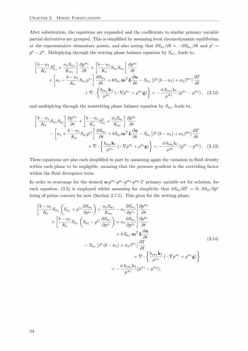
Chapter 3. Model Formulations
After substitution, the equations are expanded and the coefficients to similar primary variable
partial derivatives are grouped. This is simplified by assuming local thermodynamic equilibrium
at the representative elementary points, and also noting that ∂Sn1/∂t = −∂Sw1/∂t and pc =
pn − pw. Multiplying through the wetting phase balance equation by Sw1 , leads to,[b− n1Ks
S2w1
+n1Sw1
Kw1
]∂pw1
∂t+
[b− n1Ks
Sn1Sw1
]∂pn1
∂t
+
[n1 −
b− n1Ks
Sw1pc1
]∂Sw1
∂t+ bSw1m
TL∂u
∂t− Sw1 [β
s (b− n1) + n1βw1 ]
∂T
∂t
+∇ ·krw1k1
µw1(−∇pw1 + ρw1g)
= − α krw1k1
µw1(pw1 − pw2) , (3.12)
and multiplying through the nonwetting phase balance equation by Sn1 , leads to,[b− n1Ks
Sw1Sn1
]∂pw1
∂t+
[b− n1Ks
S2n1 +
n1Sn1Kn1
]∂pn1
∂t
−[n1 +
b− n1Ks
Sn1pc1
]∂Sw1
∂t+ bSn1m
TL∂u
∂t− Sn1 [β
s (b− n1) + n1βn1 ]
∂T
∂t
+∇ ·krn1k1
µn1(−∇pn1 + ρn1g)
= − α krn1k1
µn1(pn1 − pn2) . (3.13)
These equations are also each simplified in part by assuming again the variation in fluid density
within each phase to be negligible, meaning that the pressure gradient is the overriding factor
within the fluid divergence term.
In order to rearrange for the desired u-pw1-pn1-pw2-pn2-T primary variable set for solution, for
each equation, (3.3) is employed whilst assuming for simplicity that ∂Sw/∂T = 0; ∂Sw/∂pc
being of prime concern for now (Section 2.7.1). This gives for the wetting phase,[b− n1Ks
Sw1
(Sw1 + pc1
∂Sw1
∂pc1
)+n1Sw1
Kw1
− n1∂Sw1
∂pc1
]∂pw1
∂t
+
[b− n1Ks
Sw1
(Sn1 − pc1
∂Sw1
∂pc1
)+ n1
∂Sw1
∂pc1
]∂pn1
∂t
+ b Sw1 mTL
∂u
∂t
− Sw1 [βs (b− n1) + n1β
w1 ]∂T
∂t
+ ∇ ·krw1k1
µw1(−∇pw1 + ρw1g)
= − α krw1k1
µw1(pw1 − pw2),
(3.14)
54
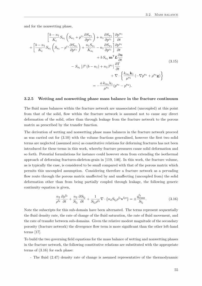
3.2. Mass balance
and for the nonwetting phase,[b− n1Ks
Sn1
(Sw1 + pc1
∂Sw1
∂pc1
)+ n1
∂Sw1
∂pc1
]∂pw1
∂t
+
[b− n1Ks
Sn1
(Sn1 − pc1
∂Sw1
∂pc1
)+n1Sn1Kn1
− n1∂Sw1
∂pc1
]∂pn1
∂t
+ b Sn1 mTL
∂u
∂t
− Sn1 [βs (b− n1) + n1β
n1 ]∂T
∂t
+ ∇ ·krn1k1
µn1(−∇pn1 + ρn1g)
= − α krn1k1
µn1(pn1 − pn2).
(3.15)
3.2.5 Wetting and nonwetting phase mass balance in the fracture continuum
The fluid mass balances within the fracture network are unassociated (uncoupled) at this point
from that of the solid, flow within the fracture network is assumed not to cause any direct
deformation of the solid, other than through leakage from the fracture network to the porous
matrix as prescribed by the transfer function.
The derivation of wetting and nonwetting phase mass balances in the fracture network proceed
as was carried out for (3.10) with the volume fractions generalised, however the first two solid
terms are neglected (assumed zero) as constitutive relations for deforming fractures has not been
introduced for these terms in this work, whereby fracture pressures cause solid deformation and
so forth. Potential formulations for instance could however stem from extending the isothermal
approach of deforming fractures-skeleton-grain in [119, 146]. In this work, the fracture volume,
as is typically the case, is considered to be small compared with that of the porous matrix which
permits this uncoupled assumption. Considering therefore a fracture network as a pervading
flow route through the porous matrix unaffected by and unaffecting (uncoupled from) the solid
deformation other than from being partially coupled through leakage, the following generic
continuity equation is given,
n2ρf2
∂ρf2
∂t+n2Sf2
∂Sf2∂t
+1
Sf2ρf2∇ · n2Sf2ρf2vf2s = ±q
f2trans
Sf2. (3.16)
Note the subscripts for this sub-domain have been alternated. The terms represent sequentially
the fluid density rate, the rate of change of the fluid saturation, the rate of fluid movement, and
the rate of transfer between sub-domains. Given the relative modest magnitude of the secondary
porosity (fracture network) the divergence flow term is more significant than the other left-hand
terms [17].
To build the two governing field equations for the mass balance of wetting and nonwetting phases
in the fracture network, the following constitutive relations are substituted with the appropriate
terms of (3.16) for each phase:
- The fluid (2.47) density rate of change is assumed representative of the thermodynamic
55
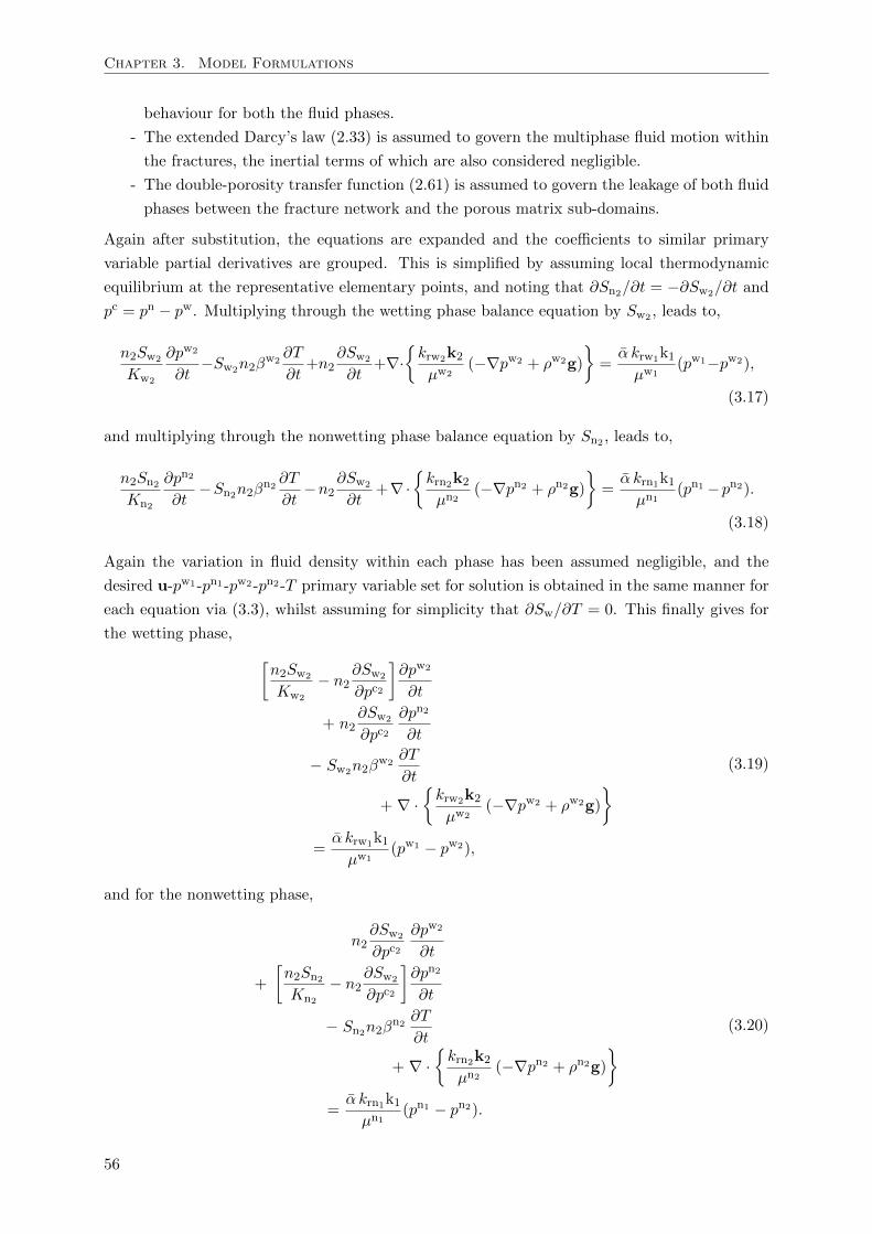
Chapter 3. Model Formulations
behaviour for both the fluid phases.
- The extended Darcy’s law (2.33) is assumed to govern the multiphase fluid motion within
the fractures, the inertial terms of which are also considered negligible.
- The double-porosity transfer function (2.61) is assumed to govern the leakage of both fluid
phases between the fracture network and the porous matrix sub-domains.
Again after substitution, the equations are expanded and the coefficients to similar primary
variable partial derivatives are grouped. This is simplified by assuming local thermodynamic
equilibrium at the representative elementary points, and noting that ∂Sn2/∂t = −∂Sw2/∂t and
pc = pn − pw. Multiplying through the wetting phase balance equation by Sw2 , leads to,
n2Sw2
Kw2
∂pw2
∂t−Sw2n2β
w2∂T
∂t+n2
∂Sw2
∂t+∇·
krw2k2
µw2(−∇pw2 + ρw2g)
=α krw1k1µw1
(pw1−pw2),
(3.17)
and multiplying through the nonwetting phase balance equation by Sn2 , leads to,
n2Sn2Kn2
∂pn2
∂t−Sn2n2βn2
∂T
∂t−n2
∂Sw2
∂t+∇·
krn2k2
µn2(−∇pn2 + ρn2g)
=α krn1k1µn1
(pn1 −pn2).
(3.18)
Again the variation in fluid density within each phase has been assumed negligible, and the
desired u-pw1-pn1-pw2-pn2-T primary variable set for solution is obtained in the same manner for
each equation via (3.3), whilst assuming for simplicity that ∂Sw/∂T = 0. This finally gives for
the wetting phase, [n2Sw2
Kw2
− n2∂Sw2
∂pc2
]∂pw2
∂t
+ n2∂Sw2
∂pc2∂pn2
∂t
− Sw2n2βw2∂T
∂t
+ ∇ ·krw2k2
µw2(−∇pw2 + ρw2g)
=α krw1k1µw1
(pw1 − pw2),
(3.19)
and for the nonwetting phase,
n2∂Sw2
∂pc2∂pw2
∂t
+
[n2Sn2Kn2
− n2∂Sw2
∂pc2
]∂pn2
∂t
− Sn2n2βn2 ∂T
∂t
+ ∇ ·krn2k2
µn2(−∇pn2 + ρn2g)
=α krn1k1µn1
(pn1 − pn2).
(3.20)
56
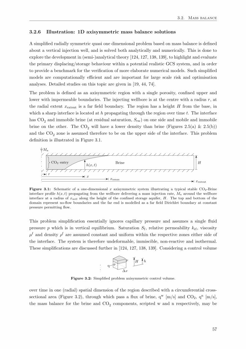
3.2. Mass balance
3.2.6 Illustration: 1D axisymmetric mass balance solutions
A simplified radially symmetric quasi one dimensional problem based on mass balance is defined
about a vertical injection well, and is solved both analytically and numerically. This is done to
explore the development in (semi-)analytical theory [124, 127, 138, 139], to highlight and evaluate
the primary displacing/storage behaviour within a potential realistic GCS system, and in order
to provide a benchmark for the verification of more elaborate numerical models. Such simplified
models are computationally efficient and are important for large scale risk and optimisation
analyses. Detailed studies on this topic are given in [19, 44, 74].
The problem is defined as an axisymmetric region with a single porosity, confined upper and
lower with impermeable boundaries. The injecting wellbore is at the centre with a radius r, at
the radial extent xextent is a far field boundary. The region has a height H from the base, in
which a sharp interface is located at h propagating through the region over time t. The interface
has CO2 and immobile brine (at residual saturation, Srw) on one side and mobile and immobile
brine on the other. The CO2 will have a lower density than brine (Figures 2.5(a) & 2.5(b))
and the CO2 zone is assumed therefore to be on the upper side of the interface. This problem
definition is illustrated in Figure 3.1.
Figure 3.1: Schematic of a one-dimensional x axisymmetric system illustrating a typical stable CO2-Brineinterface profile h(x, t) propagating from the wellbore delivering a mass injection rate, Mn around the wellboreinterface at a radius of xwell along the height of the confined storage aquifer, H. The top and bottom of thedomain represent no-flow boundaries and the far end is modelled as a far field Dirichlet boundary at constantpressure permitting flow.
This problem simplification essentially ignores capillary pressure and assumes a single fluid
pressure p which is in vertical equilibrium. Saturation Sf , relative permeability krf , viscosity
µf and density ρf are assumed constant and uniform within the respective zones either side of
the interface. The system is therefore undeformable, immiscible, non-reactive and isothermal.
These simplifications are discussed further in [124, 127, 138, 139]. Considering a control volume
Figure 3.2: Simplified problem axisymmetric control volume.
over time in one (radial) spatial dimension of the region described with a circumferential cross-
sectional area (Figure 3.2), through which pass a flux of brine, qw [m/s] and CO2, qn [m/s],
the mass balance for the brine and CO2 components, scripted w and n respectively, may be
57
Chapter 3. Model Formulations
visualised by assuming step changes in space ∆x and time ∆t,
∆[qwhxρw]x+∆xx ∆t = −∆[(1− Srw)hxnρ
w + SrwHxnρw]t+∆t
t ∆x (3.21)
∆[qn(H − h)xρn]x+∆xx ∆t = −∆[(1− Srw)(H − h)xnρn]t+∆t
t ∆x (3.22)
which reduce when ∆x → 0 and ∆t → 0 to a set of coupled continuity equations, which may
also be derived by expressing the general fluid mass balance (3.6) in one dimension with the
saturations in terms of the interface height.
After [124], in order to facilitate the solution of (3.21) and (3.22), the concept of small compress-
ibilities are introduced for the porous medium and fluids. Further to Section 2.6.10, the concept
of compressibility is extended for a porous medium in this context, using the notation of [209],
where subscripts b, c, and p denote bulk, confining and pore. Firstly, bulk compressibilities are
further defined for both constant pore and confining pressures, respectively,
cbc = − 1
Vb
(∂Vb∂pc
)pp
, cbp =1
Vb
(∂Vb∂pp
)pc
. (3.23)
Secondly, pore compressibilities are introduced, likewise for both constant pore and confining
pressures,
cpc = − 1
Vp
(∂Vp∂pc
)pp
, cpp =1
Vp
(∂Vp∂pp
)pc
. (3.24)
Note that cbc is taken equivalent to 1/KT (2.28), which is the reciprocal of the dry (drained) bulk
modulus of the solid grain skeleton (matrix). The compressibility of the solid grain mineralogy
constituting the matrix is therefore defined,
cr = − 1
Vr
(∂Vr∂p
)∆pc=∆pp
, (3.25)
where cr is taken equivalent to 1/Ks (2.28).
In reservoir sciences and engineering the deformation of the rock formation is often taken in the
form of a porosity compressibility, where the confining (overburden) pressures may be considered
constant,
cnp =1
n
(∂n
∂pp
)pc
. (3.26)
For a given material model the various forms of system compressibility, as have been outlined,
are interrelated. For a linear poroelastic solid model, as discussed in [209], since n = Vp/Vb, the
relationships cbp = cbc − cr and cpp = [cbc − (1+n)cr]/n may be derived. Expanding (3.26) and
introducing the compressibility relationships, considering that cbc = 1/KT and cbc = cr/(1− b)
after (2.28), the following expression is given,
cnp =1
n
(∂n
∂pp
)pc
=1
KT
(b
n− 1
). (3.27)
This expression relates the porosity compressibility, as utilised in the following semi-analytical
formulations, to parameters describing the compressibility of a porous medium which are often
58
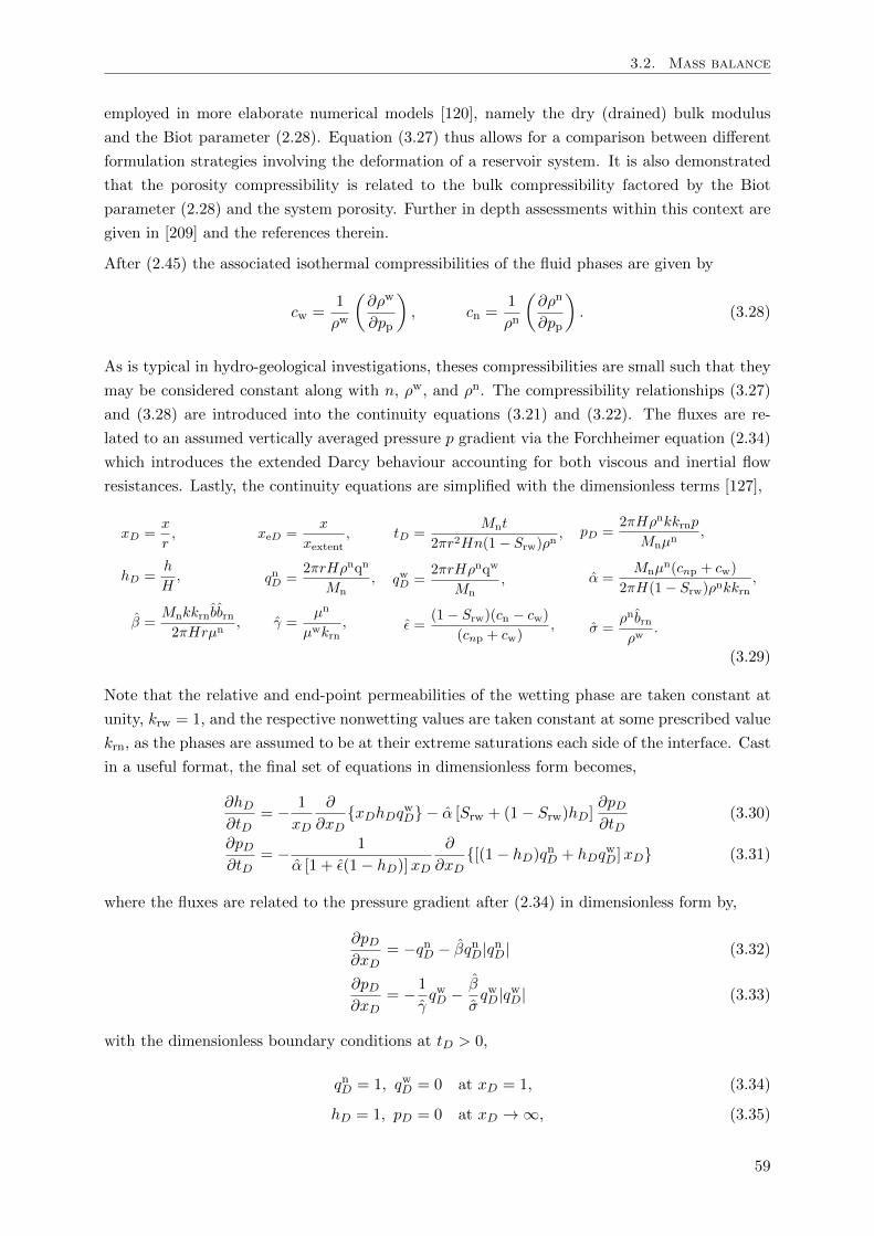
3.2. Mass balance
employed in more elaborate numerical models [120], namely the dry (drained) bulk modulus
and the Biot parameter (2.28). Equation (3.27) thus allows for a comparison between different
formulation strategies involving the deformation of a reservoir system. It is also demonstrated
that the porosity compressibility is related to the bulk compressibility factored by the Biot
parameter (2.28) and the system porosity. Further in depth assessments within this context are
given in [209] and the references therein.
After (2.45) the associated isothermal compressibilities of the fluid phases are given by
cw =1
ρw
(∂ρw
∂pp
), cn =
1
ρn
(∂ρn
∂pp
). (3.28)
As is typical in hydro-geological investigations, theses compressibilities are small such that they
may be considered constant along with n, ρw, and ρn. The compressibility relationships (3.27)
and (3.28) are introduced into the continuity equations (3.21) and (3.22). The fluxes are re-
lated to an assumed vertically averaged pressure p gradient via the Forchheimer equation (2.34)
which introduces the extended Darcy behaviour accounting for both viscous and inertial flow
resistances. Lastly, the continuity equations are simplified with the dimensionless terms [127],
xD =x
r,
hD =h
H,
β =Mnkkrnbbrn2πHrµn
,
xeD =x
xextent,
qnD =2πrHρnqn
Mn,
γ =µn
µwkrn,
tD =Mnt
2πr2Hn(1− Srw)ρn,
qwD =2πrHρnqw
Mn,
ε =(1− Srw)(cn − cw)
(cnp + cw),
pD =2πHρnkkrnp
Mnµn,
α =Mnµ
n(cnp + cw)
2πH(1− Srw)ρnkkrn,
σ =ρnbrnρw
.
(3.29)
Note that the relative and end-point permeabilities of the wetting phase are taken constant at
unity, krw = 1, and the respective nonwetting values are taken constant at some prescribed value
krn, as the phases are assumed to be at their extreme saturations each side of the interface. Cast
in a useful format, the final set of equations in dimensionless form becomes,
∂hD∂tD
= − 1
xD
∂
∂xDxDhDqwD − α [Srw + (1− Srw)hD]
∂pD∂tD
(3.30)
∂pD∂tD
= − 1
α [1 + ε(1− hD)]xD
∂
∂xD[(1− hD)q
nD + hDq
wD]xD (3.31)
where the fluxes are related to the pressure gradient after (2.34) in dimensionless form by,
∂pD∂xD
= −qnD − βqnD|qnD| (3.32)
∂pD∂xD
= −1
γqwD − β
σqwD|qwD| (3.33)
with the dimensionless boundary conditions at tD > 0,
qnD = 1, qwD = 0 at xD = 1, (3.34)
hD = 1, pD = 0 at xD → ∞, (3.35)
59
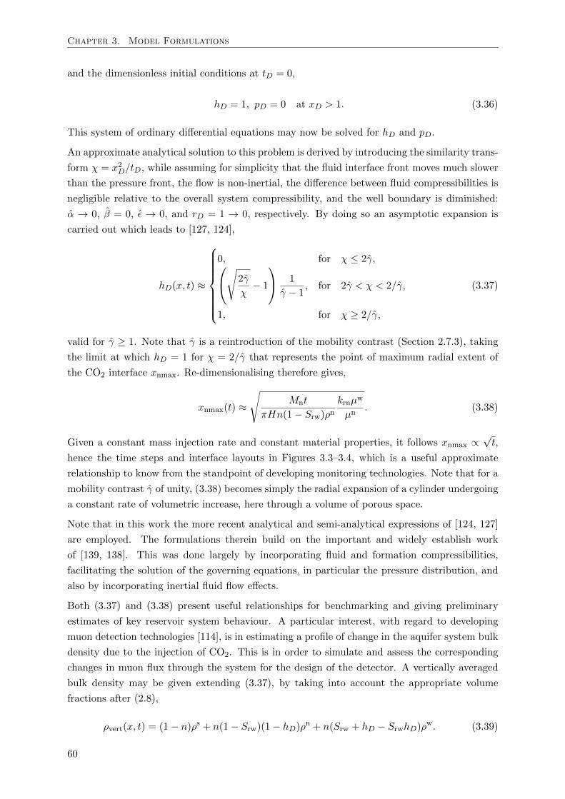
Chapter 3. Model Formulations
and the dimensionless initial conditions at tD = 0,
hD = 1, pD = 0 at xD > 1. (3.36)
This system of ordinary differential equations may now be solved for hD and pD.
An approximate analytical solution to this problem is derived by introducing the similarity trans-
form χ = x2D/tD, while assuming for simplicity that the fluid interface front moves much slower
than the pressure front, the flow is non-inertial, the difference between fluid compressibilities is
negligible relative to the overall system compressibility, and the well boundary is diminished:
α → 0, β = 0, ε → 0, and rD = 1 → 0, respectively. By doing so an asymptotic expansion is
carried out which leads to [127, 124],
hD(x, t) ≈
0, for χ ≤ 2γ,√2γ
χ− 1
1
γ − 1, for 2γ < χ < 2/γ,
1, for χ ≥ 2/γ,
(3.37)
valid for γ ≥ 1. Note that γ is a reintroduction of the mobility contrast (Section 2.7.3), taking
the limit at which hD = 1 for χ = 2/γ that represents the point of maximum radial extent of
the CO2 interface xnmax. Re-dimensionalising therefore gives,
xnmax(t) ≈
√Mnt
πHn(1− Srw)ρnkrnµw
µn. (3.38)
Given a constant mass injection rate and constant material properties, it follows xnmax ∝√t,
hence the time steps and interface layouts in Figures 3.3–3.4, which is a useful approximate
relationship to know from the standpoint of developing monitoring technologies. Note that for a
mobility contrast γ of unity, (3.38) becomes simply the radial expansion of a cylinder undergoing
a constant rate of volumetric increase, here through a volume of porous space.
Note that in this work the more recent analytical and semi-analytical expressions of [124, 127]
are employed. The formulations therein build on the important and widely establish work
of [139, 138]. This was done largely by incorporating fluid and formation compressibilities,
facilitating the solution of the governing equations, in particular the pressure distribution, and
also by incorporating inertial fluid flow effects.
Both (3.37) and (3.38) present useful relationships for benchmarking and giving preliminary
estimates of key reservoir system behaviour. A particular interest, with regard to developing
muon detection technologies [114], is in estimating a profile of change in the aquifer system bulk
density due to the injection of CO2. This is in order to simulate and assess the corresponding
changes in muon flux through the system for the design of the detector. A vertically averaged
bulk density may be given extending (3.37), by taking into account the appropriate volume
fractions after (2.8),
ρvert(x, t) = (1− n)ρs + n(1− Srw)(1− hD)ρn + n(Srw + hD − SrwhD)ρ
w. (3.39)
60
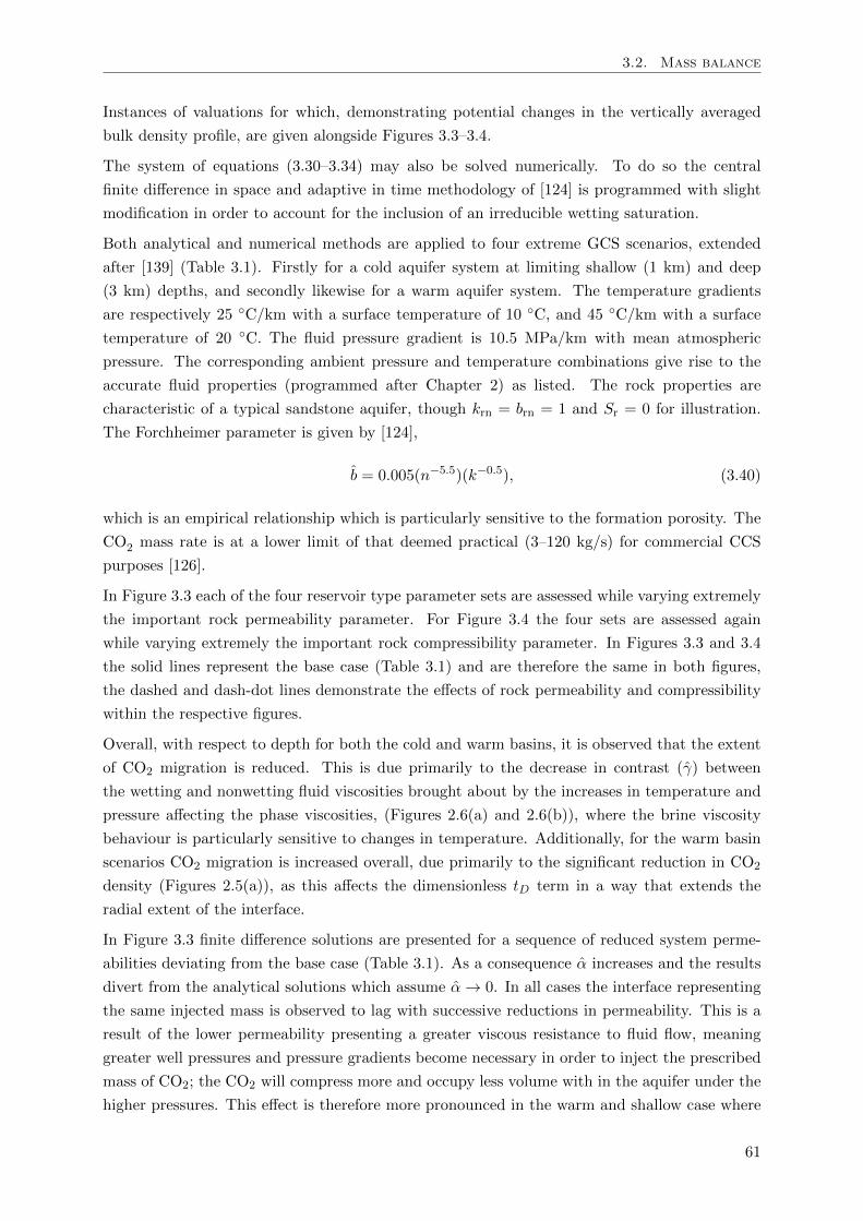
3.2. Mass balance
Instances of valuations for which, demonstrating potential changes in the vertically averaged
bulk density profile, are given alongside Figures 3.3–3.4.
The system of equations (3.30–3.34) may also be solved numerically. To do so the central
finite difference in space and adaptive in time methodology of [124] is programmed with slight
modification in order to account for the inclusion of an irreducible wetting saturation.
Both analytical and numerical methods are applied to four extreme GCS scenarios, extended
after [139] (Table 3.1). Firstly for a cold aquifer system at limiting shallow (1 km) and deep
(3 km) depths, and secondly likewise for a warm aquifer system. The temperature gradients
are respectively 25 C/km with a surface temperature of 10 C, and 45 C/km with a surface
temperature of 20 C. The fluid pressure gradient is 10.5 MPa/km with mean atmospheric
pressure. The corresponding ambient pressure and temperature combinations give rise to the
accurate fluid properties (programmed after Chapter 2) as listed. The rock properties are
characteristic of a typical sandstone aquifer, though krn = brn = 1 and Sr = 0 for illustration.
The Forchheimer parameter is given by [124],
b = 0.005(n−5.5)(k−0.5), (3.40)
which is an empirical relationship which is particularly sensitive to the formation porosity. The
CO2 mass rate is at a lower limit of that deemed practical (3–120 kg/s) for commercial CCS
purposes [126].
In Figure 3.3 each of the four reservoir type parameter sets are assessed while varying extremely
the important rock permeability parameter. For Figure 3.4 the four sets are assessed again
while varying extremely the important rock compressibility parameter. In Figures 3.3 and 3.4
the solid lines represent the base case (Table 3.1) and are therefore the same in both figures,
the dashed and dash-dot lines demonstrate the effects of rock permeability and compressibility
within the respective figures.
Overall, with respect to depth for both the cold and warm basins, it is observed that the extent
of CO2 migration is reduced. This is due primarily to the decrease in contrast (γ) between
the wetting and nonwetting fluid viscosities brought about by the increases in temperature and
pressure affecting the phase viscosities, (Figures 2.6(a) and 2.6(b)), where the brine viscosity
behaviour is particularly sensitive to changes in temperature. Additionally, for the warm basin
scenarios CO2 migration is increased overall, due primarily to the significant reduction in CO2
density (Figures 2.5(a)), as this affects the dimensionless tD term in a way that extends the
radial extent of the interface.
In Figure 3.3 finite difference solutions are presented for a sequence of reduced system perme-
abilities deviating from the base case (Table 3.1). As a consequence α increases and the results
divert from the analytical solutions which assume α→ 0. In all cases the interface representing
the same injected mass is observed to lag with successive reductions in permeability. This is a
result of the lower permeability presenting a greater viscous resistance to fluid flow, meaning
greater well pressures and pressure gradients become necessary in order to inject the prescribed
mass of CO2; the CO2 will compress more and occupy less volume with in the aquifer under the
higher pressures. This effect is therefore more pronounced in the warm and shallow case where
61
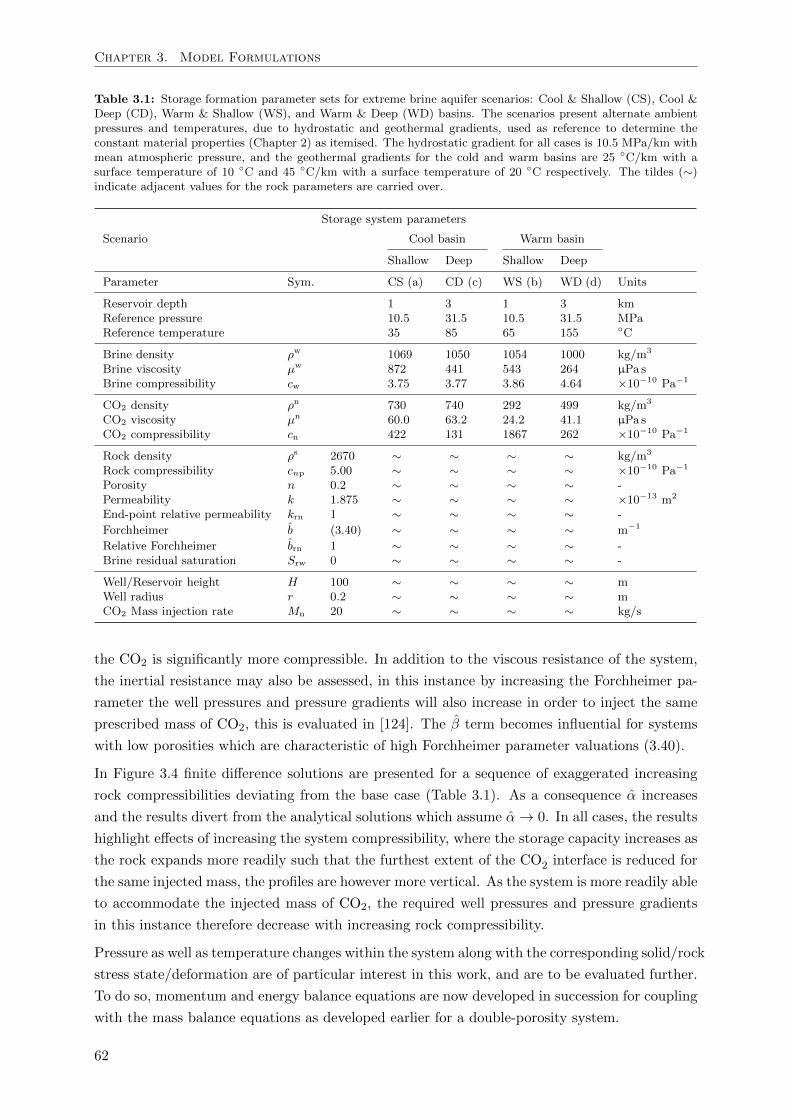
Chapter 3. Model Formulations
Table 3.1: Storage formation parameter sets for extreme brine aquifer scenarios: Cool & Shallow (CS), Cool &Deep (CD), Warm & Shallow (WS), and Warm & Deep (WD) basins. The scenarios present alternate ambientpressures and temperatures, due to hydrostatic and geothermal gradients, used as reference to determine theconstant material properties (Chapter 2) as itemised. The hydrostatic gradient for all cases is 10.5 MPa/km withmean atmospheric pressure, and the geothermal gradients for the cold and warm basins are 25 C/km with asurface temperature of 10 C and 45 C/km with a surface temperature of 20 C respectively. The tildes (∼)indicate adjacent values for the rock parameters are carried over.
Storage system parameters
Scenario Cool basin Warm basin
Shallow Deep Shallow Deep
Parameter Sym. CS (a) CD (c) WS (b) WD (d) Units
Reservoir depth 1 3 1 3 kmReference pressure 10.5 31.5 10.5 31.5 MPaReference temperature 35 85 65 155 C
Brine density ρw 1069 1050 1054 1000 kg/m3
Brine viscosity µw 872 441 543 264 µPa sBrine compressibility cw 3.75 3.77 3.86 4.64 ×10⁻¹⁰ Pa−1
CO2 density ρn 730 740 292 499 kg/m3
CO2 viscosity µn 60.0 63.2 24.2 41.1 µPa sCO2 compressibility cn 422 131 1867 262 ×10−10 Pa−1
Rock density ρs 2670 ∼ ∼ ∼ ∼ kg/m3
Rock compressibility cnp 5.00 ∼ ∼ ∼ ∼ ×10−10 Pa−1
Porosity n 0.2 ∼ ∼ ∼ ∼ -Permeability k 1.875 ∼ ∼ ∼ ∼ ×10−13 m2
End-point relative permeability krn 1 ∼ ∼ ∼ ∼ -
Forchheimer b (3.40) ∼ ∼ ∼ ∼ m−1
Relative Forchheimer brn 1 ∼ ∼ ∼ ∼ -Brine residual saturation Srw 0 ∼ ∼ ∼ ∼ -
Well/Reservoir height H 100 ∼ ∼ ∼ ∼ mWell radius r 0.2 ∼ ∼ ∼ ∼ mCO2 Mass injection rate Mn 20 ∼ ∼ ∼ ∼ kg/s
the CO2 is significantly more compressible. In addition to the viscous resistance of the system,
the inertial resistance may also be assessed, in this instance by increasing the Forchheimer pa-
rameter the well pressures and pressure gradients will also increase in order to inject the same
prescribed mass of CO2, this is evaluated in [124]. The β term becomes influential for systems
with low porosities which are characteristic of high Forchheimer parameter valuations (3.40).
In Figure 3.4 finite difference solutions are presented for a sequence of exaggerated increasing
rock compressibilities deviating from the base case (Table 3.1). As a consequence α increases
and the results divert from the analytical solutions which assume α→ 0. In all cases, the results
highlight effects of increasing the system compressibility, where the storage capacity increases as
the rock expands more readily such that the furthest extent of the CO2 interface is reduced for
the same injected mass, the profiles are however more vertical. As the system is more readily able
to accommodate the injected mass of CO2, the required well pressures and pressure gradients
in this instance therefore decrease with increasing rock compressibility.
Pressure as well as temperature changes within the system along with the corresponding solid/rock
stress state/deformation are of particular interest in this work, and are to be evaluated further.
To do so, momentum and energy balance equations are now developed in succession for coupling
with the mass balance equations as developed earlier for a double-porosity system.
62
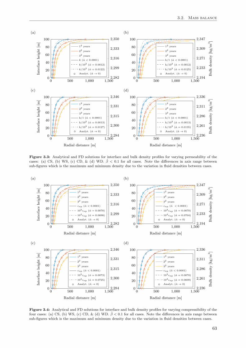
3.2. Mass balance
(a)
0 500 1,000 1,5000
20
40
60
80
100Interface
height[m
]
12 years
22 years
32 years
k (α < 0.0001)
k/102 (α = 0.0012)
k/103 (α = 0.0122)
Analyt. (α → 0)
2,282
2,299
2,316
2,333
2,350
(b)
0 500 1,000 1,5000
20
40
60
80
100
12 years
22 years
32 years
k/1 (α < 0.0001)
k/102 (α = 0.0012)
k/103 (α = 0.0125)
Analyt. (α → 0)
2,194
2,233
2,271
2,309
2,347
Bulk
den
sity
[kg/m
3]
(c)
0 500 1,000 1,5000
20
40
60
80
100
Radial distance [m]
Interface
height[m
]
12 years
22 years
32 years
k/1 (α < 0.0001)
k/102 (α = 0.0013)
k/103 (α = 0.0127)
Analyt. (α → 0)
2,284
2,300
2,315
2,331
2,346
(d)
0 500 1,000 1,5000
20
40
60
80
100
Radial distance [m]
12 years
22 years
32 years
k/1 (α < 0.0001)
k/102 (α = 0.0013)
k/103 (α = 0.0135)
Analyt. (α → 0)
2,236
2,261
2,286
2,311
2,336
Bulk
den
sity
[kg/m
3]
Figure 3.3: Analytical and FD solutions for interface and bulk density profiles for varying permeability of thecases: (a) CS, (b) WS, (c) CD, & (d) WD. β < 0.1 for all cases. Note the differences in axis range betweensub-figures which is the maximum and minimum density due to the variation in fluid densities between cases.
(a)
0 500 1,000 1,5000
20
40
60
80
100
Radial distance [m]
Interface
height[m
]
12 years
22 years
32 years
cnp (α < 0.0001)
103cnp (α = 0.0070)
104cnp (α = 0.0698)
Analyt. (α → 0)
2,282
2,299
2,316
2,333
2,350
(b)
0 500 1,000 1,5000
20
40
60
80
100
Radial distance [m]
12 years
22 years
32 years
cnp (α < 0.0001)
103cnp (α = 0.0070)
104cnp (α = 0.0704)
Analyt. (α → 0)
2,194
2,233
2,271
2,309
2,347
Bulk
den
sity
[kg/m
3]
(c)
0 500 1,000 1,5000
20
40
60
80
100
Radial distance [m]
Interface
height[m
]
12 years
22 years
32 years
cnp (α < 0.0001)
103cnp (α = 0.0073)
104cnp (α = 0.0725)
Analyt. (α → 0)
2,284
2,300
2,315
2,331
2,346
(d)
0 500 1,000 1,5000
20
40
60
80
100
Radial distance [m]
12 years
22 years
32 years
cnp (α < 0.0001)
103cnp (α = 0.0070)
104cnp (α = 0.0699)
Analyt. (α → 0)
2,236
2,261
2,286
2,311
2,336
Bulk
den
sity
[kg/m
3]
Figure 3.4: Analytical and FD solutions for interface and bulk density profiles for varying compressibility of thefour cases: (a) CS, (b) WS, (c) CD, & (d) WD. β < 0.1 for all cases. Note the differences in axis range betweensub-figures which is the maximum and minimum density due to the variation in fluid densities between cases.
63
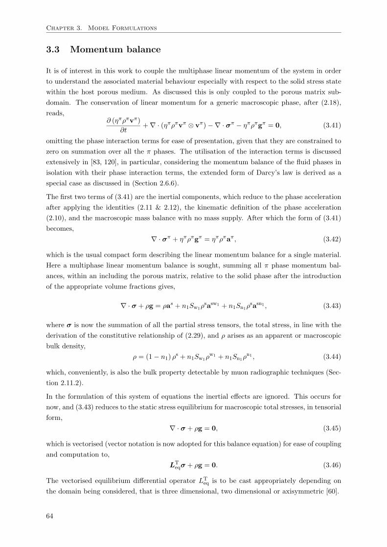
Chapter 3. Model Formulations
3.3 Momentum balance
It is of interest in this work to couple the multiphase linear momentum of the system in order
to understand the associated material behaviour especially with respect to the solid stress state
within the host porous medium. As discussed this is only coupled to the porous matrix sub-
domain. The conservation of linear momentum for a generic macroscopic phase, after (2.18),
reads,∂ (ηπρπvπ)
∂t+∇ · (ηπρπvπ ⊗ vπ)−∇ · σπ − ηπρπgπ = 0, (3.41)
omitting the phase interaction terms for ease of presentation, given that they are constrained to
zero on summation over all the π phases. The utilisation of the interaction terms is discussed
extensively in [83, 120], in particular, considering the momentum balance of the fluid phases in
isolation with their phase interaction terms, the extended form of Darcy’s law is derived as a
special case as discussed in (Section 2.6.6).
The first two terms of (3.41) are the inertial components, which reduce to the phase acceleration
after applying the identities (2.11 & 2.12), the kinematic definition of the phase acceleration
(2.10), and the macroscopic mass balance with no mass supply. After which the form of (3.41)
becomes,
∇ · σπ + ηπρπgπ = ηπρπaπ, (3.42)
which is the usual compact form describing the linear momentum balance for a single material.
Here a multiphase linear momentum balance is sought, summing all π phase momentum bal-
ances, within an including the porous matrix, relative to the solid phase after the introduction
of the appropriate volume fractions gives,
∇ · σ + ρg = ρas + n1Sw1ρsasw1 + n1Sn1ρ
sasn1 , (3.43)
where σ is now the summation of all the partial stress tensors, the total stress, in line with the
derivation of the constitutive relationship of (2.29), and ρ arises as an apparent or macroscopic
bulk density,
ρ = (1− n1) ρs + n1Sw1ρ
w1 + n1Sn1ρn1 , (3.44)
which, conveniently, is also the bulk property detectable by muon radiographic techniques (Sec-
tion 2.11.2).
In the formulation of this system of equations the inertial effects are ignored. This occurs for
now, and (3.43) reduces to the static stress equilibrium for macroscopic total stresses, in tensorial
form,
∇ · σ + ρg = 0, (3.45)
which is vectorised (vector notation is now adopted for this balance equation) for ease of coupling
and computation to,
LTeqσ + ρg = 0. (3.46)
The vectorised equilibrium differential operator LTeq is to be cast appropriately depending on
the domain being considered, that is three dimensional, two dimensional or axisymmetric [60].
64
3.4. Energy/enthalpy balance
To build a multiphase governing field equation for the momentum balance of the system, the
following constitutive relations are substituted with the appropriate terms of (3.46):
- The total stress tensor is decomposed as of (2.29), into an effective stress component
responsible for the deformation of the solid skeleton and grains, and fluid pressure com-
ponents. The unit tensor and pressure tensors here are vectorised in line with the vectori-
sation at (3.45) and with (3.11).
- The effective stress may now be related to solid displacements by selecting an appropriate
constitutive solid model extended in order to account for thermal effects,
σ′′ = Del(ε− εTh) or dσ′′ = DT(dε− dεTh), (3.47)
where for the latter,
dε = Ldu and dεTh = m (βs/3) dT. (3.48)
The total strain vector is represented by ε and the thermal strain vector by εTh, Del
and DT are the linear elastic and tangential stress/strain matrices, βs is again the solid
thermal expansion coefficient, and m is the unit vector. The primary variables being the
solid displacements u and the multiphase temperature T . Note that within the parenthesis
of (3.47) other strain effects may be incorporated such as creep strains and initial strains.
- The external body force vector is taken as the acceleration due to the Earth’s gravitational
field.
Noting that the mechanical loads are carried only by the porous matrix continuum as discussed,
expanding puts the primary variables into the following form,
LTeq
[DelLu−Delm (βs/3)T − bmSw1p
w1 − bmSn1pn1]+ ρg = 0, (3.49)
which may also be cast in an incremental/time differentiated form for symmetry of the system
of balance equations and in order to incorporate non-linear material behaviour. This treatment
is carried out in Chapter 4.
3.4 Energy/enthalpy balance
For the balance of energy, any surplus mean macroscopic effects due to phase interaction are
neglected. It is demonstrated that these terms may be subjected to a summation of zero over
all the overlapping phases [120] when prescribing a multiphase energy balance for the system as
a whole for which there is no net increase of energy due to phase interaction. For the individual
phase equations these terms are therefore omitted for ease of presentation. The external energy
supply terms which are not required are also omitted. That is, any chemical, electromagnetic,
radiative and nuclear forms of external energy supply are neglected. Reduced from the general
macroscopic balance (2.18), an appropriate energy balance for a single phase is therefore given.
The terms of which express sequentially, the rate of change of internal and kinetic energies,
the rate of change of internal and kinetic energies by convective transport, the rate of work
done by stresses/pressures and energy change by heat conduction, and the rate of work done by
65
Chapter 3. Model Formulations
external/gravitational forces, as follows,
∂ηπρπ (uπ + 1/2 vπ · vπ)
∂t+∇ · [ηπρπ (uπ + 1/2 vπ · vπ)vπ]
−∇ · (σπ · vπ − qπ)− ηπρπ (gπ · vπ) = 0. (3.50)
Manipulating the energy balance (3.50), and substituting both the general mass and momentum
balance equations, leads to an expression of the rate of change of internal energy,
∂ηπρπuπ
∂t+∇ · (ηπρπuπvπ) +∇ · qπ + ηπpπ (∇ · vπ)− τπ : ∇vπ = 0. (3.51)
This manipulation essentially subtracts the rate of change of kinetic energy within the system
from (3.50), leaving an equation of the rate of change of internal energy [28, 120]. Note that the
partial stress tensor has also become decomposed into a partial pressure and deviatoric stress.
The terms now conveniently express, sequentially, the rate of change of internal energy, the
rate of change of internal energy by convective transport, the rate of internal energy change by
heat conduction, the reversible rate of internal energy change by compression/expansion, and
the irreversible rate of internal energy change by viscous dissipation (mechanical into internal
energy). Energy may be recoverable from this last term if the material is viscoelastic and
therefore able to store elastic energy. Using the identity (2.11) and the material derivative (2.9)
with the equation of continuity, (3.51) is transformed into the useful form,
ηπρπDuπ
Dt+∇ · qπ + ηπpπ (∇ · vπ)− τπ : ∇vπ = 0. (3.52)
To build a multiphase governing field equation to account for the thermal behaviour of the
system, the following developments are made for (3.52):
- First, the specific internal energy u is modified to the specific enthalpy h. As stated for
(2.40), in terms of specific (intensive) properties,
uπ = hπ − pπvπ = hπ − pπ
ρπ, (3.53)
making the standard assumption that the thermodynamic relationships derived for a sys-
tem in equilibrium is appropriate for use in a non-equilibrium system if it is applied locally.
The pressure term is the intrinsic hydrostatic component of the stress tensor (fluid pres-
sure) and v is specific volume. Differentiating, applying the quotient/reciprocal rule, and
expanding (3.53) yields,
ρπDuπ
Dt= ρπ
Dhπ
Dt+pπ
ρπDρπ
Dt− Dpπ
Dt, (3.54)
which presents a relationship that may be introduced into (3.52) in order to produce a
balance of enthalpy.
- The enthalpy balance allows for the introduction of system temperature. As enthalpy is a
function of pressure and temperature (an ideal gas being a function of temperature only),
66
3.4. Energy/enthalpy balance
hπ = hπ(pπ, T π), therefore taking the total differential,
dhπ =
(∂hπ
∂T π
)p
dT π +
(∂hπ
∂pπ
)T
dpπ, (3.55)
and on substituting the specific heat capacity relationship after (2.40) for the first differen-
tial and using Maxwell’s standard thermodynamic relation [39] for the second along with
(2.46) after some manipulation, gives,
dhπ = cπpdTπ +
[vπ − T π
(∂vπ
∂T π
)p
]dpπ = cπpdT
π +1
ρπ(1− T πβπ) dpπ. (3.56)
The density rate term of (3.54) is treated by expanding the mass balance D(ηπρπ)/Dt +
ηπρπ (∇ · vπ). Introducing this along with (3.56), into (3.54), finally gives,
ρπDuπ
Dt= ρπcπp
DT π
Dt− T πβπ
Dpπ
Dt− pπ
ηπDηπ
Dt− pπ (∇ · vπ) . (3.57)
The assumption that the enthalpy is a function of pressure and temperature restricts the
formulation to Newtonian fluids, which is a practical assumption for small/low-weight
molecule fluids, such as those under prime consideration here within the ranges of interest
[90]. Note that,
T πβπ = −Tπ
ρπ
(∂ρπ
∂T π
)p
= −(∂ ln ρπ
∂ lnT π
)p
(3.58)
is a volume coefficient of expansion. Note also that the Joule-Thomson coefficient (Sec-
tion 2.6.8.3) can be derived form (3.56) assuming constant enthalpy dhπ = 0, for further
developments therefore,
µπJT =
(∂T π
∂pπ
)h
= − 1
cπp
[vπ − T π
(∂vπ
∂T π
)p
]=
vπ
cπp(T πβπ − 1) . (3.59)
- The constitutive relationship adopted for the heat flux vector qπ is Fourier’s law (2.44),
which introduces the thermal conductivities of the media. However, when dealing with a
porous multiphase medium an effective conductivity is generally prescribed [120, 129, 137,
208] due to the complex geometrical mixture of the phases. Considering the phases to be
in parallel an upper-bound overall effective thermal conductivity is given by,
χeff = (1− n12)χs + (n1Sw1 + n2Sw2)χ
w + (n1Sn1 + n2Sn2)χn. (3.60)
Alternatively, considering the phases to be in series, a lower-bound overall effective thermal
conductivity is given by,
1
χeff
=(1− n12)
χs+
(n1Sw1 + n2Sw2)
χw+
(n1Sn1 + n2Sn2)
χn. (3.61)
Further developments to this effect are discussed in [129, 137, 208] for single porosity
media with single and multiple fluid phases, for a double-porosity multiple fluid phase
67
Chapter 3. Model Formulations
model further research is warranted. The upper bound is assumed in this work for now.
Applying the relationships, as itemised above, sequentially to (3.52) presents,
ηπρπcπpDT π
Dt− ηπβπT πDp
π
Dt− pπ
Dηπ
Dt−∇ · (χπ
eff∇T π)− τπ : ∇vπ = 0. (3.62)
The second and third terms, giving change due to mechanical work by pressure/temperature
and volume fraction variation, and the fifth term, giving change due to viscous dissipation (an
irreversible part of the internal energy increase which may be characterised for a fluid by its
viscosity and dilatational viscosity [28]), are usually neglected for geo-applications [120]. The
volume coefficient of expansion in the second term for an incompressible material (constant
density), is ∂ ln ρ/∂ lnT = 0, which is the same result for a system with constant pressure,
Dp/Dt = 0. Also, for an ideal gas ∂ ln ρ/∂ lnT = −1. Neglecting these terms presents the basic
classical energy balance for multiphase media to which additional terms are generally added
depending on the application.
For the consideration of energy balance the compressibility of the system is typically ignored,
particularly in coupled geomechanical models [120], as its effect is generally negligible and there-
fore left uncoupled. In order to assess the extent of validity of such simplifications for fully
coupled GCS model applications marks a point for further research. From the discussion in Sec-
tion 2.6.8.3 on the importance of understanding the thermal effects of pressure variation within
the CO2 phase, the variation of phase pressure and the viscous dissipation terms are retained
in this work from the general equation (3.62) for the CO2 phase alone, assuming these effects
to be negligible in the less compressible phases. The negligibility of the pressure changes may
be assessed by the condition βT (gβ/cp)lc 1, and the viscous dissipation by the condition
(gβ/cp)lc 1, if not met the respective differential terms are required [95, 137]. This is po-
tentially the case for various CO2 thermodynamic parametrisations. On retained these terms
an additional relationship is needed for the viscous dissipation term, for flow in porous media
governed by Darcy’s law, this is given by the term, ηπvπ · ∇pπ [4, 95, 137].
In essence, the isobaric thermal expansion coefficients of the solid and wetting phases, as derived
here, are considered negligible in the energy balance formulation, noting that they are orders of
magnitude lower than for the nonwetting phase, over the pressures and temperatures of interest.
A similar assumption is made in [129]. The convective heat flux of the solid is also ignored as
its movement is negligible with respect to the fluids. Given that all the phases are considered
to be in local thermodynamic equilibrium,
T s = Tw1 = Tw2 = T n1 = T n2 = T. (3.63)
In all therefore, for the solid phase the enthalpy balance is
ηsρscsp∂T
∂t−∇ · (χs
eff∇T ) = 0, (3.64)
for the wetting phase,
ηwiρwicwip
∂T
∂t+ ηwiρwicwi
p vwi · ∇T −∇ ·(χwieff∇T
)= 0, (3.65)
68
3.4. Energy/enthalpy balance
and for the nonwetting phase,
ηniρnicnip∂T
∂t+ ηniρnicnip v
ni ·∇T − ηniβniT ∂pni
∂t− ηni (βniT − 1)vni ·∇pni −∇·
(χnieff∇T
)= 0,
(3.66)
where i = 1, 2. Hence, on summation of all the enthalpy balance equations the following mul-
tiphase macroscopic balance equation is given, conveniently in terms of the desired primary
variables,
(ρcp)eff∂T
∂t+ (ρcpv)eff · ∇T −
2∑i=1
niSniβniT
∂pni
∂t
−2∑
i=1
niSni (βniT − 1)vni · ∇pni −∇ · (χeff∇T ) = 0, (3.67)
where,
(ρcp)eff = (1− n12) ρscsp + (n1Sw1 + n2Sw2) ρ
wcwp + (n1Sn1 + n2Sn2) ρncnp (3.68)
(ρcpv)eff = ρwcwp (n1Sw1vw1 + n2Sw2v
w2) + ρncnp (n1Sn1vn1 + n2Sn2v
n2) (3.69)
χeff = (1− n12)χs + (n1Sw1 + n2Sw2)χ
w + (n1Sn1 + n2Sn2)χn. (3.70)
The respective fluid material properties of density, specific isobaric heat capacity, and ther-
mal/heat conductivity, in the porous matrix and the fissure/fracture network, are considered
to be the same (ρf1 = ρf2 , cf1p = cf2p , χf1 = χf2) for tractability. All phases are considered to
be in local thermodynamic equilibrium, and the pressure variations are assumed to be within a
reasonable range such that the material properties in each sub-domain vary negligibly from one
another with respect to temperature and pressure changes. The volume fraction velocities of
the fluids may be given by substituting Darcy’s law (2.6.6). The solid velocity is left uncoupled
as the associated heat convection is assumed negligible as mentioned.
Efficient preliminary solutions to simplified governing equations extended for GCS application
were presented for the key mass balance equations. Such extension with solutions for the mo-
mentum balance, assessing for instance any first order uplift over a GCS reservoir due to pre-
scribed pressure changes, appear more open for study with direct reference to GCS. Solutions are
however given for simple geotechnical consolidation/deformation problems as of [120] and the
references therein. For the energy balance, research has presented solutions for simplified energy
balance equations extended for GCS, which also highlight the prominent thermal considerations
as adopted here, for reference [128, 129].
For designing a muon detection system an estimation of density change due to injection is re-
quired [114]. In determining this, the mass balance of the system is the most influential aspect,
unless the coupled mechanical and/or thermal effects become severe. Simple uncoupled single-
porosity mass balance solutions have therefore been presented in Section 3.2.6 as of (3.39) for the
purposes of simple first-order estimation. A coupled or uncoupled momentum balance solution is
of indirect importance because an estimate of mechanical/pressure changes would indicate if the
69
Chapter 3. Model Formulations
muon detection equipment would become damaged, and therefore what installation tolerances
should be set. Likewise, the energy balance is also of importance because components currently
under development, to be installed subsurface as part of the muon detector system, are sensitive
to temperature, therefore, estimates of thermal fluctuations around the muon detection system
are desirable. Any (thermal-electrical) coupling or response to this effect is also demanded and
unresearched.
3.5 Summary of governing field equations
The six non-linear governing field equations as derived are given in compact form. This is
to highlight the coupling between terms and equations, for ease of reference, and for further
numerical computation. The mass balances within the porous continuum, for the wetting phase,
λw1
∂pw1
∂t+ λw1n1
∂pn1
∂t+ λw1sL
∂u
∂t− λw1T
∂T
∂t
+∇ · Kw1 (−∇pw1 + ρw1g) = −λw1l2 (pw1 − pw2) , (3.71)
and for the nonwetting phase,
λn1w1
∂pw1
∂t+ λn1
∂pn1
∂t+ λn1sL
∂u
∂t− λn1T
∂T
∂t
+∇ · Kn1 (−∇pn1 + ρn1g) = −λn1l2 (pn1 − pn2) . (3.72)
The mass balances within the fissured/fractured continuum, for the wetting phase,
λw2
∂pw2
∂t+ λw2n2
∂pn2
∂t− λw2T
∂T
∂t+∇ · Kw2 (−∇pw2 + ρw2g) = λw1l2(p
w1 − pw2), (3.73)
and for the nonwetting phase,
λn2w2
∂pw2
∂t+ λn2
∂pn2
∂t− λn2T
∂T
∂t+∇ · Kn2 (−∇pn2 + ρn2g) = λn1l2(p
n1 − pn2). (3.74)
The multiphase momentum balance,
LTeq [DelLu−Delm (βs/3)T − bmSw1p
w1 − bmSn1pn1 ] + ρg = 0. (3.75)
The multiphase enthalpy balance,
(ρcp)eff∂T
∂t+ (ρcpv)eff · ∇T −
2∑i=1
niSniβniT
∂pni
∂t
−2∑
i=1
niSni (βniT − 1)vni · ∇pni −∇ · (χeff∇T ) = 0. (3.76)
The subscripts to the λ terms additionally denote and emphasise the important direct cross-
coupling relationships within the mass balance equations. For instance, the wetting phase in the
porous matrix domain w1, sequentially, relates firstly to itself presenting a compressibility term,
70
3.5. Summary of governing field equations
then to the nonwetting phase in the matrix domain -n1, to the solid phase (porous matrix) -s,
to the thermal behaviour -T, and to the wetting phase in the fracture network domain -l2. The
latter all presenting coupling terms.
Note that, as derived, the only cross-coupling term between the sub-domains is the λw1l2 trans-
fer/leakage term. As discussed, further elaborations on solid deformation due directly to the
differential pressure between matrix and fracture sub-domains would result in λf1f2 and λf2f1terms. Here these terms are essentially zero and any additional deformation due to the fracture
network is coupled solely by any transfer via the double-porosity transfer/leakage function, the
fracture network itself is therefore considered undeformable, which however is largely considered
appropriate given the relatively small volume fraction of the fissure/fracture network often en-
counter in practice. For more appreciable volume fractions thereof, clearly further formulations
would be required involving constitutive relationships encompassing grain, skeleton, and the
fissure/fracture network as a natural extension.
Furthermore, this system of equations may be reduced straightforwardly in order to account for
a single-porosity system (with no fissure/fracture equations), an undeformable system (with no
momentum balance), or an isothermal system (with no energy balance), by cancelling/uncou-
pling the appropriate cross-coupling terms/equations. The results by doing so are essentially
special cases which coincide with the typical results explored within the literature.
71

Chapter 4
Spatial Discretisation
The standard Galerkin finite element procedure is employed in order to spatially discretise
the developed system of equations over a domain. During this process the appropriate initial
and boundary conditions for the system sub-domains are introduced. This is to allow for the
numerical solution of the coupled partial differential governing field equations.
The governing equations to be solved are posed in the following general form [207], where x is
a vector of the multiple primary variable unknowns, satisfying the differential equation set,
A(x) =
A1(x)...
= 0 (4.1)
within the domain Ω, with boundary conditions,
B(x) =
B1(x)...
= 0 (4.2)
on the boundaries of the domain Γ, as illustrated in Figure 4.1. A and B prescribe known
operators or functions. The differential equation set may be single and can be non-linear.
The finite element method seeks a solution for unknowns in the approximate form,
x ≈ x =nds∑n=1
Nnxn = Nx (4.3)
where x are now discrete unknowns at nodal points, and N are appropriate shape functions for
interpolating the unknowns in terms of independent spatial coordinates defined locally within
elements bound by a certain number of nodal points, nds. Casting the approximating equations
in integral form permits the approximation to be gathered element-wise and assembled [207],
where the number of elements, els, constitute the domain,
∫ΩA dΩ +
∫ΓBdΓ =
els∑e=1
(∫Ωe
A dΩ +
∫Γe
BdΓ
)= 0, (4.4)
73
Chapter 4. Spatial Discretisation
provided that the integrals can be performed.
Figure 4.1: Visualisation of domain and boundary for an arbitrary problem
4.1 Method of weighted residuals (Galerkin procedure)
The weighted residual-Galerkin procedure, the determination of variational functionals for which
stationarity is sought, virtual work, and direct stiffness methods are procedures for acquiring
formulations giving solutions to governing equations. The first method mentioned is utilised
in this work due to its generality, which makes it applicable to a variety of physical problems
[118, 207].
In order to solve the differential equations an approach is taken which attempts to find an
approximation by solving element-wise over a domain for equilibrium at discrete points (4.3).
It generally follows that the accuracy of a solution increases with an increase in the number of
discrete nodal points within the domain at an expense related to the extra computation involved.
By introducing an approximation such as (4.3) to the exact field a residual error is now defined,
r = rΩ + rΓ. A solution is now sought that will minimize this error over the whole domain and
its boundary. This is done by forcing a zero value for an appropriate number of integrals of the
residual over the domain and boundary, weighted in different ways by weighting functions.
Adopting the following reformulation of (4.1) and (4.2),∫ΩvTA(x) dΩ +
∫ΓvTB(x) dΓ = 0 (4.5)
where vT and vT are sets of arbitrary functions. Equations (4.5) are satisfied equivalent to the
original differential equations (4.1) and their boundary conditions (4.2). Importantly, it follows
that if (4.5) is satisfied for all v then (4.1) and (4.2) are satisfied at all points of the domain and
on the boundary [207].
It is assumed here that the integrals can be evaluated. To this effect the continuity (differen-
tiability class) of A and B must be considered. If in any term nth-order derivatives are present
then the function x must have continuous n − 1 derivatives, otherwise difficulties are encoun-
tered when integrating. As is generally applicable, carrying out an integration by parts over the
74
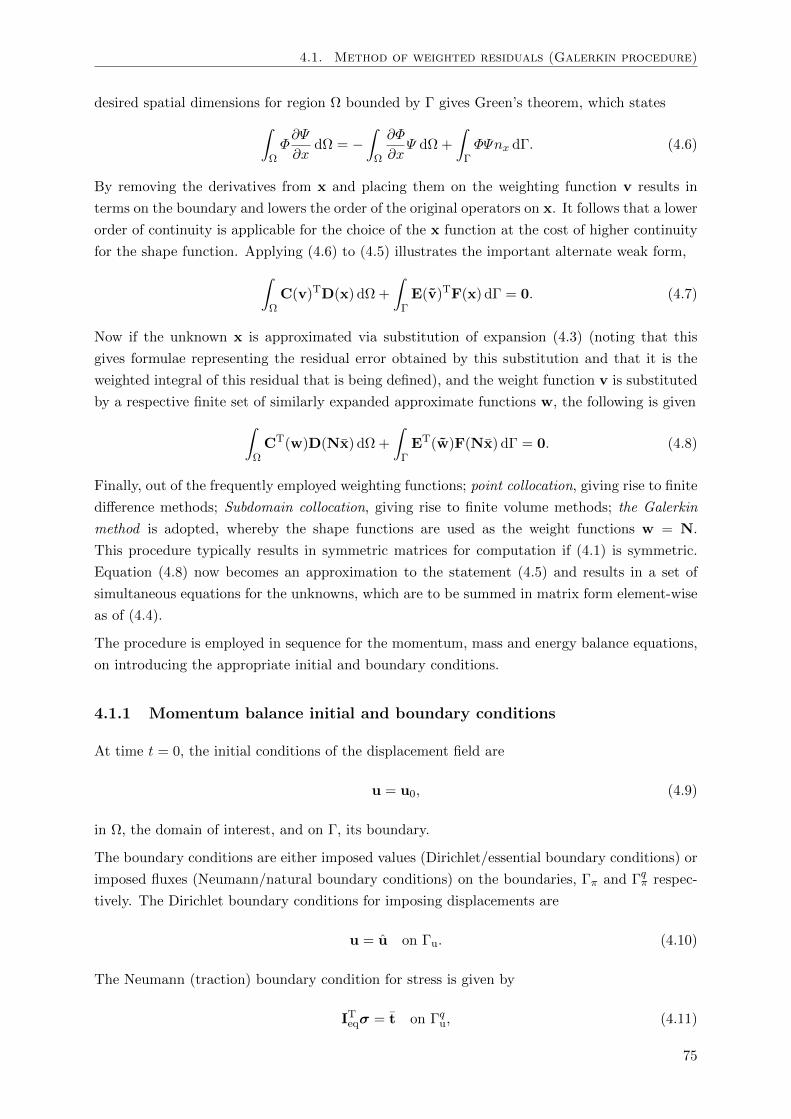
4.1. Method of weighted residuals (Galerkin procedure)
desired spatial dimensions for region Ω bounded by Γ gives Green’s theorem, which states∫ΩΦ∂Ψ
∂xdΩ = −
∫Ω
∂Φ
∂xΨ dΩ +
∫ΓΦΨnx dΓ. (4.6)
By removing the derivatives from x and placing them on the weighting function v results in
terms on the boundary and lowers the order of the original operators on x. It follows that a lower
order of continuity is applicable for the choice of the x function at the cost of higher continuity
for the shape function. Applying (4.6) to (4.5) illustrates the important alternate weak form,∫ΩC(v)TD(x) dΩ +
∫ΓE(v)TF(x) dΓ = 0. (4.7)
Now if the unknown x is approximated via substitution of expansion (4.3) (noting that this
gives formulae representing the residual error obtained by this substitution and that it is the
weighted integral of this residual that is being defined), and the weight function v is substituted
by a respective finite set of similarly expanded approximate functions w, the following is given∫ΩCT(w)D(Nx) dΩ +
∫ΓET(w)F(Nx) dΓ = 0. (4.8)
Finally, out of the frequently employed weighting functions; point collocation, giving rise to finite
difference methods; Subdomain collocation, giving rise to finite volume methods; the Galerkin
method is adopted, whereby the shape functions are used as the weight functions w = N.
This procedure typically results in symmetric matrices for computation if (4.1) is symmetric.
Equation (4.8) now becomes an approximation to the statement (4.5) and results in a set of
simultaneous equations for the unknowns, which are to be summed in matrix form element-wise
as of (4.4).
The procedure is employed in sequence for the momentum, mass and energy balance equations,
on introducing the appropriate initial and boundary conditions.
4.1.1 Momentum balance initial and boundary conditions
At time t = 0, the initial conditions of the displacement field are
u = u0, (4.9)
in Ω, the domain of interest, and on Γ, its boundary.
The boundary conditions are either imposed values (Dirichlet/essential boundary conditions) or
imposed fluxes (Neumann/natural boundary conditions) on the boundaries, Γπ and Γqπ respec-
tively. The Dirichlet boundary conditions for imposing displacements are
u = u on Γu. (4.10)
The Neumann (traction) boundary condition for stress is given by
ITeqσ = t on Γqu, (4.11)
75
Chapter 4. Spatial Discretisation
where Ieq is the appropriate matrix related to the usual unit normal vector to the boundary,
which is cast in view of the domain type after (3.46).
4.1.2 Momentum balance discretisation
Applying the weighted residual method to (3.75) and (4.11) presents,∫ΩwT
(LT
eqσ + ρg)dΩ +
∫Γqu
wT(ITeqσ − t
)dΓ = 0. (4.12)
Applying Green’s theorem (4.6), and limiting the weighting functions such that w = 0 on Γu
and w = −w on Γqu gives,∫
Ω(Leqw)T σ dΩ =
∫ΩwTρg dΩ +
∫Γqu
wTtdΓ. (4.13)
The primary variables are interpolated and thus expressed via the following shape functions and
discrete nodal values after (4.4),
u = Nuu (4.14)
pfi = Nppfi (4.15)
T = NT T (4.16)
which are introduced into (4.13). The trial/weight functions are replaced with the shape func-
tions following the Galerkin procedure. Finally, reinstating the total stress components as of
(3.75), presents∫Ω(LeqNu)
TDelLNu dΩ u −∫Ω(LeqNu)
T bmSw1Np dΩ pw1 −∫Ω(LeqNu)
T bmSn1Np dΩ pn1
−∫Ω(LeqNu)
TDelm (βs/3)NT dΩ T =
∫ΩNT
u ρg dΩ +
∫Γqu
NTu t dΓ. (4.17)
The discretised primary variables have been taken out of the integrals because they are nodal
values and do not depend on the volume integration.
4.1.3 Mass balance initial and boundary conditions
At time t = 0, the initial conditions of the pressure fields are
pfi = pfi0 , (4.18)
in Ω, the domain of interest, and on Γ, its boundary.
The Dirichlet boundary conditions for imposing pressures are
pfi = pfi on Γf . (4.19)
76
4.1. Method of weighted residuals (Galerkin procedure)
The Neumann boundary condition for the fluids, imposing a mass flux across the boundary,
after (2.33), is given by,
qfi = ρfikrfiki
µfi
(−∇pfi + ρfig
)T· n on Γq
f . (4.20)
where n is the usual unit normal vector to the boundary.
4.1.4 Mass balance discretisation
Applying the weighted residual method to a generic version of the mass balances for the porous
matrix continua (3.71) and (3.72), and to the boundary condition (4.20) presents,
∫ΩwT
[λ∂pw1
∂t+ λ
∂pn1
∂t+ λL
∂u
∂t− λ
∂T
∂t+∇ ·
Kf1
(−∇pf1 + ρf1g
)+ λ
(pf1 − pf2
)]dΩ
+
∫Γqf
wT
[Kf1
(−∇pfi + ρfig
)T· n− qfi
ρfi
]dΓ = 0. (4.21)
Applying Green’s theorem (4.6) to the divergence operator, and limiting the weighting functions
such that w = 0 on Γf and w = −w on Γqf , whilst expanding in part and rearranging, gives
∫Ω
[wTλ
∂pw1
∂t+wTλ
∂pn1
∂t+wTλL
∂u
∂t−wTλ
∂T
∂t+wTλ
(pf1 − pf2
)]dΩ
+
∫Ω(∇w)TKf1∇pf1 dΩ =
∫Ω(∇w)TKf1ρ
f1g dΩ −∫Γqf
wT qfi
ρfidΓ. (4.22)
The primary variables are interpolated and thus expressed via shape functions and discrete
nodal values, as of (4.4), which are introduced into (4.22). The trial/weight functions are also
replaced with the shape functions, giving the following form for both porous matrix continuity
equations,
∫ΩNT
p λNp dΩ∂pw1
∂t+
∫ΩNT
p λNp dΩ∂pn1
∂t+
∫ΩNT
p λLNu dΩ∂u
∂t−∫ΩNT
p λNT dΩ∂T
∂t
+
∫ΩNT
p λNp dΩ pf1 −∫ΩNT
p λNp dΩ pf2 +
∫Ω(∇Np)
TKf1∇Np dΩ pf1
=
∫Ω(∇Np)
TKf1ρf1g dΩ −
∫Γqf
NTp
qf1
ρf1dΓ. (4.23)
Carrying out the same procedure for the fissured/fractured domain continua (3.73) and (3.74),
gives the following form for the two continuity equations,
∫ΩNT
p λNp dΩ∂pw2
∂t+
∫ΩNT
p λNp dΩ∂pn2
∂t−∫ΩNT
p λNT dΩ∂T
∂t
−∫ΩNT
p λNp dΩ pf1 +
∫ΩNT
p λNp dΩ pf2 +
∫Ω(∇Np)
TKf2∇Np dΩ pf2
=
∫Ω(∇Np)
TKf2ρf2g dΩ −
∫Γqf
NTp
qf2
ρf2. dΓ. (4.24)
77
Chapter 4. Spatial Discretisation
The λ and Kfi coefficients will be stipulated for their respective terms when the system of
equations is cast fully in matrix form in Section 4.2.
4.1.5 Energy balance initial and boundary conditions
At time t = 0, the initial conditions of the temperature field are
T = T0, (4.25)
in Ω, the domain of interest, and on Γ, its boundary.
The Dirichlet boundary conditions for imposing temperature are
T = T on ΓT. (4.26)
The Neumann boundary condition for heat transfer across the boundary, after (2.32), is given
by,
(−χeff∇T )T · n = qT on Γq
T . (4.27)
where n is the usual unit normal vector to the boundary and qT is the prescribed heat flux.
4.1.6 Energy balance discretisation
Applying the weighted residual method to the energy balance equation for the bulk medium
(3.76) presents,
∫ΩwT
[(ρcp)eff
∂T
∂t+ (ρcpv)eff · ∇T −∇ · (χeff∇T )
]dΩ
−∫ΩwT
[2∑
i=1
niSniβniT
∂pni
∂t+
2∑i=1
niSni (βniT − 1)vni · ∇pni
]dΩ
+
∫ΓqT
wT[(−χeff∇T )
T · n− qT]dΓ = 0. (4.28)
Applying Green’s theorem (4.6) to the divergence operator, and limiting the weighting functions
such that w = 0 on ΓT and w = −w on ΓqT , whilst expanding in part and rearranging gives,
∫ΩwT
[(ρcp)eff
∂T
∂t+ (ρcpv)eff · ∇T
]dΩ +
∫Ω(∇w)Tχeff∇T dΩ
−∫ΩwT
[2∑
i=1
niSniβniT
∂pni
∂t+
2∑i=1
niSni (βniT − 1)vni · ∇pni
]dΩ +
∫ΓqT
wTqTdΓ = 0. (4.29)
The primary variables are interpolated with shape functions from discrete nodal values, after
(4.4), which are incorporated into (4.29). The trial/weight functions are replaced with the shape
functions, following the Galerkin procedure, giving finally,
78
4.2. The spatially discretised system of equations
∫ΩNT
T (ρcp)eff NT dΩ∂T
∂t+
∫ΩNT
T (ρcpv)eff · ∇NT dΩ T +
∫Ω(∇NT )
Tχeff∇NT dΩ T
−∫ΩNT
Tn1Sn1βn1TNp dΩ
∂pn1
∂t−∫ΩNT
Tn1Sn1 (βn1T − 1)vn1 · ∇Np dΩ pn1
−∫ΩNT
Tn2Sn2βn2TNp dΩ
∂pn2
∂t−∫ΩNT
Tn2Sn2 (βn2T − 1)vn2 · ∇Np dΩ pn2
= −∫ΓqT
NTTq
T dΓ. (4.30)
Note that for all governing equations, the essential boundary conditions are automatically sat-
isfied by the choice of functions on Γπ, and that the natural boundary conditions are satisfied
automatically during the weak formulation. During the discretisation process the gradient and
divergence operators, which now operate on the shape function arrays, have become ∇ and ∇T
respectively, where for three dimensions
∇ =
∂∂x∂∂y∂∂z
. (4.31)
4.2 The spatially discretised system of equations
Reinstating the full coefficients represented by the λ terms and casting all the spatially discretised
governing equations in matrix form presents an ordinary differential equation set in respect of
time, whereby the components of system coupling are conveniently highlighted,
K1 Quw1 Qun1 0 0 QuT
Qwu1 Sw1 Qwn1 0 0 Qw1T
Qnu1 Qnw1 Sn1 0 0 Qn1T
0 0 0 Sw2 Qwn2 Qw2T
0 0 0 Qnw2 Sn2 Qn2T
0 0 QTn1 0 QTn2 CT
d
dt
u
pw1
pn1
pw2
pn2
T
+
0 0 0 0 0 0
0 Hw1 + Lw 0 −Lw 0 0
0 0 Hn1 + Ln 0 −Ln 0
0 −Lw 0 Hw2 + Lw 0 0
0 0 −Ln 0 Hn2 + Ln 0
0 0 HTn1 0 HTn2 HT
u
pw1
pn1
pw2
pn2
T
=
ddt fu
fw1
fn1
fw2
fn2
fT
(4.32)
where the sub-matrices are
K1 =
∫ΩBTDelBdΩ, (4.33)
Quw1 = −∫ΩBTbSw1mNp dΩ, (4.34)
79
Chapter 4. Spatial Discretisation
Qun1 = −∫ΩBTbSn1mNp dΩ, (4.35)
QuT = −∫ΩBTDelm (βs/3)NT dΩ, (4.36)
fu =
∫ΩNT
u
[(1− n1)ρ
s + n1Sw1ρw1 + n1Sn1ρ
n1]g dΩ +
∫Γqu
NTu t dΓ (4.37)
Qwu1 =
∫ΩNT
p bSw1mTBdΩ = QT
uw1, (4.38)
Sw1 =
∫ΩNT
p
[b− n1Ks
Sw1
(Sw1 + pc1
∂Sw1
∂pc1
)+n1Sw1
Kw1
− n1∂Sw1
∂pc1
]Np dΩ, (4.39)
Qwn1 =
∫ΩNT
p
[b− n1Ks
Sw1
(Sn1 − pc1
∂Sw1
∂pc1
)+ n1
∂Sw1
∂pc1
]Np dΩ, (4.40)
Qw1T = −∫ΩNT
p Sw1 [βs (b− n1) + n1β
w1 ] NT dΩ, (4.41)
Hw1 =
∫Ω(∇Np)
T krw1k1
µw1∇Np dΩ, (4.42)
Lw =
∫ΩNT
p
α krw1k1µw1
Np dΩ, (4.43)
fw1 =
∫Ω(∇Np)
T krw1k1
µw1ρw1g dΩ−
∫Γqf
NTp
qw1
ρw1dΓ
, (4.44)
Qnu1 =
∫ΩNT
p bSn1mTBdΩ = QT
un1, (4.45)
Qnw1 =
∫ΩNT
p
[b− n1Ks
Sn1
(Sw1 + pc1
∂Sw1
∂pc1
)+ n1
∂Sw1
∂pc1
]Np dΩ, (4.46)
Sn1 =
∫ΩNT
p
[b− n1Ks
Sn1
(Sn1 − pc1
∂Sw1
∂pc1
)+n1Sn1Kn1
− n1∂Sw1
∂pc1
]Np dΩ, (4.47)
Qn1T = −∫ΩNT
p Sn1 [βs (b− n1) + n1β
n1 ] NT dΩ, (4.48)
Hn1 =
∫Ω(∇Np)
T krn1k1
µn1∇Np dΩ, (4.49)
Ln =
∫ΩNT
p
α krn1k1µn1
Np dΩ, (4.50)
fn1 =
∫Ω(∇Np)
T krn1k1
µn1ρn1g dΩ−
∫Γqf
NTp
qn1
ρn1dΓ
, (4.51)
Sw2 =
∫ΩNT
p
[n2Sw2
Kw2
− n2∂Sw2
∂pc2
]Np dΩ, (4.52)
Qwn2 =
∫ΩNT
p n2∂Sw2
∂pc2Np dΩ, (4.53)
Qw2T = −∫ΩNT
p Sw2n2βw2 NT dΩ, (4.54)
Hw2 =
∫Ω(∇Np)
T krw2k2
µw2∇Np dΩ, (4.55)
fw2 =
∫Ω(∇Np)
T krw2k2
µw2ρw2g dΩ−
∫Γqf
NTp
qw2
ρw2dΓ
, (4.56)
80
4.3. Shape functions & isoparametric finite elements
Qnw2 =
∫ΩNT
p n2∂Sw2
∂pc2Np dΩ, (4.57)
Sn2 =
∫ΩNT
p
[n2Sn2Kn2
− n2∂Sw2
∂pc2
]Np dΩ, (4.58)
Qn2T = −∫ΩNT
p Sn2n2βn2 NT dΩ, (4.59)
Hn2 =
∫Ω(∇Np)
T krn2k2
µn2∇Np dΩ, (4.60)
fn2 =
∫Ω(∇Np)
T krn2k2
µn2ρn2g dΩ−
∫Γqf
NTp
qn2
ρn2dΓ, (4.61)
QTn1 = −∫ΩNT
T n1Sn1βn1T Np dΩ, (4.62)
QTn2 = −∫ΩNT
T n2Sn2βn2T Np dΩ, (4.63)
CT =
∫ΩNT
T (ρcp)eff NT dΩ, (4.64)
HTn1 = −∫ΩNT
T n1Sn1 (βn1T − 1)vn1 · ∇Np dΩ, (4.65)
HTn2 = −∫ΩNT
T n2Sn2 (βn2T − 1)vn2 · ∇Np dΩ, (4.66)
HT =
∫ΩNT
T (ρcpv)eff · ∇NT + (∇NT )Tχeff∇NT dΩ, (4.67)
fT = −∫ΓqT
NTTq
T dΓ. (4.68)
The listed matrices distribute the associated properties over the domain and on its boundaries,
where the subscripts denote the associated primary variable, sub-domain, and therefore any
coupling. Symbols K, Q, S, C, H, and L, refer to stiffness, coupling, compressibility, thermal
capacity, conductivity, and leakage matrices respectively. Note that B = LNu is the strain
operator, and f are forcing vectors, distributing body and traction forces, and fluid/thermal
fluxes.
4.3 Shape functions & isoparametric finite elements
The primary variables u, pfi and T , are expressed in terms of values at a finite number of discrete
nodal points in space as an approximate representation of the continuum in that space. This
involves the partitioning of the continuum into finite elements for separate integration before
assembly with the other elements constituting the domain of interest. Within an element the
primary variables are expressed in terms of values on the element’s boundary, whereby those
nodes on the boundary are to ensure continuity between the elements. This is to be satisfied by
the choice of element nodal shape functions N.
In this work, the system of equations is solved over a 2D axisymmetric domain as rotated about
some vertical extent along which a mass flux may be applied, representative of an idealised
body of prospective reservoir with a central wellbore. This is typically assumed in both 1D
81
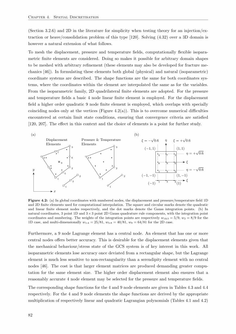
Chapter 4. Spatial Discretisation
(Section 3.2.6) and 2D in the literature for simplicity when testing theory for an injection/ex-
traction or heave/consolidation problem of this type [120]. Solving (4.32) over a 3D domain is
however a natural extension of what follows.
To mesh the displacement, pressure and temperature fields, computationally flexible isopara-
metric finite elements are considered. Doing so makes it possible for arbitrary domain shapes
to be meshed with arbitrary refinement (these elements may also be developed for fracture me-
chanics [46]). In formulating these elements both global (physical) and natural (isoparametric)
coordinate systems are described. The shape functions are the same for both coordinates sys-
tems, where the coordinates within the element are interpolated the same as for the variables.
From the isoparametric family, 2D quadrilateral finite elements are adopted. For the pressure
and temperature fields a basic 4 node linear finite element is employed. For the displacement
field a higher order quadratic 9 node finite element is employed, which overlaps with specially
coinciding nodes only at the vertices (Figure 4.2(a)). This is to overcome numerical difficulties
encountered at certain limit state conditions, ensuring that convergence criteria are satisfied
[120, 207]. The effect in this context and the choice of elements is a point for further study.
(a) (b)
Figure 4.2: (a) In global coordinates with numbered nodes, the displacement and pressure/temperature field 1Dand 2D finite elements used for computational interpolation. The square and circular marks denote the quadraticand linear finite element nodes respectively, and the dot marks denote the Gauss integration points. (b) Innatural coordinates, 3 point 1D and 3×3 point 2D Gauss quadrature rule components, with the integration pointcoordinates and numbering. The weights of the integration points are respectively w1&3 = 5/9, w2 = 8/9 for the1D case, and multi-dimensionally w1-4 = 25/81, w5-8 = 40/81, w9 = 64/81 for the 2D case.
Furthermore, a 9 node Lagrange element has a central node. An element that has one or more
central nodes offers better accuracy. This is desirable for the displacement elements given that
the mechanical behaviour/stress state of the GCS system is of key interest in this work. All
isoparametric elements lose accuracy once deviated from a rectangular shape, but the Lagrange
element is much less sensitive to non-rectangularity than a serendipity element with no central
nodes [46]. The cost is that larger element matrices are produced demanding greater compu-
tation for the same element size. The higher order displacement element also ensures that a
reasonably accurate 4 node element may be selected for the pressure and temperature fields.
The corresponding shape functions for the 4 and 9 node elements are given in Tables 4.3 and 4.4
respectively. For the 4 and 9 node elements the shape functions are derived by the appropriate
multiplication of respectively linear and quadratic Lagrangian polynomials (Tables 4.1 and 4.2)
82
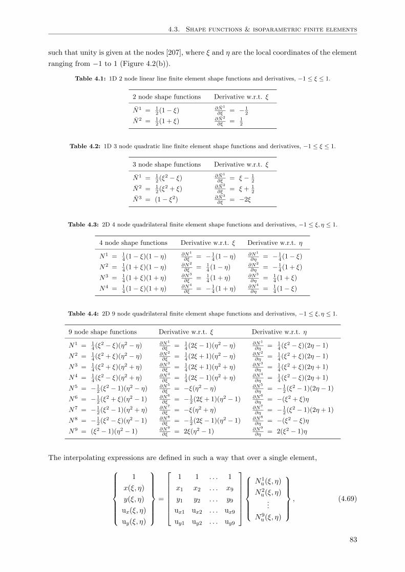
4.3. Shape functions & isoparametric finite elements
such that unity is given at the nodes [207], where ξ and η are the local coordinates of the element
ranging from −1 to 1 (Figure 4.2(b)).
Table 4.1: 1D 2 node linear line finite element shape functions and derivatives, −1 ≤ ξ ≤ 1.
2 node shape functions Derivative w.r.t. ξ
N1 = 12 (1− ξ) ∂N1
∂ξ = − 12
N2 = 12 (1 + ξ) ∂N2
∂ξ = 12
Table 4.2: 1D 3 node quadratic line finite element shape functions and derivatives, −1 ≤ ξ ≤ 1.
3 node shape functions Derivative w.r.t. ξ
N1 = 12 (ξ
2 − ξ) ∂N1
∂ξ = ξ − 12
N2 = 12 (ξ
2 + ξ) ∂N2
∂ξ = ξ + 12
N3 = (1− ξ2) ∂N3
∂ξ = −2ξ
Table 4.3: 2D 4 node quadrilateral finite element shape functions and derivatives, −1 ≤ ξ, η ≤ 1.
4 node shape functions Derivative w.r.t. ξ Derivative w.r.t. η
N1 = 14 (1− ξ)(1− η) ∂N1
∂ξ = − 14 (1− η) ∂N1
∂η = − 14 (1− ξ)
N2 = 14 (1 + ξ)(1− η) ∂N2
∂ξ = 14 (1− η) ∂N2
∂η = − 14 (1 + ξ)
N3 = 14 (1 + ξ)(1 + η) ∂N3
∂ξ = 14 (1 + η) ∂N3
∂η = 14 (1 + ξ)
N4 = 14 (1− ξ)(1 + η) ∂N4
∂ξ = − 14 (1 + η) ∂N4
∂η = 14 (1− ξ)
Table 4.4: 2D 9 node quadrilateral finite element shape functions and derivatives, −1 ≤ ξ, η ≤ 1.
9 node shape functions Derivative w.r.t. ξ Derivative w.r.t. η
N1 = 14 (ξ
2 − ξ)(η2 − η) ∂N1
∂ξ = 14 (2ξ − 1)(η2 − η) ∂N1
∂η = 14 (ξ
2 − ξ)(2η − 1)
N2 = 14 (ξ
2 + ξ)(η2 − η) ∂N2
∂ξ = 14 (2ξ + 1)(η2 − η) ∂N2
∂η = 14 (ξ
2 + ξ)(2η − 1)
N3 = 14 (ξ
2 + ξ)(η2 + η) ∂N3
∂ξ = 14 (2ξ + 1)(η2 + η) ∂N3
∂η = 14 (ξ
2 + ξ)(2η + 1)
N4 = 14 (ξ
2 − ξ)(η2 + η) ∂N4
∂ξ = 14 (2ξ − 1)(η2 + η) ∂N4
∂η = 14 (ξ
2 − ξ)(2η + 1)
N5 = − 12 (ξ
2 − 1)(η2 − η) ∂N5
∂ξ = −ξ(η2 − η) ∂N5
∂η = − 12 (ξ
2 − 1)(2η − 1)
N6 = − 12 (ξ
2 + ξ)(η2 − 1) ∂N6
∂ξ = − 12 (2ξ + 1)(η2 − 1) ∂N6
∂η = −(ξ2 + ξ)η
N7 = − 12 (ξ
2 − 1)(η2 + η) ∂N7
∂ξ = −ξ(η2 + η) ∂N7
∂η = − 12 (ξ
2 − 1)(2η + 1)
N8 = − 12 (ξ
2 − ξ)(η2 − 1) ∂N8
∂ξ = − 12 (2ξ − 1)(η2 − 1) ∂N8
∂η = −(ξ2 − ξ)η
N9 = (ξ2 − 1)(η2 − 1) ∂N9
∂ξ = 2ξ(η2 − 1) ∂N9
∂η = 2(ξ2 − 1)η
The interpolating expressions are defined in such a way that over a single element,
1
x(ξ, η)
y(ξ, η)
ux(ξ, η)
uy(ξ, η)
=
1 1 . . . 1
x1 x2 . . . x9
y1 y2 . . . y9
ux1 ux2 . . . ux9
uy1 uy2 . . . uy9
N1
u(ξ, η)
N2u(ξ, η)...
N9u(ξ, η)
, (4.69)
83
Chapter 4. Spatial Discretisation
1
x(ξ, η)
y(ξ, η)
pfi(ξ, η)
T (ξ, η)
=
1 1 1 1
x1 x2 x3 x4
y1 y2 y3 y4
pfi1 pfi2 pfi3 pfi4T1 T2 T3 T4
N1
p/T (ξ, η)
N2p/T (ξ, η)
N3p/T (ξ, η)
N4p/T (ξ, η)
, (4.70)
where the subscript numbers refer to the node of the element (Figure 4.2(a)). Note that C0
continuity is achieved across element boundaries.
The shape function matrix for the 9 node finite element with the same number of shape functions
is given for computation as
Nu =
[N1
u 0 N2u 0 . . . N9
u 0
0 N1u 0 N2
u . . . 0 N9u
], (4.71)
allocated in such a way that
x(ξ, η)
y(ξ, η)
= Nu
x1
y1...
x9
y9
=
9∑
n=1Nn
u xn
9∑n=1
Nnu yn
, (4.72)
and likewise for displacements ux and uy acting in the global x and y coordinates respectively,
ux
uy
= Nu
ux1
uy1
...
ux9
uy9
. (4.73)
4.3.1 2D Jacobian matrix and determinant
It is required that the shape function derivatives over the local parent element be related to
the derivatives over the distorted global element. To achieve this, ξ, η → x, y mapping is
carried out using an elemental Jacobian matrix, J. It is derived here using the chain rule which
immediately gives the relationship∂N∂ξ∂N∂η
=
[∂x∂ξ
∂y∂ξ
∂x∂η
∂y∂η
]︸ ︷︷ ︸
J
∂N∂x∂N∂y
. (4.74)
The derivatives ∂N/∂ξ ∂N/∂ηT may be determined readily due to the regular structure
of the parent element (Figure 4.2(b), and Tables 4.3 and 4.4), in order that the derivatives
∂N/∂x ∂N/∂yT may be determined for the global element satisfying the governing equations,
84
4.3. Shape functions & isoparametric finite elements
the inverse of the Jacobian is required such that∂N∂x∂N∂y
= J−1
∂N∂ξ∂N∂η
. (4.75)
Knowing the shape function derivatives at some point in the parent element, and a given global
element’s nodal (vertices) coordinates [x,y]e (independent of ξ and η), in view of (4.72), differ-
entiating x and y with respect to ξ and η is possible. The Jacobian components at the point
within the given element are therefore obtained numerically via,
J =
[∂x∂ξ
∂y∂ξ
∂x∂η
∂y∂η
]=
nds∑n=1
[∂Nn∂ξ xn
∂Nn∂ξ yn
∂Nn∂η xn
∂Nn∂η yn
]=
[∂N1∂ξ . . . ∂Nnds
∂ξ∂N1∂η . . . ∂Nnds
∂η
]x1 y1...
...
xnds ynds
(4.76)
where the diagonal terms account for the rate of stretching along the coordinate axes and the
off-diagonal terms map the shearing of the element. The inverse of the Jacobian is obtained by,
J−1 =1
|J|
[∂y∂η −∂y
∂ξ
−∂x∂η
∂x∂ξ
]=
1
|J|
[J22 −J12−J21 J11
](4.77)
where the Jacobian determinant,
|J| = ∂x
∂ξ
∂y
∂η− ∂x
∂η
∂y
∂ξ= J11J22 − J12J21. (4.78)
The following important derivatives may now be computed,
∂N
∂x=
1
|J|
(∂y
∂η
∂N
∂ξ− ∂y
∂ξ
∂N
∂η
)=
1
|J|
(J22
∂N
∂ξ− J12
∂N
∂η
), (4.79)
∂N
∂y=
1
|J|
(∂x
∂ξ
∂N
∂η− ∂x
∂η
∂N
∂ξ
)=
1
|J|
(J11
∂N
∂η− J21
∂N
∂ξ
). (4.80)
4.3.2 Gauss-Legendre quadrature for axisymmetric numerical integration
The evaluation of the complex integral equations of (4.32) is carried out via numerical integration
through a multi-dimension Gauss-Legendre quadrature rule [46]. The quadrature rule employed
is illustrated in Figure 4.2(a) for the 2D case with
∫∫ 1
−1f(ξ, η) dξdη =
ips∑i=1
f(ξi, ηi)wi, (4.81)
where i is the Gauss integration point as weighted by wi over the summation. Note that a 3
point rule has been selected for the appropriate accuracy, meaning that there are 9 Gaussian
integration points within each element. The coupled displacement, pressure and temperature
elements are occupied by the same 9 integration points during computation.
Within an axisymmetric domain, each element is essentially a 3D ring-element about the cen-
tral axis, meaning, dΩ = 2πxdxdy, where x is the radial extent (Figure 2.4) and dxdy is the
85
Chapter 4. Spatial Discretisation
infinitesimal cross-sectional area at the point of interest. As 2π is constant it may be taken
out of all the integrals and cancelled throughout the system of equations. Hence, dΩ may be
interpreted xdxdy, and similarly dΓ as xdy.
In order to apply the quadrature rule to the irregular global axisymmetric elements they have
to be transformed into the canonical from,
∫Ωe
f(x, y)x dxdydθ ⇒∫ 2π
0
∫ 1
−1
∫ 1
−1f [x(ξ, η), y(ξ, η)]x(ξ, η) |J(ξ, η)| dξdηdθ
= 2π
ips∑i=1
f [x(ξi, ηi), y(ξi, ηi)]x(ξi, ηi) |J(ξi, ηi)|wi. (4.82)
Note that the integration is now expressed entirely in terms of ξ and η by an area transformation,
where the area of the differential quadrilateral is computed via the geometric cross product
dxdy =∂x
∂ξdξ
∂y
∂ηdη − ∂x
∂ηdη
∂y
∂ξdξ =
∣∣∣∣∣ ∂x∂ξ
∂y∂ξ
∂x∂η
∂y∂η
∣∣∣∣∣dξdη = |J|dξdη, (4.83)
which reintroduces the Jacobian determinant, as gathered by the computation (4.76) which may
now be employed at the integration points for the purpose of (4.77–4.80) and (4.82).
4.4 General Finite Element Formulations
The following subsections itemise and compute the various general matrix and vector types
which constitute the full system of equations (4.32).
4.4.1 Tangential stiffness element matrix
The tangential stiffness matrix of (4.32), element-wise after (4.4) is of the form,
Se =
∫Ωe
BTDB dΩ, (4.84)
based on the global coordinate system (Figure 4.2(a)), which is to be transformed in terms
the natural coordinate system (Figure 4.2(b)) for computation. Employing therefore the Gauss
quadrature rule (4.82) presents
Se =
ips∑i=1
BTi DBi x(ξi, ηi) |J(ξi, ηi)|wi. (4.85)
For the axisymmetric case, D (illustrated here as being constant over the domain) relates ax-
isymmetric stress-strains as covered in Section 2.6.4, and B is the kinematic relationship of
86
4.4. General Finite Element Formulations
element strains to nodal displacements which is given by LNu, where
L =
∂∂x 0
0 ∂∂y
1x 0∂∂y
∂∂x
. (4.86)
Hence, the differential operator matrix given for the 2D axisymmetric case is therefore
B = LNu =
∂N1
u∂x 0 . . . ∂N9
u∂x 0
0 ∂N1u
∂y . . . 0 ∂N9u
∂yN1
ux 0 . . . N9
ux 0
∂N1u
∂y∂N1
u∂x . . . ∂N9
u∂y
∂N9u
∂x
. (4.87)
Utilising the Jacobian formulation leading to (4.79) and (4.80), the isoparametric mapping
formulation for computation is given as
Bi =
1|J|
(J22
∂N1u
∂ξ − J12∂N1
u∂η
)0 . . .
0 1|J|
(J11
∂N1u
∂η − J21∂N1
u∂ξ
). . .
N1ux 0 . . .
1|J|
(J11
∂N1u
∂η − J21∂N1
u∂ξ
)1|J|
(J22
∂N1u
∂ξ − J12∂N1
u∂η
). . .
(ξi,ηi)
. (4.88)
The radius x is also taken at the integration point, and is interpolated from the element nodal
coordinates xe,x(ξi, ηi) = Nu(ξi, ηi)xe. (4.89)
Note that a partial derivative is not required for the kinematic relationship of the circumferential
hoop strain, after (2.31). The 1/x terms however cause a diverging near-singular or singular
integral as the elements approach the axis of symmetry (x → 0). This may exhibit strong
behaviour when integrating numerically and requires consideration when implementing, as is
discussed in [43] and the references therein.
4.4.2 Laplace element matrix
The Laplace matrices of (4.32) element-wise after (4.4) are of the form,
Le =
∫Ωe
(∇Np/T
)TΠ∇Np/T dΩ, (4.90)
which are based on the global coordinate system (Figure 4.2(a)) and are to be transformed with
the natural coordinate system (Figure 4.2(b)) for computation. Employing the Gauss quadrature
rule (4.82) presents
Le =
ips∑i=1
(∇Np/T
)TiΠ(ξi, ηi)
(∇Np/T
)ix(ξi, ηi) |J(ξi, ηi)|wi. (4.91)
87
Chapter 4. Spatial Discretisation
For the axisymmetric case, after (4.31) the ∇ operator is reduced as follows, given that by
definition no gradient is present in the z (Figure 2.4) circumferential sense,
∇ =
∂∂x∂∂y
, (4.92)
with respect to the 4 node finite element (4.70), hence
∇Np/T =
[∂N1
∂x∂N2
∂x∂N3
∂x∂N4
∂x∂N1
∂y∂N2
∂y∂N3
∂y∂N4∂y
]. (4.93)
Utilising the Jacobian formulation leading to (4.79) and (4.80), the isoparametric mapping of
the global derivatives for computation at the integration points is therefore
(∇Np/T
)i= [J(ξi, ηi)]
−1
[∂N1
∂ξ∂N2
∂ξ∂N3
∂ξ∂N4
∂ξ∂N1
∂η∂N2
∂η∂N3
∂η∂N4
∂η
](ξi,ηi)
, (4.94)
where the natural derivatives of the polynomial shape functions are gathered as of Table 4.3 for
the integration points.
The generic Π term is tensorial in the computation as it includes either the 2D permeability or
conductivity tensor, respectively of the form
k1/2 =
[kx1/2 0
0 ky1/2
], χeff =
[χxeff 0
0 χyeff
]. (4.95)
4.4.3 Mass element matrix
The mass matrices of (4.32) element-wise after (4.4) are of the form,
Me =
∫Ωe
(Np/T
)TΠNp/T dΩ, (4.96)
which is transformed after (4.82) in terms of the natural coordinate system (Figure 4.2(b)), in
order that the Gauss quadrature rule may be employed,
Me =
ips∑i=1
(Np/T
)TiΠ(ξi, ηi)
(Np/T
)ix(ξi, ηi) |J(ξi, ηi)|wi. (4.97)
where, (Np/T
)i=[N1 N2 N3 N4
](ξi,ηi)
. (4.98)
In this instance, the generic Π term is scalar, and the term ‘mass matrix’ is used here in a generic
sense but is formally only applicable if Π contains the mass density of the material.
88
4.4. General Finite Element Formulations
4.4.4 Advection element matrix
The advective matrices of (4.32) element-wise after (4.4) are of the form,
Ae =
∫Ωe
(Np/T
)TΠ · ∇Np/T dΩ, (4.99)
which is transformed after (4.82) in terms of the natural coordinate system (Figure 4.2(b)), in
order that the Gauss quadrature rule may be employed,
Ae =
ips∑i=1
(Np/T
)TiΠ(ξi, ηi) ·
(∇Np/T
)ix(ξi, ηi) |J (ξi, ηi) |wi. (4.100)
where the terms(Np/T
)iand
(∇Np/T
)iare determined as of (4.98) and (4.94) respectively.
The generic Π term is vectorial given that it incorporates the fluid velocity field, computed in
the form
vw/n1/2 =
vxw/n1/2
vyw/n1/2
. (4.101)
4.4.5 Displacement and pressure coupling element matrices
The matrices coupling the solid displacements with the mass balance equations in (4.32), element-
wise after (4.4), are of the form,
Qeu = −
∫Ωe
BTΠmNp/T dΩ, (4.102)
which is transformed after (4.82) in terms of the natural coordinate system (Figure 4.2(b)), in
order that the Gauss quadrature rule may be employed,
Qeu = −
ips∑i=1
BTi Π(ξi, ηi)m
(Np/T
)ix(ξi, ηi) |J (ξi, ηi) |wi. (4.103)
where the terms Bi and(Np/T
)iare determined as of (4.88) and (4.98) respectively.
The pressure coupling matrix is related accordingly via transposing (4.103), that is Qep =
−(Qeu)
T, where the negative sign has arisen because of the alternate convention between solid
stress and fluid pressure, which have been defined and carried throughout as tension-positive
and compression-positive respectively (Section 2.6.3).
4.4.6 Body force/source element vectors
The vector distributing body forces (source vector) within the system (4.32), element-wise after
(4.4), is of the form,
Beu =
∫Ωe
NTu bdΩ, (4.104)
89
Chapter 4. Spatial Discretisation
which is transformed after (4.82) in terms of the natural coordinate system (Figure 4.2(b)), in
order that the Gauss quadrature rule may be employed,
Beu =
ips∑i=1
(Nu)Ti b(ξi, ηi)x(ξi, ηi) |J (ξi, ηi) |wi. (4.105)
where (Nu)i is determined after (4.71) via,
(Nu)i =
[N1
u 0 N2u 0 . . . N9
u 0
0 N1u 0 N2
u . . . 0 N9u
](ξi,ηi)
, (4.106)
For the mass balance equations the gradient operator may also be incorporated, as of the form
Bep =
∫Ωe
(∇Np)T bdΩ, (4.107)
which is transformed after (4.82) in terms of the natural coordinate system (Figure 4.2(b)), in
order that the Gauss quadrature rule may be employed,
Bep =
ips∑i=1
(∇Np)Ti b(ξi, ηi)x(ξi, ηi) |J (ξi, ηi) |wi, (4.108)
where (∇Np)i is determined as of (4.71).
4.4.7 Surface force/flux element vectors
Finally, the surface force/flux vectors in (4.32) element-wise after the second boundary term in
(4.4) are of the form
T eu =
∫Γe
NTu t dΓ, T e
p/T =
∫Γe
NTp/T q dΓ, (4.109)
which are transformed after applying (4.82) one dimensionally in terms of the natural coordinate
system (Figure 4.2(b)), in order that the Gauss quadrature rule may be employed,
T eu =
ips∑i=1
(Nu
)Tit(ξi)x(ξi) |J (ξi) |wi, T e
p/T =
ips∑i=1
(Np/T
)Tiq(ξi)x(ξi) |J (ξi) |wi, (4.110)
where,
(Nu
)i=
[N1
u 0 N2u 0 N3
u 0
0 N1u 0 N2
u 0 N3u
](ξi,ηi)
,(Np/T
)i=[N1
p/T N2p/T
](ξi,ηi)
,
(4.111)
which are the 1D cases given that the functions (4.110) are applied to the domain boundary
via line elements. The Jacobian is also computed in the 1D sense from components of (4.76)
depending on the orthogonality of the surface line to which the function is applied.
90
4.5. Global matrix assembly and programming aspects
4.5 Global matrix assembly and programming aspects
The quadrature rule summations for the general element matrices and vectors applied with the
corresponding coefficients may now be carried out over the element integration points as located
and weighted in Figure 4.2(b). The corresponding valuations of the shape functions and their
derivatives may be gathered as of Tables 4.1–4.4.
The numerical integration processes as detailed are carried out over each element, the resulting
element matrices and vectors are to be assembled globally in a numerical form representative of
(4.32) and solved for the primary and secondary variable set over time. Due to the numerous
physics and couplings which have been formulated and the potentially large domain sizes of
geological interest, care is taken in programming for the assembly and solution of the multi-
field initial-boundary value problem encountered. The Matlab programming environment is
employed for coding the numerical formulations developed in this thesis because of its high-
level language which is designed for effective prototyping and efficient matrix/vector operations.
The C/C++ language is also employed for low-level collaborative coding in order to model and
integrate the muon transport physics (Section 2.11.2.3).
The system of equation (4.32) has three coefficient arrays which may be assembled as follows,
Ckl =
els∑e=1
Cekl, Kkl =
els∑e=1
Kekl, Fk =
els∑e=1
Fek, (4.112)
where k and l index the rows and columns respectively corresponding to the degrees of freedom
belonging to all the primary variables at all the finite element nodes within the system. If
constructed explicitly in this fashion for the large coefficient matrices of (4.32), particularly large
sparse numerical arrays are encountered which pose computational problems, principally in term
of memory (re)allocation. To overcome this the element matrices are assembled vectorised into
a triplicate storage form of three full columns for each coefficient matrix, that is [k l C ] and
[k l K ], which in turn are leveraged easily within the Matlab environment.
Research on improving the efficiency in implementing the finite element method in the Matlab
environment is ongoing, see [6, 155] amongst others, including development of the environment
itself. Several approaches are observed to this effect, which are based both generally in applica-
tion and on specific physics applications and finite element types. The novel implementations
involve full vectorisation of the finite element procedures, as discussed in Section 4.4, via an
embedding of simultaneous linear algebra rule matrix operations and element by element array
operations, which apply well with nodal element iso-parametrisation. Application with respect
to coupled multi-physics and finite elements discussed in this work extends naturally and has
been employed in part. However, further study is warranted and would demonstrate even greater
efficiencies for the competitive implementation of research finite element code involving large
coupled arrays. For now, the standard approaches are generally used which follow Section 4.4
accordingly, for the purposes of initially benchmarking the development of the modelled physics.
91
Chapter 4. Spatial Discretisation
4.6 Meshing and mesh refinement
The element mesh of overlapping 4 and 9 node elements is constructed in the global coordi-
nate system with Blossom quadrilaterals for the purposes of mesh refinement and adaptation
(hence the choice of iso-parametrisation as discussed). These refined/adapted mesh elements are
realised through an indirect quadrilateralisation method, whereby a refined Delaunay triangula-
tion of some appropriate spatial function is merged into unstructured quadrilaterals through the
Blossom algorithm [156]. This produces a high-quality refined (Blossom-Quad) mesh, efficient
in terms of both element shape and field size.
For numerical accuracy and efficiency, modelling injection scenarios often requires that the ele-
ments be refined around the wellbore to an extent which lessens outwards, often as a logarithmic
function. This is particularly due to the convergence of flow lines (due to the pressure gradient)
about the wellbore, and given that the initial stages of fluid injection will also present high
gradients across the induced fluid interface before it begins to disperse as it moves outwards.
Furthermore, localised high gradients will continue to occur across the fluid interface as it mi-
grates through the domain. By refining the mesh in these locations and unrefining it in others,
where and when appropriate, significant improvements would be presented by directly capturing
more detail as required. In order to refine the mesh appropriately, the mesh density may be
correlated with an error indicator over the spatial domain. The view is that the high gradient
in capillary pressure (and relatedly saturation) at the fluid interface denotes a region requiring
mesh refinement. Therefore, a capillary pressure (or saturation) gradient criterion norm may be
suggested in order to adapt the mesh,
‖∇pc‖ =
√(∂pc
∂x
)2
+
(∂pc
∂y
)2
+
(∂pc
∂z
)2
. (4.113)
Note that this gradient is highest at the start of injection around the wellbore (for a homoge-
neous medium), and as the fluid interface migrates outward the gradient is lessened as the fluid
interface disperses, which is a non-linear function of the van Genuchten (pressure-saturation)
parametrisation. In this work a basic mesh design is carried out in view of these observations
in Section 6.3.
With respect to adaptive spatial discretisation, interesting level-set and extended finite element
methods have been employed in order to track and model the high gradient fluid interface
(saturation front) phenomena within coupled (isothermal hydro-mechanical) multiphase fluid
systems. These methods however introduce complication and require the extra computation of
additional sub-vectors within the system of equations containing the necessary extra degrees of
freedom [187, 186].
92
Chapter 5
Temporal Integration & Solution
Control
The finite element formulations discretising the space domain now presents a system of nonlinear
first-order ordinary differential equations, concisely of the form
C(X)dX
dt+K(X)X = F(X), (5.1)
where C denotes a capacity matrix, K a conductivity matrix, and F a supply vector.
The system of differential equations is typical of a ‘non-structural’ problem (heat transfer, field
problems and fluid flows). These ‘non-structural’ (first-order) problems are different from ‘struc-
tural’ (second-order) problems primarily because the time integration of the governing equation
is concerned only with first-order derivatives in time. It has arisen in this form due to the omis-
sion of inertial effects within the model formulation, in assuming the physical processes involved
behave slow enough such that any acceleration terms are approximately zero. That is, X ≈ 0.
Finite difference schemes in time are well practised for the temporal integration of numerical
equations in the form of (5.1), for which a discretising time-step size ∆t is selected. Coupled
subsurface consolidation/heave and extraction/injection scenarios simulated over large time do-
mains, certainly at the scales necessary for modelling GCS, present behaviour that warrant
the selection of a vast range of time-step sizes during a single simulation. This is prominent
with respect to (5.1) because the capacity term will generally dissipate over time as the dis-
placements, pressures and temperatures often exhibit steady-state and/or limit-state behaviour,
depending on the system, some time after the initial supply or loading on the system. Uniform
time-stepping is observed to be either inefficient and/or inaccurate as it essentially assumes that
the system behaves constantly throughout. Also, heuristically changing the step size does not
give a clear indication for controlling or indeed optimising successive time-step sizes. Therefore,
an automatic and adaptive time-stepping scheme is desired in this work over uniform stepping
and/or heuristic methods for the selection of ∆t.
A sensible method for adapting the time-step sizes is through control of the local truncation
error of the solution scheme discretising the time domain [77, 78, 178]. Firstly, an estimate of
93
Chapter 5. Temporal Integration & Solution Control
the local truncation error must be acquired. Two main approaches which determine an error
estimate though comparing solutions of different accuracy are:
- Step-doubling (Richardson extrapolation), where the temporal integration is performed
twice with the same method, once for a full initial time-step size and then again for two
half step sizes of the original [78, 173].
- Embedded methods, where multiple methods of different consistency order operate over
the same time-step size [78].
The later approach is adopted in this work due to a series of inherent benefits which will be
discussed. A requirement is that the two embedded integration methods are single-step (though
may be multiple-stage) procedures so that the time-step size can be easily adjusted as the
integration proceeds. Two such temporal integration methods of adjacent order are therefore
described below and embedded. The embedded scheme utilised is one advocated by [102, 176],
where it is employed for solving consolidation problems with a single pore fluid phase, and for
Richards flow equations. It is developed in this work for the case of multiphase flow in deforming
porous media in the context of a GCS scenario (Equation 5.1).
From estimating the local truncation errors during the temporal integration it is then demon-
strated that successive time-step sizes can be coordinated effectively through control theory
[178]. Here further constraints in line with PI (proportional and integral feedback) control
strategies for nonlinear systems [75, 76] are incorporated. The notion of PI control theory for
multiple processes in porous media is also highlighted in [200]. The importance in behaviour
of the different sub-vectors in the solution vector X on error control is also a point for further
study, particularly with respect to staggering the system of equations (4.32) depending on the
degree of coupling between the various system components [120].
Additionally, the coefficients (constitutive functions) C and K as well as the non-trivial forcing
conditions of F are dependent on X. This nonlinearity of the system is dealt with during the
integration of each time-step via linearisation with iterative methods. For this, a fixed-point
(Picard) iteration procedure is incorporated into the workflow. This procedure is known to be
robust for coupled nonlinear problems but demonstrates slow, at best linear, convergence rates.
To improve on this an acceleration method is also incorporated. Anderson mixing [11] is re-
searched for this purpose as it improves performance with minimal intrusion. This acceleration
method has been used successfully in electronic structure computations [198], and has emerged
more recently for significantly improving the modelling of certain FSI problems over other ac-
celeration methods [68]. Its formulation appears to be unresearched in the context of coupled
porous media HTMC modelling.
Newton-type procedures can however be employed in order to give quadratic convergence rates,
but require the computation of Jacobian information in order to linearise the system of equations.
This Jacobian is computationally expensive to acquire, and efficient convergence also requires
that it has certain continuity properties. Such continuity is not shown in some parametrisa-
tions of van Genuchten models [199], where it is noted that fixed-point methods have lower
requirements for continuity. It is also noted that Brooks-Corey saturation models are used with
94
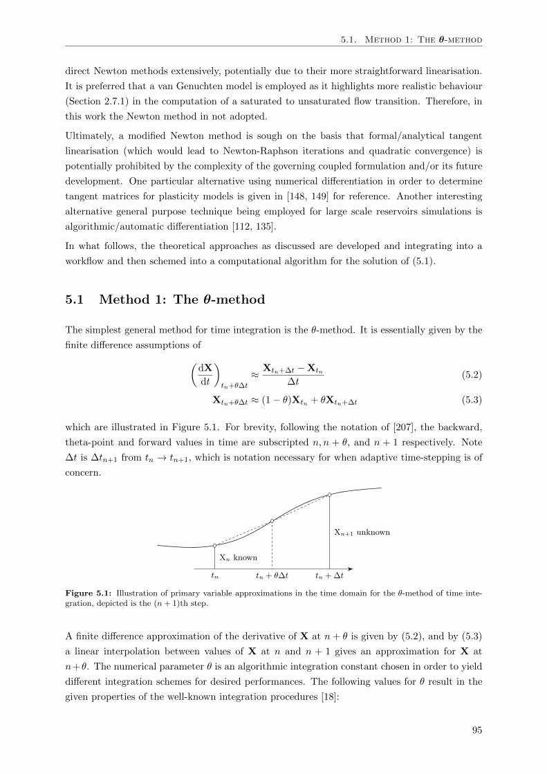
5.1. Method 1: The θ-method
direct Newton methods extensively, potentially due to their more straightforward linearisation.
It is preferred that a van Genuchten model is employed as it highlights more realistic behaviour
(Section 2.7.1) in the computation of a saturated to unsaturated flow transition. Therefore, in
this work the Newton method in not adopted.
Ultimately, a modified Newton method is sough on the basis that formal/analytical tangent
linearisation (which would lead to Newton-Raphson iterations and quadratic convergence) is
potentially prohibited by the complexity of the governing coupled formulation and/or its future
development. One particular alternative using numerical differentiation in order to determine
tangent matrices for plasticity models is given in [148, 149] for reference. Another interesting
alternative general purpose technique being employed for large scale reservoirs simulations is
algorithmic/automatic differentiation [112, 135].
In what follows, the theoretical approaches as discussed are developed and integrating into a
workflow and then schemed into a computational algorithm for the solution of (5.1).
5.1 Method 1: The θ-method
The simplest general method for time integration is the θ-method. It is essentially given by the
finite difference assumptions of(dX
dt
)tn+θ∆t
≈ Xtn+∆t −Xtn
∆t(5.2)
Xtn+θ∆t ≈ (1− θ)Xtn + θXtn+∆t (5.3)
which are illustrated in Figure 5.1. For brevity, following the notation of [207], the backward,
theta-point and forward values in time are subscripted n, n + θ, and n + 1 respectively. Note
∆t is ∆tn+1 from tn → tn+1, which is notation necessary for when adaptive time-stepping is of
concern.
Figure 5.1: Illustration of primary variable approximations in the time domain for the θ-method of time inte-gration, depicted is the (n+ 1)th step.
A finite difference approximation of the derivative of X at n+ θ is given by (5.2), and by (5.3)
a linear interpolation between values of X at n and n + 1 gives an approximation for X at
n+θ. The numerical parameter θ is an algorithmic integration constant chosen in order to yield
different integration schemes for desired performances. The following values for θ result in the
given properties of the well-known integration procedures [18]:
95
Chapter 5. Temporal Integration & Solution Control
θ = 0, explicit Euler forward method, conditionally stable, first-order accurate in ∆t,
θ = 0.5, implicit trapezoidal rule, unconditionally stable, second-order accurate in ∆t,
θ = 1, implicit Euler backward method, unconditionally stable, first-order accurate in ∆t.
In order to develop a scheme for a solution at n+1 with a known or initial value at n, consider
(5.1) at n+ θ,
Cn+θ
(dX
dt
)n+θ
+Kn+θ Xn+θ = Fn+θ, (5.4)
where the discretised forms (5.2) and (5.3) are substituted giving,
Cn+θ
(Xn+1 −Xn
∆t
)+Kn+θ [(1− θ)Xn + θXn+1] = Fn+θ. (5.5)
Expanding and grouping the terms gives the following common single-stage single-step schemes
for the solution of Xn+1, which belong to the weighted Euler difference family,
[C + θ∆tK]n+θ Xn+1 = [C − (1− θ)∆tK]n+θ Xn +∆tFn+θ. (5.6)
The coefficient matrices and forcing conditions here are evaluated as
Cn+θ = C(Xn + θ∆tXn+θ) (5.7)
Kn+θ = K(Xn + θ∆tXn+θ) (5.8)
Fn+θ = F(Xn + θ∆tXn+θ) (5.9)
which are strongly dependent on the primary/state variables, highlighting the requirement for
an appropriate iterative strategy for the solution of (5.10).
This result is also derived via a more general weighted residual form [207], and is denoted as
the SS11 algorithm. In SSpj notation this is a Single-Step method of a polynomial approxi-
mation/expansion of degree one, p = 1, to solve a differential equation of first-order, j = 1
(O(∆tj)). It is now presented in the more computationally/algorithmically useful two-stage
single-step form of
[C + θ∆tK]n+θ Xn+θ = −Kn+θXn +Fn+θ (5.10)
Xn+1 = Xn +∆tXn+θ (5.11)
where Xn+θ is the O(∆t) approximation of (dX/dt)n+θ over the time-step ∆t, (5.2). This
two-stage form also follows from rearranging (5.5) in terms of Xn+θ and on inspection again of
(5.2).
5.2 Method 2: The Thomas-Gladwell method
A class of algorithms proposed in [207] deals with multi-stage single-step methods for both first-
and second-order differential equations. A particular method known as the SS21 algorithm of
which [190] proposes a more generalised form is incorporated. This method has three integration
96
5.3. Embedded backward-Euler/Thomas-Gladwell pair
parameters which makes it flexible for efficient embedding with the θ-method. The method is
presented as a two-stage single-step procedure as follows,
[ϕ2∆tC + ϕ3∆t2K] ¨Xn = −C ˙Xn −K[Xn + ϕ1∆t
˙Xn] +Fn+ϕ1 (5.12)
Xn+1 = Xn +∆t ˙Xn +1
2∆t2 ¨Xn (5.13)
where
¨Xn = ( ˙Xn+1 − ˙Xn)/∆t (5.14)
is the approximation of (d2X/dt2)n as an average estimate over the time step ∆t. The coefficent
matrices and forcing conditions are evaluated as
Cn+ϕ = C(Xn + ϕ1∆t˙Xn + ϕ3∆t
2 ¨Xn) (5.15)
Kn+ϕ = K(Xn + ϕ1∆t˙Xn + ϕ3∆t
2 ¨Xn) (5.16)
Fn+ϕ = F(Xn + ϕ1∆t˙Xn + ϕ3∆t
2 ¨Xn). (5.17)
The schemes of (5.12) are unconditionally stable given 2ϕ3 ≥ ϕ1 ≥ 0.5 and ϕ2 ≥ 0.5 [190]. They
are also second-order accurate, O(∆t2) convergent, for first-order ODEs given ϕ1 = ϕ2 [104].
Equation (5.12) is rearranged such that it can be embedded with the Euler schemes via the
substitution of (5.14) as follows
[ϕ2C + ϕ3∆tK] ˙Xn+1 = [(ϕ2 − 1)C ˙Xn + (ϕ3 − ϕ1)∆tK ˙Xn]−KXn +Fn+ϕ1 (5.18)
Xn+1 = Xn +1
2∆t( ˙Xn + ˙Xn+1) (5.19)
The SS11 equation (5.10) and the rearranged Thomas-Gladwell equation (5.18) are of the same
form and can be made the same by setting θ = ϕ1 = ϕ3 and ϕ2 = 1. However, updates to the
schemes (5.11) and (5.19) approximate with adjacent O(∆t) and O(∆t2) accuracies respectively,
given θ 6= 0.5. Setting in this manner where the derivatives ˙Xn+1 ≡ Xn+θ coincide, means that
the solution of one nonlinear system is required at each time-step thereby promoting considerable
efficiency.
5.3 Embedded backward-Euler/Thomas-Gladwell pair
The two integration methods are embedded via setting θ = ϕ1,2,3 = 1. This employs the
fully implicit backward Euler method which is prevalent in hydrogeology and in engineering
practice due to its robustness in the face of stiff ODE systems (typical of the discretisations
in this work), unconditional stability, damping behaviour towards unwanted oscillations1, and
resilience to abrupt changes in forcing/boundary conditions. Its first-order accuracy is also
sufficient for the practicalities involved with subsurface modelling. However, embedded with
the Thomas-Gladwell method an estimate of its local truncation error can be given for adaptive
97
Chapter 5. Temporal Integration & Solution Control
purposes.
Combining the methods as outlined the embedded system is now given,
[C +∆tK]n+1 Xn+1 = [Fn+1 −Kn+1Xn] (5.20)
Xn+1 = Xn +∆tXn+1 (5.21)
Xn+1 = Xn +1
2∆t(Xn+1 + Xn) (5.22)
where Xn+1 and Xn+1 are now the local first- and second-order estimates. The coefficent
matrices and forcing conditions are evaluated as
Cn+1 = C(Xn+1) (5.23)
Kn+1 = K(Xn+1) (5.24)
Fn+1 = F(Xn+1). (5.25)
Essentially, by averaging the derivatives as of (5.22) the accuracy of the approximation is raised
locally. Note however that the backward Euler method is employed as the solution and thus the
evaluation of (5.21) is carried to the next time-step as Xn throughout. It is the O(∆t2) estimate
of the local truncation error of (5.21), occurring at the n+1 step, that is given by the difference
|Xn+1 − Xn+1| =1
2∆t|Xn+1 − Xn| =
1
2∆t2|Xn|, (5.26)
which can also be shown through Taylor expansion.
5.4 Nonlinear solver
The coupled problem (5.20) is to be solved at a fixed point in time. In abstract form it can be
viewed as a fixed-point problem
Xn+1 = f(Xn+1) (5.27)
which is equivalent to the nonlinear system
g(Xn+1) = 0 (5.28)
given by the residual operator g as defined by
g(Xn+1) ≡ f(Xn+1)−Xn+1. (5.29)
This problem can be solved by successive substitution in the way of
Xs+1n+1 = f(Xs
n+1) (5.30)
1 This seems in apparent contradiction with Section 5.1, where θ = 0.5 demonstrates better performance thanθ = 1. However explanation is that the accuracy of discretisation is judged both in time and space.
98
5.4. Nonlinear solver
where s denotes the iteration count within each time-step. For any initial input vector, X0n+1,
this process is convergent if the function f satisfies the assumption of the Banach contraction
mapping theorem [145]. A fixed-point iteration is also described as a self-consistent field (SCF)
iteration, which finds x ∈ Rn such that x = f(x) given f : Rn → Rn. Self-consistence is achieved
when the input and output vectors coincide or, equivalently, when the residual vector tends to
zero [145].
5.4.1 Solver
At each iteration the set of linearised equations to be solved are of the form Ax = b (Equa-
tion 5.20). Due to the formulation as it stands which is typical of a monolithic coupled finite
element problem, A is sparse and unsymmetric. This burden on solving for x is placed on the
UMFPACK (Unsymmetrical Multi-Frontal) solver [51]. These routines use direct sparse LU
factorisation (Cholesky decomposition) where the matrix is computed as an assemblage of sub-
matrices (which can be referred to as elements analogous with the FE method) which coordinate
as a front [98] of subsets to which dense matrix operations can then be applied. This process can
be carried out with multiple fronts [52] in order to save time and allow for work to be carried
out parallelised if desired amongst other efficiencies as explored in associated work. UMFPACK
is written in ANSI/ISO C and is interfaced in this work within the Matlab environment.
If larger (and potentially 3D) domains are modelled, partitioned and/or projected (conju-
gate gradient-like) iterative methods may be required such as the biconjugate gradient sta-
bilised method (Bi-CGSTAB). Pre-conditioning may also be required in order to prevent ill-
conditioning, however such methods show potential for coupled consolidation equations [67].
5.4.2 Anderson acceleration and mixing
A straightforward fixed-point procedure alone gives slow convergence. Noting that calls to the
solver for coupled and generally for subsurface (large-scale) problems are particularly expensive,
fixed-point procedures are sometimes not an option, particularly when many solver calls do
not bring about convergence. On the other hand difficulties also arise using standard Newton
methods because the Jacobian is explicitly required at each iteration. The Jacobian in some
instances is unavailable analytically or difficult and/or expensive to obtain numerically.
An effective nonlinear solver is devised in this work through selective time-stepping, as discussed
in the following section, and via a modified fixed-point method which employs Anderson mixing
in order to improve and accelerate convergence of the iterations for each selected time-step.
Firstly, a simple mixing scheme is introduced. Consider ‘mixing’ the input and output vectors
of a fixed-point iteration in the following linear fashion in order to produce an input vector for
the forthcoming iteration, s+ 1,
Xs+1 = Xs + βs(f(Xs)−Xs) (5.31)
= Xs + βsRs (5.32)
99
Chapter 5. Temporal Integration & Solution Control
where R now denotes the residual vector as of (5.29), and 0 ≤ βs ≤ 1 is a mixing or damping
parameter which can be altered over the iterations. Note that field operator f was introduced
in (5.27) to denote the operation performed on the primary variables in order to solve (5.20),
however it may also be considered as a general nonlinear operation. Setting βs = 0 will take
the old input vector through again and βs = 1 will take the output vector directly through,
essentially undamped. This factor is beneficial for systems which are prone to producing oscil-
lations or divergence when the initial estimates are far from the solution. Again convergence
is relatively slow, however it is to be viewed that this is due to (5.32) taking information only
from the immediate iteration vectors.
Anderson acceleration mixing improves on this notion by processing information of the vectors
from previous successive iterations powerfully in order to bring about faster convergence. The
processing may begin after some initial iterations have been computed sstartA, as some initial
iterations may not pose as useful a degree of information on indicating system convergence as
the iterations which follow. For the same reason some maximum number of the latest iterations
mmax may be specified for processing alone if/once reached. Considering therefore a modified
form of Anderson acceleration where the latest m + 1 iteration inputs (Xs−m, . . . ,Xs), are
processed with the corresponding residual outputs (Rs−m, . . . ,Rs) via the linear combinations,
Xs = Xs −s−1∑
i=s−m
γi(s)∆Xi = Xs −X sγ(s) (5.33)
Rs = Rs −s−1∑
i=s−m
γi(s)∆Ri = Rs −Rsγ(s) (5.34)
where ∆Xi = Xi+1 − Xi and ∆Ri = Ri+1 − Ri, and the arrays X s = [∆Xs−m, . . . ,∆Xs−1]
and Rs = [∆Rs−m, . . . ,∆Rs−1]. Essentially, Xs and Rs are weighted averages of the previous
vectors Xs−m, . . . ,Xs and Rs−m, . . . ,Rs respectively, weighted through the arguments γ(s) =
(γs−m, . . . , γs−1)T determined by the minimisation
minγ(s)=(γs−m,...,γs−1)T
‖Rs −Rsγ(s)‖2, (5.35)
which minimises the weighted average of the corresponding residuals in order to find a tan-
gent/Newton direction for the next iteration from the optimal linear combination of vectors, X
and R, within the space spanned by previous iterations. The successive unconstrained least-
squares problem (5.35) is solved efficiently by updating factors in a R = QR decomposition
[198]. Note that the notion of weighted averages is visualised easier on expanding (5.33 & 5.34),
and had the formulation begun in this manner a constrained least-squares problem would be
encountered. On solving the unconstrained version, the accelerated update is then given by
combining the results of (5.33), (5.34) and (5.35) in the form of (5.32) giving
Xs+1 = Xs + βsRs (5.36)
= Xs + βsRs − (X s + βsRs)γ(s), (5.37)
which weights the latest specified m vector iterations and residuals in a manner that minimises
100
5.5. Control theory: Adaptive time-step size control
the weighted average residual for accelerated convergence. On setting mmax = 0, the scheme
defaults to simple mixing as no iterations are processed/weighted. Anderson acceleration mixing
(5.37) is also shown to be equivalent to a multisecant quasi-Newton (secant updating) method
[62, 198], where Newton steps are shown to be formed in the way of implicitly approximated
inverse Jacobians, for g(X) ≡ f(X)−X, (potentially better than updating the Jacobian itself)
from all the available secant information depending on m. This different but complementary
point of view happens to derive an equivalent Broyden update (second Broyden method), a
vantage which might prove useful for further developments.
This non-intrusive device for improving the convergence of vector sequences is employed at each
time-step and is also able to benefit from receiving improved initial estimates from the embedded
temporal integration scheme due to the higher order information available.
5.4.3 Tolerance
A residual tolerance, τR must be specified in order for the convergence procedure to terminate
when
‖Xs+1n+1 −Xs
n+1‖ ≤ τR = τ rR‖Xs+1n+1‖+ τaR. (5.38)
The convergence check combines both a relative, τ rR and a much smaller absolute, τaR tolerance
[180] such that any ill-conditioning with the relative measure is avoided if any near zero values
were to appear in the solution vector. It is also sensible to monitor the sub-vectors of each of
the coupled domains independently, such that
maxX=u,pfi ,T
‖Xs+1
n+1 −Xsn+1‖
τ rR‖Xs+1n+1‖+ τaR
≤ 1 (5.39)
benefits the formulation, especially if the sub-vectors are computed in a staggered manner where
each may undergo different rates of time stepping depending on their respective error control.
It is common for either the Euclidean norm ‖ · ‖2 or the maximum norm ‖ · ‖∞ (which renders a
‘critical’ node with the maximum error) to be used in these circumstances, for both truncation
and residual errors.
5.5 Control theory: Adaptive time-step size control
5.5.1 Optimal error control for the integration procedure
From the converged iterations the local truncation error estimate can now be determined as of
(5.26), which in turn can be used to control errors within the system through selective time-
stepping. Firstly, following the control-theoretical techniques for time-step size selection for
differential equations [76, 179], the elementary local error control algorithm is given. For an
integration method of order p the local truncation error ε is asymptotically proportional to the
101
Chapter 5. Temporal Integration & Solution Control
time-step size ∆t. This is shown via Taylor expansion [78], considering
ε = y(t0 +∆t)− y1 (5.40)
expanded by
y(t0 +∆t) = y(t0) + y(t0)∆t+ y(t0)∆t2
2!+ . . . (5.41)
hence, while introducing appropriate subscript indices,
εn = Φn∆tp+1n +O(∆tp+2
n ) (5.42)
where Φ contains error coefficients and differentials of the method, which may also be regarded
as a function, Φ(t, x). If it is assumed that Φ varies slowly (and is therefore assumed constant),
a discrepancy between the local truncation error at n and a desired tolerance τT can therefore
be eliminated via the elementary controller:
∆tn+1 = ∆tn
(τTεn
) 11+p
. (5.43)
This control strategy can also be demonstrated more directly with the proposed embedded
methods. From (5.26) and (5.14), if the error to be controlled is
Xn+1 − Xn+1 =1
2∆tn+1(Xn+1 − Xn) =
1
2(∆tn+1)
2Xn ≈ (∆tn+1)2Xn − Xn
(∆tn)2, (5.44)
if Xn ≈ Xn−1, which is permissible while considering O(∆t) accuracy and slow variation, and
if it is required that this error at n+ 1 is to be less than a tolerance τT, then
(∆tn+1)2 ‖Xn − Xn‖
(∆tn)2≤ τT = τ rT‖Xn‖+ τaT, (5.45)
from which
∆tn+1 ≤ ∆tn
(τ rT‖Xn‖+ τaT‖Xn − Xn‖
) 12
(5.46)
gives an appropriate indication for the next time-step size with information gathered from the
current time-step n [103].
If after initial step size control on computation of Xn+1, εn+1 > τT, then the step is rejected
and repeated with the new more accurate error estimate εn+1 replacing εn, along with ∆tn+1
replacing ∆tn in the control equation. This is such that the step is repeated with a smaller step
size and so on until the step is accepted. Hence, where large truncation errors are prevalent
then the scheme will reduce the step sizes accordingly.
Clearly rejected steps give unwanted computational expense, so a more stable scheme which can
anticipate step size reductions before rejection is desirable. The elementary scheme may lead to
poor error control due to:
- The properties of the system of equation may change significantly with the solution such
102
5.5. Control theory: Adaptive time-step size control
that Φn and Φn−1 do not approximate.
- The error may behave as if p + 1 is either smaller or larger than expected due to the
stiffness of the problem or if higher-order terms become dominant [178].
In order to account more robustly for the error trends during computation both integral and
proportional factors are incorporated into the controller [77]:
∆tn+1 = ∆tn
(τTεn
)kI(εn−1
εn
)kP
. (5.47)
The PI controller accounts for error trends whereby if ε is progressively decreasing over the
steps the proportional factor will be become greater than 1, and provided kP > 0, a faster step
size growth will occur than with the integral factor alone, and conversely for a progressively
increasing error a faster step size reduction will occur. The integral and proportional gain
parameters kI and kP are an area of study for a given system of equations and should be chosen
to obtain suitable dynamics for that system.
The PI controller is incorporated into the design of the time integration algorithm, complement-
ing the acceleration method, as discussed.
5.5.2 Optimal convergence control for an accelerated fixed-point iteration
method
It is sought that the step size be further restricted (if necessary) such that there is optimal
convergence. To do so the controller must aim for a convergence rate Copt that provides the most
efficient integration [75, 145]. The convergence rate C is proportional to the size of time-step
and the (unknown) Jacobian, and if the change in Jacobian is small then a successive step size
can be given by
∆tCn+1 = ∆tnCopt
Cn, (5.48)
such that in the next step Cn+1 → Copt. A more sophisticated control is generally not sought
given the significant approximations in estimating the parameters involved.
A inexpensive option for determining the convergence rate is through considering three consec-
utive iterations, whereby
Cn = maxCsn = max
s
‖Xs+1n −Xs
n‖‖Xs
n −Xs−1n ‖
(5.49)
which gives an estimate of the asymptotic convergence rate that is generally linear for both
fixed-point and modified newton-methods [75].
An optimal convergence rate Copt, is however still required such that the controller can aim
for the most efficient integration. In the literature [75, 145] methods are demonstrated for es-
timating its value for given systems, with estimates given for both fixed-point and modified
newton-methods. There is therefore potential scope for formulation specifically for the acceler-
ated fixed-point procedure by considering the quasi-Newton Jacobian information as is discussed.
In this work, control is dictated by computational accuracy for now, balancing computational
103
Chapter 5. Temporal Integration & Solution Control
accuracy with computational effort per unit step is therefore a point for further study as is dis-
cussed further in Section 6.8. The view is that a step size increase should not cause an increase
in computational effort per unit step, a value of C should therefore be sought that minimises
s/∆t.
5.5.3 Management of truncation error and convergence control
In order that an optimal selection of time-step size is made in terms of balancing accuracy and
unnecessary computational effort per unit step, the minimum ∆tn+1 from both control criteria
(if known) is selected,
∆tn+1 = min(∆tεn+1, ∆tCn+1). (5.50)
For the final algorithm, filtering by judicious coding is applied in order to prevent any aggressive
stepping,
∆t+ = ∆t ·max(fmin,min(fmax, s · fε, s · fC)). (5.51)
This ensures that stepping will progress in a controlled manner, or as desired for investigation,
due to the lower and upper factor bounds, fmin and fmax respectively, with none to minimal
rejected steps, enforced by a safety factor, s ≈ 0.51/1+p [77, 78, 102, 173]. Tighter enforcement
may also follow after rejected steps and the error values should also be coordinated in this filter
with the machine precision, on which the code runs.
5.6 Initial variable values and time-step size
5.6.1 Initial derivative
An initial derivative Xn is required for the update (5.22) at the first time-step. This is provided
by solving (5.20) for ∆t = 0 with the initial and boundary conditions, that is
[C0]X0 = [F0 −K0X0]. (5.52)
Afterwards, the successive solutions for Xn+1 are substituted in the next step as Xn.
5.6.2 Initial time-step size
A coarse initial time-step size estimate may be selected and then handled by the controller. If
the time-step size is too large it will be rejected by the controller and reduced, if too small it
will be increased. A coarse estimate may therefore prove inefficient, in order to provide a more
consistent estimation for ∆t0 the following is given
∆t0 =s · τ
11+p
T
‖X0‖/‖X0‖, (5.53)
which is in line with (5.46) and is based on series expansion [102, 173].
104
5.7. Conditioning spatial and temporal discretisation
5.6.3 Initial estimate for the nonlinear solver
It is clear that the selection ofX0n+1 for the first iteration of the nonlinear solver in each time-step
is important for the robustness and efficiency of the solver, as it is from this value that the final
solution must converge. Generally Xn is reused for this purpose, however with the adaptive
scheme employed higher order information is available in order to give a quadratic estimate
[176], simply
X0n+1 = Xn + (∆tn+1)Xn +
1
2(∆tn+1)
2Xn−1 (5.54)
where the last term can be related to the truncation error (5.26) and therefore ensures accuracy
while also being implicitly controlled by the adaptive scheme.
5.7 Conditioning spatial and temporal discretisation
For modelling a consolidation/heave and/or extraction/injection scenario the controller deter-
mines relatively small initial time-step sizes. This is in order to avoid the prescribed truncations
errors given the order in accuracy of the time integration scheme (5.20) and the high initial
variable gradients at the onset of an instantaneous forcing (traction/flux) condition. Note that
the step sizes will generally increase as the system of equations steps through time due to the
transient nature of equation (5.1).
For small step sizes however, in coupled Biot-type formulations, it is observed and reported (i.e.
[177, 176] and the references therein) that during the early stages of loading (with particular
reference to consolidation problems) spatial oscillations occur in the pore pressure distribution
at free draining boundaries. These oscillations dissipate over time, however they can be avoided.
The problem arises particularly due to ill-conditioning of the [C +∆tK] matrix, where if ∆t is
relatively small it can exacerbate the difference in magnitude between the matrix pivots and
thus cause numerical difficulties. The differences in magnitude come from the simultaneous
integration of the coupled solid mechanical and fluid flow equations which in themselves bring
about matrix terms of opposite numerical extremes.
So although decreasing the early step sizes controls the temporal discretisation truncation error,
doing so may cause spatial oscillations. Rather than increasing the initial step sizes to placate
spacial oscillations at the cost of larger truncation errors which will also stress the convergence
behaviour of the nonlinear solver, it is sought to reduce the critical step size of the system
at which spacial oscillations occur in order to facilitate the controller and nonlinear solver, as
developed. Note also that for a nonlinear system larger uncontrolled step sizes also require more
iterations which may oscillate and/or fail to converge.
A critical step size may be indicated by assessing in particular the system parameters and finite
elements sizes which directly affect the ill-conditioning, as is discussed in [65, 177]. For consol-
idation problems in particular, the critical step size is inversely proportional to the mechanical
stiffness and conductivity of the porous system and proportional to the characteristic size of
the finite element mesh refinement at the boundary involved. Therefore, by refining the mesh
appropriately spacial oscillations are avoided.
105
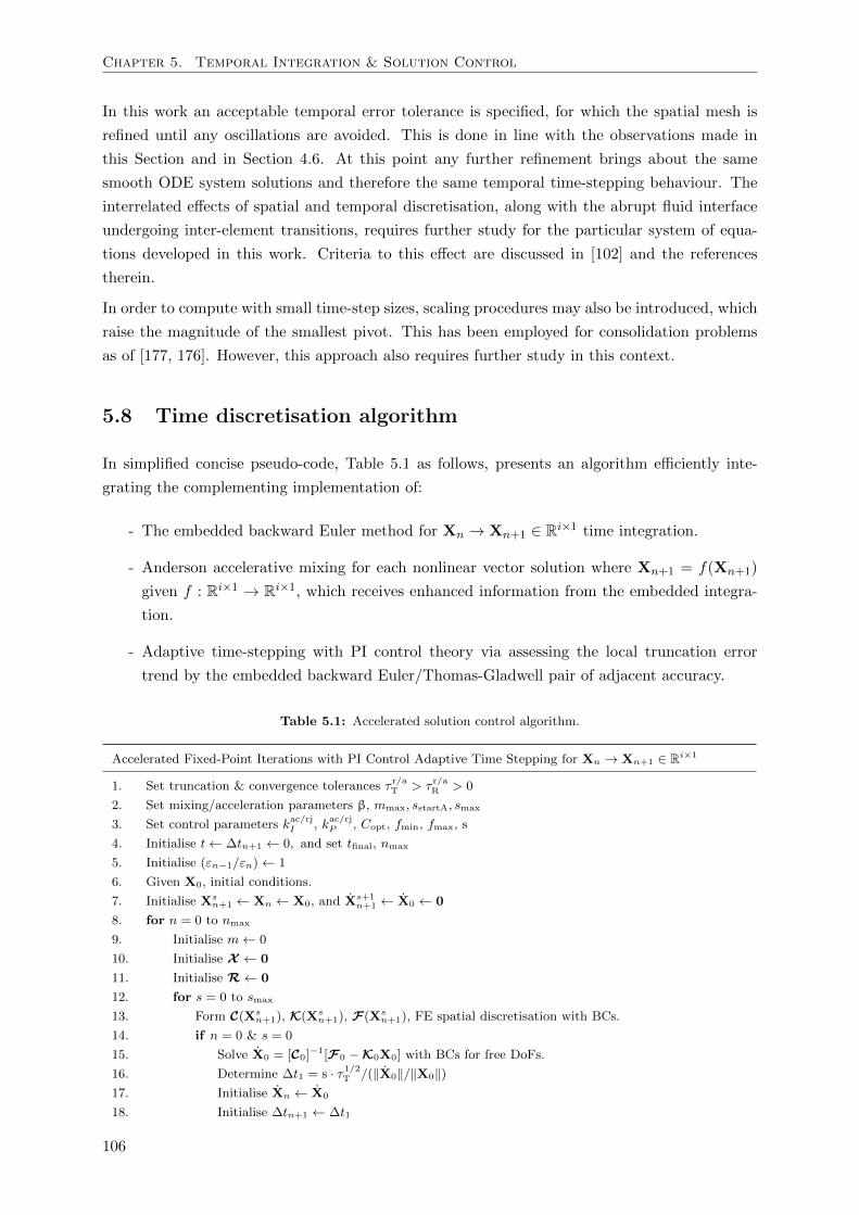
Chapter 5. Temporal Integration & Solution Control
In this work an acceptable temporal error tolerance is specified, for which the spatial mesh is
refined until any oscillations are avoided. This is done in line with the observations made in
this Section and in Section 4.6. At this point any further refinement brings about the same
smooth ODE system solutions and therefore the same temporal time-stepping behaviour. The
interrelated effects of spatial and temporal discretisation, along with the abrupt fluid interface
undergoing inter-element transitions, requires further study for the particular system of equa-
tions developed in this work. Criteria to this effect are discussed in [102] and the references
therein.
In order to compute with small time-step sizes, scaling procedures may also be introduced, which
raise the magnitude of the smallest pivot. This has been employed for consolidation problems
as of [177, 176]. However, this approach also requires further study in this context.
5.8 Time discretisation algorithm
In simplified concise pseudo-code, Table 5.1 as follows, presents an algorithm efficiently inte-
grating the complementing implementation of:
- The embedded backward Euler method for Xn → Xn+1 ∈ Ri×1 time integration.
- Anderson accelerative mixing for each nonlinear vector solution where Xn+1 = f(Xn+1)
given f : Ri×1 → Ri×1, which receives enhanced information from the embedded integra-
tion.
- Adaptive time-stepping with PI control theory via assessing the local truncation error
trend by the embedded backward Euler/Thomas-Gladwell pair of adjacent accuracy.
Table 5.1: Accelerated solution control algorithm.
Accelerated Fixed-Point Iterations with PI Control Adaptive Time Stepping for Xn → Xn+1 ∈ Ri×1
1. Set truncation & convergence tolerances τr/aT > τ
r/aR > 0
2. Set mixing/acceleration parameters β, mmax, sstartA, smax
3. Set control parameters kac/rjI , k
ac/rjP , Copt, fmin, fmax, s
4. Initialise t← ∆tn+1 ← 0, and set tfinal, nmax
5. Initialise (εn−1/εn)← 1
6. Given X0, initial conditions.
7. Initialise Xsn+1 ← Xn ← X0, and Xs+1
n+1 ← X0 ← 0
8. for n = 0 to nmax
9. Initialise m← 0
10. Initialise X ← 0
11. Initialise R← 0
12. for s = 0 to smax
13. Form C(Xsn+1), K(Xs
n+1), F(Xsn+1), FE spatial discretisation with BCs.
14. if n = 0 & s = 0
15. Solve X0 = [C0]−1[F0 −K0X0] with BCs for free DoFs.
16. Determine ∆t1 = s · τ1/2T /(‖X0‖/‖X0‖)17. Initialise Xn ← X0
18. Initialise ∆tn+1 ← ∆t1
106
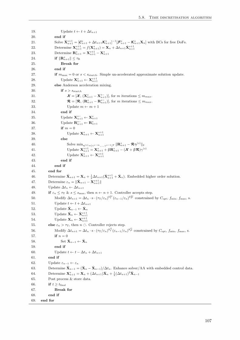
5.8. Time discretisation algorithm
19. Update t← t+∆tn+1
20. end if
21. Solve Xs+1n+1 = [Cs
n+1 +∆tn+1Ksn+1]
−1[Fsn+1 −Ks
n+1Xn] with BCs for free DoFs.
22. Determine Xs+1n+1 = f(Xs
n+1) = Xn +∆tn+1Xs+1n+1
23. Determine Rsn+1 = Xs+1
n+1 −Xsn+1
24. if ‖Rsn+1‖ ≤ τR
25. Break for
26. end if
27. if mmax = 0 or s < sstartA. Simple un-accelerated approximate solution update.
28. Update Xsn+1 ← Xs+1
n+1
29. else Anderson acceleration mixing.
30. if s > sstartA
31. X = [X , (Xsn+1 −Xs−
n+1)], for m iterations ≤ mmax.
32. R = [R, (Rsn+1 −Rs−
n+1)], for m iterations ≤ mmax.
33. Update m← m+ 1
34. end if
35. Update Xs−n+1 ← Xs
n+1
36. Update Rs−n+1 ← Rs
n+1
37. if m = 0
38. Update Xsn+1 ← Xs+1
n+1
39. else
40. Solve minγ(s)=(γs−m,...,γs−1)T ‖Rsn+1 −Rγ(s)‖2
41. Update Xs+1n+1 = Xs
n+1 + βRsn+1 − (X + βR)γ(s)
42. Update Xsn+1 ← Xs+1
n+1
43. end if
44. end if
45. end for
46. Determine Xn+1 = Xn + 12∆tn+1(X
s+1n+1 + Xn). Embedded higher order solution.
47. Determine εn = ‖Xn+1 −Xs+1n+1‖
48. Update ∆tn ← ∆tn+1
49. if εn ≤ τT & s ≤ smax, then n← n+ 1. Controller accepts step.
50. Modify ∆tn+1 = ∆tn · s · (τT/εn)kacI (εn−1/εn)
kacP constrained by Copt, fmin, fmax, s.
51. Update t← t+∆tn+1
52. Update Xn−1 ← Xn
53. Update Xn ← Xs+1n+1
54. Update Xn ← Xs+1n+1
55. else εn > τT, then n . Controller rejects step.
56. Modify ∆tn+1 = ∆tn · s · (τT/εn)krjI (εn−1/εn)
krjP constrained by Copt, fmin, fmax, s.
57. if n = 0
58. Set Xn−1 ← Xn
59. end if
60. Update t← t−∆tn +∆tn+1
61. end if
62. Update εn−1 ← εn
63. Determine Xn−1 = (Xn − Xn−1)/∆tn. Enhance solver/AA with embedded control data.
64. Determine Xsn+1 = Xn + (∆tn+1)Xn + 1
2(∆tn+1)
2Xn−1
65. Post process & store data.
66. if t ≥ tfinal67. Break for
68. end if
69. end for
107
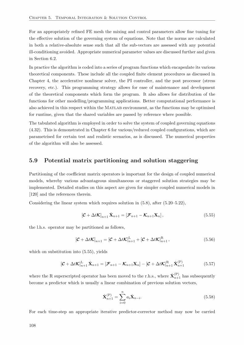
Chapter 5. Temporal Integration & Solution Control
For an appropriately refined FE mesh the mixing and control parameters allow fine tuning for
the effective solution of the governing system of equations. Note that the norms are calculated
in both a relative-absolute sense such that all the sub-vectors are assessed with any potential
ill-conditioning avoided. Appropriate numerical parameter values are discussed further and given
in Section 6.2.
In practice the algorithm is coded into a series of program functions which encapsulate its various
theoretical components. These include all the coupled finite element procedures as discussed in
Chapter 4, the accelerative nonlinear solver, the PI controller, and the post processor (stress
recovery, etc.). This programming strategy allows for ease of maintenance and development
of the theoretical components which form the program. It also allows for distribution of the
functions for other modelling/programming applications. Better computational performance is
also achieved in this respect within the Matlab environment, as the functions may be optimised
for runtime, given that the shared variables are passed by reference where possible.
The tabulated algorithm is employed in order to solve the system of coupled governing equations
(4.32). This is demonstrated in Chapter 6 for various/reduced coupled configurations, which are
parametrised for certain test and realistic scenarios, as is discussed. The numerical properties
of the algorithm will also be assessed.
5.9 Potential matrix partitioning and solution staggering
Partitioning of the coefficient matrix operators is important for the design of coupled numerical
models, whereby various advantageous simultaneous or staggered solution strategies may be
implemented. Detailed studies on this aspect are given for simpler coupled numerical models in
[120] and the references therein.
Considering the linear system which requires solution in (5.8), after (5.20–5.22),
[C +∆tK]n+1 Xn+1 = [Fn+1 −Kn+1Xn] , (5.55)
the l.h.s. operator may be partitioned as follows,
[C +∆tK]n+1 = [C +∆tK]Ln+1 + [C +∆tK]Rn+1 , (5.56)
which on substitution into (5.55), yields
[C +∆tK]Ln+1 Xn+1 = [Fn+1 −Kn+1Xn]− [C +∆tK]Rn+1 X(P)n+1 (5.57)
where the R superscripted operator has been moved to the r.h.s., where X(P)n+1 has subsequently
become a predictor which is usually a linear combination of previous solution vectors,
X(P)n+1 =
n∑i=0
aiXn−i. (5.58)
For each time-step an appropriate iterative predictor-corrector method may now be carried
108
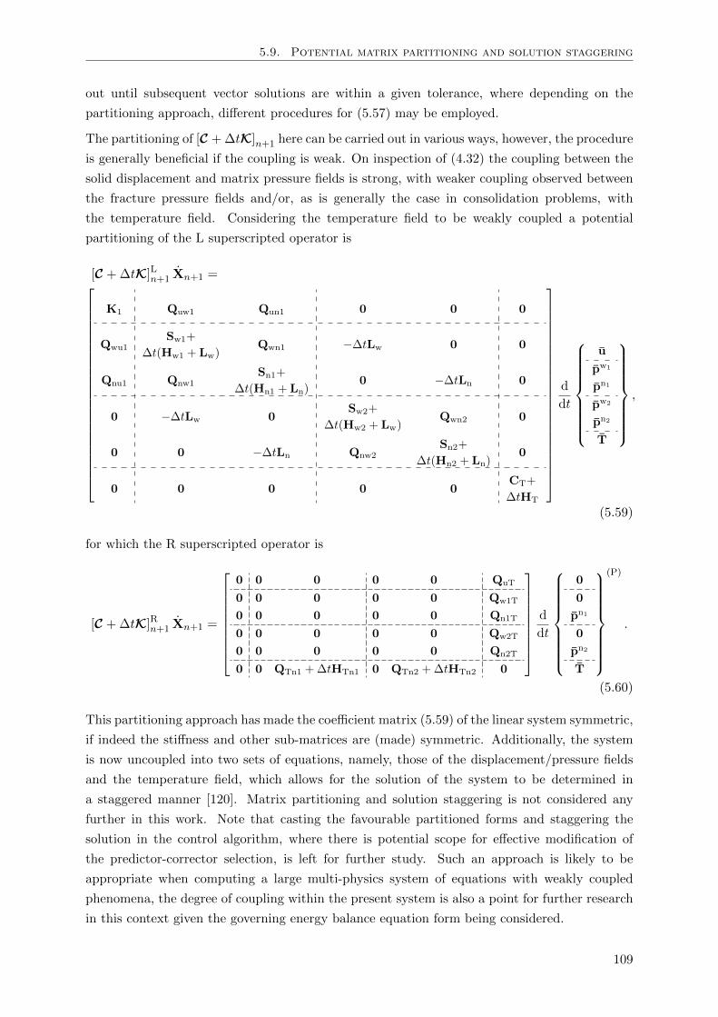
5.9. Potential matrix partitioning and solution staggering
out until subsequent vector solutions are within a given tolerance, where depending on the
partitioning approach, different procedures for (5.57) may be employed.
The partitioning of [C +∆tK]n+1 here can be carried out in various ways, however, the procedure
is generally beneficial if the coupling is weak. On inspection of (4.32) the coupling between the
solid displacement and matrix pressure fields is strong, with weaker coupling observed between
the fracture pressure fields and/or, as is generally the case in consolidation problems, with
the temperature field. Considering the temperature field to be weakly coupled a potential
partitioning of the L superscripted operator is
[C +∆tK]Ln+1 Xn+1 =
K1 Quw1 Qun1 0 0 0
Qwu1Sw1+
∆t(Hw1 + Lw)Qwn1 −∆tLw 0 0
Qnu1 Qnw1Sn1+
∆t(Hn1 + Ln)0 −∆tLn 0
0 −∆tLw 0Sw2+
∆t(Hw2 + Lw)Qwn2 0
0 0 −∆tLn Qnw2Sn2+
∆t(Hn2 + Ln)0
0 0 0 0 0CT+
∆tHT
d
dt
u
pw1
pn1
pw2
pn2
T
,
(5.59)
for which the R superscripted operator is
[C +∆tK]Rn+1 Xn+1 =
0 0 0 0 0 QuT
0 0 0 0 0 Qw1T
0 0 0 0 0 Qn1T
0 0 0 0 0 Qw2T
0 0 0 0 0 Qn2T
0 0 QTn1 +∆tHTn1 0 QTn2 +∆tHTn2 0
d
dt
0
0
pn1
0
pn2
T
(P)
.
(5.60)
This partitioning approach has made the coefficient matrix (5.59) of the linear system symmetric,
if indeed the stiffness and other sub-matrices are (made) symmetric. Additionally, the system
is now uncoupled into two sets of equations, namely, those of the displacement/pressure fields
and the temperature field, which allows for the solution of the system to be determined in
a staggered manner [120]. Matrix partitioning and solution staggering is not considered any
further in this work. Note that casting the favourable partitioned forms and staggering the
solution in the control algorithm, where there is potential scope for effective modification of
the predictor-corrector selection, is left for further study. Such an approach is likely to be
appropriate when computing a large multi-physics system of equations with weakly coupled
phenomena, the degree of coupling within the present system is also a point for further research
in this context given the governing energy balance equation form being considered.
109

Chapter 6
Model Results & Performance
In this Chapter the physical and numerical model parametrisations, as introduced and devel-
oped throughout Chapters 2–5, are first discussed further and allocated appropriate base case
valuations for study. Secondly, several key modelling aspects are discussed in the following
sections. Once covered, the numerical model is then trialled through a series of scenarios for
the for verification and validation. This is done in a manner where various simplified subsets
or sub-couplings of the full discretised system of equations are assessed in turn, increasing in
complexity. This approach, along with the realistic physical parametrisations, also allows for the
effects of various couplings within the numerical system to be highlighted. Finally, the numerical
properties and performance of the control algorithm, as developed in Chapter 5, is also assessed.
6.1 Physical parameter base set
The system of equations (4.32) is solved with a series of model parameters which characterise
the hydro-thermo-mechanical-chemical behaviour of the phases within the reservoir system,
as introduced in Chapter 2 and worked into the system of governing field equations. These
parameters are collected and listed in Table 6.1, along with their symbol, valuation and units.
The parameters are initially valued with reference to four extreme scenarios belonging to the
brine aquifer subset of potential geostorage sites, as previously introduced in Section 3.2.6.
For the fluid phases in particular, the parameters are essentially thermophysical properties of
the fluid and are therefore well referenced functions of pressure, temperature and composition
(p-T -x), as discussed in Section 2.6.8.
Following from Chapter 2, EoS program functions are coded that process p-T -x data to give
value to the required fluid properties as parametrised in this work. This stands in part for
future development with respect to updating nonlinear material behaviour. For initial investi-
gation however, unlike for the multiphase flow and saturation behaviour, the individual intrinsic
material phase properties are assumed constant which is generally meaningful in this context
given the extent to which they vary with respect to p-T -x over the ranges of interest. That is,
the primary state variables (u-pw1-pn1-pw2-pn2-T ) are considered to vary moderately such that
the material properties of the system may be considered constant. Therefore, the EoS program
111
Chapter 6. Model Results & Performance
functions are used to initially parametrise the model accurately from reference p-T -x data based
on the reservoir scenario/initial conditions. The six thermophysical properties (ρ-µ-K-β-cp-χ)
of each fluid phase are thus listed in Table 6.1 for reference only, as a numerical simulation may
be parametrised via reference or initial p-T -x data alone in order to describe the fluids.
The thermophysical properties for the CO2 phase are solved for after the work of [20, 64, 166,
181], and for the H2O phase after [8, 7, 58, 105, 106, 151, 160, 161], in which the ranges
of validity, extents of physical accuracy, and the compromise of computational demand and
physical accuracy, of the equations of state developed, are discussed in detail.
For Table 6.1, the CO2-rich phase is parametrised as pure CO2, and the H2O-rich (brine) phase
as a H2O-NaCl solution, both at the reference reservoir p-T values, with no cross composi-
tion/mutual solubility (miscibility), which are acceptable investigative assumptions as discussed
in Section 2.6.8. Sodium chloride is selected as the dissolved component in water as it is the most
common and dominate solute in this context. The salinity of the H2O-NaCl solution (brine)
is parametrised at a mass fraction of 0.1 (mass of salt solute to mass of solution), which is a
molality of 1.9 mol/kg (moles of salt solute to mass of solvent). The accurate thermodynamic
description of saline aqueous fluids are also of particular importance for the modelling and pre-
diction of other engineered and natural large scale hydrogeothermal processes [58]. It is also
because of this that sufficient equations of state exist that efficiently describe this fluid at the
relatively high pressures, temperatures and salinities of interest.
There exist various complexities and points of inversion in the fluid property trends in response
to changes in p-T -x (Section 2.6.8). In addition to the charts given in Section 2, Table 6.1
demonstrates the extent and contrast in property variation between the two fluid phases, over a
realistic range of storage system scenarios. These properties alone can also be used for predicting
important underling storage behaviour (Section 2.7.3). Over the range of pressures and tem-
peratures of interest here, the brine phase properties vary in a relatively slight manner, though
its viscosity shows particular sensitively to temperature. An increase in salinity has the effect
of generally moderate increases in fluid density, viscosity, and bulk modulus, and reductions in
the thermal capacity and conductivity. For the CO2 phase, greater sensitivity is demonstrated
overall with respect to changes in pressure and temperature, though the parameter values gen-
erally remain within the same orders of magnitude. This sensitivity is a consequence of the CO2
phase being within scope of its critical region (Section 2.6.8).
Listed next in Table 6.1, the solid phase (porous medium) physical properties are given char-
acterising its mechanical and thermal behaviour (Section 2.6.4). The valuations are typical of
sandstone formation rock, the mechanical and thermal parameters are determined after [99]
and [141, 129] respectively. Tabulated next are the saturation parameters (Section 2.7), char-
acterising the rock-brine-CO2 system saturation behaviour of the two (matrix and fracture)
sub-domains. The parameterisations for the matrix sub-domain are typical realistic base case
values, demonstrating significant saturation-capillary pressure behaviour and wetting residual
saturation. Note that in practice the rock parameter values will vary in space and due to varia-
tions in pressure and temperature depending on the formation, in this chapter these parameters
are initially considered constant and uniform for the purpose of investigation.
112
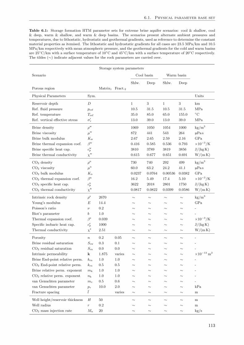
6.1. Physical parameter base set
Table 6.1: Storage formation HTM parameter sets for extreme brine aquifer scenarios: cool & shallow, cool& deep, warm & shallow, and warm & deep basins. The scenarios present alternate ambient pressures andtemperatures, due to lithostatic, hydrostatic and geothermal gradients, used as reference to determine the constantmaterial properties as itemised. The lithostatic and hydrostatic gradients for all cases are 23.5 MPa/km and 10.5MPa/km respectively with mean atmospheric pressure, and the geothermal gradients for the cold and warm basinsare 25C/km with a surface temperature of 10C and 45C/km with a surface temperature of 20C respectively.The tildes (∼) indicate adjacent values for the rock parameters are carried over.
Storage system parameters
Scenario Cool basin Warm basin
Shlw. Deep Shlw. Deep
Porous region Matrix1 Fract.2
Physical Parameters Sym. Units
Reservoir depth D 1 3 1 3 km
Ref. fluid pressure pref 10.5 31.5 10.5 31.5 MPa
Ref. temperature Tref 35.0 85.0 65.0 155.0 C
Ref. vertical effective stress σ′v 13.0 39.0 13.0 39.0 MPa
Brine density ρw 1069 1050 1054 1000 kg/m3
Brine viscosity µw 872 441 543 264 µPa s
Brine bulk modulus Kw 2.67 2.65 2.59 2.16 GPa
Brine thermal expansion coef. βw 0.416 0.585 0.536 0.793 ×10⁻³/K
Brine specific heat cap. cwp 3810 3789 3819 3856 J/(kgK)
Brine thermal conductivity χw 0.615 0.677 0.651 0.691 W/(mK)
CO2 density ρn 730 740 292 499 kg/m3
CO2 viscosity µn 60.0 63.2 24.2 41.1 µPa s
CO2 bulk modulus Kn 0.0237 0.0764 0.00536 0.0382 GPa
CO2 thermal expansion coef. βn 16.2 5.49 17.4 5.10 ×10⁻³/K
CO2 specific heat cap. cnp 3622 2018 2801 1750 J/(kgK)
CO2 thermal conductivity χn 0.0817 0.0822 0.0399 0.0586 W/(mK)
Intrinsic rock density ρs 2670 ∼ ∼ ∼ ∼ kg/m3
Young’s modulus E 14.4 ∼ ∼ ∼ ∼ GPa
Poisson’s ratio ν 0.2 ∼ ∼ ∼ ∼ -
Biot’s parameter b 1.0 ∼ ∼ ∼ ∼ -
Thermal expansion coef. βs 0.039 ∼ ∼ ∼ ∼ ×10−3/K
Specific isobaric heat cap. csp 1000 ∼ ∼ ∼ ∼ J/(kgK)
Thermal conductivity χs 2.51 ∼ ∼ ∼ ∼ W/(mK)
Porosity n 0.2 0.05 ∼ ∼ ∼ ∼ -
Brine residual saturation Srw 0.3 0.1 ∼ ∼ ∼ ∼ -
CO2 residual saturation Srn 0.0 0.0 ∼ ∼ ∼ ∼ -
Intrinsic permeability k 1.875 varies ∼ ∼ ∼ ∼ ×10−13 m2
Brine End-point relative perm. krn 1.0 1.0 ∼ ∼ ∼ ∼ -
CO2 End-point relative perm. krn 0.5 0.5 ∼ ∼ ∼ ∼ -
Brine relative perm. exponent mk 1.0 1.0 ∼ ∼ ∼ ∼ -
CO2 relative perm. exponent nk 1.0 1.0 ∼ ∼ ∼ ∼ -
van Genuchten parameter mv 0.5 0.6 ∼ ∼ ∼ ∼ -
van Genuchten parameter pv 10.0 2.0 ∼ ∼ ∼ ∼ kPa
Fracture spacing l varies ∼ ∼ ∼ ∼ m
Well height/reservoir thickness H 50 ∼ ∼ ∼ ∼ m
Well radius r 0.2 ∼ ∼ ∼ ∼ m
CO2 mass injection rate Mn 20 ∼ ∼ ∼ ∼ kg/s
113
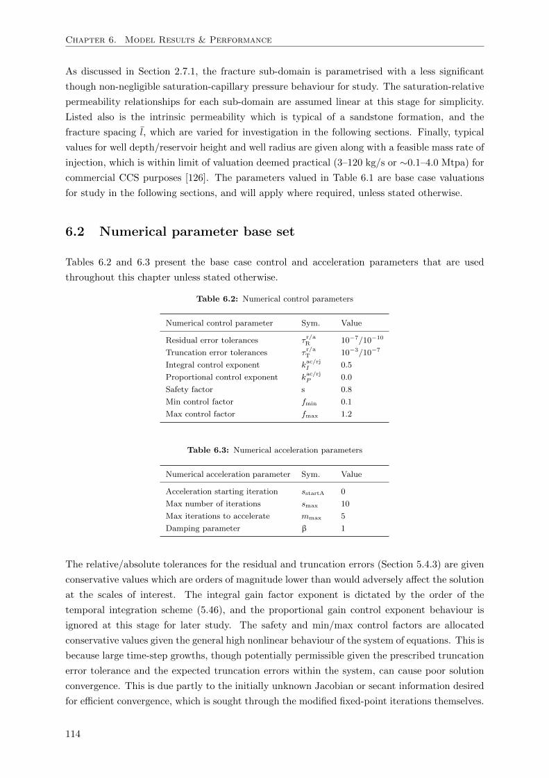
Chapter 6. Model Results & Performance
As discussed in Section 2.7.1, the fracture sub-domain is parametrised with a less significant
though non-negligible saturation-capillary pressure behaviour for study. The saturation-relative
permeability relationships for each sub-domain are assumed linear at this stage for simplicity.
Listed also is the intrinsic permeability which is typical of a sandstone formation, and the
fracture spacing l, which are varied for investigation in the following sections. Finally, typical
values for well depth/reservoir height and well radius are given along with a feasible mass rate of
injection, which is within limit of valuation deemed practical (3–120 kg/s or ∼0.1–4.0 Mtpa) for
commercial CCS purposes [126]. The parameters valued in Table 6.1 are base case valuations
for study in the following sections, and will apply where required, unless stated otherwise.
6.2 Numerical parameter base set
Tables 6.2 and 6.3 present the base case control and acceleration parameters that are used
throughout this chapter unless stated otherwise.
Table 6.2: Numerical control parameters
Numerical control parameter Sym. Value
Residual error tolerances τr/aR 10−7/10−10
Truncation error tolerances τr/aT 10−3/10−7
Integral control exponent kac/rjI 0.5
Proportional control exponent kac/rjP 0.0
Safety factor s 0.8
Min control factor fmin 0.1
Max control factor fmax 1.2
Table 6.3: Numerical acceleration parameters
Numerical acceleration parameter Sym. Value
Acceleration starting iteration sstartA 0
Max number of iterations smax 10
Max iterations to accelerate mmax 5
Damping parameter β 1
The relative/absolute tolerances for the residual and truncation errors (Section 5.4.3) are given
conservative values which are orders of magnitude lower than would adversely affect the solution
at the scales of interest. The integral gain factor exponent is dictated by the order of the
temporal integration scheme (5.46), and the proportional gain control exponent behaviour is
ignored at this stage for later study. The safety and min/max control factors are allocated
conservative values given the general high nonlinear behaviour of the system of equations. This is
because large time-step growths, though potentially permissible given the prescribed truncation
error tolerance and the expected truncation errors within the system, can cause poor solution
convergence. This is due partly to the initially unknown Jacobian or secant information desired
for efficient convergence, which is sought through the modified fixed-point iterations themselves.
114
6.3. Mesh design
The acceleration parameters dictate a scenario where the accelerative mixing occurs from the
first iteration over a maximum of 5 consecutive iterations, with the maximum total number
of iterations set at 10. The damping parameter is fixed at unity, which is an undamped con-
figuration meaning that all residual vectors are passes straight through to the next iteration
un-damped (Section 5.4.2).
6.3 Mesh design
As discussed in Chapters 4 and 5 the adaptivity of spatial discretisation is important and demon-
strates interrelation with the temporal discretisation. For infiltrating variably saturated flows,
coarse spatial discretisation may demonstrate initial oscillations in the spatial solutions and os-
cillation in the time-step size adaptation, assuming that these oscillations are associated with the
saturation front undergoing abrupt transition through the elements. After [102], the Courant
number is trialled as a criterion in order to heuristically balance the space-time discretisation,
Cr = v∆t
∆x, (6.1)
where v is the front velocity, and ∆t and ∆x are the step sizes to be adapted in time and space
respectively. The method trialled initially requires selecting an appropriate temporal truncation
error tolerance from which an initial time-step size, ∆t0 after (5.53), is acquired. Then the
spacial discretisation is selected via Cr ∼ 1. This may either be done heuristically through trial
or via knowledge of an estimate of the front velocity and a rate of growth, r, for ∆t.
For the latter case, a 1D (quasi-2D) axisymmetric front velocity may be estimated after (3.38)
which gives a relationship for the front location as x = C√t, where C is dependent on the
physical system properties (assumed constant) and x is the position of the front, from which a
front velocity v(x) may be given by differentiating, that is v = C2/2x. Relating the time-step
size as of ∆t = ∆t0rn, via geometric series the following time at n may be given,
tn =x2
C2= ∆t0
n∑k=0
rk = ∆t01− rn+1
1− r, (6.2)
which may be isolated for n in terms of the variable x, hence an expression for ∆t(x) may be
given. Letting ∆x(x) = v(x)∆t(x) from the Courant criterion, on substitution the following
analytical function is derived which gives an estimate of the necessary element size ∆x as a
function of position x, in the space domain for its spatial discretisation (meshing) in anticipation
of the front,
∆x(x) =
(C2
2x
)∆t0r
ln
(−x2(1−r)
C2∆t0+1
)ln r
−1. (6.3)
The expression requires an estimate for r, which may be acquired from an initial trial run
of the system of equations in order to determine an estimate of the growth behaviour of ∆t,
which is also dependent on the numerical settings within the controller. In practice however,
the spatial refinement need only be this strict if the saturation behaviour exhibits a sharp
115
Chapter 6. Model Results & Performance
fluid interface/transition, and the refinement criterion formulated should therefore be viewed as
some maximum degree of mesh refinement necessary, particularly for the near well region. An
appropriate spacial discretisation is illustrated in Figure 6.5, which is based on the guidance
and approximate form of (6.3). Note finally that if r is unsteady exhibiting fluctuations during
temporal integration, which is generally the case for relatively coarse meshes through which
sharp fluid interfaces/high numerical gradient attempt to pass, this is generally indicative that
the mesh needs refinement.
6.4 Full saturation to partial saturation flow transition
The GCS problem scenarios considered in this work initially consist of a fully saturated domain
of a wetting fluid phase, into which an initially non-existent nonwetting fluid is injected causing
the domain to become partially saturated. A physical transition therefore has to be modelled
from a single fluid system to a multiple fluid system. Two relevant methods of air/gas-water
desaturation occurring over an originally fully saturated domain are analysed in [120] relevant
to hydro-mechanical coupled equations.
The first method assumes negligibly small, though finite minimum values for the desaturating
nonwetting phase relative permeability and saturation. These values are prescribed and enforced
within the system of equations over the domain regions which are undergoing fully saturated
stages. By doing so the nonwetting phase continuity equation(s) are continuously maintained
throughout computation (see [120, 168] and the references therein).
The second method proposes switching, element-by-element, solutions from single-phase to
multi-phase flow at a specified saturation or capillary pressure. However, in practice there
are various complications in that oscillations occur in the solutions and in the nonlinear iter-
ations during switching of the governing equations [69, 120]. This method also requires that
a minimum nonwetting phase relative permeability be set in order to avoid oscillations in the
solution which would otherwise be due to very small diagonal terms in the coefficient matrices
causing numerical difficulties (ill-conditioning).
This presents an interesting aspect which requires further research in this context. Given the
scope of this work, the first method is adopted for its simplicity at this stage. The minimum
value for the relative permeability of the wetting phase is set to a value of 0.0001 [69, 120].
6.5 Stress recovery
The solid strains of the porous medium are post-processed in order to give the effective stress
state, considering (2.30), (3.47) and (4.87), from
σ′′ = Del(ε− εTh) = DelLNuu−Delm(βs/3)NT T. (6.4)
In accordance with Section 4.4.1, this operation may be performed over the isoparametric finite
elements at points within the natural coordinate system of the element. It is performed for
116
6.6. Visualisation and data management
the 9 node finite element at the 3×3 Gauss-Legendre quadrature points. These points are used
for sampling as they are optimal for determining the stresses (gradients) because they have the
property of superconvergence, as is discussed in [207] following the Herrmann theorem for prob-
lems of elasticity. The function (displacements) sought is demonstrated to be optimally accurate
sampled at the nodes, whereas the gradients of this function (stresses) are optimally sampled
at the Gauss points. This superconvergence is however lost on distortion of the (isoparametric)
element.
For analysis the computed stress components may then be extrapolated from the inner Gauss
points onto the finite element nodes via use of the element shape functions. Due to the degree of
continuity between the elements, discrepancies in the stresses computed at nodes shared by ad-
jacent elements will require averaging. This straight forward technique will however reintroduce
inaccuracies, particularly for higher order elements [207].
For this reason superconvergent patch recovery (SPR), as described in [207], is employed for the
9 node quadratic displacement finite element. The patch of elements surrounding each node is
processed by determining the Gauss point stresses over the patch through which a quadratic
polynomial (same order as the displacement element shape function) is fitted via a least squares
method, in order to recover stresses of superconvergent accuracy at the node for analysis. For
further interesting alternate developments in this context, see [147] and the references therein.
6.6 Visualisation and data management
Model data are output in Visualization Toolkit (VTK) format and rendered with open-source
VTK based libraries for quality visualisation and interaction [2, 13, 169]. This proves effective for
large domains in space and time with multiple overlaid degrees of freedom, allowing additionally
for the parallelisation of large data sets.
6.7 Model verification
The coupled hydro-mechanical, multiphase hydraulic, and fractured hydro-mechanical aspects
of the numerical model are first benchmarked with emphasis on parametrisation taken from
Table 6.1. The coupled hydro-thermal, hydro-thermo-mechanical and fractured hydro-thermo-
mechanical aspects are then benchmarked with reference to a specific subset of parameters which
give rise to some interesting coupled thermal effects as are discussed. This incremental bench-
marking approach introducing increasing complexity, covering geometrically idealised, though
realistic, engineering scenarios is also aimed at providing insight into the physical phenomena
as described by the system of governing equations.
Table 6.4 summarises the engineering problems modelled in the subsections which are to follow,
through which the numerical model is employed with increasing complexity.
117
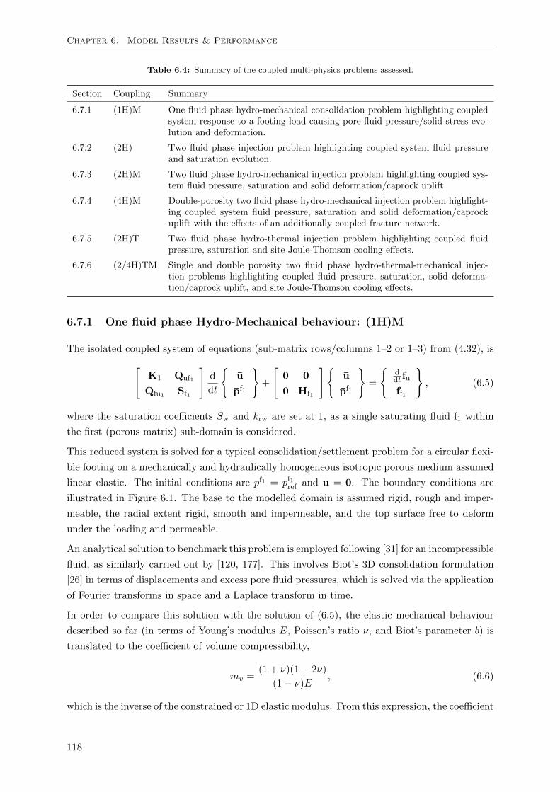
Chapter 6. Model Results & Performance
Table 6.4: Summary of the coupled multi-physics problems assessed.
Section Coupling Summary
6.7.1 (1H)M One fluid phase hydro-mechanical consolidation problem highlighting coupledsystem response to a footing load causing pore fluid pressure/solid stress evo-lution and deformation.
6.7.2 (2H) Two fluid phase injection problem highlighting coupled system fluid pressureand saturation evolution.
6.7.3 (2H)M Two fluid phase hydro-mechanical injection problem highlighting coupled sys-tem fluid pressure, saturation and solid deformation/caprock uplift
6.7.4 (4H)M Double-porosity two fluid phase hydro-mechanical injection problem highlight-ing coupled system fluid pressure, saturation and solid deformation/caprockuplift with the effects of an additionally coupled fracture network.
6.7.5 (2H)T Two fluid phase hydro-thermal injection problem highlighting coupled fluidpressure, saturation and site Joule-Thomson cooling effects.
6.7.6 (2/4H)TM Single and double porosity two fluid phase hydro-thermal-mechanical injec-tion problems highlighting coupled fluid pressure, saturation, solid deforma-tion/caprock uplift, and site Joule-Thomson cooling effects.
6.7.1 One fluid phase Hydro-Mechanical behaviour: (1H)M
The isolated coupled system of equations (sub-matrix rows/columns 1–2 or 1–3) from (4.32), is[K1 Quf1
Qfu1 Sf1
]d
dt
u
pf1
+
[0 0
0 Hf1
]u
pf1
=
ddt fu
ff1
, (6.5)
where the saturation coefficients Sw and krw are set at 1, as a single saturating fluid f1 within
the first (porous matrix) sub-domain is considered.
This reduced system is solved for a typical consolidation/settlement problem for a circular flexi-
ble footing on a mechanically and hydraulically homogeneous isotropic porous medium assumed
linear elastic. The initial conditions are pf1 = pf1ref and u = 0. The boundary conditions are
illustrated in Figure 6.1. The base to the modelled domain is assumed rigid, rough and imper-
meable, the radial extent rigid, smooth and impermeable, and the top surface free to deform
under the loading and permeable.
An analytical solution to benchmark this problem is employed following [31] for an incompressible
fluid, as similarly carried out by [120, 177]. This involves Biot’s 3D consolidation formulation
[26] in terms of displacements and excess pore fluid pressures, which is solved via the application
of Fourier transforms in space and a Laplace transform in time.
In order to compare this solution with the solution of (6.5), the elastic mechanical behaviour
described so far (in terms of Young’s modulus E, Poisson’s ratio ν, and Biot’s parameter b) is
translated to the coefficient of volume compressibility,
mv =(1 + ν)(1− 2ν)
(1− ν)E, (6.6)
which is the inverse of the constrained or 1D elastic modulus. From this expression, the coefficient
118
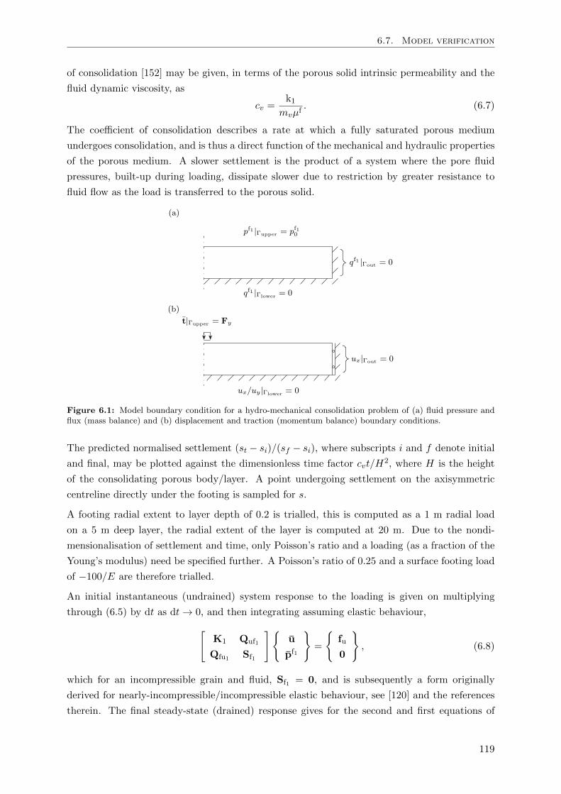
6.7. Model verification
of consolidation [152] may be given, in terms of the porous solid intrinsic permeability and the
fluid dynamic viscosity, as
cv =k1
mvµf. (6.7)
The coefficient of consolidation describes a rate at which a fully saturated porous medium
undergoes consolidation, and is thus a direct function of the mechanical and hydraulic properties
of the porous medium. A slower settlement is the product of a system where the pore fluid
pressures, built-up during loading, dissipate slower due to restriction by greater resistance to
fluid flow as the load is transferred to the porous solid.
Figure 6.1: Model boundary condition for a hydro-mechanical consolidation problem of (a) fluid pressure andflux (mass balance) and (b) displacement and traction (momentum balance) boundary conditions.
The predicted normalised settlement (st − si)/(sf − si), where subscripts i and f denote initial
and final, may be plotted against the dimensionless time factor cvt/H2, where H is the height
of the consolidating porous body/layer. A point undergoing settlement on the axisymmetric
centreline directly under the footing is sampled for s.
A footing radial extent to layer depth of 0.2 is trialled, this is computed as a 1 m radial load
on a 5 m deep layer, the radial extent of the layer is computed at 20 m. Due to the nondi-
mensionalisation of settlement and time, only Poisson’s ratio and a loading (as a fraction of the
Young’s modulus) need be specified further. A Poisson’s ratio of 0.25 and a surface footing load
of −100/E are therefore trialled.
An initial instantaneous (undrained) system response to the loading is given on multiplying
through (6.5) by dt as dt→ 0, and then integrating assuming elastic behaviour,[K1 Quf1
Qfu1 Sf1
]u
pf1
=
fu
0
, (6.8)
which for an incompressible grain and fluid, Sf1 = 0, and is subsequently a form originally
derived for nearly-incompressible/incompressible elastic behaviour, see [120] and the references
therein. The final steady-state (drained) response gives for the second and first equations of
119
Chapter 6. Model Results & Performance
(6.5), respectively,
Hf1pf1 = ff1 and K1u = fu −Quf1p
f1 , (6.9)
assuming that the coefficient matrices are independent of any system responses.
In between the limit states, consolidation occurs due to compression of the void spaces as load
is transferred from the pore fluid to the solid skeleton. This occurs as the instantaneous fluid
pressure on loading dissipates, coupled with the fluid flow from the pore space due to the
induced dissipating pore pressure gradient. This process is plotted over time for the sampled s
in Figure 6.2 for the system described. Agreement is demonstrated between the distinct solution
methods; one employing transforms (solid black line) and the other employing the finite element
method in space and finite differencing in time (dotted marks as discretised in time). In [120],
a similar comparison is made with a coarse mesh, where at the early (faster rate) stages of
settlement, oscillations in the solution occur, which slightly overestimate the settlement while
gradually correcting.
The mesh is refined in the present investigation using the Blossom-quadrilateral elements (Sec-
tion 4.6), with an element size of 0.05 m below the footing to a size of 1.0 m at the far boundary.
The numerical control parameters of Table 6.5 are specified in order to examine the effect of the
solution control algorithm (Section 5.8) on the time-stepping. Note that this problem requires
no nonlinear convergence due to the coefficient matrices remaining constant as only one fluid
phase is considered.
Table 6.5: Consolidation problem numerical control parameters
Numerical control parameter Sym. Value
Truncation error tolerance τ rT 10−2
Integral control exponent kac/rjI 0.5
Safety factor s 0.9
Max control factor fmax 10
For this problem the controller is allocated to adapt the time-stepping only for truncation errors
occurring at the degree of freedom corresponding to the vertical displacement (settlement) of
the sample point centrally located under the footing. Referring to Figure 6.2, beginning with an
initial time-step size estimate from (5.53), the step size changes are controlled by the maximum
permitted control factor of fmax = 10. This is because the initial system computes well below
the truncation error tolerance of τ rT = 10−2 (blue dot marks). However, when the time-steps
begin to step over greater changes in settlement with respect to time, the truncation errors rise
and subsequent decreases in the control factor occur to a minimum of f ≈ 1.3 along the region
at highest gradient before relaxing again at the end of the consolidation process. Note that
further reduction in the truncation error tolerance brings about even further refinement in this
manner.
For comparison the controller is allocated to time-step at a fixed control factor rate of f = 10
(red cross marks), which is thus unresponsive to any change in the local truncation error. It
is observed that the settlement prediction becomes increasingly underestimated with respect to
120
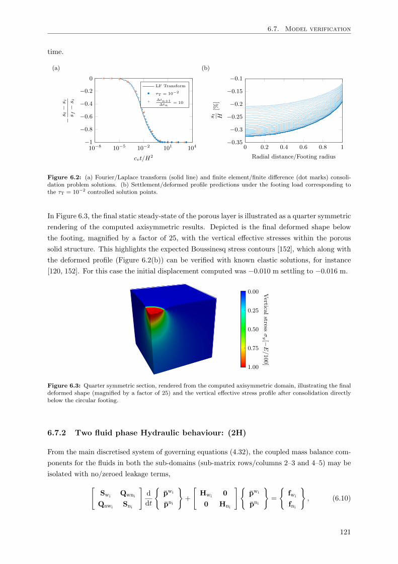
6.7. Model verification
time.
(a)
10−8 10−5 10−2 101 104−1
−0.8
−0.6
−0.4
−0.2
0
cvt/H2
−s t−s i
s f−s i
LF Transform
τT = 10−2
∆tn+1∆tn
= 10
(b)
0 0.2 0.4 0.6 0.8 1−0.35
−0.3
−0.25
−0.2
−0.15
−0.1
Radial distance/Footing radius
s t H[%
]
Figure 6.2: (a) Fourier/Laplace transform (solid line) and finite element/finite difference (dot marks) consoli-dation problem solutions. (b) Settlement/deformed profile predictions under the footing load corresponding tothe τT = 10−2 controlled solution points.
In Figure 6.3, the final static steady-state of the porous layer is illustrated as a quarter symmetric
rendering of the computed axisymmetric results. Depicted is the final deformed shape below
the footing, magnified by a factor of 25, with the vertical effective stresses within the porous
solid structure. This highlights the expected Boussinesq stress contours [152], which along with
the deformed profile (Figure 6.2(b)) can be verified with known elastic solutions, for instance
[120, 152]. For this case the initial displacement computed was −0.010 m settling to −0.016 m.
Figure 6.3: Quarter symmetric section, rendered from the computed axisymmetric domain, illustrating the finaldeformed shape (magnified by a factor of 25) and the vertical effective stress profile after consolidation directlybelow the circular footing.
6.7.2 Two fluid phase Hydraulic behaviour: (2H)
From the main discretised system of governing equations (4.32), the coupled mass balance com-
ponents for the fluids in both the sub-domains (sub-matrix rows/columns 2–3 and 4–5) may be
isolated with no/zeroed leakage terms,[Swi Qwni
Qnwi Sni
]d
dt
pwi
pni
+
[Hwi 0
0 Hni
]pwi
pni
=
fwi
fni
, (6.10)
121
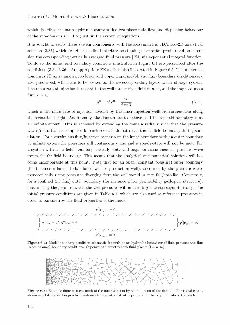
Chapter 6. Model Results & Performance
which describes the main hydraulic compressible two-phase fluid flow and displacing behaviour
of the sub-domains (i = 1, 2.) within the system of equations.
It is sought to verify these system components with the axisymmetric 1D/quasi-2D analytical
solution (3.37) which describes the fluid interface positioning (saturation profile) and on exten-
sion the corresponding vertically averaged fluid pressure [124] via exponential integral function.
To do so the initial and boundary conditions illustrated in Figure 6.4 are prescribed after the
conditions (3.34–3.36). An appropriate FE mesh is also illustrated in Figure 6.5. The numerical
domain is 2D axisymmetric, so lower and upper impermeable (no flux) boundary conditions are
also prescribed, which are to be viewed as the necessary sealing layers to the storage system.
The mass rate of injection is related to the wellbore surface fluid flux qn, and the imposed mass
flux qn via,
qn = qnρn =Mn
2πrH, (6.11)
which is the mass rate of injection divided by the inner injection wellbore surface area along
the formation height. Additionally, the domain has to behave as if the far-field boundary is at
an infinite extent. This is achieved by extending the domain radially such that the pressure
waves/disturbances computed for each scenario do not reach the far-field boundary during sim-
ulation. For a continuous flux/injection scenario on the inner boundary with an outer boundary
at infinite extent the pressures will continuously rise and a steady-state will not be met. For
a system with a far-field boundary a steady-state will begin to ensue once the pressure wave
meets the far field boundary. This means that the analytical and numerical solutions will be-
come incomparable at this point. Note that for an open (constant pressure) outer boundary
(for instance a far-field abandoned well or production well), once met by the pressure wave,
monotonically rising pressures diverging from the well would in turn fall/stabilise. Conversely,
for a confined (no flux) outer boundary (for instance a low permeability geological structure),
once met by the pressure wave, the well pressures will in turn begin to rise asymptotically. The
initial pressure conditions are given in Table 6.1, which are also used as reference pressures in
order to parametrise the fluid properties of the model.
Figure 6.4: Model boundary condition schematic for multiphase hydraulic behaviour of fluid pressure and flux(mass balance) boundary conditions. Superscript f denotes both fluid phases (f = w,n.).
Figure 6.5: Example finite element mesh of the inner 262.5 m by 50 m portion of the domain. The radial extentshown is arbitrary and in practice continues to a greater extent depending on the requirements of the model.
122
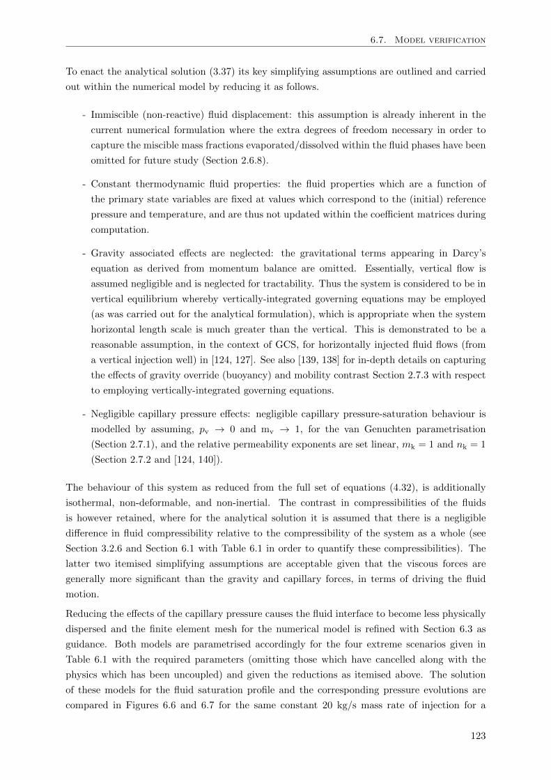
6.7. Model verification
To enact the analytical solution (3.37) its key simplifying assumptions are outlined and carried
out within the numerical model by reducing it as follows.
- Immiscible (non-reactive) fluid displacement: this assumption is already inherent in the
current numerical formulation where the extra degrees of freedom necessary in order to
capture the miscible mass fractions evaporated/dissolved within the fluid phases have been
omitted for future study (Section 2.6.8).
- Constant thermodynamic fluid properties: the fluid properties which are a function of
the primary state variables are fixed at values which correspond to the (initial) reference
pressure and temperature, and are thus not updated within the coefficient matrices during
computation.
- Gravity associated effects are neglected: the gravitational terms appearing in Darcy’s
equation as derived from momentum balance are omitted. Essentially, vertical flow is
assumed negligible and is neglected for tractability. Thus the system is considered to be in
vertical equilibrium whereby vertically-integrated governing equations may be employed
(as was carried out for the analytical formulation), which is appropriate when the system
horizontal length scale is much greater than the vertical. This is demonstrated to be a
reasonable assumption, in the context of GCS, for horizontally injected fluid flows (from
a vertical injection well) in [124, 127]. See also [139, 138] for in-depth details on capturing
the effects of gravity override (buoyancy) and mobility contrast Section 2.7.3 with respect
to employing vertically-integrated governing equations.
- Negligible capillary pressure effects: negligible capillary pressure-saturation behaviour is
modelled by assuming, pv → 0 and mv → 1, for the van Genuchten parametrisation
(Section 2.7.1), and the relative permeability exponents are set linear, mk = 1 and nk = 1
(Section 2.7.2 and [124, 140]).
The behaviour of this system as reduced from the full set of equations (4.32), is additionally
isothermal, non-deformable, and non-inertial. The contrast in compressibilities of the fluids
is however retained, where for the analytical solution it is assumed that there is a negligible
difference in fluid compressibility relative to the compressibility of the system as a whole (see
Section 3.2.6 and Section 6.1 with Table 6.1 in order to quantify these compressibilities). The
latter two itemised simplifying assumptions are acceptable given that the viscous forces are
generally more significant than the gravity and capillary forces, in terms of driving the fluid
motion.
Reducing the effects of the capillary pressure causes the fluid interface to become less physically
dispersed and the finite element mesh for the numerical model is refined with Section 6.3 as
guidance. Both models are parametrised accordingly for the four extreme scenarios given in
Table 6.1 with the required parameters (omitting those which have cancelled along with the
physics which has been uncoupled) and given the reductions as itemised above. The solution
of these models for the fluid saturation profile and the corresponding pressure evolutions are
compared in Figures 6.6 and 6.7 for the same constant 20 kg/s mass rate of injection for a
123
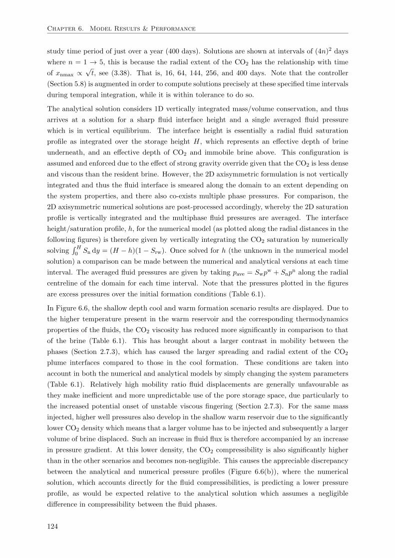
Chapter 6. Model Results & Performance
study time period of just over a year (400 days). Solutions are shown at intervals of (4n)2 days
where n = 1 → 5, this is because the radial extent of the CO2 has the relationship with time
of xnmax ∝√t, see (3.38). That is, 16, 64, 144, 256, and 400 days. Note that the controller
(Section 5.8) is augmented in order to compute solutions precisely at these specified time intervals
during temporal integration, while it is within tolerance to do so.
The analytical solution considers 1D vertically integrated mass/volume conservation, and thus
arrives at a solution for a sharp fluid interface height and a single averaged fluid pressure
which is in vertical equilibrium. The interface height is essentially a radial fluid saturation
profile as integrated over the storage height H, which represents an effective depth of brine
underneath, and an effective depth of CO2 and immobile brine above. This configuration is
assumed and enforced due to the effect of strong gravity override given that the CO2 is less dense
and viscous than the resident brine. However, the 2D axisymmetric formulation is not vertically
integrated and thus the fluid interface is smeared along the domain to an extent depending on
the system properties, and there also co-exists multiple phase pressures. For comparison, the
2D axisymmetric numerical solutions are post-processed accordingly, whereby the 2D saturation
profile is vertically integrated and the multiphase fluid pressures are averaged. The interface
height/saturation profile, h, for the numerical model (as plotted along the radial distances in the
following figures) is therefore given by vertically integrating the CO2 saturation by numerically
solving∫ H0 Sn dy = (H − h)(1− Srw). Once solved for h (the unknown in the numerical model
solution) a comparison can be made between the numerical and analytical versions at each time
interval. The averaged fluid pressures are given by taking pave = Swpw + Snp
n along the radial
centreline of the domain for each time interval. Note that the pressures plotted in the figures
are excess pressures over the initial formation conditions (Table 6.1).
In Figure 6.6, the shallow depth cool and warm formation scenario results are displayed. Due to
the higher temperature present in the warm reservoir and the corresponding thermodynamics
properties of the fluids, the CO2 viscosity has reduced more significantly in comparison to that
of the brine (Table 6.1). This has brought about a larger contrast in mobility between the
phases (Section 2.7.3), which has caused the larger spreading and radial extent of the CO2
plume interfaces compared to those in the cool formation. These conditions are taken into
account in both the numerical and analytical models by simply changing the system parameters
(Table 6.1). Relatively high mobility ratio fluid displacements are generally unfavourable as
they make inefficient and more unpredictable use of the pore storage space, due particularly to
the increased potential onset of unstable viscous fingering (Section 2.7.3). For the same mass
injected, higher well pressures also develop in the shallow warm reservoir due to the significantly
lower CO2 density which means that a larger volume has to be injected and subsequently a larger
volume of brine displaced. Such an increase in fluid flux is therefore accompanied by an increase
in pressure gradient. At this lower density, the CO2 compressibility is also significantly higher
than in the other scenarios and becomes non-negligible. This causes the appreciable discrepancy
between the analytical and numerical pressure profiles (Figure 6.6(b)), where the numerical
solution, which accounts directly for the fluid compressibilities, is predicting a lower pressure
profile, as would be expected relative to the analytical solution which assumes a negligible
difference in compressibility between the fluid phases.
124
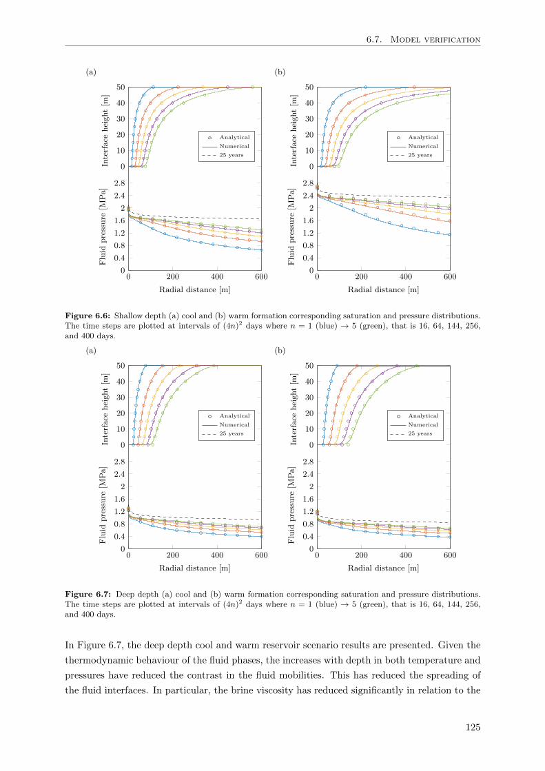
6.7. Model verification
(a)
0
10
20
30
40
50
Interface
height[m
]
Analytical
Numerical
25 years
0 200 400 6000
0.4
0.8
1.2
1.6
2
2.4
2.8
Radial distance [m]
Fluid
pressure
[MPa]
(b)
0
10
20
30
40
50
Interface
height[m
]
Analytical
Numerical
25 years
0 200 400 6000
0.4
0.8
1.2
1.6
2
2.4
2.8
Radial distance [m]Fluid
pressure
[MPa]
Figure 6.6: Shallow depth (a) cool and (b) warm formation corresponding saturation and pressure distributions.The time steps are plotted at intervals of (4n)2 days where n = 1 (blue) → 5 (green), that is 16, 64, 144, 256,and 400 days.
(a)
0
10
20
30
40
50
Interface
height[m
]
Analytical
Numerical
25 years
0 200 400 6000
0.4
0.8
1.2
1.6
2
2.4
2.8
Radial distance [m]
Fluid
pressure
[MPa]
(b)
0
10
20
30
40
50
Interface
height[m
]
Analytical
Numerical
25 years
0 200 400 6000
0.4
0.8
1.2
1.6
2
2.4
2.8
Radial distance [m]
Fluid
pressure
[MPa]
Figure 6.7: Deep depth (a) cool and (b) warm formation corresponding saturation and pressure distributions.The time steps are plotted at intervals of (4n)2 days where n = 1 (blue) → 5 (green), that is 16, 64, 144, 256,and 400 days.
In Figure 6.7, the deep depth cool and warm reservoir scenario results are presented. Given the
thermodynamic behaviour of the fluid phases, the increases with depth in both temperature and
pressures have reduced the contrast in the fluid mobilities. This has reduced the spreading of
the fluid interfaces. In particular, the brine viscosity has reduced significantly in relation to the
125
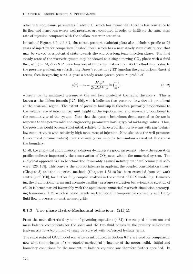
Chapter 6. Model Results & Performance
other thermodynamic parameters (Table 6.1), which has meant that there is less resistance to
its flow and hence less excess well pressures are computed in order to facilitate the same mass
rate of injection compared with the shallow reservoir scenarios.
In each of Figures 6.6 and 6.7, the excess pressure evolution plots also include a profile at 25
years of injection for comparison (dashed lines), which has a near steady state distribution that
may be viewed as a potential state towards the end of a long-term injection phase. The final
steady state of the reservoir system may be viewed as a single moving CO2 phase with a fluid
flux, qn(x) = Mn/2πxHρn, as a function of the radial distance, x. As this fluid flux is due to
the pressure gradient, on substituting Darcy’s equation (2.33) ignoring the gravitational/inertial
terms, then integrating w.r.t. x gives a steady-state system pressure profile of
p(x)− pr =Mnµ
n
2πHρnkrnkln( rx
), (6.12)
where pr is the undefined pressure at the well face located at the radial distance r. This is
known as the Thiem formula [125, 196], which indicates that pressure draw-down is prominent
at the near-well region. The extent of pressure build-up is therefore primarily proportional to
the volume rate of injection per unit height of the injection well and inversely proportional to
the conductivity of the system. Note that the system behaviours demonstrated so far are in
response to the porous solid and engineering parameters having typical mid-range values. Thus,
the pressures would become substantial, relative to the overburden, for systems with particularly
low conductivities with relatively high mass rates of injection. Note also that the well pressures
(inner nodal pressure values) must continually rise in order to maintain a constant flux across
the boundary.
In all, the analytical and numerical solutions demonstrate good agreement, where the saturation
profiles indicate importantly the conservation of CO2 mass within the numerical system. The
analytical approach is also benchmarked favourably against industry standard commercial soft-
ware [126, 139]. This conveys the appropriateness in applying the coupled consolidation theory
(Chapter 3) and the numerical methods (Chapters 4–5) as has been extended from the work
centrally of [120], for further fully coupled analysis in the context of GCS modelling. Reinstat-
ing the gravitational terms and accurate capillary pressure-saturation behaviour, the solution of
(6.10) is benchmarked favourably with the open-source numerical reservoir simulation prototyp-
ing framework [112], which is based largely on traditional incompressible continuity and Darcy
fluid flow processes on unstructured grids.
6.7.3 Two phase Hydro-Mechanical behaviour: (2H)M
From the main discretised system of governing equations (4.32), the coupled momentum and
mass balance components for the solid and the two fluid phases in the primary sub-domain
(sub-matrix rows/columns 1–3) may be isolated with no/zeroed leakage terms.
The same reduced GCS model scenarios as introduced in Section 6.7.2 are used for comparison,
now with the inclusion of the coupled mechanical behaviour of the porous solid. Initial and
boundary conditions for the momentum balance equation are therefore further specified. In
126
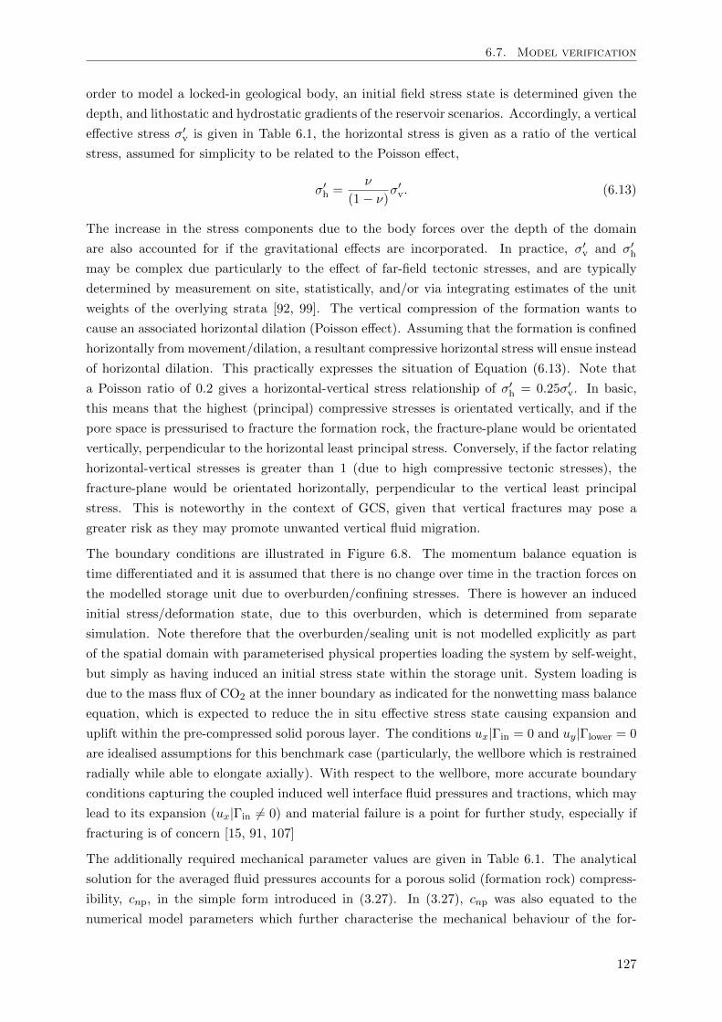
6.7. Model verification
order to model a locked-in geological body, an initial field stress state is determined given the
depth, and lithostatic and hydrostatic gradients of the reservoir scenarios. Accordingly, a vertical
effective stress σ′v is given in Table 6.1, the horizontal stress is given as a ratio of the vertical
stress, assumed for simplicity to be related to the Poisson effect,
σ′h =ν
(1− ν)σ′v. (6.13)
The increase in the stress components due to the body forces over the depth of the domain
are also accounted for if the gravitational effects are incorporated. In practice, σ′v and σ′hmay be complex due particularly to the effect of far-field tectonic stresses, and are typically
determined by measurement on site, statistically, and/or via integrating estimates of the unit
weights of the overlying strata [92, 99]. The vertical compression of the formation wants to
cause an associated horizontal dilation (Poisson effect). Assuming that the formation is confined
horizontally from movement/dilation, a resultant compressive horizontal stress will ensue instead
of horizontal dilation. This practically expresses the situation of Equation (6.13). Note that
a Poisson ratio of 0.2 gives a horizontal-vertical stress relationship of σ′h = 0.25σ′v. In basic,
this means that the highest (principal) compressive stresses is orientated vertically, and if the
pore space is pressurised to fracture the formation rock, the fracture-plane would be orientated
vertically, perpendicular to the horizontal least principal stress. Conversely, if the factor relating
horizontal-vertical stresses is greater than 1 (due to high compressive tectonic stresses), the
fracture-plane would be orientated horizontally, perpendicular to the vertical least principal
stress. This is noteworthy in the context of GCS, given that vertical fractures may pose a
greater risk as they may promote unwanted vertical fluid migration.
The boundary conditions are illustrated in Figure 6.8. The momentum balance equation is
time differentiated and it is assumed that there is no change over time in the traction forces on
the modelled storage unit due to overburden/confining stresses. There is however an induced
initial stress/deformation state, due to this overburden, which is determined from separate
simulation. Note therefore that the overburden/sealing unit is not modelled explicitly as part
of the spatial domain with parameterised physical properties loading the system by self-weight,
but simply as having induced an initial stress state within the storage unit. System loading is
due to the mass flux of CO2 at the inner boundary as indicated for the nonwetting mass balance
equation, which is expected to reduce the in situ effective stress state causing expansion and
uplift within the pre-compressed solid porous layer. The conditions ux|Γin = 0 and uy|Γlower = 0
are idealised assumptions for this benchmark case (particularly, the wellbore which is restrained
radially while able to elongate axially). With respect to the wellbore, more accurate boundary
conditions capturing the coupled induced well interface fluid pressures and tractions, which may
lead to its expansion (ux|Γin 6= 0) and material failure is a point for further study, especially if
fracturing is of concern [15, 91, 107]
The additionally required mechanical parameter values are given in Table 6.1. The analytical
solution for the averaged fluid pressures accounts for a porous solid (formation rock) compress-
ibility, cnp, in the simple form introduced in (3.27). In (3.27), cnp was also equated to the
numerical model parameters which further characterise the mechanical behaviour of the for-
127
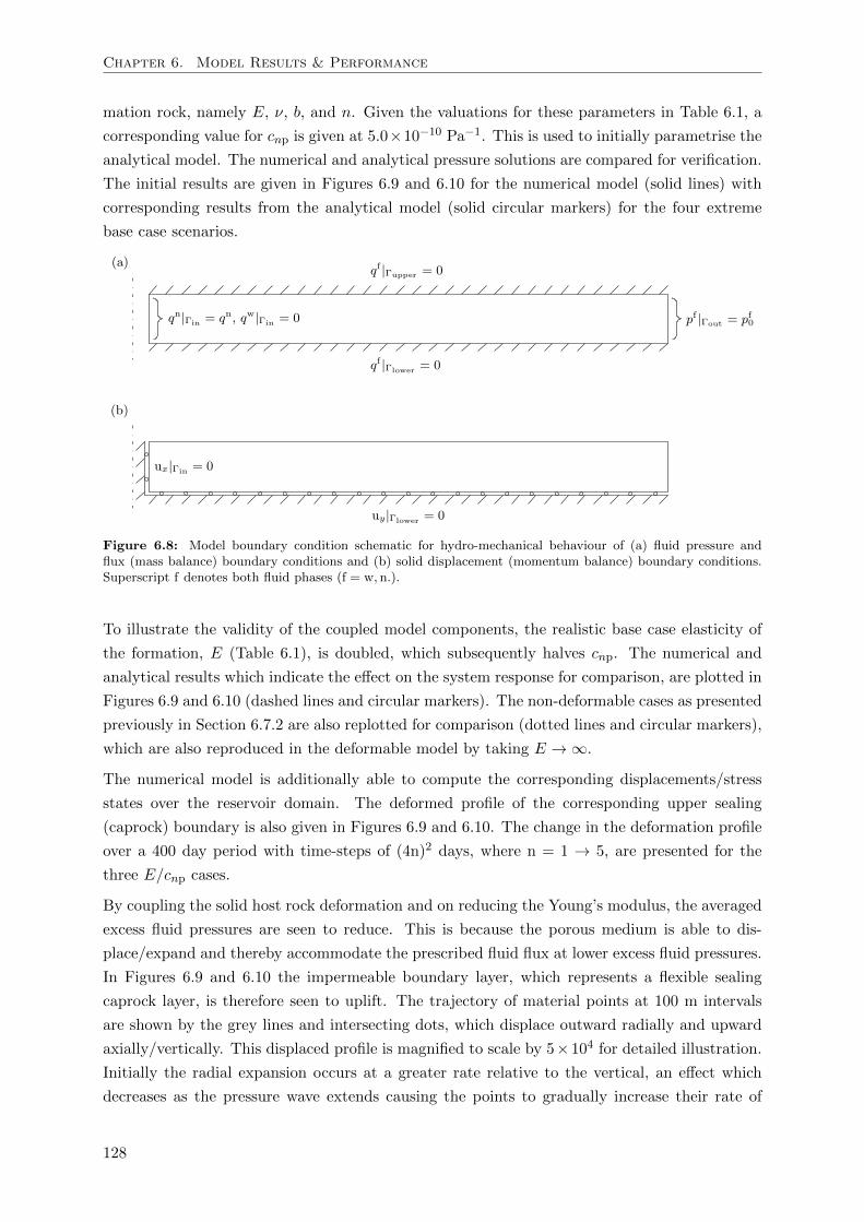
Chapter 6. Model Results & Performance
mation rock, namely E, ν, b, and n. Given the valuations for these parameters in Table 6.1, a
corresponding value for cnp is given at 5.0×10⁻¹⁰ Pa−1. This is used to initially parametrise the
analytical model. The numerical and analytical pressure solutions are compared for verification.
The initial results are given in Figures 6.9 and 6.10 for the numerical model (solid lines) with
corresponding results from the analytical model (solid circular markers) for the four extreme
base case scenarios.
Figure 6.8: Model boundary condition schematic for hydro-mechanical behaviour of (a) fluid pressure andflux (mass balance) boundary conditions and (b) solid displacement (momentum balance) boundary conditions.Superscript f denotes both fluid phases (f = w, n.).
To illustrate the validity of the coupled model components, the realistic base case elasticity of
the formation, E (Table 6.1), is doubled, which subsequently halves cnp. The numerical and
analytical results which indicate the effect on the system response for comparison, are plotted in
Figures 6.9 and 6.10 (dashed lines and circular markers). The non-deformable cases as presented
previously in Section 6.7.2 are also replotted for comparison (dotted lines and circular markers),
which are also reproduced in the deformable model by taking E → ∞.
The numerical model is additionally able to compute the corresponding displacements/stress
states over the reservoir domain. The deformed profile of the corresponding upper sealing
(caprock) boundary is also given in Figures 6.9 and 6.10. The change in the deformation profile
over a 400 day period with time-steps of (4n)2 days, where n = 1 → 5, are presented for the
three E/cnp cases.
By coupling the solid host rock deformation and on reducing the Young’s modulus, the averaged
excess fluid pressures are seen to reduce. This is because the porous medium is able to dis-
place/expand and thereby accommodate the prescribed fluid flux at lower excess fluid pressures.
In Figures 6.9 and 6.10 the impermeable boundary layer, which represents a flexible sealing
caprock layer, is therefore seen to uplift. The trajectory of material points at 100 m intervals
are shown by the grey lines and intersecting dots, which displace outward radially and upward
axially/vertically. This displaced profile is magnified to scale by 5×10⁴ for detailed illustration.
Initially the radial expansion occurs at a greater rate relative to the vertical, an effect which
decreases as the pressure wave extends causing the points to gradually increase their rate of
128
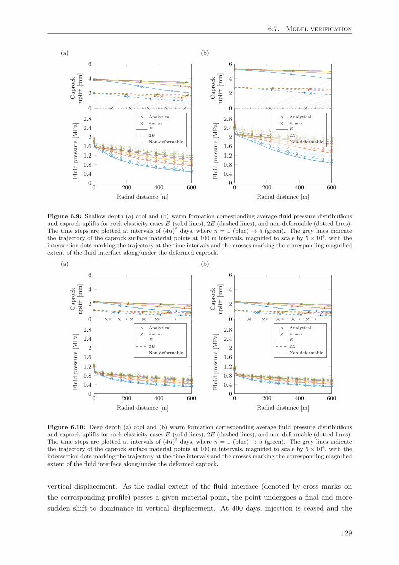
6.7. Model verification
(a)
0
2
4
6
Caprock
uplift
[mm]
0 200 400 6000
0.4
0.8
1.2
1.6
2
2.4
2.8
Radial distance [m]
Fluid
pressure
[MPa]
Analytical
xnmax
E
2E
Non-deformable
(b)
0
2
4
6
Caprock
uplift
[mm]
0 200 400 6000
0.4
0.8
1.2
1.6
2
2.4
2.8
Radial distance [m]
Fluid
pressure
[MPa]
Analytical
xnmax
E
2E
Non-deformable
Figure 6.9: Shallow depth (a) cool and (b) warm formation corresponding average fluid pressure distributionsand caprock uplifts for rock elasticity cases E (solid lines), 2E (dashed lines), and non-deformable (dotted lines).The time steps are plotted at intervals of (4n)2 days, where n = 1 (blue) → 5 (green). The grey lines indicatethe trajectory of the caprock surface material points at 100 m intervals, magnified to scale by 5 × 10⁴, with theintersection dots marking the trajectory at the time intervals and the crosses marking the corresponding magnifiedextent of the fluid interface along/under the deformed caprock.
(a)
0
2
4
6
Caprock
uplift
[mm]
0 200 400 6000
0.4
0.8
1.2
1.6
2
2.4
2.8
Radial distance [m]
Fluid
pressure
[MPa]
Analytical
xnmax
E
2E
Non-deformable
(b)
0
2
4
6
Caprock
uplift
[mm]
0 200 400 6000
0.4
0.8
1.2
1.6
2
2.4
2.8
Radial distance [m]
Fluid
pressure
[MPa]
Analytical
xnmax
E
2E
Non-deformable
Figure 6.10: Deep depth (a) cool and (b) warm formation corresponding average fluid pressure distributionsand caprock uplifts for rock elasticity cases E (solid lines), 2E (dashed lines), and non-deformable (dotted lines).The time steps are plotted at intervals of (4n)2 days, where n = 1 (blue) → 5 (green). The grey lines indicatethe trajectory of the caprock surface material points at 100 m intervals, magnified to scale by 5 × 10⁴, with theintersection dots marking the trajectory at the time intervals and the crosses marking the corresponding magnifiedextent of the fluid interface along/under the deformed caprock.
vertical displacement. As the radial extent of the fluid interface (denoted by cross marks on
the corresponding profile) passes a given material point, the point undergoes a final and more
sudden shift to dominance in vertical displacement. At 400 days, injection is ceased and the
129
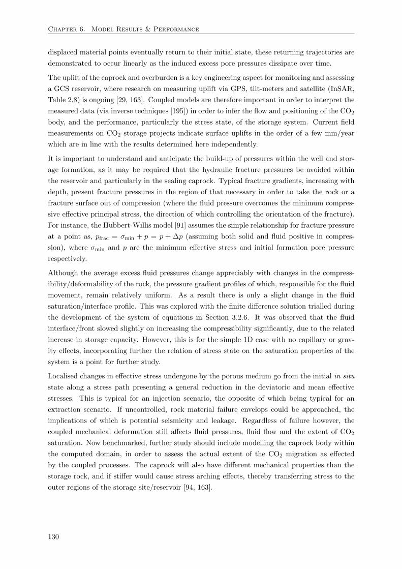
Chapter 6. Model Results & Performance
displaced material points eventually return to their initial state, these returning trajectories are
demonstrated to occur linearly as the induced excess pore pressures dissipate over time.
The uplift of the caprock and overburden is a key engineering aspect for monitoring and assessing
a GCS reservoir, where research on measuring uplift via GPS, tilt-meters and satellite (InSAR,
Table 2.8) is ongoing [29, 163]. Coupled models are therefore important in order to interpret the
measured data (via inverse techniques [195]) in order to infer the flow and positioning of the CO2
body, and the performance, particularly the stress state, of the storage system. Current field
measurements on CO2 storage projects indicate surface uplifts in the order of a few mm/year
which are in line with the results determined here independently.
It is important to understand and anticipate the build-up of pressures within the well and stor-
age formation, as it may be required that the hydraulic fracture pressures be avoided within
the reservoir and particularly in the sealing caprock. Typical fracture gradients, increasing with
depth, present fracture pressures in the region of that necessary in order to take the rock or a
fracture surface out of compression (where the fluid pressure overcomes the minimum compres-
sive effective principal stress, the direction of which controlling the orientation of the fracture).
For instance, the Hubbert-Willis model [91] assumes the simple relationship for fracture pressure
at a point as, pfrac = σmin + p = p + ∆p (assuming both solid and fluid positive in compres-
sion), where σmin and p are the minimum effective stress and initial formation pore pressure
respectively.
Although the average excess fluid pressures change appreciably with changes in the compress-
ibility/deformability of the rock, the pressure gradient profiles of which, responsible for the fluid
movement, remain relatively uniform. As a result there is only a slight change in the fluid
saturation/interface profile. This was explored with the finite difference solution trialled during
the development of the system of equations in Section 3.2.6. It was observed that the fluid
interface/front slowed slightly on increasing the compressibility significantly, due to the related
increase in storage capacity. However, this is for the simple 1D case with no capillary or grav-
ity effects, incorporating further the relation of stress state on the saturation properties of the
system is a point for further study.
Localised changes in effective stress undergone by the porous medium go from the initial in situ
state along a stress path presenting a general reduction in the deviatoric and mean effective
stresses. This is typical for an injection scenario, the opposite of which being typical for an
extraction scenario. If uncontrolled, rock material failure envelops could be approached, the
implications of which is potential seismicity and leakage. Regardless of failure however, the
coupled mechanical deformation still affects fluid pressures, fluid flow and the extent of CO2
saturation. Now benchmarked, further study should include modelling the caprock body within
the computed domain, in order to assess the actual extent of the CO2 migration as effected
by the coupled processes. The caprock will also have different mechanical properties than the
storage rock, and if stiffer would cause stress arching effects, thereby transferring stress to the
outer regions of the storage site/reservoir [94, 163].
130
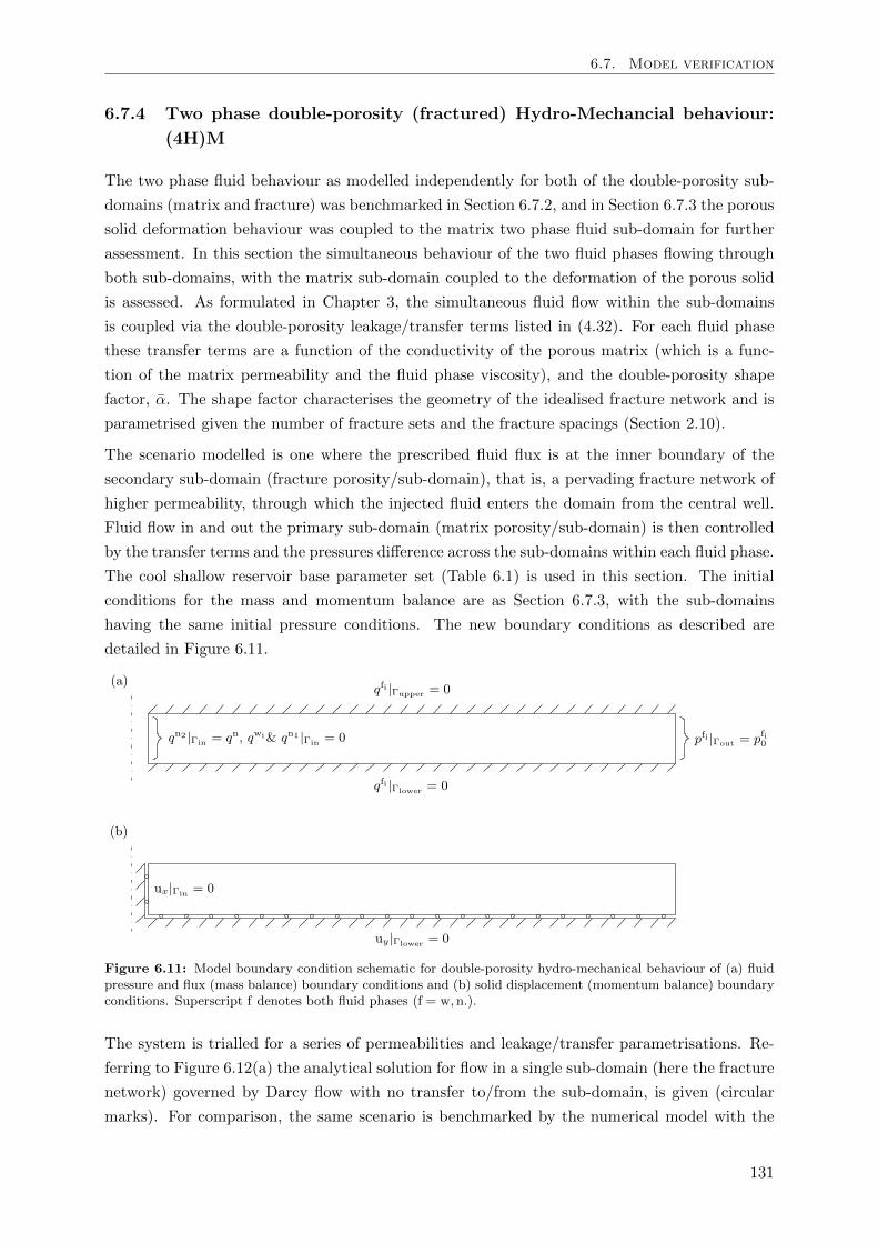
6.7. Model verification
6.7.4 Two phase double-porosity (fractured) Hydro-Mechancial behaviour:
(4H)M
The two phase fluid behaviour as modelled independently for both of the double-porosity sub-
domains (matrix and fracture) was benchmarked in Section 6.7.2, and in Section 6.7.3 the porous
solid deformation behaviour was coupled to the matrix two phase fluid sub-domain for further
assessment. In this section the simultaneous behaviour of the two fluid phases flowing through
both sub-domains, with the matrix sub-domain coupled to the deformation of the porous solid
is assessed. As formulated in Chapter 3, the simultaneous fluid flow within the sub-domains
is coupled via the double-porosity leakage/transfer terms listed in (4.32). For each fluid phase
these transfer terms are a function of the conductivity of the porous matrix (which is a func-
tion of the matrix permeability and the fluid phase viscosity), and the double-porosity shape
factor, α. The shape factor characterises the geometry of the idealised fracture network and is
parametrised given the number of fracture sets and the fracture spacings (Section 2.10).
The scenario modelled is one where the prescribed fluid flux is at the inner boundary of the
secondary sub-domain (fracture porosity/sub-domain), that is, a pervading fracture network of
higher permeability, through which the injected fluid enters the domain from the central well.
Fluid flow in and out the primary sub-domain (matrix porosity/sub-domain) is then controlled
by the transfer terms and the pressures difference across the sub-domains within each fluid phase.
The cool shallow reservoir base parameter set (Table 6.1) is used in this section. The initial
conditions for the mass and momentum balance are as Section 6.7.3, with the sub-domains
having the same initial pressure conditions. The new boundary conditions as described are
detailed in Figure 6.11.
Figure 6.11: Model boundary condition schematic for double-porosity hydro-mechanical behaviour of (a) fluidpressure and flux (mass balance) boundary conditions and (b) solid displacement (momentum balance) boundaryconditions. Superscript f denotes both fluid phases (f = w, n.).
The system is trialled for a series of permeabilities and leakage/transfer parametrisations. Re-
ferring to Figure 6.12(a) the analytical solution for flow in a single sub-domain (here the fracture
network) governed by Darcy flow with no transfer to/from the sub-domain, is given (circular
marks). For comparison, the same scenario is benchmarked by the numerical model with the
131
Chapter 6. Model Results & Performance
shape factor, α = 0 (dotted lines). That is, no mass transfer between the fracture and matrix
sub-domain takes place as the off-diagonal L coupling terms of (4.32) have become zero as a
result, and flow only occurs through the fracture sub-domain. The numerical model is now
parametrised with the more realistic capillary pressure-saturation behaviour from Table 6.1, for
both sub-domains. This is seen to cause a slight discrepancy in the numerical CO2 satura-
tion profiles with respect to the analytical solutions, due to the numerical solution exhibiting a
greater degree of dispersion.
On increasing α to a value of 0.6 m−2, which corresponds to a matrix block fracture spacing of l =
10 m (2.10), transfer between the sub-domains takes place and the solution is altered (solid lines).
At earlier time-steps, the CO2 phase is seen to advance ahead through the fracture network,
similarly to the no-transfer case, however where the fluid pressures have become elevated closer
to the injection well transfer from the fracture sub-domain has begun to occur where CO2 mass
is seen to have displaced from the fracture to the matrix saturation profile. This effect is seen
to develop over time as the pressures and CO2 phase moves outward. Note that the matrix has
a higher porosity than the fracture network so the utilisation of space becomes improved for the
transferred mass.
The corresponding pressure profiles for the averaged fluid pressures in the sub-domains falls as
a result of the transfer term increasing the overall permeability of the system. This is seen on
inspecting the discretised governing system (4.32) at steady-state for a single fluid phase. Multi-
plying out the conductivity matrix K and primary variables for the porous matrix sub-domain,
with no induced flux, gives (H1 + L)p1 − Lp2 = 0, and for the fracture sub-domain, with an
induced flux, gives −Lp1+(H2+L)p2 = f2 (where Hi are the conductivities of the domains and
L is their mutual transfer). On L = 0, H1p1 = 0 and H2p2 = f2. That is, a pressure gradient
and subsequent flow occurs only in the fracture network sub-domain. However, after substitu-
tion, when L becomes large, (H1 +H2)p2 ' (H1 +H2)p1 ≈ f2, meaning that the pressure in
the fracture sub-domain is higher and that both pressures are controlled predominantly by the
higher conductivity, here that of the fracture sub-domain, H2. Hence, on increasing L(α) from
zero, the average numerical pressure solution profile in the fracture sub-domain (solid lines) falls,
and that of the matrix rises, though to a marginally lesser pressure value than in the fracture,
depending on the magnitude of the transfer term.
The α parameter is increased further to a value of 60 m−2, corresponding to a smaller matrix
block fracture spacing of l = 1 m with the same permeabilities. As a result, more mass transfer
between the fracture and matrix sub-domain takes place at the early stages. This is seen by
the effect on the saturation profiles (dashed lines), where the CO2 more readily displace to the
matrix sub-domain.
For Figure 6.12(b) the matrix permeability alone is decreased by an order of magnitude, in
turn reducing H1(k1) and L(k1), for the same set of trials. The analytical solution therefore
remains the same because it only considers flow in the no-transfer fracture network case which
is unaffected by the matrix permeability. For the cases where transfer occurs, the effect of
reducing k1 is seen to marginally increase the averaged fluid pressures and thus the uplift of the
sealing (caprock) boundary. The marginal effect is because H2(k2) is the dominant factor, given
132
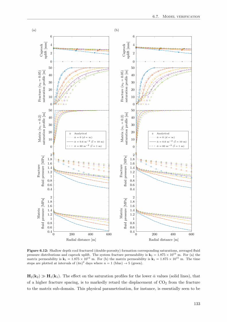
6.7. Model verification
(a)
0
2
4
6
Caprock
uplift
[mm]
0
10
20
30
40
50
Fracture
(n2=
0.05)
saturationprofile
[m]
0
10
20
30
40
50
Matrix
(n1=
0.2)
saturationprofile
[m]
0.40.60.81
1.21.41.61.82
Fracture
fluid
pressure
[MPa]
Analytical
α = 0 (d = ∞)
α = 0.6 m−2 (l = 10 m)
α = 60 m−2 (l = 1 m)
0 200 400 6000.40.60.81
1.21.41.61.82
Radial distance [m]
Matrix
fluid
pressure
[MPa]
(b)
0
2
4
6
Caprock
uplift
[mm]
0
10
20
30
40
50
Fracture
(n2=
0.05)
saturationprofile
[m]
0
10
20
30
40
50
Matrix
(n1=
0.2)
saturationprofile
[m]
0.40.60.81
1.21.41.61.82
Fracture
fluid
pressure
[MPa]
Analytical
α = 0 (d = ∞)
α = 0.6 m−2 (l = 10 m)
α = 60 m−2 (l = 1 m)
0 200 400 6000.40.60.81
1.21.41.61.82
Radial distance [m]
Matrix
fluid
pressure
[MPa]
Figure 6.12: Shallow depth cool fractured (double-porosity) formation corresponding saturations, averaged fluidpressure distributions and caprock uplift. The system fracture permeability is k2 = 1.875× 10¹³ m. For (a) thematrix permeability is k1 = 1.875 × 10¹⁴ m. For (b) the matrix permeability is k1 = 1.875 × 10¹⁵ m. The timesteps are plotted at intervals of (4n)2 days where n = 1 (blue)→ 5 (green).
H2(k2) H1(k1). The effect on the saturation profiles for the lower α values (solid lines), that
of a higher fracture spacing, is to markedly retard the displacement of CO2 from the fracture
to the matrix sub-domain. This physical parametrisation, for instance, is essentially seen to be
133
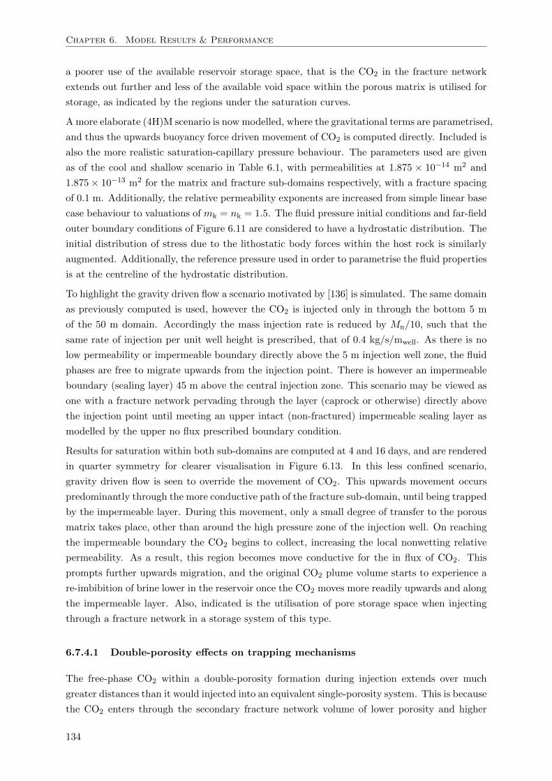
Chapter 6. Model Results & Performance
a poorer use of the available reservoir storage space, that is the CO2 in the fracture network
extends out further and less of the available void space within the porous matrix is utilised for
storage, as indicated by the regions under the saturation curves.
A more elaborate (4H)M scenario is now modelled, where the gravitational terms are parametrised,
and thus the upwards buoyancy force driven movement of CO2 is computed directly. Included is
also the more realistic saturation-capillary pressure behaviour. The parameters used are given
as of the cool and shallow scenario in Table 6.1, with permeabilities at 1.875 × 10⁻¹⁴ m2 and
1.875× 10⁻¹³ m2 for the matrix and fracture sub-domains respectively, with a fracture spacing
of 0.1 m. Additionally, the relative permeability exponents are increased from simple linear base
case behaviour to valuations of mk = nk = 1.5. The fluid pressure initial conditions and far-field
outer boundary conditions of Figure 6.11 are considered to have a hydrostatic distribution. The
initial distribution of stress due to the lithostatic body forces within the host rock is similarly
augmented. Additionally, the reference pressure used in order to parametrise the fluid properties
is at the centreline of the hydrostatic distribution.
To highlight the gravity driven flow a scenario motivated by [136] is simulated. The same domain
as previously computed is used, however the CO2 is injected only in through the bottom 5 m
of the 50 m domain. Accordingly the mass injection rate is reduced by Mn/10, such that the
same rate of injection per unit well height is prescribed, that of 0.4 kg/s/mwell. As there is no
low permeability or impermeable boundary directly above the 5 m injection well zone, the fluid
phases are free to migrate upwards from the injection point. There is however an impermeable
boundary (sealing layer) 45 m above the central injection zone. This scenario may be viewed as
one with a fracture network pervading through the layer (caprock or otherwise) directly above
the injection point until meeting an upper intact (non-fractured) impermeable sealing layer as
modelled by the upper no flux prescribed boundary condition.
Results for saturation within both sub-domains are computed at 4 and 16 days, and are rendered
in quarter symmetry for clearer visualisation in Figure 6.13. In this less confined scenario,
gravity driven flow is seen to override the movement of CO2. This upwards movement occurs
predominantly through the more conductive path of the fracture sub-domain, until being trapped
by the impermeable layer. During this movement, only a small degree of transfer to the porous
matrix takes place, other than around the high pressure zone of the injection well. On reaching
the impermeable boundary the CO2 begins to collect, increasing the local nonwetting relative
permeability. As a result, this region becomes move conductive for the in flux of CO2. This
prompts further upwards migration, and the original CO2 plume volume starts to experience a
re-imbibition of brine lower in the reservoir once the CO2 moves more readily upwards and along
the impermeable layer. Also, indicated is the utilisation of pore storage space when injecting
through a fracture network in a storage system of this type.
6.7.4.1 Double-porosity effects on trapping mechanisms
The free-phase CO2 within a double-porosity formation during injection extends over much
greater distances than it would injected into an equivalent single-porosity system. This is because
the CO2 enters through the secondary fracture network volume of lower porosity and higher
134
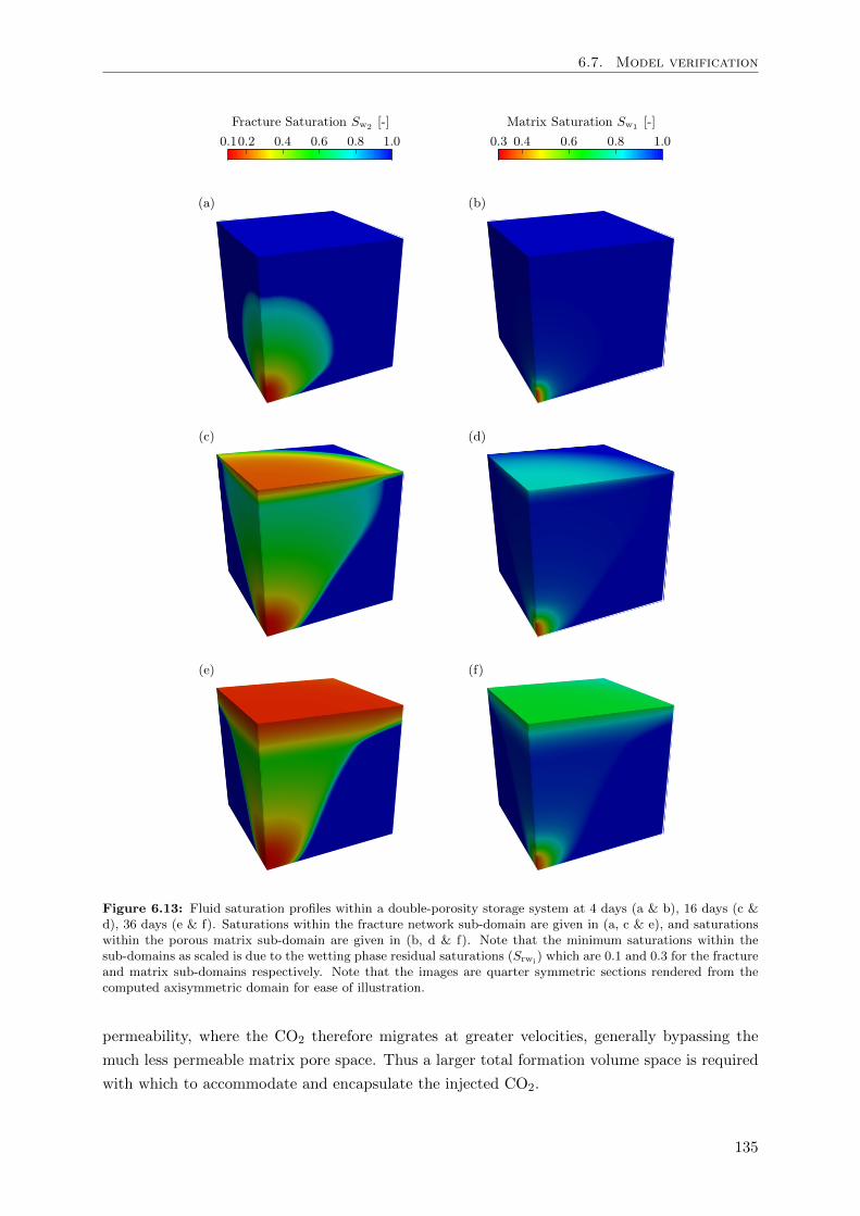
6.7. Model verification
Figure 6.13: Fluid saturation profiles within a double-porosity storage system at 4 days (a & b), 16 days (c &d), 36 days (e & f). Saturations within the fracture network sub-domain are given in (a, c & e), and saturationswithin the porous matrix sub-domain are given in (b, d & f). Note that the minimum saturations within thesub-domains as scaled is due to the wetting phase residual saturations (Srwi) which are 0.1 and 0.3 for the fractureand matrix sub-domains respectively. Note that the images are quarter symmetric sections rendered from thecomputed axisymmetric domain for ease of illustration.
permeability, where the CO2 therefore migrates at greater velocities, generally bypassing the
much less permeable matrix pore space. Thus a larger total formation volume space is required
with which to accommodate and encapsulate the injected CO2.
135
Chapter 6. Model Results & Performance
This effect poses a greater risk for structural (or stratigraphic) trapping because in a double-
porosity formation the mass of stored CO2 will occupy a larger area with a greater likelihood of
intercepting leakage pathways and spilling out from under designated trapping interfaces. This
is compounded with the issue of having the CO2 migrating in a fissure/fracture network which
may also pervade an intended sealing caprock.
However, in a double-porosity system the longer term dissolution trapping mechanisms are
significantly enhance given that the free-phase CO2 is in contact with greater interface areas of
the brine which is housed in the matrix pore space surrounding the CO2 in the fractures. In
a single-porosity formation dissolution (and reaction) occurs principally at the outer interface
boundaries of the CO2 free-phase region where it is within contact with the brine that it is
displacing. Behind this interface the CO2 has largely dried out the host brine and beyond
this interface there is no CO2 yet present for dissolution trapping to occur. Therefore, within a
single-porosity formation dissolution trapping, particularly in the short term, is generally limited
to the movement of the outer fluid interface. Alternatively, in a double-porosity formation it
is the fracture network that will dry out while the surrounding matrix pore space remains
predominantly saturated with the host brine. This is caused by the low permeability and CO2
relative permeability in the porous matrix which restricts CO2 free-phase movement through it,
wherein the host brine is not significantly displaced behind the CO2 front out in the fractures.
Although there is little fracture/matrix phase transfer, there is enhanced dissolution and diffusive
transfer across the fracture/matrix interface due to the high imposed concentration gradient
between the free-phases separated by this interface. This dissolution processes is a more definitive
trapping mechanism than free-phase storage within the matrix.
The enhanced dissolution trapping also enhances the contact area and time between dissolved
CO2 and the rock minerals within the porous matrix environment, which is also advantageous
for mineralisation trapping mechanisms to occur. An appropriately simplified study on these
interesting effects in the context of GCS is given in [38]. This is for an isothermal non-deformable
case with no/simplified free-phase CO2 movement in the pore matrix space, and thereby con-
centrates principally on the dissolution and diffusive processes. In the present study the lag
between the free-phase movements within the matrix and fracture space are addressed in detail
in conjunction with the coupled effects of pressure evolution and site deformation. Additionally
coupling phase miscibility is however a key point for further research. Due to the enhance dis-
solution into the pore matrix space in double-porosity systems, long term storage simulations
particularly after the injection stage will become inaccurate if they do not model these disso-
lution effects. This is because they will not account for the CO2 mass stored by dissolution in
the matrix pore space and over predict CO2 mass within the fracture network space. Finally, a
key design aspect when considering a double-porosity storage system is in balancing the advan-
tages promoting the rate and extent of CO2 dissolution trapping and the disadvantages limiting
structural/stratigraphic trapping.
136
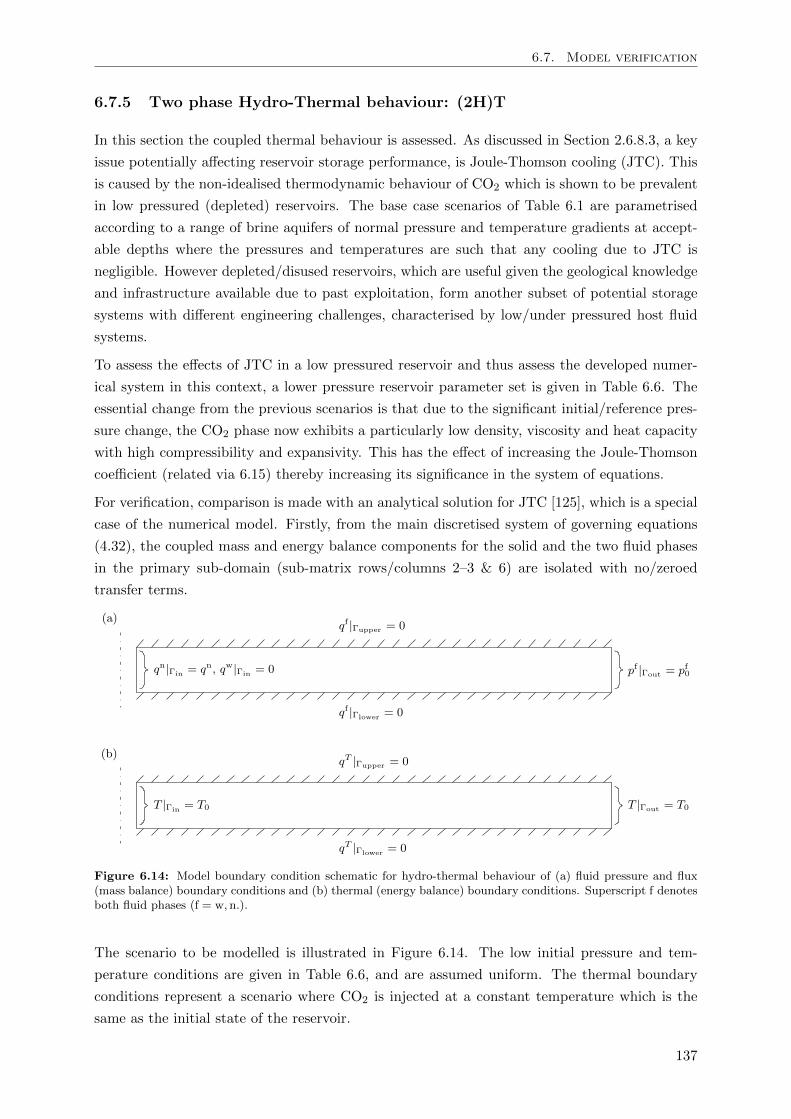
6.7. Model verification
6.7.5 Two phase Hydro-Thermal behaviour: (2H)T
In this section the coupled thermal behaviour is assessed. As discussed in Section 2.6.8.3, a key
issue potentially affecting reservoir storage performance, is Joule-Thomson cooling (JTC). This
is caused by the non-idealised thermodynamic behaviour of CO2 which is shown to be prevalent
in low pressured (depleted) reservoirs. The base case scenarios of Table 6.1 are parametrised
according to a range of brine aquifers of normal pressure and temperature gradients at accept-
able depths where the pressures and temperatures are such that any cooling due to JTC is
negligible. However depleted/disused reservoirs, which are useful given the geological knowledge
and infrastructure available due to past exploitation, form another subset of potential storage
systems with different engineering challenges, characterised by low/under pressured host fluid
systems.
To assess the effects of JTC in a low pressured reservoir and thus assess the developed numer-
ical system in this context, a lower pressure reservoir parameter set is given in Table 6.6. The
essential change from the previous scenarios is that due to the significant initial/reference pres-
sure change, the CO2 phase now exhibits a particularly low density, viscosity and heat capacity
with high compressibility and expansivity. This has the effect of increasing the Joule-Thomson
coefficient (related via 6.15) thereby increasing its significance in the system of equations.
For verification, comparison is made with an analytical solution for JTC [125], which is a special
case of the numerical model. Firstly, from the main discretised system of governing equations
(4.32), the coupled mass and energy balance components for the solid and the two fluid phases
in the primary sub-domain (sub-matrix rows/columns 2–3 & 6) are isolated with no/zeroed
transfer terms.
Figure 6.14: Model boundary condition schematic for hydro-thermal behaviour of (a) fluid pressure and flux(mass balance) boundary conditions and (b) thermal (energy balance) boundary conditions. Superscript f denotesboth fluid phases (f = w, n.).
The scenario to be modelled is illustrated in Figure 6.14. The low initial pressure and tem-
perature conditions are given in Table 6.6, and are assumed uniform. The thermal boundary
conditions represent a scenario where CO2 is injected at a constant temperature which is the
same as the initial state of the reservoir.
137
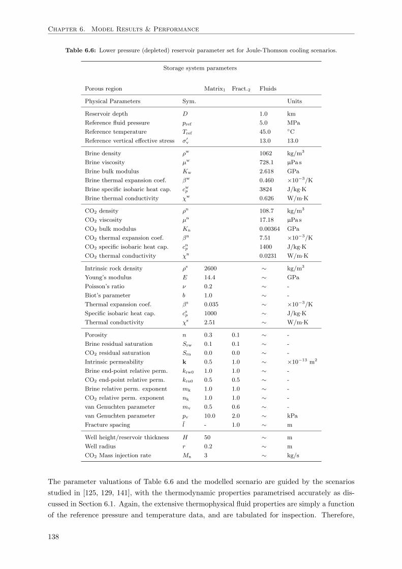
Chapter 6. Model Results & Performance
Table 6.6: Lower pressure (depleted) reservoir parameter set for Joule-Thomson cooling scenarios.
Storage system parameters
Porous region Matrix1 Fract.2 Fluids
Physical Parameters Sym. Units
Reservoir depth D 1.0 km
Reference fluid pressure pref 5.0 MPa
Reference temperature Tref 45.0 C
Reference vertical effective stress σ′v 13.0 13.0
Brine density ρw 1062 kg/m3
Brine viscosity µw 728.1 µPa s
Brine bulk modulus Kw 2.618 GPa
Brine thermal expansion coef. βw 0.460 ×10⁻³/K
Brine specific isobaric heat cap. cwp 3824 J/kg·KBrine thermal conductivity χw 0.626 W/m·K
CO2 density ρn 108.7 kg/m3
CO2 viscosity µn 17.18 µPa s
CO2 bulk modulus Kn 0.00364 GPa
CO2 thermal expansion coef. βn 7.51 ×10⁻³/K
CO2 specific isobaric heat cap. cnp 1400 J/kg·KCO2 thermal conductivity χn 0.0231 W/m·K
Intrinsic rock density ρs 2600 ∼ kg/m3
Young’s modulus E 14.4 ∼ GPa
Poisson’s ratio ν 0.2 ∼ -
Biot’s parameter b 1.0 ∼ -
Thermal expansion coef. βs 0.035 ∼ ×10−3/K
Specific isobaric heat cap. csp 1000 ∼ J/kg·KThermal conductivity χs 2.51 ∼ W/m·K
Porosity n 0.3 0.1 ∼ -
Brine residual saturation Srw 0.1 0.1 ∼ -
CO2 residual saturation Srn 0.0 0.0 ∼ -
Intrinsic permeability k 0.5 1.0 ∼ ×10−13 m2
Brine end-point relative perm. krw0 1.0 1.0 ∼ -
CO2 end-point relative perm. krn0 0.5 0.5 ∼ -
Brine relative perm. exponent mk 1.0 1.0 ∼ -
CO2 relative perm. exponent nk 1.0 1.0 ∼ -
van Genuchten parameter mv 0.5 0.6 ∼ -
van Genuchten parameter pv 10.0 2.0 ∼ kPa
Fracture spacing l - 1.0 ∼ m
Well height/reservoir thickness H 50 ∼ m
Well radius r 0.2 ∼ m
CO2 Mass injection rate Mn 3 ∼ kg/s
The parameter valuations of Table 6.6 and the modelled scenario are guided by the scenarios
studied in [125, 129, 141], with the thermodynamic properties parametrised accurately as dis-
cussed in Section 6.1. Again, the extensive thermophysical fluid properties are simply a function
of the reference pressure and temperature data, and are tabulated for inspection. Therefore,
138
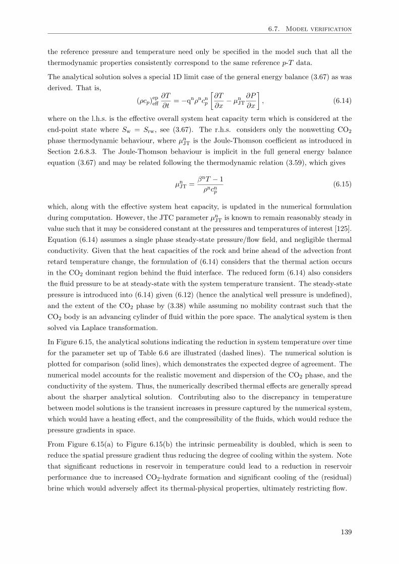
6.7. Model verification
the reference pressure and temperature need only be specified in the model such that all the
thermodynamic properties consistently correspond to the same reference p-T data.
The analytical solution solves a special 1D limit case of the general energy balance (3.67) as was
derived. That is,
(ρcp)epeff
∂T
∂t= −qnρncnp
[∂T
∂x− µnJT
∂P
∂x
], (6.14)
where on the l.h.s. is the effective overall system heat capacity term which is considered at the
end-point state where Sw = Srw, see (3.67). The r.h.s. considers only the nonwetting CO2
phase thermodynamic behaviour, where µnJT is the Joule-Thomson coefficient as introduced in
Section 2.6.8.3. The Joule-Thomson behaviour is implicit in the full general energy balance
equation (3.67) and may be related following the thermodynamic relation (3.59), which gives
µnJT =βnT − 1
ρncnp(6.15)
which, along with the effective system heat capacity, is updated in the numerical formulation
during computation. However, the JTC parameter µnJT is known to remain reasonably steady in
value such that it may be considered constant at the pressures and temperatures of interest [125].
Equation (6.14) assumes a single phase steady-state pressure/flow field, and negligible thermal
conductivity. Given that the heat capacities of the rock and brine ahead of the advection front
retard temperature change, the formulation of (6.14) considers that the thermal action occurs
in the CO2 dominant region behind the fluid interface. The reduced form (6.14) also considers
the fluid pressure to be at steady-state with the system temperature transient. The steady-state
pressure is introduced into (6.14) given (6.12) (hence the analytical well pressure is undefined),
and the extent of the CO2 phase by (3.38) while assuming no mobility contrast such that the
CO2 body is an advancing cylinder of fluid within the pore space. The analytical system is then
solved via Laplace transformation.
In Figure 6.15, the analytical solutions indicating the reduction in system temperature over time
for the parameter set up of Table 6.6 are illustrated (dashed lines). The numerical solution is
plotted for comparison (solid lines), which demonstrates the expected degree of agreement. The
numerical model accounts for the realistic movement and dispersion of the CO2 phase, and the
conductivity of the system. Thus, the numerically described thermal effects are generally spread
about the sharper analytical solution. Contributing also to the discrepancy in temperature
between model solutions is the transient increases in pressure captured by the numerical system,
which would have a heating effect, and the compressibility of the fluids, which would reduce the
pressure gradients in space.
From Figure 6.15(a) to Figure 6.15(b) the intrinsic permeability is doubled, which is seen to
reduce the spatial pressure gradient thus reducing the degree of cooling within the system. Note
that significant reductions in reservoir in temperature could lead to a reduction in reservoir
performance due to increased CO2-hydrate formation and significant cooling of the (residual)
brine which would adversely affect its thermal-physical properties, ultimately restricting flow.
139
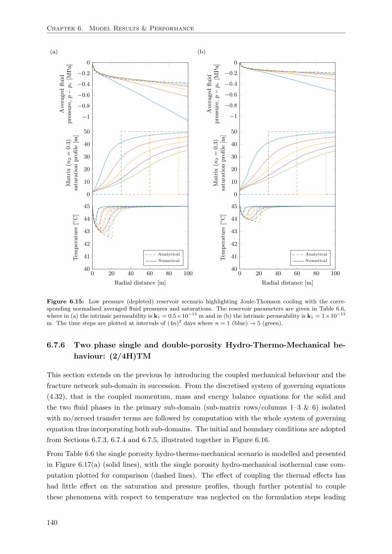
Chapter 6. Model Results & Performance
(a)
−1
−0.8
−0.6
−0.4
−0.2
0Averaged
fluid
pressure,p−pr[M
Pa]
0
10
20
30
40
50
Matrix
(n2=
0.3)
saturationprofile
[m]
0 20 40 60 80 10040
41
42
43
44
45
Radial distance [m]
Tem
perature
[C]
Analytical
Numerical
(b)
−1
−0.8
−0.6
−0.4
−0.2
0
Averaged
fluid
pressure,p−pr[M
Pa]
0
10
20
30
40
50
Matrix
(n2=
0.3)
saturationprofile
[m]
0 20 40 60 80 10040
41
42
43
44
45
Radial distance [m]
Tem
perature
[C]
Analytical
Numerical
Figure 6.15: Low pressure (depleted) reservoir scenario highlighting Joule-Thomson cooling with the corre-sponding normalised averaged fluid pressures and saturations. The reservoir parameters are given in Table 6.6,where in (a) the intrinsic permeability is k1 = 0.5×10⁻¹³ m and in (b) the intrinsic permeability is k1 = 1×10⁻¹³
m. The time steps are plotted at intervals of (4n)2 days where n = 1 (blue)→ 5 (green).
6.7.6 Two phase single and double-porosity Hydro-Thermo-Mechanical be-
haviour: (2/4H)TM
This section extends on the previous by introducing the coupled mechanical behaviour and the
fracture network sub-domain in succession. From the discretised system of governing equations
(4.32), that is the coupled momentum, mass and energy balance equations for the solid and
the two fluid phases in the primary sub-domain (sub-matrix rows/columns 1–3 & 6) isolated
with no/zeroed transfer terms are followed by computation with the whole system of governing
equation thus incorporating both sub-domains. The initial and boundary conditions are adopted
from Sections 6.7.3, 6.7.4 and 6.7.5, illustrated together in Figure 6.16.
From Table 6.6 the single porosity hydro-thermo-mechanical scenario is modelled and presented
in Figure 6.17(a) (solid lines), with the single porosity hydro-mechanical isothermal case com-
putation plotted for comparison (dashed lines). The effect of coupling the thermal effects has
had little effect on the saturation and pressure profiles, though further potential to couple
these phenomena with respect to temperature was neglected on the formulation steps leading
140
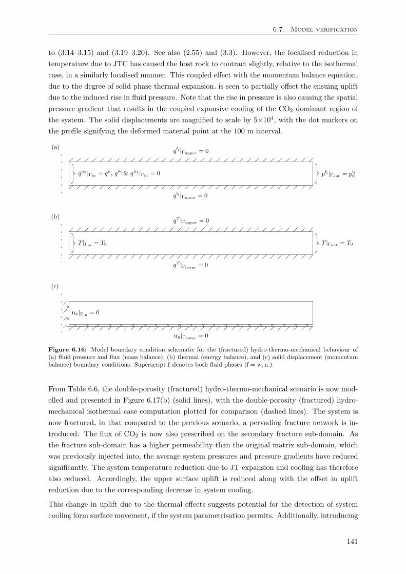
6.7. Model verification
to (3.14–3.15) and (3.19–3.20). See also (2.55) and (3.3). However, the localised reduction in
temperature due to JTC has caused the host rock to contract slightly, relative to the isothermal
case, in a similarly localised manner. This coupled effect with the momentum balance equation,
due to the degree of solid phase thermal expansion, is seen to partially offset the ensuing uplift
due to the induced rise in fluid pressure. Note that the rise in pressure is also causing the spatial
pressure gradient that results in the coupled expansive cooling of the CO2 dominant region of
the system. The solid displacements are magnified to scale by 5×10⁴, with the dot markers on
the profile signifying the deformed material point at the 100 m interval.
Figure 6.16: Model boundary condition schematic for the (fractured) hydro-thermo-mechanical behaviour of(a) fluid pressure and flux (mass balance), (b) thermal (energy balance), and (c) solid displacement (momentumbalance) boundary conditions. Superscript f denotes both fluid phases (f = w, n.).
From Table 6.6, the double-porosity (fractured) hydro-thermo-mechanical scenario is now mod-
elled and presented in Figure 6.17(b) (solid lines), with the double-porosity (fractured) hydro-
mechanical isothermal case computation plotted for comparison (dashed lines). The system is
now fractured, in that compared to the previous scenario, a pervading fracture network is in-
troduced. The flux of CO2 is now also prescribed on the secondary fracture sub-domain. As
the fracture sub-domain has a higher permeability than the original matrix sub-domain, which
was previously injected into, the average system pressures and pressure gradients have reduced
significantly. The system temperature reduction due to JT expansion and cooling has therefore
also reduced. Accordingly, the upper surface uplift is reduced along with the offset in uplift
reduction due to the corresponding decrease in system cooling.
This change in uplift due to the thermal effects suggests potential for the detection of system
cooling form surface movement, if the system parametrisation permits. Additionally, introducing
141
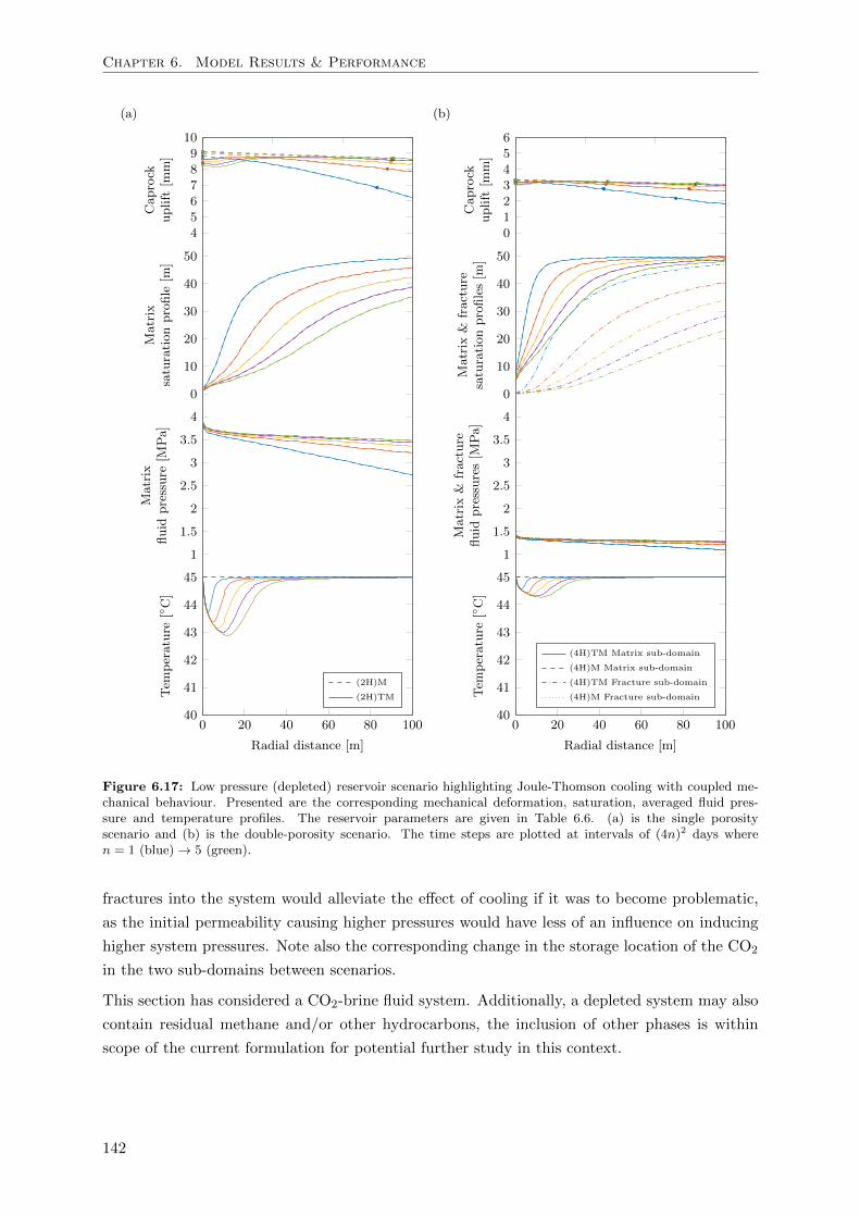
Chapter 6. Model Results & Performance
(a)
456789
10Caprock
uplift
[mm]
0
10
20
30
40
50
Matrix
saturationprofile
[m]
1
1.5
2
2.5
3
3.5
4
Matrix
fluid
pressure
[MPa]
0 20 40 60 80 10040
41
42
43
44
45
Radial distance [m]
Tem
perature
[C]
(2H)M
(2H)TM
(b)
0123456
Caprock
uplift
[mm]
0
10
20
30
40
50
Matrix
&fracture
saturationprofiles[m
]
1
1.5
2
2.5
3
3.5
4
Matrix
&fracture
fluid
pressures[M
Pa]
0 20 40 60 80 10040
41
42
43
44
45
Radial distance [m]
Tem
perature
[C]
(4H)TM Matrix sub-domain
(4H)M Matrix sub-domain
(4H)TM Fracture sub-domain
(4H)M Fracture sub-domain
Figure 6.17: Low pressure (depleted) reservoir scenario highlighting Joule-Thomson cooling with coupled me-chanical behaviour. Presented are the corresponding mechanical deformation, saturation, averaged fluid pres-sure and temperature profiles. The reservoir parameters are given in Table 6.6. (a) is the single porosityscenario and (b) is the double-porosity scenario. The time steps are plotted at intervals of (4n)2 days wheren = 1 (blue)→ 5 (green).
fractures into the system would alleviate the effect of cooling if it was to become problematic,
as the initial permeability causing higher pressures would have less of an influence on inducing
higher system pressures. Note also the corresponding change in the storage location of the CO2
in the two sub-domains between scenarios.
This section has considered a CO2-brine fluid system. Additionally, a depleted system may also
contain residual methane and/or other hydrocarbons, the inclusion of other phases is within
scope of the current formulation for potential further study in this context.
142
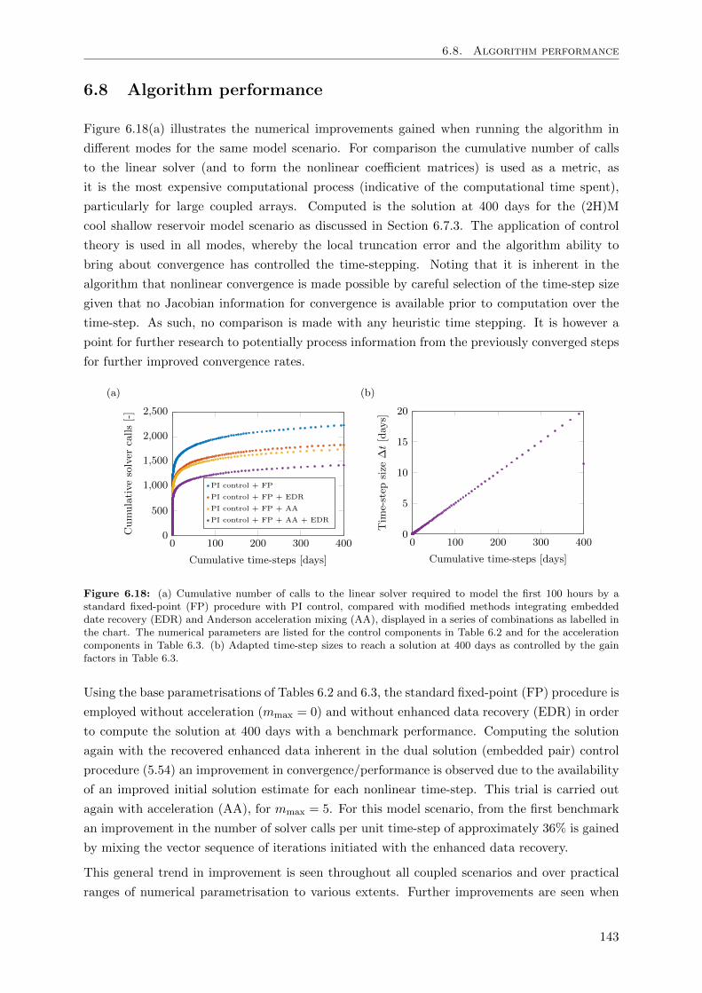
6.8. Algorithm performance
6.8 Algorithm performance
Figure 6.18(a) illustrates the numerical improvements gained when running the algorithm in
different modes for the same model scenario. For comparison the cumulative number of calls
to the linear solver (and to form the nonlinear coefficient matrices) is used as a metric, as
it is the most expensive computational process (indicative of the computational time spent),
particularly for large coupled arrays. Computed is the solution at 400 days for the (2H)M
cool shallow reservoir model scenario as discussed in Section 6.7.3. The application of control
theory is used in all modes, whereby the local truncation error and the algorithm ability to
bring about convergence has controlled the time-stepping. Noting that it is inherent in the
algorithm that nonlinear convergence is made possible by careful selection of the time-step size
given that no Jacobian information for convergence is available prior to computation over the
time-step. As such, no comparison is made with any heuristic time stepping. It is however a
point for further research to potentially process information from the previously converged steps
for further improved convergence rates.
(a)
0 100 200 300 4000
500
1,000
1,500
2,000
2,500
Cumulative time-steps [days]
Cumulativesolver
calls[-]
PI control + FP
PI control + FP + EDR
PI control + FP + AA
PI control + FP + AA + EDR
(b)
0 100 200 300 4000
5
10
15
20
Cumulative time-steps [days]
Tim
e-step
size
∆t[day
s]
Figure 6.18: (a) Cumulative number of calls to the linear solver required to model the first 100 hours by astandard fixed-point (FP) procedure with PI control, compared with modified methods integrating embeddeddate recovery (EDR) and Anderson acceleration mixing (AA), displayed in a series of combinations as labelled inthe chart. The numerical parameters are listed for the control components in Table 6.2 and for the accelerationcomponents in Table 6.3. (b) Adapted time-step sizes to reach a solution at 400 days as controlled by the gainfactors in Table 6.3.
Using the base parametrisations of Tables 6.2 and 6.3, the standard fixed-point (FP) procedure is
employed without acceleration (mmax = 0) and without enhanced data recovery (EDR) in order
to compute the solution at 400 days with a benchmark performance. Computing the solution
again with the recovered enhanced data inherent in the dual solution (embedded pair) control
procedure (5.54) an improvement in convergence/performance is observed due to the availability
of an improved initial solution estimate for each nonlinear time-step. This trial is carried out
again with acceleration (AA), for mmax = 5. For this model scenario, from the first benchmark
an improvement in the number of solver calls per unit time-step of approximately 36% is gained
by mixing the vector sequence of iterations initiated with the enhanced data recovery.
This general trend in improvement is seen throughout all coupled scenarios and over practical
ranges of numerical parametrisation to various extents. Further improvements are seen when
143
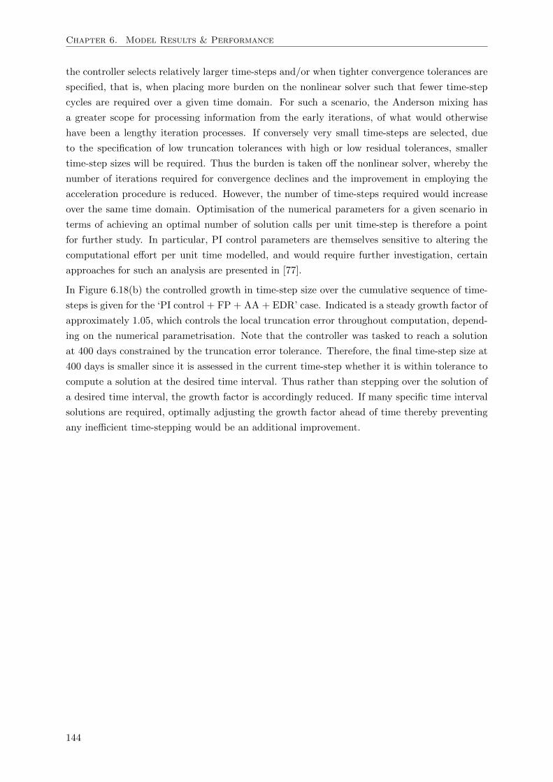
Chapter 6. Model Results & Performance
the controller selects relatively larger time-steps and/or when tighter convergence tolerances are
specified, that is, when placing more burden on the nonlinear solver such that fewer time-step
cycles are required over a given time domain. For such a scenario, the Anderson mixing has
a greater scope for processing information from the early iterations, of what would otherwise
have been a lengthy iteration processes. If conversely very small time-steps are selected, due
to the specification of low truncation tolerances with high or low residual tolerances, smaller
time-step sizes will be required. Thus the burden is taken off the nonlinear solver, whereby the
number of iterations required for convergence declines and the improvement in employing the
acceleration procedure is reduced. However, the number of time-steps required would increase
over the same time domain. Optimisation of the numerical parameters for a given scenario in
terms of achieving an optimal number of solution calls per unit time-step is therefore a point
for further study. In particular, PI control parameters are themselves sensitive to altering the
computational effort per unit time modelled, and would require further investigation, certain
approaches for such an analysis are presented in [77].
In Figure 6.18(b) the controlled growth in time-step size over the cumulative sequence of time-
steps is given for the ‘PI control + FP + AA + EDR’ case. Indicated is a steady growth factor of
approximately 1.05, which controls the local truncation error throughout computation, depend-
ing on the numerical parametrisation. Note that the controller was tasked to reach a solution
at 400 days constrained by the truncation error tolerance. Therefore, the final time-step size at
400 days is smaller since it is assessed in the current time-step whether it is within tolerance to
compute a solution at the desired time interval. Thus rather than stepping over the solution of
a desired time interval, the growth factor is accordingly reduced. If many specific time interval
solutions are required, optimally adjusting the growth factor ahead of time thereby preventing
any inefficient time-stepping would be an additional improvement.
144
Chapter 7
Muographic Modelling Applications
How to efficiently/cost-effectively monitor a GCS site in a passive and continuous manner is an
existing problem. The model formulation, numerical implementation and coding of this work
are also developed for the purpose of assessing and developing muon radiography as a novel
and unconventional solution to this problem. As outlined in Chapters 1 and 2, this work has
been carried out as part of a collaborative project on the interrelated demand for the effective
governance, monitoring and modelling of GCS. A key vision of this project is the notion of
employing cosmic-ray muon imaging as a passive and continuous monitoring aid for GCS [114].
Cosmic-ray muon tomography and transmission imaging (Section 2.11.2) have been proven to
be feasible for imaging stationary and dynamic large scale objects [10, 188]. The first studies
on applying this technique for imaging a realistic geo-stored CO2 body are presented in the
following two sections.
Firstly, Section 7.1 presents and implements a workflow for embedding the numerical code with a
particle transport simulation code in order to model and assess the conceptual viability of using
muon radiography as a means to monitor geo-stored CO2. This is carried out for a realistic
though idealised site for study purposes. The full extensive account of this study is given in the
co-authored work of [108]. Due to the various specialisations involved, which are beyond the
scope of this thesis, complementary details are primarily given in this section with respect to the
multi-physics modelling strategy and code integration which made the multifaceted simulation
possible.
Secondly, in Section 7.2, an alternative method for modelling muon radiography is adopted
based on the co-authored work of [23]. This method is based on muon survival statistics rather
than explicit muon-by-muon simulations through the subsurface. The muon physics is therefore
implemented in a highly simplified manner, however the method is significantly more compu-
tationally efficient in comparison. This approach is demonstrated to be ideal for screening and
optimising storage scenarios. To this effect, a realistic, non-idealised and challenging real-world
CO2 storage scenario is assessed using this approach and is discussed.
145
Chapter 7. Muographic Modelling Applications
7.1 Modelling muon radiography for monitoring a GCS site
The site selected for the study is situated offshore above Boulby Mine, Cleveland, UK. Though
no CO2 will be stored there, the site is selected because the mine below is accessible and has
research facilities for prototyping and testing muon detectors. Additionally, the geological data
above the mine is available to the research team and is well understood for the purpose of
processing for simulation.
7.1.1 Modelling methodology
The object-orientated programming framework Geant4 [1] (Section 2.11.2.3) is used to host the
present simulation. A virtual environment is constructed of a ∼40 km2 geological area extending
from the sea surface to a subsurface muon detector; it represents the medium through which
the muons will travel, interact and decay. This geological body is populated with the known
Boulby geological data. The detector is conceptualised of plastic scintillator and photo-sensor
technology with an effective detection surface area corresponding to 1000 m2, and is located at
a trial depth within the mine of 776 m below the seabed. This depth is selected as it is the
depth for a test site within the mine for muon detector prototyping to take place. The results
of this simulation are therefore to aid muon detector design for GCS applications, which is also
ongoing research.
The energy spectrum of cosmic-ray muons arriving through the sea surface is described by the
Gaisser parametrisation [66] (Section 2.11.2), which accounts for the correlations between muon
energy and trajectory (zenith angle). Monte Carlo methods are used to sample according to the
parametrisation in order to generate muons. The Geant4.9.6 ‘shielding’ physics list [1] is used
to simulate the loss of muon energy through the subsurface due to interaction with the matter
of the modelled subsurface. To assess the sufficiency of this modelling approach the reader is
referred to [1, 108, 113].
The muon energy loss is principally related to the density and composition (mean atomic number
and weight) of the bulk medium through which they travel and interact (Section 2.11.2). If the
muon energy becomes low enough the muon will stop or decay and be absorbed. By altering
the bulk density and composition of the bulk medium the observable muon flux through it
will therefore change. As a result, it is possible to map the bulk density and composition by
observing changes in the muon flux emerging form the medium of interest, if indeed a known or
steady flux is entering the medium.
The simulation is initially carried out over the geological body of interest in order to establish
a statistically independent expectation count of muon events over time through the detector
without CO2 in place. The muon flux reaching the simulated detector is determined to be
approximately 2.3 × 10⁻⁷ cm−2 s−1 (200 m−2 day−1). Subsurface muon flux distributions are
tabulated and discussed further in [113].
146
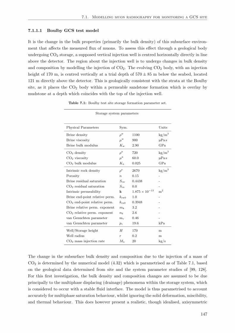
7.1. Modelling muon radiography for monitoring a GCS site
7.1.1.1 Boulby GCS test model
It is the change in the bulk properties (primarily the bulk density) of this subsurface environ-
ment that affects the measured flux of muons. To assess this effect through a geological body
undergoing CO2 storage, a supposed vertical injection well is centred horizontally directly in line
above the detector. The region about the injection well is to undergo changes in bulk density
and composition by modelling the injection of CO2. The evolving CO2 body, with an injection
height of 170 m, is centred vertically at a trial depth of 570 ± 85 m below the seabed, located
121 m directly above the detector. This is geologically consistent with the strata at the Boulby
site, as it places the CO2 body within a permeable sandstone formation which is overlay by
mudstone at a depth which coincides with the top of the injection well.
Table 7.1: Boulby test site storage formation parameter set.
Storage system parameters
Physical Parameters Sym. Units
Brine density ρw 1100 kg/m3
Brine viscosity µw 900 µPa s
Brine bulk modulus Kw 2.90 GPa
CO2 density ρn 720 kg/m3
CO2 viscosity µn 60.0 µPa s
CO2 bulk modulus Kn 0.025 GPa
Intrinsic rock density ρs 2670 kg/m3
Porosity n 0.15 -
Brine residual saturation Srw 0.4438 -
CO2 residual saturation Srn 0.0 -
Intrinsic permeability k 1.875× 10⁻¹³ m2
Brine end-point relative perm. krw0 1.0 -
CO2 end-point relative perm. krn0 0.3948 -
Brine relative perm. exponent mk 3.2 -
CO2 relative perm. exponent nk 2.6 -
van Genuchten parameter mv 0.46 -
van Genuchten parameter pv 19.6 kPa
Well/Storage height H 170 m
Well radius r 0.2 m
CO2 mass injection rate Mn 20 kg/s
The change in the subsurface bulk density and composition due to the injection of a mass of
CO2 is determined by the numerical model (4.32) which is parametrised as of Table 7.1, based
on the geological data determined from site and the system parameter studies of [99, 128].
For this first investigation, the bulk density and composition changes are assumed to be due
principally to the multiphase displacing (drainage) phenomena within the storage system, which
is considered to occur with a stable fluid interface. The model is thus parametrised to account
accurately for multiphase saturation behaviour, whilst ignoring the solid deformation, miscibility,
and thermal behaviour. This does however present a realistic, though idealised, axisymmetric
147
Chapter 7. Muographic Modelling Applications
fluid interface with a density/composition contrast through which the effect on the muon flux
can be computed in order to assess the feasibility of using muon radiography to detect a moving
CO2 body/brine-CO2 interface. The idealised model is meaningful for this first conceptual
study because it gives a realistic though basic bulk density/composition contrast, which allows
for ease of interpreting the results and practically assessing the changes in muon flux through
the geological body.
The mudstone above the storage region is assumed to be impermeable, and given the relatively
low mass injection rate per unit well height, the CO2 body modelled during injection demon-
strates significant buoyancy effects collecting as a relatively thin layer away from the injection
well under the sandstone/mudstone interface whilst migrating radially (7.2(a)).
The numerical model outputs are used to give a bulk composition and to compute a macroscopic
bulk density by summation of the product of the intrinsic phase densities and their corresponding
volume fractions, after the review of Section 2.1.2 and as used for the bulk density in the
momentum balance formulation (3.44),
ρ = (1− n)ρs + nSnρn + nSwρ
w. (7.1)
The current simulation framework is constrained to simulate muon interactions through one
static geological scenario at a time. The information provided by the numerical model is therefore
produced for a sequence of 10 sequential time intervals which correspond to (2n)2 days, where
n = 1 → 10, from the start of CO2 injection. This stepping was chosen given the relationship of
the radial fluid interface extent with time (xnmax ∝√t), such that the CO2 body to be tracked
is extending over a uniform distance for each interval. Given the parametrisation of Table 7.1,
that is an approximate radial extent increase of 36 m per time interval until an approximate
distance of 360 m from the well is reached at 400 days (this may also be verified by (3.38)).
Therefore, the storage formation state at time interval n, as computed, represents an average
storage system state between the period (2n− 1)2 to (2n+ 1)2 days.
7.1.1.2 Model integration
The numerically computed bulk density and composition states of the storage formation are
embedded in the Geant4 framework by exploiting its object-orientated architecture by making
use of the voxel (volumetric pixel) processing capabilities within its libraries. The voxelisation
capabilities are typically utilised for constructing medical phantoms to undergo simulation with
radiography. This code integration may be visualised in Figure 7.1, which outlines a workflow for
embedding the numerical model nodal solutions with the existing object-orientated architecture.
Essentially, the GeometryConstruction class handles the modelled physical objects of matter
(geological body and detector) with which particles are to interact. This is informed of the local
voxelised changes in bulk density and composition from the numerical model nodal solutions via
the PhantomConfiguration and VoxelParametrisation classes.
For example, Figure 7.2(a) illustrates the bulk density as computed by the numerical model at
n = 4 (64 days). Figure 7.2(b) illustrates the corresponding voxelisated form which is embedded
148
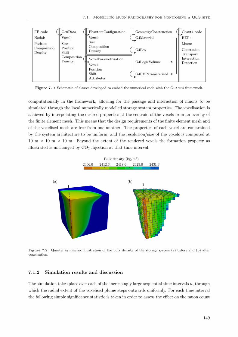
7.1. Modelling muon radiography for monitoring a GCS site
Figure 7.1: Schematic of classes developed to embed the numerical code with the Geant4 framework.
computationally in the framework, allowing for the passage and interaction of muons to be
simulated through the local numerically modelled storage system properties. The voxelisation is
achieved by interpolating the desired properties at the centroid of the voxels from an overlay of
the finite element mesh. This means that the design requirements of the finite element mesh and
of the voxelised mesh are free from one another. The properties of each voxel are constrained
by the system architecture to be uniform, and the resolution/size of the voxels is computed at
10 m × 10 m × 10 m. Beyond the extent of the rendered voxels the formation property as
illustrated is unchanged by CO2 injection at that time interval.
Figure 7.2: Quarter symmetric illustration of the bulk density of the storage system (a) before and (b) aftervoxelisation.
7.1.2 Simulation results and discussion
The simulation takes place over each of the increasingly large sequential time intervals n, through
which the radial extent of the voxelised plume steps outwards uniformly. For each time interval
the following simple significance statistic is taken in order to assess the effect on the muon count
149
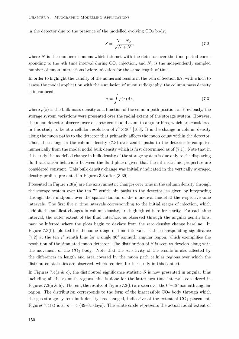
Chapter 7. Muographic Modelling Applications
in the detector due to the presence of the modelled evolving CO2 body,
S =N −N0√N +N0
, (7.2)
where N is the number of muons which interact with the detector over the time period corre-
sponding to the nth time interval during CO2 injection, and N0 is the independently sampled
number of muon interactions before injection for the same length of time.
In order to highlight the validity of the numerical results in the vein of Section 6.7, with which to
assess the model application with the simulation of muon radiography, the column mass density
is introduced,
σ =
∫ρ(z) dz, (7.3)
where ρ(z) is the bulk mass density as a function of the column path position z. Previously, the
storage system variations were presented over the radial extent of the storage system. However,
the muon detector observes over discrete zenith and azimuth angular bins, which are considered
in this study to be at a cellular resolution of 7 × 36 [108]. It is the change in column density
along the muon paths to the detector that primarily affects the muon count within the detector.
Thus, the change in the column density (7.3) over zenith paths to the detector is computed
numerically from the model nodal bulk density which is first determined as of (7.1). Note that in
this study the modelled change in bulk density of the storage system is due only to the displacing
fluid saturation behaviour between the fluid phases given that the intrinsic fluid properties are
considered constant. This bulk density change was initially indicated in the vertically averaged
density profiles presented in Figures 3.3 after (3.39).
Presented in Figure 7.3(a) are the axisymmetric changes over time in the column density through
the storage system over the ten 7 zenith bin paths to the detector, as given by integrating
through their midpoint over the spatial domain of the numerical model at the respective time
intervals. The first five n time intervals corresponding to the initial stages of injection, which
exhibit the smallest changes in column density, are highlighted here for clarity. For each time
interval, the outer extent of the fluid interface, as observed through the angular zenith bins,
may be inferred where the plots begin to deviate from the zero density change baseline. In
Figure 7.3(b), plotted for the same range of time intervals, is the corresponding significance
(7.2) at the ten 7 zenith bins for a single 36 azimuth angular region, which exemplifies the
resolution of the simulated muon detector. The distribution of S is seen to develop along with
the movement of the CO2 body. Note that the sensitivity of the results is also affected by
the differences in length and area covered by the muon path cellular regions over which the
distributed statistics are observed, which requires further study in this context.
In Figures 7.4(a & c), the distributed significance statistic S is now presented in angular bins
including all the azimuth regions, this is done for the latter two time intervals considered in
Figures 7.3(a & b). Therein, the results of Figure 7.3(b) are seen over the 0–36 azimuth angular
region. The distribution corresponds to the form of the inaccessible CO2 body through which
the geo-storage system bulk density has changed, indicative of the extent of CO2 placement.
Figures 7.4(a) is at n = 4 (49–81 days). The white circle represents the actual radial extent of
150
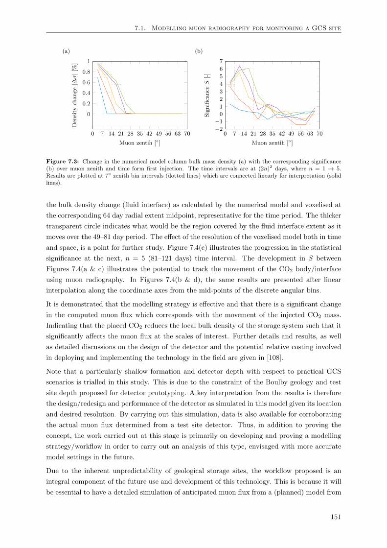
7.1. Modelling muon radiography for monitoring a GCS site
(a)
0 7 14 21 28 35 42 49 56 63 70
0
0.2
0.4
0.6
0.8
1
Muon zentih []
Den
sity
change|∆σ|[%]
(b)
0 7 14 21 28 35 42 49 56 63 70−2−10
1
2
3
4
5
6
7
Muon zentih []
SignificanceS
[-]
Figure 7.3: Change in the numerical model column bulk mass density (a) with the corresponding significance(b) over muon zenith and time form first injection. The time intervals are at (2n)2 days, where n = 1 → 5.Results are plotted at 7 zenith bin intervals (dotted lines) which are connected linearly for interpretation (solidlines).
the bulk density change (fluid interface) as calculated by the numerical model and voxelised at
the corresponding 64 day radial extent midpoint, representative for the time period. The thicker
transparent circle indicates what would be the region covered by the fluid interface extent as it
moves over the 49–81 day period. The effect of the resolution of the voxelised model both in time
and space, is a point for further study. Figure 7.4(c) illustrates the progression in the statistical
significance at the next, n = 5 (81–121 days) time interval. The development in S between
Figures 7.4(a & c) illustrates the potential to track the movement of the CO2 body/interface
using muon radiography. In Figures 7.4(b & d), the same results are presented after linear
interpolation along the coordinate axes from the mid-points of the discrete angular bins.
It is demonstrated that the modelling strategy is effective and that there is a significant change
in the computed muon flux which corresponds with the movement of the injected CO2 mass.
Indicating that the placed CO2 reduces the local bulk density of the storage system such that it
significantly affects the muon flux at the scales of interest. Further details and results, as well
as detailed discussions on the design of the detector and the potential relative costing involved
in deploying and implementing the technology in the field are given in [108].
Note that a particularly shallow formation and detector depth with respect to practical GCS
scenarios is trialled in this study. This is due to the constraint of the Boulby geology and test
site depth proposed for detector prototyping. A key interpretation from the results is therefore
the design/redesign and performance of the detector as simulated in this model given its location
and desired resolution. By carrying out this simulation, data is also available for corroborating
the actual muon flux determined from a test site detector. Thus, in addition to proving the
concept, the work carried out at this stage is primarily on developing and proving a modelling
strategy/workflow in order to carry out an analysis of this type, envisaged with more accurate
model settings in the future.
Due to the inherent unpredictability of geological storage sites, the workflow proposed is an
integral component of the future use and development of this technology. This is because it will
be essential to have a detailed simulation of anticipated muon flux from a (planned) model from
151
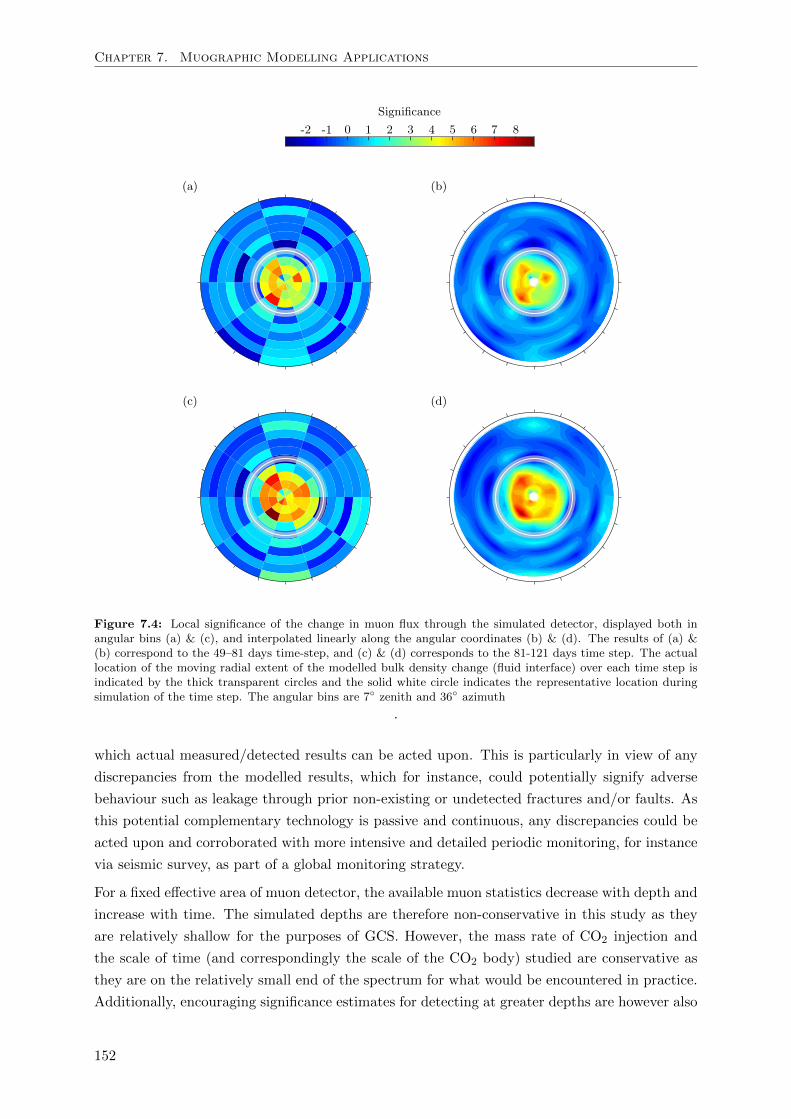
Chapter 7. Muographic Modelling Applications
Figure 7.4: Local significance of the change in muon flux through the simulated detector, displayed both inangular bins (a) & (c), and interpolated linearly along the angular coordinates (b) & (d). The results of (a) &(b) correspond to the 49–81 days time-step, and (c) & (d) corresponds to the 81-121 days time step. The actuallocation of the moving radial extent of the modelled bulk density change (fluid interface) over each time step isindicated by the thick transparent circles and the solid white circle indicates the representative location duringsimulation of the time step. The angular bins are 7 zenith and 36 azimuth
.
which actual measured/detected results can be acted upon. This is particularly in view of any
discrepancies from the modelled results, which for instance, could potentially signify adverse
behaviour such as leakage through prior non-existing or undetected fractures and/or faults. As
this potential complementary technology is passive and continuous, any discrepancies could be
acted upon and corroborated with more intensive and detailed periodic monitoring, for instance
via seismic survey, as part of a global monitoring strategy.
For a fixed effective area of muon detector, the available muon statistics decrease with depth and
increase with time. The simulated depths are therefore non-conservative in this study as they
are relatively shallow for the purposes of GCS. However, the mass rate of CO2 injection and
the scale of time (and correspondingly the scale of the CO2 body) studied are conservative as
they are on the relatively small end of the spectrum for what would be encountered in practice.
Additionally, encouraging significance estimates for detecting at greater depths are however also
152
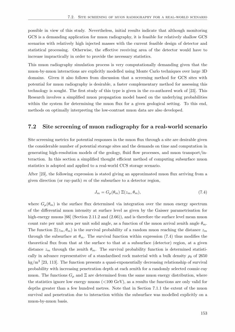
7.2. Site screening of muon radiography for a real-world scenario
possible in view of this study. Nevertheless, initial results indicate that although monitoring
GCS is a demanding application for muon radiography, it is feasible for relatively shallow GCS
scenarios with relatively high injected masses with the current feasible design of detector and
statistical processing. Otherwise, the effective receiving area of the detector would have to
increase impractically in order to provide the necessary statistics.
This muon radiography simulation process is very computationally demanding given that the
muon-by-muon interactions are explicitly modelled using Monte Carlo techniques over large 3D
domains. Given it also follows from discussion that a screening method for GCS sites with
potential for muon radiography is desirable, a faster complementary method for assessing this
technology is sought. The first study of this type is given in the co-authored work of [23]. This
Research involves a simplified muon propagation model based on the underlying probabilities
within the system for determining the muon flux for a given geological setting. To this end,
methods on optimally interpreting the low-contrast muon data are also developed.
7.2 Site screening of muon radiography for a real-world scenario
Site screening metrics for potential responses in the muon flux through a site are desirable given
the considerable number of potential storage sites and the demands on time and computation in
generating high-resolution models of the geology, fluid flow processes, and muon transport/in-
teraction. In this section a simplified thought efficient method of computing subsurface muon
statistics is adopted and applied to a real-world CCS storage scenario.
After [23], the following expression is stated giving an approximated muon flux arriving from a
given direction (or ray-path) m of the subsurface to a detector region,
Jm = Gµ(θm) Ξ(zm, θm), (7.4)
where Gµ(θm) is the surface flux determined via integration over the muon energy spectrum
of the differential muon intensity at surface level as given by the Gaisser parametrisation for
high-energy muons [66] (Section 2.11.2 and (2.66)), and is therefore the surface level mean muon
count rate per unit area per unit solid angle, as a function of the muon arrival zenith angle θm.
The function Ξ(zm, θm) is the survival probability of a random muon reaching the distance zm
through the subsurface at θm. The survival function within expression (7.4) thus modifies the
theoretical flux from that at the surface to that at a subsurface (detector) region, at a given
distance zm through the zenith θm. The survival probability function is determined statisti-
cally in advance representative of a standardised rock material with a bulk density ρ0 of 2650
kg/m3 [23, 113]. The function presents a quasi-exponentially decreasing relationship of survival
probability with increasing penetration depth at each zenith for a randomly selected cosmic-ray
muon. The functions Gµ and Ξ are determined from the same muon energy distribution, where
the statistics ignore low energy muons (<100 GeV), as a results the functions are only valid for
depths greater than a few hundred metres. Note that in Section 7.1.1 the extent of the muon
survival and penetration due to interaction within the subsurface was modelled explicitly on a
muon-by-muon basis.
153
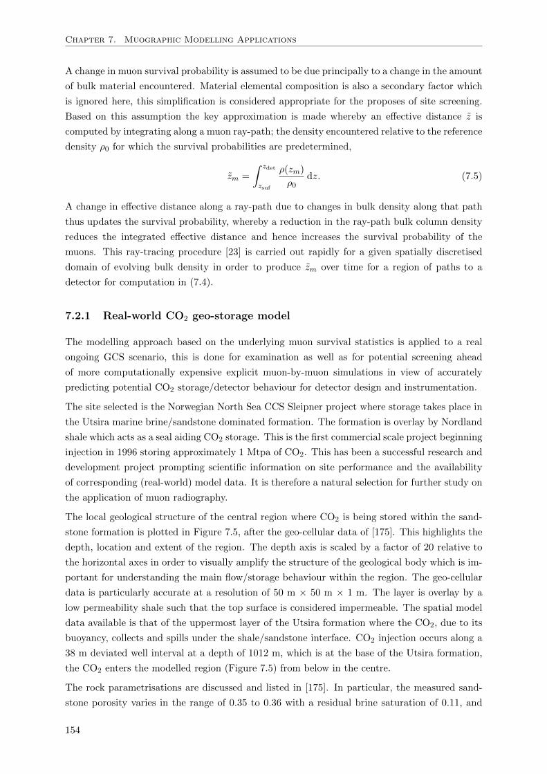
Chapter 7. Muographic Modelling Applications
A change in muon survival probability is assumed to be due principally to a change in the amount
of bulk material encountered. Material elemental composition is also a secondary factor which
is ignored here, this simplification is considered appropriate for the proposes of site screening.
Based on this assumption the key approximation is made whereby an effective distance z is
computed by integrating along a muon ray-path; the density encountered relative to the reference
density ρ0 for which the survival probabilities are predetermined,
zm =
∫ zdet
zsuf
ρ(zm)
ρ0dz. (7.5)
A change in effective distance along a ray-path due to changes in bulk density along that path
thus updates the survival probability, whereby a reduction in the ray-path bulk column density
reduces the integrated effective distance and hence increases the survival probability of the
muons. This ray-tracing procedure [23] is carried out rapidly for a given spatially discretised
domain of evolving bulk density in order to produce zm over time for a region of paths to a
detector for computation in (7.4).
7.2.1 Real-world CO2 geo-storage model
The modelling approach based on the underlying muon survival statistics is applied to a real
ongoing GCS scenario, this is done for examination as well as for potential screening ahead
of more computationally expensive explicit muon-by-muon simulations in view of accurately
predicting potential CO2 storage/detector behaviour for detector design and instrumentation.
The site selected is the Norwegian North Sea CCS Sleipner project where storage takes place in
the Utsira marine brine/sandstone dominated formation. The formation is overlay by Nordland
shale which acts as a seal aiding CO2 storage. This is the first commercial scale project beginning
injection in 1996 storing approximately 1 Mtpa of CO2. This has been a successful research and
development project prompting scientific information on site performance and the availability
of corresponding (real-world) model data. It is therefore a natural selection for further study on
the application of muon radiography.
The local geological structure of the central region where CO2 is being stored within the sand-
stone formation is plotted in Figure 7.5, after the geo-cellular data of [175]. This highlights the
depth, location and extent of the region. The depth axis is scaled by a factor of 20 relative to
the horizontal axes in order to visually amplify the structure of the geological body which is im-
portant for understanding the main flow/storage behaviour within the region. The geo-cellular
data is particularly accurate at a resolution of 50 m × 50 m × 1 m. The layer is overlay by a
low permeability shale such that the top surface is considered impermeable. The spatial model
data available is that of the uppermost layer of the Utsira formation where the CO2, due to its
buoyancy, collects and spills under the shale/sandstone interface. CO2 injection occurs along a
38 m deviated well interval at a depth of 1012 m, which is at the base of the Utsira formation,
the CO2 enters the modelled region (Figure 7.5) from below in the centre.
The rock parametrisations are discussed and listed in [175]. In particular, the measured sand-
stone porosity varies in the range of 0.35 to 0.36 with a residual brine saturation of 0.11, and
154
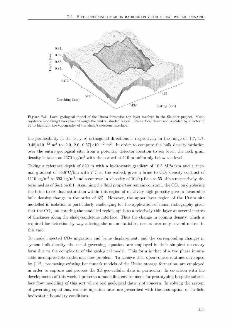
7.2. Site screening of muon radiography for a real-world scenario
Figure 7.5: Local geological model of the Utsira formation top layer involved in the Sleipner project. Muonray-trace modelling takes place through the central shaded region. The vertical dimension is scaled by a factor of20 to highlight the topography of the shale/sandstone interface.
the permeability in the [x, y, z] orthogonal directions is respectively in the range of [1.7, 1.7,
0.48]×10−12 m2 to [2.0, 2.0, 0.57]×10−12 m2. In order to compute the bulk density variation
over the entire geological site, from a potential detector location to sea level, the rock grain
density is taken as 2670 kg/m2 with the seabed at 110 m uniformly below sea level.
Taking a reference depth of 820 m with a hydrostatic gradient of 10.5 MPa/km and a ther-
mal gradient of 35.6C/km with 7C at the seabed, gives a brine to CO2 density contrast of
1110 kg/m3 to 693 kg/m3 and a contrast in viscosity of 1040 µPa·s to 55 µPa·s respectively, de-termined as of Section 6.1. Assuming the fluid properties remain constant, the CO2 on displacing
the brine to residual saturation within this region of relatively high porosity gives a favourable
bulk density change in the order of 6%. However, the upper layer region of the Utsira site
modelled in isolation is particularly challenging for the application of muon radiography given
that the CO2, on entering the modelled region, spills as a relatively thin layer at several metres
of thickness along the shale/sandstone interface. Thus the change in column density, which is
required for detection by way altering the muon statistics, occurs over only several metres in
this case.
To model injected CO2 migration and brine displacement, and the corresponding changes in
system bulk density, the usual governing equations are employed in their simplest necessary
form due to the complexity of the geological model. This form is that of a two phase immis-
cible incompressible isothermal flow problem. To achieve this, open-source routines developed
by [112], promoting existing benchmark models of the Utsira storage formation, are employed
in order to capture and process the 3D geo-cellular data in particular. In co-action with the
developments of this work it presents a modelling environment for prototyping bespoke subsur-
face flow modelling of this sort where real geological data is of concern. In solving the system
of governing equations, realistic injection rates are prescribed with the assumption of far-field
hydrostatic boundary conditions.
155
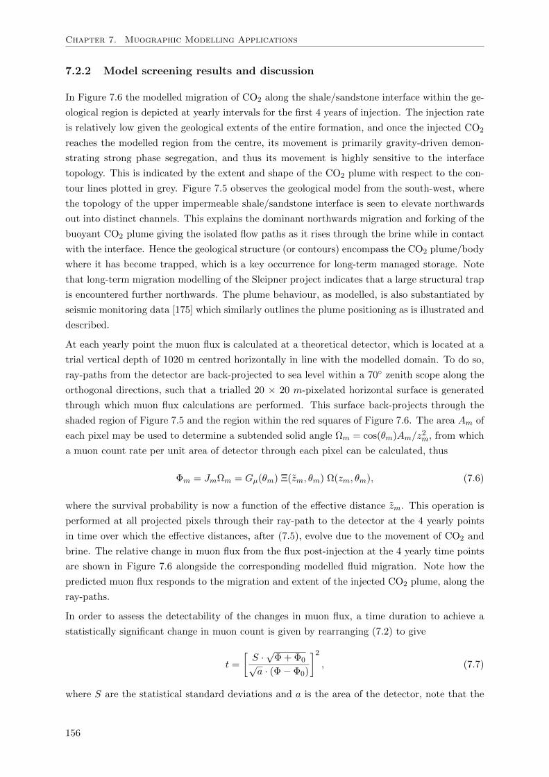
Chapter 7. Muographic Modelling Applications
7.2.2 Model screening results and discussion
In Figure 7.6 the modelled migration of CO2 along the shale/sandstone interface within the ge-
ological region is depicted at yearly intervals for the first 4 years of injection. The injection rate
is relatively low given the geological extents of the entire formation, and once the injected CO2
reaches the modelled region from the centre, its movement is primarily gravity-driven demon-
strating strong phase segregation, and thus its movement is highly sensitive to the interface
topology. This is indicated by the extent and shape of the CO2 plume with respect to the con-
tour lines plotted in grey. Figure 7.5 observes the geological model from the south-west, where
the topology of the upper impermeable shale/sandstone interface is seen to elevate northwards
out into distinct channels. This explains the dominant northwards migration and forking of the
buoyant CO2 plume giving the isolated flow paths as it rises through the brine while in contact
with the interface. Hence the geological structure (or contours) encompass the CO2 plume/body
where it has become trapped, which is a key occurrence for long-term managed storage. Note
that long-term migration modelling of the Sleipner project indicates that a large structural trap
is encountered further northwards. The plume behaviour, as modelled, is also substantiated by
seismic monitoring data [175] which similarly outlines the plume positioning as is illustrated and
described.
At each yearly point the muon flux is calculated at a theoretical detector, which is located at a
trial vertical depth of 1020 m centred horizontally in line with the modelled domain. To do so,
ray-paths from the detector are back-projected to sea level within a 70 zenith scope along the
orthogonal directions, such that a trialled 20 × 20 m-pixelated horizontal surface is generated
through which muon flux calculations are performed. This surface back-projects through the
shaded region of Figure 7.5 and the region within the red squares of Figure 7.6. The area Am of
each pixel may be used to determine a subtended solid angle Ωm = cos(θm)Am/z2m, from which
a muon count rate per unit area of detector through each pixel can be calculated, thus
Φm = JmΩm = Gµ(θm) Ξ(zm, θm) Ω(zm, θm), (7.6)
where the survival probability is now a function of the effective distance zm. This operation is
performed at all projected pixels through their ray-path to the detector at the 4 yearly points
in time over which the effective distances, after (7.5), evolve due to the movement of CO2 and
brine. The relative change in muon flux from the flux post-injection at the 4 yearly time points
are shown in Figure 7.6 alongside the corresponding modelled fluid migration. Note how the
predicted muon flux responds to the migration and extent of the injected CO2 plume, along the
ray-paths.
In order to assess the detectability of the changes in muon flux, a time duration to achieve a
statistically significant change in muon count is given by rearranging (7.2) to give
t =
[S ·
√Φ+ Φ0√
a · (Φ− Φ0)
]2, (7.7)
where S are the statistical standard deviations and a is the area of the detector, note that the
156
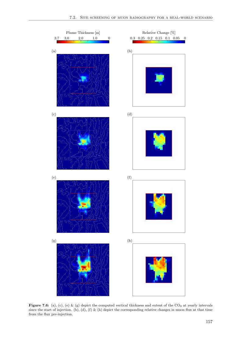
7.2. Site screening of muon radiography for a real-world scenario
Figure 7.6: (a), (c), (e) & (g) depict the computed vertical thickness and extent of the CO2 at yearly intervalssince the start of injection. (b), (d), (f) & (h) depict the corresponding relative changes in muon flux at that timefrom the flux pre-injection.
157
Chapter 7. Muographic Modelling Applications
number of muon events is N = Φ · a · t. Considering a statistically reliable significance of S = 3
and a detector area of 1000 m2 [108, 114], the results of Table 7.2 are produced based on the
total muon flux to the detector for the studied site.
Table 7.2: Changes in total muon flux during CO2 injection.
Time of injection Total Muon Flux Time for statistical significance
T [year] Φ [m−2days−1] t [days]
0 145.068 -
1 145.198 155
2 145.270 64
3 145.292 52
4 145.314 43
The predicted time values of Table 7.2 required for detecting the changes in total flux for this
scenario are reasonable after the first year with respect to the rate at which the plume evolves
globally on a yearly basis. However by assessing the total flux any localised plume features are
ignored. That is, the statistics will become overly challenging when resolving over distinct detec-
tor angular/pixelated observation regions. This is both in terms of the relatively low changes in
muon flux over time for this site/scenario and more generally in terms of achieving useful angular
resolutions in practice, which is ongoing research in muon borehole detector design [108, 114].
Nevertheless, the outlined workflow presents a useful method for potential site screening and
optimally locating and configuring (multiple) potential muon detectors. Additionally, simple
methods have been employed in this study for data analysis, utilising information theory based
methods would improve the analysis of the available data [23].
For thin horizontal CO2 plume regions in particular, the periods of time required to acquire the
necessary statistics in order to reliably determine plume positioning are likely to be too great if
the plume is particularly mobile. However, once such a plume has become immobile within a
large structural geological trap, by design it is to remain there for geological periods, which will
present enough time for the relevant statistics to be gathered to monitor and ensure that long-
term structural trapping is occurring. This prompts muon radiography as a potential long-term
passive monitoring strategy component to indicate if and how structural traps post-injection
phase are retaining even potentially thin CO2 plumes once they have become immobile.
7.3 Evaluation
A landmark is made in the development of muon radiography for monitoring GCS, in that a
modelling framework is developed which allows for the complete multifaceted simulation of the
proposed technology as it would operate in the field. From this framework the first detailed
simulations of muon radiography for monitoring geo-stored CO2 is carried out and assessed for
realistic scenarios. The results indicate that muon radiography is sensitive to subsurface CO2
injection and movement on the scales of interest, demonstrating the conceptual viability of the
technology for GCS. In this thesis it is the fluid flow modelling in view of this application and
158
7.3. Evaluation
key components to the multifaceted modelling strategy which are developed, as is discussed.
The simulations involve realistic calibration in terms of geological data, CO2-brine fluid flow
behaviour, muon radiography and muon detector configuration, though as is discussed various
idealisations are assumed for the purposes of study and development at this stage.
The technology is demonstrated to be conceptually viable, however GCS is a demanding ap-
plication for muon radiography. Initial study indicates that only shallow storage systems at
depths of approximately 1 km with deep injection layers are feasible for this technology given
the otherwise adverse muon statistics with increased depth and reduced plume height. As such,
this technology may be envisaged as a low-resolution passive-continuous monitoring aid as part
of a monitoring strategy with other techniques. The potential use of this technology will also
depend largely on the practicality/relative cost of deploying and instrumenting a muon detector
subsurface in the field. Initial estimates indicate that the use of modified existing wells and mul-
tilateral sidetrack drilling technology is feasible and the costs involved are potentially favourable
in comparison with established alternative monitoring technologies.
The angular scope of a muon detector is demonstrated to cover a region of approximately a
square kilometre. Given the significant long-term lateral extent of realistic CO2 plumes which
may be over several square kilometres, multiple detectors may be required as part of a monitoring
strategy in order to capture the entire movement of the plume. Furthermore, multiple detectors
which collect information from overlapping subsurface regions would allow for the additional
re-construction of a 3D tomographic images of the bulk density variations via triangulation of
the muon statistics.
Further study may also consider other monitoring applications for muon radiography, which are
of particular concern for reasons of safety, understanding and/or effectiveness. Speculatively,
application such as monitoring the extent of hydraulic fracturing and the ensuing enhanced
hydrocarbon recovery, the monitoring of inaccessible glacial/ice shelf melting, the movement
of large contaminated regions of groundwater including leachate, as well as monitoring for the
purposes of mining and subsurface tunnelling and/or excavation works.
Furthermore, it is envisaged from this work that various monitoring technologies could be sim-
ulated within the same framework (coupled and/or uncoupled with the storage system model)
including for instance muon radiography, electrokinetics, and seismology. From this a series
of detection resolutions and attributes could be ascertained in order to compare, contrast and
combine in order to determine an optimal monitoring strategy for a given storage scenario. As
such, this may operate as part of a larger framework in order that a holistic approach is taken
in terms of the engineered storage and monitoring design, in that it may be optimised in terms
of the complete enviro-socio-economic cost-benefits involved.
159

Chapter 8
Conclusions & Further Work
8.1 Conclusions
In this work, an in-house research-code framework is developed for modelling fully coupled
geological scale HTM multiphase processes in deformable fractured porous media with the addi-
tional modelling of muon radiography. This is carried out as part of a multi-disciplinary project
on the governance, monitoring and modelling of geological carbon storage in view of recent CCS
initiatives.
The framework developed essentially operates as a toolkit, offering computational reach for
the study and development of both the physical and numerical aspects of the coupled system
modelled, in addition to its application. As such, aspects of the framework, its formulations
and methodologies may be incorporated with other research and/or numerical codes. As well
as offering alternative numerical methods, the findings of this thesis are also in essence to
highlight the coupled nature of GCS systems. This is particularly for developing GCS monitoring
techniques, and to help indicate when the effect of storage system couplings are important during
engineering decision making processes.
The following key observations are made which have further engineering implications, which also
corroborate and expand up on existing studies.
- The fully coupled HTM double-porosity model formulation and its implementation per-
formed well in the verification and validation studies. The numerical solutions match the
analytical versions as expected for all the benchmark hydraulic, thermal and mechanical
scenarios. To achieve this the numerical model is appropriately simplified/parametrised,
as is discussed in detail, in order to enact the simplified analytical solutions. On en-
abling/parametrising the further sophistications of the numerical model, the solutions
followed expected trends in respect of the additional phenomena being accounted for. As
such, the enacted analytical model solutions may be viewed as special or uncoupled cases.
This also demonstrates the physical relaxations made when using simplified models and
their appropriateness in comparison with fully coupled models. Particularly sensitive re-
laxations which should be considered when employing simplified/analytical models are
161
Chapter 8. Conclusions & Further Work
potential coupled double-porosity effects, deformation effects in relatively high pressured
and compressible formations, thermal effects in low pressured (depleted) formations, and
any fluid phase saturation behaviour if a high resolution model is required.
- This work demonstrates the effectiveness of a fully coupled non-isothermal multiphase Biot-
type double-porosity modelling formulation implemented with the finite element method
and with a specifically devised adaptive control theoretical accelerated nonlinear solver.
These discretisation methods are advocated given the complexity of the full system of
equations and the need to refine and/or adapt the spatial and temporal discretisations as
a result of this complexity.
- The performance of the additionally coupled aspects have a significant effect on the re-
sponse of the storage system, however they are in general very site specific. Therefore when
implementing similar models it is important to be clear on what phenomena and outcome
it is necessary to assess given the site to be modelled. Especially given the additional
complexities and computational expense in solving fully coupled formulations.
- Coupling the mechanical behaviour demonstrates that there is appreciable storage for-
mation deformation in the order of several millimetres with which the coupled pore fluid
pressures are particularly sensitive. Indicating potential for seismicity, fracturing and
fault/fracture reactivation. A progressive reduction in the stiffness of the formation pro-
gressively reduces the necessary pore fluid pressures, along with additional site deforma-
tion. The manner in which the formation deforms is also indicative of the pressure and
fluid phase distributions. These effects are most prominent for shallow and warm forma-
tions, where reductions in pressure due to coupled solid deformation are in the order of
5–10%.
- Incorporating a pervading fissure/fracture network as an additionally coupled hydraulic
sub-domain within the porous system alters and limits key HTM storage system behaviour
considerably. In particular, this significantly alters the pore pressure and fluid phase dis-
tributions and hence the deformation of the formation. During injection the low porosity
high permeabiltiy fracture network is demonstrated to become readily occupied by the CO2
and globally controls fluid migration within the system. This amplifies the radial outreach
and buoyancy migration of the free-phase CO2, compared to an equivalent single-porosity
system. Relatedly, free-phase CO2 movement in the more abundant surrounding matrix
pore space for efficient and more manageable structural storage becomes more restricted.
This is particularly important when considering the potential extent and integrity of site
specific structural trapping mechanisms. As it could mean that the injected volume ex-
tends out uncontrolled primarily in the low volume fracture space in a manner without
transferring to the porous matrix space, which is difficult to predict and monitor. This
restriction and the general system performance is particularly sensitive to the fracture
geometry and permeability parametrisations.
- The double-porosity system however potentially enhances dissolution and mineral trapping
due to the increased contact area between the free-phases at the fracture/matrix interface.
162
8.1. Conclusions
This interface will present a high concentration gradient where CO2 diffusion will take
place promoting more definitive dissolution and mineral trapping within the matrix pore
space blocks. This advantage should however be balanced with the previous point on the
potential reduced structural trapping performance. Implementing double-porosity models
simulating long-term storage will become inaccurate if they ignore this dissolution process,
thereby overestimating the mass of CO2 present in the fracture network space and under-
estimating the entire long-term storage performance of the site. Modelled and managed
correctly double-porosity systems are a potential asset of particular importance for CO2
storage.
- In this work the lag between free-phase movements between the fracture/matrix sub-
domains is addressed in conjunction with the coupled pore pressure evolution and site
deformation. The extent of the CO2 free-phase interface in the matrix pore space is demon-
strated to lag at approximately 25% of the extent within the fracture network space. This
result is decreased further on lowering the matrix permeability and the degree of fractur-
ing. In a double-porosity system the porous matrix regions which are demonstrated to
become more readily occupied by the injected CO2 are those within the vicinity of the
injection well and along impermeable boundaries. In between, the free-phase CO2 passes
readily through the fracture network with little transfer to the porous matrix space, given
realist parameterisation.
- Coupling the thermal behaviour is particularly important for low pressured storage forma-
tions with high pressure gradients. This is given the significant reduction in temperature
which can occur along these gradients due to the expansive cooling of the injected CO2.
Additionally coupling the mechanical response demonstrates that the deformation of the
formation is responsive to reductions in temperature due to this cooling effect, where the
uplift of the formation due to the pressure evolution is partially offset by the coupled ther-
mal evolution. This could have engineering implications for monitoring purposes and for
controlling solid stress states. The offset in uplift due to cooling is however demonstrated
to be almost an order of magnitude less than the overall deformation. Although large
deformation offsets could be indicative of excessive formation cooling. On pervading the
formation with a fracture network, thereby creating a double-porosity system, the tem-
perature reduction, deformation and offset effects are significantly diminished. This is due
particularly to the reduced pressure gradient which is controlled by the higher permeability
of the fracture network.
- It is demonstrated that the extent of appropriateness in employing various system couplings
depends on the storage scenario under consideration and on the information desired.
- In this thesis a fully coupled numerical model is applied in increasing complexity where
various numerical terms are explicitly coupled and uncoupled in order to highlight various
phenomena. This may be heeded by engineers implementing GCS models so they may be
aware of the exact physical and numerical inclusions and omissions being made. This is
typically obscured within the literature when applying existing numerical models to new
scientific scenarios.
163
Chapter 8. Conclusions & Further Work
- Extending the usual Euler backward implicit time-stepping scheme with control theory
by computing an additionally embedded solution of adjacent order to efficiently adapt
the time-stepping is effective for modelling coupled GCS scenarios. This approach also
indicates to the modeller the local truncation errors involved during time-stepping which
may be of importance given the low order of the discretisation scheme. By controlling
the time-stepping it also pre-emptively aids the nonlinear solver, as it is constrained from
attempting computation over excessively large time-steps.
- As an alternative to employing a Newton-type method for solving the complex coupled
nonlinear systems, an accelerated fixed-point-type procedure is employed. This improves
convergence over a standard fixed-point procedure by processing optimised linear combi-
nations of previous iteration vector sequences. This scheme is demonstrated to be effective
for modelling coupled multi-physics multiphase GCS/injection scenarios. Embedded con-
trol theoretical data may also be used to enhance the convergence of this acceleration
method. The control/acceleration algorithm developed in this thesis demonstrated an
overall improvement in computational efficiency of over 30% in terms of reduced number
of required calls to the linear solver, compared to un-accelerated cases for the types of sys-
tems modelled in this thesis. The extent of this improvement is dependent on the coupled
system employed and the balance of the selected numerical tolerances and control parame-
ters. The approach developed is most applicable for large complex nonlinear system arrays
which are difficult/expensive to linearise via Newton-type methods.
- In the literature extensive studies have been carried out on the interrelation between
various modelling and monitoring processes for GCS. This thesis studies novel interrela-
tionships for the muographic monitoring of GCS. The workflow developed to achieve this
has the advantaged that it allows for any other models, results or measurements of sub-
surface processes to be implemented. This is essentially because the muon radiographic
processes and the subsurface modelling processes are uncoupled on the scales of interest,
such that they may be modelled sequentially.
- The Boulby CO2 storage test model presents a scenario with a feasible but relatively low
mass injection rate per unit height of well. This is a vertical well, located within a re-
gion assumed axially symmetric directly beneath an impermeable flat mudstone/sandstone
horizontal layer. The characteristics of the CO2 plume in this site are ones of significant
buoyancy with horizontal migration along an impermeable seal. One year of constant CO2
injection at 20 kg/s CO2, stores approximately 0.63 Mt of CO2 within a radial extent of
360 m form the injection well which has a height of 170 m. During this injection period
the column density changes through the storage system to the detector, located at a depth
of 776 m, are in the order of . 1%. These changes are seen to be resolved statistically at a
feasible angular resolution in under approximately 50 days of injection/monitoring. This
is however only achieved over the angular regions to the detector which correspond to the
core location of CO2 plume, where the thinner outer interface regions appear largely un-
detected. This highlights the current feasible resolution conceivable with this technology
and what it quantitatively can achieve during the initial injection stages of GCS.
164
8.2. Further work
- The top layer of the Sleipner CO2 storage test model presents a challenging scenario
where an especially thin layer of CO2 . 4 m migrates under an assumed impermeable
shale/sandstone layer with a complex topography consisting of various flow channels. This
presents a challenge for the application of muon radiography for monitoring purposes. A
screening procedure is adopted in order to asses the relative changes in muon flux though
designated back projected pixel regions. This gives indication of where relative flux changes
will occur for this site, in practice the time required for a feasible sized borehole detector to
resolve these changes with statistical significance demonstrates the application to be overly
demanding. However when assessing the total muon flux it is resolvable in approximately
50 days after two years of injection once the plume has reached a more substantial size.
- Monitoring GCS is a challenging application for muon radiography. This study demon-
strates feasibility for relatively shallow storage formations at depths of approximately 1 km
with relatively deep injection layers. This is due to the significant reduction in the muon
statistics over time with detector depth and small contrasts in column bulk density. How-
ever, immobile plume regions, potentially within structural traps, will remain in place by
design for geological periods which will present enough time for the relevant muon statis-
tics to be gathered to ensure that immobile structural trapping is occurring. Given the
extent of realistic CO2 plumes, multiple detectors may also be required in order to cover
the long-term lateral extents of CO2 migration.
8.2 Further work
The conclusions drawn are evidence for the importance in considering coupled hydro-thermo-
mechanical behaviour when modelling GCS systems. The numerical methods and modelling
methodologies developed may also be adopted and extended extensively for further research
studies.
Further work would extend naturally in the way of 3D spatial discretisation encompassing all
coupled phenomena which would allow for the modelling of real-world storage scenarios. This
is an interesting prospect given that spatially accurate GCS system data is becoming widely
available for the interests of scientific research. Parallel areas of research on the miscible/chemical
behaviour of the phases may also be incorporated by allowing for the extra degrees of freedom
accounting for species component mass fractions within the phases at the formulation stage,
this is discussed as being of particular importance for double-porosity systems. The aspect of
phase miscibility and component reactivity is further facilitated by the existing hydro-thermal
framework bases. Additionally, the variability of the system parameters could be studied further
in response to the HTM processes, particularly the thermophysical fluid properties, as well as
variability in porosity, permeability, and residual saturation.
Further to modelling an exiting pervading fissure/fracture network within a partially saturated
porous medium, is addressing coupled fracture initiation, propagation and dynamics due to
combined mechanical hydraulic and thermal effects and loads. This would generally have ap-
plication outside of GCS, with particular application to hydraulic fracturing (for the release of
165
Chapter 8. Conclusions & Further Work
hydrocarbons) and the dynamics of fractures and faults. In order to capture this phenomena
explicitly, advanced adaptive discretisation techniques would be required in view potentially of
interface element, partition-of-unity, and spline/isogeometric techniques.
Further development for the control/acceleration algorithm should be on the interrelatedness of
the spatial discretisation, further optimisation via convergence rate control, and the importance
of the individual coupled sub-vector sequences, as well as harnessing information from previous
time-step iteration sequences. Additionally, there is also scope to partition the full discretised
system of equations and stagger the temporal integration. This would follow further investigation
on the strength of coupling between all the HTM processes. Comparative studies may also be
conducted to assess the cost-benefit of this numerical approach with numerical differentiation
and algorithmic/automatic differentiation techniques. This would be to understand how they
may be incorporated, and for which scenarios each may be optimally employed.
Given the large number of numerical and physical parameters inherent in the model, further
parametric studies and sensitivity analyses would be beneficial in order to understand their
relative importance. This should be carried out with further verification and validation scenarios,
moving towards more realistic GCS site selection in particular.
With a valid modelling/monitoring methodology and framework in place, a natural extension for
further work is on more representative physical modelling of GCS systems with which to further
assess the effect on subsurface muon flux. As such, spatially complex 3D storage models may
be employed further within the framework, potentially involving observed and/or computed
real-world CO2 geo-storage data. From such studies, the extent to which localised storage
features can be interpreted or inferred, such as faults, fractures, channels and traps, may also be
assessed. It is also of interest to account for the effect of density and compositional changes on
muon flux due to excessive sub-critical compression/expansion of the fluids and the miscibility
and chemical reactivity of the phases. This is particularly with respect to the long-term storage
and monitoring of the plume once it has become idle after injection, where the acquisition of
more muon data will also be achievable. Additionally, in line with the ethos of the efficient
simplified muon flux screening approach, multiple speculative GCS scenarios could be assessed
in batch via simplified (semi-)analytical models in order to understand the global possibilities
and impact of muographic monitoring.
In this work a single detector array is considered for monitoring purposes, whereby changes
in the line-of-sight muon flux over an angular distribution are used to interpret the movement
of the CO2 body. Future studies would include also the simulation of multiple muon detector
arrays located at various points beneath the GCS system. This would allow for the additional
re-construction of a 3D tomographic image of the density and composition variations via trian-
gulation of the muon statistics. The study of multiple detector arrays is also necessitated for
this technology given that long-term storage scenarios would need to be monitored over greater
lateral extents than is achievable with a single detector array.
166
References
[1] S. Agostinelli and Others. Geant4—a simulation toolkit. Nuclear Instruments and Meth-
ods in Physics Research Section A: Accelerators, Spectrometers, Detectors and Associated
Equipment, 506:250–303, 2003.
[2] J. Ahrens, B. Geveci, and C. Law. ParaView: An End-User Tool for Large Data Visual-
ization. Elsevier, 2005.
[3] E.C. Aifantis. Introducing a multi-porous medium. Developments in Mechanics, 8:209–211,
1977.
[4] A.K. Al-Hadhrami, L. Elliott, and D.B. Ingham. A New Model for Viscous Dissipation
in Porous Media Across a Range of Permeability Values. Transport in Porous Media, 53:
117–122, 2003.
[5] R. Al-Khoury and L.J. Sluys. A computational model for fracturing porous media. Inter-
national Journal for Numerical Methods in Engineering, 70:423–444, 2007.
[6] J. Alberty, C. Carstensen, and S.A. Funken. Remarks around 50 lines of Matlab: short
finite element implementation. Numerical Algorithms, 20:117–137, 1999.
[7] A.A. Aleksandrov, E.V. Dzhuraeva, and V.F. Utenkov. Viscosity of Aqueous Solutions of
Sodium Chloride. High Temperature, 50:354–358, 2012.
[8] A.A. Aleksandrov, E.V. Dzhuraeva, and V.F. Utenkov. Thermal Conductivity of Sodium
Chloride Aqueous Solutions. Thermal Engineering, 60:190–194, 2013.
[9] J. Allison and Others. Geant4 Developments and Applications. IEEE Transaction on
Nuclear Science, 53:270–278, 2006.
[10] L.W. Alvarez, J.A. Anderson, F. El-Bedwei, J. Burkhard, A. Fakhry, A. Girgis, A. Goneid,
F. Hassan, D. Iverson, G. Lynch, Z. Miligy, A.H. Moussa, M. Sharkawi, and L. Yazolino.
Search for Hidden Chambers in the Pyramids. Science, 167:832–839, 1970.
[11] D.G. Anderson. Iterative Procedures for Nonlinear Integral Equations. Journal of the
Association for Computing Machinery, 12:547–560, 1965.
[12] H. Askes. Advanced spatial discretisation strategies for localised failure: Mesh adaptivity
and meshless methods. PhD thesis, Delft University of Technology, 2000.
[13] U. Ayachit. The ParaView Guide: A Parallel Visualization Application. Kitware, 2015.
[14] S. Bachu, W.D. Gunter, and E.H. Perkins. Aquifer Disposal of CO2: Hydrodynamic and
Mineral Trapping. Energy Conversion and Management, 35:269–279, 1994.
[15] O.R. Barani, A.R. Khoei, and M. Mofid. Modeling of cohesive crack growth in partially
saturated porous media; a study on the permeability of cohesive fracture. International
Journal of Fracture, 167:15–31, 2011.
167
References
[16] G.I. Barenblatt. The mathematical theory of equilibrium cracks in brittle fracture. Ad-
vances in Applied Mechanics, 7:55–129, 1962.
[17] G.I. Barenblatt, I.P. Zheltov, and I.N. Kochina. Basic Concepts in the Theory of Seepage
of Homogeneous Liguids in Fissured Rocks (Strata). Journal of Applied Mathematics and
Mechanics, USSR, 24:1286–1303, 1960.
[18] K.-J. Bathe. Finite Element Procedures. Prentice Hall, 1995.
[19] D. Bau, B.M. Cody, and A. Gonzalez-Nicolas. An iterative global pressure solution for the
semi-analytical simulation of geological carbon sequestration. Computational Geosciences,
19:781–789, 2015.
[20] I.H. Bell, J. Wronski, S. Quoilin, and V. Lemort. Pure and Pseudo-pure Fluid Ther-
mophysical Property Evaluation and the Open-Source Thermophysical Property Library
CoolProp. Industrial & Engineering Chemistry Research, 53:2498–2508, 2014.
[21] S.M. Benson and D.R. Cole. CO2 Sequestration in Deep Sedimentary Formations. Ele-
ments, 4:325–331, 2008.
[22] S.M. Benson and P. Cook. Underground geological storage. In IPCC Special Report on
Carbon dioxide Capture and Storage, chapter 5, pages 195–276. 2005.
[23] C.J. Benton, C.N. Mitchell, M. Coleman, S.M. Paling, D.L. Lincoln, L. Thompson,
J. Klinger, S.J. Telfer, S.J. Clark, and J.G. Gluyas. Optimizing geophysical muon ra-
diography using information theory. Geophysical Journal International, (in preparation).
[24] S. Berg and H. Ott. Stability of CO2-brine immiscible displacement. International Journal
of Greenhouse Gas Control, 11:188–203, 2012.
[25] S. Berg, S. Oedai, and H. Ott. Displacement and mass transfer between saturated and
unsaturated CO2-brine systems in sandstone. International Journal of Greenhouse Gas
Control, 2011.
[26] M.A. Biot. General Theory of Three-Dimensional Consolidation. Journal of Applied
Physics, 12:155–164, 1941.
[27] M.A. Biot and D.G. Willis. The Elastic Coefficients of the Theory of Consolidation.
Journal of Applied Mechanics, pages 594–601, 1957.
[28] R.B. Bird, W.E. Stewart, and E.N. Lightfoot. Transport Phenomena. John Wiley & Sons,
2nd edition, 2002.
[29] R.C. Bissell, D.W. Vasco, M Atbi, M Hamdani, M Okwelegbe, and M.H. Goldwater. A Full
Field Simulation of the In Salah Gas Production and CO2 Storage Project Using a Coupled
Geo-mechanical and Thermal Fluid Flow Simulator. Energy Procedia, 4:3290–3297, 2011.
[30] T.A. Boden, G. Marland, and R.J. Andres. Global, Regional, and National Fossil-Fuel CO2
Emissions. Carbon Dioxide Information Analysis Center, Oak Ridge National Laboratory,
U.S. Department of Energy, Oak Ridge, Tenn., U.S.A, 2015.
168
References
[31] J.R. Booker. The Consolidation of a Finite Layer Subject to Surface Loading. International
Journal of Solids and Structures, 10:1053–1065, 1974.
[32] R.M. Bowen. Incompressibe Porous Media Models by Use of The Theory of Mixtures.
International Journal of Engineering Science, 18:1129–1148, 1980.
[33] R.M. Bowen. Compressible Porous Media Models by Use of The Theory of Mixtures.
International Journal of Engineering Science, 20:697–735, 1982.
[34] R.H. Brooks and A.T. Corey. Hydraulic Properties of Porous Media. Hydrology Papers
Colorado State University, 1964.
[35] R.N. Brooks and A.T. Corey. Properties of Porous Media Affecting Fluid Flow. Journal
of the Irrigation and Drainage Division, pages 61–88, 1966.
[36] E.V. Bugaev, A. Misaki, V.A. Naumov, T.S. Sinegovskaya, S.I. Sinegovsky, and N. Taka-
hashi. Atmospheric muon flux at sea level, underground, and underwater. Physical Review
D, 58:054001, 1998.
[37] N.T. Burdine. Relative Permeability Calculations from Pore-size Distribution Data. Petr.
Trans., Am. Inst. Mining Metall. Eng., 1953.
[38] J.F. Carneiro. Numerical simulations on the influence of matrix diffusion to carbon se-
questration in double porosity fissured aquifers. International Journal of Greenhouse Gas
Control, 3:431–443, 2009.
[39] Y.A. Cengel and M.A. Boles. Thermodynamics: An Engineering Approach. McGraw-Hill,
5th edition, 2006.
[40] Y. Chen, L.J. Durlofsky, M. Gerritsen, and X.H. Wen. A coupled local-global upscaling
approach for simulating flow in highly heterogeneous formations. Advances in Water
Resources, 26:1041–1060, 2003.
[41] H. Class, R. Helmig, and P. Bastian. Numerical simulation of non-isothermal multiphase
multicomponent processes in porous media. 1. An efficient solution technique. Advances
in Water Resources, 25:533–550, 2002.
[42] H. Class, A. Ebigbo, R. Helmig, H.K. Dahle, J.M. Nordbotten, M. A. Celia, P. Audigane,
M. Darcis, J. Ennis-King, Y. Fan, B. Flemisch, S.E. Gasda, M. Jin, S. Krug, D. Labregere,
A. Naderi Beni, Rajesh J. Pawar, A. Sbai, S.G. Thomas, L. Trenty, and L. Wei. A bench-
mark study on problems related to CO2 storage in geologic formations. Computational
Geosciences, 13:409–434, 2009.
[43] J.D. Clayton and J.J. Rencis. Numerical integration in the axisymmetric finite element
formulation. Advances in Engineering Software, 31:137–141, 2000.
[44] B.M. Cody, D. Bau, and A. Gonzalez-Nicolas. Stochastic injection-strategy optimization
for the preliminary assessment of candidate geological storage sites. Hydrogeology Journal,
23:1229–1245, 2015.
169
References
[45] B.D. Coleman and W. Noll. The Thermodynamics of Elastic Materials with Heat Con-
duction and Viscosity. Archive for Rational Mechanics and Analysis, 13:167–178, 1963.
[46] R.D. Cook, D.S. Malkus, M.E. Plesha, and R.J. Witt. Concepts and Applications of Finite
Element Analysis. John Wiley & Sons, 4th edition, 2002.
[47] O. Coussy. Poromechanics. John Wiley & Sons, 2004.
[48] O. Coussy. Mechanics and Physics of Porous Solids. John Wiley & Sons, 2010.
[49] A.K. Dahaghi. Numerical Simulation and Modeling of Enhanced Gas Recovery and CO2
Sequestration in Shale Gas Reservoirs: A Feasibility Study. SPE International Conference
on CO2 Capture, Storage, and Utilization, 2010.
[50] L.P. Dake. Fundamentals of reservoir engineering. Elsevier Science, 1998.
[51] T.A. Davis. Direct Methods for Sparse Linear Systems. SIAM, 2006.
[52] T.A. Davis and I.S. Duff. An Unsymmetric-pattern Multifrontal Method for Sparse LU
Factorization. SIAM Journal on Matrix Analysis and Applications, 18:140–158, 1997.
[53] R. de Boer. Development of Porous Media Theories – A Brief Historical Review. Transport
in Porous Media, 9:155–164, 1992.
[54] R. de Boer. Theoretical poroelasticity—a new approach. Chaos, Solitons & Fractals, 25:
861–878, 2005.
[55] R. de Boer and W. Ehlers. Uplift, Friction and Capilliarity: Three Fundamental Effects
for Liquid-saturated Porous Solids. International Journal of Solids and Structures, 26:
43–57, 1990.
[56] J.J. de la Porte, C.A. Kossack, and R.W. Zimmerman. The Effect of Fracture Relative
Permeabilities and Capillary Pressures on the Numerical Simulation of Naturally Fractured
Reservoirs. Society of Petroleum Engineers, 2005.
[57] R.H. Dean, X. Gai, C.M. Stone, and S.E. Minkoff. A Comparison of Techniques for
Coupling Porous Flow and Geomechanics. Society of Petroleum Engineers, pages 132–140,
2006.
[58] T. Driesner. The system H2O-NaCl. Part II: Correlations for molar volume, enthalpy, and
isobaric heat capacity from 0 to 1000 C, 1 to 5000 bar, and 0 to 1 XNaCl. Geochimica et
Cosmochimica Acta, 71:4902–4919, 2007.
[59] L.J. Durlofsky. Upscaling of Geocellular Models for Reservoir Flow Simulation: A Review
of Recent Progress. 7th International Forum on Reservoir Simulation, 2003.
[60] A. El-Hamalawi and M.D. Bolton. A posteriori error estimation in axisymmetric geotech-
nical analyses. Computers and Geotechnics, 29:587–607, 2002.
[61] A. Estublier and A.S. Lackner. Long-term simulation of the Snøhvit CO2 storage. Energy
Procedia, 1:3221–3228, 2009.
170
References
[62] V. Eyert. A Comparative Study on Methods for Convergence Acceleration of Iterative
Vector Sequences. Journal of Computational Physics, 124:271–285, 1996.
[63] C.L. Farmer. Upscaling: A review. International Journal for Numerical Methods in Fluids,
40:63–78, 2002.
[64] A. Fenghour, W.A. Wakeman, and V. Vesovic. The Viscosity of Carbon Dioxide. Journal
of Physical and Chemical Reference Data, 27:31–44, 1998.
[65] M. Ferronato, G. Gambolati, and P. Teatini. Ill-conditioning of finite element poroelasticity
equations. International Journal of Solids and Structures, 38:5995–6014, 2001.
[66] T.K. Gaisser. Cosmic Rays and Particle Physics. Cambridge University Press, 1990.
[67] G. Gambolati, G. Pini, and M. Ferronato. Direct, partitioned and projected solution to
finite element consolidation models. International Journal for Numerical and Analytical
Methods in Geomechanics, 26:1371–1383, 2002.
[68] V. Ganine, N.J. Hills, and B.L. Lapworth. Nonlinear acceleration of coupled fluid-structure
transient thermal problems by Anderson mixing. International Journal for Numerical and
Analytical Methods in Fluids, 71:939–959, 2013.
[69] D. Gawin, B. A. Schrefler, and M. Galindo. Thermo-hydro-mechanical analysis of partially
saturated porous materials. Engineering Computations, 13:113–143, 1996.
[70] H.R. Ghafouri and R.W. Lewis. A Finite Element Double Porosity Model for Hetero-
geneous Deformable Porous Media. International Journal for Numerical and Analytical
Methods in Geomechanics, 20:831–844, 1996.
[71] D.K. Gledhill and J.W. Morse. Calcite dissolution kinetics in Na-Ca-Mg-Cl brines.
Geochimica et Cosmochimica Acta, 70:5802–5813, 2006.
[72] J. Gluyas and S.A. Mathias. Geological Storage of Carbon Dioxide (CO2): Geoscience,
Technologies, Environmental Aspects and Legal Frameworks. Woodhead Publishing Series
in Energy, 2014.
[73] B. Gong, M. Karimi-Fard, and L.J. Durlofsky. Upscaling Discrete Fracture Characteriza-
tions to Dual-Porosity, Dual-Permeability Models for Efficient Simulation of Flow With
Strong Gravitational Effects. Society of Petroleum Engineers Journal, 13, 2008.
[74] A. Gonzalez-Nicolas, D. Bau, B.M. Cody, and A. Alzraiee. Stochastic and global sensitivity
analyses of uncertain parameters affecting the safety of geological carbon storage in saline
aquifers of the Michigan Basin. International Journal of Greenhouse Gas Control, 37:
99–114, 2015.
[75] K. Gustafsson and G. Soderlind. Control Stratergies for the Iterative Solution of Nonlinear
Equations in ODE Solvers. SIAM J. Sci. Comput., 18:23–40, 1997.
[76] K. Gustafsson, M. Lundh, and G. Soderlind. A PI Stepsize Control For The Numerical
Solution of Ordinary Differential Equations. BIT, 28:270–287, 1988.
171
References
[77] E. Hairer and G. Wanner. Solving Ordinary Differential Equations II: Stiff and
Differential-Algebraic Problems. Springer, 2nd edition, 1996.
[78] E. Hairer, S.P Nørsett, and G. Wanner. Solving Ordinary Differential Equations I: Nonstiff
Problems. Springer, 1987.
[79] G. E. Hammond, P. C. Lichtner, and R. T. Mills. Evaluating the performance of paral-
lel subsurface simulators: An illustrative example with PFLOTRAN. Water Resources
Research, 50:208–228, 2014.
[80] M. Hassanizadeh and W.G. Gray. General conservation equations for multi-phase systems:
1. Averaging procedure. Advances in Water Resources, 2:131–144, 1979.
[81] M. Hassanizadeh and W.G. Gray. General conservation equations for multi-phase sys-
tems: 2. Mass momenta, energy, and entropy equations. Advances in Water Resources, 2:
191–203, 1979.
[82] M. Hassanizadeh and W.G. Gray. General conservation equations for multi-phase systems:
3. Constitutive theory for porous media flow. Advances in Water Resources, 3:25–40, 1980.
[83] S.M. Hassanizadeh. Derivation of basic equations of mass transport in porous media, Part
2. Generalized Darcy’s and Fick’s laws. Advances in Water Resources, 9:207–222, 1986.
[84] S.M. Hassanizadeh. Derivation of basic equations of mass transport in porous media, Part
1. Macroscopic balance laws. Advances in Water Resources, 9:196–206, 1986.
[85] S.M. Hassanizadeh. Mechanics and thermodynamics of multiphase flow in porous media
including interphase boundaries. Advances in Water Resources, 13:169–186, 1990.
[86] S.M Hassanizadeh and W.G. Gray. Mechanics and thermodynamics of multiphase flow in
porous media including interphase boundaries. Advances in Water Resources, 13:169–186,
1990.
[87] H. Hassanzadeh, M. Pooladi-Darvish, A.M. Elsharkawy, D.W. Keith, and Y. Leonenko.
Predicting PVT data for CO2-brine mixtures for black-oil simulation of CO2 geological
storage. International Journal of Greenhouse Gas Control, 2:65–77, 2008.
[88] C. He and L.J. Durlofsky. Structured flow-based gridding and upscaling for modeling
subsurface flow. Advances in Water Resources, 29:1876–1892, 2006.
[89] W. He, C. Beyer, J.H. Fleckenstein, E. Jang, O. Kolditz, D. Naumov, and T. Kalbacher. A
parallelization scheme to simulate reactive transport in the subsurface environment with
OGS#IPhreeqc 5.5.7-3.1.2. Geoscientific Model Development, 8:3333–3348, 2015.
[90] E. Heidaryan, T. Hatami, M. Rahimi, and J. Moghadasi. Viscosity of pure carbon dioxide
at supercritical region: Measurement and correlation approach. The Journal of Supercrit-
ical Fluids, 56:144–151, 2011.
[91] M.K Hubbert and D.G Willis. Mechanics of Hydraulic Fracturing. Society of Petroleum
Engineers of AIME, 1972.
172
References
[92] J.A. Hudson and J.P. Harrison. Engineering Rock Mechanics. Elsevier Ltd, 1997.
[93] International Energy Agency (IEA). World Energy Outlook Special Report 2015: Energy
and Climate Change. 2015.
[94] IEAGHC. Caprock Systems for CO2 Geological storage. 2011.
[95] D.B. Ingham, A. Bejan, E. Mamut, and I. Pop. Emerging Technologies and Techniques in
Porous Media. Springer, 2004.
[96] IPCC. Summary for Policymakers. In IPCC Special Report Carbon Dioxide Capture and
Storage. 2005.
[97] IPCC. Climate Change 2014: Synthesis Report. Contribution of Working Groups I, II and
III to the Fifth Assessment Report of the Internation Panel on Climate Change, 2014.
[98] B.M. Irons. A frontal solution scheme for finite element analysis. International Journal
for Numerical Methods in Engineering, 2:5–32, 1970.
[99] J.C. Jaeger, N.G.W. Cook, and R.W. Zimmerman. Fundamentals of Rock Mechancis.
Blackwell Publishing, 4th edition, 2007.
[100] K. Jihoon, E.L. Sonnenthal, and J. Rutqvist. Formulation and sequential numerical al-
gorithms of coupled fluid/heat flow and geomechanics for multiple porosity materials.
International Journal for Numerical Methods in Engineering, 92:425–456, 2012.
[101] G. Kaufmann and W. Dreybrodt. Calcite dissolution kinetics in the system
CaCO3-H2O-CO2 at high undersaturation. Geochimica et Cosmochimica Acta, 71:
1398–1410, 2007.
[102] D. Kavetski, P. Binning, and S.W. Sloan. Adaptive time stepping and error control in a
mass conservative numerical solution of the mixed form of Richards equation. Advances
in Water Resources, 24:595–605, 2001.
[103] D. Kavetski, P. Binning, and S.W. Sloan. Adaptive backward Euler time stepping with
truncation error control for numerical modelling of unsaturated fluid flow. International
Journal for Numerical Methods in Engineering, 53:1301–1322, 2002.
[104] D. Kavetski, P. Binning, and S.W. Sloan. Truncation error and stability analysis of it-
erative and non-iterative ThomasGladwell methods for first-order non-linear differential
equations. International Journal for Numerical Methods in Engineering, 60:2031–2043,
2004.
[105] J. Kestin, M. Sokolov, and W.A. Wakeham. Viscosity of Liquid Water in the Range −8C
to 150C. Journal of Physical and Chemical Reference Data, 7:941–948, 1978.
[106] J. Kestin, H.E. Khalifa, and R.J. Correia. Tables of the Dynamic and Kinematic Viscosity
of Aqueous NaCl Solutions in the Temperature Range 20–150 C and the Pressure Range
0.1–35 MPa. Journal of Physical and Chemical Reference Data, 10:71–87, 1981.
173
References
[107] A.R. Khoei, S. Moallemi, and E. Haghighat. Thermo-hydro-mechanical modeling of im-
permeable discontinuity in saturated porous media with X-FEM technique. Engineering
Fracture Mechanics, 96:701–723, 2012.
[108] J. Klinger, S.J. Clark, M. Coleman, J.G. Gluyas, V.A. Kudryavtsev, D.L. Lincoln, S. Pal,
S.M. Paling, N.J.C. Spooner, S. Telfer, L.F. Thompson, and D. Woodward. Simulation
of muon radiography for monitoring CO2 stored in a geological reservoir. International
Journal of Greenhouse Gas Control, 42:644–654, 2015.
[109] K.G. Knauss, J.W. Johnson, and C.I. Steefel. Evaluation of the impact of CO2, co-
contaminant gas, aqueous fluid and reservoir rock interactions on the geologic sequestra-
tion of CO2. Chemical Geology, 217:339–350, 2005.
[110] O. Kolditz, S. Bauer, N. Bottcher, D. Elsworth, U.-J. Gorke, C.-I. McDermott, C.-H. Park,
A.K. Singh, J. Taron, and W. Wang. Numerical simulation of two-phase flow in deformable
porous media: Application to carbon dioxide storage in the subsurface. Mathematics and
Computers in Simulation, 82:1919–1935, 2012.
[111] O. Kolditz, U.-J. Gorke, H. Shao, and W. Wang, editors. Thermo-Hydro-Mechanical-
Chemical Processes in Fractured Porous Media: Benchmarks and Examples. Springer,
2012.
[112] S. Krogstad, K.-A. Lie, O. Møyner, H.M. Nilsen, X. Raynaud, and B. Skaflestad. MRST-
AD – An Open-Source Framework for Rapid Prototyping and Evaluation of Reservoir
Simulation Problems. Society of Petroleum Engineers, 2015.
[113] V.A. Kudryavtsev. Muon simulation codes MUSIC and MUSUN for underground physics.
Computer Physics Communications, 180:339–346, 2009.
[114] V.A. Kudryavtsev, N.J.C. Spooner, J.G. Gluyas, C. Fung, and M. Coleman. Monitoring
subsurface CO2 emplacement and security of storage using muon tomography. Interna-
tional Journal of Greenhouse Gas Control, 11:21–24, 2012.
[115] S.H. Lee, M.F. Lough, and C.L. Jensen. Hierarchical modeling of flow in naturally fractured
formations with multiple length scales. Water Resources Research, 37:443–455, 2001.
[116] P. Lemonnier and B. Bourbiaux. Simulation of Naturally Fractured Reservoirs. State of
the Art. Oil & Gas Science and Technology – Revue de l’Institut Francais du Petrole, 65:
263–286, 2010.
[117] R.J. Lenhard, J.C. Parker, and S. Mishra. On the Correspondence Between Brooks-Corey
and van Genuchten Models. Journal of Irrigation and Drainage Engineering, 115:744–751,
1989.
[118] R.W Lewis and H.R Ghafouri. A Novel Finite Element Double Porosity Model for Mul-
tiphase Flow through Deformable Fractrured Porous Media. International Journal for
Numerical and Analytical Methods in Geomechanics, 21:789–816, 1997.
174
References
[119] R.W. Lewis and W.K.S. Pao. Numerical Simulation of Three-Phase Flow in Deforming
Fractured Reservoirs. Oil and Gas Science and Technology, 57:499–514, 2002.
[120] R.W. Lewis and B.A. Schrefler. The Finite Element Method in the Static and Dynamic
Deformation and Consolidation of Porous Media. John Wiley & Sons, 2nd edition, 1998.
[121] D. Li, S. Bauer, K. Benisch, B. Graupner, and C. Beyer. OpenGeoSys-ChemApp: A
coupled simulator for reactive transport in multiphase systems and application to CO2
storage formation in Northern Germany. Acta Geotechnica, 9:67–79, 2014.
[122] J. Liu, Y. Sano, and A. Nakayama. A simple mathematical model for determining the
equivalent permeability of fractured porous media. International Communications in Heat
and Mass Transfer, 36:220–224, 2009.
[123] I. Masters, W.K.S. Pao, and R.W. Lewis. Coupling Temperature to a Double-Porosity
Model of Deformable Porous Media. International Journal for Numerical Methods in
Engineering, 49:421–438, 2000.
[124] S.A. Mathias, P.E. Hardisty, M.R. Trudell, and R.W. Zimmerman. Approximate Solutions
for Pressure Buildup During CO2 Injection in Brine Aquifers. Transport in Porous Media,
79:265–284, 2009.
[125] S.A. Mathias, J.G. Gluyas, C.M. Oldenburg, and C. Tsang. Analytical solution for Joule-
Thomson cooling during CO2 geo-sequestration in depleted oil and gas reservoirs. Inter-
national Journal of Greenhouse Gas Control, 4:806–810, 2010.
[126] S.A. Mathias, J.G. Gluyas, G.J. Gonzalez Martınez de Miguel, and S.A. Hosseini. Role of
partial miscibility on pressure buildup due to constant rate injection of CO2 into closed
and open brine aquifers. Water Resources Research, 47, 2011.
[127] S.A. Mathias, G.J. Gonzalez Martınez de Miguel, K.E. Thatcher, and R.W. Zimmerman.
Pressure Buildup During CO2 Injection into a Closed Brine Aquifer. Transport in Porous
Media, 89:383–397, 2011.
[128] S.A. Mathias, J.G. Gluyas, G.J. Gonzalez Martınez de Miguel, S.L. Bryant, and D. Wilson.
On relative permeability data uncertainty and CO2 injectivity estimation for brine aquifers.
International Journal of Greenhouse Gas Control, 12:200–212, 2013.
[129] S.A. Mathias, J.N. McElwaine, and J.G. Gluyas. Heat transport and pressure buildup
during carbon dioxide injection into depleted gas reservoirs. Journal of Fluid Mechanics,
756:89–109, 2014.
[130] M. Melenk and I. Babuskab. The partition of unity finite element method: Basic theory
and applications. Computational Methods Applied Mechanical Engineering, 139:289–314,
1996.
[131] P. Moonen. Continuous-discontinuous modelling of hygrothermal damage processes in
porous media. PhD thesis, Delft University of Technology, 2009.
175
References
[132] H.J. Morel-Seytoux, P.D. Meyer, M. Nachabe, J. Tourna, M.T. van Genuchten, and R.J.
Lenhard. Parameter Equivalence for the Brooks-Corey and van Genuchten soil character-
istics: Preserving the effective capillary drive. Water Resources Research, 32:1251–1258,
1996.
[133] Y. Mualem. A New Model for Predicting the Hydraulic Conductivity of Unsaturated
Porous Media. Water Resources Research, 12:513–522, 1976.
[134] United Nations. Transforming our world: the 2030 Agenda for Sustainable Development,
2015.
[135] R. D. Neidinger. Introduction to Automatic Differentiation and MATLABObject-Oriented
Programming. SIAM Review, 52:545–563, 2010.
[136] R. Neumann, P. Bastian, and O. Ippisch. Modeling and simulation of two-phase two-
component flow with disappearing nonwetting phase. Computational Geosciences, 17:
139–149, 2013.
[137] D.A. Nield and A. Bejan. Convection in Porous Media. Springer, 4th edition, 2012.
[138] J.M. Nordbotten and M.A. Celia. Similarity solutions for fluid injection into confined
aquifers. Journal of Fluid Mechanics, 561:307–327, 2006.
[139] J.M. Nordbotten, M.A. Celia, and S. Bachu. Injection and Storage of CO2 in Deep Saline
Aquifers: Analytical Solution for CO2 Plume Evolution During Injection. Transport in
Porous Media, 58:339–360, 2005.
[140] D.M. O’Carroll, K.G. Mumford, L.M. Abriola, and J.I. Gerhard. Influence of wettability
variations on dynamic effects in capillary pressure. Water Resources Research, 46:1–13,
2010.
[141] C.M. Oldenburg. Joule-Thomson cooling due to CO2 injection into natural gas reservoirs.
Energy Conversion and Management, 48:1808–1815, 2007.
[142] J. Oliver. Modelling Strong Discontinuites in Solid Mechanics via Strain Softening Con-
stitutive equations. Part 2: Numerical Simulation. International Journal for Numerical
Methods in Engineering, 39:3601–3623, 1996.
[143] J. Oliver. On the discrete constitutive models induced by strong discontinuity kinematics
and continuum constitutive equations. International Journal of Solids and Structures, 37:
7207–7229, 2000.
[144] J. Oliver, A.E. Huespe, M.D.G. Pulido, and E. Chaves. From continuum mechanics to
fracture mechanics: the strong discontinuity approach. Engineering Fracture Mechanics,
69:113–136, 2002.
[145] J.M. Ortega and W.C. Rheinboldt. Iterative Solutions of Nonlinear Equations in Several
Variables. Academic Press, 1970.
176
References
[146] W.K.S. Pao and R.W. Lewis. Three-dimensional finite element simulation of three-phase
flow in a deforming fissured reservoir. Computer Methods in Applied Mechanics and En-
gineering, 191:2631–2659, 2002.
[147] D.J. Payen and K.-J. Bathe. The use of nodal point forces to improve element stresses.
Computers & Structures, 89:485–495, 2011.
[148] A. Perez-Foguet, A. Rodrıguez-Ferran, and A. Huerta. Numerical differentiation for non-
trivial consistent tangent matrices: an application to the MRS-Lade model. International
Journal for Numerical Methods in Engineering, 48:159–184, 2000.
[149] A. Perez-Foguet, A. Rodrıguez-Ferran, and A. Huerta. Numerical differentiation for local
and global tangent operators in computational plasticity. Computer Methods in Applied
Mechanics and Engineering, 189:277–296, 2000.
[150] S. Pesente, S. Vanini, M. Benettoni, G. Bonomi, P. Calvini, P. Checchia, E. Conti,
F. Gonella, G. Nebbia, S. Squarcia, G. Viesti, A. Zenoni, and G. Zumerle. First results
on material identification and imaging with a large-volume muon tomography prototype.
Nuclear Instruments and Methods in Physics Research Section A: Accelerators, Spectrom-
eters, Detectors and Associated Equipment, 604:738–746, 2009.
[151] K.S. Pitzer, C.J. Peiper, and H.R. Busey. Thermodynamic Properties of Aqueous Sodium
Chloride Solutions. Journal of Physical and Chemical Reference Data, 13:1–102, 1984.
[152] W. Powrie. Soil Mechanics: Concepts and Applications. Spon Press, 2nd edition, 2004.
[153] J.M. Prausnitz, R.N. Lichtenthaler, and E. Gomes de Azevedo. Molecular Thermodynam-
ics of Fluid-Phase Equilibria. Prentice Hall, 2nd edition, 1986.
[154] W.C. Priedhorsky, K.N. Borozdin, G.E. Hogan, C. Morris, A. Saunders, L.J. Schultz, and
M.E. Teasdale. Detection of high-Z objects using multiple scattering of cosmic ray muons.
Review of Scientific Instruments, 74:4294–4279, 2003.
[155] T. Rahmam and J. Valdman. Fast MATLAB assembly of FEM matrices in 2D and 3D:
nodal elements, 2010.
[156] J.-F. Remacle, J. Lambrechts, B. Seny, E. Marchandise, A. Johnen, and C. Geuzaine.
Blossom-Quad: a non-uniform quadrilateral mesh generator using a minimum cost perfect
matching algorithm. International Journal for Numerical Methods in Engineering, 89:
1102–1119, 2012.
[157] Ph. Renard and G. de Marsily. Calculating equivalent permeability: a review. Advances
in Water Resources, 20:253–278, 1997.
[158] L. A. Richards. Capillary conduction of liquids through porous mediums. Journal of
Applied Physics, 1:318–333, 1931.
[159] B.A. Robinson, H.S. Viswanathan, and A.J. Valocchi. Efficient numerical techniques for
modeling multicomponent ground-water transport based upon simultaneous solution of
177
References
strongly coupled subsets of chemical components. Advances in Water Resources, 23:
307–324, 2000.
[160] P.S.Z. Rogers and K.S. Pitzer. Volumetric Properties of Aqueous Sodium Chloride Solu-
tions. Journal of Physical and Chemical Reference Data, 11:15–81, 1982.
[161] A.M. Rowe and J.C.S. Chou. Pressure-Volume-Temperature-Concentration Relation of
Aqueous NaCl Solutions. Journal of Chemical and Engineering Data, 15:61–66, 1970.
[162] J. Rutqvist. Status of the TOUGH-FLAC simulator and recent applications related to
coupled fluid flow and crustal deformations. Computers & Geosciences, 37:739–750, 2011.
[163] J. Rutqvist. The Geomechanics of CO2 Storage in Deep Sedimentary Formations. Geotech-
nical and Geological Engineering, 30:525–551, 2012.
[164] J.E. Santos, J. German Rubino, and C.L. Ravazzoli. A numerical upscaling procedure to
estimate effective plane wave and shear moduli in heterogeneous fluid-saturated poroelastic
media. Computer Methods in Applied Mechanics and Engineering, 198:2067–2077, 2009.
[165] J.H. Saunders, M.D. Jackson, and C.C. Pain. Fluid flow monitoring in oil fields using
downhole measurements of electrokinetic potential. Geophysics, 73:E165–E180, 2008.
[166] G. Scalabrin, P. Marchi, F. Finezzo, and R. Span. A Reference Multiparameter Thermal
Conductivity Equation for Carbon Dioxide with an Optimized Functional Form. Journal
of Physical and Chemical Reference Data, 35:1549–1575, 2006.
[167] B.A. Schrefler and L. Simoni. Comparison between different finite element solutions for
immiscible two phase flow in deforming porous media. Computer Methods and Advances
in Geomechanics, 1991.
[168] B.A. Schrefler and Z. Xiaoyong. A Fully Coupled Model for Water Flow and Airflow in
Deformable Porous Media. Water Resources Research, 29:155–167, 1993.
[169] W. Schroeder, K. Martin, and B. Lorensen. The Visualization Toolkit. Kitware, 4th
edition, 2006.
[170] L.J. Schultz, K.N. Borozdin, J.J. Gomez, G.E. Hogan, J.A. McGill, C.L. Morris, W.C.
Priedhorsky, A. Saunders, and M.E. Teasdale. Image reconstruction and material Z dis-
crimination via cosmic ray muon radiography. Nuclear Instruments and Methods in Physics
Research Section A: Accelerators, Spectrometers, Detectors and Associated Equipment,
519:687–694, 2004.
[171] L.J. Schultz, G.S. Blanpied, K.N. Borozdin, A.M. Fraser, N.W. Hengartner, A.V. Kli-
menko, C.L. Morris, C. Orum, and M.J. Sossong. Statistical Reconstruction for Cosmic
Ray Muon Tomography. IEEE Transactions on Image Processing, 16:1985–1993, 2007.
[172] A. Settari and F.M. Mourits. A Coupled Reservoir and Geomechanical Simulation System.
Society of Petroleum Engineers, 3:219–226, 1998.
178
References
[173] L.F. Shampine. Local Error Estimate by Doubling. Computing, 34:179–190, 1985.
[174] H.Y. She and B.E. Sleep. The effect of temperature on capillary pressure-saturation rela-
tionships for air-water and perchloroethylene-water systems. Water Resources Research,
34:2587–2597, 1998.
[175] V. Singh, A. Cavanagh, H. Hansen, B. Nazarian, M. Iding, and P. Ringrose. Reservoir
Modeling of CO2 Plume Behavior Calibrated Against Monitoring Data From Sleipner,
Norway. SPE Annual Technical Conference & Exhibition, 2010.
[176] S.W. Sloan and A.J. Abbo. Biot Consolidation Analysis with Automatic Time Stepping
and Error Control Part 1: Theory and Implementation. International Journal for Numer-
ical and Analytical Methods in Geomechanics, 23:467–492, 1999.
[177] S.W. Sloan and A.J. Abbo. Biot Consolidation Analysis with Automatic Time Stepping
and Error Control Part 2: Applications. International Journal for Numerical and Analyt-
ical Methods in Geomechanics, 23:493–529, 1999.
[178] G. Soderlind. Automatic control and adaptive time-stepping. Numerical Algorithms, 31:
281–310, 2002.
[179] G. Soderlind. Time-step selection algorithms: Adaptivity, control, and signal processing.
Applied Numerical Mathematics, 56:488–502, 2006.
[180] G. Soderlind and L. Wang. Evaluating numerical ODE/DAE methods, algorithms and
software. Journal of Computational and Applied Mathematics, 185:244–260, 2006.
[181] R. Span and W. Wagner. A New Equation of State for Carbon Dioxide Covering the Fluid
Region from the Triple-Point Temperature to 1100 K at Pressures up to 800 MPa. Journal
of Physical and Chemical Reference Data, 25:1509–1596, 1996.
[182] R. Span and W. Wagner. Equations of State for Technical Applications. I. Simultaneously
Optimized Functional Forms for Nonpolar and Polar Fluids. International Journal of
Thermophysics, 24:1–39, 2003.
[183] N. Spycher and K. Pruess. CO2-H2O mixtures in the geological sequestration of CO2. II.
Partitioning in chloride brines at 12–100C and up to 600 bar. Geochimica et Cosmochimica
Acta, 69:3309–3320, 2005.
[184] N. Spycher, K. Pruess, and J. Ennis-King. CO2-H2O mixtures in the geological seques-
tration of CO2. I. Assessment and calculation of mutual solubilities from 12 to 100C and
up to 600 bar. Geochimica et Cosmochimica Acta, 67:3015–3031, 2003.
[185] M. Stephenson. Returning Carbon to Nature: Coal, Carbon Capture, and Storage. Elsevier,
2013.
[186] M. Talebian, R. Al-Khoury, and L.J. Sluys. A Computational Model for Coupled Multi-
physics Processes of CO2 Sequestration in Fractured Porous Media. Advances in Water
Resources, 59:238–255, 2013.
179
References
[187] M. Talebian, R. Al-Khoury, and L.J. Sluys. Coupled Electrokinetic-Hydromechanic Model
for CO2 Sequestration in Porous Media. Transport in Porous Media, 98:287–321, 2013.
[188] H.K.M. Tanaka, T. Kusagaya, and H. Shinohara. Radiographic visualization of magma
dynamics in an erupting volcano. Nature Communications, 5:1–9, 2014.
[189] K. Terzaghi. Erdbaumechanik auf bodenphysikalischer Grundlage. 1925.
[190] R.M. Thomas and I. Gladwell. Variable-order variable-step algorithms for second-order
systems. Part 1: The methods. International Journal for Numerical Methods in Engineer-
ing, 26:39–53, 1988.
[191] T.K. Tokunaga. DLVO-Based Estimates of Adsorbed Water Film Thicknesses in Geologic
CO2 Reservoirs. American Chemical Society, 28:8,001–8,009, 2012.
[192] F.L. Toth, editor. Geological Disposal of Carbon Dioxide and Radioactive Waste: A Com-
parative Assessment, volume 44 of Advances in Global Change Research Series. Springer,
2011.
[193] United Nations. Adoption of the Paris Agreement. Framework Convention on Climate
Change, 2015.
[194] M.Th. van Genuchten. A Closed-form Equation for Predicting the Hydraulic Conductivity
of Unsaturated Soils. Soil Science Society of America Journal, 44:892–898, 1980.
[195] D.W. Vasco, A. Rucci, A. Ferretti, F. Novali, R.C. Bissell, P.S. Ringrose, A.S. Mathieson,
and I.W. Wright. Satellite-based measurements of surface deformation reveal fluid flow
associated with the geological storage of carbon dioxide. Geophysical Research Letters, 37:
1–5, 2010.
[196] V. Vilarrasa, D. Bolster, M. Dentz, S. Olivella, and J. Carrera. Effects of CO2 Compress-
ibility on CO2 Storage in Deep Saline Aquifers. Transport in Porous Media, 85:619–639,
2010.
[197] V. Vilarrasa, D. Bolster, S. Olivella, and J. Carrera. Coupled hydromechanical modeling
of CO2 sequestration in deep saline aquifers. International Journal of Greenhouse Gas
Control, 4:910–919, 2010.
[198] H.F. Walker and P. Ni. Anderson Acceleration for Fixed-Point Iterations. SIAM Journal
on Numerical Analysis, 49(4):1715–1735, jan 2011.
[199] H.F. Walker, C.S. Woodward, and U.M. Yang. An Accelerated Fixed-Point Iteration For
Solution of Variably Saturated Flow. International Conference on Water Resources, 2010.
[200] W. Wang, T. Schnicke, and O. Kolditz. Parallel Finite Element Method and Time Stepping
Control for Non-Isothermal Poro-Elastic Problems. Tech Science Press, 21:217–235, 2011.
[201] J.E. Warren and P.J. Root. The Behavior of Naturally Fractured Reservoirs. Society of
Petroleum Engineers Journal, pages 245–255, 1963.
180
References
[202] G.N. Wells and L.J. Sluys. A new method for modelling cohesive cracks using fnite ele-
ments. International Journal for Numerical Methods in Engineering, 50:2667–2682, 2001.
[203] X.H. Wen and J.J. Gomez-Hernandez. Upscaling hydraulic conductivities in heterogeneous
media: An overview. Journal of Hydrology, 183:ix–xxxii, 1996.
[204] M.D. White and M. Oostrom. Subsurface Transport Over Multiple Phases. 2003.
[205] T. Xu, E. Sonnenthal, N. Spycher, and K. Pruess. TOUGHREACT—A simulation pro-
gram for non-isothermal multiphase reactive geochemical transport in variably saturated
geologic media: Applications to geothermal injectivity and CO2 geological sequestration.
Computers & Geosciences, 32:145–165, 2006.
[206] Z. Ziabakhsh-Ganji and H. Kooi. An Equation of State for thermodynamic equilibrium of
gas mixtures and brines to allow simulation of the effects of impurities in subsurface CO2
storage. International Journal of Greenhouse Gas Control, 11:S21–S34, 2012.
[207] O.C. Zienkiewicz, R.L. Taylor, and J.Z. Zhu. The Finite Element Method: Its Basis and
Fundamentals. Elsevier Butterworth-Heinemann, 6th edition, 2005.
[208] R.W. Zimmerman. Thermal Conductivity of Fluid-Saturated Rocks. Journal of Petroleum
Science and Engineering, 3:219–227, 1989.
[209] R.W. Zimmerman, W.H. Somerton, and M.S. King. Compressibility of Porous Rocks.
Journal of Geophysical Research, 91:12,765–12,777, 1986.
181