the valuation of ipo and seo firms

Ž .Journal of Empirical Finance 8 2001 375–401www.elsevier.comrlocatereconbase

The valuation of IPO and SEO firms

Gary Koopa, Kai Li b,)

a Department of Economics, UniÕersity of Glasgow, Glasgow, G12 8RT, UKb Faculty of Commerce, UniÕersity of British Columbia, 2053 Main Mall, VancouÕer,

BC, Canada V6T 1Z2

Accepted 8 June 2001

Abstract

Ž .We examine the pricing of initial public offering IPO and seasoned equity offeringŽ .SEO firms using a stochastic frontier methodology. The stochastic frontier frameworkmodels the difference between the maximum possible value of the firm and its actualmarket capitalization at the time of the offering as a function of observable firm character-istics. Using a new data set, we find that commonly used pricing factors do indeedinfluence valuation. Ceteris paribus, firms in industries with great earnings potential aremore highly valued, and IPO firms are underpriced. Theories regarding underwriterreputation or windows of opportunity for equity issuance are not supported in our empiricalresults.q2001 Elsevier Science B.V. All rights reserved.

JEL classification:G30, Corporate finance—general; G32, Financing policy; G14, Information andmarket efficiency; C11, Bayesian analysis; C15, Statistical simulation methodsKeywords:Misvaluation; Underpricing; Stochastic frontier; Bayesian inference; Gibbs sampling

1. Introduction

Valuation plays a central role in corporate finance for several reasons. First,corporate control transactions such as hostile takeovers and management buyoutsrequire the valuation of equity. Second, privately held corporations that need to seta price for their initial public offerings, or public firms that require further equityfinancing, must first establish the value of their equity. Finally, the estimatedequity value is important in setting the capital structure of these issuing firms.

) Corresponding author. Tel.:q1-604-822-8353; fax:q1-604-822-4695.Ž .E-mail address:[email protected] K. Li .

0927-5398r01r$ - see front matterq2001 Elsevier Science B.V. All rights reserved.Ž .PII: S0927-5398 01 00033-0

( )G. Koop, K. LirJournal of Empirical Finance 8 2001 375–401376

Standard finance models imply that the value which the market places on afirm’s equity should reflect the firm’s expected future profitability. In the absenceof data on the latter, it is common to use variables that might proxy for future

Žprofitability e.g. net income, revenue, earnings per share, total assets, debt,.industry affiliation, etc. in an effort to value equity. One purpose of the present

paper is to investigate the roles of various potential explanatory variables invaluing equity using a new, extensive data set involving many firms and manyexplanatory variables. However, it is often the case that firms, which are similar interms of these observable characteristics will be valued quite differently by themarket. We refer to this difference asAmisvaluationB. Accordingly, a secondpurpose of this paper is to investigate this misvaluation using stochastic frontiermethods. The questions of particular interest are whether initial public offeringŽ . Ž .IPO and seasoned equity offering SEO firms are valued in a different manner

Žand whether they exhibit different patterns of misvaluation e.g. are IPOs under-.priced relative to SEOs? .

Using a sample of 2969 IPO and 3771 SEO firms between 1985 and 1998, weŽ .find that IPO firms are misvalued e.g. underpriced , while SEO firms are almost

efficiently priced. Furthermore, the market capitalization of an offering firm ispositively related to net income, revenue, total assets, and underwriter fees, andnegatively related to its debt level. Ceteris paribus, firms in industries with greatearnings potential such as chemical products, computer, electronic equipment,scientific instruments, and communications are more highly valued, whereas firmsin more traditional industries such as oil and gas, manufacturing, transportationand financial services are valued less. Finally, we find no evidence that under-writer reputation or macroeconomic factors are related to misvaluation.

Ž .Hunt-McCool et al. 1996 is the paper most closely related to our own. Theirpaper examines the IPO underpricing phenomenon using a stochastic frontiermethodology. The authors stress that the advantage of stochastic frontier models isthat they can be used to measure the extent of underpricing without usingaftermarket information. This property could be very useful to corporate execu-tives involved in IPOs when they select underwriters and determine the offer price.

Ž .Hunt-McCool et al. 1996 conclude that the measure of premarket underpricingcannot explain away most anomalies in aftermarket returns and that the measure of

ŽIPO underpricing is sensitive to the issue period e.g. hot versus nonhot IPO.periods . The contributions of our work can be illustrated in contrast to their

methodology. A first difference is that we apply the stochastic frontier modelingapproach to both IPO and SEO firms. By construction, the stochastic frontier

Ž .methodology uses firms that are efficiently priced e.g. not misvalued to estimatethe frontier, and then misvalued firms are measured relative to this frontier. Thisof course, assumes that some of the firms are efficient. Seen in this way, it isinteresting to see what happens if we include data both on firms that we expect to

Ž .be undervalued e.g. most IPO firms and on those that we expect to be efficientlyŽ .priced e.g. many SEO firms . This is an important distinction between our paper

( )G. Koop, K. LirJournal of Empirical Finance 8 2001 375–401 377

Ž .and the work of Hunt-McCool et al. 1996 . The latter only uses data on IPOs andcannot answer general questions such as,AAre IPOs underpriced?B. They can onlyanswer questions such as,AAre some IPOs underpriced relative to other IPOs?B.However, if all IPO firms are massively and equally mispriced, their econometric

Žmethodology will misleadingly indicate full efficiency e.g. with no efficient firms.to define the pricing frontier, the frontier will be fit through misvalued IPO firms .

In sum, it is important to include SEO firms to help define the efficient pricingfrontier. Of course, if SEOs are consistently overpriced, then IPOs may appearunderpriced using our approach even if they are efficiently priced. Furthermore,apparent undervaluation may simply reflect the influence of omitted explanatoryvariables. Such qualifications must be kept in mind when interpreting our results.Nevertheless, we feel that the stochastic frontier methodology, using both IPOsand SEOs, provides a new and interesting way of looking at the data and even ifour findings are not definitive, they are suggestive.

Ž .A second contrast with the work of Hunt-McCool et al. 1996 is our use of themarket value of common equity as the dependent variable. Hunt-McCool et al.Ž .1996 use the offer price as a dependent variable. Since the market value ofcommon shares is more comparable across firms than the stock price, we wouldargue that our approach is more sensible and our results have more generalimplications.

Third, by explicitly modeling misvaluation at the time of the offering as afunction of observable firm characteristics, we categorize firm-specific character-istics into pricing factors and factors that are associated with misvaluation. Hence,our paper offers further evidence on the determinants of time-varying adverseselection costs in equity issues.

Finally, the Bayesian approach adopted in this paper overcomes some statisticalŽproblems which plague stochastic frontier models see e.g. Koop et al., 1995,

.1997, 2000 . For instance using classical econometric methods, it is impossible toget consistent estimates and confidence intervals for measures of firm-specificunderpricing. Since the latter is a crucial quantity, the fact that our Bayesianapproach provides exact finite sample results is quite important.

In summary, our work combines two distinct areas of research—the valuationliterature and the stochastic frontier literature—to shed light on the determinationof market capitalization in the equity issuing process. The rest of the paperproceeds as follows. In the next section, we describe the data before introducingthe stochastic frontier model in Section 3. Our choice of explanatory variables arediscussed in Section 4. We report the empirical results in Section 5 and concludein Section 6.

2. Data

The initial sample of domestic US public equity offerings consists of 6828 IPOsŽand 6403 SEOs for the period between 1985 and 1998 obtained from Securities


Ž ..Data Corporation SDC . For inclusion in the final sample, we impose thefollowing criteria. First, issuing firms must have an offer price exceeding US$1and a market capitalization of at least US$20 million in December 1998 purchas-

Ž . Ž .ing power. Similar criteria have been used by Ritter 1991 and Teoh et al. 1998ain choosing their IPO samples. The first filter reduces the IPO sample from 6828to 5737 firms, and the SEO sample from 6403 to 5851 firms. Second, issuingfirms must have available accounting data in the year prior to the offering. It

Ž .appears that the data availability on debt and earnings per share EPS is thepoorest. More specifically, the lack of availability of debt and EPS data reducesIPO firms from 5737 to 3642, a hefty 37% reduction in the IPO sample; and thelack of availability of debt and EPS data reduces SEO firms from 5851 to 4409, a25% reduction in the SEO sample. In the end, the second filter further reduces theIPO sample to 2969 firms and the SEO sample to 3771 firms.1 The offer price istaken from SDC or, if omitted there, from Standard and Poor’s Daily Stock Price

Ž .Record. Firm-specific information at the prior fiscal year end that is closest tothe IPO or SEO offer date is also taken from SDC or, if not available, fromCompustat, Moody’s or Annual Reports in LexisrNexis. The 6740 equity offersŽ .including both IPOs and SEOs were conducted by 4880 different companies,with only 12 firms conducting more than five SEOs during the 1985–1998 sample

Žperiod. Overall, these offers represent 54% of the aggregate gross proceeds in.December 1998 purchasing power of all firms issuing equity in the 1985–1998

period. Tables 1–4 provide descriptive statistics for 2969 IPO and 3771 SEO firmsin our sample.

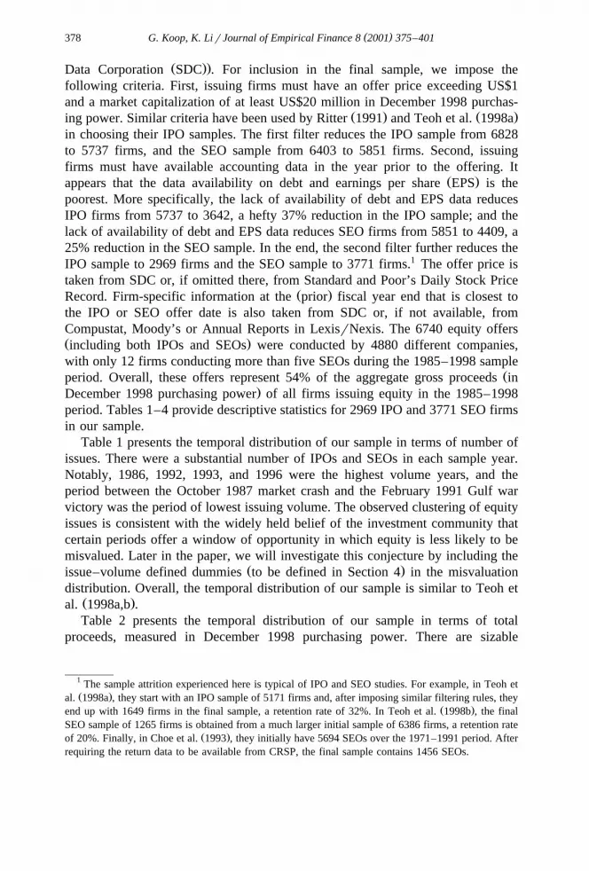
Table 1 presents the temporal distribution of our sample in terms of number ofissues. There were a substantial number of IPOs and SEOs in each sample year.Notably, 1986, 1992, 1993, and 1996 were the highest volume years, and theperiod between the October 1987 market crash and the February 1991 Gulf warvictory was the period of lowest issuing volume. The observed clustering of equityissues is consistent with the widely held belief of the investment community thatcertain periods offer a window of opportunity in which equity is less likely to bemisvalued. Later in the paper, we will investigate this conjecture by including the

Ž .issue–volume defined dummies to be defined in Section 4 in the misvaluationdistribution. Overall, the temporal distribution of our sample is similar to Teoh et

Ž .al. 1998a,b .Table 2 presents the temporal distribution of our sample in terms of total

proceeds, measured in December 1998 purchasing power. There are sizable

1 The sample attrition experienced here is typical of IPO and SEO studies. For example, in Teoh etŽ .al. 1998a , they start with an IPO sample of 5171 firms and, after imposing similar filtering rules, they

Ž .end up with 1649 firms in the final sample, a retention rate of 32%. In Teoh et al. 1998b , the finalSEO sample of 1265 firms is obtained from a much larger initial sample of 6386 firms, a retention rate

Ž .of 20%. Finally, in Choe et al. 1993 , they initially have 5694 SEOs over the 1971–1991 period. Afterrequiring the return data to be available from CRSP, the final sample contains 1456 SEOs.


Table 1Sample characteristics: issues distribution

Year Number Number Total number Percentageof IPOs of SEOs of offers

1985 121 214 335 5.01986 307 317 624 9.31987 217 199 416 6.21988 88 92 180 2.71989 79 151 230 3.41990 78 123 201 3.01991 211 328 539 8.01992 267 345 612 9.11993 343 432 775 11.51994 244 233 477 7.11995 243 359 602 8.91996 381 414 795 11.81997 237 343 580 8.61998 153 221 374 5.5Total 2969 3771 6740 100

The sample consists of 2969 US IPO firms and 3771 US firms conducting seasoned equity offerings inthe period between 1985 and 1998 with an offer price of at least US$1 and a market capitalization ofUS$20 million in December 1998 purchasing power. The sample firm must also have sufficientaccounting data in the year prior to the offering. The distribution of the sample by IPO or SEO year isreported.

Table 2Sample characteristics: proceeds distribution

Year IPO proceeds SEO proceeds Total proceeds Percentage

1985 6.19 15.00 21.19 3.81986 17.54 22.12 39.66 7.21987 13.38 14.35 27.73 5.01988 4.08 5.30 9.39 1.71989 5.30 8.04 13.34 2.41990 3.82 8.82 12.64 2.31991 14.37 28.38 42.75 7.71992 18.79 32.75 51.54 9.31993 25.52 40.00 65.52 11.81994 13.89 21.30 35.19 6.41995 17.47 35.47 52.93 9.61996 30.38 43.69 74.07 13.41997 17.15 37.38 54.54 9.81998 19.19 34.18 53.37 9.6Total 207.08 346.77 553.85 100

The sample consists of 2969 US IPO firms and 3771 US firms conducting seasoned equity offerings inthe period between 1985 and 1998 with an offer price of at least US$1 and a market capitalization ofUS$20 million in December 1998 purchasing power. The sample firm must also have sufficientaccounting data in the year prior to the offering. The proceeds are measured in December 1998

Ž .purchasing power US$ billion . The distribution of the total proceeds by IPO or SEO year is reported.


Table 3Sample characteristics: industry distribution

Industry Two-digit SIC codes IPO SEO Full Percentagesample sample sample

Oil and gas 13, 29 57 169 226 3.4Chemical products 28 156 247 403 6.0Manufacturing 30–34 125 151 276 4.1Computers 35, 73 529 453 982 14.6Electronic equipment 36 230 213 443 6.6Transportation 37, 39, 40–42, 44, 45 179 203 382 5.7Scientific instruments 38 152 152 304 4.5Communications 48 108 118 226 3.4Utilities 49 47 214 261 3.9Retail 53, 54, 56, 57, 59 194 234 428 6.4Financial services 60–65, 67 396 732 1128 16.7Health 80 133 139 272 4.0All others 1, 2, 6, 7, 8, 9, 10, 15, . . . 663 746 1409 20.7Total 2969 3771 6740 100

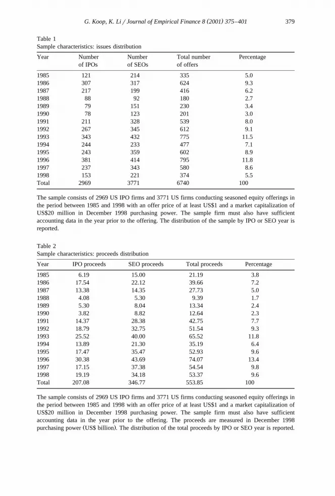
The sample consists of 2969 US IPO firms and 3771 US firms conducting seasoned equity offerings inthe period between 1985 and 1998 with an offer price of at least US$1 and a market capitalization ofUS$20 million in December 1998 purchasing power. The sample firm must also have sufficientaccounting data in the year prior to the offering. The distribution of the sample by two-digit SIC codeis reported.

variations in the volume of equity issues, and the general pattern in volume issimilar to that in terms of number of issues as reported in Table 1.

Table 3 provides a breakdown of SIC codes of our equity offering firms. Thepresence of 74 separate two-digit SIC codes, with 28 of these representing at least

Ž .1% of the sample 68 issuers , indicates a wide selection of industries. It appearsthat about 80% of all offers arise from the 12 industries defined in Table 3. Notsurprisingly for our sampling period of 1985–1998, there is a much higher

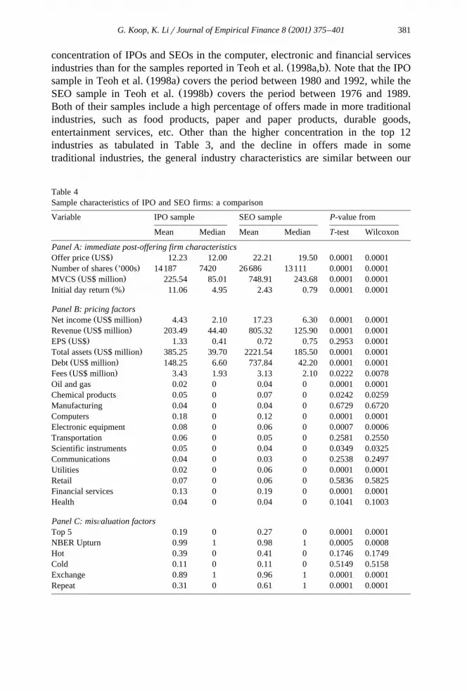
Note to Table 4:This table presents summary statistics of the IPO and SEO samples. There are 2969 IPO and 3771 SEOfirms. All accounting data are measured in the year prior to the offer. MVCS is the market value ofcommon stock. Initial day return is obtained as the percentage difference between the first day closingprice and the offer price. EPS is the earnings per share. Debt is the sum of the long-term, short-termand subordinate debt. Fees are the total fees paid to the underwriters in an issue. Top 5 is a dummyvariable, it equals one if the lead manager of the offer belongs to the top five underwriters ranked bymarket shares, and zero otherwise. NBER Upturn is a business cycle dummy variable constructed usingthe NBER chronology, it equals one if the issue month is an NBER peak, and zero otherwise. Hot is anissue volume dummy variable, it equals one if the volume of the issuing month exceeds the topquartile, and zero otherwise. Cold is another issue volume dummy variable, it equals one if the volumeof the issuing month falls below the bottom quartile, and zero otherwise. Exchange is a dummyvariable that equals one if the shares of the issuing firm are traded on NYSE, AMEX or NASDAQ, andzero otherwise. Repeat is a dummy variable that equals one if the issuer made multiple offers during

Ž .the 1985–1998 sample period including the case when the first time it is an IPO , and zero otherwise.


concentration of IPOs and SEOs in the computer, electronic and financial servicesŽ .industries than for the samples reported in Teoh et al. 1998a,b . Note that the IPO

Ž .sample in Teoh et al. 1998a covers the period between 1980 and 1992, while theŽ .SEO sample in Teoh et al. 1998b covers the period between 1976 and 1989.

Both of their samples include a high percentage of offers made in more traditionalindustries, such as food products, paper and paper products, durable goods,entertainment services, etc. Other than the higher concentration in the top 12industries as tabulated in Table 3, and the decline in offers made in sometraditional industries, the general industry characteristics are similar between our

Table 4Sample characteristics of IPO and SEO firms: a comparison

Variable IPO sample SEO sample P-value from

Mean Median Mean Median T-test Wilcoxon

Panel A: immediate post-offering firm characteristicsŽ .Offer price US$ 12.23 12.00 22.21 19.50 0.0001 0.0001

Ž .Number of shares ’000s 14187 7420 26686 13111 0.0001 0.0001Ž .MVCS US$ million 225.54 85.01 748.91 243.68 0.0001 0.0001

Ž .Initial day return % 11.06 4.95 2.43 0.79 0.0001 0.0001

Panel B: pricing factorsŽ .Net income US$ million 4.43 2.10 17.23 6.30 0.0001 0.0001

Ž .Revenue US$ million 203.49 44.40 805.32 125.90 0.0001 0.0001Ž .EPS US$ 1.33 0.41 0.72 0.75 0.2953 0.0001

Ž .Total assets US$ million 385.25 39.70 2221.54 185.50 0.0001 0.0001Ž .Debt US$ million 148.25 6.60 737.84 42.20 0.0001 0.0001Ž .Fees US$ million 3.43 1.93 3.13 2.10 0.0222 0.0078

Oil and gas 0.02 0 0.04 0 0.0001 0.0001Chemical products 0.05 0 0.07 0 0.0242 0.0259Manufacturing 0.04 0 0.04 0 0.6729 0.6720Computers 0.18 0 0.12 0 0.0001 0.0001Electronic equipment 0.08 0 0.06 0 0.0007 0.0006Transportation 0.06 0 0.05 0 0.2581 0.2550Scientific instruments 0.05 0 0.04 0 0.0349 0.0325Communications 0.04 0 0.03 0 0.2538 0.2497Utilities 0.02 0 0.06 0 0.0001 0.0001Retail 0.07 0 0.06 0 0.5836 0.5825Financial services 0.13 0 0.19 0 0.0001 0.0001Health 0.04 0 0.04 0 0.1041 0.1003

Panel C: misÕaluation factorsTop 5 0.19 0 0.27 0 0.0001 0.0001NBER Upturn 0.99 1 0.98 1 0.0005 0.0008Hot 0.39 0 0.41 0 0.1746 0.1749Cold 0.11 0 0.11 0 0.5149 0.5158Exchange 0.89 1 0.96 1 0.0001 0.0001Repeat 0.31 0 0.61 1 0.0001 0.0001


Ž .sample and those of Teoh et al. 1998a,b . To account for different earningspotential and pricing practices across industries, later in our stochastic frontiermodel, we include industry dummies as pricing factors.

Table 4 compares sample characteristics of IPO firms with those of SEO firms.In Panel A of Table 4, we present some immediate post-offering firm character-

Žistics. The offering prices in IPOs average about US$12.23 per share median.US$12.20 , while the average offering price in SEOs is about US$22.21 per share

Ž .median US$19.50 . The differences in both the mean and median offer prices arestatistically significant. In terms of the number of shares outstanding after theoffer, IPOs are also significantly smaller with mean number of shares outstanding

Ž . Žat 14 187 000 median 7 420 000 as compared to 26 686 000 shares median.13 111 000 after SEOs. As a result, it is not surprising to find that the mean

Ž .market capitalization MVCS of IPOs is about US$226 million and the median isabout US$85 million, about one third of the values for SEOs that have the mean

Ž .market capitalization of about US$749 million median US$244 million . Consis-Žtent with the existing evidence on IPO underpricing e.g. Kim and Ritter, 1999;

.Teoh et al., 1998a; Hunt-McCool et al., 1996; Ritter, 1991 , IPOs in our sample onŽ .average experience a much larger first day price runup at 11.06% median 4.95%

Ž .as compared to the runup of 2.43% median 0.79% of an average SEO in oursample.

3. Stochastic frontier modeling

The stochastic frontier model, developed by Meeusen and van den BroeckŽ . Ž .1977 and Aigner et al. 1977 , has been widely used in many areas ofeconomics. However, it has been most commonly used in microeconomic studiesof production relationships, and we shall begin by adopting the terminology of thisliterature to describe the basic ideas underlying stochastic frontier modeling.

Standard textbook models of production state that the amount of outputproduced by thei th firm, Y , should depend on the inputs used in the productioni

process,X , where X is a k=1 vector of inputs. The production technology usedi i

for transforming inputs into outputs is given by,

Ys f X ,b , 1Ž . Ž .i i

Ž .where b is a vector of parameters andf P describes the maximum possibleoutput that can be obtained from a given level of inputs.

However in practice, firms may not achieve maximum output; e.g. they maynot be efficient. If we allow for firm-specific inefficiency and the usual measure-ment error that econometricians add, we obtain the following stochastic frontier

Ž .model for firm i i s1, . . . , N ,

Ys f X ,b t ´ , 2Ž . Ž .i i i i

where 0-t -1 is the efficiency of firmi , with values oft near one implying ai i

firm is near full efficiency, and´ reflects measurement error. It is standard toi


Ž . Ž . 2take logs of Eq. 2 and assumef P is log linear in X, yielding,

y sxX bqÕ yu , 3Ž .i i i i

Ž . Ž . Ž . Ž .where y s ln Y , x s ln X , Õ s ln ´ and u syln t . We make thei i i i i i i iŽ 2.usual assumption thatÕ is N 0, s and is distributed independently ofu . It isi i

common to refer tou as inefficiency since higher values of this variable arei

associated with lower efficiency. Given 0-t -1, it follows that u )0. It is thisi iŽ .latter fact that allows us to distinguish between the two errors in Eq. 3 . Common

distributions for u are the truncated Normal or various members of the GammaiŽ .class. Ritter and Simar 1997 have noted some identification problems, which

occur if we allow the distribution ofu to be too flexible. For instance, thei

truncated Normal distribution becomes indistinguishable from the Normal if thetruncation point is too far out in the tail of the distribution. The unrestrictedGamma distribution runs into similar problems. For this reason, researchers haveworked with restricted versions of these general classes. Hunt-McCool et al.Ž .1996 use a Normal truncated at the point zero. Meeusen and van den BroeckŽ . Ž .1977 and Koop et al. 1997 use an exponential distribution. Van den Broeck et

Ž . Ž .al. 1994 and Koop et al. 1995 extend this by working with Erlang distributionsŽ .e.g. Gamma distributions with integer degrees of freedom . Here, we work withan exponential distribution.3 This efficiency distribution for firmi depends on oneunknown parameter, the mean, which we denote byl .i

In the present paper, we interpret theAoutputB y as being the market value ofŽan offering firm’s equity e.g. the offer price times the number of shares

.outstanding after the issue . Investors establish this by looking at various factorsŽrelating to the future profitability of the firm e.g. net income, revenue, earnings

.per share, total assets, debt levels, and industry affiliation , which can be inter-preted asAinputsB, x, used for producing the stock market value. TheAproductionfrontierB, now called theAvaluation frontierB, captures the maximum that investorsare willing to pay for shares in a firm with given characteristics. In the presentpaper, we refer tox as Apricing factorsB. If two firms with similar values forpricing factors are yielding different stock market values, this is evidence that the

Ž .equity of one of the firms is misvalued relative to its characteristics . Thisunderpricing is labelledAinefficiencyB in the stochastic frontier literature andAmisvaluationB in the present paper.

We use the Bayesian methods to estimate the stochastic frontier model de-scribed above. The advantages of such an approach are described in some previous

Ž .work e.g. van den Broeck et al., 1994; Koop et al., 1997, 2000 . Of particular

2 Ž .Or, if translog technology is assumed, thenf P is log linear in X and powers ofX.3 Ž . ŽIn an earlier version of this paper Koop and Li, 1998 , we worked with the Erlang distribution of

.which the exponential is a special case . However, empirical results were qualitatively similar for thevarious members of the Erlang class and, accordingly, we focus here only on the simpler exponentialdistribution.


interest is the fact that adoption of the Bayesian methods allows us to calculatepoint estimates and standard deviations of any feature of interest includingu , thei

Ž .measure of misvaluation in Eq. 3 . The latter feature is often of primaryŽ .importance yet, as Jondrow et al. 1982 demonstrate, non-Bayesian point esti-

mates are inconsistent. Furthermore, it is difficult to obtain meaningful standarderrors for u using non-Bayesian approaches.4

i

Above, we have stressed that stochastic frontier models require the specifica-tion of a distribution for the measure of misvaluationu . Early work tended toi

Žassume that these mispricings were drawn from some common distributions e.g.. Ž .l 'l for all i . However, Koop et al. 2000 reason that this might be tooi

restrictive an assumption. For instance, it might be the case that firm- and issueŽ .period-specific characteristics as suggested in Choe et al. 1993 and Bayless and

Ž . Ž .Chaplinsky 1996 or type of offers IPOs versus SEOs should be related tomisvaluation. We can model such features by allowing the misvaluation distribu-tion to depend onm observable characteristics of firmi , w where js1, . . . , m.5i j

In particular, we assumeu to be distributed as an exponential distribution withi

meanl where,im

yw i jl s f , 4Ž .Łi jjs1

where f )0 for js1, . . . , m. The preceding specification is chosen since itj

fulfills the technical requirement that the mean of the misvaluation distribution ispositive.

It is worth stressing that in such a specification, we can directly test whether aparticular firm characteristic tends to be associated with misvaluation. Note that iff s1, then thej th firm characteristic has no effect on the misvaluation distribu-j

Ž .tion, whereas iff )1 -1 then thej th characteristic is associated with a lowerjŽ .higher degree of misvaluation. For instance,w is a dummy variable that equalsi 2

one if firm i makes an SEO, and zero otherwise. Then a finding off )1 is2Ž .associated with IPO underpricing. As shown in Koop et al. 2000 , the Bayesian

approach allows us both to estimatef and to statistically test whether it is equal2

to one or not.Ž . Ž .To summarize, in the framework of Eqs. 3 and 4 , the researcher is forced to

draw on theory to decide whether a variable is an input in the valuation equationŽ .in which case it belongs inx or whether it should affect the level of mispricingŽ .in which case it belongs inw . Alternative methods typically just enter all

Žpossible explanatory variables asx’s e.g. as explanatory variables which enter.linearly in a regression model .

4 Ž .It is possibly for these reasons that Hunt-McCool et al. 1996 never provide firm-specificestimates of underpricing.

5 In practice, all of ourw ’s are 0–1 dummy variables. This greatly simplifies our computationali jŽ .methods. Furthermore, we always setw s1 e.g. we put an intercept in the model .i1


4. The explanatory variables

In Section 3, we have outlined a framework where the dependent variable is themarket value of common equity. The variables used to explain the dependentvariable are broken down intoApricing factorsB that are expected to directly affectthe value of a stock andAmisvaluation factorsB. In this section, we motivate whywe label some of our explanatory variables as the former and some as the latter.

4.1. The pricing factors

We draw on standard finance theories to select explanatory variables that areexpected to influence valuation of equity issuing firms. In Myers and MajlufŽ .1984 , investors use information about issuing firms to condition their assessmentof firm value. Firms that issue in line with the predictions of capital structuretheory are likely to be viewed by investors as having a reason for issue and hence,be valued fairly. Consistent with the above argument, we use issuer characteristicssuch as profitability, level of operations, risk, and underwriter fees as pricingfactors in obtaining our valuation frontier.

Ž . Ž .Krinsky and Rotenberg 1989 and Ritter 1984 have shown a positiverelationship between historical accounting information and firm value. The first setof pricing factors we include in the valuation equation relates to profitability.

Ž .According to Teoh et al. 1998b , cashflows are the ultimateAbottom lineB forvaluation. We use net income and sales revenue over the 12-month period before

Ž .the offer as reported in the firm’s prospectus as proxies for the profitability of aŽ . Ž .firm. Following Kim and Ritter 1999 , we also include earnings per share EPS

in the fiscal year prior to the offer to measure a firm’s ability to generate incomefor shareholders. On the other hand, past performance does not necessarilyrepresent future performance, especially in the case of IPOs. Following Kim and

Ž . Ž . Ž .Ritter 1999 , Ritter 1991 and Downes and Heinkel 1982 , we introduce 12Ž . Ž .industry dummy variables listed in Table 3 as the proxy for perceived earnings

potential. Finally, to control for the level of operations, total assets is also includedin the valuation equation.

Default risk is measured by total debt, which is the sum of long-term debt,short-term debt and subordinate debt. We expect that firms with a heavy burden ofdebt have a greater chance of bankruptcy, and as a result, ceteris paribus, themarket value of a firm is negatively associated with its debt level.6

Another factor which is related to the value of the firm is the total compensa-Ž .tion paid to the underwriter. According to Hughes 1986 , underwriters’ compen-

sation will be higher for companies that are more likely to suffer from the

6 A referee has pointed out that the variance of EPS prior to the offer date could be used as a proxyfor the perceived risk of IPOs at the time of offering. We have some EPS data for our sample of IPOsprior to the offering, but the data points are insufficient for us to obtain a valid measure of variance. Infuture work, we plan to collect more data and use the variance of EPS as our measure of risk.


information asymmetry problem. This variable is defined as total fees paid by theissuing firm.

Panel B of Table 4 presents summary statistics of the pricing factors. SEOfirms in our sample are more profitable. The mean net income of IPO firms is

Ž .about US$4.43 million median US$2.10 million , while the mean net income ofŽ .SEO firms is about US$17.23 million median US$6.30 million . Both the mean

and the median are statistically different across the two groups of firms. The sameholds true for the mean and median sales revenue. In terms of earnings per shareŽ .EPS , IPO firms in our sample are doing as well as SEO firms. The mean EPS ofUS$1.33 for IPOs is not statistically different from that of SEOs. We use totalassets prior to the offer to measure the level of operations. As expected, the meantotal assets of IPO firms is about US$385 million, only one-fifth of the mean totalassets of SEO firms. One might argue that the very large mean value we get for

Ž .the total assets of an average SEO firm US$2221.54 million could be driven by afew extreme observations in the sample. When comparing the median total assetsof IPOs versus that of SEOs, we see the same result: the median total assets of

Ž .IPOs US$39.7 million is about one-fifth of the median total assets of SEOsŽ .US$185.5 million . The difference in size between IPO and SEO firms could beexplained by the difference in the number of years since incorporation. Unfortu-

Žnately, the data on the year of incorporation is so poor e.g. less than 30% of the.sample firms have it that we have been unable to get reliable measurements for

this variable. Finally, SEO firms in our sample on average have a much higherŽ .debt level mean US$738 million, median US$42 million than their IPO counter-

Ž .parts mean US$148 million, median US$6.6 million .The Fees variable indicates that IPOs pay significantly more to their underwrit-

ers than SEOs do. The mean total fees paid by IPO firms to their group ofŽ .underwriters is about US$3.43 million median US$1.93 million , while the mean

Ž .fees paid by SEO firms is about US$3.13 million median US$2.10 million . Thisresult is consistent with the fact that IPO firms tend to be younger firms and theunderwriting of IPOs is more involved.7

The industry distribution across the IPO and SEO samples can be summarizedas follows. Over the 1985–1998 sample period, there is a higher concentration ofIPOs compared to SEOs in the computer, electronic equipment and scientificinstrument industries. In contrast, there is a higher concentration of SEOs in moretraditional industries such as oil and gas, chemical products, utilities and financialservices. The industry distribution across the IPO and SEO samples is similar formanufacturing, transportation, communications, retail and health industries.

7 Ž .Chen and Ritter 2000 find that during 1995–1998, 90% of IPOs raising between US$20 andŽ .US$80 million have spread feesrgross proceeds of exactly 7%. In our sample of IPOs during

1985–1998, the average spread is 2.4%. Given that our sample covers a longer period and the averageŽ .size of the offerings in our sample is bigger than that in Chen and Ritter 2000 , it seems reasonable for

Ž .our IPO sample to have varying and lower than 7% spreads.


4.2. The misÕaluation factors

The extended stochastic frontier model adopted in this paper allows for firm-and issue period-specific characteristics to directly affect misvaluation.

Mispricing is costly to the issuing firms. Therefore, low risk firms attempt toreveal their low risk characteristic to the market. According to Carter and

Ž .Manaster 1990 , one way they can do so is by selecting underwriters with highprestige. This implies that offers underwritten by reputable Wall Street firms willbe less likely to be misvalued at the time of offering. We rank all underwriters bytheir market shares over the 1985–1998 sample period, and create a dummyvariable Top 5 that equals one if the lead underwriter of a deal belongs to the topfive investment banks, and zero otherwise.8 We expect the coefficient associatedwith this underwriter reputation dummy variable to be greater than one in themisvaluation distribution.

Ž .According to Choe et al. 1993 , the adverse selection effects of equityofferings decrease when more promising economic conditions for new investmentexist. As a result, there will be less of a mispricing problem during economicbooms. In this paper, we introduce a dummy variable NBER Upturn that equalsone if the economy is at an upturn based on the NBER business cycle chronologyand zero otherwise.9

Ž .On the other hand, Bayless and Chaplinsky 1996 point out that periodsselected by equity issue–volume differ rather markedly from those selected usingmacroeconomic criteria. They believe that there is not a simple and direct linkbetween the business cycle and the decision to issue. Instead Bayless and

Ž .Chaplinsky 1996 use the aggregate issue–volume to designate hot versus nonhotissue periods for seasoned equity. The rationale behind their designation of issueperiods is as follows. If information costs are a significant deterrent to equityissue, then reductions in adverse selection costs should stimulate firms to issue

Ž .equity. Ritter 1991 finds that issuers are successfully timing new issues to takeadvantage of windows of opportunity and the cost of external equity capital ofissuers in high-volume years is lowest and their post IPO performance fares the

Ž .worst. Following Bayless and Chaplinsky 1996 , we introduce two issue–volumedefined dummy variables Hot and Cold. First, we rank the monthly equity issue

8 The top five underwriters ranked by market shares over the 1985–1998 sample period areMerrill-Lynch, Goldman, Sachs, Morgan Stanley Dean Witter, Salomon Smith Barney and Lehman

Ž .Brothers according to Securities Data. In Carter and Manaster 1990 , the rankings of underwriters aredetermined by examining the actual issue announcements available either from the Investment Dealer’sDigest or from The Wall Street Journal. They assign an integer rank, zero to nine, for each underwriterin the announcement according to its position. Four out of our top five underwriters overlap with theirtop five ranked underwriters.

9 The NBER defines a recession as a recurring period of decline in total output, income, employmentand trade that usually lasts from 6 months to a year and is marked by widespread contractions in manysectors of the economy.


volume in December 1998 purchasing power into quartiles.10 High volume issueŽ .periods Hot are months where the equity volume of the month exceeds the upper

Ž .quartile. Low volume issue periods Cold are months where the equity volume ofthe month falls below the lower quartile. We use the offers falling between theupper and lower quartile cutoffs as the benchmark for normal periods. We expect

Žthat firms issuing in the hot market years are less likely to be undervalued more.likely to be overvalued .

ŽAll the above issue timing factors are not specific to the firm e.g. every firm.which issues in a Hot period will have the same value for this variable . This

provides further justification for considering these variables as reflecting misvalua-tion. That is, valuation should largely reflect firm-specific characteristics ratherthan timing of equity issuance.

As an aside, it is worth noting that other variables have been constructed toŽ .capture the ideas developed in Choe et al. 1993 and Bayless and Chaplinsky

Ž .1996 that market and macroeconomic conditions at the time of issue can affectinvestors’ estimates of the value of equity, and result in clustering in equity issues.

Ž .Following Bayless and Chaplinsky 1996 , we obtained the measures of thechange in the price–earnings ratio for the S&P 500 Stock Index, the change in theS&P 500 Stock Index, the change in the Index of Industrial Production, the

Ž .default premium and the term premium Fama and French, 1989 as proxies foraggregate economic conditions. The first three of these are the average level of thevariable in the 3 months prior to issue relative to the average value of the variablein the last 24 months. The other two macro variables are measured over the 3months preceding the offering announcement. However, in our empirical work we

Žfound them to be statistically insignificant even if they were put in the valuation.frontier or simply in an OLS regression . Furthermore, they are closely related to

the NBER Upturn and the HotrCold dummies described above. To simplify theanalysis we do not present empirical results involving these variables in this paper.

Valuation errors are also predicted when the uncertainty concerning the valueŽ .of firm assets in place increases. In Choe et al. 1993 , stock price volatility is

included as a proxy to capture the potential negative impact on equity issuanceactivity of market uncertainty about the value of the firm’s assets. We expect thatvolatile stock markets are associated with equity misvaluation. Our market riskvariable is the daily S&P 500 return variance measured over the 3-month periodprior to the month of the stock offering. However, in our preliminary analysis of

Žthe data we found that the risk variable is statistically insignificant even if it is put.in the valuation frontier or simply in an OLS regression . We opt not to include it

in our final analysis.11

10 Ž .Real dollar volume is monthly nominal issue volume US$ millions deflated by the monthlyconsumer price index.

11 This provides some evidence that the results in our paper are not sensitive to the preciseclassification of at least some of the explanatory variables.


It is well known that listing on NYSE, AMEX and NASDAQ demands morestringent registration requirements. As a result, we would expect that firms withshares traded on these three exchanges are less likely to be mispriced. Weintroduce a dummy variable Exchange that equals one if the shares of the issuingfirm are traded on NYSE, AMEX or NASDAQ, and equals zero otherwise.

Since the market does not have prior experience in valuing IPO firms, wewould expect that the chances that they are mispriced are greater. Accordingly, weintroduce a dummy variable SEO that equals one for a seasoned equity offering,and equals zero otherwise.

Along the same lines, if a public firm repetitively come to the market for freshequity, the market should have a more accurate valuation of the equity of the firm.Hence, we expect that firms with multiple equity offers are less likely to bemispriced. We introduce a dummy variable Repeat that equals one if the firm

Žcomes to the market more than once for equity over the sample period including.the case when the first time it is an IPO , and equals zero otherwise.

Panel C of Table 4 presents summary statistics of the misvaluation factors.Overall, SEO firms are more likely to have a Top 5 underwriter as their leadunderwriter and the shares of SEO firms are more likely to be traded on NYSE,AMEX or NASDAQ. On the other hand, IPOs are more likely to take place duringthe upturns of the NBER business cycle as compared to SEOs. We do not findsignificant difference between IPOs and SEOs based on the issue–volume defined

Ž .indicators e.g. hot and cold issue periods ; both types of offers are more likely tooccur in the hot issue periods. This finding is consistent with the pattern seen inTable 1 that there is clustering of IPOs and SEOs over the sample periods of 1986,1992, 1993 and 1996. Finally, we see more repeat issuers in the SEO sampleŽ . Ž .61% than in the IPO sample 31% . Note that our repeat dummy equals one ifthe firm comes to the market more than twice for equity over the 1985–1998

Ž .sample period including the case when the first time it is an IPO . Overall, moreŽ .than 72% of our sample 4880 firms are first-time issuers on the market, and less

than 7% of our sample come to the market for equity more than twice during thesample period.

5. Empirical results from stochastic frontier model

5.1. Basic findings

The output,y, used in the stochastic frontier model is the log of market valueŽof common stock MVCS, e.g. the offer price times the number of shares

.outstanding after the issue . The inputs or pricing factors,x, we use are discussedin Section 4.1. Further details and a listing of all variables are given in Table 4.

Ž .Variables that are positive for all firms are logged except the intercept . Formally,


we include an intercept, net income, revenue, EPS, the log of total assets, the logŽ .of debt, the log of fees and industry affiliation in the valuation frontier Eq. 3 . In

Ž .the misvaluation distribution Eq. 4 , an intercept is included along with the 0–1dummies explained in Section 4.2 and labelled SEO, Top 5, NBER Upturn, Hot,Cold, Exchange, and Repeat.

Table 5 contains point estimates and standard deviations for the valuationŽ . Ž . 12frontier parameters e.g.b in Eq. 3 , plus OLS estimates and standard errors.

It can be seen that OLS and stochastic frontier estimates are very similar. Both tellthe story that net income, revenue, book value of total assets, underwriter fees andearnings potential are strongly positively associated with the market value of theoffering firm, while debt has a strong negative association. These results are

Ž .consistent with those found in other studies, such as Hunt-McCool et al. 1996 ,Ž .and Kim and Ritter 1999 . The only somewhat surprising thing is the lack of a

role of earnings per share in explaining market value. According to Teoh et al.Ž .1998a,b , it is a common practice that IPO and SEO firms raise reported earningsby altering discretionary accounting accruals. As a result, earnings per sharebecomes a less relevant pricing factor. Our result is consistent with the findings in

Ž .Teoh et al. 1998a,b . In contrast, many of the industry dummies are highlysignificant, indicating the different profit potential in different industries is farmore important than past accounting data. In particular, firms in industries withgreat earnings potential such as chemical products, computers, electronic equip-ment, scientific instruments, and communications are more highly valued, whereasfirms in more traditional industries such as oil and gas, manufacturing, transporta-tion and financial services are valued less than comparable firms in most other

13 Ž .industries. According to Choe et al. 1993 , utility offerings are much morefrequent and predictable and are less likely to be associated with adverse selectiongiven the extensive regulation of industry profits and frequent regulatory pressureto undertake equity offerings. We find that utilities are more highly valued, whichis consistent with the above explanation. On the other hand, the massive failure ofSavings and Loans companies in the 1980s and the sovereign debt crises of manyThird World countries in the 1990s probably explain the severe underpricingexperienced by the financial services firms in our sample.

The posterior means and standard deviations of the coefficients on the variablesŽ Ž ..in the misvaluation distribution e.g.f in Eq. 4 are presented in Table 6.

Remember that iff )1, then misvaluation factorj is associated with a higherjŽ .degree of efficiency e.g. less misvaluation . Iff -1, then the factor is associatedj

12 The intercept has a different interpretation in the stochastic frontier and OLS results and is notpresented.

13 A referee questioned whether financial firms should be dropped from our study since they have acapital structure, which is heavily oriented towards debt. We found that omitting these firms did notcause any substantive changes in our results.


Table 5Ž .Posterior and OLS properties ofb in Eq. 3

Stochastic Frontier Model OLS regression

Mean S.D. Estimate S.E.y4 y5 y4 y5Net income 8.4=10 6.2=10 8.8=10 6.8=10y5 y6 y5 y6Revenue 2.9=10 2.6=10 3.1=10 2.9=10

y5 y4 y4 y4EPS y4.5=10 4.0=10 y2.9=10 3.6=10Total assets 0.375 0.008 0.423 0.008Debt y0.043 0.005 y0.054 0.005Fees 0.752 0.010 0.699 0.010Oil and gas y0.174 0.042 y0.110 0.045Chemical products 0.277 0.034 0.322 0.036Manufacturing y0.119 0.040 y0.137 0.042Computers 0.172 0.026 0.175 0.027Electronic equipment 0.186 0.033 0.191 0.035Transportation y0.162 0.035 y0.160 0.037Scientific instruments 0.200 0.039 0.217 0.040Communications 0.181 0.044 0.170 0.046Utilities 0.206 0.040 0.245 0.044Retail y0.025 0.033 y0.029 0.035Financial services y0.532 0.026 y0.582 0.027Health y0.023 0.040 y0.017 0.042

ŽThis table presents point estimates and standard deviations for the valuation frontier parameters i.e.bŽ ..in Eq. 3 under the stochastic frontier model, and point estimates and standard errors under the OLS

regression, respectively. The sample consists of 2969 US IPO firms and 3771 US firms conductingseasoned equity offerings in the period between 1985 and 1998. The dependent variable is the marketvalue of common equity, obtained as the product of the offer price and the number of sharesoutstanding after the issue.

with more misvaluation, andf s1 indicates that the factor has no effect. Bayesj

factors for the latter hypothesis are presented in Table 6.Clearly, the SEO variable is strongly significant with a magnitude indicating

that IPOs are underpriced relative to SEOs. None of the other variables arestrongly significant. There is some evidence in favor of the hypothesis that firmsthat have issued equity more than once are priced more efficiently than those who

Žonly issued equity a single time. The variables relating to the timing of issue e.g..NBER Upturn, Hot and Cold all seem to have no effect on the degree of

Žmisvaluation. The variables reflecting the trading location of the shares Ex-. Ž .change and the choice of underwriter Top 5 are also insignificant. The latter

Žresult, combined with the important role of underwriter fees presented above e.g.Ž ..the Fees variable was very significant in the valuation frontier Eq. 3 indicate

that it is the amount of money spent on underwriting, rather than the choice of aparticular underwriter, which is important.

The role of the explanatory variables in the misvaluation distribution can bepartly understood throughf, but an examination of the misvaluation distributions


Table 6Ž .Posterior properties off in Eq. 4

Mean S.D. Bayes factor

Intercept 4.288 2.144 –SEO 25.197 5.318 0.000Top 5 1.035 0.082 19.196NBER upturn 0.758 0.294 4.223Hot 1.074 0.069 14.152Cold 0.993 0.103 15.903Exchange 0.898 0.090 8.665Repeat 1.202 0.082 0.713

This table presents point estimates and standard deviations of the coefficients on the variables in theŽ Ž ..misvaluation distribution i.e.f in Eq. 4 under the stochastic frontier model. The sample consists of

2969 US IPO firms and 3771 US firms conducting seasoned equity offerings in the period betweenŽ1985 and 1998. Bayes factors give the evidence in favor ofH : f s1 i.e. the factorj has no effect0 j

.on misvaluation . Values of Bayes factors greater than one indicate support forH . SEO is a dummy0

variable that equals one if the offer is a seasoned equity offer, and zero otherwise. Top 5 is a dummyvariable, it equals one if the lead manager of the offer belongs to the top five underwriters ranked bymarket shares, and zero otherwise. NBER upturn is a business cycle dummy variable constructed usingthe NBER chronology, it equals one if the issue month is an NBER peak, and zero otherwise. Hot is anissue volume dummy variable, it equals one if the volume of the issuing month exceeds the topquartile, and zero otherwise. Cold is another issue volume dummy variable, it equals one if the volumeof the issuing month falls below the bottom quartile, and zero otherwise. Exchange is a dummyvariable that equals one if the shares of the issuing firm are traded on NYSE, AMEX or NASDAQ, andzero otherwise. Repeat is a dummy variable that equals one if the issuer made multiple offers during

Ž .the 1985–1998 sample period including the case when the first time it is an IPO , and zero otherwise.

themselves is more informative. In the stochastic frontier literature, it is commonto work with efficiency,t , rather than inefficiency,u . As noted in Section 3,i i

Ž .t sexp yu and, since efficiency is bounded between zero and one, it is easieri i

to interpret. For instance, a value of 0.85 indicates that the market value of theŽfirm is only 85% of the maximum it could be or equivalently, the firm is

.undervalued by about 15% . Hence for the remainder of this paper, we will presentresults relating to misvaluation usingt . An advantage of the Bayesian approach isi

that, unlike traditional econometric approaches, we can derive the entire posteriordistribution of the efficiency of any firm and hence, can calculate both pointestimates and standard deviations. Note that the underpricing distribution varies

Žacross firms e.g. depends onw, a vector containing an intercept and the 0–1. Ž .dummies and hence, we cannot present results for every firm here 6740 of them .

Instead, we group firms by their underpricing distributions. With seven dummyvariables there are too many groups to be easily presented. We choose to focus onthe SEO, Top 5 and Repeat dummies. In particular, we divide firms into eightgroups depending on the values of these three dummies. For instance, SEOrTop5rRepeat represents SEOs that were underwritten by the Top 5 investment banks


and came to the market to issue equity more than once. We can derive anefficiency distribution corresponding to this group of firms. We refer to the resultas theAEfficiency Distribution for a Typical Firm with SEOs1, Top 5s1 andRepeats1B. Each of these eight groups of firms has HotsColdsNBER UpturnsExchanges1. Since the coefficients on these latter variables are all very closeto one, these choices have virtually no impact on the results. For more explana-tion, formalization and computation details of this type of efficiency distribution,

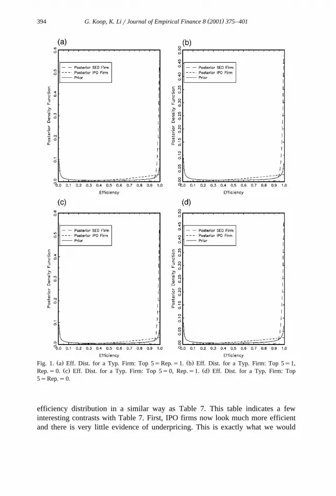
Ž .see van den Broeck et al. 1994, pp. 279–280 .Fig. 1 plots the efficiency distributions for a typical firm in the eight groups

along with the prior we use. Table 7 gives the means and standard deviations ofthese eight efficiency distributions. These plots tell the most important parts of ourempirical story.

First, SEO firms tend to be quite efficient and there is little variability acrossfirms. That is, the bulk of the probability in the efficiency distribution lies between0.95 and 1, indicating it is rare for a SEO firm to be undervalued by more than5%.

Second, the efficiency distributions of IPO firms are extremely disperse andthere is a great deal of evidence for underpricing. The mean of the IPO efficiencydistribution for each group of firms is in the region of 0.70–0.75. This indicatesthat, on average, IPO firms are valued at only 70–75% of what the valuationfrontier says is the maximum possible. However, the high standard deviationassociated with this distribution indicates that some individual IPO firms arevalued quite efficiently and some very inefficiently.

Third, the lack of influence of the other explanatory variables on misvaluationŽ .except possibly for Repeat having a minor role is clearly visible in Fig. 1 andTables 6 and 7.

Fourth, the prior we are using is quite noninformative. Furthermore, since theposterior efficiency distributions are very different from the prior, it is clear thatthe prior has little effect on our results.

5.2. Further discussion of results

As discussed in Section 3, the paper most related to ours is Hunt-McCool et al.Ž .1996 . These authors use a stochastic frontier methodology but only use IPOfirms. We have argued above that this is not a good way to investigate IPOunderpricing. Our approach addresses the issue of whether IPOs are underpricedrelative to a valuation frontier determined by all issuing firms. The Hunt-McCoolet al. approach addresses the issue of whether some IPOs are underpriced relativeto other IPOs. It is instructive to ask what would have happened if we had adoptedthe Hunt-McCool et al. approach. Accordingly, we repeat all of our empiricalanalyses using only the 2969 IPO firms.

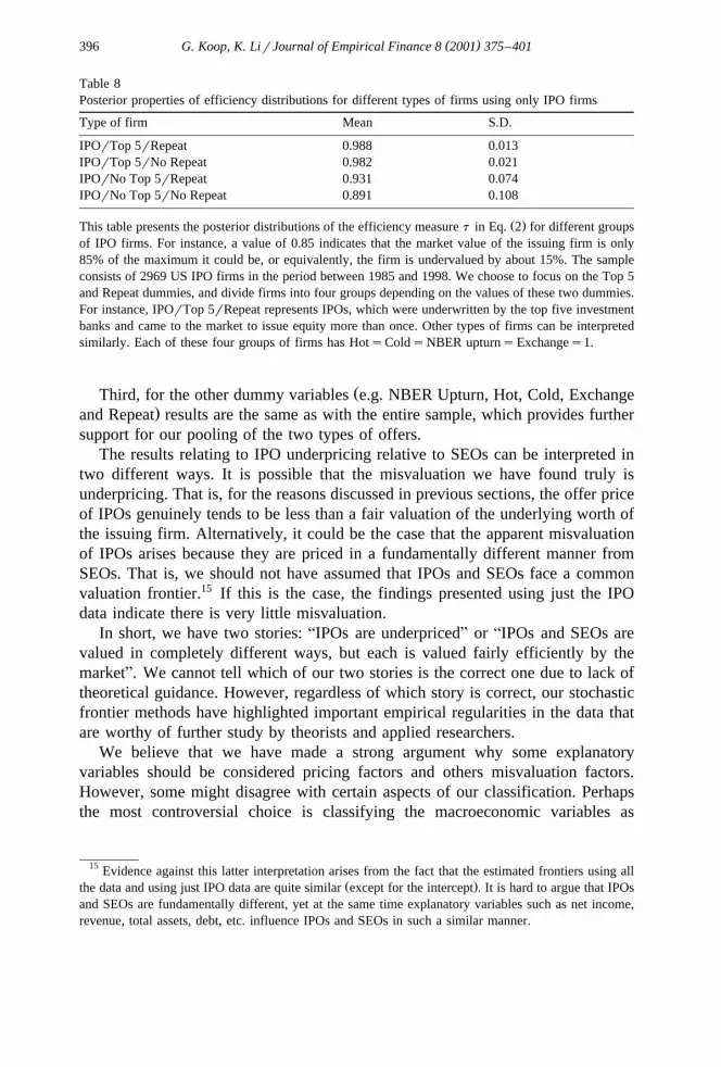
Ž .The results relating to the valuation frontier not reported are quite similar tothose obtained with the full sample in Table 5, which provides some support forour pooling of the two types of offers. Table 8 presents results relating to the


Ž . Ž .Fig. 1. a Eff. Dist. for a Typ. Firm: Top 5sRep.s1. b Eff. Dist. for a Typ. Firm: Top 5s1,Ž . Ž .Rep.s0. c Eff. Dist. for a Typ. Firm: Top 5s0, Rep.s1. d Eff. Dist. for a Typ. Firm: Top

5sRep.s0.

efficiency distribution in a similar way as Table 7. This table indicates a fewinteresting contrasts with Table 7. First, IPO firms now look much more efficientand there is very little evidence of underpricing. This is exactly what we would


Table 7Posterior properties of efficiency distributions for different types of firms

Type of firm Mean S.D.

SEOrTop 5rRepeat 0.986 0.013SEOrTop 5rNo Repeat 0.984 0.016SEOrNo Top 5rRepeat 0.986 0.014SEOrNo Top 5rNo Repeat 0.983 0.017IPOrTop 5rRepeat 0.759 0.191IPOrTop 5rNo Repeat 0.724 0.210IPOrNo Top 5rRepeat 0.753 0.193IPOrNo Top 5rNo Repeat 0.718 0.212

Ž .This table presents the posterior distributions of the efficiency measuret in Eq. 2 for different groupsof issuing firms. For instance, a value of 0.85 indicates that the market value of the issuing firm is only85% of the maximum it could be, or equivalently, the firm is undervalued by about 15%. The sampleconsists of 2969 US IPO firms and 3771 US firms conducting seasoned equity offerings in the periodbetween 1985 and 1998. We choose to focus on the SEO, Top 5 and Repeat dummies, and divide firmsinto eight groups depending on the values of these three dummies. For instance, SEOrTop 5rRepeatrepresents SEOs, which were underwritten by the top five investment banks and came to the market toissue equity more than once. Other types of firms can be interpreted similarly. Each of these eightgroups of firms has HotsColdsNBER upturnsExchanges1.

expect. Since the data set no longer contains efficient SEO firms, the benchmarkagainst which IPO firms are being compared is lower.14

Second, for IPO firms there is evidence that choosing an underwriter from thetop five investment banks does have some effect. In particular, IPOs underwrittenby the top five underwriters tend to be valued more highly than those which arenot. This result presumably does not hold for SEO firms and, given the predomi-nance of SEOs in the total sample, gets swamped when we use the entire data set.Apparently, underwriter certification is more important for IPO firms than for the

Ž .SEO firms, a result that is consistent with Hughes 1986 .

14 Based on the results reported in Table 7, we see that IPO firms on average are undervalued byŽ .25–30%, while Hunt-McCool et al. 1996 conclude that their sample of IPOs are on average

underpriced by 8–9%. We attribute the drastic difference in results to the following factors. First, theŽ .sample is different. Hunt-McCool et al. 1996 use a data set covering 1035 IPOs over the period

Ž1975–1984, and their first day return is 10%. We employ a more recent covering the 1985–1998. Ž .period and larger IPO data set with 2969 observations , the first day return in our IPO sample is 11%.

Hence, a small portion of the difference in results could be driven by the difference in data employed.Ž .Second, our methodology is an improved version of Hunt-McCool et al. 1996 . We apply the

Žstochastic frontier modeling approach to both IPO and SEO firms. Using only IPO firms as did byŽ .. ŽHunt-McCool et al. 1996 , we find the average IPO underpricing is much lower, at around 5% see

.our Table 8 . In sum, we are inclined to attribute the bulk of the difference in results on IPOunderpricing to the difference in methodology employed.


Table 8Posterior properties of efficiency distributions for different types of firms using only IPO firms

Type of firm Mean S.D.

IPOrTop 5rRepeat 0.988 0.013IPOrTop 5rNo Repeat 0.982 0.021IPOrNo Top 5rRepeat 0.931 0.074IPOrNo Top 5rNo Repeat 0.891 0.108

Ž .This table presents the posterior distributions of the efficiency measuret in Eq. 2 for different groupsof IPO firms. For instance, a value of 0.85 indicates that the market value of the issuing firm is only85% of the maximum it could be, or equivalently, the firm is undervalued by about 15%. The sampleconsists of 2969 US IPO firms in the period between 1985 and 1998. We choose to focus on the Top 5and Repeat dummies, and divide firms into four groups depending on the values of these two dummies.For instance, IPOrTop 5rRepeat represents IPOs, which were underwritten by the top five investmentbanks and came to the market to issue equity more than once. Other types of firms can be interpretedsimilarly. Each of these four groups of firms has HotsColdsNBER upturnsExchanges1.

ŽThird, for the other dummy variables e.g. NBER Upturn, Hot, Cold, Exchange.and Repeat results are the same as with the entire sample, which provides further

support for our pooling of the two types of offers.The results relating to IPO underpricing relative to SEOs can be interpreted in

two different ways. It is possible that the misvaluation we have found truly isunderpricing. That is, for the reasons discussed in previous sections, the offer priceof IPOs genuinely tends to be less than a fair valuation of the underlying worth ofthe issuing firm. Alternatively, it could be the case that the apparent misvaluationof IPOs arises because they are priced in a fundamentally different manner fromSEOs. That is, we should not have assumed that IPOs and SEOs face a commonvaluation frontier.15 If this is the case, the findings presented using just the IPOdata indicate there is very little misvaluation.

In short, we have two stories:AIPOs are underpricedB or AIPOs and SEOs arevalued in completely different ways, but each is valued fairly efficiently by themarketB. We cannot tell which of our two stories is the correct one due to lack oftheoretical guidance. However, regardless of which story is correct, our stochasticfrontier methods have highlighted important empirical regularities in the data thatare worthy of further study by theorists and applied researchers.

We believe that we have made a strong argument why some explanatoryvariables should be considered pricing factors and others misvaluation factors.However, some might disagree with certain aspects of our classification. Perhapsthe most controversial choice is classifying the macroeconomic variables as

15 Evidence against this latter interpretation arises from the fact that the estimated frontiers using allŽ .the data and using just IPO data are quite similar except for the intercept . It is hard to argue that IPOs

and SEOs are fundamentally different, yet at the same time explanatory variables such as net income,revenue, total assets, debt, etc. influence IPOs and SEOs in such a similar manner.


Žmisvaluation factors. Note however, that these are found to be insignificant even.if they are put in the valuation frontier and hence, this classification choice is

irrelevant for our empirical results. Furthermore, our decisions for variablesrelating to underwriters might be controversial. However, our empirical resultsŽ .especially those which relate to the IPO underpricing issue are qualitatively thesame regardless of whether these variables are included as pricing or misvaluationfactors.

6. Conclusion

In this paper, we have examined the pricing of IPOs and SEOs using astochastic frontier methodology. The model introduces a systematic one-sidederror term that captures misvaluation defined as the difference between themaximum value of the firm and its actual market capitalization at the time of theoffering. To uncover the sources of mispricing, we further model the misvaluationdistribution in the pricing equation as a function of observable firm- and issueperiod-specific characteristics.

Data for the analysis are comprised of 2969 IPO and 3771 SEO firms betweenthe period of 1985 and 1998. Our estimated valuation frontier is reasonable.Measures of profitability, level of operations, risk and underwriter fees are foundto have significant explanatory power. Ceteris paribus, firms in industries withgreat earnings potential such as chemical products, computers, electronic equip-ment, scientific instruments, and communications are more highly valued, whereasfirms in more traditional industries such as oil and gas, manufacturing, transporta-tion and financial services are valued less. The variables included to explainmisvaluation are mostly insignificant. For instance, variables reflecting under-writer reputation or windows of opportunity are not significant. However, thedummy variable for whether the issue is a SEO or an IPO is highly significant,indicating that IPOs are underpriced relative to SEOs.

The advantage of stochastic frontier models is that they can be used to measurethe level of mispricing in the premarket without resorting to aftermarket informa-tion. This property is important to management of the offering firm in selectingunderwriters and determining if the suggested offer price is appropriate. Webelieve the stochastic frontier approach has many more practical applications infinance.

Acknowledgements

Ž .We are very grateful to Franz Palm the editor and two anonymous referees fortheir insightful comments. We also thank Werner Antweiler, Joy Begley, SugatoChakravarty, Laura Field, Adlai Fisher, Ron Giammarino, Rob Heinkel, BurtonHollifield, Raymond Kan, Jo McCarthy, Will McNally, Vasant Naik, N.R. Prab-


Ž .hala, Joshua Slive, Jay Ritter especially , Mark Steel and participants of the 2001ISBA Regional Meeting for helpful discussions, and D.G. Marlowe, Jinhan Paeand Daniel Smith for research assistance. Li acknowledges financial support fromthe Social Sciences and Humanities Research Council of Canada and the HSSresearch grant at the University of British Columbia. The usual caveat applies.

Appendix A. Computational methods

Bayesian estimation is based on the posterior distribution, which is proportionalŽ . Ž .to the likelihood function times the prior. Eqs. 3 and 4 given in Section 3

specify the likelihood functions which depend on the parameter vectorusŽ X y2 X.X Ž .X Ž .b ,s ,f wherefs f , . . . , f . As discussed in Fernandez et al. 1997 ,1 m

proper priors are required forsy2 and f for the posterior and its moments toexist. We assume independent Gamma priors for these parameters. In particular,y2 Ž y2 y2. Ž y2 . Ž .s is f s Nn ,s and f is f f Nn ,s , where f PNa,b is theG 0 0 h G h h h G

ŽGamma distribution witha degrees of freedom and meanb see Poirier, 1995,. Žpages 98–99 . Note that, if degrees of freedom are close to zero relative to the.sample sizeN , then the prior is noninformative relative to the data. Loosely

speaking, a prior withn degrees of freedom contains as much information as ah

data set withn observations. Setting degrees of freedom close to zero results in ah

prior very close to the standard flat noninformative prior.With these general considerations in mind, we elicit the following values for

the prior hyperparameters. Forsy2, we have very little prior information and,hence, setn s10y6. With such a selection, the choice ofsy2 does not matter0 0

Ž . y2much see formulae below . For the record, we sets s1. In van den Broeck et0Ž .al. 1994 , a prior elicitation strategy is described forf for the casems1, which1

y2 Ž . Ž Ž ) ..setsn sn and s s 1 r yln t . For this case, or for firms withw s0 for1 1 i j

js2, . . . , m, this prior is quite uninformative but implies prior median efficiencyis t ), a natural quantity to elicit. Here we sett )s0.90. Note thatf s1 forj

Žjs2, . . .m implies that w has no effect on inefficiency since one to anyi j.exponent is still one . This is a hypothesis we test in the paper. A common

Bayesian practice is to centre the prior over the restriction being tested. Thisimplies sy2s1 for js2, . . . , m. In order to ensure a relatively noninformativej

prior we setn s1 for js2, . . . , m. Hence, we have used a relatively noninfor-j

mative prior which is centered over the hypothesis that thew ’s have no effect oni

pricing efficiency. Forb we use a noninformative, improper, uniform prior.The posterior corresponding to this prior is analytically intractable and must be

analyzed using simulation methods. In particular, a Gibbs sampler with dataŽ .augmentation can be set-up for this model see Koop et al., 1995, 1997 involving

the following conditional distributions.For the frontier coefficients,

y1Xy2 2ˆ<p bNData,s ,f ,u s f b b ,s x x , A1Ž . Ž .Ž . Ž .N


Ž .where f .Na,b indicates the multivariate Normal distribution with meana andN

covariance matrixb, x is an N=k matrix containing observations for allexplanatory variables for all firms,y is an N=1 vector containing observations

Ž .Xfor the dependent variable for all firms,us u , . . . , u , and1 N

y1X Xb̂s x x x y. A2Ž . Ž .

For the measurement error precision,

y2 <p s Data,b ,f ,uŽ .

n qN0y2 <s f s n qN, . A3Ž .XG 0 2ž /n qN s q yyxbqu yyxbquŽ . Ž . Ž .0 0

For the parameters in the inefficiency distribution,

< y2 Žyh.p f Data,b ,s ,f ,uŽ .h

N

2 n q2 wÝh ihN ž /is1

<s f f 2 n q2 w , , A4Ž .ÝG h h ih Nž /is1 2 w i jn s q2 w u f� 0Ý Łh h ih i j

j/his1

Žyh. Ž .where f s f , . . . , f , f , . . . , f . The w ’s must be 0–1 dummy1 hy1 hq1 m ih

variables for the preceding conditional to have a Gamma form. Note that, ifn isi

set very near to zero, then all of the prior hyperparameters have a negligible effecton the above distributions. In this sense, the empirical results in this paper arebased on a noninformative prior.

For u,

< y2 < 2 2 Np uData,b ,s ,f ,u s f u xbyyys h ,s I I ueR , A5Ž .Ž . Ž . Ž .N N q

Ž y1 y1.X Ž .where hs l , . . . , l , I is the N=N identity matrix and I P is the1 N N

indicator function. That is, the conditional foru is truncated Normal.A Gibbs sampler can be set-up using the preceding conditional distributions

which involve only the well known Gamma, Normal and truncated Normaldistributions. We calculate Bayes factors for testing whetherf s1 for is2, . . . ,i

Ž .m using the Savage–Dickey density ratio see Verdinelli and Wasserman, 1995 .Ž .In previous work with such models, Koop et al. 1995 have found that the Gibbs

sampler is numerically well behaved. Hence, we do not provide numericalstandard errors and convergence diagnostics. Our final results are based on 50 000


passes through the Gibbs sampler with an initial 5000 discarded to mitigate initialcondition effects. Experimental runs using different starting values indicate thatinitial condition effects are minimal.

References

Aigner, D., Lovell, K., Schmidt, P., 1977. Formulation and estimation of stochastic frontier productionmodels. Journal of Econometrics 6, 21–37.

Bayless, M., Chaplinsky, S., 1996. Is there a window of opportunity for seasoned equity issuance?Journal of Finance 51, 253–278.

Carter, R., Manaster, S., 1990. Initial public offerings and underwriter reputation. Journal of Finance45, 1045–1067.

Chen, H., Ritter, J.R., 2000. The seven percent. Journal of Finance 55, 1105–1132.Choe, H., Masulis, R., Nanda, V., 1993. Common stock offerings across the business cycles: theory

and evidence. Journal of Empirical Finance 1, 3–33.Downes, D.H., Heinkel, R., 1982. Signaling and the valuation of unseasoned new issues. Journal of

Finance 37, 1–10.Fama, E., French, K., 1989. Business conditions and expected returns on stocks and bonds. Journal of

Financial Economics 25, 23–50.Fernandez, C., Osiewalski, J., Steel, M.F.J., 1997. On the use of panel data in stochastic frontier

models with improper priors. Journal of Econometrics 79, 169–193.Hughes, P.J., 1986. Signaling by direct disclosure under asymmetric information. Journal of Account-

ing and Economics 8, 120–142.Hunt-McCool, J., Koh, S.C., Francis, B.B., 1996. Testing for deliberate underpricing in the IPO

premarket: a stochastic frontier approach. Review of Financial Studies 9, 1251–1269.Jondrow, J., Lovell, K., Materov, I., Schmidt, P., 1982. On the estimation of technical inefficiency in

the stochastic frontier production function model. Journal of Econometrics 19, 233–238.Kim, M., Ritter, J.R., 1999. Valuing IPOs. Journal of Financial Economics 53, 409–437.Koop, G., Li, K., 1998. The valuation of IPO, SEO and post-Chapter 11 firms: a stochastic frontier

approach. http:rrfinance.commerce.ubc.carresearchrabstractsrUBCFIN98-9.html.Koop, G., Steel, M.F.J., Osiewalski, J., 1995. Posterior analysis of stochastic frontier model using

Gibbs sampling. Computational Statistics 10, 353–373.Koop, G., Osiewalski, J., Steel, M.F.J., 1997. Bayesian efficiency analysis through individual effects:

hospital cost frontiers. Journal of Econometrics 76, 77–105.Koop, G., Osiewalski, J., Steel, M.F.J., 2000. Modeling the sources of output growth in a panel of

countries. Journal of Business and Economic Statistics 18, 284–299.Krinsky, I., Rotenberg, W., 1989. Signaling and the valuation of unseasoned new issues revisited.

Journal of Financial and Quantitative Analysis 24, 257–266.Meeusen, W., van den Broeck, J., 1977. Efficiency estimation from Cobb-Douglas production

functions with composed error. International Economic Review 18, 435–444.Myers, S., Majluf, N., 1984. Corporate financing and investment decisions when firms have informa-

tion that investors do not have. Journal of Financial Economics 39, 575–592.Poirier, D.J., 1995. Intermediate Statistics and Econometrics: A Comparative Approach. MIT Press,

Cambridge, MA.Ritter, J.R., 1984. The hot issue market of 1980. Journal of Business 57, 215–241.Ritter, J.R., 1991. The long-run performance of initial public offerings. Journal of Finance 46, 3–27.Ritter, C., Simar, L., 1997. Pitfalls of Normal-Gamma stochastic frontier models. Journal of Productiv-

ity Analysis 8, 167–182.Teoh, S.H., Welch, I., Wong, T.J., 1998a. Earnings management and the long-run market performance

of initial public offerings. Journal of Finance 53, 1935–1975.


Teoh, S.H., Welch, I., Wong, T.J., 1998b. Earnings management and the underperformance ofseasoned equity offerings. Journal of Financial Economics 50, 63–99.

van den Broeck, J., Koop, G., Osiewalski, J., Steel, M.F.J., 1994. Stochastic frontier models: aBayesian perspective. Journal of Econometrics 61, 273–302.

Verdinelli, I., Wasserman, L., 1995. Computing Bayes factors using a generalization of the Savage–Dickey density ratio. Journal of the American Statistical Association 90, 614–618.

the valuation of ipo and seo firms

Documents