the use of elevation data in flood inundation modelling: a comparison of ers interferometric sar and...

Intl. J. River Basin Management Vol. 3, No. 1 (2005), pp. 3–20

© 2005 IAHR & INBO

The use of elevation data in flood inundation modelling: a comparison of ERSinterferometric SAR and combined contour and differential GPS dataM.D. WILSON, Department of Geography, University of Exeter, Tremough Campus, Penryn TR13 9EZ, UK.Tel.: 01326 371 868; e-mail: [email protected]

P.M. ATKINSON, School of Geography, University of Southampton, Highfield, Southampton SO17 1BJ, UK.Tel.: 023 8059 4617; e-mail: [email protected]

ABSTRACTThree internationally-available elevation models were assessed for suitability for use in the prediction of flood inundation. The elevation data wereselected because they represent data which may be available in data-poor developing countries. These were a contour data set, a remotely senseddataset (interferometric SAR) and a dataset which may be obtained rapidly through a differential global positioning system (DGPS) survey. The latterdataset was known to have much less uncertainty than the contour dataset and was, therefore, accepted as a benchmark against which to test the othertwo. Each dataset was used to predict flood inundation for an event in the United Kingdom in 1998 using the two-dimensional model LISFLOOD-FP.The contour dataset was different in spatial character (overly smooth) to the DGPS dataset and resulted in substantial differences in the timing andextent of flood inundation. The interferometric SAR dataset was also different in spatial character (overly rough) to the DGPS dataset although thedifferences in the timing and extent of flooding were not as great as for the contour dataset. However, results demonstrate potential problems with theuse of satellite remotely sensed topographic data in flood hazard assessment over small areas.

Keywords: Flood inundation; modelling; floodplain topography; flood hazard management; LISFLOOD-FP.

1 Introduction

Globally, flooding as a whole accounts for 40% of all natural haz-ards and half of all deaths caused by natural disasters, with mostflood events occurring in developing, tropical regions (Ohl andTapsell, 2000). Further, climate change may lead to an increase inthe frequency and magnitude of prolonged rainfall and flooding(Arnell and Reynard, 1996; Arnell, 1999; Mirza, 2002; Mirza,2003). Such a trend creates a need to assess flood risk outside therealm of current experience using vulnerability and adaptationassessment strategies (Mirza, 2003), for which flood inunda-tion models coupled to geographical information systems maybe highly useful (Zerger and Wealands, 2004). Flood inundationmodels allow river discharge upstream to be related directly toflood extent downstream. Flood inundation models are, there-fore, potentially very useful predictive tools that can be used ina variety of real and “what-if” scenarios. Such scenarios may berelated to (i) climate change (e.g., frequency and magnitude offlood events) or (ii) change on the floodplain (e.g., land use andland cover). Flood inundation models allow management ques-tions to be tackled with regard to each of these. In this paper,the DGPS supplemented dataset was accepted as having muchless uncertainty in the floodplain representation than the contourdataset and was, thus, used as a benchmark against which thecontour dataset could be evaluated.

Received on August 13, 2004. Accepted on January 7, 2005.

3

Models are limited by the availability and use of appro-priate data (Wheater, 2002). However, high quality data areoften unavailable, especially in data-poor developing countries(Klosterman, 1995; Bishop et al., 2000; Jakeman and Letcher,2003). Moreover, it is recognised that the United Nations Devel-opment Programme adaptation policy framework (UNDP, 2001)requires a large amount of data which is often not availablein many developing countries (Mirza, 2003). In such areas, itbecomes important to determine the appropriateness of differ-ent types of widely available data. More specifically, in termsof flooding, it is important to determine the accuracy of datarequired for the prediction of flood inundation extent.

Floodplain topography is the principal variable that affectsmovement of the flood wave. Land surface height data are, thus,a critical input to a hydraulic model of flood inundation, control-ling the flow of water across the floodplain. The greater the detailrepresented in the land surface data (i.e. the finer the spatial res-olution), the greater the potential horizontal accuracy possible inpredicting flood inundation extent. However, the spatial resolu-tion (horizontal), numerical precision (vertical) and accuracies ofdifferent elevation data sets vary greatly, and can produce largedifferences in model output. This has implications for the routineuse of flood inundation models for flood risk assessment. It is,therefore, important to assess the suitability of the different eleva-tion data sets available for use with flood inundation modelling.

4 M.D. Wilson and P.M. Atkinson

The principal aim of this paper was to assess the suitability ofwidely available topographic data for use in areas (e.g. developingcountries) where fine spatial-resolution data (e.g. laser altimeterdata) are unavailable. In this paper, three digital elevation modelswere used to predict flood inundation for a site in the UK. Eachelevation dataset is available via equivelents globally. Thus, suchdata may be used at large spatial scales in remote catchments. Thethree elevation models selected were (i) interferometric syntheticaperture radar (InSAR) topography generated from the EuropeanRemote Sensing (ERS) satellites, (ii) contour data with a verticalfrequency of 5 m, and (iii) these same contour data supplementedwith differential global positioning system (DGPS) survey datato increase the detail represented on the floodplain.

The two-dimensional model, LISFLOOD-FP (Bates andDe Roo, 2000), was selected since it allows a standardised datastructure in all simulations and relies on high-quality topographicdata to allow accurate predictions. The LISFLOOD-FP model isdescribed in the next section.

2 LISFLOOD-FP

In recent years, several simplified two-dimensional flood inun-dation models have been developed either as stand-alone models(e.g. Bladé et al., 1994; Metzger and Musy, 1999; Beffa and Con-nell, 2001; Coe et al., 2002; Vénere and Clausse, 2002; Thomasand Nicholas, 2002), or tightly coupled to or embedded withingeographical information systems (GIS) (e.g. Bechteler et al.,1994; Estrela and Quintas, 1994; Liu et al., 2003). Such modelsdiscretise the floodplain as a regular grid and treat flow in thechannel one-dimensionally. They were designed for computa-tional efficiency and are capable of predicting large flood eventsover long periods of time. For example Coe et al. (2002) applieda coarse spatial resolution storage cell model to the whole of theAmazon basin.

The design philosophy of LISFLOOD-FP was to producethe simplest physical representation that can accurately simu-late dynamic flood spreading when compared to validation data(Bates and Horritt, 2002). Within the limitations of available val-idation data, LISFLOOD-FP has been found to be capable ofsimilar accuracy to more complex models such as TELEMAC-2D (Horritt and Bates, 2001b; Horritt and Bates, 2002). It was,therefore, used in research here.

Using river discharge, LISFLOOD-FP is capable of predict-ing inundation extent and has been used with accurate resultson the river Severn, UK (Horritt and Bates, 2002) and onthe river Meuse, Netherlands (De Roo et al., 2000a; De Rooet al., 2000b; De Roo et al., 2003). It is a raster-basedflood inundation model (Bates and De Roo, 2000; De Rooet al., 2000b; Horritt and Bates, 2001b; Horritt and Bates, 2001a).The model consists of the one-dimensional linear kinematic waveapproximation for channel flow (e.g. Chow et al., 1988; Moussaand Bocquillon, 1996; Rutschmann and Hager, 1996) for down-stream flood wave propagation and a two-dimensional diffusivewave approximation of floodplain flow to enable simulation offloodplain water depths and hence inundation extent.

2.1 Channel flow

The kinematic wave (Lighthill and Whitham, 1955) is a simpli-fied version of the full dynamic wave equations and assumes thatfriction and gravity forces balance each other, and governs whenthe frictional resistance force balances the gravitational force ofthe flow. It neglects the local acceleration, convective accelera-tion, and pressure terms of the Saint-Venant momentum equation,and combines with the continuity equation to give (Singh, 1996):

δQ

δx+ αβQβ−1 δQ

δt− q = 0 (1)

where Q is the channel discharge, x is the longitudinal distancealong the channel, t is the time interval, β is a momentum cor-rection factor (set at 0.6), q is the lateral flow per unit lengthalong the channel, which allows the channel to be coupled to thefloodplain, and α is the channel geometry and friction parameteras defined by:

α =(

nP2/3

1.49S1/20

)3/5

(2)

where n is the Manning friction coefficient (Manning, 1891), P isthe wetted perimeter of the channel, and S0 is the channel slope.Equation 2 describes each channel cell, enabling the channel tovary as needed downstream. The wetted perimeter (P) may beobtained from cross sections of the channel.

The kinematic wave approximation is useful for applicationswhere backwater effects are negligible. Lighthill and Whitham(1955) showed that for typical floods, kinematic waves becomedominant as dynamic waves decay exponentially. The implicitfinite difference linear numerical solution of the kinematic wavewas used here (Chow et al., 1988).

2.2 Overland flow

Flow on the floodplain was based on a simple continuity equation,which states that the change in volume in a cell over time is equalto the fluxes into and out of it (Estrela and Quintas, 1994):

dhi,j

dt= Q

i,jx − Q

i+1,jx + Q

i,jy − Q

i,j+1y

�x�y(3)

where hi,j is the water free surface height at the node (i, j) attime, t, and �x and �y are the cell dimensions. Floodplain flowis described by (Horritt and Bates, 2001b):

Qi,jx = h

5/3flow

n

(hi,j − hi+1,j

�x

)1/2

�y (4)

Qi,jy = h

5/3flow

n

(hi,j − hi,j+1

�y

)1/2

�x (5)

where Qi,jx and Q

i,jy are the flow between cells in the x and y

directions, respectively. The depth available for flow, hflow, isdefined as the difference between the maximum free and bedsurface heights in the two cells. Values for the Manning frictioncoefficient, n, are published for a wide variety of land covers(Chow, 1959; Chow et al., 1988).

The use of elevation data in flood inundation modelling 5

The advantage of a simple flood inundation scheme (such asthat used in LISFLOOD-FP) over finite element models (suchas TELEMAC 2D) is its computational efficiency, with approx-imately 40 times fewer floating-point operations per cell, pertime step (Bates and De Roo, 2000). Further, the use of a rasterdata structure makes the incorporation of multiple data sets inthe model relatively straightforward, particularly from remotelysensed sources.

3 Model validation

Areas of calm, open water are readily identifiable using satelliteSAR sensors since they are characterised by low backscatter andgenerally appear dark in the image. Further, the long wavelengthsSAR uses are able to penetrate cloud and light rain, features oftenassociated with flooding which prevent the use of optical sensors.SAR imagery has, therefore, been used extensively for floodmonitoring and mapping (e.g. Biggin and Blyth, 1996; Profetiand MacIntosh, 1997; Thorley et al., 1997; Badji and Dautre-bande, 1997; Horritt et al., 2001; Brivio et al., 2002). However,detection may be complicated by the presence of dense veg-etation (Townsend, 2002) or buildings or a roughened watersurface caused by wind, which may increase backscatter. Afurther problem with SAR imagery is speckle, a multiplica-tive noise (Lee, 1981). Techniques which reduce this noise andattempt to utilise the inherent spatial information in the imageryare, therefore, attractive. Such techniques include the statisticalactive contour model (Horritt, 1999; Horritt et al., 2001), andautologistic regression (Atkinson, 2000), as used here.

3.1 Autologistic regression

Autologistic regression is a simple method which may be usedto map flood inundation from SAR imagery (Atkinson, 2000).Spatial information is incorporated into a logistic model by theinclusion of an autocovariate. The full, autologistic model is thus:

pi = exp(λi + ρp′

i

)1 + exp

(λi + ρp′

i

) (6)

where pi is the probability of flooding in pixel i, the parameterρ is the regression coefficient for the autocovariate, p′

i, and λi isthe regression model:

λi = α +m−1∑k=1

βkxki (7)

for m parameters α and (k = 1, 2, . . . , m − 1), m − 1 spatialcovariates xk and location i. For each pixel i, the autocovariate,p′

i, is a function of neighbouring pixels j:

p′i =

∑j �=i

λijp̂j (8)

where λij is effectively a distance weighted function and p̂j isthe estimated probability in neighbouring pixels. The weightingfunction λij is usually chosen to decrease smoothly with separat-ing distance between the estimate at i and the neighbour at j (for

example, inverse distance weighting or exponential function).Autologistic regression was used here to predict inundation extentfrom an ERS-2 SAR image acquired close to the flood peak,and to produce a binary flood inundation map for use in modelvalidation.

3.2 Model validation against binary inundation extent

Given spatially-distributed binary data of flood inundation, pre-dicted inundation may be converted to binary and comparedto validation imagery (Bates and De Roo, 2000; Horritt andBates, 2001a; Horritt and Bates, 2002; Aronica et al., 2002)

F =∑

i PD1M1i∑

i PD1M1i +∑

i PD1M0i +∑

i PD0M1i

(9)

where Pi are pixels predicted as inundated by both the data andthe model (D1M1), by the data only (D1M0), by the model only(D0M1), or predicted as uninundated by both the data and themodel (D0M0). The measure penalises both over- and under-prediction of inundation by the model, and ranges between 0(where observed and predicted areas are completely different) to1 (where observed and predicted areas are identical). Since thenon-flooded area is excluded from the measure, a large domaindoes not artificially skew model accuracy.

4 Field site and data

Following substantial heavy rain on 9 and 10 April 1998, theriver Nene in Northamptonshire, England, was subject to severeflooding (>1 in 100 year return frequency). Thousands of peoplewere affected severely, with personal and property damage lossestimated at £350 million (US$588 million) (Bye and Horner,1998). The area of flooding simulated is immediately upstream(west) of Peterborough (Lat. 52.57◦N, Lon. 0.26◦W), on a 12km reach of the river starting at Wansford. The geology of thearea consists mainly of Jurassic sediments, great oolite, inferioroolite, upper lias and cornbrash upstream of Peterborough, andOxford clay and Kellaways beds downstream. There are riverterrace deposits comprised mainly of sand and gravel upstreamof Peterborough. Land use on the site is mainly arable and pastoralagriculture, with some small urban areas in addition to the muchlarger town of Peterborough.

4.1 Hydrograph and channel

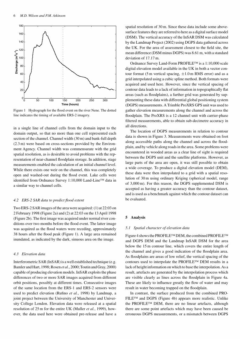
A hydrograph for the upstream (west) end of the reach (Figure 1)was obtained from the Environment Agency, Anglian Region,with a temporal frequency of 15 minutes. This was obtained usingthe Wansford ultrasonic gauge, with all flows contained withinbank due to extensive earth works. The duration of the floodevent was approximately 300 hours, or 12.5 days. The flood peakoccurred at 08:00 on 12 April 1998.

The location of the channel was obtained from Ordnance Sur-vey 1:10,000 scale Land-Line™ data, and cells were assigned aschannel based on the proportion of channel covered. This resulted


0 50 100 150 200 250 3000

20

40

60

80

100

120

140

160

180

Dis

char

ge

(m3 s-1

)

Time (hours)

Figure 1 Hydrograph for the flood event on the river Nene. The dottedline indicates the timing of available ERS-2 imagery.

in a single line of channel cells from the domain input to thedomain output, so that no more than one cell represented eachsection of the channel. Channel width (30 m) and bank-full depth(2.3 m) were based on cross-sections provided by the Environ-ment Agency. Channel width was commensurate with the gridspatial resolution, as is desirable to avoid problems with the rep-resentation of near-channel floodplain storage. In addition, stagemeasurements enabled the calculation of an initial channel level.While there exists one weir on the channel, this was completelyopen and washed-out during the flood event. Lake cells wereidentified from Ordnance Survey 1:10,000 Land-Line™ data ina similar way to channel cells.

4.2 ERS-2 SAR data to predict flood extent

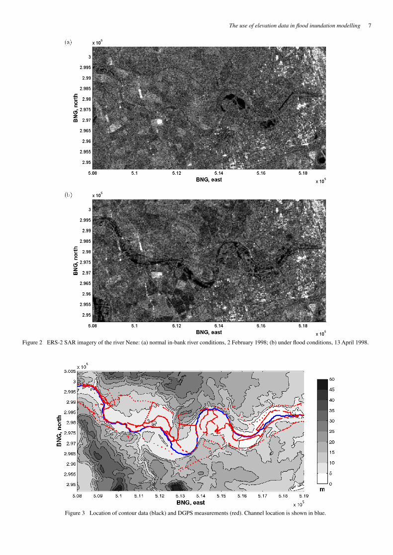
Two ERS-2 SAR images of the area were acquired: (1) at 22:03 on2 February 1998 (Figure 2a) and (2) at 22:03 on the 13 April 1998(Figure 2b). The first image was acquired under normal river con-ditions over two months before the flood event. The latter imagewas acquired as the flood waters were receding, approximately38 hours after the flood peak (Figure 1). A large area remainedinundated, as indicated by the dark, sinuous area on the image.

4.3 Elevation data

Interferometric SAR (InSAR) is a well established technique (e.g.Bamler and Hart, 1998; Rosen et al., 2000;Toutin and Gray, 2000)capable of producing elevation models. InSAR exploits the phasedifferences of two or more SAR images acquired from differentorbit positions, possibly at different times. Consecutive imagesof the same location from the ERS-1 and ERS-2 sensors wereused to predict elevation (Rufino et al., 1998) by Landmap, ajoint project between the University of Manchester and Univer-sity College London. Elevation data were released at a spatialresolution of 25 m for the entire UK (Muller et al., 1999), how-ever, the data used here were obtained pre-release and have a

spatial resolution of 30 m. Since these data include some above-surface features they are referred to here as a digital surface model(DSM). The vertical accuracy of the InSAR DSM was calculatedby the Landmap Project (2002) using DGPS data gathered acrossthe UK. For the area of assessment closest to the field site, themean difference (DSM minus DGPS) was 8.61 m, with a standarddeviation of 17.17 m.

Ordnance Survey Land-Form PROFILE™ is a 1:10,000 scaledigital elevation model available in the UK in both a vector con-tour format (5 m vertical spacing, ±1.0 m RMS error) and as agrid interpolated using a cubic spline method. Both formats wereacquired and used here. However, since the vertical spacing ofcontour data leads to a lack of information in topographically flatareas (such as floodplains), a further grid was generated by sup-plementing these data with differential global positioning system(DGPS) measurements. A Trimble ProXRS GPS unit was used togather elevation measurements along the channel and across thefloodplain. The ProXRS is a 12 channel unit with carrier-phasefiltered measurements, able to obtain sub-decimetre accuracy inall directions.

The location of DGPS measurements in relation to contourdata is shown in Figure 3. Measurements were obtained on footalong accessible paths along the channel and across the flood-plain, and by vehicle along roads in the area. Some problems wereencountered in wooded areas as a clear line of sight is requiredbetween the DGPS unit and the satellite platforms. However, aslarge parts of the area are open, it was still possible to obtaina wide coverage. To produce a digital elevation model (DEM),these data were then interpolated to a grid with a spatial reso-lution of 30 m using ordinary Kriging (spherical model, rangeof 3,000 m). For this reason, the DGPS supplemented DSM isaccepted as having a greater accuracy than the contour dataset,and is used as a benchmark against which the contour dataset canbe evaluated.

5 Analysis

5.1 Spatial character of elevation data

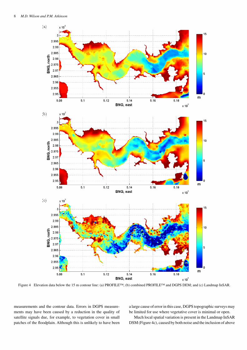
Figure 4 shows the PROFILE™ DEM, the combined PROFILE™and DGPS DEM and the Landmap InSAR DSM for the areabelow the 15 m contour line, which covers the entire length ofthe channel and gives a good indication of the floodplain area.As floodplains are areas of low relief, the vertical spacing of thecontours used to interpolate the PROFILE™ DEM results in alack of height information on which to base the interpolation. As aresult, artefacts are generated by the interpolation process whichare visible clearly as lines across the floodplain in Figure 4a.These are likely to influence greatly the flow of water and mayresult in water becoming trapped on the floodplain.

In contrast, the surface produced from the combined PRO-FILE™ and DGPS (Figure 4b) appears more realistic. Unlikethe PROFILE™ DEM, there are no linear artefacts, althoughthere are some point artefacts which may have been caused beerroneous DGPS measurements, or a mismatch between DGPS


Figure 2 ERS-2 SAR imagery of the river Nene: (a) normal in-bank river conditions, 2 February 1998; (b) under flood conditions, 13 April 1998.

Figure 3 Location of contour data (black) and DGPS measurements (red). Channel location is shown in blue.


Figure 4 Elevation data below the 15 m contour line: (a) PROFILE™; (b) combined PROFILE™ and DGPS DEM; and (c) Landmap InSAR.

measurements and the contour data. Errors in DGPS measure-ments may have been caused by a reduction in the quality ofsatellite signals due, for example, to vegetation cover in smallpatches of the floodplain. Although this is unlikely to have been

a large cause of error in this case, DGPS topographic surveys maybe limited for use where vegetative cover is minimal or open.

Much local spatial variation is present in the Landmap InSARDSM (Figure 4c), caused by both noise and the inclusion of above


5.09 5.095 5.1 5.105 5.11 5.115 5.12 5.125 5.13

x 105

6

8

10

12

14

16

18

20

22

24

BNG, east

Ele

vati

on

(m

)

Landmap InSAR

PROFILE

DGPS and PROFILE

Figure 5 Cross-section of floodplain elevation along the line BNG298,000 north.

surface features. For flood inundation modelling, surface featuresmay be desirable as flood water flow is influenced by surfaceobstructions as well as slope. However, problems are caused inareas of dense trees, for example, as the higher elevation predictedfor trees in the DSM relative to the surrounding area obstructsthe flow of water in the model, when in reality water wouldflow through the forest stand. In such a case, ground elevationis preferable to canopy elevation. In this case, the floodplain isrelatively open such that the influence of forest is unlikely to beproblematic.

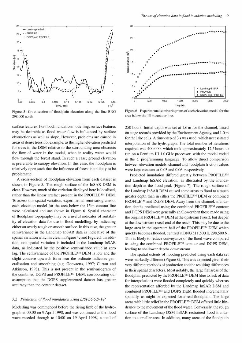
A cross-section of floodplain elevation from each dataset isshown in Figure 5. The rough surface of the InSAR DSM isclear. However, much of the variation displayed here is localised,rather than the linear artefact present in the PROFILE™ DEM.To assess this spatial variation, experimental semivariograms ofeach elevation model for the area below the 15 m contour linewere calculated and are shown in Figure 6. Spatial characterof floodplain topography may be a useful indicator of suitabil-ity of elevation data for use in flood modelling, by indicatingeither an overly rough or smooth surface. In this case, the greatersemivariance in the Landmap InSAR data is indicative of thespatial variation which is clear in Figure 4c and Figure 5. In addi-tion, non-spatial variation is included in the Landmap InSARdata, as indicated by the positive semivariance value at zerolag. The semivariance of the PROFILE™ DEM is low and theslight concave upwards form near the ordinate indicates gen-eralisation and smoothing (e.g. Goovaerts, 1997; Curran andAtkinson, 1998). This is not present in the semivariogram ofthe combined DGPS and PROFILE™ DEM, corroborating ourassumption that the DGPS supplemented dataset has greateraccuracy than the contour dataset.

5.2 Prediction of flood inundation using LISFLOOD-FP

Modelling was commenced before the rising limb of the hydro-graph at 00:00 on 9 April 1998, and was continued as the floodwave receded through to 10:00 on 19 April 1998, a total of

0 500 1000 1500 2000 2500 30000

5

10

15

20

25

30

Sem

ivar

ian

ce (

m2 )

Lag (m)

Landmap InSARPROFILEDGPS and PROFILE

Figure 6 Experimental semivariograms of each elevation model for thearea below the 15 m contour line.

250 hours. Initial depth was set at 1.6 m for the channel, basedon stage records provided by the Environment Agency, and 1.0 mfor the lake cells. A time-step of 3 s was used, which necessitatedinterpolation of the hydrograph. The total number of iterationsrequired was 400,000, which took approximately 12.5 hours torun on a Pentium III 1.0 GHz processor, with the model codedin the C programming language. To allow direct comparisonbetween elevation models, channel and floodplain friction valueswere kept constant at 0.03 and 0.06, respectively.

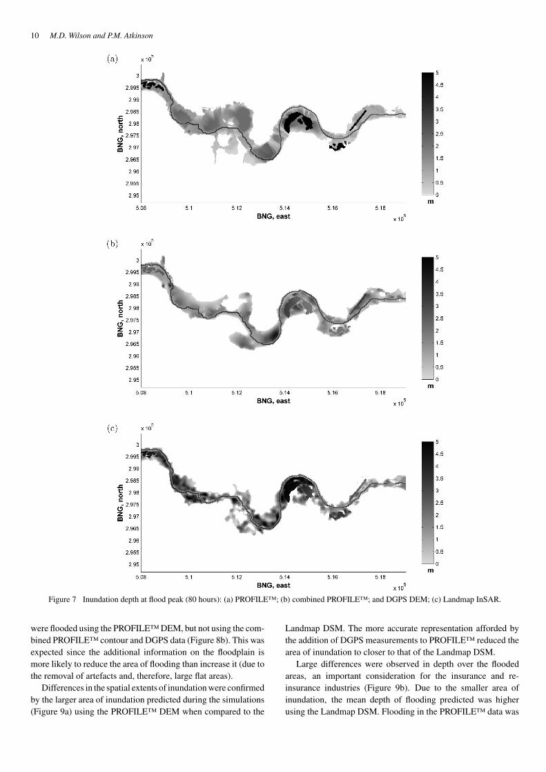
Predicted inundation differed greatly between PROFILE™and Landmap InSAR elevation, as illustrated by the inunda-tion depth at the flood peak (Figure 7). The rough surface ofthe Landmap InSAR DSM caused some areas to flood to a muchgreater depth than in either the PROFILE™ DEM or combinedPROFILE™ and DGPS DEM. Away from the channel, inunda-tion depths predicted using the combined PROFILE™ contourand DGPS DEM were generally shallower than those made usingthe original PROFILE™ DEM at the upstream (west), but deeperat the downstream (east) end of the reach. This may be due to thelarge area in the upstream half of the PROFILE™ DEM whichquickly becomes flooded, centred at BNG 511,500 E, 298,500 N.This is likely to reduce conveyance of the flood wave comparedto using the combined PROFILE™ contour and DGPS DEM,leading to shallower depths downstream.

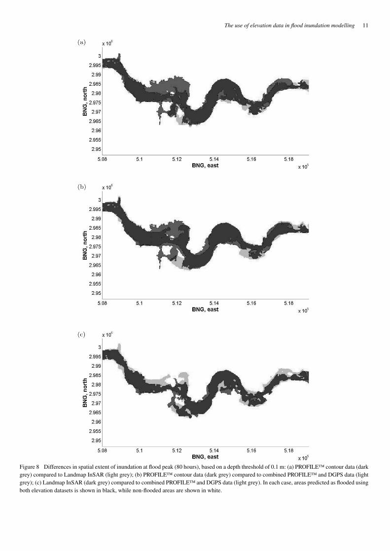
The spatial extents of flooding predicted using each data setwere markedly different (Figure 8). This was expected given theirvery different methods of production and the resulting differencesin their spatial characters. Most notably, the large flat areas of thefloodplain predicted by the PROFILE™ DEM (due to lack of datafor interpolation) were flooded completely and quickly whereasthe representation afforded by the Landmap InSAR DSM andcombined PROFILE™ and DGPS DEM flooded incrementallyspatially, as might be expected for a real floodplain. The largeareas with little relief in the PROFILE™ DEM offered little hin-drance to the movement of the flood water. Conversely, the roughsurface of the Landmap DSM InSAR restrained flood inunda-tion to a smaller area. In addition, many areas of the floodplain


Figure 7 Inundation depth at flood peak (80 hours): (a) PROFILE™; (b) combined PROFILE™; and DGPS DEM; (c) Landmap InSAR.

were flooded using the PROFILE™ DEM, but not using the com-bined PROFILE™ contour and DGPS data (Figure 8b). This wasexpected since the additional information on the floodplain ismore likely to reduce the area of flooding than increase it (due tothe removal of artefacts and, therefore, large flat areas).

Differences in the spatial extents of inundation were confirmedby the larger area of inundation predicted during the simulations(Figure 9a) using the PROFILE™ DEM when compared to the

Landmap DSM. The more accurate representation afforded bythe addition of DGPS measurements to PROFILE™ reduced thearea of inundation to closer to that of the Landmap DSM.

Large differences were observed in depth over the floodedareas, an important consideration for the insurance and re-insurance industries (Figure 9b). Due to the smaller area ofinundation, the mean depth of flooding predicted was higherusing the Landmap DSM. Flooding in the PROFILE™ data was


Figure 8 Differences in spatial extent of inundation at flood peak (80 hours), based on a depth threshold of 0.1 m: (a) PROFILE™ contour data (darkgrey) compared to Landmap InSAR (light grey); (b) PROFILE™ contour data (dark grey) compared to combined PROFILE™ and DGPS data (lightgrey); (c) Landmap InSAR (dark grey) compared to combined PROFILE™ and DGPS data (light grey). In each case, areas predicted as flooded usingboth elevation datasets is shown in black, while non-flooded areas are shown in white.


0 50 100 150 200 250 3000

2

4

6

8

10

12(a) (b)

(c) (d)

Flo

od

ed a

rea

(km

2 )

Time (hours)


0 50 100 150 200 250 3000.6

0.8

1

1.2

1.4

1.6

1.8

2

2.2

Mea

n d

epth

of

flo

od

inu

nd

atio

n (

m)

Time (hours)


0 50 100 150 200 250 3000

20

40

60

80

100

120

140

160

180D

isch

arg

e (m

3 s-1

)

Time (hours)

InflowOutflow, Landmap InSAROutflow, PROFILEOutflow, DGPS and PROFILE

0 50 100 150 200 250 3000

0.2

0.4

0.6

0.8

1

1.2

1.4

1.6

1.8

2

Flo

od

vo

lum

e (m

3 x 1

07 )

Time (hours)


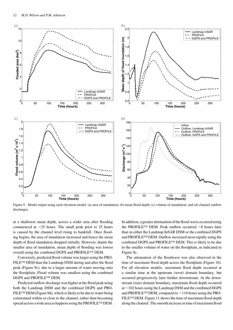
Figure 9 Model output using each elevation model: (a) area of inundation; (b) mean flood depth; (c) volume of inundation; and (d) channel outflowdischarges.

at a shallower mean depth, across a wider area after floodingcommenced at ∼25 hours. The small peak prior to 25 hoursis caused by the channel level rising to bankfull. Once flood-ing begins, the area of inundation increased and hence the meandepth of flood inundation dropped initially. However, depite thesmaller area of inundation, mean depth of flooding was lowestoverall using the combined DGPS and PROFILE™ DEM.

Conversely, predicted flood volume was larger using the PRO-FILE™ DEM than the Landmap DSM during and after the floodpeak (Figure 9c), due to a larger amount of water moving ontothe floodplain. Flood volume was smallest using the combinedDGPS and PROFILE™ DEM.

Predicted outflow discharge was higher at the flood peak usingboth the Landmap DSM and the combined DGPS and PRO-FILE™ DEM (Figure 9d), which is likely to be due to water beingconstrained within or close to the channel, rather than becomingspread across a wide area as happens using the PROFILE™ DEM.

In addition, a greater attenuation of the flood-wave occurred usingthe PROFILE™ DEM. Peak outflow occurred ∼8 hours laterthan in either the Landmap InSAR DSM or the combined DGPSand PROFILE™ DEM. Outflow increased most rapidly using thecombined DGPS and PROFILE™ DEM. This is likely to be dueto the smaller volume of water on the floodplain, as indicated inFigure 9c.

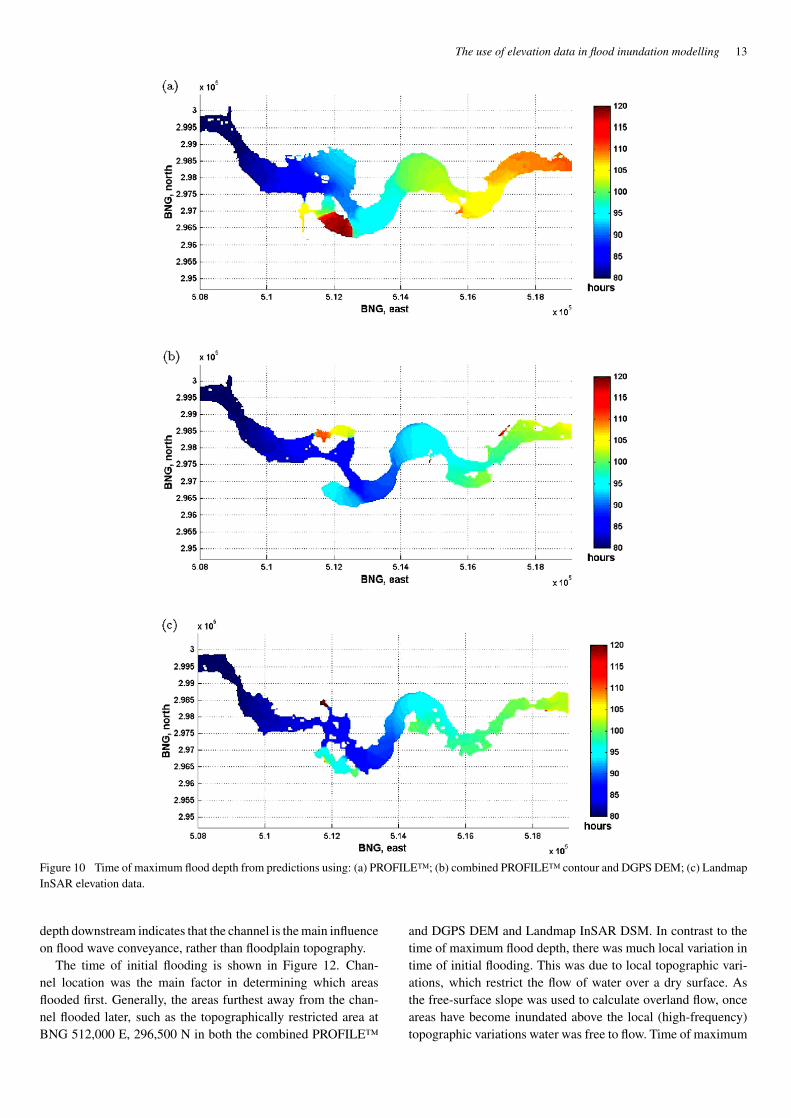
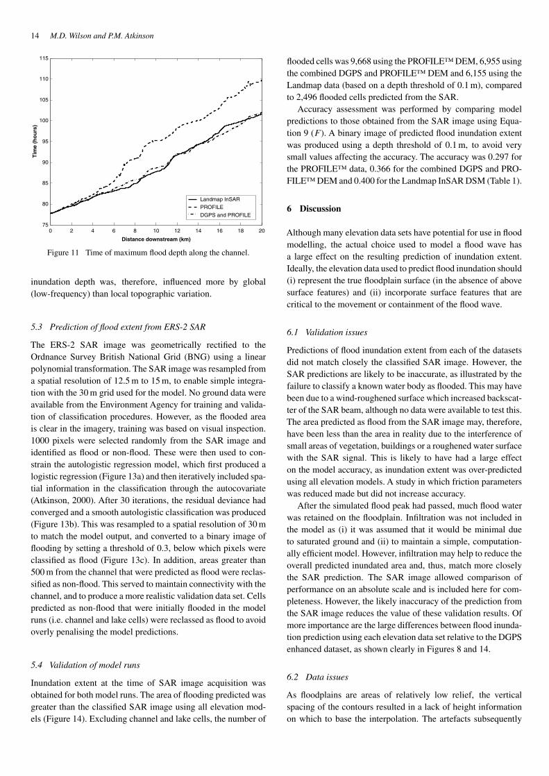
The attenuation of the floodwave was also observed in thetime of maximum flood depth across the floodplain (Figure 10).For all elevation models, maximum flood depth occurred ata similar time at the upstream (west) domain boundary, butoccurred progressively later further downstream. At the down-stream (east) domain boundary, maximum flood depth occurredat ∼102 hours using the Landmap DSM and the combined DGPSand PROFILE™ DEM, compared to ∼110 hours using the PRO-FILE™ DEM. Figure 11 shows the time of maximum flood depthalong the channel. The smooth increase in time of maximum flood


Figure 10 Time of maximum flood depth from predictions using: (a) PROFILE™; (b) combined PROFILE™ contour and DGPS DEM; (c) LandmapInSAR elevation data.

depth downstream indicates that the channel is the main influenceon flood wave conveyance, rather than floodplain topography.

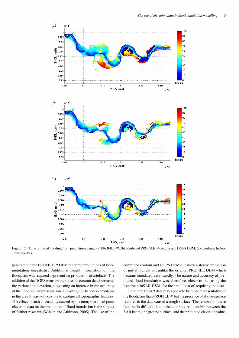
The time of initial flooding is shown in Figure 12. Chan-nel location was the main factor in determining which areasflooded first. Generally, the areas furthest away from the chan-nel flooded later, such as the topographically restricted area atBNG 512,000 E, 296,500 N in both the combined PROFILE™

and DGPS DEM and Landmap InSAR DSM. In contrast to thetime of maximum flood depth, there was much local variation intime of initial flooding. This was due to local topographic vari-ations, which restrict the flow of water over a dry surface. Asthe free-surface slope was used to calculate overland flow, onceareas have become inundated above the local (high-frequency)topographic variations water was free to flow. Time of maximum


0 2 4 6 8 10 12 14 16 18 2075

80

85

90

95

100

105

110

115

Distance downstream (km)

Tim

e (h

ou

rs)

Landmap InSAR

PROFILE

DGPS and PROFILE

Figure 11 Time of maximum flood depth along the channel.

inundation depth was, therefore, influenced more by global(low-frequency) than local topographic variation.

5.3 Prediction of flood extent from ERS-2 SAR

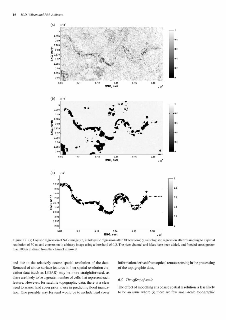
The ERS-2 SAR image was geometrically rectified to theOrdnance Survey British National Grid (BNG) using a linearpolynomial transformation. The SAR image was resampled froma spatial resolution of 12.5 m to 15 m, to enable simple integra-tion with the 30 m grid used for the model. No ground data wereavailable from the Environment Agency for training and valida-tion of classification procedures. However, as the flooded areais clear in the imagery, training was based on visual inspection.1000 pixels were selected randomly from the SAR image andidentified as flood or non-flood. These were then used to con-strain the autologistic regression model, which first produced alogistic regression (Figure 13a) and then iteratively included spa-tial information in the classification through the autocovariate(Atkinson, 2000). After 30 iterations, the residual deviance hadconverged and a smooth autologistic classification was produced(Figure 13b). This was resampled to a spatial resolution of 30 mto match the model output, and converted to a binary image offlooding by setting a threshold of 0.3, below which pixels wereclassified as flood (Figure 13c). In addition, areas greater than500 m from the channel that were predicted as flood were reclas-sified as non-flood. This served to maintain connectivity with thechannel, and to produce a more realistic validation data set. Cellspredicted as non-flood that were initially flooded in the modelruns (i.e. channel and lake cells) were reclassed as flood to avoidoverly penalising the model predictions.

5.4 Validation of model runs

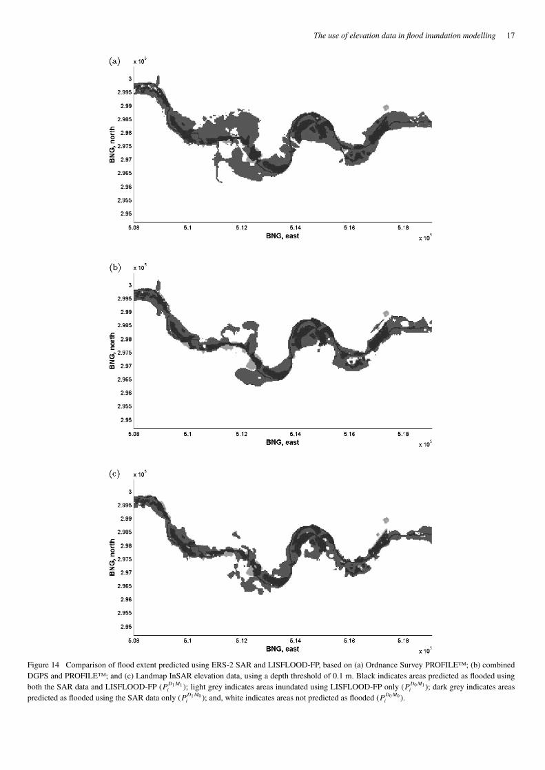
Inundation extent at the time of SAR image acquisition wasobtained for both model runs. The area of flooding predicted wasgreater than the classified SAR image using all elevation mod-els (Figure 14). Excluding channel and lake cells, the number of

flooded cells was 9,668 using the PROFILE™ DEM, 6,955 usingthe combined DGPS and PROFILE™ DEM and 6,155 using theLandmap data (based on a depth threshold of 0.1 m), comparedto 2,496 flooded cells predicted from the SAR.

Accuracy assessment was performed by comparing modelpredictions to those obtained from the SAR image using Equa-tion 9 (F ). A binary image of predicted flood inundation extentwas produced using a depth threshold of 0.1 m, to avoid verysmall values affecting the accuracy. The accuracy was 0.297 forthe PROFILE™ data, 0.366 for the combined DGPS and PRO-FILE™ DEM and 0.400 for the Landmap InSAR DSM (Table 1).

6 Discussion

Although many elevation data sets have potential for use in floodmodelling, the actual choice used to model a flood wave hasa large effect on the resulting prediction of inundation extent.Ideally, the elevation data used to predict flood inundation should(i) represent the true floodplain surface (in the absence of abovesurface features) and (ii) incorporate surface features that arecritical to the movement or containment of the flood wave.

6.1 Validation issues

Predictions of flood inundation extent from each of the datasetsdid not match closely the classified SAR image. However, theSAR predictions are likely to be inaccurate, as illustrated by thefailure to classify a known water body as flooded. This may havebeen due to a wind-roughened surface which increased backscat-ter of the SAR beam, although no data were available to test this.The area predicted as flood from the SAR image may, therefore,have been less than the area in reality due to the interference ofsmall areas of vegetation, buildings or a roughened water surfacewith the SAR signal. This is likely to have had a large effecton the model accuracy, as inundation extent was over-predictedusing all elevation models. A study in which friction parameterswas reduced made but did not increase accuracy.

After the simulated flood peak had passed, much flood waterwas retained on the floodplain. Infiltration was not included inthe model as (i) it was assumed that it would be minimal dueto saturated ground and (ii) to maintain a simple, computation-ally efficient model. However, infiltration may help to reduce theoverall predicted inundated area and, thus, match more closelythe SAR prediction. The SAR image allowed comparison ofperformance on an absolute scale and is included here for com-pleteness. However, the likely inaccuracy of the prediction fromthe SAR image reduces the value of these validation results. Ofmore importance are the large differences between flood inunda-tion prediction using each elevation data set relative to the DGPSenhanced dataset, as shown clearly in Figures 8 and 14.

6.2 Data issues

As floodplains are areas of relatively low relief, the verticalspacing of the contours resulted in a lack of height informationon which to base the interpolation. The artefacts subsequently


Figure 12 Time of initial flooding from predictions using: (a) PROFILE™; (b) combined PROFILE™ contour and DGPS DEM; (c) Landmap InSARelevation data.

generated in the PROFILE™ DEM rendered predictions of floodinundation unrealistic. Additional height information on thefloodplain was required to prevent the production of artefacts. Theaddition of the DGPS measurements to the contour data increasedthe variance in elevation, suggesting an increase in the accuracyof the floodplain representation. However, due to access problemsin the area it was not possible to capture all topographic features.The effect of such uncertainty caused by the interpolation of pointelevation data on the prediction of flood inundation is the subjectof further research (Wilson and Atkinson, 2005). The use of the

combined contour and DGPS DEM did allow a steady predictionof initial inundation, unlike the original PROFILE DEM whichbecame inundated very rapidly. The nature and accuracy of pre-dicted flood inundation was, therefore, closer to that using theLandmap InSAR DSM, for the small cost of acquiring the data.

Landmap InSAR data may appear to be more representative ofthe floodplain than PROFILE™ but the presence of above-surfacefeatures in the data caused a rough surface. The removal of thesefeatures is difficult due to the complex relationship between theSAR beam, the ground surface, and the predicted elevation value,


Figure 13 (a) Logistic regression of SAR image; (b) autologistic regression after 30 iterations; (c) autologistic regression after resampling to a spatialresolution of 30 m, and conversion to a binary image using a threshold of 0.3. The river channel and lakes have been added, and flooded areas greaterthan 500 m distance from the channel removed.

and due to the relatively coarse spatial resolution of the data.Removal of above-surface features in finer spatial resolution ele-vation data (such as LiDAR) may be more straightforward, asthere are likely to be a greater number of cells that represent eachfeature. However, for satellite topographic data, there is a clearneed to assess land cover prior to use in predicting flood inunda-tion. One possible way forward would be to include land cover

information derived from optical remote sensing in the processingof the topographic data.

6.3 The effect of scale

The effect of modelling at a coarse spatial resolution is less likelyto be an issue where (i) there are few small-scale topographic


Figure 14 Comparison of flood extent predicted using ERS-2 SAR and LISFLOOD-FP, based on (a) Ordnance Survey PROFILE™; (b) combinedDGPS and PROFILE™; and (c) Landmap InSAR elevation data, using a depth threshold of 0.1 m. Black indicates areas predicted as flooded usingboth the SAR data and LISFLOOD-FP (PD1M1

i ); light grey indicates areas inundated using LISFLOOD-FP only (PD0M1i ); dark grey indicates areas

predicted as flooded using the SAR data only (PD1M0i ); and, white indicates areas not predicted as flooded (PD0M0

i ).


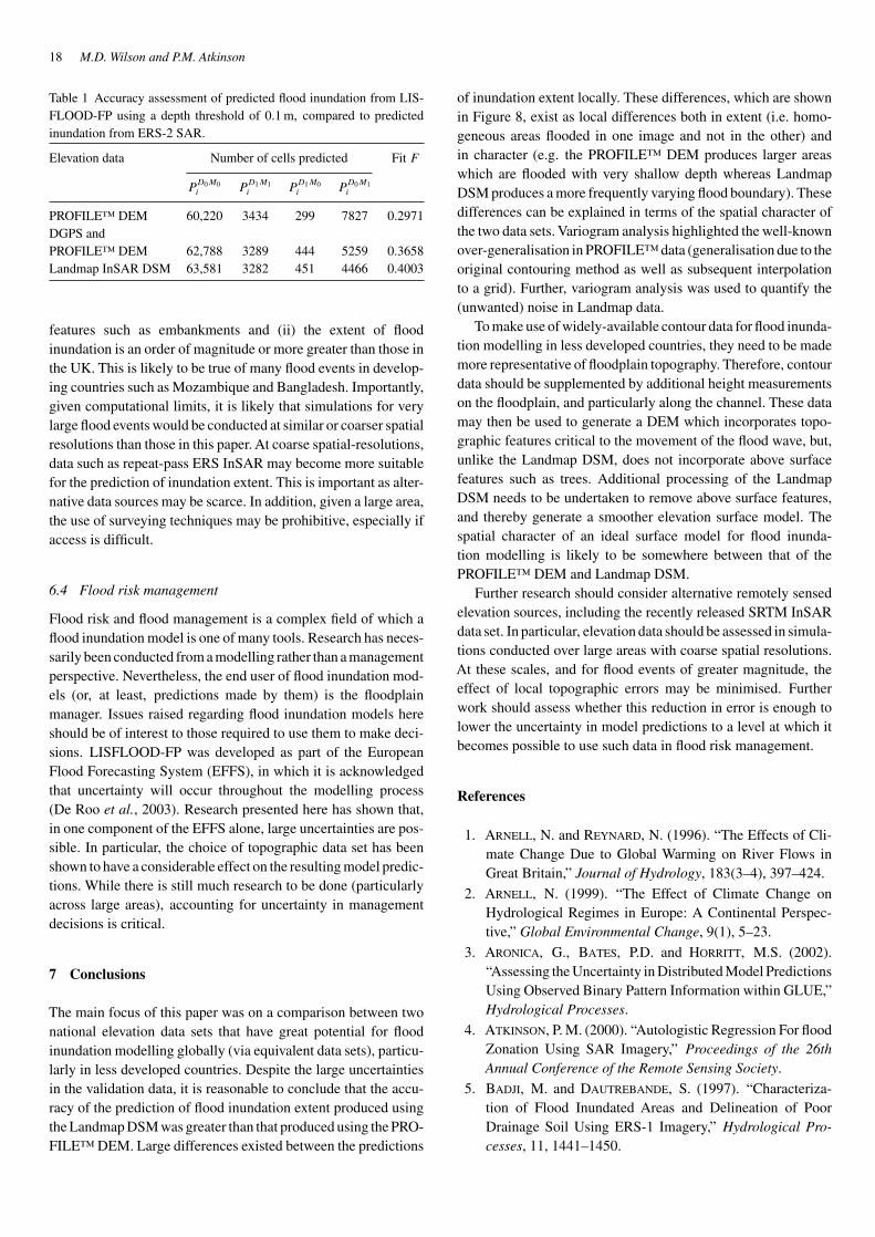
Table 1 Accuracy assessment of predicted flood inundation from LIS-FLOOD-FP using a depth threshold of 0.1 m, compared to predictedinundation from ERS-2 SAR.

Elevation data Number of cells predicted Fit F

PD0M0i P

D1M1i P

D1M0i P

D0M1i

PROFILE™ DEM 60,220 3434 299 7827 0.2971DGPS andPROFILE™ DEM 62,788 3289 444 5259 0.3658Landmap InSAR DSM 63,581 3282 451 4466 0.4003

features such as embankments and (ii) the extent of floodinundation is an order of magnitude or more greater than those inthe UK. This is likely to be true of many flood events in develop-ing countries such as Mozambique and Bangladesh. Importantly,given computational limits, it is likely that simulations for verylarge flood events would be conducted at similar or coarser spatialresolutions than those in this paper. At coarse spatial-resolutions,data such as repeat-pass ERS InSAR may become more suitablefor the prediction of inundation extent. This is important as alter-native data sources may be scarce. In addition, given a large area,the use of surveying techniques may be prohibitive, especially ifaccess is difficult.

6.4 Flood risk management

Flood risk and flood management is a complex field of which aflood inundation model is one of many tools. Research has neces-sarily been conducted from a modelling rather than a managementperspective. Nevertheless, the end user of flood inundation mod-els (or, at least, predictions made by them) is the floodplainmanager. Issues raised regarding flood inundation models hereshould be of interest to those required to use them to make deci-sions. LISFLOOD-FP was developed as part of the EuropeanFlood Forecasting System (EFFS), in which it is acknowledgedthat uncertainty will occur throughout the modelling process(De Roo et al., 2003). Research presented here has shown that,in one component of the EFFS alone, large uncertainties are pos-sible. In particular, the choice of topographic data set has beenshown to have a considerable effect on the resulting model predic-tions. While there is still much research to be done (particularlyacross large areas), accounting for uncertainty in managementdecisions is critical.

7 Conclusions

The main focus of this paper was on a comparison between twonational elevation data sets that have great potential for floodinundation modelling globally (via equivalent data sets), particu-larly in less developed countries. Despite the large uncertaintiesin the validation data, it is reasonable to conclude that the accu-racy of the prediction of flood inundation extent produced usingthe Landmap DSM was greater than that produced using the PRO-FILE™ DEM. Large differences existed between the predictions

of inundation extent locally. These differences, which are shownin Figure 8, exist as local differences both in extent (i.e. homo-geneous areas flooded in one image and not in the other) andin character (e.g. the PROFILE™ DEM produces larger areaswhich are flooded with very shallow depth whereas LandmapDSM produces a more frequently varying flood boundary). Thesedifferences can be explained in terms of the spatial character ofthe two data sets. Variogram analysis highlighted the well-knownover-generalisation in PROFILE™ data (generalisation due to theoriginal contouring method as well as subsequent interpolationto a grid). Further, variogram analysis was used to quantify the(unwanted) noise in Landmap data.

To make use of widely-available contour data for flood inunda-tion modelling in less developed countries, they need to be mademore representative of floodplain topography. Therefore, contourdata should be supplemented by additional height measurementson the floodplain, and particularly along the channel. These datamay then be used to generate a DEM which incorporates topo-graphic features critical to the movement of the flood wave, but,unlike the Landmap DSM, does not incorporate above surfacefeatures such as trees. Additional processing of the LandmapDSM needs to be undertaken to remove above surface features,and thereby generate a smoother elevation surface model. Thespatial character of an ideal surface model for flood inunda-tion modelling is likely to be somewhere between that of thePROFILE™ DEM and Landmap DSM.

Further research should consider alternative remotely sensedelevation sources, including the recently released SRTM InSARdata set. In particular, elevation data should be assessed in simula-tions conducted over large areas with coarse spatial resolutions.At these scales, and for flood events of greater magnitude, theeffect of local topographic errors may be minimised. Furtherwork should assess whether this reduction in error is enough tolower the uncertainty in model predictions to a level at which itbecomes possible to use such data in flood risk management.

References

1. Arnell, N. and Reynard, N. (1996). “The Effects of Cli-mate Change Due to Global Warming on River Flows inGreat Britain,” Journal of Hydrology, 183(3–4), 397–424.

2. Arnell, N. (1999). “The Effect of Climate Change onHydrological Regimes in Europe: A Continental Perspec-tive,” Global Environmental Change, 9(1), 5–23.

3. Aronica, G., Bates, P.D. and Horritt, M.S. (2002).“Assessing the Uncertainty in Distributed Model PredictionsUsing Observed Binary Pattern Information within GLUE,”Hydrological Processes.

4. Atkinson, P. M. (2000). “Autologistic Regression For floodZonation Using SAR Imagery,” Proceedings of the 26thAnnual Conference of the Remote Sensing Society.

5. Badji, M. and Dautrebande, S. (1997). “Characteriza-tion of Flood Inundated Areas and Delineation of PoorDrainage Soil Using ERS-1 Imagery,” Hydrological Pro-cesses, 11, 1441–1450.


6. Bamler, R. and Hart, P. (1998). “SyntheticAperture RadarInterferometry,” Inverse Problems, 14, R1–R54.

7. Bates, P. and De Roo, A. (2000). “A Simple Raster-Based Model for Flood Inundation Simulation,” Journal ofHydrology, 236, 54–77.

8. Bates, P. and Horritt, M. (2002). MDSF LISFLOOD-FPuser manual and technical note, Technical report, Universityof Bristol.

9. Bechteler, W., Hartmann, S. and Otto, A. (1994). Cou-pling of 2D and 1D models and integration into geographicinformation systems (GIS), in W. White and J. Watts (eds.),2nd International Conference on River Flood Hydraulics,John Wiley and Sons Ltd., York, England.

10. Beffa, C. and Connell, R. (2001). “Two-DimensionalFlood Plain Flow. I: Model Description,” Journal of Hydro-logic Engineering, 6(5), 397–405.

11. Biggin, D. and Blyth, K. (1996). “A Comparison of ERS-1 Satellite Radar and Aerial Photography for River FloodMapping’, Journal of the Chartered Institution of Water andEnvironmental Management, 10(1), 59–64.

12. Bishop, I., Escobar, F., Karuppannan, S., Williamson, I.,Yates, P., Suwarnarat, K. and Yaqub, H. (2000). “Spa-tial Data Infrastructures for Cities in Developing Countries:Lessons from the Bangkok Experience,” Cities, 17(2),85–96.

13. Bladé, E., Gómez, M. and Dolz, J. (1994). Quasi-TwoDimensional Modelling of Flood Inundation of Flood Rout-ing in Rivers and Floodplains by Means of Storage Cells, inP. Molinaro and L. Natele (eds.), Modelling of flood prop-agation over initially dry areas, American Society of CivilEngineers, New York.

14. Brivio, P., Colombo, R., Maggi, M. and Tomasoni, R.(2002). “Integration of Remote Sensing Data and Gis forAccurate Mapping of FloodedAreas,” International Journalof Remote Sensing, 23(3), 429–441.

15. Bye, P. and Horner, M. (1998). Easter 1998 Floods,Volume 1: Report by the Independent Review Team tothe Environment Agency, Technical report, EnvironmentAgency.

16. Chow, T. (1959). Open-Channel Hydraulics, McGraw-HillBook Company.

17. Chow, V., Maidment, D. and Mays, L. (1988). AppliedHydrology, McGraw-Hill Inc.

18. Coe, M., Heil Costa, M., Botta, A. and Birkett, C.(2002). “Long-Term Simulations of Discharge and Floodsin the Amazon Basin,” Journal of Geophysical Research,107(D20), LBA–11 1–17.

19. Curran, P. and Atkinson, P. (1998). “Geostatistics andremote sensing,” Progress in Physical Geography, 22(1),61–78.

20. De Roo,A., Gouweleeuw, B., Thielen, J., Bartholmes, J.,Bongioannini-Cerlini, P., Todini, E., Bates, P., Horritt,M., Hunter, N., Beven, K., Pappenberger, F., Heise,E., Rivin, G., Hils, M., Hollingsworth, A., Holst, B.,

Kwadijk, J., Reggiani, P., Van Dijk, M., Sattler, K.and Sprokkereef, E. (2003). “Development of a EuropeanFlood Forecasting System,” International Journal of RiverBasin Management, 1(1), 49–59.

21. De Roo, A., Odijk, M., Schmuck, G., Price, D.,Somma, F., Van Der Knijff, J., Stam, M. and Bates, P.(2000a). Using the LISFLOOD model to simulate floods inthe Oder and the Meuse catchment, in ‘European Confer-ence on Advances in Flood Research’, Vol. 2.

22. De Roo, A., Van Der Knijff, J., Schmuck, G. andBates, P. (2000b). A simple floodplain inundation model toassist in floodplain management, in U. Maione, B. MajoneLehto and R. Monti (eds.), New Trends in Water and Envi-ronmental Engineering for Safety and Life: Eco-compatibleSolutions for Aquatic Environments, Balkema, Rotterdam.

23. Estrela, T. and Quintas, L. (1994). Use of a GIS inthe modelling of flows on floodplains, in W. White andJ. Watts (eds.), 2nd International Conference on River FloodHydraulics, John Wiley and Sons Ltd., York, England.

24. Goovaerts, P. (1997). Geostatistics for Natural ResourcesEvaluation, Oxford University Press, New York.

25. Horritt, M., Mason, D. and Luckman, A. (2001).“Flood Boundary Delineation from Synthetic ApertureRadar Imagery Using a StatisticallyActive Contour Model,”International Journal of Remote Sensing, 22(13), 2489–2507.

26. Horritt, M. and Bates, P. (2001a). “Effects of SpatialResolution on a Raster Based Model of Flood flow,” Journalof Hydrology, 253, 239–249.

27. Horritt, M. and Bates, P. (2001b). “Predicting FloodplainInundation: Raster-Based Modelling versus the Finite Ele-ment Approach,” Hydrological Processes, 15(5), 825–842.

28. Horritt, M. and Bates, P. (2002). “Evaluation of 1Dand 2D Numerical Models for Predicting River FloodInundation,” Journal of Hydrology, 268, 87–99.

29. Horritt, M. (1999). “A Statistical Active Contour Modelfor SAR Image Segmentation,” Image andVision Computing17, 213–224.

30. Jakeman, A. and Letcher, R. (2003). “Integrated Assess-ment and Modelling: Features, Principles and Examplesfor Catchment Management,” Environmental Modelling andSoftware, 18, 491–501.

31. Klosterman, R. (1995). “The Appropriateness of Geo-graphic Information Systems for Regional Planning in theDeveloping World,” Computers, Environment and UrbanSystems, 19(1), 1–13.

32. Landmap Project (2002). Website: http://www.landmap.ac.uk.

33. Lee, J. S. (1981). “Refined Filtering of Image NoiseUsing Sing Local Statistics,” Computer Graphics and ImageProcessing, 15, 380–389.

34. Lighthill, M. and Whitham, G. (1955). “On KinematicWaves: 1. Flood Movement in Long Rivers,” Proceedingsof the Royal Society of London, 229, 281–316.


35. Liu, Y., Gebremeskel, S., De Smedt, F., Hoffmann, L.and Pfister, L. (2003). “A Diffusive Transport Approach forFlow Routing in GIS-Based Flood Modelling,” Journal ofHydrology, 283, 91–106.

36. Manning, R. (1891). “On the Flow of Water in OpenChannels and Pipes,” Transactions of the Institute of CivilEngineers Ireland, 20, 161–207.

37. Metzger, R. and Musy, A. (1999). 2D Flood Map-ping Hydraulic Models: Towards a Simplified TopographicApproach, in G. Li, L. Wang and J. Gao (eds.), ‘99Symposium on Flood Control’, Beijing.

38. Mirza, M. (2002). “Global Warming Changes in theProbability of Occurrence of Floods in Bangladesh andImplications,” Global Environmental Change, 12, 127–138.

39. Mirza, M. (2003). “Climate Change and Extreme WeatherEvents: Can Developing Countries Adapt?,” Climate Policy,3, 233–248.

40. Moussa, R. and Bocquillon, C. (1996). “Criteria for theChoice of Flood-Routing Methods in Natural Channels,”Journal of Hydrology, 186, 1–30.

41. Muller, J.-P., Morley, J., Walker, A., Barnes, J.,Cross, P., Dowman, I., Mitchell, K., Smith, A.,Chugani, K. and Kitmitto, K. (1999). The LANDMAPProject for the Creation of Multi-Sensor Geocoded andTopographic Map Products for the British ISles based onERS-Tandem Interferometry, in Proc. Second InternationalWorkshop on ERS SAR Interferometry on Advancing ERSSAR Interferometry from Applications towards Operations,ESA, Belgium.

42. Ohl, C. and Tapsell, S. (2000). “Flooding and HumanHealth: The Dangers Posed are notAlways Obvious,” BritishMedical Journal, 321, 1167–1168.

43. Profeti, G. and MacIntosh, H. (1997). “Flood Manage-ment Through Landsat TM and ERS SAR Data: A CaseStudy,” Hydrological Processes, 11, 1397–1408.

44. Rosen, P., Hensley, S., Joughin, I., Li, F., Madsen, S.,Rodriguez, E. and Goldstein, R. (2000). “SyntheticAperture Radar Interferometry,” Proceedings of the IEEE,88(3), 333–382.

45. Rufino, G., Moccia, A. and Esposito, S. (1998). “DEMGeneration by Means of ERS Tandem Data,” IEEE Transac-tions on Geoscience and Remote Sensing, 36(6), 1905–1912.

46. Rutschmann, P. and Hager, W. (1996). “Diffusion ofFloodwaves,” Journal of Hydrology. 178, 19–32.

47. Singh, V. (1996). Kinematic Wave Modeling in WaterResources: Surface Water Hydrology, John Wiley and Sons.

48. Thomas, R. and Nicholas, A. (2002). “Simulation ofBraided River Flow Using a New Cellular Routing Scheme,”Geomorphology, 43, 179–195.

49. Thorley, N., Clandillon, S. and P., D. F. (1997). “TheContribution of Spaceborne SAR and Optical Data in Mon-itoring Flood Events: Examples in Northern and SouthernFrance,” Hydrological Processes, 11, 1409–1413.

50. Toutin, T. and Gray, L. (2000). “State-of-the-Art of Ele-vation Extraction from Satellite SAR Data,” Journal ofPhotogrammetry and Remote Sensing, 55, 13–33.

51. Townsend, P. (2002). “Relationships between Forest Struc-ture and the Detection of Flood Inundation in ForestedWetlands Using C-Band SAR,” International Journal ofRemote Sensing, 23(3), 443–460.

52. UNDP (2001). Elaborating an Adaptation Policy Frame-work with Technical Support Papers, Technical report,United Nations Development Programme.

53. Vénere, M. and Clausse, A. (2002). “A Computa-tional Environment for Water Flow Along Floodplains,”International Journal of Computational Fluid Dynamics,16(4), 327–330.

54. Wheater, H. S. (2002). “Progress in and Prospects for Flu-vial Flood Modelling,” Philisophical Transactions of theRoyal Society of London Series A, 360(1796), 1409–1431.

55. Wilson, M. and Atkinson, P. (2005). Prediction Uncer-tainty in Elevation and its Effect on Flood InundationModelling, in P. Atkinson, G. Foody, S. Darby and F. Wu(eds.), CRC Press, Boca Raton, Florida.

56. Zerger, A. and Wealands, S. (2004). “Beyond Modelling:Linking Models with GIS for Flood Risk Management,”Natural Hazards, 33, 191–208.

the use of elevation data in flood inundation modelling: a comparison of ers interferometric sar and...

Documents