the transformative complex absorbing potential method: a bridge between complex absorbing potentials...

J. Phys. B: At. Mol. Opt. Phys.31 (1998) 2279–2304. Printed in the UK PII: S0953-4075(98)88537-4

The transformative complex absorbing potential method: abridge between complex absorbing potentials and smoothexterior scaling

U V Riss† and H-D Meyer‡Theoretische Chemie, Physikalisch-Chemisches Institut, Universitat Heidelberg,Im Neuenheimer Feld 253, 69 120 Heidelberg, Germany

Received 20 October 1997, in final form 16 February 1998

Abstract. The derivation of the transformative complex absorbing potential (TCAP) methodand its performance are discussed. This approach was developed in a previous paper(1995 J. Phys. B: At. Mol. Opt. Phys. 28 1475) and illustrates the relation between complexabsorbing potentials (CAPs) and the smooth exterior scaling (SES) method. Starting from anenergy-dependent CAP one arrives at an SES-like Hamiltonian via an elementary similaritytransformation. Developing this idea further leads to the so-called TCAP equation. It differsfrom the SES Schrodinger equation in two respects. Firstly, the potential is not transformed and,secondly, an additional correction term appears. Neglecting this rather small term leads to aHamilton operator that is easy to apply to time-dependent as well as time-independent problems.This Hamiltonian can be extended order by order ending up in the full SES Hamiltonian. Bynumerical application it is demonstrated that the TCAP approach is very efficient and can easilybe generalized to the multi-dimensional case for which formulae are provided.

1. Introduction

Absorbing boundary conditions in the form of complex absorbing potentials (CAPs) werefirst introduced in time-dependent quantum mechanical calculations to avoid artificialreflections caused by the use of finite basis sets or grids (Kosloff and Kosloff 1986).These CAPs are located in the asymptotic region where the motion becomes (almost) free.They generate an absorbing region that annihilates outgoing wavepackets, and thus preventsundesired reflections.

Besides the CAP method, other techniques based on complex symmetric Hamiltonians(Lowdin 1988) have successfully been applied to generate absorbing areas. One of theseis the complex scaling method. Based on rigorous mathematical theorems (Aguilar andCombes 1971, Balsev and Combes 1971, Simon 1972, 1973) this method has undergonea continuous development and a variety of applications (Reinhardt 1982, Moiseyev 1991,1998a). Although the approach was originally formulated for time-independent calculationsof resonance states, it appears to also be useful in time-dependent calculations (McCurdyand Stroud 1991, McCurdyet al 1991).

Both methods have pros and cons. Due to their non-physical nature, CAPs lead toartificial perturbations of the system. They not only absorb the wavepacket, but also

† E-mail address: [email protected]‡ E-mail address: [email protected]

0953-4075/98/102279+26$19.50c© 1998 IOP Publishing Ltd 2279

2280 U V Riss and H-D Meyer

produce reflections themselves. Therefore a central problem concerning the applicationof CAPs lies in the minimization of these reflections (Kosloff and Kosloff 1986, Neuhauserand Baer 1989a, b, Vibok and Balint-Kurti 1992a, b, Macıas et al 1994, Riss and Meyer1996). But beside this problem the CAP method stands out due to its straightforward andsimple applicability. Turning to the complex scaling method one finds that this approachis transformative, i.e. it consists in an unbounded similarity transformation of the Hamiltonoperator (Lowdin 1988, Riss 1998), and the solution of the transformed Schrodinger equationis strictly equivalent to the solution of the original equation (with different boundaryconditions, however). This transformation causes no unphysical perturbation but requiresthe analytical continuation of the scattering potential. Here technical difficulties often arise.To remove these problems a large number of techniques have been suggested (McCurdy andRescigno 1978, Simon 1979, Morgan and Simon 1981, Lipkinet al 1989). At present themost flexible of these approaches seems to be the smooth exterior scaling (SES) (Lipkinet al1989, Moiseyev and Hirschfelder 1988, Romet al 1990, Rescignoet al 1997, McCurdyet al 1997). In the SES method the wavepacket is propagated along an arbitrary (smooth)path in the complex coordinate plane, and is absorbed when the path leaves the real axis.

Although the SES and the CAP ansatz are based on similar ideas, the relation betweenboth approaches is not completely clear. In a recent paper (Riss and Meyer 1995, to bereferred to as I) we demonstrated that the construction of reflection-free CAPs leads ina natural way to a connection between the SES and the CAP ansatz. The connectionbetween SES and CAP has also been investigated by Rom and co-workers (1991) and byMoiseyev (1998b). The former work considers the role of additional (unbounded) operatorsin a complex scaling framework, while the latter starts from SES and arrives at a CAP byessentially replacing differential operators by their eigenvalues.

A deeper understanding of SES and CAP as well as their relation may allow acombination of both approaches. This combination should maintain the main advantagesof both, i.e. a method which can be implemented simply and which avoids too muchperturbation of the physical system.

Here we will study the relationship between the CAP and SES approaches in the lightof the TCAP ansatz. The TCAP method proceeds from the original CAP and leadsto a Hamilton operator that is very similar to that resulting from the smooth exteriorscaling transformation (see I). In contrast to SES this Hamiltonian contains the original(unscaled) potential and includes an additional correction term. This correction term israther complicated but, in general, small and can be neglected to a good approximation.Doing so one arrives at an Hamiltonian that can also be viewed as an SES Hamiltonian butleaving the potential unscaled.

This approach (i.e. neglecting the correction terms), which we refer to as TCAPmethod, is examined using time-dependent calculations. The approximate character becomesmanifest in residual reflection which does not appear in TCAP with corrections and SES.Thus it is important to study the reflection produced by the approximation. This is done bynumerical as well as analytical considerations. To this end we will use similar techniquesas in our investigation on the CAP reflection (Riss and Meyer 1996, to be referred toas II). The analytical investigations are performed applying WKB like and perturbativeapproaches. The numerical investigation consists of wavepacket propagations. These areperformed by solving the time-dependent Schrodinger equation applying the short-iterativeArnoldi–Lanczos method (Arnoldi 1951, Saad 1980, Pollard and Friesner 1994) and the fastFourier transform (FFT) technique (Kosloff 1988). The flux into the reflection channel iscalculated by additional boundary CAPs (see II as well as Jackle and Meyer 1996) in orderto obtain an energy-resolved analysis of the reflection.

Transformative complex absorbing potential method 2281

The paper is organized as follows. In section 2 we give a brief summary of the derivationof the TCAP method and demonstrate its connection to the SES and the CAP method. Insection 3 we review the numerical procedure applied. In section 4 we present numericalresults of time-dependent calculations using the TCAP method. A discussion of the resultsfollows in section 5. In two appendices we demonstrate how the approach is generalized tothe multi-dimensional case. Throughout the paper a unit system is used with ¯h = 1.

2. Theoretical investigation

2.1. Energy-dependent CAPs

In the following we will direct the reader from the CAP to the TCAP approach. We beginthe investigation with the one-dimensional time-independent Schrodinger equation

Hψ±E ≡ −1

2m

d2ψ±Edx2

+ V (x)ψ±E = Eψ±E (2.1)

whereE denotes a real, positive energy,m the mass,V (x) a usual scattering potential, andψ±E (x) scattering eigenfunctions that obey the boundary conditions

ψ±E (x)→ e±ikx for x →∞ (2.2)

with k = √2mE. Different from bound state eigenfunctions the solutionsψ±E (x) donot vanish in the asymptotic region. This behaviour is connected to the fact that everywavepacket (with positive mean energy) will spread unlimitedly.

In practical calculations it is necessary to prevent an unlimited movement since onlyfinite basis sets or grids are available. This problem led to the introduction of complexabsorbing potentials (CAPs). The CAP is usually represented as−iηW whereη describesa positive strength parameter andW a local potential with non-negative real part. TheCAP is simply added to the Hamilton operator and generates an absorbing region where thewavepackets are damped. The CAP method has become quite popular in the recent yearsdue to this structural straightforwardness.

For the sake of simplicity let the CAP start atx = 0 and be located on the interval[0,∞). The introduction of the CAP leads to the effective Schrodinger equation

(H − iηW)ψW±E = EψW±

E . (2.3)

Sinceψ±E andψW±E obey the same Schrodinger equation outside the absorbing region one

may express the latter set of functions by the first set. We thus write

ψW±E (x) = ψ±E (x)+R±ψ∓E (x) for x < 0 (2.4)

whereR± denotes the reflection coefficient. One observes that outside the absorbing regionψ±E and ψW±

E differ by theR±ψ∓E term. This term describes the artificial reflection ofwavepackets at the imaginary barrier−iηW . The coefficientR± characterizes the strength ofthe reflection|R±|2. In the ideal caseR± = 0 is valid, i.e. there is no artificial perturbationasx < 0. A CAP (or any other modification) for which this is true is said to be reflection-free.

Inside the absorbing region the wavefunctionψW+E vanishes:∣∣ψW+

E (x)∣∣→ 0 for x →∞ (2.5)

while the second solutionψW−E grows:∣∣ψW−

E (x)∣∣→∞ for x →∞. (2.6)


Figure 1. Schematic representation of the absorption in a time-dependent picture. The dampingof a wavepacket during propagation from timet0 to t1 is demonstrated. The broken curveindicates the CAP. The wavepackets contain only waves with negative (upper panel) and positive(lower panel) momenta. In the former case the waves (i.e.ψW+E ) have to grow forx →∞, inthe latter case the waves (i.e.ψW−E ) have to decrease because the wavepacket formed by thesewaves has to decrease in time.

Switching to the time-dependent picture the behaviour (2.5) and (2.6) can be madeplausible. In figure 1 the propagation of a wavepacket interacting with the CAP is depictedschematically. If the wavepacket moves into the absorbing region the absolute value of thewave must decrease forx →∞. If the wavepacket moves out of the absorbing region theabsolute value of the wave still decreases in time, but increases forx → ∞. This makesclear whyψW+

E andψW−E behave in a different way forx →∞.

Turning to the practical use of CAPs a fundamental task consists in the optimizationof their absorption properties. Although the reflected partR±ψ∓E is, in general, small andvanishes forη → 0 (Riss and Meyer 1993), the use of finite basis sets or grids requiresthe construction ofefficientCAPs. Such CAPs, which are restricted to a fixed finite region,should give the most absorption and cause a minimum of reflection without becoming toocomplicated. A first step to this aim consists in determining optimal strength parametersηopt.

The optimal strength depends on the energyE of the wave to be damped. In general,an energy-independent CAP does not absorb the wave sufficiently for high energies andproduces too much reflection for small energies. By scaling the CAP strength with theenergy it is possible to reduce this unbalance. This was demonstrated in I. The optimal


parameterηopt(E) can be set proportional to the energyE of the wave to be absorbed:

ηopt(E) = E aopt(E). (2.7)

The new parameteraopt(E) is still energy dependent, but to a lesser extent thanη. Hencean improvement of the performance is expected if one takes the linear energy dependenceinto account and approximatesaopt(E) by a constant.

If the CAP overlaps with the scattering potential one has to consider the energy shiftcaused by the potential. This is done (to first order) by scaling the CAP strength withE − V (x) instead ofE. In order to compare the formulae with later results we alsointroduce a factor 2. This ansatz leads to

η(E) := 2(E − V (x))a (2.8)

wherea is the parameter to be optimized. The corresponding Schrodinger equation thenreads

T ψW±E + V (1+ 2iaW)ψW±

E = E(1+ 2iaW)ψW±E (2.9)

where

T := − 1

2m

d2

dx2. (2.10)

Equation (2.9) represents a generalized eigenvalue problem which can be reduced to anordinary eigenvalue problem by a kind of Lowdin transformation (Lowdin 1950). Thismeans that the operatorH is replaced by the operator(1+ 2iaW)−1/2H(1+ 2iaW)−1/2. Inthe present case this can be simply performed since the operator(1+ 2iaW) is diagonal inthe spatial representation. Introducing the function

f (x) :=√

1+ 2iaW(x) (2.11)

and transforming equation (2.9) results in

f (x)−1 T f (x)−1ψW±E + V (x) ψW±

E = EψW±E (2.12)

where ψW±E = f (x)ψW±

E . Equation (2.12) represents anequivalent formulationofthe energy-dependent CAP approach of equation (2.9), but is expressed as an ordinaryeigenvalue problem that can be solved in the usual manner. In the following we willsee that equation (2.12) is closely connected to the smooth exterior scaling and that thefunctionf can be interpreted as the derivative of a complex coordinate path. In particular,equation (2.12) leads to a linkage of CAP and SES theory. Finally we emphasize thatthe form off is not bound to be that of equation (2.11); actuallyf may be chosen quitegenerally (see below, section 2.3).

2.2. Transformative complex absorbing potentials

We want to define a transformation of the Hamilton operator that generates an absorbingregion. Every wavepacketψ(t) that enters this region is to be damped. In order tomake clear how such a transformation can be constructed we demonstrate how such atransformation must affect the time-independent wavesψ±E . To this end we transformψ±Eto a suitable form introducing the local quantum momentumκ± defined as

κ±(E, x) := −idψ±Edx

/ψ±E . (2.13)

It satisfies the differential equation

iκ ′± = κ2± − 2m(E − V ) (2.14)


subject to the boundary condition

κ±(E, x)→±k for x →∞. (2.15)

The local quantum momentaκ+ andκ− are connected through

κ−(E, x) = −κ∗+(E, x). (2.16)

In the case when the energy or the coordinate becomes complex the complex conjugateE∗

or x∗ must appear on the right-hand side of equation (2.16), respectively.The exact solutionψ±E may now be expressed using the local momentum as

ψ±E (x) = ψ±E (0) exp

{i∫ x

0κ±(E, ξ)dξ

}. (2.17)

For sake of simplicity we will omit the normalization factorψ±E (0) in the following andwrite

ψ±E (x) = exp

{i∫ x

κ±(E, ξ)dξ

}. (2.18)

To construct a damping transformation we have to recall the asymptotic behaviour(2.5) and (2.6) of the CAP wavefunctionsψW+

E and ψW−E . If the local momentum is

positive (i.e. the wavepacket moves in the direction of the absorbing region), the absolutevalue of the wave must decrease forx → ∞. If the local momentum is negative (i.e. thewavepacket moves out of the absorbing region) the absolute value of the wave must increasefor x →∞. Regarding equation (2.18), such a behaviour can be achieved by multiplyingκ± with a suitable complex factorf (x). Here we assume thatf (x) is twice differentiableand satisfies

f (x) = 1 for x < 0

π/2> arg(f (x)) > θ for largex and someθ > 0

|f (x)| > ε for someε > 0.

(2.19)

Here the last condition ensures thatf −1 is non-singular and together with the secondcondition it guarantees that the associated coordinate path (see below) goes to infinity. Wenow define the transformationUf defined by

ψf±E (x) := Ufψ±E (x)

:= f 1/2(x) exp

{i∫ x

f (ξ) κ±(E, ξ)dξ

}. (2.20)

The transformationUf complies with the requirements mentioned above. Due to the secondof the conditions (2.19) the wavefunction is damped if the local momentum is positiveand grows if it is negative. Moreover,ψ±E (x) = ψ

f±E (x) is valid for x < 0. Thus the

approach is reflection free. If we return to the preliminary CAP considerations we note that,in particular, the functionf of (2.11) satisfies all conditions (2.19) providedW satisfiessuitable conditions (Riss and Meyer 1993).

Next we want to derive the corresponding Schrodinger equation of whichψf±E are the

solutions. To this end we define the operators

Pf := f (x)−1/2 1

i

d

dxf (x)−1/2 (2.21)

and

Tf := 1

2mP 2f . (2.22)


Applying these operators to the transformed wavefunction (2.20) we obtain

Pfψf±E (x) = κ±(E, x)ψf±

E (x) (2.23)

Tfψf±E (x) = 1

2m

(κ±(E, x)2− iκ ′±(E, x)f (x)

−1)ψf±E (x). (2.24)

With the aid of equation (2.14) it now follows that(Tf + V + i

2m

(f (x)−1− 1

)κ ′±(E, x)

)ψf±E (x) = Eψf±

E (x). (2.25)

This is the TCAP equation with the correction previously derived in I. It is a complicatedequation becauseκ ′± depends on the energyE. Moreover, the computation ofκ ′± requires ingeneral a similar effort to solving the original problem (2.1). However, since the knowledgeof the derivative of the local momentum is only required in the absorbing, i.e. asymptotic,region it may be computed approximately by WKB or perturbation theory. Thus in time-independent calculations equation (2.25) may be solved iteratively, as done in I.

To arrive at a simpler form of the Hamilton operator that also allows the treatment oftime-dependent problems, we define the TCAP Hamiltonian

HTCAP := Tf + V (2.26)

and propose to solve the time-independent or time-dependent Schrodinger equation withthis (non-Hermitian) Hamiltonian. The neglect of the correction term

Wcorr := i

2m

(f (x)−1− 1

)κ ′±(E, x) (2.27)

is justified becausef −1 − 1 vanishes in the non-absorbing region, andκ ′± is small in theabsorbing region (provided that it lies far enough in the asymptotic region). In fact,Wcorr

vanishes identically ifV is a cut-off potential which has no overlap with the absorbingregion.

In general the neglect ofWcorr introduces some errors in the wavefunctions. Theseerrors stem from reflections caused by the TCAP, i.e. by the modified kinetic energy. Toinvestigate these reflections we write the generalized eigensolutions toHTCAP as

ψTCAPE (x) = A(x)ψf+

E (x)+ B(x)ψf−E (x). (2.28)

Solving

HTCAPψTCAPE = EψTCAP

E (2.29)

yields differential equations forA(x) andB(x) (see appendix A). Here we have omittedthe ‘+’ for ψTCAP

E since—as well as forψCAPE andψSES

E to be discussed below—only thissolution is of interest. The boundary conditions are given byA(x)→ 1 andB(x)→ 0 forx →∞ sinceψTCAP

E andψf+E both vanish forx →∞ but ψf−

E does not.A(x) andB(x)become constant outside the absorbing region whereψ

f±E = ψ±E . The reflection probability

|R+|2 is simply given by|B(0)/A(0)|2 (note that the absorbing region was located in theinterval [0,∞)). Solving forB(x) by a first-order treatment and keepingA(x) to zerothorder (see appendix A) yields

|R+|2 =∣∣∣∣ ∫ ∞

0

−κ ′−(E, x)κ+(E, x)− κ−(E, x) (f (x)− 1)

× exp

{i∫ x

0f (ξ)(κ+(E, ξ)− κ−(E, ξ))dξ

}dx

∣∣∣∣2. (2.30)


With the aid of the simple approximation (see I)κ+ ≈ k, κ− ≈ −k, andκ ′− ≈ mV ′/k onearrives at

|R+|2 ≈∣∣∣∣ ∫ ∞

0

V ′(x)E

(f (x)− 1) exp

{2ik

∫ x

0f (ξ) dξ

}dx

∣∣∣∣2. (2.31)

Inspection of this expression shows that the neglect ofWcorr is, in general, a validapproximation since the productV ′(x)(f (x)− 1) is usually small.

If the absorption region is finite the wave cannot completely be absorbed. In this casealso a transmitted part of the wavefunction appears. In analogy to the considerations in IIthe transmitted part of the wavefunction can be approximated by settingA = 1 andB = 0in equation (2.28). This results in

ψTCAPE (x) ≈ ψf+

E (x) = exp

(i∫ x

0κ+(E, ξ) f (ξ)dξ

). (2.32)

By evaluation of this wavefunction at the end of the absorbing region one obtains thefollowing formula for the transmission:

|T |2 = exp

{−2kIm

∫ L

0f (x) dx

}(2.33)

whereL denotes the length of the absorbing region, andκ+ is approximated byk. This issufficient for an estimate as desired here.

If the functionf has the particular form

f (x) =√

1+ 2ia(x/L)n (2.34)

we gave an efficient approximation in II to evaluate the expression (2.33) as a function ofa andk:

log |T |2 = −2akL

n+ 1

{1+ 4n+ 4

3n+ 1a2+

(n+ 2

2n+ 2

)8

a4

}−1/8

. (2.35)

Conversely the expression (2.33) can be used to determine a lower limit for the parametera

in order to secure an upper limit of the transmission. This minimal value of the parametera can be determined as a function of the acceptable maximal transmission:

a = − log |T |22kL

(n+ 1)

{1+ (n+ 1)3

6n+ 2

(log |T |2kL

)2

+((n+ 2)2

8n+ 8

log |T |2kL

)4}1/4

. (2.36)

In general,|T |2 decreases faster with growingE than |R+|2. Therefore at high energies|R+|2 is dominant. Note that—opposite to the CAP method—the transmission decreaseswith increasing energy.

2.3. Connection to smooth exterior scaling

Let the mappingz = F(x) define a smooth path in the complex plane for which we choose

F(x) =∫ x

0f (ξ) dξ (2.37)

i.e. F(x) = x for x 6 0 and arg(F (x)) > θ > 0 for x → ∞. In particular, it holds thatf (x) = F ′(x). We assume here thatf is twice differentiable. However, if one is willing towork with δ functions and derivatives thereof, it is also possible to use an only piecewisecontinuous functionf . Such a situation occurs if one regards (non-smooth) exterior scaling(Scrinzi and Elander 1993, Kurasov and Elander 1994).


The wavefunction that results from the SES transformation with respect to the pathF(x) then reads

ψSESE (x) := SFψ+E (x)

:= f 1/2(x) ψ+E (F (x))

= f 1/2(x) exp

{i∫ x

f (ξ) κ+(E, F (ξ))dξ

}. (2.38)

Here the wavefunctionψ+E is assumed to be analytic in a region that contains the real axis,the pathF and the domain in between. The third line of equation (2.38) shows that TCAP(with correction) and SES generate very similar wavefunctions.κ+(E, ξ) is merely replacedby κ+(E, F (ξ)). If ψ+E satisfies equation (2.1) thenψSES

E obeys

HSESψSESE (x) ≡ (Tf + V (F(x)))ψSES

E (x) = EψSESE (x) (2.39)

i.e. there is no correction term but the original potentialV (x) is replaced by the scaledpotentialV (F(x)). The TCAP ansatz and SES thus yield very similar methods which, infact, become identical for cut-off potentials that vanish forx > 0.

Since the Schrodinger equation (2.39) is equivalent (via a complex-unitarytransformation (Riss 1998)) to the original Schrodinger equation (2.1), the resulting solutionis reflection free. The same is true for the solution of the TCAP equation with correctionterm (2.25). In contrast, the Hamilton operatorHTCAP leads only to a reflection-reducedsolution. From an SES point of viewHTCAP describes an approximate approach obtainedby replacingV (F(x)) by V (x). This approximation may appear rather crude since it is notclear that the correction termV (F(x)) − V (x) is small. The replacement only becomescomprehensible if one uses equation (2.25) as a standard of comparison. Here it is obviousthat the correction termWcorr is rather small. In particular, equation (2.31) demonstrateshow the scattering potential and the path form are related to the reflection.

In fact, the TCAP HamiltonianHTCAP can be regarded as a zeroth-order approximationof HSES with respect to the Taylor expansion

V (F(x)) = V (x)+ V ′(x)(F (x)− x)+ 12V′′(x)(F (x)− x)2+ · · · (2.40)

and the absorption properties of the operatorHTCAP can be improved by going to higher-order approximations forV (F(x)). To this end one has to consider the corresponding Taylorexpansion ofκ+(E, F (x)):

κ+(E, F (x)) = κ+(E, x)+ κ ′+(E, x)(F (x)− x)+ 12κ′′+(E, x)(F (x)− x)2+ · · · . (2.41)

To demonstrate how the proceeding looks we consider the first-order approximation. Thefirst-order term in equation (2.41) has to be included in the model wavefunction (2.20):

(1)ψf+E (x) = f 1/2(x) exp

{i∫ x

f (ξ)(κ+(E, ξ)+ κ ′+(E, ξ)(F (ξ)− ξ)) dξ

}. (2.42)

The wavefunction(1)ψf+E leads to the effective Schrodinger equation:

Tf(1)ψ

f+E (x)+ V (x) (1)ψf+

E (x)+ V ′(x)(F (x)− x) (1)ψf+E (x)+ (1)Wcorr

(1)ψf+E (x)

= E (1)ψf+E (x) (2.43)

where the correction term(1)Wcorr is given as

(1)Wcorr(x) = i

2m

(f (x)−1− 1

)κ ′′+(E, x)(F (x)− x). (2.44)

In contrast to the correction termWcorr the first-order correction term contains the secondderivative of κ+ instead of the first derivative and the expression is multiplied with the


factorF(x)− x. Especially for potentials with fast vanishing higher-order derivatives, e.g.inverse power potentials, such higher-order corrections may lead to a significant reductionof the perturbation. From equation (2.43), the first-order TCAP operator is

(1)HTCAP = Tf + V (x)+ V ′(x)(F (x)− x). (2.45)

By a numerical example we will show that this approach indeed produces less reflectionthan the zeroth-order TCAP approach.

2.4. Connection to the CAP method

After examination of the TCAP approach we can now use the new insight to discuss theCAP approach. In fact, both approaches have much in common. To show this we first usethe chain rule and write the scaled kinetic energy as

Tf = f −1Tf −1+WT (2.46)

where

WT (x) = 3

8m

f ′(x)2

f (x)4− 1

4m

f ′′(x)f (x)3

. (2.47)

Using equation (2.46) for representing the reflection-free TCAP equation (2.25) we cometo (

f −1Tf −1+ V +WT +Wcorr)ψf+E (x) = Eψf+

E (x). (2.48)

Comparing equation (2.48) with the energy-dependent CAP approach represented byequation (2.12) we find that the difference only consists in the additional term(WT +Wcorr).If we multiply equation (2.48) from the left withf and insertff −1 in front of ψf+

E (x),this results in(

T + Vf 2+WT f2+Wcorrf

2)ψCAPE (x) = Ef 2ψCAP

E (x) (2.49)

where

ψCAPE (x) = f (x)−1ψ

f+E (x) = f (x)−1/2 exp

{i∫ x

f (ξ) κ+(E, ξ)dξ

}. (2.50)

Now we want to apply the opposite method to that in section 2.1, i.e. we proceed from thepath functionf to a corresponding potentialW . Recalling definition (2.11) we can use thefunction f to definethe potentialW :

iηW(x) := 1

2m

(f (x)2− 1

)κ+(E, x)2. (2.51)

With this definition one obtains

K(E, x) := f (x) κ+(E, x) =√κ+(E, x)2+ 2iηmW(x) (2.52)

and can expressf by

f (x) =√

1+ 2i(ηm/κ+(E, x)2

)W(x). (2.53)

It is to be noticed that the relation (2.11) is restored if we set

a = ηm

κ+(E, x)2(2.54)

which, using equation (2.14), may be written as

η = 2(E − V (x))a + iκ ′

ma (2.55)


i.e. we restore ourad hoc ansatz (2.8) except for the small additional term iaκ ′/m. Ifwe now substitutef in equation (2.49) by the expression (2.53) and use the differentialequation (2.14) we obtain a CAP which slightly differs fromW by an additional energydependent term, but the resulting Hamiltonian is still reflection free. The calculation (seeI) yields

(T + V − iηW − iηW1)ψCAPE (x) = EψCAP

E (x) (2.56)

where

W1(x) := 1

4

W ′′(x)K(E, x)2

− i5

8

ηmW ′(x)2

K(E, x)4− 1

2

κ(E, x)κ ′(E, x)W ′(x)K(E, x)4

+iκ ′(E, x)W(x)

K(E, x)2+ κ(E, x)K(E, x) . (2.57)

Equation (2.57) is the so-called RCAP equation (see I). It is strictly equivalent toequation (2.25). The RCAP is thus a reflection-free CAP which, however, depends onthe energy (through bothκ andκ ′) in a very complicated manner. Discarding the energy-dependent termW1 one arrives at the usual CAP:−iηW(x).

Let us summarize the results: the CAP method is related to the TCAP method by atransformation of the Hamiltonian and the neglect of all energy dependent correction terms.Since TCAP and SES are closely related this establishes also a relation between the SESand CAP method.

3. Numerical method

The numerical method mainly follows the treatment as described in II. LetH denotethe Hamiltonian matrix of the Hamilton operator under consideration (including absorbingterms). All matrix elements are evaluated with respect to the complex symmetric scalarproduct: Hij =

∫φiHφj dx, i.e. without complex conjugation (Moiseyevet al 1978). In

the following computationsH was constructed using the Fourier method (Kosloff 1988).Throughout the numerical investigations dimensionless reduced variables and massm = 1are assumed.

The only major difference to the procedure in II consists in the application of theshort-iterative Arnoldi–Lanczos method (Arnoldi 1951, Saad 1980, Pollard and Friesner1994) instead of the Newton method. The former is a generalization of the usual short-iterative Lanczos method (Park and Light 1986, Leforestieret al 1991) which allows theapplication of the algorithm to non-Hermitian matrices. One of us has already used thismethod successfully for large-scale wavepacket propagation with respect to CAP modifiedHamiltonians (Beck and Meyer 1997).

Let us briefly sketch the applied algorithm. For a given initial vectorv0 one constructsn Lanczos vectors by the following iterative scheme: starting from the normalized vectorv0 := ψ/‖ψ‖ one computes the vectorvj+1 recursively fromv0, . . . ,vj according to

(I) u(0)j+1 =Hvj(II) Ki,j =

⟨vi∣∣u(i)j+1

⟩(i = 0, . . . , j)

(III) u(i+1)j+1 = u(i)j+1−Ki,jvi (i = 0, . . . , j)

(IV) Kj+1,j =∥∥u(j+1)

j+1

∥∥(V) vj+1 = 1

Kj+1,ju(j+1)j+1 .

(3.1)


From the coefficientsKi,j one obtains an upper Hessenberg matrixK which is diagonalizedaccording to

K = Z∆Z−1 (3.2)

where∆ is the diagonal eigenvalue matrix andZ the corresponding eigenvector matrix.Then the time evolution operatorU (t) can be expressed (with respect to the Lanczos vectorsvj ) as

U (t) = Ze−it∆Z−1. (3.3)

This matrix is then used to propagate the vectorv0. The propagation error (correspondingto a k-dimensional Krylov space) can be predicted approximately by the expression (Parkand Light 1986)

err(1t) = 1

k!1tk

k−1∏j=0

Kj+1,j . (3.4)

This formula was used for a stepwise adjustment of the dimension of the Krylov space toachieve a desired accuracy limit, i.e. the construction of the Lanczos vectors for each timestep was terminated when the expression (3.4) became smaller then a fixed error limit.

We now turn to the performance of the computation of the reflection. For thisinvestigation one has to bear in mind that every Hamilton operatorH containing a potentialV produces (generic) reflections. This means that in order to study the (additional) TCAPreflection it is necessary to consider the deviation from these generic reflections. This isachieved by analysing the differenceψ(t)−ψ0(t), whereψ0(t) is the wavepacket propagatedwith respect to the unperturbed HamiltonianH andψ(t) that propagated with respect tothe TCAP HamiltonianHTCAP.

To determineψ0(t) we used a one-dimensional grid at the two ends of which analysingCAPs were placed. The procedure is the same as in II. One obtains reflection andtransmission as functions of the energyE. The wavefunctionψ0(t) was stored for thefollowing calculation and used to compute the differenceψ(t)− ψ0(t).

The computation of the TCAP wavepacketψ(t) was performed in a similar way butthis time a high potential barrier (Vb = 6000) was placed at the end of the absorbingregion that was located on the interval [0, L]. This scenario may be more realistic and, inparticular, describes the situation correctly if DVR grids (or basis sets) are used that forcethe wavefunction to vanish at the end of the grid. Consequently only reflection occurs sincethe transmitted (not absorbed) part of the wavepacket is reflected by the barrierVb andappears as reflection, too. Thus we find two contributions to the reflection:

|Rtot |2 =∣∣R+ + T 2

∣∣2 (3.5)

where the transmission is squared due to the absorption after the reflection at the end of thegrid. It is to be noticed that particularly for low energies (kL < 2π ) the reflection shows asignificant increase. The reflected transmission decreases faster with growing energy thanthe actual reflection, i.e. except for low energies the total reflection is determined by|R+|2.

The total reflection is then computed by the flux into the corresponding channel. Asdescribed in II this flux can be calculated by an additional boundary CAPWR. The energyresolved total reflection is computed from the wavepacketψ(t) − ψ0(t) via the analysingCAPWR by the following integral (see II as well as Jackle and Meyer 1996):

|R|2 = 1

π |1(E)|2∫ ∞

0dt∫ ∞

0dt ′ e−iE(t−t ′)〈ψ(t)− ψ0(t)|WR|ψ(t ′)− ψ0(t

′)〉. (3.6)


Due to the rather large length of the analysing CAP,L = 30, it can be regarded as reflection-free (in comparison to other sources of reflection). The normalization1(E) depends on theinitial wavepacket:

1(E) =√

m

2πk

∫ ∞−∞

ψ(t = 0, x)eikx dx. (3.7)

Throughout the numerical section we use dimensionless reduced variables. To this endwe introduce a unit lengthx0 and use the new coordinatesx = x/x0. The Schrodingerequation (2.1) is then multiplied withmx2

0. Hereby we obtain the new quantities

L = L/x0 E = mx20E (3.8)

as well as the new functions

V (x) = mx20V (x/x0) f (x) = f (x/x0). (3.9)

For sake of simplicity we continue to writex, L,E, V, f instead of x, L, E, V , f ,respectively. The relations above can be used to adapt the presented results to everyparticular physical system.

For the calculations a grid of 4096 points with a spacing of1x = 0.025 was used. Thetime steps of the propagation were1t = 0.005 and the total propagation timeT = 10.The error limit for the Lanczos–Arnoldi integrator was err= 10−11 resulting in an averageddimension of the Lanczos matrix of about 30.

4. Numerical results

We begin the numerical investigation with a Hamiltonian that does not contain a scatteringpotential. In this case the TCAP method and the smooth exterior scaling coincide and themethod is reflection free. In the computation we use an absorbing region of finite lengthL which implies that the wavefunction cannot be fully absorbed. Transmission is causedby insufficient absorption (see equation (2.33)), while the reflection is a purely numericalartefact.

The corresponding computation yields an almost constant reflection over the entireenergy range under considerationE = 10–500. It is a typical feature of purely numerical(grid) effects that they cause a nearly energy-independent reflection. The amount ofreflection depends on the form of the path, determined byf , and on the grid parameters.The reflection decreases when the path becomes smoother. Typical values of the numericalreflection are 10−15 or even smaller (ifHTCAP is evaluated according to equation (2.26), seebelow). The transmission behaves in the opposite way. If the path does not go far enoughinto the complex plane significant effects occur. In general the transmission changes muchfaster with respect to the path form than the reflection. This can be understood if onecompares equations (2.30) and (2.33). The reflection formula (2.30) contains an additionalintegration which damps variations inf , while the transmission is mainly determined byan exponential function which changes sensitively withf .

For all the following calculations we introduced a hard barrierVb at the end of theabsorbing region. Thus all transmission is converted into additional reflection according toequation (3.5). Both parts superimpose each other but show different behaviour with respectto the form of path as stated above. Thus the form of the path has to be adapted. This wasdone by adjustment of path parameters.


Since we later want to compare the TCAP absorption to the CAP absorption we firstdefine a potential function

W(x) ={

0 x 6 0

x3 x > 0(4.1)

which leads to a cubic CAP. The potentialW is then used to construct the path functionfaccording to equation (2.11). In this manner it is secured that CAP and TCAP are treatedon the same footing. In particular,f contains the parametera which was varied to balanceactual reflection and reflected transmission to optimize the absorption.

Turning to the technical performance of the TCAP method there are two different waysto evaluate the HamiltonianHTCAP. On the one hand, we can evaluateHTCAP directlyapplyingTf as defined by equations (2.22) and (2.21). We will further refer to this form asHTCAP. On the other hand, we can use equation (2.46). Here the commutators betweenT

andf (x)−1/2 are calculated explicitly and the resulting Hamiltonian reads

H1FFT= f (x)−1 T f (x)−1+WT (4.2)

whereWT is defined as in equation (2.47). Both forms are mathematically equivalent butdiffer with respect to their numerical performance. Using for example the FFT method,as in the present investigation, the evaluation ofTf (HTCAP form) requires twice as manyFourier transforms as the evaluation ofT (H1FFT form). Since these are rather expensive itis advantageous to apply theH1FFT form which requires only one forward and one backwardFourier transform. But in contrast toHTCAP the form H1FFT contains two additionalpotential-like terms beside the differential term. They account for the difference betweenf −1P 2f −1 and

(f −1/2Pf −1/2

)2. The numerical evaluation of this difference term introduces

an additional error. In the following we will examine the numerical performance of the twoforms in more detail.

In figure 2 the reflections for the Hamiltoniansf −1Tf −1 (dotted curves),HTCAP (brokencurves), and the alternative Hamiltonian formH1FFT (full curves) are compared usingan absorption lengthL = 1.0 and a vanishing potentialV ≡ 0. The calculations wereperformed for two different path parameters:a = 5 and 20. The two uppermost curves forthe transformed energy scaled CAP show a behaviour similar to that of energy-independentCAPs (cf figure 4) unless one proceeds to high energies. In the latter case the reflection forthe energy-independent CAPs increases significantly, whereas the reflection forf −1Tf −1

converges to theH1FFT results which show an almost constant reflection. This behaviourcan be explained by the fact that the additional potential-like terms inH1FFT become smallercompared to the kinetic energy termf −1Tf −1 if the energy increases. The main differencesbetweenf −1Tf −1 andH1FFT appear for small energies (E < 50) where the additional termslead to a reduction of the reflection by six orders of magnitude. With respect to the parametera the operatorsf −1Tf −1 andH1FFT show the same behaviour: the reflection grows withthe parametera. The only exception appears in theH1FFT curve for a = 5 and energiesE < 12. Here another effect occurs that will be discussed below.

Turning to theHTCAP reflection we observe two effects superimposed upon eachother. For low energies the reflection is mainly caused by incomplete absorption (reflectedtransmission). This part shows a nearly linear decrease. Here the TCAP with the largerparameter (a = 20) leads to a stronger absorption and produces less reflection. For higherenergies the numerical error caused by using a finite grid becomes apparent. This errorcauses an almost constant reflection with respect to the energy. Here the smaller parametera = 5 causes a smaller numerical reflection.


Figure 2. Reflection as a function of the energyE for V ≡ 0 using the Hamiltoniansf−1Tf−1,HTCAP, andH1FFT, respectively. The absorption length isL = 1. The parameters area = 5anda = 20. The results forf−1Tf−1 are represented by the dotted curves, those forH1FFT bythe full curves, and those forHTCAP by the broken curves.

Comparing this to the reflection behaviour of theH1FFT form one observes that here theeffects described previously are covered by additional numerical effects that are related tothe special form ofH1FFT. The validity of the representation (4.2) rests on a compensationbetweenf −1Tf −1 and the two additional terms. However, since these terms can be ratherlarge, the evaluation of the sum leads to a numerical error. Since the single contributionsgrow with the value ofa this error also grows witha. Like the grid error this numericaleffect is also almost energy independent (at least for high energies) but it is larger by afactor of 108 than theHTCAP reflection.

In order to judge the significance of this effect it is important to note that, in general,the bottleneck of the CAP and TCAP method lies in the low-energy behaviour. Moreover, areflection probability of 10−7 is, in general, sufficiently small and a non-vanishing potentialwill introduce reflections of the same order (see below). Thus,H1FFT is of more relevancethan a first glance at figure 2 might indicate. However, to separate principle from numericaleffects we have used theHTCAP form exclusively in the following investigation.

In order to investigate the TCAP method in its approximate form we included a scatteringpotential. Two cases were considered. On the one hand we examined a slowly vanishingCoulombic potential

VC(x) ={

1 x 6 0

(1+ x)−1 x > 0(4.3)

and, on the other hand, a rapidly vanishing Gaussian potential

VG(x) ={

1 x 6 0

e−x2

x > 0.(4.4)


Figure 3. Reflection as a function of the energyE for the Coulombic (upper curve) and theGaussian (lower curve) potential. These calculations were performed without an absorbing region(except for the analysing CAPs which were used to determine the reflection and transmission).All following reflection curves that include absorption regions are obtained by analysing thedifference between the CAP perturbed or TCAP perturbed and the unperturbed wavefunctions(see text).

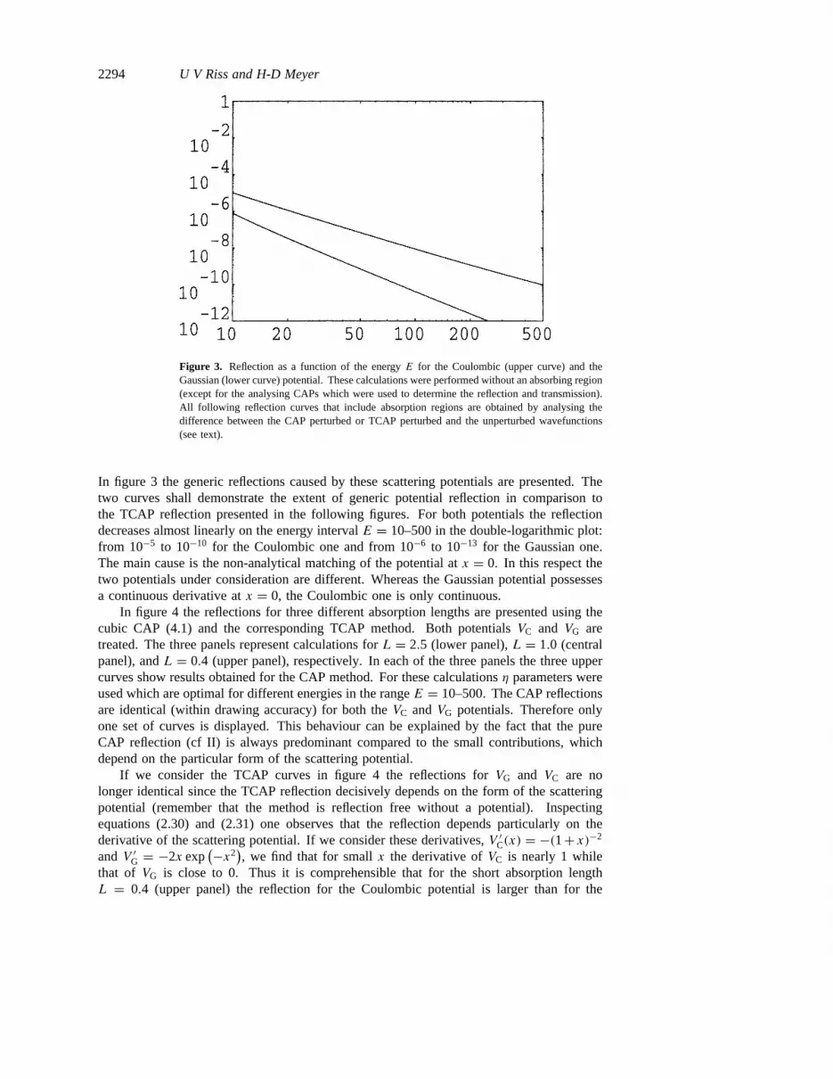
In figure 3 the generic reflections caused by these scattering potentials are presented. Thetwo curves shall demonstrate the extent of generic potential reflection in comparison tothe TCAP reflection presented in the following figures. For both potentials the reflectiondecreases almost linearly on the energy intervalE = 10–500 in the double-logarithmic plot:from 10−5 to 10−10 for the Coulombic one and from 10−6 to 10−13 for the Gaussian one.The main cause is the non-analytical matching of the potential atx = 0. In this respect thetwo potentials under consideration are different. Whereas the Gaussian potential possessesa continuous derivative atx = 0, the Coulombic one is only continuous.

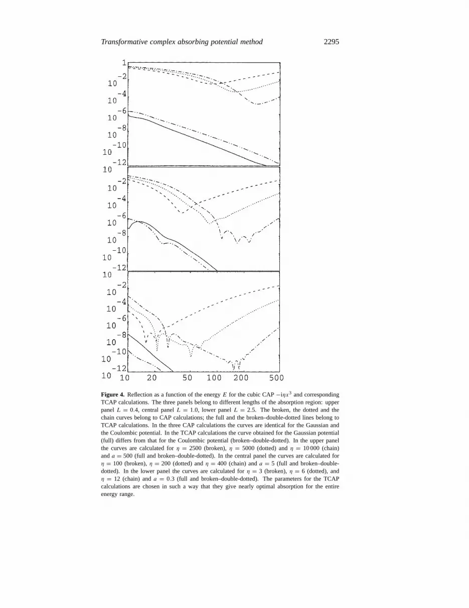
In figure 4 the reflections for three different absorption lengths are presented using thecubic CAP (4.1) and the corresponding TCAP method. Both potentialsVC and VG aretreated. The three panels represent calculations forL = 2.5 (lower panel),L = 1.0 (centralpanel), andL = 0.4 (upper panel), respectively. In each of the three panels the three uppercurves show results obtained for the CAP method. For these calculationsη parameters wereused which are optimal for different energies in the rangeE = 10–500. The CAP reflectionsare identical (within drawing accuracy) for both theVC andVG potentials. Therefore onlyone set of curves is displayed. This behaviour can be explained by the fact that the pureCAP reflection (cf II) is always predominant compared to the small contributions, whichdepend on the particular form of the scattering potential.

If we consider the TCAP curves in figure 4 the reflections forVG and VC are nolonger identical since the TCAP reflection decisively depends on the form of the scatteringpotential (remember that the method is reflection free without a potential). Inspectingequations (2.30) and (2.31) one observes that the reflection depends particularly on thederivative of the scattering potential. If we consider these derivatives,V ′C(x) = −(1+ x)−2

andV ′G = −2x exp(−x2

), we find that for smallx the derivative ofVC is nearly 1 while

that of VG is close to 0. Thus it is comprehensible that for the short absorption lengthL = 0.4 (upper panel) the reflection for the Coulombic potential is larger than for the


Figure 4. Reflection as a function of the energyE for the cubic CAP−iηx3 and correspondingTCAP calculations. The three panels belong to different lengths of the absorption region: upperpanelL = 0.4, central panelL = 1.0, lower panelL = 2.5. The broken, the dotted and thechain curves belong to CAP calculations; the full and the broken–double-dotted lines belong toTCAP calculations. In the three CAP calculations the curves are identical for the Gaussian andthe Coulombic potential. In the TCAP calculations the curve obtained for the Gaussian potential(full) differs from that for the Coulombic potential (broken–double-dotted). In the upper panelthe curves are calculated forη = 2500 (broken),η = 5000 (dotted) andη = 10 000 (chain)anda = 500 (full and broken–double-dotted). In the central panel the curves are calculated forη = 100 (broken),η = 200 (dotted) andη = 400 (chain) anda = 5 (full and broken–double-dotted). In the lower panel the curves are calculated forη = 3 (broken),η = 6 (dotted), andη = 12 (chain) anda = 0.3 (full and broken–double-dotted). The parameters for the TCAPcalculations are chosen in such a way that they give nearly optimal absorption for the entireenergy range.


Figure 5. Reflection as a function of the energyE for L = 1.0. The curves represent results forboth potentialsVG (full and dotted curves) andVC (broken and broken–double-dotted curves)using the two parametersa = 3 (full and broken curves) anda = 5 (dotted and broken–double-dotted curves). While fora = 3 incomplete absorption is the predominant effect, fora = 5 thegenuine reflection at the absorption region is important.

Gaussian potential. When the lengthL is increasedV ′G grows in the first instance whileV ′Cdecreases. Consequently, the reflection for the Gaussian potential then prevails over thatfor the Coulombic one for the valuesL = 1.0 (central panel) andL = 2.5 (lower panel).

In figure 5 the performance of the TCAP forVC andVG, with fixed lengthL = 1.0, canbe observed using different values of the strength parametera. In section 2.2 we have seenthat for smalla values the reflection is dominated by the insufficient absorption while forlargera values the reflection from the absorption region prevails. A small valuea = 3 anda larger valuea = 5 as strength parameters were used. For the small value the curves forthe two potentials are almost equal. Regarding equation (2.33) describing the transmissionone recognizes that this contribution is virtually independent of the particular potential form.This leads to the obvious similarity of the two curves. In contrast, for the large valuea = 5,we observe a difference between the reflections forVC andVG. Here the difference of theκ ′ terms appearing in equation (2.31) becomes important.

The next figure concerns the comparison of the zeroth- and first-order HamiltoniansHTCAP and(1)HTCAP, respectively. Since the first-order Hamiltonian requires the knowledgeof the potential derivative, it is only reasonable to use(1)HTCAP if V ′ is available in asimple manner. In the case ofVC andVG this is obviously the case. The additional term in(1)HTCAP requires the evaluation of the differenceF(x)−x. To this end one has to computethe integral (2.37). To simplify this computation we applied the approximation

F(x)− x ≈ ia∫ x

0W(ξ) dξ. (4.5)

Here we take advantage of the fact thatF(x)− x is strongly damped byV ′ for largex andthat it is therefore possible to expand the square root in equation (2.37). The advantageof equation (4.5) is that the integral can be computed analytically. Thus we obtain the


Figure 6. Reflection as a function of the energyE in the Gaussian case for zeroth- and first-order TCAP Hamiltonians. Three pairs of curves are plotted. From the top to bottom the pairsbelong to the absorption lengthsL = 0.4, L = 1.0, andL = 2.5. The samea values wereused as in figure 4. The full curves represent zeroth-order TCAP calculations, while the dottedcurves represent a first-order TCAP calculation. The results for the Coulombic case are similar.

Hamilton operator

(1)HTCAP ≈ Tf + V (x)+ iaV ′(x)∫ x

0W(ξ) dξ. (4.6)

For this Hamilton operator the reflection was calculated for both potentialsVC andVG.In figure 6 the effect of the improvement is demonstrated forVG. The Coulombic

potential leads to similar results and so only the results forVG are displayed. The fullcurves are obtained usingHTCAP, while the dotted curves correspond to(1)HTCAP. The threepairs of curves are computed for the three absorption lengthsL = 0.4, 1.0 and 2.5 (topdown). Independently of the particular lengthL the operator(1)HTCAP leads to a reflectionwhich is, in general, one order of magnitude smaller than that caused byHTCAP. Althoughthe approximation (4.6) may appear rather crude these results show that it is neverthelessuseful. If higher derivatives of the scattering potential are available it is possible to useeven higher-order TCAP operators. The method can therefore be gradually adapted tothe accuracy limited by the finite basis set. It is to be noticed that a higher order is onlyprofitable if the reflection is dominated by the|R+|2 contribution since the transmission partis largely independent of the potential. For optimized paths this assumption is generallyvalid.

Finally, it shall be examined as to what extent equations (2.30) and (2.31) can be usedto describe the reflection quantitatively. Thus in figure 7 the numerically obtained reflectioncurves (full curves) are compared to those calculated by application of equation (2.31)(dotted curves) forL = 0.4 (upper set of curves) andL = 2.5 (lower set of curves). Inboth cases one observes small differences between the numerical result and its analyticalapproximation. These differences can be explained by the approximate description ofκ± ≈ ±k andκ ′+ ≈ mV ′/k. If we use a better approximation, namely equation (2.39) in I,we obtain acomplete agreement(within the accuracy of the graph) between the numericaland the analytical results (broken curves). A small deviation appears forL = 2.5 when


Figure 7. Reflection as a function of the energyE in the Gaussian case from analytical andnumerical calculations. The curves were computed forL = 0.4 (upper set of curves) andL = 2.5 (lower set of curves). The full curves represent numerical results. The dotted curves arecomputed with the simple approximation formula (2.31), while the broken curves were computedusing a second-order WKB approximation forκ+(E, x) andκ ′+(E, x) (cf equation (2.39) in Rissand Meyer 1995).

E > 150. This can be explained by grid effects. The reflection is less than 10−18 andhere numerical errors as discussed above in connection with figure 3 appear. Hence in thiscase the approximate analytical treatment yields an even more accurate description than thenumerical one.

5. Discussion

We started with the CAP approach which was modified in such a way that the CAP strengthη was scaled linearly with the local kinetic energyE − V (x). By this ansatz one obtains ageneralized eigenvalue problem which can be converted into an ordinary eigenvalue problemby a simple transformation. Thereby the CAP is moved to the kinetic energy operator whileall potential-like CAP terms in the Hamiltonian disappear.

The principal idea of such a transformation was then examined in more detail byconstructing a model wavefunction that follows the same ideas and leads to a similarSchrodinger equation. This led to the so-called TCAP equation (with correction term)which defines a reflection-free Hamilton operator. The included correction term containsthe local quantum momentum which is in a complicated way energy dependent. Due tothis dependence it is difficult to apply the exact form of the operator in time-dependentcalculations.

By further inspection one observes that the correction term becomes small if thederivativeV ′ is small within the absorbing region. Therefore it is often possible, as agood approximation, to discard this term. One obtains the HamiltonianHTCAP that caneasily be applied in time-dependent calculations. This Hamiltonian can be regarded as alink between TCAP with corrections and SES ansatz. The difference betweenHTCAP andthe corresponding smooth exterior scaling Hamiltonian is that the latter uses the analyticcontinuation of the scattering potentialV (F(x)), whereas TCAP uses the original potential


V (x). From an SES point of viewHTCAP thus neglects the differenceV (F(x))−V (x) andit is not obvious that this is justified. From the TCAP point of view one neglects theκ ′+contribution and it is clear (see equation (2.31) that this is a valid approximation.

Furthermore, by perturbational techniques it is possible to obtain an approximateanalytical description for the TCAP reflection. These approximations not only describethe dependence of the reflection on potential and path form, but also yield a very accuratequantitative description of the reflection as a function of energy. It is then easy to determinethe reflection without performing elaborate wavepacket calculations.

By numerical investigations of the TCAP reflection properties it could be shown thatespecially for small absorption regions the method achieves an absorption that is much betterthan that of the usual CAP method. Several effects were discussed. Firstly, there existdifferent forms of evaluation of the TCAP operatorHTCAP which differ by their numericalperformance. Two forms were presented and their pros and cons were discussed. One formexceeds by its numerical accuracy the other by its reduced numerical effort. Secondly, theinfluence of the special potential form was discussed in the light of two examples, a Gaussianand a Coulomb potential. The numerical reflection behaviour for these potentials could beunderstood in the light of the derived analytical formula. Thirdly, it was demonstratedthat the TCAP approach can be gradually improved, yielding a system of approximationsof different order which finally ends in the smooth exterior scaling method for infiniteorder. The first-order improvement was tested numerically and it led to a reduction of thereflection by one order of magnitude. As a general result it is possible to adapt the cost ofthe calculation to the desired accuracy.

Since the TCAP method only requires the transformation of the kinetic energy it canbe easily generalized to the multi-dimensional case without a multi-dimensional analyticcontinuation of the scattering potential. It is demonstrated in appendices B and C how sucha transformation can be performed. In appendix B the case of a separable path deformationis treated. This diagonal case is still close to the one-dimensional case considered aboveand the more important one in applications. But it is possible to extend the approach evenbeyond this restriction. This technically more elaborate case is treated in appendix C.

Acknowledgments

The authors thank N Moiseyev and C W McCurdy for helpful discussions andG Worth for critically reading the manuscript. Financial support by the DeutscheForschungsgemeinschaft is gratefully acknowledged.

Appendix A

In this appendix we use the ansatz (2.28) to derive a formula describing the reflection causedby the TCAP operator. Throughout this appendixm = 1 is assumed. Applying the modifieddifferential operator∇f := iPf := f −1/2 d/dxf −1/2 to the wavefunction (2.28) and usingthe constraint

A′(x) ψf+E (x)+ B ′(x) ψf−

E (x) = 0 (A.1)

leads to

∇f ψf

E (x) = iκ+(E, x)A(x) f (x)1/2 eiQ+(x) + iκ−(E, x) B(x) f (x)1/2 eiQ−(x)

= iκ+(E, x)A(x)ψf+E (x)+ iκ−(E, x) B(x)ψ

f−E (x) (A.2)


where

Q±(x) =∫ x

0κ±(ξ) f (ξ)dξ. (A.3)

The twofold application of∇f yields

∇2f ψ

f

E (x) =(iκ ′+(E, x)f (x)

−1− κ+(E, x)2)A(x) f (x)1/2 eiQ+(x)

+(iκ ′−(E, x)f (x)−1− κ−(E, x)2)B(x) f (x)1/2 e−Q−(x)

+iκ+(E, x) f (x)−1A′(x) f (x)1/2 eiQ+(x)

+iκ−(E, x) f (x)−1B ′(x) f (x)1/2 eiQ−(x). (A.4)

The definition ofκ± (2.13) implies that the following differential equation is valid:

iκ ′± = κ2± − 2m(E − V ) (A.5)

to the boundary conditionκ±(x) → ±k for x → ∞. This differential equation combinedwith equation (A.4) results in the relation

κ+(E, x)A′(x) f −1(x) eiQ+(x) + κ−(E, x) B ′(x) f −1(x) eiQ−(x)

= κ ′+(E, x)(1− f −1(x)

)A(x) eiQ+(x)

+κ ′−(E, x)(1− f −1(x)

)B(x) eiQ−(x). (A.6)

The combination of this equation and the constraint (A.1) yields the following coupledsystem of differential equations:

A′(x) = κ ′+(E, x)κ+(E, x)− κ−(E, x)A(x)(f (x)− 1)

+ κ ′−(E, x)κ+(E, x)− κ−(E, x)B(x)(f (x)− 1) ei(Q−(x)−Q+(x))

B ′(x) = κ ′+(E, x)κ−(E, x)− κ+(E, x)A(x)(f (x)− 1) ei(Q+(x)−Q−(x))

+ κ ′−(E, x)κ−(E, x)− κ+(E, x)B(x)(f (x)− 1).

(A.7)

In the zeroth-order approximation we can assume thatA(x) = 1 andB(x) = 0 and useκ+(E, x) = −κ−(E, x) andQ+(x) = −Q−(x) so that the second equation in (A.7) can besolved. One obtains

B(x) = −∫ ∞x

κ ′+(E, ξ)2κ+(E, ξ)

e2iQ+(ξ)(f (ξ)− 1) dξ. (A.8)

In a first-order approximation one obtains|R+|2 = |B(0)/A(0)|2 = |B(0)|2 so thatequation (A.8) evaluated atx = 0 describes the TCAP reflection.

Appendix B

In this appendix the TCAP ansatz is generalized to the multi-dimensional case in thediagonal case, i.e. the coordinates in each dimension are deformed separately. Here theformalism is closer to the one-dimensional case and therefore easier to understand. Thegeneral consideration will follow in appendix C. In the following we assume mass-scaledcoordinates and write the kinetic energy as− 1

2

∑k ∂

2/∂x2k . For the more general case see

appendix C.


In order to construct a suitable model wavefunction it is necessary to define a multi-dimensional analogue of theκ function:

κ(E,x) = −i1

ψ(x)∇ψ(x). (B.1)

The functionκ(x) corresponds to the differential equation

i∇ · κ = κ · κ− 2E0+ 2V. (B.2)

The next step consists in the definition of a multi-dimensional path. This path is given by avector fieldF (x). For the sake of simplicity we first consider the case of a diagonal vectorfield, i.e.Fk(x) = Fk(xk). We definefk(xk) := F ′k(xk), in analogy tof (r) := F ′(r) knownfrom the one-dimensional case. It follows that

ψ(x) :=∏k

(fk(xk)

1/2 exp

(i∫ xk

0fk(zk) κk(E, z) dzk

))

=(∏

k

fk(xk)

)1/2

exp

(i∑k

∫ xk

0fk(zk) κk(E, z) dzk

). (B.3)

The modified momentum operator for this wavefunction is defined by

PFl = fl(xl)−1/2Plfl(xl)−1/2 =

(∏k

fk(xk)

)1/2

fl(xl)−1Pl

(∏k

fk(xk)

)−1/2

(B.4)

with Pl = −i∂/∂xl . Application of this operator to the wavefunction (B.3) yields

PFl = κlψ. (B.5)

The kinetic energy operator that results from this representation can be written as

(P F )2 =∑l

fl(xl)−1/2Plfl(xl)

−1Plfl(xl)−1/2

=(∏

k

fk(xk)

)1/2∑l

Pl

(fl(xl)

−1

(∏k

fk(xk)

)fl(xl)

−1Pl

(∏k

fk(xk)

)−1/2). (B.6)

If one applies this operator to the wavefunction which was defined above the result is

(P F )2ψ =∑l

P Fl (κl(E,x)ψ(x))

=(∏

k

fk(x)1/2

)∑l

Pl

(fl(x)

−1

(∏k

fk(xk)−1/2 κl(E,x) ψ(x)

))=(∏

k

fk(xk)1/2

)∑l

Pl

(fl(xl)

−1∏k

fk(xk)−1/2ψ(x)

)κl(E,x)

+(∏

k

fk(xk)−1

)fl(xl)

−1∑l

Pl(κl(E,x))ψ(x)

=∑l

κ2l (E,x) ψ(x)− i

(∏k

fk(xk)

)−1∑l

fl(xl)∂κl

∂xlψ(x)

= 2(V (x)− E0)ψ(x)+ i∑l

(1− fl(xl)−1

)∂κl∂xl

ψ(x). (B.7)

Thus we obtain a form analogous to the one-dimensional case. The methods developed inthis paper can hence be applied to the multi-dimensional case with virtually no modificationif the vector fieldF (x) is diagonal.


Appendix C

In the following we consider the non-diagonal case. Here we have to use the vector fieldF (x) instead of the functionsFl(xl). Moreover, the functionsfl(xl) must be replaced bythe functional matrix

Fij := ∂Fj

∂xi(C.1)

from which we derive the determinant

f := det(F ). (C.2)

Applying the matrix form one can write the multi-dimensional wavefunction as

ψ(x) := f 1/2 exp

(i∫ x

0(Fκ) · dz

). (C.3)

The corresponding generalization of the momentum operatorP = −i∇ reads

P Fψ = f 1/2F−1P (f −1/2ψ). (C.4)

In particular, the application of this operator to a (x depending) vectora leads to

P F · a = f 1/2(F−1P

)· (f −1/2a) (C.5)

which is to be interpreted as∑k

P Fk ak(x) = f (x)1/2∑k

∑l

(F (x)−1)klPl(f (x)−1/2ak(x)

). (C.6)

Making use of equation (C.4) we find

P Fψ = κψ (C.7)

for the wavefunction (C.3). For further calculations it is required that the relation

P ·((fF−1)Ta

) = ((fF−1)P)· a (C.8)

i.e.∑k

∑l

Pk(f (x) · (F (x)−1)lk · al(x)

) =∑l

∑k

f (x) · (F (x)−1)lk · Pkal(x) (C.9)

is valid. This is equivalent to the well known condition

∂2Fk

∂xl∂xm= ∂2Fk

∂xm∂xl(C.10)

for all k, l andm. Regarding equation (C.8) it appears to be useful to multiply the matrixF−1 with the functionf . Moreover, it is possible to make use of the following commutatorrelation: [

P , f −α] = iαf −(α+1)∇f (C.11)

for all constantsα. It is to be noticed that the application of the modified momentumoperator toψ(x) = f 1/2ψ(F (x)) yields the expression

P Fψ(x) = −if 1/2(∇ψ

)(F (x)). (C.12)


This corresponds to the one-dimensional case and shows that the definitions above arereasonable. If we apply the modified operator of the kinetic energy to the wavefunction itfollows that

(P F )2ψ = P F ·(κψ

)= f 1/2(F−1P ) · (f −1/2κψ)

= f 1/2(F−1P (f −1/2ψ)

)· κ− if 1/2

((F−1∇) · κ

)f −1/2ψ

= κ · κψ − i(F−1∇) · κψ= 2(V − E0)ψ + i

(((I − F−1)∇

)· κ)ψ (C.13)

whereI denotes the identity matrix. Obviously this general form of the operator correspondsto the one-dimensional case.

If we assume a non-diagonal form of the kinetic energy operator

T = −∑k

∑l

∂

∂xkAkl(x)

∂

∂xk= P · (AP ) (C.14)

we have to modify the equation forκ in the following way:

i∇ · (Aκ) = κ · (Aκ)− 2E0+ 2V. (C.15)

While the definition of the modified wavefunction (C.3) remains unchanged the modifiedkinetic energy operator has to be substituted byP F · (AP F ). We obtain an analogue toequation (C.13):

P F · (AP F )ψ = −2(E0− V )ψ + i(((I − F−1)∇

)· (Aκ)

)ψ. (C.16)

Starting with the Hamilton operatorH = 12P · (AP )+ V (x) one defines

HF := 12P

F · (AP F )ψ + V (x)+W(x) (C.17)

where the corrective potential is given as

W = 12i((I − F−1)∇

)· (Aκ) (C.18)

i.e.

W(x) = 12i∑k

∑l

∑m

(δkl − (F (x)−1)kl

)· ∂∂xl

((A(x))km · κm(E,x)) . (C.19)

Due to this constructionH and HF are identical for small|x| whereF (x) = I. Inparticular it is possible to neglect the corrective potentialW(x) for suitableF (x) leadingto an approximate form as in the one-dimensional case.

For technical reasons the operatorP F · (AP F ) determined by

P F · (AP Fψ) = f 1/2(F−1P ) ·(AF−1P (f −1/2ψ)

)(C.20)

can also represented by

P F ·AP F = P · (F−1)TAF−1P − 12f−3∇ ·

((fF−1)TA(fF−1)(∇f )

)+ 5

4f−4(∇f ) · (fF−1)TA(fF−1)(∇f ) (C.21)

or analogously forA = I by

P F · P F = P · (F−1)TF−1P − 12f−3 · tr

((fF−1)H(f )(fF−1)T

)+ 5

4f−4(∇f ) · (fF−1)T (fF−1)(∇f ) (C.22)

where tr denotes the trace of the matrix andH(f ) the Hessian matrix tof . This form hasthe advantage that the momentum operator only appears at the beginning and at the end of


every term, i.e. the momentum operator can directly be applied to the wavefunctionψ . Thesecond and third terms in equations (C.21) and (C.22) are only product operators. We seethat also in the fully general multi-dimensional case the method presented in this paper canbe applied in an efficient way.

References

Aguilar J and Combes J M 1971Commun. Math. Phys.22 269–79Arnoldi W E 1951Quart. Appl. Math.9 17–29Balsev E and Combes J M 1971Commun. Math. Phys.22 280–94Beck M H and Meyer H-D 1997Z. Phys.D 42 113–29Jackle A and Meyer H-D 1996J. Chem. Phys.105 6778–86Kosloff R 1988J. Phys. Chem.92 2087–100Kosloff R and Kosloff D 1986J. Comput. Phys.63 363–76Kurasov P B and Elander N 1994Phys. Rev.A 49 5095–7Leforestier Cet al 1991J. Comput. Phys.94 59–80Lipkin N, Moiseyev N and Brandas E 1989Phys. Rev.A 40 549–53Lowdin P O 1950J. Chem. Phys.18 365–75——1988Adv. Quantum. Chem.19 87–138Macıas D, Brouard S and Muga J G 1994Chem. Phys. Lett.228 672–7McCurdy C W and Rescigno T N 1978Phys. Rev. Lett.41 1364–8McCurdy C W, Rescigno T N and Byrum D 1997Phys. Rev.A 56 1958–69McCurdy C W and Stroud C K 1991Comput. Phys. Commun.63 323–30McCurdy C W, Stroud C K and Wisinski M K 1991 Phys. Rev.A 43 5980–90Moiseyev N 1991Israel J. Chem.31 311–22——1998aPhys. Rep.C submitted——1998bJ. Phys. B: At. Mol. Opt. Phys.submittedMoiseyev N, Certain P R and Weinhold F 1978Mol. Phys.36 1613–30Moiseyev N and Hirschfelder J O 1988J. Chem. Phys.88 1063–5Morgan D J III and Simon B 1981J. Phys. B: At. Mol. Phys.14 L167–71Neuhauser D and Baer M 1989aJ. Chem. Phys.90 4351–5——1989bJ. Chem. Phys.91 4651–7Park T J and Light J C 1986J. Chem. Phys.85 5870–6Pollard W T and Friesner R A 1994J. Chem. Phys.100 5054–65Reinhardt W P 1982Ann. Rev. Phys. Chem.33 223–55Rescigno T N, Baertschy M, Byrum D and McCurdy C W 1997Phys. Rev.A 55 4253–62Riss U V 1998Helv. Phys. Acta71 288–313Riss U V and Meyer H-D 1993J. Phys. B: At. Mol. Opt. Phys.26 4503–35——1995J. Phys. B: At. Mol. Opt. Phys.28 1475–93——1996J. Chem. Phys.105 1409–19Rom N, Engdahl E and Moiseyev N 1990J. Chem. Phys.93 3413–9Rom N, Lipkin N and Moiseyev N 1991Chem. Phys.151 199–204Saad Y 1980Lin. Alg. Appl.24 269–95Scrinzi A and Elander N 1993J. Chem. Phys.98 3866–75Simon B 1972Commun. Math. Phys.27 1–9——1973Ann. Math.97 247–74——1979Phys. Lett.71A 211–4Vibok A and Balint-Kurti G G 1992aJ. Phys. Chem.96 8712–9——1992bJ. Chem. Phys.96 7615–22

the transformative complex absorbing potential method: a bridge between complex absorbing potentials...

Documents