the taylor rule in estimating the performance of inflation targeting programs: the case of turkey

Global Economy JournalVolume 11, Issue 1 2011 Article 7

The Taylor Rule in Estimating thePerformance of Inflation Targeting Programs:

The Case of Turkey

Ekrem Erdem∗ Selim Kayhan†

∗Erciyes University, [email protected]†Bozok University, [email protected]

Copyright c©2011 Berkeley Electronic Press. All rights reserved.

The Taylor Rule in Estimating thePerformance of Inflation Targeting Programs:

The Case of Turkey∗

Ekrem Erdem and Selim Kayhan

Abstract

In this study, we aim to analyse the performance of inflation targeting program named “ATransition Program into a Powerful Economy” in particular since 2002 until the end of 2009 byusing Taylor rule in a different way. We divide inflation targeting period in accordance with thegovernors of the CBRT, Sureyya Serdengecti and Durmus Yilmaz, as a most important elementthat affects inflation targeting program among other factors.

Results imply that Mr. Serdengecti did not follow a pure Taylor rule while Mr. Yilmaz does.In Serdengecti period, the CBRT does not take in account output gap movements and exchangerate while deciding short term interest rate as said in Taylor rule. But the CBRT takes into accountoutgap movements and exchange rate movements in Yilmaz period, and these variables have im-portant portion in discussing of short term interest rate while it is not so necessary in Serdengectiperiod.

KEYWORDS: Taylor rule, inflation targeting, Turkey

∗This paper was presented at the 20th international conference of the International Trade andFinance Association in Las Vegas, NV, May 25, 2010.

1. INTRODUCTION Since the financial crisis in November 2000 and February 2001, the ruling government has brought into force an economic program named “A Transition Program into a Powerful Economy” to make some radical structural changes in the economy as a whole and in the financial system and the Central Bank of Republic of Turkey (CBRT) in particular. The most important changes were in defining the CBRT legally, determining the primary purpose of the bank as ‘inflation’ and starting the inflation targeting program. In this program, floating exchange rate regime also started to be practiced instead of pegging exchange rate regime (CBRT: 2002: 108). After the election of November 2002, the new government of Mr. Erdogan’s Justice and Development Party continued practicing this program strongly.

Another important shift, while inflation targeting program was under way, was that the governor of the CBRT changed in March 2006. Mr. Durmus Yilmaz came into office instead of Mr. Sureyya Serdengecti at the end of the first quarter of 2006 by suggestion of the ruling new government. This change connoted some questions about the performance of the inflation targeting program in the context of the CBRT’s independency. One of these questions was that whether the relationship between the government and the new governor of the CBRT would effect monetary policies. Another important question was that which governer of the CBRT would give more importance to inflation rate in policy decisions. The last question was whether the government would have an impact on the CBRT’s decisions about the inflation targeting regime in the new period.

In this study, we aimed to analyse the performance of the inflation targeting program from the beginning of 2002 to the end of 2009, using Taylor rule in a different way. We divided inflation targeting period in accordance with the governorship of the CBRT as one of the most important element that affects inflation targeting program among other factors and then the policy reaction functions were estimated for each governor’s period separately. Results of these equations and coefficients will provide us with some insights into the success of each governor and how important the independence of central banks and politics in fighting inflation are. 2. OUTLOOK OF THE TURKISH ECONOMY IN INFLATION TARGETING ERA

Chronic high inflation problem was one of the most important sources of economic instability in Turkey. So it is useful to analyse while investigating the Turkish economy. It was permanently high in the periods covering the end of 70’s, 80’s and 90’s. By the beginning of the new stabilisation program named “A

1

Erdem and Kayhan: The Performance of Inflation Targeting Regime in Turkey

Published by Berkeley Electronic Press, 2011

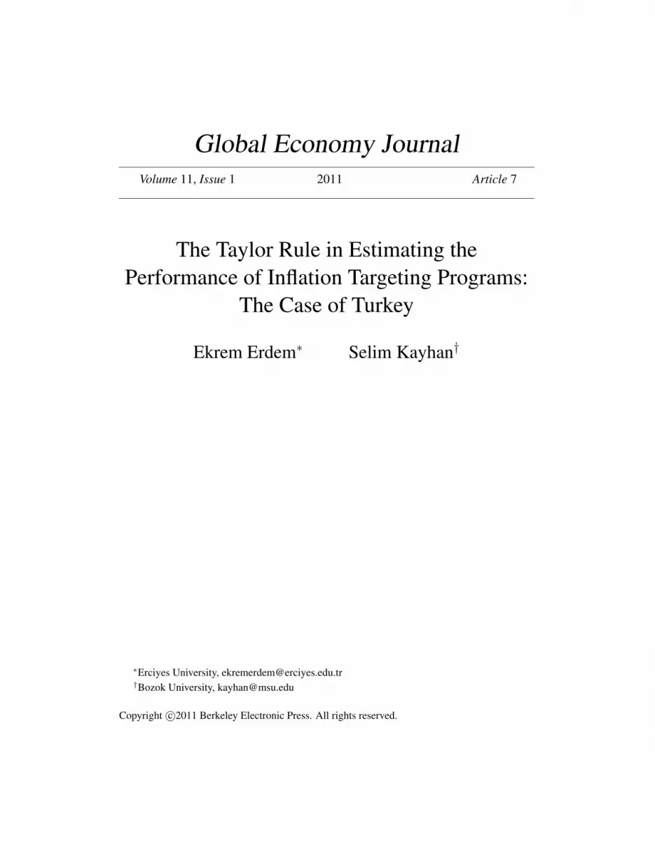
Transition Program into a Powerful Economy”, CBRT began to target implicitly. In 2004, inflation was under 10 percent. Decreasing inflation below this level was important, because it was over 10 percent level for thirty years in the Turkish economy (Erdem et al: 2009). The inflation target and the movement of the actual inflation are presented in Graphic 1. When the CBRT began to target inflation in 2001, Mr. Serdengecti was the governor of the bank. In March 2006, Mr. Yilmaz came into the Office instead of Mr. Serdengecti. In our study, we denote two periods as Serdengecti period and Yilmaz period, respectively.

Graphic 1. Inflation Targeting Period 2002 - 2009

0

10

20

30

40

50

60

70

80

M1 2002 M1 2003 M1 2004 M1 2005 M1 2006 M1 2007 M1 2008 M1 2009

Actual Inflation Rate Inflation Rate Target

Serdengecti Period2002-2006

Yilmaz Period2006-2009

Source: IMF, International Financial Statistics 2009.

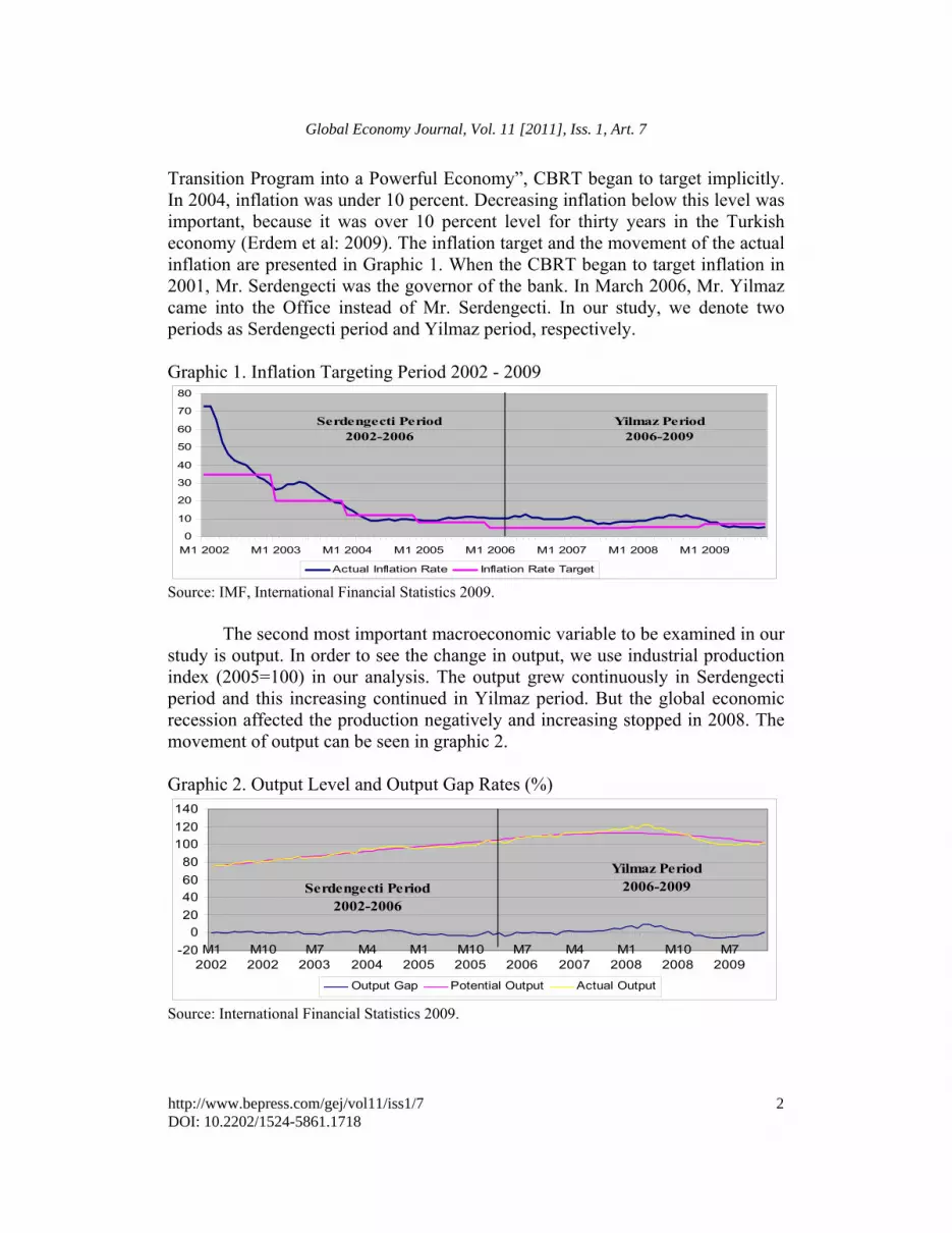
The second most important macroeconomic variable to be examined in our study is output. In order to see the change in output, we use industrial production index (2005=100) in our analysis. The output grew continuously in Serdengecti period and this increasing continued in Yilmaz period. But the global economic recession affected the production negatively and increasing stopped in 2008. The movement of output can be seen in graphic 2.

Graphic 2. Output Level and Output Gap Rates (%)

-20

0

20

40

60

80

100

120

140

M12002

M102002

M72003

M42004

M12005

M102005

M72006

M42007

M12008

M102008

M72009

Output Gap Potential Output Actual Output

Serdengecti Period2002-2006

Yilmaz Period2006-2009

Source: International Financial Statistics 2009.

2

Global Economy Journal, Vol. 11 [2011], Iss. 1, Art. 7

http://www.bepress.com/gej/vol11/iss1/7DOI: 10.2202/1524-5861.1718

Another important point about the output is the difference between actual output and its potential, named “Output Gap”. The movement of output gap in the Turkish economy can be seen in graph 2. The actual output fluctuated around its potential during the governorship of Mr. Serdengecti and the fluctuations were smooth. The output gap increased positively until the end of 2008 and then it decreased under its potential because of the recession. It is clear that the behaviour of the output gap was more agressive than Serdengecti period. In Serdengecti period, fluctuation range was between 2 percent and -4 percent, although it was between 9 percent and -6 percent in Yilmaz period.

Exchange rate is another variable that we have to examine, because floating exchange rate can affect inflation rate directly via pass through effect on the price level and indirectly through the financial system. Calvo and Reinhart (2002) mentioned that according to the effect of exchange rate in inflation rate, government could maintain exchange rate, although it is floating in competitive market and named it as “fear of floating” hypothesis. In this context, it is another important issue whether the CBRT intervenes exchange rate as a part of “fear of floating” hypothesis.

By the beginning of the inflation targeting regime, the CBRT (2009) had announced that exchange rates would not be used as a policy instrument and would be determined according to the demand and supply conditions of exchange rates. According to the announcement of the CBRT, exchange rate would be determined in competitive market. But the CRBT (2009) reported that although there was no exchange rate need to maintain, to have a strong foreign currency reserve position was useful to correct the effects of internal and external shocks and to boost confidence in the country for such an emerging economy. So the CBRT issues exchange tenders to collect foreign currency when exchange supply exceeds exchange supply to exchange demand. The CBRT bought 64,6 billion foreign exchange during the inflation targeting regime.

3. THE TAYLOR RULE John B. Taylor (1993a) suggested a different monetary policy rule has a dynamic pattern and put it in a plan to practice monetary policy rules. That is why starting by examining his proposals about characteristics of a rule and about how it might be practiced before we describe his monetary policy reaction function will be a plausible explanation.

According to him, there is no need to follow mechanically any algebraic formula to practice monetary policy rule. Also constant installation is not needed. It means that instrumental variable does not cost a certain value. Taylor (1993b) emphasized not to confuse discretionary policy practice and his proposal. Because practicing a policy rule needs responsibility and judgement, so computers cannot

3



https://www.researchgate.net/publication/4887831_Discretion_Versus_Policy_Rules_in_Pratice?el=1_x_8&enrichId=rgreq-3142bb17-ef46-45b4-ba36-1453b9c7ed66&enrichSource=Y292ZXJQYWdlOzIyNzM3ODUxNztBUzoyMTg4MTY0NjMyODIxNzZAMTQyOTE4MTMxODg5NQ==

achieve it and so the weight of variables can change according to the situation of economy. The last point is that if a policy rule is to have any meaning, it must be in place for a reasonably long period of time. For a policy rule, several business cycles would certainly be sufficient, but, for many purposes, several years would do just as well (Taylor; 1993b; 5).

Taylor (1993a) suggests that policy makers makes responses to deviation of inflation from its target level introduced by themselves and to deviation of actual output from its potential level by using short term nominal interest rate. If inflation deviates higher than the target or actual output goues beyond its potential, short term nominal interest rates will increase. It will decrease if inflation rate is below its target or actual output falls down under its potential. So in equilibrium, short term nominal interest rate inflation will be on target and all sources possible for production in economy will be material in the process of production. In this context, we can express the relationship between variables by constructing an equation. In equation, i , fi , , * , h , y , *y and g denote short term interest rate, real interest rate, actual inflation rate, target inflation rate, inflation rate reaction coefficient, actual GDP or GDP growth rate, potantial GDP or potential GDP growth rate and GDP gap reaction coefficient, respectively.

*

**

y

yyghii f (1)

When the actual inflation is equal to the inflation target and the output

level is equal to its potential, short term nominal interest rate will be equal to the sum of the real interest rate and actual inflation. So there will be no importance of values of coefficients g and h .

Sizes of coefficients h and g show preferences of policy makers about which goal is important for them. This is because they represent Monetarist and Keynesian policy proposals that contrast entirely. Namely, if coefficient g is valued zero and coefficient h high, it can be interpreted as a pure Monetarist rule. So monetary authority takes only on board deviations in inflation and neglect the output gap. If coefficient h is zero and coefficient g is valued high, it can be interpreted as Keynesian rule. In such a case monetary authority only consider unemployment, neglects deviations in actual inflation (Akat; 2004; 7).

Although Taylor did not replace exchange rate in his original paper in 1993, he pointed out that there are some indirect effects of exchange rates on interest rates. Because of this reason, to determine the response of interest rate to a shock in exchange rate is hard (Taylor; 2001; 264). Taylor (2001) also suggests that exchange rate has zero coefficient for a closed economy and nonzero coefficient for an open economy. For this reason, it is recommended that

4



https://www.researchgate.net/publication/4887831_Discretion_Versus_Policy_Rules_in_Pratice?el=1_x_8&enrichId=rgreq-3142bb17-ef46-45b4-ba36-1453b9c7ed66&enrichSource=Y292ZXJQYWdlOzIyNzM3ODUxNztBUzoyMTg4MTY0NjMyODIxNzZAMTQyOTE4MTMxODg5NQ==

including exchange rate into the reaction function is useful for open economies, especially when foreign exchange has high pass through effect on inflation rate of these economies. So it would be useful to include exchange rate variable for Turkey, such a country has open economy and a floating exchange rate.

So in order to see the performance of inflation targeting period for each governer of the CBRT and to understand their emphasis on macroeconomic variables, Taylor’s rule and monetary policy reaction function is a good instrument to use in our analyses. Departing from original monetary policy reaction function, we include exchange rate to the function to see whether the CBRT has intervened exchange rate by using short term nominal interest rate during the inflation targeting era to clear negative effects on inflation rate which is another question to be examined. 4. THE LITERATURE

There is a vast literature which uses a type of Taylor monetary policy reaction function. Most of them focus developed economies like the U.S.A. and European Union countries, especially Germany. In recent years, the number of studies which examine emerging economies arised. Among emerging economies, inflation targeting countries have drawn special attention among monetary policy reseachers. A group of studies took country groups into account. For instance, Sergi and Hsing (2010) examined three countries exersized inflation targeting programs and found that Canada, New Zealand and Australia follow Taylor type policy rule while they target inflation. In another one, Teles and Zaidan (2009) analysed twelwe emerging economies and at the end of their study, they implied that Poland, Brazil and Turkey made their policy decisions according to Taylor rule.

Several authors examined Turkish economy by using a Taylor type monetary policy reaction function in their studies. Some of them are examined in this section. Kesriyeli and Yalcin (1998) and Ongan (2004) studied Turkish economy. They tried to apply Taylor rule into the Turkish economy. Although they examined the same period, Kesriyeli and Yalcin (1998) found that rule is not sufficient for reducing inflation in Turkey, while Ongan (2004) implied that it is also useful for the Turkish economy. Caglayan (2005) also found similar results to Ongan’s. Aklan and Nargelecekenler (2008a and 2008b) and Onur (2008) analysed the Turkish economy and they implied that interest rate reacts inflation rate, output gap and also exchange rate in the context of Taylor rule.

5



https://www.researchgate.net/publication/5147987_Taylor_Rule_in_Practice_Evidence_from_Turkey?el=1_x_8&enrichId=rgreq-3142bb17-ef46-45b4-ba36-1453b9c7ed66&enrichSource=Y292ZXJQYWdlOzIyNzM3ODUxNztBUzoyMTg4MTY0NjMyODIxNzZAMTQyOTE4MTMxODg5NQ==

5. DATA AND MODEL

Although stabilisation program started in april 2001, the CBRT has started to announce inflation target per year since 2002. So we employ monthly data spanning the period 2002M1 - 2009M11 in two episodes. The first episode consists of Serdengecti period (January 2002-March 2006) and the second episode consists of Yilmaz period (April 2006- November 2009).

Data belonging to interest rate, CPI and industrial production, except exchange rate, were obtained from International Financial Statistics 2010 published by International Monetary Fund and exchange rate data were obtained from official website of the CBRT. Interbank interest rate and real effective exchange rate are used as a proxy for the short term nominal interest rate and exchange rate, respesctively. Data are shown in Table 1.

Table 1. The Data Set Variables Explanations Source INT Interbank Interest Rate IFS INFGAP Derived from CPI (2005=100) IFS OUTGAP Derived from Ind. Prod. Index (2005=100) IFS REAL Real Exchange Rate (1995=100) CBRT

Consumer price index (2005=100) is used to derive monthly actual inflation rate. Actual inflation rate is deseasonalized by using TRAMO/SEATS program and then the difference between actual inflation rate and inflation target is found. The announcements of the CBRT were taken form its official website as a proxy of inflation target for five years. Also, the revised target announcements of the CBRT were taken from its inflation report published at the beginning of the years 2007, 2008 and 2009 because the bank changed its target later according to change in global economic environment. The revised inflation target table can be seen in Table 2.

Table 2. Inflation Target per year (%) 2002 2003 2004 2005 2006 2007 2008 2009 Inf. Target 35% 20% 12% 8% 5% 5,1% 5,5% 6,8%

Source: The CBRT Inflation Report, 2007-1, 2008-I and 2009-I.

Output is measured by industrial production index (2005=100) and it is also deseasonalized by using TRAMO/SEATS program. Potential output is obtained by using HP filter. Then output gap is obtained by the difference between actual output and potential output. Output gap is divided by potential output to get the output gap rate. We used VAR methodology developed by Sims

6



(1980) to analyse the time series which belong to macroeconomic varibles, we could write the reduced form of VAR,

tt uYLA )( (2)

where tY is a 4x1 vector of variables and consists of

REALOUTGAPINFGAPINTYt ,,, (3)

toj

jj uandIALALA ,)( 0 is an error term normally distributed

with a semidefinite covariance matrix u . Given that, )(LA is invertible and the

reduced VAR model can be written in terms of (MA) representation (Bjornland and Halversen: 2008: 9). While 1)()( LALB , tt uLBY )( .

We assume that tu is linearly related to a vector of four independent

structural shocks specified as ret

ytt

itt ,,, . t is an mx1 vector of

structural disturbances or shocks (Horvath and Rusnak: 2009: 4). We identify it

as short term nominal interest rate shock, t as interest rate target gap shock, yt

as output gap shock and ret as real exchange rate shock. If we normalize the

structural shocks to have unit variance, the realtionship between the error terms and structural shocks can be written as follows,

,tt Au with )(5 ttEI . (4)

By substituting for equation (5) into (4), the model can be written in the

form of a structural MA presentation, tt LCX )( , where ALBLC )()( . In

order to derive the impulse and responses and the variance decomposition, the matrix A needs to be identified. So the only restriction A coming from the eq. 4 implies,

.)()( AAAAEuuE ttttu (5)

There are a lot of different decompositions which satisfy eAA , so we

do not have a unique MA presentation in terms of the structural shocks. We know

that for two different decompositions, AAe and AAe ~~

, it must be the case

that QAA~

with Q being an orthogonal matrix, i.e. 5IQQ . A property of this

7



https://www.researchgate.net/publication/39728822_How_Important_Are_Foreign_Shocks_in_a_Small_Open_Economy_The_Case_of_Slovakia?el=1_x_8&enrichId=rgreq-3142bb17-ef46-45b4-ba36-1453b9c7ed66&enrichSource=Y292ZXJQYWdlOzIyNzM3ODUxNztBUzoyMTg4MTY0NjMyODIxNzZAMTQyOTE4MTMxODg5NQ==

type of matrix is that columns 41 ,...,qqQ are orthonormal which tells us that

its vectors are mutually perpendicular, i.e. < ji qq , >=0 for i≠j, and of unit length,

i.e. 1iq .

In the matrix e , there are 2/)( 2 nn number of restrictions required to

identify the system. Traditional VAR methodology proposes the identification restrictions based upon on a recursive structure known as Cholesky decomposition (Ioannidis: 1995: 256). Cholesky decomposition seperates the residuals into orthogonal shocks by restrictions imposed on the basis of arbitrary ordering of the variables and implies that the first variable responds only to its own exogenous shocks, the second responds to the first variable’s exogenous shocks and its own exogenous shocks. So the structure of matrix will be lower triangular, where all elements above the principal diagonal are zero (McCoy: 1997: 5).

After the identification of restrictions, impulse response function is employed to reflect the dynamic effect of each exogenous variable response to the individual unitary impulse from other variables. The impulse response function can explain the current and lagged effect over time of shocks in the error term (Liu: 2008: 243). The variance decomposition is another test in the VAR analysis. Variance decomposition gives information about the dynamic structure of the system. The main pupose of variance decomposition is to introduce effects of each random shock on prediction error variance for future periods ( Ozgen and Guloglu: 2004: 9). 6. EMPIRICAL RESULTS Both of the governership periods were analysed seperately and empirical results were obtained for either period. In the following subsection we analysed Serdengecti period first. and then gave the empirical analysis results of Yilmaz period. So we had some insight into the monetary policy application of either governeor by using impulse response and variance decomposition methodology. 6.1. Serdengecti Period The preliminary step in the application of VAR methodology is the determination of stationary of variables because time series must be included into the model while it is stationary. Otherwise, the model will be spurious. For this reason, we used Phillips-Perron (1988) test to test the null hypothesis that a time series is nonstationary I(1). Schwarz information criterion was selected to control the stationarity for unit root test methodology.

8



Table 3. Phillips-Perron Unit Root Test Results for Serdengecti Period INT INFGAP OUTGAP REAL Critical

Values I(0) I(1) I(0) I(1) I(0) I(1) I(0) I(1)

1 -1.05 -5.16 -4.57 -4.54 -2.76 -9.12 -0.66 -4.48 0.01= -3.57 0.05= -2.92 0.10= -2.59

2 -1.49 -5.28 -3.59 -5.10 -3.15 -9.01 -2.20 -4.50 0.01= -4.15 0.05= -3.50 0.10= -3.18

1 Intercept (c) term; 2 Trend (t) and intercept (c) term. Note: MacKinnon (1996) critical values were used. All variables were made with Phillips-Perron test according to Schwarz information criterion.

According to these results, all variables are characterized by a unit process, implying that all of them appear to be I(1). In order to choose the right lag we used Akaike information criterion and we found lag length as two. Also, the results of autocorrelation LM test support the number of lag, and there is no serial correlation problem between residuals.

Graphic 3. Impulse Response Functions for Serdengecti Period Response of INT to INT Shock Response of INT to OUTGAP Shock

Response of INT to INFGAP Shock Response of INT to REAL Shock

Impulse response test results can be seen in Graphic 3. According to the

results, short term nominal interest rate responses positively in the first quarter after a positive shock of 1 percent in inflation rate gap. But positive response

9



finishes rapidly in three months and then response becomes negative unnecessarily and dies out at the end of the year. In case of a positive shock in the rate of gap between the actual output and the potential output, interest rate responses negatively. Response of short term nominal interest rate dies out after six months. Short term nominal interest rate responses to a shock in exchange rate negatively. But reaction does not continue so long and it finishes after the fifth lag.

Variance decomposition of the short term nominal interest rate is given in Table 4. The ordering of INFGAP, OUTGAP, RET and INT is based on the simple Taylor rule which includes exchange rate. In the second month, output gap rate can explain a variation of 13 percent in short term interest rate and inflation rate gap can describe a variation of only 2 percent in short term nominal interest rate. While output gap rate can explain a variation of up to 14 percent in the third month, inflation rate gap can explain a variation of up to only 4 percent at the end of the year.

Ability of the exchange rate in the explanation of the variation in the interest rate is small and it can explain a variation of only 4 percent in interest rate. And then it increases to 6,5 percent and stays persistent during the year.

Table 4. Variance Decomposition of Interest Rate in Serdengecti Period

Period S.E. DINFGAP DOUTGAP DLRET DLINT

1 0.031567 0.400089 2.834989 4.303174 92.46175 3 0.036456 2.653575 14.66859 4.303174 76.12890 6 0.037584 4.205079 14.07950 6.588748 75.12668 9 0.037622 4.347056 14.06012 6.578088 75.01474

12 0.037624 4.456876 14.05999 6.577626 75.00955 Cholesky Ordering: INFGAP, OUTGAP, RET ana INT.

6.2. Yilmaz Period To apply VAR methodology, we practiced Phillips-Perron unit root test for Yilmaz period also. Results are given in Table 5. As can be seen in the table, except interest rate and output gap, other variables are stationary at 1 percent in the first differences. Interest rate is stationary at 5 percent in its first difference for both stationary tests and output gap rate is stationary at 5 percent level in the first difference in Dickey Fuller-GLS test while it is stationary at 1 percent level in the first difference in Phillips Perron test.

To choose right lag length, we also used Akaike information criterion and we found lag length four for Yilmaz period. Also, we used autocorrelation LM test and we found that there is no serial correlation problem between residuals.

10



Table 5. Phillips-Perron Unit Root Test Results for Yilmaz Period INT INFGAP OUTGAP REAL Critical

Values I(0) I(1) I(0) I(1) I(0) I(1) I(0) I(1)

1 1.29 -2.36 -0.83 -6.13 -1.50 -6.38 -1.81 -5.33 0.01= -3.57 0.05= -2.92 0.10= -2.59

2 -0.80 -3.57 -1.81 -6.08 -1.65 -6.33 -2.11 -5.30 0.01= -4.15 0.05= -3.50 0.10= -3.18

1 Intercept (c) term; 2 Trend (t) and intercept (c) term. Note: MacKinnon (1996) critical values were used. All variables were made with Phillips Perron test according to Schwarz information criterion.

We obtained impulse response test results as in graphic 4. Short term nominal interest rate reponses inflation rate gap shock positively. It is persistent for seven months and then response turns to negative. Response of short term nominal interest rate to a positive shock on the rate of difference between the actual output and the potential output is positive. A positive shock on the output gap rate causes short term interest rate to increase for fifteen months, and then increase in short term interest rate dies out. A positive shock in exchange rate causes an increase in the short term nominal interest rate. Although response is small, it is persistent for fifteen months.

The results of variance decomposition process of the variables is shown in Table 6. The order of variables’ inclusion into the model is same as in the first model. Variance in short term nominal interest rate can be described in the first period mainly by itself. In the second period, inflation rate has the highest explanation ability among the variables, but it is small. The explanation ability of output gap rate and exchange rate rise gradually, but the ability of exchange rate is still small.

Ouput gap rate can explain a variance of 22 percent in the short term nominal interest rate in the twelfth period and it is persistent for more than one year. It implies that output gap rate in one of the determinators of short term nominal interest rate.

While explanation ability of output gap increases, explanation ability of inflation gap rate is stable and low in the first months, but after the nine months, it increases and explains a variance of 9 percent in interest rate in twelfth period. Lastly, exchange rate also has a little effect on the variance of the short term interest rate. It increases gradually up to 7 percent and it stays constant there along the period we examine.

11



Graphic 4. Impulse Response Graphics of Yilmaz Period Response of INT to INT Shock Response of INT to OUTGAP Shock

Response of INT to INFGAP Shock Response of INT to REAL Shock

Table 6. Variance Decomposition of Interest Rate in Yilmaz Period

Period S.E. DINFGAP DOUTGAP DLRET DLINT

1 0.019580 0.711781 1.005047 0.793684 97.48949 3 0.033155 3.930564 2.221852 5.739516 88.10807 6 0.041926 3.597341 11.17712 6.954961 78.27058 9 0.046905 6.603739 20.22734 7.581901 65.58702 12 0.050358 9.699030 21.52729 7.071874 61.70181

Cholesky Ordering: INFGAP, OUTGAP, RET ana INT. 7. CONCLUSION

In this study we aimed to analyse the inflation targeting regime in two episodes. We considered the governorship of the bank and we analysed each governor’s inflation targeting performance.

In Serdengecti period, inflation rate gap shock is responded by short term interest rate positively. This result is consistent with Taylor rule. Another variable output gap rate is responded by short term interest rate negatively. This is not consisted with suggestions of Taylor. Response of short term interest rate to exchange rate is so small and it can be interpreted as exchange rate shocks disregarded by the CBRT. Explanation abilities of variables to variance in short term nominal interest rate give some insights into what affects the CBRT’s

12



interest rate policy decisions. In this regard, output gap rate has the most weight in Serdengecti period.

In Yilmaz period, inflation rate gap shock is also responded by short term interest rate positively. Response is bigger than Serdengecti period. Response of short term nominal interest rate to a shock in output gap rate is positive as in original policy reaction function suggested by Taylor. Another important point is that short term interest rate responses exchange rate shock positively. It means the CBRT takes into account exchange rate increases in its policy reaction function in order to clear negative effects of exchange rates on the price level.

Explanation abilities of variables to variance in the short term nominal interest rate increase in Yilmaz period. Output gap rate is the most important explanatory variable and it can explain upto a variance of 22 percent and inflation rate gap can explain up to 9 percent in twelve months. Exchange rate can explain variance only up to 7 percent.

We imply that Mr. Serdengecti did not follow a pure Taylor rule while Mr. Yilmaz does. The CBRT does not take into account output gap movements and exchange rate while deciding short term interest rate as mentioned in Taylor rule. But the CBRT takes into account outgap movements and exchange rate movements in Yilmaz period and these variables have important portion in the discussion of short term interest rate while it is not so necessary in Serdengecti period.

As a result, inflation rate is a component of policy decisions about short term nominal interest rate for both periods. Results imply that other macoreconomic variables are taken into consideration in Yilmaz period. But when we combine the results of econometric analysis with the macroeconomic variables’ outlook for eight years, it implies that differences between coefficients of monetary policy reaction function do not affect the performance of inflation targeting regime. This implies that the CBRT continues its independency during Yilmaz period, although questions arise about it.

REFERENCES

Akat, A.S., “Dalgali Kur ve Para Politikasi Bir Parasal Kural Onerisi” Gulten Kazgan’a Armagan: Cumhuriyet Donemi Turkiye Ekonomisi, İstanbul Bilgi Universitesi Yayinlari, İstanbul, 2004.

Aklan, N.A. and Nargelecekenler, M., “Taylor Rule in Practice: Evidence from Turkey” International Advanced Economic Resources, 14, 156-166, 2008a.

Aklan, N.A. and Nargelecekenler, M., “Taylor Kurali: Turkiye Uzerine Bir Degerlendirme” Ankara Universitesi SBF Dergisi, 63(2), 21-40, 2008b.

13



Bjornland, C.H. and Halvorsen, J.I., “How Does Monetary Policy Respond to Exchange Rate Movements? New International Evidence” NHH Dept. of Economics Discussion Paper, no. 23, 2008.

Caglayan, E., “Turkiye’de Taylor Kurali’nin Gecerliliginin Ekonometrik Analizi” Marmara Universitesi I.I.B.F. Dergisi, 20(1), 2005.

Calvo, G.A. and Reinhart C.M., “Fear of Floating” NBER Working Paper Series, no. 7993, 2000.

CBRT, “2001 Annual Report” The Central Bank of the Republic of Turkey Publication, Ankara, April 2002.

CBRT, “Money and Exchange Rate Policy for 2010” The Central Bank of the Republic of Turkey Publication, Ankara, December 2009.

Erdem, E., Sanlioglu, O., Ilgun, M.F., “Turkiye’de Hukumetlerin Makro Ekonomik Performansi” Detay Yayincilik, Ankara, 2009.

Horvath, R., Rusnak, M., “How Important are Foreign Shocks in a Small Open Economy? The Case of Slovakia” Global Economy Journal, 9(1), 1-15, 2009.

Ioannidis, C., Laws, J., Matthews, K., Morgan, B., “Business Cycle Analysis and Forecasting with a Structural Vector Autoregression Model for Wales” Journal of Forecasting, 14, 251-265, 1995.

Kesriyeli, M., Yalcin, C., “Taylor Kurali ve Uygulamasi Uzerine Bir Not” CBRT Discussing Paper, no. 9802, 1998.

Liu, C., Luo, Z.Q., Ma, L., Picken, D., “Identifying House Price Diffusion Patterns Among Australian State Capital Cities” International Journal of Strategic Propoerty Management, 12, 237-250, 2008.

McCoy, D., “How Useful is Structural VAR Analysis for Irish Economics” Eleventh Annual Conference of the Irish Economic Association, Athlone, April 1997.

Ongan, T.H., “Enflasyon Hedeflemesi ve Taylor Kurali: Turkiye Ornegi” Maliye Konferanslari, no. 45, 1-12, 2004.

Onur, S., “Turkiye Ekonomisi’nde Faiz Oranlari-Enflasyon İliksisi Uzerine Bir Model Denemesi” Journal of Qafqaz University, 24, 2008.

Ozgen, F.B., Guloglu, B., “Analysis of Economic Effects of Domestic Debt in Turkey Using VAR Technique” METU Studies in Development, 31, 93-114, 2004.

Phillips, P.C.B. and Perron, P., “Testing for a Unit Root in Time Series Regression” Biometrika, 75(2), 335-346, 1988.

Sergi, B.S. and Hsing, Y., “Responses of Monetary Policy to Inflation, The Output Gap, ana Real Exchange Rates: The Case of Australia, Canada ana New Zealand” Global Economy Journal, 10(2), 1-9, 2010.

Sims, C.A., “Macroeconomics and Reality” Econometrica, 48, 1-47, 1980.

14



Taylor, J.B., “Discretion Versus Policy Rules in Practice” Carnegie-Rochester Conference Series on Public Policy, 39, 195-214, 1993a.

Taylor, J.B., “Macroeconomic Policy in a World Economy: From Econometric Design to Practical Operation” W.W. Norton & Company, New York, 1993b.

Taylor, J.B., “The Role of The Exchange Rate in Monetary Policy Rules” The American Economic Review, 91(2), 263-268, 2001.

Teles, V.K. and Zaidan, M., “Taylor Principle and Inflation Stability in Emerging Market Countries” FGV Discussing Paper, no.197, 2009.

15



the taylor rule in estimating the performance of inflation targeting programs: the case of turkey

Documents