f!) Pergamon Computers Math. Applic. Vol. 30, No.8, pp. 41-55, 1995

Elsevier Science Ltd. Printed in Great Britain

0898-1221(95)00136-0

The Sensitivity and Accuracy of Fourth Order Finite-Difference Schemes on Nonuniform Grids in One Dimension

J. E. CASTILLO Department of Mathematics, San Diego State University

San Diego, CA 92182, U.S.A.

J. M. HYMAN AND M. J. SHASHKOV Los Alamos National Laboratory, Group T-7

MS-B284, Los Alamos, NM 87545, U.S.A.

S. STEINBERG* Department of Mathematics, University of New Mexico

Albuquerque, NM 87131, U.S.A.

(Received January 1995; accepted March 1995)

Abstract-We construct local fourth-order finite difference approximations of first and second derivatives, on nonuniform grids, in one dimension. The approximations are required to satisfy symmetry relationships that come from the analogous higher-dimensional fundamental operators: the divergence, the gradient, and the Laplacian. For example, we require that the discrete divergence and gradient be negative adjoint of each other, DIV* = -GRAD, and the discrete Laplacian is defined as LAP = DIVGRAD. The adjointness requirement on the divergence and gradient guarantees that the Laplacian is a symmetric negative operator. The discrete approximations we derive are fourth-order on smooth grids, but the approach can be extended to create approximations of arbitrarily high order. We analyze the loss of accuracy in the approximations when the grid is not smooth and include a numerical example demonstrating the effectiveness of the higher order methods on nonuniform grids.

1. INTRODUCTION Difference approximations that retain the symmetry properties of the continuum operators are called mimetic. Partial differential equations solved with mimetic difference approximations often automatically satisfy discrete versions of conservation laws and analogies to Stoke's theorem that are true in the continuum and therefore are more likely to produce physically faithful results. These symmetries are easily preserved by local discrete high-order approximations on uniform grids, but are difficult to retain in high-order approximations on nonuniform grids. The main goal of this research is to construct local high-order mimetic difference approximations of differential operators on nonuniform grids. Local approximations only use function values at nearby points in the computational grid and are especially efficient on computers with distributed memory. High-order approximations can often be used to solve partial differential equation (PDEs) to a prescribed accuracy with only a fraction of the grid points that would be required by a first or second order method [1].

Because our eventual goal is to construct high-order mimetic approximations in two and three dimensions, we derive two approximations of the first derivative, analogous to the divergence and

-This author was financed in part by the Schlumberger Foundation and the U.S. Department of Energy through the New Mexico Waste-management Education and Research Consortium (WERC) and Sandia National Laboratories and the Department of Energy under Contract DE-AC04-76DP00789, M. G. Marietta, Technical Monitor.

41

42 J. E. CASTILLO et al.

the gradient, and require they be the negative adjoint of each other. The symmetry requirements for these operators are obtained analogous to the higher-dimensional case. The second derivative (Laplacian) is approximated by the composition of the first-order operators and consequently is a symmetric operator. This approach, based on the support-operator method [2,3], guarantees that the resulting difference scheme has the desired symmetry properties. One of the most costly parts of many simulations is the inversion of the discrete Laplacian. Some of the most efficient methods for solving these equations require the discrete Laplacian to be a negative definite, symmetric operator. Mimetic discretizations of the Laplacian or, more generally, symmetric elliptic operators, automatically produce discrete operators that are symmetric and negative definite [2,3].

The use of higher-order approximations reduces the number of points needed in the discretiza­tion and consequently reduces the computational cost to achieve a desired accuracy [1]. This savings is inversely proportional to the number of grid points raised to the order of the method. Also, because the number of grid points in a calculation increases as the power of the dimension, the higher-order methods are extremely effective in higher dimensions. If, however, the higher­order approximations are less accurate or less stable than low order methods on rough grids, then all of the advantages may be lost.

The methods we consider are based on using the mapping method. In the mapping method, a function defined on a nonuniform grid is first mapped to a function defined on a uniform reference grid. The derivatives are approximated on the uniform reference grid and then these approximations are mapped back to the original nonuniform grid space. The accuracy of the approximation depends as much upon the smoothness of the grid as the smoothness of the function being differentiated. Thus, a fourth-order approximation on smooth grids degenerates to lower order on rough grids. In this paper we will analyze this loss of accuracy and verify that it occurs gracefully. We also verify that even on relatively rough grids, the fourth-order discretizations are computationally more efficient than the standard second-order discretization.

The importance of errors introduced into second-order difference scheme by nonuniform grids has been extensively studied [4-13], but there has been little analysis or numerical comparisons for higher-order approximations on nonuniform grids [1,14]. The construction and analysis of the higher-order schemes proceeds by first using Lagrange interpolation to construct higher­order approximations on a uniform grid and then using the mapping method [15,16] to extend the approximation to nonuniform grids. The resulting approximation is then shown to be an example of a support-operator [2,3] method, and consequently that the scheme is mimetic.

It can be difficult to generate a smooth grid for complex domains. Consequently, it is important to understand the impact of roughness in the grid on the quality of the approximations. We prove analytically, and confirm numerically, that the approximations we propose are fourth-order accurate on smooth grids and that the accuracy of the approximation decreases slowly as the smoothness of the grid decreases. The numerical verification is first done using an analytic transformation, with a jump in one of its derivatives, to map the grid. Next, we numerically study the accuracy of the difference approximations on a sequence of random perturbations of different order with respect to the uniform grid spacing.

After defining the notation and basic ideas, we construct the higher-order mimetic approxima­tions and analyze their errors and compare their accuracy and efficiency in numerical experiments.

2. DISCRETIZATIONS AND TRUNCATION ERRORS

In this section, we discuss the discretization of the domain, the distinction between discrete scalar and vector functions and the definition of the truncation errors.

We introduce two discretizations for the first derivative based on the projections of the gradient and divergence operators. In higher dimensions, the gradient grad operates on a scalar function to produce a vector function, while the divergence div operates on a vector function to produce

Nonuniform Grids in One Dimension 43

a scalar function. In one dimension, a vector function w = (wx, 0, 0) has only one component and div is the derivative of this component. The grad is the usual derivative of a scalar function. We require the approximations to satisfy symmetry properties that come from an analogy to the higher-dimensional divergence, gradient, and Laplacian. In the continuum, the divergence and gradient are negative adjoints of each other, div* = -grad, and the Laplacian is given by D.. = div grad. The adjointness requirement on the divergence and gradient implies that the Laplacian is a negative symmetric operator. One goal here is to construct high-order discrete analogs, DIV and GRAD, of the divergence and gradient so that DIV* = -GRAD and then use LAP = DIV GRAD as an approximation of the second derivative. The approximations constructed are fourth-order, but the construction can be extended to create approximations of arbitrarily high order.

The domain for the functions to be discretized, without loss of generality, can be chosen as the unit interval. This interval is divided into cells with endpoints called nodes. We denote functions defined at the nodes nodal functions. These functions are analogous to vector functions, while cell functions are analogous to scalar functions defined at some point within the cells.

Consider the domain [0,1] and the irregular grid with nodes {Xi, i = 1, ... , M}, with Xi < Xi+1

(see Figure 1). The size of the grid is measured by D..x = maxl~i~M-llxi+l - xd. In one dimension, discrete vector functions have one component, W = (W X, 0, 0) with values defined at the nodes: WX = {WX1 , WX2 , •.• , WXM}.

U312 U 512 U i-ll2 U i+II2 UM

_I12

G I G I 9 9 I 9 191 9 9 2 i-I i+1 M-1 M

WX1

WX2 WXi•1 WX. WXi+I WXM_1 WXM

I

Figure 1. One-dimensional grid.

Within a cell with end points Xi and Xi+l, we introduce the point Xi+l/2' On uniform grids, the point x is the midpoint Xi+l/2 = Xi+l/2 == (Xi+l + xi)/2 of the cell, and it is near the midpoint on nonuniform grids. The point Xi+1/2 is the location where the discrete scalar function values U = (U3/ 2 , ... , UM - 1/ 2 ), are defined (see Figure 1). (An exact definition of Xi+l/2 will be given later.)

To maintain the analogy that vector functions are defined on the nodes and scalar functions are defined on the cells, the discrete divergence DIV maps nodal functions to cell functions, and the discrete gradient GRAD operator maps cell functions to nodal functions. The two simplest natural approximations of these operators are

(GRAD U)i = ~i+l/2 - ~i-l/2 . Xi+l/2 - Xi-l/2

(2.1)

We define the truncation error as the difference between the projection to a grid point of the derivative of a smooth function and the discrete difference approximation of the derivative using values of the smooth function projected to the grid points. The cell projection operator Ph maps a smooth scalar function to discrete cell-valued funct~ons

(2.2)

The nodal projection operator Ph maps a smooth vector function to its values at the nodes

(2.3)

If w is a smooth vector function, then the truncation error of the discrete divergence 7/JOIV is the nodal function

7/JDIVW = Ph (~:) - DIV (Ph W). (2.4)

44 J. E. CASTILLO et al.

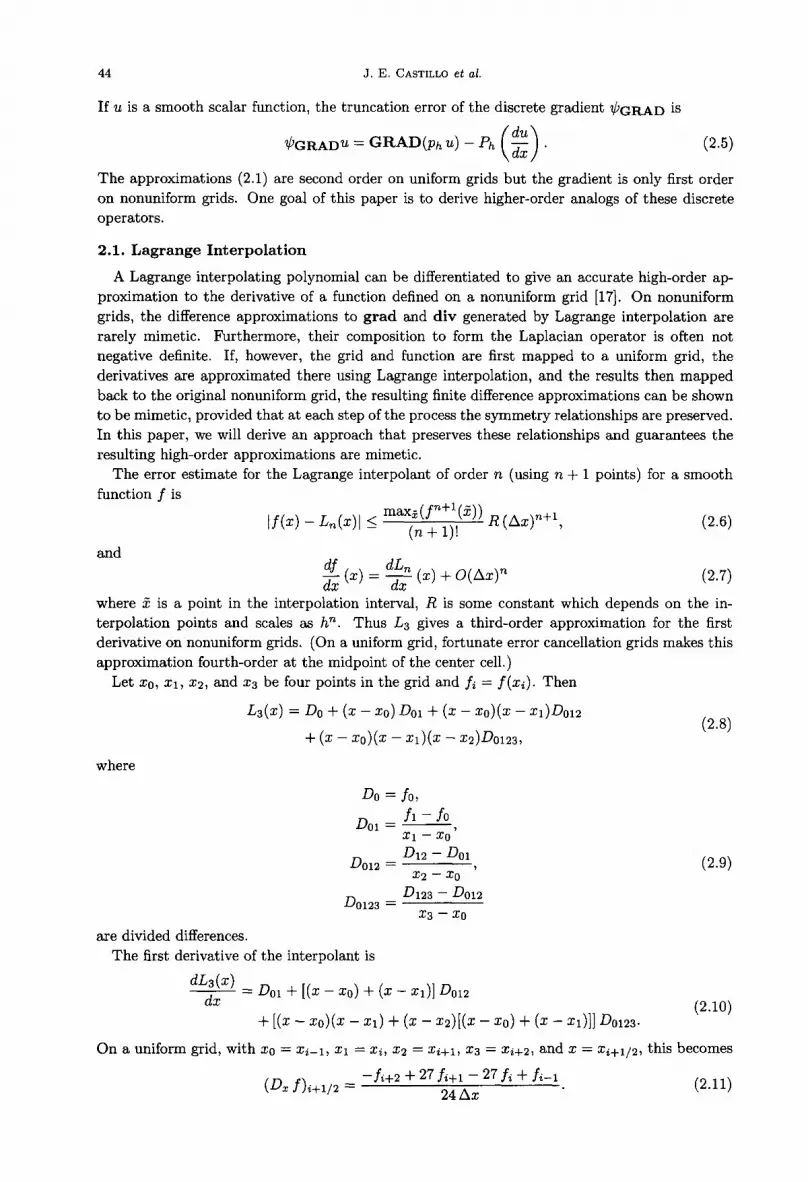
If u is a smooth scalar function, the truncation error of the discrete gradient 7fGRAD is

7fGRADU = GRAD (Ph U) - Ph (~~) . (2.5)

The approximations (2.1) are second order on uniform grids but the gradient is only first order on nonuniform grids. One goal of this paper is to derive higher-order analogs of these discrete operators.

2.1. Lagrange Interpolation

A Lagrange interpolating polynomial can be differentiated to give an accurate high-order ap­proximation to the derivative of a function defined on a nonuniform grid [17J. On nonuniform grids, the difference approximations to grad and div generated by Lagrange interpolation are rarely mimetic. Furthermore, their composition to form the Laplacian operator is often not negative definite. If, however, the grid and function are first mapped to a uniform grid, the derivatives are approximated there using Lagrange interpolation, and the results then mapped back to the original nonuniform grid, the resulting finite difference approximations can be shown to be mimetic, provided that at each step of the process the symmetry relationships are preserved. In this paper, we will derive an approach that preserves these relationships and guarantees the resulting high-order approximations are mimetic.

The error estimate for the Lagrange interpolant of order n (using n + 1 points) for a smooth function f is

and

If(x) - Ln(x)1 ::; maxt~~n~)l/X)) R (LlX)n+l,

df (x) = dLn (x) + O(LlX)n dx dx

(2.6)

(2.7)

where x is a point in the interpolation interval, R is some constant which depends on the in­terpolation points and scales as hn. Thus L3 gives a third-order approximation for the first derivative on nonuniform grids. (On a uniform grid, fortunate error cancellation grids makes this approximation fourth-order at the midpoint of the center cell.)

Let xo, Xl, X2, and X3 be four points in the grid and fi = f(Xi). Then

L3(X) = Do + (x - XO) DOl + (x - Xo)(x - xI)Do12 (2.8)

where

Do = fo,

DOl = it - fo, Xl - Xo

D D12 - DOl

012 = , (2.9) X2 - Xo

D Dl23 - D012

0123 = X3 - Xo

are divided differences. The first derivative of the interpolant is

dL3(X) ~ = DOl + [(x - xo) + (x - Xl)J DOl2

+ [(x - xo)(x - Xl) + (x - X2)[(X - xo) + (x - Xl)JJ D0123· (2.10)

On a uniform grid, with Xo = Xi-I, Xl = Xi, X2 = Xi+l, X3 = Xi+2, and x = Xi+l/2, this becomes

(D f) - - fi+2 + 27 fi+l - 27Ji + fi-l x i+l/2 - 24 Llx . (2.11)

Nonuniform Grids in One Dimension 45

2.2. The Mapping Method

The mapping method is described in the books [15,16J and it was also used in [14J to construct high-order approximations. The main idea is to assume that the grid is given by a smooth mapping X,

i = 1, ... ,M, (2.12)

where the ei give a uniform grid with mesh spacing h = l/(M - 1) in the interval [O,lJ which is called logical space (the grid is called the logical grid). The first derivative is defined by

df = df (dx)-1 dx de de

(2.13)

This approach transforms the problem of approximating a derivative on a nonuniform grid to approximating two derivatives, $ and ~ on a uniform grid.

The second derivative can be constructed using the chain rule

(2.14)

where all derivatives are approximated on a uniform grid, or it can be constructed as a composition of the DIV and GRAD operators. The chain rule direct approach does not preserve many of the symmetry properties of the Laplacian, such as the divergence form, and is considerably more complicated in higher dimensions. Therefore, we will only consider constructing the higher derivatives as a composition of the elementary operators DIV and GRAD.

The truncation error of difference approximations constructed by the mapping method depends on the smoothness of the grid. If De approximates ;, on a uniform grid to O(hq ), where h =

ei+l - ei, then the approximation of Dx on a nonuniform grid

i(e) = f(x(e)), (2.15)

is also O(hq). For example, if second-order central-differences are used to approximate the derivatives on the

logical grid in (2.13)

the truncation error 'l/J

Ui+1 - Ui-I

Xi+1 - Xi-I (2.16)

(2.17)

is, in general, first-order with respect to ~x. If the transformation is smooth, then the coefficient of the second derivative is O(h2),

(Xi+1 - Xi) - (Xi - Xi-I) = h2 Xi+! - 2 Xi + Xi-I = h2 d2x 0 (h2)

2 2 h2 2 de + . (2.18)

In solving PDEs, often it is natural to require that the function being differentiated, f(x), is smooth, but the grid may be prescribed by a process where we cannot assume that X(e) is smooth. Consequently i(e) = f(X(e)) may not be smooth, even when f is well behaved as a function of x. Therefore, estimates of the truncation error in (2.18) for high-order approximations must include an analysis based on both the smoothness of the function and the transformation.

46 J. E. CASTILLO et al.

3. HIGH-ORDER APPROXIMATIONS

In this section, the mapping method is used to construct high-order approximations for the divergence and gradient.

3.1. The Operator DIV

On a uniform grid (2.11),

(DIVW) = -WXi+2 + 27WXi+l - 27WXi + WXi- 1

i+l/2 24h (3.1)

provides a fourth-order approximation for the divergence at ~i+l/2 = (~i + ~i+l)/2 with the truncation error

(3.2)

On a nonuniform grid, using this formula in (2.13) for smooth functions and transformations, the mapping method approximation for the divergence

(DIVW) = -WXi+2 + 27WXi+l - 27WXi + WXi- 1

i+l/2 -Xi+2 + 27 Xi+l - 27 Xi + Xi-l (3.3)

is O(h4) accurate at the image of ~i+l/2' Xi+l/2 = X(~i+l/2)' Usually Xi+l/2 =j:. Xi+l/2 == (Xi + xi+l)/2. Because the difference between Xi+l/2 and Xi+l/2 is O(.6.x2), this distinction only plays a role for high-order methods. In our truncation error analysis we are careful to ensure that the midpoint projection is the image under the transformation of the midpoint in logical space and not the center point of the central interval. If function X (~) is not known explicitly, then this point can be approximated by Lagrange interpolation to fourth-order by

(3.4)

Note that on rough grids the denominator in (3.3) can vanish. Even though X is a one­to-one mapping, the numerical approximation of the map may not be, causing the difference approximation to fail. Luckily, this only occurs on very rough grids.

3.2. The Operator GRAD

The formula for the operator GRAD is obtained similarly. On a uniform grid, (2.11) translated by 1/2 is a fourth-order approximation for the gradient

( ). _ -Ui+3/2 + 27 Ui+l/2 - 27 Ui- 1/ 2 + Ui- 3/ 2

GRADU t - 24h . (3.5)

On a nonuniform grid, for smooth functions and transformations the approximation

( ). _ -Ui+3/2 + 27 Ui+l/2 - 27 Ui- 1/ 2 + Ui- 3/ 2

GRAD U t - A 27 A 27 A A

-Xi+3/2 + Xi+l/2 - Xi-l/2 + Xi-3/2 (3.6)

is fourth-order accurate at the image X(~i)' that is at Xi.

3.3. The Integral Identity

In the support-operator method, the approximations of the divergence and gradient must satisfy a difference analog of integral identity

i udivwdV + i (w,gradu)dV = f u(w,ii)dS. (3.7)

Nonuniform Grids in One Dimension 47

This identity can also be written in terms of inner products,

(f,g)H = Iv f gdV, ( ii, 6)?-l = Iv (ii, 6) dV. (3.8)

For functions which are equal to zero on the boundary, the integral identity (3.7) is

(u, div 'Iii) H + (gradu, 'Iii)?-l = O. (3.9)

That is, differential operators div and grad are negative adjoints of each other:

grad = -div*. (3.10)

A discrete analog of the adjoint relationship (3.10) can be found by introducing the following inner products in spaces of discrete functions:

(3.11)

where the volumes of the cell VCH1 / 2 and the volumes of the nodes VNi are

VCH1 / 2 = -XH2 + 27 Xi+1 - 27 Xi + Xi-I,

V Ni = -XH3/2 + 27 Xi+1/2 - 27 Xi-l/2 + Xi-3/2' (3.12)

If the discrete functions are zero near the boundary, then

L UHI/ 2 (DIVW) VCH1/ 2 + L WXi (GRADU)i VNi = 0, i+l/2 .

~

(3.13)

or

(u, DIV W) H" + (GRAD U, W)?-l" = 0, (3.14)

and consequently the discrete operators are also negative adjoints of each other:

GRAD = -DIV*. (3.15)

The volumes VC and VN must be positive to insure that the expression (3.11) satisfies the axioms of an inner product. To illustrate how this failure can occur, consider the function Ui = 1 for i = io and Ui = 0 for all other i, and then

(3.16)

which must be positive. When a volume VC is zero or negative the length of a nonzero vector is zero or negative, and then the expression given in (3.11) does not satisfy the axioms of an inner product. Similar results hold for the inner product of discrete vectors. This can produce some nonphysical consequences; for example, some quantity which is always positive in the physical model, such as energy, can be zero or negative. Thus, to use the mapping method for some given grid, one must check that VC and V N are always positive.

4. ERRORS ON ROUGH GRIDS

The accuracy of the discrete divergence, gradient and Laplacian operators depends upon the smoothness of the grid transformation. In this section, we analyze the truncation errors for DIV, GRAD and LAP on grids generated by an analytic transformation with different levels of differentiability and on randomly generated grids. We describe the analytic grid transformation as Ck when the first k derivatives of the map are continuous. (In our examples, the k+ 1 derivative

48 J. E. CASTILLO et al.

has a jump discontinuity.) For our random grid examples, the identity map is perturbed by a random multiple of hk.

The first set of examples are based on the analytic map

X(~) = (4.1)

r:-:; ~:-:; 1,

where k .

_ '"' bj * (1 - r)J d - 1 + L..- .,

j=1 J.

is introduced for normalization of mapping. The number of terms in sum, k, is a parameter. This function produces a family of mappings with varying smoothness at the point ~ = r. The CO grid is defined by setting bi = 1 for 1 ~ i ~ k. The C 1 mapping (shown in Figure 2) is defined by setting b1 = 0 and bi = 1 for i > 1. Smoother mappings are defined similarly.

1.6

1.4

1.2

1

0.8

0.6

0.4

0.2

0 0 0.2 0.4 0.6 0.8 1

Figure 2. The C 1 transformation X(~) and its first two derivatives.

If f is a Ck-l function and the kth derivative is bounded, then

k-l f{j) hj Fk hk f(x+h) = L -'1- +k!'

j=O J (4.2)

where Fk is some average value of f(k). For a CO mapping with bounded derivatives, by Taylor series expansion about the point Xi, we can express

(4.3)

where Ci±k are bounded by the first derivative of X. For a Cl mapping with bounded second derivative, we have

(dX) k2 Xi±k = Xi ± k h d:[ i + 2" h2

Ci±k (4.4)

where Ci±k are bounded by the second derivative of X.

Nonuniform Grids in One Dimension 49

The second set of examples is constructed using random perturbations of a uniform grid. We define the O(hk) grid by

(4.5)

where the Ri'S are random numbers uniformly distributed in [-1/4,1/4].

4.1. Truncation Error Analysis

After analyzing the truncation errors of the second-order approximations to DIV and GRAD on rough grids, we compare them with the fourth-order approximations. In the analysis, we expand the discrete operators at the points Xi+l/2 and Xi-l/2, evaluate the derivatives at the fourth-order accurate approximation (3.4), and then analyze how the continuity of the grid trans­formation affects the truncation error.

Let us at first consider operators given by formulas (2.1), which have second order truncation errors on a smooth grid. We need to mention here that the definition of Xi+l/2 has to be consistent with the formal order of the approximation; then for second order approximation,

and

If w(x) is a smooth function of x, then a Taylor expansion about Xi+l/2 gives an expression for the truncation error for operator DIV, given by formula (2.1),

For a scalar function u, the truncation error for GRAD, (2.1), at Xi is

,I. I. Ui+l/2 - Ui-l/2 n (dU) O(h) 't'GRADU x = , , - rh - ~ . , Xi+l/2 - Xi-l/2 dx

(4.6)

(4.7)

The truncation error for GRAD is one order less than the error for DIV, because Xi is not necessarily the midpoint of Xi-l/2 and Xi+l/2'

The truncation error for the fourth order operator DIV, (3.3), operating on a smooth func­tion w(x), is obtained by Taylor series about Xi+l/2

(4.8)

where

Ak = 27 [(Xi+l - Xi+l/2)k - (Xi - Xi+l/2)k]

+ [(Xi-l - Xi+l/2l- (Xi+2 - Xi+l/2)k] . (4.9)

The denominator

Ai = -xi+2 + 27 Xi+! - 27 Xi + Xi-l (4.10)

is order h. The image of the midpoint in logical space plays a critical role in our analysis. Because,

in general, the mapping is not known explicitly, it is important to accurately approximate this

CAIIIA 30-8-E

50 J. E. CASTILLO et al.

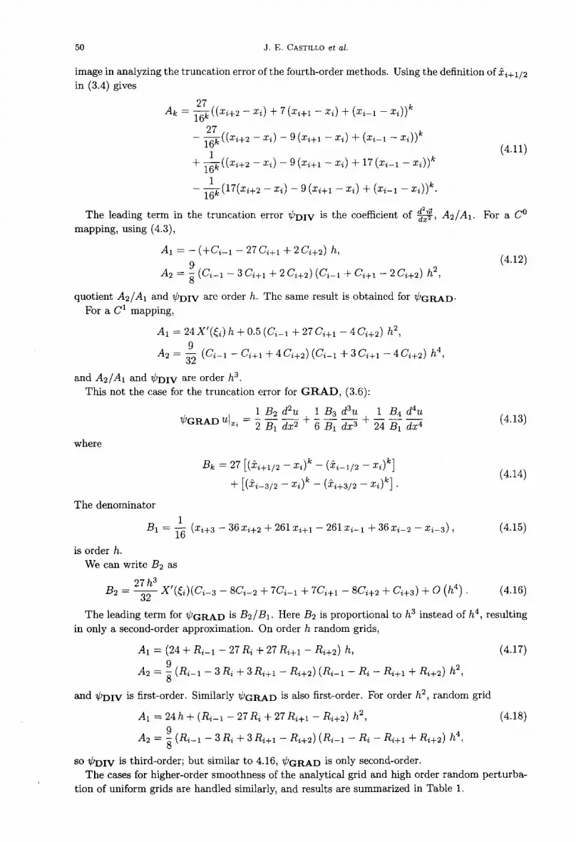
image in analyzing the truncation error of the fourth-order methods. Using the definition of XHI/2 in (3.4) gives

27 k Ak = 16k ((XH2 - Xi) + 7 (Xi+l - Xi) + (Xi-l - Xi))

27 k - 16k ((XH2 - Xi) - 9 (Xi+l - Xi) + (Xi-l - Xi))

1 k + 16k ((XH2 - Xi) - 9(XHI - Xi) + 17(Xi-l - Xi)) ( 4.11)

1 k - 16k (17(XH2 - Xi) - 9 (XHI - Xi) + (Xi-l - Xi)) .

The leading term in the truncation error 7PDIV is the coefficient of ~,A2/Al. For a CO mapping, using (4.3),

Al = - (+Ci - 1 - 27 Ci+l + 2 C H2) h,

9 2 A2 = "8 (Ci - 1 - 3 CHI + 2 C H2 ) (Ci - 1 + CHI - 2 C H2) h ,

quotient A2/ Al and 7PDIV are order h. The same result is obtained for 7PGRAD. For a C1 mapping,

Al = 24X'(~i) h + 0.5 (Ci - 1 + 27 Ci+l - 4 C H2 ) h2,

9 4 A2 = 32 (Ci - 1 - CHI + 4 Ci+2 ) (Ci - 1 + 3 CHI - 4 C H2) h ,

and A2/Al and 7PDIV are order h3. This not the case for the truncation error for GRAD, (3.6):

where

The denominator

1 B2 d2u 1 B3 d3u 1 B4 d4u 7PGRAD ul x ; = "2 Bl dx2 + "6 Bl dX3 + 24 Bl dx4

Bk = 27 [(XH1/2 - Xi)k - (Xi-l/2 - Xi)k]

+ [(Xi-3/2 - Xi)k - (Xi+3/2 - Xi)k] .

1 Bl = 16 (XH3 - 36 xH2 + 261 xHl - 261 Xi-l + 36 Xi-2 - Xi-3) ,

is order h. We can write B2 as

(4.12)

(4.13)

(4.14)

(4.15)

(4.16)

The leading term for 'l/IGRAD is B2/B1 . Here B2 is proportional to h3 instead of h4, resulting in only a second-order approximation. On order h random grids,

Al :::: (24 + Ri-l - 27 Ri + 27 Ri+l - Ri+2) h, (4.17)

9 2 A2 :::: "8 (Ri- l - 3Ri + 3Ri+l - R H 2) (Ri-l - Ri - Ri+l + RH2 ) h ,

and 7PDIV is first-order. Similarly 7PGRAD is also first-order. For order h2 , random grid

Al = 24 h + (Ri- 1 - 27 Ri + 27 RHl - RH2 ) h2, (4.18)

9 4 A2 = "8 (Ri- l - 3 Ri + 3 Ri+l - R H2 ) (Ri- l - Ri - RHI + RH2 ) h ,

so 7PDIV is third-order; but similar to 4.16, 7PGRAD is only second-order. The cases for higher-order smoothness of the analytical grid and high order random perturba­

tion of uniform grids are handled similarly, and results are summarized in Table 1.

Nonuniform Grids in One Dimension

Table 1. Theoretical estimates for the order of approximation of the fourth-order discrete operators, analyzed in Section 4.

Mapping GRAD DIV LAP CO 1 1 0

C1 2 3 1

C2 3 4 2

C3 4 4 3

C4 4 4 4

4.2. Truncation Error for the Laplacian

51

Because DIV = -GRAD", the Laplacian LAP = DIV GRAD is symmetric and nega­tive (but may not be negative definite). We now estimate its truncation error in terms of the truncation errors for the divergence and gradient.

For a uniform grid, the superposition of DIV, (3.3), and GRAD, (3.6), is

1 (LAP U);+1/2 = 576 h2 (Ui+7/2 - 54 U;+5/2 + 783 Ui+3/2

-1460 U;+1/2 + 783 Ui - 1/ 2 - 54 Ui - 3/ 2 + Ui - 5/ 2) . (4.19)

The standard fourth-order Laplacian with a minimal stencil is

(LAP U) = -U'+5/2 + 16U,+3/2 - 30U,+1/2 + 16U._ 1/ 2 - U.- 3/ 2 .+1/2 12h2 (4.20)

Although this approximation of the Laplacian has a smaller stencil than (4.19), it cannot be decomposed into a product of GRAD and DIV = -GRAD*.

Combining (2.4) and (2.5), the truncation error for the Laplacian can be written as

'lfJLAP = Ph(divgrad) - DIVGRAD(Ph u). (4.21)

Using

( 4.22)

this can be rewritten as

'lfJDIVGRAD u = Ph(div grad u) - DIV (Ph(gradu) - DIV'lfJGRAD· (4.23)

Next, using the definition of'lfJDIV and taking w = grad u to transform first two terms in (4.23), we have

'lfJDlV GRAD u = 'lfJDIV(grad u) - DIV 'lfJGRAD( u). (4.24)

The truncation error of the first term on the right-hand side of this equation is the same as for DIV, but the truncation error for the second term is one order less than for the GRAD. Because this truncation error was estimated by using the estimates for the individual operators independently, there may be some undetected cancellation and the truncation error may be less than these estimates. However, the numerical results for random grids confirm that the estimates are, in fact, optimal. Similar results can be obtained for the operator grad div and its approximation GRAD DIV.

In summary, on the rough grids the truncation error for LAP is one order less than that of GRAD, and the truncation error for DIV is one order higher than the truncation error for GRAD; for smooth grids and for a very smooth grid (G3 and higher) the truncation errors for both operators are fourth order.

52 J. E. CASTILLO et al.

5. NUMERICAL EXPERIMENTS

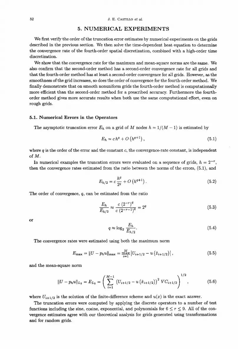
We first verify the order of the truncation error estimates by numerical experiments on the grids described in the previous section. We then solve the time-dependent heat equation to determine the convergence rate of the fourth-order spatial discretization, combined with a high-order time discretization.

We show that the convergence rate for the maximum and mean-square norms are the same. We also confirm that the second-order method has a second-order convergence rate for all grids and that the fourth-order method has at least a second-order convergence for all grids. However, as the smoothness of the grid increases, so does the order of convergence for the fourth-order method. We finally demonstrate that on smooth nonuniform grids the fourth-order method is computationally more efficient than the second-order method for a prescribed accuracy. Furthermore the fourth­order method gives more accurate results when both use the same computational effort, even on rough grids.

5.1. Numerical Errors in the Operators

The asymptotic truncation error Eh on a grid of M nodes h = l/(M - 1) is estimated by

(5.1)

where q is the order of the error and the constant c, the convergence-rate constant, is independent ofM.

In numerical examples the truncation errors were evaluated on a sequence of grids, h = 2-r ,

then the convergence rates estimated from the ratio between the norms of the errors, (5.1), and

(5.2)

The order of convergence, q, can be estimated from the ratio

(5.3)

or

(5.4)

The convergence rates were estimated using both the maximum norm

(5.5)

and the mean-square norm

(5.6)

where Ui +1/2 is the solution of the finite-difference scheme and u(x) is the exact answer.

The truncation errors were computed by applying the discrete operators to a number of test functions including the sine, cosine, exponential, and polynomials for 6 ::; r ::; 9. All of the con­vergence estimates agree with our theoretical analysis for grids generated using transformations and for random grids.

Nonuniform Grids in One Dimension

5.2. Numerical Error for the Heat Equation

The time-dependent one-dimensional heat equation,

8u. 82u 8t = dlV grad u = 8x2' 0< x < 271",

with periodic boundary conditions and the exact solution

u(X,t) = e- t sin(x)

53

(5.7)

(5.8)

was solved to determine how the accuracy depends upon the smoothness of the grid. Five grids, each with M points, were used: a uniform grid, a smooth periodic grid,

Xi = 271" (i - 1)h + 0.2 sin(271" (i - l)h), i = 1, ... ,M,

and three random perturbations of the uniform grid,

Xl = 0,

Xi = 271"(i -1)h+Ri271"hs,

XM =271",

i = 2, ... ,M -1,

where the ~, i = 2, ... , M - 1 are random numbers, Ri E (-1/4,1/4), and s = 3,2, l.

(5.9)

The spatial derivatives were approximated by the second- (2.1) and fourth- (3.3), (3.6) order approximations. The equations were integrated in time by a variable-order, variable-time step Adams-Bashforth-Moulton method to time accuracy of 10-9 , so that the errors related to time­integration are negligible.

The accuracy of the solutions at t = 1 are displayed in Table 2. The type of the grid is in the first column, the number of grid points M is in the second column, the order of the method on a uniform grid is in third column, the next two columns give the maximum and mean-square error norms, and the estimated orders of convergence are in next two columns. Note that the order of convergence for the maximum and mean-square norms are the same.

The second-order method has a second-order convergence rate for all grids and the fourth-order method has at least a second-order convergence for all grids. However, as the smoothness of the grid increases, so does the order of convergence for the fourth-order method.

5.3. Efficiency of the Second- and Fourth-Order Methods

The fourth-order approximation of the Laplacian requires 2.6 times as many arithmetic op­erations as the second-order approximation (13 arithmetic operations for fourth-order versus 5 for the second-order method). We compared the two methods in solving the previous example by using M = 16 cells for the fourth-order method and 2.6 M = 42 cells for the second-order method. The results in Table 3 for the max and L2 norm errors demonstrate that the fourth­order method is significantly more accurate than the second-order method on the smooth grids. On rough grids, the fourth-order method is only slightly worse, even with far fewer mesh points. These results agree with similar comparisons of finite difference and finite volume methods on nonuniform grids [1J.

When using these approximations to solve systems of partial differential equations, often the cost of applying the discrete operator is small compared with the cost of evaluating the function that is to be operated on. For example, in a fluid dynamics calculation where the equation-of­state is evaluated by a table lookup, it may cost up to thirty arithmetic operations to evaluate the pressure at a mesh point. The five extra arithmetic operators for the fourth-order method compared to the second-order method is small compared to the large gain in accuracy. The real gain comes from requiring fewer mesh points in a calculation that has the same accuracy.

54 J. E. CASTILLO et al.

Table 2. Convergence analysis, and comparison of sccond- and fourth-order schemes. The con­vergence rates using the maximum, qrnax, and L2 norm, q2 are computed on the series of grids with M = 17,33, and 65 points. These estimates agree with the theoretical estimates from Sec­tion 4.

Type of grid M Order max-norm L2-norm qmax q2

Uniform grid 17 2 4.17E - 03 7.43E - 03 1.90 1.91

4 6.3lE - 05 l.l2E - 04 3.80 3.80

33 2 1.11E - 03 1.96E - 03 1.95 1.96

4 4.52E - 06 8.02E - 06 3.90 3.91

65 2 2.86E - 04 5.06E - 04 - -

4 3.0lE - 07 5.32E - 07 - -

Smooth grid 17 2 4.78E - 03 8.06E - 03 1.90 1.92

4 1.53E - 04 2.24E - 04 3.75 3.79

33 2 1.28E - 03 2.12E - 03 1.95 1.94

4 l.l3E - 05 1.62E - 05 3.88 3.91

65 2 3.29E - 04 5.51E - 04 - -

4 7.66E - 07 1.07E - 06 - -

Random grid 17 2 4.6lE - 03 7.45E - 03 2.02 1.91

O(h3) 4 5.26E - 04 5.04E - 04 3.91 3.81

33 2 l.l3E - 03 1.96E - 03 1.97 1.96

4 3.49E - 05 3.59E - 05 4.32 4.31

65 2 2.87E - 04 5.06E - 04 - -

4 1.74E - 06 1.80E - 06 - -

Random grid 17 2 5.73E - 03 7.83E - 03 2.14 1.97

O(h2) 4 1.41E - 03 l.l4E - 03 3.04 2.64

33 2 1.30E - 03 1.99E - 03 2.10 1.97

4 1.71E - 04 1.83E - 04 3.40 3.36

65 2 3.03E - 04 5.08E - 04 - -

4 1.6lE - 05 1.77E - 05 - -

Random grid 17 2 9.36E - 03 1.02E - 02 1.96 1.91

O(h) 4 4.46E - 03 4.02E - 03 2.04 1.87

33 2 2.40E - 03 2.71E - 03 2.38 2.23

4 1.08E - 03 1.09E - 03 2.73 2.47

65 2 4.6lE - 04 5.75E - 04 - -

4 1.62E - 04 1.96E - 04 - -

Also, when solving time dependent equations with an explicit method, the stability restriction for the time step is a function of the mesh spacing. For the heat equation, the stability bound depends approximately upon 1/ min(~x)2. Thus, if the time step is limited by the stability, rather than accuracy, the fewer mesh points required by the fourth-order method allow much larger time steps for the same accuracy.

From this example, we conclude that for grids with varying degrees of smoothness, the fourth­order method is generally more efficient than the second-order method.

6. CONCLUSIONS

By combining the support-operators method with mapping, we have derived new mimetic fourth-order accurate discretizations of the divergence, gradient, and Laplacian on nonuniform grids. The discrete divergence is the negative of the adjoint of the discrete gradient and con­sequently the Laplacian is symmetric and negative. We verified our analytical estimates of the truncation errors by computational experiments on both smooth and rough grids. The methods displayed fourth-order truncation errors on smooth grids, and this accuracy degraded gradually as the smoothness of the grid degenerated.

Nonuniform Grids in One Dimension 55

Table 3. Comparison of accuracy of second- and fourth-order methods.

Type of grid M Order max-norm L2-norm

Uniform 42 2 6.54E - 4 l.l5E - 3

16 4 6.31E - 5 l.l2E - 4

Smooth 42 2 7.54E - 4 1.05E - 3

16 4 1.53E - 4 2.24E - 4

Random grid 42 2 6.54E - 4 l.l5E - 3

O(h4) 16 4 2.28E - 4 2.12E - 4

Random grid 42 2 6.57E - 4 1.15E - 3

O(h3) 16 4 5.26E - 4 5.04E - 4

Random grid 42 2 7.41E - 4 1.16E - 3

O(h2) 16 4 1.41E - 3 1.14E - 3

Random grid 42 2 1.43E - 3 1.53E - 3

O(h) 16 4 4.46E - 3 4.02E - 3

A numerical investigation of the order of convergence for the heat equation verified that the fourth-order method converges to at least second-order in even the roughest grids, and the order of convergence increases from 2 to 4 as the smoothness of the grid increases. Moreover, the fourth-order method was significantly more accurate than the second order-method when both methods use the same computational effort.

REFERENCES 1. J.M. Hyman, R.J. Knapp and J.C. Scovel, High order finite volume approximation of differential operators

on nonuniform grids, Physica D 60, 112-138 (1992). 2. A.A. Samarskii, V.F. Tishkin, A.P. Favorskii and M.Yu. Shashkov, Operational finite-difference schemes,

Diff. Eqns. 17,863-885 (1981). 3. M. Shashkov and S. Steinberg, Support-operator finite-difference algorithms for general elliptic problems,

Journal of Computational Physics (to appear). 4. J.E. Castillo and M. Shashkov, Grid Genemtion Methods Consistent with Finite-Difference Schemes,

LA-UR-93-2932, Los Alamos National Laboratory, Los Alamos, NM, (1993). 5. J.C. Ferreri and M.A. Ventura, On the accuracy of boundary fitted finite-difference calculations, International

Journal for Numerical Methods in Fluids 4,359-375 (1984). 6. R.G. Hindman, Generalized coordinate forms of governing fluid equations and associated geometrically in­

duced errors, AIAA Journal 20, 1359 (1982). 7. J.D. Hoffman, Relationship between the truncation errors of centered finite-difference approximations on

uniform and nonuniform meshes, Journal of Computational Physics 46, 469-474 (1982). 8. D. Lee and Y.M. Tsuei, A formulae for estimation of truncation error of convection terms in a curvilinear

coordinate system, Journal of Computational Physics 98,90-100 (1992). 9. R.W. MacCormac and A.J. Paullay, The influence of the computational mesh on accuracy for initial value

problems with discontinuous or non-unique solutions, Computers €9 Fluids 2, 339-361 (1974). 10. C.W. Mastin, Error analysis and difference equations on curvilinear coordinate systems, In Large Scale

Scientific Computation Proceeding of a Conference Conducted by the Mathematical Research Center, The University of Wisconsin-Madison, May 17-19, 1983, (Edited by S.V. Parter), pp. 195-214, Academic Press, (1984).

11. C.W. Mastin and J.F. Thompson, Errors in finite-difference computations on curvilinear coordinate systems, MSSU-EIRS-ASE-80-4, Mississippi State University, Engineering & Industrial Research Station (1980).

12. E.K. de Rivas, On the use of nonuniform grids in finite-difference equations, Journal of Computational Physics 10, 202-210 (1972).

13. H.H. Wong and G.D. Raithby, Improved finite-difference methods based on a critical evaluation of the approximation errors, Numerical Heat Transfer 2, 139-163 (1979).

14. J.M. Hyman, Accurate monotonicity preserving cubic interpolation, SIAM J. Sci. Stat. Comput. 4, 645-654 (1983).

15. P. Knupp and S. Steinberg, FUndamentals of Grid Genemtion, CRC Press, Boca Raton, (1993). 16. J.F. Thompson, Z.U.A. Warsi and C.W. Mastin, Numerical Grid Genemtion: Foundations and Applications,

North-Holland, New York, (1985). 17. J.M. Hyman and B. Larrouturou, The numerical differentiation of discrete functions using polynomial inter­

polation methods, Appl. Math. and Compo 10/11, 487-506 (1982).