the routine fitting of kinetic data to models - cell press

THE ROUTINE FITTING OF

KINETIC DATA TO MODELS:

A MATHEMATICAL FORMALISM

FOR DIGITAL COMPUTERS

MONES BERMAN, EZRA SHAHN, and MARJORY F. WEISS

From the National Institute of Arthritis and Metabolic Diseases, National Institutesof Health, Bethesda. Mr. Shahn's present address is the Johnson Foundation for Medi-cal Physics, Philadelphia.

ABSTRACT A mathematical formalism is presented for use with digital com-puters to permit the routine fitting of data to physical and mathematical models.Given a set of data, the mathematical equations describing a model, initial con-ditions for an experiment, and initial estimates for the values of model parame-ters, the computer program automatically proceeds to obtain a least squares fitof the data by an iterative adjustment of the values of the parameters. Whenthe experimental measures are linear combinations of functions, the linear co-efficients for a least squares fit may also be calculated. The values of both theparameters of the model and the coefficients for the sum of functions may beunknown independent variables, unknown dependent variables, or known con-stants. In the case of dependence, only linear dependencies are provided for inroutine use. The computer program includes a number of subroutines, each oneof which performs a special task. This permits flexibility in choosing varioustypes of solutions and procedures. One subroutine, for example, handles lineardifferential equations, another, special non-linear functions, etc. The use ofanalytic or numerical solutions of equations is possible.

INTRODUCTION!

Physical and mathematical models provide a useful technique for the study of bio-logical systems. Although no formalism has been developed as yet for the buildingof models, one may distinguish several stages in this process: (a) choice is made fortype of model, (b) degree of complexity of model is defined, (c) values for theparameters of the model are calculated, (d) judgment is made whether model iscompatible with the data, and (e) model is revised when it is inconsistent with thedata.

This paper deals chiefly with the third of the above outlined stages, namely, thederivation of values for model parameters to fit the data. This can be a considerable

275

task even for a relatively simple model, and only through the use of high speedcomputers has it become possible to treat more complex models. In an accompany-ing paper (5) some of the other stages of model building are discussed for a specialclass of models known as linear compartmental systems.

Originally, the methods described in this paper were developed for the solution oflinear compartmental systems, such as are encountered with isotope tracer experi-ments (2-4, 9). They have been extended since to include a variety of linear andnon-linear systems, and also serve as a link in a broader formalism for model build-ing which is under development.The procedures described are sufficiently flexible to accept fragmentary or "soft"

data, the type frequently encountered in biological experiments. They also permitthe pooling of data from several experiments and other sources into a single mathe-matical framework so that a solution may be obtained that is at once compatiblewith all the information available on the system.The computer program developed for this was written in FORTRAN (1) and

has been compiled' for routine use on an IBM 7090 computer2 having a 32,000word storage capacity. It includes many subroutines which permit various optionson the types of problems and methods of solution. At present it is possible to treatsimultaneously twenty-five separate functions that may arise as responses of a sys-tem having up to fifty-five parameters of which a maximum of twenty-five may bevariable.

In principle, the program can be adapted to computers having a smaller storagecapacity than the one employed here. This, however, would require a fair amount ofreprogramming and may also result in a reduction in the complexity of the systemsthat could be treated. As may be apparent from the accompanying paper (5), thelatter could be a serious limitation in the development of models.The statistical procedures employed are based mostly on reference (7). A more

complete discussion of the principles has recently been presented by Box ( 11 ), whoalso describes a computer program having a number of features similar to the onesdescribed here.When using the computer program, the data and model are entered in a certain

format and the type of solution required is specified. A number of solutions (lineardifferential equations, sums of exponentials, etc.) are available for routine use, andothers may be added as special subroutines when desired. The types of problems ormodels that can be treated are limited to those that can be described and solvedmathematically. The solutions may be either analytical or numerical.1 Binary program decks can be made available to potential users. Detailed instructions for thepreparation of data for automatic processing, and a description of the computer printout areavailable with the program deck.2 We wish to take this opportunity to thank the National Bureau of Standards for the use oftheir computer, the computer personnel for their cooperation, and Mr. A. Beam for manyassists.

BIOPHYSICAL JOURNAL VOLUME 2 1962276

SYSTEMS TREATED

The computer program is applicable to physical or mathematical models whichcan be described by a discrete number of parameters xi and for which a number ofresponse functions

fi(t)--fi(Xig ..* Xm 9 t) (j = It 29 ..* * n)[1to a set of initial conditions may be specified.

In the case of linear compartmental systems, for example, the function fj is speci-fied by a set of differential equations (2):

dA(t) -E12 Xisfi(t) (j = 1, 2, * n) [2]dt i-

and the xjj are the parameters of the system equivalent to the xi in equation [1].The experimentally measured quantities, Qk(t), for such a system are usually a

linear combination of the functions fj:Qk(t) = 0Jkfi(t) (k = 1, 2, ,n) [3]

i-1

where the afkj are time independent coefficients either known or unknown. For thespecial case where the measured quantity is proportional to the function fk, thisreduces to

Qk(t) = 0°kkfA(t).

Given a set of observed quantities Qk(t), together with the set of equationsdescribing the model, and a set of initial conditions, the program is designed tosearch for the values of the parameters xi and the coefficients rkjwhich will yield aleast squares solution for the observed quantities. This is accomplished by an itera-tive procedure requiring initial estimates for the independently variable xi only.

In general, the xi and akj may be independent variables, dependent variables, orfixed. When the xi and okj are independent variables, their range of variation can bespecified; when they are dependent variables, only linear dependence relations maybe specified routinely, but special dependence relations may be added when desired.

SOLUTION OF SYSTEM EQUATIONS

Given a model, initial conditions, and initial estimates of the values of the param-eters xi, it is first necessary to determine the functions fj(t) of [1]. This is accom-plished in the computer program by using an analytical or numerical proceduredepending on the kinds of functions and on the methods available for their de-termination. A separate subroutine is employed for each kind of function and theproper subroutine is specified by a code number which forms part of the input ofeach problem. Values of f,(t) corresponding to each experimental datum areobtained.

M. BERMAN, E. SHAHN, AND M. F. WEISS Fitting Data to Models 277

Some of the subroutines used routinely in the program include:(a) Linear differential equations: solved numerically using a 4th order Runge-Kutta

method (6).(b) Sum of exponentials: solved analytically.(c) Radiation survival of mixed cells populations: solved analytically.(d) Non-linear binding problem (special): solved numerically using 4th order

Runge-Kutta method.(e) Sum of Gaussians: solved analytically.Other subroutines may be added as required.When the measured quantities Qj(t) are linear combinations of functions, [3]

applies:

Qi(t) =f oafj(t) (i = 1, 2, , 1) [4]j-1

Once values of the fj(t) are available, the problem reduces to finding a set of coef-ficients a that will yield a best fit to the data.

Since the data correspond to measurements at specific times tk, [4] may be indexedfor each k:

Qik =ai,ifik= 1, 2, ***,1) [5]

If all the data are arranged in a linear array and identified by successive values ofk, the subscript i may be dropped and [5] may be redefined in terms of new sub-scripts

Qk =a fik (k= 1, 2, , m) [6]j'-1

where m is the number of experimental observations and h is the total number ofthe original ai. One may solve for the unknown ar in terms of the Qk and the knownas by rearrangement of [6], yielding the set of equations of condition [7]:

a h

E ,fik = Qk E i fik (k = 1, 2, ***,m) [7]j-1 i-r+1

where the 7' represent the known qr, and r is the number of unknown oa.The ae can be determined by linear regression analysis (7). Using matrix notation

the set of normal equations generated from the equations of condition is

wf )(ar) = (f wQ) [8]where cf is a column matrix of the as, f is an r x m matrix of the f,k, fT is the trans-pose of f, Q is a column matrix of the elements

(QA - £i-r+1


and w is a diagonal matrix in which the element Wkk represents the relative statisticalweight of the kth observation.

The least squares solution for a follows from [8]:

0f = (f7Wy-fTWQ) [9]

The matrix (fTwf)-1 multiplied by the weighted sum of squares of the fitted dataand divided by the number of degrees of freedom in the data is the variance-covari-ance matrix for the unknown ax, conditional on the specified values of the xi. Thesquare root of the kth diagonal elements is the standard error for the kth variable.The correlation coefficient between the ith and tph variable is given by the squareroot of the ratio of the i,jth element to the product of the ilx and jth diagonal elements.

The variance-covariance matrix of the e is modified when the xi are alsovariable.When the number of equations of condition are inadequate to permit a solution

of the unknown a, the resulting normal equations are singular or ill conditioned(near singular) and a unique solution for all the ay is not possible. The additionof more equations of condition may not improve the situation if they are "nearly"dependent on the already available ones. In such cases it is necessary to introduceadditional assumptions about the ay to permit a solution.

If some a are linearly dependent on xk and/or other al", a "dependence" sub-routine in the program substitutes for the dependent variables and solves the set ofequations in terms of the independent variables only. Certain non-linear dependen-cies may also be treated if the dependence subroutine is properly modified.The uncertainties for the dependent variables may be obtained from the variance-

covariance matrix of the independent variables. If the dependent variable u is ex-pressed as a linear combination of independent variables (xi);

u =-2 11xI + 12X2 + * * * + IIX. [10]

the variance of u is (7)VAR u = 1T7Al

where A is the variance-covariance matrix of the xi and 1 is a column matrix of the4.

CORRECTIONS FOR INITIAL ESTIMATES

The solution of the functions f4(t) and the linear coefficients qg permits the calcu-lation of a theoretical value Fi(t) = X ajift(t) corresponding to each measuredquantity Qj(t). The solution corresponding to a least squares fit, F40(t), may be re-lated to the calculated function F,(t) using a Taylor expansion

F,0(t) = Fi(t) +a F;O(t) (5x,) + 2 Ed2F((t)(5xk) + * , [11]

j X, j.k O'X, OXk


where Sxj is the difference between the given value xi and its value for a least squaressolution.

Approximation of equation [11] with only the first order term yields

E Fi(t) bx; = Fi°(t) - Fi(t). [12]

The best available estimate for F40(t) is Qj(t) and its substitution in [12] for eachexperimental value of i and t produces a set of equations of condition for the vari-ables Sxj

Fi(t) 6x, = Qi(t) - Fi(t). [13]axiA set of normal equations may be generated from [13] in a way similar to thatused for the aH in [8] and a least squares solution for the Sxj obtained. These consti-tute estimates for the corrections of the variables xj to approximate a least squaresfit of the data.The solution for the Sx1 also yields a variance-covariance matrix which permits

an estimation of uncertainties of the x; and of the variables dependent on the xj. Suchan estimate, however, is only valid when obtained in the neighborhoodvof a leastsquares fit, and is subject to re-examination in the case of extensive non-linearities.When linear dependencies of xj on other xi and of <Jkl on other ,pq and/or xi are

specified, proper substitutions are made in the calculations so that the partial deriva-tives include the dependencies.

The coefficients aFj(t)laxj for each observed i and t are calculated numerically.A small increment Axj is introduced for the variable Xj and the new value Fi(t) iscalculated, from which the AFi(t) = Fi(t) - Fi(t) is easily determined. The coef-ficient aF (t)/lax is then approximated with AF (t)/Ax1.

There are several reasons for using AF4/Axj instead of aF (t) laxj:(a) For some functions it is not possible to derive OFi(t)/lx, analytically.(b) The method is general and independent of the type of function Fi(t).(c) A decoupling is obtained indirectly between the variables x; and the aij. To

calculate a change in AFi for a change in Ax1 a new set of aij has to be calculated.Thus, in effect, the aij are treated in the calculation of AFj(t)lAxj as dependentparameters. This partitions a single interdependent variable space into 2 smallerindependent spaces, thereby reducing the possibilities of singular or ill conditionednormal equations.

(d) The use of a finite Axi may compensate for non-linearities of the functionwith respect to the variables.

CONVERGENCE

Because the functions Fi(t) are in general non-linear with respect to the variables,a first order approximation is usually inadequate to obtain a least squares solution


in one step, and an iterative procedure must be employed. The newly calculatedvalues of one iteration are used as initial estimates for the following one, and con-vergence to a least squares solution is a critical aspect of the procedure.

Several factors may be responsible for failure to converge. One is a high degreeof non-linearity of the functions with respect to the variables xi, resulting in poorextrapolation in the calculation of the correction vector. A second factor, inadequacyof the data, may result in failure to resolve the proposed model and lead to eithersingular or ill conditioned normal equations. In the case of singularity no correctionvector can be calculated, and in the case of ill conditioned equations the calculatedvector is nearly meaningless, especially in the neighborhood of the least squares fit,since it is very sensitive to the statistical fluctuations of the data. A third factor thatmay lead to failure to converge to a least squares fit is a poor choice of initial esti-mates for the values of the parameters. In this case convergence to a local minimumin the sums of squares surface may result.To deal with the above factors and to accelerate convergence some empirical

procedures were introduced into the program. First, every variable is assigned anupper and lower limit for its value and the magnitude of the correction vector islimited not to exceed these limits. When a variable is already at a limit, and thecalculated correction is in a direction beyond it, that variable is fixed at the limitand treated as a constant for the remainder of the iteration. A new correction vectoris calculated for the remaining variables.

In addition to the limitation imposed by the limits of the variables, a correctionvector is also tested to determine whether its magnitude can be optimized to yield alowest sum of squares. This is accomplished by multiplying the magnitude of thecorrection vector by a factor k. The value of k is determined from the set of equa-tions

k[Fi'(t) - Fi(t)] = [Qi(t) - Fi(t)] (i = 1, *-, m) [14]

in which F,(t) is the calculated value for the ith observation before the correctionwas made and F4'(t) is the calculated value of the same observation after adjust-ment by the initial correction vector. The experimental value for the ith observationis Qj(t). When the differences between the calculated and observed values arelinearly related to the magnitude of the correction vector, a lowest sum of squareswill be obtained for the value of k:

.E [Fi'(t) - Fi(t)][Qi(t) - Fi(t)]k = i-I m [15]

E [Fi'(t)- Fi(t)]2i -1

Usually, k is not related linearly to the difference between the calculated and ob-served values of the data, and a "best" value for it is obtained by iterating [15]several times. Limits have also been incorporated to prevent wild excursions and to


force convergence. The correction vector multiplied by the calculated value of k isaccepted as the final set of corrections and the new values for the parameters serveas initial estimates for the next complete iteration.The use of the factor k speeds up convergence and prevents divergence in the

case of ill conditioned normal equations. The magnitude of k may also serve as ameasure for the degree of ill conditioning.When the normal equations are ir conditioned it is sometimes possible (10) to

determine mathematically the variables that give rise to the "near dependence" byinserting appropriate dependence assumptions. Such a procedure does not yield aunique solution but does guarantee convergence to a "near" least squares solution.

In the case of both singular and ill conditioned normal equations, when furtherassumptions about the variables of the system are made to permit a least squaressolution, the variance-covariance matrix is conditional on the assumptions made.The entire convergence procedure is terminated when the rate of decrease in the

sum of squares with respect to a previous iteration reaches a preassigned value orwhen a desired number of iterations has been performed, whichever occurs first.

TEST OF FITTED MODEL

When the final fit of the data is obtained, the initial choice of the model may bere-examined in view of the fit obtained. The following three possibilities may arise.

1. The data are adequate to define the model and the final fit yields a randomscatter of the data about the theoretically calculated values. The calculated correc-tion terms tend to zero as the solution converges to a least squares fit and the un-certainties in the variable parameters is relatively small compared to their values.In this case the proposed model is considered compatible with the data.

2. The data are inadequate to permit a definition of the model. This can be rec-ognized by the singularity or the ill-conditioned behavior of the normal equationsas discussed in the preceding section. In some cases it may be sufficient to state thatthe model is indeterminate. When, however, a model solution is still desired, itis necessary to introduce one or more additional constraints to permit a solution.The choice of constraints may follow procedures discussed in the previous sectionor may be based on criteria similar to those followed in choosing the initial model.After a constraint is imposed the data must be refitted to the new model and thefinal results re-examined.

3. The data are adequate to define the model but do not have a random scatterabout the calculated values. The presence of systematic deviations suggests that themodel is inadequate to fit the data and that it requires additional degrees of freedom.Again, the rationale for extending the model may be the same as discussed earlier,although some modifications may suggest themselves from the nature of the incon-sistencies of the fit.To judge how well a model fits the data a "reference" fit is introduced for com-

BIoPoYsIcAL JOURNAL VOLUME 2 1962282

parison (8). A reference fit may be obtained by fitting the data to a model having atleast one or two more degrees of freedom than the model considered. Such degreesof freedom may be introduced by the release of constraints or the introduction ofadditional parameters in the model. Several reference models may be considered,each with one more degree of freedom than the previous one, and, when the sumof squares fails to improve significantly with increasing degrees of freedom, or whenthe degrees of freedom are too great to permit convergence, the reference fit isconsidered acceptable.A comparison between the model fit and the reference fit may be used to de-

termine the acceptability of the former. The comparison may be made on the basisof sums of squares or the presence of systematic deviation. The level at whichacceptance of a model is set is arbitrary and is not made automatically by theprogram.

SPECIAL FEATURES

The main features of the methodology have been described in the preceding partof the paper. Special features helpful for calculations of certain models may be gen-erated from these. Such features include the simulation of analog computer opera-tions, use of function generators, solution for input functions and the evaluationof transfer functions of systems. A more detailed description of applications tolinear compartmental systems is presented separately (5).

EXAMPLEThe paper deals mainly with the mathematical formalism for the routine fittingof data to models using high speed digital computers. To demonstrate specificallywhere and how, in the over-all employment of models, the computer program isused, a simple example is given.

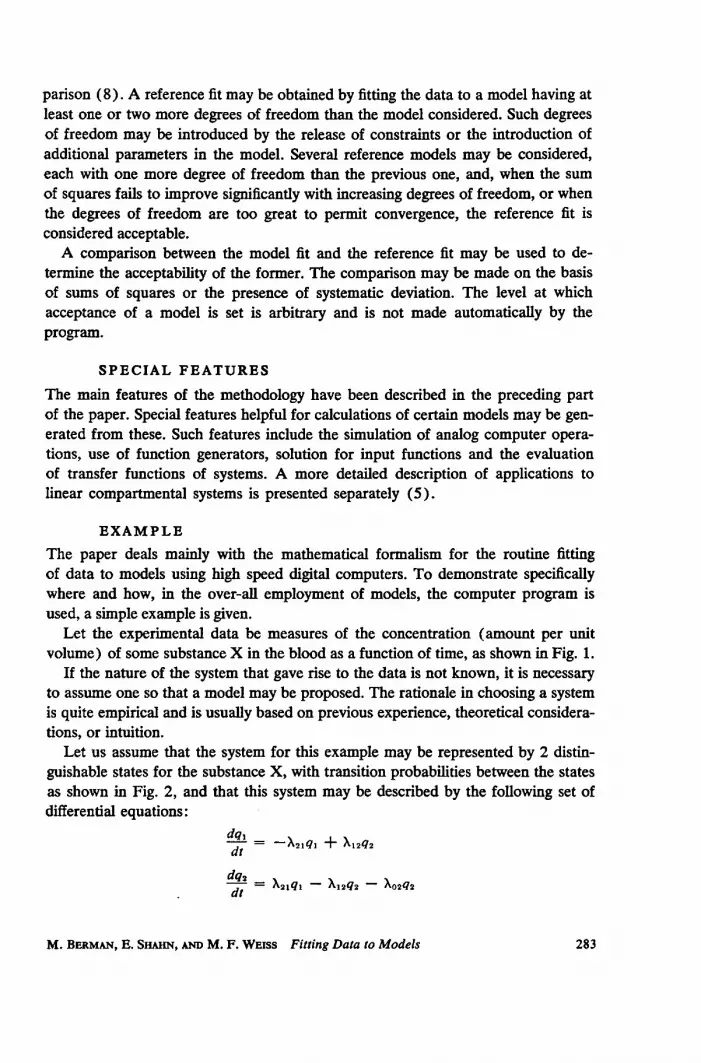
Let the experimental data be measures of the concentration (amount per unitvolume) of some substance X in the blood as a function of time, as shown in Fig. 1.

If the nature of the system that gave rise to the data is not known, it is necessaryto assume one so that a model may be proposed. The rationale in choosing a systemis quite empirical and is usually based on previous experience, theoretical considera-tions, or intuition.

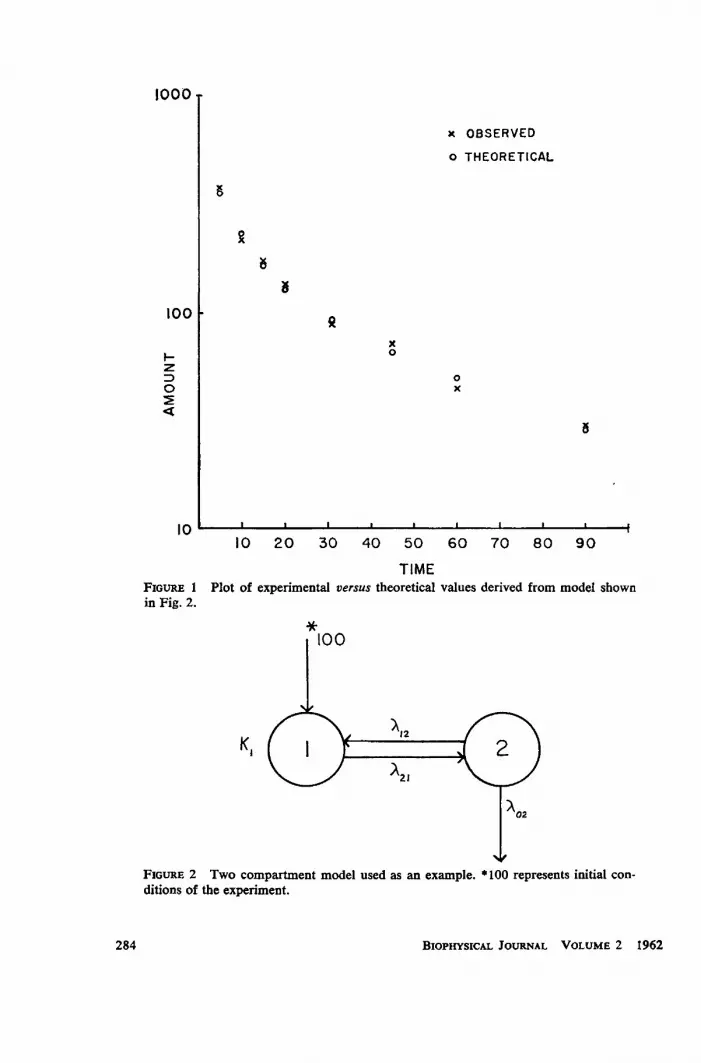
Let us assume that the system for this example may be represented by 2 distin-guishable states for the substance X, with transition probabilities between the statesas shown in Fig. 2, and that this system may be described by the following set ofdifferential equations:

dt= -X21q, + X12q2dt

d-2 - X2 q1 - X12q2 - 0qdt


x OBSERVED

0 THEORETICAL

x0

0x

5

I I I I I I t

10 20 30 40 50 60 70 80 90

TIMEFIGURE 1 Plot of experimental versus theoretical values derived from model shownin Fig. 2.

100

)'12K, ( 2 )

A02

FIGuRE 2 Two compartment model used as an example. *100 represents initial con-

ditions of the experiment.


100

z0

I

1000 T

284

The qi represent amount of material in compartment i, and AXj is a transition proba-bility per unit time from the jth to the ilb state. A02 represents loss to the outside.State I represents the blood and state 2 is unidentified.

Since the data are measures of the concentration of material in state 1, and sincethe volume of distribution is unknown, a proportionality constant, ki, is introducedbetween the data and ql. A solution for the model parameters implies the calcula-tion of a set of values for X12, A21, X02, and k1 that will yield a least squares fit of thedata. This is performed completely and automatically on the computer provided theinitial conditions of the experiment are specified and initial estimates are providedfor the values of X12, X21, and 02. No initial estimates are required for kl.To set the problem up for the computer the following information is listed in a

prescribed format and placed behind the program deck:Number of states (compartments) involved: 2Initial conditions: ql(O) = 100

q2(0) = 0Type of model involved: linear differential equations (entered by code)

Parameters of model

Parameter Initial estimates

X12 0.01X21 0.10X02 0.05ki

Data

Compartment Time Observed amount Statistical weight

1 5 375 1.01 10 219 2.91 15 172 4.71 20 135 7.81 30.1 91 17.0

etc.

The program includes a library of various types of models and automaticallyselects the proper set of equations for the problem in accord with the code specified.When a problem requires a special type of model that is not in the library, a newsubroutine has to be written for it and added to the library. Such a subroutine is asmall part of the entire program and involves instructions only for the solution ofa given set of equations. The available subroutines in the library of the programare usually written with sufficient generality to apply to many models within a class.Thus, for example, the subroutine for the solution of linear differential equationsdeals with any linear system up to 25 compartments interconnected in any arbi-

M. BERMAN, E. SHAHN, AND M. F. WEIss Fitting Data to Models 285

trary manner, with a total number of non-zero coefficients not more than 55 and anumber of variable parameters less than 25.The final output of the computer is a printout of a least squares set of values for

A12, X21, A02 and k1, their uncertainties, and a comparison between the values pre-dicted by the model and the experimental values:

Computer output

Compartment Time Experimental value Theoretical value

1 5 375. 362.1 10 219. 233.1 15 172. 167.1 20 135. 130.1 30.1 91. 93.1 45 73. 67.1 60 45. 50.1 90 30. 29.

Final parameter valuesX12 = 0.0267 i 0.0070x21 = 0.115 :4 0.030X02 = 0.0237 0.0040ki = 6.19 4 1.10

In general, the final values obtained must be interpreted in accord with the man-ner of convergence, as discussed in the text. If the calculated fit is "good," the as-sumed model is acceptable. If, however, the final solution is not unique (large stand-ard errors) or inconsistent (systematic deviations between calculated and observedvalues), the assumed model has to be modified by changes in the number of inde-pendent parameters or compartments, or by the introduction of a different type ofmodel. The entire procedure has to be repeated for any new model.

Preliminary report presented at the 5th Annual Biophysical Society Meeting, St. Louis.Received for publication, January 14, 1962.

REFERENCES

1. IBM Reference Manual-709/7090 FORTRAN Programming System, IBM, 1961.2. BERMAN, M. and SCHOENFELD, R., Invariants in experimental data on linear kinetics and

the formulation of models. J. Appl. Physics, 1956, 27, 1361.3. GARDNER, D. G., GARDNER, J. C., LAUSH, G., and MEINKE, W. W., Method for the analysis

of multi-component exponential decay curves. J. Chem. Physics, 1959, 31, 978.4. PERL, W., A method for curve-fitting by exponential functions, Internat. J. Appl. Radiation

and Isotopes, 1960, 8, 211.5. BERMAN, M., WEIss, M. F., and SHAHN, E., Some formal approaches to the analysis of

kinetic data in terms of linear compartmental systems, Biophysic. J., 1962, 2, 289.6. LEVY, H., and BAGGOTT, E. A., Numerical Solutions of Differential Equations, New York,

Dover Publications, Inc., 1950.

286 BIoPHYsIcAL JOURNAL VOLUME 2 1962

7. WHIrrAKER, E., and ROBINSON, G., The Calculus of Observation, London, Blackie andSon Ltd., 1956, Chapter IX.

8. BERMAN, M., Application of differential equations to the study of the thyroid system, Proc.4th Berkeley Symp. Mathematical Statistics, Berkeley, University of California Press,1961, 7.

9. BERMAN, M., and SCHOENFELD, R., A note on unique models in tracer kinetics, Exp. CellResearch, 1960, 20, 574.

10. HEAD, J. W., and OULTON, G. M., The solution of "ill-conditioned" linear simultaneousequations, Aircraft Eng., 1958, 30, 309.

11. Box, G. E. P., Fitting empirical data, Ann. New York Acad. Sc., 1960, 86, 792.

M. BERMAN, E. SHAHN, AND M. F. Wriss Fitting Data to Models 287

the routine fitting of kinetic data to models - cell press

Documents