The role of homing in visual topological navigation

Ming Liu, Cedric Pradalier, Francois Pomerleau, Roland Siegwart

Autonomous Systems Lab, ETH Zurich, Switzerland

[firstname.lastname]@mavt.ethz.ch, rsiegwart@ethz.ch

Abstract—Visual homing has been widely studied in the pastdecade. It enables a mobile robot to move to a Home positionusing only information extracted from visual data. However,integration of homing algorithms into real applications is notwidely studied and poses a number of significant challenges.Failures often occur due to moving people within the scene andvariations in illumination. We present a novel integrated indoortopological navigation framework, which combines odometrymotion with visual homing algorithms. We show robustnessto scene variation and real-time performance through a seriesof tests conducted in four real apartments and several typicalindoor scenes, including doorways, offices etc.

I. INTRODUCTION

V ISUAL navigation encompasses a range of techniques,

including appearance-based navigation [1], [2] and fea-

ture map based navigation [3], [4]. Broadly speaking, it uses

visual sensor information to map an unknown environment,

localize the robot within a map and automatically drive the

robot from waypoint to waypoint. Several mapping algo-

rithms based on range finders have attracted attention, such

as gmapping1 and karto2, but require considerable cost

and weight budget. Reliable visual navigation algorithms are

still necessary.

Concerning visual sensors, perspective cameras [4], stereo

vision systems [5], or omnidirectional cameras [6] have been

use in visual navigation systems. Among these sensors, omni-

directional camera has been widely used in visual navigation

system, because of its 360◦ panoramic view.

There are several existing approaches in this field. An

important difference among those approaches is perception.

Initially regional template matching [1] [7], and texture based

methods [8] were used. However, these approaches were not

tested with large scale maps in general. The development of

the visual keypoint descriptors, such as SIFT[9] and SURF

[10], along with developments in computer vision techniques

has significantly advanced the evolution of visual navigation.

Plenty of visual navigation algorithms have been thus devel-

oped using these features [5], [11], [12]. Several practical

descriptors for omnidirectional vision were also developed

for topological mapping or navigation, such as fingerprint

of the environment [13], vertical line based descriptors [14],

FACT (fast adaptive color tags) [15], [16] and so on.

This work was supported by the EU project Robots@home (IST-6-045350) and EU FP7 project NIFTi (contract # 247870)

1http://www.ros.org/wiki/gmapping2http://kartorobotics.com

Fig. 1. An application instance in a 130m2 apartment at Vienna Operning

There are two main frameworks of visual navigation algo-

rithms amongst others. The first method requires to first track

and then reconstruct [17], [4], [14], [5] the environment using

a set of features. These methods are usually able to provide

a global metric representation of the environment. However,

there are risks that the constructed map may be lost due to

error accumulation, leading to failure. The second framework

is known as topological visual navigation. They are usually

based on key-frame matching [2] to first localize the robot,

before techniques such as visual homing [18], [19], [20],

[21], [12] are used to reach predefined topological nodes.

Topological visual navigation provides several advantages

over the former framework including:

a) Sparse representation: Topological maps used for

a topological visual navigation are created incrementally,

where only feature changes are considered. A typical repre-

sentation of the environment is a collection of visual features

at certain poses. The computational and memory cost is

usually low.

b) Independence from precise maps: Visual homing is

less sensitive to error accumulation, commonly occurring in

metric mapping. As such, a precise map of the environment

is not required to ensure its success.

c) Lightweight planning: The path planning in metric

maps can be computationally very expensive. In the contrary,

visual topological navigation incurs a relatively low cost as

planning is based on graph structure.

In our work, we adopt visual homing for visual topological

navigation using an omnidirectional camera as the only

sensor for navigation. A stereo vision system is also used

for local obstacle avoidance.

A. Contributions

The goal of this work is to present a generalized

lightweight visual navigation framework, which integrates

When this constraint is met, the current node is exclu-

sively located. Otherwise, the localization will return several

possibilities which have to be verified at a later time. At

extreme cases, the robot might be incorrectly localized,

causing navigation process based on the localization to fail.

The localization process can be triggered again at the failure

poses.

D. Navigation

A global planner based on Dijkstra algorithm will perform

path planning over all topological nodes in the graph. It

results in a sequence of nodes which the robot needs to follow

in order to navigate from the current position to the target

position. As such, the topological navigation is decomposed

into several node-to-node phases. Each node-to-node action

is performed through the NAVIGATION state shown in figure

3.

The ALIGNMENT state means the robot attempts to

align its orientation (heading direction) with the pose

saved in the database. The translation between two nodes

is handled by a two-phase method: general positioning

(state=GENERAL POSITIONING) and pose stabilization

(state=POSE STABILIZATION). The former is a combina-

tion of obstacle avoidance and odometry based position con-

trol. The latter is used to correct the accumulated odometry

error for pose stabilization.

�����

������������� ��

������ ������� ��

���������������������������������

������������

��� ����������

��������������

��������������

��������

����� ������

��������

������� ���������!����

"�� ��������

��������������

�������#�����

������������

$

%

%

%

$

$

Fig. 4. The flow chart of the general positioning process

The procedure of general positioning is shown in figure

4. Two exceptions during the positioning process are “Tar-

get arrived” and “Obstacle detected”. When obstacle(s) are

detected, the system will switch to an exclusive obstacle

avoidance control process. The mechanism ensures that when

the robot’s path is not blocked. In particular, the obstacle

avoidance mode will take over the motion control using a

naive obstacle contour following law. We set the time span

for obstacle avoidance mode to 6 seconds for experiments in

a typical apartment environment. After the obstacle avoidance

process, the robot will try to reach the target again using the

“Heading to the Target” process. The “heading to the Target”

process is based on the odometry difference between current

position and the target position.

As for the finishing conditions, there are two possible

states during general positioning. They both can trigger

the finish of this procedure. During the process of general

positioning, once enough positively matched keypoints are

observed, the working state will switch to pose stabilization

automatically. This means the current position is near enough

for a robust pose stabilization process. Second, when the

odometry of the current position matches the target odometry

within a bounded error region, the state-machine will also

switch to the POSE STABILIZATION state.

�����

��������� �����

� ���������

��������� �����

� ����������� ���

���������

������

�����

��������������������

�

�

�������

������

������

������ ������

�

�

�� ���!�������

"

#�����������

Fig. 5. The flow chart of the pose stabilization process

The pose stabilization is organized under the image based

visual servoing (IBVS) framework as shown in figure 5. It

uses an omnidirectional camera as the only sensor, and tries

to correct the error in the image space by controlling the

robot motion. It is able to perform a visual homing algorithm

in real-time, by which the accumulated odometry error will

be corrected. The algorithm retrieves the target image and

features from the database and matches the current image

with the target image. These images features are fed into the

core visual servoing algorithm to generate homing vectors

which directs to the target waypoint. For example, we could

use the homing algorithm introduced in [12], where the

homing vectors are calculated from the scale differences and

the bearing angles. The algorithm shown in Eq. 1 and 2.(

vx

vy

)

=n

∑i=1

λi (si − s∗i )

(

cosβi

sinβi

)

(1)

vx

vy

ω

= λ

−s∗1l∗1l21

cosβ1 −s∗1l∗1l21

sinβ1 0

......

...

−s∗nl∗nl2n

cosβn −s∗nl∗nl2n

sinβn 0

−1l1

sinβ1 −1l1

cosβ1 −1

......

...

−1ln

sinβn −1ln

cosβn −1

+

s1 − s∗1...

sn − s∗nβ1 −β ∗

1...

βn −β ∗

n

(2)

where vx and vy are the velocity components in the 2D

navigation plane; si is the observed scale of a keypoint and

s∗i is the target scale of the corresponding reference keypoint;

βi is the bearing angle of the corresponding keypoint. The

proof of stability based on Lyapunov theory and evaluation

of the algorithm was given in [12].

III. NODE VALIDATION

In order to enhance the robustness of the navigation

system, we analysis the bottlenecks of the algorithm. One

important fact is that sometimes the visual features are not

stable enough for the navigation; in other words, the quality

of references is poor. This problem is common to any visual

navigation method, however an efficient metric to assess it is

unavailable. To this end, we use entropy analysis to evaluate

this quality.

To illustrate the problem, let us consider the two simulated

situations shown in figure 6. In both cases, 160 features can

(a) Good Feature Distribution (b) Bad Feature Distribution

Fig. 6. Effect of different feature distribution

be observed, marked with blue ‘*’s. We show the green ‘*’s

as the starting position and the red filled circles as the home

position. The robot uses the same visual homing method in

equation 1 to move from the starting position to the home

position automatically. The paths marked by black ‘*’s are

the simulated trajectories.

Figure 6(b) shows an extreme case of the feature dis-

tribution, i.e. most of the features are from one certain

direction. Figure 6(a) depicts the case that 160 features are

isotropically distributed on the simulated walls. Although in

both cases the robot can observe the same amount of features

and manages to move to the home position, the simulated

trajectories are dramatically different. We could infer that

a more isotropic distribution leads to a smoother trajectory.

Moreover, it results in smoother control variables for the

actuators.

We now consider the distributions of the features in a real

situation. We took an image using an omnidirectional camera,

and changed the feature distribution manually, using a plain

paper to intentionally cover the field of view. A screen-shot

of the angular feature distributions is shown in figure 7. The

bottom histograms show how many features lie in a given

vertical sector of the unwrapped omnidirectional image.

The number followed by the percent sign is the positive

matching ratio, the integer in squared brackets is the maxi-

mum number of matching points within a single bin in the

histogram. After that is the number of matching keypoints

and at the end is the score “S”, which should reflect the

isotropicness of the distribution. The score “S” is calculated

from the entropy of the distribution of the positive matches

using

S =−∑ pi ln pi (3)

where pi is the ratio of the matches in each bin over the

whole histogram. The maximum score can be calculated

from a uniformly distributed histogram. Empirically, if S is

(a) Good Feature distribution

(b) Bad Feature distribution

Fig. 7. Histograms of the feature distribution. There are two kinds of circlesthat mark the matching keypoints : green (brighter) and red (darker). Thegreen (brighter) circles mark the matching results after RANSAC; the red(darker) circles mark the rejected matches.

greater than 80% of this maximum score, the reference home

position is acceptable. 3 It’s worth noticing that the number of

matched features (82) is still high in figure 7(b). Typically, in

a less textured indoor environment, the homing method can

work with a minimum number of positive matches around

40. This indicates that the number of positive matches can

not fully indicate the quality of the description.

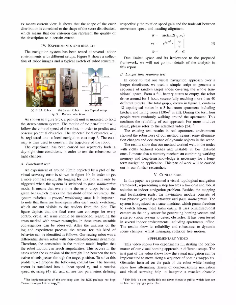
(a) Scores of matched features (b) AAE regarding to position(2,3)

Fig. 8. Relation between AAE and characteristics in features

In order to further valid this metric for node evaluation,

we carried out a test on a widely cited indoor dataset [22].

Taking position (2,3) as reference, the average angular error

(AAE) and the score are shown in figure 8. According to

[23], AAE is obtained as follows:

AAE(ss) =1

mn

m

∑x=1

n

∑y=1

AE(ss,cvxy)

where AE is the absolute angular error between the calculated

homing vector and ground truth. ss means saved scene, and

3In figure 7, there are 256 bins in the histogram. The maximum score iscalculated by S = ln256 = 5.55, therefore the score threshold is 4.4