HAL Id: hal-01106940https://hal.archives-ouvertes.fr/hal-01106940

Submitted on 24 Feb 2020

HAL is a multi-disciplinary open accessarchive for the deposit and dissemination of sci-entific research documents, whether they are pub-lished or not. The documents may come fromteaching and research institutions in France orabroad, or from public or private research centers.

L’archive ouverte pluridisciplinaire HAL, estdestinée au dépôt et à la diffusion de documentsscientifiques de niveau recherche, publiés ou non,émanant des établissements d’enseignement et derecherche français ou étrangers, des laboratoirespublics ou privés.

Distributed under a Creative Commons Attribution| 4.0 International License

The Relationship Between Bore Resonance Frequenciesand Playing Frequencies in Trumpets

Pauline Eveno, Jean François Petiot, Joël Gilbert, Benoît Kieffer, René Causse

To cite this version:Pauline Eveno, Jean François Petiot, Joël Gilbert, Benoît Kieffer, René Causse. The RelationshipBetween Bore Resonance Frequencies and Playing Frequencies in Trumpets. Acta Acustica unitedwith Acustica, Hirzel Verlag, 2014, 2 (100), pp.362-374. �10.3813/AAA.918715�. �hal-01106940�

The Relationship Between Bore ResonanceFrequencies and Playing Frequencies inTrumpets

P. Eveno1)∗, J.-F. Petiot2), J. Gilbert3), B. Kieffer1), R. Caussé1)1) Institut de Recherche et Coordination Acoustique/Musique (UMR CNRS 9912), 1 place Igor Stravinsky,75004 Paris, France. pauline.eveno@mail.mcgill.ca

2) Institut de Recherche en Communications et Cybernétique de Nantes (UMR CNRS 6597), 1 rue de la Noë,BP 92101, 44321 Nantes Cedex 3, France.

3) Laboratoire d’Acoustique de l’Université du Maine (UMR CNRS 6613), Avenue Olivier Messiaen,72085 Le Mans Cedex 9, France.

SummaryThe aim of this work is to study experimentally the relationship between the resonance frequencies of the trumpet,extracted from its input impedance, and the playing frequencies of notes, as played by musicians. Three differenttrumpets have been used for the experiment, obtained by changing only the leadpipe of the same instrument.After a measurement of the input impedance of these trumpets, four musicians were asked to play the first fiveregimes of the instrument, for four different fingerings. This was done for three dynamic levels and repeatedthree times. Statistical methods were implemented to assess the variability in the playing frequencies, and tostudy quantitatively their relationships with the bore resonance frequencies. A limited influence of the musicianon the instrument overall intonation is observed, as well as a weak influence of the dynamic levels on the pitch ofthe notes. The results show that for most of the regimes, variations of the resonance frequency lead to same ordervariations of the playing frequency of the corresponding note. We noticed also that the sum function, derivedfrom the input impedance, does not give a better prediction of the playing frequency than the input impedanceitself.

1. Introduction

Measuring and computing wind musical instruments inputimpedance is now well mastered [1, 2, 3, 4, 5, 6]. As partof a larger project aimed toward helping instrument mak-ers to design and characterise their musical instruments,this work focuses on how the bore resonance frequencies,taken from the input impedance, can be related to the play-ing frequencies. Indeed, instrument makers are primarilyinterested in the overall intonation of their instruments inplaying situations, and therefore they need some predictiveindicators.

Some studies attempt to find a solution to this issue bytaking the coupling between the instrument and the musi-cian into account. The case of reed instruments is treated

∗ New affiliation:Computational Acoustic Modeling Laboratory, Schulich School of Musicof McGill University, 555 Sherbrooke Street West, Montréal, Canada.pauline.eveno@mail.mcgill.ca

by Gilbert et al. [7] and Farner et al. [8] by using the har-monic balance technique adapted to self-sustained oscilla-tions of wind instruments such as clarinets. The resonator(i.e. the instrument body) is the linear part, treated in fre-quency domain, while the driving system (the reed) is thenonlinear part, treated in time domain. The harmonic bal-ance technique can also be used for brass instruments [9].Three control parameters representing the “virtual” mu-sician have to be defined: the pressure inside the mouth,the resonance frequency of the lips, and the inverse of lipsmass density. Depending on the choice of these parame-ters, it is possible to obtain a series of playing frequencies,such as those obtained by the musician. The coupling be-tween the musician and the instrument can also be investi-gated using a simplified model in which a single mechan-ical lip mode is coupled to a single mode of the acousticalresonator, as done by Cullen et al. [10] for the trombone. Itis also possible to predict the intonation of the instrumentby synthesizing the notes it can produce. Many studies arecarried out on physical modelling using temporal methods[11, 12].

For the saxophone, for some advanced performancetechniques (bugling and altissimo playing), musicians can

1

use the resonance of their vocal tract to play a note closeto a weak bore resonance, or even decrease the soundingpitch to several semitones below the standard pitch for thesame fingering [13, 14, 15]. It seems that this technique isnot used by trumpet players [16, 17].

The musician has a significant role in determining theplaying frequencies, this aspect being difficult to take intoaccount. Therefore, the first aim of this paper is to de-termine an order of magnitude of the brass player’s in-fluence on the overall intonation of the instrument. Then,it aims at finding some objective indicators from the in-put impedance which can predict the playing frequencieswithout taking the musician’s behaviour into account, asintended by Pratt and Bowsher [18] and previously byWogram [19]. This will be done by recording a large num-ber of notes played by several musicians on three trumpets.

Section 2 presents some basic information about theacoustics of the trumpet. Section 3 describes the recordingof notes played by the musicians on the different trum-pets and the analysis of the data. From these measure-ments, an analysis of the musicians’ behaviour is pre-sented in section 4. In section 5, the playing frequencies ofthe recorded notes are compared to the bore resonance fre-quencies taken from the input impedance of the trumpets.Section 6 presents the data first as a normal distributionand then, in order to minimize the influence of the musi-cian on the results, it focuses on frequency differences in-stead of the frequencies themselves. Finally, the relevanceof the sum function [19], a function made from the inputimpedance to predict the intonation, is discussed.

2. Trumpet resonances and playing fre-quencies: Preliminary discussion

Campbell and Greated [20] as well as Fletcher and Ross-ing [21] give a large overview on brass instruments. Asummary about trumpets is reported here as well as a dis-cussion on the coupling with the musician.The acoustic response of an instrument at different

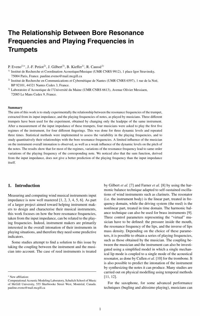
frequencies can be characterised by its input impedance(impedance computed or measured at the input of the en-tire instrument, that is to say at the input plane of themouthpiece). A typical input impedance of a brass in-strument (see Figure 1) shows a large number of boreresonance frequencies, where the impedance amplitude ismaximum and the phase is passing through zero. Someof these resonance frequencies are associated with a note(or oscillation regime) that the musician can play. In theexample of Figure 1, corresponding to the basic fingeringof a B trumpet where all the three valves are up, the reso-nances 2 to 6 correspond to the series of concert notes B 3,F4, B 4, D5, F5 (harmonic series of B 2). The first reso-nance does not correspond to a normally playable note onthe trumpet. The three valves offer height combinations,which allow the construction of the whole chromatic scale,since the activation of a valve produces an elongation ofthe air column which lower the resonance frequencies ofthe instrument. The first valve brings down the frequency

Figure 1. Measurement of the input impedance amplitude (in dB)and phase (in rad) of the trumpet called NORM with all the threevalves up, with the notes corresponding to each impedance peakabove (concert pitch of a B trumpet). The trumpet and the set-upused for the measurement are presented in Section 3.1.

of one tone, the second of a semitone, and the last one ofone and a half tones. In the rest of the article, a pressedvalve will be noted 1 and a valve up will be noted 0.An initial estimation of the instrument intonation can

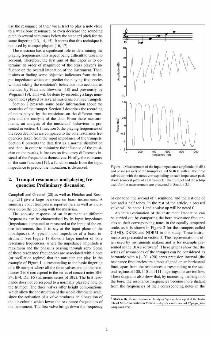
be carried out by comparing the bore resonance frequen-cies to their corresponding notes in the equally-temperedscale, as it is shown in Figure 2 for the trumpets calledCHMQ, DKNR and NORM in this study. These instru-ments are presented in section 3. This representation is of-ten used by instruments makers and is for example pre-sented in the BIAS software1. These graphs show that theseries of resonances of the trumpet can be considered asharmonic with a [−20,+20] cents precision interval (theresonance frequencies are almost aligned on an horizontalline), apart from the resonances corresponding to the sec-ond regime of 100, 110 and 111 fingerings that are too low.These diagrams also show that, by increasing the length ofthe bore, the resonance frequencies become more distantfrom the frequencies of their corresponding notes in the

1 BIAS is the Brass Instrument Analysis System developed at the Insti-tute of Music Acoustics in Vienna: http://www.bias.at/?page_id=5&sprache=2.

2

(a) (b) (c)

Figure 2. Intonation graph of trumpet (a) CHMQ, (b) DKNR and (c) NORM, obtained by calculating the difference in cents betweeneach resonance frequency of the input impedance of each trumpet for the four fingerings and its corresponding note in the equally-tempered scale.

equally-tempered scale. Consequently, if we assume thatthe resonance frequencies are representative of the play-ing frequencies, notes should be easier to play in tune withthe 000 fingering than with the 111 fingering.

However, this affirmation has to be considered cau-tiously because this graph forgets an important element ofthe trumpet playing: the musician. Indeed, these diagramsare only estimations of the intonation because the play-ing frequencies are not exactly equal to the bore resonancefrequencies. The differences between those frequencies re-sult from a complex aeroelastic coupling between the lipsof the musician and the resonator. Thus, the intonation ofthe instrument is not only controlled by the closest reso-nance frequency but possibly conditioned by upper reso-nance frequencies of the resonator [22].

Furthermore, a wind instrument is not an instrumentwith a fixed sound, that is to say the musician can mod-ify the pitch and the timbre of the played note by control-ling his/her embouchure and “bending” the notes. The em-bouchure represents the capacity of the musician to con-trol the mechanical parameters of his/her vibrating lips, bymodifying his/her facial musculature as well as the supportforce of the lips on the mouthpiece. This also includes theability to control the air flow between the lips.

3. Set-Up and Data Analysis

3.1. Set-Up

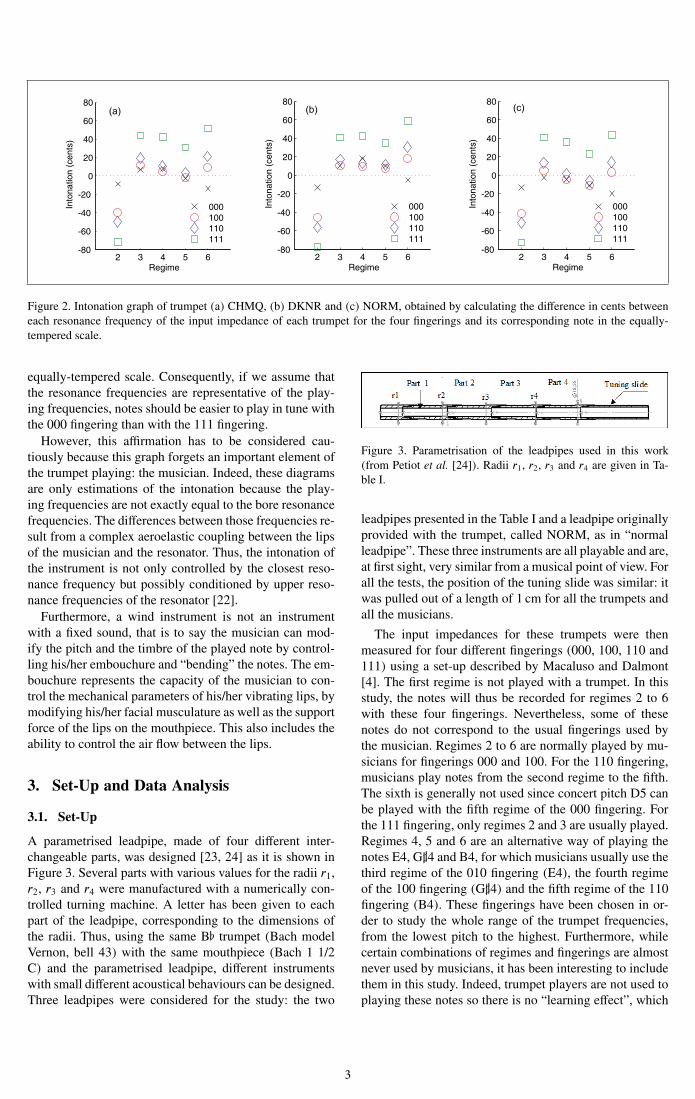
A parametrised leadpipe, made of four different inter-changeable parts, was designed [23, 24] as it is shown inFigure 3. Several parts with various values for the radii r1,r2, r3 and r4 were manufactured with a numerically con-trolled turning machine. A letter has been given to eachpart of the leadpipe, corresponding to the dimensions ofthe radii. Thus, using the same B trumpet (Bach modelVernon, bell 43) with the same mouthpiece (Bach 1 1/2C) and the parametrised leadpipe, different instrumentswith small different acoustical behaviours can be designed.Three leadpipes were considered for the study: the two

Figure 3. Parametrisation of the leadpipes used in this work(from Petiot et al. [24]). Radii r1, r2, r3 and r4 are given in Ta-ble I.

leadpipes presented in the Table I and a leadpipe originallyprovided with the trumpet, called NORM, as in “normalleadpipe”. These three instruments are all playable and are,at first sight, very similar from a musical point of view. Forall the tests, the position of the tuning slide was similar: itwas pulled out of a length of 1 cm for all the trumpets andall the musicians.

The input impedances for these trumpets were thenmeasured for four different fingerings (000, 100, 110 and111) using a set-up described by Macaluso and Dalmont[4]. The first regime is not played with a trumpet. In thisstudy, the notes will thus be recorded for regimes 2 to 6with these four fingerings. Nevertheless, some of thesenotes do not correspond to the usual fingerings used bythe musician. Regimes 2 to 6 are normally played by mu-sicians for fingerings 000 and 100. For the 110 fingering,musicians play notes from the second regime to the fifth.The sixth is generally not used since concert pitch D5 canbe played with the fifth regime of the 000 fingering. Forthe 111 fingering, only regimes 2 and 3 are usually played.Regimes 4, 5 and 6 are an alternative way of playing thenotes E4, G 4 and B4, for which musicians usually use thethird regime of the 010 fingering (E4), the fourth regimeof the 100 fingering (G 4) and the fifth regime of the 110fingering (B4). These fingerings have been chosen in or-der to study the whole range of the trumpet frequencies,from the lowest pitch to the highest. Furthermore, whilecertain combinations of regimes and fingerings are almostnever used by musicians, it has been interesting to includethem in this study. Indeed, trumpet players are not used toplaying these notes so there is no “learning effect”, which

3

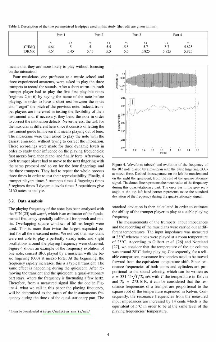
Table I. Description of the two parametrised leadpipes used in this study (the radii are given in mm).

Part 1 Part 2 Part 3 Part 4

r1 r2 r2 r3 r3 r4 r4 r5CHMQ 4.64 5 5 5.5 5.5 5.7 5.7 5.825DKNR 4.64 5.45 5.45 5.5 5.5 5.825 5.825 5.825

means that they are more likely to play without focusingon the intonation.Four musicians, one professor at a music school and

three experienced amateurs, were asked to play the threetrumpets to record the sounds. After a short warm-up, eachtrumpet player had to play the five first playable notes(regimes 2 to 6) by saying the name of the note beforeplaying, in order to have a short rest between the notesand “forget” the pitch of the previous note. Indeed, trum-pet players are interested in testing the flexibility of theirinstrument and, if necessary, they bend the note in orderto correct the intonation defects. Nevertheless, the task forthe musician is different here since it consists of letting theinstrument guide him, even if it means playing out of tune.The musicians were then asked to play the note with theeasiest emission, without trying to correct the intonation.These recordings were made for three dynamic levels inorder to study their influence on the playing frequencies:first mezzo forte, then piano, and finally forte. Afterwards,each trumpet player had to move to the next fingering withthe same protocol and so on for the four fingerings andthe three trumpets. They had to repeat the whole processthree times in order to test their reproducibility. Finally, 4trumpet players times 3 trumpets times 4 fingerings times5 regimes times 3 dynamic levels times 3 repetitions give2160 notes to analyse.

3.2. Data Analysis

The playing frequency of the notes has been analysed withthe YIN [25] software2, which is an estimator of the funda-mental frequency specially calibrated for speech and mu-sic. Overlapping square windows of 68 ms length wereused. This is more than twice the largest expected pe-riod for all the measured notes. We noticed that musicianswere not able to play a perfectly steady note, and slightoscillations around the playing frequency were observed.Figure 4 shows an example of the frequency evolution ofone note, concert B 3, played by a musician with the ba-sic fingering (000) at mezzo forte. At the beginning, thefrequency rapidly increases: this is a typical transient. Thesame effect is happening during the quiescent. After re-moving the transient and the quiescent, a quasi-stationarypart stays, where the frequency is fluctuating a few hertz.Therefore, from a measured signal like the one in Fig-ure 4, what we call in this paper the playing frequency,will be determined as the mean of the instantaneous fre-quency during the time t of the quasi-stationary part. The

2 It can be downloaded at http://audition.ens.fr/adc/

Figure 4. Waveform (above) and evolution of the frequency ofthe B 3 note played by a musician with the basic fingering (000)at mezzo forte. Dashed lines separate, on the left the transient andon the right the quiescent, from the rest of the quasi-stationarysignal. The dotted line represents the mean value of the frequencyduring this quasi-stationary part. The error bar in the grey rect-angle at the top left-hand corner represents twice the standarddeviation of the frequency during the quasi-stationary signal.

standard deviation is then calculated in order to estimatethe ability of the trumpet player to play at a stable playingfrequency.

The measurements of the trumpets’ input impedancesand the recording of the musicians were carried out at dif-ferent temperatures. The input impedance was measuredat 23◦C whereas notes were played at a room temperatureof 25◦C. According to Gilbert et al. [26] and Noreland[27], we consider that the temperature of the air columnwas around 28◦C during playing. Consequently, for a reli-able comparison, resonance frequencies need to be movedforward from the equivalent temperature shift. Since res-onance frequencies of both cones and cylinders are pro-portional to the sound velocity, which can be written asc = 331.45 T/T0 m/s with T the temperature in Kelvinand T0 = 273.16K, it can be considered that the res-onance frequencies of a trumpet are proportional to thesquare root of the temperature expressed in Kelvin. Con-sequently, the resonance frequencies from the measuredinput impedances are increased by 14 cents which is theequivalent of 5◦C in order to be at the same level of theplaying frequencies’ temperature.

4

Finally, the frequency of the resonances is precisely de-termined with a peak fitting technique using a least squaremethod on the complex impedance [28]. This method rep-resents the impedance in the Nyquist plot. In this plot, theresonance is locally a circle that should go through the ex-perimental points. Then, the resonance frequency is theangle of the point, which is the furthest from the origin.This method is the one used by Macaluso and Dalmont [4]and leads to an estimation of the resonance frequency withan uncertainty of about 5 cents. The resonance frequencycould also be determined with the phase zero crossing.Nevertheless, as explained in [29, p. 149], the amplitudeof the impedance gives more information about the tun-ing and the ease of playing than the phase, that is why thisdefinition of the resonance frequency was chosen.

4. Musicians’ behaviours

4.1. Descriptive analysis of the playing frequencies

In order to study the behaviour of each musician, we rep-resent by a boxplot the differences (in cents) betweeneach playing frequency and its respective resonance fre-quency for all the notes played. A boxplot is a convenientway of graphically representing a distribution of numeri-cal data through their five-number summaries: the smallestobservation (sample minimum), lower quartile (25th per-centile, bottom of the box), median, upper quartile (75th

percentile, top of the box), and largest observation (samplemaximum).One boxplot per dynamic level allows one to study the

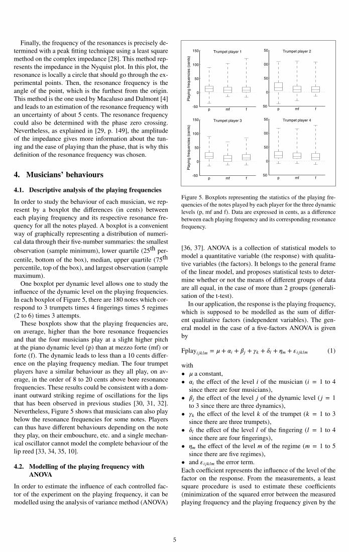
influence of the dynamic level on the playing frequencies.In each boxplot of Figure 5, there are 180 notes which cor-respond to 3 trumpets times 4 fingerings times 5 regimes(2 to 6) times 3 attempts.These boxplots show that the playing frequencies are,

on average, higher than the bore resonance frequenciesand that the four musicians play at a slight higher pitchat the piano dynamic level (p) than at mezzo forte (mf) orforte (f). The dynamic leads to less than a 10 cents differ-ence on the playing frequency median. The four trumpetplayers have a similar behaviour as they all play, on av-erage, in the order of 8 to 20 cents above bore resonancefrequencies. These results could be consistent with a dom-inant outward striking regime of oscillations for the lipsthat has been observed in previous studies [30, 31, 32].Nevertheless, Figure 5 shows that musicians can also playbelow the resonance frequencies for some notes. Playerscan thus have different behaviours depending on the notethey play, on their embouchure, etc. and a single mechan-ical oscillator cannot model the complete behaviour of thelip reed [33, 34, 35, 10].

4.2. Modelling of the playing frequency withANOVA

In order to estimate the influence of each controlled fac-tor of the experiment on the playing frequency, it can bemodelled using the analysis of variance method (ANOVA)

Figure 5. Boxplots representing the statistics of the playing fre-quencies of the notes played by each player for the three dynamiclevels (p, mf and f). Data are expressed in cents, as a differencebetween each playing frequency and its corresponding resonancefrequency.

[36, 37]. ANOVA is a collection of statistical models tomodel a quantitative variable (the response) with qualita-tive variables (the factors). It belongs to the general frameof the linear model, and proposes statistical tests to deter-mine whether or not the means of different groups of dataare all equal, in the case of more than 2 groups (generali-sation of the t-test).In our application, the response is the playing frequency,

which is supposed to be modelled as the sum of differ-ent qualitative factors (independent variables). The gen-eral model in the case of a five-factors ANOVA is givenby

Fplayijklm = µ + αi + βj + γk + δl + ηm + εijklm (1)

with• µ a constant,• αi the effect of the level i of the musician (i = 1 to 4

since there are four musicians),• βj the effect of the level j of the dynamic level (j = 1

to 3 since there are three dynamics),• γk the effect of the level k of the trumpet (k = 1 to 3

since there are three trumpets),• δl the effect of the level l of the fingering (l = 1 to 4

since there are four fingerings),• ηm the effect of the level m of the regime (m = 1 to 5

since there are five regimes),• and εijklm the error term.Each coefficient represents the influence of the level of thefactor on the response. From the measurements, a leastsquare procedure is used to estimate these coefficients(minimization of the squared error between the measuredplaying frequency and the playing frequency given by the

5

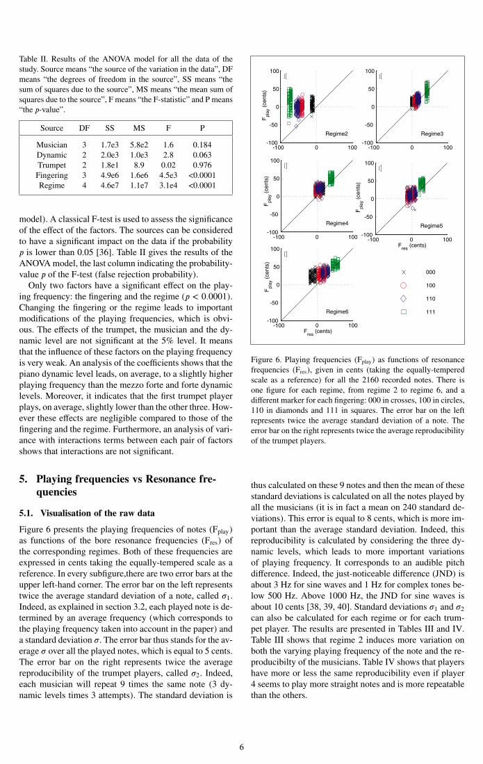
Table II. Results of the ANOVA model for all the data of thestudy. Source means “the source of the variation in the data”, DFmeans “the degrees of freedom in the source”, SS means “thesum of squares due to the source”, MS means “the mean sum ofsquares due to the source”, F means “the F-statistic” and P means“the p-value”.

Source DF SS MS F P

Musician 3 1.7e3 5.8e2 1.6 0.184Dynamic 2 2.0e3 1.0e3 2.8 0.063Trumpet 2 1.8e1 8.9 0.02 0.976Fingering 3 4.9e6 1.6e6 4.5e3 <0.0001Regime 4 4.6e7 1.1e7 3.1e4 <0.0001

model). A classical F-test is used to assess the significanceof the effect of the factors. The sources can be consideredto have a significant impact on the data if the probabilityp is lower than 0.05 [36]. Table II gives the results of theANOVAmodel, the last column indicating the probability-value p of the F-test (false rejection probability).Only two factors have a significant effect on the play-

ing frequency: the fingering and the regime (p < 0.0001).Changing the fingering or the regime leads to importantmodifications of the playing frequencies, which is obvi-ous. The effects of the trumpet, the musician and the dy-namic level are not significant at the 5% level. It meansthat the influence of these factors on the playing frequencyis very weak. An analysis of the coefficients shows that thepiano dynamic level leads, on average, to a slightly higherplaying frequency than the mezzo forte and forte dynamiclevels. Moreover, it indicates that the first trumpet playerplays, on average, slightly lower than the other three. How-ever these effects are negligible compared to those of thefingering and the regime. Furthermore, an analysis of vari-ance with interactions terms between each pair of factorsshows that interactions are not significant.

5. Playing frequencies vs Resonance fre-quencies

5.1. Visualisation of the raw data

Figure 6 presents the playing frequencies of notes (Fplay)as functions of the bore resonance frequencies (Fres) ofthe corresponding regimes. Both of these frequencies areexpressed in cents taking the equally-tempered scale as areference. In every subfigure,there are two error bars at theupper left-hand corner. The error bar on the left representstwice the average standard deviation of a note, called σ1.Indeed, as explained in section 3.2, each played note is de-termined by an average frequency (which corresponds tothe playing frequency taken into account in the paper) anda standard deviation σ. The error bar thus stands for the av-erage σ over all the played notes, which is equal to 5 cents.The error bar on the right represents twice the averagereproducibility of the trumpet players, called σ2. Indeed,each musician will repeat 9 times the same note (3 dy-namic levels times 3 attempts). The standard deviation is

Figure 6. Playing frequencies (Fplay) as functions of resonancefrequencies (Fres), given in cents (taking the equally-temperedscale as a reference) for all the 2160 recorded notes. There isone figure for each regime, from regime 2 to regime 6, and adifferent marker for each fingering: 000 in crosses, 100 in circles,110 in diamonds and 111 in squares. The error bar on the leftrepresents twice the average standard deviation of a note. Theerror bar on the right represents twice the average reproducibilityof the trumpet players.

thus calculated on these 9 notes and then the mean of thesestandard deviations is calculated on all the notes played byall the musicians (it is in fact a mean on 240 standard de-viations). This error is equal to 8 cents, which is more im-portant than the average standard deviation. Indeed, thisreproducibility is calculated by considering the three dy-namic levels, which leads to more important variationsof playing frequency. It corresponds to an audible pitchdifference. Indeed, the just-noticeable difference (JND) isabout 3 Hz for sine waves and 1 Hz for complex tones be-low 500 Hz. Above 1000 Hz, the JND for sine waves isabout 10 cents [38, 39, 40]. Standard deviations σ1 and σ2can also be calculated for each regime or for each trum-pet player. The results are presented in Tables III and IV.Table III shows that regime 2 induces more variation onboth the varying playing frequency of the note and the re-producibilty of the musicians. Table IV shows that playershave more or less the same reproducibility even if player4 seems to play more straight notes and is more repeatablethan the others.

6

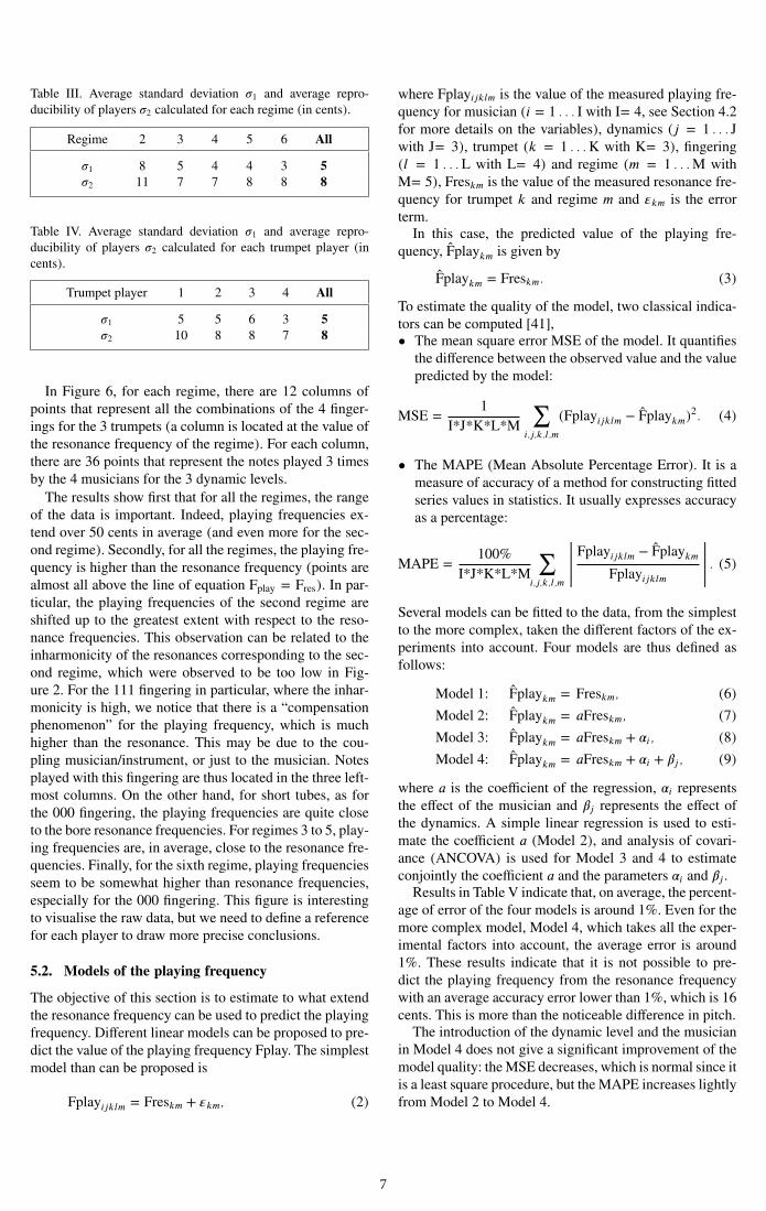
Table III. Average standard deviation σ1 and average repro-ducibility of players σ2 calculated for each regime (in cents).

Regime 2 3 4 5 6 All

σ1 8 5 4 4 3 5σ2 11 7 7 8 8 8

Table IV. Average standard deviation σ1 and average repro-ducibility of players σ2 calculated for each trumpet player (incents).

Trumpet player 1 2 3 4 All

σ1 5 5 6 3 5σ2 10 8 8 7 8

In Figure 6, for each regime, there are 12 columns ofpoints that represent all the combinations of the 4 finger-ings for the 3 trumpets (a column is located at the value ofthe resonance frequency of the regime). For each column,there are 36 points that represent the notes played 3 timesby the 4 musicians for the 3 dynamic levels.

The results show first that for all the regimes, the rangeof the data is important. Indeed, playing frequencies ex-tend over 50 cents in average (and even more for the sec-ond regime). Secondly, for all the regimes, the playing fre-quency is higher than the resonance frequency (points arealmost all above the line of equation Fplay = Fres). In par-ticular, the playing frequencies of the second regime areshifted up to the greatest extent with respect to the reso-nance frequencies. This observation can be related to theinharmonicity of the resonances corresponding to the sec-ond regime, which were observed to be too low in Fig-ure 2. For the 111 fingering in particular, where the inhar-monicity is high, we notice that there is a “compensationphenomenon” for the playing frequency, which is muchhigher than the resonance. This may be due to the cou-pling musician/instrument, or just to the musician. Notesplayed with this fingering are thus located in the three left-most columns. On the other hand, for short tubes, as forthe 000 fingering, the playing frequencies are quite closeto the bore resonance frequencies. For regimes 3 to 5, play-ing frequencies are, in average, close to the resonance fre-quencies. Finally, for the sixth regime, playing frequenciesseem to be somewhat higher than resonance frequencies,especially for the 000 fingering. This figure is interestingto visualise the raw data, but we need to define a referencefor each player to draw more precise conclusions.

5.2. Models of the playing frequency

The objective of this section is to estimate to what extendthe resonance frequency can be used to predict the playingfrequency. Different linear models can be proposed to pre-dict the value of the playing frequency Fplay. The simplestmodel than can be proposed is

Fplayijklm = Freskm + εkm, (2)

where Fplayijklm is the value of the measured playing fre-quency for musician (i = 1 . . . I with I= 4, see Section 4.2for more details on the variables), dynamics (j = 1 . . . Jwith J= 3), trumpet (k = 1 . . .K with K= 3), fingering(l = 1 . . .L with L= 4) and regime (m = 1 . . .M withM= 5), Freskm is the value of the measured resonance fre-quency for trumpet k and regime m and εkm is the errorterm.In this case, the predicted value of the playing fre-

quency, F̂playkm is given by

F̂playkm = Freskm. (3)

To estimate the quality of the model, two classical indica-tors can be computed [41],• The mean square error MSE of the model. It quantifies

the difference between the observed value and the valuepredicted by the model:

MSE =1

I*J*K*L*Mi,j,k,l,m

(Fplayijklm − F̂playkm)2. (4)

• The MAPE (Mean Absolute Percentage Error). It is ameasure of accuracy of a method for constructing fittedseries values in statistics. It usually expresses accuracyas a percentage:

MAPE =100%

I*J*K*L*Mi,j,k,l,m

Fplayijklm − F̂playkmFplayijklm

. (5)

Several models can be fitted to the data, from the simplestto the more complex, taken the different factors of the ex-periments into account. Four models are thus defined asfollows:

Model 1: F̂playkm = Freskm, (6)

Model 2: F̂playkm = aFreskm, (7)

Model 3: F̂playkm = aFreskm + αi, (8)

Model 4: F̂playkm = aFreskm + αi + βj, (9)

where a is the coefficient of the regression, αi representsthe effect of the musician and βj represents the effect ofthe dynamics. A simple linear regression is used to esti-mate the coefficient a (Model 2), and analysis of covari-ance (ANCOVA) is used for Model 3 and 4 to estimateconjointly the coefficient a and the parameters αi and βj .

Results in Table V indicate that, on average, the percent-age of error of the four models is around 1%. Even for themore complex model, Model 4, which takes all the exper-imental factors into account, the average error is around1%. These results indicate that it is not possible to pre-dict the playing frequency from the resonance frequencywith an average accuracy error lower than 1%, which is 16cents. This is more than the noticeable difference in pitch.

The introduction of the dynamic level and the musicianin Model 4 does not give a significant improvement of themodel quality: theMSE decreases, which is normal since itis a least square procedure, but the MAPE increases lightlyfrom Model 2 to Model 4.

7

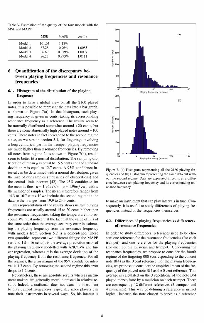
Table V. Estimation of the quality of the four models with theMSE and MAPE.

MSE MAPE coeff a

Model 1 101.03 1.18%Model 2 87.28 0.96% 1.0085Model 3 86.69 0.979% 1.0097Model 4 86.23 0.993% 1.0111

6. Quantification of the discrepancy be-tween playing frequencies and resonancefrequencies

6.1. Histogram of the distribution of the playingfrequency

In order to have a global view on all the 2160 playednotes, it is possible to represent the data into a bar graph,as shown on Figure 7(a). In that histogram, each play-ing frequency is given in cents, taking its correspondingresonance frequency as a reference. The results seem tobe normally distributed somewhat around +20 cents, butthere are some abnormally high played notes around +100cents. These notes in fact correspond to the second regimesince, as we saw in section 5.1, for fingerings involvinga long cylindrical part in the trumpet, playing frequenciesare much higher than resonance frequencies. By removingall notes from regime 2, as shown in Figure 7(b), resultsseem to better fit a normal distribution. The sampling dis-tribution of mean µ is equal to 15.5 cents and the standarddeviation σ is equal to 12.7 cents. A 95% confidence in-terval can be determined with a normal distribution, giventhe size of our samples (thousands of observations) andthe central limit theorem [42]. The 95% confidence forthe mean is thus [µ − 1.96σ/

√n µ + 1.96σ/

√n], with n

the number of samples. The mean µ therefore ranges from14.3 to 16.7 cents. If we include the second regime in thedata, µ then ranges from 19.9 to 23.3 cents.

This representation of the results shows us that playingfrequencies are usually around 15 to 20 cents higher thanthe resonance frequencies, taking the temperature into ac-count. We must notice that the fact that the value of µ is ofthe same order than the average accuracy error in estimat-ing the playing frequency from the resonance frequencywith models from Section 5.2 is a coincidence. Thesetwo quantities represent two different things: the MAPE(around 1% - 16 cents), is the average prediction error ofthe playing frequency modelled with ANCOVA and lin-ear regression, whereas µ is the average deviation of theplaying frequency from the resonance frequency. For allthe regimes, the error margin of the 95% confidence inter-val is 1.7 cents. By removing the second regime this errordrops to 1.2 cents.Nevertheless, these are absolute results whereas instru-

ment makers are generally more interested in relative re-sults. Indeed, a craftsman does not want his instrumentto play defined frequencies, especially since players cantune their instruments in several ways. So, his interest is

(a)

(b)

Figure 7. (a) Histogram representing all the 2160 playing fre-quencies and (b) Histogram representing the same data but with-out the second regime. Data are expressed in cents, as a differ-ence between each playing frequency and its corresponding res-onance frequency.

to make an instrument that can play intervals in tune. Con-sequently, it is useful to study differences of playing fre-quencies instead of the frequencies themselves.

6.2. Differences of playing frequencies vs differencesof resonance frequencies

In order to study differences, references need to be cho-sen: one reference for the resonance frequencies (for eachtrumpet), and one reference for the playing frequencies(for each couple musician and trumpet). Concerning theresonance frequencies, we propose to consider the fourthregime of the fingering 000 (corresponding to the concertnote B 4) as the 0 cent reference. For the playing frequen-cies, we propose to consider the empirical mean of the fre-quency of the played note B 4 as the 0 cent reference. Thisaverage is calculated on the 3 repetitions of the note B 4played mezzo forte by a musician on each trumpet. Thereare consequently 12 different references (3 trumpets and4 musicians). This way of defining a reference is in factlogical, because the note chosen to serve as a reference

8

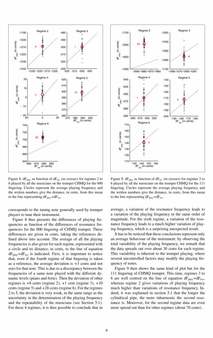
Figure 8. dFplay as function of dFres (in crosses) for regimes 2 to6 played by all the musicians on the trumpet CHMQ for the 000fingering. Circles represent the average playing frequency andthe written numbers give the distance, in cents, from this meanto the line representing dFplay=dFres.

corresponds to the tuning note generally used by trumpetplayers to tune their instrument.

Figure 8 thus presents the differences of playing fre-quencies as function of the differences of resonance fre-quencies for the 000 fingering of CHMQ trumpet. Thesedifferences are given in cents, taking the references de-fined above into account. The average of all the playingfrequencies is also given for each regime, represented witha circle and its distance, in cents, to the line of equationdFplay=dFres is indicated. First, it is important to noticethat, even if the fourth regime of that fingering is takenas a reference, the average deviation is +3 cents and notzero for that note. This is due to a discrepancy between thefrequencies of a same note played with the different dy-namic levels (piano and forte). Then the deviation of otherregimes is +8 cents (regime 2), +1 cent (regime 3), +10cents (regime 5) and+28 cents (regime 6). For the regimes2 to 5, the deviation is very weak, in the same range as theuncertainty in the determination of the playing frequencyand the repeatability of the musicians (see Section 5.1).For these 4 regimes, it is thus possible to conclude that in

Figure 9. dFplay as function of dFres (in crosses) for regimes 2 to6 played by all the musicians on the trumpet CHMQ for the 111fingering. Circles represent the average playing frequency andthe written numbers give the distance, in cents, from this meanto the line representing dFplay=dFres.

average, a variation of the resonance frequency leads toa variation of the playing frequency in the same order ofmagnitude. For the sixth regime, a variation of the reso-nance frequency leads to a much higher variation of play-ing frequency, which is a surprising unexpected result.

It has to be noticed that these conclusions represent onlyan average behaviour of the instrument: by observing thetotal variability of the playing frequency, we remark thatthe data spreads out over about 30 cents for each regime.This variability is inherent to the trumpet playing, whereseveral uncontrolled factors may modify the playing fre-quency of notes.

Figure 9 then shows the same kind of plot but for the111 fingering of CHMQ trumpet. This time, regimes 3 to6 are well centred on the line of equation dFplay=dFres,whereas regime 2 gives variations of playing frequencymuch higher than variations of resonance frequency. In-deed, it was explained in section 5.1 that the longer thecylindrical pipe, the more inharmonic the second reso-nance is. Moreover, for the second regime data are evenmore spread out than for other regimes (about 70 cents).

9

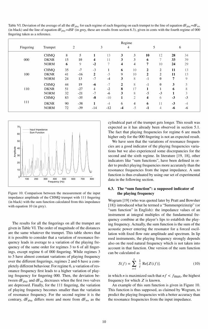
Table VI. Deviation of the average of all the dFplay for each regime of each fingering on each trumpet to the line of equation dFplay=dFres

(in black) and the line of equation dFplay=dSF (in grey, these are results from section 6.3), given in cents with the fourth regime of 000fingering taken as a reference.

RegimeFingering Trumpet 2 3 4 5 6

000CHMQ 8 5 1 13 3 3 10 12 28 34DKNR 15 10 4 11 3 3 6 7 33 39NORM 6 9 -2 7 4 4 7 10 24 29

100CHMQ 35 -7 -3 1 6 10 2 2 11 13DKNR 41 -16 2 -5 9 10 2 2 11 13NORM 24 13 -7 -4 3 8 -1 0 7 9

110CHMQ 44 19 -6 -7 2 8 -1 0 3 5DKNR 51 -27 4 -2 8 17 1 1 6 8NORM 32 -21 -7 -6 3 8 -5 -3 1 3

111CHMQ 83 -35 -8 -10 1 2 4 6 -3 -3

DKNR 90 -38 1 -4 6 4 6 11 -3 -4NORM 72 -39 -14 -12 -4 -5 -1 4 -6 -6

Figure 10. Comparison between the measurement of the inputimpedance amplitude of the CHMQ trumpet with 111 fingering(in black) with the sum function calculated from this impedancewith equation 10 (in grey).

The results for all the fingerings on all the trumpet aregiven in Table VI. The order of magnitude of the distancesare the same whatever the trumpet. This table shows thatit is possible to consider that a variation of resonance fre-quency leads in average to a variation of the playing fre-quency of the same order for regimes 3 to 6 of all finger-ings, except regime 6 of 000 fingering. While regimes 3to 5 have almost constant variations of playing frequencyover the different fingerings, regimes 2 and 6 have a com-pletely different behaviour. For regime 6, a variation of res-onance frequency first leads to a higher variation of play-ing frequency for fingering 000. Then, the deviation be-tween dFplay and dFres decreases when the first two valvesare depressed. Finally, for the 111 fingering, the variationof playing frequency becomes smaller than the variationof resonance frequency. For the second regime it is thecontrary, dFplay differs more and more from dFres as the

cylindrical part of the trumpet gets longer. This result wasexpected as it has already been observed in section 5.1.The fact that playing frequencies for regime 6 are muchhigher only for the 000 fingering is not an expected result.

We have seen that the variations of resonance frequen-cies are a good indicator of the playing frequencies varia-tions but we also experienced some discrepancies for thesecond and the sixth regime. In literature [19, 18], otherindicators like “sum functions”, have been defined in or-der to predict playing frequencies more accurately than theresonance frequencies from the input impedance. A sumfunction is thus evaluated by using our set of experimentaldata in the following section.

6.3. The “sum function”: a supposed indicator ofthe playing frequency

Wogram [19] (who was quoted later by Pratt and Bowsher[18]) introduced what he termed a “Summenprizinzip” (or“sum function” in English): the impedance values of aninstrument at integral multiples of the fundamental fre-quency combine at the player’s lips to establish the play-ing frequency. Actually, the sum function is the sum of theacoustic power entering the resonator for a forced oscil-lation with fixed flow rate amplitude and spectrum. In lipreed instruments, the playing frequency strongly dependsalso on the reed natural frequency which is not taken intoaccount in that function. One version of the sum functioncan be calculated as

S(f ) =n

i=1

1iRe[Z(if )]. (10)

in which n is maximized such that nf < fmax, the highestfrequency for which Z is known.

An example of this sum function is given in Figure 10.This function is thus supposed, as claimed by Wogram, topredict the playing frequencies with a better accuracy thanthe resonance frequencies from the input impedance.

10

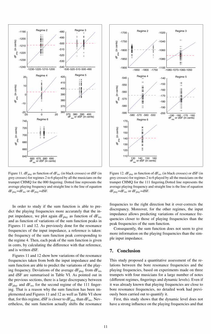
Figure 11. dFplay as function of dFres (in black crosses) or dSF (ingrey crosses) for regimes 2 to 6 played by all the musicians on thetrumpet CHMQ for the 000 fingering. Dotted line represents theaverage playing frequency and straight line is the line of equationdFplay=dFres or dFplay=dSF.

In order to study if the sum function is able to pre-dict the playing frequencies more accurately that the in-put impedance, we plot again dFplay as function of dFresand as function of variations of the sum function peaks inFigures 11 and 12. As previously done for the resonancefrequencies of the input impedance, a reference is taken:the frequency of the sum function peak corresponding tothe regime 4. Then, each peak of the sum function is givenin cents, by calculating the difference with that reference,and is written dSF.Figures 11 and 12 show how variations of the resonance

frequencies taken from both the input impedance and thesum function are able to predict the variations of the play-ing frequency. Deviations of the average dFplay from dFresand dSF are summarised in Table VI. As pointed out inthe previous sections, there is a large discrepancy betweendFplay and dFres for the second regime of the 111 finger-ing. That is a reason why the sum function has been im-plemented and Figures 11 and 12 as well as Table VI showthat, for this regime, dSF is closer to dFplay than dFres. Nev-ertheless, the sum function actually shifts the resonance

Figure 12. dFplay as function of dFres (in black crosses) or dSF (ingrey crosses) for regimes 2 to 6 played by all the musicians on thetrumpet CHMQ for the 111 fingering.Dotted line represents theaverage playing frequency and straight line is the line of equationdFplay=dFres or dFplay=dSF.

frequencies to the right direction but it over-corrects thediscrepancy. Moreover, for the other regimes, the inputimpedance allows predicting variations of resonance fre-quencies closer to those of playing frequencies than thepeak frequencies of the sum function.Consequently, the sum function does not seem to give

more information on the playing frequencies than the sim-ple input impedance.

7. Conclusion

This study proposed a quantitative assessment of the re-lations between the bore resonance frequencies and theplaying frequencies, based on experiments made on threetrumpets with four musicians for a large number of notes(different regimes, fingerings and dynamic levels). Even ifit was already known that playing frequencies are close tobore resonance frequencies, no detailed work had previ-ously been carried out to quantify it.First, this study shows that the dynamic level does not

have a strong influence on the playing frequencies and that

11

the four musicians have relatively the same “global” be-haviour, as they all play on average in the order of 8 to 20cents above the bore resonance frequencies.

Second, a closer analysis of the data shows that the av-erage standard deviation of the playing frequency is about5 cents, which means that a played note is stable with anuncertainty of 5 cents. Furthermore, the average repeata-bility of a musician, calculated on his 9 repetitions of asame note, is about 8 cents. Therefore, there is no needto find a predictor of the playing frequency more accuratethan 8 cents.Then, by representing the played notes as an histogram

it is possible to conclude that, from regime 3 to 6, playingfrequencies are in average 15 cents higher than the reso-nance frequencies. The error margin on the estimation ofthat mean is 1.2 cents at a 95% confidence level.

Finally, by examining differences instead of just fre-quencies themselves, the impact of the musicians’ be-haviour is diminished. Moreover, craftsmen often work bymaking small changes in the geometry of their instrumentsand studying the differences induced by the modification.So, focusing on differences is a way to get closer to thecraftsman’s process.Regime 4 played with the 000 fingering is thus taken

as a reference to calculate those differences, since it is thenote generally used to tune the instruments. Results showthat a variation of bore resonance frequency leads in aver-age to a variation of playing frequency of the same orderfor regime 3 to 6 (but surprisingly, except the sixth regimefor the 000 fingering). For regime 2, this rule is not sat-isfied because the notes are played at a higher frequencythan the bore resonance. The inharmonicity of the notes ofregime 2 could be a reason to explain this behaviour. Theseresults might show that the inharmonicity plays a role onthe control of the playing frequencies. It should indeed bepossible that, when the bore resonance frequency corre-sponding to the played note is in an harmonic relationshipwith the other resonances, a variation of the resonance fre-quency leads to a variation of the playing frequency of thesame range. On the other hand, when the bore resonancefrequencies are inharmonic, that relation is not valid anymore. This is shown in the study of Dalmont et al. [43] forone saxophone fingering. Nevertheless, further analysis isrequired to support this explanation.An attempt was made to model this effect with the sum

function. For the second regime, played frequencies areactually closer to the sum function peaks frequencies thanto the bore resonances. Nevertheless, a discrepancy stillexists and the prediction of the sum function is less ac-curate for other regimes. In conclusion, the sum func-tion does not seem to be more relevant than the inputimpedance in order to predict playing frequencies. Theresonance frequency is thus a good objective indicator forpredicting the playing frequency, as it does not take the in-fluence of the musician into account. This is interesting forcraftsmen whose instruments need to be played by virtualmusicians, and who often proceed by small adjustments ontheir instruments.

Our results are obtained with three particular trumpetsthat do not represent all the possible trumpets in the mar-ket. We must refrain any generalization of the results to thetrumpet in general, further studies are needed to prove therobustness of the relationship playing frequency/resonancefrequency.

Also, for further work, it will then be interesting to com-pare these results with measurements using an artificialmouth [44] and simulations.

Acknowledgement

This research was funded by the French National ResearchAgency ANR within the PAFI project (Plateforme d’Aideà la Facture Instrumentale in French). The authors wouldlike to thank all the trumpet players who participated inthis study as well as A. Burke, K. Cedergren, J.-P. Dal-mont, D. Lopatin, A. Mamou-Mani and R. Piéchaud forproofreading and valuable talks.

References

[1] J. Backus: Input impedance curves for the brass instru-ments. J. Acoust. Soc. Am. 60 (1976) 470–480.

[2] R. Caussé, J. Kergomard, X. Lurton: Input impedance ofbrass musical instruments - Comparison between experi-ment and numerical models. J. Acoust. Soc. Am. 75 (1984)241–245.

[3] P. Eveno, J.-P. Dalmont, R. Caussé, J. Gilbert: Wave propa-gation and radiation in a horn: comparisons between mod-els and measurements. Acta Acustica united with Acustica98 (2012) 158–165.

[4] C. A. Macaluso, J.-P. Dalmont: Trumpet with near-perfectharmonicity: design and acoustic results. J. Acoust. Soc.Am. 129 (2011) 404–414.

[5] J.-P. Dalmont: Acoustic impedance measurement. Journalof Sound and Vibration 243 (2001) 427–459.

[6] P. Dickens, J. Smith, J. Wolfe: Improved precision in mea-surements of acoustic impedance spectra using resonance-free calibration loads and controlled error distribution. J.Acoust. Soc. Am 121 (2007) 1471–1481.

[7] J. Gilbert, J. Kergomard, E. Ngoya: Calculation of thesteady-state oscillations of a clarinet using the harmonicbalance technique. J. Acoust. Soc. Am. 86 (1989) 35–41.

[8] S. Farner, C. Vergez, J. Kergomard, A. Lizée: Contribu-tion to harmonic balance calculations of self-sustained pe-riodic oscillations with focus on single-reed instruments. J.Acoust. Soc. Am. 119 (2006) 1794–1804.

[9] E. Poirson, J.-F. Petiot, J. Gilbert: Study of the brightness oftrumpet tones. J. Acoust. Soc. Am. 118 (2005) 2656–2666.

[10] J. S. Cullen, J. Gilbert, D. Campbell: Brass instruments:Linear stability analysis and experiments with an artificialmouth. Acta Acustica united with Acustica 86 (2000) 704–724.

[11] S. Bilbao: Numerical sound synthesis. Finite differenceschemes and simulation in musical acoustics. Wiley, 2009,Ch. Acoustic tubes, 249–286.

[12] L. Trauntmann, R. Rabenstein: Digital sound synthesisby physical modeling using the functional transformation

12

method. Kluwer Academic / Plenum publishers, 2003, Ch.Classical synthesis methods based on physical models, 63–94.

[13] P. Guillemain, C. Vergez, D. Ferrand, A. Farcy: An instru-mented saxophone mouthpiece and its use to understandhow an experienced musician plays. Acta Acustica unitedwith Acustica 96 (2010) 622–634.

[14] G. Scavone, A. Lefebvre, A. da Silva: Measurement ofvocal-tract influence during saxophone performance. J.Acoust. Soc. Am. 123 (2008) 2391–2400.

[15] J.-M. Chen, J. Smith, J. Wolfe: Saxophonists tune vocaltract resonances in advanced performance techniques. J.Acoust. Soc. Am. 129 (2011) 415–426.

[16] T. Kaburagi, N. Yamada, T. Fukui, E. Minamiya: A metho-dological and preliminary study on the acoustic effect ofa trumpet player’s vocal tract. J. Acoust. Soc. Am. 130(2011) 536–545.

[17] J.-M. Chen, J. Smith, J. Wolfe: Do trumpet players tuneresonances of the vocal tract? J. Acoust. Soc. Am. 131(2012) 722–727.

[18] R. Pratt, J. Bowsher: The objective assessment of trombonequality. Journal of Sound and Vibration 65 (1979) 521–547.

[19] K. Wogram: Ein beitrag zur ermittlung der stimmungvon blechblasininstrumenten (in english: A contribution tothe measurement of the intonation of brass instruments).Dissertation. Technische Universität Carolo Wilhelmina,Braunschweig, 1972.

[20] M. Campbell, C. Greated: The musician’s guide to acous-tics. Schirmer Books, 1988, Ch. 9. Brass instruments, 303–407.

[21] N. H. Fletcher, T. D. Rossing: The physics of musical in-struments. Springer-Verlag, 1991, Ch. 14. Lip-driven Brassinstruments, 365–393.

[22] A. Benade, D. Gans: Sound production in wind instru-ments. Ann. N.Y. Acad. Sci. 155 (1968) 247–263.

[23] E. Poirson, J.-F. Petiot, J. Gilbert: Integration of user per-ceptions in the design process: Application to musical in-strument optimization. J. Mech. Des 129 (2007) 1206–1214.

[24] J.-F. Petiot, E. Poirson, J. Gilbert: Study of the relationsbetween trumpets’ sounds characteristics and the inputimpedance. Proceedings of Forum Acusticum 2005, Bu-dapest, Hungary, 747–752.

[25] A. de Cheveigné, H. Kawahara: YIN, a fundamental fre-quency estimator for speech and music. J. Acoust. Soc.Am 111 (2002) 1917–1930.

[26] J. Gilbert, L. M. L. Ruiz, S. Gougeon: Influence de la tem-pérature sur la justesse d’un instrument à vent (in english:Influence of the temperature on the intonation of a wind in-strument). Proceedings of Congrès Français d’Acoustique2006, Tours.

[27] D. Noreland: An experimental study of temperature varia-tions inside a clarinet. Proceedings of the Stockholm Mu-sic Acoustics Conference 2013, SMAC 2013, Stockholm,Sweden.

[28] J.-C. Le Roux: Le haut-parleur électrodynamique: esti-mation des paramètres électroacoustiques aux basses fré-quences et modélisation de la suspension (in english: Theelectrodynamic loudspeaker: Estimate of the electroacous-tic parameters at low frequencies and suspension mod-elling). Dissertation. Université du Maine, 1994.

[29] P. Eveno: L’impédance d’entrée pour l’aide à la facture desinstruments de musique à vent : mesures, modèles et lienavec les fréquences de jeu (in english: The input impedancefor the support of the musical instruments making: mea-surements, models and link with the playing frequencies).Dissertation. Université Pierre et Marie Curie, 2012.

[30] V. Fréour, G. Scavone: Acoustical interaction between vi-brating lips, dowstream air column, and upstream airwaysin trombone performance. J. Acoust. Soc. Am. 134 (2013)3887–3898.

[31] N. Fletcher: Excitation mechanisms in woodwind and brassinstruments. Acustica 43 (1979) 63–72.

[32] C. Vergez, X. Rodet: Dynamical systems and physical mod-els of trumpet-like instruments. Acta Acustica united withAcustica 86 (2000) 147–162.

[33] M. Campbell: Brass instruments as we know them today.Acta Acustica united with Acustica 90 (2004) 600–610.

[34] S. Adachi, M. Sato: Time-domain simulation of sound pro-duction in the brass instrument. J. Acoust. Soc. Am. 97(1995) 3850–3861.

[35] S. Yoshikawa: Acoustical behaviour of brass player’s lips.J. Acoust. Soc. Am. 97 (1995) 1929–1939.

[36] R. Christensen: Plane answers to complex questions: Thetheory of linear model. Springer Texts in Statistics,Springer, 2002, Ch. 7. Multifactor Analysis of Variance,156–195.

[37] H. Scheffé: The analysis of variance. New York: Wiley,1959.

[38] B. Kollmeier, T. Brand, B. Meyer: Springer handbook ofspeech processing. Springer, 2008, Ch. Perception ofSpeech and Sound, 65.

[39] T. Letowski: A note on the difference limen for frequencydifferentiation. J. Sound Vib. 85 (1982) 579–583.

[40] W. M. Hartmann: Pitch, periodicity, and auditory organiza-tion. J. Acoust. Soc. Am. 100 (1996) 3491–3502.

[41] J. Armstrong: Principles of forecasting: a handbook for re-searchers and practitioners. Kluwer Academic Publishers,Norwell, MA, 2001, Ch. 14. Evaluating forecasting meth-ods, 443–472.

[42] R. Christensen: Plane answers to complex questions: Thetheory of linear model. Springer Texts in Statistics,Springer, 2002, Ch. E. Inference for One Parameter, 451–458.

[43] J.-P. Dalmont, B. Gazengel, J. Gilbert, J. Kergomard: Someaspects of tuning and clean intonation in reed instruments.Applied Acoustics 46 (1995) 19–60.

[44] J. Gilbert, S. Ponthus, J.-F. Petiot: Artificial buzzing lipsand brass instruments: Experimental results. J. Acoust. Soc.Am. 104 (1998) 1627–1631.

13