the proton as a dosimetric and diagnostic probe
TRANSCRIPT
HAL Id: tel-01127000https://tel.archives-ouvertes.fr/tel-01127000
Submitted on 6 Mar 2015
HAL is a multi-disciplinary open accessarchive for the deposit and dissemination of sci-entific research documents, whether they are pub-lished or not. The documents may come fromteaching and research institutions in France orabroad, or from public or private research centers.
L’archive ouverte pluridisciplinaire HAL, estdestinée au dépôt et à la diffusion de documentsscientifiques de niveau recherche, publiés ou non,émanant des établissements d’enseignement et derecherche français ou étrangers, des laboratoirespublics ou privés.
The proton as a dosimetric and diagnostic probeCécile Bopp
To cite this version:Cécile Bopp. The proton as a dosimetric and diagnostic probe. Other [cond-mat.other]. Universitéde Strasbourg, 2014. English. NNT : 2014STRAE023. tel-01127000
UNIVERSITE DE STRASBOURG
ECOLE DOCTORALE PHYSIQUE ET CHIMIE-PHYSIQUE (ED182)INSTITUT PLURIDISCIPLINAIRE HUBERT CURIEN, CNRS, UMR 7178
THESE presentee par
Cecile BOPPsoutenue le : 13 Octobre 2014
pour obtenir le grade de : Docteur de l’Universite de Strasbourg
Discipline/Specialite : Physique subatomique pour la sante
Le proton :sonde dosimetrique et diagnostique
The proton as a dosimetricand diagnostic probe
THESE dirigee par :David BRASSE Directeur de recherche, PHC Strasbourg
Marc ROUSSEAU Maıtre de conferences, IPHC Strasbourg
RAPPORTEURS :Katia PARODI Professor, LMU Munchen
Joel HERAULT Physicien Medical, CAL Nice
EXAMINATEURS :Benoıt GALL Professeur, IPHC Strasbourg
Jean COLIN Professeur, LPC Caen


A ma maman,qui m’a donne envie d’etudier la physique!


“I always heard there is no end to ’em. It’s all down todimensions, I heard, like what we see is only the tip ofthe whatever, you know, the thing that is mostlyunderwater –”“Hippopotamus?”“Alligator?”“Ocean?”
– Terry Pratchett

Remerciements
Ce manuscrit conclut trois annees de travail au sein du groupe ImaBio de l’InstitutPuridisciplinaire Hubert Curien. Ce furent trois annees hautes en couleur et tresenrichissantes.
Je remercie vivement Katia Parodi, Joel Herault et Benoıt Gall pour avoir participea mon jury de these. Je tiens a remercier tout particulierement Jean Colin, pour avoirete a l’origine de l’idee de ce travail de these. Merci, j’ai trouve cela passionnant! Merciegalement pour l’interet porte a mon travail, et les discussions interessantes qui s’en sontsuivies.Durant ces trois annees, j’ai travaille sous la direction de David Brasse et MarcRousseau, envers lesquels je suis reconnaissante de la chance qu’ils m’ont donnee. Merciparticuliement a David pour avoir ete un “mentor” depuis bien plus longtemps que ca,et avoir grandement contibue a mon choix de carriere. Merci de m’avoir aiguille dans cetravail, pour les discussions conceptuelles, et pour les quelques tirades dont je garde descitations... interessantes. Merci chef!
Je tiens egalement a remercier les nombreuses personnes qui ont relu mon manuscrit.Chaque point de vue a ete constructif. Merci donc a David et Marc, mais aussi aPatrice Marchand, Harold Barquero, Marie Vanstalle, Christian Finck, Valerie Brasse,Alex (non, tu n’auras pas le droit a ton nom entier), a mon pere et surtout a ReginaRescigno, qui a lu ce document maintes et maintes fois!
Surtout, je tiens a remercier l’ensemble du groupe ImaBio. Quelqu’un m’a dit unjour que je m’amusais tellement a travailler que je ne remarquais meme plus que jetravaillais. Cela n’etait pas faux. C’est grace a tout le groupe.
J’ai eu la chance d’etre accompagnee au quotidien par mes co-locataires successifsdu bureau 138. Je remercie Khodor Koubar, pour avoir supporte mes grimaces pendantplus de deux ans. Je remercie Emmanuel Brard, pour l’ambiance qu’il a mis dans cebureau (la difference a ete notable apres ton depart!), ainsi que pour toute l’aide qu’ilm’a apporte et tout ce que j’ai pu apprendre en le regardant travailler. Je suis encore loinde coder aussi proprement, mais tu as ete une bonne source d’inspiration! Je remercieegalement Harold Barquero, pour avoir fait ces trois ans de chemin avec moi. Ce futun plaisir de partager les bons moments et les periodes de stress epiques avec toi! Je
i
REMERCIEMENTS
remercie aussi Benjamin Auer, mon jumeau cache / retrouve, pour m’avoir rendu mesgrimaces coup pour coup. Bon courage pour la suite! Enfin, je tiens a remercier toutparticulierement Regina Rescigno, pour la vie dans le bureau, ainsi que pour les heureset jours de discussions sur l’imagerie proton. Je suis ravie que nous ayons pu partagerce theme de travail. Ce fut un plaisir de travailler avec toi dans la bonne humeur et avecune motivation infaillible.
Et au reste du groupe, qui a rendu chaque jour tres agreable, merci egalement. Merciau chef, pour l’animation du groupe. Je remercie aussi tout particulierement VirgileBekaert, pour la place reservee dans son bureau et pour m’avoir bien aide a conserver cequ’il me reste de sante mentale pendant la redaction. Merci aussi a Bernard Humbert,pour le petit moment de discussion qui met de bonne humeur tous les matins... j’attendsencore la neige! Je remercie egalement Ali Ouadi et Patrice Marchand, pour leur humourtoujours tres delicat. Patrice, merci non seulement pour ta companie “agreable” en pausecafe, mais aussi pour toutes les discussions qui m’ont permis d’avoir une meilleure vued’ensemble sur beaucoup de choses. Je tiens a remercier Jacques Wurtz, qui sait toujourstout! Merci egalement a Lionel Thomas, pour avoir motive l’equipe piscine. Je ne pensepas que j’aurais tenu si longtemps sans ta motivation sans faille. A Patrice Laquerriere,je tiens a dire merci du fond du coeur pour la glace! Je remercie egalement BrunoJessel, pour les karaokes dont je garde des souvenirs... terrifiants! Merci aussi a MarieVanstalle, pour les “clap clap clap clap clap” et a Christian Finck, pour avoir ete unebonne victime de nos sourires. Et merci Marc, pour avoir ajoute un cote sale aux pausescafe. Et je n’oublie evidemment pas les autres, qui ont participe a la bonne humeur et al’ambiance du groupe durant ces trois ans : Nicholas Chevillon, Arnaud Bertrand, ZiadEl Bitar, Jean-Michel Galonne, Jackie Sahr, Rachid Sefri, Xiaochao Fang et ChristianFuchs.Merci a tous, et tout specialement merci pour les pingouins lors de ma soutenance! Vousetiez beaux avec vos t-shirts!
Merci egalement a Nicholas Rudolf et Christophe Helfer, qui ne font pas partied’ImaBio, mais c’est comme si...
Je tiens ensuite a remercier tous mes amis, les facultatifs evidemment, qui m’ontaccompagnee depuis bien longtemps et en particulier pendant ces annees de these. MerciJulien, Nono, Camille, Papillon, Tutur, Aurore, Max, Christophe, Manu, Marsou, Anne-Cha, Cecile, Marc et Marie-Laure.
J’exprime egalement toute ma gratitude envers ma famille, qui m’a toujours soutenueet encouragee dans mes choix. Merci a mes parents. Un clin d’oeil special a ma maman,sans qui j’aurais du manger au RU... je suis convaincue que ta cuisine a ete determinantedans ma reussite de cette these! A Muriel, Emilie, Jean-Christophe et Nathan, pour avoirete la pour moi.Merci egalement a Marie-Odile, qui a grandement participe au succes qu’a ete mon potde these ainsi qu’a Noelie et Nina: le jour de ma soutenance a ete l’accomplissement dema these, mais aussi de ce que j’attendais depuis de nombreuses annees (LE coussin!!).Merci a tous ceux qui sont venus pour ma soutenance, et a ceux qui n’ont pas pu venir
ii
mais qui ont pense a moi.Merci aussi a Francois, pour s’etre toujours enquis de l’avancement de mes travaux, enme demandant semaine apres semaine : “Alors, tu les as trouves tes protons?”.
Enfin, merci Alex, pour avoir ete a mes cotes pendant cette aventure qu’a ete lathese. Merci de m’avoir soutenue et supportee, merci pour tout!
iii

REMERCIEMENTS
iv
CONTENTS
Contents
Summary in French / Resume de la these en francais ix
List of Figures xxi
List of Tables xxv
Glossary xxvii
Introduction 1
1 Particle therapy and the need for particle imaging 5
1.1 Particle beam therapy . . . . . . . . . . . . . . . . . . . . . . . . . . . . . 61.1.1 The ballistic advantage . . . . . . . . . . . . . . . . . . . . . . . . 6
1.1.1.1 Photon depth-dose distribution . . . . . . . . . . . . . . . 61.1.1.2 Protons and heavier ions depth-dose distribution . . . . . 7
1.1.2 Biological advantage . . . . . . . . . . . . . . . . . . . . . . . . . . 81.1.2.1 Relative biological effectiveness . . . . . . . . . . . . . . . 91.1.2.2 The oxygen effect . . . . . . . . . . . . . . . . . . . . . . 121.1.2.3 Dependence of the phase in the cell cycle . . . . . . . . . 131.1.2.4 In brief... . . . . . . . . . . . . . . . . . . . . . . . . . . . 13
1.1.3 Clinical trials, cost and cost-effectiveness . . . . . . . . . . . . . . 141.1.3.1 Protons . . . . . . . . . . . . . . . . . . . . . . . . . . . . 141.1.3.2 Carbon ions . . . . . . . . . . . . . . . . . . . . . . . . . 16
1.2 Treatment planning and uncertainties in particle beam therapy . . . . . . 171.2.1 Treatment planning for particle beam therapy . . . . . . . . . . . . 17
1.2.1.1 X-ray CT imaging . . . . . . . . . . . . . . . . . . . . . . 171.2.1.2 Conversion of X-ray CT numbers . . . . . . . . . . . . . 18
1.2.2 Range uncertainty . . . . . . . . . . . . . . . . . . . . . . . . . . . 201.2.2.1 Origins of the range uncertainty . . . . . . . . . . . . . . 201.2.2.2 Consequences for treatment planning and treatment . . . 23
1.2.3 Delivered dose uncertainty . . . . . . . . . . . . . . . . . . . . . . . 261.2.3.1 Biological dose uncertainty . . . . . . . . . . . . . . . . . 261.2.3.2 Physical dose uncertainty . . . . . . . . . . . . . . . . . . 26
1.2.4 Improving treatment planning . . . . . . . . . . . . . . . . . . . . 27
v
CONTENTS
1.2.4.1 Taking full advantage of the LET . . . . . . . . . . . . . 281.2.4.2 PTV definition and treatment plan optimization . . . . . 281.2.4.3 Improving CT images . . . . . . . . . . . . . . . . . . . . 291.2.4.4 Improving the conversion to RSP with DECT . . . . . . 301.2.4.5 Upcoming possibilities for X-ray CT imaging? . . . . . . 31
1.2.5 Proton imaging as a potential answer? . . . . . . . . . . . . . . . . 31
2 Proton imaging – state of the art 33
2.1 Review of the physics principles: interactions of protons with matter . . . 342.1.1 Proton energy loss . . . . . . . . . . . . . . . . . . . . . . . . . . . 342.1.2 Multiple Coulomb scattering . . . . . . . . . . . . . . . . . . . . . 372.1.3 Nuclear interactions . . . . . . . . . . . . . . . . . . . . . . . . . . 38
2.2 The first era of proton imaging - discovery . . . . . . . . . . . . . . . . . . 392.2.1 Proton computed tomography using energy loss . . . . . . . . . . . 392.2.2 Marginal range radiography . . . . . . . . . . . . . . . . . . . . . . 402.2.3 Nuclear scattering imaging . . . . . . . . . . . . . . . . . . . . . . 412.2.4 Multiple scattering radiography . . . . . . . . . . . . . . . . . . . . 422.2.5 In brief . . . . . . . . . . . . . . . . . . . . . . . . . . . . . . . . . 43
2.3 The second era of proton imaging - treatment planning and quality assurance 442.3.1 Proton computed tomography for imaging the relative stopping
power . . . . . . . . . . . . . . . . . . . . . . . . . . . . . . . . . . 442.3.2 Proton tomographs . . . . . . . . . . . . . . . . . . . . . . . . . . . 46
2.3.2.1 Tracking . . . . . . . . . . . . . . . . . . . . . . . . . . . 482.3.2.2 Energy/range measurement . . . . . . . . . . . . . . . . . 49
2.3.3 Expected performances of pCT . . . . . . . . . . . . . . . . . . . . 502.3.3.1 Path estimation and spatial resolution . . . . . . . . . . . 502.3.3.2 On dose and density resolution . . . . . . . . . . . . . . . 52
2.3.4 Different approaches to pCT . . . . . . . . . . . . . . . . . . . . . 522.4 Positioning of this work . . . . . . . . . . . . . . . . . . . . . . . . . . . . 53
3 Simulation and reconstruction platform for proton CT 55
3.1 Simulation of a proton tomograph . . . . . . . . . . . . . . . . . . . . . . 563.1.1 Monte Carlo simulation using GATE . . . . . . . . . . . . . . . . . 56
3.1.1.1 GEANT4 . . . . . . . . . . . . . . . . . . . . . . . . . . . 573.1.1.2 GATE . . . . . . . . . . . . . . . . . . . . . . . . . . . . . 57
3.1.2 Scanner description . . . . . . . . . . . . . . . . . . . . . . . . . . 583.1.3 Data output . . . . . . . . . . . . . . . . . . . . . . . . . . . . . . . 583.1.4 Execution of the simulations . . . . . . . . . . . . . . . . . . . . . 603.1.5 Description of the phantoms used . . . . . . . . . . . . . . . . . . . 60
3.1.5.1 The Forbild phantom . . . . . . . . . . . . . . . . . . . . 603.1.5.2 The Zubal head phantom . . . . . . . . . . . . . . . . . . 62
3.2 Analytical image reconstruction . . . . . . . . . . . . . . . . . . . . . . . . 633.2.1 2D Radon transform . . . . . . . . . . . . . . . . . . . . . . . . . . 633.2.2 Central-slice theorem . . . . . . . . . . . . . . . . . . . . . . . . . . 643.2.3 Filtered Back-projection algorithm . . . . . . . . . . . . . . . . . . 653.2.4 Specificities . . . . . . . . . . . . . . . . . . . . . . . . . . . . . . . 65
vi
3.2.4.1 On the generation of projections . . . . . . . . . . . . . . 653.2.4.2 On the Filtered Back-projection algorithm implementation 66
3.3 Iterative reconstruction with the Algebraic Reconstruction Techniquealong the most likely path . . . . . . . . . . . . . . . . . . . . . . . . . . . 663.3.1 The ART algorithm . . . . . . . . . . . . . . . . . . . . . . . . . . 663.3.2 Most likely path . . . . . . . . . . . . . . . . . . . . . . . . . . . . 68
3.3.2.1 Maximum likelihood formalism . . . . . . . . . . . . . . . 683.3.2.2 Implementation for parallel-beam geometry . . . . . . . . 703.3.2.3 Validation . . . . . . . . . . . . . . . . . . . . . . . . . . 71
3.3.3 Implementation specificities . . . . . . . . . . . . . . . . . . . . . . 733.3.3.1 Data management . . . . . . . . . . . . . . . . . . . . . . 733.3.3.2 Regularization . . . . . . . . . . . . . . . . . . . . . . . . 743.3.3.3 Raytracing . . . . . . . . . . . . . . . . . . . . . . . . . . 763.3.3.4 Boundary detection . . . . . . . . . . . . . . . . . . . . . 77
4 Further studies of the most likely path approximation 79
4.1 Preamble: image reconstruction of the relative stopping power . . . . . . 804.1.1 Analytical image reconstruction . . . . . . . . . . . . . . . . . . . . 804.1.2 Iterative image reconstruction . . . . . . . . . . . . . . . . . . . . 84
4.2 Improving spatial resolution? Most likely path in a non-uniform medium . 884.2.1 Scattering of particles in a non-uniform medium and implementa-
tion in the MLP . . . . . . . . . . . . . . . . . . . . . . . . . . . . 884.2.2 Results . . . . . . . . . . . . . . . . . . . . . . . . . . . . . . . . . 904.2.3 Discussion . . . . . . . . . . . . . . . . . . . . . . . . . . . . . . . . 92
4.3 Impact of the tracking system properties on the path estimation . . . . . 924.3.1 Materials and methods . . . . . . . . . . . . . . . . . . . . . . . . . 94
4.3.1.1 Uncertainty propagation in the MLP . . . . . . . . . . . 944.3.1.2 Uncertainties due to the acquisition system . . . . . . . . 944.3.1.3 Quantification of the uncertainty . . . . . . . . . . . . . . 95
4.3.2 Results . . . . . . . . . . . . . . . . . . . . . . . . . . . . . . . . . 964.3.3 Discussion on the acquisition system . . . . . . . . . . . . . . . . . 974.3.4 Conclusions and perspectives . . . . . . . . . . . . . . . . . . . . . 102
5 Proton imaging beyond the stopping power 105
5.1 Preliminary study on the exploitation of the outputs . . . . . . . . . . . . 1065.1.1 Description of the study . . . . . . . . . . . . . . . . . . . . . . . . 106
5.1.1.1 Definition of the observables . . . . . . . . . . . . . . . . 1065.1.1.2 Monte Carlo simulation . . . . . . . . . . . . . . . . . . . 107
5.1.2 Influence of the chemical composition . . . . . . . . . . . . . . . . 1095.1.2.1 Differentiation of materials . . . . . . . . . . . . . . . . . 1095.1.2.2 Influence of the chemical composition for a fixed electron
density . . . . . . . . . . . . . . . . . . . . . . . . . . . . 1105.1.3 Statistical uncertainty . . . . . . . . . . . . . . . . . . . . . . . . . 1105.1.4 Conclusion . . . . . . . . . . . . . . . . . . . . . . . . . . . . . . . 111
5.2 Qualitative approach to image reconstruction using the scattering andtransmission rate . . . . . . . . . . . . . . . . . . . . . . . . . . . . . . . . 112
vii
CONTENTS
5.2.1 Simulation and reconstruction process . . . . . . . . . . . . . . . . 1125.2.2 Results . . . . . . . . . . . . . . . . . . . . . . . . . . . . . . . . . 114
5.2.2.1 Image quality . . . . . . . . . . . . . . . . . . . . . . . . . 1145.2.2.2 Contrast . . . . . . . . . . . . . . . . . . . . . . . . . . . 122
5.2.3 Discussion . . . . . . . . . . . . . . . . . . . . . . . . . . . . . . . . 1245.2.4 Conclusion . . . . . . . . . . . . . . . . . . . . . . . . . . . . . . . 127
5.3 Quantitative approach: a step towards stoichiometric composition? . . . . 1275.3.1 Reconstruction using the transmission rate . . . . . . . . . . . . . 1285.3.2 Reconstruction using the scattering . . . . . . . . . . . . . . . . . . 129
5.3.2.1 Reconstruction principle . . . . . . . . . . . . . . . . . . 1295.3.2.2 Model validation . . . . . . . . . . . . . . . . . . . . . . . 1305.3.2.3 Reconstruction of the scattering length . . . . . . . . . . 1325.3.2.4 Conclusion . . . . . . . . . . . . . . . . . . . . . . . . . . 133
5.3.3 Towards the stoichiometric composition? . . . . . . . . . . . . . . . 1345.3.3.1 Overview of the information . . . . . . . . . . . . . . . . 1345.3.3.2 Discussion . . . . . . . . . . . . . . . . . . . . . . . . . . 1365.3.3.3 Conclusion . . . . . . . . . . . . . . . . . . . . . . . . . . 136
Conclusions and perspectives 139
A Materials and properties 147
B Differential approximations to multiple Coulomb scattering 149
Bibliography 153
viii
Summary in FrenchResume de la these en francais
Le cancer est la premiere cause de mortalite au monde [International Agency for Researchon Cancer, 2008]. Avec une elevation continue des risques, le nombre de morts dues aucancer est en constante augmentation. Trois grandes categories de traitements sontaccessibles de nos jours : la chirurgie, la radiotherapie et les traitements medicamenteux(chimiotherapie et immunitherapie). Au total, pres de la moitie des patients atteintsde cancer sont traites par radiotherapie, seule ou combinee a un autre traitement. Laradiotherapie dite “conventionnelle” est basee sur l’utilisation de rayons X afin d’irradierun tissu cancereux. Cependant, il est egalement possible d’utiliser des particules chargeespour deposer de l’energie dans l’organisme. L’idee date de 1946, lorsque Robert R.Wilson suggere que la forme du depot de dose de protons, caracterise par un pic enfin de parcours, pourrait etre avantageuse lors d’un traitement [Wilson, 1946]. Depuisune decenie, les methodes therapeutiques utilisant des faisceaux de protons ou d’ionscarbones (nommees de facon generale hadrontherapie) sont en plein essor. Il y a, al’heure actuelle, deux centres de traitement par protontherapie en France : le CentreAntoine Lacassagne a Nice et le Centre de Protontherapie d’Orsay. Dans le cadre duprojet d’infrastructure “France HADRON”, deux projets de centres de traitement parions carbones sont egalement evoques: le projet ETOILE a Lyon et le projet ARCHADEa Caen.
Deux arguments existent pour l’utilisation de particules chargees en radiotherapie.Le premier est qu’elles presentent un atout de nature physique : la courbe de depot dedose en profondeur des particules chargees est intrinsequement plus avantageuse que celledes photons (comme illustre sur la Figure 1.1 page 7). Le pic de Bragg en fin de parcoursdes particules permet de cibler precisement une zone a irradier, tout en epargnant defacon efficace les tissus sains adjacents. Il n’y a, dans le cas d’une irradiation avec desprotons, aucune dose deposee en aval du pic de Bragg. Pour les particules plus lourdes,telles les ions carbone, la courbe de depot de dose presente une extension, c’est a direun depot de dose en aval du pic de Bragg, due aux particules secondaires generees parles interactions nucleaires. Le deuxieme argument, qui concerne principalement les ionscarbones, est qu’il existe un avantage biologique a l’utilisation de ces particules. En effet,le transfert d’energie lineique (TEL) des ions carbone est bien plus eleve que celui desphotons. De ce fait, les ionisations au passage des particules sont plus concentrees autour
ix
SUMMARY IN FRENCHRESUME DE LA THESE EN FRANCAIS
de la trace de l’ion et la probabilite de generer des lesions complexes a l’ADN, c’est-a-dire de detruire efficacement des cellules, est plus grande. De plus, les particules a TELeleve presentent egalement une efficacite accrue sur les tumeurs hypoxiques. L’avantagedu carbone n’est pas tant le TEL eleve (c’est egalement le cas des neutrons) mais le faitqu’il augmente au fur et a mesure de la propagation dans le materiau, venant renforcerl’avantage confere par le pic de Bragg.
La planification de traitement en hadrontherapie est calculee a partir d’imagesacquises avec un tomodensitometre X. Elle peut etre basee soit sur des modeles depropagation analytiques des faisceaux, soit sur des simulations Monte Carlo. Dans lepremier cas, il faut connaıtre le pouvoir d’arret des materiaux afin de predire la positiondu pic de Bragg; dans le second, il faut connaıtre la densite et la composition chimiquedes materiaux. Dans les deux cas, une conversion de l’image de tomodensitometrie X,representant les coefficients d’attenuations moyens de rayons X, est necessaire. Cesconversions ne sont ni lineaires, ni bijectives, et introduisent une incertitude sur leparcours des particules [Jiang et al., 2007; Yang et al., 2012; Paganetti, 2012]. A celas’ajoute une incertitude sur les valeurs reconstruites dans l’image de tomodensitometrieX, due a des phenomenes physiques tel que le durcissement de faisceau, a des effetsde reconstruction tels la taille des voxels, le bruit, les effets de volume partiel ou lesartefacts metalliques [Schaffner and Pedroni, 1998; Chvetsov and Paige, 2010; Espanaand Paganetti, 2011; Wei et al., 2006; Jakel et al., 2007]. Au final, l’incertitude surle parcours des particules a comme consequence l’elargissement des marges necessairesautour de la zone a irradier. Des exemples de marges sont donnes par Paganetti [2012]:3.5% du parcours + 1 mm pour le Massachussets General Hospital; 3.5% du parcours+ 3 mm pour le MD Anderson Proton Therapy Center, Loma Linda University MedicalCenter, Roberts Proton Therapy Cernter; et 2.5% + 1.5 mm pour le University of FloridaProton Therapy Institute.A cette incertitude s’ajoute egalement une incertitude sur la dose deposee. Celle-ciprovient d’une incertitude sur l’efficacite biologique relative (la ponderation a apportera la dose physique deposee pour obtenir la dose biologique), ainsi que d’une incertitudesur la dose physique deposee. En effet, pour predire avec precision la dose deposee,il faut connaıtre non seulement les pouvoirs d’arret des materiaux, mais egalementla diffusion des particules ainsi que les interactions nucleaires. Pour la planificationde traitement analytique, une conversion a partir des images de tomodensitometrieX est possible. Comme pour les pouvoirs d’arret, des courbes de calibration ontete etablies [Szymanowski and Oelfke, 2003; Palmans and Verhaegen, 2005; Batin,2008]. Cela permet de reduire les erreurs a quelques pourcents. Cependant, dans lamesure ou les processus physiques impliques sont tres differents, ces conversions restentapproximatives.
Lors d’une planification de traitement par rayons X, l’image de tomodensitometriequi est utilisee est acquise en utilisant la meme sonde que pour le traitement. Dans lamesure ou ca n’est pas le cas en hadrontherapie, des conversions sont necessaires. Lesincertitudes induites par la conversion d’informations representatives des interactions dephotons dans la matiere en interactions de particules chargees font que les traitements enhadrontherapie ne sont probablement pas aussi precis qu’ils pourraient l’etre. L’imagerieproton a ete proposee comme solution afin de cartographier directement les pouvoirs
x
d’arrets des tissus et de s’affranchir ainsi de la conversion des images X. Cela permettraitde reduire l’incertitude sur le parcours des particules, de diminuer les marges autour dela zone a irradier et ainsi d’accroıtre l’interet et l’efficacite de la hadrontherapie.
La recherche en imagerie proton est passee par deux phases distinctes. Entre lesannees 1960 et 1980, l’utilisation des protons en imagerie medicale a ete etudiee sansa priori. Pendant cette periode, differentes possibilites pour l’utilisation des protons ontete examinees:
– L’imagerie proton utilisant la perte d’energie des particules [Cormack, 1963, 1964;Cormack and Koehler, 1976; Hanson et al., 1978]. Le principe est detaille plus loindans le texte. Les bases de l’imagerie proton telle qu’elle est etudiee actuellement,utilisant la perte d’energie des protons pour produire des images du pouvoir d’arretdes particules dans les tissus, ont ete etablies. Des experiences ont ete menees, et ilen est ressorti que la qualite des images produites etait similaire a celle obtenue entomodensitometrie X, pour une dose inferieure. L’impact des multiples diffusionsde Coulomb sur la resolution spatiale des radiographies etait important, mais pasrhedibitoire dans la mesure ou l’imagerie X etait egalement de moindre qualiteque de nos jours. Cependant, comme aucun avantage significatif en matiere dediagnostic n’a ete montre et qu’une installation avec un accelerateur est nettementplus couteuse qu’un tube a rayons X, l’idee a ete delaissee.
– L’imagerie proton utilisant la fin de parcours [Koehler, 1968; Steward and Koehler,1973b,a, 1974; Steward, 1976]. Il s’agit d’une imagerie de transmission, ou lenombre de protons transmis est compte. L’objet a imager est place dans unbain d’eau, afin que la meme longueur soit parcourue par le faisceau pour toutesles positions d’une radiographie. L’energie du faisceau est choisie de sorte quela position du film radiographique, en sortie de la cuve d’eau, corresponde a lapente descendante du pic de Bragg. Ainsi, une faible variation dans la densitede materiau traverse resulte en un decalage de la position du pic, qui se traduitpar une importante difference dans le nombre de particules detectees. Outre lesdiffusions de Coulomb, l’inconvenient principal de cette methode est la necessite deplonger l’objet dans un bain d’eau et d’ajuster l’energie du faisceau et le contrastepour chaque objet image.
– L’imagerie utilisant les diffusions nucleaires [Saudinos et al., 1975; Charpak et al.,1976; Berger and Duchazeaubeneix, 1978; Charpak et al., 1979]. Des protons dehaute energie (entre 500 MeV et 1 GeV) sont envoyes sur un objet et les protonslargement devies par les interactions quasi-elastiques avec les noyaux sont detectes.Les vertex d’interactions peuvent ensuite etre reconstruits et sont indicatifs de lacomposition de materiaux. Les images reconstruites etaient, a l’epoque, de qualitesimilaire a l’imagerie X. En outre, il a ete montre que l’utilisation des informationssur les noyaux de reculs detectes permet de produire des images correspondant ala concentration en hydrogene des materiaux. Comme pour les autres methodesd’imagerie utilisant les protons, les travaux se sont arretes au debut des annees1980. Il est raisonnable de penser que cela est du aux progres en imagerie X eta l’emergence de l’imagerie par resonance magnetique permettant de visualiserl’hydrogene dans les tissus.
xi
SUMMARY IN FRENCHRESUME DE LA THESE EN FRANCAIS
– L’imagerie utilisant les diffusions multiples [West and Sherwood, 1972; West, 1975].L’idee est de detecter les interfaces entre differents materiaux en exploitant lesirregularitees generees sur le flux de photons. Des objets relativement fins sontimages avec des faisceaux d’assez haute energie (150-200 MeV pour des souris)afin que l’amplitude des diffusions soit relativement faible et que le flux soit peuattenue. Cette methode etant difficilement applicable a des objets epais, aucuneutilisation clinique n’a pu etre envisagee.
A la fin de cette periode d’exploration, les travaux sur l’imagerie proton ont etedelaisses au profit d’autres modalites d’imagerie medicale. Au debut des annees 1990,la hadrontherapie a genere un regain d’interet pour l’imagerie proton utilisant la perted’energie des particules, afin de l’utiliser a la place de l’imagerie X pour la planificationde traitement.
Le principe est le suivant : des protons, d’energie suffisamment elevee pour que le picde Bragg se situe en aval de l’objet, sont envoyes (typiquemment, 200 MeV pour l’imaged’une tete, 250 MeV pour un torse). En mesurant l’energie ou le parcours residuel desparticules en sortie, et en se basant sur l’equation de Bethe-Bloch decrivant la perted’energie de particules chargees dans un milieu, il est possible de reconstruire une imagedes pouvoirs d’arret relatifs des materiaux (relatifs a celui de l’eau). Ce processus estdetaille dans l’equation 2.14 page 45. Il est a noter que l’equation de Bethe-Bloch decritla perte d’energie moyenne des particules sur leur chemin. Du fait des diffusions multiplesde Coulomb, considerer que les protons traversent l’objet en ligne droite resulte en uneresolution spatiale dans l’image reconstruite tres degradee.
Afin de pouvoir tenir compte au mieux de la trajectoire de chaque proton, untomographe a protons est constitue, en plus du calorimetre ou detecteur de parcours(“range-meter”), de deux ensembles d’au moins deux trajectographes, en amont et enaval du patient [Schulte et al., 2004]. Un tel systeme est illustre sur la Figure 2.6page 46. Plusieurs groupes ont developpe des prototypes de scanners a protons, basessur differentes technologies : detecteurs gazeux, detecteurs a scintillation ou detecteurssilicium pour la trajectographie [Pemler et al., 1999; Gearhart et al., 2012; Saraya et al.,2013; Sadrozinski et al., 2013; Civinini et al., 2013; Amaldi et al., 2011]; calorimetresen cristal inorganiques, ou detecteurs de parcours en scintillateurs plastiques pour lamesure de l’energie ou du parcours residuel [Pemler et al., 1999; Gearhart et al., 2012;Saraya et al., 2013; Sadrozinski et al., 2013; Civinini et al., 2013; Amaldi et al., 2011;Hurley et al., 2012].
Les etudes publiees jusqu’a present indiquent qu’une resolution sur les pouvoirsd’arrets reconstruits de l’ordre de 1% (ce qui serait satisfaisant pour la planification detraitement) est atteignable en imagerie proton, pour une dose inferieure a celle delivreelors d’une acquisition tomographique en rayons X [Schulte et al., 2005; Erdelyi, 2010].En ce qui concerne la resolution spatiale, les etudes ont montre qu’une resolution spatialede l’ordre de 1 mm pourrait etre atteinte, ce qui serait satisfaisant pour la planificationde traitement [Penfold et al., 2010; Rit et al., 2013]. Cependant, la resolution spatialedans une image est tres dependante de l’algorithme de reconstruction choisi.
Il y a actuellement deux categories d’algorithmes de reconstruction consideres pourl’imagerie proton. D’une part, la reconstruction analytique, basee sur des donnees
xii
arrangees en projections; d’autre part les reconstructions basees sur des methodesalgebriques, qui peuvent etre effectuees en mode liste, c’est a dire proton a proton. Cettedeuxieme categorie est particulierement adaptee a la prise en compte de la trajectoireindividuelle de chaque particule.L’approximation la plus precise dont on dispose actuellement pour l’estimation de latrajectoire d’une particule dans un milieu est la trajectoire la plus probable dans unmilieu homogene [Williams, 2004; Schulte et al., 2008]. Celle-ci est calculee a partirdes informations sur les positions et directions de chaque proton, en entree et sortie del’objet considere. Pour l’imagerie proton, nous supposons que l’objet est constitue d’eau.En utilisant une approximation gaussienne aux diffusions multiples de Coulomb, il estpossible d’exprimer la probabilite de passage d’une particule a une position et avec unangle donne, connaissant ses positions et directions en entree et en sortie.
L’idee principale de ces travaux de these est d’etudier le potentiel de l’imagerieproton, sur la base d’un systeme ideal. Un systeme tel qu’etudie actuellement permetd’avoir acces, en plus de l’information sur l’energie ou le parcours restant, a desinformations sur le taux de transmission des particules ainsi que sur la diffusion dechaque proton. Actuellement, ces donnees ne sont pas exploitees en tant que sourcespotentielles d’informations sur les materiaux. Cependant, elles sont representatives desinteractions des particules dans la matiere. En partant de cette constatation, le but aete de determiner si, et dans quelle mesure, ces donnees peuvent etre exploitees. Quellesinformations sur les materiaux peut-on en extraire? Y a-t-il un interet, pour le diagnosticou pour ameliorer la planification de traitement, a utiliser ces informations?
Afin d’etudier un tomographe a protons, des simulations Monte Carlo utilisantGeant4 [Agostinelli et al., 2003] on ete effectuees. Un scanner a protons a ete simuleen utilisant la plateforme Gate [Jan et al., 2011], qui est basee sur le code Geant4.L’avantage de Gate est que la plateforme a ete developpee specifiquement pour lesactivites en imagerie medicale, simplifiant la gestion du temps et des mouvements dedetecteurs. Les outils necessaires a la reconstruction d’images ont ete implementes lorsde cette these.
Une etude preliminaire (section 5.1 page 106), considerant un faisceau de protonsmono-energetique et unidirectionnel envoye dans des cubes de materiaux homogenes, aete effectuee. Differentes observables ont ete definies : la moyenne de la distribution enenergie, la deviation standard de la distribution en energie, l’angle moyen de sortie ainsique le taux de transmission des particules. Les resultats ont indique que l’informationsur la deviation standard de la distribution en energie ne sera pas exploitable : lesvaleurs observees varient tres peu selon les materiaux, et une resolution en energiedu calorimetre de l’ordre de 0.1% serait necessaire. Les informations sur la diffusionet le taux de transmission de particules, pourraient cependant etre utilisables afind’aider a distinguer des materiaux presentant des pouvoirs d’arret proches. Neanmoins,l’incertitude statistique sur ces observables est beaucoup plus elevee que sur l’energiemesuree, ce qui sera un desavantage majeur pour l’exploitation de ces donnees. Afin depouvoir considerer un nombre eleve de protons sans deposer une forte dose dans uneregion localisee, des acquisitons tomographiques ont ete considerees.
xiii
SUMMARY IN FRENCHRESUME DE LA THESE EN FRANCAIS
Une etude de reconstruction qualitative des informations sur la transmission etla diffusion des particules a ete menee (section 5.2 page 112). Une acquisitiontomographique d’un fantome de tete, dans laquelle deux tumeurs de compositionschimiques differentes mais de pouvoir d’arret similaire ont ete inserees. Differentesimages ont ete reconstruites, en utilisant un algorithme de reconstruction analytique :
– des images du pouvoir d’arret relatif, pour reference.
– des images utilisant directement l’information sur l’angle moyen des particules ensortie.
– des images utilisant une information sur la diffusion cumulee. En effet, il estpossible que deux particules entrent et sortent d’un objet avec le meme angle,mais en ayant diffuse de maniere differente. Afin d’avoir une information plusrepresentative du parcours des particules, la trajectoire de chaque proton a eteestimee utilisant la trajectoire la plus probable. La diffusion cumulative a ensuiteete definie comme la distance de deviation spatiale entre l’entree et la sortiede l’objet, calculee en additionnant le module de l’angle de diffusion a chaqueprofondeur estimee. Ceci est represente sur la figure 5.5 page 114.
– des images utilisant le taux de transmission des protons, reconstruites de faconsimilaire a l’imagerie X, en considerant la loi d’attenuation de Beer-Lambert.
– des images utilisant un taux de transmission lineaire, pour laquelle seuls lesprotons detectes avec une deviation spatiale inferieure a un seuil (ici, 10 mm)sont consideres comme transmis.
Le rapport signal a bruit, le contraste et le rapport contraste a bruit dans desregions d’intetet des images ont ete etudies. Les resultats montrent que l’utilisationdes differentes informations permet d’ameliorer le contraste entre des regions depouvoirs d’arret similaires et d’accentuer des differences de composition entre les tissus.L’image de diffusion cumulee, en particulier, presente des caracteristiques visuelles tresinteressantes : un contour d’intensite plus elevee a l’interface de certains tissus permet dedistinguer facilement les tumeurs. Cela pourrait etre un atout en matiere de diagnostic.Bien que les etudes actuelles sur l’imagerie proton ne soient pas axees sur l’utilisationpotentielle en diagnostic, ces resultats pourraient inciter a reconsiderer la question.
Cependant, les images presentant les proprietes visuelles les plus interessantes enterme de contraste et de detectabilite des tumeurs sont egalement les plus difficiles ainterpreter de maniere quantitative. En effet, les valeurs reconstruites dans les voxelsdes images de diffusion, diffusion cumulative et transmission lineaire en particuliersont representatives de plusieurs processus physiques. Afin de pouvoir extraire desinformations quantitatives des images reconstruites en utilisant la diffusion et latransmission des protons, les processus physiques impliques ont ete examines plus endetails (section 5.3 page 127) :
– le taux de transmission des particules dans un milieu est representatif desinteraction nucleaires inelastiques. Dans la gamme d’energie utilisee en imagerieproton (80 a 250 MeV), les sections efficaces d’interactions nucleaires de la plupartdes elements constituant les tissus sont dans une region de plateau, et donc
xiv
constantes. De ce fait, une reconstruction de coefficient d’attenuation, sur le memeprincipe que l’imagerie X, permet de reconstruire une carte de ces sections efficacesd’interactions nucleaires.
– la diffusion de particules chargees dans un milieu depend des proprietes en termesde diffusion du dit milieu, ainsi que de l’energie des particules (et donc les proprietesdes materiaux en termes de perte d’energie). De ce fait, l’information sur ladiffusion des protons qui est enregistree a la sortie de l’objet est le resultat deces deux proprietes. Afin d’isoler la partie dependant uniquement des proprietesde diffusion, il est necessaire d’estimer l’energie des particules. Cela peut etrefait en utilisant l’image de pouvoir d’arret relatif. En consequence, les deuxcomposantes peuvent etre deconvoluees, et il est possible de cartographier lesproprietes de diffusion des tissus, representes dans ce travail par la longueur dediffusion (“scattering length” en anglais).
Les resultats ainsi obtenus constituent la preuve de concept qu’il est possible dereconstruire des images quantifiables en utilisant les informations sur la diffusion et letaux de transmission des protons. Dans le contexte de la planification de traitement enhadrontherapie, deux applications peuvent etre entrevues : la premiere est l’utilisationdirecte de ces informations pour la planification de traitement analytique; la secondeest l’extraction des informations sur la composition stoechiometrique des materiauxafin d’ameliorer la planification de traitement basee sur la simulation Monte Carlo.Les resultats obtenus ont permis de mettre en evidence que l’on dispose, au final, detrois equations pour caracteriser chaque materiau (une venant du pouvoir d’arret relatif,une de la diffusion, une de la transmission). Le detail est presente section 5.3.3 page134. Cependant, il faut connaıtre la densite ainsi que les proportions massiques detous les elements pour caracteriser un materiau. De ce fait, determiner directement lacomposition chimique a partir des informations obtenues est impossible, car le systemeest sous-determine. Neanmoins, l’information additionnelle obtenue par la diffusion et letaux de transmission pourrait etre utilisee comme contrainte supplementaire lors d’uneconversion de l’image des pouvoirs d’arret en composition chimique.
Les limites de ces deux approches pour ameliorer la planification de traitement enhadrontherapie dependront toutefois de la precision et de l’exactitude des images desections efficaces d’interactions nucleaires et des longueurs de diffusion reconstruites. Lesimages reconstruites dans ce travail souffrent d’un bruit important, du a l’incertitudestatistique sur les mesures, et d’une resolution spatiale limitee. Il est possible de diminuerl’impact de l’incertitude statistique en augmentant le nombre de particules utiliseespour une acquisition (en multipliant par 10, c’est-a-dire en utilisant 1000 protons parmillimetre carre de projection et 256 projections, la dose a l’objet est du meme ordre quelors d’une acquisition avec un tomodensitometre X). Plusieurs pistes pour ameliorer laqualite de ces images ont ete degagees a l’issue de ce travail et sont brievement resumeesdans les deux paragraphes suivants.
xv
SUMMARY IN FRENCHRESUME DE LA THESE EN FRANCAIS
– Imagerie de transmission :
Bien qu’augmenter d’un facteur superieur a dix le nombre de particules etudieesne puisse pas etre envisage en raison de la dose, il serait possible de rearranger lenombre de protons par projection et le nombre de projections. Cela permettraitd’atteindre un equilibre different, potentiellement plus favorable, entre l’incertitudestatistique et les effets en termes de reconstruction d’images dus a la reduction dunombre de projections.
La trajectoire rectiligne utilisee pour la reconstruction analytique du taux detransmission pourrait etre complexifiee. Il serait possible d’ameliorer les imagesreconstruites en considerant un chemin de projection et retro-projection plusrealiste, tenant compte de la diffusion des particules au fur et a mesure de leurpropagation. Une possiblilite pour cela serait dans un premier temps de considererque l’objet est constitue d’eau. Il serait egalement possible d’utiliser l’imagede diffusion afin d’adapter l’elargissement du faisceau constitue par les protonsconsideres en fonction des materiaux traverses.
La supposition que les sections efficaces d’interactions nucleaires sont constantesdans la gamme d’energie utilisee est moins appropriee pour les elements les pluslourds tel que le calcium present dans les os par exemple. Pour ameliorer cetteapproximation, il serait possible de proceder de maniere iterative, en utilisant unepremiere image pour segmenter l’os, estimer la proportion d’elements lourds, etcorriger la reconstruction des sections efficaces d’interaction en fonction de l’energiedes particules (qui peut etre estimee, ici aussi, a partir de l’image de pouvoird’arret).
– Imagerie de diffusion :
Une reconstruction proton a proton, en mode liste et tenant compte de la trajectoirede chaque particule, pourrait permettre d’ameliorer la resolution spatiale desimages de la longueur de diffusion. Dans un cadre different, l’imagerie utilisantles muons cosmiques pour detecter les materiaux a numero atomiques eleves pourdes applications de securite, utilise egalement la diffusion des particules [Perry,2013]. Un algorithme statistique, muon a muon, a ete propose [Schultz et al.,2007]. La grande difference par rapport a l’imagerie proton est que dans notrecas, il faudra tenir compte de la perte d’energie dans l’objet. Or, la methodologiepresentee precedemment, utilisant l’image de pouvoir d’arret, permet de faire cela.Un algorithme statistique, type ML-EM, pour une reconstruction proton a proton,pourrait donc etre considere.
Pour ce travail, les reconstructions des differents processus physiques ont eteeffectuees de maniere separee. Cependant, un parangon d’algorithme de reconstructionpour l’imagerie proton serait multi-parametrique afin de prendre en compte toutes lesinformations simultanement. Un algorithme statistique serait un bon candidat, avec pourbut de maximiser la probabilite de detecter un ensemble de longueur equivalent eau(energie), taux de transmission, diffusion pour chaque particule ou groupe de particulesconsidere.
xvi
De telles perspectives ne sont pas uniques a l’imagerie proton et des etudes similairespourraient etre menees en imagerie carbone par exemple.
Le travail presente dans cette these et la preuve de concept de la possibilite d’uneimagerie quantitative utilisant la diffusion et le taux de transmission de protons, sontbases sur des simulations Monte Carlo. De ce fait, en plus de l’optimisation desalgorithmes de reconstruction, une validation sur des donnees experimentales seranecessaire avant de conclure reellement sur le potentiel de l’approche proposee.
Dans des conditions cliniques, deux facteurs additionnels devront etre consideres :les caracteristiques du faisceau et les caracteristiques des detecteurs.Les caracteristiques du faisceau en termes de dispersion en energie et de dispersionspatiale auront un impact sur les resultats. La dispersion en energie impacteraprincipalement l’image de pouvoir d’arret, mais egalement toute autre image basee surla perte d’energie. La dispersion spatiale et angulaire du faisceau aura des consequencesnegatives sur les images reconstruites a partir des donnees organisees en projections.Une reconstruction particule a particule, pour le pouvoir d’arret et la diffusion, pourraattenuer cet effet.Les caracteristiques du systeme de trajectographie joueront un role essentiel dansl’imagerie de la diffusion et du taux de transmission des protons. Pour la transmission,une efficacite de detection inferieure a 100% ajoutera a l’incertitude statistique dejaimportante. En ce qui concerne l’imagerie utilisant la diffusion des protons, il estprobable que, si un interet clinique y est trouve, des trajectographes avec une resolutionspatiale meilleure que celle des prototypes actuels seront preferes.L’effet des proprietes du systeme de trajectographie, plus precisement de la resolutionspatiale, du budget de matiere (“material budget”, rapport entre l’epaisseur et lalongueur de radiation du materiau) et du positionnement des trajectographes surl’estimation de la trajectoire la plus probable a egalement ete etudie (section 4.3 page92). Pour ce faire, une formulation analytique de la propagation d’incertitude a etedeveloppee. La methode proposee permet de mettre en avant les points cles dans ledeveloppement d’un systeme de trajectographie pour un tomographe a protons. Laresolution spatiale et le budget de matiere sont de la plus haute importance. Cependant,pour un systeme donne, la position des plans de trajectographe peut etre optimisee afinde limiter l’erreur sur la trajectoire. Cette methode pourra etre utilisee dans les phasesde recherche et de developpement afin de comparer des choix instrumentaux.
De maniere plus generale, le cahier des charges d’un tomographe a protons en termesde flux de particules a soutenir est representatif des defis qu’il reste a relever avantque ce type de systeme puisse etre utilise en routine clinique pour la planification detraitement. Il est estime que la duree d’une acquisition devrait etre de l’ordre de 5minutes [Schulte et al., 2004]. Pour obtenir une resolution suffisante sur les pouvoirsd’arrets reconstruits, il faut utiliser environ 100 fois plus de protons qu’il n’y a de voxelsdans l’image [Sadrozinski et al., 2011]. Pour une image de tete, de 300×300×200 mm3
avec des voxels de 1 mm3, et en comptant qu’environ 20% des protons sont arretes enraison des interactions nucleaires, cela revient a un flux de particules de 7.5 MHz (surtout le detecteur). Cependant, la structure temporelle du faisceau de l’accelerateur doit
xvii
SUMMARY IN FRENCHRESUME DE LA THESE EN FRANCAIS
egalement etre consideree. L’accelerateur du centre de protontherapie d’Orsay est uncyclotron IBA Proteus 235 qui delivre des paquets de protons de 3.2 ns toutes les 9.37 ns[Richard, 2012] : cela ne pose pas de defi particulier au niveau des detecteurs. Le nouvelaccelerateur du centre de protontherapie de Nice est un IBA S2C2, un synchrocyclotronqui delivre des paquets de 50 µs toutes les 1 ms [Conjat et al., 2013]. Pour obtenir untaux moyen de particules de 7.5 MHz, le taux de particules au sein d’un paquet doit etred’environ 150 MHz. Il faut egalement noter que les accelerateurs de traitement ne sontpas concus pour delivrer des intensites aussi basses (7.5 MHz de particules representeune intensite de 1.2 pA) et qu’il faudra donc adapter la ligne de faisceau pour l’imagerie.
Au debut de ce travail de these, le systeme d’acquisition du prototype le plus rapidepouvait soutenir un flux limite a 1 MHz par le calorimetre [Johnson et al., 2013]. Au vudes flux de protons a soutenir pour passer en routine clinique, tout laisse a penser quepour les prochaines generations de prototypes, des scintillateurs plastiques rapides serontpreferes pour la mesure d’energie ou de parcours restant. Un resultat encourageant ence sens est l’annonce tres recente d’un nouveau systeme, base sur des fibres scintillantespour la trajectographie et le detecteur de parcours [Lo Presti et al., 2014]. Ce prototypeen cours de developpement devrait pouvoir soutenir des flux de 10 MHz.
L’imagerie proton est une modalite exceptionnelle, dans la mesure ou chaqueparticule subit une longue serie d’interactions et que chaque interaction est une sourced’information sur le materiau traverse. Cela genere des defis, notamment en termede traitement de donnees, reconstruction d’images et d’analyse. Cependant, il s’agitegalement d’une formidable source d’informations. Au vu des resultats presentes danscette these, l’utilisation des informations sur la diffusion et le taux de transmissiondes particules pour obtenir des informations qualitatives pourrait avoir un interetdiagnostique. Les images reconstruites en utilisant la diffusion cumulee, en particulier,permettent de distinguer clairement les tumeurs dans le cerveau.Dans le contexte de la hadrontherapie, il y a actuelement deux applications a l’imagerieproton. La premiere est l’imagerie portale, afin de verifier le positionnement du patientou d’utiliser le faisceau de protons comme sonde pour verifier que leur parcours est enadequation avec ce qui est predit dans la planification de traitement. La deuxieme estl’utilisation de la tomographie proton afin d’etre utilisee comme base pour la planificationde traitement. Pour la planification de traitement analytique, l’imagerie proton permetde reconstruire les pouvoirs d’arret relatifs des materiaux, ce qui aiderait a reduirel’incertitude sur le parcours des particules. De plus, les informations quantitativesobtenues a partir des images reconstruites utilisant la diffusion et le taux de transmissionpourraient aider a ameliorer la prediction de la dose deposee. Cependant, les methodesMonte Carlo deviennent de plus en plus importantes, et avec le portage des codes surprocesseurs graphiques et le subsequent gain en temps de calcul, cette tendance vaprobablement s’accentuer. Pour la planification de traitement Monte Carlo, les imagesde pouvoir d’arret relatif n’apportent d’information que sur une seule propriete desmateriaux, exactement comme l’imagerie X. La conversion en composition chimiquesera toujours requise. L’imagerie proton presente l’avantage par rapport a l’imagerie Xque les pouvoirs d’arret relatifs ne sont pas la seule information qui peut etre exploitee.La derniere section de ce travail a montre un premier pas vers l’exploitation quantitative
xviii
de ces informations afin de caracteriser la composition chimique des tissus. Meme si lesresultats ont montre que la caracterisation complete et directe n’est pas possible, il a etemis en avant que ces informations pourraient apporter des contraintes a la conversion depouvoir d’arret en composition chimique, et donc ameliorer la planification de traitementen terme de prediction de parcours et de depot de dose.Les travaux qui feront suite a cette these devront explorer les limites de l’approche multi-parametrique de l’imagerie proton presentee ici. Le plus grand defi restera d’obtenirune precision suffisante sur les informations extraites de la diffusion et du taux detransmission, malgre l’incertitude statistique sur les mesures. Pour cela, multiplier lenombre de particules etudie par un facteur dix sera bienvenu, mais les consequencessur le flux de particules qu’un tomographe devra soutenir sont importantes. Une etudecomplete de l’amelioration que cela pourra apporter a la precision de la planification detraitement sera donc necessaire, afin de determiner si des developpement instrumentauxseront justifies.
xix

SUMMARY IN FRENCHRESUME DE LA THESE EN FRANCAIS
xx
List of Figures
1.1 Depth-dose distributions for X-ray and proton beams . . . . . . . . . . . . 71.2 Relative biological effectiveness . . . . . . . . . . . . . . . . . . . . . . . . 91.3 Proton and carbon ion tracks . . . . . . . . . . . . . . . . . . . . . . . . . 101.4 RBE vs. LET . . . . . . . . . . . . . . . . . . . . . . . . . . . . . . . . . . 101.5 Overkill effect . . . . . . . . . . . . . . . . . . . . . . . . . . . . . . . . . . 111.6 Physical and biological dose of a carbon ion SOBP . . . . . . . . . . . . . 121.7 Conversion from HU to RSP . . . . . . . . . . . . . . . . . . . . . . . . . 191.8 Sources of range uncertainty in proton therapy . . . . . . . . . . . . . . . 201.9 Conversion from HU to nonelastic nuclear cross section . . . . . . . . . . . 271.10 Conversion from HU to lateral and angular scaling factors . . . . . . . . . 28
2.1 Electronic stopping power of protons in water . . . . . . . . . . . . . . . . 352.2 Dose deposit of 70 MeV protons in water . . . . . . . . . . . . . . . . . . . 352.3 Total nuclear cross-section for protons on some elements . . . . . . . . . . 382.4 Concept of proton marginal range radiography . . . . . . . . . . . . . . . 412.5 Proton scattering radiography . . . . . . . . . . . . . . . . . . . . . . . . . 432.6 Proton tomograph . . . . . . . . . . . . . . . . . . . . . . . . . . . . . . . 462.7 Different path estimations for pCT image reconstruction . . . . . . . . . . 51
3.1 pCT scanner simulated with GATE . . . . . . . . . . . . . . . . . . . . . . 593.2 Original Forbild phantom . . . . . . . . . . . . . . . . . . . . . . . . . . . 613.3 Modified Forbild phantom . . . . . . . . . . . . . . . . . . . . . . . . . . . 613.4 Original Zubal phantom . . . . . . . . . . . . . . . . . . . . . . . . . . . . 623.5 Original Zubal phantom in RSP grayscale . . . . . . . . . . . . . . . . . . 623.6 Central-slice theorem . . . . . . . . . . . . . . . . . . . . . . . . . . . . . . 633.7 Object with inserts and corresponding sinogram . . . . . . . . . . . . . . . 643.8 Hyperplanes intersecting at the point representing the solution . . . . . . 673.9 MLP computation . . . . . . . . . . . . . . . . . . . . . . . . . . . . . . . 683.10 Polynomials for the computation of the MLP . . . . . . . . . . . . . . . . 723.11 Proton path and corresponding MLP . . . . . . . . . . . . . . . . . . . . . 723.12 RMS error on the lateral displacement for the MLP . . . . . . . . . . . . 733.13 Illustration of data order effect on the convergence of ART . . . . . . . . 743.14 Raytracing on a curved trajectory . . . . . . . . . . . . . . . . . . . . . . 763.15 Raytracing using directions up to the object boundary . . . . . . . . . . . 78
xxi
LIST OF FIGURES
4.1 Binning of projections for reconstruction with FBP . . . . . . . . . . . . . 814.2 RMS error on the path estimation for different binning options . . . . . . 814.3 FBP reconstructions of the Forbild phantom for different binning options 824.4 RSP profile through the left ear pattern of the Forbild phantom . . . . . . 834.5 ART reconstruction of the Forbild phantom . . . . . . . . . . . . . . . . . 854.6 Convergence of the ART algorithm for a given set of parameters . . . . . 864.7 Profile through the left ear pattern of the Forbild phantom for FBP and
ART reconstructions . . . . . . . . . . . . . . . . . . . . . . . . . . . . . . 864.8 Different sequences of slabs of air, water and bone . . . . . . . . . . . . . 904.9 Proton path in a multi-slab material with the computed MLP and slab-MLP 914.10 RMS error between the real and estimated proton paths using the MLP
and slab-MLP . . . . . . . . . . . . . . . . . . . . . . . . . . . . . . . . . . 914.11 Illustration of the effect of the tracking system properties on the MLP
estimation . . . . . . . . . . . . . . . . . . . . . . . . . . . . . . . . . . . . 934.12 Distribution of positions and directions upon entrance and exit of the cube 954.13 Distribution of positions and directions upon entrance of the cube in an
extreme case . . . . . . . . . . . . . . . . . . . . . . . . . . . . . . . . . . 964.14 1-σ error envelope as a function of the depth in the object, due to the
resolution and positioning of the trackers . . . . . . . . . . . . . . . . . . 974.15 1-σ error envelope as a function of the depth in the object, due to the
resolution and positioning of the trackers, to the material budget and theintrinsic uncertainty on the MLP . . . . . . . . . . . . . . . . . . . . . . . 98
4.16 1-σ error on the MLP as a function of the resolution of the trackers . . . . 994.17 1-σ error on the MLP as a function of distance between trackers . . . . . 994.18 1-σ error on the MLP as a function of material budget of the trackers . . 1004.19 Projection of the average MLP uncertainty along the axis of the resolution 1004.20 Projection of the average MLP uncertainty along the axis of the distance
between trackers . . . . . . . . . . . . . . . . . . . . . . . . . . . . . . . . 1014.21 Projection of the average MLP uncertainty along the axis of the material
budget . . . . . . . . . . . . . . . . . . . . . . . . . . . . . . . . . . . . . . 101
5.1 Energy and angular distribution of 200 MeV protons after 20 cm of water 1075.2 Cube segmented in its depth . . . . . . . . . . . . . . . . . . . . . . . . . 1085.3 Behaviour of the defined observables with depth for 200 MeV protons in
water . . . . . . . . . . . . . . . . . . . . . . . . . . . . . . . . . . . . . . . 1085.4 Illustration of two proton paths with the same entrance parameters and
same exit angle . . . . . . . . . . . . . . . . . . . . . . . . . . . . . . . . . 1135.5 Cumulative scattering along a proton path . . . . . . . . . . . . . . . . . . 1145.6 RSP image reconstructions of the Zubal phantom. . . . . . . . . . . . . . 1165.7 Image reconstructions of the Zubal phantom using the scattering. . . . . . 1175.8 Image reconstructions of the Zubal phantom using the cumulative scattering.1185.9 Image reconstructions of the Zubal phantom using the transmission rate. . 1195.10 Image reconstructions of the RSP of the Zubal phantom and using the
scattering, cumulative scattering, transmission and linear transmission. . . 1205.11 Histogram of reconstructed RSP values in the ROI . . . . . . . . . . . . . 122
xxii
LIST OF FIGURES
5.12 Histogram of the values in the ROI of the image reconstructed from thetransmission rate . . . . . . . . . . . . . . . . . . . . . . . . . . . . . . . . 122
5.13 Histogram of the values in the ROI of the image reconstructed from thescattering . . . . . . . . . . . . . . . . . . . . . . . . . . . . . . . . . . . . 123
5.14 Histogram of the values in the ROI of the image reconstructed from thecumulative scattering . . . . . . . . . . . . . . . . . . . . . . . . . . . . . . 123
5.15 Histogram of the values in the ROI of the image reconstructed from thelinear transmission rate . . . . . . . . . . . . . . . . . . . . . . . . . . . . 123
5.16 Enlargements of the cumulative scattering image and the phantom in RSP 1265.17 Scattering evaluation of the different models and the simulation . . . . . . 1315.18 Normalized difference between the scattering models and the simulation
for different thickness of water . . . . . . . . . . . . . . . . . . . . . . . . 1315.19 Comparison between the differential Moliere model and the simulation for
different materials . . . . . . . . . . . . . . . . . . . . . . . . . . . . . . . 1325.20 Image reconstruction of the inverse scattering length for the Zubal phantom1335.21 Expected and reconstructed values of inverse scattering length in the ROIs.133
xxiii

LIST OF FIGURES
xxiv
List of Tables
2.1 Design specifications for a pCT scanner for therapeutic applications, takenfrom [Schulte et al., 2004]. . . . . . . . . . . . . . . . . . . . . . . . . . . . 47
3.1 Coefficients of the fifth-degree polynomial fitting 1β2(u)p2(u)
, in c2/MeV2
divided by the appropriate powers of mm for water. . . . . . . . . . . . . 71
4.1 Coefficients of the fifth-degree polynomial fitting 1β2(u)p2(u)
in c2/MeV2
divided by the appropriate powers of mm for air and bone. . . . . . . . . 894.2 Instrumental choices for pCT tracking system, parameters and RMS error
on the MLP at the center of a 20 cm object. For comparison, the distancebetween trackers was set to 15 cm and the distance to the object to 10 cm.102
5.1 Average of the observables after 20 cm of material. . . . . . . . . . . . . . 1095.2 Mean values and deviation D to reference carcinoma after 15 cm of material.1105.3 Resolution on the different observables for 100 and 25000 protons after
20 cm of water. . . . . . . . . . . . . . . . . . . . . . . . . . . . . . . . . . 1115.4 SNR of the different reconstructed images for 100 and 1000 protons per
square millimetre of projection . . . . . . . . . . . . . . . . . . . . . . . . 1215.5 Contrast C between the mean values in the two carcinoma ROI and the
brain ROI for the different reconstructed images . . . . . . . . . . . . . . 1245.6 CNR between the two carcinoma ROI and the brain ROI for the different
reconstructed images . . . . . . . . . . . . . . . . . . . . . . . . . . . . . . 125
A.1 Materials used in the Monte Carlo simulations. . . . . . . . . . . . . . . . 148
xxv

LIST OF TABLES
xxvi
Glossary
Acronyms used in the document
ART . . . . . . . . . . . . . . . . . . . . . . . . . . . . . . . . . . . . . . . . . . . . . Algebraic Reconstruction TechniqueASD-POCS . . . . . . . . . . . . . . . . Adaptive Steepest Descent - Projection Onto Convex SetsCNR . . . . . . . . . . . . . . . . . . . . . . . . . . . . . . . . . . . . . . . . . . . . . . . . . . . . . . . . .Contrast to Noise RatioCPU . . . . . . . . . . . . . . . . . . . . . . . . . . . . . . . . . . . . . . . . . . . . . . . . . . . . . . . . . Central Processing UnitCT . . . . . . . . . . . . . . . . . . . . . . . . . . . . . . . . . . . . . . . . . . . . . . . . . . . . . . . . . . .Computed TomographyCTV . . . . . . . . . . . . . . . . . . . . . . . . . . . . . . . . . . . . . . . . . . . . . . . . . . . . . . . . . .Clinical Target VolumeDECT . . . . . . . . . . . . . . . . . . . . . . . . . . . . . . . . . . Dual-Energy (X-ray) Computed TomographyFBP . . . . . . . . . . . . . . . . . . . . . . . . . . . . . . . . . . . . . . . . . . . . . . . . . . . . . . . . Filtered Back-ProjectionGEM . . . . . . . . . . . . . . . . . . . . . . . . . . . . . . . . . . . . . . . . . . . . . . . . . . . . . . . . .Gas Electron MultiplierGPU . . . . . . . . . . . . . . . . . . . . . . . . . . . . . . . . . . . . . . . . . . . . . . . . . . . . . . Graphical Processing UnitGTV . . . . . . . . . . . . . . . . . . . . . . . . . . . . . . . . . . . . . . . . . . . . . . . . . . . . . . . . . . . Gross Target VolumeIMRT . . . . . . . . . . . . . . . . . . . . . . . . . . . . . . . . . . . . . . . . . . . . Intensity-Modulated RadioTherapyIMPT . . . . . . . . . . . . . . . . . . . . . . . . . . . . . . . . . . . . . . . . . . . Intensity-Modulated ProtonTherapyIVI . . . . . . . . . . . . . . . . . . . . . . . . . . . . . . . . . . . . . . . . . . . . . . . . . . . . . . . Interaction Vertex ImagingkV-CT . . . . . . . . . . . . . . . . . . . . . . . . . . . . . . . . . . .kilo-Voltage (X-ray) Computed TomographyLET . . . . . . . . . . . . . . . . . . . . . . . . . . . . . . . . . . . . . . . . . . . . . . . . . . . . . . . . . . Linear Energy TransferMCS . . . . . . . . . . . . . . . . . . . . . . . . . . . . . . . . . . . . . . . . . . . . . . . . . . . .Multiple Coulomb ScatteringMLP . . . . . . . . . . . . . . . . . . . . . . . . . . . . . . . . . . . . . . . . . . . . . . . . . . . . . . . . . . . . . . . Most Likely PathMRI . . . . . . . . . . . . . . . . . . . . . . . . . . . . . . . . . . . . . . . . . . . . . . . . . . . . Magnetic Resonance ImagingMV-CT . . . . . . . . . . . . . . . . . . . . . . . . . . . . . . . .Mega-Voltage (X-ray) Computed TomographyOER . . . . . . . . . . . . . . . . . . . . . . . . . . . . . . . . . . . . . . . . . . . . . . . . . . . . .Oxygen Enhancement RatiopCT . . . . . . . . . . . . . . . . . . . . . . . . . . . . . . . . . . . . . . . . . . . . . . . . . . proton Computed TomographyPET . . . . . . . . . . . . . . . . . . . . . . . . . . . . . . . . . . . . . . . . . . . . . . . . . .Positron Emission TomographyPMMA . . . . . . . . . . . . . . . . . . . . . . . . . . . . . . . . . . . . . . . . . . . . . . . . . . . Poly(methyl methacrylate)PMT . . . . . . . . . . . . . . . . . . . . . . . . . . . . . . . . . . . . . . . . . . . . . . . . . . . . . . . . . . . Photomultiplier tubePTV . . . . . . . . . . . . . . . . . . . . . . . . . . . . . . . . . . . . . . . . . . . . . . . . . . . . . . . . Planning Target VolumeRBE . . . . . . . . . . . . . . . . . . . . . . . . . . . . . . . . . . . . . . . . . . . . . . . . . Relative Biological EffectivenessRE . . . . . . . . . . . . . . . . . . . . . . . . . . . . . . . . . . . . . . . . . . . . . . . . . . . . . . . . . . . . . . . . . . . . Relative ErrorRSP . . . . . . . . . . . . . . . . . . . . . . . . . . . . . . . . . . . . . . . . . . . . . . . . . . . . . . . . .Relative Stopping PowerRMS . . . . . . . . . . . . . . . . . . . . . . . . . . . . . . . . . . . . . . . . . . . . . . . . . . . . . . . . . . . . . . Root Mean SquareROI . . . . . . . . . . . . . . . . . . . . . . . . . . . . . . . . . . . . . . . . . . . . . . . . . . . . . . . . . . . . . . . .Region of InterestSiPM . . . . . . . . . . . . . . . . . . . . . . . . . . . . . . . . . . . . . . . . . . . . . . . . . . . . . . . . . Silicon photomultiplier
xxvii
GLOSSARY
SNR . . . . . . . . . . . . . . . . . . . . . . . . . . . . . . . . . . . . . . . . . . . . . . . . . . . . . . . . . . . . Signal to Noise RatioSOBP . . . . . . . . . . . . . . . . . . . . . . . . . . . . . . . . . . . . . . . . . . . . . . . . . . . . . . . .Spread-Out Bragg PeakSPECT . . . . . . . . . . . . . . . . . . . . . . . . . . . . . . . . . . . . . . . . . Single Photon Emission TomographyTV . . . . . . . . . . . . . . . . . . . . . . . . . . . . . . . . . . . . . . . . . . . . . . . . . . . . . . . . . . . . . . . . . . . Total VariationWEPL . . . . . . . . . . . . . . . . . . . . . . . . . . . . . . . . . . . . . . . . . . . . . . . . Water-Equivalent Path Length
Symbols used in the document
A . . . . . . . . . . . . . . . . . . . . . . . . . . . . . . . . . . . . . . . . . . . . . . . . . . . . . . . . . . . . . . . . . . . . . . .Mass numberc . . . . . . . . . . . . . . . . . . . . . . . . . . . . . . . . . . . . . . . . . . . . . . . . . . . . . . . . . . . . . . . . . . . . . . . speed of lightE . . . . . . . . . . . . . . . . . . . . . . . . . . . . . . . . . . . . . . . . . . . . . . . . . . . . . . . . . . . . . . . . . . . . . . . . . . . . .EnergyI . . . . . . . . . . . . . . . . . . . . . . . . . . . . . . . . . . . . . . . . . . . . . . . . . . . . . . . . . . . . . . . . . Ionization potentialme . . . . . . . . . . . . . . . . . . . . . . . . . . . . . . . . . . . . . . . . . . . . . . . . . . . . . . . . . . . . . . . . . . . . . electron massMu . . . . . . . . . . . . . . . . . . . . . . . . . . . . . . . . . . . . . . . . . . . . . . . . . . . . . . . . . . . . . molar mass constantn . . . . . . . . . . . . . . . . . . . . . . . . . . . . . . . . . . . . . . . . . . . . . . . . . . . . . . . . . . . . . . . . . . . . .electron densityN . . . . . . . . . . . . . . . . . . . . . . . . . . . . . . . . . . . . . . . . . . . . . . . . . . . . . . . . . . . . . . . . . . . . . atomic densityNA . . . . . . . . . . . . . . . . . . . . . . . . . . . . . . . . . . . . . . . . . . . . . . . . . . . . . . . . . . . . . . . . .Avogadro numberp . . . . . . . . . . . . . . . . . . . . . . . . . . . . . . . . . . . . . . momentum (of a particle), product of m and vre . . . . . . . . . . . . . . . . . . . . . . . . . . . . . . . . . . . . . . . . . . . . . . . . . . . . . . . . . . . . classical electron radiusS . . . . . . . . . . . . . . . . . . . . . . . . . . . . . . . . . . . . . . . . . . . . . . . . . . . . . . . . . . . . . . . . . . . . . stopping powerT . . . . . . . . . . . . . . . . . . . . . . . . . . . . . . . . . . . . . . . . . . . . . . . . . . . . . . . . . . . . . . . . . . . .scattering powerv . . . . . . . . . . . . . . . . . . . . . . . . . . . . . . . . . . . . . . . . . . . . . . . . . . . . . . . . . . . . . . velocity (of a particle)w . . . . . . . . . . . . . . . . . . . . . . . . . . . . . . . . . . . . . . . . . . . . . . . . . . . . . . . . . . . . . . . . . . . .mass proportionX0 . . . . . . . . . . . . . . . . . . . . . . . . . . . . . . . . . . . . . . . . . . . . . . . . . . . . . . . . . . . . . . . . . . . radiation lengthXS . . . . . . . . . . . . . . . . . . . . . . . . . . . . . . . . . . . . . . . . . . . . . . . . . . . . . . . . . . . . . . . . . . scattering lengthZ . . . . . . . . . . . . . . . . . . . . . . . . . . . . . . . . . . . . . . . . . . . . . . . . . . . . . . . . . . . . . . . . . . . . Charge number
α . . . . . . . . . . . . . . . . . . . . . . . . . . . . . . . . . . . . . . . . . . . . . . . . . . . . . . . . . . . . . .fine-structure constantβ . . . . . . . . . . . . . . . . . . . . . . . . . . . . . . . . . . . . . . . . . . . . . . . . . . . . . . . . . . . . . . . ratio between v and cǫ0 . . . . . . . . . . . . . . . . . . . . . . . . . . . . . . . . . . . . . . . . . . . . . . . . . . . . . . . . . . . . . . . vacuum permittivityκ . . . . . . . . . . . . . . . . . . . . . . . . . . . . . . . . . . . . . . . . . . . . . . total macroscopic nuclear cross-sectionµ . . . . . . . . . . . . . . . . . . . . . . . . . . . . . . . . . . . . . . . . . . . . . . . . . . . . . . . . .mass attenuation coefficient
sometimes used to denote a mean valueρ . . . . . . . . . . . . . . . . . . . . . . . . . . . . . . . . . . . . . . . . . . . . . . . . . . . . . . . . . . . . . . density (of a material) . . . . . . . . . . . . . . . . . . . . . . . . . . . . . . . . . . . . . . . . . . . . . . . . . . . . . . relative stopping power (RSP)σ . . . . . . . . . . . . . . . . . . . . . . . . . . . . . . . . . . . . . . . . . . . . . . . . . . . .microscopic nuclear cross-section
sometimes used to denote the root mean square of a distributionΦ . . . . . . . . . . . . . . . . . . . . . . . . . . . . . . . . . . . . . . . . . . . . . . . . . . . . . . . . . . . . . . . . . . . . . particle fluence
xxviii
Introduction
Cancer is a disease characterized by an unregulated cell growth leading to the formationof malignant tumours. The earliest known descriptions of cancer appear in papyri thatwere discovered and translated in the 19th century. The Edwin Smith and George Eberspapyri contain descriptions of cancer written around 1600 BC. It is believed that theydate from sources nearly one millennium older. The word cancer itself originates fromAntiquity. Hippocrates, by comparing tumours to a crab, with a central body andextensions appearing as “legs”, gave for the first time the Greek names of “karkinos”and “karkinoma”.
Cancer is the leading cause of death in the world, causing about 7.6 million deaths in2008 [International Agency for Research on Cancer, 2008], which corresponds to about13 % of the deaths. In France, it is the first cause of death for men, and the secondfor women (the first being circulatory diseases, but cancer is a close second), with atotal of 148,000 deaths in 2012. The same year, 355,000 new cases have been diagnosed.Between 1980 and 2012, the number of cancers increased by 110 %, with 40 % to 55 %due to the elevation of the risks (the rest being due to the increase and ageing of thepopulation) [Grosclaude et al., 2013]. The worldwide expected number of deaths due tocancer in 2030 is 13.1 million.
There are three major approaches available for the treatment of cancer.
– Surgery remains the foundation of cancer treatments. It aims at curing the cancerby removing the cancerous lesion. It is a local treatment, and while undoubtedlyeffective if the whole tumour is removed and there are no metastases, it is limitedby the accessibility of the lesion.
– Drug-based treatments, such as chemotherapy and immunotherapy are non-localized treatments. This in an advantage because these treatments can aimat treating metastasis or cancer cells that have not been detected during thediagnosis. Chemotherapy aims at curing the cancer using drugs that will affect thecancerous cells. Limitations of current chemotherapy mainly involve the deliveryof the drug to the tumour through blood vessels: this may be a problem for braintumours or for hypoxic tumours that do not have the appropriate blood supply.Immunotherapy is less common in clinical routine, but uses drugs to influence thepatient’s immune response. Limitations involve the targeting of the lesion, thatmay differ between patients for example.
1
INTRODUCTION
– Radiotherapy is a local or regional treatment of cancer using ionizing radiationsin order to damage the DNA of cancerous tissues and lead to cell death. Twokinds of radiotherapy can be distinguished: (i) internal radiotherapy, also calledbrachytherapy or curietherapy. A radioactive element is inserted inside the lesion.This technique will be limited by the possibility to insert the radioactive elementin the target; (ii) external radiotherapy, which will be simply referred to asradiotherapy throughout this document. The lesion is irradiated by a beam, fromone direction or from multiple ones. Limitations will depend on the ability totarget precisely the tumour while sparing the healthy tissues and organs at risk.
All three approaches can be used either alone or combined together, whether for curativeor palliative purposes. Between 45 % and 55 % of all cancer patients receive radiotherapyduring the course of their treatment, more than half of them with a curative intent (theintent being palliative for the other cases).
The emergence of medical physics began at the end of the 19th century. The“kickstart” was given by the discovery of X-rays by Rontgen in 1895. X-rays weresoon used for imaging purposes. From the first experiments, it was noticed that theseradiations could generate acute skin reactions. The idea to use these radiations fortreatment soon followed. The first therapeutic use of X-rays dates back to January 1896.Around the same time, Becquerel discovered radioactivity, and the Curies, radium. Thebeginning of the 20th century saw the first texts about radiotherapy, as well as thoseabout the use of radium for treatment (curietherapie).
The idea to use heavier and charged particles came later. The first to propose protonsfor a medical use was Wilson [1946]. He suggested that the way protons deposit theirenergy along their path could be of benefit for treatment. The first clinical use occurredin 1954 in Berkley [Skarsgard, 1998]. In the following years, other particles were tested:pi-mesons, helium, heavier ions (such as carbon, neon, ...).
In France, about 200,000 patients are treated every year with external radiotherapy.There are 174 treatment facilities with 444 (more or less sophisticated) machines inthe country [IAEA, 2013], amongst which two centres for proton therapy: the Centrede Protontherapie d’Orsay (CPO), and the Centre Antoine Lacassagne (CAL) in Nice;others are in project. In the context of the national infrastructure “France HADRON”project, there are two potential centres for carbon therapy [ARCHADE; ETOILE].
According to the data centralized by the Particle Therapy Cooperative Group [2014],there are nowadays in the world:
– 6 centres for carbon ion therapy, and more than 5 in project
– 37 centres for proton therapy, and more than 34 in project
Since the beginning, more than 100,000 patients have been treated with ion beam therapy(all ions considered). Current studies estimate the need for such treatments to 1 protontherapy facility (with 3 to 4 treatment rooms) per 5 million inhabitants, and one carbonion therapy centre per 35 million inhabitants [Amaldi and Kraft, 2006].
2
Throughout this work, the terms “particle therapy”, “particle beam therapy” or“hadron therapy” will be used in order to designate proton or ion beam therapy. Theother particles, that have also been used for medical purposes like neutrons or mesonsfor example will not be included in these terms. Moreover, the generic term of “ion beamtherapy” will refer to beams of particles from helium to carbon. This term was preferredto “heavy ion” therapy or “light ion” therapy, as both terms are currently in use, and cancause ambiguities. As an example, the Japanese facility HIMAC (Heavy Ion MedicalAccelerator in Chiba) refers to heavy ions, whereas the european project ENLIGHT(European Network for LIGht ion Hadron Therapy) refers to light ions [Wambersieet al., 2004].
The terms “standard radiotherapy” and “conventional radiotherapy” will encompassall techniques of X-ray therapy.
In the context of particle beam therapy, proton imaging is being investigated asa mean to improve treatment planning. Indeed, treatment planning nowadays makesuse of X-ray CT images, and requires a conversion from the information it brings oninteractions of photons in matter, in order to predict the interaction of charged particlesin the tissues. Proton imaging has been put forward as a mean to directly map therelative stopping power of the particles in the tissues. In order to do so, the energy lossof the particles is recorded.
The main objective of this thesis was to investigate the potential use of all informationrecorded during a pCT scan. The data on the scattering of the particles is currentlyused to take multiple scattering into account; however, it is also representative of theinteractions of the particles in the tissues, and could bring information. Moreover, sincethe positions and directions of each particle are recorded both upstream and downstreamfrom the object, information on the transmission rate of the particles is also available.To this day, these data are not used as a source of information on the nature of thetissues. Could they be? How much information on the materials can we extract fromthese data? Will there be an interest, for either treatment planning or diagnostics, tothe use of these information?
The first chapter presents an overview of particle beam therapy, pointing out themany advantages as well as the challenges that remain to this day. Indeed, the ballisticof charged particles is undoubtedly an asset of both proton therapy and carbon therapy.An additional advantage in terms of biological effects (tumour cell death for a given dosedeposit) needs to be considered for carbon therapy. However, uncertainties on the rangeof the particles and on the delivered dose prevent these techniques from being as efficientas they could be. In this context, proton imaging has been put forward to improve theestimation of the range of the particles.
The second chapter presents the state of the art of proton tomography. Many pathswere explored before proton imaging was put forward and studied in the context ofparticle beam therapy treatment planning. The aim is now to map the relative stoppingpower of the materials. One key point to image reconstruction in proton tomography isthe estimation of the proton paths. Therefore, a proton tomograph records not only theenergy loss of the particles, but also their positions and directions. Two research axesare developed in this work. The first concerns the path estimation, the second concerns
3
INTRODUCTION
the potential use of all information gathered during a proton scan.Chapter three describes the Monte Carlo simulation of a proton scanner set up using
the Gate platform. The algorithms and tools implemented for image reconstruction arealso detailed.
The fourth chapter describes the studies carried out on the path approximation. Themost accurate path estimation available nowadays is the “most likely path”, computedusing the positions and directions of each particle, assuming the object has the energyloss and scattering properties of water. Therefore, the definition of the most likelypath of a particle in a non-uniform medium, made of slabs, was put forward. Then, amethod for fast analytical uncertainty propagation in the most likely path computationis detailed. It was used to evaluate the impact of the tracking system properties in termsof spatial resolution, material budget and positioning, on the path estimation.
The fifth and last chapter describes the investigation on the use of the diverseinformation recorded during a proton scan, and more particularly the scattering andthe transmission rate of these particles. A preliminary study highlights the potentialinterest as well as the limitations of the use of these pieces of information. Then, aqualitative reconstruction study draws attention to the possible use of the combinationof the physical processes for diagnostic purposes. Finally, a quantitative study of imagesreconstructed using all the information available is proposed, and shows a path to getcloser to the chemical composition of the tissues, indicating that these data could be ofuse for treatment planning.
Finally, the main conclusions on proton imaging and on the use of the transmissionrate and scattering of the particles are presented. Perspectives in terms of imagereconstruction are highlighted, and directions for future work in terms of proton imagingfor hadrontherapy treatment planning are given.
4
Chapter 1
Particle therapy and the needfor particle imaging
Contents
1.1 Particle beam therapy . . . . . . . . . . . . . . . . . . . . . . . 6
1.1.1 The ballistic advantage . . . . . . . . . . . . . . . . . . . . . . 6
1.1.1.1 Photon depth-dose distribution . . . . . . . . . . . . . 6
1.1.1.2 Protons and heavier ions depth-dose distribution . . . 7
1.1.2 Biological advantage . . . . . . . . . . . . . . . . . . . . . . . . 8
1.1.2.1 Relative biological effectiveness . . . . . . . . . . . . . 9
1.1.2.2 The oxygen effect . . . . . . . . . . . . . . . . . . . . 12
1.1.2.3 Dependence of the phase in the cell cycle . . . . . . . 13
1.1.2.4 In brief... . . . . . . . . . . . . . . . . . . . . . . . . . 13
1.1.3 Clinical trials, cost and cost-effectiveness . . . . . . . . . . . . 14
1.1.3.1 Protons . . . . . . . . . . . . . . . . . . . . . . . . . . 14
1.1.3.2 Carbon ions . . . . . . . . . . . . . . . . . . . . . . . 16
1.2 Treatment planning and uncertainties in particle beamtherapy . . . . . . . . . . . . . . . . . . . . . . . . . . . . . . . . 17
1.2.1 Treatment planning for particle beam therapy . . . . . . . . . . 17
1.2.1.1 X-ray CT imaging . . . . . . . . . . . . . . . . . . . . 17
1.2.1.2 Conversion of X-ray CT numbers . . . . . . . . . . . 18
1.2.2 Range uncertainty . . . . . . . . . . . . . . . . . . . . . . . . . 20
1.2.2.1 Origins of the range uncertainty . . . . . . . . . . . . 20
1.2.2.2 Consequences for treatment planning and treatment . 23
1.2.3 Delivered dose uncertainty . . . . . . . . . . . . . . . . . . . . . 26
1.2.3.1 Biological dose uncertainty . . . . . . . . . . . . . . . 26
1.2.3.2 Physical dose uncertainty . . . . . . . . . . . . . . . . 26
1.2.4 Improving treatment planning . . . . . . . . . . . . . . . . . . 27
1.2.4.1 Taking full advantage of the LET . . . . . . . . . . . 28
5
CHAPTER 1. PARTICLE THERAPY AND THE NEED FOR PARTICLEIMAGING
1.2.4.2 PTV definition and treatment plan optimization . . . 28
1.2.4.3 Improving CT images . . . . . . . . . . . . . . . . . . 29
1.2.4.4 Improving the conversion to RSP with DECT . . . . 30
1.2.4.5 Upcoming possibilities for X-ray CT imaging? . . . . 31
1.2.5 Proton imaging as a potential answer? . . . . . . . . . . . . . . 31
1.1 Particle beam therapy
Radiation therapy aims at breaking the DNA of cancerous cells, leading to their death.In order to do so, a dose is deposited, as locally as possible to avoid damaging healthytissues. The damage to the lesion will then depend on two main factors: the physical dosedeposit (quantifying the amount of radiation sent to the region) and the effectiveness ofthis radiation on the cancerous cells. The damages can be either direct (by breaking thesugar backbone of the DNA) or indirect (through the generation of free radicals that, inturn, will damage the DNA).
Today, the rationale and means of proton and heavier ion therapy are welldocumented in the literature [Schardt et al., 2010; Linz, 2012; Goitein, 2010]. Thissection will go over the basic principles, both interesting and pertinent to give anoverview and basic knowledge on the context of this work on proton imaging.
1.1.1 The ballistic advantage
The main argument put forward when particle therapy is discussed is the particularlyadvantageous depth-dose distribution of these particles. The dose delivered in a volumeis defined as the total absorbed energy per mass unit of the irradiated material:
D =dǫ
dm(1.1)
with dǫ the mean energy transferred by the ionizing radiation to the mass of matter dm.The dose is expressed in Gray (Gy), with 1 Gy = 1 J/kg.
The aim of radiotherapy has always been to deliver a dose to a defined target whilesparing the healthy tissues around it. The ideal case would be to have the possibilityto localize the whole dose deposition into the target, while delivering no dose at allto the surrounding tissues. This, however, is impossible with external beam therapy.Nevertheless, particle beams allow for a dose distribution that is much more favourable,in light of this consideration, than photon beams. The next two sections will presentthe depth-dose distributions of photons and of charged particles, illustrating this point.
1.1.1.1 Photon depth-dose distribution
In the range of energy used in conventional radiotherapy (X-rays of voltage typicallybetween 4 and 25 MV), photons generate secondary electrons when going throughmaterials. These electrons, in turn, produce multiple ionization events, and damagethe cells, which is of interest in radiotherapy. As most of the damages are caused
6
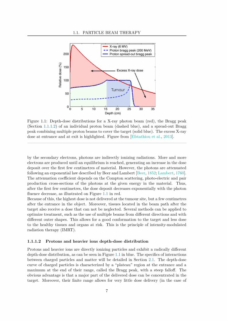
1.1. PARTICLE BEAM THERAPY
Figure 1.1: Depth-dose distributions for a X-ray photon beam (red), the Bragg peak(Section 1.1.1.2) of an individual proton beam (dashed blue), and a spread-out Braggpeak combining multiple proton beams to cover the target (solid blue). The excess X-raydose at entrance and at exit is highlighted. Figure from [Efstathiou et al., 2013].
by the secondary electrons, photons are indirectly ionizing radiations. More and moreelectrons are produced until an equilibrium is reached, generating an increase in the dosedeposit over the first few centimetres of material. However, the photons are attenuatedfollowing an exponential law described by Beer and Lambert [Beer, 1852; Lambert, 1760].The attenuation coefficient depends on the Compton scattering, photo-electric and pairproduction cross-sections of the photons at the given energy in the material. Thus,after the first few centimetres, the dose deposit decreases exponentially with the photonfluence decrease, as illustrated on Figure 1.1 in red.Because of this, the highest dose is not delivered at the tumour site, but a few centimetresafter the entrance in the object. Moreover, tissues located in the beam path after thetarget also receive a dose that can not be neglected. Several methods can be applied tooptimize treatment, such as the use of multiple beams from different directions and withdifferent outer shapes. This allows for a good conformation to the target and less doseto the healthy tissues and organs at risk. This is the principle of intensity-modulatedradiation therapy (IMRT).
1.1.1.2 Protons and heavier ions depth-dose distribution
Protons and heavier ions are directly ionizing particles and exhibit a radically differentdepth-dose distribution, as can be seen in Figure 1.1 in blue. The specifics of interactionsbetween charged particles and matter will be detailed in Section 2.1. The depth-dosecurve of charged particles is characterized by a “plateau” region at the entrance and amaximum at the end of their range, called the Bragg peak, with a steep falloff. Theobvious advantage is that a major part of the delivered dose can be concentrated in thetarget. Moreover, their finite range allows for very little dose delivery (in the case of
7
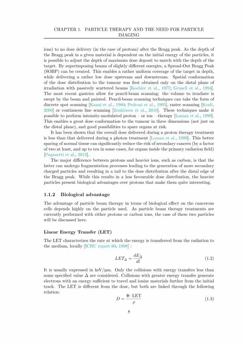
CHAPTER 1. PARTICLE THERAPY AND THE NEED FOR PARTICLEIMAGING
ions) to no dose delivery (in the case of protons) after the Bragg peak. As the depth ofthe Bragg peak in a given material is dependent on the initial energy of the particles, itis possible to adjust the depth of maximum dose deposit to match with the depth of thetarget. By superimposing beams of slightly different energies, a Spread-Out Bragg Peak(SOBP) can be created. This enables a rather uniform coverage of the target in depth,while delivering a rather low dose upstream and downstream. Spatial conformationof the dose distribution to the tumour was first obtained only on the distal plane ofirradiation with passively scattered beams [Koehler et al., 1977; Grusell et al., 1994].The most recent gantries allow for pencil-beam scanning: the volume to irradiate isswept by the beam and painted. Pencil-beam scanning techniques can take the form ofdiscrete spot scanning [Kanai et al., 1980; Pedroni et al., 1995], raster scanning [Kraft,2000] or continuous line scanning [Zenklusen et al., 2010]. These techniques make itpossible to perform intensity-modulated proton – or ion – therapy [Lomax et al., 1999].This enables a great dose conformation to the tumour in three dimensions (not just onthe distal plane), and good possibilities to spare organs at risk.
It has been shown that the overall dose delivered during a proton therapy treatmentis less than that delivered during a photon treatment [Lomax et al., 1999]. This bettersparing of normal tissue can significantly reduce the risk of secondary cancers (by a factorof two at least, and up to ten in some cases, for organs inside the primary radiation field)[Paganetti et al., 2012].
The major difference between protons and heavier ions, such as carbon, is that thelatter can undergo fragmentation processes leading to the generation of more secondarycharged particles and resulting in a tail to the dose distribution after the distal edge ofthe Bragg peak. While this results in a less favourable dose distribution, the heavierparticles present biological advantages over protons that make them quite interesting.
1.1.2 Biological advantage
The advantage of particle beam therapy in terms of biological effect on the cancerouscells depends highly on the particle used. As particle beam therapy treatments arecurrently performed with either protons or carbon ions, the case of these two particleswill be discussed here.
Linear Energy Transfer (LET)
The LET characterizes the rate at which the energy is transferred from the radiation tothe medium, locally [ICRU report 60, 1998] :
LET∆ =dE∆
dl(1.2)
It is usually expressed in keV/µm. Only the collisions with energy transfers less thansome specified value ∆ are considered. Collisions with greater energy transfer generateelectrons with an energy sufficient to travel and ionize materials further from the initialtrack. The LET is different from the dose, but both are linked through the followingrelation:
D =Φ · LET
ρ(1.3)
8
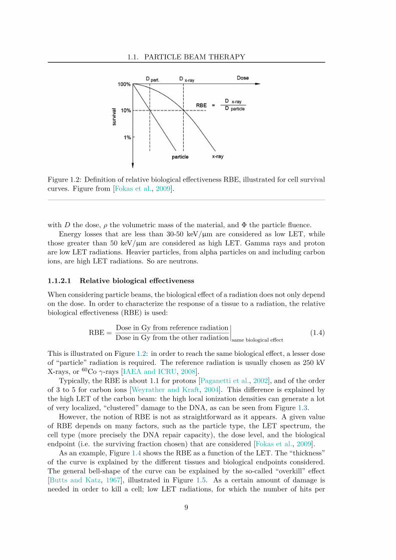
1.1. PARTICLE BEAM THERAPY
Figure 1.2: Definition of relative biological effectiveness RBE, illustrated for cell survivalcurves. Figure from [Fokas et al., 2009].
with D the dose, ρ the volumetric mass of the material, and Φ the particle fluence.Energy losses that are less than 30-50 keV/µm are considered as low LET, while
those greater than 50 keV/µm are considered as high LET. Gamma rays and protonare low LET radiations. Heavier particles, from alpha particles on and including carbonions, are high LET radiations. So are neutrons.
1.1.2.1 Relative biological effectiveness
When considering particle beams, the biological effect of a radiation does not only dependon the dose. In order to characterize the response of a tissue to a radiation, the relativebiological effectiveness (RBE) is used:
RBE =Dose in Gy from reference radiationDose in Gy from the other radiation
∣
∣
∣
∣
same biological effect
(1.4)
This is illustrated on Figure 1.2: in order to reach the same biological effect, a lesser doseof “particle” radiation is required. The reference radiation is usually chosen as 250 kVX-rays, or 60Co γ-rays [IAEA and ICRU, 2008].
Typically, the RBE is about 1.1 for protons [Paganetti et al., 2002], and of the orderof 3 to 5 for carbon ions [Weyrather and Kraft, 2004]. This difference is explained bythe high LET of the carbon beam: the high local ionization densities can generate a lotof very localized, “clustered” damage to the DNA, as can be seen from Figure 1.3.
However, the notion of RBE is not as straightforward as it appears. A given valueof RBE depends on many factors, such as the particle type, the LET spectrum, thecell type (more precisely the DNA repair capacity), the dose level, and the biologicalendpoint (i.e. the surviving fraction chosen) that are considered [Fokas et al., 2009].
As an example, Figure 1.4 shows the RBE as a function of the LET. The “thickness”of the curve is explained by the different tissues and biological endpoints considered.The general bell-shape of the curve can be explained by the so-called “overkill” effect[Butts and Katz, 1967], illustrated in Figure 1.5. As a certain amount of damage isneeded in order to kill a cell; low LET radiations, for which the number of hits per
9
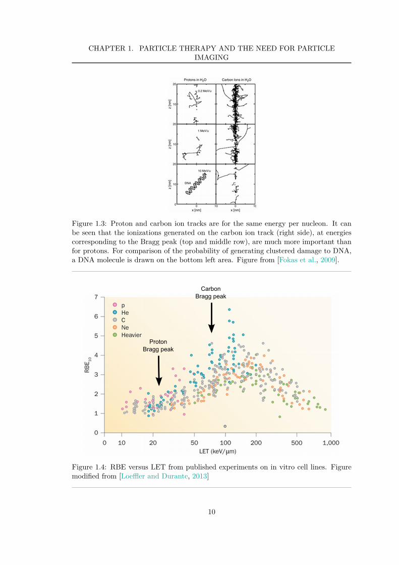
CHAPTER 1. PARTICLE THERAPY AND THE NEED FOR PARTICLEIMAGING
Figure 1.3: Proton and carbon ion tracks are for the same energy per nucleon. It canbe seen that the ionizations generated on the carbon ion track (right side), at energiescorresponding to the Bragg peak (top and middle row), are much more important thanfor protons. For comparison of the probability of generating clustered damage to DNA,a DNA molecule is drawn on the bottom left area. Figure from [Fokas et al., 2009].
Figure 1.4: RBE versus LET from published experiments on in vitro cell lines. Figuremodified from [Loeffler and Durante, 2013]
10
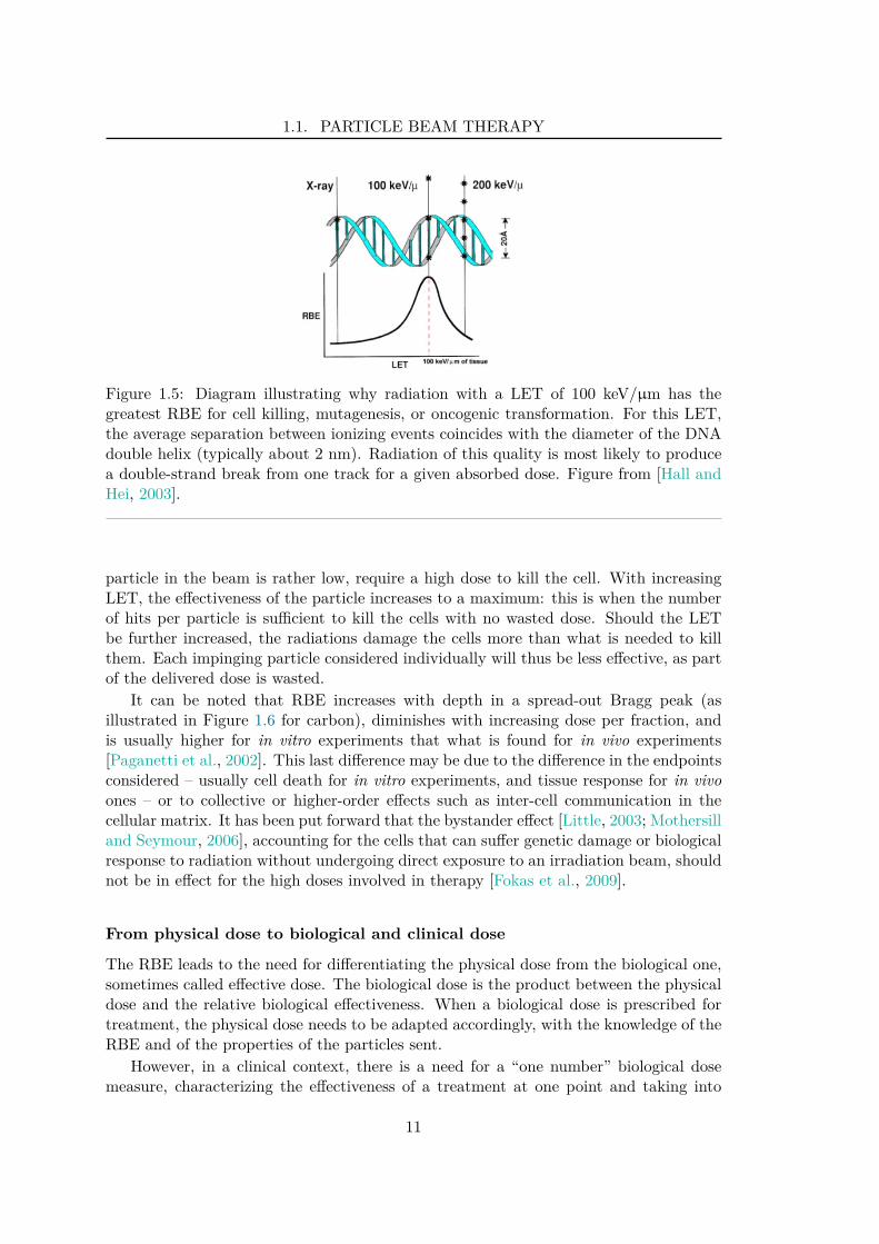
1.1. PARTICLE BEAM THERAPY
Figure 1.5: Diagram illustrating why radiation with a LET of 100 keV/µm has thegreatest RBE for cell killing, mutagenesis, or oncogenic transformation. For this LET,the average separation between ionizing events coincides with the diameter of the DNAdouble helix (typically about 2 nm). Radiation of this quality is most likely to producea double-strand break from one track for a given absorbed dose. Figure from [Hall andHei, 2003].
particle in the beam is rather low, require a high dose to kill the cell. With increasingLET, the effectiveness of the particle increases to a maximum: this is when the numberof hits per particle is sufficient to kill the cells with no wasted dose. Should the LETbe further increased, the radiations damage the cells more than what is needed to killthem. Each impinging particle considered individually will thus be less effective, as partof the delivered dose is wasted.
It can be noted that RBE increases with depth in a spread-out Bragg peak (asillustrated in Figure 1.6 for carbon), diminishes with increasing dose per fraction, andis usually higher for in vitro experiments that what is found for in vivo experiments[Paganetti et al., 2002]. This last difference may be due to the difference in the endpointsconsidered – usually cell death for in vitro experiments, and tissue response for in vivoones – or to collective or higher-order effects such as inter-cell communication in thecellular matrix. It has been put forward that the bystander effect [Little, 2003; Mothersilland Seymour, 2006], accounting for the cells that can suffer genetic damage or biologicalresponse to radiation without undergoing direct exposure to an irradiation beam, shouldnot be in effect for the high doses involved in therapy [Fokas et al., 2009].
From physical dose to biological and clinical dose
The RBE leads to the need for differentiating the physical dose from the biological one,sometimes called effective dose. The biological dose is the product between the physicaldose and the relative biological effectiveness. When a biological dose is prescribed fortreatment, the physical dose needs to be adapted accordingly, with the knowledge of theRBE and of the properties of the particles sent.
However, in a clinical context, there is a need for a “one number” biological dosemeasure, characterizing the effectiveness of a treatment at one point and taking into
11
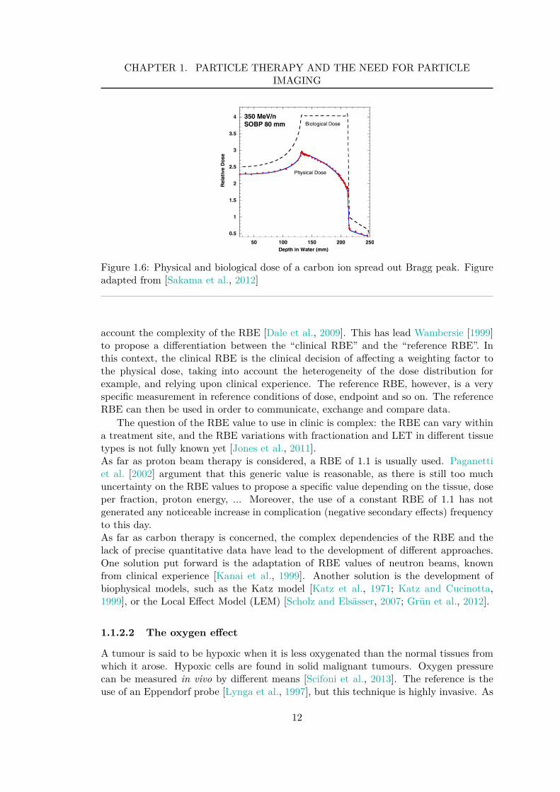
CHAPTER 1. PARTICLE THERAPY AND THE NEED FOR PARTICLEIMAGING
Figure 1.6: Physical and biological dose of a carbon ion spread out Bragg peak. Figureadapted from [Sakama et al., 2012]
account the complexity of the RBE [Dale et al., 2009]. This has lead Wambersie [1999]to propose a differentiation between the “clinical RBE” and the “reference RBE”. Inthis context, the clinical RBE is the clinical decision of affecting a weighting factor tothe physical dose, taking into account the heterogeneity of the dose distribution forexample, and relying upon clinical experience. The reference RBE, however, is a veryspecific measurement in reference conditions of dose, endpoint and so on. The referenceRBE can then be used in order to communicate, exchange and compare data.
The question of the RBE value to use in clinic is complex: the RBE can vary withina treatment site, and the RBE variations with fractionation and LET in different tissuetypes is not fully known yet [Jones et al., 2011].As far as proton beam therapy is considered, a RBE of 1.1 is usually used. Paganettiet al. [2002] argument that this generic value is reasonable, as there is still too muchuncertainty on the RBE values to propose a specific value depending on the tissue, doseper fraction, proton energy, ... Moreover, the use of a constant RBE of 1.1 has notgenerated any noticeable increase in complication (negative secondary effects) frequencyto this day.As far as carbon therapy is concerned, the complex dependencies of the RBE and thelack of precise quantitative data have lead to the development of different approaches.One solution put forward is the adaptation of RBE values of neutron beams, knownfrom clinical experience [Kanai et al., 1999]. Another solution is the development ofbiophysical models, such as the Katz model [Katz et al., 1971; Katz and Cucinotta,1999], or the Local Effect Model (LEM) [Scholz and Elsasser, 2007; Grun et al., 2012].
1.1.2.2 The oxygen effect
A tumour is said to be hypoxic when it is less oxygenated than the normal tissues fromwhich it arose. Hypoxic cells are found in solid malignant tumours. Oxygen pressurecan be measured in vivo by different means [Scifoni et al., 2013]. The reference is theuse of an Eppendorf probe [Lynga et al., 1997], but this technique is highly invasive. As
12
1.1. PARTICLE BEAM THERAPY
a consequence, efforts have been directed to tracers for Positron Emission Tomography(PET), although challenges, such as the difficulty to correlate the uptake to the effectiveoxygen content, remain. The potential use of functional Magnetic Resonance Imaging(MRI) has also been put forward [Krishna et al., 2001].
It was shown quite early in the history of radiotherapy that hypoxic tumours areresistant to X-rays, which can lead to a failure of the therapy [Moulder and Rockwell,1987]. This is characterized by the Oxygen Enhancement Ratio (OER), which is definedas the ratio between the dose required to cause an effect in a hypoxic cell to the doserequired to cause the same effect to a normal cell:
OER =Dose required in hypoxic conditions
Dose required with standard oxygenation
∣
∣
∣
∣
same biological effect
(1.5)
Indeed, for low-LET particles, hypoxic cells are 2.5 to 3 times more radio-resistant thanwell oxygenated cells. This effect diminishes with increasing LET of the impingingparticles, with the OER tending towards one for high-LET particles [Barendsen et al.,1963; Wambersie et al., 2004].
A generally accepted explanation for this is the “oxygen fixation hypothesis” [Halland Giaccia, 2012]: in the presence of oxygen, the free radicals produced by the radiationin the cell can form an organic peroxide, which is a non-restorable form of the target.As this can not happen without the presence of molecular oxygen, it is said that oxygenfixes (sets) the damage. Thus, the quantity of damage inflicted to a cell is higher whenthe oxygen pressure is higher.
Most of the damages produced by high-LET particles are so-called direct damages,breaking the DNA. Low-LET radiations, however, rely more heavily on indirect damagesinduced by free radicals, and their effect is therefore more dependent on the oxygenstatus.
1.1.2.3 Dependence of the phase in the cell cycle
The radio-sensitivity of cells also depends on their replication phase [Fidorra and Linden,1977]. This can be explained by the change in DNA compactness, or by the presence of areplication check-point. For example, the cells regularly “check” if the replication processwas performed correctly (in phase G2), leading to a decrease in the radio-sensitivity justbefore the beginning of this phase [Hansen Ree et al., 2006]. Tissue cells are usuallyasynchronous, but an extreme stress such as a first irradiation modifies that. Becauseof this, it is important during fractionated treatment of radiotherapy to randomize thetime of irradiation in order to reduce the risks of recurrently hitting in a radio-resistantphase.
It was shown that high-LET particles are more potent inducers of cell cycle delays,and are less sensitive to the cell phase [Fournier and Taucher-Scholz, 2004]. The benefitof the reduction in the variation of the cell radio-sensitivity along its mitotic cycle in thecase of high-LET particles remains unclear [Wambersie et al., 2004].
1.1.2.4 In brief...
Particle beam therapy, in this context carbon therapy even more so than protontherapy, shows a great radio-biological advantage over standard radiotherapy, with a
13
CHAPTER 1. PARTICLE THERAPY AND THE NEED FOR PARTICLEIMAGING
high RBE and a low OER. The benefit for treatment however, is not strictly due tothese characteristics; neutron beams also show high RBE and low OER [Weyrather andKraft, 2004]. The superiority of ion beam therapy comes from the fact that the beamquality changes along the depth, and that the RBE increases, reinforcing the advantagesof the depth-dose distribution. This leads to a good tumour response without the severeside effects in the normal tissues of neutron therapy [Skarsgard, 1998]. However, muchresearch on the RBE values, mechanisms of cell death and repair pathways, is stillongoing [Dale et al., 2009].
1.1.3 Clinical trials, cost and cost-effectiveness
Hadron therapy is currently quite a trendy topic. From the previous sections, one cansee all the advantages that these treatments can bring. However, even more questionscome with it. Because of the difference in the LET and biological effects, the cases ofprotons and carbon ions are not the same.
1.1.3.1 Protons
Proton beams can present a much higher dose conformity to the lesion than X-ray beams.Four arguments are put forward by Goitein [2010]:
– For the same dose to the target volume, protons deliver a lower physicaldose to the uninvolved normal tissues than do high energy X-rays
– There is very little difference in tissue response per unit dose betweenprotons of therapeutic energies as compared with high-energy X-rays,so that the only relevant differences are physical
– There is no medical reason to irradiate any tissue judged not to containmalignant cells
– Radiation damages normal tissues, as it does tumors, and the severityof that damage increases with increasing dose
The conclusion is that protons are intrinsically better than photons for therapy. However,it has not been demonstrated yet that, in a clinical setting, protons are better for alltumour localisations. The use of proton beams to treat prostate cancer, for example, issubject to controversies [Efstathiou et al., 2013]. Two distinct points are discussed. Thefirst is whether or not particle beam therapy is better than X-ray beam therapy. Thesecond is whether particle beam therapy is worth the additional expenses, compared toconventional radiotherapy.
While physicists in general have no trouble stating that protons are intrinsicallymore favourable than photons for treating tumours, the conclusion that it should bewidespread and put into routine clinical practice is not so obvious for all the scientificcommunity. As an example, W. Robert Lee advocates that “the burden of proof lies upona person making claims rather than shifting the burden of proof to the others” [Sakuraiet al., 2012]. Thus, people claiming that particle beam therapy is better have to supportthis claim with clinical results, ensuing from randomized clinical trials. As pointed outby Olsen et al. [2007], this position is also supported by the Helsinki declaration (a text
14
1.1. PARTICLE BEAM THERAPY
adopted by the world medical association on the ethical principles for medical researchinvolving human subjects). Article 6 therein states:
Even the best proven prophylactic, diagnostic, and therapeutic methodsmust continuously be challenged through research for their effectiveness.
These arguments for randomized clinical trials comparing proton treatments tophoton treatments are the source of a problem of ethics for some. The main causeis the need for the two arms of a trial (here, the two treatments compared) to be inequipoise: one needs not to know whether one is better or not – otherwise it wouldmean sending patients to receive a treatment that you believe is not the best. Goitein[2010] highlights this notion of equipoise:
There is a school of thought which distinguishes between ‘clinical equipoise’(the lack of definitive clinical results which show the arms to be different)and what is somewhat pejoratively described as ‘theoretical equipoise’ whichis based on other than clinical data.
It can also be stated that no such phase III clinical trials were requested before the usein routine of intensity-modulated radiotherapy, or stereotaxic radio-surgery for example[Suit et al., 2008]. In turn, randomized clinical trials are better suited and can bringvery useful to compare one thing at a time, so that it can be scientifically interpreted[Goitein, 2010]. Randomized trials are undeniably useful to help determine an optimizedfractionation schedule for example, or to answer the ‘bath or shower dilemma’: whethera low dose to a large area of healthy tissues is preferable or not to a more localized higherdose. Another imperative of randomized clinical trials is the time frame in which theytake place [Glimelius and Montelius, 2007]. The gain needs to be clinically relevant anddetectable within three to five years. However, treatment technology is evolving todayat a rate so fast that it means to acquire “today’s evidence on yesterday’s technology”[Olsen et al., 2007]. Clinical trials therefore need to be a worldwide effort not to taketoo much time to collect the necessary data. Current clinical trials can be found onluneat [Particle Therapy Cooperative Group] and [US National Institute of Health]. Somephase III randomized trials involve the evaluation of side-effects for prostate cancer forexample. Indeed, as a polemic surrounds the pertinence of directing prostate cancerpatients towards proton therapy, the clinical trials could help bring an answer.
Nevertheless, even though the ethics of randomized clinical trials can be discussedin the scientific community, a last argument gives incentive to perform them. Onereason why there is such debate about proton treatments, when there was not for othertreatment modalities, is the cost of particle beam therapy [Goitein and Cox, 2008]:
Can anyone seriously believe that, if protons were cheaper than X-rays, therewould be similar objections raised as to their widespread use?
Current societies rely on health insurance systems to pay for treatments. And as inany such system, the question of cost-effectiveness of the treatments appears. It can notbe neglected because a high cost associated to a treatment with no clear advantage overa cheaper one limits the availability of resources for other patients [Efstathiou et al.,2013].
15
CHAPTER 1. PARTICLE THERAPY AND THE NEED FOR PARTICLEIMAGING
The main problem encountered is that studies reporting on the cost-effectiveness ofparticle beam therapy often have to rely on assumptions, and authors suffer from thelack of data, both on the cost and on the effectiveness [Lundkvist et al., 2005]. Differentstudies have evaluated the cost of a proton treatment to be between two and four timesthat of X-ray therapy [Goitein and Jermann, 2003; Peeters et al., 2010]. However,a reduction in the number of fractions of a proton treatment may reduce this ratio.Similarly, the widespread use of proton therapy may reduce the costs.
It has been put forward that the key to cost-effectiveness for proton therapy mayreside in the selection of patient [Ramaekers, 2013]. Not all patients would benefit froma proton treatment rather than IMRT. For some cases, such as paediatric cancer orspecific treatment sites close to organs at risk (eye, head and neck), there is very littledoubt that proton therapy is advantageous. For tumour sites that are not recognizedas systematically better treated by protons, the scientific community in Netherlands forexample has proposed a system of patient selection based on normal tissue complicationprobability and in silico treatment plans [Eekers, 2014]. Results collected after treatmentof these patients may then help improve models and evaluate the efficiency for a well-selected patient population, that surely will be more advantageous than to consider allpotential patients.
1.1.3.2 Carbon ions
The case of randomized clinical trials for carbon beam therapy is not as controversial asfor proton beam therapy. The main reason is the difference in the biological impact of thehigh-LET particles: the effectiveness is quite different than that of photons. Randomizedclinical trials would be of great interest to test the impact of LET by comparingprotons to carbon ions for example. Such current trials involve, amongst others, thecomparison of proton therapy to carbon therapy for skull-base chondrosarcoma [USNational Institute of Health, 2014].
However, the same question in the matter of cost-effectiveness stands. It is animportant question, not so much from the scientific point of view of a physicist, butfrom the point of view of the clinical world, and investment politics. This is because“We do not yet know whether, overall, any improvements in clinical results achievedwith hadron therapy are sufficient to warrant such an extensive investment of time andmoney” [Lodge et al., 2007].
There are indications that particle beam therapy could be cost-effective, for locallyrecurrent rectal cancer [Mobaraki et al., 2010] or some tumours which are typicallytreated by a combination of surgery and radiotherapy and for which the tumour controlrate can clearly be increased using ions [Jakel et al., 2007].
The lack of data however, both on the cost and on the effectiveness, is greater thanfor protons, due to the limited number of centres and patients treated [Mobaraki et al.,2010]. Few facilities have been operating for long enough to have “good” data, leadingto large uncertainties on the cost estimates [Jakel et al., 2007]. The cost of carbontherapy amounts up to nearly five times that of X-ray therapy [Peeters et al., 2010].However, the potential reduction of the number of fractions and the increased tumourcontrol probability could lead to a reduction of long term cost and relative cost comparedto standard radiotherapy [Goitein and Jermann, 2003; Pijls-Johannesma et al., 2008;
16
1.2. TREATMENT PLANNING AND UNCERTAINTIES IN PARTICLE BEAMTHERAPY
Peeters et al., 2010]. As far as the effectiveness is concerned, randomized clinical trialswould be a good way to quantify this.
1.2 Treatment planning and uncertainties in particle beamtherapy
1.2.1 Treatment planning for particle beam therapy
Like for conventional radiotherapy, the treatment planning for particle beam therapyis based on the information about the tissues obtained from an X-ray computedtomography (CT) image. On this image, the contours of the tumour region and theorgans at risk are drawn by the physician. Other imaging modalities can be used forcomplementary information, such as positron emission tomography (PET) or magneticresonance imaging (MRI) images. A treatment plan based on MRI images was alsoproposed by Rank et al. [2013], but the values were converted to pseudo CT numbers.Therefore, even in that case, the following explications stand from section 1.2.1.2 on.The CT image is then used in the treatment planning system, in order to calculate andoptimize the dose delivery. Two types of treatment plan calculation exist nowadays:the first is analytical, the second is based on Monte Carlo simulations. For analyticaldose calculations, the X-ray CT image is converted into a relative stopping power (RSP)image, with water as a reference. Beam spread and nuclear interactions are also scaledusing the CT image. For Monte Carlo dose calculations, the CT numbers are convertedinto material compositions.
The following sections briefly describe the principle of X-ray imaging, and theconversion from CT numbers used for treatment planning.
1.2.1.1 X-ray CT imaging
The basic principle of X-ray CT is the following: after sending an X-ray flux I0, theflux I upon exit from the object can be measured. Usually, a photon beam of voltagebetween 30 and 150 kV is sent through matter. The photon flux is attenuated followingan exponential law, according to the linear attenuation coefficient of the materials. Thislinear attenuation coefficient µ(x, y, z, E), in a point of coordinates (x, y, z), depends onthe energy of the photons E. For a given ray reaching the detector at the position (u, v)after the path Li, the projection measurement is:
I(u, v) =∫
Ii(E) exp(
−∫
Li
µ (x, y, z, E) dl
)
dE (1.6)
where Ii(E) takes into account the energy dependence of the incident ray sourcespectrum, and the detector sensitivity.
The images acquired with a CT scanner are usually scaled to represent a map of theCT numbers of the tissues. The CT numbers are expressed in Hounsfield Units (HU),defined as:
CT =(
µmat − µwater
µwater
)
× 1000 (1.7)
with µwater the linear attenuation coefficient of water.
17
CHAPTER 1. PARTICLE THERAPY AND THE NEED FOR PARTICLEIMAGING
Because the source emission presents an energy spectrum, the values of massattenuation coefficients, and therefore CT numbers, represent average values for thegiven spectrum.
The linear mass attenuation coefficient µ can be semi-empirically expressed as follows[Jackson and Hawkes, 1981]:
µ = ρne
(
KphZ3.62 + KcohZ1.86 + KKN)
(1.8)
with ρ the density of material. For a material composed of different elements:
Z =[
∑
λiZ3.62i
]1/3.62(1.9)
Z =[
∑
λiZ1.86i
]1/1.86(1.10)
λi =(ne)i
ne(1.11)
where Zi is the atomic number of each element, (ne)i the electron density of each element,ne the total electron density and Kph, Kcoh and KKN are coefficients for the photo-electric effect, coherent (Rayleigh) scattering and Compton scattering respectively.
1.2.1.2 Conversion of X-ray CT numbers
To proceed to analytical dose calculation for ion beam therapy, it is necessary to convertthe CT numbers into the RSP of the materials (described in section 2.1), in orderto predict the energy loss of the particles. It can be seen from Figure 1.7 that CTnumbers and RSP are strongly correlated. This is because the electron density of thematerials greatly contributes to both. The use of such a conversion in order to use X-rayCT scans for radiotherapy treatment planning was introduced by Mustafa and Jackson[1983]. Different methods can be used to obtain a conversion curve, the most frequentlyused being the stoichiometric approach [Schneider et al., 1996], based on the elementaldecomposition of tissue substitutes. Because of the X-ray CT acquisition, the calibrationis scanner-dependent. It also depends on the position of the object in the field of view.The data obtained from the calibration can then be fitted, by a broken line for example.The method has been improved with patient-specific optimization of the Hounsfield look-up table [Schneider et al., 2005]. Other approaches have also been put forward, such asthe polybinary tissue model-based calibration [Kanematsu and Matsufuji, 2003].
Monte Carlo simulations, on the other hand, require the description of materialswith their elemental composition and mass density. It means that a conversion fromCT numbers to materials is required. In order to do so, conversions based on astoichiometric calibration, similar to the one that can be used for the conversion torelative stopping power, have been put forward [Jiang et al., 2007]. The principle isthe following [Schneider, 2000]: the CT image is segmented and thresholds are appliedto differentiate groups of materials with similar CT numbers. A constant elementalcomposition is attributed to each group, and the materials are adjusted inside eachgroup by varying the mass density.
18
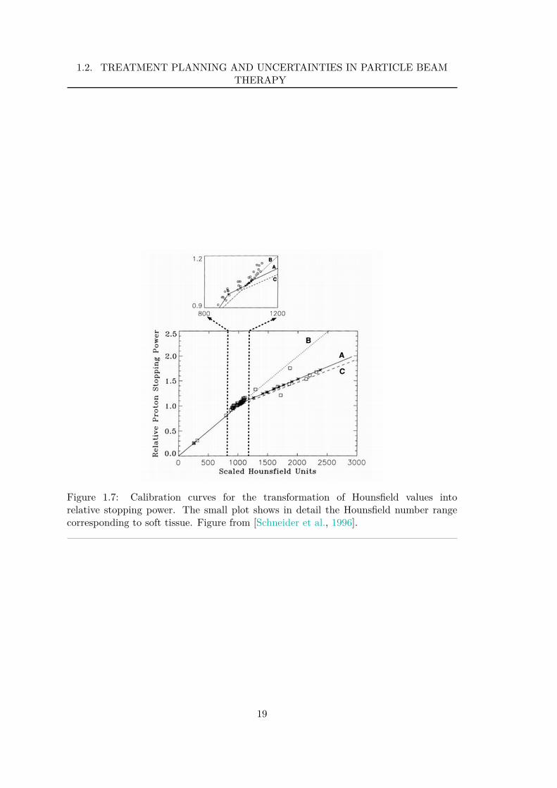
1.2. TREATMENT PLANNING AND UNCERTAINTIES IN PARTICLE BEAMTHERAPY
Figure 1.7: Calibration curves for the transformation of Hounsfield values intorelative stopping power. The small plot shows in detail the Hounsfield number rangecorresponding to soft tissue. Figure from [Schneider et al., 1996].
19
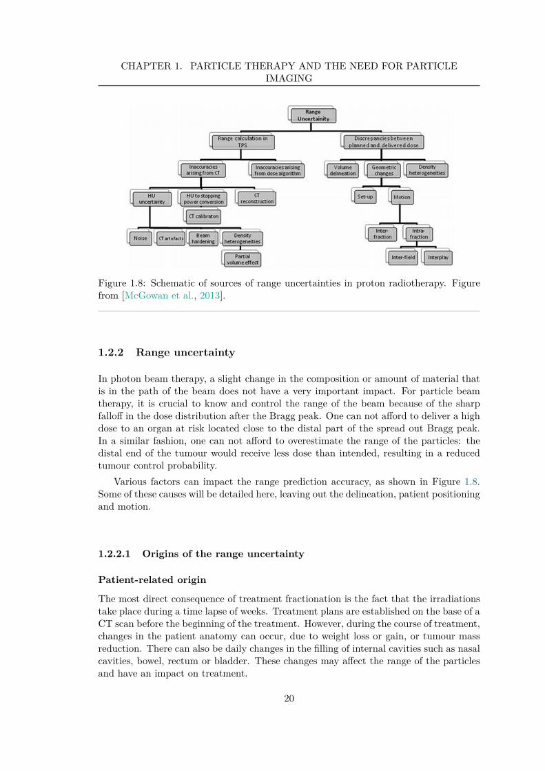
CHAPTER 1. PARTICLE THERAPY AND THE NEED FOR PARTICLEIMAGING
Figure 1.8: Schematic of sources of range uncertainties in proton radiotherapy. Figurefrom [McGowan et al., 2013].
1.2.2 Range uncertainty
In photon beam therapy, a slight change in the composition or amount of material thatis in the path of the beam does not have a very important impact. For particle beamtherapy, it is crucial to know and control the range of the beam because of the sharpfalloff in the dose distribution after the Bragg peak. One can not afford to deliver a highdose to an organ at risk located close to the distal part of the spread out Bragg peak.In a similar fashion, one can not afford to overestimate the range of the particles: thedistal end of the tumour would receive less dose than intended, resulting in a reducedtumour control probability.
Various factors can impact the range prediction accuracy, as shown in Figure 1.8.Some of these causes will be detailed here, leaving out the delineation, patient positioningand motion.
1.2.2.1 Origins of the range uncertainty
Patient-related origin
The most direct consequence of treatment fractionation is the fact that the irradiationstake place during a time lapse of weeks. Treatment plans are established on the base of aCT scan before the beginning of the treatment. However, during the course of treatment,changes in the patient anatomy can occur, due to weight loss or gain, or tumour massreduction. There can also be daily changes in the filling of internal cavities such as nasalcavities, bowel, rectum or bladder. These changes may affect the range of the particlesand have an impact on treatment.
20
1.2. TREATMENT PLANNING AND UNCERTAINTIES IN PARTICLE BEAMTHERAPY
Biological range uncertainty
As far as protons are concerned, the average value of the RBE at the centre of aSOBP (spread-out Bragg peak) was shown to be 1.1 [Schulz-Ertner et al., 2006]. Thisapproximation of a single, generic RBE is frequently used in clinical therapy centres anddoes not take the LET-dependence into account. Therefore, the use of such a singlevalue has been reassessed and it was shown that while the approximation is reasonable,a local “hot region” at the end of the SOBP generates an extension of the biologicalrange [Paganetti et al., 2002]. This extension can be of the order of the millimetre. Thisdifference builds up with the increasing range of the incoming particles, but decreaseswith the dose, and thus is dependent on the fractionation scheme [Carabe et al., 2012].These uncertainties will affect the precision of the dose calculation algorithm.
Physical origin of range uncertainty
As the range is computed based on the converted CT images, range uncertainty has twosources: the CT numbers themselves (accuracy, noise, artefacts in the image), and theconversion [Yang et al., 2012].
– Voxel size, noise, and partial volume effect:These factors have been shown to have an impact on the predicted range of theparticles. For a given system, the noise in the image is inversely proportional tothe size of the image voxels. It was shown that an increase in the noise of the CTimage, and thus a fluctuation of the CT numbers that are converted to stoppingpower, leads to a linear increase in the range uncertainty [Chvetsov and Paige,2010]. As an illustration, they reported an uncertainty (standard deviation) ofthe range between 0.3% and 0.7% for voxels in the CT image of 3×3×3 mm3
and a 2.5% noise level. However, large voxel size also has a negative effect onthe range calculation [Chvetsov and Paige, 2010; Espana and Paganetti, 2011],especially because small inhomogeneities have an impact on the calculated range.This effect is important in regions such as the lung. Espana and Paganetti [2011]show, for example, a difference between planned and expected range up to 4 mmfor a heterogeneous random lung, assuming treatment plan with a 2×2×2.5 mm3
grid.
– Beam hardening:X-ray sources used for CT images are polychromatic, meaning that a spectrum ofenergy is generated, generally between 30 and 140 kV for clinical CT scanners.However, the linear mass attenuation coefficients that rule the fluence loss ofthe photons are energy-dependent, as can be seen in Equation 1.6. Thereby thespectrum is modified and its mean shifted towards higher energies throughout thepenetration in the object to image. This generates artefacts in the reconstructedCT image typically characterized by a cupping effect (the profile of an homogeneousmedium appears brighter on the extremities and darker at the centre where CTnumbers are under-estimated) and by dark streaks in the image. It has been shownthat beam hardening effects can cause considerable errors in the range prediction,especially for high-density materials [Schaffner and Pedroni, 1998]. They estimatethat the determination of the stopping power value from calibrated CT images in
21
CHAPTER 1. PARTICLE THERAPY AND THE NEED FOR PARTICLEIMAGING
clinical situations and in high-density material is therefore only accurate to about±1.5% due to beam hardening.
– Metal artefacts:The presence of metal, for hip prosthesis or dental filling for example, greatlydegrades the accuracy of the reconstructed image. The density of metal is beyondthe normal range that can be handled by the acquisition system of a CT scanner.The resulting extreme attenuation of photons generates incomplete attenuationprofiles which, in turn, translates into very bright spots in the image at thelocation of the metal and in bright and dark streaks coming from that point.As a consequence, the reconstructed CT numbers are erroneous. This can havea great impact on the treatment plan accuracy for proton and heavier ion beamtherapy, with a range variation up to 18% for steel hip prosthesis should the beamgo through the implant [Jakel and Reiss, 2007]. Because of this, treatment plannersdo their best to avoid beam paths through the metal. However, the artefacts causevariations of the CT numbers of the tissues in the whole image, affecting the othertissues as well. The impact is less important in these other tissues, but can not beneglected. While metal artefacts also have an impact on treatment plans of otherradiations, whether photons or electrons, it was shown that its impact is mostimportant for particle therapy due to the potential error on the range prediction[Wei et al., 2006].
– Conversion from CT numbers:The accuracy on the obtained RSP values also depends on the parametrisation ofthe fit for the calibration curve, the goodness of the approximation between thetissue substitutes and the composition of real body tissues, the mean excitationpotential chosen for the calculation and the energy-dependence of the RSP [Yanget al., 2012]. It is estimated that the use of a stoichiometric calibration generatesan uncertainty of about 0.5% [Paganetti, 2012]. It can be noted that, even with avery accurate calibration procedure, an uncertainty will always remain: because ofthe difference in the interaction mechanisms between charged particles and photonsin matter, the transformation from CT numbers to RSP is not bijective.
Monte Carlo dose calculations allow for accurate considerations of the physicalprocesses. However, information on the elemental composition and mass density ofeach tissue is needed and extracted from the planning CT image. This process alsorelies on the calibration of material composition and density with the CT numbers.In a similar fashion to the RSP conversion, the transformation from one to the otheris not linear, and assumptions on the materials and density are made. Jiang et al.[2007] conclude their study by stating that “Radiation therapy with heavy chargedparticle beams requires more accurate knowledge on the relative stopping powerin order to convert Hounsfield numbers [to materials] ”. Nevertheless, Paganetti[2012] estimates that the uncertainties on the range using this method should besmaller than the ones for analytical dose calibration.
22
1.2. TREATMENT PLANNING AND UNCERTAINTIES IN PARTICLE BEAMTHERAPY
1.2.2.2 Consequences for treatment planning and treatment
Range uncertainty and margins for treatment planning
One consequence is that the beam direction is never chosen so that a critical structure isplaced just distal to the Bragg peak, for fear of over-shooting and damaging the criticalstructure. Beam directions are chosen so that the lateral penumbra, which is ratherwell-known, is used to spare critical organs. This means that the sharpness of the peakand the advantage of the no-dose behind it are not fully exploited.
Another consequence is the increase of the ‘safety margins’ and thus the irradiatedvolume, also called planning target volume (PTV). Typically, the PTV is defined inthe following way: the Gross Tumour Volume (GTV) seen on X-ray CT, MRI, PET orSPECT (Single-Photon Emission Computed Tomography) images is delineated. ThisGTV is contained in a larger volume, the Clinical Target Volume (CTV), that aims attaking into account the potential microscopic spread of the disease that could not beseen on the images. The PTV encapsulates the last volumes adding margins accountingfor uncertainties in planning or treatment delivery.
In order to take the range uncertainty into account, the margins added whenestablishing the PTV in particle therapy are rather large. Here are examples of marginsused for proton therapy [Paganetti, 2012]:
– Massachusetts General Hospital (Boston): 3.5% of range + 1 mm
– MD Anderson Proton Therapy Center (Huston), Loma Linda University MedicalCenter, Roberts Proton Therapy Center at the University of Pennsylvania: 3.5%+ 3 mm
– University of Florida Proton Therapy Institute: 2.5% + 1.5 mm
The need for these margins somehow reduces the attractiveness of ion beam therapy.While a precision weapon is available, allowing for better a sparing of the normal tissues,we are limited by the range uncertainty, causing the voluntary irradiation of a portionof normal tissue.
Quality control for ion beam therapy
The question of the precision in the irradiation has produced the need to worry moreabout quality control in ion beam therapy than previously for conventional radiotherapy.Means to verify the conformity of the irradiation to the treatment plan were investigated,and different methods have been proposed [Knopf and Lomax, 2013]. Amongst thesemethods, some are real-time measurements during the irradiations, others are pre- orpost- irradiation controls; some methods are invasive, others not. Here is a brief summaryof the potential solutions that have been investigated:
– Range probes and particle radiography (pre-irradiation control):
The idea of a range probe is the following: before treatment, a particle pencilbeam of energy sufficient to pass completely through the patient is sent andthe residual range is measured upon exit. This makes it possible to check theexpected range [Romero et al., 1995; Watts et al., 2009; Mumot et al., 2010]. This
23
CHAPTER 1. PARTICLE THERAPY AND THE NEED FOR PARTICLEIMAGING
approach has been implemented in many proton therapy centres. It was shownon Monte Carlo simulations performed using real X-ray CT data that in vivorange estimates at the level of 0.5% could be achieved [Mumot et al., 2010]. Thedose delivered is low – in the plateau region – and the method is fast. Based onthe same principle of measuring the residual range of the particles, the protonradiography concept makes use of a two-dimensional fluence of protons. In orderto increase spatial resolution, a proton radiography system measuring the entranceand exit coordinates with the range measurements has been proposed [Schneiderand Pedroni, 1995].
These concepts, first developed with protons, work the same way for ions, likecarbon [Ohno et al., 2004; Shinoda et al., 2006; Parodi, 2014].
– Point dose measurements (real-time control, direct, invasive):
It has been proposed to control the dose deposit in vivo using implantabledosimeters and using the time-dependence of the distribution delivered by rangemodulated passive scattering fields, using ionization chambers [Lu, 2008b] or semi-conductor diodes [Gottschalk et al., 2011]. This proposition was later generalizedto measuring SOBPs generated by complementary field pairs [Lu, 2008a] and forintensity modulated proton therapy (IMPT) plans [Lu, 2009]. The advantage ofthis method is that it provides a real-time and precise measurement of the dosedeposit. The potential sub-millimetric precision has yet to be confirmed in clinicalstudies on patients. Nevertheless, this technique presents the major drawback ofbeing invasive and provides information on a limited number of points that haveto be carefully chosen.
– Positron emission tomography (real-time or post-irradiation, indirect):
Nuclear interactions of protons or ions in the matter can generate the activationof the materials [Graffman and Jung, 1975; Bennett et al., 1978]. The productionof β+ emitters, of half life between 2 and 20 minutes in particular, is appropriatefor PET. Proton beams generate mostly 11C, 13N, 15O [Litzenberg and Bajema,1992], while carbon beams produce 10C, 11C, 15O [Enghardt, 2004a]. The detectionin coincidence of the photon pairs resulting from the annihilation of the emittedpositrons with electrons in the medium then allows for in vivo range verification.The activity profile obtained depends on the nature of the beam but is, both forproton and carbon therapy, strongly correlated to the dose distribution [Enghardt,2004b].
It has been shown that this technique makes it possible to detect deviations inthe patient positioning or local changes in the patient anatomy in the course of afractionated treatment [Enghardt, 2004b; Schardt et al., 2010].
PET monitoring can be performed either in-beam (during the irradiation) or off-line (just after the irradiation). Off-line PET imaging has the obvious advantagethat commercially available scanners can be used. In contrast, in-beam PETrequires the inclusion of the PET system around the treatment bed, generating
24
1.2. TREATMENT PLANNING AND UNCERTAINTIES IN PARTICLE BEAMTHERAPY
higher costs and challenges in image reconstruction due to the limited angle.Nevertheless, downsides of off-line PET are the diminished activity due to thewaiting time between the irradiation and the imaging, and a degraded spatialcorrelation between the activity map and the dose distribution due to the biologicalwashout processes [Parodi, 2012].
– Prompt gamma imaging (real-time control, indirect):
The de-excitation process of nuclear interactions occurring as the protons or ionspass into the matter generates the prompt emission of photons. The presenceof these gammas was first considered in the context of PET imaging for dosemonitoring of therapy, as background noise [Parodi et al., 2005]. The idea to usethem as actual information was proposed soon thereafter for proton beams [Minet al., 2006; Polf et al., 2009] and for carbon beams [Testa et al., 2008]. The promptgamma emission profile is correlated to the Bragg peak position and could thusbe used in order to verify its position. However, the falloff of the gamma profiledoes not correspond to the dose falloff. As a consequence, only a consistent andpredictable falloff difference enables range verification [Moteabbed et al., 2011].Prompt gamma imaging can be performed in a similar fashion to SPECT imaging,using a collimated gamma-camera [Bom et al., 2012; Smeets et al., 2012], or usinga Compton camera [Kormoll et al., 2011; Roellinghoff et al., 2011].
– Interaction vertex imaging (real-time control for ion beam therapy, indirect):
Interaction vertex imaging (IVI) is based on the detection of secondary chargedparticles exiting from the patient during the irradiation with ions (not withprotons) [Amaldi et al., 2010; Henriquet et al., 2012]. The advantage of IVI overprompt gamma and PET monitoring is the potentially greater number of particlesto detect. However, the difficulty resides in the fact that the charged particlesdetected undergo multiple Coulomb scattering before their exit from the patient,challenging the spatial resolution achievable with such a technique [Rescigno et al.,2014].
– Magnetic resonance imaging (post-irradiation verification):
MRI can not be used to verify the treatment delivered during or just after thedelivery, but makes it possible to see changes in the tissues as a consequence ofthe irradiation, one or two weeks after. MRI-visible changes in the tissues enablethe observation of the delivered dose in vivo. However, it was shown that visualanalysis of MRI images only was not sufficient to detect the distal dose edge afterproton therapy treatment of the spine [Gensheimer et al., 2010]. Different methodsare still being investigated.
The use of range probes or particle radiography makes it possible to check beforeirradiation if the energy loss of the particles used as probes corresponds to that predictedby the image of the treatment plan. Range prediction inaccuracies and potential
25
CHAPTER 1. PARTICLE THERAPY AND THE NEED FOR PARTICLEIMAGING
patient mis-alignment or anatomical changes could be detected, thus reducing the rangeuncertainty. This technique does not, however, enable verification of the deliveredtreatment.
To be able to check in real time if the dose delivered during irradiation correspondsto that planned would be ideal. However, the point dose measurement is the onlymethod currently available that can give this information before the treatment iscomplete. The major drawback is that it is invasive, and limited in the number ofmeasurement points. As far as the non-invasive methods are concerned, prompt gammaimaging has the advantage that the time-scale of the emission is small enough not to beaffected by biological washout processes. The production rate is higher than for PET.However, the potentially lower detection efficiency or resolution of a SPECT imager orCompton camera compared to a PET imager may result in an unfavourable trade-off.Moreover, prompt gamma monitoring is, like interaction vertex imaging, still in an ratherearly stage of research and development, whereas off-line PET has already been usedextensively in routine [Parodi, 2012].
1.2.3 Delivered dose uncertainty
The uncertainty on the delivered dose during particle beam therapy has two sources: oneis the uncertainty on the biological dose, knowing the physical dose exactly; the secondis the uncertainty on the physical dose delivered.
1.2.3.1 Biological dose uncertainty
The uncertainty on the biological dose delivered is a direct consequence of the uncertaintyon the RBE values (see Section 1.1.2.1). It was shown that the higher the degree ofnormal tissue sparing, the less important the radiobiological factors become. This isfavourable to particle beam therapy except, maybe, in very hypo-fractionated treatments[Jones et al., 2011]. Nevertheless, Dale et al. [2009] conclude their study on the impactof RBE uncertainty that “an overall dosimetric uncertainty of around ±3%, as soughtwith conventional X-ray therapy, will be impossible to attain without comprehensiveappreciation of, and allowance for, RBE effects”.
1.2.3.2 Physical dose uncertainty
In order to obtain an accurate treatment plan, knowledge of the stopping power of thematerials is essential, but not sufficient. Information about the spread of the beam aswell as the fluence of the particles is needed in order to predict the dose deposition.Because the range uncertainty can result in direct failure of the treatment or unforeseendamage to critical organs, it is considered of utmost importance. While the uncertaintyon the delivered dose probably has less consequences, it is also worth mentioning.
As a first approach, both the scattering of the particles and the fluence attenuationof the beam were assumed to be that of water for all the materials considered,adjusting only the density to ensure the range accuracy with conventional heterogeneity-correction algorithms. It was shown to be a practical and sufficient approximation[Matsufuji and Tomura, 1998]. However, different works have shown a strong correlationbetween CT numbers and not only relative stopping powers but also scatter angle
26
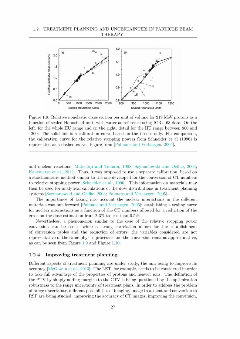
1.2. TREATMENT PLANNING AND UNCERTAINTIES IN PARTICLE BEAMTHERAPY
Figure 1.9: Relative nonelastic cross section per unit of volume for 219 MeV protons as afunction of scaled Hounsfield unit, with water as reference using ICRU 63 data. On theleft, for the whole HU range and on the right, detail for the HU range between 800 and1200. The solid line is a calibration curve based on the tissues only. For comparison,the calibration curve for the relative stopping powers from Schneider et al (1996) isrepresented as a dashed curve. Figure from [Palmans and Verhaegen, 2005].
and nuclear reactions [Matsufuji and Tomura, 1998; Szymanowski and Oelfke, 2003;Kanematsu et al., 2012]. Thus, it was proposed to use a separate calibration, based ona stoichiometric method similar to the one developed for the conversion of CT numbersto relative stopping power [Schneider et al., 1996]. This information on materials maythen be used for analytical calculations of the dose distributions in treatment planningsystems [Szymanowski and Oelfke, 2003; Palmans and Verhaegen, 2005].
The importance of taking into account the nuclear interactions in the differentmaterials was put forward [Palmans and Verhaegen, 2005]: establishing a scaling curvefor nuclear interactions as a function of the CT numbers allowed for a reduction of theerror on the dose estimation from 2-3% to less than 0.5%.
Nevertheless, a phenomenon similar to the case of the relative stopping powerconversion can be seen: while a strong correlation allows for the establishmentof conversion tables and the reduction of errors, the variables considered are notrepresentative of the same physics processes and the conversion remains approximative,as can be seen from Figure 1.9 and Figure 1.10.
1.2.4 Improving treatment planning
Different aspects of treatment planning are under study, the aim being to improve itsaccuracy [McGowan et al., 2013]. The LET, for example, needs to be considered in orderto take full advantage of the properties of protons and heavier ions. The definition ofthe PTV by simply adding margins to the CTV is being questioned by the optimizationrobustness to the range uncertainty of treatment plans. In order to address the problemof range uncertainty, different possibilities of imaging, image treatment and conversion toRSP are being studied: improving the accuracy of CT images, improving the conversion,
27
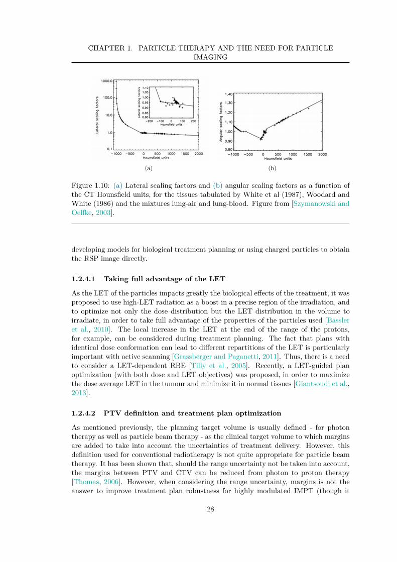
CHAPTER 1. PARTICLE THERAPY AND THE NEED FOR PARTICLEIMAGING
(a) (b)
Figure 1.10: (a) Lateral scaling factors and (b) angular scaling factors as a function ofthe CT Hounsfield units, for the tissues tabulated by White et al (1987), Woodard andWhite (1986) and the mixtures lung-air and lung-blood. Figure from [Szymanowski andOelfke, 2003].
developing models for biological treatment planning or using charged particles to obtainthe RSP image directly.
1.2.4.1 Taking full advantage of the LET
As the LET of the particles impacts greatly the biological effects of the treatment, it wasproposed to use high-LET radiation as a boost in a precise region of the irradiation, andto optimize not only the dose distribution but the LET distribution in the volume toirradiate, in order to take full advantage of the properties of the particles used [Bassleret al., 2010]. The local increase in the LET at the end of the range of the protons,for example, can be considered during treatment planning. The fact that plans withidentical dose conformation can lead to different repartitions of the LET is particularlyimportant with active scanning [Grassberger and Paganetti, 2011]. Thus, there is a needto consider a LET-dependent RBE [Tilly et al., 2005]. Recently, a LET-guided planoptimization (with both dose and LET objectives) was proposed, in order to maximizethe dose average LET in the tumour and minimize it in normal tissues [Giantsoudi et al.,2013].
1.2.4.2 PTV definition and treatment plan optimization
As mentioned previously, the planning target volume is usually defined - for photontherapy as well as particle beam therapy - as the clinical target volume to which marginsare added to take into account the uncertainties of treatment delivery. However, thisdefinition used for conventional radiotherapy is not quite appropriate for particle beamtherapy. It has been shown that, should the range uncertainty not be taken into account,the margins between PTV and CTV can be reduced from photon to proton therapy[Thomas, 2006]. However, when considering the range uncertainty, margins is not theanswer to improve treatment plan robustness for highly modulated IMPT (though it
28
1.2. TREATMENT PLANNING AND UNCERTAINTIES IN PARTICLE BEAMTHERAPY
was found satisfying for other deliveries of protons such as single-field uniform dose andlow modulation of IMPT) [Albertini et al., 2011]. This is because the degradation ofdose uniformity inside the target has some importance in IMPT. Heuristic approachessuch as choosing beam angles with the less inhomogeneities in the beam path, or placingno organ at risk just behind the distal edge of the peak have been applied. It was alsoproposed to define a beam-specific PTV [Park et al., 2012], taking into account the rangeuncertainty and setup errors independently for each beam angle.
Rather than the re-definition of a more appropriate planning target volume, someefforts are also put towards the inclusion of the uncertainties directly into the planningsystem in order to determine the most robust solution [McGowan et al., 2013]. Differentmethods have been proposed, such as a probabilistic approach [Unkelbach et al., 2007],a robust formulation [Unkelbach et al., 2007] or a worst-case optimization [Pflugfelderet al., 2008]. More recently, the inclusion of robustness to range uncertainty in a multi-criteria objective framework was implemented [Chen et al., 2012]. These approacheshave been tested, and showed less sensitivity to range and setup errors that traditionalmargins, assuring a better coverage of the clinical target volume.
1.2.4.3 Improving CT images
The improvement of the CT image quality, mainly the reduction of beam hardening andmetal artefacts, leads to a more accurate range prediction. Different methods for imageartefact correction have been proposed.
Beam hardening correction
Three kinds of methods for beam-hardening correction exist. The first is filtering: thebeam is hardened so that the measured spectrum tends towards a monochromatic one[Paiva et al., 1998; Krimmel et al., 2005]. The second way to proceed is linearisation[Herman, 1979; Hammersberg and Mangard, 1998; Kachelrieß et al., 2006]: the acquiredprojections are corrected to mimic monochromatic data. The third kind of methodis post-reconstruction [Nalcioglu and Lou, 1979; Olson et al., 1981], for which a firstreconstructed image of the object is used in order to estimate the distribution of thedifferent materials, and their effect on the energy spectrum.
Metal artefacts correction
Metal artefact reduction techniques are either based on the completion of missing datausing synthetic data, or on the modification of the reconstruction algorithm to ignore themissing data [Man et al., 2000; Abdoli et al., 2012]. Another possibility is the registrationof kilo-voltage (kV) and mega-voltage (MV) CT images [Newhauser et al., 2008]. It hasbeen shown that correcting for metal artefacts improves significantly the quality of thetreatment plan [Wei et al., 2006] and diminishes the risk of potentially dramatic errors.
29
CHAPTER 1. PARTICLE THERAPY AND THE NEED FOR PARTICLEIMAGING
1.2.4.4 Improving the conversion to RSP with DECT
Dual-energy X-ray CT (DECT) acquisition has been put forward as a possible tool toimprove treatment planning and reduce the range uncertainty. MV-CT has been putforward as a mean to overcome the problem of metal artefacts in kV-CT [Newhauseret al., 2008]. In the aforementioned paper, the use of an hybrid approach using registeredkV- and MV-CT images has been proposed. This makes it possible to keep the bettersensitivity and contrast of kV-CT. DECT can be even more interesting, in that it makesit possible to access more information on the materials.
Principle of DECT
DECT is a technique that has been first proposed in the late seventies [Alvarez andMacovski, 1976]. The attenuation coefficient of a material (Equation 1.8) can be re-written to take into account a continuous spectrum of energy j:
µj = ne
∑
i
wij
[
Z4F (Eij , Z) + G (Eij , Z)]
(1.12)
with ne the electron density of the material, wi the fraction by weight of element i servingas the weighting factor for the energy Eij , and Z the effective atomic number [Johns,1983] defined as:
Z =
(
∑
i
wiZ3.5i
)1/3.5
(1.13)
with Zi the atomic number of the element i.A CT acquisition with two different energy spectra gives access to two linear
attenuation coefficients. Thereby, two different evaluations of Equation 1.12 are availablethat can be solved iteratively for Z which makes it possible, in turn, to calculate ne.
Application to treatment planning
DECT gives access to the electron density of the materials, which is a great part ofthe relative stopping power. An electron density image obtained from kV-kV DECTused for the conversion to Water-Equivalent Path Length (WEPL, projection of theRSP, detailed in Section 2.3.1) makes it possible to reduce the range uncertainty, andthe image shows less noise than single energy CT [Hunemohr et al., 2013]. The othercomponent of the stopping power depends on the ionization potential of the material.An empirical relationship between the logarithm of this ionization potential and theeffective atomic number has been put forward [Yang et al., 2010]. It was shown thatkV-MV DECT gives better results than kV-kV or MV-MV DECT [Yang et al., 2011].
Nevertheless, performing DECT is not so trivial, as it either requires the registrationof two CT images, or a simultaneous acquisition with two sources. Moreover, whileDECT involving MV-CT shows great results, the image is still affected by beamhardening and the trade-off between the image quality and the dose needs to be carefullyconsidered.
30
1.2. TREATMENT PLANNING AND UNCERTAINTIES IN PARTICLE BEAMTHERAPY
1.2.4.5 Upcoming possibilities for X-ray CT imaging?
Other modalities of X-ray CT imaging exist, that have not been investigated in thecontext of treatment planning for particle beam therapy, but could be of interest.
Spectral CT
Spectral CT consists in detecting and exploiting the energy distribution of thetransmitted photons [Giersch et al., 2005]. The principle is similar to that of DECT,except that spectral CT only uses one source but employs energy thresholds in thedetector.The advantage over DECT is that it does not require image registration, nor multiplesources. It could moreover bring more information in the sense that it is not limited totwo energies. However, challenges in the covering of large areas, high resolution, uniformperformance and long duration operation remain [Shikhaliev and Fritz, 2011; Xu et al.,2012].
Phase contrast CT
Phase contrast CT [Momose et al., 1996] is a technique that makes it possible to accessthe two informations of DECT, namely the electron density and effective atomic number,with only one CT acquisition, thus only one dataset [Qi et al., 2010]. The electron densitycan be determined from refractive index decrement through a linear relationship. Theeffective atomic number can be explicitly derived from the ratio of the linear attenuationto refractive index decrement using a power function plus a constant. If proven efficient,this method could have the advantage over DECT due to the lower dose (only oneCT acquisition) and because there is no need for registration nor for two sources anddetectors.
Neither spectral CT nor phase contrast CT have been considered yet for improvingtreatment planning – as both are in rather early developmental stages and challengesremain to their spread in clinical setting [Xu et al., 2012; Bravin et al., 2013].Nevertheless, they may one day become potential solutions.
1.2.5 Proton imaging as a potential answer?
As we have seen in section 1.2.2.2, proton imaging can help reduce range uncertaintyby checking the expected range with the treatment planning stopping power. However,proton imaging may well help reducing range uncertainty by being an alternative tothe conversion of CT numbers, and directly mapping the relative stopping power of thematerials. This is why proton computed tomography is currently being investigatedby different groups and collaborations worldwide. Moreover, a proton beam carriesmore information on the materials encountered than just its energy loss. Whether thisinformation could also be useful to reduce the delivered dose uncertainty is a path thathas not been explored yet. Chapter 2 describes the principles of proton imaging, andChapter 5 describes the investigations on the potential use of all the information recordedduring a proton scan to help reduce range and dose uncertainties.
31
CHAPTER 1. PARTICLE THERAPY AND THE NEED FOR PARTICLEIMAGING
– Particle beam therapy presents many advantages in terms of dose depositand sparing of healthy tissues.
– Treatment planning for particle beam therapy requires the conversionfrom CT numbers either to stopping powers of charged particles in thetissues, or to stoichiometric composition of the tissues.
– The uncertainty on the range of particles results in an increase of themargins around the volume to irradiate.
– The uncertainty on the dose deposit is higher than for X-ray therapy.
– Proton computed tomography has been put forward as a mean to reducethe range uncertainty.
Summary
32

Chapter 2
Proton imagingstate of the art
Contents
2.1 Review of the physics principles: interactions of protonswith matter . . . . . . . . . . . . . . . . . . . . . . . . . . . . . . 34
2.1.1 Proton energy loss . . . . . . . . . . . . . . . . . . . . . . . . . 34
2.1.2 Multiple Coulomb scattering . . . . . . . . . . . . . . . . . . . 37
2.1.3 Nuclear interactions . . . . . . . . . . . . . . . . . . . . . . . . 38
2.2 The first era of proton imaging - discovery . . . . . . . . . . . 39
2.2.1 Proton computed tomography using energy loss . . . . . . . . . 39
2.2.2 Marginal range radiography . . . . . . . . . . . . . . . . . . . . 40
2.2.3 Nuclear scattering imaging . . . . . . . . . . . . . . . . . . . . 41
2.2.4 Multiple scattering radiography . . . . . . . . . . . . . . . . . . 42
2.2.5 In brief . . . . . . . . . . . . . . . . . . . . . . . . . . . . . . . 43
2.3 The second era of proton imaging - treatment planning andquality assurance . . . . . . . . . . . . . . . . . . . . . . . . . . . 44
2.3.1 Proton computed tomography for imaging the relative stoppingpower . . . . . . . . . . . . . . . . . . . . . . . . . . . . . . . . 44
2.3.2 Proton tomographs . . . . . . . . . . . . . . . . . . . . . . . . . 46
2.3.2.1 Tracking . . . . . . . . . . . . . . . . . . . . . . . . . 48
2.3.2.2 Energy/range measurement . . . . . . . . . . . . . . . 49
2.3.3 Expected performances of pCT . . . . . . . . . . . . . . . . . . 50
2.3.3.1 Path estimation and spatial resolution . . . . . . . . . 50
2.3.3.2 On dose and density resolution . . . . . . . . . . . . . 52
2.3.4 Different approaches to pCT . . . . . . . . . . . . . . . . . . . 52
2.4 Positioning of this work . . . . . . . . . . . . . . . . . . . . . . . 53
33
CHAPTER 2. PROTON IMAGING – STATE OF THE ART
This chapter goes over the interactions between protons and matter in a first part.A second part is dedicated to the history of proton imaging, leading to the state of theart. Finally, this thesis is introduced in its context.
2.1 Review of the physics principles: interactions ofprotons with matter
This section consists in an overview of the principles of interactions of proton withmatter. Protons going through a medium lose their energy through inelastic collisionswith atomic electrons. This energy loss is described by the Bethe-Bloch formula, detailedin Section 2.1.1. Protons also undergo elastic collisions with electrons and nuclei, thatdeflect them from their trajectory. However, as the electrons weigh much less than theprotons, this contribution to the energy loss is not significant. The scattering of protonsin matter is detailed in Section 2.1.2. The inelastic collisions with nuclei that particlesalso undergo are presented in Section 2.1.3.
2.1.1 Proton energy loss
Inelastic collisions of protons with atomic electrons lead to excitations (where electronsare still bound to the nucleus) and ionizations (where electrons are stripped off thenucleus). In the energy range considered for proton imaging (typically between 20 and300 MeV), the mean energy loss per unit path length, also called stopping power S, iswell-described by the Bethe-Bloch theory [Bethe, 1930; Bloch, 1933]:
S (I, E) = −dE
dx=
4πne
mec2β2
(
e2
4πǫ0
)2 [
ln
(
2mec2β2
I (1 − β2)
)
− β2
]
(2.1)
where e is the proton charge, ǫ0 the vacuum permittivity, β = v/c with v the particlevelocity and c the speed of light, me is the rest mass of the electron and I is the meanexcitation potential (also called mean ionization potential). Here, ne represents thedensity of electrons in the material, that can be expressed as:
ne =NA · Z · ρ
A · Mu(2.2)
where ρ is the density of material, Z and A are its atomic and mass numbers, NA isthe Avogadro number and Mu the molar mass constant.
Shell and density corrections can be added to the formula, but are unnecessary inthe context of proton imaging - they affect the end of the range of the particle that isnot considered in proton imaging. The electronic stopping power of protons in water isrepresented in Figure 2.1.
Through Equation 2.1, one can see what leads to the peculiar shape of the Braggcurve, that characterizes the stopping power of the material as a function of the depth,and particularly the peak (Bragg peak) for low values of β at the end of the range, ascan be seen of Figure 2.2.
34
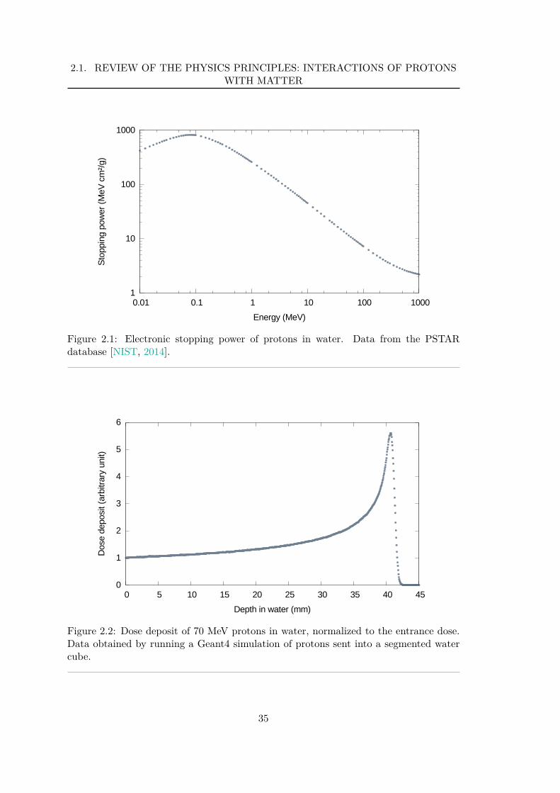
2.1. REVIEW OF THE PHYSICS PRINCIPLES: INTERACTIONS OF PROTONSWITH MATTER
1
10
100
1000
0.01 0.1 1 10 100 1000
Sto
ppin
g p
ow
er
(MeV
cm
²/g)
Energy (MeV)
Figure 2.1: Electronic stopping power of protons in water. Data from the PSTARdatabase [NIST, 2014].
0
1
2
3
4
5
6
0 5 10 15 20 25 30 35 40 45
Dose d
eposit (
arb
itra
ry u
nit)
Depth in water (mm)
Figure 2.2: Dose deposit of 70 MeV protons in water, normalized to the entrance dose.Data obtained by running a Geant4 simulation of protons sent into a segmented watercube.
35
CHAPTER 2. PROTON IMAGING – STATE OF THE ART
As a first approximation, the ionization potential of atoms can be determined as:
I = (10 eV) · Z
where Z is the atomic number of the atoms of the material. Nevertheless, theapproximation does not fit the data very well for elements of atomic number less than15, and more precise tabulated data are now available [ICRU report 48, 1994]. Theionization potential of atoms and molecules depends on their atomic structure, and alsoon the state of the material (gas or condensed material). The determination of the I-values is particularly complex in the case of compounds. As an example, a wide rangeof values has been put forward for the ionization potential of liquid water, ranging from67.2 eV to 81.8 eV [Besemer et al., 2013].
An approximation for the calculation of the I-value of compound materials,recommended by the ICRU [ICRU report 37, 1984] is:
ln I =
∑ni=1
(
wiZi
Ailn Ii
)
∑ni=1
(
wiZi
Ai
) (2.3)
with wi, Zi, Ai and Ii the mass proportion, the atomic and mass numbers, and theI-value of the element i respectively.
Straggling of the energy loss
Both the number of collisions and the energy transferred for each collision are ruled bystatistical processes. A mono-energetic beam of protons sent through a material will exitwith an energy distribution, representing these statistical fluctuations. This straggling ofthe energy loss can be characterized by the variance of the outgoing energy distribution.It was shown [Schulte et al., 2005] that for thinner objects (≤ 15 cm), this variance isbest described by Bohr’s theory [Bohr, 1948]. Let us define:
κ2 (x) = ηe4πn
mec2
(
e2
4πǫ0
)21 − 1
2β2 (E (Ein, x))1 − β2 (E (Ein, x))
(2.4)
where ηe is the relative electron density with respect to water.Let d be the thickness of material. Bohr’s theory then predicts:
σ2B (d) =
∫ d
0κ2 (x) dx (2.5)
For thicker objects, Tschalar’s theory [Tschalar, 1968b,a] is more appropriate:
d
dxσ2
T (x) = κ2 (x) − 2(
d
dES (E (x))
)
σ2T (x) + higher order terms (2.6)
Therefore, the straggling depends on the energy of the protons, and on the electrondensity of the materials.
36
2.1. REVIEW OF THE PHYSICS PRINCIPLES: INTERACTIONS OF PROTONSWITH MATTER
2.1.2 Multiple Coulomb scattering
Protons in the energy range considered undergo multiple small-angle deflections due tothe Coulomb field of the nuclei, and deviate from their original path. The Coulombscattering distribution can be represented by the theory of Moliere [Moliere, 1947, 1948;Bethe, 1953]. The distribution of exit angles and positions of a mono-energetic, uni-directional beam of particles is roughly gaussian for small angles but shows a tail atlarger angles. In the framework of proton computed tomography (pCT), the gaussianapproximation of multiple Coulomb scattering (MCS) will be used to estimate thetrajectory of the particles during image reconstruction (Section 3.3.2). The exit angulardistribution of a mono-energetic parallel beam of protons for “thin” objects (l ≪ X0) inthis approximation is a normal distribution of which the mean is zero and the standarddeviation can be described by the following empirical formula [Lynch and Dahl, 1991]:
σ(l, E) =13.6
β(E)p(E)
√
l
X0
[
1 + 0.038 · ln(
l
X0
)]
(2.7)
where β and p are the scaled velocity and momentum of the proton at energy E, X0 isthe radiation length of the material and l the proton path length in the material. Forthicker objects, an integration of this equation on the energy range in the material needsto be considered.
Other approximations exist, both for the central gaussian part of the distribution,as well as for the whole distribution with corrections for single scattering [Kanematsu,2008; Gottschalk, 2009]. Some will be of interest for the study presented in Section 5.3and are detailed in Appendix B.
The radiation length of a material is defined as the mean length required to reducethe energy of an electron by the factor 1/e by bremsstrahlung. It is usually measured ing.cm−2. For a single element of charge and mass numbers Z and A respectively, it canbe approximated by the following empirical formula:
X0 =716.4 · A
Z(Z + 1) ln 287√Z
g.cm−2 (2.8)
For compound materials, the combined radiation length X0 of a sample of mass W0 canbe expressed as:
W0
X0=∑
i
Wi
Xi(2.9)
with Wi and Xi the mass and radiation length of the i-th component.This, however, remains an approximation. The calculation of the radiation length
of water using this formula gives 35.2 g.cm−2, whereas the value of 36.1 g.cm−2 is wellestablished [Hagiwara, 2002]
37
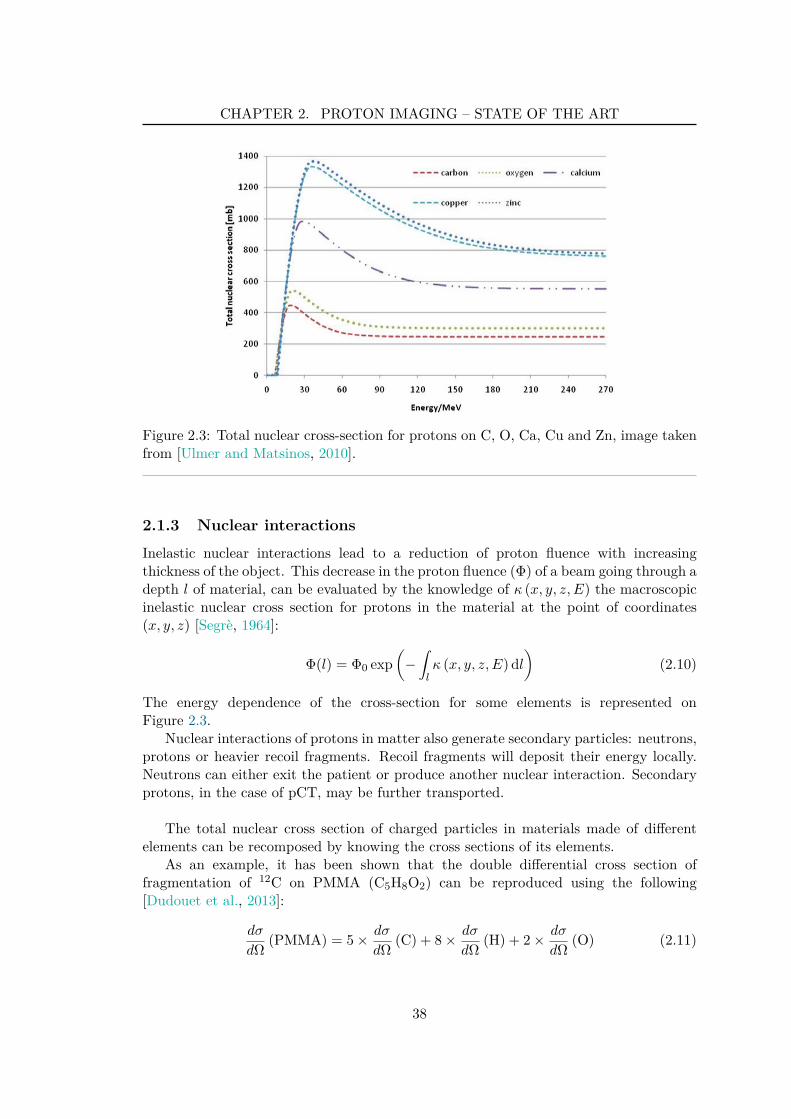
CHAPTER 2. PROTON IMAGING – STATE OF THE ART
Figure 2.3: Total nuclear cross-section for protons on C, O, Ca, Cu and Zn, image takenfrom [Ulmer and Matsinos, 2010].
2.1.3 Nuclear interactions
Inelastic nuclear interactions lead to a reduction of proton fluence with increasingthickness of the object. This decrease in the proton fluence (Φ) of a beam going through adepth l of material, can be evaluated by the knowledge of κ (x, y, z, E) the macroscopicinelastic nuclear cross section for protons in the material at the point of coordinates(x, y, z) [Segre, 1964]:
Φ(l) = Φ0 exp(
−∫
lκ (x, y, z, E) dl
)
(2.10)
The energy dependence of the cross-section for some elements is represented onFigure 2.3.
Nuclear interactions of protons in matter also generate secondary particles: neutrons,protons or heavier recoil fragments. Recoil fragments will deposit their energy locally.Neutrons can either exit the patient or produce another nuclear interaction. Secondaryprotons, in the case of pCT, may be further transported.
The total nuclear cross section of charged particles in materials made of differentelements can be recomposed by knowing the cross sections of its elements.
As an example, it has been shown that the double differential cross section offragmentation of 12C on PMMA (C5H8O2) can be reproduced using the following[Dudouet et al., 2013]:
dσ
dΩ(PMMA) = 5 × dσ
dΩ(C) + 8 × dσ
dΩ(H) + 2 × dσ
dΩ(O) (2.11)
38
2.2. THE FIRST ERA OF PROTON IMAGING - DISCOVERY
2.2 The first era of proton imaging - discovery
The work on proton imaging went through two distinct eras. Between the 1960’s andthe 1980’s the potential of proton medical imaging was explored for the first time.Different means to use protons for medical imaging were proposed: the concept of protoncomputed tomography nowadays known uses the energy loss of the particles (Section2.2.1), but it evolved from marginal range radiography (Section 2.2.2). During the sametime, nuclear scattering imaging (Section 2.2.3) and multiple scattering imaging (Section2.2.4) were also investigated. After the beginning of the 1980’s, with the developmentand improvement of X-ray imaging, and considering the “intrinsic” limitations of theproton imaging concepts proposed (the deterioration of the spatial resolution due tomultiple scattering), the research in this field was put on hold. The interest in protonimaging was only renewed in the 1990’s, with the explicit intent to help with rangecontrol and treatment planning for particle beam therapy.
2.2.1 Proton computed tomography using energy loss
The first suggestion of proton imaging was made by Cormack [1963, 1964]. He suggested“the determination of a variable density of matter with constant chemical composition,using the energy loss of charged particles in the matter”. This idea was exposed as anapplication amongst others in the formulation of the image reconstruction problem. Heput forward, in his paper, that this problem can be posed in the same manner than theattenuation of X-rays for imaging, if one can assume that the tissues vary only in densityand not in chemical composition. This assumption, in the case of an object consisting ofbone and soft tissue, is a rough approximation that will impact the results. In this lineof thought, Cookson et al. [1972] measured the “density profile” of an object by lookingat the energy loss of a 12 MeV proton beam.
The same year saw the first tomographic reconstruction of an object imaged with840 MeV alpha particles. The stopping power along the beam line was computed from theaverage energy degradation: the basic principle was the same as what is done nowadays[Goitein, 1972]. Still with alpha particles, of 900 MeV this time, a clinical brain imagingsystem was proposed, with three multi-wire proportional counters upstream from thepatient to measure the beam position and a range counter telescope consisting in 13scintillation counters for measuring the residual range of the particles upon exit. In thisconfiguration, the patient sat upright on a rotating chair, with the top of the head ina water bath [Crowe et al., 1975], in order to even the depth of materials the particlesgo through. The brain images reconstructed from the alpha particle scan showed gooddensity resolution with a dose advantage of an order of magnitude compared to X-rayimages.
Experiments on computed tomography using the energy loss of protons wereperformed at the Harvard cyclotron laboratory shortly after that [Cormack and Koehler,1976]. The proposed system used a hyperpure germanium calorimeter to measure theexit energy of the particles. At the time, advantages and disadvantages of protons overX-rays were described [Hanson et al., 1978]:
39
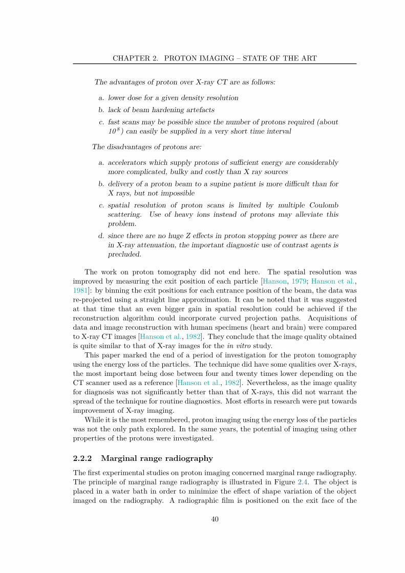
CHAPTER 2. PROTON IMAGING – STATE OF THE ART
The advantages of proton over X-ray CT are as follows:
a. lower dose for a given density resolution
b. lack of beam hardening artefacts
c. fast scans may be possible since the number of protons required (about10 8 ) can easily be supplied in a very short time interval
The disadvantages of protons are:
a. accelerators which supply protons of sufficient energy are considerablymore complicated, bulky and costly than X ray sources
b. delivery of a proton beam to a supine patient is more difficult than forX rays, but not impossible
c. spatial resolution of proton scans is limited by multiple Coulombscattering. Use of heavy ions instead of protons may alleviate thisproblem.
d. since there are no huge Z effects in proton stopping power as there arein X-ray attenuation, the important diagnostic use of contrast agents isprecluded.
The work on proton tomography did not end here. The spatial resolution wasimproved by measuring the exit position of each particle [Hanson, 1979; Hanson et al.,1981]: by binning the exit positions for each entrance position of the beam, the data wasre-projected using a straight line approximation. It can be noted that it was suggestedat that time that an even bigger gain in spatial resolution could be achieved if thereconstruction algorithm could incorporate curved projection paths. Acquisitions ofdata and image reconstruction with human specimens (heart and brain) were comparedto X-ray CT images [Hanson et al., 1982]. They conclude that the image quality obtainedis quite similar to that of X-ray images for the in vitro study.
This paper marked the end of a period of investigation for the proton tomographyusing the energy loss of the particles. The technique did have some qualities over X-rays,the most important being dose between four and twenty times lower depending on theCT scanner used as a reference [Hanson et al., 1982]. Nevertheless, as the image qualityfor diagnosis was not significantly better than that of X-rays, this did not warrant thespread of the technique for routine diagnostics. Most efforts in research were put towardsimprovement of X-ray imaging.
While it is the most remembered, proton imaging using the energy loss of the particleswas not the only path explored. In the same years, the potential of imaging using otherproperties of the protons were investigated.
2.2.2 Marginal range radiography
The first experimental studies on proton imaging concerned marginal range radiography.The principle of marginal range radiography is illustrated in Figure 2.4. The object isplaced in a water bath in order to minimize the effect of shape variation of the objectimaged on the radiography. A radiographic film is positioned on the exit face of the
40
2.2. THE FIRST ERA OF PROTON IMAGING - DISCOVERY
(a) (b)
Figure 2.4: Illustration of the marginal range radiography concept. (a) illustrates theflux-depth curves for protons and X-rays passing through a homogeneous medium, andhighlights the higher sensitivity of protons. (b) shows the depth-dose curve of protons aswell as the setup of the specimen and photographic film. The figures are from [Steward,1979].
water tank. The beam energy is set so that the film is situated at the middle of thesharp fluence descent following the Bragg peak. The information exploited is the numberof particles impinging on the emulsion.
The first experiment was performed by Koehler [1968]. It was followed by others,and this technique demonstrated great promises for diagnostics of tumours, strokes, orbreast carcinoma [Steward and Koehler, 1973b,a, 1974]. The technique showed gooddetectability of the malignancies compared to the X-ray radiographs available at thetime, despite the limitation in the spatial resolution caused by the scattering of protons.This method made it possible to have a much higher contrast than with X-rays for agiven, or even less, dose [Steward, 1976].
This technique, however, requires careful consideration to properly match the beamenergy to the object and to the placement of the detector. Indeed, the contrast is set bythe falloff region of the Bragg peak: the sharper the falloff, the higher the contrast; butthe shorter the range of structural variations that can be seen. Thus, this can be alsoperformed with ions, but a compromise between the range of variations and the contrastneeds to be established for each application [Steward, 1979]. The second drawback ofthis technique is that multiple scattering degrades the spatial resolution.
2.2.3 Nuclear scattering imaging
The application of nuclear scattering to radiography (NSR) was proposed in 1975[Saudinos et al., 1975]. The principle is to use higher energy protons, between 500 MeVand 1 GeV. The idea is to detect protons scattered at wide angles by nuclear interactions.The positions and directions of the particles are recorded upstream from the objectto image with two position-sensitive detectors. Downstream from the object, otherposition-sensitive detectors are used to record the passage of largely scattered protonsand recoil protons. The intersection of the lines describing the trajectory of the incoming
41
CHAPTER 2. PROTON IMAGING – STATE OF THE ART
and scattered particle give the position of the interactions. This makes it possibleto obtain three-dimensional images using a single beam direction. This technique is,however, intrinsically limited in its spatial resolution due to the multiple scattering ofthe secondary protons in the object.
Further work demonstrated the possibility to separate the contributions of scatteringon hydrogen from that on heavier elements, such as carbon or oxygen [Charpak et al.,1976]. Experiments on biological materials confirmed this possibility to treat the data inorder to obtain “hydrogen” radiographs in addition to the “standard” nuclear scatteringradiographs [Berger and Duchazeaubeneix, 1978]. Later experiments made it possible toreconstruct images from a preserved human head [Charpak et al., 1979; Duchazeaubeneixet al., 1980]. The images were compared to those obtained with an X-ray tomograph.Charpak et al. [1979] conclude that:
As compared to X-ray CAT [computer-assisted tomography], NSR offers thefollowing advantages:
– the same image quality can be obtained with radiation doses severaltimes smaller, mainly because of the large effective use of the incomingradiation (about 6% of beam particles produce useful nuclear scatteringevents, in a 20 cm thick object with unit density);
– the image obtained is fully three-dimensional allowing the display ofthe density distributions in arbitrary planes of reference by simple datamanipulation;
– the unique feature of hydrogen selection allows one level of chemicalanalysis that may prove useful to detect structure having very closedensity but different hydrogen content.
As for the other techniques for imaging with protons, no further work was publishedafter the beginning of the 1980’s. One possible explanation for that is the following:as X-ray imaging technology progressed greatly, the “same image quality” soon becameunreachable. Furthermore, with the development of magnetic resonance imaging, adifferent possibility to visualize the hydrogen became available, without the need forhigh-energy proton accelerators.
2.2.4 Multiple scattering radiography
Another, less explored, way of producing images with protons was shown to be multiplescattering radiography. The concept was first explained in the beginning of the 1970’s byWest and Sherwood [1972]. The idea is the following: when a parallel beam of protonsgoes through a uniform depth of material, the intensity of particles exiting is uniform,as every point receives an equal number of Coulomb scattered particles. The same goesfor outside of the object. At the boundary, however, less particles reach the detector:particles impinging just on the edge of the object are scattered in the non-object partof the edge. This discontinuity makes it possible to generate bright and dark outlines ofthe object on radiographic film, as illustrated on Figure 2.5.
Again, this technique provides information of a different nature compared to the othermethods of imaging with protons. As it is particularly well-adapted to thin objects, it
42
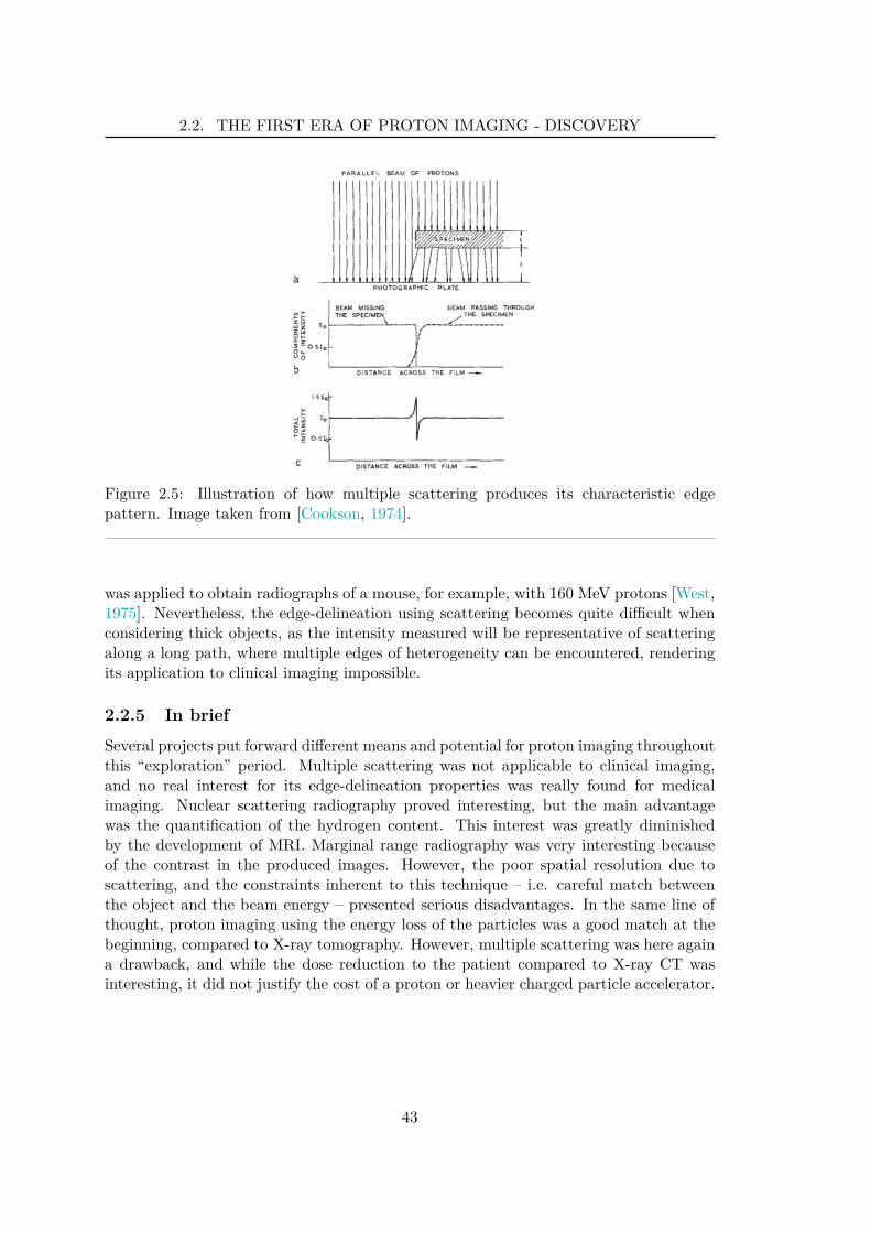
2.2. THE FIRST ERA OF PROTON IMAGING - DISCOVERY
Figure 2.5: Illustration of how multiple scattering produces its characteristic edgepattern. Image taken from [Cookson, 1974].
was applied to obtain radiographs of a mouse, for example, with 160 MeV protons [West,1975]. Nevertheless, the edge-delineation using scattering becomes quite difficult whenconsidering thick objects, as the intensity measured will be representative of scatteringalong a long path, where multiple edges of heterogeneity can be encountered, renderingits application to clinical imaging impossible.
2.2.5 In brief
Several projects put forward different means and potential for proton imaging throughoutthis “exploration” period. Multiple scattering was not applicable to clinical imaging,and no real interest for its edge-delineation properties was really found for medicalimaging. Nuclear scattering radiography proved interesting, but the main advantagewas the quantification of the hydrogen content. This interest was greatly diminishedby the development of MRI. Marginal range radiography was very interesting becauseof the contrast in the produced images. However, the poor spatial resolution due toscattering, and the constraints inherent to this technique – i.e. careful match betweenthe object and the beam energy – presented serious disadvantages. In the same line ofthought, proton imaging using the energy loss of the particles was a good match at thebeginning, compared to X-ray tomography. However, multiple scattering was here againa drawback, and while the dose reduction to the patient compared to X-ray CT wasinteresting, it did not justify the cost of a proton or heavier charged particle accelerator.
43
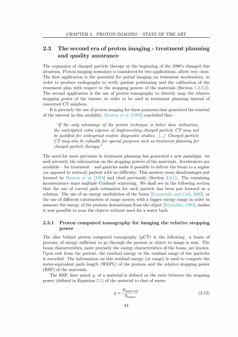
CHAPTER 2. PROTON IMAGING – STATE OF THE ART
2.3 The second era of proton imaging - treatment planningand quality assurance
The expansion of charged particle therapy at the beginning of the 1990’s changed thissituation. Proton imaging nowadays is considered for two applications, albeit very close.The first application is the potential for portal imaging on treatment accelerators, inorder to produce radiographs to verify patient positioning and the calibration of thetreatment plan with respect to the stopping powers of the materials (Section 1.2.2.2).The second application is the use of proton tomography to directly map the relativestopping power of the tissues, in order to be used in treatment planning instead ofconverted CT numbers.
It is precisely the use of proton imaging for these purposes that generated the renewalof the interest in this modality. Hanson et al. [1982] concluded that :
“If the only advantage of the proton technique is better dose utilization,the anticipated extra expense of implementing charged particle CT may notbe justified for widespread routine diagnostic studies. [...] Charged particleCT may also be valuable for special purposes such as treatment planning forcharged particle therapy.”
The need for more precision in treatment planning has generated a new paradigm: weseek precisely the information on the stopping powers of the materials. Accelerators areavailable – for treatment – and gantries make it possible to deliver the beam to a supine(as opposed to vertical) patient with no difficulty. This answers most disadvantages putforward by Hanson et al. [1978] and cited previously (Section 2.2.1). The remaininginconvenience stays multiple Coulomb scattering. We shall see in the following sectionthat the use of curved path estimation for each particle has been put forward as asolution. The use of an energy modulation of the beam [Zygmanski and Gall, 2000], orthe use of different calorimeters or range meters with a bigger energy range in order tomeasure the energy of the protons downstream from the object [Schneider, 1994], makesit now possible to scan the objects without need for a water bath.
2.3.1 Proton computed tomography for imaging the relative stoppingpower
The idea behind proton computed tomography (pCT) is the following: a beam ofprotons, of energy sufficient to go through the patient or object to image is sent. Thebeam characteristics, more precisely the energy characteristics of the beam, are known.Upon exit from the patient, the residual energy or the residual range of the particlesis recorded. The information on this residual energy (or range) is used to compute thewater-equivalent path length (WEPL) of the protons and the relative stopping power(RSP) of the materials.
The RSP, here noted , of a material is defined as the ratio between the stoppingpower (defined in Equation 2.1) of the material to that of water:
=Smaterial
Swater(2.12)
44
2.3. THE SECOND ERA OF PROTON IMAGING - TREATMENT PLANNINGAND QUALITY ASSURANCE
The WEPL, here noted L, of a particle at the exit of the patient is the distance thisparticle would have had to go through in water to exit with the same energy, and iscalculated by:
L =∫
l (~r) dl (2.13)
with l the path of the proton in the material.From the integration of the Bethe-Bloch formula, the WEPL is equal to the
integration of the reciprocal stopping power of water, thus:
∫ Eout
Ein
dE
Swater (E)=∫
l (~r) dl (2.14)
By measuring the energy Eout upon exit from the patient, and knowing the energyEin at the entry, the left side of Equation 2.14 can be computed. As an alternative,a calibration of the system makes it possible to access directly pre-computed WEPL[Hurley et al., 2012]. In consequence, it is possible to reconstruct the RSP on the rightside of the same equation. It can be noted that, in order to do so, the path l of a protonneeds to be estimated.
It can be put forward that, since the stopping powers depend on the energy (Section2.1.1), so do the RSP, and the reconstructed values are an average over the energy ofthe particles throughout their propagation. However, in the energy range consideredfor proton imaging, this variation can be neglected. Indeed, consider an image of ahead with a 200 MeV beam; the energy of the exiting protons will be approximately of80 MeV. The variation in the RSP values will be less than 0.1% for materials such asmuscle or adipose tissue, and less than 0.3% for skull for example (using the materialsdefined in Appendix A), which is less than the expected resolution of 1% on the RSPvalues (Section 2.3.3.2).
Terminology: On relative stopping power and relative electron density inpCT
Early papers on proton imaging state that the aim of a pCT image reconstruction is tomap the relative electron density of the materials. More recent papers state that theaim is to map the relative stopping power of the materials. The difference is lexical. Inthe first approach, one wants to reconstruct the values of the relative electron densitybut, as no information on the ionization potential of the material is known, it is assumedto be that of water. The reconstruction of the RSP is strictly equivalent, except thatthe unknown ionization potential of the material remains implicit in the formulation,avoiding the approximation. The result is the same, the terminology was modified inorder to not have to make an assumption on the ionization potential.
Nevertheless, for quantification of the images, the “precision” of estimation of therelative stopping power values is characterized by the “density resolution”, even when itis said that the RSP is reconstructed.
45
CHAPTER 2. PROTON IMAGING – STATE OF THE ART
Figure 2.6: Proton tomograph as studied nowadays. It consists in four trackers, twoupstream and two downstream of the object and of a calorimeter or range meter. Theparticles are tracked one by one.
2.3.2 Proton tomographs
The multiple scattering and explicit apparition of the proton path l in Equation 2.14 leadto a proposition design for a pCT scanner that to records the positions and directionsof the particles, upstream and downstream from the object, as well as the energy ofthe particles. An attempt was made to record both the positions and energy of theprotons using silicon strip detectors (SSD) [Johnson et al., 2003]. However, the limitedenergy resolution (around 20%) lead to the separation of the tracking and the energymeasurement systems. The typical design of proton CT apparatus studied nowadaysconsists of:
– two sets of (at least) two tracker planes, upstream and downstream from the object,giving access to the information on the positions and directions of each particle,
– a calorimeter or range meter in order to measure the residual energy or range ofeach proton.
Such a system is illustrated on Figure 2.6.The specifications of a proton CT apparatus have been described by Schulte et al.
[2004], and are detailed in Table 2.1.Different groups are currently working on proton radiography and tomography,
amongst which some are more advanced:
– in the U.S.A., the pCT collaboration, with the University of California Santa Cruz,Loma Linda University and California State University San Bernardino. Otherworks have been published by the Northern Illinois University and Fermilab.
– in Italy, the PRIMA collaboration involving researchers from Insituto Nazionaledi Fisica Nucleare (INFN) and the University of Firenze.
– in Switzerland, the Paul Scherrer Institute and TERA foundation.
46
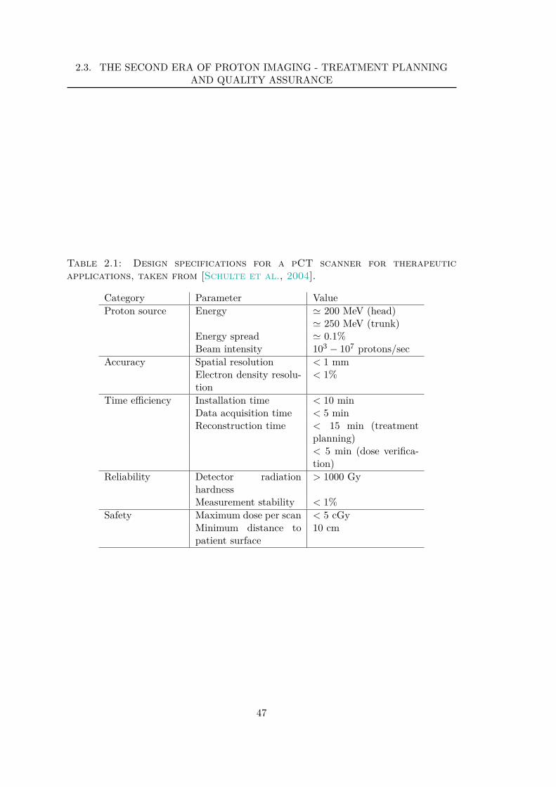
2.3. THE SECOND ERA OF PROTON IMAGING - TREATMENT PLANNINGAND QUALITY ASSURANCE
Table 2.1: Design specifications for a pCT scanner for therapeuticapplications, taken from [Schulte et al., 2004].
Category Parameter ValueProton source Energy ≃ 200 MeV (head)
≃ 250 MeV (trunk)Energy spread ≃ 0.1%Beam intensity 103 − 107 protons/sec
Accuracy Spatial resolution < 1 mmElectron density resolu-tion
< 1%
Time efficiency Installation time < 10 minData acquisition time < 5 minReconstruction time < 15 min (treatment
planning)< 5 min (dose verifica-tion)
Reliability Detector radiationhardness
> 1000 Gy
Measurement stability < 1%Safety Maximum dose per scan < 5 cGy
Minimum distance topatient surface
10 cm
47
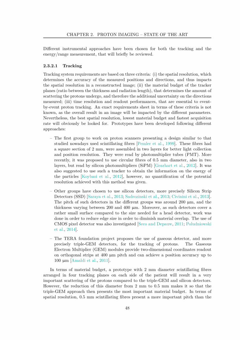
CHAPTER 2. PROTON IMAGING – STATE OF THE ART
Different instrumental approaches have been chosen for both the tracking and theenergy/range measurement, that will briefly be reviewed.
2.3.2.1 Tracking
Tracking system requirements are based on three criteria: (i) the spatial resolution, whichdetermines the accuracy of the measured positions and directions, and thus impactsthe spatial resolution in a reconstructed image; (ii) the material budget of the trackerplanes (ratio between the thickness and radiation length), that determines the amount ofscattering the protons undergo, and therefore the additional uncertainty on the directionsmeasured; (iii) time resolution and readout performances, that are essential to event-by-event proton tracking. An exact requirements sheet in terms of these criteria is notknown, as the overall result in an image will be impacted by the different parameters.Nevertheless, the best spatial resolution, lowest material budget and fastest acquisitionrate will obviously be looked for. Prototypes have been developed following differentapproaches:
– The first group to work on proton scanners presenting a design similar to thatstudied nowadays used scintillating fibres [Pemler et al., 1999]. These fibres hada square section of 2 mm, were assembled in two layers for better light collectionand position resolution. They were read by photomultiplier tubes (PMT). Morerecently, it was proposed to use circular fibres of 0.5 mm diameter, also in twolayers, but read by silicon photomultipliers (SiPM) [Gearhart et al., 2012]. It wasalso suggested to use such a tracker to obtain the information on the energy ofthe particles [Koybasi et al., 2012], however, no quantification of the potentialresolution achieved with this method was given.
– Other groups have chosen to use silicon detectors, more precisely Silicon StripDetectors (SSD) [Saraya et al., 2013; Sadrozinski et al., 2013; Civinini et al., 2013].The pitch of such detectors in the different groups was around 200 µm, and thethickness varying between 200 and 400 µm. Moreover, as such detectors cover arather small surface compared to the size needed for a head detector, work wasdone in order to reduce edge size in order to diminish material overlap. The use ofCMOS pixel detector was also investigated [Seco and Depauw, 2011; Poludniowskiet al., 2014].
– The TERA foundation project proposes the use of gaseous detector, and moreprecisely triple-GEM detectors, for the tracking of protons. The GaseousElectron Multiplier (GEM) modules provide two-dimensional coordinates readouton orthogonal strips at 400 µm pitch and can achieve a position accuracy up to100 µm [Amaldi et al., 2011].
In terms of material budget, a prototype with 2 mm diameter scintillating fibresarranged in four tracking planes on each side of the patient will result in a veryimportant scattering of the protons compared to the triple-GEM and silicon detectors.However, the reduction of this diameter from 2 mm to 0.5 mm makes it so that thetriple-GEM approach then presents the most important material budget. In terms ofspatial resolution, 0.5 mm scintillating fibres present a more important pitch than the
48
2.3. THE SECOND ERA OF PROTON IMAGING - TREATMENT PLANNINGAND QUALITY ASSURANCE
solid state detectors that are considered and the triple-GEM. However, there may besome disadvantages to gaseous detectors in a clinical context. As mentioned before, thespatial resolution of the reconstructed image will depend on these parameters, as theywill impact the path estimation. The evaluation of their importance will be presentedin Section 4.3.
Last but not least is the need to consider timing performances and data acquisitionrate of a prototype. The event-by-event tracking of the particles generates a particularchallenge. Different projects for proton scanners are well on their way towards clinicalapplications. However, increasing the data rate to support clinically useful proton fluxesis an essential step [Sadrozinski et al., 2013]. In terms of single-proton tracking, thesimultaneous recording of two events on the tracking planes makes it impossible tomatch trajectories before and after the patient; the information can therefore not betreated. As a consequence, for a given number of proton histories to get a certain imagequality, the acquisition time as well as the dose to the patient will depend on the particlerate that can be handled. Developments on the acquisition system are made, in orderto sustain data rates exceeding 1 or 2 MHz with the silicon trackers [Sadrozinski et al.,2011, 2013; Steinberg et al., 2012; Johnson et al., 2012, 2013]. This requirement hasbeen estimated for the synchrotron beam of the Loma Linda Univesity Medical Center:proton bunches are spaced by 110 ns intervals, and only single-proton bunches can beused because of the particle rate supported by the calorimeter [Johnson et al., 2013].The group working with GEM detectors reported the development of a fast acquisitionsystem in order to sustain a particle rate of 1 MHz [Bucciantonio et al., 2013].
2.3.2.2 Energy/range measurement
As far as the energy/range measurement is concerned, the most important criterionis the resolution on the measured WEPL. The two approaches, i.e. calorimeter andrange-meter, have been explored:
– The first approach consists in recording the energy of the outgoing protonsand calculate or calibrate their WEPL accordingly. For this, different crystalcalorimeters were investigated: NaI(Tl) crystal read by a PMT [Saraya et al.,2013], CsI(Tl) crystal read by photodiodes [Hurley et al., 2012] or YAG:Ce crystalread by silicon photodiodes [Civinini et al., 2013]. Hurley et al. [2012] show thatdirect calibration of detector response to WEPL is possible. However, the use ofsegmented block calorimeters results in a non-uniformity of the detector response.
– The second option is to record the residual range of the particles that givesaccess, in the same fashion, to the WEPL. Range counters using stacks of plasticscintillator plates, of thickness between 3 and 4 mm were proposed. The lightemission can then be either directly collected [Sadrozinski et al., 2013] using SiPMreadout, or indirectly collected, through the use of wavelength shifting fibres andreadout by PMTs [Pemler et al., 1999] or by SiPMs [Amaldi et al., 2011].
Resolution on the measured WEPL using a block calorimeter depends on the WEPL.For large WEPL, an increase in the sensitivity to the deposited energy in the calorimeterresults in a decrease of uncertainty [Hurley et al., 2012]. The range-meter approach,however, shows a constant resolution on the measured WEPL, depending only on the
49
CHAPTER 2. PROTON IMAGING – STATE OF THE ART
thickness of the slabs constituting the range meter [Sadrozinski et al., 2011]. Therefore,the calorimeter approach shows an advantage for larger WEPL while the range-meterapproach is more interesting for shorter WEPL.
In order to take advantage of both approaches, a hybrid multi-stage solution wasproposed by Sadrozinski et al. [2013]. It consists of two polystyrene blocks read byPMTs, which would perform better than the CsI calorimeter over the entire range ofinterest, and only slightly worse than the 4-mm slabs range-meter for short WEPL.Nevertheless, the increase in the acquisition rate of the tracking system may generatean additional constraint on the calorimeter in terms of particle rate to handle.
Comment on other charged particle imaging
It can be put forward that other charged particles can be used for imaging of the relativestopping power. Carbon imaging, in particular, is also investigated since there are clinicalfacilities that have carbon ion accelerators. Carbon imaging is very similar to protonimaging in its concept [Parodi, 2014]. The idea is to use the energy loss of carbon ions toproduce images of the electron density (or RSP) of the materials. The main differenceis that carbon ions undergo less scattering in the materials. Therefore, there is no needto measure the directions of the particles. For the energy/range measurements, differentexperimental approaches were taken, such as the use of plastic scintillators [Ohno et al.,2004; Shinoda et al., 2006], flat-pannel detector [Telsemeyer et al., 2012] or the use ofan ionization chamber (IC) stack [Rinaldi et al., 2013]. The same technologies could beused for proton imaging.
2.3.3 Expected performances of pCT
2.3.3.1 Path estimation and spatial resolution
As proton radiographic images are greatly affected by multiple scattering, leading to aspatial resolution much less satisfying than X-ray CT, the estimation of individual protontrajectories for image reconstruction has taken a lot of importance. Different algorithmicapproaches have been investigated for reconstruction, either using analytical or iterativereconstruction algorithms. In the case of analytical reconstruction, the data is binnedinto projection for reconstruction, while iterative reconstructions make it possible toconsider individual trajectories for each proton. This will be discussed more in detail inthe next chapter.
Nevertheless, the path of the protons, denoted l in Equation 2.14, is of key importanceto reach the millimetric spatial resolution (Table 2.1). The first approach that was taken,in a similar fashion to X-ray CT, consisted in only taking into account the position ofthe particles on the calorimeter [Hanson et al., 1981], as illustrated on Figure 2.7(a).With the addition of a position-sensitive tracker before the object [Pemler et al., 1999],one may define the trajectory of a proton as a straight line between an upstream and adownstream tracker, as illustrated on Figure 2.7(b). With further addition of trackersin order to record the angle of the particles before and after the object, one may definethe trajectory of protons as broken straight lines [Li et al., 2004; Vanzi et al., 2013](Figure 2.7(c)). However, an additional advantage can be found in the knowledge ofthe direction of each particle, in that it allows the definition of curved trajectories, as
50
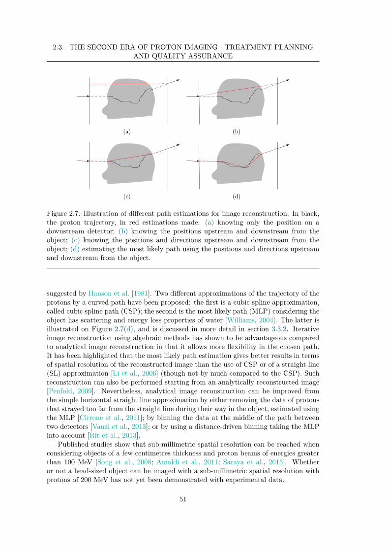
2.3. THE SECOND ERA OF PROTON IMAGING - TREATMENT PLANNINGAND QUALITY ASSURANCE
(a) (b)
(c) (d)
Figure 2.7: Illustration of different path estimations for image reconstruction. In black,the proton trajectory, in red estimations made: (a) knowing only the position on adownstream detector; (b) knowing the positions upstream and downstream from theobject; (c) knowing the positions and directions upstream and downstream from theobject; (d) estimating the most likely path using the positions and directions upstreamand downstream from the object.
suggested by Hanson et al. [1981]. Two different approximations of the trajectory of theprotons by a curved path have been proposed: the first is a cubic spline approximation,called cubic spline path (CSP); the second is the most likely path (MLP) considering theobject has scattering and energy loss properties of water [Williams, 2004]. The latter isillustrated on Figure 2.7(d), and is discussed in more detail in section 3.3.2. Iterativeimage reconstruction using algebraic methods has shown to be advantageous comparedto analytical image reconstruction in that it allows more flexibility in the chosen path.It has been highlighted that the most likely path estimation gives better results in termsof spatial resolution of the reconstructed image than the use of CSP or of a straight line(SL) approximation [Li et al., 2006] (though not by much compared to the CSP). Suchreconstruction can also be performed starting from an analytically reconstructed image[Penfold, 2009]. Nevertheless, analytical image reconstruction can be improved fromthe simple horizontal straight line approximation by either removing the data of protonsthat strayed too far from the straight line during their way in the object, estimated usingthe MLP [Cirrone et al., 2011]; by binning the data at the middle of the path betweentwo detectors [Vanzi et al., 2013]; or by using a distance-driven binning taking the MLPinto account [Rit et al., 2013].
Published studies show that sub-millimetric spatial resolution can be reached whenconsidering objects of a few centimetres thickness and proton beams of energies greaterthan 100 MeV [Song et al., 2008; Amaldi et al., 2011; Saraya et al., 2013]. Whetheror not a head-sized object can be imaged with a sub-millimetric spatial resolution withprotons of 200 MeV has not yet been demonstrated with experimental data.
51
CHAPTER 2. PROTON IMAGING – STATE OF THE ART
2.3.3.2 On dose and density resolution
For improvement of treatment planning, it is necessary to reach a resolution on thereconstructed relative stopping powers of less than the 3% achievable with X-ray CT,with 1% being ideal. The density resolution that can be achieved with a pCT dependson the energy of the protons and on the number of protons available per voxel of thereconstructed image. This leads to a trade-off between the delivered dose and the densityresolution [Satogata et al., 2003; Denyak et al., 2011].
Impinging particles with lower energy will lose more energy, leading to an increase inthe dose deposit for a given number of protons. However, since the particles depositedmore energy, a greater contrast is expected. On the contrary, the use of higher energyprotons makes it possible, for a given dose to the patient, to have more protons tocalculate the average energy loss on, and the effects of multiple scattering will be lessimportant. In addition, the range straggling will be smaller. Therefore, a compromisebetween the energy and the number of particles is needed, but higher energy protonsmay be of interest because of the reduction in scattering. Nevertheless, the increasein the energy of the beam is constrained by the technical specificities of the clinicalaccelerators for proton therapy, most of which can reach energy of 230 MeV [ParticleTherapy Cooperative Group, 2014]. Most studies performed nowadays, in the contextof proton imaging for a head scanner, consider protons of energy close to 200 MeV[Coutrakon et al., 2013; Sadrozinski et al., 2013; Amaldi et al., 2011].
For a given beam energy and object size, the density resolution depends on thenumber of impinging particles and voxel size. Current studies are based on a ratio of 100between the number of protons detected and the image volume (in mm3) [Sadrozinskiet al., 2011] or, in the context of radiography, 100 protons per mm2-projection pixel[Amaldi et al., 2011]. Different estimations of the achievable density resolution weremade [Schulte et al., 2005; Erdelyi, 2010], and results are in agreement (with a
√2
factor difference unaccounted for). Nevertheless, these studies indicate that a 1% densityresolution should be achievable for a dose to the object of a few mGy.
2.3.4 Different approaches to pCT
It can be noted that, since the beginning of this work, other groups have shown interestin investigating proton imaging under different angles. The use of multiple scatteringinformation in order to detect tissue inhomogeneities was investigated by Raytchev andSeco [2013]. They demonstrated the possibility to use this information in order tomeasure the depth and thickness of an inhomogeneity using a graphical fingerprintmethod, for simple geometries. Multiple scattering images were also investigated byAso et al. [2012] and Plautz et al. [2012].
52
2.4. POSITIONING OF THIS WORK
2.4 Positioning of this work
The work presented in this thesis aims at exploring the potential of proton computedtomography. The design of a proton scanner, as studied nowadays, has been presentedin the last section. Two points can be considered:
– The aim of proton imaging today is the mapping of the relative stopping power ofthe materials, in order to be used in treatment planning for particle therapy. It hasbeen shown that this technique makes it possible to access this information witha 1% uncertainty, which would reduce the range uncertainty and considerablyincrease the benefit of ion beam therapy. However, reaching a satisfactorymillimetric spatial resolution in a reconstructed image remains a challenge.
– With a system that records not only the residual range or energy of each particle,but also their positions and directions upstream and downstream from the object,information on the scattering and transmission rate is available. This informationis little used to this day: the scattering is used to estimate a trajectory but notas an information in itself; the transmission rate is not exploited at all. It waspresented in the first chapter that, in addition to an uncertainty on the rangeof particles, charged particle therapy also suffers from uncertainty on the dosedeposit. Part of this uncertainty is on the physical dose deposit in the tissues, dueto the incomplete knowledge of tissue composition and properties for treatmentplanning.
These assertions are at the origin of the work presented in the next chapters.After setting up the tools for simulation and reconstruction of pCT images, detailedin Chapter 3, investigations on most likely path estimation are presented in Chapter 4.In particular, the definition of the MLP as well as the impact of the tracking systemproperties (spatial resolution, material budget and location) on the path estimation werestudied. Chapter 5 focuses on the potential use of all the outputs of a proton scanner inorder to gain more information on the tissues and their composition. This informationmight, in turn, help reduce the uncertainty on the dose deposit.
53
CHAPTER 2. PROTON IMAGING – STATE OF THE ART
– Through the years, different means to use protons for medical imaginghave been put forward.
– Today, proton computed tomography using the energy loss of the particlesin order to map the relative stopping powers of the particles in the tissuesis studied.
– In addition to the calorimeter or range-metre, a proton tomograph makesuse of a tracking system to record the position and direction of eachparticle upstream and downstream from the object. This makes it possibleto take the scattering of the particles into account during the imagereconstruction process.
– Previous studies have shown that a resolution on the relative stoppingpower values of the order of 1% is achievable for a dose to the patient of afew mGy. A sub-millimetric spatial resolution stays a challenge, but maybe reached by using a curved path estimation for each proton.
Summary
54
Chapter 3
Simulation and reconstructionplatform for proton CT
Contents
3.1 Simulation of a proton tomograph . . . . . . . . . . . . . . . . 56
3.1.1 Monte Carlo simulation using GATE . . . . . . . . . . . . . . . 56
3.1.1.1 GEANT4 . . . . . . . . . . . . . . . . . . . . . . . . . 57
3.1.1.2 GATE . . . . . . . . . . . . . . . . . . . . . . . . . . . 57
3.1.2 Scanner description . . . . . . . . . . . . . . . . . . . . . . . . 58
3.1.3 Data output . . . . . . . . . . . . . . . . . . . . . . . . . . . . . 58
3.1.4 Execution of the simulations . . . . . . . . . . . . . . . . . . . 60
3.1.5 Description of the phantoms used . . . . . . . . . . . . . . . . . 60
3.1.5.1 The Forbild phantom . . . . . . . . . . . . . . . . . . 60
3.1.5.2 The Zubal head phantom . . . . . . . . . . . . . . . . 62
3.2 Analytical image reconstruction . . . . . . . . . . . . . . . . . . 63
3.2.1 2D Radon transform . . . . . . . . . . . . . . . . . . . . . . . . 63
3.2.2 Central-slice theorem . . . . . . . . . . . . . . . . . . . . . . . . 64
3.2.3 Filtered Back-projection algorithm . . . . . . . . . . . . . . . . 65
3.2.4 Specificities . . . . . . . . . . . . . . . . . . . . . . . . . . . . . 65
3.2.4.1 On the generation of projections . . . . . . . . . . . . 65
3.2.4.2 On the Filtered Back-projection algorithm implemen-tation . . . . . . . . . . . . . . . . . . . . . . . . . . . 66
3.3 Iterative reconstruction with the Algebraic ReconstructionTechnique along the most likely path . . . . . . . . . . . . . . 66
3.3.1 The ART algorithm . . . . . . . . . . . . . . . . . . . . . . . . 66
3.3.2 Most likely path . . . . . . . . . . . . . . . . . . . . . . . . . . 68
3.3.2.1 Maximum likelihood formalism . . . . . . . . . . . . . 68
3.3.2.2 Implementation for parallel-beam geometry . . . . . . 70
3.3.2.3 Validation . . . . . . . . . . . . . . . . . . . . . . . . 71
55
CHAPTER 3. SIMULATION AND RECONSTRUCTION PLATFORM FORPROTON CT
3.3.3 Implementation specificities . . . . . . . . . . . . . . . . . . . . 73
3.3.3.1 Data management . . . . . . . . . . . . . . . . . . . . 73
3.3.3.2 Regularization . . . . . . . . . . . . . . . . . . . . . . 74
3.3.3.3 Raytracing . . . . . . . . . . . . . . . . . . . . . . . . 76
3.3.3.4 Boundary detection . . . . . . . . . . . . . . . . . . . 77
In order to investigate the potential of proton imaging, a dedicated simulation andreconstruction platform was set up.
3.1 Simulation of a proton tomograph
The simulation of the proton tomograph was set up using the GATE platform. Thissection details the simulation.
3.1.1 Monte Carlo simulation using GATE
Monte Carlo methods are a broad class of computational algorithms that rely on random(or pseudo-random) number generation to calculate numerical results. The applicationof Monte Carlo methods to particle transport dates from the 1940’s, first by E. Fermifor modelling properties of the neutron, soon followed by J. von Neumann, S. Ulam andN. Metropolis in the context of the Manhattan project [Metropolis and Ulam, 1949].The latter developed a program in order to simulate the stochastic process of neutrontransportation. The code-name “Monte Carlo” was chosen at the time as a reference tothe city, known for the gambling games.
The particle is generated at a given position, with a given direction and energy. Theprinciple of particle transport in a Monte Carlo simulation code can be schematicallyexplained in three steps:
(i) First, the mean free path λ of the particle in the considered medium is computed.The interaction length of the particle (the distance that will be travelled beforethe next interaction), noted x is then randomly selected. It follows a probabilitydensity defined as:
p(x) =1λ
exp (−x/λ) (3.1)
For this distance, the particle will go in a straight line, in the direction defined atthe end of the previous step, and with the energy defined previously.
(ii) The physical process happening during the interaction is randomly selected in thelist of possibilities, according to the cross-section of each process.
(iii) Once the interaction process is selected, the final state of the particle after theinteraction can be computed: the new energy and direction of the particle is thusknown for the next step.
The trajectory of each particle is modelled step by step until exit of the medium orcomplete absorption.
56
3.1. SIMULATION OF A PROTON TOMOGRAPH
The use of Monte Carlo techniques and simulations for applications in medicalphysics, imaging or treatment, saw a rapid growth since the beginning of the 1970’s[Raeside, 1976].
3.1.1.1 GEANT4
The Geant4 (GEometry ANd Tracking 4) simulation code [Geant4 website] is anopen access toolbox [Agostinelli et al., 2003] developed by the CERN and written inC++. It was initially conceived for high-energy physics in order to track particles inan experimental setup. The detector response can be simulated and particles can betracked inside volumes. It makes use of both models and experimental cross-sections.One precision concerning the workflow of Monte Carlo simulations, detailed in theprevious section, can be made concerning multiple Coulomb scattering (MCS, section2.1.2). The “detailed” simulation of MCS, with all the collisions and interactions, iscomputationally very expensive. This has lead to the development of “condensed”simulations: the global effect of the collisions is simulated after each track segment.Most Geant4 multiple scattering models belong to this second class [Urban, 2006],though hybrid approaches using both condensed and detailed simulation processes alsoexist [Ivanchenko et al., 2010].For condensed MCS models, multiple scattering is not selected amongst the processesin step (ii), but is applied at each step. The basis function for each Monte Carlo step ofcharged particles in a media becomes [Ivanchenko et al., 2010]:
– propose step limit,
– convert this step length into “true” step length taking into account scattering alongthe step,
– sample scattering angle and turn particle direction at the end of the step,
– sample displacement of end point.
Geant4 is nowadays used in many scientific fields, such as biological and medicalsciences, radioprotection, aeronautics, or for spatial applications. In the context of pCT,it was validated in the pertinent energy range [Milhoretto et al., 2012] and extensivelyused for detector development [Cirrone et al., 2007; Steinberg et al., 2012; Zatserklyaniyet al., 2012]. It was also very often used as a basis of work for image reconstructiondevelopments [Williams, 2004; Li et al., 2004; Penfold, 2010; Aso et al., 2012].
3.1.1.2 GATE
While Geant4 is a complete toolbox, allowing for a total control on the simulation,the management of time is quite complex. This has lead to the specific developmentof simulation codes dedicated to medical imaging, that are based on Geant4, suchas GATE (Geant4 Application for Emission Tomogaphy). GATE [Jan et al., 2011] isnowadays developed by a dedicated international collaboration, OpenGate [Opengatecollaboration]. It has the advantage of allowing an easy management of time, includingmovement of the source(s) and detector(s) as well as a simplified management ofgeometry for detectors and phantoms.
57
CHAPTER 3. SIMULATION AND RECONSTRUCTION PLATFORM FORPROTON CT
Easy setup of a simulation is made possible by a user interface. All aspects of thesimulation are described in a macro file:
– geometry and movements of the detectors,
– geometry and movements of the source,
– geometry and movements of the phantom,
– physical interactions of each particle type,
– response function of the detector.
As indicated by the name, GATE was developed for emission tomography purposes. Ithas however expanded over the years, supporting imaging systems such as a genericscanner type and adapting for radiotherapy applications.
3.1.2 Scanner description
A proton tomograph was simulated with GATE version 6.2 using a “CTscanner”geometry. The scanner, illustrated on Figure 3.1, contains two “modules”, one upstreamand one downstream of the phantom. Throughout this work, a 30×30 cm2 protonsource generating the mono-energetic 200 MeV protons all in the same direction wasused. The upstream module contains one tracking plane: this parallel beam geometry,and the subsequent knowledge of the direction of the particles makes the second oneunnecessary. The downstream module contains two tracking planes and a calorimeter.
As this work aims at exploring the potential of proton imaging, a “perfect” scannerwas simulated. The silicon tracker planes were 10 µm thick, and recorded the exactposition of interaction of the particles without pixelization. Cuts on the particles energywere applied in the calorimeter region so that any proton reaching this volume woulddeposit all its energy immediately. The inner trackers were separated by 50 cm. Thedistance between the two downstream trackers was set to 20 cm. These geometricalparameters were set arbitrarily because, as the exact positions are recorded, they haveno effect on the computation of the direction of the particles. However, it was chosen toimplement a scanner, and not just an upstream and downstream plane with actors, tomake it easily possible to include detector effects in further works.
3.1.3 Data output
During the simulation, GATE generates a “Hits”, a “Singles” and a “Run” file.The “Run” file contains the number of particles generated per run, i.e. per projectionangle. The “Hits” file contains the information on all interactions in the sensitivematerials (where interactions are recorded), here the trackers and the calorimeter. Itcontains, amongst others: the run ID, the ID of the event and of the primary parentparticle, the ID of the volume of interaction, the interaction position and energy deposit.The “Singles” file is slightly different as it contains information averaged over thedetection element. It is associated to the notion of “digitizers”. The digitizer moduleaims at simulating the behaviour of the scanner detectors and signal processing chain.
58
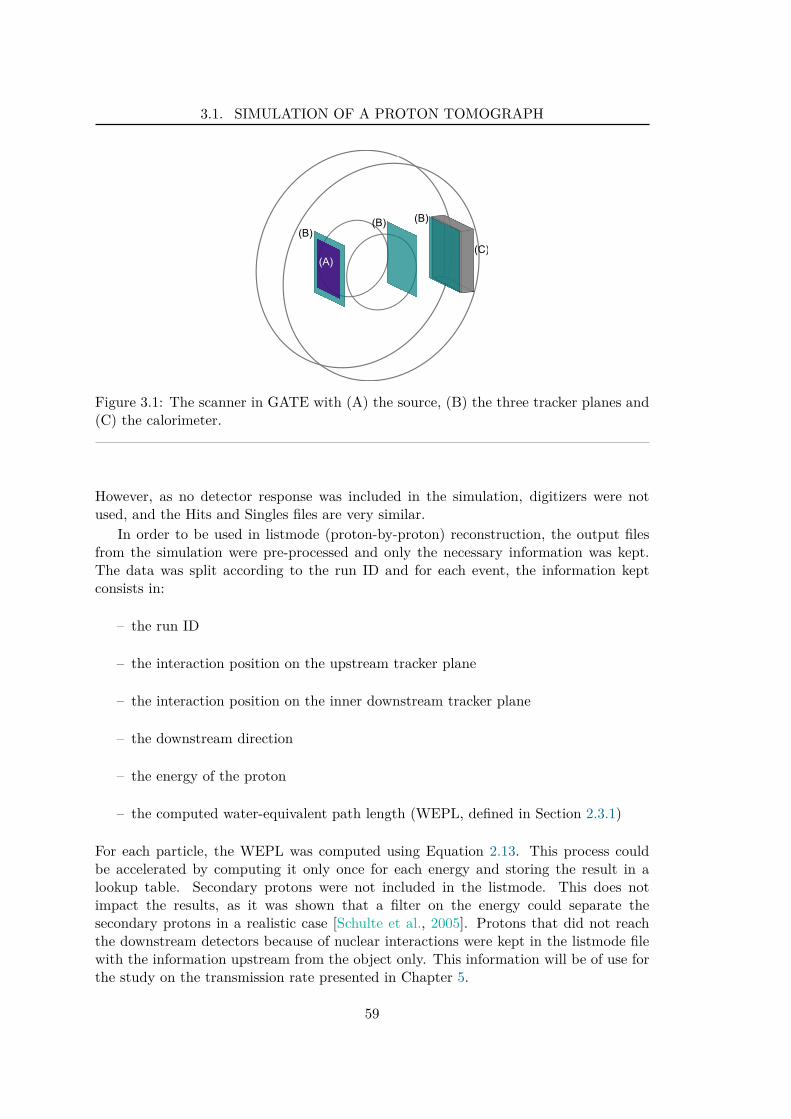
3.1. SIMULATION OF A PROTON TOMOGRAPH
Figure 3.1: The scanner in GATE with (A) the source, (B) the three tracker planes and(C) the calorimeter.
However, as no detector response was included in the simulation, digitizers were notused, and the Hits and Singles files are very similar.
In order to be used in listmode (proton-by-proton) reconstruction, the output filesfrom the simulation were pre-processed and only the necessary information was kept.The data was split according to the run ID and for each event, the information keptconsists in:
– the run ID
– the interaction position on the upstream tracker plane
– the interaction position on the inner downstream tracker plane
– the downstream direction
– the energy of the proton
– the computed water-equivalent path length (WEPL, defined in Section 2.3.1)
For each particle, the WEPL was computed using Equation 2.13. This process couldbe accelerated by computing it only once for each energy and storing the result in alookup table. Secondary protons were not included in the listmode. This does notimpact the results, as it was shown that a filter on the energy could separate thesecondary protons in a realistic case [Schulte et al., 2005]. Protons that did not reachthe downstream detectors because of nuclear interactions were kept in the listmode filewith the information upstream from the object only. This information will be of use forthe study on the transmission rate presented in Chapter 5.
59
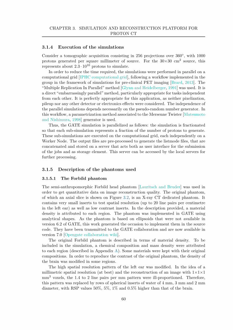
CHAPTER 3. SIMULATION AND RECONSTRUCTION PLATFORM FORPROTON CT
3.1.4 Execution of the simulations
Consider a tomographic acquisition consisting in 256 projections over 360, with 1000protons generated per square millimeter of source. For the 30×30 cm2 source, thisrepresents about 2.3 · 1010 protons to simulate.
In order to reduce the time required, the simulations were performed in parallel on acomputational grid [IPHC computational grid], following a workflow implemented in thegroup in the framework of simulations for pre-clinical PET imaging [Brard, 2013]. The“Multiple Replication In Parallel” method [Glynn and Heidelberger, 1991] was used. It isa direct “embarrassingly parallel” method, particularly appropriate for tasks independentfrom each other. It is perfectly appropriate for this application, as neither pixelization,pileup nor any other detector or electronics effects were considered. The independence ofthe parallel simulations depends necessarily on the pseudo-random number generator. Inthis workflow, a parametrization method associated to the Mersenne Twister [Matsumotoand Nishimura, 1998] generator is used.
Thus, the GATE simulation is parallelized as follows: the simulation is fractionatedso that each sub-simulation represents a fraction of the number of protons to generate.These sub-simulations are executed on the computational grid, each independently on aWorker Node. The output files are pre-processed to generate the listmode files, that areconcatenated and stored on a server that acts both as user interface for the submissionof the jobs and as storage element. This server can be accessed by the local servers forfurther processing.
3.1.5 Description of the phantoms used
3.1.5.1 The Forbild phantom
The semi-anthropomorphic Forbild head phantom [Lauritsch and Bruder] was used inorder to get quantitative data on image reconstruction quality. The original phantom,of which an axial slice is shown on Figure 3.2, is an X-ray CT dedicated phantom. Itcontains very small inserts to test spatial resolution (up to 20 line pairs per centimetrein the left ear) as well as low contrast inserts. In the description provided, a materialdensity is attributed to each region. The phantom was implemented in GATE usinganalytical shapes. As the phantom is based on ellipsoids that were not available inversion 6.2 of GATE, this work generated the occasion to implement them in the sourcecode. They have been transmitted to the GATE collaboration and are now available inversion 7.0 [Opengate collaboration wiki].
The original Forbild phantom is described in terms of material density. To beincluded in the simulation, a chemical composition and mass density were attributedto each region (described in Appendix A). Some materials were kept with their originalcompositions. In order to reproduce the contrast of the original phantom, the density ofthe brain was modified in some regions.
The high spatial resolution pattern of the left ear was modified. In the idea of amillimetric spatial resolution (at best) and the reconstruction of an image with 1×1×1mm3 voxels, the 1.4 to 2 line pairs per mm pattern were ill-proportioned. Therefore,this pattern was replaced by rows of spherical inserts of water of 4 mm, 3 mm and 2 mmdiameter, with RSP values 50%, 5%, 1% and 0.5% higher than that of the brain.
60
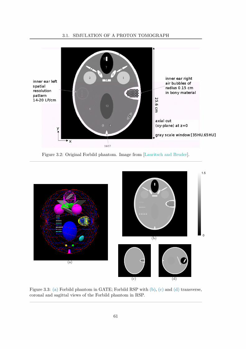
3.1. SIMULATION OF A PROTON TOMOGRAPH
Figure 3.2: Original Forbild phantom. Image from [Lauritsch and Bruder].
(a)
(b)0
1.5
(c) (d)
Figure 3.3: (a) Forbild phantom in GATE; Forbild RSP with (b), (c) and (d) transverse,coronal and sagittal views of the Forbild phantom in RSP.
61
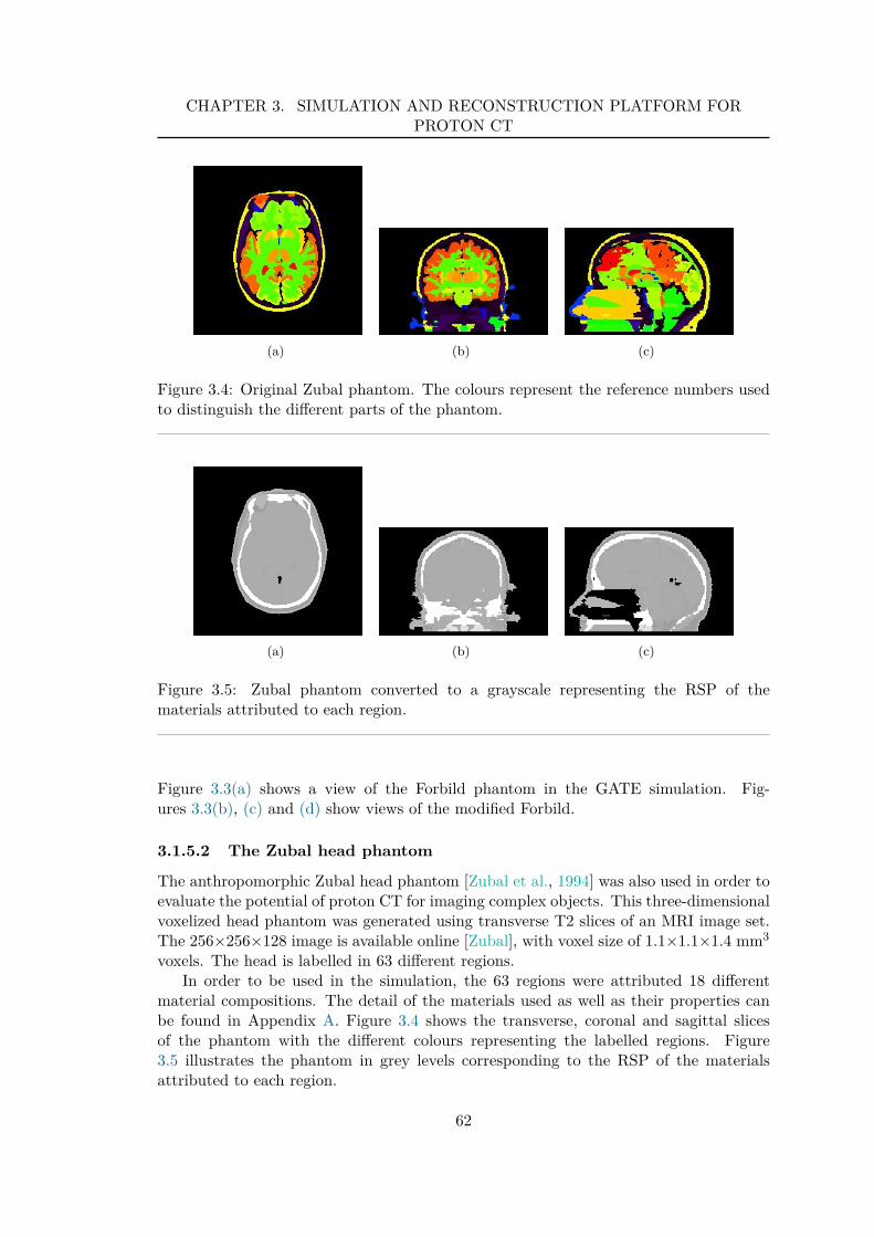
CHAPTER 3. SIMULATION AND RECONSTRUCTION PLATFORM FORPROTON CT
(a) (b) (c)
Figure 3.4: Original Zubal phantom. The colours represent the reference numbers usedto distinguish the different parts of the phantom.
(a) (b) (c)
Figure 3.5: Zubal phantom converted to a grayscale representing the RSP of thematerials attributed to each region.
Figure 3.3(a) shows a view of the Forbild phantom in the GATE simulation. Fig-ures 3.3(b), (c) and (d) show views of the modified Forbild.
3.1.5.2 The Zubal head phantom
The anthropomorphic Zubal head phantom [Zubal et al., 1994] was also used in order toevaluate the potential of proton CT for imaging complex objects. This three-dimensionalvoxelized head phantom was generated using transverse T2 slices of an MRI image set.The 256×256×128 image is available online [Zubal], with voxel size of 1.1×1.1×1.4 mm3
voxels. The head is labelled in 63 different regions.In order to be used in the simulation, the 63 regions were attributed 18 different
material compositions. The detail of the materials used as well as their properties canbe found in Appendix A. Figure 3.4 shows the transverse, coronal and sagittal slicesof the phantom with the different colours representing the labelled regions. Figure3.5 illustrates the phantom in grey levels corresponding to the RSP of the materialsattributed to each region.
62
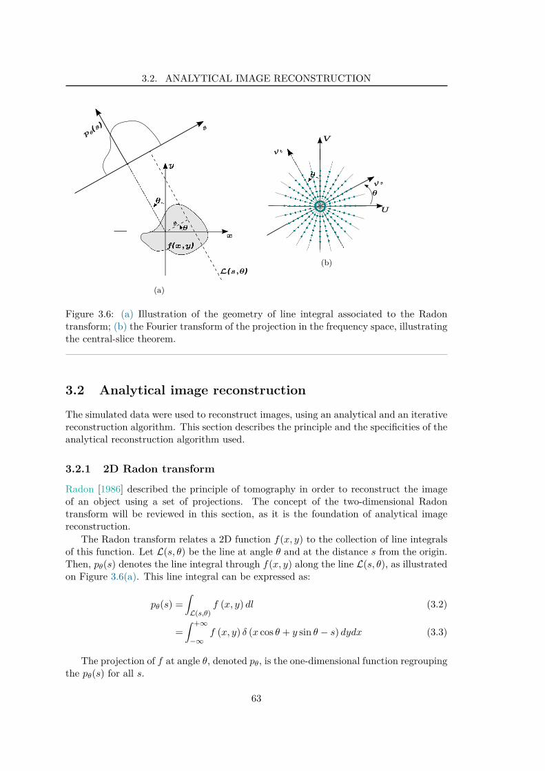
3.2. ANALYTICAL IMAGE RECONSTRUCTION
(a)
(b)
Figure 3.6: (a) Illustration of the geometry of line integral associated to the Radontransform; (b) the Fourier transform of the projection in the frequency space, illustratingthe central-slice theorem.
3.2 Analytical image reconstruction
The simulated data were used to reconstruct images, using an analytical and an iterativereconstruction algorithm. This section describes the principle and the specificities of theanalytical reconstruction algorithm used.
3.2.1 2D Radon transform
Radon [1986] described the principle of tomography in order to reconstruct the imageof an object using a set of projections. The concept of the two-dimensional Radontransform will be reviewed in this section, as it is the foundation of analytical imagereconstruction.
The Radon transform relates a 2D function f(x, y) to the collection of line integralsof this function. Let L(s, θ) be the line at angle θ and at the distance s from the origin.Then, pθ(s) denotes the line integral through f(x, y) along the line L(s, θ), as illustratedon Figure 3.6(a). This line integral can be expressed as:
pθ(s) =∫
L(s,θ)f (x, y) dl (3.2)
=∫ +∞
−∞f (x, y) δ (x cos θ + y sin θ − s) dydx (3.3)
The projection of f at angle θ, denoted pθ, is the one-dimensional function regroupingthe pθ(s) for all s.
63
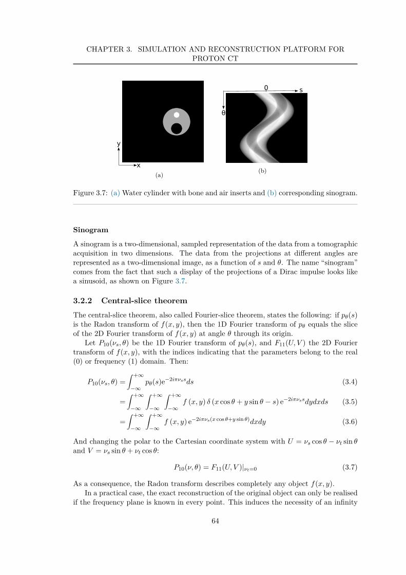
CHAPTER 3. SIMULATION AND RECONSTRUCTION PLATFORM FORPROTON CT
(a)(b)
Figure 3.7: (a) Water cylinder with bone and air inserts and (b) corresponding sinogram.
Sinogram
A sinogram is a two-dimensional, sampled representation of the data from a tomographicacquisition in two dimensions. The data from the projections at different angles arerepresented as a two-dimensional image, as a function of s and θ. The name “sinogram”comes from the fact that such a display of the projections of a Dirac impulse looks likea sinusoid, as shown on Figure 3.7.
3.2.2 Central-slice theorem
The central-slice theorem, also called Fourier-slice theorem, states the following: if pθ(s)is the Radon transform of f(x, y), then the 1D Fourier transform of pθ equals the sliceof the 2D Fourier transform of f(x, y) at angle θ through its origin.
Let P10(νs, θ) be the 1D Fourier transform of pθ(s), and F11(U, V ) the 2D Fouriertransform of f(x, y), with the indices indicating that the parameters belong to the real(0) or frequency (1) domain. Then:
P10(νs, θ) =∫ +∞
−∞pθ(s)e−2iπνssds (3.4)
=∫ +∞
−∞
∫ +∞
−∞
∫ +∞
−∞f (x, y) δ (x cos θ + y sin θ − s) e−2iπνssdydxds (3.5)
=∫ +∞
−∞
∫ +∞
−∞f (x, y) e−2iπνs(x cos θ+y sin θ)dxdy (3.6)
And changing the polar to the Cartesian coordinate system with U = νs cos θ − νt sin θand V = νs sin θ + νt cos θ:
P10(ν, θ) = F11(U, V )|νt=0 (3.7)
As a consequence, the Radon transform describes completely any object f(x, y).In a practical case, the exact reconstruction of the original object can only be realised
if the frequency plane is known in every point. This induces the necessity of an infinity
64
3.2. ANALYTICAL IMAGE RECONSTRUCTION
of projections. As the number of projections is limited, a limited number of radial linesrepresenting the information on the frequency plane is available. This is illustrated onFigure 3.6(b), where the blue dots represent the sampled information. This generatesan over-sampling of the low frequencies and a lack of information in the high-frequencydomain. Moreover, the passage from the function P10(ν, θ) defined in the polar space toF11(U, V ) defined in the Cartesian space requires interpolation.
3.2.3 Filtered Back-projection algorithm
The direct back-projection of each sinogram value onto the object space along thecorresponding ray does not, however, allow to recover the object f(x, y). Instead, itgenerates a blurred version of the object, called laminogram or layergram [Smith et al.,1973]. It is possible to deconvolve the laminogram by a cone filter in order to recoverthe original image: this is the backproject-filter method. It is also possible to applythe filter to the projections, before the back-projection operation: this is the filteredback-projection (FBP) method. We have:
f (x, y) =∫ +∞
−∞
∫ +∞
−∞F11 (U, V ) e2iπ(Ux+V y)dUdV (3.8)
Changing from the Cartesian to the polar coordinate system with, as previously, U =ν cos θ and V = ν sin θ (νt = 0, ν = νs), we obtain:
f (x, y) =∫ π
0
∫ +∞
−∞F11 (ν cos θ, ν sin θ) e2iπν(x cos θ+y sin θ)|ν|dνdθ (3.9)
=∫ π
0
[∫ +∞
−∞P10 (ν, θ) e2iπν(x cos θ+y sin θ)|ν|dν
]
dθ (3.10)
=∫ π
0
∫ +∞
−∞pθ (s) h (x cos θ + y sin θ − s) dsdθ (3.11)
with h the inverse Fourier transform of the ramp function |ν|.As the introduction of the ramp filter amplifies high frequency noise, it is necessary
to apodize the ramp filter using a 1D lowpass filter. However, as the sharp transitiongenerated by a cut-off can lead to artefacts in the image, “smoother” apodizing filtersare used, which further reduce the high frequencies.
3.2.4 Specificities
3.2.4.1 On the generation of projections
The listmode data acquisitions make it possible to know the exact position of interactionof each proton on every tracker plane. As mentioned in the previous chapter (Section2.3.3.1), different possibilities exist for binning the data into projections. The questiontakes all its importance in proton imaging, more than in X-ray imaging, because ofmultiple scattering. For example, taking into account only the position of interactionat the entrance of the calorimeter results in a very poor spatial resolution of thereconstructed image. Whatever the binning procedure chosen, the straight line L(s, θ)will only be an approximation of the particles path.
65
CHAPTER 3. SIMULATION AND RECONSTRUCTION PLATFORM FORPROTON CT
Different binning options were used throughout this work (detailed in Section 4.1.1).As the geometry used for this work is based on a parallel beam, the positions of entrancein the object will be the same than the positions of interaction on the upstream trackerplane (in the xy plane). Upon exit, however, as the particles will have acquired an angle,the position on the tracker planes will strongly depend on the position of the plane (inz, the distance to the object). For an object to image without lateral discontinuities inthe path of the particles in the xy plane, the path approximation of a straight line fromthe upstream position will represent the average path of the particles. Therefore, thiswas used for the study of the scattering and transmission rate of the particles (presentedin Chapter 5).
3.2.4.2 On the Filtered Back-projection algorithm implementation
The FBP algorithm used for this work had been previously implemented in the group.The three-dimensional reconstructed image is the concatenation of a series of two-dimensional image slices reconstructed with a 2D sinogram each.
For the apodization, a Hamming filter [Fessler, 2009] with a cut-off at the Nyquistfrequency [Nyquist, 2002] was used.
3.3 Iterative reconstruction with the Algebraic Recon-struction Technique along the most likely path
Iterative reconstruction algorithms have the advantage of easily allowing a proton-by-proton reconstruction using the definition of curved projection and back-projectionpaths. Reconstructions using the data binned into projections as well as in listmodeformat can be performed, which may present an advantage in terms of spatial resolutionfor proton CT.
Algebraic reconstruction techniques are nowadays mainly used in the context oflimited-angle tomography and sparse-view tomography [Intes et al., 2002; Sidky andPan, 2008; Han et al., 2011]. Statistical algorithms for image reconstruction areoften preferred in emission or transmission imaging modalities. The advantage of astatistical reconstruction algorithm is that it makes it possible to include statisticaland physical models into the reconstruction [Vandenberghe et al., 2001]. However,an appropriate formulation of the pCT image reconstruction problem has not beendeveloped yet. Nevertheless, it was shown that algebraic methods are adapted to thepCT image reconstruction problem [Penfold, 2010], leading to the choice of implementingthe Algebraic Reconstruction Technique (ART) algorithm. In addition, a curved pathestimation of the most likely path (MLP) for each proton in the reconstruction processwas implemented.
3.3.1 The ART algorithm
The ART algorithm belongs to the class of “projection methods”, as first proposed byKaczmarz [1937] and further developed by Tanabe [1971].
66
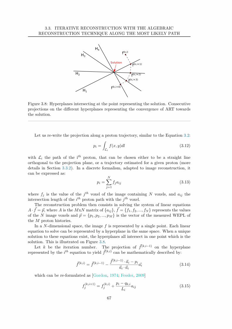
3.3. ITERATIVE RECONSTRUCTION WITH THE ALGEBRAICRECONSTRUCTION TECHNIQUE ALONG THE MOST LIKELY PATH
Figure 3.8: Hyperplanes intersecting at the point representing the solution. Consecutiveprojections on the different hyperplanes representing the convergence of ART towardsthe solution.
Let us re-write the projection along a proton trajectory, similar to the Equation 3.2:
pi =∫
Li
f(x, y)dl (3.12)
with Li the path of the ith proton, that can be chosen either to be a straight lineorthogonal to the projection plane, or a trajectory estimated for a given proton (moredetails in Section 3.3.2). In a discrete formalism, adapted to image reconstruction, itcan be expressed as:
pi =N∑
j=1
fjaij (3.13)
where fj is the value of the jth voxel of the image containing N voxels, and aij theintersection length of the ith proton path with the jth voxel.
The reconstruction problem then consists in solving the system of linear equationsA · ~f = ~p, where A is the MxN matrix of aij, ~f = f1, f2, ..., fN represents the valuesof the N image voxels and ~p = p1, p2, ..., pM is the vector of the measured WEPL ofthe M proton histories.
In a N -dimensional space, the image f is represented by a single point. Each linearequation to solve can be represented by a hyperplane in the same space. When a uniquesolution to these equations exist, the hyperplanes all intersect in one point which is thesolution. This is illustrated on Figure 3.8.
Let k be the iteration number. The projection of ~f (k,i−1) on the hyperplanerepresented by the ith equation to yield ~f (k,i) can be mathematically described by:
~f (k,i) = ~f (k,i−1) −~f (k,i−1) ·~ai − pi
~ai ·~ai~ai (3.14)
which can be re-formulated as [Gordon, 1974; Fessler, 2009]
f(k,i+1)j = f
(k,i)j +
pi − qk,i
Liaij (3.15)
67
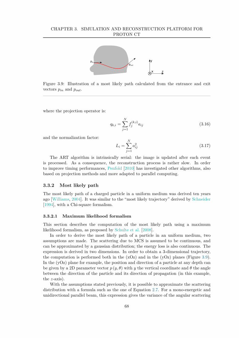
CHAPTER 3. SIMULATION AND RECONSTRUCTION PLATFORM FORPROTON CT
Figure 3.9: Illustration of a most likely path calculated from the entrance and exitvectors pin and pout.
where the projection operator is:
qk,i =N∑
j=1
f(k,i)j aij (3.16)
and the normalization factor:
Li =N∑
j=1
a2ij (3.17)
The ART algorithm is intrinsically serial: the image is updated after each eventis processed. As a consequence, the reconstruction process is rather slow. In orderto improve timing performances, Penfold [2010] has investigated other algorithms, alsobased on projection methods and more adapted to parallel computing.
3.3.2 Most likely path
The most likely path of a charged particle in a uniform medium was derived ten yearsago [Williams, 2004]. It was similar to the “most likely trajectory” derived by Schneider[1994], with a Chi-square formalism.
3.3.2.1 Maximum likelihood formalism
This section describes the computation of the most likely path using a maximumlikelihood formalism, as proposed by Schulte et al. [2008].
In order to derive the most likely path of a particle in an uniform medium, twoassumptions are made. The scattering due to MCS is assumed to be continuous, andcan be approximated by a gaussian distribution; the energy loss is also continuous. Theexpression is derived in two dimensions. In order to obtain a 3-dimensional trajectory,the computation is performed both in the (xOz) and in the (yOz) planes (Figure 3.9).In the (yOz) plane for example, the position and direction of a particle at any depth canbe given by a 2D parameter vector p (y, θ) with y the vertical coordinate and θ the anglebetween the direction of the particle and its direction of propagation (in this example,the z-axis).
With the assumptions stated previously, it is possible to approximate the scatteringdistribution with a formula such as the one of Equation 2.7. For a mono-energetic andunidirectional parallel beam, this expression gives the variance of the angular scattering
68
3.3. ITERATIVE RECONSTRUCTION WITH THE ALGEBRAICRECONSTRUCTION TECHNIQUE ALONG THE MOST LIKELY PATH
for a thin object (l ≪ X0). Should one consider only one particle, this describes thevariance of the Gaussian angular scattering probability distribution.
Let pin and pout be the two-dimensional parameter vectors characterizing the entranceand exit parameters of the particle, so that:
pin =
(
yin
θin
)
pout =
(
yout
θout
)
with yin and yout the lateral coordinates at entrance (depth zin) and exit (depth zout),and θin and θout the angles upon entry and exit. Let p1 be the 2D parameter vectorcharacterizing the position and direction of the particle at depth z1.
In the bayesian formalism, one can express the posterior likelihood of finding theparticle in the state p1 as:
L (p1|pout) = L (pout|p1)L (p1)
L (pout)(3.18)
As we start with the knowledge that the particle did exit the object with pout and enteredit with pin, this can be re-written as:
L (p1|pout) = L (pout|p1) L (p1|pin) (3.19)
The most likely location and direction can be derived by finding the vector p1 maximizingthis likelihood. It can be put forward that L (p1|pin) and L (pout|p1) are determined bythe scattering inside the object. As an example, one can write the likelihood of findinga proton with the parameters p1 knowing pin = (0, 0) as:
L
(
p1|pin =
(
00
))
= exp(
−12
pT1 Σ−1
1 p1
)
(3.20)
where pT denotes the transpose of p. Therefore, knowledge of the scattering matrices isrequired.
Let Σ1 be the scattering matrix whose elements correspond to the variances andcovariances of y1 and θ1 acquired between zin and z1 :
Σ1 =
(
σ2y1
σ2y1θ1
σ2θ1y1
σ2θ1
)
(3.21)
The elements of this matrix are computed using Equation 2.7 from Lynch and Dahl[1991] presented in the previous chapter. However, the object can not be approximatedby a “thin” object, and the order of magnitude of the distance traversed can go from afew millimetres to about 20 cm in the case of a head. Therefore, the previous formulaneeds to be integrated over the depth considered:
σ2y1
(zin, z1) = E20
(
1 + 0.038 lnz1 − zin
X0
)2
×∫ z1
zin
(z1 − u)2
β2 (u) p2 (u)du
X0(3.22)
σ2θ1
(zin, z1) = E20
(
1 + 0.038 lnz1 − zin
X0
)2
×∫ z1
zin
1β2 (u) p2 (u)
du
X0(3.23)
69
CHAPTER 3. SIMULATION AND RECONSTRUCTION PLATFORM FORPROTON CT
σ2y1θ1
(zin, z1) = E20
(
1 + 0.038 lnz1 − zin
X0
)2
×∫ z1
zin
zin − u
β2 (u) p2 (u)du
X0(3.24)
with X0 the radiation length of the material (31.6 cm for water) and E0 = 13.6 MeV.The equivalent Σ2 can be computed for the scattering between z1 and zout.
In order to allow for the explicit evaluation of the integrals, the energy-loss term 1β2p2
is approximated by a fifth-degree polynomial. This polynomial is obtained by fitting theenergy loss of protons with the same characteristics as the beam used, in the materialof interest – here water – using a Monte Carlo simulation.
Let Rin and R1 be the matrices changing the local coordinates system of the incomingproton according to the location of the proton path at entry depth zin and at depth z1:
Rin =
(
1 z1 − zin
0 1
)
, R1 =
(
1 zout − z1
0 1
)
(3.25)
The posterior likelihood of p1 can then be written as:
L (p1|pout) = exp(
−12[
(
pT1 − pT
inRTin
)
Σ−11 (p1 − Rinpin)
+(
pTout − pT
1 RT1
)
Σ−12 (pout − R1p1)
]
)
(3.26)
≡ exp(
−χ2)
(3.27)
Differentiating the expression of χ2 with respect to y1 and θ1, setting the result tozero and solving for p1, one can obtain the maximum likelihood proton path formula:
pMLP =(
Σ−11 + RT
1 Σ−12 R1
)−1 (
Σ−11 Rinpin + RT
1 Σ−12 pout
)
(3.28)
Uncertainty on the path
An advantage of this formulation is that it makes it possible to consider the error on thismost likely path: a one-sigma envelope on the positions determined can be computedusing the inverse of the curvature matrix. The error matrix is defined as:
ǫy1θ1(z1) = 2
(
Σ−11 + RT
1 Σ−12 R1
)−1(3.29)
and the variance in the lateral displacement at depth z1 is given by the element in thefirst row and first column of this matrix.
3.3.2.2 Implementation for parallel-beam geometry
The fifth-degree polynomial was calculated as described in [Schulte et al., 2008], usinga Geant4 simulation of a mono-directional and mono-energetic 200 MeV proton beam,sent into a 20 cm deep cube of water. For each proton, the energy in each 1 mm-slicewas recorded and the value of 1
β2p2 was calculated as:
1β2(u)p2(u)
=(E (u) + Ep)2 c2
(E (u) + 2Ep)2 E2 (u)(3.30)
70
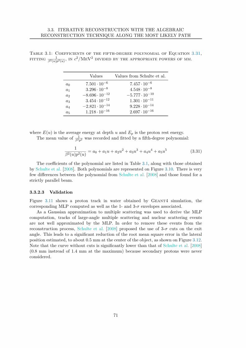
3.3. ITERATIVE RECONSTRUCTION WITH THE ALGEBRAICRECONSTRUCTION TECHNIQUE ALONG THE MOST LIKELY PATH
Table 3.1: Coefficients of the fifth-degree polynomial of Equation 3.31,fitting 1
β2(u)p2(u), in c2/MeV2 divided by the appropriate powers of mm.
Values Values from Schulte et al.
a0 7.501 · 10−6 7.457 · 10−6
a1 3.296 · 10−8 4.548 · 10−8
a2 −8.696 · 10−12 −5.777 · 10−10
a3 3.454 · 10−12 1.301 · 10−11
a4 −2.821 · 10−14 9.228 · 10−14
a5 1.218 · 10−16 2.697 · 10−16
where E(u) is the average energy at depth u and Ep is the proton rest energy.The mean value of 1
β2p2 was recorded and fitted by a fifth-degree polynomial:
1β2(u)p2(u)
= a0 + a1u + a2u2 + a3u3 + a4u4 + a5u5 (3.31)
The coefficients of the polynomial are listed in Table 3.1, along with those obtainedby Schulte et al. [2008]. Both polynomials are represented on Figure 3.10. There is veryfew differences between the polynomial from Schulte et al. [2008] and those found for astrictly parallel beam.
3.3.2.3 Validation
Figure 3.11 shows a proton track in water obtained by Geant4 simulation, thecorresponding MLP computed as well as the 1- and 3-σ envelopes associated.
As a Gaussian approximation to multiple scattering was used to derive the MLPcomputation, tracks of large-angle multiple scattering and nuclear scattering eventsare not well approximated by the MLP. In order to remove these events from thereconstruction process, Schulte et al. [2008] proposed the use of 3-σ cuts on the exitangle. This leads to a significant reduction of the root mean square error in the lateralposition estimated, to about 0.5 mm at the center of the object, as shown on Figure 3.12.Note that the curve without cuts is significantly lower than that of Schulte et al. [2008](0.8 mm instread of 1.4 mm at the maximum) because secondary protons were neverconsidered.
71
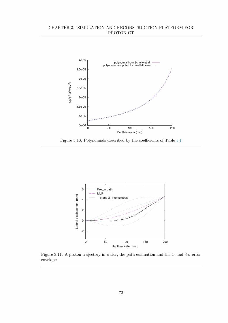
CHAPTER 3. SIMULATION AND RECONSTRUCTION PLATFORM FORPROTON CT
5e-06
1e-05
1.5e-05
2e-05
2.5e-05
3e-05
3.5e-05
4e-05
0 50 100 150 200
1/β
2p
2 (
c2/M
eV
2)
Depth in water (mm)
polynomial from Schulte et al.polynomial computed for parallel beam
Figure 3.10: Polynomials described by the coefficients of Table 3.1
-2
0
2
4
6
0 50 100 150 200
La
tera
l d
isp
lace
me
nt
(mm
)
Depth in water (mm)
Proton path
MLP
1-σ and 3- σ envelopes
Figure 3.11: A proton trajectory in water, the path estimation and the 1- and 3-σ errorenvelope.
72
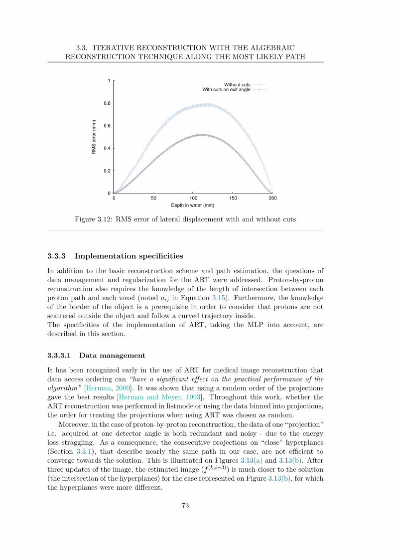
3.3. ITERATIVE RECONSTRUCTION WITH THE ALGEBRAICRECONSTRUCTION TECHNIQUE ALONG THE MOST LIKELY PATH
0
0.2
0.4
0.6
0.8
1
0 50 100 150 200
RM
S e
rro
r (m
m)
Depth in water (mm)
Without cutsWith cuts on exit angle
Figure 3.12: RMS error of lateral displacement with and without cuts
3.3.3 Implementation specificities
In addition to the basic reconstruction scheme and path estimation, the questions ofdata management and regularization for the ART were addressed. Proton-by-protonreconstruction also requires the knowledge of the length of intersection between eachproton path and each voxel (noted aij in Equation 3.15). Furthermore, the knowledgeof the border of the object is a prerequisite in order to consider that protons are notscattered outside the object and follow a curved trajectory inside.The specificities of the implementation of ART, taking the MLP into account, aredescribed in this section.
3.3.3.1 Data management
It has been recognized early in the use of ART for medical image reconstruction thatdata access ordering can “have a significant effect on the practical performance of thealgorithm” [Herman, 2009]. It was shown that using a random order of the projectionsgave the best results [Herman and Meyer, 1993]. Throughout this work, whether theART reconstruction was performed in listmode or using the data binned into projections,the order for treating the projections when using ART was chosen as random.
Moreover, in the case of proton-by-proton reconstruction, the data of one “projection”i.e. acquired at one detector angle is both redundant and noisy - due to the energyloss straggling. As a consequence, the consecutive projections on “close” hyperplanes(Section 3.3.1), that describe nearly the same path in our case, are not efficient toconverge towards the solution. This is illustrated on Figures 3.13(a) and 3.13(b). Afterthree updates of the image, the estimated image (f (k,i+3)) is much closer to the solution(the intersection of the hyperplanes) for the case represented on Figure 3.13(b), for whichthe hyperplanes were more different.
73
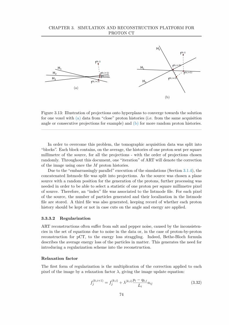
CHAPTER 3. SIMULATION AND RECONSTRUCTION PLATFORM FORPROTON CT
(a)
(b)
Figure 3.13: Illustration of projections onto hyperplans to converge towards the solutionfor one voxel with (a) data from “close” proton histories (i.e. from the same acquisitionangle or consecutive projections for example) and (b) for more random proton histories.
In order to overcome this problem, the tomographic acquisition data was split into“blocks”. Each block contains, on the average, the histories of one proton sent per squaremillimetre of the source, for all the projections - with the order of projections chosenrandomly. Throughout this document, one “iteration” of ART will denote the correctionof the image using once the M proton histories.
Due to the “embarrassingly parallel” execution of the simulations (Section 3.1.4), theconcatenated listmode file was split into projections. As the source was chosen a planesource with a random position for the generation of the protons, further processing wasneeded in order to be able to select a statistic of one proton per square millimetre pixelof source. Therefore, an “index” file was associated to the listmode file. For each pixelof the source, the number of particles generated and their localization in the listmodefile are stored. A third file was also generated, keeping record of whether each protonhistory should be kept or not in case cuts on the angle and energy are applied.
3.3.3.2 Regularization
ART reconstructions often suffer from salt and pepper noise, caused by the inconsisten-cies in the set of equations due to noise in the data or, in the case of proton-by-protonreconstruction for pCT, to the energy loss straggling. Indeed, Bethe-Bloch formuladescribes the average energy loss of the particles in matter. This generates the need forintroducing a regularization scheme into the reconstruction.
Relaxation factor
The first form of regularization is the multiplication of the correction applied to eachpixel of the image by a relaxation factor λ, giving the image update equation:
f(k,i+1)j = f
(k,i)j + λ(k,i) pi − qk,i
Liaij (3.32)
74
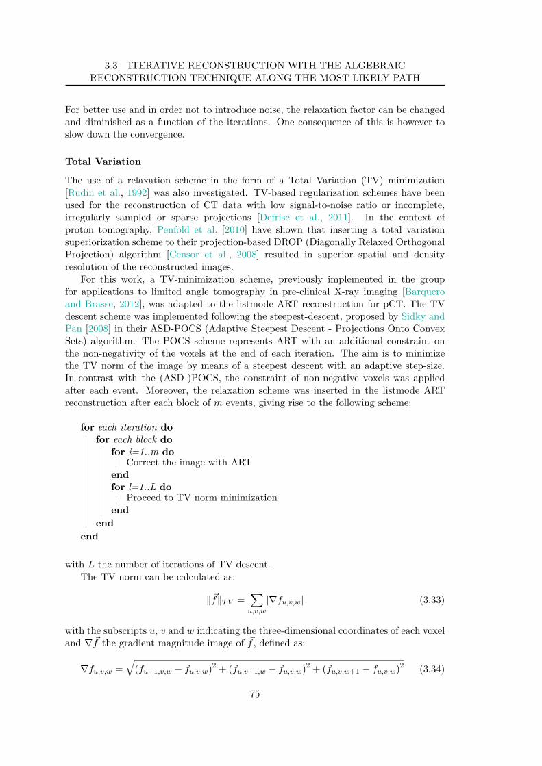
3.3. ITERATIVE RECONSTRUCTION WITH THE ALGEBRAICRECONSTRUCTION TECHNIQUE ALONG THE MOST LIKELY PATH
For better use and in order not to introduce noise, the relaxation factor can be changedand diminished as a function of the iterations. One consequence of this is however toslow down the convergence.
Total Variation
The use of a relaxation scheme in the form of a Total Variation (TV) minimization[Rudin et al., 1992] was also investigated. TV-based regularization schemes have beenused for the reconstruction of CT data with low signal-to-noise ratio or incomplete,irregularly sampled or sparse projections [Defrise et al., 2011]. In the context ofproton tomography, Penfold et al. [2010] have shown that inserting a total variationsuperiorization scheme to their projection-based DROP (Diagonally Relaxed OrthogonalProjection) algorithm [Censor et al., 2008] resulted in superior spatial and densityresolution of the reconstructed images.
For this work, a TV-minimization scheme, previously implemented in the groupfor applications to limited angle tomography in pre-clinical X-ray imaging [Barqueroand Brasse, 2012], was adapted to the listmode ART reconstruction for pCT. The TVdescent scheme was implemented following the steepest-descent, proposed by Sidky andPan [2008] in their ASD-POCS (Adaptive Steepest Descent - Projections Onto ConvexSets) algorithm. The POCS scheme represents ART with an additional constraint onthe non-negativity of the voxels at the end of each iteration. The aim is to minimizethe TV norm of the image by means of a steepest descent with an adaptive step-size.In contrast with the (ASD-)POCS, the constraint of non-negative voxels was appliedafter each event. Moreover, the relaxation scheme was inserted in the listmode ARTreconstruction after each block of m events, giving rise to the following scheme:
for each iteration dofor each block do
for i=1..m doCorrect the image with ART
endfor l=1..L do
Proceed to TV norm minimizationend
end
end
with L the number of iterations of TV descent.The TV norm can be calculated as:
‖~f‖T V =∑
u,v,w
|∇fu,v,w| (3.33)
with the subscripts u, v and w indicating the three-dimensional coordinates of each voxeland ∇~f the gradient magnitude image of ~f , defined as:
∇fu,v,w =√
(fu+1,v,w − fu,v,w)2 + (fu,v+1,w − fu,v,w)2 + (fu,v,w+1 − fu,v,w)2 (3.34)
75
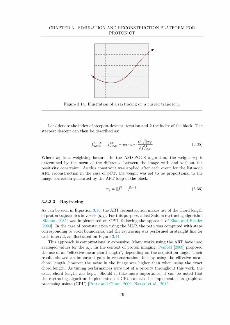
CHAPTER 3. SIMULATION AND RECONSTRUCTION PLATFORM FORPROTON CT
Figure 3.14: Illustration of a raytracing on a curved trajectory.
Let l denote the index of steepest descent iteration and k the index of the block. Thesteepest descent can then be described as:
f l+1,ku,v,w = f l,k
u,v,w − w1 · w2 · ∂‖~f‖T V
∂f l,ku,v,w
(3.35)
Where w1 is a weighting factor. In the ASD-POCS algorithm, the weight w2 isdetermined by the norm of the difference between the image with and without thepositivity constraint. As this constraint was applied after each event for the listmodeART reconstruction in the case of pCT, the weight was set to be proportional to theimage correction generated by the ART loop of the block:
w2 = ‖~fk − ~fk−1‖ (3.36)
3.3.3.3 Raytracing
As can be seen in Equation 3.15, the ART reconstruction makes use of the chord lengthof proton trajectories in voxels (aij). For this purpose, a fast Siddon raytracing algorithm[Siddon, 1985] was implemented on CPU, following the approach of Zhao and Reader[2003]. In the case of reconstruction using the MLP, the path was computed with stepscorresponding to voxel boundaries, and the raytracing was performed in straight line foreach interval, as illustrated on Figure 3.14.
This approach is computationally expensive. Many works using the ART have usedaveraged values for the aij . In the context of proton imaging, Penfold [2009] proposedthe use of an “effective mean chord length”, depending on the acquisition angle. Theirresults showed an important gain in reconstruction time by using the effective meanchord length, however the noise in the image was higher than when using the exactchord length. As timing performances were not of a priority throughout this work, theexact chord length was kept. Should it take more importance, it can be noted thatthe raytracing algorithm implemented on CPU can also be implemented on graphicalprocessing usints (GPU) [Pratx and Chinn, 2009; Nassiri et al., 2012].
76
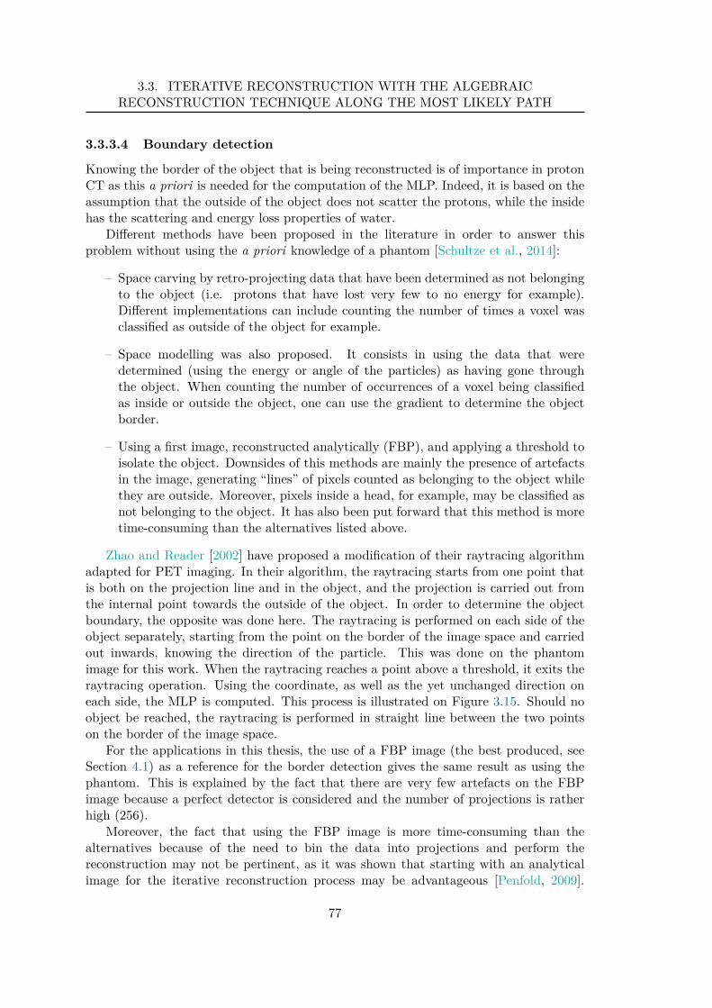
3.3. ITERATIVE RECONSTRUCTION WITH THE ALGEBRAICRECONSTRUCTION TECHNIQUE ALONG THE MOST LIKELY PATH
3.3.3.4 Boundary detection
Knowing the border of the object that is being reconstructed is of importance in protonCT as this a priori is needed for the computation of the MLP. Indeed, it is based on theassumption that the outside of the object does not scatter the protons, while the insidehas the scattering and energy loss properties of water.
Different methods have been proposed in the literature in order to answer thisproblem without using the a priori knowledge of a phantom [Schultze et al., 2014]:
– Space carving by retro-projecting data that have been determined as not belongingto the object (i.e. protons that have lost very few to no energy for example).Different implementations can include counting the number of times a voxel wasclassified as outside of the object for example.
– Space modelling was also proposed. It consists in using the data that weredetermined (using the energy or angle of the particles) as having gone throughthe object. When counting the number of occurrences of a voxel being classifiedas inside or outside the object, one can use the gradient to determine the objectborder.
– Using a first image, reconstructed analytically (FBP), and applying a threshold toisolate the object. Downsides of this methods are mainly the presence of artefactsin the image, generating “lines” of pixels counted as belonging to the object whilethey are outside. Moreover, pixels inside a head, for example, may be classified asnot belonging to the object. It has also been put forward that this method is moretime-consuming than the alternatives listed above.
Zhao and Reader [2002] have proposed a modification of their raytracing algorithmadapted for PET imaging. In their algorithm, the raytracing starts from one point thatis both on the projection line and in the object, and the projection is carried out fromthe internal point towards the outside of the object. In order to determine the objectboundary, the opposite was done here. The raytracing is performed on each side of theobject separately, starting from the point on the border of the image space and carriedout inwards, knowing the direction of the particle. This was done on the phantomimage for this work. When the raytracing reaches a point above a threshold, it exits theraytracing operation. Using the coordinate, as well as the yet unchanged direction oneach side, the MLP is computed. This process is illustrated on Figure 3.15. Should noobject be reached, the raytracing is performed in straight line between the two pointson the border of the image space.
For the applications in this thesis, the use of a FBP image (the best produced, seeSection 4.1) as a reference for the border detection gives the same result as using thephantom. This is explained by the fact that there are very few artefacts on the FBPimage because a perfect detector is considered and the number of projections is ratherhigh (256).
Moreover, the fact that using the FBP image is more time-consuming than thealternatives because of the need to bin the data into projections and perform thereconstruction may not be pertinent, as it was shown that starting with an analyticalimage for the iterative reconstruction process may be advantageous [Penfold, 2009].
77
CHAPTER 3. SIMULATION AND RECONSTRUCTION PLATFORM FORPROTON CT
Figure 3.15: Raytracing using directions up to the object boundary.
Should a border detection method similar to the one used for this work be used, thevoxels inside the object but under the threshold will not be a problem. Should anothermethodology be applied, for which it is necessary to mark the pixels inside the objectbut under the threshold as “in” the object, a simple region-growth algorithm could beused. The main disadvantage of using a FBP image is the potential artefacts that maybe above a given threshold. Image processing techniques, such as edge-detection filters,as suggested by Penfold [2010], could overcome this problem.
– A Monte Carlo simulation of a proton scanner was set up using the GATEplatform.
– An anthropomorphic phantom and a semi-anthropomorphic phantomwere adapted to be implemented in the simulation.
– A dedicated reconstruction platform was set up: a proton-by-protonreconstruction algorithm (ART) was implemented. The required tools forimage reconstruction taking into account the path of each particle wereimplemented as well (most likely path computation, raytracing, borderdetection).
Summary
78
Chapter 4
Further studies of the mostlikely path approximation
Contents
4.1 Preamble: image reconstruction of the relative stopping power 80
4.1.1 Analytical image reconstruction . . . . . . . . . . . . . . . . . . 80
4.1.2 Iterative image reconstruction . . . . . . . . . . . . . . . . . . 84
4.2 Improving spatial resolution? Most likely path in a non-uniform medium . . . . . . . . . . . . . . . . . . . . . . . . . . . 88
4.2.1 Scattering of particles in a non-uniform medium and implemen-tation in the MLP . . . . . . . . . . . . . . . . . . . . . . . . . 88
4.2.2 Results . . . . . . . . . . . . . . . . . . . . . . . . . . . . . . . 90
4.2.3 Discussion . . . . . . . . . . . . . . . . . . . . . . . . . . . . . . 92
4.3 Impact of the tracking system properties on the pathestimation . . . . . . . . . . . . . . . . . . . . . . . . . . . . . . . 92
4.3.1 Materials and methods . . . . . . . . . . . . . . . . . . . . . . . 94
4.3.1.1 Uncertainty propagation in the MLP . . . . . . . . . 94
4.3.1.2 Uncertainties due to the acquisition system . . . . . . 94
4.3.1.3 Quantification of the uncertainty . . . . . . . . . . . . 95
4.3.2 Results . . . . . . . . . . . . . . . . . . . . . . . . . . . . . . . 96
4.3.3 Discussion on the acquisition system . . . . . . . . . . . . . . . 97
4.3.4 Conclusions and perspectives . . . . . . . . . . . . . . . . . . . 102
79
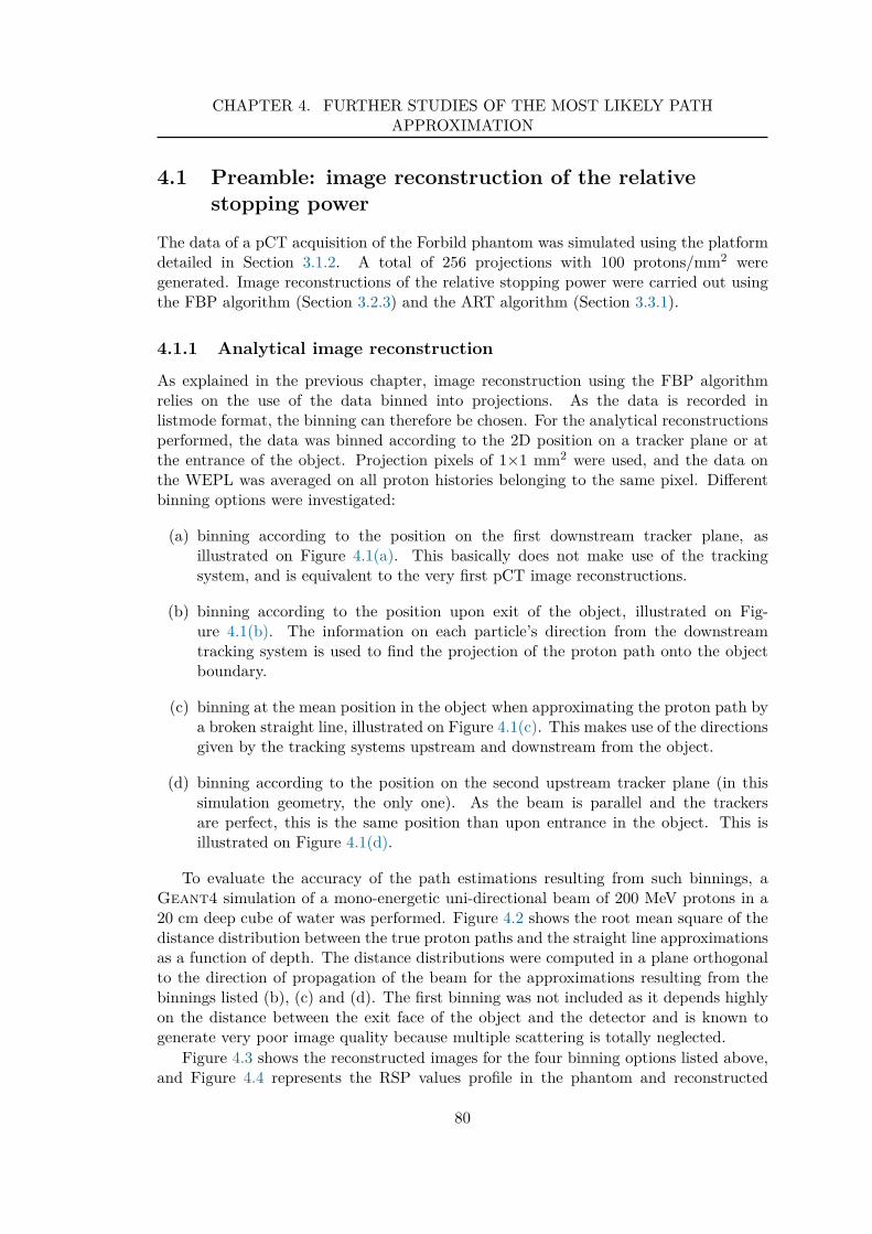
CHAPTER 4. FURTHER STUDIES OF THE MOST LIKELY PATHAPPROXIMATION
4.1 Preamble: image reconstruction of the relativestopping power
The data of a pCT acquisition of the Forbild phantom was simulated using the platformdetailed in Section 3.1.2. A total of 256 projections with 100 protons/mm2 weregenerated. Image reconstructions of the relative stopping power were carried out usingthe FBP algorithm (Section 3.2.3) and the ART algorithm (Section 3.3.1).
4.1.1 Analytical image reconstruction
As explained in the previous chapter, image reconstruction using the FBP algorithmrelies on the use of the data binned into projections. As the data is recorded inlistmode format, the binning can therefore be chosen. For the analytical reconstructionsperformed, the data was binned according to the 2D position on a tracker plane or atthe entrance of the object. Projection pixels of 1×1 mm2 were used, and the data onthe WEPL was averaged on all proton histories belonging to the same pixel. Differentbinning options were investigated:
(a) binning according to the position on the first downstream tracker plane, asillustrated on Figure 4.1(a). This basically does not make use of the trackingsystem, and is equivalent to the very first pCT image reconstructions.
(b) binning according to the position upon exit of the object, illustrated on Fig-ure 4.1(b). The information on each particle’s direction from the downstreamtracking system is used to find the projection of the proton path onto the objectboundary.
(c) binning at the mean position in the object when approximating the proton path bya broken straight line, illustrated on Figure 4.1(c). This makes use of the directionsgiven by the tracking systems upstream and downstream from the object.
(d) binning according to the position on the second upstream tracker plane (in thissimulation geometry, the only one). As the beam is parallel and the trackersare perfect, this is the same position than upon entrance in the object. This isillustrated on Figure 4.1(d).
To evaluate the accuracy of the path estimations resulting from such binnings, aGeant4 simulation of a mono-energetic uni-directional beam of 200 MeV protons in a20 cm deep cube of water was performed. Figure 4.2 shows the root mean square of thedistance distribution between the true proton paths and the straight line approximationsas a function of depth. The distance distributions were computed in a plane orthogonalto the direction of propagation of the beam for the approximations resulting from thebinnings listed (b), (c) and (d). The first binning was not included as it depends highlyon the distance between the exit face of the object and the detector and is known togenerate very poor image quality because multiple scattering is totally neglected.
Figure 4.3 shows the reconstructed images for the four binning options listed above,and Figure 4.4 represents the RSP values profile in the phantom and reconstructed
80
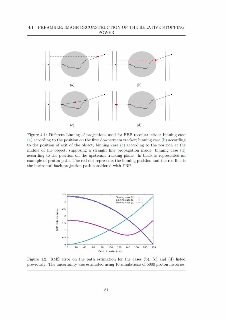
4.1. PREAMBLE: IMAGE RECONSTRUCTION OF THE RELATIVE STOPPINGPOWER
(a) (b)
(c) (d)
Figure 4.1: Different binning of projections used for FBP reconstruction: binning case(a) according to the position on the first downstream tracker; binning case (b) accordingto the position of exit of the object; binning case (c) according to the position at themiddle of the object, supposing a straight line propagation inside; binning case (d)according to the position on the upstream tracking plane. In black is represented anexample of proton path. The red dot represents the binning position and the red line isthe horizontal back-projection path considered with FBP.
0
0.5
1
1.5
2
2.5
3
3.5
0 20 40 60 80 100 120 140 160 180 200
RMS
dist
ance
(mm
)
Depth in water (mm)
Binning case (b)Binning case (c)Binning case (d)
Figure 4.2: RMS error on the path estimation for the cases (b), (c) and (d) listedpreviously. The uncertainty was estimated using 10 simulations of 5000 proton histories.
81
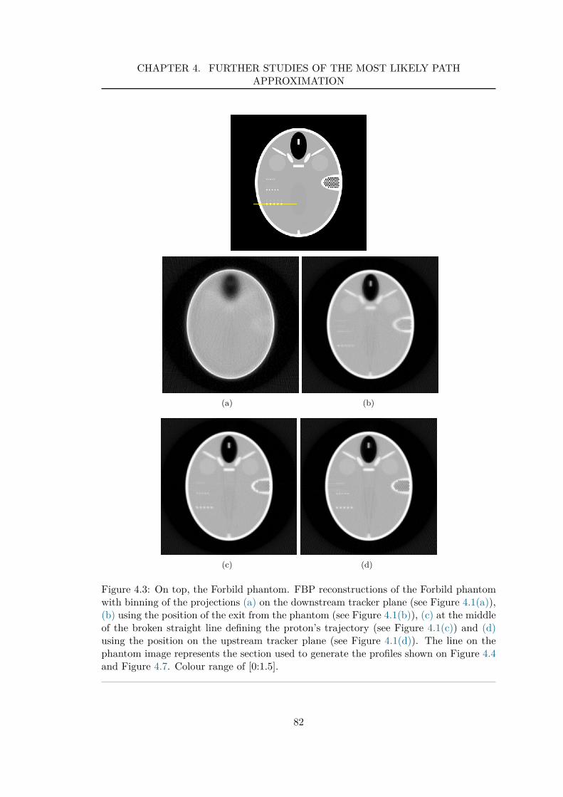
CHAPTER 4. FURTHER STUDIES OF THE MOST LIKELY PATHAPPROXIMATION
(a) (b)
(c) (d)
Figure 4.3: On top, the Forbild phantom. FBP reconstructions of the Forbild phantomwith binning of the projections (a) on the downstream tracker plane (see Figure 4.1(a)),(b) using the position of the exit from the phantom (see Figure 4.1(b)), (c) at the middleof the broken straight line defining the proton’s trajectory (see Figure 4.1(c)) and (d)using the position on the upstream tracker plane (see Figure 4.1(d)). The line on thephantom image represents the section used to generate the profiles shown on Figure 4.4and Figure 4.7. Colour range of [0:1.5].
82
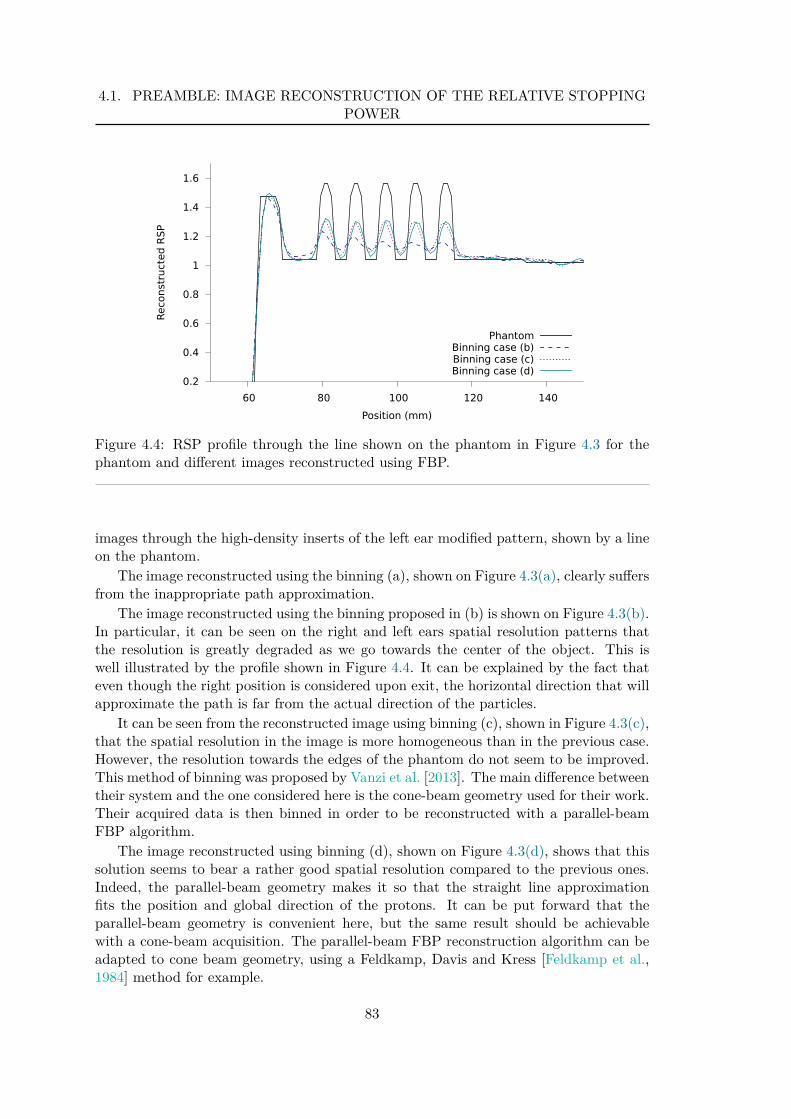
4.1. PREAMBLE: IMAGE RECONSTRUCTION OF THE RELATIVE STOPPINGPOWER
0.2
0.4
0.6
0.8
1
1.2
1.4
1.6
60 80 100 120 140
Reco
nstr
ucte
d RS
P
Position (mm)
PhantomBinning case (b)Binning case (c)Binning case (d)
Figure 4.4: RSP profile through the line shown on the phantom in Figure 4.3 for thephantom and different images reconstructed using FBP.
images through the high-density inserts of the left ear modified pattern, shown by a lineon the phantom.
The image reconstructed using the binning (a), shown on Figure 4.3(a), clearly suffersfrom the inappropriate path approximation.
The image reconstructed using the binning proposed in (b) is shown on Figure 4.3(b).In particular, it can be seen on the right and left ears spatial resolution patterns thatthe resolution is greatly degraded as we go towards the center of the object. This iswell illustrated by the profile shown in Figure 4.4. It can be explained by the fact thateven though the right position is considered upon exit, the horizontal direction that willapproximate the path is far from the actual direction of the particles.
It can be seen from the reconstructed image using binning (c), shown in Figure 4.3(c),that the spatial resolution in the image is more homogeneous than in the previous case.However, the resolution towards the edges of the phantom do not seem to be improved.This method of binning was proposed by Vanzi et al. [2013]. The main difference betweentheir system and the one considered here is the cone-beam geometry used for their work.Their acquired data is then binned in order to be reconstructed with a parallel-beamFBP algorithm.
The image reconstructed using binning (d), shown on Figure 4.3(d), shows that thissolution seems to bear a rather good spatial resolution compared to the previous ones.Indeed, the parallel-beam geometry makes it so that the straight line approximationfits the position and global direction of the protons. It can be put forward that theparallel-beam geometry is convenient here, but the same result should be achievablewith a cone-beam acquisition. The parallel-beam FBP reconstruction algorithm can beadapted to cone beam geometry, using a Feldkamp, Davis and Kress [Feldkamp et al.,1984] method for example.
83
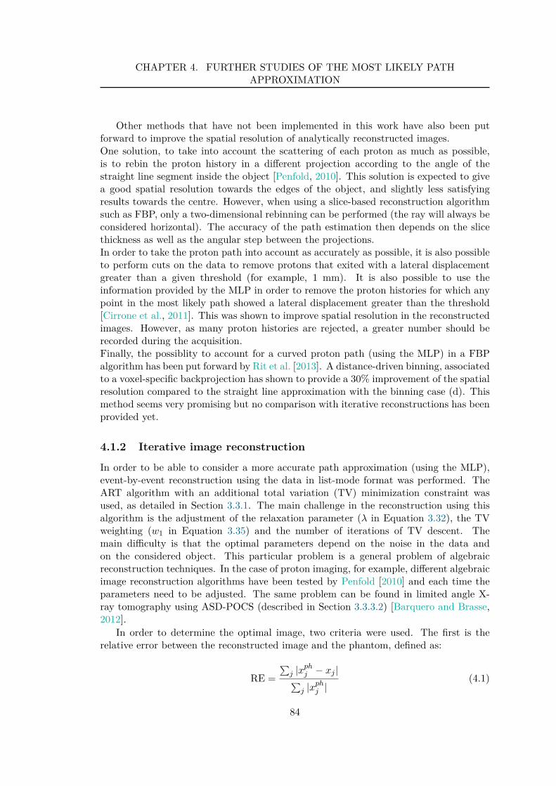
CHAPTER 4. FURTHER STUDIES OF THE MOST LIKELY PATHAPPROXIMATION
Other methods that have not been implemented in this work have also been putforward to improve the spatial resolution of analytically reconstructed images.One solution, to take into account the scattering of each proton as much as possible,is to rebin the proton history in a different projection according to the angle of thestraight line segment inside the object [Penfold, 2010]. This solution is expected to givea good spatial resolution towards the edges of the object, and slightly less satisfyingresults towards the centre. However, when using a slice-based reconstruction algorithmsuch as FBP, only a two-dimensional rebinning can be performed (the ray will always beconsidered horizontal). The accuracy of the path estimation then depends on the slicethickness as well as the angular step between the projections.In order to take the proton path into account as accurately as possible, it is also possibleto perform cuts on the data to remove protons that exited with a lateral displacementgreater than a given threshold (for example, 1 mm). It is also possible to use theinformation provided by the MLP in order to remove the proton histories for which anypoint in the most likely path showed a lateral displacement greater than the threshold[Cirrone et al., 2011]. This was shown to improve spatial resolution in the reconstructedimages. However, as many proton histories are rejected, a greater number should berecorded during the acquisition.Finally, the possiblity to account for a curved proton path (using the MLP) in a FBPalgorithm has been put forward by Rit et al. [2013]. A distance-driven binning, associatedto a voxel-specific backprojection has shown to provide a 30% improvement of the spatialresolution compared to the straight line approximation with the binning case (d). Thismethod seems very promising but no comparison with iterative reconstructions has beenprovided yet.
4.1.2 Iterative image reconstruction
In order to be able to consider a more accurate path approximation (using the MLP),event-by-event reconstruction using the data in list-mode format was performed. TheART algorithm with an additional total variation (TV) minimization constraint wasused, as detailed in Section 3.3.1. The main challenge in the reconstruction using thisalgorithm is the adjustment of the relaxation parameter (λ in Equation 3.32), the TVweighting (w1 in Equation 3.35) and the number of iterations of TV descent. Themain difficulty is that the optimal parameters depend on the noise in the data andon the considered object. This particular problem is a general problem of algebraicreconstruction techniques. In the case of proton imaging, for example, different algebraicimage reconstruction algorithms have been tested by Penfold [2010] and each time theparameters need to be adjusted. The same problem can be found in limited angle X-ray tomography using ASD-POCS (described in Section 3.3.3.2) [Barquero and Brasse,2012].
In order to determine the optimal image, two criteria were used. The first is therelative error between the reconstructed image and the phantom, defined as:
RE =
∑
j |xphj − xj |
∑
j |xphj |
(4.1)
84
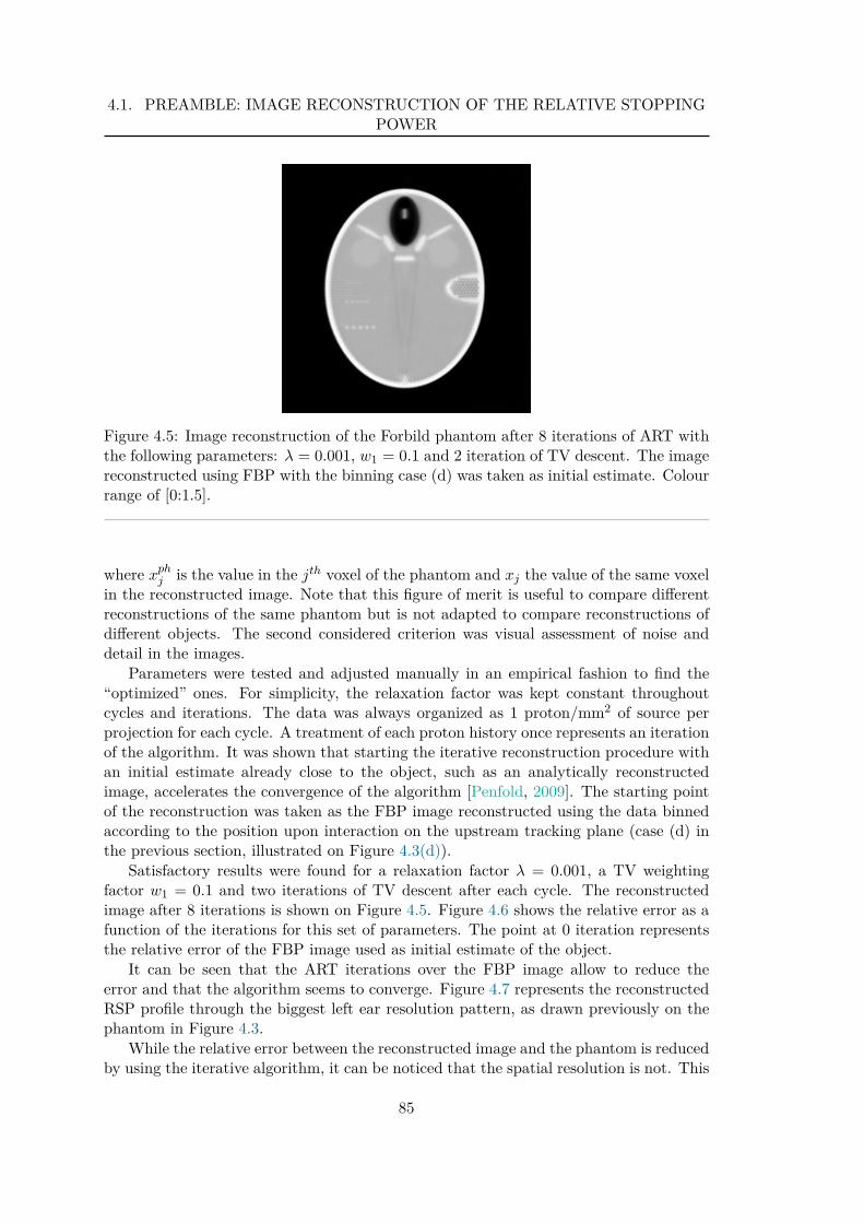
4.1. PREAMBLE: IMAGE RECONSTRUCTION OF THE RELATIVE STOPPINGPOWER
Figure 4.5: Image reconstruction of the Forbild phantom after 8 iterations of ART withthe following parameters: λ = 0.001, w1 = 0.1 and 2 iteration of TV descent. The imagereconstructed using FBP with the binning case (d) was taken as initial estimate. Colourrange of [0:1.5].
where xphj is the value in the jth voxel of the phantom and xj the value of the same voxel
in the reconstructed image. Note that this figure of merit is useful to compare differentreconstructions of the same phantom but is not adapted to compare reconstructions ofdifferent objects. The second considered criterion was visual assessment of noise anddetail in the images.
Parameters were tested and adjusted manually in an empirical fashion to find the“optimized” ones. For simplicity, the relaxation factor was kept constant throughoutcycles and iterations. The data was always organized as 1 proton/mm2 of source perprojection for each cycle. A treatment of each proton history once represents an iterationof the algorithm. It was shown that starting the iterative reconstruction procedure withan initial estimate already close to the object, such as an analytically reconstructedimage, accelerates the convergence of the algorithm [Penfold, 2009]. The starting pointof the reconstruction was taken as the FBP image reconstructed using the data binnedaccording to the position upon interaction on the upstream tracking plane (case (d) inthe previous section, illustrated on Figure 4.3(d)).
Satisfactory results were found for a relaxation factor λ = 0.001, a TV weightingfactor w1 = 0.1 and two iterations of TV descent after each cycle. The reconstructedimage after 8 iterations is shown on Figure 4.5. Figure 4.6 shows the relative error as afunction of the iterations for this set of parameters. The point at 0 iteration representsthe relative error of the FBP image used as initial estimate of the object.
It can be seen that the ART iterations over the FBP image allow to reduce theerror and that the algorithm seems to converge. Figure 4.7 represents the reconstructedRSP profile through the biggest left ear resolution pattern, as drawn previously on thephantom in Figure 4.3.
While the relative error between the reconstructed image and the phantom is reducedby using the iterative algorithm, it can be noticed that the spatial resolution is not. This
85
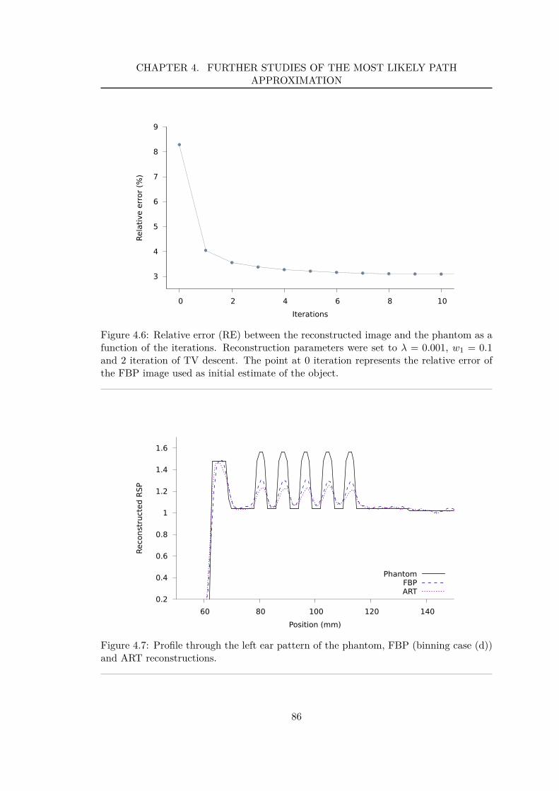
CHAPTER 4. FURTHER STUDIES OF THE MOST LIKELY PATHAPPROXIMATION
3
4
5
6
7
8
9
0 2 4 6 8 10
Rela
tive
erro
r (%
)
Iterations
Figure 4.6: Relative error (RE) between the reconstructed image and the phantom as afunction of the iterations. Reconstruction parameters were set to λ = 0.001, w1 = 0.1and 2 iteration of TV descent. The point at 0 iteration represents the relative error ofthe FBP image used as initial estimate of the object.
0.2
0.4
0.6
0.8
1
1.2
1.4
1.6
60 80 100 120 140
Reco
nstr
ucte
d RS
P
Position (mm)
PhantomFBPART
Figure 4.7: Profile through the left ear pattern of the phantom, FBP (binning case (d))and ART reconstructions.
86
4.1. PREAMBLE: IMAGE RECONSTRUCTION OF THE RELATIVE STOPPINGPOWER
result is surprising because a more accurate path estimation would intuitively lead to abetter spatial resolution. However, it can be explained by the fact that the weightingfactor of the TV may not be optimal. As the TV minimisation results in a reduction ofthe gradients, inappropriate weighting may result in a blur.
Discussion
Because it will not impact the main conceptual arguments of this thesis work, theoptimization of the parameters for the ART algorithm was not performed.However, should such an optimization be of interest, two main things need to beconsidered. The first is the image used as a starting point, here the FBP image. Itcan be put forward that this image shows some streak artefacts which might affect theART algorithm. The second thing to consider is the optimization of the parametersfor the ART algorithm. The search for the optimized parameters could be performedautomatically. This would require a set of figures of merit to test the different aspectsof image quality. Indeed, the RE considered here represents a general criterion on thewhole image, favouring the low frequencies, and is not indicative of the spatial resolutionor noise. A comprehensive quantification of image quality would in addition need toconsider noise, spatial resolution and potential artefacts. A huge amount of computationtime will also be necessary to systematically test the possibilities. The reconstructionalgorithm set-up here, in particular the ray-tracing and MLP computation, couldbe implemented for computation on graphical processing units (GPU). The gain incomputation time would make it possible to consider such a systematic search. Inorder not to have to test all possibilities, a search following an experimental designcould be performed, as can be done in experimental sciences. Furthermore, it needs tobe considered that the optimized parameters determined on a simulation with perfectdetectors and with such a semi-anthropomorphic phantom may be different from theones required to optimize image quality in clinical conditions.
Nevertheless, the path approximation is of key importance in order to achieve thebest spatial resolution possible with proton imaging. In this context, the MLP is themost accurate path approximation that has been proposed to this day. The sequel of thischapter aims at further investigating the MLP, from two different points of view. Thecomputation of the MLP is performed assuming all materials have the scattering andenergy loss properties of water. This is often the case for first approximations. However,in regions with important proportions of bone or air, such as the thorax or nasal cavity,this approximation may not be the most appropriate. Therefore, a MLP estimation innon-homogeneous medium consisting of slabs was derived and studied in Section 4.2.Section 4.3 aims at investigating the impact of the tracking system parameters (spatialresolution, material budget, positioning of the tracking planes) on the path estimation.
87
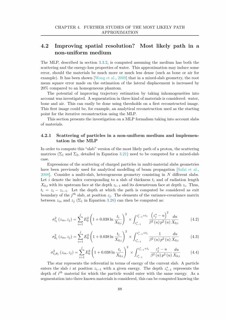
CHAPTER 4. FURTHER STUDIES OF THE MOST LIKELY PATHAPPROXIMATION
4.2 Improving spatial resolution? Most likely path in anon-uniform medium
The MLP, described in section 3.3.2, is computed assuming the medium has both thescattering and the energy-loss properties of water. This approximation may induce someerror, should the materials be much more or much less dense (such as bone or air forexample). It has been shown [Wong et al., 2009] that in a mixed-slab geometry, the rootmean square error made on the estimation of the lateral displacement is increased by20% compared to an homogeneous phantom.
The potential of improving trajectory estimation by taking inhomogeneities intoaccount was investigated. A segmentation in three kind of materials is considered: water,bone and air. This can easily be done using thresholds on a first reconstructed image.This first image could be, for example, an analytical reconstruction used as the startingpoint for the iterative reconstruction using the MLP.
This section presents the investigation on a MLP formalism taking into account slabsof materials.
4.2.1 Scattering of particles in a non-uniform medium and implemen-tation in the MLP
In order to compute this “slab” version of the most likely path of a proton, the scatteringmatrices (Σ1 and Σ2, detailed in Equation 3.21) need to be computed for a mixed-slabcase.
Expressions of the scattering of charged particles in multi-material slabs geometrieshave been previously used for analytical modelling of beam propagation [Safai et al.,2008]. Consider a multi-slab, heterogeneous geometry consisting in N different slabs.Let i denote the index corresponding to a slab of thickness ti and of radiation lengthX0,i with its upstream face at the depth zi−1 and its downstream face at depth zi. Thus,ti = zi − zi−1. Let the depth at which the path is computed be considered as exitboundary of the jth slab, at position zj . The elements of the variance-covariance matrixbetween zin and zj (Σ1 in Equation 3.28) can then be computed as:
σ2t1
(zin, zj) =j∑
i=1
E20
(
1 + 0.038 lnti
X0,i
)2
×∫ z∗
i−1+ti
z∗
i−1
(
z∗j − u
)2
β2 (u) p2 (u)du
X0,i(4.2)
σ2θ1
(zin, zj) =j∑
i=1
E20
(
1 + 0.038 lnti
X0,i
)2
×∫ z∗
i−1+ti
z∗
i−1
1β2 (u) p2 (u)
du
X0,i(4.3)
σ2t1θ1
(zin, zj) =j∑
i=1
E20
(
1 + 0.038 lnti
X0,i
)2
×∫ z∗
i−1+ti
z∗
i−1
z∗j − u
β2 (u) p2 (u)du
X0,i(4.4)
The star represents the referential in terms of energy of the current slab. A particleenters the slab i at position zi−1 with a given energy. The depth z∗
i−1 represents thedepth of ith material for which the particle would enter with the same energy. As asegmentation into three known materials is considered, this can be computed knowing the
88
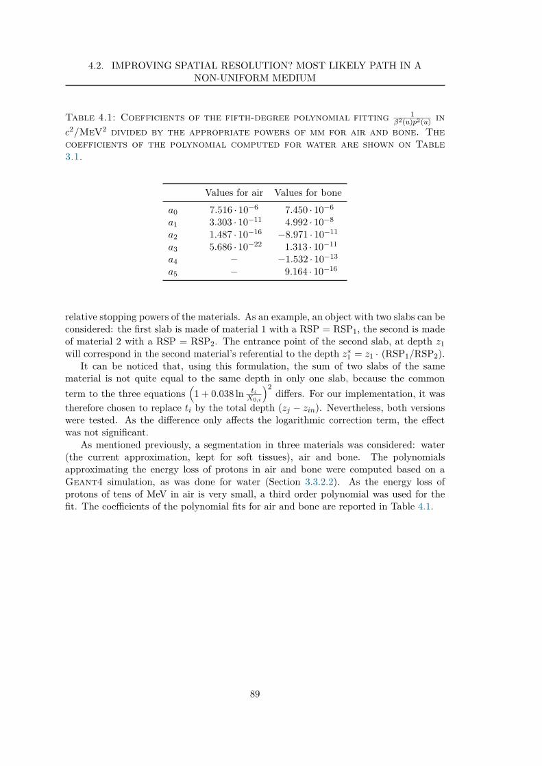
4.2. IMPROVING SPATIAL RESOLUTION? MOST LIKELY PATH IN ANON-UNIFORM MEDIUM
Table 4.1: Coefficients of the fifth-degree polynomial fitting 1β2(u)p2(u)
in
c2/MeV2 divided by the appropriate powers of mm for air and bone. Thecoefficients of the polynomial computed for water are shown on Table3.1.
Values for air Values for bone
a0 7.516 · 10−6 7.450 · 10−6
a1 3.303 · 10−11 4.992 · 10−8
a2 1.487 · 10−16 −8.971 · 10−11
a3 5.686 · 10−22 1.313 · 10−11
a4 − −1.532 · 10−13
a5 − 9.164 · 10−16
relative stopping powers of the materials. As an example, an object with two slabs can beconsidered: the first slab is made of material 1 with a RSP = RSP1, the second is madeof material 2 with a RSP = RSP2. The entrance point of the second slab, at depth z1
will correspond in the second material’s referential to the depth z∗1 = z1 · (RSP1/RSP2).
It can be noticed that, using this formulation, the sum of two slabs of the samematerial is not quite equal to the same depth in only one slab, because the common
term to the three equations(
1 + 0.038 ln ti
X0,i
)2differs. For our implementation, it was
therefore chosen to replace ti by the total depth (zj − zin). Nevertheless, both versionswere tested. As the difference only affects the logarithmic correction term, the effectwas not significant.
As mentioned previously, a segmentation in three materials was considered: water(the current approximation, kept for soft tissues), air and bone. The polynomialsapproximating the energy loss of protons in air and bone were computed based on aGeant4 simulation, as was done for water (Section 3.3.2.2). As the energy loss ofprotons of tens of MeV in air is very small, a third order polynomial was used for thefit. The coefficients of the polynomial fits for air and bone are reported in Table 4.1.
89
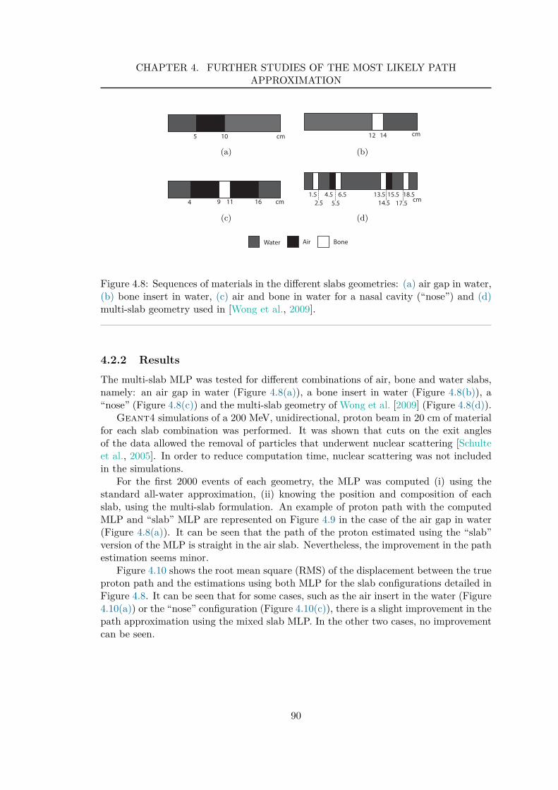
CHAPTER 4. FURTHER STUDIES OF THE MOST LIKELY PATHAPPROXIMATION
5 10 cm
(a)
12 14 cm
(b)
4 9 11 16 cm
(c)
1.5
2.5
4.5 6.5
5.5
13.5
14.5
15.5
17.5
18.5 cm
(d)
Water Air Bone
Figure 4.8: Sequences of materials in the different slabs geometries: (a) air gap in water,(b) bone insert in water, (c) air and bone in water for a nasal cavity (“nose”) and (d)multi-slab geometry used in [Wong et al., 2009].
4.2.2 Results
The multi-slab MLP was tested for different combinations of air, bone and water slabs,namely: an air gap in water (Figure 4.8(a)), a bone insert in water (Figure 4.8(b)), a“nose” (Figure 4.8(c)) and the multi-slab geometry of Wong et al. [2009] (Figure 4.8(d)).
Geant4 simulations of a 200 MeV, unidirectional, proton beam in 20 cm of materialfor each slab combination was performed. It was shown that cuts on the exit anglesof the data allowed the removal of particles that underwent nuclear scattering [Schulteet al., 2005]. In order to reduce computation time, nuclear scattering was not includedin the simulations.
For the first 2000 events of each geometry, the MLP was computed (i) using thestandard all-water approximation, (ii) knowing the position and composition of eachslab, using the multi-slab formulation. An example of proton path with the computedMLP and “slab” MLP are represented on Figure 4.9 in the case of the air gap in water(Figure 4.8(a)). It can be seen that the path of the proton estimated using the “slab”version of the MLP is straight in the air slab. Nevertheless, the improvement in the pathestimation seems minor.
Figure 4.10 shows the root mean square (RMS) of the displacement between the trueproton path and the estimations using both MLP for the slab configurations detailed inFigure 4.8. It can be seen that for some cases, such as the air insert in the water (Figure4.10(a)) or the “nose” configuration (Figure 4.10(c)), there is a slight improvement in thepath approximation using the mixed slab MLP. In the other two cases, no improvementcan be seen.
90
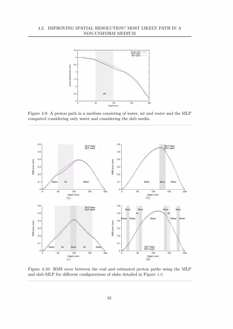
4.2. IMPROVING SPATIAL RESOLUTION? MOST LIKELY PATH IN ANON-UNIFORM MEDIUM
-3
-2.5
-2
-1.5
-1
-0.5
0
0.5
0 50 100 150 200
Late
ral dis
pla
cem
ent (m
m)
Depth (mm)
AIR
proton pathMLP waterMLP slabs
Figure 4.9: A proton path in a medium consisting of water, air and water and the MLPcomputed considering only water and considering the slab media.
0
0.1
0.2
0.3
0.4
0.5
0.6
0 50 100 150 200
RM
S e
rror
(mm
)
Depth (mm)
AirWater Water
MLP slabsMLP water
(a)
0
0.1
0.2
0.3
0.4
0.5
0.6
0 50 100 150 200
RM
S e
rror
(mm
)
Depth (mm)
BoneWater Water
MLP slabsMLP water
(b)
0
0.1
0.2
0.3
0.4
0.5
0.6
0 50 100 150 200
RM
S e
rror
(mm
)
Depth (mm)
AirWater Bone Air Water
MLP slabsMLP water
(c)
0
0.1
0.2
0.3
0.4
0.5
0.6
0 50 100 150 200
RM
S e
rror
(mm
)
Depth (mm)
Bone
Air
Bone Bone
Air
Bone
Water Water Water Water Water
MLP slabsMLP water
(d)
Figure 4.10: RMS error between the real and estimated proton paths using the MLPand slab-MLP for different configurations of slabs detailed in Figure 4.8.
91
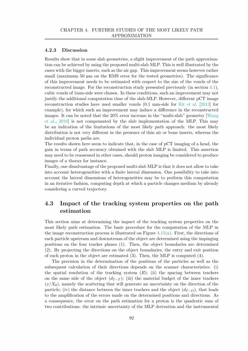
CHAPTER 4. FURTHER STUDIES OF THE MOST LIKELY PATHAPPROXIMATION
4.2.3 Discussion
Results show that in some slab geometries, a slight improvement of the path approxima-tion can be achieved by using the proposed multi-slab MLP. This is well illustrated by thecases with the bigger inserts, such as the air gap. This improvement seems however rathersmall (maximum 50 µm on the RMS error for the tested geometries). The significanceof this improvement needs to be estimated with respect to the size of the voxels of thereconstructed image. For the reconstruction study presented previously (in section 4.1),cubic voxels of 1mm-side were chosen. In these conditions, such an improvement may notjustify the additional computation time of the slab-MLP. However, different pCT imagereconstruction studies have used smaller voxels (0.1 mm-side for Rit et al. [2013] forexample), for which such an improvement may induce a difference in the reconstructedimages. It can be noted that the 20% error increase in the “multi-slab” geometry [Wanget al., 2010] is not compensated by the slab implementation of the MLP. This maybe an indication of the limitations of the most likely path approach: the most likelydistribution is not very different in the presence of thin air or bone inserts, whereas theindividual proton paths are.The results shown here seem to indicate that, in the case of pCT imaging of a head, thegain in terms of path accuracy obtained with the slab MLP is limited. This assertionmay need to be reassessed in other cases, should proton imaging be considered to produceimages of a thorax for instance.Finally, one disadvantage of the proposed multi-slab MLP is that it does not allow to takeinto account heterogeneities with a finite lateral dimension. One possibility to take intoaccount the lateral dimensions of heterogeneities may be to perform this computationin an iterative fashion, computing depth at which a particle changes medium by alreadyconsidering a curved trajectory.
4.3 Impact of the tracking system properties on the path
estimation
This section aims at determining the impact of the tracking system properties on themost likely path estimation. The basic procedure for the computation of the MLP inthe image reconstruction process is illustrated on Figure 4.11(a). First, the directions ofeach particle upstream and downstream of the object are determined using the impingingpositions on the four tracker planes (1). Then, the object boundaries are determined(2). By projecting the directions on the object boundaries, the entry and exit positionof each proton in the object are estimated (3). Then, the MLP is computed (4).
The precision in the determination of the positions of the particles as well as thesubsequent calculation of their directions depends on the scanner characteristics: (i)the spatial resolution of the tracking system (R); (ii) the spacing between trackerson the same side of the object (dT −T ); (iii) the material budget of the inner trackers(x/X0), namely the scattering that will generate an uncertainty on the direction of theparticle; (iv) the distance between the inner trackers and the object (dT −O), that leadsto the amplification of the errors made on the determined positions and directions. Asa consequence, the error on the path estimation for a proton is the quadratic sum oftwo contributions: the intrinsic uncertainty of the MLP derivation and the instrumental
92
4.3. IMPACT OF THE TRACKING SYSTEM PROPERTIES ON THE PATHESTIMATION
(1) (1)
(1')
(1')(2)
(3')
(3)(4)
(a)
(b)
Figure 4.11: Illustration of the estimation of the most likely path with (a) exact data,and (b) taking into account uncertainties due to the tracking system. The numbersrepresent the steps in the MLP computation detailed in the text. The z-axis representsthe direction of propagation of the particle at the given acquisition angle.
considerations. This second part is schematically illustrated on Figure 4.11(b).
Previous results demonstrate the improvement of image quality for a reduced distancebetween the inner trackers [Sadrozinski et al., 2013]. It was also shown for a specificsystem with a pitch of 228 µm, that increasing the distance between trackers dT −T tomore than 8 cm did not noticeably improve MLP accuracy [Penfold et al., 2011].The impact of the material budget of the trackers was evaluated, specifically for silicondetectors [Sadrozinski et al., 2013; Civinini et al., 2012]. The first study advocates areduction of the downstream inner tracker thickness from 400 µm to 200 µm; the secondconcludes that increasing tracker thickness from 200 µm to 320 µm has little impacton the error on the MLP, if the distance between the inner trackers and the object isneglected. However, the impact of all the parameters affecting the path estimation havenot been evaluated systematically.
The error on the MLP estimation for one proton has two sources: one is the intrinsicuncertainty of the MLP derivation, the other is a consequence of the system consideredthat induces an uncertainty on the positions and directions used as inputs for the MLPestimation. The total error on the MLP is then the quadratic sum of these two errors.The aim of the work presented in this section is to evaluate the impact of the secondpart of the error due to the acquisition and aforementioned system parameters.
93
CHAPTER 4. FURTHER STUDIES OF THE MOST LIKELY PATHAPPROXIMATION
4.3.1 Materials and methods
4.3.1.1 Uncertainty propagation in the MLP
The computation of the MLP is described in Section 3.3.2. The Equation 3.28 tocalculate the most likely position and direction of a particle at a given depth, knowingthe entrance and exit parameters pin and pout can be re-written as:
pMLP = Apin + Bpout (4.5)
where A and B are the compressed expressions of all factors multiplying pin and pout inEquation 3.28. Let Σin and Σout be the variance-covariance matrices representative ofthe uncertainties on pin and pout respectively:
Σin =
(
σ2yin
σ2yin,θin
σ2yin,θin
σ2θin
)
, Σout =
(
σ2yout
σ2yout,θout
σ2yout,θout
σ2θout
)
(4.6)
The uncertainty on yMLP at a given depth can then be calculated as:
ΣMLP = AΣinAT + BΣoutBT (4.7)
The same uncertainty propagation can be computed in the orthogonal plane.
4.3.1.2 Uncertainties due to the acquisition system
The uncertainty matrices on the entrance and exit parameters can be split in twocontributions: (i) the distance between the trackers and their intrinsic spatial resolutionand (ii) the scattering inside the innermost detector. For a strictly symmetrical system,the first contribution will be the same on both sides of the object, while the second willnot, as it depends on the energy of the particles. Moreover, both contributions need tobe projected onto the surface of the object.
For a given system, the matrices can be computed by smearing multiple realizationsof the same ‘event’. Consider, for example for the upstream side of the (yOz) plane, aparticle interacting on the first two tracker planes at the positions (y1, z1) and (y2, z2).These interaction points can be smeared using random values generated on a Gaussiandistribution, of which the full-width at half maximum is given by the resolution of thetrackers. The resolution of the trackers is defined here as 2.35 times the root meansquare (RMS) error on the interaction position of one event, which is known a priori.The smeared positions (y′
1, z1) and (y′2, z2) can be used to compute the incidence angle of
the particle θ′. This angle is in turn smeared into θin using random values generated ona Gaussian distribution to account for the scattering due to the material of the secondtracker plane. The RMS of this Gaussian distribution can be computed using a Gaussianapproximation to multiple scattering, with the following empirical formula [Lynch andDahl, 1991]:
σ(l, E) =13.6
β(E)p(E)
√
x
X0
[
1 + 0.038 · ln(
x
X0
)]
(4.8)
where E, β and p are the energy, scaled velocity and momentum of the proton, X0 isthe radiation length of the material and x its thickness. The material budget of different
94
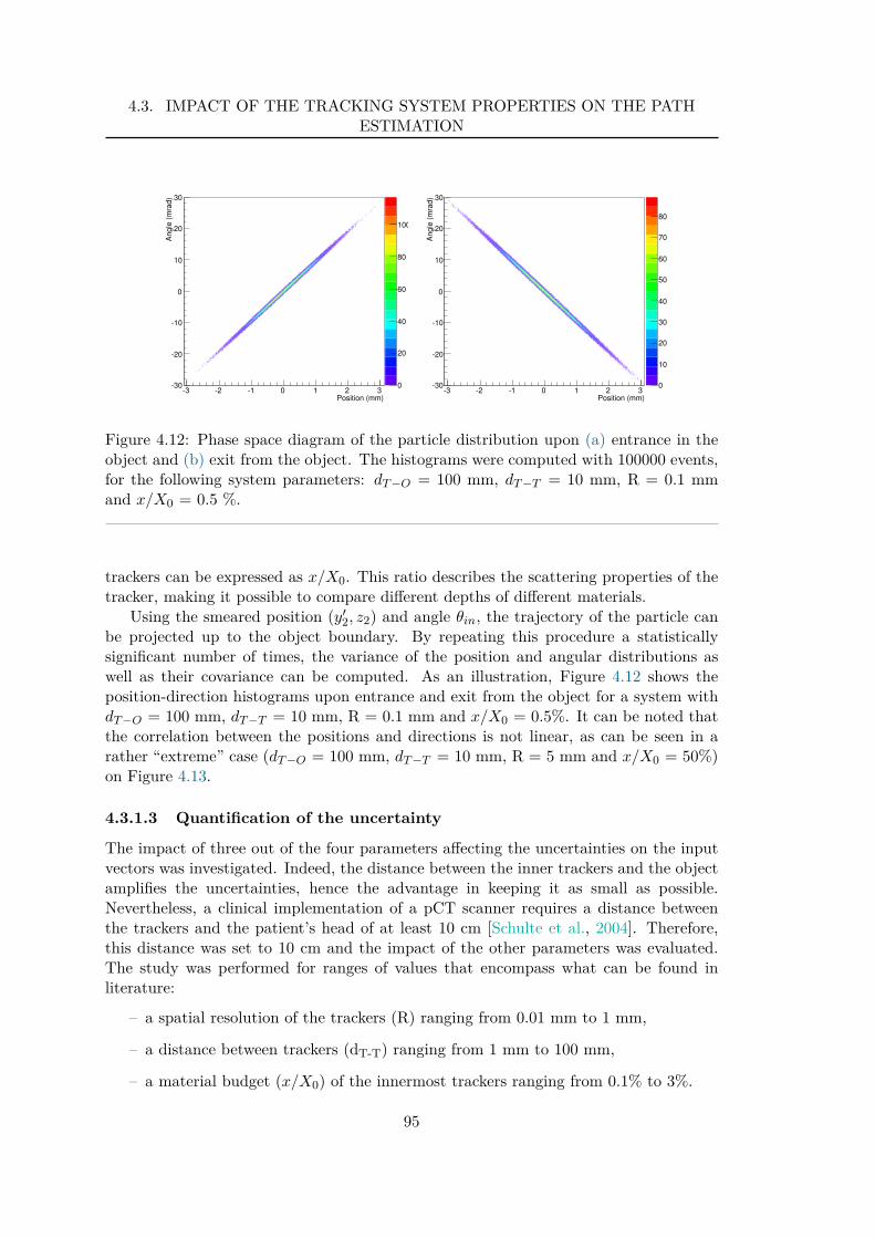
4.3. IMPACT OF THE TRACKING SYSTEM PROPERTIES ON THE PATHESTIMATION
0
20
40
60
80
100
Position (mm)-3 -2 -1 0 1 2 3
Angle
(m
rad)
-30
-20
-10
0
10
20
30
0
10
20
30
40
50
60
70
80
Position (mm)-3 -2 -1 0 1 2 3
Angle
(m
rad)
-30
-20
-10
0
10
20
30
Figure 4.12: Phase space diagram of the particle distribution upon (a) entrance in theobject and (b) exit from the object. The histograms were computed with 100000 events,for the following system parameters: dT −O = 100 mm, dT −T = 10 mm, R = 0.1 mmand x/X0 = 0.5 %.
trackers can be expressed as x/X0. This ratio describes the scattering properties of thetracker, making it possible to compare different depths of different materials.
Using the smeared position (y′2, z2) and angle θin, the trajectory of the particle can
be projected up to the object boundary. By repeating this procedure a statisticallysignificant number of times, the variance of the position and angular distributions aswell as their covariance can be computed. As an illustration, Figure 4.12 shows theposition-direction histograms upon entrance and exit from the object for a system withdT −O = 100 mm, dT −T = 10 mm, R = 0.1 mm and x/X0 = 0.5%. It can be noted thatthe correlation between the positions and directions is not linear, as can be seen in arather “extreme” case (dT −O = 100 mm, dT −T = 10 mm, R = 5 mm and x/X0 = 50%)on Figure 4.13.
4.3.1.3 Quantification of the uncertainty
The impact of three out of the four parameters affecting the uncertainties on the inputvectors was investigated. Indeed, the distance between the inner trackers and the objectamplifies the uncertainties, hence the advantage in keeping it as small as possible.Nevertheless, a clinical implementation of a pCT scanner requires a distance betweenthe trackers and the patient’s head of at least 10 cm [Schulte et al., 2004]. Therefore,this distance was set to 10 cm and the impact of the other parameters was evaluated.The study was performed for ranges of values that encompass what can be found inliterature:
– a spatial resolution of the trackers (R) ranging from 0.01 mm to 1 mm,
– a distance between trackers (dT-T) ranging from 1 mm to 100 mm,
– a material budget (x/X0) of the innermost trackers ranging from 0.1% to 3%.
95
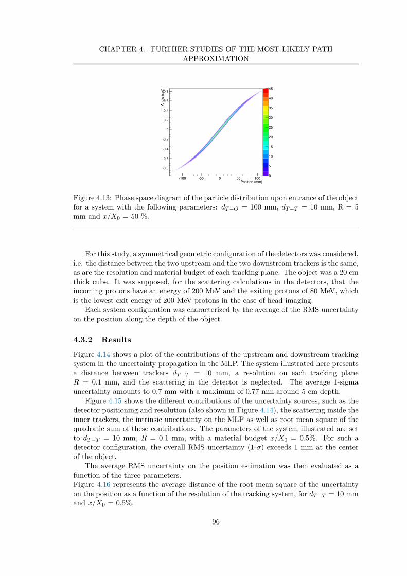
CHAPTER 4. FURTHER STUDIES OF THE MOST LIKELY PATHAPPROXIMATION
0
5
10
15
20
25
30
35
40
45
Position (mm)-100 -50 0 50 100
Angle
(ra
d)
-0.8
-0.6
-0.4
-0.2
0
0.2
0.4
0.6
0.8
Figure 4.13: Phase space diagram of the particle distribution upon entrance of the objectfor a system with the following parameters: dT −O = 100 mm, dT −T = 10 mm, R = 5mm and x/X0 = 50 %.
For this study, a symmetrical geometric configuration of the detectors was considered,i.e. the distance between the two upstream and the two downstream trackers is the same,as are the resolution and material budget of each tracking plane. The object was a 20 cmthick cube. It was supposed, for the scattering calculations in the detectors, that theincoming protons have an energy of 200 MeV and the exiting protons of 80 MeV, whichis the lowest exit energy of 200 MeV protons in the case of head imaging.
Each system configuration was characterized by the average of the RMS uncertaintyon the position along the depth of the object.
4.3.2 Results
Figure 4.14 shows a plot of the contributions of the upstream and downstream trackingsystem in the uncertainty propagation in the MLP. The system illustrated here presentsa distance between trackers dT −T = 10 mm, a resolution on each tracking planeR = 0.1 mm, and the scattering in the detector is neglected. The average 1-sigmauncertainty amounts to 0.7 mm with a maximum of 0.77 mm around 5 cm depth.
Figure 4.15 shows the different contributions of the uncertainty sources, such as thedetector positioning and resolution (also shown in Figure 4.14), the scattering inside theinner trackers, the intrinsic uncertainty on the MLP as well as root mean square of thequadratic sum of these contributions. The parameters of the system illustrated are setto dT −T = 10 mm, R = 0.1 mm, with a material budget x/X0 = 0.5%. For such adetector configuration, the overall RMS uncertainty (1-σ) exceeds 1 mm at the centerof the object.
The average RMS uncertainty on the position estimation was then evaluated as afunction of the three parameters.Figure 4.16 represents the average distance of the root mean square of the uncertaintyon the position as a function of the resolution of the tracking system, for dT −T = 10 mmand x/X0 = 0.5%.
96
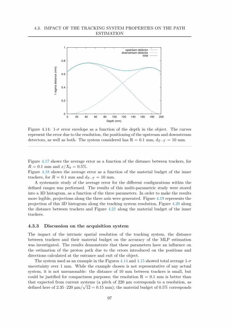
4.3. IMPACT OF THE TRACKING SYSTEM PROPERTIES ON THE PATHESTIMATION
0
0.2
0.4
0.6
0.8
1
0 20 40 60 80 100 120 140 160 180 200
1-s
igm
a d
ista
nce
(m
m)
Depth (mm)
upstream detectordownstream detector
total
Figure 4.14: 1-σ error envelope as a function of the depth in the object. The curvesrepresent the error due to the resolution, the positioning of the upstream and downstreamdetectors, as well as both. The system considered has R = 0.1 mm, dT −T = 10 mm.
Figure 4.17 shows the average error as a function of the distance between trackers, forR = 0.1 mm and x/X0 = 0.5%.Figure 4.18 shows the average error as a function of the material budget of the innertrackers, for R = 0.1 mm and dT −T = 10 mm.
A systematic study of the average error for the different configurations within thedefined ranges was performed. The results of this multi-parametric study were storedinto a 3D histogram, as a function of the three parameters. In order to make the resultsmore legible, projections along the three axis were generated. Figure 4.19 represents theprojection of this 3D histogram along the tracking system resolution, Figure 4.20 alongthe distance between trackers and Figure 4.21 along the material budget of the innertrackers.
4.3.3 Discussion on the acquisition system
The impact of the intrinsic spatial resolution of the tracking system, the distancebetween trackers and their material budget on the accuracy of the MLP estimationwas investigated. The results demonstrate that these parameters have an influence onthe estimation of the proton path due to the errors introduced on the positions anddirections calculated at the entrance and exit of the object.
The system used as an example in the Figures 4.14 and 4.15 showed total average 1-σuncertainty over 1 mm. While the example chosen is not representative of any actualsystem, it is not unreasonable: the distance of 10 mm between trackers is small, butcould be justified for compactness purposes; the resolution R = 0.1 mm is better thanthat expected from current systems (a pitch of 220 µm corresponds to a resolution, asdefined here of 2.35 · 220 µm/
√12 = 0.15 mm); the material budget of 0.5% corresponds
97
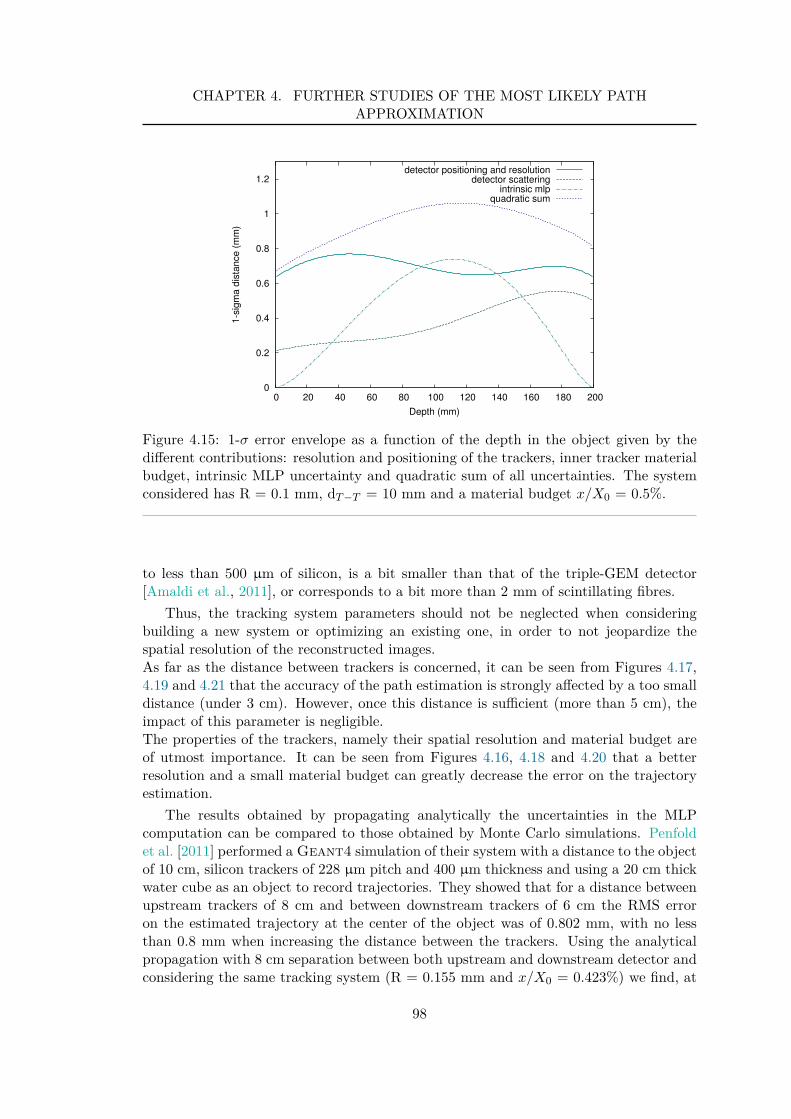
CHAPTER 4. FURTHER STUDIES OF THE MOST LIKELY PATHAPPROXIMATION
0
0.2
0.4
0.6
0.8
1
1.2
0 20 40 60 80 100 120 140 160 180 200
1-s
igm
a d
ista
nce
(m
m)
Depth (mm)
detector positioning and resolutiondetector scattering
intrinsic mlpquadratic sum
Figure 4.15: 1-σ error envelope as a function of the depth in the object given by thedifferent contributions: resolution and positioning of the trackers, inner tracker materialbudget, intrinsic MLP uncertainty and quadratic sum of all uncertainties. The systemconsidered has R = 0.1 mm, dT −T = 10 mm and a material budget x/X0 = 0.5%.
to less than 500 µm of silicon, is a bit smaller than that of the triple-GEM detector[Amaldi et al., 2011], or corresponds to a bit more than 2 mm of scintillating fibres.
Thus, the tracking system parameters should not be neglected when consideringbuilding a new system or optimizing an existing one, in order to not jeopardize thespatial resolution of the reconstructed images.As far as the distance between trackers is concerned, it can be seen from Figures 4.17,4.19 and 4.21 that the accuracy of the path estimation is strongly affected by a too smalldistance (under 3 cm). However, once this distance is sufficient (more than 5 cm), theimpact of this parameter is negligible.The properties of the trackers, namely their spatial resolution and material budget areof utmost importance. It can be seen from Figures 4.16, 4.18 and 4.20 that a betterresolution and a small material budget can greatly decrease the error on the trajectoryestimation.
The results obtained by propagating analytically the uncertainties in the MLPcomputation can be compared to those obtained by Monte Carlo simulations. Penfoldet al. [2011] performed a Geant4 simulation of their system with a distance to the objectof 10 cm, silicon trackers of 228 µm pitch and 400 µm thickness and using a 20 cm thickwater cube as an object to record trajectories. They showed that for a distance betweenupstream trackers of 8 cm and between downstream trackers of 6 cm the RMS erroron the estimated trajectory at the center of the object was of 0.802 mm, with no lessthan 0.8 mm when increasing the distance between the trackers. Using the analyticalpropagation with 8 cm separation between both upstream and downstream detector andconsidering the same tracking system (R = 0.155 mm and x/X0 = 0.423%) we find, at
98
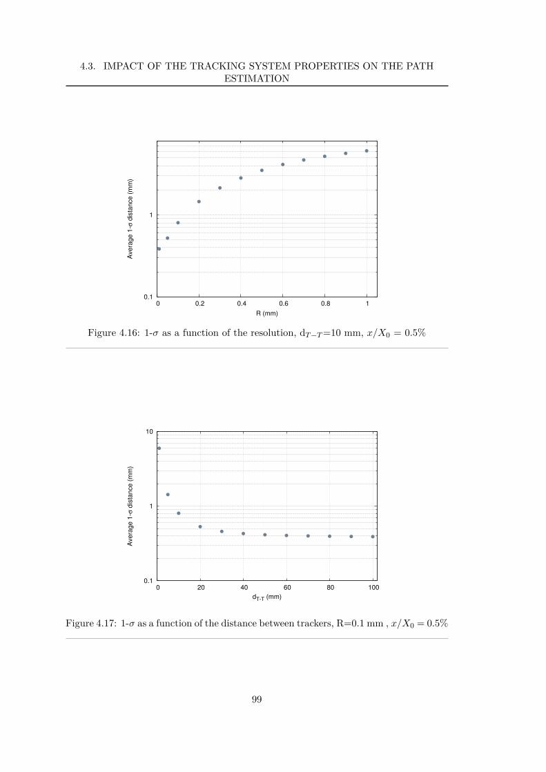
4.3. IMPACT OF THE TRACKING SYSTEM PROPERTIES ON THE PATHESTIMATION
0.1
1
0 0.2 0.4 0.6 0.8 1
Ave
rag
e 1
-σ d
ista
nce
(m
m)
R (mm)
Figure 4.16: 1-σ as a function of the resolution, dT −T =10 mm, x/X0 = 0.5%
0.1
1
10
0 20 40 60 80 100
Ave
rag
e 1
-σ d
ista
nce
(m
m)
dT-T (mm)
Figure 4.17: 1-σ as a function of the distance between trackers, R=0.1 mm , x/X0 = 0.5%
99
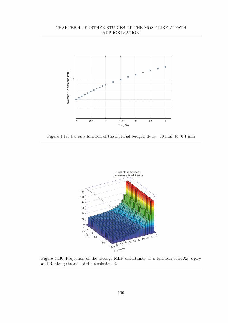
CHAPTER 4. FURTHER STUDIES OF THE MOST LIKELY PATHAPPROXIMATION
1
0 0.5 1 1.5 2 2.5 3
Ave
rag
e 1
-σ d
ista
nce
(m
m)
x/X0 (%)
Figure 4.18: 1-σ as a function of the material budget, dT −T =10 mm, R=0.1 mm
(%)0
x/X
00.5
11.5
22.5
3
(mm)T-Td
0102030405060708090100
0
20
40
60
80
100
120
Sum of the average
uncertainty for all R (mm)
Figure 4.19: Projection of the average MLP uncertainty as a function of x/X0, dT −T
and R, along the axis of the resolution R.
100
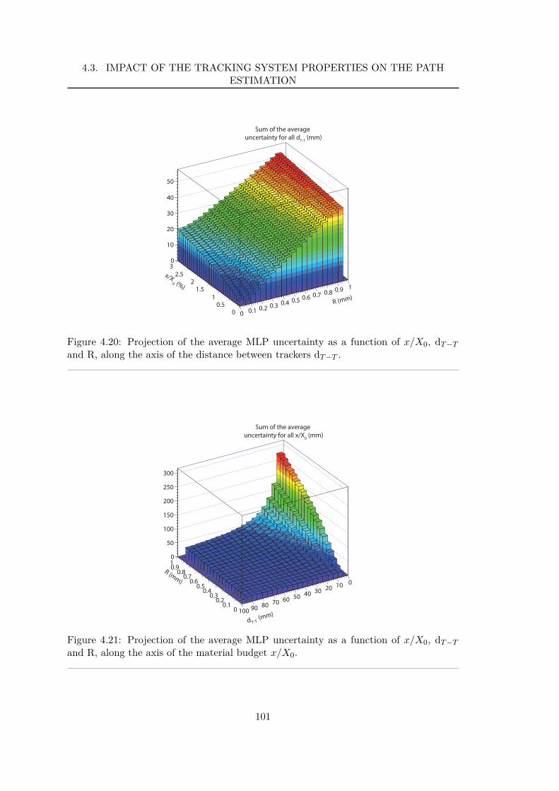
4.3. IMPACT OF THE TRACKING SYSTEM PROPERTIES ON THE PATHESTIMATION
R (mm)
0 0.1 0.2 0.3 0.4 0.5 0.6 0.7 0.8 0.9 1 (%)
0
x/X
00.5
11.5
22.5
30
10
20
30
40
50
Sum of the average
uncertainty for all dT-T
(mm)
Figure 4.20: Projection of the average MLP uncertainty as a function of x/X0, dT −T
and R, along the axis of the distance between trackers dT −T .
R (mm
)
00.1
0.20.3
0.40.5
0.60.7
0.80.91
(mm)T-Td
0102030405060708090100
0
50
100
150
200
250
300
Sum of the average
uncertainty for all x/X0 (mm)
Figure 4.21: Projection of the average MLP uncertainty as a function of x/X0, dT −T
and R, along the axis of the material budget x/X0.
101
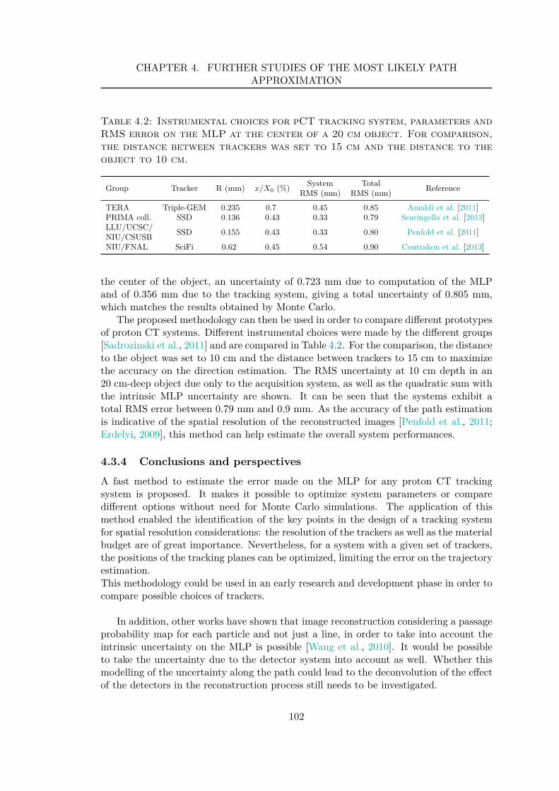
CHAPTER 4. FURTHER STUDIES OF THE MOST LIKELY PATHAPPROXIMATION
Table 4.2: Instrumental choices for pCT tracking system, parameters andRMS error on the MLP at the center of a 20 cm object. For comparison,the distance between trackers was set to 15 cm and the distance to theobject to 10 cm.
Group Tracker R (mm) x/X0 (%)System Total
ReferenceRMS (mm) RMS (mm)
TERA Triple-GEM 0.235 0.7 0.45 0.85 Amaldi et al. [2011]PRIMA coll. SSD 0.136 0.43 0.33 0.79 Scaringella et al. [2013]LLU/UCSC/
SSD 0.155 0.43 0.33 0.80 Penfold et al. [2011]NIU/CSUSBNIU/FNAL SciFi 0.62 0.45 0.54 0.90 Coutrakon et al. [2013]
the center of the object, an uncertainty of 0.723 mm due to computation of the MLPand of 0.356 mm due to the tracking system, giving a total uncertainty of 0.805 mm,which matches the results obtained by Monte Carlo.
The proposed methodology can then be used in order to compare different prototypesof proton CT systems. Different instrumental choices were made by the different groups[Sadrozinski et al., 2011] and are compared in Table 4.2. For the comparison, the distanceto the object was set to 10 cm and the distance between trackers to 15 cm to maximizethe accuracy on the direction estimation. The RMS uncertainty at 10 cm depth in an20 cm-deep object due only to the acquisition system, as well as the quadratic sum withthe intrinsic MLP uncertainty are shown. It can be seen that the systems exhibit atotal RMS error between 0.79 mm and 0.9 mm. As the accuracy of the path estimationis indicative of the spatial resolution of the reconstructed images [Penfold et al., 2011;Erdelyi, 2009], this method can help estimate the overall system performances.
4.3.4 Conclusions and perspectives
A fast method to estimate the error made on the MLP for any proton CT trackingsystem is proposed. It makes it possible to optimize system parameters or comparedifferent options without need for Monte Carlo simulations. The application of thismethod enabled the identification of the key points in the design of a tracking systemfor spatial resolution considerations: the resolution of the trackers as well as the materialbudget are of great importance. Nevertheless, for a system with a given set of trackers,the positions of the tracking planes can be optimized, limiting the error on the trajectoryestimation.This methodology could be used in an early research and development phase in order tocompare possible choices of trackers.
In addition, other works have shown that image reconstruction considering a passageprobability map for each particle and not just a line, in order to take into account theintrinsic uncertainty on the MLP is possible [Wang et al., 2010]. It would be possibleto take the uncertainty due to the detector system into account as well. Whether thismodelling of the uncertainty along the path could lead to the deconvolution of the effectof the detectors in the reconstruction process still needs to be investigated.
102
4.3. IMPACT OF THE TRACKING SYSTEM PROPERTIES ON THE PATHESTIMATION
– A formulation of the most likely path computation taking into accountslabs of different materials was investigated. A slight improvementcompared to assuming all the object is made of water was noted.
– The impact of the tracking system properties (positioning, spatialresolution and material budget of the tracking planes) on the estimationof the most likely path was investigated:
– The analytical propagation of the uncertainty in the pathcomputation was established.
– The resolution and material budget of the system are of keyimportance.
– The methodology put forward was used to compare existing systems,and can be used in early development stages to compare technologicalchoices.
Summary
103

CHAPTER 4. FURTHER STUDIES OF THE MOST LIKELY PATHAPPROXIMATION
104
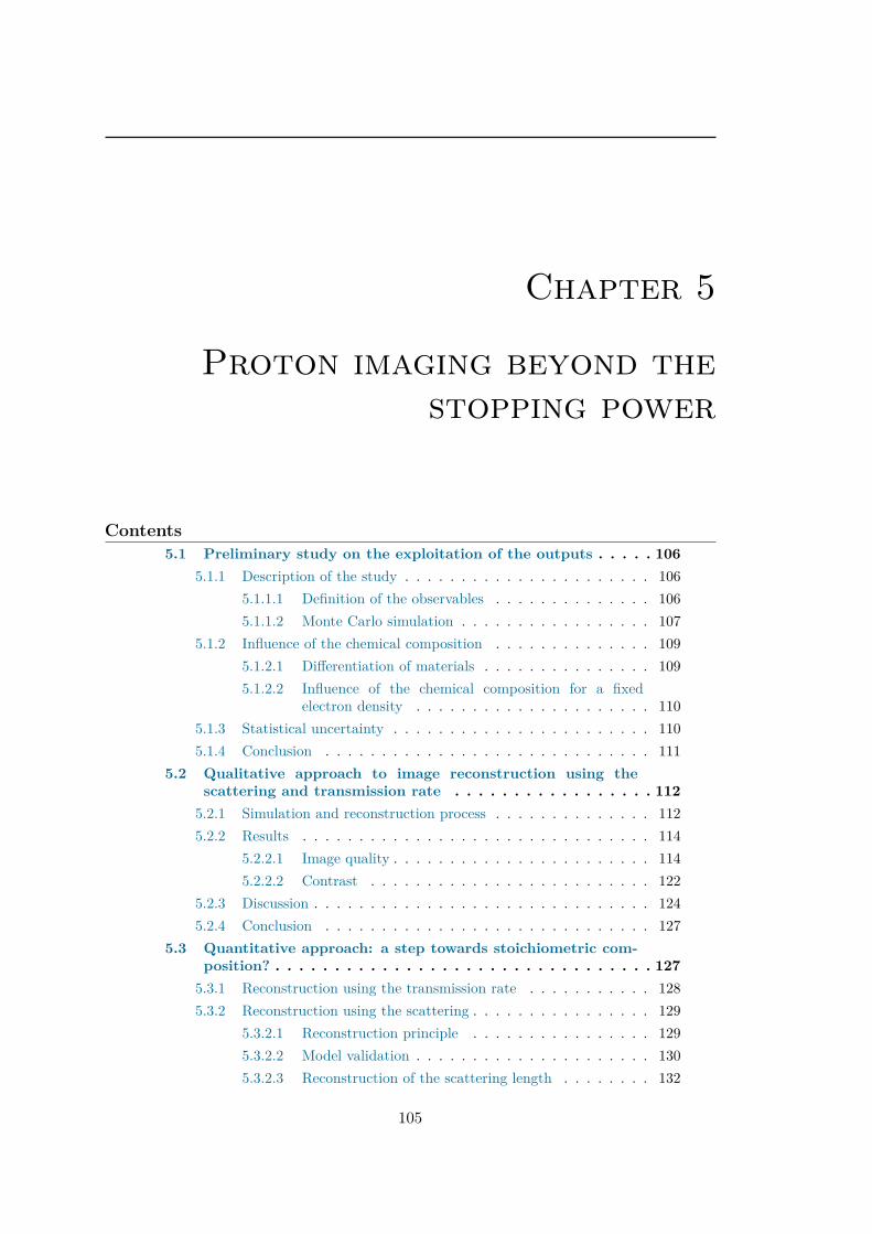
Chapter 5
Proton imaging beyond thestopping power
Contents
5.1 Preliminary study on the exploitation of the outputs . . . . . 106
5.1.1 Description of the study . . . . . . . . . . . . . . . . . . . . . . 106
5.1.1.1 Definition of the observables . . . . . . . . . . . . . . 106
5.1.1.2 Monte Carlo simulation . . . . . . . . . . . . . . . . . 107
5.1.2 Influence of the chemical composition . . . . . . . . . . . . . . 109
5.1.2.1 Differentiation of materials . . . . . . . . . . . . . . . 109
5.1.2.2 Influence of the chemical composition for a fixedelectron density . . . . . . . . . . . . . . . . . . . . . 110
5.1.3 Statistical uncertainty . . . . . . . . . . . . . . . . . . . . . . . 110
5.1.4 Conclusion . . . . . . . . . . . . . . . . . . . . . . . . . . . . . 111
5.2 Qualitative approach to image reconstruction using thescattering and transmission rate . . . . . . . . . . . . . . . . . 112
5.2.1 Simulation and reconstruction process . . . . . . . . . . . . . . 112
5.2.2 Results . . . . . . . . . . . . . . . . . . . . . . . . . . . . . . . 114
5.2.2.1 Image quality . . . . . . . . . . . . . . . . . . . . . . . 114
5.2.2.2 Contrast . . . . . . . . . . . . . . . . . . . . . . . . . 122
5.2.3 Discussion . . . . . . . . . . . . . . . . . . . . . . . . . . . . . . 124
5.2.4 Conclusion . . . . . . . . . . . . . . . . . . . . . . . . . . . . . 127
5.3 Quantitative approach: a step towards stoichiometric com-position? . . . . . . . . . . . . . . . . . . . . . . . . . . . . . . . . 127
5.3.1 Reconstruction using the transmission rate . . . . . . . . . . . 128
5.3.2 Reconstruction using the scattering . . . . . . . . . . . . . . . . 129
5.3.2.1 Reconstruction principle . . . . . . . . . . . . . . . . 129
5.3.2.2 Model validation . . . . . . . . . . . . . . . . . . . . . 130
5.3.2.3 Reconstruction of the scattering length . . . . . . . . 132
105

CHAPTER 5. PROTON IMAGING BEYOND THE STOPPING POWER
5.3.2.4 Conclusion . . . . . . . . . . . . . . . . . . . . . . . . 1335.3.3 Towards the stoichiometric composition? . . . . . . . . . . . . . 134
5.3.3.1 Overview of the information . . . . . . . . . . . . . . 1345.3.3.2 Discussion . . . . . . . . . . . . . . . . . . . . . . . . 1365.3.3.3 Conclusion . . . . . . . . . . . . . . . . . . . . . . . . 136
As presented in the first chapter, uncertainties in hadron therapy treatments are oftwo kinds:
– the range uncertainty, mainly due to the use of X-ray images as a base for treatmentplanning (Section 1.2.2),
– the uncertainty on the delivered dose, due to the fact that we only have access tothe CT numbers of the materials and not their exact composition and properties(Section 1.2.3).
Hitherto, proton imaging has been put forward as a way to directly map the RSP ofthe materials (Section 2.3). Nevertheless, the acquisition system of a pCT apparatus, asstudied nowadays (described in Section 2.3.1, and illustrated in Figure 2.6), records notonly the exit energy of each proton, but also its positions and direction upstream anddownstream from the object allowing for the evaluation of the scattering it underwent. Inaddition, such a system makes it possible to access the transmission rate of the particles.
The aim of this study is to investigate the potential use of these outputs as sourcesof information on the tissue composition.
5.1 Preliminary study on the exploitation of the outputs
The preliminary study aimed at determining which information could be used and atidentifying potential key points or limitations for their exploitation.
5.1.1 Description of the study
5.1.1.1 Definition of the observables
Physics processes of interactions between protons and matter are detailed in Section 2.1.After a given depth of material, an initially mono-energetic unidirectional proton beamexhibits an energy distribution (as illustrated on Figure 5.1(a)), a spatial and angulardistribution (as illustrated on Figure 5.1(b)), as well as a reduction of fluence.
To investigate the potential information carried by these outputs, observables werechosen for this study:
– the average energy upon exit from the object,
– the root-mean square of the energy distribution upon exit of the object. It isrepresentative of the energy loss straggling,
– the mean value of the non-projected angular distribution upon exit of the object,
– the transmission rate of the particles.
106
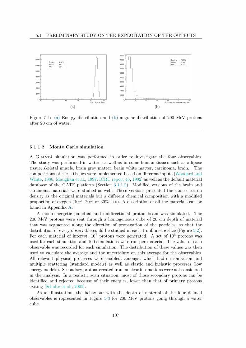
5.1. PRELIMINARY STUDY ON THE EXPLOITATION OF THE OUTPUTS
Entries 81571
Mean 87.32
RMS 5.547
Kinetic Energy (MeV)0 20 40 60 80 100
0
2000
4000
6000
8000
10000
12000
14000
Entries 81571
Mean 87.32
RMS 5.547
(a)
Entries 81571
Mean 3.548
RMS 4.187
2D non-projected angle (degrees)0 5 10 15 20 25 30
0
2000
4000
6000
8000
10000
12000
14000
16000
18000
20000
Entries 81571
Mean 3.548
RMS 4.187
(b)
Figure 5.1: (a) Energy distribution and (b) angular distribution of 200 MeV protonsafter 20 cm of water.
5.1.1.2 Monte Carlo simulation
A Geant4 simulation was performed in order to investigate the four observables.The study was performed in water, as well as in some human tissues such as adiposetissue, skeletal muscle, brain grey matter, brain white matter, carcinoma, brain... Thecompositions of these tissues were implemented based on different inputs [Woodard andWhite, 1986; Maughan et al., 1997; ICRU report 46, 1992] as well as the default materialdatabase of the GATE platform (Section 3.1.1.2). Modified versions of the brain andcarcinoma materials were studied as well. These versions presented the same electrondensity as the original materials but a different chemical composition with a modifiedproportion of oxygen (10%, 20% or 30% less). A description of all the materials can befound in Appendix A.
A mono-energetic punctual and unidirectional proton beam was simulated. The200 MeV protons were sent through a homogeneous cube of 20 cm depth of materialthat was segmented along the direction of propagation of the particles, so that thedistribution of every observable could be studied in each 1-millimetre slice (Figure 5.2).For each material of interest, 107 protons were generated. A set of 105 protons wasused for each simulation and 100 simulations were run per material. The value of eachobservable was recorded for each simulation. The distribution of these values was thenused to calculate the average and the uncertainty on this average for the observables.All relevant physical processes were enabled, amongst which hadron ionisation andmultiple scattering (standard models) as well as elastic and inelastic processes (lowenergy models). Secondary protons created from nuclear interactions were not consideredin the analysis. In a realistic scan situation, most of those secondary protons can beidentified and rejected because of their energies, lower than that of primary protonsexiting [Schulte et al., 2005].
As an illustration, the behaviour with the depth of material of the four definedobservables is represented in Figure 5.3 for 200 MeV protons going through a watercube.
107
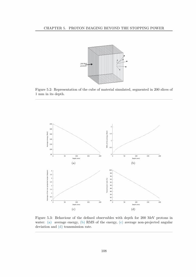
CHAPTER 5. PROTON IMAGING BEYOND THE STOPPING POWER
200 MeV
protons
Figure 5.2: Representation of the cube of material simulated, segmented in 200 slices of1 mm in its depth.
80
100
120
140
160
180
200
0 50 100 150 200
Avera
ge e
nerg
y (
MeV
)
Depth (mm)
(a)
0
0.5
1
1.5
2
0 50 100 150 200
RM
S o
f th
e e
nerg
y (
MeV
)
Depth (mm)
(b)
0
0.5
1
1.5
2
2.5
3
3.5
4
0 50 100 150 200
Avera
ge o
f th
e n
on-p
roje
cte
d a
ngle
(degre
s)
Depth (mm)
(c)
80
82
84
86
88
90
92
94
96
98
100
0 50 100 150 200
Tra
nsm
issio
n r
ate
(%
)
Depth (mm)
(d)
Figure 5.3: Behaviour of the defined observables with depth for 200 MeV protons inwater: (a) average energy, (b) RMS of the energy, (c) average non-projected angulardeviation and (d) transmission rate.
108
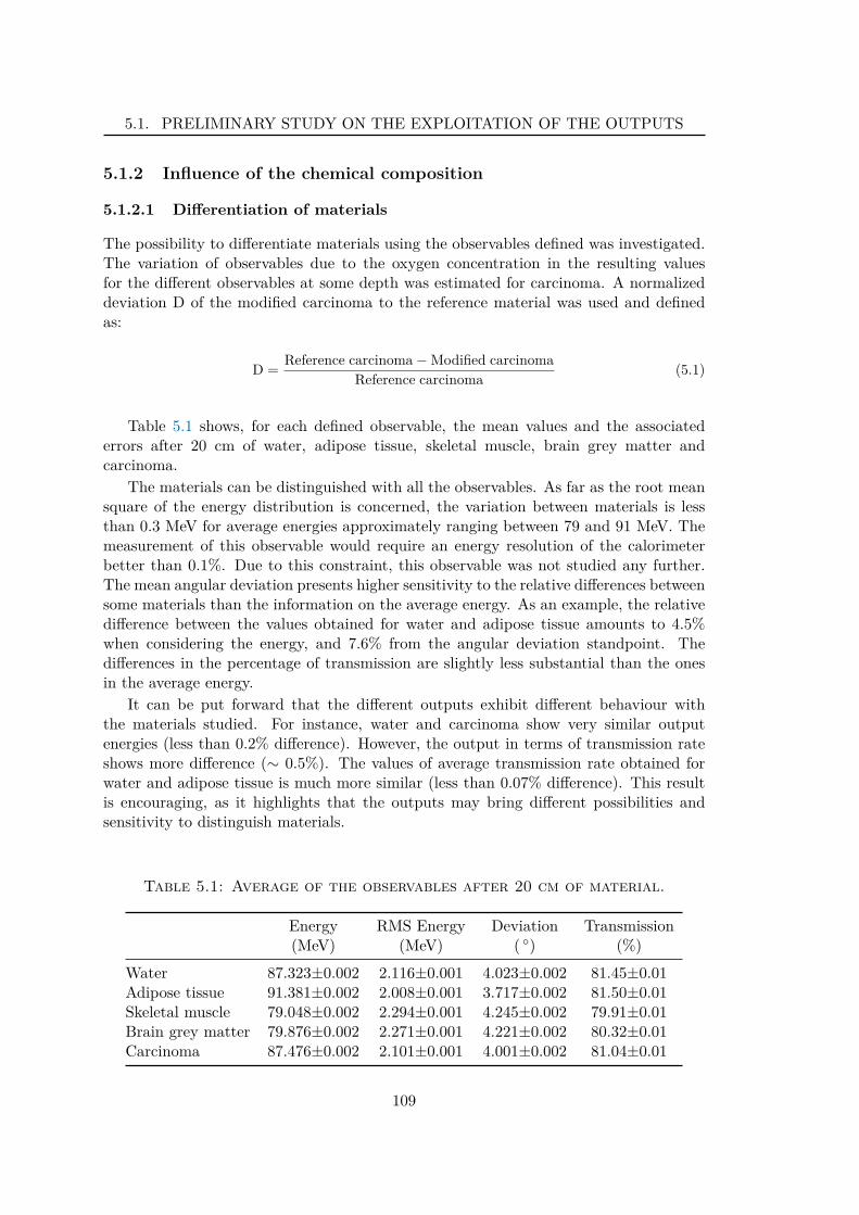
5.1. PRELIMINARY STUDY ON THE EXPLOITATION OF THE OUTPUTS
5.1.2 Influence of the chemical composition
5.1.2.1 Differentiation of materials
The possibility to differentiate materials using the observables defined was investigated.The variation of observables due to the oxygen concentration in the resulting valuesfor the different observables at some depth was estimated for carcinoma. A normalizeddeviation D of the modified carcinoma to the reference material was used and definedas:
D =Reference carcinoma − Modified carcinoma
Reference carcinoma(5.1)
Table 5.1 shows, for each defined observable, the mean values and the associatederrors after 20 cm of water, adipose tissue, skeletal muscle, brain grey matter andcarcinoma.
The materials can be distinguished with all the observables. As far as the root meansquare of the energy distribution is concerned, the variation between materials is lessthan 0.3 MeV for average energies approximately ranging between 79 and 91 MeV. Themeasurement of this observable would require an energy resolution of the calorimeterbetter than 0.1%. Due to this constraint, this observable was not studied any further.The mean angular deviation presents higher sensitivity to the relative differences betweensome materials than the information on the average energy. As an example, the relativedifference between the values obtained for water and adipose tissue amounts to 4.5%when considering the energy, and 7.6% from the angular deviation standpoint. Thedifferences in the percentage of transmission are slightly less substantial than the onesin the average energy.
It can be put forward that the different outputs exhibit different behaviour withthe materials studied. For instance, water and carcinoma show very similar outputenergies (less than 0.2% difference). However, the output in terms of transmission rateshows more difference (∼ 0.5%). The values of average transmission rate obtained forwater and adipose tissue is much more similar (less than 0.07% difference). This resultis encouraging, as it highlights that the outputs may bring different possibilities andsensitivity to distinguish materials.
Table 5.1: Average of the observables after 20 cm of material.
Energy RMS Energy Deviation Transmission(MeV) (MeV) ( ) (%)
Water 87.323±0.002 2.116±0.001 4.023±0.002 81.45±0.01Adipose tissue 91.381±0.002 2.008±0.001 3.717±0.002 81.50±0.01Skeletal muscle 79.048±0.002 2.294±0.001 4.245±0.002 79.91±0.01Brain grey matter 79.876±0.002 2.271±0.001 4.221±0.002 80.32±0.01Carcinoma 87.476±0.002 2.101±0.001 4.001±0.002 81.04±0.01
109
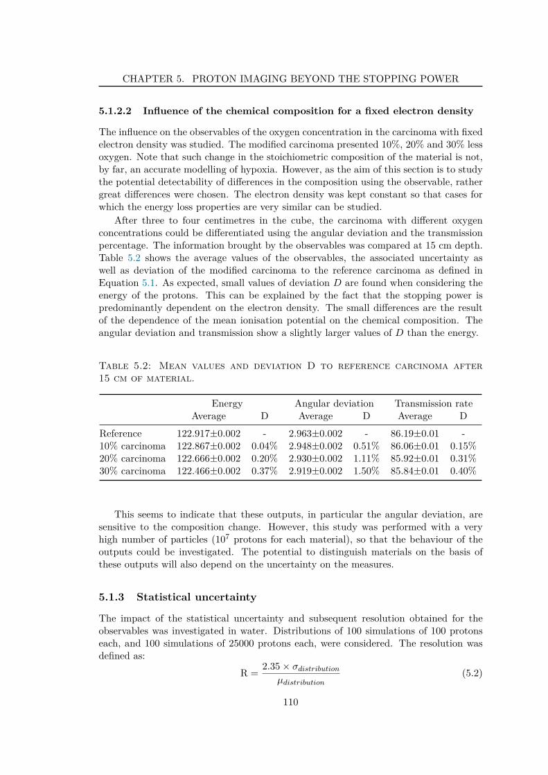
CHAPTER 5. PROTON IMAGING BEYOND THE STOPPING POWER
5.1.2.2 Influence of the chemical composition for a fixed electron density
The influence on the observables of the oxygen concentration in the carcinoma with fixedelectron density was studied. The modified carcinoma presented 10%, 20% and 30% lessoxygen. Note that such change in the stoichiometric composition of the material is not,by far, an accurate modelling of hypoxia. However, as the aim of this section is to studythe potential detectability of differences in the composition using the observable, rathergreat differences were chosen. The electron density was kept constant so that cases forwhich the energy loss properties are very similar can be studied.
After three to four centimetres in the cube, the carcinoma with different oxygenconcentrations could be differentiated using the angular deviation and the transmissionpercentage. The information brought by the observables was compared at 15 cm depth.Table 5.2 shows the average values of the observables, the associated uncertainty aswell as deviation of the modified carcinoma to the reference carcinoma as defined inEquation 5.1. As expected, small values of deviation D are found when considering theenergy of the protons. This can be explained by the fact that the stopping power ispredominantly dependent on the electron density. The small differences are the resultof the dependence of the mean ionisation potential on the chemical composition. Theangular deviation and transmission show a slightly larger values of D than the energy.
Table 5.2: Mean values and deviation D to reference carcinoma after15 cm of material.
Energy Angular deviation Transmission rateAverage D Average D Average D
Reference 122.917±0.002 - 2.963±0.002 - 86.19±0.01 -10% carcinoma 122.867±0.002 0.04% 2.948±0.002 0.51% 86.06±0.01 0.15%20% carcinoma 122.666±0.002 0.20% 2.930±0.002 1.11% 85.92±0.01 0.31%30% carcinoma 122.466±0.002 0.37% 2.919±0.002 1.50% 85.84±0.01 0.40%
This seems to indicate that these outputs, in particular the angular deviation, aresensitive to the composition change. However, this study was performed with a veryhigh number of particles (107 protons for each material), so that the behaviour of theoutputs could be investigated. The potential to distinguish materials on the basis ofthese outputs will also depend on the uncertainty on the measures.
5.1.3 Statistical uncertainty
The impact of the statistical uncertainty and subsequent resolution obtained for theobservables was investigated in water. Distributions of 100 simulations of 100 protonseach, and 100 simulations of 25000 protons each, were considered. The resolution wasdefined as:
R =2.35 × σdistribution
µdistribution(5.2)
110
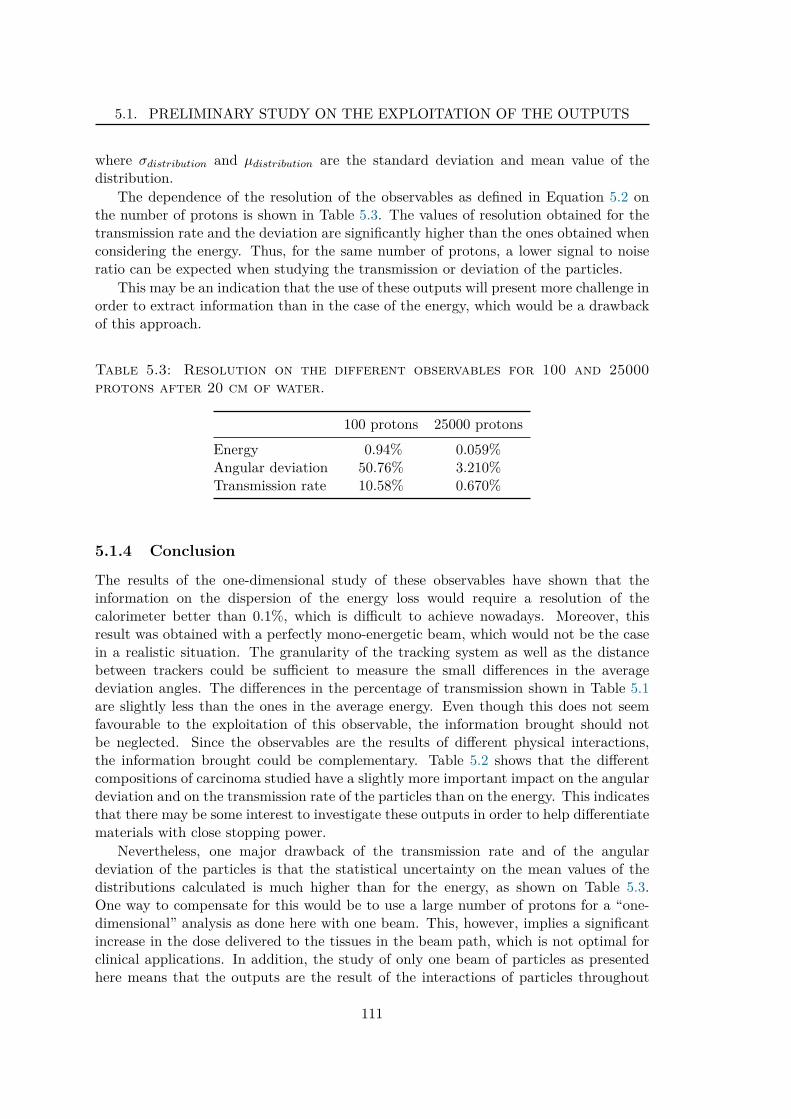
5.1. PRELIMINARY STUDY ON THE EXPLOITATION OF THE OUTPUTS
where σdistribution and µdistribution are the standard deviation and mean value of thedistribution.
The dependence of the resolution of the observables as defined in Equation 5.2 onthe number of protons is shown in Table 5.3. The values of resolution obtained for thetransmission rate and the deviation are significantly higher than the ones obtained whenconsidering the energy. Thus, for the same number of protons, a lower signal to noiseratio can be expected when studying the transmission or deviation of the particles.
This may be an indication that the use of these outputs will present more challenge inorder to extract information than in the case of the energy, which would be a drawbackof this approach.
Table 5.3: Resolution on the different observables for 100 and 25000protons after 20 cm of water.
100 protons 25000 protons
Energy 0.94% 0.059%Angular deviation 50.76% 3.210%Transmission rate 10.58% 0.670%
5.1.4 Conclusion
The results of the one-dimensional study of these observables have shown that theinformation on the dispersion of the energy loss would require a resolution of thecalorimeter better than 0.1%, which is difficult to achieve nowadays. Moreover, thisresult was obtained with a perfectly mono-energetic beam, which would not be the casein a realistic situation. The granularity of the tracking system as well as the distancebetween trackers could be sufficient to measure the small differences in the averagedeviation angles. The differences in the percentage of transmission shown in Table 5.1are slightly less than the ones in the average energy. Even though this does not seemfavourable to the exploitation of this observable, the information brought should notbe neglected. Since the observables are the results of different physical interactions,the information brought could be complementary. Table 5.2 shows that the differentcompositions of carcinoma studied have a slightly more important impact on the angulardeviation and on the transmission rate of the particles than on the energy. This indicatesthat there may be some interest to investigate these outputs in order to help differentiatematerials with close stopping power.
Nevertheless, one major drawback of the transmission rate and of the angulardeviation of the particles is that the statistical uncertainty on the mean values of thedistributions calculated is much higher than for the energy, as shown on Table 5.3.One way to compensate for this would be to use a large number of protons for a “one-dimensional” analysis as done here with one beam. This, however, implies a significantincrease in the dose delivered to the tissues in the beam path, which is not optimal forclinical applications. In addition, the study of only one beam of particles as presentedhere means that the outputs are the result of the interactions of particles throughout
111
CHAPTER 5. PROTON IMAGING BEYOND THE STOPPING POWER
their propagation in the medium. Information on the localization of heterogeneities forexample could hardly be obtained this way.A different solution is to consider an image reconstruction approach. By reconstructingimages of the different outputs, it would be possible to study a voxel of the image ora region of interest. The information contained in this region is then representative ofall protons that went through this volume. The higher statistical uncertainty on thescattering and transmission rate of the particles could then be taken into account byhaving a multi-scale approach: a voxel of the RSP image can be studied, whereas largerregions can be looked at when considering the other images. Assuming that this regionis constituted of only one material, on the basis of the RSP image for example, the datareconstructed from a large number of particles can be studied without increasing theoverall dose. The next section will present such a tomographic study.
In addition, it may be highlighted that all results and conclusions on the potentialinterest in the outputs presented in this work are obtained from Monte Carlo simulationdata. It is an advantage in terms of conceptual study, as it allows for the investigationof the behaviour of particles without any experimental or detection effects. While itdoes not mean that the exact same results would be obtained in real conditions, MonteCarlo techniques and Geant4 in particular have been used for years in proton therapyand are more accurate than analytical dose calculations [Paganetti, 2012]. The Geant4simulation code has been validated with experimental data for applications in protonimaging [Cuttone et al., 2005; Milhoretto et al., 2012].
5.2 Qualitative approach to image reconstruction using
the scattering and transmission rate
In order to evaluate the potential of imaging using the scattering and transmission, imagereconstruction studies were performed. The first approach taken was rather qualitative:if we reconstruct images, what can we get? As the results of the previous sectionhighlighted, the statistical uncertainty on the measured outputs is quite significant.The first approach thus aims at answering the following question: may the informationcollected on the scattering and transmission be used to produce images that could be ofimportance?
5.2.1 Simulation and reconstruction process
Simulated pCT scan data of a modified version of the Zubal head phantom (Section3.1.5.2) were generated using GATE (Sections 3.1.1.2 and 3.1.2). Two lesions wereinserted inside the brain. They were assigned the composition of modified carcinoma,with the same electron density but with different proportions of oxygen. A descriptionof the composition and properties of the two carcinoma and the brain region can befound in Appendix A.In order to reduce simulation time and increase the number of particles studied, thedata considered for this study were produced by only considering a 1.26 cm thick slice ofthe head. This is sufficient to get consistent results for the reconstruction of the centralslice. As a head is comparable to a 20 cm-deep water object, this thickness encompassesmore than 90% of the scattered particles.
112
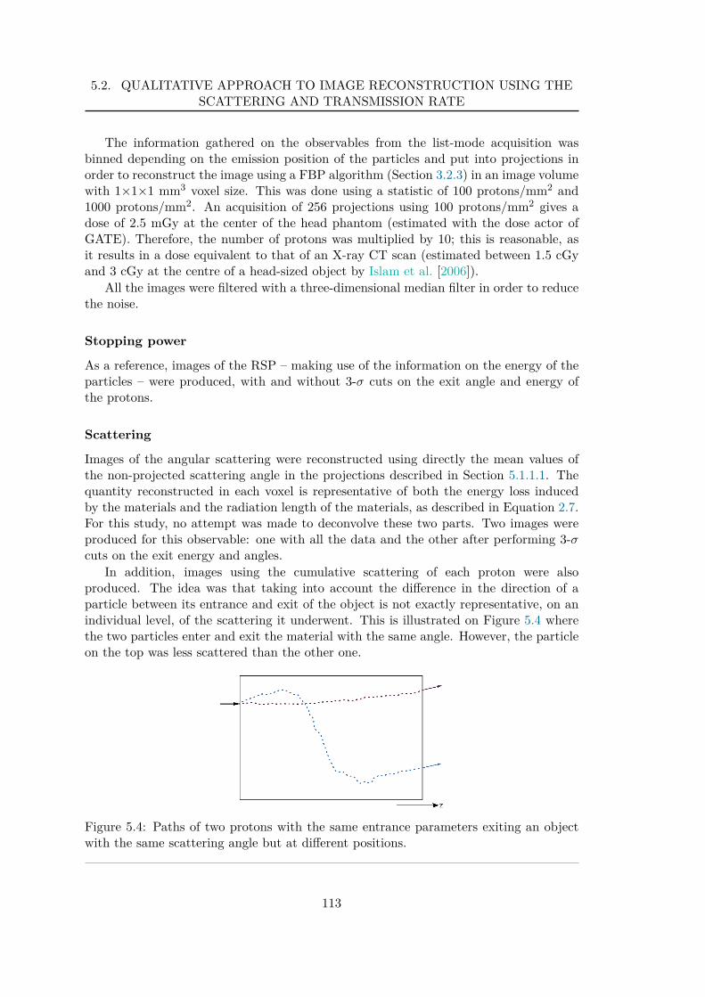
5.2. QUALITATIVE APPROACH TO IMAGE RECONSTRUCTION USING THESCATTERING AND TRANSMISSION RATE
The information gathered on the observables from the list-mode acquisition wasbinned depending on the emission position of the particles and put into projections inorder to reconstruct the image using a FBP algorithm (Section 3.2.3) in an image volumewith 1×1×1 mm3 voxel size. This was done using a statistic of 100 protons/mm2 and1000 protons/mm2. An acquisition of 256 projections using 100 protons/mm2 gives adose of 2.5 mGy at the center of the head phantom (estimated with the dose actor ofGATE). Therefore, the number of protons was multiplied by 10; this is reasonable, asit results in a dose equivalent to that of an X-ray CT scan (estimated between 1.5 cGyand 3 cGy at the centre of a head-sized object by Islam et al. [2006]).
All the images were filtered with a three-dimensional median filter in order to reducethe noise.
Stopping power
As a reference, images of the RSP – making use of the information on the energy of theparticles – were produced, with and without 3-σ cuts on the exit angle and energy ofthe protons.
Scattering
Images of the angular scattering were reconstructed using directly the mean values ofthe non-projected scattering angle in the projections described in Section 5.1.1.1. Thequantity reconstructed in each voxel is representative of both the energy loss inducedby the materials and the radiation length of the materials, as described in Equation 2.7.For this study, no attempt was made to deconvolve these two parts. Two images wereproduced for this observable: one with all the data and the other after performing 3-σcuts on the exit energy and angles.
In addition, images using the cumulative scattering of each proton were alsoproduced. The idea was that taking into account the difference in the direction of aparticle between its entrance and exit of the object is not exactly representative, on anindividual level, of the scattering it underwent. This is illustrated on Figure 5.4 wherethe two particles enter and exit the material with the same angle. However, the particleon the top was less scattered than the other one.
Figure 5.4: Paths of two protons with the same entrance parameters exiting an objectwith the same scattering angle but at different positions.
113
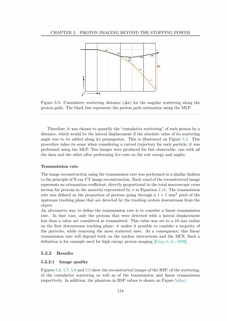
CHAPTER 5. PROTON IMAGING BEYOND THE STOPPING POWER
Figure 5.5: Cumulative scattering distance (∆x) for the angular scattering along theproton path. The black line represents the proton path estimation using the MLP.
Therefore, it was chosen to quantify the “cumulative scattering” of each proton by adistance, which would be the lateral displacement if the absolute value of its scatteringangle was to be added along its propagation. This is illustrated on Figure 5.5. Thisprocedure takes its sense when considering a curved trajectory for each particle; it wasperformed using the MLP. Two images were produced for this observable: one with allthe data and the other after performing 3-σ cuts on the exit energy and angles.
Transmission rate
The image reconstruction using the transmission rate was performed in a similar fashionto the principle of X-ray CT image reconstruction. Each voxel of the reconstructed imagerepresents an attenuation coefficient, directly proportional to the total macroscopic crosssection for protons in the material represented by κ in Equation 2.10. The transmissionrate was defined as the proportion of protons going through a 1 × 1 mm2 pixel of theupstream tracking plane that are detected by the tracking system downstream from theobject.An alternative way to define the transmission rate is to consider a linear transmissionrate. In that case, only the protons that were detected with a lateral displacementless than a value are considered as transmitted. This value was set to a 10 mm radiuson the first downstream tracking plane: it makes it possible to consider a majority ofthe particles, while removing the most scattered ones. As a consequence, this lineartransmission rate will depend both on the nuclear interactions and the MCS. Such adefinition is for example used for high energy proton imaging [King et al., 1999].
5.2.2 Results
5.2.2.1 Image quality
Figures 5.6, 5.7, 5.8 and 5.9 show the reconstructed images of the RSP, of the scattering,of the cumulative scattering as well as of the transmission and linear transmissionrespectively. In addition, the phantom in RSP values is shown on Figure 5.6(a).
114
5.2. QUALITATIVE APPROACH TO IMAGE RECONSTRUCTION USING THESCATTERING AND TRANSMISSION RATE
For easier inter-comparison, Figure 5.10 shows images reconstructed using the differentobservables using 1000 protons/mm2/projection.
Visual assessment
Visual assessment of the images makes it possible to determine the following: the RSPimages (Figure 5.6) seem to present a much higher quality than the images reconstructedusing the other data. This is not surprising, as it was shown that proton imaging (ofthe RSP) makes it possible to reach a satisfactory density and spatial resolution to beused in a clinical setting. The effect of the 3-σ cuts on the data is not clearly visible,nor is the effect of the increase in the statistics. Indeed, as the statistical uncertaintyon the measured energy (that is translated to noise in the projections and therefore inthe images) is very low, using 1000 protons per square millimetre of projection is notnecessary.Nevertheless, the images reconstructed using the other observables all show someanatomical information.In the case of the reconstructions using the scattering (Figure 5.7), it can be seen thatthe cuts help distinguish the tumours in the case of 100 protons/mm2. The improvementin terms of reduction of noise in the image when using 1000 protons/mm2 is considerable.The lesions can be clearly seen on the image of 1000 protons/mm2 with cuts.The images reconstructed using the cumulative scattering (Figure 5.8) exhibit interestingvisual properties. Increasing the number of protons treated from 100 to 1000/mm2 allowsa much easier differentiation of the internal structures of the head. Moreover, the borderof the two lesions appears clearly, in bright, allowing for a good detection. The imagesreconstructed using the transmission rate (Figures 5.9(a) and 5.9(b)) show an importantlevel of noise, that is reduced with the increase in the number of particles studied. It canbe seen that the images reconstructed using the linear transmission (Figures 5.9(c) and5.9(d)) show a much greater contrast between the soft tissues and the bones than anyother. However, for all the transmission images, the tumours can not be distinguished.
Signal to noise ratio
The signal to noise ratio (SNR) of the reconstructed images was evaluated. A numberof N = 10 regions of interest (ROI) of 200 mm3 each were drawn inside an area madeof skeletal muscle (arrows in Figure 5.6(a)). The SNR was defined as:
SNR =1N
∑Ni=0 µi
√
1N
∑Ni=0
(
µi − 1N
∑Ni=0 µi
)2(5.3)
with µi the mean value of the ith ROI.Results are presented in Table 5.4. As expected from the results shown in Table 5.3,
the statistical uncertainty on the transmission rate and scattering induces a much lowerSNR in the images reconstructed from these observables than from the RSP. Indeed, inthe cases of the cumulative scattering and of the (linear) transmission, the SNR is anorder of magnitude lower than for the images of the RSP.
115
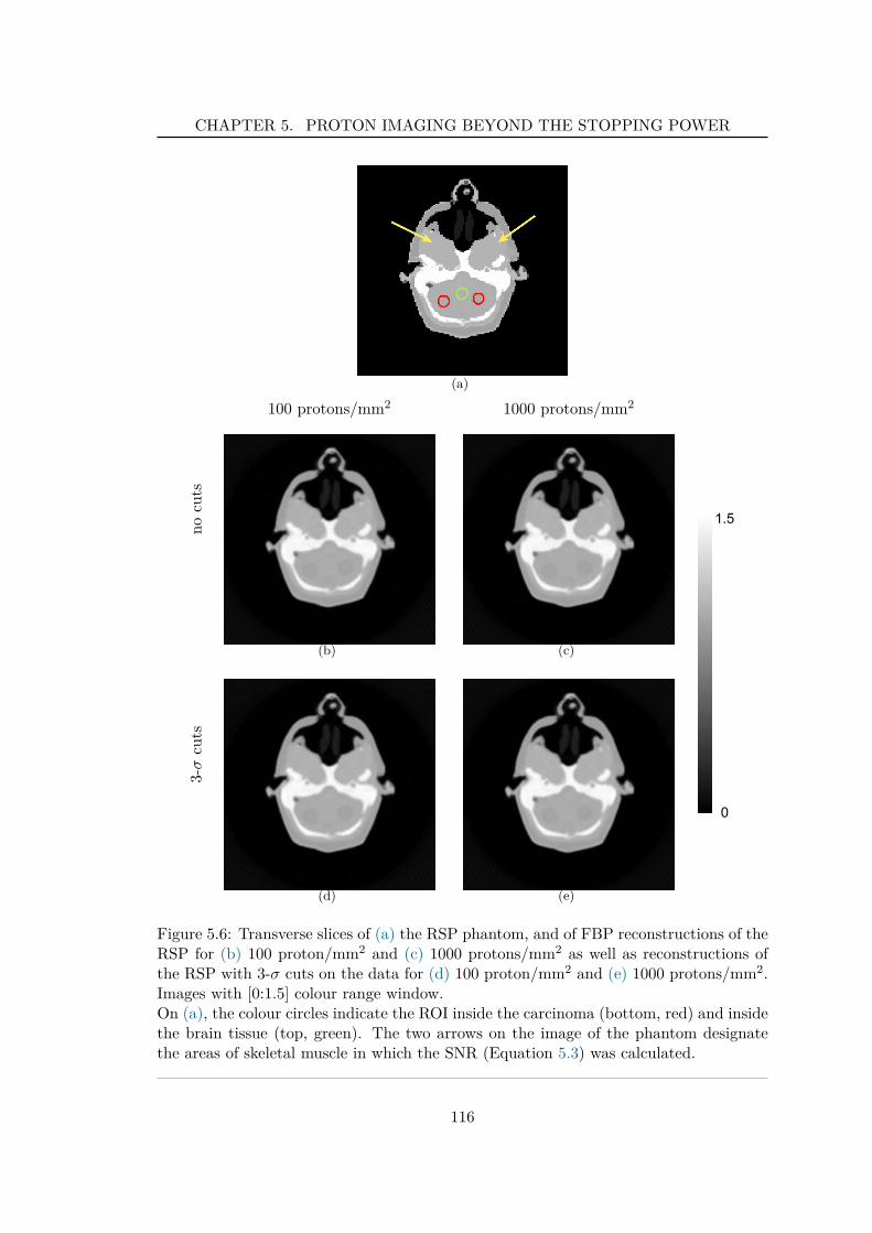
CHAPTER 5. PROTON IMAGING BEYOND THE STOPPING POWER
(a)
100 protons/mm2 1000 protons/mm2
nocu
ts
(b) (c)
0
1.5
3-σ
cuts
(d) (e)
Figure 5.6: Transverse slices of (a) the RSP phantom, and of FBP reconstructions of theRSP for (b) 100 proton/mm2 and (c) 1000 protons/mm2 as well as reconstructions ofthe RSP with 3-σ cuts on the data for (d) 100 proton/mm2 and (e) 1000 protons/mm2.Images with [0:1.5] colour range window.On (a), the colour circles indicate the ROI inside the carcinoma (bottom, red) and insidethe brain tissue (top, green). The two arrows on the image of the phantom designatethe areas of skeletal muscle in which the SNR (Equation 5.3) was calculated.
116
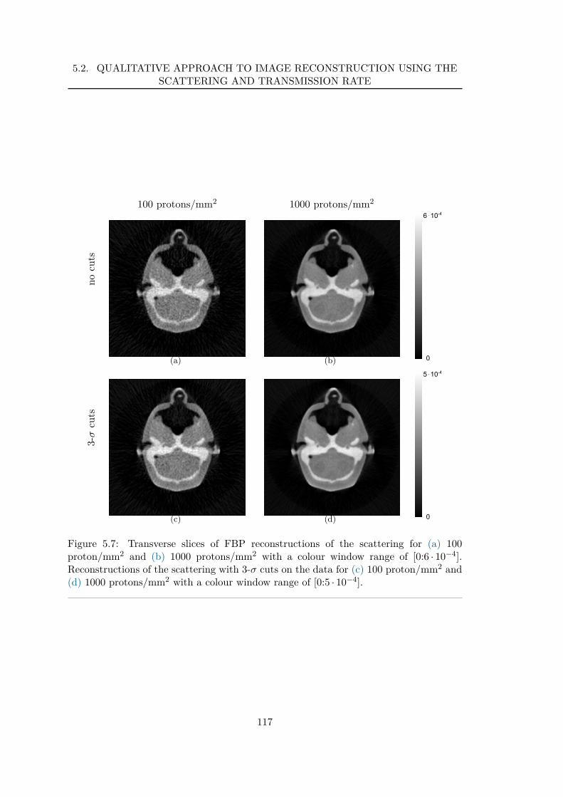
5.2. QUALITATIVE APPROACH TO IMAGE RECONSTRUCTION USING THESCATTERING AND TRANSMISSION RATE
100 protons/mm2 1000 protons/mm2
nocu
ts
(a) (b) 0
6⋅10-4
3-σ
cuts
(c) (d) 0
5⋅10-4
Figure 5.7: Transverse slices of FBP reconstructions of the scattering for (a) 100proton/mm2 and (b) 1000 protons/mm2 with a colour window range of [0:6 · 10−4].Reconstructions of the scattering with 3-σ cuts on the data for (c) 100 proton/mm2 and(d) 1000 protons/mm2 with a colour window range of [0:5 · 10−4].
117
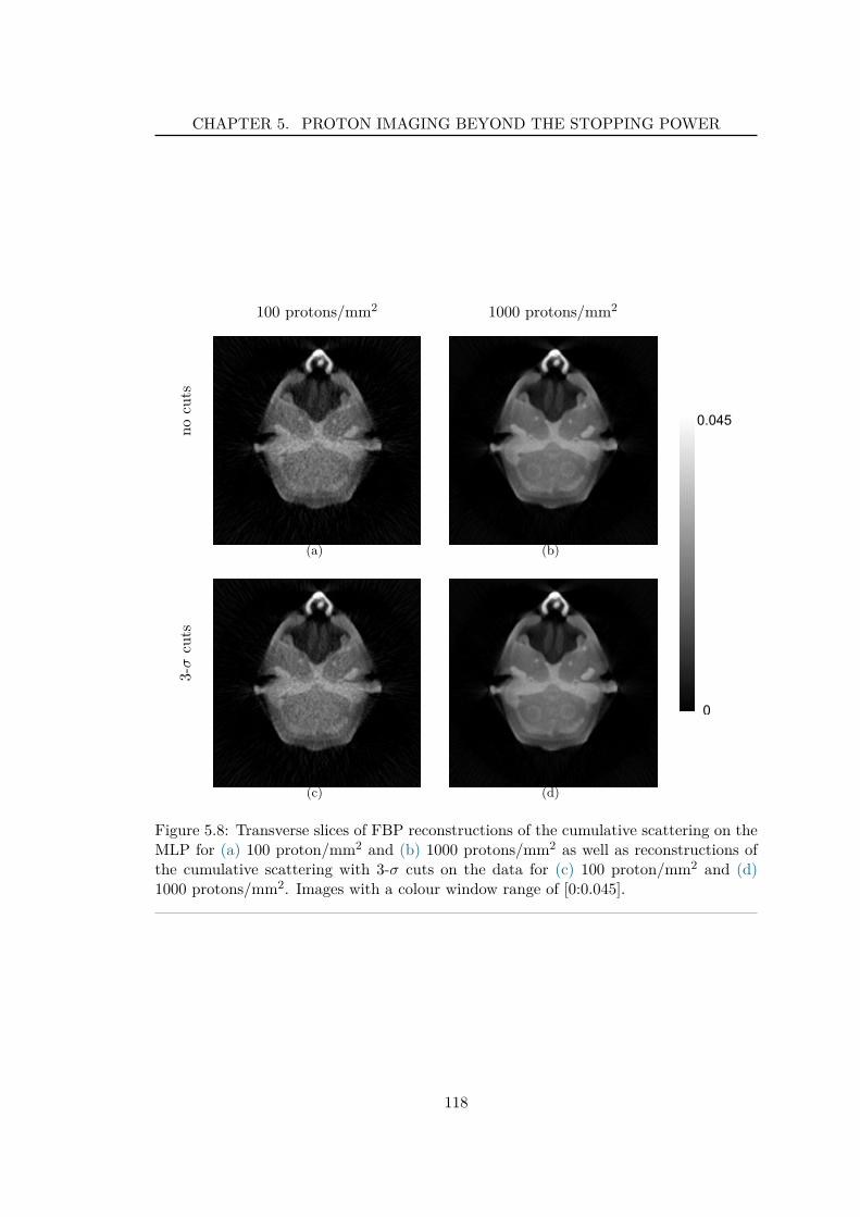
CHAPTER 5. PROTON IMAGING BEYOND THE STOPPING POWER
100 protons/mm2 1000 protons/mm2
nocu
ts
(a) (b)
0
0.045
3-σ
cuts
(c) (d)
Figure 5.8: Transverse slices of FBP reconstructions of the cumulative scattering on theMLP for (a) 100 proton/mm2 and (b) 1000 protons/mm2 as well as reconstructions ofthe cumulative scattering with 3-σ cuts on the data for (c) 100 proton/mm2 and (d)1000 protons/mm2. Images with a colour window range of [0:0.045].
118
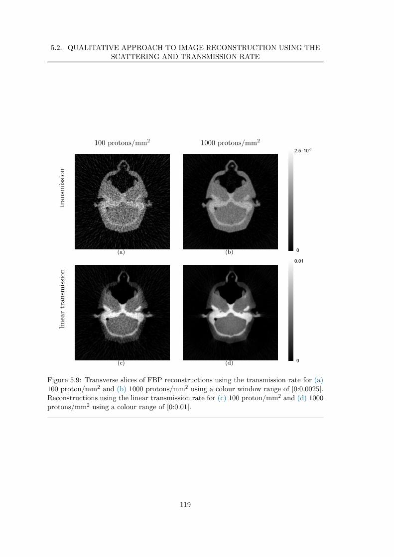
5.2. QUALITATIVE APPROACH TO IMAGE RECONSTRUCTION USING THESCATTERING AND TRANSMISSION RATE
100 protons/mm2 1000 protons/mm2
tran
smis
sion
(a) (b) 0
2.5⋅10-3
linea
rtr
ansm
issi
on
(c) (d) 0
0.01
Figure 5.9: Transverse slices of FBP reconstructions using the transmission rate for (a)100 proton/mm2 and (b) 1000 protons/mm2 using a colour window range of [0:0.0025].Reconstructions using the linear transmission rate for (c) 100 proton/mm2 and (d) 1000protons/mm2 using a colour range of [0:0.01].
119
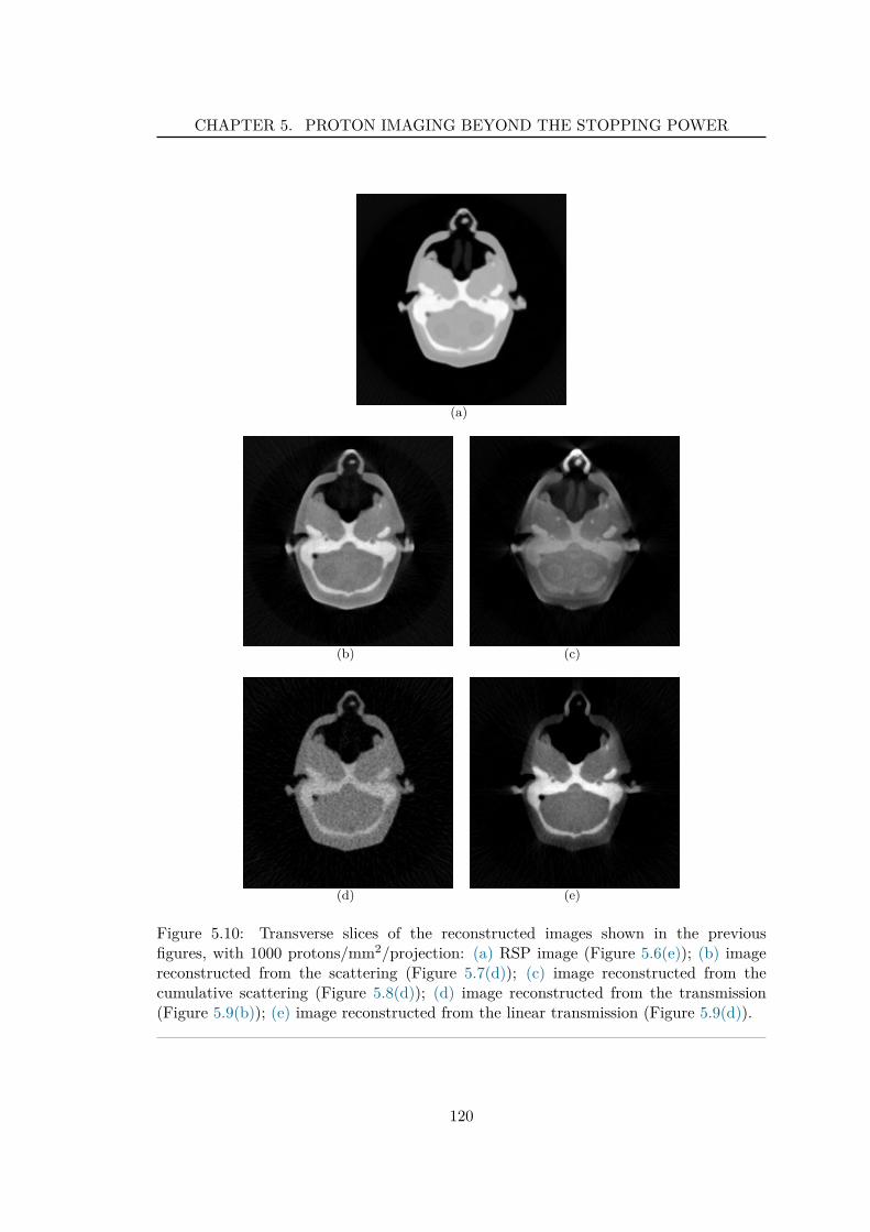
CHAPTER 5. PROTON IMAGING BEYOND THE STOPPING POWER
(a)
(b) (c)
(d) (e)
Figure 5.10: Transverse slices of the reconstructed images shown in the previousfigures, with 1000 protons/mm2/projection: (a) RSP image (Figure 5.6(e)); (b) imagereconstructed from the scattering (Figure 5.7(d)); (c) image reconstructed from thecumulative scattering (Figure 5.8(d)); (d) image reconstructed from the transmission(Figure 5.9(b)); (e) image reconstructed from the linear transmission (Figure 5.9(d)).
120
5.2. QUALITATIVE APPROACH TO IMAGE RECONSTRUCTION USING THESCATTERING AND TRANSMISSION RATE
Table 5.4: SNR of the different reconstructed images for 100 and 1000protons/mm2/projection
Image 100 protons/mm2 1000 protons/mm2
RSP 298 318RSP - with cuts 300 320Angular scattering 47 51Angular scattering - with cuts 55 49Cumulated scattering 19 19Cumulated scattering - with cuts 22 20Transmission 27 64Linear transmission 23 20
Region of interest study
Three ROI were defined in the reconstructed images as follows: one inside each carcinomaand one in the brain tissue. Each 3D cylindrical ROI has a volume of 406 mm3. Theyare represented by the circles on Figure 5.6(a). The study was performed on the imagesreconstructed using 1000 protons/mm2.
It is possible to evaluate the accuracy of the reconstructed images in the case of theRSP and in the case of the transmission.For the RSP, the expected values were computed analytically using the Bethe formulaand knowing the stoichiometric composition of the materials simulated. Figure 5.11shows the reconstructed values inside the three ROI, as well as the expected value forthe RSP images. It can be seen that the values reconstructed in the ROI, for the imageswith and without the 3-σ cuts on the data, are quite close to the expected values.Figure 5.12 shows the reconstructed values as well as the expected values for thetransmission image. The expected values were calculated using the information onthe transmission rate of protons inside an homogeneous cube of the materials (Section5.1.1.2). While the reconstructed values are really close to the expected ones, theuncertainty on the average, represented on the histogram by the error bars, aresignificant.
The values in the reconstructed images using the scattering, cumulative scatteringand linear transmission rate is difficult to interpret because they depend on multiplephysics processes. As a consequence, no expected values could be determined for theseimages. Figures 5.13, 5.14 and 5.15 show the reconstructed values in the three ROI forthe images produced from the scattering, cumulative scattering and linear transmissionrate, respectively. It can be seen from Figure 5.13 that some difference between thethree ROI can be distinguished. For both images, with and without the 3-σ cuts, thevalues in the carcinoma ROI can be set apart from the values in the brain ROI. As far asthe cumulative scattering goes (Figure 5.14), the noise in the regions of interest resultsin the fact that the different ROI can not be well differentiated. Finally, in the case of
121
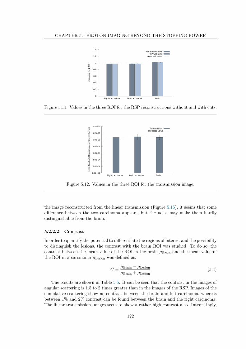
CHAPTER 5. PROTON IMAGING BEYOND THE STOPPING POWER
0
0.2
0.4
0.6
0.8
1
1.2
1.4
Right carcinoma Left carcinoma Brain
reco
nstr
ucte
d RS
P
expected value
RSP without cutsRSP with cuts
Figure 5.11: Values in the three ROI for the RSP reconstructions without and with cuts.
0.0e+00
2.0e-04
4.0e-04
6.0e-04
8.0e-04
1.0e-03
1.2e-03
1.4e-03
Right carcinoma Left carcinoma Brain
reco
nstr
ucte
d at
tenu
atio
n co
effici
ent (
1/m
m)
expected valueTransmission
Figure 5.12: Values in the three ROI for the transmission image.
the image reconstructed from the linear transmission (Figure 5.15), it seems that somedifference between the two carcinoma appears, but the noise may make them hardlydistinguishable from the brain.
5.2.2.2 Contrast
In order to quantify the potential to differentiate the regions of interest and the possibilityto distinguish the lesions, the contrast with the brain ROI was studied. To do so, thecontrast between the mean value of the ROI in the brain µBrain and the mean value ofthe ROI in a carcinoma µLesion was defined as:
C =µBrain − µLesion
µBrain + µLesion(5.4)
The results are shown in Table 5.5. It can be seen that the contrast in the images ofangular scattering is 1.5 to 2 times greater than in the images of the RSP. Images of thecumulative scattering show no contrast between the brain and left carcinoma, whereasbetween 1% and 2% contrast can be found between the brain and the right carcinoma.The linear transmission images seem to show a rather high contrast also. Interestingly,
122
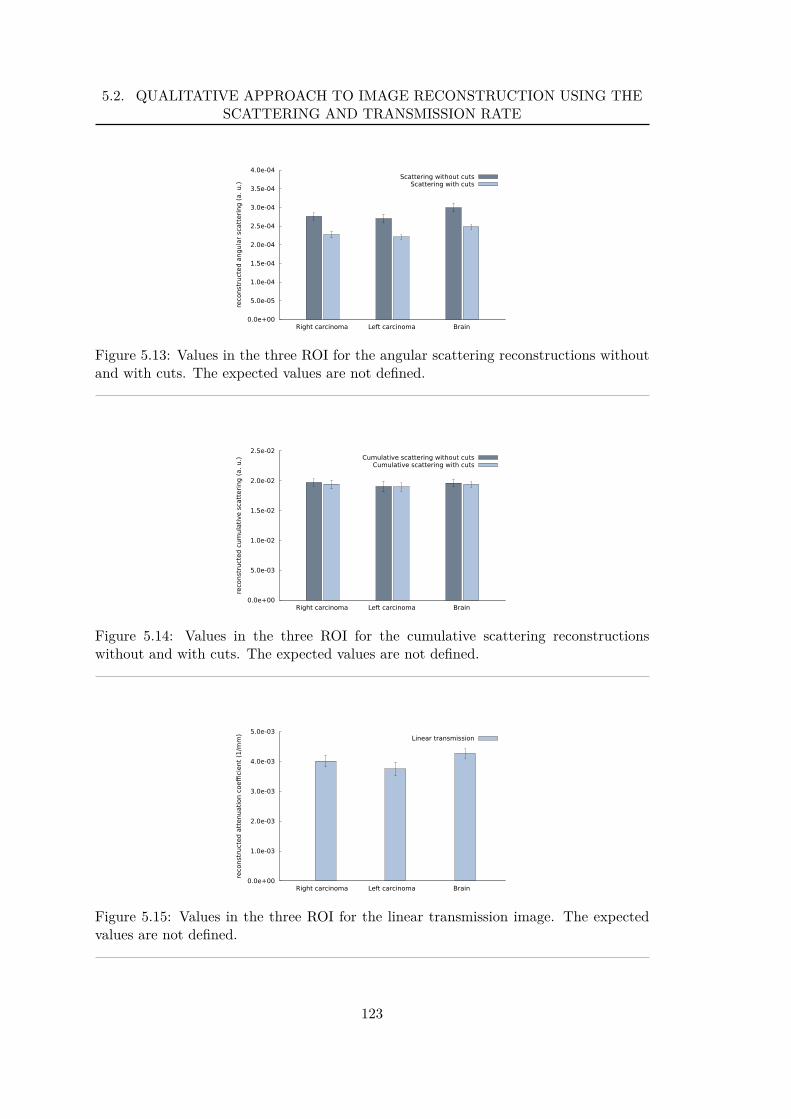
5.2. QUALITATIVE APPROACH TO IMAGE RECONSTRUCTION USING THESCATTERING AND TRANSMISSION RATE
0.0e+00
5.0e-05
1.0e-04
1.5e-04
2.0e-04
2.5e-04
3.0e-04
3.5e-04
4.0e-04
Right carcinoma Left carcinoma Brain
reco
nstr
ucte
d an
gula
r sca
tterin
g (a
. u.)
Scattering without cutsScattering with cuts
Figure 5.13: Values in the three ROI for the angular scattering reconstructions withoutand with cuts. The expected values are not defined.
0.0e+00
5.0e-03
1.0e-02
1.5e-02
2.0e-02
2.5e-02
Right carcinoma Left carcinoma Brain
reco
nstr
ucte
d cu
mul
ativ
e sc
atte
ring
(a. u
.) Cumulative scattering without cutsCumulative scattering with cuts
Figure 5.14: Values in the three ROI for the cumulative scattering reconstructionswithout and with cuts. The expected values are not defined.
0.0e+00
1.0e-03
2.0e-03
3.0e-03
4.0e-03
5.0e-03
Right carcinoma Left carcinoma Brain
reco
nstr
ucte
d at
tenu
atio
n co
effici
ent (
1/m
m) Linear transmission
Figure 5.15: Values in the three ROI for the linear transmission image. The expectedvalues are not defined.
123
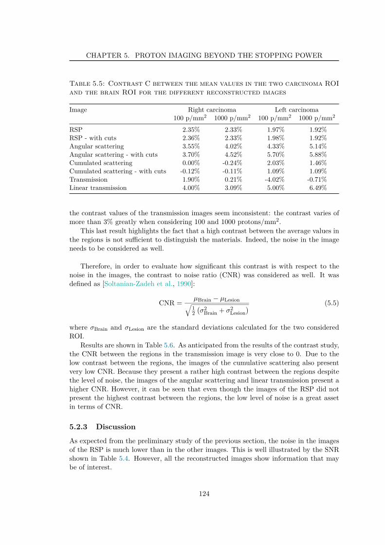
CHAPTER 5. PROTON IMAGING BEYOND THE STOPPING POWER
Table 5.5: Contrast C between the mean values in the two carcinoma ROIand the brain ROI for the different reconstructed images
Image Right carcinoma Left carcinoma100 p/mm2 1000 p/mm2 100 p/mm2 1000 p/mm2
RSP 2.35% 2.33% 1.97% 1.92%RSP - with cuts 2.36% 2.33% 1.98% 1.92%Angular scattering 3.55% 4.02% 4.33% 5.14%Angular scattering - with cuts 3.70% 4.52% 5.70% 5.88%Cumulated scattering 0.00% -0.24% 2.03% 1.46%Cumulated scattering - with cuts -0.12% -0.11% 1.09% 1.09%Transmission 1.90% 0.21% -4.02% -0.71%Linear transmission 4.00% 3.09% 5.00% 6.49%
the contrast values of the transmission images seem inconsistent: the contrast varies ofmore than 3% greatly when considering 100 and 1000 protons/mm2.
This last result highlights the fact that a high contrast between the average values inthe regions is not sufficient to distinguish the materials. Indeed, the noise in the imageneeds to be considered as well.
Therefore, in order to evaluate how significant this contrast is with respect to thenoise in the images, the contrast to noise ratio (CNR) was considered as well. It wasdefined as [Soltanian-Zadeh et al., 1990]:
CNR =µBrain − µLesion
√
12
(
σ2Brain + σ2
Lesion
)
(5.5)
where σBrain and σLesion are the standard deviations calculated for the two consideredROI.
Results are shown in Table 5.6. As anticipated from the results of the contrast study,the CNR between the regions in the transmission image is very close to 0. Due to thelow contrast between the regions, the images of the cumulative scattering also presentvery low CNR. Because they present a rather high contrast between the regions despitethe level of noise, the images of the angular scattering and linear transmission present ahigher CNR. However, it can be seen that even though the images of the RSP did notpresent the highest contrast between the regions, the low level of noise is a great assetin terms of CNR.
5.2.3 Discussion
As expected from the preliminary study of the previous section, the noise in the imagesof the RSP is much lower than in the other images. This is well illustrated by the SNRshown in Table 5.4. However, all the reconstructed images show information that maybe of interest.
124
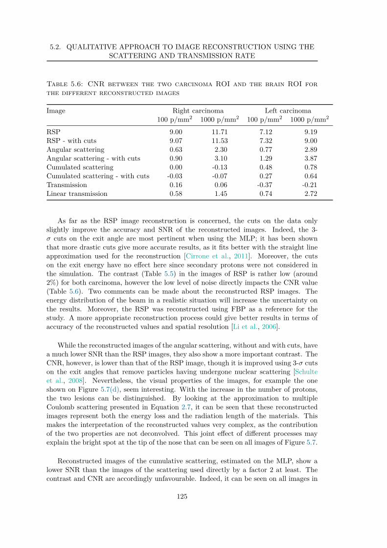
5.2. QUALITATIVE APPROACH TO IMAGE RECONSTRUCTION USING THESCATTERING AND TRANSMISSION RATE
Table 5.6: CNR between the two carcinoma ROI and the brain ROI forthe different reconstructed images
Image Right carcinoma Left carcinoma100 p/mm2 1000 p/mm2 100 p/mm2 1000 p/mm2
RSP 9.00 11.71 7.12 9.19RSP - with cuts 9.07 11.53 7.32 9.00Angular scattering 0.63 2.30 0.77 2.89Angular scattering - with cuts 0.90 3.10 1.29 3.87Cumulated scattering 0.00 -0.13 0.48 0.78Cumulated scattering - with cuts -0.03 -0.07 0.27 0.64Transmission 0.16 0.06 -0.37 -0.21Linear transmission 0.58 1.45 0.74 2.72
As far as the RSP image reconstruction is concerned, the cuts on the data onlyslightly improve the accuracy and SNR of the reconstructed images. Indeed, the 3-σ cuts on the exit angle are most pertinent when using the MLP; it has been shownthat more drastic cuts give more accurate results, as it fits better with the straight lineapproximation used for the reconstruction [Cirrone et al., 2011]. Moreover, the cutson the exit energy have no effect here since secondary protons were not considered inthe simulation. The contrast (Table 5.5) in the images of RSP is rather low (around2%) for both carcinoma, however the low level of noise directly impacts the CNR value(Table 5.6). Two comments can be made about the reconstructed RSP images. Theenergy distribution of the beam in a realistic situation will increase the uncertainty onthe results. Moreover, the RSP was reconstructed using FBP as a reference for thestudy. A more appropriate reconstruction process could give better results in terms ofaccuracy of the reconstructed values and spatial resolution [Li et al., 2006].
While the reconstructed images of the angular scattering, without and with cuts, havea much lower SNR than the RSP images, they also show a more important contrast. TheCNR, however, is lower than that of the RSP image, though it is improved using 3-σ cutson the exit angles that remove particles having undergone nuclear scattering [Schulteet al., 2008]. Nevertheless, the visual properties of the images, for example the oneshown on Figure 5.7(d), seem interesting. With the increase in the number of protons,the two lesions can be distinguished. By looking at the approximation to multipleCoulomb scattering presented in Equation 2.7, it can be seen that these reconstructedimages represent both the energy loss and the radiation length of the materials. Thismakes the interpretation of the reconstructed values very complex, as the contributionof the two properties are not deconvolved. This joint effect of different processes mayexplain the bright spot at the tip of the nose that can be seen on all images of Figure 5.7.
Reconstructed images of the cumulative scattering, estimated on the MLP, show alower SNR than the images of the scattering used directly by a factor 2 at least. Thecontrast and CNR are accordingly unfavourable. Indeed, it can be seen on all images in
125
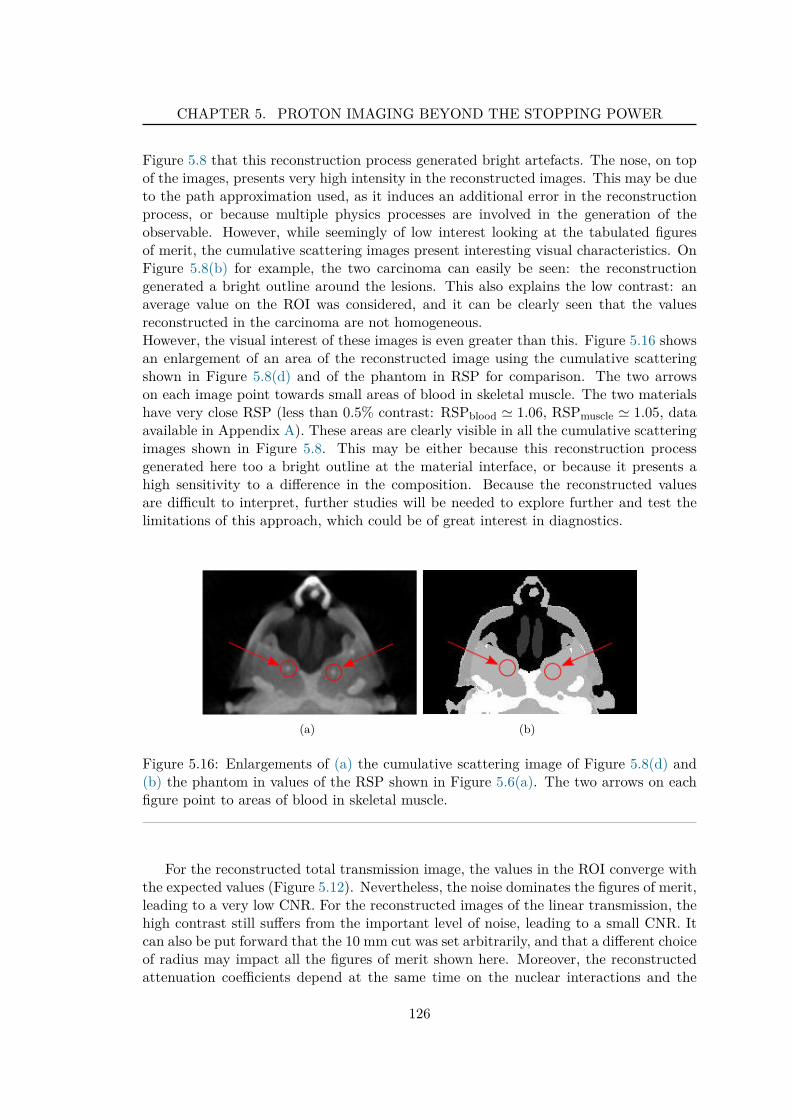
CHAPTER 5. PROTON IMAGING BEYOND THE STOPPING POWER
Figure 5.8 that this reconstruction process generated bright artefacts. The nose, on topof the images, presents very high intensity in the reconstructed images. This may be dueto the path approximation used, as it induces an additional error in the reconstructionprocess, or because multiple physics processes are involved in the generation of theobservable. However, while seemingly of low interest looking at the tabulated figuresof merit, the cumulative scattering images present interesting visual characteristics. OnFigure 5.8(b) for example, the two carcinoma can easily be seen: the reconstructiongenerated a bright outline around the lesions. This also explains the low contrast: anaverage value on the ROI was considered, and it can be clearly seen that the valuesreconstructed in the carcinoma are not homogeneous.However, the visual interest of these images is even greater than this. Figure 5.16 showsan enlargement of an area of the reconstructed image using the cumulative scatteringshown in Figure 5.8(d) and of the phantom in RSP for comparison. The two arrowson each image point towards small areas of blood in skeletal muscle. The two materialshave very close RSP (less than 0.5% contrast: RSPblood ≃ 1.06, RSPmuscle ≃ 1.05, dataavailable in Appendix A). These areas are clearly visible in all the cumulative scatteringimages shown in Figure 5.8. This may be either because this reconstruction processgenerated here too a bright outline at the material interface, or because it presents ahigh sensitivity to a difference in the composition. Because the reconstructed valuesare difficult to interpret, further studies will be needed to explore further and test thelimitations of this approach, which could be of great interest in diagnostics.
(a) (b)
Figure 5.16: Enlargements of (a) the cumulative scattering image of Figure 5.8(d) and(b) the phantom in values of the RSP shown in Figure 5.6(a). The two arrows on eachfigure point to areas of blood in skeletal muscle.
For the reconstructed total transmission image, the values in the ROI converge withthe expected values (Figure 5.12). Nevertheless, the noise dominates the figures of merit,leading to a very low CNR. For the reconstructed images of the linear transmission, thehigh contrast still suffers from the important level of noise, leading to a small CNR. Itcan also be put forward that the 10 mm cut was set arbitrarily, and that a different choiceof radius may impact all the figures of merit shown here. Moreover, the reconstructedattenuation coefficients depend at the same time on the nuclear interactions and the
126
5.3. QUANTITATIVE APPROACH: A STEP TOWARDS STOICHIOMETRICCOMPOSITION?
scattering – and thus also on the energy loss – which lead to a difficult quantification ofthe reconstructed values. A cut set arbitrarily as a distance may also not be the mostrepresentative in a physical sense; a proportion related to the scattering angle may bemore pertinent.
5.2.4 Conclusion
This study lead to the reconstruction of images of the RSP as well as imagesusing scattering, cumulative scattering and transmission rate. As expected from thepreliminary study on the outputs of a pCT scan detailed in the previous section, thestatistical uncertainty on the observables lead to an important noise in the reconstructedimages. However, increasing the number of particles studied makes it possible to produceimages with interesting visual attributes. The image of the linear transmission, forinstance, shows an important contrast between the bone and soft tissues. Both lesionsinserted in the brain can be distinguished in the images of the scattering. The imagesreconstructed using the cumulative scattering present even more interest in terms ofqualitative information. The bright outline generated makes the lesions clearly visible.In addition, the small inserts of blood in skeletal muscle appear very brightly on thisimage, whereas the low contrast between these two materials in the image of RSP makesit impossible to separate them. This indicates that these images could present an interestin terms of diagnosis.
The fact remains that these images, in particular the scattering and cumulativescattering ones, are representative of the combination of different physical processes.Therefore, interpretation at this level can only be qualitative. The next section willpresent a method to reconstruct images using the information on the scattering andtransmission rate of the particles, for which a physical interpretation of the values isprovided.
5.3 Quantitative approach: a step towards stoichiometriccomposition?
As it was put forward in the previous section, the exploitation of information on thescattering and transmission rate of the protons may present interesting properties.However, no quantitative information on the reconstructed values were extracted. Thissection presents the investigation on a quantitative approach to the use of these data.The aim is to determine how much information on the composition of materials couldbe extracted from reconstructed images.
The reconstruction process using the transmission rate of the particles is very similarto X-ray CT image reconstruction. Therefore, the use of this information is ratherstraightforward, as will be shown in Section 5.3.1. The use of the information on thescattering, however, requires to pose the problem in a different fashion, in order todeconvolve the effect of the energy loss and the scattering. A possible reconstructionapproach is investigated in Section 5.3.2. Finally, the potential use of all the dataacquired to characterize a material is discussed.
127
CHAPTER 5. PROTON IMAGING BEYOND THE STOPPING POWER
5.3.1 Reconstruction using the transmission rate
As mentioned in Section 2.1.3, the attenuation of the proton flux follows a Beer-Lambertlaw (Equation 2.10), re-written here for convenience:
Φ(l) = Φ0 exp(
−∫
lκ (x, y, z, E) dl
)
(5.6)
where κ (x, y, z, E) is the macroscopic inelastic nuclear cross section for protons in thematerials at energy E at each position (x, y, z) and l is depth of material.
This formulation is very similar to the expression of the attenuation of a photonflux, used in X-ray imaging. As put forward in the previous section (Section 5.2.1), it ispossible to reconstruct images of the “attenuation coefficient” in a similar way to X-rayCT (Section 1.2.1.1).
For an element, the macroscopic cross section is defined as:
κ = N · σ (5.7)
with N the atomic density of the target, and σ the microscopic nuclear cross-section.Therefore, it can be re-written as:
κ = ρ
(NA
A
)
· σ (5.8)
with ρ the target volumetric mass density, NA the Avogadro number and A the targetatomic number.
For a material constituted of i elements of mass proportions wi, this can begeneralized as:
κ = ρNA
∑
i
wi1Ai
σi (5.9)
The behaviour of κ as a function of the energy is shown on Figure 2.3 for differentelements. It can be seen that for the energies considered in pCT (80-250 MeV), theinelastic nuclear interaction cross-sections of protons in light elements (oxygen andunder) are in a “plateau” region. This is not the case for calcium for example, forwhich the plateau behaviour is found at energies superior to 150 MeV.
As a first approximation, the energy-dependence of the cross-sections is neglected.As a result, a bias can be expected in the regions of materials that have a significantproportion of elements heavier than oxygen such as bone. However, this makes it possibleto use a straightforward reconstruction algorithm. Indeed, images reconstructed this wayare shown in the previous section, on Figures 5.9(a) and 5.9(b).
Therefore, each voxel of the transmission images reconstructed in the previous sectionrepresents the total macroscopic inelastic nuclear cross-section of the material. Moreover,the interaction cross sections σi (Equation 5.9) can be measured experimentally andtabulated. Thanks to this, and in light of Equation 5.9, information on the compositionof a material (i.e. its density and the mass proportion of each element) can be extracted.
128
5.3. QUANTITATIVE APPROACH: A STEP TOWARDS STOICHIOMETRICCOMPOSITION?
5.3.2 Reconstruction using the scattering
Many approximations to multiple Coulomb scattering exist, amongst which the oneused for the most likely path computation for example. Gottschalk [2009] reviewedthese approximations of the scattering power used in proton transport calculations. Thescattering power T is a differential description of the Gaussian approximation to multiplescattering, with:
T ≡ d⟨
θ2⟩
dx(5.10)
where⟨
θ2⟩
represents the variance of the projected angular distribution (previouslydenoted σ2 in Equation 2.7). The advantage of such a differential formulation is that ittakes a similar form to that of the stopping power S ≡ −dE
dx , or more generally, to theformulation of the line integrals. As a consequence, the problem becomes particularlywell-adapted to image reconstruction. However, an accurate formula for T must takeinto account the “history” of the protons, i.e. the competition between the Gaussiancore and the single scattering tail of the distributions that will affect the rate of changeof the Gaussian width. Thus, T should be non-local: it should not depend only on thelocal variables such as the mean proton energy, atomic properties and stopping power.
Different functions for T have been proposed, that recover more or less the Molierescattering angle if integrated over x for any slab [Gottschalk, 2009]. In the paper,Gottschalk reviews three local formulas:
– TF R: Fermi-Rossi approximation ,
– TIC : based on ICRU report 35,
– TLD: based on the Linear displacement ,
and two non-local formulas
– TØS : Øversas and Schneider ,
– TdH : differential Highland.
A new approximation is also proposed by Gottschalk [2009], named differential Moliere(TdM ). Details of the approximations are given in Appendix B.
5.3.2.1 Reconstruction principle
The variance of the exit scattering angle of an initially parallel beam, after a slab ofmaterial of thickness x can be written as:
θ2proj ≃
∫ x
0T(
x′) dx′ (5.11)
All formulas listed previously except the Øversas and Schneider approximation canbe re-written as T = f(E) 1
X with X the radiation length (X0), or the scattering length(XS), and f(E) a function of the energy of the protons. This makes it possible to isolatethe 1
X term. The energy-dependent term f(E) can be evaluated for each depth in theobject by making use of the image of the RSP. As the term X0 is present many times
129
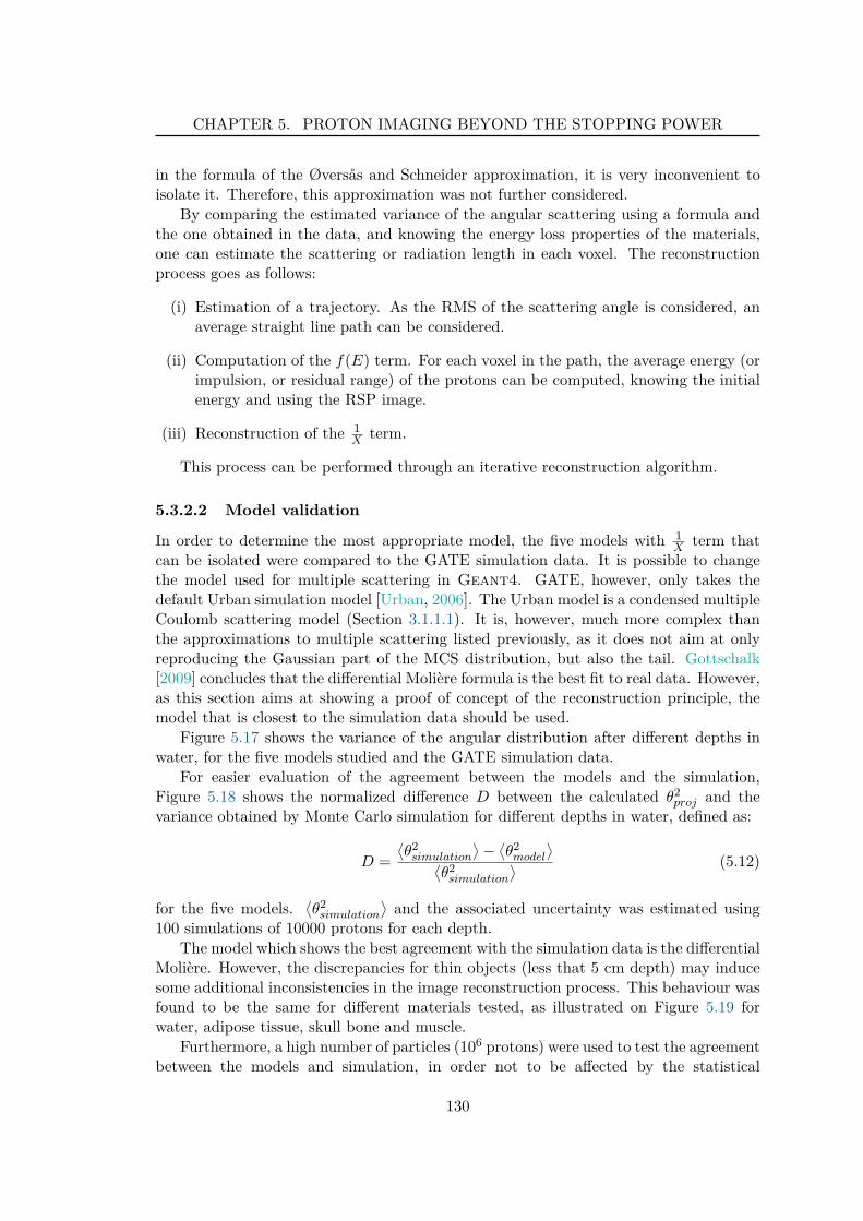
CHAPTER 5. PROTON IMAGING BEYOND THE STOPPING POWER
in the formula of the Øversas and Schneider approximation, it is very inconvenient toisolate it. Therefore, this approximation was not further considered.
By comparing the estimated variance of the angular scattering using a formula andthe one obtained in the data, and knowing the energy loss properties of the materials,one can estimate the scattering or radiation length in each voxel. The reconstructionprocess goes as follows:
(i) Estimation of a trajectory. As the RMS of the scattering angle is considered, anaverage straight line path can be considered.
(ii) Computation of the f(E) term. For each voxel in the path, the average energy (orimpulsion, or residual range) of the protons can be computed, knowing the initialenergy and using the RSP image.
(iii) Reconstruction of the 1X term.
This process can be performed through an iterative reconstruction algorithm.
5.3.2.2 Model validation
In order to determine the most appropriate model, the five models with 1X term that
can be isolated were compared to the GATE simulation data. It is possible to changethe model used for multiple scattering in Geant4. GATE, however, only takes thedefault Urban simulation model [Urban, 2006]. The Urban model is a condensed multipleCoulomb scattering model (Section 3.1.1.1). It is, however, much more complex thanthe approximations to multiple scattering listed previously, as it does not aim at onlyreproducing the Gaussian part of the MCS distribution, but also the tail. Gottschalk[2009] concludes that the differential Moliere formula is the best fit to real data. However,as this section aims at showing a proof of concept of the reconstruction principle, themodel that is closest to the simulation data should be used.
Figure 5.17 shows the variance of the angular distribution after different depths inwater, for the five models studied and the GATE simulation data.
For easier evaluation of the agreement between the models and the simulation,Figure 5.18 shows the normalized difference D between the calculated θ2
proj and thevariance obtained by Monte Carlo simulation for different depths in water, defined as:
D =⟨
θ2simulation
⟩− ⟨
θ2model
⟩
⟨
θ2simulation
⟩ (5.12)
for the five models.⟨
θ2simulation
⟩
and the associated uncertainty was estimated using100 simulations of 10000 protons for each depth.
The model which shows the best agreement with the simulation data is the differentialMoliere. However, the discrepancies for thin objects (less that 5 cm depth) may inducesome additional inconsistencies in the image reconstruction process. This behaviour wasfound to be the same for different materials tested, as illustrated on Figure 5.19 forwater, adipose tissue, skull bone and muscle.
Furthermore, a high number of particles (106 protons) were used to test the agreementbetween the models and simulation, in order not to be affected by the statistical
130
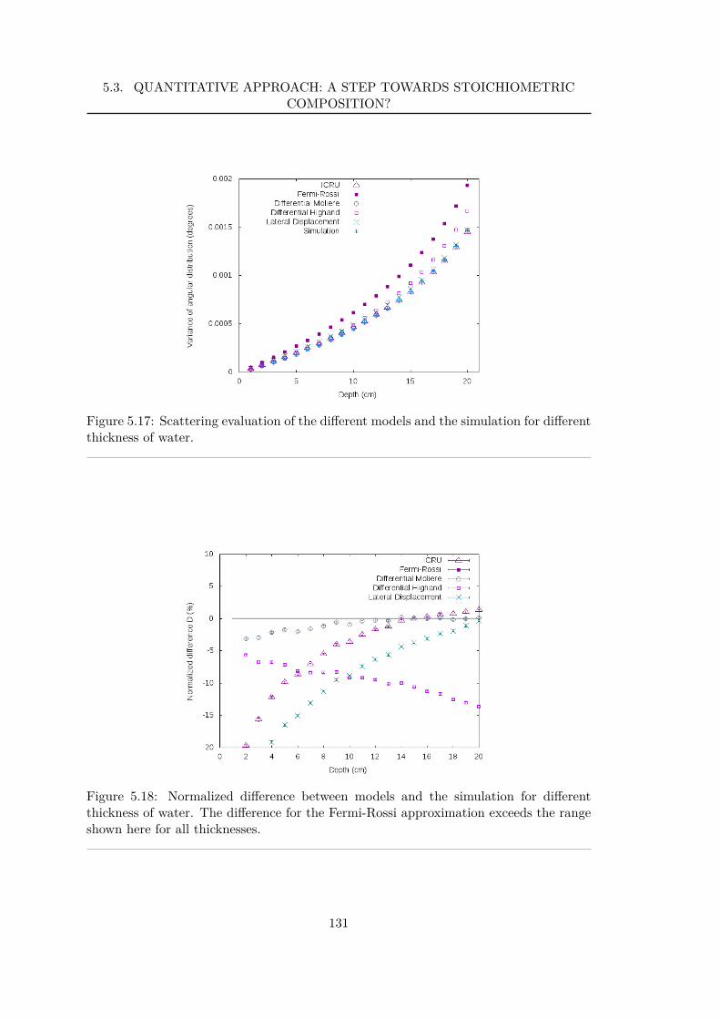
5.3. QUANTITATIVE APPROACH: A STEP TOWARDS STOICHIOMETRICCOMPOSITION?
Figure 5.17: Scattering evaluation of the different models and the simulation for differentthickness of water.
Figure 5.18: Normalized difference between models and the simulation for differentthickness of water. The difference for the Fermi-Rossi approximation exceeds the rangeshown here for all thicknesses.
131
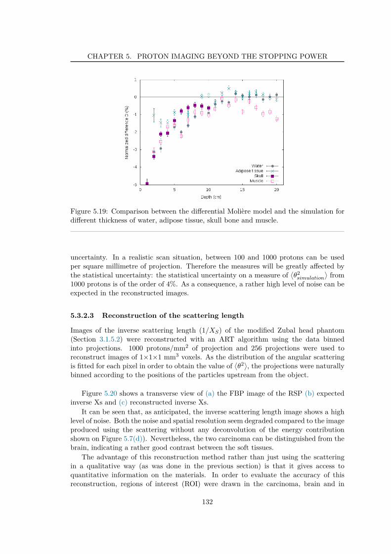
CHAPTER 5. PROTON IMAGING BEYOND THE STOPPING POWER
Figure 5.19: Comparison between the differential Moliere model and the simulation fordifferent thickness of water, adipose tissue, skull bone and muscle.
uncertainty. In a realistic scan situation, between 100 and 1000 protons can be usedper square millimetre of projection. Therefore the measures will be greatly affected bythe statistical uncertainty: the statistical uncertainty on a measure of
⟨
θ2simulation
⟩
from1000 protons is of the order of 4%. As a consequence, a rather high level of noise can beexpected in the reconstructed images.
5.3.2.3 Reconstruction of the scattering length
Images of the inverse scattering length (1/XS) of the modified Zubal head phantom(Section 3.1.5.2) were reconstructed with an ART algorithm using the data binnedinto projections. 1000 protons/mm2 of projection and 256 projections were used toreconstruct images of 1×1×1 mm3 voxels. As the distribution of the angular scatteringis fitted for each pixel in order to obtain the value of
⟨
θ2⟩
, the projections were naturallybinned according to the positions of the particles upstream from the object.
Figure 5.20 shows a transverse view of (a) the FBP image of the RSP (b) expectedinverse Xs and (c) reconstructed inverse Xs.
It can be seen that, as anticipated, the inverse scattering length image shows a highlevel of noise. Both the noise and spatial resolution seem degraded compared to the imageproduced using the scattering without any deconvolution of the energy contributionshown on Figure 5.7(d)). Nevertheless, the two carcinoma can be distinguished from thebrain, indicating a rather good contrast between the soft tissues.
The advantage of this reconstruction method rather than just using the scatteringin a qualitative way (as was done in the previous section) is that it gives access toquantitative information on the materials. In order to evaluate the accuracy of thisreconstruction, regions of interest (ROI) were drawn in the carcinoma, brain and in
132
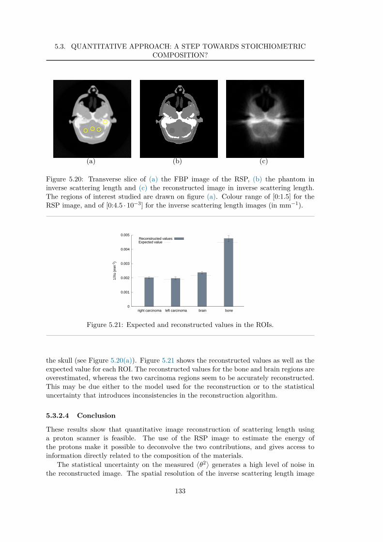
5.3. QUANTITATIVE APPROACH: A STEP TOWARDS STOICHIOMETRICCOMPOSITION?
(a) (b) (c)
Figure 5.20: Transverse slice of (a) the FBP image of the RSP, (b) the phantom ininverse scattering length and (c) the reconstructed image in inverse scattering length.The regions of interest studied are drawn on figure (a). Colour range of [0:1.5] for theRSP image, and of [0:4.5 · 10−3] for the inverse scattering length images (in mm−1).
0
0.001
0.002
0.003
0.004
0.005
right carcinoma left carcinoma brain bone
1/X
s (
mm
-1)
Expected valueReconstructed values
Figure 5.21: Expected and reconstructed values in the ROIs.
the skull (see Figure 5.20(a)). Figure 5.21 shows the reconstructed values as well as theexpected value for each ROI. The reconstructed values for the bone and brain regions areoverestimated, whereas the two carcinoma regions seem to be accurately reconstructed.This may be due either to the model used for the reconstruction or to the statisticaluncertainty that introduces inconsistencies in the reconstruction algorithm.
5.3.2.4 Conclusion
These results show that quantitative image reconstruction of scattering length usinga proton scanner is feasible. The use of the RSP image to estimate the energy ofthe protons make it possible to deconvolve the two contributions, and gives access toinformation directly related to the composition of the materials.
The statistical uncertainty on the measured⟨
θ2⟩
generates a high level of noise inthe reconstructed image. The spatial resolution of the inverse scattering length image
133
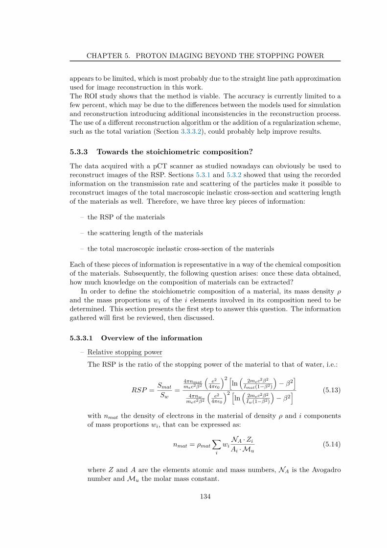
CHAPTER 5. PROTON IMAGING BEYOND THE STOPPING POWER
appears to be limited, which is most probably due to the straight line path approximationused for image reconstruction in this work.The ROI study shows that the method is viable. The accuracy is currently limited to afew percent, which may be due to the differences between the models used for simulationand reconstruction introducing additional inconsistencies in the reconstruction process.The use of a different reconstruction algorithm or the addition of a regularization scheme,such as the total variation (Section 3.3.3.2), could probably help improve results.
5.3.3 Towards the stoichiometric composition?
The data acquired with a pCT scanner as studied nowadays can obviously be used toreconstruct images of the RSP. Sections 5.3.1 and 5.3.2 showed that using the recordedinformation on the transmission rate and scattering of the particles make it possible toreconstruct images of the total macroscopic inelastic cross-section and scattering lengthof the materials as well. Therefore, we have three key pieces of information:
– the RSP of the materials
– the scattering length of the materials
– the total macroscopic inelastic cross-section of the materials
Each of these pieces of information is representative in a way of the chemical compositionof the materials. Subsequently, the following question arises: once these data obtained,how much knowledge on the composition of materials can be extracted?
In order to define the stoichiometric composition of a material, its mass density ρand the mass proportions wi of the i elements involved in its composition need to bedetermined. This section presents the first step to answer this question. The informationgathered will first be reviewed, then discussed.
5.3.3.1 Overview of the information
– Relative stopping power
The RSP is the ratio of the stopping power of the material to that of water, i.e.:
RSP =Smat
Sw=
4πnmat
mec2β2
(
e2
4πǫ0
)2 [
ln(
2mec2β2
Imat(1−β2)
)
− β2]
4πnw
mec2β2
(
e2
4πǫ0
)2 [
ln(
2mec2β2
Iw(1−β2)
)
− β2]
(5.13)
with nmat the density of electrons in the material of density ρ and i componentsof mass proportions wi, that can be expressed as:
nmat = ρmat
∑
i
wiNA · Zi
Ai · Mu(5.14)
where Z and A are the elements atomic and mass numbers, NA is the Avogadronumber and Mu the molar mass constant.
134
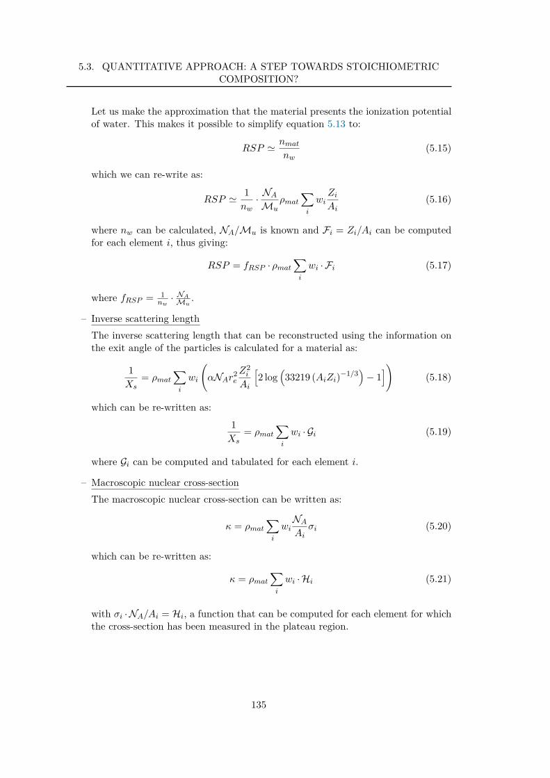
5.3. QUANTITATIVE APPROACH: A STEP TOWARDS STOICHIOMETRICCOMPOSITION?
Let us make the approximation that the material presents the ionization potentialof water. This makes it possible to simplify equation 5.13 to:
RSP ≃ nmat
nw(5.15)
which we can re-write as:
RSP ≃ 1nw
· NA
Muρmat
∑
i
wiZi
Ai(5.16)
where nw can be calculated, NA/Mu is known and Fi = Zi/Ai can be computedfor each element i, thus giving:
RSP = fRSP · ρmat
∑
i
wi · Fi (5.17)
where fRSP = 1nw
· NA
Mu.
– Inverse scattering length
The inverse scattering length that can be reconstructed using the information onthe exit angle of the particles is calculated for a material as:
1Xs
= ρmat
∑
i
wi
(
αNAr2e
Z2i
Ai
[
2 log(
33219 (AiZi)−1/3
)
− 1]
)
(5.18)
which can be re-written as:
1Xs
= ρmat
∑
i
wi · Gi (5.19)
where Gi can be computed and tabulated for each element i.
– Macroscopic nuclear cross-section
The macroscopic nuclear cross-section can be written as:
κ = ρmat
∑
i
wiNA
Aiσi (5.20)
which can be re-written as:
κ = ρmat
∑
i
wi · Hi (5.21)
with σi · NA/Ai = Hi, a function that can be computed for each element for whichthe cross-section has been measured in the plateau region.
135
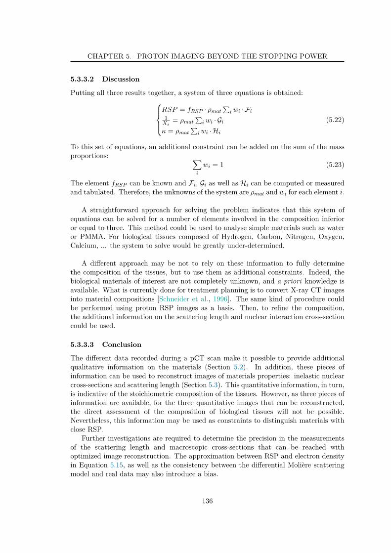
CHAPTER 5. PROTON IMAGING BEYOND THE STOPPING POWER
5.3.3.2 Discussion
Putting all three results together, a system of three equations is obtained:
RSP = fRSP · ρmat∑
i wi · Fi
1Xs
= ρmat∑
i wi · Gi
κ = ρmat∑
i wi · Hi
(5.22)
To this set of equations, an additional constraint can be added on the sum of the massproportions:
∑
i
wi = 1 (5.23)
The element fRSP can be known and Fi, Gi as well as Hi can be computed or measuredand tabulated. Therefore, the unknowns of the system are ρmat and wi for each element i.
A straightforward approach for solving the problem indicates that this system ofequations can be solved for a number of elements involved in the composition inferioror equal to three. This method could be used to analyse simple materials such as wateror PMMA. For biological tissues composed of Hydrogen, Carbon, Nitrogen, Oxygen,Calcium, ... the system to solve would be greatly under-determined.
A different approach may be not to rely on these information to fully determinethe composition of the tissues, but to use them as additional constraints. Indeed, thebiological materials of interest are not completely unknown, and a priori knowledge isavailable. What is currently done for treatment planning is to convert X-ray CT imagesinto material compositions [Schneider et al., 1996]. The same kind of procedure couldbe performed using proton RSP images as a basis. Then, to refine the composition,the additional information on the scattering length and nuclear interaction cross-sectioncould be used.
5.3.3.3 Conclusion
The different data recorded during a pCT scan make it possible to provide additionalqualitative information on the materials (Section 5.2). In addition, these pieces ofinformation can be used to reconstruct images of materials properties: inelastic nuclearcross-sections and scattering length (Section 5.3). This quantitative information, in turn,is indicative of the stoichiometric composition of the tissues. However, as three pieces ofinformation are available, for the three quantitative images that can be reconstructed,the direct assessment of the composition of biological tissues will not be possible.Nevertheless, this information may be used as constraints to distinguish materials withclose RSP.
Further investigations are required to determine the precision in the measurementsof the scattering length and macroscopic cross-sections that can be reached withoptimized image reconstruction. The approximation between RSP and electron densityin Equation 5.15, as well as the consistency between the differential Moliere scatteringmodel and real data may also introduce a bias.
136
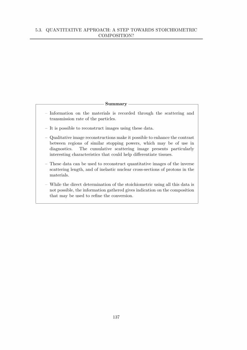
5.3. QUANTITATIVE APPROACH: A STEP TOWARDS STOICHIOMETRICCOMPOSITION?
– Information on the materials is recorded through the scattering andtransmission rate of the particles.
– It is possible to reconstruct images using these data.
– Qualitative image reconstructions make it possible to enhance the contrastbetween regions of similar stopping powers, which may be of use indiagnostics. The cumulative scattering image presents particularlyinteresting characteristics that could help differentiate tissues.
– These data can be used to reconstruct quantitative images of the inversescattering length, and of inelastic nuclear cross-sections of protons in thematerials.
– While the direct determination of the stoichiometric using all this data isnot possible, the information gathered gives indication on the compositionthat may be used to refine the conversion.
Summary
137

CHAPTER 5. PROTON IMAGING BEYOND THE STOPPING POWER
138
Conclusions and perspectives
The principle of proton imaging as studied nowadays is to use the information on theenergy loss of protons to map the stopping powers of the materials. To be of interestin treatment planning, there is need for a resolution on the relative stopping powerless than 1%. The main challenge of proton imaging is to reach satisfactory (≤ 1 mm)spatial resolution. Indeed, as protons scatter in the materials, the individual path ofeach particle needs to be estimated during the image reconstruction process. Up to now,the most accurate path estimation available consists in computing the most likely path(MLP) of the particle assuming the object has the scattering and energy loss propertiesof water. This computation is based on the positions and directions of the particlesupstream and downstream of the object. Therefore, the most common design of protonscanner consists in (i) a tracking system made of two sets of (at least) two tracker planesand (ii) a calorimeter or range-meter.
This setup gives access to data on the transmission rate and on the scattering of theparticles, that are not currently exploited as sources of information on the materials.The main objective of this thesis work was to investigate the potential use of all theinformation gathered during a proton scan, and to determine whether or not moreinformation on tissue composition could be acquired.
In order to study such a proton imaging system, a Monte Carlo simulation platformusing GATE as well as a dedicated image reconstruction platform were set up.
A preliminary one-dimensional study, presented in Section 5.1, has shown that thereis information in the scattering and transmission rate of the protons. Moreover, theresults indicate that this information can help distinguish materials with close stoppingpowers. This work allowed to point out that the major drawback to the use of thesedata is the statistical uncertainty on the measurements of the scattering and transmissionrate, which is much higher than that on the measured energy (or residual range). Inorder to consider a higher statistic in a region of the phantom, tomographic acquisitionsof a proton scanner were simulated.
The qualitative reconstruction study presented in Section 5.2 showed that the use of“extra” information can indeed improve the contrast in some regions of close stoppingpower. The different images, reconstructed by making use of the scattering, cumulativescattering, transmission rate and linear transmission rate of the particles, make it
139
CONCLUSIONS AND PERSPECTIVES
possible to highlight some differences in the composition of tissues. The distinctivecharacteristics of the reconstructed images, in particular the bright outlines at tissueinterfaces in the cumulative scattering image, could bring information of use in termsof diagnostics. While the use of proton imaging as a diagnostic tool is not currently amajor research axis, these results could be an incentive to reconsider.
However, the images which present the most interesting visual properties in termsof contrast and detectability of the lesions are also the most difficult to interpret in aquantitative manner, as they are the result of a combination of physical processes. Toreach a quantification of the values reconstructed in the image, the physical processesinvolved were more closely examined in Section 5.3:
– The transmission rate of the particles in a medium is representative of theinelastic nuclear interactions, which depend on the energy of the protons. Theapproximation that the inelastic nuclear cross-sections of interaction betweenprotons and tissues are in the plateau region is reasonable at the energies consideredin proton imaging. Therefore, a reconstruction of the “attenuation coefficient”, ina similar fashion to X-ray tomography, was performed, giving access to a map ofthe total macroscopic inelastic nuclear cross sections.
– The scattering of charged particles in a medium depends on the scatteringproperties of the medium and on the energy of the particles. As a result, theinformation on the scattering of the protons, gathered at the exit of the objectthat is imaged, is the result of these two properties. To isolate the effect ofthe scattering properties of the materials, an estimation of the energy loss of theparticles is therefore mandatory. This information can be obtained by making useof the reconstructed image of the relative stopping powers. This makes it possibleto reconstruct a map of the scattering properties of the materials, represented hereby the scattering length.
The results presented in this work constitute a proof of concept that quantitativeimaging using the transmission rate and scattering of the protons is possible. In thecontext of particle beam therapy treatment planning, two possible applications can beforeseen: the first is to directly makes use of these images to include the scatteringand nuclear interactions of the beam in analytical treatment plans; the second optionis to extract information on the stoichiometric composition of the tissues from thereconstructed images. The results obtained in the last section of this thesis indicate thatthe gathered information is not sufficient to determine directly the composition of thematerials. Nevertheless, the additional pieces of information could be used as constraints,refining the conversion from relative stopping power to stoichiometric composition thatwould be used for Monte Carlo treatment planning.
The limitations of these two approaches in order to enable more accurate treatmentplanning will depend on the accuracy of the reconstructed images. Several perspectivesto optimize the reconstruction processes can be considered, and are detailed for bothtransmission and scattering imaging in the following two pages.
140
Transmission imaging
Though the reconstruction using the transmission rate of the particles is quitestraightforward, the accuracy is limited by the statistical uncertainty on the measuredrate and by the scattering of the protons. Different solutions towards improvedtransmission images can be considered:
– Increasing the number of protons studied to more than 1000 protons per squaremillimetre of projection will not be considered because it would result in a dosehigher than that of an X-ray CT scan. However, it may be that increasing thenumber of particles per projection and decreasing the number of projections couldreduce the noise in the image. A compromise between the statistical uncertainty(and therefore noise in the projections) and the effect of fewer projections in termsof image reconstruction may need to be found. Such optimization work can befound in the literature for X-ray CT imaging for example.
– In this work, the image reconstructions of the total macroscopic nuclear crosssections were performed using FBP with the data binned upstream of the object.However, it may be considered that even the protons that were stopped in theobject underwent some scattering. While no event-by-event reconstruction canbe performed, a projection/back-projection path in the reconstruction algorithmthat would take the scattering into account could be considered. Instead ofconsidering a straight line, one could consider a probability of passage of the“beam” defined by the impinging particles from the same projection beam, thatwould be spread laterally along the propagation according to the scattering. Asa first approximation, the medium could be considered to have the scatteringproperties of water for example. Then, the image reconstruction of the scatteringlength may also be used to estimate the spread of the particle beam with itspropagation.
– The constant interaction cross-section assumption, justified by the plateau inthe cross-section values as a function of the energy, is a good approximation formost elements at the energies considered in proton imaging. However, it is lessappropriate for heavier elements, such as Calcium, present mostly in the bones.To refine this approximation, a more complex image reconstruction procedurecould be considered. The areas of bone can be segmented, from an image ofthe relative stopping power for example, and the quantity of “heavier” elementscan be estimated. The image of the relative stopping power could then be used tocompute the average energy of the particles considered and an energy-dependentcorrection could be applied.
– Post-processing techniques could be of use to reduce the level of noise in the imageand gather more representative values.
141
CONCLUSIONS AND PERSPECTIVES
Scattering imaging
The reconstructed images of the inverse scattering length of the materials also suffer fromthe statistical uncertainty and scattering of the particles (the reconstructions assuminga straight line path). The following axes for improvement of the reconstructed imagescan be put forward:
– Considering the statistical uncertainty on the variance of the measured angulardistribution, a re-arrangement of the number of particles per projections andnumber of projections might reduce this effect.
– Event-by-event path estimation and image reconstruction is possible when con-sidering scattering imaging. Following a reconstruction approach that takes intoaccount the MLP could be advantageous in terms of spatial resolution, as it doesin the case of image reconstruction of the relative stopping power.In a totally different application, event-by-event reconstruction of the informationon scattering is performed in the context of muon imaging. Muon imaging isconsidered in applications aiming at detecting materials with high atomic numbers:for homeland security, to detect uranium in containers or to image nuclear reactors[Perry, 2013]. A muon imaging device consists in two sets of multiple tracker planeson two sides of the object. Through the information on the scattering of cosmicmuons, images of the “scattering density” of materials (proportional to the inverseof the radiation length for a nominal muon energy) are reconstructed. Schultzet al. [2007] have shown that a maximum likelihood-based image reconstructionalgorithm could be used on this data. The difference of energy between theimpinging muons is taken into account by the ratio of the nominal muon energy tothe effective muon energy, estimated using the scattering of the particle inside atracking plane. As the stopping power of cosmic muons in materials is at least tentimes less than that of protons (for an average energy of cosmic muons of 4 GeVat the surface of the Earth), the energy loss inside the materials can be neglectedin the case of muon imaging. This can not be the case for proton imaging.However, the methodology proposed in the last chapter makes it possible toovercome this problem by estimating the energy of the particles by usingthe relative stopping power. Therefore, a maximum likelihood - expectationmaximization type algorithm for event-by-event reconstruction of the scatteringlength on the MLP could be considered.
While the image reconstructions of the different physical processes were performedin a separate way, a paragon of image reconstruction algorithm for proton tomographywould be multi-parametric, in order to make use of all the information at the same time.A statistical algorithm which aim would be to maximize the likelihood of detecting agiven set of:
water equivalent path length, transmission rate, scattering
for each particle or group of particles can be foreseen as a good candidate.
142
It can be highlighted that such perspectives are not unique to proton imaging andthe same studies could be performed for carbon imaging for example. In a really similarfashion to proton imaging, carbon imaging makes it possible to reconstruct the relativestopping power of carbon ions in the tissues by using the information on the energy lossof carbon ions. The scattering of carbon ions in matter is less important than that ofprotons. This is a definite advantage in terms of simplicity for path approximation inreconstruction of the relative scattering power. However, it may be possible to record thescattering of the particles anyway and investigate the potential of using this informationas well as the information on the transmission rate of carbon ions.
The work described in this thesis was performed on the basis of Monte Carlosimulations. Therefore, in addition to the optimization of the reconstruction processusing the different information, validation on experimental data is necessary beforedrawing a conclusion on the practical potential of this approach.
In clinical conditions, two additional factors need to be considered: the beamcharacteristics and the detector characteristics. The beam properties in terms of energyspread and spatial and angular distribution will have an impact on the results. Initialspread of the beam energy will mostly impact the reconstructed image of the relativestopping power, which was not the main focus of this work. The spatial and angularspread of the beam however, will impact the accuracy of the path approximation inthe reconstruction algorithm when using the data binned into projections, as was donein this work for the scattering and transmission rate images. An event-by-event imagereconstruction, at least for the scattering of the protons, may reduce this impact.The characteristics of the tracking system will play an essential role in the potentialfor imaging using the transmission rate and scattering of the particles. As far as thetransmission imaging is concerned, the detection efficiency of the tracking system will beessential, inasmuch as an additional uncertainty can be expected if not all the protonsare detected.The effect of the tracking system properties, i.e. spatial resolution, material budget andpositioning, on the trajectory estimation using the MLP was evaluated in section 4.3.This study presents the analytical propagation of the uncertainty due to the trackingsystem in the MLP. However, as this uncertainty concerns the estimation of the positionsand directions of the protons, the tracking system will have a great impact on thescattering imaging as well. Should enough interest in the scattering imaging be foundto impact the choice of detector, tracker planes with a pixel pitch less than that of thecurrent prototypes might be preferred.
The requirements of a proton system in terms of particle rate to detect is alsorepresentative of the instrumental challenges of a proton tomography system. Whileit does not impact the quality of the reconstructed images, it is of key importance beforea proton tomograph can be set up and used in clinical routine. The prototype withthe fastest acquisition rate currently reaches a rate of 2 MHz (Section 2.3.2.1). Therequirements sheet for a proton tomograph put forward by Schulte et al. [2004] (Table2.1) indicates the aim of a scan time of 5 minutes. Sadrozinski et al. [2011] indicate thatfor a satisfying resolution on the reconstructed relative stopping power, the ratio between
143
CONCLUSIONS AND PERSPECTIVES
the number of protons used in the image reconstruction process and the number of voxelsin the image should be of 100. This is consistent with all the works in the literature.Considering an average of 20% loss of particles due to nuclear interaction, this resultsin the need for a ratio of 125. Let us now consider the image of a head, of dimensions300×300×200 mm3 with 1×1×1 mm3 voxels. This is slightly smaller than the imagesreconstructed during this work, but would be sufficient for the image of a head. Theresulting acquisition rate is about 7.5 MHz.This requirement needs to be considered along with the accelerator beam structure. Thecyclotron of the proton therapy facility in Orsay is a IBA Proteus 235. The isochronouscyclotron beam is a continuous beam on a macroscopic scale, but consists in 3.2 nsbunches of particles every 9.37 ns [Richard, 2012]. This does not in itself challenge thedetectors in terms of particle rate. The new synchrocyclotron of the proton therapyfacility in Nice is the IBA S2C2, which presents a beam structure of 50 µs-bunches every1 ms [Conjat et al., 2013]. Therefore, to reach an average particle rate of 7.5 MHz, theparticle rate to detect during a bunch is about 150 MHz.The current prototypes are either limited because of the residual energy/range measure-ment [Johnson et al., 2013] or the tracking system [Bucciantonio et al., 2013].
It may be further considered that the average rate of 7.5 MHz corresponds to a beamintensity of 1.2 pA. It can be found in the literature concerning medical cyclotrons thatthe lower limit for stable beam current is of 0.1 nA [Olko and Jezabek, 2012; Denkeret al., 2012]. Indeed, in the context of treatment, intensities of the order of the nAor tens of nA are more of interest. Should an intensity of 0.1 nA be considered forimaging purposes, the required detector rate would be more than 600 MHz (though theacquisition would last less than 4 seconds). Therefore, to reach such a low intensity, thebeam line will need to be adapted, with the insertion of collimators or pepper pots forexample.
Handling such particle rates remains an instrumental challenge nevertheless, and fastplastic scintillator range-meters will probably be preferred to crystal calorimeters in thenext generations of prototypes. In this line of thought, encouraging first results of a newprototype were very recently published by Lo Presti et al. [2014]. The proposed systemis exclusively based in scintillating fibers, for both the tracking system and the residualrange detector, and should be able to handle a particle rate up to 10 MHz.
Proton imaging is a rather exceptional modality, in the sense that each particleundergoes a long series of physical interactions, and each interaction is a source ofinformation on the materials encountered. This generates great challenges, for examplein terms of data management, image reconstruction and analysis, but it also allowsfor a great wealth in terms of information gathered during a scan. In light of theresults presented in this work, the use of the scattering and transmission rate of theparticles to obtain qualitative and hopefully quantitative information could be of interestin diagnostics. The images produced using the cumulative scattering, in particular, makeit possible to distinguish the interfaces between the tissues, here the lesions in the brain,in a very distinctive way.In the context of particle beam therapy, two applications of proton imaging have beenput forward. One is portal imaging, to verify patient positioning with radiography oruse the proton beam as a range probe, to validate the treatment planning just before the
144
irradiation. The other is the use of proton tomography as a basis for treatment planning.For analytical treatment planning, proton computed tomography for imaging the relativestopping power of the materials will help reduce the range uncertainty. In addition, thequantitative information obtained through the reconstructed images using the scatteringand the transmission rate could help improve the accuracy in terms of dose deposit of thetreatment plan. However, the space taken by Monte Carlo treatment planning is moreand more important, and the reduction of computation time using graphical processingunits will probably increase this trend. For Monte Carlo treatment planning, the imagesof the relative stopping power will bring an information on one property of the materials,just like X-ray CT imaging. The conversion from this value to stoichiometric compositionwill still be required. Where proton imaging presents an advantage over X-ray imagingis that the relative stopping power is not the only information that can be exploitedfrom a tomographic acquisition. The last section of this thesis (Section 5.3.3) presentsthe first step towards the use of these information to characterize the stoichiometriccomposition of the tissues. While the direct use of these data will not provide enoughknowledge to fully characterize a tissue, the additional constraints provided by theimage reconstructions of the inverse scattering length and macroscopic inelastic nuclearcross-section could very well be used to reduce the uncertainty on the decompositionin elements from the relative stopping power value alone. This, in turn, could helpimprove the accuracy of the conversion to material composition, and therefore of thetreatment plan, both in terms of range and dose deposit predictions. Further work on thistopic should explore the limits of the multi-parametric approach to image reconstructionpresented in this work. The greatest challenge may be to reach a satisfactory accuracy onthe data obtained from the transmission and scattering despite the statistical uncertaintyon the measures. An increase in the number of particles studied by a factor 10 wouldbe welcome in order to do so. Therefore, a full study on the potential improvement oftreatment planning accuracy will be needed before determining if additional instrumentaldevelopments would be worthwhile.
145

CONCLUSIONS AND PERSPECTIVES
146
Appendix A
Materials and properties
The materials used in the Monte Carlo studies were taken from different sources:Woodard and White [1986]; Maughan et al. [1997]; Batin [2008]; Opengate collaboration[n.d.].
Table A.1 (on the next page) shows the compositions and properties of the materialsused. The letters in the last column designates the phantom(s) in which the materialswere used: (F) for the Forbild phantom, (Z) for the Zubal phantom. All materials weretested for the preliminary study on the cube presented in Section 5.1.
147
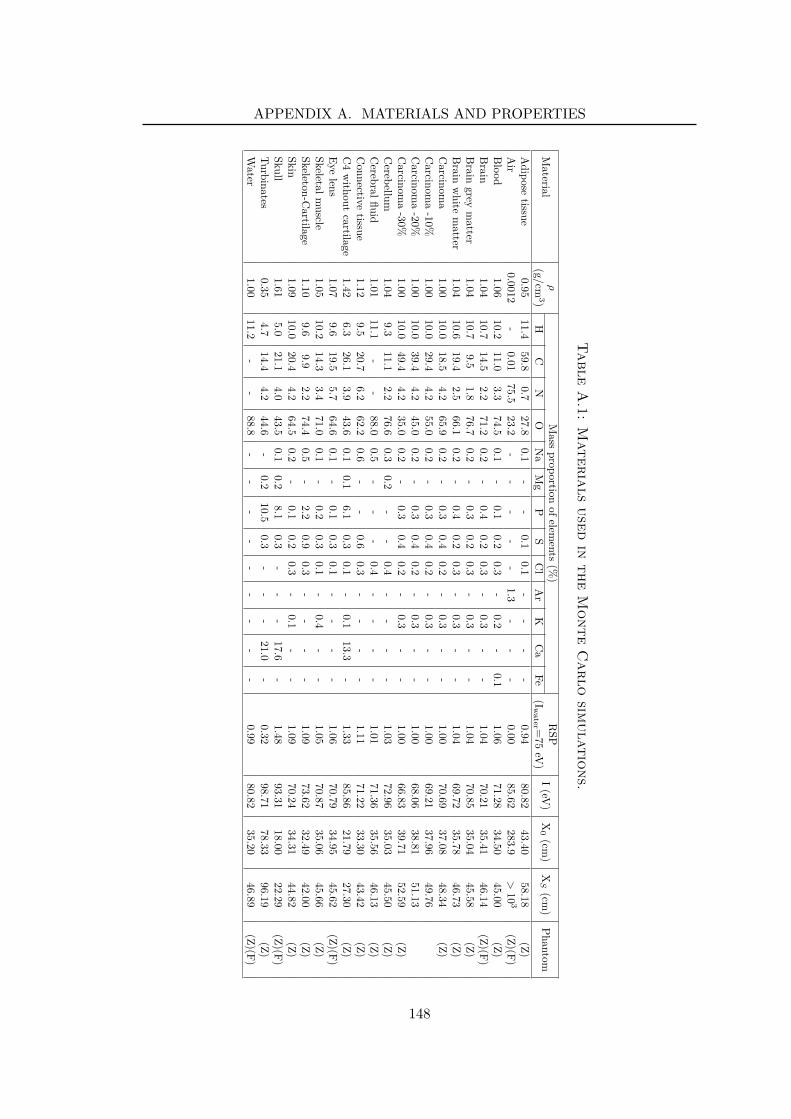
APPENDIX A. MATERIALS AND PROPERTIES
Ta
ble
A.1
:M
at
er
ials
use
din
th
eM
on
te
Ca
rlo
simu
lat
ion
s.
Material
ρM
assproportion
ofelem
ents(%
)R
SPI
(eV)
X0
(cm)
XS
(cm)
Phantom
(g/cm3)
HC
NO
Na
Mg
PS
Cl
Ar
KC
aFe
(Iwater =
75eV
)A
dipose
tissue0.95
11.459.8
0.727.8
0.1-
-0.1
0.1-
--
-0.94
80.8243.40
58.18(Z
)A
ir0.0012
-0.01
75.523.2
--
--
-1.3
--
-0.00
85.62283.9
>10
3(Z
)(F)
Blood
1.0610.2
11.03.3
74.50.1
-0.1
0.20.3
-0.2
-0.1
1.0671.28
34.5045.00
(Z)
Brain
1.0410.7
14.52.2
71.20.2
-0.4
0.20.3
-0.3
--
1.0470.21
35.4146.14
(Z)(F
)B
raingrey
matter
1.0410.7
9.51.8
76.70.2
-0.3
0.20.3
-0.3
--
1.0470.85
35.0445.58
(Z)
Brain
white
matter
1.0410.6
19.42.5
66.10.2
-0.4
0.20.3
-0.3
--
1.0469.72
35.7846.73
(Z)
Carcinom
a1.00
10.018.5
4.265.9
0.2-
0.30.4
0.2-
0.3-
-1.00
70.6937.08
48.34(Z
)C
arcinoma
-10%1.00
10.029.4
4.255.0
0.2-
0.30.4
0.2-
0.3-
-1.00
69.2137.96
49.76C
arcinoma
-20%1.00
10.039.4
4.245.0
0.2-
0.30.4
0.2-
0.3-
-1.00
68.0638.81
51.13C
arcinoma
-30%1.00
10.049.4
4.235.0
0.2-
0.30.4
0.2-
0.3-
-1.00
66.8339.71
52.59(Z
)C
erebellum
1.049.3
11.12.2
76.60.3
0.2-
-0.4
--
--
1.0372.96
35.0345.50
(Z)
Cerebral
fluid1.01
11.1-
-88.0
0.5-
--
0.4-
--
-1.01
71.3635.56
46.13(Z
)C
onnectivetissue
1.129.5
20.76.2
62.20.6
--
0.60.3
--
--
1.1171.22
33.3043.42
(Z)
C4
without
cartilage1.42
6.326.1
3.943.6
0.10.1
6.10.3
0.1-
0.113.3
-1.33
85.8621.79
27.30(Z
)E
yelens
1.079.6
19.55.7
64.60.1
-0.1
0.30.1
--
--
1.0670.79
34.9545.62
(Z)(F
)Skeletal
muscle
1.0510.2
14.33.4
71.00.1
-0.2
0.30.1
-0.4
--
1.0570.87
35.0645.66
(Z)
Skeleton-Cartilage
1.109.6
9.92.2
74.40.5
-2.2
0.90.3
--
--
1.0973.62
32.4942.00
(Z)
Skin1.09
10.020.4
4.264.5
0.2-
0.10.2
0.3-
0.1-
-1.09
70.2434.31
44.82(Z
)Skull
1.615.0
21.14.0
43.50.1
0.28.1
0.3-
--
17.6-
1.4893.31
18.0022.29
(Z)(F
)T
urbinates0.35
4.714.4
4.244.6
-0.2
10.50.3
--
-21.0
-0.32
98.7178.33
96.19(Z
)W
ater1.00
11.2-
-88.8
--
--
--
--
-0.99
80.8235.20
46.89(Z
)(F)
148
Appendix B
Differential approximations tomultiple Coulomb scattering
Brief overview of the scattering approximations found in [Gottschalk, 2009]:
Fermi-Rossi approximation (local)
TF R =(
Es
pv
)2 1X0
(B.1)
with X0 the radiation length of the material (detailed in Section 2.1.2), pv the productof the particles speed and momentum and:
Es =(
2π
α
)1/2
mec2 = 15 MeV (B.2)
ICRU report 35 (local)
TIC =(
Es
pv
)2 1XS
(B.3)
where, at the difference of the previous expression, XS represents the scattering lengthof the material. The scattering length for an element is defined as:
1ρXS
≡ αNAr2e
Z2
A
[
2 log(
33219 (AZ)−1/3)
− 1]
(B.4)
with NA Avogadro’s number and Z, A and ρ the atomic number, weight and density ofthe target material. For compounds or mixtures, a Bragg rule can be applied as for theradiation length, leading to:
1ρXS
=∑
i
wi
(
1ρXS
)
i
(B.5)
149
APPENDIX B. DIFFERENTIAL APPROXIMATIONS TO MULTIPLE COULOMBSCATTERING
Linear displacement (local)
TLD = 10−3 · ρx
Rwater(B.6)
where
ρx =X0material
X0water
(B.7)
and Rwater is the proton’s residual range in water.
Øversas and Schneider (non-local)
TØS =(
19.9 MeVp1v1
)2 1X0
(1 − t)−(1+k)
[
c0 + c1
(
t − 12
)4
+4c1
k
(
t − 12
)3
(1 − t)(
1 − (1 − t)k)
]
(B.8)
with p1v1 the product of the particles initial speed and momentum, c0 and c1 suchas:
c0 = 201200 − 23
5000ρX0 (B.9)
c1 = −112 + 43
1000ρX0 (B.10)
with ρX0 the mass radiation length of the current material and
t (x) ≡ x
R (E1, M (x))(B.11)
where E1 is the particles initial energy and M(x) the current material.
Differential Highland (non-local)
TdH = fdH (l)(
Es
pv
)2 1X0
(B.12)
with the non-local correction factor:
fdH = 0.97(
1 +ln l
20.7
)(
1 +ln l
22.7
)
(B.13)
and using l, defined as the radiative path length:
l (x) ≡∫ x
0
dx′
X0 (x′)(B.14)
150

Differential Moliere (non-local)
TdM = fdM (pv, p1v1)(
Es
pv
)2 1XS
(B.15)
where
fdM ≡ 0.5244 + 0.1975 log
(
1 −(
pv
p1v1
)2)
+ 0.2320 log (pv)
− 0.0098 log (pv) log
(
1 −(
pv
p1v1
)2)
(B.16)
151

APPENDIX B. DIFFERENTIAL APPROXIMATIONS TO MULTIPLE COULOMBSCATTERING
152
BIBLIOGRAPHY
Bibliography
Abdoli, M., Dierckx, R. a. J. O. and Zaidi, H. [2012], ‘Metal artifact reduction strategiesfor improved attenuation correction in hybrid PET/CT imaging.’, Medical physics39(6), 3343–60. 29
Agostinelli, S., Allison, J. and Amako, K. [2003], ‘GEANT4 - a simulation toolkit’,Nuclear Instruments and Methods in Physics Research Section A: Accelerators,Spectrometers, Detectors and Associated Equipment 506(3), 250–303. xiii, 57
Albertini, F., Hug, E. B. and Lomax, a. J. [2011], ‘Is it necessary to plan withsafety margins for actively scanned proton therapy?’, Physics in medicine and biology56(14), 4399–413. 29
Alvarez, R. E. and Macovski, a. [1976], ‘Energy-selective reconstructions in X-raycomputerized tomography.’, Physics in medicine and biology 21(5), 733–44. 30
Amaldi, U., Bianchi, A., Chang, Y.-H., Go, A., Hajdas, W., Malakhov, N., Samarati,J., Sauli, F. and Watts, D. [2011], ‘Construction, test and operation of a proton rangeradiography system’, Nuclear Instruments and Methods in Physics Research SectionA: Accelerators, Spectrometers, Detectors and Associated Equipment 629(1), 337–344.xii, 48, 49, 51, 52, 98, 102
Amaldi, U., Hajdas, W., Iliescu, S., Malakhov, N., Samarati, J., Sauli, F. and Watts, D.[2010], ‘Advanced Quality Assurance for CNAO’, Nuclear Instruments and Methodsin Physics Research Section A: Accelerators, Spectrometers, Detectors and AssociatedEquipment 617(1-3), 248–249. 25
Amaldi, U. and Kraft, G. [2006], ‘Particle accelerators take up the fight against cancer’,CERN Courier 18(1). 2
ARCHADE [n.d.], ‘Advanced ressource centre for hadrontherapy in europe’.URL: archade.fr ix, 2
Aso, T., Kawashima, K., Nishio, T., Lee, S. B. and Sasaki, T. [2012], ‘A study onmultiplex proton imaging using GEANT4’, 2012 IEEE Nuclear Science Symposiumand Medical Imaging Conference Record (NSS/MIC) pp. 1717–1719. 52, 57
153
BIBLIOGRAPHY
Barendsen, G., Walter, H., Fowler, J. F. and Bewley, D. K. [1963], ‘Effects of differentionizing radiations on human cells in tissue culture: III. Experiments with cyclotron-accelerated alpha-particles and deuterons’, Radiation research 19(1), 106–119. 13
Barquero, H. and Brasse, D. [2012], ‘Limited angle geometries applied to small animal X-ray imaging’, 2012 IEEE Nuclear Science Symposium and Medical Imaging ConferenceRecord (NSS/MIC) pp. 3635–3640. 75, 84
Bassler, N., Jakel, O., Sø ndergaard, C. S. and Petersen, J. r. B. [2010], ‘Dose- and LET-painting with particle therapy.’, Acta oncologica (Stockholm, Sweden) 49(7), 1170–6.28
Batin, E. [2008], Influence de la composition chimique des tissus humains sur les depotsde dose en hadrontherapie, PhD thesis. x, 147
Beer, A. [1852], ‘Bestimmung der Absorptioin des rothen Lichts in farbigenGlussigkeiten’, Annalen der Physik und Chemie . 7
Bennett, G., Archambeau, J., Archambeau, B., Meltzer, J. and Wingate, C. [1978],‘Visualization and transport of positron emission from proton activation in vivo’,Science 200(June), 1–3. 24
Berger, J. and Duchazeaubeneix, J. [1978], ‘Nuclear scattering radiography of the spineand sphenoid bone’, Journal of computer assisted tomography 2, 488–498. xi, 42
Besemer, A., Paganetti, H. and Bednarz, B. [2013], ‘The clinical impact of uncertaintiesin the mean excitation energy of human tissues during proton therapy.’, Physics inmedicine and biology 58(4), 887–902. 36
Bethe, H. [1930], ‘Zur theorie des durchgangs schneller korpuskularstrahlen durchmaterie’, Annalen der Physik 397(3), 325–400. 34
Bethe, H. [1953], ‘Moliere’s theory of multiple scattering’, Physical Review 634. 37
Bloch, F. [1933], ‘Zur Bremsung rasch bewegter Teilchen beim Durchgang durchMaterie’, Annalen der Physik 408(3). 34
Bohr, N. [1948], The Penetration of Atomic Particles Through Matter, munksgaard edn,Copenhagen. 36
Bom, V., Joulaeizadeh, L. and Beekman, F. [2012], ‘Real-time prompt γ monitoring inspot-scanning proton therapy using imaging through a knife-edge-shaped slit.’, Physicsin medicine and biology 57(2), 297–308. 25
Brard, E. [2013], La tomographie a emission de positrons a geometrie axiale : del’imagerie de la souris au cerveau humain, PhD thesis. 60
Bravin, A., Coan, P. and Suortti, P. [2013], ‘X-ray phase-contrast imaging: from pre-clinical applications towards clinics.’, Physics in medicine and biology 58(1), R1–35.31
154
Bucciantonio, M., Amaldi, U. and Kieffer, R. [2013], ‘Development of a fast proton rangeradiography system for quality assurance in hadrontherapy’, Nuclear Instruments andmethods A pp. 1–4. 49, 144
Butts, J. J. and Katz, R. [1967], ‘Theory of RBE for heavy ion bombardment of dryenzymes and viruses.’, Radiation research 30(4), 855–71. 9
Carabe, A., Moteabbed, M., Depauw, N., Schuemann, J. and Paganetti, H. [2012],‘Range uncertainty in proton therapy due to variable biological effectiveness.’, Physicsin medicine and biology 57(5), 1159–72. 21
Censor, Y., Elfving, T., Herman, G. and Nikazad, T. [2008], ‘On diagonally relaxedorthogonal projection methods’, SIAM Journal on Scientific Computing pp. 1–40. 75
Charpak, G., Guillerminet, B., Leopold, M., Melchart, G., Odyniec, G., Perrin, Y. andSauli, F. [1979], ‘Progress in Nuclear Scattering Radiography’, IEEE Transactions onNuclear Science 26(1), 654–657. xi, 42
Charpak, G., Majewski, S., Perrin, Y., Saudinos, J., Sauli, F., Towensend, D. andVinciarelli, J. [1976], ‘Further results in nuclear scattering radiography.’, Physics inmedicine and biology 21(6), 941–8. xi, 42
Chen, W., Unkelbach, J., Trofimov, A., Madden, T., Kooy, H., Bortfeld, T. and Craft,D. [2012], ‘Including robustness in multi-criteria optimization for intensity-modulatedproton therapy.’, Physics in medicine and biology 57(3), 591–608. 29
Chvetsov, A. V. and Paige, S. L. [2010], ‘The influence of CT image noise on proton rangecalculation in radiotherapy planning.’, Physics in medicine and biology 55(6), N141–9.x, 21
Cirrone, G., Bucciolini, M., Bruzzi, M., Candiano, G., Civinini, C., Cuttone, G.,Guarino, P., Lo Presti, D., Mazzaglia, S., Pallotta, S., Randazzo, N., Sipala, V.,Stancampiano, C. and Talamonti, C. [2011], ‘Monte Carlo evaluation of the FilteredBack Projection method for image reconstruction in proton computed tomography’,Nuclear Instruments and Methods in Physics Research Section A: Accelerators,Spectrometers, Detectors and Associated Equipment 658(1), 78–83. 51, 84, 125
Cirrone, G., Cuttone, G., Candiano, G., Rosa, F. D., Nigro, S. L., Presti, D. L.,Randazzo, N., Sipala, V., Bruzzi, M., Menichelli, D., Scaringella, M., Bashkirov, V.,DavidWilliams, R., Sadrozinski, H. F.-W., Heimann, J., Feldt, J., Blumenkrantz, N.,Talamonti, C. and Schulte, R. W. [2007], ‘Monte Carlo studies of a proton computedtomography system’, IEEE Transactions on Nuclear Science 54(5), 1487–1491. 57
Civinini, C., B.-M. B. M. B. M. C. M. C. G. a. P. C. G. L. D., Pallotta, S., Pugliatti, C.,Randazzo, N., Romano, F., S.-M., Sipala, V., Stancampiano, C., Talamonti, C., Tesi,M. and Vanzi, E., Z.-M. [2012], ‘Development of a Proton Computed Tomographysystem for pre-clinical tests’, 2012 IEEE Nuclear Science Symposium and MedicalImaging Conference Record (NSS/MIC) pp. 1279–1283. 93
155
BIBLIOGRAPHY
Civinini, C., Bruzzi, M., Bucciolini, M., Carpinelli, M., Cirrone, G., Cuttone, G.,Lo Presti, D., Pallotta, S., Pugliatti, C., Randazzo, N., Romano, F., Scaringella,M., Sipala, V., Stancampiano, C., Talamonti, C., Vanzi, E. and Zani, M. [2013],‘Recent results on the development of a proton computed tomography system’, NuclearInstruments and Methods in Physics Research Section A: Accelerators, Spectrometers,Detectors and Associated Equipment 732, 573–576. xii, 48, 49
Conjat, M., Mandrillon, P. and Mandrillon, J. [2013], ‘The future protontherapy facilityof the Centre Antoine Lacassagne’.URL: https://indico.in2p3.fr/getFile.py/access?sessionId=5&resId=0&materialId=0&confId=8162 xviii, 144
Cookson, J. [1974], ‘Radiography with protons’, Naturwissenschaften 194. 43
Cookson, J. A., Armitage, B. H. and Ferguson, A. T. G. [1972], ‘Proton radiography’,Non-destructive testing (August), 225–228. 39
Cormack, a. M. [1963], ‘Representation of a Function by Its Line Integrals, with SomeRadiological Applications’, Journal of Applied Physics 34(9), 2722. xi, 39
Cormack, a. M. [1964], ‘Representation of a Function by Its Line Integrals, with SomeRadiological Applications. II’, Journal of Applied Physics 35(10), 2908. xi, 39
Cormack, A. M. and Koehler, a. M. [1976], ‘Quantitative proton tomography:preliminary experiments.’, Physics in medicine and biology 21(4), 560–9. xi, 39
Coutrakon, G., Blazey, G., Boi, S., Dychkant, A., Erdelyi, B., Gearhart, A., Hedin, D.,Rykalin, V., Uzunyan, S., Zutshi, V., Krider, J., Sellberg, G., Rauch, J. E., Roman,M., Rubinov, P., Wilson, P. and National, F. [2013], ‘A new proton CT detector’,proceedings AccApp . 52, 102
Crowe, K. M., Budiriger, T. F., Cahoon, J. L., Elischer, V. P., Huesman, R. H.and Kanstein, L. L. [1975], ‘Axial scanning with 900 MeV alpha partivles’, IEEETransactions on Nuclear Science 22(3), 1752–1754. 39
Cuttone, G., Cirrone, G., Candiano, G., Di Rosa, F., Russo, G., Randazzo, N., Sipala,V., Lo Nigro, S., Lo Presti, D., Feldt, J., Heimann, J., Sadrozinski, H.-W., Seiden,A., Williams, D., Bashkirov, V., Schulte, R. W., Bruzzi, M., Menichelli, D. andScaringella, M. [2005], ‘Detailed Monte Carlo Investigation of a Proton ComputedTomography System’, IEEE Nuclear Science Symposium Conference Record, 20055, 2873–2875. 112
Dale, R. G., Jones, B. and Carabe-Fernandez, a. [2009], ‘Why more needs to be knownabout RBE effects in modern radiotherapy.’, Applied radiation and isotopes : includingdata, instrumentation and methods for use in agriculture, industry and medicine67(3), 387–92. 12, 14, 26
Defrise, M., Vanhove, C. and Liu, X. [2011], ‘An algorithm for total variationregularization in high-dimensional linear problems’, Inverse Problems 27(6), 065002.75
156
Denker, A., Bundesmann, J. and Damerow, T. [2012], ‘Status of the HZB cyclotron’,accelconf.web.cern.ch pp. 31–33. 144
Denyak, V., Paschuk, S., Schelin, H. R., Rocha, R., Setti, J., Klock, M., Evseev,I. and Yevseyeva, O. [2011], ‘Dose energy dependence in proton imaging’, NuclearInstruments and Methods in Physics Research Section A: Accelerators, Spectrometers,Detectors and Associated Equipment 652(1), 747–750. 52
Duchazeaubeneix, J., Faivre, J., Garreta, D., Guillerminet, B., Rouger, M., Saudinos,J., Palmieri, C., Raybaud, C., Salamon, G., Charpak, G., Melchart, G., Perrin,Y., Santiard, J. and Sauli, F. [1980], ‘Nuclear Scattering Radiography’, journal ofcomputer assisted tomogrpahy . 42
Dudouet, J., Juliani, D., Labalme, M., Cussol, D., Angelique, J. C., Braunn, B., Colin,J., Finck, C., Fontbonne, J. M., Guerin, H., Henriquet, P., Krimmer, J., Rousseau,M., Saint-Laurent, M. G. and Salvador, S. [2013], ‘Double-differential fragmentationcross-section measurements of 95 MeV/nucleon 12C beams on thin targets for hadrontherapy’, Physical Review C 88(2), 024606. 38
Eekers, D. [2014], ‘The maastricht protontherapy project: Zon-ptc’.URL: bhtc.sckcen.be/∼/media/Files/Bhtc/Documents/Eekers The Maastro Protontherapy Project.pdf 16
Efstathiou, J. a., Gray, P. J. and Zietman, a. L. [2013], ‘Proton beam therapy andlocalised prostate cancer: current status and controversies.’, British journal of cancer108(6), 1225–30. 7, 14, 15
Enghardt, W., C. P. F. F. H. R. P. K. P. J. P. F. [2004a], ‘Charged hadron tumourtherapy monitoring by means of PET’, Nuclear Instruments and Methods in PhysicsResearch Section A: Accelerators, Spectrometers, Detectors and Associated Equipment525(1-2), 284–288. 24
Enghardt, W., P. K. C. P. F. F. P. J. P. F. [2004b], ‘Dose quantification from in-beampositron emission tomography’, Radiotherapy and Oncology 73, S96–98. 24
Erdelyi, B. [2009], ‘A comprehensive study of the most likely path formalism for proton-computed tomography.’, Physics in Medicine and Biology 54(20), 6095–122. 102
Erdelyi, B. [2010], ‘Electron density uncertainties in proton computed tomography.’,Physics in medicine and biology 55(23), 7121–34. xii, 52
Espana, S. and Paganetti, H. [2011], ‘Uncertainties in planned dose due to the limitedvoxel size of the planning CT when treating lung tumors with proton therapy.’, Physicsin medicine and biology 56(13), 3843–56. x, 21
ETOILE [n.d.], ‘Centre ETOILE’.URL: centre-etoile.org ix, 2
Feldkamp, L., Davis, L. and Kress, J. [1984], ‘Practical cone-beam algorithm’, JOSA A1(6), 612–619. 83
157
BIBLIOGRAPHY
Fessler, J. [2009], Analytical tomographic image reconstruction methods, in ‘ImageReconstruction: Algorithms and Analysis’. 66, 67
Fidorra, J. and Linden, W. a. [1977], ‘Radiosensitivity and recovery of mouse L cellsduring the cell cycle.’, Radiation and environmental biophysics 14(4), 285–94. 13
Fokas, E., Kraft, G., An, H. and Engenhart-Cabillic, R. [2009], ‘Ion beam radiobiologyand cancer: time to update ourselves.’, Biochimica et biophysica acta 1796(2), 216–29. 9, 10,11
Fournier, C. and Taucher-Scholz, G. [2004], ‘Radiation induced cell cycle arrest: anoverview of specific effects following high-LET exposure’, Radiotherapy and Oncology73(supplement 2), 119–122. 13
Geant4 website [n.d.].URL: geant4.cern.ch 57
Gearhart, A., Johnson, E., Medvedev, V., Ronzhin, A. and Rykalin, V. [2012], ‘SiliconPhotomultiplier Choice for the Scintillating Fiber Tracker in Second GenerationProton Computed Tomography Scanner’, pp. 1–14. xii, 48
Gensheimer, M. F., Yock, T. I., Liebsch, N. J., Sharp, G. C., Paganetti, H., Madan,N., Grant, P. E. and Bortfeld, T. [2010], ‘In vivo proton beam range verificationusing spine MRI changes.’, International journal of radiation oncology, biology, physics78(1), 268–75. 25
Giantsoudi, D., Grassberger, C., Craft, D., Niemierko, A., Trofimov, A. and Paganetti,H. [2013], ‘Linear energy transfer-guided optimization in intensity modulated protontherapy: feasibility study and clinical potential.’, International journal of radiationoncology, biology, physics 87(1), 216–22. 28
Giersch, J., Firsching, M., Niederlohner, D. and Anton, G. [2005], ‘Materialreconstruction with spectroscopic pixel X-ray detectors’, Nuclear Instruments andMethods in Physics Research Section A: Accelerators, Spectrometers, Detectors andAssociated Equipment 546(1-2), 125–130. 31
Glimelius, B. and Montelius, A. [2007], ‘Proton beam therapy - do we need therandomised trials and can we do them?’, Radiotherapy and oncology : journal ofthe European Society for Therapeutic Radiology and Oncology 83(2), 105–9. 15
Glynn, P. and Heidelberger, P. [1991], ‘Analysis of parallel, replicated simulationsunder a completion time constraint’, ACM Transactions on Modeling and ComputerSimulation 1(1), 3–23. 60
Goitein, M. [1972], ‘Three-dimensional density reconstruction from a series of two-dimensional projections’, Nuclear Instruments and Methods pp. 509–518. 39
Goitein, M. [2010], ‘Trials and tribulations in charged particle radiotherapy.’,Radiotherapy and oncology : journal of the European Society for Therapeutic Radiologyand Oncology 95(1), 23–31. 6, 14, 15
158
Goitein, M. and Cox, J. D. [2008], ‘Should randomized clinical trials be required forproton radiotherapy?’, Journal of clinical oncology : official journal of the AmericanSociety of Clinical Oncology 26(2), 175–6. 15
Goitein, M. and Jermann, M. [2003], ‘The Relative Costs of Proton and X-ray RadiationTherapy’, Clinical Oncology 15(1), S37–S50. 16
Gordon, R. [1974], ‘A tutorial on ART’, IEEE Transactions on Nuclear Science 21. 67
Gottschalk, B. [2009], ‘On the scattering power of radiotherapy protons’, Medical Physics37(1), 352–367. 37, 129, 130, 149
Gottschalk, B., Tang, S., Bentefour, E. H., Cascio, E. W., Prieels, D. and Lu, H.-M.[2011], ‘Water equivalent path length measurement in proton radiotherapy using timeresolved diode dosimetry’, Medical Physics 38(4), 2282. 24
Graffman, S. and Jung, B. [1975], ‘11C and 15O induced in the mouse by 175 MeVprotons’, Acta Oncologica 14(October 1974). 24
Grassberger, C. and Paganetti, H. [2011], ‘Elevated LET components in clinical protonbeams.’, Physics in medicine and biology 56(20), 6677–91. 28
Grosclaude, P., Danzon, A. and Bossard, N. [2013], ‘Survie des personnes atteintes decancer en France’. 1
Grun, R., Friedrich, T., Elsasser, T., Kramer, M., Zink, K., Karger, C. P., Durante, M.,Engenhart-Cabillic, R. and Scholz, M. [2012], ‘Impact of enhancements in the localeffect model (LEM) on the predicted RBE-weighted target dose distribution in carbonion therapy.’, Physics in medicine and biology 57(22), 7261–74. 12
Grusell, E., Montelius, a., Brahme, a., Rikner, G. and Russell, K. [1994], ‘A generalsolution to charged particle beam flattening using an optimized dual-scattering-foiltechnique, with application to proton therapy beams.’, Physics in medicine and biology39(12), 2201–16. 8
Hagiwara, K. e. a. [2002], ‘Review of Particle Physics’, Physical Review D 66. 37
Hall, E. J. and Giaccia, A. J. [2012], Radiobiology for the radiobioogist, LippincottWilliams & Wilkins. 13
Hall, E. J. and Hei, T. K. [2003], ‘Genomic instability and bystander effects induced byhigh-LET radiation.’, Oncogene 22(45), 7034–42. 11
Hammersberg, P. and Mangard, M. [1998], ‘Correction for beam hardening artefacts incomputerised tomography.’, Journal of X-ray science and technology 8(1), 75–93. 29
Han, X., Bian, J. and Eaker, D. [2011], ‘Algorithm-enabled low-dose micro-CT imaging’,Medical Imaging, . . . 30(3), 606–620. 66
Hansen Ree, A., Stokke, T., Bratland, A., Patzke, S., Nome, R. V., Folkvord, S., Meza-zepeda, L. A., Flatmark, K., Fodstad, O. and Andersson, Y. [2006], ‘DNA damageresponses in cell cycle G2 phase and mitosis-tracking and targeting’, AnticancerResearch 26(3A), 1909–16. 13
159
BIBLIOGRAPHY
Hanson, K., Bradbury, J. and Cannon, T. [1978], ‘The application of protons tocomputed tomography’, IEEE Transactions on Nuclear Science 25(1), 657–660. xi,39, 44
Hanson, K. M. [1979], ‘Proton Computed Tomography’, IEEE Transactions on NuclearScience 26(1), 1635–1640. 40
Hanson, K. M., Bradbury, J. N., Cannon, T. M., Hutson, R. L., Laubacher, D. B.,Macek, R. J., Paciotti, M. a. and Taylor, C. a. [1981], ‘Computed tomography usingproton energy loss.’, Physics in medicine and biology 26(6), 965–83. 40, 50, 51
Hanson, K. M., Bradbury, J. N., Koeppe, R. a., Macek, R. J., Machen, D. R., Morgado,R., Paciotti, M. a., Sandford, S. a. and Steward, V. W. [1982], ‘Proton computedtomography of human specimens.’, Physics in medicine and biology 27(1), 25–36. 40,44
Henriquet, P., Testa, E., Chevallier, M., Dauvergne, D., Dedes, G., Freud, N., Krimmer,J., Letang, J. M., Ray, C., Richard, M.-H. and Sauli, F. [2012], ‘Interaction verteximaging (IVI) for carbon ion therapy monitoring: a feasibility study.’, Physics inmedicine and biology 57(14), 4655–69. 25
Herman, G. and Meyer, L. [1993], ‘Algebraic reconstruction techniques can be madecomputationally efficient’, Medical Imaging, IEEE Transactions on 12(3). 73
Herman, G. T. [1979], ‘Correction for beam hardening in computed tomography.’,Physics in medicine and biology 24(1), 81–106. 29
Herman, G. T. [2009], Fundamentals of computerized tomography: image reconstructionfrom projections, Springer. 73
Hunemohr, N., Krauss, B., Dinkel, J., Gillmann, C., Ackermann, B., Jakel, O. andGreilich, S. [2013], ‘Ion range estimation by using dual energy computed tomography.’,Zeitschrift fur medizinische Physik . 30
Hurley, R. F., Schulte, R. W., Bashkirov, V. a., Wroe, a. J., Ghebremedhin, a.,Sadrozinski, H. F.-W., Rykalin, V., Coutrakon, G., Koss, P. and Patyal, B. [2012],‘Water-equivalent path length calibration of a prototype proton CT scanner.’, Medicalphysics 39(5), 2438–46. xii, 45, 49
IAEA [2013], ‘Directory of radiotherapy centres’.URL: www-naweb.iaea.org/nahu/dirac 2
IAEA and ICRU [2008], Relative Biological Effectiveness in Ion Beam Therapy, TechnicalReport 46. 9
ICRU report 37 [1984], Stopping Powers for Electrons and Positrons. 36
ICRU report 46 [1992], Photon, Electron, Proton and Neutron Interaction Data for BodyTissues. 107
ICRU report 48 [1994], Stopping Power and Ranges for Protons and Alpha Particles. 36
160
ICRU report 60 [1998], Fundamental quantities and units for ionizing radiation. 8
International Agency for Research on Cancer [2008], ‘Globalcan 2008’.URL: globalcan.iarc.fr ix, 1
Intes, X., Ntziachristos, V., Culver, J. P., Yodh, A. and Chance, B. [2002], ‘Projectionaccess order in algebraic reconstruction technique for diffuse optical tomography.’,Physics in medicine and biology 47(1), N1–10.URL: http://www.ncbi.nlm.nih.gov/pubmed/11814231 66
IPHC computational grid [n.d.].URL: www.iphc.cnrs.fr/Infrastructure-de-Calcul-Grid.html 60
Islam, M. K., Purdie, T. G., Norrlinger, B. D., Alasti, H., Moseley, D. J., Sharpe, M. B.,Siewerdsen, J. H. and Jaffray, D. a. [2006], ‘Patient dose from kilovoltage cone beamcomputed tomography imaging in radiation therapy’, Medical Physics 33(6), 1573.113
Ivanchenko, V. N., Kadri, O., Maire, M. and Urban, L. [2010], ‘Geant4 modelsfor simulation of multiple scattering’, Journal of Physics: Conference Series219(3), 032045. 57
Jackson, D. and Hawkes, D. [1981], ‘X-ray attenuation coefficients of elements andmixtures’, Physics Reports . 18
Jakel, O., Land, B., Combs, S. E., Schulz-Ertner, D. and Debus, J. [2007], ‘On the cost-effectiveness of Carbon ion radiation therapy for skull base chordoma.’, Radiotherapyand oncology : journal of the European Society for Therapeutic Radiology and Oncology83(2), 133–8. x, 16
Jakel, O. and Reiss, P. [2007], ‘The influence of metal artefacts on the range of ionbeams.’, Physics in medicine and biology 52(3), 635–44. 22
Jan, S., Benoit, D., Becheva, E., Carlier, T., Cassol, F., Descourt, P., Frisson, T.,Grevillot, L., Guigues, L., Maigne, L., Morel, C., Perrot, Y., Rehfeld, N., Sarrut,D., Schaart, D. R., Stute, S., Pietrzyk, U., Visvikis, D., Zahra, N. and Buvat, I.[2011], ‘GATE V6: a major enhancement of the GATE simulation platform enablingmodelling of CT and radiotherapy.’, Physics in medicine and biology 56(4), 881–901.xiii, 57
Jiang, H., Seco, J. and Paganetti, H. [2007], ‘Effects of Hounsfield number conversion onCT based proton Monte Carlo dose calculations’, Medical physics 34(4), 1439–1449.x, 18, 22
Johns, H. [1983], ‘The physics of radiology’. 30
Johnson, L., Keeney, B., Ross, G., Sadrozinski, H.-W., Seiden, A., Williams, D., Zhang,L., Bashkirov, V., Schulte, R. and Shahnazi, K. [2003], ‘Initial studies on protoncomputed tomography using a silicon strip detector telescope’, Nuclear Instrumentsand Methods in Physics Research Section A: Accelerators, Spectrometers, Detectorsand Associated Equipment 514(1-3), 215–223. 46
161
BIBLIOGRAPHY
Johnson, R. P., Dewitt, J., Holcomb, C., Macafee, S., Sadrozinski, H. F., Member, S.and Steinberg, D. [2013], ‘Tracker Readout ASIC for Proton Computed TomographyData Acquisition’, IEEE Transactions on Nuclear Science pp. 1–8. xviii, 49, 144
Johnson, R. P., Dewitt, J., Macafee, S., Sadrozinski, H. F., Steinberg, D. andZatserklyaniy, A. [2012], ‘A fast tracker data acquisition system for pCT’, 2012 IEEENuclear Science Symposiwn and Medical Imaging Conference Record (NSS/MIC)pp. 2529–2531. 49
Jones, B., Underwood, T. S. a. and Dale, R. G. [2011], ‘The potential impact of relativebiological effectiveness uncertainty on charged particle treatment prescriptions.’, TheBritish journal of radiology 84 Spec No, S61–9. 12, 26
Kachelrieß , M., Sourbelle, K. and Kalender, W. a. [2006], ‘Empirical cupping correction:A first-order raw data precorrection for cone-beam computed tomography’, MedicalPhysics 33(5), 1269. 29
Kaczmarz, S. [1937], ‘Angenaherte auflosung von systemen linearer gleichungen’, BulletinInternational de l’Academie Polonaise des Sciences et des Lettres 35, 355–357. 66
Kanai, T., Endo, M., Minohara, S., Miyahara, N., Koyama-ito, H., Tomura, H.,Matsufuji, N., Futami, Y., Fukumura, A., Hiraoka, T., Furusawa, Y., Ando, K.,Suzuki, M., Soga, F. and Kawachi, K. [1999], ‘Biophysical characteristics of HIMACclinical irradiation system for heavy-ion radiation therapy.’, International journal ofradiation oncology, biology, physics 44(1), 201–10. 12
Kanai, T., Kawachi, K. and Kumamoto, Y. [1980], ‘Spot scanning system for protonradiotherapy’, Medical physics . 8
Kanematsu, N. [2008], ‘Alternative scattering power for Gaussian beam model of heavycharged particles’, Nuclear Instruments and Methods in Physics Research Section B:Beam Interactions with Materials and Atoms 266(23), 5056–5062. 37
Kanematsu, N., Inaniwa, T. and Koba, Y. [2012], ‘Relationship between electron densityand effective densities of body tissues for stopping, scattering, and nuclear interactionsof proton and ion beams’, Medical Physics 1016. 27
Kanematsu, N. and Matsufuji, N. [2003], ‘A CT calibration method based on thepolybinary tissue model for radiotherapy treatment planning’, Physics in medicineand biology 1053. 18
Katz, R., Ackerson, B., Homayoonfar, M. and Sharma, S. C. [1971], ‘Inactivation ofCells by Heavy Ion Bombardment’, Radiation research 47(2), 402–425. 12
Katz, R. and Cucinotta, F. [1999], ‘Tracks to therapy’, Radiation measurements 31, 379–388. 12
King, N. et al. [1999], ‘An 800-mev proton radiography facility for dynamic experiments’,Nucl. Instrum. Methods A 424(1), 84 – 91. 114
162
Knopf, A.-C. and Lomax, A. [2013], ‘In vivo proton range verification: a review.’, Physicsin medicine and biology 58(15), R131–60. 23
Koehler, A. [1968], ‘Proton radiography.’, pp. 9–10. xi, 41
Koehler, A., Schneider, R. and Sisterson, J. [1977], ‘Flattening of proton dosedistributions for large-field radiotherapy’, Medical Physics . 8
Kormoll, T., Fiedler, F., Schone, S., Wustemann, J., Zuber, K. and Enghardt, W. [2011],‘A Compton imager for in-vivo dosimetry of proton beamsâĂŤA design study’, NuclearInstruments and Methods in Physics Research Section A: Accelerators, Spectrometers,Detectors and Associated Equipment 626-627, 114–119. 25
Koybasi, O., Goulet, M., Depauw, N., Gingras, L., Archambault, L., Beaulieu,L. and Seco, J. [2012], ‘Development of a 2D scintillating fiber detector forproton radiography’, 2012 IEEE Nuclear Science Symposium and Medical ImagingConference Record (NSS/MIC) pp. 4318–4323. 48
Kraft, G. [2000], ‘Tumortherapy with ion beams’, Nuclear Instruments and Methods inPhysics Research Section A: Accelerators, Spectrometers, Detectors and AssociatedEquipment 454(1), 1–10. 8
Krimmel, S., Stephan, J. and Baumann, J. [2005], ‘3D computed tomography using amicrofocus X-ray source: Analysis of artifact formation in the reconstructed imagesusing simulated as well as experimental projection data’, Nuclear Instruments andMethods in Physics Research Section A: Accelerators, Spectrometers, Detectors andAssociated Equipment 542(1-3), 399–407. 29
Krishna, M. C., Subramanian, S., Kuppusamy, P. and Mitchell, J. B. [2001], ‘Magneticresonance imaging for in vivo assessment of tissue oxygen concentration.’, Seminarsin radiation oncology 11(1), 58–69. 13
Lambert, J. [1760], ‘Photometria, sive de mensura et gradinus luminis, colorum etumbrae’, Annalen der Physik und Chemie . 7
Lauritsch, G. and Bruder, H. [n.d.], ‘Forbild head phantom’.URL: www.imp.uni-erlanger.de/forbild/deutsch/results/head/head.html 60, 61
Li, T., Liang, Z., Mueller, K., Heimann, J., Johnson, L., Sadrozinski, H., Seiden, A.,Williams, D., Zhang, L., Peggs, S., Satogata, T., Bashkirov, V. and Schulte, R. W.[2004], ‘Reconstruction for proton computed tomography: a Monte Carlo study’, 2003IEEE Nuclear Science Symposium. Conference Record (IEEE Cat. No.03CH37515)pp. 2767–2770. 50, 57
Li, T., Liang, Z. and Singanallur, J. [2006], ‘Reconstruction for proton computedtomography by tracing proton trajectories: A Monte Carlo study’, Medical . . .33(3), 699–706. 51, 125
Linz, U. [2012], Ion-beam Therapy. 6
163
BIBLIOGRAPHY
Little, J. B. [2003], ‘Genomic instability and bystander effects: a historical perspective.’,Oncogene 22(45), 6978–87. 11
Litzenberg, D. and Bajema, J. [1992], ‘On-line monitoring and PET imaging of protonradiotherapy beams’, 1992 IEEE Nuclear Science Symposium and Medical ImagingConference Record (NSS/MIC) pp. 954–956. 24
Lo Presti, D., Bonanno, D., Longhitano, F., Pugliatti, C., Aiello, S., Cirrone, G.,Giordano, V., Leonora, E., Randazzo, N., Romano, F., Russo, G., Sipala, V.,Stancampiano, C. and Ventura, C. [2014], ‘A real-time, large area, high spaceresolution particle radiography system’, Journal of Instrumentation 9(06), C06012–C06012. xviii,144
Lodge, M., Pijls-Johannesma, M., Stirk, L., Munro, A. J., De Ruysscher, D. andJefferson, T. [2007], ‘A systematic literature review of the clinical and cost-effectivenessof hadron therapy in cancer.’, Radiotherapy and oncology : journal of the EuropeanSociety for Therapeutic Radiology and Oncology 83(2), 110–22. 16
Loeffler, J. and Durante, M. [2013], ‘Charged particle therapy – optimization, challengesand future directions’, Nature Reviews Clinical Oncology 10, 411–424. 10
Lomax, a. J., Bortfeld, T., Goitein, G., Debus, J., Dykstra, C., Tercier, P. a., Coucke,P. a. and Mirimanoff, R. O. [1999], ‘A treatment planning inter-comparison of protonand intensity modulated photon radiotherapy.’, Radiotherapy and oncology : journalof the European Society for Therapeutic Radiology and Oncology 51(3), 257–71. 8
Lu, H.-M. [2008a], ‘A point dose method for in vivo range verification in proton therapy.’,Physics in medicine and biology 53(23), N415–22. 24
Lu, H.-M. [2008b], ‘A potential method for in vivo range verification in proton therapytreatment.’, Physics in medicine and biology 53(5), 1413–24. 24
Lu, H.-M. [2009], ‘A Method for Intra Fractional Beam Range Control in Proton TherapyTreatment’, Medical physics 36(6), 2573. 24
Lundkvist, J., Ekman, M., Ericsson, S. R., Jonsson, B. and Glimelius, B. [2005],‘Proton therapy of cancer: potential clinical advantages and cost-effectiveness.’, Actaoncologica (Stockholm, Sweden) 44(8), 850–61. 16
Lynch, G. and Dahl, O. [1991], ‘Approximations to multiple Coulomb scattering’,Nuclear Instruments and Methods in Physics Research B 58(7991), 6–10. 37, 69, 94
Lynga, H., Sundf, K. and Rofstad, E. K. [1997], ‘Oxygen tension in human tumoursmeasured with polarographic needle electrodes and its relationship to vascular density, necrosis and hypoxia’, 44, 163–169. 12
Man, B. D., Member, S., Nuyts, J., Dupont, P., Marchal, G. and Suetens, P.[2000], ‘Reduction of metal streak artifacts in x-ray computed tomography using atransmission maximum a posteriori algorithm’, 47(3), 977–981. 29
164
Matsufuji, N. and Tomura, H. [1998], ‘Relationship between CT number and electrondensity, scatter angle and nuclear reaction for hadron-therapy treatment planning’,Physics in medicine and biology 3261. 26, 27
Matsumoto, M. and Nishimura, T. [1998], ‘Mersenne twister: a 623-dimensionallyequidistributed uniform pseudo-random number generator’, ACM Transactions onModeling and Computer Simulation 8(1), 3–30. 60
Maughan, R. L., Chuba, P. J., Porter, A. T., Ben-Josef, E. and Lucas, D. R. [1997], ‘Theelemental composition of tumors: Kerma data for neutrons’, Med. Phys. 24, 1241. 107,147
McGowan, S. E., Burnet, N. G. and Lomax, a. J. [2013], ‘Treatment planningoptimisation in proton therapy.’, The British journal of radiology 86(1021), 20120288.20, 27, 29
Metropolis, N. and Ulam, S. [1949], ‘The monte carlo method’, Journal of the Americanstatistical association 44(247), 335–341. 56
Milhoretto, E., Schelin, H. R., Evseev, I., Paschuk, S. a., Setti, J. a., Junior, S. R.,Silva, F. L., Lourenso, J. C., Denyak, V., de Assis, J., Yevseyeva, O., Lopes, R.,Hurley, F. and Schulte, R. W. [2012], ‘Comparison of Geant4 version 9.3 simulationswith experimental results from a prototype proton CT scanner’, 2012 IEEE NuclearScience Symposium and Medical Imaging Conference Record (NSS/MIC) pp. 1000–1002. 57,112
Min, C.-H., Kim, C. H., Youn, M.-Y. and Kim, J.-W. [2006], ‘Prompt gammameasurements for locating the dose falloff region in the proton therapy’, AppliedPhysics Letters 89(18), 183517. 25
Mobaraki, A., Ohno, T., Yamada, S., Sakurai, H. and Nakano, T. [2010], ‘Cost-effectiveness of carbon ion radiation therapy for locally recurrent rectal cancer.’,Cancer science 101(8), 1834–9. 16
Moliere, G. [1947], ‘Theorie der Streuung schneller geladener Teilchen I’, 2(a), 133. 37
Moliere, G. [1948], ‘Theorie der streuung schneller geladener teilchen II. Mehrfach-undvielfachstreuung’, Zeitschrift Naturforschung Teil A 3(a), 78. 37
Momose, A., Takeda, T., Itai, Y. and Hirano, K. [1996], ‘Phase-contrast X-ray computedtomography for observing biological soft tissues’, Nature medicine . 31
Moteabbed, M., Espana, S. and Paganetti, H. [2011], ‘Monte Carlo patient study onthe comparison of prompt gamma and PET imaging for range verification in protontherapy.’, Physics in medicine and biology 56(4), 1063–82. 25
Mothersill, C. and Seymour, C. B. [2006], ‘Radiation-induced bystander effects and theDNA paradigm: an ”out of field” perspective.’, Mutation research 597(1-2), 5–10. 11
165
BIBLIOGRAPHY
Moulder, J. E. and Rockwell, S. [1987], ‘Tumor hypoxia: its impact on cancer therapy.’,Cancer metastasis reviews 5(4), 313–41. 13
Mumot, M., Algranati, C., Hartmann, M., Schippers, J. M., Hug, E. and Lomax, a. J.[2010], ‘Proton range verification using a range probe: definition of concept and initialanalysis.’, Physics in medicine and biology 55(16), 4771–82. 23, 24
Mustafa, a. a. and Jackson, D. F. [1983], ‘The relation between X-ray CT numbersand charged particle stopping powers and its significance for radiotherapy treatmentplanning.’, Physics in medicine and biology 28(2), 169–76. 18
Nalcioglu, O. and Lou, R. Y. [1979], ‘Post-reconstruction method for beam hardeningin computerised tomography.’, Physics in medicine and biology 24(2), 330–40. 29
Nassiri, M. A., Hissoiny, S., Carrier, J.-F. and Despres, P. [2012], ‘Fast GPU-basedcomputation of the sensitivity matrix for a PET list-mode OSEM algorithm.’, Physicsin medicine and biology 57(19), 6279–93. 76
Newhauser, W. D., Giebeler, A., Langen, K. M., Mirkovic, D. and Mohan, R. [2008], ‘Canmegavoltage computed tomography reduce proton range uncertainties in treatmentplans for patients with large metal implants?’, Physics in medicine and biology53(9), 2327–44. 29, 30
NIST [2014], ‘Pstar database’.URL: physics.nist.gov/PhysRefData/Star/Text/PSTAR.html 35
Nyquist, H. [2002], ‘Certain topics in telegraph transmission theory’, Proceedings of theIEEE 90(2), 280–305.URL: http://ieeexplore.ieee.org/lpdocs/epic03/wrapper.htm?arnumber=989875 66
Ohno, Y., Kohno, T., Matsufuji, N. and Kanai, T. [2004], ‘Measurement of electrondensity distribution using heavy ion CT’, Nuclear Instruments and Methods in PhysicsResearch Section A: Accelerators, Spectrometers, Detectors and Associated Equipment525(1-2), 279–283. 24, 50
Olko, P. and Jezabek, M. [2012], ‘Hadron radiotherapy in poland – where are we going?’,2nd COPIGAL workshop on studies of exotic nuclei .URL: copigal.ifj.edu.pl/download/Tuesday/22 copigal olko.pdf 144
Olsen, D. R., Bruland, O. S., Frykholm, G. and Norderhaug, I. N. [2007], ‘Proton therapy- a systematic review of clinical effectiveness.’, Radiotherapy and oncology : journal ofthe European Society for Therapeutic Radiology and Oncology 83(2), 123–32. 14, 15
Olson, E., Han, K. and Pisano, D. [1981], ‘CT reprojection polychromaticity correctionfor three attenuators’, IEEE transactions on Nuclear Science 28(4). 29
Opengate collaboration [n.d.].URL: www.opengatecollaboration.org 57, 147
Opengate collaboration wiki [n.d.].URL: wiki.opengatecollaboration.org/index.php/User Guide V7.0 60
166
Paganetti, H. [2012], ‘Range uncertainties in proton therapy and the role of Monte Carlosimulations’, Physics in medicine and biology 57(11). x, 22, 23, 112
Paganetti, H., Athar, B. S., Moteabbed, M., A Adams, J., Schneider, U. and Yock, T. I.[2012], ‘Assessment of radiation-induced second cancer risks in proton therapy andIMRT for organs inside the primary radiation field.’, Physics in medicine and biology57(19), 6047–61. 8
Paganetti, H., Niemierko, A., Ancukiewicz, M., Gerweck, L. E., Goitein, M., Loeffler,J. S. and Suit, H. D. [2002], ‘Relative biological effectiveness (RBE) values forproton beam therapy.’, International journal of radiation oncology, biology, physics53(2), 407–21. 9, 11, 12, 21
Paiva, R. F. D., Lynch, J., Rosenberg, E., Bisiaux, M. and Fran, I. [1998], ‘A beamhardening correction for X-ray microtomography’, 31(1), 17–22. 29
Palmans, H. and Verhaegen, F. [2005], ‘Assigning nonelastic nuclear interaction crosssections to Hounsfield units for Monte Carlo treatment planning of proton beams.’,Physics in medicine and biology 50(5), 991–1000. x, 27
Park, P. C., Zhu, X. R., Lee, A. K., Sahoo, N., Melancon, A. D., Zhang, L. and Dong, L.[2012], ‘A beam-specific planning target volume (PTV) design for proton therapyto account for setup and range uncertainties.’, International journal of radiationoncology, biology, physics 82(2), e329–36. 29
Parodi, K. [2012], ‘PET monitoring of hadrontherapy’, Nuclear Medicine Review pp. 37–42. 25,26
Parodi, K. [2014], ‘Heavy ion radiography and tomography.’, Physica medica 30(5), 539–43. 24,50
Parodi, K., Crespo, P., Eickhoff, H., Haberer, T., Pawelke, J., Schardt, D. and Enghardt,W. [2005], ‘Random coincidences during in-beam PET measurements at microbunchedtherapeutic ion beams’, Nuclear Instruments and Methods in Physics Research SectionA: Accelerators, Spectrometers, Detectors and Associated Equipment 545(1-2), 446–458. 25
Particle Therapy Cooperative Group [2014], ‘PTCOG’.URL: ptcog.ch 2, 52
Particle Therapy Cooperative Group [n.d.], ‘PTCOG’.URL: ptcog.ch/index.php/clinical-protocols 15
Pedroni, E., Bacher, R. and Blattmann, H. [1995], ‘The 200-MeV proton therapy projectat the Paul Scherrer Institute: conceptual design and practical realization’, MedicalPhysics . 8
167
BIBLIOGRAPHY
Peeters, A., Grutters, J. P. C., Pijls-Johannesma, M., Reimoser, S., De Ruysscher, D.,Severens, J. L., Joore, M. a. and Lambin, P. [2010], ‘How costly is particle therapy?Cost analysis of external beam radiotherapy with carbon-ions, protons and photons.’,Radiotherapy and oncology : journal of the European Society for Therapeutic Radiologyand Oncology 95(1), 45–53. 16, 17
Pemler, P., Besserer, J., Boer, J. D., Dellert, M., Gahn, C., Moosburger, M., Schneider,U., Pedroni, E. and Sta, H. [1999], ‘A detector system for proton radiography onthe gantry of the’, Nuclear Instruments and Methods in Physics Research Section A:Accelerators, Spectrometers, Detectors and Associated Equipment 432, 483–495. xii,48, 49, 50
Penfold, S., a.B. Rosenfeld, Schulte, R. and Sadrozinksi, H.-F. [2011], ‘Geometricaloptimization of a particle tracking system for proton computed tomography’,Radiation Measurements 46(12), 2069–2072. 93, 98, 102
Penfold, S. N. [2010], Image reconstruction and Monte Carlo simulations in thedevelopment of proton computed tomography for applications in proton radiationtherapy, PhD thesis. 57, 66, 68, 78, 84
Penfold, S. N., Schulte, R. W., Censor, Y. and Rosenfeld, a. B. [2010], ‘Total variationsuperiorization schemes in proton computed tomography image reconstruction’,Medical Physics 37(11), 5887. xii, 75
Penfold, Scott Nicholas, S. R. C. Y. B. V. R. A. B. [2009], ‘Characteristics of proton ctimages reconstructed with filtered backprojection and iterative projection algorithms’,2009 IEEE Nuclear Science Symposium Conference Record (NSS/MIC) pp. 4176–4180. 51, 76, 77,85
Perry, J. [2013], Advanced applications of cosmic-ray muon radiography, PhD thesis.xvi, 142
Pflugfelder, D., Wilkens, J. J. and Oelfke, U. [2008], ‘Worst case optimization: amethod to account for uncertainties in the optimization of intensity modulated protontherapy.’, Physics in medicine and biology 53(6), 1689–700. 29
Pijls-Johannesma, M., Pommier, P. and Lievens, Y. [2008], ‘Cost-effectiveness of particletherapy: current evidence and future needs.’, Radiotherapy and oncology : journal ofthe European Society for Therapeutic Radiology and Oncology 89(2), 127–34. 16
Plautz, T., Bashkirov, V., Feng, V., Hurley, F., Johnson, R., Leary, C., Macafee, S.,Plumb, A., Sadrozinski, H., Schubert, K. E., Schultze, R., Steinberg, D., Witt, M. andZatserklyaniy, A. [2012], ‘200 MeV proton radiography studies with a hand phantomusing a prototype proton CT scanner’, 2012 IEEE Nuclear Science Symposium andMedical Imaging Conference Record (NSS/MIC) pp. 4113–4117. 52
Polf, J. C., Peterson, S., Ciangaru, G., Gillin, M. and Beddar, S. [2009], ‘Prompt gamma-ray emission from biological tissues during proton irradiation: a preliminary study.’,Physics in medicine and biology 54(3), 731–43. 25
168
Poludniowski, G., Allinson, N. M., Anaxagoras, T., Esposito, M., Green, S.,Manolopoulos, S., Nieto-Camero, J., Parker, D. J., Price, T. and Evans, P. M. [2014],‘Proton-counting radiography for proton therapy: a proof of principle using CMOSAPS technology’, Physics in Medicine and Biology 59(11), 2569–2581. 48
Pratx, G. and Chinn, G. [2009], ‘Fast, accurate and shift-varying line projections foriterative reconstruction using the GPU’, Medical Imaging, IEEE Transactions on28(3), 435–445. 76
Qi, Z., Zambelli, J., Bevins, N. and Chen, G.-H. [2010], ‘Quantitative imaging of electrondensity and effective atomic number using phase contrast CT.’, Physics in medicineand biology 55(9), 2669–77. 31
Radon, J. [1986], ‘On the determination of functions from their integral values alongcertain manifolds’, Medical Imaging, IEEE Transactions on MI-5(4), 170–176. 63
Raeside, D. E. [1976], ‘Monte Carlo principles and applications.’, Physics in medicineand biology 21(2), 181–97. 57
Ramaekers, B. [2013], Acknowledging Patient Heterogeneity in Health TechnologyAssessment Towards Personalized Decisions in Innovative Radiotherapy Treatments.16
Rank, C. M., Tremmel, C., Hunemohr, N., Nagel, A. M., Jakel, O. and Greilich, S.[2013], ‘MRI-based treatment plan simulation and adaptation for ion radiotherapyusing a classification-based approach.’, Radiation oncology (London, England) 8, 51.17
Raytchev, M. and Seco, J. [2013], ‘Proton radiography in three dimensions: a proof ofprinciple of a new technique.’, Medical physics 40(10), 101917. 52
Rescigno, R., Finck, C., Juliani, D., Baudot, J., Dauvergne, D., Dedes, G., Krimmer, J.,Ray, C., Reithinger, V., Rousseau, M., Testa, E. and Winter, M. [2014], ‘Simulationtoolkit with CMOS detector in the framework of hadrontherapy’, EPJ Web ofConferences 66, 10013. 25
Richard, M.-H. [2012], Design and study of a compton camera for prompt-gammaimaging during ion beam therapy, PhD thesis, Universite de Lyon. xviii, 144
Rinaldi, I., Brons, S., Gordon, J., Panse, R., Voss, B., Jakel, O. and Parodi, K.[2013], ‘Experimental characterization of a prototype detector system for carbon ionradiography and tomography.’, Physics in medicine and biology 58(3), 413–27. 50
Rit, S., Dedes, G., Freud, N., Sarrut, D. and Letang, J. M. [2013], ‘Filteredbackprojection proton CT reconstruction along most likely paths.’, Medical physics40(3), 031103. xii, 51, 84, 92
Roellinghoff, F., Richard, M.-H., Chevallier, M., Constanzo, J., Dauvergne, D., Freud,N., Henriquet, P., Le Foulher, F., Letang, J., Montarou, G., Ray, C., Testa, E.,Testa, M. and a.H. Walenta [2011], ‘Design of a Compton camera for 3D prompt-
169
BIBLIOGRAPHY
imaging during ion beam therapy’, Nuclear Instruments and Methods in PhysicsResearch Section A: Accelerators, Spectrometers, Detectors and Associated Equipment648, S20–S23. 25
Romero, J., Osborne, J., Brady, F., Caskey, W., Cebra, D., Partlan, M., Kusko, B.,King, R., Mirshad, I., Kubo, H., Daftari, I. and Chu, W. [1995], ‘Patient positioningfor protontherapy using a proton range telescope’, Nuclear Instruments and Methodsin Physics Research Section A: Accelerators, Spectrometers, Detectors and AssociatedEquipment 356(2-3), 558–565. 23
Rudin, L., Osher, S. and Fatemi, E. [1992], ‘Nonlinear total variation based noise removalalgorithms’, Physica D: Nonlinear Phenomena 60, 259–268. 75
Sadrozinski, H. F.-W., Bashkirov, V., Colby, B., Coutrakon, G., Erdelyi, B., Fusi, D.,Hurley, F., Johnson, R. P., Kashiguine, S., McAllister, S., Martinez-McKinney, F.,Missaghian, J., Scaringella, M., Penfold, S. N., Rykalin, V., Schulte, R., Schubert,K., Steinberg, D. and Zatserklaniy, A. [2011], ‘Detector development for ProtonComputed Tomography (pCT)’, 2011 IEEE Nuclear Science Symposium ConferenceRecord pp. 4457–4461. xvii, 49, 50, 52, 102, 143
Sadrozinski, H. F.-W., Johnson, R. P., Macafee, S., Plumb, A., Steinberg, D.,Zatserklyaniy, A., Hurley, V. B. F. and Schulte, R. [2013], ‘Development of a HeadScanner for Proton CT.’, Nuclear instruments and methods in physics research. SectionA, Accelerators, spectrometers, detectors and associated equipment 699, 205–210. xii,48, 49, 50, 52, 93
Safai, S., Bortfeld, T. and Engelsman, M. [2008], ‘Comparison between the lateralpenumbra of a collimated double-scattered beam and uncollimated scanning beamin proton radiotherapy.’, Physics in medicine and biology 53(6), 1729–50. 88
Sakama, M., Kanai, T., Kase, Y., Yusa, K., Tashiro, M., Torikai, K., Shimada, H.,Yamada, S., Ohno, T. and Nakano, T. [2012], ‘Design of ridge filters for spread-outBragg peaks with Monte Carlo simulation in carbon ion therapy’, Physics in Medicineand Biology 57(20), 6615. 12
Sakurai, H., Robert Lee, W. and Orton, C. G. [2012], ‘Point/counterpoint: we do notneed randomized clinical trials to demonstrate the superiority of proton therapy.’,Medical physics 39(4), 1685–7. 14
Saraya, Y., Izumikawa, T., Goto, J., Kawasaki, T. and Kimura, T. [2013], ‘Study ofspatial resolution of proton computed tomography using a silicon strip detector’,Nuclear Instruments and Methods in Physics Research Section A: Accelerators,Spectrometers, Detectors and Associated Equipment pp. 1–5. xii, 48, 49, 51
Satogata, T., Sadrozinski, H.-W. F., Dilmanian, A., Peggs, S., Ruggiero, A., Ny, U. andMember, H. F. S. [2003], ‘Dose/sensitivity in proton computed tomography’, 2003IEEE Nuclear Science Symposium Conference Record I (2), 3667–3671. 52
Saudinos, J., Charpak, G., Sauli, F., Townsend, D. and Vinciarelli, J. [1975], ‘Nuclearscattering applied to radiography.’, Physics in medicine and biology 20(6), 890–905.xi, 41
170
Scaringella, M., Brianzi, M., Bruzzi, M., Bucciolini, M., Carpinelli, M., Cirrone, G.,Civinini, C., Cuttone, G., Lo Presti, D., Pallotta, S., Pugliatti, C., Randazzo, N.,Romano, F., Sipala, V., Stancampiano, C., Talamonti, C., Tesi, M., Vanzi, E. andZani, M. [2013], ‘The PRIMA (PRoton IMAging) collaboration: Development ofa proton Computed Tomography apparatus’, Nuclear Instruments and Methods inPhysics Research Section A: Accelerators, Spectrometers, Detectors and AssociatedEquipment 730, 178–183. 102
Schaffner, B. and Pedroni, E. [1998], ‘precision of proton range calculations in protonradiotherapy treatment planning: experimental verification of the relation betweenCT-HU and proton stopping power’, Physics in medicine and biology 1579. x, 21
Schardt, D., Elsasser, T. and Schulz-Ertner, D. [2010], ‘Heavy-ion tumor therapy:Physical and radiobiological benefits’, Reviews of Modern Physics 82(1), 383–425.6, 24
Schneider, U. [1994], Proton Radiography : in proton quality control, PhD thesis. 44,68
Schneider, U. and Pedroni, E. [1995], ‘Proton radiography as a tool for quality controlin proton therapy’, Medical physics 22(4), 353–363. 24
Schneider, U., Pedroni, E. and Lomax, a. [1996], ‘The calibration of CT Hounsfield unitsfor radiotherapy treatment planning.’, Physics in medicine and biology 41(1), 111–24.18, 19, 27, 136
Schneider, U., Pemler, P., Besserer, J., Pedroni, E., Lomax, A. and Kaser-Hotz, B.[2005], ‘Patient specific optimization of the relation between CT-Hounsfield units andproton stopping power with proton radiography’, Medical physics 32(1), 195–199. 18
Schneider, W. [2000], ‘Correlation between CT numbers and tissue parameters neededfor Monte Carlo simulations of clinical dose distributions’, Physics in medicine andbiology 459. 18
Scholz, M. and Elsasser, T. [2007], ‘Biophysical models in ion beam radiotherapy’,Advances in Space Research 40(9), 1381–1391. 12
Schulte, R., Bashkirov, V., Mueller, K., Heimann, J., Johnson, L., Keeney, B.,Sadrozinski, H.-W., Seiden, a., Williams, D., Peggs, S., Satogata, T. and Woody, C.[2004], ‘Conceptual design of a proton computed tomography system for applicationsin proton radiation therapy’, IEEE Transactions on Nuclear Science 51(3), 866–872.xii, xvii, xxv, 46, 47, 95, 143
Schulte, R. W., Bashkirov, V., Klock, M. C. L., Li, T., Wroe, A. J., Evseev, I., Williams,D. C. and Satogata, T. [2005], ‘Density resolution of proton computed tomography.’,Medical physics 32(4), 1035–46. xii, 36, 52, 59, 90, 107
Schulte, R. W., Penfold, S. N., Tafas, J. T. and Schubert, K. E. [2008], ‘A maximumlikelihood proton path formalism for application in proton computed tomography’,Medical Physics 35(11), 4849. xiii, 68, 70, 71, 125
171
BIBLIOGRAPHY
Schultz, L. J., Blanpied, G. S., Borozdin, K. N., Fraser, A. M., Member, S., Hengartner,N. W., Klimenko, A. V., Morris, C. L., Orum, C. and Sossong, M. J. [2007], ‘StatisticalReconstruction for Cosmic Ray Muon Tomography’, IEEE transactions on imageprocessing 16(8), 1985–1993. xvi, 142
Schultze, B., Witt, M., Censor, Y., Schulte, R. W. and Schubert, K. E. [2014],‘Performance of Hull-Detection Algorithms For Proton Computed TomographyReconstruction’, arXiv preprint (arXiv1402.1720), 1–14. 77
Schulz-Ertner, D., Jakel, O. and Schlegel, W. [2006], ‘Radiation therapy with chargedparticles.’, Seminars in radiation oncology 16(4), 249–59. 21
Scifoni, E., Tinganelli, W., Weyrather, W. K., Durante, M., Maier, A. and Kramer,M. [2013], ‘Including oxygen enhancement ratio in ion beam treatment planning:model implementation and experimental verification.’, Physics in medicine and biology58(11), 3871–95. 12
Seco, J. and Depauw, N. [2011], ‘Proof of principle study of the use of a CMOS activepixel sensor for proton radiography.’, Medical physics 38, 622–623. 48
Segre, E. [1964], Nuclei and particles, benjamin edn, New York. 38
Shikhaliev, P. M. and Fritz, S. G. [2011], ‘Photon counting spectral CT versusconventional CT: comparative evaluation for breast imaging application.’, Physicsin medicine and biology 56(7), 1905–30. 31
Shinoda, H., Kanai, T. and Kohno, T. [2006], ‘Application of heavy-ion CT.’, Physicsin medicine and biology 51(16), 4073–81. 24, 50
Siddon, R. [1985], ‘Fast calculation of the exact radiological path for a threeâĂŘdimen-sional CT array’, Medical physics . 76
Sidky, E. and Pan, X. [2008], ‘Image reconstruction in circular cone-beam computedtomography by constrained, total-variation minimization’, Physics in medicine andbiology 53(17), 4777–4807. 66, 75
Skarsgard, L. [1998], ‘Radiobiology with heavy charged particles: a historical review.’,Physica medica: PM: an international journal devoted to the applications of physics tomedicine and biology: official journal of the Italian Association of Biomedical Physics(AIFB) 14, 1. 2, 14
Smeets, J., Roellinghoff, F., Prieels, D., Stichelbaut, F., Benilov, a., Busca, P., Fiorini,C., Peloso, R., Basilavecchia, M., Frizzi, T., Dehaes, J. C. and Dubus, a. [2012],‘Prompt gamma imaging with a slit camera for real-time range control in protontherapy.’, Physics in medicine and biology 57(11), 3371–405. 25
Smith, P., Peters, T. and Bates, R. [1973], ‘Image reconstruction from finite numbers ofprojections’, Journal of Physics A: Mathematical, Nuclear and General 6(3). 65
Soltanian-Zadeh, H., Windham, J. and Jenkins, J. [1990], ‘Error propagation ineigenimage filtering’, IEEE Trans. Med. Img. 9(4), 405–420. 124
172
Song, E., Ryu, H., Lee, J. and Kim, J. [2008], ‘Image resolution of proton radiographyby using a range modulation technique’, 52(3), 904–907. 51
Steinberg, D., Bashkirov, V., Feng, V., Hurley, R. F., Johnson, R. P., Macafee, S., Plautz,T., Sadrozinski, H. F.-W., Schulte, R. W. and Zatserklyaniy, A. [2012], ‘Monte Carlosimulations for the development a clinical proton CT scanner’, 2012 IEEE NuclearScience Symposium and Medical Imaging Conference Record (NSS/MIC) pp. 1311–1315. 49,57
Steward, V. [1976], ‘Proton (and other heavy charged particle) radiography in medicaldiagnosis’, Nuclear Science, IEEE Transactions on 23(1), 577–583. xi, 41
Steward, V. [1979], ‘Proton (Heavy Ion) Radiography in Medical Diagnosis’, NuclearScience, IEEE Transactions on 26(2), 2257–2261. 41
Steward, V. W. and Koehler, A. [1973a], ‘Proton radiographic detection of strokes’,Nature 245. xi, 41
Steward, V. W. and Koehler, A. [1974], ‘Proton radiography in the diagnosis of breastcarcinoma’, Radiology 1(110), 217–221. xi, 41
Steward, V. W. and Koehler, A. M. [1973b], ‘Proton beam radiography in tumordetection.’, Science (New York, N.Y.) 179(4076), 913–4. xi, 41
Suit, H., Kooy, H., Trofimov, A., Farr, J., Munzenrider, J., DeLaney, T., Loeffler,J., Clasie, B., Safai, S. and Paganetti, H. [2008], ‘Should positive phase III clinicaltrial data be required before proton beam therapy is more widely adopted? No.’,Radiotherapy and oncology : journal of the European Society for Therapeutic Radiologyand Oncology 86(2), 148–53. 15
Szymanowski, H. and Oelfke, U. [2003], ‘CT calibration for two-dimensional scaling ofproton pencil beams’, Physics in medicine and biology 861. x, 27, 28
Tanabe, K. [1971], ‘Projection method for solving a singular system of linear equationsand its applications’, Numerische Mathematik 17(3), 203–214. 66
Telsemeyer, J., Jakel, O. and Martisıkova, M. [2012], ‘Quantitative carbon ion beamradiography and tomography with a flat-panel detector.’, Physics in medicine andbiology 57(23), 7957–71. 50
Testa, E., Bajard, M., Chevallier, M., Dauvergne, D., Le Foulher, F., Freud, N., Letang,J.-M., Poizat, J.-C., Ray, C. and Testa, M. [2008], ‘Monitoring the Bragg peak locationof 73 MeV/u carbon ions by means of prompt γ-ray measurements’, Applied PhysicsLetters 93(9). 25
Thomas, S. J. [2006], ‘Margins for treatment planning of proton therapy.’, Physics inmedicine and biology 51(6), 1491–501. 28
Tilly, N., Johansson, J., Isacsson, U., Medin, J., Blomquist, E., Grusell, E. and Glimelius,B. [2005], ‘The influence of RBE variations in a clinical proton treatment plan for ahypopharynx cancer.’, Physics in medicine and biology 50(12), 2765–77. 28
173
BIBLIOGRAPHY
Tschalar, C. [1968a], ‘Straggling distributions of extremely large energy losses’, NuclearInstruments and Methods 64(October), 237–243. 36
Tschalar, C. [1968b], ‘Straggling distributions of large energy losses’, Nuclear Instrumentsand Methods 61, 141–156. 36
Ulmer, W. and Matsinos, E. [2010], ‘Theoretical methods for the calculation of Braggcurves and 3D distributions of proton beams’, The European Physical Journal SpecialTopics 190(1), 1–81. 38
Unkelbach, J., Chan, T. C. Y. and Bortfeld, T. [2007], ‘Accounting for rangeuncertainties in the optimization of intensity modulated proton therapy.’, Physicsin medicine and biology 52(10), 2755–73. 29
Urban, L. [2006], ‘A multiple scattering model in Geant4’, Preprint CERNOPEN-2006-077, Dec pp. 1–14. 57,130
US National Institute of Health [2014], ‘US clinical trials’.URL: clinicaltrials.gov 15, 16
Vandenberghe, S., D’Asseler, Y., Van de Walle, R., Kauppinen, T., Koole, M., Bouwens,L., Van Laere, K., Lemahieu, I. and Dierckx, R. a. [2001], ‘Iterative reconstructionalgorithms in nuclear medicine.’, Computerized medical imaging and graphics : theofficial journal of the Computerized Medical Imaging Society 25(2), 105–11. 66
Vanzi, E., Bruzzi, M., Bucciolini, M., Cirrone, G. P., Civinini, C., Cuttone, G., Lo Presti,D., Pallotta, S., Pugliatti, C., Randazzo, N., Romano, F., Scaringella, M., Sipala, V.,Stancampiano, C., Talamonti, C. and Zani, M. [2013], ‘The PRIMA collaboration:Preliminary results in FBP reconstruction of pCT data’, Nuclear Instruments andMethods in Physics Research Section A: Accelerators, Spectrometers, Detectors andAssociated Equipment 730, 184–190. 50, 51, 83
Wambersie, A. [1999], ‘RBE, reference RBE and clinical RBE: applications of theseconcepts in hadron therapy’, Strahlentherapie und Onkologie pp. 39–43. 12
Wambersie, A., DeLuca, P., Andreo, P. and Hendry, J. [2004], “‘light” or “heavy” ions:a debate of terminology?’, Radiotherapy and Oncology 73, iiii. 3, 13
Wang, D., Mackie, T. R. and TomeÌĄ, W. a. [2010], ‘On the use of a proton pathprobability map for proton computed tomography reconstruction’, Medical Physics37(8), 4138. 92, 102
Watts, D., Amaldi, U., Go, a., Chang, Y.-H., Hajdas, W., Iliescu, S., Malakhov,N., Samarati, J. and Sauli, F. [2009], ‘A proton range telescope for qualityassurance in hadrontherapy’, 2009 IEEE Nuclear Science Symposium ConferenceRecord (NSS/MIC) pp. 4163–4166. 23
Wei, J., Sandison, G. a., Hsi, W.-C., Ringor, M. and Lu, X. [2006], ‘Dosimetric impact ofa CT metal artefact suppression algorithm for proton, electron and photon therapies.’,Physics in medicine and biology 51(20), 5183–97. x, 22, 29
174
West, D. [1975], ‘The potential of proton radiography.’, Experientia. Supplementumpp. 503–506. xii, 43
West, D. and Sherwood, A. C. [1972], ‘Radiography with 160 MeV protons’, Nature 239.xii, 42
Weyrather, W. and Kraft, G. [2004], ‘RBE of carbon ions: experimental data andthe strategy of RBE calculation for treatment planning’, Radiotherapy and Oncologypp. 161–169. 9, 14
Williams, D. C. [2004], ‘The most likely path of an energetic charged particle through auniform medium’, Physics in Medicine and Biology 49(13), 2899–2911. xiii, 51, 57,68
Wilson, R. R. [1946], ‘Radiological use of fast protons.’, Radiology 47(5), 487–91. ix, 2
Wong, K., Erdelyi, B., Schulte, R. W., Bashkirov, V., Coutrakon, G., Sadrozinski, H.,Penfold, S. N., Rosenfeld, A., McDaniel, F. D. and Doyle, B. L. [2009], ‘The Effectof Tissue Inhomogeneities on the Accuracy of Proton Path Reconstruction for ProtonComputed Tomography’, AIP Conference Proceedings (1), 476–480. 88, 90
Woodard, H. and White, D. [1986], ‘The composition of body tissues’, British journalof radiology 59(708), 1209–1218. 107, 147
Xu, Q., Yu, H., Bennett, J., He, P., Zainon, R., Doesburg, R., Opie, A., Walsh,M., Shen, H., Butler, A., Butler, P., Mou, X. and Wang, G. [2012], ‘Imagereconstruction for hybrid true-color micro-CT.’, IEEE transactions on bio-medicalengineering 59(6), 1711–9. 31
Yang, M., Virshup, G., Clayton, J., Zhu, X. R., Mohan, R. and Dong, L. [2010],‘Theoretical variance analysis of single- and dual-energy computed tomographymethods for calculating proton stopping power ratios of biological tissues.’, Physics inmedicine and biology 55(5), 1343–62. 30
Yang, M., Virshup, G., Clayton, J., Zhu, X. R., Mohan, R. and Dong, L. [2011], ‘DoeskV-MV dual-energy computed tomography have an advantage in determining protonstopping power ratios in patients?’, Physics in medicine and biology 56(14), 4499–515.30
Yang, M., Zhu, X. R., Park, P. C., Titt, U., Mohan, R., Virshup, G., Clayton, J. E.and Dong, L. [2012], ‘Comprehensive analysis of proton range uncertainties related topatient stopping-power-ratio estimation using the stoichiometric calibration.’, Physicsin medicine and biology 57(13), 4095–115. x, 21, 22
Zatserklyaniy, A., Feng, V., Johnson, R. P., Lustig-Jaeger, J., Macafee, S., Plautz,T., Plumb, A., Sadrozinski, H. F.-W., Steinberg, D., Bashkirov, V., Hurley, F. andSchulte, R. W. [2012], ‘Development of a range counter with SiPM readout for protonCT’, 2012 IEEE Nuclear Science Symposium and Medical Imaging Conference Record(NSS/MIC) pp. 1326–1329. 57
175
BIBLIOGRAPHY
Zenklusen, S. M., Pedroni, E. and Meer, D. [2010], ‘A study on repainting strategiesfor treating moderately moving targets with proton pencil beam scanning at the newGantry 2 at PSI.’, Physics in medicine and biology 55(17), 5103–21. 8
Zhao, H. and Reader, A. [2002], ‘Fast projection algorithm for voxel arrays with objectdependent boundaries’, 2002 IEEE Nuclear Science Symposium Conference Record(NSS/MIC) 3(4), 1490–1494. 77
Zhao, H. and Reader, A. [2003], ‘Fast ray-tracing technique to calculate line integralpaths in voxel arrays’, 2003 IEEE Nuclear Science Symposium Conference Record(NSS/MIC) pp. 2808–2812. 76
Zubal, G. [n.d.], ‘Zubal phantom’.URL: noodle.med.yale.edu/zubal 62
Zubal, I., Harrell, C., Smith, E. and Rattner, Z. [1994], ‘Computerized three-dimensionalsegmented human anatomy’, Medical Physics . 62
Zygmanski, P. and Gall, K. [2000], ‘The measurement of proton stopping power usingproton-cone-beam computed tomography’, Physics in medicine and biology 45, 511–528. 44
176

177
Cecile BOPP
LE PROTON : SONDE DOSIMETRIQUE ET
DIAGNOSTIQUETHE PROTON AS A DOSIMETRIC AND DIAGNOSTIC
PROBE
Resume
L’imagerie proton est etudiee comme alternative a la tomodensitometrie X pour la planificationde traitement en hadrontherapie. En obtenant directement les pouvoirs d’arret relatifs destissus, l’incertitude sur le parcours des particules pourrait etre reduite. Un scanner a protonsest constitue d’un calorimetre ou d’un detecteur de parcours afin d’obtenir l’information surl’energie deposee par chaque proton dans l’objet image et de deux ensembles de trajectographesenregistrant la position et direction de chaque particule en amont et en aval de l’objet.Ce travail concerne l’etude des donnees d’un scanner a protons et l’utilisation possible detoutes les informations enregistrees. Une etude de reconstruction d’image a permis de montrerque les informations sur le taux de transmission et sur la deviation de chaque particule peuventetre utilisees pour produire des images aux proprietes visuelles interessantes pour le diagnostic.La preuve de concept de la possibilite d’une imagerie quantitative utilisant ces informationsest presentee. Ces resultats sont une premiere etape vers l’imagerie proton utilisant toutes lesdonnees enregistrees.
Mots clefs : Imagerie proton, Reconstruction, Hadrontherapie, Planification de traitement
Resume en anglais / Summary in English
Proton computed tomography is being studied as an alternative to X-ray CT imaging forcharged particle therapy treatment planning. By directly mapping the relative stopping powerof the tissues, the uncertainty on the range of the particles could be reduced. A proton scannerconsists in a calorimeter or range-meter to obtain the information on the energy lost by eachproton in the object, as well as two sets of tracking planes to record the position and directionof each particle upstream and downstream from the object.This work concerns the study of the outputs of a proton scanner and the possible use ofall the recorded information. A reconstruction study made it possible to show that theinformation on the transmission rate and on the scattering of each particle can be used toproduce images with visual properties that could be of interest for diagnostics. The proof ofconcept of the possibility of quantitative imaging using this information is also put forward.These results are the first step towards a clinical use of proton imaging with all the recorded data.
Keywords: Proton computed tomography, Image reconstruction, Charged particle therapy,Treatment planning