the p2 algorithm for dynamic calculation of quantiles and histograms without storing observations

RESEARCH CONTRlsuTlONS

Simulation Modeling and

The P’* Algorithm for Dynamic Statistical Computing Calculation of Quantiles and Robert G. Sargent Editor Histograms Without Storing

Observations

RAJ JAIN and IIMRICH CHLAMTAC

ABSTRACT: A heuristic algorithm is proposed for dynamic calculation qf the median and other quantiles. The estimates are produced dynamically as the observations are generated. The observations are not stored; therefore, the algorithm has a very small and fixed storage requirement regardless of the number of observations. This makes it ideal for implement- ing in a quantile chip that can be used in industrial controllers and recorders. The algorithm is further extended to histogram plotting. The accuracy of the al,gorithm is analyzed.

1. INTRODIJCTION In the field of simulation modeling, there is a trend toward repo:rting medians or o.%quantile:s rather than mean and st.andard deviation alone. (The p-quantile of a distributi0.n is defined as the value below which 100~ percent of th,e distribution lies.) However. unlike the mean and st.andard deviation, calculation of quantiles requires several passes through the data, and therefore, the observations have to be stored. Further, a large number of o’bservations is required to get a good esti-

0 1985 ACM OOOI-0782/85/1000-1076 750

mate of the quantiles. Thus, the amount of memory required becomes very large. In some cases, physical memory limitations make large numbers of replications impossible, and in others, the shuffling of virtual memory pages slows down the simulation considerably.

Most of the literature on median and other quantile calculations is in the area of computational complexity. Several papers [z, 3, 6, 71 have been published with the aim of reducing this complexity. For example, in these papers, it has been shown that medians and other quantiles can be calculated in linear time and memory space. The lower bound on space required to calculate the p-quantile of a sample of n observations is pn. As the number of observations grows, the space requirement grows and soon the exact calculation becomes infeasible due to storage considerations. To save space, experimenters often group the data in cells. However, this approach leads to many idiosyncrasies as described in [5].

This article addresses the storage problem by calculating quantiles dynamically as the data points are generated. The observations are not stored; instead, a few statistical counters are maintained which help refine the estimate.

1076 Conmlutlicatiom of the ACM October 7985 Volume 28 Number YO

Research Contributions

The algorithm is then generalized to produce histograms. It turns out that if many quantiles of the same variable are required (e.g., 0.10, 0.50, 0.90, 0.95, etc.), it may be more efficient as well as more accurate to calculate a complete histogram.

The Pz algorithm proposed in this article requires a very small number of memory locations and does not require prior knowledge of the range (minimum and maximum values) of observations. It can, therefore, be implemented in a chip and used for display of quantiles and histograms in real-time control applications.

In the next section, we present an intuitive development of the P2 concept, after which the P2 algorithm is described. We then analyze the performance of the algorithm. In Section 5, some variations of the P2 algorithm are described and error behavior is analyzed to confirm the superiority of the P2 design as compared to other similiar designs.

2. INTUITIVE DEVELOPMENT OF THE P* CONCEPT The problem- of quantile ,estimation can be simply stated as follows: given a sample of II observations {Xl, x2, x3, . . . , x,), find the p-quantile. A straightforward method to solve the problem is to sort the observations in increasing order and to plot a “sample cumulative distribution” function as shown in Figure 1. In the figure, X(i) denotes the ith element in the ordered set. A point estimate of the p-quantile can be obtained from this figure by reading x([(,,-~)~+~I). Here, [ .] denotes rounding to the nearest integer.

1.0

Probability (XLX)

P Marker 2

Marker 1

\ I/n

Marker 5

Marker 4

X([(n-l)p+ 11)

X

VII)

FIGURE 1. One way to calculate a p-quantile is to sort the observations and plot a sample cumulative distribution function. This requires all n observations to be stored. The P algorithm solves this problem by maintaining five markers to store five points on the curve.

Marker 3 Height q4

Marker 4 Zeight q4

Marker 5 Height qa

nl=l w2 “3 n4 ng=n

FIGURE 2. The five markers in the p? algorithm correspond to the minimum, p/2-quantile, p-quantile, (1 + p)/Squantile, and the maximum. The vertical height of each marker is equal to the estimated quantile value.

The main problem with this and other alternative approaches is that all II observations must be stored. In many situations, n can be very large; also, there may be many variables whose quantiles may be required. It is this space problem that we intend to solve in this article. Instead of storing the complete distribution function, we store only five points on it and update the points as more observations are generated. We show that a very good estimate of any quantile can be obtained by locating points at the minimum, the maximum, and at the current estimates of (p/2)-, p-, and (1 + p)/2-quantiles. This divides observations into four cells whose boundaries (called marker heights) are adjusted if necessary using a Piecewise-Parabolic (PP or P”) formula. The algorithm has been tested on many different types of random and nonrandom samples and has been observed to produce quantile estimates almost as precise as those obtained by order statistics.

3. THE P* ALGORITHM FOR QUANTILES The algorithm consists of maintaining five markers: the minimum, the p/2-, p-, and (1 + p)/Zquantiles, and the maximum. The markers are numbered l-5. Markers z and 4 are also called middle markers because they are midway between the p-quantile (marker 3) and the extremes. As shown in Figure 2 (which is a rotated version of Figure l), the vertical height of each marker is equal to the corresponding quantile value, and its horizontal location is equal to the number of observations that are less than or equal to the marker. True values of the quantiles are, obviously, not known; at any point in time, the marker heights are the current estimates of the quantiles, and these estimates are up-

October 1985 Volume 28 Number 10 Communications of the ACM 1077


dated after every observation. Thus, after II observations

if 9i = height of ith marker i = I., 2, . . ,5 and ni = horizontal position of the ith marker

i=1,2,...,5

= number of observation Xj such that

XjI9i j=1,2,...,n

then 91 = minimum of the observations so far q2 = current estimate of the p/Zquantile 93 = current estimate of the p-quantile 94 = current estimate of the (1 + p),/2-quantile 95 = maximum of the observations so far.

As a new observation comes in, it is compared with the markers, and all markers higher than the observation are moved one position to the right. The resulting locations are then examined. Ideally, the ith marker should be located at rzl such that

n; = 1

n$ = (n - 1) f + 1

n; = (n - 1)p + 1

n; = (n - 1) y + 1

n; = n.

If a marker is off to the left or right of its ideal location ni by more than one, then the value (height) and the location of the marker is adjusted using a piecewise- parabolic prediction (PP or P”) formula. The formula assumes that the curve passing through any three adjacent markers is a parabola of the form 9i =: an? + hi + C.

Thus, if a marker is moved d positions to t.he right, its new height and location are given by:

9i C 9i + pd %+i - C-1

. (ni - ni.-l + d) :z’+: 1 ““, + (ni+I - ni -- d) :z 1 :I:!} ,+ n1 I

. nit ni + d i = 2, 3, 4

where d is always either +l or -1. A one Iposition move to the left corresponds to d = -1. A derivation of the P* formula is given in the Appendix.

Other points regarding the algorithm: 1. The P2 formula need not be applied to adjust the

minimum an,d the maximum markers. If a.n observation is less than (or equal to) the current minimum, then the observation b’ecomes the minimum, its 1oc:ation n1 re- mains 1, and the locations of all the other markers are incremented by 1. Similarly, if an observation is more than the current maximum, the fifth marker’s location is incremented by 1 (as always) and the locations of the other four markers remain unchanged.

2. Successive markers must be kept at least one observation away, that is,

ni > ?Zi-1 i = 2, 3, 4, 5.

Thus, a marker may not be moved if that would result in two markers being in the same position.

3. The movement of markers to the left or to the right is always one position only. Thus, if a marker is off from its desired location by more than one position, the adjusting move is only one position. It must be noted that the desired locations nl are computed on a continuous (real) scale, while the actual locations ni are on a discrete (integer) scale.

4. For the algorithm to work correctly, the marker heights must always be in a nondecreasing order, that is, 9i 2 9i-1. Therefore, if the P2 formula predicts a value which will make new 9i less than 9i-1 or greater than 9i+i, then the parabolic prediction is ignored and 0s linear prediction is used as follows.

For a move by d positions (d = +l):

@ = @ + d h+d - 9i) %+d - ni

ni = ni + d.

Again, positive values of d correspond to right moves and negative values to left moves.

5. The first five observations are sorted and used to initialize the five marker values, and marker locations are initialized to

?li = i i = 1, 2, . . . , 5.

As is obvious by now, the marker 93 is the estimated quantile. An algorithmic description of the Pz algorithm is given in Box 1.

Example. An example of median calculation using the P2 algorithm is shown in Table I (p. 1080-1081). The observations are from an exponential distribution with a mean of 10 (median = 6.931). The first five observations 0.02, 0.5, 0.74, 3.39, and 0.83 are sorted and used to initialize the markers.

The sixth observation is 22.37. It is greater than all five existing markers, and so it “fits after” the last marker. This is mentioned in point 1, above. The fifth marker is moved one position and its height becomes 22.37. No further adjustment is necessary since all marker positions are in the desired range.

The seventh observation of 10.15 fits after marker 4. Therefore, marker 5 is moved one position to the right. The desired marker positions are 1, 2.5, 4, 5.5, and 7. Markers 3 and 4 are off from their desired position by at least one. However, marker 3 cannot be moved at this point because it must remain at least one position away from its adjacent markers (condition ni > ni-1). Marker 4 does not have this problem. It is moved one position to the right; its new height 4.47 is calculated using the PZ formula.

1078 Communications of the ACM October 1985 Volume 28 Number 10


The eighth observation of 15.43 again fits after marker 4 and results in the adjustment of markers 3 and 4. This procedure is followed as long as new observations are generated.

4. PERFORMANCE OF THE P2 ALGORITHM The performance of the PZ algorithm is measured by how close the estimated quantile comes to the parameter being estimated. Given a set of n observations, let ‘~~2 be the P2-quantile (the quantile calculated by the P2 algorithm). Sort these n observations and take the [(n - I)p + 11th element; we call this the “sample- quantile” T,, or the quantile obtained by the order statistics.

For random sequences (from a given distribution) both the P2-quantile and the sample-quantile would be random estimates of the parent quantile 8. In such cases, the goodness of an estimator is measured by its mean squared error, bias, consistency, and efficiency [4]. The following is a brief explanation of these four terms taken from [4], to which the reader is referred for details.

In estimating a parameter ~9 by the statistic (or estimator) T, the difference T - 0 is called the error, and mean squared error (MSE) is E[(T - @‘I.

The MSE can be decomposed into two parts: the variance of the estimator and a nonnegative term:

E[(T - 0)“] = var T + (E[Tj - 19)‘.

The quantity E[T] - 6’ is called the bias in T, and an estimator with zero bias is said to be unbiased.

The goodness of an estimator depends on the sample size, and it is reasonable to expect that the larger the sample, the better the inference one could expect to make. If the mean squared error of the estimator T, (based on a sample of size n) decreases to 0 as more and more observations are incorporated into its computation; that is, if

lim E[(Tn - 19)‘] = 0 ?l-m

then the estimator is said to be consistent in quadratic mean. This holds, of course, if and only if both the variance of T, and the bias tend to 0 as n becomes infinite.

If an estimator T has a mean squared error that is smaller than the mean squared error of another estimator T’ in estimating 8 from a given sample, the estimator T is thought of as making more “efficient” use of the observations. The relative efficiency of T’ with respect to T is the ratio

All of the above criteria for goodness of an estimator are related to its mean squared error. We, therefore, choose MSE as our primary performance metric and compare a P2 estimate of a quantile with that obtained by sorting the observations. To estimate MSE, we gen-

October 1985 Volume 28 Number 10

Box 1 P2 Algorithm: To calculate the p-quantile of

(Xlr . . . , x,1 A. Initialization: Sort the first five observations

(xl, XZ, x3, x4, x51 and set Marker heights qi + X(i); i=1,...,5 Marker positions ni + i; i = 1, . . . , 5 Desired marker positions

n[ t 1; ni c 1 + 2p; n; c 1 + 4p; n; c 3 + 2~; n; c 5;

Note that n/ are real variables, while ni are integers. To reduce CPU overhead, calculate and store the increment dn,f in the desired marker positions:

dni t 0; dn$ c p/2; dn$ c p;

dni t (1 + p)/2; dn; c 1;

B. For each subsequent observation Xi, j > 6, perform the following: 1. Find cell k such that qk 5 Xj C qk+i and

adjust extreme values (ql and qs) if necessary, that is,

CASE of xi

Ixi < %I 41 +Xj; k+ 1; [ql sxj<qz] kc!; [qz 5 xj < 931 k + 2; [qs 5 xi < q4] k + 3; [q4 C: Xj c q5] k c 4;

[45 < xil 95 c Xj; k t 4; END CASE;

2. Increment positions of markers k + 1 through 5:

ni+ni+l i=k,...,5

Update desired positions for all markers:

n[cn,!+dn/ i=1,...,5

3. Adjust heights of markers 2-4 if necessary: FORi=2TO4DO

BEGIN d; c n,f - ni IF ((d, z 1 and ni+r - ni > 1) or

(di 5 -1 and n+1 - ni C -1)) BEGIN

di + sign(di) Try adjusting qi using Pz formula: q[ t qi from parabolic formula IF Iqi-1 < ql C qi+l I THEN qi + qi ELSE use linear formula:

qi t qi from linear formula; vi t ni + di,

END IF; END DO;

C. Return q3 as the current estimate of p-quantile.

Communications af the ACM 1079


if. Fits afler aialker

TABLE I. An example of median calculation using P’ Algorithm ‘~~~~~~~.’ :;: “’

af@@e&&$ation j

‘, : Desired

,Le: , I marker positions

- 6 122.37 5 12 3 4 6 1.00 2.25 3.50 4.75 6.00 7 to.15 4 1 2 3 4 7 1 .oo 2.50 4.00 5.50 7.00 8 15.43 4 1 2 3 5 8 1.00 2.75 4.50 6.25 8.00 9 i38.62 5 1 2 4 6 9 l.QO 3.00 5.00' 7.00 9.00

10 'I $92 4 13 5 7 10 1 .oo 3.25 5.50 7.75 10.00 11 l34.60 4 13 5 7 11 1.00 3.50 6.00 8.50 11.00 12 '10.28 3 13 6 9 12 1.00 3.75 6.50 9.25 12.00 13 1.47 2 13 7 10 13 1 .oo 4.00 7.00 10.00 13.00 14 0.40 1 15 8 11 14 1.00 4.25 7.50 10.75 14.00 15 0.05 1 16 9 12 15 1 .oo 4.50 8.00 11.50 15.00 16 '11.39 3 1 5 8 13 16 1.00 4.75 8.50 12.25 16.00 17 0.27 1 16 9 14 17 1.00 5.00 9.00 13.00 17.00 18 0.42 1 1 6 10 14 18 1 .oo 5.25 9.50 13.75 18.00 19 0.09 1 1 7 11 15 t9 1.00 5.50 10.00 14.50 19.00 20 11.37 3 1 6 10 16 20 1.00 5.75 10.50 15.25 20.00

erate T random samples of size n each from a probability distribution with a known populationquantile 0; we calculate the sample-quantile Tsi and the P2-quantile Tpzi for the ith set. The MSE for the sample-quantile is then empirically estimated to be

Similarly, M:SE for the P2-quantile is estimated to be

Figure 3 shows MSE’s for medians of four different distributions: exponential, normal, log-normal, and uni- form. Each curve is based on 50 samples of the given distribution. Similar curves were obtained for O.lO-,

0.9@, o.%-, and 0.9%quantiles of these distributions. For all cases, the MSE of the P*-quantile is comparable to that obtained by order statistics and that both tend to zero as sample size is increased.

Figure 4 (p. 1082) shows the relative efficiency (MSEJMSErz) of the P*-quantiles with respect to the sample-quantiles. For all cases tested, the P2-quantiles seem to be almost as efficient as the sample-quantiles.

Figure 5 (p. 1083) shows the MSE curves for a s-point discrete distribution. The purpose of this figure is to show that the P* algorithm works for noncontinuous distributions. (The algorithm works perfectly on con- stant sequences.) However, if the number of possible values the distribution can take is small, one may obtain better quantile estimates by keeping a count for each value than by using P*. Also, we do not recom-

Graph 1 Graph 2

FIGURE 3. Mean squared error (ME) for medians. The ME’s for the medians estimated by the p? algorithm and the order statistics

1080 Communications of the ACM October 1985 Volume 28 Number 10


calculation using P*Algorithm

Adjust Newmarker New marker markers positions heights

1 2 3 4 6 0.02 0.15 0.74 0.83 22.37 4 1 2 3 5 7 0.02 0.15 0.74 4.47 22.37

3 4 1 2 4 6 8 0.02 0.15 2.18 8.60 22.37 2 3 4 .l 3 5 7 9 0.02 0.87 4.75 15.52 38.62

1 3 5 7 10 0.02 0.87 4.75 15.52 38.62 3 4 1 3 6 8 11 0.02 0.87 9.28 21.58 38.62

1 3 6 9 12 0.02 0.87 9.28 21.58 38.62 2 1 4 7 10 13 0.02 2.14 9.28 21.58 38.62

1 5 8 11 14 0.02 2.14 9.28 21.58 38.62 2 3 1 5 8 12 15 0.02 0.74 6.30 21.58 38.62

1 5 8 13 16 0.02 0.74 6.30 21.58 38.62 2 4 1 5 9 13 17 0.02 0.59 6.30 17.22 38.62

1 6 10 14 18 0.02 0.59 6.30 17.22 38.62 2 3 1 6 10 15 19 0.02 0.50 4.44 17.22 38.62

1 6 10 16 20 0.02 0.50 4.44 17.22 38.62

mend using the algorithm for distributions with discon- these features one by one and analyze the impact on tinuities close to the quantile being computed. the performance.

5. FEATURES OF THE Pz ALGORITHM COMPARED WITH ALTERNATIVE DESIGNS The P2 algorithm produces estimates close to those obtained by order statistics. It evolved after a series of trials with other similar designs. In this section, we briefly describe those designs and their observed performance. We justify the current choice of features of the P2 algorithm.

The three key features of P2 are: five markers, cen- trally located middle markers, and the piecewise- parabolic prediction algorithm. Let us now change

Graph 3 Graph 4

5.1 Three Markers Suppose we use only three markers instead of five, without changing the remaining features in the P* design. We locate the markers at the minimum, the p- quantile. and the maximum. The second marker is adjusted whenever its position differs from the desired location by more than one. The new value is predicted as a parabolic function of the. minimum, the p-quantile, and the maximum. This design gives much larger er- rors than the five marker design.

Another weakness of this design is that a single outlier observation may cause the error to jump to a large

are indicated by p? and 0, respectively. In each case, MSE was calculated from 50 samples of the given size.

01.tober 1985 Volume 28 Number 10 Communications of the ACM 1081


SNlPLE SIZE

d.l0-quantiles

I

0.8

SAMPLE SIZE

Graph 1 Graph 2

2,0 I d-30-quartiles , , 2.8 0.9%quantiles I I 1

* I I I I I L i i i i i I

0.0 ?- I I , 306 604 1 a SkiiPLE 51t9EB I I / I i60d 20Qd 300‘8 40654

SkflPLE SIZE

Graph 3 Graph 4

ftelative efficiency of P-quantiles with respect to tho!;c obtained by order statistics. Relative efficiency is defined as the ratio of YSE for sample-quantiles and MSE for P-quantiles. The following four distributions are shown: E = exponential with mean

1082 Conmnmicatiom of the ACM

Graph 5

October 1985 Volume 28 Number 10


value. This is due to the fact that for many statistical distributions, the minimum and maximum are statistically “unbounded” variables in the sense that they generally do not attain a stable value as the number of observations increases. Therefore, a single outlier can cause a sudden jump in the maximum or minimum value; that is immediately reflected in the predicted value of the quantile. Putting two more markers around the quantile makes the algorithm less susceptible to extreme values. A sudden jump in the maximum causes a small jump in the fourth marker and still a smaller jump in the quantile. Thus, the middle-markers in the P2-design serve as “outlier guards.”

Interestingly enough, despite the reduced accuracy, the three marker algorithm does not necessarily entail less computation. In fact, in many cases the three marker algorithm results in more frequent adjustment of markers than the five marker algorithm, and thus consumes more CPU time.

It is possible to increase the accuracy by using seven (or more] markers. Extension of P2 to a higher number of markers is straightforward. Such a design, however, requires considerable increase in CPU time as well as storage overhead. In our empirical tests, five markers were found to give sufficient accuracy (as demonstrated in Section 4).

5.2 Noncentral Middle Markers In the Pz algorithm, the two additional markers are kept at p/2- and (1 + p)/Z-quantiles, exactly halfway between the minimum and the desired quantile, and between the quantile and the maximum. When these markers are moved closer to the p-quantile marker (say at 30 percent and 70 percent for the median), the variance of the quantile estimators increases and, in the limit, when the two markers are in locations adjacent to the quantile, the algorithm behaves similarly to the

! I 00

SAMPLE SIZE

three marker algorithm, that is, it becomes outlier- sensitive. If the points are moved closer to the boundaries (minimum and maximum), their variance (and hence the variance of the quantile estimator) increases until finally the algorithm again tends to behave like the three marker algorithm.

Although any five marker algorithm is superior to the three marker design regardless of where the middle markers are placed, the central location of middle markers between the quantile and the extremes (minimum or maximum) was empirically found to be the best.

5.3 Linear Prediction In the P2 algorithm, the curves passing through any three adjacent markers are taken to be parabolic. What happens if a linear prediction is used instead? Our ex- periments show that the error increases; this result can be explained as follows: the curve passing through the markers is really the cumulative distribution function. For different distributions, this curve is different. A piecewise-parabolic curve provides a second-order ap- proximation. For most distributions (including discrete distributions), this is considerably better than a piecewise linear curve. On the same principle, it follows that a piecewise cubic prediction may provide a better ap- proximation than a parabolic prediction. However, fit- ting a cubic curve is quite cumbersome and the im- provement is not worth the cost. Thus, the piecewise- parabolic prediction provides a good trade-off between complexity and accuracy.

As with the three marker algorithm, the piecewise linear prediction does not necessarily save computation. In fact, in most cases, the piecewise linear prediction results in more frequent adjustments of markers than the Pz design and, thus, consumes more CPU time.

Figure 6 shows the relative efficiency in median

Exponential 2.0

Mesrs=i, Medm-&l.69315 ,

FIGURE 5. Mean squared error (ME) in median estimation for a FIGURE 6. Relative efficiency of P* algorithm and alternative discrete distribution. The variables take three values: 0 with designs with respect to median estimation using order statistics. probability 0.45, 1 with probability 0.10, and 2 with probability 0.45. The p2 design appears statistically most efficient.



Box 2

P2 Algorithm: To calculate a b-cell histogram of {Xl, . I &I

A. Initialization: Sort the first b + 1 observations {xl, x2, . , xb+] ] and set Marker heights 9i c- ~(~1;

Marker positions ni +- i; i=ll,...,b+l

B. For each subsequent observation x,, i 2 b + 2, perform the following:

1. Find cell k such that 9k I xj < 9k+l and adjust extreme values (9% and 9b+l) if nec- esaary, that is,

CASE OF Xj

k;<911 : 91 +Xj; k+ 1; [qi 5 Xj < 9i+l] :kci,i=l,...,b-1; [@~xj~qb+l] :k+-b;

[911+1 c q] : +,+I ‘--xi; k + b; END CASE;

2. Increment positions of markers I; + 1 through b + 1:

ni+nj+l i=k+l,...yb+l

3. Adjust heights of markers 2-b if necessary: FOR:i=2TObDO

BEGIN Calculate desired marker position n’ c 1 + (i - l)(n - 1)/b;* di=n’-ni IF ((di 2 1 and n,+l - ni > 1) or

(di 5 - 1 and ni-1 - n; < -1)) BEGIN

di c sign(di) Try adjusting 9; using P2 formula: qf c 9i from parabolic formula IF h-1 < 9l <: 9i+1I THEN 9; + 9; ELSE use linear formula:

9j c 9i from linear formula; ni+ni+di;

END IF; END DO;

C. A plot of ni/n on y-axis and 9i on x-axis gives the cumulative histogram.

s Note: Some savings in CPU time may be obtained (at the cost of increased storage) by calculating increments in desired marker posi, tions during initialization and maintaining separate counters for the desired positions. Also note that n’ is a real variable. while n, are integers.

computation for an exponentially distributed random variable using the above variations of the P2 design. This figure clearly shows that the Pz design has the highest relative efficiency among these variants. As dis- cussed in Section 4, high relative efficiency implies low mean squared error.

6. THE P2 ALGORITHM FOR HISTOGRAMS A common problem in plotting histograms of data is choosing proper cell size. If the cells are too narrow, enough observations may not fall in some cells. If cells are too wide, information is lost and the histogram does not show sufficient detail. One way to circumvent this problem is to use equiprobable cells. Particularly when the aim is to fit a distribution function, equiprobable cells are better than equal-size cells [l].

To plot a histogram using b equiprobable cells, all we need are values of b - 1 quantiles; namely, the l/b-, 2/b-, 3/b-, . (b - 1)/b-quantiles, along with the minimum and maximum. Thus, one way to calculate histograms would be to dynamically calculate these quantiles using the P2 algorithm. Each quantile would require its own set of five markers. Although the space and time requirements for this method would not be large, an even more efficient and accurate method is obtained by adapting the design as follows.

To plot a b + 1 point histogram, we make b cells bounded by b + 1 equidistant markers with values equal to the current estimates of the minimum, l/b-quantile, 2/b-quantile, . (b - 1)/b quantile, and the maximum (see Figure 7). The first b + 1 observations are sorted to initialize these b + 1 markers. Then,

LLL 91 92 q3 lb-l ‘lb+1

nl=l n2 n3 nb-1 nb nb+i=n

FIGURE 7. The p algorithm for calculating a b-cell histogram. This design consists of maintaining b + 1 equidistant markers with their heights corresponding to the minimum, l/b-quantile, 2/b- quantile, . . . , (b - 1)/b-quantile, and the maximum.

1084 Comrnunicatiom; of the ACM October 1985 Volume 28 Number 10

Research Contribufions

t Y

(W, 9i

(WI, qi.1)

1

-

/

ni+ 17 qi+t)

Di. 1 Di Di+l

x-

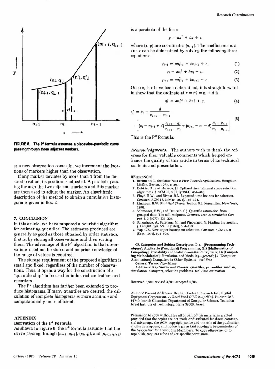
FIGURE 8. The p? formula assumes a piecewise-parabolic curve passing through three adjacent markers.

as a new observation comes in, we increment the locations of markers higher than the observation.

If any marker deviates by more than 1 from the desired position, its position is adjusted. A parabola passing through the two adjacent markers and this marker are then used to adjust the marker. An algorithmic description of the method to obtain a cumulative histogram is given in Box 2.

7. CONCLUSION In this article, we have proposed a heuristic algorithm for estimating quantiles. The estimates produced are generally as good as those obtained by order statistics, that is, by storing all observations and then sorting them. The advantage of the P’ algorithm is that observations need not be stored and no prior knowledge of the range of values is required.

The storage requirement of the proposed algorithm is small and fixed, regardless of the number of observations. Thus, it opens a way for the construction of a “quantile chip” to be used in industrial controllers and recorders.

The P2 algorithm has further been extended to produce histograms. If many quantiles are desired, the calculation of complete histograms is more accurate and computationally more efficient.

APPENDIX Derivation of the Pz Formula As shown in Figure 8, the P2 formula assumes that the curve passing through (ni-1, qi-l), (n;, qi), and (ni+l, qi+l)

is a parabola of the form

y = llx2 + bx + c

where (x, y) are coordinates (n, 4). The coefficients II, b, and c can be determined by solving the following three equations:

qi-1 = UTZ:-, + bni-1 + C. (1)

9i = ~nj! + bni + C. (2)

9i+l = UH;+~ + bni+l + C. (3)

Once a, b, c have been determined, it is straightforward to show that the ordinate at x = n,! = ni + d is

91 = ani’ + bn[ + c. (4)

91 = 9i + d ni+l - G-1

(5)

. [ (ni - ni-1 + d) E + (ni+l - ni - d) !E!@

I 7Zi - ni-1 1 .

This is the P2 formula.

Acknowledgments. The authors wish to thank the ref- erees for their valuable comments which helped en- hance the quality of this article in terms of its technical contents and presentation.

REFERENCES 1. Breimann. L. Sfatistics: With a View Towards Applications. Houghton

Mifflin, Boston, 1973, p. 207. 2. Dobkin, D., and Munroe, J.I. Optimal time minimal space selection

algorithms. J. ACM 28, 3 (July 1961), 454-463. 3. Floyd, R.W., and Rivest, R.L. Expected time bounds for selection.

Commun. ACM 18,3 (Mar. 1975), 165-173. 4. Lindgren, B.W. Stafisfical Theory. Section 5.1. Macmillan, New York,

1976. 5. Schmeiser, B.W., and Deutsch, S.J. Quantile estimation from

grouped data: The cell midpoint. Commun. Stat. B: Simulation Com- puf. 6, 3 (1977), 221-234.

6. Schonhage. A., Paterson, M., and Pippenger, N. Finding the median. J. Compuf. Sysf. Sci. 13 (1976), 184-199.

7. Yap, C.K. New upper bounds for selection. Commun. ACM 19,9 (Sept. 1976), 501-506.

CR Categories and Subject Descriptors: D.l.1 [Programming Tecb- niques]: Applicable (Functional) Programming; G.3 [Mathematics of Computing]: Probability and Statistics-statistical soffware; I.6 [Comput- ing Methodologies]: Simulation and Modeling-general; 1.7 [Computer Architecture]: Computers in Other Systems-real time

General Terms: Algorithms Additional Key Words and Phrases: quantiles, percentiles, median,

simulation, histogram, selection problems, real-time estimation

Received 5/62; revised 3/65; accepted 5/65

Authors’ Present Addresses: Raj Jain, Eastern Research Lab, Digital Equipment Corporation. 77 Reed Road (HLO Z-3/N03), Hudson, MA 01749. Imrich Chlamtac, Department of Computer Science, Technion Israel Institute of Technology, Haifa 32000, Israel.

Permission to copy without fee all or part of this material is granted provided that the copies are not made or distributed for direct commer- cial advantage, the ACM copyright notice and the title of the publication and its date appear, and notice is given that copying is by permission of the Association for Computing Machinery. To copy otherwise, or to republish, requires a fee and/or specific permission.


the p2 algorithm for dynamic calculation of quantiles and histograms without storing observations

Documents