How to Summarize the Universe:Dynamic Maintenance of QuantilesAnna C. Gilbert Yannis Kotidis S. Muthukrishnan Martin J. StraussAT&T Labs ResearchFlorham Park, NJ07032 USAfagilbert,kotidis,muthu,mstraussg@research.att.comAbstractOrder statistics, i.e., quantiles, are frequentlyused in databases both at the database serveras well as the application level. For example,they are useful in selectivity estimation duringquery optimization, in partitioning large rela-tions, in estimating query result sizes whenbuilding user interfaces, and in characterizingthe data distribution of evolving datasets inthe process of data mining.We present a new algorithm for dynamicallycomputing quantiles of a relation subject toinsert as well as delete operations. The algo-rithm monitors the operations and maintainsa simple, small-space representation (based onrandom subset sums or RSSs) of the underly-ing data distribution. Using these RSSs, wecan quickly estimate, without having to ac-cess the data, all the quantiles, each guaran-teed to be accurate to within user-speci�edprecision. Previously-known one-pass quan-tile estimation algorithms that provide sim-ilar quality and performance guarantees cannot handle deletions. Other algorithms thatcan handle delete operations cannot guaran-tee performance without rescanning the entiredatabase.We present the algorithm, its theoretical per-formance analysis and extensive experimentalresults with synthetic and real datasets. In-dependent of the rates of insertions and dele-Permission to copy without fee all or part of this material isgranted provided that the copies are not made or distributed fordirect commercial advantage, the VLDB copyright notice andthe title of the publication and its date appear, and notice isgiven that copying is by permission of the Very Large Data BaseEndowment. To copy otherwise, or to republish, requires a feeand/or special permission from the Endowment.Proceedings of the 28th VLDB Conference,Hong Kong, China, 2002

tions, our algorithm is remarkably precise atestimating quantiles in small space, as our ex-periments demonstrate.1 IntroductionMost database management systems (DBMSs) main-tain order statistics, i.e., quantiles, on the contents oftheir database relations. Medians (half-way points)and quartiles (quarter-way points) are elementary or-der statistics. In the general case, the �-quantiles ofan ordered sequence of N data items are the valueswith rank k�N , for k=1; 2; : : :1=�.Quantiles �nd multiple uses in databases. Sim-ple statistics such as the mean and variance are bothinsu�ciently descriptive and highly sensitive to dataanomalies in real world data distributions. Quantilescan summarize massive database relations more ro-bustly. Many commercial DBMSs use equi-depth his-tograms [21, 23], which are in fact quantiles, duringquery optimization in order to estimate the size of in-termediate results and pick competitive query execu-tion plans. Quantiles can also be used for determiningassociation rules for data mining applications [1, 3, 2].Quantile distribution helps design well-suited user in-terfaces to visualize query result sizes. Also, quantilesprovide a quick similarity check in coarsely comparingrelations, which is useful in data cleaning [16]. Finally,they are used as splitters in parallel database systemsthat employ value range data partitioning [22] or for�ne-tuning external sorting algorithms [9].Computing quantiles on demand in many of theabove applications is prohibitively expensive as it in-volves scanning large relations. Therefore, quantilesare precomputed within DBMSs. The central chal-lenge then is tomaintain them since database relationsevolve via transactions. Updates, inserts and deleteschange the data distribution of the values stored inrelations. As a result, quantiles have to be updatedto faithfully re ect the changes in the underlying datadistribution. Commercial database systems often hide

this problem. Database administrators may periodi-cally (say every night) force the system to recomputethe quantiles accurately. This has two well-knownproblems. Between recomputations, there are no guar-antees on the accuracy of the quantiles: signi�cantupdates to the data may result in quantiles being ar-bitrarily bad, resulting in unwise query plans duringquery optimization. Also, recomputing the quantilesby scanning the entire relation, even periodically, isstill both computationally and I/O intensive.In applications such as described above, it oftensu�ces to provide reasonable approximations to thequantiles, and there is no need to obtain precise val-ues. In fact, it su�ces to get quantiles to within a fewpercentage points of the actual values.We present a new algorithm for dynamically com-puting quantiles of a relation subject to both insertand delete operations.1 The algorithm monitors theoperations and maintains a simple, small-space repre-sentation (based on random subset sums or RSSs) ofthe underlying data distribution. Using these RSSs,we can estimate, without having to access the data,all the quantiles on demand, each guaranteed a pri-ori to be accurate to within user-speci�ed precision.The algorithm is highly e�cient, using space and timesigni�cantly sublinear in the size of the relation.Despite the commercial use of quantiles, their pop-ularity in database literature and their obvious fun-damental importance in DBMSs, no comparable solu-tions were known previously for maintaining approxi-mate quantiles e�ciently with similar a priori guaran-tees. Previously known one-pass quantile estimationalgorithms that provide similar a priori quality andperformance guarantees can not handle delete oper-ations; they are useful for refreshing statistics on anappend-only relation but are unsuitable in presence ofgeneral transactions. Other algorithms that can han-dle modify or delete operations rely on a small \back-ing sample" or \distinct sample" of the database andcannot guarantee similar performance without rescan-ning the relation.We perform an extensive experimental study ofmaintaining quantiles in presence of general transac-tions. We use synthetic data sets and transactions tostudy the performance of our algorithm (as well as aprior algorithm we extended to our dynamic setting)with varying mixes of inserts and deletes. We alsouse a real, massive data set from an AT&T warehouseof active telecommunication transactions. Our exper-iments show that our algorithm has a small footprintin space, is fast, and it performs with remarkable accu-racy in all our experiments, even in presence of rapidinserts and deletes that change underlying data distri-1Update operations of the form \change an attribute value ofa speci�ed record from its current value x to new value y" canbe thought of as a delete followed by insert, for the purposes ofour discussions here. Hence, we do not explicitly consider themhereafter.

bution substantially.In the rest of this section, we state our problemformally, discuss prior work and describe our resultsmore, before presenting the speci�cs. In Section 2,we describe the challenges in dynamically maintainingquantiles and present non-trivial adaptations of priorwork. In Section 3 we present our algorithm in detail.In Section 4, we present experimental results. Finally,Section 5 has concluding remarks.1.1 Problem De�nitionWe consider a relational database and focus on somenumerical attribute. The domain of the attribute isU = f0; : : : ; jU j � 1g, also called the Universe. Ingeneral, the domain may be a di�erent discrete setor it may be real-valued and has to be appropriatelydiscretized. Our results apply in either setting, but weomit those discussions.At any time, the database relation is a multiset ofitems drawn from the universe. We can alternatelythink of this as an array A[0 � � � jU j � 1] where A[i]represents the number of tuples in the relation withvalue i in that attribute.Transactions consist of inserts and deletes.2Insert(i) adds a tuple of value i, i.e., A[i] A[i] + 1and delete(i) removes an existing tuple with value i,i.e., A[i] A[i] � 1. Let At be the array after ttransactions and let Nt = PiAt[i]; we will drop thesubscript t whenever it is unambiguous from context.Our goal is to estimate � quantiles on demand. Inother words, we need to �nd the tuples with ranksk�N , k = 1; : : : ; 1=�. We will focus on computing �-approximate � quantiles. That is, we need to �nd a jksuch that (k�� �)N �Xi�jk A[i]and Xi<jk A[i] � (k�+ �)Nfor k = 1; : : : ; 1=�. The set of j1; : : : ; j1=� will be the� quantiles approximate up to ��N . (If � = 0, thenwe seek the exact quantiles.) Note that, for � 6= 0, theapproximation above is in fact good to relative error�1� ���; one can set � = ��0 to get the factor (1� �0).Our goal is to solve this problem using sublinearresources. It would be ideal of course to use space nomore than 1=� that it takes to store the quantiles, butthat appears to be unrealistic since the quantiles maychange substantially under inserts and deletes. There-fore, in the spirit of prior work, our data structurewill use space that is polylogarithmic in the universesize, which is typically much less than the size of the2Formally, the attribute we focus on is the key for the rela-tion.

dataset. Furthermore, we will only use time per op-eration nearly linear in the size our data structure,namely, polylogarithmic in the universe size.If no transactions are allowed, we refer to the prob-lem as static. If only insertions are allowed, we refer toit as incremental and when both insertions and dele-tions are allowed, we refer to it as dynamic. It is obvi-ous that, in a database system, At[i] � 0 at any timet, since one can not delete a tuple that is not presentin the relation. A sequence of transactions is calledwell-formed if it leads to At � 0; we will consider onlywell-formed sequences of transactions in this paper.1.2 Previous WorkSince the early 70's, there has been much focus on�nding the median of a static data set. Following thebreakthrough result of [7] that there is a comparison-based algorithm to �nd the median (and all the quan-tiles) in O(N) worst case time, more precise boundshave been derived on the precise number of compar-isons needed in the worst case [20].A series of algorithms have been developed for �nd-ing quantiles in the incremental model. The idea pre-sented in [19] leads to an algorithm that maintains anO((log2 �N)=�) space data structure on A which getsupdated for each insert. Using this data structure, �-quantiles can be produced that are a priori guaranteedto be �-approximate. This algorithm was further ex-tended in [6, 17] to be more e�cient in practice, andimproved in [14] to use only O((log �N)=�) space andtime. The approach in these papers is to maintain a\sample" of the values seen thus far, but the sample ischosen deterministically by enforcing various weight-ing conditions. Earlier, [19] had shown that any p-passalgorithm needs time (N1=p) to compute quantilesexactly and so one needs to resort to approximation inorder to get small space and fast algorithms.A di�erent line of research has been to use random-ization so that the output is �-approximate �-quantileswith probability at least 1 � � for some pre-speci�edprobability � of \failure." The intuition is that allow-ing the algorithms to only make probabilistic guaran-tees will potentially make them faster, or use smallerspace. In [17, 18], O(��1 log2 ��1 + ��1 log2 log ��1)space and time algorithm was given for this problem.Note that this is independent of N , dependent only onprobability of failure and approximation factor.Other one-pass algorithms [3, 8, 15] do not providea priori guarantees; however, performance of their al-gorithms on various data sets has been experimentallyinvestigated. Both [18] and [14] also presented exten-sive experiments on the incremental model.Despite the extensive literature above on proba-bilistic/deterministic, approximate/exact algorithmsfor �nding quantiles in the incremental model, wedo not know of a signi�cant body of work that di-rectly addresses the problem of dynamic maintenance

of quantiles. An exception is the result of [11] on dy-namic maintenance of equi-depth histograms which are�-quantiles. Using a notion of error di�erent fromours, the authors present an algorithm based on thetechnique of a \backing sample" (an appropriately-maintained random sample) and provide a priori prob-abilistic guarantees on equi-depth histogram construc-tion. Their algorithm works well for the case whendeletions are infrequent, but in general, it is forcedto rescan the entire relation in presence of frequentdeletes. In fact, the authors say \based on the over-heads, it is clear that the algorithm is best suited forinsert-mostly databases or for data warehousing envi-ronments."Another related line of research is the mainte-nance of wavelet coe�cients in presence of inserts anddeletes. This was investigated in [12, 24] where theemphasis was on maintaining the largest (signi�cant)coe�cients. In [13], an algorithm was provided for dy-namically maintaining V -Opt histograms. No a prioriguarantees for �nding quantiles can be obtained byusing these algorithms.1.3 Our Main Algorithmic ResultWe present a new algorithm for the problem ofdynamically estimating quantiles. We maintainO(log2 jU j log(log(jU j)=�)=�2) space representation ofA. This gets updated with every insertion as wellas deletion. When quantiles are demanded, we canestimate, without having to access the data, all thequantiles on demand, each guaranteed a priori to beaccurate to within user-speci�ed precision ��N withuser-speci�ed probability 1� � of success.2 Challenges and Partial solutionsIn this section, we provide some intuition into theproblem of maintaining quantiles under inserts anddeletes. We also adapt prior work on incrementalquantile-�nding algorithms to work in presence ofdeletes for comparison purposes.2.1 ChallengesIn order to understand the challenge of maintainingapproximate quantiles using small space, let us con-sider the following example. Our goal will be to main-tain four quartiles to within moderate error of �0:1N .Suppose a transaction stream consists of one millioninsertions followed by 999,996 deletions, leavingN = 4items in the relation. Our problem speci�cation es-sentially requires that, with high probability, we re-cover the database exactly.3 A space-e�cient algo-3For each pair i1; i2 of consecutive items in such a smallrelation, a quantiles algorithm gives us some j with i1 � j � i2.One can learn all four items exactly by making a few queriesabout �-quantiles for � slightly less than 1=4, on a databaseconsisting of the four original items and a few additional inserteditems with strategic, known values.

rithm knows very little about a dataset of size one mil-lion and it does not know which 999,996 items will bedeleted; yet, ultimately, it must recover the four sur-viving items. Although this is a contrived example, itillustrates the di�culty with maintaining order statis-tics in the face of deletes which dramatically changethe data distribution.Some incremental algorithms work by sampling thedata, either randomly and obliviously or with care tomake sure the samples are spaced appropriately. Someof these techniques give provable results in the incre-mental setting. In the dynamic setting, however, asample of the million items in the database at its peaksize will be of little use at the time of the query in theexample above, since the sample is unlikely to con-tain any of the four eventual items. To apply knownsampling algorithms, one needs to sample from thenet dataset at every point in time, which is di�cult ifthere is severe cancellation. For example, in [10], theauthor addresses the problem of sampling from the netdata set after inserts and deletes and states that \Ifsubstantial portion of the relation is deleted, it may benecessary to rescan the relation in order to preservethe accuracy of the guarantees."2.2 Extending Previous AlgorithmsAmong the previously known algorithms, we considerthe Greenwald-Khanna (GK) algorithm [14] in more de-tail since it provides the best known performance forthe incremental case. It has other desirable proper-ties: it uses small space and time, and does not rescanthe database for approximate quantile generation. Wewill describe ways to modify the algorithm for the dy-namic case. No a priori guarantees can be obtainedin this manner; nevertheless, this provides a usefulbenchmark with which to compare our algorithm. Pre-viously known algorithms that rely on backing or dis-tinct samples can not be extended in this manner; as aresult, rescanning of the database can not be avoidedwith those algorithms.We consider the bounded-memory form of the GKalgorithm. The algorithm �rst �lls its memory withdata points (values), as they arrive. When its mem-ory is full and additional values arrive, the GK algo-rithm kicks out some point it has (possibly the newly-arrived point), and keeps a count of the number of datapoints between samples. It chooses the point to kickout carefully, to minimize the error in its answeringprocedure, which is to return the least sample pointj such that Pi�j A[i] exceeds the desired rank. Thealgorithm further speci�es a data structure to facili-tate e�cient updates and queries. The error of thealgorithm depends on the memory available and thenumber of items in the dataset.Although the GK algorithm is designed for incremen-tal (insert-only) data, there are several ways to extendit to dynamic data.

Ignore deletions: One can simply ignore deletetransactions. This will be a reasonable solution pro-vided the rate of deletions is small compared with therate of insertions.Use two parallel GKs: One can use two instancesof GK, one for insertions and one for deletions. Forestimating each � quantile, we search for two points i1and i2 such that� each of i1 and i2 appears as a sample point in oneof the instances of GK.� there is no sample point between i1 and i2 in ei-ther of the instances.� Let iins1 be the greatest sample among insertionssuch that iins1 � i1, let idel1 be the greatest sampleamong deletions such that idel1 � i1, and similarlyfor iins2 and idel2 . We haveXj<iins1 Ains[j]� Xj<idel1 Adel[j] � �N �Xj<iins2 Ains[j]� Xj<idel2 Adel[j];where Ains and Adel are incremental datasets ofinsertions and deletions, respectively.Heuristically, one can then output i1 or i2 as an ap-proximate answer.There are several further ways to specify the abovealgorithm.� One can interpolate between i1 and i2 by return-ing i1 + (i2 � i1)�, where� = 0@ Xj<iins2 Ains[j]� Xj<idel2 Adel[j]1A� 0@ Xj<iins1 Ains[j]� Xj<idel1 Adel[j]1A :� The pair (i1; i2) is not unique, in general. One canlook for all such pairs, and combine the results foreach, say, by taking a mean or median.In our experimental section, we use the above-mentioned dual instances of the GK algorithm, calledGK2 by us. We interpolated between i1 and i2 and tooka mean over all pairs (i1; i2); this performed well.3 Our Algorithm for MaintainingQuantilesIn this section, we will �rst present the high level viewof our algorithm with the main idea. Then we willpresent speci�c details. In what follows, E[X ] and

var[X ] denote the expected value and the variance ofa random variable X respectively. At the beginning,we will assume that U is known to the algorithm; later,we will remove this assumption.3.1 High-Level View of Our AlgorithmIn order to compute approximate � quantiles we needof a way to approximate A with a priori guarantees.In fact our algorithm works by estimating range-sumsof A over dyadic intervals I . (Dyadic intervals will bede�ned shortly.)We describe the main idea behind our algorithmhere. The simplest form of a dyadic interval estimateis a point estimate, A[i]. We proceed as follows. Let Sbe a (random) set of distinct values, each drawn fromthe universe with probability 1/2. Let AS denote Aprojected onto the set S, and let kASk = Pi2SA[i]denote the number of items with values in S. We keepkASk (a single number known as a Random-Subset-Sum (RSS)) for each of several random sets S. Observethat the expected value of kASk is 12 kAk, since eachpoint is in S with probability 12 .For A[i], consider E[kASk ji 2 S], which can be es-timated by looking at counts kASk, only for the S'sthat contain i (close to half of all S's, with high prob-ability). One can show that this conditional expectedvalue is A[i] + 12 AUnfig , since the contribution of iis always counted but the contribution of each otherpoint is counted only half the time. Since we also knowkAk, we can estimate A[i] as2�A[i] + 12 AUnfig �� kAkIt turns out that this procedure yields an estimategood to within �N additively if we take an averageof O(1=�2) repetitions.We can similarly be in position to estimate thenumber of dataset items on any dyadic interval in U(de�ned below), up to ��N , by repeating the proce-dure for each dyadic resolution level up to log jU j. Ofcourse, a set S in this case is a collection of dyadicintervals from the same level, each taken with proba-bility 1/2. Similar argument as above applies.By writing any interval as a disjoint union of at mostlog jU j dyadic intervals, we can estimate the numberof dataset items in any interval. Now, we can performrepeated binary searches to �nd the quantiles left toright one at a time (i.e, �rst, second, etc.).The entire algorithm relies on summarizingA usingRSSs. Each item in 0; : : : ; jU j � 1 participates in theconstruction of RSSs. In other words, we summarizethe Universe using RSSs. This is a departure fromprevious algorithms for �nding quantiles, which relyon keeping a sample of speci�c items in the input dataset.

3.2 Algorithm DetailsWe will �rst describe our data structure and its main-tenance, before describing our algorithm for quantileestimation, and presenting its analysis and proper-ties. A dyadic interval Ij;k is an interval of the form[k2log(jUj)�j ; (k+1)2log(jUj)�j�1], for j and k integers.The parameter j of a dyadic interval is its resolutionlevel from coarse: I0;0 = U , to �ne: Ilog(jUj);i = fig.There are log(jU j) + 1 resolution levels and 2jU j � 1dyadic intervals altogether, in a tree-like structure.3.2.1 Our Data Structure and its Mainte-nanceFor each resolution level j of dyadic intervals we do thefollowing. Pick a subset of the intervals Ij;k at level j.Let S be the union of these intervals and let kASk bethe count of values in the datasets that are projectedonto S (formally, kASk =Pi2SA[i]) . We repeat thisprocess num copies = 24 log(log(jU j)=�) log(jU j)=�2times and get sets S1; : : : ; Snum copies (per level). Thecounts kASlk for all sets that we have picked compriseour Random Subset Sum summary structure. In ad-dition we store (and maintain) kAk = N exactly. Wemaintain these RSSs during inserts/deletes as follows.For insert(i), for each resolution level j, we quicklylocate the single dyadic interval Ij;k into which i falls(determined by the high order bits of i in binary).Then quickly determine those sets Sl that contain Ij;k.For each such set we increase count kASlk by one. Fordeletions we simply decrease the counters. Notice thatthis process can be extended to handle batch inser-tions/deletion by increasing/decreasing the counterswith appropriate weights.An important technical detail is how to store andindex various Sl's, which are random subsets. Thestraightforward way would be to store them explicitly,perhaps as a bitmap. This would use space O(jU j)which we can not a�ord. For our algorithm, we in-stead store certain random seeds of size O(log jU j) bitsand compute a (pseudorandom) function that explic-itly shows whether i 2 Sl or not. For this, we usethe standard 3-wise independent random variable con-struction shown below, since it works well with ourdyadic construction.We need a generator G(s; i) = Si that quickly out-puts the i'th bit of the set S, given i and a short seeds. In particular, the generator takes a O(log jU j)-bitseed and can be used to generate sets S of size O(jU j).The generator G is the extended Hamming code, e.g.,0B@ 1 1 1 1 1 1 1 10 0 0 0 1 1 1 10 0 1 1 0 0 1 10 1 0 1 0 1 0 1 1CA ;which consists of a row of 1's and then all the columns,in order. So, for each resolution level j, there's a G of

size (j + 1) � 2j . Then G(s; i) is the seed s of lengthj+1 dotted with the i'th column of G modulo 2, whichis e�cient to compute|note that the i'th column ofG is a 1 followed by the binary expansion of i. Thisconstruction is known to provide 3-wise independentrandom variables [5]. We will use this property exten-sively when we analyze our algorithm.3.2.2 Estimating QuantilesOur algorithm for estimating quantiles relies on esti-mating sum of ranges, i.e., kAIk for intervals I . Firstwe will focus on dyadic intervals and then extend it togeneral intervals. Then, we will show how to computethe quantiles.Computing kAIk for dyadic intervals I .Recall that kAIk is simply the number of values in thedataset that fall within the interval I .Given dyadic Ij;k, we want an estimate AIj;k �of AIj;k . We consider the random sets only in theresolution level j. Recall that there are num copiessuch sets. Again, using the pseudorandom construc-tion, quickly test each set to see whether it containsIj;k and ignore the remaining sets for this interval. Anatomic computation for AIj;k is 2 kASlk � kAk forASl corresponding to a set Sl containing Ij;k .Computing kAIk for arbitrary intervals.Given an arbitrary interval I , write I as a dis-joint union of at most log jU j dyadic intervals Ij;k.For each Ij;k, group the atomic computations into3 log(log(jU j)=�) groups of 8 log(jU j)=�2 each and takethe average in each group. We can get an estimate forI by summing one such average for each of the dyadicintervals Ij;k. Since we have 3 log(log(jU j)=�) groupsthis creates 3 log(log(jU j)=�) atomic estimates for I .Their median is the �nal estimate kAIk�.In what follows, it is more convenient to regard ourestimate kAIk� as an overestimate, kAIk � kAIk� �kAIk+ �N , by using a value of � half as big as desiredat top level, and adding �2N to each estimate.Computing the quantiles.We would like to estimate �-approximate �-quantiles.Recall that � is �xed in advance. For k = 1; : : : ; 1=�we want an jk such that A[0;jk) = (k�� �)N . (Herejk is the value with rank k�, not to be confused withthe resolution level j.) For each pre�x I , we can com-pute kAIk� as described above. Using binary search,�nd a pre�x [0; jk) such that A[0;jk) � < k�N � A[0;jk+1) �, and return jk. Repeat for all values ofk. We call the entire algorithm for maintenance ofquantiles the RSS algorithm.

3.2.3 Analysis of Our AlgorithmFirst we consider the correctness of our algorithm inthe lemma below and then summarize its performancein a theorem.Lemma 1 Our algorithm estimates each quantile towithin � kAk = �N with probability at least 1� �.Proof: First �x a resolution level j. Consider the setS formed by putting each dyadic interval Ij;k = Ik atlevel j into S with probability 1=2 as we did. In whatfollows, we drop the resolution level when indexing adyadic interval. Let Xk be a random variable de�nedby Xk = � 2 kAIkk ; Ik 2 S;0; otherwise;and let X = PkXk. Suppose we are presented withan interval Ik0 , dyadic at level j. We have, using 3-wiseindependence (pairwise will do),E[X jIk0 2 S] = 2 AIk0 + Xk 6=k0 E[Xk]= 2 AIk0 + Xk 6=k0 kAIkk= AIk0 + kAk :Also, since AIk0 � X � AIk0 + 2 kAk,var[X jIk0 2 S] � kAk2 :Each pre�x I is the disjoint union of r � log jU jdyadic intervals at di�erent levels, I = Ik1 [ Ik2 [ � � � [Ikr . Let Sj be a random set of intervals at level j, andlet Y be the sum of corresponding X estimates. ThenE[Y j8j Ikj 2 Sj ] = kAIk+ r kAk ;so E[Y j8j Ikj 2 Sj ]�r kAk = kAIk, as desired. (Notethat we have stored kAk exactly.) Also,var[Y j8j Ikj 2 Sj ] � log jU j kAk2 :It follows that, if we let Z be the average of8 log jU j=�2) repetitions of X , the conditional expec-tation of Z � r kAk is kAIk and the conditional vari-ance of Z � r kAk is at most �2N2=8. By the Cheby-shev inequality, jZ � kAIk j < �N with probabilityat least 7=8. Finally, if we take 3 log(log(jU j)=�) =3(log(1=�) + log log jU j) copies of Z and take a me-dian, by the Cherno� inequality, jZ � kAIk j < �Nwith probability at least 1 � �= log jU j. Both Cheby-shev and Cherno� inequalities can be found in [5], andaveraging arguments similar to above can be found infor example [4].

We performed binary search to �nd a jk such that A[0;jk) � < k�N � A[0;jk+1) �. It follows that A[0;jk) � A[0;jk) �< k�N� A[0;jk+1) �� A[0;jk+1) + �N;as desired.To estimate a single quantile, we will, log jU j times,estimate kAIk on a pre�x I , in the course of bi-nary search. Since each estimate fails with probability�= log(jU j), the probability that any estimate fails isat most log(jU j) times that, i.e., �.Therefore, by summing up space used and the timetaken for algorithms we have described, we can con-clude the following.Theorem 2 Our RSS algorithm usesO �log2(jU j) log� t log(jUj)�� � =�2� space and pro-vides �-approximate �-quantiles with probability atleast 1 � � for t queries. The time for each insert ordelete operation, and the time to �nd each quantile ondemand is proportional to the space.Note that we can �nd a single quantile with costO((log2 jU j log log(jU j=�))=�2). If we make t queries,each of which requests 1=� quantiles, we need the prob-ability of each failure to be less than ��=t in order thatthe probability of any failure to be less than �. Thisaccounts for the cost factor log(t=�).3.2.4 Extension to when U is UnknownAbove we assumed that the universe U is known inadvance. In practice, this may not be the case; fortu-nately, our algorithm can easily adapt to an increasinguniverse, with modest increased cost factor of at mostlog2 log(jU j) compared with knowing the universe inadvance.We start the algorithm as above, with a predictedrange [0; u � 1] for U . Suppose we see an insertionof i � u = jU j, where, at �rst, we assume i < u2.We then keep statistics for the universe [0; u� 1] and[0; u2 � 1], directing all insertions and deletions withvalue in [0; u�1] to the original instance of RSS and allinsertions and deletions with value in [u; u2�1] to thenew instance. In general, we may need to square thesize of the universe repeatedly, upon seeing a sequenceof insertions with growing values or even a single in-sertion with very large value. We thus get several in-stances of RSS; each but the �rst extends the previousones. The number of items in each dyadic interval canbe estimated by consulting a single instance of RSS.Thus we have speci�ed how to perform updates andqueries; it remains to analyze the costs of the datastructure.

Suppose the largest item seen is i� and let u� bethe smallest power of 2 greater than i�. Thus, if weknew i� in advance, we would use a single instanceof RSS on a universe of size u�, with cost f(u�) for fgiven in Theorem 2. The multi-instance data struc-ture we construct has largest instance on a universe ofsize at u2� and log log(u2�) instances altogether. Thusthe time and space costs of the multi-instance datastructure are at most O(f(u2�) log log(u�)). Since thedependence on u of f is polylogarithmic, the cost ofthe multi-instance dataset is just the factor log log(u�)compared with knowing u� in advance. An additionalcost factor of 2 log j is needed for the j'th instance,j = 1; 2; : : : ; log log(u�), to drive down the probabilityof failure to 1=j2, so that the overall probabilityPj 1j2remains bounded.3.3 Some Observations on Our AlgorithmOur approach of summarizing the Universe using RSSshas interesting implications for our algorithm which wesummarize here.� Previous (incremental) algorithms for quantilescan guarantee always to return a value in the in-put dataset, whereas our algorithm may return aquantile value which was not seen in the input.This does not appear to have severe implicationsin various applications of quantiles. In general,in the face of severe cancellation, an algorithmwith less than N space cannot keep track of whichitems are currently in the dataset.� The distribution on values returned by our algo-rithm depends only on the dataset active at thetime of the query. Thus, one can change the or-der of insertions and deletions without a�ectingresults. This contrasts with previously known al-gorithms for �nding quantiles where the order ofinserts impacts the approximate quantiles outputby the algorithm.� Our RSSs are composable, that is, if updates aregenerated in two separate locations, each locationcan compute random subset sums on its data,using pre-agreed common random subsets. Thesubset sums for the combined dataset is just thesum of the two subset sums. Hence, we can com-pute the quantiles of the combined data set veryquickly from their RSSs alone. Because RSSs arecomposable, our entire algorithm is easily paral-lelizable. If data is arriving quickly (for example,in the case of IP network operations data), thedata can be sent to an array of parallel machinesfor processing. Results can be composed at theend.

4 Experiments4.1 Datasets, Algorithms ImplementationTo ratify our performance claims, we present an exten-sive set of experiments, with synthetic and real datasets. The synthetic data that we used are described inTable 1.4.2 Performance of Our AlgorithmEach dataset is used to generate a population of sizeN , drawn from the range [0 : : : U � 1]. We use thisdata to compare the following algorithms:� Naive[`]: This is a simple algorithm thatmaintains exact counts on all dyadic intervalsI`;0; : : : ; I`;2`�1 at level j = ` and uses them tocompute quantiles. Estimates for intervals belowlevel ` are zero. The purpose of presenting theperformance of this algorithm is twofold. First, itallows as to verify the performance of the RSS[`](see below) implementation that maintains exactcounts at level ` and random sums below thatlevel. Second, the performance of Naive is an in-dication of the hardness of the data for computingquantiles. E.g. Naive will do well if the quantilesare fairly wide-spread.� RSS[`]: This is a implementation of a variationof our RSS algorithm. For the coarsest few levels,say, to level `, it is more e�cient to store exactsubset sums for each of the (few) dyadic intervalsat that level. This immediately lets us get kAIkfor any I dyadic at that level, in time O(1). Infact, we can store just the subset sums for thedyadic intervals at level ` itself, since any coarserinterval can be written as the disjoint union ofdyadics at level `. We refer to such an implemen-tation as RSS[`]. In our implementation, dyadicsums at level ` are stored explicitly. A short cutthat we implemented is that we store the randomsets below level ` using bitmaps instead of usingrandom seeds. This does not a�ect the qualityof the results presented here. The space require-ments are computed as if random seeds were used.� GK: This is an implementation of the Greenwald-Khanna algorithm.� GK2: This uses two GK instances, one for inser-tions and one for deletions and interpolates to es-timate the quantiles as described in Section 2.2.The rest of this section is organized as follows. Sub-section 4.2 presents a study on the performance of RSSon synthetic data. Subsection 4.3 compares our algo-rithm against the other competitors for datasets thatinclude both insertions and deletions. Finally, subsec-tion 4.4 compares all algorithms using Call Detail Datafrom AT&Ts telephony network and demonstrates the

e�ectiveness of RSS for computing quantiles on large,dynamic datasets.For these experiments we evaluate RSS for comput-ing quantiles for datasets of various sizes and distribu-tions. Naive gives us a measure of the hardness of com-puting quantiles for these datasets. The universe sizein all experiments was U = 220. In all cases we com-pute 15 quantiles at positions k 116 for k = 1; 2; : : : ; 15(e.g. median is for k = 8). The footprint of the RSS al-gorithm was 11K in all runs. All numbers are averagesover four runs with di�erent seeds/data values.Table 2 summarizes our results for Zipf distributeddata varying N . The large errors reported by Naivefor small values of k are because most of the mass ofthe Zipf distribution is concentrated on the left size ofthe domain, with 0 being the most popular item. As aresult, small errors in identifying the correct quantilesnear zero result in large errors for these quantiles. Asexpected, the errors for RSS seem to be independent ofthe population size N for a �xed domain.The results for a Normal distribution of the dataare tabulated in Table 3. This time Naive is a moreserious competitor and sometimes surpasses RSS, es-pecially for the \easy" quantiles (14/16,15/16). SinceRSS stores the same sets as Naive for level 7, the rela-tive success of Naive is due to the variance introducedby the random sets below that level. A bigger foot-print for RSS closes the gap for these cases (results areomitted due to space limitations).4.3 Comparison for Mix of Inserts/DeletesWe now investigate the performance of the algo-rithms when both insertions and deletions are present.We model the following scenario: we insert N =104; 858 items drawn uniformly from distributionD1 =Uni[1; U ], U = 220. Then we super-impose a sec-ond compact distribution D2 =Uni[U=2�U=32; U=2+U=32] with �N values. Finally, all values from the �rstdistribution are deleted so that the remaining valuesall come from D2. Parameter � controls the mass ofthe second distribution with respect to the mass ofD1.All algorithms were set up to use 11KB of memory fortheir data structures.Table 4 summarizes the average error over all quan-tiles (for k = 1; : : : ; 15) and 4 repetitions of the experi-ment. For GK we simply ignore deletions. Performanceof RSS does not depend of the volume of the data((1+�)N after all insertions, ��N in the end). Whenthe mass of D2 is much larger that the mass of theinitial distribution, even GK performs well as inser-tions/deletions (from D1) do not signi�cantly a�ectthe �nal picture. However, when the values of D2 be-come indistinguishable within the mass of D1 + D2,RSS is the clear winner with average error about 10times less the errors of GK, GK2. In these cases, evenNaive is better that both of them.Hence, under severe cancellations, summarizing the

Dataset DescriptionUni[A,B] Uniform data within range [A: : :B]Zipf Zipf distributed valuesNormal[m,v] Normal distribution with mean=m and variance=vTable 1: Synthetic DatasetsN=10,485 N=1,048,576 N=10,485,760k Naive[7] RSS[7] Naive[7] RSS[7] Naive[7] RSS[7]1 0.7526 0.0818 0.9753 0.0272 0.9812 0.00902 0.7526 0.0818 0.9753 0.0272 0.9812 0.00903 0.7526 0.0001 0.9753 0.0000 0.9812 0.00004 0.5281 0.1134 0.7031 0.1490 0.8731 0.04965 0.4154 0.0000 0.5545 0.2222 0.6014 0.07406 0.4154 0.0000 0.5545 0.2222 0.6014 0.07407 0.4154 0.0000 0.5545 0.0000 0.6014 0.00008 0.4153 0.0000 0.5545 0.0000 0.6014 0.00009 0.4154 0.0000 0.5545 0.0000 0.6014 0.000010 0.2932 0.0000 0.3888 0.0833 0.4211 0.027711 0.2932 0.0000 0.3888 0.0416 0.4211 0.013812 0.2265 0.0221 0.3001 0.0296 0.3249 0.045913 0.1754 0.0142 0.2413 0.0186 0.2637 0.015714 0.1154 0.0312 0.1562 0.0104 0.1700 0.032015 0.0595 0.0272 0.0803 0.0289 0.0873 0.0208Table 2: Errors for Zipf dataUniverse (as Naive and RSS do) seems to be the onlyviable approach.4.4 Performance with Real Data SetsFor this experiments we used Call Detail Records(CDRs) that describe usage of a small populationfrom AT&T's customers. Switches constantly gener-ate ows of CDRs that describe the activity of the net-work. Ad-hoc analysis as part of network managementfocuses on active voice calls, that is, calls currently inprogress at a switch. The goal is to get an accurate,but succinct representation of the length of all activecalls and monitor the distribution over time.The basic question we want to answer is how tocompute the median length of ongoing calls at anygiven point in time; i.e, what is the median length of acall that is currently active in the network? We thenfocus on other quantiles.Our data is presented here as a stream of transac-tions of the form(time stamp; orig tel; start time; flag)where time stamp indicates the time an action hashappened (start/end of a call), orig tel is the tele-phone number that initiates the call, start time indi-cates when a call was started and ag has two values:+1 for indicating the beginning of the call and �1 forindicating the end of the call.Given this data we de�ne a virtual array A[ti] thatcounts the number of phone calls started at time ti.

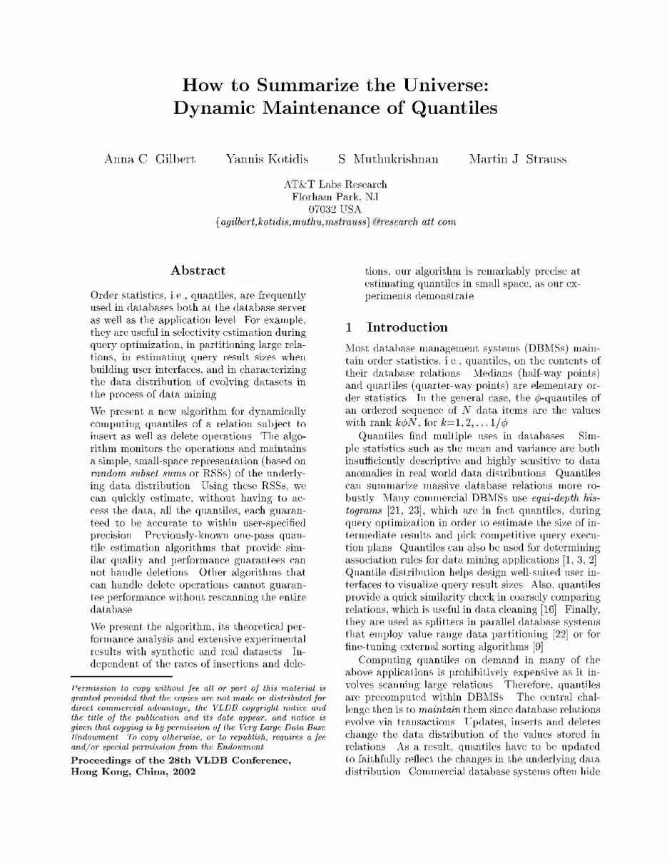
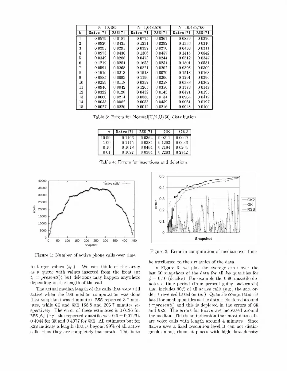
This array can be maintained in the following manner:each time a phone call starts at time ti we add 1 toA[ti] and when the call ends we subtract 1 from A[ti](notice ti is the start time in both cases). For examplethe following CDRs:12:00 999-000-0000 12:00 +112:01 999-000-0001 12:01 +112:03 999-000-0001 12:01 �112:10 999-000-0000 12:00 �1describe two phone calls. The �rst originates fromnumber 999-000-0000, starts at 12:00, and ends at12:10, while the second originates from number 999-000-0001 at 12:01 and lasts for two minutes.We used a dataset of 4.42 million CDRs coveringa period of 18 hours. All algorithms were set up touse 4KB of space (` was 6 for Naive and RSS). Fig-ure 1 shows the number of active calls over time, whileFigure 2 plots the error in computing the median ofthe ongoing calls (in resolution of 1 sec) over time (weprobed for estimates every 10,000 records). We do notinclude Naive in this �gure for clarity. RSS seems tointroduce sporadic large variations in the error of thereported median, especially when lots of deletions arehappening (e.g. near the end of the run). Our inter-polation used for GK2 does not seem to work in thiscase. As more data is processed, RSS shows a clearadvantage over both GK and GK2.This dataset stretches performance on all algo-rithms. As phone calls end and new calls are initi-ated, the mass of the distribution is smoothly shifted

N=10,485 N=1,048,576 N=10,485,760k Naive[7] RSS[7] Naive[7] RSS[7] Naive[7] RSS[7]1 0.0579 0.0181 0.0775 0.0361 0.0839 0.03202 0.0920 0.0435 0.1231 0.0292 0.1333 0.03103 0.0295 0.0295 0.0397 0.0270 0.0430 0.03114 0.0973 0.0438 0.1306 0.0457 0.1415 0.08425 0.0349 0.0288 0.0473 0.0244 0.0512 0.03476 0.1219 0.0284 0.1655 0.0254 0.1801 0.05317 0.0594 0.0268 0.0821 0.0202 0.0898 0.03098 0.1510 0.0213 0.1518 0.0079 0.1518 0.01639 0.0885 0.0093 0.1190 0.0206 0.1291 0.039610 0.0259 0.0118 0.0357 0.0258 0.0388 0.036211 0.0946 0.0042 0.1265 0.0356 0.1373 0.014712 0.0322 0.0120 0.0432 0.0143 0.0471 0.019513 0.0660 0.0214 0.0886 0.0134 0.0964 0.041214 0.0035 0.0082 0.0053 0.0459 0.0061 0.019715 0.0027 0.0220 0.0042 0.0216 0.0048 0.0100Table 3: Errors for Normal[U/2,U/50] distribution� Naive[7] RSS[7] GK GK210.00 0.1196 0.0362 0.0211 0.00091.00 0.1145 0.0384 0.1203 0.00360.10 0.1018 0.0464 0.2194 0.02040.01 0.1097 0.0304 0.2203 0.2742Table 4: Errors for insertions and deletions

0

5000

10000

15000

20000

25000

30000

35000

40000

0 50 100 150 200 250 300 350 400 450

#cal

ls

snapshot

"active calls"

Figure 1: Number of active phone calls over timeto larger values (tis). We can think of the arrayas a queue with values inserted from the front (atti = present()) but deletions may happen anywheredepending on the length of the call.The actual median length of the calls that were stillactive when the last median computation was done(last snapshot) was 4 minutes. RSS reported 3.7 min-utes, while GK and GK2 168.8 and 206.7 minutes re-spectively. The error of these estimates is 0.0126 forRSS[6] (e.g. the reported quantile was 0:5� 0:0126),0.4944 for GK and 0.4977 for GK2. All estimates but forRSS indicate a length that is beyond 99% of all activecalls, thus they are completely inaccurate. This is to

0

0.1

0.2

0.3

0.4

0.5

Snapshot

erro

r GK2GKRSS

Figure 2: Error in computation of median over timebe attributed to the dynamics of the data.In Figure 3, we plot the average error over thelast 50 snapshots of the data for all k� quantiles for� = 0:10 (deciles). For example the 0.90-quantile de-notes a time period (from present going backwards)that includes 90% of all active calls (e.g., the sort or-der is reversed based on tis.). Quantile computation ishard for small quantiles as the data is clustered aroundti=present() and this is depicted in the errors of GKand GK2. The errors for Naive are increased aroundthe median. This is an indication that most data callsare voice calls with length around 4 minutes. SinceNaive uses a �xed resolution level it can not distin-guish among them at places with high data density

0

0.1

0.2

0.3

0.4

0.5

0.6

0.7

0.8

0.9

1

0.1 0.2 0.3 0.4 0.5 0.6 0.7 0.8 0.9

quantile

erro

r

GK2GKNAÏVERSS

Figure 3: Average error over the last 50 snapshots forall �=0.1 quantiles(e.g. around the median). To our knowledge RSSseems the only viable choice for these computations.5 ConclusionsWe have presented an algorithm for maintaining dy-namic quantiles of a relation in presence of both in-sert as well as delete operations. The algorithm main-tains a small-space representation (RSSs) that sum-marizes the universe and the underlying distributionof the data within it. This algorithm is novel in that,without having to access the relation, it can estimateeach quantile to within user-speci�ed precision. Previ-ously published algorithms provide no such guaranteesunder the presence of deletions.We believe our techniques are unique for handlingmassive dynamic datasets. Drawing from the propertythat we summarize the universe instead of a snapshotof the dataset, RSSs can handle dramatic changes orshifts in the data distribution as is demonstrated fromour experiments with real datasets.AcknowledgmentsWe would like to thank David Poole for providing usthe call detail dataset and the anonymous reviewersfor their helpful comments and suggestions.References[1] R. Agrawal, T. Imielinski and A. Swami. Min-ing Associations between Sets of Items in Mas-sive Databases. In Proc. of ACM SIGMOD,pages 207{216, Washington D.C, May 1993.[2] R. Agrawal and R. Srikant. Mining Quantita-tive Association Rules in Large Relational Ta-bles. In Proceedings of ACM SIGMOD, pages1{12, Montreal Canada, June 1996.[3] R. Agrawal and A. Swami. A One-Pass Space-Ecient Algorithm for Finding Quantiles. InProceedings of COMAD, Pune, India, 1995.

[4] N. Alon, Y. Matias, M. Szegedy. The SpaceComplexity of Approximating the FrequencyMoments. JCSS 58(1): 137{147 (1999).[5] N. Alon and J. H. Spencer. The ProbabilisticMethod. Wiley and Sons, New York, 1992[6] K. Alsabti, S. Ranka and V. Singh. A One-PassAlgorithm for Accurately Estimating Quan-tiles for Disk-Resident Data. In Proceedings ofVLDB, pages 346{355, Athens, Greece, 1997.[7] M. Blum, R. W. Floyd, V. R. Pratt,R. L. Rivest and R. E. Tarjan. Time Boundsfor Selection. JCSS 7(4): 448{461, 1973.[8] F. Chen, D. Lambert and J. C. Pinheiro. Incre-mental Quantile Estimation for Massive Track-ing. In Proceedings of KDD, pages 516{522,Boston, August 2000.[9] D. J. DeWitt, J. F. Naughton andD. A. Schneider. Parallel Sorting on a Shared-Nothing Architecture using Probabilistic Split-ting. In PDIS, pages 280{291, 1991.[10] P. B. Gibbons. Distinct Sampling for Highly-Accurate Answers to Distinct Values Queriesand Event Reports. In Proc of VLDB, pages541{550, Rome, Italy, 2001[11] P. Gibbons, Y. Matias and V.Poosala. FastIncremental Maintenance of Approximate His-tograms. In Proceedings of VLDB, pages 466{475, Athens, Greece, 1997.[12] A. C. Gilbert and Y. Kotidis and S. Muthukr-ishnan and M. J. Strauss Sur�ng Waveletson Streams: One-pass Summaries for Approx-imate Aggregate Queries In Proc. of VLDB,2001.[13] A. Gilbert, S. Guha, P. Indyk, Y. Kotidis,S. Muthukrishnan, and M. Strauss. Fast,Small-Space Algorithms for Approximate His-togram Maintenance. In Proceedings of the34th ACM Symposium on Theory of Comput-ing, Montr�eal, Qu�ebec, Canada, May 2002.[14] M. Greenwald and Sanjeev Khanna. Space-E�cient Online Computation of Quantile Sum-maries. In Proceedings of ACM SIGMOD,pages 58{66, Santa Barbara, California, May2001.[15] R. Jain and I. Chlamtac. The P 2 Algo-rithm for Dynamic Calculation of Quantilesand HistogramsWithout Storing Observations.In Communications of the ACM, 28(10):1076{1085, October 1985.

[16] T. Johnson, S. Muthukrishnan, P. Dasu andV. Shkapenyuk. Mining Database Structure;Or, How to Build a Data Quality Browser. InProc. of ACM SIGMOD, to appear, 2002.[17] G.S. Manku, S. Rajagopalan, B.G. Lindsay.Approximate Medians and other Quantiles inOne Pass and with Limited Memory. In Proc ofACM SIGMOD, pages 426{435, Seattle, WA,1998.[18] G.S. Manku, S. Rajagopalan, B.G. Lindsay.Random sampling techniques for space e�cientonline computation of order statistics of largedatasets In Proc of ACM SIGMOD, 1999.[19] J. I. Munro and M. S. Paterson. Selection andSorting with Limited Storage. In TCS 12, 1980.[20] M. S. Paterson. Progress in Selection. Techni-cal Report, University of Warwick, Coventry,UK, 1997.[21] V. Poosala. Histogram-Based Estimation Tech-niques in Database Systems. Ph. D. disserta-tion, University of Wisconsin-Madion, 1997.[22] V. Poosala and Y. Ioannidis. Estimation ofQuery-Result Distribution and its Applicationin Parallel-Join Load Balancing In Proceedingsof VLDB, pages 448{459, 1996.[23] V. Poosala, Y. E. Ioannidis, P. J. Haas andE. J. Shekita. Improved Histograms for Selec-tivity Estimation of Range Predicates. In Procof ACM SIGMOD, pages 294{305, 1996.[24] Y. Matias, J. Vitter and M. Wang. DynamicMaintenance of Wavelet-based Histograms. InProceedings of VLDB, pages 101{110, Cairo,Egypt, Sept. 2000.