the north atlantic ocean as habitat for calanus finmarchicus: environmental factors and life history...
TRANSCRIPT

Accepted Manuscript
The North Atlantic Ocean as habitat for Calanus finmarchicus: environmentalfactors and life history traits
Webjørn Melle, Jeffrey A. Runge, Erica Head, Stéphane Plourde, ClaudiaCastellani, Priscilla Licandro, James Pierson, Sigrun H. Jonasdottir, CatherineJohnson, Cecilie Broms, Høgni Debes, Tone Falkenhaug, Eilif Gaard, AstthorGislason, Michael R. Heath, Barbara Niehoff, Torkel Gissel Nielsen, PierrePepin, Erling Kaare Stenevik, Guillem Chust
PII: S0079-6611(14)00074-3DOI: http://dx.doi.org/10.1016/j.pocean.2014.04.026Reference: PROOCE 1423
To appear in: Progress in Oceanography
Please cite this article as: Melle, W., Runge, J.A., Head, E., Plourde, S., Castellani, C., Licandro, P., Pierson, J.,Jonasdottir, S.H., Johnson, C., Broms, C., Debes, H., Falkenhaug, T., Gaard, E., Gislason, A., Heath, M.R., Niehoff,B., Nielsen, T.G., Pepin, P., Stenevik, E.K., Chust, G., The North Atlantic Ocean as habitat for Calanusfinmarchicus: environmental factors and life history traits, Progress in Oceanography (2014), doi: http://dx.doi.org/10.1016/j.pocean.2014.04.026
This is a PDF file of an unedited manuscript that has been accepted for publication. As a service to our customerswe are providing this early version of the manuscript. The manuscript will undergo copyediting, typesetting, andreview of the resulting proof before it is published in its final form. Please note that during the production processerrors may be discovered which could affect the content, and all legal disclaimers that apply to the journal pertain.

1 2 3 4 5 6 7 8 9 10 11 12 13 14 15 16 17 18 19 20 21 22 23 24 25 26 27 28 29 30 31 32 33 34 35 36 37 38 39 40 41 42 43 44 45 46 47 48 49 50 51 52 53 54 55 56 57 58 59 60 61 62 63 64 65
1
The North Atlantic Ocean as habitat for Calanus finmarchicus: environmental factors and life history 1
traits 2
3
4
Webjørn Melle1, Jeffrey A. Runge
2, Erica Head
3, Stéphane Plourde
4, Claudia Castellani
5, Priscilla 5
Licandro5, James Pierson
6, Sigrun H. Jonasdottir
7, Catherine Johnson
3, Cecilie Broms
1, Høgni Debes
8, 6
Tone Falkenhaug1, Eilif Gaard
8, Astthor Gislason
9, Michael R. Heath
10, Barbara Niehoff
11, Torkel 7
Gissel Nielsen7, Pierre Pepin
12, Erling Kaare Stenevik
1, Guillem Chust
13 8
9
1 Institute of Marine Research, Research Group Plankton, P.O.Box 1870, N-5817 Nordnes, Bergen, 10
Norway. 11
2 School of Marine Sciences, University of Maine, Gulf of Maine Research Institute, 350 Commercial 12
Street, Portland, ME 04101, USA. 13
3 Fisheries and Oceans Canada, Bedford Institute of Oceanography, P.O. Box 1006, Dartmouth, NS, 14
Canada B2Y 4A2. 15
4 Pêches et Océans Canada, Direction des Sciences océaniques et Environnementales, Institut Maurice-16
Lamontagne, 850 route de la Mer, C.P. 1000 Mont-Joli, QC, G5H 3Z4, Canada. 17
5 Sir Alister Hardy Foundation for Ocean Science (SAHFOS), Citadel Hill, Plymouth, PL1 2PB, 18
United Kingdom 19
6 Horn Point Laboratory, University of Maryland Center for Environmental Science, 2020 Horns Point 20
Road, Cambridge, MD 21613, USA. 21
7 National Institute for Aquatic Resources, Technical University of Denmark, Jægersborgs Allé 1, DK-22
2920 Charlottenlund, Denmark. 23
8 Faroe Marine Research Institute, Box 3051, FO-110 Torshavn, Faroe Islands. 24
1 2 3 4 5 6 7 8 9 10 11 12 13 14 15 16 17 18 19 20 21 22 23 24 25 26 27 28 29 30 31 32 33 34 35 36 37 38 39 40 41 42 43 44 45 46 47 48 49 50 51 52 53 54 55 56 57 58 59 60 61 62 63 64 65
2
9 Marine Research Institute, Skulagata 4, P.O. Box 1390, 121 Reykjavik, Iceland. 1
10 MASTS Marine Population Modeling Group, Department of Mathematics and Statistics, University 2
of Strathclyde, Livingstone Tower, 26 Richmond Street, Glasgow, G1 1XH, Scotland 3
11 Alfred Wegener Institute for Polar and Marine Research, Polar Biological Oceanography, 27570 4
Bremerhaven, Germany. 5
12 Northwest Atlantic Fisheries Centre, Fisheries and Oceans Canada, P.O. Box 5667, St. John‘s, 6
Newfoundland Canada A1C 5X1 7
13 AZTI- Tecnalia, Marine Research Division, Txatxarramendi ugartea, 48395 Sukarrieta, Spain. 8
9
10
11
12
13
14
15

1 2 3 4 5 6 7 8 9 10 11 12 13 14 15 16 17 18 19 20 21 22 23 24 25 26 27 28 29 30 31 32 33 34 35 36 37 38 39 40 41 42 43 44 45 46 47 48 49 50 51 52 53 54 55 56 57 58 59 60 61 62 63 64 65
3
1
Abstract 2
Here we present a new, pan-Atlantic compilation and analysis of data on C. finmarchicus abundance, 3
demography, dormancy, egg production and mortality in relation to basin-scale patterns of temperature, 4
phytoplankton biomass, circulation and other environmental characteristics in the context of 5
understanding factors determining the distribution and abundance of C. finmarchicus across its North 6
Atlantic habitat. A number of themes emerge: (1) the south-to-north transport of plankton in the 7
northeast Atlantic contrasts with north-to-south transport in the western North Atlantic, which has 8
implications for understanding population responses of C. finmarchicus to climate forcing, (2) 9
recruitment to the youngest copepodite stages occurs during or just after the phytoplankton bloom in 10
the east whereas it occurs after the bloom at many western sites, with up to 3.5 months difference in 11
recruitment timing, (3) the deep basin and gyre of the southern Norwegian Sea is the centre of 12
production and overwintering of C. finmarchicus, upon which the surrounding waters depend, whereas, 13
in the Labrador/Irminger Seas production mainly occurs along the margins, such that the deep basins 14
serve as collection areas and refugia for the overwintering populations, rather than as centres of 15
production, (4) the western North Atlantic marginal seas have an important role in sustaining high C. 16
finmarchicus abundance on the nearby coastal shelves, (5) differences in mean temperature and 17
chlorophyll concentration between the western and eastern North Atlantic are reflected in regional 18
differences in female body size and egg production, (6) regional differences in functional responses of 19
egg production rate may reflect genetic differences between western and eastern populations, (7) 20
dormancy duration is generally shorter in the deep waters adjacent to the lower latitude western North 21
Atlantic shelves than in the east, (8) there are differences in stage-specific daily mortality rates between 22
eastern and western shelves and basins, but the survival trajectories for cohort development from CI to 23
CV are similar, and (9) early life stage survival is much lower in regions where C. finmarchicus is 24
1 2 3 4 5 6 7 8 9 10 11 12 13 14 15 16 17 18 19 20 21 22 23 24 25 26 27 28 29 30 31 32 33 34 35 36 37 38 39 40 41 42 43 44 45 46 47 48 49 50 51 52 53 54 55 56 57 58 59 60 61 62 63 64 65
4
found with its congeners, C. glacialis and/or C. hyperboreus. This compilation and analysis provides 1
new knowledge for evaluation and parameterisation of population models of C. finmarchicus and their 2
responses to climate change in the North Atlantic. The strengths and weaknesses of modeling 3
approaches, including a statistical approach based on ecological niche theory and a dynamical approach 4
based on knowledge of spatial population dynamics and life history, are discussed, as well as needs for 5
further research. 6
7

1 2 3 4 5 6 7 8 9 10 11 12 13 14 15 16 17 18 19 20 21 22 23 24 25 26 27 28 29 30 31 32 33 34 35 36 37 38 39 40 41 42 43 44 45 46 47 48 49 50 51 52 53 54 55 56 57 58 59 60 61 62 63 64 65
5
1. Introduction 1
2
The northern North Atlantic Ocean is characterized by its circulation and water mass 3
distribution, its extensive latitudinal expanse (from roughly 40 to 75oN) and topography, and its 4
seasonally and geographically varying wide ranges of temperature, salinity and light conditions, which 5
provide a variety of habitats for its biota. Regional differences in physical features lead to differences 6
in the timing and intensity of the annual cycles of primary production, and in the distributions, 7
abundances and seasonal cycles of planktonic grazers and their predators. The distribution of any 8
zooplankton species in the North Atlantic is the manifestation of its ability to maintain itself within this 9
range of conditions, from suboptimal to optimal, that constitute its habitat. 10
11
One approach to understanding the distribution of a species is to examine and define its 12
ecological niche in terms of its range of tolerance based on a series of environmental factors (e.g. 13
Helaouët and Beaugrand, 2009). Advances in statistical and numerical techniques, such as generalized 14
linear models (GLM) and geographic information systems (GIS), have been applied to quantify species 15
distributions, in species distribution models (Elith and Leathwick, 2009), habitat distribution models 16
(Guisan and Zimmerman, 2000) and habitat suitability models (e.g. Hirzel et al., 2002). Extrapolation 17
to future distribution patterns resulting from habitat change, however, confronts the statistical and 18
ecological assumptions of these models (Elith and Leathwick, 2009). To gain predictive insight into the 19
consequences of habitat change on the abundance of a species and on shifts in its range and 20
biogeographic boundaries, it is also necessary to understand, at the species level, processes determining 21
population dynamics and life history in relation to environmental changes that affect both physiological 22
and behavioural responses and dispersal patterns. This information can be integrated into complex 23
1 2 3 4 5 6 7 8 9 10 11 12 13 14 15 16 17 18 19 20 21 22 23 24 25 26 27 28 29 30 31 32 33 34 35 36 37 38 39 40 41 42 43 44 45 46 47 48 49 50 51 52 53 54 55 56 57 58 59 60 61 62 63 64 65
6
process models (e.g. Korzukhin et al., 1996) in the marine realm by means of coupled physical-1
biological models (e.g. de Young et al., 2010). 2
3
The planktonic copepod, Calanus finmarchicus, is one of the most important multicellular 4
zooplankton species in the northern North Atlantic, based on its abundance and role in food webs and 5
biogeochemical cycles. It is the subject of a book (Marshall and Orr, revised edition, 1972) and over 6
1000 research articles since its publication. It has been the target species of several previous basin-scale 7
research programs, including investigation of C. finmarchicus migrations between oceanic and shelf 8
seas off Northwest Europe (ICOS: e.g. Heath et al., 1999), Trans-Atlantic Studies of Calanus 9
finmarchicus (TASC: e.g. Tande and Miller, 2000), the Global Ocean Ecosystem Dynamics program 10
(GLOBEC: e.g. Gifford et al., 2010), and the ongoing EURO-BASIN program. From the basin-wide 11
programs, in combination with local time series measurements and Continuous Plankton Recorder 12
(CPR) surveys, a tremendous source of information and knowledge of C. finmarchicus distribution and 13
life history traits has emerged. Basin scale themes such as the past, present and possible future 14
distribution of C. finmarchicus, based on observations and inferences from statistical and process 15
models (Planque and Fromentin, 1996; Speirs et al., 2005, 2006; Helaouët and Beaugrand, 2007, 2009; 16
Reygondeau and Beaugrand, 2011) have been investigated. In addition, process and modeling studies 17
have studied C. finmarchicus phenology, grazing, egg production, over-wintering strategy, mortality 18
and role in carbon flux budgets (e.g. Aksnes and Blindheim, 1996; Heath et al., 2000, 2004; Ohman et 19
al. 2004; Melle et al., 2004; Broms and Melle 2007; Stenevik et al., 2007; Johnson et al., 2008; Broms 20
et al., 2009; Bagoeien et al., 2012; Head et al., 2013a; Hjollo et al., 2013). We review this knowledge 21
of C. finmarchicus life history and its North Atlantic habitat in the following section. We then compile, 22
for the first time, the across-basin data sets and provide a synthesis of previously reported and new 23
information on spatially and seasonally resolved demography and life history strategies related to 24

1 2 3 4 5 6 7 8 9 10 11 12 13 14 15 16 17 18 19 20 21 22 23 24 25 26 27 28 29 30 31 32 33 34 35 36 37 38 39 40 41 42 43 44 45 46 47 48 49 50 51 52 53 54 55 56 57 58 59 60 61 62 63 64 65
7
seasonal cycles, development, reproduction, dormancy and mortality across the North Atlantic. We 1
use this information to identify the factors involved in determining distribution and abundance of C. 2
finmarchicus, including the important question of connectivity between basin and shelf populations on 3
both sides of the North Atlantic. We consider whether genetic differences between populations in the 4
northeast and northwest/central North Atlantic lead to differences in physiological and ecological 5
responses to changes in environmental conditions. Our overall objective is to provide parameter values 6
and new knowledge of C. finmarchicus life history characteristics on a North Atlantic basin scale and, 7
thus to further the development of habitat and basin-scale dynamic models that can be used to predict 8
the effects of climate change on C. finmarchicus populations. 9
10
1.1. The North Atlantic habitat 11
Ocean circulation is fundamental to the dynamics of a planktonic species‘ habitat. The North 12
Atlantic surface circulation system is made up of a series of gyres, encircled by strong boundary 13
currents (Fig. 1a). In the west, the Northwest Atlantic Subpolar Gyre, commonly referred to as the 14
Subpolar Gyre, includes the Labrador and Irminger Seas and is defined by bathymetry to the north and 15
the North Atlantic Current to the south. In the east, the Southern Norwegian Sea Gyre, a cyclonic gyre 16
over the Norwegian Basin of the southern Norwegian Sea, is bounded by bathymetry to the north and 17
by the North Atlantic Current to the south. These two gyres are interconnected, however, and together 18
can be regarded as one basin-scale North Atlantic Subpolar Gyre system, throughout which organisms, 19
including plankton, can be broadly distributed over appropriate time scales, but which nevertheless 20
shows regional differences in ecological characteristics due to the responses of individual species to 21
local conditions. 22
23

1 2 3 4 5 6 7 8 9 10 11 12 13 14 15 16 17 18 19 20 21 22 23 24 25 26 27 28 29 30 31 32 33 34 35 36 37 38 39 40 41 42 43 44 45 46 47 48 49 50 51 52 53 54 55 56 57 58 59 60 61 62 63 64 65
8
The Gulf Stream System transports warm and saline water from west to east in the North 1
Atlantic at a latitude of about 400N in the west (e.g. Reverdin et al., 2003). At about 54
0W, the Gulf 2
Stream splits into two branches, a northern branch connected to the North Atlantic Current and a 3
southern branch connected to the Azores Current. The Azores Current and the southward flowing 4
Canary Current limit the Subtropical Gyre to the north and east. The North Atlantic Current flows to 5
the northeast, with branches flowing into the Icelandic basin and Irminger Sea before the main body 6
enters the Norwegian Sea as the Norwegian Atlantic Current. Thus, the Northeast Atlantic is strongly 7
influenced by northward flowing warm and saline water. Warmer water of Atlantic origin also 8
circulates clockwise around Iceland. Cold Arctic water enters the system from the Arctic Ocean 9
through the Fram Straight as the East Greenland Current and east of Baffin Island as the Baffin Island 10
Current. North of Iceland, the East Icelandic Current separates from the East Greenland Current, 11
bringing Arctic water eastward into the western Norwegian Sea. The East Greenland Current itself 12
continues southward and meets the warmer Atlantic water of the Irminger Current, with both turning 13
around the southern tip of Greenland and entering the Labrador Sea. This northwesterly flow has a cold 14
water shelf component (the West Greenland Current) and a warmer, deeper offshore component 15
(identified as the Irminger Current), which provides a major warm water input to the Labrador Sea. The 16
main sources of water to the Labrador Shelf and Slope are the outflows from the Arctic via Hudson 17
Strait and the Baffin Island Current, and the branch of the slope water current that follows the 18
bathymetry westward across the mouth of Davis Strait. These water masses mix off Hudson Strait 19
together forming the inshore (shelf) and offshore (slope) branches of the Labrador Current moving 20
southwards. Part of the inshore branch enters the Gulf of St. Lawrence through the Strait of Belle Isle, 21
and part continues on to the Newfoundland Shelf and turns around the southeast tip of Newfoundland. 22
A substantial portion of the offshore branch turns to the northeast at the Tail of the Grand Bank to join 23
the North Atlantic Current, but a portion also flows around the Tail of the Grand Bank and along the 24
1 2 3 4 5 6 7 8 9 10 11 12 13 14 15 16 17 18 19 20 21 22 23 24 25 26 27 28 29 30 31 32 33 34 35 36 37 38 39 40 41 42 43 44 45 46 47 48 49 50 51 52 53 54 55 56 57 58 59 60 61 62 63 64 65
9
edge of the Scotian Shelf and Georges Bank (Fratantoni and MacCartney, 2010; Loder et al., 1998). 1
Cross-shelf transport of slope water at the Laurentian Channel, Scotian Gulf, and Northeast Channel 2
influences the deep water properties of the Gulf of St. Lawrence, western Scotian Shelf, and Gulf of 3
Maine, and variability in the slope water source, e.g. cold Labrador Slope water vs. warm Atlantic 4
slope water, can drive substantial changes in deep water temperatures on the western Scotian shelf and 5
in the northwest Atlantic marginal seas (Bugden,1991; Petrie and Drinkwater, 1993; Gilbert et al., 6
2005). In contrast to the northeast Atlantic, the western Atlantic shelf and slope waters are therefore 7
strongly influenced by southerly flowing cold and low salinity water of Arctic origin. As we discuss 8
later, this contrast in physical regime has implications for understanding east-west differences in effects 9
of climate forcing on species distribution. 10
11
The topography of the North Atlantic is characterised by several deep basins: the Labrador Sea 12
basin, the Iceland basin and Irminger Sea, the Norwegian Sea basin in the southern Norwegian Sea, the 13
Lofoten basin in the Northern Norwegian Sea and the Greenland Sea basin. More or less well defined 14
cyclonic gyres are located over these deep basins, which thus offer reduced dispersal for animals within 15
the gyres and possibilities for deep overwintering or deep diurnal migration. In addition to these deep 16
basins are the Norwegian deep fjords (up to 1,300 m deep) and basins or troughs (200-400 m depth) in 17
the northwest Atlantic marginal seas (Gulf of Maine and Gulf of St. Lawrence). 18
19
The geographical pattern of seas surface temperature (SST) in the North Atlantic is strongly 20
influenced by the Gulf Stream and North Atlantic Current, resulting in a southwest to northeast 21
orientation of isotherms (Fig. 1a, 2a). Because the same SST is found much farther south in the west 22
than in the east, with very different seasonal and diurnal light regimes, habitats that have similar annual 23
average temperatures in the western and eastern North Atlantic can have biologically quite different 24

1 2 3 4 5 6 7 8 9 10 11 12 13 14 15 16 17 18 19 20 21 22 23 24 25 26 27 28 29 30 31 32 33 34 35 36 37 38 39 40 41 42 43 44 45 46 47 48 49 50 51 52 53 54 55 56 57 58 59 60 61 62 63 64 65
10
conditions. For example, Georges Bank has, on average, temperatures similar to those in the southern 1
Norwegian Sea, but because it is much farther south, light levels in winter are typically sufficient to 2
support primary production. By contrast, on the eastern side of the Atlantic, although temperatures 3
remain relatively high during winter, phytoplankton production ceases, whereas in summer during the 4
growth season, the midnight sun and long days prevail. In addition, in the west cool water 5
temperatures, caused by cold winters and the influence of Arctic waters, allow for the presence of the 6
same visually guided predators much farther south than in the northeast Atlantic. 7
8
The North Atlantic pattern of primary production (PP) is strongly related to light conditions and 9
SST, but also to nutrient supply, and to mechanisms of water column vertical stabilisation and grazing. 10
The northeast Atlantic is a typical spring bloom system, although the seasonal cycle of PP differs 11
between deep basins and shelves. In the deep Norwegian Sea basin the pattern of seasonal 12
phytoplankton production has been shown to comply with Sverdrup‘s concept of critical depth 13
(Sverdrup, 1953), although newer publications indicate that the controlling mechanisms may be more 14
complex or at least regionally different (e.g. Behrenfeld, 2010; Mahavedan et al., 2012). According to 15
the critical depth concept, production will occur when the mixing depth of algal cells is less than a 16
critical depth such that net production is positive. This usually occurs in March-April and the bloom 17
starts in May-June when the pycnocline approaches the upper 30-40 m (Rey, 2004; Bagoeien et al., 18
2012; Zhai et al., 2012). The timing of the bloom may vary by more than a month among years (Rey, 19
2004) and the chlorophyll concentration of the upper mixed layer is on average less than 3 mg m-3
20
(Bagoeien et al., 2012). On the Norwegian shelf the water column is permanently stratified by a near 21
surface layer of fresh (light) coastal water or is restricted by shallow bottom depths, so that pre-bloom 22
production and blooms tend to start earlier and to some extent are more intense, providing relatively 23
high chlorophyll concentrations in the water column (Rey, 2004). During the bloom diatoms are the 24

1 2 3 4 5 6 7 8 9 10 11 12 13 14 15 16 17 18 19 20 21 22 23 24 25 26 27 28 29 30 31 32 33 34 35 36 37 38 39 40 41 42 43 44 45 46 47 48 49 50 51 52 53 54 55 56 57 58 59 60 61 62 63 64 65
11
main algal group (Rey, 2004). The post-bloom period lasts until September and is characterised by 1
flagellates, utilising re-cycled nutrients. It has been suggested that pre-bloom levels of phytoplankton 2
are lower than might be expected in the Norwegian Sea due to the grazing activity of the large 3
overwintering population of Calanus finmarchicus, which returns to the surface at this time, and that 4
the intensity of the spring bloom itself is kept low by grazing by the offspring of the overwintered C. 5
finmarchicus (Rey, 2004). 6
7
In the Irminger Sea, spatial variability in the timing and magnitude of the spring bloom is 8
considerable, reflecting differences in the seasonal timing of stratification of the surface waters 9
(Henson et al., 2006, Waniek and Holliday, 2006, Gudmundsson et al., 2009; Mahavedan et al., 2012; 10
Zhai et al., 2012). On the Iceland and Greenland shelves fringing the Irminger Sea, the growth of 11
phytoplankton usually starts in late April culminating in June and July, whereas in the central region of 12
the Irminger Sea growth usually starts in early May with a maximum in June. As in the northeast 13
Atlantic, timing of the start of the bloom is patchy and may vary interannually by as much as one 14
month, influenced by storms and mixed layer eddy restratification (Mahavedan et al., 2012). 15
16
In the northwest Atlantic regions, the timing of spring bloom initiation generally varies with 17
latitude, but there can be substantial departures from this trend among shelf areas due to local or 18
regional processes (O‘Reilly and Zetlin, 1998; Platt et al., 2010). Spring and fall blooms tend to start 19
earlier in shallow water, and spring blooms tend to be longer in shallow water (O‘Reilly et al., 1987). 20
Interannual variability in bloom timing can be high in the northwest Atlantic (Thomas et al., 2003; Platt 21
et al., 2010). In the Gulf of Maine/Georges Bank region, the spring bloom starts earliest in the shallow 22
coastal areas (January – March), later over Georges Bank (March – April), and latest in the deep basins 23
of the Gulf of Maine and over the shelf edge (April – May) (O‘Reilly et al., 1987). On the western and 24

1 2 3 4 5 6 7 8 9 10 11 12 13 14 15 16 17 18 19 20 21 22 23 24 25 26 27 28 29 30 31 32 33 34 35 36 37 38 39 40 41 42 43 44 45 46 47 48 49 50 51 52 53 54 55 56 57 58 59 60 61 62 63 64 65
12
eastern Scotian Shelf, the spring bloom starts in March or April and peaks after about a month, while in 1
the Scotian Slope waters it starts in February or March and peaks in May (Zhai et al., 2011). In the 2
Gulf of St. Lawrence, the spring bloom is earlier in the northeast and southern Gulf (April – May) than 3
in the lower St. Lawrence Estuary (June – July) (reviewed by Zhi-Ping et al., 2010). On the Grand 4
Bank and Flemish Cap, the spring bloom starts in late March or April and peaks after about a month, 5
while on the Labrador Shelf it starts in May (Fuentes-Yaco et al., 2007). The spring bloom starts 6
relatively late (April – June) in the central Labrador Sea, but slightly earlier (April – May) in the 7
northern Labrador Sea, where early stratification is driven by offshore flow of relatively freshwater 8
from the West Greenland Shelf (Frajka-Williams and Rhines, 2010). Estimates of annual primary 9
production from satellite ocean colour and temperature from 1998 – 2004 indicate that the highest 10
offshore production in the northwest Atlantic occurs on Georges Bank and in the outflow from the 11
Hudson Strait (ca. 275 – 325 gC m-2
y-1
), while the lowest production occurs in the Labrador slope 12
waters (ca. 150 gC m-2
y-1
) and southern Labrador Sea (ca. 175 – 200 gC m-2
y-1
) (Carla Caverhill, pers. 13
comm., Platt et al., 2008). 14
15
1.2. Calanus finmarchicus 16
The copepod Calanus finmarchicus is the main contributor to mesozooplankton biomass 17
throughout the North Atlantic. Population centres, defined as regions where overwintering populations 18
exceed 15,000 m-2
, have been identified in the Labrador Sea, northern Irminger Basin, northern Iceland 19
Basin, Faroe-Shetland Channel, eastern Norwegian Sea and Norwegian Trench (Heath et al., 2004). 20
Based on this criterion, slope waters off the Grand Bank of Newfoundland, the Laurentian Channel of 21
the Gulf of Saint Lawrence, deep basins in the Gulf of Maine, and slope waters of the western Scotian 22
Shelf are also population centres (Plourde et al, 2001; Head and Pepin, 2008; Maps et al., 2012). C. 23
finmarchicus makes up >80% of large copepods by abundance in the central Labrador Sea in spring 24
1 2 3 4 5 6 7 8 9 10 11 12 13 14 15 16 17 18 19 20 21 22 23 24 25 26 27 28 29 30 31 32 33 34 35 36 37 38 39 40 41 42 43 44 45 46 47 48 49 50 51 52 53 54 55 56 57 58 59 60 61 62 63 64 65
13
and summer (Head et al., 2003, sampled with a 200 m mesh net, which in this cold region catches all 1
Calanus copepodite stages), about 40-70 % of the mesozooplankton community on Flemish Cap, east 2
of the Grand Bank of Newfoundland (Anderson, 1990, sampled with 333-505 m mesh nets, which 3
excludes the youngest copepodite stages as well as smaller copepod species) , and 40-90% of the 4
zooplankton community by abundance in waters around Iceland in summer (Gislason and Astthorsson, 5
2000, sampled with a 200-m mesh net which here excludes some of the smaller stages) . There are 6
apparently two major overwintering areas, which serve as population reservoirs and distribution 7
centres , in the two subpolar gyres; one in the Labrador/Irminger Seas and the other in the southern 8
Norwegian Sea (Conover, 1988; Planque et al., 1997; Head et al., 2003; Melle et al., 2004; Heath et al., 9
2008; Broms et al., 2009). These cyclonic gyres are centred over deep ocean basins, so that they can 10
retain populations as they are overwintering at depth, a necessity for C. finmarchicus to close its life 11
cycle both spatially and inter-annually (Heath et al., 2004; Heath et al., 2008). From these distribution 12
centres C. finmarchicus is transported to the surrounding shelves and shallow seas (e.g. the Labrador, 13
Newfoundland shelves; North and Barents seas) and ultimately to more distant regions (e.g. Scotian 14
Shelf, Gulf of Maine) (Speirs et al., 2006; Heath et al., 2008). There is evidence from genetic analysis 15
that there are two to four distinct C. finmarchicus populations, with greatest differences occurring 16
between the northwest/central North Atlantic and northeast Atlantic (Unal and Bucklin, 2010). Toward 17
the Arctic domain, C. finmarchicus co-occurs with its larger congeners, C. hyperboreus and C. 18
glacialis, while in the southeast it co-occurs with the temperate water species, C. helgolandicus 19
(Conover, 1988; Hirche, 1991; Head et al., 2003; Melle et al., 2004; Bonnet et al., 2005; Hop et al., 20
2006; Broms et al., 2009). 21
22
Throughout its biogeographic range, C. finmarchicus is a dominant grazer and the main prey 23
for numerous planktivorous fish, including herring, mackerel, capelin and young blue whiting and 24
1 2 3 4 5 6 7 8 9 10 11 12 13 14 15 16 17 18 19 20 21 22 23 24 25 26 27 28 29 30 31 32 33 34 35 36 37 38 39 40 41 42 43 44 45 46 47 48 49 50 51 52 53 54 55 56 57 58 59 60 61 62 63 64 65
14
salmon (e.g. Dalpadado et al., 2000; Darbyson et al., 2003; Dommasnes et al., 2004; Skjoldal, 2004; 1
Overholtz and Link, 2007; Smith and Link, 2010; Langøy et al., 2012). The larvae of many fish species 2
also feed, sometimes almost exclusively, on the eggs and nauplii of C. finmarchicus, and copepodite 3
stages are important food for the juvenile fish in shelf and shallow sea nursery areas (Runge and de 4
Lafontaine, 1996; Heath and Lough, 2007). 5
6
During its life cycle from egg to adult (females, CVIF and males, CVIM), C. finmarchicus pass 7
through six nauplius (NI-NVI) and five copepodite stages (CI-CV). The first two naupliar stages do not 8
feed. The life cycle of C. finmarchicus is annual in its main distributional area (Conover, 1988; Heath 9
et al., 2000a; Irigoien, 2000; Hirche et al., 2001; McLaren et al., 2001; Heath et al., 2008, Broms et al. 10
2009; Bagoeien et al., 2012; Head et al., 2013b). In regions influenced by Arctic outflow, however, 11
where water temperatures are low, development rates are reduced and young copepodites (CI-CIII) are 12
found among the older overwintering stages (Broms and Melle, 2007; Heath et al., 2008), suggesting 13
that there is either a multiannual life cycle or an inability to reach stages that can survive the winter 14
within the first season, leading to expatriation (Melle and Skjoldal, 1998). Although there is only one 15
generation per year within the main distributional area within the subpolar gyre (e.g. Labrador Sea, 16
Northern Norwegian Sea) farther south (e.g. Georges Bank) there may be up to three generations per 17
year (Irigoien, 2000; Hirche et al., 2001; McLaren et al., 2001; Plourde et al., 2001; Head et al., 18
2013b). The number of generations may vary among years at the same location (Irigoien, 2000) and in 19
some areas (e.g. Newfoundland Shelf) distinct generations are not evident. 20
21
The main overwintering stage is the pre-adult CV (Conover, 1988). In the deep basins, C. 22
finmarchicus CVs spend most of the year at depths below 400-1000 m (Heath et al., 2000b, 2004; 23
Melle et al., 2004). In the northern Norwegian Sea, overwintering C. finmarchicus are most abundant 24
1 2 3 4 5 6 7 8 9 10 11 12 13 14 15 16 17 18 19 20 21 22 23 24 25 26 27 28 29 30 31 32 33 34 35 36 37 38 39 40 41 42 43 44 45 46 47 48 49 50 51 52 53 54 55 56 57 58 59 60 61 62 63 64 65
15
between about 600 and 1200 m, at temperatures less than 2 °C (Edvardsen et al., 2006). In the Iceland 1
Basin, overwintering C. finmarchicus reside between about 400 m and the bottom (> 2000 m) at 2
temperatures about 3-8 °C, while in the Irminger Basin, they reside between about 200 and 1800 m at 3
temperatures of 3-6 °C (Gislason and Astthorsson, 2000). In the northwest Atlantic, overwintering C. 4
finmarchicus occupy a broad and spatially variable depth range, in temperatures ranging from 1 to 10 5
°C (Head and Pepin, 2008). Overwintering depths are shallowest in Gulf of Maine basins, the 6
Laurentian Channel and in eastern Scotian slope waters (ca. 100 – 400 m) and deeper in western 7
Scotian slope water (400 – 950 m) and in Newfoundland slope waters (400 – 1500 m). In the western 8
part of the central Labrador Sea overwintering depths are variable, but generally <1000 m, while in the 9
eastern Labrador Sea near the Greenland shelf, C. finmarchicus overwinters at greater depths, similar to 10
those in the Irminger Sea, (Head and Pepin, 2008). Individual C. finmarchicus enter dormancy in 11
summer and fall (Hirche, 1996a), carrying with them lipid stores that make up most of their body 12
weight. These lipid stores sustain metabolism during overwintering and subsequent molting and partial 13
development of gonads in mid-late winter (Rey-Rassat et al., 2002). Dormant copepodites are 14
characterized by reduced metabolism and arrested or slowed development (Saumweber and Durbin, 15
2006). In many locations there is evidence that fourth stage copepodites (CIVs) enter dormancy, with 16
higher proportions of dormant CIV copepodites observed in the northeast Atlantic than in the northwest 17
Atlantic (Heath et al., 2004; Melle et al., 2004; Head and Pepin, 2008). The implications of CIV 18
dormancy have not been rigorously examined, although it is unlikely that CIVs can molt to CVs 19
without feeding since they are significantly smaller. The descent to overwintering depths at Weather 20
Station India occurred during at least two pulses towards the end of each of two cohorts (Irigoien, 21
2000), whereas elsewhere individuals from different generations may descend over several months 22
(e.g. Johnson et al., 2008). 23
24

1 2 3 4 5 6 7 8 9 10 11 12 13 14 15 16 17 18 19 20 21 22 23 24 25 26 27 28 29 30 31 32 33 34 35 36 37 38 39 40 41 42 43 44 45 46 47 48 49 50 51 52 53 54 55 56 57 58 59 60 61 62 63 64 65
16
Arousal from the winter diapause generally occurs in mid-late winter, when most CVs leave 1
dormancy, molt into adults and mate upon returning to the surface (e.g. Melle et al., 2004). Females 2
then lay eggs in response to food levels, for which chlorophyll a concentration is a useful proxy (Runge 3
et al., 2006). The arctic species, Calanus hyperboreus, uses internal body stores including lipids to 4
produce eggs without any external food supply (Conover, 1988), but the extent to which internal body 5
stores contribute to egg production for C. finmarchicus is still unresolved. In many populations, not all 6
CVs from the new year‘s generation enter dormancy; some molt on to adulthood, so that reproduction 7
can occur throughout the year (e.g. Durbin et al., 1997; Heath et al., 2008). 8
9
In the Norwegian Sea, studies have demonstrated that spawning occurs at relatively low food 10
concentrations and low individual rates before the spring bloom. However, population egg production 11
rates were higher during the pre-bloom period than during the bloom itself, due to the higher 12
abundance of females (Niehoff et al., 1999; Richardson et al., 1999; Stenevik et al. 2007; Debes et al., 13
2008). Regional differences in the timing and intensity of C. finmarchicus reproduction have been 14
observed (e.g., Plourde et al., 2001; Runge et al., 2006; Stenevik et al. 2007; Head et al., 2013a; Head 15
et al. 2013b), reflecting regional variations in the timing and intensity of spring blooms. These results 16
are mainly based on individual studies that have usually been limited to one or a few regions; whether 17
responses of females to environmental conditions can be generalized throughout the North Atlantic has 18
not been addressed. 19
20
The maximum abundance of CIs of the first generation has often been observed to occur during 21
the peak of bloom or just after (Hirche et al., 2001; Melle et al., 2004; Bagoeien et al., 2012), and these 22
CIs must have arisen from eggs spawned before the bloom. On the other hand, during the pre-bloom 23
period, mortality rates are thought to be high due to starvation of first feeding nauplii and/or predation 24
1 2 3 4 5 6 7 8 9 10 11 12 13 14 15 16 17 18 19 20 21 22 23 24 25 26 27 28 29 30 31 32 33 34 35 36 37 38 39 40 41 42 43 44 45 46 47 48 49 50 51 52 53 54 55 56 57 58 59 60 61 62 63 64 65
17
on eggs during the pre-bloom phase, which may include predation by the females themselves (e.g. 1
Ohman and Hirche, 2001; Plourde et al., 2001; Heath et al., 2008). The CIs-CIIIs are found exclusively 2
in the upper mixed layer or in the pycnocline, if a subsurface chlorophyll maximum develops during 3
the post-bloom phase (Melle and Skjoldal, 1989; Irigoien, 2000; Melle et al., 2004). 4
5
Mortality and survival are key parameters in Calanus finmarchicus population dynamics. In the 6
early stages (eggs, nauplii) they are especially important in determining overall recruitment success 7
(i.e., Ohman and Hirche, 2001; Ohman et al., 2002; Plourde et al., 2009a, 2009b). Survivorship of C. 8
finmarchicus is mainly governed by temperature, food availability and/or con-specific abundance, 9
which results in marked seasonal and regional differences in stage-specific mortality patterns (Ohman 10
and Hirche, 2001; Ohman et al., 2002; Ohman et al., 2004; Heath et al., 2008; Plourde et al., 2009b). In 11
the northwest Atlantic, the integration of stage-specific daily mortality rates over the entire cohort 12
developmental period revealed significant differences in survival trajectories among seasons and sub-13
areas, associated with differences in environmental conditions (Plourde et al., 2009b). The use of 14
mortality formulations corresponding to different sets of environmental conditions have enabled 15
modeling of region-specific C. finmarchicus population dynamics, a significant step forward in basin-16
wide biological modeling for the species (Runge et al., 2005; Neuheimer et al., 2010; Maps et al., 17
2010; Maps et al., 2011). 18
19
In the Norwegian Sea studies of predation mortality for C. finmarchicus copepodite stages have 20
been conducted to evaluate feeding conditions for pelagic fish stocks and to investigate top down 21
versus bottom up processes in the ecosystem. Analysis of stomach samples have shown herring, 22
mackerel and young blue whiting to be important predators on Calanus finmarchicus copepodites 23
(Dalpadado et al. 2000; Gislason and Astthorsson, 2002; Prokopchuk and Sentyabov, 2006). 24

1 2 3 4 5 6 7 8 9 10 11 12 13 14 15 16 17 18 19 20 21 22 23 24 25 26 27 28 29 30 31 32 33 34 35 36 37 38 39 40 41 42 43 44 45 46 47 48 49 50 51 52 53 54 55 56 57 58 59 60 61 62 63 64 65
18
Consumption by herring has been estimated at about 20-100 % of the annual C. finmarchicus 1
production (Dommasnes et al. 2000; Skjoldal et al. 2004; Utne et al. 2012). Other potential predatory 2
taxa in the Norwegian Sea are krill, amphipods, cnidarians, chaetognaths, large copepods and 3
mesopelagic fishes. For these taxa reliable estimates of biomass, diet and stomach evacuation rates are 4
generally not known, making their predatory impact hard to estimate. Nevertheless, it seems clear that 5
these taxa may also be important predators of C. finmarchicus copepodites (Melle et al. 2004; Skjoldal 6
et al. 2004). 7
8
2. Materials and methods 9
10
2.1. Hydrography and chlorophyll measurements and analyses 11
CTD probes were used to collect hydrographic data (temperature and salinity) at all sampling 12
stations (Fig 1b, c). Water samples for measurements of chlorophyll-a concentration were collected 13
using water bottles on a rosette on the CTD or on a hydro-wire. At most sites the hydrographic and 14
chlorophyll samples were taken in concert with the zooplankton net samples. CTD profiling depths and 15
water bottle depths varied among sampling sites. Methodologies for determination of chlorophyll a 16
concentrations are described in publications or can be retrieved from the data provider associated with 17
each station as shown in Tables 1 and 2. Temperatures (0C) were averaged over various depth ranges, 18
while chlorophyll concentrations were either integrated (mg m-2
) or averaged (mg m-3
) over various 19
depth ranges, as indicated in figure captions. At each site where time series measurements were made, 20
temperatures and chlorophyll concentrations were first averaged over 2-week periods within a given 21
year and then over the 2-week periods for all years. 22
23
1 2 3 4 5 6 7 8 9 10 11 12 13 14 15 16 17 18 19 20 21 22 23 24 25 26 27 28 29 30 31 32 33 34 35 36 37 38 39 40 41 42 43 44 45 46 47 48 49 50 51 52 53 54 55 56 57 58 59 60 61 62 63 64 65
19
The basin scale distribution of Sea Surface Temperature (SST, ºC) was calculated from data 1
available from the British Atmospheric Data Centre (BADC); [HadISST 1.1 dataset 2
(http://badc.nerc.ac.uk/home/)]. Monthly SST records (1 degree by 1 degree) or the years 2000-2009 3
were firstly averaged by year and then used to produce the overall average SST map for the period of 4
reference. 5
6
2.2. Mapping of Calanus finmarchicus distribution at the basin scale 7
The CPR survey is an upper layer plankton monitoring program that has regularly collected 8
samples (ideally at monthly intervals) in the North Atlantic and adjacent seas since 1946 (Warner and 9
Hays, 1994). Water from approximately 6 m depth (Batten et al., 2003a) enters the CPR through a 10
small aperture at the front of the sampler and travels down a tunnel where it pass through a silk filtering 11
mesh of 270 μm before exiting at the back of the CPR. The plankton filtered on the silk is analysed in 12
sections corresponding to 10 nautical miles (approx. 3 m3 of seawater filtered) and the plankton 13
microscopically identified (Jonas et al., 2004). In the present study we used the CPR data to investigate 14
the current basin scale distribution of C. finmarchicus (CV-CVI). Monthly data collected between 2000 15
and 2009 were gridded using the inverse-distance interpolation method (Isaaks and Srivastava, 1989), 16
in which the interpolated values were the nodes of a 2 degree by 2 degree grid. The resulting twelve 17
monthly matrices were then averaged within the year and the data log-transformed (i.e. log10 (x+1)). 18
The Phytoplankton Colour Index (PCI), which is a visual assessment of the greenness of the silk, is 19
used as an indicator of the distribution of total phytoplankton biomass across the Atlantic basin (Batten 20
et al., 2003b; Richardson et al., 2006). 21
22
2.3. Seasonal dynamics of Calanus finmarchicus 23

1 2 3 4 5 6 7 8 9 10 11 12 13 14 15 16 17 18 19 20 21 22 23 24 25 26 27 28 29 30 31 32 33 34 35 36 37 38 39 40 41 42 43 44 45 46 47 48 49 50 51 52 53 54 55 56 57 58 59 60 61 62 63 64 65
20
Seasonal abundance cycles of Calanus finmarchicus were derived from samples taken at sites 1
across the North Atlantic (Table 1, Fig. 1b). The sampling sites include both coastal and oceanic 2
stations and vary from relatively cold to warm water locations. Sampling frequency also differs among 3
sites; the more easily accessed coastal sites were generally visited more frequently than the offshore 4
sites. An overview of sampling sites characteristics, sampling gear and methods is provided in Table 1. 5
Temperatures and chlorophyll concentrations are provided for all sites and details on depth ranges and 6
units are given in Appendix figures 1-6. 7
8
2.4. Dormancy 9
Dormancy timing was calculated using metrics developed by Johnson et al. (2008). Briefly, 10
entry to dormancy was determined as the date when the CV portion of the total composition of the 11
copepodites and adults comprised 50% of the overall maximum CV proportion, calculated using all 12
years of data at a station. In other words, if the maximum CV proportion was 90% at a given station, 13
the date at which the proportion of CVs was greater than 45% of the total number of copepodites and 14
adults would be the dormancy start date. The end of dormancy was calculated as the first date at which 15
adults constituted more than 10% of all copepodites and adults in a given year for three consecutive 16
dates. This was done to alleviate spurious estimates of dormancy end that may result from transient 17
increases in the proportion of adults in the population. 18
19
Data (see Table 1) were gathered from the AZMP dataset (Johnson et al., 2008; Pepin, Plourde, 20
Johnson, Head, pers. comm; http://www.meds-sdmm.dfo-mpo.gc.ca/isdm-gdsi/azmp-pmza/index-21
eng.html), the TASC time series dataset (Heath et al., 2000a: 22
http://tasc.imr.no/tasc/reserved/cruiseact/timeseries.htm), the Svinoy Section and Station M datasets 23
1 2 3 4 5 6 7 8 9 10 11 12 13 14 15 16 17 18 19 20 21 22 23 24 25 26 27 28 29 30 31 32 33 34 35 36 37 38 39 40 41 42 43 44 45 46 47 48 49 50 51 52 53 54 55 56 57 58 59 60 61 62 63 64 65
21
(Melle, pers. comm.) and the Gulf of Maine PULSE and REACH time series datasets (Runge, pers 1
comm.). 2
3
2.5. Egg production 4
Observations of egg production rates (EPR) for female Calanus finmarchicus were compared 5
for different regions of the North Atlantic (Fig. 1c). The regions were diverse in size and sampling 6
frequency, ranging from a fixed time series station in the Lower St Lawrence Estuary, off Rimouski 7
(RIM), where nearly 200 experiments were carried out between May and December from 1994 to 2006 8
(RIM), to a large-scale survey in the Northern Norwegian Sea (NNWS), where about 50 experiments 9
were carried out between April and June from 2002 to 2004 (NNWS). For this analysis the stations 10
were grouped mostly along geographic lines, with only limited attention being paid to oceanographic 11
features. There is some overlap between regions, however, where stations were sometimes kept 12
together when they were sampled on the same cruise. As well, although not shown in Fig. 1c, some 13
stations other than RIM were occupied more than once during different years and/or in different 14
seasons. An inventory of the experiments used in this synthesis and of the data contributors is 15
presented in Table 2. Some of the data included here have appeared in published papers and the 16
citations are included. Previously unpublished data were also provided by C. Broms, E. Gaard, A. 17
Gislason, E. Head and S. Jónasdóttir. 18
19
Egg production in C. finmarchicus occurs in spawning bouts, which are of relatively short 20
duration and may occur once or more per day (Marshall and Orr, 1972; Hirche, 1996b). While there is 21
evidence for diel spawning periodicity in the sea (Runge, 1987; Runge and de Lafontaine, 1996), 22
females incubated in dishes for the first 24 h after capture do not always show a consistent night time 23
release of eggs, as they did for Calanus pacificus (Runge and Plourde, 1996; Head et al., in prep). 24

1 2 3 4 5 6 7 8 9 10 11 12 13 14 15 16 17 18 19 20 21 22 23 24 25 26 27 28 29 30 31 32 33 34 35 36 37 38 39 40 41 42 43 44 45 46 47 48 49 50 51 52 53 54 55 56 57 58 59 60 61 62 63 64 65
22
Because of the potential for diel egg-laying behaviour, the vast majority of egg production experiments 1
have been carried out by incubating freshly caught females for 24 h. It has been shown that female 2
Calanus that are kept and fed in vitro and then transferred to an incubation chamber lay the same 3
number of eggs over the next 24 h whether or not they are fed (Plourde and Runge, 1993; Laabir et al., 4
1995). Thus, it has been assumed that average egg production rates of freshly caught females are the 5
same during the 24 h following capture as they would have been in situ (Runge and Roff, 2000). In 6
this study we include only results from such 24 h incubation experiments, and we term the eggs laid 7
during these 24 h periods ―clutches‖, even though they may originate from more than one spawning 8
bout, and the number of eggs laid by one female during a 24 h period as the clutch size (CS). In most 9
experiments 20-30 females were incubated individually in separate chambers, and the proportion of 10
females that laid eggs over 24 h is referred to as the ―spawning frequency‖ (SF), which is here 11
expressed as a percentage per day. Egg production rates (EPRs) reported here were calculated by 12
individual contributing investigators either simply as the sum of all of the eggs produced in an 13
experiment divided by the number of females incubated and the average incubation time (generally 1 14
day), or as the average of the EPRs calculated for each experimental female individually, which takes 15
account of differences in incubation times for individual females. For the WGBB most experiments 16
were carried out using prolonged incubation periods (e.g. 36-48 h), often with relatively few females 17
(~10). For several of the analyses carried out here it was necessary to include the results of these 18
prolonged incubations. 19
20
As batches of eggs are released into the water column in situ, they may hatch and develop, or 21
they may be consumed by local predators, including female C. finmarchicus themselves, which are 22
sometimes the most abundant potential predators (Basedow and Tande, 2006). To avoid cannibalism, 23
incubations are generally set up so as to minimise contact between the females and the eggs they are 24
1 2 3 4 5 6 7 8 9 10 11 12 13 14 15 16 17 18 19 20 21 22 23 24 25 26 27 28 29 30 31 32 33 34 35 36 37 38 39 40 41 42 43 44 45 46 47 48 49 50 51 52 53 54 55 56 57 58 59 60 61 62 63 64 65
23
laying. This has been done by the investigators contributing to this work using one of five techniques 1
(see Table 2). In Method A females are incubated individually in 45-50 ml of seawater in 6-10 cm 2
diameter petri dishes. The eggs sink rapidly to the bottom surface, where they are unlikely to be caught 3
up in the females‘ feeding currents. Method B involves incubating females individually in similar but 4
smaller ―Multi-well‖ chambers, which have a volume capacity of 10-15 ml. In Method C females are 5
placed individually (or in groups of 2 or 3) in cylinders, fitted with mesh screens on the bottom, which 6
are suspended in beakers of 400-600 ml capacity (Gislason, 2005). The eggs sink through the mesh 7
and are thus separated from the females. Method D represents a modification of Method C, in which 8
there is flow of seawater through the chamber (White and Roman, 1992). Finally, in Method E, 9
individual (or groups of 2 or 3) females are incubated in bottles or beakers (up to 1 l capacity), without 10
screening (Jónasdóttir et al., 2005). For Method E the vessels are kept upright and it is assumed that 11
the eggs will sink out and become unavailable to the females relatively rapidly. 12
13
There have been relatively few comparisons of these different experimental methods. Cabal et 14
al., (1997) found that female C. finmarchicus from the Labrador Sea incubated individually in 50 ml 15
petri dishes (Method A) or 80 ml bottles (Method E) produced similar numbers of eggs after 3 days, 16
although only three experiments were done and over the first 24 h CSs were larger for Method A. 17
They also found that over 24 to 72 h periods groups of females in screened cylinders within large 18
volume chambers (Method C) gave higher egg production rates than did those in chambers without 19
screens (Method E). Runge and Roff (2000) reported egg laying in dishes (Method A) yielded similar 20
egg production rates to those for groups of 10-15 females incubated in 1.5 l screened beakers (Method 21
C). However, the beaker egg production estimates declined dramatically relative to dish estimates in 22
rough weather, presumably due to increased mixing in beakers and therefore higher loss due to 23
cannibalism. More recently, Plourde and Joly (2008) found that suspending a mesh screen within petri 24

1 2 3 4 5 6 7 8 9 10 11 12 13 14 15 16 17 18 19 20 21 22 23 24 25 26 27 28 29 30 31 32 33 34 35 36 37 38 39 40 41 42 43 44 45 46 47 48 49 50 51 52 53 54 55 56 57 58 59 60 61 62 63 64 65
24
dishes 2 mm above the bottom made no difference to the number of eggs produced by female C. 1
finmarchicus over 24 h, although it did increase the number of eggs recovered from Metridia longa 2
females, which could be seen swimming actively and sweeping the bottom with their mouthparts in the 3
unscreened dishes. In the Northeast Atlantic, at Ocean Weather Station M (included in our Southern 4
Norwegian Sea (SNWS) region), B. Niehoff (pers. comm.) found that females incubated for 24 h in 5
Multi-wells (Method B) had similar CSs to those incubated according to Method C. None of these 6
studies compared all methods and the fact that the NW Atlantic groups have used Method A, while the 7
central and NE Atlantic groups have used mainly Methods C, D or E introduces a question as to 8
whether methodological differences might have contributed to the differences found among the CSs 9
and EPRs in the different regions. Such an analysis is not possible based on the data currently 10
available, however, and the topic will not be considered further in this work, although it merits further 11
attention. 12
13
Another point on which investigators differed is how they dealt with small clutches. For the 14
Georges Bank (GB), Rimouski station (RIM) and Scotian Shelf (SS) regions and for the Labrador Sea 15
(LS) data provided by R. Campbell, clutches of <6 eggs were routinely not included in the datasets on 16
CSs, since they were regarded as being the result of interrupted spawning events. These small clutches 17
were apparently very rare (J. Runge, pers. comm.) and indeed for the LS data reported by Head et al. 18
(2013a) clutches of <6 eggs accounted for only 32 of the 1324 clutches observed, i.e. 2%. For regions 19
farther east, however, the proportions of clutches of <6 eggs were generally larger, between 13% 20
(SNWS) and 33% (Northern Norwegian Sea, NNWS). Because of this difference in data reporting, 21
CSs of <6 eggs were excluded from the calculations of average CSs for all regions. Small clutches 22
were, however, included by all investigators in their calculations of EPRs. 23
24

1 2 3 4 5 6 7 8 9 10 11 12 13 14 15 16 17 18 19 20 21 22 23 24 25 26 27 28 29 30 31 32 33 34 35 36 37 38 39 40 41 42 43 44 45 46 47 48 49 50 51 52 53 54 55 56 57 58 59 60 61 62 63 64 65
25
Previous studies of egg production have shown a significant link between clutch size and 1
female size (Runge and Plourde, 1996; Campbell and Head, 2000; Jónasdóttir et al., 2005; Runge et al., 2
2006) and most of the datasets provided for this work included measurements of the prosome lengths 3
for each individually incubated female for each egg production experiment, along with each 4
corresponding individual clutch size (Table 3). One exception to this was in the SNWS region (data 5
from Ocean Weather Station M), for which average female prosome lengths were determined for 6
groups of females that had not been used in experiments, but that had been collected on the same day. 7
In addition, there were no measurements of prosome lengths for some data from the region ―Between 8
Scotland and Iceland‖ (BIS) and the SNWS and NNWS regions. As well, prosome lengths were not 9
measured for all clutch sizes enumerated at RIM. 10
11
Egg production rates for the experiments carried out within a given region were averaged 12
seasonally (Table 2). The rationale for the grouping of months into seasons within each region was 13
based partly on observations of seasonal cycles of temperature and chlorophyll concentration, partly on 14
what could be ascertained from the literature about the timing of the appearance of females at the 15
surface after over-wintering, and partly on the availability of data. The spring months cover the period 16
when water temperatures are increasing, when the spring bloom is starting or is in progress, when 17
diatoms dominate the female diet and when the overwintered (G0) generation of females is abundant in 18
the surface layers. Spring is the time when community egg production rates, although maybe not 19
individual rates, are expected to be highest. In summer, temperatures are higher, the bloom may still be 20
in progress, but the female diet may be more varied, and some females of the new year‘s generation 21
may be present. In autumn and winter relatively few females are in the near surface layers and 22
phytoplankton levels are generally low (see Section 3.3 below). 23
24

1 2 3 4 5 6 7 8 9 10 11 12 13 14 15 16 17 18 19 20 21 22 23 24 25 26 27 28 29 30 31 32 33 34 35 36 37 38 39 40 41 42 43 44 45 46 47 48 49 50 51 52 53 54 55 56 57 58 59 60 61 62 63 64 65
26
Observations of in situ temperature and chlorophyll concentration were made at nearly all 1
experimental stations. The original aim had been to use in situ temperatures from 5 m and chlorophyll 2
concentrations integrated to 30 m in this study. Not all data were provided in this form, however. For 3
example, in some datasets temperature data were surface values or 0-10 m or 0-20 m averages and 4
chlorophyll concentrations were sometimes values integrated to 50 m. In Fig. 3 the data were 5
standardized to a comparable format by assuming that surface, 0-10 m or 0-20 m average temperatures 6
were the same as 5 m temperatures, and that the chlorophyll concentrations were uniform throughout 7
the 0-50 m depth range. These assumptions are likely to be most appropriate in spring and winter, 8
when mixed layers are relatively deep. 9
10
2.6. Mortality and survival estimation 11
Data were obtained from sampling programs in different regions of the northeast Atlantic and 12
northwest Atlantic, for which there is sampling at fixed stations sampled at least once a month 13
(sometimes 3-4 times a week, e.g., Station M) or along sections once or a few times per year (Table 1, 14
Fig. 1b). In the northwest Atlantic suitable data were collected in the Gulf of Maine (GoM), on the 15
Scotian Shelf (SS) and the Newfoundland Shelf (NLS), in the Gulf of St Lawrence (GSL) and in the 16
Labrador Sea (LS). In the northeast Atlantic appropriate data were available in areas to the south and 17
north of Iceland (the former including Station India), to the north of the Faroe Islands, in the 18
Norwegian Sea (NWS), and in the Skagerrak (Table 1). Data collected during the TASC and MarProd 19
programmes were also included (Heath et al. 2000a, 2008). Sampling in the northeast Atlantic (with the 20
exception of TASC and MarProd) and in the Labrador Sea targeted the active part of the C. 21
finmarchicus population, with sampling in the near-surface layers (different depth ranges at different 22
sites) whereas sampling in the GoM and in the AZMP region (SS, GSL, NLS) in the northwest Atlantic 23
was over the entire water column, potentially including dormant individuals at depth (Table 1). This 24

1 2 3 4 5 6 7 8 9 10 11 12 13 14 15 16 17 18 19 20 21 22 23 24 25 26 27 28 29 30 31 32 33 34 35 36 37 38 39 40 41 42 43 44 45 46 47 48 49 50 51 52 53 54 55 56 57 58 59 60 61 62 63 64 65
27
difference had to be accounted for before using the VLT method (see below). Because several of the 1
programs did not sample the diapausing component of the population, mortality and survival during the 2
overwintering period were not addressed. Temperature and chlorophyll a biomass were estimated for 3
the region-specific surface layer, which was generally shallower on the northwest Atlantic shelves than 4
in other regions. 5
We adopted the approach of Plourde et al. (2009b) using the Vertical Life Table (VLT) method to 6
estimate mortality and survival for the following stage pairs Egg-CI (which actually includes all of the 7
naupliar stages), CI-CII, CIII-CIV, CIV-CV, CV-CVI. The VLT uses the ratio in abundance of 8
adjacent stages, except for eggs, for which female population egg production rate is used rather than 9
abundance. This method is thought to be relatively robust except in highly dynamic or advective 10
environments (Ohman, 2012; Gentleman et al., 2012). In order to minimize biases due advection and 11
insufficient sampling, which are likely to induce violations to the assumptions associated with VLT, we 12
averaged stage abundances and environmental data for each month at fixed stations (e.g. Halifax 2) or 13
along transects (AZMP) or for oceanographic domains (e.g. LS, NWS, Arctic vs. sub-arctic waters) 14
sampled during each survey. This approach resulted in more robust input data, reducing the proportion 15
of discontinuous stage structures (stage abundance = 0) or negative mortality estimates that may be 16
caused by patchy plankton distributions or violations of the VLT assumptions (Plourde et al., 2009b). 17
Thus, our meta-analysis was based on replicates of robust averaged stage abundances and 18
environmental data. Only the data collected in Icelandic waters were not averaged because they were 19
collected over only two years. Overall, our data set includes 1233 monthly or transect/regional 20
averages (total n = 1334, including Icelandic data), and C. finmarchicus shows markedly different 21
phenology across its distributional range (see Fig. Appendix 1-6).We established a common metric to 22
define phases of the population dynamics so that we could compare C. finmarchicus populations at the 23
same stage of their seasonal cycles (pre-growth, growth and post-growth periods, see Plourde et al., 24
1 2 3 4 5 6 7 8 9 10 11 12 13 14 15 16 17 18 19 20 21 22 23 24 25 26 27 28 29 30 31 32 33 34 35 36 37 38 39 40 41 42 43 44 45 46 47 48 49 50 51 52 53 54 55 56 57 58 59 60 61 62 63 64 65
28
2009b), and limit potential biases in our large scale analysis (Gentleman et al., 2012). We chose to 1
restrict our analysis to the population growth period because all development stages should be actively 2
developing and because several sampling programs target the active component of the population in the 3
surface layer, both factors being optimal for the use of the VLT method (Table 1) (Plourde et al., 4
2009b). We estimated egg production rates per female (EPR) using functional relationships between 5
EPR and chlorophyll a that have been reported for each region (Gislason, 2005; Runge et al., 2006; 6
Plourde and Joly, 2008; Head et al., 2013a). EPRs were then combined with the monthly climatology 7
for CVIf abundance for each region (location) to calculate the population EPR per square metre. The 8
region-specific population growth period was defined as months with the population EPR was greater 9
than 0.15 of its regional seasonal maximum. Using this metric, the population growth period was, for 10
example, from January to August on the SS and from May to September off southern Iceland (not 11
shown). Overall, 57% of all data were collected during the population growth period (n= 757). 12
As in Plourde et al. (2009b), we used the developmental parameters of Corkett et al. (1986) to 13
estimate stage-specific development times (DT) in regions with relatively cold (<6oC) near-surface 14
temperatures during the population growth period, and those of Campbell et al. (2001) for regions that 15
were relatively warm (>6oC). We chose 6
oC because this represents the lower limit of the optimal 16
thermal habitat for C. finmarchicus (Helaouët and Beaugrand, 2007). In the northwest Atlantic, only 17
the GoM was considered to be a warm habitat, while in the central and northeast Atlantic Corkett‘s 18
parameters were used for transects/regions located in Arctic water masses north of Iceland, the Faroe 19
Islands and on the part of the Svinoy section where near-surface temperatures were <6oC. 20
Because our dataset was large, we were able to statistically exclude mortality and survival data that 21
gave unrealistic results which indicated violations of the assumptions and conditions for the application 22
of the VLT method (Plourde et al., 2009b). Based on the cumulative percentile distribution of all 23

1 2 3 4 5 6 7 8 9 10 11 12 13 14 15 16 17 18 19 20 21 22 23 24 25 26 27 28 29 30 31 32 33 34 35 36 37 38 39 40 41 42 43 44 45 46 47 48 49 50 51 52 53 54 55 56 57 58 59 60 61 62 63 64 65
29
mortality and survival values, we determined that mortality values lower than the 5th
percentile and 1
survival values greater than the 85th
percentile were anomalous, and therefore excluding mortality rates 2
< -0.20 d-1
and survival >2. Application of this procedure allowed us to objectively exclude between 3
0% (Egg-CI) and 20% (CI-CII, CII-CIII) of the mortality values (depending on the location), and 4
between 5% and 35% of survival values. 5
The data originated from sampling programs with different sampling strategies and from regions 6
showing markedly different environmental conditions (temperature, food), both being potential vectors 7
of bias in estimating stage-specific abundance and development time (stage duration, DT) and using 8
VLT (Ohman, 2012; Gentleman et al., 2012). We standardized the data in order to minimize these 9
potential biases. Here, we summarize these operations and their rationale as follows: 10
We corrected the data for the presence of overwintering stages in the GoM, GSL, on the SS and 11
NLS (northwest Atlantic), which could cause problems with the mortality estimates in stage pairs 12
CIV-CV and CV-CVI (Plourde et al., 2009b). We adapted the seasonal climatology in the activity 13
index (proportion of abundance in 0-100m/0-bottom) at RIM in the GSL based on the phenology 14
(timing of diapause) in different regions (Plourde, unpublished data, Johnson et al., 2008). This 15
correction had a stronger impact during the early and late phases of the population growth period 16
by decreasing the observed CIV-VI abundance. This adjustment made the abundances of late 17
development stages in the GoM and AZMP comparable with those found in the LS and in the 18
northeast Atlantic where sampling, which was in the upper 0-100 or 0-200 m, and which would 19
have excluded most of the overwintering stages (Østvedt, 1955; Gislason and Astthorsson, 2000; 20
Gislason et al., 2000; Heath et al., 2000b, Melle et al., 2004). 21
Sampling the 0-50 m layer along the line off northern Faroe Island and in the Skagerrak likely 22
underestimated total C. finmarchicus abundance, especially the late development stages CV and 23
1 2 3 4 5 6 7 8 9 10 11 12 13 14 15 16 17 18 19 20 21 22 23 24 25 26 27 28 29 30 31 32 33 34 35 36 37 38 39 40 41 42 43 44 45 46 47 48 49 50 51 52 53 54 55 56 57 58 59 60 61 62 63 64 65
30
CVI (Gaard and Hansen, 2000). This bias would probably have been even more important later on 1
during the population growth period, when surface temperatures are higher (Williams, 1985; 2
Bonnet et al., 2005; Jónasdóttir and Koski, 2011). Thus, at these locations, we excluded mortality 3
and survival values of stage pairs for the following stages: egg-CI CIV-CV and CV-CVI. 4
We found differences in temperature regimes and phytoplankton biomass among sampling sites 5
and regions, both parameters being important in the determination of DT for most stages in C. 6
finmarchicus (Campbell et al., 2001). In the absence of stage-specific parameters for the effect of 7
food limitation on DT, we transposed to C. finmarchicus results of an exhaustive study of the 8
effect of food and temperature on development and growth of C. pacificus (Vidal, 1980). This 9
study, which included temperatures representative of the whole distributional range of C. pacificus 10
(8oC, 12
oC, 16
oC), showed that the effect of food limitation on DT increased with temperature and 11
developmental stage. We applied these results to C. finmarchicus, separating its temperature range 12
into three categories: <6oC, 6-11
oC, >11
oC. These temperature limits were chosen because based 13
on CPR observations (Helaouët and Beaugrand, 2007) that the optimal thermal habitat for C. 14
finmarchicus CV-CVI in the North Atlantic is at surface temperatures between 6 and 11oC . 15
Overall, the impact of this food limitation formulation was greater at chlorophyll a concentrations 16
of <25 mg m-2
in the upper 0-50 m (or 0.5 mg m-3
) and at temperatures above 6oC. This effect was 17
therefore more prominent in the northeast Atlantic where conditions during the population growth 18
period were generally warmer (greater proportion of temperatures >6oC) (Fig. 17). The northeast 19
Atlantic also showed a greater proportion of stations with chlorophyll a concentrations <20 mg m-
20
2, while concentrations >100 mg m
-2 were more frequently observed in the northwest Atlantic. 21
Under these conditions, the DT for CIVs at temperature in the 6-11oC range with a chlorophyll a 22
concentration <20 mg m-2
would be 3-4 times longer than under non-limiting food conditions. 23
1 2 3 4 5 6 7 8 9 10 11 12 13 14 15 16 17 18 19 20 21 22 23 24 25 26 27 28 29 30 31 32 33 34 35 36 37 38 39 40 41 42 43 44 45 46 47 48 49 50 51 52 53 54 55 56 57 58 59 60 61 62 63 64 65
31
This adjustment diminished the proportion and amplitude of negative mortality estimates for 1
several stage pairs. 2
Different temperature regimes might also affect the size of C. finmarchicus, which could 3
influence the sampling efficiency for CI, CII and CIII, depending on the net mesh size (Nichols 4
and Thompson, 1991). We used field data collected in the GSL and on SS to establish a 5
relationship between prosome length (PL) of early stages and surface temperature (Plourde, Head, 6
unpublished). PL of both stages decreased significantly with increasing temperature. We used this 7
relationship to predict PL from surface temperature in our data set, determining a minimal PL 8
above which increasing temperature had no effect (Conway, 2006; Plourde, unpublished). PL was 9
then used to estimate the prosome width necessary to estimate sampling efficiency (Nichols and 10
Thompson, 1991; Conway, 2006). Again, the bias was likely more important in warmer 11
conditions late in the growth period, i.e. generally in the northeast Atlantic. For example, the 12
sampling efficiency for CI and CII with a 200-µm mesh rapidly diminishes between 4-12oC, with 13
less than 75% and 50% of CI and CII being sampled at temperatures equal to or higher than 12oC 14
(no effect on CIII). This adjustment reduced the proportion and amplitude of negative mortality 15
estimates in early stages pairs (CI-CII, CII-CIII), and the absolute mortality for the egg to CI 16
transition. 17
Non-parametric statistical tests (Mann-Whitney to contrast between two groups; Kruskal-Wallis 18
for more than two groups;) were used to contrast mortality and survival estimates among different 19
groups (see text below). We used non-linear regression models to describe the relationships between 20
mortality estimates in all stage pairs and temperature, and linear multiple regression models to describe 21
the relationships between mortality in early stages (egg-CI) and temperature, phytoplankton biomass 22
and CVI female (CVIf) abundance. 23

1 2 3 4 5 6 7 8 9 10 11 12 13 14 15 16 17 18 19 20 21 22 23 24 25 26 27 28 29 30 31 32 33 34 35 36 37 38 39 40 41 42 43 44 45 46 47 48 49 50 51 52 53 54 55 56 57 58 59 60 61 62 63 64 65
32
We contrasted stage-specific mortality and survival among offshore (>1000 m, deep basins) and 1
shelf (<1000 m) domains in the northeast and northwest Atlantic regions. We note, however, that the 2
offshore domain (n = 44) was under-represented relative to the shelf (n= 357) in the northwest Atlantic, 3
whereas both domains were reasonably covered in the northeast Atlantic (offshore = 146, shelf = 210). 4
Late stages of sub-arctic and temperate Calanus species and other suspension feeding copepods 5
can ingest their own eggs and nauplii at high rates (see Landry, 1981; Bonnet et al., 2004; Basedow 6
and Tande, 2006), with sizeable consequences on the recruitment patterns (i.e., Ohman and Hirche, 7
2001; Ohman et al., 2008; Plourde et al., 2009a). Feeding experiments have shown that the large arctic 8
species C. hyperboreus can clear up to 5 l d-1
when fed with C. finmarchicus eggs at realistic field 9
concentrations (Plourde unpublished data), suggesting a potential for a high impact of arctic Calanus 10
species on C. finmarchicus population dynamics. Therefore, we contrasted stage-specific mortality and 11
survival of C. finmarchicus in different ‗habitats‘ defined on the basis of local temperature and on the 12
likelihood of high abundance of C. glacialis and C. hyperboreus in the surface waters, both indicative 13
of regions being under the influence of cold arctic water. In the northwest Atlantic C. hyperboreus and 14
C. glacialis are generally abundant on the shelves and slopes of the Labrador Sea, on the NLS, in the 15
GSL and part of the SS (Head et al., 1999, 2003; Plourde et al., 2003). In the central and northeast 16
Atlantic, these species are important in the arctic/polar waters off the north coast of Iceland and the 17
Faroe Islands and in the northwestern Norwegian Sea (Astthorsson and Gislason, 2003; Broms et al., 18
2009; Gislason et al., 2009). These arctic species are generally active in the surface layer from mid-19
winter (SS) or early spring (GSL, NLS) to June (SS) or July (GSL, NLS), the end of their active phase 20
in surface waters corresponding roughly to when temperatures reach 6oC (Plourde et al., 2009; Head 21
and Pepin, 2010; Plourde, unpublished). In the northeast Atlantic, C. hyperboreus and C. glacialis are 22
present in surface waters from April to July, a pattern similar to the one observed for the GSL and NLS 23
(Hirche, 1997; Melle and Skjoldal, 1998; Astthorsson and Gislason, 2003). In this analysis, we 24

1 2 3 4 5 6 7 8 9 10 11 12 13 14 15 16 17 18 19 20 21 22 23 24 25 26 27 28 29 30 31 32 33 34 35 36 37 38 39 40 41 42 43 44 45 46 47 48 49 50 51 52 53 54 55 56 57 58 59 60 61 62 63 64 65
33
therefore combined these spatial and seasonal patterns to classify our data into the following ‗habitats‘: 1
1) ‗habitats‘ with temperatures <6oC with high (n= 235) or low (n= 150) likelihood for C. finmarchicus 2
to co-occur with C. hyperboreus and C. glacialis, and 2) ‗habitats‘ with low abundance of C. 3
hyperboreus and C. glacialis with temperatures 6-11oC (n= 272) or 11-16
oC (n= 97). Given the 4
importance of mortality and survival during the egg and naupliar stages in determining the overall 5
cohort development success (Plourde et al., 2009b), this analysis primarily focused on stage pair Egg-6
CI. 7
Results for all stage pairs were integrated into survival trajectories specific to each region or 8
‗habitat‘ as in Plourde et al. (2009b). We used the average population EPR during the population 9
growth period across all study sites in the North Atlantic (50,000 eggs m-2
d-1
) to normalize the survival 10
trajectories to a common scale to allow for regional/habitats comparisons. This comparison is not 11
intended to provide actual predictions of survival in situ, but is rather a way of showing the effects of 12
varying mortality values under idealised (i.e. unchanging) conditions. 13
14
3. Results 15
16
3.1. Basin scale habitat characteristics: hydrography and chlorophyll 17
The 15oC surface isotherm, from approximately 40
o latitude (south of Long Island, New York) in 18
the west and at about 47o latitude in the east (south of Brittany, France), delimits the southern edge of 19
the northern North Atlantic (Fig. 2a). The coldest surface temperatures occur in the Labrador Sea and 20
off the east coast of Greenland. The 11-15 oC annual average surface temperature occurs in a narrow 21
band between southern New England and Long Island in the west, expanding in the drift path of the 22
1 2 3 4 5 6 7 8 9 10 11 12 13 14 15 16 17 18 19 20 21 22 23 24 25 26 27 28 29 30 31 32 33 34 35 36 37 38 39 40 41 42 43 44 45 46 47 48 49 50 51 52 53 54 55 56 57 58 59 60 61 62 63 64 65
34
Gulf Stream, to include a large area of the deep North Atlantic basin south of Iceland, the North Sea, 1
and coastal shelves of Great Britain. 2
3
The annual phytoplankton colour index (i.e. PCI, Fig. 2b), a relative index of phytoplankton 4
biomass as sampled by the silk mesh in the CPR, shows no obvious correspondence with the annual 5
pattern of sea surface temperature in the northern North Atlantic. Instead, it indicates that the areas of 6
highest phytoplankton biomass occur at the shelf margins, including the Gulf of Maine, Grand Bank, 7
North Sea and the shelf north and west of the British Isles. Higher phytoplankton biomass is also 8
indicated in Denmark Strait. In general, surface phytoplankton biomass is lower in the deep, central 9
North Atlantic basin, with the exception of the deep water south of Iceland. 10
11
Phytoplankton data from the Calanus sampling stations generally corroborate the annual patterns of 12
PCI shown in the CPR data, although they indicate that phytoplankton biomass is lower in the 13
northeast Atlantic than in the northwest, except in the northern Norwegian Sea. Two independent 14
regional analyses of the environmental data were carried out. For the first, surface layer averaged 15
temperature and chlorophyll a biomass during the C. finmarchicus population growth period (Fig. 3) 16
were calculated for the stations used in the analyses of mortality and survival. Surface layer 17
temperatures were significantly higher in the northeast Atlantic than in the northwest (Mann-Whitney 18
test, p<0.0001), but similar in offshore and shelf habitats within the northeast and northwest Atlantic 19
habitats (Mann-Whitney test, p>0.05). On the other hand, chlorophyll a biomass was greater in both 20
offshore and shelf habitats in the northwest Atlantic than in the northeast (Kruskal-Wallis test, 21
p<0.0001). For the second analysis, near surface temperatures and integrated chlorophyll standing 22
stocks (0-30 m) were calculated by season using data from stations where C. finmarchicus egg 23
production rates were measured (Fig. 4). Average 5 m temperatures were highest in summer within 24

1 2 3 4 5 6 7 8 9 10 11 12 13 14 15 16 17 18 19 20 21 22 23 24 25 26 27 28 29 30 31 32 33 34 35 36 37 38 39 40 41 42 43 44 45 46 47 48 49 50 51 52 53 54 55 56 57 58 59 60 61 62 63 64 65
35
each region, and in all seasons and regions they were generally between 4 and 10oC although they were 1
below 4oC four regions: the Scotian Shelf (SS), Labrador Sea (LS) and West Greenland Baffin Bay 2
(WGBB) in spring, and Rimouski (RIM) in winter, and above 10oC at one station the North Sea (NS) 3
in summer and autumn. Most regions were not sampled in every season, but where data are available, 4
integrated chlorophyll concentrations were highest in spring or summer, with the spring months 5
coinciding with the early to mid-bloom period, and the summer months to the mid- to post bloom 6
period. The highest average springtime chlorophyll concentration was near Iceland, north of 65oC 7
(ICE(N)) where the average 0-30 m value was 4.6 mg m-3
, the lowest was in the southern Norwegian 8
Sea region, where it was 1.1 mg m-3
. Chlorophyll concentrations were generally low in autumn and 9
winter. The Georges Bank (GB) region, located relatively far south with high winter light levels, was 10
anomalous in that integrated chlorophyll concentrations were relatively high in winter (Jan-Feb). 11
12
3.2. Distribution of Calanus finmarchicus by CPR sampling 13
The spatial distribution of the log-transformed mean annual abundance for Calanus 14
finmarchicus from CPR collections between 2000 and 2009 is shown in Figure 5. The abundance of C. 15
finmarchicus is highest in the western part of the Atlantic basin particularly off the Scotian Shelf, the 16
southern Labrador Sea, south of Greenland and in the Irminger Basin. The data show lower abundance 17
in the eastern Atlantic, where it is restricted mainly to northern regions. 18
19
3.3. Seasonal dynamics of Calanus finmarchicus in relation to chlorophyll and temperature 20
Detailed descriptions of the seasonal cycle and associated environmental variables at the 21
sampling stations compiled in Table 1 are provided in the appendix (Figs. A1- A6). Here we explore 22
general demographic patterns (abundance, recruitment timing and dormancy timing) of C. finmarchicus 23
populations across the North Atlantic. 24

1 2 3 4 5 6 7 8 9 10 11 12 13 14 15 16 17 18 19 20 21 22 23 24 25 26 27 28 29 30 31 32 33 34 35 36 37 38 39 40 41 42 43 44 45 46 47 48 49 50 51 52 53 54 55 56 57 58 59 60 61 62 63 64 65
36
1
Two indices of abundance at the study sites across the North Atlantic were calculated. The 2
annual maximum abundance of all copepodite stages combined (Fig. 6) was highest (135-265 x 103 m
-3
2) at the southern and eastern Norwegian Sea, southern Iceland shelf and eastern Labrador Sea stations. 4
Differences in abundance could not be simply explained by location on shelves or over deep ocean 5
basins. The relatively high abundance observed at Foinaven is likely due to the fact that here sampling 6
was down to the bottom (500 m), where dormant copepodites would have been captured. The autumn 7
and winter mean annual maximum abundance of stage CV (Fig. 7) shows much higher abundances (on 8
average 10-30 x 103
m-2
) along the western North Atlantic shelves and at a Norwegian fjord station. 9
Abundances in Wilkinson Basin in the Gulf of Maine are notably higher than at any other shelf site and 10
are similar to abundances of stage CV found at depth in the Norwegian and Irminger Seas (Heath et al., 11
2004). These high shelf abundances represent overwintering stage CVs in areas where the sea is deep 12
enough to allow overwintering to occur. Other sites in the central and eastern Atlantic are either too 13
shallow (e.g. Arendal, Stonehaven) for overwintering, or are very deep (e.g. Station Mike), in which 14
case the overwintering stage CVs were deeper than the depths sampled at sites used in this study. Data 15
from the overwintering period in the Labrador Sea are not shown here, but there individuals would 16
have been at depths greater 0-100 m, which is the depth range that was used for the Labrador Sea data 17
presented here (Head and Pepin, 2008; Head et al. 2013b). 18
19
Maximum abundances of Calanus finmarchicus showed a positive relationship with the annual 20
maximum temperature in the surface layer (see axes labels in Appendix Figs. 1-6 for actual depth range 21
of temperature measurements, Fig. 8). Maximum temperature gives a measure of habitat suitability if 22
there is an upper temperature limit above which population growth, reproduction or survival are 23
hampered. Abundances of C. finmarchicus peaked where maximum temperatures were around 12-13 24

1 2 3 4 5 6 7 8 9 10 11 12 13 14 15 16 17 18 19 20 21 22 23 24 25 26 27 28 29 30 31 32 33 34 35 36 37 38 39 40 41 42 43 44 45 46 47 48 49 50 51 52 53 54 55 56 57 58 59 60 61 62 63 64 65
37
0C (Fig. 8). Abundances were both high and low at higher maximum temperatures and invariably low 1
at lower maximum temperatures. If the very near shore and shallow stations of the North Sea and 2
Faroes are excluded, the maximum abundance of C. finmarchicus increased exponentially for all 3
maximum temperatures measured at the sites included here. 4
5
The timing of recruitment to stages CI-III of the first generation (G1) was investigated by 6
plotting the time of maximum abundance of CI-CIII versus the maximum annual water temperature in 7
the surface layer and the time of maximum chlorophyll concentration (Fig. 9). At all sites, except at the 8
Faroese and Rimouski stations, maximum number of CI-CIII occurred during or after the peak in 9
chlorophyll concentration. There was a weak positive correlation between the times of occurrence of 10
the chlorophyll and CI-CIII maxima (Fig. 9) and a strong, positive relationship between temperature 11
and the timing of recruitment to CI-CIII, so that recruitment at the western North Atlantic sites was up 12
to 3.5 months later than at the eastern Atlantic sites. The sites that showed delayed timing of CI-CIII 13
recruitment relative to the timing of the bloom (sites in upper left corner of Fig. 9, upper panel), were 14
sites with low temperatures, suggesting that low temperature may cause a mismatch between C. 15
finmarchicus recruitment and the bloom (Broms et al. 2009) (but see also section 3.6 for potential 16
effects of Calanus congeners on survival of C. finmarchicus early stages). There was no apparent 17
relationship between temperature and the timing of the bloom (not shown). 18
19
3.4. Dormancy 20
Considerable variability in the timing of dormancy across the range of C. finmarchicus has been 21
recorded (e.g. Planque et al., 1997; Hind et al., 2000; Johnson et al., 2008). Using the dormancy timing 22
metrics described by Johnson et al. (2008), we calculated dormancy entry and exit dates of C. 23
finmarchicus for 15 time series data sets throughout the North Atlantic (Fig. 10 a, b). In general, the 24

1 2 3 4 5 6 7 8 9 10 11 12 13 14 15 16 17 18 19 20 21 22 23 24 25 26 27 28 29 30 31 32 33 34 35 36 37 38 39 40 41 42 43 44 45 46 47 48 49 50 51 52 53 54 55 56 57 58 59 60 61 62 63 64 65
38
start date of dormancy was more variable than the end date, and the northwest Atlantic had more 1
variability in timing than the northeast Atlantic over similar spatial scales. The dormancy metrics 2
indicated that C. finmarchicus enters dormancy later at the northwest Atlantic sites but that the timing 3
of arousal occurs over a relatively short period in late winter (20-60 d) across all stations. In the 4
northwest Atlantic, the major exceptions are the Rimouski and Shediac stations in the Gulf of St. 5
Lawrence, but these may be skewed by the absence of sampling in late winter due to the presence of 6
ice cover. In the northeast Atlantic, the very late exits from dormancy at Foinhaven and Vestfjorden 7
(10 and 15 in Fig. 10) are likely due to local effects on the calculation of dormancy exit times, 8
involving the possible inclusion of a high number copepodites that may have been C. helgolandicus or 9
the short length of the time series (<2 yr). Inclusion of C. helgolandicus will be a general problem in 10
time series from the North Sea and south of the Norwegian Sea, unless C. helgolandicus have been 11
identified (Bonnet et al. 2005). Around Iceland and farther west the numbers of C. helgolandicus are 12
small. The data suggest that duration of dormancy, from time of entry to time of exit, is shorter in the 13
western North Atlantic than in the eastern North Atlantic. Our estimate of the median duration of 14
dormancy is 200 d in the northwest Atlantic and 250 d in the northeast Atlantic (270 d if two outliers, 15
Iceland and Faroes, are excluded). There are no time series with sufficient temporal resolution to make 16
these calculations in the middle of the Atlantic (e.g. in the Irminger and Labrador Seas). 17
18
19
3.5. Egg production 20
Broad-scale regional differences in egg production rate (EPR), clutch size (CS), spawning 21
frequency (SF) and prosome length (PL) were examined by averaging all observations carried out 22
within a given region during a given season (Fig 11). Average female egg production rates were 23
generally highest in spring and summer within regions, and the spring and summer rates were generally 24

1 2 3 4 5 6 7 8 9 10 11 12 13 14 15 16 17 18 19 20 21 22 23 24 25 26 27 28 29 30 31 32 33 34 35 36 37 38 39 40 41 42 43 44 45 46 47 48 49 50 51 52 53 54 55 56 57 58 59 60 61 62 63 64 65
39
higher west of the Irminger Sea (in the GB, SS, RIM and LS regions)1 and in the ICE(N) region than in 1
the Irminger Sea (IRM) or farther east. One exception to this east-west pattern was the WGBB region, 2
where rates were lower than in other western regions, particularly in spring, when chlorophyll 3
concentrations were very high and temperatures, very low (Fig. 4). Egg production rates were 4
relatively high in winter on GB, but no females laid eggs in experiments carried out during winter in 5
the RIM, IRM and SNWS regions. Average experimental clutch sizes were highest at RIM and in the 6
LS. Spawning frequencies were generally lower in autumn and winter than in spring and summer, but 7
relatively high for GB and NNWS (73% d-1
and 78% d-1
) in winter and low (13% d-1
) for SNWS in 8
summer. The highest average female prosome lengths were in the SS, RIM, LS and IRM regions and 9
the lowest, in the North Sea (NS). 10
11
Clutch size (eggs female-1
) increased with increasing prosome length in all regions and seasons, 12
except in the WGBB region, where the two were not related. Most points fell below a line that has 13
been suggested to define the upper limit to clutch size (CSmax) per unit length (Jonasdottir et al., 2005: 14
Fig. 12). One factor that contributes to variations in CS is food availability (Niehoff, 2004; Runge et 15
al., 2006; Jónasdóttir et al., 2008; Head et al., in prep.). Runge et al. (2006) reported a linear 16
relationship between CS and log transformed integrated chlorophyll concentration for females from the 17
GB region. Plots of average experimental CS versus integrated chlorophyll concentration (Intchl) in 18
other regions where the range of chlorophyll concentrations was large enough showed a rapid increase 19
in CS at low chlorophyll concentrations, reaching an upper limit at high concentrations (Fig. 13). The 20
degree of food limitation was investigated on a regional basis by comparing regional average values of 21
CS/CSmax, using the Jónasdóttir et al. (2005) relationship to estimate CSmax, including data from all 22
seasons, or from spring alone (Table 4). In spring, the average CS/CSmax values were correlated with 23
11
For identification of acronyms, see Fig. 4.

1 2 3 4 5 6 7 8 9 10 11 12 13 14 15 16 17 18 19 20 21 22 23 24 25 26 27 28 29 30 31 32 33 34 35 36 37 38 39 40 41 42 43 44 45 46 47 48 49 50 51 52 53 54 55 56 57 58 59 60 61 62 63 64 65
40
average integrated chlorophyll concentrations across all regions (P<0.05), if the anomalous WGBB 1
region was omitted, although the highest CS/CSmax value (58% at RIM) was not in the region with the 2
highest average chlorophyll concentration (ICE(N)). Despite the effect of chlorophyll concentration on 3
CS, experimental averages for CS and PL were significantly correlated in the six of twelve regions 4
(GB, SS, RIM, LS, ICE(S), NS), although not in the others. 5
6
Relationships between experimental spawning frequency and integrated chlorophyll concentration 7
(Intchl) showed patterns similar to those shown for CS versus Intchl (Fig. 13), except in the WGBB. 8
CS and SF were significantly correlated in most regions including the WGBB, the exceptions being 9
ICE(S), NNWS and NS (Fig. 14). As some of the scatter might have been due to the dependency of 10
CS on female size, CS/CSmax values were plotted against SFs. The r2 values for these relationships 11
were generally slightly higher than those for CS vs. SF, and in the NS, the correlation between 12
CS/CSmax and SF was significant (r2 = 0.12) whereas the correlation between CS and SF was not (Fig. 13
14). Thus, females that are producing large clutches produce them more frequently and in most regions 14
these increases seem to be related to increasing food intake, due to increasing chlorophyll 15
concentration. In the WGBB region, however, the low spring temperatures may limit egg production, 16
despite the high chlorophyll concentrations (Swalethorp et al., 2011; Kjellerup et al., 2012). 17
18
Egg production rates generally increased with integrated chlorophyll concentration to a saturating 19
level (Figs. 15 and 16), showing patterns that resemble those for CS and SF vs. Intchl. Elsewhere (e.g. 20
Runge et al., 2006, Head et al. 2013a) the relationship between EPR and Intchl has been fitted to an 21
Ivlev function of the general form 22
23
y = y0 + a(1-e-bx
) 24

1 2 3 4 5 6 7 8 9 10 11 12 13 14 15 16 17 18 19 20 21 22 23 24 25 26 27 28 29 30 31 32 33 34 35 36 37 38 39 40 41 42 43 44 45 46 47 48 49 50 51 52 53 54 55 56 57 58 59 60 61 62 63 64 65
41
1
where y is the EPR at chlorophyll concentration x, y0 is the EPR when the chlorophyll concentration is 2
zero (for positive y0 values), or indicates the threshold below which EPR is zero (for negative y0 3
values), and a and b are constants. Since spring was the only season for which there were 4
measurements in all regions, and in order to increase comparability among the datasets, only spring 5
data were used to examine the relationship between EPR and integrated chlorophyll standing stock. 6
The three parameter equation was fitted to all datasets, but in all regions a two parameter equation, 7
where y0 was equal to zero, gave an equally good a fit to the data. There was always a great deal of 8
scatter about the Ivlev curves (Figs. 15 and 16, Table 5). The r2 values for the Ivlev function were >
0.2 9
in two of five regions in northwest Atlantic and in two of four regions in the northeast Atlantic, but 10
<0.2 for all three regions in the central North Atlantic. 11
12
Two of the factors that might be expected to contribute to this scatter are female size and 13
temperature. Female size has a direct effect via its influence on CS, and temperature could have either 14
a direct affect, as it does on most physiological rates, or an indirect affect via its influence on female 15
size, which varies with long-term food and temperature conditions (e.g. Campbell et al., 2001). A 16
direct effect of temperature on spawning frequency has been demonstrated when groups of females 17
from a common source population are brought into the laboratory and experimental incubations are run 18
at different temperatures (Runge and Plourde, 1996; Hirche et al., 1997). In the sea, however, for 19
Georges Bank (January-June: Runge et al., 2006) and the NW Atlantic sub-polar gyre (January-June: 20
Gislason, 2005; May-June: Head et al., 2013a) there was no observable effect. In order to see whether 21
either of these factors was contributing to the variability in the expected EPR versus Intchl 22
relationships, the residuals (i.e. the EPR values observed – the EPR values predicted by the Ivlev fits) 23
were plotted against the average experimental female prosome length, or the ambient near-surface (and 24
1 2 3 4 5 6 7 8 9 10 11 12 13 14 15 16 17 18 19 20 21 22 23 24 25 26 27 28 29 30 31 32 33 34 35 36 37 38 39 40 41 42 43 44 45 46 47 48 49 50 51 52 53 54 55 56 57 58 59 60 61 62 63 64 65
42
experimental) temperature within each region. In three regions (GB, RIM, LS) the residuals were 1
positively correlated with prosome length, although the correlations were weak (r2 = 0.12-0.20) (Table 2
6). Temperature was also positively correlated with the residuals in three regions (GB, RIM, ICE(N)), 3
but in one (IRM) there was a negative correlation, and in all cases the proportion of the variance 4
accounted for was low (r2 = 0.12-0.21). Multiple regression analysis did not improve these results. 5
6
Even though temperature could not explain the scatter in the Ivlev plots, suggesting that it has no 7
substantial impact on egg production rate in most regions in spring, the very low springtime 8
temperatures in the WGBB region do appear to reduce EPRs since here, despite high chlorophyll 9
concentrations, the upper limit for EPR was 11 eggs f-1
d-1
(Table 5). As well, maximum EPRs 10
measured during summer at higher temperatures were generally much higher than those found in spring 11
at similar chlorophyll concentrations (Figs. 4 and 15). 12
13
Attempts were also made to reduce the scatter of the Ivlev plots by scaling the EPR values to 14
female size. Both EPR/PL and EPR/CSmax transformations were used, but neither led to any 15
appreciable increases in r2 values for the Ivlev curve fits. Elsewhere, EPR values have been scaled to 16
female body size in terms of body carbon (C) or body nitrogen (N) content, and EPRs have been 17
expressed as % female body C (or N) d-1
, using literature values for egg C and N content (Runge and 18
Plourde, 1996). Runge et al. (2006) found that Ivlev curve fits to Intchl vs. EPR data, where the EPRs 19
were expressed in this way, measured between January and June, tended to maximum values of 8.5% 20
body C d-1
and 7.7% body N d-1
in the GB region. The r2 value they report (r
2 = 0.42) was lower than 21
the value reported here (r2 = 0.47) for EPR expressed as eggs f
-1 d
-1 derived using only data from April 22
and May. Head et al. (2013a), using experimental data collected between May and July in the central 23
basin of the Labrador Sea, found that scaling EPRs to female body N slightly increased the r2 value for 24

1 2 3 4 5 6 7 8 9 10 11 12 13 14 15 16 17 18 19 20 21 22 23 24 25 26 27 28 29 30 31 32 33 34 35 36 37 38 39 40 41 42 43 44 45 46 47 48 49 50 51 52 53 54 55 56 57 58 59 60 61 62 63 64 65
43
the Ivlev fit for EPR vs. Intchl (r2 = 0.48 vs. 0.47), while scaling to body C reduced it (r
2 = 0.38). These 1
curves tended towards maximum EPR values of 8.5% body C d-1
and 7.2% body N d-1
, very similar to 2
the values on GB. 3
4
For a comparison of total C. finmarchicus egg production across regions, it should be noted that, 5
despite variability in estimates of individual female EPRs, total population egg production rates (eggs 6
m-2
d-1
) are strongly influenced by the abundance of females, and that the contributions of the regions 7
to the North Atlantic as a whole depend on their geographical areas. Thus, the gyres of the northeast 8
(NNWS, SNWS) and the northwest (LS, IRM) Atlantic, with their high average female abundances and 9
vast areas, account for >80% of the total North Atlantic egg production of C. finmarchicus on a daily 10
basis in spring (Table 7). On the other hand, the duration of the spawning season is probably shorter 11
for the gyres than in coastal or more southerly regions (see dormancy duration Fig. 10) and mortality 12
rates for the egg-CI transition are also relatively high (see following section). 13
14
3.6. Mortality and survival of Calanus finmarchicus 15
There were significant differences in stage specific daily mortality rates among offshore and shelf 16
habitats in the northeast and northwest Atlantic (Fig. 17a). Most notably, mortality from egg to CI was 17
lower on the shelf than in the offshore in the northwest Atlantic (Kruskal-Wallis test, p<0.0001), 18
whereas CIV-CV mortality was significantly greater in shelf habitats than in both oceanic basins 19
(Mann-Whitney test, p<0.05). Mortality estimates for stages CV-6 also showed important variability, 20
but negative values, likely due to recruitment to and/or advection of adult stages from the 21
overwintering CV stock on the shelf in the northeast Atlantic and offshore in the northwest Atlantic, 22
precluded a more detailed analysis. No significant differences among habitats and regions (eastern vs. 23
western North Atlantic) were detected for the stage pairs CI-CII and CIII-CIV (p<0.05). Daily 24

1 2 3 4 5 6 7 8 9 10 11 12 13 14 15 16 17 18 19 20 21 22 23 24 25 26 27 28 29 30 31 32 33 34 35 36 37 38 39 40 41 42 43 44 45 46 47 48 49 50 51 52 53 54 55 56 57 58 59 60 61 62 63 64 65
44
mortality rates for the egg-CI transition and the stage pairs CIV-CV and CV-CVI were positively 1
related to temperature but with relatively low coefficients of dependence, the highest being for the egg-2
CI transition (r2= 0.23, Table 8). No significant relationship between mortality and temperature was 3
detected in the other stage pairs (Table 8). 4
Because the proportion surviving through each stage pair represents the integration of daily 5
mortality over stages, variations in survival among habitats and oceanic basins were somewhat 6
different from variations depicted for daily mortality rates (Fig. 17b). Survival from egg to CI was 7
much greater for shelf than for offshore habitats on both sides of the Atlantic (habitats; M-W, 8
p<0.0001). Overall, differences in survival were significant until the CIII-CIV stage pair, but with a 9
much lower significance level (Fig. 17b). 10
Average stage-specific recruitment rate (number m-2
d-1
) was calculated using the population birth 11
rate (PopEPR) and the proportion surviving through each stage pair for the offshore and shelf habitats 12
in the northwest and northeast Atlantic (Fig. 18). Region-specific survival trajectories of the developing 13
cohort were normalized using the same PopEPR (50,000 eggs m-2
d-1
) for all regions. Survival 14
trajectories were similar, with the notable exception of recruitment to CI offshore in the northwest 15
Atlantic (low survival) and a low survival from CII to CIV in the offshore habitat in the northeast 16
Atlantic. 17
Daily mortality rates for the egg-CI transition were generally higher in habitats colder than 6oC 18
where there was a greater likelihood for C. finmarchicus to co-occur with high abundances of its 19
congeners C. hyperboreus and C. glacialis in the surface layer (Mann-Whitney test, p<0.0001) (Fig. 20
19). These latter species are thought to feed on C. finmarchicus eggs and nauplii, since both reproduce 21
before the spring bloom, so that their offspring are abundant and feeding during the bloom when C. 22
finmarchicus are spawning. Our observations are consistent with this idea, since, egg-CI survival was 23

1 2 3 4 5 6 7 8 9 10 11 12 13 14 15 16 17 18 19 20 21 22 23 24 25 26 27 28 29 30 31 32 33 34 35 36 37 38 39 40 41 42 43 44 45 46 47 48 49 50 51 52 53 54 55 56 57 58 59 60 61 62 63 64 65
45
significantly reduced in cold waters (less than 1.5% of eggs surviving to CI), with 5-6 times lower 1
survival success than in other warmer habitats (survival from egg to CI = 5.0-6.5%) (Mann-Whitney 2
test, p<0.0001). 3
Stage-specific daily mortality rates and survival through each stage pair were integrated into 4
survival trajectories for each habitat (Fig. 20). For the same population EPR, lower survival from egg 5
to CI (above) resulted in 5-6 times lower recruitment rate to CI in the colder (<6oC) habitat, relative to 6
other habitats. This large difference in survival during early stages development and recruitment to CI 7
under the same temperature regime was reflected in the later stages as well, since overall the difference 8
in recruitment to CI (survival during early stages) determined the recruitment rate to late development 9
stages in all habitats. 10
To examine more systematically potential relationships between daily mortality rate in early stages 11
(egg-CI) and environmental factors, we applied different multiple regression models to the data either 12
from (1) regions based on the bathymetry (offshore, shelf) and large oceanic basins (northeast Atlantic, 13
northwest Atlantic) or (2) thermal habitats (<6oC, 6-11
oC, 11-16
oC) and potential abundance of C. 14
hyperboreus and C. glacialis (high or low) (Table 9). In regions based on bathymetry and large oceanic 15
basins, the multiple regression models were all significant and explained between 4% and 43% of the 16
variability in egg-CI mortality, with higher levels of significance in the northwest Atlantic (20% and 17
43% in shelf and offshore regions respectively: Table 9A) than in the northeast. Temperature was 18
significant on the shelf on both sides of the Atlantic, whereas egg-CI mortality was positively 19
associated with CVIf abundance for shelf and offshore regions in the northwest Atlantic, but only 20
marginally so in the offshore northeast Atlantic. The weakest levels of significance were given by the 21
multiple regression model applied to the offshore northeast Atlantic (Table 9A). In regions determined 22
using temperature conditions and potential abundance of C. hyperboreus/C. glacialis, the multiple 23

1 2 3 4 5 6 7 8 9 10 11 12 13 14 15 16 17 18 19 20 21 22 23 24 25 26 27 28 29 30 31 32 33 34 35 36 37 38 39 40 41 42 43 44 45 46 47 48 49 50 51 52 53 54 55 56 57 58 59 60 61 62 63 64 65
46
regression models explained a greater proportion (27%) of the variability in egg-CI mortality in 1
habitats with high abundances of arctic Calanus species compared with those with low abundance 2
(Table 9B). Temperature and CVIf abundance were highly significant factors in habitats with high C. 3
hyperboreus/C. glacialis abundance, while CVIf abundance had a much lower explanatory power for 4
egg-CI mortality when the abundance of C. hyperboreus/C. glacialis was likely to be low. 5
6
4. Discussion 7
8
9
4.1. Abundance, distribution and life history characteristics of Calanus finmarchicus across its North 10
Atlantic habitat 11
The data we have compiled here represent considerable multinational effort spanning several 12
decades. Much progress has been made in understanding C. finmarchicus life histories and the 13
underlying processes needed to model its population dynamics in the context of developing climate 14
change scenarios for the North Atlantic. The ocean circulation system and its associated water mass 15
characteristics exert important influences on the distribution of C. finmarchicus, but distribution 16
patterns are also influenced by regional differences in physiology, life history and ecological 17
characteristics. Our analysis and synthesis of the assembled datasets focuses on regional similarities 18
and differences between the northwest and northeast Atlantic with respect to processes determining the 19
distributions and abundances of shelf and basin C. finmarchicus populations and life history responses 20
to environmental variables. 21
22
The mean annual distribution of C. finmarchicus in the near surface layer, based on CPR 23
measurements alone, is mainly restricted to the northern and western North Atlantic within an area 24

1 2 3 4 5 6 7 8 9 10 11 12 13 14 15 16 17 18 19 20 21 22 23 24 25 26 27 28 29 30 31 32 33 34 35 36 37 38 39 40 41 42 43 44 45 46 47 48 49 50 51 52 53 54 55 56 57 58 59 60 61 62 63 64 65
47
delimited between the 5°C and 10°C annually-averaged sea surface isotherms (Fig. 5), in agreement 1
with previous reports of mean annual maximal abundances at SSTs of between 5 and 10°C, and critical 2
SST boundaries of 9 and 12°C (Beaugrand et al., 2008; Helaouët and Beaugrand, 2009). Overall, CPR 3
data show that C. finmarchicus is more abundant in the northwest Atlantic, which is cooler and where 4
the average chlorophyll standing stock is greater, than in the northeast Atlantic (see also Longhurst, 5
1998; Helaouët and Beaugrand, 2009; Helaouët et al., 2011). However, the results (presented here as 6
well as previously published observations), based on net data that includes the population epicentres 7
within the subpolar- gyres of the Norwegian and Labrador Seas (Heath et al., 2000a; 2004; 2008; Head 8
et al., 2003; Melle et al., 2004) indicate that the highest C. finmarchicus abundances are found north of 9
the CPR routes. This supports the idea that maximum C. finmarchicus abundances are found in the 10
deep basins of these seas (Fig. 6) or close to them. In the warm northeast Atlantic particularly, this 11
changes our view of C. finmarchicus distribution compared to the perspective from CPR data alone. 12
For this reason, since 2008, the spatial coverage of CPR monitoring has been expanded to cover the 13
core areas of C. finmarchicus distribution in the Norwegian Sea. We analysed temperature 14
measurements from the vertical domain of C. finmarchicus during the productive season and calculated 15
mean maximum temperatures for the sampling sites (Fig. 8). Net data show that maximum abundances 16
of C. finmarchicus in the core area of its distribution occur at sites with maximum temperatures 17
between 11 °C and 13 °C. This is slightly higher than previously reported values (Beaugrand et al., 18
2008; Helaouët and Beaugrand, 2009). To define the temperatures ranges that are presently occupied 19
and those that are critical (i.e. beyond which C. finmarchicus is absent), further analysis that includes 20
net collected data across the species distributional range is needed. Thus we conclude that habitat and 21
population dynamics modeling in the future should include data sets obtained from CPR and net hauls, 22
which complement each other in terms of sampling coverage. 23
24

1 2 3 4 5 6 7 8 9 10 11 12 13 14 15 16 17 18 19 20 21 22 23 24 25 26 27 28 29 30 31 32 33 34 35 36 37 38 39 40 41 42 43 44 45 46 47 48 49 50 51 52 53 54 55 56 57 58 59 60 61 62 63 64 65
48
The major overwintering areas for Calanus finmarchicus in the North Atlantic are the southern 1
Norwegian Sea and the Irminger/Labrador Sea Sub-polar Gyre (Heath et al., 2004). The 24 net 2
sampling sites included here in the analyses of demography and phenology are located at various 3
distances from these two major overwintering epicentres (Table 1, Fig. 1b). Proximity to an 4
overwintering centre has been suggested to be the main prerequisite for high abundance of C. 5
finmarchicus (e.g. Heath et al., 2000a, 2008; Speirs et al., 2004; Torgersen and Huse, 2005; Head et al., 6
2013b) and to a large extent our observations are consistent with this notion, as the seven sites with 7
highest abundances are located within or close to the two major overwintering basins (Fig. 6). Station 8
Mike and the Svinøy section Atlantic and Arctic water regions are situated within the gyre of the 9
southern Norwegian Sea. The Svinøy coastal region is located on the Norwegian Shelf, on the eastern 10
rim of the southern Norwegian Sea deep basin, and coupled life-history/circulation models have 11
demonstrated that C. finmarchicus can be recruited to the shelf population from the gyre population to 12
the west (Speirs et al. 2004; Samuelsen et al. 2009). Similarly, the Westmannaey site on the southern 13
Icelandic shelf and the West Greenland shelf site on the southwestern Greenland shelf are situated 14
close to the Irminger/Labrador Seas Gyre, while the Eastern Labrador Sea site is within the gyre. The 15
overwintering female population at the central Labrador Sea site, also located within this gyre, is very 16
abundant prior to spawning but here the number of first generation copepodites is very low, indicating 17
high mortality during development and low local recruitment (Head et al., in prep). 18
19
Total maximum abundance of C. finmarchicus populations at the study sites increased with 20
increasing maximum water temperature within the range of about 3-13 0C, although some locations 21
particularly in the North Sea, seem to deviate from this trend. Apart from being more distant from the 22
overwintering epicentres these locations may also be less favourably positioned with respect to 23
advection of animals from the population centres. The earliest recruitment to the young copepodite 24

1 2 3 4 5 6 7 8 9 10 11 12 13 14 15 16 17 18 19 20 21 22 23 24 25 26 27 28 29 30 31 32 33 34 35 36 37 38 39 40 41 42 43 44 45 46 47 48 49 50 51 52 53 54 55 56 57 58 59 60 61 62 63 64 65
49
stages occurred at sites with high maximum temperatures, except at some coastal sites (Figs. 8 and 9 1
upper panel), and maximum abundance of the young stages occurred during or just after the 2
phytoplankton bloom maximum (Fig. 9 lower panel). From these three relationships it is reasonable to 3
infer that if recruitment can match an early phytoplankton bloom, production of Calanus finmarchicus 4
populations will be improved. By contrast, C. finmarchicus in cold Arctic regions of the Norwegian 5
Sea and in the northwest Atlantic tend to recruit to young stages long after the bloom and abundances 6
of the species are lower there than in Atlantic water (Broms et al., 2009, Plourde et al. 2009b). 7
8
Neither high temperatures nor recruitment during early phytoplankton blooms are enough to 9
guarantee an abundant population, since some sites are characterised by high temperature and 10
agreement between recruitment and bloom time but yet have scarce populations. One explanation that 11
we have not explored by data analysis here is unevenly distributed predation pressure among the sites. 12
In the Norwegian Sea a range of different predators have been identified and both direct and 13
circumstantial evidence of predation have been given. Predation from herring on copepods which were 14
mainly C. finmarchicus, was estimated to be similar to the annual production of the prey (Dommasnes 15
et al. 2000), Skjoldal et al. (2004) estimated pelagic fish predation on Calanus to be ~30% of annual 16
production, Utne et al. (2012) using ecosystem model simulations estimated predation from pelagic 17
fish stocks at 35 mill tonnes, or 18% of the annual C. finmarchicus production (Hjollo et al. 2012). It 18
has also been found that C. finmarchicus stock size is negatively correlated to total pelagic fish stock 19
size the previous year in the Norwegian Sea (Olsen et al. 2007, Huse et al. 2012), suggesting top down 20
controls at a large scale. Additionally, predation from macroplankton predators and mesopelagic fishes 21
may greatly exceed predation from the pelagic fish stock (Skjoldal et al. 2004). In fact, when summing 22
assumed consumption of C. finmarchicus by all the predators the total predation loss tends to be much 23
larger than the C. finmarchicus production in the Norwegian Sea, strongly suggesting that predation is 24
1 2 3 4 5 6 7 8 9 10 11 12 13 14 15 16 17 18 19 20 21 22 23 24 25 26 27 28 29 30 31 32 33 34 35 36 37 38 39 40 41 42 43 44 45 46 47 48 49 50 51 52 53 54 55 56 57 58 59 60 61 62 63 64 65
50
the terminal cause of mortality there and that new estimates on production and consumption are 1
needed. We do not have similar information on C. finmarchicus predators in the other deep basins, but 2
the presence of large pelagic fish stocks in the Norwegian Sea is one clear difference in the predatory 3
communities between the two major overwintering deep basins in the Norwegian Sea and the 4
Labrador/Irminger Seas. However, even though C. finmarchicus may be more heavily grazed in the 5
Norwegian Sea, this is also the basin with the highest C. finmarchicus abundance. Therefore, we 6
hypothesize that the Labrador and Irminger Sea possess predatory stocks made up of 7
macrozooplankton and mesopelagic fishes that inflict considerable predation pressure on C. 8
finmarchicus. 9
10
Predation on the overwintering population is another source of mortality that needs further 11
investigation, although data from the two major overwintering basins, the southern Norwegian Sea and 12
the Labrador Sea, indicate that mortality during overwintering is low and less variable than during the 13
active phase (Head et al., in prep; Melle et al., in prep). Still, losses of almost the entire population 14
from the Norwegian shelf during winter indicate that predatory or advective losses during winter may 15
be substantial in shallower regions (Slagstad and Tande 1996, Melle et al. 2004). 16
17
Predation may shape the population distribution in the regions of marginal C. finmarchicus 18
productivity such as the sites with low temperature or with a mismatch to the bloom. Our mortality rate 19
calculations suggest high predation pressure on eggs and nauplii, which we suggest is by the 20
suspension feeders, C. hyperboreus and C. glacialis (in addition to cannibalism by C. finmarchicus 21
CVIf). This occurs because C. hyperboreus and C. glacialis have multi-year life cycles and therefore 22
are present as copepodite stages early in the spring bloom, when C. finmarchicus reproduction is 23
starting (Conover, 1988). Thus, during the late spring-early summer period, recruitment of C. 24

1 2 3 4 5 6 7 8 9 10 11 12 13 14 15 16 17 18 19 20 21 22 23 24 25 26 27 28 29 30 31 32 33 34 35 36 37 38 39 40 41 42 43 44 45 46 47 48 49 50 51 52 53 54 55 56 57 58 59 60 61 62 63 64 65
51
finmarchicus is suppressed and there is a delay in the timing of maximum CI-CIII abundance until well 1
after the bloom (Section 3.6, Figs. 19, 20). This interaction with arctic congeners should be more 2
prominent at sites where CI-CIII recruits peak several weeks after the bloom, such as at the Anticosti 3
Gyre, Gaspé Current, Station 27 and Labrador Shelf sites. One exception is the lower St. Lawrence 4
estuary (RIM) where the bloom is delayed relative to the adjacent Anticosti Gyre due to freshwater 5
runoff, so that it co-occurs with the relatively late CI-III peak (Fig. 9). Surface layer temperatures in 6
cold (3oC mean) and warmer habitats (10
oC mean) during the population growth period should result in 7
development times from egg to N6 of 30 and 15 days respectively, representing only a two week 8
difference (Campbell et al., 2001). Therefore, differences in temperature alone cannot explain the long 9
delays (up to 3.5 months) observed between the timing of maximum in CI-CIII abundance and the 10
bloom at the cold water sites, but which is consistent with our suggestion of predation by the arctic 11
Calanus species. 12
13
The demographic pattern observed in the central Labrador Sea is similar to the spatial 14
demography observed within the central Irminger Basin, for which sources of overwintering 15
copepodites are hypothesized to be recruitment along the eastern and northern margins and subsurface 16
horizontal transport from the east Greenland slope and Labrador Sea (Heath et al., 2008). Recruitment 17
failure in the central Irminger Basin, likely due to high predation mortality in the early life stages 18
and/or starvation of the first feeding nauplii at persistently low food conditions, is hypothesized to 19
preclude direct descent as a major source of overwintering stage CV (Heath et al., 2008). In the central 20
Labrador Sea, food (i.e. phytoplankton) concentrations and egg production rates are higher (e.g. Fig. 21
15) than in the Irminger Basin, and early life stage mortality due to cannibalism by adult C. 22
finmarchicus and predation by C. hyperboreus and other as yet unrecognised predators (Head et al., 23
2003; Head et al., in prep.) may be more important sources of recruitment failure. 24
1 2 3 4 5 6 7 8 9 10 11 12 13 14 15 16 17 18 19 20 21 22 23 24 25 26 27 28 29 30 31 32 33 34 35 36 37 38 39 40 41 42 43 44 45 46 47 48 49 50 51 52 53 54 55 56 57 58 59 60 61 62 63 64 65
52
1
The deep basin populations appear to be the main sources of supply of C. finmarchicus 2
overwintering stages to the central and northeastern North Atlantic shelf populations. On-shelf 3
transport from the Norwegian Basin of overwintered adults prior to mid-summer and early life stages 4
later in the year is the primary source of C. finmarchicus to the relatively narrow Norwegian shelf 5
(Samuelson et al., 2009). Field and modelling studies (e.g. Heath et al., 1999; Harms et al., 2000) 6
support the hypothesis that the population of C. finmarchicus in the North Sea is sustained by annual 7
spring advection of late-stage individuals originating from high concentrations of stage CVs 8
overwintering in the deep Atlantic and Norwegian Sea, particularly the Faroe-Shetland Channel (Heath 9
et al., 1999). In the North Sea, the maximum abundance of C. finmarchicus is low (on the order of 5 x 10
103
ind. m-2
: Heath et al., 2000a; Jónasdóttir and Koski, 2011), despite relatively high egg production 11
rates (Jónasdóttir and Koski, 2011; Fig. 16). The primary factor controlling abundance in the North Sea 12
appears to be predation mortality during the early life stages (Jónasdóttir and Koski, 2011), which 13
probably also holds for the older stages, which cannot migrate vertically far enough to avoid predation, 14
because of the relatively shallow bathymetry. 15
16
Other time series sites are farther from the deep basin epicentres or have lesser degrees of direct 17
advective connection, which limits repopulation from the deep ocean overwintering sites by members 18
of the overwintering or first generations. The Arendal and the two northern Icelandic sites have long 19
transport routes from their nearest overwintering areas, the Norwegian Sea and the deep basins south of 20
Iceland (Gislason and Astthorsson, 1998; Heath et al., 2000b; Astthorsson and Gislason, 2003; See 21
Appendix and Fig. 1b), and the Faroese Shelf site is located behind a strong tidal front, within an 22
anticyclonic shelf gyre that results in a short retention time and increased dispersal of shelf plankton 23
and reduced advection of oceanic plankton onto the shelf (Debes and Eliasen, 2006). Recruitment of 24

1 2 3 4 5 6 7 8 9 10 11 12 13 14 15 16 17 18 19 20 21 22 23 24 25 26 27 28 29 30 31 32 33 34 35 36 37 38 39 40 41 42 43 44 45 46 47 48 49 50 51 52 53 54 55 56 57 58 59 60 61 62 63 64 65
53
G0/G1 on the Labrador/Newfoundland shelves that are adjacent to a deep overwintering area does not 1
seem to be as effective as the recruitment to the southern Icelandic and western Norwegian shelves 2
(Westmannaeyj and Svinøy Coast sites). This may be because the Labrador/Newfoundland shelves are 3
broad relative to the Icelandic/Norwegian shelves and are not deep enough to sustain overwintering 4
populations, and also because there are relatively high concentrations of C. hyperboreus and C. 5
glacialis present in spring, which can consume C. finmarchicus eggs and nauplii (See Sections 3.6 and 6
4.2.3). 7
8
In contrast to the northeast Atlantic, the marginal seas of the northwest Atlantic (the Gulf of St. 9
Lawrence and the Gulf of Maine) harbour local overwintering stocks, and local production is as 10
important as advective supply from the slope water in sustaining local C. finmarchicus populations. 11
Overwintering stage CVs reside at 150-175 m in the deep (300-400 m) Laurentian Channel of the Gulf 12
of St. Lawrence and the deep basins (250-400 m) of the Gulf of Maine (Plourde et al., 2001; Johnson et 13
al., 2008) at abundances (20-40 x 103 ind. m
-2) of the same order of magnitude as C. finmarchicus 14
stocks in the deep basins (e.g. Heath et al., 2000b; Halvorsen et al., 2003). As well, a modeling 15
investigation has indicated that the Gulf of St. Lawrence population is self-sustaining (Zakardjian et al., 16
2003). The roles of local production versus advective supply from the Scotian Shelf, Labrador and 17
Atlantic slope water in maintaining the Gulf of Maine basin populations are still not determined, 18
although there is evidence that coastal Gulf of Maine production is a significant local source (Maps et 19
al., 2012). Nevertheless, the relatively warm overwintering temperatures in the deep Gulf of Maine 20
reduce dormancy duration, and supply from the colder northern sources in the Gulf of St. Lawrence 21
and distant Labrador Sea may become increasingly important to maintain the population of C. 22
finmarchicus in the Gulf of Maine region under climate forcing. 23
24
1 2 3 4 5 6 7 8 9 10 11 12 13 14 15 16 17 18 19 20 21 22 23 24 25 26 27 28 29 30 31 32 33 34 35 36 37 38 39 40 41 42 43 44 45 46 47 48 49 50 51 52 53 54 55 56 57 58 59 60 61 62 63 64 65
54
When considering impacts of climate warming on C. finmarchicus distribution in the northern 1
North Atlantic, the differences in the interplay between bathymetry, advective supply and local birth 2
and mortality rates all need to be taken into account. Increasing surface layer temperature will 3
certainly be a factor at the southern geographical edge of the species range. Surprisingly, the upper 4
temperature threshold at which growth and development rates start to be constrained is not well known, 5
but is likely to be between 16-18oC (Moller et al. 2012; Runge and Preziosi, unpubl. observations). 6
Overwintering water temperature is also a factor for southern populations; for example, the warm deep 7
water temperatures in the Gulf of Maine currently appear to force C. finmarchicus to emerge from 8
diapause considerably earlier than it does in more northern regions (Saumweber and Durbin, 2006; 9
Johnson et al., 2008; Maps et al., 2010; Maps et al., 2012), an effect that is likely to be exacerbated as 10
water temperatures warm in future. At the moment the southern limit of the distribution of C. 11
finmarchicus in the northwest Atlantic (the Gulf of Maine/Georges Bank) is maintained by the stocks 12
overwintering in the basins in the Gulf of Maine (Miller et al. 1998) and along the shelf-slope region of 13
the Scotian Shelf (Head et al., 1999; Head and Pepin, 2008), in combination with advection from 14
upstream sources, including the surface layers of the Scotian Shelf and the Gulf of St. Lawrence (Head 15
et al., 1999) and ultimately the Labrador Sea, via the Labrador Shelf and Slope water currents (Greene 16
and Pershing, 2007; Head and Pepin, 2010). In the northeast Atlantic, however, the mean residual flow 17
is from south to north, resulting in warmer water incursions at higher latitudes. Maintenance of C. 18
finmarchicus on the northeast shelves will therefore depend on continuing advective supply from the 19
deep Norwegian Sea. For the North Sea, the southern edge of the northeast Atlantic shelf distribution, 20
advective supply is a function of the deep transport of C. finmarchicus from the Norwegian Sea to the 21
Faroe-Shetland Channel, together with local and regional wind fields transporting individuals into the 22
North Sea in the surface layers. The distribution of C. finmarchicus at its northern boundary and its 23
ability to colonise the Arctic may be constrained by the effects of less light and colder temperatures, 24
1 2 3 4 5 6 7 8 9 10 11 12 13 14 15 16 17 18 19 20 21 22 23 24 25 26 27 28 29 30 31 32 33 34 35 36 37 38 39 40 41 42 43 44 45 46 47 48 49 50 51 52 53 54 55 56 57 58 59 60 61 62 63 64 65
55
which lead to both a shorter phytoplankton growth season length and slower C. finmarchicus 1
development rates (Broms and Melle 2007; Broms et al. 2009; Ji et al., 2012). As well there is the 2
potential for predation on C. finmarchicus early life stages by its arctic congeners, C. glacialis and C. 3
hyperboreus. Climate change scenarios can be investigated in coupled physical-life history models for 4
shelf and offshore regions of both the northeast and northwest Atlantic, although accurate prediction of 5
future distributions will also require information on the distributions of potential predators and how 6
they respond to climate change. 7
8
4.2. Life history responses to environmental variables 9
Understanding the spatial population dynamics of C. finmarchicus, or any animal population in 10
the sea, requires the capability to quantitatively characterize birth and mortality rates, as well as 11
immigration and emigration rates. The representation of copepod life histories, including population 12
demographics, by life history models has been discussed elsewhere (e.g. Runge et al., 2005; Ji et al., 13
2010; Neuheimer et al., 2010; see also section below). Essential to this quantitative analysis is the 14
parameterization of vital rates, including development, growth, egg production and mortality. While 15
models of C. finmarchicus life cycles have already shown insight into factors controlling populations at 16
both regional (e.g. Speirs et al., 2004; Samuelson et al., 2009; Maps et al., 2012) and basin scales (e.g. 17
Speirs et al., 2006; Hjollo et al. 2013), the choice of parameter values in many cases is still open to 18
considerable uncertainty (e.g. Maps et al., 2012) due to the need for more comprehensive datasets. For 19
example, the parameterization of growth rates as functions of food availability and temperature is based 20
almost exclusively on the now classic work by Campbell et al. (2001) using C. finmarchicus collected 21
from the Gulf of Maine in the northwest Atlantic. The extent to which the physiological responses of 22
C. finmarchicus captured from the northwest Atlantic are representative of those of individuals in the 23
northeast Atlantic is still an open question in light of the finding of genetic differentiation of two and 24
1 2 3 4 5 6 7 8 9 10 11 12 13 14 15 16 17 18 19 20 21 22 23 24 25 26 27 28 29 30 31 32 33 34 35 36 37 38 39 40 41 42 43 44 45 46 47 48 49 50 51 52 53 54 55 56 57 58 59 60 61 62 63 64 65
56
perhaps as many as four populations across the species‘ range (Unal and Bucklin 2010). Here we 1
interpret the available data on diapause timing, egg production and mortality rates in relation to habitat 2
variables in order to assess the state of our understanding of parameterization of these variables across 3
the entire basin. 4
5
4.2.1. Diapause duration and timing 6
Our analysis of the pan-Atlantic demographic data (Figs. A1-A6) provides evidence for a longer 7
active period and shorter dormancy duration in the northwest Atlantic than in the northeast, although 8
not necessarily for a greater number of distinct ―generations‖. An interpretation consistent with the 9
finding of higher chlorophyll concentrations and lower surface temperatures in the northwest Atlantic 10
is that the more favourable food conditions contribute to more sustained egg laying, leading to a 11
prolonged growth season, but combined with slower development this do not necessarily result in 12
more generations. For example, at the Gulf of St. Lawrence Rimouski station, prolonged summer 13
production results in a broad period of recruitment lasing several months. Seasonally late egg 14
production in the northwest Atlantic may, however, also yield an active population of early copepodites 15
constituting a ―lost generation‖, i.e., individuals that do not enter dormancy with the bulk of the 16
population and consequently delay the metric indicating start of diapause. The presence of a fraction of 17
the population that continues to develop while most of the population enters dormancy has been 18
observed in many locations (e.g., Meise and O‘Reilly, 1996), although the offspring of these 19
individuals may not survive to reproduce. Higher overwintering temperatures in the northwest 20
Atlantic, where overwintering C. finmarchicus experience temperatures ranging from about 1 to 10 °C, 21
with highest values in Emerald Basin on the Scotian Shelf (Head and Pepin, 2008) and in the Gulf of 22
Maine (Maps et al., 2012), likely also contribute to differences in dormancy timing and duration. 23
24
1 2 3 4 5 6 7 8 9 10 11 12 13 14 15 16 17 18 19 20 21 22 23 24 25 26 27 28 29 30 31 32 33 34 35 36 37 38 39 40 41 42 43 44 45 46 47 48 49 50 51 52 53 54 55 56 57 58 59 60 61 62 63 64 65
57
There is variability in the number of identifiable generations among sampling sites, but without 1
any distinct west-east pattern (Figs A1-A6). In the coastal Gulf of Maine stage CV emerges from 2
dormancy in late December, possibly earlier (Durbin et al., 1997; Maps et al., 2012), and 2-3 3
generations are produced over the course of a season. In contrast, upstream of the Gulf of Maine on the 4
Scotian Shelf, emergence occurs in February - March and 1-2 generations are produced (Sameoto and 5
Herman, 1990; Herman et al., 1991; McLaren et al., 2001), although production may extend into the 6
fall in some areas and some years (Head and Pepin, 2008). In the adjacent slope water, emergence from 7
dormancy also occurs in February – March, but yields only one generation (Miller et al., 1991). In the 8
Gulf of St. Lawrence and on the Newfoundland Shelf, C. finmarchicus generally emerges from 9
diapause in late March-early April and produces one large summer generation followed by a smaller 10
one in autumn (Plourde et al., 2001, Johnson et al., 2008, Pepin et al., 2011). In the Iceland Basin, 11
stage CVs emerge in March-April, while in the Irminger Basin, emergence begins in February 12
(Gislason and Astthorsson, 2000). In the Irminger Basin, C. finmarchicus mainly produces one 13
generation before entering diapause in late July or early August, but a small percentage molt to 14
adulthood and continue active development (Heath et al., 2008). On the shelf south of Iceland, 2-3 15
generations are produced, with the main population peaks in May/June and June/July (Gislason et al., 16
2000). In the Norwegian Sea, Calanus finmarchicus start to emerge from dormancy in January and 17
February (Melle et al. 2004; Edvardsen et al., 2006), and there are typically one or two generations 18
annually (Petersen et al., 2000; Melle et al., 2004; Broms and Melle, 2007; Broms et al., 2009; 19
Bagoeien et al., 2012). 20
21
A qualitative assessment finds the demographic data consistent with a lipid dependent 22
mechanism (Irigoien, 2004; Johnson et al., 2008; Maps et al., 2010; 2012) to explain spatial and 23
temporal variability in dormancy timing and duration. Under this hypothesis, the food and temperature 24

1 2 3 4 5 6 7 8 9 10 11 12 13 14 15 16 17 18 19 20 21 22 23 24 25 26 27 28 29 30 31 32 33 34 35 36 37 38 39 40 41 42 43 44 45 46 47 48 49 50 51 52 53 54 55 56 57 58 59 60 61 62 63 64 65
58
conditions determine the accumulation of storage lipid in individual copepodites. Only when lipid 1
accumulates above a nominal threshold level is the signal (likely hormonal, see Tarrant et al., 2008) 2
given for that individual to prepare for diapause in stage CV. During lipid accumulation, C. 3
finmarchicus has been shown to regulate the composition of the storage lipids, biochemically altering 4
the saturation state (Clark et al., 2012). If the threshold is not attained and hence the signal not 5
received, the individual remains active and molts to adulthood. According to this hypothesis, duration 6
of dormancy is determined by the rate of storage lipid utilization, which is regulated by storage lipid 7
composition (Clark et al., 2012) and is temperature dependent (Saumweber and Durbin, 2006; Pierson 8
et al., 2013). Thus, the within-region and cross Atlantic differences in dormancy timing and duration 9
could reflect the environmental conditions experienced by individuals within each local population. 10
The warm overwintering temperatures in some areas of the northwest Atlantic may promote early 11
emergence from dormancy, for example in the Gulf of Maine (Durbin et al., 1997), where the 12
exceedingly warm (for this species) overwintering temperatures may force exit from dormancy in late 13
summer and entry into dormancy later in the fall by subsequent cohorts (Maps et al., 2012). Short 14
dormancy duration in these warm areas, and late entry in fall, may contribute to the explanation of the 15
relatively short period in late winter (days 20-60: Fig. 10) over which stage CVs emerge from 16
dormancy throughout the North Atlantic. The alternative (although not necessarily mutually exclusive) 17
hypothesis of photo-awakening (Speirs et al., 2004), in which photoperiodic cues are invoked to 18
explain synchronicity of arousal from dormancy, cannot be ruled out, however. 19
20
Future advances in understanding of dormancy timing and duration and the mechanisms to 21
explain it will require continued collection of time series data and quantitative application of the lipid 22
accumulation/metabolism hypothesis across data sets. Many of the data sets compiled here do not have 23
sufficient frequency of sample collection or length of time series to allow accurate determination of 24
1 2 3 4 5 6 7 8 9 10 11 12 13 14 15 16 17 18 19 20 21 22 23 24 25 26 27 28 29 30 31 32 33 34 35 36 37 38 39 40 41 42 43 44 45 46 47 48 49 50 51 52 53 54 55 56 57 58 59 60 61 62 63 64 65
59
dormancy timing and duration. There are fewer long-term offshore time series in the northwest Atlantic 1
than in the northeast Atlantic, and none in the middle of the basin. Further insight into dormancy 2
control will require time series observations at strategically selected stations at relatively high 3
frequency (semi-monthly to monthly) over several years (Ji et al., 2010), including biochemical and 4
perhaps genetic measurement of dormancy state in order to accurately characterise regional and 5
individual differences in timing and duration of dormancy. 6
7
4.2.2. Reproductive rates 8
Egg production rates (EPRs) are clearly strongly related to food availability throughout the 9
North Atlantic, but the goal of precisely predicting EPRs for C. finmarchicus from simple 10
environmental variables, such as chlorophyll concentration and temperature, and female size remains 11
elusive, in light of the high degree of variability reported here (e.g. Figs 15 and 16). This variability is 12
not surprising, since many other factors can also influence individual EPRs. For example, EPRs are 13
affected by food type (Marshall and Orr, 1972; Niehoff et al., 1999; Jónasdóttir et al., 2002; Niehoff, 14
2004) and although diatoms are generally dominant during spring, in some regions blooms of other 15
phytoplankton taxa, which may be inferior foods, such as the colonial prymnesiophyte Phaeocystis 16
spp., are common (Soreide et al., 2008). Young females that have recently molted may take several 17
days to attain reproductive maturity and until then are not reproductively active, effectively lowering 18
estimated per capita EPR (Plourde and Runge, 1993; Niehoff et al., 1999; Niehoff et al., 2002). As 19
well, during the later stages of the spring bloom old females may be less fecund (Diel and Tande, 1992; 20
Hirche et al., 1997; Head et al., 2013a; b) and may start to accumulate fat (Head et al., 2013a). At 21
stations where chlorophyll concentrations are very low, particularly in post-bloom conditions, females 22
are known to feed omnivorously (Ohman and Runge, 1994; Runge and de Lafontaine, 1996; Ohman 23
and Hirche, 2001, Levinsen et al., 2000), in which case chlorophyll concentration may not be an 24

1 2 3 4 5 6 7 8 9 10 11 12 13 14 15 16 17 18 19 20 21 22 23 24 25 26 27 28 29 30 31 32 33 34 35 36 37 38 39 40 41 42 43 44 45 46 47 48 49 50 51 52 53 54 55 56 57 58 59 60 61 62 63 64 65
60
appropriate measure of ―food‖ concentration. Moreover, the extent to which contemporaneous 1
estimates of chlorophyll a represent female feeding history will also be a factor; in some instances (e.g. 2
patchy, advective environments such as the RIM station), chlorophyll concentrations may change 3
substantially from day to day. 4
5
Temperature undoubtedly influences EPR in laboratory studies (Hirche et al., 1997; Rey et al., 6
1999), but the effects of changes in temperature in situ are not broadly predictable. For example, after 7
the effect of food had been accounted for, temperature had a positive correlation with EPRs in 3 study 8
regions (RIM, LS, ICE(N)), a negative correlation in one (IRM) and no relationship in the other 8 9
(Table 6). On the other hand, EPRmax for females from the WGBB region during spring, where 10
temperatures are close to 0oC, were four times lower than for those from the SS, where average 11
temperatures are only ~2oC higher (c.f. Figs. 4 and 15). Also, EPRs in the WGBB in spring were 12
substantially lower than those measured for females that were collected at in situ temperatures of ~9oC 13
and switched to 0oC (Hirche et al., 1997; Kjellerup et al., 2012) and females collected from the WGBB 14
during the spring bloom took several days to increase their EPRs when fed and incubated at higher 15
temperatures in the laboratory, implying that temperature effects may be relatively persistent. The 16
inability of C. finmarchicus females to produce eggs at high rates at these low temperatures may be one 17
factor limiting the species northern distribution at this time, since the periods of the year over which 18
high food concentrations co-occur with acceptably high temperatures decrease in duration with 19
increasing latitude, so that the effective reproductive and growth seasons are shorter. Indeed, it may be 20
that C. finmarchicus populations are not currently self-sustaining in the WGBB. This region is, 21
however, downstream of an important production area in the eastern Labrador Sea, which may serve as 22
a source of overwintering females on an annual basis. 23
24

1 2 3 4 5 6 7 8 9 10 11 12 13 14 15 16 17 18 19 20 21 22 23 24 25 26 27 28 29 30 31 32 33 34 35 36 37 38 39 40 41 42 43 44 45 46 47 48 49 50 51 52 53 54 55 56 57 58 59 60 61 62 63 64 65
61
Temperature during the spring period was negatively or positively related to female size in 7 1
study regions, and female size was positively related to egg production residuals in 3 regions (GB, 2
RIM, LS). In some regions the changes in temperature were probably associated with differences in 3
water masses among stations, and thus in the source populations for females (e.g. IRM, NNWS) of 4
varying sizes. In others, however, increasing temperatures may reflect the warming of the surface 5
layers over the spring period, and the entry of larger females, possibly from the G1 generation, into the 6
egg-laying population (e.g. GB). In addition, in stratified waters in particular, the selection of which 7
temperature accurately represents the temperature of vertically mobile females is in itself problematic. 8
9
Given the observed variability in the relationship between egg production rate and chlorophyll a 10
standing stock across regions, it is not possible at this time to identify any general parameterization of 11
egg production response to measures of food availability and temperature across the North Atlantic. In 12
some regions there is a useful fit (e.g. r2 >0.2) to an Ivlev-type relationship in spring (GB and RIM; 13
arguably also SS, LS and ICE(N)); in others (IRM, ICE (S), BIS, NNWS), there appears to be no 14
relationship with chlorophyll standing stock. It may be that each region has its own particular 15
relationship (or lack thereof), reflecting regional differences in dynamics and species composition of 16
primary producers, as well as possible physiological differences in resident C. finmarchicus. There is 17
evidence (Figs. 15 and 16; Table 5) for broad regional differences in maximum egg production rate 18
(35-60 eggs female-1
d-1
in the northwest Atlantic compared to 20-30 eggs female-1
d-1
in the northeast 19
Atlantic) and in critical concentrations, which range from 53-94 mg chl a m-2
in the upper 30 m (1.8 20
and 3.1 mg m-3
) in the northwest Atlantic, compared to 17-57 mg chl a m-2
(0.6-1.9 mg m-3
) in the 21
northeast Atlantic (with the exception of a very different relationship at ICE(N)). This factor of two 22
difference may reflect the generally smaller female size in the northeast Atlantic, although the average 23
prosome length of experimental females from GB was about the same as the one for experimental 24
1 2 3 4 5 6 7 8 9 10 11 12 13 14 15 16 17 18 19 20 21 22 23 24 25 26 27 28 29 30 31 32 33 34 35 36 37 38 39 40 41 42 43 44 45 46 47 48 49 50 51 52 53 54 55 56 57 58 59 60 61 62 63 64 65
62
females from the Norwegian Sea, where maximum egg production rates were lower by nearly a factor 1
of three. Alternatively, these broad regional differences in egg production characteristics may reflect 2
physiological and perhaps genetically differentiated responses to the food, light and temperature 3
regimes on the two sides of the North Atlantic. Consistent with this hypothesis is the apparent 4
divergence in conclusions with respect to the use of internal lipid stores to produce eggs prior to the 5
spring bloom; evidence for this process has been found in the northeast Atlantic (e.g. Niehoff et al., 6
1999; Richardson et al., 1999) but not in the northwest Atlantic (e.g. Plourde and Runge, 1993; Durbin 7
et al., 2003). Production of eggs prior to the spring bloom may reflect the fact that females in the 8
northeast Atlantic are adapted to the lower food conditions (as represented by chlorophyll standing 9
stock) that are generally found there. Differences in number of eggs could to some extent be 10
compensated by egg size, which we have not measured and would reflect genetic difference between 11
the western and eastern C. finmarchicus populations. To our knowledge egg size has not been 12
compared among sites on a basin scale. 13
14
Analysis of prosome length-dry mass measurements for female C. finmarchicus also suggests 15
differences between northwest and northeast Atlantic populations. Prosome length-dry mass 16
relationships were determined for females on Georges Bank (Runge et al., 2006) and in the sea around 17
Iceland (Gislason, 2005). Based on these relationships, a 2.6 mm female should have a dry mass of 18
289 g on Georges Bank and 165 g off Iceland, a difference of about 40%. The C and N contents of 19
a 2.6 mm female on Georges Bank are predicted to be 135 g and 29 g, respectively and a similar 20
relationship was found for females collected in the Labrador Sea (Head et al., 2013a). At Stn OWS 21
Mike (SNWS), Irigoien et al. (1998) reported a carbon content of 50 g and nitrogen content of 12 g 22
for females with an average PL of 2.6 mm (Niehoff et al., 1999) collected between April and June. 23
From these measurements, and using the spring EPRmax for the SNWS from Table 5 and literature egg 24
1 2 3 4 5 6 7 8 9 10 11 12 13 14 15 16 17 18 19 20 21 22 23 24 25 26 27 28 29 30 31 32 33 34 35 36 37 38 39 40 41 42 43 44 45 46 47 48 49 50 51 52 53 54 55 56 57 58 59 60 61 62 63 64 65
63
C and N contents (Runge and Plourde, 1996), C and N specific EPRmax values of 11.8 % body C d-1
1
and 9.4 % body N d-1
can be estimated, somewhat higher than those reported for Georges Bank or the 2
Labrador Sea (8.5% and 7.2% for C and N specific rates, respectively). Similar calculations were 3
made for the SS and WGBB regions, using EPRmax values from Table 5 and female C and N contents 4
of 168 and 33 µg for the SS (R. Campbell, unpubl. data) and 109 and 21 µg for the WGBB (Kjellerup 5
et al., 2012). For these regions the C and N specific EPRmax values were 5.1% body C d-1
and 4.9% 6
body N d-1
(SS) and 2.5% body C d-1
and 2.3% body N d-1
(WGBB). In situ temperatures were 5-9oC 7
for GB, 3-8oC for the LS, between -1 to +6
oC on the SS, and between -1.58 and +2
oC in the WGBB 8
region. Thus, over four regions in the NW Atlantic, C and N specific EPRmax values appear to increase 9
with increasing temperature. In the NE Atlantic (SNWS), average spring temperature was similar 10
(~7oC) to those on GB and in the LS, but C and N specific EPRmax values were higher. Head et al. 11
(2013a) estimated a maximum C specific EPR of 5.8 % body C d-1
and a maximum N specific rate of 12
5.9% d-1
for females from a northern Norwegian fjord, using maximum observed EPRs (Diel and 13
Tande, 1992) and average female C and N contents (Tande, 1982). Here, the average temperature was 14
~5oC, so that both the maximum EPR and temperature were lower than in the SNWS. From these few 15
datasets the extent to which C and N specific EPRmax values are the same at similar temperatures 16
among regions, or have similar relationships with temperature, is unclear. More observations of EPRs 17
in concert with measurements of female body C and N are needed to explore this and the question of 18
physiological differences among regions and populations remains open. 19
20
4.2.3. Mortality 21
We have extended the VLT approach applied by Plourde et al. (2009b) to a broader 22
dataset based on several national monitoring programs in the northeast and northwest Atlantic. 23
Results for the population active growth period show a hyperbolic decrease in mortality rate from the 24

1 2 3 4 5 6 7 8 9 10 11 12 13 14 15 16 17 18 19 20 21 22 23 24 25 26 27 28 29 30 31 32 33 34 35 36 37 38 39 40 41 42 43 44 45 46 47 48 49 50 51 52 53 54 55 56 57 58 59 60 61 62 63 64 65
64
early to late life stages, with values that are generally consistent in magnitude with those determined by 1
Ohman et al. (2002). In most cases regional variations were relatively small, which is surprising given 2
the likelihood of different predator fields among regions. Mortality rates of older copepodite stages 3
(CIV-V) active in the surface layer are highest on the shelves and positively correlated with 4
temperature, suggesting there may be higher predation mortality by visually guided predators in shelf 5
ecosystems than in the deep ocean. When integrated with stage-specific development times to construct 6
development trajectories and to estimate daily recruitment, there were relatively small differences (no 7
more than a factor of two, Fig. 18) in copepodite stage-specific daily mortalities and very similar 8
survival trajectories from CI to CV across the different regions (Fig. 18, 20). In contrast to the 9
copepodite stages, differences in daily mortality rates in Egg-CI, probably mostly caused by mortality 10
in the egg and early naupliar stages (i.e., Ohman et al. 2004, Plourde et al. 2009a), appear to translate 11
into markedly different survival trajectories, particularly in cold habitats (<6oC). Here, small 12
differences in daily mortality rates of egg-CI resulted in 5-6 times lower survival rates in regions 13
where they were likely to be co-occurring with large the arctic congeners C. hyperboreus and C. 14
glacialis (Fig. 20). Our analysis identifies these species as potentially significant sources of mortality 15
for the early stages of C. finmarchicus in cold regions that are influenced by arctic water, e.g. the 16
Labrador and Newfoundland shelves. Indeed, predation by these arctic species may represent a 17
significant constraint on expansion of the species‘ range northward in response to warming surface 18
waters. As evidenced by the observations of seasonal demography, predation by these arctic 19
copepodites on C. finmarchicus eggs and nauplii appears to have the effect of displacing the 20
recruitment window for the latter to a period either late in or after the bloom, resulting in a mismatch 21
with optimal food conditions and thus lower productivity relative to warmer regions (Fig. 8, 9). A 22
similar ‗intraguild predation‘ interaction has been hypothesized to control copepod species succession 23
at Station India, a C. finmarchicus dominated system where the abundance of several small copepod 24

1 2 3 4 5 6 7 8 9 10 11 12 13 14 15 16 17 18 19 20 21 22 23 24 25 26 27 28 29 30 31 32 33 34 35 36 37 38 39 40 41 42 43 44 45 46 47 48 49 50 51 52 53 54 55 56 57 58 59 60 61 62 63 64 65
65
species was inversely proportional to C. finmarchicus abundance, which, it has been suggested, leads to 1
their optimal recruitment window being displaced outside the period when C. finmarchicus were active 2
in the surface layer (Irigoien and Harris, 2006). 3
4
We did not investigate mortality and survival of C. finmarchicus during the overwintering 5
period on a basin-wide scale because existing data sets were inadequate for such a study. Elsewhere, 6
however, estimates of mortality rates for dormant C. finmarchicus are generally very low ranging from 7
0.004 to 0.027 d-1
, so that overwintering mortality does not appear to be very important compared to 8
mortality at other times of the year. On the other hand, predation on overwintering Calanus may be 9
important in certain locations. For example Norwegian fjords, with mesopelagic fish present had 10
mortality rates up to three times higher (0.011-0.027 d-1
) than one that had only invertebrate predators 11
(0.008–0.009 d-1
; Bagoeien et al. 2001). Few estimates of overwintering mortality have been made for 12
deep oceanic regions although there is one that has suggested that mortality of overwintering C. 13
finmarchicus is substantially lower in Irminger Sea and Iceland Basin (0.004 d-1
) relative to shelf 14
locations, a difference mainly attributed to a reduced vertical overlap between the overwintering stock 15
and mesopelagic fishes such as myctophids in the deeper regions (Bagoeien et al.; 2001, McLaren et 16
al., 2001; Gislason et al., 2007; Pepin 2013). This limited degree of vertical overlap in the centres of 17
distribution of C. finmarchicus, could represent the expression of long-term evolutionary processes 18
resulting in an optimal life-cycle strategy that minimizes mortality for the species as a whole (Gislason 19
et al. 2007). 20
21
22
4.3. Modeling mesozooplankton distribution and abundance in the North Atlantic in the context of 23
climate change: statistical and spatial dynamics modeling approaches 24

1 2 3 4 5 6 7 8 9 10 11 12 13 14 15 16 17 18 19 20 21 22 23 24 25 26 27 28 29 30 31 32 33 34 35 36 37 38 39 40 41 42 43 44 45 46 47 48 49 50 51 52 53 54 55 56 57 58 59 60 61 62 63 64 65
66
1
The compilation of information reported here represents a step toward modeling the population 2
distribution and dynamics of C. finmarchicus, and in turn, their responses to climate change drivers 3
over the North Atlantic. In the recent years, two main modeling approaches, statistical (niche-based) 4
and dynamic (mechanistic or process-based), have been employed to improve our understanding of 5
distribution patterns in Calanus spp. in the northern North Atlantic. 6
7
Statistical-based modeling is based upon the ecological niche theory relating species occurrence 8
(or abundance) to environmental variables and food as predictors. This approach has been termed 9
habitat suitability (Hirzel et al., 2002), species distribution (Elith and Leathwick, 2009) or habitat 10
distribution (Guisan and Zimmermann, 2000) modelling. Although initially habitat models were 11
applied to terrestrial species (especially vascular plants, Elith and Leathwick, 2009), more recently 12
they have also been applied to a wide variety of marine species including zooplankton to provide 13
projections of future climate-driven shifts in species distributions (Beaugrand et al., 2002; Helaouët and 14
Beaugrand, 2007; 2009; Beaugrand et al., 2008; Helaouët and Beaugrand, 2009; Reygondeau and 15
Beaugrand, 2011; Helaouët et al., 2011). Most of the zooplankton studies use distance measures, in 16
contrast to the more capable generalised additive (Chust et al., 2013b) and Maximum Entropy models 17
(Provan et al., 2009). Model validation and variable selection are critical steps in order to extrapolate 18
habitat models to conditions outside of those used to generate the model, for instance for future climate 19
scenarios or other areas (e.g. Valle et al., 2011). This is especially problematic for modeling 20
consequences of future climate change. Most of the habitat modeling software (BIOCLIM (Nix, 1986), 21
Maxent (Elith et al., 2011), dismo R package (Hijmans and Elith, 2013), Ecological Niche Factor 22
Analysis (ENFA, Hirzel et al., 2002), BIOMOD (Thuiller et al., 2009), openModeller (Muñoz et al., 23
2009)) were conceived to be applied for species with low spatial variation throughout the seasonal 24

1 2 3 4 5 6 7 8 9 10 11 12 13 14 15 16 17 18 19 20 21 22 23 24 25 26 27 28 29 30 31 32 33 34 35 36 37 38 39 40 41 42 43 44 45 46 47 48 49 50 51 52 53 54 55 56 57 58 59 60 61 62 63 64 65
67
cycle, such as sessile organisms, from a set of spatial layers of environmental variables. Species with 1
high seasonality such as zooplankton need to be modeled taking into account the temporal domain 2
explicitly (Chust et al., 2013b). 3
4
The coupled physical-life history modeling approach is mechanistic and mainly based upon 5
factors affecting spatial population dynamics (reproduction, mortality and migration rate). There are 6
two distinct methods for simulating the spatial dynamics of plankton, namely the Lagrangian 7
(Individual Based Models IBMs) and Eulerian approaches (reviewed in Runge et al., 2005). Several 8
models have been developed to simulate the spatial and population dynamics of C. finmarchicus both 9
using IBMs (e.g. Carlotti and Nival, 1992; Carlotti and Wolf, 1998; Miller et al., 1998; Hjollo et al., 10
2012; Ji et al., 2012; Maps et al., 2012; Huse et al., submitted; Pepin et al., 2013), and Eulerian (e.g.: 11
Bryant et al., 1997; Lynch et al., 1998; Tittensor et al., 2003; Zakardjian et al., 2003; Speirs et al., 12
2004; 2006; Slagstad and Tande, 2007; Maps et al., 2012) models. Eulerian models are numerically 13
more efficient than IBMs. On the other hand, the mechanistic process formulation of IBMs permits a 14
more detailed biological description of individuals (Grimm and Railsback, 2005; Maps et al., 2012). A 15
3-D IBM for C. finmarchicus in the Norwegian Sea has been developed that takes into account growth, 16
mortality, movement and reproduction of C. finmarchicus as well as adaptive traits, which control its 17
interaction with the environment (Hjollo et al., 2012). This model addresses the entire life cycle of C. 18
finmarchicus; the main life history features and vertical movement are emergent properties resulting 19
from many evolved generations using a genetic algorithm. A genetic algorithm procedure (Record et 20
al., 2010) has also been used in a Calanus IBM model to determine values for ―soft parameters‖, for 21
which available knowledge only allows a range of values to be specified (Maps et al., 2012). Uses of 22
coupled physical-biological models in the context of understanding C. finmarchicus distribution and 23
abundance include identification of advective and life history factors determining biogeographical 24

1 2 3 4 5 6 7 8 9 10 11 12 13 14 15 16 17 18 19 20 21 22 23 24 25 26 27 28 29 30 31 32 33 34 35 36 37 38 39 40 41 42 43 44 45 46 47 48 49 50 51 52 53 54 55 56 57 58 59 60 61 62 63 64 65
68
boundaries (Ji et al., 2012), assessment of advection vs. local production in maintaining regional 1
abundance (Zakardjian et al., 2003; Speirs et al., 2006), investigation of sources of supply (Pepin et al., 2
2013) and role of life history in scenarios of climate forcing (Maps et al., 2012). Variations of these 3
models will undoubtedly see application in future assessments of C. finmarchicus population 4
abundance in relation to ecosystem based management of fishery resources. 5
6
Compared with habitat suitability models, spatial dynamical models require extensive 7
computational resources, and can only be applied when demographical, physiological, and life traits of 8
species are well known. On the other hand, habitat modeling studies have often neglected dispersal 9
limitation and advection, even though they can play an important role in driving plankton spatial 10
distributions (Irigoien et al., 2011; Chust et al., 2013a, b). In line with taking a balanced view between 11
the importance of the role of dispersal limitation and of niche partitioning on zooplankton spatial 12
distributions (Irigoien et al., 2011, and Chust et al., 2013b), research efforts should focus on integrating 13
the two mechanisms in the modelling approach for zooplankton species, in the same way as has already 14
been done for fish and invertebrates (e.g. Cheung et al., 2009). Thus, a detailed dynamic approach to 15
understanding species distribution in relation to habitat can only be undertaken for species like C. 16
finmarchicus that are clearly of fundamental functional importance for the ecosystem, such that 17
resources can be devoted to acquiring the necessary data. As a direction of future research, a synthesis 18
of the two approaches, focusing on C. finmarchicus, might provide insight into the likely effects of 19
climate forcing on abundance and distribution of species in the North Atlantic. In order to obtain a 20
synoptic view of the zooplankton species community, coupling of simplified life history models to the 21
physical circulation and application of statistical habitat models is suggested. 22
23
24

1 2 3 4 5 6 7 8 9 10 11 12 13 14 15 16 17 18 19 20 21 22 23 24 25 26 27 28 29 30 31 32 33 34 35 36 37 38 39 40 41 42 43 44 45 46 47 48 49 50 51 52 53 54 55 56 57 58 59 60 61 62 63 64 65
69
4.4 Summary, research needs and directions 1
The great advancement in habitat suitability and life history and coupled physical-biological 2
modeling of C. finmarchicus populations over the past 10 years puts new demands for abundance and 3
environmental data and accurate and comprehensive parameterization of life history processes. Our 4
analysis of the combined distributional, demographic and physiological datasets has shown that the 5
best approach to model the distribution of C. finmarchicus requires a combination of different 6
approaches to monitoring data. While CPR data show the basin scale surface distribution of the 7
species, CPR coverage does not include the population centres in the Norwegian Sea or the Labrador 8
Sea; net sampling provides more targeted information on these important areas as well as on the 9
vertical distributions of C. finmarchicus populations. Vertical distribution data can be crucial in 10
identifying ambient temperatures for modelling purposes and for defining critical temperature ranges 11
within which the species may thrive or fail to survive. A more thorough analysis using net and CPR 12
data is recommended to explore this issue. We observed the highest population densities were within 13
the deep basins of the Labrador and Norwegian Seas and that locations not closely connected to these 14
deep basins by advection, had lower population densities (such as many North Sea sites). High winter 15
mortality in shallow water regions may be why these sites need replenishment from the deep basins. 16
17
Phenology associated with the C. finmarchicus life cycle was variable across the North Atlantic. 18
There was a 3.5 month difference in timing of the occurrence of the first generation, with the western 19
sites showing later occurrences relative to the spring phytoplankton bloom than the eastern sites. We 20
found that temperatures at which peak abundance occurred varied between 3 and 15 °C, with highest 21
population densities at about 13 °C. It is currently unclear whether the process models are able to 22
reflect these differences in timing and if they do not, we need to improve model parameterization. 23
24
1 2 3 4 5 6 7 8 9 10 11 12 13 14 15 16 17 18 19 20 21 22 23 24 25 26 27 28 29 30 31 32 33 34 35 36 37 38 39 40 41 42 43 44 45 46 47 48 49 50 51 52 53 54 55 56 57 58 59 60 61 62 63 64 65
70
Our analyses also yielded seasonal and spatial differences in stage specific mortality. Mortality 1
rates of young stages were particularly high in cold water areas, leading us to suggest significant 2
predation by the larger congeners, C. hyperboreus and C. glacialis, which are abundant in these areas 3
in spring. This hypothesis warrants a proper field investigation. In the population centres of C. 4
finmarchicus the major predators are other invertebrates (e.g. chaetognaths, euphausiids etc.), 5
mesopelagic and pelagic fish, and possibly adult females, the latter via cannibalistic feeding on their 6
own eggs and nauplii. We have cited several investigations where predation impact has been quantified 7
and related to the annual production of C. finmarchicus. Precise quantification of the impact of 8
predation on C. finmarchicus populations cannot be accomplished, however, until the population sizes 9
of the predators and prey are more accurately characterised. Due to short life spans and rapid and 10
spatially variable developmental rates of both prey and some of the predators, this cannot be solved by 11
more observations alone, but must involve the application of population dynamic models, preferably 12
with data assimilation capabilities. Representative sampling of predator stomachs and verification of 13
predation by other methods on a population scale is another largely neglected but challenging task, 14
given the complexity and costs involved. Studies on mortality during the overwintering period are also 15
needed in order to describe and understand the relative role of the physical environmental conditions 16
and different predator guilds (fishes, invertebrates) in controlling the survival success during this 17
portion of the life cycle in regions across the entire C. finmarchicus distribution range. Estimating 18
winter mortality in shelf areas is important in order to understand the drivers of population dynamics of 19
C. finmarchicus in these habitats and the importance of these overwintering populations to potential 20
predators that reside on the shelves and stay active during the winter. 21
22
There remain questions about the generality of parameterization of growth, reproduction and 23
diapause timing across the North Atlantic. Further detailed investigations of egg production rate 24

1 2 3 4 5 6 7 8 9 10 11 12 13 14 15 16 17 18 19 20 21 22 23 24 25 26 27 28 29 30 31 32 33 34 35 36 37 38 39 40 41 42 43 44 45 46 47 48 49 50 51 52 53 54 55 56 57 58 59 60 61 62 63 64 65
71
responses across regions are needed in order to resolve possible methodological sources for differences 1
between results obtained using females from either the northwest or the northeast Atlantic. The 2
hypothesis that apparent cross-basin differences in egg production and female body size are the 3
consequence of genetically differentiated physiological responses to habitat differences in food 4
conditions, temperature and light can be tested against the alternative: namely, that the observations 5
presented here are the consequences of differences in food and body size alone. Cross basin 6
experiments investigating growth, development and reproductive responses of C. finmarchicus 7
collected from both northwest and northeast Atlantic sites under identical experimental conditions 8
would provide insight, as would a careful cross-basin comparison of body size dry mass, carbon and 9
nitrogen relationships. Our quantitative understanding of timing of diapause entry and exit is still 10
rudimentary. Improved, long term and high frequency (i.e., semi-monthly to monthly) time series 11
sampling at a few selected sentinel sites for demographic analysis combined with biochemical (i.e., 12
body mass, lipid content, RNA/DNA ratios: Wagner et al., 1998) and perhaps genetic indicators of 13
diapauses/active state would be useful for further testing of dormancy hypotheses. 14
15
16
Acknowledgements 17
18
This work was part of the ongoing research within the EU FP7 program (EURO-BASIN; Basin-scale 19
Analysis, Synthesis & INtegration ENV.2010.2.2.1-1; www.euro-basin.eu). The work was supported 20
by the Research Council of Norway through projects HARVEST (178447) and ECCO (200508). 21
Jeffrey A. Runge was supported by the U.S. National Science Foundation through awards OCE-22
0815336 and OCE-1041081. 23
24
1 2 3 4 5 6 7 8 9 10 11 12 13 14 15 16 17 18 19 20 21 22 23 24 25 26 27 28 29 30 31 32 33 34 35 36 37 38 39 40 41 42 43 44 45 46 47 48 49 50 51 52 53 54 55 56 57 58 59 60 61 62 63 64 65
73
1
References 2
References 3
Aksnes, D.L., Blindheim, J., 1996. Circulation patterns in the North Atlantic and possible impact on 4
population dynamics of Calanus finmarchicus. Ophelia, 44, 7-28. 5
6
Anderson, J.T., 1990. Seasonal development of invertebrate zooplankton on Flemish Cap. Mar. Ecol. 7
Prog. Ser. 67, 127-140. 8
9
Astthorsson, O.S., Gislason, A., 2003. Seasonal variations in abundance, development, and vertical 10
distribution of Calanus finmarchicus, C. hyperboreus and C. glacialis in the East Icelandic Current. J. 11
Plankton Res. 25, 843-854. 12
Bagoeien, E., Kaartvedt, S., Aksnes, D. L., Eiane, K. 2001. Vertical distribution and mortality of 13
overwintering Calanus. Limnol. Oceanogr., 46: 1494-1510. 14
Bagoeien, E., Melle, W., Kaartvedt, S., 2012. Seasonal development of mixed layer depths, nutrients, 15
chlorophyll and Calanus finmarchicus in the Norwegian Sea – a basin-scale habitat comparison. Prog. 16
Oceanogr. 103, 58-79. 17
Basedow, L. and Tande, K.S., 2006. Cannibalism by female Calanus finmarchicus on naupliar stages. 18
Mar. Ecol. Prog. Ser. 327, 247-255. 19
20
1 2 3 4 5 6 7 8 9 10 11 12 13 14 15 16 17 18 19 20 21 22 23 24 25 26 27 28 29 30 31 32 33 34 35 36 37 38 39 40 41 42 43 44 45 46 47 48 49 50 51 52 53 54 55 56 57 58 59 60 61 62 63 64 65
74
Batten, S.D., Clark, R., Flinkman, J., Hays, G., John, E., John, A.W.G., Jonas, T., Lindley, J.A., 1
Stevens, D.P., Walne, A., 2003a. CPR sampling: the technical background, materials and methods, 2
consistency and comparability. Prog. Oceanogr. 58, 193-295. 3
4
Batten, S.D., Walne, A.W. Edwards, M., Groom, S.B.,2003b. Phytoplankton biomass from continous 5
plankton recorder data: an assessment of the phytoplankton colour index. J. Plankton Res. 25, 697-702. 6
7
Behrenfeld, M.J., 2010. Abandoning Sverdrup's Critical Depth Hypothesis on phytoplankton blooms. 8
Ecology 91, 977-989. 9
Beaugrand, G., Edwards, M., Brander, K., Luczak, C., Ibanez, F., 2008. Causes and projections of 10
abrupt climate-driven ecosystem shifts in the North Atlantic. Ecology Letters 11, 1157-1168. 11
12
Beaugrand, G., Reid, P.C., Ibáñez, F., Lindley, J.A., Edwards, M., 2002. Reorganization of North 13
Atlantic marine copepod biodiversity and climate. Science 296, 1692-1694. 14
Bonnet, D., Titelman, J., Harris, R. 2004. Calanus the cannibal. J. Plank. Res., 26: 937-948. 15
16
Bonnet, D., Richardson, A., Harris, R., Hirst, A., Beaugrand, G., Edwards, M., Ceballos, S., Diekman, 17
R., Lopez-Urrutia, A., Valdes, L., Carlotti, F., Molinero, J.C., Weikert, H., Greve, W., Lucic, D., 18
Albaina, A., Yahia, N.D., Umani, S.F., Miranda, A., dos Santos, A., Cook, K., Robinson, S., de 19
Puelles, M.L.F., 2005. An overview of Calanus helgolandicus ecology in European waters. Prog. 20
Oceanogr. 65, 1-53. 21
Broms, C., Melle, W., 2007. Seasonal development of Calanus finmarchicus in relation to 22
phytoplankton bloom dynamics in the Norwegian Sea. Deep-Sea Res. Part II 54, 2760-2775. 23

1 2 3 4 5 6 7 8 9 10 11 12 13 14 15 16 17 18 19 20 21 22 23 24 25 26 27 28 29 30 31 32 33 34 35 36 37 38 39 40 41 42 43 44 45 46 47 48 49 50 51 52 53 54 55 56 57 58 59 60 61 62 63 64 65
75
Broms, C., Melle, W., Kaartvedt, S., 2009. Oceanic distribution and lifecycle of Calanus species in the 1
Norwegian Sea and adjacent waters. Deep-Sea Res. Part II 56: 1910–1921. 2
Bryant, A.D., Heath, M., Gurney, W.S.C., Beare, D.J., Roberston, W., 1997. The seasonal dynamics of 3
Calanus finmarchicus: development of a three-dimensional structured population model and 4
application to the North Sea. J. Sea. Res. 38, 361-379. 5
Bugden, G.L., 1991. Changes in the temperature-salinity characteristics of the deeper waters of the 6
Gulf of St. Lawrence over the past several decades. In: Therriault, J.-C- (Ed.). The Gulf of St. 7
Lawrence: small ocean or big estuary? Can. Spec. Publ. Fish. Aquat. Sci. 113. Pp. 139-147. 8
Cabal, J., Harris, L.R., Head, E.J.H., 1997. Egg production rates of Calanus finmarchicus in the 9
Northwest Atlantic (Labrador Sea). Can. J. Fish. Aquat. Sci. 54, 1270-1279. 10
11
Campbell, R.W., Head, E.J.H., 2000. Egg production rates of Calanus finmarchicus in the western 12
North Atlantic: effect of gonad maturity, female size, chlorophyll concentration, and temperature. Can. 13
J. Fish. Aquat. Sci. 57, 518-529. 14
15
Campbell, R.G., Wagner, M.M., Teegarden, G.J., Boudreau, C.A., Durbin, E.G., 2001. Growth and 16
development rates of the copepod Calanus finmarchicus reared in the laboratory. Mar. Ecol. Prog. Ser. 17
221, 161-183. 18
19
Carlotti, F., Nival, P., 1992. Model of copepod growth and development: moulting and mortality in 20
relation to physiological processes during an individual moult cycle. Mar. Ecol. Prog. Ser.. 84, 219–21
233. 22
23

1 2 3 4 5 6 7 8 9 10 11 12 13 14 15 16 17 18 19 20 21 22 23 24 25 26 27 28 29 30 31 32 33 34 35 36 37 38 39 40 41 42 43 44 45 46 47 48 49 50 51 52 53 54 55 56 57 58 59 60 61 62 63 64 65
76
Carlotti, F., Wolf, K.U., 1998. A Lagrangian ensemble model of Calanus finmarchicus coupled with a 1
1-D ecosystem model. Fish. Oceanogr. 7, 191–204. 2
3
Cheung, W.W.L., Lam, V.W.Y., Sarmiento J.L., Kearney, K., Watson, R., Pauly D. 2009. Projecting 4
global marine biodiversity impacts under climate change scenarios. Fish and Fisheries, 10, 235-251. 5
6
Chust, G., Irigoien, X., Chave, J., Harris, R., 2013a. Latitudinal phytoplankton distribution and the 7
neutral theory of biodiversity. Global Ecol. Biogeogr. (22: 531-543). 8
9
Chust, G., Castellani, C., Licandro, P., Ibaibarriaga, L., Sagarminaga, Y., Irigoien, X., 2013b. Are 10
Calanus spp. shifting poleward in the North Atlantic? A habitat modelling approach. ICES Journal of 11
Marine Science (Advance Access published September 16, 2013), DOI: 10.1093/icesjms/fst1147. 12
13
Clark, K.A.J., Brierley, A.S., Pond, D.W., 2012. Composition of wax esters is linked to diapause 14
behavior of Calanus finmarchicus in a sea loch environment. Limnology and Oceanography, 57, 65-75. 15
16
Conover, R.J., 1988. Comparative life histories of the genera Calanus and Neocalanus in high latitudes 17
of the northern hemisphere. Hydrobiologia 167/168, 27-142. 18
19
Conway, D.V.P., 2006. Identification of the copepodite developmental stages of twenty-six North 20
Atlantic copepods. Occas. Publ. Mar. Biol. Assoc.UK 21, 28p. 21
22

1 2 3 4 5 6 7 8 9 10 11 12 13 14 15 16 17 18 19 20 21 22 23 24 25 26 27 28 29 30 31 32 33 34 35 36 37 38 39 40 41 42 43 44 45 46 47 48 49 50 51 52 53 54 55 56 57 58 59 60 61 62 63 64 65
77
Corkett, C.J., McLaren, I.A., Sevigny, J.-M., 1986. The rearing of the marine calanoid copepods 1
Calanus finmarchicus (Gunnerus), C. glacialis Jaschnov and C. hyperboreus Kroyer with comment on 2
the equiproportional rule. Syllogeus 58, 539-546. 3
4
Dalpadado, P., Ellertsen, B., Melle, W., Dommasnes, A., 2000. Food and feeding conditions of 5
Norwegian spring-spawning herring (Clupea harengus) through its feeding migrations. ICES J. Mar. 6
Sci. 57: 843–857. 7
8
Darbyson, E., Swain, D.P., Chabot, D., Castonguay, M., 2003. Diel variation in feeding rate and prey 9
consumption of herring and mackerel in the southern Gulf of St. Lawrence. J. Fish. Biol. 63, 1235-10
1257. 11
12
Debes, H.H., Eliasen, K., 2006. Seasonal abundance, reproduction and development of four key 13
copepod species on the Faroe shelf. Mar. Biol. Res.. 2, 249-259. 14
15
Debes, H., Eliasen, K., Gaard, E., 2008. Seasonal variability in copepod ingestion and egg production 16
on the Faroe shelf. Hydrobiologia 600, 247–265. 17
18
deYoung, B., Werner, F.E., Batchelder, H., Carlotti, F., Fiksen, Ø., Hofmann E., Kim, S., Kishi, M., 19
Yamazaki H., 2010. Dynamics of marine ecosystems: integration through models of physical-20
biological interactions. In: Barange, M., Harris, R., Field, J., Hoffman, E., Perry I., Werner C., (Eds.). 21
Global Change and Marine Ecosystems. Oxford University Press, pp. 89-128. 22
1 2 3 4 5 6 7 8 9 10 11 12 13 14 15 16 17 18 19 20 21 22 23 24 25 26 27 28 29 30 31 32 33 34 35 36 37 38 39 40 41 42 43 44 45 46 47 48 49 50 51 52 53 54 55 56 57 58 59 60 61 62 63 64 65
78
Diel, S., Tande, K., 1992. Does the spawning of Calanus finmarchicus in high latitudes follow a 1
reproducible pattern? Mar. Biol. 113, 21-31 2
Dommasnes, A., Melle, W., Dalpadado, P., Ellertsen, B., 2004. Herring as a major consumer in the 3
Norwegian Sea. ICES J. Mar. Sci. 61, 739-751. 4
Durbin, E.G., Campbell, R.G. Casas, M.C., Ohman, M.D., Niehoff, B., Runge, J., Wagner, M., 2003. 5
Interannual variation in phytoplankton blooms and zooplankton productivity and abundance in the Gulf 6
of Maine during winter. Mar. Ecol. Prog. Ser. 254, 81-100. 7
8
Durbin, E.G., Runge, J.A., Campbell, R., Garrahan, P., Casas, M., Plourde, S., 1997. Late Fall-Early 9
Winter recruitment of Calanus finmarchicus on Georges Bank. Mar. Ecol. Prog. Ser. 151, 103-114 10
11
Edvardsen, A., Petersen, J.M., Slagstad, D., Semenova, T., Timonin, A., 2006. Distribution of 12
overwintering Calanus in the North Norwegian Sea. Ocean Sci. 2: 87-96. 13
14
Elith, J., Leathwick, J.R., 2009. Species Distribution Models: Ecological Explanation and Prediction 15
Across Space and Time. Annu. Rev. Ecol. Evol. Syst. 40, 677-697. 16
Elith, J., Phillips, S.J., Hastie, T., Dudík, M., Chee, Y.E., Yates, C.J., 2011. A statistical explanation of 17
MaxEnt for ecologists. Diversity and Distributions, 17, 43-57. 18
Frajka-William, E., Rhines, P.B., 2010. Physical controls and interannual variability of the Labrador 19
Sea spring phytoplankton bloom in distinct regions. Deep-Sea Res. Part I 57, 541-552. 20
21

1 2 3 4 5 6 7 8 9 10 11 12 13 14 15 16 17 18 19 20 21 22 23 24 25 26 27 28 29 30 31 32 33 34 35 36 37 38 39 40 41 42 43 44 45 46 47 48 49 50 51 52 53 54 55 56 57 58 59 60 61 62 63 64 65
79
Fratantoni, P.S., MacCartney, M.S., 2010. Freshwater export from the Labrador Current to the North 1
Atlantic Current at the Tail of the Grand Banks of Newfoundland. Deep-Sea Res. Part I 157, 258-283. 2
3
Fuentes-Yaco, C., P.A. Koeller, S. Sathyendranath, T. Platt., 2007. Shrimp (Pandalus borealis) growth 4
and timing of the spring phytoplankton bloom on the Newfoundland–Labrador Shelf. Fish. Oceanogr. 5
16, 116-129 6
7
Gaard, E., Hansen, B., 2000. Variations in the advection of Calanus finmarchicus onto the Faroe Shelf. 8
ICES J. Mar. Sci. 57, 1612-1618. 9
10
Gentleman, W.C., Pepin, P., Doucette, S. 2012. Estimating mortality: clarifying assumptions and 11
sources of uncertainty in vertical methods. J. Mar. Syst., 105–108: 1–19. 12
13
Gifford, D.J., Harris, R.P., McKinnell, S.M., Peterson, W.T., St. John, M.A., 2010. Dynamics of 14
marine ecosystems: target species. In: Barange, M., Harris, R., Field, J., Hoffman, E., Perry I., Werner C., 15
(Eds.). Global Change and Marine Ecosystems. Oxford University Press, pp. 75- 88. 16
Gilbert, D., Sundby, B., Gobeil, C., Mucci, Tremblay A., G.-H. 2005. A seventy-two-year record of 17
diminishing deep-water oxygen in the St. Lawrence estuary: The northwest Atlantic connection. Limnol. 18
Oceanogr. 50, 1654-1666. 19
Gislason, A., 2005. Seasonal and spatial variability in egg production and biomass of Calanus 20
finmarchicus around Iceland. Mar. Ecol. Prog. Ser. 286, 177-291. 21
Gislason, A., Astthorsson, O.S., 1998. Seasonal variations in biomass, abundance and composition of 22
zooplankton in the subarctic waters north of Iceland. Polar Biol. 20, 85-94. 23

1 2 3 4 5 6 7 8 9 10 11 12 13 14 15 16 17 18 19 20 21 22 23 24 25 26 27 28 29 30 31 32 33 34 35 36 37 38 39 40 41 42 43 44 45 46 47 48 49 50 51 52 53 54 55 56 57 58 59 60 61 62 63 64 65
80
Gislason, A., Astthorsson, O.S., 2000. Winter distribution, ontogenetic migration, and rates of egg 1
production of Calanus finmarchicus southwest of Iceland. ICES J. Mar. Sci. 57, 1727-1739. 2
Gislason, A., Astthorsson, A.S., 2002. The food of Norwegian spring-spawning herring in the western 3
Norwegian Sea in relation to the annual cycle of zooplankton. SARSIA, 87, 236-247. 4
5
Gislason, A., Astthorsson, O.S., Petursdottir, H., Gudfinnsson, H., Bodvarsdottir, A.R., 2000. Life 6
cycle of Calanus finmarchicus south of Iceland in relation to hydrography and chlorophyll a. ICES J. 7
Mar. Sci. 57, 1619-1627. 8
Gislason, A., Eiane, K., Reynisson, P. 2007. Vertical distribution and mortality of Calanus 9
finmarchicus during overwintering in oceanic waters southwest of Iceland. Mar. Biol., 150:1253–1263. 10
Gislason, A., Gaard, E., Debes, H., Falkenhaug, T., 2008. Abundance, feeding and reproduction of 11
Calanus finmarchicus in the Irminger Sea and on the northern Mid-Atlantic Ridge in June. Deep-Sea 12
Res. Part II 55, 72-82. 13
Gislason, A., Petursdottir, H., Astthorsson, O.S., Gudmundsson, K., Valdimarsson, H., 2009. Inter-14
annual variability in abundance and community structure of zooplankton south and north of Iceland in 15
relation to environmental conditions in spring 1990-2007. J. Plankton Res. 31, 541-551. 16
Greene, C.H., Pershing, A.J., 2007. Climate drives sea change. Science 315, 1084-1085. 17
Grimm, V., Railsback, S., 2005. Individual-based modeling and ecology. Princeton University Press, 18
Princeton. 19
Gudmundsson, K., Heath, M.R., Clarke, E.D., 2009. Average seasonal changes in chlorophyll a in 20
Icelandic waters. ICES J. Mar. Sci. 66, 2133-2140 21

1 2 3 4 5 6 7 8 9 10 11 12 13 14 15 16 17 18 19 20 21 22 23 24 25 26 27 28 29 30 31 32 33 34 35 36 37 38 39 40 41 42 43 44 45 46 47 48 49 50 51 52 53 54 55 56 57 58 59 60 61 62 63 64 65
81
Guisan, A., Zimmermann, N.E., 2000. Predictive habitat distribution models in ecology. Ecol. Model, 1
135, 147-186. 2
Harms, J.H., Heath, M.R., Bryant, A.D., Backhaus, J.O., Hainbucher, D.A., 2000. Modelling the 3
Northeast Atlantic circulation: implications for the spring invasion of shelf regions by Calanus 4
finmarchicus. ICES J.Mar. Sci. 57, 1694-1707. 5
Halvorsen, E., Tande, K.S., Edvardsen, A., Slagstad, D., Pedersen, O.P., 2003. Habitat selection of 6
overwintering Calanus finmarchicus in the NE Norwegian Sea and shelf waters off Northern Norway 7
in 2000-02. Fish. Oceanogr. 12, 339-351. 8
Head, E.J.H., Gentleman, W.C., Harris, L.R., Ringuette, M. (In prep.) Stage-specific mortality rates for 9
Calanus finmarchicus in the Labrador Sea 10
Head, E.J.H., Harris, L.R., Petrie, B., 1999. Distribution of Calanus spp. on and around the Nova 11
Scotia Shelf in April: evidence for an offshore source of Calanus finmarchicus to the central and 12
western regions. Can. J. Fish. Aquat. Sci. 56, 2463-2476. 13
14
Head, E.J.H., Harris, L.R., Yashayaev, I., 2003. Distributions of Calanus spp. and other 15
mesozooplankton in the Labrador Sea in relation to hydrography in spring and summer (1995-2000). 16
Prog. Oceanogr. 59, 1-30. 17
Head, E.J.H., Harris, L.R., Ringuette, M., Campbell, R.W., 2013a Characteristics of egg production of 18
the planktonic copepod, Calanus Finmarchicus, in the Labrador Sea: 1997-2010. J. Plankton Res. 35, 19
281-298 20
1 2 3 4 5 6 7 8 9 10 11 12 13 14 15 16 17 18 19 20 21 22 23 24 25 26 27 28 29 30 31 32 33 34 35 36 37 38 39 40 41 42 43 44 45 46 47 48 49 50 51 52 53 54 55 56 57 58 59 60 61 62 63 64 65
82
Head, E.J.H., Melle, W., Pepin, P., Bagoeien, E., Broms, C., 2013b. On the ecology of Calanus 1
finmarchicus in the sub-arctic North Atlantic: a comparison of population dynamics and environmental 2
conditions in areas of the Labrador Sea-Labrador/Newfoundland shelf and Norwegian Sea Atlantic and 3
Coast waters. Prog Oceanogr. 114, 46-63. 4
Head, E.J.H., Pepin, P., 2008. Variations in overwintering depth distributions of Calanus finmarchicus 5
in the slope waters of the NW Atlantic continental shelf and the Labrador Sea. Northwest Atlantic Fish. 6
Sci. 39, 49-69. 7
8
Head, E.J.H., Pepin, P., 2010. Spatial and inter-decadal variability in plankton abundance and 9
composition in the Northwest Atlantic (1958–2006). J. Plankton Res. 32, 1633–1648. 10
Heath, M.R., Astthorsson, O.S., Dunn, J., Ellertsen, B., Gaard, E., Gislason, A., Gurney, W.S.C., Hind, 11
A.T., Irigoien, X., Melle, W., Niehoff, B., Olsen, K., Skreslet, S., Tande, K.S., 2000a. Comparative 12
analysis of Calanus finmarchicus demography at locations around the Northeast Atlantic. ICES J. Mar. 13
Sci. 57, 1562-1580. 14
15
Heath, M.R., Backhaus, J.O., Richardsson, K., McKenzie, E., Slagstad, D., Beare, D., Dunn, J., Fraser, 16
J.G., Gallego, A., Heinbucher, D., Hay, S., Jonasdottir, S., Madden, H., Mardaljevick, J., Schacht, A., 17
1999. Climate fluctuations and the spring invasion of the North Sea by Calanus finmarchicus. Fish. 18
Oceanogr. 8 (suppl. 1), 163-176. 19
Heath, M.R., Boyle, P.R., Gislason, A., Gurney, W.S.C., Hay, S.J., Head, E.J.H., Holmes, S., 20
Ingvarsdottir, A., Jonasdottir, S.H., Lindeque, P., 2004. Comparative ecology of over-wintering 21
Calanus finmarchicus in the northern North Atlantic, and implications for life-cycle patterns. ICES J. 22
Mar. Sci. 61, 698-708. 23
1 2 3 4 5 6 7 8 9 10 11 12 13 14 15 16 17 18 19 20 21 22 23 24 25 26 27 28 29 30 31 32 33 34 35 36 37 38 39 40 41 42 43 44 45 46 47 48 49 50 51 52 53 54 55 56 57 58 59 60 61 62 63 64 65
83
Heath, M.R., Fraser, J.G., Gislason, A., Hay, S.J., Jonasdottir, S.H., Richardson, K., 2000b. Winter 1
distribution of Calanus finmarchicus in the Northeast Atlantic. ICES J. Mar. Sci. 57, 1628-1635. 2
Heath, M.R., Lough, R.G., 2007. A synthesis of large-scale patterns in the planktonic prey of larval and 3
juvenile cod (Gadus morhua). Fish. Oceanogr. 16, 169–185. 4
5
Heath, M.R., Rasmussen, J., Ahmed, Y., Allen, J., Anderson, C.I.H., Brierley, A.S., Brown, L., 6
Bunker, A., Cook, K., Davidson, R., Fielding, S., Gurney, W.S.C., Harris, R., Hay, S., Henson, S., 7
Hirst, A.G., Holliday, N.P., Ingvarsdottir, A., Irigoien, X., Lindeque, P., Mayor, D.J., Montagnes, D., 8
Moffat, C., Pollard, R., Richards, S., Saunders, R.A., Sidey, J., Smerdon, G., Speirs, D., Walsham, P., 9
Waniek, J., Webster, L., Wilson, D., 2008. Spatial demography of Calanus finmarchicus in the 10
Irminger Sea. Prog. Oceanogr. 7, 39-88. 11
12
Helaouët, P., Beaugrand, G., 2007. Macroecology of Calanus finmarchicus and C. helgolandicus in the 13
North Atlantic Ocean and adjacent seas. Mar. Ecol. Prog. Ser. 345, 147-165. 14
Helaouët, P., Beaugrand, G., 2009. Physiology, Ecological Niches and Species Distribution. 15
Ecosystems 12, 1235-1245. 16
Helaouët, P., Beaugrand, G., Reid, P.C., 2011. Macrophysiology of Calanus finmarchicus in the North 17
Atlantic Ocean. Prog. Oceanogr. 91, 217-228. 18
Henson, S.A., Robinson, I., Allen, J.T.,Waniek, J.J., 2006. Effect of meteorological conditions on 19
interannual variability in timing and magnitude of the spring bloom in the Irminger Basin, North 20
Atlantic. Deep-Sea Res. Part I 53, 1601-1615. 21
22

1 2 3 4 5 6 7 8 9 10 11 12 13 14 15 16 17 18 19 20 21 22 23 24 25 26 27 28 29 30 31 32 33 34 35 36 37 38 39 40 41 42 43 44 45 46 47 48 49 50 51 52 53 54 55 56 57 58 59 60 61 62 63 64 65
84
Herman, A.W., Sameoto, D.D., Shunnian, C., Mitchell, M.R., Petrie, B., Cochrane, B., 1991. Sources 1
of zooplankton on the Nova Scotia Shelf and their aggregations within deep shelf basins. Cont. Shelf 2
Res. 8, 205-221. 3
4
Hijmans, R. J. and Elith, J. 2013. Species distribution modeling with R. URL: http://cran.r-5
project.org/web/packages/dismo/vignettes/sdm.pdf 6
7
Hind, A., Gurney, W.S.C., Heath, M., Bryant, A.D., 2000. Overwintering strategies in Calanus 8
finmarchicus. Mar. Ecol. Prog. Ser. 193, 95-107. 9
10
Hirche, H.J., 1991. Distribution of dominant Calanoid copepod species in the Greenland Sea during 11
late fall. Polar Biol. 11, 351-362. 12
13
Hirche, H.J., 1996a. Diapause in the marine copepod, Calanus finmarchicus - A review. Ophelia 44, 14
129-143. 15
16
Hirche, H.-J., 1996b. The reproductive biology of the marine copepod, Calanus finmarchicus – A 17
review. Ophelia 44, 111-128. 18
19
Hirche, H.J., 1997. Life cycle of the copepod Calanus hyperboreus in the Greenland Sea. Mar. Biol. 20
128, 607-618. 21
22
Hirche, H.J., Meyer, U., Niehoff, B., 1997. Egg production of Calanus finmarchicus: effect of 23
temperature, food and season. Mar. Biol. 127, 609-620 24

1 2 3 4 5 6 7 8 9 10 11 12 13 14 15 16 17 18 19 20 21 22 23 24 25 26 27 28 29 30 31 32 33 34 35 36 37 38 39 40 41 42 43 44 45 46 47 48 49 50 51 52 53 54 55 56 57 58 59 60 61 62 63 64 65
85
1
Hirche, H.J., Brey, T., Niehoff, B., 2001. A high-frequency time series at ocean Weather ship station M 2
(Norwegian Sea): population dynamics of Calanus finmarchicus. Mar. Ecol. Prog. Ser. 219, 205-219. 3
4
Hirzel, A.H., Hausser, J., Chessel, D., Perrin, N., 2002. Ecological-niche factor analysis: how to 5
compute habitat-suitability maps without absence data? Ecology 83, 2027-2036. 6
7
Hjollo, S.S., Huse, G., Skogen, M. D., Melle, W., 2012. Modelling secondary production in the 8
Norwegian Sea with a fully coupled physical/primary production/ individual-based Calanus 9
finmarchicus model system. Mar. Biol. Res. 8, 508-526. 10
11
Hop, H., Falk-Petersen, S., Svendsen, H., Kwasniewski, S., Pavlov, V., Pavlova, O., Soreide, J.E., 12
2006. Physical and biological characteristics of the pelagic system across Fram Strait to Kongsfjorden. 13
Prog. Oceanogr. 71, 182-231. 14
15
Huse, G., Budgell,W., Melle,W., Skogen, M., Svendsen, E., 2011. A 3d super-individual model with 16
emergent life history and behaviour for Calanus finmarchicus in the Norwegian Sea. Submitted. 17
Huse, G., Holst, J.C., Utne, K., Nottestad, L., Melle, W., Slotte, A., Ottersen, G., Fenchel, T., Uiblein, 18
F., 2012. Effects of interactions between fish populations on ecosystem dynamics in the Norwegian 19
Sea - results of the INFERNO project Preface. Marine Biology Research, 8, 415-419. 20
21

1 2 3 4 5 6 7 8 9 10 11 12 13 14 15 16 17 18 19 20 21 22 23 24 25 26 27 28 29 30 31 32 33 34 35 36 37 38 39 40 41 42 43 44 45 46 47 48 49 50 51 52 53 54 55 56 57 58 59 60 61 62 63 64 65
86
Irigoien, X., 2000. Vertical distribution and population structure of Calanus finmarchicus at station 1
India (59 degrees N, 19 degrees W) during the passage of the great salinity anomaly, 1971-1975. Deep-2
Sea Res. Part I 47, 1-26. 3
Irigoien, X., 2004. Some ideas about the role of lipids in the life cycle of Calanus finmarchicus. J. 4
Plankton Res. 26, 259-263. 5
Irigoien, X., Chust, G., Fernandes, J.A., Albaina, A., Zarauz, L., 2011. Factors determining 6
mesozooplankton species distribution and community structure in shelf and coastal waters. J.Plankton 7
Res. 33, 1182-1192. 8
Irigoien, X., Harris, R.P., 2006. Comparative population structure, abundance and vertical distribution 9
of six copepod species in the North Atlantic: Evidence for intraguild predation? Mar. Biol. Res. 2, 276-10
290. 11
Irigoien, X., Head, R., Klenke, U., Meyer-Harms, B., Harbour, D., Niehoff, B., Hirche, H.-J., Harris, 12
R., 1998. A high frequency time series at weathership M, Norwegian Sea, during the 1997 spring 13
bloom: feeding of adult female Calanus finmarchicus. Mar. Ecol. Prog. Ser. 172, 127-137. 14
Isaaks E.H., Srivastava M.R., 1989. Applied geostatistics. Oxford University Press, Oxford, England, 15
561 pp. 16
17
Ji, R., Ashjian, C. J., Campbell, R.C., Chen, C., Gao, G., Davis, C.S., Cowles, G. W., Beardsley, R.C., 18
2012. Life history and biogeography of Calanus copepods in the Arctic Ocean: An individual-based 19
modeling study. Prog. Oceanogr. 96, 40-56. 20
21

1 2 3 4 5 6 7 8 9 10 11 12 13 14 15 16 17 18 19 20 21 22 23 24 25 26 27 28 29 30 31 32 33 34 35 36 37 38 39 40 41 42 43 44 45 46 47 48 49 50 51 52 53 54 55 56 57 58 59 60 61 62 63 64 65
87
Ji, R., Edwards, M., Mackas, D., Runge, J., Thomas, A., 2010. Marine plankton phenology and life 1
history in a changing climate: Current research and future directions. J. Plankton Res. 32, 1355-1368. 2
3
Johnson, C.L., Leising, A.W., Runge, J.A., Head, E.J.H., Pepin, P., Plourde, S., Durbin, E.G., 2008. 4
Characteristics of Calanus finmarchicus dormancy patterns in the Northwest Atlantic. ICES J. Mar. 5
Sci., 65, 339-350. 6
Jonas, T.D., Walne, A., Beaugrand, G., Gregory, L., Hays, G.C., 2004. The volume of water filtered by 7
a CPR: the effect of ship speed. J. Plankton Res. 26, 1499–1506. 8
Jónasdóttir, S.H., Gudfinnsson, H.G., Gislason, A., Astthorsson, O.S., 2002. Diet composition and 9
quality for Calanus finmarchicus egg production and hatching success off south-west Iceland. Mar. 10
Biol. 140, 1195-1206. 11
Jónasdóttir, S.H., Koski, M., 2011. Biological processes in the North Sea: comparison of Calanus 12
helgolandicus and Calanus finmarchicus vertical distribution and production. J. Plankton Res. 33: 85–13
103 14
Jónasdóttir, S.H., Richardson, K., Heath, M.R., Ingvarsdóttir, A., Christoffersen A., 2008. A spring 15
production of Calanus finmarchicus at the Iceland-Scotland Ridge. Deep-Sea Res. Part I 55, 471-489. 16
Jónasdóttir, S.H., Trung N.H., Hansen, F., Gärtner, S., 2005. Egg production and hatching success in 17
the calanoid copepods Calanus helgolandicus and Calanus finmarchicus in the North Sea from March 18
to September 2001. J. Plankton Res. 27, 1239-1259. 19

1 2 3 4 5 6 7 8 9 10 11 12 13 14 15 16 17 18 19 20 21 22 23 24 25 26 27 28 29 30 31 32 33 34 35 36 37 38 39 40 41 42 43 44 45 46 47 48 49 50 51 52 53 54 55 56 57 58 59 60 61 62 63 64 65
88
Kjellerup, S., Dunweber, M., Swalethorp, R., Nielsen, T.G., Moller, E.F., Markager, S., Hansen, B.W., 1
2012. Effects of a future warmer ocean on the coexisting copepods Calanus finmarchicus and C. 2
glacialis in Disko Bay, western Greenland. Mar. Ecol. Prog. Ser. 447, 87-132. 3
Korzukhin, M.D., Ter-Mikaelian, M.T., Wagner, R.G., 1996. Process versus empirical models: which 4
approach for forest ecosystem management? Can. J. Forestry Res. 26, 879-887. 5
Laabir, M., Poulet, S.A., Ianora, A., 1995. Measuring production and viability of eggs in Calanus 6
helgolandicus. J. Plankton Res. 17, 1125-1142. 7
Landry, M. R. (1981) Switching between herbivory and carnivory by the planktonic marine copepod 8
Calanus pacificus. Mar. Biol., 65, 77–82. 9
Langøy, H., Nøttestad, L., Skaret, G., Broms, C., Fernö, A., 2012. Overlap in distribution and diets of 10
Atlantic mackerel (Scomber scombrus), Norwegian spring-spawning herring (Clupea harengus) and 11
blue whiting (Micromesistius poutassou) in the Norwegian Sea during late summer. Mar. Biol. Res. 8, 12
442-460. 13
14
Levinsen H, JT Turner, TG Nielsen TG & BW Hansen (2000). On the trophic coupling between 15
protists and copepods in Arctic marine Ecosystems.- Mar. Ecol. Prog. Ser. 204:65-77. 16
17
Loder, J.W., Petrie, B., Gawarkiewicz, G.,1998. The coastal ocean off northeaster North America: a 18
large-scale view. In: Robinson, A.R., Brink, K.H. (Eds.). The Sea. The global coastal ocean. Regional 19
studies and synthesis. Vol. 11. John Wiley and Sons, Inc., New York, pp. 125-134. 20
21
Longhurst, A., 1998. Ecological Geography of the Sea. Academic Press, London. 22

1 2 3 4 5 6 7 8 9 10 11 12 13 14 15 16 17 18 19 20 21 22 23 24 25 26 27 28 29 30 31 32 33 34 35 36 37 38 39 40 41 42 43 44 45 46 47 48 49 50 51 52 53 54 55 56 57 58 59 60 61 62 63 64 65
89
1
Lynch, D.R., Gentleman, W.C., McGillicuddy, D.J. Jr., Davis, C.S., 1998. Biological/physical 2
simulations of Calanus finmarchicus population dynamics in the Gulf of Maine. Mar. Ecol. Prog. Ser., 3
169, 189-210. 4
5
Mahavedan, A., D‘Asaro, E., Lee, C., Perry, M.J., 2012. Eddy-driven stratification initiates North 6
Atlantic spring phytoplankton blooms. Science 337, 54-58. 7
8
Maps, F., Plourde, S., Zakardjian, B., 2010. Control of dormancy by lipid metabolism in Calanus 9
finmarchicus: a population model test. Mar. Ecol. Prog. Ser. 403, 165-180. 10
Maps, F., Runge, J., Leising, A., Pershing, A., Record, N., Plourde, S., Pierson, J., 2012. Modeling the 11
timing and duration of dormancy in populations of Calanus finmarchicus on the northwest Atlantic 12
shelf. J. Plankton Res. 34, 36-54. 13
14
Maps, F., Zakardjian, B., Plourde, S., Saucier, F.J., 2011. Modeling the interactions between the 15
seasonal and diel migration behaviors of Calanus finmarchicus and the circulation in the Gulf of St. 16
Lawrence (Canada). J. Mar. Syst. 88, 183-202. 17
Marshall, S.M., Orr, A.P., 1972. The biology of a marine copepod Calanus finmarchicus Gunnerus. 18
Reprint (with a new preface by S. M. Marshall) Springer Verlag, Berlin. 19
McLaren, I.A., Head, E., Sameoto, D.D., 2001. Life cycles and seasonal distributions of Calanus 20
finmarchicus on the central Scotian Shelf. Can. J. Fish. Aquat. Sci. 58, 659-670. 21

1 2 3 4 5 6 7 8 9 10 11 12 13 14 15 16 17 18 19 20 21 22 23 24 25 26 27 28 29 30 31 32 33 34 35 36 37 38 39 40 41 42 43 44 45 46 47 48 49 50 51 52 53 54 55 56 57 58 59 60 61 62 63 64 65
90
Meise, C.J., O‘Reilly, J.E., 1996. Spatial and seasonal patterns in the abundance and age-composition 1
of Calanus finmarchicus in the Gulf of Maine and on Georges Bank, 1977-1987. Deep-Sea Res. Part II 2
43, 1473-1501. 3
4
Melle, W., Ellertsen, B., Skjoldal, H.R., 2004. Zooplankton: The link to higher trophic levels. In: 5
Skjoldal, H.R., (Ed.). The Norwegian Sea Ecosystem. Tapir, Trondheim, pp 137-202. 6
Melle, W., Skjoldal, H.R., 1989. Zooplankton reproduction in the Barents Sea: Vertical distribution of 7
eggs and nauplii of Calanus finmarchicus in relation to spring phytoplankton development. In: Ryland, 8
J.S., Tyler, P., (Eds.), Reproduction, genetics and distributions of marine organisms Olsen & Olsen, 9
Copenhagen, pp. 137-145. 10
Melle, W., Skjoldal, H.R., 1998. Spawning and development of Calanus spp. in the Barents Sea. Mar. 11
Ecol. Prog. Ser., 169, 211-228. 12
Miller, C.B., Cowles, T.J., Wiebe, P.H., Copley, N.J., Grigg, H., 1991. Phenology in Calanus-13
finmarchicus - hypotheses about control mechanisms. Mar. Ecol. Prog. Ser. 72, 79-91. 14
15
Miller, C.B., Lynch, D.R., Carlotti, F., Gentleman, W., Lewis, C.V.W., 1998. Coupling of an 16
individual-based population dynamic model of Calanus finmarchicus to a circulation model for the 17
Georges Bank region. Fish. Oceanogr. 7, 219–234. 18
19
Moller, E.F., Maar, M., Jonasdottir, S.H., Nielsen, T.G., Tonnesson, K., 2012. The effect of changes in 20
temperature and food on the development of Calanus finmarchicus and Calanus helgolandicus 21
populations. Limnology and Oceanography, 57, 211-220. 22
23

1 2 3 4 5 6 7 8 9 10 11 12 13 14 15 16 17 18 19 20 21 22 23 24 25 26 27 28 29 30 31 32 33 34 35 36 37 38 39 40 41 42 43 44 45 46 47 48 49 50 51 52 53 54 55 56 57 58 59 60 61 62 63 64 65
91
Muñoz, M.E.S., Giovanni, R., Siqueira, M.F., Sutton, T., Brewer, P., Pereira, R.S., Canhos, D.A.L. 1
Canhos, V.P., 2009. "openModeller: a generic approach to species' potential distribution modelling". 2
GeoInformatica. DOI: 10.1007/s10707-009-0090-7 3
4
Neuheimer, A.B., Gentleman, W.C., Pepin, P., Head, E.J.H., 2010. How to build and use individual-5
based models (IBMs) as hypothesis testing tools. J. Mar. Syst. 81, 122–133. 6
7
Nichols, J.H., Thompson, A.B., 1991. Mesh selection of copepodite and nauplius stages of four 8
calanoid copepod species. J. Plankton Res. 13, 661–671. 9
Niehoff, B., 2004. The effect of food limitation on gonad development and egg production of the 10
planktonic copepod Calanus finmarchicus. J. Exp. Mar. Biol. Ecol. 307, 237-259. 11
Niehoff, B., Klenke, U., Hirche, H.J., Irigoien, X., Head, R., Harris, R., 1999. A high frequency time 12
series at Weathership M, Norwegian Sea, during the 1997 spring bloom: the reproductive biology of 13
Calanus finmarchicus. Mar. Ecol. Prog. Ser. 176, 81-92. 14
Niehoff, B., Madsen, S.D., Hansen, B.W., Nielsen, T.G., 2002. Reproductive cycles of three dominant 15
Calanus species in Disko Bay, West Greenland. Mar. Biol. 140, 567-576. 16
Nix, H.A., 1986. "BIOCLIM — a Bioclimatic Analysis and Prediction System". Research report, 17
CSIRO Division of Water and Land Resources. 1983–1985: 59–60. 18
Ohman, M.D. 2012. Estimation of mortality for stage-structured zooplankton populations: What is to 19
be done? J. Mar. Syst., 93: 4–10. 20

1 2 3 4 5 6 7 8 9 10 11 12 13 14 15 16 17 18 19 20 21 22 23 24 25 26 27 28 29 30 31 32 33 34 35 36 37 38 39 40 41 42 43 44 45 46 47 48 49 50 51 52 53 54 55 56 57 58 59 60 61 62 63 64 65
92
Ohman, M.D., Eiane, K., Durbin, E.G., Runge, J.A., Hirche, H.-J., 2004. A comparative study of 1
Calanus finmarchicus mortality patterns at five localities in the North Atlantic. ICES J. Mar. Sci. 61, 2
687-697. 3
Ohman, M.D., Hirche, H.J., 2001. Density-dependent mortality in an oceanic copepod population. 4
Nature 412, 638-641. 5
Ohman, M.D., Runge, J.A., 1994. Sustained fecundity when phytoplankton resources are in short 6
supply: Omnivory by Calanus finmarchicus in the Gulf of St Lawrence. Limnol. Oceanogr. 39, 21-36. 7
Ohman, M.D., Runge, J.A., Durbin, E.G., Field, D.B., Niehoff, B., 2002. On birth and death in the sea. 8
Hydrobiologia 480, 55-68. 9
Ohman, M. D., Sullivan, B. K., Durbin, E. G., Runge, J. A. 2008. Relationship of predation potential to 10
mortality for Calanus finmarchicus on Georges Bank, N.W. Atlantic. Limnol. Oceanogr., 53: 1643-11
1655. 12
Olsen, E.M., Melle, W., Kaartvedt, S., Holst, J.C., Mork, K.A., 2007. Spatially structured interactions 13
between a migratory pelagic predator, the Norwegian spring-spawning herring Clupea harengus L., and 14
its zooplankton prey. Journal of Fish Biology, 70, 799-815. 15
16
O‘Reilly, J.E., Evans-Zetlin, C., Busch, D.A., 1987. Primary Production. In: R.H. Backus, ed., Georges 17
Bank. MIT Press, Cambridge MA, pp.221-233. 18
19
O‘Reilly, J.E., Zetlin, C., 1998. Seasonal, horizontal, and vertical distribution of phytoplankton 20
chlorophyll a in the northeast U.S. continental shelf ecosystem. NOAA Technical Report NMFS 139. 21
120 pp. 22
1 2 3 4 5 6 7 8 9 10 11 12 13 14 15 16 17 18 19 20 21 22 23 24 25 26 27 28 29 30 31 32 33 34 35 36 37 38 39 40 41 42 43 44 45 46 47 48 49 50 51 52 53 54 55 56 57 58 59 60 61 62 63 64 65
93
1
Østvedt, O.-J., 1955. Zooplankton investigations from Weather Ship M in the Norwegian Sea, 1948-2
1949. Hvalradets Skrifter 40, 1-93. 3
Overholtz, W.J., Link, J.S., 2007. Consumption impacts by marine mammals, fish, and seabirds on the 4
Gulf of Maine-Georges Bank Atlantic herring (Clupea harengus) complex during the years 1977-2002. 5
ICES J. Mar. Sci. 64, 83-96. 6
Pepin, P. 2013. Distribution and feeding of Benthosema glaciale in the western Labrador Sea: Fish–7
zooplankton interaction and the consequence to calanoid copepod populations. Deep-Sea Res. I., 75: 8
119–134 9
10
Pepin, P., Han, G., Head, E., 2013. Modelling the dispersal of Calanus finmarchicus on the 11
Newfoundland Shelf: Implications for the analysis of population dynamics from a high frequency 12
monitoring site. Fish. Oceanogr. 22, 371-387. 13
14
Pepin, P., Parrish, C. C., Head, E.J.H., 2011. Late autumn condition of Calanus finmarchicus in the 15
northwestern Atlantic: evidence of size-dependent differential feeding. Mar. Ecol. Prog. Ser. 423, 155-16
166. 17
18
Petersen, O.-P., Tande, K.S., Timonin, A., Semenova, T., 2000. A possible connection between 19
hydrography and the distribution of Calanus finmarchicus on the Norwegian midshelf in 1997. ICES J. 20
Mar. Sci. 57, 1645-1655. 21
22

1 2 3 4 5 6 7 8 9 10 11 12 13 14 15 16 17 18 19 20 21 22 23 24 25 26 27 28 29 30 31 32 33 34 35 36 37 38 39 40 41 42 43 44 45 46 47 48 49 50 51 52 53 54 55 56 57 58 59 60 61 62 63 64 65
94
Petrie, B., Drinkwater K., 1993. Temperature and salinity variability on the Scotian Shelf and in the 1
Gulf of Maine 1945-1990. J. Geophys. Res. 98, 20,079-20,089. 2
Pierson, J. J., Batchelder, H., Saumweber, W., Leising, A., Runge, J. 2013. The impact of increasing 3
temperatures on dormancy duration in Calanus finmarchicus. Journal of plankton research, 35(3), 504-4
512. 5
6
Planque, B., Fromentin, J.M., 1996. Calanus and environment in the eastern NorthAtlantic. I. Spatial 7
and temporal patterns of C. finmarchicus and C. helgolandicus. Mar. Ecol. Prog. Ser. 134, 101-109. 8
9
Planque, B., Hays, G.C., Ibanez, F., Gamble, J.C., 1997. Large scale spatial variations in the seasonal 10
abundance of Calanus finmarchicus. Deep-Sea Res. 44, Part I 315-326. 11
Planque, B., Loots, C., Petitgas, P., Lindstrom, U., Vaz, S., 2011. Understanding what controls the 12
spatial distribution of fish populations using a multi-model approach. Fish. Oceanogr. 20, 1-17. 13
Platt, T., Sathyendranath, S., Forget, M.-H., White III, G.N., Caverhill, C. Bouman, H., Devred, E., 14
Son, S.H., 2008. Operational estimation of primary production at large geographical scales. Remote 15
Sens. Environ. 112, 3437-3448. 16
17
Platt, T., Sathyendranath, S., White III, G.N., Fuentes-Yaco, C., Zhai, L., Devred, E., Tang, C., 2010. 18
Diagnostic properties of phytoplankton time series from remote sensing. Est. Coasts 33, 428-439. 19
20
Plourde, S., Joly, P., 2008. Comparison of in situ egg production rate in Calanus finmarchicus and 21
Metridia longa: discriminating between methodological and species-specific effects. Mar. Ecol. Prog. 22
Ser. 363, 165-175. 23
1 2 3 4 5 6 7 8 9 10 11 12 13 14 15 16 17 18 19 20 21 22 23 24 25 26 27 28 29 30 31 32 33 34 35 36 37 38 39 40 41 42 43 44 45 46 47 48 49 50 51 52 53 54 55 56 57 58 59 60 61 62 63 64 65
95
Plourde, S., Joly, P., Runge, J.A., Dodson, J., Zakardjian, B., 2003. Life cycle of Calanus hyperboreus 1
in the lower St. Lawrence Estuary and its relationship to local environmental conditions. Mar. Ecol. 2
Prog. Ser. 255, 219-233 3
Plourde, S., Joly, P., Runge, J.A., Zakardjian, B., Dodson, J.J., 2001. Life cycle of Calanus 4
finmarchicus in the lower St. Lawrence Estuary: the imprint of circulation and late timing of the spring 5
phytoplankton bloom. Can. J. Fish. Aquat. Sci. 58, 647-658. 6
Plourde, S., Maps, F., Joly, P., 2009a. Mortality and survival in early stages control recruitment in 7
Calanus finmarchicus. J. Plankton Res. 31, 371-388. 8
Plourde, S., Pepin, P., Head, E., 2009b. Long-term seasonal and spatial patterns in mortality and 9
survival of Calanus finmarchicus across the Atlantic Zone Monitoring Program region, Northwest 10
Atlantic. ICES J. Mar. Sci. 66, 1942-1958. 11
Plourde, S., Runge, J., 1993. Reproduction of the planktonic copepod Calanus finmarchicus in the 12
Lower St. Lawrence Estuary: relation to the cycle of phytoplankton production and evidence for a 13
Calanus pump. Mar. Ecol. Prog. Ser. 102, 217-227. 14
Prokopchuk, I., Sentyabov, E., 2006. Diets of herring, mackerel, and blue whiting in the Norwegian 15
Sea in relation to Calanus finmarchicus distribution and temperature conditions. Ices Journal of Marine 16
Science, 63, 117-127. 17
18
Provan, J., Beatty, G.E., Keating, S.L., Maggs, C.A., Savidge, G., 2009. High dispersal potential has 19
maintained long-term population stability in the North Atlantic copepod Calanus finmarchicus. 20
Proceedings of the Royal Society B: Biological Sciences, 276, 301-307. 21

1 2 3 4 5 6 7 8 9 10 11 12 13 14 15 16 17 18 19 20 21 22 23 24 25 26 27 28 29 30 31 32 33 34 35 36 37 38 39 40 41 42 43 44 45 46 47 48 49 50 51 52 53 54 55 56 57 58 59 60 61 62 63 64 65
96
Record, N., Pershing, A. Runge, J., Mayo, C., Monger, B., Chen, C., 2010. Improving ecological 1
forecasts with genetic algorithms: an application to a copepod community model. J. Mar. Systems. 82, 2
96-110. 3
Reverdin, G., Niiler, P.P., Valdimarsson, H., 2003. North Atlantic Ocean surface currents. J. Geophys. 4
Res.108, 1-21. 5
Rey, F., 2004. Phytoplankton: the grass of the sea. In: Skjoldal, H.R., (Ed.). The Norwegian Sea 6
Ecosystem. Tapir, Trondheim, pp 97-136. 7
Rey-Rassat, C., Irigoien, X., Harris, R., Carlotti, F., 2002. Energetic cost of gonad development in 8
Calanus finmarchicus and C. helgolandicus. Mar. Ecol. Prog. Ser. 238, 301-306. 9
Reygondeau, G., Beaugrand, G., 2011. Future climate-driven shifts in distribution of Calanus 10
finmarchicus. Global Change Biol. 17, 756-766. 11
Richardson A.J., Walne, A.W., John, A.W.G., Jonas, T.D., Lindley, J.A., Sims, D.W., Stevens, D. 12
Witt, M., 2006. Using continuous plankton recorder data. Prog. Oceanogr. 68, 27-74. 13
Richardson, K., Jónasdóttir, S.H., Hay, S.J., Christoffersen, A., 1999. Calanus finmarchicus egg 14
production and food availability in the Faroe-Shetland Channel and northern North Sea: October-15
March. Fish. Ocanogr. 8 (suppl. 1), 153-162. 16
Runge, J.A., 1987. Measurements of egg production rate of Calanus finmarchicus from preserved 17
samples. Can. J. Fish. Aquat. Sci. 44, 2009-2012. 18
Runge, J.A., de Lafontaine, Y., 1996. Characterization of a pelagic food web in the northern Gulf of St. 19
Lawrence: the larval redfish-Calanus- microplankton interaction. Fish. Oceanogr. 5: 21-37. 20

1 2 3 4 5 6 7 8 9 10 11 12 13 14 15 16 17 18 19 20 21 22 23 24 25 26 27 28 29 30 31 32 33 34 35 36 37 38 39 40 41 42 43 44 45 46 47 48 49 50 51 52 53 54 55 56 57 58 59 60 61 62 63 64 65
97
Runge, J.A., Plourde, S., 1996. Fecundity characteristics of Calanus finmarchicus in coastal waters of 1
eastern Canada. Ophelia 44, 171-187. 2
Runge, J.A., Roff, J.C., 2000. The measurement of growth and reproductive rates. In: Harris, R., 3
Wiebe, P., Lenz, J., Skjoldal, H.R., Huntley, M. (Eds.) ICES Zooplankton Methodology Manual. 4
Academic Press, New York, pp. 401-454. 5
Runge, J.A., Franks, P.J., Gentleman, W.C., Megrey, B.A., Rose, K.A., Werner, F.E., Zakardjian, B., 6
(Eds.), 2005. Diagnosis and prediction of variability in secondary production and fish recruitment 7
processes: developments in physical-biological modeling. Harvard University Press. 8
Runge, J.A., Plourde, S., Joly, P., Niehoff, B., Durbin, E., 2006. Characteristics of egg production of 9
the planktonic copepod, Calanus finmarchicus, on Georges Bank: 1994-1999. Deep-Sea Res. Part II 10
53, 2618-2631. 11
12
Sameoto, D.D., Herman, A.W., 1990. Life cycles and distribution of Calanus finmarchicus in deep 13
basins on the Nova Scotia shelf and seasonal changes in Calanus spp. Mar. Ecol. Prog. Ser. 66, 225-14
237. 15
16
Samuelson, A., Huse, G., Hansen, C., 2009. Shelf recruitment of Calanus finmarchicus off the west 17
coast of Norway: role of physical processes and timing of diapauses termination. Mar. Ecol. Prog. Ser. 18
386, 163-180. 19
20
Saumweber, W.J., Durbin, E.G., 2006. Estimating potential diapause duration in Calanus finmarchicus. 21
Deep-Sea Res. Part II. 53, 2597-2617. 22
23

1 2 3 4 5 6 7 8 9 10 11 12 13 14 15 16 17 18 19 20 21 22 23 24 25 26 27 28 29 30 31 32 33 34 35 36 37 38 39 40 41 42 43 44 45 46 47 48 49 50 51 52 53 54 55 56 57 58 59 60 61 62 63 64 65
98
Skjoldal, H.R., 2004. The Norwegian Sea Ecosystem. Tapir, Trondheim. 1
2
Skjoldal, H.R., Dalpadado, P., Dommasnes, A., 2004. Food webs and trophic interactions. In: The 3
Norwegian Sea ecosystem, H.R. Skjoldal, Ed. Tapir Academic, Trondheim, Norway, pp. 447—506. 4
5
Slagstad, D., Tande, K.S., 1996. The importance of seasonal vertical migration in across shelf transport 6
of Calanus finmarchicus. Ophelia 44, 189-205. 7
8
Slagstad, D., Tande, K.S., 2007. Structure and resilience of overwintering habitats of Calanus 9
finmarchicus in the Eastern Norwegian Sea. Deep-Sea Res. Part II. 54, 2702-2715. 10
11
Smith, B.E., Link, J.S., 2010. The trophic dynamics of 50 finfish and 2 squid species on the northeast 12
U.S. Continental Shelf. NOAA Tech. Mem. NMFS-NE-216, 1-646. 13
14
Soreide, J.E., Falk-Petersen, S.; Hegseth, E.N.; Hop, H.; Carroll, M.L.; Hobson, K.A.; Blachowiak-15
Samolyk, K., 2008. Seasonal feeding strategies of Calanus in the high-Arctic Svalbard region. Deep-16
Sea Res. Part II 55, 2225-2244. 17
Speirs, D.C., Gurney, W.S.C., Heath, M.R., Wood, S.N, 2005. Modelling the basin-scale demography 18
of Calanus finmarchicusin the north-east Atlantic. Fish. Oceanogr.14, 333-358. 19
Speirs, D.C., Gurney, W.S.C., Heath, M.R., Horbelt, W., Wood, S.N., de Cuevas, B.A., 2006. Ocean-20
scale modelling of the distribution, abundance and seasonal dynamics of the copepod Calanus 21
finmarchicus. Mar. Ecol. Prog. Ser. 313, 173-192. 22
23

1 2 3 4 5 6 7 8 9 10 11 12 13 14 15 16 17 18 19 20 21 22 23 24 25 26 27 28 29 30 31 32 33 34 35 36 37 38 39 40 41 42 43 44 45 46 47 48 49 50 51 52 53 54 55 56 57 58 59 60 61 62 63 64 65
99
Speirs, D.C., Gurney, W.S.C., Holmes, S.J., Heath, M.R., Wood, S.N., Clarke, E.D., Harms, I.H., 1
Hirche, H.J., McKenzie, E., 2004. Understanding demography in an advective environment: modelling 2
Calanus finmarchicus in the Norwegian Sea. J.Anim, Ecol. 73, 897-910. 3
4
Stenevik, E.K., Melle, W., Gaard, E., Gislason, A., Broms, C.T.A., Prokopchuk, I., Ellertsen, B., 2007. 5
Egg production of Calanus finmarchicus – A basin-scale study. Deep-Sea Res. Part II. 54, 2672-2685. 6
7
Sverdrup, H.U., 1953. On conditions for the vernal bloom of phytoplankton. J. Cons. Int. Explor. Mer 8
18, 287-295. 9
Swalethorp, R., Kjellerup, S., Dünweber, M., Nielsen, T.G., Møller, E.F., Rysgaard, S., Hansen, B.W., 10
2011. Production of Calanus finmarchicus, C. glacialis and C. hyperboreus in Disko Bay, western 11
Greenland, with emphasis on life strategy. Mar. Ecol. Prog. Ser. 429, 125−144. 12
Tande, K.S., 1982. Ecological investigations on the zooplankton community of Balsfjorden, Northern 13
Norway - generation cycles, and variations in body-weight and body content of carbon and nitrogen 14
related to overwintering and reproduction in the copepod Calanus finmarchicus (Gunnerus). J. Exp. 15
Mar. Biol. Ecol. 62, 129-142. 16
Tande, K.S., Miller, C.B., 2000. Population dynamics of Calanus in the North Atlantic: Results from 17
the Trans-Atlantic study of Calanus finmarchicus. ICES Jour. Mar. Sci. 57, 1527. 18
19
Tarrant, A.M., Baumgartner, M.F., Verslycke, T., Johnson, C.L. 2008. Differential gene expression in 20
diapausing and active Calanus finmarchicus (Copepoda). Mar. Ecol. Progr., 355: 193-207. 21
22
1 2 3 4 5 6 7 8 9 10 11 12 13 14 15 16 17 18 19 20 21 22 23 24 25 26 27 28 29 30 31 32 33 34 35 36 37 38 39 40 41 42 43 44 45 46 47 48 49 50 51 52 53 54 55 56 57 58 59 60 61 62 63 64 65
100
Thomas, A.C., Townsend, D.W., Weatherbee, R., 2003. Satellite-measured phytoplankton variability in 1
the Gulf of Maine. Cont. Shelf Res. 23, 971-989. 2
3
Thuiller, W., Lafourcade, B., Engler, R., Araujo, M.B., 2009. BIOMOD - a platform for ensemble 4
forecasting of species distributions. Ecography 32, 369-373. 5
Tittensor, D.P., deYoung, B., Tang, C.L., 2003. Modelling the distribution, sustainability and diapause 6
emergence timing of the copepods Calanus finmarchicus in the Labrador Sea. Fish. Oceanogr. 12: 299-7
316. 8
Torgersen, T., Huse, G., 2005. Variability in retention of Calanus finmarchicus in the Nordic Seas. 9
ICES J. M. Sci. 62, 1301-1309. 10
Unal, E., Bucklin, A., 2010. Basin-scale population genetic structure of the planktonic copepod 11
Calanus finmarchicus in the North Atlantic Ocean. Prog. Oceanogr. 87: 175-185. 12
Utne, K.R., Hjollo, S.S., Huse, G., Skogen, M., 2012. Estimating the consumption of Calanus 13
finmarchicus by planktivorous fish in the Norwegian Sea using a fully coupled 3D model system. 14
Marine Biology Research, 8, 527-547. 15
16
Valle, M., Borja, Á., Chust, G., Galparsoro, I., Garmendia, J.M., 2011. Modelling suitable estuarine 17
habitats for Zostera noltii, using Ecological Niche Factor Analysis and Bathymetric LiDAR. Est. Coast. 18
Shelf Sci. 94, 144-154. 19
Valle, M., van Katwijk, M.M., de Jong, D.J., Bouma, T.J., Schipper, A.M., Chust, G., Benito, B.M., 20
Garmendia, J.M., Borja, Á., Comparing the performance of species distribution models of Zostera 21
1 2 3 4 5 6 7 8 9 10 11 12 13 14 15 16 17 18 19 20 21 22 23 24 25 26 27 28 29 30 31 32 33 34 35 36 37 38 39 40 41 42 43 44 45 46 47 48 49 50 51 52 53 54 55 56 57 58 59 60 61 62 63 64 65
101
marina: implications for conservation. Journal of Sea Research, DOI: 1
http://dx.doi.org/10.1016/j.seares.2013.03.002. 2
Vidal, J., 1980. Physioecology of zooplankton. 2. Effects of phytoplankton concentration, temperature, 3
and body size on the development and molting rates of Calanus pacificus and Pseudocalanus sp. Mar. 4
Biol., 56: 135-146 5
Wagner, M. M., Durbin, E.G., Buckley, L.J..1998. RNA:DNA ratios as indicators of nutritional 6
condition in the copepod Calanus finmarchicus. Mar Ecol Prog Ser 162, 173-181. 7
8
Waniek, J.J., Holliday, N.P., 2006. Large-scale physical controls on phytoplankton growth in the 9
Irminger Sea, Part II: Model study of the physical and meteorological preconditioning. J. Mar. Syst. 59, 10
219-237. 11
12
Warner, A.J., Hays G.C., 1994. Sampling by the Continuous Plankton Recorder survey. Prog. 13
Oceanogr. 34, 237- 256. 14
15
White, J.R., Roman, M.R., 1992. Egg production by the calanoid copepod Acartia tonsa in the 16
mesohaline Chesapeake Bay: the importance of food resources and temperature. Mar. Ecol. Prog. Ser. 17
86, 239-249. 18
19
Williams, R., 1985. Vertical distribution of Calanus finmarchicus and C. helgolandicus in relation to 20
the development of the seasonal thermocline in the Celtic Sea. Mar. Biol. 86, 145-149. 21
22
1 2 3 4 5 6 7 8 9 10 11 12 13 14 15 16 17 18 19 20 21 22 23 24 25 26 27 28 29 30 31 32 33 34 35 36 37 38 39 40 41 42 43 44 45 46 47 48 49 50 51 52 53 54 55 56 57 58 59 60 61 62 63 64 65
102
Zakardjian, B., Sheng, A., J., Runge, J.A., Thompson, K.R., Gratton, Y., McLaren, I.A., Plourde, S., 1
2003. Effects of temperature and circulation on the population dynamics of Calanus finmarchicus in 2
the Gulf of St. Lawrence and Scotian Shelf: Study with a coupled three-dimensional hydrodynamic, 3
stage-based life-history model. J. Geophys. Res. 108 (C11), 8016. 4
5
Zhai, L., Platt, T., Tang, C., Sathyendranath, S., Hernández Walls, R., 2011. Phytoplankton phenology 6
on the Scotian Shelf. ICES J. Mar. Sci. 68, 781-791. 7
8
Zhai, L., Gudmundsson, K., Miller, P., Peng, W.J., Gudfinnsson, H., Debes, H., Hatun, H., White, 9
G.N., Walls, R.H., Sathyendranath, S., Platt, T., 2012. Phytoplankton phenology and production around 10
Iceland and Faroes. Continental Shelf Research, 37, 15-25. 11
12
Zhi-Ping, M., Saucier, F.J., Le Fouest, V., Zakardjian, B., Sennville, S., Xie, H., Starr, M. 2010. 13
Modeling the timing of the spring phytoplankton bloom and biological production of the Gulf of St. 14
Lawrence (Canada): Effects of colored dissolved organic matter and temperature. Continental Shelf 15
Research, 30, 2027-2042.16

1 2 3 4 5 6 7 8 9 10 11 12 13 14 15 16 17 18 19 20 21 22 23 24 25 26 27 28 29 30 31 32 33 34 35 36 37 38 39 40 41 42 43 44 45 46 47 48 49 50 51 52 53 54 55 56 57 58 59 60 61 62 63 64 65
103
Appendix: Calanus finmarchicus demographic patterns 1
2
Descriptions of the data sets used to characterize demographic patterns across the North 3
Atlantic are summarized in Table 1. Here we provide detailed figures of seasonal patterns of abundance 4
by stage in relation to temperature and chlorophyll concentration at the sampling sites across the North 5
Atlantic analysed in the demographic, dormancy and mortality sections above (Figs. A1-A6). Details 6
on sampling depth of chlorophyll and temperature can be read from the axes labels. 7

1 2 3 4 5 6 7 8 9 10 11 12 13 14 15 16 17 18 19 20 21 22 23 24 25 26 27 28 29 30 31 32 33 34 35 36 37 38 39 40 41 42 43 44 45 46 47 48 49 50 51 52 53 54 55 56 57 58 59 60 61 62 63 64 65
Melle et al. (Based on EH_CLJ_SP_WM revised Jul versions_JR) DRAFT 8/17/2012
104
Figure captions
Figure 1. (A) The northern North Atlantic Ocean, major warm and cold water currents and
important seas. (B) Locations of demographic stations and transects listed in Table 1. (C)
Locations of observations of C. finmarchicus egg production rates (and usually adult body
size, chlorophyll a concentrations and temperature) analyzed in this study.
Figure 2. (A) Annual average sea surface temperature (SST: oC). (B) Annual average
phytoplankton color index from Continuous Plankton Recorder data collected between 2000-
2009.
Figure 3. (A) Surface layer average temperature (oC) and (B) chlorophyll a biomass (mg m
-2)
averaged over the surface 50 m in offshore and shelf habitats in the northeast (NE) and
northwest (NW) Atlantic. See text for definition of different habitats. Values represent the
mean ± standard error.
Figure 4. (A) Average (red horizontal line) 0-30 m integrated chlorophyll concentrations (mg
m-2
) and (B) Surface layer (0-20 m) temperatures corresponding to regions across the North
Atlantic where egg production rates were measured. Black horizontal line denotes median,
vertical box boundaries show 25th and 75th percentiles, whiskers indicate 90th and 10th
percentiles and filled circles 5th and 95th percentiles. The 0-30 m chlorophyll concentration
for the NS in autumn was excluded because in autumn the females reside at 37 m (S.
Jonasdottir).

1 2 3 4 5 6 7 8 9 10 11 12 13 14 15 16 17 18 19 20 21 22 23 24 25 26 27 28 29 30 31 32 33 34 35 36 37 38 39 40 41 42 43 44 45 46 47 48 49 50 51 52 53 54 55 56 57 58 59 60 61 62 63 64 65
Melle et al. (Based on EH_CLJ_SP_WM revised Jul versions_JR) DRAFT 8/17/2012
105
Figure 5. Annual distribution and abundance of Calanus finmarchicus from Continuous
Plankton Recorder data collected between 2000-2009.
Figure 6. Mean annual maximum number of sum of all Calanus finmarchicus copepodite
stages, representing the highest abundance recorded for a single 14 day period during the
year, at demographic stations in the North Atlantic (Table 1; Fig. 1B). If there is more than
one year in the time series the value represents the mean of all years. Depth range for
abundances is given inTable 1.
Figure 7. Average number of stage CV of Calanus finmarchicus from mid-October to end of
February at demographic stations in the North Atlantic (Table 1; Fig. 1B). Error bars are
standard errors. Note that in deep basin stations most CVs are below sampling depth and the
figure cannot be used to compare deep ocean and shelf overwintering populations of C.
finmarchicus.
Figure 8. Mean annual maximum number of sum of all copepodite stages of Calanus
finmarchicus plotted against mean annual maximum temperature at the demographic stations
in the North Atlantic (Table 1; Fig. 1B). Maximum annual temperature is the highest recorded
surface layer temperature for a single 14 day period during the year. If there is more than one
year in the time series this will be the mean of all years. Depth range for temperatures is given
by axes labels in Appendix Figs. 1-6. Station at Foinaven excluded due to inclusion of the
overwintering population by sampling to the bottom.
Figure 9. (A: upper panel) Timing of Calanus finmarchicus CI-CIII maximum plotted against
maximum temperature (as calculated in Fig. 8), in 2-week intervals between April and mid-

1 2 3 4 5 6 7 8 9 10 11 12 13 14 15 16 17 18 19 20 21 22 23 24 25 26 27 28 29 30 31 32 33 34 35 36 37 38 39 40 41 42 43 44 45 46 47 48 49 50 51 52 53 54 55 56 57 58 59 60 61 62 63 64 65
Melle et al. (Based on EH_CLJ_SP_WM revised Jul versions_JR) DRAFT 8/17/2012
106
August. Solid line: linear fit of time of maximum CI-CIII (Mcop) on temperature (T). Linear
regression: Mcop = 18.03 – 0.70xT (R2 = 0.56, P < 0.0001). Lower panel: Time of CI-CIII
maximum versus time of chlorophyll maximum (Mchl) in 2-week intervals. Stippled line
indicates 1:1 correspondence. Solid line shows linear regression of Mcop on Mchl: Mcop =
5.82 + 0.51xMchl (R2 = 0.27, P = 0.03). Stations at the Labrador Slope, Labrador east, West
Greenland, Siglunes, Langanes and Svinøy Arctic were excluded from linear regression
analyses due to infrequent sampling.
Figure 10. Maps of the timing of dormancy exit (squares, upper panel) and entry (circles,
lower panel) for C. finmarchicus. Symbol color represents day of year, with the color scale to
the right of each panels. Data sources are described in Table 1 and in the text.
Figure 11. Regional averages, by season, of C. finmarchicus egg production rates, clutch
sizes, spawning frequencies and female prosome (body) lengths. Clutch sizes and prosome
lengths were determined using experimental (i.e. station) averages. Horizontal lines, boxes,
whiskers and points as in Fig. 4.
Figure 12. Relationship between clutch size (CS) and female prosome length (PL) for all
individuals from all seasons and all study regions of the North Atlantic (upper panel) and at
two study regions, as examples, the Labrador Sea (LS, lower left panel) and the North Sea
(NS, lower right panel). In all cases the line shows the clutch size upper limit for a given
prosome length derived empirically by Jónasdóttir et al. (2005).
1 2 3 4 5 6 7 8 9 10 11 12 13 14 15 16 17 18 19 20 21 22 23 24 25 26 27 28 29 30 31 32 33 34 35 36 37 38 39 40 41 42 43 44 45 46 47 48 49 50 51 52 53 54 55 56 57 58 59 60 61 62 63 64 65
Melle et al. (Based on EH_CLJ_SP_WM revised Jul versions_JR) DRAFT 8/17/2012
107
Figure 13. Relationship between integrated chlorophyll concentration and experimental
average clutch size (left column) or between integrated chlorophyll concentration and
spawning frequency (right column) at three exemplary study regions in the North Atlantic.
Figure 14. Relationship between spawning frequency and clutch size (left column) or
spawning frequency and relative clutch size (right column) at two exemplary study regions in
the North Atlantic. The lines are the linear regressions, calculated excluding points where SF
= 100%.
Figure 15. Relationships between egg production rate and integrated chlorophyll
concentration in the western study regions of the North Atlantic. Filled circles represent
experiments carried out during spring: open circles show experiments carried out during other
seasons. The curves show Ivlev functions fitted to the spring data, for which the parameters
are given in Table 5. Experiments in the WGBB region were run for 24 h or longer (30-48 h).
In all other regions experiments were run for 24 h.
Figure 16. Relationships between egg production rate and integrated chlorophyll
concentration in the eastern study regions of the North Atlantic. Filled circles represent
experiments carried out during spring: open circles show experiments carried out during other
seasons. The curves show Ivlev functions fitted to the spring data, for which the parameters
are given in Table 5. Experiments in all regions were run for 24 h.
Figure 17. (A) Stage-specific daily mortality rates and (B) proportion surviving through each
stage pairs during population growth period of C. finmarchicus in offshore and shelf habitats
1 2 3 4 5 6 7 8 9 10 11 12 13 14 15 16 17 18 19 20 21 22 23 24 25 26 27 28 29 30 31 32 33 34 35 36 37 38 39 40 41 42 43 44 45 46 47 48 49 50 51 52 53 54 55 56 57 58 59 60 61 62 63 64 65
Melle et al. (Based on EH_CLJ_SP_WM revised Jul versions_JR) DRAFT 8/17/2012
108
in the northeast (NE) and northwest (NW) Atlantic. See text for definition of different
habitats. Values represent the mean ± standard error.
Figure 18. Stage-specific daily recruitment rate during population growth period of C.
finmarchicus in offshore and shelf habitats in the northeast (NE) and northwest (NW)
Atlantic. See text for definition of different habitats. Values represent the mean ± standard
error.
Figure 19. Daily mortality rates in stage pair Egg-CI (A) and proportion surviving to CI (B)
during the population growth period of C. finmarchicus in temperature habitats with high
(black) or low (white) probable elevated abundance of C. hyperboreus and C. glacialis. See
text for definition of different habitats. Values represent the mean ± standard error.
Figure 20. Stage-specific daily recruitment rate during population growth period of C.
finmarchicus in thermal habitats <6oC (circles), 6-11
oC (squares), 11-16
oC (triangles) with
high (black) or low (white) probable abundance of C. hyperboreus and C. glacialis. See text
for definition of different habitats. Values represent the mean ± standard error.

G
G
G
G
G
G
G
G
G
G
G
G
G G
GG
G
G
G
G
GG
GG
G
G
G
G GG
G
G
G
G
G
G
G
G
G
G
G
G
G G
GG
G
G
G
G
G
G
G
G
G
G
20° E10° E0° -10° W-20° W-30° W-40° W-50° W-60° W-70° W-80° W-90° W
60° N
50° N
40° N
Water masses
G Atlantic water
G Arctic water
G Coastal water
G Atlantic water weak
Norwegian Sea
Irminger SeaLabradorSea
Gulf of Maine
Gulf of St. Lawrence
North Sea
Figure1

!!
!!
!!!
! !
!
!
!
!!
!
!!
!
!
!
!!
!
!
!
!
!
!!
!
98
76
5
4
21
3130
29
28
2725
2423
22
21
20
1918
17
1514
13
12
11
10
2616
20° E10° E0° -10° W-20° W-30° W-40° W-50° W-60° W-70° W-80° W-90° W
60° N
50° N
40° N
1 Jeffreys Ledge
2 Wilkinson Basin
4 AZMP Prince 5
5 AZMP Station Halifax 2
6 AZMP Rimouski Station
7 AZMP Anticosti Gyre
8 AZMP Gaspé Current
9 AZMP Shediac
10 AZMP Station 27
11 Labrador Shelf
12 Labrador Slope
13 Central Labrador Sea
14 Eastern Labrador Sea
15 West Greenland shelf
16 MarProd Program
17 Vestmannaeyjar
18 Siglunes section
19 Langanes-NA
20 Faroe Shelf station
21 Faroe Oceanic Section
22 Foinaven
23 Svinøy section Arctic
24 Svinøy section Atlantic
25 Weather Station Mike
26 Svinøy section coastal
27 Saltenfjorden
28 Stonehaven
29 Murchinson
30 Arendal st. 2
31 Station India
Figure1b
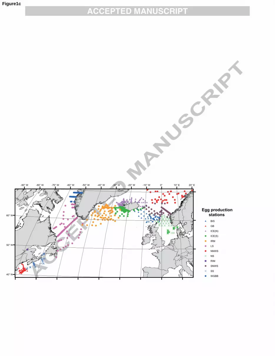
###
#
#
#
#
########
#
#
#
#
#
#############
#
##
##
#######
#
#
#
########
#
#
########################
DD
DDD
DD
D
D
DDDDD D
D
DDD
DD
DDD
DDDDD
D
DD
DDDDDDD
DDDD
DDDD
D
"
!
!!
!!!
!
!
!
!
!
!!
!!!!!!
!!
!!!!!!
!
!!!!
!!
!
!!
!
!
!
!
!
!
!
!!
!!!!
!!!!!!!
!!
!!!!!!
!
!
!
!
!!
!!!!!!!
!!!
!!
!!!!
!
!!!!
!
!!!
!
!!!
!!!
!!
!!
!!!
!
!
!
!!!
!!!!!!
!
!
!
!!!
!!
!!
!!
!!
!!
!
!!
!
!!
!!!
!
!
!
!!!!!
!!!!!
!!!
!!!!!!!!!!!!!!!
!!!!!!!!!!!!!! !
! !
!!
!
!
!!!
!
!
!!!!!!
!!
!!
!
!
!
!
!
!
!!!
!
!!
!!!!!!
!
!
!
!
!
!!!!!!!!
!
!
!
!
!!
!!
!!
!!!
!!
!!
!!
!!
!
!!
!
!!
!
!
!!!!
!!
!
!!!
!!
!
!
!!
!
!
!
!!
!!!
!
!
! ! !! !!!! !! !!!!! ! !!!!! !! !!!!!!!!!!! ! !!! !! !!!! !!!! !!!!!!!! !! !! !!!!! !!!!!!!!!!!!!!!! !! ! !! !!
!!!! ######## ##################### ### ### # ## ## ## ###### ## # ### ## ## ## # # ### ## # ## ## # ### ## ## ## #
# #
##
###
##
##
# #
##
#
#
# ####
####
# ## ##
#
# ##
##
##
#
#
######
##
##
###
!
!
!
! !
!!
! !!
!!!!
! ! !
!!!
!
!! ! ! !
!!!
! !!
!!! !
!!
!!!!!!
!!!!!
!!!!
! !
!!!!!!!!!!!!!!
!
!!!
!!
!!!!!
!!!
!!
!!
!!
!
!!
!!
!
!
D
D
DDDD
D
DDD D D D DD D D DD D D DDD D DD D D
DD
DDDDDDDDD
DDD D
D
D
DDDD
DDDDDDD
DDD
DDDD
D
D
D
DDDDDDDDDDDD
20° E10° E0° -10° W-20° W-30° W-40° W-50° W-60° W-70° W-80° W-90° W
60° N
50° N
40° N
Egg production
stations
# BIS
# GB
# ICE(N)
! ICE(S)
! IRM
! LS
! NNWS
D NS
" RIM
! SNWS
D SS
! WGBB
Figure1c

-70 -60 -50 -40 -30 -20 -10 0 10
40
50
60
-1
3
7
11
15
19
23
SST (Deg. C)
Figure2a

-70 -60 -50 -40 -30 -20 -10 0 10
40
50
60
0
0.2
0.4
0.6
0.8
1
1.2
1.4
1.6
1.8
2
3.7
PCI
Phytoplankton Colour Index
Figure2b
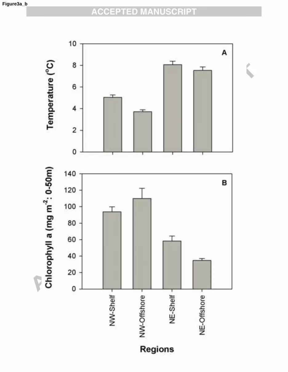

Figure4a_b


Figure6Click here to download high resolution image

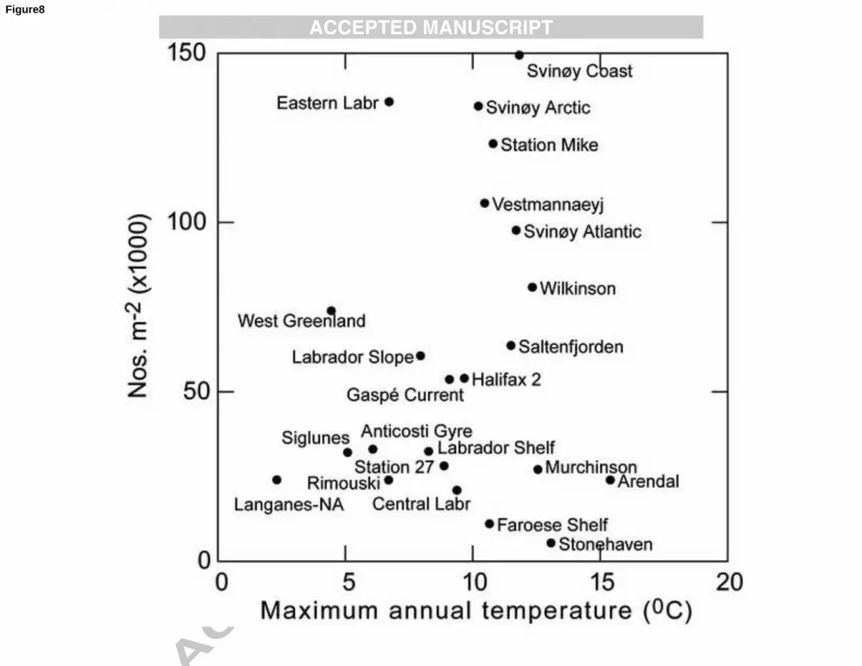

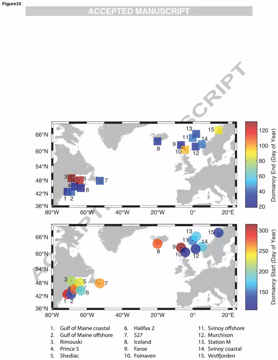
36°N
42°N
48°N
54°N
60°N
66°N
7
810
11
12
13
14
15
Do
rma
ncy E
nd
(D
ay o
f Y
ea
r)
20
40
60
80
100
120
80°W 60°W
80°W
40°W
60°W
20°W
40°W 20°W
20°E0°
0° 20°E36°N
42°N
48°N
54°N
60°N
66°N
3
4
5
6
9
Do
rma
ncy S
tart
(D
ay o
f Y
ea
r)
150
200
250
300
1 2
7
810
11
12
13
14
15
3
4
5
6
9
1 2
1010 12
1. Gulf of Maine coastal
2. Gulf of Maine oshore
3. Rimouski
4. Prince 5
5. Shediac
6. Halifax 2
7. S27
8. Iceland
9. Faroe
10. Foinaven
11. Svinoy oshore
12. Murchison
13. Station M
14. Svinoy coastal
15. Vestorden
Figure10

Figure11

0
50
100
150
200
250
300
1.0 1.5 2.0 2.5 3.0 3.5 4.0
CS = 89.7 x PL -117
Clu
tch s
ize (
eggs)
Prosome length (mm)
Prosome length (mm)
Clu
tch s
ize (
eggs)
0
40
80
120
160
200
240
280
1.0 1.5 2.0 2.5 3.0 3.5 4.0
0
40
80
120
160
200
240
280
1.0 1.5 2.0 2.5 3.0 3.5 4.0
Figure12
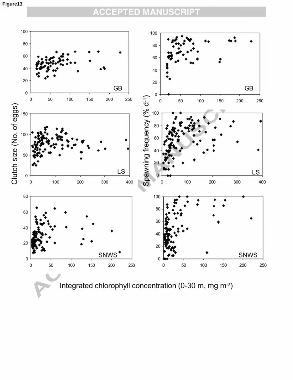
0
20
40
60
80
100
0 100 200 300 400
0
50
100
150
0 100 200 300 400
LS LS
0
20
40
60
80
100
0 50 100 150 200 250
0
20
40
60
80
0 50 100 150 200 250
0
20
40
60
80
100
0 50 100 150 200 250
0
20
40
60
80
100
0 50 100 150 200 250
Clu
tch s
ize (
No. of eggs)
GB GB
SNWS SNWS
Spaw
nin
g fre
quency (
% d
-1)
Integrated chlorophyll concentration (0-30 m, mg m-2)
Figure13

0
50
100
150
0 20 40 60 80 100
0
20
40
60
80
100
0 20 40 60 80 100
0
20
40
60
80
0 20 40 60 80 100
0
20
40
60
80
0 20 40 60 80 100
RIM RIM
NS NS
Clu
tch s
ize (
No. of eggs)
Rela
tive c
lutc
h s
ize (
% C
S/C
Sm
ax)
Spawning frequency (% d-1)
CS = 0.44SF + 65.11r2 = 0.33
CS/CSmax= 0.25SF + 45.52r2 = 0.31
CS = 0.15SF + 27.91r2 = 0.04
CS/CSmax= 0.22SF + 21.57r2 = 0.12
Figure14
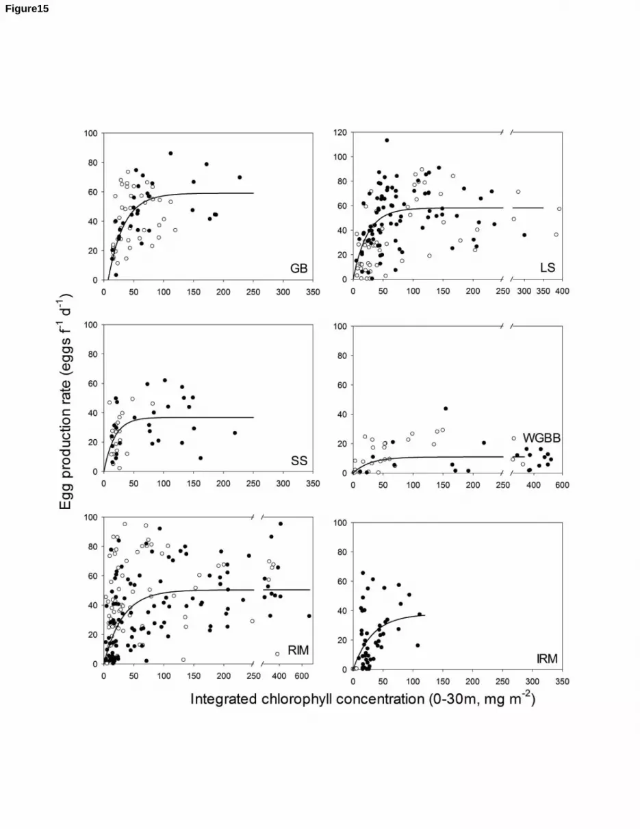
Figure15

Figure16
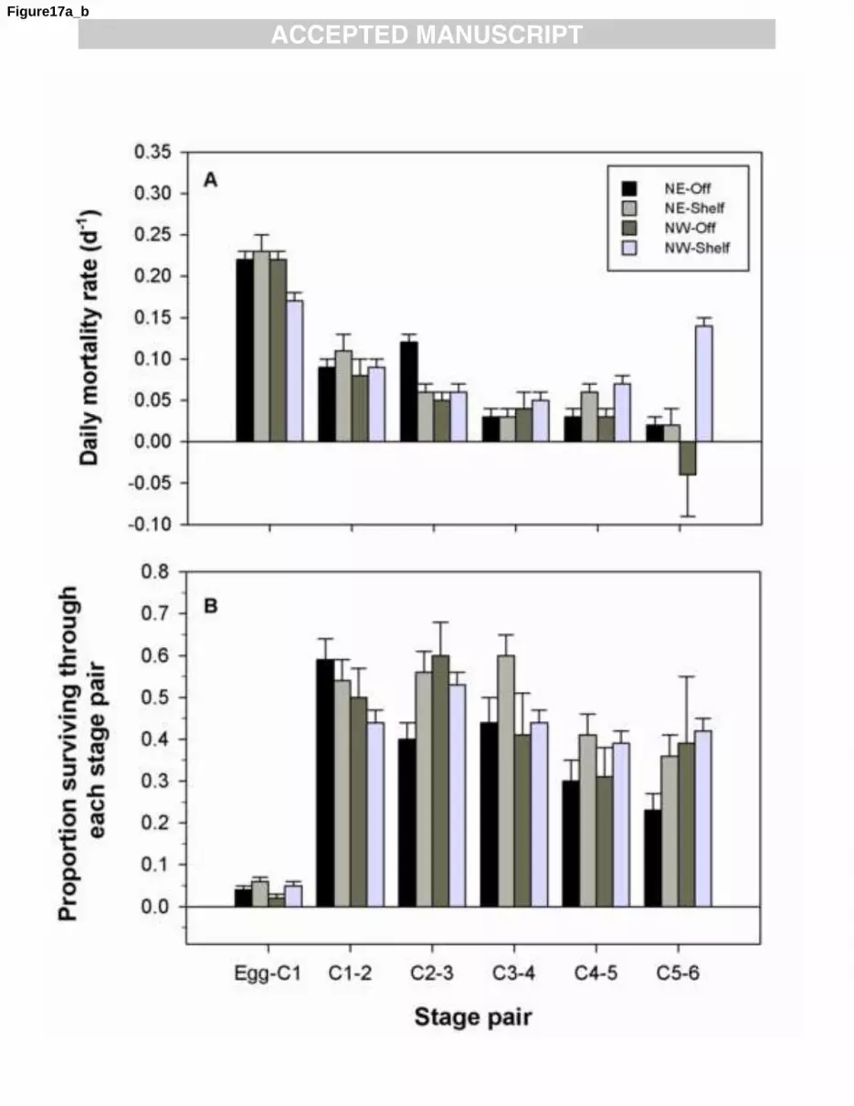
Figure17a_b

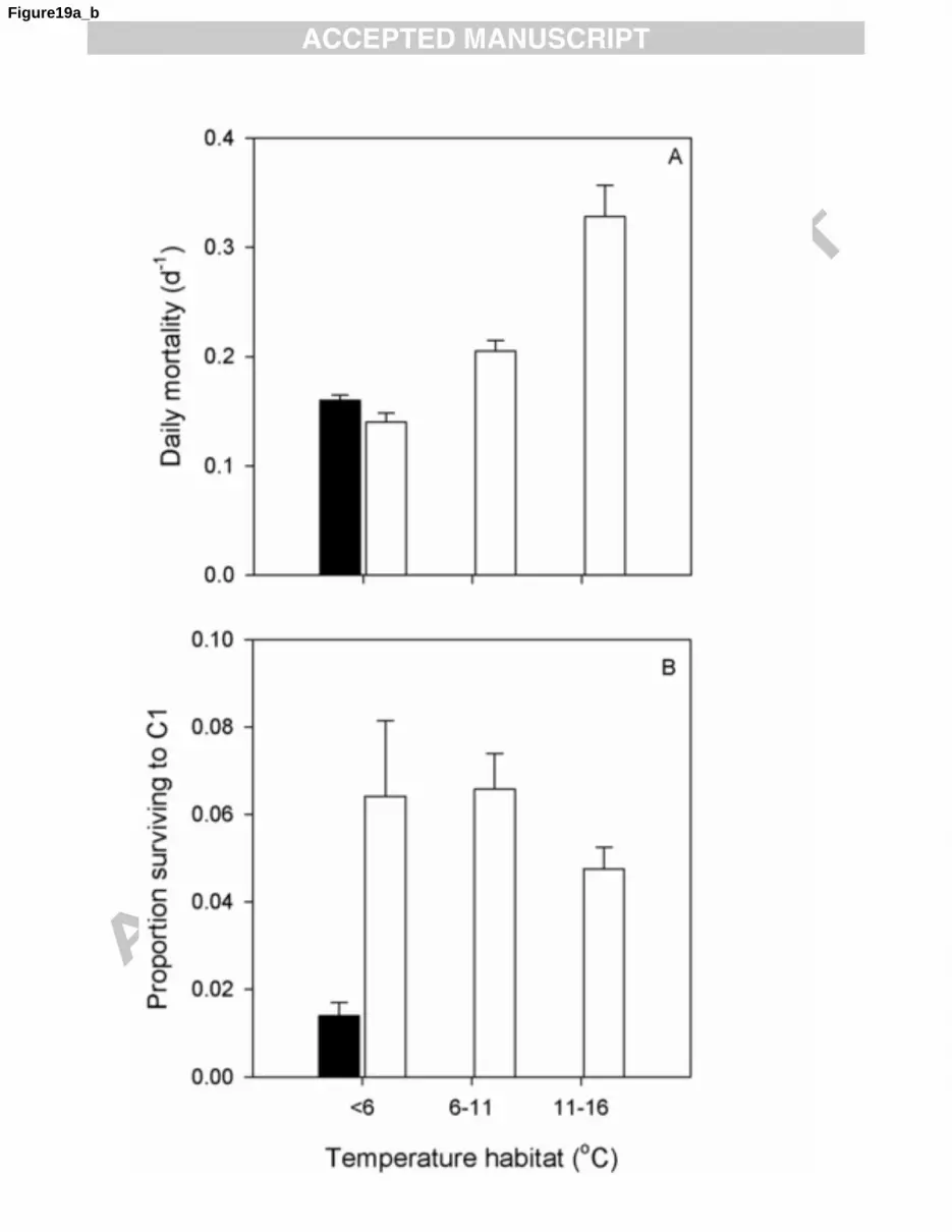
Figure19a_b


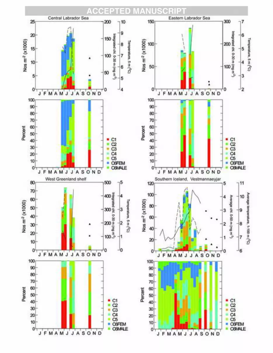

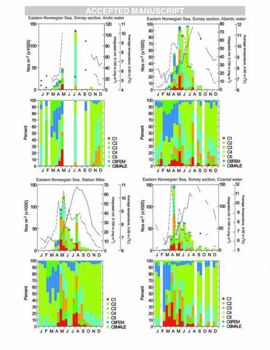

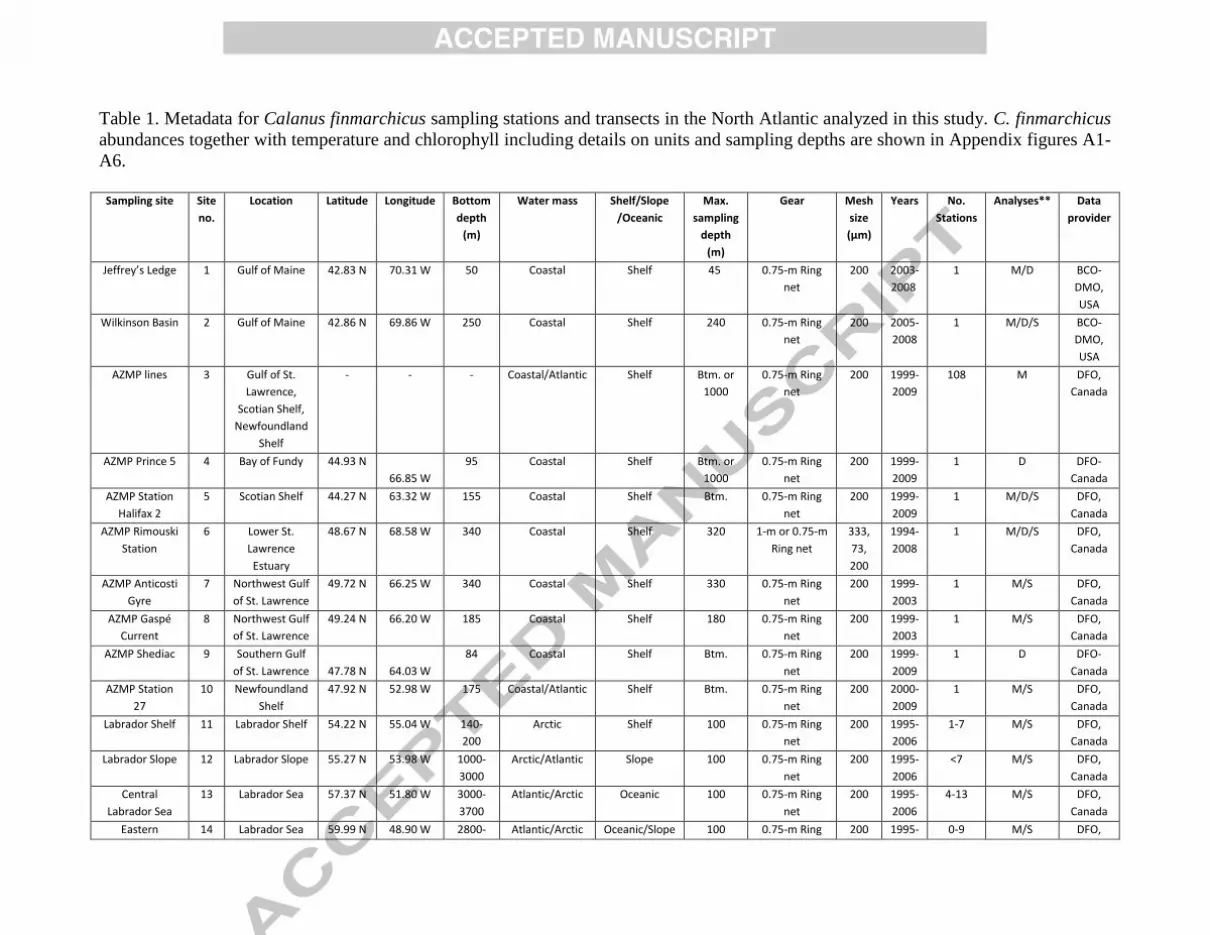
Table 1. Metadata for Calanus finmarchicus sampling stations and transects in the North Atlantic analyzed in this study. C. finmarchicus
abundances together with temperature and chlorophyll including details on units and sampling depths are shown in Appendix figures A1-
A6.
Sampling site Site
no.
Location Latitude Longitude Bottom
depth
(m)
Water mass Shelf/Slope
/Oceanic
Max.
sampling
depth
(m)
Gear Mesh
size
(µm)
Years No.
Stations
Analyses** Data
provider
Jeffrey’s Ledge 1 Gulf of Maine 42.83 N 70.31 W 50 Coastal Shelf 45 0.75-m Ring
net
200 2003-
2008
1 M/D BCO-
DMO,
USA
Wilkinson Basin 2 Gulf of Maine 42.86 N 69.86 W 250 Coastal Shelf 240 0.75-m Ring
net
200 2005-
2008
1 M/D/S BCO-
DMO,
USA
AZMP lines 3 Gulf of St.
Lawrence,
Scotian Shelf,
Newfoundland
Shelf
- - - Coastal/Atlantic Shelf Btm. or
1000
0.75-m Ring
net
200 1999-
2009
108 M DFO,
Canada
AZMP Prince 5 4 Bay of Fundy 44.93 N
66.85 W
95 Coastal Shelf Btm. or
1000
0.75-m Ring
net
200 1999-
2009
1 D DFO-
Canada
AZMP Station
Halifax 2
5 Scotian Shelf 44.27 N 63.32 W 155 Coastal Shelf Btm. 0.75-m Ring
net
200 1999-
2009
1 M/D/S DFO,
Canada
AZMP Rimouski
Station
6 Lower St.
Lawrence
Estuary
48.67 N 68.58 W 340 Coastal Shelf 320 1-m or 0.75-m
Ring net
333,
73,
200
1994-
2008
1 M/D/S DFO,
Canada
AZMP Anticosti
Gyre
7 Northwest Gulf
of St. Lawrence
49.72 N 66.25 W 340 Coastal Shelf 330 0.75-m Ring
net
200 1999-
2003
1 M/S DFO,
Canada
AZMP Gaspé
Current
8 Northwest Gulf
of St. Lawrence
49.24 N 66.20 W 185 Coastal Shelf 180 0.75-m Ring
net
200 1999-
2003
1 M/S DFO,
Canada
AZMP Shediac 9 Southern Gulf
of St. Lawrence 47.78 N 64.03 W
84 Coastal Shelf Btm. 0.75-m Ring
net
200 1999-
2009
1 D DFO-
Canada
AZMP Station
27
10 Newfoundland
Shelf
47.92 N 52.98 W 175 Coastal/Atlantic Shelf Btm. 0.75-m Ring
net
200 2000-
2009
1 M/S DFO,
Canada
Labrador Shelf 11 Labrador Shelf 54.22 N 55.04 W 140-
200
Arctic Shelf 100 0.75-m Ring
net
200 1995-
2006
1-7 M/S DFO,
Canada
Labrador Slope 12 Labrador Slope 55.27 N 53.98 W 1000-
3000
Arctic/Atlantic Slope 100 0.75-m Ring
net
200 1995-
2006
<7 M/S DFO,
Canada
Central
Labrador Sea
13 Labrador Sea 57.37 N 51.80 W 3000-
3700
Atlantic/Arctic Oceanic 100 0.75-m Ring
net
200 1995-
2006
4-13 M/S DFO,
Canada
Eastern 14 Labrador Sea 59.99 N 48.90 W 2800- Atlantic/Arctic Oceanic/Slope 100 0.75-m Ring 200 1995- 0-9 M/S DFO,

Labrador Sea 3600 net 2006 Canada
West Greenland
shelf
15 West
Greenland
60.51 N 48.30 W 130 Arctic Shelf 100 0.75-m Ring
net
200 1995-
2006
<5 M/S DFO,
Canada
MarProd
Program
16 Irminger Sea 62 N 32.20 W >3000 Atlantic Oceanic >3000 ARIES 200 2001-
2002
- M Heath et
al. 2008
Vestmannaeyjar 17 Southern
Iceland
63.37 N 19.92 W 200 Atlantic Shelf 190 Bongo 200 1997-
1998
1 M/D/S MRI,
Iceland
Siglunes section 18 Northern
Iceland
67 N 18.83 W 80-
1045
Atlantic/Arctic Shelf/slope 100 or
btm.
Bongo 335 1993-
1994
8 M/S MRI,
Iceland
Langanes-NA 19 Northeastern
Iceland
67.5 N 13.27 W 188-
1860
Atlantic/Arctic Shelf/oceanic 100 Bongo 200 1995-
1996
6 M/S MRI,
Iceland
Faroe Shelf
station
20 Faroese Shelf 62.05 N 6.62 W 55 Atlantic Shelf 50 WP-2/Bongo 100,
200
1997,
2004
1 M/D/S FAMRI,
Faroes
Faroe Oceanic
Section
21 Southern
Norwegian Sea
63.59 N 6.08 W 550-
3300
Atlantic/Arctic Oceanic 50 WP-2 200 1990-
2009
11 M FAMRI,
Faroes
Foinaven 22 Faroe-Shetland
Channel
60.32 N 4.23 W 500 Atlantic Slope 330-500 Bongo 200 1997-
1998
1 M/D/S Heath et
al. 2000
Svinøy section
Arctic
23 Central
Norwegian Sea
64.51 N 0.36 E 2932 Arctic Oceanic 200 WP2 180 1996-
2006
1-2* M/S IMR,
Norway
Svinøy section
Atlantic
24 Eastern
Norwegian Sea
63.52 N 2.66 E 1453 Atlantic Slope/oceanic 200 WP2 180 1996-
2006
7-8* M/D/S IMR,
Norway
Weather
Station Mike
25 Eastern
Norwegian Sea
66 N 2 E >1600 Atlantic Oceanic 200 Multinet/WP2 180 1997-
1998
1 M/D/S IMR,
Norway
Svinøy section
coastal
26 Eastern
Norwegian Sea
62.82 N 4.21 E 501 Coastal Shelf 200 or
btm.
WP2 180 1996-
2006
4-5* M/D/S IMR,
Norway
Saltenfjorden 27 Northern
Norwegian
Shelf
67.23 N 13.65 E 400 Coastal Shelf 370 WP2 200 1997-
1998
1 M/S Heath et
al. 2000
Stonehaven 28 North Sea,
Scotland Shelf
57 N 2 W 47 Coastal Shelf 45 Bongo 200 1997-
2008
1 M/S Heath et
al. 2000
Murchinson 29 North Sea 61.50 N 1.67 E 170 Atlantic Oceanic 150 Bongo 200 1997-
1998
1 M/D/S Heath et
al. 2000
Arendal st. 2 30 Southern
Norway Shelf
58.38 N 8.82 E 105 Coastal Shelf 50 WP2 180 1994-
2010
1 M/S IMR,
Norway
Station India 31 Northeast ATL 59 N 19 W 2000 Atlantic Oceanic 600 LHPR 270 1971-
1975
1 M X.
Irigoien
* Number of stations out of a total of 17, based on watermass distribution
** M= Mortality, D=Dormancy, S= Seasonal dynamics

Table 2. Inventory of egg production rate observations in the North Atlantic included in this
study. Regions included are Georges Bank (GB), the Scotain Shelf (SS), Rimouski Station
(RIM) in the Lower St Lawrence Estuary, Labrador Sea (LS), West Greenland/Baffin Bay
(WGBB), Irminger Sea (IRM), area North of Iceland (ICE(N)), area South of Iceland
(ICE(S)), area between Iceland and the Shetland Isles (BIS), South Norwegian Sea (SNWS),
North Norwegian Sea (NNWS) and the North Sea (NS). Contributing investigators: J.Runge
(JR), R. W. Campbell (RC), S. Plourde (SP), E. Head (EH), T.G. Nielsen (TGN), S. Madsen
(SM), K. Arendt (KA), R.Swalethorp (RS), A.Gislason (AG), M. Heath (MH), S. Jónasdóttir
(SJ), E.Gaard (EG), B. Niehoff (BN) and W.Melle (WM).
Region Number of egg production experiments Investigator(s)Method Reference
Spring Summer Autumn Winter
GB (Mar-Apr) (May-Jun) (Jan-Feb)
48 53 - 18 JR A 1
SS (Apr-May) (Jun) (Nov)
27 13 8 - RC A 2
RIM (May-Jul) (Aug-Sept) (Oct-Nov) (Dec-Apr)
110 66 18 3 SP A 3
LS (May) (Jun-Jul)
35 15 - - RC A 2
48 32 - - EH A 4
5 5 TGN, KA E 5, 6, 7
WGBB (Late Apr-May) (Jun-Jul) (Feb-Early Apr)
21 26 6 TGN, RS, SM E 7, 8, 9
IRM (May-Jun) (Jul-Aug) (Nov-Apr)
52 - - 6 AG C 10, 11, 12
16 21 7 MH C 13
ICE(N) (May-Jun)
127 - - - AG C 11
ICE(S) (Apr-Jun) (Dec-Mar)
108 - - 9 AG C 10, 11, 12
16 - - - SJ D, E 14
BIS (Apr-May) - (Oct) (Dec-Mar)
19 - 4 31 SJ E 15, 16
38 - - - EG C
SNWS (Apr-May) (Jun) (Oct) (Dec-Mar)
85 8 - 7 BN B, C 17
21 - - - EG C 14
11 - 3 12 SJ E 15, 16
4 - - - WM C 18, 19
NNWS (May) (Jun) (Apr)
36 6 - 4 WM C 18, 19
2 - - - EG C 18, 19
NS (Mar-May) (Jul-Aug) (Sep-Oct) (Jan-Feb)
56 26 4 4 SJ E 16, 20, 21
References to published data are as follows: 1, Runge et al. (2006); 2, Campbell and Head (2000); 3, Plourde and
Runge (1993) + unpubl. data; 4, Head et al. (2012) in prep.; 5, Nielsen and Hansen (1995); 6, Arendt et al.
(2010); 7, Munk et al. (2003); 8, Madsen et al. 2008; 9, Swalethorp (2011); 10 Gislason and Astthorson (2000);
11, Gislason (2005); 12, Gislason et al. (2008); 13, Heath et al. (2008); 14, Jónasdóttir et al. (2002); 15,

Richardson et al. (1999); 16, Jónasdóttir et al. (2008) + unpubl. data; 17, Niehoff et al. (1999); 18, Stenevik et al.
(2007); 19, Head et al. (2012) in press; 20, Jónasdóottir et al. (2005); 21, Jónasdóttir and Koski (2011).

Table 3. Inventory of measurements of female prosome length (PL) and clutch size (CS) of
more than 5 eggs included in this study. Regions and investigators are as in Table 2. Clutch
sizes for WGBB from experiments run for 24 h (8 in spring, 7 in summer).
Region Number of measurements Investigator(s)
Spring Summer Autumn Winter
GB (Mar-Apr) (May-Jun) - (Jan-Feb) JR
PL/CS 335/655 323/930 - 157/302
SS (Mar-Apr) (Jun) (Nov) - RC
PL/CS 773/435 250/131 154/73 -
RIM (May-Jul) (Aug-Sept) (Oct-Nov) (Apr) SP
PL/CS 1989/2434 1332/1383 145/132 8/38
LS (May) (Jun-Jul) - - RC, EH, TGN, KA
PL/CS 2691/1689 1290/632 - -
WGBB (May) (Jun-Jul) (Nov-Apr)
PL/CS 318/61 188/39 - 103/0 TGN, SM, RS
IRM (May-Jun) - - (Dec-Mar) AG
PL/CS 782/407 - - 30/0
ICE(N) (May-Jun) - - - AG
PL/CS 2074/1395 - - -
ICE(S) (Apr-June) - - (Dec-Mar) AG, SJ
PL/CS 2029/1198 - - 87/6
BIS (Apr-May) - (Sep-Oct) (Dec-Mar) SJ
PL/CS 448/200 - 30/5 264/71
SNWS (Apr-May) (Jun) (Sep-Oct) (Dec-Mar) BN, SJ, WM
PL/CS 872/1484 54/40 55/20 208/94
NNWS (May) (Jun) - (Apr) WM
PL 630/337 106/40 - 0/44
NS (Mar-May) (Jul-Aug) (Sep-Oct) (Dec-Feb) SJ
PL/CS 767/329 262/166 47/12 21/0

Table 4. Average annual and spring relative clutch size CS/CSmax (see text). CS/CSmax for
the WGBB region are averages for experiments run for 24 h, while the spring average
chlorophyll concentration is the average over all spring experiments (24-43 h duration).
Regions are as in Table 2.
Region Annual average Spring average Spring average
CS/CSmax CS/CSmax integrated chlorophyll
(%) (%) (0-30 m, mg m-2
)
GB 48 46 79.6
SS 40 42 80.5
RIM 59 58 97.5
LS 51 53 80.2
WGBB 25 27 275.1
IRM 34 34 36.4
ICE(N) 50 50 136.7
ICE(S) 42 42 63.6
BIS 34 37 42.6
NNWS 28 28 32.9
SNWS 29 29 84.2
NS 40 43 53.2

Table 5. Parameters for Ivlev functions (y = a(1 – e (-bxIntchl)
) relating egg production rate
(EPR: y) and 0-30 m integrated chlorophyll concentration (Intchl), estimates of integrated
chlorophyll concentrations (Intchl 95%) required to reach 95% of EPRmax (a), average
regional chlorophyll concentrations in spring (Avg. Intchl) and the percentage of experimental
stations in spring where the chlorophyll concentration exceeded Intchl 95% (No. of stns.).
For the WGBB region results from all experiments (24 -48 h duration) were used. Regions
are as in Table 2.
Region a b r2 Intchl Avg. Intchl No. of stns
95% in spring >Intchl 95%
(mg m-2
) (mg m-2
) (%)
GB 60.4 0.029 0.47 103.3 79.6 25
SS 36.8 0.056 0.15 53.3 80.5 63
RIM 50.3 0.032 0.26 93.6 97.5 33
LS 58.1 0.042 0.19 71.9 80.2 39
WGBB 10.9 0.035 0.07 85.5 275.1 76
IRM 35.0 0.033 0.08 90.8 36.4 8
ICE(N) 60.1 0.011 0.18 282.6 136.7 11
ICE(S) 30.1 0.062 0.13 48.6 55.1 39
BIS 19.0 0.215 0.05 13.9 42.6 63
SNWS 25.6 0.052 0.23 57.4 32.9 14
NNWS 18.9 0.174 0.08 17.2 84.2 85
NS 24.4 0.078 0.24 38.2 53.2 49

Table 6. Correlations among residuals (observed EPR – predicted EPR) from the Ivlev plots
of EPR versus Intchl with either in situ near-surface temperature (T) or prosome length (PL),
and between T and PL. Only results for correlations with P<0.05 are shown. Regions are as
in Table 2.
Region Residuals vs. T Residuals vs. PL PL vs T
(Sign, r2) (Sign, r
2) (Sign, r
2)
GB +, 0.20 +, 0.23
SS +, 0.17
RIM +, 0.12 +, 0.12 +, 0.27
LS +, 0.21 +, 0.13 +, 0.22
WGBB
IRM -, 0.15
ICE(N) +, 0.18
ICE(S)
BIS
SNWS -, 0.12
NNWS -, 0.14
NS +, 0.24
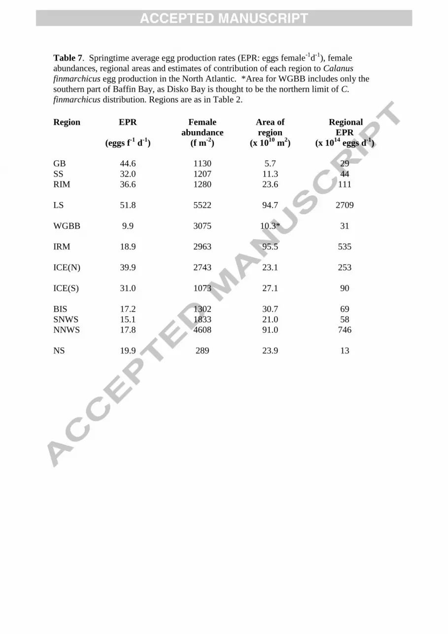
Table 7. Springtime average egg production rates (EPR: eggs female-1
d-1
), female
abundances, regional areas and estimates of contribution of each region to Calanus
finmarchicus egg production in the North Atlantic. *Area for WGBB includes only the
southern part of Baffin Bay, as Disko Bay is thought to be the northern limit of C.
finmarchicus distribution. Regions are as in Table 2.
Region EPR Female Area of Regional
abundance region EPR
(eggs f-1
d-1
) (f m-2
) (x 1010
m2) (x 10
14 eggs d
-1)
GB 44.6 1130 5.7 29
SS 32.0 1207 11.3 44
RIM 36.6 1280 23.6 111
LS 51.8 5522 94.7 2709
WGBB 9.9 3075 10.3* 31
IRM 18.9 2963 95.5 535
ICE(N) 39.9 2743 23.1 253
ICE(S) 31.0 1073 27.1 90
BIS 17.2 1302 30.7 69
SNWS 15.1 1833 21.0 58
NNWS 17.8 4608 91.0 746
NS 19.9 289 23.9 13
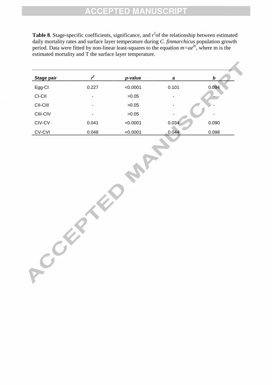
Table 8. Stage-specific coefficients, significance, and r2of the relationship between estimated
daily mortality rates and surface layer temperature during C. finmarchicus population growth
period. Data were fitted by non-linear least-squares to the equation m=aebt
, where m is the
estimated mortality and T the surface layer temperature.
Stage pair r2 p-value a b
Egg-CI 0.227 <0.0001 0.101 0.094
CI-CII - >0.05 - -
CII-CIII - >0.05 - -
CIII-CIV - >0.05 - -
CIV-CV 0.041 <0.0001 0.034 0.090
CV-CVI 0.048 <0.0001 0.044 0.098

Table 9. Calanus finmarchicus mortality and environment. Statistics of the linear multiple regression models of mortality in Egg-CI
against temperature, chlorophyll a biomass and adult female copepod abundance in different habitats. Habitats were: (A)
offshore/shelf regions in the northeast (NeATL) and northwest (NwATL) Atlantic or (B) probability that congeners C. hyperboreus
and C. glacialis occur in high abundance in the surface layer based on literature results (see text). Analyses were performed with ln-
transformed data.
Independent variable:
mortality egg-CI
A) Habitats in NeATL
and NwATL
Off-
NeATL
Shelf-
NeATL
Off-
NwATL
Shelf-
NwATL
Partial
Corr.
Coeff. p
Partial Corr.
Coeff. p
Partial Corr.
Coeff. p
Partial
Corr.
Coeff. p
Intercept 0.730 <0.0001 0.630 <0.0001 0.51 <0.0001 0.600 <0.0001
Temperature 0.020 >0.05 0.050 <0.01 0.04 >0.05 0.050 <0.0001
Chlorophyll a -0.010 >0.05 0.010 >0.05 -0.01 >0.05 -0.001 >0.05
Abundance C6f 0.010 <0.05 0.0003 >0.05 0.03 <0.0001 0.010 <0.01
r2 adjusted 0.04
0.09
0.43
0.20
p <0.05
<0.01
<0.0001
<0.0001
B) High/low C.
hyperboreus/ C. glacialis
habitats
High Low
Partial
Corr.
Coeff. p
Partial Corr.
Coeff. p
Intercept 0.670 <0.0001 0.610 <0.0001
Temperature 0.020 <0.0001 0.060 <0.0001
Chlorophyll a -0.004 >0.05 -0.004 >0.05

Abundance C6f 0.010 <0.0001 0.010 <0.01
r2 adjusted 0.27
0.14
p <0.0001
<0.0001

Highlights
We analysed demographic and egg production data sets of Calanus finmarchicus
Overwintering centres in the deep basins are essential for the species’ distribution
Female body size and egg production are related to temperature and chlorophyll
Dormancy duration is shorter in the western North Atlantic than in the east
Survival from egg to first copepodite stage is lower in cold water regions