the mps parameterization under lead time uncertainty
TRANSCRIPT
ARTICLE IN PRESS
Int. J. Production Economics 90 (2004) 369–376
*Correspondin
3-25-71-56-49.
E-mail addre
0925-5273/$ - see
doi:10.1016/j.ijpe
The MPS parameterization under lead time uncertainty
Mohamed-Aly Ould-Louly*, Alexandre Dolgui
Lab. of Industrial Systems Optimization, University of Technology of Troyes, 12 Marie Curie st., BP 2060, 10010 Troyes Cedex, France
Received 17 April 2002; accepted 21 August 2003
Abstract
The supply planning of assembly systems under lead times uncertainty is studied. The used criteria is the sum of the
average holding cost for the components, the average backlogging cost for the finished product, and the setup cost. The
decision variables are the planned lead times of components and the periodic ordering quantity. A new generalized
Newsboy model gives the optimal solution under the assumption that the lead times of the different types of
components follow the same distribution probability, and that the holding costs per period of the ordered quantities are
the same.
r 2003 Elsevier B.V. All rights reserved.
Keywords: Assembly systems; Supply planning; Inventory control; Optimization
1. Introduction
The lead time uncertainty is a major factor ofplanning perturbations and additional costs inMRP systems (Dolgui and Ould-Louly, 2001). Infact, MRP begins with the end-product need dateand uses the lead time to calculate the componentsrelease date. Clearly, the calculation does not takeinto account the actual lead time because this oneis not known at this moment. The calculation usesa forecasted value of lead time, i.e. planned lead
time.Gupta and Brennan (1995) studied MRP
systems using simulation; they showed that leadtime uncertainty has a large influence on the cost.The statistics done on simulations by Bragg et al.
g author. Tel.: +33-3-25-71-58-79; fax: +33-
sses: [email protected] (M.-A. Ould-Louly),
. Dolgui).
front matter r 2003 Elsevier B.V. All rights reserve
.2003.08.008
(1999) show that lead times substantially influencethe inventories.
In literature, the problem of planned lead timecalculation has been already studied. For example,Melnyk and Piper (1981) proposed a forecastmethod for the lead time which is issued from theused methods for random demand:
Planned lead time ¼ lead time forecast
þ safety lead time
¼ lead time meanþ k lead
time standard deviation:
But the value k calculation is not explained.However, Wemmerlov (1986) shows by simulationthat the errors of forecast increase the inventoriesand, in the same time, decrease the customerservice level. Molinder (1997) studies also thisproblem by simulation. Instead of forecasting, heproposes simulated annealing to find good safety
stock and safety lead time. His results show that
d.
ARTICLE IN PRESS
M.-A. Ould-Louly, A. Dolgui / Int. J. Production Economics 90 (2004) 369–376370
high planned lead time gives excessive inventory,and small planned lead time gives shortages anddelays.
Whybark and Wiliams (1976) found the use ofsafety lead time more efficient than safety stock.Grasso and Tayor (1984) give an opposite conclu-sion, their simulations find more prudent safetystocks.
As shown, there are a lot of simulation studiesdealing with this problem, and there are a lotof studies dealing with the problem formulation,but in our knowledge, there is no exact mathema-tical method giving the optimal planned lead
times.A particular supply planning problem under
lead time uncertainties concerns assembly systems.In fact, for assembly systems, several types ofcomponents are needed to produce one finishedproduct. So, the inventories of the different typesof components become dependent. Then thesupply planning becomes more difficult.
In the general case, the mathematics formula-tion of the cost criterion for assembly systemsupply planning is difficult. For particular cases,there are some contributions, which proposemathematics resolution. Their studies are generallylimited to a single-period problem (do not take intoaccount the dependence between periods). Forexample, Chu et al. (1993) propose a model whichgives optimal values of the planned times inassembly systems, but only for the single-periodproblem. The mathematics formulation of themulti-period problems is more difficult. In thatcase, orders may cross, that is, they may not bereceived in the same sequence in which they areplaced (He et al., 1998). Some contributionsassume that orders do not cross, then they solve,under this assumption, the single-item problem(Graves et al., 1993).
The problem difficulty, for assembly systems,resides also in the dependence between inventories.Wilhelm and Som (1998) studied a problem of thistype and showed that a renewal process candescribe end-item (finished product) inventorylevel evolution, but they did not study directlythe dependence between component inventories.This dependence was studied by Gurnani et al.(1996) but their assembly system was only with
two components, and the considered lead timedistribution was simple.
In this paper, a multi-period and multi-compo-
nent supply planning problem, for assemblysystems with random lead time and fixed demand,is investigated. The assembly systems with onetype of finished product are considered. Aprevious work gives optimal solution for the‘‘Lot for Lot’’ policy (Ould-Louly and Dolgui,2002), but this method is not efficient when thesetup cost (order cost) is significant. The contribu-tion of this paper is to find the optimal value of theplanned lead times and the optimal lot sizes (theperiodic ordering quantity, POQ) taking intoaccount the dependencies between periods andbetween component inventories. Since the demandlevel for finished product is constant, the POQ isdefined by bother planned lead time and orderperiodicity. The used optimization criteria is thesum of the average holding cost for the compo-nents, the average backlogging cost for the finishedproduct, and the setup cost. A mathematicalformulation based on Markov chains is proposedto measure the average cost on an infinite horizon,and a new generalized Newsboy model is pro-posed. This Newsboy model allows the optimiza-tion of the planned lead times and the periodicityfor the POQ policy using the explicit expression ofthe cost obtained by the Markov model.
The paper is organized as follows. Section 2deals with the problem formulation. In Section 3an average cost measure is proposed and provedfor the general case. Section 4 gives a newgeneralized Newsboy model for the planned leadtime and POQ optimization. This model isobtained under the following assumption: (i) theholding costs of the ordered quantities per periodare the same for all components and (ii) the leadtime of the different components have the samedistribution probability.
2. Problem description
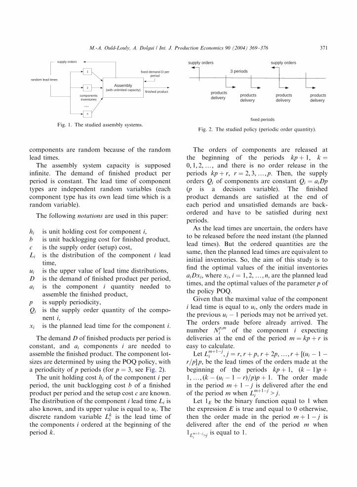
The studied system is shown in Fig. 1. Severaltypes of components are needed to producea finished product. The inventories of the
ARTICLE IN PRESS
Assembly(with unlimited capacity)
componentsinventories
random lead times
fixed demand D perperiod
finished product
supply orders
...
1
2
n
Fig. 1. The studied assembly systems.
supply orders supply orders
productsdelivery
productsdelivery
productsdelivery
3 periods
productsdelivery
fixed periods
Fig. 2. The studied policy (periodic order quantity).
M.-A. Ould-Louly, A. Dolgui / Int. J. Production Economics 90 (2004) 369–376 371
components are random because of the randomlead times.
The assembly system capacity is supposedinfinite. The demand of finished product perperiod is constant. The lead time of componenttypes are independent random variables (eachcomponent type has its own lead time which is arandom variable).
The following notations are used in this paper:
hi
is unit holding cost for component i; b is unit backlogging cost for finished product, c is the supply order (setup) cost, Li is the distribution of the component i leadtime,
ui is the upper value of lead time distributions, D is the demand of finished product per period, ai is the component i quantity needed toassemble the finished product,
p is supply periodicity, Qi is the supply order quantity of the compo-nent i;
xi is the planned lead time for the component i:The demand D of finished products per period isconstant, and ai components i are needed toassemble the finished product. The component lot-sizes are determined by using the POQ policy, witha periodicity of p periods (for p ¼ 3; see Fig. 2).
The unit holding cost hi of the component i perperiod, the unit backlogging cost b of a finishedproduct per period and the setup cost c are known.The distribution of the component i lead time Li isalso known, and its upper value is equal to ui: Thediscrete random variable Lk
i is the lead time ofthe components i ordered at the beginning of theperiod k:
The orders of components are released atthe beginning of the periods kp þ 1; k ¼0; 1; 2;y; and there is no order release in theperiods kp þ r; r ¼ 2; 3;y; p: Then, the supplyorders Qi of components are constant Qi ¼ aiDp
(p is a decision variable). The finishedproduct demands are satisfied at the end ofeach period and unsatisfied demands are back-ordered and have to be satisfied during nextperiods.
As the lead times are uncertain, the orders haveto be released before the need instant (the plannedlead times). But the ordered quantities are thesame, then the planned lead times are equivalent toinitial inventories. So, the aim of this study is tofind the optimal values of the initial inventoriesaiDxi; where xi; i ¼ 1; 2;y; n; are the planned leadtimes, and the optimal values of the parameter p ofthe policy POQ.
Given that the maximal value of the componenti lead time is equal to ui; only the orders made inthe previous ui � 1 periods may not be arrived yet.The orders made before already arrived. Thenumber N
p;mi of the component i expecting
deliveries at the end of the period m ¼ kp þ r iseasy to calculate.
Let Lmþ1�ji ; j ¼ r; r þ p; r þ 2p;y; r þ ½ðui � 1�
r=p� p; be the lead times of the orders made at thebeginning of the periods kp þ 1; ðk � 1Þp þ1;y; ðk � ðui � 1� rÞ=pÞp þ 1: The order madein the period m þ 1� j is delivered after the endof the period m when L
mþ1�ji > j:
Let 1E be the binary function equal to 1 whenthe expression E is true and equal to 0 otherwise,then the order made in the period m þ 1� j isdelivered after the end of the period m when1
Lmþ1�ji
>jis equal to 1.
ARTICLE IN PRESS
M.-A. Ould-Louly, A. Dolgui / Int. J. Production Economics 90 (2004) 369–376372
Finally, the random variables
Np;kpþri ¼
Xðui�1�rÞ=p
j¼0
1Lðk�jÞpþ1i
>jpþr;
i ¼ 1;y; n; ð1Þ
give the global state of the previous orders. In fact,N
p;mi is the number of the component i orders that
are not arrived yet (at the end of the period m; theyare already waited).
Proposition 1. The cost of the period m ¼ kp þ r
can be expressed as follows:
CkðX ; p;Np;m1 ;y;Np;m
n Þ
¼ c � 1r¼1 þ DXn
i¼1
hiaiðxi þ p � r � pNp;kpþri Þ
þ DH maxi¼1;y; n
ðpNp;kpþri þ r � p � xiÞ
þ; ð2Þ
where X ¼ ðx1;y;xnÞ and H ¼ b þPn
i¼1 hiai: The
value ðZÞþ is equal to maxfZ; 0g:
See Appendix A for the proof.This cost is a random variable. To express the
holding cost on an infinite horizon, a Markovchain can be used by analogy with the model givenin Ould-Louly and Dolgui (2001) and Dolgui andOuld-Louly (2002). In this model, a stateZAf0; 1gui�1 is a binary vector that describes theorders made in the previous ui � 1 periods. Thecomponent zk is equal to 1 if the order made k
periods ago is not arrived yet, 0 otherwise.The average cost on the infinite horizon is
CðX ; pÞ ¼1
p
Xp
r¼1
E½CrðX ; pÞ�; ð3Þ
where EðZÞ is the expected value of Z;
CrðX ; pÞ
¼ c1r¼1 þ DXn
i¼1
hiaiðxi þ p � r � pNp;nipþri Þ
þ DH maxi¼1;y; n
ðpNp;nipþri þ r � p � xiÞ
þ; ð4Þ
ni ¼ui � 1� r þ p
p: ð5Þ
In the remained sections, hi is the holding cost ofthe amount aiD; instead of the unit holding cost.
The problem is the same with this new notation,but the equations are simplified.
3. Performance measure
The problem is to minimize the objectivefunction given by Eq. (3). This minimization israther difficult because this function is not linearand, the decision variables, xi; i ¼ 1; 2;y; n; areinteger. The minimization of an objective functionwith the same structure has been considered byChu et al. (1993), but in their case the lead times ofcomponents were continuous random variables, p
equal to 1, and the decision variables were real, sothey did not have discrete optimization problem.
Theorem 1. An explicit form for average cost, given
by Eq. (3), is the following:
CðX ; pÞ
¼c
pþ
p � 1
2ðH � bÞ þ
Xn
i¼1
hi½xi � EðNpi Þ�
þ HXkX0
1�1
p
Xp
r¼1
Yn
i¼1
Fp;ri
x þ k � r þ p
p
� �" #;
ð6Þ
where Fp;ri ðxÞ ¼ PrðNp;r
i pxÞ and Npi ¼
Ppr¼1 N
p;ri :
See Appendix B for the proof.In addition, it is easy to see that the components
xi of the optimum X must satisfy 0pxipui � 1:
4. Optimization
The general optimization problem is difficultdue to the no linearity of the cost. In this section,the problem is solved under the assumption thatholding costs of the quantities Qi ¼ aiD per periodare the same, and the lead time Li of the differentcomponents have the same distribution probabil-ity. Then, the costs hi; i ¼ 1;y; n; can be noted byh; and the distributions F
p;ri ; i ¼ 1;y; n; can be
noted by F p;r: The obtained problem will be notedby P and an exact method which solves this
ARTICLE IN PRESS
M.-A. Ould-Louly, A. Dolgui / Int. J. Production Economics 90 (2004) 369–376 373
problem in polynomial time will be given. Thefollowing complementary notations are used.
Ek is the set of vectors X ; each vector’scomponent is an integer variable satisfying: xi ¼xj ; for ipk and jpk:
P1k and P2
k are applications from Ek to Ekþ1
which are defined as follows: Y ¼ P1kðX Þ means
that yi ¼ x1 for iAf1; 2;y; k þ 1g and yi ¼ xi foriAfk þ 2; k þ 3;y; ng: Y ¼ P2
kðX Þ means thatyi ¼ xkþ1 for iAf1; 2;y; k þ 1g and yi ¼ xi foriAfk þ 2; k þ 3;y; ng: Then two vectors, P1
kðX Þand P2
kðX Þ; of the set Ekþ1 are associated to everyelement X of Ek:
Theorem 2. The following equation is true under the
assumption of the problem P:
8kAf1; 2;y; n � 1g;
MinXAEkþ1
CðX ; pÞ ¼ MinXAEk
CðX ; pÞ: ð7Þ
See Appendix C for the proof.
Corollary 1. The problem P has an optimal solution
in which the initial inventories have the same value
for every type of components.
Proof. The prove is immediate by transitivity fromEq. (7): MinXAE1
CðX ; pÞ ¼ MinXAEnCðX ; pÞ:
Then, there is an optimal solution X ¼ðx;y; x;y;xÞAEn: &
This optimal solution can be calculated usingthe following theorem.
Theorem 3. The optimum X ¼ ðx;y;x;y; xÞwhich minimizes the problem P is such that the
integer x satisfies
Xp
r¼1
F p;rn x þ p � r � 1
p
� �
pbp
Hp
Xp
r¼1
F p;rn x þ p � r
p
� �: ð8Þ
See Appendix D for the proof.
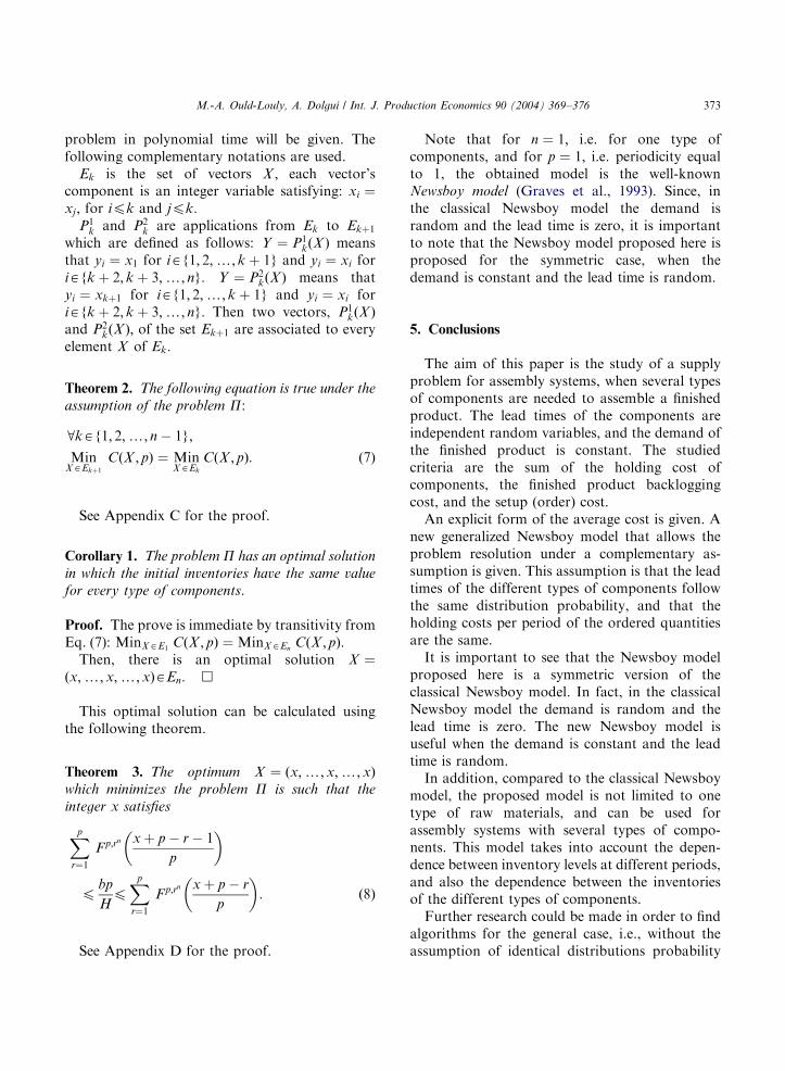
Note that for n ¼ 1; i.e. for one type ofcomponents, and for p ¼ 1; i.e. periodicity equalto 1, the obtained model is the well-knownNewsboy model (Graves et al., 1993). Since, inthe classical Newsboy model the demand israndom and the lead time is zero, it is importantto note that the Newsboy model proposed here isproposed for the symmetric case, when thedemand is constant and the lead time is random.
5. Conclusions
The aim of this paper is the study of a supplyproblem for assembly systems, when several typesof components are needed to assemble a finishedproduct. The lead times of the components areindependent random variables, and the demand ofthe finished product is constant. The studiedcriteria are the sum of the holding cost ofcomponents, the finished product backloggingcost, and the setup (order) cost.
An explicit form of the average cost is given. Anew generalized Newsboy model that allows theproblem resolution under a complementary as-sumption is given. This assumption is that the leadtimes of the different types of components followthe same distribution probability, and that theholding costs per period of the ordered quantitiesare the same.
It is important to see that the Newsboy modelproposed here is a symmetric version of theclassical Newsboy model. In fact, in the classicalNewsboy model the demand is random and thelead time is zero. The new Newsboy model isuseful when the demand is constant and the leadtime is random.
In addition, compared to the classical Newsboymodel, the proposed model is not limited to onetype of raw materials, and can be used forassembly systems with several types of compo-nents. This model takes into account the depen-dence between inventory levels at different periods,and also the dependence between the inventoriesof the different types of components.
Further research could be made in order to findalgorithms for the general case, i.e., without theassumption of identical distributions probability
ARTICLE IN PRESS
M.-A. Ould-Louly, A. Dolgui / Int. J. Production Economics 90 (2004) 369–376374
and identical holding costs. Such algorithms maybe use, for example, Branch-and-Bound methods,then the result of this paper can be used as LowerBound for the general case.
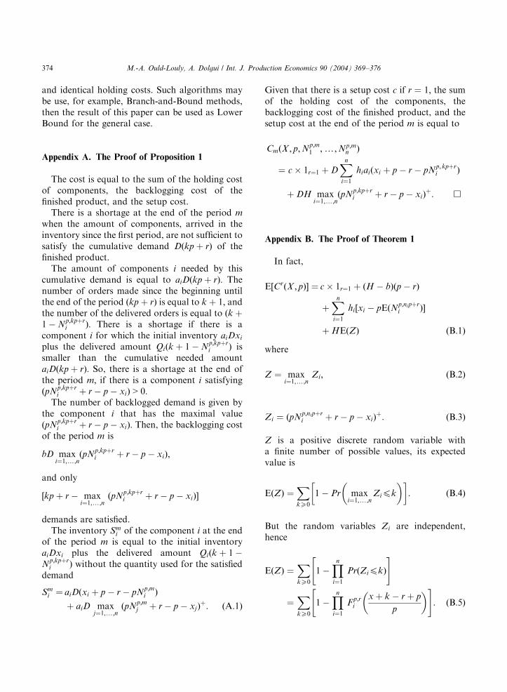
Appendix A. The Proof of Proposition 1
The cost is equal to the sum of the holding costof components, the backlogging cost of thefinished product, and the setup cost.
There is a shortage at the end of the period m
when the amount of components, arrived in theinventory since the first period, are not sufficient tosatisfy the cumulative demand Dðkp þ rÞ of thefinished product.
The amount of components i needed by thiscumulative demand is equal to aiDðkp þ rÞ: Thenumber of orders made since the beginning untilthe end of the period ðkp þ rÞ is equal to k þ 1; andthe number of the delivered orders is equal to ðk þ1� N
p;kpþri Þ: There is a shortage if there is a
component i for which the initial inventory aiDxi
plus the delivered amount Qiðk þ 1� Np;kpþri Þ is
smaller than the cumulative needed amountaiDðkp þ rÞ: So, there is a shortage at the end ofthe period m; if there is a component i satisfyingðpN
p;kpþri þ r � p � xiÞ > 0:
The number of backlogged demand is given bythe component i that has the maximal valueðpN
p;kpþri þ r � p � xiÞ: Then, the backlogging cost
of the period m is
bD maxi¼1;y;n
ðpNp;kpþri þ r � p � xiÞ;
and only
½kp þ r � maxi¼1;y;n
ðpNp;kpþri þ r � p � xiÞ�
demands are satisfied.The inventory Sm
i of the component i at the endof the period m is equal to the initial inventoryaiDxi plus the delivered amount Qiðk þ 1�N
p;kpþri Þ without the quantity used for the satisfied
demand
Smi ¼ aiDðxi þ p � r � pN
p;mi Þ
þ aiD maxj¼1;y;n
ðpNp;mj þ r � p � xjÞ
þ: ðA:1Þ
Given that there is a setup cost c if r ¼ 1; the sumof the holding cost of the components, thebacklogging cost of the finished product, and thesetup cost at the end of the period m is equal to
CmðX ; p;Np;m1 ;y;Np;m
n Þ
¼ c � 1r¼1 þ DXn
i¼1
hiaiðxi þ p � r � pNp; kpþri Þ
þ DH maxi¼1;y;n
ðpNp;kpþri þ r � p � xiÞ
þ: &
Appendix B. The Proof of Theorem 1
In fact,
E½CrðX ; pÞ� ¼ c � 1r¼1 þ ðH � bÞðp � rÞ
þXn
i¼1
hi½xi � pEðNp;nipþri Þ�
þ HEðZÞ ðB:1Þ
where
Z ¼ maxi¼1;y;n
Zi; ðB:2Þ
Zi ¼ ðpNp;nipþri þ r � p � xiÞ
þ: ðB:3Þ
Z is a positive discrete random variable witha finite number of possible values, its expectedvalue is
EðZÞ ¼XkX0
1� Pr maxi¼1;y;n
Zipk
� �� : ðB:4Þ
But the random variables Zi are independent,hence
EðZÞ ¼XkX0
1�Yn
i¼1
PrðZipkÞ
" #
¼XkX0
1�Yn
i¼1
Fp;ri
x þ k � r þ p
p
� �" #: ðB:5Þ
ARTICLE IN PRESS
M.-A. Ould-Louly, A. Dolgui / Int. J. Production Economics 90 (2004) 369–376 375
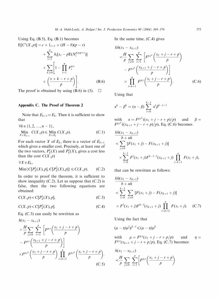
Using Eq. (B.5), Eq. (B.1) becomes
E½CrðX ; pÞ� ¼ c � 1r¼1 þ ðH � bÞðp � rÞ
þXn
i¼1
hi½xi � pEðNp;nipþri Þ�
þXkX0
1�Yn
i¼1
Fp;ri
"
�x þ k � r þ p
p
� �#: ðB:6Þ
The proof is obtained by using (B.6) in (3). &
Appendix C. The Proof of Theorem 2
Note that Ekþ1CEk: Then it is sufficient to showthat
8kAf1; 2;y; n � 1g;
MinXAEkþ1
CðX ; pÞpMinXAEk
CðX ; pÞ: ðC:1Þ
For each vector X of Ek; there is a vector of Ekþ1
which gives a smaller cost. Precisely, at least one ofthe two vectors, P1
kðX Þ and P2kðX Þ; gives a cost less
than the cost CðX ; pÞ
8XAEk;
MinfC½P1kðX Þ; p�;C½P2
kðX Þ; p�gpCðX ; pÞ: ðC:2Þ
In order to proof the theorem, it is sufficient toshow inequality (C.2). Let us suppose that (C.2) isfalse, then the two following equations areobtained:
CðX ; pÞoC½P1kðX Þ; p�; ðC:3Þ
CðX ; pÞoC½P2kðX Þ; p�: ðC:4Þ
Eq. (C.3) can easily be rewritten as
hðx1 � xkþ1Þ
>H
p
XjX0
Xp
r¼1
F p;r x1 þ j � r þ p
p
� ��
� Fp;r xkþ1 þ j � r þ p
p
� �
�Fp;rk x1 þ j � r þ p
p
� � Yn
i¼kþ2
Fp;rk xi þ j � r þ p
p
� �:
ðC:5Þ
In the same time, (C.4) gives
khðx1 � xkþ1Þ
oH
p
XjX0
Xp
r¼1
F p;rk x1 þ j � r þ p
p
� ��
� Fp;rk xkþ1 þ j � r þ p
p
� �
�Yn
i¼kþ1
F p;r xi þ j � r þ p
p
� �: ðC:6Þ
Using that
ak � bk ¼ ða� bÞXk�1
l¼0
albk�1�l
with a ¼ Fp;rk
ððx1 þ j � r þ pÞ=pÞ and b ¼F p;rk
ððxkþ1 þ j � r þ pÞ=pÞ; Eq. (C.6) becomes
khðx1 � xkþ1Þb þ nh
oXjX0
½F ðx1 þ jÞ � F ðxkþ1 þ jÞ�
�Xk�1
l¼0
Flðx1 þ jÞFk�1�lðxkþ1 þ jÞYn
i¼kþ1
F ðxi þ jÞ;
that can be rewritten as follows:
khðx1 � xkþ1Þb þ nh
oXk�1
l¼0
XjX0
½F ðx1 þ jÞ � F ðxkþ1 þ jÞ�
� F lðx1 þ jÞFk�lðxkþ1 þ jÞYn
i¼kþ2
F ðxi þ jÞ: ðC:7Þ
Using the fact that
ðm� ZÞmlZk�lpðm� ZÞmk
with m ¼ Fp;rðx1 þ j � r þ p=pÞ and Z ¼F p;rðxkþ1 þ j � r þ p=pÞ; Eq. (C.7) becomes:
hðx1 � xkþ1Þ
oH
p
XjX0
Xp
r¼1
F p;r x1 þ j � r þ p
p
� ��
ARTICLE IN PRESS
M.-A. Ould-Louly, A. Dolgui / Int. J. Production Economics 90 (2004) 369–376376
� Fp;r xkþ1 þ j � r þ p
p
� �
�Fp;rk x1 þ j � r þ p
p
� � Yn
i¼kþ2
Fp;r xi þ j � r þ p
p
� �:
ðC:8Þ
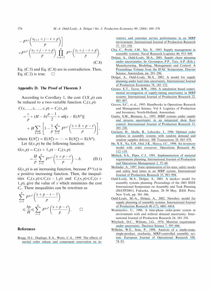
Eq. (C.5) and Eq. (C.8) are in contradiction. Then,Eq. (C.2) is true. &
Appendix D. The Proof of Theorem 3
According to Corollary 1, the cost CðX ; pÞ canbe reduced to a two-variable function Ceðx; pÞ:
Cðx;y;x;y; x; pÞ ¼ Ceðx; pÞ
¼c
pþ ðH � bÞ
p � 1
2þ nh½x � EðNpÞ�
þ HXkX0
1�1
p
Xp
r¼1
Fp;rn x þ k þ p � r
p
� �" #;
where EðNp1 Þ ¼ EðNp
2 Þ ¼ ? ¼ EðNpn Þ ¼ EðNpÞ:
Let Gðx; pÞ be the following function:
Gðx; pÞ ¼Ceðx þ 1; pÞ � Ceðx; pÞ
¼H
p
Xp
r¼1
Fp;rn x þ p � r
p
� �� b: ðD:1Þ
Gðx; pÞ is an increasing function, because Fp;rðxÞ isa positive increasing function. Then, the inequal-ities Ceðx; pÞpCeðx � 1; pÞ and Ceðx; pÞpCeðx þ1; pÞ; give the value of x which minimizes the costCe: These inequalities can be rewritten asXp
r¼1
F p;rn x þ p � r � 1
p
� �
pbp
Hp
Xp
r¼1
F p;rn x þ p � r
p
� �: &
References
Bragg, D.J., Duplaga, E.A., Watis, C.A., 1999. The effects of
partial order release and component reservation on in-
ventory and customer service performance in an MRP
environment. International Journal of Production Research
37, 523–538.
Chu, C., Proth, J.M., Xie, X., 1993. Supply management in
assembly systems. Naval Research Logistics 40, 933–949.
Dolgui, A., Ould-Louly, M.A., 2001. Supply chain planning
under uncertainties. In: Groumpos, P.P., Tzes, A.P. (Eds.),
Manufacturing, Modeling, Management and Control: A
Proceedings Volume from the IFAC Symposium. Elsevier
Science, Amsterdam, pp. 291–296.
Dolgui, A., Ould-Louly, M.A., 2002. A model for supply
planning under lead time uncertainty. International Journal
of Production Economics 78, 145–152.
Grasso, E.T., Tayor, B.W., 1984. A simulation based experi-
mental investigation of supply/timing uncertainty in MRP
systems. International Journal of Production Research 22,
485–497.
Graves, S.C., et al., 1993. Handbooks in Operations Research
and Management Science, Vol 4. Logistics of Production
and Inventory, North-Holland, Amsterdam.
Gupta, S.M., Brennan, L., 1995. MRP systems under supply
and process uncertainty in an integrated shop floor
control. International Journal of Production Research 33,
205–220.
Gurnani, H., Akella, R., Lehoczky, J., 1996. Optimal order
policies in assembly systems with random demand and
random supplier delivery. IIE Transactions 28, 865–878.
He, X.X., Xu, S.H., Ord, J.K., Hayya, J.C., 1998. An inventory
model with order crossover. Operations Research 46,
112–119.
Melnyk, S.A., Piper, C.J., 1981. Implementation of material
requirements planning. International Journal of Production
and Operations Management 2, 52–60.
Molinder, A., 1997. Joint optimisation of lot-sizes, safety stocks
and safety lead times in an MRP system. International
Journal of Production Research 35, 983–994.
Ould-Louly, M.A., Dolgui, A., 2001. A markov model for
assembly systems planning. Proceedings of the 2001 IEEE
International Symposium on Assembly and Task Planning
(ISATP2001), Fukuoka, Japan, 28–30 May, IEEE Press,
New York, pp. 301–306.
Ould-Louly, M.-A., Dolgui, A., 2002. Newsboy model for
supply planning of assembly systems. International Journal
of Production Research 40 (17), 4401–4414.
Wemmerlov, U., 1986. A time-phase order-point system in
environment with and without demand uncertainty. Inter-
national Journal of Production Research 24, 343–358.
Whybark, D.C., Wiliams, J.G., 1976. Material requirement
under uncertainty. Decision Science 7, 595–606.
Wilhelm, W.E., Som, P., 1998. Analysis of a single-stage,
single-product, stochastic, MRP-controlled assembly sys-
tem. European Journal of Operational Research 108,
74–93.