the memory game
TRANSCRIPT
Theoretical Computer Science 110 (1993) 169-196
Elsevier 169
Mathematical Games
The memory game*
Uri Zwick**
Mathematics Instilute, Uniuersify qf‘ Warwick, C’otrentry CV4 7AL, UK, and
Computer Science Dc~partment, Tel Aric Uniaersity, Tel Aoiv 69978, Israel
Michael S. Paterson Depurtment gf Compuler Scienca, L’niwrsitF qf Warwick, Cooentry CV4 7AL, UK
Communicated by R.K. Guy
Received August 1991
Revised July 1992
Abstract
Zwick, U. and MS. Paterson, The memory game, Theoretical Computer Science 110 (1993)
I69- 196.
The memory game, or concentration, as it is sometimes called, is a popular card game played by
children and adults around the world. Good memory is one of the qualities required in order to
succeed in it. This, however, is not enough. When it is assumed that the players have perfect memory,
the memory game can be seen as a game of strategy. The game is analysed under this assumption
and the optimal strategy is found. It is simple and perhaps unexpected.
In contrast to the simplicity of the optimal strategy, the analysis leading to its optimality proof is
rather involved. It supplies an interesting example of concrete mathematics of the sort used in the
analysis of algorithms. It is doubtful whether this analysis could have been carried out without resort
to experimentation and a substantial use of automated symbolic computations.
1. The game
A pack containing n pairs of identical cards is shuffled and the cards are spread face
down on a table. Each player in turn flips two cards, one after the other. If the two
Correspondence to: U. Zwick, Computer Science Department, Tel Aviv University, Tel Aviv 69978, Israel. Email addresses of the authors: [email protected] and msp(&dcs.warwick.ac.uk.
*This work was partially supported by the ESPRIT II BRA Programme of the EC under contract # 3075 (ALCOM).
**Most of this work has been carried out while this author was visiting the University of Warwick.
0304-3975/93/$06.00 8 1993-Elsevier Science Publishers B.V. All rights reserved
170 U. Zwick, MS. Paterson
cards flipped are identical (i.e., they form a pair), they are removed from the table into
the possession of the player who flipped them and he/she gets another turn. If the two
cards are not identical then they are flipped back and the turn passes to the next
player. The game continues until all the cards are removed from the table (or until all
the players agree to end the game) and the winner is the player possessing the largest
number of pairs. The gain (or loss, if negative) of a player at any stage is defined to be
the number of pairs he/she holds minus the average number of pairs held by the
opponents.
Any number of players can play the game but the most interesting situation occurs
when there are only two of them. We will, therefore, consider this case here.
The invention of the memory game is sometimes attributed to Christopher Louis
Pelman and the game is often called Pelmanism (refer to this entry in [4]).
A light-hearted report on some of the results obtained in this paper has recently
appeared in [S].
2. Moves, positions and strategies
Each player tries to remember the position and the identity of all the cards already
inspected. To focus our attention on the strategic questions involved, we will assume
that the players have already reached a high level of proficiency and are able to absorb
all this information (in other words, they have perfect memories).
A turn in the game is composed of two plies. The observation that triggered this
work is that at each ply the player can either inspect a new card (in which case we
assume that the outcome is uniformly distributed over all the as-yet-unflipped cards),
or an old card whose identity is already known to both players. Inspecting an old card
in the first ply, or a nonmatching old card in the second ply, are in a sense idle plies.
Idle plies are not always possible. In the beginning of the game, for example, the first
player has to flip two new cards.
There are at most three reasonable moves from each position.’ The first is to pick
no new cards at all. Such a move will be called a O-move and it is possible only if there
are at least two inspected cards on the table. The two other moves, termed l-move and
2-moue, both begin by flipping a new card. If the new card matches a previously
inspected card then in both cases the matching card is flipped, a pair is formed and the
player gets another turn. If, however, the first card flipped does not match a previously
inspected card then an idle ply is used in a l-move while a new card is inspected in
a 2-move. It can easily be seen that making an idle ply first and then flipping a new
card is always inferior to the other moves.
While playing the game the players can have two different objectives. They could
try to maximise the probability of winning the game or, alternatively, they could try to
maximise their expected gain. The two objectives lead to somewhat different optimal
1 See, however, the note at the end of the paper
The memory game 171
strategies. We will investigate here the strategy that maximises the expected gain. The
optimal strategy for the other case could presumably be obtained using similar
methods and a more involved analysis.
If a O-move maximises the expected gain for the next player then, after this O-move
is played, the situation remains exactly the same and the second player would also like
to play a O-move. Since this can go on forever, we stop the game in such a case.
A position in the game is characterised by the number n of pairs still on the table
and the number k of cards on the table which have already been inspected. We can
assume that all the inspected cards are different. In the case where the last player
played a 2-move and the second card flipped matches not the first card flipped but one
of the previously inspected cards, the resulting pair would be immediately removed by
the other player, and we may account for this as part of the present turn.
A stvabegy is a rule which determines which one of the three plausible moves should
be used in each position (n, k), where 06 kdn are integers. An optimal strategy is
a strategy which maximises the expected gain assuming that both players play
optimally. The ualue of a position is the expected future gain of the player who is first
to play from that position assuming that both players use an optimal strategy. We
shall see in the next section that the position values and an optimal strategy can be
defined mutually recursively. It is easy to see that if a player is playing according to an
optimal strategy then the expected gain from some position is at least the value of that
position, no matter what strategy the opponent may choose.
3. The optimal strategy
We define recursively the values en,k of the different positions. The only initial
condition that we need is that e 0,0 =O, that is, that no one gains from a null game.
Assume that we have already defined enC,k. for n’<n and en,k, for k’> k. We will first
define e,‘,k and en’.k which will be the expected gain from position (n, k) when
beginning with a l- or a 2-move respectively, and subsequently playing using an
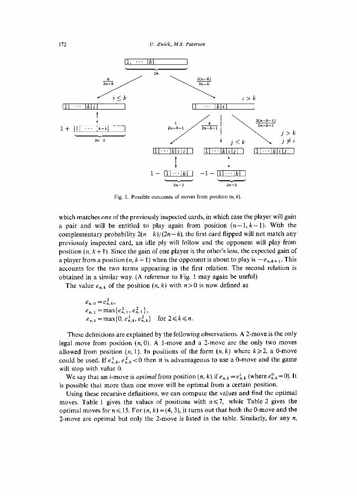
optimal strategy. Referring to Fig. 1, it is relatively easy to verify that
n,k+l>
We will explain the first relation as an example. When flipping the first card, there are
k inspected cards on the table, all of them different, and 2n - k uninspected cards. In
a l-move an uninspected card is flipped. With probability k/(2n - k), it will be a card
172 U. Zwick, M.S. Paterson
111 . . . lkl
111 . . lkliI - 1
I 1+ (11 ... Ik-11
/ s-2
r+'i'k '3;r
I
IlI...lklilil 1 Ill...lkliljl I IlI...lklil_?j )
I I 1+ 111 -_l-~l
. zn-2 zn-2
Fig. 1. Possible outcomes of moves from position (n. k).
which matches one of the previously inspected cards, in which case the player will gain
a pair and will be entitled to play again from position (n- 1, k- 1). With the
complementary probability 2( n - k)/(2n - k), the first card flipped will not match any
previously inspected card, an idle ply will follow and the opponent will play from
position (n, k + 1). Since the gain of one player is the other’s loss, the expected gain of
a player from a position (n, k + 1) when the opponent is about to play is -en,k+ 1. This
accounts for the two terms appearing in the first relation. The second relation is
obtained in a similar way. (A reference to Fig. 1 may again be useful).
The value en,k of the position (n, k) with n > 0 is now defined as
e 2 n,O=en,Ol
e n,l =max{e,l,1,e,Z,1),
en,k =max{O, e,‘,k, ei,k} for 2<k<n.
These definitions are explained by the following observations. A 2-move is the only
legal move from position (n, 0). A l-move and a 2-move are the only two moves
allowed from position (n, 1). In positions of the form (n, k) where k>2, a O-move
could be used. If c,‘&, e,“,k ~0 then it is advantageous to use a O-move and the game
will stop with value 0.
We say that an i-move is optimal from position (n, k) if en& = et,k (where ei,k = 0). It
is possible that more than one move will be optimal from a certain position.
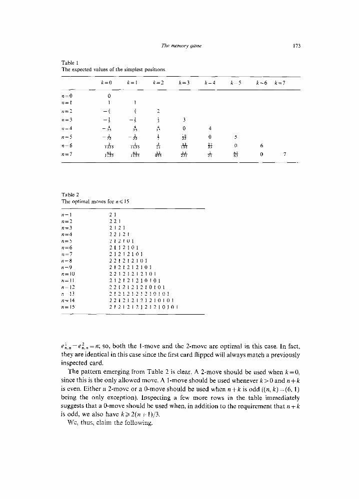
Using these recursive definitions, we can compute the values and find the optimal
moves. Table 1 gives the values of positions with n ~7, while Table 2 gives the
optimal moves for n < 15. For (n, k) =(4,3), it turns out that both the O-move and the
2-move are optimal but only the 2-move is listed in the table. Similarly, for any n,
The memory game 173
Table 1
The expected values of the simplest positions
n=O
n=l
n=2
n=3
n=4
n=5
n=6
n=7
k=O k=l k=2 k=3 k=4 k=5 k=6 k=l
0
1 1
-: s 2
4 4 f 3
-& A & 0 4
-sf -315 $ % 0 5
ii& i& 12i * 5: 0 6
fi i% &A # h % 0 7
Table 2
The optimal moves for n< 15
n=l 21
n=2 221
n=3 2121
n=4 22121
n=5 212101
n=6 2112101
n=7 21212101
n=8 221212101
n=9 2121212101
n=lO 22121212101
n=ll 212121210101
n= 12 2212121210101
n=13 21212121210101
n=14 221212121210101
n=15 2121212121210101
’ en,n =e,2,, = n; so, both the l-move and the 2-move are optimal in this case. In fact,
they are identical in this case since the first card flipped will always match a previously
inspected card.
The pattern emerging from Table 2 is clear. A 2-move should be used when k=O, since this is the only allowed move. A l-move should be used whenever k > 0 and n + k
is even. Either a 2-move or a O-move should be used when n+ k is odd ((n, k) =(6, 1)
being the only exception). Inspecting a few more rows in the table immediately
suggests that a O-move should be used when, in addition to the requirement that rr + k is odd, we also have k32(n+ 1)/3.
We, thus, claim the following.
174 U. Zwick. M.S. Paterson
Theorem 3.1.
and n+k odd 1 , en,k= ei,k if [kal and n+k even] or [(n, k)=(6, l)],
2 en,k otherwise.
Another interesting issue is the behaviour of the values e,,k themselves. The following
approximation gives their asymptotical behaviour.
Theorem 3.2.
if n + k even,
e n,k =
2n+l ifn+k odd and kd-
3 '
2(n + 1) if n+k odd and kBp
3
Ifwelet~=k/nthenweseethat,for~<l,e,,,=e,’,,-~/2(l-i)ifn+kiseven,and
e n,k=e,2,k~[(2-3A)(2-,l)/16(1-E.)3].l/n if n+k is odd and kd(2n+1)/3. Sim-
ilarly, we can get that ei,k = -[~/2(1-1,)]~(4-12%+7%2)/(2-;1)2 if n+k is even
and that e,‘,k = -[(4-81_+5L2)/16(1-E,)3]~l/n if n+k is odd and k6(2n+1)/3.
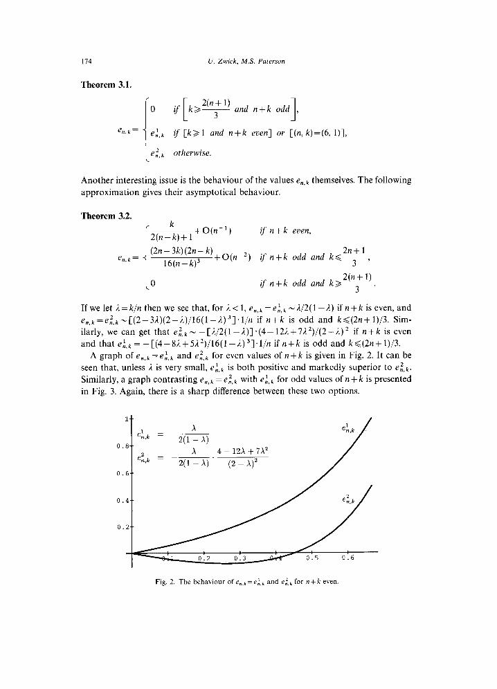
A graph of e,,k =e,‘,k and ei,k for even values of n + k is given in Fig. 2. It can be
seen that, unless 1* is very small, e,‘,k is both positive and markedly superior to e&.
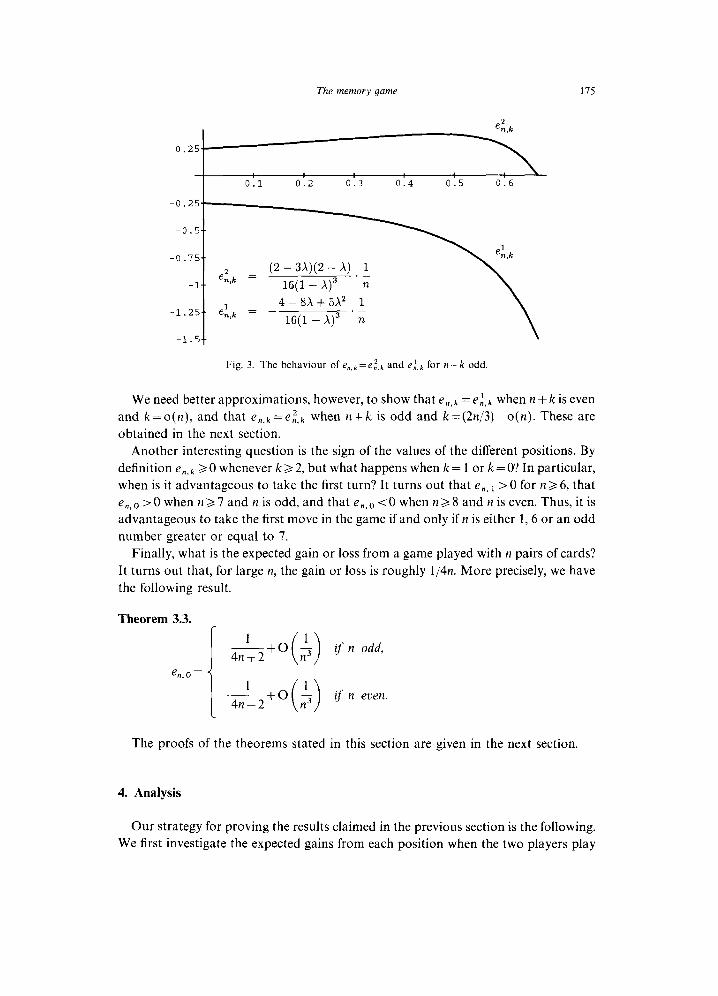
Similarly, a graph contrasting en,k =e,‘,k with e,‘,k for odd values of n + k is presented
in Fig. 3. Again, there is a sharp difference between these two options.
l--
1 x en,k =
0 .8-- 2(1- A)
0 _ 6..
Fig. 2. The behaviour of e.,, = e:,,, and ei,k for n + k even.
The memory pme 175
0.25.
2 en,k
0.1 0.2 0.3 0.4 0.5 0.6
-0.25.
-0.15.- 2 (2 3X)(2 A) - - 1
en,k = . -1.- 16(1 - A)” n
-1.25-b eA,k 4 -8X +5X2 1
-1.5s-
= - 16(1 - A)” ’ ii
Fig. 3. The behaviour of en,k =ef,k and ej,, for n+k odd.
We need better approximations, however, to show that e,,k = ei,k when n + k is even
and k=o(n), and that e,,k=ei,k when n + k is odd and k = (2n/3) - o( n). These are
obtained in the next section.
Another interesting question is the sign of the values of the different positions. By
definition e ,,k > 0 whenever k 2 2, but what happens when k = 1 or k = O? In particular,
when is it advantageous to take the first turn? It turns out that e,, I >O for n36, that
e,, 0 > 0 when n > 7 and n is odd, and that e,, e < 0 when n > 8 and n is even. Thus, it is
advantageous to take the first move in the game if and only if n is either 1,6 or an odd
number greater or equal to 7.
Finally, what is the expected gain or loss from a game played with II pairs of cards?
It turns out that, for large n, the gain or loss is roughly 1/4n. More precisely, we have
the following result.
Theorem 3.3.
( &+O($) iSn odd,
en’oj_-&j+O($) if n even.
The proofs of the theorems stated in this section are given in the next section.
4. Analysis
Our strategy for proving the results claimed in the previous section is the following.
We first investigate the expected gains from each position when the two players play
176 U. Zwick, M.S. Paterson
according to the alleged optimal strategy. Once we have tight estimations of these
values, it will be easy to prove, by induction, that these values do in fact correspond to
the optimal strategy.
4.1. Preliminary manipulations
Let e&k be the expected values of the different positions when both players play
according to the conjectured optimal strategy. As a “warm-up”, we prove the follow-
ing lemma.
Lemma 4.1. (i) e,,o = e,, 1 for odd n > 1 and (ii) e,, o =-e,, 1 for euen n # 6.
Proof. For odd n, we have e,,o = ei, o and e,, I = e,‘, 1. Using the definitions of ei,k and
e.‘,k from Section 3, we see that both ez,o and e,‘, 1 expand to the same expression
e,Zo=e,ll= 2(n- 1)
, &(l+e,-1,0)--e 2n-1 “3”
This proves the first part of the lemma. For even n 26, we have e,,. =ei,o and
e,, 1 = ei, 1 and, therefore,
en,0 +e,,l =
[
2(n- 1) &tl+en-l,O)--e
2n-1 “‘2 1 + j&Cl+e.-l,O)-~
[
2(n- 1) 2(n-2)
2n-1 .2n_2 en,2 1 2(n- 1)
=j-&(l+e.-l.O)----e
2(n-2)
2n-1 n’2 -2n_1en.3.
For even n32, we have enj2 =e,‘,2 and, thus,
en,0 +e,, 1 =A (l+e,-l,o)-
2(n- 1) 2n_1 &tl+en-i,l)
[
2(n-2) 1 2(n-2) -2n_2en,3 -2n_1en.3
=A Ce,- l,O-en-l,ll=O~
where the last equality follows from the first part of the lemma. 0
As an easy corollary, we get the following result.
Lemma 4.2. e,!, o = e,‘, o for even n # 6.
The memory game 177
’ Proof. By definition we have e “, 0 - - e,,o and ef,o = -e,, 1 and, thus, the result follows
from the second part of the previous lemma. 0
Note that l-moves are currently not allowed from positions of the form (n, 0). The
previous lemma says, however, that it would not matter if we were to allow them from
these positions with even n 26. Furthermore, the l-moves would be co-optimal in
these positions and we could, therefore, use the relation e,,. = eA,o as the defining
relation for even n # 6. This removes the anomaly of the column k = 0 seen in Table 1.
The two remaining exceptions are e6,0 =eg,, and e6,1 =e& 1.
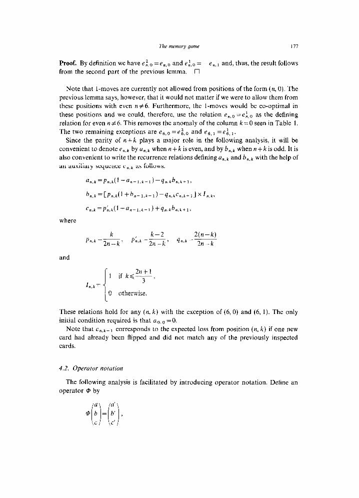
Since the parity of n+ k plays a major role in the following analysis, it will be
convenient to denote en,k by a,,k when n + k is even, and by bn,k when n + k is odd. It is
also convenient to write the recurrence relations defining an,k and bn,k with the help of
an auxiliary sequence c,,k as follows:
an,k=Pn,k(l+an-l,k-l)-qn,kbn,k+~,
bn,k=[Pn,k(l+b.-l.k-l)-qn,kCn,k+ll xln,k?
C,,k=Ph,k(l+a,-,,k-,)+q,,kbn,k+l,
where
k k-2 2(n-k) P&k =2n_k 3 Pb,k =2n_k 9 qn,k =
2n-k
and
In,k= ! 1 ifk<y,
0 otherwise.
These relations hold for any (n, k) with the exception of (6,O) and (6, 1). The only
initial condition required is that a o, ,, = 0.
Note that c,,k+l corresponds to the expected loss from position (n, k) if one new
card had already been flipped and did not match any of the previously inspected
cards.
4.2. Operator notation
The following analysis is facilitated by introducing operator notation. Define an
operator Qi by
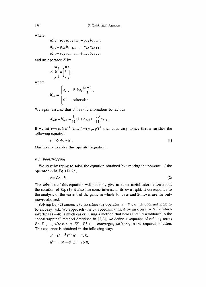
178 U. Zwick, MS. Paterson
where I
a~,k=~~,ka~-l,k-l-9q,,kb~,k+l,
b~,k=Pn,kb,-~,k-~-qn,kC,,kil,
C,,k=P~,ka,-l,k-l+qn,kbn,k+l,
and an operator Z by
where
i
b 2n+l
*,k if k<------
bh,k= 3 ’
0 otherwise.
We again assume that @ has the anomalous behaviour
1 ad,o=G.i =E(l+b5,e)-sa,,,.
If we let e =(a, b, c) T and h =(P, p, p’) T then it is easy to see that e satisfies the
following equation:
e=Z(@e+h). (1)
Our task is to solve this operator equation.
4.3. Bootstrapping
We start by trying to solve the equation obtained by ignoring the presence of the
operator Z in Eq. (I), i.e.,
e=@e+h. (2)
The solution of this equation will not only give us some useful information about
the solution of Eq. (l), it also has some interest in its own right. It corresponds to
the analysis of the variant of the game in which l-moves and 2-moves are the only
moves allowed.
Solving Eq. (2) amounts to inverting the operator (Z-Q), which does not seem to
be an easy task. We approach this by approximating @ by an operator 6 for which
inverting (I - 6) is much easier. Using a method that bears some resemblance to the
“bootstrapping” method described in [2,3], we define a sequence of refining terms
EO, E’, . . . . whose sum E” + E1 + ... converges, we hope, to the required solution.
This sequence is obtained in the following way:
E’=(Z-6)-l h’, i>O,
h’+‘=(@-@E’, i>O,
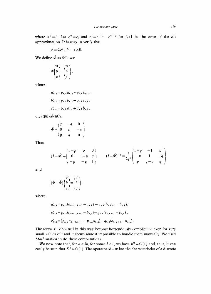
The memory game 119
where h”=h. Let e”=e, and e’=e’-’ -E’-’ for i>l be the error of the ith
approximation. It is easy to verify that
e’=@e’+h’, i>,O.
We define 6 as follows:
Thus,
and
where
a~,k=Pn,kan,k-qn,kbn,k,
b~.k=Pn,kbn.k-qn.kCn,k,
Cb,k=Pn,kan,k+qn,kbn,k,
or, equivalently,
1-P 4 0
0 1-P 4
-p -4 1
where
l+q -1 q
-P 1 -4
P 4-P 4
The terms E’ obtained in this way become horrendously complicated even for very
small values of i and it seems almost impossible to handle them manually. We used
Mathematics to do these computations.
We now note that, for k<An, for some 2.~ 1, we have ho = O(1) and, thus, it can
easily be seen that E” = 0( 1). The operator @ - 6 has the characteristics of a discrete
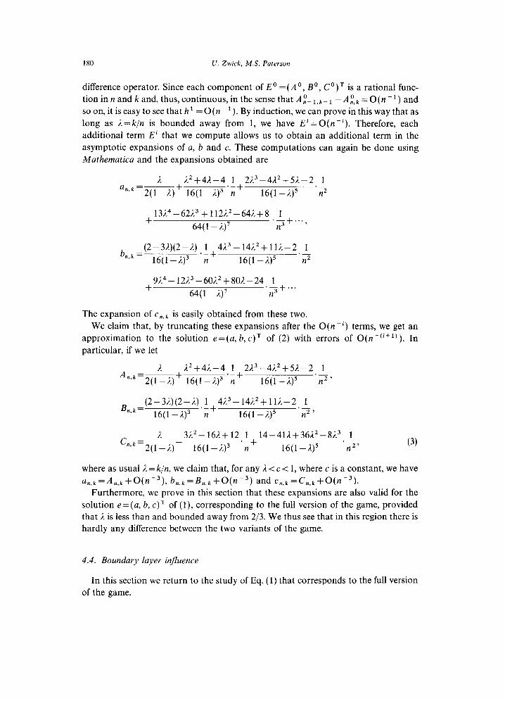
180 U. Zwick, MS. Paterson
difference operator. Since each component of E” = (A ‘, B”, C ‘) T is a rational func-
tion in n and k and, thus, continuous, in the sense that A:_ l,k_ 1 - A $ = 0( n - ’ ) and
so on, it is easy to see that h ’ = 0 (n - ’ ). By induction, we can prove in this way that as
long as A= k/n is bounded away from 1, we have E’ = O(n-‘). Therefore, each
additional term E i that we compute allows us to obtain an additional term in the
asymptotic expansions of a, b and c. These computations can again be done using
Mathematics and the expansions obtained are
;1 A2+4A--4 1 2A3-4A2+5A-2 1 a
“‘k-2(1-i)+ 16(1-A)” ‘;+ 16(1 -%)5 ‘n’
13A4-62E.3 +112E,*-64A+8 1 + ._
64(1-L)’ n3 + ... 2
b _(2-31,)(2-A) 1+423-1412+11~-2 1 n.k -
16(1 -)J3 ‘n 16(1 -L)5 ‘n’
9A4-12A3-60/?2+8011-24 1 + 64(1 -2)’ ‘n”+ “’
The expansion of c,,k is easily obtained from these two.
We claim that, by truncating these expansions after the O(n -‘) terms, we get an
approximation to the solution e =( a, b, c) T of (2) with errors of O(n -(i+l) ). In
particular, if we let
i A2+4A-4 1 2A3-4;b2+5A-2 1
A”gk-2(l A)+ 16(1-A)j ‘;+ 16(1 -A)5 ‘7’
B _(2-3A)(2-1,) 1+423-14i2+11d-2 1 n,k-
16(1 -A)3 ‘n 16(1 -A)5 ‘n”
I
A
%k =m- 3A2-1611+ 12 1 14-41;1+36A2-8A3 1
16(1 -;1)3 ‘;+ 16(1 -A)5 ‘n” (3)
where as usual A = k/n, we claim that, for any A < c < 1, where c is a constant, we have
a,,k=A.,k+O(n-3), b,,k=B,,k+O(np3) and c.,k=C,,,k+O(n-3).
Furthermore, we prove in this section that these expansions are also valid for the
solution e = (a, b, c) T of (l), corresponding to the full version of the game, provided
that I is less than and bounded away from 213. We thus see that in this region there is
hardly any difference between the two variants of the game.
4.4. Boundary layer influence
In this section we return to the study of Eq. (1) that corresponds to the full version
of the game.
The memory game 181
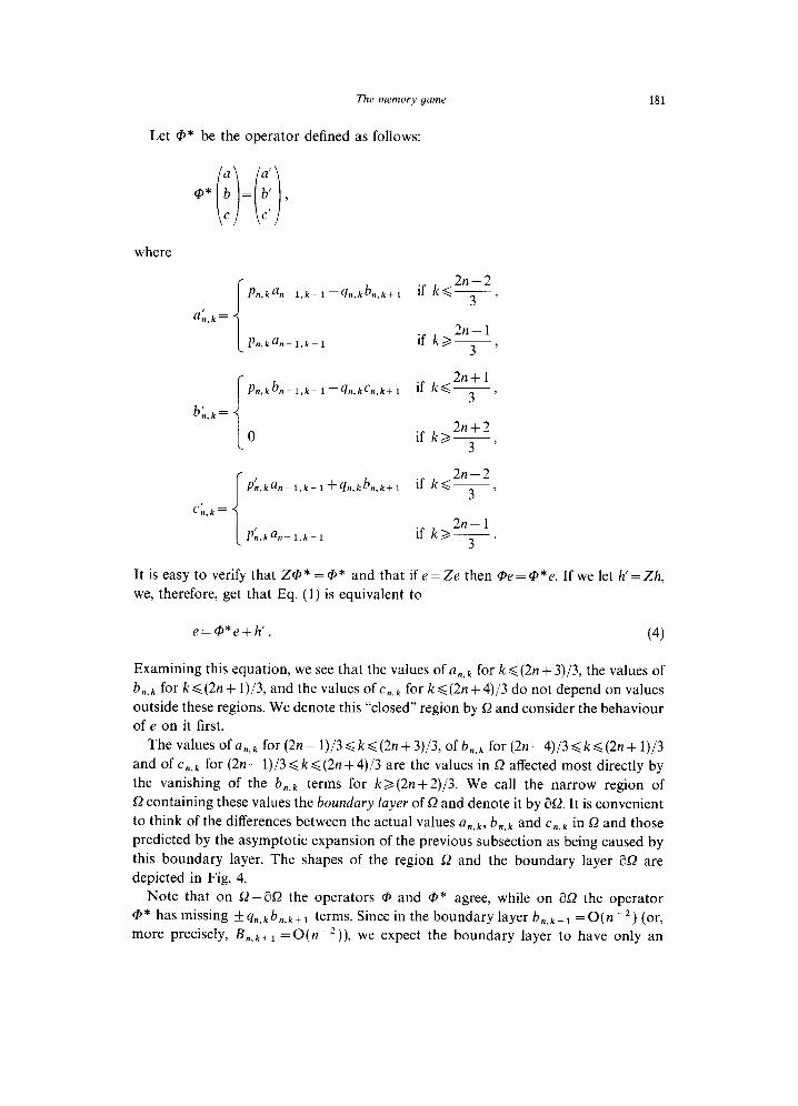
Let @* be the operator defined as follows:
where
1 2n-2
Pn,ka,-,,,-,-qq,,kb,,k+l if k<T,
an,k= ’ I hkan-l,k-1
2n+l Pn,kbn-1,k-l-qn,kCn,k+l if kGy9
bb,k= 0 if k>2n’2
‘3’ 2n-2
P~,ka,-l,k_l+qn,kbn,k+1 if kG3>
2n-1 if k3----
3 .
It is easy to verify that Z@ * = @ * and that if e = Ze then @e = @*e. If we let h’ = Zh,
we, therefore, get that Eq. (1) is equivalent to
e=@*e+k’. (4)
Examining this equation, we see that the values of a,,, k for k d (2n + 3)/3, the values of
bn,k for kd(2n+ 1)/3, and the VaheS of c,,k for k < (2n + 4)/3 do not depend on values
outside these regions. We denote this “closed” region by Q and consider the behaviour
of e on it first.
The values of a,, k for (2n- 1)/3<k<(2n+3)/3, of b,,, for (2n-4)/3<k<(2n+ 1)/3
and of c ,,k for (2n - 1)/3 d k d (2n + 4)/3 are the values in 52 affected most directly by
the vanishing of the bn,k terms for k >(2n + 2)/3. We call the narrow region of
Q containing these values the boundary layer of Q and denote it by X?. It is convenient
to think of the differences between the actual values an,k, bn,k and c,,~ in Q and those
predicted by the asymptotic expansion of the previous subsection as being caused by
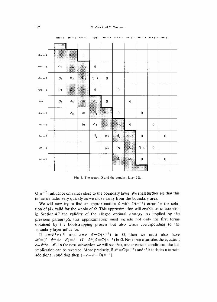
this boundary layer. The shapes of the region 52 and the boundary layer aQ are
depicted in Fig. 4.
Note that on Q- aQ the operators @ and @* agree, while on X2 the operator
@* has missing *qn,kbn,k+l terms. Since in the boundary layer bn,k+l =O(n-‘) (or,
more precisely, B,,k+r =o(n+)), we expect the boundary layer to have only an
182 U. Zwick, MS. Paterson
4m-3 4m-2 417-l 4m 4m+l 4m+2 4m+3 4m+4 4m+5 4m+6
6m-4
6m-3
61n - 2
6m+2 I
6m+4
I
6m+5 I
Fig. 4. The region Q and the boudary layer aL?
O(n -2) influence on values close to the boundary layer. We shall further see that this
influence fades very quickly as we move away from the boundary area.
We will now try to find an approximation & with O(n -3) error for the solu-
tion of (4), valid for the whole of R. This approximation will enable us to establish
in Section 4.7 the validity of the alleged optimal strategy. As implied by the
previous paragraph, this approximation must include not only the first terms
obtained by the bootstrapping process but also terms corresponding to the
boundary layer influence.
If e=@*e+h’ and s=e-d=O(n-3) in 52, then we must also have
~=(Z-~*)(e-b)=h’-(I-~*)&=O(n-3)in~.Notethat&satisfiestheequation
E = @*E + %‘. In the next subsection we will see that, under certain conditions, the last
implication can be reversed. More precisely, if 2 = 0( it -3) and if it satisfies a certain
additional condition then E = e - 6 = 0( n - 3 ).
The memory game 183
Let us first look at H=(R,S, T)T=h’-(Z-@*)E, where E=(A,B, C)‘, with
A, B, C defined in (3). Easy manipulations show that Rn,k, Sn,k, Tn,k =O(ne3) in
Q-&Q (this is ensured by the bootstrapping process) but that in aQ
R 9(2n-3k- 1) 1
n.k = 8 ‘PI’
--+O(n_3)
and
T _ _9(2n-3k-1) 1 n.k -
8 ‘$ p+O(n-3).
The quantity 2n - 3k measures the horizontal distance of position (n, k) from the
boundary layer K? This suggests that one could try to work with an approximation
&‘=(,G@‘, B, %‘)T of the form
%,,k = c,,k +y, (5)
where the An,k, Bn,kr Cn,k are again those of (3), and, thus, represent the global
behaviour in Q, while the sequences {z~}, (/I!] and {yl} represent the effect of the
boundary layer X? We expect the sequences {cI~}, {fil} and {rl} to be quickly, in fact
exponentially, diminishing, so that their contribution far from the boundary layer will
indeed be negligible.
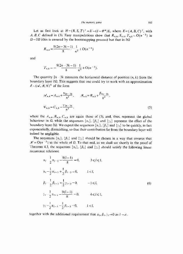
The sequences {x1}, {fiI} and {;I~} should be chosen in a way that ensures that
X=O(n -3) in the whole of Q. To that end, as we shall see shortly in the proof of
Theorem 4.3, the sequences {ccl}, {PI) and {y,} should satisfy the following linear
recurrence relations:
1 9(1-f) =O a, -- c([+ 1 -~
2 8 ’ -36161,
1 1 vp+1 +-ai-3=0,
2 1 <l,
/+I+, +;Yl-3=0> -lbl, (6)
Y++l -;s,-3 =Q 1 <I,
together with the additional requirement that CI~, PI, y[-+O as l-co.
184 U. Zwick, M.S. Paterson
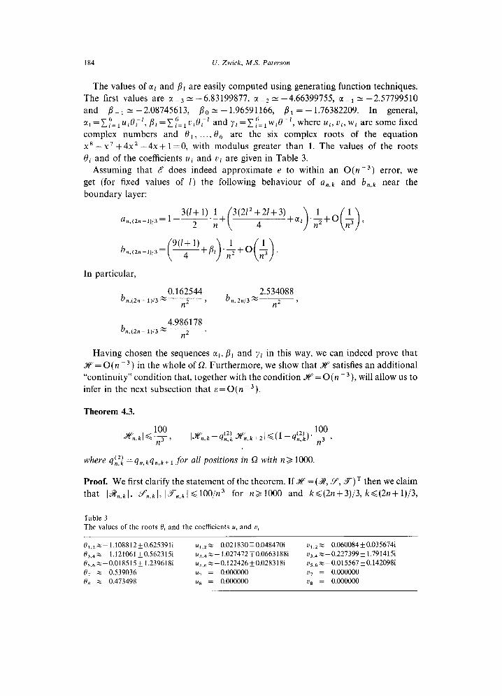
The values of c(~ and fil are easily computed using generating function techniques.
The first values are CI _3 2: -6.83199877, CI _2 2: -4.66399755, CI _i = -2.57799510
and b_1 2: -2.08745613, /?,, = -1.96591166, /I1 = - 1.76382209. In general,
a~=C~=,UiB;‘,BI=C~=1Uie;’ andy,=C~=,w,e-‘,whereui,ui,wiaresomefixed
complex numbers and 0i, . , e6 are the six complex roots of the equation
X8 -x7 +4x2 -4x + 1 =O, with modulus greater than 1. The values of the roots
8i and of the coefficients Ui and Ui are given in Table 3.
Assuming that & does indeed approximate e to within an 0(ne3) error, we
get (for fixed values of I) the following behaviour of an,k and bn,k near the
boundary layer:
In particular,
b 0.162544 2.534088
n,(2nf 1)/3 = n2 > b,,2n,3= n2 >
b 4.986178
n,t2n- 1)/3 = n2 ’
Having chosen the sequences LX~, b1 and yI in this way, we can indeed prove that
X=0(?? -3) in the whole of 52. Furthermore, we show that X satisfies an additional
“continuity” condition that, together with the condition X’= O(n -3), will allow us to
infer in the next subsection that e=0(K3).
Theorem 4.3.
where qifi = qn,kqn,k+l for all positions in Cl with na 1000.
Proof. We first clarify the statement of the theorem. If X = (2, Y, Y) T then we claim
that IS?,,kl, ILY,,~\, l.YR,k/ d 100/n3 for n> 1000 and kd(2n+3)/3, kd(2n+ 1)/3,
Table 3 The values of the roots Bi and the coefficients ui and ui
Q ,,,z-1.108812f0.625391i u1.2= 0.02 1830 T 0.04847Oi “1.2= 0.060084 + 0.035674i
0 3.4= 1.121061 kO.562315i u~,~%- 1.027472TO.0663188i ~~,~z-O.227399* 1.791415i
0 ,,,e-0.018515f 1.2396181 US.6 - --0.122426+0.028318i v,,,z-0.015567kO.142098i
8, z 0.539036 u, = 0.000000 0, = 0.000000 0s h 0.473498 us = 0.000000 cg = 0.000000
The memory yame 185
kd@+W, respectively, and that Ign,k -qhf!%,k+2 I, ly,,,k -qj,f:yn,k+2 I, l~n,k -qC2’F kf2 I<(1 -q’2’)100/n
k d (2n - :;3, Respectively. n.k
3 for n3 1000 and kg(2n-3)/3, k<(2n--5)/3,
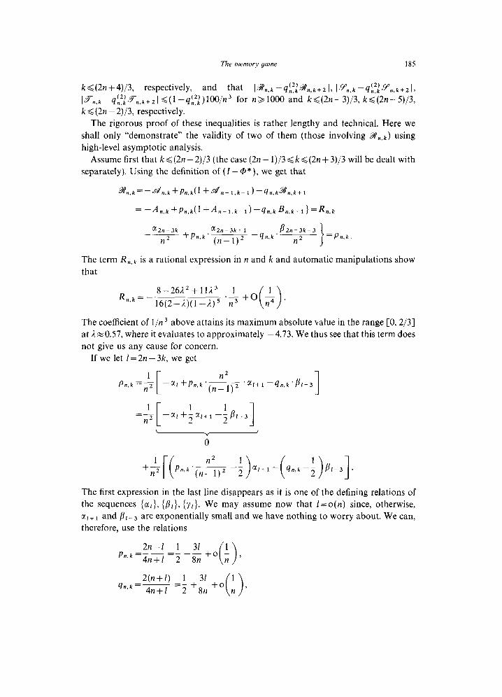
The rigorous proof of these inequalities is rather lengthy and technical. Here we
shall only “demonstrate” the validity of two of them (those involving L?J?,,~) using
high-level asymptotic analysis.
Assume first that k d (2n - 2)/3 (the case (2n - 1)/3 <k < (2n + 3)/3 will be dealt with
separately). Using the definition of (I - @* ), we get that
~)n.k=-.~n,k+Pn,k(l+~n-l,k-1)-qn,k~!n,k+1
= -A..k+p,,k(l+A,-,,k-,)-q,,kBn,k+l}=Rn,k
ff2n-3k a2n-3k+l 82n-3k-3 --
n2 +tPn.k’ cn_l12 --4n,k’ n2
=p k
“5
The term Rn,k is a rational expression in n and k and automatic manipulations show
that
R __ 8-26A2+11/23 n,k -
.i+o L 16(2-i.)(l-1,)5 n3 ( 1 n4 ’
The coefficient of l/n 3 above attains its maximum absolute value in the range [0,2/3]
at 2~0.57, where it evaluates to approximately -4.73. We thus see that this term does
not give us any cause for concern.
If we let 1= 2n - 3k, we get
Pn,k =’
n2 *-
n2 --al+Pn,k tn_,j2 ‘11+1 -qn,k’ljl-3 1
1 1 1 =-
n2 --crl+-@l+l 2 --Pi-, 2 1 c
Y I
0
[( -++I -(q,,,k+-31.
The first expression in the last line disappears as it is one of the defining relations of
the sequences {al>, {PI:, (~~1. W e may assume now that l=o(n) since, otherwise,
a,+ 1 and fli_ j are exponentially small and we have nothing to worry about. We can,
therefore, use the relations
,
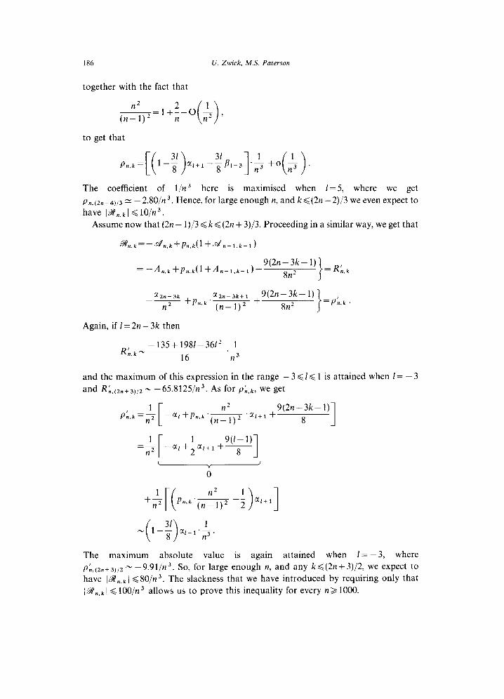
186 U. Zwick, MS. Paterson
together with the fact that
n2 -=1+;+0 J$ ) (n- 1)2 ( )
to get that
P n,k =
The coefficient of l/n3 here is maximised when 1= 5, where we get
pn,c2n-41,3 N -2.801~1~. Hence, for large enough n, and k<(2n-2)/3 we even expect to
have I.!%)n,k 1 d 10/n3.
Assume now that (2n - I)/3 d k d (2n + 3)/3. Proceeding in a similar way, we get that
XZn-3k UZn-3k+l
n2 +Pn.k’ tn_j)2 +9(2n-3k- l) 8n2
=Ph,k ’
Again, if 1=2n-3k then
Rb,k - - 135+ 1981-36l’ 1
16 ‘2
and the maximum of this expression in the range - 3 d 1 d 1 is attained when / = - 3
and %(2n+3)/2 - -65.8125/n3. As for PL,k, we get
Pb,k =;
[
n2 9(2n-3k- 1) ._ -@I+Pn,k tn_1J2 ‘al+1 + 8 1
1 =-[-.,+;Nl+l+yq
n2
The maximum absolute value is again attained when I= - 3, where
pb,c2n+3J,2 N -9.91/n3. So, for large enough n, and any k<(2n+3)/2, we expect to
have Ig,,k ) <80/n 3. The slackness that we have introduced by requiring only that
igR,,k ( < loo/n3 allows us to prove this inequality for every n 3 1000.
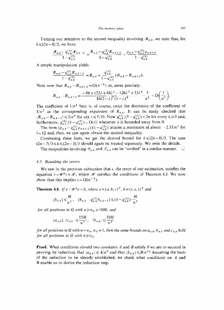
The ,nemory ymne 187
Turning our attention to the second inequality involving Bn,k, we note that, for
k<(2n- 8)/3, we have
2 n,k -4;f:%,,+z =Rn.k -4:f:R.,k+z +Pn,k -q:f:&,k+Z
l-df: l-9$ 1 -q;::
A simple manipulation yields
R n.h (2) R -q,,k n,h+Z =R
1-4:;: + q’n2: ---(R.,k-R.,k+z). n.k 1 -q;f;
Note now that R,., - Rn.k+2 =0(ne4) or, more precisely,
-88+ 152L+64;b2 -126j.3 +333v4 1 R n,h -R n,k+Z = 16(2-3.)‘(1 -i)‘j
.p+o 5. ( >
The coefficient of l/n4 here is, of course, twice the derivative of the coefficient of
l/n3 in the corresponding expansion of Rn,k. It can be easily checked that
n k+2(<3/n4 for say ;,<l/lO. Now q’,fi/(l-qLf:)<2n for every k>,O and,
EZeYnYore, q, ,/( (‘I
The term (p,Ik
1 -qb’l) = 0( 1) whenever i is bounded away from 0.
-qb~~,)‘.,k+2)/(1 -qkf:) attains a maximum of about -2.33/n3 for
I= 12 and, thus, we can again obtain the desired inequality.
Combining these facts, we get the desired bound for k<(2n- 8)/3. The case
(2n - 7)/3 <k < (2n - 3)/3 should again be treated separately. We omit the details.
The inequalities involving ,yn,k and Tn,k can be “verified” in a similar manner. 0
4.5. Bounding the errors
We saw in the previous subsection that E, the error of our estimation, satisfies the
equation E = @*E + H, where X satisfies the conditions of Theorem 4.3. We now
show that this implies E=0(nm3).
Theorem 4.4. Ife=@*e+h, where e=(a, b, c)~, h=(r,s, t)T and
for all positions in Q with n an,, 2 1000, and
for al/positions in Q with n=nO, n,, + 1, then the same bounds on a,,k, b,,k and c,,k hold
for all positions in .Q with n >no.
Proof. What conditions should two constants A and B satisfy if we are to succeed in
proving, by induction, that ) an,k 1 <A/ n3 and that ) bn,k ) < B/n3? Assuming the basis
of the induction to be already established, we check what conditions on A and
B enable us to derive the induction step.
188 lJ. Zwick, MS. Paterson
Using the induction hypothesis and the conditions on hn,k, we can bound a,,k as
follows:
la&k 1 <P&k . ian-l,k-l 1 +4&k’ lb&k+1 1 + irn,kl
+&]““+[f++[$]“H If A > B + 2H then the last expression is less than A/n 3 for any sufficiently large n and
k6(2n+3)/2. This is because in Sz we have pn,k <3+0(l).
In particular, if we choose A = 15H, B= lOH, we must verify that
for any n 3 1000 and O< kd0.67n. This inequality involves only quantities like
P,,~ and qn,k that were explicitly defined. Expanding these definitions, we find that the
claim to be verified is equivalent to the claim that
-2(4+31)(1-3n+3n2)+(8-91.)n3 30
for any n 3 1000 and 0 d E, = k/n 6 0.67. This inequality is easily verified.
The choice that A > B has so far been to our advantage. It will, however, make our
lives much more difficult in the sequel.
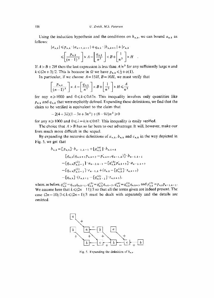
By expanding the recursive definitions of a,,&, bn,k and c&k in the way depicted in
Fig. 5, we get that
b.,k=[Pn,kl.b.~l,k-1 +[4::1+n,k+4
-[qn.k(qn,k+lPn,k+2-P~.k+lqn-l,k)l'bn-l.k+l
-[%,kP:f:+l ]‘a,-2,k-1 +[4b3:Pb,k+31’an-1,k+2
-~~n.k~j1~~+l~~rn-l.k+~Sn,k-~~bf:~~Sn,k+2~
-[~n,kl'(~n,k+l-[~:~:+l1%,k+d~
where, as before, qb2: = qn,kqn,k+1,qj13:=qjll2:q,,k+2,q~~=q~3:q",k+3 andP$ =Pn.kPn-1-k-l.
We assume here that k <(2n - 11)/3 so that all the terms given are indeed present. The
case (2n- lo)/3 < k<(2n + 1)/3 must be dealt with separately and the details are
omitted.
Fig. 5. Expanding the definition of b.,t
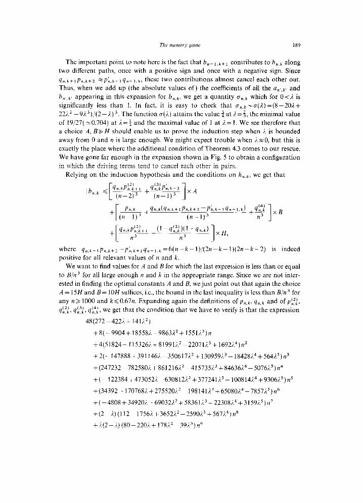
The memory game 189
The important point to note here is the fact that b,- I,k+ 1 contributes to bn,k along
two different paths, once with a positive sign and once with a negative sign. Since
q++ 1pn,k+2 ZP;,~+ 1 qn_ l,k, these two contributions almost cancel each other out.
Thus, when we add up (the absolute values of) the coefficients of all the u~,,~, and
b n’, k’ appearing in this expansion for bn,k, we get a qUantity o,,& which for 0~ 1. is
significantly less than 1. In fact, it is easy to check that b,,k -a(A) =(8 -202 +
22)“’ - 9A3)/(2 - I.) 3. The function o(i) attains the value i at A= 3, the minimal value
of 19/27( N 0.704) at i = f and the maximal value of 1 at A= 1. We see therefore that
a choice A, B$ H should enable us to prove the induction step when 1” is bounded
away from 0 and n is large enough. We might expect trouble when 3.~0, but this is
exactly the place where the additional condition of Theorem 4.3 comes to our rescue.
We have gone far enough in the expansion shown in Fig. 5 to obtain a configuration
in which the driving terms tend to cancel each other in pairs.
Relying on the induction hypothesis and the conditions on hn.k, we get that
qn.k(qn,k+lPn,k+2-P~.k+lqn-l,k) / q:ff xB
n3 1 where qn,k+1pn,k+2-p~,k+Iqn~1,k=6(n-k-1)/(2n-k-1)(2n-k-2) iS indeed
positive for all relevant values of n and k. We want to find values for A and B for which the last expression is less than or equal
to B/n3 for all large enough n and k in the appropriate range. Since we are not inter-
ested in finding the optimal constants A and B, we just point out that again the choice
A = 15H and B = 1 OH suffices, i.e., the bound in the last inequality is less than B/n 3 for
any n 3 1000 and k <0.67n. Expanding again the definitions of p,,k, qn,k and of p!,fj,
4 (2) n.k, 671;:3 q:!J, we get that the condition that we have to verify is that the expression
48(272-4226+ 1413.‘)
+8(-9904+ 185581.-9863A2+ 1551A3)n
+4(51824- 1153261+819913~2-22071~3+ 1692A4)n2
+2(-147888+3911461.-350617~2+1309591.3-18428/14+564i,5)n3
+(247232-782580~“+861216/,2-415735i3+84636a4-5076j”5)n4
+(-122384+473052i.-630812~2+377241i~3-1008141.4+9306~5)n5
+(34392- 1707683.+275520J.2- 198141i.3+650801.4-7857/15)n6
+(-4808+34920i-69032/12+583613.3-22308~4+3159~5)n7
+ (2 - I.) (112 - 1756). + 36521.2 - 2590L3 + 567A4) n*
+ A(2 - A) (80 - 22Oi + 1 78L2 - 39i.3) n9
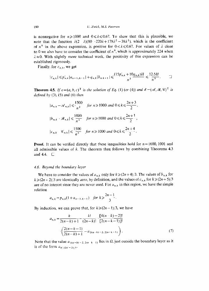
190 U. Zwick, M.S. Paterson
is nonnegative for n> 1000 and 06AGO.67. To show that this is plausible, we
note that the function 1.(2-1.)(80-2201.+ 178Eb2 -39L3), which is the coefficient
of n9 in the above expression, is positive for O~Ad0.67. For values of Iti close
to 0 we also have to consider the coefficient of n8, which is approximately 224 when
AzO. With slightly more technical work, the positivity of this expression can be
established rigorously.
Finally, for c,,k, we get
ic,,,ki <Ph,ki%-l,k-I 1 +qn,kibn,k+l I < tl%,k + l”qn,k)H 6 12.5H.
n3 q
n3
Theorem 4.5. Zf e = (a, b, c) T is the solution of Eq. (1) (or (4)) and 8 = (d, g’, W) ’ is
dejined by (3), (5) and (6) then
1500 l%k -.d,,k 167
for 1000 and
2n+3
n> Obkb- 2 ’
ibn,k 1000
-@n,k I G-
2n+l
n3 for n31OOO and Odkb-,
2
IC,,!i 1500
-g&k I d7 2n+4
for n>lOOO and O<kd- 2 .
Proof. It can be verified directly that these inequalities hold for n= 1000, 1001 and
all admissible values of k. The theorem then follows by combining Theorems 4.3
and 4.4. q
4.6. Beyond the boundary layer
We have to consider the values of fl,,,k only for k 3 (2n + 4)/3. The values of bn,k for
k 2 (2n + 2)/3 are identically zero, by definition, and the values of c&k for k 3 (2n + 5)/3
are of no interest since they are never used. For a&k in this region, we have the simple
relation
2n-1 &,k=Pn,ktl +a,- l,k- 1) for ka-
3
By induction, we can prove that, for k3(2n- 1)/3, we have
k k! [4(n-k)-2]!
an’k=2(n-k)+1-(2n ‘[2(n-k-l)]!
(7)
Notethatthevaluea3(n_k)_2,2,n~k~1) lies in 52, just outside the boundary layer as it
is of the form anS,(2nC _2113.
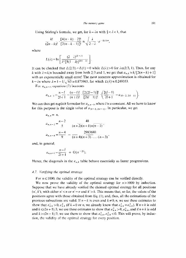
The memory game
Using Stirling’s formula, we get, for k =%n with 5~1~~ 1, that
191
k! _. [4(n-k)-2]! ~ i
(2n-k)! [2(n-k- l)]! J __ .e-L(iM 2-i ”
where
L(j_) =ln (2 _ j)‘2 -A)
1 J,“[8(1 _i)]*(r-i)
It can be checked that L(2/3) =L(l) =0 while L(J.) >0 for E,~(2/3, 1). Thus, for any
k with R = k/n bounded away from both 213 and 1, we get that a,,,!+ z k/[2(n- k) + 11 with an exponentially small error! The most accurate approximation is obtained for
k=%n where II= 1 -l/&=0.875965, for which L(%) ~0.249353.
For G,~-~, equation (7) becomes
n-l (n-l)! [2(21-l)]! 2(1-l) a ___ _-.
“.“-l=2/+1 (n+l)! [2(/-l)]! . 2[+1 -a31-2**(l-l) ( >
We can thus get explicit formulae for un.n _ [, where 1 is a constant. All we have to know
for this purpose is the single value of a31- *, 2C1_ r). In particular, we get
a n.n = n,
n-2 48 a n,n-2 =- -
5 (n+2)(n+ l)n(n- 1) ’
n-4 2983680 u n,n-4
=_ - 9 (n+4)(n+3).....(n-3)’
and, in general,
n-l a -- + O(n-*‘).
n-n-l -21+ 1
Hence, the diagonals in the e,,k table behave essentially as linear progressions.
4.7. Verijjing the optimal strategy
For n < 1000, the validity of the optimal strategy can be verified directly.
We now prove the validity of the optimal strategy for n> 1000 by induction.
Suppose that we have already verified the claimed optimal strategy for all positions
(n’, k’), with either n’ < n or n’ = n and k’ > k. This means that, so far, the values of the
positions agree with those obtained from Eq. (1) and, thus, all the estimations of the
previous subsections are valid. If n+ k is even and k#O, n, we use these estimates to
show that e,‘,k >O, ez,k (if k=O or n, we already know that e,‘,k =ef,k). If n+k is odd
and k<(2n+ 1)/3, we use these estimates to show that e,‘,k ~0, ef,k, and if n+ k is odd
and k>(2n+ 1)/3, we use them to show that ei,k, e,‘,k ~0. This will prove, by induc-
tion, the validity of the optimal strategy for every position.
192 U. Zwick, MS. Paterson
As can be seen from Figs. 2 and 3, the only inequalities for which we really need the
0( l/n’) terms in our approximations are those that claim that es,k =bn,k >O when
n+ k is odd and kd(2n+ 1)/3, and that e,“,k < 0 when n + k is odd and k 3 (2n + 2)/3.
Even here, the 0( l/n’) terms are needed only when /1z$.
5. Variants of the game
As the reader has probably realised by now, there is no point in flipping back the
cards after inspection if both players will remember them anyway. This convention
also allows the game to be played as a game of strategy by players with imperfect
memories. A O-move now simply corresponds to a decision to end the game, while
a l-move will mean literally the inspection of one new card, without the useless ritual
of inspecting an old one too. With these new conventions, it seems natural to allow
O-moves and l-moves from all positions (even those of the form (n, 0) and (n, 1)) and
we shall do so throughout this section.
What is the effect of allowing 0- and l-moves from positions of the form (n, 0) and
O-moves from positions of the form (n, l)? Since the value of every position in the new
game is, by definition, nonnegative, some changes are bound to occur but, as we shall
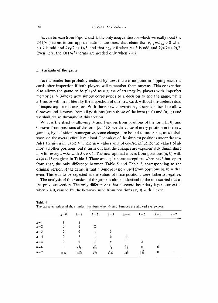
soon see, the overall effect is minimal. The values of the simplest positions under the new
rules are given in Table 4. These new values will, of course, influence the values of al-
most all other positions, but it turns out that the changes are exponentially diminishing
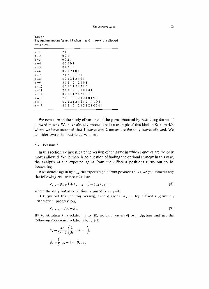
in n for every k=h with %<c< 1. The new optimal moves from positions (n, k) with
k < n d 15 are given in Table 5. There are again some exceptions when n < 5 but, apart
from that, the only difference between Table 5 and Table 2, corresponding to the
original version of the game, is that a O-move is now used from positions (n, 0) with n
even. This was to be expected as the values of these positions were hitherto negative.
The analysis of this version of the game is almost identical to the one carried out in
the previous section. The only difference is that a second boundary layer now exists
when I. ~0, caused by the O-moves used from positions (n, 0) with n even.
Table 4
The expected values of the simplest positions when 0- and l-moves are allowed everywhere
k=O k=l k=2 k=3 k=4 k=5 k=6 k=l
n=l 1 1 n=2 0 : 2
n=3 0 0 : 3
n=4 0 : : 0 4
n=5 0 0 : 4 0 5
n=6 0 di * h E 0 6
n=l &?S &A 7% AS & +% 0 7
The memory game 193
Table 5 The optimal moves for n < 15 when 0- and l-moves are allowed
everywhere
n=l 21
n=2 021 n=3 002 1 n=4 02101
n=5 002101
n=6 0212101
n=l 21212101
n=8 021212101
n=9 2121212101
n=lO 02121212101
n=ll 212121210101
n= 12 0212121210101
n=l3 21212121210101
n=14 021212121210101
n=l5 2121212121210101
We now turn to the study of variants of the game obtained by restricting the set of
allowed moves. We have already encountered an example of this kind in Section 4.3,
where we have assumed that l-moves and 2-moves are the only moves allowed. We
consider two other restricted versions.
5.1. Version 1
In this section we investigate the version of the game in which l-moves are the only
moves allowed. While there is no question of finding the optimal strategy in this case,
the analysis of the expected gains from the different positions turns out to be
interesting.
If we denote again by en.k the expected gain from position (n, k), we get immediately
the following recurrence relation:
en,k=Pn,k(l+en-l.k-l)-qn,ken.k+l, (8)
where the only initial condition required is e,,. =O.
It turns out that, in this version, each diagonal en,n_r for a fixed Y forms an
arithmetical progression,
e n,n-r =ay,n+p,. (9)
By substituting this relation into (8), we can prove (9) by induction and get the
following recurrence relations for Y > 1:
194 U. Zwick, MS. Paterson
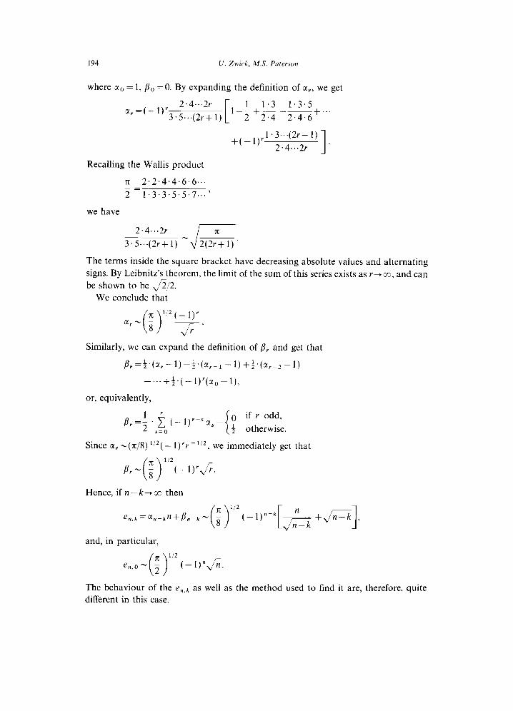
where a0 = 1, /IO =O. By expanding the definition of a,., we get
c(, =(_ 1)’ 2.4...2r 1 1.3 1.3.5
3.5...(2r+ 1) l-2 +2-m+“’
+(-1)’ 1 .3...(2r-1) 1 2.4...2r ’
Recalling the Wallis product
rt 2.2.4.4.6.6... 2 =1.3.3.5.5.7../
we have
The terms inside the square bracket have decreasing absolute values and alternating
signs. By Leibnitz’s theorem, the limit of the sum of this series exists as Y+ co, and can
be shown to be $12.
We conclude that
7c 0 1/2(-l)r
u,- - 8 J’
Similarly, we can expand the definition of /I, and get that
/II=+.(C(I-l)-+.(rX_-l -l)++.(C(I_2-l)
-...+f.(-l)‘(cco-l),
or, equivalently,
Since CC, -(n/8) ‘j2( - l)lv P1’2, we immediately get that
fir- ; 0 1’2( - 1,rJ;.
Hence, if n-k-+ co then
e n,k=C(n-kn+bn-k
and, in particular,
The behaviour of the en,k as well as the method used to find it are, therefore, quite
different in this case.
Thr memory fame 195
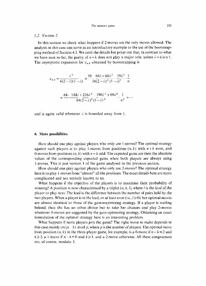
5.2. Version 2
In this section we check what happens if 2-moves are the only moves allowed. The
analysis in this case can serve as an introductory example to the use of the bootstrap-
ping method of Section 4.3. We omit the details but point out that, in contrast to what
we have seen so far, the parity of n + k does not play a major role, unless ;1= k/n z 1.
The asymptotic expansion for en,k obtained by bootstrapping is
2 2 16-64jV+64i2 - 19j.3 1
e”*k=4(2-j_)(1-i.) + 16(2-/I)’ (1 -i)’ ‘n
64- 144i.+216E.2 - 1981.3 +69Eb4 1 +
64(2-i)3(1-3.)3 ‘7 -I-‘..
and is again valid whenever I. is bounded away from 1.
6. More possibilities
How should one play against players who only use l-moves? The optimal strategy
against such players is to play l-moves from positions (n, k) with n + k even, and
O-moves from positions (n, k) with n + k odd. The expected gains are then the absolute
values of the corresponding expected gains when both players are always using
l-moves. This is just version 1 of the game analysed in the previous section.
How should one play against players who only use 2-moves? The optimal strategy
here is to play l-moves from “almost” all the positions. The exact details here are more
complicated and not entirely known to us.
What happens if the objective of the players is to maximise their probability of
winning? A position is now characterised by a triplet (n, k, I), where 1 is the lead of the
player to play next. The lead is the difference between the number of pairs held by the
two players. When a player is in the lead, or at least even (i.e., />O), her optimal moves
are almost identical to those of the gain-maximising strategy. If a player is trailing
behind, then she has no other choice but to take her chances and play 2-moves
whenever O-moves are suggested by the gain-optimising strategy. Obtaining an exact
formulation of the optimal strategy here is an interesting problem.
What happens if more players join the game? The right move to make depends in
this case mainly on (n-k) mod p, where p is the number of players. The optimal move
from position (n, k) in the three-player game, for example, is a O-move if n-k = 2 and
k 3 3, a l-move if n-k = 0 and k 2 1, and a 2-move otherwise. All these congruences
are, of course, modulo 3.
196 U. Zwick, MS. Paterson
We assumed in this paper that the players have perfect memories. What happens if
the players have imperfect memories?
7. Concluding remarks
The optimal strategy for playing the memory game turns out to be very simple. The
analysis and proof presented here were however extremely involved. Is there an easier
way of proving the results stated in Section 3?
While the results of this work are mainly of recreational value, we hope that the
methods used here will prove useful elsewhere. We would like to stress again the
indispensable role played in this work by experimentation and by automated sym-
bolic computations.
Acknowledgment
The first author thanks Tamir Shalom and his daughter Loran for interesting him
in the problem, and Yuval Peres for his help in the initial analysis attempts.
Note added in proof. After completing this work, we heard that Sabih H. Gerez and
Frits Gobel [l] had previously considered the analysis of the memory game. They had
empirically found the optimal strategy of Section 3 and explained parts of it theo-
retically. They also considered the version of the game in which O-moves are not
allowed. They discovered that in this version a surprising move optimises the expected
profit from positions of the form (n, n- 1) where n38. In this move, a new card is
flipped in the first ply. If this does not match any known card, a second new card is
flipped. But if the first card flipped does match a known card then an old card not
matching the first card is chosen in the second ply. This sacrifice deliberately leaves
a matching pair on the table! The next player would collect this pair but then be in
a similarly awkward position in which the sacrifice move is again optimal. With this
new move e,, n _ 1 z - 312 + 5/2n.
References
[l] S.H. Gerez, An analysis of the “Memory” game (in Dutch), 65-afternoon project report, Department
of Electrical Engineering, University of Twente, Holland, June 1983. [Z] D.H. Greene, D.E. Knuth, Mathematics for the Analysis of Algorithms, 2nd edn. (BirkhCuser, Base],
1982).
[3] R.L. Graham, D.E. Knuth and 0. Patashnik, Concrete Mathematics: A Foundation for Computer
Science (Addison-Wesley, Reading, MA, 1989).
[4] Oxford English Dictionary (Oxford Univ. Press, Oxford, 2nd edn., 1989).
[S] I.N. Stewart, Concentration: a winning strategy, Scienhjic American 265(4) (October 1991) 103-105.