the magnitude and duration of late ordovician-early silurian glaciation
TRANSCRIPT
www.sciencemag.org/cgi/content/full/science.1200803/DC1
Supporting Online Material for
The Magnitude and Duration of Late Ordovician–Early Silurian Glaciation
Seth Finnegan,* Kristin Bergmann, John M. Eiler, David S. Jones, David A. Fike, Ian Eisenman, Nigel C. Hughes, Aradhna K. Tripati, Woodward W. Fischer
*To whom correspondence should be addressed. E-mail: [email protected]
Published 27 January 2010 on Science Express DOI: 10.1126/science.1200803
This PDF file includes:
Materials and Methods Figs. S1 to S13 Table S1 References
1
Supporting Online Material
Contents:
Materials and Methods
A. Geologic setting
B. Age assignments
C. Constraints on calcification depth
D. Collection and preparation of samples
E. Δ47 analysis and standardization
F. Determination of δ18
Owater
G. Estimating ice volumes from δ18
Owater
G. Trace elemental analysis
H. Assessing post-depositional alteration of proxy (δ18
O, Δ47) signals
I. Within-bed variability and potential vital effects
J. Comparison with Cenozoic proxy data and with climate model simulations
Supplementary Figures and Captions
Fig. S1: Simplified stratigraphic columns of sampled basins
Fig. S2: SEM images and photographs of representative samples
Fig. S3: Comparison of sediment and skeletal isotopic and elemental composition,
sample 910-10-RC1
Fig. S4: Δ47 temperature and δ18
O profiles adjacent to Jurassic dike at Falaise de
Puyjalons, Anticosti Island
Fig. S5: Δ47 temperature versus δ18
O for co-occurring skeletal and secondary phases
Fig. S6: Log10Fe/Sr vs. Log10Mn/Sr
Fig. S7: Sr, Mn, and Fe concentrations and PC1 scores versus Δ47
Fig. S8: Taxon-specific PC1 scores versus Δ47
Fig. S9: Temperature, δ18
Owater, and δ18
O times series based only on fully assayed samples
Fig. S10: Temperature, δ18
Owater, and δ18
O times series based only on rugose corals
Fig. S11: Ice volume versus δ18
Owater for different assumed values of δ18
Oice
Fig. S12: Temperature, δ18
Owater, and δ18
O times series assuming an early Hirnantian age
for the sub-Laframboise Ellis Bay Formation
Fig. S13: Tropical SST versus δ18
Owater for Late Ordovician-Early Silurian and Cenozoic
proxy datasets and versus polar temperature for IPCC model runs
Supplementary Tables
Table S1: Source, locality, stratigraphic context, age, δ13
C, δ18
O, Δ47, temperature,
δ18
Owater, and trace metal data for samples referred to in text and SOM
2
A. Geologic setting
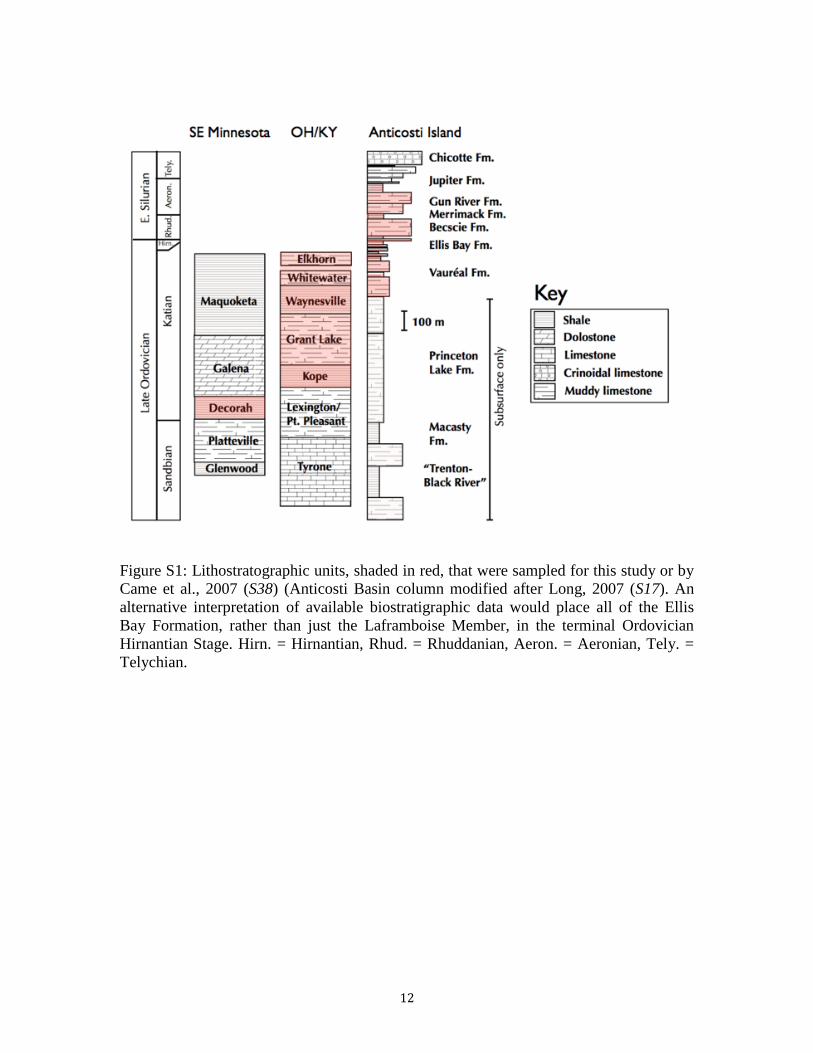
All samples were collected from Laurentia (core North America). Late Katian-Aeronian
samples come from the exceptionally complete and fossiliferous record of Anticosti
Island in the Gulf of St. Lawrence, Québec (S1-S4) and early-late Katian samples come
from two classic and well-described cratonic successions in the U.S. midcontinent (upper
Mississippi Valley of IA-WI-MN-IL (S5, S6) and Cincinnati Arch of OH-KY-IN (S7-
S10); (Fig S1). Laurentia was rotated ~45° clockwise from its current orientation and
straddled the equator during Late Ordovician and Early Silurian time (S11, S12), and all
of the sampled units were located in continental shelf and epicontinental seaways within
tropical latitudes.
Sedimentation in the Anticosti Basin began in Late Cambrian time and subsidence and
sedimentation rates reached a Middle to Late Ordovician maximum due to crustal loading
associated with thrust sheets from the advance of the Taconic Arc (S13-S15). Subsidence
continued into the Early Silurian, finally waning with the maturation of Taconic
mountain building near the end of Early Silurian time (S15). Similar to contemporaneous
sections elsewhere, the Anticosti Basin shows evidence of a dramatic shallowing of sea
level in the latest Ordovician Hirnantian Stage (S3, S4, S16-S19). However, perhaps
because of the relatively high rates of subsidence and sediment accumulation, it is one of
the few Late Ordovician depocenters in Laurentia where sedimentation continued through
Hirnantian time without a major nonconformity (S20). Minor nonconformities are
present, however (S4), and there is controversy regarding how much of Hirnantian time is
represented in the section and whether this is apportioned to the entire Ellis Bay
Formation or only to the very condensed uppermost (Laframboise) member of the Ellis
Bay Formation and the lowermost portion of the overlying Becscie Formation(see “Age
assignments” below).
Hirnantian-aged sediments are thin, discontinuous, and largely unfossiliferous in the
upper Mississippi Valley (S21, S22) and are entirely absent on the Cincinnati Arch (S9,
S22). However, these successions also contain strata considerably older than those
exposed at the surface on Anticosti. Both the upper Mississippi Valley and Cincinnati
Arch successions were deposited on the flanks of persistent basement highs (The
Kankakee Arch, formed by subsidence in the adjacent Michigan and Illinois Basins
(S23), and the Cincinnati Arch, a forebulge associated with the Taconic Orogeny (S8,
S23)). Consequently, they are thinner and less deeply buried than coeval successions in
adjacent cratonic and foreland basins. Paleozoic sedimentation in the upper Mississippi
Valley ceased in Silurian time, and the total preserved thickness of post-Ordovician
sediments is, in most places, << 100 m (S23). Sedimentation continued into the
Mississippian on the flanks of the Cincinnati Arch, such that the preserved thickness of
post-Ordovician sediments in this region ranges from 0 in southern Ohio and central
Kentucky to >500 m in east-central and west-central Kentucky (S23). Although more
than three km of sediments accumulated in the Anticosti Basin (S24),only the upper third
of this package is exposed at the surface4. Hence even the stratigraphically lowest
exposed sediments, the upper portion of the late Katian Vauréal Formation, are thought to
3
have experienced < 1 km of post-depositional burial (though the possibility that Late
Silurian-Devonian sediments were deposited but have been eroded away cannot be
discounted (S13, S25, S26)).
B. Age assignments
We assigned ages to samples based primarily on the stages indicated for formations by
Bergstrom et al., 2010 (S27), Buggisch et al. 2010 (S28), Long, 2007 (S15), and Achab et
al., 2010 (S1). Where multiple samples from a formation or set of formations falling
within a single stage are included, we interpolated ages, where possible, based on relative
stratigraphic position. For samples from multiple localities that could not be correlated at
sub-stage resolution, we assigned them all the same age. Samples from the Elkhorn
Formation and the lowermost Becscie Formation were ordered based on their δ13
C
values, with reference to the δ13
C curves published by Bergstrom et al., 2010 (S27), and
Desrochers et al. (S4). Correlation between the Katian sequences on Anticosti and in the
Cincinnati Arch region is based on the assignment of both the youngest Ordovician unit
the Cincinnati Arch region (Elkhorn Formation) and the oldest exposed unit on Anticosti
(lower Vauréal Formation) to the D. complanatus graptolite zone (S1, S27).
There is uncertainty regarding the precise age of the lower Ellis Bay Formation. Carbon
isotopic evidence suggests that only the Laframboise Member and the overlying
lowermost Becscie Formation are Hirnantian in age, with the underlying members of the
Ellis Bay Formation usually regarded as of Latest Katian age (S20). Although the lower
Ellis Bay Formation is richly fossiliferous, relatively few age-diagnostic taxa have been
recovered from it (S20), and multiple hypotheses persist over the identity and
biostratigraphic utility of these taxa. We follow Bergstrom et al., 2006 (S29) and Kaljo et
al., 2008 (S31) in placing the base of the Hirnantian near the base of the Laframboise
Member, but others have suggested that all or most of the Ellis Bay Formation is in fact
of Hirnantian age (S1, S3, S4, S31-S33). Using this alternative age model to construct our
time series (Fig. S12) does not change our inferences about the magnitude or overall
duration of glaciation, but would confine δ18
Owater values exceeding 1‰ to the Hirnantian
Stage.
C. Constraints on calcification depth
All three of the sample basins represent storm-influenced mixed carbonate-clastic ramp-
platform depositional settings above storm wave base (S4, S6, S17, S34-S37). Limiting
the bathymetric range of sampling is important because pelagic calcified organisms were
largely absent from early Paleozoic oceans, and the calcitic taxa available for
geochemical analyses were benthic. Restricting our analyses to these units ensures
estimates of the chemistry and temperature of the relatively homogenous upper ~100
meters of a well-mixed water column. The shallowest depositional environment in the
Anticosti sequence is represented by the Laframboise Member of the Ellis Bay
Formation, which records a large and globally recognized eustatic regression (S3, S19,
S38). The fact that this unit shows evidence of dramatic cooling, rather than the slightly
higher temperatures that should be associated with shallowing in the absence of any
4
climate change, argues strongly against a major role for depth changes in driving
observed temperature trends.
D. Collection and preparation of samples
Samples from the Vauréal, Ellis Bay, Becscie, Merrimack, and Gun River Formations
(Fig. S1) were collected by SF, WWF, DSJ, and DAF during fieldwork on Anticosti
Island in June and July of 2009. Sample localities and coordinates are given in table S1;
measured stratigraphic sections and additional locality information are available upon
request. Samples from the Jupiter Formation and their Δ47 and bulk isotope values
previously described in Came et al., 2007 (S38). Samples from the Decorah Formation
were collected at Wang‟s Corner, MN by KB in the summer of 2009. Samples from the
Kope, Bellevue and Waynesville formations of the Cincinnati Arch region were collected
by SF and KB in the summer of 2010, with additional samples from the Kope,
Waynesville, Whitewater and Elkhorn formations graciously provided by Brenda Hunda
from the collections of the Cincinnati Museum of Natural History. Samples were
collected from a variety of lithofacies, but focused where possible on shales from which
individual fossils could be manually separated. Slabs of cemented wackestone-packstone
beds with well-preserved fossils and mud drapes on the upper surface were also collected
in localities from which individual fossils could not be freed from the matrix. Fossils
were manually flaked from the surfaces of these slabs using a dental pick. For
brachiopods, this flaking focused on the secondary prismatic calcite layer to minimize
matrix contamination (S39-S41). In addition, several in-situ tabulate coral colonies were
collected from lime mudstone-dominate units. Following initial preparation to remove
them from the matrix all samples were sonicated for 2 hours to remove residual matrix
material; nevertheless this material could not always be completely removed and the
presence of variable amounts of residual matrix material containing late-stage diagenetic
carbonate phases likely accounts for many of the samples that give relatively high (38-
45° C) Δ47 temperatures and have altered trace metal signatures despite pristine textures
(Table S1). Following sonification, samples were either powdered with a mortar and
pestle (trilobite and brachiopod material) or microrotary drill (rugose and tabulate corals).
Some whole-rock slabs were also drilled to obtain matrix micrites for comparison with
fossils. Only the apical ends of rugose corals were drilled, following removal of the
outermost layer of skeletal material with an abrasive bit, to avoid the matrix and
secondary cements commonly found within the calice. Tabulate corals, all of which
preserved clear textural evidence of post-depositional alteration, were sampled in
multiple spots to evaluate Δ47 gradients associated with the amount of recrystallization
and/or post-depositional void filling by diagenetic cements.
E. Δ47 analysis and standardization
Approximately 10 mg of powder was used for each measurement; some samples were
measured as much as 5 times to reduce analytical uncertainty and to evaluate sample
heterogeneity. CO2 was extracted from powders by phosphoric acid digestion at 90° C
following the standard procedures outlined in Ghosh et al., 2006 (S42). Extracted CO2
5
was analyzed on a Finnigan MAT253 gas source mass spectrometer configured to collect
in the mass-44 to mass-49 range. The sample gas and a reference gas were analyzed 8
times each (8 acquisitions) in the course of each measurement. δ18
O and δ13
C were
measured along with δ47 for each acquisition. Acquisition-to-acquisition standard
deviations were on average 0.03 for δ47, 0.04‰ for δ18
O, and 0.02‰ for δ13
C. Three
isotopologues contribute to the mass-47 ion beam ( 18
O13
C16
O, 17
O12
C18
O and 17
O13
C17
O)
but the signal is dominated by the abundance of 18
O13
C16
O due to the rarity of 17
O.
Variations in the mass-47/mass-44 ratio (R47
) are converted to Δ47 by comparing them to
CO2 gases of known δ18
O and δ13
C composition that were heated to 1000° C for two
hours to achieve a stochastic R47
value for that composition. Δ47 is defined as the ‰
difference between the R47
value measured for a given sample and the R47
value that
would be expected for that sample if its stable carbon and oxygen isotopes were
randomly distributed among all possible isotopologues. Heated gases of three different
known compositions were used to minimize uncertainty in the Δ47 standardization, and
standardization of each sample was based only heated gases analyzed in the week prior to
its analysis.
Δ47 values were converted to carbonate growth temperature estimates based on the
relationship (S42):
Δ47 = 50.0592(106 T
-2)-0.02
where T is temperature in degrees Kelvin.
F. Determination of δ18
Owater
Determination of δ18
Owater is based on the low-temperature inorganic calcite fractionation
equation of Kim and O‟Neil, 1997 (S43):
1000lnα~(Calcite-H20) = 18.03 ( 103T
-1) - 32.42
G. Estimating ice volumes from δ18
Owater
For converting δ18
Owater to ice volume estimates we assume that the δ18
Owater value in an
ice-free world would be ~-1.0 as estimated by Savin, 1977 (S44) , and we assume that the
total volume of all surface water reservoirs has remained constant at 1,403,120,000 km3.
The major uncertainty in this calculation is the assumption of mean oxygen isotopic
composition of glacial ice (δ18
Oice) in the Late Ordovician-Early Silurian, a quantity that
is not measurable from the rock record. To accommodate this we calculated inferred ice
volumes for a given δ18
Owater value assuming multiple values for δ18
Oice (Fig. S11). If the
Gondwanan ice sheets had a mean δ18
Oice values similar to that of the last glacial
maximum (~-40‰, a weighted average that assumes a value of -30‰ for the now-
vanished Laurentide ice sheet(S46) and values of -30‰ and -55‰, respectively, for
remaining ice sheets in Greenland and Antarctica), observed Hirnantian δ18
Owater values
imply ice volumes exceeding the estimated 84,000,000 km3 (S46, S47) present during the
LGM. Only for δ18
Oice values lighter than -60‰ do observed Hirnantian δ18
Owater values
6
imply ice volumes lower than those of the LGM. Because ~-60‰ is the close to the most
extreme depletion observed in snow anywhere in the present day (S48) we regard it as
unlikely that the mean δ18
Oice of the Gondwanan ice sheet was this isotopically light.
Consequently the Hirnantian glacial maximum was likely characterized by very large ice
volumes, substantially higher than the LGM.
Our use of -1.0‰ as an ice-free baseline assumes that the O18
/O16
ratio of the oceans has
not changed since the Ordovician, but our arguments about trends in ice volume are not
tied to this assumption; we would reconstruct a similar relative ice volume trajectory for
any assumed ice-free baseline value. Although weathering inputs and hydrothermal
exchange processes may influence the oxygen isotopic composition of seawater (S49),
the residence time of oxygen isotopes in the ocean with respect to these processes is
much longer than the duration of the reconstructed δ18
Owater excursion.
H. Trace elemental analysis
A large and representative subset of samples (54 in total, 51 of which are skeletal
carbonates) were analyzed for concentrations of Sr, Mn, and Fe using inductively coupled
plasma atomic emission spectroscopy. Sample powders were dissolved in weak nitric
acid. Standards for Sr, Fe, and Mn were prepared in nitric acid of the same concentration
to minimize matrix effects. Sample and standard solutions were run on a Thermo iCAP
6300 radial view ICP-OES, using a Cetac ASX 260 autosampler with solutions aspirated
to the Ar plasma using a peristaltic pump. Three standard solutions (blank, 1 ppm, and 10
ppm) were run between every multiple of 10 sample unknowns. Reproducibility is better
than 5%, assessed by multiple runs of known standard concentrations.
I. Assessing post-depositional alteration of proxy (δ18
O, Δ47) signals
All Paleozoic carbonate successions have undergone episodes of diagenesis and, in many
cases, metamorphism. Because clumped isotope paleothermometry records aspects of the
solid state ordering of isotopologues, it is sensitive to post-depositional recrystallization:
original calcitic phases can be partially or entirely replaced by new phases that record
ambient (geothermal) temperatures at depth. Applying this proxy to estimate ancient
temperatures depends on selecting fossil material that has been minimally impacted by
diagenesis. In this section we provide a discussion of the observations, field tests,
techniques, and criteria we used to assess and understand the effects of post-depositional
alteration.
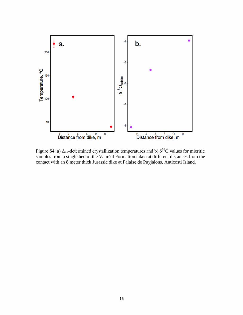
Dike test
One way of determining the quality of clumped isotope temperature estimates is to
examine the trend of the proxy across expected gradients in post-depositional alteration.
A section of the Vauréal Formation at Falaise de Puyjalons is bisected by an 8 m thick
Jurassic-aged quartz-tholeiitic dike (S50). Samples (collected by T. Raub) taken from
0.70, 4.95, and 13.35 meters from the contact with the dike, display the expected thermal
gradient of decreasing temperature with greater distance from the intrusion. A total
7
temperature differential of 180° C is observed in this field test (Fig. S4a), with
temperatures falling from 219° C near the dike to 39° C – suggestive of original ocean
temperatures with a relatively mild diagenetic overprint – 13.35 meters away from the
contact. δ18
Ocalcite shows the opposite trend increasing by ~4‰ over the same interval
(Fig. S4b), suggesting that the alteration during contact heating with the dike occurred in
the presence of a meteoric aquifer.
Textural analysis
We used light microscopy to examine the textural details and preservation state of all
samples, and scanning electron microscopy to examine a representative subset consisting
of 20 samples (Fig. S2). Most of the brachiopod and trilobite material examined shows
apparently excellent preservation with well-defined calcitic prisms clearly visible and
little evidence of recrystallization or secondary precipitation (Fig. S2a-d). Still, some of
these samples have trace metal compositions suggestive of moderate diagenetic alteration
and low Δ47 values indicative of relatively high crystallization temperatures (Figs. S6-S8,
Table S1). In some cases, particularly for samples that were manually flaked from
strongly lithified limestone slabs, it is clear that this reflects a variable admixture of
micritic matrix material and secondary cements that could not be removed from the
fossils. In most cases, however, it is not clear whether it represents matrix contamination
or cryptic recrystallization/secondary precipitation within the skeletal material. Tabulate
corals, by contrast, always preserve clear textural evidence of pervasive recrystallization
and secondary void-filling calcite precipitation (Fig. S2e-f). These samples also tend to
return strongly positive (altered) scores on trace metal composition PC 1 and low Δ47
values corresponding to crystallization temperatures ranging from 43 to 62° C. Rugose
corals often show a range of preservation states within a single corallite (Figs S2g-i, S3)
with prominent diagenetic alteration fronts and secondary calcite phases a common
feature (Figs S2i, S3). We avoided individuals, such as that shown in Fig S2i, that
appeared to be pervasively altered in extensive regions. More commonly, diagenetic
fronts are limited to discrete regions around the periphery of the corallite (Fig. S2g, S3)
and can be easily avoided even at the relatively coarse sampling scale dictated by our
material requirements.
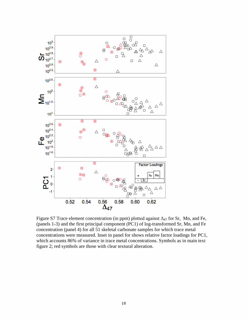
Trace element composition
Both theory and empirical patterns suggest that diagenetic stabilization of calcite tends to
drive increases in the concentration of Mn and Fe and decreases in the concentration of
Sr (S39, S51-S55). Our dataset provides support for this view from comparing
concentrations of these elements to Δ47 values (Fig. 2, Fig. S6a-c; Table S1). Mn and Fe
show strong negative correlations, indicating increasing concentration at higher
crystallization temperatures, and Sr shows a weak positive correlation with Δ47. We used
a principal components analysis (PCA) of log-transformed Sr, Mn, and Fe abundances to
summarize this information in a single eigenvector (PC 1, which receives strong positive
loadings from Mn and Fe and weak negative loading from Sr and explains 86% of the
variance in log trace metal concentrations among the 51 samples). PC 1 is strongly
correlated with Δ47 (Fig. S6d), but the relationship is not linear, showing a pronounced
8
step between 0.580 and 0.590 above which there is no apparent association between the
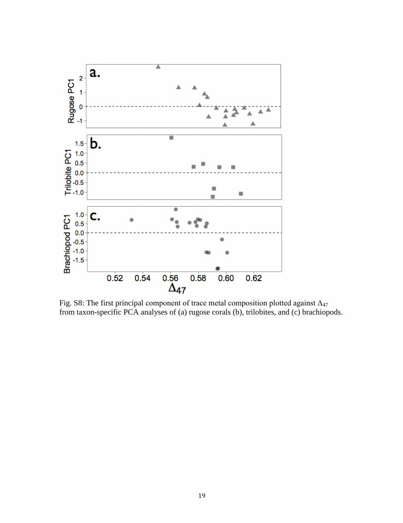
two variables. Because trace metal systematics vary among the taxa included here it is
somewhat reductive to include all samples in a single principal components analysis.
Hence, we also did separate PCA analyses of trace metal composition for brachiopiods,
for rugose corals, and for trilobites. All three groups show evidence of a similar
relationship between trace metal composition and Δ47 (Fig. S7).
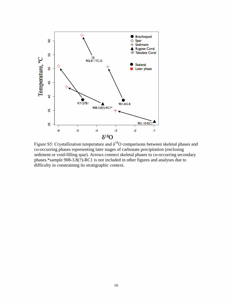
Comparisons among co-occurring phases
Selecting the least-altered samples depends on understanding the direction (with respect
to Δ47 and bulk isotopic composition) of diagenetic alteration vector trajectories. One
approach to characterizing alteration trajectories is to compare co-occurring phases that
precipitated in a known sequence based on petrographic relations. (for example, skeletal
material versus void-filling spar or enclosing sediment). Five such comparisons are
shown in fig. S5; in each case the later phase is lighter in δ18
O and precipitated at higher
temperature than the earlier (skeletal) phase. This does not mean that skeletal phases are
unaltered, as the temperatures indicated for some suggest very substantial contamination
by secondary phases (fig. S5). However, it allows us to characterize the trajectory of
diagenetic alteration and to establish that in all of the units thus evaluated diagenesis is
largely driven by interaction with relatively high-temperature and 18
O-depleted fluids.
This provides a framework for determining which samples have been most affected by
diagenetic alteration when multiple samples from the same stratigraphic horizon are
compared. Such comparisons support a primary origin for the Hirnantian δ18
O excursion.
For example, of four rugose corals analyzed from horizon 901-12, two give relatively low
temperatures (901-12-RC1, 30°C, and 901-12-RC2, 30°C) and two give relatively high
temperatures (901-12-RC3, 40°C, and 901-12-LRC, 40°C). The former are isotopically
heavy (δ13
C = 4.06, 4.47, δ18
O = -0.80, -0.16), whereas the latter are relatively depleted
(δ13
C = 3.11, 3.70, δ18
O = -3.17, -3.13). Therefore either the hotter samples have been
altered by interaction with warm and isotopically light fluids or the colder samples have
been altered by interaction with cold and isotopically heavy fluids. Low-temperature
fluids ( ≤ 30°C in order to have produced observed Δ47 temperatures) must occur very
close to the surface, and hence would generally be expected to have a strong meteoric
influence and be isotopically light with respect to oxygen and carbon.
Even if a realistic alteration scenario involving low-temperature but isotopically heavy
fluids could be envisioned, our data do not support such a model. The expectation, were
this the case, would be that within the Laframboise Member the most altered materials
would be isotopically heaviest and the least altered materials would be isotopically
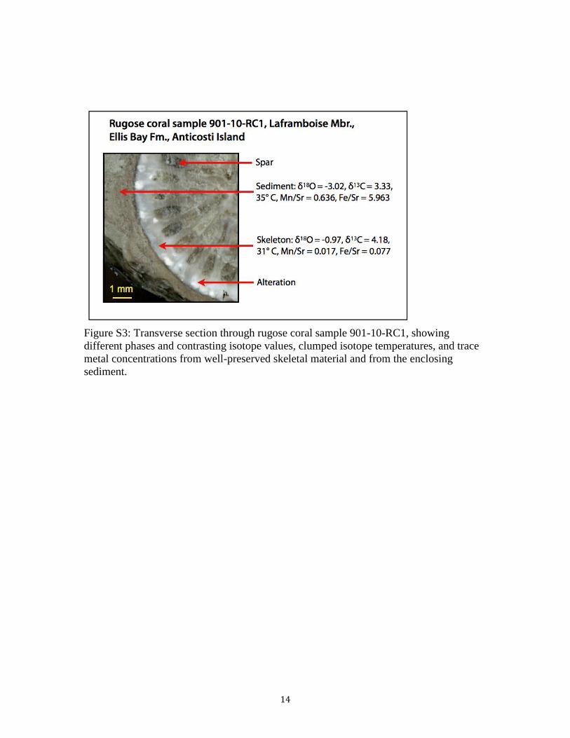
lightest. In fact, we observe the opposite pattern. For example, the skeletal material of
sample 901-10-RC1 (a rugose coral) has a Δ47 temperature of 31°C, δ13
C of 4.18, and
δ18
O of -0.97, whereas the enclosing sediment has a Δ47 temperature of 35°C, δ13
C of
3.33, and δ18
O of -3.02 (Figs. S3, S5)-much more similar to the values observed in the
relatively high-temperature skeletal material from samples 901-12-RC3 and 901-12-LRC,
and also characteristic, in terms of δ13
C and δ18
O, of whole-rock values for this section.
9
Consequently, it is extremely difficult to explain the Hirnantian excursion (which is
similar to that seen in other sections, see below) as a diagenetic artifact.
Comparison with published data
Comparison with previously published results from other sections provides a way of
checking whether the proxy values we observe are plausibly primary. With the exception
of one previous paper (S38) (the results of which are included in our dataset) no other
Δ47.data are available for Late Ordovician-Early Silurian fossils or sediments. However,
we can compare our δ18
O data with several published studies from Anticosti and from
other regions. Within the Hirnantian Laframboise Member of the Ellis Bay Formation,
we observe δ18
O values in skeletal carbonates ranging from -4.59 to -0.16 (VPDB).
Samples that appear to be strongly altered based on trace metal and Δ47 data (see criteria
in next section) have values ranging from -4.59 to -3.13, whereas those that appear to be
less altered have values ranging from -1.44 to -0.16. The former values are similar to
those observed in whole-rock analyses of Hirnantian sediments from Anticosti (S56) and
the Baltic (S57), whereas the latter values are in the same range as the heaviest values
reported from well-preserved Hirnantian brachiopods in Baltic sections (S19, S58, S59).
A single brachiopod analyzed from the interval of the δ13
C excursion in the Laframboise
Member attains a value (~-2‰) intermediate between these ranges (S19), but the other
two examined for this analysis (S19) had δ18
O values similar to whole-rock values for
this section, raising the possibility that all three may be compromised. Taken as a whole,
these observations suggest that the heavy δ18
O values we observe are capturing a primary
signal and reinforce our interpretation and that of others that the lighter values in whole-
rock samples (and in the altered corals) reflect a diagenetic overprint. It should also be
noted that the best-preserved δ18
O values we observe from before and after the Hirnantian
excursion, are also similar to previously published δ18
O values from these time-intervals
(S19, S58-S63), as is the magnitude of the excursion relative to this baseline.
J. Within-bed variability and potential vital effects
The influence of disequilibrium „vital‟ effects on the Δ47 system appears to be relatively
minor among extant taxa (S42, S64), but vital effects on δ18
O are widespread among both
modern and ancient taxa. There is particular uncertainty in this area with regard to rugose
corals; these are an important part of our dataset because they are the only well-preserved
taxon that could be extracted from the Laframboise Member. Relatively little is known
about whether rugose corals exhibit vital effects similar to those of modern scleractinian
corals (to which they were not closely related). Brand (S53, S65) found that the best-
preserved rugose corals in the Pennsylvanian Kendrick Fauna (KY) were on average
~5‰ lighter in δ18
O than co-occurring brachiopods, and ascribed this to a vital effect.
However, he also found that “altered” rugose corals had δ18
O and δ13
C values very
similar to that of co-occurring brachiopods and molluscs,which he ascribed to rapid
cementation in the marine or shallow sediment system. It is also noteworthy that the
Pennsylvanian rugose corals examined by Brand may originally have been composed of
high-magnesium calcite or even aragonite (S66), whereas those of Devonian and younger
age were composed originally of intermediate or low-magnesium calcite (S67, S68).
10
Regardless, we see no evidence of a consistent difference in δ18
O or Δ47 between rugose
corals and co-occurring taxa (Fig. 3), and the vital effect observed in Kendrick Fauna
rugose corals operates in the wrong direction to explain the Hirnantian excursion -also
seen in brachiopods from contemporaneous sections- in our time series. Although it
would be ideal to construct a curve from a single taxonomic group, this is extremely
challenging for the preserved Hirnantian rock record of North America. We therefore
focused our sampling on rugose corals for this unit and then made an effort to examine
rugose corals in as many other units as possible. To illustrate that this is a robust strategy,
we can define the entire Hirnantian excursion using only rugose corals (Fig. S10). This
provides powerful evidence that the excursion is not an artifact of alteration or of
taxonomic heterogeneity. Even if there were a vital effect in Late Ordovician-Early
Silurian rugose corals, it could note account for the relative changes in temperature and in
δ18
Owater that we observe through this interval.
K. Comparison with Cenozoic proxy data and with climate model simulations
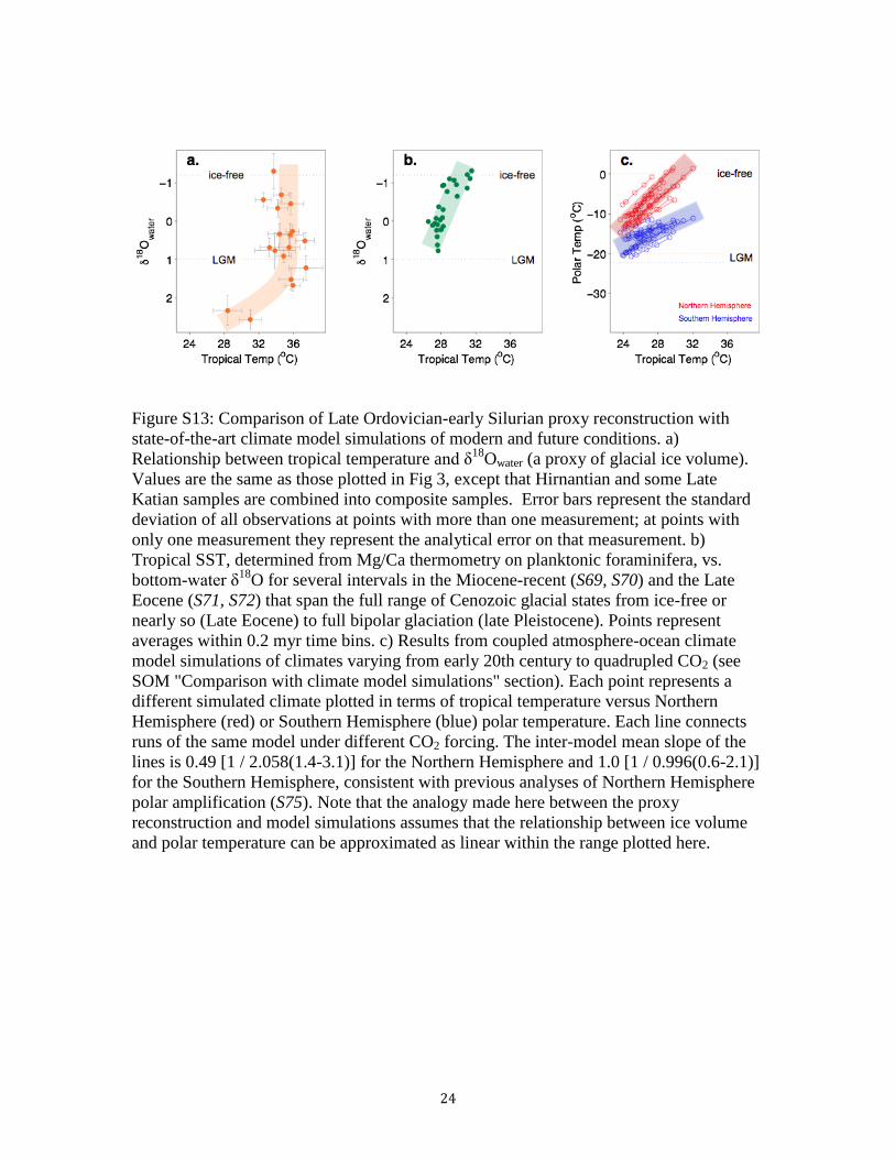
Figure S13a plots δ18
Owater versus tropical SST, using the lowest-temperature sample
from each interval as the best (e.g. least-altered) estimate as in figure 3. The nonlinearity
of this relationship is striking, implying that the initial growth of Gondwanan ice sheets
had little effect on tropical ocean temperatures and that following the Hirnantian
maximum temperatures returned to the pre-Hirnanian range despite the persistence of
moderate ice sheets. The context for evaluating this observation can be drawn by
comparing the time series data with Cenozoic climate proxy records and climate model
simulations of the response to increasing atmospheric CO2 concentrations.
In panel b, there is no evidence for a nonlinear relationship between mean inferred
bottom water δ18
O and mean tropical SST (determined by Mg/Ca paleothermometry on
planktonic foraminifera), examined during several intervals in the Miocene-recent (S69,
S70) and the Late Eocene (S71, S72). These data capture an interval of more than 35 Ma,
and span the full range of Cenozoic glacial states from ice-free or nearly so (Late Eocene)
to full bipolar glaciation (late Pleistocene) (Fig. S13b).
Simulations of state-of-the- art coupled atmosphere-ocean climate models carried out in
association with the Intergovernmental Panel on Climate Change Fourth Assessment
Report (S73) also display a linear relationship (Fig. S13c). For each model, we examine
five different climates, each constructed from a 50-year average. We average years 1900-
1950 and 1950-2000 from the "Climate of the 20th Century" simulation, years 2000-2050
and 2050-2100 from the SRES A1B simulation (a 720 ppm stabilization experiment), and
the first 50 years after quadrupling in the "1% yr-1 CO2 increase to quadrupling"
simulation. The tropical average temperature is computed from the time-mean surface air
temperature for each climate by taking a zonal mean, linearly interpolating from the
varied model grids onto a uniform latitudinal grid with 1 degree spacing, and then taking
a spatial average between 20°S and 20°N. The Northern Hemisphere and Southern
Hemisphere polar averages are computed using the same method but averaging instead
over 70°N to 90°N or 70°S to 90°S, respectively. We include only the 15 models which
reported results from these three simulations in the WCRP CMIP3 multi-model dataset:
11
CCCMA CGCM3.1 T47 (Canada), CNRM CM3 (France), GFDL CM2.0 (USA), GFDL
CM2.1 (USA), GISS ER (USA), INGV SXG (Italy), INM CM3.0 (Russia), IPSL CM4
(France), MIROC3.2 medres (Japan), MIUB ECHO-G (Germany/Korea), MPI ECHAM5
(Germany), MRI CGCM2.3.2 (Japan), NCAR CCSM3.0 (USA), NCAR PCM1 (USA),
UKMO HadGEM1 (UK). When multiple ensemble members are available from a model,
we consider only the first member. Note that the CO2 quadrupling simulations are
initialized from either pre-industrial or present-day conditions, depending on the model.
This difference is expected to account for some of the inter-model differences in
temperature at the time of quadrupling. We acknowledge the modeling groups, the
Program for Climate Model Diagnosis and Intercomparison (PCMDI), and the WCRP's
Working Group on Coupled Modelling (WGCM) for their roles in making the WCRP
CMIP3 multi-model dataset available for further study. Support of this dataset is
provided by the Office of Science, U.S. Department of Energy. We consider "ice-free"
conditions as those with annual-mean polar-average surface air temperature warmer than
0°C. To approximate last glacial maximum ("LGM" in Fig. S12b) polar temperatures, we
apply previously-published results from five different coupled atmosphere-ocean climate
model simulations of the difference between LGM and pre-industrial climates (S74). For
the Northern Hemisphere, we add the inter-model mean results for central Greenland
annual mean temperature change from their study (their Fig 4a) to the inter-model mean
in our analysis for the temporal mean over years 1900-1950. For the Southern
Hemisphere, we apply the same procedure to the central Antarctica results that they
report (their Fig 4b).
From this analysis, several notable differences between our data and the Cenozoic proxy
reconstructions and model simulations are clear. The pole-to-equator temperature
gradient implied by the clumped isotope proxy reconstruction is larger than any of the
model simulations, even under 4X CO2 simulations. This implies that, except for perhaps
the Hirnantian interval, Late Ordovician-early Silurian climate was not as efficient at
transporting heat from the equator to the poles. Additionally, there is a contrast between
the apparently nonlinear relationship suggested by the Ordovician-Silurian proxy time
series and the linear relationship between tropical and polar temperatures in the models
and quasi-linear relationship, between tropical SST and bottom water δ18
O in the
Cenozoic proxy data (highlighted by thick shaded lines in all three panels of Fig. S13).
We hypothesize that this dissemblance arises primarily from the differences between
modern and Ordovician landmass distributions and associated ocean circulations.
Ultimately, these differences provide support for the notion that Late Ordovician-early
Silurian climate operated in a distinct fashion from that of the Late Eocene to Today.
12
Figure S1: Lithostratographic units, shaded in red, that were sampled for this study or by
Came et al., 2007 (S38) (Anticosti Basin column modified after Long, 2007 (S17). An
alternative interpretation of available biostratigraphic data would place all of the Ellis
Bay Formation, rather than just the Laframboise Member, in the terminal Ordovician
Hirnantian Stage. Hirn. = Hirnantian, Rhud. = Rhuddanian, Aeron. = Aeronian, Tely. =
Telychian.
13
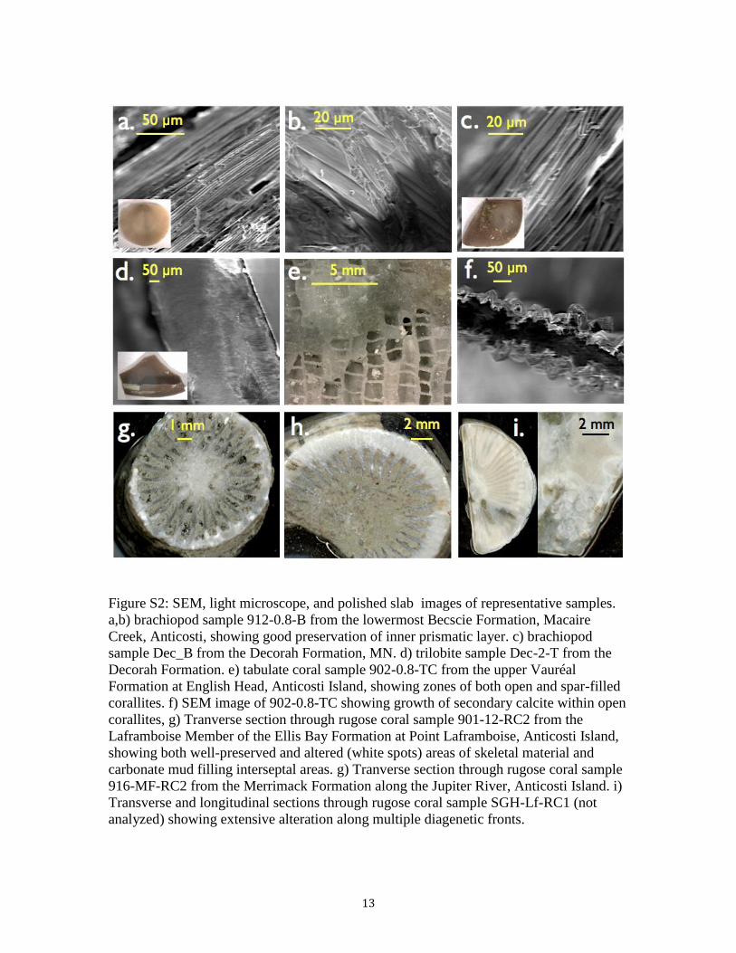
Figure S2: SEM, light microscope, and polished slab images of representative samples.
a,b) brachiopod sample 912-0.8-B from the lowermost Becscie Formation, Macaire
Creek, Anticosti, showing good preservation of inner prismatic layer. c) brachiopod
sample Dec_B from the Decorah Formation, MN. d) trilobite sample Dec-2-T from the
Decorah Formation. e) tabulate coral sample 902-0.8-TC from the upper Vauréal
Formation at English Head, Anticosti Island, showing zones of both open and spar-filled
corallites. f) SEM image of 902-0.8-TC showing growth of secondary calcite within open
corallites, g) Tranverse section through rugose coral sample 901-12-RC2 from the
Laframboise Member of the Ellis Bay Formation at Point Laframboise, Anticosti Island,
showing both well-preserved and altered (white spots) areas of skeletal material and
carbonate mud filling interseptal areas. g) Tranverse section through rugose coral sample
916-MF-RC2 from the Merrimack Formation along the Jupiter River, Anticosti Island. i)
Transverse and longitudinal sections through rugose coral sample SGH-Lf-RC1 (not
analyzed) showing extensive alteration along multiple diagenetic fronts.
14
Figure S3: Transverse section through rugose coral sample 901-10-RC1, showing
different phases and contrasting isotope values, clumped isotope temperatures, and trace
metal concentrations from well-preserved skeletal material and from the enclosing
sediment.
15
Figure S4: a) Δ47-determined crystallization temperatures and b) δ18
O values for micritic
samples from a single bed of the Vauréal Formation taken at different distances from the
contact with an 8 meter thick Jurassic dike at Falaise de Puyjalons, Anticosti Island.
16
Figure S5: Crystallization temperature and δ
18O comparisons between skeletal phases and
co-occurring phases representing later stages of carbonate precipitation (enclosing
sediment or void-filling spar). Arrows connect skeletal phases to co-occurring secondary
phases.*sample 908-3.8(?)-RC1 is not included in other figures and analyses due to
difficulty in constraining its stratigraphic context.
17
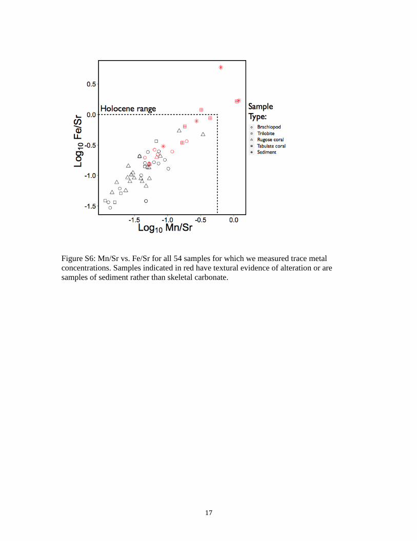
Figure S6: Mn/Sr vs. Fe/Sr for all 54 samples for which we measured trace metal
concentrations. Samples indicated in red have textural evidence of alteration or are
samples of sediment rather than skeletal carbonate.
18
Figure S7 Trace element concentration (in ppm) plotted against Δ47 for Sr, Mn, and Fe,
(panels 1-3) and the first principal component (PC1) of log-transformed Sr, Mn, and Fe
concentration (panel 4) for all 51 skeletal carbonate samples for which trace metal
concentrations were measured. Inset in panel for shows relative factor loadings for PC1,
which accounts 86% of variance in trace metal concentrations. Symbols as in main text
figure 2; red symbols are those with clear textural alteration.
19
Fig. S8: The first principal component of trace metal composition plotted against Δ47
from taxon-specific PCA analyses of (a) rugose corals (b), trilobites, and (c) brachiopods.
20
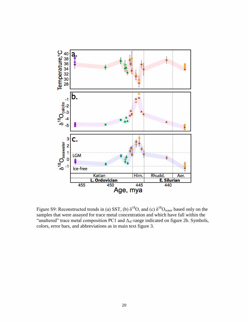
Figure S9: Reconstructed trends in (a) SST, (b) δ18
O, and (c) δ18
Owater based only on the
samples that were assayed for trace metal concentration and which have fall within the
“unaltered” trace metal composition PC1 and Δ47 range indicated on figure 2b. Symbols,
colors, error bars, and abbreviations as in main text figure 3.
21
\
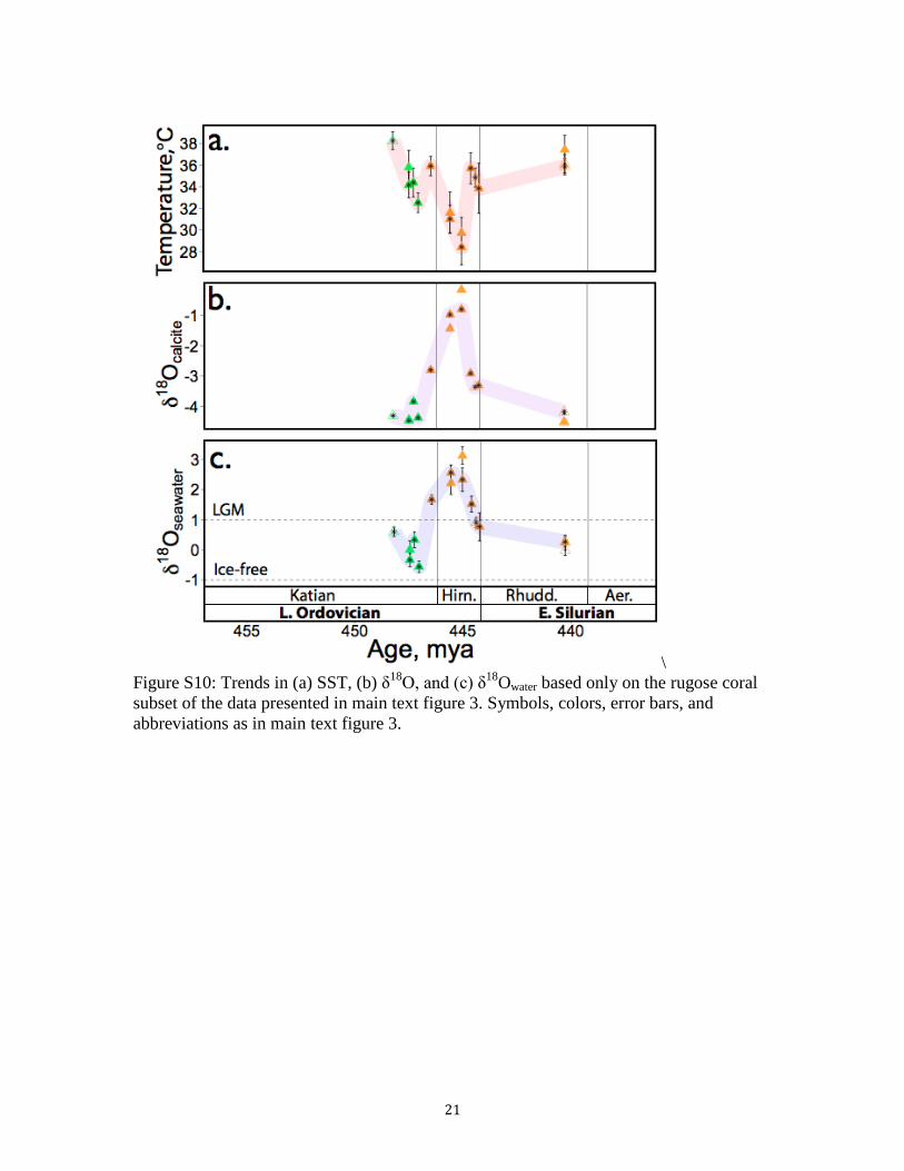
Figure S10: Trends in (a) SST, (b) δ18
O, and (c) δ18
Owater based only on the rugose coral
subset of the data presented in main text figure 3. Symbols, colors, error bars, and
abbreviations as in main text figure 3.
22
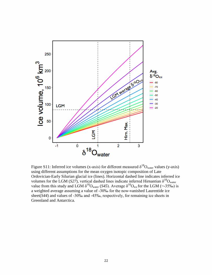
Figure S11: Inferred ice volumes (x-axis) for different measured δ18
Owater values (y-axis)
using different assumptions for the mean oxygen isotopic composition of Late
Ordovician-Early Silurian glacial ice (lines). Horizontal dashed line indicates inferred ice
volumes for the LGM (S27), vertical dashed lines indicate inferred Hirnantian δ18
Owater
value from this study and LGM δ18
Owater (S45). Average δ18
Oice for the LGM (~-35‰) is
a weighted average assuming a value of -30‰ for the now-vanished Laurentide ice
sheet(S44) and values of -30‰ and -45‰, respectively, for remaining ice sheets in
Greenland and Antarctica.
23
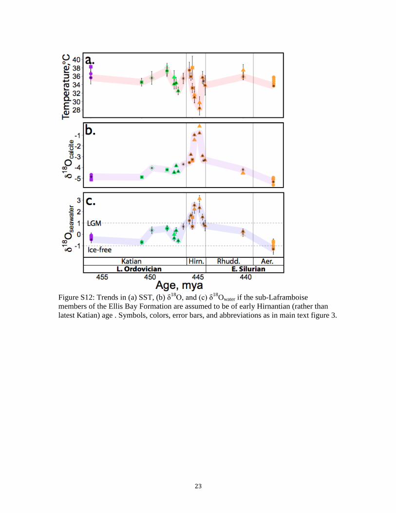
Figure S12: Trends in (a) SST, (b) δ
18O, and (c) δ
18Owater if the sub-Laframboise
members of the Ellis Bay Formation are assumed to be of early Hirnantian (rather than
latest Katian) age . Symbols, colors, error bars, and abbreviations as in main text figure 3.
24
Figure S13: Comparison of Late Ordovician-early Silurian proxy reconstruction with
state-of-the-art climate model simulations of modern and future conditions. a)
Relationship between tropical temperature and δ18
Owater (a proxy of glacial ice volume).
Values are the same as those plotted in Fig 3, except that Hirnantian and some Late
Katian samples are combined into composite samples. Error bars represent the standard
deviation of all observations at points with more than one measurement; at points with
only one measurement they represent the analytical error on that measurement. b)
Tropical SST, determined from Mg/Ca thermometry on planktonic foraminifera, vs.
bottom-water δ18
O for several intervals in the Miocene-recent (S69, S70) and the Late
Eocene (S71, S72) that span the full range of Cenozoic glacial states from ice-free or
nearly so (Late Eocene) to full bipolar glaciation (late Pleistocene). Points represent
averages within 0.2 myr time bins. c) Results from coupled atmosphere-ocean climate
model simulations of climates varying from early 20th century to quadrupled CO2 (see
SOM "Comparison with climate model simulations" section). Each point represents a
different simulated climate plotted in terms of tropical temperature versus Northern
Hemisphere (red) or Southern Hemisphere (blue) polar temperature. Each line connects
runs of the same model under different CO2 forcing. The inter-model mean slope of the
lines is 0.49 [1 / 2.058(1.4-3.1)] for the Northern Hemisphere and 1.0 [1 / 0.996(0.6-2.1)]
for the Southern Hemisphere, consistent with previous analyses of Northern Hemisphere
polar amplification (S75). Note that the analogy made here between the proxy
reconstruction and model simulations assumes that the relationship between ice volume
and polar temperature can be approximated as linear within the range plotted here.
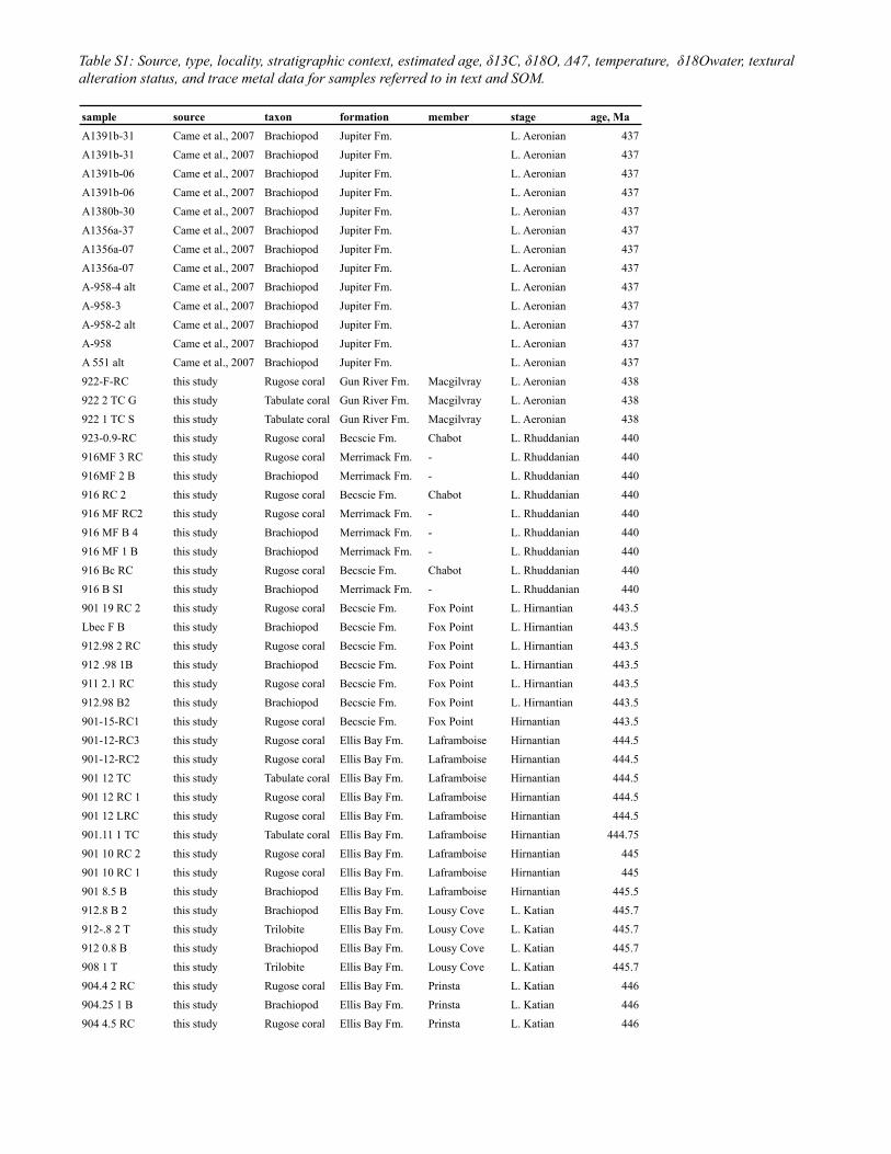
Table S1: Source, type, locality, stratigraphic context, estimated age, δ13C, δ18O, Δ47, temperature, δ18Owater, textural alteration status, and trace metal data for samples referred to in text and SOM.
sample source taxon formation member stage age, MaA1391b-31 Came et al., 2007 Brachiopod Jupiter Fm. L. Aeronian 437A1391b-31 Came et al., 2007 Brachiopod Jupiter Fm. L. Aeronian 437A1391b-06 Came et al., 2007 Brachiopod Jupiter Fm. L. Aeronian 437A1391b-06 Came et al., 2007 Brachiopod Jupiter Fm. L. Aeronian 437A1380b-30 Came et al., 2007 Brachiopod Jupiter Fm. L. Aeronian 437A1356a-37 Came et al., 2007 Brachiopod Jupiter Fm. L. Aeronian 437A1356a-07 Came et al., 2007 Brachiopod Jupiter Fm. L. Aeronian 437A1356a-07 Came et al., 2007 Brachiopod Jupiter Fm. L. Aeronian 437A-958-4 alt Came et al., 2007 Brachiopod Jupiter Fm. L. Aeronian 437A-958-3 Came et al., 2007 Brachiopod Jupiter Fm. L. Aeronian 437A-958-2 alt Came et al., 2007 Brachiopod Jupiter Fm. L. Aeronian 437A-958 Came et al., 2007 Brachiopod Jupiter Fm. L. Aeronian 437A 551 alt Came et al., 2007 Brachiopod Jupiter Fm. L. Aeronian 437922-F-RC this study Rugose coral Gun River Fm. Macgilvray L. Aeronian 438922 2 TC G this study Tabulate coral Gun River Fm. Macgilvray L. Aeronian 438922 1 TC S this study Tabulate coral Gun River Fm. Macgilvray L. Aeronian 438923-0.9-RC this study Rugose coral Becscie Fm. Chabot L. Rhuddanian 440916MF 3 RC this study Rugose coral Merrimack Fm. - L. Rhuddanian 440916MF 2 B this study Brachiopod Merrimack Fm. - L. Rhuddanian 440916 RC 2 this study Rugose coral Becscie Fm. Chabot L. Rhuddanian 440916 MF RC2 this study Rugose coral Merrimack Fm. - L. Rhuddanian 440916 MF B 4 this study Brachiopod Merrimack Fm. - L. Rhuddanian 440916 MF 1 B this study Brachiopod Merrimack Fm. - L. Rhuddanian 440916 Bc RC this study Rugose coral Becscie Fm. Chabot L. Rhuddanian 440916 B SI this study Brachiopod Merrimack Fm. - L. Rhuddanian 440901 19 RC 2 this study Rugose coral Becscie Fm. Fox Point L. Hirnantian 443.5Lbec F B this study Brachiopod Becscie Fm. Fox Point L. Hirnantian 443.5912.98 2 RC this study Rugose coral Becscie Fm. Fox Point L. Hirnantian 443.5912 .98 1B this study Brachiopod Becscie Fm. Fox Point L. Hirnantian 443.5911 2.1 RC this study Rugose coral Becscie Fm. Fox Point L. Hirnantian 443.5912.98 B2 this study Brachiopod Becscie Fm. Fox Point L. Hirnantian 443.5901-15-RC1 this study Rugose coral Becscie Fm. Fox Point Hirnantian 443.5901-12-RC3 this study Rugose coral Ellis Bay Fm. Laframboise Hirnantian 444.5901-12-RC2 this study Rugose coral Ellis Bay Fm. Laframboise Hirnantian 444.5901 12 TC this study Tabulate coral Ellis Bay Fm. Laframboise Hirnantian 444.5901 12 RC 1 this study Rugose coral Ellis Bay Fm. Laframboise Hirnantian 444.5901 12 LRC this study Rugose coral Ellis Bay Fm. Laframboise Hirnantian 444.5901.11 1 TC this study Tabulate coral Ellis Bay Fm. Laframboise Hirnantian 444.75901 10 RC 2 this study Rugose coral Ellis Bay Fm. Laframboise Hirnantian 445901 10 RC 1 this study Rugose coral Ellis Bay Fm. Laframboise Hirnantian 445901 8.5 B this study Brachiopod Ellis Bay Fm. Laframboise Hirnantian 445.5912.8 B 2 this study Brachiopod Ellis Bay Fm. Lousy Cove L. Katian 445.7912-.8 2 T this study Trilobite Ellis Bay Fm. Lousy Cove L. Katian 445.7912 0.8 B this study Brachiopod Ellis Bay Fm. Lousy Cove L. Katian 445.7908 1 T this study Trilobite Ellis Bay Fm. Lousy Cove L. Katian 445.7904.4 2 RC this study Rugose coral Ellis Bay Fm. Prinsta L. Katian 446904.25 1 B this study Brachiopod Ellis Bay Fm. Prinsta L. Katian 446904 4.5 RC this study Rugose coral Ellis Bay Fm. Prinsta L. Katian 446
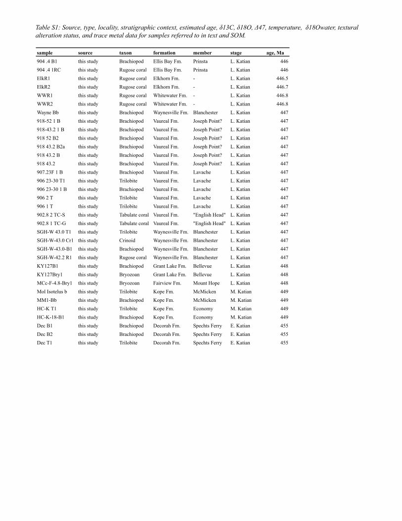
Table S1: Source, type, locality, stratigraphic context, estimated age, δ13C, δ18O, Δ47, temperature, δ18Owater, textural alteration status, and trace metal data for samples referred to in text and SOM.
sample source taxon formation member stage age, Ma904 .4 B1 this study Brachiopod Ellis Bay Fm. Prinsta L. Katian 446904 .4 1RC this study Rugose coral Ellis Bay Fm. Prinsta L. Katian 446ElkR1 this study Rugose coral Elkhorn Fm. - L. Katian 446.5ElkR2 this study Rugose coral Elkhorn Fm. - L. Katian 446.7WWR1 this study Rugose coral Whitewater Fm. - L. Katian 446.8WWR2 this study Rugose coral Whitewater Fm. - L. Katian 446.8Wayne Bb this study Brachiopod Waynesville Fm. Blanchester L. Katian 447918-52 1 B this study Brachiopod Vaureal Fm. Joseph Point? L. Katian 447918-43.2 1 B this study Brachiopod Vaureal Fm. Joseph Point? L. Katian 447918 52 B2 this study Brachiopod Vaureal Fm. Joseph Point? L. Katian 447918 43.2 B2a this study Brachiopod Vaureal Fm. Joseph Point? L. Katian 447918 43.2 B this study Brachiopod Vaureal Fm. Joseph Point? L. Katian 447918 43.2 this study Brachiopod Vaureal Fm. Joseph Point? L. Katian 447907.23F 1 B this study Brachiopod Vaureal Fm. Lavache L. Katian 447906 23-30 T1 this study Trilobite Vaureal Fm. Lavache L. Katian 447906 23-30 1 B this study Brachiopod Vaureal Fm. Lavache L. Katian 447906 2 T this study Trilobite Vaureal Fm. Lavache L. Katian 447906 1 T this study Trilobite Vaureal Fm. Lavache L. Katian 447902.8 2 TC-S this study Tabulate coral Vaureal Fm. "English Head" L. Katian 447902.8 1 TC-G this study Tabulate coral Vaureal Fm. "English Head" L. Katian 447SGH-W 43.0 T1 this study Trilobite Waynesville Fm. Blanchester L. Katian 447SGH-W-43.0 Cr1 this study Crinoid Waynesville Fm. Blanchester L. Katian 447SGH-W-43.0-B1 this study Brachiopod Waynesville Fm. Blanchester L. Katian 447SGH-W-42.2 R1 this study Rugose coral Waynesville Fm. Blanchester L. Katian 447KY127B1 this study Brachiopod Grant Lake Fm. Bellevue L. Katian 448KY127Bry1 this study Bryozoan Grant Lake Fm. Bellevue L. Katian 448MCc-F-4.8-Bry1 this study Bryozoan Fairview Fm. Mount Hope L. Katian 448Mol Isotelus b this study Trilobite Kope Fm. McMicken M. Katian 449MM1-Bb this study Brachiopod Kope Fm. McMicken M. Katian 449HC-K T1 this study Trilobite Kope Fm. Economy M. Katian 449HC-K-18-B1 this study Brachiopod Kope Fm. Economy M. Katian 449Dec B1 this study Brachiopod Decorah Fm. Spechts Ferry E. Katian 455Dec B2 this study Brachiopod Decorah Fm. Spechts Ferry E. Katian 455Dec T1 this study Trilobite Decorah Fm. Spechts Ferry E. Katian 455
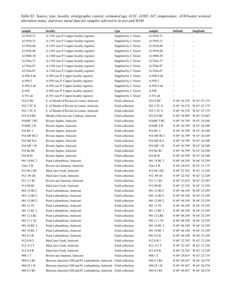
Table S1: Source, type, locality, stratigraphic context, estimated age, δ13C, δ18O, Δ47, temperature, δ18Owater, textural alteration status, and trace metal data for samples referred to in text and SOM.
sample locality type sample latitude longitudeA1391b-31 A-1391 (see P. Copper locality register) Supplied by J. Veizer A1391b-31 - -A1391b-31 A-1391 (see P. Copper locality register) Supplied by J. Veizer A1391b-31 - -A1391b-06 A-1391 (see P. Copper locality register) Supplied by J. Veizer A1391b-06 - -A1391b-06 A-1391 (see P. Copper locality register) Supplied by J. Veizer A1391b-06 - -A1380b-30 A-1380 (see P. Copper locality register) Supplied by J. Veizer A1380b-30 - -A1356a-37 A-1356 (see P. Copper locality register) Supplied by J. Veizer A1356a-37 - -A1356a-07 A-1356 (see P. Copper locality register) Supplied by J. Veizer A1356a-07 - -A1356a-07 A-1356 (see P. Copper locality register) Supplied by J. Veizer A1356a-07 - -A-958-4 alt A-958 (see P. Copper locality register) Supplied by J. Veizer A-958-4 alt - -A-958-3 A-958 (see P. Copper locality register) Supplied by J. Veizer A-958-3 - -A-958-2 alt A-958 (see P. Copper locality register) Supplied by J. Veizer A-958-2 alt - -A-958 A-958 (see P. Copper locality register) Supplied by J. Veizer A-958 - -A 551 alt A-551 (see P. Copper locality register) Supplied by J. Veizer A 551 alt - -922-F-RC E. of Mouth of Riviere la Loutre, Anticosti Field collection 922-F-RC N 49° 36.374' W 63° 47.175'922 2 TC G E. of Mouth of Riviere la Loutre, Anticosti Field collection 922 2 TC G N 49° 36.374' W 63° 47.175'922 1 TC S E. of Mouth of Riviere la Loutre, Anticosti Field collection 922 1 TC S N 49° 36.374' W 63° 47.175'923-0.9-RC Mouth of Riviere aux Cailloux, Anticosti Field collection 923-0.9-RC N 49° 38.969' W 63° 52.063'916MF 3 RC Riviere Jupiter, Anticosti, Field collection 916MF 3 RC N 49° 36.799' W 63° 26.548'916MF 2 B Riviere Jupiter, Anticosti Field collection 916MF 2 B N 49° 36.799' W 63° 26.548'916 RC 2 Riviere Jupiter, Anticosti Field collection 916 RC 2 N 49° 36.799' W 63° 26.548'916 MF RC2 Riviere Jupiter, Anticosti Field collection 916 MF RC2 N 49° 36.799' W 63° 26.548'916 MF B 4 Riviere Jupiter, Anticosti Field collection 916 MF B 4 N 49° 36.799' W 63° 26.548'916 MF 1 B Riviere Jupiter, Anticosti Field collection 916 MF 1 B N 49° 36.799' W 63° 26.548'916 Bc RC Riviere Jupiter, Anticosti Field collection 916 Bc RC N 49° 36.799' W 63° 26.548'916 B SI Riviere Jupiter, Anticosti Field collection 916 B SI N 49° 36.799' W 63° 26.548'901 19 RC 2 Point Laframboise, Anticosti Field collection 901 19 RC 2 N 49° 48.350' W 64° 25.259'Lbec F B Riviere aux Saumon, Anticosti Field collection Lbec F B N 49° 24.015' W 62° 23.175'912.98 2 RC MacCaire Creek, Anticosti Field collection 912.98 2 RC N 49° 22.762' W 62° 12.320'912 .98 1B MacCaire Creek, Anticosti Field collection 912 .98 1B N 49° 22.762' W 62° 12.320'911 2.1 RC Riviere aux Saumon, Anticosti Field collection 911 2.1 RC N 49° 23.853' W 62° 23.583'912.98 B2 MacCaire Creek, Anticosti Field collection 912.98 B2 N 49° 22.762' W 62° 12.320'901-15-RC1 Point Laframboise, Anticosti Field collection 901-12-RC3 N 49° 48.350' W 64° 25.259'901-12-RC3 Point Laframboise, Anticosti Field collection 901-12-RC3 N 49° 48.350' W 64° 25.259'901-12-RC2 Point Laframboise, Anticosti Field collection 901-12-RC2 N 49° 48.350' W 64° 25.259'901 12 TC Point Laframboise, Anticosti Field collection 901 12 TC N 49° 48.350' W 64° 25.259'901 12 RC 1 Point Laframboise, Anticosti Field collection 901 12 RC 1 N 49° 48.350' W 64° 25.259'901 12 LRC Point Laframboise, Anticosti Field collection 901 12 LRC N 49° 48.350' W 64° 25.259'901.11 1 TC Point Laframboise, Anticosti Field collection 901.11 1 TC N 49° 48.350' W 64° 25.259'901 10 RC 2 Point Laframboise, Anticosti Field collection 901 10 RC 2 N 49° 48.350' W 64° 25.259'901 10 RC 1 Point Laframboise, Anticosti Field collection 901 10 RC 1 N 49° 48.350' W 64° 25.259'901 8.5 B Point Laframboise, Anticosti Field collection 901 8.5 B N 49° 48.350' W 64° 25.259'912.8 B 2 MacCaire Creek, Anticosti Field collection 912.8 B 2 N 49° 22.762' W 62° 12.320'912-.8 2 T MacCaire Creek, Anticosti Field collection 912-.8 2 T N 49° 22.762' W 62° 12.320'912 0.8 B MacCaire Creek, Anticosti Field collection 912 0.8 B N 49° 22.762' W 62° 12.320'908 1 T Riviere aux Saumon, Anticosti Field collection 908 1 T N 49° 24.015' W 62° 23.175'904.4 2 RC Between Junction Cliff and Pt. Laframboise, Anticosti Field collection 904.4 2 RC N 49° 49.567' W 64° 26.574'904.25 1 B Between Junction Cliff and Pt. Laframboise, Anticosti Field collection 904.25 1 B N 49° 49.567' W 64° 26.574'904 4.5 RC Between Junction Cliff and Pt. Laframboise, Anticosti Field collection 904 4.5 RC N 49° 49.567' W 64° 26.574'
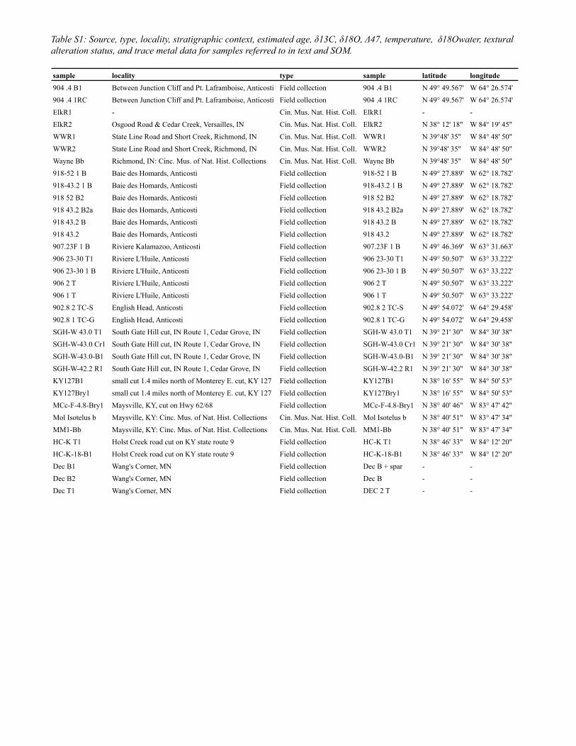
Table S1: Source, type, locality, stratigraphic context, estimated age, δ13C, δ18O, Δ47, temperature, δ18Owater, textural alteration status, and trace metal data for samples referred to in text and SOM.
sample locality type sample latitude longitude904 .4 B1 Between Junction Cliff and Pt. Laframboise, Anticosti Field collection 904 .4 B1 N 49° 49.567' W 64° 26.574'904 .4 1RC Between Junction Cliff and Pt. Laframboise, Anticosti Field collection 904 .4 1RC N 49° 49.567' W 64° 26.574'ElkR1 - Cin. Mus. Nat. Hist. Coll. ElkR1 - -ElkR2 Osgood Road & Cedar Creek, Versailles, IN Cin. Mus. Nat. Hist. Coll. ElkR2 N 38° 12' 18" W 84° 19' 45"WWR1 State Line Road and Short Creek, Richmond, IN Cin. Mus. Nat. Hist. Coll. WWR1 N 39°48' 35" W 84° 48' 50"WWR2 State Line Road and Short Creek, Richmond, IN Cin. Mus. Nat. Hist. Coll. WWR2 N 39°48' 35" W 84° 48' 50"Wayne Bb Richmond, IN: Cinc. Mus. of Nat. Hist. Collections Cin. Mus. Nat. Hist. Coll. Wayne Bb N 39°48' 35" W 84° 48' 50"918-52 1 B Baie des Homards, Anticosti Field collection 918-52 1 B N 49° 27.889' W 62° 18.782'918-43.2 1 B Baie des Homards, Anticosti Field collection 918-43.2 1 B N 49° 27.889' W 62° 18.782'918 52 B2 Baie des Homards, Anticosti Field collection 918 52 B2 N 49° 27.889' W 62° 18.782'918 43.2 B2a Baie des Homards, Anticosti Field collection 918 43.2 B2a N 49° 27.889' W 62° 18.782'918 43.2 B Baie des Homards, Anticosti Field collection 918 43.2 B N 49° 27.889' W 62° 18.782'918 43.2 Baie des Homards, Anticosti Field collection 918 43.2 N 49° 27.889' W 62° 18.782'907.23F 1 B Riviere Kalamazoo, Anticosti Field collection 907.23F 1 B N 49° 46.369' W 63° 31.663'906 23-30 T1 Riviere L'Huile, Anticosti Field collection 906 23-30 T1 N 49° 50.507' W 63° 33.222'906 23-30 1 B Riviere L'Huile, Anticosti Field collection 906 23-30 1 B N 49° 50.507' W 63° 33.222'906 2 T Riviere L'Huile, Anticosti Field collection 906 2 T N 49° 50.507' W 63° 33.222'906 1 T Riviere L'Huile, Anticosti Field collection 906 1 T N 49° 50.507' W 63° 33.222'902.8 2 TC-S English Head, Anticosti Field collection 902.8 2 TC-S N 49° 54.072' W 64° 29.458'902.8 1 TC-G English Head, Anticosti Field collection 902.8 1 TC-G N 49° 54.072' W 64° 29.458'SGH-W 43.0 T1 South Gate Hill cut, IN Route 1, Cedar Grove, IN Field collection SGH-W 43.0 T1 N 39° 21' 30" W 84° 30' 38"SGH-W-43.0 Cr1 South Gate Hill cut, IN Route 1, Cedar Grove, IN Field collection SGH-W-43.0 Cr1 N 39° 21' 30" W 84° 30' 38"SGH-W-43.0-B1 South Gate Hill cut, IN Route 1, Cedar Grove, IN Field collection SGH-W-43.0-B1 N 39° 21' 30" W 84° 30' 38"SGH-W-42.2 R1 South Gate Hill cut, IN Route 1, Cedar Grove, IN Field collection SGH-W-42.2 R1 N 39° 21' 30" W 84° 30' 38"KY127B1 small cut 1.4 miles north of Monterey E. cut, KY 127 Field collection KY127B1 N 38° 16' 55" W 84° 50' 53"KY127Bry1 small cut 1.4 miles north of Monterey E. cut, KY 127 Field collection KY127Bry1 N 38° 16' 55" W 84° 50' 53"MCc-F-4.8-Bry1 Maysville, KY, cut on Hwy 62/68 Field collection MCc-F-4.8-Bry1 N 38° 40' 46" W 83° 47' 42"Mol Isotelus b Maysville, KY: Cinc. Mus. of Nat. Hist. Collections Cin. Mus. Nat. Hist. Coll. Mol Isotelus b N 38° 40' 51" W 83° 47' 34"MM1-Bb Maysville, KY: Cinc. Mus. of Nat. Hist. Collections Cin. Mus. Nat. Hist. Coll. MM1-Bb N 38° 40' 51" W 83° 47' 34"HC-K T1 Holst Creek road cut on KY state route 9 Field collection HC-K T1 N 38° 46' 33" W 84° 12' 20"HC-K-18-B1 Holst Creek road cut on KY state route 9 Field collection HC-K-18-B1 N 38° 46' 33" W 84° 12' 20"Dec B1 Wang's Corner, MN Field collection Dec B + spar - -Dec B2 Wang's Corner, MN Field collection Dec B - -Dec T1 Wang's Corner, MN Field collection DEC 2 T - -
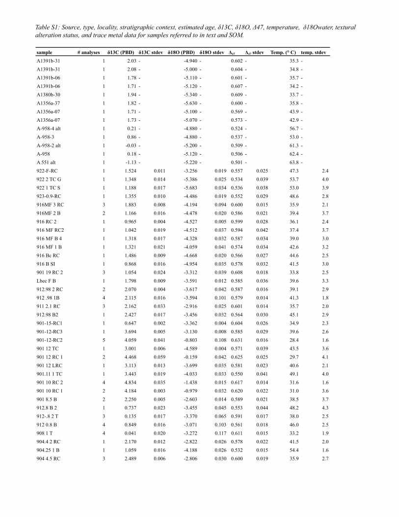
Table S1: Source, type, locality, stratigraphic context, estimated age, δ13C, δ18O, Δ47, temperature, δ18Owater, textural alteration status, and trace metal data for samples referred to in text and SOM.
sample # analyses δ13C (PBD) δ13C stdev δ18O (PBD) δ18O stdev Δ47 Δ47 stdev Temp. (° C) temp. stdevA1391b-31 1 2.03 - -4.940 - 0.602 - 35.3 -A1391b-31 1 2.08 - -5.000 - 0.604 - 34.8 -A1391b-06 1 1.78 - -5.110 - 0.601 - 35.7 -A1391b-06 1 1.71 - -5.120 - 0.607 - 34.2 -A1380b-30 1 1.94 - -5.340 - 0.609 - 33.7 -A1356a-37 1 1.82 - -5.630 - 0.600 - 35.8 -A1356a-07 1 1.71 - -5.100 - 0.569 - 43.9 -A1356a-07 1 1.73 - -5.070 - 0.573 - 42.9 -A-958-4 alt 1 0.21 - -4.880 - 0.524 - 56.7 -A-958-3 1 0.86 - -4.880 - 0.537 - 53.0 -A-958-2 alt 1 -0.03 - -5.200 - 0.509 - 61.3 -A-958 1 0.18 - -5.120 - 0.506 - 62.4 -A 551 alt 1 -1.13 - -5.220 - 0.501 - 63.8 -922-F-RC 1 1.524 0.011 -3.256 0.019 0.557 0.025 47.3 2.4922 2 TC G 1 1.348 0.014 -5.386 0.025 0.534 0.039 53.7 4.0922 1 TC S 1 1.188 0.017 -5.683 0.034 0.536 0.038 53.0 3.9923-0.9-RC 1 1.355 0.010 -4.486 0.019 0.552 0.029 48.6 2.8916MF 3 RC 3 1.883 0.008 -4.194 0.094 0.600 0.015 35.9 2.1916MF 2 B 2 1.166 0.016 -4.478 0.020 0.586 0.021 39.4 3.7916 RC 2 1 0.965 0.004 -4.527 0.005 0.599 0.028 36.1 2.4916 MF RC2 1 1.042 0.019 -4.512 0.037 0.594 0.042 37.4 3.7916 MF B 4 1 1.318 0.017 -4.328 0.032 0.587 0.034 39.0 3.0916 MF 1 B 1 1.321 0.021 -4.059 0.041 0.574 0.034 42.6 3.2916 Bc RC 1 1.486 0.009 -4.668 0.020 0.566 0.027 44.6 2.5916 B SI 1 0.868 0.016 -4.954 0.035 0.578 0.032 41.5 3.0901 19 RC 2 3 1.054 0.024 -3.312 0.039 0.608 0.018 33.8 2.5Lbec F B 1 1.798 0.009 -3.591 0.012 0.585 0.036 39.6 3.3912.98 2 RC 2 2.070 0.004 -3.617 0.042 0.587 0.016 39.1 2.9912 .98 1B 4 2.115 0.016 -3.594 0.101 0.579 0.014 41.3 1.8911 2.1 RC 3 2.162 0.033 -2.916 0.025 0.601 0.014 35.7 2.0912.98 B2 1 2.427 0.017 -3.456 0.032 0.564 0.030 45.1 2.9901-15-RC1 1 0.647 0.002 -3.362 0.004 0.604 0.026 34.9 2.3901-12-RC3 1 3.694 0.005 -3.130 0.008 0.585 0.029 39.6 2.6901-12-RC2 5 4.059 0.041 -0.803 0.108 0.631 0.016 28.4 1.6901 12 TC 1 3.001 0.006 -4.589 0.004 0.571 0.039 43.5 3.6901 12 RC 1 2 4.468 0.059 -0.159 0.042 0.625 0.025 29.7 4.1901 12 LRC 1 3.113 0.013 -3.699 0.035 0.581 0.023 40.6 2.1901.11 1 TC 1 3.443 0.019 -4.033 0.033 0.550 0.041 49.1 4.0901 10 RC 2 4 4.834 0.035 -1.438 0.015 0.617 0.014 31.6 1.6901 10 RC 1 2 4.184 0.003 -0.979 0.032 0.620 0.022 31.0 3.6901 8.5 B 2 2.250 0.005 -2.603 0.014 0.589 0.021 38.5 3.7912.8 B 2 1 0.737 0.023 -3.455 0.045 0.553 0.044 48.2 4.3912-.8 2 T 3 0.135 0.017 -3.370 0.065 0.591 0.017 38.0 2.5912 0.8 B 4 0.849 0.016 -3.071 0.103 0.561 0.018 46.0 2.5908 1 T 4 0.041 0.020 -3.272 0.117 0.611 0.015 33.2 1.9904.4 2 RC 1 2.170 0.012 -2.822 0.026 0.578 0.022 41.5 2.0904.25 1 B 1 1.059 0.016 -4.188 0.026 0.532 0.015 54.4 1.6904 4.5 RC 3 2.489 0.006 -2.806 0.030 0.600 0.019 35.9 2.7
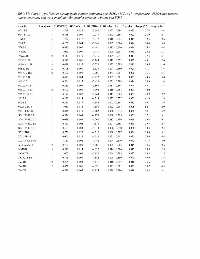
Table S1: Source, type, locality, stratigraphic context, estimated age, δ13C, δ18O, Δ47, temperature, δ18Owater, textural alteration status, and trace metal data for samples referred to in text and SOM.
sample # analyses δ13C (PBD) δ13C stdev δ18O (PBD) δ18O stdev Δ47 Δ47 stdev Temp. (° C) temp. stdev904 .4 B1 3 1.769 0.026 -3.542 0.077 0.594 0.023 37.4 3.4904 .4 1RC 1 0.838 0.003 -2.773 0.003 0.588 0.023 38.9 2.1ElkR1 3 1.422 0.017 -4.377 0.018 0.614 0.019 32.5 2.6ElkR2 1 -0.207 0.004 -3.846 0.007 0.606 0.044 34.4 3.8WWR1 2 -0.945 0.000 -4.441 0.013 0.600 0.026 35.8 4.4WWR2 1 -1.019 0.003 -4.471 0.008 0.607 0.039 34.2 3.3Wayne Bb 2 -0.143 0.019 -4.216 0.009 0.594 0.017 37.3 3.1918-52 1 B 1 0.397 0.006 -3.149 0.012 0.572 0.027 43.1 2.6918-43.2 1 B 3 0.499 0.017 -3.370 0.072 0.585 0.011 39.5 1.6918 52 B2 2 0.308 0.001 -3.327 0.027 0.580 0.020 41.1 3.6918 43.2 B2a 2 0.302 0.008 -3.701 0.043 0.601 0.020 35.5 3.5918 43.2 B 1 0.479 0.004 -3.432 0.007 0.581 0.033 40.6 3.0918 43.2 1 0.506 0.015 -3.426 0.031 0.588 0.016 38.9 1.4907.23F 1 B 1 -0.289 0.007 -3.863 0.017 0.564 0.040 45.3 3.8906 23-30 T1 2 -0.372 0.008 -4.090 0.018 0.584 0.029 40.0 5.1906 23-30 1 B 1 -0.194 0.007 -4.064 0.013 0.565 0.031 44.9 2.9906 2 T 1 -0.292 0.014 -4.214 0.027 0.577 0.031 41.8 2.9906 1 T 4 -0.240 0.013 -4.144 0.072 0.561 0.012 46.1 1.6902.8 2 TC-S 1 1.041 0.012 -4.183 0.022 0.507 0.026 62.1 2.9902.8 1 TC-G 1 -0.016 0.010 -4.782 0.020 0.533 0.038 54.1 3.9SGH-W 43.0 T1 1 -0.524 0.003 -4.170 0.008 0.595 0.035 37.1 3.1SGH-W-43.0 Cr1 1 -0.078 0.063 -4.267 0.082 0.586 0.069 39.4 6.1SGH-W-43.0-B1 1 0.413 0.004 -4.878 0.007 0.585 0.030 39.7 2.7SGH-W-42.2 R1 1 -0.589 0.003 -4.310 0.006 0.590 0.026 38.3 2.3KY127B1 1 0.730 0.027 -4.712 0.060 0.587 0.036 39.0 3.2KY127Bry1 1 0.090 0.018 -4.050 0.021 0.601 0.051 35.6 4.4MCc-F-4.8-Bry1 1 -1.367 0.002 -4.444 0.004 0.570 0.043 43.6 4.0Mol Isotelus b 2 -0.760 0.000 -4.901 0.005 0.605 0.015 34.6 2.6MM1-Bb 3 -0.595 0.014 -4.627 0.016 0.586 0.017 39.5 2.5HC-K T1 1 -1.007 0.002 -5.880 0.004 0.585 0.027 39.8 2.5HC-K-18-B1 1 -0.175 0.003 -4.842 0.008 0.580 0.040 40.9 3.6Dec B1 2 -0.275 0.003 -4.671 0.018 0.597 0.018 36.6 3.2Dec B2 2 0.432 0.006 -4.871 0.025 0.601 0.025 35.7 4.3Dec T1 2 -0.528 0.005 -5.135 0.029 0.590 0.018 38.3 3.2
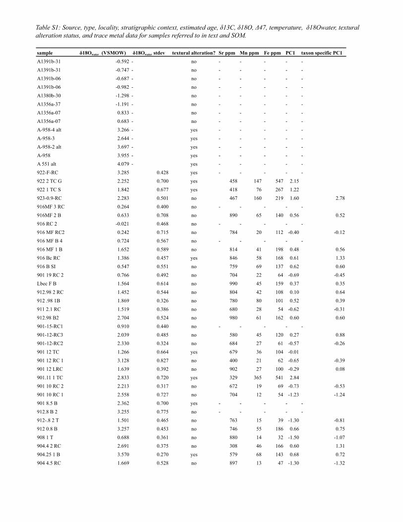
Table S1: Source, type, locality, stratigraphic context, estimated age, δ13C, δ18O, Δ47, temperature, δ18Owater, textural alteration status, and trace metal data for samples referred to in text and SOM.
sample δ18Owater (VSMOW) δ18Owater stdev textural alteration? Sr ppm Mn ppm Fe ppm PC1 taxon specific PC1A1391b-31 -0.592 - no - - - - -A1391b-31 -0.747 - no - - - - -A1391b-06 -0.687 - no - - - - -A1391b-06 -0.982 - no - - - - -A1380b-30 -1.298 - no - - - - -A1356a-37 -1.191 - no - - - - -A1356a-07 0.833 - no - - - - -A1356a-07 0.683 - no - - - - -A-958-4 alt 3.266 - yes - - - - -A-958-3 2.644 - yes - - - - -A-958-2 alt 3.697 - yes - - - - -A-958 3.955 - yes - - - - -A 551 alt 4.079 - yes - - - - -922-F-RC 3.285 0.428 yes - - - - -922 2 TC G 2.252 0.700 yes 458 147 547 2.15922 1 TC S 1.842 0.677 yes 418 76 267 1.22923-0.9-RC 2.283 0.501 no 467 160 219 1.60 2.78916MF 3 RC 0.264 0.400 no - - - - -916MF 2 B 0.633 0.708 no 890 65 140 0.56 0.52916 RC 2 -0.021 0.468 no - - - - -916 MF RC2 0.242 0.715 no 784 20 112 -0.40 -0.12916 MF B 4 0.724 0.567 no - - - - -916 MF 1 B 1.652 0.589 no 814 41 198 0.48 0.56916 Bc RC 1.386 0.457 yes 846 58 168 0.61 1.33916 B SI 0.547 0.551 no 759 69 137 0.62 0.60901 19 RC 2 0.766 0.492 no 704 22 64 -0.69 -0.45Lbec F B 1.564 0.614 no 990 45 159 0.37 0.35912.98 2 RC 1.452 0.544 no 804 42 108 0.10 0.64912 .98 1B 1.869 0.326 no 780 80 101 0.52 0.39911 2.1 RC 1.519 0.386 no 680 28 54 -0.62 -0.31912.98 B2 2.704 0.524 no 980 61 162 0.60 0.60901-15-RC1 0.910 0.440 no - - - - -901-12-RC3 2.039 0.485 no 580 45 120 0.27 0.88901-12-RC2 2.330 0.324 no 684 27 61 -0.57 -0.26901 12 TC 1.266 0.664 yes 679 36 104 -0.01901 12 RC 1 3.128 0.827 no 400 21 62 -0.65 -0.39901 12 LRC 1.639 0.392 no 902 27 100 -0.29 0.08901.11 1 TC 2.833 0.720 yes 329 365 541 2.84901 10 RC 2 2.213 0.317 no 672 19 69 -0.73 -0.53901 10 RC 1 2.558 0.727 no 704 12 54 -1.23 -1.24901 8.5 B 2.362 0.700 yes - - - - -912.8 B 2 3.255 0.775 no - - - - -912-.8 2 T 1.501 0.465 no 763 15 39 -1.30 -0.81912 0.8 B 3.257 0.453 no 746 55 186 0.66 0.75908 1 T 0.688 0.361 no 880 14 32 -1.50 -1.07904.4 2 RC 2.691 0.375 no 308 46 166 0.60 1.31904.25 1 B 3.570 0.270 yes 579 68 143 0.68 0.72904 4.5 RC 1.669 0.528 no 897 13 47 -1.30 -1.32
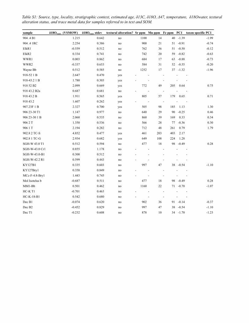
Table S1: Source, type, locality, stratigraphic context, estimated age, δ13C, δ18O, Δ47, temperature, δ18Owater, textural alteration status, and trace metal data for samples referred to in text and SOM.
sample δ18Owater (VSMOW) δ18Owater stdev textural alteration? Sr ppm Mn ppm Fe ppm PC1 taxon specific PC1904 .4 B1 1.215 0.642 no 1100 14 40 -1.39 -1.99904 .4 1RC 2.254 0.386 no 900 21 51 -0.91 -0.74ElkR1 -0.559 0.512 no 762 36 51 -0.50 -0.12ElkR2 0.334 0.741 no 742 20 59 -0.82 -0.63WWR1 0.003 0.862 no 684 17 63 -0.88 -0.73WWR2 -0.337 0.653 no 584 31 52 -0.55 -0.20Wayne Bb 0.512 0.585 no 1252 17 37 -1.32 -1.96918-52 1 B 2.647 0.470 yes - - - - -918-43.2 1 B 1.780 0.303 yes - - - - -918 52 B2 2.099 0.669 yes 772 49 205 0.64 0.75918 43.2 B2a 0.687 0.681 no - - - - -918 43.2 B 1.911 0.565 yes 805 57 179 0.65 0.71918 43.2 1.607 0.262 yes - - - - -907.23F 1 B 2.327 0.700 yes 505 98 185 1.13 1.30906 23-30 T1 1.147 0.977 no 640 29 90 -0.25 0.46906 23-30 1 B 2.060 0.535 no 860 39 169 0.33 0.34906 2 T 1.350 0.536 no 566 28 77 -0.36 0.30906 1 T 2.194 0.282 no 712 48 261 0.79 1.79902.8 2 TC-S 4.852 0.477 yes 461 203 403 2.17902.8 1 TC-G 2.934 0.682 yes 649 108 224 1.28SGH-W 43.0 T1 0.512 0.594 no 477 18 98 -0.49 0.28SGH-W-43.0 Cr1 0.855 1.178 no - - - - -SGH-W-43.0-B1 0.300 0.512 no - - - - -SGH-W-42.2 R1 0.599 0.443 no - - - - -KY127B1 0.335 0.603 no 997 47 38 -0.54 -1.10KY127Bry1 0.358 0.849 no - - - - -MCc-F-4.8-Bry1 1.443 0.745 no - - - - -Mol Isotelus b -0.687 0.511 no 477 18 98 -0.49 0.28MM1-Bb 0.501 0.462 no 1160 22 71 -0.70 -1.07HC-K T1 -0.701 0.463 no - - - - -HC-K-18-B1 0.542 0.680 no - - - - -Dec B1 -0.074 0.620 no 902 36 91 -0.14 -0.37Dec B2 -0.452 0.829 no 997 47 38 -0.54 -1.10Dec T1 -0.232 0.608 no 878 10 34 -1.70 -1.23
25
Supplemental references
S1. A. Achab, E. Asselin, A. Desrochers, J. F. Riva, C. Farley, Geological Society of
America Bulletin 123, 186 (2011).
S2. C. R. Barnes, Bulletin of the British Museum. Natural History. Geology Series 43,
195 (1988).
S3. P. Copper, Canadian Journal of Earth Sciences 38, 153 (Feb, 2001).
S4. A. Desrochers, C. Farley, A. Achab, E. Asselin, J. F. Riva, Palaeogeography,
Palaeoclimatology, Palaeoecology 296, 248 (2010).
S5. N. R. Emerson, J. A. Simo, C. W. Byers, J. Fournelle, Palaeogeography,
Palaeoclimatology, Palaeoecology 210, 215 (2004).
S6. J. Simo, N. R. Emerson, C. W. Byers, G. A. Ludvigson, Geology [Geology] 31, 545
(2003).
S7. M. E. Patzkowsky, S. M. Holland, Special Paper - Geological Society of America
306, 131 (1996).
S8. M. C. Pope, S. M. Holland, M. E. Patzkowsky, Special Publication of the
International Association of Sedimentologists 41, 255 (2009).
S9. C. E. Brett, T. J. Algeo, Guidebook - Kentucky Geological Survey 1, Series 12, 34
(2001).
S10. S. M. Holland, M. E. Patzkowsky, Special Paper - Geological Society of America
306, 117 (1996).
S11. C. R. Scotese, W. S. McKerrow, in Advances in Ordovician Geology, C. R. Barnes,
S. H. Williams, Eds. (Geological Society of Canada, 1991), vol. Paper 90-9, pp.
271-282.
S12. L. R. M. Cocks, T. H. Torsvik, Journal of the Geological Society 159, 631
(December 1, 2002, 2002).
S13. N. Pinet, P. Keating, D. Lavoie, P. Brouillette, American Journal of Science 310, 89
(2010).
S14. N. Pinet, D. Lavoie, P. Keating, P. Brouillette, Tectonophysics 460, 34 (2008).
S15. D. G. F. Long, Canadian Journal of Earth 44, 413 (2007).
S16. S. Zhang, C. R. Barnes, Palaeogeography, Palaeoclimatology, Palaeoecology 180,
5 (2002).
S17. D. G. F. Long, Canadian Journal of Earth Sciences 44, 413 (2007).
S18. D. G. F. Long, P. Copper, Canadian Journal of Earth Sciences 24, 1807 (1987).
S19. P. J. Brenchley et al., Geology 22, 295 (Apr, 1994).
S20. A. Delabroye, M. Vecoli, Earth Science Reviews 98, 269 (2010).
S21. B. J. Witzke, R. C. Heathcote, E. A. Bettis, R. R. Anderson, R. J. Heathcote, Field
Trip Guidebook - Geological Society of Iowa 63, 39 (1997).
S22. O. E. Childs, AAPG Bulletin 69, 173 (1985).
S23. S. Root, C. M. Onasch, Tectonophysics 305, 205 (1999).
S24. R. Bertrand, Canadian Journal of Earth 27, 731 (1990).
S25. L. Quinn et al., Canadian Journal of Earth 41, 587 (2004).
S26. B. R. Shaw, M. Etemadi, Anonymous, AAPG Bulletin 75, 671 (1991).
S27. S. M. Bergstrom, S. Young, B. Schmitz, Palaeogeography, Palaeoclimatology,
Palaeoecology 296, 217 (2010).
26
S28. W. Buggisch et al., Geology 38, 327 (2010).
S29. S. M. Bergstrom, M. M. Saltzman, B. Schmitz, Geological Magazine 143, 657
(2006).
S30. D. Kaljo, L. Hints, P. Mannick, J. Nolvak, Estonian Journal of Earth Sciences 57,
197 (2008).
S31. P. Copper, D. G. F. Long, Newsletters on Stratigraphy 21, 59 (1989).
S32. M. J. Melchin, Lethaia 41, 155 (2008).
S33. A. Achab, E. Asselin, A. Desrochers, J. F. Riva, C. Farley, Geological Society of
America Bulletin 123, 186 (2011).
S34. P. I. McLaughlin, C. E. Brett, AAPG Bulletin 84, 1389 (2000).
S35. P. I. McLaughlin, C. E. Brett, S. L. Taha McLaughlin, S. R. Cornell,
Palaeogeography, Palaeoclimatology, Palaeoecology 210, 267 (2004).
S36. T. Sami, A. Desrochers, Sedimentology 39, 355 (1992).
S37. S. A. Young, M. R. Saltzman, W. I. Ausich, A. Desrochers, D. Kaljo,
Palaeogeography, Palaeoclimatology, Palaeoecology 296, 367 (2010).
S38. R. E. Came, Nature 449, 198 (2007).
S39. I. S. Al-Aasm, J. Veizer, Journal of Sedimentary Petrology 52, 1101 (1982).
S40. B. Wenzel, C. Lecuyer, M. Joachimski, Geochimica et Cosmochimica Acta 64,
1859 (2000).
S41. R. van Geldern et al., Palaeogeography, Palaeoclimatology, Palaeoecology 240,
47 (2006).
S42. P. Ghosh, Geochimica et Cosmochimica Acta 70, 1439 (2006).
S43. S.-T. Kim, J. R. O'Neil, Geochimica et Cosmochimica Acta 61, 3461 (1997).
S44. S. M. Savin, Annual Review of Earth and Planetary Sciences 5, (1977).
S45. D. P. Schrag et al., Quaternary Science Reviews 21, 331 (2002).
S46. K. Lambeck, Y. Yokoyama, P. Johnston, A. Purcell, Earth and planetary science
letters 181, 513 (2000).
S47. Y. Yokoyama, Nature 406, 713 (2000).
S48. V. Masson-Delmotte et al., Journal of Climate 21, 3359 (2008).
S49. J. G. C. Walker, K. C. Lohmann, Geophysical Research Letters 16, 263 (1989).
S50. R. K. Wanless, R. D. Stevens, Geological Association of Canada Proceedings 23,
77 (1971).
S51. U. Brand, Chemical Geology 204, 23 (2004).
S52. U. Brand, J. Veizer, Journal of Sedimentary Research 50, 1219 (1981).
S53. U. Brand, Chemical Geology 40, 167 (1983).
S54. I. S. Al-Aasm, J. Veizer, Journal of Sedimentary Petrology 56, 763 (1986).
S55. G. A. Shields et al., Geochimica et Cosmochimica Acta 67, 2005 (2003).
S56. D. G. F. Long, Palaeogeography, Palaeoclimatology, Palaeoecology 104, 49
(1993).
S57. D. Kaljo, L. Hints, T. Martma, J. Nılvak, Chemical Geology 175, 49 (2001).
S58. J. D. Marshall, P. D. Middleton, Journal of the Geological Society of London 147, 1
(1990).
S59. L. Hints et al., Estonian Journal of Earth Sciences 59, 1 (2010).
S60. H. Qing, J. Veizer, Geochimica et Cosmochimica Acta 58, 4429 (1994).
S61. A. Prokoph, G. A. Shields, J. Veizer, Earth Science Reviews [Earth Sci. Rev.]. 87,
3 (2008).
27
S62. G. A. Shields et al., Geochimica et Cosmochimica Acta 67, 2005 (Jun, 2003).
S63. J. n. Veizer et al., Chemical Geology 161, 59 (1999).
S64. A. K. Tripati et al., Geochimica et Cosmochimica Acta 74, 5697 (2010).
S65. U. Brand, Chemical Geology 32, 17 (1981).
S66. J. E. Sorauf, Journal of Paleontology 51, 150 (1977).
S67. J. E. Sorauf, Bolotin de la Real Sociedad Espanola de Historia Natural 92, 77
(1997).
S68. G. E. Webb, J. E. Sorauf, Geology 30, 415 (2002).
S69. A. K. Tripati, C. D. Roberts, R. A. Eagle, Science 326, 1394 (December 4, 2009,
2009).
S70. R. J. Stouffer, S. Manabe, Climate Dynamics 20, 759 (2003).
S71. A. K. Tripati et al., Paleoceanography 18, 1101 (2003).
S72. C. H. Lear, Y. Rosenthal, H. K. Coxall, P. A. Wilson, Paleoceanography 19, 4015
(2004).
S73. IPCC, Ed., Climate Change 2007: The Physical Science Basis. Contribution of
Working Group I to the Fourth Assessment Report of the Intergovernmental Panel
on Climate Change, (Cambridge University Press, Cambridge, U.K., and New
York, N.Y., 2007).
S74. V. Masson-Delmotte et al., Climate Dynamics 26, 513 (2006).
S75. M. M. Holland, C. M. Bitz, Climate Dynamics 21, (2003).