Environmental Conservation (2015) 42 (2): 139–151 C© Foundation for Environmental Conservation 2014 doi:10.1017/S0376892914000277

The legacy of a crowded ocean: indicators, status, and trends ofanthropogenic pressures in the California Current ecosystem

KELLY S. ANDREWS 1 ∗, G REGORY D. WILLIAMS 1 , JAME AL F . SAMH OU RI 1 ,KRISTIN N . MARSHALL 1 , VLADLENA GERTSEVA 2 AND PHIL L IP S. LEVIN 1

1Conservation Biology Division, Northwest Fisheries Science Center, National Marine Fisheries Service, National Oceanic and AtmosphericAdministration, 2725 Montlake Blvd E, Seattle, WA 98112, USA, and 2Fishery Resource, Analysis and Monitoring Division, Northwest FisheriesScience Center, National Marine Fisheries Service, National Oceanic and Atmospheric Administration, 2725 Montlake Boulevard E, Seattle, WA98112, USADate submitted: 18 December 2013; Date accepted: 17 June 2014; First published online 19 August 2014

SUMMARY

As human population size and demand for seafoodand other marine resources increase, understandingthe influence of human activities in the oceanand on land becomes increasingly critical to themanagement and conservation of marine resources.In order to account for human influence on marineecosystems while making management decisions,linkages between various anthropogenic pressures andecosystem components need to be determined. Thoselinkages cannot be drawn until it is known how differentpressures have been changing over time. This paperidentifies indicators and develops time series for 22anthropogenic pressures acting on the USA’s portion ofthe California Current ecosystem. Time series suggestthat seven pressures have decreased and two haveincreased over the short term, while five pressureswere above and two pressures were below long-termmeans. Cumulative indices of anthropogenic pressuressuggest a slight decrease in pressures in the 2000scompared to the preceding few decades. Dynamicfactor analysis revealed four common trends thatsufficiently explained the temporal variation foundamong all anthropogenic pressures. This reduced set oftime series will be a useful tool to determine whetherlinks exist between individual or multiple pressuresand various ecosystem components.

Keywords: cumulative effects, energy development, humanactivities, marine ecosystems, multiple pressures, oceanmanagement, pollution, stressors, transportation, toxics

INTRODUCTION

Human activities in, on and around the ocean are variedand growing. These activities generate many benefits,including production of food, employment, energy andlivelihoods (Guerry et al. 2012). However, they are also

∗Correspondence: Kelly Andrews e-mail: kelly.andrews@noaa.gov

associated with pressures on the ecosystem that have negativeconsequences, such as loss or modification of habitat,depletions and introductions of species, physical, visual andauditory disturbances, and toxic and non-toxic contamination(Eastwood et al. 2007). Despite the increasing urgency ofthese influences (Wilson et al. 2005; Halpern et al. 2007),full accounting of how anthropogenic pressures in the marineenvironment have changed over time is rare.

Importantly, these pressures do not act upon theecosystem independently, but rather collectively. They aredisparate and broadly based, ranging from terrestrial-basedpollution, commercial shipping activities, and offshore energydevelopment to fisheries and coastal development, all of whichexert cumulative effects on the ecosystem and could benefitfrom a holistic management approach (Vinebrooke et al. 2004;Crain et al. 2008; Halpern et al. 2008). Quantifying thecumulative effects from multiple pressures is a challengingtask, however, because there is a limited understanding ofhow pressures interact and whether the cumulative effects areadditive, synergistic or antagonistic (Darling & Côté 2008;Hoegh-Guldberg & Bruno 2010). The strength and directionof these interactions may also have different consequences fordifferent taxa or ecosystem components (Crain et al. 2008).Additionally, the intensity and trends of many anthropogenicpressures are likely correlated with each other due to ultimatedrivers such as human population growth, seafood demandor economic conditions, and so are best understood in thecontext of one another (see for example Link et al. 2002).

Previous studies that aim to evaluate the effect of cumulativepressures on marine ecosystems have primarily focusedon spatially-explicit analyses which have revealed pressureshotspots in ecosystems across the globe (Ban & Alder2008; Halpern et al. 2008, 2009; Stelzenmüller et al. 2010;Hayes et al. 2012). These analyses are particularly usefulfor describing patterns of spatial variation among individualand cumulative pressures; they provide a framework foridentifying vulnerable habitats or regions and focusing limitedmanagement resources on these regions of concern. Thesespatially-explicit analyses, however, generally provide only a‘snapshot’ in time which can make it challenging to determinewhat management actions are necessary.

140 K. S. Andrews et al.

Without an understanding of the legacy of anthropogenicpressures in an area, it is difficult to interpret currentand potential future conditions. For instance, the ecologicalconsequences of oil extraction in a previously untouched arealike the North Slope of Alaska are likely to be very differentthan in a historically high-use environment such as the NorthSea. Without a temporal reference of the current intensityof the pressures, it is unknown whether the intensities ofthese pressures are at levels of concern or whether thesepressures are increasing, decreasing or remaining the same.Temporal analyses can provide this important context andhelp focus management actions on pressures that might be atunacceptable levels (Rockström et al. 2009) or that may exhibitunacceptable changes over time. Time series data for manyhuman-related pressures are however, often buried in stateand federal agency reports, described at small spatial scales,and measured inconsistently among local, state and federalentities. Thus, it is important to develop a standardized setof time series that reflect the current intensity and historicaltrends of these pressures that could also be used to evaluate thecumulative intensity of these pressures at scales appropriatefor management.

Here, we developed standardized time series of indicatorsfor 22 anthropogenic pressures acting across the entire USA’sportion of the California Current Large Marine Ecosystem(hereafter, the California Current ecosystem [CCE]). Thesetime series were used to quantify and evaluate the intensityand temporal trends of each pressure. We then used severalapproaches to describe the relative intensity and trends ofthese pressures as a whole. First, we used simple additivemodels to quantify the relative status and trends of cumulativepressures in the CCE. Second, we used multivariate modelsto determine (1) whether pressures were correlated, (2) howthe composition of pressures changed over time, (3) whetherthere were shared trends in the time series of pressures, and(4) whether these trends were related to specific drivers suchas coastal population abundance or economic activity. Oursynthesis, and corresponding methodological approaches toquantify the intensity and trends of these pressures, providea foundation for future integrative analyses on ecologicalcomponents (such as risk analysis and management strategyevaluations) across the CCE.

METHODS

Indicators of anthropogenic pressures

We developed indicators for 22 anthropogenic pressures inthe CCE. The pressures selected were derived primarily fromthose identified in spatially-explicit analyses by Halpern et al.(2009) and from vulnerability analyses by Teck et al. (2010);they ranged in scope from land-based pressures, such asinorganic pollution and nutrient input, to at-sea pressures,such as commercial shipping and offshore oil and gas activities.Ultimately, we evaluated 41 different indicators and selectedthe best indicator to describe the intensity and trends of each

pressure. Indicators were evaluated (Appendix 1, Table S1,see supplementary material at Journals.cambridge.org/ENC)using the indicator selection framework developed by Levinet al. (2011), Kershner et al. (2011) and James et al. (2012).Briefly, we evaluated each indicator according to 18 criteriausing the scientific literature to determine whether there wassupport for each criterion for each indicator. This resultedin a matrix of references and notes with a correspondingvalue of literature support (1 for ‘support’, 0.5 for ‘ambiguoussupport’, 0 for ‘no support’; Appendix 1, Table S1, seesupplementary material at Journals.cambridge.org/ENC).These values were summed across criteria for each indicatorand the highest scoring indicator was chosen for each pressure.

Data for all indicators were compiled from state andfederal reports and databases to create the longest possibletime series (Table 1). Compatible data from the statesof California, Oregon and Washington were pooled tocharacterize pressures at the scale of the CCE. For some land-based pressures (Appendix 2, see supplementary material atJournals.cambridge.org/ENC), data from other states wereincluded if watersheds in these states drained into the PacificOcean (such as Idaho, Montana and Wyoming). The FraserRiver in Canada drains into the upper reaches of the CCE andmay contribute a significant amount of pressures associatedwith runoff and input of freshwater and sediments to coastalhabitats. However, there were numerous complexities tryingto combine datasets from the USA and Canada for nearly allrelevant pressures. To reduce the effects of differences in thedatasets, we limited our analysis to USA data.

The status of each indicator was evaluated against twocriteria: recent short-term trend (increasing, decreasing orremaining the same over the last five years) and short-term status relative to the mean and variance of long-termconditions (higher than, lower than or within historic levels)(Levin & Schwing 2011). An indicator’s trend was consideredto have changed in the short term if the modelled trend overthe last five years of the time series showed an increase ordecrease of more than one standard deviation (SD) of the meanof the entire time series. An indicator’s status was consideredto be above or below historical levels if the mean of the lastfive years was greater than or less than one SD from the meanof the full time series, respectively. We used the mean andstandard deviation of the entire series, as opposed to someearlier period of comparison (such as the first five years ofthe dataset), because there were no good temporal referencepoints for these pressures that made sense to compare themost recent five years of data against. The long-term mean andstandard deviation of a time series serves as a ‘moving window’temporal target that is widely used in marine managementapplications (Samhouri et al. 2012). Defining the ‘short-term’ as the last five years of the dataset is consistent withother management review processes that occur at the scaleof large marine ecosystems (see for example Essential FishHabitat reviews [National Marine Fisheries Service 2013]and National Oceanic and Atmospheric Administration’sIntegrated Ecosystem Assessments [Levin & Schwing 2011]).

Anthropogenicpressuresin

theC

aliforniaC

urrent141

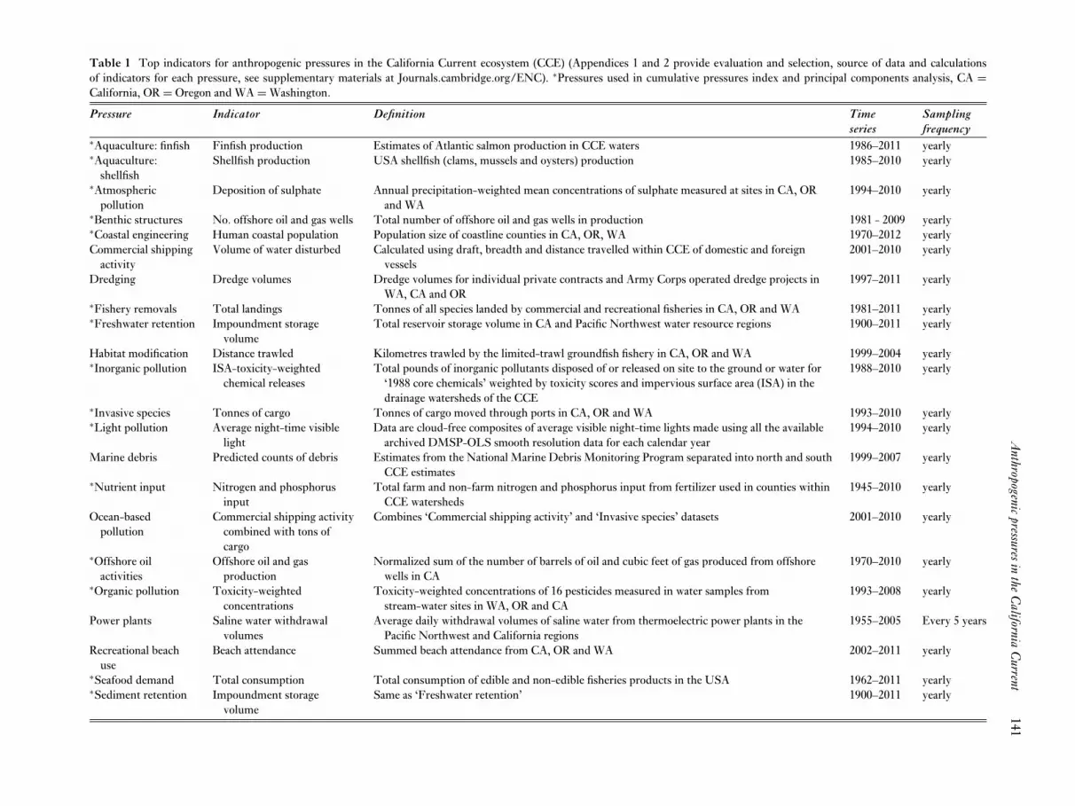
Table 1 Top indicators for anthropogenic pressures in the California Current ecosystem (CCE) (Appendices 1 and 2 provide evaluation and selection, source of data and calculationsof indicators for each pressure, see supplementary materials at Journals.cambridge.org/ENC). ∗Pressures used in cumulative pressures index and principal components analysis, CA =California, OR = Oregon and WA = Washington.

Pressure Indicator Definition Time Samplingseries frequency

∗Aquaculture: finfish Finfish production Estimates of Atlantic salmon production in CCE waters 1986–2011 yearly∗Aquaculture:

shellfishShellfish production USA shellfish (clams, mussels and oysters) production 1985–2010 yearly

∗Atmosphericpollution

Deposition of sulphate Annual precipitation-weighted mean concentrations of sulphate measured at sites in CA, ORand WA

1994–2010 yearly

∗Benthic structures No. offshore oil and gas wells Total number of offshore oil and gas wells in production 1981 - 2009 yearly∗Coastal engineering Human coastal population Population size of coastline counties in CA, OR, WA 1970–2012 yearlyCommercial shipping

activityVolume of water disturbed Calculated using draft, breadth and distance travelled within CCE of domestic and foreign

vessels2001–2010 yearly

Dredging Dredge volumes Dredge volumes for individual private contracts and Army Corps operated dredge projects inWA, CA and OR

1997–2011 yearly

∗Fishery removals Total landings Tonnes of all species landed by commercial and recreational fisheries in CA, OR and WA 1981–2011 yearly∗Freshwater retention Impoundment storage

volumeTotal reservoir storage volume in CA and Pacific Northwest water resource regions 1900–2011 yearly

Habitat modification Distance trawled Kilometres trawled by the limited-trawl groundfish fishery in CA, OR and WA 1999–2004 yearly∗Inorganic pollution ISA-toxicity-weighted

chemical releasesTotal pounds of inorganic pollutants disposed of or released on site to the ground or water for

‘1988 core chemicals’ weighted by toxicity scores and impervious surface area (ISA) in thedrainage watersheds of the CCE

1988–2010 yearly

∗Invasive species Tonnes of cargo Tonnes of cargo moved through ports in CA, OR and WA 1993–2010 yearly∗Light pollution Average night-time visible

lightData are cloud-free composites of average visible night-time lights made using all the available

archived DMSP-OLS smooth resolution data for each calendar year1994–2010 yearly

Marine debris Predicted counts of debris Estimates from the National Marine Debris Monitoring Program separated into north and southCCE estimates

1999–2007 yearly

∗Nutrient input Nitrogen and phosphorusinput

Total farm and non-farm nitrogen and phosphorus input from fertilizer used in counties withinCCE watersheds

1945–2010 yearly

Ocean-basedpollution

Commercial shipping activitycombined with tons ofcargo

Combines ‘Commercial shipping activity’ and ‘Invasive species’ datasets 2001–2010 yearly

∗Offshore oilactivities

Offshore oil and gasproduction

Normalized sum of the number of barrels of oil and cubic feet of gas produced from offshorewells in CA

1970–2010 yearly

∗Organic pollution Toxicity-weightedconcentrations

Toxicity-weighted concentrations of 16 pesticides measured in water samples fromstream-water sites in WA, OR and CA

1993–2008 yearly

Power plants Saline water withdrawalvolumes

Average daily withdrawal volumes of saline water from thermoelectric power plants in thePacific Northwest and California regions

1955–2005 Every 5 years

Recreational beachuse

Beach attendance Summed beach attendance from CA, OR and WA 2002–2011 yearly

∗Seafood demand Total consumption Total consumption of edible and non-edible fisheries products in the USA 1962–2011 yearly∗Sediment retention Impoundment storage

volumeSame as ‘Freshwater retention’ 1900–2011 yearly

142 K. S. Andrews et al.

The historical status of each indicator should be placedin context with the amount of data available for each timeseries. For shorter time series, the mean of the last fiveyears was not likely different from the mean of the entiretime series; thus, the relative status for indicators withshort time series was more closely related to the availabilityof data and not historic trends. However, indicators werechosen because they were the most fundamentally sounddatasets (Appendix 1, Table S1, see supplementary materialat Journals.cambridge.org/ENC) and most of the indicatorschosen will continue to be measured, thus providingmeaningful comparisons into the future.

Summarizing anthropogenic pressures as a whole

We employed three different methods to examine the statusand trends of pressures as a whole. First, we calculateda cumulative pressures index using a subset of pressures.Second, we used principal components analysis to examinecorrelations and temporal shifts among pressures. Last, weused dynamic factor analysis to determine whether the22 pressures could be reduced to a smaller number of commontrends.

Cumulative pressures indexIn order to calculate a cumulative pressures index, wedetermined the longest period for which there were the mostpressures with continuous data available. For the years 1994–2008, we had annual data available for 15 of the 22 pressures(Table 1). Data from these time series were normalized(mean = 0, SD = 1) across the years 1994–2008 so that allpressures were on the same scale. We then used two methodsto calculate a cumulative pressures index. The first methodwas an additive model in which all 15 normalized pressurevalues were summed for each year.

The second method weighted the relative importance ofeach pressure according to vulnerability scores determined byTeck et al. (2010). Briefly, vulnerability scores were developedthrough surveys of experts, in which experts estimated thevalue of five components of ecosystem vulnerability based onthe relative exposure and sensitivity of a habitat to a specificpressure. These five values were then combined to create asingle vulnerability score for each habitat to each pressure.In our analysis, we used the mean vulnerability scores foreach pressure averaged across all habitat types (‘Score mean’in table 6 of Teck et al. (2010)). We then normalized meanvulnerability scores of all pressures listed in Teck et al.(2010) to a scale of 0 to 1 and used the scores relevant toour 15 pressures as weightings. Mean vulnerability scoreswere averaged across pressure categories when more than onerelated to one of our 15 pressures (for example, four nutrientinput pressures were identified in Teck et al. 2010). Finally,we multiplied each normalized pressure value in the timeseries by its respective weighting value and summed across allpressures for each year.

Correlations and temporal shifts among pressuresWe used principal components analysis (PCA; PRIMER6.0; Clarke & Gorley 2006) to identify correlations amongpressures and to reduce the number of multivariatedimensions to a smaller set that explained most of the varianceof the datasets. Because PCA cannot accommodate missingvalues, we used the same set of 15 pressures from 1994–2008that we used above to get the greatest number of pressuresacross the longest period of time. Loadings greater than0.30 were considered relevant for interpretation of the results(Tabachnick & Fidell 1996). We used the principal componentscores across years to examine how the importance of each axischanged over time.

Common trends among pressuresWe used dynamic factor analysis (DFA; Zuur et al. 2003a, b) tocharacterize underlying common trends among the time seriesof anthropogenic pressures. The objective of DFA is to reducethe number of multivariate dimensions needed to describepatterns in data, based on time series models that explicitlyaccount for temporal autocorrelation common in time seriesdata. The DFA framework consists of two models: it combines(1) a random-walk model that captures the underlying sharedtrends among a set of time series and any covariates, and (2)a model that describes how well each time series is describedby each underlying trend.

In the DFA framework, a set of one or more hidden commontrends (linear combinations of a set of random walks) sharedby the time series data explains their temporal variations (Zuuret al. 2003a). DFA is particularly useful for our set of timeseries because it can account for missing values; thus, we canincorporate a larger number of pressures across a longer periodthan was possible for the cumulative pressures index or thePCA. Because DFA allows for the inclusion of covariates, wecould also explore explanatory drivers of the pressures suchas population size and economic growth.

Using the MARSS package in R (Holmes et al. 2012;R Development Core Team 2012), we tested modelswith 1–5 common trends and models including zero, oneor two covariates (coastal human population abundanceand gross domestic product of the USA’s West Coast).Preliminary analyses tested five commonly used variance-covariance matrix structures available in the MARSSpackage and suggested ‘diagonal and equal’ was the mostappropriate (Appendix 3, see supplementary material atJournals.cambridge.org/ENC). This model structure hadobservation variances (along the diagonal) that were equaland covariances that were equal to zero.

Prior to the analysis, time series of all 22 pressures (Table 1)were normalized across the period of interest (1985–2011).We limited the time series to this period because longer timeseries have proportionately greater influence than shorter timeseries in determining common trends and only a third of theindicators had longer time series (Table 1). We used Akaike’smodel selection criterion (AICc; Burnham & Anderson 1998)values to determine the fewest common trends and covariates

Anthropogenic pressures in the California Current 143

Figure 1 Examples of the status and trends of anthropogenic pressures in the California Current ecosystem. Each pressure is represented byspecific indicator datasets (Table 1 and Appendix 2, see supplementary material at Journals.cambridge.org/ENC). Arrows to the right ofeach panel represent whether the modelled trend over the last five years (shaded) increased (↗) or decreased (↘) by more than 1 SD or waswithin 1 SD (↔) of the long-term trend. Symbols below the arrows represent whether the mean of the last five years was greater than (+),less than (-) or within (•) 1 SD of the mean of the full time series (dotted line). Solid lines are ±1 SD of the mean of the full time series.

required to explain the full set of time series. We used anoblique rotation method (promax) to calculate factor loadingsas it helped separate factor loadings among trends betterthan the default orthogonal method (varimax). DFA factorloadings > 0.2 were considered relevant for interpretingwhether pressures were represented by a specific trend (Zuuret al. 2003b). Loading values represent coefficient values thatwhen multiplied by the respective trend value and summedacross all trends produce fitted values for each year for eachpressure (Appendix 3, Fig. S27, see supplementary materialat Journals.cambridge.org/ENC).

For the covariate ‘coastal population abundance’, we useddata from the USA Census Bureau (2010–2012: http://www.census.gov/popest/data/datasets.html) and the NationalBureau of Economic Research (1970–2009: http://www.nber.org/data/census-intercensal-county-population.html).We limited data to ‘coastal’ counties in California, Oregonand Washington, as defined by National Oceanic andAtmospheric Administration (http://www.census.gov/geo/landview/lv6help/coastal_cty.pdf). For the covariate ‘grossdomestic product’ (GDP), data were summed annually acrossthe states of California, Oregon and Washington from 1963–2011 (Bureau of Economic Analysis; http://www.bea.gov/iTable/index_nipa.cfm) using ‘Regional Data’ by state acrossall industries.

RESULTS

Indicators of anthropogenic pressures

Indicators of anthropogenic pressures in the CCE (Table 1)were chosen based on rankings in the indicator evaluationmatrix (Appendix 1, S1, see supplementary material at Journ-als.cambridge.org/ENC). Descriptions, status and trends

of individual indicators are described in Appendix 2 (seesupplementary material at Journals.cambridge.org/ENC),but examples of indicator time series show that the short-term status and trend of anthropogenic pressures in theCCE varied widely (Fig. 1). Most indicators showed eithersignificant short-term trends or their current status wasat historically high or low levels (Fig. 2). Indicators ofinorganic, organic and ocean-based pollution, commercialshipping activity, recreational use, invasive species andhabitat modification all weakened over the short-term, whileindicators of dredging and marine debris (in the northernCCE) intensified; all of these pressures remained withinhistoric levels. In contrast, indicators of seafood demand,sediment and freshwater retention, power plant activity andcoastal engineering remained relatively constant over theshort-term, but were above historic levels, while indicatorsof offshore oil and gas activity and related benthic structureswere at historically low levels. Nutrient input and shellfishaquaculture were at historically high levels, but nutrient inputweakened over the last five years of its time series (Figs 1and 2), while shellfish aquaculture has continued to intensify(Fig. 2 and Appendix 2, Fig. S2, see supplementary materialat Journals.cambridge.org/ENC).

Cumulative pressures index

The ‘additive’ and ‘weighted’ methods provided qualitativelysimilar estimates (Fig. 3). However, the additive index showeda positive trend (adjusted r2: 0.51, F1,13 = 15.7, p = 0.002),whereas the weighted index showed no trend (adjusted r2:0.12, F1,13 = 2.9, p = 0.110) across the entire period. Using thesame criteria to define the recent short-term status and trendsof individual pressures, there was a short-term decrease in

144 K. S. Andrews et al.

Figure 2 Short-term status andtrends of anthropogenic pressuresin the California Currentecosystem. The short-term trendindicates whether the indicatorincreased, decreased or remainedthe same over the last five years.The short-term status indicateswhether the mean of the last fiveyears was higher, lower, or withinhistorical levels of the full timeseries. Data points outside thedotted lines (± 1.0 SD) areconsidered to be increasing ordecreasing over the short term orthe current status is higher orlower than the long-term mean ofthe time series. Numbers inparentheses in the legend are thenumber of years of data for eachpressure. The ‘Cumulativepressures’ indicator (see Fig. 3) isthe additive sum of 15 of thesepressures, which had annual datafrom 1994–2008 (asterisks).

Figure 3 Indices of cumulative pressures from 1994–2008 using 15anthropogenic pressures (asterisks in Fig. 2) which had data duringthis period. Each index was normalized prior to plotting to placethem on the same scale. ‘Additive’ is the sum of all pressure valueseach year; ‘Weighted’ is the sum of pressure values multiplied bytheir respective weighting values (derived from Teck et al. 2010)(see Fig. 1 for description of symbols, lines, and shading).

cumulative pressures using the weighted index, whereas therewas no significant change in the short-term trend using theadditive index (Fig. 3). The short-term status for both indiceswas within historic levels of this time series.

Correlations and temporal shifts among pressures

The first two axes of the PCA explained c. 68% of thetotal variation in the same 15 1994–2008 time series usedto calculate the cumulative pressures index, and the first four

axes explained 86% (Appendix 3, Fig. S25, see supplementarymaterial at Journals.cambridge.org/ENC). Plotting the scoresof the first two principal components across time showedclear changes in the composition of pressures over this period(Fig. 4). In the 1990s, there was strong influence by oil and gasactivities, light pollution and benthic structures, while coastalengineering, seafood demand, nutrient input, aquaculture andorganic and inorganic pollution became more important to thismultivariate measurement in the 2000s. The change in theposition of the PCA score observed in 2002 can be attributedto a particularly large increase in atmospheric pollution thatyear and the abrupt change that occurred in 2006 was relatedto large increases of inorganic (Appendix 2, Fig. S12, seesupplementary material at Journals.cambridge.org/ENC) andorganic (Appendix 2, Fig. S20, see supplementary material atJournals.cambridge.org/ENC) pollution.

Sediment retention and freshwater input also loadedheavily on PC1, but in the complete time series for thesepressures, they are relatively stable from 1994 to 2008(Appendix 2, Figs S9 and S22, see supplementary materialat Journals.cambridge.org/ENC) and thus would have littleinfluence on any changes in cumulative pressure if the entiretime series could have been used. ‘Fisheries removals’, whichwas quite variable during this time period, was the onlypressure that did not load significantly on PC1 or PC2, butloaded heavily on PC3.

Common trends

Model selection criteria revealed a model with either four orfive common trends with no covariates sufficiently explainedthe time series of pressure indicators (Table 2). Because the

Anthropogenic pressures in the California Current 145

Figure 4 Principal componentsanalysis using indicators of 15anthropogenic pressures (asterisksin Fig. 2) that had data from1994–2008. Pressures identifiedalong each axis had eigenvectors >

0.3 for one of the first two principalcomponents, while the values inparentheses are the loading valuesfor the predominant principalcomponent for each pressure (seeFig. 2 for abbreviations).

Table 2 Model selection criteria from the top ten dynamic factor analysis models using all 23 indicator time series from 1985 to 2011and comparing among different variance-covariance structures (R matrix), 1–5 trends and with 0–2 covariates. K = number of parameters;AICc = Akaike information criterion corrected for small sample sizes; �AICc = difference between each model and the lowest AICc fromall possible models; population = coastal population abundance estimate; GDP = gross domestic product of the USA’s west coast states.(See Appendix 3, see supplementary material at Journals.cambridge.org/ENC for description of each R matrix structure.)

R matrix Trends Covariate(s) K AICc �AICc Akaike weight Cumulative Akaike weightDiagonal and equal 4 None 87 875.5 0.00 0.49 0.49Equal variance-covariance 5 None 107 877.2 1.68 0.21 0.70Diagonal and equal 5 None 106 877.4 1.89 0.19 0.89Diagonal and equal 3 Population 90 879.6 4.12 0.06 0.95Equal variance-covariance 4 None 88 881.9 6.42 0.02 0.97Equal variance-covariance 3 Population 91 882.7 7.19 0.01 0.98Diagonal and equal 2 Both 92 884.5 8.97 0.01 0.99Diagonal and equal 4 Population 110 885.4 9.90 0.00 0.99Diagonal and equal 3 GDP 90 885.8 10.30 0.00 1.00Equal variance-covariance 2 Both 93 887.3 11.75 0.00 1.00

model with four trends was more than twice as likely to bethe best model as the two models with five trends, we usedthe 4-trend model to describe the common trends below.The 4-trend model had tight fits with most of the indicatortime series, though a notable exception was ‘Fisheriesremovals’ (Appendix 3, Fig. S27, see supplementary materialat Journals.cambridge.org/ENC).

Trend 1 showed a relatively monotonic increase from1985 to the early 2000s followed by a more variable periodduring the rest of the 2000s (Table 3). Eight pressureshad their highest loadings on this trend and were notrelated to any other trend. These pressures were relatedto food supply, construction and energy production. Mostof these pressures were positively correlated with trend 1,

146 K. S. Andrews et al.

Table 3 Common trends and factor loadings identified from the four-trend dynamic factor analysis model using 23 pressures and time-series data from 1985 to 2011. ǂPressures related to each trend (absolute value of factor loadings > 0.2). ∗Trend most related to each pressure.Negative loadings mean that a pressure is related to the inverse of the trend shown above each column. Factor loadings are the coefficientsthat when multiplied by the trend value and summed across all trends produce predicted values for each pressure.

Broad category of pressures Pressures

Terrestrial pollutants Atmospheric pollution 0.01 –0.53ǂ∗ 0.12 0.28ǂInorganic pollution − 0.12 0.01 0.09 0.77ǂ∗

Organic pollution − 0.19 − 0.01 0.00 1.02ǂ∗

Nutrient input 0.17 0.12 − 0.19 0.39ǂ∗

Transportation Dredging 0.05 − 0.03 0.14 − 0.58ǂ∗

Commercial shipping − 0.01 0.27ǂ − 0.43ǂ∗ 0.36ǂOcean–based pollution − 0.01 0.47ǂ − 0.48ǂ∗ 0.17Invasive species − 0.08 0.60ǂ∗ − 0.15 0.07

Coastal disturbance Marine debris (south) 0.02 − 0.34ǂ∗ − 0.11 − 0.13Marine debris (north) 0.00 0.38ǂ − 1.36ǂ∗ 0.04Recreational use 0.26ǂ 0.05 − 0.89ǂ∗ − 0.18Light pollution − 0.10 0.08 − 0.41ǂ∗ − 0.20Habitat modification − 0.09 − 0.18 − 0.62ǂ∗ − 0.14

Food Fisheries removals 0.22ǂ∗ − 0.01 − 0.19 − 0.14Shellfish aquaculture 0.15 0.22ǂ 0.25ǂ − 0.31ǂ∗

Finfish aquaculture 0.29ǂ∗ − 0.06 − 0.05 − 0.20Seafood demand 0.22ǂ∗ 0.11 0.06 − 0.01

Construction Coastal engineering 0.27ǂ∗ − 0.01 0.04 − 0.13Freshwater retention 0.28ǂ∗ − 0.12 0.03 − 0.08Sediment retention 0.28ǂ∗ − 0.12 0.03 − 0.08Benthic structures − 0.27ǂ∗ 0.03 0.11 − 0.01

Energy Oil and gas activities − 0.26ǂ∗ 0.04 − 0.12 0.07Power plant activity 0.08 − 0.45ǂ 0.14 0.54ǂ∗

but oil and gas activities and related benthic structureswere negatively correlated (Table 3; Appendix 3, Fig. S28,see supplementary material at Journals.cambridge.org/ENC).Trends 2–4 showed a variety of peaks and valleys at varioustimes throughout the period. Six of eight pressures that loadedheavily on trend 2 also loaded heavily on trend 3 or 4 (Table 3),suggesting some correlation among these three trends incertain periods. Pressures associated with transportation andcoastal disturbance tended to have higher loadings on trend3, while pressures associated with the input of terrestrialpollutants were generally related to trend 4 (Table 3).

Because all four trends were estimated simultaneously,we cannot statistically determine which trend was mostimportant; however, comparing the results from models withone, two and three common trend(s) with the trends foundin the 4-trend model (Zuur et al. 2003a) suggested that trend1 was the most important as it was nearly identical to thetrend found in the 1-trend model and other monotonic trendsfound in the 2- and 3-trend models (Appendix 3, Fig. S29, seesupplementary material at Journals.cambridge.org/ENC).

The inclusion of covariates did not significantly increasethe fit of the DFA model to the pressures time series data in

the top three models, but trend 1 from the 4-trend model washighly correlated with both covariates (population abundanceversus trend 1: r = 0.98; GDP versus trend 1: r = 0.95).

It is important to note that the strength of the relationshipbetween each pressure and each common trend is a functionof the length of each time series. For example, the time seriesfor marine debris in the northern CCE was strongly related tothe inverse of trend 3 and less positively related to trend 2 foronly a short period of that trend (data for marine debris onlyavailable from 1999 to 2007; Tables 1 and 3). In contrast, thetime series for seafood demand (data available from 1962 to2011; Table 1) was related to trend 1 across the entire periodfrom 1985–2011 (Table 3).

DISCUSSION

One central tenet of ecosystem-based management is toaddress the multiple activities occurring both on land (forexample agricultural and industrial practices) and in the ocean(such as fishing and energy exploration) that affect variouscomponents of marine ecosystems (Leslie & McLeod 2007).Spatial analyses have quantified individual and cumulative

Anthropogenic pressures in the California Current 147

pressures across the CCE (Halpern et al. 2009), but priorto this work there have not been companion analysesconducted to determine the temporal status and trends ofthese anthropogenic pressures.

In this study, most indicators of pressures showed eithersignificant short-term trends or their current intensity wasat historically high or low levels. Taken together, theseresults support two primary conclusions: (1) decreasing trendsof several pressures (such as shipping related indicators,industrial pollution and recreational activity) potentiallyreflect slowing economic conditions during the economicrecession that began around December 2007 (see Grusky et al.2011), and (2) most pressures at historically high intensitylevels have levelled off and are not continuing to increase. Anexception to these general conclusions is shellfish aquaculture,which continues to increase despite being at historically highlevels. The time series for seafood demand and dredging alsosuggest that these pressures will be increasing at historicallyhigh levels if current trends continue over the next few years.In addition, new pressures related to wind/wave/tidal energywill need to be incorporated into this framework as activitiesassociated with these technologies will undoubtedly increaseover the next several decades.

Since each of the catalogued pressures is associated withone or more human activities, the connotation of their statusand trend depends on one’s perspective. For example, adecreasing trend in fisheries removals may be positive forsome conservation outcomes, while at the same time, it couldbe negative in the short term for human well-being in coastalcommunities (Levin et al. 2009). Understanding the trade-offs resulting from dynamic changes in these pressures for thesocial, economic and biological components of the ecosystemis essential for making informed management decisions (Link2010; Kaplan & Leonard 2012). The time series developedhere can be used to inform such decisions in the USA’s portionof the CCE, and to populate science-based decision supporttools that link biological components of marine ecosystemswith human communities and economies.

In addition to quantifying the intensity and trends ofindividual pressures, the ultimate goal of this work was toreduce the large number of pressures to a manageable numberof trends that could subsequently be used in integrativeanalyses that investigate linkages between pressures andstate variables across the CCE. In our first method thatcalculated two indices of cumulative pressures across theCCE, we found statistical differences in the status and trendsbetween the additive and weighted models, but they providedqualitatively similar results. These results suggest that, at thescale of the USA’s portion of the CCE, either model couldbe useful for capturing the overall variation in cumulativepressures. The weighted model may be most useful whenexamining relationships between cumulative pressures andspecific species where the sensitivity of each species to eachpressure could be used as weightings (see Maxwell et al.2013). For resource managers interested in the potentialimpacts of these pressures in specific habitats, habitat-specific

vulnerability scores for each pressure (Teck et al. 2010) couldbe used instead of the average vulnerability score across allhabitats. The habitat-specific vulnerability scores would beweighted by the proportion of area of each habitat withinthe region of interest in order to calculate the weighting foreach pressure. In this application, the difference betweenadditive and weighted models could be quite significantdepending on the relative size of the habitats present in theregion-of-interest and their relative vulnerability to variouspressures.

A clear limitation of any analysis attempting to combinemultiple pressures into a cumulative index is the lack ofdata on the strength and form of interactions between them(Halpern & Fujita 2013). Without a clear understandingof the potential synergistic and antagonistic interactionsamong multiple pressures (Crain et al. 2008; Darling & Côté2008; Brown et al. 2013), an additive index can be used todescribe the cumulative effect of multiple pressures actingon the system (Halpern et al. 2009). However, an increasingbody of work has more realistically described effects ofmultiple pressures on fish populations, as well as on fisheries(Kaplan et al. 2010; Ainsworth et al. 2011; Brown et al.2013), and there has been increasing effort to empiricallyevaluate the strength and direction of interactions amongmultiple pressures (Lefebvre et al. 2012; Lischka & Riebesell2012; Sunda & Cai 2012). This research will help betterunderstand cumulative effects of multiple pressures on variousspecies, habitats and ecosystems, and reduce uncertainty inquantifying these effects.

Of the two multivariate approaches to reduce the numberof pressures into a manageable number of trends, principalcomponents analysis (PCA) allowed us to reduce a set of 15pressures down to two principal components that explained68% of the variation. The analysis showed large changes inthe composition of pressures during the 1994–2008 period.The relative changes among pressures may reflect changesin regulatory actions, business practices, economic activity,technological advances and social norms over this period. Theprincipal component score framework has been suggested as away to measure the relative status of an ecosystem and to derivespecific control rules, analogous to single species management(Link et al. 2002). As the PCA score moves around inmultidimensional space, managers could determine whetherthis point falls outside of acceptable conditions (Rockströmet al. 2009; Samhouri et al. 2011, 2012). Once this occurs or isapproached, pressures that are correlated with the movementoutside the acceptable range could be subject to regulatoryactions or incentives to reduce these pressures on the marineecosystem.

However, we caution against the use of PCA as a way toreduce or combine multiple variables when those variablesare time series (see Link et al. 2002; Sydeman et al. 2013)for two primary reasons: (1) PCA assumes that each yearis independent from the year before and after, thus it doesnot account for autocorrelation that is present in time seriesdata, and (2) PCA does not allow for missing data, which are

148 K. S. Andrews et al.

common in time series data, thus reducing the set of timeseries that can potentially be used or adding in uncertaintyassociated with using averaged or predicted data to fill inmissing values. In contrast, DFA is an analogous dimension-reducing methodology that explicitly accounts for the natureof time series data and can explicitly account for missing data,as well as incorporate the effects of explanatory variables (Zuuret al. 2003b; Holmes et al. 2012).

Using DFA, we were able to include all pressure timeseries and increase the number of years in the analysis from15 to 27 compared to the cumulative pressures index andthe PCA. The DFA reduced the 23 pressure time series tofour underlying common trends. Ideally, this analysis wouldremove the effects of assumed drivers (covariates) and thenreveal correlations between each pressure and one commontrend. In our analysis, the covariates did not help removeunderlying variation, but only seven of the 23 pressures wererelated to multiple common trends, making interpretation ofthe results more reasonable. Despite its flexibility in dealingwith missing data and autocorrelation within time series, thecorrelations of these seven pressures with multiple trendshighlights a caution in over-aggregating pressures data intoa single index or even into a few common trends, as highly-variable pressures can load significantly onto multiple trends.In addition, the pressures are only related to the specific periodof the trend for which there are pressure data. Alternativenonlinear approaches for reducing the dimensionality of largedata sets have shown promise, in some instances, of being ableto explain more of the total variance in the data (for exampleKenfack et al. 2014) or in estimating the true dimensionality ofthe data set (for example Tenenbaum et al. 2000) compared tothe linear methods we used, but nonlinear methods have alsobeen prone to detect nonlinearities and multi-modal trendswhere none exist (Christiansen 2005; Andersen et al. 2009).

A second goal of ecosystem-based management is toidentify thresholds and/or reference points of pressures thataffect ecosystem state variables. Recent studies have begunto identify thresholds for individual pressures on marineecosystem components (Samhouri et al. 2010; Large et al.2013), but there has been no attempt at identifying thresholdsacross multiple pressures. Reducing 23 pressure time seriesto four common trends provides a way forward to identifyrelationships, including thresholds, between pressures andecosystem components. The trends presented here, forexample, could be used by themselves or in conjunction withoceanographic indices to explore the parameter space which isfavourable for the dynamics of specific ecosystem componentsor could be used as covariates in models to help accountfor ‘unknown factors’ that are not measured directly in moststudies (see for example Auth et al. 2011).

Importantly, we do not fully understand the relationshipbetween most ecosystem components and the intensity levelsof these pressures, either individually or collectively; thus, it isdifficult to predict whether changes in ‘pressures’ will translateto detectable changes in ‘impacts’ on an ecosystem component.Also, given that many of these pressures are correlated (such

as pressures that load on the same DFA trend), it may bedifficult to disentangle effects of individual pressures andappropriately identify management responses. Each of theseconcerns highlights the need for increased empirical testingof the effects of these pressures on ecosystem responses.

It was surprising that the covariates coastal populationabundance and economic activity did not significantlyimprove the fit of DFA models to the time series ofanthropogenic pressures. However, trend 1 appeared toexplain the greatest amount of variation across the set ofpressures and was highly correlated with both covariates.Coastal population abundance and gross domestic productmay be drivers of anthropogenic pressures as a whole inthe CCE but institutional controls (laws and governance),market forces, technological advances and/or cultural normslikely interacted with these drivers at various times duringthis period to modify the relationship between pressures anddrivers. For example, implementation of the Clean WaterAct (http://www.epw.senate.gov/water.pdf) over the yearshas provided incentives and regulations which reduced themagnitude of certain industrial pollutants (Adler et al. 1993;Houck 2002), even though it likely reduced profits in theshort-term. Similarly, social norms have changed the waysome people feel about littering our roadways and waterways(Lee & Kotler 2011; Naquin et al. 2011), thus reducing perperson littering in some regions even though the numbersof humans and the amount of waste produced has continuedto increase over time (USEPA [United States EnvironmentalProtection Agency] 2011; Brogle 2012). At some point, weexpect our governing institutions, technological capabilitiesand/or social awareness to modify the effects of pressuresultimately caused by increases in the number of humans onthe planet.

CONCLUSIONS

Despite the uncertainties about the strength and direction ofinteractions among pressures, it is important to understandhow the intensities of multiple pressures have been changingover time. The determination of common trends amongpressures can help reduce the number of variables includedin ecosystem assessments and may help identify commondrivers for multiple pressures. Incorporating numerousanthropogenic pressures into the framework of ecosystem-based management is necessary to understand linkagesbetween these pressures and various biological components,and more importantly, will allow identification of thresholds(Samhouri et al. 2010; Large et al. 2013) and considerationof trade-offs among socioeconomic, cultural and biologicalcomponents of the ecosystem (Rosenberg & McLeod 2005;Link 2010). Combining spatial and temporal patterns ofanthropogenic pressures will provide a better understandingof how pressures are changing over time and space and allowmanagers to make better use of limited funding and resources.Recently developed ‘end-to-end’ ecosystem models (such asAtlantis; Fulton et al. 2011) and coupled ecological/economic

Anthropogenic pressures in the California Current 149

models (Kaplan & Leonard 2012) allow examination of theeffects and interactions of anthropogenic, oceanographic andclimatic pressures on multiple ecological components andhuman communities. Our analyses highlight the great varietyof trends in anthropogenic pressures and may be useful forimproving hindcasts of ecosystem dynamics in these end-to-end models. Now, marine ecologists, fisheries scientists,and social scientists need to develop creative methods to testthe validity of model results in the field in order to increaseresource managers’ and stakeholders’ confidence in their useas part of the decision-making process.

ACKNOWLEDGEMENTS

We thank L.L. LaMarca, M.L. Morningstar, J.E. Kerwin,C. Elvidge, M. Cummings, C.A. Ribic, J.M. Gronberg,L. Hillmann, and L. Burnett for help gathering data.N. Tolimieri provided R code for time series plots andstatistical advice in the PCA. E.J. Ward, M.D. Scheuerell,A.O. Shelton, and E.E. Holmes provided sage advice withthe DFA. The initial selection and evaluation of pressureindicators were greatly helped by reviews from six anonymousreviewers during review of National Oceanic and AtmosphericAdministration’s 2012 Integrated Ecosystem Assessment forthe California Current. This research received no specificgrant from any funding agency, commercial or not-for-profitsectors, and we know of no conflicts of interest related to thisresearch.

Supplementary material

To view supplementary material for this article, please visitJournals.cambridge.org/ENC.

References

Adler, R.W., Landman, J.C. & Cameron, D.M. (1993) The CleanWater Act 20 Years Later. Washington, DC, USA: IslandPress.

Ainsworth, C., Samhouri, J., Busch, D., Cheung, W.W., Dunne,J. & Okey, T.A. (2011) Potential impacts of climate changeon Northeast Pacific marine foodwebs and fisheries. ICESJournal of Marine Science: Journal du Conseil 68: 1217–1229.

Andersen, T., Carstensen, J., Hernandez-Garcia, E. & Duarte, C.M.(2009) Ecological thresholds and regime shifts: approaches toidentification. Trends in Ecology and Evolution 24: 49–57.

Auth, T.D., Brodeur, R.D., Soulen, H.L., Ciannelli, L. & Peterson,W.T. (2011) The response of fish larvae to decadal changesin environmental forcing factors off the Oregon coast. FisheriesOceanography 20: 314–328.

Ban, N. & Alder, J. (2008) How wild is the ocean? Assessing theintensity of anthropogenic marine activities in British Columbia,Canada. Aquatic Conservation: Marine and Freshwater Ecosystems18: 55–85.

Brogle, M.R. (2012) The impacts of population density, andstate and national litter prevention programs on marine debris.

PhD dissertation. University of South Florida, Tampa, Florida,USA.

Brown, C.J., Saunders, M.I., Possingham, H.P. & Richardson, A.J.(2013) Managing for interactions between local and global stressorsof ecosystems. PLoS One 8: e65765.

Burnham, K.P. & Anderson, D.R. (1998) Model Selection andMulitmodel Inference: A Practical Information-Theoretic Approach.New York, NY, USA: Springer Science + Business MediaInc.

Christiansen, B. (2005) The shortcomings of nonlinear principalcomponent analysis in identifying circulation regimes. Journal ofClimate 18: 4814–4823.

Clarke, K.R. & Gorley, R.N. (2006) PRIMER v6: UserManual/Tutorial. Plymouth, UK: PRIMER-E.

Crain, C.M., Kroeker, K. & Halpern, B.S. (2008) Interactive andcumulative effects of multiple human stressors in marine systems.Ecology Letters 11: 1304–1315.

Darling, E.S. & Côté, I.M. (2008) Quantifying the evid-ence for ecological synergies. Ecology Letters 11: 1278–1286.

Eastwood, P., Mills, C., Aldridge, J., Houghton, C. & Rogers, S.(2007) Human activities in UK offshore waters: an assessment ofdirect, physical pressure on the seabed. ICES Journal of MarineScience: Journal du Conseil 64: 453–463.

Fulton, E.A., Link, J.S., Kaplan, I.C., Savina-Rolland, M., Johnson,P., Ainsworth, C., Horne, P., Gorton, R., Gamble, R.J. & Smith,A.D.M. (2011) Lessons in modelling and management of marineecosystems: the Atlantis experience. Fish and Fisheries 12: 171–188.

Grusky, D.B., Western, B. & Wimer, C. (2011) The Great Recession.New York, NY, USA: Russell Sage Foundation.

Guerry, A.D., Ruckelshaus, M.H., Arkema, K.K., Bernhardt, J.R.,Guannel, G., Kim, C.-K., Marsik, M., Papenfus, M., Toft,J.E. & Verutes, G. (2012) Modeling benefits from nature: usingecosystem services to inform coastal and marine spatial planning.International Journal of Biodiversity Science, Ecosystem Services andManagement 8: 107–121.

Halpern, B.S. & Fujita, R. (2013) Assumptions, challenges, andfuture directions in cumulative impact analysis. Ecosphere 4:art131.

Halpern, B.S., Kappel, C.V., Selkoe, K.A., Micheli, F., Ebert,C.M., Kontgis, C., Crain, C.M., Martone, R.G., Shearer, C.& Teck, S.J. (2009) Mapping cumulative human impacts toCalifornia Current marine ecosystems. Conservation Letters 2: 138–148.

Halpern, B.S., Selkoe, K.A., Micheli, F. & Kappel, C.V. (2007)Evaluating and ranking the vulnerability of global marineecosystems to anthropogenic threats. Conservation Biology 21:1301–1315.

Halpern, B.S., Walbridge, S., Selkoe, K.A., Kappel, C.V., Micheli,F., D’Agrosa, C., Bruno, J.F., Casey, K.S., Ebert, C., Fox, H.E.,Fujita, R., Heinemann, D., Lenihan, H.S., Madin, E.M.P., Perry,M.T., Selig, E.R., Spalding, M., Steneck, R. & Watson, R. (2008)A global map of human impact on marine ecosystems. Science 319:948–952.

Hayes, K.R., Clifford, D., Moeseneder, C., Palmer, M. & Taranto,T. (2012) National Indicators of Marine Ecosystem Health:Mapping Project. Report prepared for the Australian GovernmentDepartment of Sustainability, Environment, Water, Populationand Communities. CSIRO Wealth from Oceans Flagship, Hobart,Australia.

150 K. S. Andrews et al.

Hoegh-Guldberg, O. & Bruno, J.F. (2010) The impact of climatechange on the world’s marine ecosystems. Science 328: 1523–1528.

Holmes, E.E., Ward, E.J. & Scheuerell, M.D. (2012) Analysisof multivariate time-series using the MARSS package. NOAAFisheries, Northwest Fisheries Science Center, 2725 MontlakeBlvd E., Seattle, WA 98112, USA [www document]. URLhttp://cran.r-project.org/web/packages/MARSS/vignettes/UserGuide.pdf

Houck, O.A. (2002) The Clean Water Act TMDL program: law, policy,and implementation. Environmental Law Institute, Washington,DC, USA.

James, C.A., Kershner, J., Samhouri, J., O’Neill, S. & Levin,P.S. (2012) A methodology for evaluating and ranking waterquantity indicators in support of ecosystem-based management.Environmental Management 49: 703–719.

Kaplan, I.C. & Leonard, J. (2012) From krill to conveniencestores: Forecasting the economic and ecological effects of fisheriesmanagement on the US West Coast. Marine Policy 36: 947–954.

Kaplan, I.C., Levin, P.S., Burden, M. & Fulton, E.A. (2010)Fishing catch shares in the face of global change: a framework forintegrating cumulative impacts and single species management.Canadian Journal of Fisheries and Aquatic Sciences 67: 1968–1982.

Kenfack, S.C., Mkankam, K.F., Alory, G., du Penhoat,Y., Hounkonnou, N.M., Vondou, D.A. & Bawe, G.N.(2014) Sea surface temperature patterns in Tropical Atlantic:principal component analysis and nonlinear principal componentanalysis. Nonlinear Processes Geophysical Discussion 1: 235–267.

Kershner, J., Samhouri, J.F., James, C.A. & Levin, P.S. (2011)Selecting indicator portfolios for marine species and food webs: aPuget Sound case study. PLoS One 6.

Large, S.I., Fay, G., Friedland, K.D. & Link, J.S. (2013) Definingtrends and thresholds in responses of ecological indicators tofishing and environmental pressures. ICES Journal of MarineScience: Journal du Conseil 70: 755–767.

Lee, N.R. & Kotler, P. (2011) Social marketing: Influencing Behaviorsfor Good. New York, NY, USA: Sage.

Lefebvre, S.C., Benner, I., Stillman, J.H., Parker, A.E., Drake,M.K., Rossignol, P.E., Okimura, K.M., Komada, T. & Carpenter,E.J. (2012) Nitrogen source and pCO2 synergistically affectcarbon allocation, growth and morphology of the coccolithophoreEmiliania huxleyi: potential implications of ocean acidificationfor the carbon cycle. Global Change Biology 18: 493–503.

Leslie, H.M. & McLeod, K.L. (2007) Confronting the challenges ofimplementing marine ecosystem-based management. Frontiers inEcology and the Environment 5: 540–548.

Levin, P.S., James, A., Kersner, J., S. Kersner, Francis, T.,Samhouri, J.F. & Harvey, C.J. (2011) The Puget Sound ecosystem:what is our desired future and how do we measure progress alongthe way? In: Puget Sound Science Update, Chapter 1a [wwwdocument]. URL http://www.psp.wa.gov/scienceupdate.php

Levin, P.S., Kaplan, I., Grober-Dunsmore, R., Chittaro, P.M.,Oyamada, S., Andrews, K. & Mangel, M. (2009) A framework forassessing the biodiversity and fishery aspects of marine reserves.Journal of Applied Ecology 46: 735–742.

Levin, P.S. & Schwing, F.B. (2011) Technical background foran integrated ecosystem assessment of the California Current:

Groundfish, salmon, green sturgeon, and ecosystem health. USDepartment of Commerce, NOAA Technical MemorandumNMFS-NWFSC-109, USA: 330 pp.

Link, J. (2010) Ecosystem-Based Fisheries Management: ConfrontingTradeoffs. Cambridge, UK: Cambridge University Press.

Link, J.S., Brodziak, J.K.T., Edwards, S.F., Overholtz, W.J.,Mountain, D., Jossi, J.W., Smith, T.D. & Fogarty, M.J. (2002)Marine ecosystem assessment in a fisheries management context.Canadian Journal of Fisheries and Aquatic Sciences 59: 1429–1440.

Lischka, S. & Riebesell, U. (2012) Synergistic effects of oceanacidification and warming on overwintering pteropods in theArctic. Global Change Biology 18: 3517—3528.

Maxwell, S.M., Hazen, E.L., Bograd, S.J., Halpern, B.S.,Breed, G.A., Nickel, B., Teutschel, N.M., Crowder, L.B.,Benson, S. & Dutton, P.H. (2013) Cumulative human impactson marine predators. Nature Communications 4: art 2688.

Naquin, M., Cole, D., Bowers, A. & Walkwitz, E. (2011)Environmental health knowledge, attitudes and practices ofstudents in grades four through eight. ICHPER-SD Journal ofResearch 6: 45–50.

National Marine Fisheries Service (2013) Groundfish essentialfish habitat synthesis report. National Marine FisheriesService/Northwest Fisheries Science Center [www docu-ment]. URL http://www.pcouncil.org/wp-content/uploads/D6b_NMFS_SYNTH_ELECTRIC_ONLY_APR2013BB.pdf

R Development Core Team (2012) R: A language and environmentfor statistical computing. R Foundation for Statistical Computing,Vienna, Austria. ISBN 3–900051–07–0 [www document]. URLhttp://www.R-project.org

Rockström, J., Steffen, W., Noone, K., Persson, A., Chapin,F.S., Lambin, E.F., Lenton, T.M., Scheffer, M., Folke, C. &Schellnhuber, H.J. (2009) A safe operating space for humanity.Nature 461: 472–475.

Rosenberg, A.A. & McLeod, K.L. (2005) Implementing ecosystem-based approaches to management for the conservation ofecosystem services: politics and socio-economics of ecosystem-based management of marine resources. Marine Ecology ProgressSeries 300: 271–274.

Samhouri, J.F., Lester, S.E., Selig, E.R., Halpern, B.S., Fogarty,M.J., Longo, C. & McLeod, K.L. (2012) Sea sick? Setting targetsto assess ocean health and ecosystem services. Ecosphere 3: art41.

Samhouri, J.F., Levin, P.S. & Ainsworth, C.H. (2010) Identifyingthresholds for ecosystem-based management. PLoS One 5: 1–10.

Samhouri, J.F., Levin, P.S., James, C.A., Kershner, J. & Williams,G. (2011) Using existing scientific capacity to set targets forecosystem-based management: a Puget Sound case study. MarinePolicy 35: 508–518.

Stelzenmüller, V., Lee, J., South, A. & Rogers, S. (2010)Quantifying cumulative impacts of human pressures on the marineenvironment: a geospatial modelling framework. Marine EcologyProgress Series 398: 19–32.

Sunda, W.G. & Cai, W.J. (2012) Eutrophication induced CO2-acidification of subsurface coastal waters: interactive effects oftemperature, salinity, and atmospheric pCO2. EnvironmentalScience and Technology 46: 10651–10659.

Sydeman, W.J., Santora, J.A., Thompson, S.A., Marinovic, B. &Lorenzo, E.D. (2013) Increasing variance in North Pacific climaterelates to unprecedented ecosystem variability off California.Global Change Biology 19: 1662–1675.

Anthropogenic pressures in the California Current 151

Tabachnick, B.G. & Fidell, L.S. (1996) Using Multivariate Statistics.New York, NY, USA: Harper Collins College Publishers.

Teck, S.J., Halpern, B.S., Kappel, C.V., Micheli, F., Selkoe,K.A., Crain, C.M., Martone, R., Shearer, C., Arvai, J.,Fischhoff, B., Murray, G., Neslo, R. & Cooke, R. (2010) Usingexpert judgment to estimate marine ecosystem vulnerabilityin the California Current. Ecological Applications 20: 1402–1416.

Tenenbaum, J.B., Silva, V.d. & Langford, J.C. (2000) A globalgeometric framework for nonlinear dimensionality reduction.Science 290: 2319–2323.

USEPA (2011) Municipal solid waste in the United States: 2011Facts and Figures. US Environmental Protection Agency.Office of Solid Waste. EPA530-R-13–001. [www document].URL http://www.epa.gov/waste/nonhaz/municipal/pubs/MSWcharacterization_fnl_060713_2_rpt.pdf

Vinebrooke, R.D., Cottingham, K.L., Norberg, J., Scheffer, M.,Dodson, S.I., Maberly, S.C. & Sommer, U. (2004) Impacts ofmultiple stressors on biodiversity and ecosystem functioning: therole of species co-tolerance. Oikos 104: 451–457.

Wilson, K., Pressey, R.L., Newton, A., Burgman, M., Possingham,H. & Weston, C. (2005) Measuring and incorporating vulnerabilityinto conservation planning. Environmental Management 35: 527–543.

Zuur, A.F., Fryer, R.J., Jolliffe, I.T., Dekker, R. & Beukema,J.J. (2003a) Estimating common trends in multivariate timeseries using dynamic factor analysis. Environmetrics 14: 665–685.

Zuur, A.F., Tuck, I.D. & Bailey, N. (2003b) Dynamic factoranalysis to estimate common trends in fisheries time series.Canadian Journal of Fisheries and Aquatic Sciences 60: 542–552.