the laminar flow field at the interface of a sierpinski carpet configuration

The laminar flow field at the interface of a Sierpinski carpet

configuration

Ravid Rosenzweig1 and Uri Shavit1

Received 5 December 2006; revised 5 June 2007; accepted 3 July 2007; published 2 October 2007.

[1] The problem of laminar flow in a combined free and saturated porous domain wasinvestigated using a Sierpinski carpet configuration. The three-dimensional steady statemicroscale velocities were measured using a particle image velocimeter and computednumerically. The macroscale velocity profiles were then obtained by averaging themicroscale velocities. A comparison between the measured and computed velocitiesshowed a good fit. The macroscale velocity profile was calculated using the modifiedBrinkman equation (MBE), which was recently derived for two-dimensional brushconfigurations. The MBE was developed for unidirectional, laminar flows, assuming thatthe porous medium planar porosity follows a step function. A new analytical solutionof the MBE was developed and applied using no calibration or curve fitting. It was shownthat although the MBE was originally derived for a unidirectional microscopic flow field,the macroscopic representation of the complex microscopic flow in the Sierpinskiconfiguration can be well described by the solutions of the MBE.

Citation: Rosenzweig, R., and U. Shavit (2007), The laminar flow field at the interface of a Sierpinski carpet configuration, Water

Resour. Res., 43, W10402, doi:10.1029/2006WR005801.

1. Introduction

[2] Flows in combined free and saturated porous domainsare found in a variety of natural environments as well as in along list of industrial applications. Natural coupled flowproblems include flows in fractured rocks, wetland flows,and overland flows during rainfall events. Among the manyindustrial applications, which involve flows in combinedporous and free domains, are processes such as filtering,cooling, and drying. In all these cases, the knowledge of theflow field within and above the interface is very important,as it is required for modeling the associated mass and heattransport problems (e.g., contaminant transport, nutrientsupply, resuspension, and dissolution).[3] Modeling the interface flow is difficult since the

governing equations of the free and porous flows are verydifferent from each other and involve both microscopic andmacroscopic formulations. The flow inside the porousmedia is typically treated using the macroscopic Darcylaw whereas the free flow region is modeled by themicroscopic Navier-Stokes equations. In contrast to theDarcy law, the Navier-Stokes equations, being microscopic,require the knowledge of the detailed flow domain geom-etry. Furthermore, they involve both inertial and viscousterms, which are missing in the Darcy law. In the lack ofsuch high-order terms, the Darcy law cannot model theporous flow near the interface, as it fails to describe thepenetration of high velocities into the porous media.Consequently, the interface velocity and velocity gradientremain unknown, leaving the flow field above the interface

unresolved. Modeling the flow field at the interface musttherefore represent the effect of both the Darcy flow in theporous media and the free flow above it, bridging theinherent differences between the two regions.[4] Two main approaches were widely used for treating

the laminar flow at the interface of porous media. The firstis based on a velocity jump condition postulated by Beaversand Joseph [1967], which enables the coupling of the Darcylaw with the high-order Stokes equation. The Beavers andJoseph slip condition relates the interface velocity gradientand the relative slip velocity through the permeability and adimensionless empirical parameter, aBJ, known as the‘‘Beavers and Joseph slip coefficient.’’[5] The Beavers and Joseph slip condition was exten-

sively investigated. While some of the studies have verifiedit both experimentally [Beavers et al., 1970; Taylor, 1971]and theoretically [Murdoch and Soliman, 1999; Saffman,1971; Zhou and Mendosa, 1993], others have studied thesensitivity of aBJ to different parameters. The later studiesshowed that aBJ changes as a function of flow conditions[James and Davis, 2001; Sahraoui and Kaviany, 1992],interface location [Saffman, 1971], and surface microstruc-ture [Beavers et al., 1974; Sahraoui and Kaviany, 1992].Moreover, the behavior of aBJ with respect to the porousmedia properties was found to be nonconsistent and geom-etry dependent [Sahraoui and Kaviany, 1992]. Thereforethe use of the Beavers and Joseph slip condition requires thereadjustment of aBJ separately for each flow problem.[6] The second approach for treating the interface problem

involves the solution of the Brinkman equation [Brinkman,1947],

� @ ph i@x

� mk

uh i þ m*@2 uh i@z2

¼ 0 ð1Þ

1Department of Civil and Environment Engineering, Technion, IsraelInstitute of Technology, Haifa, Israel.

Copyright 2007 by the American Geophysical Union.0043-1397/07/2006WR005801$09.00

W10402

WATER RESOURCES RESEARCH, VOL. 43, W10402, doi:10.1029/2006WR005801, 2007ClickHere

for

FullArticle

1 of 17

http://dx.doi.org/10.1029/2006WR005801

[7] Here m* is an apparent viscosity, m is the fluidviscosity, k is the permeability, @hpi/@x is a pressuregradient, and hui is the superficial averaged velocity. TheBrinkman equation is a superposition of the Darcy law andthe Stokes equation. As such, it is reduced to the Stokesequation at the free flow region and to the Darcy law deepinside the porous domain. The apparent viscosity m* isusually different from the fluid viscosity m and is thought tobe dependent on both the fluid and the porous structure[Kaviany, 1995]. As the resistance applied on the fluid ismodeled by the Darcy term, the apparent viscosity isexpected to be the same as the fluid viscosity. This expec-tation, however, is not always supported by the literature,which exhibits various results regarding the desired appar-ent viscosity value. Brinkman himself recommended usingthe ratio m*/m = 1 as a first approximation, where atheoretical justification was later given by Howells [1974]for a random, dilute array of spheres. While most of thestudies found that m*/m > 1 [Givler and Altobelli, 1994; Kimand Russel, 1985; Martys et al., 1994; Sahraoui andKaviany, 1992; Starov and Zhdanov, 2001], others cameto the opposite conclusion, indicating that m*/m < 1 [Gupteand Advani, 1997; Koplik et al., 1983; Larson and Higdon,1986]. Larson and Higdon [1986, 1987], investigating theflow over a cylinders array, found that the ratio m*/m dependson the flow orientation, with m*/m > 1 obtained for flowparallel to the cylinders and m*/m < 1 obtained for flowperpendicular to the cylinders. Ochoa-Tapia and Whitaker[1995] have derived the Brinkman equation using a detailedvolume averaging procedure. They claimed that the apparentviscosity concept is actually the result of a mismatchbetween superficial averaged properties and intrinsic aver-aged properties and showed that m*/m = 1/n, with n beingthe medium porosity. Although most studies claimed that theapparent viscosity is not the same as the fluid viscosity, theratio m*/m = 1 is often being used in the lack of a clearmethodology for choosing the most suitable value for theapparent viscosity [Basu and Khalili, 1999; Choi and Waller,1997; James and Davis, 2001; Prinos et al., 2003].[8] The applicability of the Brinkman equation at differ-

ent porosities was widely addressed. Some authors arguedthat the Brinkman equation is valid only for high-porositymedia. They noted that the theoretical justifications givenfor the Brinkman equation were to a large extent based on adiluteness assumption [Lundgren, 1972]. Analytical studies,such as those by Kim and Russel [1985] and Durlofsky andBrady [1987], concluded that the Brinkman equation isvalid only for porosities above 0.8. On the other hand,other studies showed that the Brinkman equation works wellin much lower porosities. Martys et al. [1994], for instance,exhibited an excellent fit between the Brinkman solutionand an averaged microscale Stokes solution for porousmedia having porosities as low as 0.5.[9] In practice, the interface flow is often modeled by

matching the solution of the Stokes equation at the free flowregion with the solution of the Brinkman equation inside theporous region. At the boundary between the porous mediumand the free fluid, velocity and shear stress continuity areimposed. This matching, also known as the ‘‘two-domainapproach,’’ requires a priori knowledge of the interfacelocation, which is missing in many of the practicalproblems. Moreover, several authors [Costa et al., 2004;

Gartling et al., 1996] argued that the shear stress continuitycondition is not physically accurate since the free fluidstress at the interface is supported by both the solid matrixand the pore fluid. Therefore the Brinkman equation isexpected to somewhat overpredict the velocity and thepenetration depth in the porous media [Gartling et al.,1996]. Indeed, James and Davis [2001] and Sahraoui andKaviany [1992] have reported such overpredictions.[10] To overcome these limitations, some studies used the

‘‘single-domain approach,’’ in which the Brinkman equa-tion is being solved in the entire domain. The transitionfrom the free fluid to the porous region is achieved throughspecifying the spatial variation of properties such as thepermeability, the apparent viscosity, or the porosity [Goyeauet al., 2003]. The single-domain approach enables us tomodel both the porous media and the free flow using one setof equations. Furthermore, it avoids the need to specifyboundary conditions between the domains since velocityand stress continuity across the interface are readily satis-fied. For these reasons, the single domain approach isparticularly used in numerical studies [Basu and Khalili,1999; Choi and Waller, 1997; Vafai and Kim, 1990a].However, the use of this approach does not prevent, inmost cases, the need to define the interface location, asterms such as the Darcy term are dropped at the interface,while others take on a different value.[11] Despite its disadvantages, the Brinkman equation

was extensively used (see examples given by Gupte andAdvani [1997]). While some of the studies utilized theoriginal form of equation (1), others added various termssuch as a quadratic drag term (Forchheimer term) or a time-dependent term to account for more generalized flow cases[Choi and Waller, 1997; Costa et al., 2004; Gartling et al.,1996; Vafai and Kim, 1990b; Vafai and Thiyagaraja, 1987].Regardless of the formulation being used, the solution of theBrinkman equation, as in the case of the Beavers and Josephslip condition, remains dependent on an unknown empiricalparameter (the apparent viscosity).[12] In a series of papers, Breugem and Boersma [2005]

and Breugem et al. [2006] applied direct numerical simula-tion (DNS) to solve both the microscopic and macroscopicturbulent flow inside and above a three-dimensional porousmedium made of cubes. By using the results of the volumeaveraging theory developed by Whitaker [1999], they wereable to evaluate the significance of velocity and pressuresubfilter terms and compare the macroscopic formulationwith the average result of their DNS. In another importantpaper, Breugem et al. [2005] examined the jump conditionproposed by Ochoa-Tapia and Whitaker [1995] whilesolving the flow problem of a laminar boundary layer overa permeable wall. Although these detailed numerical inves-tigations provide excellent insight, they were not verifiedagainst measurements.[13] Measurements of the detailed velocity field inside a

porous medium and near its surface are difficult to obtain.As a result, the experimental data concerning the interfaceflow are very limited and mostly restricted to simple orderedgeometries (e.g., cylinders array [Bijeljic et al., 2001;Prinos et al., 2003]) in bounded flow problems (i.e.,a nonslip condition is applied at the top boundary [Gupteand Advani, 1997; Tachie et al., 2003]). Another limitationis that most of these studies focused on high-permeability

2 of 17

W10402 ROSENZWEIG AND SHAVIT: FLOW AT THE INTERFACE OF POROUS MEDIA W10402

and high-porosity media (e.g., a porosity of 0.84–0.99given by Tachie et al. [2003] and a porosity of 0.9–0.975given by Tachie et al. [2004]). These limited data cannotprovide the needed generalization to specify the values ofthe above empirical parameters. Subsequently, withoutspecific experimental fitting, the available models can, atbest, provide an approximated solution. Therefore there is aclear need for more experimental, numerical, and theoreticalstudies to accurately predict the interface flow without therequirement for empirical fittings.[14] Recently, we presented a modification of the Brink-

man equation and named it the MBE (the modified Brink-man equation) [Shavit et al., 2002, 2004]. The MBE wasdeveloped for a given set of assumptions as described in thenext paragraph. We showed that when these assumptionsare not violated and when the porosity, permeability, fluidviscosity, fluid height, and pressure gradient (dP/dx) areknown, the MBE provides a complete macroscopic solutionof the interface flow for any two-dimensional brush con-figuration. The MBE was found to be accurate within awide range of porosities (as tested for n = 0.15–0.825), withno need for empirical adjustments.[15] The derivation of the MBE is based on three major

assumptions: The flow is microscopically unidirectional, thechange of the planar porosity (area filled with water dividedby the total area, at a given horizontal plane) follows a stepfunction at the interface, and the velocity regime is laminar,keeping the porous media Reynolds number bellow unity.The first assumption limits the MBE to two-dimensionalconfigurations such as the infinite series of rectangulargrooves studied by Shavit et al. [2002, 2004]. The secondassumption means that the interface location is well definedand that the planar porosity, immediately bellow the inter-face, is uniform and equal to the porosity deep inside theporous media. Note that the averaging approach that wasimplemented in the MBE and generated a linear prescribedporosity function is a key feature of the MBE derivation.Finally, the third assumption imposes an upper limit on thevelocity and allows the Darcy law to be used for the closuremodel.[16] In order to expand the application of the MBE, the

importance of these three assumptions should be examined.The current paper examines a three-dimensional flow casein which all three velocity components coexist. This flowcase violates the first assumption, i.e., the flow is notmicroscopically unidirectional. We will show that evenwhen the microscopic flow field is not perfectly unidirec-tional, the MBE could be used to predict the macroscopicvelocity profile. We chose a porous media model that ismade of a series of vertical square columns with a geomet-rical arrangement that follows a Sierpinski carpet fractal.Although the Sierpinski carpet arrangement generates aflow that is not microscopically unidirectional, it maintainsthe previous general pattern by means of channeling most ofthe flow in grooved like geometry. The other two assump-tions were not tested here. These assumptions are notviolated as the planar porosity follows a step function,and the fluid used was a glycerol solution by which thepore-scale Reynolds number was kept bellow unity.[17] The three-dimensional microscopic velocity field

within the Sierpinski carpet was measured in a laboratoryphysical model using a particle image velocimeter (PIV)

system and computed numerically. The macroscopic veloc-ity profile was then obtained by averaging the computedand measured microscale velocities and compared with thesolution of the MBE.[18] We first describe the Sierpinski carpet geometry. We

then present the mathematical derivation of the MBE and itsanalytical solution, followed by a description of the exper-imental setup, the PIV system, and the numerical methods.The results section includes a description of the measuredand computed microscale velocity fields, followed by acomparison between the averaged microscale results and thesolution of the MBE. We end by examining the behavior ofthe pressure gradient in the free and porous regions.

2. The Sierpinski Carpet Geometry

[19] The Sierpinski carpet is a fractal set. It is created bydividing a square (N = 0) into nine identical squares,removing the middle one (N = 1) and repeating theprocedure with each of the remaining squares (N = 2). Thisprocedure can be repeated as much as desired, with eachrepetition called a construction stage (N is the total numberof construction stages). In the current study we simulate athree-dimensional coupled free and porous domain using aninfinite array of N = 2 Sierpinski sets (Figure 1a) elongatedin the z direction and covered on top by a free fluid layer ofheight h. The removed squares represent the solid phase(shaded squares in Figure 1) while the fluid phase occupiesthe rest of the volume resulting in a porosity of 0.79. A sideview of the Sierpinski set is shown in Figure 1b. Thedimensions of the Sierpinski structure are specified inFigure 1 with the columns height hp and the length of theSierpinski unit L being 36 mm.[20] The geometry of the Sierpinski carpet represents a

three-dimensional flow case in which all the velocity com-ponents coexist and a fully developed velocity field cannotdevelop locally. The periodic structure of the Sierpinskicarpet consists of repeating units, which are characterizedby a microstructure that contains several length scales. Manyof the previous studies have used simple periodic arrays(such as a cylinders lattice), most of which were limited totwo-dimensional domains [James and Davis, 2001; Larsonand Higdon, 1987; Prinos et al., 2003; Sahraoui andKaviany, 1992]. The combination of the three, dimension-ality, periodicity, and the existence of several length scales,provides a better representation of natural porous media[Adler, 1992]. In addition, the Sierpinski structure providessome important technical advantages. Cylinders generateoptical noise due to refraction, imposing major obstacleswhen using PIV inside the porous media. The right anglebetween the laser beam and the side faces of the Sierpinskicolumns is such that optical refraction is reduced. Finally,the periodical and symmetrical nature of the Sierpinski setallows investigation of the average velocity at only half ofthe basic Sierpinski unit, substantially reducing the experi-mental and computational costs. The investigated domainused for both the PIV measurements and numerical simu-lations is shown in Figure 1c.

3. Mathematical Derivation

[21] The modified Brinkman equation (MBE) is a spa-tially averaged form of the Navier-Stokes equations for a

W10402 ROSENZWEIG AND SHAVIT: FLOW AT THE INTERFACE OF POROUS MEDIA

3 of 17

W10402

steady state, unidirectional, laminar flow, assuming a New-tonian fluid, a stagnant solid phase, and constant fluidproperties. The averaging operator was applied assumingthe porous media is represented by a brush configuration.The term ‘‘brush’’ follows the example given by Taylor[1971] who studied the flow inside and above a set ofparallel walls. Such a geometry imposes a unidirectionallaminar flow. Shavit et al. [2002] showed that averaging theNavier-Stokes (microscopic) flow equations over a repre-sentative elementary volume (REV) results in the followingmacroscopic equation:

� @ Ph i@x

þ m@2q uh if

@z2� n

kuh if

!¼ 0; ð2Þ

where huif is the average intrinsic velocity in the x direction,n is the porosity of the porous media, q is the porositywithin the REV, P is the generalized pressure, and x and zare the horizontal-streamwise and vertical coordinates,respectively.

[22] In the current paper we study the flow within andabove the Sierpinski carpet configuration. As mentionedabove, not all the assumptions made in the development ofthe MBE are valid for this flow case. Furthermore, theperiodic structure of the Sierpinski carpet has to be consid-ered when applying the averaging procedure. For thesereasons, the averaging procedure is revisited.[23] We start with the x component of the Navier-Stokes

equations,

r@u

@tþ @ u2ð Þ

@xþ @ uvð Þ

@yþ @ uwð Þ

@z

� �¼ � @p

@xþ gr sin b

þ m@2u

@x2þ @2u

@y2þ @2u

@z2

� �; ð3Þ

where u, v, and w are the velocity components in the x, y,and z directions, r is the fluid density, p is the pressure, g isthe gravitational acceleration, and b is the angle of x withrespect to the horizon (b is assumed to be small). Followingthe generalized volume averaging method presented by

Figure 1. (a) Top view of a representative section of the infinite Sierpinski sets array. (b) Side view ofone Sierpinski set. (c) Top view of the domain used for the particle image velocimeter (PIV) experimentsand for the numerical simulations. Boundary conditions are specified.

4 of 17


Quintard and Whitaker [1994a], we define an averagingoperator as

fh i xj ¼Z8

m r� xð Þ f rð Þd8 ð4Þ

where h�ijx is the superficial average of property f,evaluated at x which is the centroid of the representativeelementary volume (REV). 8 is the total volume of the REV,including both the solid and fluid phases, r is a positionvector, and m is a volume fraction weighting function. Theintrinsic average h�i f is obtained over the fluid phase suchthat h�i f = h�i/q, where q is

q xð Þ ¼Z8

m r� xð Þ g rð Þd8; ð5Þ

with g(r) being an indicator function which equals onewhen r points to the fluid phase and zero when it points tothe solid.[24] The main difficulty in applying a spatial averaging

operation rises in terms that involve derivatives. Accordingto the averaging theorem, the average of a gradient, hrfi isthe gradient of the averaged property rhfi plus an integralover the solid-fluid interfacial area S. In the generalizedaveraging theorem [Quintard and Whitaker, 1994a] thisrelation takes the form

rfh i xj ¼ r fh i xj þZS

n̂ m r� xð Þ f rð ÞdS; ð6Þ

with n̂ being a unit normal vector pointing outward from thefluid phase. We apply the spatial averaging operators (4)–(6)on the Navier-Stokes equation (3), assuming that the solidphase is stagnant (the velocity of the solid-fluid interface iszero), and the fluid properties are constant. The averagedform of equation (3) is

r@u

@tþ @ u2ð Þ

@xþ @ uvð Þ

@yþ @ uwð Þ

@z

� �¼ � @p

@x

� �þ gr sinbh i

þ m@2u

@x2þ @2u

@y2þ @2u

@z2

� �: ð7Þ

[25] Applying Equation (6) on the viscous and pressureterms on the right-hand side of equation (7) yields

� @p

@x

� �þ gr sinbh i þ m

@2u

@x2þ @2u

@y2þ @2u

@z2

� �¼ � @ ph i

@x

þ gr sinbh i þ m@2 uh i@x2

þ @2 uh i@y2

þ @2 uh i@z2

��

�ZS

n̂x m r� xð Þp dS þ mZS

n̂x m r� xð Þ @u

@x

� �dS

0@

þZS

n̂y m r� xð Þ @u

@y

� �dS þ

ZS

n̂z m r� xð Þ @u

@z

� �dS

1A: ð8Þ

[26] The integral terms in equation (8) represent the total

drag force fxTOT as applied on the fluid by the solid phase.

As shown in equation (8), fxTOT consists of two components:

the form drag fxFORM, which represents the contribution of

the pressure, and the viscous drag (skin friction) fxVISC,

which represents the contribution of the viscous shear,

f FORMx ¼ �ZS

n̂x m r� xð Þp dS

f VISCx ¼ mZS

n̂x m r� xð Þ @u

@x

� �dS

0@ þ

ZS

n̂y m r� xð Þ @u

@y

� �dS

þZS

n̂z m r� xð Þ @u

@z

� �dS

1A: ð9Þ

[27] We rewrite equation (7) using equations (8) and (9)and assume steady state conditions and zero velocity at thesolid-fluid interface. When the averaging theorem is notapplied to decompose the divergence of the viscous shear,the equation shows the form drag alone,

r@ u2ð Þ@x

þ @ uvð Þ@y

þ @ uwð Þ@z

� �

¼ � @ ph i@x

þ gr sinbh i þ m@2u

@x2þ @2u

@y2þ @2u

@z2

� �þ f FORMx :

ð10Þ

[28] However, when the averaging theorem is used todecompose the viscous shear, both form drag and viscousdrag appear in the equation,

r@ u2ð Þ@x

þ @ uvð Þ@y

þ @ uwð Þ@z

� �¼ � @ ph i

@xþ gr sin bh i

þ m@2 uh i@x2

þ @2 uh i@y2

þ @2 uh i@z2

� �þ f FORMx þ f VISCx : ð11Þ

[29] When the pore-scale Reynolds number is small (<1),

the total drag force ( fxTOT = fx

FORM + fxVISC) is commonly

replaced by a closure model which is proportional to the

velocity, fxTOT = �mahui. Applying the closure model and

rewriting equation (11) gives

r@ u2ð Þ@x

þ @ uvð Þ@y

þ @ uwð Þ@z

� �¼ � @ ph i

@xþ gr sin bh i

þ m@2 uh i@x2

þ @2 uh i@y2

þ @2 uh i@z2

� a uh i� �

: ð12Þ

[30] Quintard and Whitaker [1994a] discussed the properaveraging volume and weighting function for differentporous environments. In particular, they distinguishedbetween ordered and disordered porous media and showedthat a different averaging procedure should be used for each


5 of 17

W10402

case. In disordered media, Quintard and Whitaker [1994a]proposed to use a top-hat weighting function,

m ¼ m8 �1

8 r� xj j r0

0 r� xj j � r0

;

(ð13Þ

where r0 is the radius of the averaging volume. Thisweighting function is valid as long as the averaging volumeis large enough with respect to the length scale of themicroscopic structure. The advantage of periodic (ordered)structures is that the size of the averaging volume is equal tothe periodic unit cell which is significantly smaller than therequired volume for disordered structures. However, usingequation (13) for ordered media will result in fluctuatingmacroscopic pressure. Obviously, this is undesired sincemacroscopic properties should not change drastically oversmall length scales. In order to solve this, Quintard andWhitaker [1994a] suggested using a ‘‘cellular average’’ inwhich the procedure given by (13) is repeated twice. This isequivalent to a triangular weighting function, mc, given by[Breugem and Boersma, 2005]

m ¼ mc � m8 � m8 ¼li � r � xj ji �

l2ir � xj ji li

0 r � xj ji� li

;

8<: ð14Þ

where li and jr � xji are the unit cell length and a relativeposition in the i direction. The m8 * m8 describe thisaveraging operator using a convolution. Quintard andWhitaker [1994b] showed that when the velocity field isperiodic (as in steady laminar flow through a periodic porousdomain), the cellular averaging is needed for the pressureterm alone. Hence the fluctuating pressure field formed bythe Sierpinski carpet requires the use of the cellular averagingprocedure (14). This pressure field is different whencomparing the flow in the grooved sets [Shavit et al., 2002,2004] with the flow in the Sierpinski configuration.While thepressure in the grooved sets is spatially continuous, andtherefore no form drag exists (i.e., fxTOT = fx

VISC), the pressurein the Sierpinski carpet is discontinuous and contributes to thedrag exerted by the solid phase (i.e., fx

TOT = fxFORM + fx

VISC).[31] Applying the averaging theorem (6) on the left-hand

side of equation (7) yields

@ u2ð Þ@x

þ @ uvð Þ@y

þ @ uwð Þ@z

� �¼ @

@xuh i uh i þ u00u00h ið Þ

þ @

@yuh i vh i þ u00v00h ið Þ þ @

@zuh i wh i þ u00w00h ið Þ; ð15Þ

where the nonlinear terms were decomposed as

fifj

� �¼ fih i fj

� �þ f00

i f00j

D Eð16Þ

with f = h�i + f00. Equation (16) consists of a hiddenassumption that h�i = hh�ii, which means that the averagedproperty contains no small-scale variations. As pointed outby Whitaker [1999] this requirement is fundamental in the

averaging procedure and will be satisfied if an appropriateREV and weighting functions are chosen. The challenge inapplying the average theorem near the interface is related tothe difficulty of maintaining the above length scalerequirement. As will be shown, the choice of an appropriatesize for the REV is inherent to the MBE and served as themain tool in matching the macroscopic model with theaveraged microscopic flow [Shavit et al., 2004].[32] Equation (12) can be simplified in the Sierpinski

flow case since the average velocities in the cross flowdirections (hvi and hwi) and the derivatives of the averagevelocity in the stream-wise direction are all zero. Further-more, the terms that contain velocity fluctuations can beneglected due to the low Reynolds number conditions.Finally, we note that the term @2hui/@y2 is zero due to thesymmetry of the Sierpinski carpet geometry. Equation (12)is therefore simplified as follows:

� @ ph i@x

þ gr sin bh i þ m@2 uh i@z2

� a uh i� �

¼ 0: ð17Þ

[33] Following Shavit et al. [2002, 2004], we derive themacroscopic equation for the Sierpinski case by substitutinghui = qhuif in the viscous term, using the generalizedpressure P = p � rg sin bx and substituting ahui = nhuif/kin the closure term,

� @ Ph i@x

þ m@2q uh if

@z2� n

kuh if

!¼ 0: ð18Þ

[34] The appearance of equations (18) and (2) is the samebut the closure in equation (18) represents both the formdrag and viscous drag, while the closure in equation (2)represents the viscous drag alone. Another differencebetween the two equations is the averaging of the pressuregradient (top-hat averaging for equation (2) and cellularaveraging for equation (18)). In the current case study, @hpi/@x(as in equation (17)) is zero and the sole drivingforce is due to gravity. To be consistent with Shavit etal. [2002, 2004] and to keep the generality for theanalytical solution (presented in the next section), we usedhere the generalized pressure P. Note that equations (17)and (18) are not identical to the formulations given byWhitaker [1999, equation 4.2–34, p. 173]. The differencebetween the formulations is a result of the closure used byWhitaker [1999] and the closure used here.[35] When the planar porosity follows a step function

at the interface (here and in the grooved geometry[Shavit et al., 2004]), its volume average changes linearlybetween one outside the porous media and n inside theporous media,

q ¼

1 z � Hrev

21� n

Hrev

� � zþ 1þ n

2

� ��Hrev

2 z Hrev

2

n z �Hrev

2

;

8>>>>><>>>>>:

ð19Þ

6 of 17


where Hrev is the height of the REV and z is the verticalcoordinatewith z = 0 at the interface. Substituting equation (19)into equation (18) results in the MBE as follows:

� @ Ph i@x

þ m@2 uh if

@z2

!¼ 0 z � Hrev

220að Þ

� @ Ph i@x

þ m1� n

Hrev

� � zþ 1þ n

2

� �@2 uh if

@z2þ 2 1� nð Þ

Hrev

@ uh if

@z� n

kuh if

!¼ 0

�Hrev

2 z Hrev

220bð Þ

� @ Ph i@x

þ m n@2 uh if

@z2� n

kuh if

!¼ 0 z �Hrev

220cð Þ

8>>>>>>>>>><>>>>>>>>>>:

[36] The MBE is a set of three linear differential equations.It converges to the Brinkman equation in the porous regionand to the Stokes equation in the nonporous region. Theintermediate region reflects the transition between the Stokesflow and the porous media flow. As the velocity verticalvariations in the porous media decay, the Brinkman equationand the Darcy equation become identical. The only unknownparameter in the MBE is the height of the averaging volumeHrev, which should be determined empirically. Note that indeveloping the MBE we chose to vary the porosity in theviscous term alone while keeping a constant porosity in theclosure term across the interface region (q = n). Likewise,the permeability in the closure term was also kept constant.[37] Shavit et al. [2004] investigated the applicability of

equation (20) by using 37 geometrical sets representing avariety of brush configurations. Each set contained groovesand walls arranged symmetrically to create a wide range ofvalues of porosity and permeability. It was found that Hrev isbest described by the following relation:

Hrev n; kð Þ ¼ ae�bnffiffiffik

p; ð21Þ

with a ffi 8.49 and b ffi 2.29. It was shown that equation (20)together with equation (21) provides an accurate tool forcalculating the macroscopic velocity profile within andabove brush configurations, given the fundamental proper-ties of the porous media n and k, the fluid viscosity, the flowheight, and the flow driving force dP/dx.

4. Analytical Solution

[38] In the works by Shavit et al. [2002, 2004] the MBEwas solved numerically. Here we present an analyticalsolution of the MBE for flow in a semi-infinite porousmedium (�1 z 0) covered by a fluid layer of height h.This flow domain definition is particularly useful since inmost practical applications the influence of the free flowregion on the porous media flow is limited to a small layernear the interface. In this case, replacing the bottomboundary condition with an infinite depth porous mediawould not affect the velocity profile at the vicinity of theporous region and at the interface region [Kuznetsov, 1998].[39] The analytical solution was developed considering the

following boundary conditions; zero shear at the top boundary,

d uh if

dz¼ 0 z ¼ h ð22Þ

while deep inside the porous media the velocity obeys theDarcy law,

uh if¼ � @ Ph i@x

k

mnz ! �1: ð23Þ

[40] Further, we demand that the velocity huif and thevelocity gradient dhuif/dz will be continuous throughout theentire domain (�1 z h). Solving the first and thirdequations (equation (20a) and equation (20c)) is straightfor-ward, while the solution of equation (20b) is more complexand requires a series expansion solution. The solution ofequations (20a)–(20c) together with the boundary condi-tions (22) and (23) gives

uh if¼ 1

2m@ Ph i@x

z2 � 1

m@ Ph i@x

h zþ C4 h � z � Hrev

224að Þ

uh if¼ C2 S0 zð Þ þ C3 S1 zð Þ � @ Ph i@x

k

mn�Hrev

2 z Hrev

224bð Þ

uh if¼ C1 ez= ffiffikp � @ Ph i

@x

k

mn�1 z �Hrev

224cð Þ

8>>>>>><>>>>>>:

where S1 and S0 are sums of the power series given by

Si zð Þ ¼X1m¼0

aim zm i ¼ 0; 1 ð25Þ

aim ¼ � a

baim�1 þ

c

bm m� 1ð Þ aim�2 m � 2 ð26Þ

with a00 = 1, a1

0 = 0, a01 = 0, a1

1 = 1, a = (1 � n)/Hrev, b =(1 + n)/2, and c = n/k. The values of the constants C1, C2,C3, and C4 are found from the continuity of the velocityand the velocity gradient at z = ±Hrev/2 as follows:

C1 ¼ffiffiffik

p eHrev=2

ffiffik

pC2 D0 �Hrev=2ð Þ þ C3 D1 �Hrev=2ð Þð Þ

ð27Þ

C2 ¼G h� Hrev=2ð Þ

D0 Hrev=2ð Þ þ D1 Hrev=2ð Þ B ð28Þ

C3 ¼h� Hrev=2ð Þ B G

D0 Hrev=2ð Þ þ D1 Hrev=2ð Þ B ð29Þ

C4 ¼ C2 S0 Hrev=2ð Þ þ C3 S1 Hrev=2ð Þ þ G k=n� G h Hrev=2þ 1=2 G Hrev=2ð Þ2; ð30Þ


7 of 17

W10402

with

B ¼ S0 �Hrev=2ð Þ=ffiffiffik

p� D0 �Hrev=2ð Þ

D1 �Hrev=2ð Þ � S1 �Hrev=2ð Þ=ffiffiffik

p ð31Þ

G ¼ � 1

m@ Ph i@x

ð32Þ

and D0 and D1 being the derivatives of S0 and S1 given by

Di zð Þ ¼ dSi zð Þ=dz ¼X1m¼1

maim zm�1 i ¼ 0; 1: ð33Þ

[41] Equations (24)–(33) together with equation (21)provide a complete solution of the laminar velocity profileacross the entire domain, from deep inside the porous mediathrough the interface, to the free flow region, and the freefluid surface. At the porous region (equation (24c)), thevelocity decays exponentially to the Darcian velocity. Thisexponential velocity profile is often found when matchingthe Brinkman equation at the porous region with the Stokesequation at the free flow region [Berkowitz, 1989; Nealand Nader, 1974]. The length scale associated withequation (24c) is the Brinkman screening distance,

ffiffiffik

p.

This is in agreement with other studies, which definedffiffiffik

pas

the characteristic length scale of the interface phenomenon[Berkowitz, 1989; Haber and Mauri, 1983; Neal and Nader,1974]. Note that the height of the averaging volumeHrev alsoscales with

ffiffiffik

p.

[42] At the interface region (equation (24b)), the velocityis expressed as a combination of two power series solutions.The interface velocity (at z = 0) is given by

uh ifz¼0¼ C2 þ G k=n: ð34Þ

[43] The second term on the right-hand side is theDarcian velocity, while C2 represents the velocity increasecaused by the penetration of high velocities into the porousdomain. As shown by equation (28), C2 is proportional tothe free flow height h and to the pressure gradient. Theeffect of h on the interface velocity is quite intuitive; highfluid level results in an increased fluid velocity, and a highershear at the porous surface. High pressure gradient has asimilar effect. The influence of the porous media andinterface region geometries on the interface velocity issomewhat more complicated and is reflected by the

dependence of C2 on Hrev and on the power seriessolutions.[44] The velocity at the free flow region (equation (24a))

has a parabolic shape, similar to the classical one-dimensionalStokes flow. As C2 and C4 are of order

ffiffiffik

p, the influence of

the nonzero interface velocity on the free flow solution isnegligible when

ffiffiffik

p� h. However, in cases where a thin

fluid layer flows over a high permeability surface,the influence of the interface velocity on the free flow canbe important (e.g., thin fractures within a moderatelypermeable formation [Berkowitz, 1989]).

5. Experimental Methods

5.1. Setup

[45] A laboratory model was assembled by using Plexi-glas square columns whose dimensions are specified inFigure 1. Five parallel rows of 29 Sierpinski sets weremounted on a 20-mm-thick Perspex plate, which was in-stalled in a 220-cm-long, 20-cm-wide glass flume (Figure 2).In order to prevent preferential flow along the flume side-walls, an additional row of 4-mm columns was added oneach side of the model. Fluid was recirculated through theflume using a pump (PE 50M, Foras), a 100-L collectingtank, and a heat exchanger. The flow rate, fluid density, andtemperature were constantly monitored by a Coriolis accel-eration flow meter (Elite CMF025, Micro-Motion). Toreduce inlet effects, a flow-straightening section was inserted35.5 cm downstream from the flume inlet and 40 cmupstream from the Sierpinski carpet array. The straightenerwas made of three rows of 5-mm-diameter vertical glass rodsplaced in a staggered arrangement across the flume width. Aperforated honeycomb sponge was pressed between the firsttwo rows, and a perforated cooper board was placed betweenthe second and the third rows. Following Kaftori et al.[1994], the fluid level was controlled by an array of largeand heavy cylinders (3 cm in diameter) positioned at theflume outlet (Figure 2). Changing the gaps between thecylinders allowed setting the fluid to the desired level.The flume was positioned on a tunable optical table suchthat the flume slope could be modified. The slope was set toobtain a constant vertical distance between the top of theSierpinski structure (z = 0) and the free fluid surface.[46] Particle image velocimetery (PIV) was used to mea-

sure the velocity field at two-dimensional horizontal crosssections. The PIV system consists of a 160 mJ per pulseNd:YAG double laser system (Twins made of two Brilliantlasers, Quantel), an 8-bit 1-K � 1-K charge-coupled device

Figure 2. Experimental setup (dimensions are in millimeters).

8 of 17


(CCD) camera (Kodak, Megaplus ES 1), an articulated arm,light sheet optics, an image acquisition system, and a PIVanalysis software (Vidpiv4g, ILA-GMbH). The articulatedarm was mounted on top of a mechanical drive device(ITEM), enabling the vertical movement of the arm. The farend of the arm was attached to a 0.01-mm grades microm-eter (Mitutoyo), by which the light sheet was accuratelypositioned.

5.2. Procedure

[47] An aqueous glycerol solution containing about 90%glycerol by weight (referred to in the text as glycerol) wasused as the working fluid. The glycerol temperature wascarefully maintained within a range of 29�C ± 0.5�Cthroughout the experiments. At this temperature, the mea-sured glycerol density was 1.225 ± 0.001 g cm�3. Thekinematic viscosity of the glycerol was measured using acapillary tube viscometer and was found to be 86.4 cst at29�C. Velocity measurements were obtained for two fluidlevels: h = 4.25 ± 0.25 mm and h = 9 ± 0.5 mm, applying aconstant flow rate of 36.5 ± 0.5 cm3 s�1 in bothexperiments. At these conditions, the table slope was0.4 ± 0.05% and 0.3 ± 0.05%, in the low-level and high-level experiments, respectively.[48] As the glycerol attenuates the laser light, resulting in

an insufficient illumination at the middle of the flume,velocity measurements were obtained along the inner halfof the second row of sets. Preliminary measurements ensuredthat the flow field at this location is not influenced by thesidewalls. The measurements were performed at the tenthSierpinski unit, allowing the flow to form a fully periodicpattern. To achieve high spatial resolution, the measurementdomain was divided into two horizontal 1.8-cm � 1.8-cmsubdomains (‘‘upstream’’ and ‘‘downstream’’). The twosubdomains were measured separately, where a transverserail was used to shift the camera between the two subdo-mains. The height of the camera above the measurement areawas adjusted such that the images covered an area of about2.3 cm � 2.3 cm with a 440 pixel/cm ratio.[49] The glycerol was seeded with hollow glass spheres

(Potters), having an arithmetic mean diameter of 11.7 mmand a density of 1.1 g cm�3 [Shavit et al., 2003]. The Stokessettling velocity of the particles was 10�5 cm s�1, whichresults in an approximately 4 orders of magnitude differencebetween the particles settling velocity and the glycerolDarcian velocity (�0.1 cm s�1). As the particles settlingvelocity was negligible relative to the fluid velocities, wesafely assume that the particles movement accuratelyrepresents the fluid motion [Prasad, 2000].[50] Measurements were performed at multiple horizontal

planes, starting as close as possible to the top free boundaryand moving downward till 2 cm below the interface, wherethe Darcy law governs the flow and the average velocity isinvariant of the vertical position. The vertical spacingbetween measurement planes was 0.5 mm at the interfaceregion. This spacing was increased toward the top andbottom boundaries. The total number of horizontal planeswas 25 at the low-level experiment and 26 at the high-levelexperiment. The time between laser pulses was set to allowa maximum displacement of 5 ± 1 pixels, obtaining theminimum time between pulses (4 ms) near the top boundaryand the maximum time (18 ms) in the lowest measurementplane. Five hundred realizations at 5-Hz frequency were

acquired at each of the two subdomains. The uncertainty inestimating the x component averaged velocity, s, wascomputed as follows. When the number of realizations islarger than 30, it is common to assume that the velocity isnormally distributed [Wernet, 2000]. Thus the uncertainty ina 95% confidence interval is given by s = 1.96 � s/

ffiffiffiffiffiM

p,

where M is the number of realizations and s is the standarddeviation,

s ¼

ffiffiffiffiffiffiffiffiffiffiffiffiffiffiffiffiffiffiffiffiffiffiffiffiffiffiffiffiffiffiffiffiffiffiffiffiffiffiffiffiffiffiffiffiffiffiffiffiffiffi1

M � 1

XMi¼1

uh ifi� uh if� �2vuut ; ð35Þ

huiif is the spatial average velocity (macroscopic velocity)

obtained at the ith instantaneous realization, and uh if is theensemble average of the macroscopic velocity. In terms ofnotation, this is the only place where the temporal(ensemble) averaging appears explicitly, while in the restof the paper huif denotes both spatially and temporallyaveraged velocity. As the measurement domain was dividedinto two subdomains, which were not measured instanta-neously, the uncertainty was calculated separately for eachsubdomain. The maximum uncertainty calculated for 500realizations was about 1.2%, indicating that the sample sizeis sufficient for estimating the macroscopic velocity with arelatively high precision.

5.3. Image and Data Analysis

[51] A fast Fourier transform–based cross-correlationalgorithm was used to calculate the velocity vectors (u, v),applying a uniform interrogation area of 32 � 32 pixelswith 50% overlap (16 pixels separation between vectors).Areas occupied by columns were marked and excludedfrom the analysis. A signal to noise filter with a 1.1–1.12threshold followed by a global velocity filter rejected 5–15% of the velocity vectors, with a few realizations reaching20%. These rejected vectors were then replaced using a5 � 5 kernel interpolation. As expected, a lower rejectionrate was obtained in the frames taken above the Sierpinskicolumns (about 10%).[52] An ensemble average was obtained by using the

500 instantaneous realizations acquired at each subdomain.The averaged vector maps were fairly smooth, yet in someframes a few erroneous vectors that survived the filteringand averaging procedures remained. These vectorswere removed by a local median filter with one standarddeviation + 0.4 pixel tolerance, applied on the average field,followed by a 5 � 5 kernel interpolation. The number ofvectors removed in this second filtering step was less than1% of the total vector number.[53] Out of the 2.3-cm � 2.3-cm frames, only the vectors

that were within the 1.8 cm � 1.8 cm upstream ordownstream subdomains were included in the analysis.Each velocity field obtained at a horizontal plane (upstream+ downstream) was composed of between 3772 vectors(within the Sierpinski columns) to 4950 vectors (in the freeflow region). This data set was the basis from which otherquantities were derived, as specified later in the text.

6. Numerical Methods

[54] Numerical solutions of the steady state, laminar,three-dimensional flow within and above the Sierpinski


9 of 17

W10402

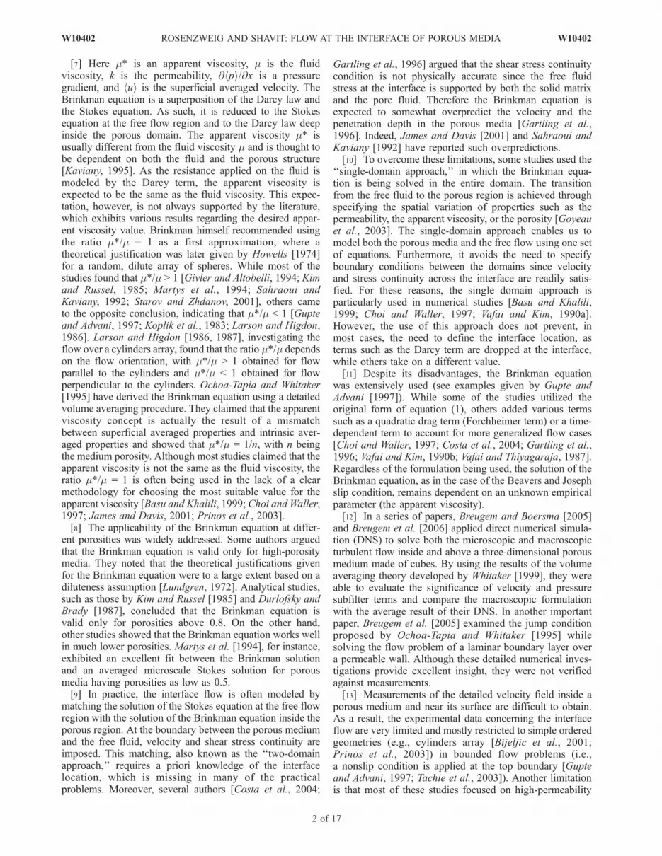
carpet were obtained using the computational domainshown in Figure 1c. The boundary conditions applied weresymmetric conditions on the sides, a periodic condition atthe inlet and outlet, a zero shear (free fluid surface) at thetop (z = h), and a no-slip condition on the walls (Figure 1c).For the periodic condition, the pressure gradient across theperiodic unit H = [P(X + L) � P(X)]/L was specified.[55] The Sierpinski carpet geometry and mesh were

generated using the commercial grid generator GAMBIT 2.Hexahedral-wedge cells were used to cover the three-dimensional flow domain. The mesh was refined near thewalls and at the interface region (Figure 3) and includedbetween 102,510 and 152,600 cells, corresponding to thelow-level and high-level flow cases. Preliminary numericalsimulations examined the mesh density and showed thatrefining the mesh had a negligible effect on the results[Rosenzweig, 2005].[56] The 3-D steady state Navier-Stokes equations were

solved using the finite volume commercial CFD packageFLUENT 6. Solutions were obtained using the segregateddouble precision solver, applying a laminar viscous model,a second-order upwind discretization scheme for themomentum, and a standard scheme for the pressure. Forpressure-velocity coupling, the SIMPLE algorithm waschosen. A solution convergence was achieved after amaximum number of 20,000 iterations, keeping all relativeresiduals below 10�12, and monitoring the volumetric flowrate over a horizontal surface, ensuring that an invariablevalue is obtained.

7. Results and Discussion

[57] Table 1 presents the main characteristics of themeasured flow field: the relative free-flow depth h/(h + hp),the Darcian velocity huid, the maximum averaged velocitymeasured at the top free boundary huimax, and the

Reynolds number calculated in two ways. Reh characterizesthe free-flow region and is based on the averaged velocity atthe top free boundary and the fluid level above the columns h.Red is the ‘‘porous media Reynolds number’’ defined bythe square root of the permeability (k = 0.0237 cm2,[Rosenzweig, 2005]) and the Darcian velocity huid [Bear,1972]. The values of the free-flow Reynolds numberindicate a laminar flow regime, in which the inertia issmall in comparison with the viscous terms. The lowvalues of the porous Reynolds number (Red < 1) indicatethat Darcy’s law is valid within these flow conditions[Bear, 1972].

7.1. Microscale Velocity Field

[58] Ensemble average velocity fields were calculated foreach of the measurement planes. Figure 4 shows a vectormap of the average velocity field measured 2.5 mm belowthe interface (experiment 1, Table 1). The x and y axescorrespond to the coordinate system defined in Figure 1. Asshown, the velocity field consists of low-velocity regionsnear the columns and higher-velocity regions in between.The highest velocities are found between the rows of smallcolumns (1.4 cm < y < 1.8 cm) where an 8-mm gap formsthe widest free passage and therefore provides the lowestflow resistance. The glycerol streamlines seem to wrap thecolumns and create small low-velocity regions around them.As the flow bypasses the large 1.2-cm column, largepositive y component velocities are seen in the upstreamsubdomain and almost symmetric negative velocities arefound in the downstream subdomain. This general stream-line deflection caused by the large column is expected torepeat it self in Sierpinski carpets of higher N (constructionstages).[59] The microscale velocity field above and within the

Sierpinski set was also obtained by a numerical solution ofthe three-dimensional, steady state, laminar, Navier-Stokes

Figure 3. A horizontal cross section of the computational mesh at z = �2.6 cm.

Table 1. Maximum Macroscopic Velocity, Darcian Velocity, and Reynolds Numbers

Experiment h, mm h/(h + hp) huid, cm s�1 huimax, cm s�1 Reh, huimax h/n Red, huidffiffiffik

p/n

1 4.25 ± 0.25 0.106 ± 0.005 0.355 1.85 0.856 0.0632 9 ± 0.5 0.2 ± 0.009 0.13 2.23 2.19 0.023

10 of 17


equations. The fluid properties were identical to those of theglycerol solution used in the experiments (r = 1.225 g cm�3,u = 86.4 cst). The pressure gradient was adjusted such thatthe Darcian velocity deep inside the Sierpinski carpet willmatch the measured velocity (Table 1). Thus the pressuregradientsobtainedwere�15.5gcm�2s�2and�5.5gcm�2s�2,in the low-level and high-level experiments, respectively.Contours of u and v computed at a horizontal plane 2.5 mmbelow the interface are shown in Figures 5a and 5b,respectively. The flow pattern generated by the numericalsolution agrees well with the PIV results (Figure 4),showing the near-columns’ low-velocity regions and thehigh-velocity regions between them. Figure 5b shows thatthe numerical solution was able to reproduce the positiveand negative values of v obtained in the upstream anddownstream subdomains. While this comparison shows thegeneral flow patterns, a more detailed comparison betweenthe PIV and the numerical results is presented later in thissection. Since the PIV measurements provide informationonly on u and v, the numerical solution is the only sourcefrom which we can explicitly draw information on thew velocity component. The numerical solution shows thatlarge values of w are limited to the interface region (notshown here), whereas in the rest of the domain the values ofware an order of magnitude smaller and the flow is essentiallytwo-dimensional.[60] Figure 6 shows a comparison between the ensemble

averaged u profiles measured at the domain inlet (x = 0 cm)and outlet (x = 3.6 cm) 8 mm below the interface. Thesemeasured velocity profiles are also compared with thecorresponding velocity profile obtained from the numericalsolution. As the velocities in the inlet and outlet areperiodically coupled in the numerical solution, only onecurve is needed to represent the velocity in both boundaries.The three velocity profiles exhibit a good fit in both shapeand velocity values, indicating the periodicity of themeasured velocity field and the accuracy of the numericalsolution.

7.2. Macroscopic Velocity Profile

[61] The macroscopic velocity profiles were obtained byspatially averaging the measured and computed velocities.The ensemble average of the measured velocities (u) werespatially averaged over each of the horizontal planes,yielding one single value out of every velocity field such asthe one shown in Figure 4. Thus the average velocityobtained in a specific vertical position is a result ofaveraging between 1,886,000 values below the interface and2,475,000 values above it. The averaging of the numericalsolution was done in a similar way, where the onlydifference was that instead of an area averaging, an Hrevthick averaging volume was used. The size of the Hrev,2.15 mm, was calculated according to equation (21) (n =0.79, k = 0.0237 cm2) [Shavit et al., 2004]. The macroscopicvelocity profiles obtained from the PIV measurements andfrom the numerical solution were then compared with theMBE solution. As the fluid level was measured with someuncertainty (Table 1), the fluid levels used for themicroscale numerical solution and for the MBE solutionwere those that provided the best fit, within the uncertaintyboundaries. No other fit was applied.[62] Figure 7 shows a comparison between the velocity

profiles obtained by the numerical solution, the MBEsolution, and the experiments (Figure 7a for h = 4 mmand Figure 7b for h = 8.5 mm). The velocity profiles werealso compared with the combined Brinkman equation(inside the Sierpinski structure) and Stokes equation (inthe free flow, not shown here). It was found that theBrinkman equation fails to describe the velocity profile atthe interface and porous regions and that the solution is verysensitive to the apparent viscosity ratio. Since similar resultswere obtained for the 2-D CTB configuration [see Shavit etal., 2002, Figure 10], and for the sake of clarity, theseresults are not repeated here. Figure 7 shows a good fitbetween the measured velocity profiles, the averagednumerical solutions, and the MBE solutions. The measured

Figure 4. The ensemble average velocity field measured 2.5 mm below the interface in experiment 1.(a) The upstream subdomain. (b) The downstream subdomain.


11 of 17

W10402

and numerically computed velocities are almost identicalexcept for the region near the top free boundary wheresmaller velocities were measured in the experiments. TheMBE also shows a good agreement with the averagedmicroscale results, where a small under-prediction is seen atthe interface region. This under-prediction was alsoobserved in the two-dimensional brush configurations[Shavit et al., 2002, 2004], though it was mainly observedbelow the interface. We recall that the MBE was originallydeveloped for unidirectional laminar flows, whereas theflow within the Sierpinski carpet is unidirectional just in themacroscopic level. While deriving equation (18) weassumed that the nonlinear terms on the left-hand side ofequation (12) are negligible. We therefore expect that theMBE will provide a good prediction of the macroscopicvelocity within and above the Sierpinski set just when theinertia is negligible (i.e., Red < 1). Since the MBE solutionis an approximation of the low Reynolds number flow, it isnot surprising that the results of the MBE in the two-

dimensional brush configurations [Shavit et al., 2002, 2004]are slightly better than those obtained for the Sierpinski case(Figure 7).[63] Figure 8 shows a comparison between solutions of

the MBE and PIV measurements obtained recently byAgelinchaab et al. [2006] (see their Figures 9a, 9c, 9d,Re = 0.1). Agelinchaab et al. [2006] generated a porousmedia using various arrays of small vertical cylinders whichwere placed inside a channel bounded on top by animpermeable wall. Here we show results obtained for threeporosities, n = 0.51, 0.78, and 0.95. For consistency wepresent the intrinsic averaged velocity and not the super-ficial velocity. The values of the Hrev were calculated byequation (21) using the permeability and porosity reportedby Agelinchaab et al. [2006]. The MBE was solvednumerically since the analytical solution (equation (24))could not be applied due to the different boundary conditionat the top surface. The pressure gradients were computedby fitting the velocity either inside the porous media (for

Figure 5. Contours of (a) u (cm s�1) and (b) v (cm s�1) obtained by the numerical solution 2.5 mmbelow the interface. Solutions were obtained for dP/dx = �15.5 g cm�2 s�2 and h = 4 mm.

12 of 17


n = 0.78 where the average velocity forms a constant valuewith depth) or by using the maximum velocity, as reported inTable 2 of Agelinchaab et al. [2006] (for n = 0.51 the porousmedia velocities are nearly zero and for n = 0.95 there is noreference constant velocity inside the porous region). Finally,the MBE profiles were shifted upward by 0.5 mm to accountfor possible errors reported by Agelinchaab et al. [2006]. Theresults show that the MBE follows the measurements in bothshape and values (with a better fit in the case of the highporosity; n = 0.95) with the exception of a few overpredictions above the interface. Figure 8 serves as anotherindication that the MBE is a powerful model that needs nofitting of empirical parameters such as the Brinkman’sapparent viscosity.

7.3. Pressure Gradient

[64] In this section we present the pressure field as wascalculated from our PIV measurements and compare theseresults with the pressure numerical solution. The groovedgeometry, which was used when the MBE was derived, is aspecial case where no microscopic pressure fluctuationsexist. The Sierpinski geometry, however, introduces suchfluctuations, which will be examined in the following. We

begin by using a combination of equations (7) and (10) todecompose the average of the generalized pressure gradient,

@P

@x

� �¼ @ Ph i

@x� f FORMx : ð36Þ

Since

@ Ph i@x

¼ @ ph i@x

� @ rg sinbxh i@x

¼ 0� rg sinbh i; ð37Þ

Figure 6. Ensemble average velocity profiles measuredalong the inlet (crosses) and outlet (asterisks) periodicboundaries. These velocities are compared with the velocityprofile obtained by the numerical solution (solid curve). Thevelocity profiles were measured 8 mm below the interfacein experiment 2.

Figure 7. A comparison between macroscopic velocityprofiles obtained by the modified Brinkman equation(MBE) solution, the averaged microscale numerical solution,and the PIV measurements. (a) Experiment 1: h = 4 mm,dP/dx = �15.5 g cm�2 s�2. (b) Experiment 2: h = 8.5 mm,dP/dx = �5.5 g cm�2 s�2.


13 of 17

W10402

we may write that the average gradient of the generalizedpressure is the sum of the average gravity term and the formdrag,

@P

@x

� �¼ � rg sinbh i � f FORMx : ð38Þ

[65] We continue by following Adler [1992], who showedthat for spatially periodic structures such as the Sierpinski

array, the pressure gradient can be expressed as asuperposition of two terms,

@P

@x¼ H þ @~P

@x; ð39Þ

in which H is constant and ~P is the periodic component ofthe pressure (~P(x + L) = ~P(x), where L is the length of theperiodic unit, 36 mm in the current Sierpinski set). H is theconstant macroscopic pressure gradient in Darcy law [Adler,1992;Quintard and Whitaker, 1994b], in the MBE [Shavit etal., 2004], and in the microscopic numerical solution.Averaging the pressure gradient over the fluid domain yields

@P

@x

� �f

¼ H þ @~P

@x

� �f

: ð40Þ

Equation (38) divided by the porosity is equivalent toequation (40). Such a comparison shows that the last term in(40) is equivalent to the form drag (the last term in (38)).[66] The microscopic behavior of the pressure fluctua-

tions is demonstrated in Figure 9, where a contour plot of ~Pin a horizontal plane 16 mm below the interface is shown.Figure 9 shows the pressure discontinuity formed across thecolumns. Low pressure appears behind the columns, buildsup in the streamwise direction, and reaches a maximum atthe front of the next column. This pattern results in apositive gradient in the streamwise direction as was previ-ously shown by Raupach and Shaw [1982].[67] The behavior of ~P above the columns is different.

Since ~P is a continuous periodic function, the average of itsgradient is zero. This result is expected since h@~P/@xi f isequivalent to the form drag, which is absent above thecolumns. Thus the value of the averaged pressure gradient,h@P/@xi f, is expected to be a function of its vertical position,even though the macroscopic pressure gradient H isconstant.

Figure 8. Intrinsic averaged velocity computed by theMBE and measured by Agelinchaab et al. [2006]. Themeasured values were reproduced from Figures 9a, 9c, and9d of Agelinchaab et al. [2006], Re = 0.1, and a cylindervertical length of 14 mm. Hrev was calculated byequation (21). The pressure gradients that were used tosolve the MBE were �0.3, �0.5, and �0.214 g cm�2 s�2

for n = 0.51, 0.78, and 0.95, respectively.

Figure 9. Contours of the periodic pressure (g cm�2 s�2) obtained from the numerical solution 16 mmbelow the interface. The solution was obtained for dP/dx = H = �15.5 g cm�2 s�2 and h = 4 mm(experiment 1).

14 of 17


[68] We begin with an attempt to estimate the pressuregradient h@P/@xi f by using the measured 2-D velocity fieldand then compare it with the results of the microscalenumerical solutions and the MBE. We start with the xcomponent Navier-Stokes equation assuming steady stateconditions and neglecting the w component,

@P

@x¼ �r u

@u

@xþ v

@u

@y

� �þ m

@2u

@x2þ @2u

@y2þ @2u

@z2

� �: ð41Þ

[69] Deep below the interface (z ! �1) the velocityfield is assumed to be independent of the vertical position,and thus the last term on the right-hand side vanishes. Allthe other velocity terms can be estimated from the averagevelocity data (u, v) obtained by the PIV measurements.Figure 10 presents the inertia and viscous terms, computedfrom the ensemble-averaged velocity fields and averagedover each of the horizontal planes. Figure 10 shows thatdeep below the interface, the calculated terms are indeedindependent of the vertical position. As expected from thelow Reynolds numbers, the viscous terms below theinterface (dashed line) are dominant while the inertia terms(solid line) are close to zero. Above the interface, however,all the terms are comparably small, suggesting that otherterms are dominant in this region.[70] Following these observations, the averaged pressure

gradients deep below the interface h@P/@xiz!�1f(exp) are

calculated according to

@P

@x

� �f expð Þ

z!�1¼ �r u

@u

@xþ v

@u

@y

� �þ m

@2u

@x2þ @2u

@y2

� �� f

: ð42Þ

By neglecting the inertial terms (as shown in Figure 10) andrecalling that @2hui/@x2 = @2hui/@y2 = 0, we note that deepinside the porous domain, equation (11) which provides thegeneral force balance per unit volume, becomes

� rg sinbh i � f FORMx ¼ f VISCx : ð43Þ

[71] Equations (38) and (43) show that the averagepressure gradient h@P/@xi is equivalent to the viscous drag.This gives each of the terms in equation (40) a clearphysical meaning, where the first term on the left-hand sideis equivalent to the viscous drag, the first term on the right-hand side is equivalent to the macroscopic driving force,and the second term is equivalent to the form drag.[72] We continue by comparing the pressure gradients

h@P/@xiz!�1f(exp) with the averaged pressure gradients obtained

from the numerical solution h@P/@xiz!�1f(num) . Table 2 shows a

good agreement between the numerical and the experi-mental results, with a perfect agreement in experiment 2 anda 3.6% difference in experiment 1. As expected, the resultsof the pressure analysis indicate that the h@~P/@xi f term isnot negligible. This becomes evident when comparing theestimated values of h@~P/@xi f (i.e., �10 g cm�2 s�2 inexperiment 1 and �3.5 g cm�2 s�2 in experiment 2, Table 2and equation (40)) with the values of H (i.e., �15.5 g cm�2

s�2 in experiment 1 and �5.5 g cm�2 s�2 in experiment 2).Note that despite the increased weight of the h@~P/@xi f term,the MBE provides a good prediction of the macroscopicflow. The significance of this successful comparison is thatboth viscous and form drag can be modeled using the sameclosure fx

TOT = �mahui. Since this conclusion is limited tolow Reynolds number flows, it is expected that the MBEwill have to be adjusted in order to model high Reynoldsnumber flows. At these flow regimes the form dragbecomes more dominant [Hoffmann, 2004] and scales withthe square of the velocity [Joseph et al., 1982]. In this case,Darcy’s permeability may not describe the total dragaccurately and other closure models, such as the Forchhei-mer expansion, will have to be used instead.[73] Next we try to evaluate the pressure gradient in the

free flow region where neither form drag, nor viscousdrag exists. Since the last term on the right-hand side ofequation (41) is now significant, the pressure gradient cannotbe calculated directly from the two-dimensional velocityfields and the velocity variation along the vertical coordinateshould also be evaluated. To do this, we apply the spatial

Figure 10. Averaged velocity terms of the x component Navier-Stokes equation evaluated from the PIVmeasurements (experiment 2). The solid line represents the inertia terms, while the dashed line representsthe viscous terms.


15 of 17

W10402

averaging theorem [Whitaker, 1999], which shows that inthe absence of a solid phase, h@2u/@z2i f = @2hui f/@z2. Theterm h@2u/@z2i f in the free flow region was estimated fromthe average velocity profiles (Figure 7) using a second-orderpolynomial curve fit. In both experiments the value ofmh@2u/@z2iz+f(exp) was found to be dominant in comparisonwith the other terms of equation (41) (Figure 10). Havingevaluated all the terms of equation (41), the averagepressure gradient above the interface h@P/@xiz+f(exp) � mh@2u/@z2iz+f(exp) can now be calculated and compared with thetheoretical result h@P/@xi f = H (equation (40), givenh@~P/@xi f = 0). Table 2 shows a good agreement between thetwo terms obtained in experiment 2, whereas in experiment 1a 35% difference was found. This result may reflect theincreased effect of the interface on the thin free flow region inexperiment 1, which influences the evaluation of the pressuregradient in two ways. First, the quality of the parabolic fit isreduced since the interface average velocity deviates from theparabolic profile. Second, the vertical velocity component atthe interface region is nonnegligible, while we ignored it inour calculations.

8. Conclusions

[74] In this study we examined the modified Brinkmanequation (MBE) as a tool to predict the macroscopicvelocity profile across a Sierpinski carpet interface. Theaverage flow equations were developed for the Sierpinskiflow case and the MBE was rederived. It was shown that theMBE can describe the macroscopic velocity at the interfaceof a Sierpinski carpet, even though it was originally derivedfor the much simpler case of brush configurations. Althoughthe macroscopic formulations for the two flow cases havean identical form, the permeability term in the brushconfiguration represents the viscous drag alone, whereasin the Sierpinski carpet it accounts for both the viscous dragand form drag.[75] The microscopic velocity field, measured by a par-

ticle image velocimeter, was found to be in good agreementwith the velocity field that was computed numerically. Themeasured and computed microscopic velocities were thenspatially averaged to provide vertical profiles of the mac-roscopic velocity. The results were compared with solutionsof the MBE applying no calibration or fitting. The compar-ison between the average velocities and the MBE solutionsshows that the MBE provides a good prediction of the

velocity profile within and above the Sierpinski carpet aslong as the Reynolds number is kept small (Red < 1). Thepredictions of the MBE were slightly better for the brushconfigurations than for the current Sierpinski case. Thiscould be expected since the MBE provides an exact solutionfor the unidirectional microscopic flow within the brushconfigurations, while the solution for the three-dimensionalSierpinski flow is valid under the assumption of lowReynolds number conditions. Finally, the MBE succeededin predicting the results of PIV measurements that wererecently obtained by Agelinchaab et al. [2006] inside andabove cylinder arrays with porosities of 0.51–0.95.[76] The macroscopic modeling was further examined by

using the measured velocities to calculate the averagedpressure gradient and to quantify the form drag generatedby the pressure fluctuations inside the Sierpinski structure.It was shown that the pressure gradient calculated from theexperimental data is in good agreement with the numericalresults. The results show that in contrast to the brushconfiguration, where the pressure is continuous, the formdrag generated within the Sierpinski carpet is not negligibleand that the closure model represents successfully bothviscous and form drag. Since the MBE does not include aquadratic drag term, it is postulated that higher Reynoldsnumber flows and different geometries will require anadjustment of the closure models and the moving averageprocedure to provide a macroscopic modeling of such flowregimes.

[77] Acknowledgments. The authors would like to acknowledge theGrand Water Research Institute at the Technion and the Joseph and EdithFisher Career Development Chair for their generous funding. The financialsupport provided by the Israeli ministry of Agriculture, the Rieger Foun-dation, the Gutwirth Foundation, and the Wolf Foundation is gratefullyacknowledged. We would also like to thank Amir Polak, Mordechai Amir,and Sarah Curzon for their important technical assistance.

ReferencesAdler, P. M. (1992), Porous Media: Geometry and Transport, Butterworth-Heinemann, Oxford, U.K.

Agelinchaab, M., M. F. Tachie, and D. W. Ruth (2006), Velocity measure-ment of flow through a model three-dimensional porous medium, Phys.Fluids, 18, doi:017105.

Basu, A. J., and A. Khalili (1999), Computation of flow through a fluid-sediment interface in a benthic chamber, Phys. Fluids, 11, 1395–1405.

Bear, J. (1972), Dynamics of Fluids in Porous Media, Elsevier, New York.Beavers, G. S., and D. D. Joseph (1967), Boundary conditions at a naturallypermeable wall, J. Fluid Mech., 30, 197–207.

Beavers, G. S., E. M. Sparrow, and R. A. Magnuson (1970), Experimentson coupled parallel flows in a channel and a bounding porous medium,J. Basic Eng., 92, 843–848.

Beavers, G. S., E. M. Sparrow, and B. A. Masha (1974), Boundary-condi-tion at a porous surface which bounds a fluid-flow, AIChE J., 20, 596–597.

Berkowitz, B. (1989), Boundary-conditions along permeable fracture walls:Influence on flow and conductivity, Water Resour. Res., 25, 1919–1922.

Bijeljic, B., M. D. Mantle, A. J. Sederman, L. F. Gladden, and T. D.Papathanasiou (2001), Slow flow across macroscopically rectangularfiber lattices and an open region: Visualization by magnetic resonanceimaging, Phys. Fluids, 13, 3652–3663.

Breugem, W. P., and B. J. Boersma (2005), Direct numerical simulations ofturbulent flow over a permeable wall using a direct and a continuumapproach, Phys. Fluids, 17, doi:025103.

Breugem, W., B. J. Boersma, and R. E. Uittenbogaard (2005), The laminarboundary layer over a permeable wall, Transp. Porous Media, 59, 267–300.

Breugem, W. P., B. J. Boersma, and R. E. Uittenbogaard (2006), Theinfluence of wall permeability on turbulent channel flow, J. Fluid Mech.,562, 35–72.

Table 2. Averaged Pressure Gradients Calculated From the PIV

Measurements and Numerical Solutionsa

ExpressionExperiment 1(h = 4 mm)

Experiment 2(h = 8.5 mm)

H, g cm�2 s�2 �15.5 �5.5

h@P/@xiz!�1f (exp) , g cm�2 s�2 �5.5 �2.0

h@P/@xiz!�1f (num) , g cm�2 s�2 �5.7 �2.0

h@P/@xiz+f (exp), g cm�2 s�2 �11.55 �5.88

aH is the macroscopic pressure gradient (equation (40)) used in the MBEsolution and in the microscale numerical solution. The superscripts ‘‘exp’’and ‘‘num’’ indicate properties that were calculated from the measuredvelocity data and the numerical solution, respectively. The subscripts ‘‘z !�1’’ and ‘‘z+’’ indicate properties that were evaluated deep below theinterface and in the free flow region, respectively.

16 of 17


Brinkman, H. C. (1947), A calculation of the viscous force exerted by aflowing fluid on a dense swarm of particles, Appl. Sci. Res., 1, 27–34.

Choi, C. Y., and P. M. Waller (1997), Momentum transport mechanism forwater flow over porous media, J. Environ. Eng., 123, 792–799.

Costa, V. A. F., L. A. Oliveira, B. R. Baliga, and A. C. M. Sousa (2004),Simulation of coupled flows in adjacent porous and open domains usinga control-volume finite-element method, Numer. Heat Transfer A, 45,675–697.

Durlofsky, L., and J. F. Brady (1987), Analysis of the Brinkman equation asa model for flow in porous-media, Phys. Fluids, 30, 3329–3341.

Gartling, D. K., C. E. Hickox, and R. C. Givler (1996), Simulation ofcoupled viscous and porous flow problems, Int. J. Comput. FluidDyn., 7, 23–48.

Givler, R. C., and S. A. Altobelli (1994), A determination of the effectiveviscosity for the Brinkman-Forchheimer flow model, J. Fluid Mech.,258, 355–370.

Goyeau, B., D. Lhuillier, D. Gobin, and M. G. Velarde (2003), Momentumtransport at a fluid-porous interface, Int. J. Heat Mass Transfer, 46,4071–4081.

Gupte, S. K., and S. G. Advani (1997), Flow near the permeable boundaryof a porous medium: An experimental investigation using LDA, Exp.Fluids, 22, 408–422.

Haber, S., and R. Mauri (1983), Boundary-conditions for Darcy flowthrough porous-media, Int. J. Multiphase Flow, 9, 561–574.

Hoffmann, M. R. (2004), Application of a simple space-time averagedporous media model to flow in densely vegetated channels, J. PorousMedia, 7, 183–191.

Howells, I. D. (1974), Drag due to motion of a Newtonian fluid through asparse random array of small fixed rigid objects, J. Fluid Mech., 64,449–475.

James, D. F., and A. M. J. Davis (2001), Flow at the interface of a modelfibrous porous medium, J. Fluid Mech., 426, 47–72.

Joseph, D. D., D. A. Nield, and G. Papanicolaou (1982), Non-linear equa-tion governing flow in a saturated porous-medium, Water Resour. Res.,18, 1049–1052.

Kaftori, D., G. Hetsroni, and S. Banerjee (1994), Funnel-shaped vorticalstructures in wall turbulence, Phys. Fluids, 6, 3035–3050.

Kaviany, M. (1995), Principles of Heat Transfer in Porous Media, Springer,New York.

Kim, S., and W. B. Russel (1985), Modeling of porous-media by renorma-lization of the Stokes equations, J. Fluid Mech., 154, 269–286.

Koplik, J., H. Levine, and A. Zee (1983), Viscosity renormalization in theBrinkman equation, Phys. Fluids, 26, 2864–2870.

Kuznetsov, A. V. (1998), Analytical investigation of Couette flow in acomposite channel partially filled with a porous medium and partiallywith a clear fluid, Int. J. Heat Mass Transfer, 41, 2556–2560.

Larson, R. E., and J. J. L. Higdon (1986), Microscopic flow near the surfaceof two-dimensional porous-media: 1. Axial-flow, J. Fluid Mech., 166,449–472.

Larson, R. E., and J. J. L. Higdon (1987), Microscopic flow near the surfaceof two-dimensional porous-media: 2. Transverse flow, J. Fluid Mech.,178, 119–136.

Lundgren, T. S. (1972), Slow flow through stationary random beds andsuspensions of spheres, J. Fluid Mech., 51, 273–299.

Martys, N., D. P. Bentz, and E. J. Garboczi (1994), Computer-simulationstudy of the effective viscosity in Brinkman equation, Phys. Fluids, 6,1434–1439.

Murdoch, A. I., and A. Soliman (1999), On the slip-boundary condition forliquid flow over planar porous boundaries, Proc. R. Soc. London A, 455,1315–1340.

Neal, G. H., and W. K. Nader (1974), Practical significance of Brinkmanextension of Darcy law: Coupled parallel flows within a channel and abounding porous medium, Can. J. Chem. Eng., 52, 475–478.

Ochoa-Tapia, J. A., and S. Whitaker (1995), Momentum-transfer at theboundary between a porous-medium and a homogeneous fluid: 1. The-oretical development, Int. J. Heat Mass Transfer, 38, 2635–2646.

Prasad, K. A. (2000), Particle image velocimetry, Curr. Sci., 9, 51–60.Prinos, P., D. Sofialidis, and E. Keramaris (2003), Turbulent flow over andwithin a porous bed, J. Hydraul. Eng., 129, 720–733.

Quintard, M., and S. Whitaker (1994a), Transport in ordered and disorderedporous-media: 2. Generalized volume averaging, Transp. Porous Media,14, 179–206.

Quintard, M., and S. Whitaker (1994b), Transport in ordered and disorderedporous-media: 3. Closure and comparison between theory and experi-ment, Transp. Porous Media, 15, 31–49.

Raupach, M. R., and R. H. Shaw (1982), Averaging procedures for flowwithin vegetation canopies, Boundary Layer Meteorol., 22, 79–90.

Rosenzweig, R. (2005), The macroscopic velocity profile near permeableinterfaces: PIV measurements, numerical simulations, and an analyticalsolution of the laminar problem, M.S. thesis, Technion Isr. Inst. of Tech-nol., Haifa, Israel.

Saffman, P. G. (1971), Boundary condition at surface of a porous medium,Stud. Appl. Math., 50, 93–101.

Sahraoui, M., and M. Kaviany (1992), Slip and no-slip velocity boundary-conditions at interface of porous, plain media, Int. J. Heat Mass Transfer,35, 927–943.

Shavit, U., G. Bar-Yosef, R. Rosenzweig, and S. Assouline (2002), Mod-ified Brinkman equation for a free flow problem at the interface ofporous surfaces: The Cantor-Taylor brush configuration case, WaterResour. Res., 38(12), 1320, doi:10.1029/2001WR001142.

Shavit, U., S. Moltchanov, and Y. Agnon (2003), Particle resuspension inwaves using visualization and PIV measurements: Coherence and inter-mittency, Int. J. Multiphase Flow, 29, 1183–1192.

Shavit, U., R. Rosenzweig, and S. Assouline (2004), Free flow at the inter-face of porous surfaces: A generalization of the Taylor brush configura-tion, Transp. Porous Media, 54, 345–360.

Starov, V. M., and V. G. Zhdanov (2001), Effective viscosity and perme-ability of porous media, Colloids Surf. A, 192, 363–375.

Tachie, M. F., D. F. James, and I. G. Currie (2003), Velocity measurementsof a shear flow penetrating a porous medium, J. Fluid Mech., 493, 319–343.

Tachie, M. F., D. F. James, and I. G. Currie (2004), Slow flow through abrush, Phys. Fluids, 16, 445–451.

Taylor, G. I. (1971), A model for the boundary condition of a porousmaterial: 1, J. Fluid Mech., 49, 319–326.

Vafai, K., and S. J. Kim (1990a), Analysis of surface enhancement by aporous substrate, J. Heat Transfer, 112, 700–706.

Vafai, K., and S. J. Kim (1990b), Fluid-mechanics of the interface regionbetween a porous-medium and a fluid layer: An exact solution, Int. J.Heat Fluid Flow, 11, 254–256.

Vafai, K., and R. Thiyagaraja (1987), Analysis of flow and heat-transfer atthe interface region of a porous-medium, Int. J. Heat Mass Transfer, 30,1391–1405.

Wernet, M. P. (2000), Development of digital particle imaging velocimetryfor use in turbomachinery, Exp. Fluids, 28, 97–115.

Whitaker, S. (1999), The Method of Volume Averaging, Kluwer, Dordrecht,Netherlands.

Zhou, D., and C. C. Mendosa (1993), Flow through porous bed of turbulentstream, Eng. Mech., 119, 365–383.

��R. Rosenzweig and U. Shavit, Department of Civil and Environmental

Engineering, Technion, Israel Institute of Technology, Haifa 32000, Israel.([email protected])


17 of 17

W10402

the laminar flow field at the interface of a sierpinski carpet configuration

Documents