the kinematic decoupling of parallel manipulators using joint-sensor data

644 IEEE TRANSACTIONS ON ROBOTICS AND AUTOMATION, VOL. 16, NO. 6, DECEMBER 2000

The Kinematic Decoupling of Parallel Manipulators

Using Joint-Sensor DataLuc Baron, Member, IEEE, and Jorge Angeles, Senior Member, IEEE

Abstract|In this paper we decouple the translational and

rotational degrees of freedom of the end-e�ector of parallel

manipulators, and hence, decompose the direct kinematics

problem into two simpler sub-problems. Most of the redun-

dant joint-sensor layouts produce a linear decoupling equa-

tion expressing the least-square solution of position for a

given orientation of the end-e�ector. The resulting orienta-

tion problem can be cast as a linear algebraic system con-

strained by the proper orthogonality of the rotation matrix.

Although this problem is nonlinear, we propose a procedure

that provides what we term a decoupled polar least-square

estimate. The resulting procedure is fast, robust to mea-

surement noise, and produces estimates with about the same

accuracy as a procedure for nonlinear systems if suÆcient

redundancy is used.

Keywords|Kinematics, decoupling, parallel manipulator,

sensor redundancy, least squares.

I. Introduction

PARALLEL manipulators consist of two main bodiescoupled via n legs. One body is arbitrarily designated

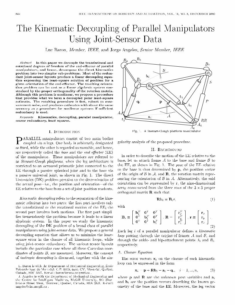
as �xed, while the other is regarded as movable, and hence,are respectively called the base and the end-e�ector (EE)of the manipulator. These manipulators are referred toas Stewart-Gough platforms, when the leg architecture isrestricted to an actuated prismatic joint connected to theEE through a passive spherical joint and to the base viaa passive universal joint, as shown in Fig. 1. The directkinematics (DK) problem pertains to the determination ofthe actual pose|i.e., the position and orientation|of theEE relative to the base from a set of joint-position readouts.

Kinematic decoupling refers to the separation of the kine-matic relations into two parts: the �rst part involves onlythe translational or the rotational motion of the EE; thesecond part involves both motions. The �rst part simpli-�es tremendously the problem because it leads to a linearalgebraic system. In this paper we study the kinematicdecoupling of the DK problem of a broad class of parallelmanipulators using joint-sensor data. We propose a generaldecoupling equation that allows us to minimize the least-square error in the closure of all kinematic loops, whileusing joint-sensor redundancy. The various sensor layoutsinclude the particular case where all three Cartesian coor-dinates of points Bi are measured. Moreover, the conceptof isotropic decoupling is discussed, together with the sin-

L. Baron is with the Department of Mechanical Engineering, �EcolePolytechnique de Montr�eal, C.P. 6079, succ. CV, Montr�eal, Qu�ebec,Canada, H3C 3A7. E-mail: [email protected] .

J. Angeles is with the Department of Mechanical Engineering andthe Centre for Intelligent Machines, McGill University, 817 Sher-brooke Street West, Montreal, Quebec, Canada, H3A 2K6. E-mail:[email protected] .

A

B

A1

A2

A3

A4

A5

A6

B1

B2

B3B4

B5

B6

ai

bi

qi p

RR

P

S

Fig. 1. A Stewart-Gough platform manipulator

gularity analysis of the proposed procedure.

II. Background

In order to describe the motion of the EE relative to thebase, let us attach frame A to the base and frame B tothe EE, as shown in Fig. 1. The pose of the EE relativeto the base is thus determined by p, the position vectorof the origin of B in A, and R, the rotation matrix repre-senting the orientation of B in A. Alternatively, the saidorientation can be represented by r, the nine-dimensionalarray constructed from the three rows of the 3� 3 properorthogonal matrix R such that

Rbi = Bir; (1)

with

Bi �

24bTi 0

T0T

0T

bTi 0

T

0T

0T

bTi

35 ; R =

24rTx

rTy

rTz

35 ; r �

24rx

ry

rz

35 :

(2)Each leg i of a parallel manipulator de�nes a kinematic

loop passing through the origins of frames A and B, andthrough the ankle- and hip-attachment points Ai and Bi,respectively.

A. Closure Equation

The error vectors xi on the closure of each kinematicloop can be expressed in the form

xi = p+Rbi � ai � qi; i = 1; :::; n; (3)

where p and R are the unknown pose variables and ai

and bi are the position vectors describing the known ge-ometry of the base and the EE. Moreover, the leg vector

BARON AND ANGELES: THE KINEMATIC DECOUPLING OF PARALLEL MANIPULATORS USING JOINT-SENSOR DATA 645

qi is only known from the kinematic equation of the leg,together with the readouts of the position sensors locatedon the di�erent joints along that leg. Since the joints ofparallel manipulators are not necessarily all instrumented,we have to eliminate the contribution of the unmeasuredjoint quantities in the leg kinematics. For this purpose, weuse an elimination method introduced earlier by the au-thors [1], which is based on the orthogonal decompositionof the hip-point motion into two parts, one measured andone unmeasured, lying in two orthogonal subspaces of IR3.For quick reference, we brie y recall this method below.The measurement subspace of leg i, denoted Mi, is de-

�ned as the subspace of IR3 containing the maximum of theavailable information from the joint-sensor readouts on theposition of the hip-attachment point of the correspondingleg i. Conversely, the subspace orthogonal toMi, denotedM?

i and called the orthogonal measurement subspace, isthe subspace of IR3 containing all the uncertainty associ-ated with this sensor layout. Any vector ( � ) of IR3 canbe decomposed into two orthogonal parts, [ � ]M , the com-ponent lying in Mi, and [ � ]M? , the component lying inM?

i , using the measurement projector Mi and an orthog-

onal complement of Mi, denoted by M?i , as follows:

( � ) = [ � ]M + [ � ]M? =Mi( � ) +M?i ( � ): (4)

These two projectors are de�ned for the four possible di-mensions of the measurement subspaces of IR3 as:

Mi =

8>><>>:

1

P

L

O

; M?i =

8>><>>:

O

L

P

1

;

3-D measurement2-D measurement1-D measurement0-D measurement

; (5)

where 1 and O are the 3 � 3 identity and zero matrices,while the plane and line projectors, P and L, are de�nedas

P � 1� L; L � eeT; (6)

in which e is a unit vector along line L and normal tothe plane P . Properly speaking, the identity matrix isnot a projector, for the latter is necessarily singular, butwe include this matrix in the above list for completeness.The projection of xi onto Mi, denoted [xi]M , allows theelimination of the unmeasured part of qi, i.e.,

[xi]M =Mi(p+Rbi � ai)�Miq0i : (7)

Vector q0i is de�ned as qi, with a value of zero assigned tothe position of the unmeasured joint motions. This vector,although di�erent from qi, shares the same projection ontoMi as qi. Moreover, this vector is readily computed withthe readouts of position sensors.

B. Problem Formulation

The DK problem pertains to the determination of theactual pose of the EE, from a set of joint-position readouts.This problem can be stated as

z =1

2

nXi=1

[xi]TM [xi]M ! min

p;R(8a)

which is an optimization problem subject to the proper-orthogonality constraint of R, i.e.:

RTR = 13�3; and det(R) = +1; (8b)

with [xi]M de�ned in (7). Apparently, this optimizationproblem is linear in p and R, but subject to a quadraticconstraint on R, and hence, must be treated as a con-strained nonlinear least-square problem. Furthermore, thetwo unknowns, p and R, are coupled, thereby making itnecessary to solve for both simultaneously.

C. Survey of the State-of-the-Art

Using only the position of the six prismatic joints as in-put data, the DK problem of Stewart-Gough platforms canadmit up to 40 real possible solutions [2]. The underlying40th-degree polynomial can be obtained with a procedureproposed by Husty [3]. However, the real-time computa-tion of the 40 roots of this polynomial is prohibitively ex-pensive with current technology, and thus, cannot be usedfor online implementation. Alternatively, it is well-knownthat the inverse kinematics of serial manipulators is greatlysimpli�ed when the translational and rotational degrees offreedom are decoupled [4]. This kinematic decoupling isobtained when three consecutive revolute axes intersect ata point, a geometric condition ful�lled by most of today'sserial manipulators within their last three joints. Similarly,the DK of parallel manipulators can also be decoupled un-der some geometric conditions, e.g., the 6-4 architecture [5],the collinearity of �ve points of B [6] or the (3�1�1�1)2

architecture [7]. Although closed-form solution proceduresexist for these manipulators, their geometries do not corre-spond to those of practical use, and hence, an online proce-dure is still needed for those of general geometry. Moreover,all real solutions of the DK problem are equally possible,and thus, it is impossible for the controller to distinguishthe actual solution among the set of possible ones with onlythe six leg lengths. Di�erent approaches have also beenproposed to cope with multiple solutions, e.g., the additionof a passive instrumented leg [8], the of use extra sensorson the passive joints [9], or the use of redundant sensorson any of the passive or actuated joints [10]. Here, we usethe last approach of redundant sensors because it allowsus to determine a decoupling equation from a set of linearkinematics relationships, thereby producing a decouplingof the DK problem without having to impose restrictivegeometrical conditions.

III. Kinematic Decoupling

The kinematic decoupling thus refers to the separationof the kinematic relations into two parts: the �rst part in-volves only the rotational motion of the EE; the secondpart involves both the rotational and the translational mo-tions. In fact, the second part is a relation between the twounknowns p and R such that

p = p(R) (9)

The foregoing relation is henceforth called the decoupling

equation, while the �rst part is obtained upon substitution


of (9) into (7). In this section, we propose a decouplingequation based on the closure of all the kinematic loopsin order to obtain a complete decoupling of the problem,rather than only partial decoupling, as proposed by Yuan[11].

A. Decoupling Equation

For a given R, the normality condition of the optimiza-tion problem of (8) yields a linear relationship between pand R, which is chosen as the decoupling equation.

Theorem 1: Let �aM , �BM and �qM be the means of the

projection of ai, Bi and q0i onto the measurement subspaces

Mi, while �M is the mean of the measurement projectors

Mi. Under a general combination of 3-D, 2-D, 1-D and

0-D measurements of the position of the hip-attachment

points, the decoupling equation is given as

�aM + �qM = �Mp+ �BMr; (10a)

where

�aM �1

n

nXi=1

Miai; �qM �1

n

nXi=1

Miq0i ; (10b)

�M �1

n

nXi=1

Mi;�BM �

1

n

nXi=1

MiBi: (10c)

Proof : See the Appendix.When all the leg-attachment points of the manipulator

are under 3-D measurement, we have:

Mi = 13�3; 8 i = 1; : : : ; n; (11)

the closer equation (7) becomes identical to (3) and Theo-rem 1 reduces to

Corollary 1: Let ao, bo and qo be the mean values of

the sets faign1 , fbig

n1 and fqig

n1 , respectively. Under a 3-

D measurement of the position of the leg hip-attachment

points, the decoupling equation is given as

ao + qo = p+Rbo; (12a)

where

ao �1

n

nXi=1

ai; qo �1

n

nXi=1

qi; bo �1

n

nXi=1

bi: (12b)

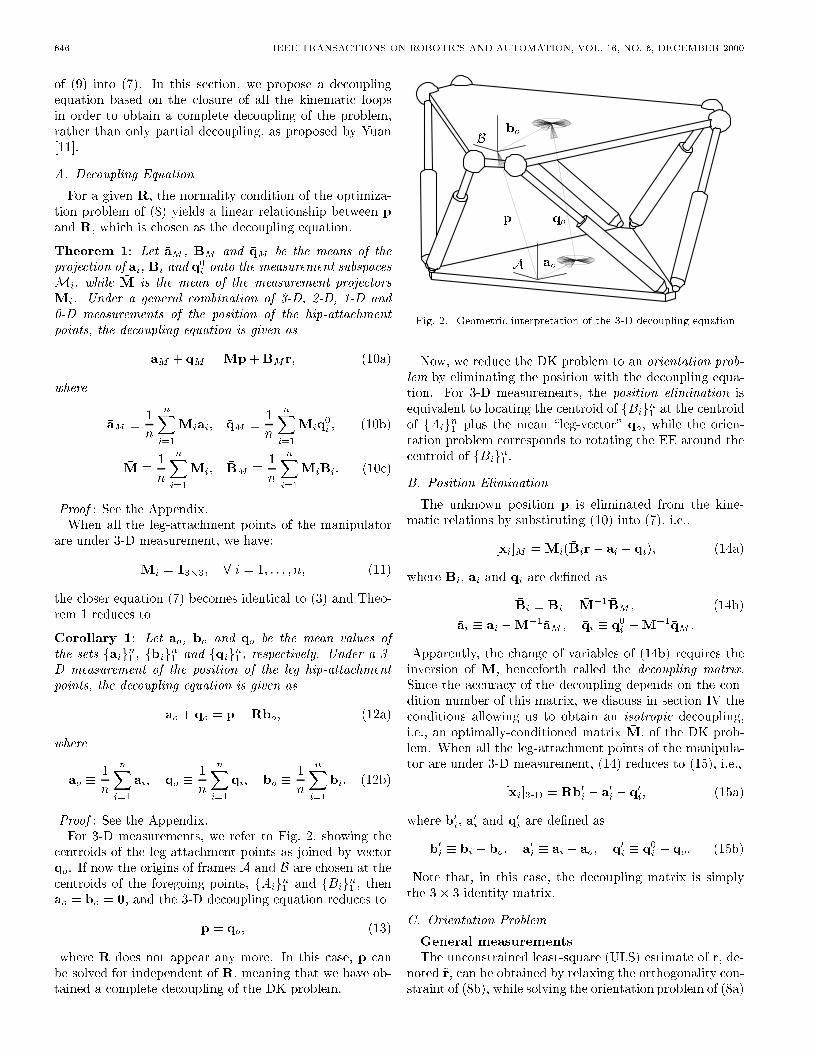
Proof : See the Appendix.For 3-D measurements, we refer to Fig. 2, showing the

centroids of the leg-attachment points as joined by vectorqo. If now the origins of frames A and B are chosen at thecentroids of the foregoing points, fAig

n1 and fBig

n1 , then

ao = bo = 0, and the 3-D decoupling equation reduces to

p = qo; (13)

where R does not appear any more. In this case, p canbe solved for independent of R, meaning that we have ob-tained a complete decoupling of the DK problem.

A

B

ao

bo

p qo

Fig. 2. Geometric interpretation of the 3-D decoupling equation

Now, we reduce the DK problem to an orientation prob-

lem by eliminating the position with the decoupling equa-tion. For 3-D measurements, the position elimination isequivalent to locating the centroid of fBig

n1 at the centroid

of fAign1 plus the mean \leg-vector" qo, while the orien-

tation problem corresponds to rotating the EE around thecentroid of fBig

n1 .

B. Position Elimination

The unknown position p is eliminated from the kine-matic relations by substituting (10) into (7), i.e.,

[xi]M =Mi( �Bir� �ai � �qi); (14a)

where �Bi, �ai and �qi are de�ned as

�Bi � Bi � �M�1 �BM ; (14b)

�ai � ai � �M�1�aM ; �qi � q0i �

�M�1�qM :

Apparently, the change of variables of (14b) requires theinversion of �M, henceforth called the decoupling matrix.Since the accuracy of the decoupling depends on the con-dition number of this matrix, we discuss in section IV theconditions allowing us to obtain an isotropic decoupling,i.e., an optimally-conditioned matrix �M, of the DK prob-lem. When all the leg-attachment points of the manipula-tor are under 3-D measurement, (14) reduces to (15), i.e.,

[xi]3-D = Rb0i � a

0i � q

0i; (15a)

where b0i, a0i and q

0i are de�ned as

b0i � bi � bo; a

0i � ai � ao; q

0i � q

0i � qo: (15b)

Note that, in this case, the decoupling matrix is simplythe 3� 3 identity matrix.

C. Orientation Problem

General measurements

The unconstrained least-square (ULS) estimate of r, de-noted ~r, can be obtained by relaxing the orthogonality con-straint of (8b), while solving the orientation problem of (8a)


with [xi]M de�ned as in (14). This estimate is found as theLS solution of a 3n�9 linear algebraic system, with n � 3,namely,

B0M~r = (a0M + q

0M ); (16a)

where matrix B0M and vectors a0M and q0M are de�ned as

B0M �

264M1

�B1

...Mn

�Bn

375 ; (16b)

a0M �

264M1�a1

...Mn�an

375 ; q

0M �

264M1�q1

...Mn�qn

375 :

The ULS estimate ~r of (16) is symbolically obtained via

the generalized inverse of B0M , B0 y

M , namely,

~r = B0 yM (a0M + q

0M ); B

0 yM � (B0 T

M B0M )�1B0 T

M : (17)

Due to unavoidable noise and the assumption of indepen-dence of the nine components of R, the ULS estimate ~Rmay not be orthogonal. The closest orthogonal estimate isobtained as the polar projection1 of ~R over the constraintmanifold of (8b). This second estimate, henceforth calledthe decoupled polar least-square (DPLS) estimate, and de-noted �R, is computed as the orthogonal factor of the polardecomposition of ~R, i.e.,

�R = �Q; ~R = �Q �W; (18)

where the 3�3 matrices �Q and �W are, respectively, orthog-onal and either positive-semide�nite or positive-de�nite.Once �R is known, �p can be computed as the LS approxi-mation of

Mp = (aM + qM � �bM ); (19a)

with

M �

264M1

...Mn

375 ; �bM �

264M1

�Rb1...

Mn�Rbn

375 ; (19b)

aM �

264M1a1

...Mnan

375 ; qM �

264M1q

01

...Mnq

0n

375 :

1In the plane, a polar projection can be geometrically interpretedas the projection of a point of the plane onto the unit circle centeredat the origin of the plane; this projection is the intersection of thecircle with the line joining the point with the center of the circle.Obviously, of the two intersections, the one closest to the point ischosen.

3-D measurements

When all leg-attachment points are under 3-D measure-ment, the decoupled DK problem of (8) can be recast asan optimization problem, namely,

z =1

2tr(XT

X)! minR

(20a)

X � RB�A (20b)

subject to (8b), with the 3�nmatricesX, B andA de�nedas

X � [ [x1]3-D : : : [xn]3-D ]; (20c)

B � [b01 : : :b0n]; A � [a01 + q

01 : : : a

0n + q

0n]:

This optimization problem is well known in the �eld ofcomputational statistics as the orthogonal Procrustes prob-lem [13]. Although the foregoing objective function isquadratic in R, it is possible to transform it into a lin-ear form with the aid of an equality constraint. Indeed,upon substitution of (20b) into (20a), and simplifying thesecond term of the right-hand side (RHS), gives:

z =1

2tr(AT

A) +1

2tr(BT

B)� tr(ATRB): (21)

Now, using the properties of the trace operator, the thirdterm of the RHS of (21) can be rearranged as

tr(ATRB) = tr(BAT

R): (22)

Therefore, the quadratic objective function of (21) reducesto the linear form:

z =1

2tr(AT

A) +1

2tr(BT

B)� tr(BATR); (23)

still constrained by the proper orthogonality of R.Since the unknown, R, appears only in the last term,

which is negative, the minimization of z, as given in (23),is equivalent to the maximization of its last term alone, i.e.,

� = tr(BATR)! max

R

(24)

subject to (8b). This quadratically-constrained least-square problem can be readily solved by resorting to theresult below:

Lemma 1: Let C and R be two n � n matrices with

C = QW, where Q is orthogonal and W is symmetric

and positive-semide�nite. Moreover, let

� = tr(CTR)! max

R

(25a)

subject toR

TR = 1 (25b)

The maximum of � is given by R = Q.

Proof : See the Appendix.By virtue of Lemma 1, the solution of (24), namely, the

DPLS estimate �R, is readily found to be

�R = �Q; ABT = �Q �W; (26)

where the orthogonal matrix �Q and the symmetric positive-semide�nite matrix �W are obtained as the two factors ofthe polar decomposition of the product ABT . Once �R isknown, (19) can be used to solve for �p.


IV. Singularity Analysis

It is recalled that joint-sensor redundancy is used here tocope with both the measurement noise and the nonlinearityof the problem at hand, and hence, the procedure is meantfor use with 9 to 18 sensors. There are several conditionsunder which the procedure does not provide an estimate ofthe actual pose of the end-e�ector, as we discuss below.

First, the kinematic decoupling of (10a) does not existwhen the measurement subspaces fMig

n1 do not span IR3.

In fact, the change of variable of (14) requires the inversionof the decoupling matrix �M. The accuracy of the decou-pling depends on the condition number of �M, i.e.,

�( �M) =�3

�1; where �1 � �2 � �3 � 0; (27)

where f�i g31 are the singular values of �M. This number

expresses \how well" the set of measurement subspacesfMig

n1 span IR3. Matrices with the optimum condition

number of unity are called isotropic, an isotropic decou-pling being thus one that provides equal accuracy in alldirections. In an earlier work [12], we proposed necessary,but not suÆcient, geometrical conditions for isotropic de-coupling. For example, we showed that isotropy is reach-able with the geometry of an industrial Stewart-Gough ma-nipulator if the yoke joints are oriented on the base in aparticular way. In the case of 3-D measurements, the de-coupling matrix is the identity, and hence, the decouplingalways exists and is, additionally, isotropic.

Second, the full rank of BM cannot be guaranteed with-out considering the manipulator geometry, the location ofthe EE and the joint-sensor layout. The singularity analy-sis of BM can be conducted along the same lines of that forJacobian matrices. The solution of the orientation problemof (16) requires the full rank of BM , i.e. rank(BM ) � 9,and hence, the use of a minimum of nine sensors. How-ever, the nine unknowns of R are not independent and canbe reduced to a minimum of four unknowns if necessary,the others being rather computed a posteriori with (8b).This approach is necessary when the geometry of the end-e�ector is made of coplanar hip-attachment points, as isthe case of Stewart-Gough platforms. Assume that thesepoints are in the x-y plane of frame B. The z component ofbi is zero, and hence, it is not possible to solve for the 3rd,6th and 9th components of r with (16). In this case, it ismandatory to eliminate the corresponding columns in BM ,and then solve a posteriori for the remaining componentsof r. In the case of 3-D measurements, a similar situa-tion arises when the hip-attachment points are coplanar.The third row of B is zero, and hence, it is not possibleto solve for the 3rd column of R, i.e. the 3rd, 6th and 9th

components of its equivalent r. In this case, one or evena few columns can be added to matrices A and B in or-der to render them of full rank. An additional column k

can be derived from the columns i and j of A and B as(a0k + q

0k) = (a0i + q

0i)� (a0j + q

0j) and b

0k = b

0i � b

0j .

The performance of each of the two versions of the DPLSsolution procedure is now assessed.

V. Performance Assessment

In order to evaluate the performance of the DPLS pro-cedure, we consider two performance indices: the compu-

tational cost of the procedure and the accuracy of theirestimates while using noisy input data. The DPLS pro-cedure is compared with a traditional constrained least-square (CLS) procedure requiring an initial guess togetherwith an iterative technique based on Newton's method inorder to converge toward its CLS estimate. It is noteworthythat the computation of the DPLS estimate f�p; �Rg of theactual solution fp;Rg of the DK problem does not requireiterations as for the computation of the CLS estimate.

A. Computational Cost

Let us denote by (�)g and (�)3 the two versions of theprocedures under general and 3-D position measurementsof all the hip-attachment points of a parallel manipula-tor of general geometry. The computational cost of theseprocedures is measured with the number of oating-point-operations| ops|using the assumptions below:1. The generalized inverse is computed via Householder re- ections and back-substitutions of a p � q linear algebraicsystem with p � q, which requires q2(p� q=3) ops [13];2. The inversion of the symmetric 3� 3 decoupling matrixrequires 41 ops in general and no ops when isotropic;3. The orthogonal factor of the polar decomposition iscomputed via Higham's polar-decomposition algorithm[14], which requires 59 ops per iteration and an averageof 3 iterations, for a total of 177 ops;4. The origin of frames A and B is chosen at the centroidof fAig

n1 and fBig

n1 in order to avoid the calculation of

ao = bo = 0;5. The number of instrumented legs n is set to six.As shown in Fig. 3, the computational cost of the CLS

procedure increases with the number of iterations, whilethe cost of the DPLS procedure remains constant. For anyjoint-sensor layout, the actual computational cost of theprocedures is between the upper bound (�)g and the lowerbound (�)3. Moreover, the computational cost is further

1 2 3 4 5 6 7 8 9 100

500

1000

1500

2000

2500

3000

3500

4000

4500

5000

Number of iteration

Com

puta

tiona

l cos

t (flo

ps)

DPLS3

DPLSg

CLS3

CLSg

Fig. 3. Computational cost of the various solution procedures


Fig. 4. Prototype parallel manipulator

reduced with some speci�c geometries. With general mea-surements, the DPLSg procedure is more eÆcient than theCLSg procedure if the latter requires more than three itera-tions. With 3-D measurements, the DPLS3 procedure is al-ways more eÆcient than the CLS3 procedure. Apparently,the kinematic decoupling produces a strong reduction of ops with 3-D measurements, which makes it attractivefor online computations.

B. Estimation Accuracy

The estimation accuracy is measured with the positionand orientation errors between the estimate and the actualpose, Æ and �, respectively, which are de�ned below:

Æ � kp� �pk; � � kvect( �RTR)k; (28)

where vect(�) is the axial vector of its 3 � 3 matrix argu-

ment [17]. The geometry of the manipulator is chosen asthe Stewart-Gough platform used in 500-series ight sim-ulators produced by CAE Electronics Ltd., with a scalefactor of 1:50. The noisy input data are obtained eitherdirectly from measurements on an experimental prototypeor from simulations by adding a Gaussian zero-mean noiseto the theoretical joint readouts; the noisy data are thensubmitted to each of the DPLS and CLS procedures inorder to compute their estimates. For simulation, the ac-tual poses of the EE are known from the prescribed tra-jectory; for experiments, these poses have to be computedfrom very accurate measurements taken with a coordinatemeasuring machine (CMM). Shown in Fig. 4 is the exper-imental prototype, manufactured with rather loose toler-ances. Moreover, the joints of the prototype operate underno feedback loop. The EE is held at a speci�c pose by astand placed between the two end-plates. A single instru-mented leg is used, that is manually placed at each of thesix leg locations. Potentiometers are installed on the �rstthree joints. The output voltage of these sensors is sent to amulti-channel 12-bit A/D converter. The resulting digitalvalues are the noisy input data to each of the estimationprocedures.

TABLE I

Different layouts for 3-D measurements

Sensors Type Layouts

18 A f�1; �2; �3; �4; �5; �6g

15 B f1; �2; �3; �4; �5; �6g, f�1; 2; �3; �4; �5; �6g, f�1; �2; 3; �4; �5; �6g

f�1; �2; �3; 4; �5; �6g, f�1; �2; �3; �4; 5; �6g, f�1; �2; �3; �4; �5; 6g

C f1; 2; �3; �4; �5; �6g, f�1; �2; 3; 4; �5; �6g, f�1; �2; �3; �4; 5; 6g

D f�1; 2; 3; �4; �5; �6g, f�1; �2; �3; 4; 5; �6g, f1; �2; �3; �4; �5; 6g

12 E f1; �2; �3; 4; �5; �6g, f�1; 2; �3; �4; 5; �6g, f�1; �2; 3; �4; �5; 6g

F f1; �2; 3; �4; �5; �6g, f�1; �2; 3; �4; 5; �6g, f1; �2; �3; �4; 5; �6g

f�1; 2; �3; 4; �5; �6g, f�1; �2; �3; 4; �5; 6g, f�1; 2; �3; �4; �5; 6g

G f�1; 2; �3; 4; �5; 6g, f1; �2; 3; �4; 5; �6g

H f1; �2; �3; 4; �5; 6g, f1; �2; �3; 4; 5; �6g, f1; �2; 3; �4; �5; 6g

f�1; 2; 3; �4; �5; 6g, f�1; 2; �3; 4; 5; �6g, f�1; 2; 3; �4; 5; �6g

9 I f�1; �2; 3; �4; 5; 6g, f�1; �2; 3; 4; �5; 6g, f1; 2; �3; �4; 5; �6g

f�1; 2; �3; �4; 5; 6g, f1; 2; �3; 4; �5; �6g, f1; �2; 3; 4; �5; �6g

J f�1; �2; �3; 4; 5; 6g, f�1; �2; 3; 4; 5; �6g, f�1; 2; 3; 4; �5; �6g

f1; 2; 3; �4; �5; �6g, f1; 2; �3; �4; �5; 6g, f1; �2; �3; �4; 5; 6g

�i : 3-D measurement of the position hip-attachment point of leg i.

i : Unmeasured position of the hip-attachment point of leg i.

3-D measurements

With 3-D measurements, the linear DPLS3 procedureprovides identical estimates to those of the nonlinear CLS3procedure, although di�erent from the actual poses, andhence, both procedures have equal accuracies. Accuracydepends on the number of sensors and their distributionover the manipulator joints. Table I classi�es di�erent lay-outs for 3-D measurements, while Fig. 5 shows their relativeaccuracies. Apparently, layout A produces the best accu-racy, because it uses the maximum number of sensors, i.e.,6 legs � 3 sensors/leg = 18 sensors. Accuracy reduces asthe number of sensors is reduced, but at the same time dif-

3 4 5 6 7

0.26

0.28

0.3

0.32

0.34

0.36

0.38

0.4

A

B

CDEFG

HI

J

3 4 5 6 70

0.02

0.04

0.06

0.08

0.1

AB

CDEFG

H

IJ

�Æ(mm)

��(mrad)

ALL CLS3=DPLS3

ALL CLS3=DPLS3

(a) Number of instrumented legs

(b) Number of instrumented legs

Fig. 5. Relative position �Æ (mm) and orientation �� (mradian) errors

of the CLS3 and DPLS3 estimates


ferent distributions of sensors arise. Layouts C to F, thatuse 4 legs � 3 sensors/leg = 12 sensors, produce di�erentlevels of accuracy, because of the di�erent distributions ofthe sensors. Moreover, layout G, which uses only 9 sensors,produces a better accuracy than layout C, which uses 12sensors. Indeed, the good distribution of sensors in layoutG enhances its accuracy.

General measurements

With general measurements, the linear DPLSg proce-dure does not produce identical estimates as the nonlin-ear CLSg procedure, and hence, both procedures have dif-ferent accuracies, while using the same set of noisy inputdata. A nine-sensor layout is used on the experimental pro-totype, i.e., f �R �RP; �RRP; �R �RP; �RRP; �R �RP; �RRPg, where�R �RP denotes the presence of a position sensor on the �rsttwo revolute joints and no sensor on the prismatic joint,while �RRP denotes the presence of a position sensor onthe �rst revolute joint only.

0 10 20 30 40 50 60 70 80 90 1000

5

10

15

20

0 10 20 30 40 50 60 70 80 90 1000

10

20

30

40

50

Æ

(mm)

�

(mrad.)

(a) Experimental trajectory (%)

(b) Experimental trajectory (%)

+ ! DPLS

* ! CLS

Fig. 6. The position Æ (mm) and orientation � (mradian) errors ofthe DPLS and CLS estimates relative to the actual pose along anexperimental trajectory

As shown in Fig. 6, the position and orientation errorsof the two estimates relative to the actual pose vary fromlocation to location within the workspace of the manipu-lator. After several thousands of DK solutions, with bothsimulated and experimental data, we did not notice anysigni�cant di�erences between the accuracies of the two es-timates. At some locations, one procedure is better; atother locations, the other procedure is better.

VI. Conclusions

The DK problem of parallel manipulators is greatly sim-pli�ed with the help of the concept of kinematic decou-pling. In serial manipulators a similar decoupling occursin manipulators with spherical wrists. Joint-sensor redun-dancy is used here to cope with the nonlinearity of the DKproblem, rather than applying restrictive geometrical con-straints, while also considering the unavoidable noise onmeasurements by means of a least-square estimate, termedhere decoupled polar least-squares, or DPLS for brevity.

The linear DPLS estimate must be considered as a good al-ternative to the nonlinear CLS estimate, because althoughdi�erent from the latter, it provides estimates of the ac-tual solution with about the same accuracy as the latterwithout requiring iterative computations.

Acknowledgments

The research work reported here was supported byNSERC (Natural Sciences and Engineering Research Coun-cil, of Canada) Grants OGPIN 013 and RGPIN 203618.

Appendix

Theorem 1:Proof: Upon substitution of (7) and (1) into (8a), the

decoupling equation is derived as the normality conditionof z with respect to p, i.e.,

dz

dp= (

nXi=1

Mi)p+ (

nXi=1

MiBi)r (29)

� (

nXi=1

Miai)� (

nXi=1

Miq0i ) = 0;

from which (10) of Theorem 1 is readily obtained. Thisnormality condition yields a minimum when the Hessianmatrix of z with respect to p, i.e.,

d2z

dp2=

nXi=1

Mi = n �M; (30)

is strictly positive-de�nite. This condition arises when thedirect sum of the n measurement subspaces, i.e. M1�: : :�Mn, yields IR

3.

Corollary 1:Proof: Upon substitution of (7) and (11) into (8a),

the 3-D decoupling equation is derived as the normalitycondition of z with respect to p, i.e.,

dz

dp= np+R

nXi=1

bi �

nXi=1

ai �

nXi=1

qi = 0; (31)

from which (12) of Corollary 1 is readily obtained. Thiscondition leads always to a minimum because the Hessianmatrix of z with respect to p, i.e.

d2z

dp2= n13�3; (32)

is the sum of n � 1 identity matrices, the result thus beingalways symmetric and strictly positive de�nite.Lemma 1:Proof: Let us introduce the n� n orthogonal matrix

Z such that:

Z � QTR: (33)

Then (25a) reduces to

� = tr(CTR) = tr(WT

QTR) = tr(WT

Z) (34)


SinceW is symmetric and positive-semide�nite, it has non-negative eigenvalues �1 � �2 � �3 (� 0), and the corre-sponding unit eigenvectors v1;v2;v3 are mutually orthog-onal. Hence W can be represented as

W =WT =

3Xi=1

�ivivTi ; (35)

which is also known as the spectral decomposition of W.By virtue of the invariance of the trace under a cyclicchange of the factors of a matrix product, i.e., tr(ABC) =tr(BCA) = tr(CAB), and upon substitution of (35) into(34), we obtain:

� =

3Xi=1

�itr(vivTi Z) =

3Xi=1

�itr(vTi Zvi) =

3Xi=1

�i(vi;Zvi);

(36)where (vi;Zvi) denotes the inner product of vectors vi andZvi. The three inner products of (36) are bounded by theCauchy-Schwartz inequality as

(vi;Zvi) � kvik kZvik = 1; (37)

where the maximum value of unity is reached when theorthogonal matrix Z is equal to the identity matrix. Us-ing (33), the maximum of the objective function of (36) isreached for

Z = 1 = QTR; (38)

and hence, R = Q.

References

[1] Baron, L. and Angeles, J., \The Direct Kinematics of ParallelManipulators Under Joint-Sensor Redundancy", IEEE Trans.on Robotics and Automation, Vol. 16, No. 1, pp. 12{19, 2000.

[2] Dietmaier, P., \The Stewart-Gough Platform of General Geome-try Can Have 40 Real Postures", Advances in Robot Kinematics:Analysis and Control, Kluwer Academic Publishers, pp. 7{16,Strobl-Salzburg, Austria, June 29{July 3, 1998.

[3] Husty, M. L., \An Algorithm for Solving the Direct Kinematicsof General Stewart-Gough-Type Platforms", Mechanism andMachine Theory, Vol. 31, No. 4, pp. 365{380, 1996.

[4] Pieper, D. L., \The Kinematics of Manipulators Under Com-puter Control", Ph.D. Thesis, Stanford University, 1968.

[5] Innocenti, C. and Parenti-Castelli, V., \Direct Kinematics of6-4 Fully Parallel Manipulators with Position and OrientationUncoupled", Proc. European Robotics and Intel. Syst. Conf.,Corfu, 1991.

[6] Zhang, C.-D. and Song, S.-M., \Forward Kinematics of a Classof Parallel (Stewart) Platforms with Closed-Form Solutions", J.Robotic Systems, Vol. 9, No. 1, pp. 93{112, 1992.

[7] Bruyninckx, H., \Closed-Form Forward Position Kinematics fora (3-1-1-1)2 Fully Parallel Manipulator", IEEE Trans. Roboticsand Automation, Vol. 14, No. 2, pp. 326{328, 1998.

[8] Arai, T. et al., \Design, Analysis and Construction of a Pro-totype Parallel Link Manipulator", IEEE Int. Conf. on Intel.Robots and Syst., IROS'90, pp. 205{212, July 1990.

[9] Tancredi, L., Teillaud, M. and Merlet, J.-P., \Extra Sensors forSolving the Forward Kinematics Problem of Parallel Manipula-tors", Ninth World Cong. Theory of Machines and Mechanisms,pp. 2122{2126, 1995.

[10] Baron, L. and Angeles, J., \The On-Line Direct Kinematics ofParallel Manipulators Under Joint-Sensor Redundancy", Ad-vances in Robot Kinematics: Analysis and Control, Kluwer Aca-demic Publishers, pp. 127{136, Strobl-Salzburg, Austria, June29{July 3, 1998.

[11] Yuan, J. S.-C., \A General Photogrammetric Method for Deter-mining Object Position and Orientation", IEEE Trans. Roboticsand Automation, Vol. 5, No. 2, pp. 129{142, 1989.

[12] Baron, L. and Angeles, J., \The Isotropic Decoupling of the Di-rect Kinematics of Parallel Manipulators Under Sensor Redun-dancy", IEEE Int. Conf. Robotics and Automation, pp. 1541{1546, Nagoya, Japan, May 1995.

[13] Golub, G. H. and Van Loan, C. F., Matrix Computations, TheJohns Hopkins University Press, Baltimore, 1989.

[14] Higham, N. J., \Computing the Polar Decomposition{WithApplications", SIAM J. Scienti�c and Statistical Computing,Vol. 7, No. 4, pp. 1160{1175, 1986.

[15] Cala�ore, G. and Bona, B., \Constrained Optimal Fitting ofThree-Dimensional Vector Paterns", IEEE Trans. Robotics andAutomation, Vol. 14, No. 5, pp. 838{844, 1998.

[16] Li, Z., Gou, J. and Chu, Y., \Geometric Algorithms for Work-piece Localization", IEEE Trans. Robotics and Automation,Vol. 14, No. 6, pp. 864{878, 1998.

[17] Angeles, J., Fundamentals of Robotic Mechanical Systems: The-ory, Methods and algorithms, Springer-Verlag, New York, 1997.

Luc Baron (S'94{M'97) received his B.Eng.and M.A.Sc. degrees from Ecole Polytechnique,Montreal, Canada, in 1983 and 1985, respec-tively, and the Ph.D. degree from McGill Uni-versity, Montreal, Canada, in 1997, all in me-chanical engineering. From 1986 to 1993, heheld cross appointments as faculty lecturer atEcole Polytechnique, the engineering faculty ofUniversity of Montreal, and as Research En-gineer at Walsh Automation Inc. Since 1997,Dr. Baron is Assistant Professor in the Depart-

ment of Mechanical Engineering at Ecole Polytechnique. His currentresearch interests are in the �eld of robotics and industrial automa-tion, kinematics, synthesis and control of manipulators. Dr. Baron isa member of IEEE, an Associate Member of ASME and a registeredengineer in Quebec.

Jorge Angeles (SM'99) graduated as Engi-neer (Electromechanical Systems) at Universi-dad Nacional Aut�onoma de M�exico (UNAM),from which he also received the M.Eng. de-gree in Mechanical Engineering, in 1969 and1970, respectively; in 1973, Angeles obtainedthe Ph.D. degree in Applied Mechanics fromStanford University. Between 1973 and 1984,he taught at UNAM, where he also served asChairman of the Graduate Division of Mechan-ical Engineering and Associate Dean of Grad-

uate Studies in Electrical and Mechanical Engineering. In 1991, hereceived an Alexander von Humboldt Research Award that allowedhim to spend one year as Visiting Professor at the Technical Univer-sity of Munich. Since 1984, Angeles is with the Department of Me-chanical Engineering of McGill University, where he is aÆliated withthe Centre for Intelligent Machines. He has authored or co-authoredvarious books in the areas of kinematics and dynamics of mechanicalsystems as well as numerous technical papers in refereed journals andconference proceedings. His research interests focus on the theoreticaland computational aspects of multibody mechanical systems for pur-poses of design and control. Besides his research activities, ProfessorAngeles is a consultant to various Canadian and international cor-porations in matters of automation, design, and robotics. ProfessorAngeles is an ASME Fellow, a Fellow of the Canadian Society of Me-chanical Engineering, a Senior Member of the IEEE, Past-Presidentof IFToMM (International Federation for the Theory of Machinesand Mechanisms), and member of various professional and learnedsocieties. Professional registration as an engineer includes Quebec,Mexico, and Germany.

the kinematic decoupling of parallel manipulators using joint-sensor data

Documents