16-311-Q INTRODUCTION TO ROBOTICS

LECTURE 5 (CONTINUED): KINEMATIC CONSTRAINTS DEGREES OF FREEDOM/MOBILITY

INSTRUCTOR: GIANNI A. DI CARO

2

M O B I L E R O B O T M A N E U V E R A B I L I T Y

Mathematically, the degree of maneuverability 𝜹M

is defined as the sum of: Degree of mobility, 𝜹𝙢 and Degree of steerability, 𝜹𝘴

𝜹M = 𝜹𝙢 + 𝜹𝘴

The kinematic mobility (maneuverability) of a robot chassis is its ability to directly move in the environment, which is the result of:

2. The additional freedom contributed by steering and spinning steerable wheels

Determine the Degree of steerability, 𝜹𝘴: degrees of controllable freedom based on steering wheels and then moving

1. The rule that every standard wheel must satisfy its no sliding and rolling constraints (↔ Each wheel imposes zero or more constraints on the motion)

Determine the Degree of mobility, 𝜹𝙢: degrees of controllable freedom based on changes in wheels’ velocity

3

M A N E U V E R A B I L I T Y A N D ( N O N ) H O L O N O M Y

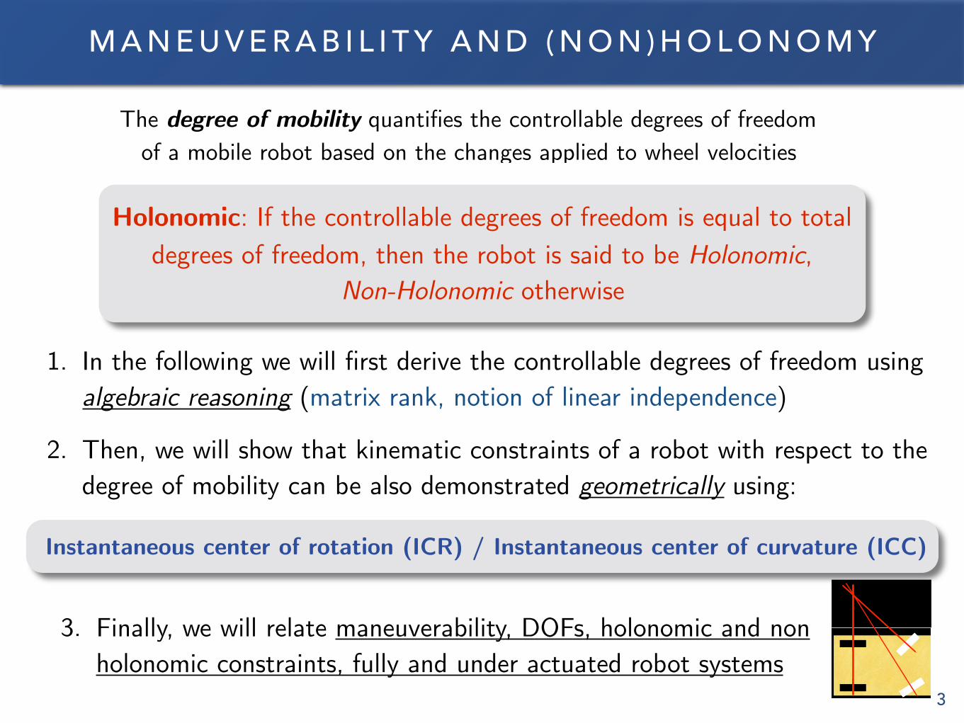
The degree of mobility quantifies the controllable degrees of freedom of a mobile robot based on the changes applied to wheel velocities

Instantaneous center of rotation (ICR) / Instantaneous center of curvature (ICC)

Holonomic: If the controllable degrees of freedom is equal to total degrees of freedom, then the robot is said to be Holonomic,

Non-Holonomic otherwise

1. In the following we will first derive the controllable degrees of freedom using algebraic reasoning (matrix rank, notion of linear independence)

2. Then, we will show that kinematic constraints of a robot with respect to the degree of mobility can be also demonstrated geometrically using:

3. Finally, we will relate maneuverability, DOFs, holonomic and non holonomic constraints, fully and under actuated robot systems

4

R E C A P : T Y P E S O F W H E E L S

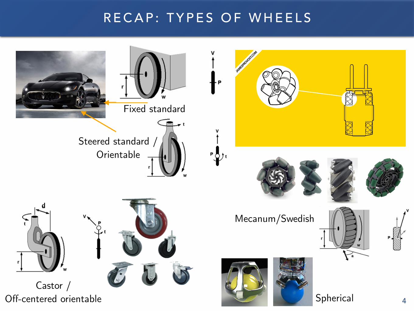
Steered standard / Orientable

Fixed standard

Castor / Off-centered orientable

d

Mecanum/Swedish

Spherical

5

F I X E D S TA N D A R D W H E E L

⇠R = R(✓)⇠I = R(✓)

2

664

x

y

✓

3

775

Reference wheel point A (on the axle) is in polar coordinates: A(l, α)

β: angle of wheel plane wrt chassis

• Rolling constraint (pure rolling at the contact point): All motion along the direction of the wheel plane is determined by wheel spin

• Sliding constraint: The component of the wheel’s motion orthogonal to the wheel plane must be zero

P' v

Wheel plane

Wheel axle

YR

XR

A

6

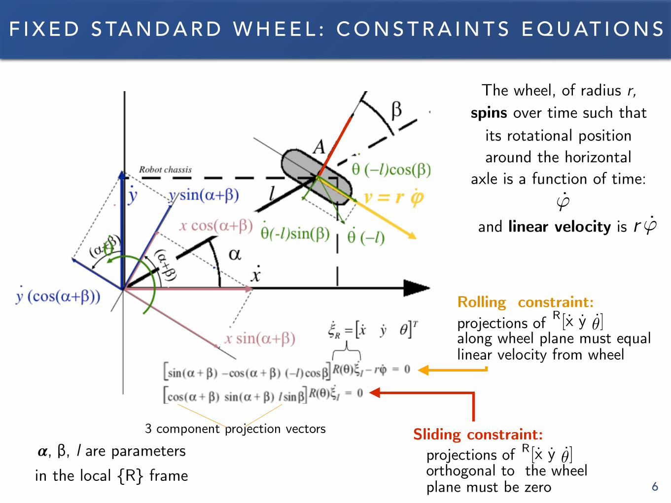
F I X E D S TA N D A R D W H E E L : C O N S T R A I N T S E Q U AT I O N S

The wheel, of radius r, spins over time such that

its rotational position around the horizontal

axle is a function of time:

and linear velocity is r

Rolling constraint: projections of

Sliding constraint:𝜶, β, l are parameters in the local {R} frame

along wheel plane must equal linear velocity from wheel

projections of orthogonal to the wheel plane must be zero

3 component projection vectors

''

R[x y

˙✓]

R[x y

˙✓]

7

FIXED STANDARD WHEEL: ROLLING CONSTRAINT

90-(𝜶+𝜷)

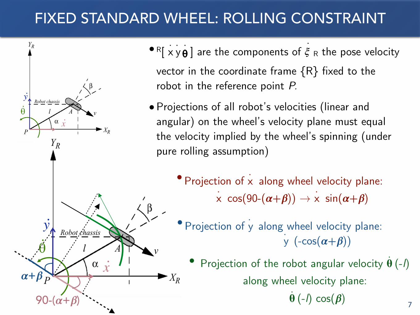
• R[ x. y.

𝝷. ] are the components of 𝜉

. R the pose velocity

vector in the coordinate frame {R} fixed to the robot in the reference point P.

• Projections of all robot’s velocities (linear and angular) on the wheel’s velocity plane must equal the velocity implied by the wheel’s spinning (under pure rolling assumption)

• Projection of x. along wheel velocity plane:

x. cos(90-(𝜶+𝜷)) → x

. sin(𝜶+𝜷)

• Projection of y. along wheel velocity plane:

y. (-cos(𝜶+𝜷))

𝜶+𝜷• Projection of the robot angular velocity 𝛉

. (-l)

along wheel velocity plane: 𝛉. (-l) cos(𝜷)

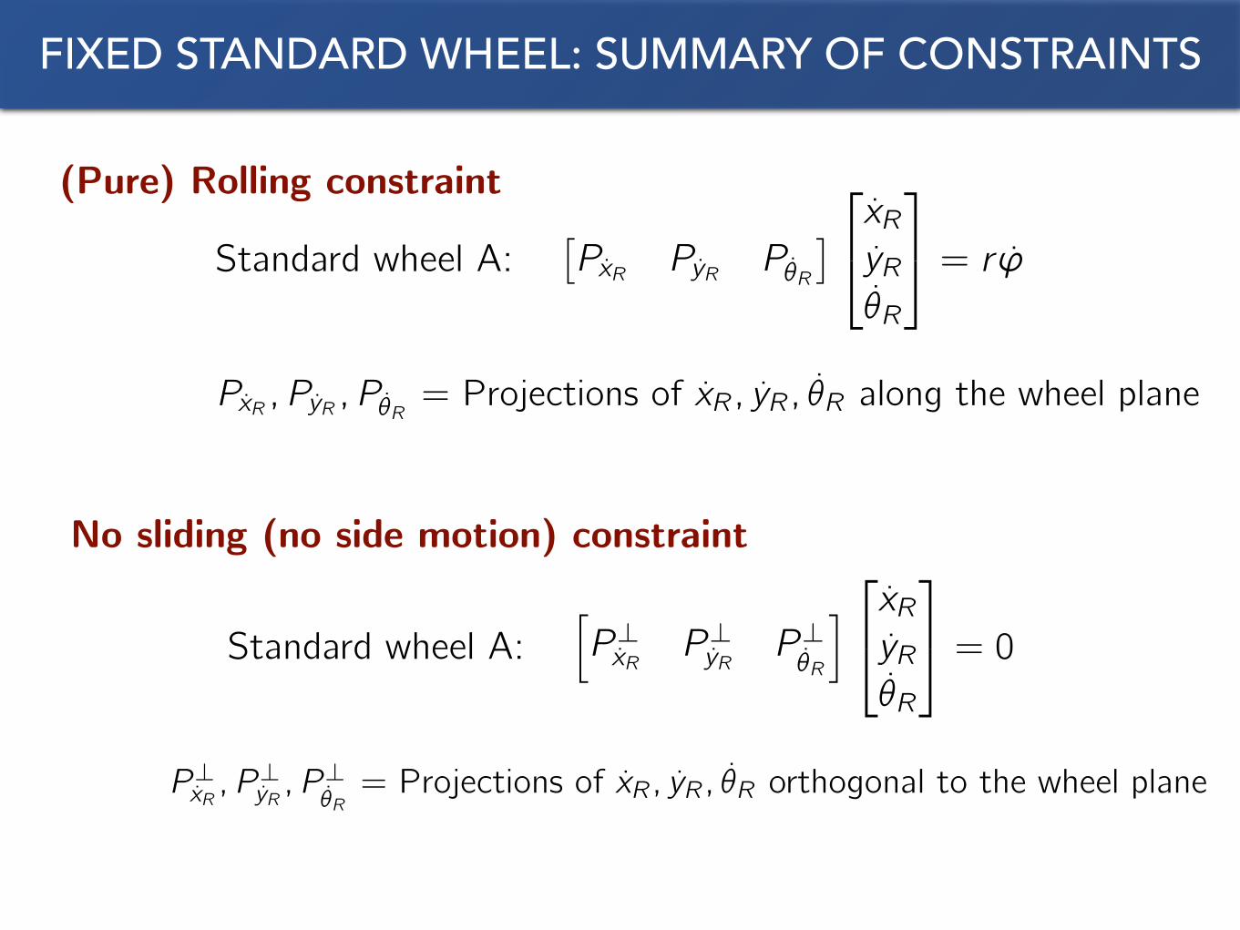
FIXED STANDARD WHEEL: SUMMARY OF CONSTRAINTS

Standard wheel A:⇥P

x

R

P

y

R

P

✓

R

⇤2

4x

R

y

R

✓

R

3

5 = r '

P

x

R

, P

y

R

, P

✓

R

= Projections of x

R

, y

R

,

˙

✓

R

along the wheel plane

(Pure) Rolling constraint

No sliding (no side motion) constraint

Standard wheel A:hP

?x

R

P

?y

R

P

?✓

R

i2

4x

R

y

R

✓

R

3

5 = 0

P

?x

R

, P

?y

R

, P

?✓

R

= Projections of x

R

, y

R

,

˙

✓

R

orthogonal to the wheel plane

9

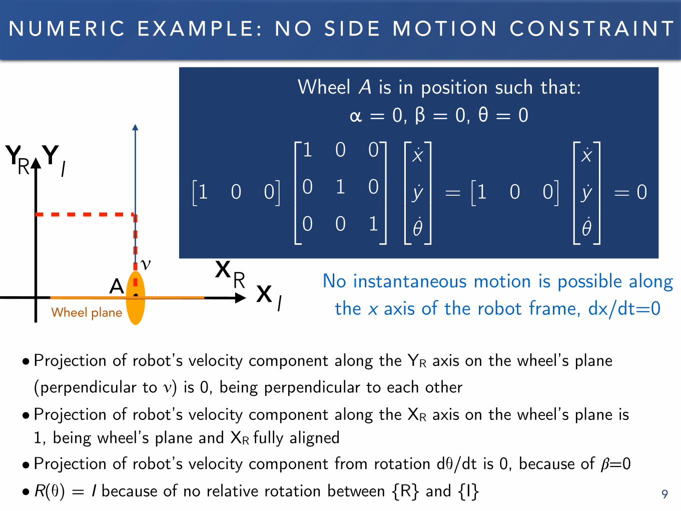
N U M E R I C E X A M P L E : N O S I D E M O T I O N C O N S T R A I N T

⇥1 0 0

⇤

2

664

1 0 0

0 1 0

0 0 1

3

775

2

664

x

y

✓

3

775 =⇥1 0 0

⇤

2

664

x

y

✓

3

775 = 0

α = 0, β = 0, θ = 0 Wheel A is in position such that:

XR

YR

X I

YI

Av

.

• Projection of robot’s velocity component along the YR axis on the wheel’s plane (perpendicular to v) is 0, being perpendicular to each other

• Projection of robot’s velocity component along the XR axis on the wheel’s plane is 1, being wheel’s plane and XR fully aligned

• Projection of robot’s velocity component from rotation d𝜃/dt is 0, because of 𝛽=0 • R(𝜃) = I because of no relative rotation between {R} and {I}

Wheel plane

No instantaneous motion is possible along the x axis of the robot frame, dx/dt=0

10

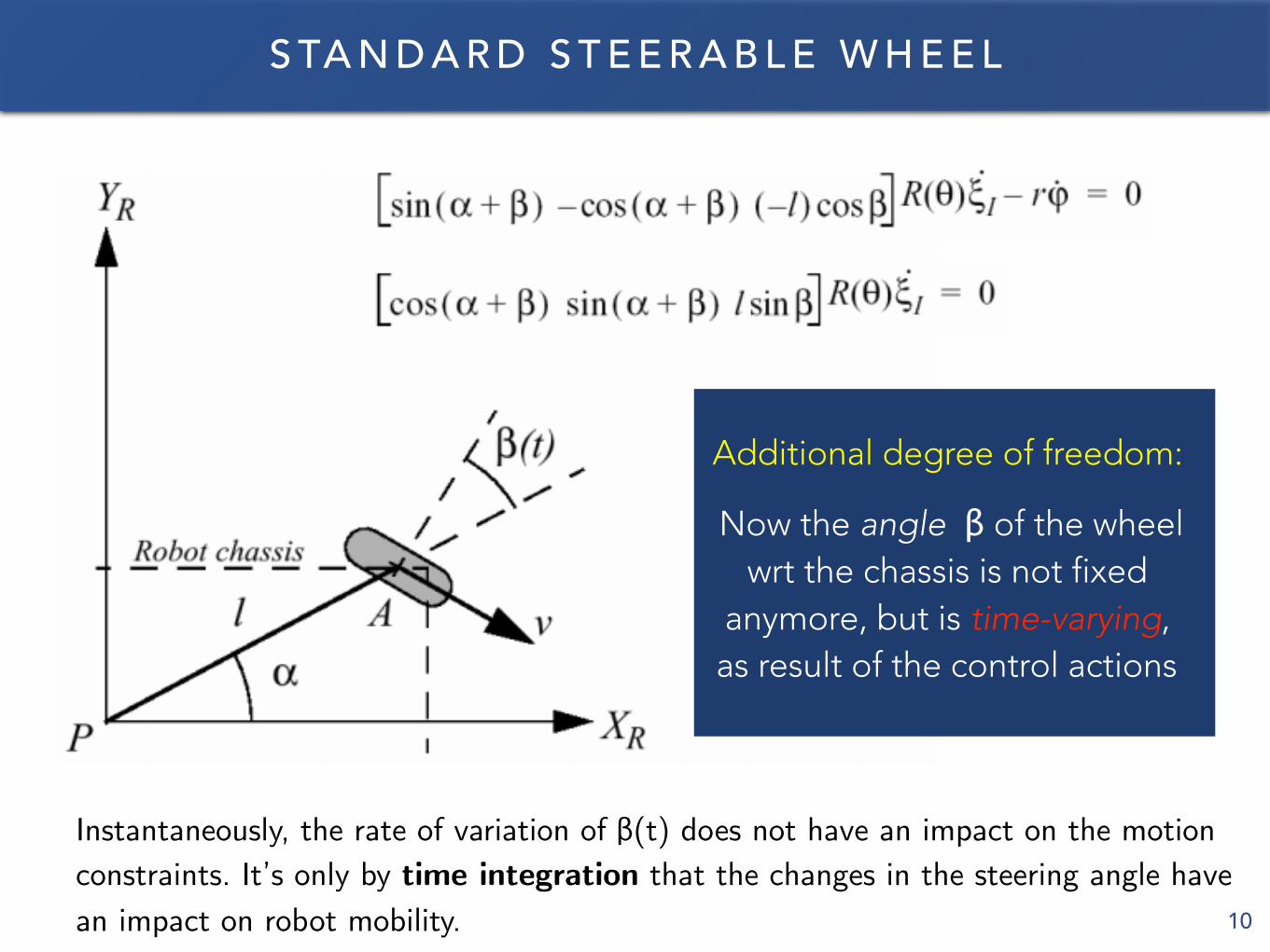
S TA N D A R D S T E E R A B L E W H E E L

Additional degree of freedom:

Now the angle β of the wheel wrt the chassis is not fixed

anymore, but is time-varying, as result of the control actions

Instantaneously, the rate of variation of β(t) does not have an impact on the motion constraints. It’s only by time integration that the changes in the steering angle have an impact on robot mobility.

11

C A S T O R W H E E L

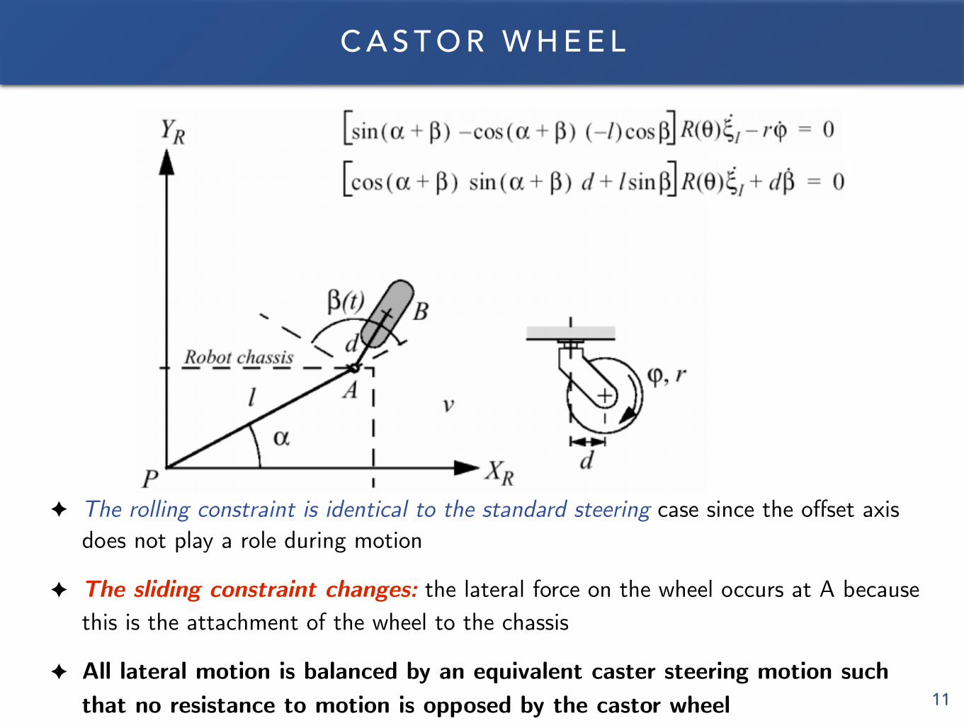
✦ The rolling constraint is identical to the standard steering case since the offset axis does not play a role during motion

✦ The sliding constraint changes: the lateral force on the wheel occurs at A because this is the attachment of the wheel to the chassis

✦ All lateral motion is balanced by an equivalent caster steering motion such that no resistance to motion is opposed by the castor wheel

12

C A S T O R W H E E L

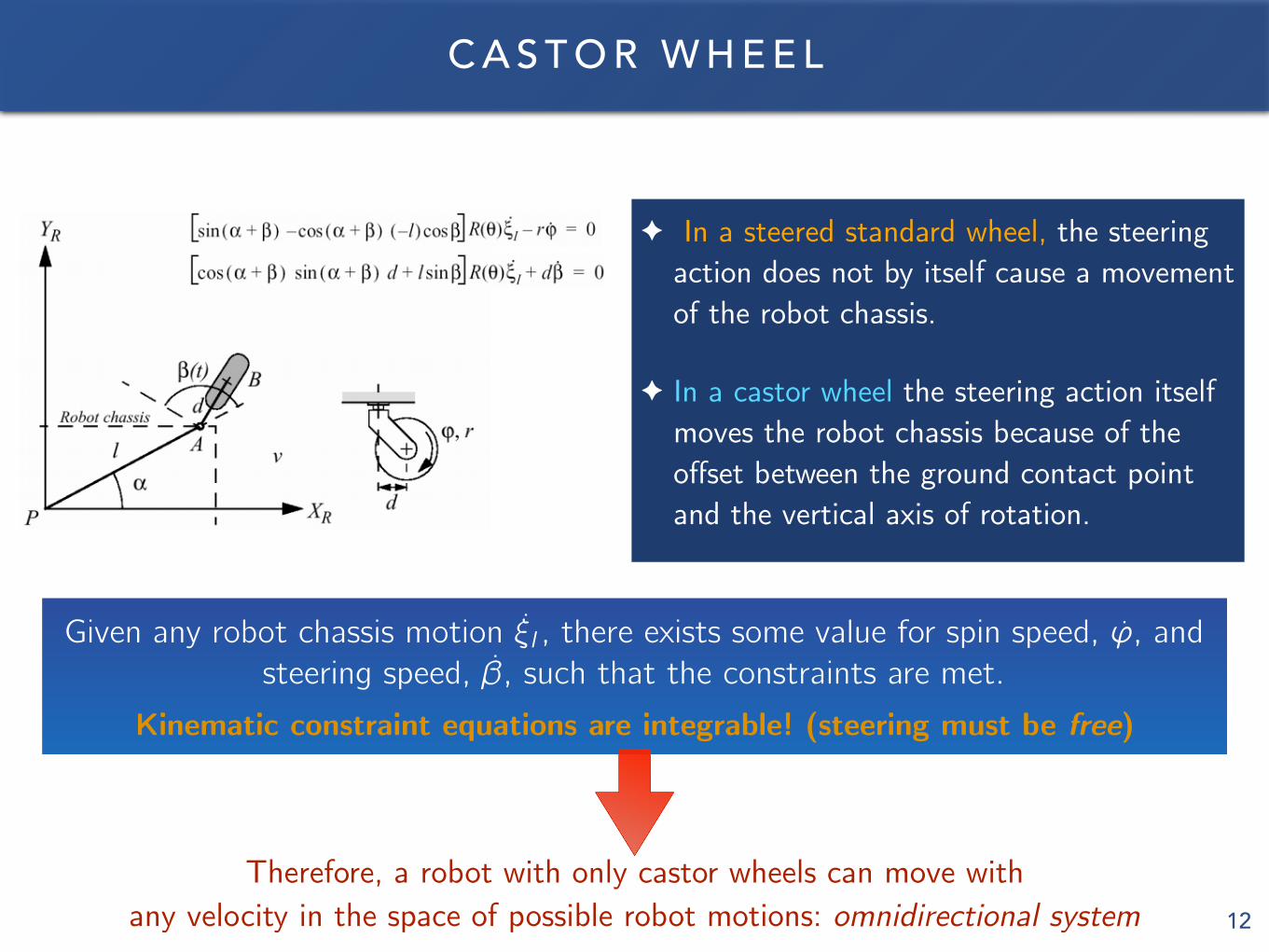
✦ In a steered standard wheel, the steering action does not by itself cause a movement of the robot chassis.

✦ In a castor wheel the steering action itself moves the robot chassis because of the offset between the ground contact point and the vertical axis of rotation.

Given any robot chassis motion

˙⇠I , there exists some value for spin speed, ', andsteering speed,

˙�, such that the constraints are met.

Kinematic constraint equations are integrable! (steering must be free)

Therefore, a robot with only castor wheels can move with any velocity in the space of possible robot motions: omnidirectional system

13

S W E D I S H W H E E L

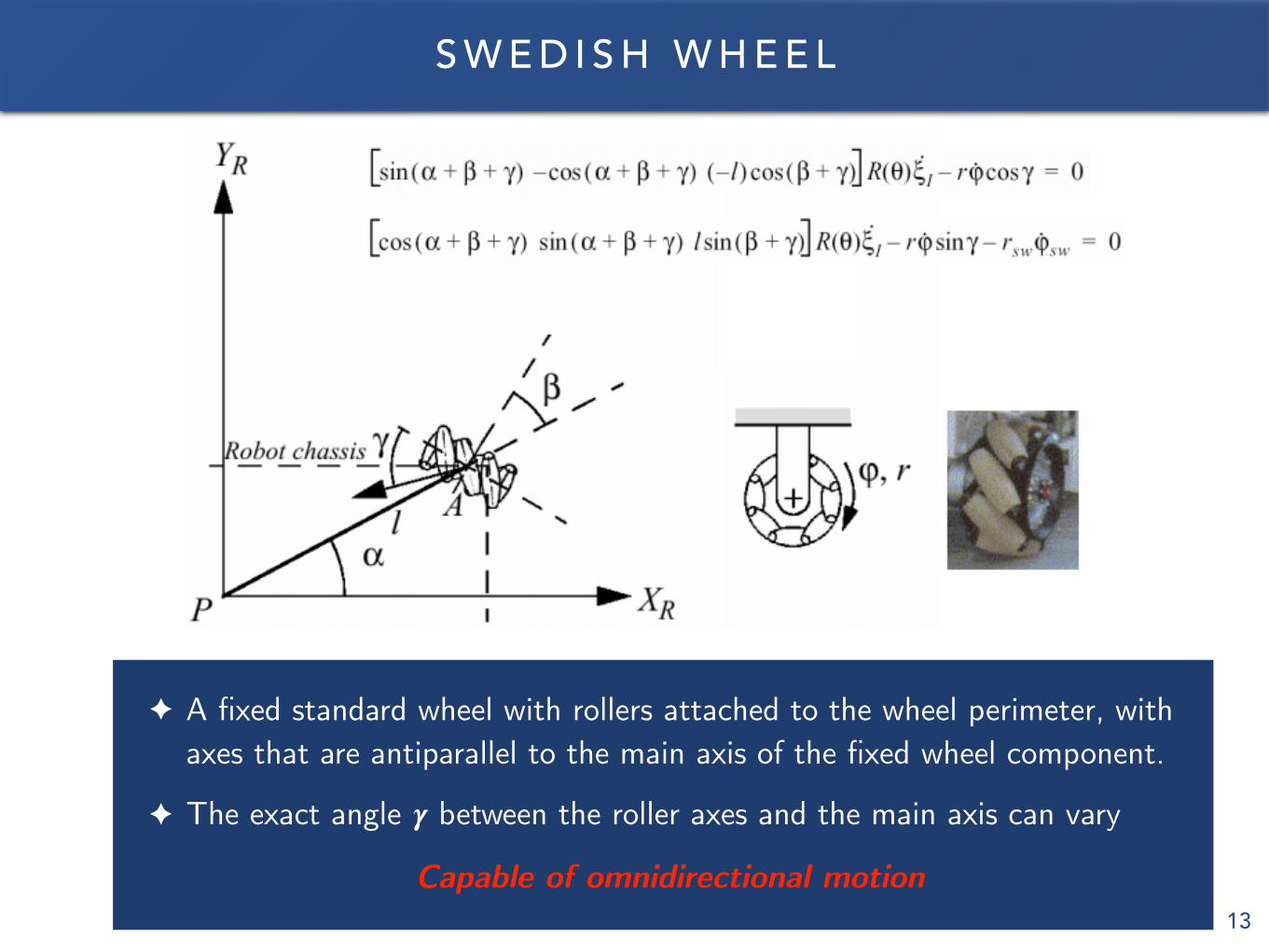
✦ A fixed standard wheel with rollers attached to the wheel perimeter, with axes that are antiparallel to the main axis of the fixed wheel component.

✦ The exact angle 𝜸 between the roller axes and the main axis can vary

Capable of omnidirectional motion

14

S P H E R I C A L W H E E L

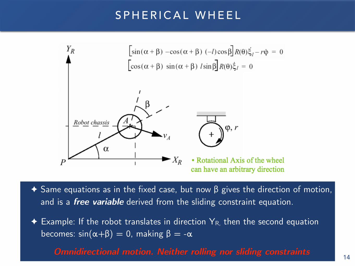
✦ Same equations as in the fixed case, but now β gives the direction of motion, and is a free variable derived from the sliding constraint equation.

✦ Example: If the robot translates in direction YR, then the second equation becomes: sin(α+β) = 0, making β = -α

Omnidirectional motion. Neither rolling nor sliding constraints

15

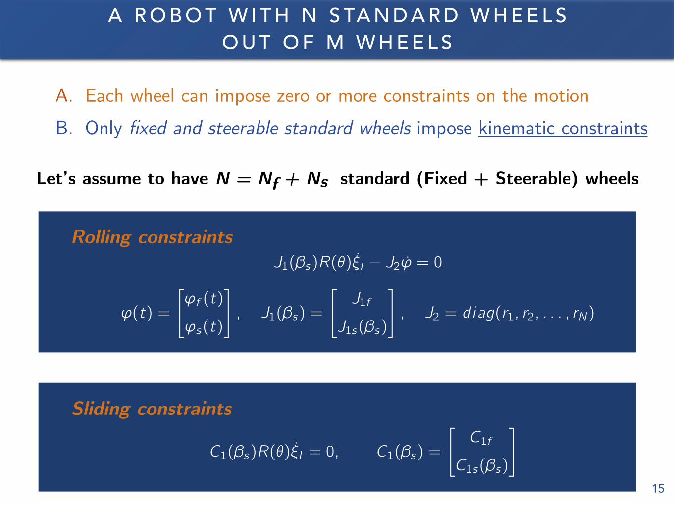
A R O B O T W I T H N S TA N D A R D W H E E L S O U T O F M W H E E L S

A. Each wheel can impose zero or more constraints on the motion B. Only fixed and steerable standard wheels impose kinematic constraints

Let’s assume to have N = Nf + Ns standard (Fixed + Steerable) wheels

• Rolling constraints:

J1(�s)R(✓)⇠I � J2' = 0

'(t) =

"'f (t)

's(t)

#

, J1(�s) =

"J1f

J1s(�s)

#

, J2 = diag(r1, r2, . . . , rN)

• Lateral movement:

C1(�s)R(✓)⇠I = 0, C1(�s) =

"C1f

C1s(�s)

#

Rolling constraints

Sliding constraints

16

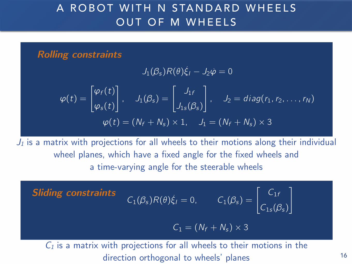
A R O B O T W I T H N S TA N D A R D W H E E L S O U T O F M W H E E L S

Sliding constraints

• Rolling constraints:

J1(�s)R(✓)⇠I � J2' = 0

'(t) =

"'f (t)

's(t)

#

, J1(�s) =

"J1f

J1s(�s)

#

, J2 = diag(r1, r2, . . . , rN)

'(t) = (Nf + Ns)⇥ 1, J1 = (Nf + Ns)⇥ 3

Rolling constraints

J1 is a matrix with projections for all wheels to their motions along their individual wheel planes, which have a fixed angle for the fixed wheels and

a time-varying angle for the steerable wheels• Lateral movement:

C1(�s)R(✓)⇠I = 0, C1(�s) =

"C1f

C1s(�s)

#

C1 = (Nf + Ns)⇥ 3

C1 is a matrix with projections for all wheels to their motions in the direction orthogonal to wheels’ planes

17

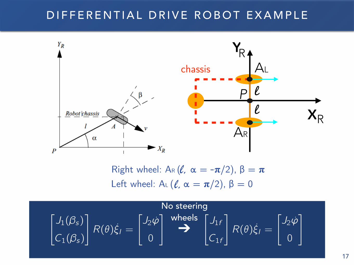
D I F F E R E N T I A L D R I V E R O B O T E X A M P L E

XR

YR

P

AR

AL

l

l

chassis

Right wheel: AR ( α = -𝛑/2), β = 𝛑 Left wheel: AL ( α = 𝛑/2), β = 0

l,l,

"J1(�s)

C1(�s)

#

R(✓)⇠I =

"J2'

0

# "J1f

C1f

#

R(✓)⇠I =

"J2'

0

#

➔

No steering wheels

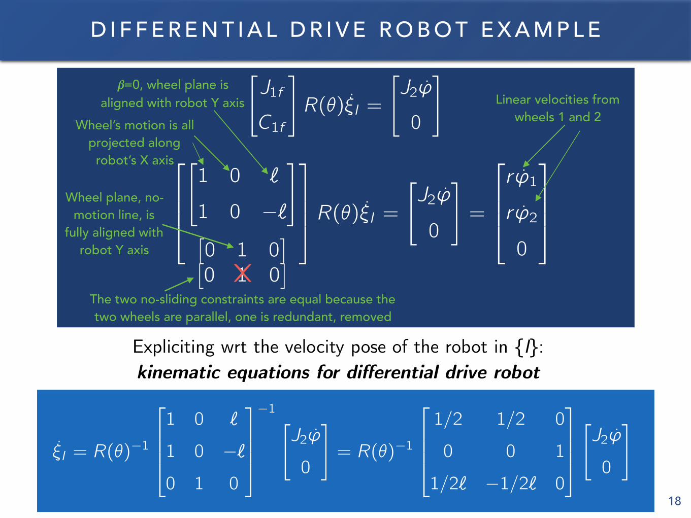
18

D I F F E R E N T I A L D R I V E R O B O T E X A M P L E"J1f

C1f

#

R(✓)⇠I =

"J2'

0

#

2

664

"1 0 `

1 0 �`

#

⇥0 1 0

⇤

3

775R(✓)⇠I =

"J2'

0

#

=

2

664

r '1

r '2

0

3

775

Expliciting wrt the velocity pose of the robot in {I}: kinematic equations for differential drive robot

⇠I = R(✓)�1

2

664

1 0 `

1 0 �`

0 1 0

3

775

�1 "J2'

0

#

= R(✓)�1

2

664

1/2 1/2 0

0 0 1

1/2` �1/2` 0

3

775

"J2'

0

#

𝜷=0, wheel plane is aligned with robot Y axis

Wheel’s motion is all projected along

robot’s X axis

Wheel plane, no-motion line, is

fully aligned with robot Y axis

Linear velocities from wheels 1 and 2

The two no-sliding constraints are equal because the two wheels are parallel, one is redundant, removed

⇥0 1 0

⇤⨉