the impact of thematic resolution on the patch-mosaic model of natural landscapes
TRANSCRIPT
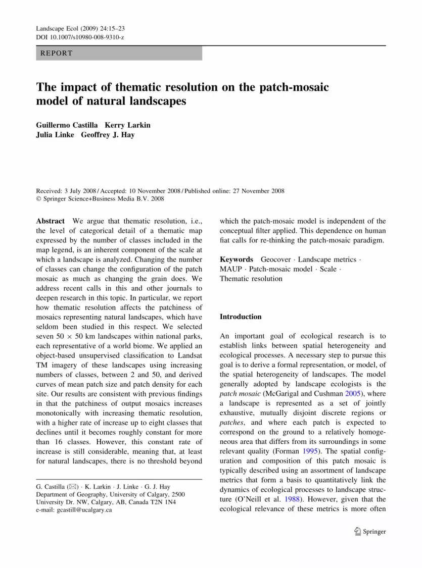
REPORT
The impact of thematic resolution on the patch-mosaicmodel of natural landscapes
Guillermo Castilla AElig Kerry Larkin AEligJulia Linke AElig Geoffrey J Hay
Received 3 July 2008 Accepted 10 November 2008 Published online 27 November 2008
Springer Science+Business Media BV 2008
Abstract We argue that thematic resolution ie
the level of categorical detail of a thematic map
expressed by the number of classes included in the
map legend is an inherent component of the scale at
which a landscape is analyzed Changing the number
of classes can change the configuration of the patch
mosaic as much as changing the grain does We
address recent calls in this and other journals to
deepen research in this topic In particular we report
how thematic resolution affects the patchiness of
mosaics representing natural landscapes which have
seldom been studied in this respect We selected
seven 50 9 50 km landscapes within national parks
each representative of a world biome We applied an
object-based unsupervised classification to Landsat
TM imagery of these landscapes using increasing
numbers of classes between 2 and 50 and derived
curves of mean patch size and patch density for each
site Our results are consistent with previous findings
in that the patchiness of output mosaics increases
monotonically with increasing thematic resolution
with a higher rate of increase up to eight classes that
declines until it becomes roughly constant for more
than 16 classes However this constant rate of
increase is still considerable meaning that at least
for natural landscapes there is no threshold beyond
which the patch-mosaic model is independent of the
conceptual filter applied This dependence on human
fiat calls for re-thinking the patch-mosaic paradigm
Keywords Geocover Landscape metrics MAUP Patch-mosaic model Scale Thematic resolution
Introduction
An important goal of ecological research is to
establish links between spatial heterogeneity and
ecological processes A necessary step to pursue this
goal is to derive a formal representation or model of
the spatial heterogeneity of landscapes The model
generally adopted by landscape ecologists is the
patch mosaic (McGarigal and Cushman 2005) where
a landscape is represented as a set of jointly
exhaustive mutually disjoint discrete regions or
patches and where each patch is expected to
correspond on the ground to a relatively homoge-
neous area that differs from its surroundings in some
relevant quality (Forman 1995) The spatial config-
uration and composition of this patch mosaic is
typically described using an assortment of landscape
metrics that form a basis to quantitatively link the
dynamics of ecological processes to landscape struc-
ture (OrsquoNeill et al 1988) However given that the
ecological relevance of these metrics is more often
G Castilla (amp) K Larkin J Linke G J Hay
Department of Geography University of Calgary 2500
University Dr NW Calgary AB Canada T2N 1N4
e-mail gcastillucalgaryca
123
Landscape Ecol (2009) 2415ndash23
DOI 101007s10980-008-9310-z
presumed than established (Li and Wu 2004) it is
imperative to understand what these metrics really
measure before establishing such a link (Buyantuyev
and Wu 2007) In particular an understanding and
characterization of their scale dependence is a
prerequisite for a meaningful use of these metrics
(Wu 2004)
The evolution of the concept of scale in Landscape
Ecology (for a review see Wu 2007) has influenced
research directed towards the effects of scale on
landscape metrics Traditionally scale has been
regarded as exclusively composed of grain and extent
(eg Wiens 1989) As a result most landscape pattern
analysis papers addressing scale effects focused on
these two items (eg Turner et al 1989 Wu et al
2002 Wu 2004) In addition to grain and extent we
suggest as implied by Gergel (2006) that there are
two more components that should be included in the
concept of scale minimum mapping unit (MMU) and
thematic resolution Following Levinrsquos (1992) anal-
ogy of scale as a window of perception we can
imagine this window placed in the floor of the gondola
of a balloon and characterized by four elements (1)
the extent which is the combination of the altitude of
the balloon the dimensions of the window frame and
the height of the observerrsquos eye over the window (2)
the grain which is the smallest terrain detail seen by
the naked eye at a given altitude (3) the MMU which
is the minimum size a pattern has to exceed in order to
be cognitively processed and (4) the thematic reso-
lution ie the number of classes into which we
arrange the scene in order to comprehend it This last
component can be conceived of as a special coating
applied to the window pane of the gondola (ie a
filter) that gives similar appearance to patterns having
the same meaning thus grouping them together when
they are adjacent
Changing any of these four scale components
changes the number and shape of patches representing
a landscape Given that the values chosen for these
four components are more dependent on the particular
application than on the landscape being analyzed this
scale dependence hampers the usefulness of the patch-
mosaic model to derive valid inferences That is
landscape pattern analysis relies on areal units
(patches) whose actual delineation may change due
to a discretionary decision (the choice of scale) where
this change will lead to disparate analytical results
This unavoidable spatial problem is known as the
Modifiable Areal Unit Problem or MAUP (Openshaw
1984) Consequently the more sensitive the patch-
mosaic model of a given landscape is to a change in
scale the more the results of its analysis can be
questioned Hence the need to assess the impact of
each scale component on the resulting model espe-
cially those (MMU and thematic resolution) that have
been less studied After briefly commenting on MMU
we focus on thematic resolution
That grain and MMU are not synonymous should be
clear However there are many raster land-cover maps
that contain isolated pixels thus assuming this equiv-
alence What is neglected is that the map is deemed to
portray not only the location of patches but also their
shape and in order to represent (even schematically)
this shape it is necessary to use a grain several times
smaller than the smallest patch For example to
represent a circular patch in raster format a grain at
least 20 times smaller than its area is required
Different MMUs will lead to different patch mosaics
therefore the choice of MMU has an important impact
on landscape pattern analysis as has been reported
elsewhere (Stohlgren et al 1997 Saura 2002 Langford
et al 2006 Kendall and Miller 2008)
That thematic resolution should be considered an
inherent component of scale is not as obvious as with
the MMU since it is not a spatially explicit aspect
(McGarigal and Cushman 2005) However it has a
definite impact on the size distribution of patches
which certainly is a scale issue The choice of
thematic resolution has been shown to be of impor-
tance in numerous studies for example in the
performance of both habitat-relationship models
(Karl et al 2000) and coral reef fish-distribution
models (Kendall and Miller 2008) and in biodiver-
sity monitoring (Bailey et al 2007) Despite its
manifest relevance research on the effects of the-
matic resolution on landscape pattern analysis
remains insufficient as evidenced by recent calls on
this subject in this (Buyantuyev and Wu 2007) and
other (Huang et al 2006) journals The goal of this
paper is to contribute to this topic with new insights
from natural landscapes Since the number of patches
is expected to increase with the number of classes we
will focus on the patchiness of the resulting mosaics
as measured by mean patch size (MPS) and patch
density (PD)
There are four recent studies that explicitly address
this topic Baldwin et al (2004) used 420 contiguous
16 Landscape Ecol (2009) 2415ndash23
123
400 9 400 pixel landscapes of 100 m grain resam-
pled from a land-cover map derived from Landsat
TM imagery acquired over the managed forest area of
Ontario Canada Their original 26 class map was
reclassified to form 4 broader classifications of 16 8
4 and 2 landcover types They plotted the global
mean value of selected landscape metrics (including
MPS and PD) against the number of classes and
found a dramatic increase in the number of patches
for coarse thematic resolution and a smaller increase
after 10 classes Li et al (2005) used 13 simulated
1000 9 1000 pixel landscapes with the number of
classes ranging from 2 to 100 They also reported that
the total number of patches initially increases quickly
with the number of classes reaching a sill at around
20 classes Huang et al (2006) used three 72 km2
landscapes in Arizona (urban mountainous and
dessert grassland) mapped at both 15 and 30 m grain
and 2ndash35 classes They also found a rapid increase of
the number of patches for less than 10 classes and
almost insignificant changes for more than 16 classes
Buyantuyev and Wu (2007) studied a multi-temporal
series (5 dates from 1985 to 2000 at 30 m grain) over
a single 6400 km2 heavily used arid landscape in
central Arizona They used five classification levels
respectively with 2 4 6 9 and 12 classes They also
found a monotonic increase in the number of patches
with increasing thematic resolution although with a
more stable rate (almost linear) than in previous
studies
Except for two of the landscapes in Huang et al
(2006) all these landscapes contained a significant
presence of cultural patterns Therefore there is a
need to confirm if previous findings also apply to
natural landscapes ie landscapes lacking anthro-
pogenic patterns In particular since the greater the
anthropogenic impact in the landscape the stronger
the manifestation of a patch mosaic (Solon 2005) it
can be expected that the patch-mosaic model of
natural landscapes will be even more sensitive to
thematic resolution We test this by quantifying the
patchiness of mosaics derived from Landsat imagery
of protected natural landscapes using increasing
thematic resolution As a secondary goal related to
the search of scaling relations to translate information
across scales (Wu 2007) we also test whether the
level of patchiness for a given thematic resolution can
be estimated as a function of the mean patch size of
the binary mosaic
Methods
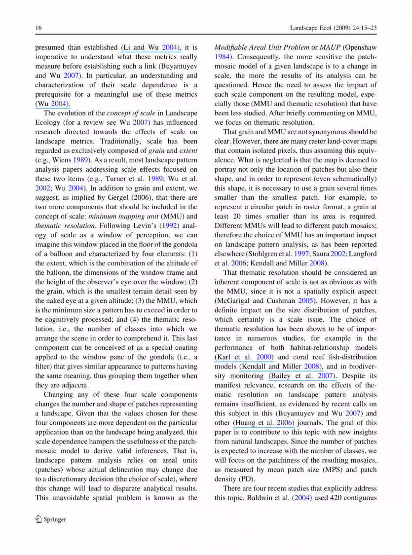
We selected seven national parks from across the world
(Fig 1) large enough to encompass a 50 by 50 km
square area and representative of the following biomes
tropical rainforest desert savanna steppe tundra
taiga and temperate forest plus montane grassland
(Table 1) These seven samples are not meant for
deriving conclusions about specific biomes but rather
to capture the global diversity of natural landscapes
For each park we identified the GeocoverTM 1990
mosaic encompassing it and downloaded the image
from the official ftp site (ftpglcfumiacsumdeduglcf
Mosaic_Landsat) Each GeocoverTM mosaic is a 24 bit
GeoTIFF file made of ortho-rectified (to UTM
WGS84) Landsat TM images acquired circa 1990
Each covers a rectangle of 5 latitude and 6 longitude
Fig 1 Location of the
National Parks selected for
this study (background
image downloaded from
NASArsquos Visible Earthmdash
httpvisibleearthnasagov)
Landscape Ecol (2009) 2415ndash23 17
123
at 285 m pixel size and includes 3 TM bands (band 7
[Short Wavelength InfraRed] as red band 4 [Near
InfraRed] as green and band 2 [green wavelength] as
blue ie a RGB 742 color composite) (Tucker et al
2004) After assuring no visible anthropogenic fea-
tures we clipped a 50 9 50 km square area within each
park and resampled the images to 30 m using cubic
convolution As a result we obtained seven 278
Megapixel (1667 columns by 1667 rows) 3-channel
images that constitute the dataset for this study
(Fig 2andashg)
Each image was subject to the following object-
based unsupervised classification process which was
designed and implemented in IDL (ITTVIS 2008) by
the first author (1) The image was filtered using the
Gradient Inverse Weighted Edge Preserving Smooth-
ing (GIWEPS Castilla 2003) which removes coarse
texture in the image without blurring edges (2) The
gradient magnitude (ie an edge image) of the
filtered image was computed as in Castilla et al
(2008) (3) The area of influence of each gradient
minimum was delimited using a watershed algorithm
(Vincent and Soille 1991) This resulted in a partition
consisting of homogeneous regions which can be
regarded as the finest patch mosaic that can be
derived from the original image before applying any
conceptual filter (ie classification) (4) The few
regions (typically less than 1 of the total area of the
image) within this partition that were smaller than
the MMU (9 pixels 081 ha) were aggregated to the
most similar adjacent region (5) The mean value of
each remaining region (hereafter patch) in each band
of the original image was computed This represents
the coordinates of the patch in the 3D feature space
defined by the three bands of the image or in remote
sensing parlance the patchrsquos signature Then for each
thematic resolution ncl (ncl = 50 48 46hellip 4 2) the
following process was applied (6) Each patch was
assigned to one of the ncl possible classes using the
patchesrsquo signatures as input to the K-means algorithm
(Tou and Gonzalez 1974) (7) Adjacent patches
belonging to the same class were merged together
and the signature of each new merger was recom-
puted as the area weighted mean of the patches
forming it Finally (8) steps 6 and 7 were repeated
until ncl = 2 This resulted in a stack of 25 nested
patch mosaics per landscape of increasing thematic
resolution ranging from 2 to 50 classes
After producing the 175 patch-mosaics (25 mosa-
ics for each of the 7 landscapes) we computed the
mean patch size (MPS) and patch density (PD) of
each mosaic and plotted them against the number of
classes thus obtaining seven MPS curves and seven
PD curves (Fig 3a b) The MPS curves were
individually fitted to an inverse power law of the
form MPS = kncla where k is a constant and a is the
exponent of the power law We also fitted the portion
of the MPS curves that appear linear (ncl [ [16 50])
to a straight line in order to ascertain whether the rate
of decrease in MPS for finer thematic resolutions can
be assumed both constant and negligible for all
landscapes (Fig 3c) Finally in order to evaluate the
possibility of estimating the patchiness of a landscape
mosaic at a specific thematic resolution as a function
of the patchiness of its binary mosaic we plotted the
seven values of a against the mean patch size of the
binary landscape MPS2 (Fig 3d)
Results and discussion
In the GeocoverTM images of the seven 2500 km2
landscapes used in this study (Fig 2andashg) forested
areas appear as shades of dark green grasslands and
Table 1 Study site names biomes countries centre coordinates and image acquisition year
Site name Biome Country Latitude Longitude Year
Amazon National Park Rainforest Brazil 423S 5709W 1992
Death Valley National Park Desert USA 3646N 11697W 1990
Kakadu National Park Savanna Australia 1338S 13208E 1990
Khan Khentee National Park Steppe Mongolia 4906N 10871E 1989
Tuktut Nogait N Park Tundra Canada 6859N 12207W 1992
Vodzolersky National Park Taiga Russia 6311N 3756E 1986
Yellowstone National Park Temp forest montane grassland USA 4477N 11075W 1990
18 Landscape Ecol (2009) 2415ndash23
123
open forest as light green water as black to dark blue
ice or snow as cyan and bare soil and rocks as
magenta red purple or pale pink The selected sites
represent a variety of natural landscapes
encompassing most world biomes from tundra to
tropical rainforest As an example of the type of patch
mosaics created using this method the mosaic
obtained for ten classes in the SW quarter of the
Fig 2 (andashg) GeocoverTM 1990 images (RGB 742) of the
seven 50 9 50 km2 landscapes used in this study (h) A detail
of the mosaic obtained for 10 classes in landscape g (i) A
further detail of the mosaics for the lower left corner of
landscape g at four different thematic resolutions respectively
16 8 4 and 2 classes
Landscape Ecol (2009) 2415ndash23 19
123
Yellowstone landscape (Fig 2g) is displayed in
Fig 2h A further detail with examples corresponding
to 2 4 8 and 16 classes can be appreciated in Fig 2i
Although we made no attempt to link the defined
radiometric classes to specific land-cover classes
(which would have been difficult given our lack of
ground truth for the seven landscapes) the output
patches visually portray the spatial structure in the
images and the resulting hierarchy of nested mosaics
adequately captures the diversity of image hues and
tones Therefore assuming a general correspondence
between radiometric similarity and semantic simi-
larity (which is the underlying premise of all
classification algorithms) it can be expected that
other classification strategies even if they would
have led to different mosaics (ie even if they are
subject to the aggregation problem within MAUP)
would have exhibited similar trends in the increase of
patchiness with thematic resolution which is the
question being addressed in this report
The mean patch size (MPS) and patch density
(PD) curves obtained for each landscape when plotted
against the number of classes (ncl) are presented in
Fig 3a and b respectively All MPS curves (Fig 3a)
follow an inverse power law which starts leveling off
near eight classes and becomes linear for ncl [ 16
This overall behavior is consistent with previous
findings however the rate of decrease when the
Fig 3 Four plots describing the impact of thematic resolution on the patchiness of the studied landscapes including scaling
relations The landscapes are named after the biome they represent
20 Landscape Ecol (2009) 2415ndash23
123
curves become linear cannot be qualified as lsquoalmost
insignificantrsquo as in Huang et al (2006) The linear fit
of the MPS curves for ncl [ 16 yielded a high
coefficient of determination (r2 [ 095) for all
curves meaning that the rate of decrease can be
assumed constant in all landscapes beyond 16 classes
averaging 025 ha per additional class This linear
decrease leads to a MPS at 50 classes that is between
15 and 3 times smaller than the one for 16 classes
(Fig 3c) This can be also appreciated in the PD
curves (Fig 3b) which unlike that obtained by Li
et al (2005) for simulated landscapes do not reach a
sill and continue to grow steadily
Another interesting observation is that the shape of
the MPS curves in particular the way the bend in the
curve is reached ie the point in the curve beyond
which the rate of decrease can be assumed constant
appears to be dependent on the patchiness of the
corresponding binary landscape (ie the MPS for
ncl = 2 or MPS2) In general landscapes with a
more heterogeneous binary mosaic (ie with lower
MPS2) reach a constant rate of decrease at higher
thematic resolution than those with a higher MPS2
which translates into a smaller exponent in the
inverse power law defining the MPS curve Given
the limited number of landscapes we evaluated no
predictive generalization can be attempted However
if the tundra landscape is excluded (Fig 2e where
the MPS2 is several times larger than in other
landscapes because its binary mosaicmdashin this case
water versus non watermdashconsisted of scattered lakes
in a land matrix that occupies 98 of the extent)
there is a clear linear relationship (r2 [ 09 Fig 3d)
between MPS2 and the exponent of the inverse power
law describing the decline in MPS with increasing
thematic resolution As an aside we acknowledge
that we noticed this behavior because it is akin to that
observed by dissecting a forest landscape with evenly
spaced straight narrow roads or cutlines (Linke et al
2008) These authors reported that the rate of
decrease in MPS as a function of increasing cutline
density was inversely related to the original mosaic
heterogeneity (ie the MPS value before introducing
cutlines) Our observation suggests that a scaling
relation predicting the patchiness of a mosaic for a
given thematic resolution can be derived as a function
of MPS2 providing none of the two classes in the
binary landscape is overwhelmingly predominant
([95) This is a topic of further investigation
Conclusions and final remarks
Our results confirm previous conclusions that the-
matic resolution has an important impact on the
spatial configuration of the patch-mosaic model and
thus can significantly affect the value of landscape
metrics derived from it Specifically the patch
density of the mosaic model of natural landscapes
increases monotonically with the number of classes
considered with a higher rate of increase for smaller
numbers of classes (8) which declines rapidly until
it becomes roughly constant for more than 16 classes
However this constant rate cannot be deemed
insignificant as suggested previously since it leads
to a Mean Patch Size (MPS) at 50 classes that is
between 15 and 3 times smaller than the one for 16
classes Another relatively novel aspect of our study
is that we were able to derive a scaling law that
reliably estimated for six of the seven landscapes the
exponent of the inverse power law describing the
decline in MPS with increasing thematic resolution as
a linear function of the MPS of the binary mosaic of
each landscape
The dependence of the patch-mosaic model on the
conceptual filter we apply to the landscape should not
be surprising provided we are ready to accept that
patches as well as the hierarchies in which they are
nested are human constructs Any given patch is an
instance of some particular class therefore different
classification schemes will in all likelihood lead to
different ways of partitioning the same landscape into
patches However we tend to reify these units and
regard them as natural Thus we are inclined to think
of the patch mosaic as a geographic reality rather than
what it really is a model The multiplicity of patch
mosaics that can be generated from the same
landscape using different choices of scale (grain
extent MMU and thematic resolution) is testimony to
this dependence and to the sensitivity of this model to
MAUP Since the latter hinders the validity of
landscape pattern analysis we concur with Turner
(2005) and McGarigal and Cushman (2005) that the
patch-mosaic paradigm must be extended to include
other forms of representing and analyzing the spatial
heterogeneity of landscapes In particular it would be
desirable that (1) the patch-mosaic model is embed-
ded in a hierarchical framework allowing for multi-
scale representation and analysis (2) attributes for
each individual boundary (separating a pair of
Landscape Ecol (2009) 2415ndash23 21
123
adjacent patches) are included related to the magni-
tude of environmental gradients across the boundary
and to the uncertainty of boundary placement and (3)
a concerted effort establishes standards on the choice
of the four components scale for specific applications
so as to enhance the comparability between different
places andor times
Acknowledgments This research was supported in part by
the Alberta Ingenuity Fund (AIF) the Natural Sciences and
Engineering Research Council of Canada (NSERC) the
University of Calgary and the Alberta Biodiversity
Monitoring Institute (ABMI) We thank our colleague Stefan
Steiniger and two anonymous reviewers for their helpful
comments
References
Bailey D Billeter R Aviron S Schweiger O Herzog F (2007)
The influence of thematic resolution on metric selection
for biodiversity monitoring in agricultural landscapes
Landscape Ecol 22(3)461ndash473 doi101007s10980-006-
9035-9
Baldwin DJ Weaver K Schnekenburger F Perera AH (2004)
Sensitivity of landscape pattern indices to input data
characteristics on real landscapes implications for their
use in natural disturbance emulation Landscape Ecol
19255ndash271 doi101023BLAND000003044296122ef
Buyantuyev A Wu J (2007) Effects of thematic resolution on
landscape pattern analysis Landscape Ecol 227ndash13
doi101007s10980-006-9010-5
Castilla G (2003) Object-oriented analysis of remote sensing
images for land cover mapping conceptual foundations and
a segmentation method to derive a baseline partition for
classification PhD Thesis Polytechnic University of
Madrid Available from httpoaupmes1330107200302_
castilla_castellanopdf
Castilla G Hay GJ Ruiz JR (2008) Size-constrained region
merging (SCRM) an automated delineation tool for
assisted photointerpretation Photogramm Eng Rem S
74(4)409ndash419
Forman RTT (1995) Land mosaics the ecology of landscapes
and regions Cambridge University Press Cambridge
Gergel SE (2006) New directions in landscape pattern analysis
and linkages with remote sensing In Franklin SE Wulder
MA (eds) Understanding forest disturbance and spatial
pattern remote sensing and GIS approaches Taylor and
Francis London pp 173ndash208
Huang C Geiger EL Kupfer JA (2006) Sensitivity of land-
scape metrics to classification scheme Int J Remote Sens
27(14)2927ndash2948 doi10108001431160600554330
ITTVIS (2008) What is IDL Available from httpwww
ittviscomProductServicesIDLaspx Accessed October
2008
Karl JW Wright NM Heglund PJ Garton EO Scott JM Hutto
RL (2000) Sensitivity of species habitat-relationship
model performance to factors of scale Ecol Appl
10(6)1690ndash1705 doi1018901051-0761(2000)010
[1690SOSHRM]20CO2
Kendall MS Miller T (2008) The influence of thematic and
spatial resolution on maps of a coral reef ecosystem Mar
Geod 31(2)75ndash102 doi10108001490410802053617
Langford WT Gergel SE Dietterich TG Cohen W (2006) Map
misclassification can cause large errors in landscape pattern
indices examples from habitat fragmentation Ecosystems
(N Y Print) 9474ndash488 doi101007s10021-005-0119-1
Levin SA (1992) The problem of pattern and scale in ecology
Ecology 73(6)1943ndash1967 doi1023071941447
Li H Wu J (2004) Use and misuse of landscape indices
Landscape Ecol 19389ndash399 doi101023BLAND
000003044115628d6
Li X He HS Bu R Wen Q Chang Y Hu Y Li Y (2005) The
adequacy of different landscape metrics for various
landscape patterns Pattern Recognit 38(12)2626ndash2638
doi101016jpatcog200505009
Linke J Franklin SE Hall-Beyer M Stenhouse GB (2008)
Effects of cutline density and land cover heterogeneity on
landscape metrics in Western Alberta Can J Rem Sens
34(4)390ndash404
McGarigal K Cushman SA (2005) The gradient concept of
landscape structure In Wiens J Moss M (eds) Issues and
perspectives in landscape ecology Cambridge University
Press UK pp 112ndash119
OrsquoNeill RV Krummel JR Gardner RH et al (1988) Indices of
landscape pattern Landscape Ecol 1153ndash162 doi
101007BF00162741
Openshaw S (1984) The modifiable areal unit problem Geo
Books Norwich
Saura S (2002) Effects of minimum mapping unit on land cover
data spatial configuration and composition Int J Remote
Sens 23(22)4853ndash4880 doi10108001431160110114493
Solon J (2005) Incorporating geographical (biophysical) prin-
ciples in studies of landscape systems In Wiens J Moss
M (eds) Issues and perspectives in landscape ecology
Cambridge University Press Cambridge pp 11ndash20
Stohlgren TJ Chong GW Kalkhan MA Schell LD (1997)
Multiscale sampling of plant diversity effects of minimum
mapping unit size Ecol Appl 7(3)1064ndash1074 doi101890
1051-0761(1997)007[1064MSOPDE]20CO2
Tou JT Gonzalez RC (1974) Pattern recognition principles
Addison-Wesley Publishing Company Reading
Tucker CJ Grant DM Dykstra JD (2004) NASArsquos global or-
thorectified Landsat data set Photogramm Eng Rem S
70(3)313ndash322
Turner MG (2005) Landscape Ecology in North America past
present and future Ecology 86(8)1967ndash1974 doi10
189004-0890
Turner MG OrsquoNeill RV Gardner RH Milne BT (1989)
Effects of changing spatial scale on the analysis of land-
scape pattern Landscape Ecol 3153ndash162 doi101007
BF00131534
Vincent L Soille P (1991) Watersheds in digital spaces an
efficient algorithm based on immersion simulations IEEE
Trans Pattern Anal Mach Intell 13(6)583ndash598
doi1011093487344
Wiens JA (1989) Spatial scaling in ecology Funct Ecol 3385ndash
397 doi1023072389612
22 Landscape Ecol (2009) 2415ndash23
123
Wu J (2004) Effects of changing scale on landscape pattern
analysis scaling relations Landscape Ecol 19125ndash138
doi101023BLAND000002171140074ae
Wu J (2007) Scale and scaling a cross-disciplinary perspective
In Wu J Hobbs R (eds) Key topics in landscape ecology
Cambridge University Press Cambridge pp 115ndash143
Wu J Shen W Sun W Tueller PT (2002) Empirical patterns of
the effects of changing scale on landscape metrics Land-
scape Ecol 17761ndash782 doi101023A1022995922992
Landscape Ecol (2009) 2415ndash23 23
123
presumed than established (Li and Wu 2004) it is
imperative to understand what these metrics really
measure before establishing such a link (Buyantuyev
and Wu 2007) In particular an understanding and
characterization of their scale dependence is a
prerequisite for a meaningful use of these metrics
(Wu 2004)
The evolution of the concept of scale in Landscape
Ecology (for a review see Wu 2007) has influenced
research directed towards the effects of scale on
landscape metrics Traditionally scale has been
regarded as exclusively composed of grain and extent
(eg Wiens 1989) As a result most landscape pattern
analysis papers addressing scale effects focused on
these two items (eg Turner et al 1989 Wu et al
2002 Wu 2004) In addition to grain and extent we
suggest as implied by Gergel (2006) that there are
two more components that should be included in the
concept of scale minimum mapping unit (MMU) and
thematic resolution Following Levinrsquos (1992) anal-
ogy of scale as a window of perception we can
imagine this window placed in the floor of the gondola
of a balloon and characterized by four elements (1)
the extent which is the combination of the altitude of
the balloon the dimensions of the window frame and
the height of the observerrsquos eye over the window (2)
the grain which is the smallest terrain detail seen by
the naked eye at a given altitude (3) the MMU which
is the minimum size a pattern has to exceed in order to
be cognitively processed and (4) the thematic reso-
lution ie the number of classes into which we
arrange the scene in order to comprehend it This last
component can be conceived of as a special coating
applied to the window pane of the gondola (ie a
filter) that gives similar appearance to patterns having
the same meaning thus grouping them together when
they are adjacent
Changing any of these four scale components
changes the number and shape of patches representing
a landscape Given that the values chosen for these
four components are more dependent on the particular
application than on the landscape being analyzed this
scale dependence hampers the usefulness of the patch-
mosaic model to derive valid inferences That is
landscape pattern analysis relies on areal units
(patches) whose actual delineation may change due
to a discretionary decision (the choice of scale) where
this change will lead to disparate analytical results
This unavoidable spatial problem is known as the
Modifiable Areal Unit Problem or MAUP (Openshaw
1984) Consequently the more sensitive the patch-
mosaic model of a given landscape is to a change in
scale the more the results of its analysis can be
questioned Hence the need to assess the impact of
each scale component on the resulting model espe-
cially those (MMU and thematic resolution) that have
been less studied After briefly commenting on MMU
we focus on thematic resolution
That grain and MMU are not synonymous should be
clear However there are many raster land-cover maps
that contain isolated pixels thus assuming this equiv-
alence What is neglected is that the map is deemed to
portray not only the location of patches but also their
shape and in order to represent (even schematically)
this shape it is necessary to use a grain several times
smaller than the smallest patch For example to
represent a circular patch in raster format a grain at
least 20 times smaller than its area is required
Different MMUs will lead to different patch mosaics
therefore the choice of MMU has an important impact
on landscape pattern analysis as has been reported
elsewhere (Stohlgren et al 1997 Saura 2002 Langford
et al 2006 Kendall and Miller 2008)
That thematic resolution should be considered an
inherent component of scale is not as obvious as with
the MMU since it is not a spatially explicit aspect
(McGarigal and Cushman 2005) However it has a
definite impact on the size distribution of patches
which certainly is a scale issue The choice of
thematic resolution has been shown to be of impor-
tance in numerous studies for example in the
performance of both habitat-relationship models
(Karl et al 2000) and coral reef fish-distribution
models (Kendall and Miller 2008) and in biodiver-
sity monitoring (Bailey et al 2007) Despite its
manifest relevance research on the effects of the-
matic resolution on landscape pattern analysis
remains insufficient as evidenced by recent calls on
this subject in this (Buyantuyev and Wu 2007) and
other (Huang et al 2006) journals The goal of this
paper is to contribute to this topic with new insights
from natural landscapes Since the number of patches
is expected to increase with the number of classes we
will focus on the patchiness of the resulting mosaics
as measured by mean patch size (MPS) and patch
density (PD)
There are four recent studies that explicitly address
this topic Baldwin et al (2004) used 420 contiguous
16 Landscape Ecol (2009) 2415ndash23
123
400 9 400 pixel landscapes of 100 m grain resam-
pled from a land-cover map derived from Landsat
TM imagery acquired over the managed forest area of
Ontario Canada Their original 26 class map was
reclassified to form 4 broader classifications of 16 8
4 and 2 landcover types They plotted the global
mean value of selected landscape metrics (including
MPS and PD) against the number of classes and
found a dramatic increase in the number of patches
for coarse thematic resolution and a smaller increase
after 10 classes Li et al (2005) used 13 simulated
1000 9 1000 pixel landscapes with the number of
classes ranging from 2 to 100 They also reported that
the total number of patches initially increases quickly
with the number of classes reaching a sill at around
20 classes Huang et al (2006) used three 72 km2
landscapes in Arizona (urban mountainous and
dessert grassland) mapped at both 15 and 30 m grain
and 2ndash35 classes They also found a rapid increase of
the number of patches for less than 10 classes and
almost insignificant changes for more than 16 classes
Buyantuyev and Wu (2007) studied a multi-temporal
series (5 dates from 1985 to 2000 at 30 m grain) over
a single 6400 km2 heavily used arid landscape in
central Arizona They used five classification levels
respectively with 2 4 6 9 and 12 classes They also
found a monotonic increase in the number of patches
with increasing thematic resolution although with a
more stable rate (almost linear) than in previous
studies
Except for two of the landscapes in Huang et al
(2006) all these landscapes contained a significant
presence of cultural patterns Therefore there is a
need to confirm if previous findings also apply to
natural landscapes ie landscapes lacking anthro-
pogenic patterns In particular since the greater the
anthropogenic impact in the landscape the stronger
the manifestation of a patch mosaic (Solon 2005) it
can be expected that the patch-mosaic model of
natural landscapes will be even more sensitive to
thematic resolution We test this by quantifying the
patchiness of mosaics derived from Landsat imagery
of protected natural landscapes using increasing
thematic resolution As a secondary goal related to
the search of scaling relations to translate information
across scales (Wu 2007) we also test whether the
level of patchiness for a given thematic resolution can
be estimated as a function of the mean patch size of
the binary mosaic
Methods
We selected seven national parks from across the world
(Fig 1) large enough to encompass a 50 by 50 km
square area and representative of the following biomes
tropical rainforest desert savanna steppe tundra
taiga and temperate forest plus montane grassland
(Table 1) These seven samples are not meant for
deriving conclusions about specific biomes but rather
to capture the global diversity of natural landscapes
For each park we identified the GeocoverTM 1990
mosaic encompassing it and downloaded the image
from the official ftp site (ftpglcfumiacsumdeduglcf
Mosaic_Landsat) Each GeocoverTM mosaic is a 24 bit
GeoTIFF file made of ortho-rectified (to UTM
WGS84) Landsat TM images acquired circa 1990
Each covers a rectangle of 5 latitude and 6 longitude
Fig 1 Location of the
National Parks selected for
this study (background
image downloaded from
NASArsquos Visible Earthmdash
httpvisibleearthnasagov)
Landscape Ecol (2009) 2415ndash23 17
123
at 285 m pixel size and includes 3 TM bands (band 7
[Short Wavelength InfraRed] as red band 4 [Near
InfraRed] as green and band 2 [green wavelength] as
blue ie a RGB 742 color composite) (Tucker et al
2004) After assuring no visible anthropogenic fea-
tures we clipped a 50 9 50 km square area within each
park and resampled the images to 30 m using cubic
convolution As a result we obtained seven 278
Megapixel (1667 columns by 1667 rows) 3-channel
images that constitute the dataset for this study
(Fig 2andashg)
Each image was subject to the following object-
based unsupervised classification process which was
designed and implemented in IDL (ITTVIS 2008) by
the first author (1) The image was filtered using the
Gradient Inverse Weighted Edge Preserving Smooth-
ing (GIWEPS Castilla 2003) which removes coarse
texture in the image without blurring edges (2) The
gradient magnitude (ie an edge image) of the
filtered image was computed as in Castilla et al
(2008) (3) The area of influence of each gradient
minimum was delimited using a watershed algorithm
(Vincent and Soille 1991) This resulted in a partition
consisting of homogeneous regions which can be
regarded as the finest patch mosaic that can be
derived from the original image before applying any
conceptual filter (ie classification) (4) The few
regions (typically less than 1 of the total area of the
image) within this partition that were smaller than
the MMU (9 pixels 081 ha) were aggregated to the
most similar adjacent region (5) The mean value of
each remaining region (hereafter patch) in each band
of the original image was computed This represents
the coordinates of the patch in the 3D feature space
defined by the three bands of the image or in remote
sensing parlance the patchrsquos signature Then for each
thematic resolution ncl (ncl = 50 48 46hellip 4 2) the
following process was applied (6) Each patch was
assigned to one of the ncl possible classes using the
patchesrsquo signatures as input to the K-means algorithm
(Tou and Gonzalez 1974) (7) Adjacent patches
belonging to the same class were merged together
and the signature of each new merger was recom-
puted as the area weighted mean of the patches
forming it Finally (8) steps 6 and 7 were repeated
until ncl = 2 This resulted in a stack of 25 nested
patch mosaics per landscape of increasing thematic
resolution ranging from 2 to 50 classes
After producing the 175 patch-mosaics (25 mosa-
ics for each of the 7 landscapes) we computed the
mean patch size (MPS) and patch density (PD) of
each mosaic and plotted them against the number of
classes thus obtaining seven MPS curves and seven
PD curves (Fig 3a b) The MPS curves were
individually fitted to an inverse power law of the
form MPS = kncla where k is a constant and a is the
exponent of the power law We also fitted the portion
of the MPS curves that appear linear (ncl [ [16 50])
to a straight line in order to ascertain whether the rate
of decrease in MPS for finer thematic resolutions can
be assumed both constant and negligible for all
landscapes (Fig 3c) Finally in order to evaluate the
possibility of estimating the patchiness of a landscape
mosaic at a specific thematic resolution as a function
of the patchiness of its binary mosaic we plotted the
seven values of a against the mean patch size of the
binary landscape MPS2 (Fig 3d)
Results and discussion
In the GeocoverTM images of the seven 2500 km2
landscapes used in this study (Fig 2andashg) forested
areas appear as shades of dark green grasslands and
Table 1 Study site names biomes countries centre coordinates and image acquisition year
Site name Biome Country Latitude Longitude Year
Amazon National Park Rainforest Brazil 423S 5709W 1992
Death Valley National Park Desert USA 3646N 11697W 1990
Kakadu National Park Savanna Australia 1338S 13208E 1990
Khan Khentee National Park Steppe Mongolia 4906N 10871E 1989
Tuktut Nogait N Park Tundra Canada 6859N 12207W 1992
Vodzolersky National Park Taiga Russia 6311N 3756E 1986
Yellowstone National Park Temp forest montane grassland USA 4477N 11075W 1990
18 Landscape Ecol (2009) 2415ndash23
123
open forest as light green water as black to dark blue
ice or snow as cyan and bare soil and rocks as
magenta red purple or pale pink The selected sites
represent a variety of natural landscapes
encompassing most world biomes from tundra to
tropical rainforest As an example of the type of patch
mosaics created using this method the mosaic
obtained for ten classes in the SW quarter of the
Fig 2 (andashg) GeocoverTM 1990 images (RGB 742) of the
seven 50 9 50 km2 landscapes used in this study (h) A detail
of the mosaic obtained for 10 classes in landscape g (i) A
further detail of the mosaics for the lower left corner of
landscape g at four different thematic resolutions respectively
16 8 4 and 2 classes
Landscape Ecol (2009) 2415ndash23 19
123
Yellowstone landscape (Fig 2g) is displayed in
Fig 2h A further detail with examples corresponding
to 2 4 8 and 16 classes can be appreciated in Fig 2i
Although we made no attempt to link the defined
radiometric classes to specific land-cover classes
(which would have been difficult given our lack of
ground truth for the seven landscapes) the output
patches visually portray the spatial structure in the
images and the resulting hierarchy of nested mosaics
adequately captures the diversity of image hues and
tones Therefore assuming a general correspondence
between radiometric similarity and semantic simi-
larity (which is the underlying premise of all
classification algorithms) it can be expected that
other classification strategies even if they would
have led to different mosaics (ie even if they are
subject to the aggregation problem within MAUP)
would have exhibited similar trends in the increase of
patchiness with thematic resolution which is the
question being addressed in this report
The mean patch size (MPS) and patch density
(PD) curves obtained for each landscape when plotted
against the number of classes (ncl) are presented in
Fig 3a and b respectively All MPS curves (Fig 3a)
follow an inverse power law which starts leveling off
near eight classes and becomes linear for ncl [ 16
This overall behavior is consistent with previous
findings however the rate of decrease when the
Fig 3 Four plots describing the impact of thematic resolution on the patchiness of the studied landscapes including scaling
relations The landscapes are named after the biome they represent
20 Landscape Ecol (2009) 2415ndash23
123
curves become linear cannot be qualified as lsquoalmost
insignificantrsquo as in Huang et al (2006) The linear fit
of the MPS curves for ncl [ 16 yielded a high
coefficient of determination (r2 [ 095) for all
curves meaning that the rate of decrease can be
assumed constant in all landscapes beyond 16 classes
averaging 025 ha per additional class This linear
decrease leads to a MPS at 50 classes that is between
15 and 3 times smaller than the one for 16 classes
(Fig 3c) This can be also appreciated in the PD
curves (Fig 3b) which unlike that obtained by Li
et al (2005) for simulated landscapes do not reach a
sill and continue to grow steadily
Another interesting observation is that the shape of
the MPS curves in particular the way the bend in the
curve is reached ie the point in the curve beyond
which the rate of decrease can be assumed constant
appears to be dependent on the patchiness of the
corresponding binary landscape (ie the MPS for
ncl = 2 or MPS2) In general landscapes with a
more heterogeneous binary mosaic (ie with lower
MPS2) reach a constant rate of decrease at higher
thematic resolution than those with a higher MPS2
which translates into a smaller exponent in the
inverse power law defining the MPS curve Given
the limited number of landscapes we evaluated no
predictive generalization can be attempted However
if the tundra landscape is excluded (Fig 2e where
the MPS2 is several times larger than in other
landscapes because its binary mosaicmdashin this case
water versus non watermdashconsisted of scattered lakes
in a land matrix that occupies 98 of the extent)
there is a clear linear relationship (r2 [ 09 Fig 3d)
between MPS2 and the exponent of the inverse power
law describing the decline in MPS with increasing
thematic resolution As an aside we acknowledge
that we noticed this behavior because it is akin to that
observed by dissecting a forest landscape with evenly
spaced straight narrow roads or cutlines (Linke et al
2008) These authors reported that the rate of
decrease in MPS as a function of increasing cutline
density was inversely related to the original mosaic
heterogeneity (ie the MPS value before introducing
cutlines) Our observation suggests that a scaling
relation predicting the patchiness of a mosaic for a
given thematic resolution can be derived as a function
of MPS2 providing none of the two classes in the
binary landscape is overwhelmingly predominant
([95) This is a topic of further investigation
Conclusions and final remarks
Our results confirm previous conclusions that the-
matic resolution has an important impact on the
spatial configuration of the patch-mosaic model and
thus can significantly affect the value of landscape
metrics derived from it Specifically the patch
density of the mosaic model of natural landscapes
increases monotonically with the number of classes
considered with a higher rate of increase for smaller
numbers of classes (8) which declines rapidly until
it becomes roughly constant for more than 16 classes
However this constant rate cannot be deemed
insignificant as suggested previously since it leads
to a Mean Patch Size (MPS) at 50 classes that is
between 15 and 3 times smaller than the one for 16
classes Another relatively novel aspect of our study
is that we were able to derive a scaling law that
reliably estimated for six of the seven landscapes the
exponent of the inverse power law describing the
decline in MPS with increasing thematic resolution as
a linear function of the MPS of the binary mosaic of
each landscape
The dependence of the patch-mosaic model on the
conceptual filter we apply to the landscape should not
be surprising provided we are ready to accept that
patches as well as the hierarchies in which they are
nested are human constructs Any given patch is an
instance of some particular class therefore different
classification schemes will in all likelihood lead to
different ways of partitioning the same landscape into
patches However we tend to reify these units and
regard them as natural Thus we are inclined to think
of the patch mosaic as a geographic reality rather than
what it really is a model The multiplicity of patch
mosaics that can be generated from the same
landscape using different choices of scale (grain
extent MMU and thematic resolution) is testimony to
this dependence and to the sensitivity of this model to
MAUP Since the latter hinders the validity of
landscape pattern analysis we concur with Turner
(2005) and McGarigal and Cushman (2005) that the
patch-mosaic paradigm must be extended to include
other forms of representing and analyzing the spatial
heterogeneity of landscapes In particular it would be
desirable that (1) the patch-mosaic model is embed-
ded in a hierarchical framework allowing for multi-
scale representation and analysis (2) attributes for
each individual boundary (separating a pair of
Landscape Ecol (2009) 2415ndash23 21
123
adjacent patches) are included related to the magni-
tude of environmental gradients across the boundary
and to the uncertainty of boundary placement and (3)
a concerted effort establishes standards on the choice
of the four components scale for specific applications
so as to enhance the comparability between different
places andor times
Acknowledgments This research was supported in part by
the Alberta Ingenuity Fund (AIF) the Natural Sciences and
Engineering Research Council of Canada (NSERC) the
University of Calgary and the Alberta Biodiversity
Monitoring Institute (ABMI) We thank our colleague Stefan
Steiniger and two anonymous reviewers for their helpful
comments
References
Bailey D Billeter R Aviron S Schweiger O Herzog F (2007)
The influence of thematic resolution on metric selection
for biodiversity monitoring in agricultural landscapes
Landscape Ecol 22(3)461ndash473 doi101007s10980-006-
9035-9
Baldwin DJ Weaver K Schnekenburger F Perera AH (2004)
Sensitivity of landscape pattern indices to input data
characteristics on real landscapes implications for their
use in natural disturbance emulation Landscape Ecol
19255ndash271 doi101023BLAND000003044296122ef
Buyantuyev A Wu J (2007) Effects of thematic resolution on
landscape pattern analysis Landscape Ecol 227ndash13
doi101007s10980-006-9010-5
Castilla G (2003) Object-oriented analysis of remote sensing
images for land cover mapping conceptual foundations and
a segmentation method to derive a baseline partition for
classification PhD Thesis Polytechnic University of
Madrid Available from httpoaupmes1330107200302_
castilla_castellanopdf
Castilla G Hay GJ Ruiz JR (2008) Size-constrained region
merging (SCRM) an automated delineation tool for
assisted photointerpretation Photogramm Eng Rem S
74(4)409ndash419
Forman RTT (1995) Land mosaics the ecology of landscapes
and regions Cambridge University Press Cambridge
Gergel SE (2006) New directions in landscape pattern analysis
and linkages with remote sensing In Franklin SE Wulder
MA (eds) Understanding forest disturbance and spatial
pattern remote sensing and GIS approaches Taylor and
Francis London pp 173ndash208
Huang C Geiger EL Kupfer JA (2006) Sensitivity of land-
scape metrics to classification scheme Int J Remote Sens
27(14)2927ndash2948 doi10108001431160600554330
ITTVIS (2008) What is IDL Available from httpwww
ittviscomProductServicesIDLaspx Accessed October
2008
Karl JW Wright NM Heglund PJ Garton EO Scott JM Hutto
RL (2000) Sensitivity of species habitat-relationship
model performance to factors of scale Ecol Appl
10(6)1690ndash1705 doi1018901051-0761(2000)010
[1690SOSHRM]20CO2
Kendall MS Miller T (2008) The influence of thematic and
spatial resolution on maps of a coral reef ecosystem Mar
Geod 31(2)75ndash102 doi10108001490410802053617
Langford WT Gergel SE Dietterich TG Cohen W (2006) Map
misclassification can cause large errors in landscape pattern
indices examples from habitat fragmentation Ecosystems
(N Y Print) 9474ndash488 doi101007s10021-005-0119-1
Levin SA (1992) The problem of pattern and scale in ecology
Ecology 73(6)1943ndash1967 doi1023071941447
Li H Wu J (2004) Use and misuse of landscape indices
Landscape Ecol 19389ndash399 doi101023BLAND
000003044115628d6
Li X He HS Bu R Wen Q Chang Y Hu Y Li Y (2005) The
adequacy of different landscape metrics for various
landscape patterns Pattern Recognit 38(12)2626ndash2638
doi101016jpatcog200505009
Linke J Franklin SE Hall-Beyer M Stenhouse GB (2008)
Effects of cutline density and land cover heterogeneity on
landscape metrics in Western Alberta Can J Rem Sens
34(4)390ndash404
McGarigal K Cushman SA (2005) The gradient concept of
landscape structure In Wiens J Moss M (eds) Issues and
perspectives in landscape ecology Cambridge University
Press UK pp 112ndash119
OrsquoNeill RV Krummel JR Gardner RH et al (1988) Indices of
landscape pattern Landscape Ecol 1153ndash162 doi
101007BF00162741
Openshaw S (1984) The modifiable areal unit problem Geo
Books Norwich
Saura S (2002) Effects of minimum mapping unit on land cover
data spatial configuration and composition Int J Remote
Sens 23(22)4853ndash4880 doi10108001431160110114493
Solon J (2005) Incorporating geographical (biophysical) prin-
ciples in studies of landscape systems In Wiens J Moss
M (eds) Issues and perspectives in landscape ecology
Cambridge University Press Cambridge pp 11ndash20
Stohlgren TJ Chong GW Kalkhan MA Schell LD (1997)
Multiscale sampling of plant diversity effects of minimum
mapping unit size Ecol Appl 7(3)1064ndash1074 doi101890
1051-0761(1997)007[1064MSOPDE]20CO2
Tou JT Gonzalez RC (1974) Pattern recognition principles
Addison-Wesley Publishing Company Reading
Tucker CJ Grant DM Dykstra JD (2004) NASArsquos global or-
thorectified Landsat data set Photogramm Eng Rem S
70(3)313ndash322
Turner MG (2005) Landscape Ecology in North America past
present and future Ecology 86(8)1967ndash1974 doi10
189004-0890
Turner MG OrsquoNeill RV Gardner RH Milne BT (1989)
Effects of changing spatial scale on the analysis of land-
scape pattern Landscape Ecol 3153ndash162 doi101007
BF00131534
Vincent L Soille P (1991) Watersheds in digital spaces an
efficient algorithm based on immersion simulations IEEE
Trans Pattern Anal Mach Intell 13(6)583ndash598
doi1011093487344
Wiens JA (1989) Spatial scaling in ecology Funct Ecol 3385ndash
397 doi1023072389612
22 Landscape Ecol (2009) 2415ndash23
123
Wu J (2004) Effects of changing scale on landscape pattern
analysis scaling relations Landscape Ecol 19125ndash138
doi101023BLAND000002171140074ae
Wu J (2007) Scale and scaling a cross-disciplinary perspective
In Wu J Hobbs R (eds) Key topics in landscape ecology
Cambridge University Press Cambridge pp 115ndash143
Wu J Shen W Sun W Tueller PT (2002) Empirical patterns of
the effects of changing scale on landscape metrics Land-
scape Ecol 17761ndash782 doi101023A1022995922992
Landscape Ecol (2009) 2415ndash23 23
123
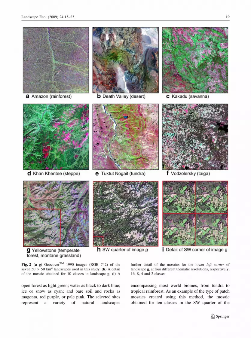
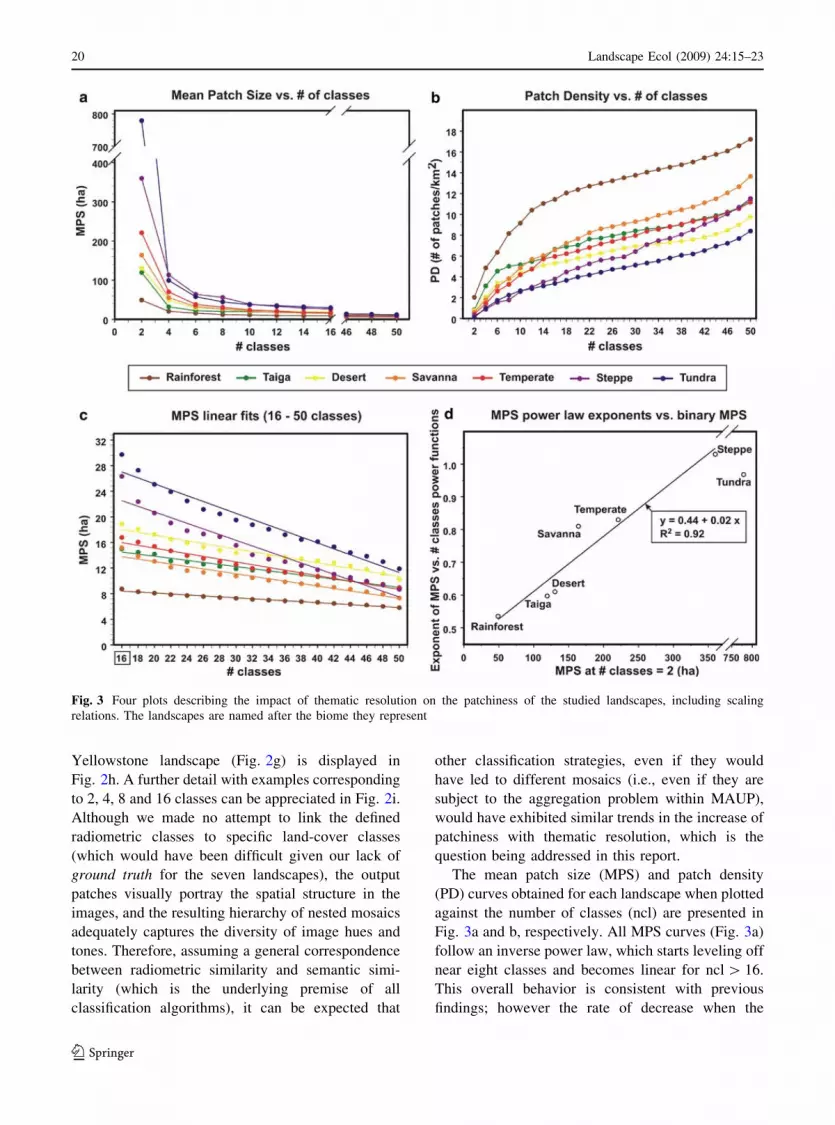