the geographic distribution of indonesia’s east java manufacturing industries

__________________ Région et Développement n° 33-2011 ___________________

THE GEOGRAPHIC DISTRIBUTION OF INDONESIA’S EAST JAVA MANUFACTURING

INDUSTRIES

Andi IRAWAN Abstract - This study investigates the spatial distribution of large and medium manufacturing industries in Indonesia’s East Java province. The topics of investigation include the degree of localisation and co-localisation, the randomness of the observed localisation, and the industrial structures of cities. The factors that contribute to the localisation and specialisation are also examined. Applying the notion of neighbourhood effects and the approach of spatial dependence model, some sorts of agglomeration spillovers are observed. Key-words: AGGLOMERATION ECONOMIES, LOCALISATION, SPECIALISATION JEL classification: C31, R12, R58

Department of Urban and Regional Planning and Regional Economics Applications Laboratory (REAL), University of Illinois at Urbana-Champaign, USA; [email protected]

186 Andi Irawan

INTRODUCTION

Among Indonesia‟s 32 provinces, East Java is both the second most populous region and the second largest regional economy in the country. In terms of economic size, the Central Statistics Agency (BPS) records that East Java‟s share

1 of national gross domestic product (GDP) was 15.5% in 2001 and

second to Jakarta whose share was 16.3% in the same year (BPS, 2002a). A sizeable portion of East Java economy is attributable to the manufacturing sector. In 2002, the sector contributed a little over 14% of the province‟s total employment (BPS, 2002a).

Indeed, manufacturing industries have long been playing a significant role in the East Java economy. Mackie (1993) observes that East Java‟s manu-facturing base had been well developed even before the World War II in comparison with other provinces within the country. Furthermore, he concludes that the growth of manufacturing industries, particularly in the late 1980s, has become a major driving force of East Java‟s development since the 1960s. Recent data shows that manufacturing industries‟ share of East Java GDP consistently fell within the range of 26% to 28% in a period of 1998-2002 (BPS, 2002b). Given its contribution to the economy, manufacturing employment is spread across the province.

Manufacturing industries in East Java are heavily concentrated geogra-phically. Dick (1993: 243) notes that “employment in the large and medium sector is quite heavily concentrated”. Yet, Dick‟s (1993) study is rather a narration on history of East Java manufacturing industries and an elaborative discussion on some main industries. It does not examine the underlying forces of such observed geographic concentration. In addition, annual growth of East Java manufacturing industries in post 1998 economic crisis was relatively stable at 1.6%, based on the 1993 constant price. Thus, East Java manufacturing industries is worth studying using the current available data.

With regard to this phenomenon of industrial agglomeration, this study is aiming at investigating the spatial pattern of East Java‟s industrial activities. This study can further examine Dick‟s (1993) initial observation with more rigorous approach to provide insights on these following questions: Does the concentration remain? How concentrated are the industries? How does the geographic distribution of these industries determine the economic structure of East Java cities? Also, this study can provide insights on policy/planning application in the face of agglomeration economies. It is of importance, espe-cially after Indonesia has embarked decentralisation at city level since 2001. East Java is a developed and a populous province in Indonesia whose high number of cities and large geographical area. No more than three provinces in Indonesia have all these characteristics. To my knowledge, there has been no study to address these issues for East Java manufacturing industries using considerably better concentration index and incorporating spatial perspective.

1 It is measured as a ratio of a province‟s regional GDP to Indonesian GDP at a 1993 constant price. The oil and gas sector is excluded in both numerator and denominator.

Région et Développement 187

Following Overman et al. (2003), it starts with an attempt to address two different, but related questions: first is how concentrated a particular industry is and how specialised a particular city is. To address these questions, the cons-truction of some geographical localisation indices (as well as a co-localisation index) and a city specialisation index is needed.

In addressing the question of spatial distribution of firms, researchers have traditionally used concentration indices to examine whether there is agglomeration or dispersion of firms in a given territory (Marcon and Puech, 2003). Since many concentration indices exist, a sensible selection should be made. For a descriptive analysis of localisation and specialisation, this study will primarily use Ellison and Glaeser Index (EG-Index) and Krugman‟s Specialisation Index (Kspec).

The EG-Index of agglomeration and co-agglomeration is able to allow the statistical significance test for the difference between the mean values of geographic concentration and the weighted Herfindahl Index. In other words, this index has a property to see whether employment is only as concentrated as would be expected if locations were chosen randomly by plants in the industry. Because this index is derived from a model that formalises the firms‟ location choices and explicitly takes into account of the agglomeration forces, i.e. natural advantages and spillovers (Ellison and Glaeser, 1997), a statement that suggests that the concentration of East Java manufacturing industries is due to agglomeration forces can then have a sounder basis. A comparison between the 2 and 3-digit industrial code will be made.

The Kspec is chosen because of these particular reasons: first, this study is not in the context of a single industry and second, considering that cities and industries differ in size, this study needs to normalise the share of location i in total employment of industry k and the share of industry k in region‟s i total employment of all industries (Overman et al., 2003). In absolute terms, degree of employment divergence is obtained by Kspec where computational issues are simpler than Gini Coefficient (Krugman, 1991). In addition, since a geographic visualisation is often helpful for a descriptive analysis, relevant maps of spatial pattern of activity will be produced.

The findings detect disparities in the share of large and medium manufacturing employment across 37 cities/municipalities within the province. With a 2.6 skewness statistics in the distribution of the manufacturing employ-ment share, industrial activities are clearly not evenly distributed across places. In both the 2 and 3-digit industrial code, a positive skewness statistics is also obtained in the distribution of various industrial concentration indices that this study develops. In other words, some industries are more localised than the others. Furthermore, this study finds that such observed localisation of industrial activities is higher than would be expected if the firms had chosen locations in a random manner. The industrial localisation also implies that some cities have a different industrial structure in comparison or are more specialised in some activities than the other cities, for which this study provides some evidences.

188 Andi Irawan

Next, this study also seeks possible explanations on what might constitute the observed pattern of industrial agglomeration by carrying out a regression analysis of the determinants of the geographical concentration of industries and of the extent of specialisation across places. In line with most main empirical works on the subject (for example, Amiti, 1997 and Haaland et al., 1999), the underlying forces for localisation and specialisation broadly include variables that represent industry and place characteristics. The industry characteristics consist of the differences in relative technology, in factors intensity, and in scale economies as well as the extent of linkage between firms/industries. General hypothesis is that all these forces will promote geographical concentration of industry and are positively linked to it. The link between area characteristics and its degree of specialisation is not that straightforward, as it depends on each individual characteristic under investigation (Midelfart-Knarvik et al., 2000).

Provided that agglomeration literatures recognise pure external economies as one of the three classic Marshallian sources of external economies due to the interactions between agents (Krugman, 1991), this study also gives considerations to the possible occurrence of spatial spillovers between places which is perceived to have a relationship with a place‟s own corresponding characteristic. To capture spillover effects, spatial dependence regression models (Fotheringham et al., 2000) at a single point of time using a location‟s specialisation index and share of total manufacturing employment as dependent variable are performed to see whether spillovers, apart from locations‟ charac-teristics, are contributing to the places‟ specialisation and manufacturing employment share.

There are some striking features that support a particular prediction given by a particular underlying theory on agglomeration phenomena and/or a priori conventional beliefs. Some model specifications provide evidences that differences in relative technology and scale economies do affect geographical concentration. In addition, there are some findings that spatial spillovers modestly account for differences in manufacturing employment share and the degree of specialisation across East Java cities and somewhat improve explanatory power of the model than the one that is otherwise only explained by underlying area characteristics alone.

The next two sections present the methodology and findings on industrial localisation and on cities‟ specialisation, respectively. Section 3 addresses issues for further research. Section 4 concludes and sheds a light on policy implications.

1. INDUSTRIAL CONCENTRATION

1.1. Methodology

Data

To construct selected concentration indices, this section uses the data sets produced by the East Java Central Statistics Agency (BPS) and is officially published as the Direktori Perusahaan (Companies Directory) (BPS, 2002c). It


lists establishments/plants of large and medium2 scale manufacturing industries

in Indonesia‟s East Java province. The directory provides information on the name, the address (including the location code up to the village level), the main products, the industrial classification code in the five-digit Indonesian standard industrial code (ISIC), and the number of employment of the establishments. By the two-digit ISIC, Indonesia classifies its manufacturing activities into 23 sectors. By the three-digit code, there are 66 industries.

To construct selected explanatory variables, the required data is obtained from the BPS‟ Indikator Sosial-Ekonomi (Social-Economic Indicators) (BPS, 2002b) that provides various indicators in East Java‟s social-economic features, particularly from the section of industrial indicators. This particular section summarises some basic industrial information that also includes industrial input, output, value-added, and labour costs in monetary terms at market prices by the two-digit ISIC. Other information, such as number of firms, is listed by city-level.

To apply the selected methods to the data, appropriate aggregation is made. As for a descriptive analysis, aggregation is made to the two and three-digit industrial code, whereas for regression analysis, data is aggregated to the two-digit code. For both analyses, the spatial unit is at the city level.

Concentration Measures

To measure geographic concentration, researchers generally use three main indices, namely: Herfindahl, GINI, and Ellison and Glaeser (hereafter, referred as EG) Index (Marcon and Puech, 2003). Unlike the former two indices, the EG Index is comparable across activities

3 and takes into account the

industrial concentration4, affected by the size of firms. Moreover, the EG Index

is a „model-based‟ index of geographic concentration that is derived from a model that formalises firms‟ location decisions with regard to two types of agglomeration forces (i.e. natural advantages and spillovers). In this regard, the Index is able to make a meaningful statement on whether some industrial localisations occur just by chance (i.e. in a random manner) or if there are agglomeration forces at work.

Calculating the deviation of the observed industry‟s geographic concentration and the concentration that would result from firms locating randomly makes such a distinction. Ellison and Glaeser (1997) call the former as raw geographical concentration, G, which is calculated as ∑ -

,

2 BPS defines an establishment as „large‟ if it has 100 or more employment and as „small‟ if it has 20 up to 99 employments. The directory includes all manufacturing establishments that were still in active production activities by October 2002. 3 As Marcon and Puech (2003) argue, this property is needed to allow comparison on activity‟s concentration between sectors, since the distribution of all economic activity is taken into account. Herfindahl Index suffers this property, so that it is only able to assess spatial concentration. 4 These properties, of which Gini Index lacks, are important, considering the fact that concentration may occur because of either numerous small-sized firms or few numbers of large firms being located in the same geographic area (Devereaux, 1999).

190 Andi Irawan

where refers to share of the industry‟s employment in area i and is for the share of aggregate manufacturing employment in area i.

They show that if neither of the agglomeration forces mentioned above are present (hence, firms would locate in a random manner), the expected value

of G, denoted by E(G), is ( ∑

) , where ( ∑

) refers to the overall manufacturing activity across locations and H is Herfindahl Index. Therefore, the following is the EG Index, denoted by γ, for any given industry:

( ∑

)

( ∑

)

As Ellison and Glaeser show, the scale of index allows researchers to test the statistical significance of the index against a non-agglomeration benchmark (i.e. E(γ) = 0), i.e. if the observed concentration is only generated by random location choices, with no natural advantages or industry-specific spillovers.

In addition, to assess the tendency of firms from r different more specific sub-sectors belonging to some broad sectors to close together, this study also computes Ellison and Glaeser‟s co-agglomeration index, , defined as follows:

[

∑

] ∑

∑

where G is the raw concentration of the employment in the groups as a whole;

and are the employment share of the kth industry and the plant Herfindahl Index in that industry, respectively;

is the EG Index of the kth

industry; and H =∑

.

As comparison, the absolute and relative concentration indices (as in Haaland et al., 1999) are also computed. For a k

th industry, relative concen-

tration index, , and absolute concentration index is computed as follows:

√

∑

√

∑

where is for the share of the employment in industry k in city i, depicts city i‟s share in total manufacturing employment, and n the number of cities.

Industry Characteristics

For a given industry (recall that industry is indexed with k), the following four explanatory variables for the degree of concentration are constructed: differences in technology, denoted as ; differences in factors intensity


to capture Heckscher-Ohlin‟s effects, denoted as ; differences in scale economies; denoted as ; and for linkages, measured with intermediate goods intensity.

Following Haaland et al. (1999), the index is defined as follows:

√

∑ [

(

)

∑ (

)

∑ (

)

∑ ∑ (

)

]

where and refer to value-added and employment, respectively with sub-index k represents the industry, sub-index i corresponds to the city, and n is the number of cities. Note that this measure is rather a proxy than a direct measure for differences in technology, as it technically measures differences in labour productivity.

Following Amiti (1999), the index HOk is defined as:

*(∑

∑ ) (

∑ ∑

∑ ∑ )+

where LC represents labour costs. In this regard, the data used for LC aggregates wages, benefits, insurance, and other labour costs. As in Amiti (1999) and Paluzie et al. (2001), scale economies and a proxy for linkages are defined as:

∑

∑

∑

∑

where NF depicts number of firms and X is industrial output (measured in monetary terms). 1.2. Industrial Agglomeration Exists

A procedure of the t-test statistics (Mason and Lind, 1996) on the

significance mean difference between mean value of G and ( ∑

) suggest that geographic concentration of East Java industries does exist. The

mean value of G and ( ∑

) across the 20 two-digit sectors5 is 0.13 and

0.06, respectively and the difference between these two numbers is significant at the 5% level of significance. By the three-digit industries, the mean value of

5 Recall that not all Indonesia‟s the 23 two-digit sectors (or the 66 industries by the three-digit ISIC) is available in East Java.

192 Andi Irawan

G and ( ∑

) across the 51 industries is 0.24 and 0.13, respectively and its mean difference is also significant at the 5% level of significance. It is observed that the computed value of both two statistics (i.e. the expected value

of G and ( ∑

) ) is higher in a finer classification of industries.

In both types of industrial code, the expected value of the EG Index, , is highly significantly different from zero (at the 1% level of significance). This also yields the same highly significant result. The result of the hypothesis test against a non-agglomeration benchmark (i.e. = 0) is consistent with the previous tests. These results demonstrate that the concentration of industries is not on a random basis. In other words, the plants in an industry choose their locations not in an independent random manner. It implies that the there are natural advantages and industry specific spillovers at work for the observed concentration.

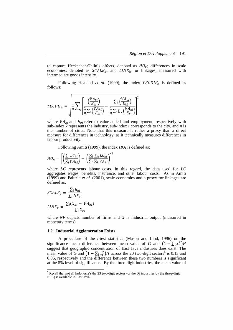
Table 1.1. Raw Concentration Attributable to Spillovers / Comparative Advantage: Fraction of Industries with ∑

/ G in Range

Following Ellison and Glaeser (1997), a rough measure of the portion of raw concentration that is attributable to some spillovers / natural advantage is then developed, defined as the ratio between ∑

and G. Table 1.1.

lists the frequency with which the ∑ /G ratio falls into a number of

intervals for both the two and three-digit industries. This table roughly, but clearly, indicates that most, if not all, East Java manufacturing activities are subject to some sorts of spillovers/natural advantage, regardless of the type of industrial classification.

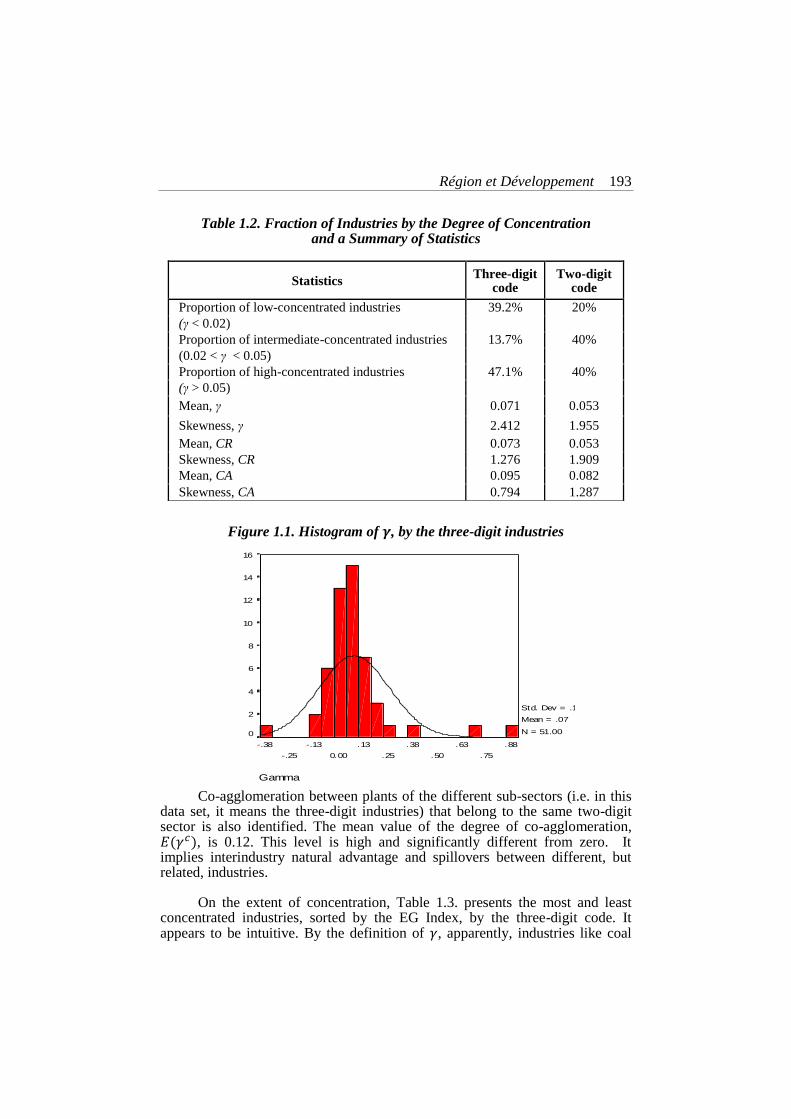
On the patterns of concentration, Table 1.2. provides a statistical

summary on the distribution of industrial concentration, whereas Figure 1.1 visually describes the localisation distribution by three-digit code. The most striking features include: First, the large number of industries falls into the range that Ellison and Glaeser (1997) describe as very localised (if the value of > 0.05). By the three-digit code, the high-concentrated industries account for about 47% of industries. Second, the distribution is substantially skewed in positive direction, indicating that most values are less than mean (Lee and Wong, 2001). Third, this pattern is also present if a broader industrial code (i.e. the two-digit sectors) and other concentration indices (i.e. and ) are used.

Range 3-digit ISIC 2-digit ISIC

< 0 0.196 0.15

.00 - .25 0.157 0.10

.25 - .50 0.235 0.10

.50 - .75 0.314 0.50

.75 - 1.00 0.098 0.15


Table 1.2. Fraction of Industries by the Degree of Concentration and a Summary of Statistics

Figure 1.1. Histogram of , by the three-digit industries

Co-agglomeration between plants of the different sub-sectors (i.e. in this

data set, it means the three-digit industries) that belong to the same two-digit sector is also identified. The mean value of the degree of co-agglomeration, , is 0.12. This level is high and significantly different from zero. It implies interindustry natural advantage and spillovers between different, but related, industries.

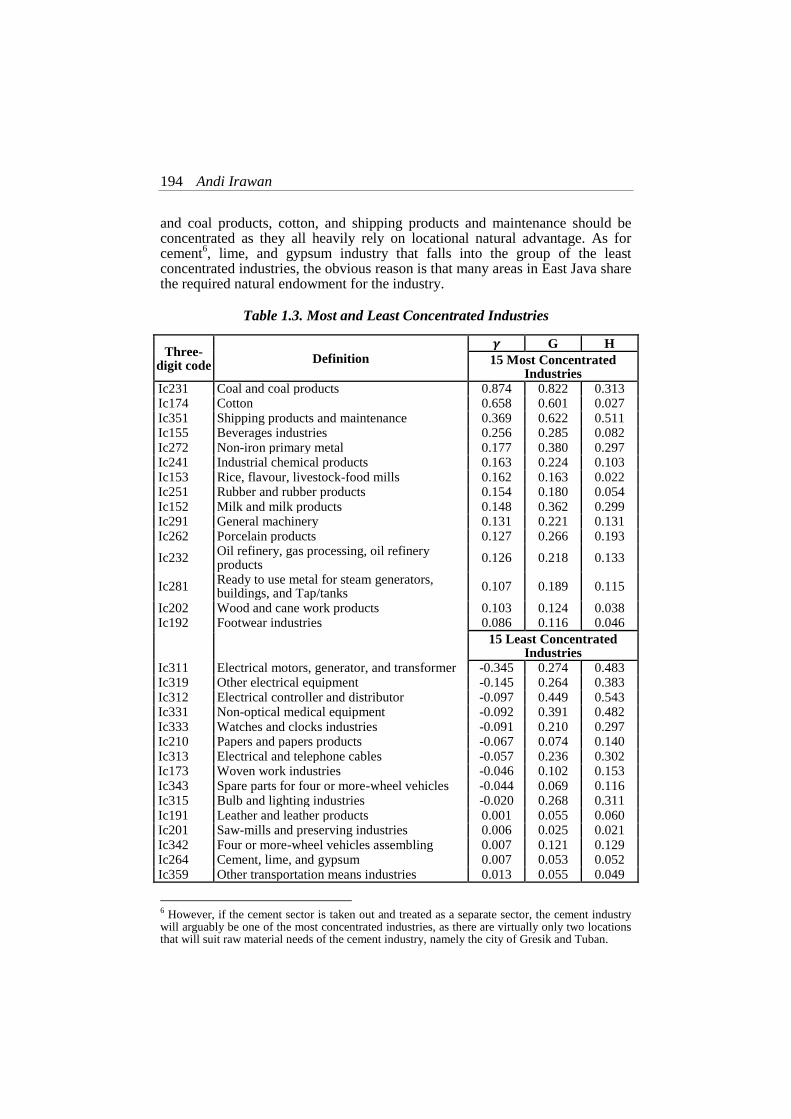
On the extent of concentration, Table 1.3. presents the most and least

concentrated industries, sorted by the EG Index, by the three-digit code. It appears to be intuitive. By the definition of , apparently, industries like coal

Gamma

.88

.75

.63

.50

.38

.25

.13

0.00

-.13

-.25

-.38

Num

ber

of in

dust

ries

16

14

12

10

8

6

4

2

0

Std. Dev = .18

Mean = .07

N = 51.00

Statistics Three-digit

code Two-digit

code

Proportion of low-concentrated industries 39.2% 20%

(γ < 0.02)

Proportion of intermediate-concentrated industries 13.7% 40%

(0.02 < γ < 0.05)

Proportion of high-concentrated industries 47.1% 40%

(γ > 0.05)

Mean, γ 0.071 0.053

Skewness, γ 2.412 1.955

Mean, CR 0.073 0.053

Skewness, CR 1.276 1.909

Mean, CA 0.095 0.082

Skewness, CA 0.794 1.287

194 Andi Irawan

and coal products, cotton, and shipping products and maintenance should be concentrated as they all heavily rely on locational natural advantage. As for cement

6, lime, and gypsum industry that falls into the group of the least

concentrated industries, the obvious reason is that many areas in East Java share the required natural endowment for the industry.

Table 1.3. Most and Least Concentrated Industries

Three-digit code

Definition

G H

15 Most Concentrated Industries

Ic231 Coal and coal products 0.874 0.822 0.313 Ic174 Cotton 0.658 0.601 0.027 Ic351 Shipping products and maintenance 0.369 0.622 0.511 Ic155 Beverages industries 0.256 0.285 0.082 Ic272 Non-iron primary metal 0.177 0.380 0.297 Ic241 Industrial chemical products 0.163 0.224 0.103 Ic153 Rice, flavour, livestock-food mills 0.162 0.163 0.022 Ic251 Rubber and rubber products 0.154 0.180 0.054 Ic152 Milk and milk products 0.148 0.362 0.299 Ic291 General machinery 0.131 0.221 0.131 Ic262 Porcelain products 0.127 0.266 0.193

Ic232 Oil refinery, gas processing, oil refinery products

0.126 0.218 0.133

Ic281 Ready to use metal for steam generators, buildings, and Tap/tanks

0.107 0.189 0.115

Ic202 Wood and cane work products 0.103 0.124 0.038 Ic192 Footwear industries 0.086 0.116 0.046

15 Least Concentrated

Industries

Ic311 Electrical motors, generator, and transformer -0.345 0.274 0.483 Ic319 Other electrical equipment -0.145 0.264 0.383 Ic312 Electrical controller and distributor -0.097 0.449 0.543 Ic331 Non-optical medical equipment -0.092 0.391 0.482 Ic333 Watches and clocks industries -0.091 0.210 0.297 Ic210 Papers and papers products -0.067 0.074 0.140 Ic313 Electrical and telephone cables -0.057 0.236 0.302 Ic173 Woven work industries -0.046 0.102 0.153 Ic343 Spare parts for four or more-wheel vehicles -0.044 0.069 0.116 Ic315 Bulb and lighting industries -0.020 0.268 0.311 Ic191 Leather and leather products 0.001 0.055 0.060 Ic201 Saw-mills and preserving industries 0.006 0.025 0.021 Ic342 Four or more-wheel vehicles assembling 0.007 0.121 0.129 Ic264 Cement, lime, and gypsum 0.007 0.053 0.052 Ic359 Other transportation means industries 0.013 0.055 0.049

6 However, if the cement sector is taken out and treated as a separate sector, the cement industry will arguably be one of the most concentrated industries, as there are virtually only two locations that will suit raw material needs of the cement industry, namely the city of Gresik and Tuban.


1.3. Underlying Agglomeration Forces

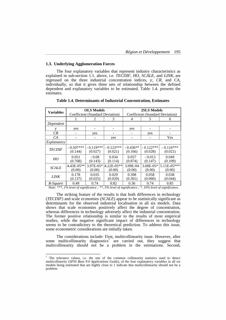
The four explanatory variables that represent industry characteristics as explained in sub-section 1.1. above, i.e. TECDIF, HO, SCALE, and LINK, are regressed on the three industrial concentration indices, , CR, and CA, individually, so that it gives three sets of relationship between the defined dependent and explanatory variables to be estimated. Table 1.4. presents the estimates.

Table 1.4. Determinants of Industrial Concentration, Estimates

Note: ***, 1% level of significance ; **, 5% level of significance ; *, 10% level of significance.

The striking feature of the results is that both differences in technology (TECDIF) and scale economies (SCALE) appear to be statistically significant as determinants for the observed industrial localisation in all six models. Data shows that scale economies positively affect the degree of concentration, whereas differences in technology adversely affect the industrial concentration. The former positive relationship is similar to the results of most empirical studies, while the negative significant impact of differences in technology seems to be contradictory to the theoretical prediction. To address this issue, some econometric considerations are initially taken.

The considerations include: First, multicollinearity issue. However, after some multicollinearity diagnostics

7 are carried out, they suggest that

multicollinearity should not be a problem in the estimations. Second,

7 The tolerance values, i.e. the one of the common collinearity statistics used to detect multicollinerity (SPSS Base 9.0 Applications Guide), of the four explanatory variables in all six models being estimated that are highly close to 1 indicate that multicollinearity should not be a problem.

Variables OLS Models 2SLS Models

Coefficient (Standard Deviation) Coefficient (Standard Deviation)

1 2 3 4 5 6

Dependent

yes - - yes - -

CR - yes - - yes -

CA - - yes - - Yes

Explanatory

TECDIF - 0.507***

(0.144) - 0.119***

(0.027) - 0.123***

(0.021) - 0.436** (0.166)

- 0.122*** (0.028)

- 0.116*** (0.021)

HO 0.051

(0.768) - 0.08

(0.143) 0.034

(0.114) 0.057

(0.874) - 0.013 (0.147)

0.049 (0.109)

SCALE 4.43E-05**

(0.00) 3.97E-05*

(0.00) 4.22E-05**

(0.00) 3.09E-04

(0.00) 3.68E-05*

(0.00) 5.11E-05***

(0.00)

LINK 0.178

(0.137) 0.035

(0.025) 0.029

(0.020) 0.398

(0.361) 0.058

(0.060) 0.038

(0.044)

R-Square 0.49 0.74 0.82 0.36 0.74 0.85

196 Andi Irawan

heteroscedasticity, which is common in any work with cross-section data. Yet, after checking both the normal probability plot of residuals and the plot of standardised predicted values against standardised residuals (as suggested in Maddala, 2002), heteroscedasticity should not be a likely problem. In addition, taking into account that the relationships between dependent and independent variables are, in practice, non-linear, this study did experiment of log trans-formation (as suggested in Thomas, 1997). Still, the estimates with all variables in natural-base log form for both the OLS models and 2SLS models yield the same result, i.e. negative significant impact of technological differences on the predictor variables.

The 2SLS estimation method is employed to deal with the endogeneity issues in the relationships between the dependent and independent variables in general and, particularly, to deal with the observed negative relationship between TECDIF and the response variables. This study is concerned with endogeneity problem because the relationship between agglomeration and its determinants are apparently characterised with circular causation. Though such circular argument in “economic geography and development economics is a virtue, not a vice!” (Krugman and Elizondo, 1996: 139), of course, estimations work requires it to be addressed. To do so, this study uses the mean value of an industry‟s output and input ratio during the period of 1998-2001. As shown, the negative impact of TECDIF is still observed. By this, some possible expla-nations are proposed.

First, recall that this study, so do some other authors mentioned above, proxies differences in technology by differences in labour productivity. As there is generally a positive relationship between productivity and wages, an industry with the high value of TECDIF might first induce geographic concentration by attracting firms in the sector, but later, as wages increase, it might also encourage dispersion. In addition, with not so well established industrial relationship, quite often, labour strikes are the primary means for industrial dispute, especially in more „urbanised‟ cities where unions are generally stronger. By regional standards, the incidence of strikes in some of East Java‟s areas has been much higher than in the other areas and the geographic scope of strikes is widening. This possible counter-force for localisation

8 is also observed

in the de-centralisation case of Brazilian automobile industry, which is basically an industry with high level of productivity (Rodríguez-Pose and Arbix, 2001).

In addition, such endogenous firms‟ decision with respect to the local business can be expected as East Java‟s manufacturing industries are considerably, in spite of by loose criteria, hardly categorised as „high-tech‟ industries that require very specific skills. These industries are mostly rather standardised manufacturing activities (Dick, 1993). In Storper‟s (1997) terms, these sectors are „de-territorialised‟ activities those are able to easily decen-tralise without difficulties in finding suitable labour. Unlike a few cities in other provinces, East Java does not have the following considerably more „high-tech‟

8 Apart from harsh territorial competition among Brazilian‟s state governments that offers, from firms‟ point of view, some advantages.


industries, namely: storage and recording media (Ic223), synthetic fibre (Ic243), and optical instrument and photography equipment (Ic332).

Next, it may also be due to the way TECDIF is defined. In order to best capture the impact of technological differences, Torstensson (1996) suggests that wages must be approximately the same across places in the sample, which is clearly not the case in this study. In fact, the local minimum wages that are annually set by the regional government differ across East Java‟s cities. Moreover, labour productivity (hence, wages) itself may also be endogenous that is greatly affected by local variation in exogenous amenities, such as climate, air quality, and physical geography (Roback, 1982).

Regarding scale economies, while its impact is significant and its expected positive correlation is easier to interpret, its impact magnitude is harder to interpret. Interpreting the estimated coefficients in this case appears to be much less straightforward than in the case of interpreting price elasticity from the estimated coefficients in typical hedonic equations (for example, as in Cheshire and Shepperd, 1995). It is partly due to the natural consequence of the model specification. The specified models only assess static agglomeration, whereas various types of externality that are attributable to localisation of activities may be best viewed in dynamic framework. In addition, more sophisticated measures for scale economies, such as expenditure structure in city i for industry k (Davis and Weinstein, 1999), can be considered. Never-theless, the estimate follows what theory predicts, i.e. scale economies promote industry to spatially agglomerate.

Data shows that differences in resource intensity and industrial linkage have no significant impact on the observed concentration, though the direction of relationships is as expected. On the resource intensity, this result is similar to several European studies (Amiti, 1997; Brűlhart, 1998; Haaland et al., 1999; and Paluzie et al., 2001). All these studies suggest that endowment intensity has no or little effect and is possibly decreasing overtime. Some authors suggest that it is partly related to the process of economic integration that allows freer resources mobility. In this respect, intercity resources mobility within East Java shares the same feature, since trade barriers should not be a problem. This may bring another implication.

The absent of trade barriers may also make the industrial linkage, measured as intermediate goods intensity, not significant as the determinant of concentration. This study did an experiment by regressing this linkage variable with co-agglomeration index, , with model where only the LINK variable was in the model and with the full model with the other three independent variables. In both cases, it is not statistically significant. This study however acknow-ledges that the LINK specification does not distinguish two somewhat different things, i.e. firms‟ intra-industry linkages and firms‟ interindustry linkages. Considering that the latter is stronger than the former

9, a more precise variable

definition to measure a firms‟ intra-industry linkage may result in significant

9 As suggested in the Krugman and Venables‟s (1996) industrial localisation/specialisation model.

198 Andi Irawan

impact of LINK on localisation and co-localisation. In this regard, while the value of and the hypothesis test result on indicate such firms‟ intra-industry linkages (within the same two-digit industries), data is less able to capture the underlying forces.

2. THE SPECIALISATION OF CITIES

2.1. Methodology

Data

This section uses the same data sets that are used in Section 1, i.e. the Direktori Perusahaan (Companies Directory) (BPS, 2002c) and the Indikator Sosial-Ekonomi (Social-Economic Indicators) (BPS, 2002b). The former is used to compute the chosen specialisation index for descriptive analysis, whereas the latter is used to construct the defined exogenous variables for regression analysis. In addition, a digital map of East Java province with city as the lowest spatial unit is used to visually describe geographical inequalities and to help perform the spatial dependence model.

Specialisation Index

Following Midelfart-Knarvik et al. (2000), the Krugman Specialisation Index (Kspec) is used and defined as follows:

∑ (

∑

∑

∑ ∑ )

Under this formula, to construct the measure of specialisation of each city, , this study performs the following steps. First, for each city i, it calculates the share of industry k in that city‟s manufacturing employment, as expressed in the first terms. Then, it calculates the share of the same industry in the employment of all other cities, as expressed in the second terms. Finally, the degree of specialisation for a particular city can be obtained by measuring the difference between the industrial structure of city i and all other cities by taking the absolute value of the difference between these two shares. It takes a minimum value of zero if city i has an industrial structure identical to the other East Java‟s cities and takes a value of two if it has no common industries with the other cities, so that [0,2].

Similarly, a matrix of bilateral differences between the industrial structures of pairs of cities can be constructed by comparing the industry share for each city with the corresponding shares of every other individual cities (Midelfart-Knarvik et al., 2000). In this investigation on the spatial inequalities in manufacturing activities, this study also computes the city i‟s share of total East Java manufacturing employment, denoted


City Characteristics

In the previous section, the concern is whether particular industry characteristics are associated with the degree of concentration. This section considers an important related issue, namely whether particular endowments of a city may affect the industrial structures of the city and its manufacturing share. To do so, this study considers several characteristics, provided in a matrix form denoted X, that are thought to be important in understanding industrial location patterns. These characteristics include population density, agricultural share, share of population with a particular education qualification, GDP, and GDP per capita, and market potential.

2.2. Industrial Structure Across Cities

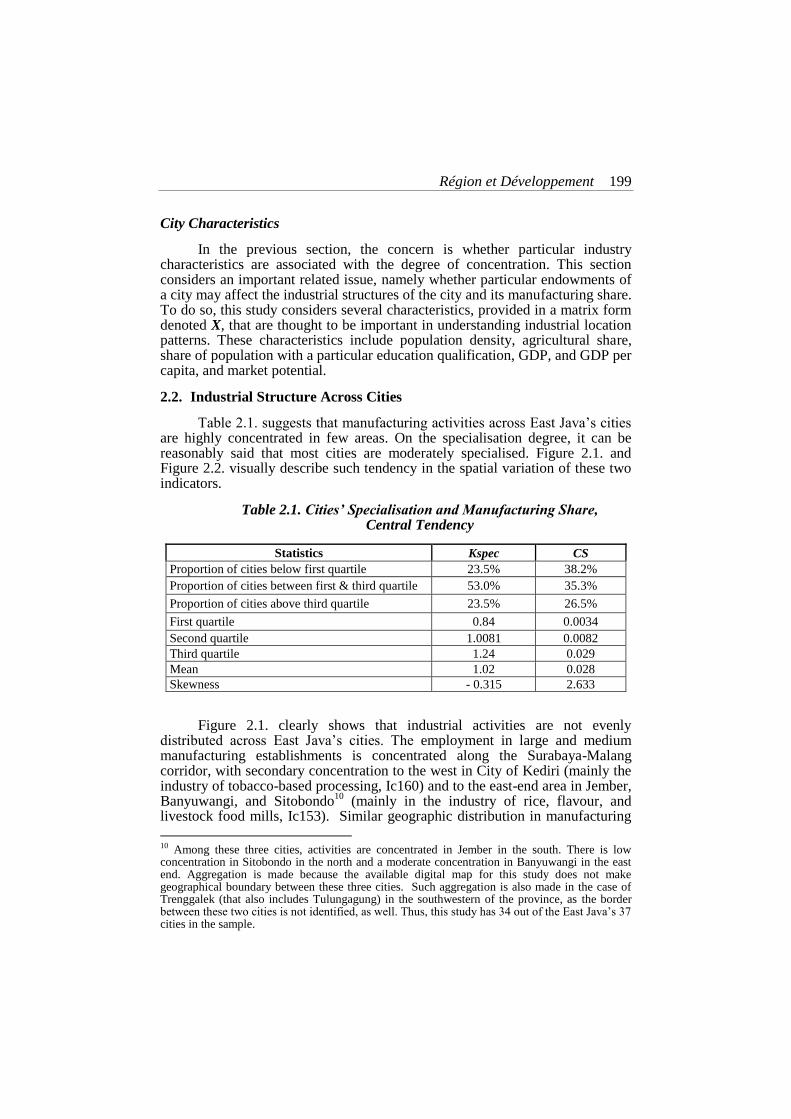
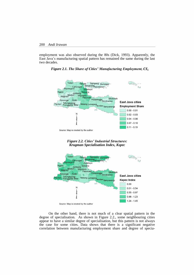
Table 2.1. suggests that manufacturing activities across East Java‟s cities are highly concentrated in few areas. On the specialisation degree, it can be reasonably said that most cities are moderately specialised. Figure 2.1. and Figure 2.2. visually describe such tendency in the spatial variation of these two indicators.

Table 2.1. Cities’ Specialisation and Manufacturing Share, Central Tendency

Statistics Kspec CS

Proportion of cities below first quartile 23.5% 38.2%

Proportion of cities between first & third quartile 53.0% 35.3%

Proportion of cities above third quartile 23.5% 26.5%

First quartile 0.84 0.0034

Second quartile 1.0081 0.0082

Third quartile 1.24 0.029

Mean 1.02 0.028

Skewness - 0.315 2.633

Figure 2.1. clearly shows that industrial activities are not evenly

distributed across East Java‟s cities. The employment in large and medium manufacturing establishments is concentrated along the Surabaya-Malang corridor, with secondary concentration to the west in City of Kediri (mainly the industry of tobacco-based processing, Ic160) and to the east-end area in Jember, Banyuwangi, and Sitobondo

10 (mainly in the industry of rice, flavour, and

livestock food mills, Ic153). Similar geographic distribution in manufacturing

10 Among these three cities, activities are concentrated in Jember in the south. There is low concentration in Sitobondo in the north and a moderate concentration in Banyuwangi in the east end. Aggregation is made because the available digital map for this study does not make geographical boundary between these three cities. Such aggregation is also made in the case of Trenggalek (that also includes Tulungagung) in the southwestern of the province, as the border between these two cities is not identified, as well. Thus, this study has 34 out of the East Java‟s 37 cities in the sample.

200 Andi Irawan

employment was also observed during the 80s (Dick, 1993). Apparently, the East Java‟s manufacturing spatial pattern has remained the same during the last two decades.

Figure 2.1. The Share of Cities’ Manufacturing Employment,

Figure 2.2. Cities’ Industrial Structures: Krugman Specialisation Index, Kspec

On the other hand, there is not much of a clear spatial pattern in the

degree of specialisation. As shown in Figure 2.2., some neighbouring cities appear to have a similar degree of specialisation, but this pattern is not always the case for some cities. Data shows that there is a significant negative correlation between manufacturing employment share and degree of specia-


lisation. With the coefficient of correlation is equal to – 0.46, its magnitude is quite moderate. One possible interpretation is that East Java‟s manufacturing agglomeration may rather exhibit Jacobs externalities. A city‟s initial industrial concentration attracted new plants, but the new entrants might not necessarily come from the same industry. Thus, when more and more establishments were coming into the city, the city‟s manufacturing share went up, but at the same time, the city was increasingly becoming more diversified or less specialised. Data shows that Surabaya, which is the capital city of East Java and the largest sub-regional economy of the province with 18% manufacturing employment share, has Kspec value of 0.42. It suggests that the most urbanised city in the province is the one that is not very specialised.

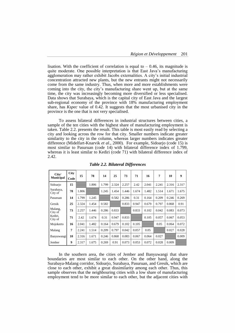
To assess bilateral differences in industrial structures between cities, a

sample of the ten cities with the highest share of manufacturing employment is taken. Table 2.2. presents the result. This table is most easily read by selecting a city and looking across the row for that city. Smaller numbers indicate greater similarity to the city in the column, whereas larger numbers indicates greater difference (Midelfart-Knarvik et al., 2000). For example, Sidoarjo (code 15) is most similar to Pasuruan (code 14) with bilateral difference index of 1.799, whereas it is least similar to Kediri (code 71) with bilateral difference index of 2.42.

Table 2.2. Bilateral Differences

City/ Municipal

City 15 78 14 25 73 71 16 7 10 9

Code

Sidoarjo 15 1.806 1.799 2.324 2.257 2.42 2.041 2.241 2.316 2.317

Surabaya, City of

78 1.806 1.245 1.454 1.446 1.674 1.482 1.514 1.671 1.675

Pasuruan 14 1.799 1.245 0.582 0.286 0.31 0.164 0.209 0.246 0.269

Gresik 25 2.324 1.454 0.582 0.833 0.947 0.679 0.797 0.868 0.91

Malang, City of

73 2.257 1.446 0.286 0.833 0.833 0.102 0.042 0.083 0.073

Kediri, City of

71 2.42 1.674 0.31 0.947 0.833 0.105 0.057 0.067 0.053

Mojokerto 16 2.041 1.482 0.164 0.679 0.102 0.105 0.05 0.064 0.072

Malang 7 2.241 1.514 0.209 0.797 0.042 0.057 0.05 0.027 0.028

Banyuwangi 10 2.316 1.671 0.246 0.868 0.083 0.067 0.064 0.027 0.009

Jember 9 2.317 1.675 0.269 0.91 0.073 0.053 0.072 0.028 0.009

In the southern area, the cities of Jember and Banyuwangi that share boundaries are most similar to each other. On the other hand, along the Surabaya-Malang corridor, Sidoarjo, Surabaya, Pasuruan, and Gresik, which are close to each other, exhibit a great dissimilarity among each other. Thus, this sample observes that the neighbouring cities with a low share of manufacturing employment tend to be more similar to each other, but the adjacent cities with

202 Andi Irawan

high manufacturing employment share tend to have a different industrial structure.

The bilateral differences among cities along the Surabaya-Malang corridor may provide an additional insight. The Jacobs externalities in these cities, as implied by the negative association between the degree of con-centration and the degree of specialisation, are possibly confined within their geographic boundaries. So, even though manufacturing employment are concentrated in the cities along the Surabaya-Malang corridor and, to some extent, these cities have industry structures in common with the rest of East Java, these cities tend to be different among each other. These cities appear to be the case of urbanisation economies (Feldman, 2000).

2.3. Determinants of Specialisation

Apart from city characteristics, the key exogenous variable in econometric analysis to study the determinants of specialisation is market potential. This variable is to capture “the role of market access in the spatial distribution of economic activity” (Hanson, 1998: 9). It is also referred as peripherality index and defined as follows (Copus, 1999):

∑

where is the market potential or peripherality index for location i, M is economic mass variable in location j, and dij is the distance between location i and j. This common expression is basically distance-based weighted for a particular variable. As this study lacks of direct information on the distance between pairs of cities, it will construct market potential, MP, variable with the following approach: first, select GDP as an economic mass variable; second, treat this variable as a spatial lag exogenous variable using distance-based weight method, available in GeoDa (Anselin, 2003).

As suggested in Frost and Spence (1995), self-potential measure should be also considered, defined as a mass variable divided by 0.33r, where r is the radius of the area under consideration. In this regard, this study assumes that each city is a perfect circle to compute its radius, given the information of its geographic size. As opposed to market potential, MP, this self-potential, SELFPOT, is treated as a „standard‟ exogenous variable.

The other exogenous variables include cities‟ agricultural share, AGRSHR; percent population who holds a degree equivalent to junior high school, JHS; percent population who holds a degree equivalent to senior high school, SHS; population density, POPDEN; and living standard measured as per capita income, GDPCAP.

The relationships to be estimated can be expressed in the following full basic model (in matrix form):


(1)

where is dependent variable, is spatial lag exogenous variable (i.e. market potential, MP), X is exogenous variables, and is spatial lag of the dependent

variable (Anselin, 1988). To elaborate more, is an N (i.e. sample size) by 1 vector of observations on the dependent variable; is an N by 1 vector

composed of elements ∑ , the spatial lags of dependent variables (the weight matrix expresses the geographical proximity between city i and city j

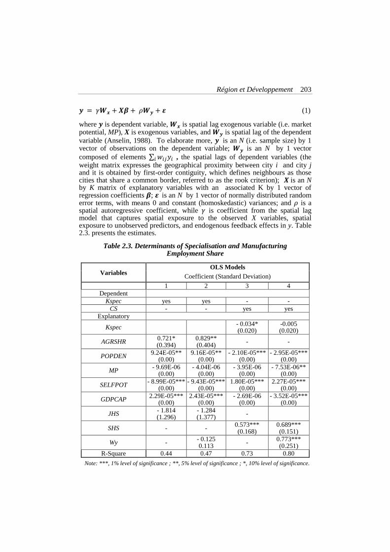
and it is obtained by first-order contiguity, which defines neighbours as those cities that share a common border, referred to as the rook criterion); is an N by K matrix of explanatory variables with an associated K by 1 vector of regression coefficients ; is an N by 1 vector of normally distributed random error terms, with means 0 and constant (homoskedastic) variances; and is a spatial autoregressive coefficient, while is coefficient from the spatial lag model that captures spatial exposure to the observed X variables, spatial exposure to unobserved predictors, and endogenous feedback effects in y. Table 2.3. presents the estimates.

Table 2.3. Determinants of Specialisation and Manufacturing Employment Share

Variables OLS Models

Coefficient (Standard Deviation)

1 2 3 4

Dependent

Kspec yes yes - -

CS - - yes yes

Explanatory

Kspec - 0.034* (0.020)

-0.005 (0.020)

AGRSHR 0.721* (0.394)

0.829** (0.404)

- -

POPDEN 9.24E-05**

(0.00) 9.16E-05**

(0.00) - 2.10E-05***

(0.00) - 2.95E-05***

(0.00)

MP - 9.69E-06

(0.00) - 4.04E-06

(0.00) - 3.95E-06

(0.00) - 7.53E-06**

(0.00)

SELFPOT - 8.99E-05***

(0.00) - 9.43E-05***

(0.00) 1.80E-05***

(0.00) 2.27E-05***

(0.00)

GDPCAP 2.29E-05***

(0.00) 2.43E-05***

(0.00) - 2.69E-06

(0.00) - 3.52E-05***

(0.00)

JHS - 1.814 (1.296)

- 1.284 (1.377)

-

SHS - - 0.573*** (0.168)

0.689*** (0.151)

Wy - - 0.125 0.113

- 0.773*** (0.251)

R-Square 0.44 0.47 0.73 0.80

Note: ***, 1% level of significance ; **, 5% level of significance ; *, 10% level of significance.

204 Andi Irawan

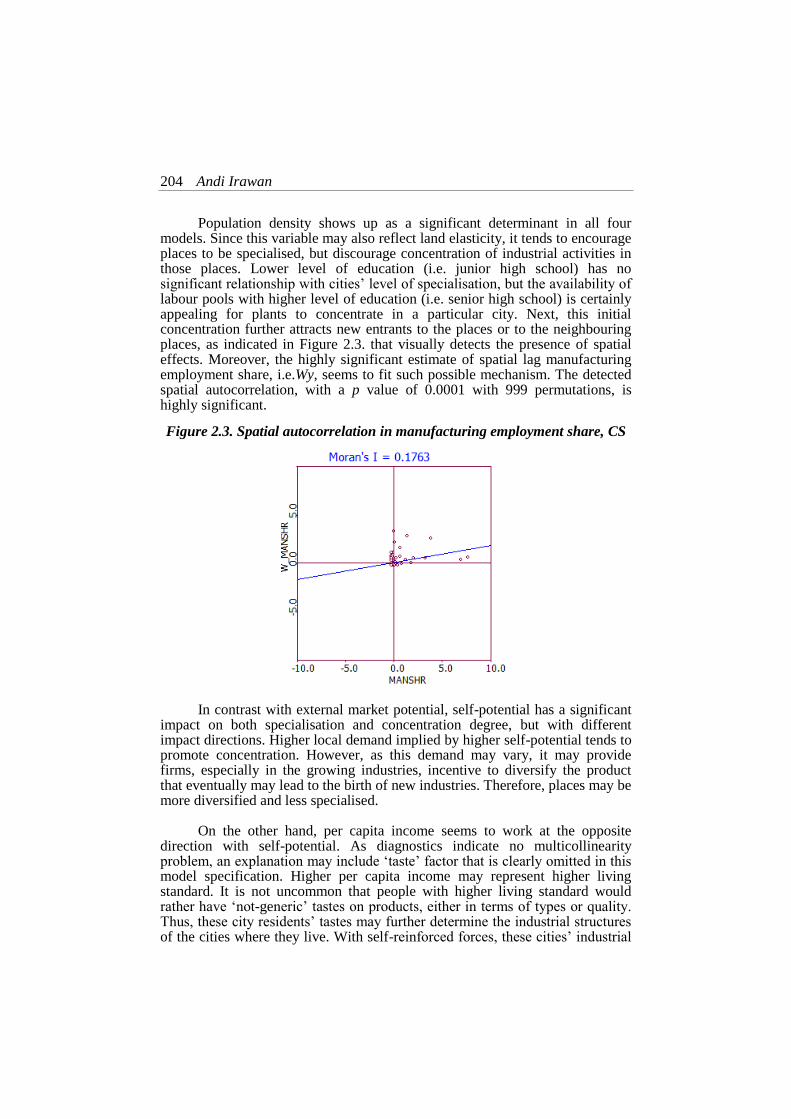
Population density shows up as a significant determinant in all four models. Since this variable may also reflect land elasticity, it tends to encourage places to be specialised, but discourage concentration of industrial activities in those places. Lower level of education (i.e. junior high school) has no significant relationship with cities‟ level of specialisation, but the availability of labour pools with higher level of education (i.e. senior high school) is certainly appealing for plants to concentrate in a particular city. Next, this initial concentration further attracts new entrants to the places or to the neighbouring places, as indicated in Figure 2.3. that visually detects the presence of spatial effects. Moreover, the highly significant estimate of spatial lag manufacturing employment share, i.e.Wy, seems to fit such possible mechanism. The detected spatial autocorrelation, with a p value of 0.0001 with 999 permutations, is highly significant.

Figure 2.3. Spatial autocorrelation in manufacturing employment share, CS

In contrast with external market potential, self-potential has a significant

impact on both specialisation and concentration degree, but with different impact directions. Higher local demand implied by higher self-potential tends to promote concentration. However, as this demand may vary, it may provide firms, especially in the growing industries, incentive to diversify the product that eventually may lead to the birth of new industries. Therefore, places may be more diversified and less specialised.

On the other hand, per capita income seems to work at the opposite

direction with self-potential. As diagnostics indicate no multicollinearity problem, an explanation may include „taste‟ factor that is clearly omitted in this model specification. Higher per capita income may represent higher living standard. It is not uncommon that people with higher living standard would rather have „not-generic‟ tastes on products, either in terms of types or quality. Thus, these city residents‟ tastes may further determine the industrial structures of the cities where they live. With self-reinforced forces, these cities‟ industrial


structure may be increasingly deviating from the industrial structures of other cities. Hence, by measure definition, the level of specialisation will go up. As with the relation between per capita income and the degree of concentration, data gives mixed result depending on the model specification.

3. FURTHER RESEARCH AGENDA

As discussed, the presented findings have some issues and limitations. More limitations are discussed in this section.

As for the EG Index, despite its desirable features, it is still unable to satisfy the criteria that localisation measures “should be defined over the correct spatial units” (Overman et al., 2003). The EG Index certainly does not treat space as continuous. Instead, as other indices commonly do, it treats all locations as boxes that have no relative geography, i.e. describing the location of economic activity on a single scale. In other words, a spatial geographic unit is arbitrarily chosen (e.g. cities as in the case of this study) and the extent of concentration is then calculated based on a set of these spatial units. Therefore, changing the boundary may change the measure and, as it does not take into account the distance between sub-units, very different spatial configurations may end up with the same value (Combes and Overman, 2004).

To address these problems, researchers frequently use Kernel density estimates to determine spatial concentration by analysing the distribution of points (Fotheringham et al., 2000). However, this approach of point patterns analysis heavily relies on more sophisticated data as demonstrated in Duranton and Overman (2002) and Marcon and Puech (2003) and often faces a problem of edge effects due to the spatial point that occurs outside study area.

As for estimations, time-series or panel data method of estimations can be considered to capture the dynamic of agglomeration and help control fixed effects, due to some omitted variables that affect firms‟ location decision, such as local business environments, nature of competition, technological changes, and public policy. It has been discussed that the relationships between variables can be really complex. Such complexity may come from endogeneity or the possibility that the dependent variable is sensitive to its own lags, lags of another endogenous variables, or current and past values of exogenous variables. In this regard, non-linear relationship or reduced form, or structural form can be estimated (Enders, 1995). This kind of approach has been increa-singly common in the studies on spatial inequalities or agglomeration studies, for examples: Combes and Lafourcade (2001), Hanson and Xiang (2002), and Head and Mayer (2004). Still, evidence is highly mixed.

The incorporation of spatial lag manufacturing employment outcomes increases the explanatory power for explaining the pattern of cities‟ share in manufacturing employment. The impact of other city characteristics is mode-rated. It implies that demographic variables alone may not be enough in explaining the concentration of industrial activities across places. However, the

206 Andi Irawan

model specified may not be inadequate in addressing the problem of causality between endogenous and exogenous variables.

In addition, though the weighting method used in estimations is distance-

based weighted, as spillovers are often subject to the distance decay effects (Audretsch, 1998; Jaffe, 1989), a finer digital map is certainly needed, which this study cannot afford. The operational definition of some variables, e.g. market potential, is rather arbitrary due to the data limitation. Addressing this problem may improve the explanatory power of the models, though it may still yield some possible mixed results.

Overall, the estimates performed observe that city characteristics and

spatial spillovers account for city‟s specialisation and share in manufacturing employment. However, due to the limitations discussed above, a cautious interpretation is advised.

4. CONCLUSION AND POLICY IMPLICATION

Throughout the analysis, this study has shown that the spatial pattern of industrial activities in East Java is also subject to some sorts of agglomeration forces that have been outlined by literature. Despite there are several mixed-evidence and observations that do not totally follow what theories have predicted, nevertheless the various results also share the common theme in the field of study on agglomeration, most notably the impact of scale economies. This study also offers some interesting insights on spatial spillovers. While this study is done under static framework, a casual comparison with the spatial patterns during the last two decades suggest that spatial imbalance have persisted and may continually persist unless there are some forces that are capable to create catastrophe. In this regard, any short-term policy, especially without solid framework in assessing these forces that intends to intervene with the observed spatial pattern may appear to be useless.

Under current decentralisation regime, city governments in East Java province are likely tempted to pursue some sorts of territorial competition policy to affect firms‟ location decisions. The common development strategies as presented in city governments‟ development strategic planning and as frequently stated in the press by government officers include attracting investments that create jobs and establishing industrial estates through various incentives, most notably the financial ones. Both already „rich‟ and „poor‟ cities view these seemingly uniform policies as a priority. However, the two categories of cities have different capability in offering incentives. Again, this territorial competition disproportionately favours already „rich‟ cities.

Competition for investment might be inevitable, but it is not always beneficial. Extreme rivalry among places using financial instruments to influence location decisions may end up in a destructive process and undermine any potential gains. Rodríguez-Pose and Gill (2003) use the Brazilian auto-mobile industry as an example for strategy of waste. They show that the excessive use of tax discounts or the donation of land in order to attract


investment had offset the gains of the investment made by firms. The spending of public money to finance such competition diverts public resources to some private actors, rather than being used in growth enhancing policies with positive overall effects.

In this direction, such competition is a negative-sum game (Cheshire and Gordon, 1998). Even if the subsidies or incentives are considerably small, engaging in competition could be of a zero-sum game. Within a regional-national system, attracting inward investment could be merely a distribution of economic activity from one place to other places. It implies that public expenditures are wasteful. Places that offer more incentives are the ones that are going to receive more investments, even though they might be the places without the right preconditions for the attracted investments. As such, it can create allocative inefficiency and price distortions. The firms that were once sponsored by the Italian government to move to the Italian Mezzogiorno eventually relocated back to the Northern Italy that provides better competitive advantage (Rodríguez-Pose, 2002).

Moreover, competition by incentives policies makes investments too

much dependent on subsidies. It gives private sectors higher bargaining power than competing governments. The fierce competition between places encou-rages the former to engage in rent-seeking behaviour or “becoming increasingly adept at extracting subsidies” (Cheshire and Gordon, 1998). It can also raise fiscal burden with increasing level of government debt and cutting public expenditure in welfare and social policies. Taking into account the actual devolutionary process, it should be also noted that territorial competition is deliberately done for political reasons, making the “development” more visible to the voters.

Rather addressing territorial equity, competition may instead promote an uneven geographical distribution of the economic activity. Because richer regions are able to spend more on incentives and poorer regions are in disadvantageous position (Dyker, 1999), economic activities may locate even more in the most successful areas, reinforcing an already uneven concentration of investments and worsening regional disparities.

REFERENCES

Amiti, M., 1997, “Specialisation pattern in Europe”, CEP Discussion Paper no. 363.

Anselin, L., 1988, Spatial Econometrics: Methods and Models, Norwell, MA: Kluwer Academic Publishers.

Anselin, L., 2003, GeoDa 9.0 User’s Guide, SAL and CSISS.

Audretsch, D., 1998, “Agglomeration and the location of innovative activity”, Oxford Review of Economic Policy, vol. 14, pp. 18-29.

208 Andi Irawan

BPS, 2002a, Statistik Indonesia, Jakarta: Badan Pusat Statistik.

BPS, 2002b, Analisis Indikator Makro Sosial & Ekonomi Jawa Timur Tahun 1998-2002:Buku 4, Data Makro Indikator Sosial & Ekonomi Jawa Timur 1998-2002, Surabaya: Badan Pusat Statistik

Jawa Timur. BPS, 2002c, Direktori Perusahaan: Statistik Industri Besar dan Sedang di Jawa Timur 2002, Surabaya: Badan Pusat Statistik Jawa Timur.

Brűlhart, M., 1998, “Economic geography, industry, location and trade: the evidence”, World Economy, vol. 21, pp. 775-801.

Cheshire, P. and I. Gordon, 1998, “Territorial competition: some lessons from policy”, Annals of Regional Science, vol. 32, pp. 321-346.

Cheshire, P. and S. Shepperd, 1995, “On the price of land and the value of amenities”, Economica, vol. 62, pp. 247-267.

Combes, P.-P and M. Lafourcade, 2001, “Transport costs decline and regional inequlities: evidence from France”, CEPR Discussion Paper no. 2894.

Combes, P-P. and H. Overman, 2004, “The spatial distribution of economic activities in the European Union”, in V. Henderson and J-F. Thisse (eds.), Handbook of Urban and Regional Economics, vol. 4. Chapter 64, pp. 2845-2909, Amsterdam: Elsevier B.V.

Copus, A., 1999, “A new peripherality index for NUTS III regions of the European Union”, A Report for the European Commission, Aberdeen: Rural Policy Group, SAC.

Davis, D. and D. Weinstein, 1999, “Economic geography and regional production structure: an empirical investigation”, European Economic Review, vol. 43, pp. 379-407.

Devereaux, M., R. Griffith, and H. Simpson, 2004, “The geographic distribution of production activity in the UK”, Regional Science and Urban Economics, vol. 34, pp. 533-564.

Dick, H., 1993, “Manufacturing”, in H. Dick, J.J. Fox, and J. Mackie (eds.), Balanced Development: East Java in the New Order, pp. 230-255, Oxford: Oxford University Press.

Duranton, G. and H.G. Overman, 2002, “Testing for localisation using micro-geographic data”, CEPR Discussion Paper no. 3379.

Dyker, D., 1999, The European Economy, London: Longman.

Ellison, G. and E.L. Glaeser, 1997, “Geographic concentration in U.S. manufacturing industries: a dartboard approach”, Journal of Political Economy, vol. 105, pp. 889-927.

Enders, W., 1995, Applied Econometric Time Series, Canada: John Wiley & Sons.


Feldman, M. P., 2000, “Location and innovation: the new economic geography of innovation, spillovers and agglomeration”, in G. Clark, M. Gertlers and M. Feldman (eds.), The Oxford Handbook of Economic Geography, pp. 373-394, Oxford: Oxford University Press.

Fotheringham, A. S., C. Brunshon and M. Charlton, 2000, Quantitative Geography: Perspective on Spatial Data Analysis, London: SAGE Publications.

Frost, M. and N. Spence, 1995, “The rediscovery of accessbility and economic potential: the critical issue of self-potential”, Environment and Planning A, vol. 27, pp. 1833-1848.

Haaland, J.I., H.J. Kind, K.H. Midelfart-Knarvik, and J. Torstensson, 1999, “What determines the economic geography of Europe?”, CEPR Discussion Paper no. 2072.

Hanson, G., 1998, “Market potential, increasing returns, and geographic concentration”, NBER Working Paper no. 6429.

Hanson, G. and C. Xiang, 2002, “The home market effect and bilateral trade patterns”, NBER Working Paper no. 9076.

Head, K. and T. Mayer, 2004, “The empirics of agglomeration and trade”, in V. Henderson and J-F. Thisse (eds.), Handbook of Urban and Regional Economics Vol. 4, Chapter 59, pp. 2609-2669, Amsterdam: Elsevier B.V.

Jaffe, A., 1989, “Real effects of academic research”, American Economic Review, vol. 79, pp. 957-970.

Krugman, P., 1991, Geography and Trade, Cambridge, Mass: MIT Press.

Krugman, P. and R. Livas Elizondo, 1996, “Trade policy and the third world metropolis”, Journal of Development Economics, vol. 49, pp. 137-150.

Krugman, P. and A. Venables, 1996, “Integration, specialisation, and adjustment”, European Economic Review, vol. 40, pp. 959-967.

Lee, J. and D. Wong, 2001, Statistical Analysis with ArcView GIS, Canada: John Wiley & Sons.

Mackie, J., 1993, “The East Java economy: from dualism to balanced development”, in H. Dick, J.J. Fox, and J. Mackie (eds.), Balanced Development: East Java in the New Order, pp. 23-53, Oxford: Oxford University Press.

Maddala, G. S., 2002, Introduction to Econometrics, 3rd

edition, England: John Wiley & Sons.

Marcon, E. and F. Puech, 2003, “Evaluating the geographic concentration of industries using distance-based methods”, Journal of Economic Geography, vol. 3, pp. 409-428.

Mason, R. D. and D. A. Lind, 1996, Statistical Techniques in Business and Economics, Irwin McGraw-Hill.

210 Andi Irawan

Midelfart-Knarvik, K.H., H.G. Overman, S.J. Redding, and A.J. Venables, 2000, “The European industry”, Economic Papers no. 142, Brussels: European Commission.

Overman, H. G., S. Redding, and A. J. Venables, 2003, “The economic geography of trade, production, and income: a survey of empirics”, in E. Kwan Choi and J. Harrigan (eds.), pp. 353-387, Handbook of International Trade, Blackwell Pub.

Paluzie, E., J. Pons, and D. Tirado, 2001, “Regional integration and specialisation patterns in Spain”, Regional Studies, vol. 35, pp. 285-296.

Roback, J., 1982, “Wages, rents, and the quality of life”, Journal of Political Economy, vol. 82, pp. 34-55.

Rodríguez-Pose , A., 2002, The role of the ILO in implementing local economic development strategies in a globalised world, Geneva: ILO.

Rodríguez-Pose , A. and G. Arbix, 2001, “Strategies of waste: bidding wars in the Brazilian automobile sector”, International Journal of Urban and Regional Research, vol. 25, pp. 134-154.

Rodríguez-Pose , A. and N. Gill, 2003, “The global trend towards devolution and its implications”, Environment and Planning C: Government and Policy, vol. 21, pp. 333-351.

SPSS Base 9.0 Applications Guide.

Storper, M., 1997, The Regional World: Territorial Development in a Global Economy, New York: The Guilford Press.

Thomas, R., 1997, Modern Econometrics, Essex: Addison-Wesley-Longman.

Torstensson, J., 1996, “Technical differences and inter-industry trade in the Nordic countries”, Scandinavian Journal of Economics, vol. 98, pp. 507-524.

LA DISTRIBUTION GÉOGRAPHIQUE DES INDUSTRIES MANUFACTURIÈRES DANS LA PROVINCE EST

DE JAVA EN INDONÉSIE

Résumé - Cette étude s’intéresse à répartition géographique des moyennes et grandes industries manufacturières dans la province Est de Java en Indonésie. Le but est d’analyser les facteurs qui contribuent à la localisation et la co-localisation des industries et à la spécialisation industrielle des villes. En analysant les effets de voisinage et en utilisant un modèle de dépendance spatiale, certains types d’économies d’agglomération peuvent être mis en évidence.

the geographic distribution of indonesia’s east java manufacturing industries

Documents