MATHEMATICS OF COMPUTATIONVOLUME 61. NUMBER 203JULY 1993, PAGES 319-.349

THE FACTORIZATION OF THE NINTH FERMAT NUMBER

A. K. LENSTRA. H. W. LENSTRA. JR.. NI. S. MANASSE. AND J. M. POLLARD

Dedicated to the nietnori vi D. II Lehiner

ABsTRAcT. In this paper we exhibit the full prime factorization of the ninth

Fermat number F9 = 2512 + I . It is the product of three prime factors that

have 7, 49, and 99 decimal digits. We found the two largest prime factors by

means of the number field sieve, which is a factoring algorithm that depends on

arithmetic in an algebraic number field. In the present case, the number field

used was Q(/) . The calculations were done on approximately 700 worksta

tions scattered around the world, and in one of the final stages a supercomputer

was used. The entire factorization took four months.

INTRODUCTION

For a nonnegative integer k. the kth Fermar number Fk is defined by Fk22& + I The ninth Fermat number F9 = 2512 + I has 155 decimal digits:

F9 = 13407807929942597099574024998205846127479365820592393

377723561443721764030073 546976801874298166903427690031

858186486050853753882811946569946433649006084097.

It is the product of three prime numbers:

F9 =

where p, and p99 have 7, 49, and 99 decimal digits:

V7 = 2424833,

49 = 7455602825647884208337395736200454918783366342657,

99 = 741640062627530801524787141901937474059940781097519

023905821316144415759504705008092818711693940737.

In binary, p7, p49, and p99 have 22, 163, and 329 digits:

Received by the editor March 4. 1991 and, in revised form. August 3. 1992.

1991 Mathematics Subject C1assfication. Primary I 1Y05, I 1Y40.

Key words and phrases. Fermat number, factoring algorithm.

© 1993 Amertcan Mathernai,cal Socieu0025-5i8 93 5100+5.25 per page

319

320 A. K. LENSTRA, H. W. LENSTRA. JR., M. S. MANASSE, AND J. M. POLLARD THE FACTORIZATION OF THE NINTH FERMAT NUMBER 321

= 1001 010000000000000001,

O49 lOl000llOOlllll0000llOOlOll000lOlOOllOOllllOOllOl

iOiiOOllllllOOllOllOlOOlllllOl0000l000llillOlOlOllOOlO

loilOiOiOilil00000ll000lOlOOllOOlOOlOiOiOi0000lOl00000

000001,

D99lOlOllOllOOllOl1OOOllllOlOllOl0OOOOOlOOll 100101010000

101110011110100011001010111000110001111001100101110011

OlOOll000llOlllllOOll000lOOllOOlOlOlOOlOll000lOllOOllO

011110000110110010000110 111011001010010110001100001011

llillllllOOlOOl000lOlOlOlOlOOllllOlOl000llOOlOOllllOlO

010100000000101101 101010111001 000100110001 101101 100000

000001.

The binary representation of F9 itself consists of 511 zeros surrounded by 2ones.

In this paper we discuss several aspects of the factorization of the ninth Fermat number. Section 1 is devoted to Fermat numbers and their place in numbertheory and its history. In §2 we address the general problem of factoring integers, and we describe the basic technique that many modern factoring methodsrely on. In §3 we return to the ninth Fermat number, and we explain why previous factoring attempts of F9 failed. We factored the number by means of thenumber field sieve. This method depends on a few basic facts from algebraicnumber theory, which are reviewed in §4. Our account of the number fieldsieve, in §5, can be read as an introduction to the more complete descriptionsthat are found in [28] and [10]. The actual sieving forms the subject of §6. Thefinal stage of the factorization of F9, which involved the solution of a hugelinear system, is recounted in §7.

1. FERMAT NUMBERS

Fermat numbers were first considered in 1640 by the French mathematician Pierre de Fermat (1601—1665), whose interest in the problem of factoringintegers of the form 2m ± arose from their connection with “perfect”, “amicable”, and “submultiple” numbers [47; 48, Chapter II, §IV]. He remarked thata number of the form 2m + 1 , where m is a positive integer, can be primeonly if m is a power of 2, which makes 2m + 1 a Fermat number. A Fermatnumber that is prime is called a Fermat prime. Fermat repeatedly expressedhis strong belief that all Fermat numbers were prime. Apparently, this beliefwas based on his observation that each prime divisor p of Fk must satisfy astrong condition, namely p 1 mod 2k+l

. In present-day language, one wouldformulate his proof of this as follows. If 22k —1 mod p, then (2 mod p)has multiplicative order 2k+l

, and so 2k+I divides p — 1 , by Fermat’s own“little” theorem, which also dates from 1640. It is not clear whether Fermatwas aware of the stronger condition p 1 mod 2k+2 for prime divisors p ofFk, k > 2. To prove this, it suffices to replace (2 mod p), in the argument

above, by its square root (22’(22 —1) mod p). which has order 2k+2• (It is

amusing to note that also (FkI modp has order 2k+2, because its square isan odd power of (2 mod p).) Incidentally, from the binary representations ofthe prime factors of F9 we see that

ord2(p7— 1) 16, ord2(p49 — 1) = 11. ord-,(p99 — 1) = 11,

where ord2 counts the number of factors 2.The first five Fermat numbers F0 = 3, F1 = 5, F, = 17, F = 257, and

F4 = 65537 are indeed prime, but to this day these remain the only knownFermat primes. Nowadays it is considered more likely, on loose probabilisticgrounds, that there are only finitely many Fermat primes. It may well be thatF0 through F4 are the only ones. On similar grounds, it is considered likelythat all Fermat numbers are squarefree, with perhaps finitely many exceptions.

As for F5, Fermat knew that any prime divisor of F5 must be among 193,449, 577, 641, 769 , which is the sequence of primes that are 1 mod 26,

with F3 257 omitted (distinct Fermat numbers are clearly relatively prime).Thus it is difficult to understand how he missed the factor 641, which is onlythe fourth one to try; among those that are 1 mod 2 , it is the first! One isled to believe that Fermat did not seriously attempt to verify his conjecturenumerically, or that he made a computational error if he did. The factor 641of F5 was found by Euler in 1732, who thereby refuted Fermat’s belief [18].The cofactor F5/641 = 6700417 is also prime.

Gauss showed in 1801 that Fermat primes are of importance in elementarygeometry: a regular n-gon can be constructed with ruler and compasses if andonly if n is the product of a power of 2 and a set of distinct Fermat primes[19].

Since the second half of the nineteenth century, many mathematicians havebeen intrigued by the problem of finding prime factors of Fermat numbers and,more generally, numbers of the form 2m ± 1 . Somewhat later, this interest wasextended to the larger class of Cunningham numbers b’ + 1 (with b smalland m large) [16, 7]. The best factoring algorithms were usually applied tothese numbers, so that the progress made in the general area of factoring largeintegers was reflected in the factorization of Fermat and Cunningham numbers.

The effort required for the complete prime factorization of a Fermat numbermay be expected to be substantially larger than for the preceding one, since thelatter has only half as many digits (rounded upwards) as the former. In severalcases the factorization could be accomplished only by means of a newly inventedmethod. In 1880, Landry factored F6 , but his method was never published (see[25; 17, Chapter XV, p. 377; 20; 50]). In 1970, Morrison and Brillhart foundthe factorization of F7 with the continued fraction method [36]. Brent and thefourth author factored F8 in 1980 by means of a modified version of Pollard’srho method [6]. In 1988, Brent used the elliptic curve method to factor F1(see [4, 5]). Most recently, F9 was factored in 1990 by means of the numberfield sieve.

Unlike methods previously used, the number field sieve is far more effectiveon Fermat and Cunningham numbers than on general numbers. Factoring general numbers of the order of magnitude of F with the number field sieve—orwith any other known method—requires currently substantially more time andfinancial resources than were spent on F : and factoring general numbers ofthe order of magnitude of lOIS F9 is not yet practically feasible.

322 A. K. LENSTRA. H. W, LENSTiA. JR.. M. S. M.ANASSE AND J. M. POLLARD THE FACTORIZATION OF THE NINTH FERMAT NVMBER 323

The fact that the number field sieve performs abnormally well on Fermat

and Cunningham numbers implies that these numbers are losing their value as

a yardstick to measure progress in factoring. One wonders which class of num

bers will take their place. Good test numbers for factoring algorithms should

meet several conditions. They should be defined a priori, to avoid the impres

sion that the factored numbers were generated by multiplying known factors.

They should be easy to compute. They should not have known arithmetic prop

erties that might be exploited by a special factorization algorithm. For any size

range, there should be enough test numbers so that one does not quickly run

out, but few enough to spark competition for them. They should have some

mathematical significance, so that factoring them is a respectable activity. The

last condition is perhaps a controversial one but do we want to factor numbers

that are obtained from a pseudorandom number generator, or from the digits

of it (see [2, 44])? The values of the partition function [1] meet the conditions

above reasonably well, although they appear to be too highly divisible by small

primes. In addition, their factorization is financially attractive (see [42]). We

offer them to future factorers as test numbers. Nonetheless, factoring Fermat

numbers remains a challenging problem, and it is likely to exercise a special

fascination for a long time to come.In addition to the more or less general methods mentioned above, a very

special method has been used to search for factors of Fermat numbers. It

proceeds not by fixing k and searching for numbers p dividing Fk, but by

fixing p and searching for numbers k with Fk 0 mod p. To do this, one

first chooses a number p = u 2’ ± 1 with u odd and 1 relatively large. that is

free of small prime factors; one can do this by fixing one of u, / and sieving

over the other. Next one determines, by repeated squarings modulo p, the

residue classes(22k

mod p), k 2, 3 From what we proved above about

prime factors of Fermat numbers it follows that if no value k <1 — 2 is found

with22k

—1 mod p, then p does not divide any Fk, k > 2; in this case p is

discarded. If a value of k is found with 22&— 1 mod p—which one expects,

loosely, to happen with probability 1/u, if p is prime—then p is a factor of

Fk. The primality of p is then usually automatic from knowledge that one may

have about smaller prime factors of Fk or, if p is sufficiently small, from the

fact that all its divisors are 1 mod 2k+2

Many factors of Fermat numbers have been found by the method just

sketched. In 1903, A. E. Western [15] found the prime factor p 2424833

37 + 1 of F9. In 1984, Keller found the prime factor 5 . 223473 + 1 of

F23471 ; the latter number is the largest Fermat number known to be composite.

If no factor of Fk can be found, one can apply a primality test that is es

sentially due to Pepin [37]: for k > 1 , the number Fk is prime if and only if3(FA—1)/2 —1 mod Fk . This congruence can be checked in time O((logF)3).

and in time O((logF)2)(for any positive e) if one uses fast multiplication

techniques. One should not view Pepin’s test as a polynomial-time algorithm,

however. In fact, the input is k , and from log Fk 2k log 2 we see that the time

that the test takes is a douhli’ exponential function of the length (logk)/log2 of

the input. Pepin’s test has indeed been applied only for a very limited collection

of values of k.Known factors of Fk can be investigated for primality by means of general

primality tests. In this way. Brillhart [22. p. 1101 found in 1967 that the numberF9/2424833, which has 148 decimal digits, is composite. En 1988, Brent andMorain found that F11 divided by the product of four relatively small primefactors is a prime number of 564 decimal digits, thereby completing the primefactonzation of F11.

The many results on factors of Fermat numbers that have been obtained bythe methods above, as well as bibliographic information, can be found in [1 7,Chapter XV; 16, 7, 41, 23]. For up-to-date information one should consult thecurrent issues of Mathematics of Computation, as well as the updates to [7] thatare regularly published by S. S. Wagstaff, Jr. We give a brief summary of thepresent state of knowledge.

The complete prime factorization of Fk is known for k < 9, for k 11and for no other k. One or more prime factors of Fk are known for all k < 32except k = 14, 20, 22, 24, 28, and 31, as well as for 76 larger values of k,the largest being k = 23471. For k = 10, 12, 13, 15, 16, 17, and 18 thecofactor is known to be composite. No nontrivial factor is known of F14 orF20, but it is known that these numbers are composite. For k = 22, 24, 28, 3 1and all except 76 values of k > 32, it is unknown whether Fk is prime orcomposite.

The smallest Fermat number that has not been completely factored is F10.Its known prime factors are

11131 .212 + 1 = 45592577,

395937.214+1=6487031809.

The cofactor has 291 decimal digits. Unless it has a relatively small factor, it isnot likely to be factored soon.

The factorization of Fermat numbers is of possible interest in the theory offinite fields. Let m be a nonnegative integer, and let the field K be obtained bym successive quadratic extensions of the two-element field, so that # K = 22’”

an elegant explicit description of K was given by Conway [14, Chapter 6] andanother by Wiedemann [49]. It is easy to see that the multiplicative group ofK is a direct sum of m cyclic groups of orders F0, F1 , ... , Fm_i . Therefore,knowledge of the prime factors of Fermat numbers is useful if one wishes todetermine the multiplicative order of a given nonzero element of K, or if onesearches for a primitive root of K.

2. FAcToRING INTEGERS

In this section, n is an odd integer greater than 1. It should be thought ofas an integer that we want to factor into primes. We denote by Z the ring ofintegers, by Z/nZ the ring of integers modulo n, and by (Z/nZ)* the groupof units (i.e., invertible elements) of Z/nZ.

2.1. Factoring with square roots of 1. The subgroup {x Z/nZ: x2 I }of (Z/nZ)* may be viewed as a vector space over the two-element field F2 =

Z/2Z, the vector addition being given by multiplication. Many factoring algorithms depend on the elementary fact that the dimension of this vector space isequal to the number of distinct prime factors of n . In particular, if n is not

a power of a prime number, then there is an element x E Z/nZ, x ±1,

324 A. K. LENSTRA, H. W. LENSTRA. JR., M. S. MANASSE. AND J. M. POLLARD THE FACTOR1ZATION OF THE NINTH FERMAT NUMBER 325

such that x2 = 1 . Moreover, explicit knowledge of such an element x,say x = (y mod n), leads to a nontrivial factorization of n. Namely, from

1 mod n, y ±1 mod n, it follows that n divides the product of y —

and y + 1 without dividing the factors, so that gcd(y — 1 , n) and gcd(y + 1 , n)are nontrivial divisors of n. They are in fact complementary divisors, so thatonly one of the gcd’s needs to be calculated; this can be done with Euclid’salgorithm. We conclude that, to factor n, it suffices to find x Z/nZ withx2 = 1, x ±1.

2.2. Repeated prime factors. The procedure just sketched will fail if n is aprime power, so it is wise to rule out that possibility before attempting to factorn in this way. To do this, one can begin by subjecting n to a primality test,as in [27, §5]. If n is prime, the factorization is finished. Suppose that n isnot prime. One still needs to check that n is not a prime power. This checkis often omitted, since in many cases it is considered highly unlikely that n isa prime power if it is not prime; it may even be considered highly likely thatn is squarefree, that is, not divisible by the square of a prime number. Forexample, suppose that n is the unfactored portion of some randomly drawninteger, and one is certain that it has no prime factor below a certain boundB. Then the probability for n not to be squarefree is O(l/(BlogB)), in asense that can be made precise, and the probability that n is a proper powerof a prime number is even smaller. A similar statement may be true if n is theunfactored portion of a Cunningham number, since, to our knowledge, no suchnumber has been found to be divisible by the square of a prime factor that wasdifficult to find. Whether other classes of test numbers that one may proposebehave similarly remains to be seen; if the number n to be factored is providedby a “friend”, or by a colleague who does not yet have sufficient understandingof the arithmetical properties of the numbers that his computations produce, itmay be unwise to ignore the possibility of repeated prime factors.

2.3. Squarefreeness tests. No squarefreeness tests for integers are known thatare essentially faster than factoring (see [9, §7]). This is often contrasted withthe case of polynomials in one variable over a field K, in which case it sufficesto take the gcd with the derivative. This illustrates that for many algorithmicquestions the well-known analogy between Z and K[X] appears to break down.Note also that for many fields K, including finite fields and algebraic numberfields, there exist excellent practical factoring algorithms for K[X] (see [26]),which have no known analogue in Z.

There do exist factoring methods that become a little faster if one wishesonly to test squarefreeness; for example, if n is not a square—which can easilybe tested—then to determine whether or not n is squarefree it suffices to dotrial division up to n’!3 instead of &12.

There is also a factoring method that has great difficulties with numbers nthat are not squarefree. Suppose, for example, that p is a large prime for whichp — 1 and p + 1 both have a large prime factor, and that n has exactly twofactors p. The factoring method described in [43], which depends on the useof “random class groups”, does not have a reasonable chance of finding am’nontrivial factor of n, at least not within the time that is conjectured in [43J(see [32, §11]).

2.4. Recognizing powers. Ruling out that n is a prime power is much easierthan testing n for squarefreeness. One way to proceed is by testing that n isnot a proper power. Namely, if n = in’, where m, / are integers and I > 1then m 3, 2 < / < [(log n)/ log 3], and one may assume that l is prime.Hence, the number of values to be considered for I is quite small, and thisnumber can be further reduced if a better lower bound for m is known, suchas a number B as in §2.2. For each value of I, one can calculate an integer m0for which mo

— n”I < 1 , using Newton’s method, and test whether n =

this is the case if and only if n is an /th power. One can often save time bycalculating m0 only if n satisfies the conditions

and

1 mod j2 (mod8 if? = 2)

E 1 mod qfor several small primes q with q 1 mod 1. These are necessary conditionsfor a number n that is free of small prime factors to be an lth power, if I isprime.

2.5. Ruling our prime powers. There is a second, less well-known way toproceed, which tests only that n is not a prime power. It assumes that onehas already proved that n is composite by means of Fermat’s theorem, whichstates that a’1 a mod n for every integer a, if n is prime. Hence, if aninteger a has been found for which a’1 a mod n, then one is sure that n iscomposite. If n is a prime power, say n k, then Fermat’s theorem impliesthat a” a mod p and hence also that a’1 = a”” a mod p; that is, p dividesa’1 — a, so it’ also divides gcd(a’1 — a, n). This suggests the following approach.Having found an integer a for which (a’1 — a mod n) is nonzero, we calculatethe gcd of that number with n. If the gcd is 1, we can conclude that n is nota prime power. If the gcd is not I, then the gcd is a nontrivial factor of n,which is usually more valuable than the information that n is or is not a primepower.

Nowadays one often proves compositeness by using a variant of Fermat’stheorem that depends on the splitting

i—I

a’1 — a = a (aU— 1). fl(a’12’+ 1),

where n—l=u.2’,with u oddand t=ord2(n—l). Hence, if n isprime,then for any integer a one of the t + 2 factors on the right is divisible by n.This variant has the advantage that the converse is true in a strong sense: if nis not prime, then most integers a have the property that none of the factors onthe right is 0 mod n (see [40] for a precise statement and proof); such integersa are called witnesses to the compositeness of n. Currently, if one is sure thatthe number n to be factored is composite, it is usually because one has foundsuch a witness. Just as above, a witness a can be used to check that n is infact not a prime power: calculate a’1 — a (mod n), which one does most easilyby first squaring the number al42’ (mod n) that was last calculated; if it isnonzero, one verifies as before that gcd(a — a. n) = I , and if it is zero thenone of the t +2 factors on the right has a nontrivial factor in common with n,which can readily be found. (In the latter case, a is in fact not a prime power.since the odd parts of the t + 2 factors are pairwise relatively prime.)

326 A. K. LENSTRA, H. W. LENSTRA JR.. M. S. MANASSE. ND J. M. POLLARD THE FACTORIZAT1ON OF THE NINTH FERMAT NUMBER 327

As we mentioned in § I, the number F/2424833 was proved to be compositeby Brillhart in 1967. We do not know whether he or anybody else proved that itis not a prime power until this fact became plain from its prime factorization.We did not, not because we thought it was not worth our time, but simplybecause we did not think of it. If it had been a prime power, our method wouldhave failed completely, and we would have felt greatly embarrassed towards themany people who helped us in this project. One may believe that the risk thatwe were unconsciously taking was extremely small, but until the number wasfactored this was indeed nothing more than a belief. In any case, it would bewise to include, in the witness test described above, the few extra lines that provethat the number is not a prime power, and to explicitly publish this informationabout a number rather than just saying that it is composite.

2.6. A general scheme. For the rest of this section we assume that n, besidesbeing odd and greater than 1, is not a prime power. We wish to factor n intoprimes. As we have seen, each x E Z/nZ with x2 1, X ±1 gives rise to anontrivial factor of n. In fact, it is not difficult to see that the full factorizationof n into powers of distinct prime numbers can be obtained from a set ofgenerators of the F2-vector space {x E Z/nZ:x2 l} . (If we make this vectorspace into a Boolean ring with x *v (1 + x + v — xv)/2 as multiplication, thena set of ring generators also suffices.) The question is how to determine sucha set of generators. Several algorithms have been proposed to do this, most ofthem following some refinement of the following scheme.

Step 1. Selecting the factor base. Select a collection of nonzero elementsa € Z/nZ, with p ranging over some finite index set P. How this selectiontakes place depends on the particular algorithm; it is usually not done randomly,but in such a way that Step 2 below can be performed in an efficient manner.The collection (aP)PEP is called the factor base. We shall assume that all aare units of Z/nZ. In practice, this is likely to be true. since if n is difficultto factor, one does not expect one of its prime factors to show up in one of thea ‘s; one can verify the assumption, or find a nontrivial factor of n, by meansof a gcd computation. Denote by Z” the additive abelian group consisting ofall vectors (vP)PEp with v, E Z, and let f: Z’ — (Z/nZ)* be the group homomorphism (from an additively to a multiplicatively written group) that sends(v,,),,p to

fJ,,p a . This map is surjective if and only if the elements agenerate (Z/nZ)*

. For the choices of a that are made in practice that is usually the case, although we are currently unable to prove this. (In general, hardlyanything has been rigorously proved about practical factoring algorithms.)

Step 2. Collecting relations. Each element v = (v,,)p of the kernel of fis a relation between the a. in the sense that a,/ = 1 . In the secondstep, one looks for such relations by a method that depends on the algorithm.One stops as soon as the collection V of relations that have been found hasslightly more than # P elements. One hopes that V generates the kernel of .1’,although this is again typically beyond proof. Note that the kernel of I is offinite index in z1’, so that by a well-known theorem from algebra it is freelygenerated by #P elements; therefore, the hope is not entirely unreasonable.

Step 3. Finding dependencies. For each i E V. let ‘U E (Z/2Z)1’= F be thevector that one obtains from i by reducing its coordinates modulo 2. Since# V > # P, the vectors ‘U are linearly dependent over F2 . In Step 3. one finds

explicit dependencies by solving a linear system. The matrix that describes thesystem tends to be huge and sparse, which implies that special methods can beapplied (see [24]). Nevertheless, one usually employs ordinary Gaussian elimination. The size of the matrices may make it desirable to modify Gaussianelimination somewhat; see §7. Each dependency that is found can be writtenin the form = 0 for some subset W c V. and each such subset givesrise to a vector w

= (Z1,v)/2 E Z1’ for which 2 . w belongs to the kernelof f. Each such w, in turn, gives rise to an element x = f(w) (Z/nZ)*satisfying x2 = f(2 w) 1, and therefore possibly to a decomposition of ninto two nontrivial factors. If the factorization is trivial (because x = ±1),or, more generally, if the factors that are found are themselves not prime powers, then one repeats the same procedure starting from a different dependencybetween the vectors ‘U. Note that it is useless to use a dependency that is alinear combination of dependencies that have been used earlier. Also, if severalfactorizations of n into two factors are obtained, they should be combined intoone factorization of n into several factors by a few gcd calculations. One stopswhen all factors are prime powers; if indeed f is surjective and V generatesthe kernel of f, this is guaranteed to happen before all dependencies betweenthe ‘U are exhausted.

2.7. The rational sieve and smoothness. A typical example is the rational sieve.In this factoring algorithm the factor base is selected to be

P = {p: p is prime, p <B},

a,, = (p mod n) (p E P),

where B is a suitably chosen bound. Collecting relations between the a,, isdone as follows. Using a sieve, one searches for positive integers b with theproperty that both b and n + b are B-smooth, that is, have all their primefactors smaller than or equal to B. Replacing both sides in the congruenceb n + b mod n by their prime factorizations, we see that each such b givesrise to a multiplicative relation between the a,, . The main merit of the resulting factoring algorithm—which is, essentially, the number field sieve, with thenumber field chosen to be the field of rational numbers—is that it illustrates thescheme above concisely. The rational sieve is not recommended for practicaluse, not because it is inefficient in itself, but because other methods are muchfaster.

The choice of the “smoothness bound” B is very important: if B, and hence#P, is chosen too large, one needs to generate many relations, and one may endup with a matrix that is larger than one can handle in Step 3. On the otherhand, if B is chosen too small, then not enough integers b will be found forwhich both b and n + b are B-smooth. The same remarks apply to the otheralgorithms that satisfy our schematic description.

In practice, the optimal value for B is determined empirically. In theory,one makes use of results that have been proved about the function cii definedby

yi(x, y) #{m E Z: 0< in <x, in is v-smooth};

so çii(x, y)/[x] is equal to the probability that a random positive integer xhas all its prime factors < y. Brief summaries of these results, which are

328 A. K. LENSTRA, H. W. LENSTRA, JR., M. S. MANASSE, AND J. M. POLLARDTHE FACTORIZATION OF THE NINTH FERMAT NUMBER 329

adequate for the purposes of factoring, can be found in [38, §2; 27, §2.A and(3.16)].

Not surprisingly, one finds that both from a practical and a theoretical pointof view the optimal choice of the smoothness bound and the performance of thefactoring algorithm depend mainly on the size of the numbers that one wishesto be smooth. The smaller these numbers are, the more likely are they to besmooth, the smaller the smoothness bound that can be taken, and the faster thealgorithm. For a fuller discussion of this we refer to [10, § 10].

In the rational sieve, one wishes the numbers b(n + b) to be smooth, andsince b is small, these numbers may be expected to be n0(I) (for n — oc).The theory of the ig-function then suggests that the optimal choice for B is

1/2B = exp((V/2 + o(l))(logn) ‘ (loglogn)1/2)

and that the running time of the entire algorithm is

exp((v1i+o(l))(Iogn)’/2(loglogn)1/2)

(n —

(n -+

(This assumes that the dependencies in Step 3 are found by a method that isfaster than Gaussian elimination.)

2.8. Other factoring algorithms. A big improvement is brought about by thecontinued fraction method [36] and by the quadratic sieve algorithm [38, 45].which belong to the same family. In these algorithms the numbers that onewishes to be smooth are only i/2+o(’) This leads to the conjectured runningtime

exp((1 + o(l))(logn)’/2(loglogn)’/2) (n —b

the smoothness bound being approximately the square root of this. Althoughthe quadratic sieve never had the honor of factoring a Fermat number, it isstill considered to be the best practical algorithm for factoring numbers withoutsmall prime factors.

In the number field sieve [28, 10], the numbers that one wishes to be smoothare o(), or more precisely

exp(O((log n)2!3(log log n)’73)),

and both the smoothness bound and the running time are conjecturally of theform

exp(O((log n)’!3(log logn)2!3))

This leads one to expect that the number field sieve is asymptotically the fastestfactoring algorithm that is known. It remains to be tested whether for numbersin realistic ranges the number field sieve beats the quadratic sieve, if one doesnot restrict to special classes of numbers like Fermat numbers and Cunninghamnumbers.

It is to be noted that the running time estimates that we just gave depend onlyon the number to be factored, and not on the size of the factor that is found.Thus, the quadratic sieve algorithm needs just as much time to find a smallprime factor as to find a large one. There exist other factoring algorithms, notsatisfying our schematic description, that are especially good at finding small

prime factors of a number. These include trial division, Pollard’s p ± 1 method.Pollard’s rho method, and the elliptic curve method (see [27, 31, 3. 34]).

3. THE NINTH FERMAT NUMBER

As we mentioned in §1, A. E. Western discovered in 1903 the factor 2424833of F9, and Brillhart proved in 1967 that F9/2424833 is composite. In thissection we let n be the numberF9/2424833. which has 148 decimal digits:

n = 5529373746539492451469451709955220061537996975706118061624681552800446063738635599565773930892l082l02l0778168305399196915314944498011438291393118209.

We review the attempts that have been made to factor n.We do not believe that the possibility of factoring n by means of the qua

dratic sieve algorithm was ever seriously considered. It would not have beenbeyond human resources, but it would have presented considerable financialand organizational difficulties.

Several factoring algorithms that are good at finding small prime factors hadbeen applied to n. Richard Brent tried Pollard’s p ± 1 method and a modifiedversion of Pollard’s rho method (see [27]), both without success. He estimatesthat if there had been a prime factor less than 1020. it would probably havebeen found by the rho method. The failure of the rho method is simply dueto the size of the least prime factor p49 of n. The p + 1 method would havebeen successful if at least one of the four numbers p49 ± 1

, p99 ± I had beenbuilt from small prime factors. The failure of this method is explained by thefactorizations

p49—l=2l9478248878l’ 1143290228161321.43226490359557706629,

+ 1 = 2.3.167982422287027

.7397205338652138126604651761133609.p99—1=211ll29268l340644377 17338437577121

16975143302271505426897585653131 126520182328037821 729720833840187223,

+ I = 2. 32. 83

.496412357849752879199991393508659621191392758432074313189974107191710682399400942498539967666627.

These factorizations were found by Richard Crandall with the p — I method andthe elliptic curve method. (He used a special second phase that he developed incollaboration with Joe Buhler, that is similar to the second phase given in [3]i

Several people, including Richard Brent, Robert Silverman, Peter Montgomery, Sam Wagstaff, and ourselves, attempted to factor ii using the elliptic curve method, supplemented with a second phase. Brent tried 5000 elliptic curves, his first-phase bound (i.e.. the bound B1 from [34]) ranging from240000 to 400000. This took 200 hours on a Fujitsu VP 100. Robert Silverman and Peter Montgomery tried 500 elliptic curves each, with a first-phasebound equal to 1 000000. We tried approximately 2000 elliptic curves, with

330 A. K. LENSTRA. H. W. LENSTRA, JR. M. S. MANASSE. \ND J. M, POLLARD THE FACTORIZATION OF THE NINTH FERMT NUMBER 331

first-phase bounds ranging from 300000 to 1 000000, during a one-week runon a network of approximately 75 Firefly workstations at Digital EquipmentCorporation Systems Research Center (DEC SRC). The elliptic curve methoddid not succeed in f’nding a factor. Our experience indicates that if there hadbeen a prime factor less than 1030, it would almost certainly have been found.If there had been a factor less than 1040 we should probably have continuedwith the elliptic curve method. Our decision to stop was justified by the finalfactorization, which the elliptic curve method did not have a reasonable chanceof finding without major technological or algorithmic improvements.

The best published lower bound for the prime factors of n that had beenrigorously established before n was completely factored is 1.4. 1014 (see[21, Table 2]). We have been informed by Robert Silverman that the workleading to [35] implied a lower bound 2048. 1010. and that he later improvedthis to 2048. 1012. The best unpublished lower bound that we are aware of is2’ 2.25. iO’, due to Gary Gostin (1987).

If we had been certain—which we were not—that n had no prime factor lessthan 1030, then we would have known that n is a product of either two, three.or four prime factors. Among all composite numbers of 148 digits that have noprime factor less than 1030, about 1 5.8% are products of three primes, about0.5% are products of four primes, and the others are products of two primes.We expected—rightly, as it turned out—to find two prime factors, but some ofus would have been more excited with three large ones.

4. ALGEBRAIC NUMBER THEORY

We factored F9 by means of the number field sieve, which is a factoring algorithm that makes use of rings of algebraic integers. The number field sieve wasintroduced in [28] as a method for factoring Cunningham numbers. Meanwhile,a variant of the number field sieve has been invented that can, in principle, factor general numbers, but it has not yet proved to be of practical value (see[10]).

In this section we review the basic properties of the ring Z[Y], which isthe ring that was used in the case of F9. A more general account of algebraicnumber theory can be found in [46], and for computational techniques we referto [11].

4.1. The number field Q( ‘,Y) and the norm map. The elements of the fieldQ(Y) can be written uniquely as expressions Z-. q1/’, with q belongingto the field Q of rational numbers. For computational purposes we identifythese elements with vectors nonsisting of five rational components q0, q1

, qq3, q4, and addition and subtraction in the field are then just vector additionand subtraction. From the rule 2 one readily deduces how elements ofthe field are to be multiplied. Explicitly, multiplying an element of the field by/3 0q1.iT amounts to multiplying the corresponding column vector bythe matrix

q0 2q4 2q3 2q2 2q1qj qo 2q4 2q3 2q,q2 q1 q0 2q4 2q3q3 q2 q1 q0 2q4q4 q3 q q q0

The norm N(/3) of /3 is defined to be the determinant of this matrix, whichis a rational number. Note that the norm can be written as a homogeneousfifth-degree polynomial in the q, , with integer coefficients. We have

N(/Jy) N(fl)N(y) for /3, y E Q(),because the matrix belonging to fly is the product of the two matrices belongingto /3 and y. Applying this to y = , and using that N(l) I , we find thatN(/3)#0 whenever fl0.

The norm is one of the principal tools for studying the multiplicative structureof the field, and almost all that the number field sieve needs to know aboutmultiplication is obtained from the norm map. In particular, for the purposesof the number field sieve no multiplication routine is needed.

Below it will be useful to know that

(4.2) N(a—bY’)=a--2’b fora.hQ, 1 <i<4.

One proves this by evaluating the determinant of the corresponding matrices.Division in the field can be done by means of linear algebra. since finding

y/,B is the same as solving the equation j3 . x = y, which can be written as asystem of five linear equations in five unknowns. There exist better methods,but we do not discuss these, since the number field sieve needs division just aslittle as it needs multiplication.

4.3. The number ring Z[Y] and smoothness. The elements Z= rp/’ of

Q(Y) for which all r1 belong to Z form a subring, which is denoted by Z[/].If /3 belongs to Z[Y], then the matrix associated with /3 has integer entries,so its determinant N(fl) belongs to Z. If B is a positive real number, thena nonzero element /3 of Z[Y] will be called B-smooth if the absolute valueN(fl)I of its norm is B-smooth in the sense of §2.7. We note that IN(J3H can

be interpreted as the index of the subgroup flZ[Y] = {j3y: y e Z[Y]} ofZ[Y]:

(4.4) IN(fl) = #(Z[Y]//3Z[Y]) for /3 e Z[Y], /3 0.

This follows from the following well-known lemma in linear algebra: if A is ak x k matrix with integer entries and nonzero determinant, and we view A asa map Z —* Zk, then the index of AZk in Zk is finite and equal to detA.

4.5. Ring homomorphisms. We will need to know a little about ring homomorphisms defined on Z[/]. Let R be a commutative ring with 1. If

vS’: Z[Y] —+ R is a ring homomorphism, then the element c (Y) of Rclearly satisfies c5 = 2, where 2 now denotes the element I + 1 of R. Conversely, if c R satisfies c5 = 2, then there is a unique ring homomorphismçt’: Z[Y] — R satisfying = c. namely the map defined by

( ri’) r,c’ (r1 E Z)

here the r, on the right are interpreted as elements of R . just as we put 2 = I + Iabove. We conclude that giving a ring homomorphism from Z[Y] to R is thesame as giving an element c of R that satisfies c5 = 2.

332 A. K. LENSTRA, H. W. LENSTRA. JR., M. S. MANASSE, AND J M. POLLARD THE FACTORIZATION OF THE NINTH FERMAT NUMBER 333

Example. Let n=(2512±l)/2424833, and put R=Z/nZ and c= (2205 mod n).We have 2512 —1 mod n, and therefore

c5 =(2m25 mod n) = (2. (2512)2 mod n) (2 mod n).Hence, there is a ring homomorphism : Z[/ — Z/nZ with p(\Y) =(2205 mod n). This ring homomorphism will play an important role in thefollowing section.

4.6. Fifth roots of 2 in finite fields. One of the first things to do if one wishesto understand the arithmetic of a ring like Z[Y] is to find ring homomorphismstofinitefie/ds of small cardinality. As we just saw, this comes down to finding.for several small prime numbers p, an element c that lies in a finite extension ofthe field F,, = Z/pZ and that satisfies c5 = 2. First we consider the case that clies in F,, itself. Each such c gives rise to a ring homomorphism Z[Y} — F,,,which will be denoted by ‘u,,. The first seven examples of such pairs (p, c)are

(4.7) (2,0), (3, 2), (5, 2), (7, 4), (13, 6), (17, 15), (19, 15).For example, the presence of the pair (17, 15) on this list means that 1 552 mod 17; and the absence of other pairs (1 7, c) means that (1 5 mod 1 7) isthe only zero of X5 —2 in F17. Note that the prime p = 11 is skipped, and thatall other primes less than 20 occur exactly once on the list. In general, each primep that is not congruent to 1 mod 5 occurs exactly once. To prove this, let pbe such a prime and let k be a positive integer satisfying 5k 1 mod (p — 1).Then the two maps f, g: F,, —+ F,, defined by f(x) x5, g(x) = areinverse to each other. Hence, there is a unique fifth root of 2 in F,,, and it isgiven by (2k modp). For a prime p with p 1 mod 5 the fifth-power mapis five-to-one. Therefore, such a prime either does not occur at all, or it occursfive times. For example, p = 11 does not occur, and p = 151 gives rise to thefive pairs

(4.8) (151,22), (151,25), (151,49), (151,90), (151, 116).Asymptotically, one out of every five primes that are 1 mod 5 is of the secondsort.

The case that c lies in a proper extension of F,, is fortunately not neededin the number field sieve. It is good to keep in mind that such c ‘s neverthelessexist. For example, in a field F81 of order 81 the polynomial (X5—2)/(X—.2)X4 + 2X3 + X2 + 2X + I has four zeros; these zeros are conjugate over F3,and they are fifth roots of 2. In the field F361 = Fi9(i) (with i2 = —1). thepolynomial X5 —2 has, in addition to the zero (15 mod 19) from (4.7), twopairs of conjugate zeros, namely 11 ± 3/ and 10 + 7/.4.9. Ideals and prime ideals. We recall from algebra that an ideal of z/jis an additive subgroup b c Z[/1 with the property that ,By b for all /3 E band all ;.‘ Z[Y}. The zero ideal {0} will not be of any interest to us. Thenorm Nb of a nonzero ideal b c Z[/] is defined to be the index of b inZ[/], that is. Nb #(Z[Yj/b) this is finite, since b contains flZ[Y] forsome nonzero /3, and fiZ[Yj has already finite index (see (4.4)).We also recall from algebra that a subset of Z[Yj is an ideal if and onlyif it is the kernel of some ring homomorphism that is defined on Z[Yj. We

call a nonzero ideal a prime ideal, or briefly a prime of Z[Y]. if it is equalto the kernel of a ring homomorphism from Z[/] to some finite field: and ifthat finite field can be taken to be a prime field F,, then the ideal is called afirst-degree prime. Thus (4.7) can be viewed as a table of the “small” first-degreeprimes of Z[/]

If p is a first-degree prime, corresponding to a pair (p, c), then the maptVp,c induces an isomorphism Z[’Y]/p F,,, and therefore Np is equal to theprime number p. Conversely, if p is a nonzero ideal of prime norm p, thenp is a first-degree prime; this is because Z[/]/p is a ring with p elements.and therefore isomorphic to F,,.

In general, the norm of a prime p is a power p’ of a prime number p. andf is called the degree of p. For example, the conjugacy classes of fifth rootsof 2 in F81 and F361 indicated above give rise to one fourth-degree prime ofnorm 81 and two second-degree primes of norm 361. These are the smallestnorms of primes of Z[Yj that are of degree greater than 1.

4.10. Generators of ideals. Most of what we said so far about the ring Z[ /]is, with appropriate changes, valid for any ring that one obtains by adjoiningto Z a zero of an irreducible polynomial with integer coefficients and leadingcoefficient I. At this point, however, we come to a property that does not holdin this generality. Namely,

(4.11) Z[Y] is a principal ideal domain.

which means that every ideal b of Z[/j is a principal ideal, that is. an idealof the form flZ[/], with /3 E Z[V]. If b flZ[/], then /3 is called agenerator of b.

For the proof of (4.11) we need a basic result from algebraic number theory(cf. [46, §10.2]). It implies that there is a positive constant M, the Minkowskiconstant, which can be explicitly calculated in terms of the ring, and which hasthe following property: if each prime ideal of norm at most M is principal.then every ideal of the ring is principal. In the case of the ring Z[/] one findsthat M = 13.92, so only the primes of norm at most 1 3 need to be looked at.From 13 < 81 we see that all these primes are first-degree primes.

We conclude that to prove (4. 11) it suffices to show that the first-degree primescorresponding to the pairs (2,0), (3, 2), (5.2). (7,4). and (13,6) areprincipal. This can be done without the help of an electronic computer. asfollows. Trying a few values for a. b. and i in (4.2). one finds that theelement 1— has norm —7. By (4.4). the ideal (1 Y3)Z[Y] has norm7, so it is a first-degree prime, corresponding to a pair (p, c) with p = 7.But there is only one such pair, namely the pair (7, 4) . We conclude that

the prime corresponding to the pair (7. 4) is equal to (1 — Y3)Z[YJ. andtherefore principal. The argument obviously generalizes to an’ prime numberp that occurs exactly once as the norm of a prime: in other words, if p is aprime number with p I mod 5. and p is the unique prime of norm p. thenfor it E Z[Y] we have

(4.12) p=nZ[]N(iz)=p

Applying this to it = ‘,Y, p = 2. we find that the prime corresponding to(2. 0) is principal. The prime of norm 3 IS taken care of by it = i + ‘Y. the

THE FACTORIZATION OF THE NINTH FERMAT NVMBER 335334 A. K. LEN5TR. H. W. LENSTR.. JR.. M. S. MANASSE, ND J M POLLARD

primeofnorrn 5 by = i+2, andlheprjmeofnorm l3by 3—2.This proves (4.11).

It will be useful to have a version of (4.12) that is also valid for primes thatare 1 mod 5. Let p be a first-degree prime of Z[/]. corresponding to a pair(p. c), and let r Z[Yj. Then we have

(4.13) and JN(ir)H=p.To prove =, suppose that p = rZ[/]. Then we have r E p. and p is thekernelof (ir)=0 .AIso,from(44)weseethat IN(=Npp.To prove r, suppose that t’,() = 0 and N(ir)I = p. Then r belongsto the kernel p of 1, so Z[/j is contained in p. Since they both haveindex p in Z[Y], they must be equal. This proves (4.13).

52 53.Example. The number r 1 + — 2 \/ is found to have norm —151.Substituting successively the values c 22, 25, 49. 90, 116 listed in (4.8) for

we find that only c = 116 gives rise to a number that is 0 mod 151 . Hence,it generates the prime corresponding to the pair (151, 116). (Alternatively,one can determine the correct value of c by calculating the gcd of X5 — 2 andI + X2 — 2X in F151[X], which is found to be X — 116.)4.14. Unique factorizatjon. A basic theorem in algebra asserts that principalideal domains are unique factorization domains. Thus (4.11) implies that thenonzero elements of Z[Y] can be factored into prime elements in an essentiallyunique way. More precisely, let for every prime p of Z[Yj an element 7rwith p = irZ[/] be chosen. Then there exist for every nonzero /1 e Z[Y}uniquely determined nonnegative integers in(p) such that m(p) = 0 for all butfinitely many p, and such that

fi 6 fl 7T”,

where belongs to the group Z[s/ of units of Z[sY], and where the productranges over all primes p of Z[’/j. We have m(p) > 0 if and only if fi E p.and in this case we say that p occurs in /3. We shall call m(p) the number offactors p in /.. Note that we have

(4.15) IN(fl) llNpmp

because N(it) = Np and N(e)( 1, both by (4.4).

Examples. First let /3 = —1 + sY. The norm of /3 is 15, so from (4.15) we seethat only the primes of norms 3 and 5 occur in /3. each with exponent 1. Usingthe generators 1 + and i + that we found above for these primes, weobtain the prime factorization

—l+v2 =61.(1±V2).(l+V2 ),where 61 —l + Note that 8j is indeed a unit, by N(61) 1 and (4.4).Similarly, one finds that the prime factorization of the element 1 + of norm9 is given by

where 6, —1 +2 — /3

+ . The factorization of the number 5 is quite

special: it is given by

(4.16)

where 83 = 8?62

5 = 6 (1 +

4.17. Units. The Dirichiet unit theorem (see [46, §12.41) describes the unit

groups of general rings of algebraic integers. It implies that the group Z[y]*

of units of Z[Y] is generated by two multiplicatively independent units of

infinite order, together with the unit 60 = — I . We found that we could take

these two units of infinite order to be the elements 1 and 62 from the examples

just given, in the sense that every unit 6 that we ever encountered was of the

form8 e0)e)62), with v(0), v(l), v(2) Z.

We never attempted to prove formally that even’ unit is of this form, although

this would probably have been easy from the material that we accumulated.

There exist good algorithms that can be used to verify this (see [8]).

Given a unit 6, one can find the integers v ( i) in the following way. It is easily

checked that N(eo) = —l and that N(81) = N(62) = 1 . Hence, N(6) = e0)

(_1)v(0), and this determines v(0) (mod 2). Next let c1 exp((log2)/5) and

c2 = exp((2iri +log2)/5); these are complex fifth roots of 2. Denote by çt’j the

ring homomorphism from Z[Y] to the field of complex numbers that maps

to c, for i = 1, 2. Then we have

logçL/1(6)j = v(l) .logz(e)) +v(2) .logp(e2),

1ogItI2(6) = v(1) .1ogçti2(&1)+v(2) .logI2(6,)I.

Adirect calculation shows that0, so v(1), v(2) can be solved uniquely from a system of two linear equations.

Since the v(i) are expected to be integers, we can do the computation in limited

precision and round the result to integers. The inverse of the coefficient matrix

can be computed once and for all.

4.18. A table of first-degree primes. The table (4.7) of first-degree primes of

norm up to 19 was, for the purpose of factoring F9, extended up to 1294973;

see §6 for the considerations leading to the choice of this limit. We made the

table by treating all prime numbers p < 1294973 individually. For primes p

that are not 1 mod 5 we found c with the formula c 2k mod p given in §4.6.

For primes p that are 1 mod 5 we first checked whether 2(P_l)15 1 modp,

which is a necessary and sufficient condition for 2 to have a fifth root modulo p.

If this condition was satisfied—which occurred for 4944 primes, ranging from

151 to 1294471—then the five values of c (mod p) were found by means of a

standard algorithm for finding zeros of polynomials over finite fields (see [26]).

The entire calculation took only a few minutes on a DEC31 00 workstation. We

found that there are 99500 first-degree primes of norm up to 1294973, of which

the last one is given by (1294973, 1207394).

4.19. A table of prime elements. For each of the 99500 primes p in our

table we also needed to know an explicit generator n. These can be found by

means of a brute-force search, as follows. Calculate the norms of all elements1 + = 62 .(l +

I336 A. K. LENSTRA, H. W. LENSTRA, JR.. M. S. MANASSE, AND J. M. POLLARD

> r/’ e Z[Y’] for which the integers r, are below some large bound:since the norm is a polynomial of degree five in the r1, one can use a differencescheme in this calculation. Whenever an element is found of which the absolutevalue of the norm is equal to p for one of the pairs (p, C) in the table, then oneknows that a generator of a prime of norm p has been found. If p 1 mod 5.then c is uniquely determined by p, and the pair (p, c) can be crossed off thelist. If p 1 mod 5, then we use (4.13) to determine the correct value of cfor which (p, c) can be crossed off the list.What we actually did was slightly different. We did not search among theelements r/’ as just described, but only among the elements that be-

long to the subring Z[a] of Z[v], where a = —v’ . This enabled us touse a program that was written for a previous occasion. We considered all1092846526 expressions 0s,a’ E Z[a] for which the s1 have no commonfactor, for which s1 0 if s11 through s4 are 0, and that lie in the “sphere”Z=s26”5 15000. In this way we determined 49726 of the 99500 generators. For the other 49774 first-degree prime ideals p the same search producedgenerators for the ideals ap of norm 8 . Np, so that we could determine theproper generators by dividing out a. The whole calculation took only a fewhours on a single workstation.We found it convenient to have N(ir) > 0 for all p. To achieve this, onecan replace by —7t,, if necessary.

5. THE NUMBER FIELD SIEVE

As in §3, we let n be the numberF9/2424833. The account of the numberfield sieve that we give in this section is restricted to the specific case of thefactorization of the number n.To factor n with the number field sieve, we made use of the ring Z[Y]that was discussed in the previous section. As we saw in §4.5, there is a ringhomomorphism ç: Z[Y} —* Z/nZ that maps sY to 2205 mod n. An important role is played by the element a —Y3, which has the property that(a) = (26I5 mod n) = (2103 mod ii). What is important about this is that2103 is very small with respect to n; it is not much bigger than Note thatfor any a, b e Z we have

(5.1) ç(a + ba) = (a + 2’°3b) (in Z/nZ).This equality plays the role that the congruence b n + b mod n played in therational sieve from §2.7.

In the rational sieve, the factor base was formed by all prime numbers up to acertain limit B. In the present case the factor base was selected as follows. Letthe set Pc Z[sY’] consistof: (i)the 99700 prime numbers p B1 = 1295377:(ii) the three generating units & , e , and 87 (see §4.17): (iii) the generators ir.,of the 99500 first-degree primes p ofZ[/] with Np < B2 1294973 (see§4.l8 and 4.19). For each p P. let a,, ço(p) E Z/nZ. These formed thefactor base.Relations were found in several ways. In the first place, there are relationsthat are already valid in Z[Y}. before ( is applied. Three such relations aregiven by = 1, 2

=. and 5 = (l+) (see (4.16)). butwe did not

THE FACTORIZAT10N OF THE NINTH FERMAT NUMBER 337

use these (the first one is in fact useless). In addition, there is one such relation

for each of the 4944 prime numbers p 1 mod 5 that occur five times in the

table of pairs (p, c) from §4.18. Such a prime number p factors in as

(5.2) prrr8.fIJtp.

where is a unit and p ranges over the five primes of norm p. To see this,

observe that from w,(p) = 0 it follows that each of these p’s occurs in p.

Since this accounts for the full norm p5 of p (Cf. (4.15)), we obtain (5.2).

The unit occurring in (5.2) can be expressed in e and e2 by means of the

method explained in §4.17 (the unit i does not occur, since p and the

are of positive norm). Note that for this method we do not need to know the

unit itself, but only the numbers log lw,(8)l for i = 1, 2, and these can by

(5.2) be computed from the corresponding quantities for p and ir.. The 4944

relations found in this way constituted no more than 2.5% of the 200000

relations that we needed.We found the remaining 195000 relations between the a,, by searching

for pairs of integers a, b, with b > 0, satisfying the following conditions:

(5.3) gcd(a,b)1

(5.4) a + 2’°3b is built up from prime numbers < B1 and at most

one larger prime number P1 which should satisfy B1 < Pi <

108;

(5.5) a5 — 8b5( is built up from prime numbers <B2 arid at most one

larger prime number P2, which should satisfy B2 <P2 < lOs.

If the large prime P1 in (5.4) does not occur, then we write P1 = 1 , and likewise

for P2 in (5.5). Pairs a, b for which P1 P2 1 will be called fill relations,

and the other pairs partial relations.We note that the number a5 — Sb5 equals the norm of a + ha. by (4.2).

Hence, condition (5.5), with P2 1 , is equivalent to the requirement that

a + ba be B2-smooth, in the terminology of §4.3.Before we describe, in §6, how the search for such pairs was performed. let

us see how they give rise to relations between the a11. We begin with a lemma

concerning the prime factorizatiOn of elements of the form a + ha

Lemma. Let a, b e Z, gcd(a, h) I . Then all prImeS p that occur n a + ha

are first-degree primes.

ProQf. Suppose that p occurs in a + ha, and let yj be a ring homomorPhism

from Z[/] to a finite field F such that p is the kernel of i. Let p be the

characteristic of F, so that F,, is a subfield of F . We have a + ha p. so

çii(a + ba) = 0, and therefore

(5.6) V(a) =

Note that (a) and (h) belong to F,,. because a. h Z. If b) 0. then

by (5.6) we have VI(a) = 0 as well. so h and a are both divisible by p. which

contradicts that gcd(a. h) = 1. Hence. (h) 0. and from (5.6) we flow see

that w(°) _W(a)/VI(h) also belongs to F,. We claim that yR2) belongs 10

THE FACTORIZAT OF THE NINTH FERMAT NUMBER 339338 A. K. LENSTRA. H. W. LENSTRA, JR., M. S. MANASSE. AND J. M. POLLARD

F,, as well. If p 2. we have ?/i(2)= 0. so 0, which doesbelong to F, . If p 2. then a2 = 2/ implies that ç’(7) ()2/ç’(2),which belongs to F,,. From çt’(’Y) E F,, it follows that ig maps all of Z[Y]to F,,. Hence, p is the kernel of a ring homomorphism from Z[Yj to F,,,which by definition means that it is a first-degree prime. This proves the lemma.The lemma reduces the factorization of a + ha, with gcd(a, b) 1 , tothe factorization of its norm a5

— 8b5, as follows. Let p be a prime numberdividing a5 — 8b5. If p 1 mod 5, then p is the norm of a unique primep, and the number of factors p in a + ha must be equal to the number offactors p in a5 — 8b5. If p 1 mod 5, then we have to determine whichfifth root c of 2 (mod p) is involved. By (5.6), we must have (c mod p)3(a mod p)/(b mod p), and this uniquely determines c, since c3 c’3 mod pgives 2c 2c’ mod p upon squaring. Once we have determined c, we knowwhich p occurs in a + ba. and again the number of factors p in a + ha isequal to the number of factors p in a5 — 8b5.Let us now first consider the case that a, b is a full relation. Then thefactorization of a + ha has the form

a + ba = 6 flwhere 8 is a unit and p ranges over the first-degree primes of norm at mostB2. We just explained how the exponents ii(p) can be determined from theprime factorization of a5 8b5. We can write

8= fJev(1)

1=0

where the v(i) are determined as in §4.17; just as with (5.2), it is not necessaryto calculate 6 for this. Factoring a + 2’°3b. we obtain an identity of the form

a + 2’°3b = flpW(P)

with p ranging over the prime numbers < B and w(p) E Z0 (if a + 2’°3b <0, use —a, —b instead of a, b). Now replace, in (5.1). both sides by theirfactorizations. Then we find that

fl ()UP) fl )iv(P)

In this way, each full relation a, b gives rise to a relation between the a,,.With partial relations the situation is a bit more complicated. They give riseto relations between the a,, only if they are combined into cycles, as describedin [301. In each cycle, one takes an alternating product of relations q(a + ha)qi(a+2103b), in such a way that the large prime ideals and prime numbers cancel.This leads to a relation between the a/) , by a procedure that is completely similarto the one above. It is not necessary to know generators ir for the large primeideals, since these are divided out.

If, in (5.5), we have P2 > 1, then the additional prime ideal corresponds to

the pair (p2 c mod P2). where c a2/(2b2) this is uniquely determined by

P2 unless P2 1 mod 5.

6. SIEvING

The search for pairs a, b satisfying conditions (5.3), (5.4), and (5.5) wasperformed by means of a standard sieving technique that is a familiar ingredient

of the quadratic sieve algorithm (see [381). For a description of this technique

as it is used in the number field sieve, we refer to [28] and [10, §4 and 5].We used 2.2 million values of b , all satisfying 0 < b < 2.5 106. For each b,

we sieved a + 2’°3b with the primes < B1 , and we sieved a5 — 8b5 with the

primes B2, each over l0 consecutive a-values centered roughly at 8115 . b.The best values for a are those that are close to 81/S . b. If we take for

instance b 106 , then for such a ‘s we are asking for simultaneous smoothnessof two numbers close to iO and 8. 1030; for b = iO this becomes 1038 and

8 The quadratic sieve algorithm when applied to n would depend on

the smoothness of numbers close to /ii times the sieve length, which amounts

to at least 1080. This is the main reason why the number field sieve performsbetter for this value of n than the quadratic sieve. The comparison is still veryfavorable when a is further removed from the center of its interval, although

the numbers become larger. The tails of the interval are less important, so the

fact that centering it at 0 would have been better did not bother us.Smaller b-values are more likely to produce good pairs a, b than larger ones.

The best approach is therefore to process the b-values consecutively starting at

1, until the total number of full relations plus the number of independent cycles

among the partial relations that have been found equals 195000. One can

only hope that this happens before b assumes prohibitively large values. Of

course, B1 and B2 must have been selected in such a way that one is reasonablyconfident that this approach will succeed. This is discussed below.

We started sieving in mid-February 1990 on approximately 35 workstationsat Belicore. On the workstations we were using (DEC3IOO’S and SPARC’S)each b took approximately eight minutes to process. We had to split up theaintervalS of length 108 into 200 intervals of length 5. iO , in order to avoid

undue interference with other programs. After a month of mostly night-time

use of these workstations, the first range of l0 b ‘s was covered. MidMarCh,the network of Firefly workstations at DEC SRC was also put to work. Thisapproximately tripled our computing power. With these forces we could have

finished the sieving task within another seven months. However, at the time,

we did not know this, Since we did not know how far we would have to go with

b.Near the end of March it was rumored that we had a competitor. After

attempts to join forces had failed, we decided to accelerate a little by following

the strategy described in [29]. We posted messages on various electronic bulletinboards, such as sci.cryPt and sci.math, soliciting help. A sieving program, plus

auxiliary driver programs to run it, were made available at a central machine

at DEC SRC in Palo Alto to anyone who expressed an interest in helping US.

After contacting one of us persoflallY either by electronic mail or by telephone,

a possible contributor was also provided with a unique range of consecutive

IiI

I

p

I

340 A. K. LENSTRA, H. W. LENSTRA. JR.. M. S. MANASSE. AND J. M. POLLARDb-values. The size of the range assigned to a particular contributor dependedon the amount of free computing time the contributor expected to be able todonate. Each range was sized to last for about one week, after which a new rangewas assigned. This allowed us to distribute the available b ‘s reasonably evenlyover the contributors, so that the b ‘s were processed more or less consecutively.

It is difficult to estimate precisely how many workstations were enlisted in thisway. Given that we had processed 2.2 million b ‘s by May 9, and assuming thatwe mostly got night-time cycles, we must have used the equivalent of approximately 700 DEC3 100 workstations. We thus achieved a sustained performanceof more than 3000 mips for a period of five weeks, at no cost. (Mips is a unitof speed of computing, 1 mips being one million instructions per second.) Thetotal computational effort amounted to about 340 mips-years (1 mips-year isabout 3.15. 1013 instructions). We refer to the acknowledgments at the end ofthis paper for the names of many of the people and institutions who respondedto our request and donated computing time.Each copy of the sieving program communicated the pairs a, h that itfound by electronic mail to DEC SRC, along with the corresponding pair p1P2 and, in the case P2 > 1, P2 1 mod 5, the residue class (a/b mod P2).In order not to overload the mail system at DEC SRC, the pairs were sent atregular intervals. At DEC SRC, these data were stored on disk. Notice thatthe corresponding two factorizations were not sent, due to storage limitations.These were later recomputed at DEC SRC, but only for the relations that turnedout to be useful in producing cycles. The residue class (a/b mod P2) couldalso have been recomputed, but since it simplified the cycle counting we foundit more convenient to send it along. Notice that (a/b modp) distinguishesbetween the five prime ideals of norm P2When we ran the quadratic sieve factoring algorithm in a similar manner (see[29]), we could be wasteful with inputs: we made sure that different inputs weredistributed to our contributors, but not that they were actually processed. Wecould afford this approach because we had millions of inputs, each of whichwas in principle capable of producing thousands of relations. For the numberfield sieve the situation is different: each b produces only a small numberof relations, if any, and the average yield decreases as b increases. In ordernot to lose our rather scarce and valuable “good” inputs (i.e., the small hvalues), we wanted to be able to monitor what happened to them after theywere given out. For this reason, each copy of the sieving program also reportedthrough electronic mail which h ‘s from its assigned range it had completed.This allowed us to check them off from the list of b ‘s we had distributed. Valuesthat were not checked off within approximately ten days were redistributed.Occasionally this led to duplications, but these could easily be sorted out.By May 7 we had used approximately 2.1 million h’s less than 2.5 million.and we had collected 44106 full relations and 2999903 partial relations. Thelatter gave rise to a total of 158105 cycles. Since 44106 + 158105 is wellover 195000, this was already more than we needed. Nevertheless, to facilitatefinding the dependencies, we went on for two more days. By May 9, after approximately 2.2 million h’s, we had 45719 full relations and 176025 cyclesamong 3 114327 partial relations. Only about one fifth of these 3 114327 relations turned out to be useful, in the sense that they actually appeared in oneof the 1 76025 cycles. It took a few hours on a single workstation to find the

THE FACTOR1ZATION OF THE NINTH FERMAT NUMBER 341

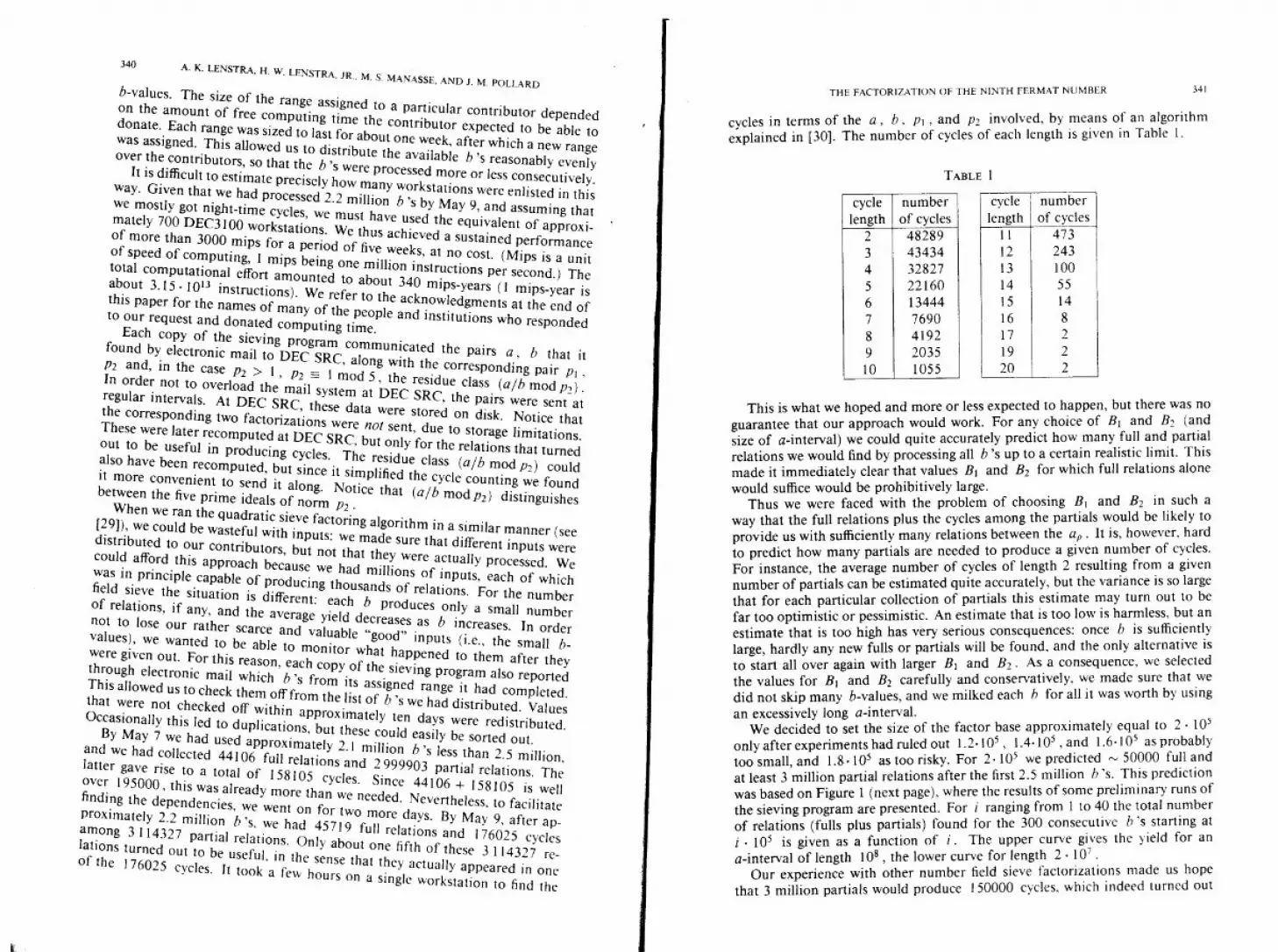
cycles in terms of the a, b . . and p2 involved, b means of an algorithmexplained in [30]. The number of cycles of each length is given in Table 1.

TABLE 1

number,length of cycles

434343282722160

67 \ 134447690

8 41929 2035

This is what we hoped and more or less expected to happen, but there was noguarantee that our approach would work. For any choice of B1 and B’ (and

Size of a-interval) we could quite accurately predict how many full and partialrelations we would find by processing all b ‘s up to a certain realistic limit. This

made it immediatelY clear that values B1 and B2 for which full relations alonewould suffice would be prohibitivelY large.

Thus we were faced with the problem of choosing B1 and B2 in such a

way that the full relations plus the cycles among the partials would he likely to

provide us with sufficiently many relations between the a. it is, however, hard

to predict how many partials are needed to produce a given number of cycles.

For instance, the average number of cycles of length 2 resulting from a given

number of partialS can be estimated quite accurately, but the variance is so large

that for each particular collection of partials this estimate may turn out to be

far too optimistic or pessimistic. An estimate that is too low is harmless. but an

estimate that is too high has very serious0seqUence5 once b is sufficientlY

large, hardly any new fulls or partials will be found. and the only alternative is

to start all over again with larger B1 and B2. As a onsequeflce. we selected

the values for B1 and B2 carefully and onservatily. we made sure that we

did not skip many b-values, and we milked each h for all it was worth by using

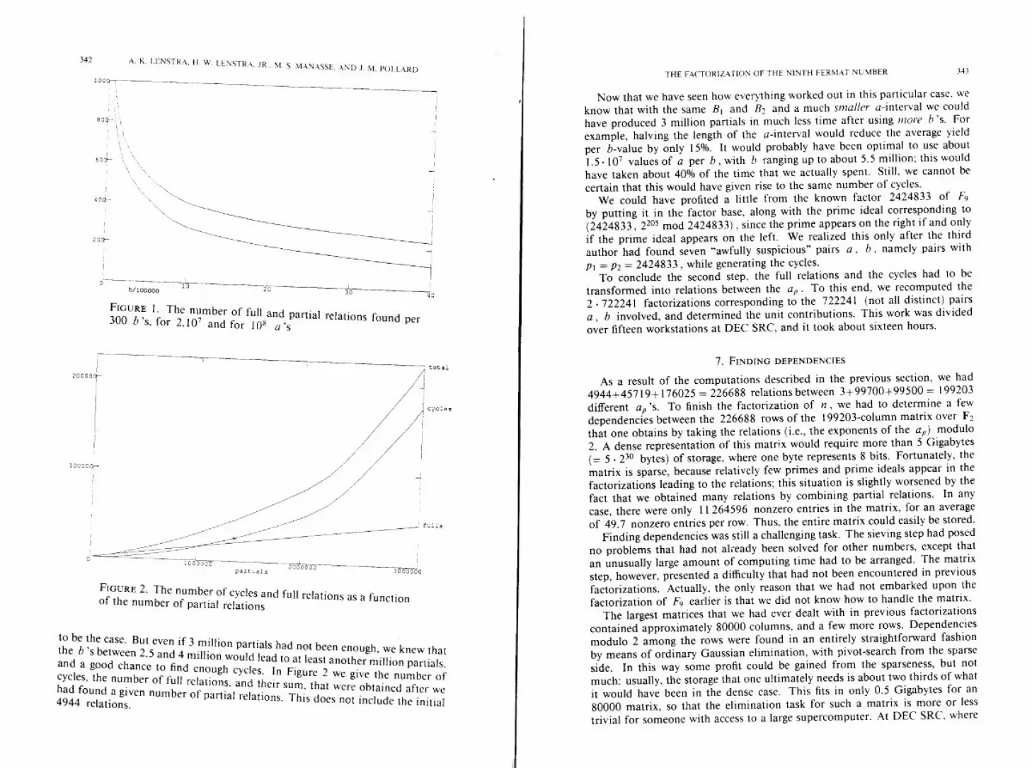
an excessively long ainterval.We decided to set the size of the factor base approximatelY equal to 2. 1 O

only after experiments had ruled out 1.2’ iO, 1.4’ iO , and 1.6’ iO as probablY

too small, and 1.8’ iO as too risky. For 2• iO we predicted 50000 full and

at least 3 million partial relations after the first 2.5 million h ‘s. This prediction

was based Ofl Figure 1 (next page), where the results of some prelimifla’ runs of

the sieving program are presented. For i ranging from I to 40 the total number

of relations (fulls plus partials) found for the 300 consecutive h ‘s starting at

l0 is given as a function of 1. The upper curve gives the ield for an

ainterval of length to8, the lower curve for length 2 l0.

Our experience with other number field sieve factorizat1o made us hope

that 3 million partials would produce 150000 cycles which indeed turned out

1I

III

I1

I

I

342 A. K. LENSTR H. W. FENSTR JR \1. S. \lNS5F ND J M POLLRO

40b/boo00

FIGURE 1. The number of full and partial relations found per300 h’s, for 2.1O and for 108 a’s

t0t0j

20000 Q—

7/

/ // / I

./ /

fulls

-- --——

partuals

FIGURE 2. The number of cycles and full relations as a functionof the number of partial relations

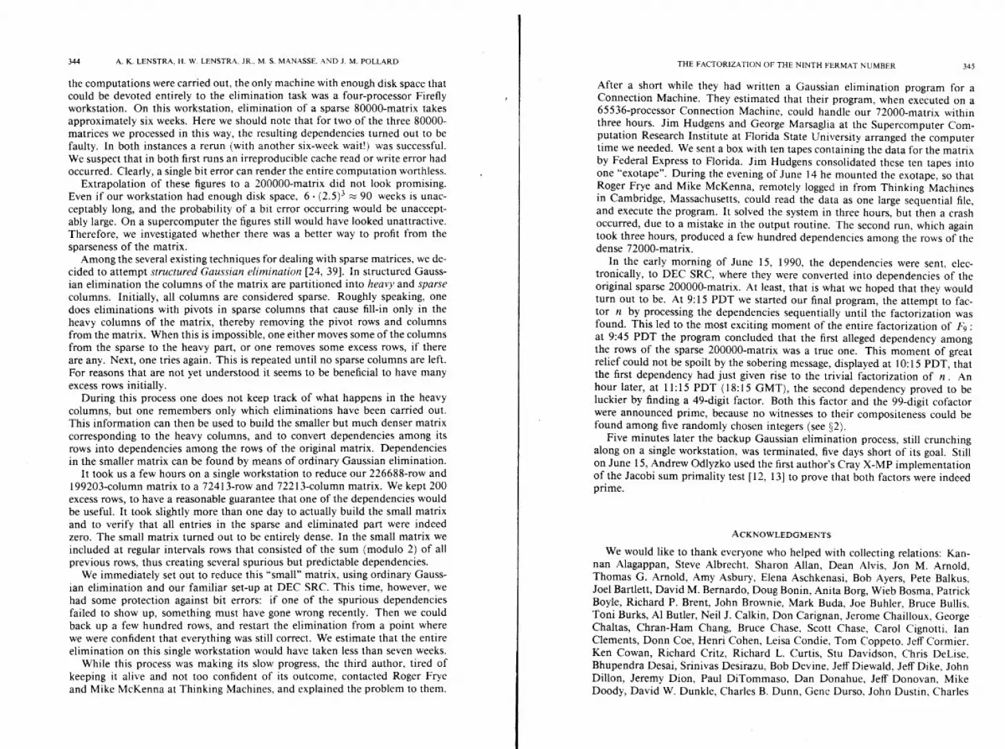
to be the case. But even if 3 million partials had not been enough, we knew thatthe b ‘s between 2.5 and 4 million would lead to at least another million partials,and a good chance to find enough cycles. In Figure 2 we give the number ofcycles, the number of full relations, and their sum, that were obtained after wehad found a given number of partial relations. This does not include the initial4944 relations.

THE FACTORIZATION OF THE NINTH FERMAT NUMBER 343

Now that we have seen how everything worked out in this particular case. we

know that with the same B and B and a much smaller a-interval we could

have produced 3 million partials in much less time after using more h ‘s. For

example, halving the length of the a-interval would reduce the average yield

per b-value by only 15%. It would probably have been optimal to use about

1.5. iO values of a per b, with b ranging up to about 5.5 million this would

have taken about 40% of the time that we actually spent. Still, we cannot be

certain that this would have given rise to the same number of cycles.

We could have profited a little from the known factor 2424833 of F9

by putting it in the factor base, along with the prime ideal corresponding to

(2424833, 2205 mod 2424833). since the prime appears on the right if and only

if the prime ideal appears on the left. We realized this only after the third

author had found seven “awfully suspicious” pairs a, b, namely pairs with

P1 = P2 2424833, while generating the cycles.

To conclude the second step. the full relations and the cycles had to be

transformed into relations between the a. To this end, we recomputed the

2 . 722241 factorizations corresponding to the 722241 (not all distinct) pairs

a, b involved, and determined the unit contributions. This work was divided

over fifteen workstations at DEC SRC. and it took about sixteen hours.

7. FINDING DEPENDENCIES

As a result of the computations described in the previous section, we had

4944+45719+ 176025 = 226688 relations between 3+99700+99500 199203

different a ‘s. To finish the factorization of n, we had to determine a few

dependencies between the 226688 rows of the 199203-column matrix over F

that one obtains by taking the relations (i.e., the exponents of the a,,) modulo

2. A dense representation of this matrix would require more than 5 Gigabytes

(= 5 230 bytes) of storage, where one byte represents 8 bits. Fortunately. the

matrix is sparse, because relatively few primes and prime ideals appear in the

factorizations leading to the relations; this situation is slightly worsened by the

fact that we obtained many relations by combining partial relations. In any

case, there were only 11 264596 nonzero entries in the matrix, for an average

of 49.7 nonzero entries per row. Thus, the entire matrix could easily be stored.

Finding dependencies was still a challenging task. The sieving step had posed

no problems that had not already been solved for other numbers, except that

an unusually large amount of computing time had to be arranged. The matrix

step, however, presented a difficulty that had not been encountered in previous

factorizations. Actually, the only reason that we had not embarked upon the

factorization of F9 earlier is that we did not know how to handle the matrix.

The largest matrices that we had ever dealt with in previous factorizations

contained approximately 80000 columns, and a few more rows. Dependencies

modulo 2 among the rows were found in an entirely straightforward fashion

by means of ordinary Gaussian elimination, with pivot-search from the sparse

side. In this way some profit could be gained from the sparseness, but not

much: usually, the storage that one ultimately needs is about two thirds of what

it would have been in the dense case. This fits in only 0.5 Gigabytes for an

80000 matrix, so that the elimination task for such a matrix is more or less

trivial for someone with access to a large supercomputer. At DEC SRC. where

1D0

401—,

400-

200--

12000 0 /

//

344 A. K. I..ENSTRA. H. W. LENSTRA. JR.. M. S. MANASSE, .ND J. M. POLLARD THE FACTORIZATION OF THE NINTH FERMAT NUMBER 345

the computations were carried out, the only machine with enough disk space thatcould be devoted entirely to the elimination task was a four-processor Fireflyworkstation. On this workstation, elimination of a sparse 80000-matrix takesapproximately six weeks. Here we should note that for two of the three 80000-matrices we processed in this way, the resulting dependencies turned out to befaulty. In both instances a rerun (with another six-week wait!) was successful.We suspect that in both first runs an irreproducible cache read or write error hadoccurred. Clearly, a single bit error can render the entire computation worthless.

Extrapolation of these figures to a 200000-matrix did not look promising.Even if our workstation had enough disk space, 6 (2.5) 90 weeks is unacceptably long, and the probability of a bit error occurring would be unacceptably large. On a supercomputer the figures still would have looked unattractive.Therefore, we investigated whether there was a better way to profit from thesparseness of the matrix.

Among the several existing techniques for dealing with sparse matrices, we decided to attempt structured Gaussian elimination [24, 39]. In structured Gaussian elimination the columns of the matrix are partitioned into heavy and sparsecolumns. Initially, all columns are considered sparse. Roughly speaking, onedoes eliminations with pivots in sparse columns that cause fill-in only in theheavy columns of the matrix, thereby removing the pivot rows and columnsfrom the matrix. When this is impossible, one either moves some of the columnsfrom the sparse to the heavy part, or one removes some excess rows, if thereare any. Next, one tries again. This is repeated until no sparse columns are left.For reasons that are not yet understood it seems to be beneficial to have manyexcess rows initially.

During this process one does not keep track of what happens in the heavycolumns, but one remembers only which eliminations have been carried out.This information can then be used to build the smaller but much denser matrixcorresponding to the heavy columns, and to convert dependencies among itsrows into dependencies among the rows of the original matrix. Dependenciesin the smaller matrix can be found by means of ordinary Gaussian elimination.

It took us a few hours on a single workstation to reduce our 226688-row and199203-column matrix to a 72413-row and 72213-column matrix. We kept 200excess rows, to have a reasonable guarantee that one of the dependencies wouldbe useful. It took slightly more than one day to actually build the small matrixand to verify that all entries in the sparse and eliminated part were indeedzero. The small matrix turned out to be entirely dense. In the small matrix weincluded at regular intervals rows that consisted of the sum (modulo 2) of allprevious rows, thus creating several spurious but predictable dependencies.

We immediately set out to reduce this “small” matrix, using ordinary Gaussian elimination and our familiar set-up at DEC SRC. This time, however, wehad some protection against bit errors: if one of the spurious dependenciesfailed to show up, something must have gone wrong recently. Then we couldback up a few hundred rows, and restart the elimination from a point wherewe were confident that everything was still correct. We estimate that the entireelimination on this single workstation would have taken less than seven weeks.

While this process was making its slow progress, the third author, tired ofkeeping it alive and not too confident of its outcome, contacted Roger Fryeand Mike McKenna at Thinking Machines, and explained the problem to them.

After a short while they had written a Gaussian elimination program for aConnection Machine. They estimated that their program, when executed on a65536-processor Connection Machine, could handle our 72000-matrix withinthree hours. Jim Hudgens and George Marsaglia at the Supercomputer Computation Research Institute at Florida State University arranged the computertime we needed. We sent a box with ten tapes containing the data for the matrixby Federal Express to Florida. Jim Hudgens consolidated these ten tapes intoone “exotape”. During the evening of June 14 he mounted the exotape, so thatRoger Frye and Mike McKenna, remotely logged in from Thinking Machinesin Cambridge, Massachusetts, could read the data as one large sequential file,and execute the program. It solved the system in three hours, but then a crashoccurred, due to a mistake in the output routine. The second run, which againtook three hours, produced a few hundred dependencies among the rows of thedense 72000-matrix.

In the early morning of June 15, 1990, the dependencies were sent, electronically, to DEC SRC, where they were converted into dependencies of theoriginal sparse 200000-matrix. At least, that is what we hoped that they wouldturn out to be. At 9:15 PDT we started our final program, the attempt to factor n by processing the dependencies sequentially until the factorization wasfound. This led to the most exciting moment of the entire factorization of F9:at 9:45 PDT the program concluded that the first alleged dependency amongthe rows of the sparse 200000-matrix was a true one. This moment of greatrelief could not be spoilt by the sobering message, displayed at 10:15 PDT, thatthe first dependency had just given rise to the trivial factorization of n. Anhour later, at 11:15 PDT (18:15 GMT), the second dependency proved to beluckier by finding a 49-digit factor. Both this factor and the 99-digit cofactorwere announced prime, because no witnesses to their compositeness could befound among five randomly chosen integers (see §2).

Five minutes later the backup Gaussian elimination process, still crunchingalong on a single workstation, was terminated, five days short of its goal. Stillon June 15, Andrew Odlyzko used the first author’s Cray X-MP implementationof the Jacobi sum primality test [12, 131 to prove that both factors were indeedprime.

AcKNOwLEDGMENTs

We would like to thank everyone who helped with collecting relations: Kannan Alagappan, Steve Albrecht. Sharon Allan. Dean Alvis, Jon M. Arnold,Thomas G. Arnold, Amy Asbury. Elena Aschkenasi, Bob Ayers, Pete Balkus.Joel Bartlett, David M. Bernardo, Doug Bonin, Anita Borg, Wieb Bosma. PatrickBoyle, Richard P. Brent, John Brownie, Mark Buda, Joe Buhier, Bruce Bullis,Toni Burks, Al Butler, Neil J. Calkin, Don Carignan, Jerome Chailloux, GeorgeChaltas, Chran-Ham Chang, Bruce Chase, Scott Chase, Carol Cignotti, IanClements, Donn Coe, Henri Cohen, Leisa Condie, Tom Coppeto, Jeff Cormier.Ken Cowan, Richard Critz, Richard L. Curtis, Stu Davidson, Chris DeLise.Bhupendra Desai, Srinivas Desirazu, Bob Devine. Jeff Diewald. Jeff Dike, JohnDillon, Jeremy Dion, Paul DiTommaso, Dan Donahue, Jeff Donovan, MikeDoody, David W. Dunkle, Charles B. Dunn, Gene Durso. John Dustin. Charles

346 A. K. LENSTR, H. W. LEcSTR, JR., NI. S. MA.\SSE, AD J. NI. POLLRI) THE FACTORIZATION OF THE NINTH FERMAT NUMBER 347

Dyer, Alan Eustace, Marc Evans, Mike Ferrara, Ed Flecchia. John Forecast.

Joel Foss, Chris Franklin. Sandy Fraser. Hania Gajewska. Sachin Galgalikar.

Edward A. Gardner. Eran Gartner. Morrie Gasser. Eric Gauthier. Lance J. Gay.

Carl Gerstle, David Gibson, Stephen Gildea, Andy Goldstein, Mike Greenfield,

Tim Greenwood, Liz Guth, Ramsey Haddad, Kenneth J. Haduch, Lori Ha

gen, John C. Hallyburton, Jr.. Gary Harding, Bob Harris, Charles Haynes, B. J.

Herbison. Ted Hess, Max Hilison, Buren Hoffman, Jim Horning. Felix S. Hsu.

Han Hsu, Scott Huddleston, Gary Huff. Peter Ilieve. Frank Infante. Philippe

Jacquet, Jeff Janock, Jeff Jenkins, Mike Johnson, Kevin Jones, Dave Juitt, Bill

Kalsow, Irving Kaplansky, Harsh Kapoor, Philip L. Karlton, Bill Katz, Christo

pher A. Kent, Jeff Kenyon, Alan Kirby. Manfred Koethe, John T. Kohl. David

M. Kuchta, Rick Landau, Sundaram Laxman, Ted Lemon. Bill Licea-Kane.

John Linn, Walter Lioen, Todd Little, Jim Lo, Mark Longo, Kevin Lynch, Pat

Madden, Joseph A. Martin, Robert N. Mayo, Murray S. Mazer, James T. Mc

Cartney, Joel McCormack, Ellen McDermott, Randall V. Meyers, Michael J.

Miano, Steven Miller, Thomas Mitchell, Jeffrey Mogul. Bruce Moore. Francois

Morain, A. E. Mossberg, David Mostardi. Victoria Murphy. Gopal Nagarajan.

Jeff E. Nelson, Chuck Newman, Marc Nozell, Vinay Nulkar, Paul E. Oppen

heimer, Lisa Palermo, Bill Parke, Tom Patterson, Eileen Perez, Don Pettini,

Nigel Poole, Eric D. Postpischil, Edward G. Prentice. Dennis Racca. Ram

gopal Ramgiri, Ram Rao, Jon Reeves, Brian Reid, August G. Reinig, Herman

te Riele, John Riley, Buzzy Ritter, John Robinson. D. C. Rocks, David M.

Rosenberg, Eduardo Santiago, Sanjay Saxena, Richard Schedler, Jeffrey I.

Schiller, Michael Sciafani, Jeff Sebring, Mike Sekurski. Shekhar Sengupta, Mark

Shand, Robert Shen, our competitor, John Simakauskas, Al Simons, Michael

Soha, Kiran Somalwar, Bill Sommerfeld, Bob Souza, Vivian Sovinsky. Jerry

Stange, Alan Stanier, John T. Stapleton, Jorge Stolfi, Geof Stone, Steve Strange,

Richard Swan, Ed Taranto, Pahtiban Thilagar, Benjamin J. Thomas III, Bob

Thomas, Gary Thomas, Mathews Thomas, Dennis Ting, Ward Travis, Win

Treese, Tom Truscott, Jim Turner, Percy Tzelnic, Bob Unnold, Srinivasa Up

pugunduri, Mohan Vaghul, Virendra Verma, Brick Verser, Paul Vixie, David

Wall, David F. Wall, Chuck Wan, Bradley M. Waters, Dave Weiss, Dan White,

Bill Whitney, Dick Wilkins, Dik Winter, Ted Wobber, Frank M. Woodall, Jr.,

Tom Woodburn, John Wray, Frank Zereski, Paul Zimmermann. John Zornig.

plus many people at Beilcore and MSRI, at DEC’s research laboratories CRL.

PRL, SRC, and WRL, and at WSE and WSL. This list is incomplete, since

some of our contributors were known to us only as electronic addresses that

were no longer in service when we tried to get their names. We apologize for

any omissions and misspellings.We are also grateful to the people who helped with Gaussian elimination:

Andrew Odlyzko and Carl Pomerance for theoretical assistance, Jim Hudgens,

George Marsaglia and the Supercomputer Computation Research Institute at

Florida State University for computing time on the Connection Machine, and

Roger Frye and Mike McKenna at Thinking Machines for writing and running

a Gaussian elimination program on the Connection Machine.

The Mathematical Sciences Research Institute in Berkeley is gratefully ac

knowledged for giving us the opportunity to meet with various people involved

in this project. We also thank our competitor for spurring us on, and Richard

Brent, Richard Crandall, Wilfrid Keller, Robert Silverman. and Sam Wagstaff

I

for providing information concerning previous F9 factoring attempts and factors of Fermat numbers in general. We thank Cynthia Hibbard and Lyle Ramshaw for their comments on an earlier version of this paper.

The first author would like to thank DEC SRC and Bob Taylor for theirhospitality and support in the summer of 1989, when most of the programmingfor the implementation of the number field sieve was done. The second authoris grateful to the Institute for Advanced Study in Princeton and the Universitéde Franche-Comté in Besançon for their hospitality and support while this paperwas being written. The second author was supported by NSF under Grant No.DMS 90-02939.

BIBLIOGRAPHY

1. G. E. Andrews, The theory ofpartitions, Addison-Wesley, Reading, MA, 1976.

2. A. 0. L. Atkin and F. Morain, Elliptic curves and primality proving, Research report 1256.INRIA, June 1990.

3. R. P. Brent, Some integer factorization algorithms using elliptic curves, Austral. Comp. Sci.Comm. 8 (1986), 149—163.

4. —, Factorization of the eleventh Fermat number (preliminary report), Abstracts Amer.Math. Soc. 10 (1989), 89T-1 1-73.

5. —, Parallel algorithms for integer frictorisatjon, Number Theory and Cryptography (J. H.Loxton. ed.), London Math. Soc. Lecture Note Series, vol. 154, Cambridge Univ. Press.Cambridge, 1990, pp. 26—37.

6. R. P. Brent and J. M. Pollard, Factorization of the eighth Fermat number, Math. Comp. 36(1981), 627—630.

7. J. Brilihart, D. H. Lehmer, J. L. Seifridge, B. Tuckerman, and S. S. Wagstaff, Jr.. Factorizations of bPz + 1. b 2. 3. 5.6, 7, 10, 11, 12 up to high powers, 2nd ed.. Contemp.Math., vol. 22, Amer. Math. Soc., Providence, RI, £988.

8. J. A. Buchmann, A generalization of Voronoi’s unit algorithm. II, J. Number Theory 20(1985), 192—209.

9. J. A. Buchmann and H. W. Lenstra. Jr., .4pproxzmating rings of integers in number fields,in preparation.

10. J. P. Buhler, H. W. Lenstra, Jr., and C. Pomerance, Factoring integers with the number fieldsieve (to appear).

11. H. Cohen, A course in computational algebraic number theory, Springer-Verlag (to appear).

12. H. Cohen and A. K. Lenstra, Implementation of a new primalitv test, Math. Comp. 48(1987), 103—121. Sl—S4.

13. H. Cohen and H. W. Lenstra, Jr., Primality testing and Jacobi sums, Math. Comp. 42(1984), 297—330.

14. J. H. Conway, On numbers and games. Academic Press, London, £976.

15. A. Cunningham and A. E. Western. On Fermat’s numbers. Proc. London Math. Soc. (2) 1(1904), 175.

16. A. J. C. Cunningham and H. J. Woodall, Faclorisation of (v’ + I), v = 2. 3, 5, 6, 7, 10.Ii, 12 up to high powers (n), Hodgson, London, 1925.

17. L. E. Dickson, History of the theory of’numnhers. vol. I. Carnegie Inst. of Washington. Washington. 1919.

£8. L. Euler, Observationes de theoremate quodam Fermatiano aliisque ad numeros primos spectantibus, Comm. Acad. Sci. Petropol. 6 (1732/1733). 103—107: Leonhardi Euleri OperaOmnia, Ser. 1. vol. 11. Teubner, Leipzig, 1915, pp. 1—5.

19. C. F. Gauss, Disquisitiones arithmeticae. Fleischer, Leipzig, £801.

20 A. Gérardin, Methodes de Landri’, L’intermédiajre des Mathématiciens 16 (1909). 199—201.

348 A. K. LENSTRA, H. W. LENSTRA, JR., M. S. MANASSE, AND J. M. POLLARD

21. G. B. Gostin and P. B. McLaughlin, Jr., Six new factors of Fermat numbers, Math. Comp.

38 (1982), 645—649.

22. J. C. Hallyburton, Jr., and J. Brilihart, Two new factors of Fermat numbers, Math. Comp.

29 (1975), 109—112; corrigendum, ibid. 30 (1976), 198.

23. W. Keller, Factors ofFermat numbers and large primes of the form k 2’ + I . II, submittedfor publication.

24. B. A. LaMacchia and A. M. Odlyzko, Solving large sparse linear systems over finite fields, Advances in Cryptology, Proc. Crypto ‘90, Lecture Notes in Comput. Sci., vol. 537, Springer-Verlag, Berlin and New York, 1991, pp. 109—133.

25. F. Landry, Note sur Ia decomposition du nombre 264 + 1 (Extrait), C. R. Acad. Sci. Paris91(1880), 138.

26. A. K. Lenstra, Factorization ofpolynomials, pp. 169—198 in [33].

27. A. K. Lenstra and H. W. Lenstra, Jr., Algorithms in number theory, Handbook of TheoreticalComputer Science, Volume A, Algorithms and Complexity (J. Van Leeuwen, ed), Elsevier,Amsterdam, 1990, Chapter 12.

28. A. K. Lenstra, H. W. Lenstra, Jr., M. S. Manasse, and J. M. Pollard, The number field sieve,(to appear). Extended abstract: Proc. 22nd Annual ACM Sympos. Theory of Computing(STOC) (Baltimore, May 14—16, 1990), pp. 564—572.

29. A. K. Lenstra and M. S. Manasse, Factoring by electronic mail, Advances in Cryptology,Eurocrypt ‘89, Lecture Notes in Comput. Sci., vol. 434, Springer-Verlag, Berlin and NewYork, 1990, pp. 355—371.

30. , Factoring with two large primes, Math. Comp. (to appear).

31. H. W. Lenstra, Jr., Factoring integers with elliptic curves, Ann. of Math. (2)126 (1987),649—673.

32. H. W. Lenstra, Jr., and C. Pomerance, A rigorous time boundforfactoring integers, J. Amer.

Math. Soc. 5 (1992), 483—5 16.

33. H. W. Lenstra, Jr., and R. Tijdeman (eds.), Computational methods in number theory,Math. Centre Tracts, no. 154/155, Mathematisch Centrum, Amsterdam, 1983.

34. P. L. Montgomery, Speeding the Pollard and elliptic curve methods of fiictorization, Math.Comp. 48 (1987), 243—264.

35. P. L. Montgomery and R. D. Silverman, An FFT extension to the P — I factoring algorithm.Math. Comp. 54 (1990), 839—854.

36. M. A. Morrison and J. Brillhart, A method offactoring and the factorization of F7, Math.

Comp. 29 (1975), 183—205.

37. T. Pepin, Surlaformule 22 + 1, C. R. Acad. Sci. Paris 85(1877), 329—331.

38. C. Pomerance, Analysis and comparison of some integer factoring algorithms, pp. 89—139

in [33].

39. C. Pomerance and J. W. Smith, Reduction of huge, sparse matrices over finite fields viacreated catastrophes, Experiment. Math. 1 (1992), 89—94.

40. M. 0. Rabin, Probabilistic algorithm for testing primality, J. Number Theory 12 (1980),128—138.

41. H. Riesel, Prime numbers and computer methodsforfactorization, Birkhäuser, Boston, 1985.

42. RSA Data Security Corporation, Inc., sci.crypt, May 18, 1991; information available by

sending electronic mail to challenge-rsa-listrsa.com.

43. C. P. Schnorr and H. W. Lenstra, Jr., A Monte Carlo factoring algorithm with linear storage,Math. Comp. 43 (1984), 289—311.

44. D. Shanks, On Gauss and composition. I, Number theory and applications, NATO Adv.

Sci. Inst. Ser. C: Math. Phys. Sci. 265, Kluwer, Dordrecht, 1989. see p. 174.

45. R. D. Silverman. The multiple polynomial quadratic sieve, Math. Comp. 48 (1987), 329—339.

46. 1. N. Stewart and D. 0. Tall, .4lgebraic number theory, Chapman and Hall, London, 1979.

J

THE FACTORIZATION OF THE NINTH FERMAT NUMBER 349

47. P. Tannery and C. Henry (eds.), Oeuvres de Fermat, vol. 11, Correspondance. GauthierVillars, Paris, 1894.

48. A. Weil, Number theory: an approach through history, Birkhauser, Boston, 1983.49. D. Wiedemann, An iterated quadratic extension of GF(2), Fibonacci Quart. 26 (1988).

290—295.

50. H. C. Williams, How was F6 factored?, Math. Comp. 61(1993). 463—474.

BELLc0RE, ROOM 2Q334, 445 Souni STREET, MORRISTOWN. NEw JERsEY 07960E-mail address: lenstra@bellcore.com

DEPARTMENT OF MATHEMATICS, UNIVERSITY OF CALIFORNIA, BERKELEY, CALIFORNIA 94720E-mail address: hwlmath.berkeley.edu

DEC SRC, 130 LyrroN AVENUE, PALO ALTO, CALIFORNIA 94301E-mail address: msm@src.dec.com

TIDMARSH COTTAGE, MANOR FARM LANE, TIDMARSH, READING, BERKSHIRE, RG8 8EX.ENGLAND

J

ADDENDUM

A. K. LENsTR&, H. W. LENsTRA, JR., M. S. MANAssE & J. M. POLLARD,

The factorization of the ninth Fermat number, Math. Comp. 61 (1993),

319—349.

In Section 1 of this article we questioned the wisdom of using numbers ob

tained from the digits of ir as test numbers for factoring algorithms. In this con

text it is of interest to observe that Gauss uses the number 314159265 = [10ir]

to illustrate factoring methods (see [19, Art. 329]). This was pointed out by

D. Shanks, who supplied the revised reference [44] as printed. Gauss uses also

the number 43429448 = [108/log 10] and its factors in his examples (see [19,

Arts. 325, 328.1, 329]), as well as the numerator of a continued fraction approxi

mation to ir (see [19, Art. 328.11]). Any reader who wishes to follow in Gauss’s

footsteps will find a plentiful supply of digits of it in our original reference

[44]:D. Shanks and J. W. Wrench, Jr., Calculation of it to 100,000 decimals,

Math. Comp. 16 (1962), 76—99.

A. K. LENsTRA

H. W. LENsTRA, JR.

M. S. MANAssE

J. M. POLLARD

1357