the energy-gdp nexus; addressing an old question with new
TRANSCRIPT
Tjalling C. Koopmans Research Institute
Tjalling C. Koopmans Research Institute
Utrecht School of Economics
Utrecht University
Kriekenpitplein 21-22
3584 EC Utrecht
The Netherlands
telephone +31 30 253 9800
fax +31 30 253 7373
website www.koopmansinstitute.uu.nl
The Tjalling C. Koopmans Institute is the research institute
and research school of Utrecht School of Economics.
It was founded in 2003, and named after Professor Tjalling C.
Koopmans, Dutch-born Nobel Prize laureate in economics of
1975.
In the discussion papers series the Koopmans Institute
publishes results of ongoing research for early dissemination
of research results, and to enhance discussion with colleagues.
Please send any comments and suggestions on the Koopmans
institute, or this series to [email protected]
çåíïÉêé=îççêÄä~ÇW=tofh=ríêÉÅÜí
How to reach the authors
Please direct all correspondence to the last author.
R.J.Coers
M. Sanders
Utrecht University
Utrecht School of Economics
Kriekenpitplein 21-22
3584 TC Utrecht
The Netherlands.
E-mail: [email protected]
This paper can be downloaded at: http:// www.uu.nl/rebo/economie/discussionpapers
Utrecht School of Economics
Tjalling C. Koopmans Research Institute
Discussion Paper Series 12-01
The Energy-GDP Nexus;
Addressing an old question with new
methods
R. J. Coers
M. Sanders
Utrecht School of Economics
Utrecht University
January 2012
Abstract This paper reassesses the causal relationship between per capita energy use and
gross domestic product, while controlling for capital and labour (productivity) inputs in a panel of 30 OECD countries over the past 40 years. The paper uses panel unit
root and cointegration testing and specifies an appropriate vector error correction
model to analyse the nexus between income and energy use. In doing so we
contribute to an old debate using modern tools that shed a new light. There is some
evidence that over the short-run bidirectional causality exists. Our results also show a strong unidirectional causality running from capital formation and GDP to energy
usage. In the long run the reverse causality, found in recent work, is lost. We then show that we can reproduce these earlier results in our data if we reproduce a
slightly misspecified model for the Engle-Granger two-step procedure used in these
earlier papers. Our findings thus imply that results are very sensitive to model
misspecification and careful testing of specifications is required. Our results have some strong policy implications. They suggest that policies aimed at reducing energy
usage or promoting energy efficiency are not likely to have a detrimental effect on economic growth, except over the very short run.
Keywords: Energy; GDP; capital; labour; causality; cointegration.
JEL classification: C23; O10; Q40; Q43
Acknowledgements The authors would like to thank Adriaan Kalwij and participants in the Tjalling Koopmans Institute research seminars for helpful comments on methodological parts of the research. The Utrecht University library staff is also gratefully acknowledge for assistance in the data collection.
3
1. Introduction
Energy use and per capita GDP are highly correlated over time and space. This
correlation has lent support to the claim of “resource economics” that energy is an
essential input in the economy, but can also be explained by mainstream arguments
that posit energy use is the result of higher income and high income elasticities on
energy intensive products and services. Empirically the direction of causation is
notoriously hard to establish and an ongoing debate has unfolded in the literature
since the seminal article by Kraft and Kraft (1978). Due to rapid developments in
econometrics much of the early work in this field was outdated before a consensus
could be reached on the direction of the relationship. The answer to this question,
however, is of growing importance, because the direction of causality has big
implications for public policy in the fields of climate change and energy security. If
energy can be shown to “cause” economic activity, then all efforts should be put in
getting and maintaining access to a cheap but greener and safer energy supply. If
energy use is found to be a consequence of economic activity and driven by growing
incomes and demand, however, than the response should be to reduce energy
demand using market based and regulatory instruments. Bidirectional causation
and/or neutrality (no causation) would call for an appropriate mix of both approaches.
The question has and continues to attract the attention of many scholars in the field
(see e.g. Mehrara (2007) and Stern (2000) for overviews of this debate). The
contributions of this paper are that it will reassesses the causal relation between
energy and income by means of a literature study and state of the art econometric
analysis. The literature review serves to position the paper. Then we analyse a panel
of 30 OECD countries over the time period between 1960 and 2000. Therein lies our
first contribution as to our knowledge the issue has not been studied in a panel of
such breath (30 countries) or length (40 years) to date.3 Between them these
countries account for about 65 (1960) to 55 % (2000) of world GDP and comparable
percentages of global energy use and greenhouse gas emissions.4 Our second
contribution comes from the fact that we employ appropriate state-of-the-art
multivariate panel data cointegration techniques to assess the specific mechanism by
which the causality between income and energy use runs. A final contribution follows
when we show that a slightly misspecified error correction term causes our results to
3 Only in an unpublished working paper by Sinha (2009) did we find a panel of comparable dimensions (88 countries and 28 years), but that paper adds more diversity among countries, notably adding 58 developing countries, at the cost of losing the ability to control for capital as such data are lacking. We agree with Narayan and Smyth (2008) and Lee, Chang and Chen (2008) that not controlling for capital is a serious omission that can bias the results and we argue that the time dimension is much more relevant when we study the causal relationship between energy use and GDP. We therefore chose depth over breath and our sample contains longer time series on much more similar (OECD) countries. 4 See for example Energy Information Administration (2006)
4
be overturned, explaining why our results differ from those in the few studies that
have employed multivariate panel cointegration techniques (e.g. Mahadevan and
Asafu-Adjaye (2007), Narayan and Smyth (2008), Lee, Chen and Chang (2008)) and
stressing the importance of appropriate specification. Finally, we contrast our results
to those in Sinha (2009) who analyses a much broader set of countries (including 58
developing countries) over a shorter time span without controlling for capital. We
conclude that, with a correct model specification and controlling for capital intensity,
GDP growth drives energy use in the long run (>2 years) and not the other way
around in the OECD. OECD countries should therefore not hesitate and implement
energy demand reducing policies to achieve climate objectives and reduce energy
dependency.
The remainder of the paper is structured as follows; section 2 starts with an overview
of previous studies conducted in this field. Section 3 describes our data, introduces
the methodology and presents the results of the empirical analysis, after which
section 4 concludes.
2. Literature review
The topic of causality between energy use and economic growth has been under study
for 30 years and scores of papers have been published on the topic.5 Despite these
efforts, however, a consensus has not emerged. In this section we do not intend to be
complete in our review of the literature, but rather discuss some selected publications
that are representative for many others. Previous work by different authors can
broadly be divided into four categories of results (no causation, causation from energy
to GDP, causation from GDP to energy and bidirectional causation) and five categories
of methodologies (Simple causality tests, Bivariate and Multivariate VECM, Bivariate
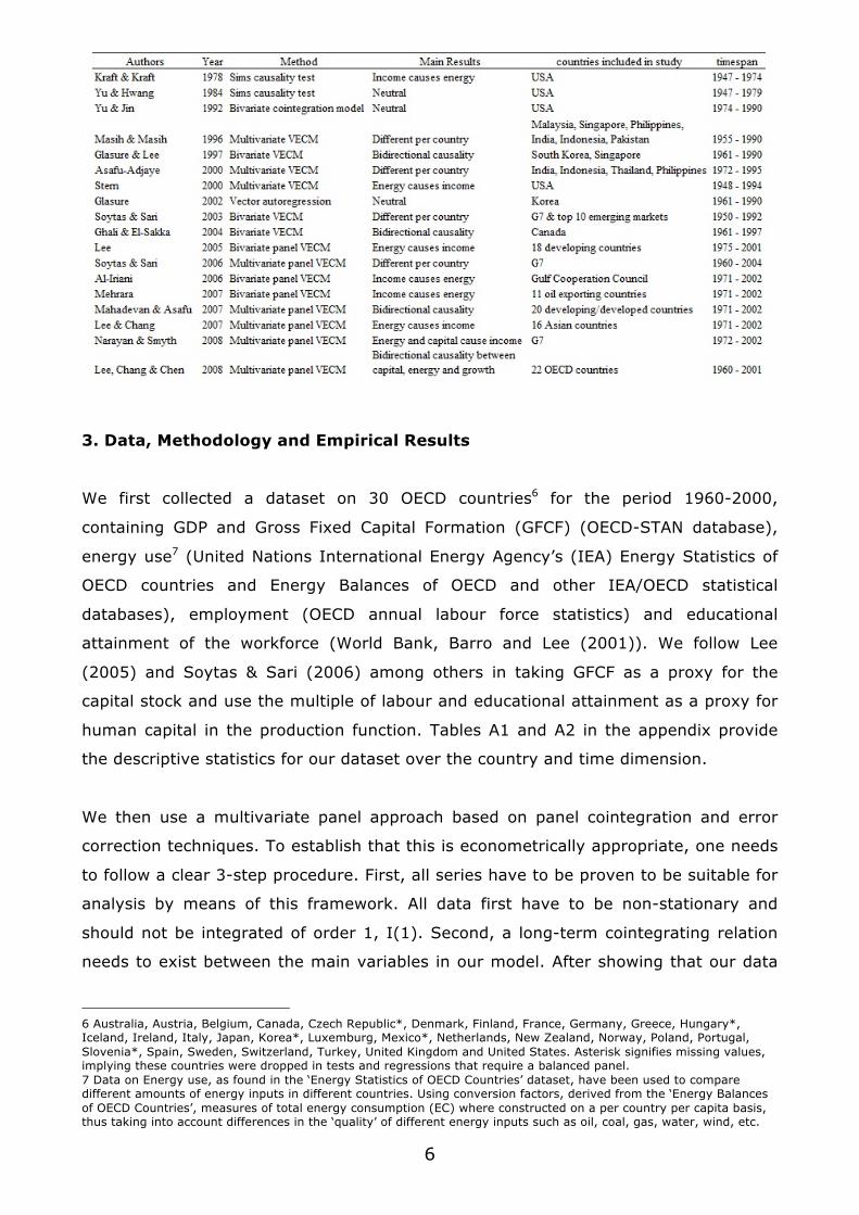
and Multivariate Panel VECM). Table 1 gives an overview of some representative
papers in this literature. First there are several publications finding unidirectional
causality between energy and income, either from energy to income or vice versa.
Second, the hypothesis of the ‘neutrality’ of energy to income has been confirmed
using different methodologies. And finally, different authors have claimed bidirectional
causality exists.
Following Mehrara (2007), these publications can also be divided into four
‘generations’. The first generation (e.g. Kraft and Kraft (1978) and Yu and Hwang
(1984)) of the literature used a ‘traditional’ VAR regression approach to infer causality
5 See Mehrara (2007) for an excellent overview.
5
between the two series under study, assuming stationarity of the data under study.
Analysis by means of this methodology was conducted from 1978 to the end of the
1980’s. With the rise of stationarity testing and correction in econometrics the
analysis evolved and measures were taken to account for the presence of unit roots in
time series. Second-generation publications (e.g. Masih and Masih (1996) and Glasure
and Lee (1997)) made use of error correction models (ECM) and cointegration to
assess Granger (1988) causality in a bivariate framework. Making use of the new
methodology, first generation studies where put aside as the regression results could
be considered ‘spurious’. Building upon this, the third generation (e.g. Asafu-Adjaye
(2000) and Stern (2000)) used a multivariate ECM approach following Johansen’s
(1991) causality testing method to account for omitted variable bias, a critique by
which second-generation studies are repeatedly refuted. This third generation
framework allowed for a correction of other inputs into the production function, such
as capital, labour, prices, etc. However, with such specifications, country and time
specific effects were not taken into account. Therefore, a fourth generation literature
(e.g. Lee (2005, 2006), Soytas and Sari (2003, 2006), Ghali and El-Sakka (2004) and
Sinha (2009)) is published from approximately 2003 onwards and makes use of
(bivariate) panel cointegration and panel error correction models to allow for these
specific time and country dimension effects. Unfortunately none of the published
studies in this generation to date have made use of the full benefits of large variation
in data made possible by panel analysis. This is mainly caused by lack of data, which
confines most panels to less than 10 members (most studies above have less than 20
countries and span at most 40 years). Notable exception is an unpublished working
paper Sinha (2009) that has analysed 88 countries over 28 years.
In what we consider a fifth generation, papers start using the multivariate panel VECM
tools to also control for capital-energy complementarities (e.g. Lee and Chang (2008),
Lee, Chang and Chen (2008), Naryan and Smyth (2008)). These papers generally
conclude that energy consumption Granger causes economic growth and income,
where only Lee, Chang and Chen also find the reverse causation. This contrasts
sharply with our finding that income (growth) and capital Granger cause energy use
but not the other way around. We can trace this back to the specification of our error
correction term and discuss these differences at some length in our results section.
6
3. Data, Methodology and Empirical Results
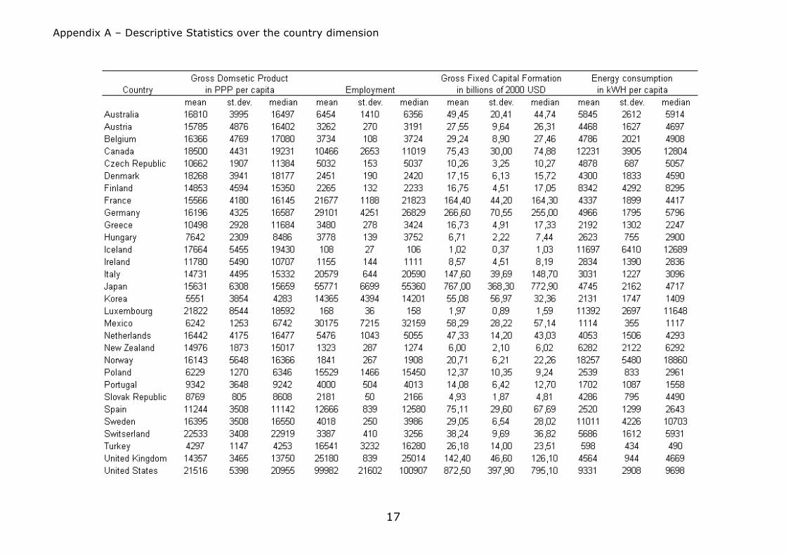
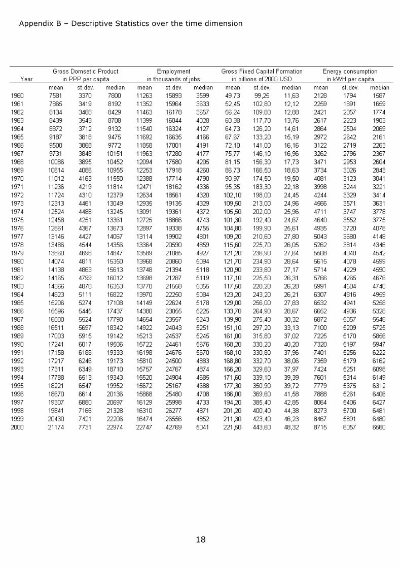
We first collected a dataset on 30 OECD countries6 for the period 1960-2000,
containing GDP and Gross Fixed Capital Formation (GFCF) (OECD-STAN database),
energy use7 (United Nations International Energy Agency’s (IEA) Energy Statistics of
OECD countries and Energy Balances of OECD and other IEA/OECD statistical
databases), employment (OECD annual labour force statistics) and educational
attainment of the workforce (World Bank, Barro and Lee (2001)). We follow Lee
(2005) and Soytas & Sari (2006) among others in taking GFCF as a proxy for the
capital stock and use the multiple of labour and educational attainment as a proxy for
human capital in the production function. Tables A1 and A2 in the appendix provide
the descriptive statistics for our dataset over the country and time dimension.
We then use a multivariate panel approach based on panel cointegration and error
correction techniques. To establish that this is econometrically appropriate, one needs
to follow a clear 3-step procedure. First, all series have to be proven to be suitable for
analysis by means of this framework. All data first have to be non-stationary and
should not be integrated of order 1, I(1). Second, a long-term cointegrating relation
needs to exist between the main variables in our model. After showing that our data
6 Australia, Austria, Belgium, Canada, Czech Republic*, Denmark, Finland, France, Germany, Greece, Hungary*, Iceland, Ireland, Italy, Japan, Korea*, Luxemburg, Mexico*, Netherlands, New Zealand, Norway, Poland, Portugal, Slovenia*, Spain, Sweden, Switzerland, Turkey, United Kingdom and United States. Asterisk signifies missing values, implying these countries were dropped in tests and regressions that require a balanced panel. 7 Data on Energy use, as found in the ‘Energy Statistics of OECD Countries’ dataset, have been used to compare different amounts of energy inputs in different countries. Using conversion factors, derived from the ‘Energy Balances of OECD Countries’, measures of total energy consumption (EC) where constructed on a per country per capita basis, thus taking into account differences in the ‘quality’ of different energy inputs such as oil, coal, gas, water, wind, etc.
7
satisfy the requirements for using this method, we proceed to specify the model and
present our results.
3.1. Unit Root Tests
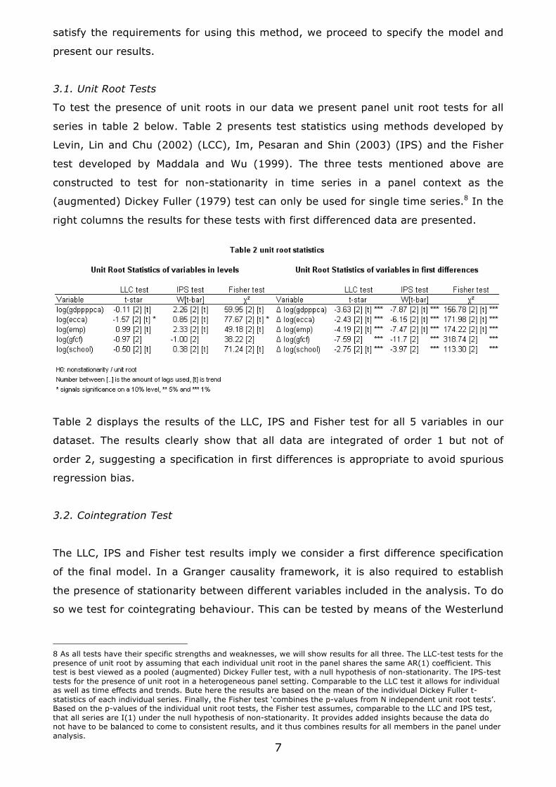
To test the presence of unit roots in our data we present panel unit root tests for all
series in table 2 below. Table 2 presents test statistics using methods developed by
Levin, Lin and Chu (2002) (LCC), Im, Pesaran and Shin (2003) (IPS) and the Fisher
test developed by Maddala and Wu (1999). The three tests mentioned above are
constructed to test for non-stationarity in time series in a panel context as the
(augmented) Dickey Fuller (1979) test can only be used for single time series.8 In the
right columns the results for these tests with first differenced data are presented.
Table 2 displays the results of the LLC, IPS and Fisher test for all 5 variables in our
dataset. The results clearly show that all data are integrated of order 1 but not of
order 2, suggesting a specification in first differences is appropriate to avoid spurious
regression bias.
3.2. Cointegration Test
The LLC, IPS and Fisher test results imply we consider a first difference specification
of the final model. In a Granger causality framework, it is also required to establish
the presence of stationarity between different variables included in the analysis. To do
so we test for cointegrating behaviour. This can be tested by means of the Westerlund
8 As all tests have their specific strengths and weaknesses, we will show results for all three. The LLC-test tests for the presence of unit root by assuming that each individual unit root in the panel shares the same AR(1) coefficient. This test is best viewed as a pooled (augmented) Dickey Fuller test, with a null hypothesis of non-stationarity. The IPS-test tests for the presence of unit root in a heterogeneous panel setting. Comparable to the LLC test it allows for individual as well as time effects and trends. Bute here the results are based on the mean of the individual Dickey Fuller t-statistics of each individual series. Finally, the Fisher test ‘combines the p-values from N independent unit root tests’. Based on the p-values of the individual unit root tests, the Fisher test assumes, comparable to the LLC and IPS test, that all series are I(1) under the null hypothesis of non-stationarity. It provides added insights because the data do not have to be balanced to come to consistent results, and it thus combines results for all members in the panel under analysis.
8
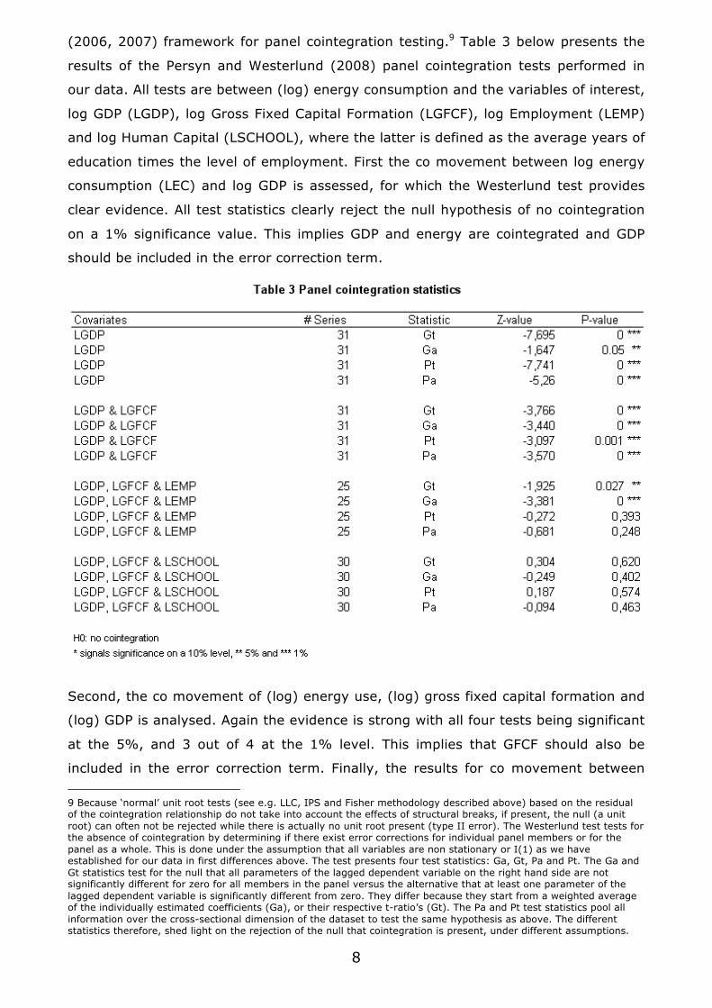
(2006, 2007) framework for panel cointegration testing.9 Table 3 below presents the
results of the Persyn and Westerlund (2008) panel cointegration tests performed in
our data. All tests are between (log) energy consumption and the variables of interest,
log GDP (LGDP), log Gross Fixed Capital Formation (LGFCF), log Employment (LEMP)
and log Human Capital (LSCHOOL), where the latter is defined as the average years of
education times the level of employment. First the co movement between log energy
consumption (LEC) and log GDP is assessed, for which the Westerlund test provides
clear evidence. All test statistics clearly reject the null hypothesis of no cointegration
on a 1% significance value. This implies GDP and energy are cointegrated and GDP
should be included in the error correction term.
Second, the co movement of (log) energy use, (log) gross fixed capital formation and
(log) GDP is analysed. Again the evidence is strong with all four tests being significant
at the 5%, and 3 out of 4 at the 1% level. This implies that GFCF should also be
included in the error correction term. Finally, the results for co movement between
9 Because ‘normal’ unit root tests (see e.g. LLC, IPS and Fisher methodology described above) based on the residual of the cointegration relationship do not take into account the effects of structural breaks, if present, the null (a unit root) can often not be rejected while there is actually no unit root present (type II error). The Westerlund test tests for the absence of cointegration by determining if there exist error corrections for individual panel members or for the panel as a whole. This is done under the assumption that all variables are non stationary or I(1) as we have established for our data in first differences above. The test presents four test statistics: Ga, Gt, Pa and Pt. The Ga and Gt statistics test for the null that all parameters of the lagged dependent variable on the right hand side are not significantly different for zero for all members in the panel versus the alternative that at least one parameter of the lagged dependent variable is significantly different from zero. They differ because they start from a weighted average of the individually estimated coefficients (Ga), or their respective t-ratio’s (Gt). The Pa and Pt test statistics pool all information over the cross-sectional dimension of the dataset to test the same hypothesis as above. The different statistics therefore, shed light on the rejection of the null that cointegration is present, under different assumptions.
9
four vectors, including employment and/or human capital suggest these variables are
not cointegrated with energy consumption and shall be used as general control
variables in the regression framework outlined below.10 From these tests it can be
concluded that the cointegration term in our model must be specified in terms of
energy, capital and GDP, along the lines of Mehrara (2007).11
3.3. Model specification
Because cointegration is found, causality is best assessed using the Engle-Granger
framework (Engle and Granger (1987), Granger (1988), Granger and Lin (1995)). We
use a vector error correction model, or VECM, specification, which basically consists of
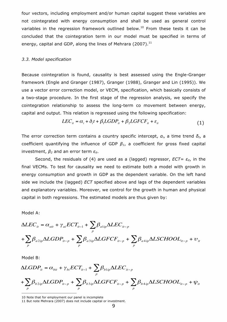
a two-stage procedure. In the first stage of the regression analysis, we specify the
cointegration relationship to assess the long-term co movement between energy,
capital and output. This relation is regressed using the following specification:
The error correction term contains a country specific intercept, αi, a time trend δt, a
coefficient quantifying the influence of GDP β1, a coefficient for gross fixed capital
investment, β2 and an error term εit.
Second, the residuals of (4) are used as a (lagged) regressor, ECT= εit, in the
final VECMs. To test for causality we need to estimate both a model with growth in
energy consumption and growth in GDP as the dependent variable. On the left hand
side we include the (lagged) ECT specified above and lags of the dependent variables
and explanatory variables. Moreover, we control for the growth in human and physical
capital in both regressions. The estimated models are thus given by:
Model A:
Model B:
10 Note that for employment our panel is incomplete 11 But note Mehrara (2007) does not include capital or investment.
€
LECit =α i + δit + β1LGDPit + β2LGFCFit + εit
€
ΔLECit =αait + γ aiECTit−1 + βa1ipΔLECit− pp∑
+ βa2ipΔLGDPit− pp∑ + βa3ipΔLGFCFit− p
p∑ + βa4 ipΔLSCHOOLit− p
p∑ +υ it
(1)
€
ΔLGDPit =αbit + γ biECTit−1 + βb1ipΔLECit− pp∑
+ βb2ipΔLGDPit− pp∑ + βb3ipΔLGFCFit− p
p∑ + βb4 ipΔLSCHOOLit− p
p∑ +ψit
10
where subscripts a and b signal coefficients from the first or the latter model,
subscripts i and t denote the country and time dimension of the regression and Δ
signifies first differences. Subscript p denotes the lag length used for the different
explanatory variables, from t – 1 to t – p, conditional on their significance. The
coefficients labelled βa,b1ip to βa,b4ip quantify the relation between their respective
(lagged) explanatory variables and the explained variable and the error terms are
denoted by υit and ψit respectively. Finally, the relation between the ECT and the
explained variable is quantified by the coefficient γa,bi for models A and B,
respectively. This coefficient will capture the long run causal relationship between the
dependent variable and energy consumption. If it is significant in model A, the
causality runs from GDP to energy use, whereas significance in model B suggests
reverse long run causality.
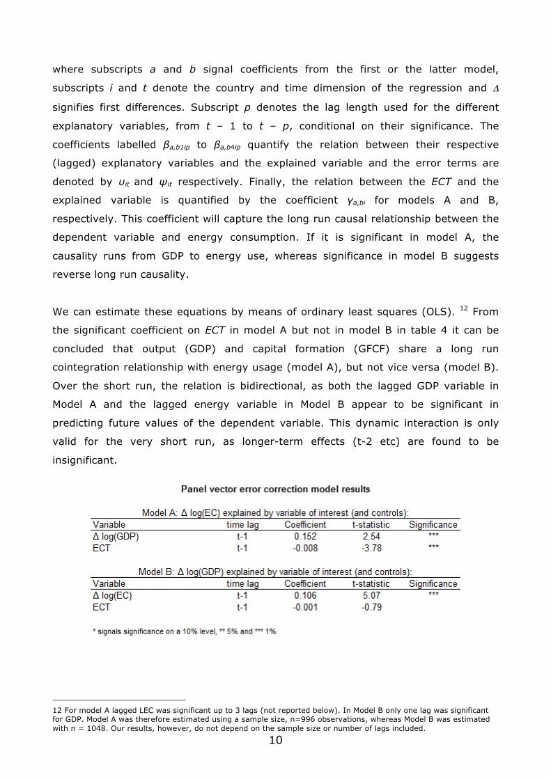
We can estimate these equations by means of ordinary least squares (OLS). 12 From
the significant coefficient on ECT in model A but not in model B in table 4 it can be
concluded that output (GDP) and capital formation (GFCF) share a long run
cointegration relationship with energy usage (model A), but not vice versa (model B).
Over the short run, the relation is bidirectional, as both the lagged GDP variable in
Model A and the lagged energy variable in Model B appear to be significant in
predicting future values of the dependent variable. This dynamic interaction is only
valid for the very short run, as longer-term effects (t-2 etc) are found to be
insignificant.
12 For model A lagged LEC was significant up to 3 lags (not reported below). In Model B only one lag was significant for GDP. Model A was therefore estimated using a sample size, n=996 observations, whereas Model B was estimated with n = 1048. Our results, however, do not depend on the sample size or number of lags included.
11
In conclusion, our results strongly suggest that there is no evidence of a long run
causal relationship from energy use to output in the OECD over the past 40 years. In
the (very) short run the causality seems to run in both directions, but this makes
perfect sense. In the period under investigation the OECD experienced several
significant energy price hikes, causing a drop in energy use, followed by short run
economic contractions. Over the longer run, however, such negative effects wear of
rapidly and the long run causality runs from income to energy use. These results are
in stark contrast to results reported in recent papers (published papers by Narayan
and Smyth (2008), Lee and Chang (2008), Lee, Chang and Chen (2008) on the one
hand and a working paper by Sinha (2009) on the other) using similar data and
empirical methods in the literature. The following sections will first contrast our results
to those reported by Lee, Chang and Chen (2008) and Narayan and Smyth (2008).
Given the less than complete description of the analysis and results in Sinha’s (2009)
working paper, a final section is necessarily more speculative in contrasting our
results to his.
3.4. The importance of the error term specification
Narayan and Smyth (2008) (NS) and Lee, Chang and Chen (2008) (LCC) are largely
based on the same procedures and type of data, studying the G7 and 22 OECD
countries for 3 and 4 decades, respectively. They concluded that energy, as well as
capital, Granger cause output and that therefore energy should be seen as a vital
input in the production function. Our analysis “nests” these earlier studies as our data
has been broadened by including more countries (notably Czech Republic, Hungary,
South Korea, Luxemburg, Mexico, Poland, Slovenia and Turkey) and controls for
additional inputs (e.g. human capital). Excluding these variables, years and countries
from the estimation and running our analysis in per worker terms as in Lee, Chang
and Chen and Narayan and Smyth, however, does not affect our overall conclusion.13
Therefore our opposite conclusions probably follow from a different model
specification. The Lee, Chang and Chen (2008) and Narayan and Smyth (2008) results
13 We use (first differences in the log) of gross fixed capital formation as our proxy for the capital stock as do NS, whereas LCC use (first differences in log of) capital stocks as constructed by Kamps (2006). This, however, is not likely to affect the results qualitatively. In a VECM specification the final regression is done in log first differences, i.e. in growth rates. And we feel it is reasonable to assume that the variation in growth rates of GFCF and the capital stock itself are highly correlated for countries close to their steady states. The standard neoclassical growth model predicts that in steady state all variables, including the capital stock, depreciation and net investment and gross fixed capital formation grow at the common rate of labour augmenting technical change. If we assume all OECD countries are close to their steady state, we know that the level of GFCF is close to the level of deprecation and consequently proportional to the capital stock if depreciation rates are more or less stable. These assumptions are not very strong for OECD countries. This makes it very unlikely that LCC come to opposite conclusions based on their different proxy for the capital stock.
12
can be obtained in our data also by using their specification for the cointegration term,
namely:14
If we use (2) instead of (1) in an Engle-Granger two-step procedural estimation,
energy and capital inputs are found to Granger cause output over the long and short
term in our data as well. The question is then, however, if these authors are justified
in using (2) instead of (1). For this to be the case it must thus be shown that
specification (2) is truly the long run equilibrium, or cointegration, relationship. NS
and LCC offer theoretical arguments and references to earlier papers, but in the end
assume this specification without testing for its appropriateness explicitly.
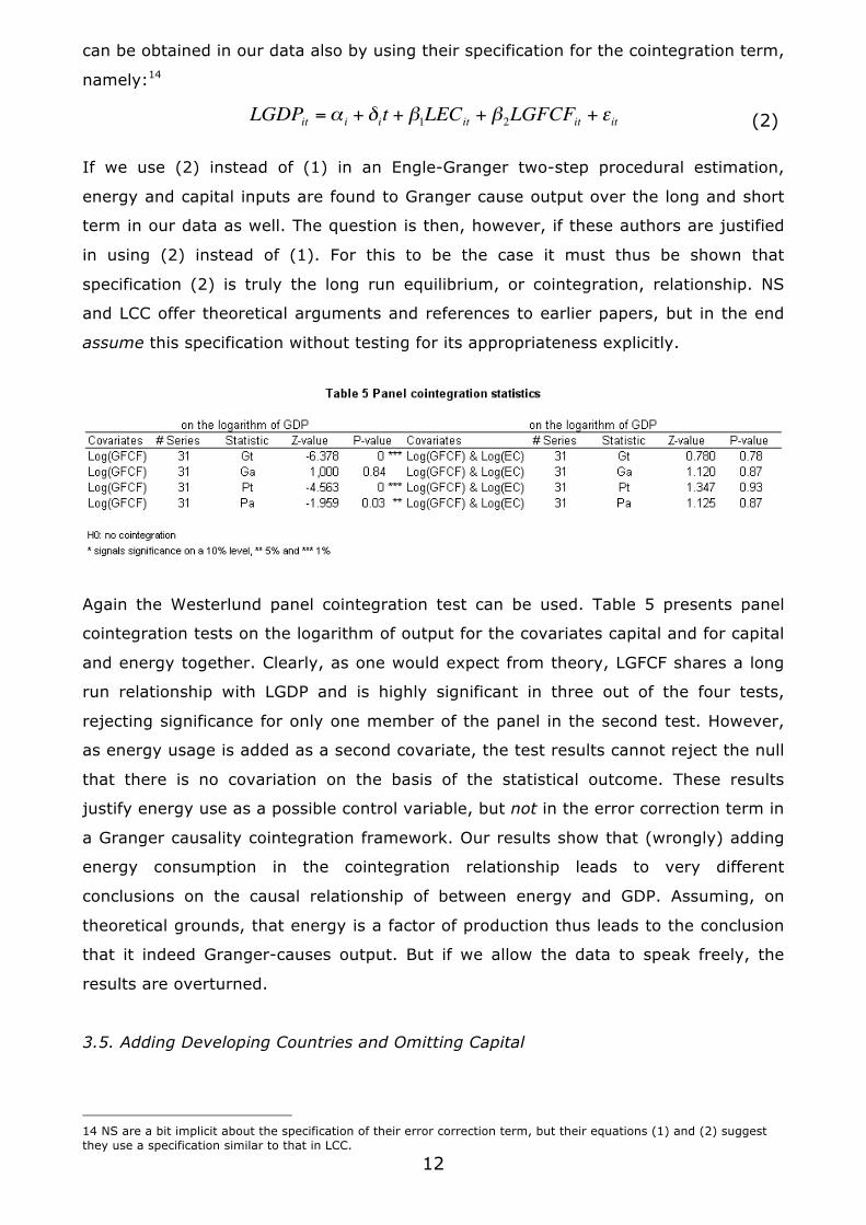
Again the Westerlund panel cointegration test can be used. Table 5 presents panel
cointegration tests on the logarithm of output for the covariates capital and for capital
and energy together. Clearly, as one would expect from theory, LGFCF shares a long
run relationship with LGDP and is highly significant in three out of the four tests,
rejecting significance for only one member of the panel in the second test. However,
as energy usage is added as a second covariate, the test results cannot reject the null
that there is no covariation on the basis of the statistical outcome. These results
justify energy use as a possible control variable, but not in the error correction term in
a Granger causality cointegration framework. Our results show that (wrongly) adding
energy consumption in the cointegration relationship leads to very different
conclusions on the causal relationship of between energy and GDP. Assuming, on
theoretical grounds, that energy is a factor of production thus leads to the conclusion
that it indeed Granger-causes output. But if we allow the data to speak freely, the
results are overturned.
3.5. Adding Developing Countries and Omitting Capital
14 NS are a bit implicit about the specification of their error correction term, but their equations (1) and (2) suggest they use a specification similar to that in LCC.
€
LGDPit =α i + δit + β1LECit + β2LGFCFit + εit (2)
13
The analysis in Sinha (2009) is presented in such a way that it is hard to reproduce in
our data. In his paper Sinha does state that for the 30 OECD countries in his sample
results are “quite similar” to those for the entire sample, that is, he finds a significant
long run relationship in both directions. When we redo our analysis, restricting our
sample from 1975 to 2000, we do not find this reverse causality, suggesting our
model specifications (or data) must differ. An obvious difference in the two papers is
the fact that we follow Narayan and Smyth (2008) in controlling for capital (proxied
by gross fixed capital formation). Given that capital is typically complementary to
energy use and OECD countries are highly capital intensive, the omission of this
variable will bias Sinha’s results. Sinha (2009) probably did not include this variable
because such data are notoriously hard to come by for developing countries. Dropping
capital from our analysis, however, does not change our results qualitatively. Again, it
seems, the specification of the error correction term is the main culprit, although we
cannot be certain, as Sinha (2009) is not explicit about his specification.
Another explanation suggests itself, however. Taking 58 developing countries
increases the weight of developing countries in the panel along two dimensions. It
shortens the time dimension and broadens the cross-section. The available evidence
on developing countries only (e.g. Lee (2005)) suggests that for developing countries
the causation may well run the other way in the long run. Given their largely resource
and agriculture driven economies, developing countries may experience growth only if
energy use can first increase to build up the manufacturing sector and industrial
infrastructures. Adding 58 such countries (without adjusting for their much smaller
share in global GDP and energy use) can then “bias” the results towards finding
bidirectional causality as well. This suggests a multi-regime modelling approach would
be more appropriate in such broad panels.
3.5. Summary
The results of our vector error correction model clearly show strong unidirectional
causality from GDP and capital formation to energy use, as the cointegration term is
significant at the 1% level in model A and not at all in model B. However, model B
confirms that there are some short run influences of energy use running in the
opposite direction. Contrasting our results to those found by other authors we
conclude that the differences are probably caused by our specification of the error
correction term. We can only be sure, however, if we exactly reproduce their results
using their data, which we do not have. Tests in our data, however, show that our
specification is the one the properties of the data would suggest, also if we limit our
14
panel to the dimensions and variables used in the other studies. Furthermore we
argue that excluding capital and including developing countries without properly
weighing them may well have biased results in earlier studies towards finding
evidence for a causal link from energy use to GDP.
4. Conclusion
We show that in the OECD Granger causality runs from output growth and capital
formation, or broadly stated ‘economic activity’ to energy use, and not the other way
around. Energy can therefore not be seen as a vital input into the production function
complementing capital and labour. This results stands in direct opposition to results
found earlier in the literature. As we have shown, however, those results were
obtained under the assumption that energy is an input in the production function.
Testing for the appropriate specification of the long run relationship between energy
use and GDP, suggests the error correction term should not be specified as suggested
by the KLEMs-production function. More empirical research is urgently needed to
establish this result more robustly. Quick wins would be to provide specification tests
for the Lee, Chang and Chen (2008) and Narayan and Smyth (2008) datasets. It
would furthermore be interesting to collect capital stock data on developing countries
to extend the panel, including the important capital stock proxy, to developing
countries.
The issue at hand is of key importance. Policies aiming at reducing either industrial or
residential demand for energy can therefore only be expected to have a small short-
run detrimental effect on overall economic activity. Additionally, the fear that
prolonging the Kyoto protocol might negatively influence global economic recovery is
unfounded if our results are found to be robust. When energy use is not a vital input
in the production function, recovery policies should focus on capital, labour and
productivity inputs (education and R&D etc.) and there is no reason why a reduction
of greenhouse gas emissions by increasing energy prices, pricing carbon emissions or
implementing energy efficiency measures, should cause a fall in output over the
longer term. However, as stated, there may be a short lived and short run negative
effect, validating the argument that the implementation of these policies in the worst
part of the downturn of the business cycle may not be the optimal solution. Starting
negotiations now to have policies in place in a few years, however, seems like a good
prospect for both the environment and the economy.
15
References
Al-Iriani, M.A. (2005). Energy-GDP relationship revisited: AN example from GCC countries using panel causality, Energy Policy, 34, pp. 3342-3350.
Asafu-Adjaye, J. (2000). The relationship between energy consumption, energy prices and economic growth: Time series evidence from Asian developing countries. Energy Economics, 22, pp. 615–625.
Barro, R.J. and J.W. Lee (2001). Schooling quality in a cross–section of countries. Economica, 68(272), pp 465 – 488.
Dickey, D.A. and W. A. Fuller (1979). Distribution of the estimators for autoregressive time series with a unit root. Journal of the American statistical association.
Energy Information Administration (2006). International Energy Annual 2006. Washington D.C..
Engle, R.F. and C.W.J. Granger (1987). Co-Integration and Error Correction: Representation, Estimation, and Testing. Econometrica, Vol. 55, No. 2, pp. 251-276.
Erol, U.,and E.S.H. Yu (1987). On the causal relationship between energy and income for industrialized countries. Journal of Energy and Development, 13, pp. 113–122.
Granger, C. W. J. (1988) Causality, cointegration, and control. Journal of Economic Dynamics and Control, 12(2-3), pp 551-559.
Granger, C.W.J. and J.L. Lin (1995) Causality in the Long Run. Econometric Theory, 11(3), pp. 530-536.
Ghali, K.H., and M.I.T. El-Sakka (2004). Energy use and output growth in Canada: A multivariate cointegration analysis. Energy Economics, 26(2), pp. 225–238.
Glasure, Y. U. (2002). Energy and national income in Korea: Further evidence on the role of omitted variables. Energy Economics, 24, pp.355–365.
Glasure, Y. U., and A.R. Lee (1997). Cointegration, error-correction, and the relationship between GDP and energy: The case of South Korea and Singapore. Resource and Energy Economics, 20, pp. 17–25.
Im, K.S., M.H. Pesaran and Y. Shin (2003) Testing for Unit Roots in Heterogeneous Panels. Journal of Econometrics, 115, pp. 53-74.
Johansen, S. (1991). Estimation and hypothesis testing of cointegration vectors in Gaussian vector autoregressive models. Econometrica, 59, 1551–1580.
Kraft, J., and A. Kraft (1978). On the relationship between energy and GNP, Journal of Energy and Development. 3, pp. 401–403.
Levin, A., C.F. Lin and C.S.J. Chu (2002) Unit Root Tests in Panel Data: Asymptotic and Finite Sample Properties. Journal of Econometrics, 108, pp. 1-24.
Lee, C.C. (2005). Energy consumption and GDP in developing countries: A cointegrated panel analysis. Energy Economics, 27, pp. 415–427.
Lee, C.C. (2006). The causality relationship between energy consumption and GDP in G-11 countries revisited. Energy Policy, 34, 1086–1093.
Lee, C.C. and C.P. Chang (2008) Energy consumption and economic growth in Asian economies: A more comprehensive analysis using panel data, Resource and Energy Economics, 30, pp. 50-65.
Lee, C.C., C.P. Chang and P.F. Chen (2008) Energy-income causality in OECD countries revisited: The key role of capital stock, Energy Economics, 30, pp. 2359-2373.
Mehrara, M. (2007) Energy consumption and economic growth: the case of oil exporting countries, Energy Policy, 35, pp. 2939-2945.
16
Maddala, G.S. and S. Wu (1999). A Comparative Study of Unit Root Tests with Panel Data and a New Simple Test. Oxford Bulletin of Economics and Statistics, 61, pp. 631-652.
Mahadevan, R. and J. Asafu-Adjaye (2007) Energy consumption, economic growth and prices: A reassessment using panel VECM for developed and developing countries, Energy Policy, 35(4), pp. 2481-2490.
Masih, A.M.M., and R. Masih (1996). Energy consumption, real income and temporal causality: Results from a multi-country study based on cointegration and error-correction modeling techniques. Energy Economics, 18, pp. 165–183.
Masih, A.M.M., and R. Masih (1998). A multivariate cointegrated modeling approach in testing temporal causality between energy consumption, real income and prices with an application to two Asian LDCs. Applied Economics, 30, pp. 1287–1298.
Narayan, P.K. and R. Smyth (2008). Energy consumption and real GDP in G7 countries: New evidence from panel cointegration with structural breaks, Energy Economics, 30 pp. 2331 – 2341.
Persyn, D. and J. Westerlund (2008) Error-correction-based cointegration tests for panel data. The Stata Journal, 8(2), pp. 232-241.
Sinha, D. (2009). The energy consumption-GDP nexus: Panel data evidence from 88 countries. MPRA working paper, 18446.
Soytas, U., and R. Sari (2003). Energy consumption and GDP: Causality relationship in G-7 countries and emerging markets. Energy Economics, 25, 33–37.
Soytas, U., and R. Sari (2006). Energy consumption and income in G-7 countries, Journal of Policy Modeling, 28(7), pp. 739-750.
Stern, D. I. (2000). A multivariate cointegration analysis of the role of energy in the US economy. Energy Economics, 22, pp. 267–283.
Westerlund, J. (2006). Testing for panel cointegration with multiple structural breaks. Oxford Bulletin of Economics and Statistics, 68, pp. 101-132.
Westerlund, J. (2007). Testing for Error Correction in Panel Data, Oxford Bulletin of Economics and Statistics, 69(6), pp. 709 – 748.
Yu, E.S.H., and B.K. Hwang (1984). The relationship between energy and GNP: Further results. Energy Economics, 6, pp. 186–190.
Yu, E.S.H., and J.C. Jin (1992). Cointegration tests of energy consumption, income, and employment. Resources and Energy, 14, pp. 259–266.
Acknowledgements STATA modules
Levinlin and Ipshin test: F. Bornhorst, European University Institute, Italy and C. F. Baum, Boston College, Boston MA, USA.
Xtfisher: Scott Merryman, Risk Management Agency, US Dept. of Agriculture, Washingthon DC, USA.
17
Appendix A – Descriptive Statistics over the country dimension
18
Appendix B – Descriptive Statistics over the time dimension