the effects of economic development, time, urbanization - d
TRANSCRIPT
THE EFFECTS OF ECONOMIC DEVELOPMENT, TIME, URBANIZATION, WOMEN’S RIGHTS PROGRAMS, WOMEN’S MICROCREDIT PROGRAMS,
AND WOMEN’S MARKET-ORIENTED PROGRAMS ON GENDER INEQUALITY IN INDIA
by
Amy Marie Kubichek
B.A. in Sociology and Philosophy, Hope College, 1995
M.A. in Applied Social Research, West Virginia University, 2004
Submitted to the Graduate Faculty of
the School of Arts and Sciences name of school in partial fulfillment
of the requirements for the degree of
Doctor of Philosophy in Sociology
University of Pittsburgh
2011
ii
UNIVERSITY OF PITTSBURGH
SCHOOL OF ARTS AND SCIENCES
This dissertation was presented
by
Amy M. Kubichek
It was defended on
February 28, 2011
and approved by
John Markoff, Ph.D., Distinguished University Professor, Department of Sociology
Vijai Singh, Ph.D., Professor, Department of Sociology; Executive Administrator, Office of the Chancellor
Steven E. Finkel, Ph.D., Daniel Wallace Professor, Department of Political Science
Nuno Themudo, Ph.D., Assistant Professor, International Affairs, Graduate School of Public and International Affairs
Dissertation Advisor: Lisa D. Brush, Ph.D., Associate Professor, Department of Sociology

iii
Copyright © by Amy M. Kubichek
2011
iv
Since India’s independence in 1947, economists, scholars, and practitioners coming from
various development paradigms have implemented numerous programs to mitigate female
poverty and gender inequality in India. However, gender disparities in education, health care,
and the overall female/male sex ratio persist. Whether these development programs designed for
women truly promote large-scale gender equality is still open to debate. In my research, I use
longitudinal quantitative methods to analyze district-level data from six Indian states for the
period 1961-2001 that I have gathered from various sources, such as the Census of India,
directories of women’s organizations and NGOs, and women’s development web sites. I
examine whether economic growth and urbanization (associated with modernization theory),
women’s rights programs, women’s market-based programs, and women’s microfinance
programs lead to increases in female/male literacy ratios and female/male child sex ratios. I also
analyze how region and various women’s programs interact to affect gender equality over time.
I find that economic growth is associated with a decrease in female/male child sex ratios and
female/male literacy ratios. Urbanization leads to a small increase in female/male literacy ratios,
but has no impact on female/male child sex ratios. I also find that there is no relationship
between the presence of women’s rights programs, market programs, or microfinance programs
THE EFFECTS OF ECONOMIC DEVELOPMENT, TIME, URBANIZATION, WOMEN’S RIGHTS PROGRAMS, WOMEN’S MICROCREDIT PROGRAMS,
AND WOMEN’S MARKET-ORIENTED PROGRAMS ON GENDER INEQUALITY IN INDIA
Amy M. Kubichek, PhD
University of Pittsburgh, 2011
v
with variation in either female/male child sex ratios or female/male literacy ratios over time. The
passage of time accounts for most of the variation in both female/male child sex ratios and
female/male literacy ratios. This suggests that there are other factors that lead to changes in
female/male child sex ratios and female/male literacy ratios that I do not account for in this
study.
vi
TABLE OF CONTENTS
PREFACE .............................................................................................................................. XXIV
1.0 CHAPTER ONE: INTRODUCTION ...................................................................... 1
2.0 CHAPTER TWO: GENDERED THEORIES OF DEVELOPMENT ................ 12
2.1 BRIEF HISTORY OF GENDERED DEVELOPMENT THEORIES .......... 12
2.1.1 Modernization theory ................................................................................. 12
2.1.2 Women-In-Development (WID) Theory ................................................... 19
2.1.3 Women and Development (WAD) Theory ............................................... 24
2.1.4 Neoliberal Theory ....................................................................................... 27
2.1.5 Gender-and-Development (GAD) Theory ................................................ 38
2.2 RESEARCH METHODS AND EMPIRICAL STUDIES OF
DEVELOPMENT ............................................................................................... 43
2.2.1 Modernization Studies ................................................................................ 43
2.2.2 Women-in-Development Studies ............................................................... 48
2.2.3 Women and Development (WAD) Studies ............................................... 51
2.2.4 Neoliberal Studies ....................................................................................... 53
2.2.5 Gender and Development (GAD) Studies ................................................. 57
2.2.6 Studies testing multiple theories ................................................................ 59
vii
2.2.7 Studies on women and microcredit ........................................................... 68
3.0 CHAPTER THREE: THEORIES OF DEVELOPMENT AND WOMEN’S
EMPOWERMENT: A RECONCEPTUALIZATION .......................................... 75
3.1 INTRODUCTION............................................................................................... 75
3.1.1 Microlending as a strategy for more gender-equitable development .... 77
3.1.2 Women’s collective action as a strategy for equitable development and
empowerment .............................................................................................. 79
3.2 CONCEPTIONS OF POWER........................................................................... 85
3.2.1 “Power over”, “power to”, “power within”, and “power with” ............. 85
3.2.2 Agency, resources, and opportunity structure ......................................... 89
3.2.3 Modernization programs: fostering Western values for economic growth
....................................................................................................................... 93
3.2.4 WID programs: empowering women to participate in the labor force . 98
3.2.5 GAD programs: empowering women to transform institutions........... 104
3.2.6 Neoliberal programs: empowering women to help themselves ............ 111
3.3 CONCLUSION ................................................................................................. 121
4.0 CHAPTER FOUR – DEVELOPMENT AND GENDER INEQUALITY: FROM
THEORY TO HYPOTHESES .............................................................................. 124
4.1 INTRODUCTION............................................................................................. 124
4.2 SOCIO-CULTURAL CONTEXT OF GENDER INEQUALITY ................ 125
4.2.1 National-level changes related to gender inequality .............................. 125
4.2.2 Regional context of gender inequality ..................................................... 128
4.3 MEASURES OF GENDER INEQUALITY ................................................... 135
viii
4.3.1 Female/male sex ratio ............................................................................... 135
4.3.2 Female/male child sex ratio ...................................................................... 138
4.3.3 Female/male literacy ratio ........................................................................ 143
4.3.4 Measures of gender inequality not included in this study ..................... 148
4.4 HYPOTHESES ................................................................................................. 150
4.5 CONCLUSION ................................................................................................. 156
5.0 CHAPTER FIVE: DATA AND METHODS ........................................................ 157
5.1 INTRODUCTION............................................................................................. 157
5.2 DATA COLLECTION ..................................................................................... 158
5.2.1 Data from Census of India ....................................................................... 160
5.2.2 Data on women’s development programs............................................... 162
5.3 VARIABLES ..................................................................................................... 165
5.3.1 Independent variables .............................................................................. 165
5.3.2 Dependent variables.................................................................................. 167
5.3.3 Control variable ........................................................................................ 169
5.3.4 Dealing with time ...................................................................................... 170
5.3.5 Causality .................................................................................................... 171
5.4 ANALYTIC METHODS .................................................................................. 175
5.4.1 Descriptive statistics.................................................................................. 175
5.4.2 Statistical modeling ................................................................................... 180
5.4.3 Fixed-effects models .................................................................................. 181
5.4.4 Model specification ................................................................................... 183
5.4.5 Statistical methods .................................................................................... 189
ix
5.5 CONCLUSION ................................................................................................. 192
6.0 CHAPTER SIX: DESCRIPTIVE STATISTICS ................................................. 194
6.1 INTRODUCTION............................................................................................. 194
6.1.1 Means and distributions of continuous independent and dependent
variables ..................................................................................................... 195
6.2 REGIONAL AND STATE-WISE VARIATION ........................................... 199
6.2.1 Women’s development programs by region ........................................... 199
6.2.2 Continuous independent variables and measures of gender inequality by
region .......................................................................................................... 203
6.2.3 Variation in presence of women’s programs by state............................ 208
6.2.4 Continuous independent variables and measures of gender inequality by
state............................................................................................................. 213
6.2.5 Correlations between all continuous independent variables and
measures of gender inequality ................................................................. 215
6.3 VARIATION IN INDEPENDENT AND DEPENDENT VARIABLES BY
TIME PERIOD ................................................................................................. 218
6.3.1 Variation in presence of women’s programs by region and year ......... 219
6.3.2 Variation in presence of women’s programs by state and year............ 223
6.3.3 Variation in continuous independent variables and measures of gender
inequality by state and year ..................................................................... 232
6.3.4 Overall change in continuous independent variables and measures of
gender inequality over time ...................................................................... 240
6.4 CONCLUSION ................................................................................................. 246
x
7.0 CHAPTER SEVEN: VARIATION IN THE FEMALE/MALE CHILD SEX
RATIO ..................................................................................................................... 248
7.1 INTRODUCTION............................................................................................. 248
7.2 MODERNIZATION AND THE FEMALE/MALE CHILD SEX RATIO .. 249
7.2.1 Models with unlagged independent variables and regional interaction
effects .......................................................................................................... 249
7.2.2 Models with unlagged independent variables and state-wise interaction
effects .......................................................................................................... 251
7.2.3 Models with lagged independent variables and regional interaction
effects .......................................................................................................... 255
7.2.4 Models with lagged independent variables and state-wise interaction
effects .......................................................................................................... 257
7.3 WOMEN-IN-DEVELOPMENT AND FEMALE/MALE CHILD SEX
RATIO ............................................................................................................... 259
7.3.1 Models with unlagged independent variables and regional interaction
effects .......................................................................................................... 259
7.3.2 Models with unlagged independent variables and state-wise interaction
effects .......................................................................................................... 262
7.3.3 Models with lagged independent variables and regional interaction
effects .......................................................................................................... 265
7.3.4 Models with lagged independent variables and state-wise interaction
effects .......................................................................................................... 266
xi
7.4 GENDER-AND-DEVELOPMENT AND THE FEMALE/MALE CHILD
SEX RATIO ....................................................................................................... 268
7.4.1 Models with unlagged independent variables and regional interaction
effects .......................................................................................................... 268
7.4.2 Models with unlagged independent variables and state-wise interaction
effects .......................................................................................................... 270
7.4.3 Models with lagged independent variables and regional interaction
effects .......................................................................................................... 272
7.4.4 Models with lagged independent variables and state-wise interaction
effects .......................................................................................................... 274
7.5 NEOLIBERAL HYPOTHESES AND THE FEMALE/MALE CHILD SEX
RATIO ............................................................................................................... 276
7.5.1 Models with unlagged independent variables and regional interaction
effects .......................................................................................................... 276
7.5.2 Models with unlagged independent variables and state-wise interaction
effects .......................................................................................................... 278
7.5.3 Models with lagged independent variables and regional interaction
effects .......................................................................................................... 281
7.5.4 Models with lagged independent variables and state-wise interaction
effects .......................................................................................................... 283
7.6 DISCUSSION .................................................................................................... 285
7.6.1 Results for Modernization hypotheses .................................................... 285
7.6.2 Results for Women-in-Development hypotheses.................................... 292
xii
7.6.3 Results for Gender-and-Development hypotheses ................................. 295
7.6.4 Results for Neoliberal hypotheses............................................................ 296
7.7 CONCLUSION ................................................................................................. 298
8.0 CHAPTER EIGHT: VARIATION IN THE FEMALE/MALE LITERACY
RATIO ..................................................................................................................... 300
8.1 INTRODUCTION............................................................................................. 300
8.2 MODERNIZATION HYPOTHESES AND VARIATION IN THE
FEMALE/MALE LITERACY RATIO .......................................................... 301
8.2.1 Models with unlagged independent variables and regional interaction
effects .......................................................................................................... 301
8.2.2 Models with unlagged independent variables and state-wise interaction
effects .......................................................................................................... 303
8.2.3 Models with lagged independent variables and regional interaction
effects .......................................................................................................... 306
8.2.4 Models with lagged independent variables and state-wise interaction
effects .......................................................................................................... 309
8.3 WOMEN-IN-DEVELOPMENT HYPOTHESES AND THE
FEMALE/MALE LITERACY RATIO .......................................................... 313
8.3.1 Models with unlagged independent variables and regional interaction
effects .......................................................................................................... 313
8.3.2 Models with unlagged independent variables and state-wise interaction
effects .......................................................................................................... 316
xiii
8.3.3 Models with lagged independent variables and regional interaction
effects .......................................................................................................... 320
8.3.4 Models with lagged independent variables and state-wise interaction
effects .......................................................................................................... 322
8.4 GENDER-AND-DEVELOPMENT HYPOTHESES AND THE
FEMALE/MALE LITERACY RATIO .......................................................... 324
8.4.1 Models with unlagged independent variables and regional interaction
effects .......................................................................................................... 324
8.4.2 Models with unlagged independent variables and state-wise interaction
effects .......................................................................................................... 326
8.4.3 Models with lagged independent variables and regional interaction
effects .......................................................................................................... 330
8.4.4 Models with lagged independent variables and state-wise interaction
effects .......................................................................................................... 332
8.5 NEOLIBERAL HYPOTHESES AND FEMALE/MALE LITERACY RATIO
........................................................................................................................... 334
8.5.1 Models with unlagged independent variables and regional interaction
effects .......................................................................................................... 334
8.5.2 Models with unlagged independent variables and state-wise interaction
effects .......................................................................................................... 336
8.5.3 Models with lagged independent variables and regional interaction
effects .......................................................................................................... 339
xiv
8.5.4 Models with lagged independent variables and state-wise interaction
effects .......................................................................................................... 341
8.6 DISCUSSION .................................................................................................... 345
8.6.1 Results for Modernization hypotheses .................................................... 345
8.6.2 Results for Women-in-Development hypotheses.................................... 352
8.6.3 Results for Gender-and-Development hypotheses ................................. 360
8.6.4 Results for Neoliberal hypotheses............................................................ 361
8.7 CONCLUSION ................................................................................................. 364
9.0 CHAPTER NINE: CONCLUSION....................................................................... 367
APPENDIX A ............................................................................................................................ 386
BIBLIOGRAPHY ..................................................................................................................... 390
xv
LIST OF TABLES
Table 2.1 Modernization, Women-in-Development, Gender-and-Development, and Neoliberal
Perspectives on Gender and Economic Development ............................................... 42
Table 3.1 Approach to material development and aspects of empowerment ............................ 92
Table 5.1 Districts with no development organizations versus districts with missing data on
organizations ........................................................................................................... 164
Table 6.1 Means and Standard Deviations of Independent and Dependent Variables ........... 195
Table 6.2 Means and Standard Deviations of Independent and Dependent Variables, Outliers
Omitted .................................................................................................................... 197
Table 6.3 Count and Percent of Women's Rights Programs by Region ..................................... 200
Table 6.4 Count and Percent of Women's Market Programs by Region .................................... 200
Table 6.5 Count and Percent of Women's Microfinance Programs by Region .......................... 202
Table 6.6 Two-Sample T-Test for per capita SDP by Region .................................................... 203
Table 6.7 Two-Sample T-Test for Logged per capita SDP by Region ....................................... 203
Table 6.8 Two-Sample T-Test for Urbanization by Region ....................................................... 204
Table 6.9 Two-Sample T-Test for % Pop. Comprised of Scheduled Castes by Region ............ 205
Table 6.10 Two-Sample T-Test for Female/Male Sex Ratio by Region .................................... 205
xvi
Table 6.11 Two-Sample T-Test for Female/Male Child Sex Ratio by Region .......................... 206
Table 6.12 Two-Sample T-Test for Male Literacy Rate by Region ........................................... 207
Table 6.13 Two-Sample T-Test for Female Literacy Rate by Region ....................................... 207
Table 6.14 Two-Sample T-Test for Female/Male Literacy Ratio by Region ............................. 208
Table 6.15 Count and Percent of Women's Rights Programs by State ....................................... 210
Table 6.16 Count and Percent of Women's Market Programs by State ...................................... 211
Table 6.17 Count and Percent of Women's Microfinance Programs by State ............................ 212
Table 6.18 Inter-State Comparison of Means for Continuous Independent and Dependent
Variables .................................................................................................................. 214
Table 6.19 Pairwise Correlations of Lagged and Unlagged Independent Variables and Unlagged
Dependent Variables ............................................................................................... 216
Table 6.20 Count and Percent of Women’s Rights Programs in North by Year ........................ 220
Table 6.21 Count and Percent of Women's Rights Programs in South by Year ........................ 220
Table 6.22 Count and Percent of Women's Market Programs in North by Year ....................... 221
Table 6.23 Count and Percent of Women's Market Programs in South by Year ....................... 221
Table 6.24 Count and Percent of Women's Microfinance Programs in North by Year.............. 222
Table 6.25 Count and Percent of Women's Microfinance Programs in South by Year.............. 222
Table 6.26 Count and Percent of Women's Rights Programs in Andhra Pradesh by Year ........ 224
Table 6.27 Count and Percent of Women's Rights Programs in Karnataka by Year ................. 224
Table 6.28 Count and Percent of Women's Rights Programs in Tamil Nadu by Year ............... 225
Table 6.29 Count and Percent of Women's Rights Programs in Gujarat by Year ...................... 225
Table 6.30 Count and Percent of Women's Rights Programs in Madhya Pradesh by Year ....... 226
Table 6.31 Count and Percent of Women's Rights Programs in Rajasthan by Year .................. 226
xvii
Table 6.32 Count and Percent of Women's Market Programs in Andhra Pradesh by Year ....... 227
Table 6.33 Count and Percent of Women's Market Programs in Karnataka by Year ................ 227
Table 6.34 Count and Percent of Women's Market Programs in Tamil Nadu by Year .............. 228
Table 6.35 Count and Percent of Women's Market Programs in Gujarat by Year ..................... 228
Table 6.36 Count and Percent of Women's Market Programs in Madhya Pradesh by Year ...... 229
Table 6.37 Count and Percent of Women's Market Programs in Rajasthan by Year ................. 229
Table 6.38 Count and Percent of Women's Microfinance Programs in Andhra Pradesh by Year
..................................................................................................................................................... 230
Table 6.39 Count and Percent of Women's Microfinance Programs in Karnataka by Year ...... 230
Table 6.40 Count and Percent of Women's Microfinance Programs in Tamil Nadu by Year .... 231
Table 6.41 Count and Percent of Women's Microfinance Programs in Gujarat by Year ........... 231
Table 6.42 Count and Percent of Women's Microfinance Programs in Madhya Pradesh by Year
..................................................................................................................................................... 232
Table 6.43 Count and Percent of Women's Microfinance Programs in Rajasthan by Year ....... 232
Table 6.44 Per Capita SDP for Census Years 1961-2001 (in 1961 Constant Rupees) ............... 233
Table 6.45 Ln(Per Capita SDP) for Census Years 1961-2001 ................................................... 233
Table 6.46 Percent of Urbanization for Andhra Pradesh ............................................................ 234
Table 6.47 Percent of Urbanization for Karnataka ..................................................................... 234
Table 6.48 Percent of Urbanization for Tamil Nadu .................................................................. 235
Table 6.49 Percent of Urbanization for Gujarat .......................................................................... 235
Table 6.50 Percent of Urbanization for Madhya Pradesh ........................................................... 235
Table 6.51 Percent of Urbanization for Rajasthan ...................................................................... 235
Table 6.52 Female/Male Sex Ratio for Andhra Pradesh ............................................................ 236
xviii
Table 6.53 Female/Male Sex Ratio for Karnataka ...................................................................... 236
Table 6.54 Female/Male Sex Ratio for Tamil Nadu ................................................................... 236
Table 6.55 Female/Male Sex Ratio for Gujarat .......................................................................... 236
Table 6.56 Female/Male Sex Ratio for Madhya Pradesh ........................................................... 236
Table 6.57 Female/Male Sex Ratio for Rajasthan ...................................................................... 236
Table 6.58 F/M Child Sex Ratio for Andhra Pradesh ................................................................. 237
Table 6.59 F/M Child Sex Ratio for Karnataka .......................................................................... 237
Table 6.60 F/M Child Sex Ratio for Tamil Nadu ....................................................................... 237
Table 6.61 F/M Child Sex Ratio for Gujarat .............................................................................. 237
Table 6.62 F/M Child Sex Ratio for Madhya Pradesh ................................................................ 238
Table 6.63 F/M Child Sex Ratio for Rajasthan........................................................................... 238
Table 6.64 F/M Literacy Ratio for Andhra Pradesh ................................................................... 239
Table 6.65 F/M Literacy Ratio for Karnataka ............................................................................ 239
Table 6.66 F/M Literacy Ratio for Tamil Nadu .......................................................................... 239
Table 6.67 F/M Literacy Ratio for Gujarat ................................................................................. 239
Table 6.68 F/M Literacy Ratio for Madhya Pradesh .................................................................. 239
Table 6.69 F/M Literacy Ratio for Rajasthan ............................................................................. 239
Table 6.70 Change Scores for Continuous Independent and Dependent Variables ................... 243
Table 6.71 OLS Regressions of Continuous Variables on Time Period..................................... 245
Table 7.1 Fixed-Effects Models Testing Modernization Hypotheses for Female/Male Child Sex
Ratio (Unlagged Independent Variables) ................................................................... 249
Table 7.2 Fixed-Effects Models Testing Modernization Hypotheses for Female/Male Child Sex
Ratio (Unlagged Independent Variables) ................................................................... 252
xix
Table 7.3 Fixed-Effects Models Testing Modernization Hypotheses for Female/Male Child Sex
Ratio (Lagged Independent Variables) ....................................................................... 256
Table 7.4 Fixed-Effects Models Testing Modernization Hypotheses for Female/Male Child Sex
Ratio (Lagged Independent Variables) ....................................................................... 258
Table 7.5 Fixed-Effects Models Testing WID Theory (Unlagged Independent Variables) ....... 260
Table 7.6 Fixed-Effects Models Testing WID Hypotheses for Female/Male Child Sex Ratio
(Unlagged Independent Variables) ........................................................................... 264
Table 7.7 Fixed-Effects Models Testing WID Hypotheses for Female/Male Child Sex Ratio
(Lagged Independent Variables) ............................................................................... 265
Table 7.8 Fixed-Effects Models Testing WID Hypotheses for Female/Male Child Sex Ratio
(Lagged Independent Variables) ............................................................................... 267
Table 7.9 Fixed-Effects Models Testing GAD Hypotheses for Female/Male Child Sex Ratio
(Unlagged Independent Variables) .......................................................................... 269
Table 7.10 Fixed-Effects Models Testing GAD Hypotheses for Female/Male Child Sex Ratio
(Unlagged Independent Variables) .......................................................................... 271
Table 7.11 Fixed-Effects Models Testing GAD Hypotheses for Female/Male Child Sex Ratio
(Lagged Independent Variables) ............................................................................. 273
Table 7.12 Fixed-Effects Models Testing GAD Hypotheses for Female/Male Child Sex Ratio
(Lagged Independent Variables) ............................................................................. 274
Table 7.13 Fixed-Effects Models Testing Neoliberal Hypotheses for Female/Male Child Sex
Ratio (Unlagged Independent Variables) ................................................................ 277
Table 7.14 Fixed-Effects Models Testing Neoliberal Hypotheses for Female/Male Child Sex
Ratio (Unlagged Independent Variables) ................................................................ 279
xx
Table 7.15 Fixed-Effects Models Testing Neoliberal Hypotheses for Female/Male Child Sex
Ratio (Lagged Independent Variables) .................................................................... 281
Table 7.16 Fixed-Effects Models Testing Neoliberal Hypotheses for Female/Male Child Sex
Ratio (Lagged Independent Variables) .................................................................... 284
Table 8.1 Fixed-Effects Models Testing Modernization Hypotheses for Female/Male Literacy
Ratio (Unlagged Independent Variables) ................................................................ 301
Table 8.2 Fixed-Effects Models Testing Modernization Hypotheses for Female/Male Literacy
Ratio (Unlagged Independent Variables).................................................................. 304
Table 8.3 Fixed-Effects Models Testing Modernization Hypotheses for Female/Male Literacy
Ratio (Lagged Independent Variables) ..................................................................... 307
Table 8.4 Fixed-Effects Models Testing Modernization Hypotheses for Female/Male Literacy
Ratio (Lagged Independent Variables) ..................................................................... 310
Table 8.5 Fixed-Effects Models Testing WID Hypotheses for Female/Male Literacy Ratio
(Unlagged Independent Variables) ........................................................................... 313
Table 8.6 Fixed-Effects Models Testing WID Hypotheses for Female/Male Literacy Ratio
(Unlagged Independent Variables) ........................................................................... 317
Table 8.7 Fixed-Effects Models Testing WID Hypotheses for Female/Male Literacy Ratio
(Lagged Independent Variables) ............................................................................... 321
Table 8.8 Fixed-Effects Models Testing WID Theory for Female/Male Literacy Ratio (Lagged
Independent Variables) ............................................................................................. 322
Table 8.9 Fixed-Effects Models Testing GAD Hypotheses for Female/Male Literacy Ratio
(Unlagged Independent Variables) ........................................................................... 325
xxi
Table 8.10 Fixed-Effects Models Testing GAD Hypotheses for Female/Male Literacy Ratio
(Unlagged Independent Variables) .......................................................................... 327
Table 8.11 Fixed-Effects Models Testing GAD Hypotheses (Lagged Independent Variables). 330
Table 8.12 Fixed-Effects Models Testing GAD Hypotheses for Female/Male Literacy Ratio
(Lagged Independent Variables) ............................................................................. 333
Table 8.13 Fixed-Effects Models Testing Neoliberal Hypotheses for Female/Male Literacy Ratio
(Unlagged Independent Variables) ........................................................................... 335
Table 8.14 Fixed-Effects Models Testing Neoliberal Hypotheses for Female/Male Literacy Ratio
(Unlagged Independent Variables) ........................................................................... 337
Table 8.15 Fixed-Effects Models Testing Neoliberal Hypotheses for Female/Male Literacy Ratio
(Lagged Independent Variables) ............................................................................... 340
Table 8.16 Fixed-Effects Models Testing Neoliberal Hypotheses for Female/Male Literacy Ratio
(Lagged Independent Variables) ............................................................................... 342
Table 9.1 Outcomes of Modernization Hypotheses .................................................................... 370
Table 9.2 Outcomes of Women-in-Development Hypotheses ................................................... 373
xxii
LIST OF FIGURES
Figure 5.1 Sample set-up for district-period data set .................................................................. 171
Figure 6.1Variation in Female/male sex ratio over time ............................................................ 241
Figure 6.2 Variation in female/male child sex ratio over time ................................................... 242
Figure 6.3 Variation in female/male literacy ratio over time ...................................................... 243
Figure 7.1 Women’s microfinance programs, market programs, and predicted female/male child
sex ratio ..................................................................................................................... 286
Figure 7.2 Ln(per capita SDP) and predicted female/male child sex ratio by state .................... 287
Figure 7.3 Women’s microfinance programs, market programs, and predicted female/male child
sex ratio ..................................................................................................................... 289
Figure 7.4 Lagged ln(per capita SDP) and predicted female/male child sex ratio ..................... 290
Figure 7.5 Lagged ln(per capita SDP) and predicted state-wise female/male child sex ratio .... 291
Figure 7.6 Women’s market programs, microfinance programs, and predicted female/male child
sex ratio ..................................................................................................................... 293
Figure 7.7 Lagged ln(per capita SDP) and predicted female/male child sex ratio ..................... 294
Figure 7.8 Women’s market programs and predicted female/male child sex ratio .................... 296
Figure 7.9 Women’s market programs and predicted female/male child sex ratio .................... 297
xxiii
Figure 8.1 Ln(per capita SDP) and predicted female/male literacy ratio ................................... 346
Figure 8.2 Urbanization and predicted female/male literacy ratio ............................................. 347
Figure 8.3 Ln(per capita SDP) and state-wise predicted female/male literacy ratio .................. 348
Figure 8.4 Lagged ln(per capita SDP) and predicted female/male literacy ratio by region ....... 350
Figure 8.5 Lagged urbanization and predicted female/male literacy ratio ................................. 351
Figure 8.6 Ln(per capita SDP) and predicted female/male literacy ratio ................................... 353
Figure 8.7 Women’s market programs, microfinance programs, and predicted female/male
literacy ratio ........................................................................................................... 354
Figure 8.8 Women’s market programs, microfinance programs, and state-wise predicted
female/male literacy ratio ...................................................................................... 355
Figure 8.9 Women’s market programs and state-wise predicted female/male literacy ratio ...... 356
Figure 8.10 Lagged ln(per capita SDP) and predicted female/male literacy ratio ...................... 358
Figure 8.11 Lagged ln(per capita SDP) and predicted female/male literacy ratio ...................... 359
Figure 8.12 Women’s microfinance programs, market programs, and predicted female/male
literacy ratio .......................................................................................................... 360
Figure 8.13 Women’s microfinance programs and state-wise predicted female/male literacy ratio
..................................................................................................................................................... 362
Figure 8.14 Lagged effect of women’s microfinance programs and state-wise predicted
female/male literacy ratio ..................................................................................... 364
xxiv
PREFACE
I would like to thank my dissertation advisor, Lisa Brush, for her guidance and encouragement to
me throughout the research process, from the initial stages as I wrestled with developing my
research questions to the final stages of writing drafts of my dissertation. I would also like to
thank my other committee members, John Markoff, Steve Finkel, Vijai Singh, and Nuno
Themudo for reading drafts of my work and for making suggestions as I completed the
dissertation. I am especially grateful to Steve Finkel for his advice as I carried out the statistical
analyses of my data. His knowledge and expertise of longitudinal modeling have been
invaluable to me. Special thanks to Amy Wung, Justin and Starry Ray, Krista and Cleve Cook,
Ben and Christy Cramer, Mom and Dad, and many others for their prayers and support as I
pursued graduate studies. And last but certainly not least, I would like to thank my husband John
for his unwavering love, encouragement, and support to me through the many ups and downs I
experienced during the process of researching and writing about women’s status and the
development process in India.
1
1.0 CHAPTER ONE: INTRODUCTION
Since the 1950s, policy-makers, scholars, and practitioners have developed numerous programs
and policies to alleviate poverty in developing nations, yet today extreme poverty persists in
many countries. In 2010, 1.44 billion people had to sustain themselves on $1.25 or less a day
(UN Human Development Report 2010). If one considers not only income/economic measures
but also deprivation in other measures of well-being such as health and nutrition, children’s
school enrollment, and the availability of potable water, cooking fuel, and toilets, then this
number increases to 1.75 billion people who experienced deprivation in two to six of these
categories (UN Human Development Report 2010). This is roughly one-third of the population
across 104 nations worldwide. Roughly 23% of the world’s population lives in South Asia,
which is also home to the largest percentage (51%) of the world’s population who are
multidimensionally poor (World Bank 2009, UN Human Development Report 2010). About
12% of the world’s population lives in Sub-Saharan Africa, which is home to 28% of the world’s
multidimensionally poor.
In many developing nations (and more affluent nations as well), poverty goes hand-in-
hand with gender inequality. Despite the efforts of development practitioners to address the
needs of women, severe gender inequalities persist in the developing world. Women around the
world are more likely than men to suffer deprivation in terms of access to health care, nutritional
resources, employment, education, and property ownership (UNDR 2010). Moreover,
2
worldwide the female/male sex ratio, defined as the number of females per 1,000 males, is
unnaturally low. Based on Sen’s definition of “missing women” (Sen 2005), in 2010 there were
over 134 million women that were missing worldwide (UNDR 2010:76). In South Asia the
average number of years of schooling that girls complete is under 60% of the average number of
years of schooling that boys complete (Barro and Lee 2010, cited in UN HDR 2010).
India is one country where widespread poverty and gender inequality persist. Even
though India has been industrializing and becoming more economically developed since winning
its independence in 1947, the overall poverty rate is still high. From 1950-51 to 2009-2010,
India’s GDP per capita increased from about Rs. 6,200 to about Rs. 37,100 a year (Census of
India 2011). However, during the period of 2000-2008, almost 42% of India’s population of
over 1 billion lived on $1.25 or less a day. About 55% of the population suffered from multiple
forms of deprivation in 2010, such as lack of nutrition, education, or potable water, or from poor
sanitation conditions (UN HDR 2010). In eight states of India alone, 421 million people suffer
deprivation in multiple dimensions of human well-being, making South Asia the region of the
world where multidimensional poverty is most intense.
There are still great gender disparities in education, health care, and the overall
female/male sex ratio in India. Throughout the 20th century and even into the 21st century,
gender inequality has worsened on some measures. The female/male sex ratio in India, defined
as the number of females per 1,000 males, has dropped from 972 in 1901 to 933 in 2001 (Bhan
2001) and has increased to 940 by 2011 (Census of India website 2011). This means that from
2001 to 2010 there were 60 “missing” females per every 1,000 males, due to factors such as
unequal nutritional and health care compared to men and boys, outright neglect, and female
infanticide (Dreze and Sen 2004). Moreover, the female/male sex ratio at birth has declined
3
from 929 females per 1,000 males in 1990 to 922 females per 1,000 males in 2010 (UN HDR
2010). This implies that a number of Indian couples practice sex-selective abortion to ensure
that they get the desired number of sons. Researchers for the International Center for Research
on Women (ICRW) analyzed data from the National Family Health Survey on over 50,000 ever-
married rural Indian women and their children under five years old (Pande and Malhotra 2006).
They found that almost 60% of the women considered the ideal number of boys to be two or
more, whereas only about 23% of the women thought that two or more girls was the ideal
number (Pande and Malhotra 2006). They also found that by the time children are five years of
age, 13% more boys than girls have received vaccinations, and that 6% fewer boys than girls are
notably stunted due to lack of nutrition (Pande and Malhotra 2006). Although overall female
literacy in India has increased almost 12 percentage points from 2001 to 2011, the current female
literacy rate of about 65% is still lower than that of males, which is about 82% (Census of India
2011, Bhan 2001). In 2010, about 50% of men at least 25 years of age had completed at least
secondary education, whereas only about 27% of women aged 25 years or older had completed
secondary education (UN HDR 2010). Moreover, while 85% of Indian men participate in the
labor force, only about 36% of women do so.
Since the end of World War II until the present, policy-makers, scholars, and
practitioners have developed numerous programs and policies that were intended to alleviate
poverty in developing nations. During the 1950s-1960s, modernization theory was the
predominant paradigm of development. In this period, the U.S. and other wealthy member
nations of the UN started focusing on giving technical aid and money to less-developed,
formerly colonized countries to improve their economies (Tinker 1990). The goal of policy-
makers and practitioners who took the modernization approach was to instill modern, Western,
4
and rationalistic values within the cultures of less-developed nations, with the belief that this
would bring about economic growth and increased industrialization. These modernization
policy-makers and practitioners targeted men with their development projects in order to bring
about economic growth, and especially to promote capital-intensive agricultural methods that
required the use of high-yielding varieties of seeds, heavy use of pesticides and fertilizers – all
goods produced in the global North (McMichael 2000). Modernization policy-makers and
practitioners assumed that the benefits of the projects would trickle down to all members of
society, including women. As societies modernized, their developmental trajectories would
converge, coming to resemble the U.S. and other Western nations.
The women-in-development (WID) approach to development had its beginnings among
feminist scholars in the early 1970s. Since the U.N. World Conference for the International
Women’s Year in 1975, scholars and practitioners have recognized that they must take women’s
needs into account when developing programs to alleviate poverty (Tinker 1990). The focus of
WID theory was economic development (Tinker 1997). WID theorists, like modernization
theorists, assumed that industrialization and the rise of capitalism are both inevitable and
beneficial to all societies (Jaquette and Staudt 2006). Unlike modernization theorists, WID
theorists argued that industrialization and development programs will benefit women only if
women are included in this process (Boserup 1970, Tinker 1997). Women-in-Development
advocates argued that development programs that allocated resources to women’s concerns
would help increase food production, enhance the well-being of families, and increase women’s
equality. However, they did not challenge cultural norms such as female seclusion and son
preference that oppress women and girls (Jaquette and Staudt 2006).
5
Many feminists critiqued the WID theoretical framework, and argued that it had not gone
far enough in addressing the needs of women in the global South, particularly the unequal power
relations between women and men (Jaquette and Staudt 2006). These feminists formulated the
gender-and-development (GAD) theoretical framework during the 1980s to address these issues.
The development of the GAD framework was influenced by socioeconomic and political factors,
and is a more holistic approach than the WID framework. GAD theorists argued that the
development process includes more than economic development, such as an improvement in
individuals’ lives in the political, economic, social, and cultural arenas. This contrasts with the
WID framework, which focuses on gender relations in the economic and legal/political spheres
only. Caroline Moser, one of the founders of GAD theory, emphasized the importance of
establishing women’s property rights, training women to do traditionally “male” occupations,
and providing needed services to women workers, such as child care and transportation (Moser
1989, cited in Jaquette and Staudt 2006). GAD policymakers critique the women’s programs
started under the auspices of the WID paradigm because they focused exclusively upon women
rather than bringing women’s issues into other development programs. Therefore, GAD
policymakers sought to “mainstream” women’s interests into development projects that included
both women and men. GAD scholars and practitioners placed importance on activism, such as
awareness-raising about institutions that oppress women, organizing the community, and
coalition building (Visvanathan 1997). Whereas WID theorists and practitioners emphasized
women’s need for greater access to credit or waged labor, GAD theorists and practitioners
argued that women need to organize to gain political power in the economic system.
The neoliberal theory of development came to dominate the world stage starting in the
1980s, and is still the prevailing development paradigm today. Neoliberal policy-makers and
6
practitioners assume that rational and informed individuals are able to calculate, predict, and then
practice the most efficient way of gaining wealth (Nelson 2006). The goal of the neoliberal
approach is to strengthen poor people’s ability to participate in the market, such as by loaning
them a small amount of capital to start or expand small businesses, or by giving squatters the title
to private property. Although the goal of practitioners and policy-makers that take the neoliberal
approach is macro-level economic development, their focus is on the individual—giving
individuals the power to ‘lift themselves out of poverty’. Neoliberal practitioners and policy
makers view financial assets as the most important resource for women. Although some
neoliberal practitioners do recognize the need for educational and informational resources, they
focus only on education and training related to finance and entrepreneurship.
Researchers have conducted a myriad of studies related to theories of development, yet
which development approach is best in raising women’s status and remedying the problem of
gender inequality is still open for debate. Researchers have conducted numerous studies on how
microlending impacts women in Bangladesh, whether related to their emotional well-being,
decision-making power, or to other issues (see, e.g., Todd 1996, Rahman 1999, Hashemi et. al.
1996, Goetz and Sen Gupta 1996, Ahmed et. al. 2001, Kabeer 2001). Researchers have carried
out impact evaluations or case studies on the effectiveness of women’s rights programs or
microlending programs in India, such as SEWA and the Federation of Thrift and Credit
Associations (Carr et. al. 1996). These micro-level case studies are appropriate for evaluating
the impact that a particular program has in a localized region, such as in a few towns or villages.
Some researchers highlight the positive effects of women’s involvement in micro-credit
programs, such as increased control over economic resources and greater participation in family
decision-making (Todd 1996, Hashemi et al. 1996). Other researchers draw a more negative
7
conclusion about the effects of microcredit on women’s status, arguing that many women do not
retain control over the loans that they have taken out, and must turn the loans over to their
husbands or other male household members (Goetz and Sen Gupta 1994, Rahman 1999).
However, none of these studies have compared the effects of women’s development programs
that come from very different development paradigms on women’s lives, such as a women’s
development program that actively challenges patriarchal cultural norms and a women’s
development program that provides micro-loans.
Other researchers have conducted cross-national, longitudinal studies on how nations’
economic development is related to overall women’s status and gender inequality (see Forsythe
et al. 2000, Young et. al. 1994, and Dijkstra and Hanmer 2000). Several of them use databases
of international development organizations, such as the WISTAT database, the Gender-related
Development Indicators, or the Gender Empowerment Measure, and some also cluster nations
by region or cultural values. While some cross-national studies assess the impacts of several
development paradigms on gender equality, none seem to do this for a single nation. However, it
could very well be true that development programs of the same paradigm (say, economic
growth) will not have the same effect on increasing gender equality in all nations. However,
little if any research has been done comparing how the presence of various types of development
programs coming from different development paradigms affect changes in gender inequality and
economic development more generally in a single nation such as India.
Strategies for increasing gender equality in developing countries that are grounded in
modernization, WID, GAD, or neoliberal theory operate with different sets of logics. Is there a
way of assessing the impact that women’s programs coming from different development
paradigms have on changes in gender inequality and economic development more generally? If
8
so, which development approach is most effective in raising gender equality in India? Are the
WID analysts right about the hypothesized importance of incorporating women into economic
development programs and processes? These are some of the central questions that I address in
this dissertation. My study addresses these issues by analyzing the effects that economic growth,
urbanization, and women’s development programs associated with different development
paradigms have on district-level changes on gender inequality in India from 1961-2001. In
carrying out this research, I hope to add to the knowledge about how the presence of women’s
rights programs, microfinance programs, and other market programs impact overall patterns of
gender inequality in particular regions of a country. My research has wider policy implications
because it accounts for changing development strategies of different time periods, thus allowing
development practitioners to assess which strategy has had the most impact on raising gender
equality in a single developing nation.
The research design of this study has several advantages over both micro-level studies of
one or two women’s development programs at the individual or village level and macro-level
studies on changes in gender inequality that take the nation as the unit of analysis. First, I use a
longitudinal research design that includes data across five decades. A longitudinal design allows
me to examine how the proliferation of women’s development programs under modernization,
WID, GAD, and neoliberal frameworks affects changes in gender inequality over time. This is
because I can test whether economic growth or the presence of women’s programs at earlier
time-points are correlated with changes in gender inequality at later time-points. This allows me
to make stronger causal inferences than if I measured the presence of women’s programs and
gender inequality at only one time-point. Also, by analyzing data across several decades, I am
able to examine the long-range effects of economic growth, urbanization, and the presence of
9
women’s programs better than prior studies on women’s development programs, such as the
studies of women’s microcredit programs mentioned earlier.
Second, by taking the district rather than the individual as the unit of analysis I can more
easily compare the effects of several types of women’s programs on gender inequality. A
district-level study can control for the particularities of each individual development program to
assess the overall effect of that type of program on raising women’s status on a larger scale than
the village or census block. I include districts from six different states, three of which are in
southern India and three of which are in northern India. This is a benefit over micro-level studies
since it allows one to examine how regional variations affect the impact that economic growth
and different development programs have on changes in women’s status. This is important for a
vast country like India, since patriarchal norms tend to be stronger in northern states than in
southern states (Dreze and Sen 2004).
Third, my meso-level research design has certain advantages over cross-national studies.
There are some cross-national studies that assess the relative merits of different development
paradigms by analyzing the effects of economic growth or trade openness on measures of gender
inequality. However, it could very well be true that development policies of the same paradigm
(say, policies promoting economic growth or trade openness) will not have the same effect on
increasing gender equality in all nations. By studying one nation such as India, I am able to take
into account India’s particular national and regional characteristics, such as certain patriarchal
institutions, forms of governance, and development policies that the government has
implemented.
In chapter two of this dissertation, I introduce the debates among modernization, WID,
GAD, and neoliberal theorists as they pertain to the impact of economic development strategies
10
on women’s status and changes in gender inequality. I discuss how modernization, women-in-
development, gender-and-development, and neoliberal theorists have made competing claims
about the best ways of promoting economic growth, how the process of development impacts
women, and the best ways of raising gender equality in developing nations.
In chapter 3, I discuss how many development organizations stress the importance of
women’s “empowerment,” yet how this word has taken on different meanings for organizations
that come from different development paradigms. I highlight women’s microlending
organizations and women’s rights organizations in India and Bangladesh as examples of how
some organizations equate “empowerment” with economic power, whereas others equate it with
challenging social structures that reinforce gender inequalities. I also review various
conceptualizations of power, and explain how conceptualizations of power and empowerment
can help us classify development programs as modernization, WID, GAD, or neoliberal-type
programs. Finally, I provide examples of Indian development programs of each type.
In chapter four, I discuss the cultural context of gender inequality in India, including how
variation in regional patriarchal norms affects the status of women and girls. I next provide a
detailed discussion of the three measures of gender inequality that I use in this study: the
female/male sex ratio, female/male child sex ratio, and female/male literacy ratio. I discuss how
cultural norms such as marriage patterns, son preference, and female seclusion have negatively
impacted female/male sex ratios, child sex ratios, and literacy ratios in India. I then develop my
hypotheses to test the competing claims of modernization, WID, GAD, and neoliberal theorists
regarding these three measures of gender inequality.
In chapter five, I discuss my data collection processes, including the states I chose for the
study, the unit of analysis, and sources of data. I discuss how I collected the data on women’s
11
programs, on the measures of gender inequality, and on measures of urbanization and economic
growth. Next, I talk about how I deal with time using longitudinal data and issues of causality.
After this, I discuss the analytic methods I employ, including descriptive statistics and the
statistical models I use to test the hypotheses.
In chapter six, I lay the groundwork for the statistical models that I present in chapters
seven and eight by carrying out descriptive analyses on all of my variables. I find that the
presence of women’s rights programs, market programs, and microfinance programs all vary
significantly over time. This variation in presence of women’s programs over time is statistically
significant in both regions and in all six states. Change-score analyses and OLS regressions
reveal that changes over time in SDP per capita, urbanization, female/male child sex ratio, and
female/male literacy ratio are all statistically significant. However, change in the female/male
sex ratio over time is not statistically significant, which is why I do not use it as a dependent
variable. In chapter seven, I present results for the statistical models related to changes in the
female/male child sex ratio, while in chapter eight I discuss the results of the statistical models
related to changes in the female/male literacy ratio over time. Finally, in chapter nine I conclude
the dissertation by discussing the findings of my study, the policy implications of my research,
and areas for exploration in future studies.
.
12
2.0 CHAPTER TWO: GENDERED THEORIES OF DEVELOPMENT
2.1 BRIEF HISTORY OF GENDERED DEVELOPMENT THEORIES
2.1.1 Modernization theory
Modernization theory has its beginnings in the post-World War II era of the U.S. (So 1990).
Unlike most countries that were involved in World War II, the U.S. was strengthened by
involvement in the war and in the re-construction of Western Europe during the 1950s. The
colonial empires of European nations began to crumble, and as they did, new nation-states in
Latin America, Africa, and Asia emerged. During this same period, the Soviet Union
successfully spread communism to Eastern Europe, Korea, and China. American policy-makers
were concerned that these newly post-colonial states in the “Third World” would turn to
communism as their new form of political economy if the U.S. did not promote political stability
and capitalist routes to economic growth in these newly-liberated countries (Chirot 1981:261-
262, cited in So 1990:17). The U.S. government as well as private foundations provided support
for economists, sociologists, political scientists, and other social scientists to carry out studies of
these new, less-developed nations to attempt to explain why some nations are industrialized,
while others are not (So 1990, Webster 1990). During the 1960s, other wealthy member nations
of the UN also started focusing on giving technical aid and money to less-developed, formerly
13
colonized countries to improve their economies (Tinker 1990). These UN members and other
development planners used a modernization theoretical framework as they carried out their
development projects (Tinker 1997, Visvanathan 1997).
Modernization theorists drew their inspiration from evolutionary theory to explain how
societies modernize. They argued that as societies modernize, they start out in a simple,
undifferentiated phase and move through the different phases until they become complex,
differentiated societies (So 1990). Modernization theorists also viewed progress and change in
societies as an irreversible yet gradual process, taking generations to occur. They argued that
industrialization was a linear, inevitable process, and that less-developed nations would follow
the same path as Western industrialized nations as they became more modern. As societies
modernized, their developmental trajectories would converge, coming to resemble the U.S. and
other Western nations. They also argued that modernization is a systematic process, and that all
institutions and aspects of a society will undergo change; that democracy and capitalism develop
hand-in-hand, with political freedoms following and reinforcing market forces. Moreover,
changes in one social institution will cause changes in other institutions (So 1990).
Modernization theorists also drew from the functionalist theories of Emile Durkheim,
Max Weber, and especially Talcott Parsons (So 1990). The greatest influence of Parsons on the
modernization school was Parsons’ “pattern variables” of traditional versus modern societies.
According to Parsons, there are four pattern variables that characterize either traditional or
modern societies (Parsons 1951, cited in So 1990). First, societies may be characterized with
either “affective” or “affective-neutral” relationships among individuals. People in traditional
societies tend to have emotional, personal relationships with others, whereas people in modern
societies tend to have more impersonal, detached relationships with others. Second, traditional

14
societies are particularistic, while modern societies are universalistic. That is, in traditional
societies social obligations and trust bind people together, and individuals know personally all
the people with whom they come in contact. In modern societies, one interacts with many
people, including many strangers, in one’s day-to-day life, and therefore there must be universal
norms that guide people’s interactions. Third, traditional societies have a collectivist orientation,
whereas modern societies have an individualist orientation. In traditional societies, one must
sacrifice for the sake of loyalty to one’s family and community, and innovation and creativity are
discouraged in order to maintain stability in the society. In modern societies, however,
individuals are encouraged to develop their talents and skills and advance in their careers;
individual risk-taking and acting on material interest, in this theory, leads to aggregate and
socially beneficial technological innovation and economic growth. Fourth, the status of
individuals in traditional societies is ascribed to them depending on factors such as gender,
family, caste, etc, whereas the status of individuals in modern societies is achieved—that is, it’s
based on one’s talents, skills, and achievements (Parsons 1951, cited in So 1990).
The modernization school of theorists borrowed from Parsons’ conception of “pattern
variables” to argue that cultural aspects of a society greatly affect whether that society will
develop into a modern, industrialized society with a capitalist economy, or remain what they saw
as a “backward,” undeveloped society. These “modern” expectations and values include the
values of achieved rather than ascribed status, greater autonomy from authorities and parents,
greater social and geographic mobility, and the values of a scientific and entrepreneurial
orientation rather than an orientation to tradition and the past (Webster 1990, Inkeles and Smith
1974). Moreover, as societies modernize – specifically, as they conform to capitalist market
15
discipline and competition and adopt democratic political institutions and practices - they will
become more individualistic and less collectivist (Friedman 1962).
According to modernization scholars, the modernization process affects women in
positive ways (Jaquette 1982). They argued that as people in a society adopt “modern”
expectations and values, women’s mobility increases and they gain more freedom to act on their
own (Jaquette 1982). Some modernization theorists argued that as societies become more
industrialized and forms of birth control become more readily available, women would gain
greater control over their own fertility. Women would be stimulated intellectually by being able
to take advantage of the employment opportunities in the cities (Rosen and LaRaia 1972, in
Jaquette 1982). The day-to-day experiences would expose them to the values of achievement
and competency, which they would internalize (Rosen and LaRaia 1972, in Jaquette 1982).
Moreover, as traditional societies become more modern and adopt modern values, they become
less authoritarian and male-dominated, and more egalitarian and democratic (Jaquette 1982).
Modernization theorists viewed the modernization process, as well as development programs, as
either gender-neutral or as more beneficial to women than to men. This is because women living
in traditional societies face more restrictions than men, and therefore benefit more when their
societies become more modern.
Although modernization theory was the main development paradigm in the 1950s for
social scientists conducting research on how nations become more economically developed,
there were scholars who criticized the theory for several reasons. Some critics have charged
modernization theorists with being ethnocentric, as modernization theorists from the U.S. and
Western Europe assumed that the values of their own countries were modern values, and that the
values of non-Western nations that differed from Western values were “primitive” (So 1990).
16
These critics also argued that modernization theorists assumed that modernization is a
unidirectional process, and that there are no alternative paths to development other than the path
that Western nations took to become economically developed (that is, capitalist industrialization
powered by ecologically and economically unsustainable fossil fuel consumption and capital-
intensive, export-oriented agriculture). Other critics questioned modernization theorists’
assumption that traditional and modern values are mutually exclusive in a society. They argued
that even in Western “modern” societies, traditional values like strong family ties often exist
alongside modern values such as high achievement motivation. Moreover, these critics argued
that it is not really possible to completely replace the values of non-Western societies with
Western values because a society’s values change extremely slowly over time. Still other critics
faulted modernization researchers for being very abstract and generalizing to all developing
nations without grounding their analyses in any particular time period or providing an in-depth
analysis of any one particular country.
Neo-Marxists criticized modernization theorists and researchers for not taking into
consideration the history of colonialism, and the negative impact decades of resource extraction,
exploitation, colonial rule, and “dependent development” had on the newly-freed, less developed
nations. They pointed out that the nations that modernization theorists considered economically
advanced are the very nations that had dominated the nations that are considered “backward” (So
1990). Others have criticized modernization practitioners and policy-makers for promoting
capital-intensive agricultural methods that required the use of high-yielding varieties of seeds,
heavy use of pesticides and fertilizers, and intensive use of irrigation systems (Webster 1990,
McMichael 2000). They argued that these intensive farming methods depleted the soil of
nutrients, requiring farmers to increase the amount of fertilizers that they used in order to
17
maintain the same level of produce from the land (Webster 1990). Moreover, wealthy farmers’
use of these modern agricultural methods resulted in declining working conditions for
agricultural laborers who had to work with the pesticides and fertilizers (McMichael 2000). Still
others have argued that farmers’ use of these modern agricultural methods in developing nations
has led to economic inequality in rural areas, especially in India and some Latin American
countries (McMichael 2000). They argued that rich farmers could afford to buy the expensive
inputs required by modern farming methods, which resulted in larger crops and greater
prosperity. Poorer farmers could not afford to use these “modern,” capital-intensive methods,
however, and had difficulty competing with the wealthier farmers’ higher crop yields. The result
was that poorer farmers became more vulnerable to market forces, and sometimes were forced to
lease their land to wealthier farmers, thus losing their access to even subsistence farming for their
own needs.
Although classic modernization theory of the 1950s-1960s has come under attack from
many quarters, there are some social theorists who have refined the theory to take the critics’
complaints into account. Inglehart and Welzel (2005) have developed a new version of
modernization theory that differs from the earlier modernization school in important ways.
Whereas earlier modernization theorists believed that changes in societies’ cultural values lead to
socioeconomic modernization, Inglehart and Welzel argued that the reverse is true. They argued
that economic development in societies leads to changes in cultural values, not the other way
around. More specifically, as societies shift from an agricultural economy to an industrial
economy and become more economically developed, people have greater economic security,
levels of poverty decrease, and people’s life expectancy increases, thus leading to less reliance
on supernatural powers for their survival. Socioeconomic development also leads to increases in
18
social complexity and the specialization of occupations. There is an increased diversity in social
interactions, which frees people from tight communal ties they experienced in more traditional
societies. As societies move from having primarily agricultural economies to industrial
economies, the cultural values and beliefs of those societies shift from traditional values to
secular-rational values (Inglehart and Welzel 2005).
Unlike earlier modernization theorists, who saw the socioeconomic modernization
process as inevitable and irreversible, Inglehart and Welzel (2005) argued that socioeconomic
modernization is probabilistic rather than deterministic. They state that “…other things being
equal, socioeconomic development tends to make people more secular, tolerant, and trusting and
to place more emphasis on self-expression, participation, and quality of life” (Inglehart and
Welzel 2005:46). Aspects of cultural and historical heritage, such as religion, continue to
influence societal values and people’s behavior, and mediate the effects of modernization on
changes in cultural values. Historical value systems such as those of Islam, Protestantism, and
Confucianism impact the rate that values change in modernizing societies. Inglehart and Welzel
do seem to equate modernization with industrialization. They observed that even though
industrialization began in the West, East Asia has been leading the way in the modernization
process in recent decades. Moreover, cultural modernization is reversible. For example, if there
is an economic collapse such as that which the post-Soviet states experienced in the 1990s,
people in that society may shift from holding self-expressive values to survival values as
economic security becomes more tenuous (Inglehart and Welzel 2005).
Inglehart and Welzel (2005) have presented compelling evidence in support of their
modified modernization theory. They have carefully tested the causal relationships between
changes in nations’ levels of economic development and the values that their citizens hold. They
19
have taken other development theorists’ critiques of “classical” modernization theory into
account and have built a more nuanced model than earlier modernization theorists, recognizing
that the values that a nation’s people hold are dependent not only on economic factors such as
GDP/per capita, but also on historical and cultural factors unique to each nation.i
2.1.2 Women-In-Development (WID) Theory
Women members of the United Nations conceived of the women-in-development (WID)
framework that evolved during the early 1970s as a response to the United Nations’ and donors’
realization that development programs based on modernization theory did not benefit women as
much as expected (Tinker 1997, Jaquette and Staudt 2006). UN members and development
planners had focused on helping men, and if they thought about it at all, apparently believed that
this aid would “trickle down” and eventually benefit everyone in the societies, including women
(Tinker 1997, Visvanathan 1997). However, in response to pressure from feminist activists and
academics, Canadian and European donors, as well as UN agencies, started viewing women’s
status and poverty as development issues (Jaquette and Staudt 2006). In 1973, USAID created
the Office of Women in Development to address this problem. The UN General Assembly
pronounced the year of 1975 as “International Women’s Year”, and held an International
Conference on Women that year in Mexico City (Jaquette and Staudt 2006). The Plan of Action
that was drafted at this Conference highlighted the economic disparities between women and
men and emphasized the importance of women’s legal rights, but did not address women’s
political representation. The General Assembly created the International Development Strategy
for the Second Development Decade, and in it they stated the necessity of fostering the “full
20
integration of women in the total development effort” (Tinker 1997:34). Women-in-
Development advocates argued that development programs that allocated resources to women’s
concerns would help increase food production, enhance the well-being of families, and increase
women’s equality, all within cultural norms (Jaquette and Staudt 2006). Such programs included
agricultural inputs and training for women, as well as income-generating projects. In some
cases, these income-generating projects were successful in decreasing poverty and assisting
women to become more economically independent. WID proponents also pressed for
evaluations of development projects to determine how they affected women and men. The WID
office within USAID sponsored country studies that utilized anthropological methods and “time
budgets” to understand the quality of women’s lives. When the results of these studies showed
that women worked more hours per day than men, USAID initiated projects that brought new
time-saving technologies to women, such as water pumps and better stoves. By 1987, the World
Bank had created a special emphasis on WID, and in 1988 the World Bank stipulated that every
project proposal needed to be analyzed to determine if it addressed women’s issues and needs
before the project was approved (Prugl and Lustgarten 2006). WID theorists and practitioners
have been successful in bringing women to the attention of development planners, and have
legitimized the creation and implementation of development programs with women in mind.
Moreover, WID advocates have been successful in pressuring governments to start
disaggregating official statistical information by sex to determine how women and men may be
benefiting from economic development and industrialization differently (Tinker 1997).
The focus of WID theory was economic development (Tinker 1997). WID theorists, like
modernization theorists, assumed that industrialization and the rise of capitalism are both
inevitable and beneficial to all societies, even though many women from developing countries
21
viewed socialism as a potentially effective development strategy (Jaquette and Staudt 2006).
Unlike modernization theorists, WID theorists argued that industrialization and development
programs will benefit women only if women are included in this process (Boserup 1970, Tinker
1997). WID theorists argued that there has been a gender bias in modernization-grounded
programming for economic development and that these putatively gender-blind but in fact
androcentric programs have ignored the economic activities carried out by women (Tinker
1997). They also argued that not integrating women into development programs is irrational and
inefficient, and that programs that do not include women are less productive than they would be
if women were included (Jaquette 1982). WID theorists stated that development programs
grounded on gender-blind and androcentric modernization theory assume that male household
heads would provide for the needs of women, and that women’s subsequent marginalization
from the economic sphere is both inevitable and unproblematic. WID theorists further argued
that urbanization and the shift from subsistence to market-oriented production forced women into
the modern economic system. These women were paid less than what they needed to survive,
and thus their dependence on men was intensified. Women’s exploitation in the modern
economic system had even more deleterious effects for the large percentage of women who were
the heads of households and did not receive support from men (Jaquette 1982).
Women-in-development theorists not only criticized development programs coming
from a modernization perspective; they also critiqued the modernization process itself. Some
feminists viewed urbanization and the rise of capitalism as processes that separate women from
their traditional social and economic roles and force them into the manufacturing sector where
they are exploited and paid less than what they need to survive (Jaquette 1982). In Women’s
Role in Economic Development, a classic work in the WID literature, Ester Boserup (1970)
22
analyzed data on women’s changing economic roles in the Caribbean, Africa, Asia, and Latin
America. She argued that colonialism and capitalism, two specific forms of modernization, have
negatively affected women in less-developed, former colonized countries. For instance,
European colonial governments established Western farming techniques in the African colonies
they ruled over. Because of their Eurocentric view that men were “naturally” superior to women
in farming, they introduced these more efficient farming methods to African men, but not to
women. Women continued to use hand tools to cultivate crops. Even in regions where
traditionally women were agricultural workers and men were not, European colonialists refused
to teach new agricultural techniques to women. In addition to this, colonizers made their
colonized societies shift from subsistence agriculture to the cultivation of cash crops, which they
relegated to men. Women’s status in African societies decreased on two counts: They continued
to use less efficient methods of farming, and therefore were less productive. They also continued
to produce crops for their families’ immediate needs, while men gained extra money from
growing cash crops (Boserup 1970). In a market society, subsistence farming is undervalued. If
women are engaged in subsistence farming in a market society, both their economic power and
their standing in civil society suffer.
Female workers in less-developed nations were marginalized as these nations became
more economically developed, and their economic gains were much less than men’s economic
gains (Boserup 1970). Women were the ones who were primarily responsible for subsistence
activities, such as collecting firewood, fetching water, and growing and preparing food for their
households. These subsistence activities were usually not reported as income or production in
official government statistics, even though they did have economic value (Boserup 1970).
Therefore, women’s economic production remained invisible. For example, one researcher of
23
women who made lace in Narsapur, India found that even though there were roughly 100,000
women involved in making lace for this booming industry in 1978, the 1971 Census of India did
not record any of these women as working in a paying occupation (Mies 1982). WID theorists
also stressed the need to help relieve or at least compensate women for the extra burdens they
carried in trying to provide for their households (Tinker 1997).
Although WID theory and the projects that were initiated under this paradigm addressed
the issues of gender inequity in the economic sphere, there are some feminist researchers and
practitioners who criticized the WID paradigm. Some feminists did acknowledge that WID
theory brought about a change in the way development is conceptualized, and that development
planners no longer view women only in their domestic role. However, other feminists argued
that WID took too much of a welfarist approach, and couldn’t make a substantial difference in
women’s lives (Jaquette and Staudt 2006). Some theorists criticized Boserup and the WID
theorists because they did not demand that structural changes be made within the current social
system (Visvanathan 1997). Others critiqued WID theorists and policymakers for not
challenging patriarchal cultural norms in their development projects (Jaquette and Staudt 2006).
Beneria and Sen (1997) critiqued Boserup because she assumed that the process of
modernization is inevitable and beneficial. They argued that her modernization assumptions hurt
her analysis because she ignored how capital accumulation started during colonial times and
affected women’s work and technological change. They said that Boserup ignored how
colonialists’ replacement of subsistence agriculture in African societies with cash crops became a
catalyst for further exploitation by the capitalist system. Others argued that the WID-supported
projects maintained the dominance of Western nations (Mueller 1986, cited in Jaquette and
Staudt 2006). Other scholars argued that the WID theory fails to address new problems/issues of
24
how trade liberalization affects women (Barker and Feiner 2004). As Barker and Feiner
(2004:106) note, under the WID framework, “Women’s subordination was seen as the result of
conflicts between individual women and men, not the result of the impact of globalization on the
complex intersections of gender, race, class, and nationality”. However, some WID scholars
argued that some of these critiques are unfounded (Jaquette and Staudt 2006).ii
2.1.3 Women and Development (WAD) Theory
Feminist theorists who were critical of the WID approach to development drew upon
dependency theory and Marx and Engels’ theory of class conflict to formulate the Women-and-
Development, or WAD approach (Visvanathan 1997, Hartwick and Peet 2009). Both WAD and
dependency theory were grounded in Marx’s theory of class conflict, and both focused on how
economic systems affect developing countries. WAD theorists agreed with dependency theorists
that the process of modernization has increased the poverty of people in peripheral nations, but
WAD theorists went a step further and argued that modernization has especially impoverished
women. Unlike dependency theory, which failed to analyze how peripheral countries’ economic
dependence on core countries affects men and women differently, WAD theory paid special
attention to how colonialism and the resulting capitalist accumulation affects the lives of women
in peripheral countries.
WAD theorists such as Etienne and Leacock (1980, cited in Hartwick and Peet 2009)
emphasized social relations as important in understanding socioeconomic and gender
inequalities. They especially drew upon Frederick Engels’ (1942) ideas about the development of
new economic systems and how they led to greater gender inequality. They used a historical
25
framework of production to explain socioeconomic and gender inequalities. They agreed with
Engels’ (1942) argument that the agricultural revolution and the private ownership of property
gave rise to hierarchies in societies which previously had little social stratification. As societies’
modes of production transformed from agricultural production to pre-industrial and then to
capitalist modes of production, there was a shift from production for direct use (“use-values”) to
production for trade for other goods and services (“exchange-values”). This also led to the
private ownership of property, an increase in stratified relations, and a heightened distinction
between women’s domestic roles and men’s public roles (Hartwick and Peet 2009, Engels 1942).
Engels argued that men’s desire to keep property within the family lineage and their desire to
control the labor of children led men to try to control their wives’ sexuality. This desire to retain
property within the family arose once people no longer had communal ownership of property.
(Engels 1942).
Unlike WID theorists, WAD theorists emphasized the importance of women’s work in
both reproductive and productive spheres. They argued that reproduction and production are
inseparable, and that both are necessary for human existence (Hartwick and Peet 2009). WAD
theorists went further than Marxist theorists by arguing that productive and reproductive work
are equally necessary to meet human needs. Moreover, women engage in both reproductive
work such as bearing children, providing emotional nurturing to children and men, and providing
sexual satisfaction to men, and productive work to meet material needs such as clothing, shelter,
and food (Hartwick and Peet 2009). Moreover, throughout much of human history, there were
few distinctions between reproductive and productive work, and these tasks were carried out in
the same physical space, and at the same time. It is only in recent history, especially through the
process of “development,” that productive and reproductive activities have become dichotomized
26
and now occur in separate spaces. These separate spheres came to be characterized by the
relegation of women’s reproductive and productive (yet largely unpaid) work to the domestic
sphere, while men performed “real” paid work in the public sphere. WAD theorists further
argued that the surplus production of capitalism is based on women’s unpaid labor, and that the
processes of development are intersected by class and gender (Hartwick and Peet 2009).
Beneria and Sen (1997) took the WAD approach and argued that capitalist accumulation
in developing countries heightened class differentiation, and also lowered women’s status. They
also argued that capital accumulation was the cause of increased commercial agriculture, not
European imperialism. They also stated that capitalism led to different forms of stratification in
rural areas of developing countries, such as landless laborers and poor peasants at the bottom,
and capitalist farmers at the top. These new forms of class stratification can affect women’s
work differently in different regions of a country (Beneria and Sen 1997). Beneria and Sen also
critiqued Boserup for not taking women’s reproductive roles into account, and how women’s
domestication as well as exclusion from social production are linked to discrimination against
women.
Other feminist scholars have made several critiques of WAD theory. Some feminists
criticized WAD researchers for paying attention to women’s experiences only, and ignoring
men’s experiences (Acevedo 1995). They argued that WAD researchers have failed to analyze
the relations between women and men, and thus are one-dimensional. Other feminist scholars
argued that WAD researchers have not addressed gender relations within classes, and have not
fully examined all of the ways in which patriarchal relations are played out, and how they affect
women, in various “modes of production” (Rathgeber 1990, cited in Hartwick and Peet 2009).
These critics argued that WAD scholars have focused so much on women’s exploitation in the
27
international economy that they have not addressed patriarchal relations within particular
societies. Other critics argued that WAD development planners have made the same mistake
that WID planners made by classifying all “Third World women” into one category without
analyzing how race, ethnicity, or class affect women’s lives (Chua et. al. 2000, Hartwick and
Peet 2009). Kabeer (1994, cited in Hartwick and Peet 2009) critiqued WAD and other
dependency feminists for holding to the goal of bringing about structural transformations in
societies, which Kabeer believed to be unrealistic and too difficult to actually bring about.
2.1.4 Neoliberal Theory
The neoliberal theory of development came to dominate the world stage starting in the 1980s,
and is still the prevailing development paradigm today. Neoliberal theory derives some of its
core assumptions from the classical school of economics of the 1700s and 1800s (Nelson 2006),
and is also rooted in the economic theories that were popular in Austria and Germany in the late
1800s to early 1900s (Hartwick and Peet 2009). Two of the most influential early neoliberal
theorists were Friedrich Hayek, an economist from Austria, and Milton Friedman. Hayek wrote
a book titled The Road to Serfdom (1944) as a warning against what he viewed as the dangers of
socialism. Hayek believed that political, economic, and personal freedom are the highest values
that a society can have, and that Western civilizations since the period of the European
Renaissance were founded on individual freedom (Hayek 1944). He argued that the individual
should be able to express and act on his or her own views, interests, and preferences. According
to Hayek, the development of commerce and the rise of capitalism in the West led to greater
opportunities for individuals to choose their own lifestyle, and to become free from the shackles
28
of tradition. The political and economic freedom enjoyed by individuals in Western societies has
led to innovation, an increase in the development of scientific discoveries, and the invention of
new technologies. In a free enterprise society, Hayek argued, any individual is free to try out
new ideas and pursue knowledge in order to be innovative. He went on to argue that in a
competitive capitalist economy, people have the incentive to work hard and excel at what they do
because they know they will be rewarded with higher pay (Hayek 1944). Hayek did
acknowledge that in a capitalist society the rich have more opportunities to pursue their interests
than the poor do. He also recognized that it is very improbable that an individual born in poverty
will be able to attain the kind of wealth that someone who inherits wealth has. However, Hayek
argued that a poor individual still has the freedom to pursue the goal of accumulating wealth in a
capitalist society. Moreover, a poor person in a capitalist society is much freer than a person
who is well-off materially in a communist society (Hayek 1944).
Hayek contrasted the liberal definition of freedom with the socialist definition of
freedom. According to Hayek, the “new freedom” of socialism is the freedom from need, a re-
distribution of wealth, and equity in the variety of choices that different people have (Hayek
1944). Hayek stated that the goals of socialism are to gain social justice, equality, and security
for all individuals in a society. However, Hayek argued, a socialist state would place the control
of production and the ownership of property in the hands of the government. This means that the
socialist government would gain a kind of power that it didn’t previously have, which is the
power to control what occupations individuals held, and what pay they would receive for their
work. In a capitalist society in which individuals own property, the power over production is
spread among many individuals throughout society. Therefore, a single group of people cannot
control the economic outcome of the masses.
29
Milton Friedman is another economic theorist who had a profound impact on neoliberal
economic theory. Friedman, like Hayek, viewed individual freedom as one of the highest values,
and argued that competitive capitalism can lead to both economic freedom and political freedom
(Friedman 1962). He believed the main challenge of social organization relates to how to
coordinate the economic activities of the entire population of a society. In a complex society
where there is a highly specialized division of labor, individuals are interdependent, yet they still
value freedom. Friedman argued that a society can coordinate all of these economic activities
either through a totalitarian state, which would mean a loss of freedom, or through the voluntary
transactions of individuals in the marketplace. He contended that in a competitive capitalist
economy, people buy and sell goods and services under mutually agreeable terms. This
voluntary cooperation between individuals is beneficial to all individuals or groups involved in
the transaction if all parties are informed and agree to the terms of the transaction. This
voluntary cooperation can only occur if there are private enterprises rather than state-run
enterprises so that individuals are making the exchanges. Also, all individuals must have the
freedom to either exchange or not exchange with the other party. The free market economy
protects both buyers and sellers in that no one is coerced into buying a certain product or good
from a particular seller because there are other sellers from whom the individual can buy.
According to Friedman, a competitive capitalist economy also makes it possible for individuals
as consumers (rather than as citizens) to collectively make decisions on a greater spectrum of
issues, thus making it unnecessary for the state to make decisions on all of these issues.
Friedman advocated for limited government power, and argued that the government’s
primary function is to protect individual freedom (Friedman 1962). He also stated that the
government’s role is to protect the nation from foreign enemies, to preserve the rule of law,
30
including private property, and to promote competitive markets. The role of the government is
to interpret laws and enforce laws in order to prevent people from infringing upon another
individual’s freedom. Friedman also contended that the government should not enforce minimal
standards in housing, nutrition, health, and overall standards of living. This is because this
would bring about stagnation in society since individuals would no longer have the incentive to
experiment and invent new ideas, products, and services. According to Friedman, governments
should also not impose barriers to international trade, such as tariffs, quotas on different types of
imported products, or exchange rates (Friedman 1962).
Neoliberal theorists’ assumptions about economic systems are grounded in the classical
economic theories developed by Adam Smith in the 1700s and John Stuart Mill in the 1800s
(Nelson 2006). Along with Adam Smith, neoliberal theorists take a mechanistic view of
markets, and assume that markets automatically bring about the greatest social good as
individuals act out of self-interest. Moreover, just as John Stuart Mill believed that there are
laws that govern human nature, neoliberal theorists of today follow the economic theory of John
Stuart Mill in that they assume that there are laws that govern human nature. Like Mill, they
assume that individuals are naturally able to rationally calculate the most efficient way of gaining
wealth (Nelson 2006). They argue that humans make choices that maximize their own self-
interest, and that in a society where there is a specialized division of labor they often must
cooperate with others to increase their productivity (Hartwick and Peet 2009). That is, even as
rational individuals seek to maximize their own interests, they must consider the needs and well-
being of others so that they can continue to exchange goods and services with them in the future.
Market forces harmonize relationships between employees and employers, consumers and
entrepreneurs, etc. As thousands of individuals throughout a given society make decisions every
31
day on how much to pay for services and commodities and what to buy, the exchange rates for
goods will naturally adjust so that capital and labor will be paid their true value (Palley 2005,
cited in Hartwick and Peet 2009). Also, as these individuals freely make decisions about what
to buy and for how much, factors of production will be utilized most efficiently (Hartwick and
Peet 2009). When all individuals pursue their own interests and well-being, this increases the
welfare of the whole society. They particularly argue that states should not regulate business or
otherwise interfere with the operation of the “invisible hand” by which individual pursuit of
wealth yields maximum efficiency and benefits for all (Nelson 2006, Hartwick and Peet 2009).
They believe that a society with a socialist state would lead to economic crises because no group
of government rulers or officials has enough knowledge about the market and exchange rates to
allocate resources in an efficient way (Hartwick and Peet 2009).
Neoliberal scholars contend that free-trade policies have a positive impact on economic
development, arguing that the “new globalizers” that have greatly increased their trade have also
had increases in the rates of economic growth, and are catching up economically with the
wealthy countries (Dollar and Kraay 2001). These globalizers include nations such as China,
India and Brazil. However, “non-globalizing” nations have experienced a decrease in economic
growth rates during the 1970s and 1980s, and only a small increase in growth rates during the
1990s. Moreover, neoliberal policy-makers argue that nations that have squandered the money
they have borrowed need to exercise fiscal discipline as laid out by the structural adjustment
programs in order to get their economies in sound fiscal shape (Barker and Feiner 2004).
Theorists and practitioners adopting the neoliberal perspective agree with modernization
theorists and practitioners that wealthier, more powerful nations and organizations can give
power to the poor in less-developed nations. By “power”, and “empowerment”, theorists and
32
policy-makers that take the neoliberal approach to development mean economic empowerment.
Theorists and practitioners that take the neoliberal perspective argue that the poor are powerless
due to their “weak economic position” (Wong 2003:312) in society. They argue that if
development agencies strengthen the poor economically, they will automatically gain the power
to start and invest in their own microenterprises, power to build sturdier homes that will hold up
to the forces of nature, power to provide adequate healthcare for all members in the household,
power to send all of their children to school—in short, the power to live healthier, more
productive lives. The goal of the neoliberal approach is to strengthen poor people’s ability to
participate in the market, such as by giving them a small amount of capital or helping them
establish a title on land where they may have been squatters. Although the goal of practitioners
and policy-makers that take the neoliberal approach is macro-level economic development, their
focus is on the individual—giving individuals the power to ‘lift themselves out of poverty’.
Neoliberal practitioners and policy makers view financial assets as the most important resource
for women, although some do recognize the need for educational and informational resources,
such as training in finance and entrepreneurship.
Beginning in the early 1980s, the World Bank and International Monetary Fund (IMF)
started to take a neoliberal approach to lending money to developing countries in response to the
economic crises in Latin America in the 1970s to early 1980s (Hartwick and Peet 2009). These
institutions advocated structural adjustment programs (SAPs) for developing nations
experiencing economic crises as a condition to receiving loans. The World Bank and the IMF
trained local officials in borrower nations, designed SAPs as a way to carry out neoliberal
policies, and produced publications, research, and courses promoting neoliberal policies (Drake
2005). The World Bank and IMF stipulated the terms under which debt-ridden nations were
33
allowed to borrow funds. These terms for borrowing nations included the exercise of fiscal
discipline in government expenditures, such as a decrease in public expenditures on government
subsidies for education, health care, social services, and defense (Hartwick and Peet 2009). In
order to receive loans from the IMF and the World Bank, developing nations also needed to
liberalize trade by decreasing tariffs and eradicating restrictions on the number of imports
allowed in the country, allowing interest rates and currency values to be determined by the
market rather than the state, and privatizing state industries. Moreover, the World Bank and
other international financial institutions advised borrowing nations to allow foreign direct
investment because these nations needed the skills and capital that foreign firms can bring.
Borrowing nations were therefore advised to eliminate barriers to foreign firms, and allow
competition between domestic and foreign firms. Latin American nations were the first to take
up these policy prescriptions to deal with the debt crisis they faced in the early 1980s (Drake
2005). They did this partly because they owed debt to U.S. banks, and it made sense to them to
therefore to comply with the U.S.’s policy prescriptions. Latin American nations also followed
the advice of the IMF and World Bank so that they could enter the international market more
easily and gain access to the funds that these international institutions could provide (Drake
2005). Other countries in Asia and Africa later complied with the terms that the World Bank and
other international financial institutions had set in order for these nations to borrow funds from
them (Hartwick and Peet 2009).
Other scholars like Roy and Sideras (2006) took a more neutral view to trade
liberalization. They argued that while increased openness to global markets has had positive
effects for some countries such as Vietnam, Malaysia, and Thailand, unrestrained trade
liberalization has spelled disaster for Latin American nations. Some scholars pointed out that in
34
some countries such as India, gender discrimination and female deprivation has been occurring
for centuries, and is not necessarily caused by India’s trade liberalization policies in the 1990s
(Roy and Sideras 2006). Roy and Sideras argued that the majority of India’s rural economy is
still comprised of small-scale farmers, and that therefore cheap food imports from wealthy
nations into India has not had much negative impact on India’s farmers. Moreover, they argued,
increases in information flows into India means that cultural norms of gender discrimination are
weakening (Roy and Sideras 2006).
Women and development scholars have debated whether the liberalization of the global
market has resulted in “pull” factors that draw women to new opportunities in the economic
realm, or to “push” factors that force women out of their domestic roles and into the workforce to
help provide for their families (Nisonoff 1997). Lim (1990) argued that most women working in
export manufacturing in the developing world have better working conditions and higher job
security than people working in other sectors within the same countries. She stated that usually
women who work in the factories are from wealthier urban areas rather than impoverished rural
areas. Those who are from rural areas usually come from families that earn a high enough
income to pay for them to migrate to the cities. Most of the women are drawn to work in export
factories to gain a higher standard of living for themselves and for their families, rather than
forced to work there because their families live in destitute poverty. Lim contended that women
who have these job opportunities are better off than if they did not have them. In some of the
newly industrialized countries (NICs) such as S. Korea, Taiwan, and Singapore, where there is a
multitude of export manufacturers, women are able to negotiate their working conditions more
successfully, and they increase their skill levels. Often there is a greater demand for employees
35
than supply of workers, so employers create better working conditions and raise wages to attract
employees to meet their demand for labor (Lim 1990).
Most WAD scholars who have studied women who work for MNCs have underscored
the negative conditions that these women experience (Nisonoff 1997). According to Elson and
Pearson (1997), the factories in developing countries that are subcontracted to do work for
MNCs hire a work staff that is made up of a high proportion of women because they have found
that the costs of production are lower than if they hire men. Both subcontracted factories and the
governments that host them say that women are “naturally fitted” for factory work due to what
they view as women’s natural abilities and personality traits. Women are viewed as being more
docile and obedient than men, and therefore more accepting of the harsh working conditions and
stringent control that employers have over employees. Women are also seen as better fitted for
doing the tedious, repetitious work in factories. In addition to this, women already have lower
economic status in the developing countries where MNCs subcontract work, and they are paid
less than men in these factories. Employers often assume that women work at the factories to
earn extra spending money, whereas they assume men work there to support their families (Elson
and Pearson 1997), and don’t consider that these women may work in factories in order to
survive.
Most feminist scholars sharply disagreed that integration into the global economy is
beneficial for women in developing countries. They argued that neoliberal policies have overall
had a deleterious effect on both women and men. They argued that governments’ decreased
social spending has led to decreases in incomes and increases in male unemployment. This has
resulted in more and more women entering the paid labor force, not out of choice, but to
supplement their husbands’ incomes (Jaquette and Staudt 2006, Marious-Gnanou 2003). For
36
instance, some feminist scholars observed that when India liberalized its economy in the 1990s
and focused on developing industries for export, there were decreases in the incomes of rural
households as well as decreases in government support for rural families, and women had to
enter the labor market to supplement their husbands’ income (Marius-Gnanou 2003). Many of
these newly-employed women entered the casual labor force, doing piece-work such as rope-
making or tailoring. In rural areas, this non-agricultural “pay-by-piece” work earns the least
amount of money, yet women are forced into these low positions due to lack of education and
job skills. Many feminist scholars argued that the structural adjustment programs (SAPs)
imposed on borrowing nations by the IMF have led to increased deprivation and hardship for the
already-poor, and that the greatest burden is borne by women (Barker and Feiner 2004). This is
because women must work more hours for the same pay than they had previously received and
they must do more of the domestic “caring” work as borrowing countries cut spending on social
services such as health care and education.
The neoliberal and modernization paradigms of development share some similarities, but
also have some differences. Like modernization practitioners, neoliberal practitioners argue that
the benefits of economic development will trickle down to all members of a society.
Modernization and neoliberal theorists and policy-makers agree that macro-level economic
development should be the main goal of development programs. Both theories also place
emphasis on having a rational, entrepreneurial outlook to the world. However, modernization
theorists emphasize the need to instill this outlook in individuals, whereas neoliberal theorists
assume that individuals (including women) already have a rational outlook and will use
economic resources efficiently. Also, whereas practitioners and policy-makers that take a
modernization approach advocate the importance of state intervention in the development
37
process, policy-makers that come from a neoliberal perspective advocate withdrawing state
intervention from the market and opening the nation’s economy to foreign trade. Many
theorists and practitioners from the 1980s onward come from a neoliberal framework, and argue
that the most effective path to economic development for less-developed nations is through a
decreased role of the state in economic decisions, decreases in state expenditures in areas such as
health care, education, and welfare services, and increased participation in the global economy.
The modernization approach, however, does encourage the state to partner in this process.
Modernization theorists and policy-makers argue that the state should partner with development
organizations and donors from industrialized, Western nations to introduce modern, Western
technologies in agricultural and industrial production, and to instill in its citizens the values of
Western nations in order to spur on economic growth.
Whereas modernization theorists take an androcentric approach to development, neo-
liberal theorists often take an instrumentalist approach and view women as the means through
which development occurs most efficiently. Modernization policy-makers and practitioners
focused their programs on men, assuming that the benefits that men gained from the programs
would trickle down to women as well. Neoliberal policy-makers agree that as societies become
more economically developed, the benefits will trickle down to all members of society, including
women. However, whereas modernization development programs that related to agricultural
production tended to exclude women, many development programs under the neoliberal
paradigm not only include women, but target women in order to bring about economic growth.
38
2.1.5 Gender-and-Development (GAD) Theory
The Gender-and-development (GAD) theoretical framework evolved during the 1980s, with the
convergence of different feminist perspectives. This framework comes out of feminist activism
and a division among the Marxist feminists, especially those who did not believe that class
analysis could completely explain the oppression of women (Visvanathan 1997). It is also born
out of feminists’ criticisms that WID has not gone far enough in addressing the needs of women
in the global South, particularly the unequal power relations between women and men (Jaquette
and Staudt 2006). GAD theorists argue that the development process includes more than
economic development, such as an improvement in individuals’ lives in the political, economic,
social, and cultural arenas. This contrasts with the WID framework, which focuses on gender
relations in the economic and legal/political spheres only. The development of the GAD
framework was influenced by socioeconomic and political factors, and is a more holistic
approach than the WID framework. GAD proponents argue that gender roles are socially
constructed, not biologically determined, and may vary greatly in different societies (Jaquette
and Staudt 2006). Caroline Moser, one of the founders of GAD theory, emphasized the
importance of establishing women’s property rights, training women to do traditionally “male”
occupations, and providing needed services to women workers, such as child care and
transportation (Moser 1989, cited in Jaquette and Staudt 2006). GAD policymakers criticize the
women’s programs started under the auspices of the WID paradigm because they focused
exclusively upon women rather than bringing women’s issues into other development programs.
Therefore, GAD policymakers sought to “mainstream” women’s interests into development
projects that included both women and men. GAD scholars and practitioners place importance
39
on activism, such as strategies for public education, organizing the community, and coalition
building (Visvanathan 1997).
The GAD framework, unlike the WID and WAD frameworks, does not focus solely on
women’s economic roles in societies (Young 1997). GAD theorists focus on the social
relations between women and men, rather than focusing on women alone. They examine how
the domestic and public spheres overlap in women’s lives, and how each influences what women
do in the other sphere. For example, women’s domestic work may inhibit them from
participating in the market since they need to fit their waged labor around the work of child care,
fetching water, cooking, and caring for livestock. They also look at ascribed relations based on
individuals’ positions in kinship and marriage networks versus their achieved relations based on
involvement in the social, economic, and political spheres. Whereas WID theorists and
practitioners emphasize women’s need for greater access to credit or waged labor, GAD theorists
and practitioners argue that women need to organize to gain political power in the economic
system. GAD theorists and practitioners also argue that anti-poverty and welfare policies must
be implemented before equity is achieved in a society, whereas WID theorists emphasize the
equity approach over the anti-poverty or welfare approach (Young 1997). Both WID and GAD
theorists argue that women’s economic independence is important, and that health, education,
and population programs are not enough to raise gender equality (Jaquette and Staudt 2006).
Although GAD theorizing contributed a new way of analyzing women’s issues and
addressed some of the weaknesses of WID theory, GAD is not without its critics. Some scholars
argue that because GAD focuses so much on “difference”, that is, the different ways in which
gender is socially constructed in various cultures, GAD advocates cannot take a solid stance
against “cultural” arguments for the oppression of women (Jaquette and Staudt 2006). GAD
40
practitioners cannot argue that there is a universal standard by which we can judge some cultural
norms or behaviors as oppressive to women, regardless of the differences of societies in which
women live (Prugl and Meyer 1999, cited in Jaquette and Staudt 2006). Other scholars argue
that GAD’s focus on gender rather than women clouds unequal power relations between women
and men (Jahan 1995, cited in Jaquette and Staudt 2006).
Some scholars and policy-makers point out the difficulty in implementing GAD
development strategies. At the Fourth Women’s Conference in 1995 at Beijing, some women
from the global South criticized GAD for being process-oriented rather than focusing on the
results that programs had (Baden and Goetz 1998, cited in Jaquette and Staudt 2006). Even
some proponents of the GAD approach find GAD problematic because it is difficult to translate
theories and distinctions between WID and GAD into actual development programs. For
example, the United Nations Development Fund (UNDP) focuses on organizational processes in
order to mainstream gender into all of its programs to reach the goal of gender equality (Prugl
and Lustgarten 2006). However, it does not analyze the causes of gender inequality, nor does it
outline the impacts they are trying to make. The UNDP 2003 Report found that by trying to
“mainstream” gender into all of its programs, there is the danger that women’s issues become
low on the priority list of any single program. The authors of the UNDP 2003 Report state, “By
making gender mainstreaming everybody’s job, it can easily become nobody’s job. The budget
implications are significant: cross-cutting issues seldom sit atop dedicated pots of money”
(UNDP 2003:7, cited in Prugl and Lustgarten 2006:59). Other scholars criticize both WID and
GAD programs, stating that programs under both paradigms have been co-opted into the status
quo, neoliberal agenda. For instance, they argue that under the UNDP’s gender mainstreaming
and gender equality programming, gender equality is seen as instrumental in decreasing poverty,
41
increasing economic growth, and rectifying bad governance, rather than being an end in itself
worth pursuing (UNDP 2002:iv, cited in Prugl and Lustgarten 2006).
Jaquette and Staudt (2006) also point out that even though GAD practitioners viewed
development programs that included both women and men as the ideal, they often needed to
initiate gender-specific programs. This was due partly to the cultural context in which these
programs operated. Men and women often did not have the same work schedules, so programs
that included both women and men often were not feasible. Also, it is often easier for women to
assume leadership positions in exclusively female groups due to patriarchal cultural norms.
Jaquette and Staudt conclude that in practice, development programs under GAD are not all that
different than programs under WID (2006).
Table 2.1 on the following page summarizes the modernization, women-in-development,
gender-and-development, and neoliberal perspectives on women and development. In chapter
four I discuss the gender inequality measures that I include in my study, along with the measures
I use to test hypotheses related to modernization, WID, GAD, and neoliberal theories.
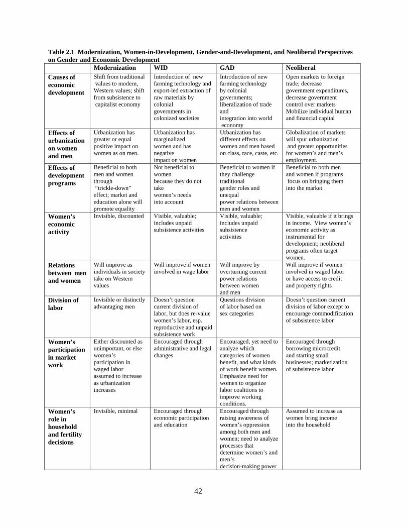
42
Table 2.1 Modernization, Women-in-Development, Gender-and-Development, and Neoliberal Perspectives on Gender and Economic Development
Modernization WID GAD Neoliberal Causes of economic development
Shift from traditional values to modern, Western values; shift from subsistence to capitalist economy
Introduction of new farming technology and export-led extraction of raw materials by colonial governments in colonized societies
Introduction of new farming technology by colonial governments; liberalization of trade and integration into world economy
Open markets to foreign trade; decrease government expenditures, decrease government control over markets Mobilize individual human and financial capital
Effects of urbanization on women and men
Urbanization has greater or equal positive impact on women as on men.
Urbanization has marginalized women and has negative impact on women
Urbanization has different effects on women and men based on class, race, caste, etc.
Globalization of markets will spur urbanization and greater opportunities for women’s and men’s employment.
Effects of development programs
Beneficial to both men and women through “trickle-down” effect; market and education alone will promote equality
Not beneficial to women because they do not take women’s needs into account
Beneficial to women if they challenge traditional gender roles and unequal power relations between men and women
Beneficial to both men and women if programs focus on bringing them into the market
Women’s economic activity
Invisible, discounted Visible, valuable; includes unpaid subsistence activities
Visible, valuable; includes unpaid subsistence activities
Visible, valuable if it brings in income. View women’s economic activity as instrumental for development; neoliberal programs often target women.
Relations between men and women
Will improve as individuals in society take on Western values
Will improve if women involved in wage labor
Will improve by overturning current power relations between women and men
Will improve if women involved in waged labor or have access to credit and property rights
Division of labor
Invisible or distinctly advantaging men
Doesn’t question current division of labor, but does re-value women’s labor, esp. reproductive and unpaid subsistence work
Questions division of labor based on sex categories
Doesn’t question current division of labor except to encourage commodification of subsistence labor
Women’s participation in market work
Either discounted as unimportant, or else women’s participation in waged labor assumed to increase as urbanization increases
Encouraged through administrative and legal changes
Encouraged, yet need to analyze which categories of women benefit, and what kinds of work benefit women. Emphasize need for women to organize labor coalitions to improve working conditions.
Encouraged through borrowing microcredit and starting small businesses; marketization of subsistence labor
Women’s role in household and fertility decisions
Invisible, minimal Encouraged through economic participation and education
Encouraged through raising awareness of women’s oppression among both men and women; need to analyze processes that determine women’s and men’s decision-making power
Assumed to increase as women bring income into the household
43
2.2 RESEARCH METHODS AND EMPIRICAL STUDIES OF DEVELOPMENT
There have been numerous studies that researchers have conducted over the years to assess the
strengths and weaknesses of various development theories in their ability to explain why some
countries are wealthy while others are poor. Some are cross-national studies that test the
development claims of multiple theories, while other studies assess the impact of women’s
development programs on changes in gender inequality. Other researchers have developed
quantitative ways of operationalizing dimensions of women’s status, gender parity, and women’s
empowerment. In this section I will first discuss each development theory and the research
methods that scholars have used to carry out their studies. I will then highlight a few examples
of empirical research that scholars have conducted under each development framework.
2.2.1 Modernization Studies
Because modernization researchers came from several social science fields, the research methods
they employed have been quite varied. For example, anthropologist Clifford Geertz (1963) used
ethnographic methods to study two towns in Indonesia, one with traditional cultural traits and
one with relatively modern cultural traits. Psychologist David McClelland (1968) used the
method of content-analysis to analyze folk stories, folk songs, and other popular literature from
different countries to determine if they reflected the modern value of high achievement
motivation (McClelland 1968, cited in So 1990). McClelland believed that a country’s popular
literature would reflect the overall cultural values of that country. Inkeles and Smith (1974) also
took a psychological approach, and studied how certain character traits predispose individuals to
being more open to modernization. While McClelland focused on individuals’ “achievement
44
motive” and desire to be successful as the main factor leading economic growth, Inkeles and
Smith conducted a cross-national survey study to determine which psychological traits are
characteristic of “modern” men. Some of the earlier modernization researchers took an
economic approach, and thus used quantitative methods to study the modernization process. Still
other researchers, such as Lipset (1963), took a cross-national, quantitative approach to
analyzing the relationship between economic wealth, industrialization, urbanization, education,
and the presence of a democratic government (in So 1990:48-52). Most of the classic
modernization researchers took a cross-sectional approach in their research (So 1990).
Although most of the classic modernization researchers took a highly generalized,
ahistorical approach, the “new” modernization researchers conducted historical case-studies to
learn how the modernization process occurs in a specific nation (So 1990). These researchers
often used comparative methods to analyze why nations experience different development
trajectories. Inglehart and Welzel (2005) were among these new modernization researchers, and
used cross-national, longitudinal methods to analyze the relationship between economic growth
and the rise of modern cultural values. However, very few “classic” or “new” modernization
studies analyzed the different roles that women and men play in the modernization process, or
how the modernization process affects men and women differently. Some of these classic
modernization researchers excluded women altogether from their studies, such as the work of the
scholars I discuss next.
In their book, Becoming Modern: Individual Change in Six Developing Countries, Alex
Inkeles and David Smith (1974) emphasized the role of culture and values in the process of
economic development. However, they seemed to consider only men’s values as important,
since they excluded women from their study. Also, throughout their book they refer to “making
45
men modern”. They conducted interviews with men in six developing nations that had become
substantially industrialized: Argentina, Chile, East Pakistan (now Bangladesh), India, Israel, and
Nigeria. They interviewed men ranging from those who worked in agriculture to those who
worked at factories in cities. The goal of their study was to determine if there are certain
characteristics of a society that influence individuals to take a more “modern” outlook. Inkeles
and Smith examined whether industrialization that has already taken place in a society influences
people’s values and personality. They also examined the psychological traits of individuals that
could lead the society to becoming more industrialized. After analyzing their data, Inkeles and
Smith concluded that there are six criteria that cut across societies by which one can know if an
individual has a modern personality. First, the “modern man” will be open to new experiences
and trying new activities. Second, he has a certain level of autonomy from authorities, and is not
controlled by what parents or rulers say he must do. Third, an individual with a modern
personality will have a scientific outlook and believe that humans can develop technology to
control nature. Fourth, the modern individual will have a “mobility orientation” – that is, he will
be ambitious in his career, and will be willing to move to a new location if it means taking a
higher-status position or a job with better pay. Fifth, the modern individual tends to plan ahead
to meet long-term goals, rather than making decisions that affect him only in the present
moment. Finally, the modern individual is involved in volunteer organizations or community
politics. Inkeles and Smith concluded that one can train people to take on these Western values
through Western-style education, textbooks, and even movies (Inkeles and Smith 1974).
I highlight Inkeles and Smith’s study for a couple of reasons. First, it is considered one
of the “classic” studies within the modernization school (So 1990), and also because the study
takes a characteristically androcentric perspective. Throughout the book, Inkeles and Smith
46
referred to “making men modern”, thus assuming that the subjects of modernization are
masculine. Moreover, they excluded women from participating in the study altogether. Because
they included only men in their study, they seemed to consider only men’s opinions and values
to be important in discovering which psychological traits led individuals to take on a more
modern outlook. Moreover, they seemed to assume that only men in the six countries of their
study engaged in waged labor, an assumption that modernization policy-makers and practitioners
made when implementing development programs. Inkeles and Smith did not consider how
gender may have impacted how widespread certain “modern” characteristics were in the six
countries in their study. For example, if they had interviewed both men and women, they might
have found that far fewer of their respondents had a “mobility orientation” or autonomy from
authority, simply because in many countries women lacked agency to act on their own decisions.
Inglehart and Norris’s (2003) study is one of the few that gave an explanation of how
socioeconomic modernization affects women’s status and gender equality. Like Inglehart and
Welzel (2005), they argued that economic development causes societal values to change. These
changes in cultural values lead to predictable (but not inevitable) decreases in gender inequality.
They analyzed data from UNDP Human Development Reports and the World Values Surveys
for a large number of societies around the world. They found that as nations shift from an
agricultural to an industrial economy and cultural values change from traditional to secular-
rational values, there are sharp increases in female enrollment in primary and secondary school,
female literacy rates increase by almost two times, and prevalence of contraceptive use doubles.
Gender roles in areas of childcare and family begin to change, but are not completely
transformed (Inglehart and Norris 2003). Women in these societies are able to enter the paid
workforce, they gain the right to vote, and they start to participate in government. Overall, the
47
shift from an agricultural to an industrial economy leads to increases in women’s well-being as
reflected from increased scores on the UNDP Gender-Related Development Index (Inglehart and
Norris 2003).
Inglehart and Norris’ (2003) views on how socioeconomic and cultural modernization
affects women differed from those of earlier modernizations theorists in several ways. Whereas
earlier modernization theorists assumed that the effects of modernization would benefit women
as much as if not more than it benefits men, Inglehart and Norris argued that socioeconomic and
cultural modernization are necessary but not sufficient for greater gender equality to occur.
Other cultural and historical factors influence how much impact economic development has on
increases in gender equality. Cultural shifts in people’s attitudes regarding gender equality can
bolster women’s rights, structural reforms, and support for women’s organizations. Inglehart
and Norris (2003) argued that nations also need policy reforms aimed to increase women’s
opportunities and to reduce discrimination against women. They recognized that drastic cuts in
government welfare expenditures (as neoliberals recommended in SAPs) can negatively affect
women more than men since women tend to be the primary caregivers for the elderly and for
children. A decline in a society’s economy may also lead to a decrease in women’s wages and
employment rates (Inglehart and Norris 2003). Inglehart and Norris (2003) recognized that
economic development is not the only factor that leads to increases in women’s well-being and
in gender equality, and that policy decisions also impact how women fare in a society.
48
2.2.2 Women-in-Development Studies
Women-in-Development researchers primarily used quantitative research methods when carrying
out their studies. During the late 1970s, WID policymakers in USAID funded studies of sex-
disaggregated data, such as studies analyzing census data of various nations, in order to detect
trends in women’s changing status from the 1950s onward. As mentioned earlier, they put
pressure on national governments to disaggregate national census data by sex (Tinker 1997), and
they sponsored country studies that utilized anthropological methods and “time budgets” to
better understand the quality of women’s lives. Moreover, the UN Statistical Office developed
the Gender-related Development Index (GDI) and Gender Empowerment Measure (GEM) in
1995 as indices of gender parity for the goal of influencing policy (Jaquette and Staudt 2006;
UNDP 1995). The goal of these two measures is “to place the problem of gender inequality
firmly on the social agenda” (UNDP 1995). The Gender-related Development Index measures
gender disparities in living standards and basic capabilities, whereas the Gender Empowerment
Measure considers women’s political, economic, and professional participation. The GDI uses
the same measures as the Human Development Index (HDI), except that it is weighted by the
level of disparity between women and men on these indicators. The GDI measures “overall
achievements of women and men in the three dimensions of the HDI – life expectancy,
educational attainment, adjusted real income – after taking note of inequalities between women
and men” (UNDP 1995:73). The score that a nation receives for the HDI is “penalized” for
levels of gender disparity so that the GDI score for a nation will be lower than its HDI score,
depending on how much gender disparity these indicators reveal. In 1995, GDI estimates were
calculated for 130 countries. One of the drawbacks to the GDI is that it does not include data on
49
agricultural wages or wages from the informal sector. About 17% of India’s gross domestic
product comes from the agricultural sector (CIA World Factbook 2009). This means that the
HDI and GDI scores for India could be skewed downward since the income from the agricultural
sector is not accounted for. The GEM includes variables that measure the percentage of
parliamentary seats held by women, the percentage of professional, technical, administrative, and
managerial positions held by women, and women’s per capita income in unadjusted purchasing
power parity (PPP) dollars (UNDP 1995).
The UN Statistical Office also developed the “Women’s Indicators and Statistics
Database” (WISTAT) in 1988 (Young et. al. 1994, www.unstats.un.org 2010). This database
consists of sex-disaggregated data in a wide range of topics, including population statistics,
education and literacy; economic activity; households, marital status and fertility (including sex-
disaggregated data for percentage of 15-19 year-olds who have ever been married); health and
health services; reproductive health and rights; political participation, including year that women
gained suffrage; and violence (both domestic violence against women and sex-disaggregated
data on deaths by types of violence); and nations’ GDP.
Pathak and Biswas (2004) carried out an empirical descriptive study of male and female
workforce and labor force participation rates in eastern India from 1971 to 1991. They analyzed
data disaggregated by sex and by rural/urban area from the Census of India for the states of
Bihar, Orissa, and West Bengal. The variables that they analyzed include percentage of the
population 15-61 years of age in the labor force and percentage of population 15-61 years of age
in the work force, both disaggregated by sex and urban/rural areas. Labor force participation
included everyone between 15-61 years of age who either was employed or was willing to be
employed, such as those who were unemployed and looking for work. Work force participation
50
included only those who actually were employed and earning wages. Pathak and Biswas also
examined the female/male sex ratios for the various occupational groups recorded in the India
Census. Another variable that they included in their analyses is the “sexual equality index for
labor force participation in the workforce” (Pathak and Biswas 2004:140), which was the ratio of
female to male workforce participation rates divided by the ratio of female to male labor force
participation rates. The researchers found that West Bengal had the highest male labor force
participation rates of the three states, and that it was even higher than the national average.
However, sexual equality in labor force participation was the lowest in West Bengal throughout
the period of 1971-1991. The female labor force participation rates in all three states decreased
substantially from 1971 to 1981. The researchers surmised that this may be due to the mass
migration of people from Bangladesh into eastern India during this period looking for work.
Bihar started out with the highest gender parity in labor force participation in 1971, but by 1991
Orissa had the highest gender equality. There was improvement in gender equality in labor force
participation rates for all three states for the period of 1971-1991.
The authors found that overall the male labor force participation in the workforce was
higher than that for females, and that there was greater gender disparity in urban areas. In
general, female/male sex ratios in labor force participation and workforce participation had
increased from 1971-1991, especially in rural areas. However, the female/male sex ratio for
labor force participation declined in urban Orissa and Bihar from 1981-1991, and the
female/male workforce participation ratio declined from 1971-1991 in urban West Bengal. This
was true even though overall, West Bengal experienced the greatest increase in female/male sex
ratio in the workforce participation rate from 1971-1991.
51
2.2.3 Women and Development (WAD) Studies
Most of the research carried out by WAD scholars used qualitative research, especially case
studies of how capital penetration in one region affects women’s lives and work in both
productive and reproductive spheres. WAD scholars focused on both class relations and women
in their analyses, and sometimes treated women as if they belonged to a single class. Because
WAD theory draws on dependency theory, WAD scholars analyzed the relationships between
women’s participation in the labor market in peripheral countries and the impact that foreign
capital from core countries has on these women. Some of these researchers used comparative
case-study methods, such as Lee’s (1998) study of women factory workers in southeastern China
and Hong Kong. Other studies used historical and/or ethnographic methods to study how
foreign markets affect women in a single developing country, such as Talcott’s (2003) study of
women in the floriculture industry of Columbia. These studies stressed the negative impact that
foreign capital has on Southern women’s conditions in the labor market.
One of the classic WAD empirical studies is Maria Mies’ book The Lace Makers of
Narsapur: Indian Housewives Produce for the World Market (1982). She carried out this
qualitative case study for the Programme on Rural Women within the International Labor
Organization. Mies carried out a qualitative case study in 1978 of the lace making industry in
Narsapur, which is in West Godavari district, Andhra Pradesh. At the time of her study, the lace
trade brought in 90% of Andhra Pradesh’s export revenue in handicrafts, and over 100,000
women were involved in the lace industry. She studied the production relations in the lace-
making industry, and interviewed women lace-makers, male exporters, middlewomen and
middlemen, marketing agents, as well as women who produced and sold lace independently.
52
Mies studied all stages of lace production in great detail, including the materials the women used
to make lace, the different patterns and styles of lacework, and the types of lacework made by
women of different skill levels. She also studied the history of the lace-making industry in
Narsapur, which had been in existence for at least 100 years. She found that the beginning of the
lace export industry was closely connected to British colonial penetration, and that the labor
force made up of poor women has remained the same since that time.
In her study, Mies argued that the Green Revolution, with its emphasis on agriculture for
export rather than for subsistence needs, the use of high-yielding seed varieties, and the heavy
use of fertilizers and insecticides that farmers could not really afford, caused the “pauperization
of peasants” (Mies 1982:173). Many farmers’ crops did not yield as much as they expected and
they were not able to make up their losses from these capital-intensive farming methods. As a
result, many of them lost their land. As agrarian capital changed to merchant capital, there was
an increase in inequality between marginal peasants and landless laborers on the one hand, and
rich peasants who benefited economically from capitalist farming on the other. This
“pauperization of peasants” led to a large supply of women who were willing to work for very
low wages in order to help provide for their households. Women’s subsistence work greatly
increased, since they were now doing low-paid labor as well as more household production than
previously so their families could survive. However, most of the women lace makers were not
able to get out of poverty.
Mies found that women lace makers spent 6-8 hours a day making lace, and another 7
hours on domestic work. The work life of women who made lace had also lengthened since
these women usually began working at 8 years of age, and continued working as lace-makers
until they were 70 or 80 years old. The detailed, repetitive work of lace making caused physical
53
problems such as worsening eyesight, headaches, dizziness, backaches, fever, and rheumatism.
Because lace making was so low-paying, daughters were usually required to stay home to help
make lace instead of going to school. This only perpetuated the cycle of these women’s misery,
since the daughters were illiterate and had no alternative but to continue in the lace making
industry as adults.
Although women lace makers usually spent a full day at this task, and continued making
lace throughout their lives, Mies found that there was a widespread belief that these women were
mainly housewives who made lace in their leisure time. Exporters, merchants, and middlemen
did not recognize lace making as waged labor, which made possible the expansion of capital
accumulation through the lace making industry throughout the 1970s. The “housewife ideology”
kept women isolated in their homes so that they could not organize with other lace makers to
fight for higher wages. Moreover, the lace makers themselves viewed lace making as part of
their other domestic tasks, and were unable to see that they were actually working for the
exporters, not for their own households. Therefore, they did not value their own work, and were
reluctant to insist on higher wages. Because these women lacked education and physical
mobility, even the women who made and sold lace independently lost their ability to market their
own products as men increasingly took control of the lace market (Mies 1982).
2.2.4 Neoliberal Studies
The neoliberal paradigm of development has its roots in economic theory. Most of the
development studies carried out under this framework come from an economic perspective, use
quantitative methods, and take the nation as their unit of analysis. Many of the neoliberal studies
54
are cross-national, longitudinal studies that analyze the relationships between trade openness and
economic variables such as economic growth, within-nation changes in economic inequality, and
between-nation changes in economic inequality (Dollar and Kraay 2001, Seshanna and
DeCornez 2003). Some studies use a cross-sectional design to analyze cross-national data on
how international trade is related to intra-national income distributions (Chakrabarti 2000). One
of the standard measures of both between-country and within-country economic inequality is the
Gini coefficient, which measures the difference between completely equal income distribution
and actual income distribution, with 100 being the highest level of inequality (Marger 2005).
Levels of economic development are usually measured by countries’ GDP or GDP per capita,
while trade openness is calculated by such measures as percent of GNP contributed by foreign
investment, percent of GNP contributed by exports, and inter-country trade/GDP ratio
(Firebaugh and Beck 1994, Dollar and Kraay 2001, Alderson and Nielsen 2002). Some studies
under the neoliberal paradigm also analyze how trade openness affects demographic and health
indicators in developing countries (Firebaugh and Beck 1994). Almost none of these researchers
analyze gender-disaggregated data for the countries in their studies, such as the effects of trade
openness on income inequality between men and women, or on changes in rates of income
inequality for men versus women. This is true even though some neoliberal studies analyze the
relationship between levels of trade and income inequality as measured by household-level Gini
coefficients (Alderson and Nielsen 2002).
Although these studies are useful in giving us a broad picture of how trade openness
affects average changes in countries’ economic development or income inequality, or even the
impact that trade liberalization has on regions of the world, they tell us little, if anything, about
how trade liberalization has affected changes in gender inequality. One could imagine a
55
scenario in which a world-systems researcher used sex-disaggregated, cross-national data and
variables for trade openness and the Gini-coefficient to estimate the average effect that
integration into the world economy has on women worldwide. However, even with such a study
one cannot gain insights into how integration into the world-economy affects changes in
women’s quality of life, such as their health, their ability to leave home without permission, or
their ability to make decisions about how many children to have.
Dollar and Kraay (2001), researchers for the World Bank, carried out a cross-national
study on globalization, trade, and changes in poverty in developing nations. They first analyzed
data on changes in tariffs, share of trade as percentage of GDP, and changes in GDP for 103
countries from the 1970s through the 1990s. They found that for the developing nations that
globalized the fastest after 1980, there was an average increase of 17 percentage points in trade
as percentage of GDP. These globalizers had also decreased tariffs by an average of 22
percentage points, and had experienced an average increase in GDP growth rates of 2.1
percentage points from the 1970s to the 1990s. In contrast, about two-thirds of the developing
nations decreased tariffs by an average of 11 percentage points, experienced a decrease in trade
as a percentage of GDP, and a decrease in growth rates from this same period. Wealthy nations
experienced an average increase in trade of 13 percentage points, yet also experienced a decrease
in GDP growth rates from the 1970s through the 1990s. From these exploratory analyses they
found that the “new globalizers” were catching up with the wealthy, industrialized nations in
terms of GDP. They therefore concluded that an increase in international trade leads to a
decrease in between-country economic inequality. Dollar and Kraay acknowledged that the
“new globalizers” initiated other policy reforms in addition to decreases in tariffs, such as
reforms in exchange rates and expansion of private property rights.
56
Once Dollar and Kraay (2001) had carried out these exploratory analyses, they utilized
fixed-effects panel regression models to analyze within-country changes in GDP and trade
volumes. Through the use of this model, they were able to control for time-invariant country
characteristics such as geography. They included initial income and trade volume (exports +
imports/GDP) and other control variables as the independent variables, and average annual
change in GDP as the dependent variable. They found that increases in trade volumes were
strongly related to increases in GDP, and that these results were statistically significant. This
was true even after they included lagged independent and dependent variables to control for
potential endogeneity (Dollar and Kraay 2001). They found that on average, a 100% increase in
trade volumes led to a 48% increase in average change in GDP each decade. In a previous study
(Dollar and Kraay 2000, cited in Dollar and Kraay 2001), the authors analyzed the relationship
between globalization, changes in average income within countries, and changes in average
incomes of the poorest quintile of a country’s population. They found that there was no
significant relationship between changes in within-country average per capita GDP and changes
in inequality (Dollar and Kraay 2001:23). There was also no relationship between changes in
trade volumes and changes in within-country income inequality. Dollar and Kraay therefore
concluded that for developing nations, increases in trade volumes leads to increases in average
income, including the average income of the poorest 20% of a country’s population, and do not
increase the degree of income inequality (Dollar and Kraay 2001).
57
2.2.5 Gender and Development (GAD) Studies
Most GAD studies take a qualitative approach to studying the relationships between women and
men, and how cultural norms circumscribe the choices and activities that women are able to be
engaged in, both in the public sphere and the private sphere. Because GAD researchers
emphasize the importance in bringing the private sphere into the public, many of them focus
their attention on gender dynamics within the household, including how patriarchal norms such
as son preference lead to gender inequities in access to food and nutrition. Some GAD
researchers carry out qualitative case studies of gender dynamics and social hierarchies within a
single development organization. Qualitative methods lend themselves especially well to GAD
studies because GAD researchers are interested in studying the relationships between women and
men, and also the relationships between different classes of women both in the public sphere
and the private sphere. Although it’s sometimes possible to use quantitative methods to study
aspects of the private sphere, such as Bangladeshi couples’ gender preferences for children
(Muhuri and Preston 1991), usually qualitative methods are better at picking up the subtle
nuances in gestures, attitudes, and cultural norms. Some of these studies evaluate the impact that
development programs have on women, such as whether women who borrow microcredit have
greater decision-making power in other areas of their life, and the effect that borrowing has on
how their husbands treat them. Researchers who take the GAD perspective examine not just
changes in women’s status and well-being, but women’s status relative to men, and also their
status and roles relative to women of other statuses.
Some GAD researchers carry out studies similar to the studies of WAD researchers, such
as studies of how women’s living conditions and gender roles are impacted by working for
58
multinational corporations. One way to distinguish GAD research from WAD research is to note
that GAD researchers focus not only on the effects of capital accumulation on women’s status,
but also how this impacts relations between women and men. One such study is Fernandez-
Kelly’s (1997) case study of a maquiladora, or borderlands assembly plant, in Ciudad Juarez in
the 1980s. Maquiladoras are usually small, and subcontract work from U.S. corporations.
Eighty-five percent of the employees at maquiladoras at the time of her study were women, and
one-third of the female employees at maquiladoras in Ciudad Juarez were the head of their
households.
Fernandez-Kelly carried out participant observations at a garment factory in Ciudad
Juarez. At this factory, women worked forty-eight hours a week, sitting at sewing machines on
metal folding chairs as they sewed clothing. Many of the women experienced chronic back pain,
and were paid either minimum wage or by piecework. Because Mexico had a law requiring that
women be granted eighty-two days at full-pay during pregnancy leave, the maquiladoras refused
to hire women who were pregnant. Small firms sometimes fired women if they learned that they
were pregnant (Fernandez-Kelly 1997). Fernandez-Kelly found that some women took jobs at
these factories in part because of increased rates of male unemployment. Therefore, they needed
to take jobs at factories either to help support their children, or to contribute to their parents’
income (Fernandez-Kelly 1997). She also discovered that even though women made up the
large majority of the workforce at factories subcontracted by MNCs, they still seemed to be
defined primarily by their domestic role. In the case of the women working at the garment
factory in Ciudad Juarez, fathers and husbands often pressured them to quit their jobs and to
fulfill conventional roles as mothers and caretakers of the home. They still had to reconcile the
conflict between possibly becoming the primary breadwinners in their household and the
59
ideological conception that a woman belongs primarily in the domestic sphere (Fernandez-Kelly
1997). Also, even though many women worked at factories, including electronics factories, their
work was still “invisible” in the sense that employers did not recognize the skills that they
brought to the workplace, but instead believed they were naturally fitted for factory work, and
thus unskilled. Her description of the maquiladora can provide a deeper understanding of the
dynamics between women and men, and between employers and employees in developing
countries where MNCs have a presence.
2.2.6 Studies testing multiple theories
In the previous sections, I reviewed the research methods of modernization, WID, WAD,
neoliberal, and GAD theories, along with some empirical studies associated with each theoretical
tradition. These studies provide insights into the development process, although not all of them
examine how development affects women’s status and changes in gender inequality. All of these
theories (and the research associated with them) put forth contested visions of how the
modernization process occurs, which nations benefit, and women’s place in the development
process. However, none of these studies have tested the strengths and weaknesses of multiple
theories in their ability to explain changes in gender inequality in developing nations. In this
section, I discuss the research methods and empirical findings of scholars who test hypotheses of
multiple development theories. These studies take the nation as the unit of analysis, although
some studies also cluster nations by region or cultural values. They are all necessarily
quantitative studies since they are all macro-level studies and must have comparable measures
across nations. All of them are longitudinal studies, although some of them include cross-
60
sectional analyses as well. Several of them use databases of international development
organizations, such as the Women’s Indicators and Statistics Microcomputer Data Base
(WISTAT), or indices of women’s status and gender inequality such as the Gender-Related
Development Index (GDI) or the Gender Empowerment Measure. I now turn to a review of
some of these studies.
Young et al. (1994) argued that there are important differences between measures of
women’s status and gender inequality. Indicators of women’s status show the absolute level of
women’s procurement of resources valued by society. Studies that measure women’s status may
show that women have attained higher levels of health and education, for instance, but they do
not compare how much women’s status has improved compared to the status of men. Young et
al. took a GAD perspective, and argued that gender inequality is “the departure from parity in the
representation of women and men in key dimensions of social life” (Young et al. 1994:57).
These key dimensions include political systems, health and nutritional systems, economic
systems, educational systems, and family systems. Young et al. analyzed quantitative data from
“Women’s Indicators and Statistics Microcomputer Data Base” (WISTAT), which was published
by the UN Statistical Office in 1988. They examined data on physical well-being (number of
females per 100 males for various age groups, infant mortality rates, percent of births attended
by health staff), public power (ratio of females to 100 males holding seats in national
legislatures), family formation (total fertility rate, contraception use by men and women),
education (ratio of women to 100 men who are illiterate, ratio of women per 100 men enrolled at
different levels of schooling), and economic activity (ratio of women per 100 men considered
economically active). They looked at data from 70 countries, and divided the data into four
development-level categories based on the World Bank’s (1980) GNP per capita income
61
categories. They tested the following two hypotheses: 1. Economic development leads to greater
gender equality (modernization theory), and 2. At all economic development levels there are
significant gender inequalities (WID and GAD arguments). Young et al. (1994) found that there
were greater gender disparities in health at higher income levels than at lower income levels,
such as the number of females per 100 males. Infant mortality was lower and the number of
trained attendants present at births was higher at higher national income levels. This seems to
show that women’s needs related to childbearing are neglected in the lowest-income nations.
There was greater gender inequality in illiteracy and lack of schooling among lower-income
nations than among higher-income nations. The researchers found that women in lower-middle
income nations had less control over their fertility than women in upper-middle income nations.
They also found that there was poor representation of women in government positions for
nations at any of the four income levels (Young et. al. 1994).
The study by Young et al. (1994) shows mixed support for modernization, WID, and
GAD theories. The fact that infant mortality was lower for higher-income nations supports
modernization theory. This is because according to modernization theory, as nations become
more industrialized they will have more advanced forms of technology, including medical
technology, which should result in lower infant mortality levels. Young et al. also found that the
fertility rate of upper-middle income nations is lower than that of lower-middle income nations,
which supports modernization theorists’ assumption that women in more modernized,
industrially developed nations will have greater access to birth control than women in less
developed nations (Jaquette 1982). The fact that there was less gender inequality in illiteracy
rates and lack of schooling in higher-income nations than in lower-income nations also lends
support for modernization theory. However, the researchers’ finding that the female/male sex
62
ratio was lower for higher-income nations than lower-income nations does not support
modernization theory. This finding lends more support to the GAD perspective than the WID
perspective because GAD proponents measure women’s status relative to men’s status instead of
using measures of women’s status only. GAD theorists focus on the relations between women
and men as the analytical category, whereas WID theorists focus on women alone as the
analytical category (Visvanathan 1997). GAD theorists also focus on all aspects of women’s
lives, whereas WID theorists focus only on the economic and political spheres. Finally, the
researchers’ finding that the percentage of government positions held by women is low in nations
at any income level lends support to both WID and GAD theories. Although the results of this
study show mixed support for modernization, WID, and GAD perspectives, the researchers
conclude that economic growth does not necessarily lead to greater gender equality, and that
policymakers need to consider the needs of women in developing nations as well as in
developed, industrialized nations (Young et al. 1994).
Forsythe et al. (2000) carried out a study to determine: 1. whether economic growth
strategies have undermined or fostered women’s status, and 2. whether there have been changes
in gender inequality along with changes in women’s status. They examined cross-sectional data
to determine the correlation between economic growth and women’s status and gender
inequality, and they also examined how economic growth affects changes in women’s status and
gender inequality over time. They used the Human Development Index (HDI) and the Gender-
Related Development Index (GDI) created by the United Nations for 130 nations in 1970 and
1992 (Forsythe et. al. 2000). They used the GDI as a measure for women’s well-being. The
researchers also used the GI, which is the “weight of the [gender] gap relative to a country’s
HDI” as a measure of gender inequality (Forsythe et. al. 2000:583). They analyzed cross-
63
sectional data for 1970 and 1992, and found that there was a strong, significant relationship
between GDP per capita and women’s income, educational attainment, and life expectancy.
They also found that there was a strong relationship between economic growth and an increase in
women’s status “as measured by the GDI” (Forsythe et. al. 2000:607) for the period of 1970-
1992, and that women’s status improved for all the nations in the study. These findings seem to
support modernization theory, since this theory assumes that an increase in a nation’s economic
development will lead to an increase in women’s status. However, when the researchers
analyzed the relationship between economic development and gender inequality as measured by
the GI, they found mixed results. Their examination of cross-sectional data at first seemed to
show that there was a curvilinear (inverted-U) relationship between levels of economic
development and gender inequality. However, once the researchers introduced dummy variables
for nations with majority Muslim population and nations that were Latin American nations, the
relationship between economic development levels and gender inequality disappeared (Forsythe
et al. 2000). The dummy variables for majority Muslim population and for Latin American
nations were significantly related to gender inequality. These two variables seemed to explain
away the relationship between economic development and gender inequality in the cross-
sectional analysis. Although their longitudinal analysis showed that gender inequality decreased
for most nations from 1970-1992, gender inequality actually increased for ten nations, including
India. Nations with the greatest initial levels of gender inequality tended to have the greatest
relative decreases in gender inequality. The longitudinal analysis also showed an inverted-U
relationship between economic development and gender inequality as measured by the GI. The
authors concluded that this finding supports the GAD perspective, since this perspective argues
that economic growth will not necessarily lead to an increase in gender equality (Forsythe et al.
64
2000). However, WID theorists also argue that economic development does not necessarily lead
to an increase in gender equality. Still, this finding does provide support for the GAD
perspective because the GI measures women’s relative status compared to men’s status.
In a third study, Dijkstra and Hanmer (2000) assessed the validity of using the UNDP’s
Gender-Related Development Index (GDI) as a measure of gender inequality. Although they did
not explicitly test the claims of modernization, WID, and GAD theories, they did take a GAD
perspective in determining the best way to measure gender inequality. The researchers critiqued
the GDI because it does not differentiate between a nation’s absolute standards of living and
gender inequality. For example, if a nation has a high level of gender equality but a low score on
human development, it will still receive a low GDI score. They argued that the GDI assesses
some aspects of gender-related development, but that this information must be placed in the
context of a nation’s culture, ideology, and history (Dijkstra and Hanmer 2000). This reflects the
holistic nature of the GAD perspective, as opposed to the WID perspective’s focus on women’s
involvement in the economy (Young 1997). If one wants to assess women’s levels of well-being
in various nations, one needs to examine not only human development indicators (HDI) and
GDP per capita, but also female/male literacy ratios, infant and maternal mortality rates, levels of
violence against women, and qualitative data regarding gender relations. This reflects the GAD
theorists’ claims that one must look at more than just the economic sphere when evaluating the
development process (Young 1997). The researchers developed the Relative Status of Women
(RSW) Index, which is a new measure of women’s status (Dijkstra and Hanmer 2000). The
RSW Index includes female/male ratios of life expectancy and education, some of the GDI
measures, and an income indicator that measures the ratio of “implicit rate of return to women’s
and men’s labor time” (Dijkstra and Hanmer 2000:52). They found that for the top ten ranking
65
nations on gender equality, women do score better than men for a long, healthy life and for
educational levels. However, they added that the RSW does not measure violence against
women or other facets of gender relations. They concluded that they cannot determine whether
the RSW score for a particular nation increases due to a true increase in women’s well-being or
due to a decrease in men’s well-being (Dijkstra and Hanmer 2000). This also reflects a GAD
perspective since the GAD perspective takes both women’s and men’s concerns into account.
Clark et al. (1991) conducted a quantitative, cross-national study to examine the impact
that economic growth, commodity concentration, and culture have on the percentage of the labor
force comprised of women. They analyzed data on 75-105 nations that came from Women…A
World Survey (Sivard 1985, cited in Clark et al. 1991). Clark et al. included four indicators for
dependency theory, all which had been measured around 1967. This provided a sufficient lag
time to pick up any long-term effects that economic dependency might have on women’s
participation in the labor force. They included two variables in order to test the effects of classic
economic dependency: foreign-trade structure and commodity concentration. In order to test the
effects of dependent development, they used a measure of overall foreign investment and a
measure of “foreign investment in extraction”. In order to test the modernization hypothesis that
economic development will have a positive impact on women’s labor force participation, Clark
et al. included logged GNP per capita for the year 1965. They also included a variable
measuring the ratio of women’s to men’s enrollment in higher education during the years of
1960 and 1985. This is because one explanation of economic development’s association with
women’s increased participation in the labor force is that with economic development comes a
great increase in people’s educational attainment, including an increase in women’s enrollment
in higher education, which then leads to women’s increased labor force participation. The
66
researchers also included dummy variables for the broad cultural categories of Islamic, Latin-
American, non-Islamic African, Marxist, Western, and non-Islamic Asian.
Clark et al. started with cross-sectional regression analyses of the effects of the economic
development variables, dependency variables, and female/male enrollment rates in higher
education on women’s labor force participation rates. They found that three of the dependency
variables had a statistically significant, negative relationship with female/male labor force
participation in 1980. Logged GNP per capita had a negative, statistically significant
relationship with female/male labor force participation only when foreign trade structure, which
was not significant, was included in the model. Women’s share of higher education had no
significant relationship with their labor force participation rates. Once the researchers added the
dummy variables for cultural regions (with Western nations as the reference category), only one
of the dependency variables had a negative, statistically significant relationship with women’s
share of the labor force in 1980. GNP per capita was positively and significantly related to
women’s labor force participation in only one of the models. Overall, women’s share of the
labor force was much less in Islamic nations and Latin American nations than in Western
nations, and countries they classified as Marxist had a positive, significant relationship with
women’s share of the labor force. African and Asian nations had no significant relationship with
women’s labor force participation.
The researchers then ran panel analyses to see how the same independent variables, plus
female labor force participation in 1960, affected changes in women’s/men’s labor force
participation from 1960 to 1980. They found that women’s share of the labor force in 1960 was
the most strongly associated with women’s share of the labor force in 1980. They found that
overall, economic dependency had a negative effect on women’s share of the labor force,
67
women’s enrollment in higher education in 1960 had a positive, weak relationship with their
share of the labor force in 1980, and that GNP per capita had a positive relationship with
women’s share of the labor force in 1980. Once they added the culture variables into the models,
commodity concentration had a negative, significant effect on changes in women’s share in the
labor force, and logged GNP per capita continued to have a positive, significant effect on
changes in women’s share in the labor force. Islamic nations still had a negative, significant
effect on changes in women’s labor force participation, even after controlling for all of the
dependency variables. The other culture variables were either weakly related to changes in
women’s share of the labor force, or not significantly related at all. Women’s share of higher
education in 1960 had no significant relationship with changes in women’s share of the labor
force. Overall, Clark et al. concluded that their study lends the most support for the positive
impact that economic development has on women’s share of the labor force.
However, the authors of this study did not go into detail on the types of longitudinal
models that they used. They said that they used panel models, but panel models include a range
of longitudinal models, such as fixed-effects models, difference models, random effects models,
and mixed effects models. In the cross-sectional analyses, they included women’s share of
higher education in 1985 as an independent variable, even though the dependent variable is
women’s share in the labor market in 1980. They did not explain why they used an independent
variable measured at a later time point than their dependent variable. Moreover, they never
mentioned using tests for autocorrelation or robust standard errors. Therefore, it is not clear how
reliable their results really are.
68
2.2.7 Studies on women and microcredit
Microcredit programs have become an increasingly popular strategy among NGOs, donor
agencies, and development policy-makers for improving women’s status and lifting families out
of poverty. Researchers have conducted numerous studies on the impact of women’s microcredit
programs on women’s status in South Asia (particularly Bangladesh), with mixed results. Most
of these are micro-level case studies, and use either qualitative methods or a combination of
qualitative methods and survey interviews. The researchers conducting these studies often use a
quasi-experimental design with a treatment group of women who are borrowers and a control
group of women who are not borrowers. Other researchers compare the effects of two NGOs’
microcredit programs on women’s status, such as Hashemi et al.’s (1996) study of women
borrowers from the Grameen Bank and BRAC in Bangladesh. Some researchers highlight the
positive effects of microcredit on women, such as increased control over economic resources and
greater participation in family decision-making (Todd 1996, Hashemi et. al. 1996). Other
researchers draw more negative conclusions about the effects of microcredit on women’s status,
arguing that many women borrowers do not retain control over the loans they have taken out,
and must turn the loans over to their husbands or other male household members (Goetz and Sen
Gupta 1994, Rahman 1999). Below I highlight two studies of Grameen Bank borrowers in
Bangladesh, each of which came from different development paradigms. While Todd (1996)
came from a neoliberal approach and came to positive conclusions about microcredit’s
empowering effect on women borrowers, Rahman (1999) took a GAD approach and emphasized
how the lending practices of the Grameen Bank re-created patriarchal relations between women
and men.
69
Todd (1996) conducted a qualitative study for one year on 40 women in Bangladesh
who were long-term members of the Grameen Bank centers at Ghatail and at Shajanpur, as well
as 20 female non-members from the same villages. She found that the women who borrowed
microcredit from the Grameen Bank had gained decision-making power within the household,
were in better physical health, and experienced less domestic violence than women who didn’t
borrow microloans. She also found that 27 of the Grameen Bank borrowers in her study were
actively involved in managing the household, economic activities, and household budget, and
that some of these women were the primary decision-makers regarding land cultivation and
leasing in new land. However, she conceded that since she only studied women from two
Grameen Bank centers and that these women had borrowed loans for a longer period of time than
that of most Grameen Bank borrowers, her findings were not representative of all Grameen Bank
borrowers.
Todd’s study supports the neoliberal perspective since she found that increasing women’s
access to credit was sufficient in raising their status and decision-making power in the
household. Like neoliberal scholars, she advocated increasing women’s access to economic
resources within the existing social structure rather than challenging social inequalities, such as
female seclusion, in order to increase women’s well-being. While Todd’s study may seem to
also support WID theory since WID theorists emphasized the need to include women in waged
labor, her study contradicts WID theory in a couple of ways. Whereas WID scholars are
concerned about women’s double burden of domestic and economic responsibilities once they
start to engage in income-generating activities, Todd (1996) found that the women in her study
were proud to be doing extra work if it meant bringing more income into the household and did
70
not mind the double burden of work. In contrast to WID scholars, Todd did not address
women’s occupational exclusion or their exclusion from suffrage.
Rahman (1999) took a GAD perspective in his study of the lending structure and lending
processes of the Grameen Bank. He studied Grameen Bank workers and borrowers in a village
of the Tangail zone in which the Grameen Bank had been operating for fifteen years. Rahman
found that the Grameen Bank re-created the existing patriarchal system in its organizational
structure and lending practices. For instance, he observed that the Grameen Bank targeted
primarily women because bank workers viewed them as submissive, passive, and easily
disciplined. Men made up the majority of bank workers, and were addressed by the women
borrowers as “sir”, thus reinforcing the men’s higher status. Women borrowers often had to rely
on men to invest the loans, and did not have a say in how these loans were used. Moreover,
Rahman observed that bank workers faced institutional pressure to persuade borrowers to take
out successively larger loans. This often caused the women borrowers to fall into a “debt trap,”
taking out subsequent loans to pay off prior loans. This debt burden often led to increased
tension and violence against the women borrowers within households. Like other GAD scholars,
Rahman argued that it is important to examine power relations between men and women within
households and between male bank workers and female borrowers.
2.3 CONCLUSION
From the myriad of studies that researchers have already conducted related to theories of
development, it is not apparent which development approach is best in raising gender equality, or
at least in a particular nation. There are some cross-national studies that assess the impacts of
71
several development paradigms on gender equality, but none that seem to do this for a single
nation (a country study). As pointed out by Roy and Sideras (2006), trade liberalization has
benefited some nations, but has had disastrous effects on other nations. It could very well be true
that development programs of the same paradigm (say, economic growth) will not have the same
effect on increasing gender equality in different nations. Even though Inglehart and Norris
(2003) found that overall economic growth leads to greater gender equality in all regions, their
analyses do not address how economic growth affects gender equality in any single country.
There are also micro-level case studies on the impacts of various women’s development
programs on women’s status in India and Bangladesh, which are appropriate for evaluating the
impact that a particular program has in a localized region. However, the findings of these studies
cannot be generalized to a larger region of the country, much less the entire country.
My study helps to address some of these issues by analyzing the effects that women’s
development programs associated with different development paradigms have on district-level
changes on gender inequality in India. A meso-level study of a single nation such as India is
advantageous because it incorporates some of the strengths of both micro-level and macro-level
studies. Such a study can take into account the particular characteristics of one nation, such as
cultural norms regarding gender roles, forms of governance, and particular development policies
that the nation’s government has implemented. With a meso-level study that takes the district or
county as the unit of analysis it is possible to compare how development programs affect
changes in gender inequality across larger regions within the country, such as states or provinces.
This is a benefit over micro-level studies of a single women’s organization, since it allows one to
examine how regional variations affect the impact that different development programs have on
changes in women’s status. This is important for a vast country like India, since patriarchal
72
norms tend to be stronger in northern states than in southern states (Dreze and Sen 2004).
Moreover, even the same types of development programs may have different effects on gender
inequality since each development organization will have a unique organizational culture and its
own particular way of implementing its women’s programs. A meso-level study can control for
the particularities of each development program to assess the overall effect of that type of
program on raising women’s status.
However, how does one classify the thousands of development programs that exist in
India? This is the issue I take up in the next chapter.
NOTES TO CHAPTER TWO
i Not all scholars agreed with modernization theorists’ explanation for how societies become economically developed. Whereas the modernization theorists stressed the importance of factors that are internal to a society in bringing about economic development, the thinkers of the dependency school argued that external factors are primarily what determine whether or not a nation becomes developed (So 1990). They criticized the modernization theorists for not taking colonial relations into account when examining why some nations became wealthy, capitalist democracies while others remained in poverty and were susceptible to authoritarian regimes. Dependency theorists maintained that the continued exploitation of former colonial nations in Africa, Asia, and Latin America by post-imperialist nations is the main reason why some nations become wealthy with high levels of education and good health care systems, while other nations remain in poverty. Continued dependency of less-developed or “peripheral” nations on wealthy or “core” nations is caused by a flow of economic surplus from less-developed countries to the more powerful, industrialized nations. Therefore, “dependency” is primarily an economic condition. Moreover, dependency theorists argued that less-developed, peripheral nations and wealthy, industrialized core nations are becoming more and more polarized in terms of levels of economic development. Capital flows from the periphery to the core causes the less-developed nations to become underdeveloped, and Western nations benefit from this unequal economic relationship (So 1990).
According to dependency theorists, true, long-lasting development cannot occur for developing nations as long as they continue economic relations with wealthy, industrialized nations. Therefore, they argued, peripheral countries should sever economic ties with wealthy nations. They should accept less foreign aid and technology, not more, and should not adopt Western values. Rather, peripheral nations should become self-reliant, carve their own path to development rather than following the path set out for them by Western nations. They should use their own resources so that they can gain independence from “core” countries. Moreover, dependency theorists argued that elites in peripheral countries benefit from economic relations with Western nations. Therefore, the peripheral countries need a socialist revolution in order to overthrow the ruling elites and establish a new economic order (So 1990).
Dependency theorists and researchers took a gender-blind approach, and did not include a gender analysis. They seemed to assume that peripheral countries’ dependency on core countries affects all citizens of peripheral countries the same way, or at least everyone within a particular social class the same way, regardless of their gender. The policy suggestions of dependency theorists did not consider how women and men may be affected differently, either. If peripheral nations sever ties with core industrialized nations, how will this affect women? If peripheral
73
countries increase their own industrialization in order to produce more for their own economies/societies, who will be involved in this increased economic production? Men and women? Men only? Dependency theorists are silent on this issue.
ii The world-systems perspective emerged in the early 1970s as a response to various scholarly debates that were going on from 1945-1970 (Wallerstein 2004). One of the debates was in regard to the “core-periphery” concept that scholars of the dependency school had developed and whether this concept could really explain the relationship between wealthy Western countries and less-developed countries. The economies of East Asian nations were rapidly expanding, even though some of these East Asian nations had been colonies of other nations in the past (So 1990). These nations clearly did not fit the deterministic pattern of peripheral nations dependent on core nations. Another debate among economic historians of Western nations was over whether feudalistic societies transitioned into capitalistic societies because of internal factors such as class relations, or external factors such as trade flows (Wallerstein 2004). Scholars who emphasized external factors suggested that perhaps a larger region than the country should be the unit of analysis when examining changes in economic structures of the past.
World-systems theorists took the historical system as the unit of analysis rather than the state or society. According to Wallerstein, the founder world-systems theory, a “world-system” is “…a spatial/temporal zone which cuts across many political and cultural units, one that represents an integrated zone of activity and institutions which obey certain systemic rules” (Wallerstein 2004:17). According to world-systems theorists, capitalist world-economies (world-systems in which market exchanges were most important) started to develop about 1500 A.D. World-economies covered a large span of the world, and each world-economy was made up of several political structures. Some of these political structures gained a monopoly in the world-economies, and received more than their fair share of the surplus. By the late 1800s, only one world-economy existed which spanned the globe.
Like dependency theorists, world-systems theorists argued that core states monopolize the processes of production, and that peripheral states have production processes that must compete with the quasi-monopolies of core states (Wallerstein 2004). Wallerstein and other world-systems theorists extended the core-periphery concept to include semiperipheral states, or states that have a combination of peripheral-like and core-like production processes. These semi-peripheral states try to keep from slipping into a peripheral relationship with the core countries, and must compete with each other to be the hosts of corporations from core states that relocate factories to them in order to cut costs of production. Wallerstein argued that during periods of economic contraction, former leading industries are likely to re-locate work to some peripheral countries, but not to all of them. It is this relocation of work to semiperipheral states that Wallerstein referred to as “development.” This core-periphery-semiperiphery system can explain why some countries such as Brazil, India, and S. Korea are becoming more successful economically while many other peripheral and semiperipheral states are not (Wallerstein 2004).
Feminist scholars from within the world-systems framework have criticized the theory for excluding women’s economic role in the global market (Ward 1993, Dunaway 2002). Feminist scholars such as Kathryn Ward (1993) and Wilma Dunaway (2002) argued that world-systems scholars do not take into account all of feminist scholars’ research that shows how economic development has negatively impacted women’s status vis-à-vis men. Dunaway (2002) argued that world-systems researchers ignore feminist scholars’ work, even when feminist scholars take a world-systems approach to capitalist accumulation. Moreover, world-systems researchers do not acknowledge how important women’s work is to the maintenance of the world-system (Ward 1993). Feminist world-systems scholars critiqued other world-systems researchers for several reasons. These feminist scholars argued that world-systems researchers assume that women are incorporated into the world-system as household members (Ward 1993, Dunaway 2002). These world-systems researchers take an androcentric view of economic participation, and ignore women’s work in the informal sector and the domestic sphere (Ward 1993, Dunaway 2002). Dunaway (2002) argued that most of the scholars who have done research on agricultural households have not paid attention to gender inequities within households or between male and female agricultural laborers, even though women have always played an important role in agriculture. Ward (1993) acknowledged that some researchers have tried to bring women into world-systems analysis by using the household as the unit of analysis (Wallerstein 1984, Smith 1984, cited in Ward 1993). These researchers have tried to deal with the fact that women do carry out unwaged labor and informal paid labor in the household. They have also taken into account how unpaid labor aids in the “reproduction of the labor force and the capitalist system” (Ward 1993:529). However, Ward argued, these researchers have not acknowledged that women’s unpaid labor and domestic work is not just a result of the rise of capitalism, and that women’s subjugation to men existed before the capitalist system. Dunaway
74
emphasized the importance in using concepts that allow researchers to analyze gender, such as “resource pooling” instead of “income pooling”, since “income pooling” implies some sort of paid work, whereas “resource pooling” can include women’s non-paid subsistence work.
75
3.0 CHAPTER THREE: THEORIES OF DEVELOPMENT AND WOMEN’S
EMPOWERMENT: A RECONCEPTUALIZATION
3.1 INTRODUCTION
Strategies for increasing gender equality in developing countries that are grounded in
modernization, WID, GAD, or neoliberal theory operate with different sets of logics. As
discussed earlier, WID practitioners focus on integrating women into the development process
(Tinker 1997). From the neoliberal perspective, lending small amounts of credit to the poorest
women so that they can invest in small businesses related to activities they are already doing is a
very effective strategy for increasing women’s status. Others coming from a GAD perspective
argue that increasing women’s access to credit is not enough. They emphasize collective action,
public education, and coalition building as the most effective strategies for increasing equality
between women and men, and argue that women must challenge existing power relations
between men and women (Young 1997). There are countless development programs and
organizations coming from all of these development perspectives in India, which makes it
possible to test how women’s development programs of different types affect changes in gender
inequality. Yet how do we classify them into either modernization, WID, GAD, or neoliberal
programs? Is there a way of assessing the impact that women’s programs coming from different
development paradigms have on changes in gender inequality? One place to start is with the
76
concept of “empowerment”. Over the past couple decades, “empowerment” has become a
buzzword in development circles, and is used in both scholarly and popular literature on
women’s development. “Empowerment” is briefly defined as “…the process by which the
powerless gain greater control over the circumstances of their lives” (Presser and Sen 2000:18).
Beginning in the 1990s, the word “empowerment” became a popular part of the jargon of
development agencies, and has come to mean different things for groups with conflicting ideas
(Troutner and Smith 2004, Townsend et al. 1999). In 1995, the Beijing Platform for Action of
the Fourth World Conference on Women stated that empowerment is “fundamental for the
achievement of equality, development, and peace” (Beijing Declaration and Platform for Action
1996: 8, in Troutner and Smith 2004:9). However, because there are many conceptions of
empowerment, the criteria for empowerment are seldom explicit, and therefore empowerment is
difficult to measure. Troutner and Smith have this to say about empowerment: “Why does the
meaning of ‘empowerment’ matter so much? It matters because understandings of the term
affect pursuits of power in the real world and practical programs for change…Dominant
interpretations of the term thus inform and reinforce policies and practices that in turn strengthen
the capitalist political-economic system and the capitalist mind-set” (Troutner and Smith
2004:12). Empowerment can mean women’s enhancing their entrepreneurial skills, gaining the
power to challenge inequities that they face in their societies, overcoming the inequalities and
attitudes that keep them dependent on men, etc. In this chapter, I first discuss women’s
microcredit programs and Indian women’s social movements. Partisans in debates over
development point to both women’s microcredit programs and women’s social movements as
examples of empowerment. The fact that the programs come from basically diametrically
opposite paradigms shows how slippery the concept of “empowerment” is, and the importance in
77
clarifying this concept. I next move on to a discussion of feminist (and masculinist) conceptions
of power. Finally, I give my own re-conceptualization of women’s development programs based
on variations in a combination of notions of power and theories of development. I also give
examples of women’s programs and organizations in order to demonstrate how I use these
conceptualizations of power to classify women’s development programs as either modernization,
WID, GAD, or neoliberal-type programs.
3.1.1 Microlending as a strategy for more gender-equitable development
Numerous development programs with a focus on microlending that began in the 1970s have
drawn increasing attention from donors such as international development agencies (Mayoux
1995). Development agencies and practitioners have often hailed microcredit lending to poor
women in developing countries as a panacea for lifting families out of poverty while
empowering women, raising women’s status and lowering gender inequality (Deshmukh-
Ranadive and Murthy 2005, Mayoux 1995, Cheston and Kuhn 2002, Ahmed et. al. 2001). By
the 1990s, agencies advocated women’s micro-enterprise development as a way to alleviate
poverty. There are two reasons for this. Researchers have discovered that women spend more of
the money they earn on the needs of their family than men do, such as on children’s healthcare,
education, clothing, and food (Cheston and Kuhn 2002, Ahmed et. al. 2001, Kristof and
WuDunn 2009). Therefore, it makes sense for development programs to target women if they
want to have the greatest impact on eliminating poverty.
Lending small amounts of credit to women also helps increase their employment in
microenterprises (Ahmed et. al. 2001). This is because it allows women to invest in homestead-
78
based activities such as raising and selling poultry, paddy husking, selling produce, or grinding
mustard seeds into mustard oil. These are activities that women often do as unremunerated
work; with a small amount of capital, it is argued, they can turn these activities into small
businesses, thus generating cash income that women could potentially control (Ahmed et. al.
2001).
The Grameen Bank in Bangladesh, founded by Muhammad Yunus in 1972, is one such
microlending institution that has gained a lot of publicity and support from donor agencies as an
effective neoliberal economic development scheme. Other organizations that include
microlending as part of their development program exist in many parts of the world, such as
Ghana, Rwanda, and Tanzania in Africa; Columbia, Mexico, and Costa Rica in Latin America;
and India, Nepal, and Pakistan in South Asia (Cheston and Kuhn 2002). The Grameen Bank,
and Grameen Bank replicates in India such as SHARE Microfin Ltd., assumes that poor, landless
peasants must have access to credit in order to become free from usurious money-lenders and to
lift themselves out of poverty (Grameen Bank web site). The overall theory driving the Grameen
Bank is that it is up to individuals to innovate, work hard, and raise their own standard of living.
No state intervention is required; in fact, the neoliberal model assumes that state intervention
undermines market incentives, adds unnecessary layers of bureaucracy and opportunities for
corruption, creates dependency and reproduces poverty instead of encouraging economic
development. All the Grameen Bank does through extending credit to the very poor is overcome
a market failure, caused primarily by the demonstrably incorrect perception that there is no profit
to be had in lending to poor people without charging usurious interest. By “empowerment”,
microcredit organizations mean increasing people’s economic power (Deshmukh-Ranadive and
Murthy 2005). Although the Grameen Bank approach targets women for its lending programs, it
79
does so primarily in order to help families lift themselves out of poverty rather than to address
structural inequalities in the society based on gender or class. For example, under “Credit
Delivery System” on the Grameen Bank web site, it states that the priority of the Grameen Bank
is to make credit available to the poorest people in Bangladesh, and women make up a large
proportion of this category (Grameen Bank web site).
Most donors and international development agencies agree on the fundamental aspects of
women’s micro-enterprise development (Mayoux 1995). For instance, they agree that
microfinance institutions need to increase client participation, extend small amounts of credit to
women, and conduct studies on market viability. They also agree that development agencies
should have both micro-level and macro-level programs. However, various scholars and
practitioners disagree about the extent to which microlending to women improves their status,
makes them more empowered, and increases gender equality, or even how to measure these
concepts.
3.1.2 Women’s collective action as a strategy for equitable development and empowerment
According to the GAD theoretical perspective, it is necessary for women to engage in collective
action and to challenge existing power relations in the economy, polity, and civil society if they
are to attain gender equality. In India, the struggles against British colonial rule laid the
foundation for the women’s movements (Ray 1999, Subramaniam 2006). There have been
numerous social movements in India that have fought for women’s rights. The Constitution of
India guaranteed equal rights for women (Ganguly-Scrase 2000). However, these legal
guarantees were not upheld. Women’s organizations worked within the political system and
80
helped to frame the first few Five Year Plans (Subramaniam 2006). They agreed with Indian
political leaders and the dominant modernization development paradigm that economic growth
would “trickle down” and benefit everyone in society, including women. Before the 1970s,
Indian women’s organizations generally had affiliations with both the ruling Congress party and
with the Communist Party of India (Ganguly-Scrase 2000). During the 1970s Indian women
addressed issues related to land rights, working conditions, and inflationary prices (Ganguly-
Scrase 2000). These women’s groups emphasized basic survival needs, and thus were more
directly related to development than some of the later women’s organizations. They also focused
on the situation of tribal, peasant, and working-class women. From 1975 to 1977, Prime
Minister Indira Gandhi imposed a national emergency and repressed civil liberties (Ray 1999,
Subramaniam 2006). The Communist Party of India had by this time become fragmented into
two parties, the Communist Party of India and the Communist Party of India (Marxist) (Ray
1999). The Communist Party of India aligned itself with Indira Gandhi during the Emergency,
and thus became discredited once Indira Gandhi’s political regime came to an end and the new
political party in power restored civil rights in 1977. After the National Emergency, many
people in India no longer trusted the political institutions due to the suppression of their rights
during the Emergency, and formed organizations that maintained autonomy from political parties
(Ray 1999). A number of autonomous organizations, including many women’s organizations,
multiplied as a backlash to the loss of freedom under Indira Gandhi’s rule (Subramaniam 2006).
The political vacuum that was created when Indira Gandhi was voted out of office and the
Communist Party of India fell into disrepute allowed autonomous women’s organizations in
many states to remain strong. Many of the new women’s groups that sprang up after this period
did not affiliate themselves with political parties (Ray 1999). However, in some states such as
81
West Bengal, the Communist Party of India (Marxist) remained powerful and continued to
control the political field even after the Emergency ended. In these areas, the women’s
organizations needed to affiliate themselves with the Communist Party of India (Marxist) in
order to gain legitimacy. During this period, research organizations for the study of women’s
issues were founded, such as the Centre for Women’s Development Studies (New Delhi) and the
Research Centre for Women’s Studies (Mumbai). During the 1980s, many women’s
organizations started focusing on issues related to violence against women, such as dowry
deathsiii, rape, sex-selective abortioniv, and partner-perpetrated violence against women
(Subramaniam 2006). Although many of these organizations do not directly deal with
development issues, there are some women’s development organizations, such as the Working
Women’s Forum, that have included the women’s rights issues listed above as part of their
ideology (Mayoux 1995, citing Noponen 1987, 1990). These women’s rights organizations all
come from a GAD perspective, since GAD scholars practitioners and practitioners emphasize the
need to engage in collective action in order to challenge unequal power relations between women
and men (Young 1997).
One women’s social movement that addressed the issues of tribal people’ land rights is
the Chipko movement near the Himalayas (Ganguly-Scrase 2000). During the period of 1961-
1971, the Indian government started clearing forests and land in order to build dams and to make
room for large-scale farming. Many of the rural poor lost their land to these development
projects, and were then forced to depend on waged labor. However, agricultural work for men
grew at over two times the rate that wage work for women grew during this period, which meant
that many more women were marginalized than before. Communities that in the past relied on
gathering produce from the forests had less and less access to these forests that once had been
82
open to them. In the early 1970s, the protests erupted among people living near the Himalayas
against contractors planning to chop down trees. Women hugged the trees to keep logging
contractors from chopping them down. By 1975, women from nearby villages formed women’s
welfare organizations to fight more broadly against the destruction of forests and fields. Women
also protested against men who let their livestock graze in the women’s fields, and against
domestic violence and male alcoholism (Ganguly-Scrase 2000, Agarwal 1994). The Chipko
movement shows how women used collective action to respond to androcentric state-sponsored
welfarist development schemes that negatively impacted the rural women living in the area
where these projects were taking place. It also highlights the importance in taking into
consideration not only women’s development groups, but also the gendered character of
development projects when assessing the impacts of development organizations and projects on
women’s well-being and gender inequality.
An example of a women’s movement that has challenged patriarchal gender relations
within the family in India is the anti-dowry campaign. In 1980, feminist protestors began to
focus on the giving and taking of dowry and on dowry harassment (Ganguly-Scrase 2000). The
giving of dowry by the bride’s family to the family of the groom is part of patrilineal kinship
practices in India. Because a new bride is seen as an economic burden to her husband’s family,
her family must compensate the groom’s family by giving gifts of clothes, jewelry, and money.
In recent decades, there has been an increase in the number of communities that have started
observing the custom of dowry that had not followed this custom previouslyv. Since the late
1970s, there has been a rise in the number of cases in which women have been physically or
emotionally abused by their husband’s family in order to pressure the women’s parents to give
additional dowry items to the groom’s family (Ganguly-Scrase 2000, Subramaniam 2006). If the
83
woman’s parents do not meet the in-laws’ demands, the bride is often murdered as a result
(Ganguly-Scrase 2000, Subramaniam 2006). During the late 1970s and in the 1980s, numerous
feminist organizations in Delhi carried out an anti-dowry campaign that included exhibitions,
street theater, and demonstrations. They gained attention from the public and the media to
dowry crimes, including dowry deaths that had been reported as suicides. Women are continuing
to mobilize against dowry-related harassment, and often stage demonstrations in the workplace
or neighborhood of a husband who is harassing his wife (Ganguly-Scrase 2000).
Another organization that has challenged patriarchal gender relations is the Forum
Against Oppression of Women in Mumbai (Ray 1999). The Forum Against Oppression of
Women was first formed in 1980 as a response to the rape of Mathura, a sixteen-year-old tribal
woman, by several policemen (Ray 1999, Subramaniam 2006). The Mathura rape case led to the
mobilization of protest groups across the nation, including the Forum Against Oppression of
Women (at that time called the Forum Against Rape) (Ray 1999). Since then, the Forum has
taken on other women’s issues related to domestic violence and unequal treatment of women.
The Forum Against Oppression of Women and the Women’s Centre, both autonomous groups,
organized street demonstrations and marches in the neighborhoods of female victims of violence
such as wife battering and dowry deaths. Members of the Forum Against Oppression of Women
have participated in demonstrations, parades, and consciousness-raising activities in regard to
girls’ equality with boys (Ray 1999). The Forum, along with the women’s movement in general,
take a GAD perspective and have emphasized that violence against women occurs in the private
sphere of the family and should be made known in the public sphere (Ray 1999, Subramaniam
2006).
84
I give the examples of the anti-dowry campaign and the Forum Against Oppression of
Women because they highlight the different logics that undergird women’s rights organizations
and modernization development programs. Modernization practitioners and policy-makers
assumed that as people in a developing country adopt “modern” values and outlooks, patriarchal
norms that justify gender discrimination such as rape and dowry murders would automatically
disappear. However, both GAD practitioners and the women’s movements and organizations
mentioned above contended that the adoption of “modern” Western values and economic growth
does not automatically lead to more equitable gender relations. The GAD framework is a
holistic framework, and like some of the Indian women’s social movement organizations noted
above, it is concerned about eradicating gender inequalities in the private sphere. The women
involved in the anti-dowry campaign and the Forum Against Oppression of Women seek to
tackle gender hierarchies and cultural norms that subordinate women; so do GAD theorists and
practitioners. Moreover, the patriarchal norms that lead to dowry deaths and other forms of
domestic violence (issues that are concerns of women’s SMOs) are the same cultural norms that
lead to an unequal distribution of food, health care, and education between boys and girls (issues
that are concerns of GAD scholars and practitioners).
Microcredit institutions and women’s social movement organizations each use a very
different conception of empowerment. Microcredit institutions focus on what they call
empowering women economically so that they can start small businesses engaging in activities
that they do on a regular basis. They take an instrumental approach; the goal of these programs is
to give women the economic resources to raise the status of their entire household. In contrast,
women’s social movement organizations in India use collective action to challenge institutions,
social norms and practices that perpetuate gender inequality. Collective action requires women
85
to develop leadership skills, social solidarity, and to develop the ability to confidently interact
with public officials, all skills that feminists consider empowering. These are not the only types
of women’s organizations and programs that exist in India, however. In the next section I
discuss various conceptions of empowerment, and how these can used to categorize the wide
variety of women’s development programs.
3.2 CONCEPTIONS OF POWER
3.2.1 “Power over”, “power to”, “power within”, and “power with”
One feminist conceptualization of empowerment is that of four dimensions of power: “power
over”, “power to,” “power within,” and “power with” (Townsend et al. 1999). “Power over,” or
what Hartsock simply refers to as “power”, “is a means of getting others to act in ways they
would not otherwise act” (Hartsock 1983:4). “Power over” is a Weberian conception of power,
and refers to the capacity to carry out one’s will, even against resistance (Brush 2003). “Power
over” in the Weberian sense is held by those who have the most military strength, those who
hold political sway, and those who have the economic resources to influence others to carry out
their will (Brush 2003). “Power over” is a zero-sum game: in order for women and dalits to gain
power, men and people of upper-castes must lose some of their power (Brush 2003, Townsend et
al. 1999, Troutner and Smith 2004). It is also enforced by social norms that require those who
have less power to do the will of those with more power (Townsend et al. 1999). It can also be
enforced by violence, threats, or fear (Townsend et al. 1999).
86
Although some feminist scholars and practitioners emphasize “power over,” and the need
to challenge existing social hierarchies in order to bring about greater gender equality, other
feminists associate “power over” with oppression, especially men’s oppression of women
(Townsend et al. 1999). They argue that development interventions that focus on “power over”
will not accomplish much because of the negative connotations that this type of power has
(Townsend et al. 1999). Other scholars argue that women do not seek “power over” men, but
rather an equal balance of power between women and men so that women have space to
maneuver (Troutner and Smith 2004).
Nancy Hartsock introduced the concept of “power to” as a feminist conception of power
(Hartsock 1983, cited in Troutner and Smith 2004). According to Hartsock, “power to” is a
productive power, and is “the ability to bring about meaningful change” (Troutner and Smith
2004:5). During the 1970s and 1980s, feminists of the global South used the “power to”
conception of empowerment to analyze gender inequalities in the distribution and control of
resources (Troutner and Smith 2004). “Power to” is also the kind of power that neoliberal
scholars/practitioners refer to when they talk about the merits of microcredit in giving women the
“power to” start small businesses.
A third dimension of power is “power within”. “Power within” is an improvement in an
individual’s self-image, including an increased perception that she or he has the ability as well as
the right to make decisions (Townsend et al. 1999). It also means an increase in one’s self-
esteem, self-confidence, and an enhanced ability to affect change in a sphere broader than
oneself. Women gain power within through some form of education, such as learning new skills
(Troutner and Smith 2004). Once a woman’s self-concept has been transformed in this way, it
can give her the courage she needs to rise up against gender inequality. “Power within” is
87
necessary in order to be involved in decision-making (Rowlands 1997, cited in Troutner and
Smith 2004).
A fourth dimension of power is “power with”, which refers to collective action and
cooperation to reach goals and solve problems, and includes capacity-building, solidarity, and
social networks (Townsend et. al. 1999, Wong 2003). Some scholars viewed this kind of
collective action as also giving women social capital, which refers to “features of social
organization, such as trust, norms, and networks that can improve the efficiency of society
facilitating coordinated action” (Putnam 1993:167, Townsend et al. 1999). “Power with” is
closely linked to “power within”. Some feminist scholars argued that “power over” is an overly
masculine form of power based on domination and competition, embedded in a history of
Western patriarchal social relations as far back as ancient Greece (Hartsock 1983). These
scholars and practitioners argued that development organizations must focus on “power with”
rather than “power over” in order to bring about greater gender equality. “Power with,” they
argued, is a more communal, feminine conception of power. One of the assumptions of the
feminist conception of “power with” is that women do not benefit from modernization or
capitalist development, or male-led, top-down development projects. Therefore, they must take
action for themselves and make demands on those who maintain power. They need to be
“empowered” to do this skillfully and to get the results they are seeking (Troutner and Smith
2004).
Some scholars evaluate and critique the underlying framework, especially notions of
power, on which development organizations’ policies and practices are based. Wong (2003)
used these conceptions of power to evaluate and critique the development policies of the World
Bank and the IMF during the period when they followed the neoliberal paradigm of development
88
during the 1980s to mid-1990s, the post-Washington Consensus period from the mid-1990s to
late 1990s, and in 2001 when they placed an emphasis on empowerment as an important
component of development in the World Development Report (World Bank 2001, cited in Wong
2003). Wong critiqued the World Bank and the majority of micro-credit schemes for their
neoliberal perspective and for focusing primarily on ‘power to’ and ‘power with’, and not giving
enough attention to ‘power over,’ especially coercive and violent forms of ‘power over’ that
occur in stratified societies. She argued that the World Bank takes an instrumental approach to
empowerment, and tries to include women in the market by helping them get control over
economic resources. The World Bank and micro-credit programs do not deal with the unequal
distribution of power or other inequalities in societies, or how these inequalities help determine
who has control over resources and decision-making processes (Wong 2003). This is in contrast
to many people’s movements in India, such as women’s, dalit, or agricultural movements, which
do focus on overturning hierarchical power structures.
Feminist scholars’ conceptualizations of empowerment as “power over,” “power to,”
“power within”, and “power with” provide insights into how to think about the ways in which
development organizations from different historical time periods operate under different
development paradigms as they plan and implement their programs. These scholars rightly point
out that different aspects of power can coexist in the same place at the same point in time, and
that there are no clear boundaries between one dimension of power and another. The four
dimensions of power that they discuss are useful conceptual tools for examining the wide array
of development programs and organizations that have existed in India from the time of India’s
emancipation from British rule up to the present. Moreover, Wong’s paper (2003) shows how
analyzing the ways in which development agencies conceptualize power can shed light on how
89
the paradigms that these agencies operate under are related to the effects that their development
interventions have on women’s status and gender inequality.
As useful as the four dimensional model of power is for analyzing organizations’
development ideologies and interventions, there are some problems with using these four
dimensions of power in order to classify different types of development programs. As several
feminist scholars have pointed out, these dimensions of power are not mutually exclusive (Wong
2003). This means that some development programs may rely on more than one dimension of
power. For example, rights-based women’s organizations/programs may use “power over” to
examine ways in which women are oppressed by patriarchal cultural norms, and then use “power
with” to collectively challenge these inequalities. Also, many women’s microcredit self-help
groups utilize both “power to” and “power with”.
3.2.2 Agency, resources, and opportunity structure
Alsop et al. (2006) conceptualized empowerment very differently. They defined empowerment
as “a group’s or individual’s capacity to make effective choices, that is, to make choices and then
transform those choices into desired actions and outcomes” (2006:10). They argued that there
are two factors that affect empowerment – opportunity structure and agency. Agency refers to a
group’s or individual’s ability to imagine different options and then choose from among those
options. Agency depends on the assets one has, which include human assets (such as education),
social assets, financial assets, material assets, psychological assets, organizational assets, and
informational assets. However, agency is not enough in order for one to be empowered, because
90
there may be aspects of one’s opportunity structure that hold one back from acting on and
realizing the choices one makes (Alsop et al. 2006).
Opportunity structure refers to the institutional context that affects individuals’ or groups’
ability to act on the choices they desire to make. Both formal and informal institutions make up
the opportunity structure in which an individual group acts. Formal institutions include
regulatory frameworks, laws, and rules “that govern the operation of political processes, public
services, private organizations, and markets” (Alsop et al. 2006:12). Informal institutions
include informal value systems, cultural practices, and behavioral norms that exist in
communities and households. Informal institutions also include “unofficial” rules that govern
incentives and relationships in organizations such as how Bangladeshi women borrowers from
the Grameen Bank address male bank workers deferentially, calling them “sir” (Rahman 1999).
For the process of empowerment to take place, there needs to be an opportunity structure
that allows people to use their assets (such as education and information) to achieve their
choices. Alsop et al. said that empowerment is “a dynamic process through which the interaction
of agency and opportunity structure has the potential to improve the capacity of individuals or
groups to make effective choices” (2006:15).
It is important to note that Alsop et al.’s conceptual framework for empowerment and
Townsend et al.’s four dimensions of power are not mutually exclusive conceptualizations of
empowerment. Rather, Alsop et al.’s resource/agency/opportunity structure subsumes the four
dimensions of power. For example, the women’s rights organizations described in the preceding
paragraphs use collective action, a form of “power with”, to struggle to expand women’s
opportunity structure so that they are able to act on their choices. Women’s microcredit groups
91
use “power with,” “power to,” and “power within” to utilize the financial resources loaned to
them in order to start and expand small businesses.
Kishor and Gupta (2007) stated that empowerment is the power to accomplish one’s
goals, and is realized when individuals gain increased ability to obtain resources, gain an
awareness of their own rights, and believe that gender equality can be achieved. Kishor and
Gupta argue that in order to assess women’s empowerment, it is important to measure: 1. the
evidence of empowerment, 2. women’s access to sources of empowerment, and 3. whether
women are in a social environment where empowerment can take place. Evidence of
empowerment includes women’s ability to participate in making decisions in the household,
women’s financial autonomy, their physical mobility, and measures of beliefs and attitudes that
women hold regarding women’s subordinate status. Kishor and Gupta’s sources of
empowerment were knowledge and any potential access that women may have to resources.
Kishor and Gupta stressed that sources of empowerment should not be taken as evidence of
empowerment since women may or may not use the resources available to them. Conditions of
empowerment refer to women’s living arrangements, both past and current, and the
“characteristics of people who directly influence the opportunities available” to women (Kishor
and Gupta 2007:382). These conditions of empowerment echo Alsop et al.’s opportunity
structures, except that opportunity structures refer not to the values and characteristics of
individual people, but to institutions and social norms.
I build on Alsop et al.’s and Kishor and Gupta’s conceptualizations of empowerment as
an analytical framework to classify the myriad of development programs in India into either
modernization, WID, GAD, or neoliberal programs (see Table 3.1 below). This table
demonstrates how development programs that are grounded in different development paradigms
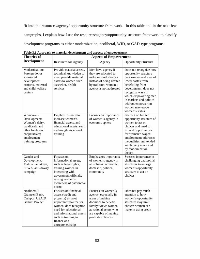
92
fit into the resources/agency/ opportunity structure framework. In this table and in the next few
paragraphs, I explain how I use the resources/agency/opportunity structure framework to classify
development programs as either modernization, neoliberal, WID, or GAD-type programs.
Table 3.1 Approach to material development and aspects of empowerment Theories of Development
Aspects of Empowerment Resources for Agency Agency Opportunity Structure
Modernization: Foreign donor sponsored development projects, maternal and child welfare centers
Provide material assets, technical knowledge to men; provide material assets to women such as shelter, health services
Men have agency if they are educated to make rational choices instead of being limited by tradition; women’s agency is not addressed
Does not recognize how opportunity structure bars women and men of lower castes from benefitting from development; does not recognize ways in which empowering men in markets and politics without empowering women may erode women’s status
Women-in- Development: Women’s dairy, handicraft, and other livelihood cooperatives; employment training programs
Emphasizes need to increase women’s financial assets, and educational assets, such as through vocational training
Focuses on importance of women’s agency in economic sphere
Focuses on limited opportunity structure of women to act on choices and need to expand opportunities for women’s waged employment; addresses inequalities unintended and largely unnoticed by modernization theory
Gender-and- Development: Mahila Samakhya, SEWA, anti-dowry campaign
Focuses on informational assets, such as legal rights, training women in interacting with government officials, raising women’s awareness of patriarchal norms
Emphasizes importance of women’s agency in all spheres: economic, domestic, political, community
Stresses importance in challenging patriarchal structures to enlarge women’s opportunity structure to act on choices
Neoliberal: Grameen Bank, Cashpor, USAID Gemini Project
Focuses on financial assets (credit and property) as most important resource for women; does recognize need for educational and informational assets such as training in finance and entrepreneurship
Focuses on women’s agency, especially in areas of making decisions to benefit family; views women as rational actors who are capable of making profitable choices
Does not pay much attention to how women’s opportunity structure may limit choices women can make in using credit
93
3.2.3 Modernization programs: fostering Western values for economic growth
Theorists, policy-makers, and practitioners who take the modernization approach view macro-
level economic growth as the goal of their development interventions. Policy-makers who take
the modernization approach to development view individuals as having agency if they have
adopted modern, Western values such as individualism, a strong achievement-motive, and a
rationalist, entrepreneurial outlook on the world. They contrast “modern” societies in which
individuals are free to move to new locations and raise their social status based on their own
efforts with “traditional” societies in which individuals do not have agency because they are
bound by the status they are born into, and therefore have fewer opportunities to act on their
choices. They view people in less-developed societies as passive recipients of their development
interventions who are in need of development organizations to give them technological, material,
educational, and cultural resources so that they can become rational citizens who are liberated
from the traditions of the past. Once they bring new knowledge and technology from the West to
individuals in less-developed societies, these individuals will experience increased profits in
agriculture and higher living standards, thus spurring on economic growth. The irony is that even
though modernization practitioners argue that individuals are freer to make their own decisions
and chart their own course in life once they adopt Western values and practices, they denied
people in developing nations agency because they did not accept the possibility that individuals
may choose to follow their traditional values and practices rather than those of the industrialized
West. They also believed that everyone in the society would reap the benefits of economic
development, such as better health, more education, and an overall higher living standard,
regardless of their present position in society. They did not consider how the formal and
94
informal institutions like female seclusion and son preference limited women’s access to
resources such as food, health care, and education. Organizations that come from the
androcentric modernization approach take men’s experiences and perspectives as their point of
reference, and view women’s experiences as a deviation from this norm. They do not consider
how new agricultural technologies may affect men and women differently, and how they might
actually disempower women by de-valuing women’s subsistence work. They assume that even
if they introduce Western technological advances to men only, women will benefit too.
The first four Five-Year Plans that India’s government leaders formulated after India won
its independence in 1947 were grounded in modernization theory. Prime Minister Jawaharlal
Nehru and the Congress party implemented policies and programs to bring about industrial and
agricultural modernization (Berry 2007). The First Five-Year Plan implemented welfare-
oriented programs, placed an emphasis on agricultural development, and focused on
disseminating material and financial resources for the well-being of the rural poor (Singh 2005).
These programs were paternalistic, and viewed the rural poor as passive recipients. The Third
and Fourth Five-Year Plans (1961-66 and 1969-1974, respectively) implemented growth-
oriented strategies, and assumed that increases in wealth and production would trickle-down to
the most impoverished (Singh 2005). These programs included the Intensive Agricultural
District Programme, the High Yielding Varieties Programme, and the Intensive Cattle
Development Programme. The goal of these programs was to bring about a rapid increase in
agricultural production through a combination of services and inputs to individual farmers (Singh
2005). The government leaders and those who implemented these programs incorrectly assumed
that women were not involved in agricultural work, and these programs targeted men only (Berry
2007). This was despite the fact that many women were involved in agricultural work, either to
95
supplement their husbands’ income or because they were the main providers for their families
(Berry 2007).
The policy-makers who created the agricultural development programs were not the only
ones to take a modernization perspective in their planning during the 1950s-1960s. The
Education Commission and other education policy-makers in India took a modernization
perspective as well. During the first three Five-Year Plans, the Indian government placed a high
priority on technical education, and most of the achievements in education after India’s
independence took place in this area (Naik 1965). J. P. Naik, the Member-Secretary of the
Education Commission in 1964, stated that the “relentless pursuit of knowledge” (Naik 1965:94)
is what sets apart a modern society from a traditional society. Therefore, he argued, the Indian
government needed to emphasize university education, and post-graduate research and teaching.
Naik also maintained that “…education is the most important single factor which leads to
economic growth…” (Naik 1965:35). He contended that education should inculcate attitudes
and values in students that would promote democratic thinking. He stated that teachers should
encourage discussion, free thinking, and group participation in activities. Students should also
develop attitudes that will spur on economic growth, such as working hard, a willingness to do
manual labor, cooperation, and thriftiness (Naik 1965). Naik also stated that technology and
science should be central in the educational system. He emphasized the importance in teaching
children to have a rational, secular, empirical outlook. He also maintained that it was important
to teach science to adults as well, so that they would develop scientific attitudes that they could
apply to their work in agriculture and industry. Naik argued that this would lead to an increase
in efficiency and therefore an increase in production (Naik 1965). He also stated that it was
important to have a strong family-planning program in which adults are educated and motivated
96
to limit the number of children they have. He said this was important so that the overall birth rate
would decrease to 50% of what it currently was. They stated that at the secondary level of
education (grades 9-10), there should be an expansion in the number of facilities that provide
vocational and technical education, and that this education should be designed around the current
employment needs of India.
One example of a modernization program is the Community Development Programme
(CDP) started by Nehru in 1952 to encourage farming households to implement modern
agricultural and home science practices (Berry 2007). He patterned the CDP after the programs
of the U.S. Agricultural Extension Service. The Ford Foundation funded the Comparative
Extension Project, which was part of the Community Development Programme. The
Comparative Extension Project promoted modern, capital-driven agricultural practices that were
also being promoted in the U.S. Project workers encouraged Indian farmers to change the crops
that they grew according to market demand rather than planting the same crops season after
season. Project workers also promoted capital-intensive methods of farming that they viewed
more progressive than farmers’ traditional practices of investing little money. They encouraged
farmers to make agricultural decisions apart from religious or social considerations, and to
produce crops to sell on the market rather than for subsistence needs (Berry 2007). Like other
modernization practitioners, those who implemented the Comparative Extension Project assumed
that rural Indian farmers utilized traditional farming methods unreflexively, and must be taught
to take a more rational, entrepreneurial approach to farming in order to spur on economic growth
(Berry 2007). The Comparative Extension Project was clearly androcentric since project
workers only provided men with agricultural knowledge and inputs, even though there were
women who worked as farm laborers or who participated in agricultural production for
97
subsistence needs of their households (Berry 2007). It also promoted “progressive” agriculture,
which was seen as connected to the market, consumerism, and the desire to accumulate material
wealth. These project workers did not consider how these “modern” farming methods robbed
women of their agency and their access to resources, and also lowered their status.
Although the agricultural programs of the First through Fourth Five-Year Plans were
primarily for men, the Indian government did create some programs for women. The First Five-
Year Plan (1951-56) and Second Five Year Plan (1956-1961) took a welfarist approach to
women and development (Subramaniam 2006). During this period, the Planning Commission
put forth the “Plans and Prospects for Social Welfare in India, 1951-61,” which stated that social
services were to be provided for any group of people that were handicapped in some way, either
physically, mentally, socially, or economically (Chaudhuri 2007). This statement included
women as a class of handicapped people. The Indian state viewed women as beneficiaries of
development programs, but did not consult women in the formulation of the policies or in
implementing them (Subramaniam 2006). The Third and Fourth Five-Year Plans continued to
provide welfare services for women, but still excluded women from the policy-making process.
Men in government positions designed the women’s programs and defined what they believed to
be “women’s interests.” They viewed women as dependents of the state, and did not address
women’s rights. The government leaders who designed the welfare programs assumed that
women would have access to them, and did not consider how unequal gender relations
constrained women’s access to the services (Subramaniam 2006).
During the same period that Nehru founded the Comparative Extension Project, foreign
donors and development organizations provided training and education for rural Indian women
(Berry 2007). These donors and organizations trained women in the areas of Western, modern
98
forms of health and nutrition, contraceptive use, and how to be better home-makers and mothers
(Berry 2007). Rural Indian women were the targets of these development programs, and were
not participants in deciding how to implement these programs (Berry 2007). Development
planners assumed that they had to “give” the Indian women resources. Like other practitioners
coming from a modernization perspective, they assumed that the Western value of small family
size is superior to values of less-developed societies. Development interventions included
introducing contraceptives to women and encouraging them to limit the size of their families.
They did not recognize the possibility that rural, Indian women might choose to have many
children to help provide for them in their old age (Tinker 1997).
3.2.4 WID programs: empowering women to participate in the labor force
The WID approach to development focuses on the importance of women’s agency in the
economic sphere, and also emphasizes the need to increase women’s educational and financial
assets, such as through vocational training. As do those who take the modernization approach,
those who take the WID approach see power as something that development organizations can
give to people in less-developed nations, and that this power is economic power. Unlike
modernization advocates, however, WID proponents stress that women’s opportunities to act on
their choices is limited, and that it’s necessary to expand opportunities for women to participate
in the market. Scholars and practitioners also argue that economic institutions are not gender-
neutral, and that women do not have equal access to paid labor as men. They argue that in many
cases industrialization, the shift from subsistence agriculture to agriculture for export, and the
introduction of new farming technology and techniques has had a negative impact on women’s
99
economic position and overall well-being (Boserup 1970). Although WID practitioners argue
that it is important to expand women’s opportunities to participate in waged labor, they neglect
other aspects of women’s empowerment. Like modernization practitioners, WID practitioners
do not challenge traditional gender roles, and they don’t pay attention to how women’s limited
choices within the household negatively impact their well-being. WID practitioners attempt to
expand the opportunities for women in the economic sphere, but they do not challenge the
power-holders in institutions who maintain unequal power relations between women and men.
One example of a development organization that takes the WID approach to women’s
programs is India Development Service. India Development Service (IDS) was founded in 1979
in Dharwad district, Karnataka, in an especially poor, drought-prone blockvi (Viswanath 1991).
The goal of IDS is to develop people’s skills, create cooperatives, bring new life to traditional
occupations, and to provide employment opportunities that the people did not already have. All
of the women’s programs of IDS are geared toward giving women more opportunities to be
involved in paid labor and to increase their incomes. Like other WID projects, IDS has let
traditional gender roles in occupations guide them in their decisions about what types of
programs to implement. Some of the projects that they have started for women include the dairy
project, the spinning project, and the leather project.
The dairy project started in 1981, and serves only women because women are the ones
who traditionally care for livestock. The women needed a supplementary form of income source
due to low agricultural yields, and there was a market for milk in nearby towns. The goal of this
project is to help women buy livestock through access to bank loans, to provide veterinary care
and training so that women can properly care for livestock, to increase fodder production, and to
increase avenues for collecting, distributing, and marketing milk. IDS started dairy cooperatives
100
and rented buildings for the refrigeration of the milk. The dairy cooperative members brought
their milk to the dairy every day and were paid once a week, and one member of the cooperative
was paid to distribute the milk to customers. Some women were trained and paid to test the milk
for quality that was brought to the dairy each day.
The spinners project started in 1984-85, and assists 70-75 spinners. The goal of the
project is to provide women employment security as they pursue their traditional occupation of
spinning. The villages of the block that IDS serves had been well-known for decades for their
wool production, spinning, and weaving of wool products. Because the wool industry is
comprised of shepherds, spinners and weavers, IDS provides assistance to people in all three of
these occupations. In a single household, women will card and spin the wool, and men will
weave it into kamblis, or blankets, to be sold. IDS assists spinners in accessing credit from
banks, which allows them greater decision-making power when they purchase wool. With the
cash they borrow from the bank, the women are able to buy higher-quality wool at the best price
rather than being forced to buy wool at usurious rates from dishonest wool merchants. IDS has
also provided the women with material resources in the form of improved technology for storing
and spinning the wool, and has provided educational resources by helping them with improving
and marketing their product. Although the spinners project has empowered women to escape the
exploitation of dishonest wool merchants, IDS does not help the women to organize and directly
challenge the power of these exploitative merchants.
The leather project was originally started for men since leatherwork is traditionally a
Scheduled Caste, male occupation. However, in 1986 IDS decided to switch to training women
only since the Scheduled Caste women needed a reliable income source. The goal of the
program is to train women so that they can start their own leather-making businesses. The
101
women’s training program began in 1986, and included training in literacy, marketing and
manufacturing. The women were trained in making leather slippers, and spent the first year
learning how to create different styles and produce the slippers. In the second year, they learned
how to improve the quality of their work and how to market their products (Viswanath 1991).
The women also receive a stipend while in the training program that is twice as much as they
could make doing agricultural labor.
The women’s programs of IDS have had mixed success. For instance, even though in
1985 the amount of milk that was being produced and brought to the dairy was as high as 105
liters a day, this amount dropped to only 30 liters a day by 1987. Also, when the dairy project
initially started, women often used the bank loans that were meant for buying cattle to pay off
other expenses instead. Even though IDS helps women in the spinners project to procure bank
loans to buy wool, ultimately any increases in household income will go to the entire household
rather than to the women themselves. This is because the men are the ones who weave the spun
yarn into the final product to be sold. The spinners project may help increase the income of the
entire household, but it is not clear how much women benefit from this. Even though women
spinners are brought into the market, they may not have gained decision-making power in how
the money is spent. Also, in the area that IDS serves, women are usually the last to eat at
mealtimes, and they get whatever is left after everyone else has eaten (Viswanath 1991).
Women’s unequal access within the household to basic resources needed to survive is not
addressed by the spinners’ project, nor by the other projects for women. The leather project has
some positive aspects, such as making it possible for women to set up their own leather units
near their homes. This will ensure better working conditions than if these women worked as
agricultural laborers. Another aspect of this project that is cited as being beneficial is that it
102
means they can work close to home and look after young children, so that older children can
attend school instead of baby-sitting. The leather project empowers women to gain access to
economic resources through waged labor. However, IDS does not address the challenges may
face as they try to produce leather products at the same time as carrying out their other domestic
tasks, and how their dual roles in both economic and domestic work may inhibit them from
producing as much as they might otherwise. One potential drawback is that the leather that
women have access to in the training program is of mediocre quality, so the quality of their final
products suffers. Also, they could face potential competition from well-established leather
companies in the area that produce higher-quality leather (Viswanath 1991).
A prime example of an organization that takes the WID approach to development is the
Shri Mahila Griha Udyog Lijjat Papad (hereafter SMGULP). Although SMGULP is not a
development organization per se, it does fit under the WID framework because its focus is on
bringing women into the paid labor force. Moreover, the work that the women do is work that
women traditionally do in India. It was started by seven young women in 1959 (Ramanathan
2007). The seven women started a business making papad, a thin flatbread, on their terraces in
Mumbai. They chose to make and sell papads because they had the ingredients readily available
in their own kitchens, the papads were easy to make and stayed fresh a long time, and because
people throughout India eat papads with meals or as snacks. The women decided not to ask
anyone for donations so that the organization could remain independent of the political interests
of donor agencies (Ramanathan 2007). More than 150 women worked with the organization
within two years of when the original seven women founded it. In three years there were over
300 women members, and the leaders of the organization began distributing rolls of dough to the
women in the morning, which the women returned the next morning in the form of freshly-made
103
papads. The women are paid daily for the papads they make. There are no employers or
employees per se, and all of the members who make papads own the organization. All of the
members share any losses or profits that the organization makes, thus encouraging the members
to try to increase sales and production (Ramanathan 2007). SMGULP therefore emphasizes the
“power-with” dimension of power. The organization began to diversify production into other
areas in the 1970s, such as divisions for printing, milling flour, making spices, and making
packaging.
Shri Mahila Griha Udyog Liggat Papad is clearly a WID organization because it takes
women’s needs into account, such as allowing women to make papads at home so they can
fulfill their dual roles as economic producers and housewives, and it utilizes a skill that almost
all Indian women have (making papads). It provides the material resources (dough) women
need to earn money, and it certainly provides economic resources to women. SMGULP also
draws on “power-with,” since the institution operates as a large collective with branches in
various states, and all of the decisions are consensual-based (Ramanathan 2007). SMGULP has
successfully expanded the opportunity of many women to be involved in the market, and has also
strengthened women’s agency. By working together, the women members of the organization
have exercised their power to expand the business, diversify production into related divisions
such as flour milling, printing, and packaging, and increase employment from seven members at
its inception to about 40,000 members in 2007 (Ramanathan 2007). SMGULP only allows
women to become members, and thus the decisions are made by women and for women. This is
in contrast to some development organizations that take a gender-blind approach to development,
such as the Grameen Bank, in which most of the people in leadership positions are men.
104
SMGULP does not take a GAD approach to development because it does not challenge current
gender roles or unequal power relations between women and men.
3.2.5 GAD programs: empowering women to transform institutions
Gender and Development (GAD) programs and organizations consider both women’s agency
and the opportunity structure in which they live/find themselves to be vital for gender equality.
These programs and organizations stress the importance in challenging men’s “power over”
women in order to enlarge the opportunity structure for women to act on their decisions.
Moreover, they emphasize the need to educate women about their legal rights, and many seek to
educate women in how to interact with police officers, government officials, and others who are
part of formal institutions in order to expand women’s opportunities to participate in the public
sphere. Some GAD programs focus on the process of empowerment, such as bringing to
women’s attention how cultural norms such as dowry reinforce girl children’s lower status vis-à-
vis boy children. Others focus on transforming formal institutions so that women can gain
greater space to act and make their voices heard, such as in panchayat raj (village council)
institutions. The GAD approach to development contrasts with the WID approach to
development because the GAD approach says that including women’s needs in the development
process and integrating women into the paid labor force (formal or nonformal) is not enough to
raise women’s status and bring about greater gender equality. Moreover, unlike modernization
or neoliberal practitioners, organizations and practitioners that take the GAD approach do not see
macro-level economic growth as the goal that development agencies should be pursuing, and
they critique the blind pursuit of economic growth. GAD scholars and practitioners challenge
105
traditional gender roles and gender hierarchies, and work toward overturning cultural values and
norms that place a higher value on men and boys than on women and girls. They argue that it is
also important to examine relations between males and females within the household, such as
how boys are privileged over girls in terms of access to health care and education.
Development interventions that take a GAD approach educate women about their legal
rights, as well as educate the public about issues such as violence against women, women’s
reproductive rights, and women’s literacy and education. Some GAD organizations are social
movement organizations that put pressure on governments to change or enforce laws that are
meant to enlarge the spaces in which women have to act and make decisions. Development
interventions taking the GAD approach often emphasize the importance of making the private
sphere public. These organizations and social movements include anti-dowry and anti-rape
campaigns (Subramaniam 2006), certain women’s labor union movements such as SEWA
(Crowell 2003), and women’s social movement organizations that struggle to uphold the equality
of female and male children (Ray 1995).
The Self-Employed Women’s Association (SEWA) in India is an example of a social
movement organization that takes the GAD approach to development. The Self Employed
Women’s Association (SEWA) in India was founded in 1972 and is primarily a labor union
whose members fight to gain fair wages for poor women in the informal sector, such as
headloaders, bidi (cigarette) rollers, cart pullers, and vegetable vendors (Mayoux 1995; Crowell
2003). During the 1970s, vegetable vendors organized to fight for their right to sell vegetables in
the market free from police harassing them or forcing them to pay bribes. During the past thirty
years or so, SEWA has challenged men’s “power over” women, and has helped women organize
to obtain minimum wages for self-employment and to pressure the government to pass laws
106
against exploitation of home-based workers (Bhowmik and Jhabvala 1996). SEWA is especially
a feminist organization because it views meeting needs and rights of women as essential for
development to take place. The women themselves are not only members of SEWA; they also
decide who will lead the organization and create development strategies (Crowell 2003). Thus,
SEWA places a high priority on women’s agency and on widening the space in which women
can act and lead. SEWA organizers also educate women about their legal rights, and SEWA
produces a magazine called “Ansuya” with women’s success stories that are read at group
meetings (Bhowmik and Patel 1996). SEWA also provides financial resources in the form of
microloans through SEWA Mahila Sahakari Bank which it founded in 1974 (Mayoux 1995;
Crowell 2003), but this is only one of several programs for women. SEWA, like other GAD
theorists and practitioners argue that women need to mobilize and fight for political and
institutional change in order to eradicate gender inequality.
As a labor union and social movement organization, SEWA is doing just that. For
instance, women who collect gum from trees to sell to the Gujarat state government have
mobilized to pressure the government into paying them a fair wage for the gum (Crowell 2003).
Ela Bhatt, one of the founders of SEWA, states that the organization fights against direct
exploitation of women in the nonformal sector, as well as against government support of those
who exploit these women (Bhatt 1989).
Another development organization that operates under the GAD paradigm is the
government-sponsored program Mahila Samakhya. Mahila Samakhya is a “hybrid” organization
in that it is government-sponsored at the national level, but is run through NGOs at the local
level (Sharma 2008). It was started around the same period that the Indian government started to
liberalize the economy and cut expenditures on welfare programs. It was organized by feminists
107
and sponsored by the civil servant, Anil Bordia, and initially funded by the Dutch government in
1989. The feminists who created Mahila Samakhya believed that the main impediments to
development are social hierarchies and women’s lack of knowledge about their rights and the
various government programs they could turn to for support. Feminists saw Mahila Samakhya
as an opportunity to further their goals of gender equality in the political arena, and a way of
promoting gender equality on a much larger scale than what they had been doing (Sharma 2008).
At the federal level, Mahila Samakhya falls under the jurisdiction of the Ministry of Human
Resource Development and is run by development activists and feminists. At the state level,
Mahila Samakhya’s work is carried out by NGOs (Sharma 2008). The objective of Mahila
Samakhya is to educate women to enable them to gain greater control over their own lives
(Subramaniam 2006). This is accomplished through the process of organizing women into
sanghas (groups), consciousness-raising to help women interpret their experiences in new ways,
and discussion of cultural norms that reinforce women’s low status.
I next highlight two researchers who conducted qualitative studies on Mahila Samakhya,
who came to very different conclusions in terms of how empowering Mahila Samakhya really is
for the women who are involved with the organization. Sharma (2008) carried out her study in
Uttar Pradesh, a northern state known for its strong patriarchal norms. Subramaniam (2006)
conducted her study in the southern state of Karnataka, which has more egalitarian gender norms
compared to Uttar Pradesh. I seek to highlight how even the same women’s organization or
program may have different success rates in lowering gender inequality in different regions of
the country.
Sharma (2008) carried out a qualitative study of the Mahila Samakhya program in the
state of Uttar Pradesh to examine how “empowerment is conceptualized and implemented as a
108
strategy of development and governance and what it does on the ground” (Sharma 2008:xix.)
She spent over 20 months carrying out ethnographic fieldwork, mostly during 1998-1999. She
interviewed women who were either sangha (group) members or who worked for Mahila
Samakhya. She conducted participant observation in two adjacent villages, one with Mahila
Samakhya present, and one without. She also conducted institutional ethnographic work to
analyze the practices and organization of Mahila Samakhya by making visits to MS locations in
Andhra Pradesh, Gujarat, Assam, Rajasthan, and Maharashtra. She went to staff meetings, went
with program functionaries on their daily rounds, and in total interviewed over 90 people from
all institutional levels of Mahila Samakhya. Although the purpose of Mahila Samakhya is to
empower women to take greater control over their lives, Sharma found that there are gender and
class inequalities between women who staff Mahila Samakhya and the men who serve as state
bureaucrats, and that MS bureaucrats reproduce gender inequalities (Sharma 2008). For
instance, state bureaucrats conceive of the empowerment “social work” that staff workers do as
being “naturally” feminine work, and therefore non-skilled labor. The women staff workers of
MS are also not considered “heads of households,” even though in reality many staff workers
were divorced, widowed, or evicted from their homes by their husbands. As a result, these
women were not paid enough to live on. In two states where Mahila Samakhya first started, the
staff tried to unionize in order to get more regular pay. However, the mobilizations were
quelled, and many of the staff workers in one state were fired. One of her informants stated that
the Indian government “does not integrate the element of struggle that lies at the heart of
empowerment” (Sharma 2008:67). This can be seen in how women staff workers are not
allowed to get involved in any protests or mobilization efforts against the state, even if the
sangha members that the staff workers oversaw planned the protests. Sangha members’ matters
109
were usually related to legal issues, land titles, meeting basic needs, and dealing with police, all
of which were matters related to bureaucracies. The MS employees were disempowered by state
authorities from helping the women in the sanghas (Sharma 2008).
Subramaniam (2006) also conducted a qualitative case study of Mahila Samakhya, but
she came to very different conclusions from those Sharma drew. Subramaniam carried out her
fieldwork in 1998-99 and 2001-2002 in four districts of Karnataka state. She took both a macro
and micro approach. At the macrolevel, she examined party politics and the women’s movement
in India, and analyzed the Indian state’s Five-Year Plans, as well as the three government
“Reports on Women”. At the microlevel, she carried out ethnographic work on a sample of 31
women’s sanghas under the Mahila Samakhya program in Karnataka in 1998 (MSK hereafter).
The sanghas in Karnataka are informal groups of scheduled caste and scheduled tribe women
with about 20 women per group. The MSK program is not target-driven and desired outcomes
are defined at the village-level by the women in the sanghas rather than by the state. MSK’s
goal is to bring about changes in formal and informal institutions so that women have a broader
space in which to act and make their voices heard. Sangha members discuss their beliefs, local
cultural norms, and the importance in schooling for girls. One of the goals of MSK is to create a
demand for educating girls, with the aim of changing gender relations in the society.
Subramaniam discovered that some aspects of MSK did help women challenge gender
inequalities in their lives and communities. The sangha leaders, or sahayoginis, provide
information on laws, women’s rights, and assistance from government programs to the sangha
members. Being a part of these collectives helps to increase the women’s self-confidence and
self-esteem (psychological resources). MSK also conducts training workshops and programs
where women from different sanghas and villages come together and meet other women. At
110
these training meetings the women learn about aspects of social life that lead to gender
inequality, such as child marriage. There are also village, taluk, and district-level meetings that
create a space for women to express their ideas, and for consciousness-raising to take place.
Consciousness-raising helps the women to interpret their experiences in new ways, and helps
them to think of themselves as individuals and also as members of a collective instead of just
members of a family. Once they see themselves as individuals who can take on roles other than
that of wife or mother, the women begin to see how they can take action in order to bring about
change in their lives. They gain “power within” in the form of courage and a changed identity,
and they gain “power with” in the form of solidarity in order to challenge those who have
“power over them”. The women in the sanghas share information and experiences, which
creates solidarity among the women so that they can fight injustice, such as caste hierarchies.
The sangha members that Subramaniam observed did start challenging caste-based
discrimination in their villages, and in some cases the men joined them in this struggle.
Although MSK is successful in many ways in empowering women, Subramaniam found
that new forms of inequality developed at intermediate organizational levels (Subramaniam
2006). The sahayoginis learn how to interact with local-level officials and gain new knowledge
through their positions as MSK staff workers, which leads to their own empowerment.
However, this often leads to unequal power relations between the sahayoginis and the sangha
members since the sahayoginis have a greater access to knowledge and information than the
sangha members do. Also, even though the sahayoginis provide information to sangha members
and stress that the village members themselves must decide whether to form a sangha, what
goals to set, and how to take action, there is a tendency for the sanghas to become overly
dependent on the leadership of the sahayoginis. The sahayoginis themselves must deal with
111
threats from powerful groups in the villages as they carry out their work. Additionally, even
though MSK holds training programs for women running for office and elected to the Panchayat
Raj, many times men discourage the women from attending the training sessions. Moreover,
men often try to coerce the women elected to the Panchayat Raj to be mere signatories for the
plans that men in the Panchayat Raj want to carry out (Subramaniam 2006).
3.2.6 Neoliberal programs: empowering women to help themselves
Like development programs that come from the modernization perspective, development
programs that come from the neoliberal perspective have economic growth as their ultimate goal.
With the neoliberal approach to development, the focus is on integrating as many people as
possible into the market, whether as business owners, wage laborers, or farmers growing cash
crops rather than crops for subsistence needs. However, whereas modernization practitioners and
policy-makers stressed the importance of state intervention in order to bring about economic
growth, neoliberal policy-makers stressed the need for governments to decrease spending on
welfare programs to encourage individual responsibility (Hyatt 2001, Goldstein 2001).
According to neoliberal ideology, government intervention to alleviate poverty is disempowering
for the poor because it perpetuates the poor’s dependence on state support, thus robbing them of
the self-confidence that they would gain by relying on themselves to meet their own needs (Hyatt
2001). Empowerment, then, for the neoliberal policy-maker means the withdrawal of state
intervention so that the individual can realize self-management, take over responsibility for his or
her own needs, as well as work with others to take care of the needs of the community such as
maintaining infrastructure and educational facilities (Hyatt 2001, Goldstein 2001, Sharma 2008).
112
According to the neoliberal paradigm, any kind of economic failure or success is dependent on
the individual, not on structural factors (Goldstein 2001).vii In the Indian context, these structural
factors include widespread discrimination against dalits or women, government corruption, and
the state’s failure to enforce laws such as women’s property rights.
The development interventions of organizations and practitioners that take a neoliberal
approach often center on microfinance—lending small amounts of capital to people and
encouraging them to start small businesses. Development programs and practitioners that take
this approach are concerned with economic efficiency and spurring on as much economic growth
in a society as possible. These development organizations, and especially microfinance
institutions, overwhelmingly target women because women make up 70% of the world’s poorest,
they tend to use the economic resources they bring into the household for the entire family rather
than on luxury items for themselves, and they are seen as more docile and cooperative with MFI
rules (Cheston and Kuhn 2002, Ahmed et. al. 2001, Kristof and WuDunn 2009). That is, they
take an instrumental approach by giving women credit since they believe this is the most
efficient way to alleviate poverty and raise the living standards of the poor. Microcredit
programs and organizations that come from a neoliberal perspective take individual women’s
agency as a given, and assume that if they are given financial resources in the form of credit,
they can and will make profitable decisions in investing those resources. However, they do not
consider how structural factors limit the choices that women are able to make, such as how
women’s unequal access to waged labor and their limited mobility in the public sphere may
leave them no option other than economic work in the informal sector, the very work that
microcredit loans are generally used for. Unlike organizations that take the GAD approach to
development, organizations that use the neoliberal approach to development do not attempt to
113
challenge patriarchal social structures to expand women’s opportunities to participate in the
public sphere, such as in waged employment or politics.
Microcredit organizations and programs assert that they empower women by giving them
a way to increase their income and to provide for their families’ needs. However, in some
respects, these neoliberal microcredit programs may actually disempower women. For example,
microcredit programs usually require women to form small groups in order to take out loans.
This is because the women targeted for loans have nothing to use as collateral against the default
of the loan. The women in these small groups, it is argued, put pressure on one another to pay
back their share of the loan in a timely manner, and therefore act as “social collateral” so that the
group can take out subsequent loans (Todd 1996). Women exercise disciplinary power over
themselves and other group members (Lairap-Fonderson 2002). They must attend regular
meetings, make small re-payments on a regular basis (regardless of whether they have just faced
a crisis such as a major illness) and face constant surveillance and group pressure so that they
can take out subsequent loans. Moreover, while MFIs that take a neoliberal approach mainly
target women to take out loans, the majority of the bank workers are men (Rahman 1999). Thus,
women have very little power to decide how the MFIs should be managed, or the conditions
under which borrowers can take out loans.
Although the international financial institutions like the International Monetary Fund and
the World Bank began enforcing neoliberal structural adjustment policies on borrower nations
starting in the 1980s, India did not follow neoliberal economic policies until 1991 (Singh 2005).
India’s New Economic Policy consisted of de-regulation, privatization, and globalization of
businesses, and emphasized increased integration into the global economy. The reasoning
behind the New Economic Policy is that globalization will increase economic growth, and that
114
economic growth is the best way to decrease poverty and unemployment. The Indian
government therefore focused on developing industries for export (Marius-Gnanou 2003). Prior
to the 1990s, the Indian government had taken the primary responsibility in initiating and
overseeing development programs (Marius-Gnanou 2003). For instance, in the 1970s the Indian
government started several employment schemes, such as the Rural Works Programme, the Pilot
Intensive Rural Employment Projects, the National Rural Employment Programme, and the
Rural Landless Employment Guarantee Programme (Singh 2005). Beginning in the early 1990s,
the government began to assign more and more development programs over to the care of
development NGOs. This included government-sponsored microcredit programs, which
previously had been overseen by government bureaucrats (Marius-Gnanou 2003). The
government of India also started to organize micro-credit self-help groups (SHGs hereafter) and
to link them to banks beginning in 1992 (Kalpana 2008). Prior to 1999, there were other self-
employment programs in existence, such as the Development of Women and Children in Rural
Areas (DWCRA) and the Training of Rural Youth for Self-Employment (TRYSEM) (Singh
2005). In 1999, the government organized all of the state-sponsored rural development programs
under the national Swarnjayanti Gram Swarozar Yojana (SGSY) program, and focused on
lending credit and subsidies to women of below-poverty level households (Kalpana 2008). The
SGSY program replaced the DWCRA and TRYSEM programs that had existed earlier (Tapan
2005). Formal banking institutions are reluctant to lend to the rural poor because it is not
profitable for them to do so and it is difficult for banking institutions to reach them in such
remote areas. Institutions in the formal banking sector also believe that the rural poor have no
resources, do not know how to manage their money, and have too many immediate needs to be
able to invest the loans. The Indian government created the SGSY program to meet the rural
115
poor’s need for credit that the formal banking system could not fulfill. SGSY encompasses a
range of micro-enterprise development activities, such as the formation of women’s credit self-
help groups, marketing, and training (Singh 2005). SGSY provides government subsidies and
credit to individuals with the goal of raising the borrower’s family above the official poverty line
within three years (Tapan 2005). The Indian government stipulates that 50% of the program’s
recipients should come from scheduled tribes or scheduled castes. Under the SGSY, women’s
SHGs are linked to banks through the District Rural Development Agency (DRDA) and the
Block Development Offices (BDO) in order to receive both microcredit and government
subsidies. The banks that provide microcredit include national commercial banks, cooperative
banks, and rural banks. Tamil Nadu is one state in India that has actively promoted women’s
microcredit programs under SGSY (Kalpana 2008).
In the next few paragraphs I discuss in detail two different studies of women’s
microcredit programs, one in Tamil Nadu state and one in West Bengal state. Like the
researchers who studied Mahila Samakhya, the two researchers who studied these microcredit
programs came to very different conclusions about the impacts that the microcredit programs had
on raising the status of women who borrowed from them. I discuss these two cases because they
bring to light some methodological issues in studying the impact of women’s microcredit
programs on raising gender equality. The microcredit groups that both researchers studied were
facilitated directly by NGOs, although the microcredit groups in the Tamil Nadu study operated
under the auspices of a state-run scheme. Both of the researchers built an argument either for or
against the empowering effects that the formation of microcredit groups has on women.
However, they did not discuss whether the NGOs that oversee the microcredit groups also have
other types of women’s programs.
116
Kalpana (2008) carried out a qualitative study of women’s microcredit groups in the state
of Tamil Nadu, which is one state that has been actively promoting women’s microcredit
programs starting in the 1990s. In Tamil Nadu, NGOs are linked to the Tamil Nadu Women’s
Development Corporation (TNWDC) through the Tamil Nadu state scheme, Mahilar Thittam.
Mahilar Thittam trains NGOs and provides them with financial and technical help from the
Women’s Development Corporation. The NGOs then organize, train, and supervise microcredit
self-help groups (SHGs hereafter). About seventy percent of the SHGs in Tamil Nadu operate
through this state-NGO partnership, although it’s hard to obtain exact numbers (Kalpana 2008).
Kalpana conducted interviews with staff at several types of NGOs that have microcredit
programs operating under the SGSY in Tamil Nadu. She also carried out fieldwork in one
district of Tamil Nadu to study 27 women’s SHGs that were from 3-7 years old. Kalpana found
that there are a number of contraints on potential SHG members. Banks often require women to
repay their husband’s or relatives’ previous bank loans before the bank would give a loan to their
SHG. Many banks required a “no-objection” letter from all of the nearby banks stating that none
of the SHG members have relatives that owe any of these banks money. Banks often force SHG
members to drop out of the group if they have relatives who owe money as a condition for the
group to receive the loan. This is despite the fact that official SGSY rules state that “non-willful
defaulters” can still receive loans through SHGs. This pressure from the banks often leads to
conflict within families as SHG members pressure relatives to repay their loans. There is often
distrust between SHG members and bank staff because the bank staff don’t clearly explain the
interest rates on the loans to the women. Bank managers are also not understanding of the costs
that women make in order to visit the bank, since the women must take time away from waged
labor. Moreover, some of the SHGs comprised of Scheduled Caste members experienced caste-
117
based discrimination when trying to access loans, even though there is no evidence to support the
bank managers’ fears that these SHGs would not repay the loans. Kalpana found that there are
often tensions within SHGs as well. For instance, SHG coordinators often hold their own group
members to even more stringent repayment standards than the banks required, such as fining
members for every day their payment is late, sometimes even if a group member faced a family
emergency. SHG coordinators often demanded that the group members repay the loan in half the
amount of time that they were actually allowed by the bank
Although Kalpana found that there were many unintended negative consequences to
these microcredit groups, she also discovered that there are some positive aspects as well. The
women who belong to SHGs experience an increase in their social status because of their
contacts with banks and other state institutions. For example, SHGs with links to banks are
invited to all village governance meetings. SHGs also use their “official” status as leverage to
threaten abusive husbands. Also, police are more likely to listen to a complaint brought to them
by an entire SHG than to a complaint brought by an individual woman who is being harassed by
her husband or in-laws (Kalpana 2008).
Samyal (2009) conducted a qualitative case study in 2004 of women involved in a
microcredit program run by two different NGOs in the state of West Bengal. Samyal’s main
research question driving her research was, “Does microfinance promote women’s capability to
address social problems in their communities and influence social norms?” (Samyal 2009:531).
She interviewed 400 women across 59 different microcredit groups. There are very restrictive
cultural norms regarding women’s behavior in West Bengal, and women often must remain in
seclusion or be accompanied by a male relative if they go to the market. They also generally do
not have much interaction with women outside of their husband’s family, and aren’t able to
118
develop social ties with non-family members. She examined the social impact of microcredit,
and also the impact that borrowing made on the empowerment of individual women. Samyal
also discovered that women’s membership in the microcredit programs led to the development of
social capital among the women, which she defines as “the ability and tendency to offer or draw
on help in the event of personal problems and to address public problems in the community,
whether through individual or collective action” (Samyal 2009:535). Microcredit groups met
every other week, and at the meeting the women discussed members’ loan requests, as well as
personal problems and community issues. The NGOs running the microcredit programs held
microfinance training and leadership training once a year. At these training programs, the
women learned about their legal rights, and how to critique social norms, as well as finance-
related skills such as bookkeeping methods. The women attended these conventions in large
numbers, and had a greater opportunity to interact in public than they had before. The
microcredit groups are federated into village clusters, making it easier for women to organize
with women from other neighborhoods, thus increasing their collective strength.
Overall, Samyal found that one-third of the microcredit groups were involved in
collective action to solve some community problem. When she interviewed these women, she
found that none of the women had taken part in collective action before joining the microcredit
groups. Some groups took collective action to counter domestic violence, sanction men involved
in extramarital affairs or men who had abandoned their wives, and to sanction under-age
marriages. Still other groups conducted anti-liquor campaigns in villages where male alcoholism
was associated with domestic violence. Some groups mobilized to repair village roads and
attended village council meetings to demand public goods, such as water pumps and sanitation
facilities. Samyal argued that the financial incentive of receiving credit is very important in
119
recruiting and retaining group membership, but that obtaining credit is not what causes women to
engage in collective action. She argued that frequent contact with other group members fosters
intimacy, trust, and concern for other group members. Also, women in one group get to know
women in groups from nearby neighborhoods. Moreover, these social networks can lead to an
increase in women’s reputation when their groups are involved in collective action (Samyal
2009).
It is important to note that the NGOs in Samyal’s study included education about legal
rights, and taught the women to analyze social norms that promoted gender inequality. Thus,
membership in a microcredit group that fosters social networks in itself may not lead to women
gaining the collective strength that they need to challenge unequal power relations and to enlarge
the space they have in which to act. Samyal did not discuss whether the NGOs that she studied
also have women’s rights-based programs that challenge gender hierarchies, or if the NGOs only
have women’s microcredit programs. It is important to consider how all of an organization’s
programs for women may influence women to engage in collective action. If Samyal had chosen
to study two types of NGOs, one with only women’s microcredit programs and one with
women’s microcredit programs and women’s rights programs, she may have found that women’s
microcredit groups from only the second NGO engaged in collective action.
Organizations that sponsor/run women’s microcredit programs may have a range of
programs for women other than just microcredit. Other organizations may provide only
microcredit and no other programs for women. It is necessary to analyze the impact of the range
of these different programs on changes in women’s status. Researchers have conducted
numerous case studies of various women’s microcredit programs in India, and very few have
found that microcredit group members have engaged in the type of collective action that the
120
women in Samyal’s study were engaged in. For example, one researcher studied SHARE
Microfin, which is a Grameen-style microcredit organization in Andhra Pradesh (Rajivan 2005).
The researcher found that SHARE does not have women’s empowerment as one of its
objectives, and it does not provide gender training to its staff or borrowers. Although the
researcher stated that the women’s microcredit groups have the ability to bring their needs before
local political bodies, there was no group involvement in local politics, and there were very few
incidents of women’s groups engaging in collective action to deal with grievances.
The DHAN Foundation in Tamil Nadu stands in contrast to the example of SHARE
Microfin. The DHAN Foundation not only provides women with microcredit and finance-
related training; it also focuses on helping women address gender inequalities (Padia 2005,
DHAN web site). Before DHAN introduces a women’s microcredit program into a new area,
staff workers begin by meeting with women and discussing social issues such as female
infanticide, suicide, and other gender and civic issues. Once the staff have established a rapport
with the women, they begin the microcredit programs. Women’s microcredit groups have raised
issues before the local governing bodies, such as needs for electricity and facilities for potable
water. In some cases, they have solved community problems themselves if, after voicing the
problems at the village council meetings, the village council did nothing. Federations of
women’s microcredit groups have started programs for girls’ education and initiated
reproductive health awareness camps (Padia 2005).
I have highlighted all of these studies of microcredit programs in India because even
though the microcredit programs themselves would be considered neoliberal programs, the
findings of the studies are very different. At first glance, it may appear that these examples show
that not all microcredit programs have the same outcomes for the women who borrow from
121
them. However, some of the development organizations that run the women’s microcredit
programs also work towards expanding women’s rights and challenging patriarchal norms, while
other organizations do not. It is therefore important to analyze whether combinations of
different types of programs impact changes in gender inequality differently. Moreover,
microlevel case studies cannot tell us about the overall effect of women’s microcredit groups on
changes in gender inequality, whether within states or across the entire country of India.
Therefore, it would be useful to examine the effects of women’s neoliberal programs
(microcredit), GAD programs, and WID programs on changes in gender inequality over larger
regions of India, such as states or regions.
3.3 CONCLUSION
In this chapter, I have discussed how many development organizations stress the importance of
women’s “empowerment,” notwithstanding the fact that this word has taken on different
meanings for organizations that come from different development paradigms. I have highlighted
women’s microlending organizations and women’s rights organizations in India and Bangladesh
as examples of how some organizations equate “empowerment” with economic power, whereas
others equate it with challenging social structures that reinforce gender inequalities. I have also
reviewed various conceptualizations of power, and explained how conceptualizations of power
and empowerment can help us classify development programs as modernization, WID, GAD, or
neoliberal-type programs. Modernization policy-makers and practitioners provided material
assets and informational assets such as training in new agricultural methods to men. They did
not recognize how opportunity structures of women and lower-caste men prevented them from
122
benefitting from these development programs. WID practitioners emphasized women’s agency
in the economic sphere and focused on the need to expand women’s opportunity structure so that
they are able to participate more fully in waged employment. They provided educational assets
such as vocational training and also created development programs that provided greater
employment opportunities for women. GAD practitioners emphasized women’s agency in all
spheres, including the domestic, economic, and political spheres. They stressed the importance
of challenging patriarchal structures in order to enlarge women’s opportunity structures to act on
their own choices in all areas of their lives. GAD practitioners also focused on providing women
with informational assets such as education about their legal rights. Neoliberal practitioners
focused on providing women with financial assets in the form of credit, and assumed women
have the ability to make profitable business choices with the money they are given. They did not
pay attention to how women’s opportunity structures may limit the choices that women are able
to make in how to use this credit.
Finally, I have provided examples of Indian development programs of each type. In the
next chapter, I discuss my study hypotheses, data, and research methods that I use to assess the
impact of women’s programs coming from differing development paradigms and employing
different definitions of empowerment on changes in gender inequality in India.
NOTES TO CHAPTER THREE
iii Traditionally the family of the bride must give a large sum of money and other material assets, such as household goods, to the family of the groom (Subramaniam 2006, Ganguly-Scrase 2000). From the 1950s onward, grooms’ families have demanded larger and larger dowries from brides’ families, so much so that it is often very difficult for brides’ families to afford the dowries demanded of them. Often the groom’s family continues to make requests of the new bride’s family, even after she is married. If the bride’s family is unable or refuses to meet these additional requests, the new bride is often harassed or even burned to death. By the late 1970s, this had become a common enough problem to earn the name “dowry murders” (Subramaniam 2006). iv For many years, son preference has led many Indian families/parents to kill their female children through poisoning, neglect, suffocation, and other means (Ray 1999). In 1974, amniocentesis tests were introduced as a new
123
medical technology in Mumbai at the All-India Institute for Medical Sciences. These tests were originally meant to uncover congenital abnormalities. However, a study conducted in the mid-1970s revealed that the main reason why Indian couples had amniocentesis tests done was to learn the sex of the fetus. Ninety percent of couples who learned that the fetus was female desired to have an abortion (Gandhi and Shah 1991:128, cited in Ray 1999:103). Beginning in the mid-1980s, the Forum Against Oppression of Women and the Forum Against Sex Determination and Sex Preselection held campaigns against the use of amniocentesis as a sex-determination test. The Forum Against Sex Determination and Sex Preselection carried out these campaigns into the early 1990s. v Traditionally in some lower-caste communities, the groom’s family was required to pay a bride-price to the bride’s family (Ganguly-Scrase 2000). Women generally played a major role in agricultural work in communities that observed this custom. According to brahmanical ideology, the custom of bride-price is considered morally inferior to the custom of dowry. In recent decades, more and more communities that previously had practiced the giving of bride-price have taken up the practice of giving dowry instead. Some scholars believe this is due to “sanskritisation”. This refers to the observance of higher-caste customs by a lower caste so that the lower caste may raise its status. Other scholars believe the increased commodification of the economy is the main impetus for lower-caste communities have increasingly taking up the custom of dowry (Srinivas 1984, Ram 1991:185-199, Randeria and Visaria 1984, cited in Ganguly-Scrase 2000:94). vi “Blocks” and “taluks” (or “tahsils”) are administrative divisions of districts. A taluk is a higher-order division than a block, and may be comprised of a few blocks. vii There is a growing body of literature that uses Foucault’s theory of power and governance to critique the neoliberal project. According to Foucault, “government” refers to more than just the institutions that carry out political functions (Foucault 1991, cited in Hyatt 2001). Government also refers to “forms of expert intervention characteristic of modernity, including systems of welfare, social services, medicine, and urban planning, that encourage individuals to behave in ways commensurate with the interests of a liberal, well-tempered, regulated society” (Hyatt 2001:205). According to Rose (1996, cited in Hyatt 2001), the liberal state uses a variety of technologies that will inculcate the values of individual citizenship that will ensure security for the society at large. Rose goes on to argue that neoliberal states have not withdrawn from governing their societies. Rather, they have created new techniques, such as the ideology of self-discipline and self-empowerment that will enable the state to meet its objectives (Rose 1996, cited in Hyatt 2001; Rose 1993, cited in Goldstein 2001:236). Sharma (2006) argues that the neoliberal hegemony uses the rhetoric of empowerment as a form of governmentality in order to shape individuals into self-governing, entrepreneurial subject-citizens who meet the objectives of the state. Cruikshank (1996:233, cited in Sharma 2006:17) argues that self-help, self-esteem, and empowerment are all techniques that neoliberal states use to guide people to act in ways conducive of the state’s goals.
124
4.0 CHAPTER FOUR – DEVELOPMENT AND GENDER INEQUALITY: FROM THEORY TO HYPOTHESES
4.1 INTRODUCTION
In chapter two, I provided a brief history of development theories as they pertain to the impact of
economic development strategies on women’s status and changes in gender inequality. I
discussed how modernization, women-in-development, gender-and-development, and neoliberal
theorists have made competing claims about how the process of development impacts women,
and the best ways of eradicating gender inequality and female oppression in developing nations.
In chapter three, I discussed different conceptualizations of empowerment, including Alsop et
al.’s (2006) argument that there are three important aspects of empowerment: resources, agency,
and opportunity structure. I used Alsop et al.’s formulation of empowerment as an analytical
framework to sort through the many types of women’s development programs in India and to
categorize them as modernization, WID, GAD, or neoliberal-type programs. In this chapter, I
describe the socio-cultural context of gender inequality in India, including variation in gender
inequality by region and state. I next provide a detailed discussion of three measures of gender
inequality in India: the female/male sex ratio, female/male child sex ratio, and female/male
literacy ratio. I explain how these measures of gender inequality are connected to the
modernization, WID, GAD, and neoliberal development paradigms, and how they are connected
125
to conceptualizations of empowerment. Finally, I derive hypotheses to test the competing claims
of development theorists regarding changes in these three measures of gender inequality.
4.2 SOCIO-CULTURAL CONTEXT OF GENDER INEQUALITY
4.2.1 National-level changes related to gender inequality
India has undergone a number of changes from Independence in 1947 to the present that relate to
changes in women’s status and gender inequality, including rapid economic growth, legal
reforms to expand women’s rights, women’s increased political participation, changes in
women’s workforce participation rates, and changes in survival rates of both men and women.
In the next few paragraphs, I discuss the legal reforms to expand women’s rights and I also
discuss women’s political participation and workforce participation. I discuss the demographic
changes in section on measures of gender inequality. I begin here by discussing the legal
reforms that India’s leaders passed in the decades following India’s independence from Britain.
The leaders of newly independent India passed several laws to guarantee that women had
equal rights as men. They drafted what was known as the Hindu Code bill in 1946, which was to
supercede the former personal laws grounded in Hinduism that discriminated against women and
people of lower castes (Guha 2007). They passed this bill as several separate laws from 1950 to
1955 (Forbes 1996). The main purposes of the Hindu Code were to increase the status of women
and expand their legal rights, and also to eradicate caste-based inequality (Guha 2007, Forbes
1996). The Hindu Marriage Act was passed in 1955, and the Hindu Succession Act, Minority
and Guardianship Act, Adoption Act, and Maintenance Act were all passed in 1956 (Guha
126
2007). Under the Marriage Act, divorce was legalized and polygamy was outlawed. The Hindu
Marriage Act also pronounced that inter-caste marriages had equal legal status as intra-caste
marriages. Under the Hindu Succession Act, a deceased man’s wife, daughters, and sons were
guaranteed equal inheritance rights to the man’s property, and widows and daughters were given
the right to do what they wished with the property they inherited (Agarwal 2002). The
Maintenance Act ruled that if a wife was separated from her husband because he had some kind
of serious disease or he was cruel to her, the husband must provide for the material needs of his
wife (Guha 2007). The Hindu Adoption Act legalized the adoption of girls and of children from
other castes (Guha 2007, Stern 2003). Women also gained the right to vote under the Hindu
Code (Forbes 1996). In 1961, the Dowry Prohibition Act made it illegal for families to give or
take dowry when their children married (Stern 2003).
Although India’s leaders passed several laws to help bring about greater gender equality
in society, these laws have fallen short of their goals. For instance, although the Hindu
Succession Act guranteed women equal inheritance rights to their husband’s or father’s property,
it did not guarantee women’s inheritance rights to agricultural land (Agarwal 2002). Also, the
laws that comprised the Hindu Code applied to Hindus, Jains, Buddhists, and Sikhs, but it did not
apply to Muslims (Guha 2007). As a result, Muslims continued to have their own personal laws
based on a conservative interpretation of Islamic laws that severely limited women’s rights.
During the 1970s, the Ministry of Education and Social Welfare appointed a committee to
investigate women’s social status (Ministry of Education and Social Welfare 1974, cited in
Forbes 1996). This committee found that although important gains were made in terms of
women’s legal rights, the status of many women had worsened since 1947 because many of them
127
were unaware of their new legal rights. Finally, even though the Dowry Prohibition Act was
passed in 1961, the giving and taking of dowry is still widely practiced throughout India today.
Women played an important role in the struggle for independence, and they also played
an important role in politics after India gained independence in 1947. During the 1960s and
1970s, the Indian government often sent women to other nations as ambassadors, and appointed
women to represent India at the United Nations (Forbes 1996). Women held political positions
such as that of Union Health Minister in 1947, the United Nations General Assembly president in
1953, and the Congress party general secretary in 1959. The government also asked well-known
women’s organizations to contribute in creating the Five-Year Plans for India’s economic
development. Most of the women who were involved in the creation of the Five-Year Plans
were middle and upper-class women, and many of the women were also involved in the political
and social reforms from the 1920s to 1940s.
Indira Gandhi, daughter of India’s first Prime Minister Jawaharlal Nehru, succeeded in
gaining the highest government position of any woman in India. In 1959, she was elected as the
Indian National Congress Party’s president (Forbes 1996). Nehru died in 1964, and in 1966
Indira Gandhi was elected as Prime Minister of India. She held this position from 1966 to 1977,
and again from 1980-1984. She was the second woman in the world to hold the most powerful
national government position during the twentieth century (Forbes 1996).
Women were elected to only 4-5% of seats in the Lok Sabha (Lower House) of
Parliament during India’s second election (Forbes 1996). During the 1980s, this percentage rose
to about 7-8%. In the Rajya Sabha (Upper House) of Parliament, women have regularly been
elected to 7-10% of seats. In 1991, Indian women held 7.1% of seats in Parliament, which is
similar to the percentage of national government seats that women held in some Western nations.
128
During the same year, women held 6.3% of Parliament seats in the U.K., 5.7% of government
seats in France, and 6.4% of national government seats in the U.S. (Forbes 1996). In 2008,
women held 9.2% of seats in Parliament in India (UN HDR 2010). This percentage is lower than
that of some Western nations such as the Sweden (47%), Spain (33.6%), France and the U.K.
(19.6%), and the U.S. (17.0%). However, the percentage of Indian women holding
Parliamentary seats is similar to the percentage of women holding seats in the national
governments of some high-income Asian nations such as Japan (12.3%) and S. Korea (13.7%)
(UN HDR 2010).
Although women have made great strides in their political participation, their gains in
labor force participation are not so impressive. In 1983-84, the national average for women’s
workforce participation rates was 34% of women in rural areas and about 15% of women in
urban areas (NSSO 1993-94). The average workforce participation rates for men during this
same time period were almost 55% in rural areas and about 51% in urban areas. Rural women’s
average workforce participation rates fluctuated slightly between 1983 and 1993, but by 2004-05
rural women’s workforce participation rate was 32.7% (NSSO 2004-05). This is slightly less
than what it was in 1983-84. Urban women’s average workforce participation rates gradually
increased from 15.1% in 1983-84 to 16.6% in 2004-05 (NSSO 1993-94, NSSO 2004-05).
4.2.2 Regional context of gender inequality
India is a country with a great diversity in regional cultural norms related to gender inequality
such as marriage and kinship patterns, sex preference, and seclusion patterns. There are also
regional variations in restrictions on women’s property rights, the prevalence of female child
129
neglect, and strong norms of son preference. Northwestern states have a history of
institutionalized gender inequality; in this region, men are likely to impose purdah (female
seclusion), limit women’s property rights, and exhibit strong son preference. In some southern
states, in contrast, these gendered social organizational forms are less common. Consequently, in
the southern states, measures of inequality such as female/male sex ratios and female literacy
rates are higher than the national average (Dreze and Sen 2004).
In northwestern states of India, exogamous marriage patterns (marriage between partners
who are not blood-related and who are not from the same village) tend to prevail, and the new
bride moves into her in-laws’ household as a stranger, far from her natal family (Basu 1992;
Agarwal 1994). Although a young bride brings resources into the groom’s household in the form
of a large dowry provided by her parents, these resources do not give her any kind of leverage to
guarantee that her husband’s family will treat her well. Her parents give the dowry directly to
the groom’s household, and the bride has no access to these resources in the event that her living
conditions become too unbearable for her to continue living with her in-laws (Sharma 1980,
cited in Kandiyoti 1988). She faces greater restrictions in her behavior in the household of her
in-laws than in her natal household. Her husbands’ relatives greatly curtail her freedom of
movement, including her freedom to visit her parents. The new bride occupies the lowest social
position among the adults of the household, and her mother-in-law exercises a lot of control over
her. The bride’s status among her husband’s relatives does not rise until she bears children,
especially sons (Dyson and Moore 1983). The new bride is socialized to put the needs and
desires of her in-laws’ household above her own needs. This social pressure from the new wife’s
in-laws to bear sons can often result in the new wife suffering health problems due to multiple
child births.
130
Often marriage in northwestern states is used as a strategy to create alliances between
different patrilineal groups of men from different lineages (Dyson and Moore 1983). According
to the patrilineal kinship pattern of northern India, men’s power and reputations are based on
producing male heirs. Since the ability to trace the lineage of sons rests on the knowledge/belief
that female family members have had sexual relations only with their husbands, the reputation
and honor of male kin is based at least in part on the sexual fidelity of their wives. This is why
the practice of purdah, or female seclusion, is much more prevalent in the northwestern region
than the southern region of India (Basu 1992, Agarwal 1994). One study from the Committee on
the Status of Women in India (1974, cited in Dyson and Moore 1983:49) highlights this regional
variation in female seclusion practices. In 1974, the percentage of women who were in seclusion
in Gujarat, Rajasthan, and Madhya Pradesh was about 42%, 62%, and 43%, respectively. The
percentage of women who were in purdah in the southern states of Tamil Nadu, Andhra Pradesh,
and Karnataka was below 10%. Institutionalized forms of gender inequality such as female
seclusion, son preference, and dowry also obstruct the ability of women and girls to get an
education or participate in the paid labor force (Agarwal 1994). Therefore, female literacy rates
tend to be much lower than male literacy rates in northwestern states where institutionalized
gender inequality is more prevalent (Dreze and Sen 2002).
Rajasthan state is a typical example of patriarchal norms in northwestern India.
Rajasthan was historically dominated by the Rajputs, who belonged to the Kshatriya, or warrior
caste just below the Brahmins at the top of the caste hierarchy (Unnithan-Kumar 1997). The
Rajput rulers controlled their own nation-states up until India’s Independence in 1947, and the
social and cultural practices of the Rajputs still influence the people of Rajasthan today. The
Rajput clans were warriors, and created a feudal society by conquering land and peasants.
131
Kinship relations and loyalty to the rulers of “brotherhoods” were the basis for their right to own
land, and there was much rivalry between kin to gain control of land and thus increase their
prestige and power. Two of the tenets of the Rajput ethical code were to maintain the solidarity
of the brotherhood, and to protect women and other dependents of the brotherhood. Members of
a brotherhood viewed outside groups’ violation of “their” women as a challenge to that
brotherhood’s position of power. Moreover, both men’s and women’s power and honor are
linked to power over women. “Sati” (the act of a widow dying on her husband’s funeral pyre)
and “jauhar” (collective suicide) are the most extreme examples of how women’s identity was
linked to the honor of Rajput men. Historically, if a particular lineage fell to military defeat,
women sometimes committed mass suicide in order to maintain the status of the brotherhood that
had been shamed by defeat. Among royal Rajput families, a common view was that widows
who burned to their death on their husband’s funeral pyre increased the status of themselves as
well as the status of their relatives. A much more common form of gender oppression among
Rajputs today is the practice of purdah, which requires women to remain secluded in the
household and bars them from going out in public. The seclusion of higher-status women within
the household signifies the status of the household. Thus, in Rajput society only lower-status
women work in the public sphere (Unnithan-Kumar 1997).
In southern states, on the other hand, endogamous marriage (marriage between partners
within the same village) and marriage between cross-cousins is more prevalent (Dyson and
Moore 1983; Basu 1992; Agarwal 1994), and the bride can depend on her own relatives if she
has marital problems (Basu 1992, Agarwal 1994). A newly-wed woman in southern India is also
much more likely to know her husband and his family before they marry than a newly-wed
woman from northern India (Dyson and Moore 1983). Since daughters in southern states
132
typically live much closer to their parents than daughters in northern states, daughters in the
southern states can help support their aging parents much more than daughters of northern states
can. Moreover, in southern states the bride’s family is not in a lower social position than the
family of the groom. Also, nuclear families are more common in the south than in the north.
Men are just as likely to establish political, economic, and social relations with male relatives
related through marriage as with other men related by blood (Dyson and Moore 1983). Andhra
Pradesh, Karnataka, and Tamil Nadu all follow this southern kinship pattern, whereas Gujarat
and Rajasthan follow the northern kinship pattern (Dyson and Moore 1983). Madhya Pradesh is
an “intermediate” state, and has kinship patterns that fall somewhere between the northern and
southern regions.
Although there are regional differences in patriarchal norms and practices, not all states
fit neatly into the general patterns that characterize northwestern versus southern regions. Kishor
and Gupta (2007) used a sub-set of data collected from the National Family Health Survey in
1998-99 (NFHS-2) to study how much control Indian women had over various aspects of their
lives. When ever-married women respondents were asked about their ability to go to the market
without asking permission, about one-fifth of respondents from Rajasthan, Madhya Pradesh
(both northern states), and Andhra Pradesh (a southern state) said they could go to the market
without permission. Not surprisingly, in the southern state of Tamil Nadu almost 79% of
respondents stated that they could go to the market without permission. However, in the
northern state of Gujarat 55% of the women interviewed responded in the affirmative to this
question, whereas in the southern state of Karnataka only 43% of respondents stated they could
go to the market without permission. The women were also asked about whether they participate
in making decisions regarding their own health. Only about 37% of women in Madhya Pradesh
133
about 41% of women respondents in Rajasthan, stated that they participate in making decisions
about their health care. In Gujarat, about 71% of women were involved in making decisions
about their health, which is the highest percentage of the six states. In southern states, about
56% of respondents in Andhra Pradesh, 49% of respondents in Karnataka, and about 61% of
respondents in Tamil Nadu were involved in making decisions about their health care.
What is truly troubling is the percentage of women surveyed who agreed with at least one
reason justifying a husband beating his wife, and the percentage of married women who had ever
experienced violence at the hands of their husband. Possible reasons given on the NFHS survey
for husbands beating their wives included “wife shows disrespect for in-laws”, “wife neglects
house or children”, “wife does not cook food properly,” and “wife goes out without telling
husband” (Kishor and Gupta 2007:391). Gujarat had the lowest percentage of women who
agreed with at least one reason for husbands beating their wives, at about 37% (Kishor and
Gupta 2007). The percentage of women in Rajasthan and Karnataka who agreed with at least
one reason for wife-beating was about 51%. About 72% of women in Madhya Pradesh and
about 73% of women in Tamil Nadu agreed with at least one reason for wife-beating. Andhra
Pradesh had the highest percentage of surveyed women who agreed with at least one reason
given for husbands beating their wives at almost 80%.
Married women were also asked if their husband had ever beaten or physically mistreated
them. Of the women surveyed in the northern states of Gujarat and Rajasthan, about 10% of
respondents or less had experienced domestic violence, which is the lowest of the six states. In
Madhya Pradesh, Karnataka, and Andhra Pradesh, around one-fifth of the women surveyed
reported experiencing domestic violence. In Tamil Nadu, about 35% of women reported
experiencing violence, which was the highest percentage of the six states. What is surprising is
134
that in general, a greater percentage of women in the southern states than in the northern states
reported being victims of domestic violence. Kishor and Gupta do bring up the issue of how the
way in which women defined what it meant to be physically mistreated could have determined
how many women responded that they had answered yes to these questions. Therefore, it is
possible that there are many women who have experienced violence, such as being slapped, who
did not recognize this as being physically mistreated when they answered the survey questions.
It is also possible that women in different regions of India may define physical mistreatment
differently. Kishor and Gupta cited the India SAFE survey, another survey that had been
conducted around the same time as the NFHS-2 survey (International Clinical Epidemiology
Network 2000, cited in Kishor and Gupta 2007). This survey asked a sample of 9,938 married
women throughout India if their husband had ever hit, beaten, kicked, or slapped them. About
20% of the women had been hit, beaten or kicked. This is close to the 18% of women who
reported on the NFHS-2 that they had been beaten or physically mistreated by their husbands.
However, once the category of being slapped is included in the percentage of women who had
experienced violence from their husbands, the percentage of women who have experienced
violence from their husbands increased to 40%.
Patriarchal norms and institutions vary greatly across regions in India. In northwestern
states such as Gujarat and Rajasthan, institutionalized patriarchy such as female seclusion, strong
son preference, restrictions on women’s property rights, exogamous marriage, and dowry are
prevalent. The parents of a young bride typically must give a large dowry to the groom’s family
when their daughter gets married, and their daughter moves into the household of her in-laws.
While sons bring resources into the household and support their parents in their old age,
daughters deplete resources from their parents’ household. Therefore, parents have less incentive
135
to allocate household resources such as food or money for education and health care for their
daughters than for their sons. In southern states such as Andhra Pradesh, Karnataka, and Tamil
Nadu, these patriarchal norms are not as widespread. In the south, endogamous marriage
patterns are more prevalent, and married daughters help support their aged parents.
Consequently, female/male sex ratios, child sex ratios, and literacy ratios are higher in southern
states than in northern states.
4.3 MEASURES OF GENDER INEQUALITY
In this section, I discuss each of the dependent variables I have chosen for my study, including
why I find them to be good measures of gender inequality in India, how they specifically relate
to the paradigms of development and conceptualizations of empowerment from the previous
chapter, and how I measure them. I start here with a discussion of the overall female/male sex
ratio, followed by a discussion of the female/male child sex ratio. I then move on to an
examination of the female/male literacy ratio, followed by a consideration of other measures of
gender inequality that I do not use in this study.
4.3.1 Female/male sex ratio
In nations where women and men have equal access to nutrition and health care, mortality rates
for women are lower than for men at each age bracket (Sen 2005). Moreover, in European and
North American countries, the overall female/male sex ratio is 1,050 females/1,000 males.
136
However, in many parts of the world, including India, women and girls face discrimination in
access to nutrition and health care, and women’s mortality rates are unnaturally high. The
female/male sex ratio in India is unnaturally low. The overall female/male sex ratio in India
declined steadily from 970 females/1,000 males in 1901 to 930 females/1,000 males in 1971
(Dreze and Sen 2002). The female/male sex ratio remained close to 930 from 1971 to 2001. By
1991 the overall sex ratio had dropped to 927, but by 2001 it increased to 933 females/1,000
males (Census of India website 2001). Provisional population totals for the 2011 Census of India
show that the female/male sex ratio increased to 940 females/1,000 males by 2011
(Chandramouli 2011). The adult female/male mortality ratio has decreased, which is partly due
to a decrease in maternal mortality rates (Dreze and Sen 2002). During the period of 1970-72,
the female/male mortality ratio was highest for women 20-24 years of age at 165 women per 100
men who died. By 1996-98, the female/male mortality ratio for people ages 20-24 had dropped
to 130 women per 100 men who died. Also, the maternal mortality rate dropped from 407
women per 100,000 live births in 1997-98 to 301 women per 100,000 live births in 2001-2003
(UNICEF 2011). Although the overall female/male sex ratio seems to have stabilized around
930 females/1,000 males, this is still much lower than expected.
As a measure of gender inequality, the female/male sex ratio is most closely related to
modernization theory and WID theory. According to the modernization approach to
development, the benefits of development programs, economic growth, and urbanization
enhance the well-being of both women and men alike. Modernization theorists and practitioners
contended that an increase in urbanization leads to greater employment opportunities for women
and greater exposure to modern values such as competency and achievement (Rosen and LaRaia
1972, cited in Jaquette 1982). As urbanization and the rate of economic growth increase, the state
137
can invest more in infrastructure and public goods, such as medical facilities and hospitals.
Modernization practitioners and policy-makers assumed that technological advances, whether in
agricultural production or health care, would benefit women and men alike. They did not
consider the possibility that women’s lack of agency or limited opportunity structure might
prevent them from obtaining access to gainful employment or health care. If modernization
theorists are correct, increased urbanization and economic growth will lead to an enhancement in
women’s well-being, such as less gender-based oppression, better health, and lower mortality
rates. In this case, the female/male sex ratio will increase with economic growth and increased
urbanization. The fact that the female/male mortality ratio for individuals in the 20-24 age
bracket dropped from 165 women/100 men in 1970-72 to 130 wome/100 men in 1996-98 (Dreze
and Sen 2002) is evidence in support of modernization theory.
According to the WID approach to development, an increase in urbanization and the shift
from a subsistence to a market economy lead to a deterioration in women’s status. This is
because women are alienated from their traditional economic roles and are forced to work in the
market economy where their pay is lower than the amount necessary to meet their survival needs
(Jaquette 1982). WID theorists argued that women’s opportunity structure limits the types of
employment that women can obtain. Then economic growth and an increase in urbanization will
limit rather than enhance the range of employment opportunities that women may choose from.
If WID theorists are correct, then economic growth and increased urbanization actually should
lead to a decrease in the female/male sex ratio as women’s well-being declines and their
mortality rates increase. In order to address women’s deteriorating status, WID theorists and
practitioners advocated for the expansion of economic opportunities for women so that they
could meet their basic needs for well-being.
138
4.3.2 Female/male child sex ratio
Although the female/male child sex ratio is a similar measure of gender inequality as the overall
female/male sex ratio, it differs enough to warrant including it as a separate measure of gender
inequality. First, the trends of female/male child sex ratio and overall female/male sex ratio have
not followed the same trajectory. While the overall female/male sex ratio has fluctuated up and
down since 1971, the female/male sex child ratio has declined steadily from 1901 to 2001 (Dreze
and Sen 2002). Also, mortality rates are generally higher among very young children than
among older children or adults. In countries with very little gender inequality such as European
and North American countries, about 950 girls per 1,000 boys are born (Sen 2005). Sen uses
Germany’s female/male child sex ratio of 948 females/1,000 males as a rough cut-off point of
what a biologically “natural” child sex ratio is in a society with very little gender discrimination
in terms of health care and other basic needs. In India the female/male child sex ratio in 1991
was 945 girls/1,000 boys, and by 2001 this ratio had dropped to 927 girls/1,000 boys under age
six. The provisional population totals from the 2011 Census of India suggest that the child sex
ratio has continued to decline to 914 females/1,000 males by 2011 (Chandramouli 2011).
One cause of this unnaturally low female/male child sex ratio in India is the neglect of
female children. In India there is a cultural norm of son preference, leading parents to give
preferential treatment to sons in terms of nutrition, health care, and education (Dreze and Sen
2002). Since typically daughters move to their husband’s household when they are married and
parents of daughters must pay a large dowry, giving birth and raising daughters is seen as a
liability. Unlike daughters, sons bring resources into their parents’ households when they marry,
and traditionally they continue to care for their parents in their old age (Dyson and Moore 1983).
139
Therefore, parents place more importance in investing in the well-being of sons than of
daughters. For example, one study of female child mortality in Punjab revealed that mortality
rates among second-born daughters were 50% higher than mortality rates among other children
(such as first-born daughters or second-born sons), and that mortality rates were lowest for eldest
sons (Das Gupta 1987). Among many poor families that cannot afford to feed, clothe, and
properly care for all of their children, this preferential allocation of resources to sons often results
in the death of their daughters (Bhan 2001, Kristof and WuDunn 2009). Another possible cause
of lower than normal female/male child sex ratios that is often cited is the practice of female
infanticide, which can occur any time during the first year of life, but usually happens soon after
a female infant is born (Dreze and Sen 2002) . However, most cases of female child deaths
occur after female children are one year old. Therefore the majority of female child deaths must
be due to causes such as child neglect rather than female infanticide.
The unnaturally low female/male child sex ratio is not only due to female child neglect.
It can be attributed in part to the growing prevalence of sex-selective abortion. According to the
United Nations Secretariat, the biologically natural female/male birth ratio of humans is about
943-971 females/1,000 males (UN Secretariat 1998, cited in Shepherd 2008). However, in India
in 2010 the female/male sex ratio at birth was 922 females/1,000 males (UN HDR 2010).
Shepherd (2008) analyzed India regional data from the National Family Health Survey-II
collected in 1998-99. She found that in the Central cultural region (Madhya Pradesh, Rajasthan,
Uttar Pradesh, and Bihar), on average there were of 927 female births per 1,000 male births, and
that in the Western cultural region (Goa, Gujarat, Maharashtra), on average there were 938
female births per 1,000 male births. The average female/male birth ratio in these two regions of
India was well below even the lower bound of 943 female per 1,000 male births considered to be
140
biologically natural. Since these skewed ratios are for the number of children being born (and
not the female/male child sex ratio), it is safe to conclude that many Indian parents are choosing
to use ultrasound and abortion as methods to determine the sex of the fetus and abort it if it is a
female. In the Southern region (Andhra Pradesh, Karnataka, Kerala, and Tamil Nadu), the
average female/male birth ratio was 953 female births per 1,000 male births, which is in the
biologically natural range.
In India, sex-selective abortion has become a socially acceptable way for couples to attain
the family composition that they desire (Arnold et.al. 2002, cited in Shepherd 2008) and still
limit family size. Although the Indian government legalized abortion in 1971, it is illegal to use
ultrasound as a method to determine the sex of a fetus (Shepherd 2008). However, ultrasound
had become a widely-used and relatively inexpensive technique to determine the sex of a fetus
by the mid-1980s (Claycraft 1989, cited in Shepherd 2008). Moreover, portable ultrasound
equipment has made it possible for women in rural areas to undergo this test (Shepherd 2008).
According to results of a survey about ultrasound and sex-selective abortion, about 106,000 sex-
selective abortions were/are performed per year (Arnold et. al. 2002, cited in Shepherd 2008).
Moreover, some studies have shown that today Indian couples desire to have smaller families
than they did in the past. However, many families still desire to have at least one son (if not
two). For instance, one recent study of changing family composition in a village near Delhi
found that the majority of younger couples considered two to three children to be the ideal,
preferably one girl and two boys or one girl and one boy (Khanna 2010). This is in contrast to
older couples in the village who thought it was ideal to have four children, two girls and two
boys. For families that already have at least one girl but no sons, the use of ultrasound and
abortion services become a way to eliminate an unwanted female fetus. If the fetus is a female,
141
the pregnant woman can get an abortion in the hopes that the next time she is pregnant the fetus
will be a male (Das Gupta 1987, cited in Shepherd 2008; Khanna 2010).
Northwestern states have unusually low female/male child sex ratios. In Punjab,
Haryana, Delhi, and Gujarat, the child sex ratio ranges from 793 to 878 females per 1,000 males
(Sen 2005). Moreover, the child sex ratio has been rapidly declining in the states of Punjab,
Haryana, and Gujarat. Most southern states and northeastern states have female/male child sex
ratios that are above the benchmark of 948 females/1,000 males. For example, Kerala, Andhra
Pradesh, West Bengal, and Assam all have child sex ratios that fall within the range of 963 to
966 females per 1,000 males. Basu (1999) found that in southern India there were low to
moderate fertility levels, yet there has been an increase in excess female child mortality levels.
Tamil Nadu was an exception with a child sex ratio that was a little below 940 females/1,000
males. However, even this is higher than any of the child sex ratios of the northwestern states.
Basu (1999) observed that the highest level of gender discrimination exists among the classes
experiencing upward mobility (Shepherd 2008). Northern cultural marriage practices are
becoming more prevalent in southern India, such as the giving of dowry to the groom’s family,
marriage exogamy, and marriages in which the groom is of a higher caste than the bride. Sen
also observed that urban areas tend to have lower child female/male sex ratios than rural areas.
For example, urban areas of Karnataka had a child sex ratio of 939, whereas rural areas of
Karnataka had a child sex ratio of 954 (Sen 2005).
The female/male child sex ratio is closely connected to the GAD approach to
development. Many GAD researchers focus on gender dynamics within the household,
including how patriarchal norms such as son preference lead to gender inequities in the access to
food and nutrition. GAD practitioners and scholars stress the need to challenge patriarchal social
142
structures in order to enhance women’s opportunities to act on their choices. Some women’s
rights practitioners that take a GAD approach inform women about their legal rights, some
practitioners carry out campaigns against dowry, sex-selective abortion, or domestic violence,
while still others raise awareness among women and their communities about how patriarchal
norms oppress women and girls. If the GAD practitioners and programs are effective in eroding
patriarchal norms such as son preference, one would expect that Indian parents would place
equal value on daughters as on sons and would also allocate resources such as food, clothing, and
health care equally among both daughters and sons. As a result, one would expect that survival
rates of girl children would increase and the female/male child sex ratio would increase as a
result.
The female/male child sex ratio is also closely related to the neoliberal approach to
development. Many neoliberal policy-makers and practitioners target women for their
development programs because women are more likely to invest in the needs of their households,
such as food, housing, education, and nutrition for their children (Cheston and Kuhn 2002,
Kristoff and WuDunn 2009b). Neoliberal practitioners argue that providing financial assets to
women in the form of microcredit increases women’s ability to make decisions that will benefit
their families (Kristoff and WuDunn 2009b). As women bring income into the household, the
argument goes, other family members such their husband or mother-in-law value and respect
these women more. With the income from their small businesses, microcredit borrowers are able
to provide for all of the needs of their family, including the needs of their daughters. If the
neoliberal argument is correct, than this should lead to a decrease in girls’ mortality rates and a
more equal female/male child sex ratio among women who are members of microcredit
programs.
143
4.3.3 Female/male literacy ratio
Institutionalized forms of women’s subordination such as female seclusion and son preference
not only negatively impact women’s and girls’ survival rates; they also hinder women’s and
girls’ access to education. Article 45 of the Indian Constitution states, “…the State shall
endeavor to provide, within a period of 10 years from the commencement of the Constitution,
free, and compulsory education of all children until they complete the age of 14 years” (cited in
Visaria and Ramachandran 2004:32). This was written in 1950; however, gender inequities in
access to education persist. The female literacy rate rose from only about 9% in 1950-51 to
about 54% in 2001 (Dreze and Sen 2002). According to the National Family Health Survey-II
that was conducted in 1998-99, 83% of men 15-29 years of age were literate, but only 59% of
women in the same age range were literate (International Institute for Population Sciences
2000:28, cited in Visaria and Ramachandran 2004:33). There were also questions on the NFHS-
II that asked women about their views on educating boys and girls (Kishor and Gupta 2007). In
the southern states of Andhra Pradesh and Tamil Nadu, a little more than 60% of the respondents
stated that boys and girls should receive an equal level of education. The same percentage of
respondents from the northern state of Madhya Pradesh said that boys and girls should receive
equal amounts of education. Rajasthan and Gujarat had the lowest percentage of respondents
who agreed that girls and boys should receive equal amounts of education at about 46% and 57%
of respondents, respectively. In Karnataka, 70% of the women said boys and girls should receive
equal levels of education.
There are several reasons for Indian parents’ tendency to show preference to educating
boys over girls. Parents are more likely to send boys to school than girls (or for more years than
144
girls) because they believe there will be greater economic return from boys’ education than from
girls’ education (Vaid 2007). Boys have more opportunities to engage in waged labor after
completing school than girls do (Sathar and Lloyd 1994, cited in Vaid 2007). Also, spending
money on the education of girls does not benefit Indian parents because when girls get married,
they move from their parents’ home to their in-laws’ home (Vaid 2007, Dutta 2004). Therefore,
any economic resources that parents may have spent on their daughters’ education will benefit
their daughters’ in-laws rather than the daughters’ own parents. A large number of girls in rural
areas must engage in domestic labor such as caring for younger siblings, cooking, fetching water,
and collecting fodder for animals, and gathering fuel wood (Vaid 2007, Dutta 2004). Girls’
domestic responsibilities make it difficult for them to attend school. Additionally, many parents
believe that if their daughters go to school, they will shirk their household responsibilities (Dutta
2004). Since Indian society places a high value on women’s virginity before marriage, parents
take extra precautions to control their daughters’ sexuality (Desai 1994, cited in Dutta 2004).
Many parents do not allow their daughters to attend school because the schools are co-
educational, there are no female teachers, and the distance to the schools is greater than parents
feel comfortable allowing their daughters to walk alone. In Gujarat, Karnataka, and Tamil Nadu,
women make up about 33% of all teachers, and in Madhya Pradesh women make up only 25% of
teachers (Ramachandran 2004). In Madhya Pradesh, 77% of the population lives in rural areas,
but only 67% of schools are in rural areas. Moreover, about 7% of the population does not live
within one kilometer of a primary school, which is the distance set by the Government of India
as a reasonable distance for children to walk to school (Panchamukhi 2006, Ray 2006).
Moreover, about 21% of villages in Rajasthan do not have primary schools or non-formal
145
education centers (Ray 2006). This lack of adequate educational facilities/centers highlights the
difficulty that children, especially girls, may face in attending school.
In some states, female literacy rates and school enrollment rates tend to be much greater
in urban areas than rural areas. For instance, in Madhya Pradesh about 59% of urban women
were literate in 1991, but only about 20% of rural women were literate that same year
(Panchamukhi 2006). In urban areas, the net enrollment rate (NER) for girls was 87%, but girls’
NER in rural areas was only 67%. The female/male enrollment ratios are also substantially
higher in urban areas than in rural areas. The female/male upper primary school enrollment ratio
was unusually high in urban areas at 102%, whereas in rural areas the upper primary female/male
enrollment ratio was about 77%.
Girls’ enrollment rates and female/male enrollment ratios in Rajasthan follow a similar
pattern. According to a survey conducted by UNICEF in 1999-2000, while almost 89% of girls
in 6-10 years old who lived in urban areas were enrolled in school, only about 67% of girls in
rural areas were enrolled in school (Ray 2006). The female/male enrollment ratios are higher in
urban areas than rural areas as well. In urban areas, the female/male enrollment ratio for children
aged 6-10 years was 97%, whereas in rural areas the enrollment ratio was about 76%.
Although Madhya Pradesh and Rajasthan historically have had literacy rates that were
below the national average (Mehotra 2006), both states have made significant gains in literacy
rates and in female/male literacy ratios. This is due to some innovative educational programs
that the governments of the two states initiated in the late 1980s through the 1990s. In 1994, the
Indian government initiated the District Primary Education Programme (DPEP), which was a
donor-funded program aimed at improving school facilities and quality of education at a low cost
(Panchamukhi 2006). DPEP started in 33 low-literacy districts in Madhya Pradesh. In 1997, the

146
Madhya Pradesh state government started the Educational Guarantee Scheme (EGS). Under this
scheme, the state government guaranteed to provide a trained teacher to any area with no school
within a one kilometer radius, and to tribal areas with no school. The community with no school
must propose the name of a community member that they want as a teacher and provide a
building for the school. The state government provides teacher training and academic
monitoring. Moreover, the community in which an EGS school is started is involved in the
planning and assessment of students’ progress. The Rajiv Gandhi Prathamik Shiksha Mission
provided over 30,000 primary schools during the period of 1994-1998. Households that send
children to the EGS schools are not required to pay for any of the usual school expenses such as
for books, uniforms, or stationery. The Madhya Pradesh state government also initiated a
program to increase adult literacy. Through this program, adults formed groups and were then
taught for one year by a group member who was literate. The state government provided the
learning and teaching materials and also held a literacy exam at the end of one year. Over 3
million people gained literacy within one year through this program. These innovative programs
in Madhya Pradesh have resulted in an increase in the state literacy rate of 20 percentage points
between 1991-2001, and an increase in the female literacy rate of 22 percentage points during the
same period.
In Rajasthan, the state government initiated the “shiksha karmi” project in 1987-1988 to
help solve the problem of teacher absenteeism (Ray 2006). Through this program, Village
Education Committees choose two people, one woman and one man, whom they want to become
para-teachers. These two individuals are people who have had no previous training as teachers,
but they complete a training program of 41-50 days and receive periodic training thereafter.
These para-teachers then teach at the village primary school, and also teach evening classes for
147
children who are unable to attend day school. During the mid-1990s, the state government began
the Rajiv Gandhi Swarna Jayanti Pathshalas scheme due to difficulties children had in gaining
access to education. The program was modeled after the EGS in Madhya Pradesh, and the state
government created schools in villages where none previously existed within a one kilometer
radius and where there were more than 40 children 6-11 years of age. During 1999-2000, over
12,000 new schools were officially recognized by the state. These state-sponsored educational
programs in Rajasthan have led to an increase of 24 percentage points in the female literacy rate
between 1991-2001 (Ray 2006).
According to modernization theorists and practitioners, an increase in urbanization and
economic growth make it possible for the Indian government to invest more in education, such as
in building more schools so that more children have access to education within a walkable
distance from their home. Modernization theorists assumed, however, assumed that the benefits
of education would reach both boys and girls, and they did not consider how patriarchal cultural
norms such as keeping girls at home to care for siblings and carry out domestic tasks might limit
girls’ opportunities for education. In contrast, GAD theorists and practitioners stressed the
importance of raising awareness in communities and among families of the patriarchal norms
that lead parents to send their sons to school while keeping their daughters at home. According
to GAD theorists, the availability of educational facilities alone is not enough to raise gender
equality in educational opportunities. As mentioned earlier, WID theorists argued that economic
growth and urbanization spurred on by the shift from a subsistence to a market economy leads to
a deterioration in women’s status. This is because they are forced to work in the market
economy where their pay is lower than the amount necessary to meet their survival needs
(Jaquette 1982). Therefore, an increase in the number of schools and other educational
148
institutions will not necessarily lead to an increase in girls’ access to education if their mothers
cannot afford to provide for their families’ subsistence needs, much less for their children’s
school fees. Neoliberal theorists and practitioners argue that women’s access to credit alone will
enable women to start or expand small businesses. This in turn will give them the ability to
provide for the needs of their families, including education for both their daughters and sons. If
neoliberal theorists are correct, then we can expect that as more and more women gain access to
credit through microlending programs and invest in their own small businesses, the female/male
literacy ratio among the next generation of children will increase. However, neoliberal theorists
assume that women already have the ability to decide how to invest their loans and how to spend
the money that they make from their businesses. Neoliberal theorists do not consider how
patriarchal norms may curtail women’s ability to decide how her earnings are spent.
4.3.4 Measures of gender inequality not included in this study
There are several measures of gender inequality that other researchers commonly use in gender
and development studies that I do not use in my study. As discussed in section 2.2 of chapter
two, there are national-level indices such as the Gender-related Development Index (GDI) and
the Gender Empowerment Measure (GEM). The GDI measures gender disparities in living
standards, such as those related to educational attainment, life expectancy, and adjusted real
income (UNDP 1995). The GEM includes variables that measure the percentage of national
government seats held by women, the percentage of professional, technical, administrative, and
managerial positions held by women, and women’s per capita income in unadjusted purchasing
power parity dollars (UNDP 1995). Some researchers also use the “Women’s Indicators and
149
Statistics Microcomputer Database” (WISTAT) developed by the UN Statistical Office (Young
et al. 1994, www.unstats.un.org 2010). This database consists of national-level, sex-
disaggregated data on a number of different topics, such as infant mortality rates, percentage of
births attended by health staff, total fertility rates, contraceptive use, education and literacy,
women’s economic activity, the ratio of women to men that hold seats in national legislatures,
the year that women gained suffrage, domestic violence, and national GDP. The GDI, GEM,
and WISTAT include a wide range of gender inequality measures, only some of which I include
as dependent variables in my study. In the next few paragraphs, I discuss some of the
commonly-used gender inequality measures that I do not use in my study and why I do not
include them.
The female/male labor force participation ratio is one commonly used measure that I do
not include in my study. This is because previous studies on India have shown that women’s
participation in the labor force is often a sign of women’s declining status, not rising status (Mies
1982, Marius-Gnanou 2003). Researchers have found that many Indian women enter the labor
force not out of choice, but to supplement the income of under-employed male members of their
households. Moreover, usually labor-force participation rates are higher among lower-caste
women who must work in the public sphere to survive than among higher-caste women who do
not need to do so.
There are some measures of gender inequality that I do not use because the data are not
available at the district level or they are not available for the entire time period of my study. One
of these measures is women’s political participation. The Election Commission of India provides
sex-disaggregated data for national Parliamentary elections on its web site. The Election
Commission of India also provides published reports starting in the 1950s for state assembly
150
elections that include include data on the number of women candidates running for election, as
well as the number of women who were elected. However, data is not available on zilla
panchayat (district-level council) elections for 1961-2001, which is the time period of my study.
Some of the other commonly used measures of gender inequality and women’s status that
I do not include in my study are women’s contraception use, percentage of births attended by
health staff, women’s adjusted real income, and percentage of professional, technical,
administrative, and managerial positions held by women. I do not include women’s
contraception use or percentage of births attended by health staff as measures of women’s status
because these data is not readily available at the district level from 1961 to 2001. District-level
data are also not available for women’s adjusted real income, nor for percentage of professional,
technical, administrative, and managerial positions held by women.
Many researchers carrying out micro-level studies use measures of women’s
empowerment and gender inequality such as women’s decision-making power in household
decisions, their ability to go out alone in public, their attitudes toward wife-beating, whether they
have been beaten by their husbands, and their attitudes toward educating their sons and daughters
(Kishor and Gupta 2007). Although these are useful measures of gender inequality, these data
are not available at the district level for the entire time period of my study.
4.4 HYPOTHESES
In this section, I discuss the hypotheses I use to test the claims of modernization, women-in-
development, gender-and-development, and neoliberal theories regarding changes in gender
inequality in India. Because regional differences in patriarchal norms are so important in India, I
151
also formulate hypotheses that take region and state into account. I begin by stating the null
hypothesis, and then move on to a discussion of how I test modernization theory. The null
hypothesis ( ) is: There are no differences (beyond those associated with the passage of time)
in the effects of levels of economic growth, urbanization, the presence of women’s rights
programs, the presence of women’s microcredit programs, or the presence of women’s market-
based programs on district-level female/male sex ratios, female/male child sex ratios, and
female/male literacy ratios.
According to classical modernization theorists, changes in culture lead to economic
growth and greater urbanization, and that increased economic growth and urbanization have a
positive impact on women’s status. As I discussed in chapter 2, Inglehart and Welzel argued that
the causal relationship between changes in cultural values and economic growth is reversed; that
is, as nations experience economic growth and a shift from an agricultural economy to an
industrial economy, they will transition from holding traditional, religious values to holding
secular-rational values (Inglehart and Welzel 2005). They argued that economic growth leads to
an increase in people’s economic security and their ability to act on a wider range of choices.
Economic growth also leads to an increase in people’s educational levels, increased exposure to
mass media, and increased specialization of occupations, all of which make people aware of a
greater range of possible choices they may make. Both classical modernization theorists and
Inglehart and Welzel argued that economic growth and increased urbanization leads to an
increase in women’s status, regardless of whether the “modernization” of cultural values leads to
economic growth or economic growth leads to changes in cultural values. Inglehart and Welzel
used five waves of cross-national data from the World Values Survey to test their hypotheses on
economic growth, urbanization, and value change. Yet the fifth wave of World Values Survey
152
results for India reveal that the general population of India tends to hold more traditional-
religious and survival values rather than secular-rational and self-expression values
(www.worldvaluessurvey.org). Moreover, while in 2009 almost 55% of India’s GDP was from
the services sector, almost 55% of India’s labor force population worked in the agricultural
sector (CIA World Factbook 2009). The question remains, therefore, whether in general India
has experienced enough of a shift from an agricultural economy to an industrial or post-
materialist economy to really have a positive impact on women’s status. My first hypothesis
( ) tests the claims of modernization theory: An increase in urbanization and per capita SDP
will lead to an increase in female/male sex ratios, female/male child sex ratios, and female/male
literacy ratios.
Hypothesis is a regional corollary to : An increase in urbanization and economic
growth will have a greater impact on increases in female/male sex ratios, female/male child sex
ratios, and female/male literacy ratios in southern states than in northern states.
Women-in-development theorists have argued that increased modernization (such as
urbanization, the use of new farming technologies, and the rise of capitalism) has led to rising
gender inequality in developing nations (Boserup 1970, Jaquette 1982). This claim is the exact
opposite of modernization theorists’ claim that economic growth and urbanization helps to raise
women’s status. I derive hypothesis from this claim: An increase in urbanization and
economic growth alone will lead to a decrease in female/male sex ratios, female/male child sex
ratios, and female/male literacy ratios. This hypothesis is the opposite of the modernization
hypothesis . Therefore, if the results of my analyses indicate that economic growth and
153
urbanization has a negative impact on the female/male sex ratios and female/male literacy ratios,
I must reject the modernization hypothesis and accept the WID hypothesis .
However, WID theorists assumed that industrialization and the rise of capitalism are both
inevitable and beneficial to all societies as long as women are included in this process (Boserup
1970, Tinker 1997). As I discussed in chapter three, WID theorists and practitioners focused on
the importance of women’s agency in the economic sphere and on the limited opportunity
structure of women to act on choices, as well as on the need to expand opportunities for women’s
waged employment. Therefore, hypothesis states: The presence of women’s market
programs will lead to increases in female/male sex ratios, female/male child sex ratios, and
female/male literacy ratios.
Since WID practitioners emphasized the need to increase women’s economic
opportunities through both waged employment and microcredit, I develop hypothesis to test
this: The presence of women’s market programs and women’s microfinance programs jointly
will have a greater impact than women’s market programs alone on raising female/male sex
ratios, female/male child sex ratios, and female/male literacy ratios.
Finally hypothesis is: The presence of women’s market programs and women’s
microfinance programs will have a greater impact on increases in female/male sex ratios,
female/male child sex ratios, and female/male literacy ratios in southern states than in northern
states.
GAD theorists argue that the development process includes more than economic
development, such as an improvement in individuals’ lives in the political, economic, social, and
154
cultural arenas (Jaquette and Staudt 2006). Whereas WID theorists and practitioners emphasize
women’s need for greater access to waged labor, GAD theorists and practitioners stress the
importance on challenging patriarchal structures to enlarge women’s opportunity structure to act
on choices. GAD practitioners focus on informational assets, such as legal rights, training
women in interacting with government officials, raising women’s awareness of patriarchal
norms. Therefore, hypothesis is: The presence of women’s rights programs will lead to
increases in female/male sex ratios, female/male child sex ratios, and female/male literacy
ratios.
It is possible that in northern regions, women’s rights programs will have the most
difficulty in making headway in challenging patriarchal norms such as female seclusion and son
preference. In this case, one might expect that the presence of women’s programs will have less
of an impact on raising gender equality. Alternatively, the proliferation of women’s rights
programs may have a greater impact on rates of positive change in female/male sex ratios and
literacy ratios in northern areas where sex ratios and literacy ratios are initially the lowest.
Hypothesis tests this: Region will have a mediating effect on the impact of women’s rights
programs on increases in female/male sex ratios, female/male child sex ratios, and female/male
literacy ratios.
Since GAD practitioners emphasize the importance of enhancing women’s opportunity
structure in all aspects of life, including the economic sphere, I formulate hypothesis to test
the impact of all three types of women’s programs on gender inequality: The presence of
women’s rights programs, women’s market programs, and women’s microfinance programs
155
jointly will have a greater impact than women’s rights programs alone on raising female/male
sex ratios, female/male child sex ratios, and female/male literacy ratios.
Neoliberal theorists argue that if development agencies strengthen the poor economically,
they will automatically gain the power to start and invest in their own microenterprises and the
power to live healthier, more productive lives. The goal of the neoliberal approach is to
strengthen poor people’s ability to participate in the market, such as by giving them a small
amount of capital. Although the goal of practitioners and policy-makers that take the neoliberal
approach is macro-level economic development, their focus is on the individual—giving
individuals the power to ‘lift themselves out of poverty’. Neoliberal practitioners view women
as rational actors who are capable of making profitable choices, and do not pay much attention to
how women’s opportunity structure may limit the choices that women can make in using credit.
Hypothesis tests this theory: The presence of women’s microfinance programs will lead to
increases in female/male sex ratios, female/male child sex ratios, and female/male literacy
ratios.
Neoliberal policy-makers agree that as societies become more economically developed,
the benefits will trickle down to all members of society, including women. Therefore,
hypothesis is: The presence of women’s microfinance programs will have a greater impact
on increases in female/male sex ratios, female/male child sex ratios, and female/male literacy
ratios in areas that have greater economic growth than in areas that have less economic growth.
Finally, I test the impact that region may have on the extent to which women’s
microfinance programs impact changes in gender inequality with hypothesis : The presence
of women’s microfinance programs will have a greater impact on increases in female/male sex
156
ratios, female/male child sex ratios, and female/male literacy ratios in southern regions than in
northern regions.
4.5 CONCLUSION
In this chapter, I have discussed the cultural context of gender inequality in India, including how
variation in regional patriarchal norms affects the status of women and girls. I have also
discussed how cultural norms such as marriage patterns, son preference, and female seclusion
have negatively impacted female/male sex ratios, child sex ratios, and literacy ratios in India. I
then developed my hypotheses to test the claims of modernization, WID, GAD, and neoliberal
theorists regarding gender inequality as measured by sex ratios and literacy ratios. In chapter
five, I explain my methods of data collection, as well as how I measure my variables. I also
discuss my analytic methods for testing the hypotheses that I developed in this chapter.
157
5.0 CHAPTER FIVE: DATA AND METHODS
5.1 INTRODUCTION
In chapter 4, I discussed the socio-cultural context of gender inequality in India, including
variation in gender inequality by region and state. I provided a detailed discussion of the
female/male sex ratio, female/male child sex ratio, and female/male literacy ratio in India, and
how these reveal the effects that gender bias in terms of women’s and girls’ access to food,
health care, and education negatively affects their quality of life. I also explained how I derived
my hypotheses to test the competing claims of modernization, WID, GAD, and neoliberal
theories regarding changes in female/male sex ratios, female/male child sex ratios, and
female/male literacy ratios.
In this chapter, I discuss my data collection processes, including the states I chose for the
study, the unit of analysis, and sources of data. I discuss how I collected the data on women’s
programs, on the measures of gender inequality, and on measures of urbanization and economic
growth. Next, I talk about how I deal with time and issues of causality using longitudinal data
and analyses. After this, I discuss the analytic methods I employ, including descriptive statistics
and the statistical models I use to test the hypotheses.
158
5.2 DATA COLLECTION
To carry out my research on the effects of economic modernization, women’s rights programs,
women’s microcredit programs, and women’s market programs (excluding microcredit
programs) on gender inequality in India, I collected district-level India Census data, as well as
data on development programs that have existed in at least one of the six Indian states in my
study. I collected data for six states, three in southern India (Andhra Pradesh, Karnataka, and
Tamil Nadu), two in northern India (Gujarat and Rajasthan), and one in north-central India
(Madhya Pradesh). I chose these particular states in order to capture regional differences in
cultural norms, thus allowing me to test whether the impact that economic growth, urbanization,
or various types of women’s development programs have on changes in gender inequality varies
by region or states. Rajasthan and Madhya Pradesh both are known for their strong patriarchal
norms and high levels of gender inequality. Gujarat is also a northern state, but it has a history
of social activism; for instance, Gujarat is where Mahatma Gandhi initiated India’s struggles for
independence. Gandhi started an ashram, or spiritual community, in Gujarat where he taught his
followers the principles of nonviolent protest (Polak et al. 1949). He led his first civil
disobedience campaign in Gujarat state, during which he and members of the ashram marched
200 miles from Ahmedabad to the ocean in order to collect free sea salt in defiance of the British
salt tax (Polak et al. 1949). Therefore, I expected that Gujarat might have a greater proliferation
of women’s rights programs than either Rajasthan or Madhya Pradesh. I collected data at the
district level so that I would have enough cases in my study to carry out my analyses. I chose the
above-mentioned states partly because they are some of the largest states in India, and therefore
have the most districts. The number of districts per state is as follows: Andhra Pradesh (21),
Gujarat (17), Karnataka (18), Madhya Pradesh (43), Tamil Nadu (13), and Rajasthan (26).
159
Altogether there are 138 districts in my sample. These states comprised roughly 37% India’s
total population in 2001 (Census of India 2001).
I also chose these six states because I wanted to compare districts that have at least two
types of women’s programs to those that have only one, and to those that have none. In order to
do this, I needed to choose states comprised of some districts in which none of these types of
programs existed and some districts in which at least one of these types of programs existed.
The Self Employed Women’s Association is an organization that operates primarily in Gujarat
state and has several types of programs, including a women’s labor union, women’s
cooperatives, and microcredit programs. It began in 1972, which makes it the oldest of the
organizations in my study. It is also a well-known organization that is often cited in the literature
on women and development and social movements in India. The Working Women’s Forum, a
women’s organization with microcredit programs and women’s rights programs, operates in the
southern states of Tamil Nadu, Andhra Pradesh, and Karnataka. The Working Women’s Forum
was officially registered with the Indian government in 1981. Its primary service is extending
credit to women, although it also has taken a strong stand against exploitation related to caste
and dowry, and has fought for women’s reproductive rights (Mayoux 1995).
I collected data from the Census of India for the years 1961, 1971, 1981, 1991, and 2001.
I use a longitudinal design in order to be able to analyze changes in gender inequality over time.
A longitudinal design also allows me to examine how the proliferation of women’s development
programs under modernization, WID, GAD, and neoliberal frameworks affects changes in
gender inequality over time. For example, it was not until 1991 that the Indian government
started to pursue neoliberal policies and also started to promote women’s microcredit programs
as a strategy for development. By collecting and analyzing data prior to and after 1991, I can see
160
if the sudden proliferation of women’s microcredit programs has a significant impact on
measures of gender inequality. I can also control for the impacts of development programs that
started in earlier decades. First, I want to analyze the effects of various development
organizations and programs that take different approaches to materialist development on changes
in gender inequality over time. In order to determine if these organizations and programs are
affecting changes in gender inequality, I need to analyze data starting in a period before most of
these women’s development programs existed in the districts. I chose 1961 as my initial period
because it is the earliest year in which the India census was taken that is comparable to census
data collected in subsequent years (Srivastava 1983, Mitra 1994).
5.2.1 Data from Census of India
The Census of India has been conducted fourteen times from 1872 through the year 2001 (India
Census web site). The Census of India is carried out once a decade, and is a rich source of data.
For the 2001 India Census, March 1st at sunrise is considered the “census moment”.
Enumerators include anyone born before the census moment in the census count, and exclude
anyone who has died before the census moment (Census of India 2001). The 2001 Census of
India was carried out according to the Census Act of 1948. The Houselisting Operation was the
first phase, and was conducted from April to September 2000. Researchers collected data on
household assets, amenities, and housing conditions during this phase. Researchers undertook
the Population Enumeration phase (the second phase) from February 9-28, 2001, and collected
data on every individual in the country (Census of India 2001). The Census of India includes
data at the state and district levels, as well as smaller units such as the census block and village.
161
State-level data include information on slum and houseless populations, number of people
belonging to a Scheduled Tribe or Scheduled Caste, household assets and amenities, migration,
age, marital status, educational levels, and religion, among other topics (Census of India 2001
web site). District-level data include information on total population, sex ratio, and age groups;
educational attainment and number of literate males and females; Scheduled Caste and
Scheduled Tribe populations; number of people working in various employment sectors; type of
housing; and number of villages with various types of infrastructure and amenities (Census of
India 2001 web cite). There is also district-level data on educational attainment and marital
status disaggregated by age and gender.
I collected data for my variables on gender inequality, urbanization, and percentage of
district comprised of Scheduled Castes (a control variable) from the Census of India for the years
of 1961, 1971, 1981, 1991, and 2001. I was easily able to collect 2001 census data from the
Census of India websiteviii. However, the data for previous years has not been put in digital
form, so I collected these data from published volumes of the Census of India. I gathered
district-level data for measures of gender inequality and urbanization from the state-wise Social
and Cultural Tables for 1961-1991. Some of these data I also collected from the District Census
Handbooks.
Many of the districts in my study divided into geographically smaller districts over time.
In 1961 there were a total of only 138 districts in the six states of my study, but by 2001 the
districts totaled 198. Also, in 2000, an entire state was carved out of Madhya Pradesh to form
the state of Chhattisgarh (Nag 2001). In order to ensure that I had consistent and comparable
units across time, I used the original district jurisdictional areas in 1961 as my units of analysis.ix
For the purposes of this study, I also included the districts in Chhattisgarh as part of Madhya
162
Pradesh since it was only just before 2001 that it became a separate state. I made use of various
atlases of India to determine how district borders changed over time and to re-construct the
original districts in 1961x. Districts from earlier periods generally divided into more units in
later periods. A table showing how districts divided over time is given in Appendix A.
5.2.2 Data on women’s development programs
I collected data on women’s development programs from numerous sources such as journal
articles and other scholarly literature that discussed women’s programs in India. Some of these
programs and organizations are well-known and widely cited in the literature on women and
development in India, such as the Self-Employed Women’s Association in Gujarat state. The
Self Employed Women’s Association web site has links to numerous publications, including
publications with information on when and in which districts SEWA’s programs began their
work. My primary sources for information on women’s development programs were the
Directory of Organisations Working on Gender Issues (1996) and Voluntary Organisations
Working for Children and Women: Some Profiles (Sood et al. 1992). I researched the year when
each of these organizations started providing services in each district where they currently work.
Most of the listings in these directories provided information on the state and district in which
the organization was headquartered, as well as the year it was founded. It is important to
determine when the organizations began providing services in various areas because the length
of time that an organization has been lending credit to women or educating them about their legal
rights in a certain area could impact how much gender inequality is reduced in that area. For
instance, one organization may have provided services in a particular area for over 30 years,
163
whereas another organization may have provided services in a region for only 10-15 years. I
would expect that the 30-year organization would have started to impact changes in gender
inequality earlier on than the 10 or 15-year old organization. Many of the listings also stated
which districts the organizations served. If a listing for an organization stated that the area it
served was “regional” or “entire state”, I recorded only the district in which the organization’s
main office was located. For listings that did not provide the year in which the women’s
organization started, I searched for the organization on the internet to see if the organization had
a web-site that provided the necessary information.
I collected a large part of my data on women’s programs from directories and
organizations’ websites on-line. I found the on-line Directory of Development Organizations
2008, Vol. IIA: Asia and the Middle East (www.devdir.org) to be especially useful. The
Directory of Development Organizations alone had about 2,000 listings that I needed to scroll
through in order to find organizations that sounded relevant. Many of the listings in this
directory provided web sites and email addresses of the organizations. Many of the development
organizations in this directory had a variety of programs, only some of which were women’s
programs. Many of the organizations’ web sites provided information on when their women’s
programs started and in which districts. There were also a number of organizations’ web sites
that did not provide this information, or only provided the year the women’s programs started but
not the exact districts where they operated. If I could determine the year in which the women’s
programs started but not the districts in which they operated, I took the conservative route and
recorded only the district in which the organization’s office/headquarters was located. Since I
coded each of the types of women’s programs as either present or absent in a district, I needed
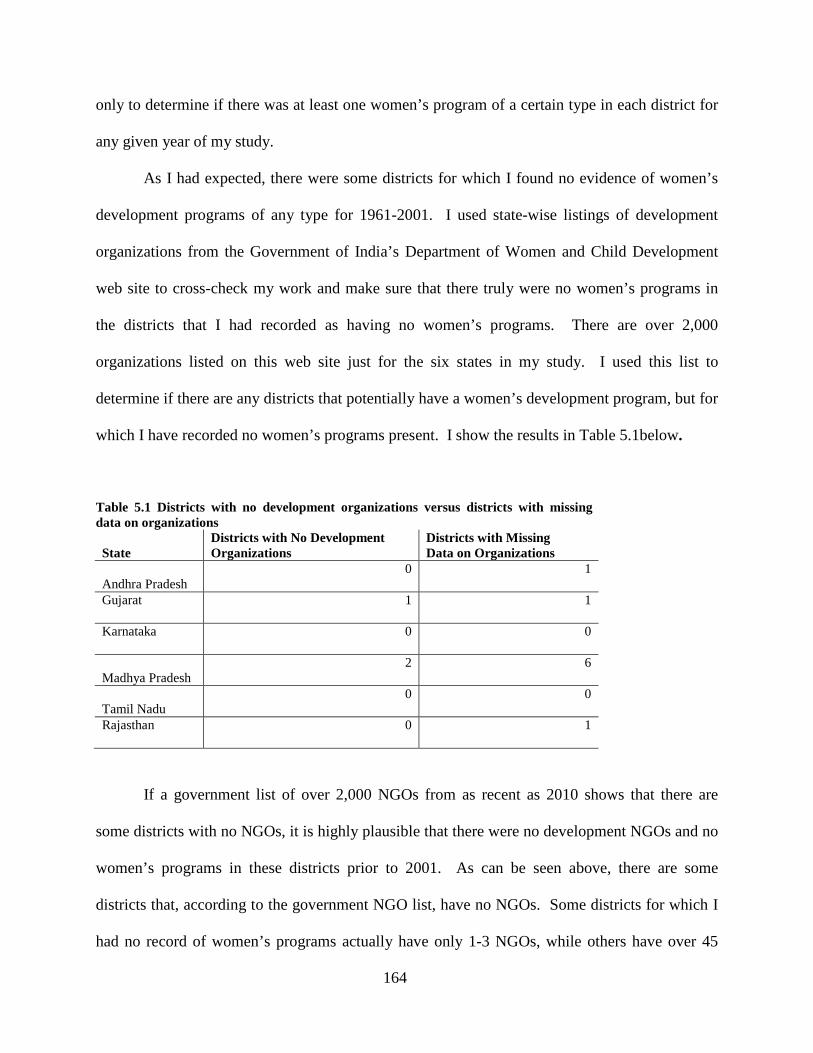
164
only to determine if there was at least one women’s program of a certain type in each district for
any given year of my study.
As I had expected, there were some districts for which I found no evidence of women’s
development programs of any type for 1961-2001. I used state-wise listings of development
organizations from the Government of India’s Department of Women and Child Development
web site to cross-check my work and make sure that there truly were no women’s programs in
the districts that I had recorded as having no women’s programs. There are over 2,000
organizations listed on this web site just for the six states in my study. I used this list to
determine if there are any districts that potentially have a women’s development program, but for
which I have recorded no women’s programs present. I show the results in Table 5.1below.
Table 5.1 Districts with no development organizations versus districts with missing data on organizations
State Districts with No Development Organizations
Districts with Missing Data on Organizations
Andhra Pradesh 0 1
Gujarat 1 1
Karnataka 0 0
Madhya Pradesh 2 6
Tamil Nadu 0 0
Rajasthan 0 1
If a government list of over 2,000 NGOs from as recent as 2010 shows that there are
some districts with no NGOs, it is highly plausible that there were no development NGOs and no
women’s programs in these districts prior to 2001. As can be seen above, there are some
districts that, according to the government NGO list, have no NGOs. Some districts for which I
had no record of women’s programs actually have only 1-3 NGOs, while others have over 45
165
development organizations. I recorded information on women’s programs as “missing data” for
these districts.
5.3 VARIABLES
5.3.1 Independent variables
The main independent variables are the presence or absence of a women’s rights program, and
the presence or absence of a women’s market-based program (other than microcredit), the
presence or absence of a women’s microcredit program, levels of urbanization, and net state
domestic product per capita. I operationalize presence or absence of “women’s rights program,”
“women’s market-based program (other),” and “women’s microcredit program” each as separate
dummy variables: (1=present, 0= absent).
I use two main independent variables in order to test my hypotheses on modernization
theory. These are “percentage of district population living in urban areas” and “net state
domestic product per capita”. The India Census defines an urban area or town as a place with
“…a municipality, corporation, cantonment board or notified town area committee, etc.” and
with “i.) a minimum population of 5,000; ii) at least 75 percent of male working population
engaged in non-agricultural pursuits; and iii) a density of population of at least 400 [people] per
sq. km (1,000 per sq. mile)” (Census of India 2001 web site). The Reserve Bank of India
provides state-wide yearly financial statistics starting from 1960-61 to 2008-09, including net
state domestic product measured in 1961 constant prices, which corrects for inflation over time.
I divide state domestic product by a state’s total population to obtain per capita state domestic
166
product. I use the natural log-transformed per capita state domestic product in my statistical
models. Although this variable is at the state level rather than the district level, I can use it as an
independent variable in my analyses.
My units of analysis are districts as they existed in 1961, but a number of districts have
divided into smaller units over time. In order to obtain the percentage of district population in
urban areas for districts with 1961 jurisdictional boundaries, I needed to aggregate data from the
districts that divided over time. For example, by the 1981 census, Hyderabad district had divided
into Hyderabad and Rangareddi districts. I re-calculated percentage of district population living
in urban areas for districts that had been a single district in earlier decades. In order to do this, I
first added the total population of Hyderabad to the total population of Rangareddi to get the total
population of Hyderabad district. I then added the urban population of Hyderabad to the urban
population of Rangareddi districts and divided this sum by the combined total population of
Hyderabad and Rangareddi to obtain the percentage of population living in urban areas for
Hyderabad district with 1961 jurisdictional boundaries.
I include “region” as an independent variable since regional variation in kinship and
patriarchal norms has such a strong impact on the status of women and girls in India. The
variable “region” is a proxy measure of historical variation in these kinship patterns and
patriarchal norms. This allows me to test the interaction effects between region and the other
independent variables in this study. This makes conceptual sense since Inglehart and Welzel
(2005) have found that nations’ paths of modernization depend in part on historical/cultural
factors. I discuss this further in the “Analytic Methods” section. I code region as (1= district
belongs to Southern region, 0 =otherwise) since Southern states tend to have greater gender
equality than Northern states. I code a district as “1” if it belongs to Tamil Nadu, Karnataka, or
167
Andhra Pradesh, and I code a district as “0” if a district belongs to Rajasthan, Gujarat, or
Madhya Pradesh. I also code each state as a separate dummy variable. For instance, for the
variable “Madhya Pradesh,” I code all the districts that belong to Madhya Pradesh as “1,” and all
the districts that do not belong to Madhya Pradesh as “0.” I code each state in this way, so that I
can include these states as separate control variables in my statistical models, omitting one state
as the reference category. This is so that I can discover if there are more localized patterns of
gender inequality than the broader categories of “North” and “South”.
5.3.2 Dependent variables
I measure district-level change in gender inequality with three variables: change in total
female/male sex ratio, change in female/male child sex ratio, and change in female/male literacy
ratio.
The Census of India defines the sex ratio as “the number of females per 1,000 males in
the population” and the child sex-ratio as “number of females in age-group 0-6 years per 1,000
males in the same age-group in the population” (Census of India 2001 web cite). The sex-ratio is
calculated by dividing “number of females” by “number of males”, and then multiplying that
number by 1,000. This gives the female/male sex ratio with a high level of precision, and also
eliminates the decimal places.
Similarly, the Census of India calculates the child sex-ratio (0-6 years) by dividing
“number of female children (0-6)” by “number of male children (0-6)”, and multiplying the
resulting figure by 1,000. The way in which the Census of India has measured female/male child
sex ratio and percentage of females and males who are literate has changed slightly across
168
decades. In census years prior to 1991, the female to male child sex ratio was based on the
number of female and male children ages 0-4 years. In 1991 and 2001, however, female/male
child sex ratio is based on the number of female and male children who are aged 0-6 years.
The 2001 Census of India defines a literate person as “a person aged 7 years and above
who can both read and write with understanding in any language”, including people who have
learned to read informally and blind people who read Braille (Census of India 2001 web cite). I
also include district-level female literacy rate and male literacy rate as separate variables, at least
in my descriptive analyses. This is to uncover whether changes in the female/male literacy ratio
is due to a faster rate of change in female literacy than male literacy, or if it is due to a decline or
leveling off of male literacy rates.
The female and male literacy rates in 1961-1981 are based on the percentage of females
and males over 4 years of age who can read and write. In 1991 and 2001, a literate person is
defined as someone at least 7 years of age who can read and write. These changes in
measurement should not make a significant difference in the results of my analyses, but it is
important to mention it here. The India Census reports district-level data for the total number of
people who are literate, and also the number of literate males and literate females.
The fact that many districts have divided over time means that I have had to re-calculate
sex ratios, child sex ratios, female/male literacy ratios, female literacy rates, and male literacy
rates for districts that had been a single district in earlier decades. For example, since Hyderabad
and Rangareddi districts had been one district at an earlier time period, I have added together the
total number of females in both districts and divided this by the total number of males in both
districts in order to get the female/male sex ratio of the jurisdictional area
Hyderabad+Rangareddi.
169
5.3.3 Control variable
During India’s pre-independence period, the female/male sex ratio was much higher for
Scheduled Castes than the national female/male sex ratio (Dreze and Sen 2004). Since India’s
independence, the female/male sex ratio among Scheduled Castes has been declining, and by
1991 it had converged with the all-India female/male sex ratio. Some researchers have noted that
over the past few decades, lower-caste groups (including Scheduled Castes) have been
increasingly adopting higher-caste cultural norms and practices as a way to raise the status of
their castes, a process they call “sanskritization” (Dreze and Sen 2004). Such norms include
female seclusion and the giving and taking of dowry. For this reason, I include “percentage of
district population comprised of scheduled castes” as a control variable in my study.
The way in which the India Census has defined membership of a Scheduled Caste is
rather complicated, and thus I give a detailed explanation. The President of India defines which
castes in each State or Union Territory are considered Scheduled Castes for those states. This
means that each state or union territory may have its own list of Scheduled Castes which is
distinct from any other state. According to the Constitution (Scheduled Castes) Order of 1950,
only Hindus could be considered members of Scheduled Castes. An amendment in 1956 ordered
that both professing Hindus and Sikhs could be considered for Scheduled Caste membership. A
further amendment in 1990 ordered that Buddhists as well as Hindus and Sikhs can be
considered for membership of Scheduled Castes (Census of India 2001). This means that district
percentages of Scheduled Castes for years after 1991 may be higher simply because “Scheduled
Caste” has been defined more broadly. For the purposes of my study, I operationalize
170
“Scheduled Caste” as the percentage of the district population made up of Scheduled Caste
members.
5.3.4 Dealing with time
The existence of women’s rights programs, microcredit programs, and other market-based
programs may very well begin in years other than when the India Census data is collected.
Because all of my dependent variables are measured during India Census years, I can still have a
“time-structured” data set (Singer and Willett 2003:12). I record presence/absence of women’s
development programs that existed prior to 1961 as occurring during 1961. In order for the
presence/absence of women’s programs to cause or predict changes in gender inequality,
measurements for the women’s program variables must precede measurements of gender
inequality. However, for women’s programs that came into existence during a Census year (i.e.
1961 or 1971), I cannot determine if they came into existence before or after the census was
taken in that year. Therefore, I record women’s development programs that started during the
period of 1961 to 1970 as existing in 1971. I code the women’s development programs that
came into existence in subsequent Census years in the same way. I set up my database as a time-
structured, “district-period” data set in order to treat my data set as longitudinal panel data
(Singer and Willett 2003:17-19, Allison 2009:15) as in Figure 5.1 below.
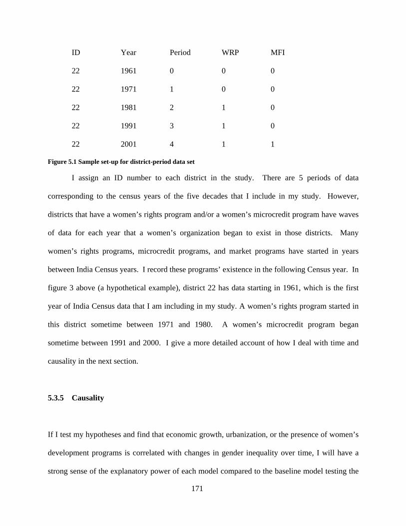
171
ID Year Period WRP MFI
22 1961 0 0 0
22 1971 1 0 0
22 1981 2 1 0
22 1991 3 1 0
22 2001 4 1 1
Figure 5.1 Sample set-up for district-period data set
I assign an ID number to each district in the study. There are 5 periods of data
corresponding to the census years of the five decades that I include in my study. However,
districts that have a women’s rights program and/or a women’s microcredit program have waves
of data for each year that a women’s organization began to exist in those districts. Many
women’s rights programs, microcredit programs, and market programs have started in years
between India Census years. I record these programs’ existence in the following Census year. In
figure 3 above (a hypothetical example), district 22 has data starting in 1961, which is the first
year of India Census data that I am including in my study. A women’s rights program started in
this district sometime between 1971 and 1980. A women’s microcredit program began
sometime between 1991 and 2000. I give a more detailed account of how I deal with time and
causality in the next section.
5.3.5 Causality
If I test my hypotheses and find that economic growth, urbanization, or the presence of women’s
development programs is correlated with changes in gender inequality over time, I will have a
strong sense of the explanatory power of each model compared to the baseline model testing the
172
null hypothesis. However, I may not know the true causal direction between these independent
variables. It is possible that there is a spurious relationship between presence of women’s
programs and changes in gender inequality, and that there are other factors that are causing both
variation in gender inequality and variation in presence/absence of women’s programs.
Alternatively, some types of women’s programs may flourish in areas that have lower levels of
gender inequality prior to their existence in those areas. In this instance, gender inequality
predicts the presence or absence of women’s programs rather than the other way around.
Another possibility is that there may be more NGOs with women’s programs present in more
economically developed states than in less economically developed states. In this case, states
that have more economic resources may attract NGOs that need sources of funding in order to
operate. Moreover, some states may implement policies that encourage the proliferation of some
types of women’s programs. There is certainly evidence that this may be the case. According to
one report, 61% of NGOs in India are in Southern states (Dasgupta 2001, cited in Singh 2007).
Moreover, 74% of microcredit SHGs are associated with NGOs existing in Southern states, and
78% of microcredit goes to SHGs in the Southern region. In contrast, only 6.9% of microcredit
goes to SHGs in the Central region, which includes the central state of Madhya Pradesh
(Dasgupta 2001, cited in Singh 2007). The so-called “BIMARU” states (Bihar, Madhya
Pradesh, Rajasthan, and Uttar Pradesh) are poorer than the southern states, so it could be that the
relative abundance of economic resources in southern states makes it possible for NGOs to start
more women’s microcredit programs than is possible in the central and northwestern states.
Also, it is important to consider other state-wide historical trends or policy changes that may
affect changes in female/male sex ratios or female/male literacy ratios apart from urbanization,
per capita SDP, or the presence of women’s development programs. For instance, Rajasthan and
173
Madhya Pradesh states implemented innovative educational programs between the late 1980s
and mid-1990s (Panchamukhi 2006, Ray 2006). Both states saw jumps in statewide female
literacy rates of over 20 percentage points between 1991 and 2001 (Panchamukhi 2006). In this
section, I describe how I will deal with these issues.
There are a few steps that I must take in order to establish causal relationships between
the variables in my study. The first step that I take in establishing causality is to determine the
temporal order among the independent variables. In order to determine if the values of an
independent variable X predict values of a dependent variable Y, the independent variable X
must be measured prior to the dependent variable Y (Inglehart and Welzel 2005). It is possible
that an increase in levels of urbanization lead to an increase in the female/male literacy ratio over
time. However, it is also possible that an increase in urbanization occurs at the same time as an
increase in the female/male literacy ratio so that the two variables are correlated without there
being a causal relationship between the two. In order to test if increases in urbanization predict
an increase in the female/male literacy ratio, I must run statistical models with lagged values of
urbanization (Singer and Willett 2003). For example, in Figure 5.1, if I recorded lagged values
of urbanization I would record the level of urbanization from 1961 as if it were the level of
urbanization at wave 2 in 1971. I also code the values of urbanization for the years they actually
occur, so that I have both lagged and unlagged data for the urbanization variable. If the results of
a statistical model with unlagged urbanization show that the relationship between urbanization
and female/male literacy ratio is statistically significant, but the relationship between lagged
urbanization and female/male literacy ratio is not significant, then I can be quite certain that
urbanization does not lead to an increase in the female/male literacy ratio.
174
There are other possible causal relationships to consider. For example, the results of a
statistical model may lead one to believe that the presence of women’s microcredit programs
leads to an increase in the female/male child sex ratio. However, one needs to consider how
other variables such as urbanization or economic growth may impact both the presence of
microcredit programs and the female/male child sex ratio. If the relationship between women’s
microcredit programs and the female/male sex ratio disappears once one introduces per capita
SDP into the model (and per capita SDP is significant), then the relationship between microcredit
programs and female/male sex ratio are both caused by per capita SDP. In this case, the
relationship between presence of microcredit programs and female/male sex ratio is spurious
(Agresti and Finlay 1997).
Yet another possible causal relationship is a chain relationship (Agresti and Finlay 1997).
For instance, there may appear to be a causal relationship between per capita SDP and
female/male sex ratio, but the relationship disappears once one introduces presence of women’s
market programs into the model. In this case, presence of women’s market programs is an
intervening variable and the direct cause of change in female/male sex ratio. In both the case of
chain relationships and spurious relationships, it is important to consider the temporal order, as
well as what theory and prior studies would suggest. It is highly implausible that a change in the
female/male child sex ratio causes change in the number of sex-selective abortions that are
performed, but it is possible that a change in the number of sex-selective abortions performed
leads to change in the female/male child sex ratio.
175
5.4 ANALYTIC METHODS
5.4.1 Descriptive statistics
Before I run my statistical models, I first carry out some exploratory analyses of my data. This is
because I must first examine how much variation over time and between regions there is in the
values of my variables in order to make decisions about the appropriate statistical methods later
on (Frees 2004). I first calculate the overall means and standard deviations as well as minimum
and maximum values for all of my continuous variables: per capita SDP, logged per capita SDP,
percentage of district population in urban areas, percent of population comprised of Scheduled
Castes, female/male sex ratio, female/male child sex ratio, male literacy rate, female literacy rate,
and female/male literacy ratio. The standard deviation tells me the spread of the distribution.
The smaller the value of a variable’s standard deviation is, the smaller the spread of all the values
are about the mean.
Once I generate overall means and standard deviations for my continuous variables, I
then generate counts and percents of each type of women’s program by region (north and south)
to determine if regional variation in the number of districts that have a certain type of women’s is
statistically significant. I generate separate region-wise crosstabulations for women’s rights
programs, women’s market programs, and women’s microfinance programs.
I use two-sample t-tests in order to determine if there is statistically significant variation
by region for each of the continuous independent variables and dependent variables. I calculate
t-tests for each of the following variables: per capita SDP, logged per capita SDP, percentage of
population in urban areas, percentage of district population comprised of Scheduled Castes,
female/male sex ratio, female/male child sex ratio, and female/male literacy ratio. I also
176
calculate two-sample t-tests for male literacy rate and female literacy rate to see if there is
statistically significant regional variation for each of these separately.
Once I explore regional variation in all of the variables, I examine regional variation in
each variable by state. I first tabulate counts and percents for each women’s program by state,
just as I do for each women’s program by region. This is important because even if there is not
statistically significant regional variation in the number of districts with women’s programs,
there may be statistically significant state-wise variation in presence of women’s programs. It is
possible that there may be one state in the north or south that has an uncharacteristically low or
high number of districts with women’s programs and that this state is causing regional variation
in presence of women’s programs to be statistically insignificant.
After this, I use one-way ANOVAs to examine whether state-wise variation in each of
the continuous variables is statistically significant. I use the Bonferroni multiple comparison
procedure to determine which pairs of states are significantly different in their mean values for
all of these variables (Agresti and Finlay 1997, Acock 2006). One of the assumptions of
ANOVA is that the variances of all groups being compared are equal (Acock 2006). I use
Bartlett’s test for equal variances to determine whether this assumption holds for the inter-state
comparison of means. If this assumption does not hold for any of the variables, I must interpret
the ANOVA results for that variable with caution.
My next step is to produce a correlation matrix of all of my variables, including lagged
independent variables. This is an important step because it gives me an initial sense of how the
variables are related to one another, including the extent to which any of the independent
variables are correlated with each other. If any of the independent variables are too strongly
correlated with each other, this is an indication that they are collinear. In this case, I must
177
include interaction terms along with the main effects of the collinear variables in the statistical
models (Arceneaux and Huber 2007). If I include only the main effects of the collinear variables
in my models, the estimates of the coefficients may be biased. Another reason why it is
important to run a correlation matrix before estimating the statistical models is because the
correlation matrix will provide clues to causal relationships that I do not consider in my original
hypotheses. For instance, one of my hypotheses is that the presence of women’s market
programs leads to an increase in female/male sex ratios and female/male literacy ratios. If the
presence of women’s market programs is indeed significantly related to an increase in
female/male sex ratios and literacy ratios, it is possible that the market programs are not causing
these changes. Another plausible explanation is that per capita SDP explains both an increase in
presence of women’s market programs and an increase in the female/male literacy ratios. In this
case, any apparent relationship between women’s market programs and female/male literacy
ratios is actually a spurious relationship (Agresti and Finlay 1997). If I find that there is no
correlation between per capita SDP and female/male literacy ratio, but there is a relationship
between women’s market programs and literacy ratio, I can be certain that the relationship
between women’s market programs and literacy ratio is not a spurious relationship (Agresti and
Finlay 1997).
Once I explore the variation in all of the variables by region and state, I investigate
variation in the variables across time periods. I first tabulate counts and percents for each type
women’s program by time period. I tabulate separate tables of counts and percents for types of
women’s programs in the northern region and in the southern region. This allows me to
determine if the variation in the presence of women’s programs is statistically significant across
178
time periods within a given region. After this, I tabulate counts and percents for each type of
women’s program across time periods and within each of the six states.
After I examine the variation in the presence of each type of women’s program over time,
I calculate means and standard deviations by time period and state for all of the continuous
independent and dependent variables except per capita SDP and logged per capita SDP. (Since
there is no district variation in per capita SDP and logged per capita SDP, I do not report means
and standard deviations for these variables.) I calculate means and standard deviations of each of
these variables separately by state. This gives me a better sense for how the variables change
over time within each state. I can also see if there is a consistent pattern in how these variables
(especially the dependent variables) change over time, and if the rate of change varies drastically
during some time periods. For example, I am able to tell if the female/male sex ratio increases or
decreases steadily over time, or if it fluctuates up and down over time. I am also able to
determine if the female/male sex ratio increases in some states while it decreases in others.
Once I run means and standard deviations for my continuous variables, I then create a
trellis plot (Frees 2004), or series of line graphs depicting how individual districts vary over time
on each of the dependent variables. I accomplish this by randomly selecting a sample of districts
for each dependent variable and plotting changes in the variables over time. Creating trellis plots
for a large number of districts allows me to visually detect time trends for each dependent
variable, such as how much the female/male literacy ratio changes over time, whether that
change is positive or negative, and whether there is a linear or curvilinear relationship between
female/male literacy ratio and time period. This informs my later decisions in statistical
modeling. For example, if there is a curvilinear relationship between female/male literacy ratio
and time period and I try to fit a linear model to the data, I might falsely conclude that there is no
179
change in female/male literacy ratio over time. These line graphs also show how much between-
district variation there is in initial values of my dependent variables and rates of change over
time. This is important because it provides a clue as to whether I should pay more attention to
between-district changes or within-district changes in the dependent variables over time.
I use change-scores to determine the amount of change in each of the continuous
independent and dependent variables from 1961 to 2001. I use the t-test to determine if this
absolute change from time period 1 (1961) to time period 5 (2001) is statistically significant.
While the change score analyses tell me which variables vary significantly over time, they do not
tell me the strength of the relationship between time and each of these variables. For this I
estimate OLS regression models of each continuous variable on time period. OLS regression
models tell me both the strength of the relationship between each variable and time, and also the
average magnitude of change per time period for each variable. The coefficients for each
variable tell me how much each variable changes over time, and the adjusted R-squared tells me
the strength of the relationship between each variable and time. Both the change score analyses
and the OLS regressions can determine which variables, if any, do not vary significantly over
time. This is especially important to determine because if any of the dependent variables does
not significantly change over time, then I cannot include it as a dependent variable for further
statistical models that include independent variables. Also, if there are any independent variables
that do not vary significantly over time, I must treat these variables as time-invariant variables in
further statistical models.
180
5.4.2 Statistical modeling
Although ordinary least squares (OLS) regression is a common data analytic method among
social scientists, it is not appropriate for analyzing longitudinal data. One can use OLS
regression with longitudinal data to describe the relationship between the independent variable
“time” and changes in the dependent variable as I describe above (Singer and Willett 2003), or to
explain the relationship between independent variables and the dependent variable for cross-
sectional data. However, OLS regression is inappropriate for analyzing longitudinal data
because there are a few assumptions of OLS that the structure of longitudinal data does not
fulfill. The first assumption of OLS is that the error terms associated with the actual
observations will be completely uncorrelated, and that the error terms taken together will have a
mean of zero (Schroeder et al. 1986). The second assumption is that variability in the error terms
is not correlated with any of the independent variables, and that the error term itself is not related
to the independent variables. Third, with OLS regression the error residuals must be
homoskedastic; that is, the variance must not become greater or lesser over time (Singer and
Willett 2003). The structure of longitudinal data violates all of these assumptions. Although the
error terms of different units may be uncorrelated, the error terms across time points for the same
unit will be correlated (Schroeder et al. 1986, Finkel 2007). For example, the error terms for
female/male literacy ratios at time 2 are likely to be correlated with the error terms for literacy
ratios at time 1. Second, the residuals for my longitudinal data may be heteroscedastic (Singer
and Willett 2003). This means that the variance in error may become larger or smaller over time.
Third, the error terms of my data may be related to at least some of the independent variables.
This is because there may be unobserved, time-invariant characteristics that are unique to
181
individual districts, and that are also related to the independent variables (Halaby 2004, Finkel
2007). For example, districts that are drought-prone (a geographical feature) may be less likely
to become more urbanized over time than districts that are not prone to drought. In an OLS
model, these unmeasured, time-invariant characteristics are treated as part of the error term. If
one uses OLS regression for data that does not fulfill the above assumptions, it can affect the
regression coefficients’ standard errors and bias the results (Schroeder et al. 1986). Either fixed-
effects or random-effects models allow for the heteroskedasticity characteristic of longitudinal
data without introducing bias. Fixed-effects models allow for correlation between the time-
invariant, unit-specific error and the independent variables as well (Halaby 2004, Finkel 2007).
5.4.3 Fixed-effects models
I use fixed-effects models to analyze the data and to test the hypotheses. There are several
advantages of using fixed-effects models, which I describe below. Fixed-effects longitudinal
models allow one to control for time-invariant characteristics of units (Allison 2009), such as
unique characteristics of nations, states, or even districts. These can include a wide range of
characteristics that one cannot directly measure, such as geographical attributes, cultural norms,
or historical attributes of states or districts. Fixed-effects models “pool” data from across time
periods to estimate “average” coefficients that explain how the dependent variable changes with
the independent variable over time (Finkel 2007). The basic equation of the fixed-effects model
is (Finkel 2007:479): .
182
In this model, there are two parts to the error term. The “U” term represents the time-
invariant unobserved heterogeneity unique to each district (Finkel 2007). The “ ” represents
the idiosyncratic error that is assumed to have a random distribution. This idiosyncratic error
varies across time and across districts. “ ” represents the coefficient of the first independent
variable “ ”. “ ” is the value of the first independent variable for “i” individuals at “t”
time periods. Thus, refers to the effect of the first independent variable for “i” districts
at “t” time points.
The strength of using fixed-effects models is that they allow me to estimate the effects of
women’s development programs on changes in gender inequality and control for these
unmeasured district-level characteristics. In OLS regression, in contrast, one cannot control for
these unmeasured characteristics (Allison 2009). In fixed-effects regression models, each unit
(in my study, each district) acts as its own control. The fixed-effects model essentially
“differences out” the time-invariant, between-district variation in values of the independent
variables. This between-district variation in values of the observed independent variables may
be confounded by unmeasured characteristics of those districts. For example, it may be possible
that some district-specific, unmeasured characteristic such as geographical conditions or cultural
norms cause variation in presence/absence of women’s programs and also cause changes in
gender inequality. The advantage of “differencing out” these unmeasured characteristics is that
it allows me to more accurately estimate the relationships between my independent variables and
dependent variables. If I use a model that does not separate the unmeasured, time-invariant
183
district characteristics from the random error term, this could result in biased estimators for my
independent variables (Allison 2009, Finkel 2007).
There are some drawbacks to using a fixed-effects regression model, however. Since a
fixed-effects model controls for any time-invariant characteristics of districts, I cannot directly
estimate the effects of observable time-invariant variables on the dependent variables, such as
the effects of “region” or “state” on gender inequality (Allison 2009). However, I can still
estimate the interaction effects of time-invariant variables and the passage of time, such as the
interaction effect of “state*period”. Another disadvantage of fixed-effects models is that they
usually produce larger p-values and standard errors than those of random-effects models. This is
because fixed-effects models use only information related to within-district variation and
discards information on between-district variation. This means that if there is a lot of between-
district variability in values of the independent variables but not much change over time, the
fixed-effects coefficients will not be precise (Allison 2009). This can result in coefficients of
independent variables that are not statistically significant (even if they are unbiased).
5.4.4 Model specification
In this section, I describe in detail the models that I estimate to test each set of hypotheses. I
estimate fixed-effects models to test all of my hypotheses. For each set of hypotheses, I estimate
a final, complete model that includes all of the variables from the previous models. This is so
that I can test the relative goodnesss-of-fit of each of the previous reduced models against the
goodness-of-fit of the final complete model (Agresti and Finlay 1997). I also estimate models
with lagged independent variables for each set of hypotheses. This is to determine whether
184
independent variables that are statistically significantly related to the dependent variables remain
statistically significant once the lagged values of the independent variables are used in the
models instead. If there is no statistically significant relationship between the lagged
independent variables and the dependent variables, then the independent variables cannot be said
to cause variation in the dependent variables. I start this section by describing how I test the first
set of hypotheses, which are derived from modernization theory.
Hypotheses and test the claims of modernization theory. states, “An
increase in urbanization and per capita SDP will lead to an increase in female/male sex ratios,
female/male child sex ratios, and female/male literacy ratios.” In order to test this hypothesis, I
estimate fixed-effects models for each of the dependent variables, and include logged per capita
SDP and percent of population in urbanized areas as the independent variables. I also include
the variable “period” to control for the effect of the passage of time on changes in the dependent
variables.
states, “An increase in urbanization and economic growth will have a greater impact
on increases in female/male sex ratios, female/male child sex ratios, and female/male literacy
ratios in southern states than in northern states.” I test this hypothesis by first estimating a
fixed-effects model that includes all of the variables from the previous model, plus the following
interaction terms: region*urban, region*logged per capita SDP. In the final model, I add
“percentage of population comprised of Scheduled Castes”, region*period, women’s rights
programs, market programs, and microfinance programs. This is so that I can determine if the
effects of the variables of interest (logged per capita SDP, urbanization, region*logged per capita
SDP, region*urbanization) remain the same after I control for these other variables. Since each
185
previous model is nested within each successive model, I can use the F-statistic to compare the
goodness-of-fit of each model to successive models. I explain the F-statistic in greater detail in
the Statistical Methods section.
Hypotheses through test the claims of WID theory. states, “An increase in
urbanization and economic growth alone will lead to a decrease in female/male sex ratios,
female/male child sex ratios, and female/male literacy ratios.” In order to test this hypothesis, I
can simply refer to the results of the model testing hypothesis 1a. If the results for the model that
tests show that urbanization and logged per capita SDP are significantly related to increases
in female/male sex ratio, child sex ratio, and literacy ratio, then I will accept hypothesis 1a and
reject hypothesis 2a. If the model that tests hypothesis 1a shows that urbanization and logged
per capita SDP are significantly related to decreases in the female/male sex ratio, child sex ratio,
and literacy ratio, then I will accept hypothesis 2a and reject hypothesis 1a.
states, “The presence of women’s market programs will lead to increases in
female/male sex ratios, female/male child sex ratios, and female/male literacy ratios.” In order
to test this hypothesis, I estimate fixed-effects models that include “women’s market programs”
as the independent variable and “period” as the control variable.
states, “The presence of women’s market programs and women’s microfinance
programs jointly will have a greater impact than women’s market programs alone on raising
female/male sex ratios, female/male child sex ratios, and female/male literacy ratios.” To test
this hypothesis, I include “market programs”, “microfinance programs”, and the interaction term
186
“market*microfinance”, as well as the control variable “period”. The interaction term tests for
the joint effect of market and microfinance programs on changes in the dependent variables.
states, “The presence of women’s market programs and women’s microfinance
programs will have a greater impact on increases in female/male sex ratios, female/male child
sex ratios, and female/male literacy ratios in southern states than in northern states.” To test
this hypothesis, I include all of the variables from the previous model, as well as the interaction
effects of market*region, microfinance*region, and market*microfinance*region. Since
“region” is a time-invariant variable, I do not include it as a main effect in the model. The last
model that I estimate includes all of the previous independent variables, as well as the interaction
effect of region*period to control for any changes in the dependent variables that are caused
solely by the changing effect of region over time. I also include the main effects of urbanization,
logged per capita SDP, and Scheduled Castes. I include all of these variables in this last model
so that all previous models are nested in this model. This is so that I can compare the goodness-
of-fit of all previous models to one final model.
My third set of hypotheses ( through ) test the claims of GAD theory. states,
“The presence of women’s rights programs will lead to increases in female/male sex ratios,
female/male child sex ratios, and female/male literacy ratios. To test this hypothesis, I estimate
fixed-effects models for each of the dependent variables that include only “women’s rights
programs” as the independent variable and “period” to control for any change in the dependent
variables that is due solely to the passage of time.
states, “Region will have a mediating effect on the impact of women’s rights
programs on increases in female/male sex ratios, female/male child sex ratios, and female/male
187
literacy ratios. To test this hypothesis, I estimate a model that includes women’s rights
programs, women’s rights*region, and period. I then estimate a model that includes these
variables, plus the Scheduled Castes variable and the interaction effect of region*period. I
include an interaction term for region and period to determine if region (apart from women’s
rights programs) can at least partly explain variation in the rates of change of female/male sex
ratios and literacy ratios.
states, “The presence of women’s rights programs, women’s market programs, and
women’s microfinance programs jointly will have a greater impact than women’s rights
programs alone on raising female/male sex ratios, female/male child sex ratios, and female/male
literacy ratios. For the fixed-effects models that I estimate to test this hypothesis, I include the
main effects for women’s rights programs, market programs, and microfinance programs. I also
include the interaction effects between each of the women’s program types, as well as the joint
effect of all three women’s program types: women’s rights*market, women’s
rights*microfinance, market*microfinance, and women’s rights*market*microfinance. Even
though I am not specifically testing the joint effect of each pair of women’s program types, I still
include interaction effects of each pair of women’s program types. This is because I must
include all components of an interaction term in order to ensure that the model does not yield
biased results (Arceneaux and Huber 2007). Once I estimate this model, I then estimate a fixed-
effects model that includes all of these variables, as well as urbanization, logged per capita SDP,
percentage of population comprised of Scheduled Castes, and region*period. This is so that I
can determine whether the effects of the women’s program variables change or remain the same
as in the previous model.
188
My last set of hypotheses ( through ) test the claims of neoliberal theory.
states, “The presence of women’s microfinance programs will lead to increases in female/male
sex ratios, female/male child sex ratios, and female/male literacy ratios.” To test this hypothesis,
I estimate fixed-effects models for each of the dependent variables that include only “women’s
microfinance programs” as the independent variable and “period” to control for any change in
the dependent variables that is due solely to the passage of time.
states, “The presence of women’s microfinance programs will have a greater impact
on increases in female/male sex ratios, female/male child sex ratios, and female/male literacy
ratios in areas that have greater economic growth than in areas that have less economic
growth.” To test this hypothesis, I estimate fixed-effects models that include the main effects for
logged per capita SDP and women’s microfinance programs, and the interaction effect for
microfinance programs*logged per capita SDP, as well as the control variable “period”.
states, “The presence of women’s microfinance programs will have a greater impact
on increases in female/male sex ratios, female/male child sex ratios, and female/male literacy
ratios in southern regions than in northern regions.” I test this hypothesis by estimating fixed-
effects models that include the main effect of microfinance programs, the interaction effect of
microfinance*region and region*period, plus the “period” control variable. Once I estimate this
model, I estimate a model that includes all of the variables from the previous model, as well as
all of the variables from the model that tests . Since both the models that test and
are nested within this subsequent model, I can compare the goodness-of-fit of both models to the
goodness-of-fit of this subsequent model. Finally, I estimate a model that includes all of the
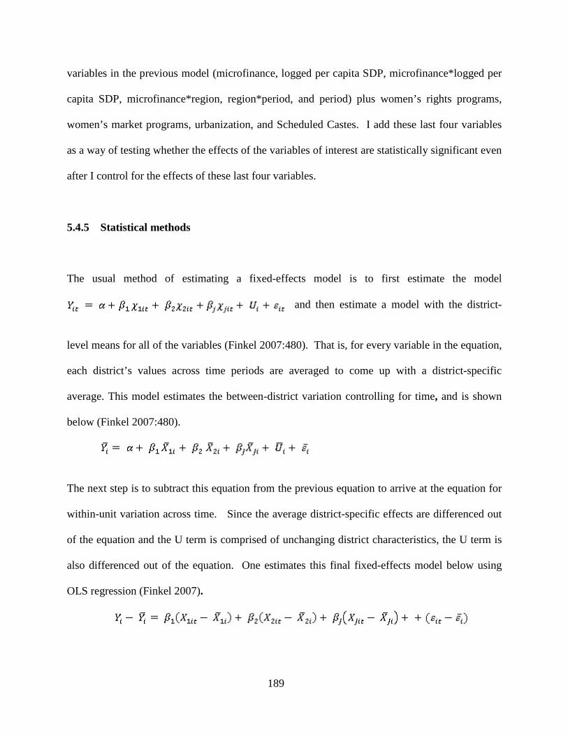
189
variables in the previous model (microfinance, logged per capita SDP, microfinance*logged per
capita SDP, microfinance*region, region*period, and period) plus women’s rights programs,
women’s market programs, urbanization, and Scheduled Castes. I add these last four variables
as a way of testing whether the effects of the variables of interest are statistically significant even
after I control for the effects of these last four variables.
5.4.5 Statistical methods
The usual method of estimating a fixed-effects model is to first estimate the model
and then estimate a model with the district-
level means for all of the variables (Finkel 2007:480). That is, for every variable in the equation,
each district’s values across time periods are averaged to come up with a district-specific
average. This model estimates the between-district variation controlling for time, and is shown
below (Finkel 2007:480).
The next step is to subtract this equation from the previous equation to arrive at the equation for
within-unit variation across time. Since the average district-specific effects are differenced out
of the equation and the U term is comprised of unchanging district characteristics, the U term is
also differenced out of the equation. One estimates this final fixed-effects model below using
OLS regression (Finkel 2007).
190
Stata reports within-R², between R², and overall R² as goodness-of-fit measures (Allison
2009). However, since fixed-effects models discard all information on between-district variance
in gender inequality, the within-R² is the appropriate goodness-of-fit statistic to examine and
report. The within- tells one the percentage of within-district variation in the dependent
variable that is explained jointly by all of the independent variables in the model. For example,
if the within- = 0.40, then this means that the statistical model explains 40% of the within-
district variation in the dependent variable (Acock 2006). The F-test statistic that is reported by
Stata tells one whether the values could have occurred just by chance. If the F-value is large,
then the probability that the values occurred by chance is small. For example, if the
probability (or p-value) that the values occurred by chance is less than 0.05, one can be quite
certain that the values are statistically significant.
The coefficients reported for each independent variable tell how large of an effect each
independent variable has on the dependent variable (Acock 2006). One uses the t-statistic for
each coefficient to determine whether the value of that coefficient could have occurred by
chance. If the p-value, or probability that the value of the coefficient is less than 0.05, one can
be 95% confident that the value of the coefficient did not occur just by chance. That is, the value
of the coefficient is statistically significant.
Rho (ρ) is a measure of the proportion of variance in the composite error term that is due
to the time-invariant component (that is, ).
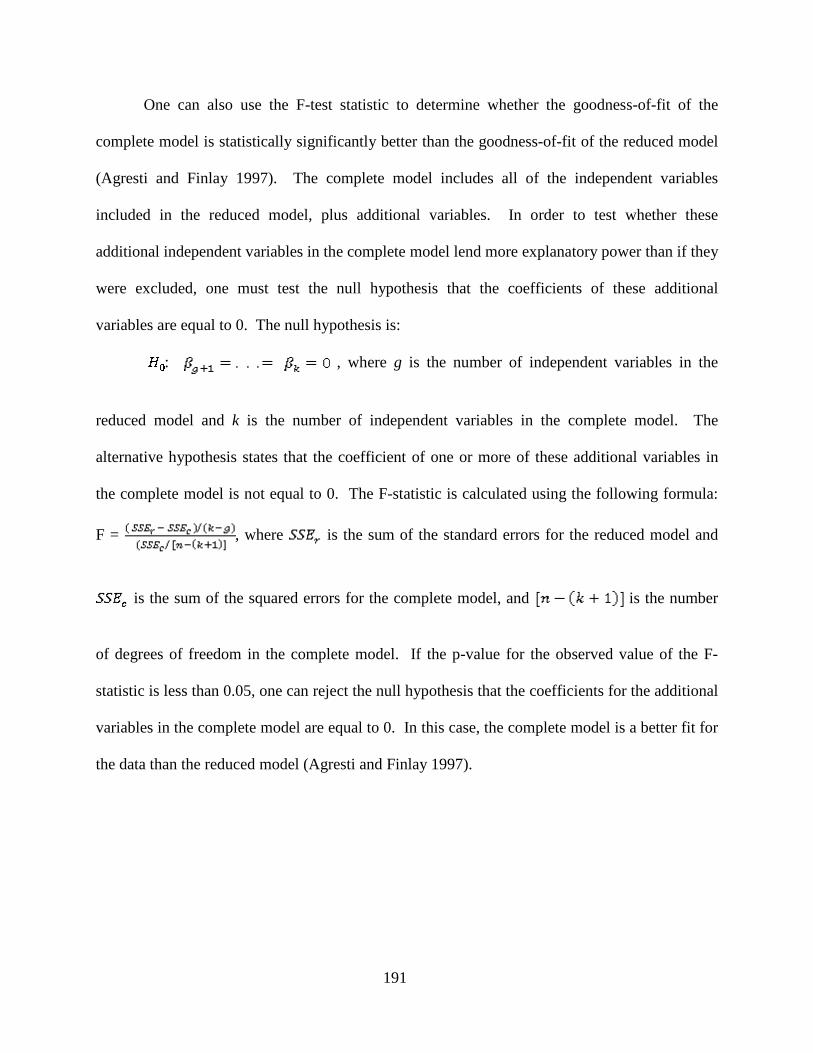
191
One can also use the F-test statistic to determine whether the goodness-of-fit of the
complete model is statistically significantly better than the goodness-of-fit of the reduced model
(Agresti and Finlay 1997). The complete model includes all of the independent variables
included in the reduced model, plus additional variables. In order to test whether these
additional independent variables in the complete model lend more explanatory power than if they
were excluded, one must test the null hypothesis that the coefficients of these additional
variables are equal to 0. The null hypothesis is:
: , where g is the number of independent variables in the
reduced model and k is the number of independent variables in the complete model. The
alternative hypothesis states that the coefficient of one or more of these additional variables in
the complete model is not equal to 0. The F-statistic is calculated using the following formula:
F = , where is the sum of the standard errors for the reduced model and
is the sum of the squared errors for the complete model, and is the number
of degrees of freedom in the complete model. If the p-value for the observed value of the F-
statistic is less than 0.05, one can reject the null hypothesis that the coefficients for the additional
variables in the complete model are equal to 0. In this case, the complete model is a better fit for
the data than the reduced model (Agresti and Finlay 1997).
192
5.5 CONCLUSION
In this chapter, I have laid the groundwork for the following chapters in which I discuss the
descriptive analyses and the results of the statistical models that I estimate. I have discussed my
data collection processes, including the states I chose for the study, the unit of analysis, and
sources of data. I have also explained how I deal with time using longitudinal data, as well as
how I deal with issues of causality. I have summarized the statistical methods I utilize to analyze
the data, including descriptive statistics and the statistical models I estimate in order to test the
hypotheses. In chapter six, I will focus on the descriptive analyses of my variables, such as the
overall means and standard deviations of the continuous variables, as well as the variation in the
presence of women’s rights programs, market programs, and microfinance programs by region
and state. I will also discuss variation in the continuous independent variables and in the
dependent variables by region and state. After this, I will describe the regional and state-wise
variation in the presence of the women’s programs over time, as well as the variation in the
continuous independent variables and the dependent variables over time within each state. I will
end the next chapter by presenting and discussing change scores and OLS regression models of
each continuous variable’s average change over time.
NOTES TO CHAPTER FIVE
viii The official Census of India website is www.Censusindia.gov.in. This website provides drop-down menus from which one may choose particular states and districts with demographic information. This website link is: www.Censusindia.gov.in/Tables_Published/Basic_Data_Sheet.aspx. ix I had considered using 2001 district boundaries in order to maintain constant boundaries from 1961-2001. However, other scholars on India at the University of Maryland at College Park have used the 1961 district boundaries as their constant units for their “Indian District Database.” Scholars at Duke University have also used 1961 district boundaries when compiling data for their longitudinal “Indian Agriculture and Climate Data Set”. By using 1961 district boundaries it is possible for me to merge data from these two data bases with my own data base for future research purposes.
193
x I first started with the state-wise maps from the Census of India website (www.censusindia.gov.in/maps/State_Maps_links) that showed the district boundaries in 2001. I then used the following atlases to compare the state and district boundaries of prior periods to the state and district boundaries in 2001: T. T. Maps. Muthiah, S., editor-in-chief. 1990. An Atlas of India, pp. 17, 44, 64, 77, 112, and 121. Oxford: Oxford University Press. For information on changes in state boundaries, I consulted this source: Nag, Prithvish, ed. Socio-Economic Atlas of India, pp. 2-3. Kolkata: Director, National Atlas and Thematic Publishing Organisation.
194
6.0 CHAPTER SIX: DESCRIPTIVE STATISTICS
6.1 INTRODUCTION
In the previous two chapters, I discussed the hypotheses and the variables of my study, and I
outlined the descriptive statistics and the analytic methods that I use to test my hypotheses. In
this chapter, I focus on the descriptive analyses of my variables. I start out by presenting and
discussing overall means and standard deviations of the continuous independent variables (per
capita SDP, urbanization, Scheduled Castes) and the dependent variables (female/male sex ratio,
female/male child sex ratio, and female/male literacy ratio). Next, I discuss variation in the
presence of women’s rights programs, market programs, and microfinance programs by region
and state. I also discuss variation in the continuous independent variables and in the dependent
variables by region and state, as well as pairwise correlations between these variables. After this,
I move on to a discussion of regional and state-wise variation in the presence of the women’s
programs over time. I then describe how the continuous independent variables and the
dependent variables change over time within each state. Finally, I present and discuss change
scores and OLS regression models of each continuous variable’s average change over time.
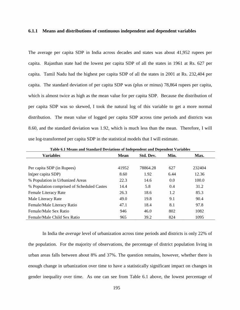
195
6.1.1 Means and distributions of continuous independent and dependent variables
The average per capita SDP in India across decades and states was about 41,952 rupees per
capita. Rajasthan state had the lowest per capita SDP of all the states in 1961 at Rs. 627 per
capita. Tamil Nadu had the highest per capita SDP of all the states in 2001 at Rs. 232,404 per
capita. The standard deviation of per capita SDP was (plus or minus) 78,864 rupees per capita,
which is almost twice as high as the mean value for per capita SDP. Because the distribution of
per capita SDP was so skewed, I took the natural log of this variable to get a more normal
distribution. The mean value of logged per capita SDP across time periods and districts was
8.60, and the standard deviation was 1.92, which is much less than the mean. Therefore, I will
use log-transformed per capita SDP in the statistical models that I will estimate.
Table 6.1 Means and Standard Deviations of Independent and Dependent Variables Variables Mean Std. Dev. Min. Max.
Per capita SDP (in Rupees) 41952 78864.28 627 232404 ln(per capita SDP) 8.60 1.92 6.44 12.36 % Population in Urbanized Areas 22.3 14.6 0.0 100.0 % Population comprised of Scheduled Castes 14.4 5.8 0.4 31.2 Female Literacy Rate 26.3 18.6 1.2 85.3 Male Literacy Rate 49.0 19.8 9.1 90.4 Female/Male Literacy Ratio 47.1 18.4 8.1 97.8 Female/Male Sex Ratio 946 46.0 802 1082 Female/Male Child Sex Ratio 965 39.2 824 1095
In India the average level of urbanization across time periods and districts is only 22% of
the population. For the majority of observations, the percentage of district population living in
urban areas falls between about 8% and 37%. The question remains, however, whether there is
enough change in urbanization over time to have a statistically significant impact on changes in
gender inequality over time. As one can see from Table 6.1 above, the lowest percentage of
196
population living in urban areas is 0%, and the highest percentage is 100%. I further examined
which districts had these most extreme values, and found that Dangs district in Gujarat state had
0% of its population living in urban areas for most decades, whereas Madras district (now
Chennai) in Tamil Nadu had 100% of its population living in urban areas from 1971-2001. It is
possible that the extreme values of these two districts may skew the results of statistical models
later on. One strategy that I can take to deal with this is to estimate models both with and
without these extreme cases and see if there is a statistically significant difference between the
two resulting models. If there is a difference between the two models, then I will keep the model
that excludes the two cases. It is not likely that including these two districts from the statistical
models will bias the results since the mean and standard deviation for percent of population in
urban areas do not differ much when these cases are excluded compared to when they are
included (see Table 6.2).
From Table 6.1, one can see that on average, the percentage of district population that is
comprised of Scheduled Castes is about 14%, with a standard deviation of about 6 percentage
points. Dangs district in Gujarat state had the lowest percentage of Scheduled Castes at less than
1% of its population, while Nilgiris district in Tamil Nadu had the highest percentage of
Scheduled Castes at about 31% of its population. It is possible that these two outliers could skew
the results of statistical models that include the Scheduled Castes variable. For example, if
female/male sex ratios or literacy ratio tend to be low for Nilgiris district, the results of the
statistical models may show that there is no statistically significant relationship between
percentage of population comprised of Scheduled Castes and female/male sex ratios or literacy
ratio. However, as can be seen from Table 6.2 below, the mean and standard deviation for
percentage of population comprised of Scheduled Castes when these two districts are omitted
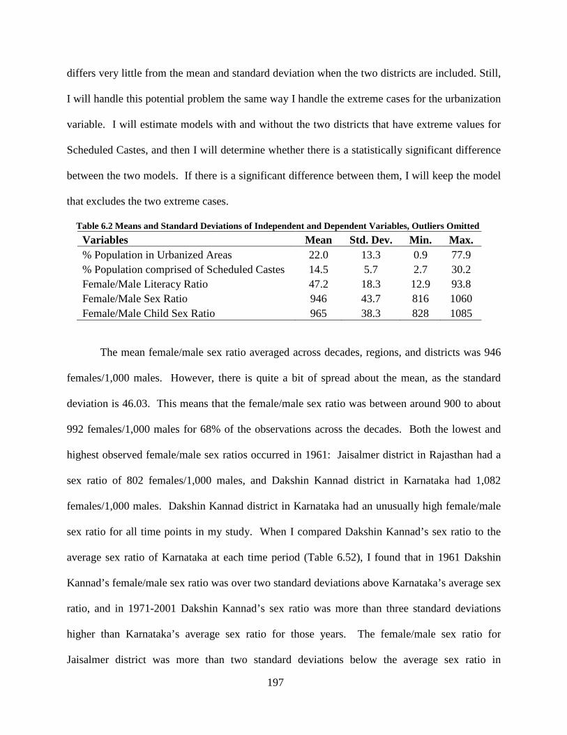
197
differs very little from the mean and standard deviation when the two districts are included. Still,
I will handle this potential problem the same way I handle the extreme cases for the urbanization
variable. I will estimate models with and without the two districts that have extreme values for
Scheduled Castes, and then I will determine whether there is a statistically significant difference
between the two models. If there is a significant difference between them, I will keep the model
that excludes the two extreme cases.
Table 6.2 Means and Standard Deviations of Independent and Dependent Variables, Outliers Omitted Variables Mean Std. Dev. Min. Max. % Population in Urbanized Areas 22.0 13.3 0.9 77.9 % Population comprised of Scheduled Castes 14.5 5.7 2.7 30.2 Female/Male Literacy Ratio 47.2 18.3 12.9 93.8 Female/Male Sex Ratio 946 43.7 816 1060 Female/Male Child Sex Ratio 965 38.3 828 1085
The mean female/male sex ratio averaged across decades, regions, and districts was 946
females/1,000 males. However, there is quite a bit of spread about the mean, as the standard
deviation is 46.03. This means that the female/male sex ratio was between around 900 to about
992 females/1,000 males for 68% of the observations across the decades. Both the lowest and
highest observed female/male sex ratios occurred in 1961: Jaisalmer district in Rajasthan had a
sex ratio of 802 females/1,000 males, and Dakshin Kannad district in Karnataka had 1,082
females/1,000 males. Dakshin Kannad district in Karnataka had an unusually high female/male
sex ratio for all time points in my study. When I compared Dakshin Kannad’s sex ratio to the
average sex ratio of Karnataka at each time period (Table 6.52), I found that in 1961 Dakshin
Kannad’s female/male sex ratio was over two standard deviations above Karnataka’s average sex
ratio, and in 1971-2001 Dakshin Kannad’s sex ratio was more than three standard deviations
higher than Karnataka’s average sex ratio for those years. The female/male sex ratio for
Jaisalmer district was more than two standard deviations below the average sex ratio in
198
Rajasthan state in 1961 (see Table 6.56). However, once I compared the mean and standard
deviation for female/male sex ratio with these two districts omitted to the mean and standard
deviation when they are included, I found that the two means were almost the same ( Table
6.2). Even though it is not likely that including these two cases would bias the results of my
statistical models later on, I will still estimate models both with and without these two cases and
determine whether there is a statistically significant difference between the two models.
Surprisingly, the average female/male child sex ratio was about 965, which was higher
than the average female/male sex ratio. The standard deviation of the female/male child sex ratio
was 39.23. This means that the majority of observations on child sex ratio were between 926
and 1,005 females per 1,000 males. The lowest observation was in a district of Madhya Pradesh
in 1981 at 824 females/1,000 males, which was more than three standard deviations below the
mean female/male child sex ratio for Madhya Pradesh in 1981 (see Table 6.63). The highest
observation was in Andhra Pradesh in 1971 at 1,095 females/1,000 males, which was well over
three standard deviations above Andhra Pradesh’s mean child sex ratio in 1971 (see Table 6.58).
Once I compared the mean female/male child sex ratio with these two extreme cases omitted to
the mean female/male child sex ratio with the cases included I found that there was almost no
difference between the two. I will still estimate statistical models both with and without these
two cases to determine whether the two models are statistically significant as an added caution.
I examined the means and standard deviations for male literacy rate and female literacy
rate to get a better sense of how much they differed. The average male literacy rate across time
periods and districts was almost 49% with a standard deviation of 19.78, and the average female
literacy rate was only about 26% with a standard deviation of 18.61. The highest male literacy
rate and female literacy rate were in Tamil Nadu in 2001, at 90% and 85%, respectively. The
199
average female/male literacy ratio was about 47%, and the standard deviation was 18.38%. This
means that on average, less than half as many females were literate as compared to males. The
majority of observations on female/male literacy ratio were between about 29% and almost 92%.
The lowest observed value for female/male literacy ratio was in 1961 in Madhya Pradesh at
8.08%, which is slightly more than two standard deviations below the mean female/male literacy
ratio for Madhya Pradesh in 1961 (see Table 6.69). The highest female/male literacy ratio was in
1981 in Gujarat at almost 98% in Sabarkantha district. This was more than two standard
deviations above the mean female/male literacy ratio for Gujarat in 1981. Once I examined the
data for Sabarkantha district more closely, I found that the female/male literacy ratio in 1971 was
about 40%, and in 1991 it was about 58%. It is highly unlikely that the female/male literacy
ratio would have dropped by about 30 percentage points from 1981 to 1991. Therefore, I will
run statistical models both with and without the female/male literacy ratio for Sabarkantha in
1981 and determine whether the two models are significantly different.
6.2 REGIONAL AND STATE-WISE VARIATION
6.2.1 Women’s development programs by region
I inspected the number and percentage of districts by region (North versus South) that had at
least one women’s rights program, women’s market program, or women’s microfinance program
present. There was a women’s rights program present in about 32% of the district-period cases
in northern India. In southern India, there was a women’s rights program present in about 35%
of the district-period cases, which is not substantially or statistically significantly higher than in
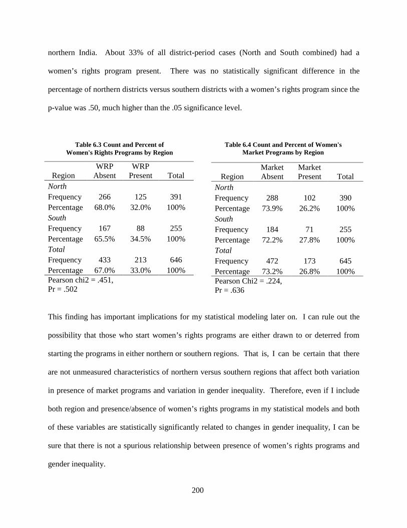
200
northern India. About 33% of all district-period cases (North and South combined) had a
women’s rights program present. There was no statistically significant difference in the
percentage of northern districts versus southern districts with a women’s rights program since the
p-value was .50, much higher than the .05 significance level.
This finding has important implications for my statistical modeling later on. I can rule out the
possibility that those who start women’s rights programs are either drawn to or deterred from
starting the programs in either northern or southern regions. That is, I can be certain that there
are not unmeasured characteristics of northern versus southern regions that affect both variation
in presence of market programs and variation in gender inequality. Therefore, even if I include
both region and presence/absence of women’s rights programs in my statistical models and both
of these variables are statistically significantly related to changes in gender inequality, I can be
sure that there is not a spurious relationship between presence of women’s rights programs and
gender inequality.
Region WRP
Absent WRP
Present Total North Frequency 266 125 391 Percentage 68.0% 32.0% 100% South Frequency 167 88 255 Percentage 65.5% 34.5% 100% Total Frequency 433 213 646 Percentage 67.0% 33.0% 100% Pearson chi2 = .451, Pr = .502
Region Market Absent
Market Present Total
North Frequency 288 102 390 Percentage 73.9% 26.2% 100% South Frequency 184 71 255 Percentage 72.2% 27.8% 100% Total Frequency 472 173 645 Percentage 73.2% 26.8% 100% Pearson Chi2 = .224, Pr = .636
Table 6.4 Count and Percent of Women's Market Programs by Region
Table 6.3 Count and Percent of Women's Rights Programs by Region

201
There was a women’s market program in about 26% of the district-period cases in
northern India, and in about 28% of the district-period cases in southern India (see Table 6.4).
About 27% of all district-period cases (North and South combined) had a women’s market
program present, which is less than the percentage of district-period cases that had a women’s
rights program present. Since the p-value was about .64 (well over .05), there was no
statistically significant difference in percentage of district-period cases with a women’s market
program in northern India versus southern India. Therefore, if my statistical models reveal that
both region and presence of women’s market programs are significantly related to changes in
gender inequality, I can be sure that region is not causing gender inequality to increase or
decrease because there are more women’s market programs in one region or the other. Also, I
can be certain that there are not unmeasured characteristics of northern versus southern regions
that affect both variation in presence of market programs and variation in gender inequality.
This does not rule out the possibility of an interaction effect between region and women’s market
programs. For instance, it could still be possible that women’s market programs have a greater
impact on raising female/male child sex ratio in southern regions than in northern regions. If
there is an interaction effect, it is not because there are more women’s market programs in the
south than in the north, however.
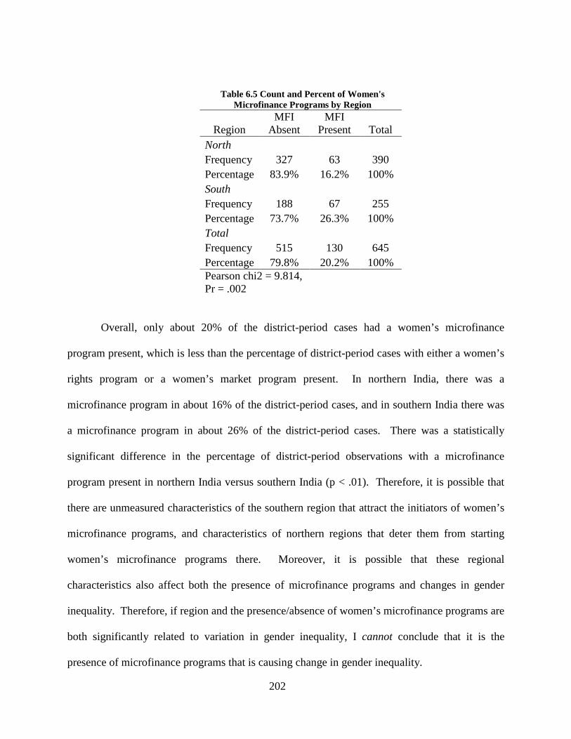
202
Table 6.5 Count and Percent of Women's Microfinance Programs by Region
Region MFI
Absent MFI
Present Total North Frequency 327 63 390 Percentage 83.9% 16.2% 100% South Frequency 188 67 255 Percentage 73.7% 26.3% 100% Total Frequency 515 130 645 Percentage 79.8% 20.2% 100% Pearson chi2 = 9.814, Pr = .002
Overall, only about 20% of the district-period cases had a women’s microfinance
program present, which is less than the percentage of district-period cases with either a women’s
rights program or a women’s market program present. In northern India, there was a
microfinance program in about 16% of the district-period cases, and in southern India there was
a microfinance program in about 26% of the district-period cases. There was a statistically
significant difference in the percentage of district-period observations with a microfinance
program present in northern India versus southern India (p < .01). Therefore, it is possible that
there are unmeasured characteristics of the southern region that attract the initiators of women’s
microfinance programs, and characteristics of northern regions that deter them from starting
women’s microfinance programs there. Moreover, it is possible that these regional
characteristics also affect both the presence of microfinance programs and changes in gender
inequality. Therefore, if region and the presence/absence of women’s microfinance programs are
both significantly related to variation in gender inequality, I cannot conclude that it is the
presence of microfinance programs that is causing change in gender inequality.
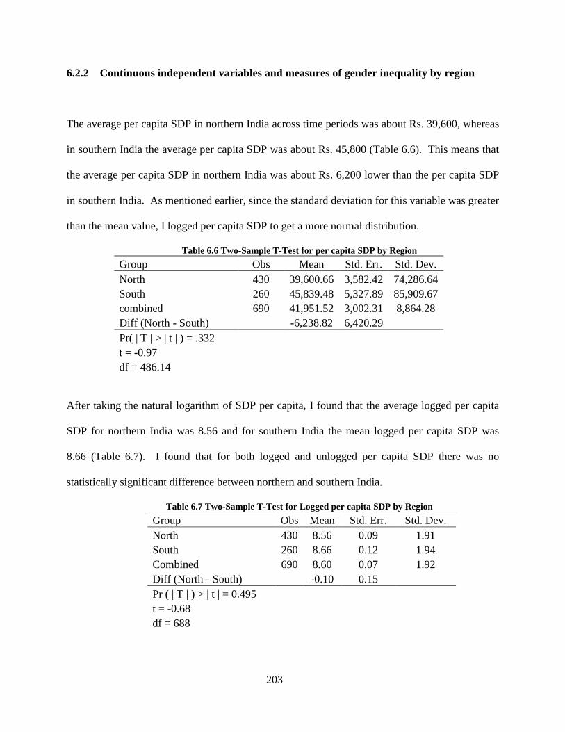
203
6.2.2 Continuous independent variables and measures of gender inequality by region
The average per capita SDP in northern India across time periods was about Rs. 39,600, whereas
in southern India the average per capita SDP was about Rs. 45,800 (Table 6.6). This means that
the average per capita SDP in northern India was about Rs. 6,200 lower than the per capita SDP
in southern India. As mentioned earlier, since the standard deviation for this variable was greater
than the mean value, I logged per capita SDP to get a more normal distribution.
Table 6.6 Two-Sample T-Test for per capita SDP by Region Group Obs Mean Std. Err. Std. Dev. North 430 39,600.66 3,582.42 74,286.64 South 260 45,839.48 5,327.89 85,909.67 combined 690 41,951.52 3,002.31 8,864.28 Diff (North - South) -6,238.82 6,420.29 Pr( | T | > | t | ) = .332 t = -0.97 df = 486.14
After taking the natural logarithm of SDP per capita, I found that the average logged per capita
SDP for northern India was 8.56 and for southern India the mean logged per capita SDP was
8.66 (Table 6.7). I found that for both logged and unlogged per capita SDP there was no
statistically significant difference between northern and southern India.
Table 6.7 Two-Sample T-Test for Logged per capita SDP by Region Group Obs Mean Std. Err. Std. Dev. North 430 8.56 0.09 1.91 South 260 8.66 0.12 1.94 Combined 690 8.60 0.07 1.92 Diff (North - South) -0.10 0.15 Pr ( | T | ) > | t | = 0.495 t = -0.68 df = 688
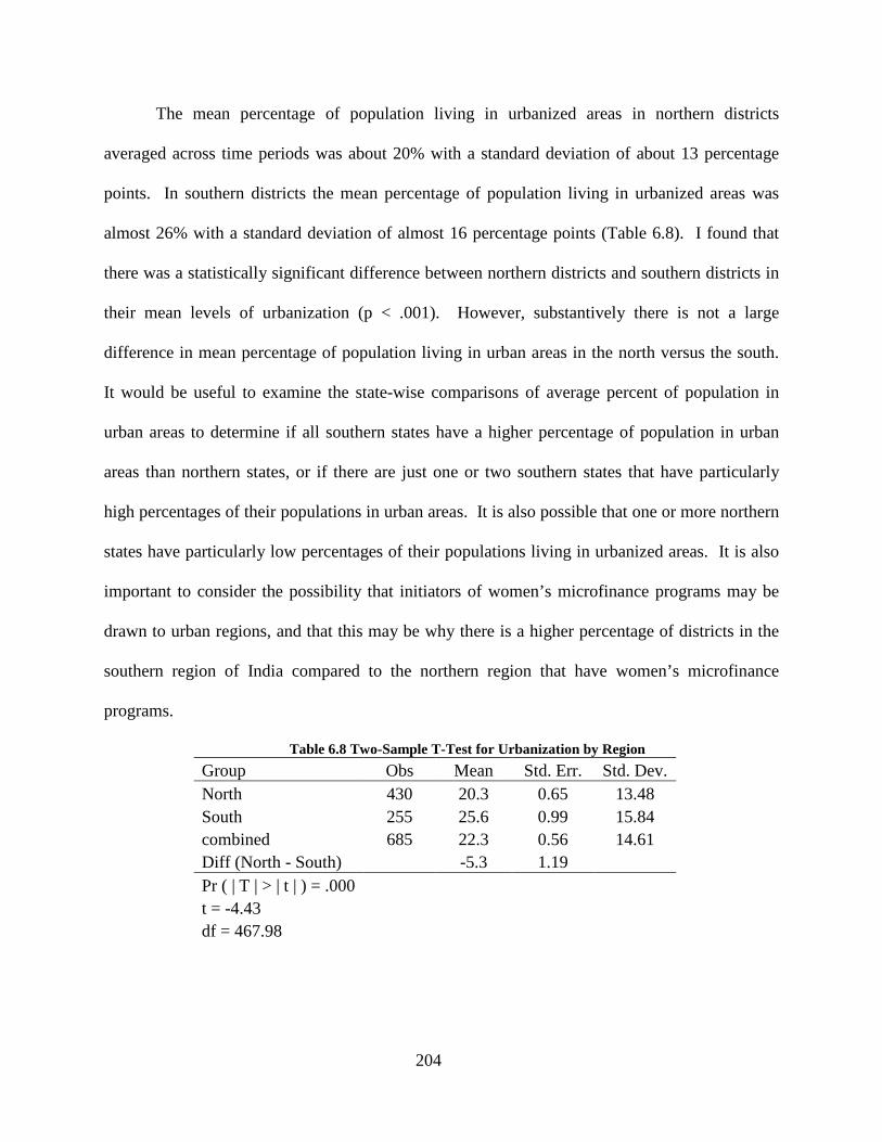
204
The mean percentage of population living in urbanized areas in northern districts
averaged across time periods was about 20% with a standard deviation of about 13 percentage
points. In southern districts the mean percentage of population living in urbanized areas was
almost 26% with a standard deviation of almost 16 percentage points (Table 6.8). I found that
there was a statistically significant difference between northern districts and southern districts in
their mean levels of urbanization (p < .001). However, substantively there is not a large
difference in mean percentage of population living in urban areas in the north versus the south.
It would be useful to examine the state-wise comparisons of average percent of population in
urban areas to determine if all southern states have a higher percentage of population in urban
areas than northern states, or if there are just one or two southern states that have particularly
high percentages of their populations in urban areas. It is also possible that one or more northern
states have particularly low percentages of their populations living in urbanized areas. It is also
important to consider the possibility that initiators of women’s microfinance programs may be
drawn to urban regions, and that this may be why there is a higher percentage of districts in the
southern region of India compared to the northern region that have women’s microfinance
programs.
Table 6.8 Two-Sample T-Test for Urbanization by Region Group Obs Mean Std. Err. Std. Dev. North 430 20.3 0.65 13.48 South 255 25.6 0.99 15.84 combined 685 22.3 0.56 14.61 Diff (North - South) -5.3 1.19 Pr ( | T | > | t | ) = .000 t = -4.43 df = 467.98
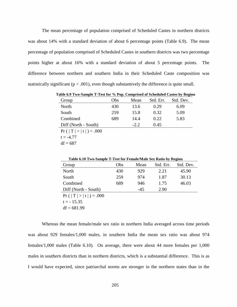
205
The mean percentage of population comprised of Scheduled Castes in northern districts
was about 14% with a standard deviation of about 6 percentage points (Table 6.9). The mean
percentage of population comprised of Scheduled Castes in southern districts was two percentage
points higher at about 16% with a standard deviation of about 5 percentage points. The
difference between northern and southern India in their Scheduled Caste composition was
statistically significant (p < .001), even though substantively the difference is quite small.
Table 6.9 Two-Sample T-Test for % Pop. Comprised of Scheduled Castes by Region Group Obs Mean Std. Err. Std. Dev. North 430 13.6 0.29 6.09 South 259 15.8 0.32 5.09 Combined 689 14.4 0.22 5.83 Diff (North - South) -2.2 0.45 Pr ( | T | > | t | ) = .000 t = -4.77 df = 687
Table 6.10 Two-Sample T-Test for Female/Male Sex Ratio by Region Group Obs Mean Std. Err. Std. Dev. North 430 929 2.21 45.90 South 259 974 1.87 30.13 Combined 689 946 1.75 46.03 Diff (North - South) -45 2.90 Pr ( | T | > | t | ) = .000 t = - 15.35 df = 681.99
Whereas the mean female/male sex ratio in northern India averaged across time periods
was about 929 females/1,000 males, in southern India the mean sex ratio was about 974
females/1,000 males (Table 6.10). On average, there were about 44 more females per 1,000
males in southern districts than in northern districts, which is a substantial difference. This is as
I would have expected, since patriarchal norms are stronger in the northern states than in the
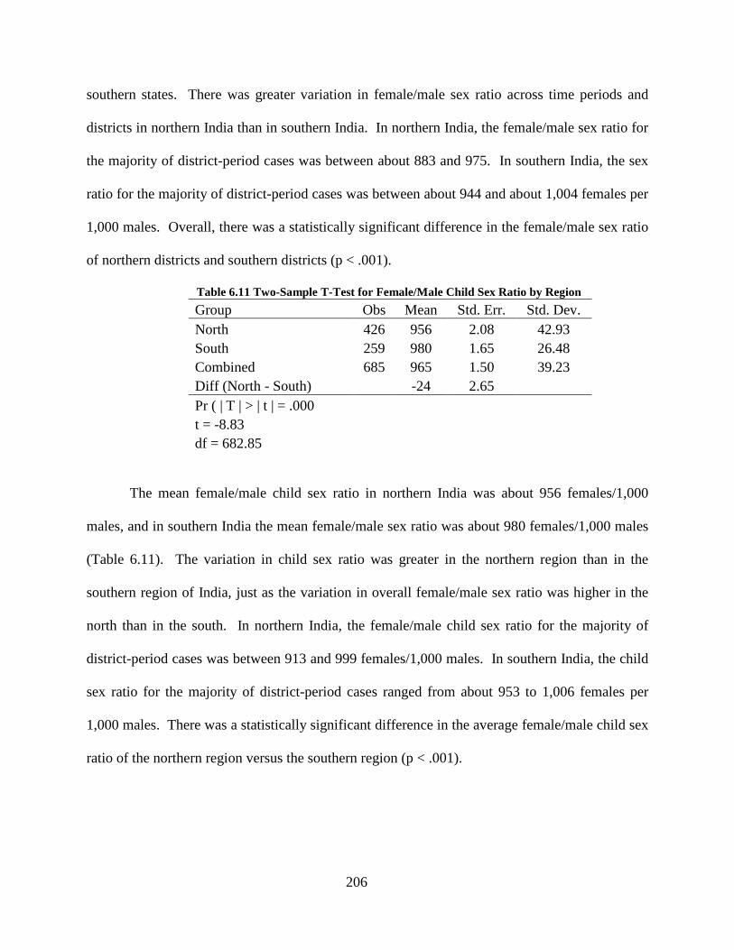
206
southern states. There was greater variation in female/male sex ratio across time periods and
districts in northern India than in southern India. In northern India, the female/male sex ratio for
the majority of district-period cases was between about 883 and 975. In southern India, the sex
ratio for the majority of district-period cases was between about 944 and about 1,004 females per
1,000 males. Overall, there was a statistically significant difference in the female/male sex ratio
of northern districts and southern districts (p < .001).
Table 6.11 Two-Sample T-Test for Female/Male Child Sex Ratio by Region Group Obs Mean Std. Err. Std. Dev. North 426 956 2.08 42.93 South 259 980 1.65 26.48 Combined 685 965 1.50 39.23 Diff (North - South) -24 2.65 Pr ( | T | > | t | = .000 t = -8.83 df = 682.85
The mean female/male child sex ratio in northern India was about 956 females/1,000
males, and in southern India the mean female/male sex ratio was about 980 females/1,000 males
(Table 6.11). The variation in child sex ratio was greater in the northern region than in the
southern region of India, just as the variation in overall female/male sex ratio was higher in the
north than in the south. In northern India, the female/male child sex ratio for the majority of
district-period cases was between 913 and 999 females/1,000 males. In southern India, the child
sex ratio for the majority of district-period cases ranged from about 953 to 1,006 females per
1,000 males. There was a statistically significant difference in the average female/male child sex
ratio of the northern region versus the southern region (p < .001).
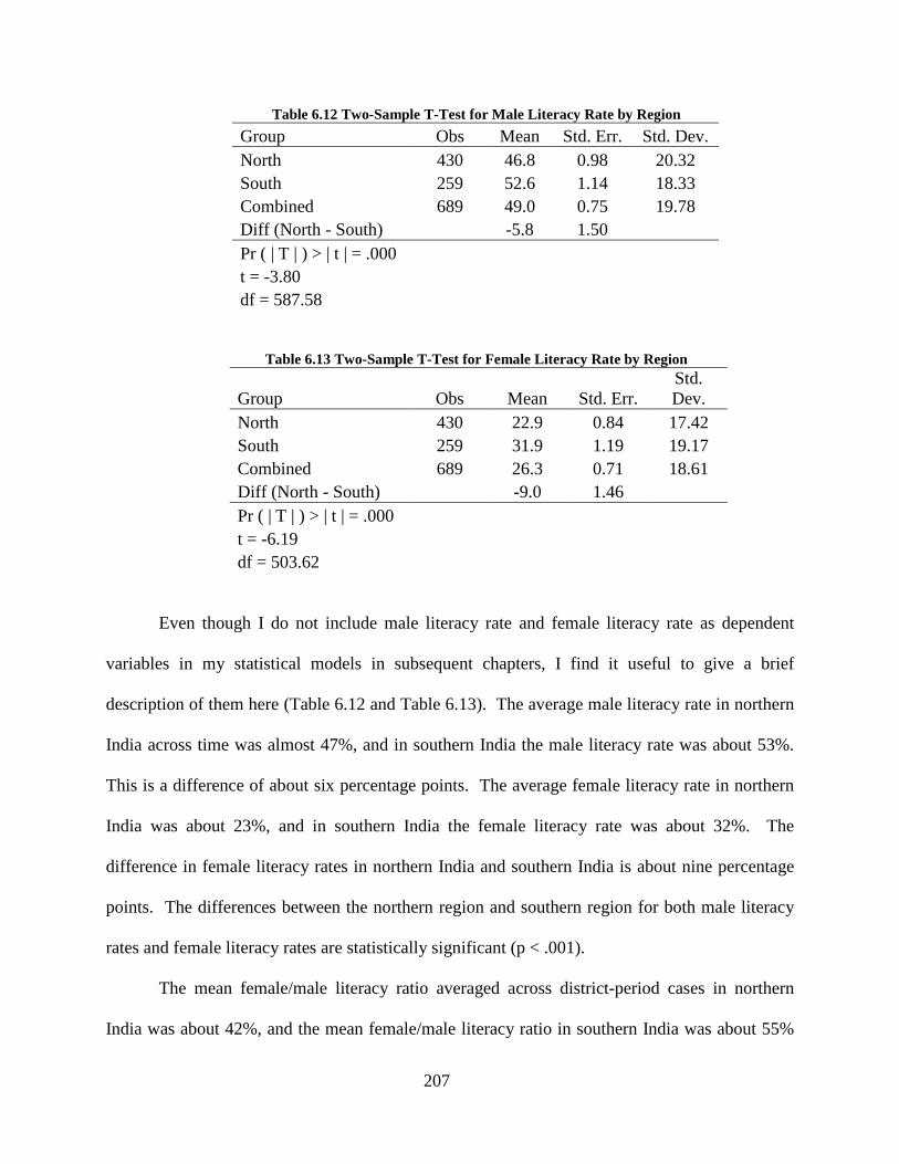
207
Table 6.12 Two-Sample T-Test for Male Literacy Rate by Region Group Obs Mean Std. Err. Std. Dev. North 430 46.8 0.98 20.32 South 259 52.6 1.14 18.33 Combined 689 49.0 0.75 19.78 Diff (North - South) -5.8 1.50 Pr ( | T | ) > | t | = .000 t = -3.80 df = 587.58
Table 6.13 Two-Sample T-Test for Female Literacy Rate by Region
Group Obs Mean Std. Err. Std. Dev.
North 430 22.9 0.84 17.42 South 259 31.9 1.19 19.17 Combined 689 26.3 0.71 18.61 Diff (North - South) -9.0 1.46 Pr ( | T | ) > | t | = .000 t = -6.19 df = 503.62
Even though I do not include male literacy rate and female literacy rate as dependent
variables in my statistical models in subsequent chapters, I find it useful to give a brief
description of them here (Table 6.12 and Table 6.13). The average male literacy rate in northern
India across time was almost 47%, and in southern India the male literacy rate was about 53%.
This is a difference of about six percentage points. The average female literacy rate in northern
India was about 23%, and in southern India the female literacy rate was about 32%. The
difference in female literacy rates in northern India and southern India is about nine percentage
points. The differences between the northern region and southern region for both male literacy
rates and female literacy rates are statistically significant (p < .001).
The mean female/male literacy ratio averaged across district-period cases in northern
India was about 42%, and the mean female/male literacy ratio in southern India was about 55%
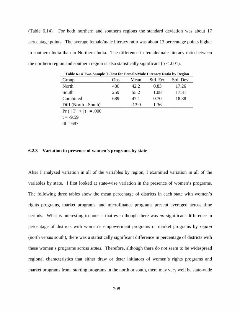
208
(Table 6.14). For both northern and southern regions the standard deviation was about 17
percentage points. The average female/male literacy ratio was about 13 percentage points higher
in southern India than in Northern India. The difference in female/male literacy ratio between
the northern region and southern region is also statistically significant (p < .001).
Table 6.14 Two-Sample T-Test for Female/Male Literacy Ratio by Region Group Obs Mean Std. Err. Std. Dev. North 430 42.2 0.83 17.26 South 259 55.2 1.08 17.31 Combined 689 47.1 0.70 18.38 Diff (North - South) -13.0 1.36 Pr ( | T | > | t | = .000 t = -9.59 df = 687
6.2.3 Variation in presence of women’s programs by state
After I analyzed variation in all of the variables by region, I examined variation in all of the
variables by state. I first looked at state-wise variation in the presence of women’s programs.
The following three tables show the mean percentage of districts in each state with women’s
rights programs, market programs, and microfinance programs present averaged across time
periods. What is interesting to note is that even though there was no significant difference in
percentage of districts with women’s empowerment programs or market programs by region
(north versus south), there was a statistically significant difference in percentage of districts with
these women’s programs across states. Therefore, although there do not seem to be widespread
regional characteristics that either draw or deter initiators of women’s rights programs and
market programs from starting programs in the north or south, there may very well be state-wide
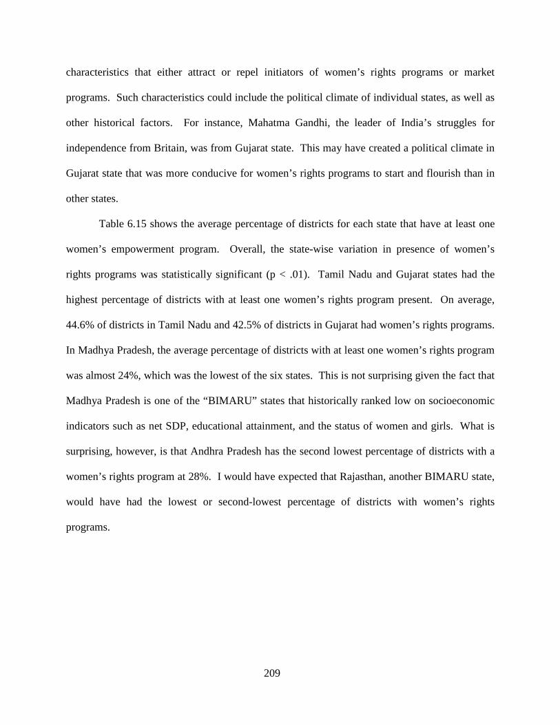
209
characteristics that either attract or repel initiators of women’s rights programs or market
programs. Such characteristics could include the political climate of individual states, as well as
other historical factors. For instance, Mahatma Gandhi, the leader of India’s struggles for
independence from Britain, was from Gujarat state. This may have created a political climate in
Gujarat state that was more conducive for women’s rights programs to start and flourish than in
other states.
Table 6.15 shows the average percentage of districts for each state that have at least one
women’s empowerment program. Overall, the state-wise variation in presence of women’s
rights programs was statistically significant (p < .01). Tamil Nadu and Gujarat states had the
highest percentage of districts with at least one women’s rights program present. On average,
44.6% of districts in Tamil Nadu and 42.5% of districts in Gujarat had women’s rights programs.
In Madhya Pradesh, the average percentage of districts with at least one women’s rights program
was almost 24%, which was the lowest of the six states. This is not surprising given the fact that
Madhya Pradesh is one of the “BIMARU” states that historically ranked low on socioeconomic
indicators such as net SDP, educational attainment, and the status of women and girls. What is
surprising, however, is that Andhra Pradesh has the second lowest percentage of districts with a
women’s rights program at 28%. I would have expected that Rajasthan, another BIMARU state,
would have had the lowest or second-lowest percentage of districts with women’s rights
programs.
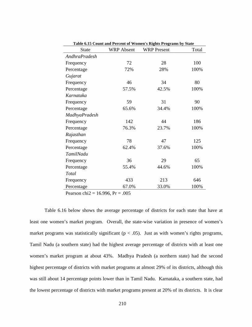
210
Table 6.15 Count and Percent of Women's Rights Programs by State State WRP Absent WRP Present Total
AndhraPradesh Frequency 72 28 100 Percentage 72% 28% 100% Gujarat Frequency 46 34 80 Percentage 57.5% 42.5% 100% Karnataka Frequency 59 31 90 Percentage 65.6% 34.4% 100% MadhyaPradesh Frequency 142 44 186 Percentage 76.3% 23.7% 100% Rajasthan Frequency 78 47 125 Percentage 62.4% 37.6% 100% TamilNadu Frequency 36 29 65 Percentage 55.4% 44.6% 100% Total Frequency 433 213 646 Percentage 67.0% 33.0% 100% Pearson chi2 = 16.996, Pr = .005
Table 6.16 below shows the average percentage of districts for each state that have at
least one women’s market program. Overall, the state-wise variation in presence of women’s
market programs was statistically significant (p < .05). Just as with women’s rights programs,
Tamil Nadu (a southern state) had the highest average percentage of districts with at least one
women’s market program at about 43%. Madhya Pradesh (a northern state) had the second
highest percentage of districts with market programs at almost 29% of its districts, although this
was still about 14 percentage points lower than in Tamil Nadu. Karnataka, a southern state, had
the lowest percentage of districts with market programs present at 20% of its districts. It is clear
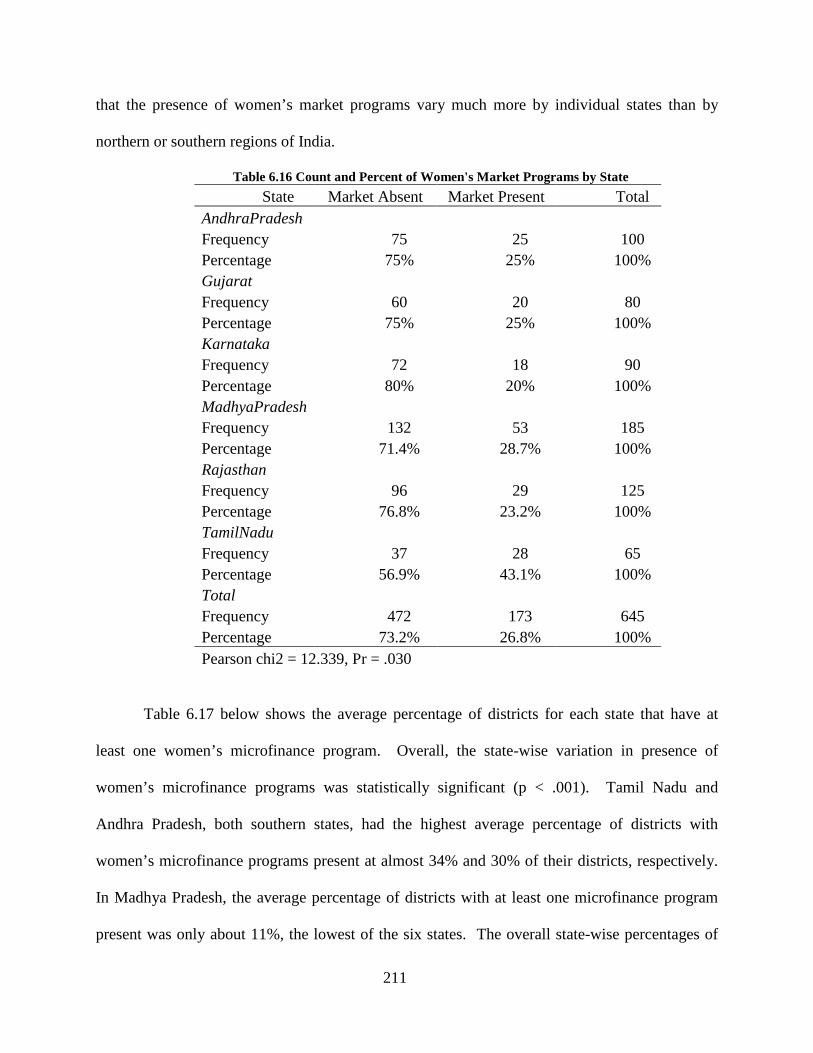
211
that the presence of women’s market programs vary much more by individual states than by
northern or southern regions of India.
Table 6.16 Count and Percent of Women's Market Programs by State State Market Absent Market Present Total
AndhraPradesh Frequency 75 25 100 Percentage 75% 25% 100% Gujarat Frequency 60 20 80 Percentage 75% 25% 100% Karnataka Frequency 72 18 90 Percentage 80% 20% 100% MadhyaPradesh Frequency 132 53 185 Percentage 71.4% 28.7% 100% Rajasthan Frequency 96 29 125 Percentage 76.8% 23.2% 100% TamilNadu Frequency 37 28 65 Percentage 56.9% 43.1% 100% Total Frequency 472 173 645 Percentage 73.2% 26.8% 100% Pearson chi2 = 12.339, Pr = .030
Table 6.17 below shows the average percentage of districts for each state that have at
least one women’s microfinance program. Overall, the state-wise variation in presence of
women’s microfinance programs was statistically significant (p < .001). Tamil Nadu and
Andhra Pradesh, both southern states, had the highest average percentage of districts with
women’s microfinance programs present at almost 34% and 30% of their districts, respectively.
In Madhya Pradesh, the average percentage of districts with at least one microfinance program
present was only about 11%, the lowest of the six states. The overall state-wise percentages of
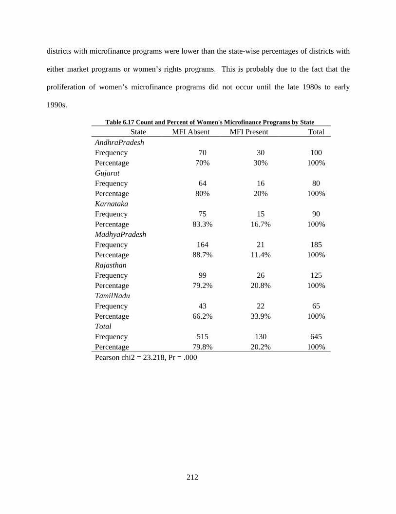
212
districts with microfinance programs were lower than the state-wise percentages of districts with
either market programs or women’s rights programs. This is probably due to the fact that the
proliferation of women’s microfinance programs did not occur until the late 1980s to early
1990s.
Table 6.17 Count and Percent of Women's Microfinance Programs by State State MFI Absent MFI Present Total
AndhraPradesh Frequency 70 30 100 Percentage 70% 30% 100% Gujarat Frequency 64 16 80 Percentage 80% 20% 100% Karnataka Frequency 75 15 90 Percentage 83.3% 16.7% 100% MadhyaPradesh Frequency 164 21 185 Percentage 88.7% 11.4% 100% Rajasthan Frequency 99 26 125 Percentage 79.2% 20.8% 100% TamilNadu Frequency 43 22 65 Percentage 66.2% 33.9% 100% Total Frequency 515 130 645 Percentage 79.8% 20.2% 100% Pearson chi2 = 23.218, Pr = .000
213
6.2.4 Continuous independent variables and measures of gender inequality by state
Once I examined the state-wise variation in presence of women’s development programs, I used
one-way ANOVAs to analyze state-wise variation in the other independent variables as well as
variation in my measures of gender inequality. One-way ANOVAs tell me whether overall there
are statistically significant differences between states on these variables. I give the results in
Table 6.18 below. All of the inter-state comparisons for these variables were significant except
for per capita SDP and logged per capita SDP. I used the Bonferroni multiple comparison
procedure to determine which pairs of states were significantly different in their mean values for
all variables except for per capita SDP and logged per capita SDP (Agresti and Finlay 1997,
Acock 2006). One of the assumptions of ANOVA is that the variances of all groups being
compared are equal (Acock 2006). I used Bartlett’s test for equal variances to determine whether
this assumption held for the inter-state comparison of means in given in Table 6.17, and found
that this assumption held only for the inter-state comparison of female/male literacy ratio. This
means that I must interpret all of the other ANOVA results with caution.
I found that there were no statistically significant differences in per capita SDP or logged
per capita SDP across the six states in my study. This surprised me because the states of Madhya
Pradesh and Rajasthan (among other northern states) are known as poorer states in India. There
were statistically significant differences in levels of urbanization across the six states, however.
In Madhya Pradesh and Rajasthan, the average percentage of each state’s population living in
urbanized areas was a little less than 19%. These two states had the lowest levels of urbanization
of all six states, which is as I would have expected. Tamil Nadu had the highest level of
urbanization, with almost 36% of its population living in urban areas on average. It’s interesting
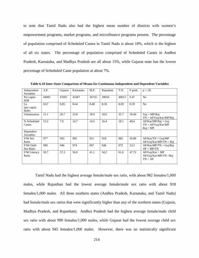
214
to note that Tamil Nadu also had the highest mean number of districts with women’s
empowerment programs, market programs, and microfinance programs present. The percentage
of population comprised of Scheduled Castes in Tamil Nadu is about 18%, which is the highest
of all six states. The percentage of population comprised of Scheduled Castes in Andhra
Pradesh, Karnataka, and Madhya Pradesh are all about 15%, while Gujarat state has the lowest
percentage of Scheduled Caste population at about 7%.
Table 6.18 Inter-State Comparison of Means for Continuous Independent and Dependent Variables
Tamil Nadu had the highest average female/male sex ratio, with about 982 females/1,000
males, while Rajasthan had the lowest average female/male sex ratio with about 918
females/1,000 males. All three southern states (Andhra Pradesh, Karnataka, and Tamil Nadu)
had female/male sex ratios that were significantly higher than any of the northern states (Gujarat,
Madhya Pradesh, and Rajasthan). Andhra Pradesh had the highest average female/male child
sex ratio with about 990 females/1,000 males, while Gujarat had the lowest average child sex
ratio with about 945 females/1,000 males. However, there was no statistically significant
Independent Variables
A.P. Gujarat Karnataka M.P. Rajasthan T.N. F prob. p < .05
Per capita SDP
44091 47691 45587 36735 39050 49013 0.47 No
Ln (per capita SDP)
8.67 8.85 8.64 8.48 8.50 8.69 0.59 No
Urbanization 21.1 26.7 23.8 18.9 18.6 35.7 18.46 Guj > MP/Raj TN > AP/Guj/Kar/MP/Raj
% Scheduled Castes
15.2 7.0 14.7 14.5 16.4 18.1 48.4 AP/Kar/MP/Raj > Guj TN > AP/Guj/Kar/MP Raj > MP
Dependent Variables
F/M Sex Ratio
977 943 965 931 918 982 45.89 AP/Kar/TN > Guj/MP AP/Guj/Kar/MP/TN > Raj
F/M Child Sex Ratio
990 946 974 967 946 972 23.3 AP/Kar/MP/TN > Guj/Raj AP > MP/TN
F/M Literacy Ratio
50.7 57.3 56.0 41.1 34.2 61.6 47.72 AP/Guj/Kar > MP AP/Guj/Kar/MP/TN >Raj TN > AP
215
difference in child sex ratio between Tamil Nadu and Madhya Pradesh, nor between Karnataka
and Madhya Pradesh. Tamil Nadu did have the highest average female/male literacy ratio at
almost 62%. This means that the percentage of literate females in Tamil Nadu was less than
two-thirds of the percentage of literate males. Rajasthan had the lowest average female/male
literacy ratio at about 34%. All three southern states as well as Gujarat had significantly higher
average female/male literacy ratios than Madhya Pradesh or Rajasthan.
6.2.5 Correlations between all continuous independent variables and measures of gender inequality
After examining variation in all of the independent variables and measures of gender inequality
by region and by state, I next analyzed the relationships among all of the continuous independent
variables and the measures of gender inequality. It is important to inspect the correlations among
the independent variables to determine whether any of them are collinear. For future statistical
models, the main effects as well as interaction terms of any collinear independent variables must
be included (Arceneaux and Huber 2007). If any of the collinear variables are excluded from the
models, the coefficients of the collinear variables that are included will be biased. Another
reason for inspecting the pairwise correlations between independent and dependent variables is
to assist in determining possible causal relationships between independent variables and
measures of gender inequality. In Table 6.19 below I describe the pairwise correlations among
all of the lagged and unlagged continuous independent variables as well as the gender inequality
measures. Since almost all of the pairwise correlations are significant at the .001 level and very
few correlations are not statistically significant, I break with convention in how I report
statistical significance. I leave all pairwise correlations that are significant at the .001 level
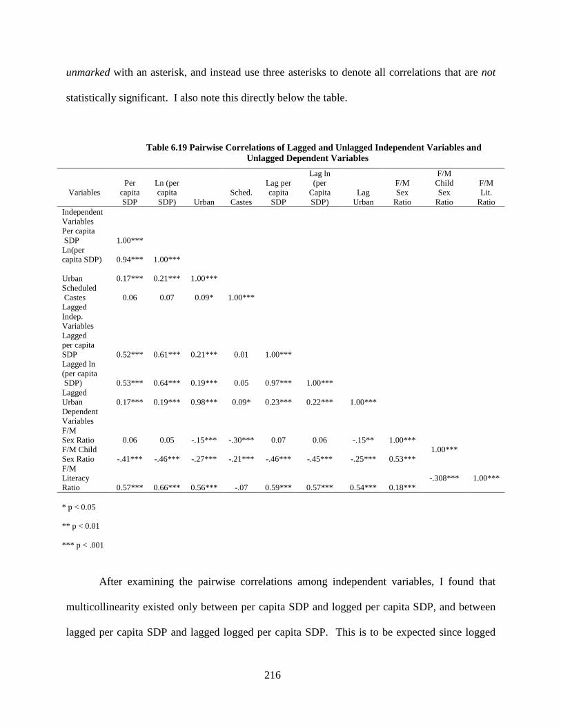
216
unmarked with an asterisk, and instead use three asterisks to denote all correlations that are not
statistically significant. I also note this directly below the table.
Table 6.19 Pairwise Correlations of Lagged and Unlagged Independent Variables and Unlagged Dependent Variables
After examining the pairwise correlations among independent variables, I found that
multicollinearity existed only between per capita SDP and logged per capita SDP, and between
lagged per capita SDP and lagged logged per capita SDP. This is to be expected since logged
Variables Per
capita SDP
Ln (per capita SDP) Urban
Sched. Castes
Lag per capita SDP
Lag ln (per
Capita SDP)
Lag Urban
F/M Sex
Ratio
F/M Child Sex
Ratio
F/M Lit.
Ratio Independent Variables
Per capita SDP 1.00***
Ln(per capita SDP) 0.94*** 1.00***
Urban 0.17*** 0.21*** 1.00***
Scheduled Castes 0.06 0.07 0.09* 1.00***
Lagged Indep. Variables
Lagged per capita SDP 0.52*** 0.61*** 0.21*** 0.01 1.00***
Lagged ln (per capita SDP) 0.53*** 0.64*** 0.19*** 0.05 0.97*** 1.00***
Lagged Urban 0.17*** 0.19*** 0.98*** 0.09* 0.23*** 0.22*** 1.00***
Dependent Variables
F/M Sex Ratio 0.06 0.05 -.15*** -.30*** 0.07 0.06 -.15** 1.00***
F/M Child Sex Ratio -.41*** -.46*** -.27*** -.21*** -.46*** -.45*** -.25*** 0.53***
1.00***
F/M Literacy Ratio 0.57*** 0.66*** 0.56*** -.07 0.59*** 0.57*** 0.54*** 0.18***
-.308*** 1.00***
* p < 0.05
** p < 0.01
*** p < .001
217
per capita SDP is a transformation of per capita SDP. Thus, I would only include one of these
two variables in any given statistical model. Lagged values of per capita SDP, logged per capita
SDP, and urbanization were all strongly correlated with unlagged values of per capita SDP,
logged per capita SDP, and urbanization, respectively. However, there was only a weak to
moderately weak relationship between lagged or unlagged values of urbanization and lagged or
unlagged values of per capita SDP. This suggests that current levels of per capita SDP and
urbanization cause subsequent levels of per capita SDP and urbanization. Since there is only a
weak to moderately weak relationship between urbanization and per capita SDP, any possible
causal relationship between these two variables would also be weak. Percentage of population
comprised of Scheduled Castes significantly and weakly related only to urbanization.
The overall female/male sex ratio was statistically related to only urbanization and
Scheduled Castes. There was a negative, weak relationship between sex ratio and urbanization,
and a negative, moderate relationship between sex ratio and Scheduled Castes. There was a
strong, negative relationship between female/male child sex ratio and lagged and unlagged per
capita SDP. There was a moderately weak to moderate relationship between child sex ratio and
lagged and unlagged urbanization. There was a strong relationship between overall female/male
sex ratio and female/male child sex ratio. This means that districts that have a relatively high
female/male sex ratio also have a relatively high female/male child sex ratio. Female/male
literacy ratio was very strongly correlated with both lagged and unlagged values of per capita
SDP and urbanization. However, there was no significant relationship between female/male
literacy ratio and Scheduled Castes. Oddly, there was a moderate, negative relationship between
female/male child sex ratio and female/male literacy ratio. This means that districts that have
relatively higher child sex ratios tend to have lower female/male literacy ratios. It is possible
218
that increases in per capita SDP lead simultaneously to lower female/male child sex ratios and
higher female/male literacy ratios.
6.3 VARIATION IN INDEPENDENT AND DEPENDENT VARIABLES BY TIME PERIOD
In the previous sections, I explored variation in per capita SDP, urbanization, percentage of
population comprised of Scheduled Castes, presence of women’s development programs, and
measures of gender inequality by region and state. Although these exploratory analyses
described differences between states or regions in the average level of urbanization, per capita
SDP, or percentage of districts with certain types of women’s programs, they could not tell us if
there were differences between states or regions during different time periods. For example,
there was no statistically significant difference in per capita SDP between northern and southern
regions, but is there significant change in per capita SDP over time? Also, there was no
significant difference between northern and southern regions in the presence of women’s rights
programs and women’s market programs. Yet is there significant change in presence of these
types of women’s programs within regions over time? In the next few sections of this chapter, I
explore variation in the independent variables and dependent variables between regions, states,
and time periods. I begin with a discussion of how the presence of women’s programs varies by
region and year.
219
6.3.1 Variation in presence of women’s programs by region and year
Although there was no significant difference between regions in the average percentage of
districts that had at least one women’s rights program, there was significant change within
regions in percentage of districts with women’s rights programs over time (Table 6.20 and Table
6.21). In the northern region, the percentage of districts with women’s rights programs in 1961
was only about 5%, but by 2001 almost 71% of districts had at least one women’s rights
program. Between 1981 and 1991 the percentage of northern districts with women’s rights
programs increased by about 36 percentage points. In the southern region, the percentage of
districts with women’s rights programs was only about 2%, but by 2001 that percentage rose to
about 82%. There was no change in percentage of southern districts with women’s rights
programs between 1961 and 1971. In the southern region, the largest gains were made between
1981 and 1991 when the percentage of districts with women’s rights programs present rose by
about 47 percentage points.
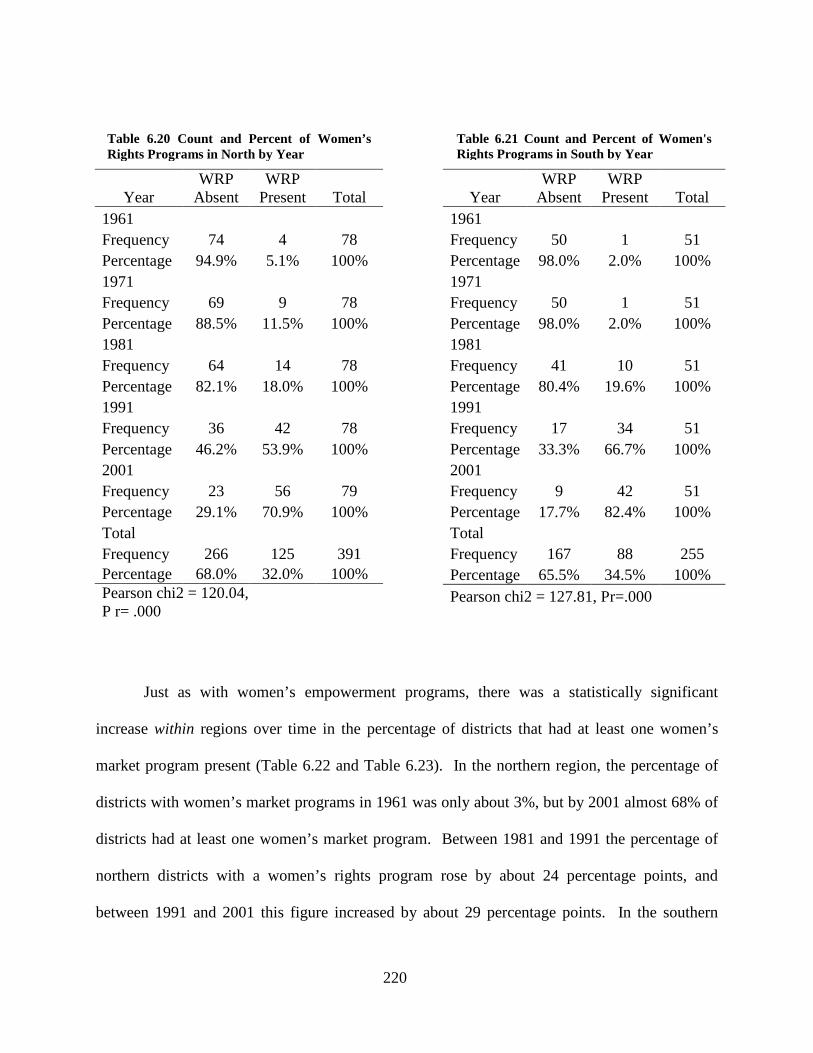
220
Just as with women’s empowerment programs, there was a statistically significant
increase within regions over time in the percentage of districts that had at least one women’s
market program present (Table 6.22 and Table 6.23). In the northern region, the percentage of
districts with women’s market programs in 1961 was only about 3%, but by 2001 almost 68% of
districts had at least one women’s market program. Between 1981 and 1991 the percentage of
northern districts with a women’s rights program rose by about 24 percentage points, and
between 1991 and 2001 this figure increased by about 29 percentage points. In the southern
Year WRP
Absent WRP
Present Total 1961 Frequency 74 4 78 Percentage 94.9% 5.1% 100% 1971 Frequency 69 9 78 Percentage 88.5% 11.5% 100% 1981 Frequency 64 14 78 Percentage 82.1% 18.0% 100% 1991 Frequency 36 42 78 Percentage 46.2% 53.9% 100% 2001 Frequency 23 56 79 Percentage 29.1% 70.9% 100% Total Frequency 266 125 391 Percentage 68.0% 32.0% 100% Pearson chi2 = 120.04, P r= .000
Year WRP
Absent WRP
Present Total 1961 Frequency 50 1 51 Percentage 98.0% 2.0% 100% 1971 Frequency 50 1 51 Percentage 98.0% 2.0% 100% 1981 Frequency 41 10 51 Percentage 80.4% 19.6% 100% 1991 Frequency 17 34 51 Percentage 33.3% 66.7% 100% 2001 Frequency 9 42 51 Percentage 17.7% 82.4% 100% Total Frequency 167 88 255 Percentage 65.5% 34.5% 100% Pearson chi2 = 127.81, Pr=.000
Table 6.21 Count and Percent of Women's Rights Programs in South by Year
Table 6.20 Count and Percent of Women’s Rights Programs in North by Year
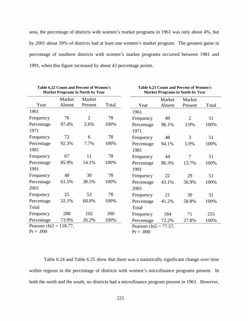
221
area, the percentage of districts with women’s market programs in 1961 was only about 4%, but
by 2001 about 59% of districts had at least one women’s market program. The greatest gains in
percentage of southern districts with women’s market programs occurred between 1981 and
1991, when this figure increased by about 43 percentage points.
Year Market Absent
Market Present Total
1961 Frequency 76 2 78 Percentage 97.4% 2.6% 100% 1971 Frequency 72 6 78 Percentage 92.3% 7.7% 100% 1981 Frequency 67 11 78 Percentage 85.9% 14.1% 100% 1991 Frequency 48 30 78 Percentage 61.5% 38.5% 100% 2001 Frequency 25 53 78 Percentage 32.1% 68.0% 100% Total Frequency 288 102 390 Percentage 73.9% 26.2% 100% Pearson chi2 = 118.77, Pr = .000
Table 6.24 and Table 6.25 show that there was a statistically significant change over time
within regions in the percentage of districts with women’s microfinance programs present. In
both the north and the south, no districts had a microfinance program present in 1961. However,
Year Market Absent
Market Present Total
1961 Frequency 49 2 51 Percentage 96.1% 3.9% 100% 1971 Frequency 48 3 51 Percentage 94.1% 5.9% 100% 1981 Frequency 44 7 51 Percentage 86.3% 13.7% 100% 1991 Frequency 22 29 51 Percentage 43.1% 56.9% 100% 2001 Frequency 21 30 51 Percentage 41.2% 58.8% 100% Total Frequency 184 71 255 Percentage 72.2% 27.8% 100% Pearson chi2 = 77.57, Pr = .000
Table 6.23 Count and Percent of Women's Market Programs in South by Year
Table 6.22 Count and Percent of Women's Market Programs in North by Year
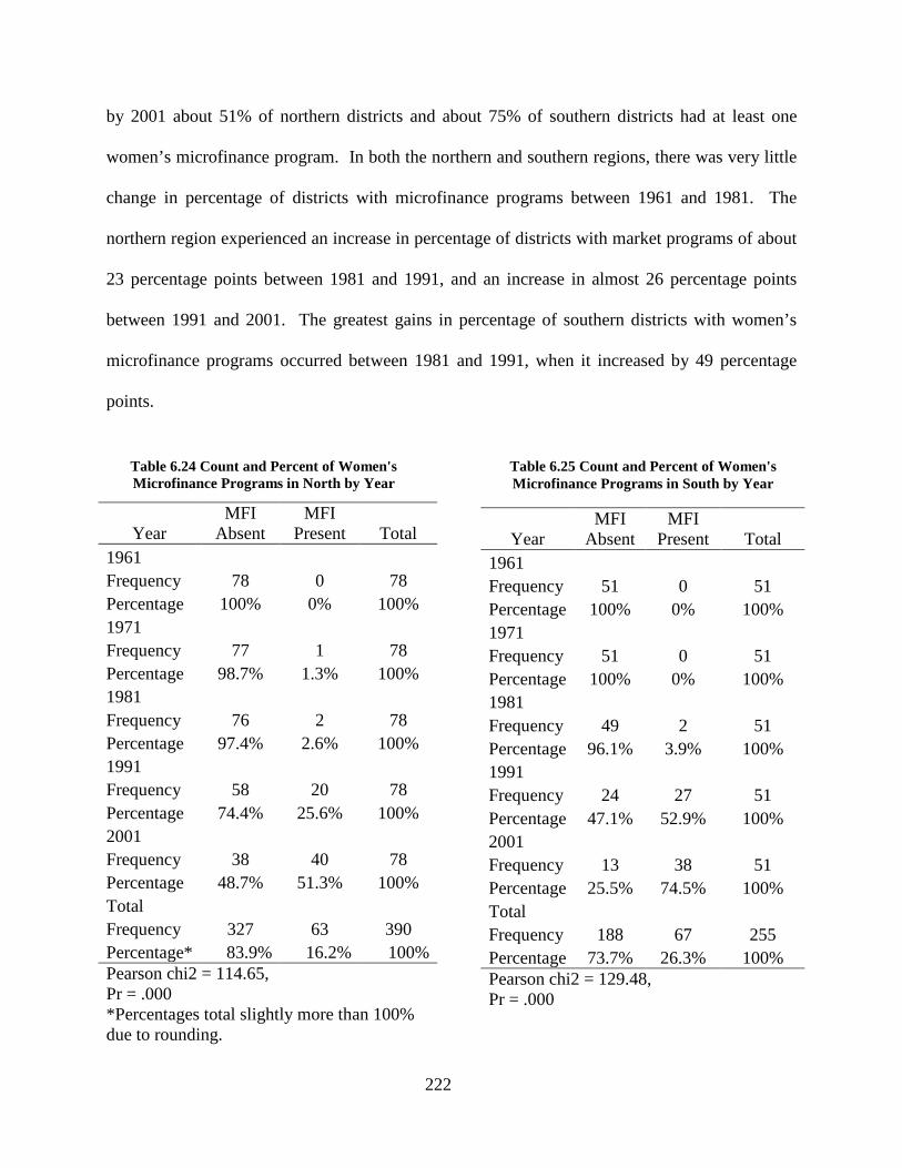
222
by 2001 about 51% of northern districts and about 75% of southern districts had at least one
women’s microfinance program. In both the northern and southern regions, there was very little
change in percentage of districts with microfinance programs between 1961 and 1981. The
northern region experienced an increase in percentage of districts with market programs of about
23 percentage points between 1981 and 1991, and an increase in almost 26 percentage points
between 1991 and 2001. The greatest gains in percentage of southern districts with women’s
microfinance programs occurred between 1981 and 1991, when it increased by 49 percentage
points.
*Percentages total slightly more than 100% due to rounding.
Year MFI
Absent MFI
Present Total 1961 Frequency 78 0 78 Percentage 100% 0% 100% 1971 Frequency 77 1 78 Percentage 98.7% 1.3% 100% 1981 Frequency 76 2 78 Percentage 97.4% 2.6% 100% 1991 Frequency 58 20 78 Percentage 74.4% 25.6% 100% 2001 Frequency 38 40 78 Percentage 48.7% 51.3% 100% Total Frequency 327 63 390 Percentage* 83.9% 16.2% 100% Pearson chi2 = 114.65, Pr = .000
Year MFI
Absent MFI
Present Total 1961 Frequency 51 0 51 Percentage 100% 0% 100% 1971 Frequency 51 0 51 Percentage 100% 0% 100% 1981 Frequency 49 2 51 Percentage 96.1% 3.9% 100% 1991 Frequency 24 27 51 Percentage 47.1% 52.9% 100% 2001 Frequency 13 38 51 Percentage 25.5% 74.5% 100% Total Frequency 188 67 255 Percentage 73.7% 26.3% 100% Pearson chi2 = 129.48, Pr = .000
Table 6.25 Count and Percent of Women's Microfinance Programs in South by Year
Table 6.24 Count and Percent of Women's Microfinance Programs in North by Year
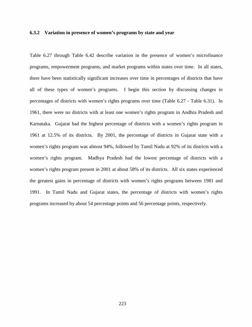
223
6.3.2 Variation in presence of women’s programs by state and year
Table 6.27 through Table 6.42 describe variation in the presence of women’s microfinance
programs, empowerment programs, and market programs within states over time. In all states,
there have been statistically significant increases over time in percentages of districts that have
all of these types of women’s programs. I begin this section by discussing changes in
percentages of districts with women’s rights programs over time (Table 6.27 - Table 6.31). In
1961, there were no districts with at least one women’s rights program in Andhra Pradesh and
Karnataka. Gujarat had the highest percentage of districts with a women’s rights program in
1961 at 12.5% of its districts. By 2001, the percentage of districts in Gujarat state with a
women’s rights program was almost 94%, followed by Tamil Nadu at 92% of its districts with a
women’s rights program. Madhya Pradesh had the lowest percentage of districts with a
women’s rights program present in 2001 at about 58% of its districts. All six states experienced
the greatest gains in percentage of districts with women’s rights programs between 1981 and
1991. In Tamil Nadu and Gujarat states, the percentage of districts with women’s rights
programs increased by about 54 percentage points and 56 percentage points, respectively.
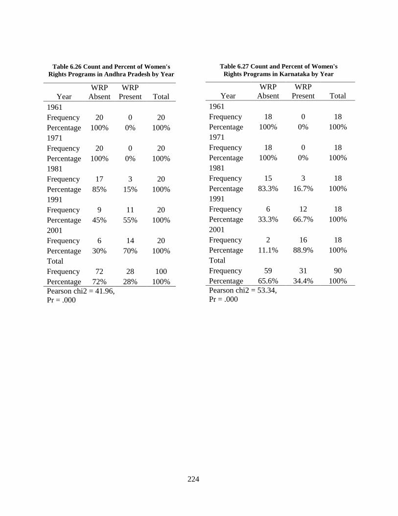
224
Year WRP
Absent WRP
Present Total 1961 Frequency 20 0 20 Percentage 100% 0% 100% 1971 Frequency 20 0 20 Percentage 100% 0% 100% 1981 Frequency 17 3 20 Percentage 85% 15% 100% 1991 Frequency 9 11 20 Percentage 45% 55% 100% 2001 Frequency 6 14 20 Percentage 30% 70% 100% Total Frequency 72 28 100 Percentage 72% 28% 100% Pearson chi2 = 41.96, Pr = .000
Year WRP
Absent WRP
Present Total 1961 Frequency 18 0 18 Percentage 100% 0% 100% 1971 Frequency 18 0 18 Percentage 100% 0% 100% 1981 Frequency 15 3 18 Percentage 83.3% 16.7% 100% 1991 Frequency 6 12 18 Percentage 33.3% 66.7% 100% 2001 Frequency 2 16 18 Percentage 11.1% 88.9% 100% Total Frequency 59 31 90 Percentage 65.6% 34.4% 100% Pearson chi2 = 53.34, Pr = .000
Table 6.27 Count and Percent of Women's Rights Programs in Karnataka by Year
Table 6.26 Count and Percent of Women's Rights Programs in Andhra Pradesh by Year
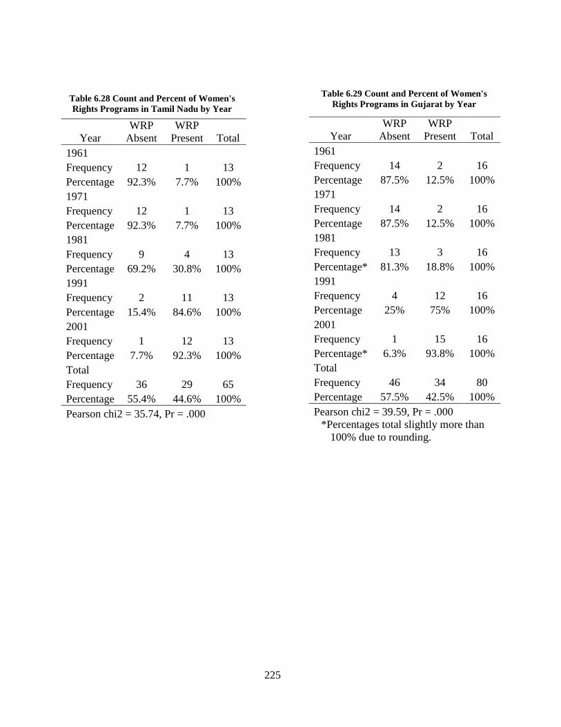
225
Year WRP
Absent WRP
Present Total 1961 Frequency 14 2 16 Percentage 87.5% 12.5% 100% 1971 Frequency 14 2 16 Percentage 87.5% 12.5% 100% 1981 Frequency 13 3 16 Percentage* 81.3% 18.8% 100% 1991 Frequency 4 12 16 Percentage 25% 75% 100% 2001 Frequency 1 15 16 Percentage* 6.3% 93.8% 100% Total Frequency 46 34 80 Percentage 57.5% 42.5% 100% Pearson chi2 = 39.59, Pr = .000
*Percentages total slightly more than 100% due to rounding.
Year WRP
Absent WRP
Present Total 1961 Frequency 12 1 13 Percentage 92.3% 7.7% 100% 1971 Frequency 12 1 13 Percentage 92.3% 7.7% 100% 1981 Frequency 9 4 13 Percentage 69.2% 30.8% 100% 1991 Frequency 2 11 13 Percentage 15.4% 84.6% 100% 2001 Frequency 1 12 13 Percentage 7.7% 92.3% 100% Total Frequency 36 29 65 Percentage 55.4% 44.6% 100% Pearson chi2 = 35.74, Pr = .000
Table 6.29 Count and Percent of Women's Rights Programs in Gujarat by Year Table 6.28 Count and Percent of Women's
Rights Programs in Tamil Nadu by Year
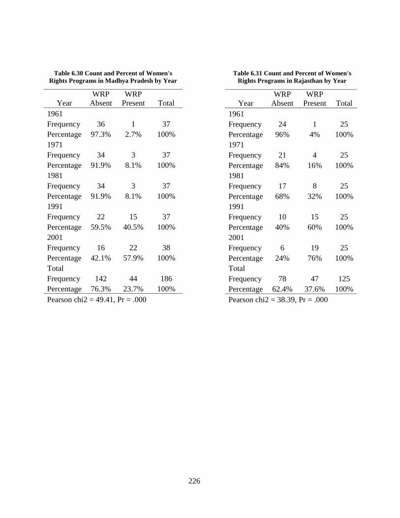
226
Year WRP
Absent WRP
Present Total 1961 Frequency 24 1 25 Percentage 96% 4% 100% 1971 Frequency 21 4 25 Percentage 84% 16% 100% 1981 Frequency 17 8 25 Percentage 68% 32% 100% 1991 Frequency 10 15 25 Percentage 40% 60% 100% 2001 Frequency 6 19 25 Percentage 24% 76% 100% Total Frequency 78 47 125 Percentage 62.4% 37.6% 100% Pearson chi2 = 38.39, Pr = .000
Year WRP
Absent WRP
Present Total 1961 Frequency 36 1 37 Percentage 97.3% 2.7% 100% 1971 Frequency 34 3 37 Percentage 91.9% 8.1% 100% 1981 Frequency 34 3 37 Percentage 91.9% 8.1% 100% 1991 Frequency 22 15 37 Percentage 59.5% 40.5% 100% 2001 Frequency 16 22 38 Percentage 42.1% 57.9% 100% Total Frequency 142 44 186 Percentage 76.3% 23.7% 100% Pearson chi2 = 49.41, Pr = .000
Table 6.31 Count and Percent of Women's Rights Programs in Rajasthan by Year
Table 6.30 Count and Percent of Women's Rights Programs in Madhya Pradesh by Year
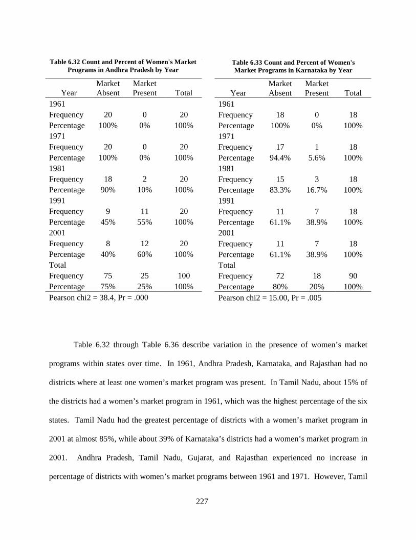
227
Table 6.32 through Table 6.36 describe variation in the presence of women’s market
programs within states over time. In 1961, Andhra Pradesh, Karnataka, and Rajasthan had no
districts where at least one women’s market program was present. In Tamil Nadu, about 15% of
the districts had a women’s market program in 1961, which was the highest percentage of the six
states. Tamil Nadu had the greatest percentage of districts with a women’s market program in
2001 at almost 85%, while about 39% of Karnataka’s districts had a women’s market program in
2001. Andhra Pradesh, Tamil Nadu, Gujarat, and Rajasthan experienced no increase in
percentage of districts with women’s market programs between 1961 and 1971. However, Tamil
Year Market Absent
Market Present Total
1961 Frequency 18 0 18 Percentage 100% 0% 100% 1971 Frequency 17 1 18 Percentage 94.4% 5.6% 100% 1981 Frequency 15 3 18 Percentage 83.3% 16.7% 100% 1991 Frequency 11 7 18 Percentage 61.1% 38.9% 100% 2001 Frequency 11 7 18 Percentage 61.1% 38.9% 100% Total Frequency 72 18 90 Percentage 80% 20% 100% Pearson chi2 = 15.00, Pr = .005
Year Market Absent
Market Present Total
Year Market Absent
Market Present Total
1961 Frequency 20 0 20 Percentage 100% 0% 100% 1971 Frequency 20 0 20 Percentage 100% 0% 100% 1981 Frequency 18 2 20 Percentage 90% 10% 100% 1991 Frequency 9 11 20 Percentage 45% 55% 100% 2001 Frequency 8 12 20 Percentage 40% 60% 100% Total Frequency 75 25 100 Percentage 75% 25% 100% Pearson chi2 = 38.4, Pr = .000
Table 6.33 Count and Percent of Women's Market Programs in Karnataka by Year
Table 6.32 Count and Percent of Women's Market Programs in Andhra Pradesh by Year
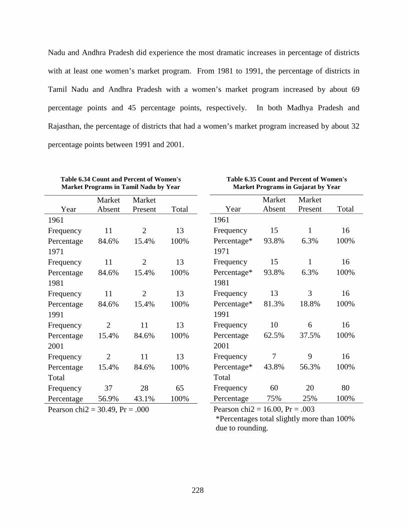
228
Nadu and Andhra Pradesh did experience the most dramatic increases in percentage of districts
with at least one women’s market program. From 1981 to 1991, the percentage of districts in
Tamil Nadu and Andhra Pradesh with a women’s market program increased by about 69
percentage points and 45 percentage points, respectively. In both Madhya Pradesh and
Rajasthan, the percentage of districts that had a women’s market program increased by about 32
percentage points between 1991 and 2001.
Year Market Absent
Market Present Total
1961 Frequency 11 2 13 Percentage 84.6% 15.4% 100% 1971 Frequency 11 2 13 Percentage 84.6% 15.4% 100% 1981 Frequency 11 2 13 Percentage 84.6% 15.4% 100% 1991 Frequency 2 11 13 Percentage 15.4% 84.6% 100% 2001 Frequency 2 11 13 Percentage 15.4% 84.6% 100% Total Frequency 37 28 65 Percentage 56.9% 43.1% 100% Pearson chi2 = 30.49, Pr = .000 *Percentages total slightly more than 100% due to rounding.
Year Market Absent
Market Present Total
1961 Frequency 15 1 16 Percentage* 93.8% 6.3% 100% 1971 Frequency 15 1 16 Percentage* 93.8% 6.3% 100% 1981 Frequency 13 3 16 Percentage* 81.3% 18.8% 100% 1991 Frequency 10 6 16 Percentage 62.5% 37.5% 100% 2001 Frequency 7 9 16 Percentage* 43.8% 56.3% 100% Total Frequency 60 20 80 Percentage 75% 25% 100% Pearson chi2 = 16.00, Pr = .003
Table 6.35 Count and Percent of Women's Market Programs in Gujarat by Year
Table 6.34 Count and Percent of Women's Market Programs in Tamil Nadu by Year
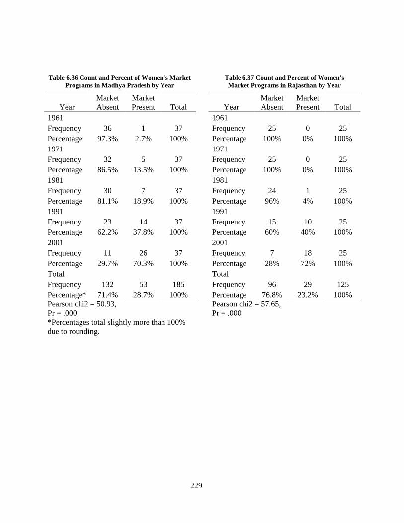
229
*Percentages total slightly more than 100% due to rounding.
Year Market Absent
Market Present Total
1961 Frequency 36 1 37 Percentage 97.3% 2.7% 100% 1971 Frequency 32 5 37 Percentage 86.5% 13.5% 100% 1981 Frequency 30 7 37 Percentage 81.1% 18.9% 100% 1991 Frequency 23 14 37 Percentage 62.2% 37.8% 100% 2001 Frequency 11 26 37 Percentage 29.7% 70.3% 100% Total Frequency 132 53 185 Percentage* 71.4% 28.7% 100% Pearson chi2 = 50.93, Pr = .000
Year Market Absent
Market Present Total
1961 Frequency 25 0 25 Percentage 100% 0% 100% 1971 Frequency 25 0 25 Percentage 100% 0% 100% 1981 Frequency 24 1 25 Percentage 96% 4% 100% 1991 Frequency 15 10 25 Percentage 60% 40% 100% 2001 Frequency 7 18 25 Percentage 28% 72% 100% Total Frequency 96 29 125 Percentage 76.8% 23.2% 100% Pearson chi2 = 57.65, Pr = .000
Table 6.37 Count and Percent of Women's Market Programs in Rajasthan by Year
Table 6.36 Count and Percent of Women's Market Programs in Madhya Pradesh by Year
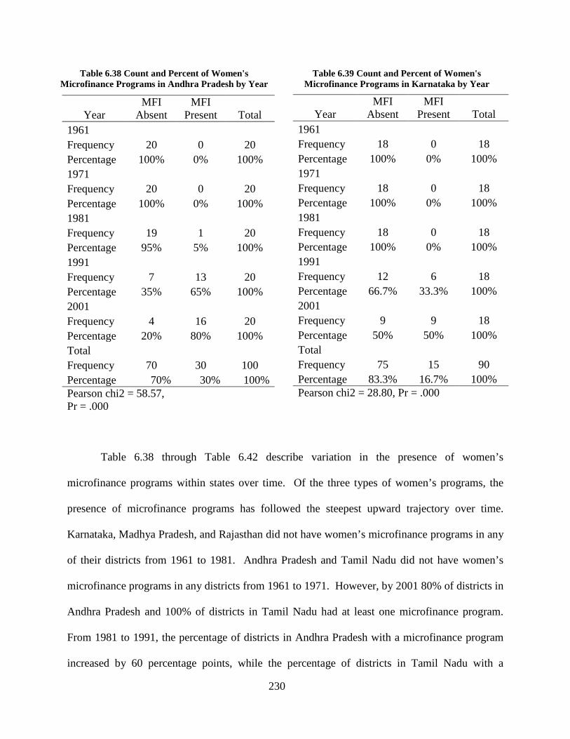
230
Table 6.38 through Table 6.42 describe variation in the presence of women’s
microfinance programs within states over time. Of the three types of women’s programs, the
presence of microfinance programs has followed the steepest upward trajectory over time.
Karnataka, Madhya Pradesh, and Rajasthan did not have women’s microfinance programs in any
of their districts from 1961 to 1981. Andhra Pradesh and Tamil Nadu did not have women’s
microfinance programs in any districts from 1961 to 1971. However, by 2001 80% of districts in
Andhra Pradesh and 100% of districts in Tamil Nadu had at least one microfinance program.
From 1981 to 1991, the percentage of districts in Andhra Pradesh with a microfinance program
increased by 60 percentage points, while the percentage of districts in Tamil Nadu with a
Year MFI
Absent MFI
Present Total 1961 Frequency 18 0 18 Percentage 100% 0% 100% 1971 Frequency 18 0 18 Percentage 100% 0% 100% 1981 Frequency 18 0 18 Percentage 100% 0% 100% 1991 Frequency 12 6 18 Percentage 66.7% 33.3% 100% 2001 Frequency 9 9 18 Percentage 50% 50% 100% Total Frequency 75 15 90 Percentage 83.3% 16.7% 100% Pearson chi2 = 28.80, Pr = .000
Year MFI
Absent MFI
Present Total 1961 Frequency 20 0 20 Percentage 100% 0% 100% 1971 Frequency 20 0 20 Percentage 100% 0% 100% 1981 Frequency 19 1 20 Percentage 95% 5% 100% 1991 Frequency 7 13 20 Percentage 35% 65% 100% 2001 Frequency 4 16 20 Percentage 20% 80% 100% Total Frequency 70 30 100 Percentage 70% 30% 100% Pearson chi2 = 58.57, Pr = .000
Table 6.38 Count and Percent of Women's Microfinance Programs in Andhra Pradesh by Year
Table 6.39 Count and Percent of Women's Microfinance Programs in Karnataka by Year
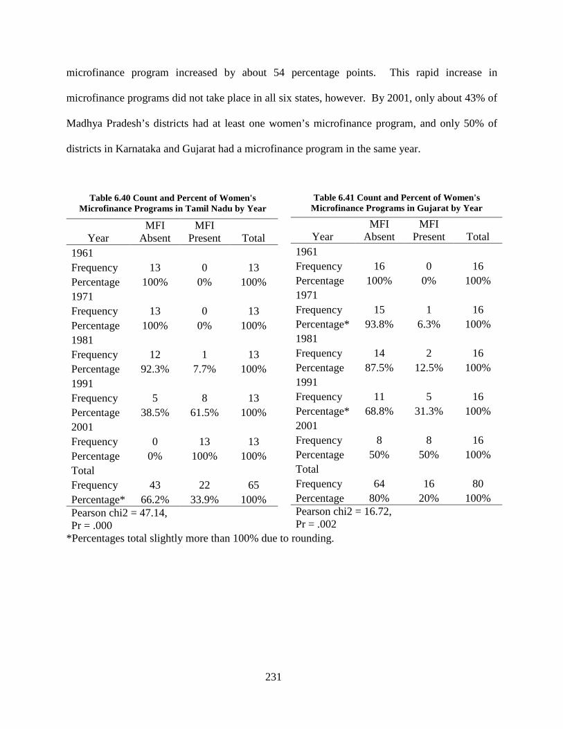
231
microfinance program increased by about 54 percentage points. This rapid increase in
microfinance programs did not take place in all six states, however. By 2001, only about 43% of
Madhya Pradesh’s districts had at least one women’s microfinance program, and only 50% of
districts in Karnataka and Gujarat had a microfinance program in the same year.
Year MFI
Absent MFI
Present Total 1961 Frequency 13 0 13 Percentage 100% 0% 100% 1971 Frequency 13 0 13 Percentage 100% 0% 100% 1981 Frequency 12 1 13 Percentage 92.3% 7.7% 100% 1991 Frequency 5 8 13 Percentage 38.5% 61.5% 100% 2001 Frequency 0 13 13 Percentage 0% 100% 100% Total Frequency 43 22 65 Percentage* 66.2% 33.9% 100% Pearson chi2 = 47.14, Pr = .000
*Percentages total slightly more than 100% due to rounding.
Year MFI
Absent MFI
Present Total 1961 Frequency 16 0 16 Percentage 100% 0% 100% 1971 Frequency 15 1 16 Percentage* 93.8% 6.3% 100% 1981 Frequency 14 2 16 Percentage 87.5% 12.5% 100% 1991 Frequency 11 5 16 Percentage* 68.8% 31.3% 100% 2001 Frequency 8 8 16 Percentage 50% 50% 100% Total Frequency 64 16 80 Percentage 80% 20% 100% Pearson chi2 = 16.72, Pr = .002
Table 6.41 Count and Percent of Women's Microfinance Programs in Gujarat by Year
Table 6.40 Count and Percent of Women's Microfinance Programs in Tamil Nadu by Year
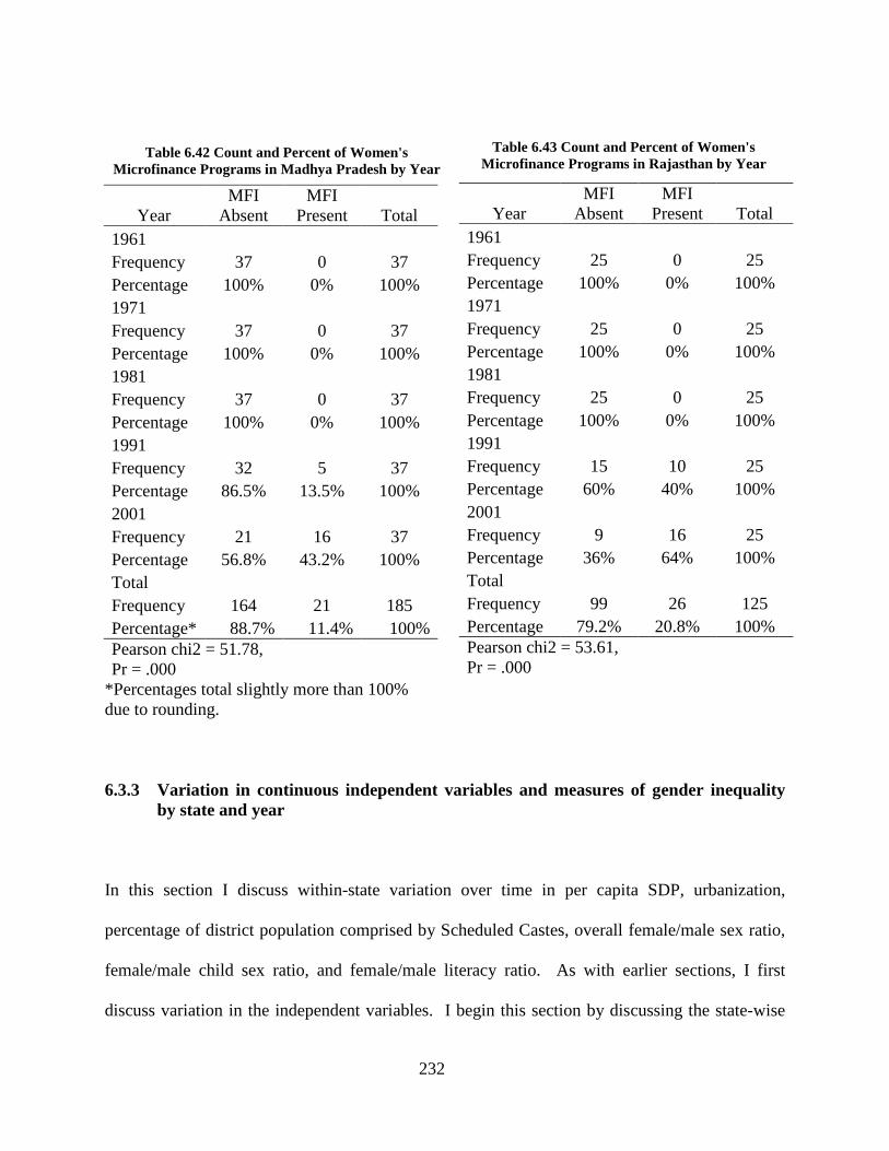
232
Year MFI
Absent MFI
Present Total 1961 Frequency 37 0 37 Percentage 100% 0% 100% 1971 Frequency 37 0 37 Percentage 100% 0% 100% 1981 Frequency 37 0 37 Percentage 100% 0% 100% 1991 Frequency 32 5 37 Percentage 86.5% 13.5% 100% 2001 Frequency 21 16 37 Percentage 56.8% 43.2% 100% Total Frequency 164 21 185 Percentage* 88.7% 11.4% 100% Pearson chi2 = 51.78, Pr = .000
*Percentages total slightly more than 100% due to rounding. 6.3.3 Variation in continuous independent variables and measures of gender inequality
by state and year
In this section I discuss within-state variation over time in per capita SDP, urbanization,
percentage of district population comprised by Scheduled Castes, overall female/male sex ratio,
female/male child sex ratio, and female/male literacy ratio. As with earlier sections, I first
discuss variation in the independent variables. I begin this section by discussing the state-wise
Year MFI
Absent MFI
Present Total 1961 Frequency 25 0 25 Percentage 100% 0% 100% 1971 Frequency 25 0 25 Percentage 100% 0% 100% 1981 Frequency 25 0 25 Percentage 100% 0% 100% 1991 Frequency 15 10 25 Percentage 60% 40% 100% 2001 Frequency 9 16 25 Percentage 36% 64% 100% Total Frequency 99 26 125 Percentage 79.2% 20.8% 100% Pearson chi2 = 53.61, Pr = .000
Table 6.43 Count and Percent of Women's Microfinance Programs in Rajasthan by Year
Table 6.42 Count and Percent of Women's Microfinance Programs in Madhya Pradesh by Year
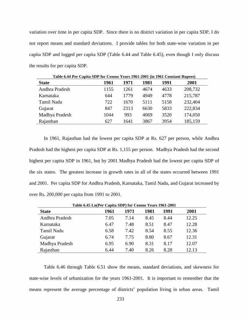
233
variation over time in per capita SDP. Since there is no district variation in per capita SDP, I do
not report means and standard deviations. I provide tables for both state-wise variation in per
capita SDP and logged per capita SDP (Table 6.44 and Table 6.45), even though I only discuss
the results for per capita SDP.
Table 6.44 Per Capita SDP for Census Years 1961-2001 (in 1961 Constant Rupees) State 1961 1971 1981 1991 2001 Andhra Pradesh 1155 1261 4674 4633 208,732 Karnataka 644 1779 4949 4778 215,787 Tamil Nadu 722 1670 5111 5158 232,404 Gujarat 847 2313 6630 5833 222,834 Madhya Pradesh 1044 993 4069 3520 174,050 Rajasthan 627 1641 3867 3954 185,159
In 1961, Rajasthan had the lowest per capita SDP at Rs. 627 per person, while Andhra
Pradesh had the highest per capita SDP at Rs. 1,155 per person. Madhya Pradesh had the second
highest per capita SDP in 1961, but by 2001 Madhya Pradesh had the lowest per capita SDP of
the six states. The greatest increase in growth rates in all of the states occurred between 1991
and 2001. Per capita SDP for Andhra Pradesh, Karnataka, Tamil Nadu, and Gujarat increased by
over Rs. 200,000 per capita from 1991 to 2001.
Table 6.45 Ln(Per Capita SDP) for Census Years 1961-2001 State 1961 1971 1981 1991 2001 Andhra Pradesh 7.05 7.14 8.45 8.44 12.25 Karnataka 6.47 7.48 8.51 8.47 12.28 Tamil Nadu 6.58 7.42 8.54 8.55 12.36 Gujarat 6.74 7.75 8.80 8.67 12.31 Madhya Pradesh 6.95 6.90 8.31 8.17 12.07 Rajasthan 6.44 7.40 8.26 8.28 12.13
Table 6.46 through Table 6.51 show the means, standard deviations, and skewness for
state-wise levels of urbanization for the years 1961-2001. It is important to remember that the
means represent the average percentage of districts’ population living in urban areas. Tamil
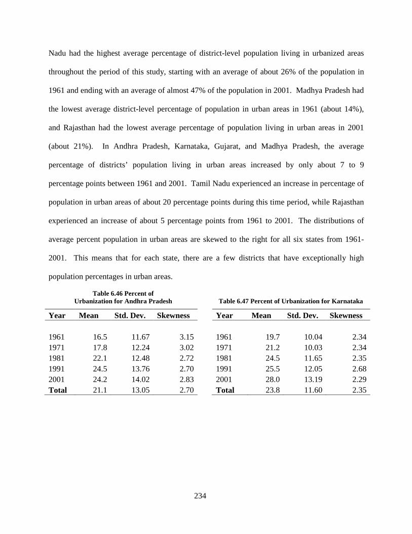
234
Nadu had the highest average percentage of district-level population living in urbanized areas
throughout the period of this study, starting with an average of about 26% of the population in
1961 and ending with an average of almost 47% of the population in 2001. Madhya Pradesh had
the lowest average district-level percentage of population in urban areas in 1961 (about 14%),
and Rajasthan had the lowest average percentage of population living in urban areas in 2001
(about 21%). In Andhra Pradesh, Karnataka, Gujarat, and Madhya Pradesh, the average
percentage of districts’ population living in urban areas increased by only about 7 to 9
percentage points between 1961 and 2001. Tamil Nadu experienced an increase in percentage of
population in urban areas of about 20 percentage points during this time period, while Rajasthan
experienced an increase of about 5 percentage points from 1961 to 2001. The distributions of
average percent population in urban areas are skewed to the right for all six states from 1961-
2001. This means that for each state, there are a few districts that have exceptionally high
population percentages in urban areas.
Year Mean Std. Dev. Skewness Year Mean Std. Dev. Skewness
1961 16.5 11.67 3.15 1961 19.7 10.04 2.34 1971 17.8 12.24 3.02 1971 21.2 10.03 2.34 1981 22.1 12.48 2.72 1981 24.5 11.65 2.35 1991 24.5 13.76 2.70 1991 25.5 12.05 2.68 2001 24.2 14.02 2.83 2001 28.0 13.19 2.29 Total 21.1 13.05 2.70 Total 23.8 11.60 2.35
Table 6.47 Percent of Urbanization for Karnataka Table 6.46 Percent of
Urbanization for Andhra Pradesh
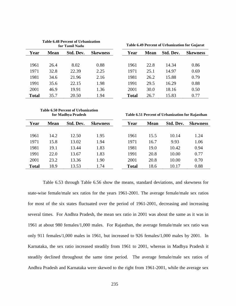
235
Year Mean Std. Dev. Skewness Year Mean Std. Dev. Skewness
1961 26.4 8.02 0.88 1961 22.8 14.34 0.86 1971 32.8 22.39 2.25 1971 25.1 14.97 0.69 1981 34.6 21.96 2.16 1981 26.2 15.88 0.79 1991 35.6 22.15 1.98 1991 29.5 16.29 0.88 2001 46.9 19.91 1.36 2001 30.0 18.16 0.50 Total 35.7 20.50 1.94 Total 26.7 15.83 0.77
Year Mean Std. Dev. Skewness Year Mean Std. Dev. Skewness
1961 14.2 12.50 1.95 1961 15.5 10.14 1.24 1971 15.8 13.02 1.94 1971 16.7 9.93 1.06 1981 19.1 13.44 1.83 1981 19.0 10.42 0.94 1991 22.0 13.67 1.83 1991 20.8 10.00 0.77 2001 23.2 13.36 1.90 2001 20.8 10.00 0.70 Total 18.9 13.53 1.74 Total 18.6 10.17 0.88
Table 6.53 through Table 6.56 show the means, standard deviations, and skewness for
state-wise female/male sex ratios for the years 1961-2001. The average female/male sex ratios
for most of the six states fluctuated over the period of 1961-2001, decreasing and increasing
several times. For Andhra Pradesh, the mean sex ratio in 2001 was about the same as it was in
1961 at about 980 females/1,000 males. For Rajasthan, the average female/male sex ratio was
only 911 females/1,000 males in 1961, but increased to 926 females/1,000 males by 2001. In
Karnataka, the sex ratio increased steadily from 1961 to 2001, whereas in Madhya Pradesh it
steadily declined throughout the same time period. The average female/male sex ratios of
Andhra Pradesh and Karnataka were skewed to the right from 1961-2001, while the average sex
Table 6.49 Percent of Urbanization for Gujarat Table 6.48 Percent of Urbanization
for Tamil Nadu
Table 6.51 Percent of Urbanization for Rajasthan Table 6.50 Percent of Urbanization
for Madhya Pradesh
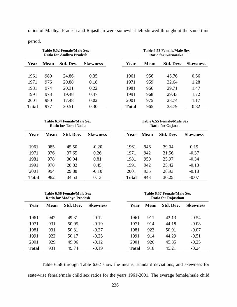
236
ratios of Madhya Pradesh and Rajasthan were somewhat left-skewed throughout the same time
period.
Year Mean Std. Dev. Skewness Year Mean Std. Dev. Skewness
1961 980 24.86 0.35 1961 956 45.76 0.56 1971 976 20.88 0.18 1971 959 32.64 1.28 1981 974 20.31 0.22 1981 966 29.71 1.47 1991 973 19.48 0.47 1991 968 29.43 1.72 2001 980 17.48 0.02 2001 975 28.74 1.17 Total 977 20.51 0.30 Total 965 33.79 0.82 Year Mean Std. Dev. Skewness Year Mean Std. Dev. Skewness
1961 985 45.50 -0.20 1961 946 39.04 0.19 1971 976 37.65 0.26 1971 942 31.56 -0.37 1981 978 30.04 0.81 1981 950 25.97 -0.34 1991 978 28.82 0.45 1991 942 25.42 -0.13 2001 994 29.88 -0.10 2001 935 28.93 -0.18 Total 982 34.53 0.13 Total 943 30.25 -0.07 Year Mean Std. Dev. Skewness Year Mean Std. Dev. Skewness
1961 942 49.31 -0.12 1961 911 43.13 -0.54 1971 931 50.05 -0.19 1971 914 44.18 -0.08 1981 931 50.31 -0.27 1981 923 50.01 -0.07 1991 922 50.17 -0.25 1991 914 44.29 -0.51 2001 929 49.06 -0.12 2001 926 45.85 -0.25 Total 931 49.74 -0.19 Total 918 45.21 -0.24
Table 6.58 through Table 6.62 show the means, standard deviations, and skewness for
state-wise female/male child sex ratios for the years 1961-2001. The average female/male child
Table 6.53 Female/Male Sex Ratio for Karnataka
Table 6.52 Female/Male Sex Ratio for Andhra Pradesh
Table 6.55 Female/Male Sex Ratio for Gujarat
Table 6.54 Female/Male Sex Ratio for Tamil Nadu
Table 6.57 Female/Male Sex Ratio for Rajasthan
Table 6.56 Female/Male Sex Ratio for Madhya Pradesh
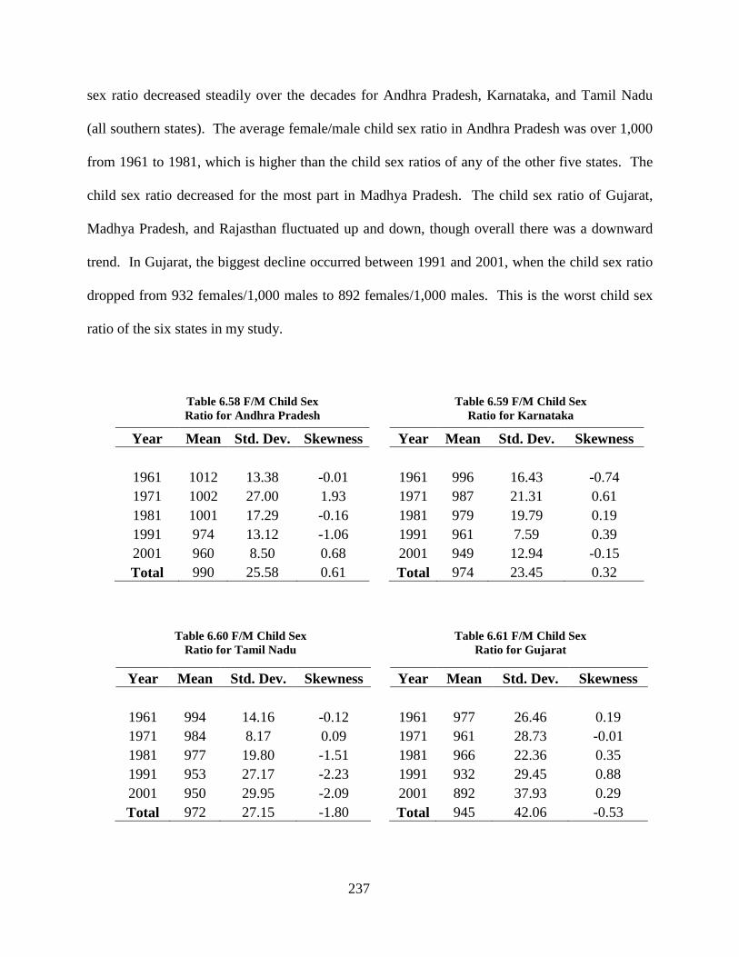
237
sex ratio decreased steadily over the decades for Andhra Pradesh, Karnataka, and Tamil Nadu
(all southern states). The average female/male child sex ratio in Andhra Pradesh was over 1,000
from 1961 to 1981, which is higher than the child sex ratios of any of the other five states. The
child sex ratio decreased for the most part in Madhya Pradesh. The child sex ratio of Gujarat,
Madhya Pradesh, and Rajasthan fluctuated up and down, though overall there was a downward
trend. In Gujarat, the biggest decline occurred between 1991 and 2001, when the child sex ratio
dropped from 932 females/1,000 males to 892 females/1,000 males. This is the worst child sex
ratio of the six states in my study.
Year Mean Std. Dev. Skewness Year Mean Std. Dev. Skewness
1961 994 14.16 -0.12 1961 977 26.46 0.19 1971 984 8.17 0.09 1971 961 28.73 -0.01 1981 977 19.80 -1.51 1981 966 22.36 0.35 1991 953 27.17 -2.23 1991 932 29.45 0.88 2001 950 29.95 -2.09 2001 892 37.93 0.29 Total 972 27.15 -1.80 Total 945 42.06 -0.53
Year Mean Std. Dev. Skewness Year Mean Std. Dev. Skewness
1961 1012 13.38 -0.01 1961 996 16.43 -0.74 1971 1002 27.00 1.93 1971 987 21.31 0.61 1981 1001 17.29 -0.16 1981 979 19.79 0.19 1991 974 13.12 -1.06 1991 961 7.59 0.39 2001 960 8.50 0.68 2001 949 12.94 -0.15 Total 990 25.58 0.61 Total 974 23.45 0.32
Table 6.59 F/M Child Sex Ratio for Karnataka
Table 6.58 F/M Child Sex Ratio for Andhra Pradesh
Table 6.61 F/M Child Sex Ratio for Gujarat
Table 6.60 F/M Child Sex Ratio for Tamil Nadu
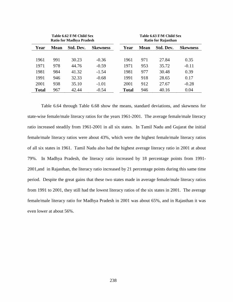
238
Table 6.64 through Table 6.68 show the means, standard deviations, and skewness for
state-wise female/male literacy ratios for the years 1961-2001. The average female/male literacy
ratio increased steadily from 1961-2001 in all six states. In Tamil Nadu and Gujarat the initial
female/male literacy ratios were about 43%, which were the highest female/male literacy ratios
of all six states in 1961. Tamil Nadu also had the highest average literacy ratio in 2001 at about
79%. In Madhya Pradesh, the literacy ratio increased by 18 percentage points from 1991-
2001,and in Rajasthan, the literacy ratio increased by 21 percentage points during this same time
period. Despite the great gains that these two states made in average female/male literacy ratios
from 1991 to 2001, they still had the lowest literacy ratios of the six states in 2001. The average
female/male literacy ratio for Madhya Pradesh in 2001 was about 65%, and in Rajasthan it was
even lower at about 56%.
Year Mean Std. Dev. Skewness Year Mean Std. Dev. Skewness
1961 991 30.23 -0.36 1961 971 27.84 0.35 1971 978 44.76 -0.59 1971 953 35.72 -0.11 1981 984 41.32 -1.54 1981 977 30.48 0.39 1991 946 32.33 -0.68 1991 918 28.65 0.17 2001 938 35.10 -1.01 2001 912 27.67 -0.28 Total 967 42.44 -0.54 Total 946 40.16 0.04
Table 6.63 F/M Child Sex Ratio for Rajasthan
Table 6.62 F/M Child Sex Ratio for Madhya Pradesh
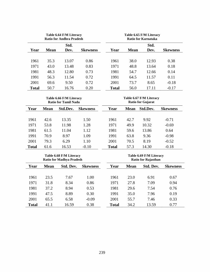
239
Year Mean Std.Dev. Skewness Year Mean Std.Dev. Skewness
1961 42.6 13.35 1.50 1961 42.7 9.92 -0.71 1971 53.8 11.98 1.28 1971 49.9 10.32 -0.69 1981 61.5 11.04 1.12 1981 59.6 13.86 0.64 1991 70.9 8.97 1.09 1991 63.8 9.36 -0.98 2001 79.3 6.29 1.10 2001 70.5 8.19 -0.52 Total 61.6 16.53 -0.10 Total 57.3 14.30 -0.18
Year Mean Std. Dev. Skewness Year Mean
Std. Dev. Skewness
1961 35.3 13.07 0.86 1961 38.0 12.93 0.38 1971 43.0 13.48 0.83 1971 48.8 13.64 0.18 1981 48.3 12.80 0.73 1981 54.7 12.66 0.14 1991 56.3 11.54 0.72 1991 64.5 11.57 0.11 2001 69.6 9.50 0.72 2001 73.7 8.65 -0.18 Total 50.7 16.76 0.20 Total 56.0 17.11 -0.17
Year Mean Std. Dev. Skewness Year Mean Std. Dev. Skewness
1961 23.5 7.67 1.00 1961 23.0 6.91 0.67 1971 31.8 8.34 0.86 1971 27.8 7.09 0.94 1981 37.2 8.94 0.53 1981 29.6 7.54 0.76 1991 47.5 8.89 0.30 1991 35.0 7.96 0.19 2001 65.5 6.58 -0.09 2001 55.7 7.46 0.33 Total 41.1 16.59 0.38 Total 34.2 13.59 0.77
Table 6.65 F/M Literacy Ratio for Karnataka
Table 6.64 F/M Literacy Ratio for Andhra Pradesh
Table 6.67 F/M Literacy Ratio for Gujarat
Table 6.66 F/M Literacy Ratio for Tamil Nadu
Table 6.69 F/M Literacy Ratio for Rajasthan
Table 6.68 F/M Literacy Ratio for Madhya Pradesh
240
6.3.4 Overall Change in Continuous Independent Variables and Measures of Gender
Inequality over Time
In the previous two sections I discussed the state-wise and regional variation in each of the
independent and dependent variables over time. Yet is the change in these variables over time
statistically significant? And if so, what is the magnitude of this change? In this section, I
discuss the absolute amount of change in each continuous variable that takes place from 1961 to
2001. I also use OLS regression to determine whether change for each variable is statistically
significant. First, however, I present and discuss line graphs that depict how the female/male sex
ratio, female/male child sex ratio, and female/male literacy ratio change over time. For each of
these dependent variables, I chose a random sample of districts and plotted their change over
time. This is useful because it gives me a visual representation of changes in female/male sex
ratio, child sex ratio, and literacy ratio.
Figure 6.1 depicts change in the female/male sex ratio over time for a random sample of
districts (n = 20). Overall, the change trajectories tend to be almost flat, especially compared to
the change trajectories for female/male child sex ratio and female/male literacy ratio depicted in
Figure 6.2 and Figure 6.3. There are a few districts that have change trajectories that do not fit
this pattern. For example, the sex ratio of district 118 rises sharply from 1971 to 1981. District
69’s sex ratio decreased relatively sharply from 1981 to 1991, and then started rising from 1991
to 2001. The sex ratio of district 129 fluctuated over time.
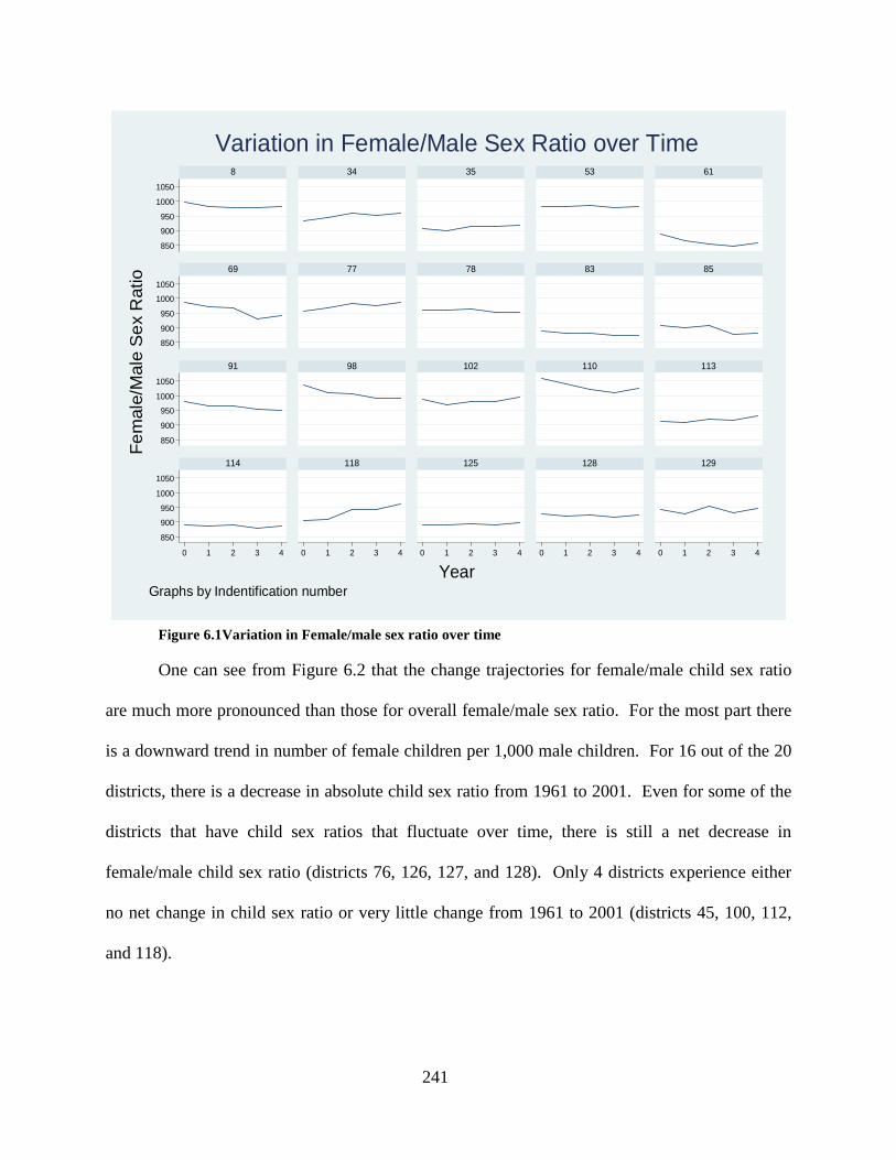
241
850
900
950
1000
1050
850
900
950
1000
1050
850
900
950
1000
1050
850
900
950
1000
1050
0 1 2 3 4 0 1 2 3 4 0 1 2 3 4 0 1 2 3 4 0 1 2 3 4
8 34 35 53 61
69 77 78 83 85
91 98 102 110 113
114 118 125 128 129
Fem
ale/
Mal
e S
ex R
atio
YearGraphs by Indentification number
Variation in Female/Male Sex Ratio over Time
Figure 6.1Variation in Female/male sex ratio over time
One can see from Figure 6.2 that the change trajectories for female/male child sex ratio
are much more pronounced than those for overall female/male sex ratio. For the most part there
is a downward trend in number of female children per 1,000 male children. For 16 out of the 20
districts, there is a decrease in absolute child sex ratio from 1961 to 2001. Even for some of the
districts that have child sex ratios that fluctuate over time, there is still a net decrease in
female/male child sex ratio (districts 76, 126, 127, and 128). Only 4 districts experience either
no net change in child sex ratio or very little change from 1961 to 2001 (districts 45, 100, 112,
and 118).
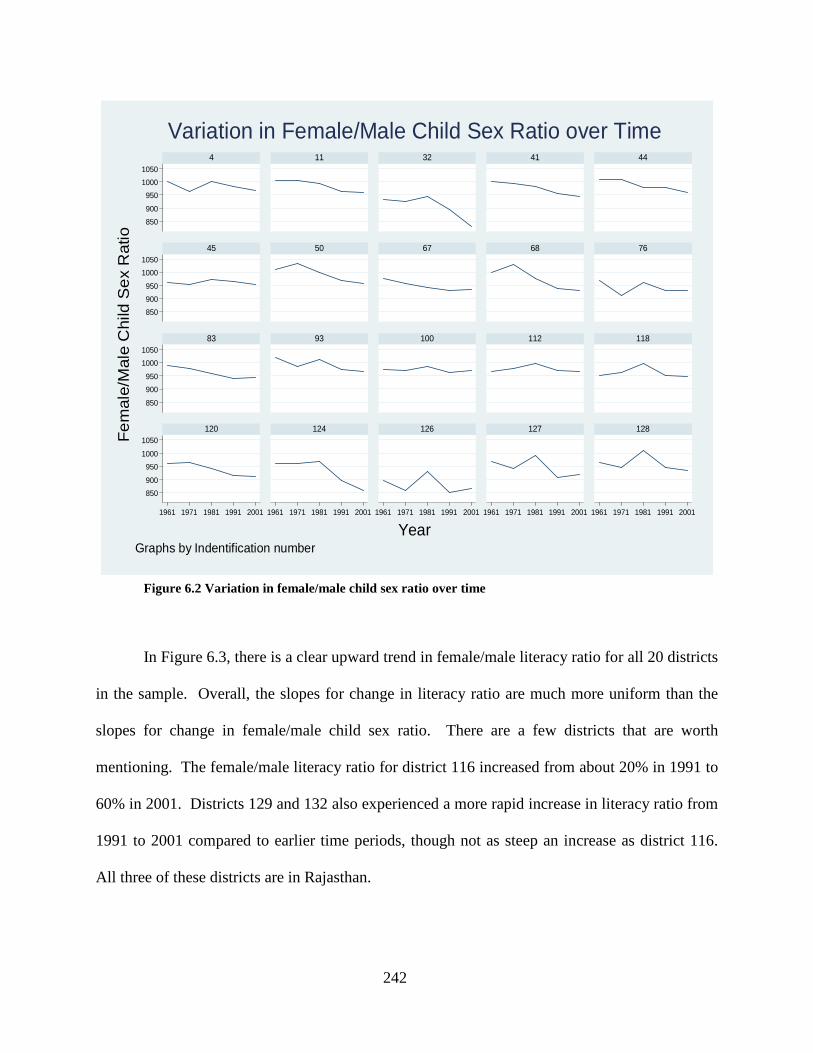
242
850900
95010001050
850900950
10001050
850
900950
10001050
850900
9501000
1050
198119711961 1991 2001 1961 19811971 1991 2001 1961 1971 1981 1991 2001 1961 1971 1981 1991 2001 1961 1971 1981 1991 2001
4 11 32 41 44
45 50 67 68 76
83 93 100 112 118
120 124 126 127 128Fem
ale/
Mal
e C
hild
Sex
Rat
io
YearGraphs by Indentification number
Variation in Female/Male Child Sex Ratio over Time
Figure 6.2 Variation in female/male child sex ratio over time
In Figure 6.3, there is a clear upward trend in female/male literacy ratio for all 20 districts
in the sample. Overall, the slopes for change in literacy ratio are much more uniform than the
slopes for change in female/male child sex ratio. There are a few districts that are worth
mentioning. The female/male literacy ratio for district 116 increased from about 20% in 1991 to
60% in 2001. Districts 129 and 132 also experienced a more rapid increase in literacy ratio from
1991 to 2001 compared to earlier time periods, though not as steep an increase as district 116.
All three of these districts are in Rajasthan.
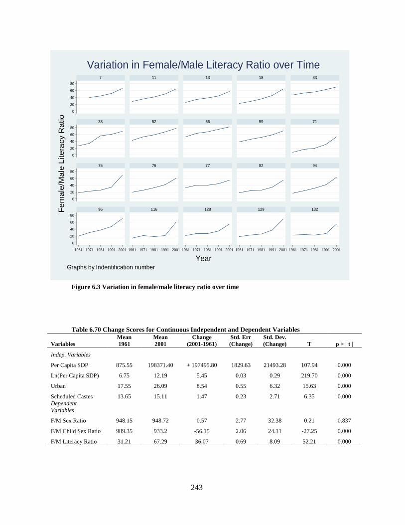
243
0
20
40
60
80
0
20
40
60
80
0
20
40
60
80
0
20
40
60
80
19811961 1971 1991 2001 1961 1971 1981 1991 2001 1961 1971 1981 1991 2001 1961 1971 1981 1991 2001 1961 1971 1981 1991 2001
7 11 13 18 33
38 52 56 59 71
75 76 77 82 94
96 116 128 129 132Fem
ale/
Mal
e Li
tera
cy R
atio
YearGraphs by Indentification number
Variation in Female/Male Literacy Ratio over Time
Figure 6.3 Variation in female/male literacy ratio over time
Table 6.70 Change Scores for Continuous Independent and Dependent Variables
Variables Mean 1961
Mean 2001
Change (2001-1961)
Std. Err (Change)
Std. Dev. (Change) T
p > | t |
Indep. Variables
Per Capita SDP 875.55 198371.40 + 197495.80 1829.63 21493.28 107.94 0.000
Ln(Per Capita SDP) 6.75 12.19 5.45 0.03 0.29 219.70 0.000
Urban 17.55 26.09 8.54 0.55 6.32 15.63 0.000
Scheduled Castes 13.65 15.11 1.47 0.23 2.71 6.35 0.000 Dependent Variables
F/M Sex Ratio 948.15 948.72 0.57 2.77 32.38 0.21 0.837
F/M Child Sex Ratio 989.35 933.2 -56.15 2.06 24.11 -27.25 0.000
F/M Literacy Ratio 31.21 67.29 36.07 0.69 8.09 52.21 0.000
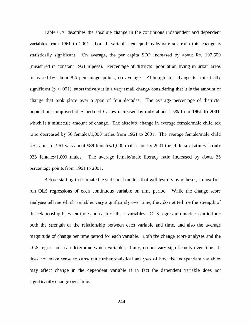
244
Table 6.70 describes the absolute change in the continuous independent and dependent
variables from 1961 to 2001. For all variables except female/male sex ratio this change is
statistically significant. On average, the per capita SDP increased by about Rs. 197,500
(measured in constant 1961 rupees). Percentage of districts’ population living in urban areas
increased by about 8.5 percentage points, on average. Although this change is statistically
significant (p < .001), substantively it is a very small change considering that it is the amount of
change that took place over a span of four decades. The average percentage of districts’
population comprised of Scheduled Castes increased by only about 1.5% from 1961 to 2001,
which is a miniscule amount of change. The absolute change in average female/male child sex
ratio decreased by 56 females/1,000 males from 1961 to 2001. The average female/male child
sex ratio in 1961 was about 989 females/1,000 males, but by 2001 the child sex ratio was only
933 females/1,000 males. The average female/male literacy ratio increased by about 36
percentage points from 1961 to 2001.
Before starting to estimate the statistical models that will test my hypotheses, I must first
run OLS regressions of each continuous variable on time period. While the change score
analyses tell me which variables vary significantly over time, they do not tell me the strength of
the relationship between time and each of these variables. OLS regression models can tell me
both the strength of the relationship between each variable and time, and also the average
magnitude of change per time period for each variable. Both the change score analyses and the
OLS regressions can determine which variables, if any, do not vary significantly over time. It
does not make sense to carry out further statistical analyses of how the independent variables
may affect change in the dependent variable if in fact the dependent variable does not
significantly change over time.
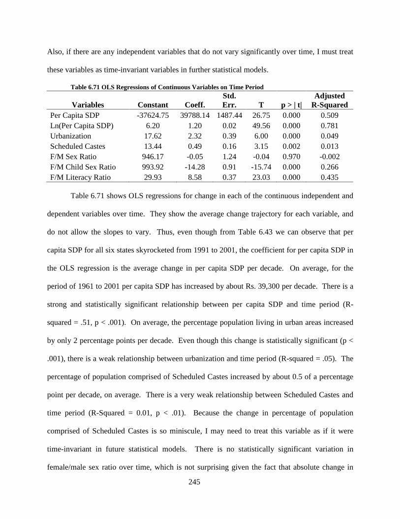
245
Also, if there are any independent variables that do not vary significantly over time, I must treat
these variables as time-invariant variables in further statistical models.
Table 6.71 OLS Regressions of Continuous Variables on Time Period
Variables Constant Coeff. Std. Err. T p > | t|
Adjusted R-Squared
Per Capita SDP -37624.75 39788.14 1487.44 26.75 0.000 0.509 Ln(Per Capita SDP) 6.20 1.20 0.02 49.56 0.000 0.781 Urbanization 17.62 2.32 0.39 6.00 0.000 0.049 Scheduled Castes 13.44 0.49 0.16 3.15 0.002 0.013 F/M Sex Ratio 946.17 -0.05 1.24 -0.04 0.970 -0.002 F/M Child Sex Ratio 993.92 -14.28 0.91 -15.74 0.000 0.266 F/M Literacy Ratio 29.93 8.58 0.37 23.03 0.000 0.435
Table 6.71 shows OLS regressions for change in each of the continuous independent and
dependent variables over time. They show the average change trajectory for each variable, and
do not allow the slopes to vary. Thus, even though from Table 6.43 we can observe that per
capita SDP for all six states skyrocketed from 1991 to 2001, the coefficient for per capita SDP in
the OLS regression is the average change in per capita SDP per decade. On average, for the
period of 1961 to 2001 per capita SDP has increased by about Rs. 39,300 per decade. There is a
strong and statistically significant relationship between per capita SDP and time period (R-
squared = .51, p < .001). On average, the percentage population living in urban areas increased
by only 2 percentage points per decade. Even though this change is statistically significant (p <
.001), there is a weak relationship between urbanization and time period (R-squared = .05). The
percentage of population comprised of Scheduled Castes increased by about 0.5 of a percentage
point per decade, on average. There is a very weak relationship between Scheduled Castes and
time period (R-Squared = 0.01, p < .01). Because the change in percentage of population
comprised of Scheduled Castes is so miniscule, I may need to treat this variable as if it were
time-invariant in future statistical models. There is no statistically significant variation in
female/male sex ratio over time, which is not surprising given the fact that absolute change in
246
female/male sex ratio from 1961 to 2001 is also not statistically significant (see Table 6.70).
Because the female/male sex ratio does not vary significantly over time, I cannot include it as a
dependent variable in my models. On average, there is a decrease in female/male child sex ratio
of about 14 females/1,000 males for each time period. The strength of the relationship between
female/male child sex ratio is moderate (R-squared = .27) and this is statistically significant (p <
.001). The female/male literacy ratio increases by about 8.6 percentage points per decade, on
average. The relationship between female/male literacy ratio and time period is both strong (R-
squared = .44) and statistically significant (p < .001).
6.4 CONCLUSION
In this chapter, I have laid the groundwork for the statistical models that I present in the next two
chapters by carrying out descriptive analyses on all of my variables. I have found that although
there is no statistically significant variation in the presence of women’s rights programs and
market programs by region, there is significant variation in the presence of these women’s
programs by state. The presence of women’s microfinance programs varied significantly by both
region and state. Urbanization and percentage of population comprised of Scheduled Castes
varied significantly by both region and state, whereas SDP per capita did not. The presence of
women’s rights programs, market programs, and microfinance programs all varied significantly
over time. This variation in presence of women’s programs over time was significant for both
regions and for all six states. Change-score analyses and OLS regressions revealed that changes
over time in SDP per capita, urbanization, female/male child sex ratio, and female/male literacy
ratio were all statistically significant. However, change in the female/male sex ratio over time

247
was not significant. Therefore, I will not keep female/male sex ratio as one of my dependent
variables. Change in percent of population comprised of Scheduled Castes was significant, so I
can treat this variable as a time-varying variable.
248
7.0 CHAPTER SEVEN: VARIATION IN THE FEMALE/MALE CHILD SEX RATIO
7.1 INTRODUCTION
In this chapter I discuss the results of the fixed-effects models for female/male child sex ratio. I
first present and discuss the results of models that test the modernization hypotheses, followed
by results of models that test the WID hypotheses. Next, I discuss the results of models testing
the GAD hypotheses and the models testing the neoliberal hypotheses. For each set of
hypotheses, I present models with both lagged and unlagged independent variables, as well as
models with regional interaction effects and state-wide interaction effects. I report robust
standard errors for each model, as well as the within-district R-squared and the significance level
of the F-statistic below each model. The “P > | F |” tests whether a more complete model is
significantly different than the previous model. I test the hypotheses in such a way such that
previous models are nested within subsequent models. This allows me to use the F-statistic to
determine whether a subsequent model is statistically significantly different (and therefore
better) than the previous model.
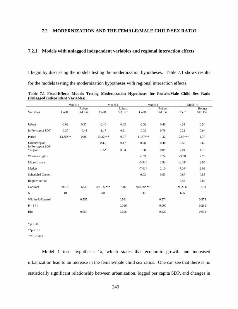
249
7.2 MODERNIZATION AND THE FEMALE/MALE CHILD SEX RATIO
7.2.1 Models with unlagged independent variables and regional interaction effects
I begin by discussing the models testing the modernization hypotheses. Table 7.1 shows results
for the models testing the modernization hypotheses with regional interaction effects.
Table 7.1 Fixed-Effects Models Testing Modernization Hypotheses for Female/Male Child Sex Ratio (Unlagged Independent Variables)
Model 1 Model 2 Model 3 Model 4
Variables Coeff. Robust
Std. Err. Coeff. Robust
Std. Err. Coeff. Robust
Std. Err. Coeff. Robust
Std. Err.
Urban -0.03 0.27 -0.40 0.42 -0.53 0.46 -.38 0.54
ln(Per capita SDP) -0.37 -0.48 -1.17 0.61 -0.32 0.76 0.21 0.94
Period -13.85*** 0.86 -13.22*** 0.97 -11.87*** 1.32 -12.87*** 1.77
Urban*region 0.43 0.47 0.78 0.48 0.53 0.60 ln(Per capita SDP) * region 1.65* 0.84 1.08 0.89 -.19 1.13
Women's rights -3.24 2.74 -3.30 2.76
Microfinance -5.92* 2.94 -6.03* 2.95
Market -7.01* 2.10 -7.20* 3.02
Scheduled Castes 0.93 0.53 0.87 0.53
Region*period 2.54 2.02
Constant 996.79 6.50 1001.22*** 7.16 982.89*** 982.86 13.39
N 681 681 636 636
Within-R-Squared 0.555 0.561 0.574 0.575
P > | F | 0.016 0.000 0.211
Rho 0.657 0.596 0.630 0.633
* p < .05
**p < .01
***p < .001
Model 1 tests hypothesis 1a, which states that economic growth and increased
urbanization lead to an increase in the female/male child sex ratios. One can see that there is no
statistically significant relationship between urbanization, logged per capita SDP, and changes in
250
the child sex ratio. Time is the only variable that is statistically significantly related to the child
sex ratio (p < .001). For the passage of each decade, the female/male child sex ratio decreases by
almost 14 females per 1,000 males. Model two tests the hypothesis that urbanization and
increased per capita SDP will have a greater effect on increases in the child sex ratio in southern
districts than in northern districts. Although the percentage of population living in urban areas
has no statistically significant impact on changes in the child sex ratio, the interaction effect
between logged per capita SDP and region is statistically significantly related to variation in the
female/male child sex ratio. In southern regions, the female/male child sex ratio increases by
about 1.7 females per 1,000 males more than in northern regions for every tenfold increase in per
capita SDP. Although the difference is statistically significant (p < .05), and thus not due to
chance, substantively this is a very small difference. The F-test shows that there is a statistically
significant difference between the second model and the first model (p < .05), indicating that the
second model is a better fit for the data even though it includes more variables and the same
number of observations. The third model controls for the effects of women’s rights programs,
market programs, microfinance programs, and the percentage of population comprised of
Scheduled Castes. Once these variables are controlled for, the interaction effect of logged per
capita SDP and region is no longer statistically significant. The presence of microfinance
programs and market programs are both significantly and negatively related to the female/male
child sex ratio (p < .05). The passage of time has the strongest negative effect on the
female/male child sex ratio ratio (p < .001), with a decrease of almost 12 females per 1,000
males for each passing decade. The F-statistic reveals that there is a statistically significant
difference between the third model and the second model (p < .001), which means that the third
model is a better fit for the data than the previous model. There is no statistically significant
251
difference between this model and the fourth model, which controls for the interaction effect of
region and time period. Therefore, the third model, which controls for the presence of women’s
rights programs, market programs, microfinance programs, and percentage of population
comprised of Scheduled Castes, is more parsimonious than the fourth model. This entire model
is strongly related to within-district variation in the female/male child sex ratio (R-squared =
0.57). Therefore, one can conclude that there is no statistically significant relationship between
values of logged per capita SDP that are contemporaneous with variation in the female/male
child sex ratio, and one can also conclude that there is no significant relationship between the
percentage of population in urbanized areas and the child sex ratio. It is useful to compare this
set of models that includes regional interaction effects with models that include state-wise
interaction effects to determine whether there is between-state variation in the female/male child
sex ratio. I turn now to a discussion of these models.
7.2.2 Models with unlagged independent variables and state-wise interaction effects
Table 7.2 shows model results for the modernization hypotheses that include state-wise
dichotomous variables rather than the region dichotomous variable. Model 2 of Table 7.2 is very
similar to model 2 of Table 7.1 Fixed-Effects Models Testing Modernization Hypotheses for
Female/Male Child Sex Ratio (Unlagged Independent Variables). In both models, the coefficient
for time period is highly significant (p < .001) and is of the same magnitude (-13.85). In the
second model of Table 7.1, the interaction term of logged per capita SDP*region is significantly
related to variation in the child sex ratio. Likewise, in the second model of Table 7.2 the
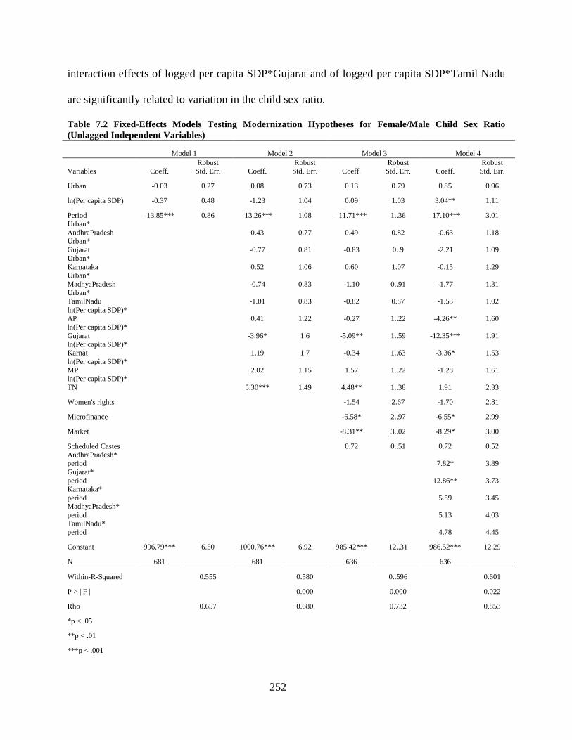
252
interaction effects of logged per capita SDP*Gujarat and of logged per capita SDP*Tamil Nadu
are significantly related to variation in the child sex ratio.
Table 7.2 Fixed-Effects Models Testing Modernization Hypotheses for Female/Male Child Sex Ratio (Unlagged Independent Variables)
Model 1 Model 2 Model 3 Model 4
Variables Coeff. Robust
Std. Err. Coeff. Robust
Std. Err. Coeff. Robust
Std. Err. Coeff. Robust
Std. Err.
Urban -0.03 0.27 0.08 0.73 0.13 0.79 0.85 0.96
ln(Per capita SDP) -0.37 0.48 -1.23 1.04 0.09 1.03 3.04** 1.11
Period -13.85*** 0.86 -13.26*** 1.08 -11.71*** 1..36 -17.10*** 3.01 Urban* AndhraPradesh 0.43 0.77 0.49 0.82 -0.63 1.18 Urban* Gujarat -0.77 0.81 -0.83 0..9 -2.21 1.09 Urban* Karnataka 0.52 1.06 0.60 1.07 -0.15 1.29 Urban* MadhyaPradesh -0.74 0.83 -1.10 0..91 -1.77 1.31 Urban* TamilNadu -1.01 0.83 -0.82 0.87 -1.53 1.02 ln(Per capita SDP)* AP 0.41 1.22 -0.27 1..22 -4.26** 1.60 ln(Per capita SDP)* Gujarat -3.96* 1.6 -5.09** 1..59 -12.35*** 1.91 ln(Per capita SDP)* Karnat 1.19 1.7 -0.34 1..63 -3.36* 1.53 ln(Per capita SDP)* MP 2.02 1.15 1.57 1..22 -1.28 1.61 ln(Per capita SDP)* TN 5.30*** 1.49 4.48** 1..38 1.91 2.33
Women's rights -1.54 2.67 -1.70 2.81
Microfinance -6.58* 2..97 -6.55* 2.99
Market -8.31** 3..02 -8.29* 3.00
Scheduled Castes 0.72 0..51 0.72 0.52 AndhraPradesh* period 7.82* 3.89 Gujarat* period 12.86** 3.73 Karnataka* period 5.59 3.45 MadhyaPradesh* period 5.13 4.03 TamilNadu* period 4.78 4.45
Constant 996.79*** 6.50 1000.76*** 6.92 985.42*** 12..31 986.52*** 12.29
N 681 681 636 636
Within-R-Squared 0.555 0.580 0..596 0.601
P > | F | 0.000 0.000 0.022
Rho 0.657 0.680 0.732 0.853
*p < .05
**p < .01
***p < .001
253
For every tenfold increase in per capita SDP, the child sex ratio in Gujarat state is lower than the
child sex ratio of Rajasthan (the reference category) by 4 females per 1,000 males. In Tamil
Nadu, the child sex ratio is higher than that of Rajasthan by about 5 females per 1,000 males for
every tenfold increase in per capita SDP.
Since Gujarat state is in the north and Tamil Nadu is in the south, the direction of these
relationships fits the results of logged per capita SDP*region in Table 7.1. This is because in
table 7.1, the child sex ratio is higher in southern areas than in northern areas for every tenfold
increase in per capita SDP. Model 3 of table 7.2 is also similar to model 3 of table 7.1. In both
models, the coefficient for period is highly statistically significant (p < .001) and of the same
magnitude. The relationships between women’s market programs and women’s microfinance
programs and variation in the child sex ratio are negative and statistically significant in model 3
of both tables 7.1 and 7.2, although at somewhat different significance levels. However, whereas
the interaction effect of logged per capita SDP*region is no longer statistically significant in
model 3 of table 7.1, the interaction effects of logged per capita SDP*Gujarat and logged per
capita SDP*Tamil Nadu remain statistically significant. Unlike the fourth model of table 7.1, the
fourth model of table 7.2 is statistically significantly different from the third model. Model 4 in
table 7.2 includes interaction terms for each state*period. The interaction effects for logged per
capita SDP*region and region*period are not significant in model 4 of table 7.1. In contrast, in
model 4 of table 7.2 the interaction effects of logged per capita SDP*Andhra Pradesh, logged per
capita SDP*Gujarat, and logged per capita SDP*Karnataka are all statistically significant.
Moreover, in model 4 of table 7.2, the interaction effects of Andhra Pradesh*period and
Gujarat*period are also statistically significantly related to changes in the child sex ratio. The
interaction effects of the logged per capita SDP*state variables seem to offset the interaction
254
effects of the state*period variables. For instance, in Rajasthan the child sex ratio increases by
about 3 females per 1,000 males with every tenfold increase in per capita SDP. For every
tenfold increase in per capita SDP, the child sex ratio in Gujarat state is lower than that of
Rajasthan state by about 12 females per 1,000 males, and the child sex ratio in Andhra Pradesh is
lower than that of Rajasthan by about 4 females per 1,000 males. However, with the passing of
each decade, the child sex ratio in Rajasthan decreases by about 17 females per 1,000 males. In
Gujarat state, the passing of each decade is associated with a child sex ratio that is higher than
that of Rajasthan by about 13 females per 1,000 males, and in Andhra Pradesh the passage of
each decade is associated with a child sex ratio that is higher than that of Rajasthan by about 8
females per 1,000 males. This means that the passage of each decade leads to a decrease in the
child sex ratio in Gujarat state of about 4 females per 1,000 males, and a decrease in the child sex
ratio in Andhra Pradesh state of about 9 females per 1,000 males. Also, the interaction effects of
log per capita SDP*Madhya Pradesh, Madhya Pradesh*period, and Karnataka*period are not
statistically significant. It seems plausible that the reason why the interaction effects of logged
per capita SDP*region and region*period are not statistically significant in the fourth model of
table 7.1 is that the state*region variables of table 7.2 have a mediating effect on the logged per
capita SDP*state variables. It is important to examine the results for the models with lagged
values of the independent variables. Models with unlagged independent variables can determine
if the values of any of the independent variables change along with variation in the child sex
ratio, but they cannot establish causality between the independent variables and the female/male
child sex ratio.
255
7.2.3 Models with lagged independent variables and regional interaction effects
Table 7.3 shows the results for the fixed-effects models with lagged independent variables that
test the modernization hypotheses. Unlike the models with unlagged independent variables, the
results of Table 7.3 show that there is a statistically significant relationship between lagged log
per capita SDP and the female/male child sex ratio (p < .01 for models 1 and 2, p < .05 for model
3). However, the lagged log per capita SDP leads to a decrease in the child sex ratio, which is
the opposite of what the modernization hypotheses predict. Once the interaction effects of
lagged log per capita SDP*region and lagged urbanization*region are controlled for in the
second model, the negative impact of lagged log per capita SDP on female/male child sex ratio
increases. A tenfold increase in lagged log per capita SDP leads to a decrease of almost 10
females per 1,000 males (p < .01). The passage of time also has a strong negative effect on the
child sex ratio (p < .001), with a decrease in the child sex ratio of about 10 females/1,000 males
for every decade that passes. The second model is statistically significantly better than the first
model (p < .05), and all of the independent variables taken as a whole have a strong relationship
with within-district variation in the female/male child sex ratio (R-squared = .52).
The third model, which controls for the presence of women’s rights programs, market
programs, microfinance programs, percentage of population comprised of Scheduled Castes, and
the interaction effect of region*time period, is not statistically significantly different from the
second model. Therefore, the second model is more parsimonious than the third model, and is
the best fit for the data. Because lagged log per capita SDP causes a decrease in the female/male
child sex ratio rather than an increase in the child sex ratio, there is no evidence supporting the
modernization hypotheses that economic growth leads to an increase in the female/male child
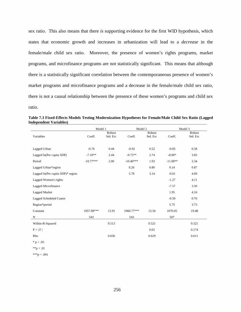
256
sex ratio. This also means that there is supporting evidence for the first WID hypothesis, which
states that economic growth and increases in urbanization will lead to a decrease in the
female/male child sex ratio. Moreover, the presence of women’s rights programs, market
programs, and microfinance programs are not statistically significant. This means that although
there is a statistically significant correlation between the contemporaneous presence of women’s
market programs and microfinance programs and a decrease in the female/male child sex ratio,
there is not a causal relationship between the presence of these women’s programs and child sex
ratio.
Table 7.3 Fixed-Effects Models Testing Modernization Hypotheses for Female/Male Child Sex Ratio (Lagged Independent Variables)
Model 1 Model 2 Model 3
Variables Coeff. Robust
Std. Err. Coeff. Robust
Std. Err. Coeff. Robust
Std. Err.
Lagged Urban -0.76 0.44 -0.92 0.52 -0.83 0.58
Lagged ln(Per capita SDP) -7.10** 2.44 -9.75** 2.74 -8.00* 3.83
Period -10.77*** 2.00 -10.40*** 1.93 -11.00** 3.34
Lagged Urban*region 0.26 0.80 0.14 0.87
Lagged ln(Per capita SDP)* region 5.78 3.14 -0.61 4.69
Lagged Women's rights -1.27 4.11
Lagged Microfinance -7.57 3.50
Lagged Market 1.95 4.16
Lagged Scheduled Castes -0.59 0.76
Region*period 5.75 3.73
Constant 1057.08*** 15.91 1060.77*** 15.50 1070.05 19.48
N 543 543 507
Within-R-Squared 0.513 0.521 0.521
P > | F | 0.02 0.174
Rho 0.656 0.629 0.611
* p < .05
**p < .01
***p < .001
257
7.2.4 Models with lagged independent variables and state-wise interaction effects
Table 7.4 shows the results for the lagged models testing the modernization hypotheses that
include the state-wise interaction terms. In model 2 of table 7.4, lagged log per capita SDP is not
statistically significantly related to variation in the child sex ratio, which is in contrast to model
two of table 7.3. Whereas in Table 7.3 the interaction term of lagged log per capita SDP*region
is not statistically significant, in table 7.4 one of the lagged log per capita SDP*state variables is
statistically significant. In model 2 of table 7.4, there is a statistically significant relationship
between lagged log per capita SDP and Madhya Pradesh (p < .05). In the second model of both
tables 7.3 and 7.4, there is a negative and statistically significant relationship between time
period and change in the child sex ratio (p < .001). Model 4 of table 7.4, which includes
interaction terms for each state*period, is substantially different than model 3 of table 7.3. While
there is no statistically significant difference between model 3 and model 2 in table 7.3, there is a
statistically significant difference between model 4 and model 3 in table 7.4 (p < .001). Model 3
of table 7.3 includes the lagged value for the interaction effect of region*period, while model 4
of table 7.4 includes the lagged values for the interaction effects of the state*period variables.
Once these new variables are included in the model, lagged log per capita SDP*Andhra Pradesh,
lagged log per capita SDP*Gujarat, lagged log per capita SDP*Madhya Pradesh, and lagged log
per capita SDP*Tamil Nadu are all statistically significantly related to variation in the child sex
ratio. Just as in model 4 of table 7.2, in model 4 of table 7.4 the interaction effects of the
state*period variables seem to have a mediating effect on the interaction effects of the lagged log
per capita SDP*state variables. For instance, for every tenfold increase in per capita SDP, the
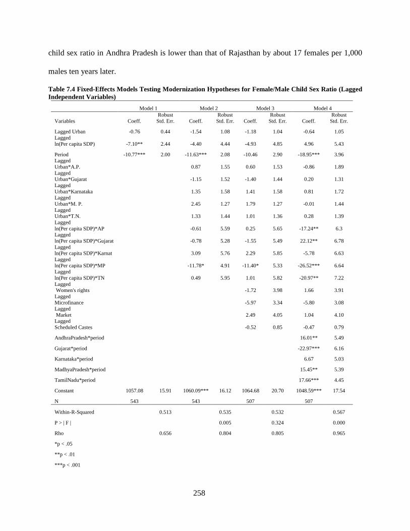
258
child sex ratio in Andhra Pradesh is lower than that of Rajasthan by about 17 females per 1,000
males ten years later.
Table 7.4 Fixed-Effects Models Testing Modernization Hypotheses for Female/Male Child Sex Ratio (Lagged Independent Variables)
Model 1 Model 2 Model 3 Model 4
Variables Coeff. Robust
Std. Err. Coeff. Robust
Std. Err. Coeff. Robust
Std. Err. Coeff. Robust
Std. Err.
Lagged Urban -0.76 0.44 -1.54 1.08 -1.18 1.04 -0.64 1.05 Lagged ln(Per capita SDP) -7.10** 2.44 -4.40 4.44 -4.93 4.85 4.96 5.43
Period -10.77*** 2.00 -11.63*** 2.08 -10.46 2.90 -18.95*** 3.96 Lagged Urban*A.P. 0.87 1.55 0.60 1.53 -0.86 1.89 Lagged Urban*Gujarat -1.15 1.52 -1.40 1.44 0.20 1.31 Lagged Urban*Karnataka 1.35 1.58 1.41 1.58 0.81 1.72 Lagged Urban*M. P. 2.45 1.27 1.79 1.27 -0.01 1.44 Lagged Urban*T.N. 1.33 1.44 1.01 1.36 0.28 1.39 Lagged ln(Per capita SDP)*AP -0.61 5.59 0.25 5.65 -17.24** 6.3 Lagged ln(Per capita SDP)*Gujarat -0.78 5.28 -1.55 5.49 22.12** 6.78 Lagged ln(Per capita SDP)*Karnat 3.09 5.76 2.29 5.85 -5.78 6.63 Lagged ln(Per capita SDP)*MP -11.78* 4.91 -11.40* 5.33 -26.52*** 6.64 Lagged ln(Per capita SDP)*TN 0.49 5.95 1.01 5.82 -20.97** 7.22 Lagged Women's rights -1.72 3.98 1.66 3.91 Lagged Microfinance -5.97 3.34 -5.80 3.08 Lagged Market 2.49 4.05 1.04 4.10 Lagged Scheduled Castes -0.52 0.85 -0.47 0.79
AndhraPradesh*period 16.01** 5.49
Gujarat*period -22.97*** 6.16
Karnataka*period 6.67 5.03
MadhyaPradesh*period 15.45** 5.39
TamilNadu*period 17.66*** 4.45
Constant 1057.08 15.91 1060.09*** 16.12 1064.68 20.70 1048.59*** 17.54
N 543 543 507 507
Within-R-Squared 0.513 0.535 0.532 0.567
P > | F | 0.005 0.324 0.000
Rho 0.656 0.804 0.805 0.965
*p < .05
**p < .01
***p < .001
259
However, with the passage of each decade, the child sex ratio in Andhra Pradesh is higher than
the child sex ratio of Rajasthan by about 16 females per 1,000 males. Likewise, for every tenfold
increase in per capita SDP, the child sex ratio in Gujarat is higher than the child sex ratio in
Rajasthan by about 22 females per 1,000 males ten years later (p < .01). With the passage of
each decade, however, the child sex ratio in Gujarat state is lower than that of Rajasthan by about
23 females per 1,000 males (p < .001). The interaction effects for Madhya Pradesh and Tamil
Nadu follow this same general pattern. One unusual finding is that in Gujarat state, although
contemporaneous values of log per capita SDP are correlated with a female/male child sex ratio
that is lower than that of Rajasthan, lagged values of log per capita SDP lead to a child sex ratio
in Gujarat that is higher than that in Rajasthan. Moreover, the state-wise interaction terms for
lagged log per capita SDP and time period do not necessarily fit the expected regional pattern.
That is, the coefficients for lagged log per capita SDP*Andhra Pradesh and lagged log per capita
SDP*Tamil Nadu are negative, even though both states are in the southern region of India. This
seems to indicate that it is the state-wise effects of logged per capita SDP (either lagged or
unlagged) on variation of the child sex ratio that matters rather than the regional (northern versus
southern) effects of logged per capita SDP on variation in child sex ratio.
7.3 WOMEN-IN-DEVELOPMENT AND FEMALE/MALE CHILD SEX RATIO
7.3.1 Models with unlagged independent variables and regional interaction effects
Table 7.5 shows results for models that test the WID hypotheses (hypotheses 2b through 2d) and
also include regional interaction effects. As mentioned in the last section, there is a statistically
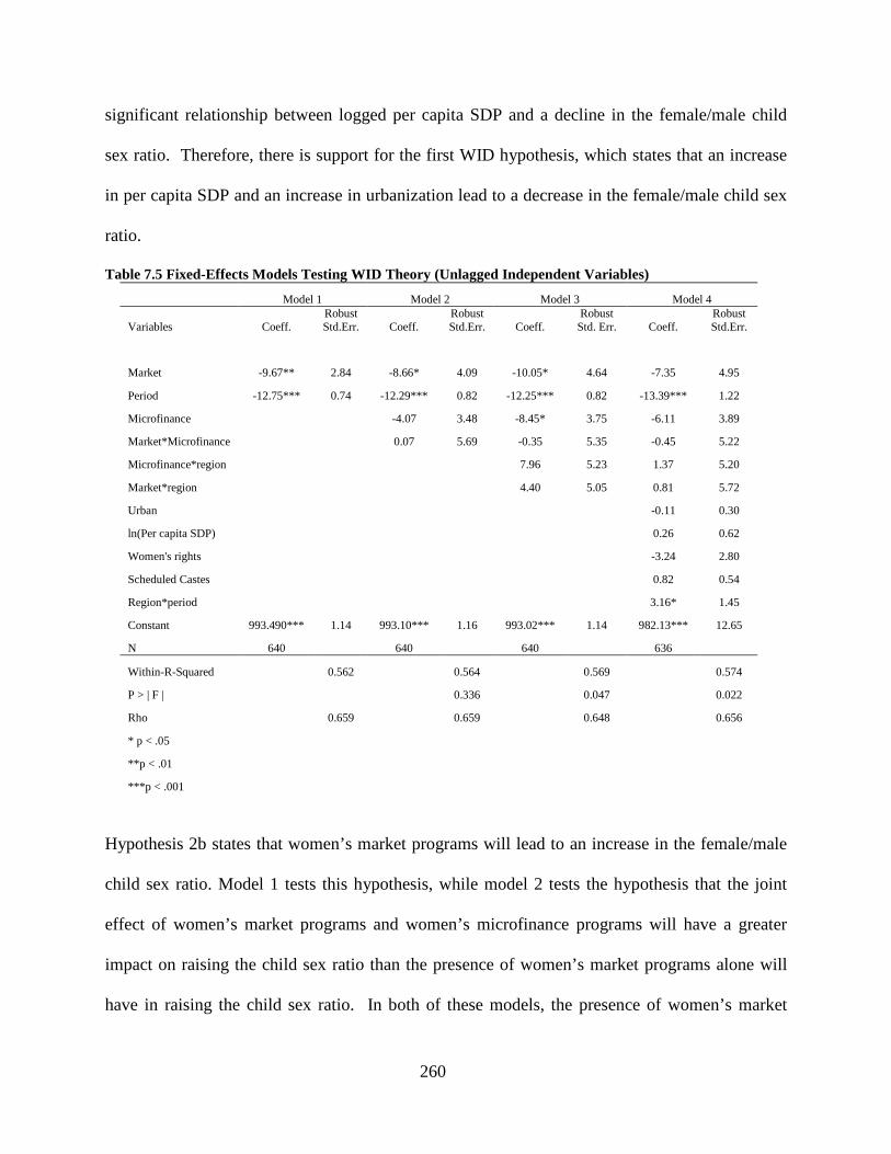
260
significant relationship between logged per capita SDP and a decline in the female/male child
sex ratio. Therefore, there is support for the first WID hypothesis, which states that an increase
in per capita SDP and an increase in urbanization lead to a decrease in the female/male child sex
ratio.
Table 7.5 Fixed-Effects Models Testing WID Theory (Unlagged Independent Variables)
Model 1 Model 2 Model 3 Model 4
Variables Coeff. Robust Std.Err. Coeff.
Robust Std.Err. Coeff.
Robust Std. Err. Coeff.
Robust Std.Err.
Market -9.67** 2.84 -8.66* 4.09 -10.05* 4.64 -7.35 4.95
Period -12.75*** 0.74 -12.29*** 0.82 -12.25*** 0.82 -13.39*** 1.22
Microfinance -4.07 3.48 -8.45* 3.75 -6.11 3.89
Market*Microfinance 0.07 5.69 -0.35 5.35 -0.45 5.22
Microfinance*region 7.96 5.23 1.37 5.20
Market*region 4.40 5.05 0.81 5.72
Urban -0.11 0.30
ln(Per capita SDP) 0.26 0.62
Women's rights -3.24 2.80
Scheduled Castes 0.82 0.54
Region*period 3.16* 1.45
Constant 993.490*** 1.14 993.10*** 1.16 993.02*** 1.14 982.13*** 12.65
N 640 640 640 636
Within-R-Squared 0.562 0.564 0.569 0.574
P > | F | 0.336 0.047 0.022
Rho 0.659 0.659 0.648 0.656
* p < .05
**p < .01
***p < .001
Hypothesis 2b states that women’s market programs will lead to an increase in the female/male
child sex ratio. Model 1 tests this hypothesis, while model 2 tests the hypothesis that the joint
effect of women’s market programs and women’s microfinance programs will have a greater
impact on raising the child sex ratio than the presence of women’s market programs alone will
have in raising the child sex ratio. In both of these models, the presence of women’s market
261
programs is statistically significantly related to a decrease in the child sex ratio. However, the F-
statistic indicates that there is no statistically significant difference between model 2 and model 1
(p > .05). Moreover, there is no significant relationship between the interaction effect of
market*microfinance programs and variation in child sex ratio. Therefore, there is no evidence
in support of the hypothesis that the joint effect of women’s market programs and women’s
microfinance programs is greater in raising the child sex ratio than the impact of market
programs alone.
Model 3 tests hypothesis 2d, which states that the presence of women’s market and
microfinance programs will have a greater positive impact on the female/male child sex ratio in
southern districts than in northern districts. Although this model is statistically significantly
better than model 2 (p < .05), the relationships between the interaction effects of market
programs*region and microfinance programs* region and variation in the female/male child sex
ratio are not statistically significant. Once these interaction effects are controlled for, however,
the presence of market programs and microfinance programs are significantly related to a
decrease in the child sex ratio in the third model (p < .05). In the fourth model, once I control for
logged per capita SDP, percentage of population comprised of Scheduled Castes, the presence of
women’s rights programs, and the interaction effect of region*time period, the presence of
market programs and microfinance programs are no longer statistically significant. In this final
model, the passage of time and the interaction effect of region*time period are the only variables
that are significantly related to a decrease in the female/male child sex ratio. The passage of
each decade is correlated with a decrease in the child sex ratio of about 13 females per 1,000
males in northern regions, and a decrease in the child sex ratio of about 10 females per 1,000
males in southern regions. There is a statistically significant difference between this model and
262
model 3 (p < .05). This model with all of the variables taken together is strongly related to
variation in the female/male child sex ratio (R-squared = .57). Overall, the results of these
models do not lend support to the WID hypotheses related to the presence of women’s programs.
The WID hypotheses predict that the presence of women’s market programs will have a positive
impact on the female/male child sex ratio, and that the joint effect of women’s market programs
and microfinance programs will have an even greater positive effect on the child sex ratio than
the effect of market programs alone. However, once all other variables are controlled for, there
is no relationship between the presence of women’s market programs nor the presence of
microfinance programs with the female/male child sex ratio. However, the results of the
modernization models show that an increase in log per capita SDP leads to a decrease in the
female/male child sex ratio. This does support the first WID hypothesis that states that an
increase in economic growth will lead to a decrease in the child sex ratio. While there is no
statistically significant relationship between log per capita SDP and contemporaneous variation
in the female/male child sex ratio, an increase in log per capita SDP leads to a decline in the
child sex ratio ten years later. With every tenfold increase in the per capita SDP, the
female/male child sex ratio declines by about 10 females/1,000 males a decade later. Moreover,
the passage of each decade is correlated with a decrease in the child sex ratio of about 10
females/1,000 males.
7.3.2 Models with unlagged independent variables and state-wise interaction effects
Table 7.6 shows model results for the WID hypotheses that include the state-wise interaction
terms rather than the region-wise interaction terms. Since the first two models do not include
263
interaction terms for market programs*state, microfinance programs*state, or state*period, these
models are the same as the first two models in Table 7.5. Model 3 of table 7.6, which includes
interaction effects for market programs*state and microfinance programs*state, is similar to
model 3 in table 7.5. In model 3 of both table 7.5 and 7.6, there is a statistically significant
relationship between the main effects women’s market programs and the main effects of
microfinance programs and variation in the child sex ratio at the 0.05 level. There is also a
statistically significant relationship between time period and change in the child sex ratio at the
0.001 level in both models. In the third model of both tables 7.5 and 7.6, the passage of each
decade is significantly related to a decrease in the child sex ratio of about 12 females per 1,000
males. There is a statistically significant difference between the third and second models of both
tables 7.5 and 7.6.
The fourth model of Table 7.6 diverges more from the fourth model of Table 7.5. In the
fourth model of table 7.5, there is a statistically significant relationship between only two
independent variables and the child sex ratio: time period and region*period. In the fourth model
of table 7.6, however, there are four independent variables that are statistically significantly
related to variation in the child sex ratio: women’s market programs, women’s microfinance
programs, time period, and the interaction effect of Gujarat state*period. While in table 7.5 the
coefficient of time period increases in magnitude somewhat from the third to the fourth model, in
table 7.6 the magnitude of the coefficient for time period decreases from the third to the fourth
model. In the fourth model of table 7.6 the coefficients for market programs and microfinance
programs increase in magnitude, and continue to have a negative relationship with the
female/male child sex ratio.
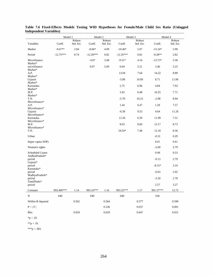
264
Table 7.6 Fixed-Effects Models Testing WID Hypotheses for Female/Male Child Sex Ratio (Unlagged Independent Variables)
Model 1 Model 2 Model 3 Model 4
Variables Coeff. Robust
Std. Err. Coeff. Robust
Std. Err. Coeff. Robust
Std. Err. Coeff. Robust
Std. Err.
Market -9.67** 2.84 -8.66* 4.09 -10.46* 5.07 -15.24* 5.99
Period -12.75*** 0.74 -12.29*** 0.82 -12.35*** 0.81 -9.28** 2.82
Microfinance -4.07 3.48 -9.51* 4.16 -13.73* 5.58 Market* microfinance 0.07 5.69 0.04 5.21 2.46 5.25 Market* A.P. 13.04 7.64 14.22 8.89 Market* Gujarat -5.89 10.09 8.71 11.06 Market* Karnataka 2.75 6.96 4.84 7.93 Market* M.P. 3.45 6.48 10.25 7.71 Market* T.N. -5.79 10.23 -2.98 8.94 Microfinance* A.P. 1.44 6.47 1.29 7.57 Microfinance* Gujarat -6.58 9.53 4.64 11.26 Microfinance* Karnataka 11.56 6.39 11.99 7.51 Microfinance* M.P. 8.03 8.00 13.17 8.73 Microfinance* T.N. 18.54* 7.48 12.18 8.36
Urban -0.31 0.29
ln(per capita SDP) 0.01 0.61
Women's rights -2.60 2.79
Scheduled Castes 0.49 0.53 AndhraPradesh* period -0.13 2.79 Gujarat* period -8.15* 3.10 Karnataka* period -0.63 2.92 MadhyaPradesh* period -3.20 2.78 TamilNadu* period 2.57 3.27
Constant 993.490*** 1.14 993.10*** 1.16 993.32*** 1.17 991.57*** 12.72
N 640 640 640 636
Within-R-Squared 0.562 0.564 0.577 0.590
P > | F | 0.336 0.037 0.001
Rho 0.659 0.659 0.647 0.651
*p < .05
**p < .01
***p < .001
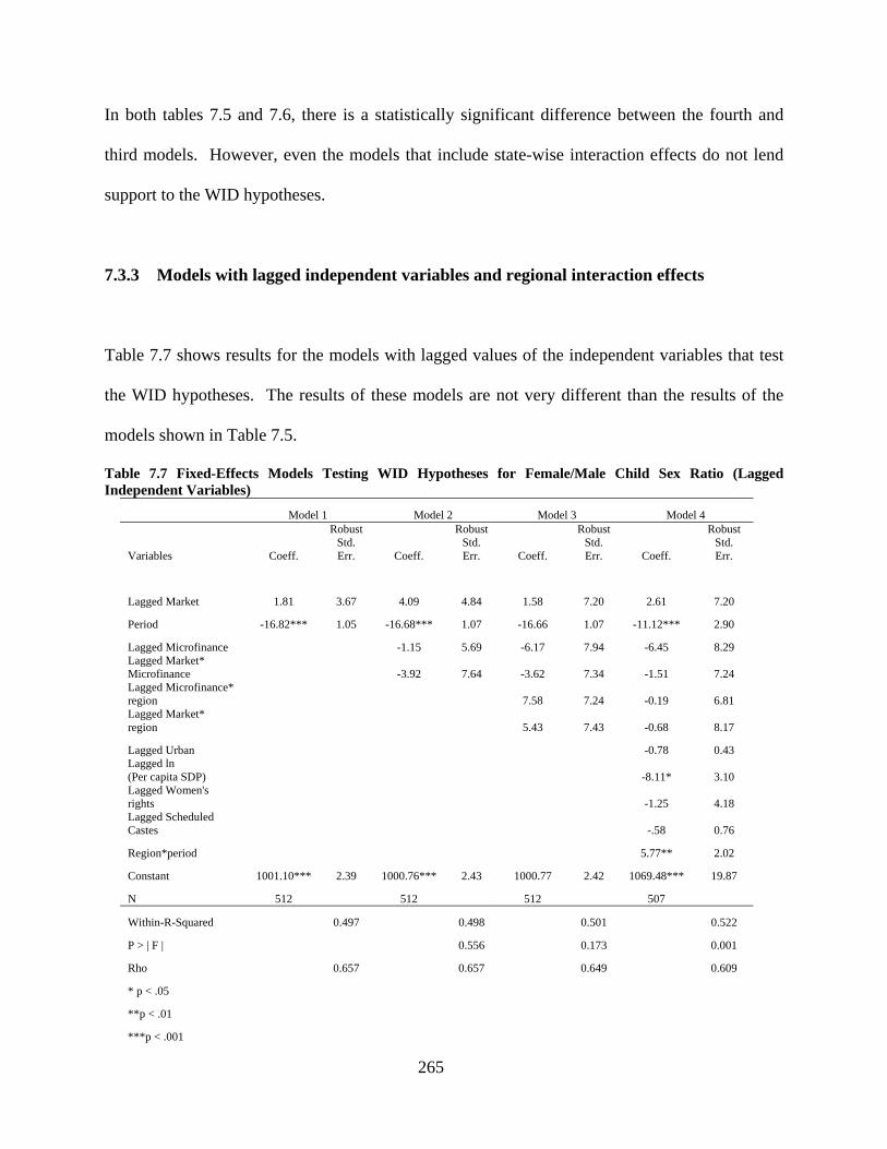
265
In both tables 7.5 and 7.6, there is a statistically significant difference between the fourth and
third models. However, even the models that include state-wise interaction effects do not lend
support to the WID hypotheses.
7.3.3 Models with lagged independent variables and regional interaction effects
Table 7.7 shows results for the models with lagged values of the independent variables that test
the WID hypotheses. The results of these models are not very different than the results of the
models shown in Table 7.5.
Table 7.7 Fixed-Effects Models Testing WID Hypotheses for Female/Male Child Sex Ratio (Lagged Independent Variables)
Model 1 Model 2 Model 3 Model 4
Variables Coeff.
Robust Std. Err. Coeff.
Robust Std. Err. Coeff.
Robust Std. Err. Coeff.
Robust Std. Err.
Lagged Market 1.81 3.67 4.09 4.84 1.58 7.20 2.61 7.20
Period -16.82*** 1.05 -16.68*** 1.07 -16.66 1.07 -11.12*** 2.90
Lagged Microfinance -1.15 5.69 -6.17 7.94 -6.45 8.29 Lagged Market* Microfinance -3.92 7.64 -3.62 7.34 -1.51 7.24 Lagged Microfinance* region 7.58 7.24 -0.19 6.81 Lagged Market* region 5.43 7.43 -0.68 8.17
Lagged Urban -0.78 0.43 Lagged ln (Per capita SDP) -8.11* 3.10 Lagged Women's rights -1.25 4.18 Lagged Scheduled Castes -.58 0.76
Region*period 5.77** 2.02
Constant 1001.10*** 2.39 1000.76*** 2.43 1000.77 2.42 1069.48*** 19.87
N 512 512 512 507
Within-R-Squared 0.497 0.498 0.501 0.522
P > | F | 0.556 0.173 0.001
Rho 0.657 0.657 0.649 0.609
* p < .05
**p < .01
***p < .001
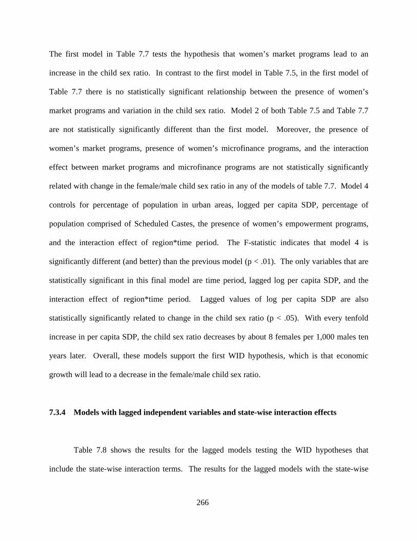
266
The first model in Table 7.7 tests the hypothesis that women’s market programs lead to an
increase in the child sex ratio. In contrast to the first model in Table 7.5, in the first model of
Table 7.7 there is no statistically significant relationship between the presence of women’s
market programs and variation in the child sex ratio. Model 2 of both Table 7.5 and Table 7.7
are not statistically significantly different than the first model. Moreover, the presence of
women’s market programs, presence of women’s microfinance programs, and the interaction
effect between market programs and microfinance programs are not statistically significantly
related with change in the female/male child sex ratio in any of the models of table 7.7. Model 4
controls for percentage of population in urban areas, logged per capita SDP, percentage of
population comprised of Scheduled Castes, the presence of women’s empowerment programs,
and the interaction effect of region*time period. The F-statistic indicates that model 4 is
significantly different (and better) than the previous model (p < .01). The only variables that are
statistically significant in this final model are time period, lagged log per capita SDP, and the
interaction effect of region*time period. Lagged values of log per capita SDP are also
statistically significantly related to change in the child sex ratio (p < .05). With every tenfold
increase in per capita SDP, the child sex ratio decreases by about 8 females per 1,000 males ten
years later. Overall, these models support the first WID hypothesis, which is that economic
growth will lead to a decrease in the female/male child sex ratio.
7.3.4 Models with lagged independent variables and state-wise interaction effects
Table 7.8 shows the results for the lagged models testing the WID hypotheses that
include the state-wise interaction terms. The results for the lagged models with the state-wise
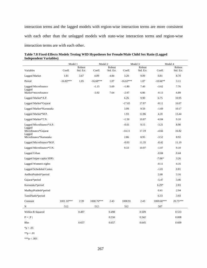
267
interaction terms and the lagged models with region-wise interaction terms are more consistent
with each other than the unlagged models with state-wise interaction terms and region-wise
interaction terms are with each other.
Table 7.8 Fixed-Effects Models Testing WID Hypotheses for Female/Male Child Sex Ratio (Lagged Independent Variables)
Model 1 Model 2 Model 3 Model 4
Variables Coeff. Robust
Std. Err. Coeff. Robust
Std. Err. Coeff. Robust
Std. Err. Coeff. Robust
Std. Err.
Lagged Market 1.81 3.67 4.09 4.84 3.20 9.09 0.81 8.70
Period -16.82*** 1.05 -16.68*** 1.07 -16.63*** 1.07 -10.66** 3.11
Lagged Microfinance -1.15 5.69 -1.80 7.40 -3.62 7.76 Lagged Market*microfinance -3.92 7.64 -2.97 6.86 -0.13 6.89
Lagged Market*A.P. 6.26 9.90 6.75 10.95
Lagged Market*Gujarat -17.65 17.87 -8.11 16.67
Lagged Market*Karnataka 3.99 9.59 -1.69 10.17
Lagged Market*M.P. 1.93 12.86 4.20 13.44
Lagged Market*T.N. -1.50 10.87 -6.84 9.10
Lagged Microfinance*A.P. -0.61 9.15 -3.21 8.90 Lagged Microfinance*Gujarat -14.11 17.19 -4.66 16.82 Lagged Microfinance*Karnataka 2.86 8.95 -3.52 8.92
Lagged Microfinance*M.P. -0.03 11.35 -0.42 11.19
Lagged Microfinance*T.N. 9.33 10.97 -1.07 9.10
Lagged Urban -0.84 0.44
Lagged ln(per capita SDP) -7.06* 3.26
Lagged Women's rights -0.11 4.16
Lagged Scheduled Castes -1.01 0.81
AndhraPradesh*period 2.68 3.16
Gujarat*period -5.47 3.46
Karnataka*period 6.29* 2.83
MadhyaPradesh*period 0.41 2.94
TamilNadu*period 6.33 3.93
Constant 1001.10*** 2.39 1000.76*** 2.43 1000.91 2.43 1069.60*** 20.75***
N 512 512 512 507
Within-R-Squared 0.497 0.498 0.509 0.533
P > | F | 0.556 0.542 0.008
Rho 0.657 0.657 0.645 0.609
*p < .05
**p < .01
***p < .001
268
In both Table 7.7 and Table 7.8, there is no statistically significant difference between model 2
and model 1, and there is also no statistically significant difference between model 3 and model
2. In both tables, there is a statistically significant difference between model 4 and model 3. In
model 4 of table 7.7, there is a statistically significant relationship between three independent
variables and variation in the child sex ratio: time period (p < .001), lagged log per capita SDP
(p < .05), and the interaction effect of region*period (p < .01). Likewise, in model 4 of table 7.8
there is a statistically significant relationship between three independent variables and the child
sex ratio: time period (p < .01), lagged log per capita SDP (p < .05), and the interaction effect of
Karnataka*period (p < .05). Both the coefficients of the interaction terms for region*period and
Karnataka*period are positive and close to the same magnitude. There is a statistically
significant relationship between lagged log per capita SDP and a decrease in the female/male
child sex ratio (p < .05) in model 4 of both tables 7.7 and 7.8. Therefore, the results of the
models in table 7.8 also provide evidence for the WID hypothesis that an increase in lagged log
per capita SDP will lead to a decrease in the female/male child sex ratio.
7.4 GENDER-AND-DEVELOPMENT AND THE FEMALE/MALE CHILD SEX RATIO
7.4.1 Models with unlagged independent variables and regional interaction effects
Table 7.9 shows results for fixed-effects models that test the GAD hypotheses that include
regional interaction effects. Hypothesis 3a states that the presence of women’s rights programs
will lead to an increase in the female/male child sex ratio. The first model tests this hypothesis.
However, as can be seen from the model results, there is no statistically significant relationship
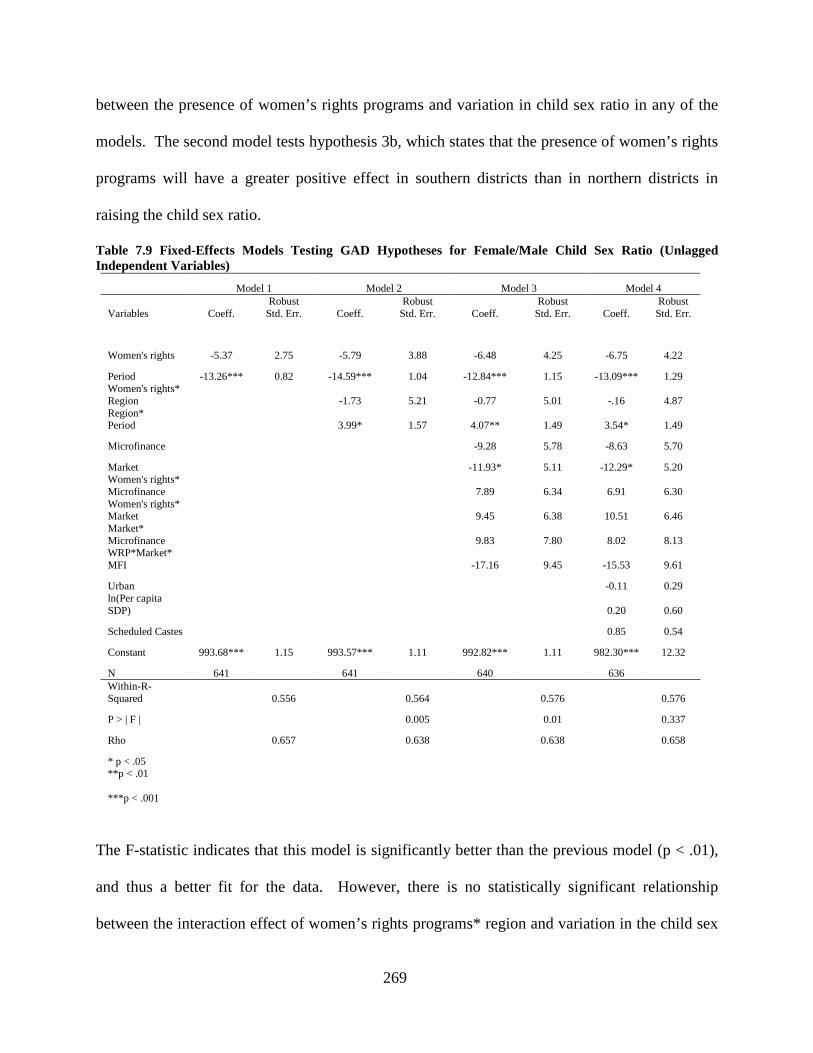
269
between the presence of women’s rights programs and variation in child sex ratio in any of the
models. The second model tests hypothesis 3b, which states that the presence of women’s rights
programs will have a greater positive effect in southern districts than in northern districts in
raising the child sex ratio.
Table 7.9 Fixed-Effects Models Testing GAD Hypotheses for Female/Male Child Sex Ratio (Unlagged Independent Variables)
Model 1 Model 2 Model 3 Model 4
Variables Coeff. Robust
Std. Err. Coeff. Robust
Std. Err. Coeff. Robust
Std. Err. Coeff. Robust
Std. Err.
Women's rights -5.37 2.75 -5.79 3.88 -6.48 4.25 -6.75 4.22
Period -13.26*** 0.82 -14.59*** 1.04 -12.84*** 1.15 -13.09*** 1.29 Women's rights* Region -1.73 5.21 -0.77 5.01 -.16 4.87 Region* Period 3.99* 1.57 4.07** 1.49 3.54* 1.49
Microfinance -9.28 5.78 -8.63 5.70
Market -11.93* 5.11 -12.29* 5.20 Women's rights* Microfinance 7.89 6.34 6.91 6.30 Women's rights* Market 9.45 6.38 10.51 6.46 Market* Microfinance 9.83 7.80 8.02 8.13 WRP*Market* MFI -17.16 9.45 -15.53 9.61
Urban -0.11 0.29 ln(Per capita SDP) 0.20 0.60
Scheduled Castes 0.85 0.54
Constant 993.68*** 1.15 993.57*** 1.11 992.82*** 1.11 982.30*** 12.32
N 641 641 640 636 Within-R-Squared 0.556 0.564 0.576 0.576
P > | F | 0.005 0.01 0.337
Rho 0.657 0.638 0.638 0.658
* p < .05 **p < .01 ***p < .001
The F-statistic indicates that this model is significantly better than the previous model (p < .01),
and thus a better fit for the data. However, there is no statistically significant relationship
between the interaction effect of women’s rights programs* region and variation in the child sex
270
ratio. This model also includes the interaction effect of region*time period, which is statistically
significantly related to variation in the child sex ratio (p < .05). The third model tests hypothesis
3c, which states that the joint effect of women’s rights programs, market programs, and
microfinance programs will have a greater positive impact on the female/male child sex ratio
than women’s rights programs alone will have on the child sex ratio. There is a statistically
significant difference between this model and model 2 (p < .05), indicating that this model is a
better fit for the data than the previous model. The joint effect of women’s rights programs,
market programs, and microfinance programs are not significantly related to variation in the
female/male child sex ratio. However, after controlling for the women’s program interaction
effects, the main effect of the presence of women’s market programs is significantly related to a
decrease in the child sex ratio (p < .05). The final model (model 4) controls for the effects of
percentage of population in urbanized areas, percentage of population comprised of Scheduled
Castes, and logged per capita SDP. However, this model is not statistically significantly
different than model 3. Therefore, model 3 is more parsimonious than model 4, and is the best of
these fixed-effects models.
7.4.2 Models with unlagged independent variables and state-wise interaction effects
The results of Table 7.10, which include interaction effects of women’s rights programs*states
and states*period, are very similar to the results of Table 7.9. In both tables 7.9 and 7.10, the
only model that is not statistically significantly different than previous models is model 4. In
model 2 of both tables, there is a negative and statistically significant relationship between time
period and change in the child sex ratio (p < .001). In model 2 of table 7.9, there is a statistically
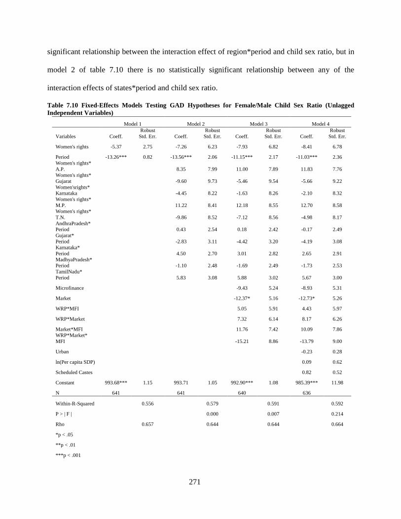
271
significant relationship between the interaction effect of region*period and child sex ratio, but in
model 2 of table 7.10 there is no statistically significant relationship between any of the
interaction effects of states*period and child sex ratio.
Table 7.10 Fixed-Effects Models Testing GAD Hypotheses for Female/Male Child Sex Ratio (Unlagged Independent Variables)
Model 1 Model 2 Model 3 Model 4
Variables Coeff. Robust
Std. Err. Coeff. Robust
Std. Err. Coeff. Robust
Std. Err. Coeff. Robust
Std. Err.
Women's rights -5.37 2.75 -7.26 6.23 -7.93 6.82 -8.41 6.78
Period -13.26*** 0.82 -13.56*** 2.06 -11.15*** 2.17 -11.03*** 2.36 Women's rights* A.P. 8.35 7.99 11.00 7.89 11.83 7.76 Women's rights* Gujarat -9.60 9.73 -5.46 9.54 -5.66 9.22 Women'srights* Karnataka -4.45 8.22 -1.63 8.26 -2.10 8.32 Women's rights* M.P. 11.22 8.41 12.18 8.55 12.70 8.58 Women's rights* T.N. -9.86 8.52 -7.12 8.56 -4.98 8.17 AndhraPradesh* Period 0.43 2.54 0.18 2.42 -0.17 2.49 Gujarat* Period -2.83 3.11 -4.42 3.20 -4.19 3.08 Karnataka* Period 4.50 2.70 3.01 2.82 2.65 2.91 MadhyaPradesh* Period -1.10 2.48 -1.69 2.49 -1.73 2.53 TamilNadu* Period 5.83 3.08 5.88 3.02 5.67 3.00
Microfinance -9.43 5.24 -8.93 5.31
Market -12.37* 5.16 -12.73* 5.26
WRP*MFI 5.05 5.91 4.43 5.97
WRP*Market 7.32 6.14 8.17 6.26
Market*MFI 11.76 7.42 10.09 7.86 WRP*Market* MFI -15.21 8.86 -13.79 9.00
Urban -0.23 0.28
ln(Per capita SDP) 0.09 0.62
Scheduled Castes 0.82 0.52
Constant 993.68*** 1.15 993.71 1.05 992.90*** 1.08 985.39*** 11.98
N 641 641 640 636
Within-R-Squared 0.556 0.579 0.591 0.592
P > | F | 0.000 0.007 0.214
Rho 0.657 0.644 0.644 0.664
*p < .05
**p < .01
***p < .001
272
Time period remains statistically significant in model 3 of both tables, although in both cases the
magnitude of the relationship between time period and child sex ratio decreases somewhat.
Moreover, in model 3 of both tables, there is a negative and statistically significant relationship
between the presence of women’s market programs and variation in the child sex ratio (p < .05).
In model 3 of table 7.9, there continues to be a positive and statistically significant relationship
between the interaction effect of region*period and change in the child sex ratio. In model 3 of
table 7.10, the interaction effect of Tamil Nadu*period is positive and almost significant with a
p-value of 0.054. However, the results of the models described in tables 7.9 and 7.10 do not lend
support to any of the GAD hypotheses.
7.4.3 Models with lagged independent variables and regional interaction effects
Table 7.11 shows the results for the models with lagged independent variables that test the GAD
hypotheses. As with the previous models with unlagged independent variables, table 7.11 shows
that in all of the models, there is no statistically significant relationship between the presence of
women’s rights programs and variation in the female/male child sex ratio. Therefore, there is no
evidence for hypothesis 3a, which states that the presence of women’s rights programs will lead
to an increase in the female/male child sex ratio. Results for these lagged models are very
similar to the results for the unlagged models with regional interaction effects. Time period and
the interaction effect of region*time period continue to be statistically significantly related to
changes in the child sex ratio. Model 3 includes main effects and interaction effects for the
women’s programs, none of which are significantly related to variation in the child sex ratio.
The F-statistic also indicates that this model is not an improved fit compared to the previous
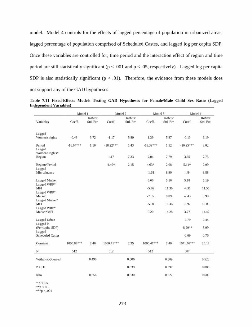
273
model. Model 4 controls for the effects of lagged percentage of population in urbanized areas,
lagged percentage of population comprised of Scheduled Castes, and lagged log per capita SDP.
Once these variables are controlled for, time period and the interaction effect of region and time
period are still statistically significant (p < .001 and p < .05, respectively). Lagged log per capita
SDP is also statistically significant (p < .01). Therefore, the evidence from these models does
not support any of the GAD hypotheses.
Table 7.11 Fixed-Effects Models Testing GAD Hypotheses for Female/Male Child Sex Ratio (Lagged Independent Variables)
Model 1 Model 2 Model 3 Model 4
Variables Coeff. Robust
Std. Err. Coeff. Robust
Std. Err. Coeff. Robust
Std. Err. Coeff. Robust
Std. Err.
Lagged Women's rights 0.43 3.72 -1.17 5.80 1.39 5.87 -0.13 6.19
Period -16.64*** 1.10 -18.22*** 1.43 -18.39*** 1.52 -10.95*** 3.02 Lagged Women's rights* Region 1.17 7.23 2.04 7.79 3.65 7.75
Region*Period 4.40* 2.15 4.63* 2.08 5.11* 2.09 Lagged Microfinance -1.68 8.90 -4.84 8.88
Lagged Market 6.66 5.16 5.18 5.19 Lagged WRP* MFI -5.76 11.36 -4.31 11.55 Lagged WRP* Market -7.85 9.09 -7.43 8.99 Lagged Market* MFI -5.90 10.36 -0.97 10.05 Lagged WRP* Market*MFI 9.20 14.28 3.77 14.42
Lagged Urban -0.79 0.44 Lagged ln (Per capita SDP) -8.20** 3.09 Lagged Scheduled Castes -0.69 0.76
Constant 1000.89*** 2.40 1000.71*** 2.35 1000.47*** 2.40 1071.76*** 20.19
N 512 512 512 507
Within-R-Squared 0.496 0.506 0.509 0.523
P > | F | 0.039 0.597 0.006
Rho 0.656 0.630 0.627 0.609
* p < .05 **p < .01 ***p < .001
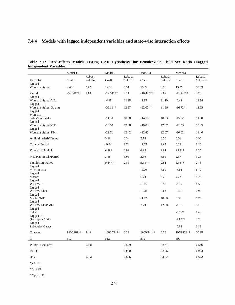
274
7.4.4 Models with lagged independent variables and state-wise interaction effects
Table 7.12 Fixed-Effects Models Testing GAD Hypotheses for Female/Male Child Sex Ratio (Lagged Independent Variables)
Model 1 Model 2 Model 3 Model 4
Variables Coeff. Robust Std. Err. Coeff.
Robust Std. Err. Coeff.
Robust Std. Err. Coeff.
Robust Std. Err.
Lagged Women's rights 0.43 3.72 12.36 9.31 13.72 9.70 13.39 10.03
Period -16.64*** 1.10 -19.63*** 2.11 -19.48*** 2.09 -11.74*** 3.20 Lagged Women's rights*A.P.
-4.15 11.35 -1.97 11.10 -0.43 11.54
Lagged Women's rights*Gujarat -33.12** 12.27 -32.65** 11.96 -36.72** 12.35 Lagged Women's rights*Karnataka -14.59 10.98 -14.16 10.93 -15.92 11.00 Lagged Women's rights*M.P. -10.63 13.38 -10.03 12.97 -11.53 13.35 Lagged Women's rights*T.N. -22.71 12.42 -22.48 12.67 -20.82 11.46
AndhraPradesh*Period 3.06 3.54 2.76 3.50 3.01 3.58
Gujarat*Period -0.94 3.74 -1.07 3.67 0.26 3.80
Karnataka*Period 6.96* 2.98 6.88* 3.01 8.89** 3.37
MadhyaPradesh*Period 3.08 3.06 2.50 3.09 2.37 3.29
TamilNadu*Period 9.44** 2.86 9.63** 2.91 9.55** 2.78 Lagged Microfinance -2.76 6.82 -6.01 6.77 Lagged Market 5.78 5.22 4.73 5.26 Lagged WRP*MFI -3.65 8.53 -2.37 8.55 Lagged WRP*Market -5.28 8.04 -5.32 7.90 Lagged Market*MFI -1.02 10.08 3.85 9.76 Lagged WRP*Market*MFI 2.79 12.90 -2.16 12.81 Lagged Urban -0.79* 0.40 Lagged ln (Per capita SDP) -8.84** 3.22 Lagged Scheduled Castes -0.88 0.81
Constant 1000.89*** 2.40 1000.73*** 2.26 1000.54*** 2.32 1078.12*** 20.65
N 512 512 512 507
Within-R-Squared 0.496 0.529 0.531 0.546
P > | F | 0.000 0.576 0.003
Rho 0.656 0.636 0.637 0.622
*p < .05
**p < .01
***p < .001
275
Table 7.12 shows results for models with lagged independent variables and state-wise interaction
terms. In both Table 7.11 and Table 7.12, time period is negatively and significantly related to a
decrease in the child sex ratio (p < .001) in all the models. Although in model 2 of table 7.11
there is no statistically significant relationship between the interaction effect of women’s rights
programs*region and variation in the child sex ratio, in model 2 of table 7.12 there is a negative
and statistically significant relationship between the interaction effect of women’s rights
programs*Gujarat state and variation in the child sex ratio (p < .01).
Since the magnitude of this relationship is so high and actually increases in model 4, it is
worth noting here. Districts in Gujarat with a women’s rights program present have about 33
fewer females/1,000 males than districts in Rajasthan with a women’s rights program present. In
model 2 of Table 7.11, there is a positive and statistically significant relationship between the
interaction effect of region*period and the child sex ratio (p < .05). Likewise, in model 2 of
Table 7.12, there is a positive and statistically significant relationship between the interaction
effects of Karnataka*period (p < .05), Tamil Nadu*period (p < .01), and change in the child sex
ratio. Since both Karnataka and Tamil Nadu are southern states, the positive relationship
between these two interaction terms and the child sex ratio is consistent with the positive
relationship between region*period and the child sex ratio in model 2 of table 7.11. However,
this does not mean that in Karnataka and Tamil Nadu the passage of time is correlated with an
increase in the child sex ratio. Rather, it means that with each passing decade, the female/male
child sex ratio in Karnataka and Tamil Nadu is higher than it is in Rajasthan, the reference
category. In both tables 7.11 and 7.12, model 3 is not statistically significantly different than
model 2, but model 4 is statistically significantly better than model 3. In model 4 of table 7.12,
the negative relationship between lagged women’s rights programs*Gujarat remains statistically
276
significant, and the magnitude of this relationship is even larger than it is in model 2. In model 4
of table 7.11, region*period remains statistically significant (p < .05), and in model 4 of table
7.12, Karnataka*period and Tamil Nadu*period remain positive and statistically significant (p <
.01). The relationship between lagged log per capita SDP and child sex ratio is negative and
statistically significant in model 4 of both tables, and the magnitude of this relationship in model
4 of table 7.12 is very similar to the magnitude of the relationship in model 4 of table 7.11.
However, in model 4 of table 7.12, lagged percentage of population in urban areas is statistically
significantly related to a decrease in the child sex ratio (p < .05), whereas in model 4 of table
7.11 it is not. The results of the models with both lagged and unlagged independent variables do
not lend any support to the GAD hypotheses.
7.5 NEOLIBERAL HYPOTHESES AND THE FEMALE/MALE CHILD SEX RATIO
7.5.1 Models with unlagged independent variables and regional interaction effects
Table 7.13 presents model results that test the neoliberal hypotheses. Model 1 tests hypothesis
4a, which states that the presence of women’s microfinance programs will lead to an increase in
the female/male child sex ratio. Although there is a statistically significant relationship between
the presence of microfinance programs and variation in the child sex ratio (p < .05), this
relationship is in the opposite direction as expected. Rather than being correlated with higher
child sex ratios, the presence of microfinance programs is correlated with lower child sex ratios.
However, the presence of women’s microfinance programs is not statistically significantly
related to variation in the female/male child sex ratio in any of the subsequent models that
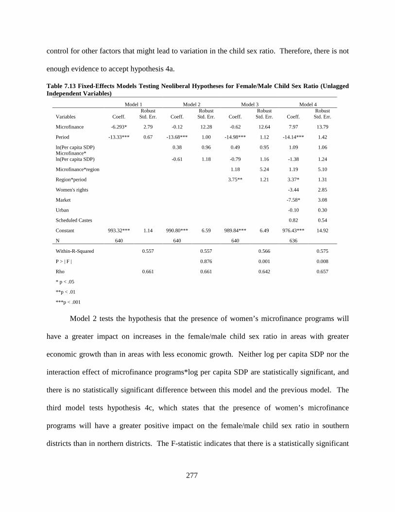
277
control for other factors that might lead to variation in the child sex ratio. Therefore, there is not
enough evidence to accept hypothesis 4a.
Table 7.13 Fixed-Effects Models Testing Neoliberal Hypotheses for Female/Male Child Sex Ratio (Unlagged Independent Variables)
Model 1 Model 2 Model 3 Model 4
Variables Coeff. Robust
Std. Err. Coeff. Robust
Std. Err. Coeff. Robust
Std. Err. Coeff. Robust
Std. Err.
Microfinance -6.293* 2.79 -0.12 12.28 -0.62 12.64 7.97 13.79
Period -13.33*** 0.67 -13.68*** 1.00 -14.98*** 1.12 -14.14*** 1.42
ln(Per capita SDP) 0.38 0.96 0.49 0.95 1.09 1.06 Microfinance* ln(Per capita SDP) -0.61 1.18 -0.79 1.16 -1.38 1.24
Microfinance*region 1.18 5.24 1.19 5.10
Region*period 3.75** 1.21 3.37* 1.31
Women's rights -3.44 2.85
Market -7.58* 3.08
Urban -0.10 0.30
Scheduled Castes 0.82 0.54
Constant 993.32*** 1.14 990.80*** 6.59 989.84*** 6.49 976.43*** 14.92
N 640 640 640 636
Within-R-Squared 0.557 0.557 0.566 0.575
P > | F | 0.876 0.001 0.008
Rho 0.661 0.661 0.642 0.657
* p < .05
**p < .01
***p < .001
Model 2 tests the hypothesis that the presence of women’s microfinance programs will
have a greater impact on increases in the female/male child sex ratio in areas with greater
economic growth than in areas with less economic growth. Neither log per capita SDP nor the
interaction effect of microfinance programs*log per capita SDP are statistically significant, and
there is no statistically significant difference between this model and the previous model. The
third model tests hypothesis 4c, which states that the presence of women’s microfinance
programs will have a greater positive impact on the female/male child sex ratio in southern
districts than in northern districts. The F-statistic indicates that there is a statistically significant
278
difference between this model and model 2 (p < .01). However, this model shows that after
controlling for the interaction effect of region*period, there is no statistically significant
relationship between the interaction effect of microfinance programs*region and variation in the
female/male child sex ratio. The final model controls for the effects of presence of women’s
rights programs, presence of women’s market programs, percentage of population living in urban
areas, and percentage of population comprised of Scheduled Castes. There is a statistically
significant difference between this last model and the previous model; thus, this last model is the
best fit for the data. As in the previous model, time period and the interaction effect between
region and time period both have a statistically significant relationship with variation in the child
sex ratio. The presence of market programs is significantly related with a child sex ratio that is
about 8 females per 1,000 males lower than the child sex ratio of districts with no market
program present (p < .05). It may appear at first glance that the presence of women’s market
programs causes a decrease in the female/male child sex ratio. However, it is important to first
examine the results of models that include lagged independent variables. If there is no
statistically significant relationship between lagged values of women’s market programs and
variation in the child sex ratio, then one cannot conclude that the presence of women’s market
programs causes variation in the child sex ratio.
7.5.2 Models with unlagged independent variables and state-wise interaction effects
The results of Table 7.14, which include interaction effects of women’s microfinance
programs*states and states*period, are very similar to the results of Table 7.13. There is a
statistically significant difference between model 3 and model 2 in both table 7.13 and table 7.14.
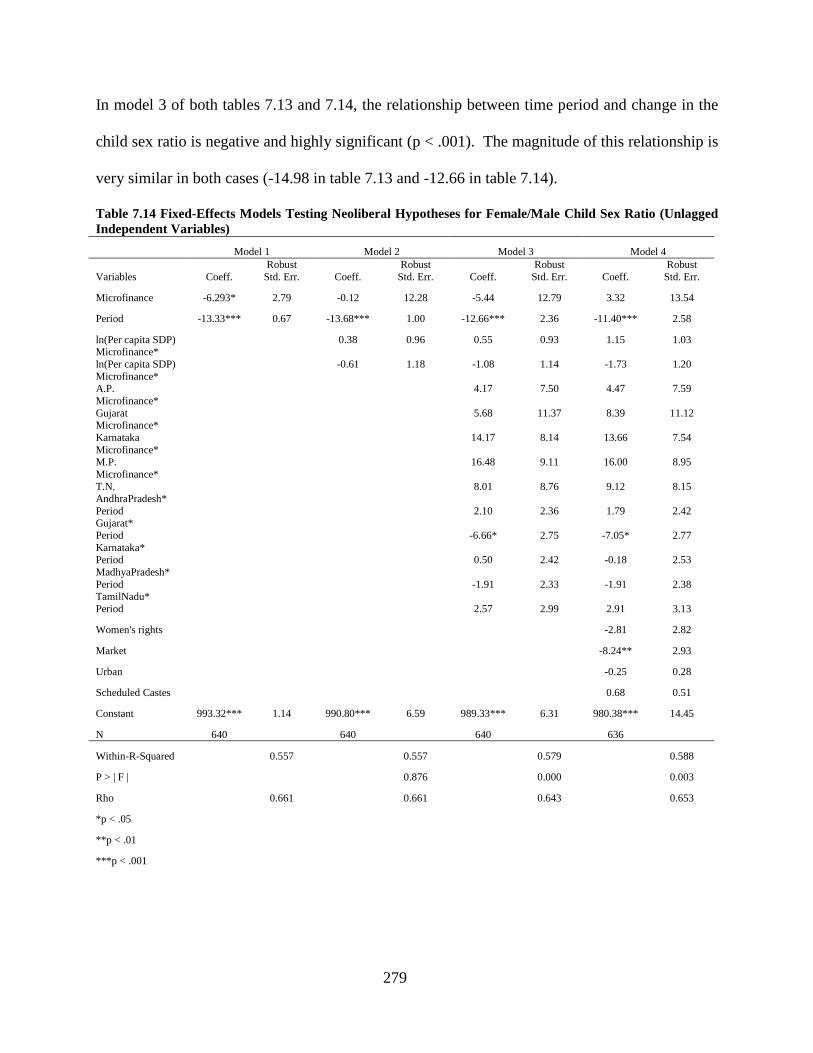
279
In model 3 of both tables 7.13 and 7.14, the relationship between time period and change in the
child sex ratio is negative and highly significant (p < .001). The magnitude of this relationship is
very similar in both cases (-14.98 in table 7.13 and -12.66 in table 7.14).
Table 7.14 Fixed-Effects Models Testing Neoliberal Hypotheses for Female/Male Child Sex Ratio (Unlagged Independent Variables)
Model 1 Model 2 Model 3 Model 4
Variables Coeff. Robust
Std. Err. Coeff. Robust
Std. Err. Coeff. Robust
Std. Err. Coeff. Robust
Std. Err.
Microfinance -6.293* 2.79 -0.12 12.28 -5.44 12.79 3.32 13.54
Period -13.33*** 0.67 -13.68*** 1.00 -12.66*** 2.36 -11.40*** 2.58
ln(Per capita SDP) 0.38 0.96 0.55 0.93 1.15 1.03 Microfinance* ln(Per capita SDP) -0.61 1.18 -1.08 1.14 -1.73 1.20 Microfinance* A.P. 4.17 7.50 4.47 7.59 Microfinance* Gujarat 5.68 11.37 8.39 11.12 Microfinance* Karnataka 14.17 8.14 13.66 7.54 Microfinance* M.P. 16.48 9.11 16.00 8.95 Microfinance* T.N. 8.01 8.76 9.12 8.15 AndhraPradesh* Period 2.10 2.36 1.79 2.42 Gujarat* Period -6.66* 2.75 -7.05* 2.77 Karnataka* Period 0.50 2.42 -0.18 2.53 MadhyaPradesh* Period -1.91 2.33 -1.91 2.38 TamilNadu* Period 2.57 2.99 2.91 3.13
Women's rights -2.81 2.82
Market -8.24** 2.93
Urban -0.25 0.28
Scheduled Castes 0.68 0.51
Constant 993.32*** 1.14 990.80*** 6.59 989.33*** 6.31 980.38*** 14.45
N 640 640 640 636
Within-R-Squared 0.557 0.557 0.579 0.588
P > | F | 0.876 0.000 0.003
Rho 0.661 0.661 0.643 0.653
*p < .05
**p < .01
***p < .001
280
In model 3 of Table 7.13, there is a positive and statistically significant relationship
between the interaction effect of region*time period and variation in the child sex ratio. In
model 3 of Table 7.14, there is a negative and statistically significant relationship between the
interaction effect of Gujarat*time period and the child sex ratio (p < .05). This means that at
every time period, the female/male child sex ratio of Gujarat state is lower than the child sex
ratio of Rajasthan by about 7 females per 1,000 males. The child sex ratio of Rajasthan
decreases by about 11 females per 1,000 males with each passing decade, while the child sex
ratio of Gujarat decreases by about 18 females per 1,000 males with each passing decade. Even
though this relationship is negative, it is still consistent with the results of model 3 in table 7.13,
which includes the interaction term of region*period. This is because Gujarat is a northern state.
If there had been a negative and statistically significant relationship between the interaction
effect of a southern state (such as Andhra Pradesh) and time period and the child sex ratio, this
would not be consistent with the results of model 3 in table 7.13. Model 4 is statistically
significantly different than model 3 in both table 7.13 and table 7.14. In both tables, the
relationship between time period and child sex ratio remains negative and highly significant (p <
.001), although in both cases the magnitude of this relationship decreases slightly. In both
models, districts with a women’s market program present have a child sex ratio that is about 8
females per 1,000 males fewer than districts without a market program present. This relationship
is statistically significant in both models (p < .05). In model 4 of table 7.13, the relationship
between the interaction effect of region*period and child sex ratio remains positive and
statistically significant. Likewise, in model 4 of table 7.14 the relationship between the
interaction effect of Gujarat*period and variation in the child sex ratio remains negative and
statistically significant.
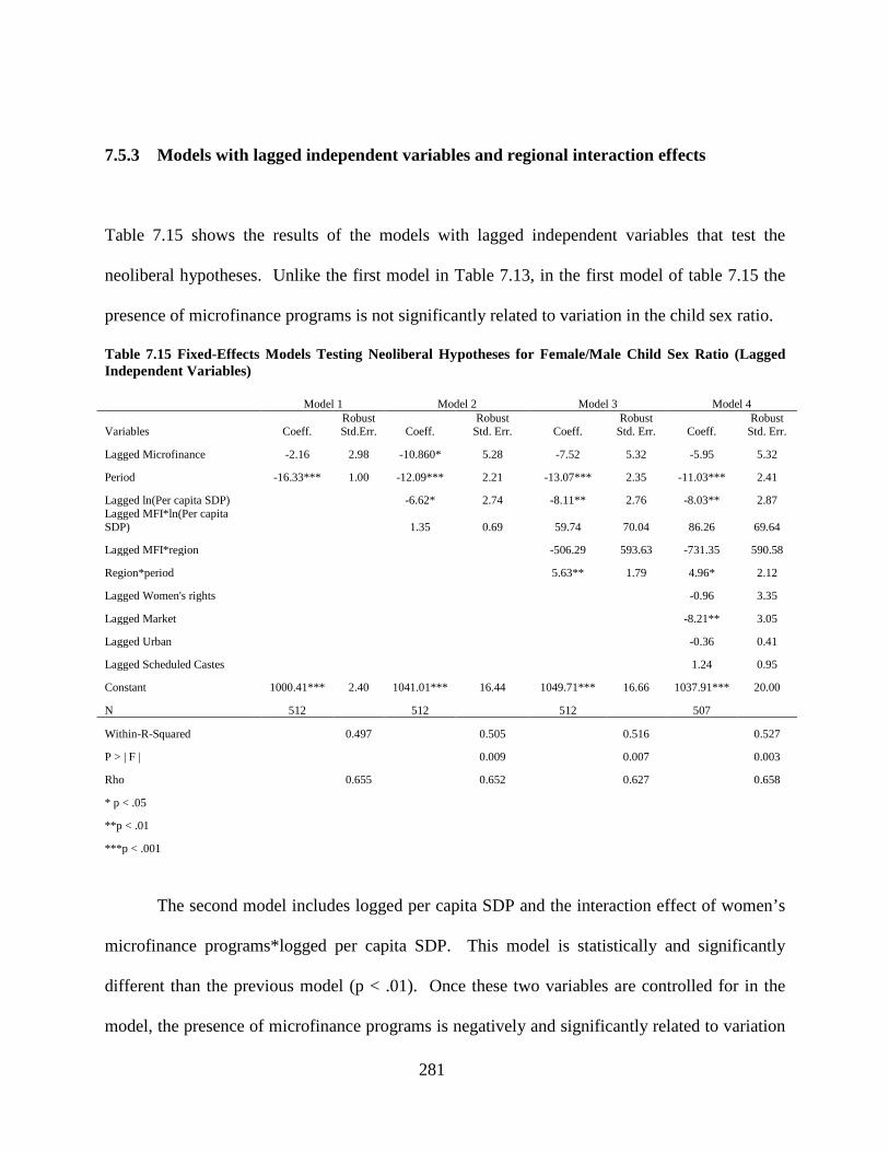
281
7.5.3 Models with lagged independent variables and regional interaction effects
Table 7.15 shows the results of the models with lagged independent variables that test the
neoliberal hypotheses. Unlike the first model in Table 7.13, in the first model of table 7.15 the
presence of microfinance programs is not significantly related to variation in the child sex ratio.
Table 7.15 Fixed-Effects Models Testing Neoliberal Hypotheses for Female/Male Child Sex Ratio (Lagged Independent Variables)
The second model includes logged per capita SDP and the interaction effect of women’s
microfinance programs*logged per capita SDP. This model is statistically and significantly
different than the previous model (p < .01). Once these two variables are controlled for in the
model, the presence of microfinance programs is negatively and significantly related to variation
Model 1 Model 2 Model 3 Model 4
Variables Coeff. Robust Std.Err. Coeff.
Robust Std. Err. Coeff.
Robust Std. Err. Coeff.
Robust Std. Err.
Lagged Microfinance -2.16 2.98 -10.860* 5.28 -7.52 5.32 -5.95 5.32
Period -16.33*** 1.00 -12.09*** 2.21 -13.07*** 2.35 -11.03*** 2.41
Lagged ln(Per capita SDP) -6.62* 2.74 -8.11** 2.76 -8.03** 2.87 Lagged MFI*ln(Per capita SDP) 1.35 0.69 59.74 70.04 86.26 69.64
Lagged MFI*region -506.29 593.63 -731.35 590.58
Region*period 5.63** 1.79 4.96* 2.12
Lagged Women's rights -0.96 3.35
Lagged Market -8.21** 3.05
Lagged Urban -0.36 0.41
Lagged Scheduled Castes 1.24 0.95
Constant 1000.41*** 2.40 1041.01*** 16.44 1049.71*** 16.66 1037.91*** 20.00
N 512 512 512 507
Within-R-Squared 0.497 0.505 0.516 0.527
P > | F | 0.009 0.007 0.003
Rho 0.655 0.652 0.627 0.658
* p < .05
**p < .01
***p < .001
282
in the female/male child sex ratio. However, the presence of microfinance programs is not
statistically significant in any of the subsequent models. Lagged log per capita SDP and time
period are statistically significantly related to a decrease in the female/male child sex ratio in this
model and all of the subsequent models. The third model includes the interaction effects of
microfinance programs*region and region*period. Just as in the models with unlagged
independent variables, in this model the interaction effect of region*period is statistically
significant but the interaction effect of microfinance programs*region is not. The fourth model
controls for the presence of women’s rights programs, the presence of women’s market
programs, percentage of population comprised of Scheduled Castes, and percentage of
population living in urban areas. Even after controlling for these variables, lagged log per capita
SDP, the passage of time, and the interaction effect of region*time period are statistically
significantly related with variation in the child sex ratio. A tenfold increase in the lagged per
capita SDP leads to a decrease in the child sex ratio of about 8 females per 1,000 males.
Although the coefficients for lagged microfinance programs*region are unusually large in
models 3 and 4 (-506.29 and -731.35, respectively), they are not statistically significant.
Surprisingly, there is a negative and statistically significant relationship between the lagged
presence of market programs and the child sex ratio. The presence of women’s market programs
is correlated with a female/male child sex ratio in subsequent decades that is lower than the child
sex ratio of districts with no market programs by about 8 females per 1,000 males (p < .01). This
last model is statistically significantly different than the previous model (p < .01), and is
therefore the best fit for the data. Overall, these models lend no support to any of the neoliberal
hypotheses.
283
7.5.4 Models with lagged independent variables and state-wise interaction effects
Table 7.16 shows the results of lagged models that include the interaction terms of lagged
microfinance*states and states*period. Overall, the results of these models are not consistent
with the results of the lagged models in Table 7.15. In spite of this, there are some similarities
between the models of the two tables. In both tables, there is a statistically significant difference
between model 3 and model 2. Also, there is a negative and statistically significant relationship
between time period and change in the child sex ratio (p < .001) in model 3 of both tables. In
both models, there is a negative and statistically significant relationship between lagged log per
capita SDP and change in the child sex ratio, although this relationship is more highly significant
and of slightly larger magnitude in model 3 of table 7.15 than in model 3 of table 7.16. Just as
there is also a positive and statistically significant relationship between the interaction effect of
region*period and variation in the child sex ratio in model 3 of table 7.15, there is also a positive
and statistically significant relationship between the interaction effect of Karnataka*period and
child sex ratio in model 3 of table 7.16. With the passing of each decade, the child sex ratio in
Karnataka is higher than the child sex ratio in Rajasthan by about 5 females per 1,000 males.
Since Karnataka is a southern state, this is consistent with the positive effect of region*period on
the female/male child sex ratio in table 7.15. However, model 4 of table 7.16 is not statistically
significantly different than model 3, unlike model 4 of table 7.15. Also, in model 3 of table 7.16,
the coefficients for the interaction effects of lagged microfinance*Andhra Pradesh, lagged
microfinance*Karnataka, and lagged microfinance*Tamil Nadu are unusually large, albeit
statistically insignificant. For all three of these interaction effects, the coefficients are larger than
-3,700. In the fourth model of table 7.16, the coefficients for these interaction variables are even
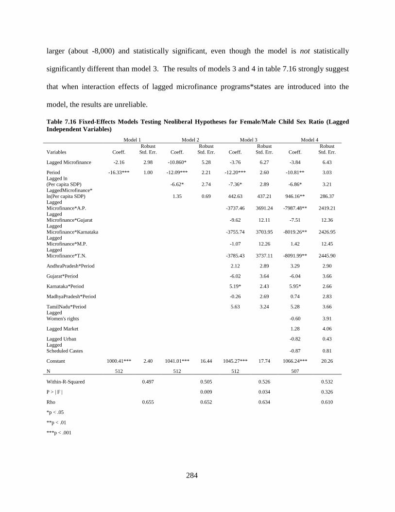
284
larger (about -8,000) and statistically significant, even though the model is not statistically
significantly different than model 3. The results of models 3 and 4 in table 7.16 strongly suggest
that when interaction effects of lagged microfinance programs*states are introduced into the
model, the results are unreliable.
Table 7.16 Fixed-Effects Models Testing Neoliberal Hypotheses for Female/Male Child Sex Ratio (Lagged Independent Variables)
Model 1 Model 2 Model 3 Model 4
Variables Coeff. Robust
Std. Err. Coeff. Robust
Std. Err. Coeff. Robust
Std. Err. Coeff. Robust
Std. Err.
Lagged Microfinance -2.16 2.98 -10.860* 5.28 -3.76 6.27 -3.84 6.43
Period -16.33*** 1.00 -12.09*** 2.21 -12.20*** 2.60 -10.81** 3.03 Lagged ln (Per capita SDP) -6.62* 2.74 -7.36* 2.89 -6.86* 3.21 LaggedMicrofinance* ln(Per capita SDP) 1.35 0.69 442.63 437.21 946.16** 286.37 Lagged Microfinance*A.P. -3737.46 3691.24 -7987.48** 2419.21 Lagged Microfinance*Gujarat -9.62 12.11 -7.51 12.36 Lagged Microfinance*Karnataka -3755.74 3703.95 -8019.26** 2426.95 Lagged Microfinance*M.P. -1.07 12.26 1.42 12.45 Lagged Microfinance*T.N. -3785.43 3737.11 -8091.99** 2445.90
AndhraPradesh*Period 2.12 2.89 3.29 2.90
Gujarat*Period -6.02 3.64 -6.04 3.66
Karnataka*Period 5.19* 2.43 5.95* 2.66
MadhyaPradesh*Period -0.26 2.69 0.74 2.83
TamilNadu*Period 5.63 3.24 5.28 3.66 Lagged Women's rights -0.60 3.91
Lagged Market 1.28 4.06
Lagged Urban -0.82 0.43 Lagged Scheduled Castes -0.87 0.81
Constant 1000.41*** 2.40 1041.01*** 16.44 1045.27*** 17.74 1066.24*** 20.26
N 512 512 512 507
Within-R-Squared 0.497 0.505 0.526 0.532
P > | F | 0.009 0.034 0.326
Rho 0.655 0.652 0.634 0.610
*p < .05
**p < .01
***p < .001
285
7.6 DISCUSSION
In the previous sections, I discussed the results of fixed-effects models that tested the
modernization, WID, GAD, and neoliberal hypotheses for female/male child sex ratio. In this
section, I briefly summarize the results of the best model for each set of hypotheses. I also
present graphical displays of the relationships between female/male child sex ratio and the
variables of interest for each set of hypotheses. I include graphs that show regional and state-
wise differences in the change trajectories of female/male child sex ratio where the regional and
state-wise interaction effects are statistically significant. These graphs depict the predicted rates
of change in the female/male child sex ratio with one independent variable at a time when all
other variables are held constant. I start by discussing the model results for the modernization
hypotheses first.
7.6.1 Results for Modernization hypotheses
As I discussed earlier in this chapter, in the first set of models that tested the modernization
hypotheses, the only variables that are significantly related to change in the female/male child
sex ratio are the presence of women’s microfinance programs, the presence of women’s market
programs, and the passing of time. All three of these variables are related to a decrease in the
child sex ratio. Figure 7.1 is a graphical display of the relationship between the presence of
women’s market programs and microfinance programs and the female/male child sex ratio
over time.
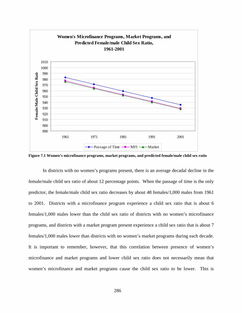
286
Women's Microfinance Programs, Market Programs, and Predicted Female/male Child Sex Ratio,
1961-2001
890900910920930940950960970980990
10001010
1961 1971 1981 1991 2001
Fem
ale/
Mal
e C
hild
Sex
Rat
io
Passage of Time MFI Market
Figure 7.1 Women’s microfinance programs, market programs, and predicted female/male child sex ratio
In districts with no women’s programs present, there is an average decadal decline in the
female/male child sex ratio of about 12 percentage points. When the passage of time is the only
predictor, the female/male child sex ratio decreases by about 48 females/1,000 males from 1961
to 2001. Districts with a microfinance program experience a child sex ratio that is about 6
females/1,000 males lower than the child sex ratio of districts with no women’s microfinance
programs, and districts with a market program present experience a child sex ratio that is about 7
females/1,000 males lower than districts with no women’s market programs during each decade.
It is important to remember, however, that this correlation between presence of women’s
microfinance and market programs and lower child sex ratio does not necessarily mean that
women’s microfinance and market programs cause the child sex ratio to be lower. This is
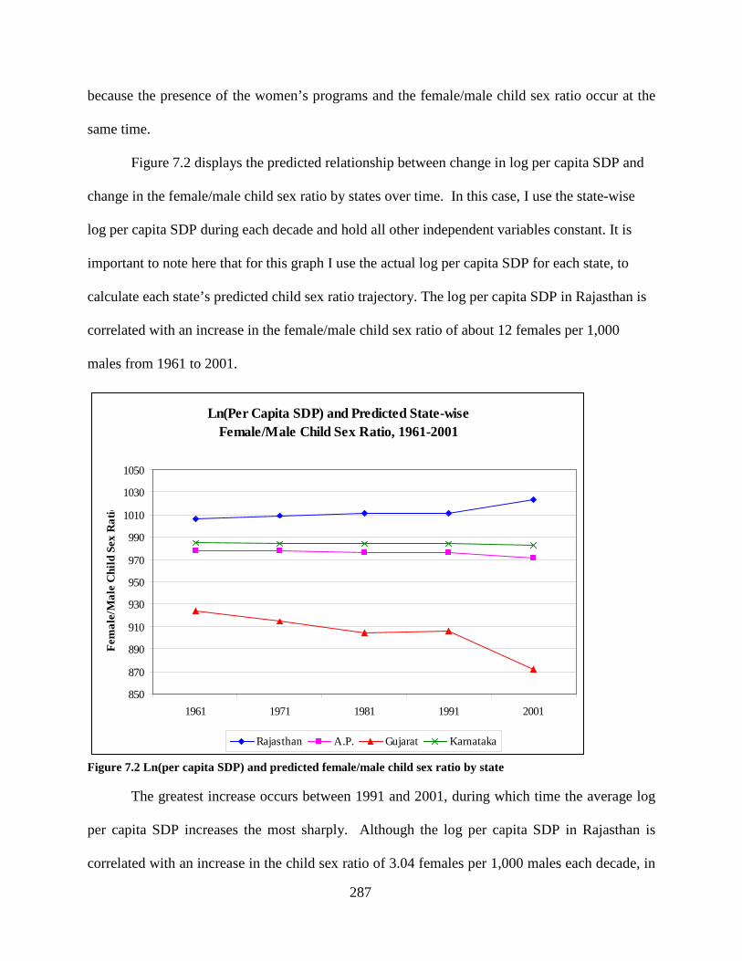
287
because the presence of the women’s programs and the female/male child sex ratio occur at the
same time.
Figure 7.2 displays the predicted relationship between change in log per capita SDP and
change in the female/male child sex ratio by states over time. In this case, I use the state-wise
log per capita SDP during each decade and hold all other independent variables constant. It is
important to note here that for this graph I use the actual log per capita SDP for each state, to
calculate each state’s predicted child sex ratio trajectory. The log per capita SDP in Rajasthan is
correlated with an increase in the female/male child sex ratio of about 12 females per 1,000
males from 1961 to 2001.
Ln(Per Capita SDP) and Predicted State-wiseFemale/Male Child Sex Ratio, 1961-2001
850
870
890
910
930
950
970
990
1010
1030
1050
1961 1971 1981 1991 2001
Fem
ale/
Mal
e C
hild
Sex
Rat
io
Rajasthan A.P. Gujarat Karnataka
Figure 7.2 Ln(per capita SDP) and predicted female/male child sex ratio by state
The greatest increase occurs between 1991 and 2001, during which time the average log
per capita SDP increases the most sharply. Although the log per capita SDP in Rajasthan is
correlated with an increase in the child sex ratio of 3.04 females per 1,000 males each decade, in
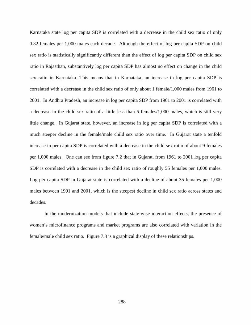
288
Karnataka state log per capita SDP is correlated with a decrease in the child sex ratio of only
0.32 females per 1,000 males each decade. Although the effect of log per capita SDP on child
sex ratio is statistically significantly different than the effect of log per capita SDP on child sex
ratio in Rajasthan, substantively log per capita SDP has almost no effect on change in the child
sex ratio in Karnataka. This means that in Karnataka, an increase in log per capita SDP is
correlated with a decrease in the child sex ratio of only about 1 female/1,000 males from 1961 to
2001. In Andhra Pradesh, an increase in log per capita SDP from 1961 to 2001 is correlated with
a decrease in the child sex ratio of a little less than 5 females/1,000 males, which is still very
little change. In Gujarat state, however, an increase in log per capita SDP is correlated with a
much steeper decline in the female/male child sex ratio over time. In Gujarat state a tenfold
increase in per capita SDP is correlated with a decrease in the child sex ratio of about 9 females
per 1,000 males. One can see from figure 7.2 that in Gujarat, from 1961 to 2001 log per capita
SDP is correlated with a decrease in the child sex ratio of roughly 55 females per 1,000 males.
Log per capita SDP in Gujarat state is correlated with a decline of about 35 females per 1,000
males between 1991 and 2001, which is the steepest decline in child sex ratio across states and
decades.
In the modernization models that include state-wise interaction effects, the presence of
women’s microfinance programs and market programs are also correlated with variation in the
female/male child sex ratio. Figure 7.3 is a graphical display of these relationships.
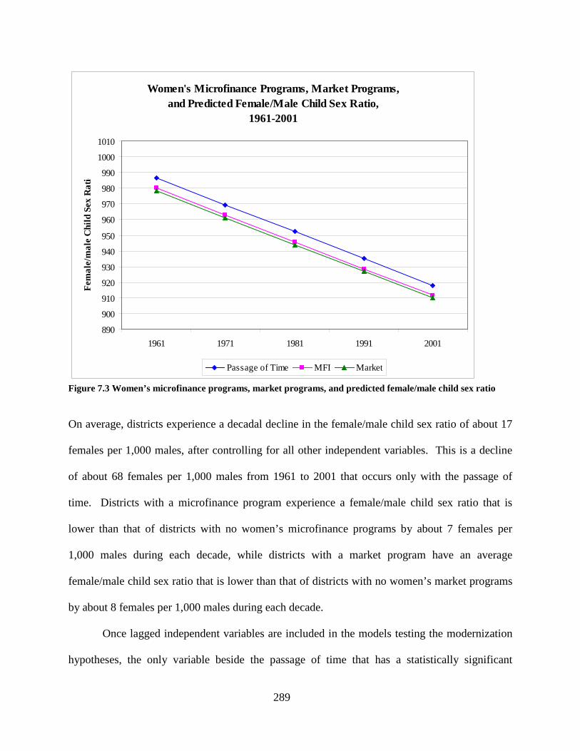
289
Women's Microfinance Programs, Market Programs, and Predicted Female/Male Child Sex Ratio,
1961-2001
890
900
910
920
930
940
950
960
970
980
990
1000
1010
1961 1971 1981 1991 2001
Fem
ale/
mal
e C
hild
Sex
Rat
io
Passage of Time MFI Market
Figure 7.3 Women’s microfinance programs, market programs, and predicted female/male child sex ratio
On average, districts experience a decadal decline in the female/male child sex ratio of about 17
females per 1,000 males, after controlling for all other independent variables. This is a decline
of about 68 females per 1,000 males from 1961 to 2001 that occurs only with the passage of
time. Districts with a microfinance program experience a female/male child sex ratio that is
lower than that of districts with no women’s microfinance programs by about 7 females per
1,000 males during each decade, while districts with a market program have an average
female/male child sex ratio that is lower than that of districts with no women’s market programs
by about 8 females per 1,000 males during each decade.
Once lagged independent variables are included in the models testing the modernization
hypotheses, the only variable beside the passage of time that has a statistically significant
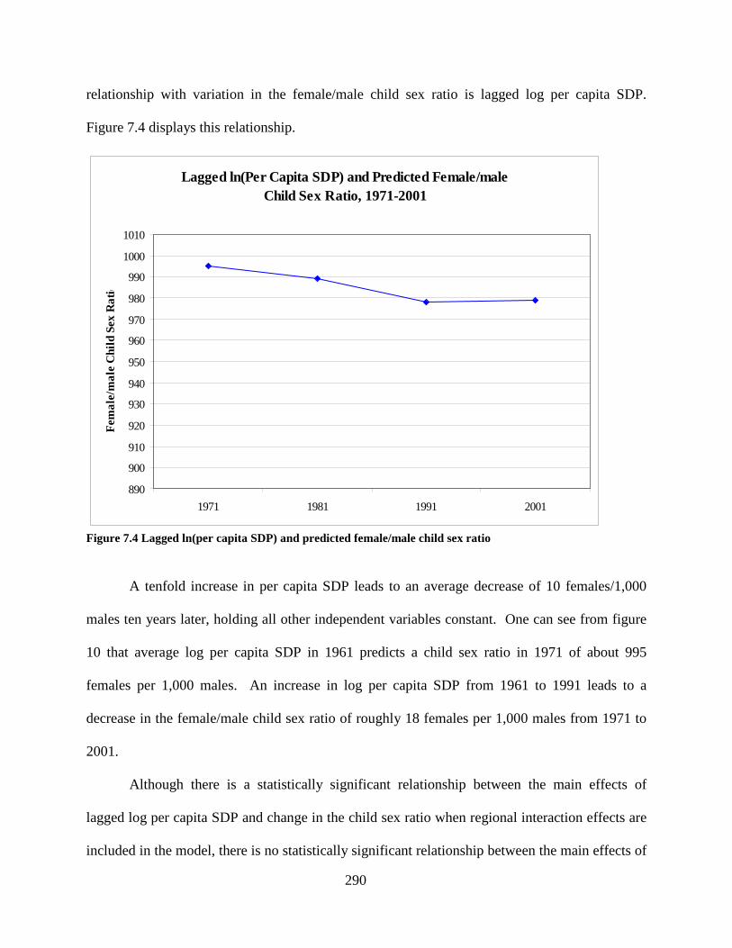
290
relationship with variation in the female/male child sex ratio is lagged log per capita SDP.
Figure 7.4 displays this relationship.
Lagged ln(Per Capita SDP) and Predicted Female/male Child Sex Ratio, 1971-2001
890
900
910
920
930
940
950
960
970
980
990
1000
1010
1971 1981 1991 2001
Fem
ale/
mal
e C
hild
Sex
Rat
io
Figure 7.4 Lagged ln(per capita SDP) and predicted female/male child sex ratio
A tenfold increase in per capita SDP leads to an average decrease of 10 females/1,000
males ten years later, holding all other independent variables constant. One can see from figure
10 that average log per capita SDP in 1961 predicts a child sex ratio in 1971 of about 995
females per 1,000 males. An increase in log per capita SDP from 1961 to 1991 leads to a
decrease in the female/male child sex ratio of roughly 18 females per 1,000 males from 1971 to
2001.
Although there is a statistically significant relationship between the main effects of
lagged log per capita SDP and change in the child sex ratio when regional interaction effects are
included in the model, there is no statistically significant relationship between the main effects of
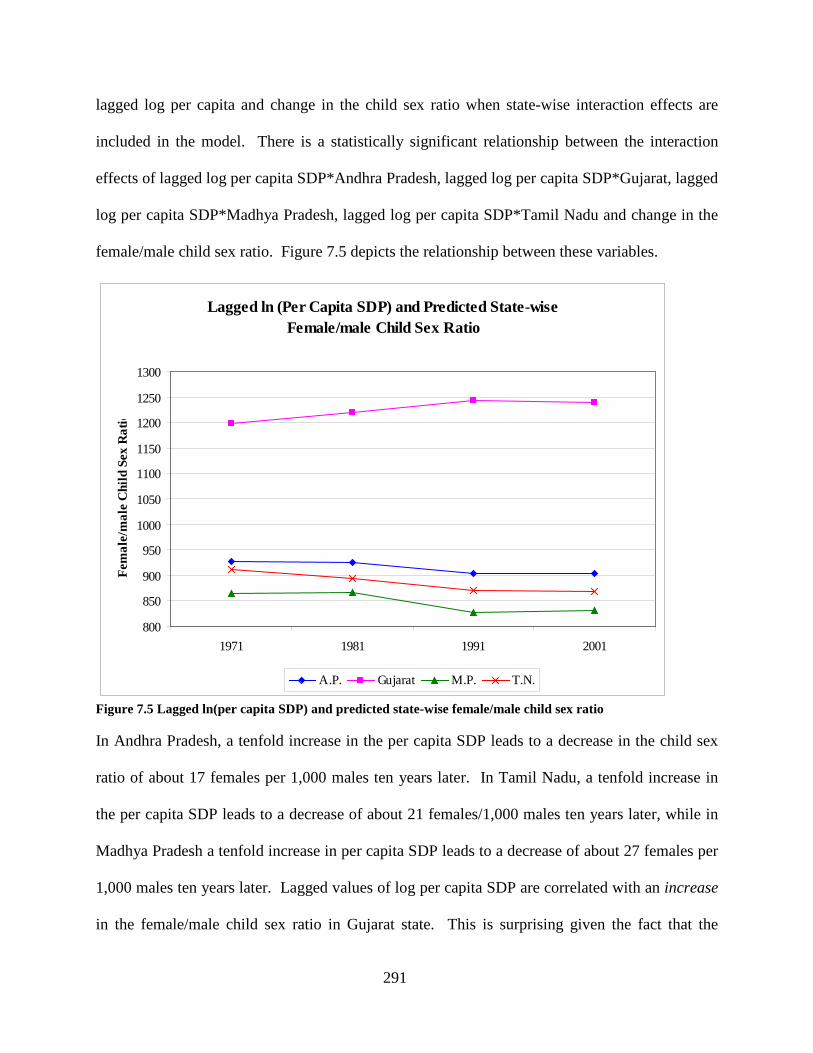
291
lagged log per capita and change in the child sex ratio when state-wise interaction effects are
included in the model. There is a statistically significant relationship between the interaction
effects of lagged log per capita SDP*Andhra Pradesh, lagged log per capita SDP*Gujarat, lagged
log per capita SDP*Madhya Pradesh, lagged log per capita SDP*Tamil Nadu and change in the
female/male child sex ratio. Figure 7.5 depicts the relationship between these variables.
Lagged ln (Per Capita SDP) and Predicted State-wise Female/male Child Sex Ratio
800
850
900
950
1000
1050
1100
1150
1200
1250
1300
1971 1981 1991 2001
Fem
ale/
mal
e C
hild
Sex
Rat
io
A.P. Gujarat M.P. T.N.
Figure 7.5 Lagged ln(per capita SDP) and predicted state-wise female/male child sex ratio
In Andhra Pradesh, a tenfold increase in the per capita SDP leads to a decrease in the child sex
ratio of about 17 females per 1,000 males ten years later. In Tamil Nadu, a tenfold increase in
the per capita SDP leads to a decrease of about 21 females/1,000 males ten years later, while in
Madhya Pradesh a tenfold increase in per capita SDP leads to a decrease of about 27 females per
1,000 males ten years later. Lagged values of log per capita SDP are correlated with an increase
in the female/male child sex ratio in Gujarat state. This is surprising given the fact that the
292
contemporaneous association between log per capita SDP and child sex ratio in Gujarat state is
negative (seeFigure 7.2). In Gujarat state, an increase in log per capita SDP from 1961 to 1991
leads to an increase in the child sex ratio of about 33 females per 1,000 males from 1971 to 2001.
In Andhra Pradesh state, an increase in log per capita SDP from 1961 to 1991 leads to a decrease
in the child sex ratio of about 25 females per 1,000 males from 1971 to 2001. In both Madhya
Pradesh and Tamil Nadu states, an increase in log per capita SDP from 1961 to 1991 leads to a
decrease in the child sex ratio of roughly 40 females per 1,000 males during the period of 1971
to 2001.
7.6.2 Results for Women-in-Development hypotheses
In the best-fitting women-in-development model that includes regional interaction effects and
unlagged independent variables, there is no statistically significant relationship between any of
the variables of theoretical interest and variation in the female/male child sex ratio. Therefore, I
do not present of a graphical display of these results. In the best-fitting women-in-development
model that includes state-wise interaction effects, there is a negative, statistically significant
relationship between the presence of women’s market programs, microfinance programs, and
variation in the female/male child sex ratio. Figure 7.6 displays the relationship between the
presence of women’s market programs, microfinance programs, and the child sex ratio, holding
all other independent variables constant (beside the passage of time). These results are similar to
the results of the modernization models that include state-wise interaction effects (see Figure
7.3). Once the interaction effects of market programs*states and microfinance programs*states
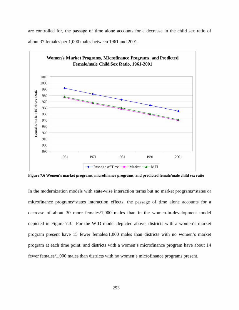
293
are controlled for, the passage of time alone accounts for a decrease in the child sex ratio of
about 37 females per 1,000 males between 1961 and 2001.
Women's Market Programs, Microfinance Programs, and Predicted Female/male Child Sex Ratio, 1961-2001
890900910920
930940950960970980
99010001010
1961 1971 1981 1991 2001
Fem
ale/
mal
e C
hild
Sex
Rat
io
Passage of Time Market MFI
Figure 7.6 Women’s market programs, microfinance programs, and predicted female/male child sex ratio
In the modernization models with state-wise interaction terms but no market programs*states or
microfinance programs*states interaction effects, the passage of time alone accounts for a
decrease of about 30 more females/1,000 males than in the women-in-development model
depicted in Figure 7.3. For the WID model depicted above, districts with a women’s market
program present have 15 fewer females/1,000 males than districts with no women’s market
program at each time point, and districts with a women’s microfinance program have about 14
fewer females/1,000 males than districts with no women’s microfinance programs present.
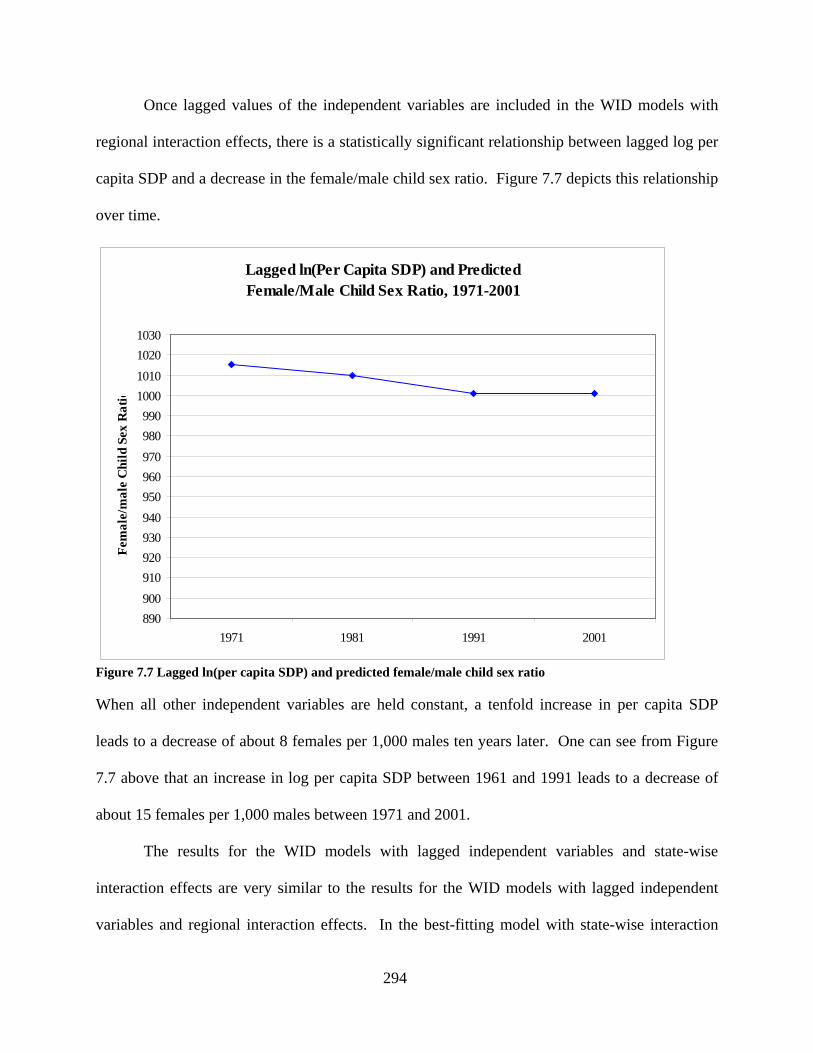
294
Once lagged values of the independent variables are included in the WID models with
regional interaction effects, there is a statistically significant relationship between lagged log per
capita SDP and a decrease in the female/male child sex ratio. Figure 7.7 depicts this relationship
over time.
Lagged ln(Per Capita SDP) and Predicted Female/Male Child Sex Ratio, 1971-2001
890900910920930940950960970980990
1000101010201030
1971 1981 1991 2001
Fem
ale/
mal
e C
hild
Sex
Rat
io
Figure 7.7 Lagged ln(per capita SDP) and predicted female/male child sex ratio
When all other independent variables are held constant, a tenfold increase in per capita SDP
leads to a decrease of about 8 females per 1,000 males ten years later. One can see from Figure
7.7 above that an increase in log per capita SDP between 1961 and 1991 leads to a decrease of
about 15 females per 1,000 males between 1971 and 2001.
The results for the WID models with lagged independent variables and state-wise
interaction effects are very similar to the results for the WID models with lagged independent
variables and regional interaction effects. In the best-fitting model with state-wise interaction
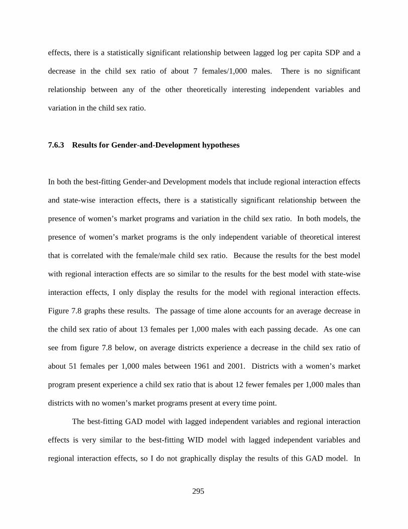
295
effects, there is a statistically significant relationship between lagged log per capita SDP and a
decrease in the child sex ratio of about 7 females/1,000 males. There is no significant
relationship between any of the other theoretically interesting independent variables and
variation in the child sex ratio.
7.6.3 Results for Gender-and-Development hypotheses
In both the best-fitting Gender-and Development models that include regional interaction effects
and state-wise interaction effects, there is a statistically significant relationship between the
presence of women’s market programs and variation in the child sex ratio. In both models, the
presence of women’s market programs is the only independent variable of theoretical interest
that is correlated with the female/male child sex ratio. Because the results for the best model
with regional interaction effects are so similar to the results for the best model with state-wise
interaction effects, I only display the results for the model with regional interaction effects.
Figure 7.8 graphs these results. The passage of time alone accounts for an average decrease in
the child sex ratio of about 13 females per 1,000 males with each passing decade. As one can
see from figure 7.8 below, on average districts experience a decrease in the child sex ratio of
about 51 females per 1,000 males between 1961 and 2001. Districts with a women’s market
program present experience a child sex ratio that is about 12 fewer females per 1,000 males than
districts with no women’s market programs present at every time point.
The best-fitting GAD model with lagged independent variables and regional interaction
effects is very similar to the best-fitting WID model with lagged independent variables and
regional interaction effects, so I do not graphically display the results of this GAD model. In
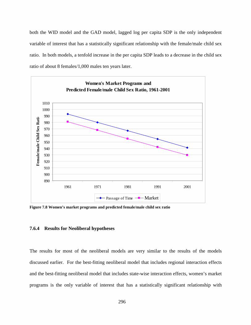
296
both the WID model and the GAD model, lagged log per capita SDP is the only independent
variable of interest that has a statistically significant relationship with the female/male child sex
ratio. In both models, a tenfold increase in the per capita SDP leads to a decrease in the child sex
ratio of about 8 females/1,000 males ten years later.
Women's Market Programs and Predicted Female/male Child Sex Ratio, 1961-2001
890900910920930940950
960970980990
10001010
1961 1971 1981 1991 2001
Fem
ale/
mal
e C
hild
Sex
Rat
io
Passage of Time Market
Figure 7.8 Women’s market programs and predicted female/male child sex ratio
7.6.4 Results for Neoliberal hypotheses
The results for most of the neoliberal models are very similar to the results of the models
discussed earlier. For the best-fitting neoliberal model that includes regional interaction effects
and the best-fitting neoliberal model that includes state-wise interaction effects, women’s market
programs is the only variable of interest that has a statistically significant relationship with
297
variation in the female/male child sex ratio. Figure 7.9 displays the results of the model with
regional interaction effects.
Women's Market Programs and Predicted Female/male Child Sex Ratio, 1961-2001
890900
910920930
940950960
970980990
10001010
1961 1971 1981 1991 2001
Fem
ale/
mal
e C
hild
Sex
Rat
io
Passage of Time Market
Figure 7.9 Women’s market programs and predicted female/male child sex ratio
In the best neoliberal model with regional interaction effects, the passage of time alone accounts
for a decrease in the child sex ratio of about 14 females per 1,000 males per decade. In districts
with no women’s programs, the female/male child sex ratio decreases by about 57 females/1,000
males between 1961 and 2001. In districts with women’s market programs, the child sex ratio is
lower by about 8 females/1,000 males compared to districts with no women’s market programs
present. In the neoliberal model with state-wise interaction effects, districts with a women’s
market program also experience a child sex ratio that is lower than the child sex ratio of districts
with no women’s market programs by about 8 females/1,000 males.
298
7.7 CONCLUSION
In this chapter, I have discussed at length the results of the models that estimate the impact of log
per capita SDP, the percentage of population living in urban areas, and the presence of women’s
market programs, women’s microfinance programs, and women’s rights programs on variation
in the female/male child sex ratio. I have also accounted for regional as well as state-wise
interaction effects, as well as the lagged effect of these variables on the child sex ratio. Although
the results of some models show that there is a statistically significant relationship between the
presence of women’s market programs and the presence of women’s microfinance programs and
variation in the female/male child sex ratio, this relationship is the opposite of what is expected.
In most cases, once lagged values of the independent variables are included in the models, the
relationship between the presence of women’s programs and variation in the child sex ratio
disappears. This means that although there is a statistically significant correlation between the
contemporaneous presence of women’s market programs and microfinance programs and a
decrease in the female/male child sex ratio, there is not a causal relationship between the
presence of these women’s programs and child sex ratio. It is possible that development
organizations start women’s programs in the districts that have very unequal gender relations and
especially high poverty rates. The evidence across the models with lagged independent variables
shows that an increase in log per capita SDP does lead to a decrease in the female/male child sex
ratio in subsequent decades. This finding supports the first WID hypothesis, which is that an
increase in economic growth leads to a decrease in the female/male child sex ratio. This also
299
means that we must reject the modernization hypothesis that predicts that an increase in per
capita SDP will lead to an increase in the female/male child sex ratio. However, this is the only
hypothesis that is supported by the results of these models. Since there is no relationship
between the lagged presence of women’s rights programs, market programs, and microfinance
programs and variation in the child sex ratio, there is no support for the WID, GAD, or neoliberal
hypotheses that predict that women’s market programs, women’s rights programs, or women’s
microfinance programs will lead to an increase in the child sex ratio.
300
8.0 CHAPTER EIGHT: VARIATION IN THE FEMALE/MALE LITERACY RATIO
8.1 INTRODUCTION
In this chapter I discuss the results of the fixed-effects models for female/male literacy ratio. I
first present and discuss the results of models that test the modernization hypotheses, followed
by results of models that test the WID hypotheses. Next, I discuss the results of models testing
the GAD hypotheses and the models testing the neoliberal hypotheses. For each set of
hypotheses, I present models with both lagged and unlagged independent variables, as well as
models with regional interaction effects and state-wide interaction effects. I report robust
standard errors for each model, as well as the within-district R-squared and the significance level
of the F-statistic below each model. The “P > | F |” tests whether a more complete model is
significantly different than the previous model. I test the hypotheses in such a way such that
previous models are nested within subsequent models. This allows me to use the F-statistic to
determine whether a subsequent model is statistically significantly different (and therefore
better) than the previous model.
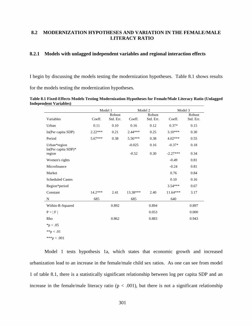
301
8.2 MODERNIZATION HYPOTHESES AND VARIATION IN THE FEMALE/MALE LITERACY RATIO
8.2.1 Models with unlagged independent variables and regional interaction effects
I begin by discussing the models testing the modernization hypotheses. Table 8.1 shows results
for the models testing the modernization hypotheses.
Table 8.1 Fixed-Effects Models Testing Modernization Hypotheses for Female/Male Literacy Ratio (Unlagged Independent Variables)
Model 1 Model 2 Model 3
Variables Coeff. Robust
Std. Err. Coeff. Robust
Std. Err. Coeff. Robust
Std. Err.
Urban 0.11 0.10 0.16 0.12 0.37* 0.15
ln(Per capita SDP) 2.22*** 0.21 2.44*** 0.25 3.10*** 0.30
Period 5.67*** 0.38 5.56*** 0.38 4.02*** 0.55
Urban*region -0.025 0.16 -0.37* 0.18 ln(Per capita SDP)* region -0.52 0.30 -2.27*** 0.34
Women's rights -0.49 0.81
Microfinance -0.24 0.81
Market 0.76 0.84
Scheduled Castes 0.10 0.16
Region*period 3.54*** 0.67
Constant 14.2*** 2.41 13.38*** 2.40 11.64*** 3.17
N 685 685 640
Within-R-Squared 0.892 0.894 0.897
P > | F | 0.053 0.000
Rho 0.862 0.883 0.943
*p < .05
**p < .01
***p < .001
Model 1 tests hypothesis 1a, which states that economic growth and increased
urbanization lead to an increase in the female/male child sex ratios. As one can see from model
1 of table 8.1, there is a statistically significant relationship between log per capita SDP and an
increase in the female/male literacy ratio (p < .001), but there is not a significant relationship
302
between percentage of population in urban areas and the female/male literacy ratio. A tenfold
increase in the per capita SDP is related to an increase in the literacy ratio of about 2 percentage
points. Model two tests the hypothesis that urbanization and increased per capita SDP will have
a greater effect on increases in the child sex ratio in southern districts than in northern districts.
However, there is no statistically significant difference between this model and the first model.
The third model controls for the effects of women’s rights programs, market programs,
microfinance programs, the percentage of population comprised of Scheduled Castes, and the
interaction effect of region*period. Once these five variables are controlled for, percent of
population living in urban areas is statistically significantly related to an increase in the
female/male literacy ratio (p < .05), although substantively it is a very small change. Log per
capita SDP continues to statistically significantly related to an increase in the literacy ratio (p <
.001). The interaction effects of percentage of population in urban areas* region and the
interaction effect of log per capita SDP*region also are significantly related with the female/male
literacy ratio once these five variables are controlled for (p < .05 and p < .001, respectively).
With every one percentage point increase in urbanization, the female/male literacy ratio in
northern regions increases by 0.37 percentage points. Since the coefficient for the urban*region
interaction term is -0.37, this means that in southern districts an increase in urbanization is
associated with no change in the female/male literacy ratio. While in northern districts a tenfold
increase in per capita SDP is associated with an increase of about 3 percentage points in the
female/male literacy ratio, in southern districts a tenfold increase in per capita SDP is associated
with an increase of a little less than 1 percentage point in the literacy ratio. While the
relationships between both urbanization and per capita SDP and the female/male literacy ratio
are statistically significant, neither urbanization nor per capita SDP seem to have much of a
303
substantive effect on the female/male literacy ratio. There is a positive, statistically significant
relationship between the interaction effect of region*period and the female/male literacy ratio (p
< .001). In southern districts, the literacy ratio is higher than in northern districts by about 4
percentage points at every time period. From the results of these models, there is evidence of the
modernization hypothesis that posits a positive correlation between log per capita SDP,
percentage of population living in urban areas, and the female/male literacy ratio.
8.2.2 Models with unlagged independent variables and state-wise interaction effects
Table 8.2 shows results for models that include state dichotomous variables rather than the
region dichotomous variable. The first model of table 8.2 is the same as the first model of Table
8.1. Model two of table 8.2 tests the hypothesis that urbanization and increased per capita SDP
will have a greater effect on increases in the child sex ratio in southern states than in northern
states. Unlike model 2 of table 8.1, model 2 of table 8.2 is statistically significantly different
than the previous model. There is a positive and statistically significant relationship between all
of the urbanization*state interaction effects (except for urban*Tamil Nadu) and the female/male
literacy ratio. (The main effect of urbanization is actually the effect of urbanization in since
Rajasthan is the reference category,) However, each of these urbanization*state interactions are
related to an increase in the female/male literacy ratio of less than one percentage point. There is
also a negative and statistically significant relationship between the interaction effect of log per
capita SDP*Gujarat (p < .001). While a tenfold increase in the per capita SDP is statistically
significantly related to an increase in the female/male literacy ratio of about 3 percentage points
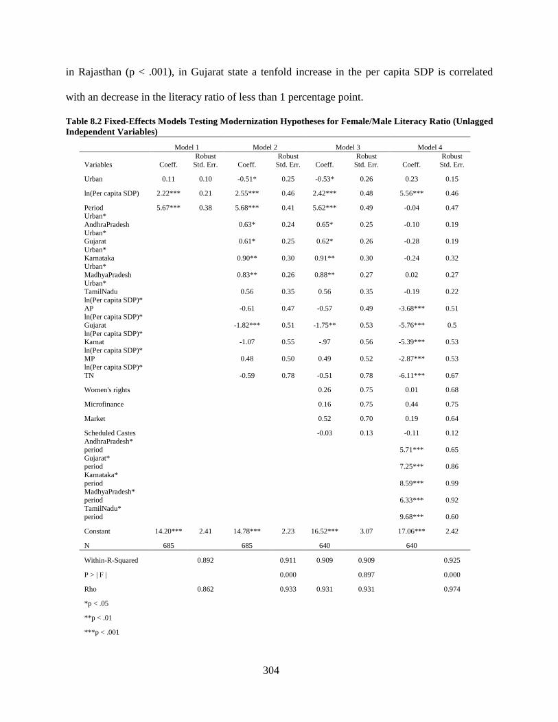
304
in Rajasthan (p < .001), in Gujarat state a tenfold increase in the per capita SDP is correlated
with an decrease in the literacy ratio of less than 1 percentage point.
Table 8.2 Fixed-Effects Models Testing Modernization Hypotheses for Female/Male Literacy Ratio (Unlagged Independent Variables)
Model 1 Model 2 Model 3 Model 4
Variables Coeff. Robust
Std. Err. Coeff. Robust
Std. Err. Coeff. Robust
Std. Err. Coeff. Robust
Std. Err.
Urban 0.11 0.10 -0.51* 0.25 -0.53* 0.26 0.23 0.15
ln(Per capita SDP) 2.22*** 0.21 2.55*** 0.46 2.42*** 0.48 5.56*** 0.46
Period 5.67*** 0.38 5.68*** 0.41 5.62*** 0.49 -0.04 0.47 Urban* AndhraPradesh 0.63* 0.24 0.65* 0.25 -0.10 0.19 Urban* Gujarat 0.61* 0.25 0.62* 0.26 -0.28 0.19 Urban* Karnataka 0.90** 0.30 0.91** 0.30 -0.24 0.32 Urban* MadhyaPradesh 0.83** 0.26 0.88** 0.27 0.02 0.27 Urban* TamilNadu 0.56 0.35 0.56 0.35 -0.19 0.22 ln(Per capita SDP)* AP -0.61 0.47 -0.57 0.49 -3.68*** 0.51 ln(Per capita SDP)* Gujarat -1.82*** 0.51 -1.75** 0.53 -5.76*** 0.5 ln(Per capita SDP)* Karnat -1.07 0.55 -.97 0.56 -5.39*** 0.53 ln(Per capita SDP)* MP 0.48 0.50 0.49 0.52 -2.87*** 0.53 ln(Per capita SDP)* TN -0.59 0.78 -0.51 0.78 -6.11*** 0.67
Women's rights 0.26 0.75 0.01 0.68
Microfinance 0.16 0.75 0.44 0.75
Market 0.52 0.70 0.19 0.64
Scheduled Castes -0.03 0.13 -0.11 0.12 AndhraPradesh* period 5.71*** 0.65 Gujarat* period 7.25*** 0.86 Karnataka* period 8.59*** 0.99 MadhyaPradesh* period 6.33*** 0.92 TamilNadu* period 9.68*** 0.60
Constant 14.20*** 2.41 14.78*** 2.23 16.52*** 3.07 17.06*** 2.42
N 685 685 640 640
Within-R-Squared 0.892 0.911 0.909 0.909 0.925
P > | F | 0.000 0.897 0.000
Rho 0.862 0.933 0.931 0.931 0.974
*p < .05
**p < .01
***p < .001
305
The third model is not statistically significantly different than the previous model. The
fourth model of table 8.2 controls for the presence of women’s rights programs, women’s
microfinance programs, and women’s market programs, as well as the interaction effects of each
state*time period. In the fourth model of Table 8.2, there is no longer a statistically significant
relationship between the percentage of population in urban areas and the female/male literacy
ratio. This is in contrast to the third model of Table 8.1. Also, there is no statistically significant
relationship between the interaction effects of urbanization*states and the literacy ratio, in
contrast to model 3 of Table 8.1 in which there is a significant relationship between
urbanization*region. In model 4 of Table 8.2 and model 3 of Table 8.1, there is a statistically
significant relationship between log per capita SDP and an increase in the female/male literacy
ratio, although in model 4 of Table 8.2 the magnitude of this relationship is almost twice as great.
In model 4 of Table 8.2, there is a statistically significant difference in the effect of log per capita
SDP in Rajasthan and the effect of log per capita SDP in all of the other states (p < .001). This is
similar to model 3 of Table 8.1, in which there is a negative and statistically significant
relationship between the interaction effect of log per capita SDP*region and the literacy ratio. In
model 4 of Table 8.2, in Rajasthan a tenfold increase in per capita SDP is correlated with a
increase in the female/male literacy ratio of about 6 percentage points. A tenfold increase in per
capita SDP is correlated with an increase in the female/male literacy ratio of about 2 percentage
points in Andhra Pradesh, only 0.17 percentage points in Karnataka, and about 3 percentage
points in Madhya Pradesh. A tenfold increase in per capita SDP is correlated with a decrease in
the female/male literacy ratio of only 0.20 percentage points in Gujarat and 0.55 percentage
points in Tamil Nadu. The greatest increase in female/male literacy ratio correlated with log per
capita SDP is in Rajasthan and Madhya Pradesh, which are both northern states. This is the
306
opposite of what is expected, since the second modernization hypothesis predicts that per capita
SDP will have a greater positive effect in southern states than in northern states. There is no
statistically significant relationship between the passage of time and the female/male literacy
ratio in Rajasthan. However, there is a positive and statistically significant relationship between
the interaction effects of states*time period and female/male literacy ratio (p < .001), which is
similar to the fact that in model 3 of table 8.1 there is a positive and statistically significant
relationship between the interaction effect of region*period. The magnitude of the relationship
between each of the state*time period interaction effects and literacy ratio is greater than the
magnitude of the relationship between the region*period interaction effect and female/male
literacy ratio. With the passing of each decade, the female/male literacy ratio increases by about
6 percentage points in Andhra Pradesh, 7 percentage points in Gujarat, 8 percentage points in
Karnataka, 6 percentage points in Madhya Pradesh, and 10 percentage points in Tamil Nadu.
Thus, from the models that include regional interaction terms and state interaction terms, there is
support for the modernization hypothesis that an increase in per capita SDP leads to an increase
in the female/male literacy ratio. It is important to consider the temporal order of the
independent and dependent variables, however. Therefore, I also estimate fixed-effects models
with ten-year lagged values of the independent variables before reaching a final conclusion.
8.2.3 Models with lagged independent variables and regional interaction effects
Table 8.3 shows the results for the fixed-effects models with lagged independent variables that
test the modernization hypotheses. The first model tests the hypothesis that increased
urbanization and economic growth will lead to an increase in the female/male literacy ratio. One
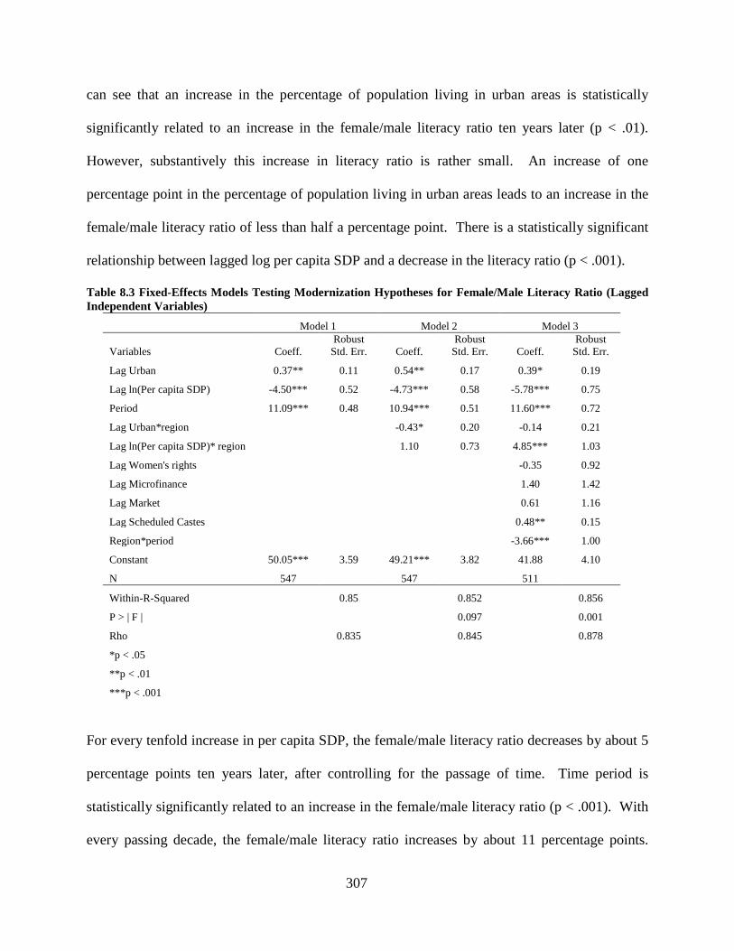
307
can see that an increase in the percentage of population living in urban areas is statistically
significantly related to an increase in the female/male literacy ratio ten years later (p < .01).
However, substantively this increase in literacy ratio is rather small. An increase of one
percentage point in the percentage of population living in urban areas leads to an increase in the
female/male literacy ratio of less than half a percentage point. There is a statistically significant
relationship between lagged log per capita SDP and a decrease in the literacy ratio (p < .001).
Table 8.3 Fixed-Effects Models Testing Modernization Hypotheses for Female/Male Literacy Ratio (Lagged Independent Variables)
Model 1 Model 2 Model 3
Variables Coeff. Robust
Std. Err. Coeff. Robust
Std. Err. Coeff. Robust
Std. Err.
Lag Urban 0.37** 0.11 0.54** 0.17 0.39* 0.19
Lag ln(Per capita SDP) -4.50*** 0.52 -4.73*** 0.58 -5.78*** 0.75
Period 11.09*** 0.48 10.94*** 0.51 11.60*** 0.72
Lag Urban*region -0.43* 0.20 -0.14 0.21
Lag ln(Per capita SDP)* region 1.10 0.73 4.85*** 1.03
Lag Women's rights -0.35 0.92
Lag Microfinance 1.40 1.42
Lag Market 0.61 1.16
Lag Scheduled Castes 0.48** 0.15
Region*period -3.66*** 1.00
Constant 50.05*** 3.59 49.21*** 3.82 41.88 4.10
N 547 547 511
Within-R-Squared 0.85 0.852 0.856
P > | F | 0.097 0.001
Rho 0.835 0.845 0.878
*p < .05
**p < .01
***p < .001
For every tenfold increase in per capita SDP, the female/male literacy ratio decreases by about 5
percentage points ten years later, after controlling for the passage of time. Time period is
statistically significantly related to an increase in the female/male literacy ratio (p < .001). With
every passing decade, the female/male literacy ratio increases by about 11 percentage points.
308
Therefore, there is partial support for the first modernization hypothesis. The second model tests
the hypothesis that urbanization and economic growth will have a greater positive impact on the
female/male literacy ratio in southern regions than in northern regions. However, this model is
not statistically significantly different than the first model. The third model controls for the
lagged effects of percentage of population comprised of Scheduled Castes, the presence of
women’s rights programs, women’s market programs, and women’s microfinance programs, as
well as the interaction effect of region*period. Once these variables are controlled for, there is a
statistically significant relationship between lagged log per capita SDP and female/male literacy
ratio (p < .001), as well as a statistically significant relationship between the interaction effect of
lagged log per capita SDP*region and an increase in the female/male literacy ratio (p < .001).
With every tenfold increase in per capita SDP, ten years later the female/male literacy ratio in
northern districts decreases by about 6 percentage points. higher than the female/male literacy
ratio in northern districts. In southern districts, every tenfold increase in per capita SDP leads to
a decrease of about 1 percentage point ten years later. In this third model, lagged urbanization is
still statistically significantly related to an increase in the female/male literacy ratio (p < .05), and
the magnitude of this relationship is very close to the magnitude of this relationship in model 1.
There is a negative, statistically significant relationship between the interaction effect of
region*period and the literacy ratio (p < .001). With the passing of each decade, the female/male
literacy ratio in southern districts is about 4 percentage points lower than it is in northern
districts. The passage of time is significantly related to an increase of almost 12 percentage
points in the female/male literacy ratio in northern districts each decade, whereas in southern
districts the passage of time is significantly related to an increase in the literacy ratio of about 7
309
percentage points each decade (p < .001). Overall, there is partial support for the modernization
hypotheses.
8.2.4 Models with lagged independent variables and state-wise interaction effects
Table 8.4 shows the results for the lagged models testing the modernization hypotheses that
include the state-wise interaction terms. The first model in Table 8.4 is the same as the first
model in Table 8.3. The second model of Table 8.4 includes the interaction effects of lagged
urbanization*states and lagged log per capita SDP*states. This model, unlike model 2 of Table
8.3, is statistically significantly different than the first model. There continues to be a positive,
statistically significant relationship between percentage of population living in urban areas and
the female/male literacy ratio (p < .001), and there still is a negative, statistically significant
relationship between lagged log per capita SDP and the literacy ratio (p < .001). There is a
negative, statistically significant relationship between all but one of the urbanization*state
interaction effects and the female/male literacy ratio. As the percentage of population living in
urban areas increases each percentage point, there is an increase in the literacy ratio of about 1
percentage point in Rajasthan. As the percentage of population living in urban areas increases
each percentage point, there is a decrease in the female/male literacy ratio ten years later of about
only 0.03 percentage points in Andhra Pradesh (p < .01) and only 0.39 percentage points in
Gujarat (p < .001), Karnataka (p < .01), and Tamil Nadu (p < .05). There is an increase in the
literacy ratio ten years later of 0.10 percentage points in Karnataka and 0.28 percentage points in
Tamil Nadu. Even though there is a statistically significant difference in the effect of
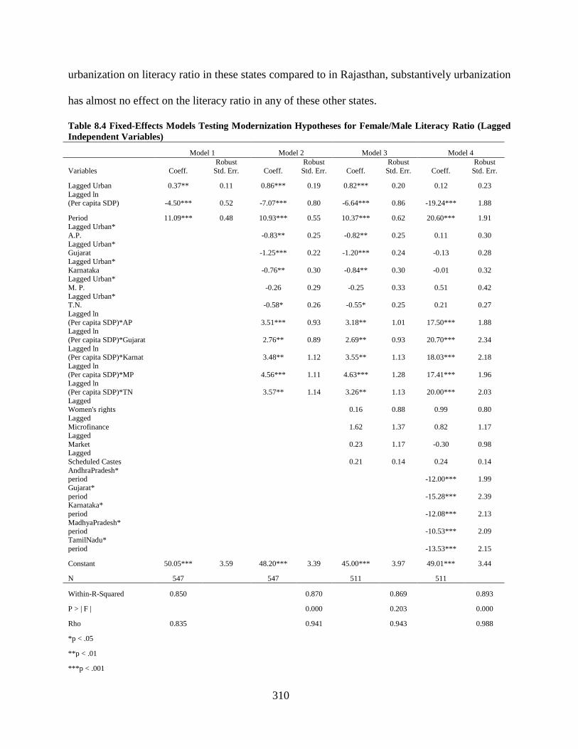
310
urbanization on literacy ratio in these states compared to in Rajasthan, substantively urbanization
has almost no effect on the literacy ratio in any of these other states.
Table 8.4 Fixed-Effects Models Testing Modernization Hypotheses for Female/Male Literacy Ratio (Lagged Independent Variables)
Model 1 Model 2 Model 3 Model 4
Variables Coeff. Robust
Std. Err. Coeff. Robust
Std. Err. Coeff. Robust
Std. Err. Coeff. Robust
Std. Err.
Lagged Urban 0.37** 0.11 0.86*** 0.19 0.82*** 0.20 0.12 0.23 Lagged ln (Per capita SDP) -4.50*** 0.52 -7.07*** 0.80 -6.64*** 0.86 -19.24*** 1.88
Period 11.09*** 0.48 10.93*** 0.55 10.37*** 0.62 20.60*** 1.91 Lagged Urban* A.P. -0.83** 0.25 -0.82** 0.25 0.11 0.30 Lagged Urban* Gujarat -1.25*** 0.22 -1.20*** 0.24 -0.13 0.28 Lagged Urban* Karnataka -0.76** 0.30 -0.84** 0.30 -0.01 0.32 Lagged Urban* M. P. -0.26 0.29 -0.25 0.33 0.51 0.42 Lagged Urban* T.N. -0.58* 0.26 -0.55* 0.25 0.21 0.27 Lagged ln (Per capita SDP)*AP 3.51*** 0.93 3.18** 1.01 17.50*** 1.88 Lagged ln (Per capita SDP)*Gujarat 2.76** 0.89 2.69** 0.93 20.70*** 2.34 Lagged ln (Per capita SDP)*Karnat 3.48** 1.12 3.55** 1.13 18.03*** 2.18 Lagged ln (Per capita SDP)*MP 4.56*** 1.11 4.63*** 1.28 17.41*** 1.96 Lagged ln (Per capita SDP)*TN 3.57** 1.14 3.26** 1.13 20.00*** 2.03 Lagged Women's rights 0.16 0.88 0.99 0.80 Lagged Microfinance 1.62 1.37 0.82 1.17 Lagged Market 0.23 1.17 -0.30 0.98 Lagged Scheduled Castes 0.21 0.14 0.24 0.14 AndhraPradesh* period -12.00*** 1.99 Gujarat* period -15.28*** 2.39 Karnataka* period -12.08*** 2.13 MadhyaPradesh* period -10.53*** 2.09 TamilNadu* period -13.53*** 2.15
Constant 50.05*** 3.59 48.20*** 3.39 45.00*** 3.97 49.01*** 3.44
N 547 547 511 511
Within-R-Squared 0.850 0.870 0.869 0.893
P > | F | 0.000 0.203 0.000
Rho 0.835 0.941 0.943 0.988
*p < .05
**p < .01
***p < .001
311
There is a negative, statistically significant relationship between lagged per capita SDP and the
literacy ratio in Rajasthan state (p < .001). There is a statistically significant difference in the
effect of lagged per capita SDP in all of the other states compared to the effect of lagged per
capita SDP in Rajasthan. With each tenfold increase in per capita SDP, there is a decrease in the
female/male literacy ratio of about 4 percentage points in Andhra Pradesh (p < .001), Gujarat (p
< .01), Karnataka (p < .01), and Tamil Nadu (p < .01), and a decrease of about 3 percentage
points in Madhya Pradesh (p < .001).
Model 3 controls for the lagged effects of women’s rights programs, market programs,
microfinance programs, and the percentage of population comprised of Scheduled Castes.
However, this model is not statistically significantly different than model 2. Model 4 of Table
8.4 controls for the interaction effects of states*time period, and is statistically significantly
different than model 3 (p < .001). This model explains about 89% of the variance in female/male
literacy ratio (R-squared = 0.893). In contrast to model 3 of Table 8.3, in model 4 of Table 8.4,
there is no statistically significant relationship between percentage of population in urban areas
and the female/male literacy ratio once the states*period interaction effects are controlled for.
There is no statistically significant relationship between the interaction effects of
urbanization*states and the female/male literacy ratio, just as there is no statistically significant
relationship between the interaction effect of urbanization*region and literacy ratio in model 3 of
Table 8.3. There is a negative, statistically significant relationship between lagged per capita
SDP and literacy ratio in Rajasthan (p < .001). A tenfold increase in per capita SDP leads to a
decrease in the female/male literacy ratio of about 19 percentage points ten years later in
Rajasthan, which is about three times the magnitude of lagged per capita SDP’s effect on literacy
ratio in the north in model 3 of Table 8.3. There is a statistically significant difference between
312
the effect of lagged log per capita SDP on the literacy ratio in Rajasthan compared to the effect
of lagged per capita SDP on the literacy ratio in each of the other states (p < .001). A tenfold
increase in the per capita SDP leads to a decrease in the literacy ratio ten years later of about 2
percentage points in Andhra Pradesh, 1 percentage point in Karnataka, and 2 percentage points in
Madhya Pradesh. In both Gujarat and Tamil Nadu, a tenfold increase in the per capita SDP leads
to an increase in the literacy ratio of about 1 percentage point. Therefore, it appears that lagged
per capita SDP has a very large, negative effect on a decrease in the female/male literacy ratio in
Rajasthan, but substantively only a very small effect on the literacy ratio in the other five states.
There is a statistically significant difference between the effect of time on the literacy ratio in
Rajasthan compared to the effect of time on the literacy ratio in all of the other states (p < .001).
The female/male literacy ratio in Rajasthan increases by about 21 percentage points with the
passing of each decade. This is about twice the magnitude of the effect of time on the literacy
ratio in model 3 of Table 8.3. With the passing of each decade, the female/male literacy ratio
increases by about 9 percentage points in Andhra Pradesh, 5 percentage points in Gujarat, 9
percentage points in Karnataka, 10 percentage points in Madhya Pradesh, and 7 percentage
points in Tamil Nadu. The relationships between the lagged interaction effects of per capita
SDP*states and states*time period and the literacy ratio are in the opposite direction as the
relationships between the lagged interaction effects of per capita SDP*region and the interaction
effects of region*time period in model 3 of Table 8.3. Therefore, there is no support for the
modernization hypothesis with the literacy ratio in Rajasthan, Andhra Pradesh, Karnataka, and
Madhya Pradesh, and only weak support for the modernization hypothesis in Gujarat and Tamil
Nadu.
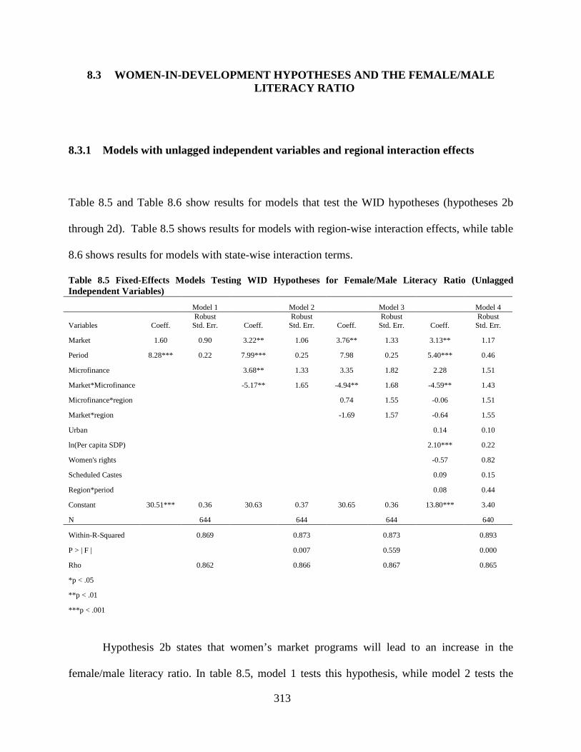
313
8.3 WOMEN-IN-DEVELOPMENT HYPOTHESES AND THE FEMALE/MALE LITERACY RATIO
8.3.1 Models with unlagged independent variables and regional interaction effects
Table 8.5 and Table 8.6 show results for models that test the WID hypotheses (hypotheses 2b
through 2d). Table 8.5 shows results for models with region-wise interaction effects, while table
8.6 shows results for models with state-wise interaction terms.
Table 8.5 Fixed-Effects Models Testing WID Hypotheses for Female/Male Literacy Ratio (Unlagged Independent Variables)
Model 1 Model 2 Model 3 Model 4
Variables Coeff. Robust
Std. Err. Coeff. Robust
Std. Err. Coeff. Robust
Std. Err. Coeff. Robust
Std. Err.
Market 1.60 0.90 3.22** 1.06 3.76** 1.33 3.13** 1.17
Period 8.28*** 0.22 7.99*** 0.25 7.98 0.25 5.40*** 0.46
Microfinance 3.68** 1.33 3.35 1.82 2.28 1.51
Market*Microfinance -5.17** 1.65 -4.94** 1.68 -4.59** 1.43
Microfinance*region 0.74 1.55 -0.06 1.51
Market*region -1.69 1.57 -0.64 1.55
Urban 0.14 0.10
ln(Per capita SDP) 2.10*** 0.22
Women's rights -0.57 0.82
Scheduled Castes 0.09 0.15
Region*period 0.08 0.44
Constant 30.51*** 0.36 30.63 0.37 30.65 0.36 13.80*** 3.40
N 644 644 644 640
Within-R-Squared 0.869 0.873 0.873 0.893
P > | F | 0.007 0.559 0.000
Rho 0.862 0.866 0.867 0.865
*p < .05
**p < .01
***p < .001
Hypothesis 2b states that women’s market programs will lead to an increase in the
female/male literacy ratio. In table 8.5, model 1 tests this hypothesis, while model 2 tests the
314
hypothesis that the joint effect of women’s market programs and women’s microfinance
programs will have a greater impact on raising the literacy ratio ratio than the presence of
women’s market programs alone will have in raising the female/male literacy ratio. In model 1,
there is no statistically significant relationship between the presence of women’s market
programs and variation in the female/male literacy ratio. There is a statistically significant
difference between model 2 and model 1. However, in model 2, there is a statistically significant
relationship between the presence of market programs (p < .01), the presence of microfinance
programs (p < .010), the joint effect of market and microfinance programs (p < .01), and the
female/male literacy ratio. Districts with a market program present have a female/male literacy
ratio that is about 3 percentage points higher than districts without a market program, and
districts with a women’s microfinance program have a literacy ratio that is about 4 percentage
points higher than districts without a microfinance program present. However, the coefficient
for the joint effect of market and microfinance programs on the literacy ratio is negative and
statistically significant (p < .01). Districts that have both a market program and microfinance
program have a female/male literacy ratio that is about 2 percentage points higher than districts
with neither market programs nor microfinance programs present. Therefore, while the joint
effect of women’s market and microfinance programs does seem to have a positive effect on the
female/male literacy ratio, the magnitude of this effect is smaller than the effect that either
market programs alone or microfinance programs alone have on the literacy ratio. Model 3 tests
the hypothesis that the presence of women’s market programs and microfinance programs will
have a greater positive effect on the female/male literacy ratio in southern districts than in
northern districts. However, there is no statistically significant difference between model 3 and
the previous model.
315
Model 4 controls for the effects of women’s rights programs, the percentage of
population comprised of Scheduled Castes, and the interaction effect of region*period. Once
these variables are controlled for, there is still a statistically significant relationship between the
presence of women’s market programs and variation in the female/male literacy ratio (p < .01).
In districts with a women’s market program present, the female/male literacy ratio is 3
percentage points greater than in districts without a women’s market program. However, there is
no statistically significant relationship between the presence of women’s microfinance programs
and the female/male literacy ratio. There is a statistically significant difference between the joint
effect of women’s market programs and microfinance programs on the female/male literacy ratio
and the effect of women’s market programs alone on the literacy ratio (p < .01). In districts
where there are both market programs and microfinance programs present, the female/male
literacy ratio is about 1 percentage point lower than in districts where there is only a market
program present. There is a statistically significant, though substantively small relationship
between log per capita SDP and an increase in the female/male literacy ratio (p < .001). With
every tenfold increase in per capita SDP, there is an increase in the literacy ratio of about 2
percentage points. The passage of time has the strongest statistically significant relationship with
an increase in the female/male literacy ratio (p < .001). With the passing of each decade, there is
an increase of about 5 percentage points in the literacy ratio. This final model is the best fit for
the data, and suggests that there is support for the second WID hypothesis that the presence of
women’s market programs leads to an increase in the female/male literacy ratio. However, it is
necessary to first examine these same models with state-wise interaction terms, as well as models
with lagged independent variables in order to establish a (possible) causal relationship between
the presence of women’s market programs and variation in the female/male literacy ratio.
316
8.3.2 Models with unlagged independent variables and state-wise interaction effects
Table 8.6 shows results for the models testing the WID hypotheses that include the state-wise
interaction effects. The first and second models are the same as the first two models of Table
8.5. Model 3 tests the hypothesis that the presence of women’s market programs and
microfinance programs will have a greater positive effect on the female/male literacy ratio in
southern districts than in northern districts. Unlike model 3 of table 8.5, model 3 of table 8.6 is
statistically significantly different than model 2 (p < .001). However, once the joint effects of
market programs*states and of microfinance programs*states are included in the model, there is
no longer a statistically significant relationship between the presence of women’s market
programs and the female/male literacy ratio. There is a statistically significant difference
between the effect of women’s market programs on the literacy ratio in Gujarat (p < .05)
compared to the effect of market programs on the literacy ratio Rajasthan. There is also a
statistically significant difference between the effect of women’s market programs on the literacy
ratio in Tamil Nadu (p < .01) compared to the effect of market programs on the literacy ratio
Rajasthan. The final model controls for the effects of percentage of population in urban areas,
log per capita SDP, the presence of women’s rights programs, percentage of population
comprised by Scheduled Castes, and the interaction effects of states*time period. Once these
variables are controlled for, there is once again a positive and statistically significant relationship
between the presence of women’s market programs and the female/male literacy ratio (p < .01).
In Rajasthan, the female/male literacy ratio is about 7 percentage points higher in districts with a
women’s market program than in districts without a market program. This is consistent with
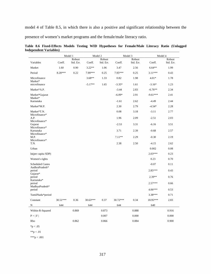
317
model 4 of Table 8.5, in which there is also a positive and significant relationship between the
presence of women’s market programs and the female/male literacy ratio.
Table 8.6 Fixed-Effects Models Testing WID Hypotheses for Female/Male Literacy Ratio (Unlagged Independent Variables)
Model 1 Model 2 Model 3 Model 4
Variables Coeff. Robust
Std. Err. Coeff. Robust
Std. Err. Coeff. Robust
Std. Err. Coeff. Robust
Std. Err.
Market 1.60 0.90 3.22** 1.06 3.47 2.56 6.64** 1.99
Period 8.28*** 0.22 7.99*** 0.25 7.95*** 0.25 3.11*** 0.43
Microfinance 3.68** 1.33 0.82 1.98 4.01* 1.78 Market* microfinance -5.17** 1.65 -3.35* 1.61 -3.16* 1.23
Market*A.P. -3.44 2.83 -6.76** 2.34
Market*Gujarat -6.09* 2.91 -9.61*** 2.41 Market* Karnataka -1.61 2.62 -4.49 2.44
Market*M.P. 2.30 2.79 -4.54* 2.28
Market*T.N. 0.08 3.18 -3.11 2.77 Microfinance* A.P. 1.96 2.09 -2.51 2.03 Microfinance* Gujarat -2.53 3.31 -6.16 3.51 Microfinance* Karnataka 3.71 2.39 -0.68 2.57 Microfinance* M.P. 7.11** 2.29 -0.30 2.19 Microfinance* T.N. 2.38 2.50 -4.15 2.62
Urban 0.002 0.08
ln(per capita SDP) 2.03*** 0.23
Women's rights 0.23 0.70
Scheduled Castes -0.07 0.11 AndhraPradesh* period 2.85*** 0.43 Gujarat* period 2.39** 0.76 Karnataka* period 2.57*** 0.66 MadhyaPradesh* period 4.06*** 0.53
TamilNadu*period 3.38*** 0.71
Constant 30.51*** 0.36 30.63*** 0.37 30.72*** 0.34 18.95*** 2.83
N 644 644 644 640
Within-R-Squared 0.869 0.873 0.888 0.916
P > | F | 0.007 0.000 0.000
Rho 0.862 0.866 0.884 0.900
*p < .05
**p < .01
***p < .001
318
In the fourth model of table 8.6, there is a positive, statistically significant relationship
between the presence of women’s microfinance programs and the female/male literacy ratio (p <
.05). This is in contrast to model 4 of Table 8.5, in which there is no statistically significant
relationship between the presence of women’s microfinance programs and the literacy ratio. In
model 4 of both Table 8.5 and Table 8.6, there is a statistically significant difference between the
joint effect of women’s market*women’s microfinance programs and the female/male literacy
ratio and the effect of just one of these women’s programs on the literacy ratio (p < .01). In
districts that have both a market program and microfinance program present, the female/male
literacy ratio is about 7.5 percentage points higher than in districts with no market or
microfinance programs present. The joint effect of women’s market programs and microfinance
programs has a greater positive effect on the literacy ratio than the effect of microfinance
programs alone. The joint effect of market and microfinance programs also has a slightly greater
positive effect on the literacy ratio than the effect that market programs alone have on the
literacy ratio. Just as there is no statistically significant relationship between the joint effect of
women’s microfinance programs*region in model 4 of Table 8.5, so there is no statistically
significant relationship between any of the interaction effects of microfinance programs*states
and the female/male literacy ratio in model 4 of Table 8.6. Although in model 4 of Table 8.5 the
joint effect of market programs*region is not statistically significant, in model 4 of Table 8.6
some of the joint effects of market*states are statistically significant. In Andhra Pradesh, the
female/male literacy ratio is only 0.12 percentage points lower in districts with a women’s
market program than in districts without a market program; and in Gujarat, the female/male
literacy ratio is about 3 percentage points lower in districts with a women’s market program than
in districts without a market program (p < .001). In Madhya Pradesh, the literacy ratio is about 2
319
percentage points higher in districts with a market program than in districts without a market
program (p < .05). Log per capita SDP has a statistically significant relationship with an increase
in the female/male literacy ratio in model 4 of both Tables 8.5 and 8.6 (p < .001). While there is
no statistically significant relationship between the interaction effect of region*period and the
literacy ratio in model 4 of Table 8.5, there is a statistically significant relationship between all of
the state*period interaction effects and an increase in the female/male literacy ratio (p < .001).
One reason for this apparent discrepancy between these two models may be the fact that the
magnitudes of the joint effects of states*period are all so close, regardless of whether the state in
question is a northern state or a southern state. There is a statistically significant difference
between the effect of time on the literacy ratio in Rajasthan and the effect of time on the literacy
ratio in all of the other states, is statistically significantly different. For instance, in the states of
Andhra Pradesh, Gujarat, Karnataka and Tamil Nadu, the female/male literacy ratio increases by
about 6 percentage points with each passing decade. In Madhya Pradesh, the literacy ratio
increases about 7 percentage points with each passing decade, which is not much higher than in
the other four states. On average, with the passing of each decade there is an increase in the
female/male literacy ratio of 5.26 percentage points in the north and an increase in the literacy
ratio of 6.04 percentage points in the south. Therefore, even in model 4 of Table 8.6 there is not
much substantive difference in the effect of time on the literacy ratio in the north compared to
the south.
The most important finding of these models is that the joint effect of women’s market
programs and microfinance programs has a greater positive impact on the female/male literacy
ratio than the impact of either market programs alone or microfinance programs alone on the
female/male literacy ratio. However, this is only true in the state of Rajasthan. Moreover, it is
320
important to remember that while there is a positive correlation between the joint effect of
market and microfinance programs and the literacy ratio, this does not mean that the presence of
both market and microfinance programs causes an increase in the literacy ratio. It is important to
examine the models with lagged independent variables before making this determination.
8.3.3 Models with lagged independent variables and regional interaction effects
Table 8.7 shows the results of the WID models that include lagged independent variables. The
first model tests the hypothesis that the presence of women’s market programs will lead to an
increase in the female/male literacy ratio. However, there is no statistically significant
relationship between the presence of women’s market programs and the literacy ratio. Model 2,
which tests the hypothesis that the joint effect of women’s market programs and women’s
microfinance programs will have a greater impact on raising the female/male literacy ratio than
either women’s market programs or microfinance programs alone, is not statistically
significantly different than model 1. Model 3 is also not statistically significantly different than
the previous model. Model 4 controls for the effects of percentage of population in urban areas,
log per capita SDP, the presence of women’s rights programs, the percentage of population
comprised of Scheduled Castes, and the interaction effect of region*period. Although there is a
statistically significant relationship between the contemporaneous presence of market programs
and the female/male literacy ratio (see Table 8.5), the results of the models in Table 8.7 show
that there is no statistically significant relationship between the presence of women’s market
programs and the female/male literacy ratio ten years later.
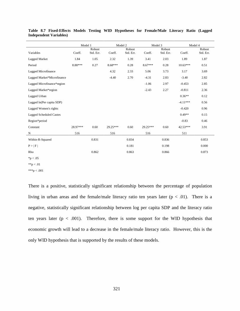
321
Table 8.7 Fixed-Effects Models Testing WID Hypotheses for Female/Male Literacy Ratio (Lagged Independent Variables)
There is a positive, statistically significant relationship between the percentage of population
living in urban areas and the female/male literacy ratio ten years later (p < .01). There is a
negative, statistically significant relationship between log per capita SDP and the literacy ratio
ten years later (p < .001). Therefore, there is some support for the WID hypothesis that
economic growth will lead to a decrease in the female/male literacy ratio. However, this is the
only WID hypothesis that is supported by the results of these models.
Model 1 Model 2 Model 3 Model 4
Variables Coeff. Robust
Std. Err. Coeff. Robust
Std. Err. Coeff. Robust
Std. Err. Coeff. Robust
Std. Err.
Lagged Market 1.84 1.05 2.32 1.39 3.41 2.03 1.89 1.87
Period 8.88*** 0.27 8.68*** 0.28 8.67*** 0.28 10.63*** 0.51
Lagged Microfinance 4.32 2.33 5.06 3.73 3.17 3.69
Lagged Market*Microfinance -4.40 2.70 -4.31 2.83 -3.40 2.82
Lagged Microfinance*region -1.06 2.97 -0.453 2.85
Lagged Market*region -2.43 2.27 -0.811 2.36
Lagged Urban 0.36** 0.12
Lagged ln(Per capita SDP) -4.11*** 0.56
Lagged Women's rights -0.420 0.96
Lagged Scheduled Castes 0.49** 0.15
Region*period -0.83 0.46
Constant 28.97*** 0.60 29.25*** 0.60 29.25*** 0.60 42.53*** 3.91
N 516 516 516 511
Within-R-Squared 0.831 0.834 0.836 0.853
P > | F | 0.181 0.198 0.000
Rho 0.862 0.863 0.866 0.873
*p < .05
**p < .01
***p < .001
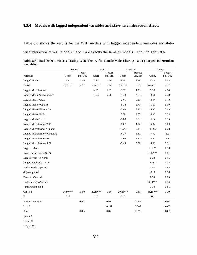
322
8.3.4 Models with lagged independent variables and state-wise interaction effects
Table 8.8 shows the results for the WID models with lagged independent variables and state-
wise interaction terms. Models 1 and 2 are exactly the same as models 1 and 2 in Table 8.6.
Table 8.8 Fixed-Effects Models Testing WID Theory for Female/Male Literacy Ratio (Lagged Independent Variables)
Model 1 Model 2 Model 3 Model 4
Variables Coeff. Robust
Std. Err. Coeff. Robust
Std. Err. Coeff. Robust
Std. Err. Coeff. Robust
Std. Err.
Lagged Market 1.84 1.05 2.32 1.39 3.44 5.38 5.08 5.38
Period 8.88*** 0.27 8.68*** 0.28 8.71*** 0.28 8.45*** 0.97
Lagged Microfinance 4.32 2.33 8.93 4.73 9.16 4.94
Lagged Market*microfinance -4.40 2.70 -3.43 2.50 -3.51 2.48
Lagged Market*A.P. -2.61 5.29 -3.94 5.43
Lagged Market*Gujarat -5.34 5.77 -5.59 5.90
Lagged Market*Karnataka -3.03 5.26 -4.35 5.69
Lagged Market*M.P. 0.68 5.62 -5.95 5.74
Lagged Market*T.N. -2.80 5.89 -5.64 5.75
Lagged Microfinance*A.P. -5.07 4.87 -5.22 5.00
Lagged Microfinance*Gujarat -12.43 6.29 -11.66 6.28
Lagged Microfinance*Karnataka -6.20 5.30 -7.99 5.2
Lagged Microfinance*M.P. -2.98 5.22 -7.62 5.3
Lagged Microfinance*T.N. -5.44 5.59 -4.98 5.31
Lagged Urban 0.33** 0.10
Lagged ln(per capita SDP) -2.92*** 0.61
Lagged Women's rights 0.72 0.95
Lagged Scheduled Castes 0.31* 0.15
AndhraPradesh*period 0.02 0.85
Gujarat*period -0.17 0.76
Karnataka*period 0.78 0.89
MadhyaPradesh*period 3.10*** 0.84
TamilNadu*period 1.14 0.81
Constant 28.97*** 0.60 29.25*** 0.60 29.28*** 0.61 38.15*** 3.79
N 516 516 516 511
Within-R-Squared 0.831 0.834 0.847 0.874
P > | F | 0.181 0.002 0.000
Rho 0.862 0.863 0.877 0.888
*p < .05
**p < .01
***p < .001
323
Unlike model 3 of Table 8.7, model 3 of Table 8.8 is significantly different than model 2
(p < .01). Model 3 of table 8.8 includes the interaction effects between lagged market*states,
lagged microfinance*states, and variation in the female/male literacy ratio. There is almost a
statistically significant difference between the lagged effect of microfinance programs on the
literacy ratio in Gujarat and the lagged effect of microfinance programs on the literacy ratio in
Rajasthan (p = .050). There is no statistically significant difference between the lagged effect of
microfinance programs on the literacy ratio in any of the other states compared to the lagged
effect of microfinance programs on the literacy ratio in Rajasthan. Moreover, the main effect of
microfinance programs is not statistically significant. None of the other interaction effects are
statistically significantly related to variation in the female/male literacy ratio. Model 4 controls
for lagged percentage of population living in urban areas, lagged log per capita SDP, lagged
percentage of population comprised of Scheduled Castes, the lagged presence of women’s rights
programs, and the interaction effects of states*time period. Once these variables are controlled
for, there is no statistically significant difference between the lagged effect of microfinance on
the literacy ratio in Gujarat and the lagged effect of microfinance on the literacy ratio in
Rajasthan. Just as in model 4 of Table 8.7, the only variables of interest that have a statistically
significant relationship with variation in the female/male literacy ratio are lagged percent of
population living in urban areas (p < .01) and lagged log per capita SDP (p < .001). There is a
small yet statistically significant difference between the effect of the passing of time on the
female/male literacy ratio in Madhya Pradesh and the effect of time on the literacy ratio in
Rajasthan (p < .001). As each decade passes, the female/male literacy ratio increases by about 8
percentage points in Rajasthan and by about 12 percentage points in Madhya Pradesh. These
324
models with the state-wise interaction terms confirm the findings of the models with lagged
independent variables and regional interaction terms. Since there is a positive, significant
relationship between percentage of population in urban areas and the female/male literacy ratio,
there is some support for the modernization hypothesis that increased urbanization will lead to an
increase in the female/male literacy ratio. However, there is also support for the first WID
hypothesis since an increase in log per capita SDP leads to a decrease in the female/male literacy
ratio ten years later.
8.4 GENDER-AND-DEVELOPMENT HYPOTHESES AND THE FEMALE/MALE LITERACY RATIO
8.4.1 Models with unlagged independent variables and regional interaction effects
Table 8.9 presents the results of models that test the GAD hypotheses regarding change in the
female/male literacy ratio. Model 1 tests the hypothesis that the presence of women’s rights
programs will have a positive effect on the female/male literacy ratio. However, the presence of
women’s rights programs is not statistically significantly related to variation in the literacy ratio.
Model 2, which tests the hypothesis that the presence of women’s rights programs will have a
greater positive effect in southern districts than in northern districts, is not statistically
significantly different than the previous model. Model 3 tests the hypothesis that the joint effect
of women’s rights programs, market programs, and microfinance programs will have a greater
positive impact on the female/male literacy ratio than the presence of women’s rights programs
alone have on the literacy ratio. There is a statistically significant relationship between this
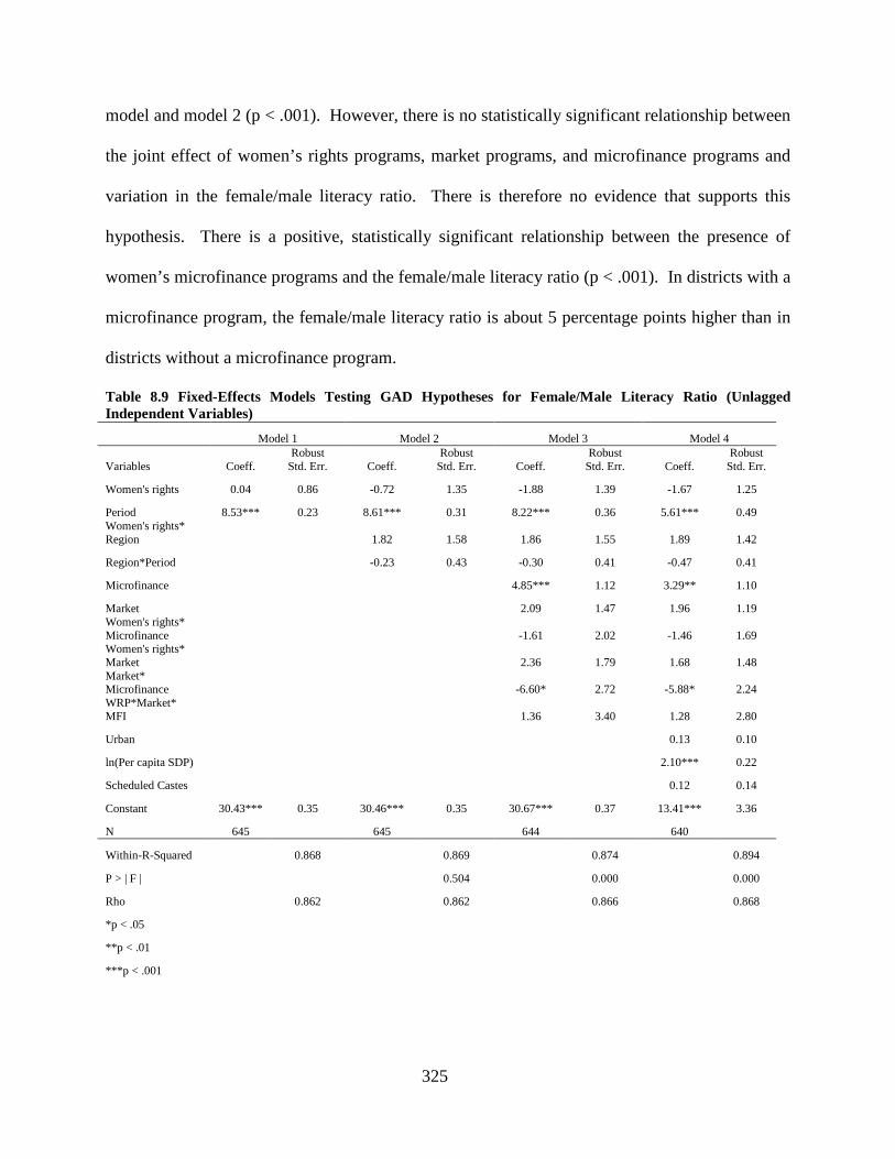
325
model and model 2 (p < .001). However, there is no statistically significant relationship between
the joint effect of women’s rights programs, market programs, and microfinance programs and
variation in the female/male literacy ratio. There is therefore no evidence that supports this
hypothesis. There is a positive, statistically significant relationship between the presence of
women’s microfinance programs and the female/male literacy ratio (p < .001). In districts with a
microfinance program, the female/male literacy ratio is about 5 percentage points higher than in
districts without a microfinance program.
Table 8.9 Fixed-Effects Models Testing GAD Hypotheses for Female/Male Literacy Ratio (Unlagged Independent Variables)
Model 1 Model 2 Model 3 Model 4
Variables Coeff. Robust
Std. Err. Coeff. Robust
Std. Err. Coeff. Robust
Std. Err. Coeff. Robust
Std. Err.
Women's rights 0.04 0.86 -0.72 1.35 -1.88 1.39 -1.67 1.25
Period 8.53*** 0.23 8.61*** 0.31 8.22*** 0.36 5.61*** 0.49 Women's rights* Region 1.82 1.58 1.86 1.55 1.89 1.42
Region*Period -0.23 0.43 -0.30 0.41 -0.47 0.41
Microfinance 4.85*** 1.12 3.29** 1.10
Market 2.09 1.47 1.96 1.19 Women's rights* Microfinance -1.61 2.02 -1.46 1.69 Women's rights* Market 2.36 1.79 1.68 1.48 Market* Microfinance -6.60* 2.72 -5.88* 2.24 WRP*Market* MFI 1.36 3.40 1.28 2.80
Urban 0.13 0.10
ln(Per capita SDP) 2.10*** 0.22
Scheduled Castes 0.12 0.14
Constant 30.43*** 0.35 30.46*** 0.35 30.67*** 0.37 13.41*** 3.36
N 645 645 644 640
Within-R-Squared 0.868 0.869 0.874 0.894
P > | F | 0.504 0.000 0.000
Rho 0.862 0.862 0.866 0.868
*p < .05
**p < .01
***p < .001
326
There is also a statistically significant difference between the joint effect of women’s market and
microfinance programs on the literacy ratio and the effect of market or microfinance programs
alone on the literacy ratio (p < .05). Districts with both a women’s market program and
microfinance program present have a literacy ratio that is only 0.34 percentage points higher than
the literacy ratio of districts with neither of these types of programs present.
The fourth model controls for percentage of population in urban areas, log per capita
SDP, and percentage of population comprised of Scheduled Castes. This model is statistically
significantly different than the previous model, and is therefore the best fit for the data (p <
.001). After controlling for these other variables, there is still a positive, statistically significant
relationship between the presence of microfinance programs and the female/male literacy ratio (p
< .01). There is also still a statistically significant difference between the joint effect of market
and microfinance programs on the literacy ratio and the effect of these two types of programs
alone on the literacy ratio (p < .05). However, the results of this last model show that districts
with both a market and microfinance program present have a female/male literacy ratio that is
lower by 0.63 percentage points than the literacy ratio of districts with only one of these two
types of women’s programs. Overall, there is no evidence from these models that support the
GAD hypotheses.
8.4.2 Models with unlagged independent variables and state-wise interaction effects
Table 8.10 provides the results for models testing the GAD hypotheses that include the state-
wise interaction terms. The first model is the same as the first model in Table 8.9. Model 2 of
Table 8.10 includes the women’s rights programs*states and the states*time period interaction
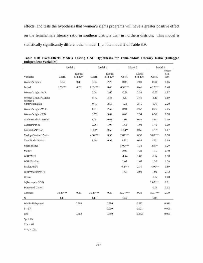
327
effects, and tests the hypothesis that women’s rights programs will have a greater positive effect
on the female/male literacy ratio in southern districts than in northern districts. This model is
statistically significantly different than model 1, unlike model 2 of Table 8.9.
Table 8.10 Fixed-Effects Models Testing GAD Hypotheses for Female/Male Literacy Ratio (Unlagged Independent Variables)
Model 1 Model 2 Model 3 Model 4
Variables Coeff. Robust
Std. Err. Coeff. Robust
Std. Err. Coeff. Robust
Std. Err. Coeff.
Robust Std. Err.
Women's rights 0.04 0.86 0.83 2.26 0.02 2.01 0.39 1.66
Period 8.53*** 0.23 7.03*** 0.46 6.38*** 0.46 4.12*** 0.48
Women's rights*A.P. 0.04 2.60 -0.20 2.34 -0.63 1.87
Women's rights*Gujarat -5.49 3.85 -6.57 3.89 -6.19 3.59 Women's rights*Karnataka -0.15 2.53 -0.80 2.45 -0.79 2.20
Women's rights*M.P. 1.51 2.67 0.91 2.52 0.25 2.05
Women's rights*T.N. 0.57 3.04 0.00 2.54 0.56 1.98
AndhraPradesh*Period 1.04 0.63 1.02 0.54 1.31* 0.50
Gujarat*Period 0.96 1.04 1.63 1.03 1.46 0.99
Karnataka*Period 1.53* 0.58 1.83** 0.65 1.75* 0.67
MadhyaPradesh*Period 2.66*** 0.55 2.87*** 0.53 3.09*** 0.50
TamilNadu*Period 1.69 0.98 1.85* 0.82 1.76* 0.69
Microfinance 5.00*** 1.31 3.07* 1.20
Market 2.09 1.31 1.75 0.99
WRP*MFI -1.44 1.87 -0.74 1.58
WRP*Market 2.07 1.67 1.36 1.38
Market*MFI -6.27** 2.30 -4.90** 1.80
WRP*Market*MFI 1.66 2.91 1.09 2.32
Urban -0.02 0.08
ln(Per capita SDP) 2.07*** 0.21
Scheduled Castes -0.06 0.12
Constant 30.43*** 0.35 30.48*** 0.29 30.74*** 0.31 18.97*** 2.79
N 645 645 644 640
Within-R-Squared 0.868 0.886 0.892 0.911
P > | F | 0.000 0.001 0.000
Rho 0.862 0.880 0.883 0.901
*p < .05
**p < .01
***p < .001
328
However, there is no statistically significant relationship between any of the women’s
rights programs*states variables and variation in the female/male literacy ratio. Therefore, I
confidently reject the hypothesis that model 2 tests. There is a statistically significant difference
between the effect of the passing of time on the literacy ratios in Karnataka (0.05) and Madhya
Pradesh (0.001) compared to the effect of the passing of time on the literacy ratio in Rajasthan.
Model 3 tests the hypothesis that the joint effect of women’s rights programs, women’s market
programs, and women’s microfinance programs will have a greater positive effect on the
female/male literacy ratio than the presence of women’s rights programs alone will have on the
literacy ratio. The results of this model show that there is no statistically significant relationship
between any of the interaction effects that include women’s rights programs, which is similar to
model 3 of table 8.9. Also similar to model 3 of Table 8.9, in model 3 of Table 8.10 there is a
statistically significant relationship between the presence of women’s microfinance programs
and an increase in the female/male literacy ratio (p < .001). Likewise, there is a statistically
significant difference between the joint effect of women’s market programs and microfinance
programs on the literacy ratio (p < .01) and the effect of market programs or microfinance
programs alone on the literacy ratio. Model 4 controls for the effects of percentage of population
in urban areas, log per capita SDP, and percentage of population comprised of Scheduled Castes,
and is statistically significantly different than model 3. After controlling for these variables,
there is still a positive, statistically significant relationship between the presence of women’s
microfinance programs and the female/male literacy ratio (p < .05). There is also a statistically
significant difference between the joint effect of women’s market programs and microfinance
programs on the literacy ratio (p < .01) and the effect of market programs or microfinance
programs alone on the literacy ratio. However, districts with both a market and microfinance
329
program have a female/male literacy ratio that is lower by only 0.08 percentage points than the
literacy ratio of districts with neither of these two types of programs. There is also a statistically
significant relationship between log per capita SDP and an increase in the literacy ratio (p <
.001). All of these statistically significant relationships are very similar to the statistically
significant relationships of model 4 of Table 8.9. Moreover, the magnitude of these variables’
relationships with the female/male literacy ratio are very close to the magnitude of these
variables’ relationships with the literacy ratio in model 4 of Table 8.9. However, whereas in
model 4 of table 8.9 there is no statistically significant difference between the effect of the
passage of time on the literacy ratio in northern districts versus southern districts, in model 4 of
table 8.10 there is a statistically significant difference between the effect of time on the literacy
ratio in Rajasthan and the effect of time on the literacy ratio in four other states. In Karnataka
and Tamil Nadu, the female/male literacy ratio increases by about 6 percentage points with each
passing decade (p < .05), and in Andhra Pradesh the literacy ratio increases by about 5
percentage points with each passing decade (p < .05). In Rajasthan, the literacy ratio increases
about 4 percentage points with each passing decade (p < .001). In Madhya Pradesh, the
female/male literacy ratio increases by about 7 percentage points with each passing decade (p <
.001). The passage of time leads to an average increase in the literacy ratio of 5.7 percentage
points each decade in both northern states and southern states. The results of the models in both
tables 8.9 and 8.10 indicate that there is no support for any of the GAD hypotheses.
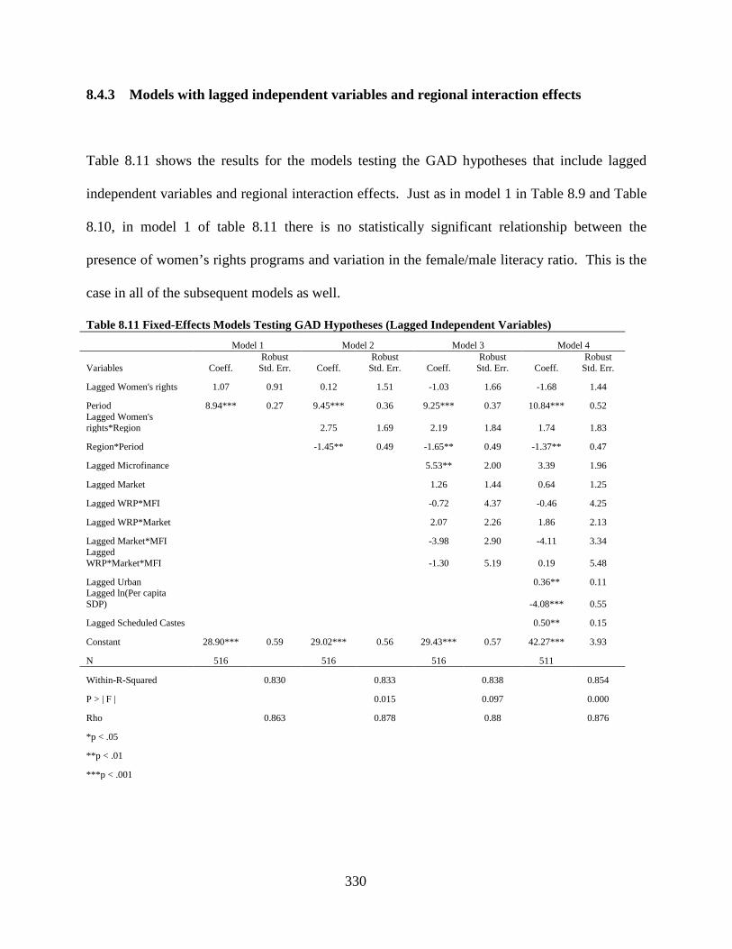
330
8.4.3 Models with lagged independent variables and regional interaction effects
Table 8.11 shows the results for the models testing the GAD hypotheses that include lagged
independent variables and regional interaction effects. Just as in model 1 in Table 8.9 and Table
8.10, in model 1 of table 8.11 there is no statistically significant relationship between the
presence of women’s rights programs and variation in the female/male literacy ratio. This is the
case in all of the subsequent models as well.
Table 8.11 Fixed-Effects Models Testing GAD Hypotheses (Lagged Independent Variables) Model 1 Model 2 Model 3 Model 4
Variables Coeff. Robust
Std. Err. Coeff. Robust
Std. Err. Coeff. Robust
Std. Err. Coeff. Robust
Std. Err.
Lagged Women's rights 1.07 0.91 0.12 1.51 -1.03 1.66 -1.68 1.44
Period 8.94*** 0.27 9.45*** 0.36 9.25*** 0.37 10.84*** 0.52 Lagged Women's rights*Region 2.75 1.69 2.19 1.84 1.74 1.83
Region*Period -1.45** 0.49 -1.65** 0.49 -1.37** 0.47
Lagged Microfinance 5.53** 2.00 3.39 1.96
Lagged Market 1.26 1.44 0.64 1.25
Lagged WRP*MFI -0.72 4.37 -0.46 4.25
Lagged WRP*Market 2.07 2.26 1.86 2.13
Lagged Market*MFI -3.98 2.90 -4.11 3.34 Lagged WRP*Market*MFI -1.30 5.19 0.19 5.48
Lagged Urban 0.36** 0.11 Lagged ln(Per capita SDP) -4.08*** 0.55
Lagged Scheduled Castes 0.50** 0.15
Constant 28.90*** 0.59 29.02*** 0.56 29.43*** 0.57 42.27*** 3.93
N 516 516 516 511
Within-R-Squared 0.830 0.833 0.838 0.854
P > | F | 0.015 0.097 0.000
Rho 0.863 0.878 0.88 0.876
*p < .05
**p < .01
***p < .001

331
Model 2 tests the hypothesis that women’s rights programs will have a greater positive impact on
female/male literacy ratio in southern districts than in northern districts. Although this model is
statistically significantly different than model 1 (p < .05), there is no statistically significant
relationship between the interaction effect of women’s rights programs*region and variation in
the literacy ratio. However, the interaction effect of region*period has a small negative, yet
statistically significant relationship with the female/male literacy ratio. In southern districts, the
literacy ratio is about 1 percentage point lower during each decade than in northern districts.
Model 3 tests the hypothesis that the joint effect of women’s rights programs, women’s market
programs, and women’s microfinance programs will have a greater positive effect on the literacy
ratio than the effect of women’s rights programs alone will have on the literacy ratio. However,
there is no statistically significant difference between model 3 and the previous model. Model 4
controls for the lagged effects of log per capita SDP, percentage of population in urban areas,
and percentage of population comprised of Scheduled Castes. This model is statistically
significantly different than the previous model, and thus is the best-fitting model for the data. In
this final model, there is still no statistically significant relationship between the lagged presence
of women’s rights programs and variation in the female/male literacy ratio, nor between the
lagged joint effect of women’s rights programs, market programs, and microfinance programs
and the literacy ratio. There is still a small yet statistically significant relationship between the
interaction effect of region*period and the female/male literacy ratio. There is also a small yet
statistically significant relationship between lagged percentage of population in urban areas and
an increase in the literacy ratio (p < .01), as well as a small yet statistically significant
relationship between lagged percentage of population comprised of Scheduled Castes and an
increase in the female/male literacy ratio (p < .01). There is a negative, statistically significant
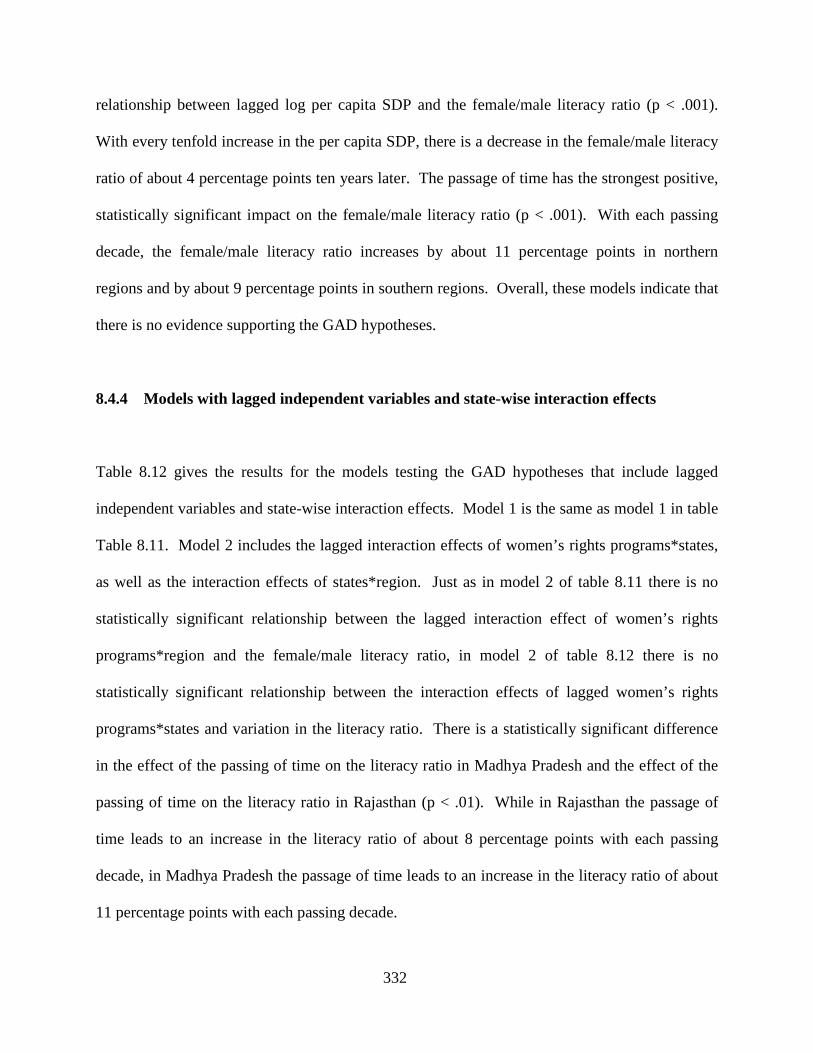
332
relationship between lagged log per capita SDP and the female/male literacy ratio (p < .001).
With every tenfold increase in the per capita SDP, there is a decrease in the female/male literacy
ratio of about 4 percentage points ten years later. The passage of time has the strongest positive,
statistically significant impact on the female/male literacy ratio (p < .001). With each passing
decade, the female/male literacy ratio increases by about 11 percentage points in northern
regions and by about 9 percentage points in southern regions. Overall, these models indicate that
there is no evidence supporting the GAD hypotheses.
8.4.4 Models with lagged independent variables and state-wise interaction effects
Table 8.12 gives the results for the models testing the GAD hypotheses that include lagged
independent variables and state-wise interaction effects. Model 1 is the same as model 1 in table
Table 8.11. Model 2 includes the lagged interaction effects of women’s rights programs*states,
as well as the interaction effects of states*region. Just as in model 2 of table 8.11 there is no
statistically significant relationship between the lagged interaction effect of women’s rights
programs*region and the female/male literacy ratio, in model 2 of table 8.12 there is no
statistically significant relationship between the interaction effects of lagged women’s rights
programs*states and variation in the literacy ratio. There is a statistically significant difference
in the effect of the passing of time on the literacy ratio in Madhya Pradesh and the effect of the
passing of time on the literacy ratio in Rajasthan (p < .01). While in Rajasthan the passage of
time leads to an increase in the literacy ratio of about 8 percentage points with each passing
decade, in Madhya Pradesh the passage of time leads to an increase in the literacy ratio of about
11 percentage points with each passing decade.
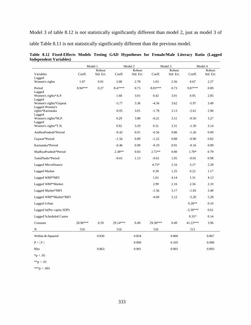
333
Model 3 of table 8.12 is not statistically significantly different than model 2, just as model 3 of
table Table 8.11 is not statistically significantly different than the previous model.
Table 8.12 Fixed-Effects Models Testing GAD Hypotheses for Female/Male Literacy Ratio (Lagged Independent Variables)
Model 1 Model 2 Model 3 Model 4
Variables Coeff. Robust
Std. Err. Coeff. Robust
Std. Err. Coeff. Robust
Std. Err. Coeff. Robust
Std. Err. Lagged Women's rights 1.07 0.91 2.08 2.78 1.03 2.56 0.67 2.27
Period 8.94*** 0.27 8.47*** 0.75 8.05*** 0.73 9.87*** 0.89 Lagged Women's rights*A.P. 1.68 3.01 0.42 3.01 0.95 2.85 Lagged Women's rights*Gujarat -3.77 3.36 -4.56 3.62 -5.97 3.49 Lagged Women's rights*Karnataka -0.05 3.01 -1.78 3.13 -2.61 2.96 Lagged Women's rights*M.P. 0.29 3.88 -0.21 3.51 -0.50 3.27 Lagged Women's rights*T.N. 0.92 3.29 0.31 3.31 -1.39 3.14
AndhraPradesh*Period -0.42 0.91 -0.56 0.86 -1.26 0.90
Gujarat*Period -1.56 0.89 -1.22 0.88 -0.90 0.82
Karnataka*Period -0.46 0.90 -0.19 0.91 -0.16 0.89
MadhyaPradesh*Period 2.38** 0.83 2.72** 0.80 1.78* 0.79
TamilNadu*Period -0.61 1.13 -0.61 1.05 -0.01 0.98
Lagged Microfinance 4.73* 2.16 3.17 2.28
Lagged Market 0.39 1.25 0.22 1.17
Lagged WRP*MFI 1.61 4.14 1.31 4.13
Lagged WRP*Market 2.99 2.16 2.56 2.10
Lagged Market*MFI -1.56 3.17 -1.83 3.48
Lagged WRP*Market*MFI -4.60 5.12 -3.20 5.28
Lagged Urban 0.28** 0.10
Lagged ln(Per capita SDP) -3.39*** 0.61
Lagged Scheduled Castes 0.35* 0.14
Constant 28.90*** 0.59 29.14*** 0.49 29.58*** 0.49 41.23*** 3.96
N 516 516 516 511
Within-R-Squared 0.830 0.854 0.860 0.867
P > | F | 0.000 0.105 0.000
Rho 0.863 0.901 0.903 0.893
*p < .05
**p < .01
***p < .001
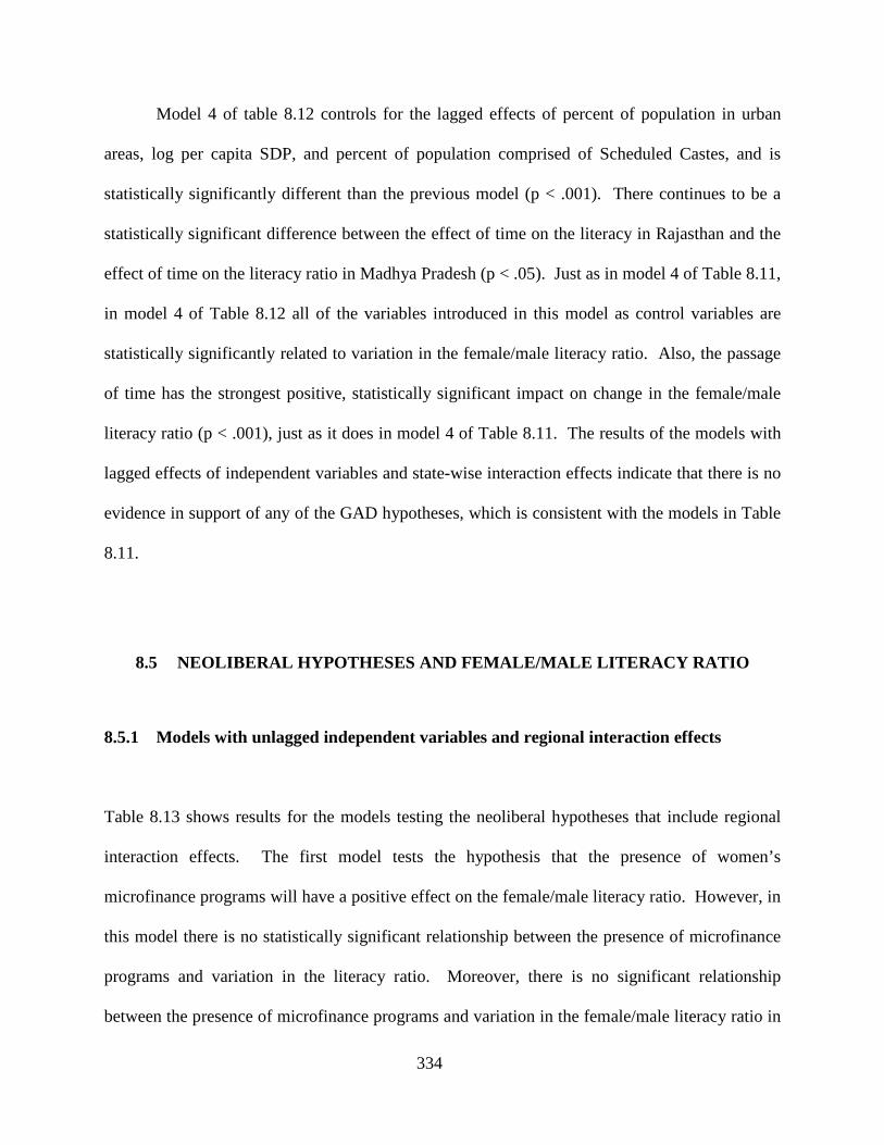
334
Model 4 of table 8.12 controls for the lagged effects of percent of population in urban
areas, log per capita SDP, and percent of population comprised of Scheduled Castes, and is
statistically significantly different than the previous model (p < .001). There continues to be a
statistically significant difference between the effect of time on the literacy in Rajasthan and the
effect of time on the literacy ratio in Madhya Pradesh (p < .05). Just as in model 4 of Table 8.11,
in model 4 of Table 8.12 all of the variables introduced in this model as control variables are
statistically significantly related to variation in the female/male literacy ratio. Also, the passage
of time has the strongest positive, statistically significant impact on change in the female/male
literacy ratio (p < .001), just as it does in model 4 of Table 8.11. The results of the models with
lagged effects of independent variables and state-wise interaction effects indicate that there is no
evidence in support of any of the GAD hypotheses, which is consistent with the models in Table
8.11.
8.5 NEOLIBERAL HYPOTHESES AND FEMALE/MALE LITERACY RATIO
8.5.1 Models with unlagged independent variables and regional interaction effects
Table 8.13 shows results for the models testing the neoliberal hypotheses that include regional
interaction effects. The first model tests the hypothesis that the presence of women’s
microfinance programs will have a positive effect on the female/male literacy ratio. However, in
this model there is no statistically significant relationship between the presence of microfinance
programs and variation in the literacy ratio. Moreover, there is no significant relationship
between the presence of microfinance programs and variation in the female/male literacy ratio in
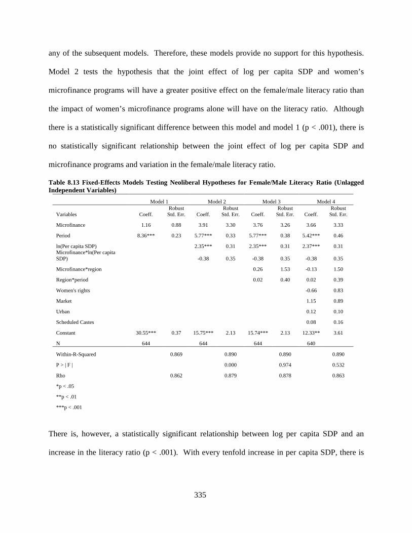
335
any of the subsequent models. Therefore, these models provide no support for this hypothesis.
Model 2 tests the hypothesis that the joint effect of log per capita SDP and women’s
microfinance programs will have a greater positive effect on the female/male literacy ratio than
the impact of women’s microfinance programs alone will have on the literacy ratio. Although
there is a statistically significant difference between this model and model 1 (p < .001), there is
no statistically significant relationship between the joint effect of log per capita SDP and
microfinance programs and variation in the female/male literacy ratio.
Table 8.13 Fixed-Effects Models Testing Neoliberal Hypotheses for Female/Male Literacy Ratio (Unlagged Independent Variables)
Model 1 Model 2 Model 3 Model 4
Variables Coeff. Robust
Std. Err. Coeff. Robust
Std. Err. Coeff. Robust
Std. Err. Coeff. Robust
Std. Err.
Microfinance 1.16 0.88 3.91 3.30 3.76 3.26 3.66 3.33
Period 8.36*** 0.23 5.77*** 0.33 5.77*** 0.38 5.42*** 0.46
ln(Per capita SDP) 2.35*** 0.31 2.35*** 0.31 2.37*** 0.31 Microfinance*ln(Per capita SDP) -0.38 0.35 -0.38 0.35 -0.38 0.35
Microfinance*region 0.26 1.53 -0.13 1.50
Region*period 0.02 0.40 0.02 0.39
Women's rights -0.66 0.83
Market 1.15 0.89
Urban 0.12 0.10
Scheduled Castes 0.08 0.16
Constant 30.55*** 0.37 15.75*** 2.13 15.74*** 2.13 12.33** 3.61
N 644 644 644 640
Within-R-Squared 0.869 0.890 0.890 0.890
P > | F | 0.000 0.974 0.532
Rho 0.862 0.879 0.878 0.863
*p < .05
**p < .01
***p < .001
There is, however, a statistically significant relationship between log per capita SDP and an
increase in the literacy ratio (p < .001). With every tenfold increase in per capita SDP, there is
336
an increase in the female/male literacy ratio of about 2 percentage points. Although this is
statistically significant, substantively this is very small.
Model 3 includes the interaction effects of microfinance*region and region*period, but is
not statistically significantly different than the previous model. Model 4, which controls for the
effects of the presence of women’s rights programs, percent of population in urban areas, and
percentage of population comprised of Scheduled Castes, is also not statistically significantly
different than the previous model. Therefore, the results of these models provide no support for
the neoliberal hypotheses.
8.5.2 Models with unlagged independent variables and state-wise interaction effects
Table 8.14 shows results for the models testing the neoliberal hypotheses that include state-wise
interaction effects. Models 1 and 2 are the same as models 1 and 2 in Table 8.13. Model 3 of
Table 8.14 includes the interaction effects of women’s microfinance programs*states and
states*period, and is statistically significantly different than model 2. This is in contrast to
model 3 of Table 8.13, which is not significantly different than the previous model. Once these
interaction effects are included in the model, there is a statistically significant relationship
between the presence of women’s microfinance programs and variation in female/male literacy
ratio (p < .05). In Rajasthan, districts with a microfinance program present have a female/male
literacy ratio that is about 9 percentage points higher than districts with no microfinance program
present. There is a statistically significant difference between the effect of microfinance
programs on the literacy ratio in Andhra Pradesh (p < .05) and the effect of microfinance
programs on the literacy ratio in Rajasthan.
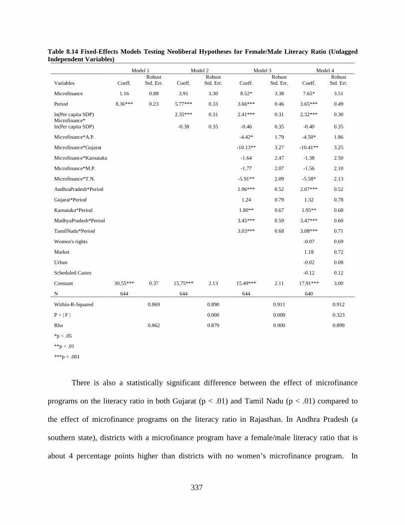
337
Table 8.14 Fixed-Effects Models Testing Neoliberal Hypotheses for Female/Male Literacy Ratio (Unlagged Independent Variables)
Model 1 Model 2 Model 3 Model 4
Variables Coeff. Robust
Std. Err. Coeff. Robust
Std. Err. Coeff. Robust
Std. Err. Coeff. Robust
Std. Err.
Microfinance 1.16 0.88 3.91 3.30 8.52* 3.38 7.65* 3.51
Period 8.36*** 0.23 5.77*** 0.33 3.66*** 0.46 3.65*** 0.49
ln(Per capita SDP) 2.35*** 0.31 2.41*** 0.31 2.32*** 0.30 Microfinance* ln(Per capita SDP) -0.38 0.35 -0.46 0.35 -0.40 0.35
Microfinance*A.P. -4.42* 1.79 -4.50* 1.86
Microfinance*Gujarat -10.13** 3.27 -10.41** 3.25
Microfinance*Karnataka -1.64 2.47 -1.38 2.50
Microfinance*M.P. -1.77 2.07 -1.56 2.10
Microfinance*T.N. -5.91** 2.09 -5.58* 2.13
AndhraPradesh*Period 1.96*** 0.52 2.07*** 0.52
Gujarat*Period 1.24 0.79 1.32 0.78
Karnataka*Period 1.80** 0.67 1.95** 0.68
MadhyaPradesh*Period 3.45*** 0.59 3.47*** 0.60
TamilNadu*Period 3.03*** 0.68 3.08*** 0.71
Women's rights -0.07 0.69
Market 1.18 0.72
Urban -0.02 0.08
Scheduled Castes -0.12 0.12
Constant 30.55*** 0.37 15.75*** 2.13 15.49*** 2.11 17.91*** 3.00
N 644 644 644 640
Within-R-Squared 0.869 0.890 0.911 0.912
P > | F | 0.000 0.000 0.323
Rho 0.862 0.879 0.900 0.899
*p < .05
**p < .01
***p < .001
There is also a statistically significant difference between the effect of microfinance
programs on the literacy ratio in both Gujarat (p < .01) and Tamil Nadu (p < .01) compared to
the effect of microfinance programs on the literacy ratio in Rajasthan. In Andhra Pradesh (a
southern state), districts with a microfinance program have a female/male literacy ratio that is
about 4 percentage points higher than districts with no women’s microfinance program. In
338
Gujarat (a northern state), districts with a microfinance program present have a female/male
literacy ratio that is about 2 percentage points lower than in districts with no microfinance
program. In Tamil Nadu (another southern state), districts with a women’s microfinance
program have a literacy ratio that is about 3 percentage points higher than districts without a
microfinance program.
The fact that there is a statistically significant relationship between some of the
microfinance*state variables and the female/male literacy ratio may seem inconsistent with the
fact that there is no statistically significant relationship between the interaction effect of
microfinance programs*region and the literacy ratio (compare to Table 8.13). However, if one
averages the coefficients for microfinance programs in the northern states and then does the same
with the coefficients for microfinance programs in southern states, one finds that the average
effect of microfinance programs on the literacy ratio in northern states and southern states is
almost identical. On average, districts in northern states with a microfinance program present
have a female/male literacy ratio that is 2.3 percentage points higher than in districts with no
microfinance programs. On average, districts in southern states with a microfinance program
present have a female/male literacy ratio that is 2.2 percentage points higher than districts with
no microfinance program. Therefore, even though there is support for the hypothesis that
women’s microfinance programs have a positive impact on the female/male literacy ratio, there
is no evidence supporting the hypothesis that women’s microfinance programs will have a
greater positive impact on the literacy ratio in southern districts than in northern districts. It
appears that the presence of microfinance programs on the female/male literacy ratio has the
strongest positive effect in Rajasthan. There is a statistically significant difference between the
effect of the passage of time on the literacy ratio in the state of Rajasthan compared to the effect
339
of the passage of time on the literacy ratio in Andhra Pradesh (p < .001), Karnataka (p < .01),
Madhya Pradesh (p < .001), and Tamil Nadu (p < .001). At first this seems rather surprising
since there is no statistically significant relationship between the interaction effect of
region*period and the literacy ratio in the models from Table 8.13. If one averages the
coefficients for time period in the northern states, one finds that with each passing decade the
female/male literacy ratio increases by an average of about 4 percentage points in the northern
region. Likewise, in the southern region, with each passing decade the female/male literacy ratio
increases by about 6 percentage points. This is a difference of only 2 percentage points between
the two regions. There is no statistically significant difference between model 4 and the previous
model, which is consistent with model 4 of Table 8.13. Therefore, model 3 is the best-fitting
model for the data. Overall, these models support the hypothesis that the presence of women’s
microfinance programs will have a positive effect on the female/male literacy ratio. However,
they do not provide support for any of the other neoliberal models.
8.5.3 Models with lagged independent variables and regional interaction effects
Table 8.15 provides results for the models testing the neoliberal hypotheses that included lagged
independent variables and regional interaction effects. The results of the first model indicate that
there is no statistically significant relationship between the presence of women’s microfinance
programs and variation in the female/male literacy ratio, which is similar to the results of the
previous models testing the neoliberal hypotheses. The second model, which includes lagged log
per capita SDP and the lagged interaction effect of women’s microfinance programs*log per
capita SDP, is statistically significantly different than the previous model.
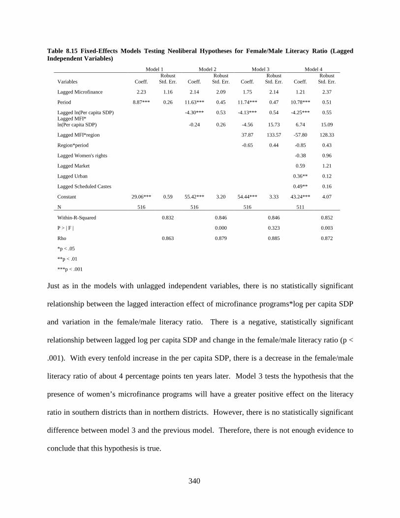
340
Table 8.15 Fixed-Effects Models Testing Neoliberal Hypotheses for Female/Male Literacy Ratio (Lagged Independent Variables)
Model 1 Model 2 Model 3 Model 4
Variables Coeff. Robust
Std. Err. Coeff. Robust
Std. Err. Coeff. Robust
Std. Err. Coeff. Robust
Std. Err.
Lagged Microfinance 2.23 1.16 2.14 2.09 1.75 2.14 1.21 2.37
Period 8.87*** 0.26 11.63*** 0.45 11.74*** 0.47 10.78*** 0.51
Lagged ln(Per capita SDP) -4.30*** 0.53 -4.13*** 0.54 -4.25*** 0.55 Lagged MFI* ln(Per capita SDP) -0.24 0.26 -4.56 15.73 6.74 15.09
Lagged MFI*region 37.87 133.57 -57.80 128.33
Region*period -0.65 0.44 -0.85 0.43
Lagged Women's rights -0.38 0.96
Lagged Market 0.59 1.21
Lagged Urban 0.36** 0.12
Lagged Scheduled Castes 0.49** 0.16
Constant 29.06*** 0.59 55.42*** 3.20 54.44*** 3.33 43.24*** 4.07
N 516 516 516 511
Within-R-Squared 0.832 0.846 0.846 0.852
P > | F | 0.000 0.323 0.003
Rho 0.863 0.879 0.885 0.872
*p < .05
**p < .01
***p < .001 Just as in the models with unlagged independent variables, there is no statistically significant
relationship between the lagged interaction effect of microfinance programs*log per capita SDP
and variation in the female/male literacy ratio. There is a negative, statistically significant
relationship between lagged log per capita SDP and change in the female/male literacy ratio (p <
.001). With every tenfold increase in the per capita SDP, there is a decrease in the female/male
literacy ratio of about 4 percentage points ten years later. Model 3 tests the hypothesis that the
presence of women’s microfinance programs will have a greater positive effect on the literacy
ratio in southern districts than in northern districts. However, there is no statistically significant
difference between model 3 and the previous model. Therefore, there is not enough evidence to
conclude that this hypothesis is true.
341
Model 4, which controls for the lagged effects of women’s rights programs, women’s
market programs, percentage of population in urban areas, and percentage of population
comprised of Scheduled Castes, is statistically significantly different than model 3. Therefore,
this final model is the best fit for the data. Even after controlling for these other variables, there
is still a negative, statistically significant relationship between lagged log per capita SDP and
change in the female/male literacy ratio. There is still no statistically significant relationship
between the presence of women’s microfinance programs and the literacy ratio, nor between the
lagged interaction effect of microfinance programs*region and the literacy ratio. There is a
small, positive, and statistically significant relationship between lagged percentage of population
in urban areas and the literacy ratio (p < .01), and between the lagged percentage of population
comprised of Scheduled Castes and the female/male literacy ratio (p < .01). The passing of time
has the strongest positive, statistically significant effect on the female/male literacy ratio (p <
.001). With the passing of each decade, the female/male literacy ratio increases by about 11
percentage points. The results of these models with lagged independent variables and regional
interaction terms do not support any of the neoliberal hypotheses.
8.5.4 Models with lagged independent variables and state-wise interaction effects
Table 8.16 shows the results for the models testing the neoliberal hypotheses that include lagged
independent variables and state-wise interaction effects. The first two models are the same as the
first two models in Table 8.15 with the regional interaction effects. Model 3 of table 8.16
includes lagged interaction effects of microfinance programs*states and states*period, and is
statistically significantly different than model 2. There is a statistically significant difference
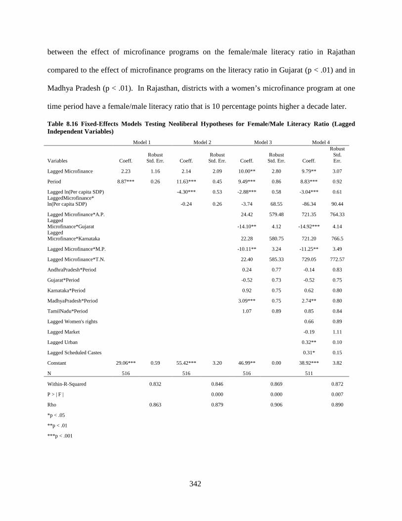
342
between the effect of microfinance programs on the female/male literacy ratio in Rajathan
compared to the effect of microfinance programs on the literacy ratio in Gujarat (p < .01) and in
Madhya Pradesh (p < .01). In Rajasthan, districts with a women’s microfinance program at one
time period have a female/male literacy ratio that is 10 percentage points higher a decade later.
Table 8.16 Fixed-Effects Models Testing Neoliberal Hypotheses for Female/Male Literacy Ratio (Lagged Independent Variables)
Model 1 Model 2 Model 3 Model 4
Variables Coeff. Robust
Std. Err. Coeff. Robust
Std. Err. Coeff. Robust
Std. Err. Coeff.
Robust Std. Err.
Lagged Microfinance 2.23 1.16 2.14 2.09 10.00** 2.80 9.79** 3.07
Period 8.87*** 0.26 11.63*** 0.45 9.49*** 0.86 8.83*** 0.92
Lagged ln(Per capita SDP) -4.30*** 0.53 -2.88*** 0.58 -3.04*** 0.61 LaggedMicrofinance* ln(Per capita SDP) -0.24 0.26 -3.74 68.55 -86.34 90.44
Lagged Microfinance*A.P. 24.42 579.48 721.35 764.33 Lagged Microfinance*Gujarat -14.10** 4.12 -14.92*** 4.14 Lagged Microfinance*Karnataka 22.28 580.75 721.20 766.5
Lagged Microfinance*M.P. -10.11** 3.24 -11.25** 3.49
Lagged Microfinance*T.N. 22.40 585.33 729.05 772.57
AndhraPradesh*Period 0.24 0.77 -0.14 0.83
Gujarat*Period -0.52 0.73 -0.52 0.75
Karnataka*Period 0.92 0.75 0.62 0.80
MadhyaPradesh*Period 3.09*** 0.75 2.74** 0.80
TamilNadu*Period 1.07 0.89 0.85 0.84
Lagged Women's rights 0.66 0.89
Lagged Market -0.19 1.11
Lagged Urban 0.32** 0.10
Lagged Scheduled Castes 0.31* 0.15
Constant 29.06*** 0.59 55.42*** 3.20 46.99** 0.00 38.92*** 3.82
N 516 516 516 511
Within-R-Squared 0.832 0.846 0.869 0.872
P > | F | 0.000 0.000 0.007
Rho 0.863 0.879 0.906 0.890
*p < .05
**p < .01
***p < .001
343
In Gujarat, districts with a women’s microfinance program during one time period have a
literacy ratio that is about 4 percentage points lower than districts without a microfinance
program ten years later. In Madhya Pradesh, districts with a women’s microfinance program
during one time period have a literacy ratio that is 0.11 percentage points lower than districts
without a microfinance program ten years later, which substantively is very small. This finding
appears to be inconsistent with the fact that there is no statistically significant relationship
between the lagged interaction effect of microfinance programs*region. However, if one
averages the coefficients for microfinance programs in the northern states, one finds that districts
with a microfinance program present have a literacy ratio that is, on average, only about 2
percentage points higher than districts with no microfinance programs ten years later.
Substantively this is not much different than in southern states where the lagged presence of
microfinance programs has no statistically significant impact on the literacy ratio ten years later.
Model 4 of table 8.16 controls for the lagged effects of women’s rights programs, women’s
market programs, percentage of population in urban areas, and percentage of population
comprised of Scheduled Castes. There is a statistically significant difference between this model
and model 3 (p < .01); thus, model 4 is the best fit for the data. There is a small, statistically
significant relationship between the percentage of population in urban areas and the female/male
literacy ratio ten years later (p < .01), and between the percentage of population comprised of
Scheduled Castes and the literacy ratio ten years later (p < .05). This is similar to the results of
model 4 of table 8.15. There continues to be a positive, statistically significant relationship
between the presence of women’s microfinance programs and variation in the female/male
literacy ratio in Rajasthan (p < .01). In Rajasthan, districts with a microfinance program present
during one decade have a female/male literacy ratio that is about 10 percentage points higher in
344
the following decade than districts with no microfinance program present. The magnitude of this
relationship is even greater than the magnitude of the relationship between the passage of time
and change in the literacy ratio. There is still a statistically significant difference between the
lagged effect of microfinance programs on the literacy ratio in Rajasthan compared to the lagged
effect of microfinance programs on the literacy ratio in Gujarat (p < .001) and in Madhya
Pradesh (p < .01). The results of this model suggest that while in Rajasthan the presence of a
women’s microfinance program during one decade has a positive impact on the literacy ratio in
the following decade, in the states of Gujarat and Madhya Pradesh the presence of a
microfinance program in one decade has a negative effect on the literacy ratio in the following
decade. Moreover, there is no statistically significant relationship between the lagged effect of
microfinance programs and the literacy ratio in any of the southern states. Therefore, this model
provides qualified support for the neoliberal hypothesis that women’s microfinance programs
have a positive impact on the female/male literacy ratio. It is important to examine the
coefficients and standard errors of the other variables in the model, though. For instance, the
coefficients for the lagged interaction effects of microfinance*Andhra Pradesh,
microfinance*Karnataka, and microfinance*Tamil Nadu are all greater than 720, which is
unusually high. The standard errors for these coefficients are even higher. These unusually high
coefficients and standard errors for these variables may be due to the fact that by including
lagged independent variables there is a loss of one wave of data. Thus, this loss of information
and degrees of freedom may lead to larger standard errors and less precise estimators (Allison
2009).
345
8.6 DISCUSSION
In the previous sections, I discussed the results of fixed-effects models that tested the
modernization, WID, GAD, and neoliberal hypotheses for female/male literacy ratio. In this
section, I briefly summarize the results of the best model for each set of hypotheses. I also
present graphical displays of the relationships between female/male literacy ratio and the
variables of interest for each set of hypotheses. I include graphs that show regional and state-
wise differences in the change trajectories of female/male child sex ratio where the regional and
state-wise interaction effects are statistically significant. These graphs depict the predicted rates
of change in the female/male literacy ratio with one independent variable at a time when all other
variables are held constant. I start by discussing the model results for the modernization
hypotheses first.
8.6.1 Results for Modernization hypotheses
In the first set of models testing the modernization hypotheses, both log per capita SDP and
percentage of population in urban areas are significantly related to an increase in the female/male
literacy ratio. Figure 8.1 Ln(per capita SDP) and predicted female/male literacy ratiois a
graphical display of the relationship between log per capita SDP and the literacy ratio when all
other independent variables are held constant.
Even though there is a positive relationship between log per capita SDP and the
female/male literacy ratio in both northern and southern districts, the magnitude of this
relationship is larger in the north than in the south. The contemporaneous effect of log per capita
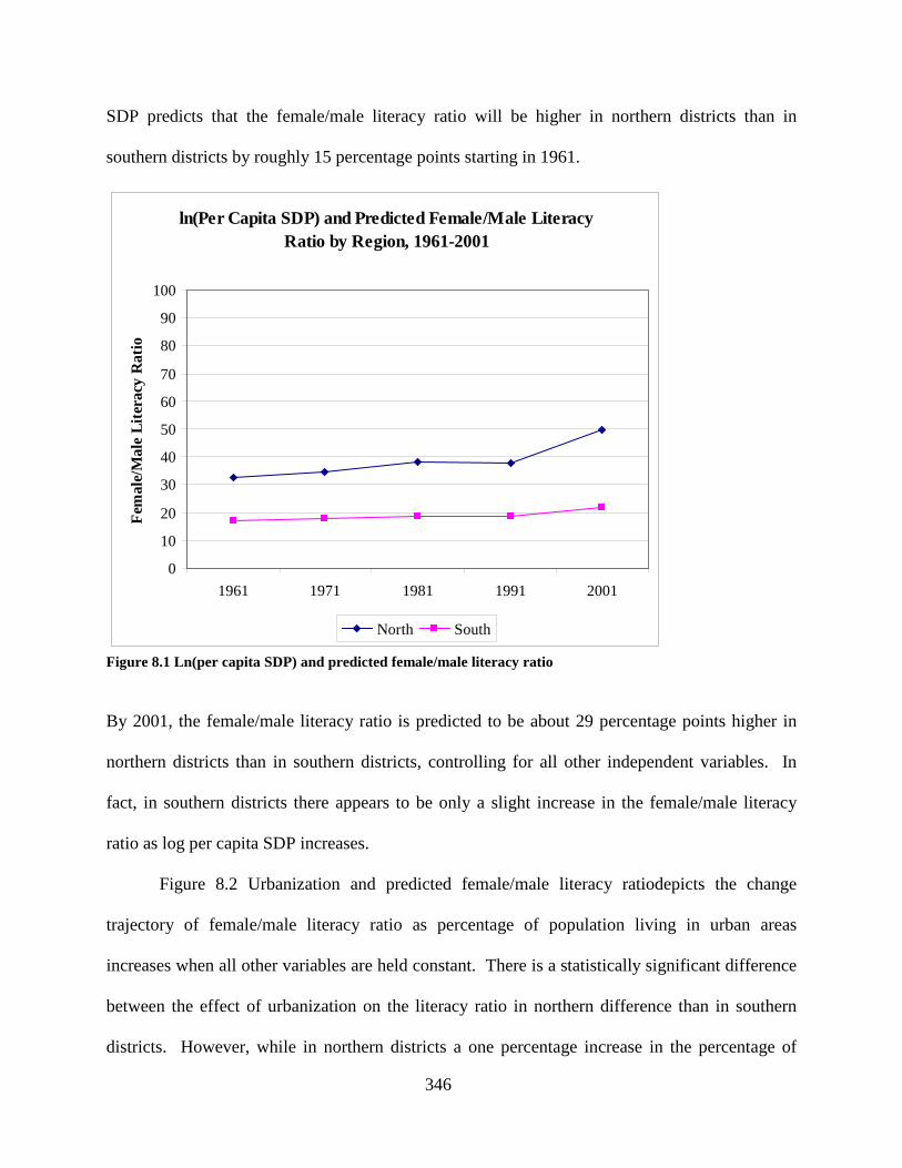
346
SDP predicts that the female/male literacy ratio will be higher in northern districts than in
southern districts by roughly 15 percentage points starting in 1961.
ln(Per Capita SDP) and Predicted Female/Male Literacy Ratio by Region, 1961-2001
0
10
20
30
40
50
60
70
80
90
100
1961 1971 1981 1991 2001
Fem
ale/
Mal
e Li
tera
cy R
atio
North South
Figure 8.1 Ln(per capita SDP) and predicted female/male literacy ratio
By 2001, the female/male literacy ratio is predicted to be about 29 percentage points higher in
northern districts than in southern districts, controlling for all other independent variables. In
fact, in southern districts there appears to be only a slight increase in the female/male literacy
ratio as log per capita SDP increases.
Figure 8.2 Urbanization and predicted female/male literacy ratiodepicts the change
trajectory of female/male literacy ratio as percentage of population living in urban areas
increases when all other variables are held constant. There is a statistically significant difference
between the effect of urbanization on the literacy ratio in northern difference than in southern
districts. However, while in northern districts a one percentage increase in the percentage of
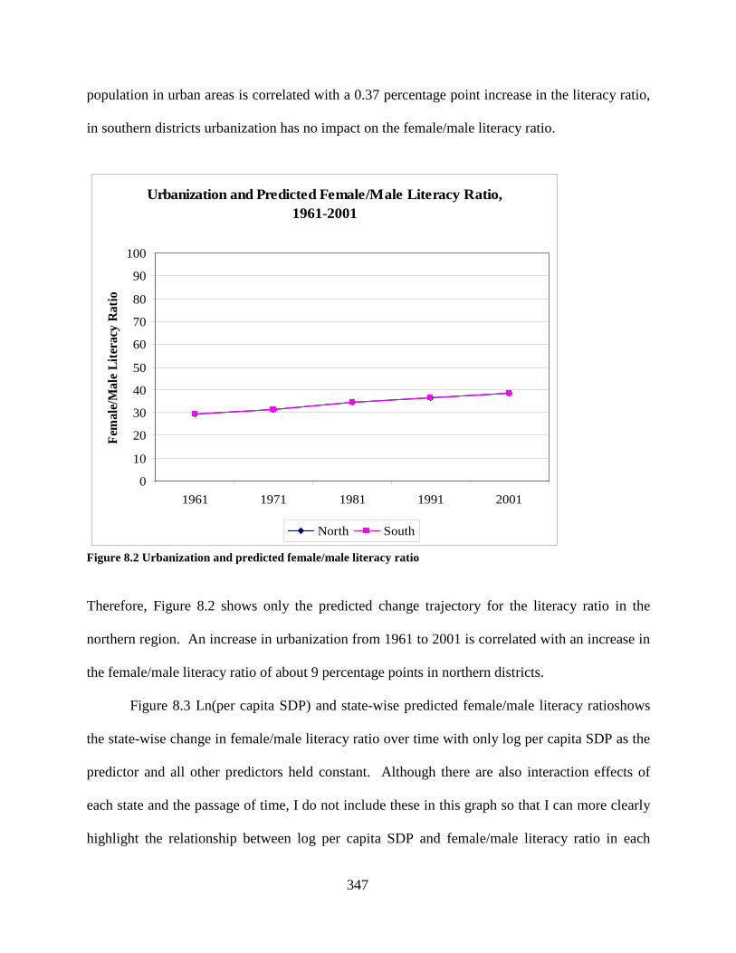
347
population in urban areas is correlated with a 0.37 percentage point increase in the literacy ratio,
in southern districts urbanization has no impact on the female/male literacy ratio.
Urbanization and Predicted Female/Male Literacy Ratio, 1961-2001
0
10
20
30
40
50
60
70
80
90
100
1961 1971 1981 1991 2001
Fem
ale/
Mal
e Li
tera
cy R
atio
North South
Figure 8.2 Urbanization and predicted female/male literacy ratio
Therefore, Figure 8.2 shows only the predicted change trajectory for the literacy ratio in the
northern region. An increase in urbanization from 1961 to 2001 is correlated with an increase in
the female/male literacy ratio of about 9 percentage points in northern districts.
Figure 8.3 Ln(per capita SDP) and state-wise predicted female/male literacy ratioshows
the state-wise change in female/male literacy ratio over time with only log per capita SDP as the
predictor and all other predictors held constant. Although there are also interaction effects of
each state and the passage of time, I do not include these in this graph so that I can more clearly
highlight the relationship between log per capita SDP and female/male literacy ratio in each
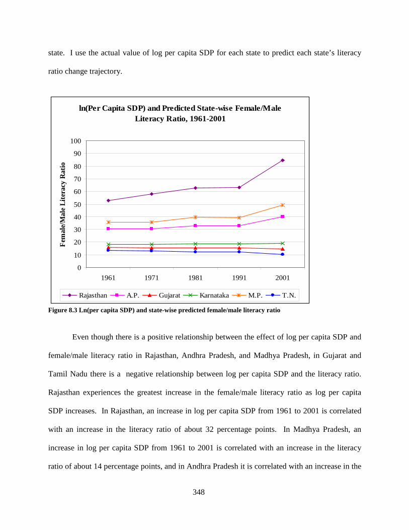
348
state. I use the actual value of log per capita SDP for each state to predict each state’s literacy
ratio change trajectory.
ln(Per Capita SDP) and Predicted State-wise Female/Male Literacy Ratio, 1961-2001
0
10
20
30
40
50
60
70
80
90
100
1961 1971 1981 1991 2001
Fem
ale/
Mal
e Li
tera
cy R
atio
Rajasthan A.P. Gujarat Karnataka M.P. T.N.
Figure 8.3 Ln(per capita SDP) and state-wise predicted female/male literacy ratio
Even though there is a positive relationship between the effect of log per capita SDP and
female/male literacy ratio in Rajasthan, Andhra Pradesh, and Madhya Pradesh, in Gujarat and
Tamil Nadu there is a negative relationship between log per capita SDP and the literacy ratio.
Rajasthan experiences the greatest increase in the female/male literacy ratio as log per capita
SDP increases. In Rajasthan, an increase in log per capita SDP from 1961 to 2001 is correlated
with an increase in the literacy ratio of about 32 percentage points. In Madhya Pradesh, an
increase in log per capita SDP from 1961 to 2001 is correlated with an increase in the literacy
ratio of about 14 percentage points, and in Andhra Pradesh it is correlated with an increase in the
349
literacy ratio of about 10 percentage points. In both Gujarat and Tamil Nadu, an increase in log
per capita SDP is correlated with a decrease in the female/male literacy ratio, although the rate of
change is very small. An increase in per capita SDP from 1961-2001 is correlated with a
decrease in the female/male literacy ratio of about 3 percentage points in Tamil Nadu. The
decrease in female/male literacy ratio correlated to per capita SDP in Gujarat was even less. In
Karnataka an increase in per capita SDP from 1961-2001 is correlated with an increase in the
literacy ratio of only about 1 percentage point. Therefore there is a statistically significant
difference between the effect of log per capita SDP on the literacy ratio in Rajasthan and the
effect of log per capita SDP on the literacy ratio in all five other states. However, in Karnataka,
Gujarat, and Tamil Nadu there is almost no predicted change at all in the female/male literacy
ratio that is correlated with log per capita SDP.
Figure 8.4 depicts the relationship between lagged log per capita SDP and regional
variation in female/male literacy ratio, controlling for all other independent variables. That is,
values of log per capita SDP in 1961 predict values of female/male literacy ratio in 1971. While
log per capita SDP is correlated with an increase in female/male literacy ratio that occurs
contemporaneously, lagged values of per capita SDP are correlated with a decrease in the
female/male literacy ratio. This is true in both northern and southern districts, although the
magnitude of this change is steeper in northern districts. Log per capita SDP in 1961 leads to a
gap in the female/male literacy ratio between northern and southern districts in 1971 of roughly
30 percentage points. Whereas a tenfold increase in per capita SDP leads to a decrease in the
female/male literacy ratio of about 6 percentage points ten years later in northern districts, a
tenfold increase in per capita SDP leads to a decrease in the literacy ratio of about 1 percentage
point in southern districts.
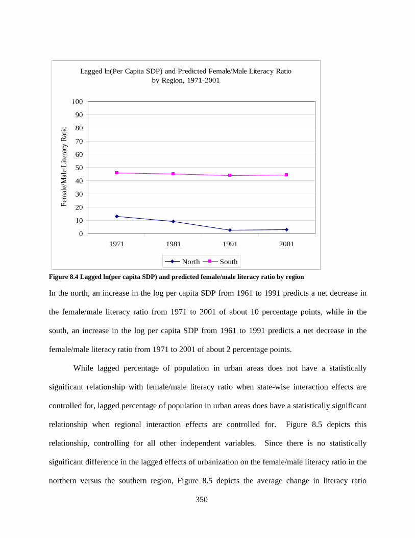
350
Lagged ln(Per Capita SDP) and Predicted Female/Male Literacy Ratio by Region, 1971-2001
0
10
20
30
40
50
60
70
80
90
100
1971 1981 1991 2001
Fem
ale/
Mal
e Li
tera
cy R
atio
North South
Figure 8.4 Lagged ln(per capita SDP) and predicted female/male literacy ratio by region
In the north, an increase in the log per capita SDP from 1961 to 1991 predicts a net decrease in
the female/male literacy ratio from 1971 to 2001 of about 10 percentage points, while in the
south, an increase in the log per capita SDP from 1961 to 1991 predicts a net decrease in the
female/male literacy ratio from 1971 to 2001 of about 2 percentage points.
While lagged percentage of population in urban areas does not have a statistically
significant relationship with female/male literacy ratio when state-wise interaction effects are
controlled for, lagged percentage of population in urban areas does have a statistically significant
relationship when regional interaction effects are controlled for. Figure 8.5 depicts this
relationship, controlling for all other independent variables. Since there is no statistically
significant difference in the lagged effects of urbanization on the female/male literacy ratio in the
northern versus the southern region, Figure 8.5 depicts the average change in literacy ratio
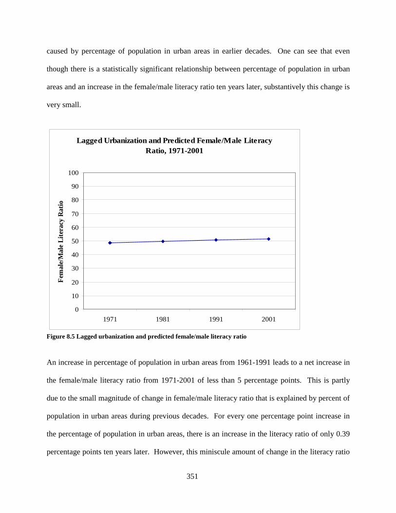
351
caused by percentage of population in urban areas in earlier decades. One can see that even
though there is a statistically significant relationship between percentage of population in urban
areas and an increase in the female/male literacy ratio ten years later, substantively this change is
very small.
Lagged Urbanization and Predicted Female/Male Literacy Ratio, 1971-2001
0
10
20
30
40
50
60
70
80
90
100
1971 1981 1991 2001
Fem
ale/
Mal
e Li
tera
cy R
atio
Figure 8.5 Lagged urbanization and predicted female/male literacy ratio
An increase in percentage of population in urban areas from 1961-1991 leads to a net increase in
the female/male literacy ratio from 1971-2001 of less than 5 percentage points. This is partly
due to the small magnitude of change in female/male literacy ratio that is explained by percent of
population in urban areas during previous decades. For every one percentage point increase in
the percentage of population in urban areas, there is an increase in the literacy ratio of only 0.39
percentage points ten years later. However, this miniscule amount of change in the literacy ratio

352
predicted by percentage of population in urban areas is also due to the low rate of change in
urbanization itself over time. On average, the percentage of population living in urban areas
increases by only 2 percentage points each decade (see Table 6.71 in chapter 6.)
8.6.2 Results for Women-in-Development hypotheses
Figure 8.6 depicts change in the female/male literacy ratio correlated with change in log per
capita SDP, controlling all other variables in the WID models constant. With every ten-fold
increase in per capita SDP, there is an increase in the female/male literacy ratio of about 2
percentage points. Although this relationship is statistically significant, one can see from the
graph that there is very little change in the female/male literacy ratio as log per capita SDP
increases from 1961 to 1991. During this period, log per capita SDP is correlated with an
increase in the literacy ratio of less than 5 percentage points. However, between 1991 and 2001
the average per capita SDP increased almost forty-fold, with an increase in the literacy ratio of
about 8 percentage points.
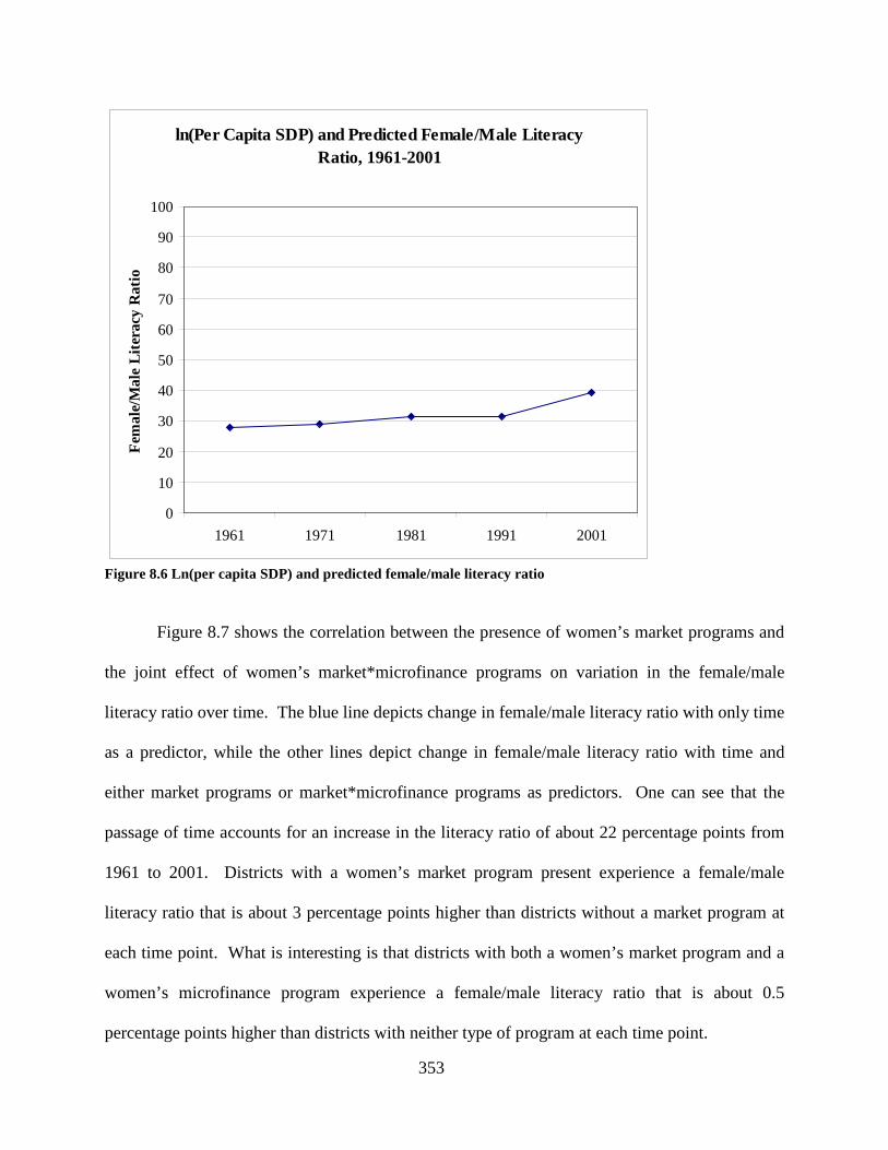
353
ln(Per Capita SDP) and Predicted Female/Male Literacy Ratio, 1961-2001
0
10
20
30
40
50
60
70
80
90
100
1961 1971 1981 1991 2001
Fem
ale/
Mal
e Li
tera
cy R
atio
Figure 8.6 Ln(per capita SDP) and predicted female/male literacy ratio
Figure 8.7 shows the correlation between the presence of women’s market programs and
the joint effect of women’s market*microfinance programs on variation in the female/male
literacy ratio over time. The blue line depicts change in female/male literacy ratio with only time
as a predictor, while the other lines depict change in female/male literacy ratio with time and
either market programs or market*microfinance programs as predictors. One can see that the
passage of time accounts for an increase in the literacy ratio of about 22 percentage points from
1961 to 2001. Districts with a women’s market program present experience a female/male
literacy ratio that is about 3 percentage points higher than districts without a market program at
each time point. What is interesting is that districts with both a women’s market program and a
women’s microfinance program experience a female/male literacy ratio that is about 0.5
percentage points higher than districts with neither type of program at each time point.
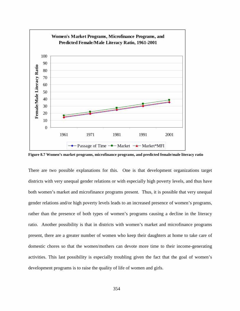
354
Women's Market Programs, Microfinance Programs, and Predicted Female/Male Literacy Ratio, 1961-2001
010
20304050
607080
90100
1961 1971 1981 1991 2001
Fem
ale/
Mal
e L
itera
cy R
atio
Passage of Time Market Market*MFI
Figure 8.7 Women’s market programs, microfinance programs, and predicted female/male literacy ratio
There are two possible explanations for this. One is that development organizations target
districts with very unequal gender relations or with especially high poverty levels, and thus have
both women’s market and microfinance programs present. Thus, it is possible that very unequal
gender relations and/or high poverty levels leads to an increased presence of women’s programs,
rather than the presence of both types of women’s programs causing a decline in the literacy
ratio. Another possibility is that in districts with women’s market and microfinance programs
present, there are a greater number of women who keep their daughters at home to take care of
domestic chores so that the women/mothers can devote more time to their income-generating
activities. This last possibility is especially troubling given the fact that the goal of women’s
development programs is to raise the quality of life of women and girls.
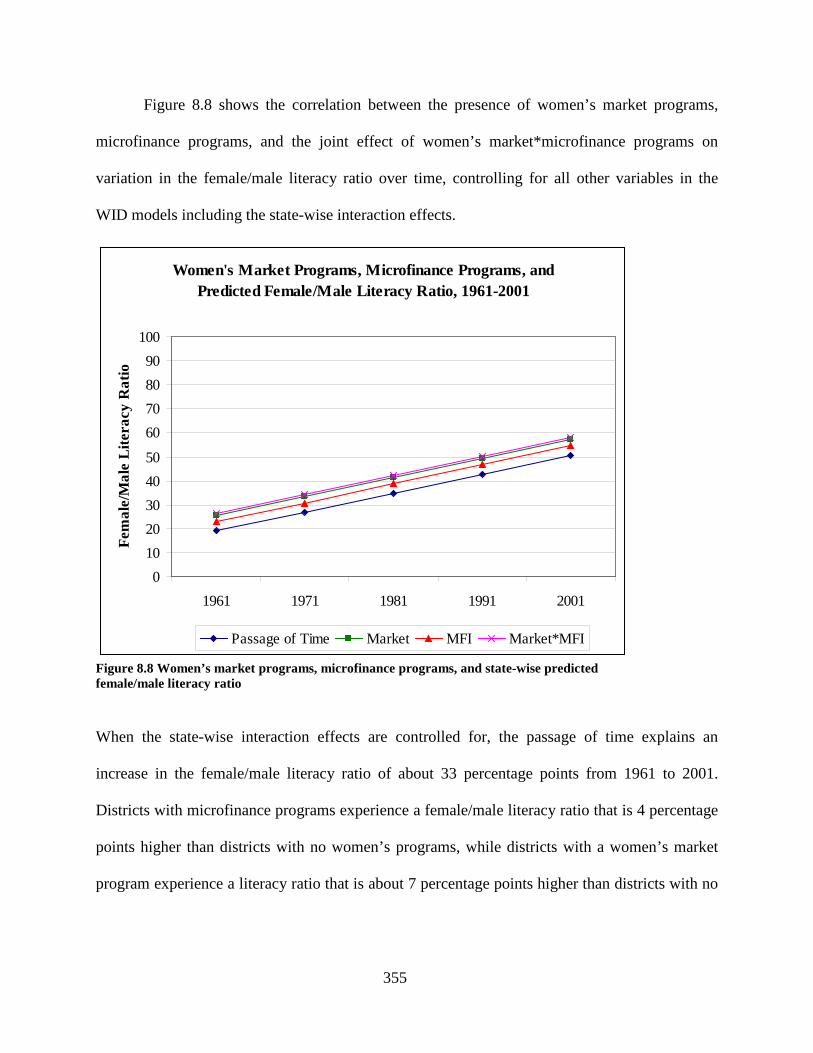
355
Figure 8.8 shows the correlation between the presence of women’s market programs,
microfinance programs, and the joint effect of women’s market*microfinance programs on
variation in the female/male literacy ratio over time, controlling for all other variables in the
WID models including the state-wise interaction effects.
Women's Market Programs, Microfinance Programs, and Predicted Female/Male Literacy Ratio, 1961-2001
01020304050
60708090
100
1961 1971 1981 1991 2001
Fem
ale/
Mal
e L
itera
cy R
atio
Passage of Time Market MFI Market*MFI
Figure 8.8 Women’s market programs, microfinance programs, and state-wise predicted female/male literacy ratio
When the state-wise interaction effects are controlled for, the passage of time explains an
increase in the female/male literacy ratio of about 33 percentage points from 1961 to 2001.
Districts with microfinance programs experience a female/male literacy ratio that is 4 percentage
points higher than districts with no women’s programs, while districts with a women’s market
program experience a literacy ratio that is about 7 percentage points higher than districts with no
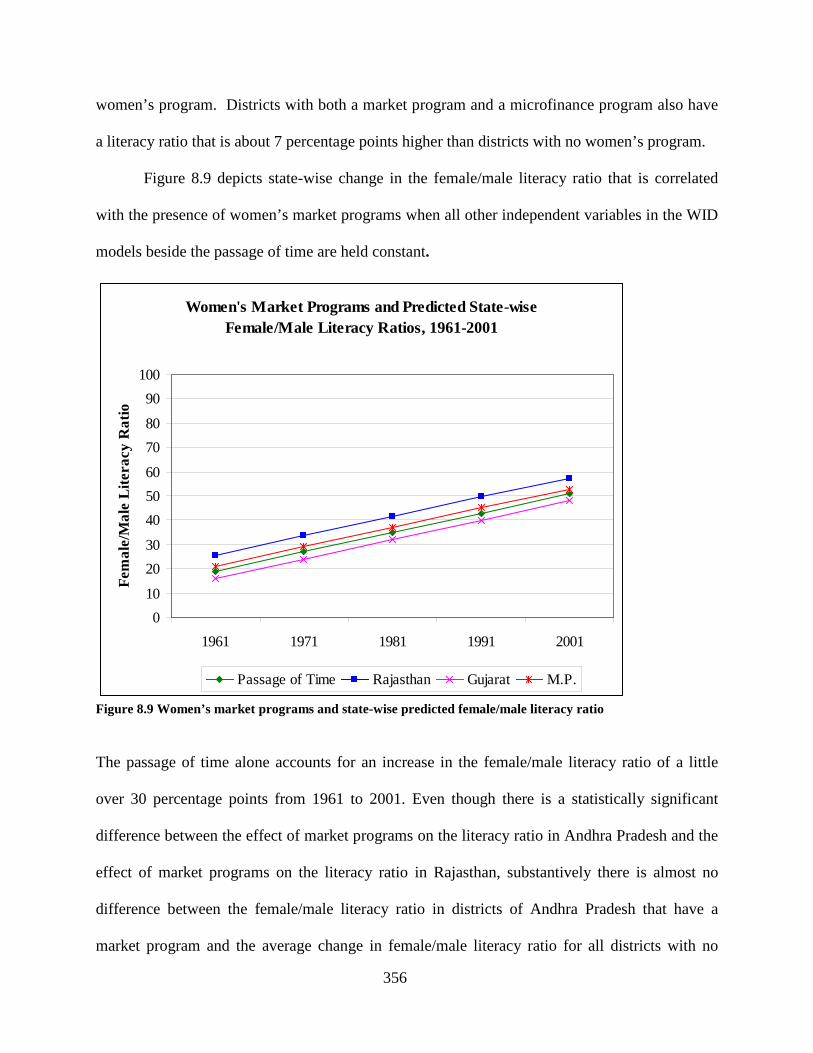
356
women’s program. Districts with both a market program and a microfinance program also have
a literacy ratio that is about 7 percentage points higher than districts with no women’s program.
Figure 8.9 depicts state-wise change in the female/male literacy ratio that is correlated
with the presence of women’s market programs when all other independent variables in the WID
models beside the passage of time are held constant.
Women's Market Programs and Predicted State-wise Female/Male Literacy Ratios, 1961-2001
010
2030
405060
7080
90100
1961 1971 1981 1991 2001
Fem
ale/
Mal
e L
itera
cy R
atio
Passage of Time Rajasthan Gujarat M.P.
Figure 8.9 Women’s market programs and state-wise predicted female/male literacy ratio
The passage of time alone accounts for an increase in the female/male literacy ratio of a little
over 30 percentage points from 1961 to 2001. Even though there is a statistically significant
difference between the effect of market programs on the literacy ratio in Andhra Pradesh and the
effect of market programs on the literacy ratio in Rajasthan, substantively there is almost no
difference between the female/male literacy ratio in districts of Andhra Pradesh that have a
market program and the average change in female/male literacy ratio for all districts with no
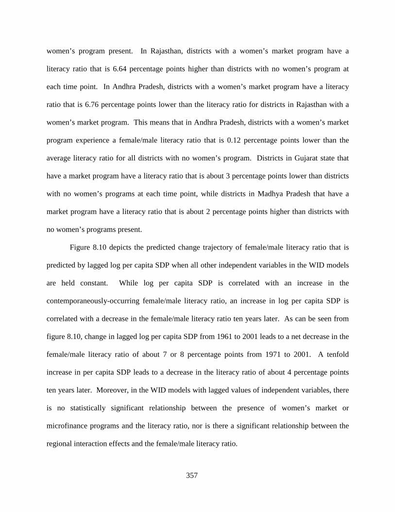
357
women’s program present. In Rajasthan, districts with a women’s market program have a
literacy ratio that is 6.64 percentage points higher than districts with no women’s program at
each time point. In Andhra Pradesh, districts with a women’s market program have a literacy
ratio that is 6.76 percentage points lower than the literacy ratio for districts in Rajasthan with a
women’s market program. This means that in Andhra Pradesh, districts with a women’s market
program experience a female/male literacy ratio that is 0.12 percentage points lower than the
average literacy ratio for all districts with no women’s program. Districts in Gujarat state that
have a market program have a literacy ratio that is about 3 percentage points lower than districts
with no women’s programs at each time point, while districts in Madhya Pradesh that have a
market program have a literacy ratio that is about 2 percentage points higher than districts with
no women’s programs present.
Figure 8.10 depicts the predicted change trajectory of female/male literacy ratio that is
predicted by lagged log per capita SDP when all other independent variables in the WID models
are held constant. While log per capita SDP is correlated with an increase in the
contemporaneously-occurring female/male literacy ratio, an increase in log per capita SDP is
correlated with a decrease in the female/male literacy ratio ten years later. As can be seen from
figure 8.10, change in lagged log per capita SDP from 1961 to 2001 leads to a net decrease in the
female/male literacy ratio of about 7 or 8 percentage points from 1971 to 2001. A tenfold
increase in per capita SDP leads to a decrease in the literacy ratio of about 4 percentage points
ten years later. Moreover, in the WID models with lagged values of independent variables, there
is no statistically significant relationship between the presence of women’s market or
microfinance programs and the literacy ratio, nor is there a significant relationship between the
regional interaction effects and the female/male literacy ratio.
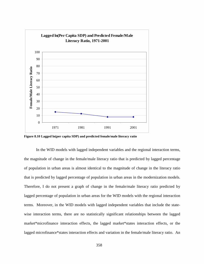
358
Lagged ln(Per Capita SDP) and Predicted Female/Male Literacy Ratio, 1971-2001
0
10
20
30
40
50
60
70
80
90
100
1971 1981 1991 2001
Fem
ale/
Mal
e Li
tera
cy R
atio
Figure 8.10 Lagged ln(per capita SDP) and predicted female/male literacy ratio
In the WID models with lagged independent variables and the regional interaction terms,
the magnitude of change in the female/male literacy ratio that is predicted by lagged percentage
of population in urban areas is almost identical to the magnitude of change in the literacy ratio
that is predicted by lagged percentage of population in urban areas in the modernization models.
Therefore, I do not present a graph of change in the female/male literacy ratio predicted by
lagged percentage of population in urban areas for the WID models with the regional interaction
terms. Moreover, in the WID models with lagged independent variables that include the state-
wise interaction terms, there are no statistically significant relationships between the lagged
market*microfinance interaction effects, the lagged market*states interaction effects, or the
lagged microfinance*states interaction effects and variation in the female/male literacy ratio. An
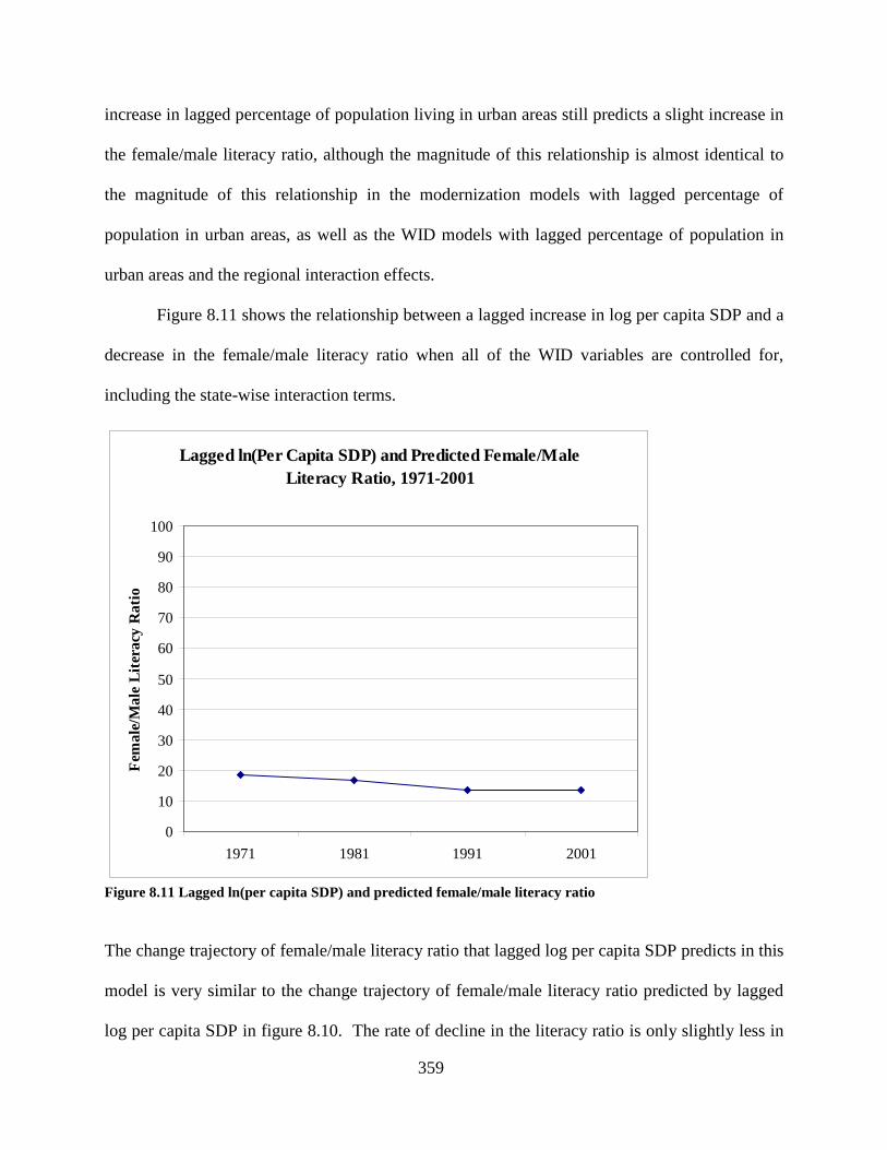
359
increase in lagged percentage of population living in urban areas still predicts a slight increase in
the female/male literacy ratio, although the magnitude of this relationship is almost identical to
the magnitude of this relationship in the modernization models with lagged percentage of
population in urban areas, as well as the WID models with lagged percentage of population in
urban areas and the regional interaction effects.
Figure 8.11 shows the relationship between a lagged increase in log per capita SDP and a
decrease in the female/male literacy ratio when all of the WID variables are controlled for,
including the state-wise interaction terms.
Lagged ln(Per Capita SDP) and Predicted Female/Male Literacy Ratio, 1971-2001
0
10
20
30
40
50
60
70
80
90
100
1971 1981 1991 2001
Fem
ale/
Mal
e Li
tera
cy R
atio
Figure 8.11 Lagged ln(per capita SDP) and predicted female/male literacy ratio
The change trajectory of female/male literacy ratio that lagged log per capita SDP predicts in this
model is very similar to the change trajectory of female/male literacy ratio predicted by lagged
log per capita SDP in figure 8.10. The rate of decline in the literacy ratio is only slightly less in
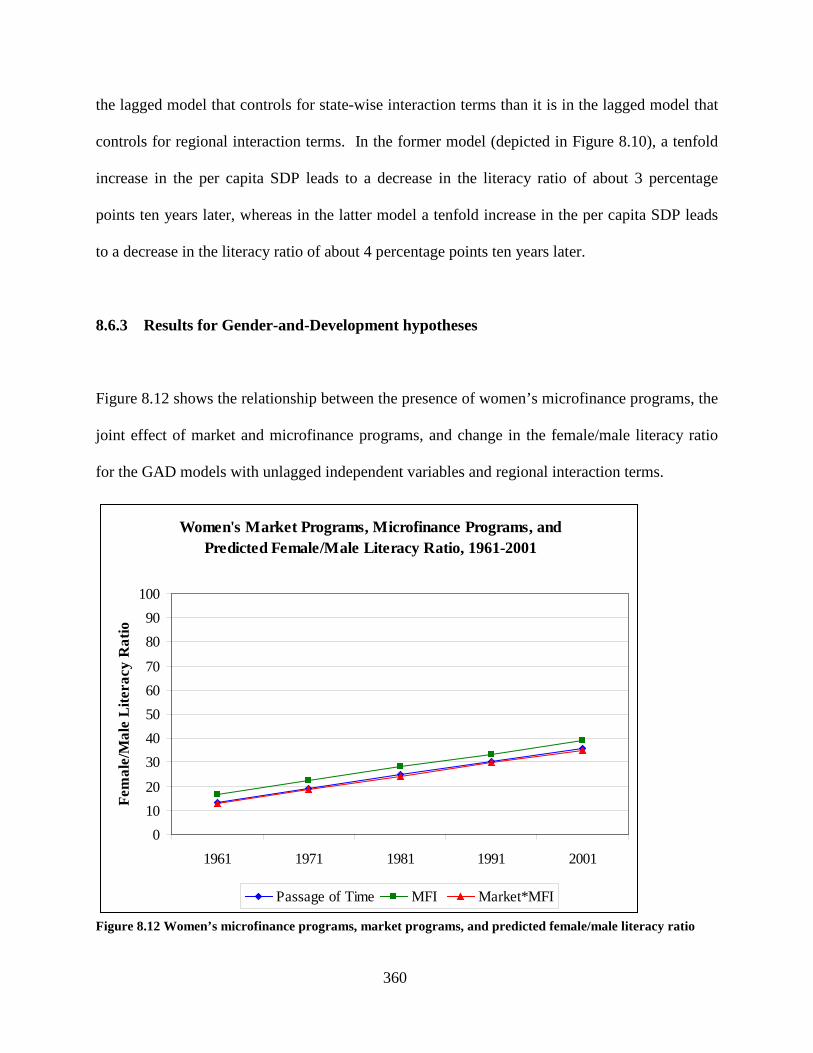
360
the lagged model that controls for state-wise interaction terms than it is in the lagged model that
controls for regional interaction terms. In the former model (depicted in Figure 8.10), a tenfold
increase in the per capita SDP leads to a decrease in the literacy ratio of about 3 percentage
points ten years later, whereas in the latter model a tenfold increase in the per capita SDP leads
to a decrease in the literacy ratio of about 4 percentage points ten years later.
8.6.3 Results for Gender-and-Development hypotheses
Figure 8.12 shows the relationship between the presence of women’s microfinance programs, the
joint effect of market and microfinance programs, and change in the female/male literacy ratio
for the GAD models with unlagged independent variables and regional interaction terms.
Women's Market Programs, Microfinance Programs, and Predicted Female/Male Literacy Ratio, 1961-2001
01020
3040506070
8090
100
1961 1971 1981 1991 2001
Fem
ale/
Mal
e L
itera
cy R
atio
Passage of Time MFI Market*MFI
Figure 8.12 Women’s microfinance programs, market programs, and predicted female/male literacy ratio
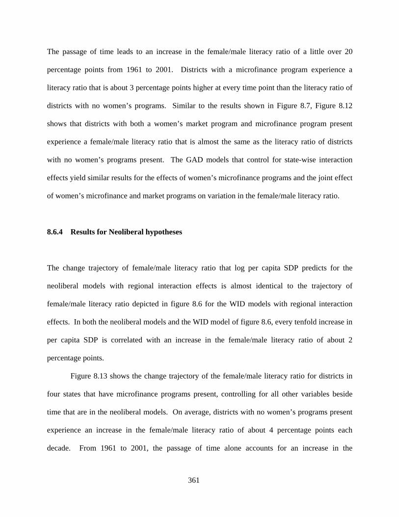
361
The passage of time leads to an increase in the female/male literacy ratio of a little over 20
percentage points from 1961 to 2001. Districts with a microfinance program experience a
literacy ratio that is about 3 percentage points higher at every time point than the literacy ratio of
districts with no women’s programs. Similar to the results shown in Figure 8.7, Figure 8.12
shows that districts with both a women’s market program and microfinance program present
experience a female/male literacy ratio that is almost the same as the literacy ratio of districts
with no women’s programs present. The GAD models that control for state-wise interaction
effects yield similar results for the effects of women’s microfinance programs and the joint effect
of women’s microfinance and market programs on variation in the female/male literacy ratio.
8.6.4 Results for Neoliberal hypotheses
The change trajectory of female/male literacy ratio that log per capita SDP predicts for the
neoliberal models with regional interaction effects is almost identical to the trajectory of
female/male literacy ratio depicted in figure 8.6 for the WID models with regional interaction
effects. In both the neoliberal models and the WID model of figure 8.6, every tenfold increase in
per capita SDP is correlated with an increase in the female/male literacy ratio of about 2
percentage points.
Figure 8.13 shows the change trajectory of the female/male literacy ratio for districts in
four states that have microfinance programs present, controlling for all other variables beside
time that are in the neoliberal models. On average, districts with no women’s programs present
experience an increase in the female/male literacy ratio of about 4 percentage points each
decade. From 1961 to 2001, the passage of time alone accounts for an increase in the
362
female/male literacy ratio of about 15 percentage points. In Andhra Pradesh and Tamil Nadu,
districts with microfinance programs experienced almost the same increase in female/male
literacy ratio, holding all other variables beside time constant.
Women's Microfinance Programs and Predicted State-wise Female/Male Literacy Ratios,
1961-2001
0
10
20
30
40
50
60
70
80
90
100
1961 1971 1981 1991 2001
Fem
ale/
Mal
e L
itera
cy R
ati
Rajasthan AP Gujarat TN
Figure 8.13 Women’s microfinance programs and state-wise predicted female/male literacy ratio
At each time point, districts in Rajasthan with microfinance programs had a literacy ratio
that was about 9 percentage points higher than districts in Rajasthan with no microfinance
programs. At each time point, districts in Andhra Pradesh with microfinance programs had a
female/male literacy ratio that was about 4 percentage points higher than the female/male
literacy ratio of districts with no women’s programs, while in Tamil Nadu districts with a
microfinance program present had a female/male literacy ratio that was about 3 percentage
points higher than the literacy ratio of districts with no women’s program present. Districts in
Gujarat state that have a microfinance program fare the worst in terms of the female/male
363
literacy ratio. In Gujarat, districts with a microfinance program have a female/male literacy ratio
that is about 2 percentage points lower than the literacy ratio for districts with no women’s
program present. The slopes of the change trajectories for districts in Andhra Pradesh, Tamil
Nadu, and Gujarat states with women’s microfinance programs are the same as the slope of the
change trajectory for all districts in Rajasthan with microfinance programs present.
While there is a statistically significant relationship between the contemporaneous
presence of women’s microfinance programs and the female/male literacy ratio in Rajasthan,
Andhra Pradesh, Tamil Nadu, and Gujarat states, there is not a statistically significant
relationship between the lagged presence of women’s microfinance programs and the literacy
ratio in Andhra Pradesh and Tamil Nadu states. There is, however, a statistically significant
relationship between the lagged presence of women’s microfinance programs and the literacy
ratio in Madhya Pradesh. Figure 8.14 displays the lagged effects of women’s microfinance
programs on change in the female/male literacy ratio for Rajasthan, Gujarat, and Madhya
Pradesh states. The passage of time alone accounts for an increase in the female/male literacy
ratio of about 27 percentage points from 1971 to 2001, controlling for the lagged effects of all
other independent variables. Districts with microfinance programs in Gujarat in previous
decades have a female/male literacy ratio that is about 15 percentage points lower than the
female/male literacy ratio of districts in Rajasthan with microfinance programs. Districts with
microfinance programs in Madhya Pradesh in previous decades have a female/male literacy ratio
that is about 12 percentage points lower than the female/male literacy ratio of districts in
Rajasthan with women’s microfinance programs.
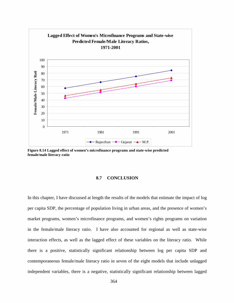
364
Lagged Effect of Women's Microfinance Programs and State-wise Predicted Female/Male Literacy Ratios,
1971-2001
0
10
20
30
40
50
60
70
80
90
100
1971 1981 1991 2001
Fem
ale/
Mal
e L
itera
cy R
ati
Rajasthan Gujarat M.P.
Figure 8.14 Lagged effect of women’s microfinance programs and state-wise predicted female/male literacy ratio
8.7 CONCLUSION
In this chapter, I have discussed at length the results of the models that estimate the impact of log
per capita SDP, the percentage of population living in urban areas, and the presence of women’s
market programs, women’s microfinance programs, and women’s rights programs on variation
in the female/male literacy ratio. I have also accounted for regional as well as state-wise
interaction effects, as well as the lagged effect of these variables on the literacy ratio. While
there is a positive, statistically significant relationship between log per capita SDP and
contemporaneous female/male literacy ratio in seven of the eight models that include unlagged
independent variables, there is a negative, statistically significant relationship between lagged
365
log per capita SDP and the female/male literacy ratio in all but one of the models that include
lagged independent variables. In one model that includes both lagged independent variables and
state-wise interaction terms, there is a small, statistically significant relationship between an
increase in log per capita SDP and an increase in the literacy ratio in Gujarat and Tamil Nadu
states. Even in this model, however, there is a negative relationship between lagged log per
capita SDP and the literacy ratio in all other states. This implies that while log per capita SDP
and female/male literacy ratio increase simultaneously, an increase in the log per capita SDP
actually leads to a decrease in the female/male literacy ratio ten years later. There is a positive,
statistically significant relationship between percentage of population living in urban areas and
the female/male literacy ratio in only one of the models that include unlagged independent
variables. However, in seven out of eight models with lagged independent variables, there is a
positive, statistically significant (though substantively very small) relationship between the
percentage of population living in urban areas and the female/male literacy ratio. Therefore,
there is evidence that supports the modernization hypothesis that an increase in percentage of
population in urban areas will lead to an increase in the female/male literacy ratio. However, the
increase in literacy ratio caused by an increase in percentage of population in urban areas is very
small—usually an increase of about 1 female/1,000 males for every 3 percentage-point increase
in urbanization. Substantively, there is stronger evidence for the WID hypothesis that an
increase in log per capita SDP will lead to a decrease in the female/male literacy ratio. There is a
positive, statistically significant relationship between the presence of market programs and
literacy ratio and/or between the presence of microfinance programs and literacy ratio in five of
the eight models with unlagged independent variables. However, there is a positive, statistically
significant relationship between the lagged effect of the presence of women’s microfinance
366
programs and the literacy ratio in only one of the eight models with lagged independent
variables. Moreover, in this model the negative interaction effects of microfinance
programs*states outweigh the positive main effect of microfinance programs in Gujarat and
Madhya Pradesh states. There is no statistically significant correlation between the presence of
women’s market programs and variation in the female/male literacy ratio in any of the models
that included lagged independent variables. Therefore, while there may be a number of districts
with women’s market programs or women’s microfinance programs and the female/male literacy
ratio may increase simultaneously, one cannot conclude that the presence of women’s market or
microfinance programs causes this increase in female/male literacy ratio. There is therefore little
to no evidence in support of the WID, GAD, or neoliberal hypotheses that relate to the presence
of women’s market, microfinance, or women’s rights programs.
367
9.0 CHAPTER NINE: CONCLUSION
Do development programs and organizations designed for women really help raise women’s
status and promote gender equality in India? Which programs and organizations benefit women
the most? Since India won independence in 1947, economists, scholars, and practitioners have
developed and implemented numerous programs to mitigate female poverty, low women’s
status, and gender inequality. However, gender disparities in education, health care, political
representation, and the overall female/male sex ratio persist (Bhan 2001).
According to early modernization scholars, as traditional societies adopt “modern,”
Western expectations and values, they become more urbanized and economically developed
(Webster 1990), less authoritarian and male-dominated, and more egalitarian and democratic
(Jacquette 1982). Development practitioners who designed programs for Indian women
grounded in the modernization paradigm focused on teaching rural women about nutrition,
childcare, and home decorating. They also tried to instill new, Western values and ideas in these
Indian women (Berry 2007).
Development agencies with a neoliberal ideology view the integration of women into the
global market as the most efficient way of boosting a developing nation’s economy (Sharma
2008), while also lifting families out of poverty, raising women’s status, and reducing gender
inequality (Mayoux 1995, Cheston and Kuhn 2002, Ahmed et. al. 2001). Nicholas Kristof and
Sheryll WuDunn, winners of the 2009 Pulitzer Prize, argue that microcredit empowers women to
368
start successful businesses, provide for the needs of their families, and counteract domestic
violence (Kristof and WuDunn 2009).
Other researchers do not see neoliberal development projects such as microcredit
schemes in such a rosy light. Feiner and Barker (2006) criticize neoliberal policymakers’
emphasis on microcredit programs, arguing that microcredit programs reproduce rather than
eradicate female poverty in poor nations. Also, Rankin (2002) argues that the social networks
women build through microlending groups may actually reinforce gender and caste hierarchies
rather than help overcome them.
Women-in-development (WID) theorists, like modernization theorists, assume that
industrialization and the rise of capitalism are beneficial for all societies (Tinker 1997).
However, they argue that women will benefit only if they are fully integrated into the economic
and political spheres (Tinker 1997).
Gender-and-Development (GAD) researchers have a very different vision of
development than those coming from a neoliberal paradigm. GAD theorists argue that it is
necessary to analyze the power relations between women and men in the domestic and public
spheres, and how these spheres overlap in women’s lives, in order to raise gender equality
(Young 1997). Whereas neoliberal researchers emphasize women’s need for greater access to
credit, GAD theorists and practitioners argue that women need to organize to gain political
power in the economic system.
The objective of this study has been to examine whether material development
(associated with modernization theory), women’s market-based development programs (based on
WID theory), women’s empowerment programs (rooted in GAD theory), or women’s
microfinance programs (based on neoliberal theory) best promote gender equality in India. I
369
have analyzed the effects that the passage of time, urbanization, state-level economic growth,
and the presence, absence, and combination of various types of women’s development programs
have on district-level variation in gender inequality in India from 1961-2001.
In the following section, I present two tables that summarize the results of the models
testing the modernization and WID hypotheses. I do not include tables summarizing the results
of the GAD models or the neoliberal models because none of the results were statistically
significant for these models. I also discuss possible reasons for why there are no statistically
significant relationships between the different types of women’s programs and the female/male
child sex ratio and literacy ratio. Finally, I discuss the policy implications of my dissertation
findings, as well as avenues for exploration in future research.
Table 9.1 below provides a summary of the results for the models testing the
modernization hypotheses about the effects of economic growth and urbanization on the
female/male child sex ratio and the female/male literacy ratio.
The results of the unlagged models for female/male child sex ratio that test the
modernization hypotheses show that there is no relationship between economic growth nor
between urbanization and the child sex ratio. However, the lagged models that test the
modernization hypotheses indicate that there is a negative correlation between per capita SDP
and the female/male child sex ratio. This is the opposite of what modernization theory predicts
in Hypothesis 1a: “An increase in urbanization and per capita SDP will lead to an increase in the
female/male child sex ratios and female/male literacy ratios.”
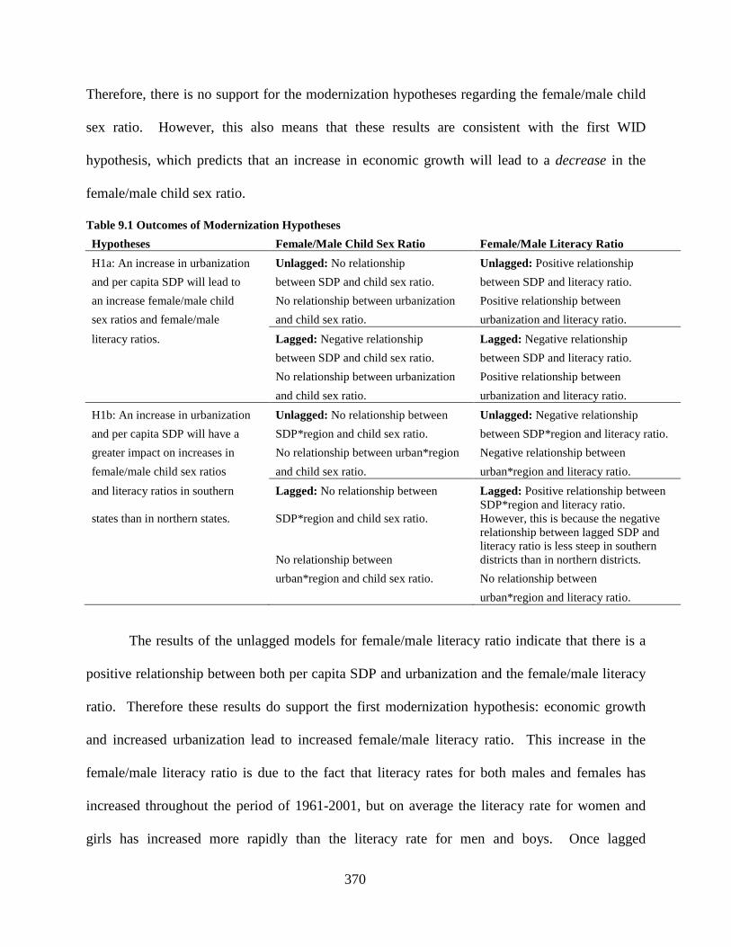
370
Therefore, there is no support for the modernization hypotheses regarding the female/male child
sex ratio. However, this also means that these results are consistent with the first WID
hypothesis, which predicts that an increase in economic growth will lead to a decrease in the
female/male child sex ratio.
Table 9.1 Outcomes of Modernization Hypotheses Hypotheses Female/Male Child Sex Ratio Female/Male Literacy Ratio H1a: An increase in urbanization Unlagged: No relationship Unlagged: Positive relationship and per capita SDP will lead to between SDP and child sex ratio. between SDP and literacy ratio. an increase female/male child No relationship between urbanization Positive relationship between sex ratios and female/male and child sex ratio. urbanization and literacy ratio. literacy ratios. Lagged: Negative relationship Lagged: Negative relationship
between SDP and child sex ratio. between SDP and literacy ratio. No relationship between urbanization Positive relationship between and child sex ratio. urbanization and literacy ratio.
H1b: An increase in urbanization Unlagged: No relationship between Unlagged: Negative relationship and per capita SDP will have a SDP*region and child sex ratio. between SDP*region and literacy ratio. greater impact on increases in No relationship between urban*region Negative relationship between female/male child sex ratios and child sex ratio. urban*region and literacy ratio. and literacy ratios in southern Lagged: No relationship between Lagged: Positive relationship between
states than in northern states. SDP*region and child sex ratio. SDP*region and literacy ratio. However, this is because the negative
No relationship between
relationship between lagged SDP and literacy ratio is less steep in southern districts than in northern districts.
urban*region and child sex ratio. No relationship between urban*region and literacy ratio.
The results of the unlagged models for female/male literacy ratio indicate that there is a
positive relationship between both per capita SDP and urbanization and the female/male literacy
ratio. Therefore these results do support the first modernization hypothesis: economic growth
and increased urbanization lead to increased female/male literacy ratio. This increase in the
female/male literacy ratio is due to the fact that literacy rates for both males and females has
increased throughout the period of 1961-2001, but on average the literacy rate for women and
girls has increased more rapidly than the literacy rate for men and boys. Once lagged

371
independent variables are included in the models, there is still a small yet positive relationship
between urbanization and the literacy ratio. However, there is a negative relationship between
lagged log per capita SDP and the female/male literacy ratio, indicating that we should reject the
first modernization hypothesis and accept the first WID hypothesis. This finding is consistent
with the results of the lagged models testing the first modernization hypothesis.
The finding that increased urbanization leads to an increase in the female/male literacy
ratio confirms the findings of other researchers who have found that in some states, female
literacy rates and school enrollment rates tend to be much greater in urban areas than rural areas.
For instance, one study found that in Madhya Pradesh about 59% of urban women were literate
in 1991, but only about 20% of rural women were literate that same year (Panchamukhi 2006).
In urban areas, the net enrollment rate (NER) for girls was 87%, but girls’ NER in rural areas
was only 67%. Girls’ enrollment rates and female/male enrollment ratios in Rajasthan follow a
similar pattern. In urban areas, the female/male enrollment ratio for children aged 6-10 years
was 97%, whereas in rural areas the enrollment ratio was about 76% (Ray 2006).
The second modernization hypothesis states that economic growth and urbanization will
have a greater positive effect on female/male child sex ratios and literacy ratios in southern
regions than in northern regions. However, the models that include unlagged independent
variables and lagged independent variables that test the second modernization hypothesis for the
female/male child sex ratio reveal that there is no relationship between the regional interaction
effect of per capita SDP and the child sex ratio, nor between the regional interaction effect of
urbanization and the child sex ratio.
The unlagged models that tested this hypothesis for the female/male literacy ratio show
that while per capita SDP has a positive relationship with the literacy ratio, the magnitude of this
372
relationship is slightly smaller in the south than in the north. While urbanization is correlated
with an increase in literacy ratios in the north, it has no impact on literacy ratios in the south.
Both findings are the opposite of what is expected from hypothesis 1b. The results for the
models with lagged independent variables reveal that there is a negative relationship between
lagged log per capita SDP and the female/male literacy ratio in northern regions. Every tenfold
increase in per capita SDP is correlated with a decrease in the female/male literacy ratio of about
6 percentage points ten years later. In southern regions, every tenfold increase in the per capita
SDP is correlated with a decrease in the literacy ratio of about 1 percentage point ten years later.
There is no relationship between lagged urbanization and the female/male literacy ratio.
Therefore, the models for female/male literacy ratio do not support the second modernization
hypothesis that states that economic growth and urbanization will have a greater positive impact
in southern regions than in northern regions.
The descriptive analyses in chapter six indicate that the female/male literacy ratio has
increased in most districts from 1961-2001. However, the model results for the modernization
hypotheses show that neither economic growth nor urbanization are causing this increase in the
female/male literacy ratio. This increase in female/male literacy rates may be due to the
educational policies that Madhya Pradesh and Rajasthan states have implemented. Madhya
Pradesh and Rajasthan historically have had literacy rates that were below the national average
(Mehotra 2006), but both states have implemented some innovative educational programs in the
late 1980s through the 1990s. The overall literacy rate in Madhya Pradesh increased 20
percentage points between 1991-2001, and the female literacy rate increased by 22 percentage
points during the same period (Panchamukhi 2006). In Rajasthan the female literacy rate
increased 24 percentage points in between 1991-2001 (Ray 2006).
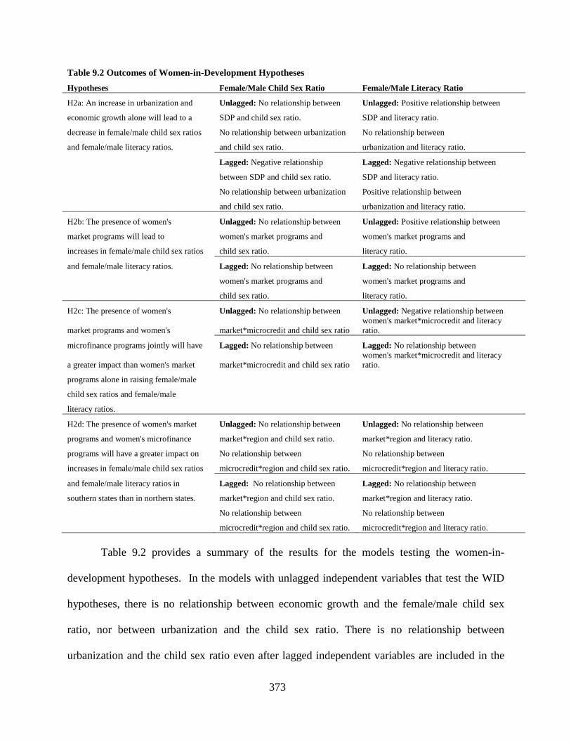
373
Table 9.2 Outcomes of Women-in-Development Hypotheses Hypotheses Female/Male Child Sex Ratio Female/Male Literacy Ratio
H2a: An increase in urbanization and Unlagged: No relationship between Unlagged: Positive relationship between
economic growth alone will lead to a SDP and child sex ratio. SDP and literacy ratio.
decrease in female/male child sex ratios No relationship between urbanization No relationship between
and female/male literacy ratios. and child sex ratio. urbanization and literacy ratio.
Lagged: Negative relationship Lagged: Negative relationship between
between SDP and child sex ratio. SDP and literacy ratio.
No relationship between urbanization Positive relationship between
and child sex ratio. urbanization and literacy ratio.
H2b: The presence of women's Unlagged: No relationship between Unlagged: Positive relationship between
market programs will lead to women's market programs and women's market programs and
increases in female/male child sex ratios child sex ratio. literacy ratio.
and female/male literacy ratios. Lagged: No relationship between Lagged: No relationship between
women's market programs and women's market programs and
child sex ratio. literacy ratio.
H2c: The presence of women's Unlagged: No relationship between Unlagged: Negative relationship between
market programs and women's market*microcredit and child sex ratio women's market*microcredit and literacy ratio.
microfinance programs jointly will have Lagged: No relationship between Lagged: No relationship between
a greater impact than women's market market*microcredit and child sex ratio women's market*microcredit and literacy ratio.
programs alone in raising female/male
child sex ratios and female/male
literacy ratios.
H2d: The presence of women's market Unlagged: No relationship between Unlagged: No relationship between
programs and women's microfinance market*region and child sex ratio. market*region and literacy ratio.
programs will have a greater impact on No relationship between No relationship between
increases in female/male child sex ratios microcredit*region and child sex ratio. microcredit*region and literacy ratio.
and female/male literacy ratios in Lagged: No relationship between Lagged: No relationship between
southern states than in northern states. market*region and child sex ratio. market*region and literacy ratio.
No relationship between No relationship between
microcredit*region and child sex ratio. microcredit*region and literacy ratio.
Table 9.2 provides a summary of the results for the models testing the women-in-
development hypotheses. In the models with unlagged independent variables that test the WID
hypotheses, there is no relationship between economic growth and the female/male child sex
ratio, nor between urbanization and the child sex ratio. There is no relationship between
urbanization and the child sex ratio even after lagged independent variables are included in the
374
models. Once lagged independent variables are included in the models, there is a negative
relationship between per capita SDP and the child sex ratio. These results confirm the findings
of the modernization models. Just as with the modernization models, I can accept the first WID
hypothesis, which states that economic growth and urbanization will lead to a decrease in the
child sex ratio.
The findings of the modernization and WID models that test the relationship between
economic growth and the female/male child sex ratio replicate the findings of some cross-
national studies about economic growth and gender inequality. For example, Young et al. (1994)
analyzed quantitative data from 70 countries on a range of gender inequality indicators related to
physical well-being, political representation, family formation, education, and economic activity.
Young et al. (1994) found that the number of females per 100 males was lower in higher-income
nations than in lower-income nations. Young et al.’s finding is similar to the finding of this
dissertation that lagged economic growth is correlated with a decrease in the female/male child
sex ratio.
In the models with unlagged independent variables that test the WID hypotheses for the
literacy ratio, there is a positive relationship between log per capita SDP and variation in the
female/male literacy ratio, which is the opposite of what hypothesis 2a predicts. However, there
is no relationship between urbanization and the literacy ratio. Once lagged independent variables
are included in the models testing the WID hypotheses, there is a negative relationship between
lagged log per capita SDP and the female/male literacy ratio. There is a positive relationship
between lagged urbanization and the literacy ratio, however. While there is a positive,
statistically significant relationship between log per capita SDP and contemporaneous
female/male literacy ratio in seven of the eight models that include unlagged independent
375
variables, there is a negative, statistically significant relationship between lagged log per capita
SDP and the female/male literacy ratio in all of the models that include lagged independent
variables. This implies that while log per capita SDP and female/male literacy ratio increase
simultaneously, an increase in the log per capita SDP actually leads to a decrease in the
female/male literacy ratio ten years later. In seven out of eight models with lagged independent
variables, there is a positive, statistically significant (though substantively very small)
relationship between the percentage of population living in urban areas and the female/male
literacy ratio. Therefore, there is evidence that supports the modernization hypothesis that an
increase in percentage of population in urban areas will lead to an increase in the female/male
literacy ratio. However, the increase in literacy ratio caused by an increase in percentage of
population in urban areas is very small—usually an increase of about 1 female/1,000 males for
every 3 percentage-point increase in urbanization. Substantively, there is stronger evidence for
the WID hypothesis that an increase in lagged log per capita SDP will lead to a decrease in the
female/male literacy ratio.
In the unlagged models testing the WID hypotheses, there is a positive relationship
between the presence of women’s market programs and the female/male literacy ratio. However,
once lagged independent variables are included in the models, there is no longer a relationship
between the presence of women’s market programs and the female/male literacy ratio. While in
models with unlagged independent variables there is a negative relationship between the joint
effect of women’s market programs*microfinance programs and the female/male literacy ratio,
in models with lagged independent variables there is no relationship between the interaction
effects of women’s market programs*microfinance programs and literacy ratio. However, there
is no correlation between the interaction effect of market programs*region and the literacy ratio,
376
nor between the interaction effect of microfinance programs*region and the literacy ratio in any
of the models testing the WID hypotheses. Moreover, there is no relationship between the
presence of market programs and the female/male child sex ratio, nor between the joint effect of
market*microfinance programs and the child sex ratio. This is the case for both models with
lagged and unlagged independent variables. There is also no difference in the impact that
women’s market programs have on the child sex ratio in northern versus southern regions. There
is therefore no evidence for hypothesis 2c or 2d.
While the results for the lagged models for change in female/male child sex ratios and
female/male literacy ratios seem to indicate that economic growth leads to a decrease in both
gender inequality measures, it is important to consider that there may be other factors that are
actually causing the changes in female/male child sex ratios and female/male literacy ratios.
Lagged per capita SDP is correlated with a decrease in female/male literacy ratios despite the
fact that female/male literacy ratios have actually increased over time. Moreover, the passage of
time seems to explain most of the variance in child sex ratios and literacy ratios, even after
including all other variables in the models. The passage of time is correlated with a decrease of
about 10 to 13 females/1,000 males per decade in 11 out of 16 models regarding change in the
female/male child sex ratio. In all but one of the unlagged models regarding change in the
female/male literacy ratio, time is correlated with an increase in the literacy ratio of between 3
and 6 percentage points per decade. In 7 out of 8 of the lagged models, time is correlated with an
increase in the female/male literacy ratio of between 8 and 12 percentage points per decade.
However, it is highly unlikely that the mere passing of time is what is causing the female/male
child sex ratio to decrease and the female/male literacy ratio to increase. Therefore, there must
be other factors that are driving the changes in female/male child sex ratios and female/male
377
literacy ratios. In the next few paragraphs I discuss some of these possible causes of the decline
in the female/male child sex ratio. I discuss the negative correlation between SDP and the
female/male literacy ratio later on in this chapter.
India has experienced rapid economic growth from the 1950s to the present. Beginning
in the 1980s, India’s economic growth began to soar. The per capita SDP increased from about
Rs. 9,400 per capita in 1980-81 to about Rs. 18,100 per capita in 2000-2001 (Chandramouli
2011). From 2000-01 to 2009-2010, the SDP per capita had more than doubled, reaching as high
as Rs. 37,000 per capita. However, there are great disparities in the distribution of this wealth.
In 2005, the poorest decile of the population controlled only 3.6% of household income, while
the richest decile of the population controlled 31.1% of India’s income (CIA World Factbook
2005). During 1994-2000, consumption expenditure per capita increased an average of 16.6% a
year in urban areas, but only increased an average of 8.7% a year in rural areas (Guha 2007).
This disparity between urban and rural areas in terms of economic growth is also reflected in the
percentages of GDP that are comprised by the (rural) agricultural sector and the mostly urban
service sector. At Independence, almost 75% of India’s employed population worked in the
agricultural sector, and the agricultural sector accounted for almost 60% of India’s GDP (Guha
2007). In 2009, the agricultural sector comprised only 17% of India’s GDP, even though over
half of the labor force worked in the agricultural sector (CIA World Factbook 2009). Moreover,
the service sector accounted for almost 55% of India’s GDP even though only about one-third of
the labor force worked in this sector. Therefore, although economic growth may not cause a
decrease in the female/male child sex ratios and female/male literacy ratios, it has not benefitted
all segments of the population equally.
378
If economic growth itself does not cause a decrease in the female/male child sex ratio,
what else may cause this decline? An examination of trends in child mortality can provide us
with some clues. The infant and child mortality rates have drastically declined over the past
several decades. Around the time of India’s independence in 1947, the infant mortality rate was
180 deaths per 1,000 live births (Dreze and Sen 2002). By 2009 the infant mortality rate had
dropped to 50 deaths per 1,000 live births (UNICEF 2011). The child mortality rate (0-4 years
old) dropped from 186 deaths per 1,000 live births in 1970 to 66 deaths per 1,000 live births in
2009 (Dreze and Sen 2002, UNICEF 2011). However, the female/male child mortality ratio
increased from the early 1970s to the late 1990s. During the period of 1970-72, the female/male
child mortality ratio (0-4 years) was 1.1 (Dreze and Sen 2002). This means that for every 100
boys under five years who died, there were 110 girls in the same age range who died. By the
period of 1996-98, the female/male child mortality ratio (0-4 years) had increased to 1.14, or 114
girls per 100 boys who died. The female/male child mortality ratio increased even more among
children 5-9 years of age. The female/male child mortality ratio increased from 110 girls per 100
boys in 1971 to 135 girls per 100 boys in 1996 (Dreze and Sen 2002). This shows that while
overall child mortality rates have decreased, female child mortality rates have decreased less for
girls than they have for boys.
The Indian government initiated the Universal Immunisation Programme in 1985, which
resulted in a dramatic increase in child immunization rates (Dreze and Sen 2002). However,
even by 1998-99, less than 50% of children aged 12-23 months were fully immunized
(International Institute of Population Sciences 2000, cited in Dreze and Sen 2002). Moreover,
even though India’s GDP increased an average of 7% per year from 1990-91 to 2000-2001, the
government spent only 0.8% of GDP on health care from 1990-1998 (Chandramouli 2011, Dreze
379
and Sen 2002). It is possible that parents who cannot afford to immunize all of their children
may give preference to their sons over their daughters in this matter.
One of the main focuses of this study has been to test the relative merits of women’s
rights programs, women’s market programs, and women’s microfinance programs in raising the
female/male child sex ratio and female/male literacy ratio. However, the results of this study
show that there is no relationship between any of these types of women’s programs and district-
level variation in the child sex ratio or literacy ratio. This is most likely because the scope and
reach of these programs is too small to impact change in the child sex ratios and literacy ratios at
the district level. Some women’s development organizations, such as the Self-Employed
Women’s Association (SEWA), have a relatively large number of members, while others operate
in only a few blocks of one or two districts. SEWA had about 500,000 members in Gujarat state
in 2005 across all of its programs, including the cooperatives (market programs), microcredit
programs, and its labor union wing (Panda 2007). The total population of Gujarat state in 2001
was over 50 million people, and over 24 million women (Census of India 2001). This means that
even if SEWA’s membership in Gujarat was as high as 500,000 members in 2001, its
membership still would have included only around 2% of Gujarat state’s women. Other
development organizations with women’s programs operate on a much smaller scale than
SEWA. For example, India Development Services operates in only one census block of
Dharwad district, Karnataka (Viswanath 1991). One limitation of my study is that it does not
take into account the overall effectiveness of the women’s programs. India Development
Services started a dairy project for women through which they gave women loans to buy cattle,
properly care for their cattle, and market their milk more effectively (Viswanath 1991).
However, many of the women used the loans they received for purposes other than purchasing
380
livestock. Moreover, the amount of milk that women brought to the dairy to be sold dropped
from 105 liters a day in 1985 to only 30 liters a day just two years later. It is unknown how
many of the women’s development programs included in this study have been successful, and
how many have faced the same kind of failure as IDS’s women’s dairy project.
Many feminist researchers in the field of development engage in heated debates over
which types of development programs are most effective in raising women’s status. Some GAD
feminists critique WID policy-makers for not challenging patriarchal cultural norms in their
development projects (Jaquette and Staudt 2006). Other feminist scholars and policy-makers
argue that GAD development strategies are difficult to implement, and that it is difficult to
translate theories of GAD approach into actual development programs. However, the findings of
this dissertation reveal that neither women’s rights programs coming from a GAD perspective
nor women’s market programs coming from a WID perspective have an impact on bringing
about large-scale changes in increasing the female/male child sex ratio and the female/male
literacy ratio. These findings also show that the main issue seems to be about whether or not
large-scale economic growth leads to an increase in women’s status (as proposed by
modernization scholars) or a decline in women’s status (as proposed by WID scholars). It is
important to stress that these findings do not suggest that women’s development programs have
little or no positive effect on the women at the village level or individual level, however.
The findings of this dissertation have important policy implications. The results of this
dissertation show that economic growth, which is the goal of both modernization and neoliberal
policy-makers, does not directly lead to an increase in female/male literacy ratios or girls’
survival rates vis-à-vis boys’ survival rates. Also, while neoliberal policy makers and
practitioners argue that nations should decrease the role of the state, especially in state
381
expenditures in areas such as health care and education, the Indian government may actually
need to increase its role in ensuring that girls’ survival rates increase and do not decline even
further. The Indian government started to follow neoliberal economic policies in the early 1990s,
and began to assign more and more development programs over to the care of development
NGOs (Marius-Gnanou 2003, Katar and Singh 2005). However, the evidence from this
dissertation shows that the programs of development NGOs do not bring about wide-scale
change in girls’ survival rates or women’s literacy rates vis-à-vis boys and men, regardless of
which development paradigm these development NGOs operate under.
While this study sheds light on which types of development programs and policies do not
help raise the status of women and girls in the areas of literacy and survival rates, it does not
answer the question of what policies actually do raise the status of women and girls in these
areas. More research needs to be done, therefore, into the factors that lead to the continual
decline of female/male child sex ratios so that Indian policy makers know how to begin to
address this problem and so that donor agencies know what types of programs they should fund.
It is encouraging to note that female/male literacy ratios have been improving from 1961-2001,
despite the negative impact that economic growth may have on female/male literacy ratios. It
may be beneficial, therefore, to carry out further research on the factors that have caused this
increase in female/male literacy ratios in order to shed light on whether certain policies that the
Indian government has implemented have led to increases in literacy ratios.
One area of research for further investigation regarding women and girls’ unequal access
to education is the relationship between economic growth and state government educational
policies to female/male literacy ratios and female/male educational completion ratios. This
dissertation shows that an increase in economic growth is correlated with an increase in the
382
female/male literacy ratio in the same decade, but is correlated with a decrease in the
female/male literacy ratio in later decades. This is despite the fact that the average female/male
literacy ratio across the states in this study increased about 13 percentage points between 1991
and 2001. The state of Madhya Pradesh experienced an average increase in the female/male
literacy ratio of about 21 percentage points between 1991 and 2001, and Rajasthan experienced
an average increase in the literacy ratio of about 18 percentage points during this period.
Rajasthan and Madhya Pradesh both implemented new educational programs in the late 1980s-
late 1990s, which could very well be the reason why the female/male literacy ratios have
increased so much in these two states. It is also possible that economic growth as measured by
per capita SDP may lead to more immediate changes in the female/male literacy ratio rather than
after a lag of ten years. For instance, as states experience economic growth, they may increase
their spending on education. This, in turn, could lead to an increase in the female/male literacy
ratio as the number of schools in villages that previously had no schools increases and girls are
easily able to walk to school. One possible strategy to disentangle the relationship between
economic growth, government policies, and female/male literacy ratios (and female/male
educational attainment levels) is to carry out a longitudinal study that includes district-level
variables for percentage of villages in districts with primary schoolsxi, female/male literacy
ratios, female/male elementary education completion ratios; and state-level variables for per
capita SDP, educational expenditures, and the presence/absence of educational policies related to
elementary education. Such a study should include a random sample of districts across all states
to ensure that districts in Rajasthan and Madhya Pradesh that implemented these educational
policies are not over-represented. It is possible that once educational policies and percentage of
383
villages with primary schools are included, per capita SDP may no longer be correlated with
female/male literacy ratios.
Another beneficial and particularly interesting avenue for further research is to
investigate the relationship between economic growth, variation in cultural norms, and the
female/male child sex ratio. The results of the current dissertation study show that an increase in
per capita SDP leads to a decline in the overall female/male child sex ratio ten years later. With
every tenfold increase in per capita SDP, the child sex ratio decreases by about 8 females per
1,000 males ten years later. The models for female/male child sex ratio also reveal that in
general, there were about 5 more females per 1,000 males in southern regions compared to
northern regions at each time period. This seems to indicate that regional variation in cultural
practices impact change in the child sex ratio. However, this does not tell us the mechanisms
through which economic growth leads to a decrease in the female/male child sex ratio, or
whether there may be some other factors that more directly impact the child sex ratio.
As I have discussed in previous chapters, Indian parents often view sons as an economic
asset and daughters as a liability. This is because typically daughters move to their husband’s
household when they are married and parents of daughters must pay a large dowry. Unlike
daughters, sons bring resources into their parents’ households when they marry, and traditionally
they continue to care for their parents in their old age (Dyson and Moore 1983). Therefore,
parents place more importance in investing in the well-being of sons than of daughters. Some
researchers have argued that the increased availability of mass media, increased upward
mobility, and an increased emphasis in Indian culture on consumerism have all led to changes in
Indians’ aspirations (Basu 1999). It is possible that the overall increase in economic growth has
led to an increase in consumerism and the desire for material goods such as television sets,
384
refrigerators, motorcycles, etc. Starting as early as the 1950s, grooms’ families had begun to
demand larger and larger dowries from brides’ families, so much so that it is often very difficult
for brides’ families to afford the dowries demanded of them (Subramaniam 2006) . It may be
possible that this increased “dowry-burden” has led to a greater number of Indian parents to
neglect or kill their daughters.
Another possibility is that it is not per capita SDP per se that causes a decline in the
female/male child sex ratio, but some other unmeasured variable such as increased access to
medical facilities. It is possible that an increase in number of medical facilities has led to an
increase in parents’ opportunity to determine the sex of a fetus through ultrasound and then abort
it if it is a female. As discussed in chapter 4, by the 1980s ultrasound had become a widely-used
and relatively inexpensive technique to determine the sex of a fetus by the mid-1980s (Claycraft
1989, cited in Shepherd 2008). Moreover, portable ultrasound equipment has made it possible
for women in rural areas to undergo this test (Shepherd 2008).
One study that I can draw upon that addresses many of these issues is the India Human
Development Survey, 2004-2005 (Desai and Andrist 2010). This nationally representative study
includes surveys related to households, villages, medical facilities, and individual men and
women. There are questions related to the number of primary health centers and maternity
centers at the village level. One segment of the study consists of a representative sample of over
27,000 women aged 25-49 across the country. While the original unit of analysis is the
individual woman, it is possible to aggregate the data at the district level as Desai and Andrist
(2010) have already done. This survey includes questions related to the types of gifts that are
typically given as part of a dowry in respondents’ communities, the prevalence of village
endogamy in their villages, as well as the prevalence of cousin-marriage in their villages. This
385
first question relates to the economic burden that parents face in order to marry their daughters.
These last two questions relate to kinship patterns that are more typical in the south than in the
north. The survey also asks questions about respondents’ practice of purdah, gender segregation
within their households, and the respondents’ ability to go to various places alone. The data
from this study is free and can be downloaded from ICPSR. Although this study does not
include data on the female/male child sex ratio, the 2011 data on the sex-ratio, female/male
literacy ratio, and other district-level variables should be available on the Census of India
website soon. The disadvantage of using the data from the India Human Development Survey is
that it is the first wave of data, so it would be only possible to carry out a cross-sectional study.
NOTES TO CHAPTER NINE xi I had originally planned to include the variable for percentage of villages in a district with
primary schools, but the Census of India did not measure the number of primary schools in
districts in a consistent way until the 1981 census. Since the period of my study begins in 1961,
I needed to omit this variable from this study.
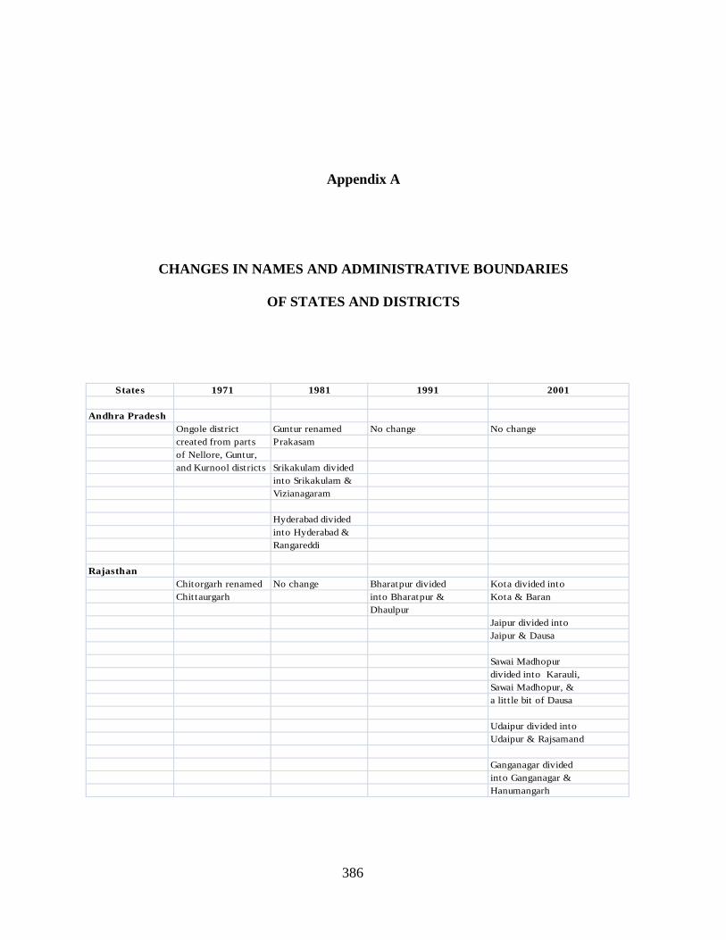
386
Appendix A
CHANGES IN NAMES AND ADMINISTRATIVE BOUNDARIES
OF STATES AND DISTRICTS
States 1971 1981 1991 2001
Andhra PradeshOngole district Guntur renamed No change No changecreated from parts Prakasamof Nellore, Guntur,and Kurnool districts Srikakulam divided
into Srikakulam &Vizianagaram
Hyderabad dividedinto Hyderabad &Rangareddi
RajasthanChitorgarh renamed No change Bharatpur divided Kota divided intoChittaurgarh into Bharatpur & Kota & Baran
DhaulpurJaipur divided intoJaipur & Dausa
Sawai Madhopurdivided into Karauli,Sawai Madhopur, &a lit t le bit of Dausa
Udaipur divided intoUdaipur & Rajsamand
Ganganagar dividedinto Ganganagar &Hanumangarh

387
APPENDIX A (continued)
States 1971 1981 1991 2001
GujaratKaira renamed No change No change Kheda dividedKheda into Kheda &
AnandBroach renamedBaruch Panch Mahals
divided into Surat divided Dohad &into Surat and Panch MahalsValsad districts
Bharuch dividedAhmedabad into Bharuch ÷d into NarmadaAhmadabad &Gandhinagar Surat & Valsad
divided into Baroda renamed Surat, Valsad, Vadodara & Navsari
Mahesana divided into Mahesana &Patan
Junagadh dividedinto Porbander& Junagadh
KarnatakaNo change Dharwar renamed Bangalore divided Bijapur divided
Dharwad into Bangalore & into Bijapur &Bangalore Rural Bagalkot
North Kanara renamed Coorg renamed Dharwad dividedUttar Kannad Kodagu into Dharwad,
Gadag, & HaveriSouth Kanara Uttar Kannadrenamed renamed Raichur dividedDakshin Kannad Uttara Kannada into Raichur &
KoppalDakshin Kannadrenamed Mysore dividedDakshina Kannada into Mysore &
Chamarajanagar
Dakshina Kannadadivided into Udupi& Dakshina Kannada
Chitradurga divided into Chitradurga &Davanagere

388
APPENDIX A (continued)
States 1971 1981 1991 2001
Madhya PradeshNo change Sehore divided into No change Mandsaur divided into
Sehore & Bhopal Mandsaur & Neemuch
Durg divided into Morena divided intoDurg & Rajnandgaon Morena & Sheopur
Shahdol divided intoShahdol & Umaria
Mandla divided intoMandla & Dindori
West Nimar dividedinto West Nimar &Barwani
Jabalpur divided intoJabalpur & Katmi
Hoshangabad dividedinto Hoshangabad &Harda
Chhattisgarh State formed from these districts: Surguja,Raipur, Raigarh,Bastar, Rajnandgaon,Durg, & Bilaspur
Surguja divided intoSurguja & Koriya
Raipur divided intoRaipur, Dhamtari, &Mahasamund
Raigarh divided intoRaigarh & Jashpur
Bastar divided intoBastar, Kanker, &Dantewada
Durg & Rajnandgaondivided into Durg,Rajnandgaon, &Kawardha
Bilaspur divided intoBilaspur, Korba, &Janjgir-Champa
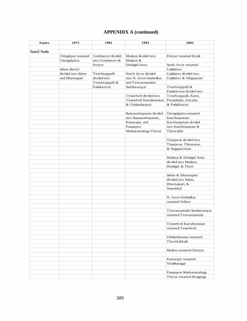
389
APPENDIX A (continued)
States 1971 1981 1991 2001
Tamil NaduChingleput renamed Coimbatore divided Madurai divided into Periyar renamed ErodeChengalpattu into Coimbatore & Madurai &
Periyar Dindigul-Anna South Arcot renamed Salem district Cuddalore; divided into Salem Tiruchirappalli North Arcot divided Cuddalore divided intoand Dharmapuri divided into into N. Arcot/Ambedkar Cuddalore & Viluppuram
Tiruchirappalli & and T iruvannamalai-Pudukkottai Sambuvarayar Tiruchirappalli &
Pudukkottai divided intoTirunelveli divided into Tiruchirappalli, Karur,T irunelveli Kattabomman Perambalur, Ariyalur, & Chidambaranar & Pudukkottai
Ramanathapuram divided Chengalpattu renamedinto Ramanathapuram, Kancheepuram;Kamarajar, and Kancheepuram dividedPasumpon into Kancheepuram &Muthuramalinga Thevar Thiruvallur
Thanjavur divided intoThanjavur, Thiruvarur,& Nagapattinam
Madurai & Dindigul-Annadivided into Madurai, Dindigul, & Theni
Salem & Dharmapuri divided into Salem,Dharmapuri, & Namakkal
N. Arcot/Ambedkarrenamed Vellore
Tiruvannamalai-Sambuvarayarrenamed Tiruvannamalai
T irunelveli Kattabommanrenamed Tirunelveli
Chidambaranar renamedThoothukkudi
Madras renamed Chennai
Kamarajar renamedVirudhunagar
Pasumpon Muthuramalinga Thevar renamed Sivaganga
390
BIBLIOGRAPHY
Acevedo, Luz Dal Alba. 1995. “Feminist Inroads in the Study of Women’s Work and Development”. Chap. 3 in Women in the Latin American Development Process. Ed. by Christine Bose and Edna Acosta-Belen. Philadelphia: Temple University Press.
Acock, Alan C. 2006. A Gentle Introduction to Stata. College Station, TX: Stata Press.
Adeney, Katharine and Andrew Wyatt. 2010. Contemporary India. Hampshire, UK and NY, USA: Palgrave Macmillan.
Agarwal, Bina. 1994. A Field of One’s Own: Gender and Land Rights in South Asia. Cambridge: Cambridge University Press.
Agarwal, Bina. 2002. “Are We Not Peasants too? Land Rights and Women’s Claims in India. Seeds. No 21:2-30.
Agresti, Alan and Barbara Finlay. 1997. Statistical Methods for the Social Sciences, 3rd ed. Upper Saddle River, NJ: Prentice Hall
Ahmed, Syed Masud, Mushtaque Chowdhury, and Abbas Bhuiya. 2001. “Micro-Credit and Emotional Well-Being: Experience of Poor Rural Women from Matlab, Bangladesh.” World Development. Vol. 29, No. 11:1957-1966.
Ahuja, Kanta. 1994. “Mobilization of Rural Women through Voluntary Efforts – A Case Study.” Pp. 1-10 in Non-Government Organizations in India. Sutlive, Vinson H. and Tomoko Hamada, eds. Williamsburg, VA: Dept. of Anthropology, College of William and Mary.
Akaike, H. 1973. “Information Theory as an Extension of the Maximum Likelihood Principle.” In B. N. Petrov and F. Csakie (Eds.) Second International Symposium on Information Theory (pp. 267-228). Akademiai Kiado, Budapest, Hungary.
Akila, R. “Reaching Global Goals in Primary Education: Some Gender Concerns for Tamil Nadu.” Chap. 12 in Toward Empowering Indian Women: Mapping Specifics of Tasks in Crucial Sectors. Ed. by R.B.S. Verma, H.S. Verma, and Nadeem Hasnain. New Delhi: Serials Publications.
Alderson, Arthur and Francois Nielsen. 1999. “Income Inequality, Development, and Dependence: A Reconsideration. American Sociological Review. Vol. 64, No. 4:606-631.
391
Alderson, Arthur and Francois Nielsen. 2002. “Globalization and the Great U-Turn: Income Inequality Trends in Sixteen OECD Countries.” American Journal of Sociology. Vol. 107, No. 5 (Mar. 2002): pp. 1,244-1,299.
Allen, Amy. 1999. The Power of Feminist Theory: Domination, Resistance, Solidarity. Boulder: Westview Press.
Allison, Paul D. 2009. Fixed Effects Regression Models. Los Angeles, London, New Delhi, Singapore, and Washington, DC: Sage Publications.
Alsop, Ruth, Mette Bertelsen, and Jeremy Holland. 2006. Empowerment in Practice: From Analysis to Implementation. Washington, DC: World Bank.
Anitha, B.K. and Anita Gurumurthy. “Being True to Feminism: The Methodology of the Status of Rural Women in Karnataka.” Chap. 10 (p. 229-251) in Building Women’s Capacities: Interventions in Gender Transformation. Ed. by Ranjani K. Murthy. New Delhi, Thousand Oaks, London: Sage Publications.
Arceneaux, Kevin and Gregory A. Huber. 2007. “What to Do (and Not Do) with Multicollinearity in State Politics Research.” State Politics and Policy Quarterly. Vol. 7, No. 1:81-101.
Arnold, F., S. Kishor, and T.K. Roy. 2002. “Sex-Selective Abortions in India.” Population and Development Review. Vol. 28, No. 4:759-785.
Arunachalam, Jaya and Brunhild Landwehr (eds.). 2003. “Structuring a Movement and Spreading It On”: History and Growth of the Working Women’s Forum (India) 1978-2003. Frankfurt and London: IKO.
Baden, Sally and Anne Marie Goetz. 1998. “Who needs [Sex] When You Can Have [Gender]?” Pp. 19-38 in Feminist Visions of Development: Gender, Analysis and Policy. Ed. by Cecile Jackson and Ruth Pearson. London: Routledge.
Balasubramanyam, K. 1967. Census of India, 1961, Volume XI: Mysore. Part IX A & B: District Census Handbooks. Delhi: Manager of Publications.
Balasubramanyam, K. 1969. Census of India, 1961, Volume XI: Mysore. Part I-C: Subsidiary Tables. Delhi: Manager of Publications.
Balasubramanyam, K. 1966. Census of India, 1961, Volume XI: Mysore. Part II-C (i): Social and Cultural Tables. Delhi: Manager of Publications.
Baran, Paul. 1957. The Political Economy of Growth. New York: Monthly Review Press.
Barker, Drucilla and Susan Feiner. 2004. “Globalization is a Feminist Issue.” Chap. 6 in Liberating Economics: Feminist Perspectives on Families, Work, and Globalization. Ann Arbor: University of Michigan Press.
392
Barro, R. J. and J. W. Lee. 2010. A New Data Set of Educational Attainment in the World, 1950-2010. NBER Working Paper 15902. Cambridge, MA: National Bureau of Economic Research.
Basu, Alaka Malwade. 1992. Culture, the Status of Women, and Demographic Behaviour: Illustrated with the Case of India. Oxford: Oxford University Press.
Basu, A. M. 1999. “Fertility Decline and Increasing Gender Imbalance in India, Including a Possible South Indian Turnaround.” Development and Change. Vol. 30, pp. 237-263.
Beneria, Lourdes and Gita Sen. “Accumulation, Reproduction and Woman’s Role in Economic Development: Boserup Revisited.” The Woman, Gender and Development Reader. 1997. London and New Jersey: Zed Books. Chap. 3.
Berry, Kim. 2007. “Lakshmi and the Scientific Housewife: A Transnational Account of Indian Women’s Development and the Production of an Indian Modernity.” Chap. 4 in The Indian State and the Women’s Problematic: Running with the Hare and Hunting with the Hounds. Ed. by R.B.S. Verma, H.S. Verma, and Nadeem Hasnain. New Delhi: Serials Publications.
Bhan, Gautam. 2001. India Gender Profile: Report Commissioned for Sida. Report no. 62. Brighton, UK: BRIDGE (development-gender), Institute of Development Studies, University of Sussex.
Bhatt, E. 1989. “Toward Empowerment.” World Development, Vol. XVII, No. 7:1059-65.
Bhowmik, Sharit and Renana Jhabvala. 1996. “Rural Women Manage their own Producer Co-operatives: Self Employed Women’s Association (SEWA)/Banaskantha Women’s Association in Western India.” Pp. 105-125 in Speaking Out: Women’s Economic Empowerment in South Asia. Ed. by Marilyn Carr, Martha Chen, and Renana Jhabvala. London: Aga Khan Foundation Canada.
Bhowmik, Sharit and Renana Patel. 1996. “Empowering Marginalized Workers: Unionization of Tobacco Workers by the Self Employed Women’s Association (SEWA) in Kheda, Gujarat.” Pp. 143-164 in Speaking Out: Women’s Economic Empowerment in South Asia. Ed. by Marilyn Carr, Martha Chen, and Renana Jhabvala. London: Aga Khan Foundation Canada.
Bose, Ashish. 1998. Supplement 1998: Demographic Diversity of India, 1991 State and District Level Data: A Reference Book. Delhi: B.R. Publishing Corporation.
Boserup, Ester. 1970. Women’s Role in Economic Development. New York: St. Martin’s Press.
Bruce, Judith. 1989. “Homes Divided.” World Development. Vol. 17, No. 7:979-991.
Brush, Lisa D. 2003. Gender and Governance. Walnut Creek, CA: Alta Mira Press.
393
Carr, Marilyn, Martha Chen, and Renana Jhabvala, eds. 1996. Speaking Out: Women’s Economic Empowerment in South Asia. London: Aga Khan Foundation Canada.
Census of India. 2001. www.censusindia.gov.in/. Office of the Registrar General and Census Commissioner. New Delhi, India.
Central Intelligence Agency. 2009. The World Factbook. www.cia.gov/library/publications/the-world-factbook/index.html. Washington, DC.
Chacko, Shubha. “’Being There was an Important Accident’: Rethinking Assumptions Based on Grassroots Experiences.” Chap. 15 (p. 328-345) in Building Women’s Capacities: Interventions in Gender Transformation. Ed. by Ranjani K. Murthy. New Delhi, Thousand Oaks, London: Sage Publications.
Chakrabarti, Avik. 2000. “Does Trade Cause Inequality?” Journal of Economic Development. Vol. 25, No. 2.
Chandramouli, C. 2011. “Size, Growth Rate and Distribution of Population.” Chap. 3 of Provisional Population Totals, Paper 1 of 2011 India Series 1. Delhi: Office of the Registrar General and Census Commissioner, India. www.censusindia.gov.in/2011-prov-results/data_files. Retrieved on April 12, 2011.
Chaudhuri, Maitrayee. 2007. “Gender in the Making of the Indian Nation-State.” Chap. 2 in The Indian State and the Women’s Problematic: Running with the Hare and Hunting with the Hounds. Ed. by R.B.S. Verma, H.S. Verma, and Nadeem Hasnain. New Delhi: Serials Publications.
Cheston, Susy and Lisa Kuhn. 2002. “Empowering Women through Microfinance.” Chap. 4 in Pathways out of Poverty: Innovations in Microfinance for the Poorest Families. Ed. by Sam Daley-Harris. Bloomfield, CT: Kumarian Press.
Chhaya, R.S. 1981. Census of India, 1981, Series 5: Gujarat. Part IV-A: Social and Cultural Tables. Delhi: Manager of Publications.
Chhaya, R.S. 1981. Census of India, 1981, Series 5: Gujarat. Parts XIII-A & B: District Census Handbooks. Delhi: Manager of Publications.
Chirot, Daniel. 1981. “Changing Fashions in the Study of the Social Causes of Economic and Political Change.” Pp. 259-282 in The State of Sociology. Ed. by James Short. Beverly Hills, CA: Sage.
Chockalingam, K. 1972. Census of India, 1971, Series 19: Tamil Nadu. Part X-A: District Census Handbooks. Delhi: Manager of Publications.
Chockalingam, K. 1978. Census of India, 1971, Series 19: Tamil Nadu. Part II-C (i & ii): Social, Cultural and Fertility Tables. Delhi: Manager of Publications.
394
Chua, Peter, Kum-Kum Bhavnani, and John Foran. 2000. “Women, Culture, Development: A New Paradigm for Development Studies?” Ethnic and Racial Studies. Vol. 23, No. 5:820-841.
Clark, Roger, Thomas Ramsbey, and Emily Adler. 1991. “Culture, Gender, and Labor Force Participation: A Cross-National Study.” Gender and Society. Vol. 5, No. 1:47-66.
Claycraft, K.R. 1989. “Gender-Specific Abortion.” The Human Life Review. Vol. 15, No. 2:36 41.
Committee on the Status of Women in India. 1974. Towards Equality: Report of the Committee on the Status of Women in India. New Delhi: Government of India.
Crowell, Daniel. 2003. The SEWA Movement and Rural Development: The Banaskanthaand Kutch Experience. New Delhi, Thousand Oaks, and London: Sage Publications.
Cruikshank, Barbara. 1999. The Will to Empower: Democratic Citizens and Other Subjects. Ithaca, NY: Cornell University Press.
Das, B.K. 1983. Census of India, 1981, Series 9: Karnataka. Part II-B (ii): Primary Census Abstract [for] Scheduled Castes and Scheduled Tribes. Delhi: Manager of Publications.
Das, B.K. 1983. Census of India, 1981, Series 9: Karnataka. Part IV-A: Social and Cultural Tables. Delhi: Manager of Publications.
Das, B.K. 1983. Census of India, 1981, Series 9: Karnataka. Part XIII A & B: District Census Handbooks. Delhi: Manager of Publications.
Das Gupta, M. “Selective Discrimination Against Female Children in Rural Punjab, India.” 1987. Population and Development Review. Vol. 13, No. 1:77-100.
Dasgupta, R. 2001. “An Informal Journey through SHGs.” Indian Journal & Agricultural Economics. Vol. 56, No. 3.
Desai, S. 1994. Gender Inequality and Demographic Behavior: India. New York: The Population Council, Inc.
Desai, Sonalde and Lester Andrist. 2010. “Gender Scripts and Age at Marriage in India.” Demography. Vol. 47, No. 3:667-687.
Deshmukh-Ranadive, Joy and Ranjani K. Murthy. 2005. “Introduction: Linking the Triad.” Chap. 1 in Micro-credit, Poverty and Empowerment: Linking the Triad. Ed. by Burra, Neera, Joy Deshmukh-Ranadive, and Ranjani K. Murthy. New Delhi: Sage Publications.
DHAN web site. www.dhan.org/kcbp; www.dhan.org/themes. Retrieved on 9/23/2010.
395
Dijkstra, A. Geske and Lucia C. Hanmer. 2000. “Measuring Socio-Economic Gender Inequality: Toward an Alternative to the UNDP Gender-Related Development Index.” Feminist Economics. Vol. 6, No. 2:41-75.
DiPrieto, William and Emmanuel Anoruo. 2005. “International Trade and Global Income Inequality.” International Journal of Applied Economics. Vol. 2, No. 1:pp. 121-131.
Directorate of Census Operations, Madhya Pradesh. 1997. Census of India, 1991, Series 13: Madhya Pradesh. Part XII A & B: District Census Handbooks. Delhi: Manager of Publications.
Doctor, C.C. 1971. Census of India, 1971, Series 5: Gujarat. Part II-C (ii): Social and Cultural Tables. Delhi: Manager of Publications.
Doctor, C.C. 1971. Census of India, 1971, Series 5: Gujarat. Parts X, A & B: District Census Handbooks. Delhi: Manager of Publications.
Dollar, David and Aart Kraay. 2001a. “Growth Is Good for the Poor.” World Bank Policy Research Working Paper No. 2587. Washington, DC: World Bank.
Dollar, David and Aart Kraay, eds. 2001b. “Trade, Growth and Poverty.” World Bank Policy Research Working Paper No. 2615. Washington, DC: World Bank.
Drake, Paul W. 2005. “The Hegemony of U.S. Economic Doctrines in Latin America.” Chap. 4 in Economic Doctrines in Latin America: Origins, Embedding and Evolution. Ed. by Fitzgerald, Valpy and Rosemary Thorp. New York and Oxford: Palgrave and Macmillan.
Dreze, Jean and Amartya Sen. 2002. India: Development and Participation, 2nd ed. Oxford: Oxford University Press.
Dreze, Jean and Amartya Sen. 2004. “Gender Inequality and Women’s Agency.” Chap. 14 in Class, Caste, Gender. Ed. by Manoranjan Mohanty. New Delhi: Sage Publications.
Dubey, K.C. 1983. Census of India, 1981, Series 11: Madhya Pradesh. Part XIII A & B: District Census Handbooks. Delhi: Manager of Publications.
Dubey, K.C. 1983. Census of India, 1981, Series 11: Madhya Pradesh. Part IV-A: Social and Cultural Tables. Delhi: Manager of Publications.
Dunaway, Wilma A. 2002. “Commodity Chains and Gendered Exploitation: Rescuing Women from the Periphery of World-Systems Thought.” Chap. 7 in The Modern/Colonial/ Capitalist World-System in the Twentieth Century: Global Processes, Antisystemic Movements, and the Geopolitics of Knowledge. Ed. by Grosfoguel, Ramon and Ana Margarita Cervantes-Rodriguez. Westport, CT and London: Greenwood Press.
Dutta, Subhabrata. 2004. “Women Education and Gender Disparity: A Study in a Rural Block of West Bengal.” Chap. 19 in Issues on Empowerment of Women. Ed. by Utpal Kumar De and Bhola Nath Ghosh. New Delhi: Mohit Publication.
396
Dyson, Tim and Mick Moore. 1983. “On Kinship Structure, Female Autonomy, and Demographic Behavior in India.” Population and Development Review. Vol. 9, No. 1:pp. 35-60.
Elson, Diane. 1999. “Labor Markets as Gendered Institutions: Equality, Efficiency and Empowerment Issues.” World Development. Vol. 27, No. 3:611-627.
Elson, Diane and Ruth Pearson. “The Subordination of Women and the Internationalization of Factory Production.” The Women, Gender and Development Reader. London: Zed Books Ltd. 1997. Pp. 191-203.
Engels, Frederick. 1942. The Origins of the Family, Private Property and the State.New York: International Publishers.
England, Paula. 1993. Theory on Gender/Feminism on Theory. New York: Aldine de Gruyter.
Etienne, M., and E. Leacock, eds. 1980. Women and Colonization. New York: Praeger.
Evans, Peter. 1979. Dependent Development: The Alliance of Multinational, State, and Local Capital in Brazil. Princeton: Princeton University Press.
Evans, Peter. 1983. “State, Local and Multinational Capital in Brazil: Prospects for the Stability of the ‘Triple Alliance’ in the Eighties.” Pp. 139-168 in Latin America in the World-Economy: New Perspectives. Ed. by Diana Tussie. New York: St. Martin’s.
Fernandez-Kelly, Maria Patricia. “Maquiladoras: The View from the Inside.” The Women, Gender and Development Reader. London: Zed Books Ltd. 1997. Pp. 203-215.
Finkel, Steven E. “Linear Panel Analysis.” Chap. 29 in Handbook of Longitudinal Research: Design, Measurement, and Analysis. Ed. by Scott Menard. 2008. Amsterdam, Boston: Elsevier/Academic Press.
Firebaugh, Glenn and Frank D. Beck. 1994. “Does Economic Growth Benefit the Masses? Growth, Dependence, and Welfare in the Third World.” American Sociological Review. Vol. 59, No. 5:631-653.
Forbes, Geraldine. 1996. Women in Modern India: Part 4, Vol. 2 of The New Cambridge History of India. Cambridge: Cambridge University Press.
Forsythe, Nancy, Roberto Patricio Korzeniewicz, and Valerie Durrant. 2000. “Gender Inequalities and Economic Growth: A Longitudinal Evaluation.” Economic Development and Cultural Change. Vol. 48, No. 3:573-617.
Foucault, Michel. 1991. “Governmentality.” Pp. 87-104 in The Foucault Effect: Studies in Governmentality. Ed. by Burchell, G., C. Gordon, and P. Miller. Chicago: Chicago University Press.
397
Frank, Andre Gunder. 1989. “The Development of Underdevelopment.” Monthly Review. Vol. 41, no. 2:37-51.
Friedman, Milton. 1962. Capitalism and Freedom. Chicago and London: University of Chicago Press.
Galab, S. and N. Chandrasekhara Rao. 2007. “Women’s Self-Help Groups, Poverty, Alleviation and Empowerment.” Chap. 12 in The Indian State and the Women’s Problematic: Running with the Hare and Hunting with the Hounds. Ed. by Verma, R.B.S., H.S. Verma, and Nadeem Hasnain. New Delhi: Serials Publications.
Gandhi, Nandita and Nandita Shah. 1991. The Issues at Stake: Theory and Practice in the Contemporary Women’s Movement in India. New Delhi: Kali for Women.
Ganguly-Scrase, Ruchira. 2000. “Diversity and the Status of Women: the Indian Experience.” Chap. 5 in Women in Asia: Tradition, Modernity, and Globalization. Ed. by Louise Edwards and Mina Roces. Ann Arbor: University of Michigan Press.
Geertz, Clifford. 1963. Peddlers and Princes: Social Development and Economic Change in Two Indonesian Towns. Chicago: University of Chicago Press.
Goetz, Anne Marie and Rina Sen Gupta. 1996. “Who Takes the Credit? Gender, Power, and Control Over Loan Use in Rural Credit Programs in Bangladesh. World Development. Vol. 24, No. 1:45-63.
Goldstein, Donna. 2001. “Microenterprise Training Programs, Neoliberal Common Sense, and the Discourses of Self-Esteem.” Chap. 9 in The New Poverty Studies: The Ethnography of Power, Politics, and Impoverished People in the United States. Ed. by Judith Goode and Jeff Maskovsky. New York and London: New York University Press.
Grameen Bank- Banking for the Poor. www.grameen-info.org. Information retrieved 2008.
Guha, Ramachandra. 2007. India after Gandhi: The History of the World’s Largest Democracy. New York: HarperCollins Publishers.
Gupta, C.S. 1962. Census of India, 1961, Volume XIV: Rajasthan. Part II-A: General Population Totals. Delhi: Manager of Publications.
Gupta, C.S. 1962. Census of India, 1961, Volume XIV: Rajasthan. Part II-C (i): Social and Cultural Tables). Delhi: Manager of Publications.
Gupta, C.S. 1962. Census of India, 1961, Volume XIV: Rajasthan. Part IX A & B: District Census Handbooks. Delhi: Manager of Publications.
Halaby, Charles N. 2004. “Panel Models in Sociological Research: Theory into Practice.” Annual Review of Sociology. Vol. 30, pp. 507-544.
398
Hartsock, Nancy C. M. 1983. Money, Sex, and Power: Toward a Feminist Historical Materialism. New York and London: Longman, Inc.
Hartwick, Elaine and Richard Peet. 2009. Theories of Development: Contentions, Arguments, Alternatives, 2nd ed. New York and London: The Guilford Press.
Hashemi, Syed M., Sidney Ruth Schuler, and Ann P. Riley. 1996. “Rural Credit Programs and Women’s Empowerment in Bangladesh.” World Development. Vol. 24, No. 4:635-653.
Hayek, Friedrich A. 1944. The Road to Serfdom. Chicago and London: University of Chicago Press.
Hyatt, Susan Brin. 2001. “From Citizen to Volunteer: Neoliberal Governance and the Erasure of Poverty.” Chap. 8 in The New Poverty Studies: The Ethnography of Power, Politics, and Impoverished People in the United States. Ed. by Judith Goode and Jeff Maskovsky. New York and London: New York University Press.
Inglehart, Ronald and Pippa Norris. 2003. Rising Tide: Gender Equality and Cultural Change Around the World. Cambridge: Cambridge University Press.
Inglehart, Ronald and Christian Welzel. 2005. Modernization, Cultural Change, and Democracy: The Human Development Sequence. New York, NY: Cambridge University Press.
Inkeles, Alex and David H. Smith. 1974. Becoming Modern: Individual Change in Six Developing Countries. Cambridge: Harvard University Press.
International Clinical Epidemiology Network (INCLEN). 2000. World SAFE and India SAFE: Studying the Prevalence of Family Violence. INCLEN Monograph Series on Critical International Health Issues. Monograph 9, Philadelphia: INCLSN.
International Institute for Population Sciences. 1995. India, National Family Health Survey (NFHS), 1992-93. Mumbai: IIPS.
International Institute for Population Sciences. 2000. India, National Family Health Survey (NFHS), 1998-99. Mumbai: IIPS.
Jagathpathi, G. 1963. Census of India, 1961, Volume VIII: Madhya Pradesh. Part II-A: General Population Tables. Delhi: Manager of Publications.
Jagathpathi, G. 1964. Census of India, 1961, Volume VIII: Madhya Pradesh. Part IX A & B: District Census Handbooks. Delhi: Manager of Publications.
Jagathpathi, G. 1965. Census of India, 1961, Volume VIII: Madhya Pradesh. Part II-C (i): Social and Cultural Tables. Delhi: Manager of Publications.
Jahan, Rounaq. 1995. The Elusive Agenda: Mainstreaming Women in Development. London: Zed Books.
399
Jaquette, Jane S. 1982. “Women and Modernization Theory: A Decade of Feminist Criticism.” World Politics. Vol. 34, No. 2: 267-284.
Jaquette, Jane S. and Kathleen Staudt. 2006. “Women, Gender, and Development.” Chap. 1 in Women and Gender Equity in Development Theory and Practice: Institutions, Resources, and Mobilization. Ed. by Jaquette, Jane S. and Gale Summerfield. Durham and London: Duke University Press.
Jejeebhoy, Shireen J. 2000. “Women’s Autonomy in Rural India: Its Dimensions, Determinants, and the Influence of Context.” Chap. 9 in Women’s Empowerment and Demographic Processes: Moving Beyond Cairo. Ed. by Harriet Presser and Gita Sen. Oxford: Oxford University Press.
Kabeer, N. 1994. Reversed Realities: Gender Hierarchies in Development Thought.London: Verso.
Kabeer, Naila. 2001. “Conflicts Over Credit: Re-Evaluating the Empowerment Potential of Loans to Women in Rural Bangladesh.” World Development. Vol. 29, No. 1:pp. 63-84.
Kalpana, K. 2008. “The Vulnerability of ‘Self-Help’: Women and Microfinance in South India.” Working Paper No. 303. Institute of Development Studies, University of Sussex, Brighton.
Kandiyoti, Deniz. 1988. “Bargaining with Patriarchy.” Gender and Society. Vol. 2, No. 3:274-290.
Khanna, Sunil K. 2010. Fetal/Fatal Knowledge: New Reproductive Technologies and Family-Building Strategies in India. Belmont, CA: Wadsworth Cengage Learning.
Kim, ChangHwan and Arthur Sakamoto. 2008. “The Rise of Intra-Occupational Wage Inequality in the United States, 1983-2002.” American Sociological Review. Vol. 73, February:129-157.
Kishor, Sunita and Kamla Gupta. 2007. “Women’s Empowerment in India and Its States: Evidence from the NFHS. Chap. 11 in The Indian State and the Women’s Problematic: Running with the Hare and Hunting with the Hounds. Ed. by Verma, R.B.S., H.S. Verma, and Nadeem Hasnain. New Delhi: Serials Publications.
Kristof, Nicholas and Sheryl WuDunn. 2009a. Half the Sky: Turning Oppression into Opportunity for Women Worldwide. Knopf Publishers.
Kristof, Nicholas and Sheryl WuDunn. 2009b. “Saving the World’s Women: How Changing the Lives of Women and Girls in the Developing World Can Change Everything.” The New York Times, August 23, 2009. Retrieved January 4, 2010. (http://www.nytimes.com/2009/08/23/magazine/23Women-t.html).
Kumar, K. Sampath. 1991. Census of India, 1991, Series 23: Tamil Nadu. Part XII A & B: District Census Handbooks. Delhi: Manager of Publications.
400
Lairap-Fonderson, Josephine. 2002. “The Disciplinary Power of Micro Credit: Examples from Kenya and Cameroon.” Chap. 11 in Rethinking Empowerment: Gender and Development in a Global/Local World. Ed. by Parpart, Jane, Shirin Rai, and Kathleen Staudt. London and New York: Routledge.
Lee, Ching Kwan. 1998. Gender and the South China Miracle: Two Worlds of Factory Women. Berkeley: University of California Press.
Lim, Linda Y. C. 1990. “Women’s Work in Export Factories: The Politics of a Cause.” Pp. 101-119 in Persistent Inequalities. Ed. by Irene Tinker. New York: Oxford University Press.
Lipset, S.M. 1963. “Economic Development and Democracy.” Pp. 27-63 in Political Man. By S. M. Lipset. Garden City, New York: Anchor.
Mahila Chetna Manch and UNIFEM. n.d. Resource Directory of Support Services to Counter Violence against Women in Madhya Pradesh. Bhopal, Madhya Pradesh and New Delhi.
Manjrekar, Nandini. 2007. “Contemporary Challenges to Women’s Eduation: Towards an Elusive Goal? Chap. 16 in Toward Empowering Indian Women: Mapping Specifics of Tasks in Crucial Sectors. Ed. by R.B.S. Verma, H.S. Verma, and Nadeem Hasnain. New Delhi: Serials Publications.
Marger, Martin N. 2005. Social Inequality: Patterns and Processes, 3rd Ed. New York: McGraw-Hill.
Marius-Gnanou, Kamala. 2003. “Rural Credit Programs and Gender Issues: A Case Study from India.” Chap. 2 in Microfinance: From Daily Survival to Social Change. Ed. by Guerin, Isabelle and Jean-Michel Servet. Pondicherry: French Institute of Pondicherry.
Marulasiddaiah, H.M. 1994. “Image of an Elephant in a Small Mirror: SWASTI – An Organization for Social Change and Development.” Pp. 49-75 in Non-Government Organizations in India. Sutlive, Vinson H. and Tomoko Hamada, eds. Williamsburg, VA: Dept. of Anthropology, College of William and Mary.
Mayoux, Linda. 1995. From Vicious to Virtuous Cycles? Gender and Micro-Enterprise Development. Occasional Paper No. 3, Fourth World Conference on Women. Geneva, Switzerland: United Nations Research Institute for Social Development.
Mehotra, Santosh, ed. 2006. The Economics of Elementary Education in India: The Challenge of Public Finance, Private Provision and Household Costs. New Delhi, Thousand Oaks, and London: Sage Publications.
McClelland, David C. 1968. “The Achievement Motive in Economic Growth,” chap. 16 In Mitchell A. Seligson and John T. Passe-Smith (eds.) Development and Underdevelopment: The Political Economy of Global Inequality, 3rd ed. 2003. Boulder and London: Lynne Rienner Publishers.
401
McMichael, Philip. 2000. Development and Social Change: A Global Perspective, 2nd Ed. Thousand Oaks: Pine Forge Press.
Mies, Maria. 1982. The Lace Makers of Narsapur: Indian Housewives Produce for the World Market. London: Zed Press.
Mitchell, J. 1966. “Women, the Longest Revolution.” New Left Review. Vol. 40: pp. 11-37.
Montecinos, Veronica and John Markoff. 2001. “From the Power of Economic Ideas to the Power of Economists.” Chap. 4 in The Other Mirror: Grand Theory through the Lens of Latin America. Ed. by Centeno, Miguel Angel and Fernando Lopez-Alves. Princeton and Oxford: Princeton University Press.
Moore, Gwen and Gene Shackman. 1996. “Gender and Authority: A Cross-National Study.” Social Science Quarterly. Vol. 77, No. 2:273-288.
Moser, Caroline. 1989. “Gender Planning in the Third World: Meeting Practical and Strategic Gender Needs.” World Development. Vol. 17, No. 11:1799-1825.
Moser, C.O.N. 1993. Gender Planning and Development. New York: Routledge. Cited in Visvanathan, Nalini. 1996. “Introduction to Part 1” in The Women, Gender and Development Reader. Ed. by Visvanathan, Nalini; Lynn Duggan; Laurie Nisonoff; and Nan Wiegersma. London and New Jersey: Zed Books.
Mueller, Adele. 1986. “The Bureaucratization of Feminist Knowledge: The Case of Women in Development.” Resources for Feminist Research. Vol. 15, No. 1:36-38.
Muhuri, P. K. and Preston, S. H. (1991). “Effects of Family Composition on Mortality Differentials by Sex Among Children in Matlab, Bangladesh.” Population and Development Review. Vol. 17, 3:415-434.
Murthy, Ranjani, K. Raju, and Amitha Kamath. 2005. “Towards Women’s Empowerment and Poverty Reduction: Lessons from the Andhra Pradesh South Asia Poverty Alleviation Programme.” Chap. 2 in Micro-credit, Poverty and Empowerment: Linking the Triad. Ed. by Burra, Neera, Joy Deshmukh-Ranadive, and Ranjani K. Murthy. New Delhi: Sage Publications.
Muthuswami, A.P. 1982. Census of India, 1981, Series 20: Tamil Nadu. Part II-B: Primary Census Abstract. Delhi: Manager of Publications.
Muthuswami, A.P. 1982. Census of India, 1981, Series 20: Tamil Nadu. Part IV-A: Social and Cultural Tables. Delhi: Manager of Publications.
Muthuswami, A.P. 1982. Census of India, 1981, Series 20: Tamil Nadu. Part XIII A & B: District Census Handbooks. Delhi: Manager of Publications.
Nag, Prithvish, ed. Socio-Economic Atlas of India, pp. 2-3. Kolkata: Director, National Atlas and Thematic Publishing Organisation.
402
Naik, J.P. 1965. Educational Planning in India. Bombay, New Delhi, Calcutta, Madras, London, and New York: Allied Publishers.
Nambiar, P.K. 1964. Census of India, 1961, Volume IX: Madras. Part II-C (i): Cultural Tables. Delhi: Manager of Publications.
Nambiar, P.K. 1965. Census of India, 1961, Volume IX: Madras. Part X: District Census Handbooks. Delhi: Manager of Publications.
Nambisan, Sobha. 1992. Census of India, 1991, Series 11: Karnataka. Part XII A & B: District Census Handbooks. Delhi: Manager of Publications.
Nambisan, Sobha. 1992. Census of India, 1991, Series 11: Karnataka. Part IV A-C: Socio-cultural Tables. Delhi: Manager of Publications.
National Sample Survey Organisation. 1997. Employment and Unemployment Situation among Social Groups in India, 1993-94, NSS 50th Round. Report No. 425. Department of Statistics, Government of India.
National Sample Survey Organisation. 1999-2000. Employment and Unemployment Situation among Social Groups in India, 1999-2000, NSS 55th Round. Report No. 469. Department of Statistics, Government of India.
National Sample Survey Organisation. 2004-2005. Employment and Unemployment Situation among Social Groups in India, 2004-05, NSS 61st Round. Report No. 516. Department of Statistics, Government of India.
NAWO. 1996. Directory of Organisations Working on Gender Issues, First Issue. New Delhi: Coordination Unit for Beijing 1995.
Nelson, Julie. 2006. Economics for Humans. Chicago: University of Chicago Press.
Ngai, Pun. 2005. Made in China: Women Factory Workers in a Global Workplace. Durham: Duke University Press. Nisonoff, Laurie. Introduction to Part 3. The Women, Gender and Development Reader. Ed. by Visvanathan, Nalini; Lynn Duggan, Laurie Nisonoff, and Nan Wiegersma. London: Zed Books Ltd. 1997. Pp. 177-190.
Nisonoff, Laurie. Introduction to Part 3. The Women, Gender and Development Reader.Ed. by Visvanathan, Nalini; Lynn Duggan, Laurie Nisonoff, and Nan Wiegersma.London: Zed Books Ltd. 1997. Pp. 177-190.
Noponen, H. 1987. “Organising Women Petty Traders and Home-Based Producers: A Case of Working Women’s Forum, India,” in A. Menefee Singh and A. Kelles-Viitanen (eds.), op. cit. Cited in From Vicious to Virtuous Cycles? Gender and Micro-Enterprise Development. By Linda Mayoux. Occasional Paper No. 3, Fourth World Conference on Women. Geneva, Switzerland: United Nations Research Institute for Social Development.
403
Noponen, H. 1990. Loans to the Working Poor: A Longitudinal Study of Credit, Gender and the Household Economy. PRIE Working Paper No. 6. New Brunswick: Rutgers University. Cited in From Vicious to Virtuous Cycles? Gender and Micro-Enterprise Development. Occasional Paper No. 3, Fourth World Conference on Women. Geneva, Switzerland: United Nations Research Institute for Social Development.
Padia, Veena. 2005. “Social Mobilization and Micro-credit for Women’s Empowerment: A Study of the DHAN Foundation.” Chap. 4 in Micro-credit, Poverty and Empowerment: Linking the Triad. Ed. by Burra, Neera, Joy Deshmukh-Ranadive, and Ranjani K. Murthy. New Delhi: Sage Publications.
Office of the Registrar General, India. 1961. Census of India 1961: A Guide to the 1961 Census Publication Programme. New Delhi: Ministry of Home Affairs.
Padmanabha, P. 1971. Census of India, 1971, Series 14: Mysore. Part II-C(i): Social and Cultural Tables and Special Tables on Scheduled Castes and Scheduled Tribes. Delhi: Manager of Publications.
Padmanabha, P. 1971. Census of India, 1971, Series 14: Mysore. Part II-C(ii): Social and Cultural Tables and Fertility Tables. Delhi: Manager of Publications.
Padmanabha, P. 1971. Census of India, 1971, Series 14: Mysore. Part X A & B: District Census Handbooks. Delhi: Manager of Publications.
Palley, T. I. 2005. “From Keynesianism to Neoliberalism: Shifting Paradigms in Economics.” Pp. 20-29 in Neoliberalism: A Critical Reader. Ed. by A. Saad-Filho and D. Johnston. London: Pluto Press.
Panchamukhi, P.R. 2006. “Universalising Elementary Education in Madhya Pradesh: Can the Successes of Decentralized Governance Offset the Problems of Public Finance, Private Provision and Private Cost?” Chap. 5 in The Economics of Elementary Education in India: The Challenge of Public Finance, Private Provision and Household Costs. Ed. by Santosh Mehotra. New Delhi, Thousand Oaks, and London: Sage Publications.
Panda, Smita Mishra. 2007. “Women’s Collective Action and Sustainable Water Management: Case of SEWA’s Water Campaign in Gujarat, India.” CAPRi Working Paper No. 61. Presented at International Research Workshop on “Gender and Collective Action” in Oct. 2005, Chiang Mai, Thailand.
Pande, Rohini and Anju Malhotra. 2006. “Son Preference and Daughter Neglect in India: What Happens to Living Girls?” Washington, DC: International Center for Research on Women.
Pandya, A.K. 1974. Census of India, 1971, Series 10: Madhya Pradesh. Part II-C(i & ii ): Social and Cultural Tables. Delhi: Manager of Publications.
Pandya, A.K. 1974. Census of India, 1971, Series 10: Madhya Pradesh. Part X A & B: District Census Handbooks. Delhi: Manager of Publications.
404
Parry, J.P. 1979. Caste and Kinship in Kangra. London: Routledge.
Parsons, Talcott. 1951. The Social System. Glencoe, IL: Free Press.
Pathak, Prasanta and Chaiti Sharma Biswas. 2004. “Temporal Change in the Contrast Between Female and Male Labour Forces and Workforces in Eastern India.” Chap. 8 in Issues on Empowerment of Women. Ed. by Kumar, Utpal and Bhola Nath Ghosh. New Delhi: Mohit Publication.
Polak, H.S., H.N. Brailsford, and Lord Pethick-Lawrence. 1949. Mahatma Gandhi. London: Odhams Press Limited.
Presser, Harriet and Gita Sen. 2000. “Women’s Empowerment and Demographic Processes: Laying the Groundwork.” Chap. 1 in Women’s Empowerment and Demographic Processes. Ed. by Presser, Harriet and Gita Sen. Oxford: Oxford University Press.
Prugl, Elisabeth and Audrey Lustgarten. 2006. “Mainstreaming Gender in International Organizations.” Pp. 53-70 in Women and Gender Equity in Development Theory and Practice. Ed. by Jaquette, Jane S. and Gale Summerfield. Durham and London: Duke University Press.
Prugl, Elisabeth and Mary K. Meyer. 1999. “Gender Politics in Global Governance.” Pp. 3-18 in Gender Politics in Global Governance. Ed. by Mary K. Meyer and Elisabeth Prugl. Lanham, MD: Rowman and Littlefield.
Putnam, R. 1993. Making Democracy Work: Civic Traditions in Modern Italy. Princeton, NJ: Princeton University Press.
Rahman, Aminur. 1999. Women and Microcredit in Rural Bangladesh: Anthropological Study of the Rhetoric and Realities of Grameen Bank Lending. Boulder, CO:Westview Press.
Rajivan, Anuradha. 2005. “Micro-credit and Women’s Empowerment: A Case Study of SHARE Micro-finance Limited.” Chap. 3 in Micro-credit, Poverty and Empowerment: Linking the Triad. Ed. by Burra, Neera, Joy Deshmukh-Ranadive, and Ranjani K. Murthy. New Delhi: Sage Publications.
Ram, K. 1991. Mukkuvar Women: Gender Hegemony and Capitalist Transformation in a South Indian Fishing Community. Sydney: Allen and Unwin.
Ramachandran, Vimala, ed. 2004. Gender and Social Equity in Primary Education: Hierarchies of Access. New Delhi, London, Thousand Oaks: Sage Publications.
Ramanathan, Malathi. 2007. “Women and Empowerment: Shri Mahila Griha Udyog Liggat Papad.” Chap. 15 in The Indian State and the Women’s Problematic: Running with the Hare and Hunting with the Hounds. Ed. by Verma, R.B.S., H.S. Verma, and Nadeem Hasnain. New Delhi: Serials Publications.
405
Randeria, S. and L. Visaria. 1984. “Sociology of Bride-Price and Dowry.” Economic and Political Weekly. Vol. 15, no. 15:648-652.
Rankin, Katharine. 2002. “Social Capital, Microfinance, and the Politics of Development.” Feminist Economics. Vol. 8, Issue 1:1-24.
Rao, S.S. Jaya. 1984. Census of India, 1981, Series 2: Andhra Pradesh. Part IV-A: Social and Cultural Tables. Delhi: Manager of Publications.
Rao, S.S. Jaya. 1984. Census of India, 1981, Series 2: Andhra Pradesh. Part IX (i): Special Tables for Scheduled Castes and Scheduled Tribes. Delhi: Manager of Publications.
Rao, S.S. Jaya. 1986. Census of India, 1981, Series 2: Andhra Pradesh. Part XIII-A & B: District Census Handbooks. Delhi: Manager of Publications.
Rathgeber, E.M. 1990. “WID, WAD, GAD: Trends in Research and Practice.” The Journal of Developing Areas. Vol. 24, pp. 489-502.
Ray, Raka. 1999. Fields of Protest: Women’s Movements in India. Minneapolis: University of Minnesota Press.
Ray, Sunil. 2006. “The Cost and Financing of Universalising Elementary Education: A Silver Lining in Rajasthan?” Chap. 4 in The Economics of Elementary Education in India: The Challenge of Public Finance, Private Provision and Household Costs. Ed. by Santosh Mehotra. New Delhi, Thousand Oaks, and London: Sage Publications.
Rose, Nikolas. 1993. “Government, Authority and Expertise in Advanced Liberalism.” Economy and Society. Vol. 22, (3):283-299.
Rose, Nikolas. 1996. “Governing ‘Advanced’ Liberal Democracies.” Pp. 37-64 in Foucault and Political Reason: Liberalism, Neo-Liberalism and Rationalities. Ed. by Barry, A., T. Osborne, and N. Rose. Chicago: University of Chicago Press.
Rosen, Bernard and Anita LaRaia. 1972. “Modernity in Women: An Index of Social Change in Brazil.” Journal of Marriage and the Family. Vol. 34, May:354. Cited in Jaquette, Jane S. 1982. “Women and Modernization Theory: A Decade of Feminist Criticism. World Politics. Vol. 34, No. 2:267-284.
Rowlands, J. 1997. Questioning Empowerment: Working with Women in Honduras. Oxford:Oxfam Publication.
Roy, Kartik C. and Jorn Sideras, eds. 2006. Institutions, Globalisation and Empowerment. Cheltenham and Northampton: Edward Elgar Publishing.
Sankar, Kalpana. 2005. “Social Mobilization and Micro-Finance for Women’s Empowerment – Lessons from ASA Trust.” Chap. 7 in Micro-credit, Poverty and Empowerment: Linking the Triad. Ed. by Burra, Neera, Joy Deshmukh-Ranadive, and Ranjani K. Murthy. New Delhi: Sage Publications.
406
Samyal, Paromita. 2009. “From Credit to Collective Action: The Role of Microfinance in Promoting Women’s Social Capital and Normative Influence.” American Sociological Review. Vol. 74(August): pp. 529-550.
Schroeder, Larry D., David L. Sjoquist, and Paula E. Stephan. 1986. Understanding Regression Analysis: An Introductory Guide. Newbury Park, CA, London, U.K.,and New Delhi, India: Sage Publications.
Schwarz, G. 1978. “Estimating the Dimensions of a Model”. Annals of Statistics. Vol. 6: pp. 461-464.
Sekhar, A. Chandra. 1965. Census of India, 1961, Volume II: Andhra Pradesh. Part I-C: Subsidiary Tables. Delhi: Manager of Publications.
Sekhar, A. Chandra. 1965. Census of India, 1961, Volume II: Andhra Pradesh. District Census Handbooks. Delhi: Manager of Publications.
Sekhar, A. Chandra. 1966. Census of India, 1961, Volume II: Andhra Pradesh. Part II-C: Cultural and Migration Tables. Delhi: Manager of Publications.
Selvarajan, E. and R. Elango. 2004. Rural Development Programmes and Externalities: The Report of the Project Funded by Planning Commission, Government of India. New Delhi: Serials Publications.
Sen, Amartya. 2005. The Argumentative Indian: Writings on Indian History, Culture and Identity. London, New York, Toronto: Penguin Books.
Seshanna, Shubhasree and Stephane DeCornez. 2003. “Income Polarization and Inequality Across Countries: An Empirical Study.” Journal of Policy Modeling. Vol. 25:pp. 335-358.
Shah, Ghanshyam. 2004. Social Movements in India: A Review of Literature. 2nd ed. New Delhi, India, London, U.K., and Thousand Oaks, CA: Sage Publications.
Sharma, Aradhana. 2006. “Crossbreeding Institutions, Breeding Struggle: Women’s Empowerment, Neoliberal Governmentality, and State (Re)Formation in India.” Cultural Anthropology. Vol. 21, No. 1:66-95.
Sharma, Aradhana. 2008. The Logics of Empowerment: Development, Gender, and Governance in Neoliberal India. Minneapolis and London: University of Minnesota Press.
Sharma, U. 1980. Women, Work and Property in North West India. London: Tavistock.
Shepherd, Mary Elizabeth. 2008. Sex-Selective Abortion in India: The Impact on Child Mortality. Youngstown, New York: Cambria Press.
Shields, L. 1995. “Women’s Experiences of the Meaning of Empowerment.” Qualitative Health Research. Vol. 15, No. 1:15-35.
407
Singer, Judith D. and John B. Willett. 2003. Applied Longitudinal Data Analysis: Modeling Change and Event Occurrence. New York, NY: Oxford Univ. Press.
Singh, Katar. 2005. “Changing Perspectives and Paradigms of Rural Development.” Chap. 2 in Rural Development: Macro-micro Realities. Ed. by Sisodia, Yatindra Singh. Jaipur: Rawat Publications.
Singh, Kesar. 2005. “Rural Development: Problems, Prospects, and Implementation Strategies.” Chap. 3 in Rural Development: Macro-micro Realities. Ed. by Sisodia, Yatindra Singh. Jaipur: Rawat Publications.
Singh, Awadhesh Kumar. 2007. “Functioning & Performance of Swashakti and Swayamsiddha Projects in India.” New Delhi: Planning Commission, Government of India.
Singh, R.P. 1991. Census of India, 1991, Series 2: Andhra Pradesh. Part IV A-C: Socio-cultural Tables. Delhi: Manager of Publications.
Singh, R.P. 1995. Census of India, 1991, Series 2: Andhra Pradesh. Parts XII A & B: District Census Handbooks. Delhi: Manager of Publications.
Sinha, Frances. 2001. “Microenterprise Promotion for Women in a Traditional, Male-Controlled Sector: The Silk Industry Project in Karnataka and West Bengal.” Chap. 3 (p. 88-115) in Building Women’s Capacities: Interventions in Gender Transformation. Ed. by Ranjani K. Murthy. New Delhi, Thousand Oaks, London: Sage Publications.
Sivard, R. 1985. Women…A World Survey. New York: Carnegie, Ford and Rockefeller Foundations.
Smith, J. 1984. “Non Wage Labor and Subsistence.” Pp. 64-89 in Households and the World-Economy. Ed. by J. Smith, I. Wallerstein, and H. Evers. Beverly Hills: Sage Publications.
Snijders, T.A.B. and R.J. Bosker. 1999. Multilevel Analysis: An Introduction to Basic and Advanced Multilevel Modeling. London: Sage Publications.
So, Alvin. 1986. “The Economic Success of Hong Kong: Insights from a World-System Perspective.” Sociological Perspectives. Vol. 29:241-258.
So, Alvin. 1990. Social Change and Development: Modernization, Dependency, and World-System Theories. Newbury Park, London, and New Delhi: Sage Publications.
Sood, Meenakshi, Neena Swaroop, and Alka Batra. 1992. Voluntary Organisations Working for Children and Women: Some Profiles. New Delhi: Resource Centre on Children, National Institute of Public Cooperation and Child Development.
Srinivas, M.N. 1966. Social Change in Modern India. Berkeley: University of California Press.
Srivastava, I.C. 1981. Census of India, 1981, Series 18: Rajasthan. Part IV-A: Social and Cultural Tables. Delhi: Manager of Publications.
408
Srivastava, I.C. 1981. Census of India, 1981, Series 18: Rajasthan. Part XIII A & B: District Census Handbooks. Delhi: Manager of Publications.
Srivastava, S.C. 1983. India Census in Perspective. New Delhi: Office of the Registrar General, India, Ministry of Home Affairs.
StataCorp LP. 2007. STATA Longitudinal/Panel Data Reference Manual,Release 10. College Station, TX: Stata Press.
Stern, Robert W. 2003. Changing India: Bourgeois Revolution on the Subcontinent, 2nd ed. Cambridge: Cambridge University Press.
Subramanian, Arvind. 2008. India’s Turn: Understanding the Economic Transformation. New Delhi: Oxford University Press.
Subramaniam, Mangala. 2006. The Power of Women’s Organizing: Gender, Caste, and Class in India. Lanham, MD: Lexington Books.
Talcott, Molly. 2003. “Gendered Webs of Development and Resistance: Women, Children, and Flowers in Bogota.” Signs. 29, 2:465-489.
Tinker, Irene, ed. 1990. Persistent Inequalities. New York: Oxford University Press.
Tinker, Irene. “The Making of a Field: Advocates, Practitioners and Scholars.”The Woman, Gender and Development Reader. 1997. London and New Jersey: Zed Books. Chap. 2.
Todd, Helen. 1996. Women at the Center: Grameen Bank Borrowers after One Decade. Boulder, CO: Westview Press.
Tomar, R.P. 1991. Census of India, 1991, Series 21: Rajasthan. Part XII A & B: District Census Handbooks. Delhi: Manager of Publications.
Townsend, J.; E. Zapata; J. Rowlands; P. Alberti; and M. Mercado. 1999. Women and Power: Fighting Patriarchies and Poverty. London: Zed Books.
Trivedi, R.K. 1961. Census of India, 1961, Volume V: Gujarat. Part II-C: Cultural and Migration Tables. Delhi: Manager of Publications.
Troutner, Jennifer and Peter Smith. 2004. “Introduction to Empowering Women: Agency, Structure, and Comparative Perspective.” Chap. 1 in Promises of Empowerment: Women in Asia and Latin America. Ed. by Smith, Peter H., Jennifer L. Troutner, and Christine Hunefeldt. Lanham, MD: Rowman and Littlefield Publishers.
T. T. Maps. Muthiah, S., editor-in-chief. 1990. An Atlas of India, pp. 17, 44, 64, 77, 112, and 121. Oxford: Oxford University Press.
UNDP. 1995. Human Development Report 1995. New York and Oxford: Oxford University Press.
409
UNDP (United Nations Development Program). 2002. Gender Equality: Practice Note. New York: UNDP.
UNDP (United Nations Development Program). 2003. Transforming the Mainstream: Gender in UNDP. New York: UNDP.
UNDP (United Nations Development Program). 2010. The Real Wealth of Nations: Pathways to Human Development, 20th Anniversary Edition. Human Development Report 2010. New York: Palgrave Macmillan.
UNICEF. 2009. UNICEF India Health Indicators. Retrieved on April 12, 2011 from www.unicef.org/infobycountry/india_statistics.html.
United Nations Secretariat. 1998. “Levels and Trends of Sex Differentials in Infant, Child and Under-five Mortality.” Pp. 84-108 in Too Young to Die: Genes or Gender?, ed. by John Cleland. New York: United Nations.
Unnithan-Kumar, Maya. 1997. Identity, Gender, and Poverty: New Perspectives on Caste and Tribe in Rajasthan. Oxford: Berghahn Books.
Vaid, Divya. 2007. “Gendered Inequality in Educational Transitions.” Chap. 15 in Toward Empowering Indian Women: Mapping Specifics of Tasks in Crucial Sectors. Ed. by R.B.S. Verma, H.S. Verma, and Nadeem Hasnain. New Delhi: Serials Publications.
Varsani, N.R. 1991. Census of India, 1991, Series 7: Gujarat. Parts XII A & B: District Census Handbooks. Delhi: Manager of Publications.
Vedantam, T. 1971. Census of India, 1971, Series 2: Andhra Pradesh. Part II-C(ii): Social and Cultural Tables and Fertility Tables. Delhi: Manager of Publications.
Vedantam, T. 1971. Census of India, 1971, Series 2: Andhra Pradesh. Part V (A): Special Tables on Scheduled Castes and Scheduled Tribes. Delhi: Manager of Publications.
Vedantam, T. 1973. Census of India, 1971, Series 2: Andhra Pradesh. Part X-A & B: District Census Handbooks. Delhi: Manager of Publications.
Verma, V.S. 1971. Census of India, 1971, Series 18: Rajasthan. Parts X A & B: District Census Handbooks. Delhi: Manager of Publications.
Verma, V.S. 1971. Census of India, 1971, Series 18: Rajasthan. Part II-A: General Population Totals. Delhi: Manager of Publications.
Verma, V.S. 1971. Census of India, 1971, Series 18: Rajasthan. Part II-C (i): Social and Cultural Tables. Delhi: Manager of Publications.
Visaria, Leela and Vimala Ramachandran. 2004. “What DPEP and Other Data Sources Reveal.” Chap. 2 in Gender and Social Equity in Primary Education: Hierarchies of Access. Ed. by Vimala Ramachandran. New Delhi, London, Thousand Oaks: Sage Publications.
410
Visvanathan, Nalini. “Introduction to Part 1.” The Woman, Gender and Development Reader. 1997. London and New Jersey: Zed Books.
Viswanath, Vanita. 1991. NGOs and Women’s Development in Rural South India: A Comparative Analysis. Boulder, San Francisco, and Oxford: Westview Press.
Wallerstein, Immanuel. 2004. World Systems Analysis: An Introduction. Duke University Press.
Ward, Kathryn B. 1993. “Reconceptualizing World System Theory to Include Women”. Chap. 3 in Theory on Gender/Feminism on Theory. Ed. by England, Paula. New York: Aldine de Gruyter.
Weber, Max. 1930. The Protestant Ethic and the Spirit of Capitalism. New York: Routledge.
Webster, Andrew. 1990. Introduction to the Sociology of Development, 2nd ed. Atlantic Highlands: Humanities Press International.
Wong, Kwok-Fu. 2003. “Empowerment as a Panacea for Poverty – Old Wine in New Bottles? Reflections on the World Bank’s Conception of Power.” Progress in Development Studies. 3,4:307-322.
World Bank. 2001. World Development Report: The State in a Changing World. New York: Oxford University Press.
Young, Gay, Lucia Fort, and Mona Danner. 1994. “Moving from the ‘Status of Women’ to ‘Gender Inequality’: Conceptualisation, Social Indicators and an Empirical Application.” International Sociology. Vol. 9, No. 1:55-85.
Young, Kate. “Gender and Development.” The Woman, Gender and Development Reader. 1997. London and New Jersey: Zed Books.
Ziegler, N. P. 1978. “Some Notes on Rajput Loyalties During the Mughal Period.” in Kingship and Authority in South Asia. Ed. by J.F. Richards. Madison: University of Wisconsin Publication Series.