the dynamics of a swirling flow in a pipe and transition to axisymmetric vortex breakdown
TRANSCRIPT

J. Fluid Mech. (1997), vol. 340, pp. 177–223. Printed in the United Kingdom
c© 1997 Cambridge University Press
177
The dynamics of a swirling flow in a pipe andtransition to axisymmetric vortex breakdown
By S. W A N G AND Z. R U S A KDepartment of Mechanical Engineering, Aeronautical Engineering and Mechanics,
Rensselaer Polytechnic Institute, Troy, NY 12180-3590, USA
(Received 20 February 1995 and in revised form 12 November 1996)
This paper provides a new study of the axisymmetric vortex breakdown phenomenon.Our approach is based on a thorough investigation of the axisymmetric unsteadyEuler equations which describe the dynamics of a swirling flow in a finite-lengthconstant-area pipe. We study the stability characteristics as well as the time-asymptoticbehaviour of the flow as it relates to the steady-state solutions. The results areestablished through a rigorous mathematical analysis and provide a solid theoreticalunderstanding of the dynamics of an axisymmetric swirling flow. The stability andsteady-state analyses suggest a consistent explanation of the mechanism leading tothe axisymmetric vortex breakdown phenomenon in high-Reynolds-number swirlingflows in a pipe. It is an evolution from an initial columnar swirling flow to anotherrelatively stable equilibrium state which represents a flow around a separation zone.This evolution is the result of the loss of stability of the base columnar state whenthe swirl ratio of the incoming flow is near or above the critical level.
1. Introduction and mathematical model1.1. Introduction
The term ‘vortex breakdown’ commonly refers to the abrupt and drastic changeof structure which may occur under certain conditions in high-Reynolds-numberswirling flows. This phenomenon is characterized by a sudden axial deceleration, thatoccurs above a certain level of swirl, leading to the formation of a free stagnationpoint which is followed by a separation region with turbulence behind it. Dependingon the level of swirl (at a given Reynolds number) the breakdown may adopt arange of shapes, from asymmetric spiral waves to a nearly axisymmetric separationzone.
The scientific interest in explaining this strongly nonlinear phenomenon has ledto many experimental, numerical and theoretical studies, and several review paperson this subject have been presented, including the reports by Hall (1972), Leibovich(1978, 1984), Escudier (1988) and Sarpkaya (1995). Although there has been extensiveresearch, the fundamental nature of these phenomena still remains largely experimen-tally and theoretically unexplained.
The continued research toward understanding vortex breakdown has mainly beenmotivated by the field of aeronautics, mostly to reduce its harmful effects on slenderaircraft configurations flying at high angles of attack (see Peckham & Atkinson 1957and Lambourne & Bryer 1962). For a confined swirling flow through a pipe or ina closed container, vortex breakdown may have potential technological applications
178 S. Wang and Z. Rusak
min w(x, 0)
w0
0ω0
ωB
(a)
(b)(c)
Columnar flowBenjamin (1962)Leibovich & Kribus (1990)
Keller et al. (1985)
Buntine & Saffman (1995)
Inviscid flow solutions:Beran & Culick (1992);Beran (1994); Lopez (1994)
Viscous flow solutions:
ω
Hall (1972)
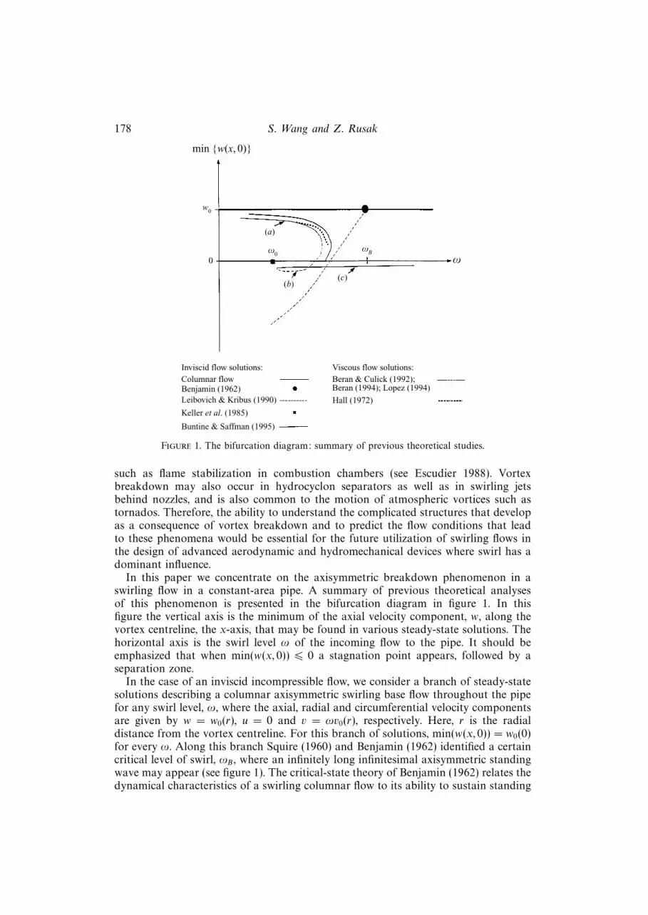
Figure 1. The bifurcation diagram: summary of previous theoretical studies.
such as flame stabilization in combustion chambers (see Escudier 1988). Vortexbreakdown may also occur in hydrocyclon separators as well as in swirling jetsbehind nozzles, and is also common to the motion of atmospheric vortices such astornados. Therefore, the ability to understand the complicated structures that developas a consequence of vortex breakdown and to predict the flow conditions that leadto these phenomena would be essential for the future utilization of swirling flows inthe design of advanced aerodynamic and hydromechanical devices where swirl has adominant influence.
In this paper we concentrate on the axisymmetric breakdown phenomenon in aswirling flow in a constant-area pipe. A summary of previous theoretical analysesof this phenomenon is presented in the bifurcation diagram in figure 1. In thisfigure the vertical axis is the minimum of the axial velocity component, w, along thevortex centreline, the x-axis, that may be found in various steady-state solutions. Thehorizontal axis is the swirl level ω of the incoming flow to the pipe. It should beemphasized that when min(w(x, 0)) 6 0 a stagnation point appears, followed by aseparation zone.
In the case of an inviscid incompressible flow, we consider a branch of steady-statesolutions describing a columnar axisymmetric swirling base flow throughout the pipefor any swirl level, ω, where the axial, radial and circumferential velocity componentsare given by w = w0(r), u = 0 and v = ωv0(r), respectively. Here, r is the radialdistance from the vortex centreline. For this branch of solutions, min(w(x, 0)) = w0(0)for every ω. Along this branch Squire (1960) and Benjamin (1962) identified a certaincritical level of swirl, ωB , where an infinitely long infinitesimal axisymmetric standingwave may appear (see figure 1). The critical-state theory of Benjamin (1962) relates thedynamical characteristics of a swirling columnar flow to its ability to sustain standing

The dynamics of swirling flow in a pipe 179
axisymmetric small-disturbance waves. Supercritical vortex flows have low swirl ratiosand are unable to support such waves, while subcritical flows having high swirl ratioscan. Benjamin (1962) also used a variational principle for the flow equations anddescribed the axisymmetric breakdown in a rather simple model, as a transition froman upstream supercritical columnar vortex flow to a downstream subcritical columnarflow, in analogy to the hydraulic jump in shallow water. Benjamin’s theory predictsa change in the total head between these two columnar states which represents achange in mechanical energy.
Randall & Leibovich (1973) showed that the critical state is a singular state of theinviscid steady equations. Using a weakly nonlinear analysis they found a branch ofsteady-state axisymmetric solutions of the Euler equations which bifurcate from thecolumnar branch when ω < ωB . These solutions describe a standing solitary wavethat develops in a base swirling flow in an infinitely long straight pipe. Leibovich &Kribus (1990) showed, using numerical continuation methods, that this standing wavebecomes larger and a closed separation zone may appear as the swirl is decreasedfrom the critical level ωB to zero. Since the flow in the separation zone is not connectedby streamlines with the upstream flow, Leibovich & Kribus (1990) used the analyticalcontinuation model to describe the flow inside the separation zone. For this branchof solutions, reversed flow develops in the separation zone and min(w(x, 0)) becomesnegative as ω is reduced from ωB to zero (see figure 1).
In another inviscid steady-state approach, Escudier & Keller (1983) and Keller,Egli & Exley (1985) described the axisymmetric vortex breakdown in an infinitelylong straight pipe as an open stagnation zone of free boundaries that appears in thebase vortex flow. Their solution describes a transition from a base upstream columnarstate to another, downstream, columnar state that has the same ‘flow force’ (resultingfrom the conservation of axial momentum along the pipe); both states are solutionsof the same columnar problem. However, a careful understanding of this solutionshows that when the vortical core radius of the base (upstream) state is fixed, thesolution is limited only to a specific value of the swirl, defined later in this paper asω0, where ω0 < ωB . For this special solution min(w(x, 0)) = 0 (see figure 1).
The effect of a changing the cross-sectional area of a tube on a stream of rotatingfluid was studied in the work of Batchelor (1967). To the best of our knowledge,Batchelor (1967) is the first to notice that the solution families for inviscid swirlingflows in a diverging pipe have a fold as swirl is increased. Batchelor’s work hasmotivated a recent theoretical study by Buntine & Saffman (1995) who examined thedevelopment of inviscid steady swirling flows in a finite-length diverging pipe. Theyinvestigated the dependence of solutions on inlet and outlet boundary conditionsand flow geometry. Their numerical computations result in an interesting bifurcationdiagram when a parallel flow condition was imposed along the pipe outlet (see figure1). There exists a limit point of swirl where the branch of solutions folds. Buntine &Saffman (1995) claimed that when a stagnation point appears along the pipe outletnon-regular solutions that should describe a separation zone must develop, and theflow inside the separation zone cannot be determined by the inlet conditions. Theyalso raised the need to study the stability of the axisymmetric and inviscid flows inthe vicinity of the limit point to clarify the influence of upstream conditions.
Hall (1967, 1972) used the quasi-cylindrical approximation to the steady and ax-isymmetric Navier–Stokes equations to describe a swirling flow with small streamwisegradients, from which he derived a parabolic equation that can be integrated alongthe pipe axis. He found that the flow along the pipe axis decelerates as the swirlincreases (see figure 1) and there is a certain level of swirl above which no solution

180 S. Wang and Z. Rusak
of the parabolic equation can be found. This indicates that the assumption of smallstreamwise gradients is no longer valid, and vortex breakdown should be inferred, inanalogy to the separation of a boundary layer.
Recent numerical computations by Beran & Culick (1992) have revealed a compli-cated bifurcation diagram of solutions of the steady and axisymmetric Navier–Stokesequations (see figure 1). They found that there exist two limit points of swirl whenthe Reynolds number is large enough. These limit points connect three branches ofsteady-state solutions of different types. Along the branch of solutions (a) the incom-ing swirl increases up to the first limit point and they describe a near columnar flowthroughout the pipe. The branch of solutions (b) begins at the first limit point andends at the secondary limit point; along this branch the incoming swirl is reduced.Solutions along the fold describe a swirling flow with a localized standing wave thatdevelops into a localized separation zone as the swirl approaches the secondary limitpoint. The branch of solutions (c) starts from the secondary limit point; along thatbranch the incoming swirl is increased and solutions describe a large separation zone.Beran & Culick (1992) indicated that there may be a possible relation between thefirst limit point in their computations and the critical swirl as defined by Benjamin(1962). They also conducted numerical computations using the quasi-cylindrical ap-proximation of Hall (1967) and found a singular behaviour as the swirl approachesthe first limit point.
More recently, Lopez (1994) and Beran (1994) studied the solutions of the un-steady axisymmetric Navier–Stokes equations. Both of these analyses showed thatthe aforementioned branches of solutions (a) and (c) are stable to small axisymmetricdisturbances, whereas the solutions along (b), in the fold, are unstable. Steady-statesolutions along the branch (b) cannot develop in a dynamical process starting fromany initial swirling flow. Moreover, starting from solutions along the fold the flowmay evolve into one of the solutions along branches (a) or (c).
The stability analyses of rotating flows study the tendency of imposed smalldisturbances to grow or decay in time and space. The analyses of Rayleigh (1916),Howard & Gupta (1962), Lessen, Singh & Paillet (1974) and Leibovich & Stewartson(1983) defined several stability criteria relating to axisymmetric and general three-dimensional disturbances. It is found, for example, that a vortex with a large rotationalcore (the ‘Q-Vortex’ model) is stable to axisymmetric perturbations when the swirlratio is greater than 0.403, and is unstable to helical perturbations only when the swirlratio is less than about 1.6. A review of vortex stability criteria is given in Leibovich(1984). It is important to note that the relation between vortex breakdown and vortexstability is yet unclear. Leibovich (1984) pointed out that breakdown can occur in avortex flow with just a little sign of instability and a vortex flow can become unstablewithout any breakdown phenomenon.
The summary of theoretical studies as presented above and in figure 1 indicates thatthere may be a possible relation between the critical swirl of the inviscid theory andvortex breakdown. Specifically, the inviscid theories of Benjamin (1962), Leibovich& Kribus (1990) and Buntine & Saffman (1995) show some correlation with theviscous computations of Hall (1972) and Beran & Culick (1992). However, figure 1demonstrates that large gaps still exist between the various theoretical approachesand the numerical computations. Specifically, the relation between the solutions ofLeibovich & Kribus (1990) and the special solution of Keller et al. (1985) is not clear.Moreover, the steady-state inviscid analyses do not provide insight into the specialbehaviour of the numerical solutions of the axisymmetric Navier–Stokes equationsof Beran & Culick (1992), Beran (1994) and Lopez (1994). The relation between
The dynamics of swirling flow in a pipe 181
the critical swirl and the first limit point as suggested by Beran & Culick (1992) isnot fully understood and there is no explanation for the existence of the secondarylimit point that appears in the viscous computations. It should also be emphasizedthat none of the known stability analyses can shed any light on the specific stabilitycharacteristics of solutions of the axisymmetric Navier–Stokes equations as found inthe numerical solutions of Beran (1994) and Lopez (1994).
The breakdown of vortex cores is a remarkable feature of swirling flows andis still a basic, largely unexplained, phenomenon. Although several explanations ofvortex breakdown have been proposed, a consistent description of this complicatedphenomenon has not yet been provided. Also, the relation between the varioustheoretical and numerical solutions is not completely clear. A theoretical approachthat clarifies the physical mechanism leading to axisymmetric vortex breakdownand that provides the conditions for which the various solutions may appear in anumerical simulation or experiment has never been derived, and is of great scientificand technological importance.
The objective of this paper is to present a new study of the axisymmetric vortexbreakdown phenomenon. Our approach is based on a thorough investigation of thedynamics of an axisymmetric swirling flow in a finite-length constant-area pipe asdescribed by the axisymmetric unsteady Euler equations (§1.2). We consider certainboundary conditions that may reflect the physical situation. Along the pipe inlet wespecify for all time the axial and circumferential velocity components as well as theazimuthal vorticity. We allow the inlet flow a degree of freedom to develop a radialvelocity, to reflect the upstream influence by disturbances that have the tendency tocast such an influence. Along the pipe outlet we pose a no-radial-flow state. We alsoconsider an initial state that describes a perturbed columnar flow along the pipe. Westudy the stability characteristics as well as the time-asymptotic behaviour as it isrelated to the steady-state solutions. The results are established through a rigorousmathematical analysis and provide a solid theoretical understanding of the dynamicsof an axisymmetric swirling flow in a pipe.
The inlet conditions described above reflect a specific vortex state. In the physicalsituation this vortex state is generated by a certain device and the mechanism ofthe vortex generation is always due to strong viscous effects. On the other hand, themechanism leading to vortex breakdown in high-Reynolds-number flows is believedto be related mainly to inviscid effects. Therefore, a proper theoretical approach tostudy the problem may separate the two issues. In this paper we concentrate on thevortex breakdown problem. The interaction between the vortex generator and thevortex breakdown phenomenon should be considered in a future study.
In this study we specify the vortex state at the pipe inlet. This condition mayprovide a realistic approximation of the flow state at the exit of a vortex generator(see, for example, the experimental results of Bruecker & Althaus 1995). In mostof the experimental apparatuses a slightly diverging pipe was used to promote theappearance of the breakdown phenomena by creating an adverse pressure gradient.The slightly diverging pipe does not allow disturbances in the flow to propagateupstream and change the inlet conditions. Our inlet conditions may reflect the physicsof such a case even though a straight pipe is used. The relation between the slightlydiverging pipe case and the straight pipe case can be established using the sameanalysis methods as described in this paper.
It should also be noticed here that the numerical simulations by Salas & Kuruvila(1989), Beran & Culick (1990), Lopez (1994), Beran (1994) and Darmofal (1996) andsome of the theoretical studies (Buntine & Saffman 1995) considered similar boundary
182 S. Wang and Z. Rusak
conditions to those used in this paper. A good correlation was found between theresults of the axisymmetric simulations and the experimental data (see Darmofal1996). These studies revealed the dynamics of swirling flows and the evolution ofthe axisymmetric vortex breakdown in a pipe and our theoretical results provide anexplanation of these investigations.
We summarize here the main steps of the analysis. We first reveal the possiblesteady-state solutions that may develop as the swirl level of the incoming flow isincreased from zero to above the critical level (see §§2–7 and Appendices A–D). Thishas been done by using a variational method to study the functional E(ψ(x, y)) whosestationary points correspond to inviscid steady-state solutions (here, ψ(x, y) is thestream function and y = r2/2). In §2 we discuss the existence and properties of asteady-state solution which is the global minimizer of E(ψ(x, y)) and show that thissolution is strongly dominated by the global minimizer of the functional E(ψ(y))which corresponds to the columnar (x-independent) problem. Therefore, in §3 weconduct a thorough study of the various solutions of the columnar problem. Theresults of §§2 and 3 are applied in §4 to describe in detail the global minimizersolutions of the steady Euler equations as the inlet swirl is increased.
In §5 we extend Benjamin’s definition of the critical state to a columnar flow ina finite-length pipe. In §6 we show the existence of a branch of min-max solutionsof E(ψ(x, y)) that naturally appears. In §7 we present the global bifurcation dia-gram of solutions of the steady Euler equations based on the above results. Theglobal bifurcation diagram also shows the relations between the various analyses ofBenjamin (1962), Leibovich & Kribus (1990) and Keller et al. (1985) and demon-strates the correlation between the inviscid theory and the numerical simulations ofhigh-Reynolds-number flows described by Beran & Culick (1992).
In §8 we summarize our recent results that revealed, for the first time, the specialrelation between the stability of swirling flows in a finite-length pipe and the criticalswirl. We show that the critical swirl is a point of exchange of stability (see Wang& Rusak 1996a, b). We also show that the stability is closely related to the globalbifurcation diagram of steady-state solutions. Moreover, the stability results providea theoretical understanding of the specific stability characteristics as described inthe numerical studies of the Navier–Stokes equations by Lopez (1994) and Beran(1994).
The stability analyses together with the study of steady-state solutions suggests aconsistent explanation of the mechanism leading to axisymmetric vortex breakdownin high-Reynolds-number swirling flows in a pipe (§9). It is an evolution from aninitial columnar swirling flow to another, relatively stable, equilibrium state whichrepresents a flow around a separation zone. This evolution is the result of theloss of stability of the columnar base state when the swirl ratio of the incomingflow is near or above the critical level. The instabilty mechanism is governed bythe interaction of disturbances propagating upstream with the inlet state. Our recentnumerical computations, guided by the present theory (Rusak, Wang & Whiting 1996),demonstrate the relations between the stability of swirling flows and the critical swirland provide the time history of the nonlinear transition.
Section 10 discusses the effects of slight viscosity on the development of a steadyswirling flow and shows the relation between the present study and the numericalcomputations using the axisymmetric Navier–Stokes equations. We find that thepresent approach, based on the Euler equations, is the inviscid-limit theory of theaxisymmetric viscous flow problem.
The dynamics of swirling flow in a pipe 183
1.2. Mathematical model
1.2.1. Basic problem
An axisymmetric incompressible and inviscid swirling flow is considered in a finite-length pipe of unit radius (0 6 r 6 1) and length x0 where 0 6 x 6 x0. The axialand radial distances are rescaled with the radius of the pipe. Let y = r2/2 where0 6 y 6 1/2. By virtue of the axisymmetry, a stream function ψ(x, y, t) can be definedwhere the radial component of velocity u = −ψx/(2y)1/2, and the axial componentof velocity w = ψy . The equations which connect the development in time, t, of thestream function ψ, the azimuthal vorticity η = rχ, where χ = −(ψyy + ψxx/2y), andthe circulation function K = rv (where v is the circumferential velocity) may be givenby (see, for example, Szeri & Holmes 1988)
Kt + ψ,K = 0, χt + ψ, χ =1
4y2(K2)x. (1)
Here the brackets ψ,K and ψ, χ are defined by
ψ,K = ψyKx − ψxKy, ψ, χ = ψyχx − ψxχy. (2)
We study the development of the flow with certain conditions posed on the boundaries.For any time, t, we set ψ(x, 0, t) = 0 to enforce axisymmetry along the pipe axis, andψ(x, 1/2, t) = w0 which gives the total mass flux across the pipe. Along the inlet, x = 0,for any time, t, an incoming flow profile described by the axial flow, the circulationand the azimuthal vorticity is given as
ψ(0, y, t) = ψ0(y), K(0, y, t) = ωK0(y),
χ(0, y, t) = −ψ0yy (or ψxx(0, y, t) = 0).
(3)
Here ω reflects the swirl level of the incoming flow. The radial velocity componentalong the inlet is found as part of the solution of the problem. We allow the inlet statea degree of freedom to develop a radial velocity, to reflect the upstream influence bydisturbances that have the tendency to cast such an influence. Along the pipe outlet,x = x0, we set the radial velocity component to zero, i.e.
ψx(x0, y, t) = 0 (4)
for all time. For a long straight pipe (x0 1) this outlet condition only weaklyaffects the upstream flow. Similar boundary conditions have been considered by Salas& Kuruvila (1989), Beran & Culick (1990) and Lopez (1994) in their numericalsimulations of the Navier–Stokes equations and by Buntine & Saffman (1995) in theirtheoretical study of a steady swirling flow in a finite-length diverging pipe using theEuler equations. These boundary conditions may also reflect the physical situation asreported in Bruecker & Althaus’s (1995) experiments. We want to point out that incertain cases where the pipe is short and diverges significantly, such as in combustionchambers and the studies by Buntine & Saffman (1995), different outlet conditionsmay have a strong effect on the flow and result in different solutions.
The problem defined by equations (1)–(4) is well posed and describes the evolutionof a swirling flow in a finite-length pipe. We consider some relevant initial conditionsfor the stream function, circulation and azimuthal vorticity, such as a perturbedcolumnar state throughout the pipe at t = 0
ψ(x, y, 0) = ψ0(y) + εψ(x, y), K(x, y, 0) = ωK0(y) + εK(x, y),
χ(x, y, 0) = −ψ0yy − εχ(x, y)
(5)

184 S. Wang and Z. Rusak
where εψ(x, y), εK(x, y) and εχ(x, y) are prescribed disturbances. Here,
ψ(x, y, t) = ψ0(y), K(x, y, t) = ωK0(y), χ(x, y, t) = −ψ0yy
is a base steady-state solution of (1)–(4) for any time t and every swirl level, ω, thatdescribes a columnar flow. Starting from the initial conditions (5), it is expected thatthe flow will develop uniquely in time. Drazin & Howard (1966) proved the uniquenessof a time-dependent solution of the Euler equations for similar boundary conditionsand any initial state. Also, we believe that the axisymmetric vortex breakdown isprimarily related to the swirl level, ω, of the incoming flow. Therefore, we fix thefunctions ψ0(y) and K0(y) and look for different solutions of (1)–(5) for various levelsof ω.
In order to understand the dynamics of a swirling flow governed by (1) withboundary conditions (3) and (4) and initial conditions (5), it is important to study thestability characteristics and the time-asymptotic behaviour, specifically as it is relatedto steady-state solutions of the problem. We will first concentrate on the analysis ofthe steady-state solutions of these equations for a given swirl level, ω, and prove theexistence of multiple steady-state solutions of the problem (1)–(4). We will derive thebifurcation diagram of steady-state solutions as the swirl level, ω, of the incomingflow is changed. The bifurcation diagram resulting from our analysis is summarized in§7. In §8 we will return to study the dynamics of a swirling flow governed by (1)–(5).We will examine the linear stability of the various steady-state solutions found inour analysis according to the recently presented results by Wang & Rusak (1996a, b).The bifurcation diagram of steady-state solutions together with the stability resultswill shed new light on the evolution of swirling flows as described by (1)–(5) (see§9).
1.2.2. Steady-state problem
When the flow is steady equations (1)–(4) may be reduced to the Squire–Longequation (SLE) (Squire 1956 and Long 1953, also known as the Bragg–Hawthorne1950 equation):
ψyy +ψxx
2y= H ′(ψ)− I ′(ψ)
2yon Ωx0
= (0, x0)× (0, 1/2) (6)
with boundary conditions
ψ(x, 0) = 0, ψ(x, 1/2) = w0,
ψ(0, y) = ψ0(y), K(0, y) = ωK0(y), ψxx(0, y) = 0, ψx(x0, y) = 0
(7)
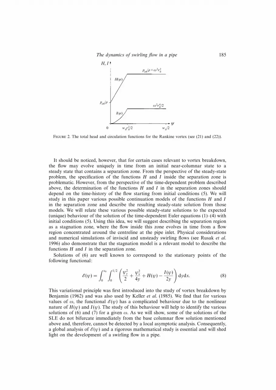
Here, H is the total head function, H = p/ρ+(u2 + w2 + v2)/2, p is the static pressureand ρ is the density. I = K2/2 is the extended circulation function. H and I areconserved along a streamline and, therefore, are functions of ψ only. These functionsmay be determined from the inlet profiles ψ0(y), K0(y) and the swirl level ω. Therefore,the columnar vortex flow ψ(x, y) = ψ0(y), K(x, y) = ωK0(y) is a base solution of (6)and (7) for any swirl level ω. For relevant inlet flows such as the Rankine vortex, theBurgers’ vortex or the ‘Q-vortex’, it can be shown that both H and I are nonlinearfunctions of ψ (see, for example, figure 2 and (21) and (22) below); H is approximatelya linear function of ψ and I is approximately a quadratic function for small ψ, andboth are almost constant when ψ is near w0 = ψ0(1/2). This nonlinearity may giverise to multiple solutions of (6) and (7) for a fixed value of ω, in addition to the basesolution.
The dynamics of swirling flow in a pipe 185
pst0/ρ
pst0/ρ + ω2r20
ω2r40/2
w0r20/2 w0/20
I(ψ)
H(ψ)
ψ
H, I
Figure 2. The total head and circulation functions for the Rankine vortex (see (21) and (22)).
It should be noticed, however, that for certain cases relevant to vortex breakdown,the flow may evolve uniquely in time from an initial near-columnar state to asteady state that contains a separation zone. From the perspective of the steady-stateproblem, the specification of the functions H and I inside the separation zone isproblematic. However, from the perspective of the time-dependent problem describedabove, the determination of the functions H and I in the separation zones shoulddepend on the time-history of the flow starting from initial conditions (5). We willstudy in this paper various possible continuation models of the functions H and Iin the separation zone and describe the resulting steady-state solution from thosemodels. We will relate these various possible steady-state solutions to the expected(unique) behaviour of the solution of the time-dependent Euler equations (1)–(4) withinitial conditions (5). Using this idea, we will suggest describing the separation regionas a stagnation zone, where the flow inside this zone evolves in time from a flowregion concentrated around the centreline at the pipe inlet. Physical considerationsand numerical simulations of inviscid and unsteady swirling flows (see Rusak et al.1996) also demonstrate that the stagnation model is a relevant model to describe thefunctions H and I in the separation zone.
Solutions of (6) are well known to correspond to the stationary points of thefollowing functional:
E(ψ) =
∫ x0
0
∫ 1/2
0
(ψ2y
2+ψ2x
4y+H(ψ)− I(ψ)
2y
)dydx. (8)
This variational principle was first introduced into the study of vortex breakdown byBenjamin (1962) and was also used by Keller et al. (1985). We find that for variousvalues of ω, the functional E(ψ) has a complicated behaviour due to the nonlinearnature of H(ψ) and I(ψ). The study of this behaviour will help to identify the varioussolutions of (6) and (7) for a given ω. As we will show, some of the solutions of theSLE do not bifurcate immediately from the base columnar flow solution mentionedabove and, therefore, cannot be detected by a local asymptotic analysis. Consequently,a global analysis of E(ψ) and a rigorous mathematical study is essential and will shedlight on the development of a swirling flow in a pipe.
186 S. Wang and Z. Rusak
2. Global minimizer of E(ψ)
2.1. Existence of global minimizer of E(ψ)
The natural step in the variational analysis is to seek the minimizer of E(ψ). Werigorously prove (see Appendix A, Theorem A.1) that the global minimizer solutionψg(x, y) of E(ψ) exists under the conditions:
1. H(ψ) and I(ψ) are bounded and piecewise smooth non-negative functions withbounded first derivatives;
2. I(ψ) 6 c|ψ|p where p is a fixed number, 1 < p 6 2, and c > 0.The boundedness of both H(ψ) and I(ψ) does not limit our approach since we are
interested in solutions with bounded mechanical energy and circulation coming intothe pipe. It should also be clarified that if assumption 1 is not satisfied it can beshown that the global minimizer of E(ψ) may not exist.
We also show in Appendix A that the global minimizer solution is a regular solutionsuch that its first derivatives are continuous everywhere. It should be pointed out thatthis solution of the SLE, (6) and (7), may allow discontinuous second derivatives butit is nonetheless a solution of the steady Euler equations. Moreover, as we later claim,in relevant cases a near columnar flow state may evolve naturally, in infinite time,into the flow state described by the global minimizer solution with discontinuoussecond derivatives. We find in this paper that, for certain values of ω, specifically forhigh swirl cases, the global minimizer of E(ψ) is not the base columnar flow solutionψ(x, y) = ψ0(y) and another solution that describes a different flow state is the globalminimizer of E(ψ).
In §2.2, we turn to the study of the columnar flow problem of (6) and (7), and thebehaviour of the columnar minimizers. In §2.3, we show the special relations betweenthe global minimizer ψg(x, y) of E(ψ) and the global minimizer of the columnarproblem.
2.2. Columnar flow
In the case of a columnar swirling flow where ψx ≡ 0 everywhere in Ωx0, equation (6)
is reduced to the ordinary differential equation
ψyy = H ′(ψ)− I ′(ψ)
2y(9)
with boundary conditions
ψ(0) = 0, ψ(1/2) = w0. (10)
Here the stream function ψ is a function of y only. The corresponding variationalprinciple is
E(ψ) =
∫ 1/2
0
(ψ2y
2+H(ψ)− I(ψ)
2y
)dy. (11)
It can be shown that for any solution of (9), E(ψ) =∫ 1/2
0(p/ρ+w2)dy, which represents
the flow force of the columnar flow in a pipe (Benjamin 1962).We can prove from an argument similar to that in Appendix A, that the minimizer
of the columnar functional E(ψ) exists for given H(ψ) and I(ψ) that satisfy the sameassumptions in Theorem A.1. Let ψs(y) denote the global minimizer of the columnarfunctional E(ψ).

The dynamics of swirling flow in a pipe 187
x10
ψ0(y)
ψ = 0x
y
x0
ψg(x, y)
ψ = w0
ψs(y)
12
Figure 3. A schematic description of the global minimizer solution ψg(x, y).
2.3. Properties of the global minimizer of E(ψ)
We prove in Appendix B the relation between ψg(x, y), the global minimizer of E(ψ),and ψs(y), the global minimizer of the columnar functional E(ψ) with the samefunctions H(ψ) and I(ψ). We show that the outlet state of the global minimizersolution, ψg(x0, y), tends to the columnar global minimizer solution, ψs(y), as thelength of the pipe x0 is increased. This means that the global minimizer of the PDE,(6) and (7), is controlled by the minimizer of the columnar problem (9) and (10). Theglobal minimizer ψg(x, y) describes a transition along the pipe from the inlet stateψ0(y) to the state ψs(y) along the outlet (see figure 3).
This result is quite natural once we notice that the global minimizer of the columnarproblem is not subjected to the inlet conditions. In certain cases, specifically whenthe swirl level is high, ψs(y) may not be the state ψ0(y) which means that E(ψs(y)) <E(ψ0(y)). Therefore, in order to minimize E(ψ) the global minimizer ψg(x, y) describesa spatial transition with a minimal contribution to E(ψ) from the inlet state ψ0(y) tothe state ψs(y). When the pipe length x0 is long we can show that the length x1 of thistransition is finite where x1 < x0 and in the range x1 < x < x0 the global minimizerψg(x, y) is very close to the columnar state given by ψs(y) (see figure 3).
2.4. Balance of flow force
Multiplying (6) by ψx on both sides and integrating, we find∫ x
0
∫ 1/2
0
(ψyyψx +
ψxxψx
2y
)dydx =
∫ 1/2
0
dy
∫ x
0
(H ′(ψ)ψx −
I ′(ψ)
2yψx
)dx.
Integration by parts and the use of boundary conditions gives
−∫ 1/2
0
dy
∫ x
0
d
(ψ2y
2
)+
∫ 1/2
0
ψ2x(x, y)− ψ2
x(0, y)
4ydy
=
∫ 1/2
0
(H(ψ(x, y))− I(ψ(x, y))
2y
)dy −
∫ 1/2
0
(H(ψ(0, y))− I(ψ(0, y))
2y
)dy. (12)
We define the function
S(x) =
∫ 1/2
0
(ψ2y(x, y)
2− ψ2
x(x, y)
4y+H(ψ(x, y))− I(ψ(x, y))
2y
)dy
= E(ψ(x, y))−∫ 1/2
0
ψ2x(x, y)
4ydy. (13)
188 S. Wang and Z. Rusak
Here, E(ψ(x, y) is calculated at a fixed cross-section x using (11). Then, for anysolution of (6), we can rewrite (12) as
S(x) = constant = S(0) for all 0 6 x 6 x0. (14)
We can show that S(0) =∫ 1/2
0(p/ρ + w2)x=0dy. The function S(x) is the ‘flow force’
that must be constant at any cross-section x along the straight pipe due to theconservation of the axial momentum. From the boundary conditions (7), we may findthat for any solution, ψ(x, y), of the problem given by (6) and (7),
E(ψ0(y))− E(ψ(x0, y)) =
∫ 1/2
0
ψ2x(0, y)
4ydy > 0. (15)
This means that for a steady-state solution of (6) and (7) we have E(ψ0(y)) >E(ψ(x0, y)). Specifically, for the global minimizer ψg(x, y) of E(ψ), where x0 is large,we find
E(ψ0)− E(ψs) =
∫ 1/2
0
ψ2gx(0, y)
4ydy > 0. (16)
In the case where the global minimizer solution of the columnar problem, ψs(y), isdifferent from the inlet state ψ0(y), we have E(ψs) < E(ψ0). Since the global minimizerof the SLE describes a transition from the inlet state ψ0(y) to the outlet state ψs(y), wecan understand from (16) that the difference E(ψ0)− E(ψs) is related in this solutionto the establishment of a radial velocity component along the inlet.
3. Study of columnar swirling flowSections 2.3 and 2.4 raise the need to study the solutions of the columnar problem,
(9) and (10), in order to identify global minimizer solutions of (6) and (7) at variouslevels of swirl.
In the theoretical studies of vortex breakdown, the inlet flow, ψ0(y) and K0(y), wascommonly approximated by one of the following models: the Rankine vortex (Kelleret al. 1985), the Burgers vortex (Leibovich & Kribus 1990) and the Q-vortex model(Leibovich 1984). Each of these vortex models is characterized by a swirl parameterω. It can be shown that in each case there exists a critical swirl level, ωB , as definedby Benjamin (1962), that can be determined by the following eigenvalue problemderived from the linearized SLE (9) and (10):
φyy −(H ′′(ψ0;ωB)− ω2
B
I ′′(ψ0)
2y
)φ = 0,
φ(0) = φ(1/2) = 0.
(17)
Here I = K20/2. Benjamin (1962) classified a columnar vortex as supercritical, critical
or subcritical according to ω < ωB, ω = ωB and ω > ωB , respectively. Benjamin’sclassification is related to the dynamics of small-disturbance waves in the base swirlingflow. Supercritical flows have a low swirl ratio and are unable to sustain axisymmetricsmall-disturbance standing waves. Subcritical flows have a high swirl ratio and areable to support such waves. At the critical state, an infinitely long small-disturbancestanding wave may develop.
From the perspective of variational methods it can be shown (see for exampleCourant & Hilbert 1953) that supercritical states (where ω < ωB) are local minimizersof the functional E(ψ).

The dynamics of swirling flow in a pipe 189
In the rest of this paper, we concentrate on the case where the inlet profile ψ0(y) ismodelled by either the Rankine or the Burgers vortex. These are used as basic analysismodels to develop our new approach because of their analytical simplicity. However,the results shown in this paper can also be extended to other relevant vortex model(see our recent results on a Q-vortex in Rusak, Whiting & Wang 1997).
3.1. The Rankine vortex
The Rankine vortex is defined as a vortex flow with uniform axial velocity
w = w0 (18)
and swirl component
v =
ωr, 0 6 r 6 r0,
ωr20/r, r0 6 r 6 1.
(19)
For a columnar state the pressure is given by
dp
dr= ρ
v2
r. (20)
Here ω is the angular speed at the centre and r0 is the vortex core size. The functionsH(ψ) and I(ψ) are calculated from (18)–(20) as (see figure 2)
H(ψ) =
pst0/ρ+ (2ω2/w0)ψ when 0 6 ψ 6 1
2w0r
20 ,
pst0/ρ+ ω2r20 when 1
2w0r
20 6 ψ 6
12w0
(21)
and
I(ψ) =
(2ω2/w2
0)ψ2 when 0 6 ψ 6 12w0r
20 ,
12ω2r4
0 when 12w0r
20 6 ψ 6
12w0.
(22)
Here pst0 is the total head at the centre, pst0 = p0 + 12ρw2
0 (where p0 is static pressureat the centre).
The stream function for the Rankine vortex has a simple form:
ψ0(y) = ψR(y) = w0y (23)
which is a solution of (9) with boundary conditions (10) for H(ψ) and I(ψ) givenby (21) and (22). Numerical solutions of the critical swirl ωB as a function of thecore radius r0 are given in Keller et al. (1985) for the Rankine vortex. It is found, forexample, that 2r0ωB/w0 = 2.405 when r0 is small. When ω < ωB, ψR = w0y describesa supercritical state and is a local minimizer of E(ψ). In the following, we developthe behaviour of E(ψ) for the Rankine vortex as ω increases from 0 to ωB with r0and w0 fixed.
Consider the special case ω = 0. E(ψ) is reduced in this case to
E(ψ) =
∫ 1/2
0
ψ2y
2dy,
ψ(0) = 0, ψ(1/2) = w0/2.
(24)
This is a strictly convex functional (see figure 4a) and the only stationary point ofE(ψ) is ψR(y) which is a global minimizer of E(ψ). When ω increases but is still small,E(ψ) remains convex and ψR(y) remains the global minimizer of E(ψ).
We will show now that when ω becomes larger, but is still less than ωB (in the
190 S. Wang and Z. Rusak
(a)
ψR = w0(y)
ω small
ω = 0
E(ψ)
(b)
ψR = w0(y) ψ∈W 1,2b (0, 1/2)
E(ψ)
ψ∈W 1,2b (0, 1/2)
(c)
ψR = w0(y)
E(ψ)
(d )
ψR = w0(y) ψ∈W 1,2b (0, 1/2)
E(ψ)
ψ∈W 1,2b (0, 1/2)
(e)
ψR = w0(y)
E(ψ)
( f )
ψR = w0(y) ψ∈W 1,2b (0, 1/2)
E(ψ)
ψ∈W 1,2b (0, 1/2)
ψK
ψsψs
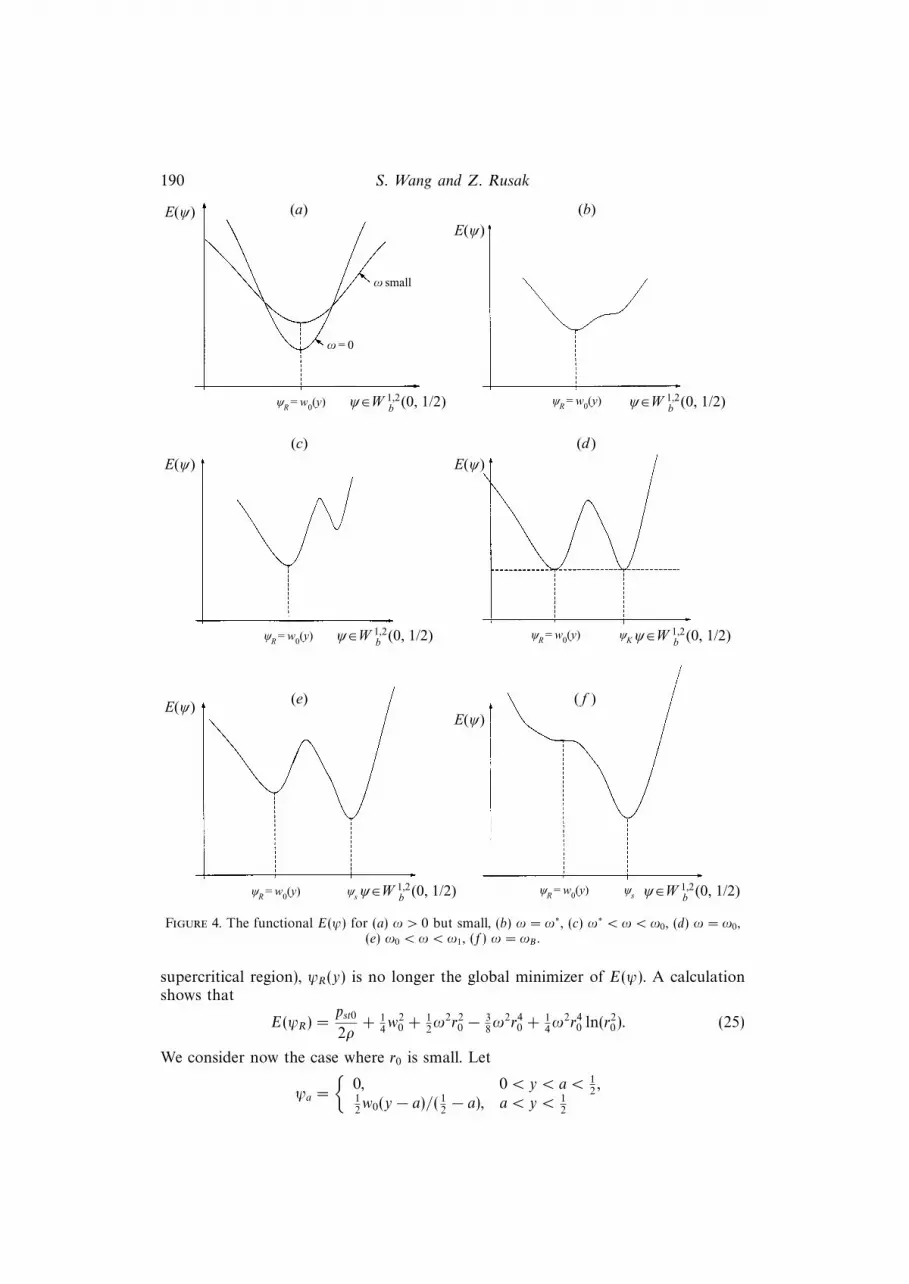
Figure 4. The functional E(ψ) for (a) ω > 0 but small, (b) ω = ω∗, (c) ω∗ < ω < ω0, (d) ω = ω0,(e) ω0 < ω < ω1, (f) ω = ωB .
supercritical region), ψR(y) is no longer the global minimizer of E(ψ). A calculationshows that
E(ψR) =pst0
2ρ+ 1
4w2
0 + 12ω2r2
0 − 38ω2r4
0 + 14ω2r4
0 ln(r20). (25)
We consider now the case where r0 is small. Let
ψa =
0, 0 < y < a < 1
2,
12w0(y − a)/( 1
2− a), a < y < 1
2
The dynamics of swirling flow in a pipe 191
y
ψ
ψR = w0 y
ψa
w0
2
a0 12
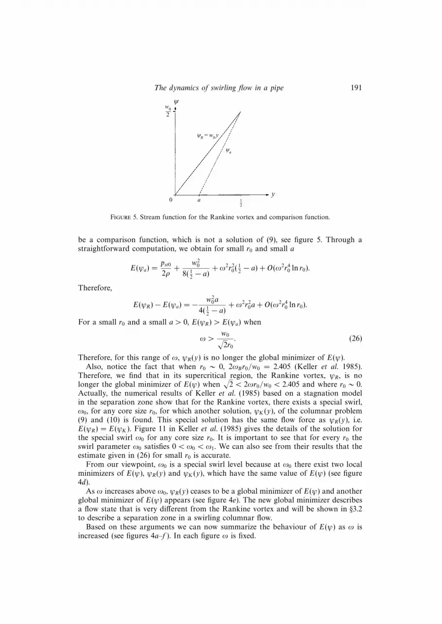
Figure 5. Stream function for the Rankine vortex and comparison function.
be a comparison function, which is not a solution of (9), see figure 5. Through astraightforward computation, we obtain for small r0 and small a
E(ψa) =pst0
2ρ+
w20
8( 12− a)
+ ω2r20( 1
2− a) + O(ω2r4
0 ln r0).
Therefore,
E(ψR)− E(ψa) = − w20a
4( 12− a)
+ ω2r20a+ O(ω2r4
0 ln r0).
For a small r0 and a small a > 0, E(ψR) > E(ψa) when
ω >w0√2r0
. (26)
Therefore, for this range of ω, ψR(y) is no longer the global minimizer of E(ψ).Also, notice the fact that when r0 ∼ 0, 2ωBr0/w0 = 2.405 (Keller et al. 1985).
Therefore, we find that in its supercritical region, the Rankine vortex, ψR , is nolonger the global minimizer of E(ψ) when
√2 < 2ωr0/w0 < 2.405 and where r0 ∼ 0.
Actually, the numerical results of Keller et al. (1985) based on a stagnation modelin the separation zone show that for the Rankine vortex, there exists a special swirl,ω0, for any core size r0, for which another solution, ψK(y), of the columnar problem(9) and (10) is found. This special solution has the same flow force as ψR(y), i.e.E(ψR) = E(ψK). Figure 11 in Keller et al. (1985) gives the details of the solution forthe special swirl ω0 for any core size r0. It is important to see that for every r0 theswirl parameter ω0 satisfies 0 < ω0 < ω1. We can also see from their results that theestimate given in (26) for small r0 is accurate.
From our viewpoint, ω0 is a special swirl level because at ω0 there exist two localminimizers of E(ψ), ψR(y) and ψK(y), which have the same value of E(ψ) (see figure4d).
As ω increases above ω0, ψR(y) ceases to be a global minimizer of E(ψ) and anotherglobal minimizer of E(ψ) appears (see figure 4e). The new global minimizer describesa flow state that is very different from the Rankine vortex and will be shown in §3.2to describe a separation zone in a swirling columnar flow.
Based on these arguments we can now summarize the behaviour of E(ψ) as ω isincreased (see figures 4a–f ). In each figure ω is fixed.
192 S. Wang and Z. Rusak
(a) When ω is small the functional E(ψ) has a unique stationary point, ψR(y),which is the global minimizer of E(ψ), see figure 4a.
(b) There exists a swirl level, ω∗, where two solutions are found, one is ψR(y) andthe other is different from ψR(y). ω∗ is actually a bifurcation point of the ODEproblem (9) and (10). See figure 4b.
(c) When ω∗ < ω < ω0, we find that ψ = ψR(y) is still the global minimizer ofE(ψ), but two other stationary points can also be found. One is a local minimizer andthe other is a min-max point of E(ψ). The behaviour of E(ψ) in this case is given infigure 4c.
(d) When ω = ω0, the solution ψK(y) obtained by Keller et al. (1985) is found,and E(ψ) is shown in figure 4d. ω0 is a threshold value of the swirl, across which thecolumnar global minimizer, ψs(y), drastically changes.
(e) When ω > ω0, we find that ψR(y) is not a global minimizer of E(ψ) since thereexists a solution, ψs(y), different from ψR(y), for which E(ψR) > E(ψs). The behaviourof E(ψ) in this case is described in figure 4e.
(f) When ω = ωB (Benjamin’s critical state), ψR(y) is actually an inflection pointof E(ψ) along a special direction, and is no longer a local minimizer. The behaviourof E(ψ) in this case is given in figure 4f.
The behaviour of E(ψ) as described in figure 4 can be confirmed by numericalcomputations (see Rusak et al. 1996). Specifically, the existence of the special swirllevels ω∗, ω0 and ωB and multiple solutions when ω > ω∗ can be verified. Then,E(ψ) for each solution can be calculated and compared one with the other to revealthe nature of each solution (local minimizer, global minimizer or min-max points ofE(ψ)).
3.2. The properties of ψs when ω > ω0
We have shown above that the columnar global minimizer ψs = ψR(y) when ω < ω0.However, when ω > ω0, ψs 6= ψR(y). In this section we study the properties of theglobal minimizer, ψs, of the columnar functional E(ψ) when ω > ω0. As we haveseen in §2, these properties are essential to understand the qualitative behaviour ofthe global minimizer ψg(x, y) of the axisymmetric functional E(ψ).
Let us consider all the solutions of (9) and (10) with H(ψ) and I(ψ) given by (21)and (22) which satisfy the condition 0 < ψ(y) < w0 for 0 < y < 1/2. This conditionis used here since the information that we have about the functions H(ψ) and I(ψ)according to (21) and (22) is limited to the range 0 < ψ(y) < w0. This conditionresults in solutions describing columnar flow states without separation zones. Thefamily of these solutions may be given by
ψrc =
12w0
(2y+(r2
0− r2c )
(2y)1/2
rc
J1(2ω(2y)1/2/w0)
J1(2ωrc/w0)
)for 0< y < 1
2r2c , 0<ψrc <
12w0r
20 ,
w0
1− r20
1− r2c
(y − 12r2c ) + 1
2w0r
20 for 1
2r2c < y < 1/2,
(27)where J1 denotes the Bessel function of the first kind, r0 is the Rankine vortex coreradius and rc < 1 is the vortical core radius of the solution ψrc . The core size, rc, isdetermined by the matching of axial velocity at r = rc:
(r20 − r2
c )ω
rc
J0(2ωrc/w0)
J1(2ωrc/w0)= −w0(r
20 − r2
c )
1− r2c
(28)
where J0 is the Bessel function of order zero. We see that rc = r0 is a trivial solution of
The dynamics of swirling flow in a pipe 193
(28). There are also infinitely many non-trivial solutions of (28), rc1 < rc2 < rc3 < ....However, analysis shows that all the solutions corresponding to rc2, rc3, ... (exceptfor rc1) give values of ψrc(y) at some 0 < y < 1
2r2c that are beyond the range
0 < ψrc(y) < w0.Direct computation using (27) and (28) shows that
E(ψrc) =pst0
2ρ+ 1
4w2
0 + ω2( 18r4c + 1
2r2
0(1− r2c ) + 1
4r4
0 ln(r2c )). (29)
Let ψrc1 be the solution corresponding to rc1; we have from (25) and (29)
E(ψrc1 )−E(ψR) =ω2r4
0
8
((r2c1 − r2
0)(r2c1 − 3r2
0)
r40
+4 ln
(rc1
r0
))> 0, when rc1 > r0. (30)
It can also be shown that rc1 > r0 when ω < ωB . Thus, we conclude from (30) thatψrc1 cannot be a minimizer of E(ψ) when ω < ωB . Actually, ψrc1 is a min-max pointof E(ψ). Therefore, when ω0 < ω < ωB , the global minimizer ψs(y) of E(ψ) mustbe some function other than the functions ψR(y) and ψrc1 (y) and ψs(y) must havevalues beyond the interval (0, w0). In particular, ψs(y) may become zero or negativesomewhere on 0 < y < 1/2, which means that a separation region may appear inthe columnar minimizer when ω > ω0. Therefore, we need to specify the functionsH(ψ) and I(ψ) for negative values of ψ (to describe the flow in the separation zone).From physical reasons, any such extension must keep H(ψ) and I(ψ) bounded andso, according to the existence theorem, the global minimizer ψs exists.
We now discuss the properties of the minimizer, ψs(y), of E(ψ) when a stagnationmodel is considered to describe the flow in the separation zone. We also considerother continuation models and their relation to the stagnation model. These resultswill be used in §4 to describe the properties of the global minimizer solution of theSLE that corresponds to each continuation model. Then, we will demonstrate thatthe stagnation model is strongly related to the expected (unique) behaviour of thesolution to the time-dependent Euler equations (1)–(5) as time tends to infinity.
3.2.1. Stagnation model
For a stagnation continuation model, H(ψ) and I(ψ) are extended to ψ < 0 as
H(ψ) = H(0) and I(ψ) = I(0) = 0 for ψ < 0. (31)
It can be shown that in this case the global minimizer solution of (9) and (10), ψs(y),must satisfy ψs(y) > 0 for any y in the domain 0 < y < 1/2. To show this, considerthe case where ψs(y) is negative in some interval (y1, y2) in 0 < y < 1/2. Accordingto the extension (31), in this interval,
∫ y2
y1(ψ2
sy/2 +H(ψ)− I(ψ)/2y)dy > 0. Therefore,
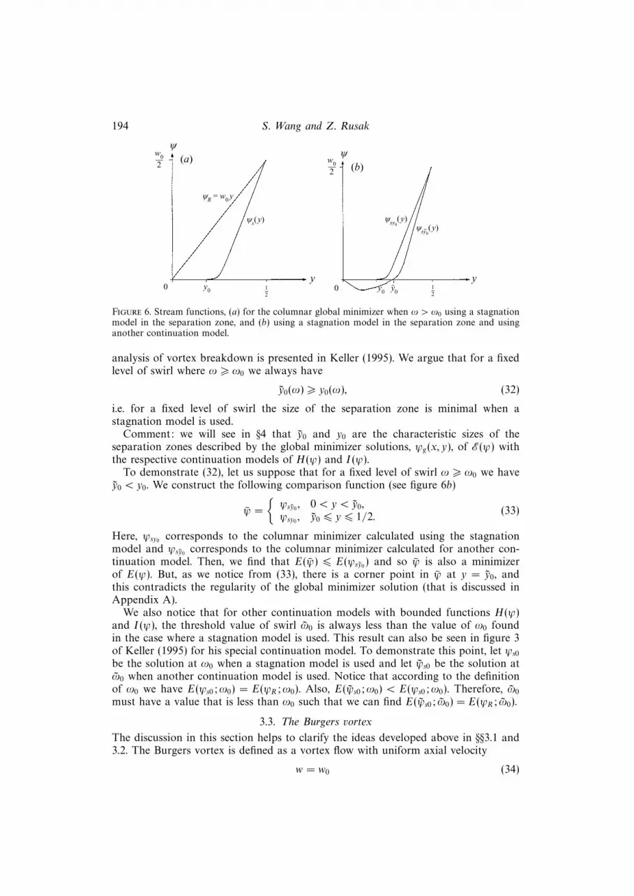
in order to minimize the contribution of this interval to E(ψ), we must have ψs = 0in the entire interval (y1, y2). From the previous arguments that no solution can be aminimizer of E(ψ) if ψ > 0 everywhere in the domain 0 < y < 1/2, we find that theminimizer solution ψs(y) of E(ψ) must have a finite stagnation region. Figure 6(a)shows the solution ψs(y) for ω > ω0, where in the interval 0 > y > y0, ψs(y) ≡ 0.
3.2.2. Relation to other continuation models
Other possible continuation models, with bounded functions H(ψ) and I(ψ), mayhave a global minimizer solution, ψs(y), with negative values in the domain 0 < y < y0
(see figure 6b). Therefore, ψs(y) may describe in such a case a columnar flow statewith regions of flow reversals. An example of using such a continuation model in the
194 S. Wang and Z. Rusak
y
ψ
ψR = w0 y
ψs(y)
0 12
y0
(a)
y
ψ
ψsy0(y)
0 12
y0
(b)
ψsy0(y)∼
y∼0
w0
2w0
2
Figure 6. Stream functions, (a) for the columnar global minimizer when ω > ω0 using a stagnationmodel in the separation zone, and (b) using a stagnation model in the separation zone and usinganother continuation model.
analysis of vortex breakdown is presented in Keller (1995). We argue that for a fixedlevel of swirl where ω > ω0 we always have
y0(ω) > y0(ω), (32)
i.e. for a fixed level of swirl the size of the separation zone is minimal when astagnation model is used.
Comment: we will see in §4 that y0 and y0 are the characteristic sizes of theseparation zones described by the global minimizer solutions, ψg(x, y), of E(ψ) withthe respective continuation models of H(ψ) and I(ψ).
To demonstrate (32), let us suppose that for a fixed level of swirl ω > ω0 we havey0 < y0. We construct the following comparison function (see figure 6b)
ψ =
ψsy0
, 0 < y < y0,ψsy0
, y0 6 y 6 1/2.(33)
Here, ψsy0corresponds to the columnar minimizer calculated using the stagnation
model and ψsy0corresponds to the columnar minimizer calculated for another con-
tinuation model. Then, we find that E(ψ) 6 E(ψsy0) and so ψ is also a minimizer
of E(ψ). But, as we notice from (33), there is a corner point in ψ at y = y0, andthis contradicts the regularity of the global minimizer solution (that is discussed inAppendix A).
We also notice that for other continuation models with bounded functions H(ψ)and I(ψ), the threshold value of swirl ω0 is always less than the value of ω0 foundin the case where a stagnation model is used. This result can also be seen in figure 3of Keller (1995) for his special continuation model. To demonstrate this point, let ψs0be the solution at ω0 when a stagnation model is used and let ψs0 be the solution atω0 when another continuation model is used. Notice that according to the definitionof ω0 we have E(ψs0;ω0) = E(ψR;ω0). Also, E(ψs0;ω0) < E(ψs0;ω0). Therefore, ω0
must have a value that is less than ω0 such that we can find E(ψs0; ω0) = E(ψR; ω0).
3.3. The Burgers vortex
The discussion in this section helps to clarify the ideas developed above in §§3.1 and3.2. The Burgers vortex is defined as a vortex flow with uniform axial velocity
w = w0 (34)
The dynamics of swirling flow in a pipe 195
2.0
1.5
1.00.6 0.8 1.0
ω
E(ψ)
1.6338
0.88 0.89ωB
1.45
1.400.70 0.75ω* ω0
ψ2(y)
ψ1(y)ψ0(y)
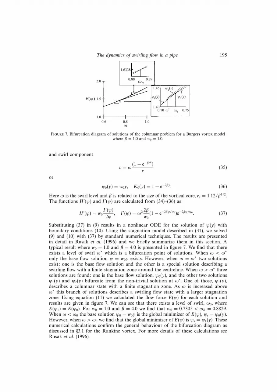
Figure 7. Bifurcation diagram of solutions of the columnar problem for a Burgers vortex modelwhere β = 1.0 and w0 = 1.0.
and swirl component
v = ω(1− e−βr
2
)
r(35)
or
ψ0(y) = w0y, K0(y) = 1− e−2βy. (36)
Here ω is the swirl level and β is related to the size of the vortical core, rc = 1.12/β1/2.The functions H ′(ψ) and I ′(ψ) are calculated from (34)–(36) as
H ′(ψ) = w0
I ′(ψ)
2ψ, I ′(ψ) = ω2 2β
w0
(1− e−2βψ/w0 )e−2βψ/w0 . (37)
Substituting (37) in (9) results in a nonlinear ODE for the solution of ψ(y) withboundary conditions (10). Using the stagnation model described in (31), we solved(9) and (10) with (37) by standard numerical techniques. The results are presentedin detail in Rusak et al. (1996) and we briefly summarize them in this section. Atypical result where w0 = 1.0 and β = 4.0 is presented in figure 7. We find that thereexists a level of swirl ω∗ which is a bifurcation point of solutions. When ω < ω∗
only the base flow solution ψ = w0y exists. However, when ω = ω∗ two solutionsexist: one is the base flow solution and the other is a special solution describing aswirling flow with a finite stagnation zone around the centreline. When ω > ω∗ threesolutions are found: one is the base flow solution, ψ0(y), and the other two solutionsψ1(y) and ψ2(y) bifurcate from the non-trivial solution at ω∗. One of those, ψ1(y),describes a columnar state with a finite stagnation zone. As ω is increased aboveω∗ this branch of solutions describes a swirling flow state with a larger stagnationzone. Using equation (11) we calculated the flow force E(ψ) for each solution andresults are given in figure 7. We can see that there exists a level of swirl, ω0, whereE(ψ1) = E(ψ0). For w0 = 1.0 and β = 4.0 we find that ω0 = 0.7305 < ωB = 0.8829.When ω < ω0 the base solution ψ0 = w0y is the global minimizer of E(ψ), ψs = ψ0(y).However, when ω > ω0 we find that the global minimizer of E(ψ) is ψs = ψ1(y). Thesenumerical calculations confirm the general behaviour of the bifurcation diagram asdiscussed in §3.1 for the Rankine vortex. For more details of these calculations seeRusak et al. (1996).
196 S. Wang and Z. Rusak
4. The properties of the global minimizer of E(ψ)
In this section, the properties of the global minimizer ψg(x, y) of E(ψ) (given by(8)) are examined. We will concentrate on the case where the inlet flow, ψ0(y), andH(ψ) and I(ψ) are described by the Rankine or Burgers vortex models. A similardiscussion can be presented for other vortex models, such as the Q-vortex, and thequalitative results are expected to be the same. We discuss the nature of the globalminimizer, ψg(x, y), when a stagnation model is considered in the separation zone aswell as other possible continuation models.
We distinguish between several cases as the swirl at the inlet is increased.
4.1. The case where 0 < ω 6 ω0
We will show first that when 0 6 ω 6 ω0, the global minimizer of E(ψ) is the basecolumnar flow
ψg(x, y) ≡ ψ0(y). (38)
When 0 6 ω 6 ω0, we have
E(ψ) =
∫ x0
0
∫ 1/2
0
(ψ2y
2+H(ψ)− I(ψ)
2y
)dydx+
∫ x0
0
∫ 1/2
0
ψ2x
4ydydx
>
∫ x0
0
∫ 1/2
0
(ψ2
0y
2+H(ψ0)−
I(ψ0)
2y
)dydx+
∫ x0
0
∫ 1/2
0
ψ2x
4ydydx
> E(ψ0) (39)
and so (38) is proven. This result shows that in the range where 0 6 ω 6 ω0, the inletflow may develop all along the pipe as a columnar flow with no axial disturbance.
4.2. The case where ω > ω0
The case where ω > ω0 is more interesting. As is known from §3.1, the base flow stateψ0(y) is no longer a global minimizer of E(ψ) in this range of ω and, therefore, therelation (39) does not hold in this case. The results of §2.3 and 2.4 can now be usedto describe the properties of the global minimizer of E(ψ) when ω > ω0.
We study two types of continuation models to describe the separation zone:
4.2.1. Stagnation model
(i) ω slightly greater than ω0: In §2.3 we found that for a long pipe the globalminimizer, ψg(x, y), is dominated by the columnar minimizer ψs(y). From §3, we alsofind that when ω is slightly greater than ω0, the columnar minimizer, ψs(y), is differentfrom the inlet state, ψ0(y), and
E(ψ0)− E(ψs) > 0 but small. (40)
From the boundary condition (4) and the momentum balance (16) we find that
E(ψ0)− E(ψs) =
∫ 1/2
0
ψ2gx(0, y)
4ydy > 0 but small.
The balance of flow force requires that the excess of E between inlet and outletbe converted into a relatively small radial flow along the inlet. Therefore, in thecase where ω is slightly greater than ω0, the global minimizer solution describes atransition from an inlet state that is almost the columnar state ψ0(y), to an outlet
The dynamics of swirling flow in a pipe 197
x10
ψ0(y)
ψ = 0x
y
x0
ψg(x, y)
ψ = w0
ψs(y)
12
x2
(a)
0
ψ0(y)ψ = 0
x
y
x0
ψg(x, y)
ψ = w0
ψs(y)
12
x2
(b)
Figure 8. The global minimizer solution ψg(x, y) when ω > ω0 and (a) ω close to ω0,(b) ω − ω0 is not small.
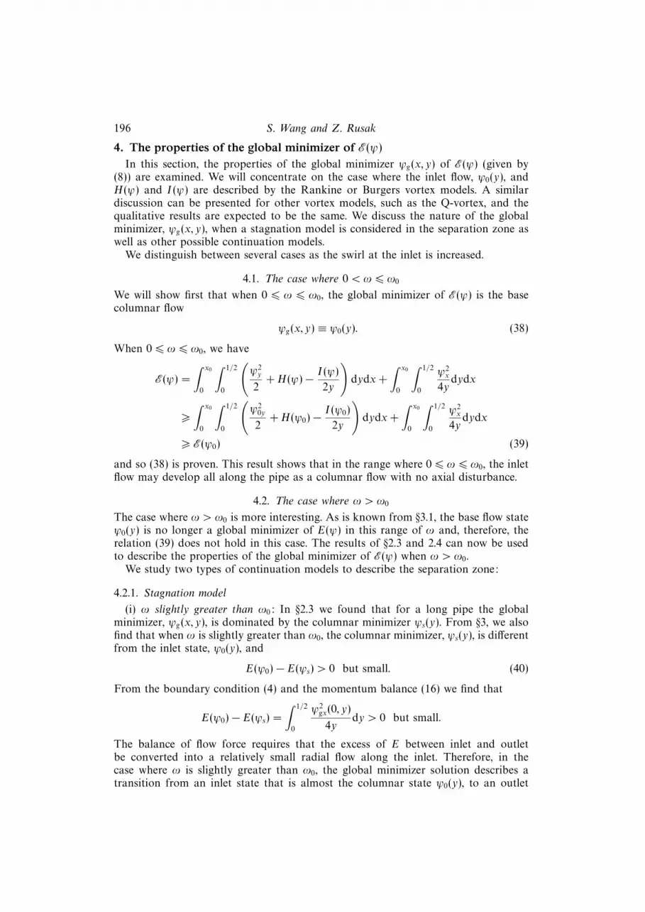
state that is the columnar flow ψs(y), see figure (8a). Since the columnar minimizer,ψs(y), must describe a separation zone (as shown in §3 for both the Rankine vortexmodel and the Burgers vortex model), the solution ψg(x, y) describes the developmentof an open breakdown zone in the swirling flow.
The transition described by the global minimizer, ψg(x, y), is composed of threeflow stages along the pipe (see figure 8a). In the range 0 < x < x1, ψg(x, y) is closeto ψ0(y). In the range x1 < x < x2, ψg(x, y) has a rather large radial flow componentand the flow has a transition from ψ0(y) to ψs(y). This transition must have theminimum of the functional E(ψ) among all the possible transitions. We may call it ‘aminimum transition stage’. In the range x2 < x < x0, ψg(x, y) is close to the columnarminimizer ψs(y). Our numerical computations confirm this schematic description (see,for example, figure 8 in Rusak et al. 1996).
We can now see that when x0 tends to infinity and ω → ω+0 the global minimizer
solution tends to the solution of Keller et al. (1985).(ii) ω > ω0, and ω − ω0 is not small: In this case∫ 1/2
0
ψ2gx(0, y)
4ydy = E(ψg(0, y))− E(ψg(x0, y))
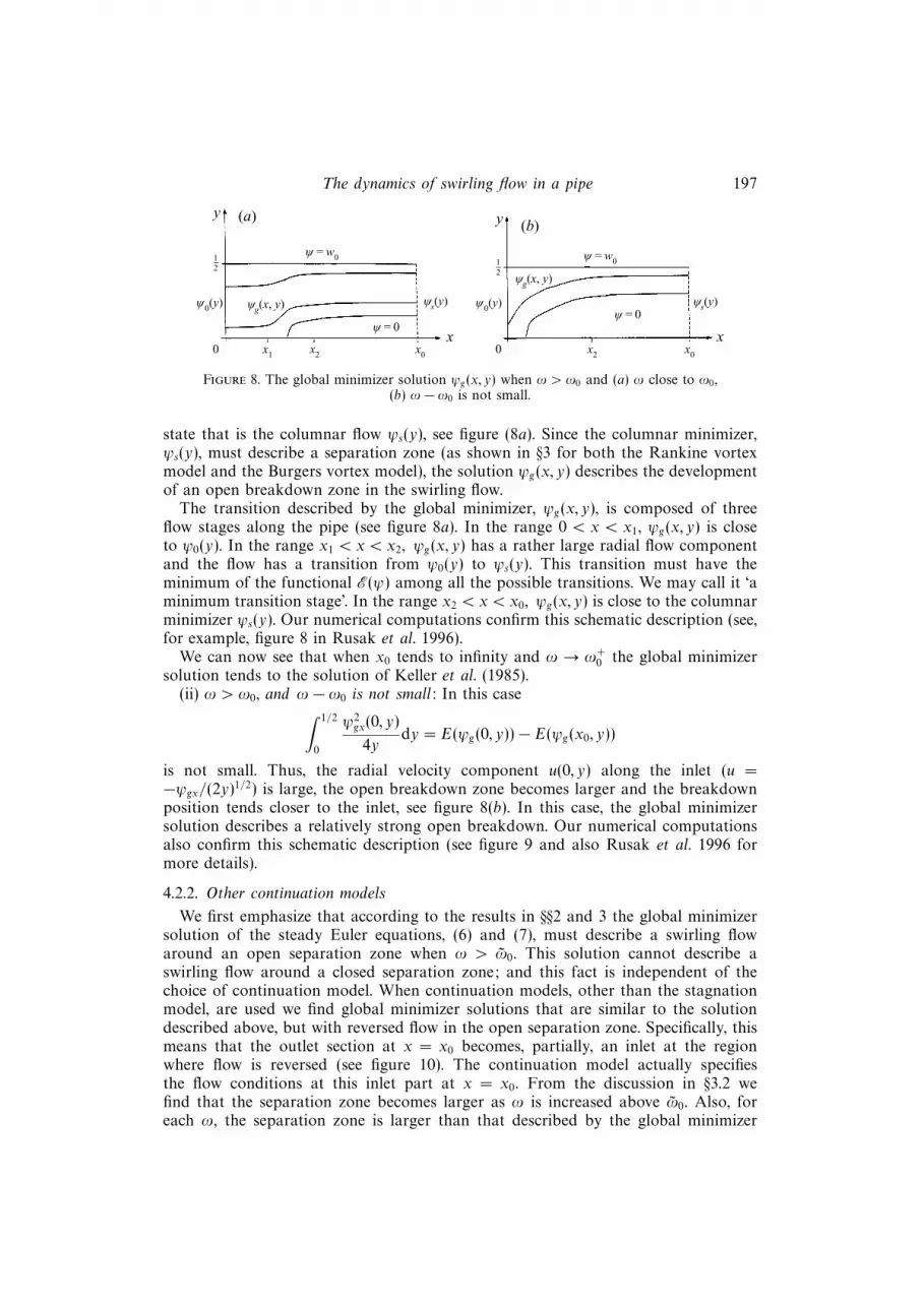
is not small. Thus, the radial velocity component u(0, y) along the inlet (u =−ψgx/(2y)1/2) is large, the open breakdown zone becomes larger and the breakdownposition tends closer to the inlet, see figure 8(b). In this case, the global minimizersolution describes a relatively strong open breakdown. Our numerical computationsalso confirm this schematic description (see figure 9 and also Rusak et al. 1996 formore details).
4.2.2. Other continuation models
We first emphasize that according to the results in §§2 and 3 the global minimizersolution of the steady Euler equations, (6) and (7), must describe a swirling flowaround an open separation zone when ω > ω0. This solution cannot describe aswirling flow around a closed separation zone; and this fact is independent of thechoice of continuation model. When continuation models, other than the stagnationmodel, are used we find global minimizer solutions that are similar to the solutiondescribed above, but with reversed flow in the open separation zone. Specifically, thismeans that the outlet section at x = x0 becomes, partially, an inlet at the regionwhere flow is reversed (see figure 10). The continuation model actually specifiesthe flow conditions at this inlet part at x = x0. From the discussion in §3.2 wefind that the separation zone becomes larger as ω is increased above ω0. Also, foreach ω, the separation zone is larger than that described by the global minimizer
198 S. Wang and Z. Rusak
0.4
0.2
0 1 2 3 4 5 6
0.4
0.2
0 1 2 3 4 5 6
0.4
0.2
0 1 2 3 4 5 6
0.4
0.2
0 1 2 3 4 5 6
t =19.0
t =13.4
t = 6.7
t = 0
0.4
0.2
0 1 2 3 4 5 6
0.4
0.2
0 1 2 3 4 5 6
0.4
0.2
0 1 2 3 4 5 6
0.4
0.2
0 1 2 3 4 5 6
t =133.0
t = 95.0
t = 57.0
t = 38.0
Figure 9. Time-history plots of the stream function for a pipe flow where the inlet state is describedby the Burgers vortex model (34) and (35) and where ω = 1.0 and β = 4.0. In these figures the topline is the pipe wall, the bottom line is the pipe centreline, the left section is the inlet and the rightsection is the outlet.
solution when a stagnation model is used. This shows that when reversed flowat x = x0 enters the separation zone, the size of this zone becomes larger. Thisalso shows that, within the inviscid and steady framework, different continuationmodels, that reflect different inlet conditions at part of the boundary at x = x0, mayresult in different global minimizer solutions for every ω > ω0. This demonstratesthe non-uniqueness of solutions of the SLE (steady Euler equation) that may existwhen various continuation models (various inlet conditions along part of the outlet)are used. In the inviscid and steady-state case, this non-uniqueness of solutions isexpected, and within this framework, the choice of the proper model is an insolubletask. The various inviscid solutions may correspond to different physical situations,
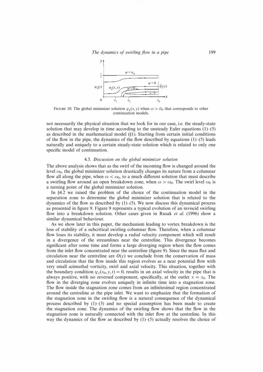
The dynamics of swirling flow in a pipe 199
0
ψ0(y) ψ = 0
x
y
x0
ψg(x, y)
ψ = w012
x2x1
ψ > 0
ψ < 0
ψs(y)∼
Figure 10. The global minimizer solution ψg(x, y) when ω > ω0 that corresponds to othercontinuation models.
not necessarily the physical situation that we look for in our case, i.e. the steady-statesolution that may develop in time according to the unsteady Euler equations (1)–(5)as described in the mathematical model (§1). Starting from certain initial conditionsof the flow in the pipe, the dynamics of the flow described by equations (1)–(5) leadsnaturally and uniquely to a certain steady-state solution which is related to only onespecific model of continuation.
4.3. Discussion on the global minimizer solution
The above analysis shows that as the swirl of the incoming flow is changed around thelevel ω0, the global minimizer solution drastically changes its nature from a columnarflow all along the pipe, when ω < ω0, to a much different solution that must describea swirling flow around an open breakdown zone, when ω > ω0. The swirl level ω0 isa turning point of the global minimizer solution.
In §4.2 we raised the problem of the choice of the continuation model in theseparation zone to determine the global minimizer solution that is related to thedynamics of the flow as described by (1)–(5). We now discuss this dynamical processas presented in figure 9. Figure 9 represents a typical evolution of an inviscid swirlingflow into a breakdown solution. Other cases given in Rusak et al. (1996) show asimilar dynamical behaviour.
As we show later in this paper, the mechanism leading to vortex breakdown is theloss of stability of a subcritical swirling columnar flow. Therefore, when a columnarflow loses its stability, it must develop a radial velocity component which will resultin a divergence of the streamlines near the centreline. This divergence becomessignificant after some time and forms a large diverging region where the flow comesfrom the inlet flow concentrated near the centreline (figure 9). Since the mass flux andcirculation near the centreline are O(y) we conclude from the conservation of massand circulation that the flow inside this region evolves as a near potential flow withvery small azimuthal vorticity, swirl and axial velocity. This situation, together withthe boundary condition ψx(x0, y, t) = 0, results in an axial velocity in the pipe that isalways positive, with no reversed component, specifically, at the outlet x = x0. Theflow in the diverging zone evolves uniquely in infinite time into a stagnation zone.The flow inside the stagnation zone comes from an infinitesimal region concentratedaround the centreline at the pipe inlet. We want to emphasize that the formation ofthe stagnation zone in the swirling flow is a natural consequence of the dynamicalprocess described by (1)–(5) and no special assumption has been made to createthe stagnation zone. The dynamics of the swirling flow shows that the flow in thestagnation zone is naturally connected with the inlet flow at the centreline. In thisway the dynamics of the flow as described by (1)–(5) actually resolves the choice of
200 S. Wang and Z. Rusak
the proper continuation model in the analysis of steady and inviscid swirling flows.The results of our numerical simulations using the unsteady Euler equations (1)–(5)(see Rusak et al. 1996 and figure 9) confirm this idea and demonstrate that in relevantcases the stagnation model is the proper model to use in the inviscid and steady-stateanalysis of swirling flows. Actually, we do not use any extra information in additionto the inlet conditions and in this way the stagnation model is not a continuationmodel.
5. The critical state of a swirling flow in a finite-length pipeWe consider now a base steady swirling columnar flow where ψ(x, y) = ψ0(y),
which is a solution of the SLE (6) and (7). A small-disturbance analysis of the SLEusing
ψ(x, y) = ψ0(y) + εψ1(x, y) + ..., (41)
where ε 1 and ψ1 is the disturbance stream function, results in the linearized SLE
ψ1yy +ψ1xx
2y−(H ′′(ψ0;ω)− ω2 I
′′(ψ0)
2y
)ψ1 = 0,
ψ1(x, 0) = ψ1(x, 1/2) = 0 for 0 6 x 6 x0,
ψ1(0, y) = ψ1x(x0, y) = 0 for 0 6 y 6 1/2.
(42)
Here, I = K20 (y)/2. This is an eigenvalue problem that has non-trivial solutions only
at specific values of ω. This eigenvalue problem was first studied by Squire (1960)and Benjamin (1962) for an infinitely long pipe. Benjamin (1962) defined the firsteigenvalue of (42) when x0 tends to infinity as the critical state, where ω = ωB .
We modify Benjamin’s critical state concept to the case of a finite-length pipe toreflect the effect of geometry. The ‘critical swirl of a flow in a finite length pipe’ isdefined as the first eigenvalue of (42) and is denoted as ω1. The critical swirl ω1 is abifurcation point of branches of solutions of the SLE where ψ1(x, y) is given by
ψ1(x, y) = Φ(y) sin
(π
2x0
x
)(43)
and where ω1 and Φ are determined by the eigenvalue problem
Φyy −(π2/4x2
0
2y+H ′′(ψ0;ω1)−
ω21 I′′(ψ0)
2y
)Φ = 0,
Φ(0) = 0, Φ(1/2) = 0.
(44)
Notice that as x0 tends to infinity ω1 tends to the critical swirl ωB of Benjamin (1962);ω1 may also be identified as the transcritical bifurcation point of first sinusoidalsolution branch described by Leibovich & Kribus (1990). Using a weakly nonlinearanalysis in the case of an infinitely long pipe, Leibovich & Kribus (1990) showed thatwhen ω < ω1 the branch of solutions bifurcating at the critical state may describe asolitary wave in the flow.
It is important to point out that from the perspective of variational methods it canbe shown (see, for example, Courant & Hilbert 1953) that the columnar flow solutionψ(x, y) = ψ0(y) is a local minimizer of the functional E(ψ) when ω < ω1. Moreover,at ω = ω1 this columnar solution is an inflection point of E(ψ) where the first andsecond variations of E(ψ) vanish. This is similar to the behaviour of the columnarfunctional E(ψ) at ωB (see figure 4f). We will use these results in the next section to
The dynamics of swirling flow in a pipe 201
x0
ψ0 ψM ψg ψ∈W1,2b
(Ω x0,1/y)
%(ψ)x0
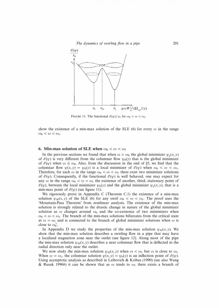
Figure 11. The functional E(ψ)/x0 for ω0 < ω < ω1.
show the existence of a min-max solution of the SLE (6) for every ω in the rangeω0 < ω < ω1.
6. Min-max solution of SLE when ω0 < ω < ω1
In the previous sections we found that when ω > ω0 the global minimizer ψg(x, y)of E(ψ) is very different from the columnar flow ψ0(y) that is the global minimizerof E(ψ) when ω 6 ω0. Also, from the discussion in the end of §5, we find that thecolumnar flow ψ(x, y) = ψ0(y) is a local minimizer of E(ψ) when ω0 < ω < ω1.Therefore, for each ω in the range ω0 < ω < ω1 there exist two minimizer solutionsof E(ψ). Consequently, if the functional E(ψ) is well behaved, one may expect forany ω in the range ω0 < ω < ω1 the existence of another, third, stationary point ofE(ψ), between the local minimizer ψ0(y) and the global minimizer ψg(x, y), that is amin-max point of E(ψ) (see figure 11).
We rigorously prove in Appendix C (Theorem C.1) the existence of a min-maxsolution ψM(x, y) of the SLE (6) for any swirl ω0 < ω < ω1. The proof uses the‘Mountain-Pass Theorem’ from nonlinear analysis. The existence of the min-maxsolution is strongly related to the drastic change in nature of the global minimizersolution as ω changes around ω0 and the co-existence of two minimizers whenω0 < ω < ω1. The branch of the min-max solutions bifurcates from the critical stateat ω = ω1 and is connected to the branch of global minimizer solutions when ω isclose to ω+
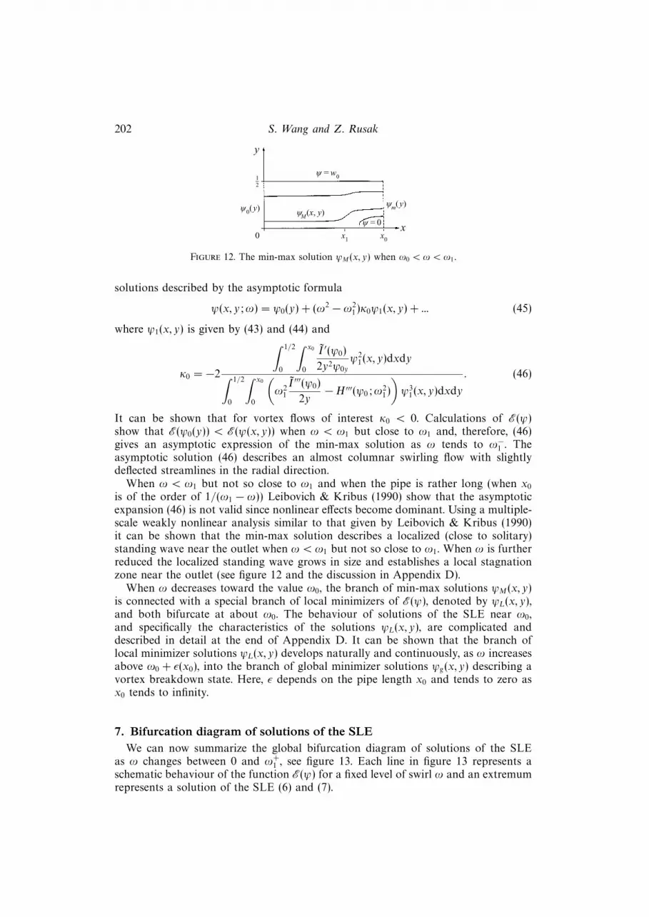
0 .In Appendix D we study the properties of the min-max solution ψM(x, y). We
show that the min-max solution describes a swirling flow in a pipe that may havea localized stagnation zone near the outlet (see figure 12). Along most of the pipethe min-max solution ψM(x, y) describes a near columnar flow that is deflected in theradial direction only near the outlet.
We now study the min-max solution ψM(x, y) when ω < ω1 but ω is close to ω1.When ω = ω1, the columnar solution ψ(x, y) = ψ0(y) is an inflection point of E(ψ).Using asymptotic analysis as described in Leibovich & Kribus (1990) (see also Wang& Rusak 1996b) it can be shown that as ω tends to ω1 there exists a branch of
202 S. Wang and Z. Rusak
0
ψ0(y)
ψ = 0 x
y
x0
ψM(x, y)
ψ = w012
x1
ψm(y)
Figure 12. The min-max solution ψM(x, y) when ω0 < ω < ω1.
solutions described by the asymptotic formula
ψ(x, y;ω) = ψ0(y) + (ω2 − ω21)κ0ψ1(x, y) + ... (45)
where ψ1(x, y) is given by (43) and (44) and
κ0 = −2
∫ 1/2
0
∫ x0
0
I ′(ψ0)
2y2ψ0y
ψ21(x, y)dxdy∫ 1/2
0
∫ x0
0
(ω2
1
I ′′′(ψ0)
2y−H ′′′(ψ0;ω
21)
)ψ3
1(x, y)dxdy
. (46)
It can be shown that for vortex flows of interest κ0 < 0. Calculations of E(ψ)show that E(ψ0(y)) < E(ψ(x, y)) when ω < ω1 but close to ω1 and, therefore, (46)gives an asymptotic expression of the min-max solution as ω tends to ω−1 . Theasymptotic solution (46) describes an almost columnar swirling flow with slightlydeflected streamlines in the radial direction.
When ω < ω1 but not so close to ω1 and when the pipe is rather long (when x0
is of the order of 1/(ω1 − ω)) Leibovich & Kribus (1990) show that the asymptoticexpansion (46) is not valid since nonlinear effects become dominant. Using a multiple-scale weakly nonlinear analysis similar to that given by Leibovich & Kribus (1990)it can be shown that the min-max solution describes a localized (close to solitary)standing wave near the outlet when ω < ω1 but not so close to ω1. When ω is furtherreduced the localized standing wave grows in size and establishes a local stagnationzone near the outlet (see figure 12 and the discussion in Appendix D).
When ω decreases toward the value ω0, the branch of min-max solutions ψM(x, y)is connected with a special branch of local minimizers of E(ψ), denoted by ψL(x, y),and both bifurcate at about ω0. The behaviour of solutions of the SLE near ω0,and specifically the characteristics of the solutions ψL(x, y), are complicated anddescribed in detail at the end of Appendix D. It can be shown that the branch oflocal minimizer solutions ψL(x, y) develops naturally and continuously, as ω increasesabove ω0 + ε(x0), into the branch of global minimizer solutions ψg(x, y) describing avortex breakdown state. Here, ε depends on the pipe length x0 and tends to zero asx0 tends to infinity.
7. Bifurcation diagram of solutions of the SLEWe can now summarize the global bifurcation diagram of solutions of the SLE
as ω changes between 0 and ω+1 , see figure 13. Each line in figure 13 represents a
schematic behaviour of the function E(ψ) for a fixed level of swirl ω and an extremumrepresents a solution of the SLE (6) and (7).
The dynamics of swirling flow in a pipe 203
ψ0 ψM
ψg
ψ∈W1,2b
(Ω x0,1/y)
%(ψ)x0
ψ0
ψL
ω1
ω0
ω0 + ε
ω < ω0
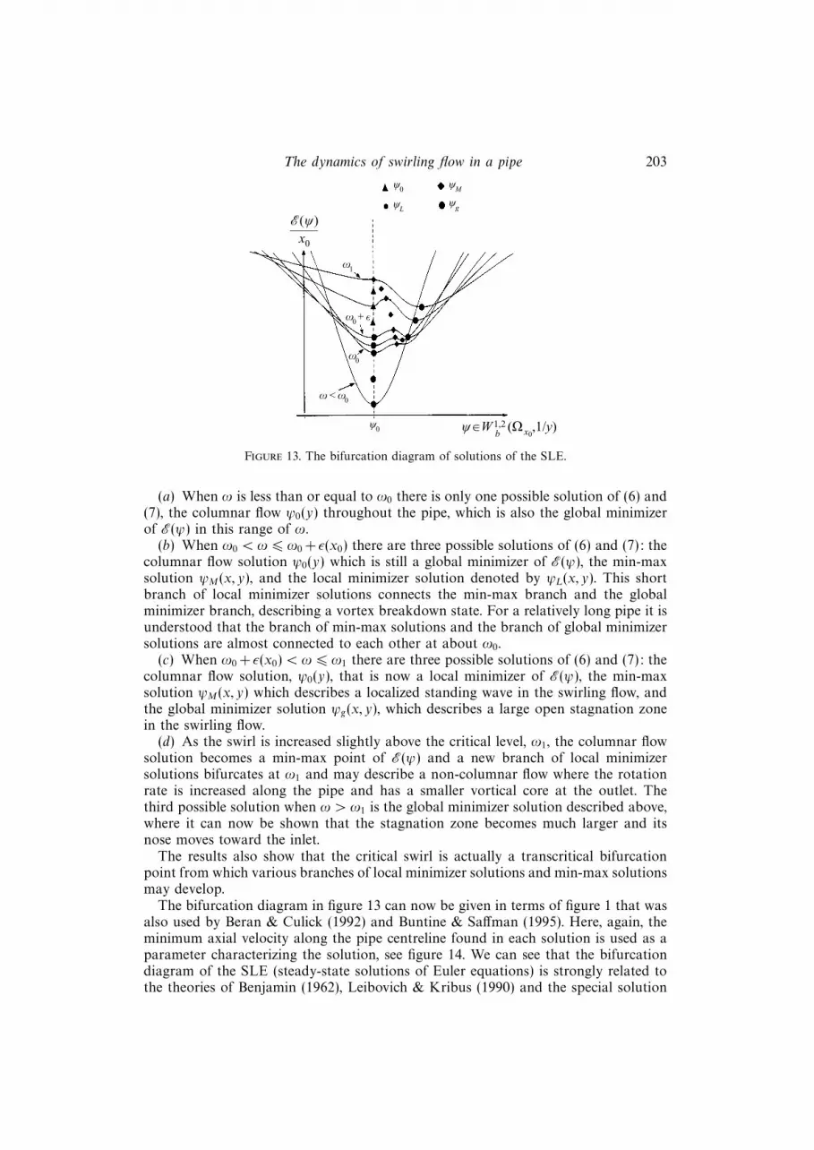
Figure 13. The bifurcation diagram of solutions of the SLE.
(a) When ω is less than or equal to ω0 there is only one possible solution of (6) and(7), the columnar flow ψ0(y) throughout the pipe, which is also the global minimizerof E(ψ) in this range of ω.
(b) When ω0 < ω 6 ω0 + ε(x0) there are three possible solutions of (6) and (7): thecolumnar flow solution ψ0(y) which is still a global minimizer of E(ψ), the min-maxsolution ψM(x, y), and the local minimizer solution denoted by ψL(x, y). This shortbranch of local minimizer solutions connects the min-max branch and the globalminimizer branch, describing a vortex breakdown state. For a relatively long pipe it isunderstood that the branch of min-max solutions and the branch of global minimizersolutions are almost connected to each other at about ω0.
(c) When ω0 + ε(x0) < ω 6 ω1 there are three possible solutions of (6) and (7): thecolumnar flow solution, ψ0(y), that is now a local minimizer of E(ψ), the min-maxsolution ψM(x, y) which describes a localized standing wave in the swirling flow, andthe global minimizer solution ψg(x, y), which describes a large open stagnation zonein the swirling flow.
(d) As the swirl is increased slightly above the critical level, ω1, the columnar flowsolution becomes a min-max point of E(ψ) and a new branch of local minimizersolutions bifurcates at ω1 and may describe a non-columnar flow where the rotationrate is increased along the pipe and has a smaller vortical core at the outlet. Thethird possible solution when ω > ω1 is the global minimizer solution described above,where it can now be shown that the stagnation zone becomes much larger and itsnose moves toward the inlet.
The results also show that the critical swirl is actually a transcritical bifurcationpoint from which various branches of local minimizer solutions and min-max solutionsmay develop.
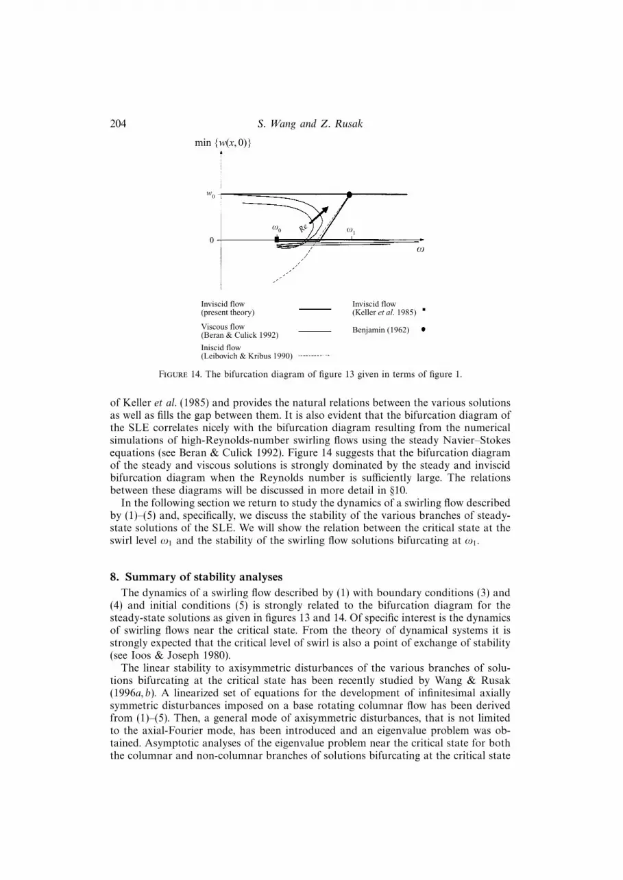
The bifurcation diagram in figure 13 can now be given in terms of figure 1 that wasalso used by Beran & Culick (1992) and Buntine & Saffman (1995). Here, again, theminimum axial velocity along the pipe centreline found in each solution is used as aparameter characterizing the solution, see figure 14. We can see that the bifurcationdiagram of the SLE (steady-state solutions of Euler equations) is strongly related tothe theories of Benjamin (1962), Leibovich & Kribus (1990) and the special solution
204 S. Wang and Z. Rusak
min w(x, 0)
w0
0
ω0
Inviscid flow(present theory)
Viscous flow(Beran & Culick 1992)
Iniscid flow(Leibovich & Kribus 1990)
Inviscid flow(Keller et al. 1985)
Benjamin (1962)
ω1Re
ω
Figure 14. The bifurcation diagram of figure 13 given in terms of figure 1.
of Keller et al. (1985) and provides the natural relations between the various solutionsas well as fills the gap between them. It is also evident that the bifurcation diagram ofthe SLE correlates nicely with the bifurcation diagram resulting from the numericalsimulations of high-Reynolds-number swirling flows using the steady Navier–Stokesequations (see Beran & Culick 1992). Figure 14 suggests that the bifurcation diagramof the steady and viscous solutions is strongly dominated by the steady and inviscidbifurcation diagram when the Reynolds number is sufficiently large. The relationsbetween these diagrams will be discussed in more detail in §10.
In the following section we return to study the dynamics of a swirling flow describedby (1)–(5) and, specifically, we discuss the stability of the various branches of steady-state solutions of the SLE. We will show the relation between the critical state at theswirl level ω1 and the stability of the swirling flow solutions bifurcating at ω1.
8. Summary of stability analysesThe dynamics of a swirling flow described by (1) with boundary conditions (3) and
(4) and initial conditions (5) is strongly related to the bifurcation diagram for thesteady-state solutions as given in figures 13 and 14. Of specific interest is the dynamicsof swirling flows near the critical state. From the theory of dynamical systems it isstrongly expected that the critical level of swirl is also a point of exchange of stability(see Ioos & Joseph 1980).
The linear stability to axisymmetric disturbances of the various branches of solu-tions bifurcating at the critical state has been recently studied by Wang & Rusak(1996a, b). A linearized set of equations for the development of infinitesimal axiallysymmetric disturbances imposed on a base rotating columnar flow has been derivedfrom (1)–(5). Then, a general mode of axisymmetric disturbances, that is not limitedto the axial-Fourier mode, has been introduced and an eigenvalue problem was ob-tained. Asymptotic analyses of the eigenvalue problem near the critical state for boththe columnar and non-columnar branches of solutions bifurcating at the critical state
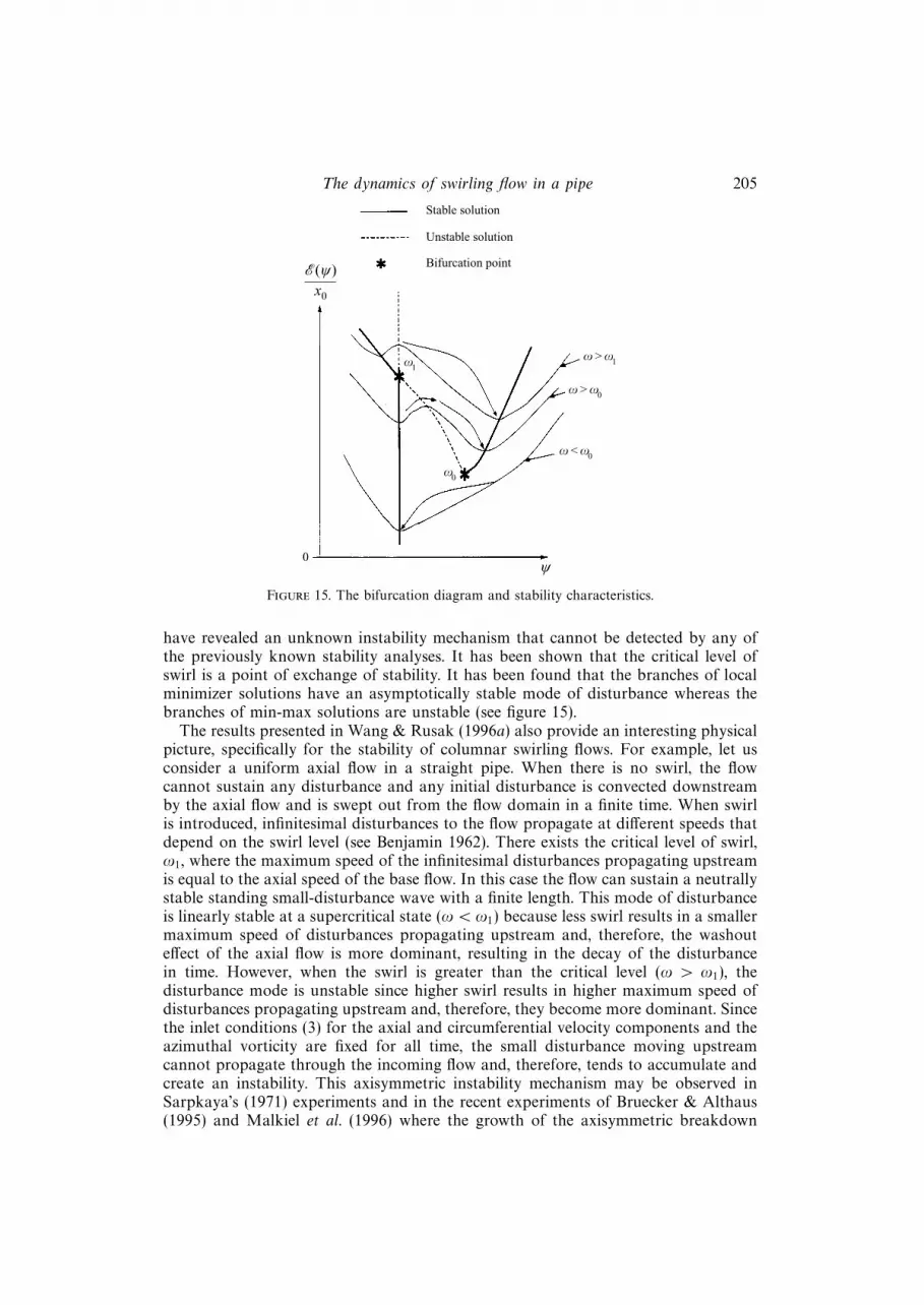
The dynamics of swirling flow in a pipe 205
%(ψ)x0
ψ
ω1
ω0
ω < ω0
ω > ω0
ω > ω1
Stable solution
Unstable solution
Bifurcation point
0
Figure 15. The bifurcation diagram and stability characteristics.
have revealed an unknown instability mechanism that cannot be detected by any ofthe previously known stability analyses. It has been shown that the critical level ofswirl is a point of exchange of stability. It has been found that the branches of localminimizer solutions have an asymptotically stable mode of disturbance whereas thebranches of min-max solutions are unstable (see figure 15).
The results presented in Wang & Rusak (1996a) also provide an interesting physicalpicture, specifically for the stability of columnar swirling flows. For example, let usconsider a uniform axial flow in a straight pipe. When there is no swirl, the flowcannot sustain any disturbance and any initial disturbance is convected downstreamby the axial flow and is swept out from the flow domain in a finite time. When swirlis introduced, infinitesimal disturbances to the flow propagate at different speeds thatdepend on the swirl level (see Benjamin 1962). There exists the critical level of swirl,ω1, where the maximum speed of the infinitesimal disturbances propagating upstreamis equal to the axial speed of the base flow. In this case the flow can sustain a neutrallystable standing small-disturbance wave with a finite length. This mode of disturbanceis linearly stable at a supercritical state (ω < ω1) because less swirl results in a smallermaximum speed of disturbances propagating upstream and, therefore, the washouteffect of the axial flow is more dominant, resulting in the decay of the disturbancein time. However, when the swirl is greater than the critical level (ω > ω1), thedisturbance mode is unstable since higher swirl results in higher maximum speed ofdisturbances propagating upstream and, therefore, they become more dominant. Sincethe inlet conditions (3) for the axial and circumferential velocity components and theazimuthal vorticity are fixed for all time, the small disturbance moving upstreamcannot propagate through the incoming flow and, therefore, tends to accumulate andcreate an instability. This axisymmetric instability mechanism may be observed inSarpkaya’s (1971) experiments and in the recent experiments of Bruecker & Althaus(1995) and Malkiel et al. (1996) where the growth of the axisymmetric breakdown
206 S. Wang and Z. Rusak
may be associated with an unstable axisymmetric eigen-mode disturbance near thepipe inlet and the upstream propagation of this disturbance.
This inviscid instability mechanism is strongly related to the critical-state conceptof Benjamin (1962). However, it should be pointed out that in the case of a swirlingflow in an infinitely long pipe, such an exchange of stability around the criticalstate does not exist since the waves are free to propagate both upstream and down-stream and there is no interaction between the waves moving upstream and the inletconditions. For example, in the case of a solid-body rotating flow with a uniformaxial velocity component in an infinitely long pipe Rayleigh’s (1916) classical stabilitycriterion predicts that the flow is stable to any axisymmetric disturbance for anyswirl level, whereas the analytical solutions presented in Wang & Rusak (1996a) havedemonstrated that such a flow in a finite-length pipe changes its stability character-istics as the swirl changes around the critical level of swirl ω1 of that flow. Whenω > ω1 the solid-body rotating flow with a uniform axial velocity component isunstable.
9. Mechanism leading to the axisymmetric vortex breakdown in a pipeThe bifurcation diagram and the stability results are now used to explain the
development in time of a swirling flow described by (1)–(5). Although not yetrigorously proven, it is strongly expected that the stability results of Wang & Rusak(1996a, b) near the critical state can be extended to the entire branches, i.e. the branchesof local and global minimizer solutions are supercritical states (this results fromthe relevant eigenvalue problem) and asymptotically linearly stable to axisymmetricdisturbances. On the other hand, the branches of min-max solutions are unstable (seefigure 15). Moreover, the above results may indicate that the branch of columnar flowsolutions is unconditionally stable to any axisymmetric disturbance when ω < ω0.This means that, for this range of swirl, any axisymmetric disturbance to a basecolumnar flow will decay in time and the flow will return to a columnar state.
In the range of incoming swirl ω0 < ω < ω1 two steady-state solutions co-exist:one is a local minimizer solution that describes a columnar swirling flow all along thepipe and the other is a global minimizer solution that describes a swirling flow witha large stagnation zone. Both solutions are stable to small, but finite, axisymmetricdisturbances. The two branches of solutions are connected by a branch of min-maxsolutions that are unstable. This suggests that in the range ω0 < ω < ω1 there existtwo basins of attraction. Which of the two solutions is actually realized depends onthe initial disturbances to the base columnar flow. When the initial disturbances arerelatively small they will decay in time and the flow will return to a columnar state allalong the pipe. However, when the initial disturbances are relatively large they willevolve in time in a complicated nonlinear dynamical process into large disturbances.These will propagate upstream, interact with the inlet state and develop into thevortex breakdown state described by the global minimizer solution.
In the range ω > ω1 the equilibrium columnar flow state is unstable and it isexpected to be absolutely unstable. Therefore, any axisymmetric disturbance will growin time through the instability mechanism that depends on the upstream propagationof waves, described in §8. In this range of relatively large incoming swirl it is expectedthat the global minimizer solution is a strong attractor. Then, the flow again will evolvenonlinearly, with large disturbance waves that propagate upstream and interact withthe inlet state. The flow will develop from a columnar state into the vortex breakdownstate described by the global minimizer solution.
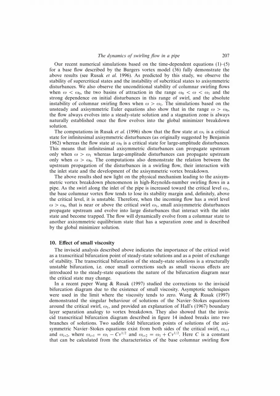
The dynamics of swirling flow in a pipe 207
Our recent numerical simulations based on the time-dependent equations (1)–(5)for a base flow described by the Burgers vortex model (36) fully demonstrate theabove results (see Rusak et al. 1996). As predicted by this study, we observe thestability of supercritical states and the instability of subcritical states to axisymmetricdisturbances. We also observe the unconditional stability of columnar swirling flowswhen ω < ω0, the two basins of attraction in the range ω0 < ω < ω1 and thestrong dependence on initial disturbances in this range of swirl, and the absoluteinstability of columnar swirling flows when ω > ω1. The simulations based on theunsteady and axisymmetric Euler equations also show that in the range ω > ω0,the flow always evolves into a steady-state solution and a stagnation zone is alwaysnaturally established once the flow evolves into the global minimizer breakdownsolution.
The computations in Rusak et al. (1996) show that the flow state at ω1 is a criticalstate for infinitesimal axisymmetric disturbances (as originally suggested by Benjamin1962) whereas the flow state at ω0 is a critical state for large-amplitude disturbances.This means that infinitesimal axisymmetric disturbances can propagate upstreamonly when ω > ω1 whereas large-amplitude disturbances can propagate upstreamonly when ω > ω0. The computations also demonstrate the relation between theupstream propagation of the disturbances in a swirling flow, their interaction withthe inlet state and the development of the axisymmetric vortex breakdown.
The above results shed new light on the physical mechanism leading to the axisym-metric vortex breakdown phenomenon in high-Reynolds-number swirling flows in apipe. As the swirl along the inlet of the pipe is increased toward the critical level ω1,the base columnar vortex flow tends to lose its stability margin and, definitely, abovethe critical level, it is unstable. Therefore, when the incoming flow has a swirl levelω > ω0, that is near or above the critical swirl ω1, small axisymmetric disturbancespropagate upstream and evolve into large disturbances that interact with the inletstate and become trapped. The flow will dynamically evolve from a columnar state toanother axisymmetric equilibrium state that has a separation zone and is describedby the global minimizer solution.
10. Effect of small viscosityThe inviscid analysis described above indicates the importance of the critical swirl
as a transcritical bifurcation point of steady-state solutions and as a point of exchangeof stability. The transcritical bifurcation of the steady-state solutions is a structurallyunstable bifurcation, i.e. once small corrections such as small viscous effects areintroduced to the steady-state equations the nature of the bifurcation diagram nearthe critical state may change.
In a recent paper Wang & Rusak (1997) studied the corrections to the inviscidbifurcation diagram due to the existence of small viscosity. Asymptotic techniqueswere used in the limit where the viscosity tends to zero. Wang & Rusak (1997)demonstrated the singular behaviour of solutions of the Navier–Stokes equationsaround the critical swirl, ω1, and provided an explanation of Hall’s (1967) boundarylayer separation analogy to vortex breakdown. They also showed that the invis-cid transcritical bifurcation diagram described in figure 14 indeed breaks into twobranches of solutions. Two saddle fold bifurcation points of solutions of the axi-symmetric Navier–Stokes equations exist from both sides of the critical swirl, ωcν1and ωcν2, where ωcν1 = ω1 − Cν1/2 and ωcν2 = ω1 + Cν1/2. Here C is a constantthat can be calculated from the characteristics of the base columnar swirling flow
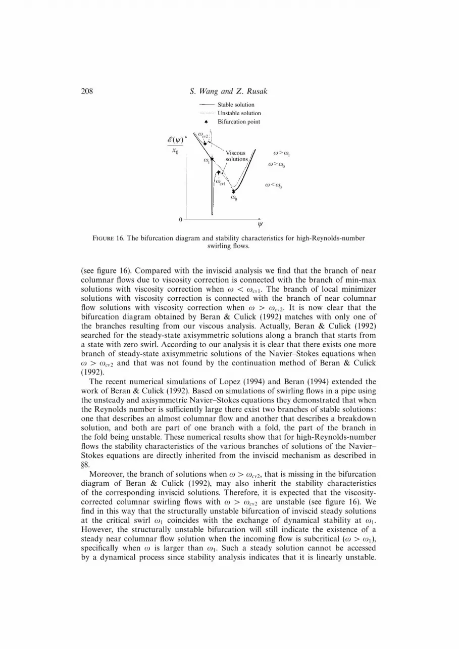
208 S. Wang and Z. Rusak
%(ψ)x0
ψ
ω1
ω0
ω < ω0
ω > ω0
ω > ω1
Stable solution
Unstable solution
Bifurcation point
0
ωcν1
ωcν2
Viscoussolutions
Figure 16. The bifurcation diagram and stability characteristics for high-Reynolds-numberswirling flows.
(see figure 16). Compared with the inviscid analysis we find that the branch of nearcolumnar flows due to viscosity correction is connected with the branch of min-maxsolutions with viscosity correction when ω < ωcν1. The branch of local minimizersolutions with viscosity correction is connected with the branch of near columnarflow solutions with viscosity correction when ω > ωcν2. It is now clear that thebifurcation diagram obtained by Beran & Culick (1992) matches with only one ofthe branches resulting from our viscous analysis. Actually, Beran & Culick (1992)searched for the steady-state axisymmetric solutions along a branch that starts froma state with zero swirl. According to our analysis it is clear that there exists one morebranch of steady-state axisymmetric solutions of the Navier–Stokes equations whenω > ωcν2 and that was not found by the continuation method of Beran & Culick(1992).
The recent numerical simulations of Lopez (1994) and Beran (1994) extended thework of Beran & Culick (1992). Based on simulations of swirling flows in a pipe usingthe unsteady and axisymmetric Navier–Stokes equations they demonstrated that whenthe Reynolds number is sufficiently large there exist two branches of stable solutions:one that describes an almost columnar flow and another that describes a breakdownsolution, and both are part of one branch with a fold, the part of the branch inthe fold being unstable. These numerical results show that for high-Reynolds-numberflows the stability characteristics of the various branches of solutions of the Navier–Stokes equations are directly inherited from the inviscid mechanism as described in§8.
Moreover, the branch of solutions when ω > ωcν2, that is missing in the bifurcationdiagram of Beran & Culick (1992), may also inherit the stability characteristicsof the corresponding inviscid solutions. Therefore, it is expected that the viscosity-corrected columnar swirling flows with ω > ωcν2 are unstable (see figure 16). Wefind in this way that the structurally unstable bifurcation of inviscid steady solutionsat the critical swirl ω1 coincides with the exchange of dynamical stability at ω1.However, the structurally unstable bifurcation will still indicate the existence of asteady near columnar flow solution when the incoming flow is subcritical (ω > ω1),specifically when ω is larger than ω1. Such a steady solution cannot be accessedby a dynamical process since stability analysis indicates that it is linearly unstable.

The dynamics of swirling flow in a pipe 209
In this way, it is the dynamical stability characteristics of solutions that play theessential role in explaining the mechanism leading to the vortex breakdown in apipe and not the structurally unstable bifurcation of inviscid solutions at the criticalswirl.
It should be pointed out that the numerical simulations of Lopez (1994) usingthe axisymmetric time-dependent Navier–Stokes equations also show that for suf-ficiently large-Reynolds-number swirling flows the separation zones in breakdownsolutions are large and essentially stagnant. These are similar in nature to thosefound in our inviscid computations. We strongly believe that the branch of break-down solutions described by Beran & Culick (1992) and Lopez (1994) when theReynolds number is large enough are global minimizer solutions with viscosity cor-rection. Moreover, the size of the separation zones in the viscous computations iscomparable to those predicted by our analysis. Based on his numerical simulationsLopez (1994) also suggested that the viscous dissipation is responsible for closingthe separation zone and this is not due to the downstream boundary condition.This suggests that in the inviscid limit the bubble will become longer and an openseparation zone will appear, as results from our inviscid approach. Furthermore,Lopez (1994) showed that the level of swirl above which breakdown solutions canbe found (his secondary limit point) for an inlet Burgers vortex (36) with β = 4.0tends to a certain limit value 1.466 as the Reynolds number is increased. Usingour method of computing ω0 (see §3.3 and figure 7) we find that the thresholdvalue for the appearance of inviscid breakdown solutions, in the geometrical scale ofLopez’s (1994) computations, is 1.461 which is in good agreement with the viscouscomputations.
The above discussion suggests that our inviscid approach based on (1)–(5) is theinviscid-limit theory of the axisymmetric and viscous flow problem. When the viscosityis small the present theory describes a dynamical behaviour of axisymmetric swirlingflows in a pipe that is close to that computed by Beran & Culick (1992) and Lopez(1994). However, it is expected that when the viscosity is much larger, the viscouseffects may change the entire dynamical behaviour. Specifically, ωcν1 and ω0 willcoincide, the fold in the bifurcation diagram in figure 16 will be eliminated andonly one branch of steady-state solutions will appear. This was actually described byBeran & Culick (1992) and Lopez (1994) for relatively low-Reynolds-number flows.The dynamical behaviour of low-Reynolds-number swirling flows is qualitativelydifferent from the high-Reynolds-number case. The exchange of stability related tothe critical swirl is lost when the viscous effects are strong. In such cases the evolutionin time from one state to another does not exist and the breakdown zone will appearand grow in size in a continuous process as the incoming swirl is increased. Large-viscosity effects will also result in closing the separation zone after a relatively shortdistance from the nose of the zone and in the creation of an internal recirculationflow in the zone through the diffusion of momentum from the outer flow into theseparation zone.
11. DiscussionWe study in this paper the dynamics of inviscid and incompressible axisymmetric
swirling flows in a finite-length pipe described by the Euler equations (1) and (2) withthe boundary conditions (3) and (4) and the initial conditions (5). This theoreticalmodel may represent a physical situation of a flow in a pipe as is found in someexperiments. The analysis is based on studying the flow stability characteristics and
210 S. Wang and Z. Rusak
the long-time dynamics of the flow as it is related to steady-state solutions ofthe problem. Under this framework we provide a theoretical understanding of thedynamics of axisymmetric swirling flows in a pipe.
We summarize the major results found in our analysis. There exist two characteristicswirl levels of the incoming flow to the pipe, ω0 and ω1, where ω0 < ω1, and both canbe determined by solving ODE problems. Swirling columnar flows with a swirl levelless than the threshold level ω0(< ω1) are unconditionally stable to any axisymmetricdisturbance. In the range ω0 < ω < ω1 we find that, starting from initial disturbances,the flow may evolve into one of two distinct steady states, depending on the size ofthe initial disturbances. When the disturbances are sufficiently small they will decayin time and the flow will return to a columnar state. However, when the initialdisturbances are large enough, they will grow in time and evolve nonlinearly into alarge stagnation region in the swirling flow. When ω > ω1, the initial disturbancesalways grow and evolve again into a vortex breakdown solution. Those resultsclarify the mechanism leading to the axisymmetric vortex breakdown phenomenonin high-Reynolds-number swirling flows. As the incoming swirl level is increasedabove ω0, and is near or above ω1, the columnar swirling flow loses its stability anddevelops into a breakdown state. This mechanism is governed by the propagation ofsmall- and large-amplitude disturbances in the pipe and its interaction with the inletconditions.
Our recent numerical computations, guided by the present study, confirm the pre-dicted results and provide details of the nonlinear dynamics of the flow (see Rusaket al. 1996). The study also shows good agreement with the numerical computationsof Beran & Culick (1992), Beran (1994) and Lopez (1994) using the axisymmetricNavier–Stokes equations when the Reynolds number is sufficiently large. The goodagreement suggests that the present approach based on the Euler equations is theinviscid-limit theory of the axisymmetric and viscous flow problem. Our recent ex-periments guided by the present study (see Malkiel et al. 1996) demonstrate the lossof stability of a columnar state and the development in time of the breakdown state.Moreover, the experiments of Malkiel et al. (1996) verify the existence of the twolimit points of swirl and the existence of two stable and steady states, one of a nearcolumnar flow and the other of a breakdown state, for the same inlet conditionswhen the swirl level is between the two limit points. The experiments also showthe appearance of a breakdown state when the inlet swirl level is above the criticalswirl.
This present model explains the suddenness of the vortex breakdown phenomena,specifically around ω0 where a large disturbance to the basic flow may occur for thefirst time as the incoming swirl is increased, the abrupt nature of the phenomena dueto the development of breakdown zones in the flow, as well as the non-uniqueness ofthe phenomena in high-Reynolds-number flows, related to the process of increasingthe incoming swirl. All of these characteristics are similar to those found in theexperiments of Sarpkaya (1971, 1995), Leibovich (1978, 1984) and Bruecker & Althaus(1995) where axisymmetric breakdown zones were found. Also, as demonstrated infigure 14, the present approach connects most of the previously suggested models ofvortex breakdown and provides guidelines for future numerical simulations of andexperiments on these complicated phenomena.
The present study is limited to inviscid and axisymmetric swirling flows and doesnot consider the vortex generation mechanism and its interaction with the vortexbreakdown phenomenon. Specifically, we would like to point out that the unsteadyand axisymmetric problem (1)–(5) has solutions that always evolve into a supercritical

The dynamics of swirling flow in a pipe 211
steady-state that is stable to axisymmetric disturbances. However, such steady-statesolutions may not necessarily be stable to non-axisymmetric disturbances. If thesesteady states are unstable to three-dimensional disturbances it is likely that unsteadyvortical flows will develop and never settle to a steady state. We believe that in order tostudy such swirling flows with three-dimensional waves it would appear important toextend our theoretical framework to investigate the development of three-dimensionaldisturbances from the axisymmetric breakdown solution of our study. These studiesmight result in more details of the flow dynamics and structure, and the possibleevolution of the spiral breakdown out of the axisymmetric breakdown as was foundin Bruecker & Althaus’s (1995) experiments.
This research was carried out with the support of the National Science Foundationunder Grant CTS-9310181. Partial support was also given by the US-Israel BinationalScience Foundation under Grant 94-00245/1.
Appendix A. Existence of global minimizerA.1. Notation and functional space
Let Ωx0= (0, x0)× (0, 1/2) where x0 is a positive number. Let
Lp(Ωx0) =
f : Ωx0
→ f, f is measurable,
∫ x0
0
∫ 1/2
0
|f|pdydx < +∞
with 1 6 p 6 ∞, and
||f||Lp(Ωx0) =
(∫ x0
0
∫ 1/2
0
|f|pdydx
)1/p
.
Let
W 1,p(Ωx0) =
f : f ∈ Lp(Ωx0
) and
∫ x0
0
∫ 1/2
0
(|fy|p + |fx|p)dydx bounded
, 1 6 p 6 ∞,
be the usual Sobolev space with the norm
||f||W 1,p(Ωx0) =
(∫ x0
0
∫ 1/2
0
(|f|p + |fy|p + |fx|p)dydx
)1/p
.
Let W 1,p(Ωx0, 1/y) be the weighted Sobolev space
W 1,p
(Ωx0
,1
y
)=
f : f ∈Lp(Ωx0
) and
∫ x0
0
∫ 1/2
0
(|fy|p+
|fx|py
)dydx<∞
, 16 p<∞
and
||f||W 1,p(Ωx0,1/y) =
(∫ x0
0
∫ 1/2
0
(|fy|p +
|fx|py
+ |f|p)
dydx
)1/p
.
Set
C∞b (Ωx0) = f ∈ C∞(Ωx0
) : f(0, y) = ψ0(y), f(x, 0) = 0 and f(x, 1/2) = w0
212 S. Wang and Z. Rusak
and let
W1,pb (Ωx0
) = the closure of C∞b (Ωx0) in W 1,p(Ωx0
)
and
W1,pb (Ωx0
, 1/y) = the closure of C∞b (Ωx0) in W 1,p(Ωx0
, 1/y).
A.2. Existence
We seek the following minimizer:
minψ∈W 1,p
b(Ωx0
,1/y)
E(ψ). (A 1)
The global minimizer (A 1), if it exists, denoted by ψg(x, y), is a weak solution of (6)and (7), i.e. ∫ x0
0
∫ 1/2
0
(ψgyφy +
ψgxφx
2y+H ′(ψg)φ−
I ′(ψg)φ
2y
)dydx = 0 (A 2)
for all φ such that (ψg +φ) ∈W 1,pb (Ωx0
, 1/y). We state the following general existenceresult:
Theorem A.1. Suppose1. H(ψ) and I(ψ) are bounded and piecewise smooth non-negative functions with
bounded first derivatives;2. I(ψ) 6 c|ψ|p where p is a fixed number, 1 < p 6 2, and c > 0;
then, the global minimizer of (A 1) exists.
The following Hardy’s inequality is crucial in our proof of this theorem:
Lemma A.1. (Hardy’s inequality, see for example Kufner 1983)Let 1 < p < ∞, u ∈ C1[0, x0] with u(0) = 0 and∫ x0
0
|u′(t)|pdt < ∞
then, we have ∫ x0
0
|u(t)|pt−pdt 6(
p
p− 1
)p ∫ x0
0
|u′(t)|pdt. (A 3)
Proof of Theorem A.1. First, we show that the functional E(ψ) is bounded frombelow for any ψ ∈W 1,2
b (Ωx0, 1/y). From the boundness of H(ψ), we immediately have
0 <
∫ x0
0
∫ 1/2
0
H(ψ)dydx < m1. (A 4)
Let 0 < yδ < 1/2 and for any ψ ∈ C∞b (Ωx0), we have∫ x0
0
∫ yδ
0
∣∣∣∣I(ψ)
y
∣∣∣∣ dydx 6 c
∫ x0
0
∫ yδ
0
|ψ|py
dydx (from assumption 2)
6 cyp−1δ
∫ x0
0
∫ yδ
0
|ψ|pyp
dydx (since y 6 yδ)
6 cyp−1δ
(p
p− 1
)p ∫ x0
0
∫ yδ
0
|ψy|pdy (Hardy’s inequality). (A 5)
The dynamics of swirling flow in a pipe 213
The above inequality can be extended to the whole space W1,2b (Ωx0
). From theboundness of I(ψ), we have
0 <
∫ x0
0
∫ 1/2
yδ
I(ψ)
2ydydx 6 myδ (A 6)
where myδ depends on yδ .We now estimate E(ψ) (equation (8)) as follows:
E(ψ) >
∫ x0
0
∫ 1/2
0
(ψ2y
2+ψ2x
4y
)dydx−
∫ x0
0
∫ yδ
0
I(ψ)
2y− myδdydx
(from (A 4) and (A 6))
>
∫ x0
0
∫ 1/2
0
(ψ2y
2+ψ2x
4y
)dydx− c
(p
p− 1
)pyp−1δ
∫ x0
0
∫ yδ
0
|ψy|pdydx− myδ
(from (A 5))
>1
4
∫ x0
0
∫ 1/2
0
(ψ2y +ψ2
x)dydx−c(
p
p−1
)pyp−1δ |Ωx0
|(2−p)/2(∫ x0
0
∫ 1/2
0
ψ2ydydx
)p/2− myδ
(from Holder inequality and where |Ωx0| is the volume of Ωx0
)
>
(1
4− cyδ
)∫ x0
0
∫ 1/2
0
(ψ2y + ψ2
x)dydx− myδ − cyδ
(from (∫ x0
0
∫ 1/2
0ψ2ydydx)p/2 6
∫ x0
0
∫ 1/2
0ψ2ydydx+ 1 and where
cyδ = c(p/(p− 1))pyp−1δ |Ωx0
|(2−p)/2)> −myδ − cyδ = m, (A 7)
where we fix yδ = yδ such that cyδ <14. The boundness of E(ψ) from below on
W1,pb (Ωx0
, 1/y) is proven.
From boundness of H(ψ) and I(ψ), E(ψ) is finite for any ψ ∈ W 1,pb (Ωx0
, 1/y) and
therefore inf E(ψ) is finite. Let ψi, where ψi ∈ W 1,pb (Ωx0
, 1/y) be the minimizingsequence, i.e.
E(ψi)→ infψ∈W 1,p
b(Ωx0
,1/y)
E(ψ).
From (A 7), ∫ x0
0
∫ 1/2
0
(ψ2iy
2+ψ2ix
4y
)dydx < ∞,
and ∫ x0
0
∫ 1/2
0
I(ψ)
2ydydx < ∞.
By virtue of some variant of the Poincare inequality (see, for example, Ziemer 1989)
||ψi||W 1,2
b(Ωx0
,1/y) < ∞.
Then, there exists a subsequence of ψi, still denoted by ψi, such that
ψi ψg weakly in W 1,2b (Ωx0
, 1/y), (A 8)
214 S. Wang and Z. Rusak
and
ψi → ψg strongly in Lp(Ωx0), 1 6 p < ∞. (A 9)
We claim
E(ψg) = infψ∈W 1,2
b(Ωx0
,1/y)
E(ψ). (A 10)
The following inequality is well known (see, for example, Struwe 1990):
limi→∞
∫ x0
0
∫ 1/2
0
(ψ2iy
2+ψ2ix
4y
)dydx >
∫ x0
0
∫ 1/2
0
(ψ2gy
2+ψ2gx
4y
)dydx. (A 11)
From (A 9) we have∫ x0
0
∫ 1/2
0
H(ψi)dydx→∫ x0
0
∫ 1/2
0
H(ψg)dydx as i→∞. (A 12)
We now estimate the term∫ x0
0
∫ 1/2
0I(ψi)/2y dydx as follows:
limi→∞
(∫ x0
0
∫ 1/2
0
I(ψi)
2ydydx−
∫ x0
0
∫ 1/2
0
I(ψg)
2ydydx
)
= limi→∞
(∫ x0
0
∫ 1/2
yδ
(I(ψi)
2y− I(ψg)
2y
)dydx
)+ lim
i→∞
∫ x0
0
∫ yδ
0
(I(ψi)
2y− I(ψg)
2y
)dydx
(here 0 < yδ < 1, and the first limit vanishes from (A 9))
= limi→∞
∫ x0
0
∫ yδ
0
(I(ψi)
2y− I(ψg)
2y
)dydx
6 limi→∞
(cyδ
∫ x0
0
∫ yδ
0
|ψiy|2dydx−∫ x0
0
∫ yδ
0
I(ψg)
2ydydx
)(from (A 7))
6 cyδM −∫ x0
0
∫ yδ
0
I(ψg)
2ydydx
(from (A 7),
∫ x0
0
∫ 1/2
0
|ψiy|2dydx is bounded
).
(A 13)
Here M > 0 is a constant. Combining (A 11), (A 12) and (A 13), we obtain
infψ∈W 1,2
b(Ωx0
,1/y)
E(ψ) = limi→∞E(ψi)
> E(ψg)− cyδM +
∫ x0
0
∫ yδ
0
I(ψg)
2ydydx
> E(ψg)− cyδM.
Let yδ → 0, then cyδM → 0 and
infψ∈W 1,2
b(Ωx0
,1/y)
E(ψ) > E(ψg).
However, we must have E(ψg) > infψ∈W 1,2
b(Ωx0
,1/y) E(ψ) and therefore we find that
E(ψg) = infψ∈W 1,2
b(Ωx0
,1/y) E(ψ). So ψg is the global minimizer of E(ψ).
Note the regularity of ψg(x, y): ψg(x, y) is a weak solution of (6) and (7) asmentioned at the beginning of this section. Let Ωo be any domain such that Ωo ⊂ Ωx0
;

The dynamics of swirling flow in a pipe 215
we show that ψg ∈ C2−δ(Ωo) for any δ > 0. Actually, from the boundness andpiecewise continuity of H ′(ψ) and I ′(ψ), we have
H ′(ψg)−I ′(ψg)
2y∈ Lp(Ωo), 1 6 p < ∞
and by using elliptic regularity theory (see, for example, Gilbarg & Trudinger 1983),we have
ψg ∈W 2,p(Ωo) for 1 6 p < ∞and then
ψg ∈ C2−2/p(Ωo) (A 14)
from the Sobolev embedding W 2,p(Ωo, 1/y) → C2−2/p(Ωo) (see, for example, Adams1975). Thus, derivatives of ψg are everywhere continuous functions on Ωx0
whetherH ′(ψ) and I ′(ψ) are continuous or not. From the Holder estimate, at any regularpoint of H ′(ψ) and I ′(ψ) we find that ψg(x, y) is twice differentiable and is a regularsolution of (6) and (7).
Appendix B. Properties of global minimizerLet
W 1,2(0, 1/2) =
ψ ∈ L2((0, 1/2)) :
∫ 1/2
0
ψ2ydy is bounded
with the norm
||ψ||W 1,2(0,1/2) =
(∫ 1/2
0
(ψ2 + ψ2y)dy
)1/2
.
Also, let
C∞b (0, 1/2) = ψ ∈ C∞(0, 1/2) : ψ(0) = 0, ψ(1/2) = w0
and
W1,2b (0, 1/2) = the closure of C∞b (0, 1/2) in W 1,2(0, 1/2).
We consider the following eigenvalue problem:
ψyy −(H ′′(ψ)− I ′′(ψ)
2y
)ψ + λψ = 0,
ψ(0) = ψ(1/2) = 0,
(B 1)
which is related to the linearized SLE in the columnar case. It is a well known fact(see, for example, Courant & Hilbert 1953) that when the smallest eigenvalue of thiseigenvalue problem is positive then the following estimate of E(ψ):
E(ψ + ψ)− E(ψ) > C||ψ||2W
1,2
b(0,1/2)
(B 2)
with C > 0, holds for every ψ with ||ψ||W 1,2
b(0,1/2) < δ, where δ is a positive number.
Equation (B 2) shows that when the smallest eigenvalue of the problem (B 1) is positiveψ is a strict minimizer of E(ψ). It is important to notice that for vortex flows ofinterest such as the Rankine vortex model (given by (18) and (19)) and the Burgers
216 S. Wang and Z. Rusak
vortex model (given by (34) and (35)) equation (B 2) always holds for the globalminimizer solution of the columnar problem.
Theorem B.1. Suppose ψs(y) is a strictly local minimizer of E(ψ) and the estimategiven by (B 2) holds around ψs(y). Let Gε with ε > 0 be the set
Gε = x ∈ (0, x0) : ||ψ(x, y)− ψs(y)||C1/2(0,1/2) > ε (B 3)
then, we have the following estimate of ‘length’ of Gε
m(Gε) < Lε (B 4)
where Lε does not depend on x0, the length of the pipe, and m(Gε) denotes the measureof Gε.
Here C1/2(0, 1/2) is the Holder space with the norm
supy1 ,y2∈(0,1/2),y1 6=y2
|ψ(y1)− ψ(y2)||y1 − y2|1/2
.
Proof. Let ψc(x, y) be the comparison function
ψc(x, y) =
ψ0(y)(1− x) + xψs(y) when 0 6 x 6 1,ψs(y) when 1 6 x 6 x0.
Here, ψ0(y) is the inlet flow and ψs is the columnar minimizer of E(ψ). Obviously,ψc ∈W 1,2
b (Ωx0, 1/y) and
E(ψc) = c+ (x0 − 1)E(ψs) (B 5)
where
c =
∫ 1
0
∫ 1/2
0
(ψ2cy
2+ψ2cx
4y+H(ψc)−
I(ψc)
2y
)dydx
and we always have c > E(ψs) > 0.For the global minimizer ψg of E(ψ), we have from the definitions of ψg and ψc
E(ψc) > E(ψg) > x0E(ψs). (B 6)
Combining (B 5) and (B 6), we obtain the following:
E(ψg)− x0E(ψs) 6 c− E(ψs). (B 7)
From the definition of E(ψ), we find
E(ψg)
x0
>1
x0
∫ x0
0
∫ 1/2
0
(ψ2gy
2+H(ψg)−
I(ψg)
2y
)dydx
and from (B 7), we obtain∫ x0
0
∫ 1/2
0
(ψ2gy
2+H(ψg)−
I(ψg)
2y
)dydx− x0E(ψs) 6 c− E(ψs). (B 8)
Let K(x) be the function
K(x) = E(ψg(x, y)), where x is fixed as we calculate E(ψg(x, y)) according to (11),
and Tδ , with δ > 0, be the set
Tδ = x ∈ (0, a) : K(x)− E(ψs) > δ. (B 9)
The dynamics of swirling flow in a pipe 217
From (B 8), we have
δ m (Tδ) 6
∫Tδ
(K(x)− E(ψs))dx 6
∫ x0
0
(K(x)− E(ψs))dx 6 c− E(ψs). (B 10)
Then,
m (Tδ) 6c− E(ψs)
δ. (B 11)
From the estimate (B 11) and Sobolev embedding W 1,2b (0, 1/2) → C1/2(0, 1/2), for any
given ε > 0, we may find a δ(ε), that depends on ε, such that
Gε ⊂ Tδand, therefore,
m (Gε) 6c− E(ψs)
δ(ε).
If Lε = (c− E(ψs))/δ(ε), we obtain (B 4) and the theorem is proven.
Comment: The proof of Theorem B.1 is general for any inlet flow ψ0(y) and isnot limited to the assumption that inlet flow is described by the Rankine or Burgersvortex models.
Appendix C. Existence of min-max solutionWe consider the case where ω0 < ω 6 ω1. We shall show that there exists a third
solution of the SLE which is not a minimizer (global or local) of E(ψ). Therefore,a traditional variational approach would not work in the search of this type ofstationary point. New methods from non-traditional variational calculus and globalanalysis are needed. The following theorem known as the ‘Mountain Pass theorem’ isour main tool in the proof of existence of the third solution of (6) and (7).
Theorem C.1. (The Mountain Pass Theorem) (see, for example, Struwe 1990)Let V be a Banach space and suppose that the functional F(v) is defined on V ,
F(v) ∈ C1(V ) and satisfies(a) there exist γ > 0, α > 0 and v0 ∈ V such that
||v − v0|| = γ ⇒ F(v) > α+ F(v0); (C 1)
(b) there exists v1 ∈ V where ||v1|| > γ and
F(v1) < α+ F(v0); (C 2)
(c) the Palais–Smale condition, i.e. for any sequence vi with
F ′(vi)→ 0 in V ′ (dual space of V)
and|F(vi)| is bounded
there exists a subsequence of vik such that
vik → v0 in V strongly.
Define the set of path P as
P = path ∈ C0([0, 1], V ) : path(0) = v0 and path(1) = v1 (C 3)
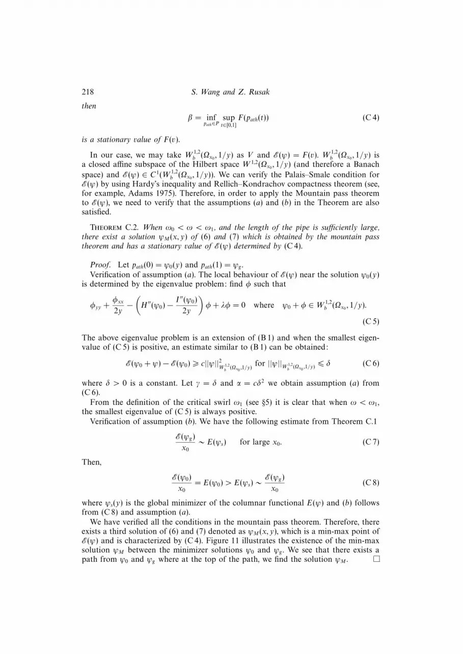
218 S. Wang and Z. Rusak
then
β = infpath∈P
supt∈[0,1]
F(path(t)) (C 4)
is a stationary value of F(v).
In our case, we may take W 1,2b (Ωx0
, 1/y) as V and E(ψ) = F(v). W 1,2b (Ωx0
, 1/y) isa closed affine subspace of the Hilbert space W 1,2(Ωx0
, 1/y) (and therefore a Banach
space) and E(ψ) ∈ C1(W 1,2b (Ωx0
, 1/y)). We can verify the Palais–Smale condition forE(ψ) by using Hardy’s inequality and Rellich–Kondrachov compactness theorem (see,for example, Adams 1975). Therefore, in order to apply the Mountain pass theoremto E(ψ), we need to verify that the assumptions (a) and (b) in the Theorem are alsosatisfied.
Theorem C.2. When ω0 < ω < ω1, and the length of the pipe is sufficiently large,there exist a solution ψM(x, y) of (6) and (7) which is obtained by the mountain passtheorem and has a stationary value of E(ψ) determined by (C 4).
Proof. Let path(0) = ψ0(y) and path(1) = ψg .Verification of assumption (a). The local behaviour of E(ψ) near the solution ψ0(y)
is determined by the eigenvalue problem: find φ such that
φyy +φxx
2y−(H ′′(ψ0)−
I ′′(ψ0)
2y
)φ+ λφ = 0 where ψ0 + φ ∈W 1,2
b (Ωx0, 1/y).
(C 5)
The above eigenvalue problem is an extension of (B 1) and when the smallest eigen-value of (C 5) is positive, an estimate similar to (B 1) can be obtained:
E(ψ0 + ψ)− E(ψ0) > c||ψ||2W 1,2
b(Ωx0
,1/y)for ||ψ||W 1,2
b(Ωx0
,1/y) 6 δ (C 6)
where δ > 0 is a constant. Let γ = δ and α = cδ2 we obtain assumption (a) from(C 6).
From the definition of the critical swirl ω1 (see §5) it is clear that when ω < ω1,the smallest eigenvalue of (C 5) is always positive.
Verification of assumption (b). We have the following estimate from Theorem C.1
E(ψg)
x0
∼ E(ψs) for large x0. (C 7)
Then,
E(ψ0)
x0
= E(ψ0) > E(ψs) ∼E(ψg)
x0
(C 8)
where ψs(y) is the global minimizer of the columnar functional E(ψ) and (b) followsfrom (C 8) and assumption (a).
We have verified all the conditions in the mountain pass theorem. Therefore, thereexists a third solution of (6) and (7) denoted as ψM(x, y), which is a min-max point ofE(ψ) and is characterized by (C 4). Figure 11 illustrates the existence of the min-maxsolution ψM between the minimizer solutions ψ0 and ψg . We see that there exists apath from ψ0 and ψg where at the top of the path, we find the solution ψM .

The dynamics of swirling flow in a pipe 219
Appendix D. Properties of the min-max solution ψM(x, y)
The solution ψM(x, y) is obtained in a rather abstract frame. We need to discussthis solution in more detail. We first show the following basic estimate
Theorem D.1.
E(ψM)
E(ψ0)→ 1 as x0 →∞, (D 1)
where x0 is the length of the pipe.
Proof. Let ψMx01be the mountain pass solution for Ωx01
where x01 is a pipe lengththat is different from x0. Let path(t) be a path which satisfies
E(ψMx01) 6 max
t∈[0,1]E(path(t)) < E(ψMx01
) + ε. (D 2)
According to Theorem C.1, such a path always exists when ω0 < ω < ω1. Now, forΩx01
with x0 > x01, we construct the following path:
path(t) =
ψ0 when 0 < x < x0 − x01,path(t)(x− (x0 − x01)), y) when x0 − x01 6 x 6 x0.
(D 3)
Notice that when x0−x01 6 x 6 x0, 0 6 x−(x0−x01) 6 x0 thus path(t)(x−(x0−x01), y)is well defined. Clearly, path(0) = ψ0 on Ωx0
and E(path(0)) 6 E(path(1)) from the factthat E(path(1)) 6 E(path(0)). Therefore, path(t) is an eligible path. Denote ψMx0
as themountain pass solution for Ωx0
. Then, from (D 2) we find
E(ψMx0) 6 max
t∈[0,1]E(path(t)) = (x0 − x01)E(ψ0) + max
t∈[0,1]E(path(t))
6 (x0 − x01)E(ψ0) + E(ψMx01) + ε. (D 4)
Dividing (D 4) by E(ψ0), we have
E(ψMx0)
E(ψ0)=E(ψMx0
)
x0E(ψ0)6
(1− x01
x0
)+E(ψMx01
)
x0E(ψ0)+ ε.
Now let x0 → ∞, we get E(ψMx0)/E(ψ0) 6 1. However, since E(ψ0) < E(ψMx0
), weobtain (D 1).
We now compare the behaviour of the min-max solution ψM(x, y) with that of theglobal minimizer solution ψg(x, y). As we have seen in Theorem B 1, we can estimateE(ψg)/x0 ∼ E(ψs) as x0 tends to infinity. From this estimate we can demonstrate thatthe solution ψg(x, y) is dominated, except for a finite transition region near the pipeinlet, by a long region where the flow is close to the columnar state ψs(y) (see figure8). However, the estimate in Theorem D 1 that E(ψM)/x0 ∼ E(ψ0) as x0 tends toinfinity, shows that the min-max solution is dominated by a long region, starting fromthe inlet, where the flow is close to the columnar state ψ0(y) (see figure 12). From theinlet condition ψM(0, y) = ψ0(y) we find that ψMx(0, y) is small and when x0 → ∞ itvanishes. Therefore, a columnar state is established at the inlet when x0 →∞.
Let ψm = ψM(x0, y). Then, from the flow force balance (15) we find that as the pipe
length becomes larger, E(ψ0) −∫ 1/2
0(ψ2
Mx(0, y)/4y)dy = E(ψm(y)). Thus, E(ψm(y)) isslightly less than E(ψ0) and so ψm(y) is not close to a columnar solution of (9) and(10), except when ω tends to ω0, where ψm(y) tends to ψK(y).
We now describe the min-max solution ψM(x, y) of (6) and (7) (see figure 12). At
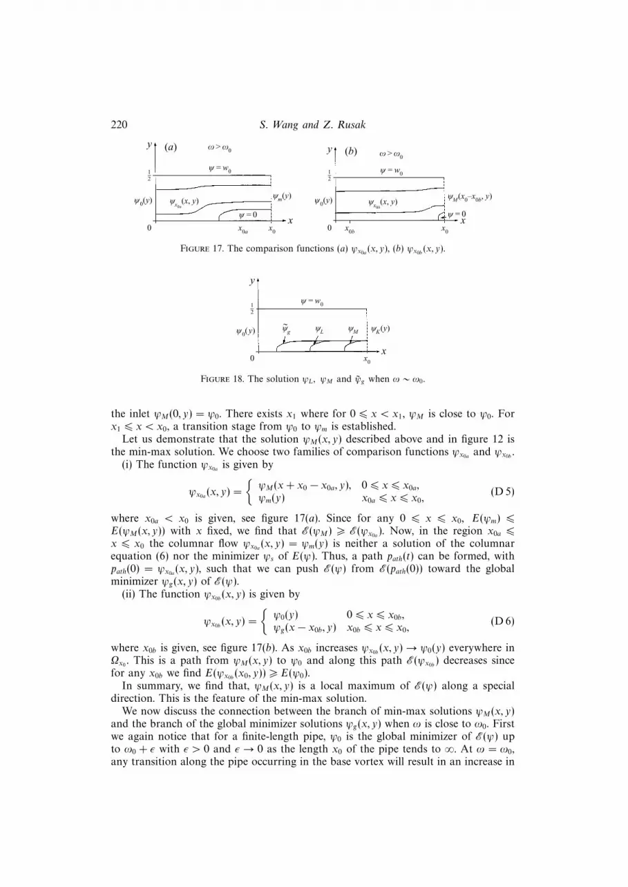
220 S. Wang and Z. Rusak
0
ψ0(y)
ψ = 0x
y
x0
ψx0a(x, y)
ψ = w0
ψm(y)
12
(a)
x0a
ω > ω0
0
ψ0(y)
ψ = 0x
y
x0
ψx0b(x, y)
ψ = w0
ψM(x0–x0b, y)
12
(b)
x0b
ω > ω0
Figure 17. The comparison functions (a) ψx0a(x, y), (b) ψx0b
(x, y).
0
ψ0(y)
x
y
x0
ψ = w0
ψK(y)
12
ψMψLψg∼
Figure 18. The solution ψL, ψM and ψg when ω ∼ ω0.
the inlet ψM(0, y) = ψ0. There exists x1 where for 0 6 x < x1, ψM is close to ψ0. Forx1 6 x < x0, a transition stage from ψ0 to ψm is established.
Let us demonstrate that the solution ψM(x, y) described above and in figure 12 isthe min-max solution. We choose two families of comparison functions ψx0a
and ψx0b.
(i) The function ψx0ais given by
ψx0a(x, y) =
ψM(x+ x0 − x0a, y), 0 6 x 6 x0a,ψm(y) x0a 6 x 6 x0,
(D 5)
where x0a < x0 is given, see figure 17(a). Since for any 0 6 x 6 x0, E(ψm) 6E(ψM(x, y)) with x fixed, we find that E(ψM) > E(ψx0a
). Now, in the region x0a 6x 6 x0 the columnar flow ψx0a
(x, y) = ψm(y) is neither a solution of the columnarequation (6) nor the minimizer ψs of E(ψ). Thus, a path path(t) can be formed, withpath(0) = ψx0a
(x, y), such that we can push E(ψ) from E(path(0)) toward the globalminimizer ψg(x, y) of E(ψ).
(ii) The function ψx0b(x, y) is given by
ψx0b(x, y) =
ψ0(y) 0 6 x 6 x0b,ψg(x− x0b, y) x0b 6 x 6 x0,
(D 6)
where x0b is given, see figure 17(b). As x0b increases ψx0b(x, y)→ ψ0(y) everywhere in
Ωx0. This is a path from ψM(x, y) to ψ0 and along this path E(ψx0b
) decreases sincefor any x0b we find E(ψx0b
(x0, y)) > E(ψ0).In summary, we find that, ψM(x, y) is a local maximum of E(ψ) along a special
direction. This is the feature of the min-max solution.We now discuss the connection between the branch of min-max solutions ψM(x, y)
and the branch of the global minimizer solutions ψg(x, y) when ω is close to ω0. Firstwe again notice that for a finite-length pipe, ψ0 is the global minimizer of E(ψ) upto ω0 + ε with ε > 0 and ε→ 0 as the length x0 of the pipe tends to ∞. At ω = ω0,any transition along the pipe occurring in the base vortex will result in an increase in
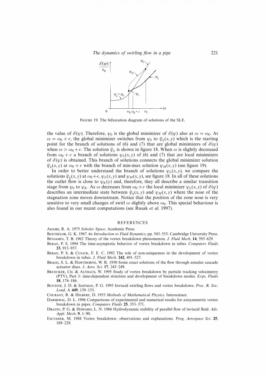
The dynamics of swirling flow in a pipe 221
ψ0
ψM
ψg
%(ψ)x0
ψL
ω1ω0
ψg = ψ0
ω0 ω0 + ε
Figure 19. The bifurcation diagram of solutions of the SLE.
the value of E(ψ). Therefore, ψ0 is the global minimizer of E(ψ) also at ω = ω0. Atω = ω0 + ε, the global minimizer switches from ψ0 to ψg(x, y) which is the startingpoint for the branch of solutions of (6) and (7) that are global minimizers of E(ψ)when ω > ω0 + ε. The solution ψg is shown in figure 18. When ω is slightly decreasedfrom ω0 + ε a branch of solutions ψL(x, y) of (6) and (7) that are local minimizersof E(ψ) is obtained. This branch of solutions connects the global minimizer solutionψg(x, y) at ω0 + ε with the branch of min-max solution ψM(x, y) (see figure 19).
In order to better understand the branch of solutions ψL(x, y), we compare thesolutions ψg(x, y) at ω0+ε, ψL(x, y) and ψM(x, y), see figure 18. In all of these solutionsthe outlet flow is close to ψK(y) and, therefore, they all describe a similar transitionstage from ψ0 to ψK . As ω decreases from ω0 + ε the local minimizer ψL(x, y) of E(ψ)describes an intermediate state between ψg(x, y) and ψM(x, y) where the nose of thestagnation zone moves downstream. Notice that the position of the zone nose is verysensitive to very small changes of swirl ω slightly above ω0. This special behaviour isalso found in our recent computations (see Rusak et al. 1997).
REFERENCES
Adams, R. A. 1975 Sobolev Space. Academic Press.
Batchelor, G. K. 1967 An Introduction to Fluid Dynamics, pp. 543–555. Cambridge University Press.
Benjamin, T. B. 1962 Theory of the vortex breakdown phenomenon. J. Fluid Mech. 14, 593–629.
Beran, P. S. 1994 The time-asymptotic behavior of vortex breakdown in tubes. Computers Fluids23, 913–937.
Beran, P. S. & Culick, F. E. C. 1992 The role of non-uniqueness in the development of vortexbreakdown in tubes. J. Fluid Mech. 242, 491–527.
Bragg, S. L. & Hawthorne, W. R. 1950 Some exact solutions of the flow through annular cascadeactuator discs. J. Aero. Sci. 17, 243–249.
Bruecker, Ch. & Althaus, W. 1995 Study of vortex breakdown by particle tracking velocimetry(PTV), Part 3: time-dependent structure and development of breakdown modes. Exps. Fluids18, 174–186.
Buntine, J. D. & Saffman, P. G. 1995 Inviscid swirling flows and vortex breakdown. Proc. R. Soc.Lond. A 449, 139–153.
Courant, R. & Hilbert, D. 1953 Methods of Mathematical Physics. Interscience.
Darmofal, D. L. 1996 Comparisons of experimental and numerical results for axisymmetric vortexbreakdown in pipes. Computers Fluids 25, 353–371.
Drazin, P. G. & Howard, L. N. 1966 Hydrodynamic stability of parallel flow of inviscid fluid. Adv.Appl. Mech. 9, 1–90.
Escudier, M. 1988 Vortex breakdown: observations and explanations. Prog. Aerospace Sci. 25,189–229.
222 S. Wang and Z. Rusak
Escudier, M. P. & Keller, J. J. 1983 Vortex breakdown: a two stage transition. AGARD CP 342,pp. 251–258.
Fraenkel, L. E. 1956 On the flow of rotating fluid past bodies in a pipe. Proc. R. Soc. Lond. A 233,506–526.
Gilbarg, D. & Trudinger, N. 1983 Elliptic Partial Differential Equations of Second Order.Springer.
Hall, M. G. 1967 A new approach to vortex breakdown. Proc. Heat Transfer and Fluid MechanicsInstitute, Univ. of California, San Diego, La Jolla, pp. 319–340.
Hall, M. G. 1972 Vortex breakdown. Ann. Rev. Fluid Mech. 4, 195–217.
Howard, L. N. & Gupta, A. S. 1962 On the hydrodynamic and hydromagnetic stability of swirlingflows. J. Fluid Mech. 14, 463–476.
Ioos, G. & Joseph, D. 1980 Elementary Stability and Bifurcation Theory. Springer.
Keller, J. J. 1995 On the interpretation of vortex breakdown. Phys. Fluids 7, 1695–1702.
Keller, J. J., Egli, W. & Exley, W. 1985 Force- and loss-free transitions between flow states. Z.Angew. Math. Phys. 36, 854–889.
Kufner, A. 1983 Weighted Sobolev Space. John Wiley & Son.
Lambourne, N. C. & Bryer, D. W. 1962 The bursting of leading-edge vortices-some observationsand discussion of the phenomenon. Aeronaut. Res. Counc. R & M 3282, pp. 1–36.
Leibovich, S. 1978 The structure of vortex breakdown. Ann. Rev. Fluid Mech. 10, 221–246.
Leibovich, S. 1984 Vortex stability and breakdown: survey and extension. AIAA J. 22, 1192–1206.
Leibovich, S. & Kribus, A. 1990 Large amplitude wavetrains and solitary waves in vortices. J.Fluid Mech. 216, 459–504.
Leibovich, S. & Stewartson, K. 1983 A sufficient condition for the instability of columnar vortices.J. Fluid Mech. 126, 335–356.
Lessen, H., Singh, P. J. & Paillet, F. 1974 The stability of a trailing line vortex. Part 1. Inviscidtheory. J. Fluid Mech. 63, 753–763.
Long, R. R. 1953 Steady motion around a symmetrical obstacle moving along the axis of a rotatingliquid. J. Met. 10, 197–203.
Lopez, J. M. 1994 On the bifurcation structure of axisymmetric vortex breakdown in a constrictedpipe. Phys. Fluids 6, 3683–3693.
Malkiel, E., Cohen, J., Rusak, Z. & Wang, S. 1996 Axisymmetric vortex breakdown in a pipe-theoretical and experimental studies. Proc. 36th Israel Annual Conf. on Aerospace Sciences(February), pp. 24–34.
Peckham, D. H. & Atkinson, S. A. 1957 Preliminary results of low speed wind tunnel tests on agothic wing of aspect ratio 1.0. Aeronaut. Res. Counc. C P 508.
Randall, J. D. & Leibovich, S. 1973 The critical state: a trapped wave model of vortex breakdown.J. Fluid Mech. 53, 481–493.
Rayleigh, Lord 1916 On the dynamics of revolving fluids. Proc. R. Soc. Lond. A 93, 148–154.
Rusak, Z., Wang, S. & Whiting, C. H. 1996 Numerical computations of axisymmetric vortexbreakdown in a pipe. AIAA Paper 96-0801.
Rusak, Z., Whiting, C. H. & Wang, S. 1997 Axisymmetric breakdown of a Q-vortex in a pipe.AIAA Paper 97-0441.
Salas, M. D. & Kuruvila, G. 1989 Vortex breakdown simulation: a circumspect study of thesteady, laminar, axisymmetric model. Computers Fluids 17, 247–262.
Sarpkaya, T. 1971 On stationary and traveling vortex breakdowns. J. Fluid Mech. 45, 545–559.
Sarpkaya, T. 1995 Vortex breakdown and turbulence. AIAA Paper 95-0433.
Squire, H. B. 1956 Rotating fluids. In Surveys in Mechanics (ed. G. K. Batchelor & R. M. Davies),pp. 139–161. Cambridge University Press.
Squire, H. B. 1960 Analysis of the vortex breakdown phenomenon. Miszallaneen der AngewandtenMechanik, pp. 306–312. Berlin: Akademie.
Struwe, M. 1990 Variational Methods: Applications to Nonlinear Partial Differential Equations andHamiltonian Systems. Springer.
Szeri, A. & Holmes, P. 1988 Nonlinear stability of axisymmetric swirling flows. Phil. Trans. R. Soc.Lond. A 326, 327–354.
Wang, S. & Rusak, Z. 1996a On the stability of an axisymmetric rotating flow. Phys. Fluids 8,1007–1016.
The dynamics of swirling flow in a pipe 223
Wang, S. & Rusak, Z. 1996b On the stability of non-columnar swirling flows. Phys. Fluids 8,1017–1023.
Wang, S. & Rusak, Z. 1997 The effect of slight viscosity on near critical swirling flows. Phys. Fluids(submitted).
Ziemer, W. P. 1989 Weakly Differentiable Functions. Springer.