numerical simulation of the dynamics of turbulent swirling
TRANSCRIPT
Technische Universität MünchenInstitut für Energietechnik
Lehrstuhl für Thermodynamik
Numerical Simulation of the Dynamics of TurbulentSwirling Flames
Luis Roberto Tay Wo Chong Hilares
Vollständiger Abdruck der von der Fakultät für Maschinenwesen derTechnischen Universität München zur Erlangung des akademischen Gradeseines
DOKTOR – INGENIEURS
genehmigten Dissertation.
Vorsitzender:Univ.-Prof. Rafael Macián-Juan, Ph.D.
Prüfer der Dissertation:1. Univ.-Prof. Wolfgang Polifke, Ph.D. (CCNY)2. Assoc. Prof. Thierry Schuller, Ph.D.École Centrale Paris / Frankreich
Die Dissertation wurde am 06.12.2011 bei der Technischen Universität München eingereicht
und durch die Fakultät für Maschinenwesen am 23.01.2012 angenommen.

Acknowledgments
The present work was accomplished at the Lehrstuhl für Thermodynamik atthe Technische Universität München from October 2006 to December 2011.The work was financially supported by my scholarship from the DeutscherAkademischer Austauschdienst (DAAD) from October 2006 to March 2010,and by the Lehrstuhl für Thermodynamik and the Loschge-Studienstiftungfrom April 2010.
First of all, I would like to express my special gratitude to my advisorProf. Wolfgang Polifke for giving me the opportunity to work at the Lehrstuhlfür Thermodynamik, for his continuous support since my scholarship appli-cation, and for his trust and advices on my work. I would like to thankProf. Thierry Schuller for being the co-examiner of the thesis and for his su-pport in reviewing my work; and to Prof. Rafael Macián-Juan for organizingand being the chairman of the thesis committee.
I am indebted to my colleagues Thomas Komarek, Stephan Föller, Dr. An-dreas Huber, Dr. Roland Kaess, Martin Hauser, Mathieu Zellhuber, Robert Le-andro, Sebastian Bomberg and Ahtsham Ulhaq who supported me during thisproject. A special thanks to Thomas for providing the experimental data forthis work. Also, I would like to thank Mathieu Zellhuber, Anja Marosky, Flo-rian Ettner, Ralf Blumental and Marek Czapp for their support in the transla-tions into German of the required documentations to submit this thesis; to myoffice colleagues Karin Stehlik, Anton Winkler, Florian Ettner, Klaus Vollmer,Ahtsham Ulhaq and Stephan Föller for the very nice work atmosphere; toMrs. Helga Bassett and Mrs. Sigrid Schulz-Reichwald for their support on ad-ministrative issues; to Dr. Joao Carneiro for the nice time during our lunchbreaks and his support on the cluster; to CERFACS for making available thecode AVBP for my simulations; to the Leibniz-Rechenzentrum (LRZ) with theproject PR32FO for letting me use their computational resources; and finallyto all my colleagues at the Lehrstuhl für Thermodynamik for the great timeand support.
Finally, I wish to thank Dr. Holger Lübcke, who introduced me on the field of
iii
gas turbine combustion during my internship in ALSTOM Power Switzerland;to Octavian Stinga and Maria Dumitrescu, with whom I lived during my stayin Munich, for all their support during this time; to Melanie Portz for all thenice time and your support, pio; and to my family, who helped me in all senseto reach this goal. Gracias Totales!
Munich, in February 2012 Luis Tay Wo Chong Hilares
iv

Abstract
The flame dynamics of a perfectly premixed axial swirl burner is investigated.The study is based on large eddy simulations (LES) of compressible reactingflow in combination with system identification (SI). The unit impulse respon-se and the transfer function of turbulent swirling flames at various operatingconditions are determined. The LES/SI approach is validated against expe-riment, showing the capability of detecting the impact of variations in ther-mal boundary conditions, power rating, combustor confinement and swirlerposition on flame dynamics. Stability limits are analyzed with a low-orderthermoacoustic network model. Results indicate that the flame transfer func-tion obtained from single burner combustors should only be used for stabilityanalysis of multi-burner gas turbines provided that boundary conditions andcombustor geometries are equivalent.
v
Zusammenfassung
Die Dynamik von perfekt vorgemischten Flammen in einem axialen Drall-brenner wurde untersucht. Die Studie erfolgte anhand von Grobstruktursim-ulation (LES) kompressibler reaktiver Strömungen in Kombination mit Sys-temidentifikationsmethoden (SI). Einheitsimpulsantworten und Flammen-transferfunktion von turbulenten Drallflammen konnten damit bei unter-schiedlichen Betriebsbedingungen bestimmt werden. Der LES/SI Ansatzwurde experimentell validiert und eignet sich somit für die Untersuchung derAuswirkungen von unterschiedlichen thermischen Randbedingungen, Leis-tung, Brennkammergröße und Drallerzeuger-Position auf die Flammendy-namik. Stabilitätsgrenzen wurden mit einem Netzwerk-Modell ermittelt. DieErgebnisse zeigen, dass Flammentransferfunktionen, die an Einzelbrennerngewonnen wurden, zur Stabilitätsanalyse in Mehrbrenner-Brennkammernnur dann verwendet werden sollten, wenn die Randbedingungen undBrennkammerabmessungen gleichwertig sind.
vi
Contents
1 Introduction 11.1 Combustion Instabilities . . . . . . . . . . . . . . . . . . . . . . . . 31.2 Overview of the Thesis . . . . . . . . . . . . . . . . . . . . . . . . . 7
2 Turbulent Reacting Flows 92.1 Turbulence . . . . . . . . . . . . . . . . . . . . . . . . . . . . . . . . 92.2 The Energy Spectrum and Turbulent Length Scales . . . . . . . . 11
2.2.1 Turbulence Modelling Approaches . . . . . . . . . . . . . . 142.3 Turbulent Premixed Combustion . . . . . . . . . . . . . . . . . . . 17
2.3.1 Combustion Regimes in Turbulent Premixed Combustion 192.4 Turbulent Premixed Combustion Modeling using LES . . . . . . 21
2.4.1 LES Filtering . . . . . . . . . . . . . . . . . . . . . . . . . . . 232.4.2 Fundamental Transport Equations for LES Reacting Flows 24
2.4.2.1 Modeling of Subgrid Terms . . . . . . . . . . . . . 262.4.2.1.1 SGS Turbulent Viscosity Models . . . . . 27
2.4.2.2 Source Terms . . . . . . . . . . . . . . . . . . . . . 292.4.3 LES Premixed Combustion Models . . . . . . . . . . . . . 29
2.4.3.1 Thickened Flame Combustion Model . . . . . . . 302.4.3.2 Dynamically Thickened Flame Combustion Model 32
3 Response of Premixed Flames to Velocity Disturbances 343.1 The Flame Transfer Function . . . . . . . . . . . . . . . . . . . . . 353.2 Determination of the Flame Transfer Function . . . . . . . . . . . 373.3 Additional Parameters Influencing the Flame Response in Pre-
mixed Flames . . . . . . . . . . . . . . . . . . . . . . . . . . . . . . 413.3.1 Influence of Combustor Thermal Boundary Conditions . 433.3.2 Influence of Confinement Ratio . . . . . . . . . . . . . . . 45
vii
CONTENTS
3.3.3 Influence of Swirler Position . . . . . . . . . . . . . . . . . 463.4 Model of Impulse and Frequency Responses to Axial Velocity
and Swirl Fluctuations . . . . . . . . . . . . . . . . . . . . . . . . . 48
4 System Identification 514.1 Background . . . . . . . . . . . . . . . . . . . . . . . . . . . . . . . 514.2 The Wiener Filter . . . . . . . . . . . . . . . . . . . . . . . . . . . . 564.3 The LES/SI Method . . . . . . . . . . . . . . . . . . . . . . . . . . . 60
5 Identification of Flame Transfer Functions using LES/SI 635.1 Experimental Set-up of the BRS Burner . . . . . . . . . . . . . . . 635.2 Reference Case with 30 kW of Power Rating . . . . . . . . . . . . . 65
5.2.1 Numerical Set-up and Boundary Conditions . . . . . . . . 655.2.2 Comparison of Mean Flame Heat Release from LES and
Experiments . . . . . . . . . . . . . . . . . . . . . . . . . . . 675.2.3 Comparison of Identified and Experimental Flame Trans-
fer Function with 30 kW . . . . . . . . . . . . . . . . . . . . 685.2.4 Comparison of Different Excitation Amplitude on Flame
Transfer Function Identification . . . . . . . . . . . . . . . 735.3 Influence of Variation in Power Rating on the Flame Transfer
Function . . . . . . . . . . . . . . . . . . . . . . . . . . . . . . . . . 755.3.1 Comparison of Mean Flow Field and Flame Heat Release
from LES and Experiments at 50 kW . . . . . . . . . . . . . 755.3.2 Comparison of Identified and Experimental Flame Trans-
fer Function with 50 kW . . . . . . . . . . . . . . . . . . . . 815.4 Influence of Thermal Boundary Conditions at the Combustor
Wall on the Flame Transfer Function . . . . . . . . . . . . . . . . . 895.4.1 Instantaneous Reaction Rate, Temperature and Axial Ve-
locity . . . . . . . . . . . . . . . . . . . . . . . . . . . . . . . 895.4.2 Mean Heat Release, Flow Field and Temperature . . . . . 915.4.3 Comparison of Identified Flame Transfer Functions . . . 93
5.5 Influence of Swirler Position on the Flame Transfer Function . . 945.5.1 Mean Flow Field and Heat Release . . . . . . . . . . . . . . 975.5.2 Comparison of Identified and Experimental Flame Trans-
fer Function with Varied Swirler Position . . . . . . . . . . 98
viii
CONTENTS
5.6 Influence of Combustor Confinement on the Flame TransferFunction . . . . . . . . . . . . . . . . . . . . . . . . . . . . . . . . . 1055.6.1 Mean Flow Field and Heat Release . . . . . . . . . . . . . . 1065.6.2 Comparison of Flame Transfer Functions . . . . . . . . . . 109
5.7 Flame Transfer Function Model . . . . . . . . . . . . . . . . . . . . 1115.7.1 Dependence of Unit Impulse Responses on Thermal Con-
ditions, Combustor Confinement and Power Rating . . . 1125.7.2 Comparison of Unit Impulse Responses with Swirler at
Varied Positions . . . . . . . . . . . . . . . . . . . . . . . . . 114
6 Stability Analysis with Low-Order Network Models 1226.1 Linear Acoustic 1D Equations . . . . . . . . . . . . . . . . . . . . . 1226.2 Low-order Network Models . . . . . . . . . . . . . . . . . . . . . . 125
6.2.1 Flame Transfer Matrix of a Compact Flame . . . . . . . . . 1266.2.2 Use of Experimental Data in Eigenfrequency Analysis
(The UIR Method) . . . . . . . . . . . . . . . . . . . . . . . 1276.3 Stability Analysis of the System . . . . . . . . . . . . . . . . . . . . 128
6.3.1 Network Model of the System . . . . . . . . . . . . . . . . . 1286.4 Results of the Stability Analysis . . . . . . . . . . . . . . . . . . . . 130
7 Summary and Conclusions 135
8 Outlook 139
A Appendices 165A.1 The Rayleigh Criterion . . . . . . . . . . . . . . . . . . . . . . . . . 165A.2 Laminar Flame Reaction Kinetics . . . . . . . . . . . . . . . . . . 166A.3 One Step Reaction Mechanism for Methane-air Mixtures . . . . 168A.4 Derivation of the Turbulent Kinetic Energy Spectrum . . . . . . . 169A.5 Generation of Signals for LES/SI . . . . . . . . . . . . . . . . . . . 170A.6 Derivation of the Linearized Acoustic Equations . . . . . . . . . . 173A.7 Description of Elements in the Network Model . . . . . . . . . . 175
A.7.1 Constant Section Duct . . . . . . . . . . . . . . . . . . . . . 175A.7.2 Flame Transfer Matrix of a Compact Flame with a Differ-
ent Reference Location . . . . . . . . . . . . . . . . . . . . . 176A.7.3 Area change . . . . . . . . . . . . . . . . . . . . . . . . . . . 178
ix
CONTENTS
A.7.4 Inlet . . . . . . . . . . . . . . . . . . . . . . . . . . . . . . . . 180A.7.5 Outlet . . . . . . . . . . . . . . . . . . . . . . . . . . . . . . . 180A.7.6 Swirler . . . . . . . . . . . . . . . . . . . . . . . . . . . . . . 181
A.8 FTF at Different Velocity Reference Position with 30 kW and 9.5%of Excitation Amplitude . . . . . . . . . . . . . . . . . . . . . . . . 181
A.9 Confidence Analysis of Flame Transfer Function . . . . . . . . . . 183A.10 Post-processing Tool for Line-of-sight Heat Release Integration
in Tecplot . . . . . . . . . . . . . . . . . . . . . . . . . . . . . . . . . 184A.10.1 Steps before running the Macro . . . . . . . . . . . . . . . 185A.10.2 Macro . . . . . . . . . . . . . . . . . . . . . . . . . . . . . . . 186
x
List of Figures
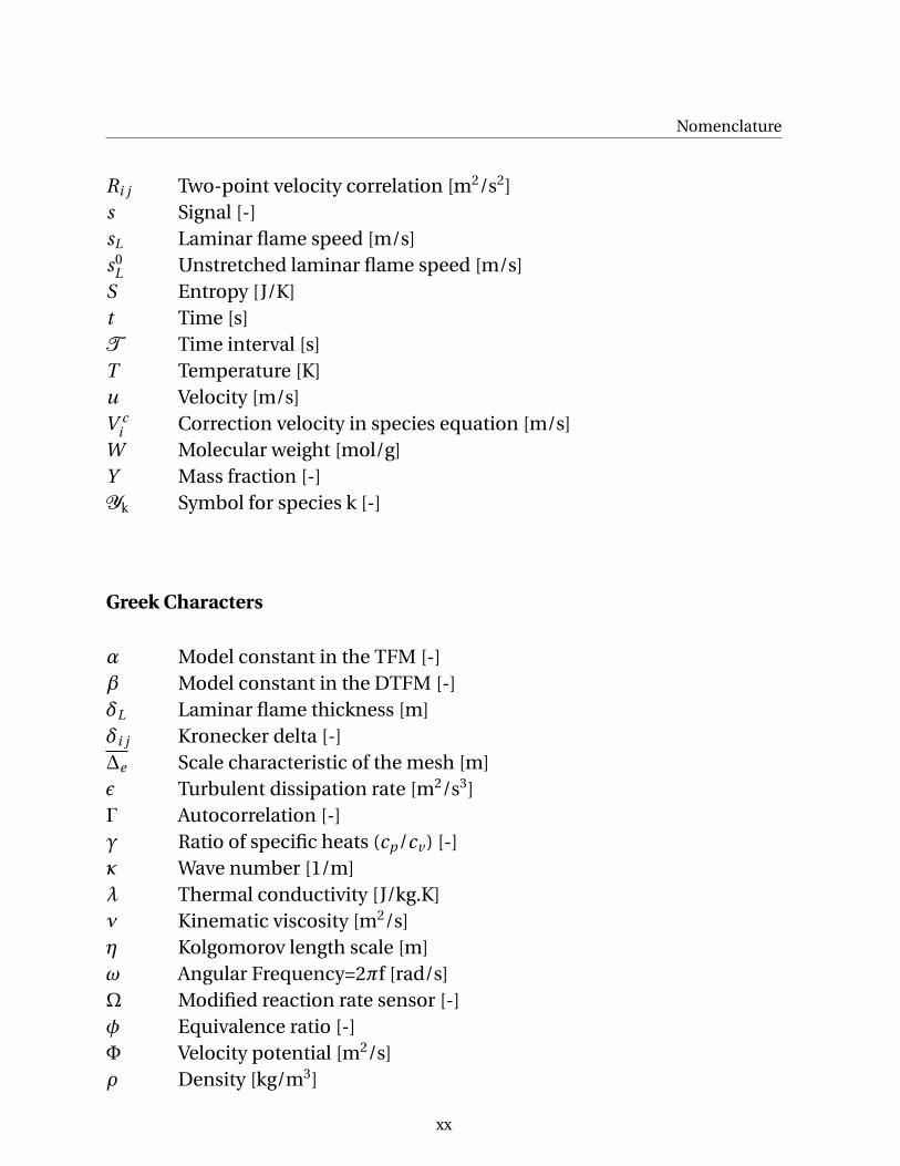
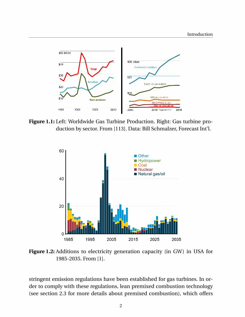
1.1 Left: Worldwide Gas Turbine Production. Right: Gas turbine pro-duction by sector. From [113]. Data: Bill Schmalzer, Forecast Int’l. 2
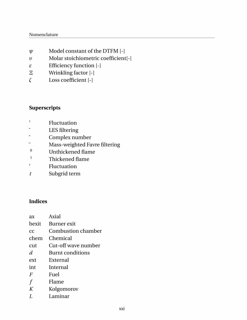
1.2 Additions to electricity generation capacity (in GW) in USA for1985-2035. From [1]. . . . . . . . . . . . . . . . . . . . . . . . . . . 2
1.3 Influence of temperature on NOx and CO emissions. From [118]. 3
1.4 Illustration of the feedback process responsible for combustioninstability in fully premixed conditions. Adapted from [223]. . . 4
1.5 Left: Damaged combustor liner [70], Right: Combustor damagecaused by high-frequency dynamics [185] . . . . . . . . . . . . . 4
2.1 Measurement of axial velocity on the center line of a turbulentjet. In [164] from the experiment of Tong and Warhaft [203]. . . . 10
2.2 Flow passing a sphere. Re=uD/ν=20000. Modified figure from[172]. Photograph by H. Werle. . . . . . . . . . . . . . . . . . . . . 12
2.3 Turbulent jets at different Reynolds numbers: (a) Low Reynoldsnumber, (b) High Reynolds number. Illustration from [201]. . . . 13
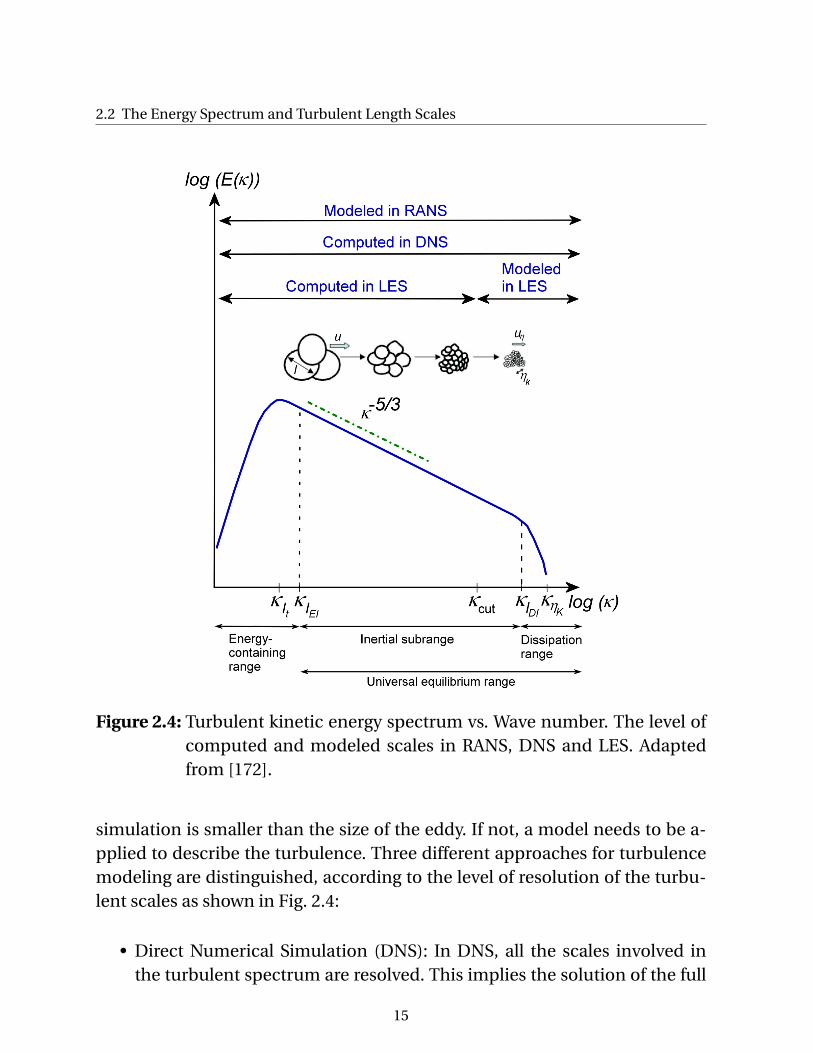
2.4 Turbulent kinetic energy spectrum vs. Wave number. The level ofcomputed and modeled scales in RANS, DNS and LES. Adaptedfrom [172]. . . . . . . . . . . . . . . . . . . . . . . . . . . . . . . . . 15
2.5 Structure of a laminar premixed flame. . . . . . . . . . . . . . . . 19
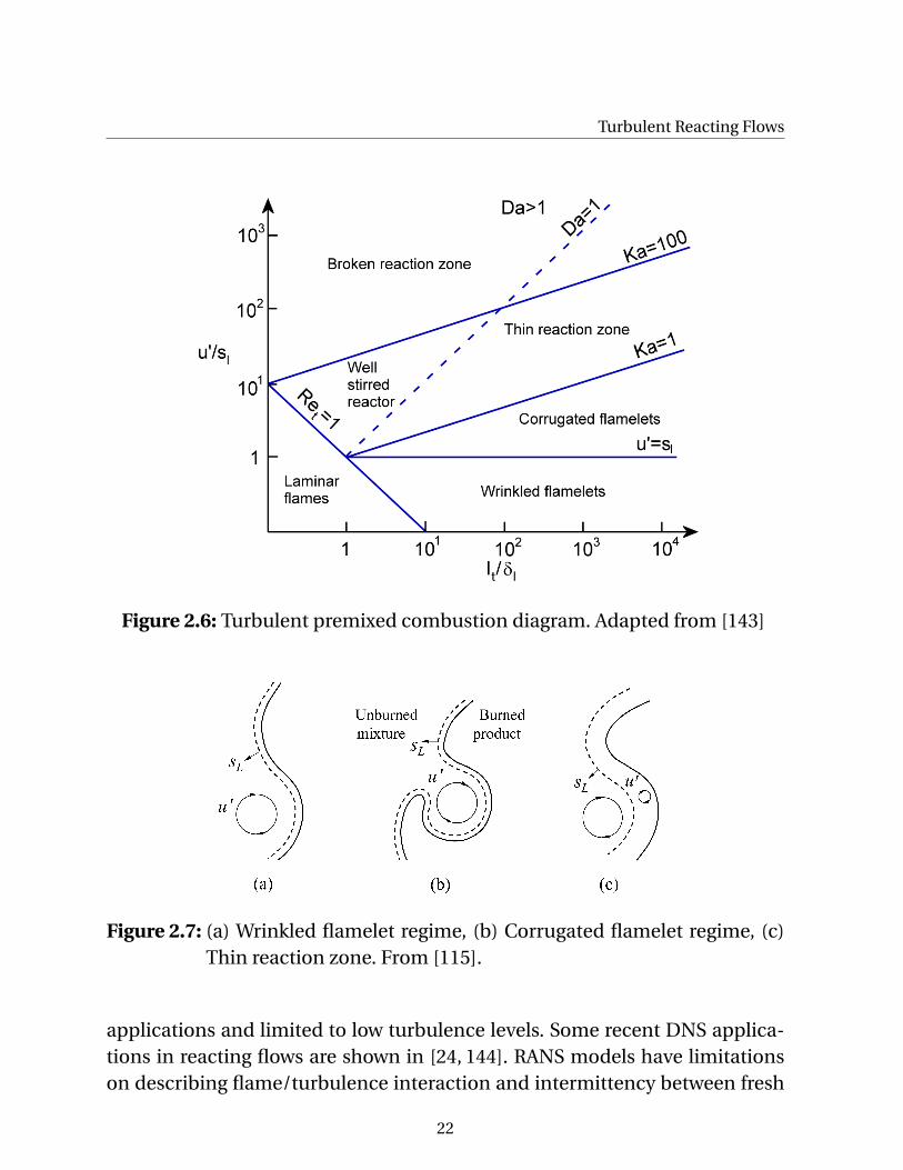
2.6 Turbulent premixed combustion diagram. Adapted from [143] . 22
2.7 (a) Wrinkled flamelet regime, (b) Corrugated flamelet regime, (c)Thin reaction zone. From [115]. . . . . . . . . . . . . . . . . . . . . 22
3.1 Overview of interaction mechanisms between heat release andacoustic waves in a fully premixed flame. Adapted from [153] . . 35
xi
LIST OF FIGURES
3.2 Scheme of determination of the flame transfer function withharmonic excitation. . . . . . . . . . . . . . . . . . . . . . . . . . . 38
4.1 Different types of systems. a)SISO, b)MIMO, c)SIMO andd)MISO. Adapted from [80]. . . . . . . . . . . . . . . . . . . . . . . 53
4.2 Unit Impulse Response of a FIR system. . . . . . . . . . . . . . . . 54
4.3 System for the Identification of the Flame Transfer Function . . 58
4.4 LES/System Identification process . . . . . . . . . . . . . . . . . . 61
5.1 Scheme of the BRS burner test rig. The sinter metal plate is ins-talled only for stability analysis. . . . . . . . . . . . . . . . . . . . 64
5.2 Scheme of the numerical set-up of the BRS burner . . . . . . . . 66
5.3 Normalized spatial heat release distribution: (a) OH chemilumi-nescence from experiments, (b) Averaged LES at nonadiabaticconditions, and (c) at adiabatic conditions. Line-of-sight inte-grated heat release for simulations. Dump plane of combustorat axial position = 0 m. . . . . . . . . . . . . . . . . . . . . . . . . . 69
5.4 Area normalized axial heat release distribution. . . . . . . . . . . 70
5.5 Flame transfer functions from experiments and LES/SI for casewith 30 kW. Excitation=6.5%. . . . . . . . . . . . . . . . . . . . . . 72
5.6 Heat release (Q ′) and acoustic velocity (u′r ) fluctuations at 0 and
70 mm upstream of the burner exit (Dump plane of combustorat z=0 mm) normalized by their mean values without filtering forcase with 30 kW. . . . . . . . . . . . . . . . . . . . . . . . . . . . . . 73
5.7 Power spectrum of acoustic velocity (u′r ) fluctuations at 0 and
70 mm upstream of the burner exit and of heat release (Q ′)normalized by their mean values without filtering for case with30 kW. . . . . . . . . . . . . . . . . . . . . . . . . . . . . . . . . . . . 74
5.8 Flame transfer functions from experiments and LES/SI for casewith 30 kW with different excitation amplitude. Harmonic exci-tation at 100 Hz for 6.5% () and 9.5% (M) of amplitude. . . . . . 76
5.9 Amplitudes from the pure-tone Fourier Transform for the nor-malized heat release and velocity fluctuations for 6.5% and 9.5%of excitation amplitude. . . . . . . . . . . . . . . . . . . . . . . . . 77
xii
LIST OF FIGURES
5.10 Mean axial velocity profiles with non-reacting flow (top) andwith reacting flow (bottom) at the middle cross plane shown inFig. 5.2 for 50 kW. o Experiments, - LES. Grey line to indicatezero-axial velocity. . . . . . . . . . . . . . . . . . . . . . . . . . . . 78
5.11 Contours of mean axial velocity (left) and velocity vectors (right)for non-reacting (top) and reacting (bottom) flow from simula-tions. Zero-axial velocity isolines in black (left) and yellow (right) 79
5.12 Turbulent kinetic energy profiles with non-reacting flow and re-acting flow from simulations at the middle cross plane shown inFig. 5.2 for 50 kW. . . . . . . . . . . . . . . . . . . . . . . . . . . . . 79
5.13 Normalized spatial heat release distribution for 50 kW: (a)OH chemiluminescence from experiments, (b) Averaged LES atnonadiabatic conditions, and (c) at adiabatic conditions. Line-of-sight integrated heat release for simulations. Dump plane ofcombustor at axial position = 0 m. . . . . . . . . . . . . . . . . . . 80
5.14 Area normalized axial heat release distribution for 50 kW. . . . . 81
5.15 Transversal mode on combustion chamber for 50 kW. Contoursof rms pressure at cross plane 10mm downstream the burner exit 81
5.16 Flame transfer function from experiments, LES/SI with a sin-gle time series (STS), multiple time series (MTS) and single jointtime series (SJTS) for 50 KW and different excitation amplitudes.(): Harmonic excitation at 160 Hz and 6.5% of amplitude. . . . 83
5.17 Heat release (Q ′) and acoustic velocity (u′r ) fluctuations at
70 mm upstream of the burner exit (Dump plane of combustorat z=0 mm) normalized by their mean values without filtering forcase with 50 kW. . . . . . . . . . . . . . . . . . . . . . . . . . . . . . 84
5.18 Snap shot of instantaneous absolute pressure and reaction rateat combustor middle cross plane during excitation with 50 kW.The time of the snap shot is indicated in Fig. 5.17. . . . . . . . . . 85
5.19 Illustration of single joint time series (SJTS) method . . . . . . . 86
5.20 Sequence of excitation signals in the single joint time series(SJTS) method for 50 kW and excitation=9.5% amplitude of themean inlet velocity. . . . . . . . . . . . . . . . . . . . . . . . . . . . 87
xiii
LIST OF FIGURES
5.21 Instantaneous reaction rate, temperature and axial velocity withadiabatic (top) and nonadiabatic (bottom) combustor walls at50 kW of power rating, φ=0.77. Velocity vectors are included onthe temperature contours . . . . . . . . . . . . . . . . . . . . . . . 90
5.22 Contours of mean axial velocity (left) and mean temperaturewith velocity vectors (right) for the 30 kW case. Zero-axial veloc-ity isolines in black. . . . . . . . . . . . . . . . . . . . . . . . . . . 92
5.23 Mean axial velocity profiles of reacting flow at various axial po-sitions of the middle cross plane for adiabatic and nonadiabaticwall boundary conditions. 30 kW case. . . . . . . . . . . . . . . . 92
5.24 Flame transfer functions from LES/SI using adiabatic and nona-diabatic combustor walls with 30 kW. Harmonic excitation at100 Hz for adiabatic () and nonadiabatic (M) conditions arealso shown. Excitation=9.5%. . . . . . . . . . . . . . . . . . . . . . 93
5.25 Instantaneous reaction rate for one cycle of a harmonic exci-tation at 100 Hz using adiabatic and nonadiabatic combustorwalls with 30 kW. Excitation=9.5% U . . . . . . . . . . . . . . . . . 95
5.26 Scheme of the numerical set-up of the burner with differentswirler positions. . . . . . . . . . . . . . . . . . . . . . . . . . . . . 96
5.27 Contours of mean axial velocity at combustor middle crossplane and at position z=-5 mm with varied swirler positions.Zero-axial velocity isolines in black. . . . . . . . . . . . . . . . . . 97
5.28 Normalized spatial (left) and axial (right) heat release distribu-tion with varied swirler positions . . . . . . . . . . . . . . . . . . . 98
5.29 Flame transfer functions from LES/SI with the swirler at position1 and 2 from Fig. 5.26 with 30kW. Harmonic excitation at 100 ()and 160 Hz (M) are also shown. Excitation=9.5%. Experimentswith the swirler at position 2 in (o). . . . . . . . . . . . . . . . . . 100
5.30 BRS burner with axial swirler at position 2 without combustionchamber . . . . . . . . . . . . . . . . . . . . . . . . . . . . . . . . . 101
5.31 Normalized area averaged axial and tangential velocity fluctua-tions on a cross-section at z=-10 mm and z=-110 mm with har-monic excitation at 100 Hz. . . . . . . . . . . . . . . . . . . . . . . 103
xiv
LIST OF FIGURES
5.32 Area averaged tangential velocity on a cross-section at variouspositions with harmonic excitation at 100 Hz. . . . . . . . . . . . 103
5.33 Area averaged axial and tangential velocity fluctuations on across-section at at z=-10 mm and z=-110 mm with harmonic ex-citation at 100 Hz. . . . . . . . . . . . . . . . . . . . . . . . . . . . . 104
5.34 Area averaged swirl number fluctuations on a cross-section atz=-10 mm and z=-110 mm with harmonic excitation at 100 Hz. . 104
5.35 Contours of mean axial velocity (left) and velocity vectors (right):Combustor chamber with 160 x 160 mm of cross section (top),Combustor chamber with 90 x 90 mm of cross section (bottom).Zero-axial velocity isolines in black (left) and yellow (right) . . . 107
5.36 Mean axial velocity profiles with low and high confinementcombustors at various positions of the middle cross plane shownin Fig. 5.2. Grey line to indicate zero-axial velocity. . . . . . . . . 108
5.37 Mean tangential velocity profiles with low and high confinementcombustors at various positions of the middle cross plane shownin Fig. 5.2. . . . . . . . . . . . . . . . . . . . . . . . . . . . . . . . . 108
5.38 Turbulent kinetic energy profiles with low and high confinementcombustors at various positions of the middle cross plane shownin Fig. 5.2. . . . . . . . . . . . . . . . . . . . . . . . . . . . . . . . . 109
5.39 Normalized spatial heat release distribution for 30 kW: (Top)Combustor chamber with 160 x 160 mm of cross section (Bot-tom) Combustor chamber with 90 x 90 mm of cross section . . . 110
5.40 Area normalized axial heat release distribution with differentcombustor cross section. . . . . . . . . . . . . . . . . . . . . . . . 110
5.41 Flame transfer functions from LES/SI with low and high confine-ment combustors with 30 kW. Excitation=9.5%. . . . . . . . . . . 112
5.42 UIRs from time lag model. . . . . . . . . . . . . . . . . . . . . . . . 115
5.43 Flame transfer function from time lag model. . . . . . . . . . . . 116
5.44 UIR from modelled, experimental and identified FTF with 30 kWat varied swirler positions. . . . . . . . . . . . . . . . . . . . . . . . 117
5.45 Flame transfer function from LES/SI and time lag model for var-ied swirler positions with 30kW. . . . . . . . . . . . . . . . . . . . 118
5.46 UIR from time lag model for the experimental FTF at position 2. 120
xv
LIST OF FIGURES
5.47 FTFs from experiments and from the time lag model for the ex-perimental FTF at position 2. Experiments in (o) . . . . . . . . . 120
6.1 Acoustic wave propagation in fluid with mean flow. Adaptedfrom [48]. . . . . . . . . . . . . . . . . . . . . . . . . . . . . . . . . . 124
6.2 Scheme of a Low-order model. . . . . . . . . . . . . . . . . . . . . 125
6.3 UIR Method . . . . . . . . . . . . . . . . . . . . . . . . . . . . . . . 128
6.4 Low-order model of premix burner test rig. . . . . . . . . . . . . . 129
6.5 Downstream reflection coefficient used in network model . . . . 130
6.6 Eigenfrequencies and cycle increments using experimental andidentified FTF in the network model at various combustorlengths with 50 kW. (4) Unstable eigenfrequency in experiments. 132
6.7 Low-order model of premix burner test rig with swirler at posi-tion 2. . . . . . . . . . . . . . . . . . . . . . . . . . . . . . . . . . . . 134
A.1 Evaluation of Rayleigh Criterion with different absolute phasebetween pressure and heat fluctuations. . . . . . . . . . . . . . . 166
A.2 DRBS Input signals in time with different frequency limit. Range:1 to 20000 iterations . . . . . . . . . . . . . . . . . . . . . . . . . . 172
A.3 DRBS Input signals in time with different frequency limit. Range:1 to 2000 iterations . . . . . . . . . . . . . . . . . . . . . . . . . . . 172
A.4 Power spectrum of DRBS Input signals with different frequencylimit. . . . . . . . . . . . . . . . . . . . . . . . . . . . . . . . . . . . 173
A.5 Autocorrelation matrix of DRBS Input signals with different fre-quency limit. . . . . . . . . . . . . . . . . . . . . . . . . . . . . . . 173
A.6 Scheme for flame transfer matrix with a different velocity refe-rence position for the FTF. Adapted from [83]. . . . . . . . . . . . 178
A.7 Scattering Matrix of the swirler including length correction. . . . 182
A.8 Flame transfer functions for case with 30 kW with acoustic velo-city (u′
r ) fluctuations measured at 0 and 70 mm upstream of theburner exit (Dump plane of combustor at z=0 mm). Excitationamplitude=9.5%. Experiments for ur at 70 mm upstream of theburner exit in circles. . . . . . . . . . . . . . . . . . . . . . . . . . . 183
xvi

LIST OF FIGURES
A.9 Flame Transfer Function from experiments and LES/SI for30 kW. Top: Confidence analysis including a histogram of am-plitudes from LES/SI at 100 Hz for 1000 sequences . . . . . . . . 185
xvii
List of Tables
2.1 LES Combustion Models . . . . . . . . . . . . . . . . . . . . . . . . 30
5.1 Boundary Conditions . . . . . . . . . . . . . . . . . . . . . . . . . . 675.2 Time lag model . . . . . . . . . . . . . . . . . . . . . . . . . . . . . 1135.3 Time lag model for experimental FTF at position 2 . . . . . . . . 119
6.1 Network Model. . . . . . . . . . . . . . . . . . . . . . . . . . . . . . 1296.2 Stability behavior from experiments and using Network Model
(NM) with experimental FTF . . . . . . . . . . . . . . . . . . . . . 1316.3 Stability analysis using Network Model (NM) with identified FTFs 1326.4 Stability analysis using Network Model (NM) with identified FTFs 1336.5 Amplitude and phase at the unstable eigenfrequency with dif-
ferent conditions at 30 kW . . . . . . . . . . . . . . . . . . . . . . . 133
A.1 One Step Reaction Mechanism . . . . . . . . . . . . . . . . . . . . 168A.2 Schmid Number . . . . . . . . . . . . . . . . . . . . . . . . . . . . . 169
xviii
Nomenclature
Latin Characters
A Pre-exponential factor of Arrhenius reaction rate [1/s], Amplitude [-]a Speed of sound [m/s], coefficient in UIR model [-]⟨aT ⟩ Effective strain rate [1/s]c Crosscorrelation [-]cp Specific heat capacity at constant pressure [J/(Kg.K)]cv Specific heat capacity at constant volume [J/(Kg.K)]D th Thermal diffusivity [m2/s]E Total energy [J/kg]Ea Activation Energy [cal/kg]E(κ) Turbulent kinetic energy spectrum [m3/s2]f Frequency [Hz]F Thickening factor [-]G∆e
LES filter [1/m3]hs,k Sensible enthalpy of species k [J/kg]∆h0
f ,k Enthalpy of formation of species k at temperature T0 = 0 K [J/kg]
k Turbulent kinetic energy [m2/s2]kx Acoustic wave number [1/m]l Length [m]L Maximum index of the UIR coefficients [-]n Interaction Index [-]Q Heat release [W]r Radius [m], Response [-]R Universal gas constant [ J/(mol.K) ]
xix
Nomenclature
Ri j Two-point velocity correlation [m2/s2]s Signal [-]sL Laminar flame speed [m/s]s0
L Unstretched laminar flame speed [m/s]S Entropy [J/K]t Time [s]T Time interval [s]T Temperature [K]u Velocity [m/s]V c
i Correction velocity in species equation [m/s]W Molecular weight [mol/g]Y Mass fraction [-]Yk Symbol for species k [-]
Greek Characters
α Model constant in the TFM [-]β Model constant in the DTFM [-]δL Laminar flame thickness [m]δi j Kronecker delta [-]∆e Scale characteristic of the mesh [m]ε Turbulent dissipation rate [m2/s3]Γ Autocorrelation [-]γ Ratio of specific heats (cp/cv ) [-]κ Wave number [1/m]λ Thermal conductivity [J/kg.K]ν Kinematic viscosity [m2/s]η Kolgomorov length scale [m]ω Angular Frequency=2πf [rad/s]Ω Modified reaction rate sensor [-]φ Equivalence ratio [-]Φ Velocity potential [m2/s]ρ Density [kg/m3]
xx
Nomenclature
ψ Model constant of the DTFM [-]υ Molar stoichiometric coefficient[-]ε Efficiency function [-]Ξ Wrinkling factor [-]ζ Loss coefficient [-]
Superscripts
′ Fluctuation¯ LES filteringˆ Complex number˜ Mass-weighted Favre filtering0 Unthickened flame1 Thickened flame′ Fluctuationt Subgrid term
Indices
ax Axialbexit Burner exitcc Combustion chamberchem Chemicalcut Cut-off wave numberd Burnt conditionsext Externalint InternalF Fuelf FlameK KolgomorovL Laminar
xxi

Nomenclature
M MixtureMF Mass FlowO Oxidizerprop Propagationr Referencestoich StoichiometricS Swirlt Turbulenttan Tangentialu Unburnt conditionsλ Wave length
Abbreviations
C SC F Collection of Small Conical FlamesC F L Courant–Friedrichs–LewyDN S Direct Numerical SimulationDT F M Dynamically Thickened Flame ModelF AR Fuel–air ratioF DF Flame Describing FunctionF E M Finite Element MethodF I R Finite Impulse ResponseFV M Finite Volume MethodF T F Flame Transfer FunctionHC High ConfinementIC Initial ConditionLES Large Eddy SimulationLC Low ConfinementLOS Line-of-SightM I MO Multiple-Input Multiple-OutputM I SO Multiple-Input Single-OutputPT Pure toneP1 Position 1
xxii

Nomenclature
P2 Position 2R AN S Reynolds Averaged Navier-StokesSGS Sub-Grid ScaleSI System IdentificationSI SO Single-Input Single-OutputT F M Thickened Flame ModelU I R Unit Impulse Response
Non-dimentional Numbers
Da Damhkohler NumberKa Karlovitz NumberM Mach NumberPr Prandtl NumberRe Reynolds NumberSc Schmid Number
Scalar-vectors-tensors
u Scalaru Vectorui Component i of the vector u
Operators
⟨ ⟩ Reynolds averaging· Scalar productsign Sign function
xxiii

Nomenclature
xxiv
1 Introduction
Gas turbines have been used for energy production and jet propulsion fordecades. During this time, significant technological developments have beenachieved as the increase in efficiency1 [16], power output, thrust, etc. Evenunder the high prices of fuel, and the strong focus on renewable energy nowa-days, the gas turbine market has a strong projection as shown in Fig. 1.1.
In the energy production sector, combined cycle power plants present someadvantages [16] to other kind of generation systems based on nuclear, windor solar energy. They have low construction costs2, load flexibility, can be builtquickly, and are very efficient [16,92]. Fossil-fuel (especially natural gas) powerplants are expected to continue as one of the major generators of electricityinto the next decades (e.g., see Fig. 1.2 for the additions to electricity genera-tion capacity in USA by sources).
In the combustion process in gas turbines, combustion products such as car-bon dioxide (CO2) and pollutants (as carbon monoxide (CO), oxides of nitro-gen (NOx)) are created due to the chemical reactions inside the combustor.CO2 and CH4 are greenhouse gases that contribute to the global warming,which can be reduced by improving the efficiency of the machine [120]. Forthe pollutants, NOx is mainly created due to the high combustion tempera-tures and contributes to the production of smog and acid rain; CO is createdfrom incomplete combustion (for example, by improper fuel/air ratios or mix-ing [220], insufficient residence time [118], etc.) or by dissociation of CO2 atvery high temperatures [118], and has consequences on human health [118]as the reduction of the capacity of the blood to absorb oxygen, production ofasphyxiation, etc. To reduce the environmental impact from the pollutants,
1For example, the first electrical gas turbine power plant produced by Brown Bovery in 1939 produced 4 MWof output with a thermal efficiency of 18% [112], while nowadays the Siemens SGT5-8000H can produce 375 MWwith an efficiency of 40% in simple cycle and 60% in combined cycle operation
2A good comparison of the production prices can be found in the report by S. Kaplan [92]
1
Introduction
Figure 1.1: Left: Worldwide Gas Turbine Production. Right: Gas turbine pro-duction by sector. From [113]. Data: Bill Schmalzer, Forecast Int’l.
Figure 1.2: Additions to electricity generation capacity (in GW) in USA for1985-2035. From [1].
stringent emission regulations have been established for gas turbines. In or-der to comply with these regulations, lean premixed combustion technology(see section 2.3 for more details about premixed combustion), which offers
2
1.1 Combustion Instabilities
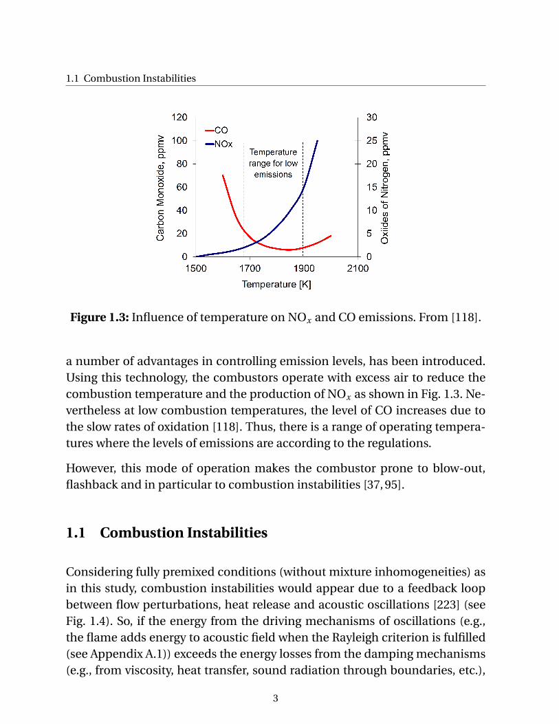
Figure 1.3: Influence of temperature on NOx and CO emissions. From [118].
a number of advantages in controlling emission levels, has been introduced.Using this technology, the combustors operate with excess air to reduce thecombustion temperature and the production of NOx as shown in Fig. 1.3. Ne-vertheless at low combustion temperatures, the level of CO increases due tothe slow rates of oxidation [118]. Thus, there is a range of operating tempera-tures where the levels of emissions are according to the regulations.
However, this mode of operation makes the combustor prone to blow-out,flashback and in particular to combustion instabilities [37, 95].
1.1 Combustion Instabilities
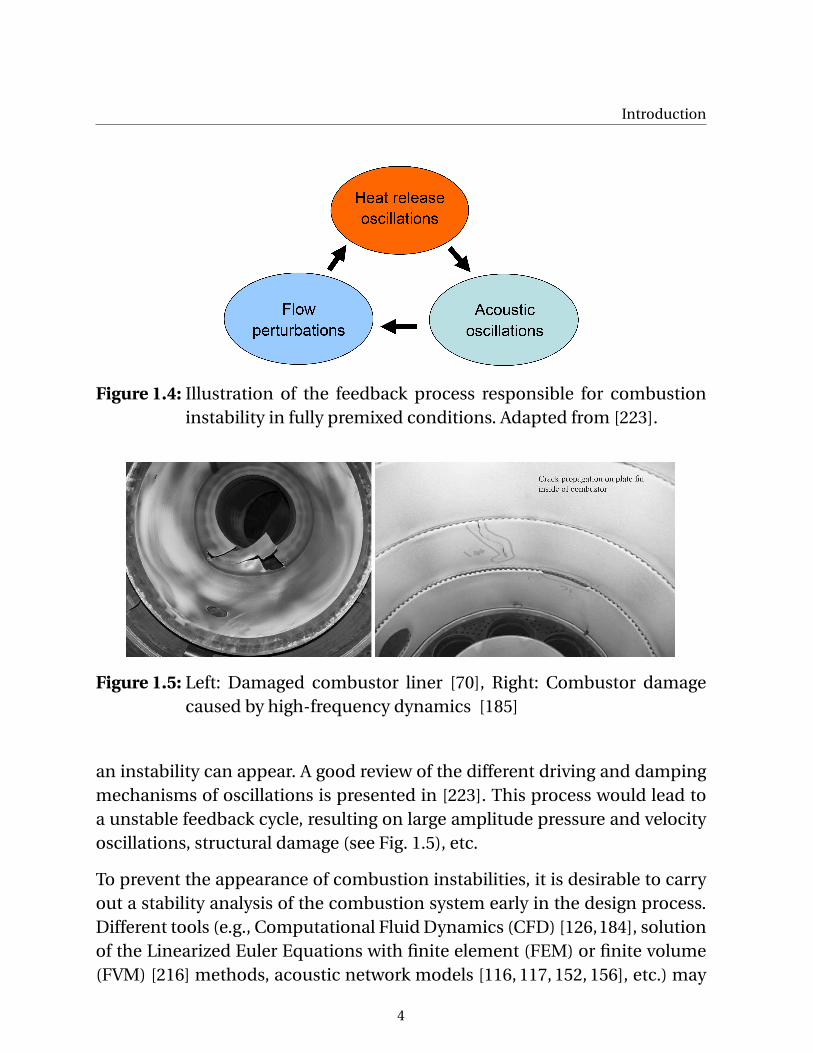
Considering fully premixed conditions (without mixture inhomogeneities) asin this study, combustion instabilities would appear due to a feedback loopbetween flow perturbations, heat release and acoustic oscillations [223] (seeFig. 1.4). So, if the energy from the driving mechanisms of oscillations (e.g.,the flame adds energy to acoustic field when the Rayleigh criterion is fulfilled(see Appendix A.1)) exceeds the energy losses from the damping mechanisms(e.g., from viscosity, heat transfer, sound radiation through boundaries, etc.),
3
Introduction
Figure 1.4: Illustration of the feedback process responsible for combustioninstability in fully premixed conditions. Adapted from [223].
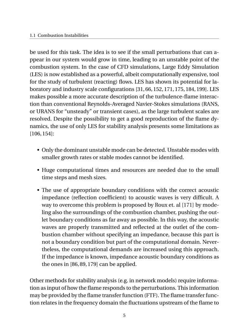
Figure 1.5: Left: Damaged combustor liner [70], Right: Combustor damagecaused by high-frequency dynamics [185]
an instability can appear. A good review of the different driving and dampingmechanisms of oscillations is presented in [223]. This process would lead toa unstable feedback cycle, resulting on large amplitude pressure and velocityoscillations, structural damage (see Fig. 1.5), etc.
To prevent the appearance of combustion instabilities, it is desirable to carryout a stability analysis of the combustion system early in the design process.Different tools (e.g., Computational Fluid Dynamics (CFD) [126,184], solutionof the Linearized Euler Equations with finite element (FEM) or finite volume(FVM) [216] methods, acoustic network models [116, 117, 152, 156], etc.) may
4
1.1 Combustion Instabilities
be used for this task. The idea is to see if the small perturbations that can a-ppear in our system would grow in time, leading to an unstable point of thecombustion system. In the case of CFD simulations, Large Eddy Simulation(LES) is now established as a powerful, albeit computationally expensive, toolfor the study of turbulent (reacting) flows. LES has shown its potential for la-boratory and industry scale configurations [31, 66, 152, 171, 175, 184, 199]. LESmakes possible a more accurate description of the turbulence-flame interac-tion than conventional Reynolds-Averaged Navier-Stokes simulations (RANS,or URANS for “unsteady” or transient cases), as the large turbulent scales areresolved. Despite the possibility to get a good reproduction of the flame dy-namics, the use of only LES for stability analysis presents some limitations as[106, 154]:
• Only the dominant unstable mode can be detected. Unstable modes withsmaller growth rates or stable modes cannot be identified.
• Huge computational times and resources are needed due to the smalltime steps and mesh sizes.
• The use of appropriate boundary conditions with the correct acousticimpedance (reflection coefficient) to acoustic waves is very difficult. Away to overcome this problem is proposed by Roux et. al [171] by mode-ling also the surroundings of the combustion chamber, pushing the out-let boundary conditions as far away as possible. In this way, the acousticwaves are properly transmitted and reflected at the outlet of the com-bustion chamber without specifying an impedance, because this part isnot a boundary condition but part of the computational domain. Never-theless, the computational demands are increased using this approach.If the impedance is known, impedance acoustic boundary conditions asthe ones in [86, 89, 179] can be applied.
Other methods for stability analysis (e.g. in network models) require informa-tion as input of how the flame responds to the perturbations. This informationmay be provided by the flame transfer function (FTF). The flame transfer func-tion relates in the frequency domain the fluctuations upstream of the flame to
5
Introduction
fluctuations of the heat release . Flame transfer functions may be obtained ex-perimentally, using velocity or pressure sensors in combination with chemilu-minescence as an indicator of heat release in the flame (see e.g. [9,78,96,137]).Unfortunately, the experimental determination of FTFs for configurations oftechnical interest is very difficult and costly. (Semi-)analytical models for theFTF have been also proposed (see e.g. [78, 85, 116, 181]). However, it is in ge-neral difficult to predict flame responses from first principles. Alternatively, itis possible to determine the FTF with CFD: First an unsteady CFD simulationis performed to generate time series of fluctuating velocity and heat releaserate. Then the FTF is reconstructed from the data using methods from systemidentification (SI) [66, 85, 158, 160, 199]. These methods should provide infor-mation about the flame dynamics with a reasonable accuracy to proceed tothe stability analysis. Having an incorrect description of the flame dynamicscan lead to a wrong prediction of the stability behavior [198]. Thus, it is im-portant to validate the modeling approaches used to obtain the flame transferfunction.
A strategy of “Divide and Conquer” [106,154,156] is applied in this work, usinga hybrid methodology for the stability analysis. The methodology is based onthe description of the different elements of the system in an acoustic networkmodel, providing the information about the flame response from LES or ex-periments. In this way, the system and boundary conditions are described ina suitable way, including an appropriate description of the flame dynamics,and reducing the demand of resources for the analysis.
Furthermore, as experimental investigations on multi-burner industrial gasturbines at operating conditions are very costly, they are often carried out in asingle burner configuration. However, for annular combustors, single burnerexperiments are in general not representative of machine conditions due tovariations in combustor wall temperatures, combustor cross section size, ope-rating pressure, flame-flame interaction between adjacent burners, etc. Suchvariations in general influence both flow field and flame shape, changing theflame dynamics, and under certain conditions the stability behavior of thesystem.
6
1.2 Overview of the Thesis
1.2 Overview of the Thesis
In this study, the flame dynamics in a perfectly premixed axial swirl burneris investigated. LES in combination with system identification methods isapplied to obtain the flame transfer function. The validation of the methodwith experimental data is carried out in a first step. Then the potential of theLES/SI approach to detect the impact of different conditions interacting withthe flame on the FTF is investigated and compared with the reference case.The influence of the differences in the flame transfer functions on stabilitylimits is analyzed with a low-order thermoacoustic model.
In Chapter 2, an overview of concepts in turbulent combustion, as the energyspectrum and combustion regimes, is presented. This is followed by the fun-damental governing equations for reacting flow LES used in the code AVBP.Finally, the Thickened Flame and Dynamically Thickened Flame combustionmodels used in this study are presented.
In Chapter 3, the flame dynamics of premixed flames submitted to velocitydisturbances is reviewed, presenting the definition of the flame transfer func-tion and the different methods to obtain it. The influences of various para-meters on the flame transfer function are shown. At the end of the chapter,the model of the flame transfer function produced by axial velocity and swirlfluctuations from Komarek and Polifke [103] is shown to describe the flamedynamics by the unit impulse responses of the different perturbations.
In Chapter 4, background about system identification for linear-time invariantsystems is presented, followed by the description and derivation of the WienerFilter. Finally, the LES/SI method for the identification of the flame transferfunction is described.
In Chapter 5, results from the identification of the flame transfer functions ob-tained using the LES/SI method for different conditions are presented. First,the experimental set-up developed by Komarek [103] is introduced; followedby the validation of the method with experiments. After that, the geometricaland operating conditions in the combustor and burner are varied by chan-ging the level of heat transfer in thermal boundary conditions at the combus-
7
Introduction
tor walls, increasing of combustor cross section area, changing the positionof the swirler and increasing the power rating, to study the impact of thesevariations on the flame dynamics. Then, the observed differences in flow fieldand flame shape are discussed in relation to the unit impulse response of theflame and a FTF model.
In Chapter 6, background about 1D acoustics and network models is pre-sented. The stability analysis of the combustion system with the different con-ditions investigated on Chapter 5 was carried out using a network model toolto evaluate and compare their eigenfrequencies and cycle increments for di-fferent combustor lengths. Results of the stability analysis for the referencecase are validated with experiments.
The summary and conclusions of the work are presented in Chapter 7, follo-wed by the outlook of the work in Chapter 8.
All the experimental data was carried out at the Lehrstuhl für Thermodynamikin TU München by T. Komarek [104].
8
2 Turbulent Reacting Flows
In turbulent reacting flows, the interaction of different complex phenomenaas turbulence and chemical reactions is present in combination with mass,momentum and heat transfer. The fundamental concepts in turbulent com-bustion are reviewed in sections 2.1 and 2.3, followed by the fundamental go-verning equations in a LES context. Finally, an overview of turbulent premixedcombustion modeling using LES is presented in section 2.4.
2.1 Turbulence
Most flows in engineering applications are turbulent. Turbulence is still oneof the most challenging and unsolved problems in physics, and its complexityincreases under the presence of chemical reactions [115]. Turbulent flows areunsteady by nature with the presence of continuous fluctuations of velocity,which can produce fluctuations in other scalars as temperature, density andmixture composition [214]. These fluctuations are generated by the presenceof vortices (called also eddies) with different scales (sizes) in the flow. Theseeddies are originated by the development of an instability (e.g., hydrodynamicinstabilities associated with sheared flows [208]). If the instability is damped(e.g., by viscous effects), the fluctuations produced by the instability woulddecay to a steady condition of a laminar flow.
An indicator of the tendency for a flow to become turbulent [115] is theReynolds number (Re) [169]. It is defined by the ratio of the inertial forces(which are related to convective effects) to the viscous forces in the flow:
Re = ul
ν, (2.1)
where ν, u and l are the kinematic viscosity, the characteristic velocity and
9
Turbulent Reacting Flows
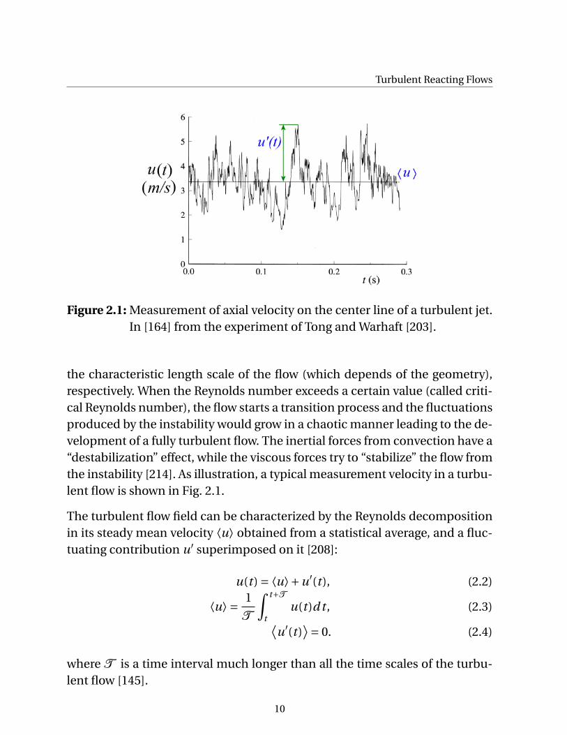
Figure 2.1: Measurement of axial velocity on the center line of a turbulent jet.In [164] from the experiment of Tong and Warhaft [203].
the characteristic length scale of the flow (which depends of the geometry),respectively. When the Reynolds number exceeds a certain value (called criti-cal Reynolds number), the flow starts a transition process and the fluctuationsproduced by the instability would grow in a chaotic manner leading to the de-velopment of a fully turbulent flow. The inertial forces from convection have a“destabilization” effect, while the viscous forces try to “stabilize” the flow fromthe instability [214]. As illustration, a typical measurement velocity in a turbu-lent flow is shown in Fig. 2.1.
The turbulent flow field can be characterized by the Reynolds decompositionin its steady mean velocity ⟨u⟩ obtained from a statistical average, and a fluc-tuating contribution u′ superimposed on it [208]:
u(t ) = ⟨u⟩+u′(t ), (2.2)
⟨u⟩ = 1
T
∫ t+T
tu(t )d t , (2.3)⟨
u′(t )⟩= 0. (2.4)
where T is a time interval much longer than all the time scales of the turbu-lent flow [145].
10
2.2 The Energy Spectrum and Turbulent Length Scales
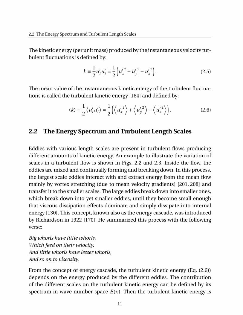
The kinetic energy (per unit mass) produced by the instantaneous velocity tur-bulent fluctuations is defined by:
k ≡ 1
2u′
i u′i =
1
2
(u′
x2 +u′
y2 +u′
z2)
. (2.5)
The mean value of the instantaneous kinetic energy of the turbulent fluctua-tions is called the turbulent kinetic energy [164] and defined by:
⟨k⟩ ≡ 1
2
⟨u′
i u′i
⟩= 1
2
(⟨u′
x2⟩+
⟨u′
y2⟩+
⟨u′
z2⟩)
. (2.6)
2.2 The Energy Spectrum and Turbulent Length Scales
Eddies with various length scales are present in turbulent flows producingdifferent amounts of kinetic energy. An example to illustrate the variation ofscales in a turbulent flow is shown in Figs. 2.2 and 2.3. Inside the flow, theeddies are mixed and continually forming and breaking down. In this process,the largest scale eddies interact with and extract energy from the mean flowmainly by vortex stretching (due to mean velocity gradients) [201, 208] andtransfer it to the smaller scales. The large eddies break down into smaller ones,which break down into yet smaller eddies, until they become small enoughthat viscous dissipation effects dominate and simply dissipate into internalenergy [130]. This concept, known also as the energy cascade, was introducedby Richardson in 1922 [170]. He summarized this process with the followingverse:
Big whorls have little whorls,Which feed on their velocity,And little whorls have lesser whorls,And so on to viscosity.
From the concept of energy cascade, the turbulent kinetic energy (Eq. (2.6))depends on the energy produced by the different eddies. The contributionof the different scales on the turbulent kinetic energy can be defined by itsspectrum in wave number space E(κ). Then the turbulent kinetic energy is
11
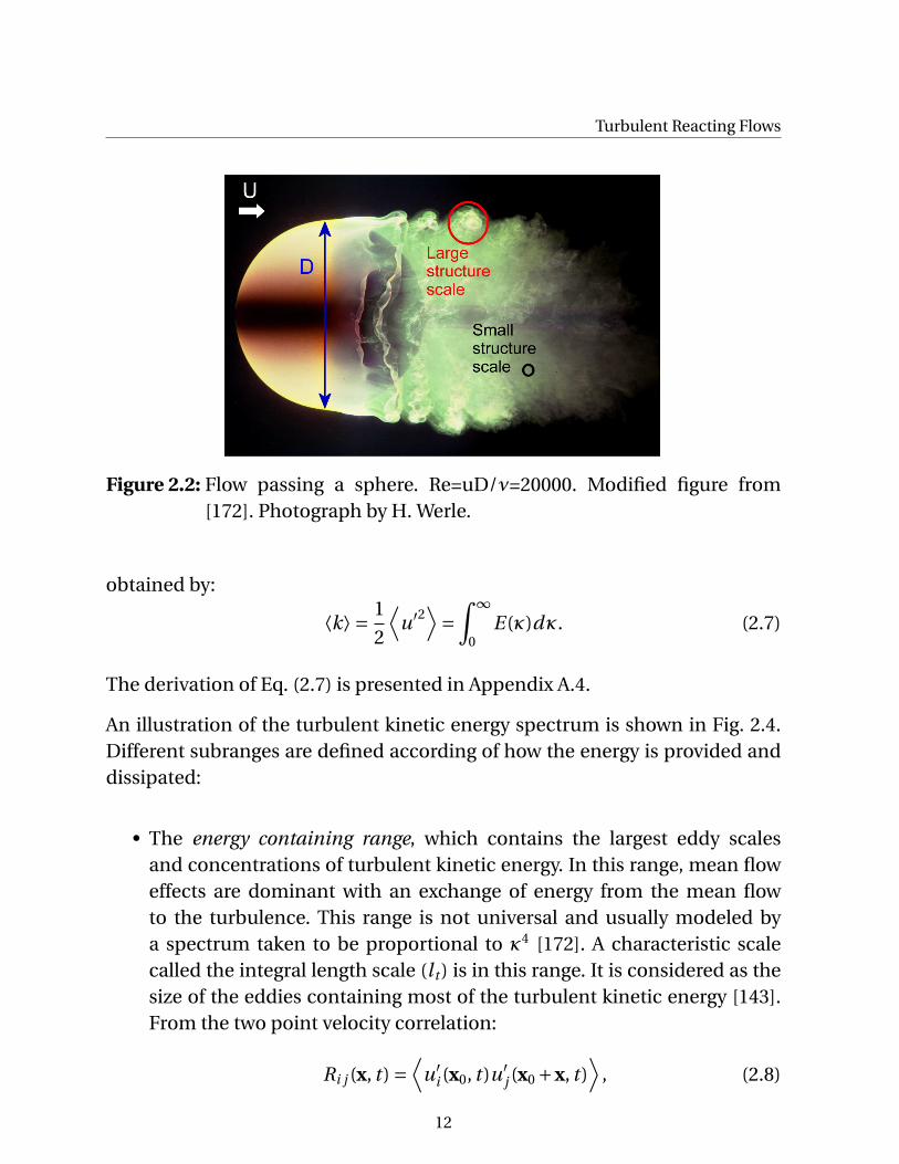
Turbulent Reacting Flows
Figure 2.2: Flow passing a sphere. Re=uD/ν=20000. Modified figure from[172]. Photograph by H. Werle.
obtained by:
⟨k⟩ = 1
2
⟨u′2
⟩=
∫ ∞
0E(κ)dκ. (2.7)
The derivation of Eq. (2.7) is presented in Appendix A.4.
An illustration of the turbulent kinetic energy spectrum is shown in Fig. 2.4.Different subranges are defined according of how the energy is provided anddissipated:
• The energy containing range, which contains the largest eddy scalesand concentrations of turbulent kinetic energy. In this range, mean floweffects are dominant with an exchange of energy from the mean flowto the turbulence. This range is not universal and usually modeled bya spectrum taken to be proportional to κ4 [172]. A characteristic scalecalled the integral length scale (lt ) is in this range. It is considered as thesize of the eddies containing most of the turbulent kinetic energy [143].From the two point velocity correlation:
Ri j (x, t ) =⟨
u′i (x0, t )u′
j (x0 +x, t )⟩
, (2.8)
12
2.2 The Energy Spectrum and Turbulent Length Scales
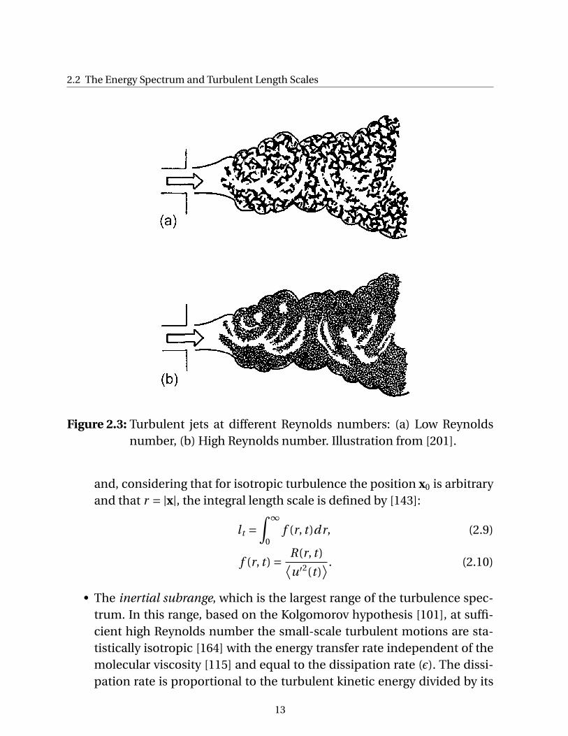
Figure 2.3: Turbulent jets at different Reynolds numbers: (a) Low Reynoldsnumber, (b) High Reynolds number. Illustration from [201].
and, considering that for isotropic turbulence the position x0 is arbitraryand that r = |x|, the integral length scale is defined by [143]:
lt =∫ ∞
0f (r, t )dr, (2.9)
f (r, t ) = R(r, t )⟨u′2(t )
⟩ . (2.10)
• The inertial subrange, which is the largest range of the turbulence spec-trum. In this range, based on the Kolgomorov hypothesis [101], at suffi-cient high Reynolds number the small-scale turbulent motions are sta-tistically isotropic [164] with the energy transfer rate independent of themolecular viscosity [115] and equal to the dissipation rate (ε). The dissi-pation rate is proportional to the turbulent kinetic energy divided by its
13
Turbulent Reacting Flows
time scale [174]:
ε∼ u′(l )2
l/u′(l )= u′(l )3
l, (2.11)
where u′(l ) and l are the velocity and length scale of an eddy, respectively.The dissipation rate is constant in this range and the energy spectrumE(κ) decreases following the κ−5/3 relation (derived by Kolgomorov [101]from dimensional analysis) and defined by:
E(κ) ∼Cκ−5/3ε2/3. (2.12)
• The dissipation range corresponds to the domain where the turbulent ki-netic energy per unit wave number exhibits a strong decrement. In thisrange, the turbulent kinetic energy is transferred to the mean flow by vis-cous effects [42]. With the increase of wave number, the Reynolds num-ber decreases (due to the smaller scales) until a point that the turbulentkinetic energy is dissipated into heat. This occurs in the smallest turbu-lent scale called the Kolgomorov length scale (ηK ) and defined by:
ηK = (ν3/ε)1/4. (2.13)
The Reynolds number produced by such an eddy with a velocity fluctua-tion u′
K is equal to one:
ReK = u′KηK
ν= 1. (2.14)
In Fig. 2.4, other scales are also defined (see [164]). The length scale lE I
is defined as the length scale that separates the energy containing rangewith the inertial subrange. It has dimensions close to lt /6. The lengthscale lD I (with lD I ≈ 60ηK [164]) divides the inertial subrange and the di-ssipation range inside the universal equilibrium range.
2.2.1 Turbulence Modelling Approaches
To simulate turbulent flows with CFD, the different length scales need to beresolved or modeled. An eddy can be resolved if the mesh size used for the
14
2.2 The Energy Spectrum and Turbulent Length Scales
Figure 2.4: Turbulent kinetic energy spectrum vs. Wave number. The level ofcomputed and modeled scales in RANS, DNS and LES. Adaptedfrom [172].
simulation is smaller than the size of the eddy. If not, a model needs to be a-pplied to describe the turbulence. Three different approaches for turbulencemodeling are distinguished, according to the level of resolution of the turbu-lent scales as shown in Fig. 2.4:
• Direct Numerical Simulation (DNS): In DNS, all the scales involved inthe turbulent spectrum are resolved. This implies the solution of the full
15
Turbulent Reacting Flows
instantaneous Navier-Stokes equations without any turbulence model[152]. The problem of using this approach is the requirement of highcomputational resources. As the smallest scales (the Kolgomorov scales)should be resolved considering at least 2 cells [164], the mesh size forthese eddies is much smaller than the geometrical lengths of practicalapplications. Considering the integral length scale as a reference mea-sure, the number of nodes required for a DNS simulation in a flow in Ddimensions is [115]:
Nnodes =(
lt
ηK
)D
= Re34 Dt , (2.15)
where:
Ret = u′lt
ν. (2.16)
is the turbulent Reynolds number. Considering the high Reynolds num-bers in technical applications, its use is still limited to flows with lowReynolds numbers.
• Reynolds Averaged Navier-Stokes (RANS) Simulations: RANS simulationsare based on the statistical description of the flow. In RANS, the instan-taneous balance equations are Reynolds-averaged to describe the evolu-tion of the mean quantities, which are of most interest in technical appli-cations. From the averaging procedure, some terms involving the turbu-lent fluctuations appear (e.g., the Reynolds stress term, scalar turbulentfluxes, etc.). The effect of turbulent fluctuations must be modeled to closethe system. This implies that the various scales on the turbulent kineticenergy spectrum are modeled as shown in Fig. 2.4. Various turbulencemodels for the Reynolds stresses have been derived and used frequentlyin different applications. Examples of these models are the two-equationmodels (e.g. k-ε [88], k-ω [218], SST [128], etc.), the Reynolds Stress clo-sures [114,190], etc. In RANS it is possible to use meshes with a size muchbigger than in DNS, being computationally affordable to simulate appli-cations with high turbulent flows. However, since only statistical infor-mation is extracted from the simulations, the intermittency of the tur-bulence is not captured, not allowing an accurate description of highlyunsteady flows [172].
16

2.3 Turbulent Premixed Combustion
• Large Eddy Simulations (LES): LES is a technique intermediate betweenDNS and RANS. In LES, the large turbulent scales (which are affected bythe flow geometry and are not universal [164]) are calculated explicitly,whereas the effects of smaller ones (which are nearly isotropic and uni-versal) are modeled using subgrid closures. To separate the large fromthe small scales, LES is based on a filtering operation considering a filterwidth. The filter function determines the size and structure of the smallscales [145]. In Fig. 2.4, the spectrum of resolved and modeled scales isseparated by a cut-off wave number defined by:
κcut = π
∆e
. (2.17)
where ∆e is a scale characteristic of the mesh. It is usually defined basedon the cell volume (Vcel l ) by:
∆e =V 1/3cel l . (2.18)
Details about the filtering procedure are shown in section 2.4.1. As thelarge scales are the ones resolved, and usually of most interest in indus-trial applications, it allows the use of a mesh with a smaller size than onefor DNS, reducing the computational effort.
2.3 Turbulent Premixed Combustion
Turbulent combustion results from the interaction between chemical reac-tions and turbulence [152]. The different turbulent eddies interact with aflame produced by an exothermic chemical reaction between a fuel and anoxidizer. The flame can be categorized depending on their mixing process be-fore ignition as follows:
• Non-premixed Flames: In this kind of flames, also called diffusion flames,fuel and oxidizer are introduced separately before combustion andbrought together, creating a zone where mixing between them takesplace by convective and diffusion effects during the combustion pro-cess [115]. The physical process was described by Warnatz et al. [214]
17

Turbulent Reacting Flows
as the process where fuel and oxidizer diffuse to the flame zone wherechemical kinetics converts them into products. The energy released andthe combustion products diffuse away from the flame zone into the fueland the oxidizer.
• Premixed Flames: In premixed Flames, the mixture is well mixed beforecombustion. The flame is present in a thin reaction zone separating re-actants and products, and it can be described as a reaction zone thatmoves with respect to the fuel mixture supporting it [46]. The structureof a laminar premix flame is illustrated in Fig. 2.5. Under the presence ofturbulence, the different zones on the flame are affected, changing theflame structure depending of the turbulence level and mixture characte-ristics. The different regimes of turbulent premixed flames are detailed insection 2.3.1. Depending on the equivalence ratio (φ) of the mixtures offuel and air, combustion in premixed flames is defined in rich (φ>1), stoi-chiometric (φ=1) and lean (φ<1) combustion. The equivalence ratio (φ)is defined by the ratio of fuel–air ratio (FAR) of the mixture with the stoi-chiometric fuel–air ratio:
φ= F AR
F ARstoich, (2.19)
F AR = mass of fuel
mass of air. (2.20)
• Partially-Premixed Flames: In partially-premixed flames, the fuel and oxi-dizer are introduced separately as in non-premixed Flames, but the mix-ing process starts before combustion. The mixing is not perfect as in pre-mixed flames and the flame is in an inhomogeneous fuel mixture. Thiskind of flame is usually present in technical applications as in aircraft gasturbines, direct injection gasoline engines, etc. [143].
As this work is focused only in turbulent premixed flames, only this kind offlame will be discussed in the following. An extended information about tur-bulent non-premixed and partially-premixed combustion theory and mode-ling is shown in [115, 143, 148, 152, 214].
18

2.3 Turbulent Premixed Combustion
Figure 2.5: Structure of a laminar premixed flame.
2.3.1 Combustion Regimes in Turbulent Premixed Combustion
As indicated before, under the presence of turbulence, the flame structure ismodified compared to a laminar flame. The main effect from turbulence isto deform the flame (mainly by the large scales), increasing its area. This iscalled the wrinkling of the flame. This results in an increase of the reactionrate and heat release compared to a laminar flame. To characterize the in-teraction between flame and turbulence in premixed turbulent combustion,regime diagrams are commonly used. These diagrams take into account thelevel of turbulence and scales in the flow and the thermo-chemical characte-ristics of the mixture to characterize the behavior of the flame. These diagramsare defined by different non-dimensional numbers as the turbulent Reynolds,Damkohler and Karlovitz numbers. The turbulent Reynolds number was de-fined previously in Eq. (2.16). The turbulent Damkohler number is defined asthe ratio of the turbulent time produced by the large eddies to the chemicaltime of a laminar flame, and expressed by:
Dat = tt
tchem= lt /u′
δL/sL. (2.21)
19
Turbulent Reacting Flows
where sL and δL are the laminar flame speed and flame thickness, respectively.δL is usually considered as the diffusion flame thickness defined by [152]:
δL =D thu
sL, (2.22)
where D thu is the thermal diffusivity at unburnt conditions. The turbulentDamkohler number is an indicator if the chemical reaction rate is faster orsmaller than the mixing rates from turbulence [204]. The turbulent Karlovitznumber is defined as the ratio of the chemical time to the Kolgomorov timeand defined by [152]:
Kat = δL/sL
η/u′K
= δ2L
η2. (2.23)
It is an indicator if the smallest eddies have any influence on the flame front[42]. It also relates the flame thickness (δL) to the Kolmogorov length scale(η). Another Karlovitz number based on the inner layer thickness δr can bedefined by:
Kar = δr /sL
η/u′K
= δ2r
η2≈ 100Kat . (2.24)
Based on Eqs. (2.16), (2.21) and (2.23), the following relation is established:
Ret = Da2t Ka2
t . (2.25)
An example of a turbulent premixed combustion diagram is the modifiedBorghi diagram by Peters [143] shown in Fig. 2.6. The following regimes canbe identified [20, 143]:
• Laminar flame regime: Laminar flames are present for Ret ≤ 1, indicatinga laminar flow field.
• Wrinkled flamelet regime: It is defined for Ret > 1, Dat > 1, Kat < 1 andu′/sL < 1. In this regime, u’ is lower than the laminar flame speed, there-fore, laminar flame propagation dominates over turbulence effects [143].The flame front is slightly wrinkled (see Fig. 2.7 (a)).
• Corrugated flamelet regime: It is defined for Ret > 1, Dat > 1, Kat < 1 andu′/sL > 1. The flame thickness is thinner than the Kolgomorov scales.
20
2.4 Turbulent Premixed Combustion Modeling using LES
Then, the flame structure is not internally modified by turbulent struc-tures as they do not penetrate in the flame. The turbulent eddies can onlywrinkle or distort the thin laminar flame zone (see Fig. 2.7 (b)).
• Thin reaction zone: In the thin reaction zone, Ret > 1, Dat > 1, Kat > 1and Kar < 1. In this regime, the small eddies with Kolgomorov size canenter into the pre-heat zone, broading the flame and enhancing the heatand mass transfer rates (see Fig. 2.7 (c)). The Kolgomorov eddies are stillbigger than the inner layer and do not penetrate into this layer. Then, thislayer is only wrinkled without affecting its structure [115].
• Well stirred reactor: It is defined for Ret > 1, Dat < 1, Kat > 1 and Kar < 1.In this regime the chemical time scale is higher than the turbulent timescale, then the reaction rate is limited by chemistry. The Kolgomorovscales are not fast enough to disturb the inner layer of the flame front [42].
• Broken reaction zone: It is defined for Ret > 1, Dat < 1 and Kar > 1. In thisregime, the Kolgomorov scales are smaller than the pre-heat zone andthe inner layer thickness and can penetrate in both layers, being stronglyaffected. A thin flame structure can not be identified.
2.4 Turbulent Premixed Combustion Modeling using LES
A detailed resolution of a combustion process is quite complicated as itrequires the solution of multi-dimensional transport equations of multiplespecies which present non-linear reaction terms following an Arrhenius law.Furthermore, different steep gradients are on the flame front, which shouldbe resolved. If turbulence is also involved, the level of complexity increases.Then it is necessary to reduce the complexity by combustion modeling. Insection 2.2.1, different turbulence modeling approaches were discussed. Thecombustion models are derived or extended (e.g., from RANS to LES) accor-ding to the turbulence modeling approach. From the turbulence modeling a-pproaches discussed in section 2.2.1, DNS is still unaffordable for technical
21
Turbulent Reacting Flows
Figure 2.6: Turbulent premixed combustion diagram. Adapted from [143]
Figure 2.7: (a) Wrinkled flamelet regime, (b) Corrugated flamelet regime, (c)Thin reaction zone. From [115].
applications and limited to low turbulence levels. Some recent DNS applica-tions in reacting flows are shown in [24, 144]. RANS models have limitationson describing flame/turbulence interaction and intermittency between fresh
22
2.4 Turbulent Premixed Combustion Modeling using LES
and burnt gases [152], which are important for analyzing the flame dynamics.LES has the advantage that intermittency is taken into account as at a giventime the flame position is known at the resolved scale level [152]. In the follo-wing, the governing equations and modeling approaches will be shown onlyin the LES context.
2.4.1 LES Filtering
In LES, the filtering procedure is applied to the variables and their transportequations in spatial (weighted average over a given volume) or a spectral space(components greater than a given cut-off frequency are suppressed) [152]. Thefiltered resolved part (φ) of the variable φ results from the convolution of thevariable with the applied filter and defined by:
φ(x) =Ñ ∞
−∞φ(ξ)G∆e
(x−ξ)dξ, (2.26)
where x is defined by the spatial coordinates (x1,x2,x3), and G∆eis the filter
function. The filter is normalized by:Ñ ∞
−∞G∆e
dξ= 1. (2.27)
The small unresolved subgrid part of the variable is defined by:
φ′(x) =φ(x)−φ(x), (2.28)
φ′(x) 6= 0. (2.29)
For reacting flows, a mass-weighted Favre filtering ( ) is applied to the vari-able [210] by: φ(x) = 1
ρ
Ñ ∞
−∞ρφ(ξ)G∆e
(x−ξ)dξ. (2.30)
The most common filter is the box-top hat filter in physical space definedby [152]:
G∆e(x) =
1/∆3
e , if |xi | ≤ ∆e/2, i = 1,2,3;
0, Otherwise(2.31)
A review of different filter definitions for G∆ecan be found in [63, 152, 211].
23

Turbulent Reacting Flows
2.4.2 Fundamental Transport Equations for LES Reacting Flows
The transport equations for LES are obtained by filtering the instantaneoustransport equations of conservation of mass, momentum, energy and species.A detailed description of the instantaneous transport equations for reactingflow is shown in [115, 152, 214, 219]. The filtered transport equations are [22,152]:
• Conservation of mass∂ρ
∂t+ ∂ρui
∂xi= 0, (2.32)
• Conservation of momentum
∂ρui
∂t+ ∂ρui u j
∂x j=−∂pδi j
∂x j+ ∂τi j
∂x j+ ∂τi j
t
∂x j, (2.33)
• Conservation of energy
∂ρE
∂t+ ∂ρu j E
∂x j=−∂[ui (pδi j −τi j )+q j +q j
t ]
∂x j+ ωT , (2.34)
• Species mass fraction
∂ρYk
∂t+ ∂ρu j Yk
∂x j= ∂[J j ,k + J j ,k
t]
∂x j+ ωk . (2.35)
where τi j , q j , J j ,k , ωT and ωk are the viscous stress tensor, the heat flux, thediffusive species flux, the heat release and the reaction rate of the k th species.The superscript t indicates subgrid turbulent terms which are modeled.
Additionally, the equation of state for an ideal gas mixture is defined by:
p = ρRT, (2.36)
R = R
Wmix, (2.37)
where R is the universal gas constant and Wmix is the molecular weight of themixture.
24
2.4 Turbulent Premixed Combustion Modeling using LES
The transport equations presented before are for conventional LES simula-tions of reacting and non-reacting flows. Nevertheless, a specific implemen-tation is necessary for the Dynamically Thickened Flame (DTFM) combustionmodel as the model introduces some modifications on the energy and speciestransport equations as shown in section 2.4.3.2. The filtered viscous stress ten-sor, heat flux and diffusive species flux are defined as:
• The filtered viscous stress tensor [22]:
τi j = 2µ
(Si j − 1
3Sl lδi j
), (2.38)
≈ 2µ
(Si j − 1
3δi j Skk
). (2.39)
where:
Si j = 1
2
(∂u j
∂xi+ ∂ui
∂x j
), (2.40)
Skk = ∂uk
∂xk. (2.41)
• The filtered diffusive species flux [22]:
J j ,k =−ρ(Dk
∂Yk
∂x j−YkV c
i
), (2.42)
≈−ρ(Dk
∂Yk
∂x j− YkVi
c)
. (2.43)
where V ci is a correction velocity added to the convection velocity in the
species equations to ensure global mass conservation [152] and definedby:
Vic =
N∑k=1
Dk∂Yk
∂x j. (2.44)
• The filtered heat flux [22]:
q j =−λ ∂T
∂x j+
N∑k=1
J j ,khs,k , (2.45)
≈−λ ∂T
∂x j+
N∑k=1
J j ,khs,k (2.46)
25
Turbulent Reacting Flows
2.4.2.1 Modeling of Subgrid Terms
The subgrid turbulent terms in the transport equations need to be mo-deled. Most subgrid models are based on the eddy-viscosity assumption(Boussinesq’s hypothesis). The subgrid stress tensor τi j
t is modeled by:
τi jt =−ρ (ui u j − ui u j
), (2.47)
= 2ρνt
(Si j − 1
3Skkδi j
). (2.48)
where νt is the SGS turbulent viscosity. Some models proposed for νt areshown in the next section.
The other terms as the subgrid diffusive and heat flux are modeled by:
• The Subgrid scale diffusive species flux:
J j ,kt = ρ (ui Yk − ui Yk
), (2.49)
=−ρ(D t
k
∂Yk
∂x j− YkVi
c,t)
. (2.50)
where,
D tk =
νt
Stc,k
, (2.51)
Vic,t =
N∑k=1
µt
ρStc,k
∂Yk
∂x j. (2.52)
Stc,k is the turbulent Schmid number equal to 0.6 for all species [22].
• The Subgrid heat flux:
q jt = ρ (
ui E − ui E)
, (2.53)
=−λt∂T
∂x j+
N∑k=1
J j ,kths,k . (2.54)
where,
λt =µtCp
Ptr
(2.55)
The turbulent Prandtl number Ptr is equal to 0.6 [22].
26
2.4 Turbulent Premixed Combustion Modeling using LES
2.4.2.1.1 SGS Turbulent Viscosity Models
In Eq. (2.48), the SGS turbulent viscosity νt was introduced to model thesubgrid stress tensor. Two models available in the code AVBP are detailed:
• The Smagorinsky Model:
The Smagorinsky model [186] is probably the most popular and the old-est LES sub-grid model. It is obtained from dimensional analysis andbased on the mixing-length hypothesis [164, 211]. Considering that:
νt ∝l 2
0
t0, (2.56)
and assuming that the cut-off length scale ∆e is representative of the sub-grid modes [211], then
l0 =Cs∆e , (2.57)
where Cs is a model constant. A theoretical value of Cs=0.18 is esti-mated using the local equilibrium hypothesis and the Kolgomorov spec-trum [63, 164, 211]. The characteristic time scale t0 is considered to beequal to the turnover time of the resolved scales [211]:
t0 = 1√2Si j Si j
. (2.58)
Then,
νt =(Cs∆e
)2√
2Si j Si j . (2.59)
The model has some drawbacks:
(a) The constant Cs has to be “tuned” for different turbulent fields (e.g.,in rotating or sheared flows, near solid walls, etc.).
(b) The model is over-dissipative in region of large mean strain [63]. It islimited to predict transition from laminar to turbulent flows.
(c) The model gives a non-zero value of the turbulent viscosity near thewall. Turbulent fluctuations are damped at the wall, so that the tur-bulent viscosity should be zero [133].
27
Turbulent Reacting Flows
Some of these drawbacks can be overcome using a dynamic formulationof the constant Cs at each point and at each time step [63, 65] (but it canbecome computationally unstable [63,211]), or using a damping function(as the Van Driest function [133, 205]) to recover the correct behavior atthe wall.
• The WALE Model:
The Wall-Adapting Local Eddy-viscosity (WALE) model from Nicoud andDucros [133] is based on the square of the velocity gradient tensor g i j
g i j =∂ui
∂x j, (2.60)
and developed for wall bounded flows in an attempt to reproduce theproper scaling at the wall (νt =O(y3)).
The SGS turbulent viscosity is defined as:
νt =(Cw∆e
)2
(Sd
i j Sdi j
)3/2
(Si j Si j
)5/2 +(Sd
i j Sdi j
)5/4(2.61)
where,
Sdi j =
1
2
(g 2
i j + g 2j i
)− 1
3δi j g 2
kk , (2.62)
= Si kSk j +Ωi kΩk j − 1
3δi j
(SmnSmn −ΩmnΩmn
), (2.63)
whereΩ the anti-symmetric part of g :
Ωi j = 1
2
(∂ui
∂x j− ∂u j
∂xi
). (2.64)
The model constant Cw = 0.4929 is set in AVBP. The WALE model is usedin the present study because [133]:
(a) the spatial operator consists of a mixing of the local strain and rota-tion rates. All the turbulence structures relevant for the kinetic ener-gy dissipation are detected by the model.
28
2.4 Turbulent Premixed Combustion Modeling using LES
(b) the eddy-viscosity goes to zero in the vicinity of a wall so that a (dy-namic) constant adjustment or a damping function are not neededfor wall bounded flows.
(c) in case of a pure shear, the model produces zero eddy viscosity, beingable to reproduce the laminar to turbulent transition process.
2.4.2.2 Source Terms
In Eqs. (2.34) and (2.35), the filtered heat release (ωT ) and the reaction rate(ωk) are introduced in the transport equations as source terms. As these termscan not be resolved on an LES mesh, modeling is necessary to be applied. Thisis detailed in the next section.
2.4.3 LES Premixed Combustion Models
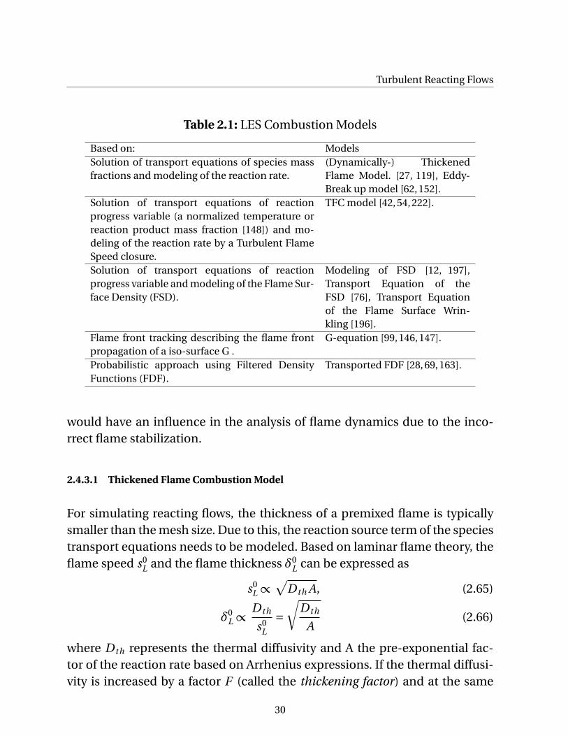
Different combustion models for LES have been developed in recent years.Most of them are an extension of RANS combustion models to the LES con-text, and based on different approaches to model the flame propagation andreaction rate. Some LES combustion models are shown in Table 2.1 indicatingtheir modeling approach.
In this investigation, the LES program AVBP [21, 22] from CERFACS was useddue to its good performance and results on highly parallel compressible react-ing flow simulations (see [3, 175, 184, 188, 191]). The Thickened Flame Model(TFM) from Colin et al. [27] and the Dynamically Thickened Flame Model(DTFM) from Legier et al. [119], which is an extension of the TFM, are avai-lable in the code. These models are based on laminar flame reaction kineticstheory. An overview of reaction kinetics for laminar flames is included in A-ppendix A.2. The TFM and DTFM models have the capabilities to predict ig-nition and flame extinction from heat losses (which is important in order toobtain the correct flame stabilization [175, 199, 200]) due to their Arrheniusformulation. Most of the other combustion models indicated in Table 2.1 donot include the influence of heat losses in their formulations, and their use
29
Turbulent Reacting Flows
Table 2.1: LES Combustion Models
Based on: ModelsSolution of transport equations of species massfractions and modeling of the reaction rate.
(Dynamically-) ThickenedFlame Model. [27, 119], Eddy-Break up model [62, 152].
Solution of transport equations of reactionprogress variable (a normalized temperature orreaction product mass fraction [148]) and mo-deling of the reaction rate by a Turbulent FlameSpeed closure.
TFC model [42, 54, 222].
Solution of transport equations of reactionprogress variable and modeling of the Flame Sur-face Density (FSD).
Modeling of FSD [12, 197],Transport Equation of theFSD [76], Transport Equationof the Flame Surface Wrin-kling [196].
Flame front tracking describing the flame frontpropagation of a iso-surface G .
G-equation [99, 146, 147].
Probabilistic approach using Filtered DensityFunctions (FDF).
Transported FDF [28, 69, 163].
would have an influence in the analysis of flame dynamics due to the inco-rrect flame stabilization.
2.4.3.1 Thickened Flame Combustion Model
For simulating reacting flows, the thickness of a premixed flame is typicallysmaller than the mesh size. Due to this, the reaction source term of the speciestransport equations needs to be modeled. Based on laminar flame theory, theflame speed s0
L and the flame thickness δ0L can be expressed as
s0L ∝
√D th A, (2.65)
δ0L ∝
D th
s0L
=√
D th
A(2.66)
where D th represents the thermal diffusivity and A the pre-exponential fac-tor of the reaction rate based on Arrhenius expressions. If the thermal diffusi-vity is increased by a factor F (called the thickening factor) and at the same
30
2.4 Turbulent Premixed Combustion Modeling using LES
time the pre-exponential factor is reduced by the same factor, the laminarflame speed is preserved and the thickness is increased by this factor. Thisprocedure affects the ratio between turbulent and chemical time scale, theDamköhler Number (Da); and hence, the reaction of the flame to turbulence.This implies that the flame is less sensitive to turbulent motions. The reactionon eddies smaller than the thickened flame thickness vanishes and the reac-tion on eddies bigger than that may be modified. An efficiency function ε isintroduced in order to compensate this effect [27]. This function is based onthe ratio of wrinkling factors of an unthickened ( 0) and a thickened ( 1) flame.The wrinkling factor is estimated by:
Ξ= 1+α∆e
s0L
⟨aT ⟩, (2.67)
⟨aT ⟩ = Γe
u′∆e
∆e, (2.68)
where ⟨aT ⟩ is the effective strain rate defined by the subgrid scale turbulentvelocity, the filter size ∆e and a function Γe which represents the integration ofthe effective strain rate induced by all scales affected by the artificial thicken-ing. Γe is defined by:
Γe
(∆e
δ1L
,u′∆e
s0l
)≈ 0.75exp
[− 1.2
(u′∆e
/s0L)0.3
](∆e
δ1
)2/3
. (2.69)
α denotes a model constant, which can be estimated by:
α= 2ln(2)
3cms(Re1/2t −1)
, (2.70)
where cms = 0.28 [27]. Finally, the efficiency function ε is defined by:
ε= Ξ(δ0L)
Ξ(δ1L)
=1+αu′
∆e
s0LΓe( ∆e
δ0L
,u′∆e
s0L
)
1+αu′∆e
s0LΓe( ∆e
δ1L
,u′∆e
s0L
). (2.71)
Then, the diffusivity and reaction rate in the species and energy filtered trans-
31
Turbulent Reacting Flows
port equations have to be modified according to [152]:
Diffusivity : D thThickening+wrinkling−−−−−−−−−−−−−→ εF D th, (2.72)
Pre-exponential factor : AThickening+wrinkling−−−−−−−−−−−−−→ ε
A
F, (2.73)
while the mass and momentum filtered equations are unmodified.
The transport equations for energy and species for the Thickened FlameModel are [22]:
• Energy
∂ρE
∂t+ ∂ρu j E
∂x j=− ∂
∂x j
ui
[pδi j −2µ
(Si j − 1
3Skkδi j
)]+ ∂
∂x j
CpεF
µ
Pr
∂T
∂x j
+ ∂
∂x j
N∑
k=1
[(εF
µ
Sc,k
)∂Yk
∂x j
−ρYk
(V c
j + V c,tj
)]hs,k
+ εωT
F,
(2.74)
• Species mass fraction
∂ρYk
∂t+ ∂ρu j Yk
∂x j= ∂
∂x j
[εF
µ
Sc,k
∂Yk
∂x j−ρYk
(V c
j + V c,tj
)]
+ εωk
F.
(2.75)
2.4.3.2 Dynamically Thickened Flame Combustion Model
The Thickened Flame Model applies the thickening in the complete domain.With this, the diffusion in non-reactive zones will be overestimated by a factorF . Legier [119] proposed the Dynamically Thickened Flame Model (DTFM)based on the Thickened Flame Model to overcome this deficiency. In the
32
2.4 Turbulent Premixed Combustion Modeling using LES
DTFM, the thickening factor F is not constant, but approaches a maximumvalue (Fmax) inside the reaction zone and unity in non-reactive zones. A “sen-sor” (S) of the reactive zone is used to indicate if the thickening should beapplied (S=1) or not (S=0). It is defined by:
S = tanh
(βF
Ω
Ωmax
), (2.76)
Ω= Y νFF Y νO
O e−ΨTaT . (2.77)
whereΨ and βF are model constants equal to 0.5 and 500, respectively [22].Ψis lower than 1 to activate the sensor S before reaction.Ω is a modified reactionrate used to activate the sensor S [174]. Ωmax is the maximum of Ω and it canbe obtained using 1D laminar flame calculations. Finally, the sensor controlsthe value of the thickening F by [22]:
F = 1+ (Fmax −1)S (2.78)
The transport equations for energy and species for the Dynamically Thicke-ned Flame model are [22]:
• Energy
∂ρE
∂t+ ∂ρu j E
∂x j=− ∂
∂x j
ui
[pδi j −2µ
(Si j − 1
3Skkδi j
)]+ ∂
∂x j
Cp
[εF
µ
Pr+ (1−S)
µt
Ptr
]∂T
∂x j
+ ∂
∂x j
N∑
k=1
[εF
µ
Sc,k+ (1−S)
µt
Stc,k
]∂Yk
∂x j
−ρYk
(V c
j + V c,tj
)hs,k
+ εωT
F,
(2.79)
• Species mass fraction
∂ρYk
∂t+ ∂ρu j Yk
∂x j= ∂
∂x j
[εF
µ
Sc,k+ (1−S)
µt
Stc,k
]∂Yk
∂x j−ρYk
(V c
j + V c,tj
)
+ εωk
F.
(2.80)
33
3 Response of Premixed Flames toVelocity Disturbances
As mention in the introduction, premix enclosed flames are prone to developinstabilities. The instabilities can develop from the appearance of hydrody-namic or acoustic perturbations inside the system. The flame has a dynamicresponse to these perturbations acting as a source or as a damper of this per-turbations. Various mechanisms are related to the fluctuations of heat release(Q ′) produced by the acoustic velocity fluctuations (u′). These mechanismsare described in Fig. 3.1 for fully premixed conditions. The flame dynamicshave also a strong influence by equivalence ratio fluctuations [83,85,121,173],which is not investigated in the present study.
From these mechanisms, the fluctuation of heat release is mainly producedby the variations in flame surface area. When the perturbation reaches theflame, a kinematic response is produced, creating modulations in flame sur-face area which are convected along the flame [83, 153, 181] and finally pro-ducing fluctuations in the heat release. With the presence of a swirler, fluctua-tions in the swirl number at the burner exit are induced by the appearance offluctuations in the tangential velocity (more details in section 3.3.3). The va-riation of the swirl number produces modulations in the flame angle, whichcreates variations of flame surface area. Additionally, the turbulence intensityin the shear layers can be modified by turbulent fluctuations induced by theperturbation, producing fluctuations in the turbulent flame speed. Externalturbulent eddies generated by the environment and not induced by the ve-locity perturbation can interact also with the flame, producing fluctuations inthe heat release. Coherent structures can develop by hydrodynamic instabi-lities [150] or at high amplitudes of the velocity perturbation [111], inducingdeformation on the flame surface area [153] by vortex roll-up.
34
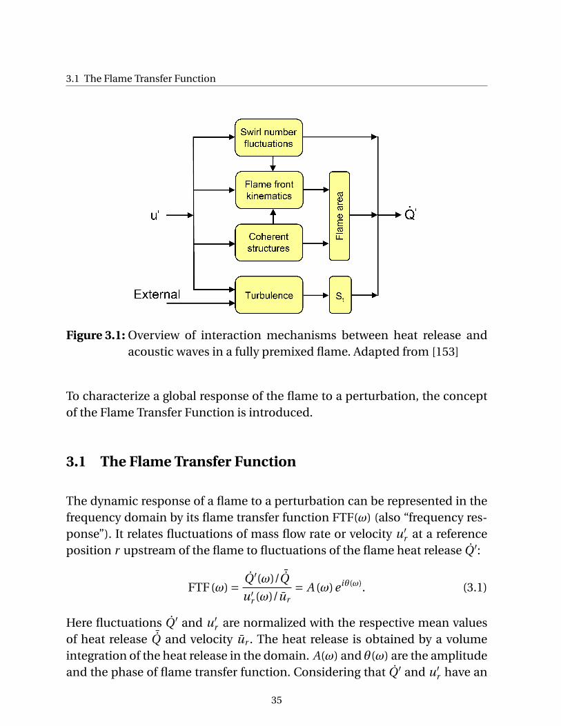
3.1 The Flame Transfer Function
Figure 3.1: Overview of interaction mechanisms between heat release andacoustic waves in a fully premixed flame. Adapted from [153]
To characterize a global response of the flame to a perturbation, the conceptof the Flame Transfer Function is introduced.
3.1 The Flame Transfer Function
The dynamic response of a flame to a perturbation can be represented in thefrequency domain by its flame transfer function FTF(ω) (also “frequency res-ponse”). It relates fluctuations of mass flow rate or velocity u′
r at a referenceposition r upstream of the flame to fluctuations of the flame heat release Q ′:
FTF(ω) = Q ′(ω)/ ¯Q
u′r (ω)/ur
= A (ω)e iθ(ω). (3.1)
Here fluctuations Q ′ and u′r are normalized with the respective mean values
of heat release ¯Q and velocity ur . The heat release is obtained by a volumeintegration of the heat release in the domain. A(ω) and θ(ω) are the amplitudeand the phase of flame transfer function. Considering that Q ′ and u′
r have an
35
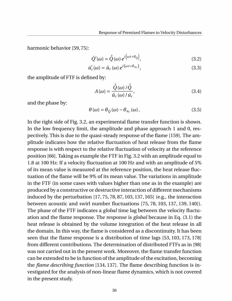
Response of Premixed Flames to Velocity Disturbances
harmonic behavior [59, 75]:
Q ′(ω) = ˆQ (ω)e i(ωt+θQ
), (3.2)
u′r (ω) = ur (ω)e i(ωt+θur ), (3.3)
the amplitude of FTF is defined by:
A (ω) =ˆQ (ω)/ ¯Q
ur (ω)/ur, (3.4)
and the phase by:θ (ω) = θQ (ω)−θur (ω) . (3.5)
In the right side of Fig. 3.2, an experimental flame transfer function is shown.In the low frequency limit, the amplitude and phase approach 1 and 0, res-pectively. This is due to the quasi-steady response of the flame [159]. The am-plitude indicates how the relative fluctuation of heat release from the flameresponse is with respect to the relative fluctuation of velocity at the referenceposition [66]. Taking as example the FTF in Fig. 3.2 with an amplitude equal to1.8 at 100 Hz: If a velocity fluctuation at 100 Hz and with an amplitude of 5%of its mean value is measured at the reference position, the heat release fluc-tuation of the flame will be 9% of its mean value. The variations in amplitudein the FTF (in some cases with values higher than one as in the example) areproduced by a constructive or destructive interaction of different mechanismsinduced by the perturbation [17, 75, 78, 87, 103, 137, 165] (e.g., the interactionbetween acoustic and swirl number fluctuations [75, 78, 103, 137, 139, 140]).The phase of the FTF indicates a global time lag between the velocity fluctu-ation and the flame response. The response is global because in Eq. (3.1) theheat release is obtained by the volume integration of the heat release in allthe domain. In this way, the flame is considered as a discontinuity. It has beenseen that the flame response is a distribution of time lags [53, 103, 173, 178]from different contributions. The determination of distributed FTFs as in [98]was not carried out in the present work. Moreover, the flame transfer functioncan be extended to be in function of the amplitude of the excitation, becomingthe flame describing function [134, 137]. The flame describing function is in-vestigated for the analysis of non-linear flame dynamics, which is not coveredin the present study.
36
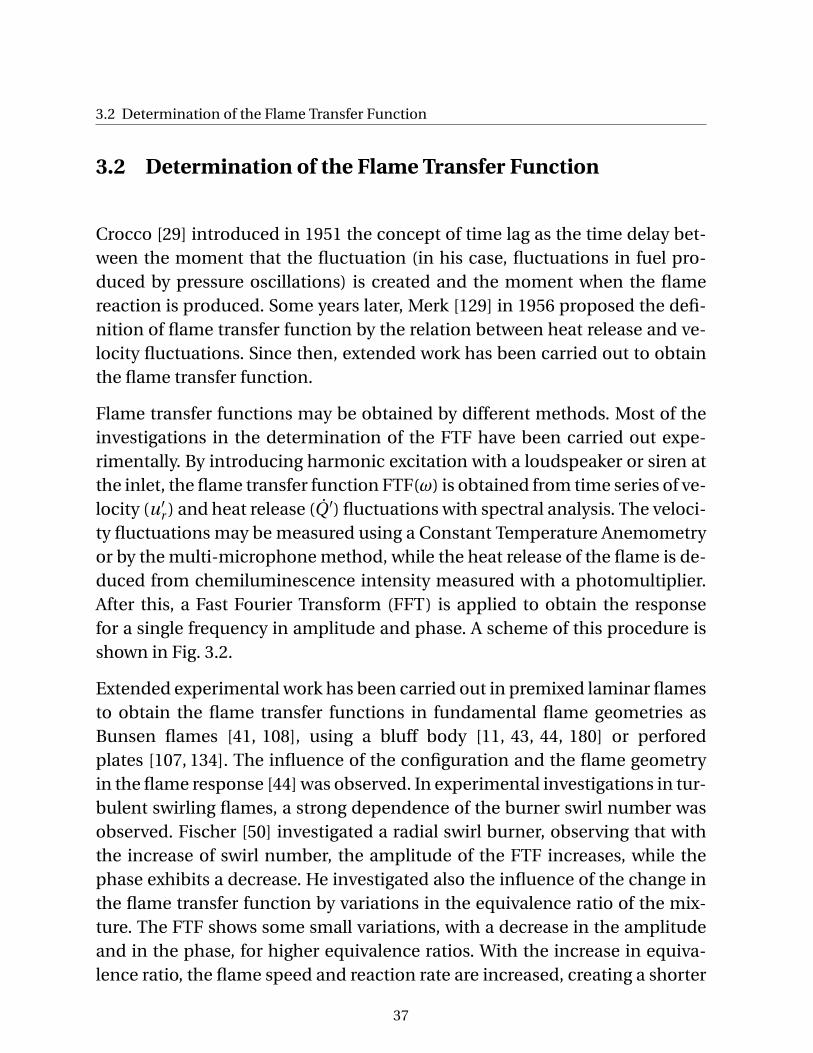
3.2 Determination of the Flame Transfer Function
3.2 Determination of the Flame Transfer Function
Crocco [29] introduced in 1951 the concept of time lag as the time delay bet-ween the moment that the fluctuation (in his case, fluctuations in fuel pro-duced by pressure oscillations) is created and the moment when the flamereaction is produced. Some years later, Merk [129] in 1956 proposed the defi-nition of flame transfer function by the relation between heat release and ve-locity fluctuations. Since then, extended work has been carried out to obtainthe flame transfer function.
Flame transfer functions may be obtained by different methods. Most of theinvestigations in the determination of the FTF have been carried out expe-rimentally. By introducing harmonic excitation with a loudspeaker or siren atthe inlet, the flame transfer function FTF(ω) is obtained from time series of ve-locity (u′
r ) and heat release (Q ′) fluctuations with spectral analysis. The veloci-ty fluctuations may be measured using a Constant Temperature Anemometryor by the multi-microphone method, while the heat release of the flame is de-duced from chemiluminescence intensity measured with a photomultiplier.After this, a Fast Fourier Transform (FFT) is applied to obtain the responsefor a single frequency in amplitude and phase. A scheme of this procedure isshown in Fig. 3.2.
Extended experimental work has been carried out in premixed laminar flamesto obtain the flame transfer functions in fundamental flame geometries asBunsen flames [41, 108], using a bluff body [11, 43, 44, 180] or perforedplates [107, 134]. The influence of the configuration and the flame geometryin the flame response [44] was observed. In experimental investigations in tur-bulent swirling flames, a strong dependence of the burner swirl number wasobserved. Fischer [50] investigated a radial swirl burner, observing that withthe increase of swirl number, the amplitude of the FTF increases, while thephase exhibits a decrease. He investigated also the influence of the change inthe flame transfer function by variations in the equivalence ratio of the mix-ture. The FTF shows some small variations, with a decrease in the amplitudeand in the phase, for higher equivalence ratios. With the increase in equiva-lence ratio, the flame speed and reaction rate are increased, creating a shorter
37
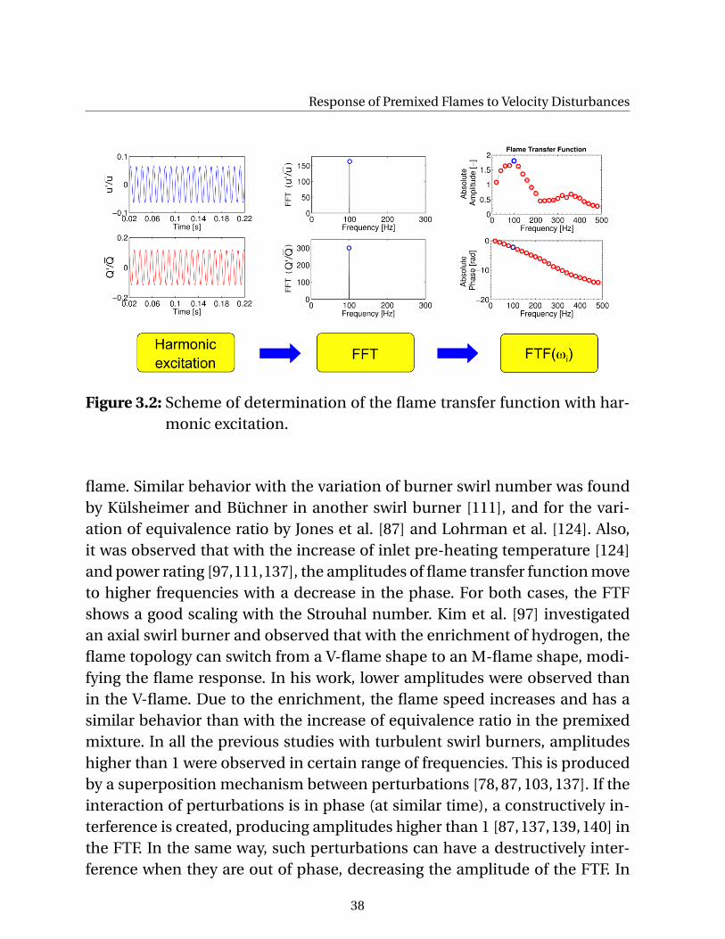
Response of Premixed Flames to Velocity Disturbances
Figure 3.2: Scheme of determination of the flame transfer function with har-monic excitation.
flame. Similar behavior with the variation of burner swirl number was foundby Külsheimer and Büchner in another swirl burner [111], and for the vari-ation of equivalence ratio by Jones et al. [87] and Lohrman et al. [124]. Also,it was observed that with the increase of inlet pre-heating temperature [124]and power rating [97,111,137], the amplitudes of flame transfer function moveto higher frequencies with a decrease in the phase. For both cases, the FTFshows a good scaling with the Strouhal number. Kim et al. [97] investigatedan axial swirl burner and observed that with the enrichment of hydrogen, theflame topology can switch from a V-flame shape to an M-flame shape, modi-fying the flame response. In his work, lower amplitudes were observed thanin the V-flame. Due to the enrichment, the flame speed increases and has asimilar behavior than with the increase of equivalence ratio in the premixedmixture. In all the previous studies with turbulent swirl burners, amplitudeshigher than 1 were observed in certain range of frequencies. This is producedby a superposition mechanism between perturbations [78, 87, 103, 137]. If theinteraction of perturbations is in phase (at similar time), a constructively in-terference is created, producing amplitudes higher than 1 [87,137,139,140] inthe FTF. In the same way, such perturbations can have a destructively inter-ference when they are out of phase, decreasing the amplitude of the FTF. In
38
3.2 Determination of the Flame Transfer Function
general, the experimental determination of FTFs for configurations of techni-cal interest is very difficult and costly, but necessary for validation. In orderto reduce the time and cost of experiments, analytical and numerical toolshave been developed to investigate the flame response. For (Semi-)analyticalmodels of the FTF, most of the models have been derived for laminar flames.A simple analytical model was proposed based on the time lag description byCrocco and Cheng [30] called the n-τ model, where the FTF is defined by:
FTF(ω) = ne iωτ, (3.6)
where n is called the interaction index and τ is the time lag between heat re-lease and velocity. If the value of n is considered constant, the interaction in-dex takes the value of 1 [59] due to the low frequency limit of the FTF, wherethe amplitude should approach unity [159]. As it is shown by Eq. (3.6), themodel does not capture variations in the amplitude of the FTF by the flamedynamics and only capture the variations in a single time lag. More advancedmodels have been derived based on the flame front kinematics and the propa-gation of a perturbation along the flame [15, 41, 51, 181], creating a deforma-tion of flame surface area. Schuller et al. [181] extended the model of Ducruixet al. [41], which is based on the works from Fleifil et al. [51] and Boyer andQuinard [15], to introduce the effects of a disturbance convected along theflame front in a conical and a V-flame. For the V-flame, similar to most flamesstabilized in swirl burners, it was observed that the FTF presents amplitudeshigher than 1 from a certain value of the flame angle with respect to the centerline, and that the amplitude is increased with the decrease of the flame angle.This behavior of V-flames was also confirmed with experiments [43], indica-ting that this kind of flame is prone to develop combustion instabilities. Addi-tional models were extended to turbulent combustion [33, 116]. However, it isin general difficult to predict flame responses from first principles, especiallyfor turbulent flames.
Alternatively, it is possible to determine the FTF with computational fluid dy-namics (CFD). Steady state CFD simulations [52, 53, 109, 110] can be used totrack the fuel particles until they are consumed to create a time lag distribu-tion and introduce it into a model. The problem of using this method is thatthe amplitude of the FTF, which describes the dynamic response of the flame
39
Response of Premixed Flames to Velocity Disturbances
to the perturbations, can not be well reproduced as some effects (e.g., flamefront kinematics, swirl fluctuations, etc.) are not considered. Instead an un-steady CFD simulation can be performed to generate time series of fluctua-ting velocity and heat release rate. Thus, the FTF is reconstructed from the ex-tracted data. The FTF can be obtained using harmonic excitation [5,68,77,93]as in the experimental determination of the FTF, applying special signals asan impulse or white noise and doing spectral analysis [66, 206], or by usingmethods from system identification (SI) [64, 66, 67, 85, 158, 160, 199]. The ad-vantage of using system identification methods is that it is possible to obtainthe frequency flame response over a range of frequencies from a single CFDsimulation, reducing the computational effort. Furthermore, it removes thecontributions in the flame response by external “noise” by correlation analy-sis and that are present on the spectral analysis. Details about SI are indicatedin Chapter 4. Gentemann and Polifke [64] investigated a radial swirl burner inan axisymmetric 2D simulation to identify the FTF using URANS and SI. Goodqualitatively agreement was obtained with experimental results. Discrepan-cies are argued to be due to limitations in the combustion and turbulencemodel to reproduce the flame and flow field. Giauque et al. [67] simulateda premixed turbulent swirl burner in a 15o sector of an annular combustorwith LES. Harmonic and white noise excitation at the inlet were applied toidentify the FTF by a FFT using the harmonic excitations and by SI methodsusing the white noise signal. Good agreement was obtained in amplitude andphase between the FTF identified by harmonic excitation and SI. Results werenot validated with experiments. Additionally, in [66] a spectral analysis wascarried out to the signals extracted using the white noise excitation. High di-fferences were found between the results obtained by the Harmonic-FFT andWhite noise/SI. Borghesi et al. [13] carried out the identification of the FTF of aconical swirl burner with aerodynamic stabilization of the flame (without theuse of bluff body as in [64] and in this study). The FTF is represented by the ele-ment T22 of the flame transfer matrix, with good agreement with experiments.Also, he indicates that the flame response is dominated by the displacement ofthe inner recirculation zone due to the aerodynamic stabilization of the flame.
Recently, Cuquel et al. [32] applied experimentally random velocity perturba-tions in combination with system identification techniques to obtain the FTF
40
3.3 Additional Parameters Influencing the Flame Response in Premixed Flames
of a laminar conical flame. With this technique, the FTF is obtained over arange of frequencies from a single experiment. For excitations in the linearregime, good agreement was achieved between the FTFs obtained with har-monic excitation and with system identification. For higher excitation ampli-tudes, the amplitude of the FTF is underestimated when random velocity per-turbations are applied.
3.3 Additional Parameters Influencing the Flame Response inPremixed Flames
As mentioned before, the FTF is influenced by different parameters. Moststudies were carried out to look at its dependence by the increase of powerrating or by modifying the mixture properties (temperature and equivalenceratio). Nevertheless, the change of other conditions in a combustion systemcan also lead to a variation on the flame response. From the practical point ofview, typical investigations on the design of gas turbines are carried out usingsingle burner test rigs. Nevertheless, when the same burner is installed on theengine, which can have similar inlet conditions (mixture, inlet flow and equi-valence ratio) as in the single burner tests, other variations can appear as thechange of thermal conditions at the combustor walls, variation of combustorcross section size, flame-flame interaction between adjacent burners, opera-ting pressure, etc. Also, the position of the swirler can be changed becauseof design reasons. These additional variations can lead to differences on theflame shape and burner aerodynamics.
Flame shape and topology have a strong influence on the flame dynamics.Schuller et al. [180] studied the self-induced instabilities of laminar premixedflames stabilized on an unconfined annular burner. The burner included abluff body rod for flame stabilization. It was observed that under similar ope-rating conditions, it was possible to obtain different flame topologies (coni-cal, V-, or M-Flame) depending on the location of the ignition point. In thisstudy, the flame transfer function of the M-flame was measured for differentequivalence ratios and incoming velocities. It was observed that there exists
41
Response of Premixed Flames to Velocity Disturbances
a strong mutual interaction (leading to annihilation) between the flames sta-bilized on both shear layers, causing an amplification behavior (amplitudeshigher than 1) on the flame transfer function for a frequency range. Durox etal. [44] investigated the same burner to measure the Flame Describing Func-tions (FDF) of the different flame geometries mentioned before. The investiga-tion included an additional configuration consisting on a Collection of SmallConical Flames (CSCF) stabilized on a perforated plate. The compared caseswere performed at slightly rich conditions (φ=1.08) for a methane-air mix-ture. Under these conditions, it was possible to obtain all flame shapes men-tioned before with the same incoming flow and equivalence ratio. The flameresponse was different between cases, concluding that the steady-state flamegeometry has a strong influence on the flame response. The CSCF, V-shapeand M-shape flames showed similar behavior with amplitudes higher than 1for low frequencies, followed by a decay in amplitude at higher frequencies.Additionally, the M-flame exhibited a broader frequency response (with am-plitudes higher than 1) than the other flames. This different flame responsecan lead also to a varied production of combustion noise [19] and stabilitybehavior [82, 96].
Variation of the flame shape and length in premixed cases can be obtainedusing the same burner by modifying operational conditions such as:
• Fuel and mixture conditions: Kim et al. [97] investigated the flame res-ponse in a lean-premixed axial swirl burner with various equivalenceratios and methane-hydrogen-air mixture compositions at atmosphericconditions. It was observed that for the same inlet velocity and mixturetemperature, a V-flame stabilized initially at certain methane-air equiva-lence ratio can change to a M-flame by the increase of equivalence ratioor by hydrogen enrichment. With the increase in these parameters, theflame speed and reaction rate are increased, and flame stabilization canbe achieved in both shear layers.
• Inlet pre-heat temperature: Huang and Yang [81] analyzed experimentallyand numerically the transition of flame structure from a stable to an un-stable state in a lean-premixed axial swirl burner. It was observed thatwith the increase of the inlet mixture temperature, a stable system with
42
3.3 Additional Parameters Influencing the Flame Response in Premixed Flames
a V-flame shape shifted to an unstable system with a M-flame. The tran-sition appears due to the increase of flame speed by the increase of inlettemperature. Then, the flame flashes back, penetrating in the outer re-circulation zone and stabilizing in the outer shear layer. Foley et al. [55]investigated also the influence of variation of equivalence ratios and in-let temperature on the flame shape, observing similar transition behavioras in the previously cited study. In their work, additional flame shapes, asa lifted flame or a flame with stabilization only in the outer shear layer,were observed.
• Operating Pressure: The increase of pressure has an influence on theflame length [17, 59, 60]. By increasing the operating pressure on theburner and keeping the same equivalence ratio, inlet pre-heating tem-perature and inlet velocity, the output power increases due to the highertotal mass flow produced by the higher density at this condition. Fur-thermore, the chemical kinetics and reaction rate changes [115] with theincrease of pressure. It was observed on references [17, 59, 60] that theflame length is reduced with the increase of operating pressure. Changeof the flame topology due to the increase in pressure was not observedon the previous cited investigations.
This investigation has a special emphasis on the influence of thermal boun-dary conditions at the combustor wall, confinement ratio and swirler positionon the flame dynamics. Previous studies related with these variations on con-ditions are reviewed in the following.
3.3.1 Influence of Combustor Thermal Boundary Conditions
Heat losses can modify the flame structure as the flame reaction has a strongdependence on the temperature [115]. In combustion systems, the burntgases approach temperatures between 1500 and 2500 K, while the combus-tor walls have temperatures between 400 and 600 K [152] because of the cool-ing to protect the material. Under nonadiabatic conditions, the heat lossescan lead to the extinction of the flame [35, 127, 187]. The influence of thermal
43
Response of Premixed Flames to Velocity Disturbances
conditions on the flame has been studied in different configurations. In nu-merical studies of flame propagation in channels with variations of thermalconditions [34, 73, 189], it was observed that the flame structure and propa-gation can change due to the quenching effects on the flame from the cooledwalls. Veynante and Poinsot [151,209] investigated with DNS a premixed flamestabilized on a back ward facing step and found a different flame stabilizationby varying the thermal conditions of the combustor walls. The flame was an-chored to the step using adiabatic wall conditions; while using nonadiabaticwalls with temperatures equal to the fuel mixture, quenching effects appearclose to the wall, resulting in a lifted flame. Similar effects on the flame stabi-lization were found by Kaess et al. [90,91] on a DNS study of a laminar conicalflame stabilized on a perforated plate with different thermal conditions at thewall. It was observed that this variation on the flame stabilization had an in-fluence on the flame response [90, 209]. Using a very similar configurationas Kaess et al., Duchaine and Poinsot [40] explored the sensitivity of premixflame FTF to changes in a variety of input parameters. With an uncertaintyin the wall plate temperature of 50 K, only a small influence in the FTF wasobserved. Higher wall temperature variations were not investigated.
In the case of combustors with swirl burners, due to the formation of an outerrecirculation zone, combustion products cooled by the combustor wall cool-ing are transported back and interact with the flame, affecting the flame sta-bilization. The flame stabilization on a premixed swirl burner with differentthermal conditions was investigated using LES by Schmitt et al. [175, 176]. U-sing adiabatic walls, the flame showed strong stabilization in the outer shearlayer; while with nonadiabatic walls, as in the experimental configuration,quenching effects appeared in the outer shear layer, having a flame stabi-lized mainly in the inner recirculation zone, and in good agreement with theone from experiments. Additionally, Waesle et al. [215] designed an uncon-fined swirl burner surrounded by co-flow gases with different temperaturesand composition. A hot exhaust gas stream is generated by a porous burnersurrounding the flame, and positioned at the same level of the burner exit. Itwas observed that different flame topologies can be obtained depending onthe surrounding gas temperature and composition. Furthermore, the level ofheat loss in the combustor changes with increasing pressure as shown by Frei-
44
3.3 Additional Parameters Influencing the Flame Response in Premixed Flames
tag et al. [59, 60]. In his work, it is observed a decrease on the heat losses perpower rating with the increase in pressure. The variation on heat losses bypressure variation can have an influence on the flame length.
3.3.2 Influence of Confinement Ratio
Strong differences on the flow field and flame structure between confined andunconfined flames have been observed [4]. The degree of confinement canhave an influence in the flame dynamics. The influence of confinement ratio(CR) in non-reacting and reacting flow has been investigated by various au-thors. The confined ratio is defined by:
C R = Abexit
Acc, (3.7)
where Abexit is the area of the burner exit using the external perimeter, andAcc is the area of the combustor cross section. Beltagui and Maccallum [10]studied non-reacting and reacting swirling flows in a cylindrical furnace com-bustor, observing variations in the flow patterns when the combustor had a di-fferent confinement ratio. In their investigations, the inner recirculation zonewas longer and bigger for the case with lower confinement ratio. Similar re-sults were found in a similar configuration by Rao et al. [167] and by Hallet andDing [74]. Birbaud et al. [11] investigated the flame dynamics for confined andunconfined laminar flames. It was observed that for low levels of confinementratio, where the flame did not have interaction with the walls, the responsewas similar to the unconfined case. For the cases with higher confinement,interaction of the flame with the wall influences the dynamics of the flametip and the flame wrinkling, changing the flame response. Fu et al. [61] in-vestigated the effect of combustor confinement on the flow field using a swirlburner at isothermal conditions. A strong influence of the confinement in thesize and strength of the inner recirculation zone (IRZ) was found. Additionally,they found that there is a level of confinement where the flow has some hys-teresis and different flow regimes can be established, changing the angle of theshear layers and the size of the IRZ. Fanaca et al. [49] investigated experimen-tally the flow field and flame on a single burner and an annular combustor. It is
45
Response of Premixed Flames to Velocity Disturbances
considered that the differences on the aerodynamics and flame shape are thecauses of discrepancies in the FTFs obtained in these configurations. Hauseret al. [75] investigated the influence of the confinement on the Flame TransferFunction in two combustors with different square section area, showing dif-ferences between cases in amplitude and phase. The differences in phase isattributed to the higher convection velocities in the high confinement com-bustor.
3.3.3 Influence of Swirler Position
Straub and Douglas [194] investigated the influence of the position of an axialswirler on the stability of a combustion system. The experiments were at pre-mix conditions with high pressure and mixture pre-heating. Different stabilitybehavior was observed in the combustor, depending on the position of theaxial swirler. In their work, the flame response was not investigated, but it ismentioned that due to the presence of the swirler, tangential velocity fluctua-tions propagating with a convective speed can reach the flame and have someeffect on it.
The flame response and flow field have a strong dependence on the swirl num-ber of the burner [50, 111], which is defined by [10, 82, 142]:
Sn = Gtan
rextGax, (3.8)
where Gax and Gtan are defined for an axisymmetric configuration by:
Gax =∫ rext
rint
ρu2ax2πr dr, (3.9)
Gtan =∫ rext
rint
ρuaxutan2πr 2dr, (3.10)
indicating the fluxes of axial and angular momentum. rext and rint are the ex-ternal and internal radius, respectively; and uax and utan are the axial and tan-gential velocity, respectively. Due to the presence of tangential velocity fluc-tuations, swirl number fluctuations can be induced, modifying the flame res-ponse and the stability behavior of the system.
46
3.3 Additional Parameters Influencing the Flame Response in Premixed Flames
A small decay in swirl number is also produced by moving the swirler to aposition more upstream to the burner exit. The axial decay in swirl numberhas been studied experimentally and numerically in tubes [6, 100, 192] andannular ducts [26, 36, 131]. It was found that the decay has an exponential be-havior [36, 100] with respect to the distance to the swirl generator. The decayappears due to the loss of angular momentum produced by the wall frictionand stresses. Additionally, Clayton and Morsi [26] have shown experimentallyin an annular duct that the axial decay of swirl increases with the increase ofswirl number.
The mechanism of the impact of swirl number fluctuations in the flame res-ponse was investigated in different previous studies [78, 103, 137, 139, 141].Hirsch [78] proposed a mechanism of how the presence of swirl fluctua-tions can induce a secondary velocity fluctuation (created by fluctuations invorticity) which influence the flame response. Wang and Yang [212] investi-gated numerically an imposed perturbation in a radial swirl burner. It wasfound that the swirler can induce two perturbations with different propaga-tion speed: One is a vortical wave with convective propagation speed, and theother is an acoustic wave propagating with the speed of sound. The flame res-ponse was not analyzed by them. Komarek and Polifke [103, 104] investigatedexperimentally and numerically the influence on the flame response by thevariation of the position of an axial swirl burner. It was observed by the useof unit impulse responses that when an acoustic perturbation is imposed atthe inlet, it travels through the swirler, and an axial and a tangential veloci-ty fluctuation are created. While the axial velocity fluctuation travels with anacoustic behavior, the tangential velocity fluctuation travels with a convectivespeed, which induces fluctuations of swirl number at the burner exit, thus in-fluencing the flame response. This variation in the flame response was ob-served experimentally [103,104] and numerically [104]. Furthermore, a modelbased on the Unit Impulse Responses of the different perturbations (see sec-tion 3.4) was developed to describe the impact of the different time lags on theflame response. Palies et al. [137,139] carried out a fundamental investigationof this mechanism on the flame response and on the mode conversion mecha-nism of the tangential velocity fluctuation in the swirler. They carried out ex-perimental measurements of the flame describing function and velocity mea-
47
Response of Premixed Flames to Velocity Disturbances
surements at the burner exit at two different frequencies to identify the variedpropagations speeds of the perturbations and the variations of swirl numberproduced by them. The impact of the variations of swirl number and by thephase between perturbations on the flame response was analyzed. It was ob-served that when the axial and tangential velocity fluctuations were almostout of phase, swirl number fluctuations were present, inducing variations onthe flame angle. Under these conditions, a destructive interaction mechanismis produced, which decreases the amplitude of the flame describing function.On the other hand, when both perturbations were almost in phase, the ampli-tude of the swirl number fluctuation decreased, and a constructive interactionmechanism is produced, showing a peak amplitude in the flame describingfunction. The investigations mentioned before demonstrate that the positionof the swirler has a strong impact on the flame response.
Finally, non-linearity is also an important issue on the studies of flame dy-namics. It appears from a saturation response of the flame to the increase ofthe amplitude of the fluctuation. This topic is not investigated in the presentstudy as it is focus on the use of tools in the linear regime as linear systemidentification with finite impulse response filters and network models usinglinearized Navier-Stokes equations. Thus the flame was excited to amplitudesin the linear regime of the flame [96]. While experimental and analytical in-vestigations has been extensively carried out in the investigation of non-lineareffects, the development of non-linear system identification tools for thermo-acoustics systems [157, 182, 183] is in its early stages, showing that a muchcomplex process needs to be carried out for the identification compared tothe linear identification tools.
3.4 Model of Impulse and Frequency Responses to Axial Ve-locity and Swirl Fluctuations
Various models have been proposed to describe the flame response as men-tioned in section 3.2. Some of these models are based on time lag distribu-tions. A model for the flame dynamics was proposed by Komarek and Po-
48

3.4 Model of Impulse and Frequency Responses to Axial Velocity and Swirl Fluctuations
lifke [103] to study the impact of fluctuations of velocity (or mass flow rate)and swirl on heat release rate. This model is based on the approaches by Lawnand Polifke [116] and Schuermans et al. [178] to model equivalence ratio fluc-tuations.
The responses to perturbations of mass flow rate and swirl are described inthe time domain by the unit impulse responses hk,MF and hk,S, respectively.Detailed description of the UIR is shown in section 4.1.
The UIR hk,MF to mass flow rate fluctuations is assumed to follow a Gau-ssian distribution of time lags with a mean τ1 and a spread σ1, correspond-ing roughly to the axial distribution of heat release and an overall convectivevelocity. An increase in the flow rate of premixture results in a correspondingincrease in heat release. Thus the transfer function between fluctuations offlow rate and heat release of a perfectly premixed flame must be unity in thelimit of zero frequency [159],
limω→ 0
FMF(ω) =L∑
k=0
hk,MF = 1 for k = 0, ...,L. (3.11)
On the other hand, fluctuations of swirl do not supply additional premixtureto the flame, therefore
limω→ 0
FS(ω) =L∑
k=0
hk,S = 0 for k = 0, ...,L, (3.12)
which implies that some coefficients hk,S must be negative.
Komarek and Polifke [103] have proposed to represent the UIR hk,S to pertur-bations of swirl as a superposition of two Gaussian distributions of equal mag-nitude but with opposite signs. The distributions are defined by their meantime lags τ2,τ3 and their spreads σ2,σ3, respectively.
The overall unit impulse response of a premix swirl flame is thus modeled as:
hk = 1
σ1
p2π
e− 12
(k∆t−τ1σ1
)2
+a
(1
σ2
p2π
e− 12
(k∆t−τ2σ2
)2
− 1
σ3
p2π
e− 12
(k∆t−τ3σ3
)2). (3.13)
The coefficient a is introduced in the present study to introduce intensity va-riations on the contribution of swirl fluctuations on the flame response. a is
49
Response of Premixed Flames to Velocity Disturbances
equal to unity in the original model of Komarek and Polifke. The correspond-ing FTF in the frequency domain (cf [116, 178]) is written as:
F T F (ω) ≈ e−iωτ1− 12ω
2σ21 +a
(e−iωτ2− 1
2ω2σ2
2 −e−iωτ3− 12ω
2σ23
). (3.14)
50
4 System Identification
The Flame Transfer Function can be determined by analytical, experimentalor numerical methods as mentioned in Chapter 3. In experiments, the systemis usually excited introducing harmonic excitation. In the presence of turbu-lent noise, fairly long time series over several hundred cycles are required toachieve good accuracy. If the flame transfer function is required over a rangeof frequencies, the procedure must be repeated many times, which is tedious,time consuming and costly.
The experimental approach of repeated, single-frequency spectral analysiscould in principle also be used to determine the flame transfer function fromCFD time series data. However, this would be compute intensive. Instead, ad-vanced methods based on System Identification (SI) from digital signal pro-cessing have been developed for the identification of the flame transfer func-tion and of acoustic elements [7, 85, 158, 160, 199]. In this chapter, basic back-ground about system identification is presented in the beginning, followed bythe description and derivation of the Wiener Filter. Finally, the LES/SI methodis described for the identification of the flame transfer function.
4.1 Background
The idea of system identification is to “reconstruct” the dynamic behavior of asystem, which is considered as a black box, based on input and output signals.A system can be categorized according to its number of inputs and outputs asfollows:
a) SISO: Single-Input Single-Output system (e.g., the FTF of a fully premixedturbulent flame, where the input is the velocity fluctuations; and the out-
51
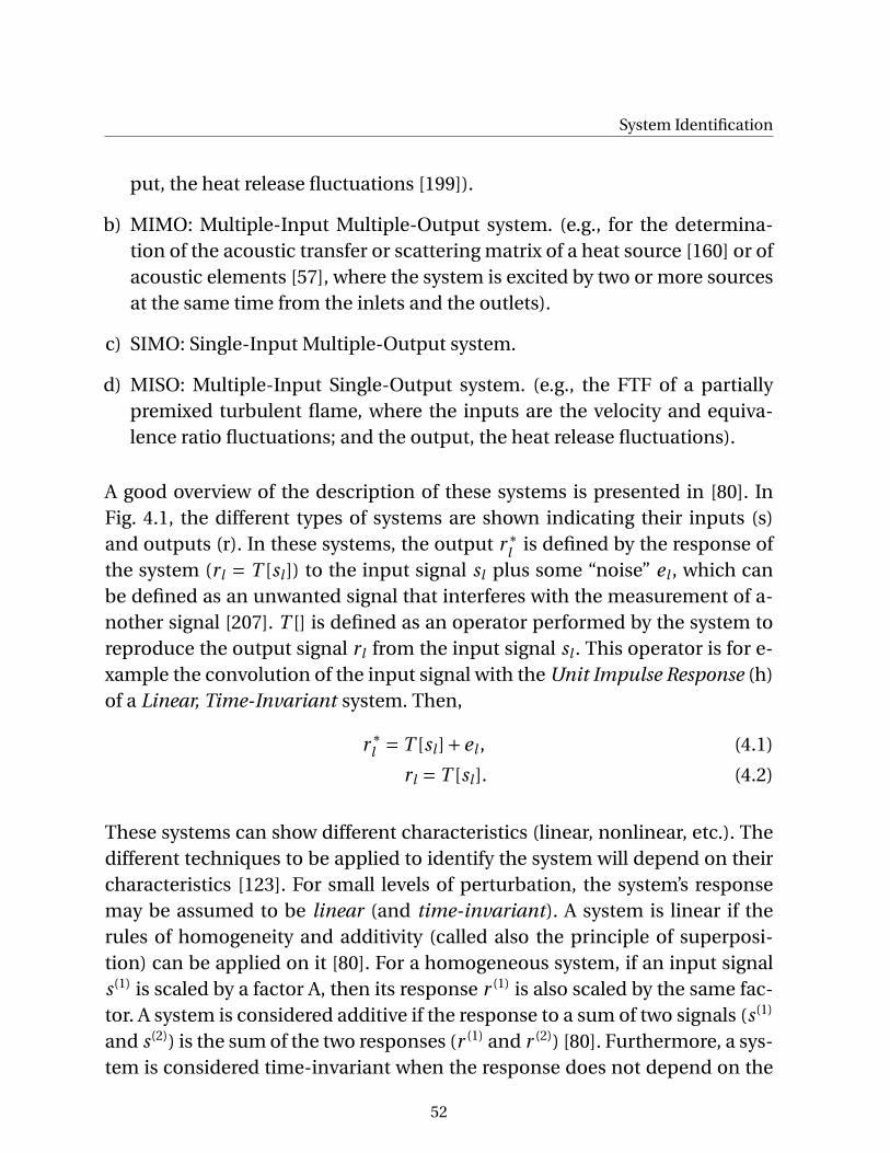
System Identification
put, the heat release fluctuations [199]).
b) MIMO: Multiple-Input Multiple-Output system. (e.g., for the determina-tion of the acoustic transfer or scattering matrix of a heat source [160] or ofacoustic elements [57], where the system is excited by two or more sourcesat the same time from the inlets and the outlets).
c) SIMO: Single-Input Multiple-Output system.
d) MISO: Multiple-Input Single-Output system. (e.g., the FTF of a partiallypremixed turbulent flame, where the inputs are the velocity and equiva-lence ratio fluctuations; and the output, the heat release fluctuations).
A good overview of the description of these systems is presented in [80]. InFig. 4.1, the different types of systems are shown indicating their inputs (s)and outputs (r). In these systems, the output r ∗
l is defined by the response ofthe system (rl = T [sl ]) to the input signal sl plus some “noise” el , which canbe defined as an unwanted signal that interferes with the measurement of a-nother signal [207]. T [] is defined as an operator performed by the system toreproduce the output signal rl from the input signal sl . This operator is for e-xample the convolution of the input signal with the Unit Impulse Response (h)of a Linear, Time-Invariant system. Then,
r ∗l = T [sl ]+el , (4.1)
rl = T [sl ]. (4.2)
These systems can show different characteristics (linear, nonlinear, etc.). Thedifferent techniques to be applied to identify the system will depend on theircharacteristics [123]. For small levels of perturbation, the system’s responsemay be assumed to be linear (and time-invariant). A system is linear if therules of homogeneity and additivity (called also the principle of superposi-tion) can be applied on it [80]. For a homogeneous system, if an input signals(1) is scaled by a factor A, then its response r (1) is also scaled by the same fac-tor. A system is considered additive if the response to a sum of two signals (s(1)
and s(2)) is the sum of the two responses (r (1) and r (2)) [80]. Furthermore, a sys-tem is considered time-invariant when the response does not depend on the
52
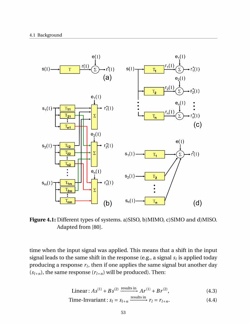
4.1 Background
Figure 4.1: Different types of systems. a)SISO, b)MIMO, c)SIMO and d)MISO.Adapted from [80].
time when the input signal was applied. This means that a shift in the inputsignal leads to the same shift in the response (e.g., a signal sl is applied todayproducing a response rl , then if one applies the same signal but another day(sl+n), the same response (rl+n) will be produced). Then:
Linear : As(1) +B s(2) results in−−−−−→ Ar (1) +Br (2), (4.3)
Time-Invariant : sl = sl+nresults in−−−−−→ rl = rl+n. (4.4)
53
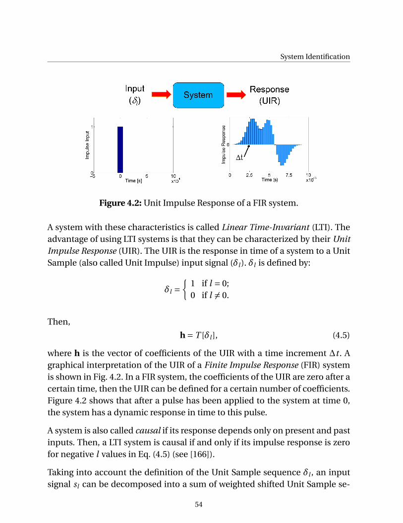
System Identification
Figure 4.2: Unit Impulse Response of a FIR system.
A system with these characteristics is called Linear Time-Invariant (LTI). Theadvantage of using LTI systems is that they can be characterized by their UnitImpulse Response (UIR). The UIR is the response in time of a system to a UnitSample (also called Unit Impulse) input signal (δl ). δl is defined by:
δl =
1 if l = 0;0 if l 6= 0.
Then,
h = T [δl ], (4.5)
where h is the vector of coefficients of the UIR with a time increment ∆t . Agraphical interpretation of the UIR of a Finite Impulse Response (FIR) systemis shown in Fig. 4.2. In a FIR system, the coefficients of the UIR are zero after acertain time, then the UIR can be defined for a certain number of coefficients.Figure 4.2 shows that after a pulse has been applied to the system at time 0,the system has a dynamic response in time to this pulse.
A system is also called causal if its response depends only on present and pastinputs. Then, a LTI system is causal if and only if its impulse response is zerofor negative l values in Eq. (4.5) (see [166]).
Taking into account the definition of the Unit Sample sequence δl , an inputsignal sl can be decomposed into a sum of weighted shifted Unit Sample se-
54

4.1 Background
quences by [166]:
sl =∞∑
k=−∞δl−k sk . (4.6)
then the response of the system to sl is the corresponding sum of weightedoutputs [166]:
rl = T [sl ] = T
[ ∞∑k=−∞
δl−k sk
], (4.7)
=∞∑
k=−∞T [δl−k] sk , (4.8)
=∞∑
k=−∞hl−k sk . (4.9)
Equation 4.9 is called the convolution operation. The convolution is commu-tative in the sense that any of the sequences can be shifted while the other isunaltered [166]. Then:
rl =∞∑
k=−∞hl−k sk =
∞∑k=−∞
hk sl−k . (4.10)
For a LTI system, the output signal rl is the convolution (Eq. (4.10)) of the in-put signal and its UIR. The goal for system identification of a LTI system is to“reconstruct” the UIR of the system.
The convolution of a causal LTI discrete system described by a FIR unit im-pulse response is defined by:
rl =L∑
k=0
hk sl−k , for k = 0, ...,L, (4.11)
hk 6= 0, for 0 ≤ k ≤ L, (4.12)
hk = 0, everywhere else. (4.13)
hk(k = 0, . . . ,L) is the k-th coefficient of the UIR h.
55
System Identification
4.2 The Wiener Filter
The Wiener filter was proposed by Norbert Wiener [217] to reduce the amountof noise present in a signal based on the Least Mean Square error estima-tion [122, 166, 207]. For our study, the Wiener filter is used to identify the di-fferent hk coefficients of the UIR, which describe the flame response in timedomain. The filter allows at the same time to reduce the influence of noisein the identification process. Different system identification methods exit inthe literature (see [122, 123]), nevertheless the Wiener filter presents the ad-vantage of being a robust system identification method which is very straightforward to implement. Furthermore, it requires only modest computationalresources and time for the identification process. This makes it attractive touse for practical applications. Before the filter is described, some statisticalterms are defined which are important for correlation analysis in discrete ran-dom processes:
• The mean value: For a sequence Xk with k=0,..,N; its mean value is de-fined by:
µX = 1
N +1
N∑k=0
X (k). (4.14)
• The cross-correlation: For two sequences Xk and Yk , the cross correlationis a measure of similarity between the two sequences [166] and definedby:
ci = limN →+∞
1
2N +1
N∑k=−N
XkYk−i for i = 0,±1,±2, .., N . (4.15)
For a sequence with a finite number of N+1 samples in a causal FIR sys-tem, the cross-correlation is estimated as:
ci = 1
N +1
N∑k=0
XkYk−i for i = 0, ...,L. (4.16)
The index i is called the lag and indicates the (time) shift between thesequences.
56
4.2 The Wiener Filter
• The auto-correlation: The autocorrelation is the cross-correlation of asignal with itself. It would sound strange to compare a signal with it-self, but with the lag i , the signal is actually being compared at diffe-rent times [193]. For a sequence with a finite number of N+1 samples ina causal FIR system, the autocorrelation is estimated as:
Γi = 1
N +1
N∑k=0
Xk Xk−i for i = 0, ...,L. (4.17)
In the following, the Wiener filter is derived in the context of the identificationof the Flame Transfer Function.
Consider the flame as the SISO system shown in Fig. 4.3, where the input sig-nal is sl =u′
r,l /u and the output signal is r ∗l =Q
′∗l / ¯Q. u′
r /u represents the acousticvelocity fluctuation u′ captured at a reference position and normalized by themean velocity. Q
′∗/ ¯Q is the heat release fluctuation from the flame includingthe influence of “noise” and normalized by its mean value. The “noise” in theoutput signal is produced by some response of the flame to some external per-turbations (e.g., from turbulent fluctuations inside the combustor) which arenot correlated to our input signal. It is assumed that the input signal and the“noise” are uncorrelated. The noise el is defined by:
el = r ∗l − rl , (4.18)
where rl = Q′l / ¯Q is the system’s output without influence of noise. rl is ob-
tained from the convolution of the input signal sl and the UIR of the flame:
el = r ∗l −
L∑k=0
hk sl−k . (4.19)
In the Least Mean Square error estimation, the idea is to minimize the errorbetween a signal and a desired signal. In our case, the error consists of theestimation error plus the noise. The mean square error is computed and mi-
57
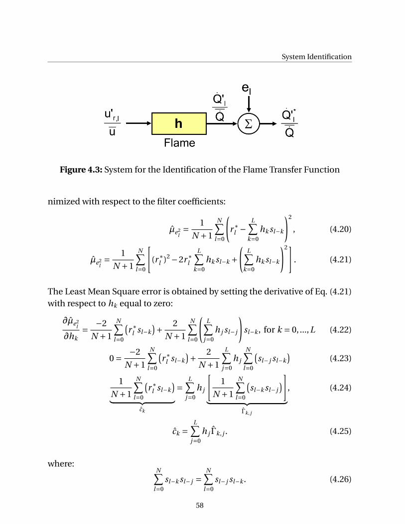
System Identification
Figure 4.3: System for the Identification of the Flame Transfer Function
nimized with respect to the filter coefficients:
µe2l= 1
N +1
N∑l=0
(r ∗
l −L∑
k=0
hk sl−k
)2
, (4.20)
µe2l= 1
N +1
N∑l=0
[(r ∗
l )2 −2r ∗l
L∑k=0
hk sl−k +(
L∑k=0
hk sl−k
)2]. (4.21)
The Least Mean Square error is obtained by setting the derivative of Eq. (4.21)with respect to hk equal to zero:
∂µe2l
∂hk= −2
N +1
N∑l=0
(r ∗
l sl−k
)+ 2
N +1
N∑l=0
(L∑
j=0
h j sl− j
)sl−k , for k = 0, ...,L (4.22)
0 = −2
N +1
N∑l=0
(r ∗
l sl−k
)+ 2
N +1
L∑j=0
h j
N∑l=0
(sl− j sl−k
)(4.23)
1
N +1
N∑l=0
(r ∗
l sl−k
)︸ ︷︷ ︸
ck
=L∑
j=0
h j
[1
N +1
N∑l=0
(sl−k sl− j
)]︸ ︷︷ ︸
Γk, j
, (4.24)
ck =L∑
j=0
h j Γk, j . (4.25)
where:N∑
l=0
sl−k sl− j =N∑
l=0
sl− j sl−k . (4.26)
58
4.2 The Wiener Filter
Considering that NÀL, the cross- and auto-correlation can be approximatedas:
ck ≈ 1
N −L+1
N∑l=L
r ∗l sl−k , for k = 0, ...,L, (4.27)
Γk, j ≈ 1
N −L+1
N∑l=L
sl−k sl− j , for j ,k = 0, ...,L. (4.28)
Equation (4.25) is defined in matrix form as:c0
c1
c2...
cL
=
Γ00 Γ01 Γ02 · · · Γ0(L)
Γ10 Γ11 Γ02 · · · Γ1(L)
Γ20 Γ21 Γ22 · · · Γ2(L)...
...... . . . ...
Γ(L)0 Γ(L)1 ΓL2 · · · Γ(L)(L)
h0
h1
h2...
hL
(4.29)
c = Γh. (4.30)
Equation (4.30) is called the Wiener-Hopf equation. By the inversion of theWiener-Hopf equation, the vector of UIR coefficients (h) is obtained:
Γ−1c = h. (4.31)
The auto-correlation matrix Γmust be inverted to obtain the UIR coefficientsh. If the matrix is ill-conditioned, the accuracy of the solution will suffer forthe solution of the linear system [80]. A system of equations is considered tobe ill-conditioned if a small change in the coefficient matrix (Γ) or a smallchange in the right hand side of the system (c) results in a large change inthe solution vector (h) [94]. In the case of ill-conditioned matrices, it is reco-mmended to use appropriate numerical methods for the solution of the sys-tem, such as the LSQR method (an algorithm for sparse linear equations andsparse least squares) from Paige and Saunders [135]. Additionally, if the inputsignal is “white noise” (defined as an uncorrelated random process with equalpower for all frequencies [207]), then the auto-correlation matrix reduces tothe unit matrix and the UIR is equal to the cross-correlation [158].
59
System Identification
4.3 The LES/SI Method
To perform the identification of the FTF, a LES simulation of the system underconsideration is set up first. The use of non-reflective boundary conditions(NRBC) should be considered to avoid the development of resonance modes,which can degenerate the identification process due to an ill-conditionedauto-correlation matrix [221]. After obtaining a statistically stabilized solu-tion, the system is excited with a broadband perturbation superimposed onthe mean flow at the inlet. As the method is based on correlation analy-sis, having a input signal that is highly decorrelated with itself with “whitenoise” characteristics allows a faster decorrelation between the input signaland noise. Nevertheless, FTF investigations are usually limited to low frequen-cies (usually lower than 1000 Hz) as the flame response of most flames is quitelow at high frequencies. Considering the small times steps used in compressi-ble LES (in the range of 10−6 and 10−7 s), the level of decorrelation with itself(shown by the Autocorrelation) of the input signal is deteriorated as shownin the analysis of Appendix A.5. To generate a signal with high decorrelationcharacteristics for a limited frequency range more advanced methods shouldbe applied as in [58], which is not investigated in this study.
Huber [83, 84] investigated various types of broadband excitation signals(overlaid multi-frequency, broadband white noise (WN) and discrete randombinary signals (DRBS)) and their influence on identification quality. Fromthese three types of excitation signals, the discrete random binary signal(which is created by a random process taking only values of ±uamp at any time)showed the best results as this kind of signal has the lowest crest factor and thehighest power spectral density with respect to the other ones [83]. Then, thiskind of signal is recommended for the excitation. A detailed description of theDRBS signal is shown in Appendix A.5.
During the excitation process, the perturbations will propagate to the flamefront and create a response in the heat release of the flame. A plane is de-fined upstream of the flame at a reference position, and area-averaged ins-tantaneous axial velocity values are exported at each time step (or in shortintervals) from this plane. The global heat release is obtained by a volume
60
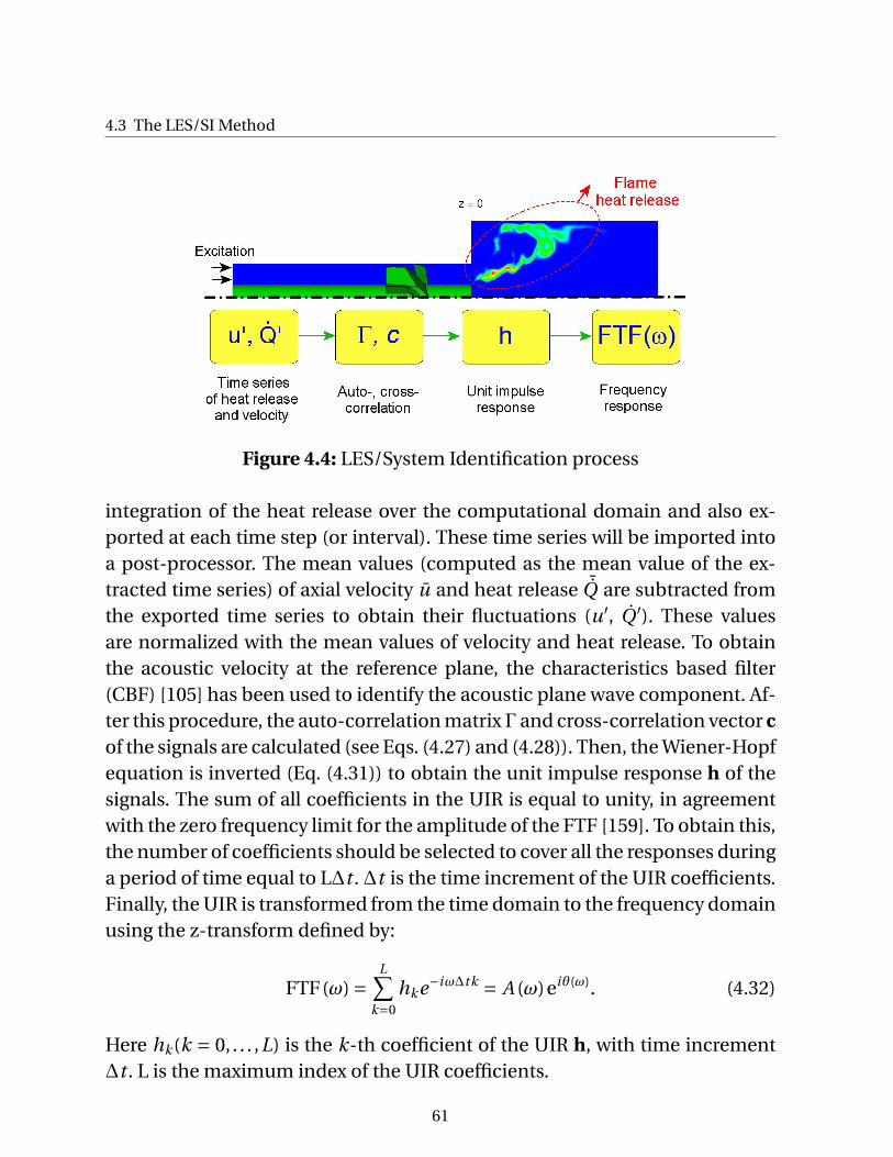
4.3 The LES/SI Method
Figure 4.4: LES/System Identification process
integration of the heat release over the computational domain and also ex-ported at each time step (or interval). These time series will be imported intoa post-processor. The mean values (computed as the mean value of the ex-tracted time series) of axial velocity u and heat release ¯Q are subtracted fromthe exported time series to obtain their fluctuations (u′, Q ′). These valuesare normalized with the mean values of velocity and heat release. To obtainthe acoustic velocity at the reference plane, the characteristics based filter(CBF) [105] has been used to identify the acoustic plane wave component. Af-ter this procedure, the auto-correlation matrixΓ and cross-correlation vector cof the signals are calculated (see Eqs. (4.27) and (4.28)). Then, the Wiener-Hopfequation is inverted (Eq. (4.31)) to obtain the unit impulse response h of thesignals. The sum of all coefficients in the UIR is equal to unity, in agreementwith the zero frequency limit for the amplitude of the FTF [159]. To obtain this,the number of coefficients should be selected to cover all the responses duringa period of time equal to L∆t .∆t is the time increment of the UIR coefficients.Finally, the UIR is transformed from the time domain to the frequency domainusing the z-transform defined by:
FTF(ω) =L∑
k=0
hke−iω∆tk = A (ω)eiθ(ω). (4.32)
Here hk(k = 0, . . . ,L) is the k-th coefficient of the UIR h, with time increment∆t . L is the maximum index of the UIR coefficients.
61

System Identification
A flow chart of the LES/SI method is given in Fig. 4.4 [199]. The advantage ofusing the LES/SI method is that it is possible to obtain the frequency flameresponse over a range of frequencies from a single CFD simulation, reducingthe computational effort (“You can shoot all the birds that you want with onlyone shot”).
62

5 Identification of Flame TransferFunctions using LES/SI
In this chapter, the flame dynamics of an axial swirl burner is investigated bythe determination of its Flame Transfer Function with the LES/SI method. Theexperimental set-up is introduced at the beginning, followed by the validationof the method with experiments. The case of a nonadiabatic combustor with30 kW is used as reference for the validation. After that, the geometrical andoperating conditions in the combustor and burner are varied by changing thethermal conditions at the combustor walls, increasing combustor cross sec-tion area, changing the position of the swirler and increasing the power rating,to study the impact of these variations on the flame dynamics. All experimen-tal data was carried out and provided by T. Komarek [104].
5.1 Experimental Set-up of the BRS Burner
The BRS (Beschaufelter RingSpalt) burner is a swirl-stabilized burner with anaxial swirl generator developed by Komarek and Polifke [103] in the frame-work of the KW 21 project GV 6 Premixed Flame Dynamics. A scheme of theexperimental set-up is shown in Fig. 5.1. The burner is operated in “perfectlypremixed” mode with a completely homogeneous mixture of natural gas andair to eliminate any equivalence ratio fluctuations. The experimental set-upconsists of a cylindrical plenum followed by the burner with the axial swirlgenerator of 30 mm length mounted on a central bluff body. The burner exithas an annular section with an inner and outer diameter of 16 and 40 mm, res-pectively. A combustor of quadratic cross section of 90×90 mm and a lengthof 300 mm follows the burner. With this combustor length, the test conditionswere stable to perform OH chemiluminescence, flow field and FTF measure-
63
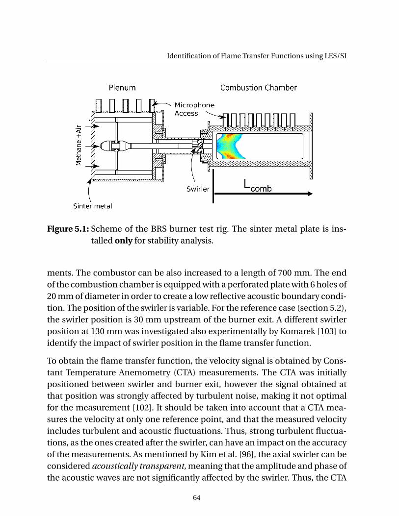
Identification of Flame Transfer Functions using LES/SI
Figure 5.1: Scheme of the BRS burner test rig. The sinter metal plate is ins-talled only for stability analysis.
ments. The combustor can be also increased to a length of 700 mm. The endof the combustion chamber is equipped with a perforated plate with 6 holes of20 mm of diameter in order to create a low reflective acoustic boundary condi-tion. The position of the swirler is variable. For the reference case (section 5.2),the swirler position is 30 mm upstream of the burner exit. A different swirlerposition at 130 mm was investigated also experimentally by Komarek [103] toidentify the impact of swirler position in the flame transfer function.
To obtain the flame transfer function, the velocity signal is obtained by Cons-tant Temperature Anemometry (CTA) measurements. The CTA was initiallypositioned between swirler and burner exit, however the signal obtained atthat position was strongly affected by turbulent noise, making it not optimalfor the measurement [102]. It should be taken into account that a CTA mea-sures the velocity at only one reference point, and that the measured velocityincludes turbulent and acoustic fluctuations. Thus, strong turbulent fluctua-tions, as the ones created after the swirler, can have an impact on the accuracyof the measurements. As mentioned by Kim et al. [96], the axial swirler can beconsidered acoustically transparent, meaning that the amplitude and phase ofthe acoustic waves are not significantly affected by the swirler. Thus, the CTA
64
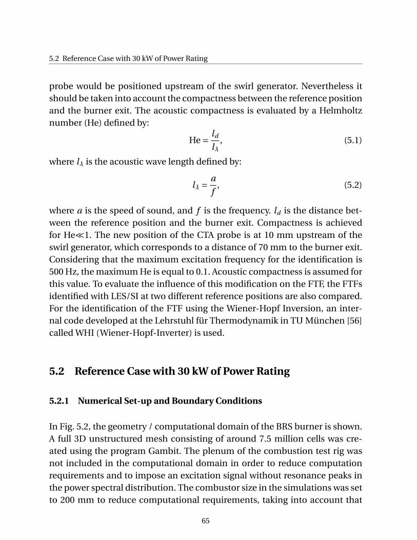
5.2 Reference Case with 30 kW of Power Rating
probe would be positioned upstream of the swirl generator. Nevertheless itshould be taken into account the compactness between the reference positionand the burner exit. The acoustic compactness is evaluated by a Helmholtznumber (He) defined by:
He = ld
lλ, (5.1)
where lλ is the acoustic wave length defined by:
lλ = a
f, (5.2)
where a is the speed of sound, and f is the frequency. ld is the distance bet-ween the reference position and the burner exit. Compactness is achievedfor He¿1. The new position of the CTA probe is at 10 mm upstream of theswirl generator, which corresponds to a distance of 70 mm to the burner exit.Considering that the maximum excitation frequency for the identification is500 Hz, the maximum He is equal to 0.1. Acoustic compactness is assumed forthis value. To evaluate the influence of this modification on the FTF, the FTFsidentified with LES/SI at two different reference positions are also compared.For the identification of the FTF using the Wiener-Hopf Inversion, an inter-nal code developed at the Lehrstuhl für Thermodynamik in TU München [56]called WHI (Wiener-Hopf-Inverter) is used.
5.2 Reference Case with 30 kW of Power Rating
5.2.1 Numerical Set-up and Boundary Conditions
In Fig. 5.2, the geometry / computational domain of the BRS burner is shown.A full 3D unstructured mesh consisting of around 7.5 million cells was cre-ated using the program Gambit. The plenum of the combustion test rig wasnot included in the computational domain in order to reduce computationrequirements and to impose an excitation signal without resonance peaks inthe power spectral distribution. The combustor size in the simulations was setto 200 mm to reduce computational requirements, taking into account that
65
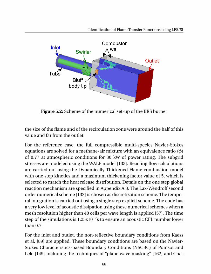
Identification of Flame Transfer Functions using LES/SI
Figure 5.2: Scheme of the numerical set-up of the BRS burner
the size of the flame and of the recirculation zone were around the half of thisvalue and far from the outlet.
For the reference case, the full compressible multi-species Navier-Stokesequations are solved for a methane-air mixture with an equivalence ratio (φ)of 0.77 at atmospheric conditions for 30 kW of power rating. The subgridstresses are modeled using the WALE model [133]. Reacting flow calculationsare carried out using the Dynamically Thickened Flame combustion modelwith one step kinetics and a maximum thickening factor value of 5, which isselected to match the heat release distribution. Details on the one step globalreaction mechanism are specified in Appendix A.3. The Lax-Wendroff secondorder numerical scheme [132] is chosen as discretization scheme. The tempo-ral integration is carried out using a single step explicit scheme. The code hasa very low level of acoustic dissipation using these numerical schemes when amesh resolution higher than 40 cells per wave length is applied [57]. The timestep of the simulations is 1.25x10⁻⁷s to ensure an acoustic CFL number lowerthan 0.7.
For the inlet and outlet, the non-reflective boundary conditions from Kaesset al. [89] are applied. These boundary conditions are based on the Navier-Stokes Characteristics-based Boundary Conditions (NSCBC) of Poinsot andLele [149] including the techniques of “plane wave masking” [162] and Cha-
66
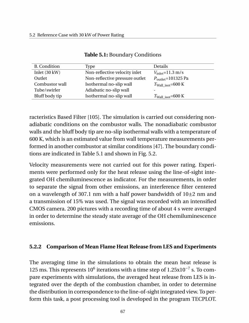
5.2 Reference Case with 30 kW of Power Rating
Table 5.1: Boundary Conditions
B. Condition Type DetailsInlet (30 kW) Non-reflective velocity inlet Vinlet=11.3 m/sOutlet Non-reflective pressure outlet Poutlet=101325 PaCombustor wall Isothermal no-slip wall TWall_isot=600 KTube/swirler Adiabatic no-slip wall -Bluff body tip Isothermal no-slip wall TWall_isot=600 K
racteristics Based Filter [105]. The simulation is carried out considering non-adiabatic conditions on the combustor walls. The nonadiabatic combustorwalls and the bluff body tip are no-slip isothermal walls with a temperature of600 K, which is an estimated value from wall temperature measurements per-formed in another combustor at similar conditions [47]. The boundary condi-tions are indicated in Table 5.1 and shown in Fig. 5.2.
Velocity measurements were not carried out for this power rating. Experi-ments were performed only for the heat release using the line-of-sight inte-grated OH chemiluminescence as indicator. For the measurements, in orderto separate the signal from other emissions, an interference filter centeredon a wavelength of 307.1 nm with a half power bandwidth of 10±2 nm anda transmission of 15% was used. The signal was recorded with an intensifiedCMOS camera. 200 pictures with a recording time of about 4 s were averagedin order to determine the steady state average of the OH chemiluminescenceemissions.
5.2.2 Comparison of Mean Flame Heat Release from LES and Experiments
The averaging time in the simulations to obtain the mean heat release is125 ms. This represents 106 iterations with a time step of 1.25x10⁻⁷ s. To com-pare experiments with simulations, the averaged heat release from LES is in-tegrated over the depth of the combustion chamber, in order to determinethe distribution in correspondence to the line-of-sight integrated view. To per-form this task, a post processing tool is developed in the program TECPLOT.
67
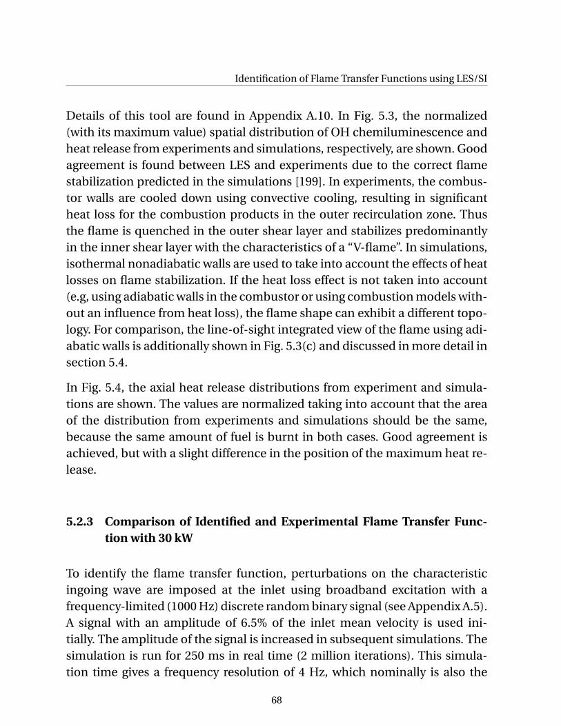
Identification of Flame Transfer Functions using LES/SI
Details of this tool are found in Appendix A.10. In Fig. 5.3, the normalized(with its maximum value) spatial distribution of OH chemiluminescence andheat release from experiments and simulations, respectively, are shown. Goodagreement is found between LES and experiments due to the correct flamestabilization predicted in the simulations [199]. In experiments, the combus-tor walls are cooled down using convective cooling, resulting in significantheat loss for the combustion products in the outer recirculation zone. Thusthe flame is quenched in the outer shear layer and stabilizes predominantlyin the inner shear layer with the characteristics of a “V-flame”. In simulations,isothermal nonadiabatic walls are used to take into account the effects of heatlosses on flame stabilization. If the heat loss effect is not taken into account(e.g, using adiabatic walls in the combustor or using combustion models with-out an influence from heat loss), the flame shape can exhibit a different topo-logy. For comparison, the line-of-sight integrated view of the flame using adi-abatic walls is additionally shown in Fig. 5.3(c) and discussed in more detail insection 5.4.
In Fig. 5.4, the axial heat release distributions from experiment and simula-tions are shown. The values are normalized taking into account that the areaof the distribution from experiments and simulations should be the same,because the same amount of fuel is burnt in both cases. Good agreement isachieved, but with a slight difference in the position of the maximum heat re-lease.
5.2.3 Comparison of Identified and Experimental Flame Transfer Func-tion with 30 kW
To identify the flame transfer function, perturbations on the characteristicingoing wave are imposed at the inlet using broadband excitation with afrequency-limited (1000 Hz) discrete random binary signal (see Appendix A.5).A signal with an amplitude of 6.5% of the inlet mean velocity is used ini-tially. The amplitude of the signal is increased in subsequent simulations. Thesimulation is run for 250 ms in real time (2 million iterations). This simula-tion time gives a frequency resolution of 4 Hz, which nominally is also the
68
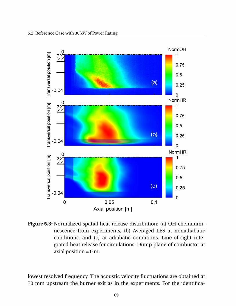
5.2 Reference Case with 30 kW of Power Rating
Figure 5.3: Normalized spatial heat release distribution: (a) OH chemilumi-nescence from experiments, (b) Averaged LES at nonadiabaticconditions, and (c) at adiabatic conditions. Line-of-sight inte-grated heat release for simulations. Dump plane of combustor ataxial position = 0 m.
lowest resolved frequency. The acoustic velocity fluctuations are obtained at70 mm upstream the burner exit as in the experiments. For the identifica-
69
Identification of Flame Transfer Functions using LES/SI
Figure 5.4: Area normalized axial heat release distribution.
tion process, the first 190000 iterations are considered as a transition periodand not taken into account. Axial velocities and volume integrated heat re-lease are extracted “on-the-fly” every 10 iterations during the simulations.The signals are then filtered to remove frequency content higher than 600Hz.The Wiener-Hopf inversion is then applied to obtain the UIR; and finally viaz-transform, the flame transfer function is identified in amplitude and phase(see Fig. 4.4). In Fig. 5.5, the flame transfer functions from experiment andLES/SI are shown with good agreement between them. The experimental andidentified FTF show amplitudes higher than 1 for frequencies below 175 Hzand a decrease at higher frequencies. The observed excess in gain of the FTF(amplitudes > 1) is related to a constructive interaction of acoustic and swirlfluctuations [78, 103, 137] (see section 5.5.2). Moreover, instabilities are moresusceptible to develop under this condition [181]. The phase of the transferfunction, which is of particular importance for thermo-acoustic instability,was also well reproduced for frequencies below 260 Hz, where the amplitudesof the experimental and identified FTF have good agreement. At higher fre-quencies, the agreement between experiment and simulations decreases, ex-hibiting high deviations in the phase. These discrepancies could be producedby limitations of the combustion model to capture the response at high fre-quencies, or also by a low signal-to-noise ratio in the identification. In LES,
70
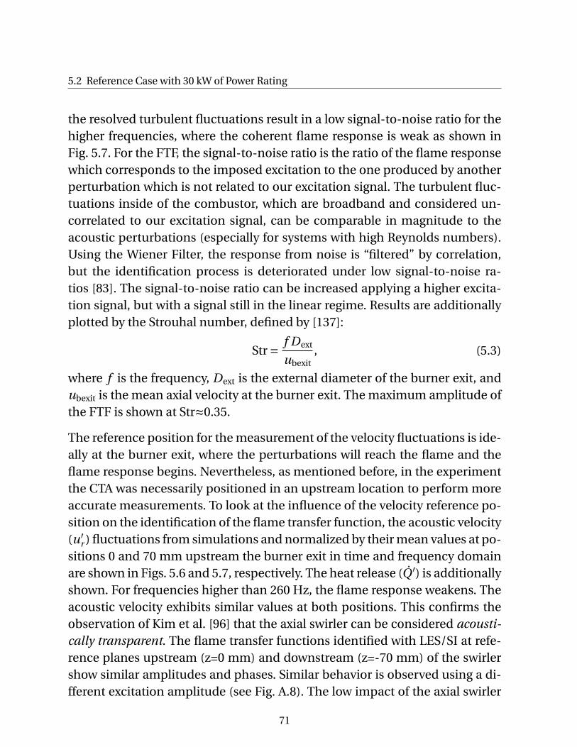
5.2 Reference Case with 30 kW of Power Rating
the resolved turbulent fluctuations result in a low signal-to-noise ratio for thehigher frequencies, where the coherent flame response is weak as shown inFig. 5.7. For the FTF, the signal-to-noise ratio is the ratio of the flame responsewhich corresponds to the imposed excitation to the one produced by anotherperturbation which is not related to our excitation signal. The turbulent fluc-tuations inside of the combustor, which are broadband and considered un-correlated to our excitation signal, can be comparable in magnitude to theacoustic perturbations (especially for systems with high Reynolds numbers).Using the Wiener Filter, the response from noise is “filtered” by correlation,but the identification process is deteriorated under low signal-to-noise ra-tios [83]. The signal-to-noise ratio can be increased applying a higher excita-tion signal, but with a signal still in the linear regime. Results are additionallyplotted by the Strouhal number, defined by [137]:
Str = f Dext
ubexit, (5.3)
where f is the frequency, Dext is the external diameter of the burner exit, andubexit is the mean axial velocity at the burner exit. The maximum amplitude ofthe FTF is shown at Str≈0.35.
The reference position for the measurement of the velocity fluctuations is ide-ally at the burner exit, where the perturbations will reach the flame and theflame response begins. Nevertheless, as mentioned before, in the experimentthe CTA was necessarily positioned in an upstream location to perform moreaccurate measurements. To look at the influence of the velocity reference po-sition on the identification of the flame transfer function, the acoustic velocity(u′
r ) fluctuations from simulations and normalized by their mean values at po-sitions 0 and 70 mm upstream the burner exit in time and frequency domainare shown in Figs. 5.6 and 5.7, respectively. The heat release (Q ′) is additionallyshown. For frequencies higher than 260 Hz, the flame response weakens. Theacoustic velocity exhibits similar values at both positions. This confirms theobservation of Kim et al. [96] that the axial swirler can be considered acousti-cally transparent. The flame transfer functions identified with LES/SI at refe-rence planes upstream (z=0 mm) and downstream (z=-70 mm) of the swirlershow similar amplitudes and phases. Similar behavior is observed using a di-fferent excitation amplitude (see Fig. A.8). The low impact of the axial swirler
71
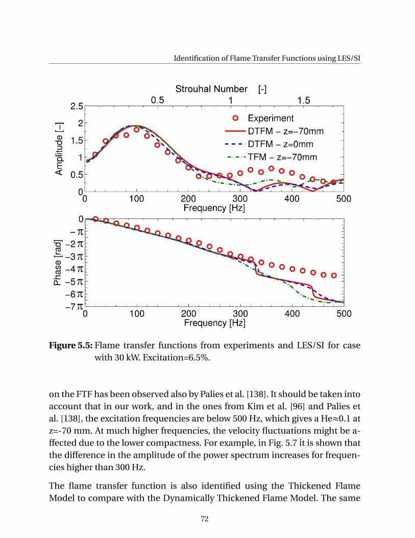
Identification of Flame Transfer Functions using LES/SI
Figure 5.5: Flame transfer functions from experiments and LES/SI for casewith 30 kW. Excitation=6.5%.
on the FTF has been observed also by Palies et al. [138]. It should be taken intoaccount that in our work, and in the ones from Kim et al. [96] and Palies etal. [138], the excitation frequencies are below 500 Hz, which gives a He≈0.1 atz=-70 mm. At much higher frequencies, the velocity fluctuations might be a-ffected due to the lower compactness. For example, in Fig. 5.7 it is shown thatthe difference in the amplitude of the power spectrum increases for frequen-cies higher than 300 Hz.
The flame transfer function is also identified using the Thickened FlameModel to compare with the Dynamically Thickened Flame Model. The same
72
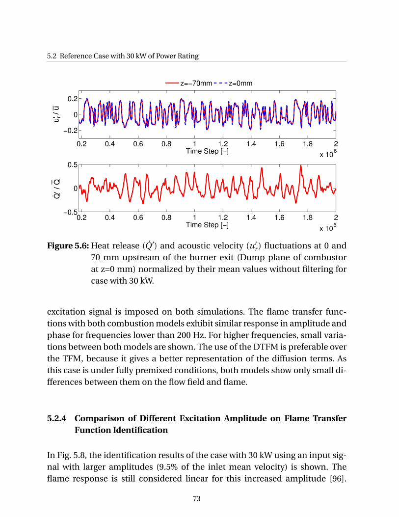
5.2 Reference Case with 30 kW of Power Rating
Figure 5.6: Heat release (Q ′) and acoustic velocity (u′r ) fluctuations at 0 and
70 mm upstream of the burner exit (Dump plane of combustorat z=0 mm) normalized by their mean values without filtering forcase with 30 kW.
excitation signal is imposed on both simulations. The flame transfer func-tions with both combustion models exhibit similar response in amplitude andphase for frequencies lower than 200 Hz. For higher frequencies, small varia-tions between both models are shown. The use of the DTFM is preferable overthe TFM, because it gives a better representation of the diffusion terms. Asthis case is under fully premixed conditions, both models show only small di-fferences between them on the flow field and flame.
5.2.4 Comparison of Different Excitation Amplitude on Flame TransferFunction Identification
In Fig. 5.8, the identification results of the case with 30 kW using an input sig-nal with larger amplitudes (9.5% of the inlet mean velocity) is shown. Theflame response is still considered linear for this increased amplitude [96].
73
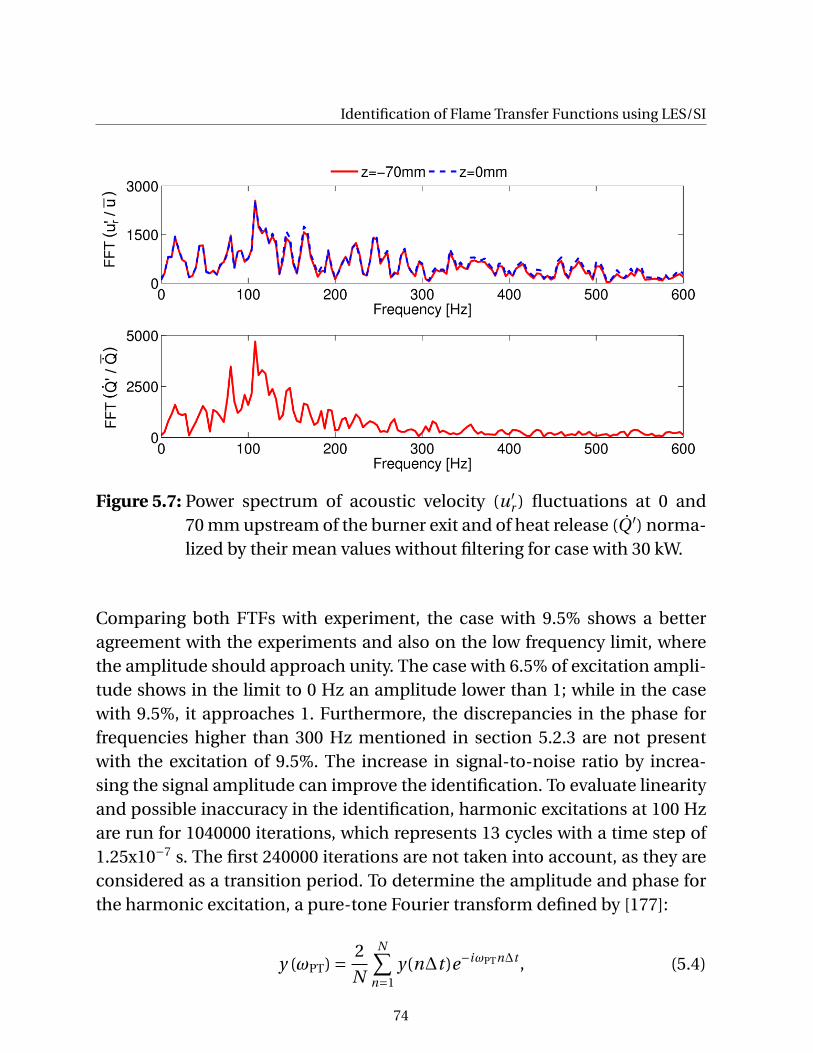
Identification of Flame Transfer Functions using LES/SI
Figure 5.7: Power spectrum of acoustic velocity (u′r ) fluctuations at 0 and
70 mm upstream of the burner exit and of heat release (Q ′) norma-lized by their mean values without filtering for case with 30 kW.
Comparing both FTFs with experiment, the case with 9.5% shows a betteragreement with the experiments and also on the low frequency limit, wherethe amplitude should approach unity. The case with 6.5% of excitation ampli-tude shows in the limit to 0 Hz an amplitude lower than 1; while in the casewith 9.5%, it approaches 1. Furthermore, the discrepancies in the phase forfrequencies higher than 300 Hz mentioned in section 5.2.3 are not presentwith the excitation of 9.5%. The increase in signal-to-noise ratio by increa-sing the signal amplitude can improve the identification. To evaluate linearityand possible inaccuracy in the identification, harmonic excitations at 100 Hzare run for 1040000 iterations, which represents 13 cycles with a time step of1.25x10−7 s. The first 240000 iterations are not taken into account, as they areconsidered as a transition period. To determine the amplitude and phase forthe harmonic excitation, a pure-tone Fourier transform defined by [177]:
y (ωPT) = 2
N
N∑n=1
y(n∆t )e−iωPTn∆t , (5.4)
74
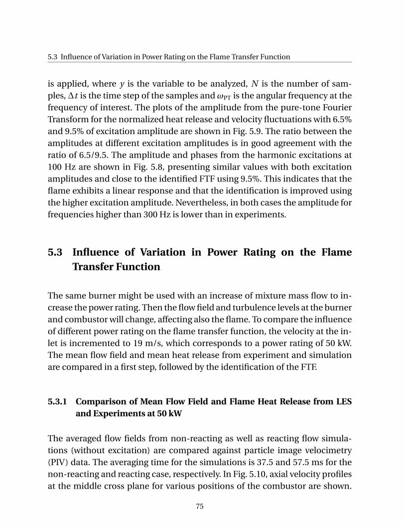
5.3 Influence of Variation in Power Rating on the Flame Transfer Function
is applied, where y is the variable to be analyzed, N is the number of sam-ples,∆t is the time step of the samples andωPT is the angular frequency at thefrequency of interest. The plots of the amplitude from the pure-tone FourierTransform for the normalized heat release and velocity fluctuations with 6.5%and 9.5% of excitation amplitude are shown in Fig. 5.9. The ratio between theamplitudes at different excitation amplitudes is in good agreement with theratio of 6.5/9.5. The amplitude and phases from the harmonic excitations at100 Hz are shown in Fig. 5.8, presenting similar values with both excitationamplitudes and close to the identified FTF using 9.5%. This indicates that theflame exhibits a linear response and that the identification is improved usingthe higher excitation amplitude. Nevertheless, in both cases the amplitude forfrequencies higher than 300 Hz is lower than in experiments.
5.3 Influence of Variation in Power Rating on the FlameTransfer Function
The same burner might be used with an increase of mixture mass flow to in-crease the power rating. Then the flow field and turbulence levels at the burnerand combustor will change, affecting also the flame. To compare the influenceof different power rating on the flame transfer function, the velocity at the in-let is incremented to 19 m/s, which corresponds to a power rating of 50 kW.The mean flow field and mean heat release from experiment and simulationare compared in a first step, followed by the identification of the FTF.
5.3.1 Comparison of Mean Flow Field and Flame Heat Release from LESand Experiments at 50 kW
The averaged flow fields from non-reacting as well as reacting flow simula-tions (without excitation) are compared against particle image velocimetry(PIV) data. The averaging time for the simulations is 37.5 and 57.5 ms for thenon-reacting and reacting case, respectively. In Fig. 5.10, axial velocity profilesat the middle cross plane for various positions of the combustor are shown.
75
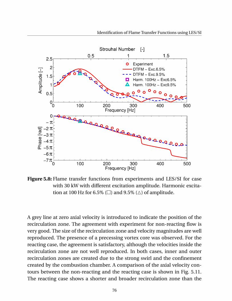
Identification of Flame Transfer Functions using LES/SI
Figure 5.8: Flame transfer functions from experiments and LES/SI for casewith 30 kW with different excitation amplitude. Harmonic excita-tion at 100 Hz for 6.5% () and 9.5% (M) of amplitude.
A grey line at zero axial velocity is introduced to indicate the position of therecirculation zone. The agreement with experiment for non-reacting flow isvery good. The size of the recirculation zone and velocity magnitudes are wellreproduced. The presence of a precessing vortex core was observed. For thereacting case, the agreement is satisfactory, although the velocities inside therecirculation zone are not well reproduced. In both cases, inner and outerrecirculation zones are created due to the strong swirl and the confinementcreated by the combustion chamber. A comparison of the axial velocity con-tours between the non-reacting and the reacting case is shown in Fig. 5.11.The reacting case shows a shorter and broader recirculation zone than the
76
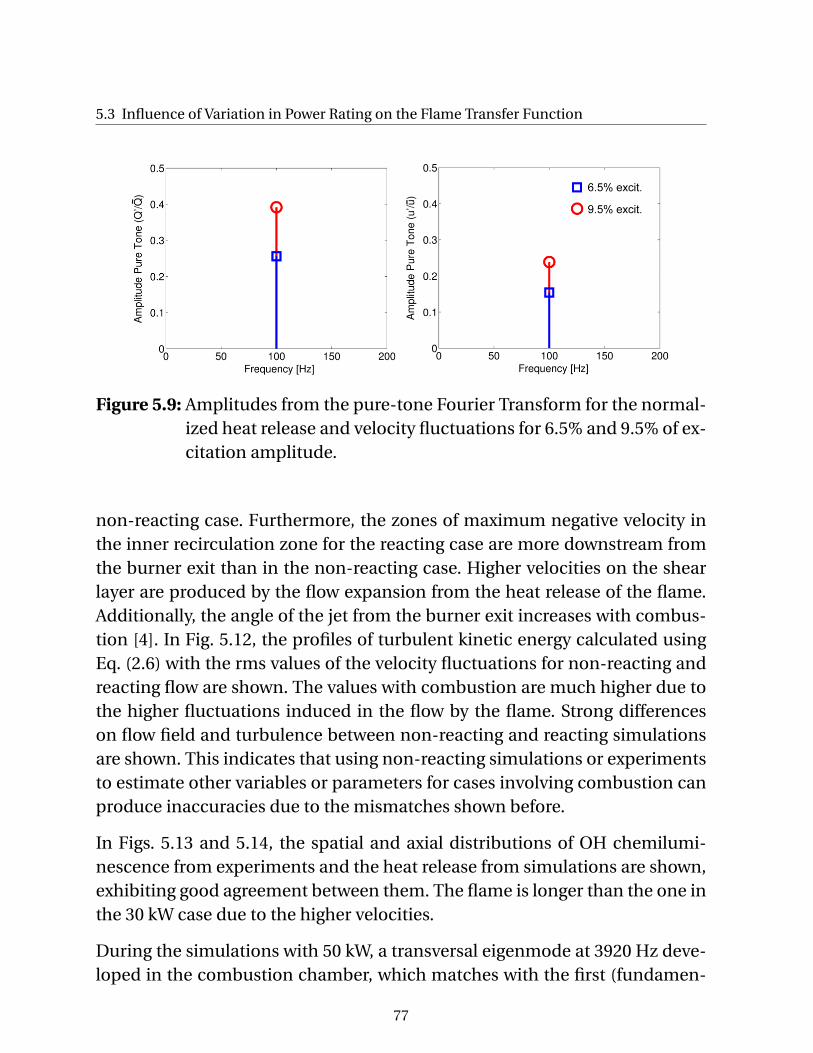
5.3 Influence of Variation in Power Rating on the Flame Transfer Function
Figure 5.9: Amplitudes from the pure-tone Fourier Transform for the normal-ized heat release and velocity fluctuations for 6.5% and 9.5% of ex-citation amplitude.
non-reacting case. Furthermore, the zones of maximum negative velocity inthe inner recirculation zone for the reacting case are more downstream fromthe burner exit than in the non-reacting case. Higher velocities on the shearlayer are produced by the flow expansion from the heat release of the flame.Additionally, the angle of the jet from the burner exit increases with combus-tion [4]. In Fig. 5.12, the profiles of turbulent kinetic energy calculated usingEq. (2.6) with the rms values of the velocity fluctuations for non-reacting andreacting flow are shown. The values with combustion are much higher due tothe higher fluctuations induced in the flow by the flame. Strong differenceson flow field and turbulence between non-reacting and reacting simulationsare shown. This indicates that using non-reacting simulations or experimentsto estimate other variables or parameters for cases involving combustion canproduce inaccuracies due to the mismatches shown before.
In Figs. 5.13 and 5.14, the spatial and axial distributions of OH chemilumi-nescence from experiments and the heat release from simulations are shown,exhibiting good agreement between them. The flame is longer than the one inthe 30 kW case due to the higher velocities.
During the simulations with 50 kW, a transversal eigenmode at 3920 Hz deve-loped in the combustion chamber, which matches with the first (fundamen-
77
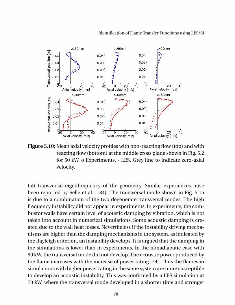
Identification of Flame Transfer Functions using LES/SI
Figure 5.10: Mean axial velocity profiles with non-reacting flow (top) and withreacting flow (bottom) at the middle cross plane shown in Fig. 5.2for 50 kW. o Experiments, - LES. Grey line to indicate zero-axialvelocity.
tal) transversal eigenfrequency of the geometry. Similar experiences havebeen reported by Selle et al. [184]. The transversal mode shown in Fig. 5.15is due to a combination of the two degenerate transversal modes. The highfrequency instability did not appear in experiments. In experiments, the com-bustor walls have certain level of acoustic damping by vibration, which is nottaken into account in numerical simulations. Some acoustic damping is cre-ated due to the wall heat losses. Nevertheless if the instability driving mecha-nisms are higher than the damping mechanisms in the system, as indicated bythe Rayleigh criterion, an instability develops. It is argued that the damping inthe simulations is lower than in experiments. In the nonadiabatic case with30 kW, the transversal mode did not develop. The acoustic power produced bythe flame increases with the increase of power rating [79]. Thus the flames insimulations with higher power rating in the same system are more susceptibleto develop an acoustic instability. This was confirmed by a LES simulation at70 kW, where the transversal mode developed in a shorter time and stronger
78
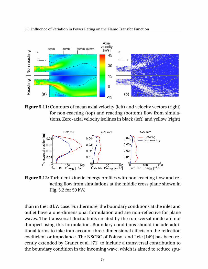
5.3 Influence of Variation in Power Rating on the Flame Transfer Function
Figure 5.11: Contours of mean axial velocity (left) and velocity vectors (right)for non-reacting (top) and reacting (bottom) flow from simula-tions. Zero-axial velocity isolines in black (left) and yellow (right)
Figure 5.12: Turbulent kinetic energy profiles with non-reacting flow and re-acting flow from simulations at the middle cross plane shown inFig. 5.2 for 50 kW.
than in the 50 kW case. Furthermore, the boundary conditions at the inlet andoutlet have a one-dimensional formulation and are non-reflective for planewaves. The transversal fluctuations created by the transversal mode are notdumped using this formulation. Boundary conditions should include addi-tional terms to take into account three-dimensional effects on the reflectioncoefficient or impedance. The NSCBC of Poinsot and Lele [149] has been re-cently extended by Granet et al. [71] to include a transversal contribution tothe boundary condition in the incoming wave, which is aimed to reduce spu-
79
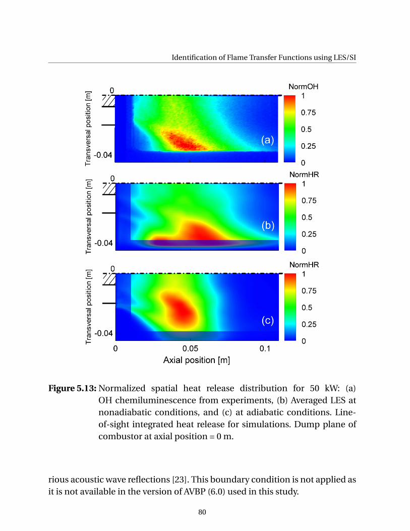
Identification of Flame Transfer Functions using LES/SI
Figure 5.13: Normalized spatial heat release distribution for 50 kW: (a)OH chemiluminescence from experiments, (b) Averaged LES atnonadiabatic conditions, and (c) at adiabatic conditions. Line-of-sight integrated heat release for simulations. Dump plane ofcombustor at axial position = 0 m.
rious acoustic wave reflections [23]. This boundary condition is not applied asit is not available in the version of AVBP (6.0) used in this study.
80
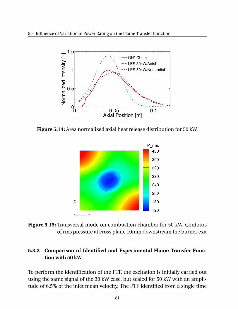
5.3 Influence of Variation in Power Rating on the Flame Transfer Function
Figure 5.14: Area normalized axial heat release distribution for 50 kW.
Figure 5.15: Transversal mode on combustion chamber for 50 kW. Contoursof rms pressure at cross plane 10mm downstream the burner exit
5.3.2 Comparison of Identified and Experimental Flame Transfer Func-tion with 50 kW
To perform the identification of the FTF, the excitation is initially carried outusing the same signal of the 30 kW case, but scaled for 50 kW with an ampli-tude of 6.5% of the inlet mean velocity. The FTF identified from a single time
81

Identification of Flame Transfer Functions using LES/SI
series of length 1800000 (STS) and filtered to 600 Hz is presented in Fig. 5.16.The level of agreement with the experimental data is not satisfactory. Strongoscillations in the amplitude and phase are present. It is expected that thesignificant disagreements are due to the influence of “noise”, i.e. turbulent“pseudo sound”, fluctuations of the heat release produced by resolved turbu-lent fluctuations, and in particular perturbations introduced by the transver-sal modes, which grow to significant amplitudes after about 750000 iterations,as shown in Figs. 5.17 and 5.18. These perturbations introduce spurious con-tributions to the auto- and cross-correlations Γ and c of signal and response,respectively, and thus deteriorate the quality of the identification scheme. Ingeneral, the identification quality can be improved by using a longer time se-ries [84]. This is not possible in the present case due to the unstable transversalmode, which kept growing in amplitude as the run continued.
Attempts to suppress the transversal mode were not successful, therefore a“work-around” is devised: In order to obtain a more robust identification,time series generated from several LES runs are combined. Two methodolo-gies were develop. In the first one, called Multiple Time Series (MTS), the auto-and cross-correlation coefficients from various runs are combined into a mul-tiple time series auto- and cross-correlation by an averaging procedure, thussuppressing the relative magnitude of uncorrelated noise. Each run startedfrom the same initial condition, but used different excitation time series, ge-nerated from various seeds of the random number generator. The combinedauto- and cross-correlation coefficients are approximated by:
Γk, j |MTS ≈MS∑i=1
(1
N −L+1
N∑l=L
sl−k sl− j
)i
, for j ,k = 0, ...,L, (5.5)
ck |MTS ≈MS∑i=1
(1
N −L+1
N∑l=L
r ∗l sl−k
)i
, for k = 0, ...,L. (5.6)
where MS is the number of multiple sequences with the number of ele-ments N. The WHI is applied using Γk, j |MTS and c|MTS as the auto- and cross-correlations. The second method is called Single Joint Time Series (SJTS). Forcreating a SJTS, first a long time series is created from the random numbergenerator as the base excitation signal (see Fig. 5.20(a)). Similar to the MTS
82
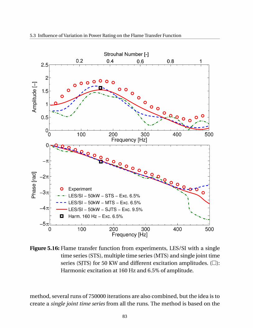
5.3 Influence of Variation in Power Rating on the Flame Transfer Function
Figure 5.16: Flame transfer function from experiments, LES/SI with a singletime series (STS), multiple time series (MTS) and single joint timeseries (SJTS) for 50 KW and different excitation amplitudes. ():Harmonic excitation at 160 Hz and 6.5% of amplitude.
method, several runs of 750000 iterations are also combined, but the idea is tocreate a single joint time series from all the runs. The method is based on the
83

Identification of Flame Transfer Functions using LES/SI
Figure 5.17: Heat release (Q ′) and acoustic velocity (u′r ) fluctuations at 70 mm
upstream of the burner exit (Dump plane of combustor atz=0 mm) normalized by their mean values without filtering forcase with 50 kW.
concept of linear and time-invariant systems. If the same system is excitedusing two different simulations (similar to say at two “different times”) andwith the same excitation signal, the response of both simulations will be simi-lar. Thus various simulations can be used to “continue” a previous one. This isillustrated in the following example: In Fig. 5.19, two input signals (normalizedvelocity fluctuations) are shown with their respective responses (normalizedheat release fluctuations). The system is excited first with signal 1 until 750000iterations. After this, the same system at the same initial point of the run withsignal 1 is excited with signal 2 also for 750000 iterations. The values of signal 2in the first 250000 iterations are the same as the last 250000 values of signal 1.It is shown that after a time interval (approx. 55000 iterations), both cases ex-hibit the same response. At this point both signals can be joined into a singlejoint time series consisting in information from signal 1 from iterations 0 to555000 and from signal 2 from iterations 555000 to 1250000. The joint timeseries can be extended with additional simulations. In this way, the influenceof the transversal mode is reduced and it is possible to obtain a single long
84
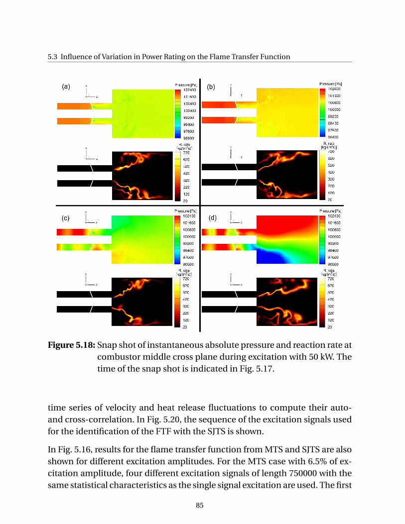
5.3 Influence of Variation in Power Rating on the Flame Transfer Function
Figure 5.18: Snap shot of instantaneous absolute pressure and reaction rate atcombustor middle cross plane during excitation with 50 kW. Thetime of the snap shot is indicated in Fig. 5.17.
time series of velocity and heat release fluctuations to compute their auto-and cross-correlation. In Fig. 5.20, the sequence of the excitation signals usedfor the identification of the FTF with the SJTS is shown.
In Fig. 5.16, results for the flame transfer function from MTS and SJTS are alsoshown for different excitation amplitudes. For the MTS case with 6.5% of ex-citation amplitude, four different excitation signals of length 750000 with thesame statistical characteristics as the single signal excitation are used. The first
85
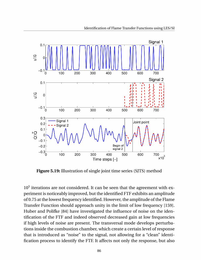
Identification of Flame Transfer Functions using LES/SI
Figure 5.19: Illustration of single joint time series (SJTS) method
105 iterations are not considered. It can be seen that the agreement with ex-periment is noticeably improved, but the identified FTF exhibits an amplitudeof 0.75 at the lowest frequency identified. However, the amplitude of the FlameTransfer Function should approach unity in the limit of low frequency [159].Huber and Polifke [84] have investigated the influence of noise on the iden-tification of the FTF and indeed observed decreased gain at low frequenciesif high levels of noise are present. The transversal mode develops perturba-tions inside the combustion chamber, which create a certain level of responsethat is introduced as “noise” to the signal, not allowing for a “clean” identi-fication process to identify the FTF. It affects not only the response, but also
86
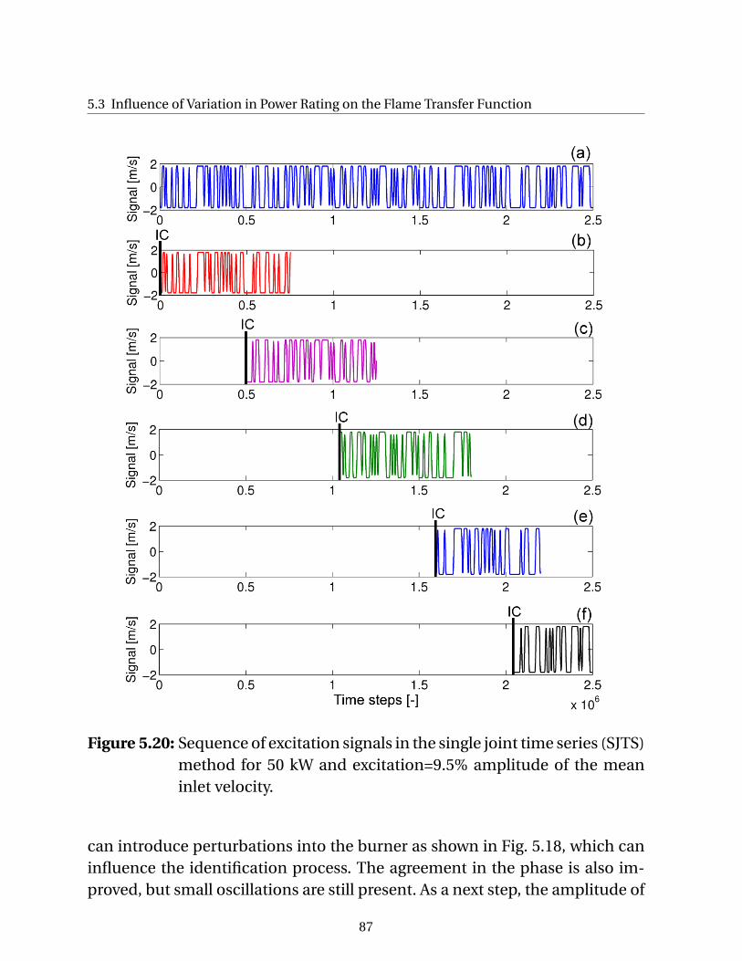
5.3 Influence of Variation in Power Rating on the Flame Transfer Function
Figure 5.20: Sequence of excitation signals in the single joint time series (SJTS)method for 50 kW and excitation=9.5% amplitude of the meaninlet velocity.
can introduce perturbations into the burner as shown in Fig. 5.18, which caninfluence the identification process. The agreement in the phase is also im-proved, but small oscillations are still present. As a next step, the amplitude of
87
Identification of Flame Transfer Functions using LES/SI
the signal is increased to 9.5% of the inlet mean velocity to increase the signal-to-noise ratio. For this case with higher excitation amplitude, the MTS andthe SJTS methods are applied using six different simulations of length 750000with a total length of 2.8 million iterations for the SJTS. The first 190000 itera-tions of the SJTS are not considered. Both methods yielded similar results andonly the results from the SJTS are shown in Fig. 5.16. Results are also plottedin Strouhal number. For this new case, the amplitude of the FTF approachesunity in the low frequency limit, with good qualitative agreement in the ampli-tude. The experimental and identified FTFs show their maximum amplitudesat similar Strouhal numbers (≈0.34), and with a good scaling with the 30 kWcase. The value of the maximum amplitude of the experimental FTF is not re-produced by the identification. The phase exhibits good agreement with theexperiment and the oscillations mentioned before are not present. Compa-ring the amplitudes in the FTF for 6.5% and 9.5%, both are qualitatively simi-lar with small discrepances between them. Furthermore, both cases exhibitlower amplitudes than the experiment. Harmonic excitation at 160 Hz with anexcitation amplitude of 6.5% is carried out for 5x10⁵ iterations, which repre-sents 10 cycles with a time step of 1.25x10⁻⁷ s. The first 105 iterations are nottaken into account. The agreement in amplitude and phase of the harmonicexcitation with the identified FTF is good. As the amplitude between the har-monic excitation and the one from the identification is in good agreement, theresponse at this frequency is well identified by the LES/SI method. This indi-cates that the lower amplitude in the identified FTF than in the experiments isnot produced by limitations of the identification process, but from other rea-sons, e.g. inaccuracies in the measurements (no information about the accu-racy of the experimental results is available), or by the lower resolution of thesimulation with higher Reynolds numbers using the same mesh. In a simu-lation using the same mesh and increasing the Reynolds number, the cut-offwave number defined by the grid size is the same. However, the energy spec-trum becomes broader [14] due to the smaller turbulent scales (see Fig. 2.3).Thus the resolved turbulent kinetic energy is decreased, and the accuracy ofthe sub-grid models (for turbulence and combustion) becomes more influen-tial on the results. Moreover, the dynamical response of the flame might bereduced with the lower resolution of the turbulent scales, producing a lower
88
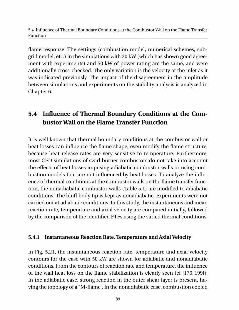
5.4 Influence of Thermal Boundary Conditions at the Combustor Wall on the Flame TransferFunction
flame response. The settings (combustion model, numerical schemes, sub-grid model, etc.) in the simulations with 30 kW (which has shown good agree-ment with experiments) and 50 kW of power rating are the same, and wereadditionally cross-checked. The only variation is the velocity at the inlet as itwas indicated previously. The impact of the disagreement in the amplitudebetween simulations and experiments on the stability analysis is analyzed inChapter 6.
5.4 Influence of Thermal Boundary Conditions at the Com-bustor Wall on the Flame Transfer Function
It is well known that thermal boundary conditions at the combustor wall orheat losses can influence the flame shape, even modify the flame structure,because heat release rates are very sensitive to temperature. Furthermore,most CFD simulations of swirl burner combustors do not take into accountthe effects of heat losses imposing adiabatic combustor walls or using com-bustion models that are not influenced by heat losses. To analyze the influ-ence of thermal conditions at the combustor walls on the flame transfer func-tion, the nonadiabatic combustor walls (Table 5.1) are modified to adiabaticconditions. The bluff body tip is kept as nonadiabatic. Experiments were notcarried out at adiabatic conditions. In this study, the instantaneous and meanreaction rate, temperature and axial velocity are compared initially, followedby the comparison of the identified FTFs using the varied thermal conditions.
5.4.1 Instantaneous Reaction Rate, Temperature and Axial Velocity
In Fig. 5.21, the instantaneous reaction rate, temperature and axial velocitycontours for the case with 50 kW are shown for adiabatic and nonadiabaticconditions. From the contours of reaction rate and temperature, the influenceof the wall heat loss on the flame stabilization is clearly seen (cf [176, 199]).In the adiabatic case, strong reaction in the outer shear layer is present, ha-ving the topology of a “M-flame”. In the nonadiabatic case, combustion cooled
89
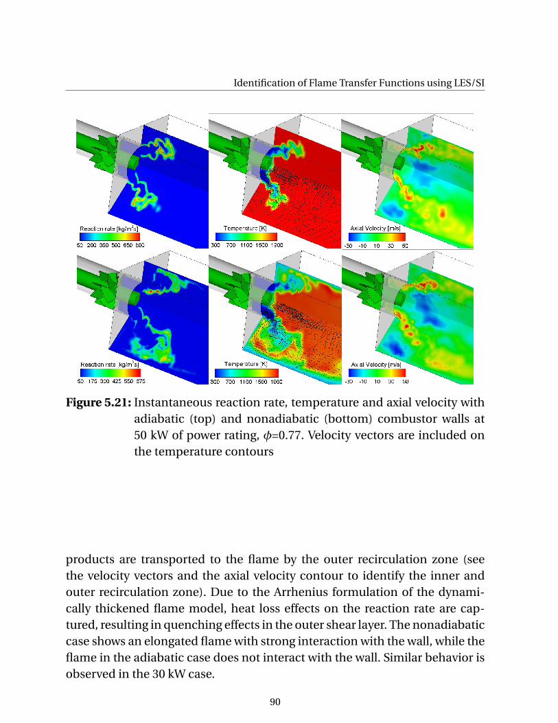
Identification of Flame Transfer Functions using LES/SI
Figure 5.21: Instantaneous reaction rate, temperature and axial velocity withadiabatic (top) and nonadiabatic (bottom) combustor walls at50 kW of power rating, φ=0.77. Velocity vectors are included onthe temperature contours
products are transported to the flame by the outer recirculation zone (seethe velocity vectors and the axial velocity contour to identify the inner andouter recirculation zone). Due to the Arrhenius formulation of the dynami-cally thickened flame model, heat loss effects on the reaction rate are cap-tured, resulting in quenching effects in the outer shear layer. The nonadiabaticcase shows an elongated flame with strong interaction with the wall, while theflame in the adiabatic case does not interact with the wall. Similar behavior isobserved in the 30 kW case.
90
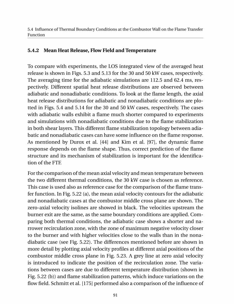
5.4 Influence of Thermal Boundary Conditions at the Combustor Wall on the Flame TransferFunction
5.4.2 Mean Heat Release, Flow Field and Temperature
To compare with experiments, the LOS integrated view of the averaged heatrelease is shown in Figs. 5.3 and 5.13 for the 30 and 50 kW cases, respectively.The averaging time for the adiabatic simulations are 112.5 and 62.4 ms, res-pectively. Different spatial heat release distributions are observed betweenadiabatic and nonadiabatic conditions. To look at the flame length, the axialheat release distributions for adiabatic and nonadiabatic conditions are plo-tted in Figs. 5.4 and 5.14 for the 30 and 50 kW cases, respectively. The caseswith adiabatic walls exhibit a flame much shorter compared to experimentsand simulations with nonadiabatic conditions due to the flame stabilizationin both shear layers. This different flame stabilization topology between adia-batic and nonadiabatic cases can have some influence on the flame response.As mentioned by Durox et al. [44] and Kim et al. [97], the dynamic flameresponse depends on the flame shape. Thus, correct prediction of the flamestructure and its mechanism of stabilization is important for the identifica-tion of the FTF.
For the comparison of the mean axial velocity and mean temperature betweenthe two different thermal conditions, the 30 kW case is chosen as reference.This case is used also as reference case for the comparison of the flame trans-fer function. In Fig. 5.22 (a), the mean axial velocity contours for the adiabaticand nonadiabatic cases at the combustor middle cross plane are shown. Thezero-axial velocity isolines are showed in black. The velocities upstream theburner exit are the same, as the same boundary conditions are applied. Com-paring both thermal conditions, the adiabatic case shows a shorter and na-rrower recirculation zone, with the zone of maximum negative velocity closerto the burner and with higher velocities close to the walls than in the nona-diabatic case (see Fig. 5.22). The differences mentioned before are shown inmore detail by plotting axial velocity profiles at different axial positions of thecombustor middle cross plane in Fig. 5.23. A grey line at zero axial velocityis introduced to indicate the position of the recirculation zone. The varia-tions between cases are due to different temperature distribution (shown inFig. 5.22 (b)) and flame stabilization patterns, which induce variations on theflow field. Schmitt et al. [175] performed also a comparison of the influence of
91
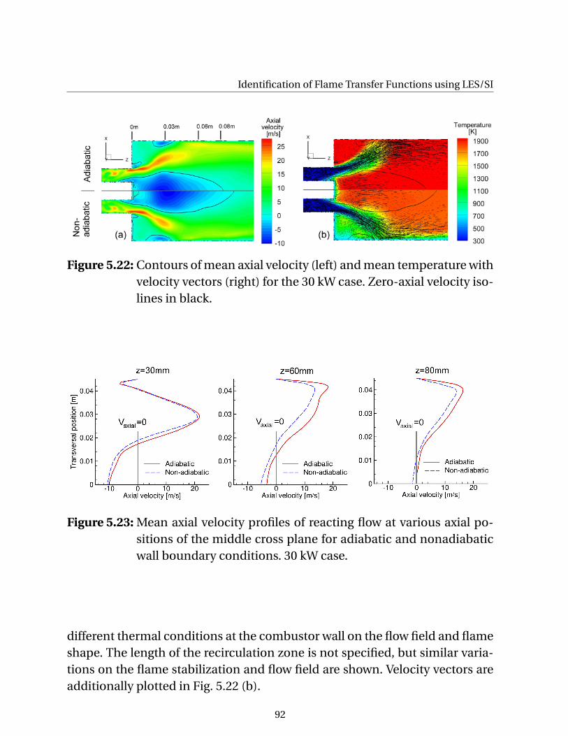
Identification of Flame Transfer Functions using LES/SI
Figure 5.22: Contours of mean axial velocity (left) and mean temperature withvelocity vectors (right) for the 30 kW case. Zero-axial velocity iso-lines in black.
Figure 5.23: Mean axial velocity profiles of reacting flow at various axial po-sitions of the middle cross plane for adiabatic and nonadiabaticwall boundary conditions. 30 kW case.
different thermal conditions at the combustor wall on the flow field and flameshape. The length of the recirculation zone is not specified, but similar varia-tions on the flame stabilization and flow field are shown. Velocity vectors areadditionally plotted in Fig. 5.22 (b).
92
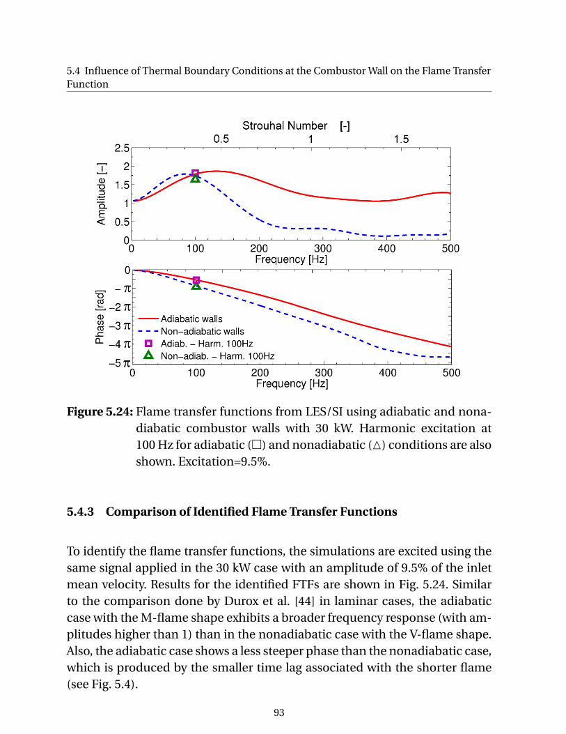
5.4 Influence of Thermal Boundary Conditions at the Combustor Wall on the Flame TransferFunction
Figure 5.24: Flame transfer functions from LES/SI using adiabatic and nona-diabatic combustor walls with 30 kW. Harmonic excitation at100 Hz for adiabatic () and nonadiabatic (M) conditions are alsoshown. Excitation=9.5%.
5.4.3 Comparison of Identified Flame Transfer Functions
To identify the flame transfer functions, the simulations are excited using thesame signal applied in the 30 kW case with an amplitude of 9.5% of the inletmean velocity. Results for the identified FTFs are shown in Fig. 5.24. Similarto the comparison done by Durox et al. [44] in laminar cases, the adiabaticcase with the M-flame shape exhibits a broader frequency response (with am-plitudes higher than 1) than in the nonadiabatic case with the V-flame shape.Also, the adiabatic case shows a less steeper phase than the nonadiabatic case,which is produced by the smaller time lag associated with the shorter flame(see Fig. 5.4).
93
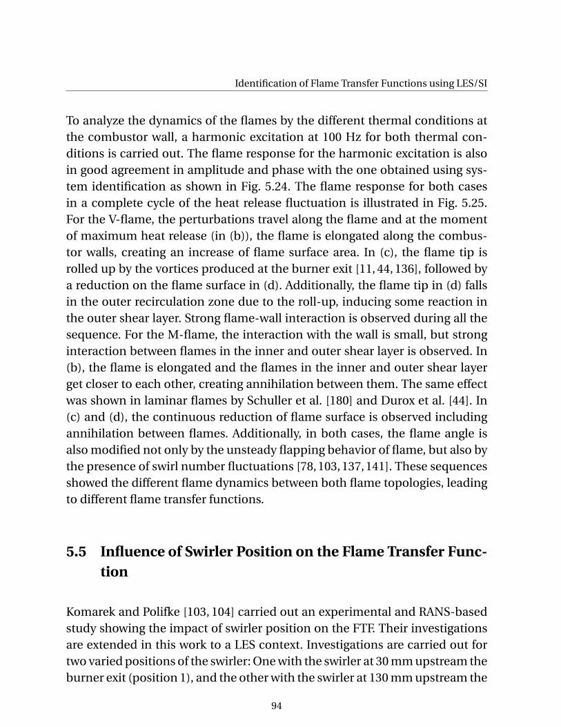
Identification of Flame Transfer Functions using LES/SI
To analyze the dynamics of the flames by the different thermal conditions atthe combustor wall, a harmonic excitation at 100 Hz for both thermal con-ditions is carried out. The flame response for the harmonic excitation is alsoin good agreement in amplitude and phase with the one obtained using sys-tem identification as shown in Fig. 5.24. The flame response for both casesin a complete cycle of the heat release fluctuation is illustrated in Fig. 5.25.For the V-flame, the perturbations travel along the flame and at the momentof maximum heat release (in (b)), the flame is elongated along the combus-tor walls, creating an increase of flame surface area. In (c), the flame tip isrolled up by the vortices produced at the burner exit [11, 44, 136], followed bya reduction on the flame surface in (d). Additionally, the flame tip in (d) fallsin the outer recirculation zone due to the roll-up, inducing some reaction inthe outer shear layer. Strong flame-wall interaction is observed during all thesequence. For the M-flame, the interaction with the wall is small, but stronginteraction between flames in the inner and outer shear layer is observed. In(b), the flame is elongated and the flames in the inner and outer shear layerget closer to each other, creating annihilation between them. The same effectwas shown in laminar flames by Schuller et al. [180] and Durox et al. [44]. In(c) and (d), the continuous reduction of flame surface is observed includingannihilation between flames. Additionally, in both cases, the flame angle isalso modified not only by the unsteady flapping behavior of flame, but also bythe presence of swirl number fluctuations [78, 103, 137, 141]. These sequencesshowed the different flame dynamics between both flame topologies, leadingto different flame transfer functions.
5.5 Influence of Swirler Position on the Flame Transfer Func-tion
Komarek and Polifke [103, 104] carried out an experimental and RANS-basedstudy showing the impact of swirler position on the FTF. Their investigationsare extended in this work to a LES context. Investigations are carried out fortwo varied positions of the swirler: One with the swirler at 30 mm upstream theburner exit (position 1), and the other with the swirler at 130 mm upstream the
94
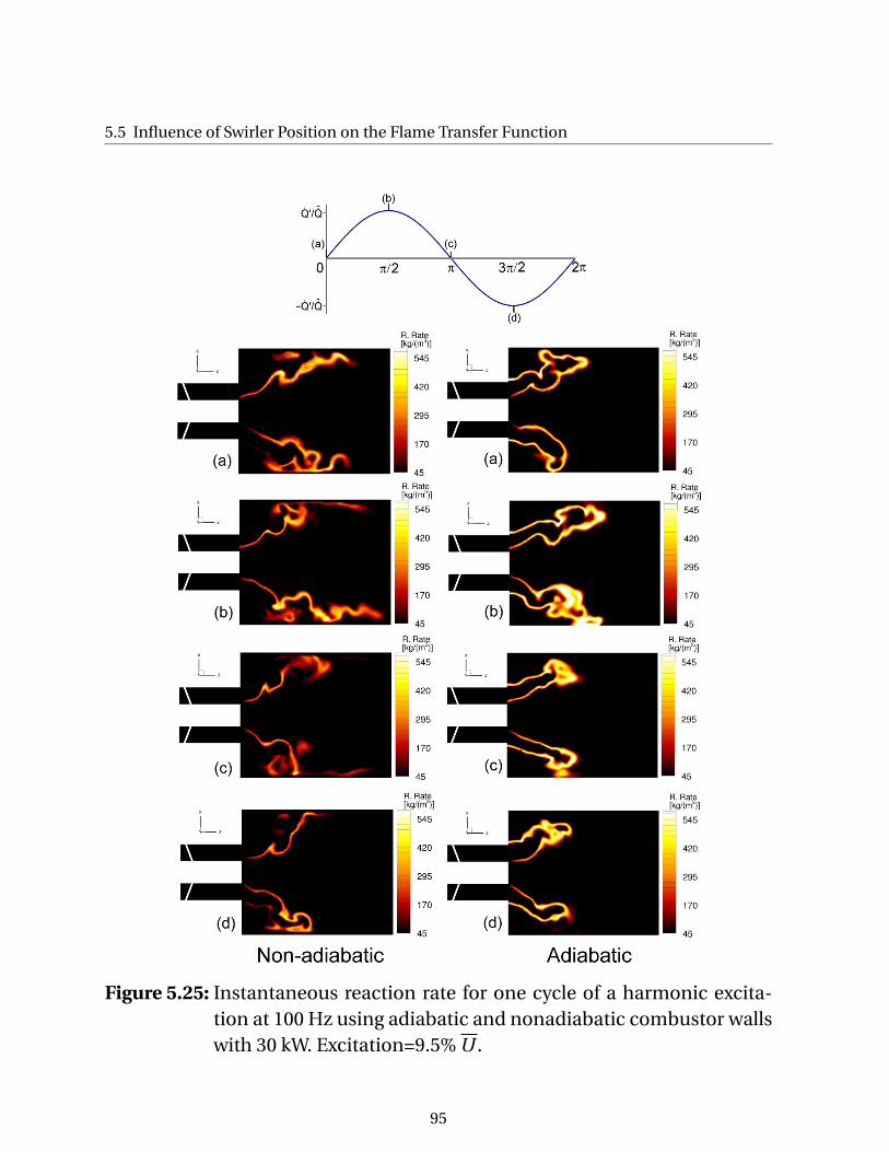
5.5 Influence of Swirler Position on the Flame Transfer Function
Figure 5.25: Instantaneous reaction rate for one cycle of a harmonic excita-tion at 100 Hz using adiabatic and nonadiabatic combustor wallswith 30 kW. Excitation=9.5% U .
95
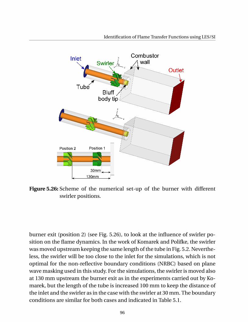
Identification of Flame Transfer Functions using LES/SI
Figure 5.26: Scheme of the numerical set-up of the burner with differentswirler positions.
burner exit (position 2) (see Fig. 5.26), to look at the influence of swirler po-sition on the flame dynamics. In the work of Komarek and Polifke, the swirlerwas moved upstream keeping the same length of the tube in Fig. 5.2. Neverthe-less, the swirler will be too close to the inlet for the simulations, which is notoptimal for the non-reflective boundary conditions (NRBC) based on planewave masking used in this study. For the simulations, the swirler is moved alsoat 130 mm upstream the burner exit as in the experiments carried out by Ko-marek, but the length of the tube is increased 100 mm to keep the distance ofthe inlet and the swirler as in the case with the swirler at 30 mm. The boundaryconditions are similar for both cases and indicated in Table 5.1.
96
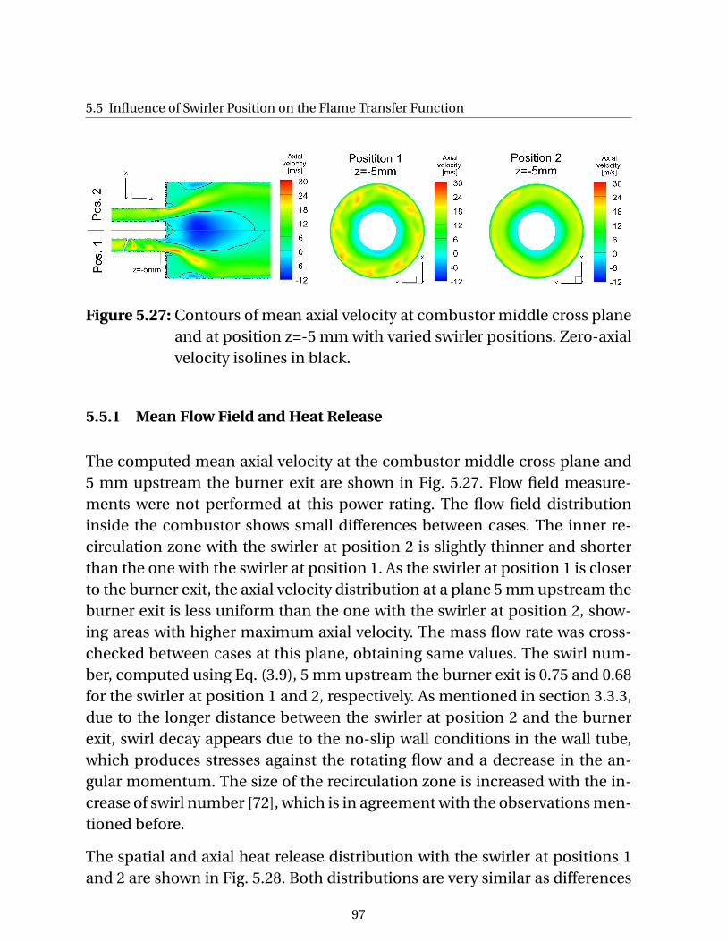
5.5 Influence of Swirler Position on the Flame Transfer Function
Figure 5.27: Contours of mean axial velocity at combustor middle cross planeand at position z=-5 mm with varied swirler positions. Zero-axialvelocity isolines in black.
5.5.1 Mean Flow Field and Heat Release
The computed mean axial velocity at the combustor middle cross plane and5 mm upstream the burner exit are shown in Fig. 5.27. Flow field measure-ments were not performed at this power rating. The flow field distributioninside the combustor shows small differences between cases. The inner re-circulation zone with the swirler at position 2 is slightly thinner and shorterthan the one with the swirler at position 1. As the swirler at position 1 is closerto the burner exit, the axial velocity distribution at a plane 5 mm upstream theburner exit is less uniform than the one with the swirler at position 2, show-ing areas with higher maximum axial velocity. The mass flow rate was cross-checked between cases at this plane, obtaining same values. The swirl num-ber, computed using Eq. (3.9), 5 mm upstream the burner exit is 0.75 and 0.68for the swirler at position 1 and 2, respectively. As mentioned in section 3.3.3,due to the longer distance between the swirler at position 2 and the burnerexit, swirl decay appears due to the no-slip wall conditions in the wall tube,which produces stresses against the rotating flow and a decrease in the an-gular momentum. The size of the recirculation zone is increased with the in-crease of swirl number [72], which is in agreement with the observations men-tioned before.
The spatial and axial heat release distribution with the swirler at positions 1and 2 are shown in Fig. 5.28. Both distributions are very similar as differences
97
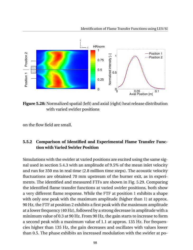
Identification of Flame Transfer Functions using LES/SI
Figure 5.28: Normalized spatial (left) and axial (right) heat release distributionwith varied swirler positions
on the flow field are small.
5.5.2 Comparison of Identified and Experimental Flame Transfer Func-tion with Varied Swirler Position
Simulations with the swirler at varied positions are excited using the same sig-nal used in section 5.4.3 with an amplitude of 9.5% of the mean inlet velocityand run for 350 ms in real time (2.8 million time steps). The acoustic velocityfluctuations are obtained 70 mm upstream of the burner exit, as in experi-ments. The identified and measured FTFs are shown in Fig. 5.29. Comparingthe identified flame transfer functions at varied swirler positions, both showa very different flame response. While the FTF at position 1 exhibits a shapewith only one peak with the maximum amplitude (higher than 1) at approx.90 Hz, the FTF at position 2 exhibits a first peak with the maximum amplitudeat a lower frequency (40 Hz), followed by a strong decrease in amplitude with aminimum value of 0.3 at 90 Hz. From 90 Hz, the gain starts to increase to forma second peak with a maximum value of 1.1 at approx. 135 Hz. For frequen-cies higher than 135 Hz, the gain decreases and oscillates with values lowerthan 0.5. The phase exhibits an increased modulation with the swirler at po-
98
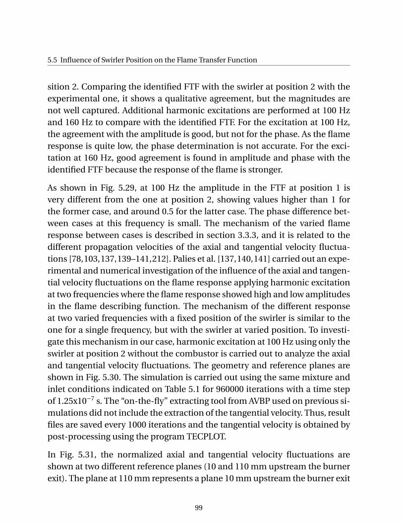
5.5 Influence of Swirler Position on the Flame Transfer Function
sition 2. Comparing the identified FTF with the swirler at position 2 with theexperimental one, it shows a qualitative agreement, but the magnitudes arenot well captured. Additional harmonic excitations are performed at 100 Hzand 160 Hz to compare with the identified FTF. For the excitation at 100 Hz,the agreement with the amplitude is good, but not for the phase. As the flameresponse is quite low, the phase determination is not accurate. For the exci-tation at 160 Hz, good agreement is found in amplitude and phase with theidentified FTF because the response of the flame is stronger.
As shown in Fig. 5.29, at 100 Hz the amplitude in the FTF at position 1 isvery different from the one at position 2, showing values higher than 1 forthe former case, and around 0.5 for the latter case. The phase difference bet-ween cases at this frequency is small. The mechanism of the varied flameresponse between cases is described in section 3.3.3, and it is related to thedifferent propagation velocities of the axial and tangential velocity fluctua-tions [78,103,137,139–141,212]. Palies et al. [137,140,141] carried out an expe-rimental and numerical investigation of the influence of the axial and tangen-tial velocity fluctuations on the flame response applying harmonic excitationat two frequencies where the flame response showed high and low amplitudesin the flame describing function. The mechanism of the different responseat two varied frequencies with a fixed position of the swirler is similar to theone for a single frequency, but with the swirler at varied position. To investi-gate this mechanism in our case, harmonic excitation at 100 Hz using only theswirler at position 2 without the combustor is carried out to analyze the axialand tangential velocity fluctuations. The geometry and reference planes areshown in Fig. 5.30. The simulation is carried out using the same mixture andinlet conditions indicated on Table 5.1 for 960000 iterations with a time stepof 1.25x10⁻⁷ s. The “on-the-fly” extracting tool from AVBP used on previous si-mulations did not include the extraction of the tangential velocity. Thus, resultfiles are saved every 1000 iterations and the tangential velocity is obtained bypost-processing using the program TECPLOT.
In Fig. 5.31, the normalized axial and tangential velocity fluctuations areshown at two different reference planes (10 and 110 mm upstream the burnerexit). The plane at 110 mm represents a plane 10 mm upstream the burner exit
99

Identification of Flame Transfer Functions using LES/SI
Figure 5.29: Flame transfer functions from LES/SI with the swirler at posi-tion 1 and 2 from Fig. 5.26 with 30kW. Harmonic excitation at 100() and 160 Hz (M) are also shown. Excitation=9.5%. Experimentswith the swirler at position 2 in (o).
at position 1. Comparing the phase between axial and tangential velocity fluc-tuations at both planes, at the plane 110 mm upstream the burner exit bothfluctuations are almost in phase; while at 10 mm upstream the burner exit,both fluctuations are almost out of phase. Relating the phase difference bet-ween perturbations with the amplitude of the identified FTFs: when the axialand tangential velocity fluctuations are in phase, amplitudes higher than 1are obtained due to a constructive mechanism induced by them. On the other
100
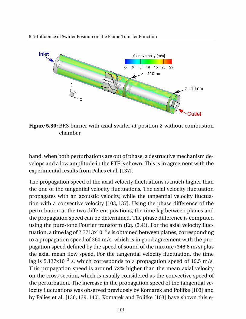
5.5 Influence of Swirler Position on the Flame Transfer Function
Figure 5.30: BRS burner with axial swirler at position 2 without combustionchamber
hand, when both perturbations are out of phase, a destructive mechanism de-velops and a low amplitude in the FTF is shown. This is in agreement with theexperimental results from Palies et al. [137].
The propagation speed of the axial velocity fluctuations is much higher thanthe one of the tangential velocity fluctuations. The axial velocity fluctuationpropagates with an acoustic velocity, while the tangential velocity fluctua-tion with a convective velocity [103, 137]. Using the phase difference of theperturbation at the two different positions, the time lag between planes andthe propagation speed can be determined. The phase difference is computedusing the pure-tone Fourier transform (Eq. (5.4)). For the axial velocity fluc-tuation, a time lag of 2.7713x10⁻⁴ s is obtained between planes, correspondingto a propagation speed of 360 m/s, which is in good agreement with the pro-pagation speed defined by the speed of sound of the mixture (348.6 m/s) plusthe axial mean flow speed. For the tangential velocity fluctuation, the timelag is 5.137x10⁻³ s, which corresponds to a propagation speed of 19.5 m/s.This propagation speed is around 72% higher than the mean axial velocityon the cross section, which is usually considered as the convective speed ofthe perturbation. The increase in the propagation speed of the tangential ve-locity fluctuations was observed previuosly by Komarek and Polifke [103] andby Palies et al. [136, 139, 140]. Komarek and Polifke [103] have shown this e-
101

Identification of Flame Transfer Functions using LES/SI
ffect in the same burner, but with a power rating of 70 kW (around 2.33 timeshigher than the one used in this study) using URANS. The propagation speedfor the tangential velocity fluctuation for the 70 kW case was 40% higher thanthe mean axial velocity on the cross section. From the axial velocity contoursin Fig. 5.27, it is observed that the distribution of axial velocities in the crosssection and along the tube show sectors with maximum velocities around thedouble of the mean axial velocity of the cross section and close to the pro-pagation speed of the tangetial velocity fluctuations [136, 139, 140]. The pro-pagation velocity of the tangential velocity fluctuation locally is not uniformand travels convectively with the local convective velocity. This effect can beobserved on Fig. 5.32, where the area averaged tangential velocity on a cross-section at different positions is shown. For positions further downstream, theharmonic oscillations become less smooth, indicating some nonuniformity inthe propagation. Furthermore, the mean tangential velocity (taken in this caseby the tangential velocity at time 0 s) is lower at positions more downstreamfrom the swirler. This is created due to the decay of swirl mentioned before.
In Fig. 5.33, the area averaged axial and tangential velocity fluctuations with-out normalization are shown. The axial velocity fluctuation did not present adecrease in amplitude, which indicates the low level of acoustic dissipationfrom the code. The tangential velocity fluctuation presented a decay of 16.4%in amplitude at the plane z=-10 mm with respect to the one at z=-110 mm,indicating that the decay in swirl affected also the tangential velocity fluctua-tions, which influence the flame response.
In Fig. 5.34, the area averaged swirl number fluctuations are shown. The casewith swirler at position 2 presents higher swirl number fluctuations in spiteof the lower tangential velocity fluctuations. This is created due to the diffe-rent phase between axial and tangential velocity fluctuations at the referenceplanes as shown in Fig. 5.33.
The results indicate that a flame with similar heat release distribution and flowfield can have a different flame response due to the varied time lag responseto the perturbations. The analysis is extended in section 5.7.2 to identify thedifferent time lags between perturbations and the discrepancies in the ampli-tudes between experimental and identified FTF in Fig. 5.29.
102
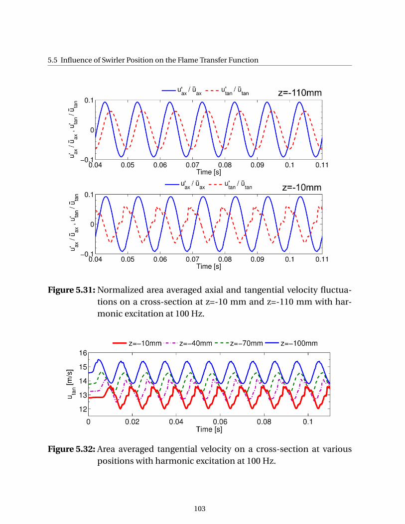
5.5 Influence of Swirler Position on the Flame Transfer Function
Figure 5.31: Normalized area averaged axial and tangential velocity fluctua-tions on a cross-section at z=-10 mm and z=-110 mm with har-monic excitation at 100 Hz.
Figure 5.32: Area averaged tangential velocity on a cross-section at variouspositions with harmonic excitation at 100 Hz.
103
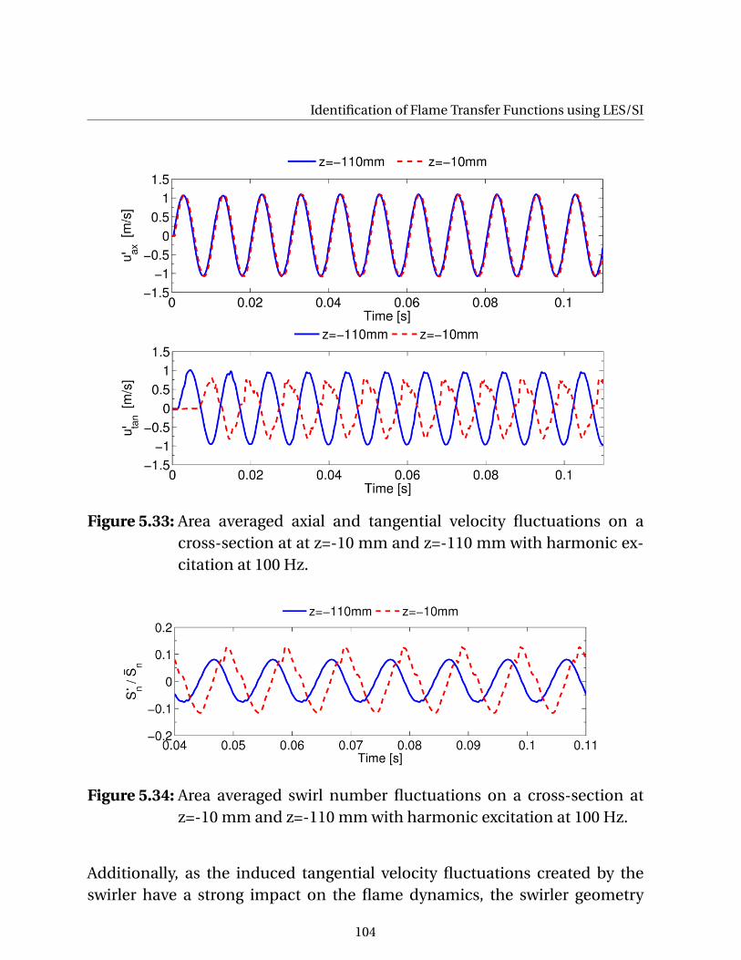
Identification of Flame Transfer Functions using LES/SI
Figure 5.33: Area averaged axial and tangential velocity fluctuations on across-section at at z=-10 mm and z=-110 mm with harmonic ex-citation at 100 Hz.
Figure 5.34: Area averaged swirl number fluctuations on a cross-section atz=-10 mm and z=-110 mm with harmonic excitation at 100 Hz.
Additionally, as the induced tangential velocity fluctuations created by theswirler have a strong impact on the flame dynamics, the swirler geometry
104
5.6 Influence of Combustor Confinement on the Flame Transfer Function
must be taken into account in CFD simulations in order to capture this effect.As shown by Komarek and Polifke in [103], introducing only axial velocity per-turbations in a simulation without the geometrical swirler, and replacing it by3D velocity profiles at a reference position, tangential velocity perturbationsare not produced and the flame responds only to axial perturbations. Thusthe constructive/destructive interaction between axial and tangential velocityfluctuations, which influence the flame response on swirling flames, does nottake effect.
5.6 Influence of Combustor Confinement on the Flame Trans-fer Function
The combustor in single burner test-rigs has in general a cross section sizeand shape that differ from the one in the industrial gas turbines. The change incombustor cross-section induces differences in the flow field and in the flame.Measurements of FTFs with varied combustor confinement ratio were carriedout by Birbaud et al. [11] in laminar cases and by Hauser et al. [75] in a radialswirl burner, showing variations between FTFs with different confinement ra-tio. In the present work, the influence of combustor confinement on the flowfield, flame and FTF is analyzed numerically with LES. The BRS burner is si-mulated using two combustors with different cross-section area. The dimen-sions of the cross-sections are similar to the ones used by Hauser et al.: Onewith 90 mm × 90 mm called high-confinement (HC) combustor (CR=0.156);and another with 160 mm × 160 mm, called low-confinement (LC) combus-tor (CR=0.049). Both cases use the same boundary conditions, as specified inTable 5.1. The length of the combustor is longer in the low-confinement com-bustor (300 mm) than in the high-confinement combustor (200 mm) to re-duce the interaction of the long recirculation zone (see section 5.6.1) with theoutlet. Experiments were not carried out in the low-confinement combustor.Mean flow field and mean heat release from simulations are compared ini-tially between cases, followed by the identification of the FTFs using the diffe-rent combustors.
105
Identification of Flame Transfer Functions using LES/SI
5.6.1 Mean Flow Field and Heat Release
In Fig. 5.35, the mean axial velocity contours and velocity vectors for the caseswith variation of combustor confinement ratio at the combustor middle crossplane are shown. The case with the low-confinement combustor shows a re-circulation zone much longer than the one with high-confinement. At around60 mm downstream of the burner exit, a “neck” is formed in the recirculationzone. Between positions 0 mm and 60 mm, the inner recirculation zone (IRZ)of the low-confinement case is narrower than the one with high-confinement;while after 60 mm, the IRZ with low-confinement becomes broader than theone with high-confinement, and extended to more downstream positions.Similar effect on the shape of the recirculation zone with the increase of con-finement was found by Fu et al. [61] in isothermal cases. Additionally, thecase with high-confinement shows a higher maximum negative velocity inthe inner recirculation zone. The flow recirculation is mainly produced bythe presence of an adverse axial pressure gradient induced by the swirlingflow [72, 125, 195], which changes due to the varied expansion ratio.
The variations mentioned before are shown in more detail in Fig. 5.36 by plo-tting axial velocity profiles at various axial positions of the combustor middlecross plane. A grey line at zero axial velocity is introduced to indicate the po-sition of the recirculation zone. Additionally, the jet angle from the burnerexit exhibits some variations between cases. From the vector plots and theaxial velocity profiles, the jet angle is slightly higher on the high-confinementcase (≈ 30 deg) than on the low-confinement case (≈ 20 deg). The incrementis produced because the recirculation zone is broader and more intense inthe high-confinement case. The increment in jet angle, but to a higher degree,was observed also by Fanaca et al. [49] in the flow field comparison betweena single burner rig and an annular combustor. Additionally, the maximum a-xial velocity with low-confinement shows a higher decay with positions moredownstream to the burner exit due to the higher area expansion. A decay inthe tangential velocity (Fig. 5.37) and turbulent kinetic energy (Fig. 5.38) isalso observed. For the turbulent kinetic energy, a higher level of turbulence isobserved with low-confinement than with high-confinement at 60 and 80 mmdownstream the burner exit. This is produced by the flame, which is longer in
106
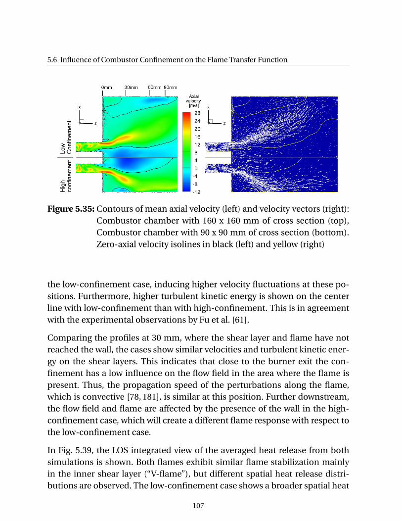
5.6 Influence of Combustor Confinement on the Flame Transfer Function
Figure 5.35: Contours of mean axial velocity (left) and velocity vectors (right):Combustor chamber with 160 x 160 mm of cross section (top),Combustor chamber with 90 x 90 mm of cross section (bottom).Zero-axial velocity isolines in black (left) and yellow (right)
the low-confinement case, inducing higher velocity fluctuations at these po-sitions. Furthermore, higher turbulent kinetic energy is shown on the centerline with low-confinement than with high-confinement. This is in agreementwith the experimental observations by Fu et al. [61].
Comparing the profiles at 30 mm, where the shear layer and flame have notreached the wall, the cases show similar velocities and turbulent kinetic ener-gy on the shear layers. This indicates that close to the burner exit the con-finement has a low influence on the flow field in the area where the flame ispresent. Thus, the propagation speed of the perturbations along the flame,which is convective [78, 181], is similar at this position. Further downstream,the flow field and flame are affected by the presence of the wall in the high-confinement case, which will create a different flame response with respect tothe low-confinement case.
In Fig. 5.39, the LOS integrated view of the averaged heat release from bothsimulations is shown. Both flames exhibit similar flame stabilization mainlyin the inner shear layer (“V-flame”), but different spatial heat release distri-butions are observed. The low-confinement case shows a broader spatial heat
107

Identification of Flame Transfer Functions using LES/SI
Figure 5.36: Mean axial velocity profiles with low and high confinement com-bustors at various positions of the middle cross plane shown inFig. 5.2. Grey line to indicate zero-axial velocity.
Figure 5.37: Mean tangential velocity profiles with low and high confinementcombustors at various positions of the middle cross plane shownin Fig. 5.2.
release distribution than the high-confinement case. This is in agreement withexperimental results performed by Hauser et al. [75] using a radial swirl burnerin similar combustors to the ones used in this study.
In Fig. 5.40, the axial heat release distributions from simulations are shown.The values are normalized taking into account that the area of the distribution
108
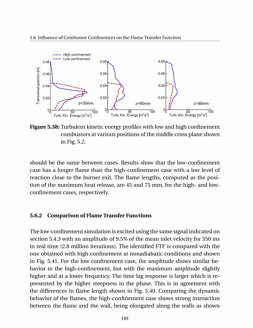
5.6 Influence of Combustor Confinement on the Flame Transfer Function
Figure 5.38: Turbulent kinetic energy profiles with low and high confinementcombustors at various positions of the middle cross plane shownin Fig. 5.2.
should be the same between cases. Results show that the low-confinementcase has a longer flame than the high-confinement case with a low level ofreaction close to the burner exit. The flame lengths, computed as the posi-tion of the maximum heat release, are 45 and 75 mm, for the high- and low-confinement cases, respectively.
5.6.2 Comparison of Flame Transfer Functions
The low-confinement simulation is excited using the same signal indicated onsection 5.4.3 with an amplitude of 9.5% of the mean inlet velocity for 350 msin real time (2.8 million iterations). The identified FTF is compared with theone obtained with high confinement at nonadiabatic conditions and shownin Fig. 5.41. For the low confinement case, the amplitude shows similar be-havior to the high-confinement, but with the maximum amplitude slightlyhigher and at a lower frequency. The time lag response is larger which is re-presented by the higher steepness in the phase. This is in agreement withthe differences in flame length shown in Fig. 5.40. Comparing the dynamicbehavior of the flames, the high-confinement case shows strong interactionbetween the flame and the wall, being elongated along the walls as shown
109
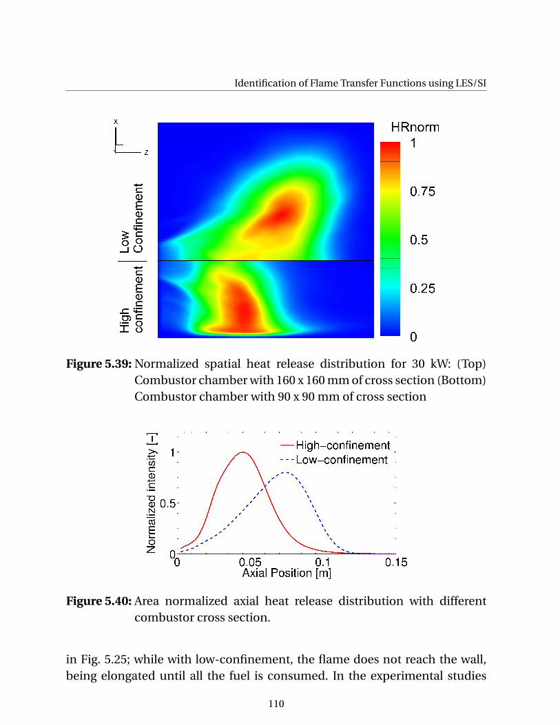
Identification of Flame Transfer Functions using LES/SI
Figure 5.39: Normalized spatial heat release distribution for 30 kW: (Top)Combustor chamber with 160 x 160 mm of cross section (Bottom)Combustor chamber with 90 x 90 mm of cross section
Figure 5.40: Area normalized axial heat release distribution with differentcombustor cross section.
in Fig. 5.25; while with low-confinement, the flame does not reach the wall,being elongated until all the fuel is consumed. In the experimental studies
110
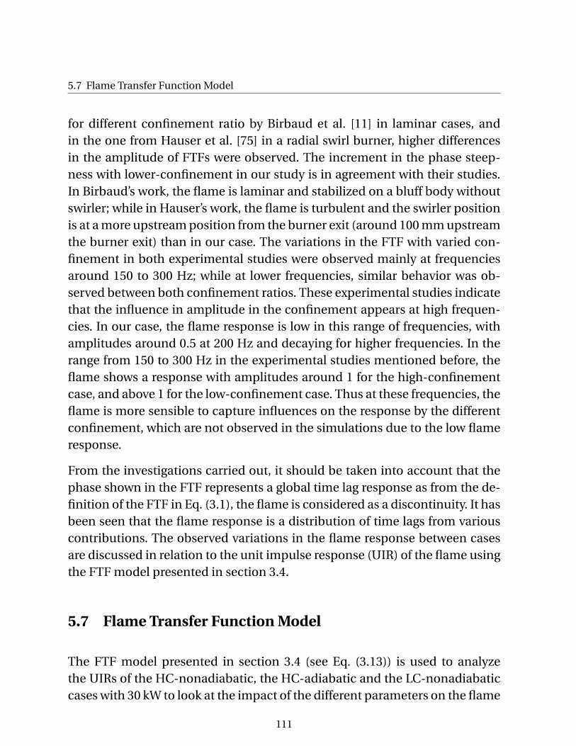
5.7 Flame Transfer Function Model
for different confinement ratio by Birbaud et al. [11] in laminar cases, andin the one from Hauser et al. [75] in a radial swirl burner, higher differencesin the amplitude of FTFs were observed. The increment in the phase steep-ness with lower-confinement in our study is in agreement with their studies.In Birbaud’s work, the flame is laminar and stabilized on a bluff body withoutswirler; while in Hauser’s work, the flame is turbulent and the swirler positionis at a more upstream position from the burner exit (around 100 mm upstreamthe burner exit) than in our case. The variations in the FTF with varied con-finement in both experimental studies were observed mainly at frequenciesaround 150 to 300 Hz; while at lower frequencies, similar behavior was ob-served between both confinement ratios. These experimental studies indicatethat the influence in amplitude in the confinement appears at high frequen-cies. In our case, the flame response is low in this range of frequencies, withamplitudes around 0.5 at 200 Hz and decaying for higher frequencies. In therange from 150 to 300 Hz in the experimental studies mentioned before, theflame shows a response with amplitudes around 1 for the high-confinementcase, and above 1 for the low-confinement case. Thus at these frequencies, theflame is more sensible to capture influences on the response by the differentconfinement, which are not observed in the simulations due to the low flameresponse.
From the investigations carried out, it should be taken into account that thephase shown in the FTF represents a global time lag response as from the de-finition of the FTF in Eq. (3.1), the flame is considered as a discontinuity. It hasbeen seen that the flame response is a distribution of time lags from variouscontributions. The observed variations in the flame response between casesare discussed in relation to the unit impulse response (UIR) of the flame usingthe FTF model presented in section 3.4.
5.7 Flame Transfer Function Model
The FTF model presented in section 3.4 (see Eq. (3.13)) is used to analyzethe UIRs of the HC-nonadiabatic, the HC-adiabatic and the LC-nonadiabaticcases with 30 kW to look at the impact of the different parameters on the flame
111
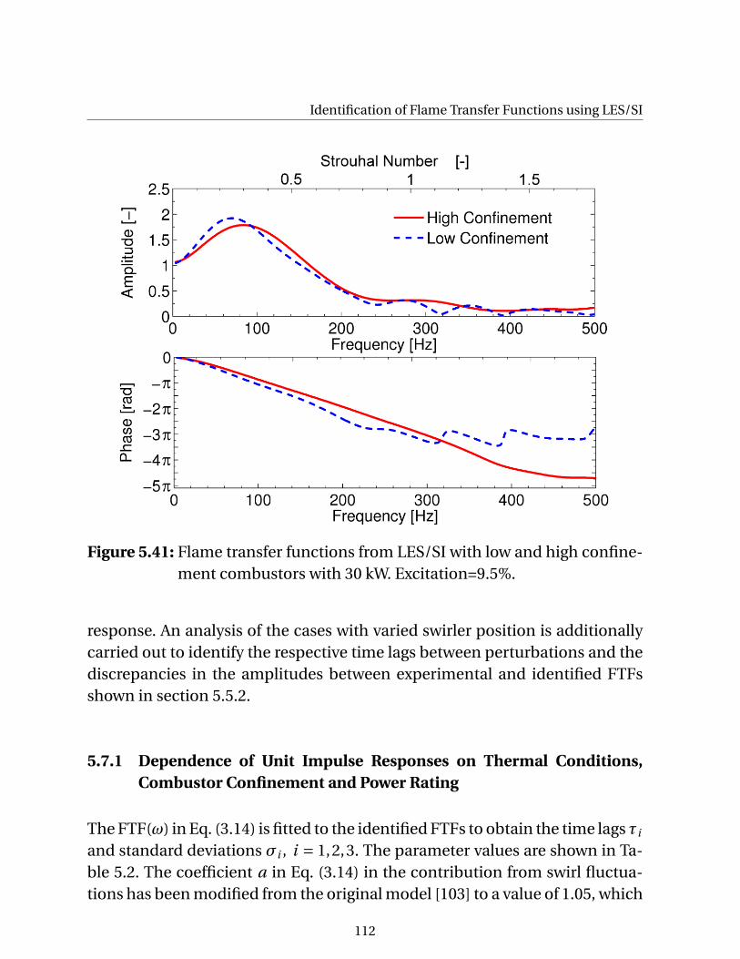
Identification of Flame Transfer Functions using LES/SI
Figure 5.41: Flame transfer functions from LES/SI with low and high confine-ment combustors with 30 kW. Excitation=9.5%.
response. An analysis of the cases with varied swirler position is additionallycarried out to identify the respective time lags between perturbations and thediscrepancies in the amplitudes between experimental and identified FTFsshown in section 5.5.2.
5.7.1 Dependence of Unit Impulse Responses on Thermal Conditions,Combustor Confinement and Power Rating
The FTF(ω) in Eq. (3.14) is fitted to the identified FTFs to obtain the time lags τi
and standard deviations σi , i = 1,2,3. The parameter values are shown in Ta-ble 5.2. The coefficient a in Eq. (3.14) in the contribution from swirl fluctua-tions has been modified from the original model [103] to a value of 1.05, which
112

5.7 Flame Transfer Function Model
Table 5.2: Time lag model
τ, σ [ms] τ1 σ1 τ2 σ2 τ3 σ3
30 kW HC-NA-P1 3.75 1 5.29 0.75 7.8 2.530 kW HC-A-P1 2.25 0.64 4.13 0.35 5.5 0.530 kW LC-NA-P1 5.3 1.6 6.0 1.0 9.9 3.030 kW HC-NA-P2 3.75 1 10.42 1.4 12.93 3.250 kW HC-Nonadiabatic 2.8 1.0 3.6 0.65 4.83 0.8
produced a better quality.
The UIRs obtained using Eq. (3.13) and 140 coefficients with a time step of1.25x10−4 s and with the parameters in Table 5.2 are shown in Fig. 5.42, indi-cating the respective time delays in the flame response to the different pertur-bations. The variation in time lags between cases are in agreement with thechanges in flame lengths shown in Figs. 5.4 and 5.40. Also, the amplitude inthe UIR of the HC-Adiabatic case is higher because the flame is shorter andreacts in the inner and outer shear layer at the same time. Thus, the standarddeviations in the model are smaller than in the other cases, indicating thatthe response is in a narrower period of time. The identified FTF for 50 kW isfitted also with the model and its parameters are included in Table 5.2. TheFTFs obtained using the model are shown in Fig. 5.43 with very good agree-ment with the identified FTFs. Additionally, the sum of all coefficients bet-ween cases is equal to unity, in agreement with the zero frequency limit forthe amplitude of the FTF [159]. The cases with higher power rating and withadiabatic walls show a broader frequency response in the FTF than the caseswith LC and HC with non-adiabatic. From the model, there is some relationbetween a broader frequency response and the period of time for the flamereaction. The flame response to the perturbations in both cases is in a shorterperiod of time as shown in Fig. 5.42 due to the stabilization in both shear la-yers in the adiabatic case, and the higher velocities in the higher power ratingcase. It is argued that the broader frequency response is produced by the con-sumption in a shorter period of time of the fuel introduced by the mass flowfluctuations. This can be shown using the Strouhal number. It is known that
113
Identification of Flame Transfer Functions using LES/SI
with only the change of power rating in a combustor system, the FTF has agood scaling behavior [8, 97, 137] with the Strouhal number (see Eq. (5.3)). InEq. (5.3), the main parameter in the scaling is the velocity ubexit. Thus, an in-crease in ubexit moves the flame response to higher frequencies. Now, usingadiabatic combustor walls the flame stabilizes in both shear layers, so the a-dditional mass flow introduced by the perturbation is consumed at the samemoment, but by 2 flames. This can be represented as a consumption 2 timesfaster. Thus, similar to the increase in power rating, the flame response movesto higher frequencies. Indeed, Durox et al. in [44], considered a similar crite-rion for normalization of the FTF in a M-flame, taking as the characteristiclength the half of the distance between inner and outer radius in an annularburner exit due to the presence of two flames. A M-flame does not scale witha V-flame by the Strouhal number due to the strong differences on the flamedynamics produced by the varied flame topology, but produces a broader fre-quency response than the V-flame, which can be understood by the shortertime necessary to consume the fuel introduced by the mass flow fluctuations.
The evaluation of the UIRs for the cases with similar position of the swirlerconfirms that the variations in flow field and flame shape can lead to a variedflame response and time lags.
5.7.2 Comparison of Unit Impulse Responses with Swirler at Varied Posi-tions
The FTF model is used to identify the various time lags and the discrepan-cies in the amplitudes between experimental and identified FTF shown in sec-tion 5.5.2. To obtain the UIR from experimental data, the inverse z-transformof an experimental FTF(ωreal) is applied:
hk = Re
(∆t
π
π/∆t∑ωreal=0
FTF(ωreal)e iωrealk∆t
), for k = 0, ...,L, (5.7)
where ∆t , ω, k, L are the time step, angular frequency, UIR coefficient index,and the maximum index of the UIR coefficients, respectively.
The UIR from the experimental FTFs in Figs. 5.8 and 5.29 at positions 1 and 2,
114
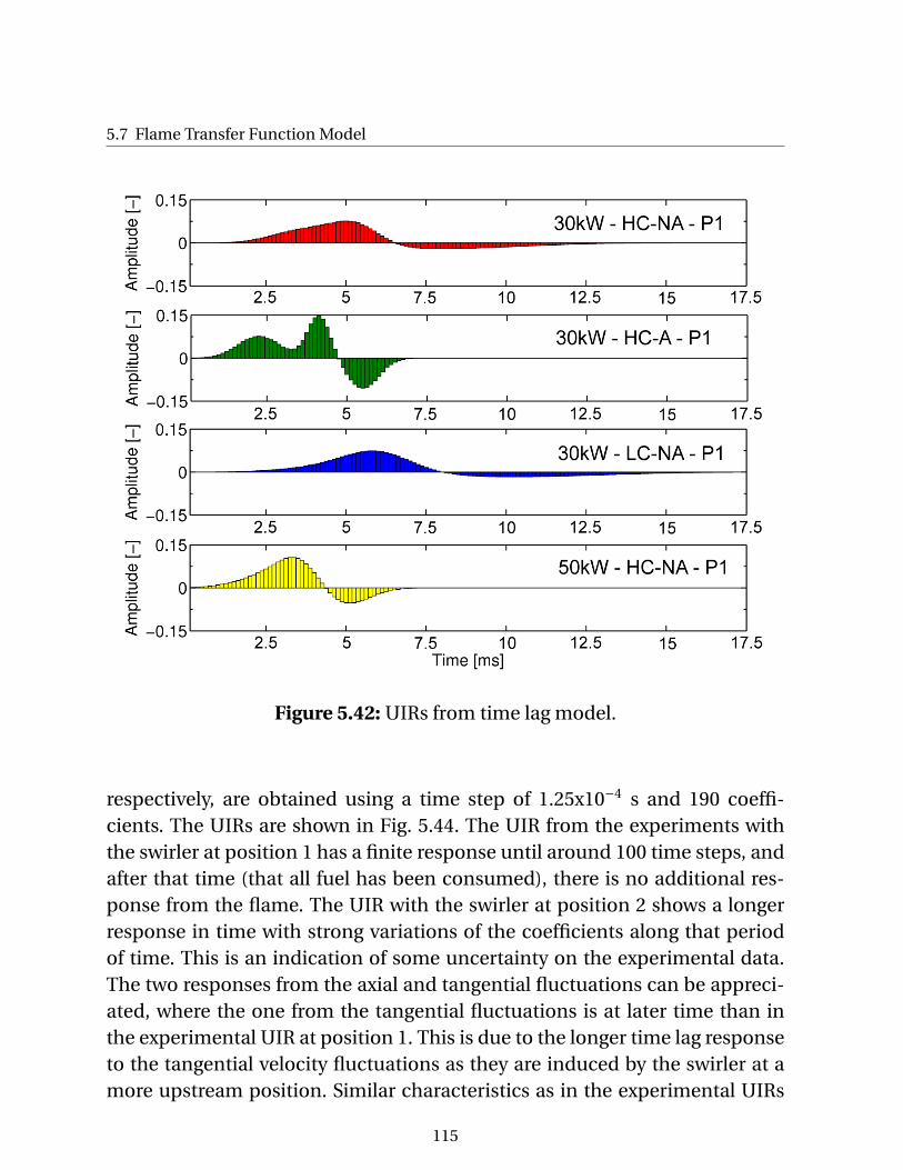
5.7 Flame Transfer Function Model
Figure 5.42: UIRs from time lag model.
respectively, are obtained using a time step of 1.25x10⁻⁴ s and 190 coeffi-cients. The UIRs are shown in Fig. 5.44. The UIR from the experiments withthe swirler at position 1 has a finite response until around 100 time steps, andafter that time (that all fuel has been consumed), there is no additional res-ponse from the flame. The UIR with the swirler at position 2 shows a longerresponse in time with strong variations of the coefficients along that periodof time. This is an indication of some uncertainty on the experimental data.The two responses from the axial and tangential fluctuations can be appreci-ated, where the one from the tangential fluctuations is at later time than inthe experimental UIR at position 1. This is due to the longer time lag responseto the tangential velocity fluctuations as they are induced by the swirler at amore upstream position. Similar characteristics as in the experimental UIRs
115
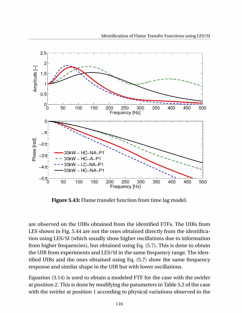
Identification of Flame Transfer Functions using LES/SI
Figure 5.43: Flame transfer function from time lag model.
are observed on the UIRs obtained from the identified FTFs. The UIRs fromLES shown in Fig. 5.44 are not the ones obtained directly from the identifica-tion using LES/SI (which usually show higher oscillations due to informationfrom higher frequencies), but obtained using Eq. (5.7). This is done to obtainthe UIR from experiments and LES/SI in the same frequency range. The iden-tified UIRs and the ones obtained using Eq. (5.7) show the same frequencyresponse and similar shape in the UIR but with lower oscillations.
Equation (3.14) is used to obtain a modeled FTF for the case with the swirlerat position 2. This is done by modifying the parameters in Table 5.2 of the casewith the swirler at position 1 according to physical variations observed in the
116

5.7 Flame Transfer Function Model
Figure 5.44: UIR from modelled, experimental and identified FTF with 30 kWat varied swirler positions.
case at position 2. First, the coefficient a in Eq. (3.13) is decreased from 1.05to 0.952 to be in agreement with the decay in swirl observed in section 5.5.1.The τ1 and σ1 from the mass flow fluctuations are not modified (as done by
117
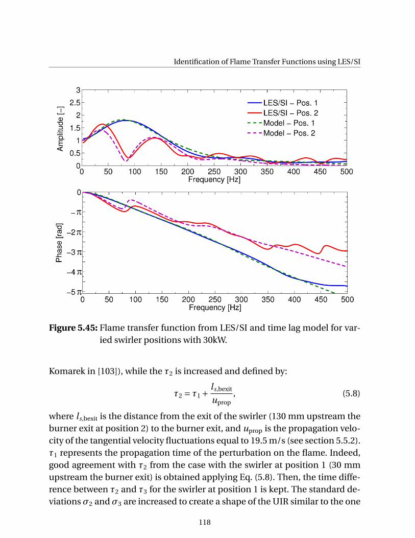
Identification of Flame Transfer Functions using LES/SI
Figure 5.45: Flame transfer function from LES/SI and time lag model for var-ied swirler positions with 30kW.
Komarek in [103]), while the τ2 is increased and defined by:
τ2 = τ1 +ls,bexit
uprop, (5.8)
where ls,bexit is the distance from the exit of the swirler (130 mm upstream theburner exit at position 2) to the burner exit, and uprop is the propagation velo-city of the tangential velocity fluctuations equal to 19.5 m/s (see section 5.5.2).τ1 represents the propagation time of the perturbation on the flame. Indeed,good agreement with τ2 from the case with the swirler at position 1 (30 mmupstream the burner exit) is obtained applying Eq. (5.8). Then, the time diffe-rence between τ2 and τ3 for the swirler at position 1 is kept. The standard de-viationsσ2 andσ3 are increased to create a shape of the UIR similar to the one
118

5.7 Flame Transfer Function Model
Table 5.3: Time lag model for experimental FTF at position 2
τ, σ [ms] τ1 σ1 τ2 σ2 τ3 σ3
30kW HC-NA-P2 Exp. 3 0.55 5.4 2.3 12.18 0.68
from the identified UIR. This increase in the standard deviations for the con-tribution of swirl fluctuations was also observed and identified by Komarek etal. [103]. Applying these changes, the UIR and FTF of the model for the swirlerat position 2 are shown in Figs. 5.44 and 5.45, respectively. Good agreementwith the identified UIRs and FTF was obtained. The model captured the twoamplitude peaks and the strong decrease between the peaks, with good agree-ment also in the phase. The amplitudes from the experimental FTF are notreproduced by the model introducing the physical modifications mentionedbefore. This modifications in the model exhibit good agreement with the iden-tified FTF. This is an indication that some inaccuracies are present in the ex-perimental data for the case measured with 30 kW of power rating with theswirler at position 2, because good agreement between the model and expe-rimental data for varied swirler positions was obtained before for a case withhigher power rating (70 kW) [103].
An additional analysis is carried out to fit the time lag model to the experimen-tal data to look the level of mismatch between τi and σi of the identified andexperimental FTFs, which can create the discrepancies shown in Fig. 5.29. Toobtain the best fit of the model to the FTF from experiments, the τi and σi inTable 5.3 are used. The UIR and FTF from experiments and with the model fitare shown in Figs. 5.46 and 5.47. Good agreement is obtained between the ex-periments and the model. However, the value of τ2 that is necessary to obtainthis agreement is unphysical as it corresponds to a propagation speed of thetangential fluctuations more than 470% higher than the mean axial velocityusing Eq. (5.8), while applying physical modifications in the model from theidentified FTF at position 1, the model is able to reproduce the identified FTFat position 2 with good agreement. This is another indication of inaccuraciesin the experimental data.
119
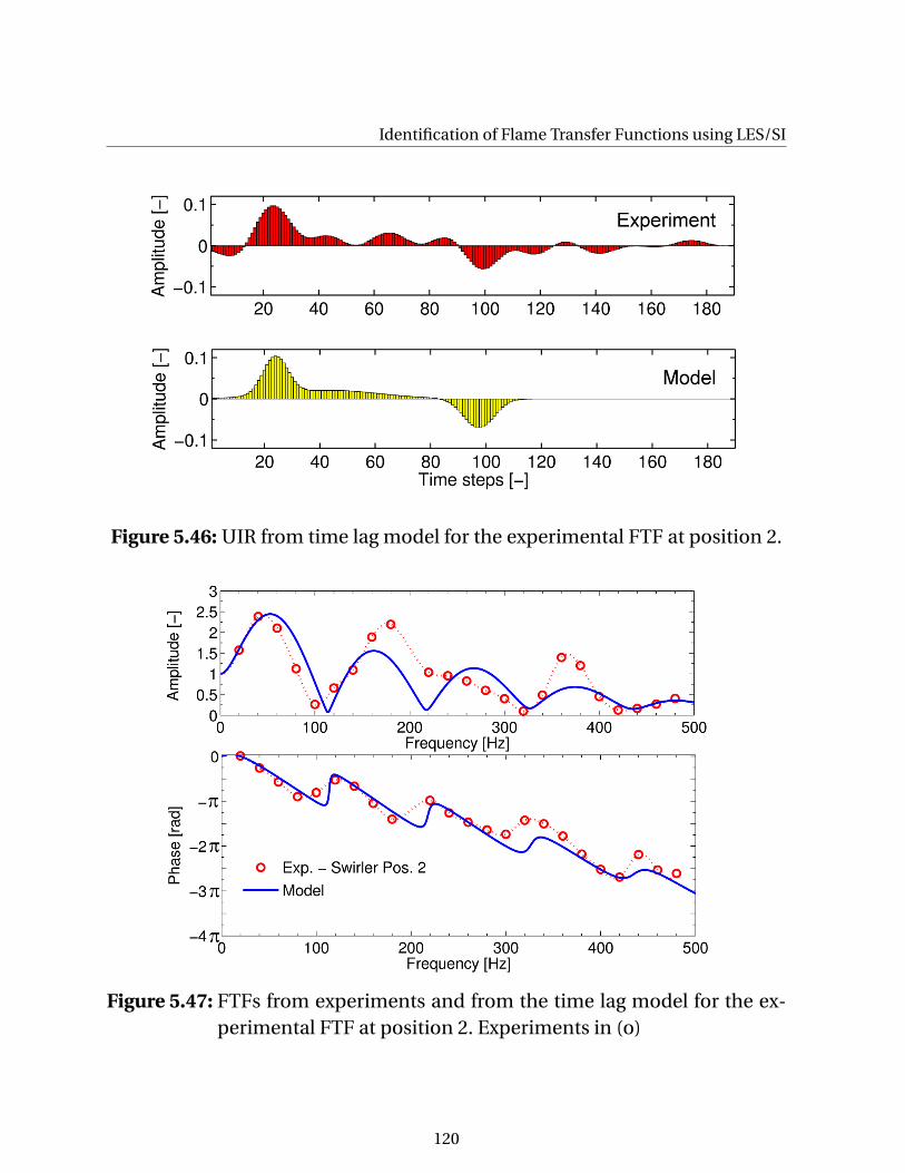
Identification of Flame Transfer Functions using LES/SI
Figure 5.46: UIR from time lag model for the experimental FTF at position 2.
Figure 5.47: FTFs from experiments and from the time lag model for the ex-perimental FTF at position 2. Experiments in (o)
120

5.7 Flame Transfer Function Model
Additionally, as shown in the analysis of the UIRs, the flame response is mainlyproduced from two contributions (which in the case of the swirler at position2 shows much higher separation due to the longer time lags). Then the systemcan be analyzed as a MISO system to identify the contributions in the flameresponse from mass flow and swirl fluctuations separately. This kind of ana-lysis was not extended in the present study, but will be investigated in futureworks.
121
6 Stability Analysis with Low-OrderNetwork Models
A final step after the identification of the flame transfer functions is the stabi-lity analysis. The LES/SI results have confirmed that the FTF does depend notonly on the burner geometry, but also on the boundary conditions that thecombustor provides for the flame (combustor wall temperature, confinement,etc.) and on the position of the swirl generator. Thus, if the burner is installedin a facility with variations in the environment interacting with the flame, theflame response will be different. The stability behavior of the system shouldbe obtained taking into account these discrepancies. Using a network model,the stability analysis is carried out to assess the impact of such discrepanciesin FTFs on combustor stability limits.
In this chapter, background about 1D acoustics and network models is pre-sented in the beginning, followed by the stability analysis of the combustionsystem with the varied conditions investigated on Chapter 5.
6.1 Linear Acoustic 1D Equations
In acoustics, the flow variables of velocity (u), pressure (p) and density (ρ)can be expressed in a similar way as in the Reynolds decomposition (see sec-tion 2.1) in a stationary mean () and a fluctuating part (′):
u(x, t ) = u +u′(x, t ), (6.1)
p(x, t ) = p +u′(x, t ), (6.2)
ρ(x, t ) = ρ+ρ′(x, t ). (6.3)
122
6.1 Linear Acoustic 1D Equations
where x and t are the position and time, respectively. The fluctuating part inthis section is referred to acoustic fluctuations without the presence of turbu-lent fluctuations.
Considering that the fluctuations are much smaller than their mean values(p ′(x,t) ¿ p), and that the flow is homentropic (homentropic refers to an isen-tropic (DS/Dt=0) and uniform (∇S=0) flow [83,161,211]) and non-viscous, theequations of mass and momentum can be linearized to obtain the linearizedconvective acoustic equations (see Appendix A.6 for the derivation):
∂ρ′
∂t+ u
∂ρ′
∂x+ ∂ρu′
∂x= 0, (6.4)
ρ
(∂u′
∂t+ u
∂u′
∂x
)+ ∂p ′
∂x= 0. (6.5)
Defining the density fluctuations ρ′ in terms of the speed of sound a and thepressure fluctuations (see Appendix A.6):
ρ′ = p ′
a2, (6.6)
replacing Eq. (6.6) in Eq. (6.4), applying the total time derivative (∂/∂t+u∂/∂x)to Eq. (6.4), the divergence (∂/∂x) to Eq. (6.5), and subtracting both equationsin order to eliminate the terms including the acoustic velocity (u′), the convec-tive wave equation is obtained:(
∂
∂t+ u
∂
∂x
)2
p ′−a2∂2p ′
∂x2= 0. (6.7)
The solution of Eq. (6.7) is [2, 161]:
p ′
ρa= f (x − (a + u)t )+ g (x + (a − u)t ) , (6.8)
which is the superposition of the traveling waves f (with a propagation speedof a+u in downstream direction) and g (with a propagation speed of a-u inupstream direction). A scheme of acoustic waves f and g in a fluid with meanflow is shown in Fig. 6.1. The term ρa is introduced for normalization and it
123
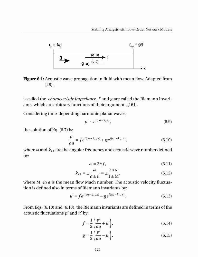
Stability Analysis with Low-Order Network Models
Figure 6.1: Acoustic wave propagation in fluid with mean flow. Adapted from[48].
is called the characteristic impedance. f and g are called the Riemann Invari-ants, which are arbitrary functions of their arguments [161].
Considering time-depending harmonic planar waves,
p ′ ∼ e i (ωt−kx x), (6.9)
the solution of Eq. (6.7) is:
p ′
ρa= f e i (ωt−kx+x) + g e i (ωt−kx−x), (6.10)
whereω and kx± are the angular frequency and acoustic wave number definedby:
ω= 2π f , (6.11)
kx± =± ω
a ± u=± ω/a
1±M, (6.12)
where M=u/a is the mean flow Mach number. The acoustic velocity fluctua-tion is defined also in terms of Riemann invariants by:
u′ = f e i (ωt−kx+x) − g e i (ωt−kx−x). (6.13)
From Eqs. (6.10) and (6.13), the Riemann invariants are defined in terms of theacoustic fluctuations p ′ and u′ by:
f = 1
2
(p ′
ρa+u′
), (6.14)
g = 1
2
(p ′
ρa−u′
). (6.15)
124
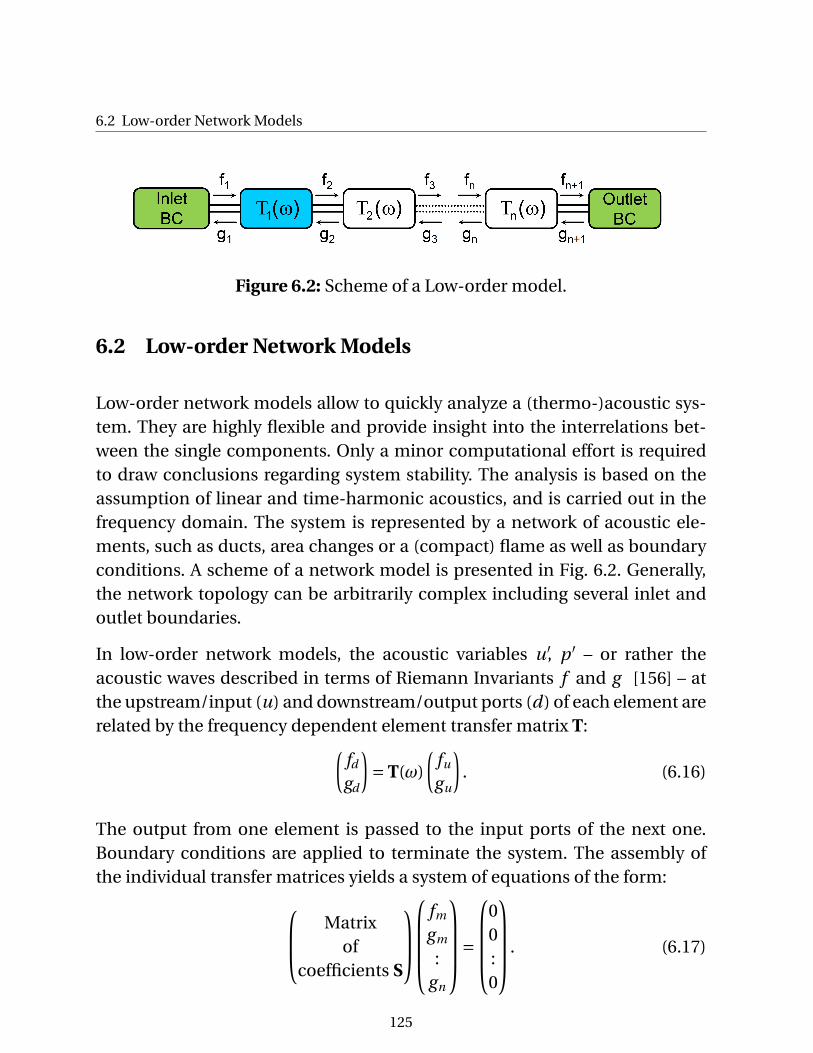
6.2 Low-order Network Models
Figure 6.2: Scheme of a Low-order model.
6.2 Low-order Network Models
Low-order network models allow to quickly analyze a (thermo-)acoustic sys-tem. They are highly flexible and provide insight into the interrelations bet-ween the single components. Only a minor computational effort is requiredto draw conclusions regarding system stability. The analysis is based on theassumption of linear and time-harmonic acoustics, and is carried out in thefrequency domain. The system is represented by a network of acoustic ele-ments, such as ducts, area changes or a (compact) flame as well as boundaryconditions. A scheme of a network model is presented in Fig. 6.2. Generally,the network topology can be arbitrarily complex including several inlet andoutlet boundaries.
In low-order network models, the acoustic variables u′, p ′ – or rather theacoustic waves described in terms of Riemann Invariants f and g [156] – atthe upstream/input (u) and downstream/output ports (d) of each element arerelated by the frequency dependent element transfer matrix T:(
fd
gd
)= T(ω)
(fu
gu
). (6.16)
The output from one element is passed to the input ports of the next one.Boundary conditions are applied to terminate the system. The assembly ofthe individual transfer matrices yields a system of equations of the form: Matrix
ofcoefficients S
fm
gm
:gn
=
00:0
. (6.17)
125
Stability Analysis with Low-Order Network Models
The characteristic equation Det(S) = 0 is fulfilled for complex eigenfrequen-cies, ω =ωr eal +iωi mag ∈ C. With harmonic time dependence exp(iωt), the ima-ginary part of an eigenfrequency indicates whether the corresponding eigen-mode grows or decays over time. The cycle increment (CI) of a mode, i.e. therelative growth in amplitude per period of the oscillation, may be defined as[83, 156]:
CI = e−2π
ωimagωreal −1. (6.18)
With this definition, CI = 0 corresponds to marginal stability. The real part ofthe eigenfrequency determines the frequency of the eigenmode.
Transfer matrices for many elements have been derived analytically and canbe found in the literature [156]. Also, for more complex elements, transfer ma-trices can be obtained from measurements or CFD simulations. The analyti-cal flame transfer matrix of a compact flame is presented in this chapter. Thedefinitions of other acoustic elements included in the network model for thestability analysis are shown in Appendix A.7.
6.2.1 Flame Transfer Matrix of a Compact Flame
In the case of a thermoacoustic problem, the flame must be incorporatedinto the system model. The flame is commonly represented by an acousti-cally “compact” element. That is, its spatial dimensions are assumed smallcompared to the acoustic wave length. Hence, it is treated as a discontinu-ity where heat is added. According to Chu [25], the acoustic variables at theupstream (u) and downstream (d) sides of the heat source then satisfy the li-nearized Rankine-Hugoniot relations [83, 156]:
( p ′
ρa
)d= (ρa)u
(ρa)d
[( p ′
ρa
)u−
(Td
Tu−1
)u′
u Mu
(1+ Q ′/ ¯Q
u′u/uu
)], (6.19)
u′d = u′
u
[1+
(Td
Tu−1
) Q ′/ ¯Q
u′u/uu
]−
( p ′
ρa
)u
Mu γ(Td
Tu−1
). (6.20)
In order to obtain a closed system of equations, the heat release fluctua-tions Q ′ in Eqs. (6.19) and (6.20) must be related to the fluctuations in the
126
6.2 Low-order Network Models
acoustic variables u′ and p ′. This is achieved by introducing the FTF fromEq. (3.1) into Eqs. (6.19) and (6.20). In general, the reference location “r ”,where the input signal u′
r is recorded, is not immediately upstream of theflame at location “u”. Thus, the flame is represented as a 6-port element inthe network, linking f ’s and g ’s at positions “u”, “d” and “r ” (see Fig. 6.4)).The element is defined in terms of Riemann invariants by [83]:(
ρd adρu au
ρd adρu au
1 −1
)(fd
gd
)=
1−Mu
(TdTu
−1)
1+Mu
(TdTu
−1)
1−Mu
(TdTu
−1)γ −1−Mu
(TdTu
−1)γ
(fu
gu
)(6.21)
+[
uu
ur
(Td
Tu−1
)FTF(ω)
](−Mu Mu
1 −1
)(fr
gr
). (6.22)
The derivation of this expression is presented in Appendix A.7.2.
6.2.2 Use of Experimental Data in Eigenfrequency Analysis (The UIRMethod)
The eigenfrequency analysis requires to evaluate coefficients of the systemmatrix S(ω) also for frequencies ω ∈ C away from the real axis. This require-ment is obviously not a problem if analytical expressions for network ele-ments are known [156]. Also, it is not a problem for a flame transfer func-tion determined with LES/SI, because the argumentω in the z-transform (seeEq. (4.32)) may be complex-valued, such that from the UIR h the transfer func-tion FTF(ω) may be evaluated anywhere in the complex plane [83].
However, in experiments the flame transfer function is determined with har-monic forcing at constant amplitude, i.e. the FTF is known only for a numberof purely real frequencies ωn ∈ R. In such a situation the FTF at intermediatefrequencies is often determined by interpolation between measured values.However, for stability analysis the FTF is needed for frequencies away fromthe real axis. Extrapolating the FTF from known values on the real axis into thecomplex plane leads that the growth or decay of oscillation amplitudes is notproperly reflected in the system matrix coefficients, if the imaginary part ofthe frequency is not taken into account.
127
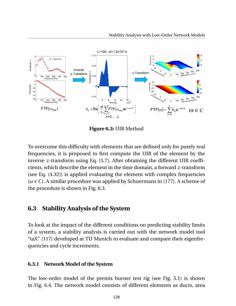
Stability Analysis with Low-Order Network Models
Figure 6.3: UIR Method
To overcome this difficulty with elements that are defined only for purely realfrequencies, it is proposed to first compute the UIR of the element by theinverse z-transform using Eq. (5.7). After obtaining the different UIR coeffi-cients, which describe the element in the time domain, a forward z-transform(see Eq. (4.32)) is applied evaluating the element with complex frequencies(ω ∈C). A similar procedure was applied by Schuermans in [177]. A scheme ofthe procedure is shown in Fig. 6.3.
6.3 Stability Analysis of the System
To look at the impact of the different conditions on predicting stability limitsof a system, a stability analysis is carried out with the network model tool“taX” [117] developed at TU Munich to evaluate and compare their eigenfre-quencies and cycle increments.
6.3.1 Network Model of the System
The low-order model of the premix burner test rig (see Fig. 5.1) is shownin Fig. 6.4. The network model consists of different elements as ducts, area
128
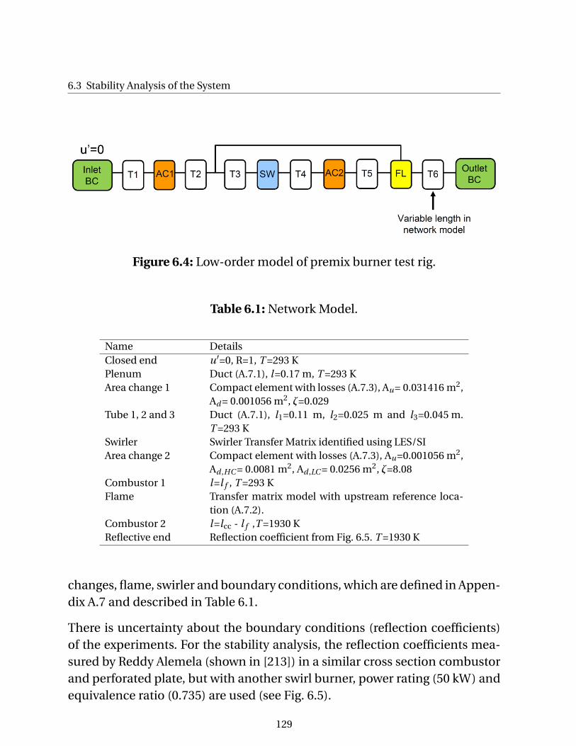
6.3 Stability Analysis of the System
Figure 6.4: Low-order model of premix burner test rig.
Table 6.1: Network Model.
Name DetailsClosed end u′=0, R=1, T =293 KPlenum Duct (A.7.1), l=0.17 m, T =293 KArea change 1 Compact element with losses (A.7.3), Au= 0.031416 m2,
Ad = 0.001056 m2, ζ=0.029Tube 1, 2 and 3 Duct (A.7.1), l1=0.11 m, l2=0.025 m and l3=0.045 m.
T =293 KSwirler Swirler Transfer Matrix identified using LES/SIArea change 2 Compact element with losses (A.7.3), Au=0.001056 m2,
Ad ,HC = 0.0081 m2, Ad ,LC = 0.0256 m2, ζ=8.08Combustor 1 l =l f , T =293 KFlame Transfer matrix model with upstream reference loca-
tion (A.7.2).Combustor 2 l =lcc - l f ,T =1930 KReflective end Reflection coefficient from Fig. 6.5. T =1930 K
changes, flame, swirler and boundary conditions, which are defined in Appen-dix A.7 and described in Table 6.1.
There is uncertainty about the boundary conditions (reflection coefficients)of the experiments. For the stability analysis, the reflection coefficients mea-sured by Reddy Alemela (shown in [213]) in a similar cross section combustorand perforated plate, but with another swirl burner, power rating (50 kW) andequivalence ratio (0.735) are used (see Fig. 6.5).
129
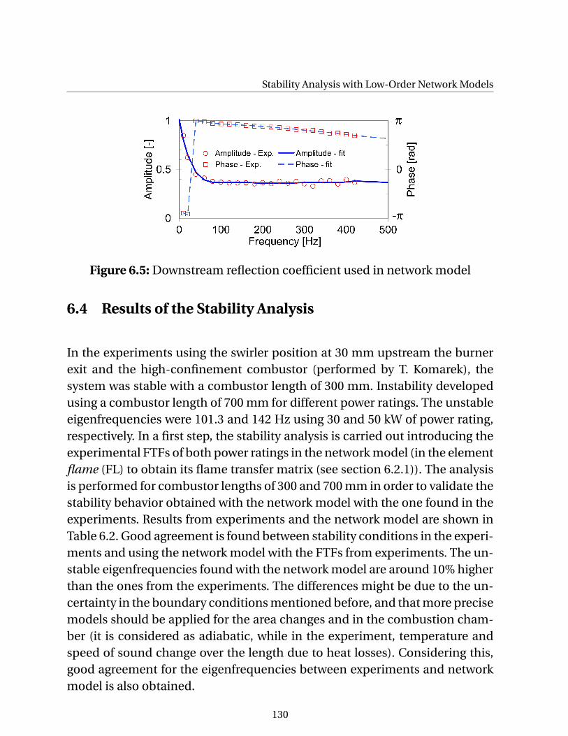
Stability Analysis with Low-Order Network Models
Figure 6.5: Downstream reflection coefficient used in network model
6.4 Results of the Stability Analysis
In the experiments using the swirler position at 30 mm upstream the burnerexit and the high-confinement combustor (performed by T. Komarek), thesystem was stable with a combustor length of 300 mm. Instability developedusing a combustor length of 700 mm for different power ratings. The unstableeigenfrequencies were 101.3 and 142 Hz using 30 and 50 kW of power rating,respectively. In a first step, the stability analysis is carried out introducing theexperimental FTFs of both power ratings in the network model (in the elementflame (FL) to obtain its flame transfer matrix (see section 6.2.1)). The analysisis performed for combustor lengths of 300 and 700 mm in order to validate thestability behavior obtained with the network model with the one found in theexperiments. Results from experiments and the network model are shown inTable 6.2. Good agreement is found between stability conditions in the experi-ments and using the network model with the FTFs from experiments. The un-stable eigenfrequencies found with the network model are around 10% higherthan the ones from the experiments. The differences might be due to the un-certainty in the boundary conditions mentioned before, and that more precisemodels should be applied for the area changes and in the combustion cham-ber (it is considered as adiabatic, while in the experiment, temperature andspeed of sound change over the length due to heat losses). Considering this,good agreement for the eigenfrequencies between experiments and networkmodel is also obtained.
130
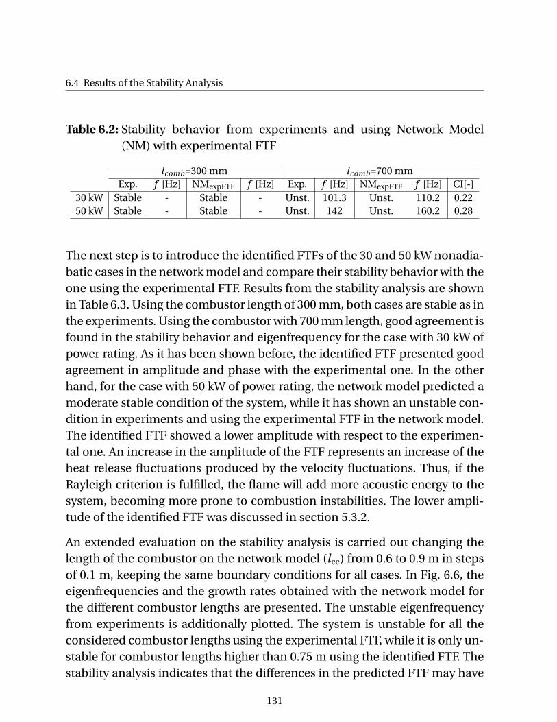
6.4 Results of the Stability Analysis
Table 6.2: Stability behavior from experiments and using Network Model(NM) with experimental FTF
lcomb=300 mm lcomb=700 mmExp. f [Hz] NMexpFTF f [Hz] Exp. f [Hz] NMexpFTF f [Hz] CI[-]
30 kW Stable - Stable - Unst. 101.3 Unst. 110.2 0.2250 kW Stable - Stable - Unst. 142 Unst. 160.2 0.28
The next step is to introduce the identified FTFs of the 30 and 50 kW nonadia-batic cases in the network model and compare their stability behavior with theone using the experimental FTF. Results from the stability analysis are shownin Table 6.3. Using the combustor length of 300 mm, both cases are stable as inthe experiments. Using the combustor with 700 mm length, good agreement isfound in the stability behavior and eigenfrequency for the case with 30 kW ofpower rating. As it has been shown before, the identified FTF presented goodagreement in amplitude and phase with the experimental one. In the otherhand, for the case with 50 kW of power rating, the network model predicted amoderate stable condition of the system, while it has shown an unstable con-dition in experiments and using the experimental FTF in the network model.The identified FTF showed a lower amplitude with respect to the experimen-tal one. An increase in the amplitude of the FTF represents an increase of theheat release fluctuations produced by the velocity fluctuations. Thus, if theRayleigh criterion is fulfilled, the flame will add more acoustic energy to thesystem, becoming more prone to combustion instabilities. The lower ampli-tude of the identified FTF was discussed in section 5.3.2.
An extended evaluation on the stability analysis is carried out changing thelength of the combustor on the network model (lcc) from 0.6 to 0.9 m in stepsof 0.1 m, keeping the same boundary conditions for all cases. In Fig. 6.6, theeigenfrequencies and the growth rates obtained with the network model forthe different combustor lengths are presented. The unstable eigenfrequencyfrom experiments is additionally plotted. The system is unstable for all theconsidered combustor lengths using the experimental FTF, while it is only un-stable for combustor lengths higher than 0.75 m using the identified FTF. Thestability analysis indicates that the differences in the predicted FTF may have
131
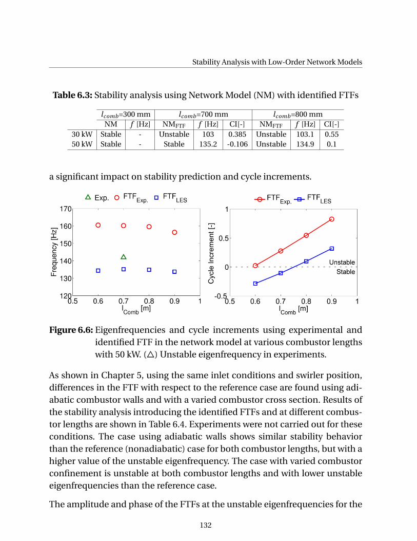
Stability Analysis with Low-Order Network Models
Table 6.3: Stability analysis using Network Model (NM) with identified FTFs
lcomb=300 mm lcomb=700 mm lcomb=800 mmNM f [Hz] NMFTF f [Hz] CI[-] NMFTF f [Hz] CI[-]
30 kW Stable - Unstable 103 0.385 Unstable 103.1 0.5550 kW Stable - Stable 135.2 -0.106 Unstable 134.9 0.1
a significant impact on stability prediction and cycle increments.
Figure 6.6: Eigenfrequencies and cycle increments using experimental andidentified FTF in the network model at various combustor lengthswith 50 kW. (4) Unstable eigenfrequency in experiments.
As shown in Chapter 5, using the same inlet conditions and swirler position,differences in the FTF with respect to the reference case are found using adi-abatic combustor walls and with a varied combustor cross section. Results ofthe stability analysis introducing the identified FTFs and at different combus-tor lengths are shown in Table 6.4. Experiments were not carried out for theseconditions. The case using adiabatic walls shows similar stability behaviorthan the reference (nonadiabatic) case for both combustor lengths, but with ahigher value of the unstable eigenfrequency. The case with varied combustorconfinement is unstable at both combustor lengths and with lower unstableeigenfrequencies than the reference case.
The amplitude and phase of the FTFs at the unstable eigenfrequencies for the
132
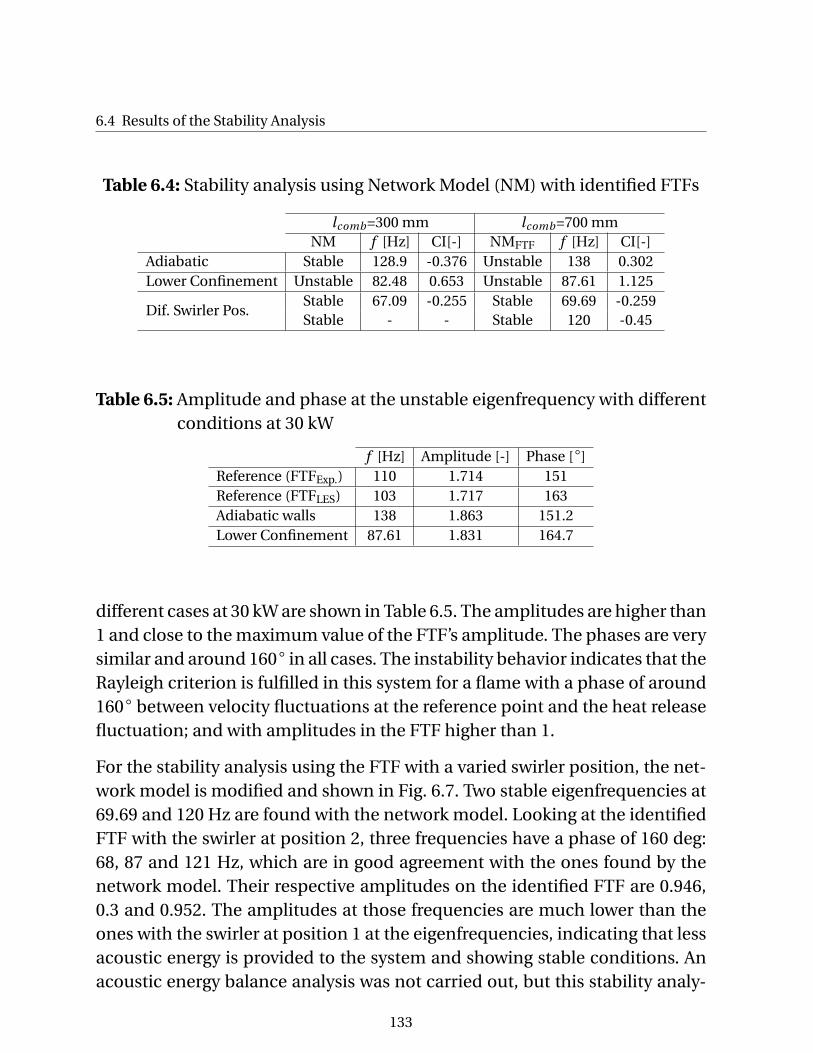
6.4 Results of the Stability Analysis
Table 6.4: Stability analysis using Network Model (NM) with identified FTFs
lcomb=300 mm lcomb=700 mmNM f [Hz] CI[-] NMFTF f [Hz] CI[-]
Adiabatic Stable 128.9 -0.376 Unstable 138 0.302Lower Confinement Unstable 82.48 0.653 Unstable 87.61 1.125
Dif. Swirler Pos.Stable 67.09 -0.255 Stable 69.69 -0.259Stable - - Stable 120 -0.45
Table 6.5: Amplitude and phase at the unstable eigenfrequency with differentconditions at 30 kW
f [Hz] Amplitude [-] Phase []Reference (FTFExp.) 110 1.714 151Reference (FTFLES) 103 1.717 163Adiabatic walls 138 1.863 151.2Lower Confinement 87.61 1.831 164.7
different cases at 30 kW are shown in Table 6.5. The amplitudes are higher than1 and close to the maximum value of the FTF’s amplitude. The phases are verysimilar and around 160 in all cases. The instability behavior indicates that theRayleigh criterion is fulfilled in this system for a flame with a phase of around160 between velocity fluctuations at the reference point and the heat releasefluctuation; and with amplitudes in the FTF higher than 1.
For the stability analysis using the FTF with a varied swirler position, the net-work model is modified and shown in Fig. 6.7. Two stable eigenfrequencies at69.69 and 120 Hz are found with the network model. Looking at the identifiedFTF with the swirler at position 2, three frequencies have a phase of 160 deg:68, 87 and 121 Hz, which are in good agreement with the ones found by thenetwork model. Their respective amplitudes on the identified FTF are 0.946,0.3 and 0.952. The amplitudes at those frequencies are much lower than theones with the swirler at position 1 at the eigenfrequencies, indicating that lessacoustic energy is provided to the system and showing stable conditions. Anacoustic energy balance analysis was not carried out, but this stability analy-
133
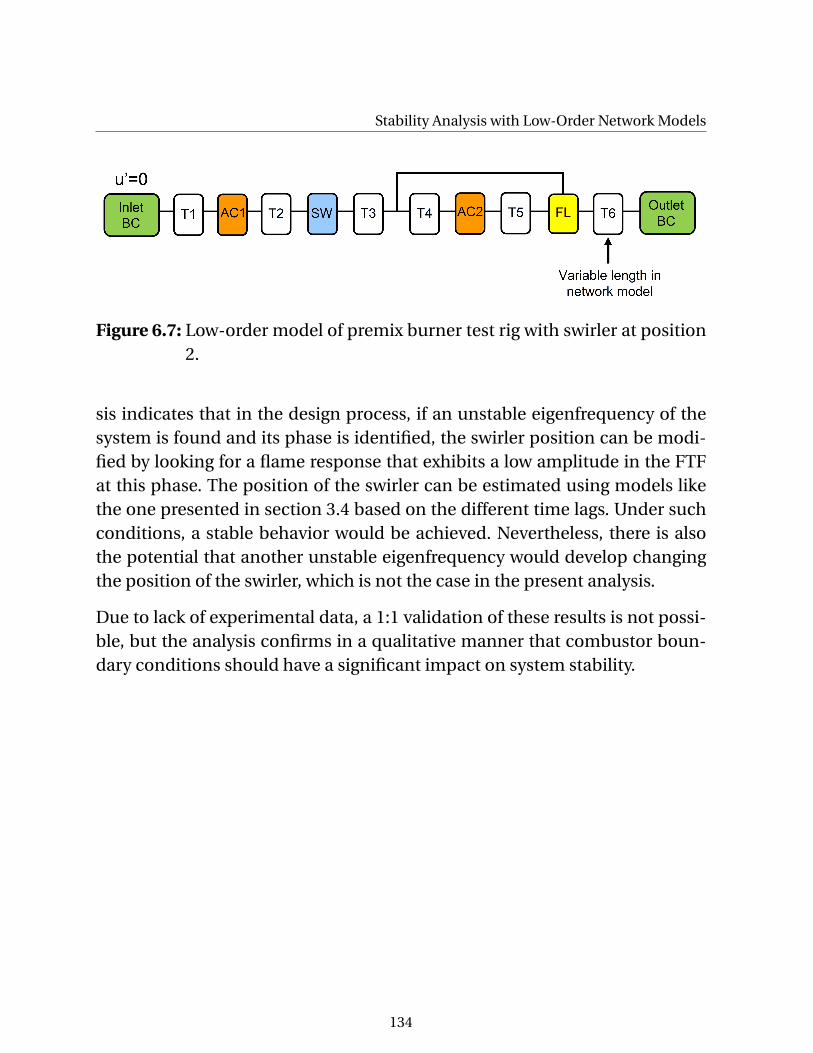
Stability Analysis with Low-Order Network Models
Figure 6.7: Low-order model of premix burner test rig with swirler at position2.
sis indicates that in the design process, if an unstable eigenfrequency of thesystem is found and its phase is identified, the swirler position can be modi-fied by looking for a flame response that exhibits a low amplitude in the FTFat this phase. The position of the swirler can be estimated using models likethe one presented in section 3.4 based on the different time lags. Under suchconditions, a stable behavior would be achieved. Nevertheless, there is alsothe potential that another unstable eigenfrequency would develop changingthe position of the swirler, which is not the case in the present analysis.
Due to lack of experimental data, a 1:1 validation of these results is not possi-ble, but the analysis confirms in a qualitative manner that combustor boun-dary conditions should have a significant impact on system stability.
134
7 Summary and Conclusions
The flame dynamics of a perfectly premixed axial swirl burner is investigated.The study is based on large eddy simulations of compressible reacting flowin combination with system identification based on correlation analysis. Theunit impulse response and the transfer function of swirling turbulent flames atvarious operating conditions are determined. The advantage of using LES/SImethods in comparison with single frequency harmonic excitations (as in thedetermination of the experimental flame transfer function) is that it is possi-ble to obtain the frequency flame response over a range of frequencies from asingle LES simulation, reducing the computational effort.
The LES/SI approach is validated against experiments taking as reference casethe swirl burner operating with 30 kW of power rating and with non-adiabaticcombustor wall boundary conditions. Application of nonadiabatic boundaryconditions are necessary to predict the correct flame structure and heat re-lease distribution. The identified flame transfer function shows good agree-ment with experiments and with harmonic excitation carried out for a sin-gle frequency. A comparison of the flame transfer functions identified withLES/SI with varied reference positions for extracting the velocity fluctuationshas shown small differences between them. Additional simulations with vari-ation of power rating, thermal boundary conditions at the combustor walls,combustor confinement and swirler position are carried out to investigatetheir impact on flame dynamics.
The case with higher power rating (50 kW) exhibits a flame longer than the onewith 30 kW due to the higher velocities. Comparing non-reacting and react-ing simulations, strong differences on flow field and turbulence are observed.In the reacting flow simulations, a transversal eigenmode developed in thecombustion chamber producing pressure oscillations in the combustor whichgrew in time. Two methodologies based on the combination of multiple time
135
Summary and Conclusions
series generated from several LES runs are derived to obtain a more robustidentification. The FTF exhibits good qualitative agreement with the experi-ment and good scaling in Strouhal number with the 30 kW case.
Changing the combustor walls to adiabatic conditions, strong reaction in theouter shear layer is obtained, having the topology of a “M-flame”. Variations inthe flow field, spatial and axial heat release distributions are observed betweenadiabatic and nonadiabatic conditions. The adiabatic flames has a shorterflame than the nonadiabatic cases due to the incorrect flame stabilizationtopology. The flame transfer function with adiabatic walls shows a broader fre-quency response (with amplitudes higher than one) and a less steeper phase(produced by the smaller time lag response to the perturbations) than thenonadiabatic case.
The work of Komarek and Polifke [103, 104] in the impact of swirler positionon the FTF is extended to a LES context. Comparing the identified flame trans-fer functions at varied swirler positions, both show a very different flame res-ponse. The mechanism of the different propagation speeds and phase bet-ween perturbations, recognized in previous investigations [78,103,137] as themechanism of the variations in the flame response, is also investigated by a-pplying harmonic excitation only to the swirler at position 2 without the com-bustor. As the induced tangential velocity fluctuations created by the swirlerhave a strong impact on the flame dynamics, the swirler geometry must betaken into account in CFD simulations in order to capture the constructi-ve/destructive interaction between axial and tangential velocity fluctuations.
The influence of combustor confinement on the flame transfer function is in-vestigated numerically using two combustors with varied cross-section area.Previous experimental studies [11, 75] in other configurations have shown animpact on the FTF by the combustor confinement. Results from the carriedout simulations show variations on the mean axial and tangential velocity, aswell for the turbulent kinetic energy and jet angle. For the mean heat release,the flames in both combustors exhibit similar flame stabilization mainly in theinner shear layer, but with different axial and spatial heat release distributions,showing a broader spatial heat release distribution and a longer flame thanthe high-confinement case. This is in agreement with the observations found
136
in the experimental work of Hauser et al. [75]. For the identified flame transferfunction with low-confinement, the amplitude shows similar behavior to theone with high-confinement, but with the maximum amplitude slightly higherand at a lower frequency. The time lag response is larger which is representedby the higher steepness in the phase.
The FTF model proposed by Komarek and Polifke [103] to describe the res-ponses to perturbations of mass flow rate and swirl in the time domain byunit impulse responses is used to analyze the varied flame response for thevarious cases analyzed before. The analysis illustrates how differences in flowfield and flame shape can influence time lags and thus the flame response inthe time or frequency domain.
Using a network model, stability analysis is carried out for two different com-bustor lengths to assess the impact of the variations in the flame transferfunctions on combustor stability limits. The stability analysis indicates thatthe variations in the predicted FTF may have a significant impact on stabilityprediction and cycle increments. Furthermore, it is shown that by changingthe position of the swirler, stable conditions are predicted for the investigatedcombustor lengths.
The present work leads to the following conclusions and contributions to pre-vious studies:
• The LES/SI approach for the identification of flame transfer functions isvalidated with a perfectly premixed axial swirl burner with good agree-ment with experiments.
• Heat loss effects on the boundary conditions and on the combustionmodel must be taken into account for the prediction of flame dynamics.Nonadiabaticity has a strong influence on flame shape and on the spatialdistribution of heat release.
• The LES/SI approach is capable of detecting the impact of variations onthermal boundary conditions at the combustor wall, power rating, com-bustor confinement and swirler position on premixed flame flame trans-fer functions.
137

Summary and Conclusions
• The identified flame transfer functions confirm previous observations inother studies, showing that the flame transfer function does depend notonly on the burner geometry, but also on the boundary conditions thatthe combustor provides to the flame (combustor wall temperature, con-finement, etc.). Furthermore, the mean flow field just downstream of theburner outlet and the flame characteristics depend on the combustorconfinement and boundary conditions.
• A model for the impact of the axial and swirl fluctuations on the flametransfer function shows the varied response and time lag distributionsfor the various cases considered.
• Variations in the flame transfer function produced by the different condi-tions have an impact on the stability behavior predicted with a thermoa-coustic low-order network model.
• There is a strong influence of the swirler position on the flame response.The stability behavior of the engine can be modified by changing the po-sition of the swirler without strong changes on the mean flow and flame.
• Results indicate that the flame transfer function obtained from singleburner combustors - be it by experimental or numerical means - shouldonly be used for stability analysis of multi-burner industrial gas turbinesprovided that operating and boundary conditions, as well as, combustorgeometries are equivalent.
138
8 Outlook
The present study shows the potential of the LES/SI method to identify theflame response for fully premixed conditions. The following ideas are pro-posed as outlook to this work:
• In technical applications, as in operating gas turbines, the mixing bet-ween fuel and air is produced moments before reaction occurs. Thus, theflame reacts in most cases under the presence of mixture inhomogeneity.The impact of equivalence ratio fluctuations on the flame response wasinvestigated previously by Huber and Polifke [85] in a RANS context as aMISO system. Application of the method on the LES context is plannedin future investigations.
• Investigation of the impact of operating pressure and multi-burner con-figurations on the flame dynamics. These conditions are typical in indus-trial gas turbines, and not considered in this study.
• It is recommended to investigate the flame dynamics using the sameburner with different combustion models and mesh resolution. Most in-dustrial applications are usually simulated with a lower level of mesh re-solution due the limited availability of computational resources. Investi-gations to quantify the impact on the flame response by the lower meshresolution have not been carried out.
• The separation of the flame response to axial and swirl fluctuations. Thesystem can be analyzed as a MISO system to identify the contributions inthe flame response from mass flow and swirl fluctuations separately.
• For the prediction of limit cycle amplitudes from stability analysis, it isnecessary to introduce the non-linear behavior of the flame with de-pendence of the perturbation amplitude by the flame describing func-
139
Outlook
tion. The system identification method shown in this study to identifythe flame dynamics is for linear time-invariant systems. The implemen-tation of non-linear system identification for thermoacoustic system isstill in its early stages, and should be further investigated.
• Finally, simulations should introduce damping effects on the wallboundary conditions. Real systems have a level of acoustic damping byvibration, which in not taken into account in CFD simulations. Further-more, the development of 3D non-reflective boundary conditions to takeinto account transversal sources is also recommended.
140

Bibliography
[1] U.S. Energy Information Administration. Annual Energy Outlook 2011with Projections to 2035. Technical Report DOE/EIA-0383, April 2011.
[2] P.R. Alemela. Measurement and Scaling of Acoustic Transfer Matrices ofPremixed Swirl Flames. PhD Thesis, Technische Universität München,2009.
[3] C. Angelberger, D. Veynante, and F. Egofopoulos. LES of Chemical andAcoustic Forcing of a Premixed Dump Combustor. Flow, Turbulence andCombustion, 65:205–222, 2000.
[4] S.S. Archer. Morphology of Unconfined and Confined Swirling Flows un-der Non-reacting and Combustion Conditions. PhD Thesis, University ofMariland, College Park, 2005.
[5] C.A. Armitage, R. Balachandran, E. Mastorakos, and R.S. Cant. Investiga-tion of the nonlinear response of turbulent premixed flames to imposedinlet velocity oscillations. Combust. Flame, 146:419–436, 2006.
[6] T. Ayinde. A Generalized Relationship for Swirl Decay in Laminar PipeFlow. Sadhana, 35:129–137, 2010. 1.
[7] B. O. Ayoola, R. Balachandran, J. H. Frank, E. Mastorakos, and C. F.Kaminski. Measurements of Local Heat Release Rates in a TurbulentPremixed Bluff Body Stabilised Flame with Acoustic Forcing. In Euro-pean Combustion Meeting, 2005.
141
BIBLIOGRAPHY
[8] H. Büchner, C. Hirsch, and W. Leuckel. Experimental Investigation onthe Dynamics of Pulsated Premixed Axial Jet Flames. Combust. Sci. andTech., 94:219–228, 1993.
[9] B.D. Bellows, Y. Neumeier, and T. Lieuwen. Forced Response of aSwirling, Premixed Flame to Flow Disturbances. Journal of Propulsionand Power, 22(5):1075–1084, 2006.
[10] S.A. Beltagui and N.R.L. Maccallum. Aerodynamics of Vane-swirledFlames in Furnaces. Journal of the Institute of Fuel, 49(401):183–193,1976.
[11] A. L. Birbaud, D. Durox, S. Ducruix, and S. Candel. Dynamics of Con-fined Premixed Flames Submitted to Upstream Acoustic Modulations.Proc. Combust. Inst., 31(1):1257–1265, 2007.
[12] M. Boger, D. Veynante, H. Boughanem, and A. Trouve. Direct NumericalSimulation Analysis of Flame Surface Density Concept for Large EddySimulation of Turbulent Premixed Combustion. Symposium (Interna-tional) on Combustion, 27(1):917 – 925, 1998. Twenty-Seventh Sympo-sium (International) on Combustion.
[13] G. Borghesi, F. Biagioli, and B. Schuermans. Dynamic Response of Tur-bulent Swirling Flames to Acoustic Perturbations. Combustion Theoryand Modelling, 13(3):487–512, 2009.
[14] W. J. T. Bos, H. Touil, and J. P. Bertoglio. Reynolds Number Dependencyof the Scalar Flux Spectrum in Isotropic Turbulence with a UniformScalar Gradient. Physics of Fluids, 17(12):125108, 2005.
[15] L. Boyer and J. Quinard. On the Dynamics of Anchored Flames. Com-bust. Flame, 82:51–65, 1990.
[16] P. Breeze. Efficiency versus Flexibility: Advances in Gas TurbineTechnology. Power Engineering International Magazine, 19(3):30–34,2011. http://www.powerengineeringint.com/articles/print/volume-19/issue-3/gas-steam-turbine-directory/efficiency-versus-flexibility-advances-in-gas-turbine-technology.html.
142

BIBLIOGRAPHY
[17] N. Bunce, J.G. Lee, B.D. Quay, and D.A. Santavicca. Mixture-forcedFlame Transfer Function Measurements and Mechanisms in a Single-Nozzle Combustor at Elevated Pressure. Number GT2011-46744 in Proc.of ASME Turbo Expo 2011, page 10, Vancouver, Canada, June 6-10 2011.ASME.
[18] H. Burchard and L. Umlauf. Turbulence in Natural Waters. Lec-ture Notes, October 2008. http://www.io-warnemuende.de/burchard-teaching.html.
[19] S. Candel, D. Durox, S. Ducruix, A.L. Birbaud, N. Noiray, and T. Schuller.Flame Dynamics and Combustion Noise: Progress and Challenges. In-ternational Journal of Aeroacoustics, 8(1-2):1–56, 2009.
[20] R.S. Cant and E. Mastorakos. An Introduction to Turbulent ReactingFlows. Imperial College Press, 2008.
[21] CERFACS. http://www.cerfacs.fr/4-26334-The-AVBP-code.php.
[22] CERFACS. AVBP 6.0 Handbook. 2008.
[23] CERFACS. AVBP Help Manual, 2011.
[24] J.H. Chen. Petascale Direct Numerical Simulation of Turbulent Com-bustion – Fundamental Insights towards Predictive Models. Proc. Com-bust. Inst., 33(1):99–123, 2011.
[25] B. T. Chu. On the Generation of Pressure Waves at a Plane Flame Front.Fourth Symposium (International) on Combustion, pages 603–612, 1953.
[26] B.R. Clayton and Y.S.M. Morsi. Determination of Principal Character-istics of Turbulent Swirling Flow along Annuli: Part1: Measurement ofTime Mean Parameters. International Journal of Heat and Fluid Flow,5(4):195–203, 1984.
[27] O. Colin, F. Ducros, D. Veynante, and T. Poinsot. A Thickened FlameModel for Large Eddy Simulations of Turbulent Premixed Combustion.Physics of Fluids, 12(7):1843–1863, 2000.
143
BIBLIOGRAPHY
[28] P.J. Colucci, F.A. Jaberi, P. Givi, and S.B. Pope. Filtered Density Functionfor Large Eddy Simulation of Turbulent Reacting Flows. Physics of Flu-ids, 10(2):499–515, 1998.
[29] L. Crocco. Aspects of Combustion Stability in Liquid Propellant RocketMotors Part1: Fundamentals. Low Frequency Instability with Monopro-pellants. J. of American Rocket Society, pages 163–178, 1951.
[30] L Crocco and S.I. Cheng. Theory of combustion instability in liquidpropellant rocket motors. Butterworths Science Publication, AGARDO-GRAPH N 8, 1956.
[31] B. Cuenot, Y. Sommerer, L.Y.M. Gicquel, and T. Poinsot. LES of ReactingFlows. 3rd International workshop on Rocket Combustion Modeling,Paris, 2006.
[32] A. Cuquel, D. Durox, and T. Schuller. Experimental Determination ofFlame Transfer Function using Random Velocity Perturbations. NumberGT2011-45881 in Proc. of ASME Turbo Expo 2011, Vancouver, Canada,page 10, Vancouver, Canada, June 6-10 2011. ASME.
[33] Y. Danning, Y. Huang, and Y. Vigor. A Generalized Model of Acoustic Re-sponse of Turbulent Premixed Flame and its Application to Gas-TurbineCombustion Instability Analysis. Combustion Science and Technology,177(5-6):1109–1150, 2005.
[34] J. Daou and M. Matalon. Influence of Conductive Heat-losses onthe Propagation of Premixed Flames in Channels. Combust. Flame,128(4):321–339, 2002.
[35] N. Darabiha, S.M. Candel, V. Giovangigli, and M.D. Smooke. Extinc-tion of Strained Premixed Propane-Air Flames with Complex Chemistry.Combust. Sci. Technol., 60:267–285, 1988.
[36] S.R. de Parias Neto, P. Legentilhomme, and J. Legrand. Finite-elementSimulation of Laminar Swirling Decaying Flow Induced by Means of aTangential Inlet in an Annulus. Computer Methods in Applied Mechanicsand Engineering, 165(1-4):189–213, 1998.
144
BIBLIOGRAPHY
[37] A.P. Dowling. The Challenges of Lean Premixed Combustion. NumberIGTC2003Tokyo KS-5 in Proceedings of the International Gas TurbineCongress, Tokio, 2003.
[38] A.P. Dowling and A.S. Morgans. Feedback Control of Combustion Oscil-lations. Annu. Rev. Fluid Mech., 37::151–182, 2005.
[39] A.P. Dowling and J.E.F. Williams. Sound and Sources of Sound. Ellis Hor-wood series in engineering science. E. Horwood, West Sussex, England,1983.
[40] F. Duchaine and T. Poinsot. Sensitivity of Flame Transfer Functions ofLaminar Flames. Proc. of the Summer Program CTR, Stanford, 2010.
[41] S. Ducruix, D. Durox, and S. Candel. Theoretical and Experimental De-terminations of the Flame Transfer Function of a Laminar PremixedFlame. Proc. Combust. Inst., 28:765–773, 2000.
[42] L. Durand. Development, Implementation, and Validation of LES Mod-els for Inhomogeneously Premixed Turbulent Combustion. PhD thesis,Technische Universität München, 2007.
[43] D. Durox, T. Schuller, and S. Candel. Combustion Dynamics of InvertedConical Flames. Proceedings of the Combustion Institute, 30(2):1717–1724, 2005.
[44] D. Durox, T. Schuller, N. Noiray, and S. Candel. Experimental Analysisof Nonlinear Flame Transfer Functions for Different Flame Geometries.Proc. Combust. Inst., 32(1):1391–1398, 2009.
[45] B. Efron and R. Tibshirani. An Introduction to the Bootstrap. Chapman& Hall, 1993.
[46] F. El-Mahallawy and S. El-Din Habik. Fundamentals and Technology ofCombustion. ELSEVIER, 2002.
[47] D. Fanaca. (Private communication).
145
BIBLIOGRAPHY
[48] D. Fanaca. Influence of Burner-Burner Interactions on the Flame Dy-namics in an Annular Combustor. PhD Thesis, Technische UniversitätMünchen, 2010.
[49] D. Fanaca, P.R. Alemela, C. Hirsch, T. Sattelmayer, and B. Schuermanns.Comparison of the Flow Field of a Swirl Stabilized Premixed Burner in anAnnular and a Single Burner Combustion Chamber. J. Eng. Gas TurbinesPower, 132(6):071502, 2010.
[50] A. Fischer. Hybride, thermoakustische Charakterisierung von Drallbren-nern. PhD thesis, Technische Universität München, 2004.
[51] A. Fleifil, A. M. Annaswamy, Z. A. Ghoneim, and A. F. Ghoniem. Responseof a Laminar Premixed Flame to Flow Oscillations: A Kinematic Modeland Thermoacoustic Instability Results. Combust. Flame, 106:487–510,1996.
[52] P. Flohr, C. O. Paschereit, and V. Bellucci. Steady CFD Analysis for GasTurbine Burner Transfer Functions. Number AIAA 2003-1346 in 41stAIAA Aerospace Sciences Meeting and Exhibit, page 11, Reno, NV, Jan6-9 2003. AIAA.
[53] P. Flohr, C. O. Paschereit, B. van Roon, and B. Schuermans. Using CFDfor Time-Delay Modeling of Premix Flames. Number 2001-GT-0376 inProc. ASME Turbo Expo 2001, page 10, New Orleans, Louisiana, June 4-72001. ASME.
[54] P. Flohr and H. Pitsch. A Turbulent Flame Speed Closure Model for LESof Industrial Burner Flows. C. Turb. Research, Annual Research Briefs,pages 169–179, 2000.
[55] C.W. Foley, I. Chterev, J. Seitzman, and T. Lieuwen. Flame Configurationsin a Lean Premixed Dump Combustor with an Annular Swirling Flow. In7th US National Combustion Meeting, number 1D16, Atlanta, GA, March2011. Eastern States Section of the Combustion Institute.
[56] S. Föller, A. Gentemann, T. Komarek, and W. Polifke. Wiener-Hopf-Inverter (WHI) - A Correlation Based Signal Analysis Tool
146

BIBLIOGRAPHY
for Single-Input, Single-Output (SISO) and Multiple-Input, Multiple-Output (MIMO) Systems. Internal Report - Lehrstuhl für Thermody-namik - Technische Universität München, December 2009.
[57] S. Föller and W. Polifke. Determination of Acoustic Transfer Matrices viaLarge Eddy Simulation and System Identification. Number AIAA-2010-3998 in 16th AIAA/CEAS Aeroacoustics Conference, Stockholm, Sweden,June 7–9 2010. AIAA.
[58] S. Föller and W. Polifke. Advances in Identification Techniques for Aero-acoustic Scattering Coefficients from Large Eddy Simulation. 11th Int.Congress on Sound and Vibration, St. Petersburg, 2011.
[59] E. Freitag. On the Measurement and Modelling of Flame TransferFunctions at Elevated Pressure. PhD Thesis, Technische UniversitätMünchen, 2009.
[60] E. Freitag, H. Konle, M. Lauer, C. Hirsch, and T. Sattelmayer. PressureInfluence on the Flame Transfer Function of a Premixed Swirling Flame.Number GT2006-90540 in Proc. of ASME Turbo Expo 2006, page 10,Barcelona, Spain, May 8-11 2006. ASME.
[61] Y. Fu, J. Cai, Jeng S.M., and Mongia H. Confinement Effects on theSwirling Flow of a Counter-Rotating Swirl Cup. Number GT2005-68622in Proc. of ASME Turbo Expo 2005, Reno. ASME, 2005.
[62] C. Fureby and C. Löfström. Large-eddy Simulations of Bluff Body Stabi-lized Flames. Symposium (International) on Combustion, 25(1):1257 –1264, 1994. Twenty-Fifth Symposium (International) on Combustion.
[63] E. Garnier, N. Adams, and P. Sagaut. Large Eddy Simulation for Com-pressible Flows. Springer Science+Business Media, 2009.
[64] A. Gentemann, C. Hirsch, K. Kunze, F. Kiesewetter, T. Sattelmayer, andW. Polifke. Validation of Flame Transfer Function Reconstruction forPerfectly Premixed Swirl Flames. Number GT2004-53776 in Proc. ofASME Turbo Expo 2004, Vienna. ASME, 2004.
147
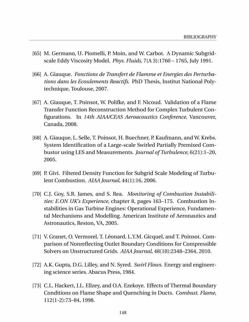
BIBLIOGRAPHY
[65] M. Germano, U. Piomelli, P. Moin, and W. Carbot. A Dynamic Subgrid-scale Eddy Viscosity Model. Phys. Fluids, 7(A 3):1760 – 1765, July 1991.
[66] A. Giauque. Fonctions de Transfert de Flamme et Energies des Perturba-tions dans les Ecoulements Reactifs. PhD Thesis, Institut National Poly-technique, Toulouse, 2007.
[67] A. Giauque, T. Poinsot, W. Polifke, and F. Nicoud. Validation of a FlameTransfer Function Reconstruction Method for Complex Turbulent Con-figurations. In 14th AIAA/CEAS Aeroacoustics Conference, Vancouver,Canada, 2008.
[68] A. Giauque, L. Selle, T. Poinsot, H. Buechner, P. Kaufmann, and W. Krebs.System Identification of a Large-scale Swirled Partially Premixed Com-bustor using LES and Measurements. Journal of Turbulence, 6(21):1–20,2005.
[69] P. Givi. Filtered Density Function for Subgrid Scale Modeling of Turbu-lent Combustion. AIAA Journal, 44(1):16, 2006.
[70] C.J. Goy, S.R. James, and S. Rea. Monitoring of Combustion Instabili-ties: E.ON UK’s Experience, chapter 8, pages 163–175. Combustion In-stabilities in Gas Turbine Engines: Operational Experience, Fundamen-tal Mechanisms and Modelling. American Institute of Aeronautics andAstronautics, Reston, VA, 2005.
[71] V. Granet, O. Vermorel, T. Léonard, L.Y.M. Gicquel, and T. Poinsot. Com-parison of Nonreflecting Outlet Boundary Conditions for CompressibleSolvers on Unstructured Grids. AIAA Journal, 48(10):2348–2364, 2010.
[72] A.K. Gupta, D.G. Lilley, and N. Syred. Swirl Flows. Energy and engineer-ing science series. Abacus Press, 1984.
[73] C.L. Hackert, J.L. Ellzey, and O.A. Ezekoye. Effects of Thermal BoundaryConditions on Flame Shape and Quenching in Ducts. Combust. Flame,112(1-2):73–84, 1998.
148

BIBLIOGRAPHY
[74] W. L. H. Hallett and C.-Y. Ding. A Momentum Integral Model for CentralRecirculation in Swirling Flow in a Sudden Expansion. The CanadianJournal of Chemical Engineering, 73(3):284–291, 1995.
[75] M. Hauser, C. Hirsch, and T. Sattelmayer. Influence of the Confinementon the Flame Transfer Function. 18th International Congress on Soundand Vibration, Rio de Janeiro, Brazil, July 10–14 2011.
[76] E. R. Hawkes and R. S. Cant. Implications of a Flame Surface DensityApproach to Large Eddy Simulation of Premixed Turbulent Combustion.Combust. Flame, 126(3):1617 – 1629, 2001.
[77] M. Hettel, P. Habisreuther, H. Büchner, H. Bockhorn, and N. Zarzalis.URANS-Modelling of Flame Transfer Functions of Turbulent PremixedJet Flames. Number GT2004-53831 in Proc. of ASME Turbo Expo 2004,Vienna. ASME, 2004.
[78] C. Hirsch, D. Fanaca, P. Reddy, W. Polifke, and T. Sattelmayer. Influ-ence of the Swirler Design on the Flame Transfer Function of PremixedFlames. Number GT2005-68195 in Proc. of ASME Turbo Expo 2005,Reno. ASME, 2005.
[79] C. Hirsch, J. Wäsle, A. Winkler, and T. Sattelmayer. A Spectral Model forthe Sound Pressure from Turbulent Premixed Combustion. Proceedingsof the Combustion Institute, 31(1):1435 – 1441, 2007.
[80] Y. Huang, J. Benesty, and J. Chen. Acoustic MIMO Signal Processing.Signals and Communication Technology. Springer-Verlag Berlin Heidel-berg, Germany, 2006.
[81] Y. Huang and V. Yang. Bifurcation of Flame Structure in a Lean-premixedSwirl-stabilized Combustor: Transition from Stable to Unstable Flame.Combust. Flame, 136(3):383–389, 2004.
[82] Y. Huang and V. Yang. Dynamics and Stability of Lean-premixed Swirl-stabilized Combustion. Progress in Energy and Combustion Science,35:293–364, 2009.
149
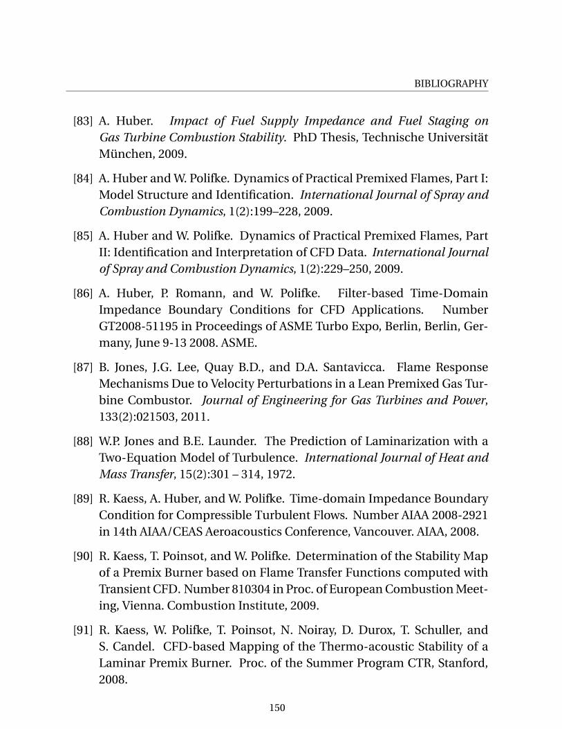
BIBLIOGRAPHY
[83] A. Huber. Impact of Fuel Supply Impedance and Fuel Staging onGas Turbine Combustion Stability. PhD Thesis, Technische UniversitätMünchen, 2009.
[84] A. Huber and W. Polifke. Dynamics of Practical Premixed Flames, Part I:Model Structure and Identification. International Journal of Spray andCombustion Dynamics, 1(2):199–228, 2009.
[85] A. Huber and W. Polifke. Dynamics of Practical Premixed Flames, PartII: Identification and Interpretation of CFD Data. International Journalof Spray and Combustion Dynamics, 1(2):229–250, 2009.
[86] A. Huber, P. Romann, and W. Polifke. Filter-based Time-DomainImpedance Boundary Conditions for CFD Applications. NumberGT2008-51195 in Proceedings of ASME Turbo Expo, Berlin, Berlin, Ger-many, June 9-13 2008. ASME.
[87] B. Jones, J.G. Lee, Quay B.D., and D.A. Santavicca. Flame ResponseMechanisms Due to Velocity Perturbations in a Lean Premixed Gas Tur-bine Combustor. Journal of Engineering for Gas Turbines and Power,133(2):021503, 2011.
[88] W.P. Jones and B.E. Launder. The Prediction of Laminarization with aTwo-Equation Model of Turbulence. International Journal of Heat andMass Transfer, 15(2):301 – 314, 1972.
[89] R. Kaess, A. Huber, and W. Polifke. Time-domain Impedance BoundaryCondition for Compressible Turbulent Flows. Number AIAA 2008-2921in 14th AIAA/CEAS Aeroacoustics Conference, Vancouver. AIAA, 2008.
[90] R. Kaess, T. Poinsot, and W. Polifke. Determination of the Stability Mapof a Premix Burner based on Flame Transfer Functions computed withTransient CFD. Number 810304 in Proc. of European Combustion Meet-ing, Vienna. Combustion Institute, 2009.
[91] R. Kaess, W. Polifke, T. Poinsot, N. Noiray, D. Durox, T. Schuller, andS. Candel. CFD-based Mapping of the Thermo-acoustic Stability of aLaminar Premix Burner. Proc. of the Summer Program CTR, Stanford,2008.
150
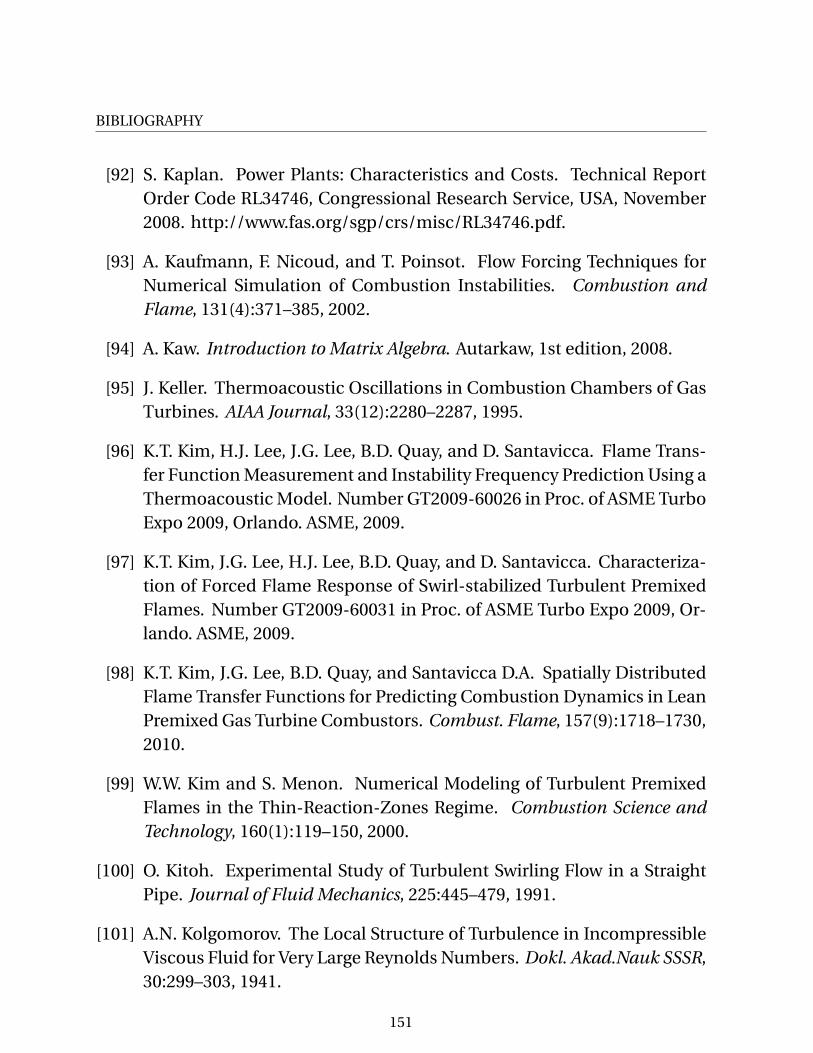
BIBLIOGRAPHY
[92] S. Kaplan. Power Plants: Characteristics and Costs. Technical ReportOrder Code RL34746, Congressional Research Service, USA, November2008. http://www.fas.org/sgp/crs/misc/RL34746.pdf.
[93] A. Kaufmann, F. Nicoud, and T. Poinsot. Flow Forcing Techniques forNumerical Simulation of Combustion Instabilities. Combustion andFlame, 131(4):371–385, 2002.
[94] A. Kaw. Introduction to Matrix Algebra. Autarkaw, 1st edition, 2008.
[95] J. Keller. Thermoacoustic Oscillations in Combustion Chambers of GasTurbines. AIAA Journal, 33(12):2280–2287, 1995.
[96] K.T. Kim, H.J. Lee, J.G. Lee, B.D. Quay, and D. Santavicca. Flame Trans-fer Function Measurement and Instability Frequency Prediction Using aThermoacoustic Model. Number GT2009-60026 in Proc. of ASME TurboExpo 2009, Orlando. ASME, 2009.
[97] K.T. Kim, J.G. Lee, H.J. Lee, B.D. Quay, and D. Santavicca. Characteriza-tion of Forced Flame Response of Swirl-stabilized Turbulent PremixedFlames. Number GT2009-60031 in Proc. of ASME Turbo Expo 2009, Or-lando. ASME, 2009.
[98] K.T. Kim, J.G. Lee, B.D. Quay, and Santavicca D.A. Spatially DistributedFlame Transfer Functions for Predicting Combustion Dynamics in LeanPremixed Gas Turbine Combustors. Combust. Flame, 157(9):1718–1730,2010.
[99] W.W. Kim and S. Menon. Numerical Modeling of Turbulent PremixedFlames in the Thin-Reaction-Zones Regime. Combustion Science andTechnology, 160(1):119–150, 2000.
[100] O. Kitoh. Experimental Study of Turbulent Swirling Flow in a StraightPipe. Journal of Fluid Mechanics, 225:445–479, 1991.
[101] A.N. Kolgomorov. The Local Structure of Turbulence in IncompressibleViscous Fluid for Very Large Reynolds Numbers. Dokl. Akad.Nauk SSSR,30:299–303, 1941.
151

BIBLIOGRAPHY
[102] T. Komarek. Private communication.
[103] T. Komarek and W. Polifke. Impact of Swirl Fluctuations on the FlameResponse of a Perfectly Premixed Swirl Burner. J. Eng. Gas TurbinesPower, 132:061503, 2010.
[104] T. Komarek, L. Tay Wo Chong, and W. Polifke. GV6: Dynamik von Vormis-chflammen. In Abschlussbericht Forschungsinitiative, pages 704–723.Kraftwerke des 21. Jahrhunderts (KW21), 2008.
[105] J. Kopitz, E. Bröcker, and W. Polifke. Characteristics-based Filter forIdentification of Planar Acoustic Waves in Numerical Simulation of Tur-bulent Compressible Flow. 12th Int. Congress on Sound and Vibration,Lisbon, 2005.
[106] J. Kopitz and W. Polifke. CFD-based Application of the Nyquist Crite-rion to Thermo-acoustic Instabilities. Journal of Computational Physics,227(14):6754–6778, 2008.
[107] V.N. Kornilov, M. Manohar, and L.P.H. de Goey. Thermo-acousticBehaviour of Multiple Flame Burner Decks: Transfer Function(de)composition. Proceedings of the Combustion Institute, 32(1):1383–1390, 2009.
[108] V.N. Kornilov, K.R.A.M. Schreel, and L.P.H. de Goey. ExperimentalAssessment of the Acoustic Response of Laminar Premixed BunsenFlames. Proceedings of the Combustion Institute, 31(1):1239–1246, 2007.
[109] W. Krebs, S. Hoffmann, B. Prade, M. Lohrmann, and H. Büchner. Ther-moacoustic Flame Response of Swirl Flames. Number GT-2002-30065 inProc. ASME Turbo Expo 2002, page 12, Amsterdam, NL, June 3-6 2002.ASME.
[110] W. Krebs, B. Prade, P. Flohr, and S. Hoffmann. Thermoacoustic StabilityChart for High-Intensity Gas Turbine Combustion Systems. CombustionScience and Technology, 174(7):99–128, 2002.
[111] C. Külsheimer and H. Büchner. Combustion Dynamics of TurbulentSwirling Flames. Combust. Flame, 131:70–84, 2002.
152
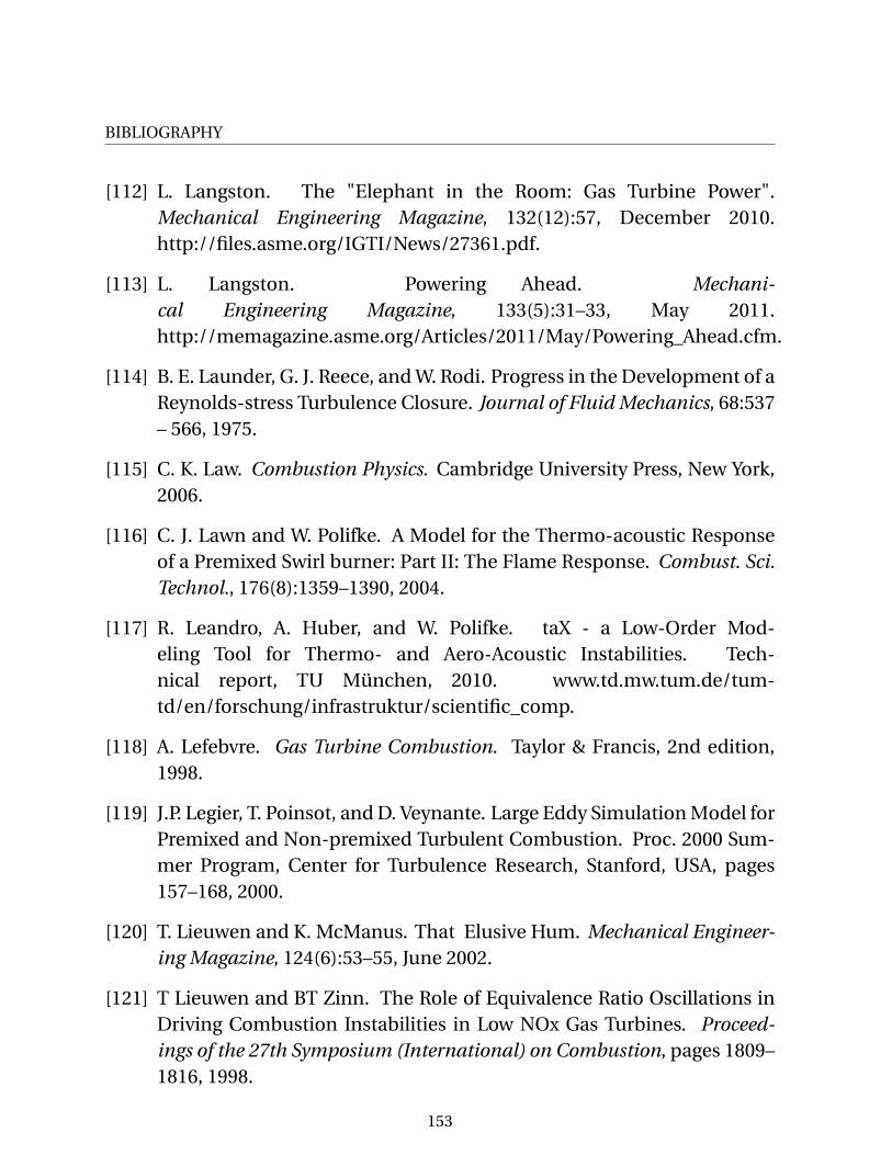
BIBLIOGRAPHY
[112] L. Langston. The "Elephant in the Room: Gas Turbine Power".Mechanical Engineering Magazine, 132(12):57, December 2010.http://files.asme.org/IGTI/News/27361.pdf.
[113] L. Langston. Powering Ahead. Mechani-cal Engineering Magazine, 133(5):31–33, May 2011.http://memagazine.asme.org/Articles/2011/May/Powering_Ahead.cfm.
[114] B. E. Launder, G. J. Reece, and W. Rodi. Progress in the Development of aReynolds-stress Turbulence Closure. Journal of Fluid Mechanics, 68:537– 566, 1975.
[115] C. K. Law. Combustion Physics. Cambridge University Press, New York,2006.
[116] C. J. Lawn and W. Polifke. A Model for the Thermo-acoustic Responseof a Premixed Swirl burner: Part II: The Flame Response. Combust. Sci.Technol., 176(8):1359–1390, 2004.
[117] R. Leandro, A. Huber, and W. Polifke. taX - a Low-Order Mod-eling Tool for Thermo- and Aero-Acoustic Instabilities. Tech-nical report, TU München, 2010. www.td.mw.tum.de/tum-td/en/forschung/infrastruktur/scientific_comp.
[118] A. Lefebvre. Gas Turbine Combustion. Taylor & Francis, 2nd edition,1998.
[119] J.P. Legier, T. Poinsot, and D. Veynante. Large Eddy Simulation Model forPremixed and Non-premixed Turbulent Combustion. Proc. 2000 Sum-mer Program, Center for Turbulence Research, Stanford, USA, pages157–168, 2000.
[120] T. Lieuwen and K. McManus. That Elusive Hum. Mechanical Engineer-ing Magazine, 124(6):53–55, June 2002.
[121] T Lieuwen and BT Zinn. The Role of Equivalence Ratio Oscillations inDriving Combustion Instabilities in Low NOx Gas Turbines. Proceed-ings of the 27th Symposium (International) on Combustion, pages 1809–1816, 1998.
153
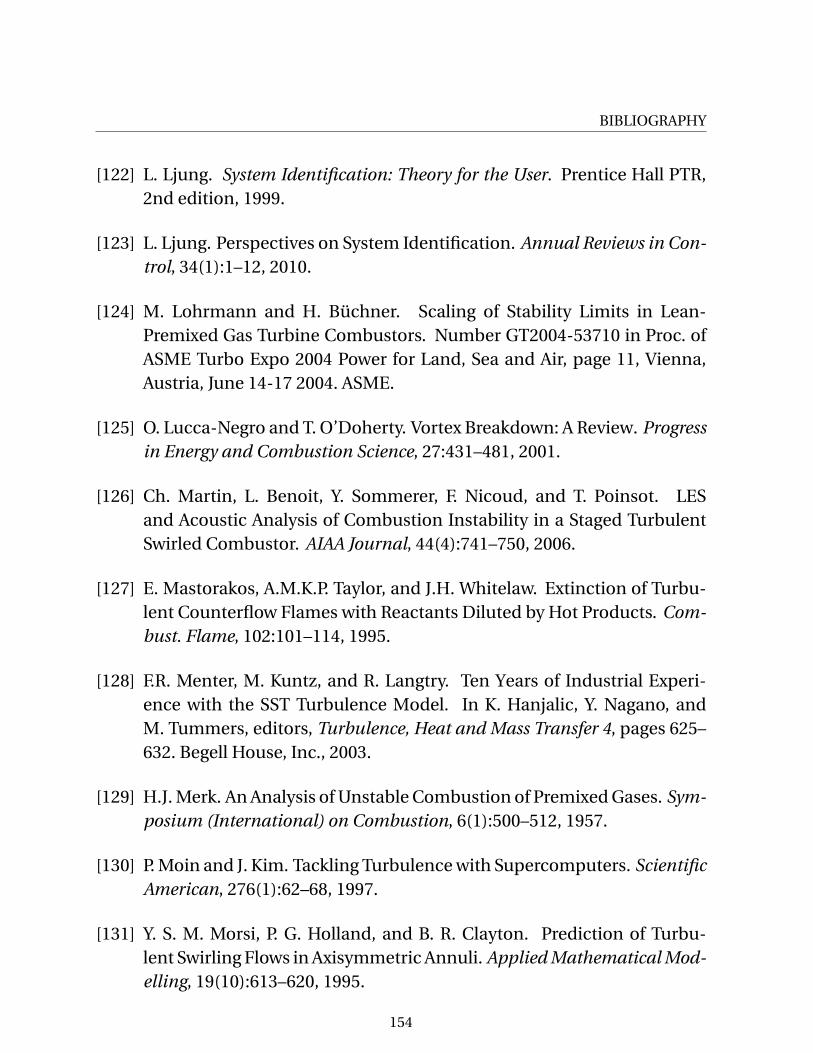
BIBLIOGRAPHY
[122] L. Ljung. System Identification: Theory for the User. Prentice Hall PTR,2nd edition, 1999.
[123] L. Ljung. Perspectives on System Identification. Annual Reviews in Con-trol, 34(1):1–12, 2010.
[124] M. Lohrmann and H. Büchner. Scaling of Stability Limits in Lean-Premixed Gas Turbine Combustors. Number GT2004-53710 in Proc. ofASME Turbo Expo 2004 Power for Land, Sea and Air, page 11, Vienna,Austria, June 14-17 2004. ASME.
[125] O. Lucca-Negro and T. O’Doherty. Vortex Breakdown: A Review. Progressin Energy and Combustion Science, 27:431–481, 2001.
[126] Ch. Martin, L. Benoit, Y. Sommerer, F. Nicoud, and T. Poinsot. LESand Acoustic Analysis of Combustion Instability in a Staged TurbulentSwirled Combustor. AIAA Journal, 44(4):741–750, 2006.
[127] E. Mastorakos, A.M.K.P. Taylor, and J.H. Whitelaw. Extinction of Turbu-lent Counterflow Flames with Reactants Diluted by Hot Products. Com-bust. Flame, 102:101–114, 1995.
[128] F.R. Menter, M. Kuntz, and R. Langtry. Ten Years of Industrial Experi-ence with the SST Turbulence Model. In K. Hanjalic, Y. Nagano, andM. Tummers, editors, Turbulence, Heat and Mass Transfer 4, pages 625–632. Begell House, Inc., 2003.
[129] H.J. Merk. An Analysis of Unstable Combustion of Premixed Gases. Sym-posium (International) on Combustion, 6(1):500–512, 1957.
[130] P. Moin and J. Kim. Tackling Turbulence with Supercomputers. ScientificAmerican, 276(1):62–68, 1997.
[131] Y. S. M. Morsi, P. G. Holland, and B. R. Clayton. Prediction of Turbu-lent Swirling Flows in Axisymmetric Annuli. Applied Mathematical Mod-elling, 19(10):613–620, 1995.
154

BIBLIOGRAPHY
[132] V. Moureau, G. Lartigue, Y. Sommerer, C. Angelberger, O. Colin, andPoinsot T. Numerical Methods for Unsteady Compressible Multi-component Reacting Flows on Fixed and Moving Grids. J. Comput.Phys., 202:710–736, 2005.
[133] F. Nicoud and F. Ducros. Subgrid-scale Stress Modeling Based on theSquare of the Velocity Gradient Tensor. Flow Turb. Combust., 62:183–200, 1999.
[134] N. Noiray, D. Durox, T. Schuller, and S. Candel. A Unified Framework forNonlinear Combustion Instability Analysis based on the Flame Describ-ing Function. Journal of Fluid Mechanics, 615:139–167, 2008.
[135] C. C. Paige and M. A. Saunders. LSQR: An Algorithm for Sparse LinearEquations and Sparse Least Squares. ACM Trans. Math. Softw., 8(1):43–71, 1982.
[136] P. Palies. Dynamique et Instabilités de Combustion des Flammes Swirlées.PhD thesis, Ecole Centrale Paris, 2010.
[137] P. Palies, D. Durox, T. Schuller, and S. Candel. The Combined Dynamicsof Swirler and Turbulent Premixed Swirling Flames. Combust. Flame,157:1698–1717, 2010.
[138] P. Palies, D. Durox, T. Schuller, and S. Candel. Swirling Flame Insta-bility Analysis Based on the Flame Describing Function Methodology.Number GT2010-22294 in Proc. of ASME Turbo Expo 2010, Glasgow, UK,page 10, Glasgow, UK, June 14-18 2010. ASME.
[139] P. Palies, D. Durox, T. Schuller, and S. Candel. Acoustic-convective ModeConversion in an Aerofoil Cascade. Journal of Fluid Mechanics, 672:545–569, 2011.
[140] P. Palies, D. Durox, T. Schuller, and S. Candel. Experimental Study onthe Effect of Swirler Geometry and Swirl Number on Flame DescribingFunctions. Combustion Science and Technology, 183(7):704–717, 2011.
155
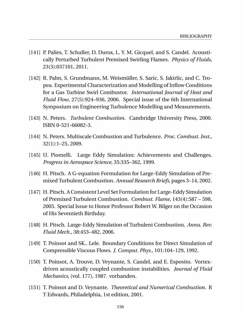
BIBLIOGRAPHY
[141] P. Palies, T. Schuller, D. Durox, L. Y. M. Gicquel, and S. Candel. Acousti-cally Perturbed Turbulent Premixed Swirling Flames. Physics of Fluids,23(3):037101, 2011.
[142] R. Palm, S. Grundmann, M. Weismüller, S. Saric, S. Jakirlic, and C. Tro-pea. Experimental Characterization and Modelling of Inflow Conditionsfor a Gas Turbine Swirl Combustor. International Journal of Heat andFluid Flow, 27(5):924–936, 2006. Special issue of the 6th InternationalSymposium on Engineering Turbulence Modelling and Measurements.
[143] N. Peters. Turbulent Combustion. Cambridge University Press, 2000.ISBN 0-521-66082-3.
[144] N. Peters. Multiscale Combustion and Turbulence. Proc. Combust. Inst.,32(1):1–25, 2009.
[145] U. Piomelli. Large Eddy Simulation: Achievements and Challenges.Progress in Aerospace Science, 35:335–362, 1999.
[146] H. Pitsch. A G-equation Formulation for Large-Eddy Simulation of Pre-mixed Turbulent Combustion. Annual Research Briefs, pages 3–14, 2002.
[147] H. Pitsch. A Consistent Level Set Formulation for Large-Eddy Simulationof Premixed Turbulent Combustion. Combust. Flame, 143(4):587 – 598,2005. Special Issue to Honor Professor Robert W. Bilger on the Occasionof His Seventieth Birthday.
[148] H. Pitsch. Large-Eddy Simulation of Turbulent Combustion. Annu. Rev.Fluid Mech., 38:453–482, 2006.
[149] T. Poinsot and SK.. Lele. Boundary Conditions for Direct Simulation ofCompressible Viscous Flows. J. Comput. Phys., 101:104–129, 1992.
[150] T. Poinsot, A. Trouve, D. Veynante, S. Candel, and E. Esposito. Vortex-driven acoustically coupled combustion instabilities. Journal of FluidMechanics, (vol. 177), 1987. vorhanden.
[151] T. Poinsot and D. Veynante. Theoretical and Numerical Combustion. RT Edwards, Philadelphia, 1st edition, 2001.
156

BIBLIOGRAPHY
[152] T. Poinsot and D. Veynante. Theoretical and Numerical Combustion. RT Edwards, Philadelphia, 2nd edition, 2005.
[153] W. Polifke. Combustion Instabilities. In Advances in Aeroacoustics andapplications, VKI lecture series, Brussels, 2004.
[154] W. Polifke. Divide et Impera - Combining CFD, System Sdentificationand System Modelling to Analyse Combustion Instabilities. NAFEMSSeminar, May 2006.
[155] W. Polifke. System Modelling and Stability Analysis. In Von Karman In-stitute, editor, Basics of Aero-acoustics and Themo-acoustics, VKI lectureseries, Brussels, 2007.
[156] W. Polifke. Low-order Analysis Tools for Aero- and Thermo-Acoustic In-stabilities. In C. Schram, editor, Advances in Aero-Acoustics and Thermo-Acoustics. Van Karman Inst for Fluid Dynamics., Brussels, 2010.
[157] W. Polifke. Non-normality and Non-linearity in Aero- and Thermo-acoustic Systems. In C. Schram, editor, Advances in Aero-Acoustics andThermo-Acoustics. Van Karman Inst for Fluid Dynamics., Brussels, 2010.
[158] W. Polifke. System Identification for Aero- and Thermo-Acoustic Appli-cations. In C. Schram, editor, Advances in Aero-Acoustics and Thermo-Acoustics. Van Karman Inst for Fluid Dynamics., Brussels, 2010.
[159] W. Polifke and C. Lawn. On the Low-frequency Limit of Flame TransferFunctions. Combust. Flame, 151(3):437–451, 2007.
[160] W. Polifke, A. Poncet, C. O. Paschereit, and K. Döbbeling. Reconstruc-tion of Acoustic Transfer Matrices by Instationary Computational FluidDynamics. J. of Sound and Vibration, 245(3):483–510, 2001.
[161] W. Polifke, J. van der Hoek, and B. Verhaar. Everything You AlwaysWanted to Know about f and g. Technical report, ABB Corporate Re-search, Baden, Switzerland, 1997.
[162] W. Polifke, C. Wall, and P. Moin. Partially Reflecting and Non-reflectingBoundary Conditions for Simulation of Compressible Viscous Flow. J.Comput. Phys., 213:437–449, 2006.
157
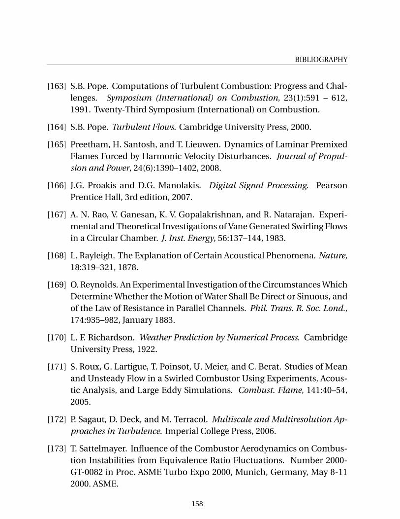
BIBLIOGRAPHY
[163] S.B. Pope. Computations of Turbulent Combustion: Progress and Chal-lenges. Symposium (International) on Combustion, 23(1):591 – 612,1991. Twenty-Third Symposium (International) on Combustion.
[164] S.B. Pope. Turbulent Flows. Cambridge University Press, 2000.
[165] Preetham, H. Santosh, and T. Lieuwen. Dynamics of Laminar PremixedFlames Forced by Harmonic Velocity Disturbances. Journal of Propul-sion and Power, 24(6):1390–1402, 2008.
[166] J.G. Proakis and D.G. Manolakis. Digital Signal Processing. PearsonPrentice Hall, 3rd edition, 2007.
[167] A. N. Rao, V. Ganesan, K. V. Gopalakrishnan, and R. Natarajan. Experi-mental and Theoretical Investigations of Vane Generated Swirling Flowsin a Circular Chamber. J. Inst. Energy, 56:137–144, 1983.
[168] L. Rayleigh. The Explanation of Certain Acoustical Phenomena. Nature,18:319–321, 1878.
[169] O. Reynolds. An Experimental Investigation of the Circumstances WhichDetermine Whether the Motion of Water Shall Be Direct or Sinuous, andof the Law of Resistance in Parallel Channels. Phil. Trans. R. Soc. Lond.,174:935–982, January 1883.
[170] L. F. Richardson. Weather Prediction by Numerical Process. CambridgeUniversity Press, 1922.
[171] S. Roux, G. Lartigue, T. Poinsot, U. Meier, and C. Berat. Studies of Meanand Unsteady Flow in a Swirled Combustor Using Experiments, Acous-tic Analysis, and Large Eddy Simulations. Combust. Flame, 141:40–54,2005.
[172] P. Sagaut, D. Deck, and M. Terracol. Multiscale and Multiresolution Ap-proaches in Turbulence. Imperial College Press, 2006.
[173] T. Sattelmayer. Influence of the Combustor Aerodynamics on Combus-tion Instabilities from Equivalence Ratio Fluctuations. Number 2000-GT-0082 in Proc. ASME Turbo Expo 2000, Munich, Germany, May 8-112000. ASME.
158
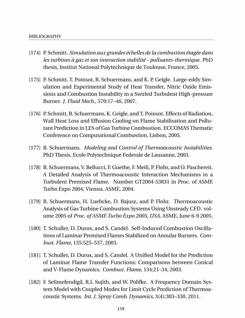
BIBLIOGRAPHY
[174] P. Schmitt. Simulation aux grandes échelles de la combustion étagée dansles turbines à gaz et son interaction stabilité - polluants-thermique. PhDthesis, Institut National Polytechnique de Toulouse, France, 2005.
[175] P. Schmitt, T. Poinsot, B. Schuermans, and K. P. Geigle. Large-eddy Sim-ulation and Experimental Study of Heat Transfer, Nitric Oxide Emis-sions and Combustion Instability in a Swirled Turbulent High-pressureBurner. J. Fluid Mech., 570:17–46, 2007.
[176] P. Schmitt, B. Schuermans, K. Geigle, and T. Poinsot. Effects of Radiation,Wall Heat Loss and Effusion Cooling on Flame Stabilisation and Pollu-tant Prediction in LES of Gas Turbine Combustion. ECCOMAS ThematicConference on Computational Combustion, Lisbon, 2005.
[177] B. Schuermans. Modeling and Control of Thermoacoustic Instabilities.PhD Thesis, Ecole Polytechnique Federale de Lausanne, 2003.
[178] B. Schuermans, V. Bellucci, F. Guethe, F. Meili, P. Flohr, and O. Paschereit.A Detailed Analysis of Thermoacoustic Interaction Mechanisms in aTurbulent Premixed Flame. Number GT2004-53831 in Proc. of ASMETurbo Expo 2004, Vienna. ASME, 2004.
[179] B. Schuermans, H. Luebcke, D. Bajusz, and P. Flohr. ThermoacousticAnalysis of Gas Turbine Combustion Systems Using Unsteady CFD. vol-ume 2005 of Proc. of ASME Turbo Expo 2005, USA. ASME, June 6-9 2005.
[180] T. Schuller, D. Durox, and S. Candel. Self-Induced Combustion Oscilla-tions of Laminar Premixed Flames Stabilized on Annular Burners. Com-bust. Flame, 135:525–537, 2003.
[181] T. Schuller, D. Durox, and S. Candel. A Unified Model for the Predictionof Laminar Flame Transfer Functions: Comparisons between Conicaland V-Flame Dynamics. Combust. Flame, 134:21–34, 2003.
[182] F. Selimefendigil, R.I. Sujith, and W. Polifke. A Frequency Domain Sys-tem Model with Coupled Modes for Limit Cycle Prediction of Thermoa-coustic Systems. Int. J. Spray Comb. Dynamics, 3(4):303–330, 2011.
159
BIBLIOGRAPHY
[183] F. Selimefendigil, R.I. Sujith, and W. Polifke. Identification of Heat Trans-fer Dynamics for Non-modal Analysis of Thermoacoustic Stability. Ap-plied Mathematics and Computation, 217(11):5134–5150, 2011. Specialissue on Fluid Flow and Heat Transfer.
[184] L. Selle, G. Lartigue, T. Poinsot, R. Koch, K.U. Schilmacher, W. Krebs,B. Prade, P. Kaufmann, and D. Veynante. Compressible Large Eddy Sim-ulation of Turbulent Combustion in Complex Geometry on Unstruc-tured Meshes. Combust. Flame, 137:489–505, 2004.
[185] J.B. Sewell and P.A. Sobieski. Monitoring of Combustion Instabilities:Calpine’s Experience, chapter 7, pages 147–162. Combustion Insta-bilities in Gas Turbine Engines: Operational Experience, FundamentalMechanisms and Modelling. American Institute of Aeronautics and As-tronautics, Reston, VA, 2005.
[186] J. Smagorinsky. General Circulation Experiments with the PrimitiveEquations, I. The Basic Experiment. Monthly Weather Review, 91(3),March 1963.
[187] M.D. Smooke, J. Crump, K. Seshadri, and V. Giovangigli. Comparison be-tween Experimental Measurements and Numerical Calculations of theStructure of Counterflow, Diluted, Methane-air, Premixed Flames. Sym-posium (International) on Combustion, 23:463–470, 1991.
[188] Y. Sommerer, D. Galley, T. Poinsot, S. Ducruix, F. Lacas, and D. Veynante.Large Eddy Simulation and Experimental Study of Flashback and Blow-off in a Lean Partially Premixed Swirled Burner. Journal of Turbulence,5:037, 2004.
[189] Z. B. Song, L. J. Wei, and Z. Z. Wu. Effects of Heat Losses on Flame Shapeand Quenching of Premixed Flames in Narrow Channels. CombustionScience and Technology, 180(2):264–278, 2008.
[190] C. G. Speziale, S. Sarkar, and T. B. Gatski. Modelling the Pressure-StrainCorrelation of Turbulence: An Invariant Dynamical System Approach.Journal of Fluid Mechanics, pages 245–272, 1991.
160
BIBLIOGRAPHY
[191] G. Staffelbach, L. Y. M. Gicquel, and T. Poinsot. Highly Parallel LargeEddy Simulations of Multiburner Configurations in Industrial Gas Tur-bines. In S. C. Kassinos, C. A. Langer, G. Laccarino, and P. Moin, editors,Complex Effects in Large Eddy Simulations, volume 56 of Lecture Notes inComputational Science and Engineering, pages 325–336. Springer BerlinHeidelberg, 2007.
[192] W. Steenbergen and J. Voskamp. The Rate of Decay of Swirl in TurbulentPipe Flow. Flow Measurement and Instrumentation, 9(2):67–78, 1998.
[193] J. Stein. Digital Signal Processing - A Computer Science Perspective. JohnWiley & Sons, Inc., New York, USA, 2000.
[194] D. L. Straub and G. A. Richards. Effect of Axial Swirl Vane Location onCombustion Dynamics. Number 99-GT-109 in Int. Gas Turbine & Aero-engine Congress & Exhibition, Indianapolis, Indiana, 1999. ASME.
[195] N. Syred. A Review of Oscillation Mechanisms and the Role of the Pre-cessing Vortex Core (PVC) in Swirl Combustion Systems. Progress in En-ergy and Combustion Science, 32(2):93–161, 2006.
[196] G. Tabor and H.G. Weller. Large Eddy Simulation of Premixed TurbulentCombustion Using Ξ Flame Surface Wrinkling Model. Flow, Turbulenceand Combustion, 72:1–27, 2004.
[197] E. Tangermann, R. Keppeler, and M. Pfitzner. Premixed TurbulentCombustion Models for Large Eddy and RANS Simulations. NumberGT2010-22298 in Proc. of ASME Turbo Expo 2010, Glasgow, UK, Glas-gow, UK, June 14-18 2010. ASME.
[198] L. Tay-Wo-Chong, S. Bomberg, A. Ulhaq, T. Komarek, and W. Polifke.Comparative Validation Study on Identification of Premixed FlameTransfer Function. Journal of Engineering for Gas Turbines and Power,134(2):021502, 2012.
[199] L. Tay Wo Chong, T. Komarek, R. Kaess, S. Föller, and W. Polifke. Identifi-cation of Flame Transfer Functions from LES of a Premixed Swirl Burner.Number GT2010-22769 in Proc. of ASME Turbo Expo 2010, Glasgow, UK,page 13, Glasgow, UK, June 14-18 2010. ASME.
161
BIBLIOGRAPHY
[200] L. Tay Wo Chong, T. Komarek, M. Zellhuber, J. Lenz, C. Hirsch, and W. Po-lifke. Influence of Strain and Heat Loss on Flame Stabilization in aNon-adiabatic Combustor. Number 810366 in Proceedings of EuropeanCombustion Meeting, Vienna. Combustion Institute, 2009.
[201] H. Tennekes and J. L. Lumley. A First Course in Turbulence. The MITPress, 11th printing edition, 1972. ISBN 0-262-200198.
[202] S. A. Thorpe. An Introduction to Ocean Turbulence. Cambridge Univer-sity Press, 2007.
[203] C. Tong and Z. Warhaft. Passive Scalar Dispersion and Mixing in a Tur-bulent Jet. J. Fluid Mech., 292:1–38, 1995.
[204] S. R. Turns. An Introduction to Combustion. McGraw-Hill, Boston, 2000.
[205] E. R. Van Driest. On Turbulent Flow near a Wall. J. Aerospace Sci.,23:1007–1011, 1956.
[206] J. van Kampen. Acoustic Pressure Oscillations Induced by Confined Tur-bulent Premixed Natural Gas Flames. PhD Thesis, University of Twente,Enschede, The Netherlands, 2006.
[207] S.V. Vaseghi. Advanced Digital Signal Processing and Noise Reduction.John Wiley & Sons, Ltd., 3rd edition, 2006.
[208] H. K. Versteeg and W. Malalasekera. Introduction to ComputationalFluid Dynamics : The Finite Volume Method . Longman Scientific &Technical, 1995.
[209] D. Veynante and T. Poinsot. Large Eddy Simulation of Combustion In-stabilities in Turbulent Combustion. Annual Reserach Briefs, pages 253–274, CTR Stanford, USA, 1997.
[210] D. Veynante and L. Vervisch. Turbulent Combustion Modeling. Progressin Energy and Combustion Science, 28(3):193 – 266, 2002.
[211] C. Wagner, T. Huettl, and P. Sagaut. Large-Eddy Simulation for Acoustics.Cambridge University Press, 2007.
162
BIBLIOGRAPHY
[212] S. Wang and V. Yang. Unsteady Flow Evolution in Swirl Injectors with Ra-dial Entry. II. External Excitations. Physics of Fluids, 17(4):045107, 2005.
[213] E. Wanke. FE-Verfahren zur Analyse der Thermoakustischen Stabil-ität nichtisentroper Strömungen. PhD Thesis, Technische UniversitätMünchen, 2010.
[214] J. Warnatz, U. Maas, and R.W. Dibble. Combustion: Physical and Chem-ical Fundamentals, Modeling and Simulation, Experiments, PollutantFormation. Springer-Verlag, Berlin/Heidelberg, 4th edition, 2006.
[215] J. Wäsle, A. Winkler, E. Rössle, and T. Sattelmayer. Development of anAnnular Porous Burner for the Investigation of Adiabatic UnconfinedFlames. 13th Int Symp on Applications of Laser Techniques to Fluid Me-chanics, Lisbon, Portugal, June 26-29 2006.
[216] K. Wieczorek and F. Nicoud. Prediction of Thermoacoustic Instabilities:Numerical Study of Mach Number Effects. In 16th AIAA/CEAS Aeroa-coustics Conference, Stockholm, Sweden, 2010.
[217] N. Wiener. Extrapolation, Interpolation, and Smoothing of StationaryTime Series. The MIT Press, 1964.
[218] D.C. Wilcox. Turbulence Modelling for CFD. DCW Industries, 1993.
[219] F. A. Williams. Combustion Theory. Benjamin/Cummings, Menlo Park,CA, 1985.
[220] S. Xiao and V. Martling. Reducing Gas Turbine NOx and COEmissions Through Improved Combustor Design. Techni-cal report, Power Systems Manufacturing, Florida, USA, 2003.http://www.psm.com/PDF/Combustor.pdf.
[221] S. W. Yuen, A. Gentemann, and W. Polifke. Influence of Boundary Re-flection Coefficient on the System Identifiability of Acoustic Two-Ports.11th Int. Congress on Sound and Vibration, St. Petersburg, 2004.
[222] V. Zimont and V. Battaglia. Joint RANS/LES Approach to Premixed FlameModelling in the Context of the TFC Combustion Model. Flow, Turbu-lence and Combustion, 77:305–331, 2006.
163
BIBLIOGRAPHY
[223] B.T. Zinn and T. Lieuwen. Combustion Instabilities: Basic Concepts,chapter 1, pages 3–26. Combustion Instabilities in Gas Turbine En-gines: Operational Experience, Fundamental Mechanisms and Mod-elling. American Institute of Aeronautics and Astronautics, Reston, VA,2005.
164
A Appendices
A.1 The Rayleigh Criterion
Lord Rayleigh [168] proposed a criterion, the so-called Rayleigh criterion, todescribe the mechanism that a periodic heat-addition process adds energy toacoustic oscillations [223]. In his words [168]:
“If heat be periodically communicated to, and abstracted from, a mass of airvibrating (for example) in a cylinder bounded by a piston, the effect producedwill depend upon the phase of the vibration at which the transfer of heat takesplace. If the heat is given to the air at the moment of greatest condensation, orbe taken from it at the moment of greatest rarefaction, the vibration is encour-aged. On the other hand, if heat be given at the moment of greatest rarefaction,or abstracted at the moment of greatest condensation, the vibration is discour-aged.”
This indicates that an oscillation can be enhanced or damped depending ofthe phase between pressure (p ′) and heat (release) (Q ′) oscillations, and proneto instability if heat is added at moment of maximum pressure. The Rayleighcriterion is formulated mathematically by [83, 156]:
R =∮
T
∫V
p ′Q ′dV d t , (A.1)
where T is the period of the oscillation and V is the volume of the domain. R isknown as the Rayleigh Index. Then, if the absolute phase between the pressureand heat (release) oscillations is lower/higher than 90 degrees, the RayleighIndex is positive/negative and the heat-addition process adds/damps energyto/from the acoustic field [223]. This is shown graphically in Fig. A.1.
Having a positive Rayleigh Index is not the only condition for an instability todevelop. The other condition is that the energy added by the flame is higher
165
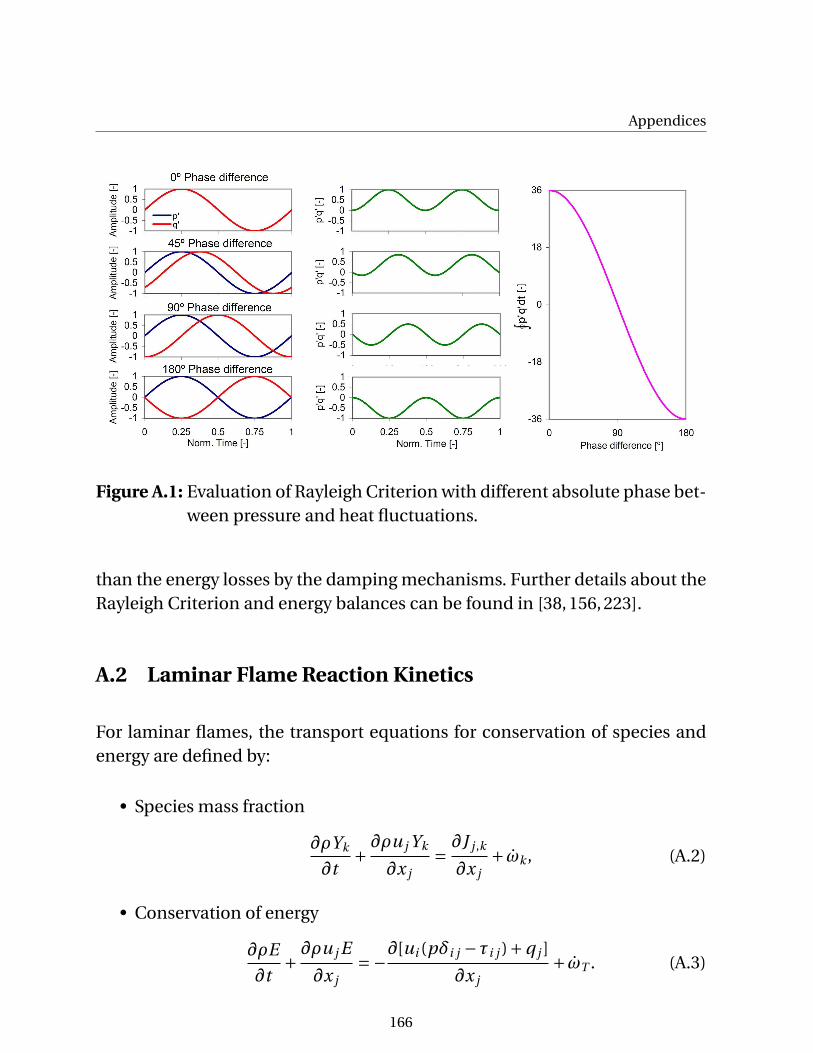
Appendices
Figure A.1: Evaluation of Rayleigh Criterion with different absolute phase bet-ween pressure and heat fluctuations.
than the energy losses by the damping mechanisms. Further details about theRayleigh Criterion and energy balances can be found in [38, 156, 223].
A.2 Laminar Flame Reaction Kinetics
For laminar flames, the transport equations for conservation of species andenergy are defined by:
• Species mass fraction
∂ρYk
∂t+ ∂ρu j Yk
∂x j= ∂J j ,k
∂x j+ ωk , (A.2)
• Conservation of energy
∂ρE
∂t+ ∂ρu j E
∂x j=−∂[ui (pδi j −τi j )+q j ]
∂x j+ ωT . (A.3)
166
A.2 Laminar Flame Reaction Kinetics
where ωT and ωk are the heat release and the reaction rate of the k th species,respectively. These source terms are closed using the Arrhenius law. For a sys-tem with N number of species Yk and M reactions [22, 152]:
N∑k=1
υ′k j YkN∑
k=1
υ′′k j Yk for j = 1, .., M . (A.4)
where Yk represents the different species k on the reaction, υ′k j and υ′′k j are themolar stoichiometric coefficients of species k in reaction j [152].
The reaction rate ωk is defined by the sum of the rates from all reactions:
ωk =M∑
k=1
ωk j =Wk
M∑k=1
υk j Rj, (A.5)
where Wk is the molecular weight of species k, υk j is defined by [152]:
υk j = υ′′k j −υ′k j , (A.6)
and Rj is the rate of progress of reaction j. Considering a only forward reac-tions, Rj is defined by:
Rj = K f j
N∏k=1
(ρYk
Wk
)υ′k j
, (A.7)
where K f j is the forward rate of reaction j. K f j is modeled using Arrhenius lawby:
K f j = A f j T β j exp
(−Ea, j
RT
), (A.8)
where A f j is the pre-exponential factor of the reaction, β j is the temperatureexponent and Ea, j is the activation energy of reaction j.
Due to the high number of reactions and species involved in the reacting pro-cess, reduced chemical mechanisms with smaller number of species and re-actions are usually used. The idea is to represent the detailed reaction me-chanism by a few reaction steps including some important species and withthe chemical kinetic constants empirically determined [115]. Thus, Eq. (A.7) ismodified by:
Rj = K f j
N∏k=1
(ρYk
Wk
)nk
, (A.9)
167
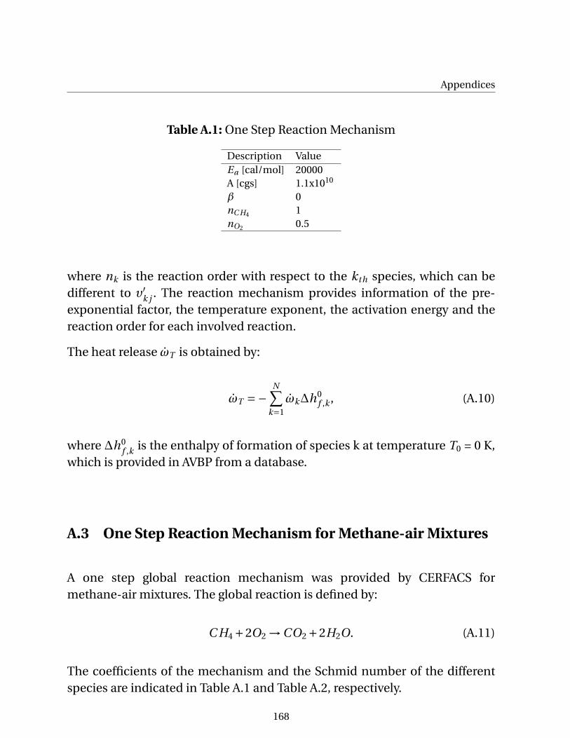
Appendices
Table A.1: One Step Reaction Mechanism
Description ValueEa [cal/mol] 20000A [cgs] 1.1x10¹⁰
β 0nC H4 1nO2 0.5
where nk is the reaction order with respect to the kth species, which can bedifferent to υ′k j . The reaction mechanism provides information of the pre-exponential factor, the temperature exponent, the activation energy and thereaction order for each involved reaction.
The heat release ωT is obtained by:
ωT =−N∑
k=1
ωk∆h0f ,k , (A.10)
where ∆h0f ,k is the enthalpy of formation of species k at temperature T0 = 0 K,
which is provided in AVBP from a database.
A.3 One Step Reaction Mechanism for Methane-air Mixtures
A one step global reaction mechanism was provided by CERFACS formethane-air mixtures. The global reaction is defined by:
C H4 +2O2 →CO2 +2H2O. (A.11)
The coefficients of the mechanism and the Schmid number of the differentspecies are indicated in Table A.1 and Table A.2, respectively.
168
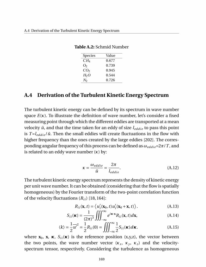
A.4 Derivation of the Turbulent Kinetic Energy Spectrum
Table A.2: Schmid Number
Species ValueC H4 0.677O2 0.739CO2 0.945H2O 0.544N2 0.726
A.4 Derivation of the Turbulent Kinetic Energy Spectrum
The turbulent kinetic energy can be defined by its spectrum in wave numberspace E(κ). To illustrate the definition of wave number, let’s consider a fixedmeasuring point through which the different eddies are transported at a meanvelocity u, and that the time taken for an eddy of size leddi e to pass this pointis T =leddi e/u. Then the small eddies will create fluctuations in the flow withhigher frequency than the ones created by the large eddies [202]. The corres-ponding angular frequency of this process can be defined asωeddi e=2π/T , andis related to an eddy wave number (κ) by:
κ= ωeddi e
u= 2π
leddi e. (A.12)
The turbulent kinetic energy spectrum represents the density of kinetic energyper unit wave number. It can be obtained (considering that the flow is spatiallyhomogeneous) by the Fourier transform of the two-point correlation functionof the velocity fluctuations (Ri i ) [18, 164]:
Ri i (x, t ) = ⟨u′
i (x0, t )u′i (x0 +x, t )
⟩. (A.13)
Si i (κ) = 1
(2π)3
Ñ ∞
−∞e iκ·xRi i (x, t )dx, (A.14)
⟨k⟩ = 1
2u′2 = 1
2Ri i (0) =
Ñ ∞
−∞
1
2Si i (κ)dκ. (A.15)
where x0, x, κ, Si i (κ) is the reference position (x,y,z), the vector betweenthe two points, the wave number vector (κx , κy , κz) and the velocity-spectrum tensor, respectively. Considering the turbulence as homogeneous
169
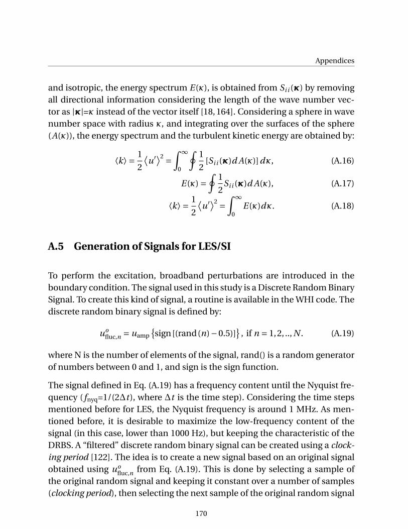
Appendices
and isotropic, the energy spectrum E(κ), is obtained from Si i (κ) by removingall directional information considering the length of the wave number vec-tor as |κ|=κ instead of the vector itself [18, 164]. Considering a sphere in wavenumber space with radius κ, and integrating over the surfaces of the sphere(A(κ)), the energy spectrum and the turbulent kinetic energy are obtained by:
⟨k⟩ = 1
2
⟨u′⟩2 =
∫ ∞
0
∮1
2[Si i (κ)d A(κ)]dκ, (A.16)
E(κ) =∮
1
2Si i (κ)d A(κ), (A.17)
⟨k⟩ = 1
2
⟨u′⟩2 =
∫ ∞
0E(κ)dκ. (A.18)
A.5 Generation of Signals for LES/SI
To perform the excitation, broadband perturbations are introduced in theboundary condition. The signal used in this study is a Discrete Random BinarySignal. To create this kind of signal, a routine is available in the WHI code. Thediscrete random binary signal is defined by:
uofluc,n = uamp
sign[(rand(n)−0.5)]
, if n = 1,2, .., N . (A.19)
where N is the number of elements of the signal, rand() is a random generatorof numbers between 0 and 1, and sign is the sign function.
The signal defined in Eq. (A.19) has a frequency content until the Nyquist fre-quency ( fnyq=1/(2∆t ), where ∆t is the time step). Considering the time stepsmentioned before for LES, the Nyquist frequency is around 1 MHz. As men-tioned before, it is desirable to maximize the low-frequency content of thesignal (in this case, lower than 1000 Hz), but keeping the characteristic of theDRBS. A “filtered” discrete random binary signal can be created using a clock-ing period [122]. The idea is to create a new signal based on an original signalobtained using uo
fluc,n from Eq. (A.19). This is done by selecting a sample ofthe original random signal and keeping it constant over a number of samples(clocking period), then selecting the next sample of the original random signal
170

A.5 Generation of Signals for LES/SI
and repeating the procedure. The clocking period is defined by:
Pclock = floor(fnyq
fc), (A.20)
where fc is the desired maximum frequency of the signal and floor(x) is a func-tion that rounds the content inside the parentheses to the largest integer notgreater than x. The “filtered” discrete random binary signal is defined by:
ufiltfluc,n =
uo
fluc,1, if n = 1
uofluc,m, if n = mPclock
ufluc,(n−1), if n 6= mPclock,
(A.21)
for m=1,2,3...,floor(N/Pclock). Using Eq. (A.21), ufiltfluc,n will take a new random
value every multiple of Pclock, creating a high power spectrum content for fre-quencies lower than fc and taking only values of ±uamp at any time. This fil-ter does not have a sharp cut-off behavior because the shape of the signal iskept with sharp corners, where high frequency content is always present. Toremove the high frequency content, an additional low-pass filter is applied,which “smooth” the sharp corners of the signal.
With a frequency limited signal, its autocorrelation does not keep all the pro-perties of a white noise signal, becoming less decorrelated with itself (shownby a level of autocorrelation for a number of time steps). In Fig. A.2, signalsgenerated using a time step of 1.25x10⁻⁵ s with different frequency contentare shown. One signal was created using Fig. A.19 without frequency limit(Pclock=1, Nyquist frequency =40000 Hz), and the other using Eq. (A.21) withfc=600 Hz followed by a rectangular low pass filter with a cut-off frequencyof 1000 Hz. Both signals have the same maximum amplitude ufluc in time.Comparing the power spectrum of the signal shown in Fig. A.4, the signal withlower frequency limit presents a much stronger signal on the frequency rangeof interest. This will improve the identification process, as the signal-to-noiseratio using the low frequency limit signal is much higher than using the onewith high frequency content. The auto-correlation matrices of both signalsare shown in Fig. A.5. It would be optimal to use a signal with high decorre-lation characteristics in a limited frequency range as shown by Foeller and
171
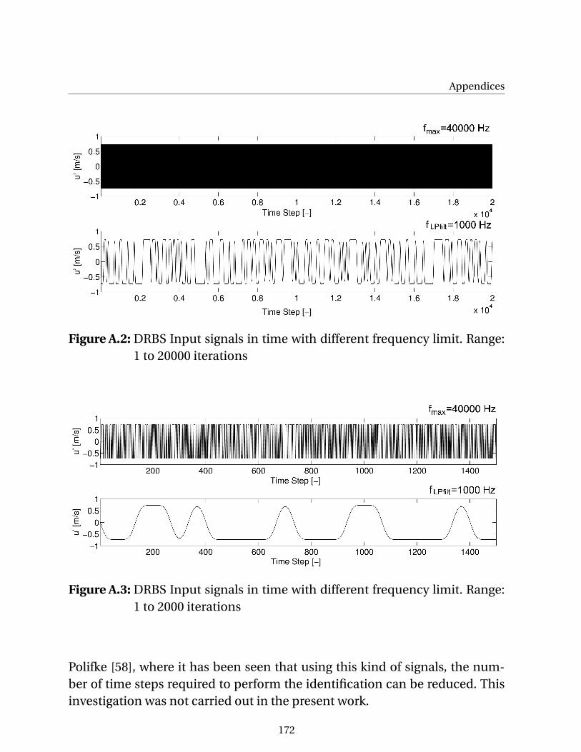
Appendices
Figure A.2: DRBS Input signals in time with different frequency limit. Range:1 to 20000 iterations
Figure A.3: DRBS Input signals in time with different frequency limit. Range:1 to 2000 iterations
Polifke [58], where it has been seen that using this kind of signals, the num-ber of time steps required to perform the identification can be reduced. Thisinvestigation was not carried out in the present work.
172
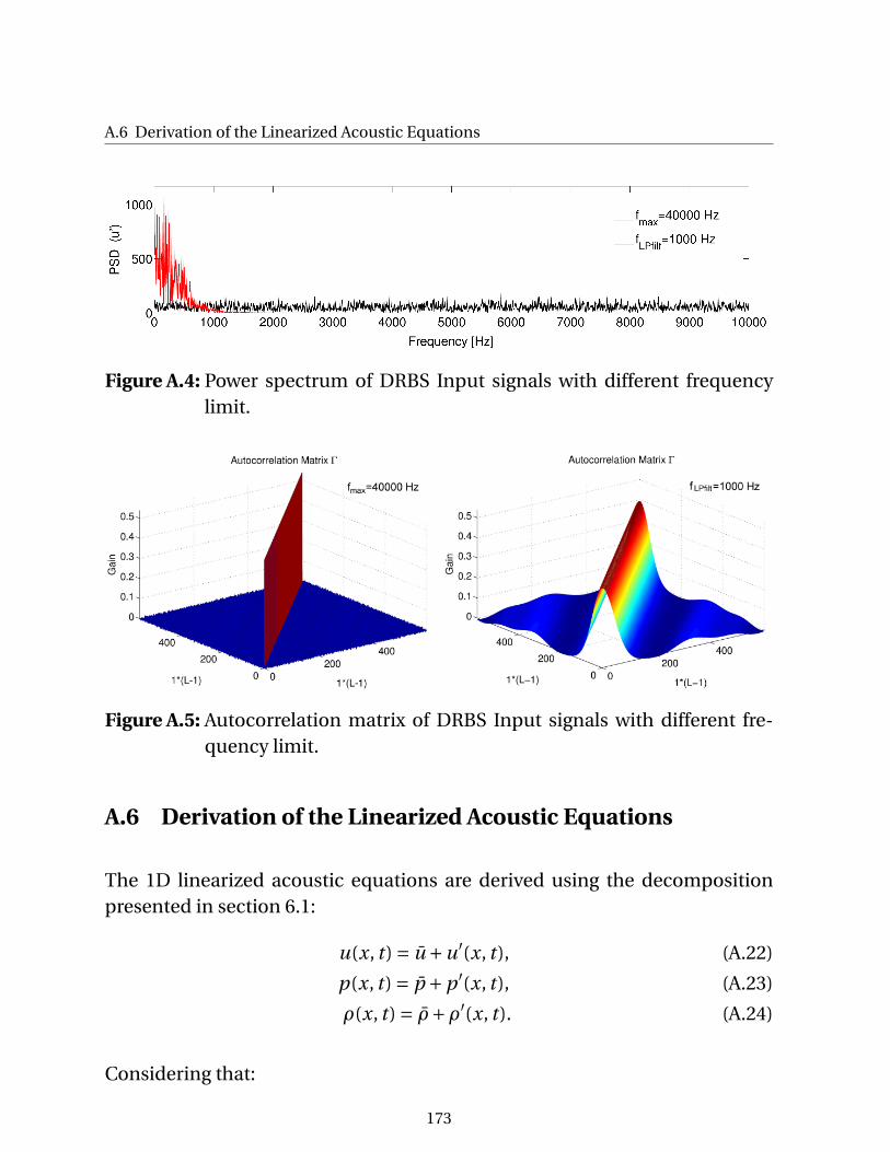
A.6 Derivation of the Linearized Acoustic Equations
Figure A.4: Power spectrum of DRBS Input signals with different frequencylimit.
Figure A.5: Autocorrelation matrix of DRBS Input signals with different fre-quency limit.
A.6 Derivation of the Linearized Acoustic Equations
The 1D linearized acoustic equations are derived using the decompositionpresented in section 6.1:
u(x, t ) = u +u′(x, t ), (A.22)
p(x, t ) = p +p ′(x, t ), (A.23)
ρ(x, t ) = ρ+ρ′(x, t ). (A.24)
Considering that:
173

Appendices
(a) The flow is homentropic,
(b) mean terms are uniform at different positions,
(c) the terms containing only mean quantities are part of the stationary solu-tion [48],
(d) only terms of first order in the fluctuations are considered (neglectinghigher order terms, e.g. ρ′u′),
the following equations are obtained:
• Conservation of mass
∂ρ
∂t+ ∂ρu
∂x= 0, (A.25)
∂(ρ+ρ′)∂t
+ ∂(ρ+ρ′)(u +u′)
∂x= 0, (A.26)
∂ρ
∂t+ ∂ρ′
∂t+ ∂
(ρu + ρu′+ρ′u +ρ′u′)
∂x= 0, (A.27)
∂ρ′
∂t+ u
∂ρ′
∂x+ ∂ρu′
∂x= 0. (A.28)
• Conservation of momentum
∂ρu
∂t+ ∂ρuu
∂x+ ∂p
∂x= 0, (A.29)
∂(ρ+ρ′)(u +u′)
∂t+ ∂
(ρ+ρ′)(u +u′)(u +u′)
∂x+ ∂
(p +p ′)∂x
= 0, (A.30)[∂ρu
∂t+ ∂ρuu
∂x+ ∂p
∂x
]︸ ︷︷ ︸
=0 from stationary solution
+[∂ρ′u∂t
+ ∂ρ′uu
∂x+ ∂ρu′u
∂x
]︸ ︷︷ ︸
= 0 from Conservation of mass
+ (A.31)
[∂ρ′u′
∂t+ ∂2
(ρ′u′u +∂ρ′u′u′)
∂x
]︸ ︷︷ ︸
=0 from neglecting high order terms
+∂ρu′
∂t+ ∂ρuu′
∂x+ ∂p ′
∂x= 0, (A.32)
ρ
(∂u′
∂t+ u
∂u′
∂x
)+ ∂p ′
∂x= 0. (A.33)
174
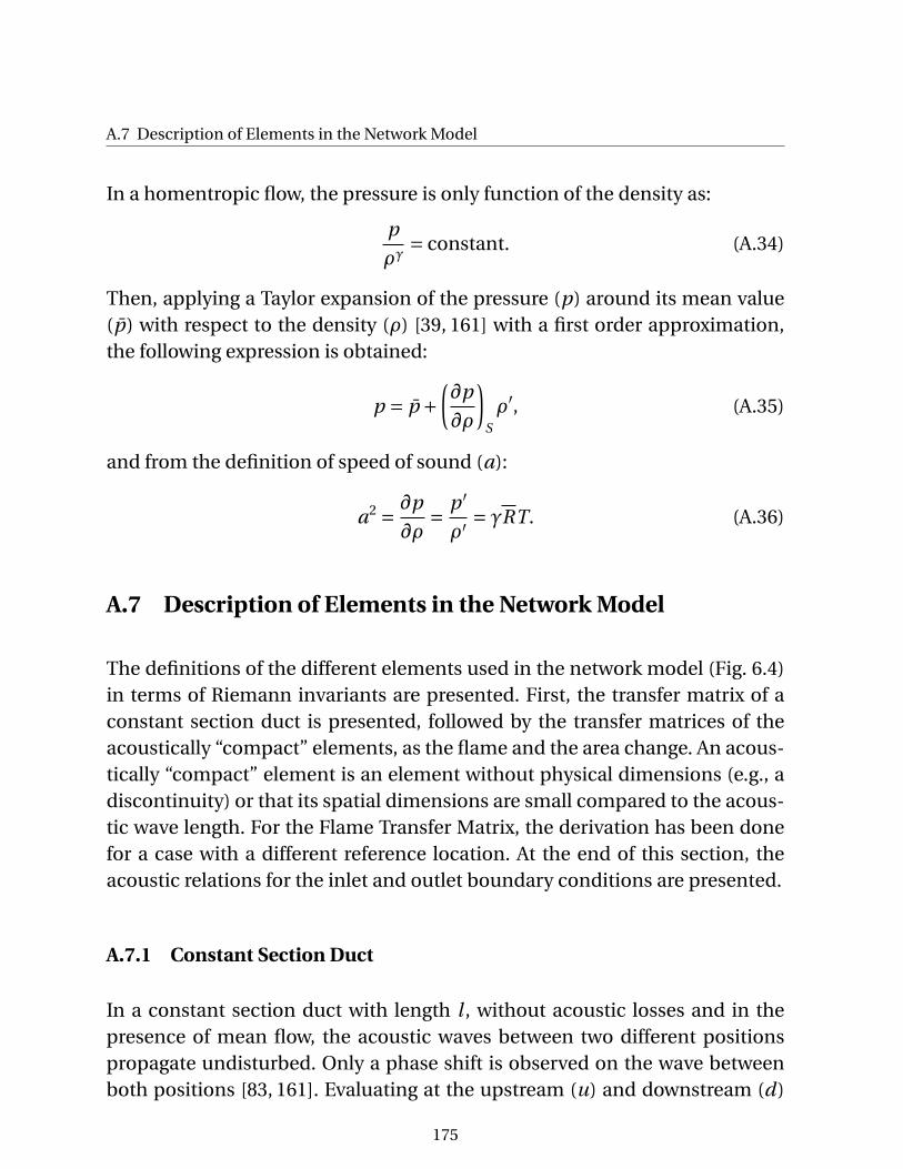
A.7 Description of Elements in the Network Model
In a homentropic flow, the pressure is only function of the density as:
p
ργ= constant. (A.34)
Then, applying a Taylor expansion of the pressure (p) around its mean value(p) with respect to the density (ρ) [39, 161] with a first order approximation,the following expression is obtained:
p = p +(∂p
∂ρ
)S
ρ′, (A.35)
and from the definition of speed of sound (a):
a2 = ∂p
∂ρ= p ′
ρ′ = γRT. (A.36)
A.7 Description of Elements in the Network Model
The definitions of the different elements used in the network model (Fig. 6.4)in terms of Riemann invariants are presented. First, the transfer matrix of aconstant section duct is presented, followed by the transfer matrices of theacoustically “compact” elements, as the flame and the area change. An acous-tically “compact” element is an element without physical dimensions (e.g., adiscontinuity) or that its spatial dimensions are small compared to the acous-tic wave length. For the Flame Transfer Matrix, the derivation has been donefor a case with a different reference location. At the end of this section, theacoustic relations for the inlet and outlet boundary conditions are presented.
A.7.1 Constant Section Duct
In a constant section duct with length l , without acoustic losses and in thepresence of mean flow, the acoustic waves between two different positionspropagate undisturbed. Only a phase shift is observed on the wave betweenboth positions [83, 161]. Evaluating at the upstream (u) and downstream (d)
175
Appendices
ends of the duct, the following equations are obtained [117, 161]:
fd = e−i kx+l fu, (A.37)
gd = e−i kx-l gu. (A.38)
where kx± is defined in Eq. (6.12). In matrix notation as in t aX :
[−e−i kx+l 00 −e−i kx-l
][fu
gu
]+
[1 00 1
][fd
gd
]=
[00
]. (A.39)
A.7.2 Flame Transfer Matrix of a Compact Flame with a Different Referen-ce Location
The flame transfer matrix defined in Eqs. (6.19) and (6.20) was extended (interms of the Riemann invariants) to consider the different reference posi-tion of velocity fluctuations in the FTF [83, 117]. This element will become a6-port instead of a 4-port element. The heat release fluctuations in Eq. (6.19)and (6.20) are defined by:
Q ′(ω)¯Q
= FTF(ω)u′
r (ω)
ur, (A.40)
where r indicates the reference position for velocity fluctuations (see Fig. A.6).Introducing Eq. (A.40) on Eqs. (6.19) and (6.20), and by replacing the acousticvariables u′ and p ′ to their definitions in Riemann Invariants f and g [156]:
u′ = f − g , (A.41)p ′
ρa= f + g , (A.42)
the following relations are derived:
176
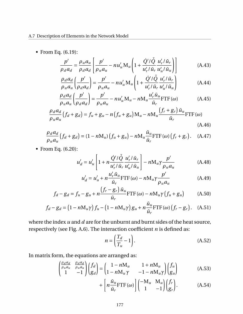
A.7 Description of Elements in the Network Model
• From Eq. (6.19):
p ′
ρd ad= ρu au
ρd ad
[p ′
ρu au−nu′
u Mu
(1+ Q ′/ ¯Q
u′r /ur
u′r /ur
u′u/uu
)](A.43)
ρd ad
ρu au
(p ′
ρd ad
)= p ′
ρu au−nu′
u Mu
(1+ Q ′/ ¯Q
u′r /ur
u′r /ur
u′u/uu
)(A.44)
ρd ad
ρu au
(p ′
ρd ad
)= p ′
ρu au−nu′
u Mu −nMuu′
r uu
urFTF(ω) (A.45)
ρd ad
ρu au
(fd + gd
)= fu + gu −n(
fu + gu
)Mu −nMu
(fr + gr
)uu
urFTF(ω)
(A.46)ρd ad
ρu au
(fd + gd
)= (1−nMu)(
fu + gu
)−nMuuu
urFTF(ω)
(fr + gr
). (A.47)
• From Eq. (6.20):
u′d = u′
u
[1+n
Q ′/ ¯Q
u′r /ur
u′r /ur
u′u/uu
]−nMuγ
p ′
ρu au(A.48)
u′d = u′
u +nu′
r uu
urFTF(ω)−nMuγ
p ′
ρu au(A.49)
fd − gd = fu − gu +n
(fr − gr
)uu
urFTF(ω)−nMuγ
(fu + gu
)(A.50)
fd − gd = (1−nMuγ
)fu −
(1−nMuγ
)gu +n
uu
urFTF(ω)
(fr − gr
). (A.51)
where the index u and d are for the unburnt and burnt sides of the heat source,respectively (see Fig. A.6). The interaction coefficient n is defined as:
n =(
Td
Tu−1
). (A.52)
In matrix form, the equations are arranged as:(ρd adρu au
ρd adρu au
1 −1
)(fd
gd
)=
(1−nMu 1+nMu
1−nMu γ −1−nMuγ
)(fu
gu
)(A.53)
+[
nuu
urFTF(ω)
](−Mu Mu
1 −1
)(fr
gr
). (A.54)
177
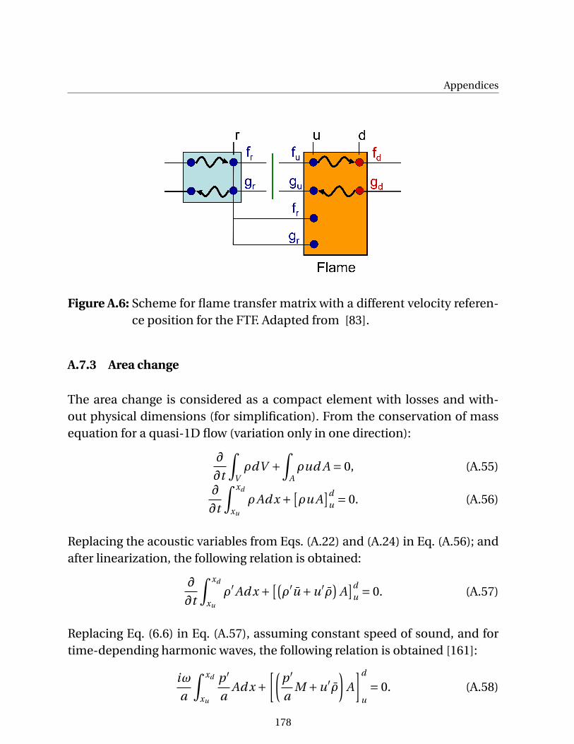
Appendices
Figure A.6: Scheme for flame transfer matrix with a different velocity referen-ce position for the FTF. Adapted from [83].
A.7.3 Area change
The area change is considered as a compact element with losses and with-out physical dimensions (for simplification). From the conservation of massequation for a quasi-1D flow (variation only in one direction):
∂
∂t
∫VρdV +
∫Aρud A = 0, (A.55)
∂
∂t
∫ xd
xu
ρAd x + [ρu A
]du = 0. (A.56)
Replacing the acoustic variables from Eqs. (A.22) and (A.24) in Eq. (A.56); andafter linearization, the following relation is obtained:
∂
∂t
∫ xd
xu
ρ′Ad x + [(ρ′u +u′ρ
)A
]du = 0. (A.57)
Replacing Eq. (6.6) in Eq. (A.57), assuming constant speed of sound, and fortime-depending harmonic waves, the following relation is obtained [161]:
iω
a
∫ xd
xu
p ′
aAd x +
[(p ′
aM +u′ρ
)A
]d
u= 0. (A.58)
178
A.7 Description of Elements in the Network Model
Considering the area change as a discontinuity, the first term in the left handside of Eq. (A.58) is neglected, obtaining:[(
p ′
aM +u′ρ
)A
]d
u= 0. (A.59)
From the Bernoulli equation for unsteady compressible flow [155]:
∂
∂x
(∂Φ
∂t+ 1
2u2 + γ
γ−1
p
ρ
)= 0, (A.60)
where γ is the ratio of specific heats andΦ is the velocity potential defined by:
∇Φ= u, (A.61)
Φ=∫ xd
xu
ud x, (A.62)
the following relation is obtained including the effects of pressure losses:
∂
∂t
∫ xd
xu
ud x +[
1
2u2 + γ
γ−1
p
ρ
]d
u
+ 1
2ζu2
d = 0. (A.63)
An approximation of ζ can be obtained by:
ζ= 2∆pt
ρ2u2d
. (A.64)
taking into account that for low Mach number flows, the steady incompressi-ble and compressible Bernoulli equations are equivalent up to second orderin Mach number [83, 161]. This information was obtained using non-reactingRANS of the full geometry (including plenum).
For a discontinuity, the first term in the left hand side of Eq. (A.63) is neglected,and by linearizing Eq. (A.63) through a series expansion:[
uu′+ γ
γ−1
p ′
ρ− γ
γ−1
pρ′
ρ2
]d
u
+ζud u′ = 0. (A.65)
Using the relation for ρ′ and the definition of speed of sound from Eq. (6.6)in Eq. (A.65); and dividing by the speed of sound, the following relation is ob-tained: [
Mu′+ p ′
ρa
]d
u
+ζMd u′ = 0. (A.66)
179
Appendices
Expressing Eqs. (A.59) and (A.65) in terms of Riemann invariants, the transfermatrix is defined by: [
1+Mu 1−Mu
Au(1+Mu) Au(−1+Mu)
][fu
gu
](A.67)
+[−(1+Md (1+ζ)) −(1−Md (1+ζ))
−Ad (1+Md ) −Ad (−1+Md )
][fd
gd
]=
[00
]. (A.68)
A.7.4 Inlet
The inlet is considered as a fully reflective inlet, the acoustic velocity fluctua-tion to zero, i.e. u′ = 0. Due to the presence of mean flow, the inlet is definedby a condition of no acoustic mass flow fluctuation [117]. The acoustic massflow fluctuation disappears at a closed end:
(ρu)′ = 0. (A.69)
Then:
u′+Mp ′
i
ρi ci= 0. (A.70)
This leads to: [1+M −1+M
][fi
gi
]= 0 (A.71)
A.7.5 Outlet
For the outlet, the reflection coefficient R(ω) in Fig. 6.5 was obtained using thedefinition:
R(ω) = g (ω)
f (ω). (A.72)
In the network model, the reflective outlet is defined by:
[R −1
][fi
gi
]= 0. (A.73)
180
A.8 FTF at Different Velocity Reference Position with 30 kW and 9.5% of ExcitationAmplitude
A.7.6 Swirler
The transfer matrix of the swirler was identified using LES/SI using only theswirler and connecting tube without the combustion chamber as shown inFig. 5.30. The identification was carried out with 30 kW of power rating. Per-turbations on the characteristic ingoing waves were imposed at the inlet andoutlet using broadband excitation with a frequency limit to 6000 Hz and anamplitude of 5% of the mean velocity. The transfer matrix was identified as aMIMO system. Further details on MIMO identification for transfer matricesare shown in [57, 160].
The transfer matrix of the swirler is shown in Fig. A.7 using the Scattering Ma-trix representation. The scattering matrix is defined by:(
fd
gu
)= S(ω)
(fu
gd
). (A.74)
where f and g are the Riemann invariants defined in Eq. (6.14). The elementsS11 and S22 of the scattering matrix represent the transmission of the acousticwaves from upstream and downstream direction through the swirler, respec-tively; while the elements S12 and S21 represent the reflection of the acousticwaves by the presence of the swirler. A length correction between the refe-rence planes and the center of the swirler is included [83]. The element is in-troduced in the network model using the identified UIRs together with the UIRmethod specified in section 6.3 for evaluation of complex eigenfrequencies.The transformation of the scattering matrix in terms of Riemann Invariants fand g can be found in [50, 83].
A.8 FTF at Different Velocity Reference Position with 30 kWand 9.5% of Excitation Amplitude
In Fig. A.8, the identified flame transfer function of the BRS burner with 30 kWwith acoustic velocity (u′
r ) fluctuations measured at different reference po-sition is shown. The excitation amplitude is 9.5% of the mean inlet velocity.The simulations were run for 2800000 iterations (0.35 s), considering the first
181
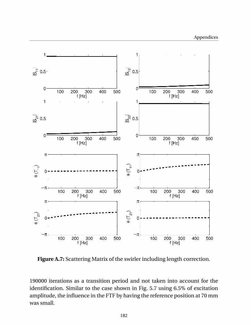
Appendices
Figure A.7: Scattering Matrix of the swirler including length correction.
190000 iterations as a transition period and not taken into account for theidentification. Similar to the case shown in Fig. 5.7 using 6.5% of excitationamplitude, the influence in the FTF by having the reference position at 70 mmwas small.
182
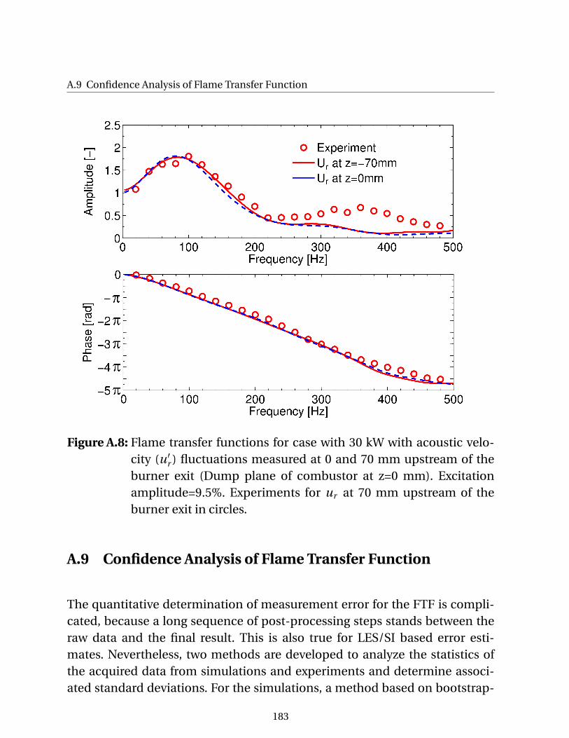
A.9 Confidence Analysis of Flame Transfer Function
Figure A.8: Flame transfer functions for case with 30 kW with acoustic velo-city (u′
r ) fluctuations measured at 0 and 70 mm upstream of theburner exit (Dump plane of combustor at z=0 mm). Excitationamplitude=9.5%. Experiments for ur at 70 mm upstream of theburner exit in circles.
A.9 Confidence Analysis of Flame Transfer Function
The quantitative determination of measurement error for the FTF is compli-cated, because a long sequence of post-processing steps stands between theraw data and the final result. This is also true for LES/SI based error esti-mates. Nevertheless, two methods are developed to analyze the statistics ofthe acquired data from simulations and experiments and determine associ-ated standard deviations. For the simulations, a method based on bootstrap-
183
Appendices
ping [45] is used. The idea is to create artificial new data by randomly draw-ing elements from the original data set. Some elements will be chosen morethan once. The procedure is repeated around 1000 times and statistical distri-butions of amplitude and phase are obtained. Standard deviations are com-puted from the distributions, indicating a measure of the deviation of the FTFidentification by different levels of noise in the signal. In our case, this ran-dom process must be done to the correlation pairs obtained from Eqs. (4.28)and (4.27), because they keep the correlation information between our origi-nal signals and responses. This procedure gives us a level of confidence thatif the identification would have been repeated with another signal, the resultswould be between this range. This method was applied for the reference casewith 30 kW and with 9.5% of excitation amplitude. For the experiments, thedata was taken with a frequency of 10 kHz for a total time of 40 s for each sin-gle frequency. Then, multiple sequences of 15 s from this data (e.g., the firstinterval from 0 to 15 s, the next from 0.05 to 15.05 s, until 40 s) are created,and by a Fast Fourier Transform (FFT), statistical distributions of amplitudeand phase are computed for each frequency. The standard deviation indicatespossible deviations created by noise included in the acquired data. The devi-ation percentage as the standard deviation over the mean of the amplitude ofthe FTF is shown in the top of Fig. A.9. Deviations lower than 2% are mostlyfound in the data. The FTF from LES/SI presents increased deviations for fre-quencies higher than 300 Hz, indicating a higher influence of noise at thosefrequencies.
A.10 Post-processing Tool for Line-of-sight Heat Release Inte-gration in Tecplot
This Macro was created to integrate the heat release from a CFD simulationwith the Z coordinate as the axial axis. If the axial axis is in other coordinate, itneeds to be adapted.
184
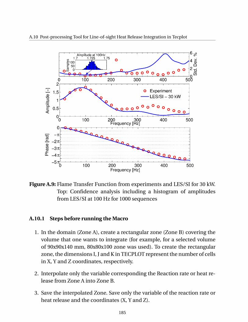
A.10 Post-processing Tool for Line-of-sight Heat Release Integration in Tecplot
Figure A.9: Flame Transfer Function from experiments and LES/SI for 30 kW.Top: Confidence analysis including a histogram of amplitudesfrom LES/SI at 100 Hz for 1000 sequences
A.10.1 Steps before running the Macro
1. In the domain (Zone A), create a rectangular zone (Zone B) covering thevolume that one wants to integrate (for example, for a selected volumeof 90x90x140 mm, 80x80x100 zone was used). To create the rectangularzone, the dimensions I, J and K in TECPLOT represent the number of cellsin X, Y and Z coordinates, respectively.
2. Interpolate only the variable corresponding the Reaction rate or heat re-lease from Zone A into Zone B.
3. Save the interpolated Zone. Save only the variable of the reaction rate orheat release and the coordinates (X, Y and Z).
185

Appendices
4. Load in TECPLOT only the saved interpolated zone (use the replace dataset option, if you have something loaded before). It muss contain only 4variables. The heat release must be the fourth variable.
5. Create a plane (define J=1) with a similar number of cells I and K as in theinterpolated zone.
6. Run the macro.
7. The macro will create a variable called V5, which is the Line-of-Sight In-tegrated heat release.
Check the $!GETFIELDVALUE and $!SETFIELDVALUE macro commands inthe Tecplot Script Manual for the index notation to identify the correspond-ing cells for the integration.
A.10.2 Macro
# Set the zone and variable:$!VarSet |indexI| = 1$!VarSet |indexJ| = 1$!VarSet |indexK| = 1$!VarSet |RootZone| = 1# The heat release is the variable number 4:$!VarSet |Variable| = 4# The destination zone is the plane (Zone 2)$!VarSet |DestZone| = 2# The destination variable containing the integration is the fifth variable,which is created by the macro.$!VarSet |Integ|=0$!AlterDataEquation = ”v5 = 0”$!VarSet |DestVar| = 5# Extract the data point:$!ActiveFieldZones = [|RootZone|]
186

A.10 Post-processing Tool for Line-of-sight Heat Release Integration in Tecplot
$!Loop |MaxK|$!VarSet |indexK| = |loop|$!Loop |MaxI|$!VarSet |indexI| = |loop|$!VarSet |Integ|=0$!Loop |MaxJ|$!VarSet |indexJ| = |loop|# Index notation for the cells:$!VarSet |nodevalue| = ((|indexK|-1)*|MaxI|*|MaxJ| + (|indexJ|-1)*|MaxI| + |in-dexI|)# Index notation for the plane:$!VarSet |nodeplane| = ((|indexK|-1)*|MaxI|*1 + (1-1)*|MaxI| + |indexI|)# Extract integrated variable:$!GetFieldValue |variab|Zone = |RootZone|Var = |Variable|Index = |nodevalue|$!VarSet |Integ|+=|variab|# Introduce integrated variable in the plane:$!SetFieldValueZone = |DestZone|Var = |DestVar|Index = |nodeplane|FieldValue = |Integ|$!EndLoop$!EndLoop$!EndLoop
187