the cost of counterparty risk and collateralization in longevity swaps
TRANSCRIPT
The cost of counterparty risk and collateralization
in longevity swaps∗
Enrico Biffis† David Blake‡ Lorenzo Pitotti§ Ariel Sun¶
Abstract
Derivative longevity risk solutions, such as bespoke and indexed longevity swaps,allow pension schemes and annuity providers to swap out of longevity risk, butintroduce counterparty credit risk, which can be mitigated if not fully eliminatedby collateralization. In this study, we examine the impact of bilateral default riskand collateral flows on the marking to market of longevity swaps, and show howdifferent rules for posting collateral during the life of these instruments can affectlongevity swap rates. For typical interest rate and mortality parameters, we findthat the cost of collateral is modest in the presence of symmetric default risk, butmore pronounced when default risk and/or collateral rules are asymmetric. Ourresults suggest that the overall cost of collateralization is comparable with thatdocumented for the interest-rate swaps market.
Keywords: longevity swap, counterparty risk, default risk, collateral, marking-to-market.
∗This version: April 3, 2011. Earlier versions were presented at the Summer School in Risk Manage-ment and Control (Swiss Institute in Rome), Longevity 6 conference (Sydney), AXA Longevity Risk andPension Funds conference (Paris), and at the University of Ulm. Disclaimer : The views and opinionsexpressed in this study are those of the authors and are not those of Algorithmics or Risk ManagementSolutions (RMS). The authors, Algorithmics and RMS do not accept any liability in respect of thecontent of this study or any claims, losses or damages arising from the use of, or reliance on, all or anypart of this study.
†Biffis ([email protected]) is at Imperial College Business School, Imperial College London,South Kensington Campus, SW7 2AZ United Kingdom.
‡Blake ([email protected]) is at the Pensions Institute, Cass Business School, 106 Bunhill Row,London, EC1Y 8TZ, United Kingdom.
§Pitotti ([email protected]) is at Imperial College London and Algorithmics, 30North Colonnade, Canary Wharf, London E14 5GP, United Kingdom.
¶Sun ([email protected]) is at Risk Management Solutions Ltd, Peninsular House, 30 MonumentStreet, London EC3R 8NB, United Kingdom.
1

1 Introduction
The market for longevity-linked securities and derivatives has recently experienced a
surge in transactions in longevity swaps. These are agreements between two parties to
exchange fixed payments against variable payments linked to the number of survivors in
a reference population (see Dowd et al., 2006). Table 1 presents a list of recent deals
that have been publicly disclosed. So far, transactions have mainly involved pension
funds and annuity providers wanting to hedge their exposure to longevity risk but with-
out having to bear any basis risk: the variable payments in such longevity swaps are
designed to match precisely the mortality experience of each individual hedger (hence
the name indemnity-based, or bespoke, longevity swaps). This is essentially a form of
longevity risk insurance, similar to annuity reinsurance in reinsurance markets. A funda-
mental difference, however, is that longevity swaps are typically collateralized, whereas
insurance/reinsurance transactions are not.1 The main reason is that longevity swaps
are often part of a wider de-risking strategy involving other collateralized instruments
(interest-rate and inflation swaps, for example), and also the fact that hedgers have been
increasingly concerned with counterparty risk2 in the wake of the Global Financial Crisis.
In this article, we provide a framework to quantify the trade-off between the exposure to
counterparty risk in longevity swaps and the cost of credit enhancement strategies such
as collateralization.
As there is no accepted framework yet for marking to market/model longevity swaps,
hedgers and hedge suppliers look to other markets to provide a reference model for
counterparty risk assessment and mitigation. In interest-rate swap markets, for example,
the most common form of credit enhancement is the posting of collateral. According to
1One rationale for this is that reinsurers aggregate several uncorrelated risks and pool-ing/diversification benefits compensate for the absence of collateral (e.g., Lakdawalla and Zanjani, 2007;Cummins and Trainar, 2009).
2Basel II (2006, Annex 4) defines ccounterparty risk as “the risk that the counterparty to a transactioncould default before the final settlement of the transaction’s cash flows”. The recent Solvency II proposalmakes explicit allowance for a counterparty risk module in its ‘standard formula’ approach; see CEIOPS(2009).
2
the International Swap and Derivatives Association (ISDA) almost every swap at major
financial institutions is ‘bilaterally’ collateralized (ISDA, 2010b), meaning that either
party is required to post collateral depending on whether the market value of the swap is
positive or negative.3 The vast majority of transactions is collateralized according to the
Credit Support Annex to the Master Swap Agreement introduced by ISDA (1994). The
Global Financial Crisis of 2008-09 highlighted the importance of bilateral counterparty
risk and collateralization for over-the-counter markets, spurring a number of responses
(e.g, ISDA, 2009; Brigo and Capponi, 2009; Assefa et al., 2010; Brigo et al., 2011).
The Dodd-Frank Wall Street Reform and Consumer Protection Act (signed into law by
President Barack Obama on July 21, 2010) is likely to have a major impact on the way
financial institutions will manage counterparty risk in the coming years.4 The recently
founded Life and Longevity Markets Association5 (LLMA) has counterparty risk at the
center of its agenda, and will certainly draw extensively from the experience garnered in
fixed-income and credit markets.
The design of collateralization strategies is intended to address the concerns aired
by pension trustees regarding the efficacy of longevity swaps, but introduces another
dimension in the traditional pricing framework used for insurance transactions. The
‘insurance premium’ embedded in a longevity swap rate reflects not only the aversion
(if any) of the counterparties to the risk being transferred and the cost of regulatory
capital involved in the transaction, but also the expected costs to be incurred from
posting collateral during the life of the swap. The fact that collateral is costly simply
reflects the costs entailed by credit risk mitigation. To sign and gauge the impact of
collateral on swap rates, we must examine the relative sensitivity of the counterparties
3“Unlike a firm’s exposure to credit risk through a loan, where the exposure to credit risk is unilateraland only the lending bank faces the risk of loss, counterparty credit risk creates a bilateral risk of loss:the market value of the transaction can be positive or negative to either counterparty to the transaction.The market value is uncertain and can vary over time with the movement of underlying market factors.”(Basel II, 2006, Annex 4).
4See, for example, “Berkshire may scale back derivative sales after Dodd-Frank”, Bloomberg, Au-gust 10, 2010.
5See http://www.llma.org.
3

to its cost. Let us first take the perspective of a hedge supplier (reinsurer or investment
bank) issuing a collateralized longevity swap to a counterparty (pension fund or annuity
provider). Whenever the swap is sufficiently out-of-the-money, the hedge supplier is
required to post collateral, which can be used by the hedger to mitigate losses in the event
of default. Although interest on collateral is (partially) rebated, there is an opportunity
cost, as the posting of collateral depletes the resources the hedge supplier can use to meet
her capital requirements at aggregate level. On the other hand, whenever the swap is
sufficiently in-the-money, the hedge supplier will receive collateral from the counterparty,
thus benefiting from capital relief in regulatory valuations. The benefits can be far larger
if collateral can be re-pledged for other purposes, as in the interest-rate swaps market.6
The same considerations can be made from the viewpoint of the hedger, but the funding
needs of the two parties are unlikely to offset each other exactly. This is particularly
relevant for transactions involving parties subject to different regulatory frameworks.
In the UK and several other countries, for example, longevity risk exposures are more
capital intensive for hedge suppliers than for pension funds.7
In the absence of collateral, and ignoring longevity risk aversion, swap rates depend
on best estimate survival probabilities for the hedged population and on the degree of
covariation between the floating leg of the swap and the defaultable term structure of
interest rates facing the hedger and the hedge supplier.8 This means that a proper
analysis of a longevity swap cannot disregard the sponsor’s covenant when the hedger
is a pension plan (see section 3 below). In the presence of collateralization, longevity
swap rates are also shaped by the expected collateral costs, and swap valuation formulae
involve a discount rate reflecting the opportunity cost of collateral. This means, in
6According to ISDA (2010b),the vast majority of collateral is rehypothecated for other purposes ininterest-rate swap markets. Currently, collateral can be re-pledged under the New York Credit SupportAnnex, but not under the English Credit Support Deed (see ISDA, 2010a).
7This asymmetry is a by-product of rules allowing, for example, liabilities to be quantified by usingoutdated mortality tables or discount rates reflecting optimistic expected returns.
8Along the same lines, Inkmann and Blake (2010) show how the discount rate for the valuation ofpension liabilities should reflect funding risk.
4

particular, that default-free valuation formulae are not appropriate even in the presence
of full collateralization and the corresponding absence of default losses (see Johannes
and Sundaresan, 2007, for the case of symmetric default risk and collateral costs in
interest-rate swaps).
For typical interest rate and mortality parameters, we find that the impact of collat-
eralization on swap rates is modest when default risk and collateral rules are symmetric.
There are two opposing effects at play here:
i) On the one hand, the receiver of the fixed survival rate (the hedge supplier) posts
collateral when mortality is lower and hence longevity exposures are more capital inten-
sive. On the other hand, she receives collateral when mortality is higher and longevity
protection less capital intensive. The overall effect is to push swap rates higher, to
compensate the hedge supplier for the positive dependence between collateral flows and
capital charges.
ii) When the hedge supplier is out-of-the-money, collateral outflows are larger in low
interest rate environments (i.e., when liabilities are discounted at a lower rate), hence
there is a negative relationship between the amount of collateral posted and the hedge
supplier’s funding costs. On the other hand, when the hedge supplier is in-the-money,
collateral inflows are larger exactly when funding costs are higher. The opposite is true
for the hedger who demands lower longevity swap rates as a compensation for the positive
dependence between its funding costs and collateral amounts.
When default risk or collateral rules are asymmetric, either of the two effects prevail
and the impact on longevity swap rates is larger. For example, we find that swap rates
increase substantially when the hedger has lower credit standing and collateral rules are
more favorable to the hedge supplier. Although collateralization introduces an explicit
link between the individual risk exposures and the hedge supplier’s funding risk (hence
some of the pooling/diversification benefits used to substitute for collateralization in the
standard insurance model may be lost), in our examples we find that the overall impact
5
of collateralization is comparable with, and typically lower than, that observed in fixed-
income markets (e.g., Johannes and Sundaresan, 2007). This means that the interest-rate
swaps market might provide the right framework for the collateralization of indemnity-
based solutions, even though the latter lack of the transparency and standardization
benefits associated with indexed-based instruments.
On the methodological side, we show how longevity swap rates must be determined
endogenously from the dynamic marking to market9 of the swap and the collateral rules
specified by the contract. To see why, note that the market value of the swap at each
valuation date depends on the evolution of the relevant state variables (mortality, in-
terest rates, credit spreads), as well as on the swap rate locked in at inception. On the
other hand, the swap’s market value will typically affect collateral amounts and, in a set-
ting where collateral is costly, will embed the market value of expected future collateral
flows. Hence, the swap rate can only be determined by explicitly taking into account the
marking-to-market process and the dynamics of collateral posting. To avoid the compu-
tational burden of nested Monte Carlo simulations, we use an iterative procedure based
on the Least-Squares Monte Carlo approach10 (see Glassermann, 2004, and references
therein). We provide several numerical examples showing how different collateralization
rules shape longevity swap rates giving rise to margins in (best estimate) survival proba-
bilities reflecting the opportunity cost of future collateral flows. Although our focus is on
longevity risk solutions, the approach can be applied to other instruments, in particular
to bespoke solutions for other risks, such as inflation and credit risk.
Our work contributes to the existing literature on longevity risk pricing in at least
three ways: i) we introduce default risk in the pricing of longevity risk solutions, and
properly address its bilateral nature; ii) we explicitly allow for collateralization rules,
which are the backbone of any real-world hedging solution and materially affect the
9Here and in the following, by ‘market value’ and ‘marking to market’ we mean that market-consistent
values are computed according to the relevant accounting/regulatory standard.10A similar approach is used by Bacinello et al. (2010) for surrender guarantees in life policies and by
Bauer et al. (2010b) for the computation of capital requirements within the Solvency II framework.
6

pricing of over-the-counter transactions; and iii) we introduce a ‘structural’ dimension in
an otherwise reduced-form pricing framework, by allowing for funding costs associated
with longevity risk exposures held by hedgers and hedge suppliers. As there is essentially
no publicly available information on swap rates, our approach11 has the advantage of
using publicly available information on credit markets and regulatory standards, without
having to rely on calibration to primary insurance market prices, approximate hedging
methods or assumptions on agents’ risk preferences (e.g., Dowd et al., 2006; Ludkovski
and Young, 2008; Bauer et al., 2010a; Biffis et al., 2010; Chen and Cummins, 2010; Cox
et al., 2010, among others).
The article is organized as follows. In the next section, we introduce longevity swaps
and formalize their payoffs. We examine the case of both indemnity-based and index-
based swaps, but, in the latter case, we ignore the issue of basis risk12 to keep the article
focused. In section 2.1, we examine the marking to market of a longevity swap during
its life time to demonstrate the impact of counterparty risk on the hedger’s balance
sheet. Section 3 introduces bilateral default risk in longevity swap valuation formulae.
We identify the main channels through which default risk affects the market value of
swaps and show why an iterative procedure is needed to compute swap rates. Section 4
introduces credit enhancement in the form of collateralization, and shows how longevity
swap rates are affected even in the presence of full cash collateralization (and hence
absence of default losses). We explain how swap rates can be computed by using an
iterative procedure based on the Least-Squares Monte Carlo approach. In section 5,
several stylized examples are provided to understand how different collateralization rules
may affect longevity swap rates. Concluding remarks are offered in section 6. Further
details and technical remarks are collected in an appendix.
11Similarly, Biffis and Blake (2010a) endogenize longevity risk premia by introducing asymmetricinformation and capital requirements in a risk-neutral setting.
12See, for example, Coughlan et al. (2011), Salhi and Loisel (2010) and Stevens, De Waegenaere andMelenberg (2010b) for some results related to this risk dimension.
7

< Table 1 about here >
2 Longevity swaps
We consider a hedger (insurer, pension fund), referred to as party A, and a hedge supplier
(reinsurer, investment bank), referred to as counterparty B. Agent A has the obligation
to pay amounts XT1 , XT2 , . . ., possibly dependent on interest rates and inflation, to each
survivor at fixed dates 0 < T1 ≤ T2, . . . of an initial population of n individuals alive
at time zero (annuitants or pensioners). We are clearly restricting our attention to
homogeneous liabilities for ease of exposition, more general situations requiring obvious
modifications. Party A’s liability at a generic payment date T > 0 is given by the
random variable (n − NT )XT , where NT counts the number of deaths experienced by
the population during the period [0, T ]. Assuming that the individuals’ death times have
common intensity13 (µt)t≥0, the expected number of survivors at time T can be written
as EP [n−NT ] = npT , with the survival probability pT given by (see the appendix)
pT := EP
[exp
(−
∫ T
0µtdt
)]. (2.1)
Here and in the following, P denotes the real-world probability measure. The intensity
could be modeled by using, for example, any of the stochastic mortality models consid-
ered in Cairns et al. (2009). For our examples, we will rely on the simple Lee-Carter
model.
Let us now consider a financial market and introduce the risk-free rate process (rt)t≥0.
We assume that a market-consistent price of the liabilities can be computed by using
a risk-neutral measure P, equivalent to P, such that the death times have the same
intensity process (µt)t≥0 (with different dynamics, in general, under the two measures;
13Intuitively, µt represents the instantaneous conditional death probability for an individual alive attime t.
8

see Biffis et al., 2010). The time-0 market value of the aggregate liability can then be
written as
EP
[∑
i
exp
(−
∫ Ti
0rtdt
)(n−NTi
)XTi
]= n
∑
i
EP
[exp
(−
∫ Ti
0(rt + µt)dt
)XTi
].
For the moment, we take the pricing measure as given: we will give it more structure
later on.
We consider two instruments which A can enter into with B to hedge its exposure:
an indemnity-based longevity swap and an index-based longevity swap. In these swaps,
in contrast with interest rate swaps, the swap rate needs to be a collection of fixed
rates pertaining to each individual payment date. The reason is that mortality increases
substantially at old ages and a fixed rate would introduce a growing mismatch between
the cashflows provided by the swap and those needed by the hedger. However, as with
interest rate swaps, we can treat a longevity swap as a portfolio of forward contracts
on the underlying floating (survival) rate.14 In this section, we ignore default risk and
focus on individual payments at maturity T > 0. In what follows, we always assume the
perspective of the hedger.
An indemnity-based longevity swap allows party A to pay a fixed rate pN ∈ (0, 1)
against the realized survival rate experienced by the population between time zero and
time T . Assuming a notional amount equal to the initial population size, n, the net
payout to the hedger at time T is15
n
(n−NT
n− pN
),
14With a slight abuse of terminology, we use the term ‘swap rate’ for individual forward rates as wellas for swap curves (collection of swap rates). We note that swap curves are often summarized by theimprovement factor applied to the survival probabilities of a reference mortality table/model.
15For ease of exposition, here and in the following sections, we consider contemporaneous settlementonly. Other settlement conventions (e.g. in arrears) have negligible effects, but make valuation formulaemore involved when bilateral and asymmetric default risk is introduced.
9
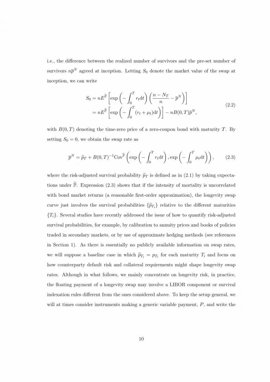
i.e., the difference between the realized number of survivors and the pre-set number of
survivors npN agreed at inception. Letting S0 denote the market value of the swap at
inception, we can write
S0 = nEP
[exp
(−
∫ T
0rtdt
)(n−NT
n− pN
)]
= nEP
[exp
(−
∫ T
0(rt + µt)dt
)]− nB(0, T )pN ,
(2.2)
with B(0, T ) denoting the time-zero price of a zero-coupon bond with maturity T . By
setting S0 = 0, we obtain the swap rate as
pN = pT +B(0, T )−1CovP(exp
(−
∫ T
0rtdt
), exp
(−
∫ T
0µtdt
)), (2.3)
where the risk-adjusted survival probability pT is defined as in (2.1) by taking expecta-
tions under P. Expression (2.3) shows that if the intensity of mortality is uncorrelated
with bond market returns (a reasonable first-order approximation), the longevity swap
curve just involves the survival probabilities pTi relative to the different maturities
Ti. Several studies have recently addressed the issue of how to quantify risk-adjusted
survival probabilities, for example, by calibration to annuity prices and books of policies
traded in secondary markets, or by use of approximate hedging methods (see references
in Section 1). As there is essentially no publicly available information on swap rates,
we will suppose a baseline case in which pTi= pTi
for each maturity Ti and focus on
how counterparty default risk and collateral requirements might shape longevity swap
rates. Although in what follows, we mainly concentrate on longevity risk, in practice,
the floating payment of a longevity swap may involve a LIBOR component or survival
indexation rules different from the ones considered above. To keep the setup general, we
will at times consider instruments making a generic variable payment, P , and write the
10
corresponding swap rate p as
p = EP [P ] +B(0, T )−1CovP(exp
(−
∫ T
0rtdt
), P
). (2.4)
The setup can easily accommodate index-based longevity swaps, standardized
instruments allowing the hedger to pay a fixed rate pI ∈ (0, 1) against the realized value
of a survival index (It)t≥0 at time T . The latter might reflect the mortality experience
of a reference population closely matching that of the liability portfolio. Examples are
represented by the LifeMetrics index developed by J.P. Morgan, the Pensions Institute
and Towers Watson,16 or the Xpect indices developed by Deutsche Boerse. 17 The
relative advantages and disadvantages of index-based versus indemnity-based swaps are
discussed in Biffis and Blake (2010b). Assuming that the index admits the representation
It = exp(−∫ t
0 µIsds), with (µIt )t≥0 representing the intensity of mortality of a reference
population, we can express the swap rate pI by using the expression (2.3) again, but with
the process µ replaced by µI and with pT replaced by the corresponding risk-adjusted
survival probability pIT .
2.1 The marking-to-market (MTM) process
Longevity swaps are not currently exchange traded and there is no commonly accepted
framework for counterparties to mark to market their positions.18 The presence of coun-
terparty default risk and collateralization rules, however, makes the MTM procedure a
very important feature of these transactions for at least three reasons. First, at each
payment date, the difference between the variable and pre-set payment generates a cash
inflow or outflow to the hedger, depending on the evolution of mortality. In the absence
of basis risk (which is the case for indemnity-based solutions), these differences show a
16See www.lifemetrics.com.17See www.xpect-index.com.18At the time of writing, LLMA was working on this issue.
11
pure ‘cashflow hedge’ of the longevity exposure in operation. Second, as market condi-
tions change (e.g., mortality patterns, counterparty default risk), the MTM procedure
could result in the swap switching status in the hedger’s balance sheet between that of
an asset and that of a liability. This may have the implication that, even if the swap pay-
ments are expected to provide a good hedge against longevity risk, the hedger’s position
may still turn into a liability if, for example, deterioration in the hedge supplier’s credit
quality shrinks the expected present value of the variable payments. Third, for solvency
requirements, it is important to value a longevity swap under extreme market/mortality
scenarios (‘stress testing’). This means, for example, that even if a longevity swap qual-
ifies as a liability on a market-consistent basis, it might still provide considerable capital
relief when valued on a regulatory basis.
To illustrate some of these points, let us consider the hypothetical situation of an
insurer A with a liability represented by a group of ten thousand 65-year-old annuitants
drawn from the population of England & Wales in 1980. We assume that party A entered
a 25-year pure longevity swap in 1980 and we follow the evolution of the contract until
maturity. The population is assumed to evolve according to the death rates reported
in the Human Mortality Database (HMD) for England & Wales.19 We assume that
interest-rate risk is hedged away through interest rate swaps, locking in a rate of 5%
throughout the life of the swap. The role of collateral is examined later on; here, we
show how the hedging instrument operates from the point of view of the hedger. For this
indemnity-based solution, the market value of each floating-for-fixed payment occurring
at a generic date T can be computed by using the valuation formula
St =nEP
t
[exp
(−
∫ T
t
rsds
)(n−Nt
nexp
(−
∫ T
t
µsds
))]− nB(t, T )pN , (2.5)
for each time t in [0, T ] at which no default has yet occurred, with B(t, T ) denoting the
19See www.mortality.org.
12
market value of a zero-coupon bond with time to maturity T−t, and EPt [·] the conditional
expectation given the information available at time t. As a simple benchmark case, we
assume that market participants receive information from the HMD and use the Lee-
Carter model to value longevity-linked cashflows. In other words, at each MTM date
(including inception), longevity swap rates are based on Lee-Carter forecasts computed
using the latest HMD information available (see Dowd et al., 2010a,b; Cairns et al., 2011,
for a comprehensive analysis of alternative mortality models). Figure 1 illustrates the
evolution of swap survival rates for an England & Wales cohort tracked from age 65
in 1980 to age 90 in 2005. It is clear that the systematic underestimation of mortality
improvements by the Lee-Carter model in this particular example will mean that the
hedger’s position will become increasingly in-the-money as the swap matures. This is
shown in Figure 2. In practice the contract may allow the counterparty to cancel the
swap or reset the fixed leg for a nonnegative fee, but we ignore these features in this
example. Figure 2 also reports the sequence of cash inflows and outflows generated by
the swap, which are lower ex-post than what was anticipated from an examination of
the MTM basis. As interest rate risk is hedged − and again ignoring default risk for
the moment − cash inflows/outflows arising in the backtesting exercise only reflect the
difference between the realized survival rates and the swap rates locked in at inception.
On the other hand, the swap’s market value reflects changes in market swap rates, which
by assumption follow the updated Lee-Carter forecasts plotted in Figure 1 and differ
from the realized survival rates. As is evident from the example depicted in Figure 2,
the credit exposure of a longevity swap is close to zero at inception and at maturity,
but may be sizable during the life of the swap, depending on the trade-off between
changes in market/mortality conditions and the residual swap payments (amortization
effect). The credit exposure is quantified by the replacement cost, i.e., the cost that
the nondefaulting counterparty would have to incur at the default time to replace the
instrument at market prices then available. As a simple example which predicts the
13
next section, let us introduce credit risk (but no default) and assume that in 1988 the
credit spread of the hedge supplier widens across all maturities by 25 and 50 basis points.
The impact of these two scenarios on the hedger’s balance sheet is dramatic, as shown
again in Figure 2, demonstrating how MTM profits and losses can jeopardize even a well
structured hedging position.
< Figure 1 about here >
< Figure 2 about here >
3 Counterparty default risk
The backtesting exercise of the previous section has demonstrated the importance of the
hedge supplier’s credit risk and the marking to market procedure in assessing the value
of a longevity swap to the hedger. As was emphasized in the introduction, however, a
correct approach should allow for the fact that counterparty risk is bilateral. This is the
case even when the hedger is a pension plan. Private sector defined benefit pension plans
in countries such as the UK are founded on trust law and rely on a promise by (rather
than a guarantee from) the sponsoring employer to pay the benefits to plan members.
This promise is known as the ‘sponsor covenant’. The strength of the sponsor covenant
depends on both the financial strength of the employer and the employer’s commitment
to the scheme.20 To take into account the impact of the sponsor covenant, we use the
sponsor’s default intensity, and refer to it as party A’s intensity of default. For large
corporate pension plans, the intensity can be derived/extrapolated from spreads observed
20In the UK, for example, The Actuarial Profession (2005, par. 3.2) defined the sponsor covenantas: “the combination of (a) the ability and (b) the willingness of the sponsor to pay (or the ability ofthe trustees to require the sponsor to pay) sufficient advance contributions to ensure that the scheme’sbenefits can be paid as they fall due.” See also The Pensions Regulator (2009).
14

in corporate bond and CDS markets. For smaller plans, an analysis of the funding level
and strategy of the scheme is required.
Assume that both party A (the hedger) and B (the hedge supplier) may default
at random times τA, τB, admitting default intensities (λAt )t≥0, (λBt )t≥0. Defining by
τ := min(τA, τB), the default time of the swap transaction, we further assume that,
on the event τ ≤ T, the nondefaulting counterparty, say party i, receives a fraction
ψj ∈ [0, 1] (i 6= j, with i, j ∈ A,B) of the market value of the swap before default,
Sτ−, if she is in-the-money, otherwise she has to pay the full pre-default market value
Sτ− to the defaulting counterparty. We can then write the market value of a swap with
notional amount n as (e.g., Duffie and Huang, 1996)
S0 =nEP
[exp
(−
∫ T
0(rt + 1St<0(1− ψA)λAt + 1St≥0(1− ψB)λBt )dt
)(P − pd
)],
(3.1)
where P denotes the variable payment and the indicator function 1H takes the value
of unity if the event H is true, zero otherwise. To understand the above formula, note
that, in our setting, the risk-neutral valuation of a defaultable claim involves the use of
a default-risk-adjusted short rate rt + λAt + λBt and dividend payment λAt (ψA1St−<0 +
1St−≥0) + λBt (ψB1St−≥0 +1St−<0) determined by the recovery rules described above. As
a result, the valuation formula (3.1) entails discounting at a spread above the risk-free
given by
Λt :=λAt + λBt − λAt (ψ
A1St<0 + 1St≥0)− λBt (ψB1St≥0 + 1St<0)
=1St<0(1− ψA)λAt + 1St≥0(1− ψB)λBt ,
showing a switching-type dependence on the characteristics of the counterparty that
is out-of-the-money at each given time prior to default. The swap rate admits the
15
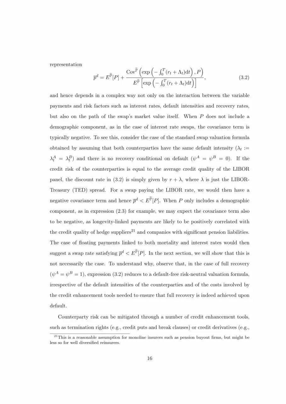
representation
pd = EP[P ] +CovP
(exp
(−∫ T
0 (rt + Λt)dt), P
)
EP
[exp
(−∫ T
0 (rt + Λt)dt)] , (3.2)
and hence depends in a complex way not only on the interaction between the variable
payments and risk factors such as interest rates, default intensities and recovery rates,
but also on the path of the swap’s market value itself. When P does not include a
demographic component, as in the case of interest rate swaps, the covariance term is
typically negative. To see this, consider the case of the standard swap valuation formula
obtained by assuming that both counterparties have the same default intensity (λt :=
λAt = λBt ) and there is no recovery conditional on default (ψA = ψB = 0). If the
credit risk of the counterparties is equal to the average credit quality of the LIBOR
panel, the discount rate in (3.2) is simply given by r + λ, where λ is just the LIBOR-
Treasury (TED) spread. For a swap paying the LIBOR rate, we would then have a
negative covariance term and hence pd < EP[P ]. When P only includes a demographic
component, as in expression (2.3) for example, we may expect the covariance term also
to be negative, as longevity-linked payments are likely to be positively correlated with
the credit quality of hedge suppliers21 and companies with significant pension liabilities.
The case of floating payments linked to both mortality and interest rates would then
suggest a swap rate satisfying pd < EP[P ]. In the next section, we will show that this is
not necessarily the case. To understand why, observe that, in the case of full recovery
(ψA = ψB = 1), expression (3.2) reduces to a default-free risk-neutral valuation formula,
irrespective of the default intensities of the counterparties and of the costs involved by
the credit enhancement tools needed to ensure that full recovery is indeed achieved upon
default.
Counterparty risk can be mitigated through a number of credit enhancement tools,
such as termination rights (e.g., credit puts and break clauses) or credit derivatives (e.g.,
21This is a reasonable assumption for monoline insurers such as pension buyout firms, but might beless so for well diversified reinsurers.
16

CDSs and credit spread options). Here we focus on collateralization, a form of direct
credit support requiring each party to post cash or securities when it is out of the money.
For simplicity, we consider the case of cash, which is by far the most common type of
collateral (e.g., ISDA, 2010a) and allows us to disregard close-out risk, the risk that the
value of collateral may change at default. In the interest-rate swaps market, Johannes
and Sundaresan (2007) find evidence of costly collateral by comparing swap market data
with swap values based on portfolio of futures and forward contracts. We cannot carry
out a similar exercise for longevity swaps, because there are no publicly available data
for these transactions. On the other hand, we can quantify the funding gains/costs
associated with the collateral flows originating from the marking to market procedure.
We will therefore model explicitly the market value of a representative longevity-linked
liability and use information on the funding cost of the counterparies to ‘synthesize’ the
dynamics of collateral costs.
4 Collateralization
Collateral agreements reflect the amount of acceptable credit exposure that each party
agrees to take on. We will consider simple collateral rules capturing the main features
of the problem. Formally, let us introduce the pre-default collateral process22 (Ct)t≥0,
which indicates how much cash, Ct, to post at each time t prior to default in response
to changes in market conditions, including, in particular, the MTM value of the swap
(we provide explicit examples below). Again, we develop our analysis from the point of
view of the hedger, so that Ct > 0 (Ct < 0) means that party A is holding (posting)
collateral. Using the notation a+ := max(a, 0) and a− := max(−a, 0), the recovery rules
take the following form:
• On the event τA ≤ min(τB, T ) (hedger’s default), party B (the hedge supplier)
22In other words, the actual collateral supporting the transaction is represented by (1τ>tCt)t≥0,hence, we are not concerned with the value taken by Ct after default.
17

recovers any collateral received by the hedger an instant prior to default, C−τA−
,
and pays the full MTM value of the swap to party A if SτA− ≥ 0. The net flow to
party A is then S+τA−
− C−τA−
.
• On the event τB ≤ min(τA, T ) (hedge supplier’s default), party A (the hedger)
pays the full MTM value of the swap to party B if SτB− < 0, and recovers any
collateral received by B an instant prior to default, C+τB−
. The net flow to party
A can then be written as −S−τB−
+ C+τB−
.
• Whenever the nondefaulting counterparty, say A, is out-of-the-money, payment
of the full MTM value of the swap is accomplished by party A recovering the
extra amount (Sτ− − Cτ−)+ in case of overcollateralization, or by party A paying
the extra amount (Cτ− − Sτ−)+ in case of undercollateralization. In case of full
collateralization, party A simply loses any collateral posted with B.
To obtain neater results, it is convenient to express the collateral before default of
either party as a fraction of the MTM value of the swap,
Ct =(cBt 1St−≥0 + cAt 1St−<0
)St−, (4.1)
where cA, cB are two nonnegative left-continuous processes giving the fraction of the
MTM value of the swap that is posted as collateral by party A or B, respectively. Fi-
nally, we introduce a nonnegative continuous process (δt)t≥0 representing the yield on
collateral, in the sense that holding/posting collateral of amount Ct yields/costs instan-
taneously the net amount δtCt (after rebate). Instead of capturing simultaneously the
perspective of both counterparties with δ, it may be convenient to introduce some asym-
metry by considering δt = δAt 1St−<0 + δBt 1St−≥0, so that δAt (δBt ) can be interpreted
as the opportunity cost of posting collateral for party A (B) when it is out-of-the-money.
Denoting by pc the swap rate available in case of collateralization, we can write the MTM
value of the swap as in (3.1), but with the spread Λ now replaced by (see the appendix
18

for a proof)
Γt =λAt (1− cAt )1St−<0 + λBt (1− cBt )1St−≥0 −
(δAt c
At 1St−<0 + δBt c
Bt 1St−≥0
)
(4.2)
In the above expression, we recognize the typical features of valuation formulae for credit-
risky securities (e.g., Duffie and Huang, 1996; Bielecki and Rutkowski, 2002): the first
two terms account for the fractional recovery of the swap MTM value in case of default
of the counterparty, the third one for the costs incurred when posting collateral before
default. The swap rate pc can finally be written as in (3.2) by using the discount rate
r + Γ. We now examine simple special cases to understand better the role of collateral
in shaping swap rates.
4.1 Full collateralization
Consider the collateral rule obtained by setting cA = cB = 1 and δA = δB = δ, mean-
ing that the full MTM value of the swap is received/posted as collateral depending on
whether the marking-to-market process results in a positive/negative value for St. As we
consider cash collateral, default is immaterial. In contrast with section 3, however, the
expression for the swap MTM value does not reduce to the usual default-free, risk-neutral
valuation formula in general, unless collateral costs are zero:
pc = EP[P ] +CovP
(exp
(∫ T
0 (δt − rt)dt), P
)
EP
[exp
(∫ T
0 (δt − rt)dt)] . (4.3)
If the cost of collateral is positively dependent on interest rates, we expect the swap
rate to be higher than pd in expression (3.2), even if the floating payment is only linked
to interest rates, reflecting the fact that (costly) collateralization commands a premium
for the payer of the fixed rate (see Johannes and Sundaresan, 2007). The intuition is
that the party paying the floating rate will have to both post collateral and incur higher
19

funding costs when the floating rate increases. As was emphasized in the introduction, in
longevity space, the cost of collateral is positively dependent on mortality improvements,
but longevity-linked liabilities are more capital intensive in low interest rate environments
(due to lower discounting of future cashflows). The combined impact of these two effects
is difficult to quantify, and we may have situations in which pc ≥ EP[P ] even if EP[P ] ≥
pd.
4.2 Partial collateralization
According to ISDA (2010a), it is typical for collateral agreements to specify collateral
triggers based on the market value of the swap or other relevant variables (credit ratings,
credit spreads, etc.) crossing pre-specified threshold levels. In indemnity-based longevity
swaps, however, it is more common to define collateral thresholds in terms of mortality
forecasts based on a model agreed at contract inception and to monitor the deaths in
the hedger’s population than in terms of the market value of the swap. This is due
to both the re-estimation risk affecting any given mortality model and the presence of
substantial model risk, which most likely would prevent the counterparties from agreeing
on a common model at future dates. The following are relevant (if somewhat stylized)
examples that are useful for our case:
a) Consider the collateral rule obtained by setting cBt = 1St−≥s(t) and cAt = 1St−≤s(t)
(for continuous functions s, s defined on [0, T ] and satisfying s ≤ s), meaning that
the hedge supplier (hedger) is required to post full collateral if the swap’s MTM
value is above (below) the appropriate time-dependent threshold. More general col-
lateral rules can be obtained by setting cBt = γBt 1St−≥s(t) and cAt = γAt 1St−≤s(t),
for suitable processes γA, γB depending on prevailing market conditions, such as
the credit standing of the counterparties.
b) Setting cBt = 1Nt−≤α(t) and cAt = 1Nt−≥β(t), for continuous functions α and β
20

satisfying 0 ≤ α ≤ β ≤ n, we see that the hedge supplier (hedger) is required
to post full collateral if realized deaths are below (above) the relevant threshold.
Given the above considerations, this collateralization rule is more suitable for an
indemnity-based longevity swap.
c) For an index-based swap, it may be more convenient to work with the mortality
intensity µI of the reference population (see section 2) and set cBt = 1∫ t
0 µIsds≤a(t)
and cAt = 1∫ t
0 µIsds≥b(t) for continuous functions a, b satisfying 0 ≤ a ≤ b. This
means that collateral posting is triggered at each time t if the realized value of the
longevity index, exp(−∫ t
0 µIsds), falls outside the interval (exp(−b(t)), exp(−a(t))).
d) As was emphasized in section 2.1, the severity of counterparty risk depends on the
credit quality of the counterparties. This is why collateralization agreements may
set collateral thresholds that explicitly depend on credit ratings or CDS spreads.
A simple example of this practice can be obtained as a special case of formulation
(a) by setting cBt = 1Nt−≤α(t)∪λBt ≥λ, c
At = 1Nt−≥β(t)∪λA
t ≥λ, meaning that,
at each time t, the hedger (hedge supplier) receives collateral when either realized
deaths fall below the level α(t) (β(t)) or the hedge supplier’s (hedger’s) default
intensity overshoots a given threshold λ ≥ 0. Note that both cA and cB can be
non zero at the same time (for example on the event Nt− ≤ α(t) ∩ λAt ≥ λ),
but expression (4.1) ensures that only the party out-of-the-money will have to post
collateral.
4.3 Computing the swap rate
The recursive nature of swap valuation formulae in the case of bilateral and asymmetric
counterparty risk was already noted by Duffie and Huang (1996). By modeling the recov-
ery rates and the difference in counterparties’ credit spreads in reduced form, however,
they could use a simpler iterative procedure to determine swap rates. Here, we explic-
21

itly allow for the impact of collateral and the marking-to-market process in the pricing
functional, and hence need a different approach. Working in a Markov setting, we let X
denote the state variable process and adopt a Least-Squares Monte Carlo approach. Ex-
ploiting the structure of the mortality model outlined in section 2 and in the appendix,
we do not model death/default times explicitly but just rely on the mortality/default in-
tensities (see algorithm 2 in Bacinello et al., 2010, for example). The procedure involves
the following steps:
Step 1. For fixed swap rate pci , generate M simulated paths of X under P along the
time grid T := 0 < t1, t2, . . . , tn = T. Denote by Sm,itj
the MTM value of the swap and
by f i,mtjthe cashflows originating from the swap (collateral flows and swap payments) at
time tj on path m and for given swap rate pci .
Step 2. Compute recursively the value of the swap at time tj (for j = n − 1, . . . , 0
with t0 = 0) as Sm,itj
= β∗j · e(Xmtj), where e(x) := (e1(x), . . . , eH(x))T and e1, . . . , eH
is a finite set of functions taken from a suitable basis, and β∗j is given by
β∗j = arg minβj∈RH
M∑
m=1
(Si,mtj+1
+ fi,mtj+1
− βj · e(Xmtj)).
At each time tj , use Sm,itj
to check whether the collateral thresholds are triggered and
determine the corresponding amount of collateral and associated costs.
Step 3. Iterate the above procedure over different values for pci until a candidate swap
rate pci∗ is found, such that the initial price of the swap, 1M
∑Mm=1 S
m,i∗
t0, is close enough
to zero. Set pc = pci∗ .
5 Examples
We use a continuous-time model for the risk-free yield curve, the LIBOR and mortality
rates, as well as for the cost of collateral. The credit risk of party B (the hedge supplier)
22

is assumed to be equal to the average credit quality of the LIBOR panel, so that the
TED spread could be seen as its default intensity if there were zero recovery upon default
(see section 3). We then set λA = λB +∆ and consider two cases: party A is either of
the same credit quality as party B (∆ = 0) or is more credit-risky (∆ > 0).
We consider a Markov setting, and describe the evolution of uncertainty by a six-
dimensional state variable vector X with the Gaussian dynamics reported in appendix B.
The first four components describe: the short rate, r = X(1), assumed to revert to the
long-run central tendency factor X(2), representing the slope of the risk-free yield curve;
the TED spread X(3), so that the LIBOR rate is given by X(1)+X(3); and the net yield
on collateral in the interest-rate swap market, X(4). The remaining two components
describe the log-intensity of mortality of a given population, log µ = X(6), and the
yield on collateral attached to longevity risk business, X(5). Under the assumption of
independence between the interest rate market and mortality, we can estimate separately
the dynamics of the two groups of factors (X(1), X(2), X(3), X(4)) and X(6). For the first
group, we use the estimates of Johannes and Sundaresan (2007) who use weekly Treasury
and swap data from 1990 to 2002 to obtain the parameter values reported in table 2. For
the intensity exp(X(6)t ), we use a continuous-time version of the Lee-Carter model; see
the appendix for details. As we do not have any publicly available transaction data from
the longevity swap market to proxy X(5), we use information on credit markets (funding
costs) and regulatory requirements (capital charges). In particular, as a first example, we
simply take δB = X(3) and δA = X(3)+∆, meaning that the net collateral costs coincide
with each party’s borrowing rate net of the risk-free rate (assuming it is rebated). In
the case of asymmetric default risk, we take ∆ = 0.01. In a second example, discussed
in detail below, we simulate the capital charges arising from holding a representative
longevity-linked liability to estimate the dynamics of X(5). In both cases, we compute
the longevity swap rates for a 25-year swap written on a population of 10,000 US males
aged 65 at the beginning of 2008.
23

< Table 2 about here >
In figure 3, we plot the swap curves obtained for different collateralization rules
against the percentiles of survival rate improvements based on Lee-Carter forecasts. We
see that margins are positive and increasing with payment maturity in the case of sym-
metric default risk, for both uncollateralized and fully collateralized transactions. As
soon as we introduce asymmetry in default risk (∆ > 0), however, margins widen in the
case of no collateralization, reflecting the fact that the hedger needs to pay an additional
premium on account of its higher credit risk. In the case of full collateralization, the
hedge supplier benefits from the negative dependence between funding costs and collat-
eral amounts discussed before: equilibrium swap rates are pushed lower and produce a
negative margin on best estimate swap rates. In figure 4, we examine the swap margins
induced by one-sided collateralization in the case of asymmetric default risk. When only
the hedge supplier has to post full collateral, swap rates are higher than best estimate
survival probabilities, meaning that the hedger has to compensate the counterparty for
bearing the cost of risk mitigation on its side, while remaining exposed to the hedger’s
default risk. The opposite is true when it is the hedger who has to post full collat-
eral when out-of-the money. In this case, swap margins are clearly negative, and again
increasing in payment maturity.
Plotting the swap rate margins against best estimate mortality improvements allows
one to interpret the swap rates as outputs of a pricing functional based on adjustments
to a reference mortality model. On the other hand, it is useful to look at the swap
spreads (in basis points) to have an idea of how they compare with those emerging in
other transactions. In table 3, we report the spreads relative to some key maturities and
collateralization rules: in absolute value, the spreads never exceed those documented in
the interest-rate swap market for fully collateralized transactions with maturities of at
most 10 years. For example, in the case of full collateralization on the hedge supplier’s
24
side only, longevity swap rates for 15- to 25-year maturities command a premium com-
parable with that found for bilaterally collateralized interest-rate swaps with maturities
of 6.5 to 10 years (see Johannes and Sundaresan, 2007). These observations suggest that
the impact of collateralization on longevity swap rates is comparable with, and possibly
even milder than, that found for the far more liquid interest-rate swap market. There
are two main reasons for this result. First, in contrast with markets where rehypotheca-
tion of collateral is the norm, regulation makes collateral less fungible in longevity swap
transactions (through segregation, for example). Second, as discussed above, interest
rate risk and longevity risk impact swap margins in opposite directions, thus diluting
the impact of collateralization on longevity swap rates.
< Table 3 about here >
< Figure 3 about here >
< Figure 4 about here >
In a second example, we ‘synthesize’ the dynamics of X(5) by using information on
regulatory requirements to quantify the capital charges accruing to the counterparties
during the life of the swap. In particular, we use the following bottom-up procedure:
Step 1: We simulate several paths of the factors X(1), . . . , X(4) and X(6) along a time
grid T := t1, t2, . . . , tk (with t1 > 0 and tk = T > t1) and under the pricing measure
P. Consistent with focusing on the baseline case of pT = pT discussed in section 2, the
P-dynamics of X(6) is assumed to be the same as under the physical measure.
Step 2: The paths simulated in the previous step are used to compute, at each date
t ∈ T , the regulatory capital needed by an insurer to hold the liability n−Nt+T , where
T < T is a representative maturity proxying the average duration of longevity-linked
25
liabilities in the longevity swap market. We use T = 15 (years) for our example. To
compute the capital requirement, we use the Solvency II framework, which is based on the
99.5% value-at-risk of the net assets over a one-year horizon. For simplicity, we assume
holders of longevity exposures to be invested in cash. The distribution of the one-year-
ahead market-consistent value of the liability usually requires nested simulation, unless
a simplified approach is adopted. In our setting, market-consistent discount factors can
be computed analytically based on the one-year-ahead simulated realizations. We use
Least-Squares Monte Carlo (see section 4.3) for the expected number of survivors.23
Step 3: We use the simulated capital charges obtained in the previous step to compute
the gains/costs incurred to reduce/increase capital at each time step along each simulated
path. We assume that capital charges are funded at the counterparties’ funding cost,
plus a spread of 6% to reflect that opportunity cost of diverting to an individual liability
funds that could be used to support insurance business at aggregate level. The simulated
realizations of the opportunity cost of capital are used to estimate the dynamics of X(5)
reported in the appendix. The parameter estimates are included in table 2.
In the case of symmetric collateralization, we find results comparable with those
obtained by using the counterparties’ funding costs for the process δ. However, figure 5
shows that margins increase (decrease) considerably when one-sided collateralization on
the hedge supplier’s (hedger’s) side is considered. The reason is that the party required
to post collateral explicitly takes into account tail events in computing collateral costs,
whereas in figure 4 funding costs where computed on the basis of the market value of
the longevity swaps.
Finally, we study the sensitivity of the longevity swap spreads to the volatility of
the net collateral cost X(5). To close off the interest-rate risk channel, we fix the factors
X(1), X(2) equal to their long-run means. Table 4 reports the results obtained for different
values of the volatility parameter σ5 in the case of symmetric default risk and bilateral
23See Stevens, De Waegenaere and Melenberg (2010a) for other approximation methods in the contextof Lee-Carter forecasts.
26

full collateralization. We see that spreads increase dramatically for large values of the
volatility parameter, but are comparable with those found in the interest-rate swap
market for reasonable volatility levels (e.g., below 5%; see Johannes and Sundaresan,
2007).
< Table 4 about here >
< Figure 5 about here >
6 Conclusion
In this study, we have provided a framework for understanding and quantifying the cost
of bilateral default risk and collateral strategies on longevity risk solutions. The results
address the concerns aired by potential hedgers regarding how to measure the trade-off
between the hedge effectiveness of longevity-linked instruments and the counterparty
risk they involve. We have described a methodology for pricing longevity swaps that
explicitly takes into account the dynamics of the marking-to-market process, the col-
lateral flows it generates, and the costs associated with the posting of collateral. We
have shown how collateral strategies can mitigate if not eliminate counterparty risk, but
inevitably introduce an extra cost that must be borne by the hedge supplier or by the
hedger, depending on whether it is longevity risk or interest rate risk that has a stronger
impact on the opportunity cost of collateral. Our most significant and useful finding is
that the overall cost of the collateralization strategies in the longevity swap market is
comparable with, and often much smaller than, that found in the (currently) much more
liquid interest-rate swap market. Hence, there is no reason to suppose that counterparty
risk in the longevity swap market will provide an insurmountable barrier to the further
development of this market. Our analysis accordingly provides a robust framework for
27

comparing the costs of credit enhancement in indemnity-based longevity swaps with the
benefits offered by competing solutions such as securitization and indexed swaps.
References
Assefa, S., T. R. Bielecki, S. Crépey and M. Jeanblan (2010). CVA computation for
counterparty risk assessment in credit portfolios. In T. Bielecki, D. Brigo and F. Patras
(eds.), Recent advancements in theory and practice of credit derivatives . Bloomberg Press.
Bacinello, A., E. Biffis and P. Millossovich (2010). Regression-based algorithms for life
insurance contracts with surrender guarantees. Quantitative Finance, vol. 10:1077–1090.
Basel II (2006). International Convergence of Capital Measurement and Capital Stan-
dards: A Revised Framework . Basel Committee on Banking Supervision.
Bauer, D., F. Benth and R. Kiesel (2010a). Modeling the forward surface of mortality.
Tech. rep.
Bauer, D., D. Bergmann and A. Reuss (2010b). Solvency II and nested simulations - A
Least-Squares Monte Carlo approach. Tech. rep.
Bielecki, T. and M. Rutkowski (2002). Credit Risk: Modeling, Valuation and Hedging .
Springer.
Biffis, E. and D. Blake (2010a). Securitizing and tranching longevity exposures. Insur-
ance: Mathematics & Economics , vol. 46(1):186–197.
Biffis, E. and D. Blake (2010b). Mortality-linked securities and derivatives. In M. Bertoc-
chi, S. Schwartz and W. Ziemba (eds.), Optimizing the Aging, Retirement and Pensions
Dilemma. John Wiley & Sons.
Biffis, E., M. Denuit and P. Devolder (2010). Stochastic mortality under measure changes.
Scandinavian Actuarial Journal , vol. 2010:284–311.
Brigo, D. and A. Capponi (2009). Bilateral counterparty risk valuation with stochastic
28
dynamical models and application to CDSs. Tech. rep., King’s College London and
California Institute of Technology.
Brigo, D., A. Pallavicini and V. Papatheodorou (2011). Collateral margining in arbitrage-
free counterparty valuation adjustment including re-hypothecation and netting. Tech.
rep., King’s College London.
Cairns, A., D. Blake, K. Dowd, G. Coughlan, D. Epstein, A. Ong and I. Balevich (2009).
A quantitative comparison of stochastic mortality models using data from England &
Wales and the United States. North American Actuarial Journal , vol. 13(1):1–35.
Cairns, A., D. Blake, K. Dowd, G. Coughlan, D. Epstein and M. Khalaf-Allah (2011).
Mortality density forecasts: An analysis of six stochastic mortality models. Insurance:
Mathematics & Economics , vol. 48:355–367.
CEIOPS (2009). SCR standard formula: Further advice on the counterparty default
risk module. Tech. rep., Committee of European Insurance and Occupational Pension
Supervisors’ Consultation Paper no. 51.
Chen, H. and J. Cummins (2010). Longevity bond premiums: The extreme value ap-
proach and risk cubic pricing. Insurance: Mathematics & Economics , vol. 46(1):150–161.
Coughlan, G., M. Khalaf-Allah, Y. Ye, S. Kumar, A. Cairns, D. Blake and K. Dowd
(2011). Longevity hedging 101: A framework for longevity basis risk analysis and hedge
effectiveness. Tech. rep., to appear in North American Actuarial Journal.
Cox, S., Y. Lin and H. Pedersen (2010). Mortality risk modeling: Applications to
insurance securitization. Insurance: Mathematics & Economics , vol. 46(1):242–253.
Cummins, J. and P. Trainar (2009). Securitization, insurance, and reinsurance. Journal
of Risk and Insurance, vol. 76(3):463–492.
Dowd, K., D. Blake, A. Cairns and P. Dawson (2006). Survivor swaps. Journal of Risk
and Insurance, vol. 73(1):1–17.
Dowd, K., A. Cairns, D. Blake, G. Coughlan, D. Epstein and M. Khalaf-Allah (2010a).
29

Backtesting stochastic mortality models: An ex-post evaluation of multi-period-ahead
density forecasts. North American Actuarial Journal , vol. 14(3):281–298.
Dowd, K., A. Cairns, D. Blake, G. Coughlan, D. Epstein and M. Khalaf-Allah (2010b).
Evaluating the goodness of fit of stochastic mortality models. Insurance: Mathematics
& Economics , vol. 47:255–265.
Duffie, D. and M. Huang (1996). Swap rates and credit quality. Journal of Finance,
vol. 51(3):921–949.
Glassermann, P. (2004). Monte Carlo Methods in Financial Engineering . Springer.
Inkmann, J. and D. Blake (2010). Managing financially distressed pension plans in the
interest of beneficiaries. Tech. rep., Pensions Institute Discusson Paper PI-0709.
ISDA (1994). Credit Support Annex . International Swaps and Derivatives Association.
ISDA (2009). Big Bang Protocol . International Swaps and Derivatives Association.
ISDA (2010a). Market review of OTC derivative bilateral collateralization practices .
International Swaps and Derivatives Association.
ISDA (2010b). 2010 Margin Survey . International Swaps and Derivatives Association.
Johannes, M. and S. Sundaresan (2007). The impact of collateralization on swap rates.
Journal of Finance, vol. 62(1):383–410.
Lakdawalla, D. and G. Zanjani (2007). Catastrophe bonds, reinsurance, and the optimal
collateralization of risk transfer. Tech. rep., RAND Corporation and Federal Reserve
Bank of New York.
Ludkovski, M. and V. Young (2008). Indifference pricing of pure endowments and life
annuities under stochastic hazard and interest rates. Insurance: Mathematics and Eco-
nomics , vol. 42(1):14–30.
Salhi, Y. and S. Loisel (2010). Joint modeling of portfolio experienced and national
mortality: A co-integration based approach. Tech. rep., ISFA Lyon.
30
Stevens, R., A. De Waegenaere and B. Melenberg (2010a). Calculating capital require-
ments for longevity risk in life insurance products: Using an internal model in line with
Solvency II. Tech. rep., Tilburg University.
Stevens, R., A. De Waegenaere and B. Melenberg (2010b). Longevity risk and hedge
effects in a portfolio of life insurance products with investment risk. Tech. rep., Tilburg
University.
The Actuarial Profession (2005). Allowing for the Sponsor Covenant in Actuarial Advice.
Sponsor Covenant Working Party Final Report.
The Pensions Regulator (2009). Scheme Funding and the Employer Covenant . www.
thepensionsregulator.gov.uk/docs/employer-covenant-statement-june-2009.
pdf.
A Details on the setup
We take as given a filtered probability space (Ω,F , (Ft)t∈[0,T ],P), and model the death
times in a population of n individuals (annuitants or pensioners) as stopping times
τ1, . . . , τn. This means that at each time t the information carried by Ft allows us to
state whether each individual has died or not. The hedger’s liability is given by the
random variable∑n
i=1 1τ i>T, which can be equivalently written as n−∑n
i=1 1τ i≤T =
n−NT (recall that the indicator function 1H takes the value of unity if the event H is
true, zero otherwise). We assume that death times coincide with the first jumps of n
conditionally Poisson processes with common random intensity of mortality (µt)t≥0 under
both P and an equivalent martingale measure P (see Biffis et al., 2010, for details). The
expected number of survivors over [0, T ] under the two measures can then be expressed
as EP[∑n
i=1 1τ i>T
]= npT and EP
[∑ni=1 1τ i>T
]= npT , with pT and pT given by
the expectation (2.1) computed under the relevant probability measure.
Consider any stopping time τ i satisfying the above assumptions, an integrable ran-
31

dom variable Y ∈ FT and a bounded process (Xt)t∈[0,T ] such that each Xt is measurable
with respect to Ft−, the information available up to, but not including, time t. Then
a security paying Y at time T in case τ i > T and Xτ i at time τ i in case τ i ≤ T has
time-zero price
EP
[∫ T
0exp
(−
∫ s
0(rt + µt)dt
)Xsµsds+ exp
(−
∫ T
0(rt + µt)dt
)Y
].
Consider now two stopping times τ i, τ j , with intensities µi, µj , jointly satisfying the
above assumptions (i.e., they are the first jump times of the components of a bivariate
conditionally Poisson process). A security paying Y at time T in case neither stopping
time has occurred (i.e., min(τ i, τ j) > T ) and Xt in case the first occurrence is at time
t ∈ [0, T ] (i.e., t = min(τ i, τ j)) has time-zero price given by the same formula, with µt
replaced by µit + µjt . This follows from the fact that the stopping time min(τ i, τ j) is
the first jump time of a conditionally Poisson process with intensity (µit + µjt )t≥0 (e.g.,
Bielecki and Rutkowski, 2002). The expressions presented in sections 2-4 all follow from
these simple results.
Proof of expression (4.2). Let (δAt , δBt )t≥0 denote the opportunity costs of collateral for
the two parties, meaning that holding collateral of amount Ct provides an instantaneous
yield equal to δBt C+t − δAt C
−t (we use the notation a+ := max(a, 0), a− := −min(a, 0)).
We assume that collateral is bounded and Ct is measurable with respect to Ft− for
all t ∈ [0, T ]. Parties A and B are assumed to have death (default) times satisfying the
properties reviewed above, in particular having intensities λA, λB. Recalling the recovery
rules described in section 4, we can then write:
S0 =EP
[exp
(−
∫ T
0(rt + λAt + λBt )dt
)(P − pd
)]
+ EP
[∫ T
0exp
(−
∫ s
0(rt + λAt + λBt )dt
)(λAs (S
+s − C−
s ) + λBs (C+s − S−
s ))ds
]
+ EP
[∫ T
0exp
(−
∫ s
0(rt + λAt + λBt )dt
)(δBs C
+s − δAs C
−s )ds
].
32

Using representation (4.1), the amount recovered by the nondefaulting counterparty at
time τ = min(τA, τB) ≤ T is
1τ=τASτ−(cAτ 1Sτ−<0 + 1Sτ−≥0) + 1τ=τBSτ−(c
Bτ 1Sτ−≥0 + 1Sτ−<0),
where we see that cA, cB replace the recovery rates ψA, ψB introduced in section 3. We
can then write
S0 =EP
[exp
(−
∫ T
0(rt + λAt + λBt )dt
)(P − pd
)]
+ EP
[∫ T
0exp
(−
∫ s
0(rt + λAt + λBt )dt
)(λAs + (λBs + δBs )c
Bs )S
+s − (λBs + (λAs + δAs )c
As )S
−s
)ds
]
=EP
[exp
(−
∫ T
0(rt + Γt)dt
)(P − pd
)],
which is nothing other than the usual risk-neutral valuation formula for a security with
terminal payoff ST = P − pd paying continuously a dividend equal to a fraction
(λAs + (λBs + δBs )cBs )1St−≥0 + (λBs + (λAs + δAs )c
As )1St−<0
of the security’s market value an instant before each t ∈ [0, T ]. Subtracting the dividend
rate from λA + λB and rearranging terms we obtain expression (4.2) for Γ.
33
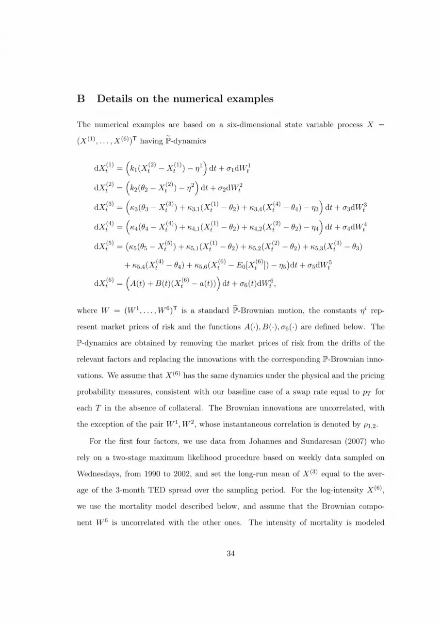
B Details on the numerical examples
The numerical examples are based on a six-dimensional state variable process X =
(X(1), . . . , X(6))T having P-dynamics
dX(1)t =
(k1(X
(2)t −X
(1)t )− η1
)dt+ σ1dW
1t
dX(2)t =
(k2(θ2 −X
(2)t )− η2
)dt+ σ2dW
2t
dX(3)t =
(κ3(θ3 −X
(3)t ) + κ3,1(X
(1)t − θ2) + κ3,4(X
(4)t − θ4)− η3
)dt+ σ3dW
3t
dX(4)t =
(κ4(θ4 −X
(4)t ) + κ4,1(X
(1)t − θ2) + κ4,2(X
(2)t − θ2)− η4
)dt+ σ4dW
4t
dX(5)t =
(κ5(θ5 −X
(5)t ) + κ5,1(X
(1)t − θ2) + κ5,2(X
(2)t − θ2) + κ5,3(X
(3)t − θ3)
+ κ5,4(X(4)t − θ4) + κ5,6(X
(6)t − E0[X
(6)t ])− η5
)dt+ σ5dW
5t
dX(6)t =
(A(t) +B(t)(X
(6)t − a(t))
)dt+ σ6(t)dW
6t ,
where W = (W 1, . . . ,W 6)T is a standard P-Brownian motion, the constants ηi rep-
resent market prices of risk and the functions A(·), B(·), σ6(·) are defined below. The
P-dynamics are obtained by removing the market prices of risk from the drifts of the
relevant factors and replacing the innovations with the corresponding P-Brownian inno-
vations. We assume that X(6) has the same dynamics under the physical and the pricing
probability measures, consistent with our baseline case of a swap rate equal to pT for
each T in the absence of collateral. The Brownian innovations are uncorrelated, with
the exception of the pair W 1,W 2, whose instantaneous correlation is denoted by ρ1,2.
For the first four factors, we use data from Johannes and Sundaresan (2007) who
rely on a two-stage maximum likelihood procedure based on weekly data sampled on
Wednesdays, from 1990 to 2002, and set the long-run mean of X(3) equal to the aver-
age of the 3-month TED spread over the sampling period. For the log-intensity X(6),
we use the mortality model described below, and assume that the Brownian compo-
nent W 6 is uncorrelated with the other ones. The intensity of mortality is modeled
34
using a continuous-time version of the Lee-Carter model (see Biffis et al., 2010). We
first use the annual central death rates my,s for US and UK males from the Hu-
man Mortality Database to estimate the model my,s = exp(α(y) + β(y)Ks) for dates
s = 1961, 1962, . . . , 2007 and ages y = 20, 21, . . . , 89 with Singular Value Decomposition.
The resulting estimates for K are then fitted with the process Ks+1 = δKKs + σKε,
with ε ∼ N(0, 1). For fixed age x = 65, the estimates for α(x + h), β(x + h)h=0,1,...
are interpolated with differentiable functions a(t), b(t). The functions A,B, σ6 are finally
obtained by setting A(t) = a′(t) + b(t)δK , B(t) = b′(t)b(t)−1 and σ6(t) = b(t)σK . The
expectation appearing in the drift of X(5) ensures that the longevity capital charges react
to departures of realized mortality from the term structure of survival rates estimated
at inception.
To estimate the dynamics of X(5), the component of collateral costs related to
longevity risk, we implement the procedure discussed in section 5, setting the dura-
tion T of the representative liability equal to 15. We simulate forward all of the other
state variables, and at each time step we compute the opportunity cost of capital arising
from the capital charges accruing to the hedge supplier based on the simulated mortality
and market conditions. We assume that funding occurs ar the LIBOR rate plus a fixed
spread of 6%, a reasonable value for the cost of internal capital. To obtain the net cost of
collateral, we take into account the rebate of the risk-free rate. We estimate the dynam-
ics of X(5) on each simulated path. We set the parameter θ5 equal to the average of X(5)
along the simulated path. The parameter estimates are computed for each simulated
path and then averaged across all simulations. The estimates are reported in table 2.
35

C Tables and figures
Date Hedger Size Term (yrs) Type Interm./supplier
Jan 08 Lucida Not disclosed 10 indexed JP MorganILS funds
Jul 2008 Canada Life GBP 500m 40 indemnity JP MorganILS funds
Feb 2009 Abbey Life GBP 1.5bn run-off indemnity Deutsche BankILS funds / Partner Re
Mar 2009 Aviva GBP 475m 10 indemnity Royal Bankof Scotland
Jun 2009 Babcock GBP 750m 50 indemnity Credit SuisseInternational Pacific Life Re
Jul 2009 RSA GBP 1.9bn run-off indemnity Goldman Sachs(Rothesay Life)
Dec 2009 Berkshire GBP 750m run-off indemnity Swiss ReCouncil
Feb 2010 BMW UK GBP 3bn run-off indemnity Deutsche BankPaternoster
Dec 2010 Swiss Re USD 50m 8 indexed ILS funds(Kortis bond)
Feb 2011 Pall (UK) GBP 70m 10 indexed JP MorganPension Fund
Table 1: Publicly announced longevity swap transactions 2008-2011.
36
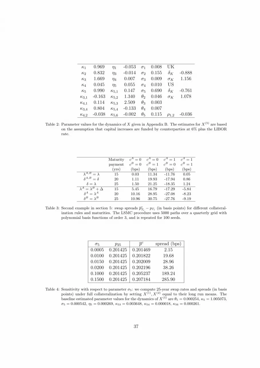
κ1 0.969 η1 -0.053 σ1 0.008 UKκ2 0.832 η3 -0.014 σ2 0.155 δK -0.888κ3 1.669 η4 0.007 σ3 0.009 σK 1.156κ4 0.045 η5 0.055 σ4 0.010 USκ5 0.990 κ5,1 0.147 σ5 0.690 δK -0.761κ3,1 -0.163 κ5,2 1.340 θ2 0.046 σK 1.078κ4,1 0.114 κ5,3 2.509 θ3 0.003κ3,4 0.804 κ5,4 -0.133 θ4 0.007κ4,2 -0.038 κ5,6 -0.002 θ5 0.115 ρ1,2 -0.036
Table 2: Parameter values for the dynamics of X given in Appendix B. The estimates for X(5) are basedon the assumption that capital increases are funded by counterparties at 6% plus the LIBORrate.
Maturity cA = 0 cA = 0 cA = 1 cA = 1payment cB = 0 cB = 1 cB = 0 cB = 1
(yrs) (bps) (bps) (bps) (bps)
λA,B = λ 15 0.03 11.34 -11.76 0.05δA,B = δ 20 1.11 19.93 -17.94 0.86δ = λ 25 1.50 21.25 -18.35 1.24
λA = λB +∆ 15 5.45 16.79 -17.29 -5.84δA = λA 20 10.16 28.95 -27.08 -8.23δB = λB 25 10.96 30.75 -27.76 -9.19
Table 3: Second example in section 5: swap spreads pcTi− pTi
(in basis points) for different collateral-ization rules and maturities. The LSMC procedure uses 5000 paths over a quarterly grid withpolynomial basis functions of order 3, and is repeated for 100 seeds.
σ5 p25 pc spread (bps)
0.0005 0.201425 0.201469 2.150.0100 0.201425 0.201822 19.680.0150 0.201425 0.202009 28.960.0200 0.201425 0.202196 38.260.1000 0.201425 0.205237 189.240.1500 0.201425 0.207184 285.90
Table 4: Sensitivity with respect to parameter σ5: we compute 25-year swap rates and spreads (in basispoints) under full collateralization by setting X(1), X(2) equal to their long run means. Thebaseline estimated parameter values for the dynamics of X(5) are θ5 = 0.000254, κ5 = 1.005073,σ5 = 0.000542, η5 = 0.000269, κ53 = 0.003648, κ54 = 0.000018, κ56 = 0.000261.
37

1980 1985 1990 1995 2000 20050.8
0.82
0.84
0.86
0.88
0.9
0.92
0.94
0.96
0.98
1
year
LC fo
reca
st
Figure 1: Survival curves computed at the beginning of each year t = 1980, . . . , 2004 for England &Wales males aged 65 + t− 1980 in year t. Forecasts are based on the Lee-Carter model usingthe latest Human Mortality Database data available at the beginning of each year t.
38

1980 1985 1990 1995 2000 2005−2500
−2000
−1500
−1000
−500
0
500
1000
year
GBP
CFsMTMMTM + 50bpsMTM + 25bps
Figure 2: Mark-to-market value of the longevity swap (MTM) and stream of cashflows with no creditrisk (CFs), and with counterparty B’s credit spreads widening by 25 and 50 basis points over1988-2005.
39

5 10 15 20 25−1
−0.8
−0.6
−0.4
−0.2
0
0.2
0.4
0.6
0.8
1
payment date
swap
mar
gin
and
perc
entil
es (
%)
25
75
45
35
65
55
Figure 3: Swap margins pcTi/pTi
− 1 computed for different maturities Ti and collateral rules, with
δA = λA and δB = λB : no collateral (squares), full collateralization (circles); λA = λB +∆,with ∆ = 0 (dashed lines) and ∆ = 0.01 (solid lines). The underlying is a cohort of 10,000US males aged 65 at the beginning of 2008. Swap rates are plotted against the percentiles ofimprovements in survival rates based on Lee-Carter forecasts.
40

5 10 15 20 25−4
−3
−2
−1
0
1
2
3
4
payment date
swap
mar
gin
and
perc
entil
es (
%)
25
75
Figure 4: Swap margins pcTi/pTi
− 1 computed for different maturities Ti and collateral rules, with
δA = λA = λB +0.01 and δB = λB : no collateral (squares), full collateralization (circles), fullcollateral posted only by party A (stars) or party B (diamonds). The underlying is a cohortof 10,000 US males aged 65 at the beginning of 2008. Swap rates are plotted against thepercentiles of improvements in survival rates based on Lee-Carter forecasts.
41

5 10 15 20 25−10
−8
−6
−4
−2
0
2
4
6
8
10
payment date
swap
mar
gin
and
perc
entil
es (%
)
25
5
75
95
Figure 5: Swap margins pcTi/pTi
− 1 computed for different maturities Ti and collateral rules, with
λA = λB and δ = X(5), where the parameter estimates of X are given in table 2. Collateralrules: no collateral (squares), full collateralization (circles), full collateral posted only by partyA (stars) or B (diamonds). Swap rates are plotted against the percentiles of improvements insurvival rates based on Lee-Carter forecasts.
42