the compound poisson risk model with a threshold dividend strategy
TRANSCRIPT

The Compound Poisson Risk Model with a Threshold Dividend
Strategy
X. Sheldon Lin
Department of Statistics
University of Toronto
Toronto, ON, M5S 3G3
Canada
tel.: (416) 946-5969
fax: (416) 978-5133
e-mail: [email protected]
Kristina P. Pavlova
Department of Statistics
University of Toronto
Toronto, ON, M5S 3G3
Canada
tel.: (416) 946-7582
fax: (416) 978-5133
e-mail: [email protected]
April 11, 2005
1

Abstract
In this paper we discuss a threshold dividend strategy implemented into the classi-
cal compound Poisson model. More specifically, we assume that no dividends are paid
if the current surplus of the insurance company is below certain threshold level. When
the surplus is above this fixed level, dividends are paid at a constant rate that does
not exceed the premium rate. This model may also be viewed as the compound Pois-
son model with the two-step premium rate. Two integro-differential equations for the
Gerber-Shiu discounted penalty function are derived and solved. When the initial sur-
plus is below the threshold, the solution is a linear combination of the Gerber-Shiu func-
tion with no barrier and the solution of the associated homogeneous integro-differential
equation. This latter function is proportional to the product of an exponential function
and a compound geometric distribution function. When the initial surplus is above the
threshold, the solution involves the respective Gerber-Shiu function with initial surplus
lower than the threshold level. These analytic results are utilized to find the probabil-
ity of ultimate ruin, the time of ruin, the distribution of the first surplus drop below
the initial level, and the joint distributions and moments of the surplus immediately
before ruin and the deficit at ruin. The special cases where the claim size distribution
is exponential and a combination of exponentials are considered in some detail.
Keywords:
compound Poisson model, deficit at ruin, Gerber-Shiu discounted penalty function, surplus
immediately before ruin, time of ruin, threshold strategy, two-step premium
Acknowledgements:
This work is partly supported by a grant from the Natural Sciences and Engineering Council
of Canada. Part of the work was completed during the first author’s visit to the Department
of Statistics and Actuarial Science, University of Hong Kong. He would like to thank K.W.
Ng and H.L. Yang for their invitation and hospitality.
1 Introduction
The classical compound Poisson risk model without constraints and related problems have
been studied extensively. See Bowers et al. (1997, Chapter 13), Gerber (1979), Klugman et
1

al. (2004), Panjer and Willmot (1992) and references therein. Recently, Gerber and Shiu
(1998) introduced a discounted penalty function with respect to the time of ruin, the surplus
immediately before ruin and the deficit at ruin to analyze these and related quantities in a
unified manner. The Gerber-Shiu discounted penalty function has proven to be a powerful
analytical tool. Various new results on the compound Poisson risk model have been obtained
since. See Gerber and Shiu (1998) and Lin and Willmot (1999, 2000). The function has also
been employed in Spare Andersen risk models (see Li and Garrido (2004a), Gerber and
Shiu (2005b) and references therein) and the compound Poisson risk model with a dividend
strategy, which will be discussed below.
Dividend strategies for insurance risk models were first proposed by De Finetti (1957) to
reflect more realistically the surplus cash flows in an insurance portfolio. Barrier strategies
for the compound Poisson risk model have been studied in a number of papers and books,
including Albrecher et al. (2005), Albrecher and Kainhofer (2002), Buhlmann (1970, Section
6.4.9), Dickson and Waters (2004), Gerber (1972), Gerber (1973), Gerber (1979), Gerber
(1981), Gerber and Shiu (1998), Gerber and Shiu (2005a), Højgaard (2002), Lin et al. (2003),
Paulsen and Gjessing (1997), and Segerdahl (1970).
Two surplus-dependent dividend strategies are of particular interest. The first is the
constant barrier strategy under which no dividend is paid when the surplus is below a
constant barrier but the total of the surplus above the barrier is paid out as dividends.
It is shown in Gerber (1969) that this strategy is optimal for the compound Poisson risk
model when the initial surplus is below the barrier. The other is the so-called threshold
strategy under which no dividends are paid when the surplus is below a constant barrier
and dividends are paid at a rate less than the premium rate when the surplus is above the
barrier. Obviously, the former strategy can be considered as a special case of the latter.
Gerber and Shiu (2005a) show that the threshold strategy is optimal when the dividend rate
is bounded from above and the individual claim distribution is exponential.
In Lin et al. (2003), the constant barrier strategy for the compound Poisson risk model is
studied thoroughly. It is shown there that the Gerber-Shiu discounted penalty function can
be expressed as a combination of two functions: the Gerber-Shiu discounted penalty function
for the compound Poisson model without a barrier and an explicit function of the tail of a
particular compound geometric distribution. Results regarding the time of ruin and related
quantities are derived. These results are generalized further by Li and Garrido (2004b).
In this paper we consider the Gerber-Shiu discounted penalty function for the compound
2

Poisson risk model under the threshold strategy. We thus provide a generalization of the
model and results in Lin et al. (2003). To introduce the model formally, let {Y1, Y2, ...} be
independent and identically distributed (i.i.d.) positive random variables representing the
successive individual claim amounts. These random variables are assumed to have common
cumulative distribution function (c.d.f.) P (y) = 1 − P (y), y ≥ 0, with probability density
function (p.d.f.) p(y) = P ′(y) and Laplace transform p(s) =∫∞
0e−sydP (y). Furthermore, let
the total number of claims up to time t, denoted by N(t) and independent of {Y1, Y2, ...}, be
a Poisson process with parameter λ > 0. Consequently, the respective i.i.d. interclaim-time
random variables {V1, V2, ...}, independent of {Y1, Y2, ...}, have an exponential distribution
with mean 1/λ. The aggregate claims process is defined by {S(t) =∑N(t)
i=1 Yi; t ≥ 0} where
S(t) = 0 if N(t) = 0.
For an insurer’s surplus process under the threshold strategy, denote u ≥ 0 to be the
initial surplus, b > 0 the constant barrier level, and c1 > 0 the annual premium rate. As
usual, we write c1 = (1 + θ1)λE{Y1}, where θ1 > 0 is the relative security loading. Let
α, 0 < α ≤ c1, be the annual dividend rate, i.e., when the surplus is above the barrier b,
dividends are paid at rate α. In this case, the net premium rate after dividend payments is
c2 = c1 − α ≥ 0. Similarly, we set c2 = (1 + θ2)λE{Y1} and note that the relative security
loading θ2 may be non-positive. The surplus process {Ub(t); t ≥ 0} can be expressed as
dUb(t) =
{c1dt− dS(t), Ub(t) ≤ b
c2dt− dS(t), Ub(t) > b,
and the time of (ultimate) ruin is defined as Tb = inf{t |Ub(t) < 0} where Tb = ∞ if ruin
does not occur in finite time. See Figure 1 for a graphical representation of a sample path
of the surplus process.
Several remarks are now made. If b = ∞, the threshold risk model reduces to the classical
model without constraints. As discussed in Lin et al. (2003), although the classical Poisson
model may be viewed as a limiting case of the present risk model, the results obtained in
this paper are not applicable. If α = c1, the threshold model coincides with the compound
Poisson model under the constant barrier strategy, studied in more detail by Lin et al. (2003).
Finally, this risk model may be interpreted as a compound Poisson model with a two-step
premium rate as discussed in Asmussen (2000, Chapter VII, Section 1) and Zhou (2004).
We now introduce the Gerber-Shiu discounted penalty function
m(u; b) = E{e−δTbw(Ub(Tb−), |Ub(Tb)|)I(Tb < ∞)|Ub(0) = u},
3

-t
6
0
u
Ub(t)
b
Ub(T−)
|Ub(T )|Tb
premium rate¾ -c1premium rate¾ -c2
Figure 1: Graphical representation of the surplus process Ub(t)
where δ ≥ 0 is interpreted as the force of interest or the variable of a Laplace transform,
w(x1, x2), x1 ≥ 0, x2 ≥ 0, is a nonnegative function of the surplus immediately before ruin,
x1, and the deficit at ruin, x2, and I(E) is the indicator function of an event E.
A number of particular cases of the discounted penalty function lead to important quanti-
ties of interest in risk theory. For instance, setting w(x1, x2) = 1 for all x1, x2 ≥ 0, we obtain
the Laplace transform of the time of ruin. When δ = 0 and w(x1, x2) = 1 for all x1, x2 ≥ 0,
the discounted penalty function reduces to the probability of ultimate ruin. Another exam-
ple is the case δ = 0 and w(x1, x2) = xh1x
l2 with h and l being nonnegative integers. The
discounted penalty function produces then the joint moments of the surplus immediately
before ruin and the deficit at ruin.
The aim of this paper is to study the Gerber-Shiu discounted penalty function and its
special cases under the threshold strategy. So far, only limited number of results have been
obtained. Asmussen (2000, Chapter VII, Section 1) discussed the probability of ruin, and
more recently Gerber and Shiu (2005a) provided two intergo-differential equations satisfied
by the Laplace transform of the time of ruin. Zhou (2004) derived some analytical expressions
related to the joint distribution of the maximal surplus before ruin, the surplus immediately
before ruin and the deficit at ruin. In this paper, we derive two integro-differential equations
and then the general solution for the discounted penalty function. Utilizing the analytical
4

expression of the solution, we obtain results on the probability of ruin, the time of ruin, and
the joint distribution and moments of the surplus immediate before ruin and the deficit at
ruin.
The rest of the paper is organized as follows. Section 2 recalls properties of the translation
operator, first employed for risk processes by Dickson and Hipp (2001) and recently discussed
by Li and Garrido (2004a) and Gerber and Shiu (2005b). A concise review of some results
obtained in Lin et al. (2003) is also recalled. In particular, we recall the general solution
of an integro-differential equation, which is satisfied by the Gerber-Shiu discounted penalty
function under the compound Poisson risk model with a constant dividend barrier strategy.
In Section 3, we derive two integro-differential equations for the discounted penalty function
under the compound Poisson risk model with a threshold strategy. In Section 4 we obtain
a renewal equation satisfied by the discounted penalty function with initial surplus above
the threshold level via the translation operator. Analytical solutions of the two integro-
differential equations are presented in Section 5. In Sections 6 to 8, we apply the analytical
solutions to the probability of ultimate ruin, the Laplace transform of the time of ruin Tb,
and the joint distribution and moments of the the surplus before ruin Ub(Tb−), and the
deficit at ruin |Ub(Tb)|. These applications are also illustrated by examples where the claim
size distribution is specified to be exponential or a combination of exponential distributions.
2 Preliminaries
In this section, we first introduce the translation operator Ts and some of its properties. We
then discuss the general solution of an integro-differential equation that is satisfied by the
Gerber-Shiu discounted penalty function under the compound Poisson risk model with and
without a dividend barrier.
Let f be a real-valued (Riemannian) integrable function and s be a nonnegative real
number (or a complex number with nonnegative real part). The translation operator Ts on
a function f is defined by
Tsf(x) =
∫ ∞
x
e−s(y−x)f(y)dy.
The operator Ts is commutative, i.e. Tr Ts = Ts Tr. Moreover,
TsTrf(x) = TrTsf(x) =Tsf(x)− Trf(x)
r − s, s 6= r. (2.1)
For more properties of the translation operator, see Gerber and Shiu (2005b).
5

As it will be seen in the next two sections, the discounted penalty function under the
threshold strategy is closely related to the discounted penalty function under the dividend
strategy. We thus need then to employ some of the notation and results obtained in Lin et
al. (2003). For convenience, we recall these results and notation here.
Consider the integro-differential equation
m′(u) =λ + δ
c1
m(u)− λ
c1
∫ u
0
m(u− y)dP (y)− λ
c1
ζ(u), u ≥ 0, (2.2)
where
ζ(t) =
∫ ∞
t
w(t, y − t)dP (y). (2.3)
It is shown in Lin et al. (2003) that the general solution of (2.2) can be expressed as
m(u) = m∞(u) + κv(u), u ≥ 0, (2.4)
where κ is an arbitrary constant, m∞ is the discounted penalty function under the classical
compound Poisson risk model with premium rate c1, and the function v satisfies the integro-
differential equation
v′(u) =λ + δ
c1
v(u)− λ
c1
∫ u
0
v(u− y)dP (y), u ≥ 0.
Furthermore, assume that the surplus process has a positive relative security loading. For
i = 1 and 2, let ρi be the nonnegative root of the Lundberg fundamental equation
cis + λp(s)− (λ + δ) = 0. (2.5)
It is then known (see Buhlmann (1970, Section 6.4.9)) that
v(u) =1−Ψ(u)
1−Ψ(0)eρ1u, u ≥ 0, (2.6)
where Ψ is the solution of the equation
Ψ′(u) =λ
c1
∫ u
0
[1−Ψ(u− y)]dP (y)− λ
c1
[1−Ψ(u)], u ≥ 0,
with
c1 =c1
p(ρ1),
and the c.d.f. P satisfying
dP (y) =e−ρ1ydP (y)
p(ρ1).
6

Therefore, Ψ is the tail of a compound geometric distribution with geometric parameter
Ψ(0) =λ
c1
∫ ∞
0
t dP (t),
and claim-size distribution, which has p.d.f. P (y)/∫∞0
t dP (t), y ≥ 0.
For i = 1 and 2, let Ai be the following c.d.f. defined through its tail
Ai(y) = 1− Ai(y) =
∫∞y
e−ρi(t−y)P (t)dt∫∞0
e−ρitP (t)dt=
TρiP (y)
TρiP (0)
, y ≥ 0. (2.7)
Obviously, it has the Laplace transform
ai(s) =
∫ ∞
0
e−sydAi(y) =ρi
1− p(ρi)· p(s)− p(ρi)
ρi − s. (2.8)
Let also define the parameter
πi =λ[1− p(ρi)]
ciρi
=λ
ci
TρiP (0), (2.9)
and observe that 0 < πi < 1 and when ρ → 0, πi → 1/(1 + θi). Then m∞ satisfies the
defective renewal equation
m∞(u) = π1
∫ u
0
m∞(u− y)dA1(y) +λ
c1
Tρ1ζ(u), u ≥ 0. (2.10)
See Gerber and Shiu (1998) or Lin and Willmot (1999) for more details concerning the
derivations.
3 Integro-Differential Equations for the Discounted Penalty Func-
tion
In this section, we derive two integro-differential equations for the discounted penalty func-
tion: one for the initial surplus below the barrier and the other for the initial surplus above
the barrier. As it will be seen later, the discounted penalty function with initial surplus
above the barrier depends on the respective function with initial surplus below the barrier.
The reverse relationship though, does not apply. We also identify a continuation condition
on the barrier.
7

Clearly, the discounted penalty function m(u; b) behaves differently, depending on whether
its initial surplus u is below or above the barrier level b. Hence, for notational convenience,
we write
m(u; b) =
{m1(u), 0 ≤ u ≤ b
m2(u), u > b.
The following theorem provides integro-differential equations for the function m(u; b).
Theorem 3.1. The discounted penalty function m(u; b) satisfies the integro-differential equa-
tions
m′(u; b) =
m′1(u) =
λ + δ
c1
m1(u)− λ
c1
∫ u
0
m1(u− y)dP (y)− λ
c1
ζ(u), 0 ≤ u ≤ b
m′2(u) =
λ + δ
c2
m2(u)− λ
c2
[ ∫ u−b
0
m2(u− y)dP (y)
+
∫ u
u−b
m1(u− y)dP (y)
]− λ
c2
ζ(u), u > b.
(3.1)
Proof. If we condition on the time and the amount of the first claim when 0 ≤ u ≤ b,
contingent on this time, there are two options: the first claim occurs before the surplus
has attained the barrier level or it occurs after attaining the barrier. When we consider
the amount of the first claim, there are two possibilities as well: after it the process starts
all over again with new initial surplus or the first claim leads to ruin. Implementing these
considerations we obtain
m(u; b) = m1(u)
=
∫ b−uc1
0
e−δt
[∫ u+c1t
0
m(u + c1t− y; b)dP (y) +
∫ ∞
u+c1t
w(u + c1t, y − u− c1t)dP (y)
]λe−λtdt
+
∫ ∞
b−uc1
e−δt
[ ∫ b+c2(t− b−u
c1
)
0
m
(b + c2
(t− b− u
c1
)− y; b
)dP (y)
+
∫ ∞
b+c2(t− b−u
c1
) w
(b + c2
(t− b− u
c1
), y − b− c2
(t− b− u
c1
))dP (y)
]λe−λtdt
=λ
∫ b−uc1
0
e−(λ+δ)tγ(u + c1t; b)dt + λ
∫ ∞
b−uc1
e−(λ+δ)tγ
(b + c2
(t− b− u
c1
); b
)dt, (3.2)
where γ(t; b) =∫ t
0m(t− y; b)dP (y) + ζ(t).
8

Now, a change of variables in (3.2) results in
m1(u) =λ
c1
e(λ+δ)u/c1
∫ b
u
e−(λ+δ)t/c1γ(t; b) dt
+λ
c2
e(λ+δ)u/c1
∫ ∞
b
e−(λ+δ)[t−(c1−c2)b/c1]/c2γ(t; b) dt, 0 ≤ u ≤ b. (3.3)
By differentiating (3.3) with respect to u we achieve
m′1(u) =
λ
c1
· λ + δ
c1
e(λ+δ)u/c1
∫ b
u
e−(λ+δ)t/c1γ(t; b) dt− λ
c1
γ(u; b)
+λ
c2
· λ + δ
c1
e(λ+δ)u/c1
∫ ∞
b
e−(λ+δ)[t−(c1−c2)b/c1]/c2γ(t; b) dt
=λ + δ
c1
m1(u)− λ
c1
γ(u; b), 0 ≤ u ≤ b,
or equivalently,
m′1(u) =
λ + δ
c1
m1(u)− λ
c1
∫ u
0
m1(u− y)dP (y)− λ
c1
ζ(u), 0 ≤ u ≤ b.
Similarly, when u ≥ b,
m(u; b) = m2(u) =λ
c2
e(λ+δ)u/c2
∫ ∞
u
e−(λ+δ)t/c2γ(t; b)dt, (3.4)
and
m′2(u) =
λ + δ
c2
m2(u)− λ
c2
γ(u; b)
=λ + δ
c2
m2(u)− λ
c2
[∫ u−b
0
m2(u− y)dP (y) +
∫ u
u−b
m1(u− y)dP (y)
]− λ
c2
ζ(u),
by which the proof is concluded.
Theorem 3.1 may be linked to previously obtained results in the literature. Namely, both
pairs of equations (5.1), (5.2) and (10.2), (10.3) in Gerber and Shiu (2005a) are special cases
of the integro-differential equations (3.1) above, although the functions (5.1) and (5.2) are
not a special case of the discounted penalty function. Another instance of an already known
result is the case when c1 = c and c2 = 0. Equation (3.2) above reduces then to equation
(2.1) in Lin et al. (2003).
We note that equation (3.1) for m1 coincides with (2.2). Consequently, the general
analytical expression (2.4) for the solution of (2.2) applies. What remains is the parameter
κ that will be determined in the next section.
9
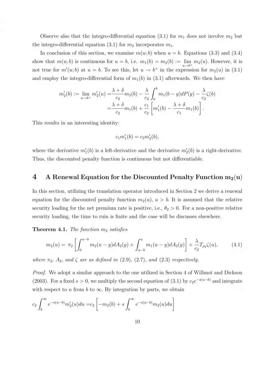
Observe also that the integro-differential equation (3.1) for m1 does not involve m2 but
the integro-differential equation (3.1) for m2 incorporates m1.
In conclusion of this section, we examine m(u; b) when u = b. Equations (3.3) and (3.4)
show that m(u; b) is continuous for u = b, i.e. m1(b) = m2(b) := limu→b+
m2(u). However, it is
not true for m′(u; b) at u = b. To see this, let u → b+ in the expression for m2(u) in (3.1)
and employ the integro-differential form of m1(b) in (3.1) afterwards. We then have
m′2(b) := lim
u→b+m′
2(u) =λ + δ
c2
m2(b)− λ
c2
∫ b
0
m1(b− y)dP (y)− λ
c2
ζ(b)
=λ + δ
c2
m1(b) +c1
c2
[m′
1(b)−λ + δ
c1
m1(b)
].
This results in an interesting identity:
c1m′1(b) = c2m
′2(b),
where the derivative m′1(b) is a left-derivative and the derivative m′
2(b) is a right-derivative.
Thus, the discounted penalty function is continuous but not differentiable.
4 A Renewal Equation for the Discounted Penalty Function m2(u)
In this section, utilizing the translation operator introduced in Section 2 we derive a renewal
equation for the discounted penalty function m2(u), u > b. It is assumed that the relative
security loading for the net premium rate is positive, i.e., θ2 > 0. For a non-positive relative
security loading, the time to ruin is finite and the case will be discusses elsewhere.
Theorem 4.1. The function m2 satisfies
m2(u) = π2
[∫ u−b
0
m2(u− y)dA2(y) +
∫ u
u−b
m1(u− y)dA2(y)
]+
λ
c2
Tρ2ζ(u), (4.1)
where π2, A2, and ζ are as defined in (2.9), (2.7), and (2.3) respectively.
Proof. We adopt a similar approach to the one utilized in Section 4 of Willmot and Dickson
(2003). For a fixed s > 0, we multiply the second equation of (3.1) by c2e−s(u−b) and integrate
with respect to u from b to ∞. By integration by parts, we obtain
c2
∫ ∞
b
e−s(u−b)m′2(u)du =c2
[−m2(b) + s
∫ ∞
b
e−s(u−b)m2(u)du
]
10
=c2s Tsm2(b)− c2m2(b)
=(λ + δ)Tsm2(b)− λ
∫ ∞
b
e−s(u−b)
∫ u−b
0
m2(u− y)dP (y)du
− λ
∫ ∞
b
e−s(u−b)
∫ b
0
m1(y)p(u− y)dydu− λTsζ(b)
=(λ + δ)Tsm2(b)− λ
∫ ∞
0
e−sy
∫ ∞
y+b
e−s(u−y−b)m2(u− y)dudP (y)
− λ
∫ b
0
m1(y)
∫ ∞
b
e−s(u−b)p(u− y)dudy − λTsζ(b)
=(λ + δ)Tsm2(b)− λp(s)Tsm2(b)− λ
∫ b
0
m1(y)Tsp(b− y)dy − λTsζ(b).
Rearranging the above terms leads to
[c2s− (λ + δ) + λp(s)]Tsm2(b) = c2m2(b)− λ
∫ b
0
m1(y)Tsp(b− y)dy − λTsζ(b). (4.2)
To determine the constant term c2m2(b) in (4.2), we substitute s there with the nonneg-
ative solution ρ2 to the Lundberg fundamental equation (2.5). Hence
c2m2(b) = λ
∫ b
0
m1(y)Tρ2p(b− y)dy + λTρ2ζ(b).
Consequently, equation (4.2) reduces to
[c2(s− ρ2) + λp(s)− λp(ρ2)]Tsm2(b) =λ
[∫ b
0
m1(y)Tρ2p(b− y)dy −∫ b
0
m1(y)Tsp(b− y)dy
]
+ λ[Tρ2ζ(b)− Tsζ(b)],
which, divided by s− ρ2, produces
[c2 − λ
p(s)− p(ρ2)
ρ2 − s
]Tsm2(b) =
[c2 − λ
1− p(ρ2)
ρ2
a2(s)
]Tsm2(b)
=λ
∫ b
0
m1(y)Tρ2p(b− y)− Tsp(b− y)
s− ρ2
dy + λTρ2ζ(b)− Tsζ(b)
s− ρ2
,
where a2(s) is given by (2.8) with i = 2. Slight rearrangements in the above equation along
with implementation of formula (2.1) lead to
c2Tsm2(b) = λ1− p(ρ2)
ρ2
a2(s)Tsm2(b) + λ
∫ b
0
m1(y)TsTρ2p(b− y)dy + λTsTρ2ζ(b).
11
We invert the operators to obtain
m2(u) = π2
∫ u−b
0
m2(u− y)dA2(y) +λ
c2
∫ u
u−b
m1(u− y)Tρ2p(y)dy +λ
c2
Tρ2ζ(u), u > b,
where π2 is as defined in (2.9) with i = 2. The above expression may be slightly simplified
by noticing that through integration by parts
Tρ2p(y)dy =
[∫ ∞
0
e−ρ2tP (t)dt
]dA2(y)
and that ∫ ∞
0
e−ρ2tP (t)dt =1− p(ρ2)
ρ2
.
Then we finally have, for u > b,
m2(u) = π2
[∫ u−b
0
m2(u− y)dA2(y) +
∫ u
u−b
m1(u− y)dA2(y)
]+
λ
c2
Tρ2ζ(u),
which is the required result.
We remark that the result in Theorem 4.1 may be restated as
m(u; b) = π2
∫ u
0
m(u− y; b)dA2(y) +λ
c2
Tρ2ζ(u), u > b.
5 Analytical Expressions for the Discounted Penalty Function
In this section, we obtain an analytical expression for the discounted penalty function. Part
of its derivation relies on results obtained in Lin and Willmot (1999) and Lin et al. (2003).
As will be seen in later sections, several results in Asmussen (2000) and Gerber and Shiu
(2005a) are special cases.
We begin with m1. Since equation (3.1) for m1 has the exact same form as equation (2.9)
in Lin et al. (2003) with c there replaced by c1 here, we may apply the same approach as far
as we obtain an initial condition for m1.
The solution m1 is then of the form
m1(u) = m∞(u) + κv(u), (5.1)
where κ is a constant, which we specify by implementing equation (5.1) and returning to
(4.1). Thus, for u = b we have
m∞(b) + κv(b) = m1(b) =m2(b)
12

= π2
∫ b
0
m∞(b− y)dA2(y) + κπ2
∫ b
0
v(b− y)dA2(y) +λ
c2
Tρ2ζ(b).
Thus,
κ =π2
∫ b
0m∞(b− y)dA2(y)−m∞(b) + λ
c2Tρ2ζ(b)
v(b)− π2
∫ b
0v(b− y)dA2(y)
.
Next, we express m∞ in terms of a compound geometric distribution. For i = 1 and 2,
introduce the following compound geometric c.d.f.
Ki(y) = 1−K i(y) =∞∑
n=0
(1− πi)πni A∗n
i (y), u ≥ 0, (5.2)
where A∗ni is the n-fold convolution of Ai with itself. Then by Theorem 2.1 in Lin and
Willmot (1999),
m∞(u) =λ
c1(1− π1)
∫ u
0
Tρ1ζ(u− y)dK1(y) +λ
c1
Tρ1ζ(u)
=λ
c1(1− π1)
[−
∫ u
0
K1(u− y)dTρ1ζ(y)−K1(u)Tρ1ζ(0) + Tρ1ζ(u)
], u ≥ 0. (5.3)
Lastly, we derive an expression for m2. Let x = u− b and g(x) = m2(x + b), x > 0. We
can then rewrite (4.1) as
g(x) = π2
∫ x
0
g(x− y)dA2(y) + h(x + b), x > 0.
where
h(x + b) = h(u) = π2
∫ u
u−b
m1(u− y)dA2(y) +λ
c2
Tρ2ζ(u), u > b.
Hence, Theorem 2.1 in Lin and Willmot (1999) applies to g(x) and we may express m2(u)
via g(x) as
m2(u) =g(x)
=1
1− π2
∫ x
0
h(x + b− y)dK2(y) + h(x + b)
=1
1− π2
∫ u−b
0
h(u− y)dK2(y) + h(u)
=− 1
1− π2
[∫ u
b
K2(u− y)dh(y) + K2(u− b)h(b)
]+ h(u). (5.4)
All above derivations are summarized by the theorem below.
13
Theorem 5.1. The discounted penalty function m(u; b) may be expressed analytically in the
following steps:
(i) m∞(u) =λ
c1(1− π1)
∫ u
0
Tρ1ζ(u− y)dK1(y) +λ
c1
Tρ1ζ(u); (5.5)
(ii) κ =π2
∫ b
0m∞(b− y)dA2(y)−m∞(b) + λ
c2Tρ2ζ(b)
v(b)− π2
∫ b
0v(b− y)dA2(y)
; (5.6)
(iii) m1(u) = m∞(u) + κ1−Ψ(u)
1−Ψ(0)eρ1u, 0 ≤ u ≤ b; (5.7)
(vi) h(u) = π2
∫ u
u−b
m1(u− t)dA2(t) +λ
c2
Tρ2ζ(u), u > b, (5.8)
(v) m2(u) =1
1− π2
∫ u−b
0
h(u− y)dK2(y) + h(u), u > b, (5.9)
where Ki, i = 1, 2, are given in (5.2).
The definitions of the remaining functions and parameters utilized in Theorem 5.1 above
are provided in Sections 2 and 3. Also note that equations (5.5) and (5.8) have alternative
forms provided by (5.3) and (5.4) respectively.
We now proceed with some important special cases in the rest of the paper.
6 The Probability of Ultimate Ruin
This section discusses the probability that the time of ruin is finite, or the probability of
ultimate ruin, and the probability of a drop below the initial surplus level as a special case.
As it is well known, many particular cases of the discounted penalty function, which
result in important quantities of interest in risk theory, are produced when δ is set to be 0.
The nonnegative solutions of the respective Lundberg fundamental equations (2.5) are then
ρ1 = ρ2 = 0. On one hand, this implies that πi = 1/(1 + θi), i = 1, 2, as noted after the
definition in (2.9). On the other hand, by (2.7) both A1 and A2 reduce to the first order
14

equilibrium distribution Pe of P, namely,
Pe(y) = 1− P e(y) =
∫ y
0
P (t)dt
E{Y1} =
∫ y
0
pe(t)dt, y ≥ 0,
where pe = P (t)/E{Y1} is the equilibrium p.d.f.
Furthermore, Tρ1ζ(u) = Tρ2ζ(u) =∫∞
uζ(t)dt and the definition of Ψ in Section 2 shows
that Ψ(u) = ψ1,∞(u), u ≥ 0, where ψ1,∞ is the probability of ultimate ruin under the
classical compound Poisson model with premium rate c1. Also, with the changes in πi and
Ai, i = 1, 2, it is clear that K1 and K2, defined by (5.2), coincide with the probabilities
of ultimate ruin ψ1,∞ and ψ2,∞ respectively. Here ψ2,∞ is the probability of ultimate ruin
under the ordinary compound Poisson model with premium rate c2. It is well known that
ψ1,∞(0) = 1/(1 + θ1) and ψ2,∞(0) = 1/(1 + θ2).
After setting δ = 0, let also assume that w(x1, x2) = 1 for all x1, x2 ≥ 0. Then m(u; b)
becomes the probability of ultimate ruin, which we denote by ψb. Also, by (2.3) ζ reduces
to P .
From Theorem 5.1 we have the following result.
Theorem 6.1. The probability of ultimate ruin for the compound Poisson risk model with
a threshold strategy is given by
ψ(u; b) =
ψ1(u) = 1− q(b) + q(b)ψ1,∞(u), 0 ≤ u ≤ b
ψ2(u) = −1 + θ2
θ2
∫ u−b
0
h(u− y)dψ2,∞(y) + h(u), u > b,
(6.1)
with
q(b) =θ2
(θ1 − θ2)ψ1,∞(b) + θ2
(6.2)
belonging to the interval [0,1] and
h(u) =1
1 + θ2
∫ u
u−b
ψ1(u− t)dPe(t) +1
1 + θ2
P e(u), u > b. (6.3)
Proof. Equation (5.6) yields
κ =
1
1 + θ2
∫ b
0
ψ1,∞(b− y)dPe(y)− ψ1,∞(b) +1
1 + θ2
P e(b)
1− ψ1,∞(b)
1− ψ1,∞(0)− 1
1 + θ2
∫ b
0
1− ψ1,∞(b− y)
1− ψ1,∞(0)dPe(y)
15

=[1− ψ1,∞(0)]
1
1 + θ2
[(1 + θ1)ψ1,∞(b)− P e(b)]− ψ1,∞(b) +1
1 + θ2
P e(b)
1− ψ1,∞(b)− 1
1 + θ2
[Pe(b)−
∫ b
0
ψ1,∞(b− y)dPe(y)
]
=[1− ψ1,∞(0)]
(1 + θ1
1 + θ2
− 1
)ψ1,∞(b)
1− ψ1,∞(b)− 1
1 + θ2
Pe(b) +1 + θ1
1 + θ2
ψ1,∞(b)− 1
1 + θ2
P e(b)
=[1− ψ1,∞(0)](θ1 − θ2)ψ1,∞(b)
(θ1 − θ2)ψ1,∞(b) + θ2
.
By equation (5.7) we have
ψ1(u) =ψ1,∞(u) +(θ1 − θ2)ψ1,∞(b)
(θ1 − θ2)ψ1,∞(b) + θ2
[1− ψ1,∞(u)]
=(θ1 − θ2)ψ1,∞(b)
(θ1 − θ2)ψ1,∞(b) + θ2
+θ2
(θ1 − θ2)ψ1,∞(b) + θ2
ψ1,∞(u), 0 ≤ u ≤ b,
which produces (6.1). The remaining part of the proof follows directly from Theorem 5.1
along with the assumptions about δ and w.
We remark that formula (6.1) implies that ψ1 is a weighted average of the probability of
ruin in the dividend case and the probability of ruin in the ordinary Poisson model.
Also, as a particular case of (6.1), we obtain the following.
Corollary 6.2. For 0 ≤ u ≤ b the probability of a drop below the initial surplus level u, is
provided by
ψ(0; b− u) =(1 + θ1)(θ1 − θ2)ψ1,∞(b− u) + θ2
(1 + θ1) [(θ1 − θ2)ψ1,∞(b− u) + θ2]. (6.4)
Proof. We find
ψ(0; b− u) =1− q(b− u) + q(b− u)ψ1,∞(0) = 1− θ1
1 + θ1
q(b− u)
=(1 + θ1)(θ1 − θ2)ψ1,∞(b− u) + θ2
(1 + θ1) [(θ1 − θ2)ψ1,∞(b− u) + θ2], 0 ≤ u ≤ b,
by employing (6.1) and (6.2).
Note that when u > b, the probability of a drop below the initial level, ψ0(0) under
the present model, reduces to the same probability under the classical compound Poisson
model with premium rate c2. The distribution of the first drop below the initial level will be
discussed in Section 8.
16

An advantage of formula (6.1) over the result of Proposition 1.10 in Asmussen (2000,
Chapter VII, Section 1) is that all functions involved in Theorem 6.1 have a known form
and hence can be computed straightforwardly. This becomes obvious when illustrated in the
following two examples.
Example 6.1. (Exponential Claim Amounts)
When the individual claim amounts are exponentially distributed with mean 1/µ, µ > 0,
upon a little algebra it is seen that
P (y) = 1− e−µy = Pe(y), y ≥ 0.
Let βi = θi
1+θiµ, i = 1, 2, be the Lundberg adjustment coefficient for the compound Poisson
risk model with premium rate ci. Then, it is well known that
ψi,∞(u) =1
1 + θi
e−βiu, u ≥ 0, i = 1, 2.
Hence, by (6.4) the probability of a drop below the initial surplus level is given by
ψ(0; b− u) =(θ1 − θ2)e
−β1(b−u) + θ2
(θ1 − θ2)e−β1(b−u) + (1 + θ1)θ2
, 0 ≤ u ≤ b.
Also, it follows from (6.1) that
ψ1(u) =1− q(b) +q(b)
1 + θ1
e−β1u, 0 ≤ u ≤ b, (6.5)
with
q(b) =(1 + θ1)θ2
(θ1 − θ2)e−β1b + (1 + θ1)θ2
(6.6)
by (6.2). Equation (6.5) yields further that (6.3) reduces to
h(u) =1
1 + θ2
{−
∫ u
u−b
[1− q(b)]de−µt − q(b)
1 + θ1
∫ u
u−b
e−β1(u−t)de−µt + e−µu
}
=1
1 + θ2
{[1− q(b)]e−µ(u−b) − [1− q(b)]e−µu +
µq(b)
1 + θ1
e−β1u
∫ u
u−b
e(β1−µ)tdt + e−µu
}
=1
1 + θ2
{[1− q(b)]e−µ(u−b) + q(b)e−µu +
µq(b)
1 + θ1
· 1
β1 − µe−β1u
[1− e−(β1−µ)b
]e(β1−µ)u
}
=1
1 + θ2
{[1− q(b)]e−µ(u−b) + q(b)e−µu − q(b)
[1− e−(β1−µ)b
]e−µu
}
=1
1 + θ2
[1− q(b) + q(b)e−β1b
]e−µ(u−b)
17

=1
1 + θ2
Q(b)e−µ(u−b), u > b, (6.7)
where Q(b) = 1− q(b) + q(b)e−β1b. Therefore, (6.1) produces
ψ2(u) =1
1 + θ2
{− 1
θ2
∫ u−b
0
Q(b)e−µ(u−y−b)de−β2y + Q(b)e−µ(u−b)
}
=1
1 + θ2
{Q(b)
β2
θ2
∫ u−b
0
e−(β2−µ)ydy + Q(b)
}e−µ(u−b)
=1
1 + θ2
{−Q(b)
β2
θ2
· 1
β2 − µ
[e−(β2−µ)(u−b) − 1
]+ Q(b)
}e−µ(u−b)
=1
1 + θ2
{Q(b)
[e−(β2−µ)(u−b) − 1
]+ Q(b)
}e−µ(u−b)
=1
1 + θ2
Q(b)e−β2(u−b), u > b. (6.8)
To summarize,
ψ(u; b) =
ψ1(u) = 1− q(b) +q(b)
1 + θ1
e−β1u, 0 ≤ u ≤ b
ψ2(u) =1
1 + θ2
[1− q(b) + q(b)e−β1b
]e−β2(u−b), u > b,
with q(b) specified by (6.6) and βi = θi
1+θiµ, i = 1, 2, which coincides with the result obtained
in Example 1.11 in Asmussen (2000, Chapter VII, Section 1).
It is easy to see that 0 ≤ Q(b) ≤ 1. Hence we obtain a Lundberg-type upper bound for
ψ2(u):
ψ2(u) ≤ 1
1 + θ2
e−β2(u−b).
¤
Example 6.2. (Combination of Exponentials Claim Amounts)
Consider now the individual claim amounts have a combination of exponentials distribu-
tion. More specifically,
P (y) =n∑
j=1
ωj e−µjy, y ≥ 0, µj > 0, j = 1, 2, . . . , n,
with∑n
j=1 ωj = 1 for a positive integer number n.
As noted in Gerber et al. (1987),
P e(y) =n∑
j=1
ω∗j e−µjy, y ≥ 0,
18

where
ω∗j =ωj/µj∑nl=1 ωl/µl
, j = 1, 2, . . . , n,
and
ψi,∞(u) =n∑
j=1
Cije−βiju, u ≥ 0, i = 1, 2,
where 0 < βi1 < βi2 < · · · < βin are the roots of∑n
j=1 [ω∗j µj/(µj − β)] = 1 + θi, i = 1, 2,
assumed to be real valued and distinct, and
Cij =
[n∑
l=1
ω∗lµl − βij
]/ [n∑
l=1
ω∗l µl
(µl − βij)2
], i = 1, 2, j = 1, 2, . . . , n.
We remark that βi1, i = 1, 2, are the Lundberg adjustment coefficients.
It follows from Corollary 6.2 that the probability of a drop below the initial surplus level
is given by
ψ(0; b− u) =(1 + θ1)(θ1 − θ2)
∑nj=1 C1je
−β1j(b−u) + θ2
(1 + θ1)[(θ1 − θ2)
∑nj=1 C1je−β1j(b−u) + θ2
] , 0 ≤ u ≤ b.
Furthermore, it is easy to see
ψ1(u) = 1− q(b) + q(b)n∑
j=1
C1je−β1ju, 0 ≤ u ≤ b,
where
q(b) =θ2
(θ1 − θ2)∑n
j=1 C1j e−β1jb + θ2
.
Before we derive an analytical expression for ψ2(u), two useful identities are presented.
Slightly changing the notation, formula (10.4.13) in Willmot and Lin (2001) becomes
n∑
l=1
βilCil
µj − βil
=θi
1 + θi
, i = 1, 2. (6.9)
Since∑n
l=1 Cil = ψi,∞(0) = 1/(1 + θi), we have
n∑
l=1
µjCil
µj − βil
=n∑
l=1
Cil +n∑
l=1
βilCil
µj − βil
=1
1 + θi
+θi
1 + θi
= 1, i = 1, 2. (6.10)
19

Analogously to equations (6.7) and (6.8) we find respectively
h(u) =1
1 + θ2
n∑j=1
ω∗j
{µj
∫ u
u−b
ψ1(u− t)e−µjtdt + e−µju
}
=1
1 + θ2
n∑j=1
ω∗j
{[1− q(b)]e−µj(u−b) + q(b)e−µju
+ q(b)n∑
l=1
µjC1l
µj − β1l
[e−β1lbe−µj(u−b) − e−µju
] }.
Using identity (6.10) with i = 1, we have
h(u) =n∑
j=1
ω∗j Qj(b)e−µj(u−b), (6.11)
where
Qj(b) = 1− q(b) + q(b)n∑
l=1
µjC1l
µj − β1l
e−β1lb, j = 1, · · · , n.
Thus,
ψ2(u) =1
θ2
n∑j=1
ω∗j Qj(b)n∑
l=1
β2lC2l
µj − β2l
e−β2l(u−b)
+n∑
j=1
ω∗j Qj(b)
{1
1 + θ2
− 1
θ2
n∑
l=1
β2lC2l
µj − β2l
}e−µj(u−b)
=1
θ2
n∑j=1
ω∗j Qj(b)n∑
l=1
β2lC2l
µj − β2l
e−β2l(u−b)
=1
θ2
n∑j=1
β2jC2j
{n∑
l=1
ω∗l Ql(b)
µl − β2j
}e−β2j(u−b), u > b,
due to identity (6.9) with i = 2. Therefore,
ψ(u; b) =
ψ1(u) = 1− q(b) + q(b)n∑
j=1
C1j e−β1ju, 0 ≤ u ≤ b
ψ2(u) =1
θ2
n∑j=1
β2jC2j
[n∑
l=1
ω∗l Ql(b)
µl − β2j
]e−β2j(u−b), u > b.
If the individual claim distribution is a mixture, i.e., ωj ≥ 0 for all j, then Cil ≥ 0 for all
l and i = 1, 2. Hence, 0 ≤ Qj(b) ≤ 1 for all j. We can again obtain a Lundberg-type upper
20

bound for ψ2(u) in this case:
ψ2(u) =1
θ2
n∑j=1
ω∗j Qj(b)n∑
l=1
β2lC2l
µj − β2l
e−β2l(u−b)
≤ 1
θ2
n∑j=1
ω∗j Qj(b)n∑
l=1
β2lC2l
µj − β2l
e−β21(u−b)
=1
1 + θ2
n∑j=1
ω∗j Qj(b)e−β21(u−b) ≤ 1
1 + θ2
e−β21(u−b), u > b.
¤
7 The time of ruin
In this section we turn our attention to another particular case of m(u; b). We consider the
defective Laplace transform of the ruin time E{e−δTbI(Tb < ∞)|Ub(0) = u} by letting δ ≥ 0 to
be arbitrary and setting w(x1, x2) = 1 for all x1, x2 ≥ 0. Recall that in this case ζ reduces to
P. Also, when δ > 0, without loss of generality we may consider E{e−δTb|Ub(0) = u} instead
of the above-mentioned Laplace transform. For δ = 0 we have the probability of ultimate
ruin, discussed in Section 6. Once the Laplace transform of the time of ultimate ruin Tb is
identified, its distribution may be obtained using an inversion method. Its moments may be
obtained by differentiation with respect to δ. Although such tasks are theoretically possible,
they are practically tedious and challenging as demonstrated in Drekic et al. (2004). It is
partly due to the fact that the discounted penalty function m(u; b) given in Theorem 5.1 is
not explicitly expressed in terms of δ. Instead, it is expressed via ρ1 = ρ1(δ) and ρ2 = ρ2(δ).
Let
L(u; b) = m(u; b)∣∣∣w≡1
,
L1(u) = m1(u)∣∣∣w≡1
, L2(u) = m2(u)∣∣∣w≡1
,
and
L∞(u) = m∞(u)∣∣∣w≡1
.
We note that the above notation is somewhat misleading as the true variable is δ that is
implicitly included in these functions. However, expressing them in terms of u is necessary
for our derivation purposes. We now utilize our main result to derive the Laplace transform
of Tb.
21
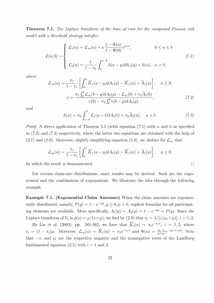
Theorem 7.1. The Laplace transform of the time of ruin for the compound Poisson risk
model with a threshold strategy satisfies
L(u; b) =
L1(u) = L∞(u) + κ1−Ψ(u)
1−Ψ(0)eρ1u, 0 ≤ u ≤ b
L2(u) =1
1− π2
∫ u−b
0
h(u− y)dK2(y) + h(u), u > b,
(7.1)
where
L∞(u) =π1
1− π1
[∫ u
0
K1(u− y)dA1(y)−K1(u) + A1(u)
], u ≥ 0,
κ =π2
∫ b
0L∞(b− y)dA2(y)− L∞(b) + π2A2(b)
v(b)− π2
∫ b
0v(b− y)dA2(y)
, (7.2)
and
h(u) = π2
∫ u
u−b
L1(u− t)dA2(t) + π2A2(u), u > b. (7.3)
Proof. A direct application of Theorem 5.1 yields equation (7.1) with κ and h as specified
in (7.2) and (7.3) respectively, where the latter two equations are obtained with the help of
(2.7) and (2.9). Moreover, slightly simplifying equation (5.3), we deduce for L∞ that
L∞(u) =π1
1− π1
[∫ u
0
K1(u− y)dA1(y)−K1(u) + A1(u)
], u ≥ 0,
by which the result is demonstrated.
For certain claim-size distributions, exact results may be derived. Such are the expo-
nential and the combination of exponentials. We illustrate the idea through the following
example.
Example 7.1. (Exponential Claim Amounts) When the claim amounts are exponen-
tially distributed, namely, P (y) = 1− e−µy, y ≥ 0, µ > 0, explicit formulae for all participat-
ing elements are available. More specifically, A1(y) = A2(y) = 1 − e−µy = P (y). Since the
Laplace transform of Y1 is p(s) = µ/(s+µ), we find by (2.9) that πi = λ/[ci(ρi +µ)], i = 1, 2.
By Lin et al. (2003), pp. 561-562, we have that K i(u) = πie−τiu, i = 1, 2, where
τi = (1 − πi)µ. Moreover, L∞(u) = K1(u) = π1e−τ1u and Ψ(u) = µ−τ1
µ+ρ1e−(ρ1+τ1)u. Note
that −τi and ρi are the respective negative and the nonnegative roots of the Lundberg
fundamental equation (2.5) with i = 1 and 2.
22
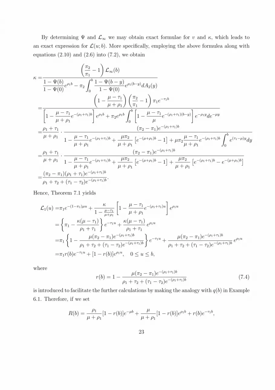
By determining Ψ and L∞ we may obtain exact formulae for v and κ, which leads to
an exact expression for L(u; b). More specifically, employing the above formulea along with
equations (2.10) and (2.6) into (7.2), we obtain
κ =
(π2
π1
− 1
)L∞(b)
1−Ψ(b)
1−Ψ(0)eρ1b − π2
∫ b
0
1−Ψ(b− y)
1−Ψ(0)eρ1(b−y)dA2(y)
=
(1− µ− τ1
µ + ρ1
)(π2
π1
− 1
)π1e
−τ1b
[1− µ− τ1
µ + ρ1
e−(ρ1+τ1)b
]eρ1b + π2e
ρ1b
∫ b
0
[1− µ− τ1
µe−(ρ1+τ1)(b−y)
]e−ρ1yde−µy
=ρ1 + τ1
µ + ρ1
· (π2 − π1)e−(ρ1+τ1)b
1− µ− τ1
µ + ρ1
e−(ρ1+τ1)b +µπ2
µ + ρ1
[e−(µ+ρ1)b − 1
]+ µπ2
µ− τ1
µ + ρ1
e−(ρ1+τ1)b
∫ b
0
e(τ1−µ)ydy
=ρ1 + τ1
µ + ρ1
· (π2 − π1)e−(ρ1+τ1)b
1− µ− τ1
µ + ρ1
e−(ρ1+τ1)b +µπ2
µ + ρ1
[e−(µ+ρ1)b − 1
]+
µπ2
µ + ρ1
[e−(ρ1+τ1)b − e−(µ+ρ1)b
]
=(π2 − π1)(ρ1 + τ1)e
−(ρ1+τ1)b
ρ1 + τ2 + (τ1 − τ2)e−(ρ1+τ1)b
.
Hence, Theorem 7.1 yields
L1(u) =π1e−(1−π1)µu +
κ
1− µ−τ1µ+ρ1
[1− µ− τ1
µ + ρ1
e−(ρ1+τ1)u
]eρ1u
=
{π1 − κ(µ− τ1)
ρ1 + τ1
}e−τ1u +
κ(µ− τ1)
ρ1 + τ1
eρ1u
=π1
{1− µ(π2 − π1)e
−(ρ1+τ1)b
ρ1 + τ2 + (τ1 − τ2)e−(ρ1+τ1)b
}e−τ1u +
µ(π2 − π1)e−(ρ1+τ1)b
ρ1 + τ2 + (τ1 − τ2)e−(ρ1+τ1)b
eρ1u
=π1r(b)e−τ1u + [1− r(b)]eρ1u, 0 ≤ u ≤ b,
where
r(b) = 1− µ(π2 − π1)e−(ρ1+τ1)b
ρ1 + τ2 + (τ1 − τ2)e−(ρ1+τ1)b
(7.4)
is introduced to facilitate the further calculations by making the analogy with q(b) in Example
6.1. Therefore, if we set
R(b) =ρ1
µ + ρ1
[1− r(b)]e−µb +µ
µ + ρ1
[1− r(b)]eρ1b + r(b)e−τ1b,
23
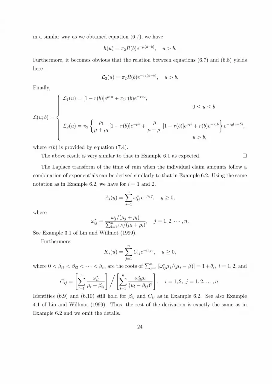
in a similar way as we obtained equation (6.7), we have
h(u) = π2R(b)e−µ(u−b), u > b.
Furthermore, it becomes obvious that the relation between equations (6.7) and (6.8) yields
here
L2(u) = π2R(b)e−τ2(u−b), u > b.
Finally,
L(u; b) =
L1(u) = [1− r(b)]eρ1u + π1r(b)e−τ1u,
0 ≤ u ≤ b
L2(u) = π2
{ρ1
µ + ρ1
[1− r(b)]e−µb +µ
µ + ρ1
[1− r(b)]eρ1b + r(b)e−τ1b
}e−τ2(u−b),
u > b,
where r(b) is provided by equation (7.4).
The above result is very similar to that in Example 6.1 as expected. ¤
The Laplace transform of the time of ruin when the individual claim amounts follow a
combination of exponentials can be derived similarly to that in Example 6.2. Using the same
notation as in Example 6.2, we have for i = 1 and 2,
Ai(y) =n∑
j=1
ω∗ij e−µjy, y ≥ 0,
where
ω∗ij =ωj/(µj + ρi)∑nl=1 ωl/(µl + ρi)
, j = 1, 2, · · · , n.
See Example 3.1 of Lin and Willmot (1999).
Furthermore,
Ki(u) =n∑
j=1
Cije−βiju, u ≥ 0,
where 0 < βi1 < βi2 < · · · < βin are the roots of∑n
j=1 [ω∗ijµj/(µj − β)] = 1+ θi, i = 1, 2, and
Cij =
[n∑
l=1
ω∗ilµl − βij
]/ [n∑
l=1
ω∗ilµl
(µl − βij)2
], i = 1, 2, j = 1, 2, . . . , n.
Identities (6.9) and (6.10) still hold for βij and Cij as in Example 6.2. See also Example
4.1 of Lin and Willmot (1999). Thus, the rest of the derivation is exactly the same as in
Example 6.2 and we omit the details.
24
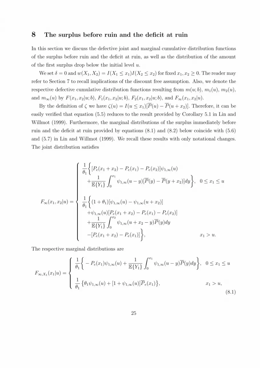
8 The surplus before ruin and the deficit at ruin
In this section we discuss the defective joint and marginal cumulative distribution functions
of the surplus before ruin and the deficit at ruin, as well as the distribution of the amount
of the first surplus drop below the initial level u.
We set δ = 0 and w(X1, X2) = I(X1 ≤ x1)I(X2 ≤ x2) for fixed x1, x2 ≥ 0. The reader may
refer to Section 7 to recall implications of the discount free assumption. Also, we denote the
respective defective cumulative distribution functions resulting from m(u; b), m1(u), m2(u),
and m∞(u) by F (x1, x2|u; b), F1(x1, x2|u; b), F2(x1, x2|u; b), and F∞(x1, x2|u).
By the definition of ζ we have ζ(u) = I(u ≤ x1)[P (u)− P (u + x2)]. Therefore, it can be
easily verified that equation (5.5) reduces to the result provided by Corollary 5.1 in Lin and
Willmot (1999). Furthermore, the marginal distributions of the surplus immediately before
ruin and the deficit at ruin provided by equations (8.1) and (8.2) below coincide with (5.6)
and (5.7) in Lin and Willmot (1999). We recall these results with only notational changes.
The joint distribution satisfies
F∞(x1, x2|u) =
1
θ1
{[Pe(x1 + x2)− Pe(x1)− Pe(x2)]ψ1,∞(u)
+1
E{Y1}∫ x1
0
ψ1,∞(u− y)[P (y)− P (y + x2)]dy
}, 0 ≤ x1 ≤ u
1
θ1
{(1 + θ1)[ψ1,∞(u)− ψ1,∞(u + x2)]
+ψ1,∞(u)[Pe(x1 + x2)− Pe(x1)− Pe(x2)]
+1
E{Y1}∫ x2
0
ψ1,∞(u + x2 − y)P (y)dy
−[Pe(x1 + x2)− Pe(x1)]
}, x1 > u.
The respective marginal distributions are
F∞,X1(x1|u) =
1
θ1
{− Pe(x1)ψ1,∞(u) +
1
E{Y1}∫ x1
0
ψ1,∞(u− y)P (y)dy
}, 0 ≤ x1 ≤ u
1
θ1
{θ1ψ1,∞(u) + [1 + ψ1,∞(u)]P e(x1)
}, x1 > u,
(8.1)
25

and
F∞,X2(x2|u) =1
θ1
{(1 + θ1)[ψ1,∞(u)− ψ1,∞(u + x2)]− ψ1,∞(u)Pe(x2)
+1
E{Y1}∫ x2
0
ψ1,∞(u + x2 − y)P e(y)dy
}. (8.2)
Hence, equations (5.4) to (5.8) produce analytical expressions for F (x1, x2|u; b).
Theorem 8.1. Let
σ(x1, x2|u) = P e(u) + P e(x1 + x2)− P e(x1)− P e(u + x2), u ≥ 0.
Then F (x1, x2|u; b) is given by
F1(x1, x2|u; b) = F∞(x1, x2|b) + κ[1− ψ1,∞(u)], 0 ≤ u ≤ b,
F2(x1, x2|u; b) = −1 + θ2
θ2
[∫ u
b
ψ2,∞(u− y)dh(y) + ψ2,∞(u− b)h(b)
]+ h(u), u > b,
with
κ =(θ1 − θ2)F∞(x1, x2|b)− P e(b) + I(b ≤ x1)σ(x1, x2|b)
(θ1 − θ2)ψ1,∞(b) + θ2
,
and
h(u) =1
1 + θ2
∫ u
u−b
F1(x1, x2|u− y; b)dPe(y) +I(u ≤ x1)
1 + θ2
σ(x1, x2|u), u > b.
Letting either x2 → ∞, or x1 → ∞ we derive either the defective marginal c.d.f. of the
surplus before ruin, or the defective marginal c.d.f. of the deficit at ruin, respectively.
Corollary 8.2. The defective marginal c.d.f. of the surplus immediately before ruin FX1(x1|u; b)
is given by
F1,X1(x1|u; b) = F∞,X1(x1|b) + κ[1− ψ1,∞(u)], 0 ≤ u ≤ b,
F2,X1(x1|u; b) = −1 + θ2
θ2
[∫ u
b
ψ2,∞(u− y)dh(y) + ψ2,∞(u− b)h(b)
]+ h(u), u > b,
where
κ =(θ1 − θ2)F∞,X1(x1|b)− P e(b) + I(u ≤ x1)[P e(b)− P e(x1)]
(θ1 − θ2)ψ1,∞(b) + θ2
,
and
h(u) =1
1 + θ2
∫ u
u−b
F1,X1(x1|u− y; b)dPe(y) +I(u ≤ x1)
1 + θ2
[P e(u)− P e(x1)], u > b.
26

In a similar manner, we obtain a respective result regarding the severity at ruin.
Corollary 8.3. The defective marginal c.d.f. of the deficit at ruin FX2(x2|u; b) may be
obtained through
F1,X2(x2|u; b) = F∞,X2(x2|b) + κ[1− ψ1,∞(u)], 0 ≤ u ≤ b,
F2,X2(x2|u; b) = −1 + θ2
θ2
[∫ u
b
ψ2,∞(u− y)dh(y) + ψ2,∞(u− b)h(b)
]+ h(u), u > b,
with
κ =(θ1 − θ2)F∞,X2(x2|b)− P e(b + x2)
(θ1 − θ2)ψ1,∞(b) + θ2
,
and
h(u) =1
1 + θ2
∫ u
u−b
F1,X2(x2|u− y; b)dPe(y) +1
1 + θ2
[P e(u)− P e(u + x2)], u > b.
When the barrier level is b − u and the initial surplus is 0, Corollary 8.3 yields the
distribution of the first surplus drop below the initial level.
Corollary 8.4. The distribution of the first surplus drop below the initial level is given by
G(x2|0) = F∞,X2(x2|b− u) +θ1
1 + θ1
κ, 0 ≤ u ≤ b,
with
κ =(θ1 − θ2)F∞,X2(x2|b− u)− P e(b− u + x2)
(θ1 − θ2)ψ1,∞(b− u) + θ2
.
It is possible to obtain joint and marginal moments of the surplus before ruin and the
deficit at ruin. We set w(x1, x2) = xh1x
l2 for an arbitrary pair of nonnegative integers h and
l. Denote then by F h,l(u; b), F h,l1 (u), F h,l
2 (u), and F h,l∞ (u) the joint moments resulting from
m(u; b), m1(u), m2(u), and m∞(u) respectively with the specific choice of w.
In order to simplify the expressions to follow, let n be a nonnegative integer and define
recursively the nth order equilibrium tail of P to be
P e,n(y) = 1− Pe,n(y) =
∫∞y
P e,n−1(t)dt∫∞0
P e,n−1(t)dt,
with P 0,e(t) = P (t) and P 1,e(t) = P e(t). If in addition, we define pn =∫∞0
yndP (y) to be the
nth moment of Y1, we can apply formula (2.4) in Lin and Willmot (2000), namely,
P e,n(y) =1
pn
∫ ∞
y
(t− y)ndP (t)
27

to find ∫ ∞
u
ζ(t)dt = pl
∫ ∞
u
thP e,l(t)dt
for this particular form of w. Therefore, equations (5.4) to (5.8) yield the following.
Theorem 8.5.
F h,l(u; b) =
F h,l1 (u) = F h,l
∞ (u) + κ[1− ψ1,∞(u)], 0 ≤ u ≤ b,
F h,l2 (u) = −1 + θ2
θ2
[∫ u
b
ψ2,∞(u− y)dh(y) + ψ1,∞(u− b)h(b)
]+ h(u), u > b,
(8.3)
where
F h,l∞ (u) =
θ1pl
p1
{∫ u
0
yh[ψ1,∞(u− y)− ψ1,∞(u)]P e,l(y)dy +
∫ ∞
u
yh[1− ψ1,∞(u)]P e,l(y)dy
},
κ =(θ2 − θ1)F
h,l∞ (b)− P e(b) + pl
p1
∫∞b
thP e,l(t)dt
(θ2 − θ1)ψ1,∞(b) + θ2
,
and
h(u) =1
1 + θ2
∫ u
u−b
F h,l1 (u− y)dPe(y) +
λpl
c2
∫ ∞
u
thP e,l(t)dt, u > b. (8.4)
To obtain marginal moments of the surplus immediately before ruin or the deficit at ruin,
simply set l = 0 or h = 0 in equations (8.3) to (8.4).
We want to point out that further simplification for the results in Theorems 8.1 and 8.5,
Corollaries 8.2, and 8.3 is possible. For example we may use the explicit expressions obtained
in Lin and Willmot (2000), pp. 29 and 32 for the joint and marginal moments F h,l∞ , F h
∞ and
F l∞ in Theorem 8.5. However, since the simplification does not provide new insight, we omit
it in this paper.
References
Albrecher, H., Hartinger, J., Tichy, R., 2005, On the distribution of dividend payments and
the discounted penalty function in a risk model with linear dividend barrier, Scancdinavian
Actuarial Journal, forthcomming.
Albrecher, H., Kainhofer, R., 2002, Risk theory with a nonlinear divident barrier, Computing,
68, 289-311.
28

Asmussen, S., 2000, Ruin Probabilities, World Scientific Publishing Co. Pte. Inc.
Bowers, N.L., Gerber, H.U., Hickman, J.C., Jones, D.A., Nesbitt, C.J., 1997, Actuarial
Mathematics, Society of Actuaries.
Buhlmann, H., 1970, Mathematical Methods in Risk Theory, Springer, New York.
De Finetti, B., 1957, Su un’impostazione alternativa della teoria collettiva del rischio, Trans-
actions of the XV International Congress of Actuaries, 2, 433-443.
Dickson, D.C.M., Hipp, C., 2001, On the time of ruin for Erlang(2) risk processes, Insurance:
Mathematics and Economics, 29, 333-344.
Dickson, D.C.M., Waters, H.R., 2004, Some optimal dividend problems, ASTIN Bulletin,
34: 49-74.
Drekic, S., Stafford, J.E., Willmot, G.E., 2004, Symbolic calculation of the moments of the
time of ruin, Insurance: Mathematics and Economics, 34, 109-120.
Gerber, H.U., 1969, Entscheidungskriterien fur den zusammengesetzten Poisson-Prozess,
Ph.D. thesis, ETHZ.
Gerber, H.U., 1972, Games of economic survival with discrete- and continuous-income pro-
cesses, Operations Research, 20, 37-45.
Gerber, H.U., 1973, Martingales in risk theory, Mutteilungen der Schweizer Vereinigung der
Versicherungsmathematiker, 205-216.
Gerber, H.U., 1979, An Introduction to Mathematical Risk Theory, S.S. Huebner Foundation,
University of Pennsylvania, Philadelphia.
Gerber, H.U., 1981, On the probability of ruin in the presence of a linear dividend barrier,
Scandinavian Actuarial Journal, 105-115.
Gerber, H.U., Goovarts, M.J., Kaas, R., 1987, On the probability and severity of ruin,
ASTIN Bulletin, vol. 17, n. 2, 151-163.
Gerber, H.U., Shiu, E.S.W., 1998, On the time value of ruin, North American Actuarial
Journal, vol. 2, n. 1, 48-78.
29

Gerber, H.U., Shiu, E.S.W., 2005a, On optimal dividend strategies in the compound Poisson
model, North American Actuarial Journal, forthcoming.
Gerber, H.U., Shiu, E.S.W., 2005b, The time value of ruin in a Sparre Andersen model,
North American Actuarial Journal, forthcoming.
Højgaard, B., 2002, Optimal dynamic premium control in non-life insurance: maximizing
divident payouts, Scandinavian Actuarial Journal, 225-245.
Klugman, S.A., Panjer, H.H., Willmot, G.E., 2004, Loss Models: From Data to Decisions,
2nd edition John Wiley and Sons, New York.
Li, S., Garrido, J., 2004a, On ruin for the Erlang(n) risk process, Insurance: Mathematics
and Economics, 34, 391-408.
Li, S., Garrido, J., 2004b, On a class of renewal risk models with a constant dividend barrier,
Insurance: Mathematics and Economics, 35, 691-701.
Lin, X.S., Willmot, G.E., 1999, Analysis of a defective renewal equation arising in ruin
theory, Insurance: Mathematics and Economics, 25, 63-84.
Lin, X.S., Willmot, G.E., 2000, The moments of the time of ruin, the surplus befor ruin, and
the deficit at ruin, Insurance: Mathematics and Economics, 27, 19-44.
Lin, X.S., Willmot, G.E., Drekic, S., 2003, The classical risk model with a constant dicvident
barrier: analysis of the Gerber-Shiu discounted penalty function, Insurance: Mathematics
and Economics, 33, 551-566.
Paulsen, J., Gjessing,H., 1997, Optimal choice of dividend barriers for a risk process with
stochastic return on investments, Insurance: Mathematics and Economics, 20, 215-223.
Panjer, H.H., Willmot, G.E., 1992, Insurance Risk Models, Society of Actuaries, Schaumburg.
Segerdahl, C., 1970, On some distributions in time connected with the collective theory of
risk, Scandinavian Actuarial Journal, 167-192.
Willmot, G.E., Dickson, D.C.M., 2003, The Gerber-Shiu discounted penalty function in the
stationary renewal risk model, Insurance: Mathematics and Economics, 32, 403-411.
30

Willmot, G.E., Lin, X.S., 2001, Lundberg approximations for compound distributions with
applications, Springer-Verlag, New York.
Zhou, X., 2004, The risk model with a two-step premium rate, preprint.
31