the classical gold standard and the mediterranean periphery
TRANSCRIPT

The classical gold standard and the Mediterranean periphery:
the Spanish case (1870-1913)
Alba Roldán Marín
ADVERTIMENT. La consulta d’aquesta tesi queda condicionada a l’acceptació de les següents condicions d'ús: La difusió d’aquesta tesi per mitjà del servei TDX (www.tdx.cat) i a través del Dipòsit Digital de la UB (diposit.ub.edu) ha estat autoritzada pels titulars dels drets de propietat intel·lectual únicament per a usos privats emmarcats en activitats d’investigació i docència. No s’autoritza la seva reproducció amb finalitats de lucre ni la seva difusió i posada a disposició des d’un lloc aliè al servei TDX ni al Dipòsit Digital de la UB. No s’autoritza la presentació del seu contingut en una finestra o marc aliè a TDX o al Dipòsit Digital de la UB (framing). Aquesta reserva de drets afecta tant al resum de presentació de la tesi com als seus continguts. En la utilització o cita de parts de la tesi és obligat indicar el nom de la persona autora. ADVERTENCIA. La consulta de esta tesis queda condicionada a la aceptación de las siguientes condiciones de uso: La difusión de esta tesis por medio del servicio TDR (www.tdx.cat) y a través del Repositorio Digital de la UB (diposit.ub.edu) ha sido autorizada por los titulares de los derechos de propiedad intelectual únicamente para usos privados enmarcados en actividades de investigación y docencia. No se autoriza su reproducción con finalidades de lucro ni su difusión y puesta a disposición desde un sitio ajeno al servicio TDR o al Repositorio Digital de la UB. No se autoriza la presentación de su contenido en una ventana o marco ajeno a TDR o al Repositorio Digital de la UB (framing). Esta reserva de derechos afecta tanto al resumen de presentación de la tesis como a sus contenidos. En la utilización o cita de partes de la tesis es obligado indicar el nombre de la persona autora. WARNING. On having consulted this thesis you’re accepting the following use conditions: Spreading this thesis by the TDX (www.tdx.cat) service and by the UB Digital Repository (diposit.ub.edu) has been authorized by the titular of the intellectual property rights only for private uses placed in investigation and teaching activities. Reproduction with lucrative aims is not authorized nor its spreading and availability from a site foreign to the TDX service or to the UB Digital Repository. Introducing its content in a window or frame foreign to the TDX service or to the UB Digital Repository is not authorized (framing). Those rights affect to the presentation summary of the thesis as well as to its contents. In the using or citation of parts of the thesis it’s obliged to indicate the name of the author.

Universitat de Barcelona
Departament d’Història Econòmica, Institucions, Política i Economia
Mundial
PhD in Economic History
The classical gold standard and the Mediterranean periphery: the Spanish
case (1870-1913).
Candidate
Alba Roldán Marín
Advisor
Jordi Catalan Vidal
July 2019


Dedicatoria / Dedication
A mi padre, allí donde esté, por todas sus horas a más de 40 grados en el
horno para intentar darme la mejor educación y por enseñarme con
su enfermedad que la vida hay que vivirla sin miedo y con una sonrisa.
A mi madre por sobrevivir, por su gran fortaleza y por su apoyo en el día a
día.
A José, mi doble y compañero de vida excepcional, que me ha prestado un
apoyo incondicional.
A mis, primero, maestros y, luego, grandes amigos de la Universitat de
Barcelona. Esta tesis es, también, vuestra. Gracias.
To my father, wherever he is, for all his hours at more than 40 degrees in the
oven to try to give me the best education and to teach me with his
illness that life must be lived without fear and with a smile.
To my mother for her great strength and support in day to day life.
To José, my double and exceptional life partner, who has given me
unconditional support.
To my, first, teachers and, later, great friends of the Universitat de Barcelona.
This thesis is, also, yours. Thank you.


6

7
Table of contents
Dedicatoria / Dedication .................................................................................................. 3
Table of contents .............................................................................................................. 7
List of figures ................................................................................................................. 10
List of tables ................................................................................................................... 13
Agradecimientos / Aknowledgements ............................................................................ 15
Introduction .................................................................................................................... 20
Overall picture of the classical gold standard .........................................................................20
Costs and benefits of being the gold standard. A brief state of the art. ...........................22
Relevance of this research in an international perspective nowadays. ............................26
Importance of the thesis questions from economic history literature. ............................27
Contribution of the thesis .............................................................................................................29
Chapter 1: “Costes y beneficios de la entrada de España en el patrón oro (1874-1914):
Una revisión”. ................................................................................................................. 37
I. Introducción .............................................................................................................................38
II. El debate historiográfico en España. ............................................................................40
¿Fue posible adoptar el patrón oro? ......................................................................................40
¿Fue deseable la adopción del patrón oro? .........................................................................45
III. Conclusión ............................................................................................................................59
Chapter 2: “Why was Europe’s southern periphery not able to adopt the gold standard?
The case of Spain, 1874-1913”....................................................................................... 62
I. Introduction ..............................................................................................................................63
II. The economic problems that prevented Spain from adopting the gold standard:
the country’s debt. ..........................................................................................................................66
The debate on the consequences of having constant deficits ........................................66
The evolution of debt in Spain, 1868-1913. .......................................................................68
Spain’s fiscal policy and the gold standard ........................................................................74
III. Theoretical framework and methodology ...................................................................76
IV. Data ........................................................................................................................................80
V. Estimating the fiscal reaction function.........................................................................80
VI. Impulse-response function ...............................................................................................85
VII. Conclusion .......................................................................................................................87
Chapter 3: “Spain and the classical gold standard. short- and long-term analyses”. ..... 89
I. Introduction ..............................................................................................................................90
II. The Spanish economy during the classical gold standard ......................................94
III. Data ........................................................................................................................................97
IV. Theoretical framework and methodology ...................................................................98

8
V. Empirical results .............................................................................................................. 100
Unit root test ............................................................................................................................. 101
Selection of lag length ........................................................................................................... 102
Cointegration test and long-run relationship ................................................................... 102
Short-run relationship ............................................................................................................ 104
Toda and Yamamoto approach to Granger causality .................................................... 106
ARDL robustness check ........................................................................................................ 107
VI. Discussion ......................................................................................................................... 109
VII. Conclusion ......................................................................................................................... 113
Chapter 4: “Did the non-adoption of the gold standard benefit or harm Spanish
economy? A counterfactual analysis between 1870-1913”. ........................................ 115
I. Introduction ............................................................................................................................... 116
II. The Spanish economy between 1870 and 1913: Attempts to adopt the gold
standard, policies and strategies. ............................................................................................. 119
III. Methodology and data ......................................................................................................... 125
IV. Empirical results ................................................................................................................... 127
Counterfactual analysis ......................................................................................................... 127
Historical decomposition of the variables ........................................................................ 133
Robustness check .................................................................................................................... 135
V. Benefits and costs of being outside the gold standard ................................................. 136
VI. Conclusion .............................................................................................................................. 138
Concluding remarks ...................................................................................................... 140
References .................................................................................................................... 146
Annexes ........................................................................................................................ 170
Annex chapter 1. .......................................................................................................................... 170
Annex chapter 2............................................................................................................................ 174
Annex chapter 3............................................................................................................................ 176
Annex 1 ...................................................................................................................................... 176
Annex 2 ...................................................................................................................................... 177
Annex chapter 4............................................................................................................................ 185

9

10
List of figures
Chapter 1
Figura 1. PIB en relación con la UE (UE = 100), 1874-1914 ........................................ 39
Figura 2. Saldo presupuestario liquidado, 1874-1913 (millones de pesetas) .................. 42
Figura 3. Inversa del tipo de cambio (libra/peseta) y deuda pública como porcentaje del
PIB, 1880-1910 ................................................................................................................ 43
Figura 4. Deuda pública como porcentaje del PIB y cantidad de dinero en
circulación(millones de pesetas), 1880-1913 .................................................................. 44
Figura 5. Gasto en deuda pública sobre el gasto total del Estado en porcentajes ........... 44
Figura 6. Índice de precios en España y Gran Bretaña (1913 = 100), 1883-1913 .......... 47
Figura 7. Rendimiento a largo plazo de los bonos del Estado para España, Gran Bretaña,
Francia e Italia (%), 1880-1914 ....................................................................................... 49
Figura 8. Kilómetros de ferrocarril construidos entre 1850 y 1910 ................................ 51
Figura 9. Flujos de capital extranjero hacia España (millones de francos), 1851-1913 .. 52
Figura 10. Hectolitros de vino exportados entre 1874 y 1910......................................... 54
Figura 11. Cantidad de mineral de hierro exportado en miles de toneladas métricas entre
1870 y 1910 ..................................................................................................................... 54
Figura 12. Inversa del tipo de cambio (libra/peseta) y PIB per cápita (1995 =100), 1883-
1914 ................................................................................................................................. 57
Chapter 2
Figure 1: Debt over GDP, 1874-1913 (as a percentage) ................................................. 68
Figure 2: Fiscal balance, 1874-1913 (percentage of GDP) ............................................. 71
Figure 3. A comparison between Spain, Italy and the UK considering budget balance,
1874-1913 (percentage of public expenditure ................................................................. 73
Figure 4: Public debt as a % of GDP and the amount of money in circulation, 1874-
1913 (in million pesetas) ................................................................................................. 76
Figure 5. Chow test of equation 1 ................................................................................... 82
Figure 6. Local impulse response function (blue) for primary balance .......................... 86
Figure 7. Local impulse response function (blue) for primary balance considering
seigniorage ...................................................................................................................... 87
Chapter 3
Figure 1. The evolution of Spanish economy ................................................................. 96
Figure 2. Local projection estimation ............................................................................106
Figure 3. CUSUM and CUSUMSQ ..............................................................................108
Annex in chapter 3
11
Figure 1. Results considering nominal effective exchange rate instead of real effective
exchange rate ................................................................................................................. 177
Figure 2. Results considering data on fiscal balance from Comín and Díaz (2005)
instead of the new data (Comín, 2017) ......................................................................... 178
Figure 3. Results considering real effective exchange rate calculated using CPI prices
(Maluquer, 2013) ........................................................................................................... 179
Figure 4. Results adding prices ..................................................................................... 180
Figure 5. Results adding capital flows .......................................................................... 181
Figure 6. Results considering banknotes in circulation instead of money supply ......... 182
Figure 7. Results considering fiscal balance over GDP instead of real fiscal balance. . 183
Chapter 4
Figure 1. Evolution of pc GDP and nominal exchange rate (pesetas/pound) ................ 120
Figure 2. Counterfactual analysis considering that Spain had a fixed exchange rate
during the whole period ................................................................................................. 129
Figure 3. Counterfactual analysis comparing output having exchange rate fixed from
1903 to 1913 (dotted line) and having exchange rate fixed at initial level for throughout
period ............................................................................................................................. 131
Figure 4. Counterfactual analysis considering a fixed exchange rate and fiscal balance
stability .......................................................................................................................... 132
Figure 5. Contribution of the components of GDP, 1870-1913 .................................... 133
Figure 6. Historical decomposition of pc GDP ............................................................. 135
Annex in Chapter 4
Figure 1. Counterfactual considering real effective exchange rate ............................... 185
Figure 2. Results considering prices .............................................................................. 186
Figure 3. Results considering capital flows ................................................................... 187
Figure 4. Results considering new data on fiscal balance from Comín (2017) ............. 188
Figure 5. Results taking variables in levels ................................................................... 189
Figure 6. Counterfactual analysis and historical decomposition considering wars ....... 190
Figure 7. Stability test for VAR..................................................................................... 191

12
13
List of tables
Annex in chapter 1
Tabla 1. Costes y beneficios de la no entrada de España en el patrón oro .................... 170
Chapter 2.
Table 1: Fiscal balance in the UK, Italy and Spain, 1874-1913 (in % of GDP) ............. 72
Table 2: Public expenditure in Europe, 1850-1910 (percentage of GDP)....................... 73
Table 3: Public expenditure on interest on debt in Europe, 1860-1910 .......................... 74
Table 4: Fiscal reaction function for Spain, 1874-1913 .................................................. 81
Table 5. Fiscal reaction function for Spain considering structural change, 1874-1913 .. 83
Annex in Chapter 2.
Table 1. Constitutions and years of duration ................................................................. 174
Chapter 3
Table 1. Unit root test .................................................................................................... 102
Table 2. Cointegration test............................................................................................ 103
Table 3. Long-run relationship ...................................................................................... 103
Table 4. Short run relationship ...................................................................................... 104
Table 5. Toda and Yamamoto causality test.................................................................. 107
Table 6. Autocorrelation and heteroscedasticity test .................................................... 108
Annex 2 in Chapter 3
Table 1. Granger causality considering nominal effective exchange rate ..................... 177
Table 2. Unit root test for fiscal data from Comín and Díaz (2005) ............................. 178
Chapter 4
Table 1. Attempts to adopt the gold standard ............................................................... 121
Table 2. Difference between having a flexible or a fixed exchange rate ...................... 130
Annex in chapter 4
Table 1. Autocorrelation and heteroskedascity tests .................................................... 191

14
15
Agradecimientos / Aknowledgements
Undertaking this PhD has been rollercoaster of experiences for me and it would not have been
possible to do without the support and guidance that I received from many people.
Mi director me recomendó un tema que consideraba de gran interés y supo entender cuáles eran
mis ventajas comparativas. De este modo, supo dar salida a mis habilidades matemáticas, a mi
pasión por la macroeconomía y a mis preocupaciones constantes sobre las cuestiones de política
económica en el marco de los sistemas monetarios de tipo de cambio fijo. Siempre estaré en deuda
por este gran acierto. Agradezco el gran compromiso con mi tesis y la voluntad de llevarla a buen
puerto. Tanto él como los proyectos de investigación que ha dirigido me permitieron lanzarme a
la piscina sin miedo. Estaré siempre agradecida y en deuda por el gran apoyo económico que
recibí y, especialmente, por poder mejorar mi formación en macroeconometría en Cambridge.
Allí pude entender que con trabajo y esfuerzo todo era posible. Agradezco la libertad con la que
he contado que me ha dado la posibilidad de hacerme a mí misma como investigadora
aprendiendo de mis propios errores. Finalmente, le estoy muy agradecida por el esfuerzo, el
compromiso y trabajo constante de los últimos meses en la lectura de los capítulos de este
documento. Sin su gran apoyo esta tesis no hubiera sido posible.
Quiero dar las gracias en especial a Marcela Sabaté por sus valiosos consejos y comentarios sobre
mi investigación y por ser siempre un gran apoyo para mi trabajo. Ella ha sido clave para el
segundo y el cuarto capítulos. Carles Sudrià me ayudó a comprender cual podía ser mi aportación
en un campo de estudio tan amplio y tan estudiado como el patrón oro en España. En esas
conversaciones nacieron dos ideas: la del cuarto capítulo y la de un artículo que, finalmente, no
ha sido incluido en la tesis pero que espero que pronto vea la luz. Pere Pascual me dio la idea del
segundo capítulo cuando yo todavía cursaba el máster. Los comentarios de José María Serrano
han sido de gran ayuda. También estoy muy agradecida a Albert Carreras quien ha atendido mis
dudas y preguntas con ilusión y me ha ofrecido buenos consejos. Xavier Tafunell, colaboró en el
último estadio de la tesis ayudándome a ver un error en la interpretación de mis resultados.
Yolanda Blasco me ayudó muchísimo al principio de este camino y le estoy absolutamente
agradecida por cada oportunidad que me dio de aprender este difícil y apasionante oficio de
investigar. Por último, quiero agradecer el excelente trabajo llevado a cabo por Marc Badia en la
coordinación del doctorado de Historia Económica.
I also want to thank the valuable feedback I received from attendees and participants in various
forums: Economic History Society Annual Conference (2017 and 2018), Iberometrics VIII
(2017), Workshop on the history of exchange rate systems (2017), Economic History PhD
seminars at University of Barcelona (2017-2018) and at University Carlos III (2018), AEHE

16
International Congress in Salamanca (2018), CHERRY workshop (2018), Department of
Economics and Related Studies Thursday Workshops at University of York (2018), Cliometrics
annual conference (2018), UB - UC3M - UV: Inter-University PhD Workshop in Economic
History (2018), World Economic History Conference (2018), Workshop on Monetary History at
University of Zaragoza (2019) and Georgia State University Spring Conference on Global and
Economic History (2019).
A research visit in York, UK, provided an excellent opportunity to improve my PhD. I greatly
appreciate the support received by Matthias Morys, who sponsored my visit. Matthias has
continued to help me after my research stay in York. I also want to thank Department of
Economics and Related Studies. There I had the opportunity of presenting the third chapter at
CHERRY workshop and Department of Economics and Related Studies seminar. I am thankful
for the comments received there. A very special thank you to Aida García who from its theoretical
point of view improved my work.
Los miembros del grupo de investigación sobre historia industrial han contribuido inmensamente
a mi desarrollo personal y profesional en Barcelona. El grupo ha sido fuente de amistad así como
también de buenos consejos e ideas para colaboraciones. Ramon se ha convertido estos últimos
dos años en un gran amigo. El valor de cada una de las conversaciones que hemos tenido y de sus
consejos es inestimable. Ha estado ahí siempre, fines de semana incluidos cuando lo he
necesitado. Aunque su ayuda ha sido vital para mi formación como investigadora, lo que más le
agradezco es su pasión por la historia económica y que todas las comidas se hagan cortas
debatiendo de tantos temas que nos apasionan. Josep Maria ha estado entre el padre que perdí y
el buen amigo. Contar con él para tomar decisiones importantes y disfrutar de su opinión y de sus
recomendaciones ha sido un lujo para mí. Supo hacer que me enamorase de la historia económica
cuando era estudiante de primero del grado de Economía y desde entonces me ha visto crecer
como persona y como investigadora. A pesar de los miles de kilómetros que separan York de
Argentina, él me siguió ofreciendo todo su apoyo durante mi estancia de investigación. Àlex ha
sido un poco como un guardián, o, al menos, así le he visto yo. Ha intentado que me sintiera
protegida y ha estado siempre disponible cuando le he necesitado. Le agradezco esas largas
charlas de despacho para enseñarme a ponderar la importancia que hay que darle a los problemas.
Miquel ha amenizado con música mañanas tristes y ha sido, junto a Marc, el alma de la fiesta en
muchas comidas. Hay amigos que ya no están. Francesc, investigador brillante y mejor persona,
me ofreció sus conocimientos y su experiencia desde el primer día. Con el creció mi amor por los
libros y valoré mucho más la humildad y la honestidad, a veces escasas, dentro de la universidad.
Yuan y Carlos llegaron a mi vida cuando menos lo esperaba para quedarse. Ellos son personas
firmes, comprometidas y con ambición que me han hecho ser mejor investigadora y persona.
17
La tesis me ha dado la oportunidad de conocer a personas excepcionales que se han convertido
en grandes amigos. Vanesa ha sido un regalo que me encontré en el departamento mi primer día
como becaria. Ella ha sido y es una amiga fiel. Se ha mantenido siempre a mi lado, me ha dado
su apoyo y me ha hecho reír cuando las cosas se ponían difíciles. Nuestros viernes que se hacían
cortos y las largas charlas en el despacho hicieron esos primeros dos años más fáciles. Lluís
Castañeda ha sido otro regalo. Su amistad, como muchos sabéis, tiene un valor incalculable. Él
ha compartido cada una de mis victorias, me ha recogido cuando me he caído, me ha abrazado
cuando ya no podía más, me ha dejado llorar para decirme, después, que no pasaba nada y que
todo saldría bien. Las comidas y cenas con él y con sus amigos y mujer han sido una experiencia
agradable y enriquecedora. Paloma siempre me ha ofrecido sus consejos. Le agradezco su
sinceridad y claridad para ayudarme a entender cómo funciona la academia. A Isma le encontré
mi primer año para compartir asignatura. Él fue un compañero magnífico y se convirtió en un
gran amigo. Su apoyo y su forma de verme mejor de lo que soy me han alegrado más de un día.
Con Albert, compañero de master y de doctorado, he podido compartir mis dudas, mis miedos y
cada uno de mis proyectos. José Luís ha sido un excelente compañero de despacho. Hemos tenido
la suerte de tener inquietudes muy parecidas. Él ha sido crítico con mis trabajos y me ha ofrecido
siempre su, tan apreciada por mí, visión de historiador. Naturally, I am responsible for the
remaining errors.
I gratefully acknowledge the funding received towards my PhD from the Ministry of Economics
and Competitiveness and FEDER, HAR2015-64769-P project, Centre d’Estudis Antoni de
Capmany and my FPU PhD fellowship from Ministry of Education and the other two fellowships
I received before this last one (ADR PhD fellowship from University of Barcelona and FI PhD
fellowship from Generalitat de Catalunya). I am also grateful to the funding received through
Economic History Society, Cliometrics Society and Young Scholars Initiative to assist to the
congresses organised by these institutions.
Por supuesto, no me podía olvidar de mi familia y amigos. Mi madre me ha ayudado
incansablemente. Ella hizo mi vida más sencilla dándome un techo y comida durante los tres
primeros años de este duro camino. Ha sabido respetar mis decisiones y darme su apoyo cuando
las cosas se ponían difíciles. Ella era, incluso, más feliz que yo cuando todo salía bien. También
le agradezco su paciencia. Es verdad que la tesis no ha permitido que pasáramos tanto tiempo
juntas como hubiera querido, pero siempre he sabido que estaba a mi lado.
José y Santa Pola me han dado la paz para poder acabar de escribir la tesis y un nuevo hogar. De
él he recibido buenos consejos y muchas recomendaciones. Hemos compartido momentos de
alegría y de desazón. Ha sabido calmarme y apoyarme. Pero, sobre todo, le agradezco su paciencia
conmigo en uno de los años más difíciles que he vivido, su capacidad para convertir en fácil todo
18
lo que parece difícil y su optimismo más allá de lo racional. No me puedo olvidar de su familia
que me ha hecho reír y sentirme querida a partes iguales.
Mis amigos, a los que hace meses que abandoné para poder acabar, me han dado momentos de
relax y desconexión. Marc ha sido siempre mi válvula de escape en Sant Adrià. Él ha soportado
muchas cenas (tortuosas, seguramente, para él) sobre mis artículos, mis congresos, mis miedos y
mis sueños. Le agradezco esa capacidad de tener siempre los pies en el suelo. Walter me ha
ayudado a tomar decisiones muy difíciles y ha estado ahí cuando necesitaba parar, reflexionar y
cuestionarme. Paco es pura felicidad. Tanto él como su mujer me han forzado a salir, cuando me
sentía demasiado cansada, para ofrecerme un poco de oxígeno. Los viernes de Xampanyet fueron
de gran ayuda. Raquel, también, me ha hecho sentir su apoyo a pesar de las dificultades para
poder coincidir.

19
20
Introduction
“There is no consensus on the cause or causes of the divergence.
(…) [We] need to change the conversation and put forward one
of the big debates – perhaps the biggest debate – in Spanish
economic historiography: to what do we owe this long
divergence?”
Albert Carreras and Xavier Tafunell (2004, p. 209)
“Examining the monetary question at that time also provides us
with a particularly interesting perspective (...) the politics of
money has multiple facets: ideological arguments and power
relations, economic factors and external responses. Its results
affect not only the economy, but the fate of society itself: so we
are facing an objectively "greater" issue."
José María Serrano (2004, p. 16)
Overall picture of the classical gold standard Can the study of the classical gold standard period help to understand this divergence?1 The gold
standard was the dominant international monetary system during the period under study: 1870-
1914. The gold standard was a monetary system characterised by fixed exchange rates, free
convertibility and perfect capital mobility that entailed an automatic mechanism to correct any
disequilibrium in the balance of payments (Martín Aceña et al., 2000, p. 3). The gold-based
system was notable for the stability of exchange rates.
The geographical scope attained by the monetary regime enables to gauge its importance and its
success. The regime went from four members in the eighteen-fifties (England, Canada, Australia
and Portugal) to twenty-eight countries prior to the First World War. Between 1870 and 1913, up
to 35 countries were linked to gold. Most European countries chose to adopt the gold standard in
the eighteen-seventies.
The monetary system based on gold spread rapidly. For their part, Portugal, Canada and Australia
had already been members of the regime since 1854, 1853 and 1852, respectively. The defeated
French were forced to pay five billion francs in war reparations to Germany, which took
1 See figure 1 in chapter 1. For a state of the art on this question, see Carreras and Tafunell (2004).
21
advantage of the situation to sell silver and buy gold. Germany, Europe’s second power, adopted
the gold standard in 1871 (Eichengreen, 1985, p. 5). Germany's decision to adopt the gold standard
was caused, mainly, by its financial relationship with the United Kingdom and the compensation
received from the French after the Franco-Prussian. The old monetary regime (a bimetallic
system) was considered a thing of the past, and so Germany could adopt the gold standard without
losing face. As Germany was the leading industrial power in continental Europe, the attractiveness
of gold increased significantly (Eichengreen, 1996). From then on, the remaining European
countries opted to join the same monetary system as their trading and financial neighbours. The
general expectation was that the gold standard would provide a solution to the shocks that assailed
the global economy in the 1870.
Denmark, Netherlands, Norway, Sweden and the countries of the Latin Monetary Union were
among the first to adopt the gold standard because of their trade with Germany. The Scandinavian
Monetary Union consisted of Norway, Denmark and Sweden joined the gold standard in 1873
(Bordo and Schwartz, 1984, p. 362). France also followed in 1873 and Italy in 1884, though the
latter only managed to remain in the system for ten years and is not regarded as a strict follower
of the rules of the gold standard.2 Austro-Hungary did not formally institute the convertibility of
its currencies into gold. However, it fixed its currency to those of countries on the gold standard,
and its exchange rate remained largely stable with the exception of specific currency crises. The
United States joined the gold standard in 1879.3 Argentina, which would repeatedly enter and
leave, took part in the gold standard in the periods 1867-1876, 1883-1885 and 1899-1914 (Ford,
1962). By 1880, most countries were on the gold standard. Brazil, whose situation resembled that
of Argentina, remained on the gold standard in the periods 1883-1889 and 1905-1914. Chile, for
its part, stayed in the regime between 1895 and 1898. Mexico, Peru and Uruguay also instituted
the convertibility of their currencies at some point. Russia and Japan adopted the gold standard in
1897 (Mosley, 2003, pp. 10 and 12). A year later, India tied its currency to pound sterling and,
thereby, to gold, as did Ceylon and Siam (Eichengreen, 1996, p. 26).
The challenges of managing the bimetallic standard were growing increasingly problematic.4
Moreover, many historians attribute the triumph of the gold standard to France's defeat in the
Franco-Prussian War due to the amounts of silver sold by Germany and the discovery of silver
mines in Nevada, California and elsewhere in the 1850s (Eichengreen, 1996, p. 24, and Sabaté,
2000, p. 47). However, according to Eichengreen, the answer lies in industrialization. The steam
2 For France, see Flandreau (1996). However, Bordo (2005, p. 223) considers that France adopted the gold
standard in 1878. For Italy, see Bordo and Rockoff (1996, p. 401), and García Iglesias (1999, p. 6). Italy
had gold convertibility from 1861 to 1866 in a bimetallic system. 3 Eichengreen (1985, p. 5), Bordo (1989, p. 19), and Bordo (2005, p. 223). Bordo (1981, p. 2), and
Eichengreen (1996, p. 30), underscore that the gold standard was limited until 1900, the year that the US
passed the Gold Standard Act, which lifted requirements on the purchase of silver. 4 For any additional information, consult De Cecco (1974).

22
engine helped overcome technical barriers. Great Britain, which had been in the monetary system
for years, had become the leading world power in the wake of a successful process of
industrialisation. In addition, the English were the primary source for external finance. As a result,
Great Britain became the model to follow for countries that were in need of capital or wanted
Great Britain as a trading partner. The triumph of monometallism, was mainly the result of Great
Britain’s importance on the world stage.
The gold standard was not the result of a planned process. Gallarotti (1995) describes it as a
system of “spontaneous order”. Bayoumi and Eichengreen (1996, p. 165) wrote that it “constitutes
an analytical mystery and an important policy question”.5 The key was considered to be
commitment, i.e., credibility (Krugman, 1991 and Svensson, 1994). There were varying degrees
of compliance with the gold standard.6 Few countries were fully committed. For many, the gold-
based monetary system was more of an aspiration than a practice (Martín Aceña et al., 2000, p.
2). In response to an economic shock, periphery often pursued measures that ran contrary to the
rules of the gold standard in order to promote recovery. If the international financial community
was convinced of a country’s commitment to gold, its short-term economic policies were less
important. A country could violate the rules of the game in the short run, because nobody doubted
that once the shock had passed it would take all necessary steps to defend convertibility and the
exchange rate (Eichengreen, 1996, pp. 42 and 46-49, and Bordo and Rockoff, 1996, p. 391).
Costs and benefits of being the gold standard. A brief state of the art. One of the successes of the gold standard was that it preserved exchange-rate stability throughout
much of the world (Triffin, 1985, p. 128). This created a climate of monetary stability that
proponents of the regime credited with contributing to economic growth. In general, however, the
positive effects of stability and growth were limited to advanced economies. A large number of
the countries on the periphery experienced major exchange-rate fluctuations and instability
(Triffin, 1985, p. 128). Joining the gold standard was easy for the industrialised economies at the
core of the regime. By contrast, it was not easy for the periphery countries, which had to undertake
painful and sometimes unbearable adjustments in their domestic economies (Martín Aceña et al.,
2000, p. 2). Despite the difficulty of those adjustments, many countries on the periphery strove to
adopt the gold standard.
Bordo and Rockoff point out that being on the gold standard was a sign of good behaviour that
led to greater access to capital markets, lower interest rates on borrowing and a higher volume of
5 Quoted in Cesarano et al. (2010). 6 Bordo and Rockoff (1996, p. 396). The different ways of following the monetary regime can be boiled
down to four: some countries remained on the gold standard throughout, some left but returned at original
parity or they followed some rule of non-convertibility, some did not join but shadowed the gold standard,
and some suspended payments and devalued their currencies.
23
capital inflows.7 In their view, belonging to the gold standard ensured that a country was following
prudent monetary and fiscal policies. Central banks were committed to gold and they could not
use monetary policy to finance government debt. It is supposed that this forced governments to
face structural problems and control the budget. Thus, it provided fiscal credibility. As a result,
the risk of default fell because there was complete trust that a member country would take action
to avoid such an outcome.8 In the same study, Bordo and Rockoff point to the need for capital in
the developing economies on the periphery as a reason for them to take all possible steps to join
the international monetary system.9 Beyond the benefit of easy access to foreign capital, Bordo
and Rockoff highlight three additional advantages for countries that joined the gold standard:
smaller fiscal deficits than non-members, a more stable growth in their money supply and lower
inflation rates (Bordo and Rockoff, 1996, p. 416). A further advantage was the possibility of
converting any currencies subject to the same standard. This promoted trade relationships and
capital movements among countries in the gold area.
The gold standard worked well for decades. However, it seems that peripheral economies were
unable to join and take advantage of this monetary system. We need to know whether peripheral
countries would have been able to adopt the gold standard and whether the benefits would have
outweighed the costs. The fact that that British capital during the period of the classical gold
standard did not flow to developing countries with lower levels of capital per worker is consistent
is an example of the so-called Lucas’ paradox.10 Contrary to positions claiming that the stability
of interest rates and the gold standard’s seal of good behaviour should result in better access to
capital and increased investment, the study found that belonging to the fixed exchange-rate system
7 Bordo and Rockoff (1996, pp. 389, 395, 396 and 416) find that the differences in long-term interest rates
charged to countries in the capital markets are correlated to their commitment to gold; the greater their
commitment, the lower their rates of interest. This reflection can also be seen in Bordo and Kydland (1995)
and in Martín Aceña, Reis and Llona (2000, p. 2). Bordo and Jonung (2001, p. 14) also state that interest
rates were lower under the classical gold standard than under subsequent monetary systems. 8 Eichengreen (1996, pp. 46-49), emphasises that trust was the factor that permitted optimal functioning of
the gold standard in the final decades of the nineteenth century and the first decade of the twentieth century.
Because of the trust placed in countries on the gold standard, they could often diverge from the rules of the
game over the short run. For additional information on the theory and rules of the game, see Martín Aceña
and Reis (2000) and Eichengreen (1985), who devote chapters and sections to theoretical models of the
gold standard. 9 Bordo and Rockoff (1996, p. 390). Martín Aceña, Reis and Llona (2000, p. 9), also stress that insufficient
domestic savings compelled countries to rely on foreign capital to finance economic development. 10 For more on the Lucas paradox, see Lucas (1990, p. 92). According to neoclassical models, if there are
two countries with different levels of capital per worker, the country with the greater level will invest in the
one with the lower level. However, the Lucas paradox observes that investment does not flow from
developed countries to developing countries in spite of the latter having a lower level of capital per worker.
With respect to work, I refer to the working paper by Clemens and Williamson (2000), in which they looked
for the determining factors in the foreign investment decisions taken by Great Britain, after they had ruled
out that developing countries did not receive capital flows because of a failure in international capital
markets.
24
was not a significant variable in explaining the destinations of British capital flows (Clemens and
Williamson, 2000, pp. 6 and 15).
Martín-Aceña et al. (2000) emphasise that the sign of good behaviour might not have been very
significant, given that some countries within the gold standard were unattractive to foreign
investors, whereas others that were not on the gold standard proved able to attract large sums of
foreign capital. In their view, even if it was a credible indicator, the costs could become excessive
for countries on the periphery. Were the costs excessive? Martín Aceña et al. (2000) also stress
that countries had to deal with a number of problems to maintain convertibility.
Moreover, many periphery countries specialised in exports of raw materials. As a result, their
export price indices were more volatile than their import indices. To maintain convertibility, the
prices of non-tradable goods needed to be as flexible as the prices of tradable goods. If they were
not flexible enough, an external shock would affect the real economy. The economies on the
periphery were debtors in the global financial system, making them vulnerable to the withdrawal
of funds in times of financial constraint (De Cecco, 1974; Temin, 1995, p. 28 and Bordo
Flandreau, 2003, p. 420). In addition, speculation was a key problem under the gold standard.
A loss of confidence would spark a speculative attack on the currency in question (Eichengreen,
1996, pp. 46-49; Bordo and Jonung, 2001, p. 14, and Bernanke, 2015, p. 26). Countries with weak
fundamentals experienced capital flight. Self-fulfilling expectations magnified and intensified the
currency and financial turmoil. Bond spreads rose to high levels, fragmenting financial markets
across borders. (Corsetti et al., 2019). Credibility varied enormously between the core and the
periphery (Hallwood et al., 1996, p. 129; Bordo and Flandreau, 2003, p. 446; Bordo and
MacDonald, 2005, p. 326 and Mitchener et al., 2010, p. 54).
In addition, Triffin notes that the adjustment mechanism of the international capital markets was
not symmetric (Triffin, 1964). A periphery country always had an interest rate that was a few
points higher than the interest rate in the core countries. The effect of an interest-rate hike to halt
the outflow of gold was different for a core country than for one on the periphery. In the latter
case, the result was not only to increase the cost of borrowing for the state and the cost of financing
investments, but it could also generate negative expectations and lead to capital flight.
The highest cost of stability was to forego the use of monetary policy instruments in response to
economic problems. In the fixed exchange rate regime, countries lost their monetary autonomy
(Obstfeld et al., 2005).11 As a consequence of maintaining fixed exchange rates, economies are
11 Obstfeld and Taylor (2003) consider that international financial history can be explained by appealing
to the economic trilemma from the standard Mundell and Fleming model. More on the trilemma can be
found in Obstfeld et al.,(2005), Obstfeld et al. (2010). For an approach focus on EMU framework see
O’Rourke (2014)

25
not able to run expansionary fiscal or monetary policies. Most economies relinquished flexibility
in their reaction to economic shocks. Accordingly, the countries on the gold standard could suffer
from more severe shocks than the countries outside this monetary system.12 In the face of this
discipline, a country could be forced to suffer sharp outflows of gold or rises in unemployment,
among other problems, without being able to apply corrective measures.13
However, this affected more peripheral or less developed economies. Many core countries did
not follow the rules of the game (Bloomfield, 1959). As most were committed to long-term gold
standard objectives, the agents considered them to be credible (Krugman, 1991; Svensson, 1994;
Bordo and Rockoff, 1996), they could violate the rules in the short term. Therefore, being on the
gold standard did not imply the complete loss of monetary policy for core countries in the short
run although this was indeed the case in the long run. The periphery had fewer opportunity to
break the rules of the game. They faced far more severe consequences than the core: the violation
of the norms in the periphery could cause a direct loss of credibility. In this way, peripheral
economies suffered from the loss of monetary policy. No less important was the brake that the
gold standard exerted on the growth of the money supply. Because the money supply was tied to
a metal, its growth did not always follow demand and this created problems of deflation.
In short, the gold standard could be a constraint on potential monetary and fiscal policy actions
in reaction to fluctuations in the economic cycle (Bordo and Kydland, 1995, pp. 436-441; Bordo
and Jonung, 2001, pp. 12-13, and Bernanke, 1995, pp. 11-12). According to Keynes, the defect
of the classical gold standard, in which the exchange rates between a country and the outside
world were fixed and the level of domestic prices had to adjust to them, was their excessive
slowness and lack of sensitivity in their way of thinking. "The classical gold standard is not
appropriate to overcome [such difficulties] in practice, simply because it cannot produce the
readjustment of domestic prices quickly enough" (Keynes, 1931/1988, p. 180). We could say that
peripheral economies such as Spain, with the essential problems that they had in the balance of
payments and in the constant public deficits, required this system to be much more flexible and
adaptable to economic changes. The gold standard worked because, for a very specific moment
of time, it provided not only stable exchange but also a stable price level (Keynes, 1931/1988, p.
179). A fluctuating exchange rate can be preventative for countries prone to spend abroad beyond
what their resources allow.
12 Bordo and Rockoff (1996, p. 416) show how the countries outside the gold standard used exchange-rate
fluctuations to cushion the impact of shocks on their economies. 13 Bordo and Jonung (2001, pp. 12-13) note that monetary and fiscal policies were subordinated to the
maintenance of convertibility. Thus, national targets were relegated to a secondary priority.
26
Relevance of this research in an international perspective nowadays. As has been seen, many of the problems posed by the gold standard are the same as the ones
raised recently by the euro in the debate between the core and the periphery or the countries of
the South and the North. Thus, I work on the debate about fixed or flexible exchange rates because
the euro crisis, the great recession and the debate about monetary sovereignty have increased the
importance of this topic. The gold standard is an important research topic for economists and
economic historians. Peripheral economies such as Spain, Italy or Portugal have suffered a great
deal in the recent euro crisis, in a context of fixed exchange rates between euro economies and
divergence from the northern countries such as Germany. Eichengreen and Temin (2010) consider
that the gold standard and the euro share the attributes of the little girl in the Longfellow poem:
“There was a little girl, who had a little curl
Right in the middle of her forehead,
And when she was good, she was very, very good,
But when she was bad she was horrid.”14
It is important to understand the impact of monetary regimes on economic growth. The era of
globalization in the 19th century is particularly relevant today, in the light of the directions
currently being taken by countries such as the US (with President Trump) or the UK (with Brexit)
during the second globalization.
The gold standard has been compared with the European Monetary Union by top scholars
(Friedman, 1997; Bordo and James, 2008; Eichengreen and Temin, 2010; Hoffmann, 2013;
James, 2012; Bordo and James, 2014¸ Eichengreen, 2014; Stiglitz, 2016, among others). Both
systems are based on fixed exchange rates and monetary and fiscal orthodoxy (Bordo and James,
2014). The gold standard, like the euro, limited government power because it prevented the
manipulation of the exchange rate and excessive fiscal and monetary policies. Hoffman (2013)
considers the euro as a proxy for the gold standard for these reasons. Bordo and James (2014, p.
276) emphasize that a period of austerity and rigour before entering a strict monetary regime is
required in order to achieve monetary and fiscal orthodoxy. Eichengreen and Temin (2010) point
out that severe crises need the stimulus of expansive monetary and fiscal policy, and that this was
not possible within the gold standard. For this reason, the topic is relevant today. The adoption of
a system of fixed exchange rates and free movement of capital eliminates monetary autonomy
(Obstfeld et al., 2005). Obstfeld et al. (2005, p. 424) qualified the gold standard as a period of
great globalization, basically with fixed exchange rates, capital mobility and, therefore, limited
monetary independence.15 However, Bordo and James (2014) point that “(…) the gold standard
14 Quote by Eichengreen and Temin (2010, p. 1). They consider that the gold standard and the euro are both
extreme forms of the fixed exchange rate: good in times of growth, but a problem in times of crisis. 15 Domestic political and economic factors affecting the adoption of the new monetary system have been
studied by Friedman (1990) and Gramm and Gramm (2004) for the United States and Flandreau (1996) for
France.

27
was a contingent rule—in the case of an emergency like a major war or a serious financial crisis
--a country could temporarily devalue its currency. The EMU has no such safety valve.”
Moreover, Sabate et al. (2019, pp. 38-40) underline “the gold standard and the EMU involved the
acceptance of a monetary objective, convertibility into specie during the standard and price
stability within the Eurozone (…) the recent crisis has resuscitated the North– South partition
that was so prevalent in the gold standard literature” and “whenever southern European
countries felt compelled to run profligate fiscal policies inconsistent with keeping their prices in
line with the international (gold) prices, they would break free from their “golden fetters”
(Eichengreen, 1992) and abandon convertibility. In this sense, history provides an interesting
contrast for the (so far) contemporary willingness of countries like Greece, Italy, Portugal and
Spain to wear what, in the form of fiscal austerity and internal deflation, have become tight (euro)
“paper fetters” (Eichengreen and Temin, 2010)”. Thus, it seems to me extremely important to
investigate on the role played by fixed exchange systems on peripheral economies such as Spain
during the classical gold standard period to learn lessons that can be useful in the present.
Importance of the thesis questions from economic history literature. In the late nineteenth century, Spain was the only European country that did not adopt the gold
standard. Spain never adopted the gold standard16 and the consequences for its economy, whether
positive or negative, remain a topic of debate to this day. The classic thesis on the issue, which
was put forward by Joan Sardà, can be considered a short-term analysis (Sardà, 1987). Sardà
stressed the positive effects for the Spanish economy that resulted from not adopting the gold
standard. Years later, Solé Villalonga and Tortella backed Sardà’s thesis using some long-term
arguments.17 In opposition, the new economic history laid out a critical thesis similarly based on
long-term arguments. The leading exponent of the critical thesis, Pablo Martín Aceña, held that
not adopting the gold standard was one of the root causes of Spain’s divergence from Europe
between 1883 and 1914 (García Iglesias, 2005, p. 13). Concretely, Martín Aceña (1993, 1997,
2000 and 2017) supports the idea that Spanish economic growth would have been higher under
the gold standard.
In the past twenty years, the question has continued to be a matter of concern for a number of the
Spanish’s most prominent economic historians. Sudrià and Tirado (2001) have revived Sardà’s
thesis, using short-term and long-term evidence to carry out a quantitative analysis whose aim has
been to define the effects and consequences of not adopting the gold standard in Spain. I refer to
16 While there has been debate on the issue, this statement appears obvious today. Indeed, it is accepted by
many scholars, including Sardà (1987); Martín Aceña (1981, p. 267); Martín Aceña (1993, p. 135); Tortella
(1994a, p. 323); Martín Aceña et al. (2011, p. 3); García Iglesias (2005, p. 62); Serrano (2004, p. 155);
Sabaté et al. (2006, p. 310); Martínez Ruiz and Nogués Marco (2014, pp. 9 and 19) and Martín Aceña
(2017). 17 Solé Villalonga (1964 and 1967) and Tortella (1981 and 1994a).

28
the volume entitled “Peseta y Protección” [in English, “Peseta and Protection”], in which Catalan
et al. (2001), Cubel (2001), Llona (2001), Ródenas et al. (2001) and Sabaté et al. (2001) seek to
show the positive effects for the Spanish economy that resulted from not adopting the gold
standard.
In 2004, Carreras and Tafunell looked at the issue from the perspective of economic growth and
Serrano made a major contribution to the debate when he published “El oro en la Restauración”
[“Gold in the Restoration”]. In Nogues-Marco’s (2007, p. 208) view, “Juan Velarde Fuertes
contends that Serrano’s argument ‘brings to an end a whole series of debates on the gold standard
and Spain’ (Serrano, 2004, p. 191); however, in my opinion, he has instead thrown them open
again”. Cubel et al. (1998), Aixalá (1999), Prados de la Escosura (2003), García Iglesias (2005),
Bru and Ródenas (2006), Sabaté et (al. (2006), Nogués Marco (2007, p. 208), Martín Aceña et al.
(2011), Escario et al. (2012), Betrán and Pons (2013), Martínez Ruiz and Nogués Marco (2014),
Martínez Ruiz and Nogués Marco (2017), Martín Aceña (2017 and 2018), Martínez Ruíz and
Nogués Marco (2018) and Sabaté et al. (2019), among others, have carried on the debate.
However, neither the classic thesis nor the critical thesis can be confirmed or rejected and so the
debate remains alive. According to Pedro Lains (2006, p. 185), “the interpretation of the
consequences of not joining the gold standard in the eighteen-eighties (...) will likewise need to
be reviewed”.
Martín Aceña et al. (2000, p. 3) add that “the debate on the feasibility and the costs and benefits
for periphery economies of being on the gold standard is still far from closed” (this is discussed
in chapter one). Moreover, recently published studies underline the relevance of the gold standard
for the Spanish case (Martín Aceña, 2017 and 2018, and Martínez Ruiz and Nogués Marco, 2017).
Martín Aceña et al. (2011) also consider that “Spain’s historic detachment from the world
monetary system cost the country dearly in terms of both its debt burden and GDP growth, two
questions that warrant further research”. This author highlights that the debt question in relation
to the gold standard needs further research for Spain. Sabate et al. (2019) stress that “the sovereign
debt crisis in the Economic and Monetary Union (EMU) reignited the discussion on the
sustainability of a single currency without a single fiscal policy”. Therefore, it seems important
to study the fiscal situation in Spain during the period of the classical gold standard (chapter 2).
Serrano (2004) underlines that “the great question of the possible effect of Spain’s monetary
strategy on the country’s development during the Restoration (…) remains to be explored”
considering that more research on the impact of monetary policy adopted during the Restoration
(Chapter 3) is required. Moreover, García-Iglesias (2005) defends that neither theory can be
confirmed or rejected (considering the two existing theses on the gold standard in Spain). Then,
my research in chapter 3 seems necessary. Martín Aceña et al. (2014) point that the cost of having

29
a different monetary system needs further research. In this way, Martín Aceña (2017, p. 35),
considers “Remaining outside the gold standard was unwise, to say the least, unless it could be
proven that its adoption would have been catastrophic for the national economy (…)” leaving
open future analyses of how the Spanish economy would have fared under a fixed exchange rate
regime (chapter 4). I find very relevant to understand what would have happened in Spain’s
economy if it would have kept the exchange rate stable. Finally, the two periods with higher
average of crises depth (understood as a cumulative loss of GDP) are the two globalization
periods, 1880-1913 and 1973-2000 (Betrán and Pons, 2013). It is the primary objective of this
dissertation to focus on the first period.
While Spain’s divergence from Europe in the late nineteenth and early twentieth centuries has
been confirmed, “the absence of a clear and generally accepted explanation for the progressive
divergence of the Spanish economy from the European economy in the three decades prior to the
outbreak of the First World War is still the main challenge for the economic historiography of
contemporary Spain” (Carreras and Tafunell, 2004, p. 221).
Contribution of the thesis Was the gold standard one of the main causes of Spain’s backwardness relative to the European
average during that period? To answer this question from the perspective of monetary history, we
need to pose a series of further questions: Was there a desire to join the gold standard? Was it
even possible to do so? W hy didn’t Spain adopt the gold standard? What were the costs and
benefits of maintaining flexible exchange rates (i.e., not adopting the gold standard) for a
backward country like Spain? Would the Spanish economy (economic growth) have been
different under a fixed exchange rate? This thesis aims to understand why Spain was not able to
adopt the gold standard, to establish the impact of having a flexible exchange rate on the Spanish
economy and to determine whether there was a cost in terms of growth due to the non-adoption
of the system.
I study the gold standard in Spain by means of an analysis of the causes and consequences. To
establish whether or not the gold standard was favourable for the Spanish economy, we need first
to determine whether membership was in fact possible. If we establish that it was possible, then
we can assess its hypothetical impact.
The first chapter presents an assessment of the costs and benefits of the monetary system based
on gold for the Spanish case between 1874 (the year in which the monopoly of issuing was granted
to the Bank of Spain) and 1913. This chapter also serves provides a brief state of the art. Therefore,
after the first chapter, the question of Spain’s possibilities of joining the gold standard is addressed
in the second chapter, and develops into an analysis of the impact of having a flexible exchange
rate on the Spanish economy in Chapter 3. Finally, we hypothesize how the Spanish economy

30
would have fared with a fixed exchange rate (Chapter 4) and the similarities and differences
between Spain and Italy for the period under study (Chapter 5). Each of the chapters of the thesis
is outlined below. It is important to recognize that it is not a finished work, nor is it intended to
be: It is an ongoing investigation in which much remains to be studied.
First, the major debates on Spain and the gold standard are reviewed in Chapter 1: “Costs and
benefits of Spain not joining the gold standard (1874-1914): A review”. This chapter presents the
state of the art. It divides the main debate on the effect on Spain of non-membership of the gold
standard into more specific discussions. First, we discussed the economic problems that made it
difficult to adopt the monetary system. Could a country with a structural problem in the balance
of payments and a large accumulation of public debt lose its ability to decide on monetary and
fiscal policy? The first chapter also introduces the themes that will be studied in chapter 2, i.e.,
the causes and consequences of not adopting the gold standard. At the end of chapter 1, an
approach is presented that differentiates between the short and the long term as a prequel to the
question proposed in chapter 3. Chapter 1 argues that the positive or negative evaluation of
Spain’s decision not to adopt the gold standard depends largely on the theoretical and temporal
perspective from which the problem is analysed. If one considers the effectiviness of monetary
policy in the short run and values short-term economic stability, then, monetary sovereignty is
essential. Therefore, a monetary system such as the gold standard should not be adopted. In
contrast, if one considers that the goal is long-term stability, then economic policy and, if
necessary, national welfare can be sacrificed in the present for a better future. Thus, a monetary
system of fixed exchange rate will be adopted. Finally, it is questioned whether the long term
could be a luxury for the Spanish economy. During the era of the gold standard, non-membership
allowed Spain to protect itself from volatile fluctuations in the economic cycle. This is discussed
in chapters 3 and 4. In summary, this first chapter presents the main issues of the thesis to be
addressed in the following chapters
In chapter 2, "Why were Mediterranean economies unable to join the gold standard? The case of
Spain", focuses on one of the main explanations: the accumulation of debt. Spain had constant
budget deficits during the end of the 19th Century. While it is true that this was not the only
problem, it is considered the be especially given the importance that other works (Sabaté et al.,
2006; Escario et al., 2011; Escario et al., 2012, and Sabaté et al., 2015) have assigned to
seigniorage. The recurrent deficit in the balance of payments was also one of the main problems
of the Spanish economy during that period. Considering that fiscal discipline was an important
element for remaining on the gold standard, this paper analyses whether or not Spain’s fiscal
policy was sustainable and, consequently, whether the country was simply unable to join the gold
standard before first solving the structural problems of its economy, which were mainly fiscal.

31
Chapter 2 is an analysis of the sustainability of Spanish public debt. It is considered that the
amount of debt relative to the budget balance must be sustainable in order to adopt the gold
standard: otherwise this would lead to gold outflows as happened in Portugal in 1891. Thus, this
paper sheds new light on the analysis of Spanish fiscal solvency by applying two different
econometric approaches following the studies of Bohn (1998 and 2007) and Afonso (2008 and
2011) respectively. It involves employing a VAR model to estimate the impulse-response
functions of public debt and fiscal deficit. I propose the second method in order to check the
robustness of fiscal reaction function results. Local impulse responses are run (instead of VAR
impulse response) due to the number of observations. While no quantitative studies have been
carried out to analyse the unsustainability of Spain’s debt for the period under study, there do
exist narrative analyses and reconstructions of historical series in Comín (1985, 1988, 1989, 1997,
1999, 2003, 2004, 2005 and 2013) as well as studies on fiscal dominance (Sabaté et al., 2006;
Escario et al., 2011; Escario et al., 2012, and Sabaté et al., 2015). As far as I know, there are no
studies on fiscal solvency for Spain during that period.
The fiscal reaction function is estimated over the period 1874-1913. The response of primary
balance to changes in public indebtedness is tested. The main findings are that primary balance
responded negatively to an increase in debt until the beginning of the twentieth century, when the
response started to be positive. Moreover, I find that seigniorage did not explain the sustainability
of the debt. This result has not been presented before for the Spanish case. According to my
results, the sustainability or unsustainability of debt depends not on the seigniorage but on the
fiscal policies adopted by Raimundo Fernández Villaverde at the beginning of the twentieth
century. In this way, there is a structural change in 1903, the result of the policies carried out by
Fernández Villaverde, which had not been found in other studies related to debt or fiscal
dominance. The year 1903 marks the point at which the debt went from unsustainable to
sustainable. In addition, it was also in 1903 when Fernández Villaverde made a draft bill to
manage the entry of Spain into the gold standard. From 1903 onwards, the debt was sustainable
and entry into the gold standard was possible. Before 1903, Spanish debt was unsustainable
(independently of considering seigniorage or not). Thus, it was very difficult to join the gold
standard due to this huge debt accumulation and the weakness of the country’s political position
until 1903. From that time on, the results suggest that Spain would have been able to join the gold
standard. In the future it will be necessary to study the sustainability of the balance of payments
and compare the results of debt sustainability and the balance of payments in Spain with a
neighbouring country such as Italy.
The second important issue is the consequences of failing to adopt the gold standard (chapters 3
and 4). First, we study whether non-adoption was positive or negative for Spain (chapter 3), in an
analysis that distinguishes between the short and the long term and links the two main theories

32
about the gold standard in Spain. In this chapter I do not study how much Spain lost or won or
what would have been better; rather, my aim is to establish whether having a different monetary
system (a flexible exchange rate) could have had a positive or a negative impact on the economy.
This chapter studies what happened by considering two different temporal approaches. I only
intend to assess the impact of having a fiduciary system (thus, of having a flexible exchange rate)
on the Spanish economy considering both the short and the long run.
The third chapter contributes to economic history of Spain by linking the two existing theories
put forward to explain (the consequences of) Spain’s decision not to adopt the gold standard in
the late nineteenth century, and does so by comparing the outcomes of short- and long-run
approaches. The question in chapter 3 is to understand what happened. What effect did the flexible
exchange rate have on the Spanish per capita gross domestic product (GDP)?18 I assume that the
classical thesis, explained above, has a mainly short-term approach while the critical thesis is
closer to a long-term analysis. Thus, chapter 3 distinguishes between the short and the long term
as previously stated in chapter one. I intend to determine which theory provides a more faithful
reflection of the repercussions of not adopting the gold standard, considering a new perspective.
In so doing, I study the short-term and the long-term separately. Finally, by using this new
approach I establish a point of union between the two theories. I also aim to examine causality
between the three macroeconomic policies under study (monetary policy, fiscal policy and
exchange rate adjustments). This allows me to understand if the path followed by exchange rate
was due to expectations, due to the monetary policy among other explanations. Moreover, I can
check in different way what was underlined by Sabaté et al. (2006), Escario et al. (2011), Escario
et al. (2012) and Sabaté et al. (2015).
To do this I use autoregressive distributed lag (ARDL) models to distinguish between the short
and the long run. The empirical results obtained from applying an autoregressive distributed lag
model (ARDL) framework are reported. This ARDL analysis reveals that the expansionary
monetary policies implemented had a positive impact on Spain’s output in the long-run. Exchange
rate had a positive impact on Spanish output in the short run but not in the long run. The study
confirms how adjustments to the exchange rate played a prominent short-run role in Spain’s
economic growth. However, in the long run, the exchange rate had non-significant impact on
Spanish GDP when new fiscal data (Comín, 2017) is used and negative and significant when
classical data on fiscal balance (Comín and Díaz, 2005) is used. Thus, both theories are correct if
a distinction is made between the long and the short term. This paper provides new empirical
evidence for the core-periphery debate through an analysis of the impact of being or not being in
18 Chapter 3 analysis is done considering real GDP.

33
the gold standard by dividing the analysis between the short- and the long-run. Thus, it sheds new
light on the developments in Spain at the time of the classical gold standard.
Although there is no chapter devoted to this issue, the appendix presents new series for the real
effective Spanish exchange rate between 1870 and 1913. Aixalá (1999) had used Sardà’s series
of wholesale prices and that had been strongly criticized (Bustelo y Tortella, 1976, p. 142; Segura,
1983, pp. 177-178; Prados de la Escosura, 1993, p. 41; Martínez Vara, 1997, p. 89 and Morellà,
1997, p. 625). Aixalá’ series appears in Martín Aceña and Pons (2005) as part of the historical
statistics book edited by Carreras and Tafunell (2005). Therefore, I decided to build two new
series for Spain: one with Leandro Prados de la Escosura’s deflator and another with Jordi
Maluquer de Motes’ Consumer Price Index. The results of this thesis do not depend on the real
effective exchange rate used; they do not change. The results for both estimations can be found
in the Annexes. Chapter 4 also uses this real effective exchange rate estimation.
Chapter 4 "Did the non-adoption of the gold standard benefit or harm Spanish economy? A
counterfactual analysis between 1870-1913" answers the following question: what would have
happened if we had had a fixed exchange rate? Spain made several attempts to adopt the monetary
system. What would have happened if one of these attempts had succeeded? The case of the
Spanish economy offers an opportunity to estimate counterfactual analysis in a country that never
adopted the gold standard19. Thus, counterfactuals are estimated in order to compare economic
growth under the gold standard (with a fixed exchange rate) and economic growth outside the
gold standard (with a flexible exchange rate).This paper is an attempt to draw an overall picture
of what would have happened if Spain had kept its exchange rate stable (if there had been no
exchange rate shocks affecting economic growth) between 1870-1913. It is said that in the face
of dramatic economic shocks, the rigidities of the monetary system could have inhibited recovery,
particularly in countries on the periphery. Would the impact of business cycles have been much
greater under a fixed exchange rate regime?
To address this question, I assess the attempts to join the gold standard. Then, I consider whether
having a flexible exchange rate damaged Spain’s economy, and whether Spain should have been
adopted the gold standard or not (counterfactual analysis). After that, the importance of
macroeconomic policies on economic growth is studied: that is, how much of the fluctuation in
economic growth is explained by each policy shock and how this effect changes over the years.
To determine whether non-adoption of the gold standard was beneficial or detrimental for the
Spanish economy, I run a counterfactual analysis of what would have happened if Spain had kept
19 Sardà (1987), Martín Aceña (1981, p. 267), Martín Aceña (1993, p. 135), Tortella (1994a, p. 323),
Serrano (2004, p. 155), García Iglesias (2005, p. 62), Sabaté et al. (2006, p. 310), Martín-Aceña et al. (2011,
p. 3), Martínez Ruíz and Nogués Marco (2014, pp. 9 and 19), Martín-Aceña (2017) and Sabaté et al. (2019).

34
its exchange rate stable. The counterfactual analysis is based on the SVAR framework20. This
study also aims to analyse how important the instruments of monetary, exchange rate and fiscal
policy were in order to explain the Spanish economic growth. I intend to understand which
variables helped to increase growth and which ones harmed the economy by analysing the
historical decomposition of the variables. As far as I know, for the Spanish case, this type of study
(with its focus on estimating a counterfactual analysis) has no precedents for the period spanning
the late nineteenth and early twentieth centuries.21
My analysis sheds new light on the discussion about the Spain’s non-adoption of the classical
gold standard, and also provides new empirical evidence for the core-periphery debate during this
period. The main finding is that the depreciation of the exchange rate had positive effects on the
Spanish economy outside the gold standard, mitigating the effects of the crises during the period
1870-1903. As Fernández Villaverde stated, this was not the time to adopt the gold standard.
Before 1903, a fixed exchange rate would have generated deeper falls in GDP than flexible
exchange rate. The historical decomposition analysis reveals that adjustments in exchange rates
and monetary policy were important for sustaining growth and played an important role in
explaining economic growth behaviour until 1903. The exchange rate level helped to improve the
terms of trade, promoted exports until the beginning of the twentieth century. The effects of fiscal
policy were less significant. After 1903, the adoption of the gold standard would have been
possible and positive. Having a fixed exchange rate would not have damaged the economy. If the
peseta exchange rate had not been permitted to separate from its historical parity, the growth of
the Spanish economy would have outpaced the actual growth at the beginning of the twentieth
century. On the other hand, had it entered in 1876, the economic shocks would have been greater
and the economy would have been negatively affected in the short term.
The results show that the non-adoption of the prevalent monetary system cannot explain the
divergence experienced by Spain before the Great War. The results in chapter 2 show how debt
became sustainable 10 years before the war. The results in chapter 3 are inconclusive; however,
considering the new data on fiscal balance, it seems that the flexible exchange rate did not have a
real impact on Spanish economy between 1870 and 1913. The results in chapter 4 are clear: having
a fixed exchange rate would have permitted a higher economic growth at the beginning of the
twentieth century but not during the last decades of the nineteenth. Therefore, the monetary
system does not seem to have been a cause of the divergence experienced by Spain during the
period under study.
20 A formal explanation of SVAR can be found in Sims (1986). 21 There are some counterfactual analysis for other cases such as Shibamoto and Shizume (2014) for Japan
or Bordo et al. (2004) for the US among others.

35
Finally, the chapters were not written in the order in which they appear in this document. Chapters
3 and 4 were written first, followed by chapter 2.

36

37
Chapter 1: “Costes y beneficios de la entrada de España en el
patrón oro (1874-1914): Una revisión”. *†
Resumen
El patrón oro fue el sistema monetario preponderante entre finales de los setenta y la Primera
Guerra Mundial. España nunca formó parte de él. El tipo de cambio de la peseta fue flexible. Las
consecuencias de no adoptar el patrón oro todavía se discuten. Una parte de los estudios destaca
el impacto negativo a largo plazo que esto pudo tener para el crecimiento económico español.
Otros señalan que el coste de formar parte de dicho sistema monetario era inasumible para un país
periférico como España. El debate sigue abierto.
Palabras clave: Patrón oro, España, tipo de cambio.
Códigos JEL: E42, E52, E63, N10
Abstract
The gold standard was the dominant monetary system between the late 1870’s and the First World
War. Spain never joined the system. The exchange rate of the peseta was flexible. The
consequences of not adopting the gold standard are still a matter of controversy. Some of the
studies stress the negative impact this could have for the Spanish long term economic growth.
The opposite view points out that the cost of being part of this monetary system was unaffordable
for a peripheral country like Spain. The debate is still open.
Key words: Gold standard, Spain, exchange rate.
JEL codes: E42, E52, E63, N10
* Quiero dar las gracias a mis compañeros del Departamento de Historia Económica, Instituciones, Política
y Economía Mundial de la Universidad de Barcelona por sus valiosas sugerencias y ayuda, especialmente
a Jordi Catalan, Pere Pascual, Carles Sudrià, Josep Maria Benaul, Alejandro Sánchez, Lluís Castañeda,
Francesc Valls, Marc Prat, Ramon Ramon, Yolanda Blasco y Javier San Julián. Me siento en deuda con
Luís Germán, Vicente Pinilla y Xavier Cussó por sus agudas observaciones y comentarios. También
agradezco a los 4 evaluadores anónimos sus aportaciones. Cualquier error es de mi exclusiva
responsabilidad. He contado, además, con el apoyo del Ministerio de Economía y Competitividad a través
del proyecto HAR2015-64769-P. † This chapter has been published in Investigaciones de Historia Económica – Economic History Research.

38
I. Introducción
El patrón oro fue el sistema monetario internacional dominante durante el periodo estudiado,
1874-1914.1 España no adoptó el patrón áureo (Sardà, 1987; Martín Aceña, 1981, p. 267; Martín
Aceña, 1993, p. 135; Tortella, 1994a, p. 323; Martín Aceña et al., 2011, p. 3; García Iglesias,
2005, p. 62; Serrano, 2004, p. 155; Sabaté et al., 2006, p. 310 y Martínez Ruíz y Nogués, 2014,
pp. 9 y 19). Las consecuencias, positivas o negativas, que la no adopción del sistema monetario
internacional tuvo para la economía española son, todavía hoy, objeto de debate.
La tesis clásica sobre la cuestión pertenece al profesor Joan Sardà y consiste en un análisis a corto
plazo. Sardà destacó los efectos positivos que la no adopción del patrón áureo tuvo para la
economía española. Años más tarde, Solé Villalonga (1964 y 1967) y Tortella (1981 y 1994a) se
posicionaron a favor de Sardà utilizando argumentos de largo plazo. La nueva historia económica
presentó la tesis crítica con argumentos de largo plazo. Su máximo exponente, Pablo Martín
Aceña, consideró la no adopción del patrón oro como una de las causas fundamentales de la
divergencia que vivió España respecto a Europa entre 1883 y 1914.
En los últimos quince años algunos de los historiadores económicos más notables del país se han
seguido preocupando por la cuestión. En el libro de homenaje a Joan Sardà, Peseta y Protección,
se debate la tesis del profesor catalán con evidencias de corto y largo plazo y se adopta un análisis
de carácter cuantitativo que aborda los efectos de la no adopción del patrón oro en España (Catalan
et al., 2001; Cubel, 2001; Llona, 2001; Ródenas et al., 2001 y Sabaté et al., 2001). Sin embargo,
para García-Iglesias (2005, p. 13), “los resultados obtenidos no permiten respuestas
contundentes”.
En el año 2004, Carreras y Tafunell aportaron una visión al problema desde el crecimiento
económico. En ese mismo año, Serrano publicó El oro en la Restauración haciendo una gran
contribución al debate. A pesar de todo, Nogués (2007, p. 208) afirma que lejos de cerrarse el
debate se ha reabierto.
Prados de la Escosura (2003), García Iglesias (2005), Bru y Ródenas (2006), Martín Aceña et al.
(2011) y Martínez Ruiz y Nogués (2014), entre otros, han continuado el debate. Sin embargo, ni
la tesis clásica ni la crítica se pueden confirmar o rechazar y el debate sigue vigente.
1 Para más información sobre las características del patrón oro, ver Eichengreen y Flandreau (1985). En
relación a su funcionamiento, ver Eichengreen (2000, pp. 42 y 46-49), Bordo y Rockoff (2000, p. 391), y
Bordo (1990, p. 14). Sobre los problemas de los patrones bimetálicos que ayudaron a la hegemonía del
patrón oro se puede ver De Cecco (1974). En esta línea, Eichengreen (2000, p. 25), destaca que fueron las
externalidades de red del nuevo régimen monetario las que provocaron una rápida adopción por parte de
los vecinos de Alemania. Compartir sistema monetario tenía ventajas. Sin embargo, Oppers (1996) y
Flandreau (1993) consideran que el patrón bimetálico se podría haber mantenido.

39
Para Carreras y Tafunell (2004, p. 221), encontrar una explicación sobre la progresiva divergencia
de la economía española respecto a la europea entre finales del siglo XIX y principios del XX
sigue siendo un gran desafío para la historiografía económica de España. 2 Martín Aceña et al.
(2000, p. 3) afirman, también, que el debate sobre la viabilidad y los costes del patrón oro en
España se mantiene, todavía, abierto.
Figura 1. PIB en relación con la UE (UE = 100), 1874-1914
Fuente: Carreras y Tafunell (2004), columna 4 del apéndice.
El presente trabajo abarca el periodo que va desde la concesión del monopolio de emisión al
Banco de España en 1874 hasta el inicio de la Primera Guerra Mundial. El objetivo es mostrar la
situación en que se encuentra hoy el debate sobre los efectos de la no adopción del patrón oro en
el crecimiento económico de España. La principal pregunta del ensayo es la siguiente: ¿Fue
posible y deseable la entrada de España en el patrón oro?
El texto pretende dar respuesta a la pregunta principal. En primer lugar se intenta contestar por
qué no se entró en el oro. En segundo lugar, se estudia si fue provechoso para España no adoptar
el patrón áureo. Por último, se expone una conclusión.
2 Véase el gráfico 1.

40
II. El debate historiográfico en España.
¿Fue posible adoptar el patrón oro?
Existen 2 visiones sobre este asunto. Por un lado, se señala que no existieron motivos que
impidieran la adopción del patrón oro en España. Según Martín Aceña (1981, p. 288), España
estaba prepa-rada para disfrutar del patrón áureo. A pesar de ello, no se hicieron las políticas
adecuadas para entrar en el oro y la decisión nunca fue tomada (Martín Aceña, 1993, pp. 155-
156; Martín Aceña et al., 2011, p. 148).
Por otro lado, se considera que no fue posible adoptar el patrón oro. La economía española tenía
importantes problemas que impedían su adhesión al oro: la balanza de pagos y la hacienda
pública. Estos se analizan a continuación.
La balanza de pagos
Sardà apuntó a la balanza de pagos como motivo que imposibilitó el acceso de España al patrón
oro (Sardà, 1987, pp. 184, 185, 193 y 210; Tortella, 1974, pp. 480-481). García Ruíz (1996, p.
164) destacó, también, la importancia de ésta para determinar qué sucedió en el estado español
entre finales del siglo XIX y principios del XX. Más recientemente, Catalan et al. (2001, p. 22) y
Ródenas et al. (2001, pp. 140-141) apuntan al mismo problema. Los problemas en la balanza de
pagos dificultaban la obtención de oro para asegurar un buen ritmo de acuñaciones. 3 A su vez si
no se podía controlar la balanza de pagos tampoco se podía mantener estable el tipo de cambio a
corto plazo. Herranz y Tirado (1996, p. 11), destacan una mayor elasticidad renta de la demanda
de importaciones frente a la de exportaciones. La economía española debía hacer frente a
estrangulamientos en los pagos exteriores. Esto afectaba a la cotización de la peseta y llevaba a
incurrir repetidamente en déficits comerciales. De este modo, el equilibrio acababa dependiendo
de elementos no comerciales de la balanza de pagos.
Entre 1876 y 1882 llegó una gran cantidad de capitales del exterior proveniente de deuda pública,
inversiones, remesas y exportaciones de vino (Llona, 2001, p. 171). Dichos capitales permitieron
paliar los déficits por cuenta corriente.
En 1882, con la crisis financiera internacional, se inicia un cambio de rumbo. La afluencia de
capitales hacia España se frenó (Sardà, 1987, p. 174; Martín Aceña, 1993, p. 155; Herranz y
Tirado, 1996, p. 12; Llona, 2001, p. 172 y Ródenas et al., 2001, p. 138). 4 Además, la bonanza del
3 Lo podemos ver en Sardà (1987, pp. 169-170): “(…) es preciso dudar mucho de que el patrón oro se
hubiera podido consolidar sin que la economía española hubiera logrado previamente equilibrar su
balanza de pagos”. 4 Sardà (1987, p. 174): “Las aportaciones de capital extranjero que habían predominado desde los sesenta
perdieron su importancia.”.

41
vino llegó a su fin. Se iniciaron salidas de oro a gran escala. 5 A tal situación se sumó la
exportación de capitales como consecuencia del arreglo de la deuda de Camacho y la tendencia
depresiva de la economía internacional hasta finales de los ochenta (Ródenas et al., 2001, p. 138).6
El déficit por cuenta de renta fue más importante a partir de 1883 y la balanza comercial continuó
con un saldo desfavorable excepto en 1888 y 1890. El pasivo de la balanza de pagos se tuvo que
saldar con oro (Sardà, 1987, p. 185).
Entre 1892 y 1901 sólo se consiguió superávit en 1896, 1897 y 1898. La partida negativa más
importante fue el servicio de la deuda.7 A partir de 1899 con el empeoramiento de la situación del
tipo de cambio aumentan las compras de deuda exterior realizadas por españoles. 8 Por el
contrario, con las políticas deflacionarias de Villaverde el déficit comercial fue de los más bajos
del periodo (Sardà, 1987, p. 204). Esto permitió sostener la balanza de pagos.
Sardà sostiene que el problema del tipo de cambio se encontraba en la balanza de pagos y que la
difícil situación de ésta derivaba de la posición de España como país deudor (Sardà, 1987, p. 205
y Llona, 2001, pp. 156 y 168). Por contra, Prados de la Escosura (2010, p. 196) apunta que la
balanza de pagos no fue responsable de la no entrada de España en el patrón oro. También,
(Martín Aceña et al., 2011, p. 5 y Martín Aceña, 1993, p. 154) señalan que éstos no significaron
una restricción en el momento de optar por el régimen monetario. Los mismos investigadores
consideran que los déficits significaron un porcentaje pequeño del PIB y que el compromiso
creíble de entrar en el oro hubiera mejorado el acceso al mercado de capitales, reducido los costes
de transacción y, con ello, mejorado la situación de la balanza de pagos. Dentro del patrón oro,
los momentos de dificultad de la balanza de pagos se hubieran solventado con entradas de capital.
Para los defensores de la tesis crítica, los problemas en la balanza de pagos son consecuencia de
no haber adoptado el patrón oro. En cambio, para los partidarios de la tesis clásica estos problemas
son una causa de que España no pudiera acceder al patrón. Se considere una causa o una
consecuencia, la balanza de pagos se encontró en una situación complicada entre 1883 y 1914.
La Hacienda pública
La insuficiencia en los recursos de la Hacienda fue el otro factor principal que hizo inviable la
vinculación de España con los sistemas monetarios de ámbito europeo (Serrano, 2004; Sabaté,
5 La Ley de Gresham actuó por la diferencia entre el valor legal y el valor real de la plata de modo que la
moneda mala (la plata) expulso a la buena (el oro). 6 La conversión fue dispuesta en la Ley del 29 de mayo de 1882 que se encuentra en la Gaceta de Madrid
de 30 de mayo de 1882. 7 Se observa lo intrínseca relación entre los problemas hacendísticos y los de la balanza de pagos. 8 Sardà (1987, pp. 193 y 195), considero causa inmediata de la situación la marcha de la balanza de pagos.

42
Gadea y Escario, 2006 y Sardà, 1987).9 El déficit público contribuyó a desequilibrar las cuentas
exteriores que iban saldándose con repetidas salidas de numerario (figura 2).
Figura 2. Saldo presupuestario liquidado, 1874-1913 (millones de pesetas).
Fuente: Comín y Díaz (2005, pp. 951-952).
Por un lado, España no implantó el patrón oro por el pánico que tenían sus políticos y el Banco
de España a que los déficits de la balanza comercial y del presupuesto causaran una salida de oro
que hiciera el proyecto inviable (Tortella, 1994a, p. 324,). Esto quedó recogido en el Dictamen
de la Comisión del patrón oro (Dictamen, 1929, pp. 24, 61 y 66). Serrano Sanz (2004, p. 156)
señala que el déficit dificultó la disciplina monetaria. 10
9 Flores de Lemus en el Dictamen de la Comisión del Patrón oro señaló, ya, este problema. Para un análisis
exhaustivo sobre la Hacienda del siglo XIX véase Comín (1988). 10 También, Jordi Nadal ha señalado como muchos de los propósitos de los gobiernos españoles se
abandonaron ante la prioridad de cumplir con las obligaciones de pago.
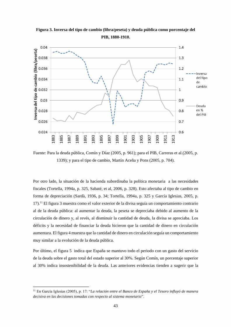
43
Figura 3. Inversa del tipo de cambio (libra/peseta) y deuda pública como porcentaje del
PIB, 1880-1910.
Fuente: Para la deuda pública, Comín y Díaz (2005, p. 961); para el PIB, Carreras et al.(2005, p.
1339); y para el tipo de cambio, Martín Aceña y Pons (2005, p. 704).
Por otro lado, la situación de la hacienda subordinaba la política monetaria a las necesidades
fiscales (Tortella, 1994a, p. 325, Sabaté, et al, 2006, p. 328). Esto afectaba al tipo de cambio en
forma de depreciación (Sardà, 1936, p. 34; Tortella, 1994a, p. 325 y García Iglesias, 2005, p.
17).11 El figura 3 muestra como el valor exterior de la divisa seguía un comportamiento contrario
al de la deuda pública: al aumentar la deuda, la peseta se depreciaba debido al aumento de la
circulación de dinero y, al revés, al disminuir la cantidad de deuda, la divisa se apreciaba. Los
déficits y la necesidad de financiar la deuda hicieron que la cantidad de dinero en circulación
aumentara. El figura 4 muestra que la cantidad de dinero en circulación seguía un comportamiento
muy similar a la evolución de la deuda pública.
Por último, el figura 5 indica que España se mantuvo todo el periodo con un gasto del servicio
de la deuda sobre el gasto total del estado superior al 30%. Según Comín, un porcentaje superior
al 30% indica insostenibilidad de la deuda. Las anteriores evidencias tienden a sugerir que la
11 En García Iglesias (2005), p. 17: “La relación entre el Banco de España y el Tesoro influyó de manera
decisiva en las decisiones tomadas con respecto al sistema monetario”.

44
situación del Tesoro dificultaba la adopción del patrón oro. Los problemas de la Hacienda
necesitaban que la peseta fuera inconvertible (Sabaté et al., 2006, p. 328).
Figura 4. Deuda pública como porcentaje del PIB y cantidad de dinero en
circulación(millones de pesetas), 1880-1913.
Fuente: Para la deuda pública, Comín y Díaz (2005, p. 961);Fuente: Para la deuda pública
Comín y Díaz (2005, p. 961), para el PIB, Carreras et al.(2005, p. 1339); para la cantidad de
dinero, Martín Aceña y Pons (2005, pp. 678, 679 y 683), sumando el metálico y los billetes en
circulación.
Figura 5. Gasto en deuda pública sobre el gasto total del Estado en porcentajes.
Fuente: Comín y Díaz (2005, p. 961).
45
¿Fue deseable la adopción del patrón oro?
La discusión sobre las consecuencias negativas o positivas de la no adopción del patrón oro la
podríamos asociar a la discusión entre tipos de cambio flexible y tipos de cambio fijos. Los
defensores del tipo de cambio flotante acostumbran a dar razones de corto plazo. Los argumentos
a favor del tipo de cambio flexible son la facilidad de ajuste en momentos de crisis gracias a una
mayor autonomía de la política macroeconómica, el efecto estabilizador del ciclo real o la mayor
simetría en los procesos de ajuste. Éstos acostumbran a estar a favor de la preservación de la
soberanía monetaria y fiscal. Por contra, los partidarios del tipo de cambio fijo suelen apostar por
las uniones monetarias y dan, sobretodo, argumentos de largo plazo. Insisten en una mayor
disciplina económica, un mayor control de la inflación, una mayor atracción de capital foráneo o
una reducción de los tipos de interés. Como corolario, estas ventajas incentivarían el crecimiento
económico a largo plazo.
Sardà (1987, p. 198I), destacó los efectos positivos que la no adopción del patrón áureo tuvo para
la economía española: “Puede decirse que la conjunción de expansión fiduciaria y proteccionismo
dio resultados felices para la economía española”. Para el profesor catalán, la posibilidad de
utilizar la política monetaria permitió mayor capacidad para afrontar shocks externos de la que
tuvieron los países del patrón oro. Cuando hubo peligro de recesión entre 1880 y 1913, la flotación
de la peseta parece haber actuado como cojín de los efectos depresivos (figura 12).
Posteriormente, Solé Villalonga (1967) y Tortella (1994a y 1997), con argumentos de largo plazo,
se posicionaron cerca de la tesis de Sardà. Tortella (1997, p. 24) destacó que, después del colapso
financiero del decenio de 1860, la desvinculación del patrón oro ayudó a España a no volver
experimentar otra crisis bancaria de grandes dimensiones hasta la de 1978-1985.
Para Martín Aceña la no adopción del patrón oro en España tuvo negativas consecuencias para el
crecimiento económico. Según el profesor madrileño, un sistema de tipos de cambio fijos limitaba
los excesos en la creación de liquidez y, por lo tanto, aumentaba la disciplina de los países
previniendo elevadas inflaciones o estanflaciones. Además, considera que seguir la regla del oro
facilitaba el acceso a los mercados de capital. Tortella (1974, pp. 480-481 y 1994a, p. 177) ataca
esta hipótesis argumentando que mantener a España en el patrón áureo era “bien de lujo” para un
país atrasado como el nuestro.12
En un primer momento el debate está en el corto plazo resaltando, por lo tanto, los costes de
adopción. Posteriormente, en los 70s, 80s y principios de los 90s, el debate se sitúa en el largo
plazo destacando, así, los beneficios de la entrada en el oro. De nuevo, a de finales de siglo, se
adopta una perspectiva de corto plazo pero añadiendo el análisis econométrico en las
12 Tortella (1994a) afirma que en un país pobre como España el oro debía ser utilizado para comprar
alimentos, tecnología, etc. Considera un despilfarro utilizar el metal amarillo como circulante.
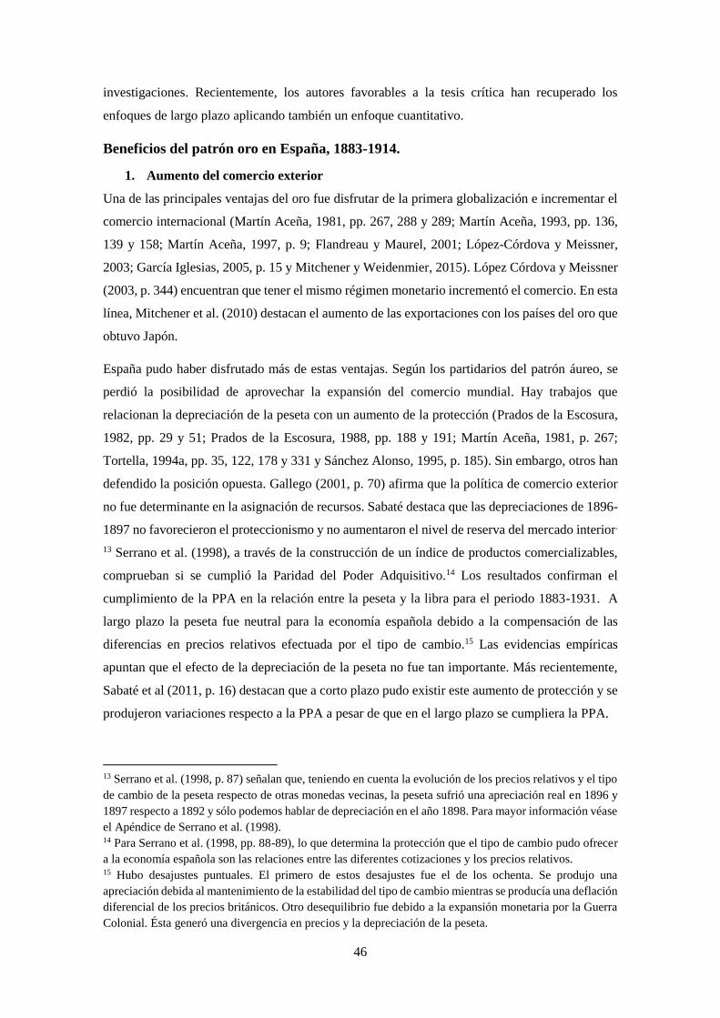
46
investigaciones. Recientemente, los autores favorables a la tesis crítica han recuperado los
enfoques de largo plazo aplicando también un enfoque cuantitativo.
Beneficios del patrón oro en España, 1883-1914.
1. Aumento del comercio exterior
Una de las principales ventajas del oro fue disfrutar de la primera globalización e incrementar el
comercio internacional (Martín Aceña, 1981, pp. 267, 288 y 289; Martín Aceña, 1993, pp. 136,
139 y 158; Martín Aceña, 1997, p. 9; Flandreau y Maurel, 2001; López-Córdova y Meissner,
2003; García Iglesias, 2005, p. 15 y Mitchener y Weidenmier, 2015). López Córdova y Meissner
(2003, p. 344) encuentran que tener el mismo régimen monetario incrementó el comercio. En esta
línea, Mitchener et al. (2010) destacan el aumento de las exportaciones con los países del oro que
obtuvo Japón.
España pudo haber disfrutado más de estas ventajas. Según los partidarios del patrón áureo, se
perdió la posibilidad de aprovechar la expansión del comercio mundial. Hay trabajos que
relacionan la depreciación de la peseta con un aumento de la protección (Prados de la Escosura,
1982, pp. 29 y 51; Prados de la Escosura, 1988, pp. 188 y 191; Martín Aceña, 1981, p. 267;
Tortella, 1994a, pp. 35, 122, 178 y 331 y Sánchez Alonso, 1995, p. 185). Sin embargo, otros han
defendido la posición opuesta. Gallego (2001, p. 70) afirma que la política de comercio exterior
no fue determinante en la asignación de recursos. Sabaté destaca que las depreciaciones de 1896-
1897 no favorecieron el proteccionismo y no aumentaron el nivel de reserva del mercado interior.
13 Serrano et al. (1998), a través de la construcción de un índice de productos comercializables,
comprueban si se cumplió la Paridad del Poder Adquisitivo.14 Los resultados confirman el
cumplimiento de la PPA en la relación entre la peseta y la libra para el periodo 1883-1931. A
largo plazo la peseta fue neutral para la economía española debido a la compensación de las
diferencias en precios relativos efectuada por el tipo de cambio.15 Las evidencias empíricas
apuntan que el efecto de la depreciación de la peseta no fue tan importante. Más recientemente,
Sabaté et al (2011, p. 16) destacan que a corto plazo pudo existir este aumento de protección y se
produjeron variaciones respecto a la PPA a pesar de que en el largo plazo se cumpliera la PPA.
13 Serrano et al. (1998, p. 87) señalan que, teniendo en cuenta la evolución de los precios relativos y el tipo
de cambio de la peseta respecto de otras monedas vecinas, la peseta sufrió una apreciación real en 1896 y
1897 respecto a 1892 y sólo podemos hablar de depreciación en el año 1898. Para mayor información véase
el Apéndice de Serrano et al. (1998). 14 Para Serrano et al. (1998, pp. 88-89), lo que determina la protección que el tipo de cambio pudo ofrecer
a la economía española son las relaciones entre las diferentes cotizaciones y los precios relativos. 15 Hubo desajustes puntuales. El primero de estos desajustes fue el de los ochenta. Se produjo una
apreciación debida al mantenimiento de la estabilidad del tipo de cambio mientras se producía una deflación
diferencial de los precios británicos. Otro desequilibrio fue debido a la expansión monetaria por la Guerra
Colonial. Ésta generó una divergencia en precios y la depreciación de la peseta.

47
2. Aislamiento internacional
Convergencia de precios
Otro de los beneficios del patrón oro fue experimentar una mayor convergencia internacional. La
no adopción del patrón áureo es considerada como una vía de desarrollo aislacionista o semi-
autárquica (Martín Aceña, 1981, pp. 267 y 290, Martín Aceña, 1993, pp. 136 y 158; Martín Aceña,
1997, p. 9; Tortella, 1994a, p. 331; García Iglesias, 2005, p. 32 y Martínez Ruíz y Nogués, 2014,
p. 90). Sin embargo, Catalan et al. (2001, p. 29) consideran que no existen evidencias para pensar
que el tipo de cambio flotante provocó un aislamiento internacional. Nadal y Sudrià (1993, pp.
208-210) demostraron como los precios de los tejidos de algodón en la península no siguieron
una trayectoria diferente a los británicos. Llona (2001, p. 160) afirma que los precios españoles
evolucionaron de forma similar a los británicos y que en España no se produjo tal aislamiento
internacional. Más recientemente, Maluquer (2013, pp. 82-83) señala que España tendió a
converger en precios con Gran Bretaña, Francia e Italia (figura 6).16 España mostró una gran
estabilidad de precios en el largo plazo. 17
Figura 6. Índice de precios en España y Gran Bretaña (1913 = 100), 1883-1913.
Fuente: Maluquer (2013) para España y Mitchell y Deane (1962) para Gran Bretaña.
16 Maluquer señala que hubo alguna desviación coincidiendo con las guerras coloniales, pero fue mínima y
que el comportamiento en precios de los cuatro países fue muy similar. En el gráfico se muestran sólo los
precios para España y Gran Bretaña. 17 Se desmiente la tendencia inflacionista que señalaba Cubel (2001) a causa de utilizar los datos del
deflactor implícito del PIB de Prados de la Escosura (1995). Prados de la Escosura en una nueva estimación
en 2003 muestra la corrección de este error suavizando los efectos inflacionistas.

48
Disminución de los tipos de interés.
Una ventaja del oro pudo ser mantener tipos de interés más bajos. Bordo y Jonung (2001, p. 14),
afirman que los tipos de interés fueron más bajos durante el patrón oro clásico que en los sistemas
monetarios posteriores. También, Bordo y Rockoff (1996, pp. 389, 395, 396 y 416) encuentran
que las diferencias entre los países en los tipos de interés cobrados a largo plazo en los mercados
de capitales están correlacionadas con su compromiso con el oro; a mayor compromiso, los tipos
de interés fueron más bajos. 18 García Iglesias (1999, p. 15) lo confirma para el caso de España.
En cambio, Carreras y Tafunell consideran que “las investigaciones realizadas [para el caso
español] no llegan a resultados sólidos o concluyentes acerca del efecto de los mayores tipos de
interés sobre el crecimiento económico”. 19 Catalan et al. (2001, p. 33) y Cubel (2001, p. 191)
sugieren que no estar en el oro provocó un aumento del tipo de interés pero la tendencia a lo largo
del periodo fue a converger con el del Reino Unido y que, en este sentido, pudo ser más importante
la disciplina fiscal que el régimen de cambio. También, Bordo y Rockoff (1996, p. 405) sugieren
la existencia de convergencia también en los tipos de interés entre España y Gran Bretaña. El tipo
de interés fue muy alto en los setenta debido a los impagos de la deuda. En cambio, cuando se
siguió una disciplina fiscal cercana al oro los tipos de interés fueron más bajos y tendieron a
converger (figura 7). Por lo tanto no parece existir una gran correlación entre el régimen cambiario
y el aumento de los tipos de interés.
Por su parte, Triffin (1964) señala que el mecanismo de ajuste del mercado internacional de
capitales no era simétrico. Un país periférico dentro del oro siempre tenía el tipo de interés unos
puntos por encima del tipo de interés de los países del núcleo. Una subida del tipo de interés en
un país periférico, además de aumentar el coste de la deuda para el Estado y el coste de
financiación de las inversiones, podía generar expectativas negativas y provocar una fuga de
capitales.
18 También, en Bordo y Kydland (1995) y en Martín Aceña et al. (2000, p. 2). 19 Carreras y Tafunell (2004, p. 217), destacan que la guerra de Cuba, que fue uno de los peores momentos
respecto a la credibilidad española y en la que riesgo del país debería estar muy alto coincidió con una
fuerte convergencia de la economía española.
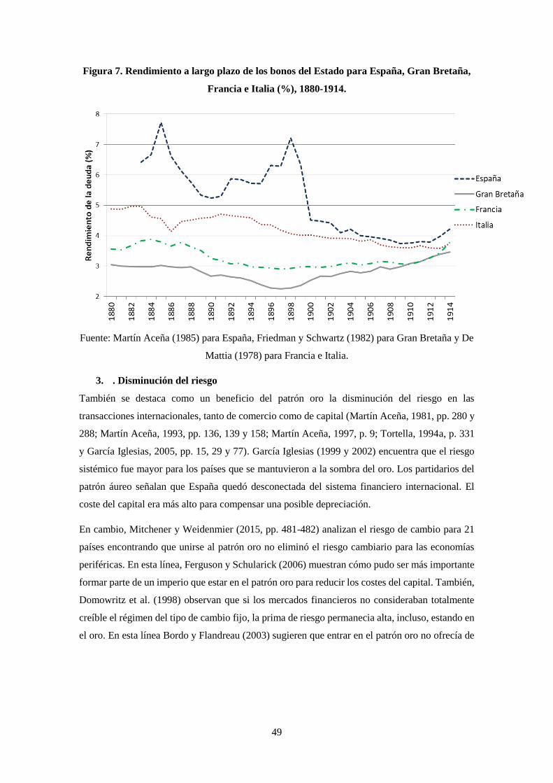
49
Figura 7. Rendimiento a largo plazo de los bonos del Estado para España, Gran Bretaña,
Francia e Italia (%), 1880-1914.
Fuente: Martín Aceña (1985) para España, Friedman y Schwartz (1982) para Gran Bretaña y De
Mattia (1978) para Francia e Italia.
3. . Disminución del riesgo
También se destaca como un beneficio del patrón oro la disminución del riesgo en las
transacciones internacionales, tanto de comercio como de capital (Martín Aceña, 1981, pp. 280 y
288; Martín Aceña, 1993, pp. 136, 139 y 158; Martín Aceña, 1997, p. 9; Tortella, 1994a, p. 331
y García Iglesias, 2005, pp. 15, 29 y 77). García Iglesias (1999 y 2002) encuentra que el riesgo
sistémico fue mayor para los países que se mantuvieron a la sombra del oro. Los partidarios del
patrón áureo señalan que España quedó desconectada del sistema financiero internacional. El
coste del capital era más alto para compensar una posible depreciación.
En cambio, Mitchener y Weidenmier (2015, pp. 481-482) analizan el riesgo de cambio para 21
países encontrando que unirse al patrón oro no eliminó el riesgo cambiario para las economías
periféricas. En esta línea, Ferguson y Schularick (2006) muestran cómo pudo ser más importante
formar parte de un imperio que estar en el patrón oro para reducir los costes del capital. También,
Domowritz et al. (1998) observan que si los mercados financieros no consideraban totalmente
creíble el régimen del tipo de cambio fijo, la prima de riesgo permanecia alta, incluso, estando en
el oro. En esta línea Bordo y Flandreau (2003) sugieren que entrar en el patrón oro no ofrecía de

50
inmediato credibilidad a los países periféricos.20 Por lo tanto, los mercados financieros no
confiaban en las restricciones aplicadas en la periferia como elemento de disciplina.
4. Incremento de la inversión
Los defensores del patrón áureo señalan que formar parte del oro permitía atraer mayor cantidad
de capitales extranjeros al aumentar la confianza de los inversores sobre la disciplina de los países
(Martín Aceña, 1981, pp. 267, 269, 288 y 289; Martín Aceña, 1993, pp. 158-159; Martín Aceña,
1997, p. 9; García Iglesias, 1999, p. 15 y Sussman y Yafeh, 2000, pp. 442-443). Bordo y Rockoff
(1996) destacan que estar en el patrón oro fue una señal de buena conducta que permitió un mejor
acceso al mercado de capitales, así como aumentar el volumen de capital atraído. En el mismo
trabajo, p. 390, apuntan a la necesidad de capital que tenían las economías en desarrollo de la
periferia como motivo por el cual los países hacían todo lo posible para adoptar el sistema
monetario internacional. En esta línea, Obstelf y Taylor (2003) encontraron, para una muestra de
muchos países, que riesgo cambiario pudo desincentivar la inversión.
Sin embargo, no está claro que los países periféricos pudieran obtener este beneficio. En un
trabajo sobre la Paradoja de Lucas se señala que el capital británico, durante periodo del patrón
oro clásico, no fue a parar a los países que tenían menos capital por trabajador y estaban
desarrollándose. 21 A pesar de las posturas que defienden que la disciplina del oro permitía tener
un mejor acceso al capital y recibir mayores inversiones, en este trabajo pertenecer al patrón áureo
es una variable no significativa para explicar el destino del capital británico (Clemens y
Williamson, 2000, pp. 6 y 15).
Por un lado, el destino de las inversiones dependía en gran medida de la existencia de un imperio
y de la capacidad de explotar las nuevas tecnologías. Por ejemplo, Italia recibió mayor inyección
de capital extranjero que España. Sin embargo, no se ha demostrado si esta inversión estuvo
directamente relacionada con el sistema monetario. Su buena relación con Alemania y la enorme
reserva hidroeléctrica de los Alpes fueron claves. España, con un territorio poca atractivo para
explotar nueva tecnología, había estado orientada a Francia y no vivió un proceso de tal
intensidad.
20 Mitchener, Shizume y Weidenmier (2010, p. 54) encuentran que la adopción del patrón oro en Japón no
disminuyó el coste del capital ni produjo un aumento de la inversión. 21 Sobre la paradoja de Lucas véase Lucas (1990, p. 92). Respecto al trabajo, véase el working paper de
Clemens y Williamson (2000). En este estudio se busca encontrar que factores fueron determinantes en las
decisiones de inversión extranjera que tomó Gran Bretaña, ya que se descarta que los países en desarrollo
no recibieran capital por una fallada del mercado internacional de capitales.

51
Figura 8. Kilómetros de ferrocarril construidos entre 1850 y 1910.
Fuente: Gómez Mendoza y San Román (2005, p. 532)
Por otro lado, los principales exportadores de capital antes de la Gran Guerra fueron Gran Bretaña
y Francia (Pollard, 1985, p. 492). 22 La mayor parte de la inversión inglesa fue hacia el Imperio y
América Latina. Ésta estuvo centrada, básicamente, en infraestructura de transportes. En 1883,
España tenía construida la mayor parte de su red ferroviaria (figura 8) (Catalan et al., 2001, p.
31). No parece que se pudiera haber recibido más inversión inglesa de haber mantenido la
convertibilidad (Catalan et al., 2001, p. 31).
En menor medida el capital francés también empezó a perder interés por el Mediterráneo (Catalan
et al. 2001, p. 31). 23 Catalan et al. (2001, p. 33) consideran que la vinculación de España al oro
no hubiera provocado mayor llegada de capitales ni un cambio significativo en el proceso de
industrialización español. En las estimaciones de inversión extranjera de Broder se observa una
tendencia a aumentar las entradas de capital en España a partir de 1900. Esto corroboraría que lo
importante eran las expectativas y no tanto el régimen de cambios (figura 9). En segundo lugar,
como dicen Carreras y Tafunell (2004, p. 212) “resulta difícil imaginar más inversión extranjera
dirigida a un país que ya había recibido tanta”.
García Ruíz (1992, p. 62) apunta que un aumento de la inversión extranjera de un 1% hubiera
incrementado el crecimiento de la renta en un 0,16%. Del mismo modo, Catalan et al. (2001)
señalan que, analizándose las tendencias a largo plazo de los principales inversores, no parece
22 En el cuadro 3 de Pollard (1985, p. 492), se observa como el 63,9% de la inversión extranjera la hacían
estos dos países. 23 Los mismos afirman que el interés por España y, también, por Portugal, Italia, Suiza y Austria, se redujo.
Para más información citan a Lévy-Leboyer (1977, p. 139), Berend y Ránki (1982, p. 78) y Broder (1993,
p. 176).
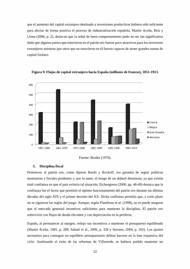
52
que el aumento del capital extranjero destinado a inversiones productivas hubiera sido suficiente
para afectar de forma positiva el proceso de industrialización española. Martín Aceña, Reis y
Llona (2000, p. 2), destacan que la señal de buen comportamiento pudo no ser tan significativa
dado que algunos países que estuvieron en el patrón oro fueron poco atractivos para los inversores
extranjeros mientras que otros que no estuvieron en él fueron capaces de atraer grandes sumas de
capital foráneo.
Figura 9. Flujos de capital extranjero hacia España (millones de francos), 1851-1913.
Fuente: Broder (1976).
5. Disciplina fiscal
Pertenecer al patrón oro, como dijeron Bordo y Rockoff, era garantía de seguir políticas
monetarias y fiscales prudentes y, por lo tanto, el riesgo de un default disminuía, ya que existía
total confianza en que el país evitaría tal situación. Eichengreen (2000, pp. 46-49) destaca que la
confianza fue el factor que permitió el óptimo funcionamiento del patrón oro durante las últimas
décadas del siglo XIX y el primer decenio del XX. Dicha confianza permitía que, a corto plazo
no se siguieran las reglas del juego. Aunque, según Flandreau et al. (1998), no se puede asegurar
que el mercado generará incentivos suficientes para mantener la disciplina. El patrón oro
sobrevivió con flujos de deuda elevados y con depreciación en la periferia.
España, al permanecer al margen, redujo sus incentivos a mantener el presupuesto equilibrado
(Martín Aceña, 1981, p. 289; Sabaté et al., 2006, p. 328 y Serrano, 2004, p. 165). Los ajustes
necesarios para conseguir un equilibrio presupuestario debían hacerse en la fase expansiva del
ciclo. Analizando el éxito de las reformas de Villaverde, se hubiera podido mantener un
53
presupuesto equilibrado durante el periodo que va de 1888 a 1895, pero no más allá. Después de
la pérdida de las colonias se consiguió equilibrar el presupuesto gracias a las medidas adoptadas
por Villaverde. Éste duraría poco, pues en 1909 el gasto bélico volvió a ser protagonista por la
intervención militar en Marruecos (Catalan et al., 2001, pp. 33-34). De todos modos, España no
utilizó todas las oportunidades que le ofrecía el sistema fiduciario y, excepto en momentos de
guerra, siempre siguió una política a la sombra del patrón oro que evitó que se cometieran excesos.
6. Integración europea
Otro de los beneficios que tenía la adopción del patrón áureo era la integración de España en el
entorno europeo (Martín Aceña, 1981, p. 290; Martín Aceña, 1993, p. 160 y Wiese, 1892-93, pp.
388-389). Los países centro del sistema económico adoptaron el patrón oro por diferentes motivos
y el resto de países les siguieron. España tendría que haber seguido el mismo ejemplo y haber
adoptado el patrón oro. Martín Aceña cita a Wiese, economista austríaco, para destacar la
importancia de seguir las decisiones de Europa.24 En la actualidad el caso sueco niega que se deba
seguir la tiranía de la mayoría.25
7. Crecimiento económico
La suma de todos los beneficios daba como resultado un mayor crecimiento económico. Uno de
los éxitos del patrón oro fue preservar la estabilidad del tipo de cambio en gran parte del mundo
(Triffin, 1985, p. 128). Así, se creó un clima de ausencia de perturbaciones monetarias que, según
los partidarios del sistema áureo, contribuyó al crecimiento económico. Por contra, se considera
que la no adopción del patrón oro contribuyó al lento crecimiento económico e industrial
experimentado por España entre finales del XIX y principios del XX (Martín Aceña, 1981, pp.
267, 288 y 289; Martín Aceña, 1993, pp. 158 y 160 y García Iglesias, 2005, pp. 16, 19 y 77).26 En
el caso español, algunas fuerzas que estimulaban el crecimiento antes de 1883 desaparecieron. La
demanda de vino por parte de Francia se disipó una vez superada la epidemia filoxérica y las
exportaciones cayeron (figura 10). Las exportaciones de minerales se estancaron por los
rendimientos decrecientes de la actividad extractiva y la difusión de procesos alternativos a la
utilización de mineral de hierro de bajo contenido fosfórico en la siderurgia europea (figura 11).
Además, las inversiones en ferrocarril habían llegado a su fin (figura 8).
24 Wiese (1898-1899, pp. 388-389): “Si Europa se equivoca adoptando el patrón oro, nosotros, a pesar de
ello, para bien o para mal, debemos unirnos en su error y de esta forma recibiremos menos daño que si
nos resistimos y nos empeñamos en ser ‘racionales’ por nuestra cuenta”. 25 Suecia aprendió de la historia de su última depresión y no adoptó la moneda única. Después del desastre
del SME decidió mantener su divisa. Esto le ha permitido un impacto menor de la crisis económica del euro
del que han tenido países como España que si adoptó la moneda única. Para el caso de Suecia, véase Catalan
(2002). 26 Véase el gráfico 1.

54
Figura 10. Hectolitros de vino exportados entre 1874 y 1910 (escala logarítmica).
Fuente: Barciela y Giráldez (2005, p. 331).
Figura 11. Cantidad de mineral de hierro exportado en miles de toneladas métricas entre
1870 y 1910.
Fuente: Carreras (2005, p. 417).
El patrón oro y España
El régimen monetario no parece un elemento capaz de explicar el atraso finisecular español ni el
causante de la divergencia respecto a Europa experimentada por España en aquellos años. Serrano
55
(2004, p. 165), también, descarta el régimen cambiario como causa del lento crecimiento
experimentado por España a finales del siglo XIX y principios del XX y considera que el culpable
fue un sector público atrasado. Asimismo, García Iglesias (2005, p. 30) señala que el sistema
monetario no fue relevante para el crecimiento. Después de un análisis cuantitativo sobre el
crecimiento de Italia, Portugal y España indica que no se puede demostrar que el régimen
monetario afectara al crecimiento económico entre 1850-1913.
Los posibles beneficios de adoptar el oro hubieran mostrado sus efectos en el largo plazo. Pero,
¿podía resistir la economía española en el corto plazo por un futuro, supuestamente, mejor? Lo
expuesto anteriormente sugiere que sin un gran coste a corto plazo, el objetivo del patrón oro
estaba muy alejado de la realidad española. En esta línea, Martín Aceña, Reis y Llona (2000, p.
2) consideran que aunque el patrón oro fuera un indicador creíble, los costes podían llegar a ser
excesivos para los países periféricos. Como afirmó Tortella (1994a), el patrón oro era demasiado
para la economía española.
Beneficios del sistema fiduciario en España, 1883-1914
1. Autonomía de la política económica
El principal beneficio de la no adopción del patrón oro fue mantener la autonomía de la política
monetaria y fiscal. Bordo (1990) y Bordo y Kydland (1995) afirman que pertenecer al patrón oro
restringía las acciones de política monetaria y fiscal a los gobiernos. Bordo y Jonung (2001, pp.
12-13), señalan que las políticas monetarias y fiscales estaban subordinadas al mantenimiento de
la convertibilidad. Así, los objetivos nacionales quedaban en un segundo plano. Como
consecuencia de mantener fija la relación entre las diferentes monedas, no se podían adoptar
políticas económicas demasiado expansivas. El patrón oro limitaba la capacidad de los gobiernos
para actuar frente a dichos shocks con instrumentos de política fiscal y monetaria. Es decir,
reducía la respuesta respecto a las perturbaciones del ciclo. Además, el sistema de funcionamiento
del patrón áureo facilitaba la transmisión de tendencias depresivas o inflacionarias de un país al
resto países. De este modo, los países del patrón oro podían experimentar mayor volatilidad
macroeconómica que aquellos países que estaban fuera del sistema monetario. Según Bordo y
Rockoff (1996, p. 416), los países que estaban fuera del oro utilizaron las fluctuaciones del tipo
de cambio para amortiguar el impacto de los shocks en sus economías. Esto podría ayudar a
explicar las dificultades que encontraron los países periféricos del sur de Europa para mantenerse
dentro del patrón oro y la importancia de mantener la autonomía de su política económica.
La pérdida de la política económica hubiera dificultado la posibilidad de utilizar instrumentos a
los que el gobierno recurría para solucionar los problemas coyunturales de la economía española
(Tortella, 1994a, p. 331; Herranz y Tirado, 1996, p. 32; Catalan, Sudrià y Tirado, 2001, p. 25;
García Iglesias, 2005, p. 15 y Martínez Ruíz y Nogués, 2014, pp. 19 y 94). Sardà (1987, p. 198)
56
afirmó que “el proteccionismo, junto a la política monetaria expansionista, tuvieron como
consecuencia evitar una baja excesiva de las inversiones, manteniendo el progreso de la
economía del país”. En conjunto, la economía española no sufre ningún retroceso fuerte con la
guerra de Cuba”. Tortella (1994a, p. 178) destaca que la política monetaria llevada a cabo fue la
más acertada de las políticas realizadas. Herranz y Tirado (1996, p. 32) señalan que adoptar el
patrón oro hubiera limitado la libertad de acción de los gobiernos españoles. Martínez Ruíz y
Nogués (2014, p. 19) confirman esta ventaja afirmando que el oro implicaba subordinar la política
monetaria a la estabilidad del tipo de cambio. Martín Aceña (1981, pp. 284-285) critica este
argumento señalando que utilizar la política monetaria de forma libre no tiene implicaciones a
largo plazo ya que los cambios en la cantidad de dinero tienen efectos insignificantes en el
crecimiento de la renta real a largo plazo.27 Años más tarde, durante la depresión de los años
treinta, fueron los países que salieron del patrón oro, los primeros en recuperarse (Bernanke, 1995,
pp. 11-12). Esto sugiere que el ejercicio autónomo de la política monetaria y fiscal es fundamental
para afrontar el impacto de los shocks económicos. En esta línea, los países europeos que están
fuera del euro han podido reaccionar mejor y más rápido ante la depresión sufrida durante los
últimos años que los países que comparten moneda.28
2. Evitar la deflación
La relación entre el funcionamiento del patrón áureo y política monetaria fue complicada. Por un
lado, la capacidad de una nación para expandir su oferta monetaria estaba limitada, entre otras
cosas, por la situación de su balanza de pagos. Un déficit en la balanza de pagos podía provocar
salidas de oro, deflación y, en última instancia, desempleo a causa de los efectos del círculo
vicioso. En esta situación, el país no podía aplicar políticas correctoras. Por otro lado, el patrón
áureo ejercía de freno sobre el crecimiento de la oferta monetaria. Ésta estaba determinada por
sus existencias de oro. Al ligar la oferta monetaria a un metal, el crecimiento de ésta no seguía a
la demanda.29 El suministro de oro limitaba el crecimiento económico y provocar una disminución
de los precios. Al reducirse los precios, las empresas se podían ver forzadas a despedir
trabajadores y esto generaba una espiral negativa que acababa produciendo falta de demanda.
¿Era España capaz de soportar tales efectos? Sardà (1987, p. 197) y Tortella (1974, p. 480)
afirman que, con el sistema fiduciario, España se mantuvo al margen de la depresión de precios
mundial. Martín Aceña (1993, p. 139) coincide con Sardà en destacar que la inconvertibilidad
evitó la deflación en España.
27 Se basa en Friedman (1970, p. 217) para hacer esta afirmación. 28 Los casos de Gran Bretaña y Suecia serían un ejemplo. Para el caso sueco, véase Catalan (2002). 29 Este defecto lo observó Keynes (1936/1960, pp. 230-231).
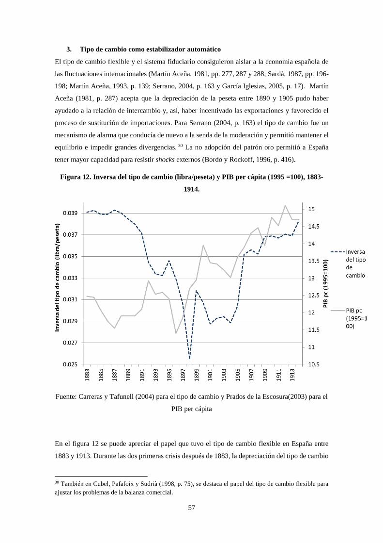
57
3. Tipo de cambio como estabilizador automático
El tipo de cambio flexible y el sistema fiduciario consiguieron aislar a la economía española de
las fluctuaciones internacionales (Martín Aceña, 1981, pp. 277, 287 y 288; Sardà, 1987, pp. 196-
198; Martín Aceña, 1993, p. 139; Serrano, 2004, p. 163 y García Iglesias, 2005, p. 17). Martín
Aceña (1981, p. 287) acepta que la depreciación de la peseta entre 1890 y 1905 pudo haber
ayudado a la relación de intercambio y, así, haber incentivado las exportaciones y favorecido el
proceso de sustitución de importaciones. Para Serrano (2004, p. 163) el tipo de cambio fue un
mecanismo de alarma que conducía de nuevo a la senda de la moderación y permitió mantener el
equilibrio e impedir grandes divergencias. 30 La no adopción del patrón oro permitió a España
tener mayor capacidad para resistir shocks externos (Bordo y Rockoff, 1996, p. 416).
Figura 12. Inversa del tipo de cambio (libra/peseta) y PIB per cápita (1995 =100), 1883-
1914.
Fuente: Carreras y Tafunell (2004) para el tipo de cambio y Prados de la Escosura(2003) para el
PIB per cápita
En el figura 12 se puede apreciar el papel que tuvo el tipo de cambio flexible en España entre
1883 y 1913. Durante las dos primeras crisis después de 1883, la depreciación del tipo de cambio
30 También en Cubel, Pafafoix y Sudrià (1998, p. 75), se destaca el papel del tipo de cambio flexible para
ajustar los problemas de la balanza comercial.

58
ayudó a la recuperación de la economía. Por ejemplo, en las crisis de 1883-1890 y 1893-1898, el
tipo de cambio jugó un papel fundamental para la recuperación de la economía española. En
Catalan y Sánchez (2012) se encuentra un análisis esquemático de la primera crisis y se destaca
la importancia que han tenido históricamente las devaluaciones o depreciaciones de la peseta para
afrontar los impactos depresivos sobre la economía española. Éste permitió amortiguar los
impactos económicos que de otro modo habrían tenido mayor intensidad y duración. 31
4. Mantener el bienestar general
Adoptar dicho sistema requería aplicar políticas contractivas. Los efectos positivos de estabilidad
y crecimiento estuvieron, en general, limitados a las economías avanzadas. Una gran parte de los
países de la periferia sufrieron grandes fluctuaciones del tipo de cambio e inestabilidad (Tortella,
1974, p. 478 y Triffin, 1985, p. 128). La adhesión al patrón oro de las economías periféricas fue
complicada y requirió dolorosos y, en ocasiones, insoportables ajustes de su economía nacional.32
Según diversos autores, éstas sólo podían empeorar la situación de la economía española (Carreras
y Tafunell, 2004, pp. 219-220). Carreras y Tafunell plantean que realizar este tipo de políticas
tenía efectos depresivos. De hecho, Tortella (1994a, p. 325) cuando analiza la velocidad del dinero
observa cómo se contrae la oferta monetaria respecto al crecimiento de la renta entre 1899 y 1908.
Los historiadores de la Universidad Pompeu Fabra cuestionan que este tipo de políticas fuesen
las más adecuadas para una economía empobrecida después de la guerra. Ellos consideran que lo
que si puede y debe criticarse del comportamiento español es haberse esforzado hasta sacrificar
el bienestar nacional por intentar incorporarse al patrón oro.33 España, al no adoptar el oro, pudo
evitar estos efectos y, sólo cuando intentaba acercarse demasiado a la disciplina del oro éstos se
dejaban notar. Serrano (2004, p. 163) destaca la estabilidad de precios experimentada por España
durante el periodo. La suma, por lo tanto, de todos beneficios hubiera dado como resultado el
mantenimiento del bienestar general.
Sistema fiduciario: ¿Coste o beneficio?
Los beneficios de no haber adoptado el patrón oro se muestran poco cuestionables. Mantener la
autonomía de la política monetaria y fiscal, evitar la deflación y estabilizar la economía mediante
31 El trabajo de Shibamoto y Shizume (2014, p. 3) encuentra que el tipo de cambio fue el elemento más
importante en el caso japonés, para salir de la crisis. El nivel de tipo de cambio promovió las
exportaciones y aumentar los precios interiores. 32 Martín Aceña, Reis y Llona (2000, p. 2). 33 Carreras y Tafunell (2004), pp. 219-220, afirman que “forzar la apreciación es siempre una receta para
el desastre económico y un retraimiento de la inversión. La dureza de las políticas de ajuste implementadas
entre 1890-1910 provocaron el estancamiento de la economía española. Cuando se abandonó el temor al
déficit para financiar la guerra de Marruecos, es decir, cuando se hizo política expansiva, el resultado fue
en términos monetarios positivo. Después de 1909 empezaron a llegar capitales extranjeros”. Martín Aceña
(1981, p. 277), también, acepta que para equilibrar la balanza de pagos se debían hacer ajustes dolorosos
para la economía española.

59
el tipo de cambio parece que pudo ser superior a todos los beneficios que hubiera conllevado la
entrada de España en el patrón áureo (Ródenas, Bru y Almenar, 2001, p. 141). España pudo
superar mejor los impactos económicos del periodo 1883-1914 por la capacidad para decidir su
política monetaria. Además el tipo de cambio permitía atenuar los shocks en la economía
española. Serrano (2004, p. 161) afirma que el tipo de cambio flotante se veía como “un resultado
ineludible” y no como una causa del retraso de España. 34
III. Conclusión
Las consecuencias, negativas o positivas, que tuvo para España la no adopción del patrón
oro entre finales del siglo XIX y principios del XX han hecho correr ríos de tinta. Se trata de un
tema controvertido y polémico en el que todavía no hay certezas sobre lo que sucedió exactamente
y ni sobre qué efectos tuvo para la economía española.
En el fondo de esta controversia de la historia económica de España se encuentran dos debates
relacionados: uno teórico y uno político. El debate teórico consiste en la eterna pugna entre el
corto y el largo plazo. En este caso se puede traducir en la lucha entre tipos de cambio flotantes y
tipos de cambio fijos. La valoración entre lo positivo o lo negativo que fue para España no adoptar
el patrón oro depende en gran medida de la óptica teórica y temporal con que se analice el
problema. Si uno considera la política monetaria efectiva en el corto y largo plazo y valora
significativamente la estabilidad a corto plazo de un país significa que la soberanía monetaria es
imprescindible. Por lo tanto, no adoptará un sistema monetario como el patrón oro. Por el
contrario, si uno considera que los monetaristas están en lo cierto y el objetivo es la estabilidad a
largo plazo significa que se está dispuesto a sacrificar la política económica en el presente y, si es
necesario, el bienestar nacional por un futuro mejor. De este modo, se puede adoptar un régimen
monetario que no permita utilizar todos los instrumentos de política económica a cambio de la
estabilidad y el crecimiento a largo plazo. Pero, ¿todos los países pueden?
El debate político, muy relacionado con el anterior, es sobre la soberanía monetaria y fiscal. Hay
disparidad de opiniones sobre en qué grado países periféricos como los del Mediterráneo, con
problemas estructurales, pueden sacrificar el uso de su política de regulación de la demanda. En
diferentes momentos históricos se ha puesto de manifiesto la incapacidad de estos países para
avanzar en un marco económico sin libertad para decidir sobre su política monetaria y fiscal.
Patente es el caso español. Durante la época del patrón oro, mantenerse al margen permitió a
España protegerse mejor de la volatilidad de las fluctuaciones del ciclo económico. En cambio a
finales del siglo XX, hipotecó su política económica en favor de la moneda única y ha acabado
experimentando una crisis bastante prolongada. Un país con un problema estructural en la balanza
de pagos no puede permitirse el lujo de perder la capacidad de decidir sobre su política monetaria
34 El Dictamen de la Comisión del Patrón Oro coincide con esta idea.
60
y su política fiscal. ¿Puede que apostar por el largo plazo sea un lujo que los países periféricos no
se pueden permitir?
Las evidencias sugieren que no fue posible entrar en el patrón áureo, a pesar de que pudiera ser
deseable. Los problemas más importantes de la economía española para adoptar el oro fueron la
balanza de pagos y la Hacienda. Los costes de haber entrado con las condiciones que tenía el país
pudieron ser demasiado altos. Parece que España no siguió un camino equivocado. A corto plazo,
la autonomía de la política monetaria y fiscal y el tipo de cambio flotante permitieron el ajuste
del país ante la volatilidad del ciclo económico, contribuyendo a amortiguarlo. España nunca
utilizó todas las posibilidades que ofrecía el sistema fiduciario y siguió una política cercana al
patrón oro (Tortella, 1974; Sardà, 1987; Martín Aceña, 1993 y 2000; Serrano Sanz, 2004, Martín
Aceña et al., 2011).
Los beneficios de haber adoptado el patrón oro pudieron ser de diversa índole: aprovechar la
expansión del comercio mundial, disfrutar de la integración económica, menor inflación y tipos
de interés más bajos, mayor nivel de inversiones, mejor gestión presupuestaria o mayor un
crecimiento económico. Sin embargo, los beneficios del sistema fiduciario pudieron ser,
presumiblemente, más elevados.

61
62
Chapter 2: “Why was Europe’s southern periphery not able to adopt
the gold standard? The case of Spain, 1874-1913”.*
Abstract
Spain had constant budget deficits at the end of the nineteenth century, and it was the only western
country unable to adopt the gold standard. I aim to establish whether the Spanish debt was
sustainable or not during the classical gold standard period, and how debt sustainability changed
due to the various policies implemented by policymakers. This paper sheds new light on the
analysis of Spanish fiscal solvency by applying two different econometric approaches: fiscal
reaction function, and impulse response analysis. This article also interprets the results using
narrative evidence and data from previous studies. I find that Spanish debt was unsustainable
between 1874 and 1903, regardless of whether seigniorage is considered. Thus, it was very
difficult for the country to join the gold standard due to its huge debt accumulation and its weak
political position until 1903. Moreover, seigniorage seems not to be important to explain debt
sustainability. From 1903, Spanish debt was sustainable due to a change in economic policy,
introduced by Raimundo Fernández Villaverde.
Key words: Classical gold standard, debt sustainability, Spain, fiscal response function.
JEL codes: E42, E52, E63, N10
* This paper has been presented at the Economic History Socierty Conference (2018), Workshop on
Monetary history at the University of Zaragoza and Economic History Seminar at the University of
Barcelona. I am grateful for the comments received in these forums. I specially thanks to Marcela Sabaté,
José María Serrano and Paolo Di Martino for the feedback received. I also appreciate the comments and
ideas from Pere Pascual, Ramon Ramon, Pilar Nogués and María Ángeles Pons. This paper would have
been impossible without the new data on fiscal balance provided by Francisco Comín. This paper has
received support from Ministry of Economics and Competitiveness, HAR2015-64769-P. Naturally, I am
responsible for the remaining errors.
63
“For the believer, salvation is in the holy fear of God; for every
finance minister, salvation is in the holy fear of the deficit.”
José Echegaray, 1905
I. Introduction
The debate on fixed exchange-rate systems has grown in importance over the past decade as a
consequence of the euro crisis. Questions such as whether any country, regardless of the economic
problems that it may have, can join a fixed exchange-rate system like the euro have engaged the
interest of economists and economic historians alike.1 In both the first and second globalizations,
peripheral economies strove to emulate advanced economies and, in many instances, their
attempts generated serious problems. In the last decades of the nineteenth century, a large number
of countries adopted the gold standard. Peripheral economies during the gold standard period had
problems of convertibility, while core countries had long convertibility records. As in the recent
phase of financial globalization, financial crises increased in the pre-1914 era (Reinhart and
Reinhart, 2008 and Powell and Tavella, 2012). There were currency crises and convertibility was
suspended (Bordo and Schwartz, 1999). Spain suffered two currency crises in this period
(Martínez-Ruíz and Nogués-Marco, 2014) and experienced large-scale accumulations of debt.
The recent sovereign debt crisis has once again highlighted the differences between core and
periphery (or North and South). The differences are the cause of the problems affecting the EMU
today and recall the difficulties experimented by peripheral countries under the gold standard.
Similarly, the euro has created a core of surplus countries and a periphery of deficit countries.
The latter have had to sacrifice their domestic economies to restore external equilibrium, and have
thus been left unable to respond to crises. The debate between core and periphery remains open,
and the stark contrast between core and periphery requires our consideration (Eichengreen and
Flandreau, 1997, and Bordo and Flandreau, 2003, p. 419).
The recent international crisis has also stressed the importance of budget balance problems.
Governments have paid more attention to the crucial issue of fiscal sustainability. There is a
considerable amount of recent literature on the topic: empirical tests of fiscal solvency (or fiscal
sustainability) based on Intertemporal Budget Constraint (IBC) and Fiscal Reaction Function
1 Because there is no tax harmonisation within the eurozone, it is possible to compare the respective
problems of the gold standard and the euro. Hoffmann (2013), Bordo and James (2014), Eichengreen (2014)
and Matthijs (2014) have done it.
64
(Bohn, 1998 and 2007) or analyses using impulse response function (Afonso, 2008 and Afonso
and Jalles, 2011 and 2017) among others. Moreover, Mendoza and Ostry (2008) show how past
increases in debt in non-advanced economies require more powerful responses of the primary
balance than in advanced economies.
Several studies have focused on the periphery and its problems of convertibility during the
classical gold standard period. A shortfall in the public coffers was one of the major problems
that prevented the periphery from joining the gold standard. Fiscal deficits contributed to
unbalanced external accounts which resulted in repeated outflows of currency, and budget deficits
led to a need for finance. Monetary policy took a back seat to fiscal needs (Tortella, 1994a, p.
325). The south tended to finance its deficits monetarily, a practice that generated a divergence
of the country's prices with respect to international prices and caused problems in the balance of
payments, gold depletion, and the suspension of convertibility.2 In this respect, the countries on
Europe’s southern periphery were often forced to monetize their debt or, in the worst case, to
declare bankruptcy, as Portugal did in 1891 after the country’s failed attempt to prop up its
exchange rate and stay on the gold standard.
The periphery was not able to remain in the gold standard. Even so, the Kingdom of Spain was
not an island in a gold-standard sea. Neither Italy nor Portugal succeeded in staying in the fixed
exchange-rate system over the long run. Portugal abandoned the gold standard in 1891 and Italy
followed suit in 1894 after a severe economic shock. Recently, Italy, Spain, Greece and Portugal
have accepted fiscal austerity and internal deflation to stay in the euro (Eichengreen and Temin,
2010). During the gold standard era, however, these countries felt compelled to break the "golden
fetters" and ran wasteful fiscal policies that were inconsistent with price stability.
The effects of the commitment to the gold standard on a country’s credibility varied according to
its economic status. Advanced countries had better access to capital because of their high level of
credibility. This, in turn, enabled them to overcome any disparities in their balance of payments
and to finance their debt. By contrast, peripheral economies needed to achieve balanced budgets
in order to keep the trust of the markets. Spain never adopted the gold standard; the country had
constant deficits and huge amounts of debt during the last decades of nineteenth century, which
made difficult to keep the exchange rate stable and maintain fiscal discipline. What happened to
the public debt? Was it sustainable? I aim to assess the importance of the fiscal problems in Spain
and if they represented a significant reason for not adopting the dominant monetary system. Could
Spain adopt the gold standard in this fiscal situation?
2 Eichengreen (1992); Bordo and Rockoff (1996); Eichengreen and Flandreau (1997) for the general
question and Martín Aceña et al. (2000) and Prados de la Escosura (2010) for the Spanish case.
65
Considering that fiscal discipline was a key element for joining and remaining on the gold
standard, this paper analyses whether or not Spain’s fiscal policy was sustainable and,
consequently, whether the country was simply unable to adopt the gold standard as a consequence
of its fiscal problems. Thus, this paper explores if its debt was sustainable or not. My main
hypothesis is that a backward economy such as Spain tended to have a deficit balance of payments
and a negative budget balance, and that this made it impossible for it to adopt the gold standard.
Pittaluga and Seghezza (2016) link the gold standard and debt sustainability by studying how
Japan was able to remain on the gold standard despite having unsustainable external debt. The
overarching goal of these studies is to analyse the fiscal behaviour during the classical gold
standard period. Martín Aceña et al. (2012) stresses that the question of Spain’s debt in relation
to membership of the gold standard needs further research. Sabate et al. (2019) consider that the
sovereign debt crisis in the Economic and Monetary Union (EMU) has reopened the discussion
on the sustainability of a single currency without a single fiscal policy, making possible
comparisons with the gold standard a century ago, such as the ones conducted by Eichengreen
and Temin (2010) and Bordo and James (2014).
To answer these questions, the paper will draw on two quantitative methods that have been used
extensively in recent years.3 The first approach was put forward by Bohn (1998, 2007 and 2008)
in his work on fiscal solvency, while the second one was used by Afonso (2008) and Afonso and
Jalles (2011) involves employing a VAR model to estimate the impulse-response functions of the
public debt and the fiscal deficit to check the robustness of the results through a VAR. While no
quantitative studies have been done to analyse the unsustainability of Spain’s debt for the period
under study, there do exist descriptive analyses and reconstructions of historical series in Comín
(1985, 1988, 1989, 1997, 1999, 2003, 2004, 2005, 2006, and 2016) as well as studies on fiscal
dominance (Sabaté et al., 2006; Escario et al. 2011; Escario et al. 2012 and Sabaté et al. 2014).4
Thus, this paper estimates the fiscal reaction function for Spain over the period 1874-1913. It is
tested how government budget primary balance tends to respond to changes in public
indebtedness.
The main findings of the paper are that primary balance responded negatively to an increase in
debt until the beginning of twentieth century when the response started to be positive. Moreover,
I discover that seigniorage was not important for the sustainability of the debt, a finding that has
3 For more on debt unsustainability, related tests and sustainability indicators, see, among others, Buiter
(1985); Blanchard (1990); Blanchard et al. (1991); Chalk and Hemming (2000); IMF (2003); Bohn (2008);
Neck and Sturm (2008) and Escolano (2010). 4 There are several studies on fiscal dominance in the peripheral countries: Frattiani and Spinelli (2001)
and Sabaté et al. (2006, 2015 and 2018) for Italy and Spain respectively, and Morys (2017) for Greece,
Bulgaria and Romania.
66
never previously been reported for the Spanish case. The sustainability or unsustainability of the
debt does not depend on seigniorage but on the economic policies (and specifically the fiscal
policies) that the country adopted. On the other hand, there is a structural change in 1903 that had
not been found in other studies of fiscal dominance. As of 1903, the debt was sustainable and
entry into the gold standard was possible. Finally, as far as I know, there are no studies on fiscal
solvency for Spain during that period.
Following this introduction, the second section proceeds to analyse the debt in Spain in the late
nineteenth and early twentieth centuries. The third section goes on to review the theoretical
framework and methodology used in the study of debt sustainability, while the fourth section sets
out the data. Lastly, the paper finishes with a presentation of the results and a brief conclusion.
II. The economic problems that prevented Spain from adopting the
gold standard: the country’s debt.
The debate on the consequences of having constant deficits
Economic growth was slow during this period. There were several debt crises such as the 1876-
1885 crisis associated with an increase in the deficit, and slowed in part by Camacho’s debt
restructuring, and the 1902-1920 crisis caused by the end of Cuban war and solved in part by
Villaverde’s fiscal policy measures (Comín, 2013).5 Why did Spain not adopt the gold standard?
Two main answers can be found in the literature. First, some scholars take the view that Spain
was simply unable to do so:6 the Spanish economy had serious problems that prevented its
membership, specifically its balance of payments and its public finances. The second answer is
the exact opposite: if the country did not adopt the international monetary system, it was because
the monetary authorities decided against membership: that is, they did not pursue the appropriate
policies to adopt the gold standard. For Martín Aceña (1981, p. 288), “Spain had no
insurmountable technical or economic impediments to adopting the gold standard”. Indeed, in
his view, the Spanish economy was primed to benefit from the international monetary system.
Yet, Martín Aceña (1993, pp. 155-56) explains that while there was no reason for Spain not to
enter the gold standard, the decision was simply never taken.7
5 Years of crisis measured by debt/GDP ratio considering the first year the top of the ratio and the last year
the minimum point after the crisis. One can find more on this measure and these two crises in Comin (2013).
Measured by budget balance/GDP these two crises ran from 1861 to 1873 and from 1895 to 1902. First,
there were deficits and then an accumulation of debt occurred. Therefore, the crises ended earlier in terms
of budget balance over GDP than in terms of debt over GDP. 6 Serrano (2004, p. 161), says that the floating exchange rate can be seen as “an inevitable result” and not
as a cause of Spain’s backwardness. The expert opinion given by the committee on the gold standard
(known as the Dictamen de la Comisión del Patrón Oro) concurs with Serrano’s idea. Also in Llona (2001,
p. 172). 7 This position is also advocated in Martín Aceña et al. (2014).
67
Despite this last view, it is considered that the shortfall in the public coffers was one of the chief
factors to make Spain’s linkage with any fixed exchange rate monetary system difficult.8 It was
also one of the most important factors that made joining the gold standard unworkable (Flores de
Lemus, 1929 and Serrano, 2004, p. 156). Serrano (2004, p. 144) considers that the Spanish
monetary and exchange problem was actually a fiscal problem. According to the Dictamen (Flores
de Lemus, 1929) the general direction of the economy was marked by prices and to a lesser extent
by the balance of payments. In this way, prices were determined by the money supply and this, in
turn, by the budgetary problems of the State. Spain’s fiscal system was predicated on insufficient
public resources (Comín, 2005). The public deficit contributed to throwing the country’s external
accounts into disequilibrium, giving rise to repeated outflows of cash.
High nominal and real interest rates, together with low GDP growth, kept the debt-to-GDP ratio
high (figure 1).9 The Spanish economy was financially underdeveloped, marked by a history of
high inflation and poor fiscal discipline. It was also unable to borrow in its own currency.10 For
most of the period, the debt-to-GDP ratio exceeded 100%.
Figure 1 shows public debt for 1874-1913. This sample of 40 years includes all periods from the
concession of monopoly of issuing to the Banco de España until the first world war. It indicates
three maximum points: 1876, 1879 and 1902.
8 The problem was already identified by Flores de Lemus in the expert opinion issued by the committee on
the gold standard (Dictamen de la Comisión del Patrón Oro). For a thorough analysis of the Spanish treasury
in the nineteenth century, see Comín (1988). 9 Triffin, for his part, notes that the adjustment mechanism of the international capital markets was not
symmetrical. A peripheral country’s interest rate was always a few points higher than in the core countries.
An interest-rate hike aimed at halting the outflow of gold had a different effect in a core country than in the
periphery. In the latter case, the result was not only to increase the cost of borrowing for the state and the
cost of financing investments, but might also generate negative expectations and lead to capital flight. 10 More on this problem in Eichengreen and Hausmann (1999)
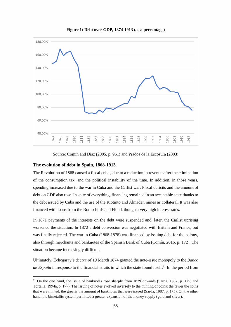
68
Figure 1: Debt over GDP, 1874-1913 (as a percentage)
Source: Comín and Díaz (2005, p. 961) and Prados de la Escosura (2003)
The evolution of debt in Spain, 1868-1913.
The Revolution of 1868 caused a fiscal crisis, due to a reduction in revenue after the elimination
of the consumption tax, and the political instability of the time. In addition, in those years,
spending increased due to the war in Cuba and the Carlist war. Fiscal deficits and the amount of
debt on GDP also rose. In spite of everything, financing remained in an acceptable state thanks to
the debt issued by Cuba and the use of the Riotinto and Almaden mines as collateral. It was also
financed with loans from the Rothschilds and Floud, though atvery high interest rates.
In 1871 payments of the interests on the debt were suspended and, later, the Carlist uprising
worsened the situation. In 1872 a debt conversion was negotiated with Britain and France, but
was finally rejected. The war in Cuba (1868-1878) was financed by issuing debt for the colony,
also through merchants and banknotes of the Spanish Bank of Cuba (Comín, 2016, p. 172). The
situation became increasingly difficult.
Ultimately, Echegaray’s decree of 19 March 1874 granted the note-issue monopoly to the Banco
de España in response to the financial straits in which the state found itself.11 In the period from
11 On the one hand, the issue of banknotes rose sharply from 1879 onwards (Sardà, 1987, p. 175, and
Tortella, 1994a, p. 177). The issuing of notes evolved inversely to the minting of coins: the fewer the coins
that were minted, the greater the amount of banknotes that were issued (Sardà, 1987, p. 175). On the other
hand, the bimetallic system permitted a greater expansion of the money supply (gold and silver).
40,00%
60,00%
80,00%
100,00%
120,00%
140,00%
160,00%
180,00%
18
74
18
76
18
78
18
80
18
82
18
84
18
86
18
88
18
90
18
92
18
94
18
96
18
98
19
00
19
02
19
04
19
06
19
08
19
10
19
12
69
1874 to 1882, Spain received significant amounts of foreign capital.12 From 1874 onwards, a
parallel has been observed between the evolution of the rates of public assets in the Banco de
España and those of the money supply (Comín, 2016, p 225). It consisted of a cooperation
between the banks and the Treasury allowing the banks to subscribe the debt with the privilege
of pledging it directly to the Banco de España (Bank of Spain).
In 1876 Salaverría, minister of Finance, carried out a debt restructuring with which the payment
of interest on the debt was resumed but at a reduced rate. The Salaverria arrangement increased
the outstanding debt (there was no treatment in favour of the holders). It was possible to pay a
part of the interest and increase the financial burden on the State. According to Comín (2016, p.
173), this did not solve the debt crisis. Despite the momentary slowdown in the growth of the debt
in 1879, the situation worsened again, as 42.3% of tax revenues went on debt, which was at 165%
of GDP (figure 1). The delay in the payment of interest would soon end; the response was to carry
out to a new conversion in order to alleviate the State's financial situation.
Then, in 1881, Camacho restructured Spain’s debt.13 One of the most important features of the
restructuring was the government’s commitment to pay interest in francs or pounds.14 Camacho's
restructuring was intended to improve the country’s creditworthiness, and it had favourable
effects on the budget and the state debt. The laws of 1881 and 1882 joined the previous dispersed
issues into two types of debt: amortizable, and perpetual internal and external debt. It was possible
to reduce the debt in circulation but not the financial burden of the budget. These measures offered
assurance that the coupons would be collected and that foreigners would be paid in gold.
In 1883, an agricultural crisis rekindled the public budget deficit. In response, the government
pursued two avenues, one of which was the Treasury’s direct loans from the Banco de España,
which rose in value from 200 million pesetas in 1884 to 409 in 1891.15 Unlike the previous period
from 1883-84 to 1891-92, the deficits remained constant (figure 2). The pressure on the public
coffers increased fiduciary circulation (figure 4)16. When Spain had a deep triple crisis in 1882
12 Martín Aceña (1981, p. 271). 13 For a more detailed explanation of the debt structuring, see Comín and Martorell (2006, pp. 389-391). 14 Roldán de Montaud (2006, p. 431). This decision had significant effects. Spaniards started to buy foreign
debt because interest paid in gold served as a hedge against any potential depreciation of the peseta
(Tortella, 1994a, p. 164). The purchase of foreign debt by Spaniards ultimately became a problem. 15 Against this backdrop, the Spanish parliament passed the Treasury law of 12 May 1888, which ended the
Treasury’s practice of requesting ongoing advances from the Banco de España (Obra de Joaquín López
Puigcerver, Gaceta de Madrid, 5-VII-1888). The law in question confirmed the close relationship forged
between the Treasury and the Banco de España since 1874, which reached its peak when the state delegated
the management of all its collections and payments to the private bank. 16 Fuentes Quintana (1990, p. 40) and Sardà (1987, p. 183).
70
(currency, banking and stock market) during this period, it coincided with a fiscal or debt crisis.
This was the most severe crisis in this period (Betran and Pons, 2018).
The volume of the debt stabilized until 1895, when it increased again due to the resumption of
war in Cuba. Spain enjoyed a budget surplus in 1893 and 1894, but the Cuban uprising of 1895,
which triggered a war with the United States, halted the trend. Financing the war drove Spain’s
debt up from 800 million to 3 billion pesetas. The monetization of the debt increased the amount
of money in circulation. The law of 14 July 1891 authorized the Banco de España to raise its
note-issue limit to 1.5 billion17. Banknotes in circulation increased from 910 million pesetas in
1894 to 1.444 billion pesetas in 1898 (figure 4). As a consequence, Spanish prices rose more than
international prices, driving down the value of the peseta.
After that, the decree of 9 August 1898 raised the note-issue ceiling from 1.5 billion to 2.5 billion
pesetas. By the end of the war, the money supply had ballooned by more than 50%. The interest
rate, which was adjusted as a function of the Treasury’s interests, fell in order to lower the cost
of debt. The funding of the war ultimately turned into a problem for the public coffers.
In 1899, Fernández Villaverde prioritized finding a solution to the debt problem, seeking to
redress the shortfall in public revenues and laying the groundwork for establishing the peseta’s
exchange rate, in a bid to return the Treasury to solvency. Before Villaverde applied this
adjustment, Spain could not find financing through the Rothschilds and its debt was suspended
on the stock exchange. Thanks to Villaverde’s efforts, the debt was restructured and the situation
of the public finances improved. Indeed, the monetary aspect of his focus on stabilization was
successful on the three fronts that it addressed (the debt, budgets, and the currency). The financial
burden of the debt decreased although the weight of the perpetual debt and the nominal interest
rate increased. An era of budget surpluses was achieved that helped the stability of the Spanish
economy (figure 2) and lent credibility to the Spanish treasury for a long period of time.
Villaverde managed the budget balance by reducing public spending without increasing the tax
burden (figure 1 and 2). However, in 1909, the budget pressure stemming from wartime spending
in Morocco and from interventionism created a budget deficit. The deficit was monetised and
borrowing went up, leading to inflation, and the legal limit on the issue of banknotes was raised
from 2 billion pesetas in 1899 to 3.5 billion in 1918.
17 Sardà (1987, p. 189), takes the view that Spain entered fully into a fiduciary money system after the
enactment of this law. By raising the note-issue limit, the debt could be monetised. This was the chief way
of financing the debt in the period. Sabaté et al. (2006, p. 520), stresses the negative association that has
been made between this law and the unwillingness of politicians to straighten out the public finances. She
notes that it is necessary to take into account the new guarantee required from the Banco de España as well
as the budget outcomes in the years that followed.
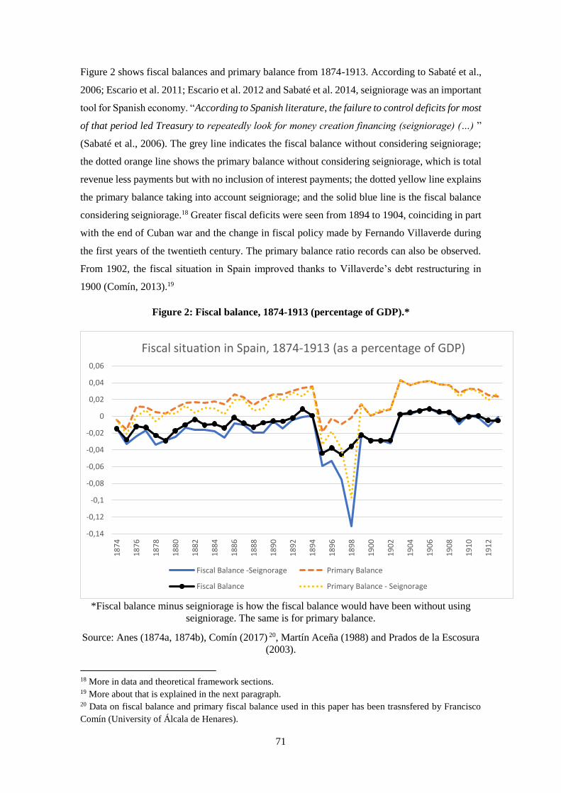
71
Figure 2 shows fiscal balances and primary balance from 1874-1913. According to Sabaté et al.,
2006; Escario et al. 2011; Escario et al. 2012 and Sabaté et al. 2014, seigniorage was an important
tool for Spanish economy. “According to Spanish literature, the failure to control deficits for most
of that period led Treasury to repeatedly look for money creation financing (seigniorage) (…) ”
(Sabaté et al., 2006). The grey line indicates the fiscal balance without considering seigniorage;
the dotted orange line shows the primary balance without considering seigniorage, which is total
revenue less payments but with no inclusion of interest payments; the dotted yellow line explains
the primary balance taking into account seigniorage; and the solid blue line is the fiscal balance
considering seigniorage.18 Greater fiscal deficits were seen from 1894 to 1904, coinciding in part
with the end of Cuban war and the change in fiscal policy made by Fernando Villaverde during
the first years of the twentieth century. The primary balance ratio records can also be observed.
From 1902, the fiscal situation in Spain improved thanks to Villaverde’s debt restructuring in
1900 (Comín, 2013).19
Figure 2: Fiscal balance, 1874-1913 (percentage of GDP).*
*Fiscal balance minus seigniorage is how the fiscal balance would have been without using
seigniorage. The same is for primary balance.
Source: Anes (1874a, 1874b), Comín (2017) 20, Martín Aceña (1988) and Prados de la Escosura
(2003).
18 More in data and theoretical framework sections. 19 More about that is explained in the next paragraph. 20 Data on fiscal balance and primary fiscal balance used in this paper has been trasnsfered by Francisco
Comín (University of Álcala de Henares).
-0,14
-0,12
-0,1
-0,08
-0,06
-0,04
-0,02
0
0,02
0,04
0,06
18
74
18
76
18
78
18
80
18
82
18
84
18
86
18
88
18
90
18
92
18
94
18
96
18
98
19
00
19
02
19
04
19
06
19
08
19
10
19
12
Fiscal situation in Spain, 1874-1913 (as a percentage of GDP)
Fiscal Balance -Seignorage Primary Balance
Fiscal Balance Primary Balance - Seignorage

72
During the nineteenth century there was no unified budget. Therefore, the increase in debt came
both from the budget deficit and the extraordinary budgets, as well as the expenses of wars or
even debt issuances for public works and subsidies to companies (Comín, 2016). According to
Comín (2013 and 2016), these debt crises were the result of high budget deficits, and the excessive
weight of short-term debt and external debt.
Comin (2016) studied Spanish debt crises using different indicators. The maximums in the series
of public debt in real terms and in ratio debt/GDP are in 1876-78 and 1902 and mark the two
crises of the Spanish debt. Public debt grew steadily between 1864 and 1878. In 1886, after
Camacho's conversion, the debt fell reaching its minimum. Subsequently, the budget deficits
returned to feed the debt between 1887 and 1901. Again, in 1902 the debt reaches a maximum.
According to Comín (2016) this was the maximum level of debt that the Spanish fiscal system
developed in 1845 could withstand. Villaverde’s stabilization would help to reverse the situation.
Between 1865 and 1883 the debt / GDP ratio was higher in Spain than in other European countries,
indicating that its debt crisis was particularly large. In 1895, after the settlement of Camacho's
debt, the path of divergence was re-established and the debt / GDP ratio increased (figure 1). The
ratio in this period was higher than that of Italy, which was one of the most indebted countries.
After 1850, excessive deficits occurred between 1861 and 1873 and 1895 and 1902. After these,
fiscal restrictions were applied. Outside the gold standard, the Spanish Treasury could avoid the
orthodoxy of budgetary equilibrium and openly resort to the inflation tax to finance the deficit.
Table 1 shows how, during the 1880s, the deficit was much higher in Spain than in Italy. There
was also a large difference between Spain and England until the beginning of the twentieth
century. During those years, in the UK the deficit never reached 1% (with the exception of
wartime), Italy only exceeded 1% in 1888, but in general was below 1% (table 1). However, Spain
usually had deficits over 1% before the twentieth century.
Table 1: Fiscal balance in the UK, Italy and Spain, 1874-1913 (in % of GDP).
Source: Comin (2017), Prados de la Escosura (2003), Baffiggi et al (2013), Fratianni and
Spinelli (2012), Mitchell et al. (1988, pp. 575-593)
UK Italy Spain
1874 0.06 -0.11 -1.47
1880 0.06 0.27 -1.71
1885 -0.004 -0.26 -1.36
1890 0.18 -0.69 -0.57
1895 0.18 -0.64 -4.39
1900 -2.65 0.59 -2.91
1905 0.48 0.56 0.64
1910 0.75 0.18 -0.05
Fiscal balance

73
Figure 3 also shows that Spain had higher deficits in terms of public expenditure than other
countries such as Italy (similar to Spain) or the UK considering the fiscal balance over public
expenditure ratio. A tendency toward change can be observed at the beginning of the twentieth
century with Villaverde new policies. Spain had deficits that were double those in Europe with a
smaller state weight (expenditure/GDP).21
Figure 3. A comparison between Spain, Italy and the UK considering budget balance,
1874-1913 (percentage of public expenditure).
Source: Comin (forthcoming), Frattiani and Spinelli (2012) and Thomas, R and Dimsdale, N
(2017)
Table 2 shows how, in general terms, Spain had lower public spending on GDP than other
countries such as France, Italy and Germany, although in some years it was higher than in the
UK. However, it was one of the countries with the highest fiscal deficits (table 1).
21 Based on the sources shown in graph 1.
-35,00%
-30,00%
-25,00%
-20,00%
-15,00%
-10,00%
-5,00%
0,00%
5,00%
10,00%
15,00%
18
74
18
76
18
78
18
80
18
82
18
84
18
86
18
88
18
90
18
92
18
94
18
96
18
98
19
00
19
02
19
04
19
06
19
08
19
10
19
12
Budget balance/Public expenditure, 1874-1913
Budget balance/ Public expenditure (Spain) Budget balance/ Public Expenditure (Italy)
Budget balance/ Public expenditure (UK)
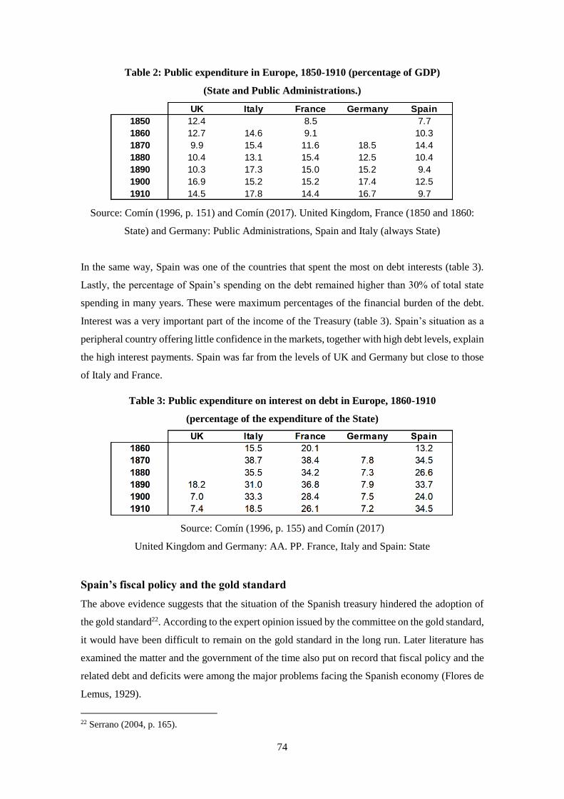
74
Table 2: Public expenditure in Europe, 1850-1910 (percentage of GDP)
(State and Public Administrations.)
Source: Comín (1996, p. 151) and Comín (2017). United Kingdom, France (1850 and 1860:
State) and Germany: Public Administrations, Spain and Italy (always State)
In the same way, Spain was one of the countries that spent the most on debt interests (table 3).
Lastly, the percentage of Spain’s spending on the debt remained higher than 30% of total state
spending in many years. These were maximum percentages of the financial burden of the debt.
Interest was a very important part of the income of the Treasury (table 3). Spain’s situation as a
peripheral country offering little confidence in the markets, together with high debt levels, explain
the high interest payments. Spain was far from the levels of UK and Germany but close to those
of Italy and France.
Table 3: Public expenditure on interest on debt in Europe, 1860-1910
(percentage of the expenditure of the State)
Source: Comín (1996, p. 155) and Comín (2017)
United Kingdom and Germany: AA. PP. France, Italy and Spain: State
Spain’s fiscal policy and the gold standard
The above evidence suggests that the situation of the Spanish treasury hindered the adoption of
the gold standard22. According to the expert opinion issued by the committee on the gold standard,
it would have been difficult to remain on the gold standard in the long run. Later literature has
examined the matter and the government of the time also put on record that fiscal policy and the
related debt and deficits were among the major problems facing the Spanish economy (Flores de
Lemus, 1929).
22 Serrano (2004, p. 165).
UK Italy France Germany Spain1850 12.4 8.5 7.71860 12.7 14.6 9.1 10.31870 9.9 15.4 11.6 18.5 14.41880 10.4 13.1 15.4 12.5 10.41890 10.3 17.3 15.0 15.2 9.41900 16.9 15.2 15.2 17.4 12.51910 14.5 17.8 14.4 16.7 9.7
75
For those who hold the view that not enough was done to adopt the gold standard, the policy
choices that were made were not in the right direction and lacked the necessary force. Martín
Aceña et al. (2014) claim that the monetary and fiscal policies adopted were not well focused on
Spain’s integration into the gold standard, and were not pursued with sufficient conviction23. The
authorities did not balance the budget nor did they follow fiscal orthodoxy. The question to answer
is whether fiscal orthodoxy really could have been followed in a country as backward as Spain.
These authors also point to the behaviour of the Banco de España to explain why Spain did not
adopt the gold standard. They note that the high rate of returns maintained by the Banco de España
helped to keep Spain off the gold standard. To join, it would have been necessary to decrease the
issue of banknotes, which would have lowered the bank’s profitability. Along these lines, the
authors concur that the Banco de España acted as a private bank by prioritizing its own earnings.
Serrano (2004), p. 165, also argues that the Banco de España took a view that was more financial
than economic. That said, however, the Bank of Portugal behaved differently, and Portugal was
not spared from leaving the gold standard due to its huge debt. In any case, a debate Banco de
España and its link or not with fiscal situation is beyond the scope of this paper.
On the one hand, Spain did not adopt the gold standard because of the fear of its politicians and
the Banco de España that deficits in the trade balance and the budget would cause an outflow of
gold that would make the project unworkable24. This fear finds expression in the expert opinion
issued by the committee on the gold standard25. Serrano Sanz notes that “the deficit was
undoubtedly an obstacle to monetary discipline at the time (...)”26.
On the other hand, the situation of the public coffers meant that monetary policy took a back seat
to fiscal needs27. In relation to the exchange rate, the result was depreciation because the amount
of money in circulation increased due to the role played by tha Banco de España.28 The deficits
and the need to finance the debt drove up the amount of money in circulation. Figure 4 below
shows that the amount of money in circulation followed a very similar behaviour to the evolution
of the public debt, given the need to finance the country’s mounting debt (Sabaté et al., 2006, p.
23 Martín Aceña, Nogués and Martínez Ruiz (2012). 24 Tortella (1994a, p. 324). 25 Dictamen (1929, pp. 24, 61 and 66). 26 Serrano (2004, p. 156). In the same vein, Sabaté et al. (2006, p. 328), point to the behaviour of the
Treasury as one of the causes of the peseta’s non-convertibility. Jordi Nadal has also noted that many of
the proposals of Spanish governments put a higher priority on payment obligations. 27 Tortella (1994a, p. 325). 28 Tortella (1994a, p. 325) and García Iglesias (2005, p. 17) consider that the relationship between the Banco
de España and the Treasury was very important in the decisions taken regarding the monetary system.
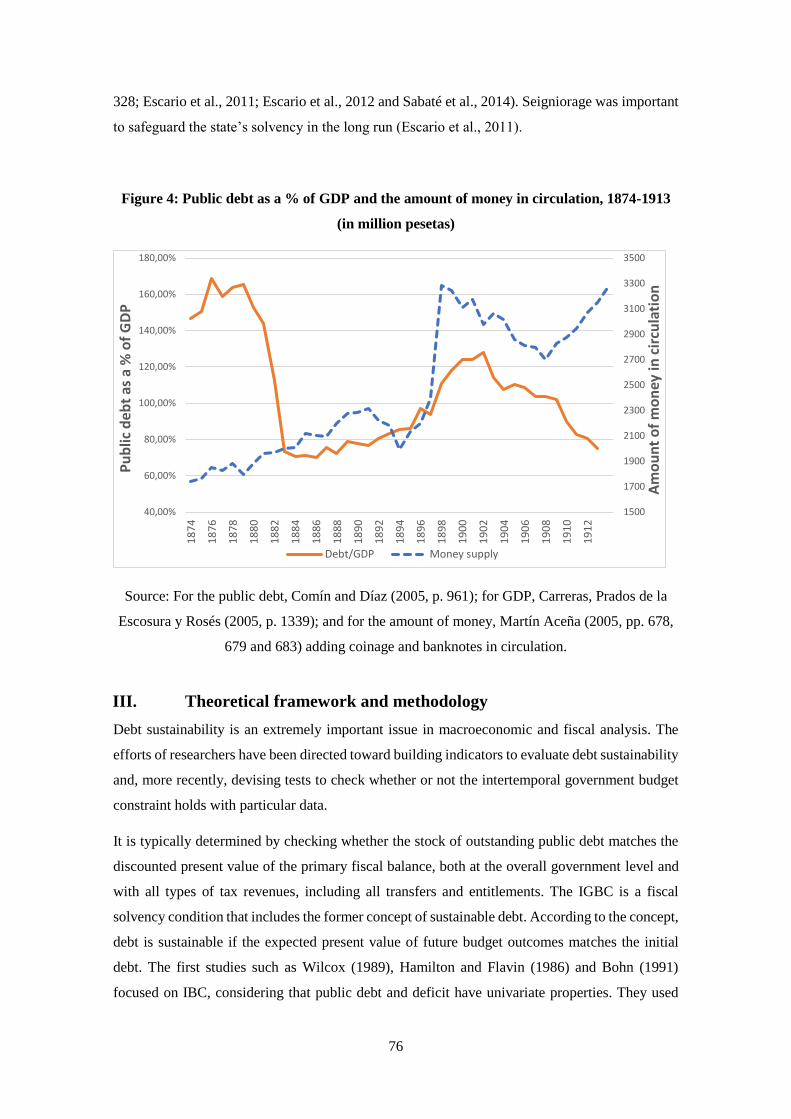
76
328; Escario et al., 2011; Escario et al., 2012 and Sabaté et al., 2014). Seigniorage was important
to safeguard the state’s solvency in the long run (Escario et al., 2011).
Figure 4: Public debt as a % of GDP and the amount of money in circulation, 1874-1913
(in million pesetas)
Source: For the public debt, Comín and Díaz (2005, p. 961); for GDP, Carreras, Prados de la
Escosura y Rosés (2005, p. 1339); and for the amount of money, Martín Aceña (2005, pp. 678,
679 and 683) adding coinage and banknotes in circulation.
III. Theoretical framework and methodology
Debt sustainability is an extremely important issue in macroeconomic and fiscal analysis. The
efforts of researchers have been directed toward building indicators to evaluate debt sustainability
and, more recently, devising tests to check whether or not the intertemporal government budget
constraint holds with particular data.
It is typically determined by checking whether the stock of outstanding public debt matches the
discounted present value of the primary fiscal balance, both at the overall government level and
with all types of tax revenues, including all transfers and entitlements. The IGBC is a fiscal
solvency condition that includes the former concept of sustainable debt. According to the concept,
debt is sustainable if the expected present value of future budget outcomes matches the initial
debt. The first studies such as Wilcox (1989), Hamilton and Flavin (1986) and Bohn (1991)
focused on IBC, considering that public debt and deficit have univariate properties. They used
1500
1700
1900
2100
2300
2500
2700
2900
3100
3300
3500
40,00%
60,00%
80,00%
100,00%
120,00%
140,00%
160,00%
180,00%
18
74
18
76
18
78
18
80
18
82
18
84
18
86
18
88
18
90
18
92
18
94
18
96
18
98
19
00
19
02
19
04
19
06
19
08
19
10
19
12
Am
ou
nt
of
mo
ney
in c
ircu
lati
on
Pu
blic
deb
t as
a %
of
GD
P
Debt/GDP Money supply

77
cointegration and unit root tests in the IGBC framework. This classic concept of debt
sustainability was used by Buiter (1985), Blanchard (1990) and Blanchard, Chouraqui, Hagemann
and Sartor (1990), who apply the intertemporal government budget constraint as a condition that
relates long-term budget balances over GDP and debt as a percentage of GDP in order to define
debt sustainability. Trehan and Wash (1988 and 1991) and Haug (1991) test solvency by
determining the order of integration of the public debt series and analysing if there is a
cointegration relation between public revenues and expenditures. Hamilton and Flavin (1986),
Hakkio and Rush (1991), Quintos (1995) apply the same focus to the US economy. Then, studies
by Hakkio and Rush (1991), Haug (1995), Quintos (1995), Martin (2000) among others, explored
the structural shocks for IBC. Other studies such as Bohn (1998) underlined the possibility of a
non-linear function on IBC.
Bohn was critical of this methodology (Bohn 1998, 2007 and 2008).29 In Bohn’s view, testing for
debt sustainability is futile, because the IGBC holds under very weak conditions if the variables
are integrated in any finite order. Bohn (1998 2007 and 2008) also shows that these
misspecification errors lead to incorrect inferences that reject fiscal solvency when it actually
exists. As Bohn (2008) stresses, neither a particular order of integration of the debt data nor the
co-integration of revenues and government outlays is necessary for debt sustainability. This
condition is very weak because it is easy to reject the hypothesis that the variables are non-
stationary after differentiating them an infinite number of times. For all these reasons, it is
necessary to study the dynamics of fiscal reactions that support fiscal solvency.30
Bohn (1998) incorporates the tax smoothing model of Barro (1979) and estimates a multiple
regression to study the systematic relationship between the primary surplus and public debt. Bohn
(1998 and 2008) defends an approach that is focused on economic intuition considering the
relationship between public debt and primary balance. Bohn (1998 and 2007) deduces a simple
rule or fiscal reaction function for testing whether debt was sustainable by solving intertemporal
optimization. Bohn (1998) believes that if an economy improves its budget balance when it sees
its debt grow, then its debt will be sustainable in the long-run. He also notes that the positive
relationship between deficit and debt is not necessary when the level of debt-GDP-ratio is low.
Bohn (1998 and 2008) shows that by identifying the fiscal reaction functions, it is possible to
study fiscal solvency and understand the dynamics among the variables. This, in turn, provides a
better understanding of deficit issues. Bohn (1998) estimates the fiscal reaction function for the
US (1916-95) and Bohn (2008) extended the analysis for 1792-2003 showing how public debt
was sustainable. As can be seen in Bohn (2008), a linear fiscal reaction function with a statistically
29 For additional information, see Bohn (2007) and D’Erasmo et al (2016). 30 In D’Erasmo et al. (2016), there is an in-depth examination of the reasons why using only the IGBC to
analyse debt sustainability is not correct.
78
significant and positive response of the primary balance to outstanding debt is sufficient for the
IGBC to hold. Bohn defines the conditions for sustainability as those in which an agent’s ability
to borrow is constrained by other agents who are willing to lend (Bohn, 2008). Bohn’s fiscal
reaction functions (2008) only require data on the budget balance, the outstanding debt and some
control variables. As a result, it has recently become more common to estimate the fiscal reaction
function, which addresses the reaction of primary surpluses to variations in the debt-to-GDP ratio
under a given debt policy (Bohn, 2008 and D’Erasmo et al., 2016).
Ihori et al (2001) applied the same methodology for the Japanese case. Shizume (2007 and 2011)
run a similar analysis appling Bohn’s method for pre- World war Japanese debt with a new dataset
of Japanese fiscal balances. Ghatak and Sanchez-Fung (2006) study the debt sustainability for
Peru, Philippines, South Africa, Thailand and Venezuela (1970-2000). Mendoza and Ostry (2008)
extended Bohn’s analysis. Some studies have sought to provide a better definition of fiscal limits,
that is, the maximum debt-to-GDP ratio that is sustainable (Ghosh, Kim, Mendoza, Ostry and
Qureshi, 2013 and D’Erasmo et al., 2016). These authors have examined the conditions for fiscal
solvency by considering changes to the fiscal balance arising from different levels of debt.31 An
analysis of debt sustainability with structural changes has been made by Shizume (2007 and
2011).
Bajo-Rubio, Díaz-Roldan and Esteve (2004 and 2006) used TAR (Threshold Vector
Autoregressive) for the Spanish case during the second half of the twentieth century. Arestis,
Cippolini and Fattouh (2004) also ran a TAR to study the fiscal dynamics depending on the
growth level. Others such as Escario et al (2012) studied fiscal dominance and solvency using
multicointegration for Spanish case in the long-run. Several studies have addressed this question
via Bohn (2008)’s single country analysis and other via panel analysis by Celasun, Debrun, and
Ostry (2007) who studied debt paths for emerging countries by estimating fiscal reaction function
from a panel regression. A VAR approach has also been used by Afonso (2008).
The approach here is the one proposed by Bohn (1998, 2007 and 2008) in his work on fiscal
solvency.32 This approach has the advantage of providing a robust method for a non-structural
empirical test that is sufficient to satisfy fiscal solvency (D’Erasmo et al., 2016). By analysing the
dynamics of fiscal adjustment, fiscal solvency can be studied by means of the characteristics of
the fiscal reaction function. The information on how to obtain the specification comes from tax-
smoothing theories on optimal taxation, which suggest that temporary changes in government
spending and decreases in income drive up normal fiscal deficits. Bohn (1998) explains that the
31 Other studies have examined debt sustainability using different approaches. Two examples are Bi, Shen
and Yang (2016) and Arellano and Bai (2017). 32 Bohn developed the analysis that we used here in 1998 with an analysis of the sustainability of the debt
between 1916 and 1995. In 2005 he extended the analysis between 1792 and 2003.

79
tax smoothing theory yields an empirical specification for primary surplus. This model uses a set
of other variables to control implying that non-debt determinants of the primary surplus are the
level of temporary government spending, 𝑔𝑡 and business cycle indicator, 𝑦𝑡.33 The idea of this
paper is to search for a systematic relationship between debt over GDP ratio and the primary
balance by estimating a regression whose empirical specification is as follows:
𝑠𝑡 = 𝜌𝑑𝑡 + 𝛽0 + 𝛽𝑔𝑔𝑡 + 𝛽𝑦𝑦𝑡 + 𝑒 (1)
where 𝑠𝑡 is primary balance over GDP, 𝑑𝑡 is public debt over GDP, gt is temporary expenditures,
𝑦𝑡 is temporary income, 𝑒 is the error term with zero mean and 𝜌, 𝛽0, 𝛽𝑔 and 𝛽𝑦 are the regression
coefficients. Both 𝑦𝑡 and 𝑔𝑡 are estimated with proxies and prove quite important for identifying
the marginal effect of the public debt. The control variables are the output gap for capturing the
impact of economic cycles on the budget (𝑦𝑡) and on defence spending (𝑔𝑡). Temporary military
expenditure is usually calculated following Barro (1986) and Bohn (1998). The sign and the
statistical significance of the 𝑑𝑡 coefficient is critical in our analysis (table 2). A positive response
of coefficient 𝜌 is a sufficient condition for fiscal solvency in a fiscal reaction function. We
employ OLS in our regressions. As a result, this coefficient is expected to be positive, indicating
that an increase in the public debt ratio is associated with an increase in the primary budget
balance. Most studies of this sort also consider seigniorage, taking into account the size of the
monetary base that went to finance the state year after year and subtracting the deficits. This
approach indicates not just whether there was fiscal solvency, but also how it was achieved. 34
In some studies, autoregressive vectors (VARs) have been used to obtain impulse-response
functions for the public debt and fiscal balance (Canzoneri et al. 2001, Afonso, 2008 and Bajo-
Rubio et al., 2014) in order to provide a further robustness check by showing additional results
from a forward looking approach. I use local projections instead of impulse response function
based on VAR analysis due to the number of observations. For the purposes of the present study,
the latter two methods have been examined because they are the most efficient and the most
commonly used in recent studies of debt sustainability and fiscal policy for different countries
and different historical periods.
33 These control variables are called 𝑍𝑡 by Bohn (1998). 34 Another different approach is done by Ghatak and Sanchez-Fung (2007) who employ a recursive t
statistical approach to explore within sample developments of debt just of the period. They fix one starting
period and change the ending year, extending it. They thus see how the results change depending on the
period under study.

80
IV. Data The data start in 1874, for historical reasons. The restoration in 1874 restored political stability to
Spain (see annex 1).35 This is the time of the gold standard throughout Europe.36 I use new data
on primary balance that has not already been published. New data on primary balance come from
Francisco Comín (2017) who is the maximum expert on Public Finances in Spain and has
recalculated the primary and budget balances.37 Moreover, I will use new data on military
expenditure from Sabaté (2016).
In the absence of monthly data, the study makes use of annual data from 1874 to 1913. St is the
ratio of the budget balance to GDP that is obtained by Comín (2005) and dt is the ratio of public
debt to GDP, also from Comín (2005). Yt is temporary output and the main data points for its
calculation come from the estimation in Prados de la Escosura (2003), while gt is temporary
spending and the data for its estimation are defence spending figures from Comín (2005) and
Sabaté (2016). The data on seigniorage are obtained in the same manner used in Escario et al
(2012) and Sabaté et al. (2006). These data come from Anés (1874a, 1874b) and Martín Aceña
(1988).
V. Estimating the fiscal reaction function
Following the specification of equation (1), the fiscal reaction function is estimated. Yt and gt are
the proxies for temporary GDP and temporary government spending, which are obtained as
follows. For economic fluctuations, individuals are assumed to be able to distinguish between
trend and cycle in real time as well as an economist can when looking backward. Like others
before, we use the Hodrick-Prescott filter (𝜆=100) to extract the trend from a series of real GDP
data. The difference between the real value and the trend is taken as a proxy for 𝑦𝑡. 38 I also use
the cyclical component of GDP to check and compare my results. Fluctuations in government
spending are basically the result of defence spending. I separate large swings in military
expenditure from other fiscal spending. Non-defence spending can be approximated with a
random walk process. The permanent component of defence spending, as a ratio of GDP, is
estimated with an autoregressive model of order two (AR2), as in Bohn (2008). The results can
also be verified by using defence spending as a proxy for 𝑔𝑡 as in D’Erasmo et al. (2016). We
take the difference between the actual and the fitted components. 𝜌 is expected to be positive and
35 More on this in Serrano (2004, pp. 25 and following). 36 To include seigniorage in our analysis, 1874 should be taken as the starting point, as there are no data on
seigniorage prior to this date 37 This data has been used before by Betrán and Pons (2018). New data solves the fiscal deficits
underestimation shown in Comín and Díaz (2005). 38 Positive values indicate that the proxy is above the trend.
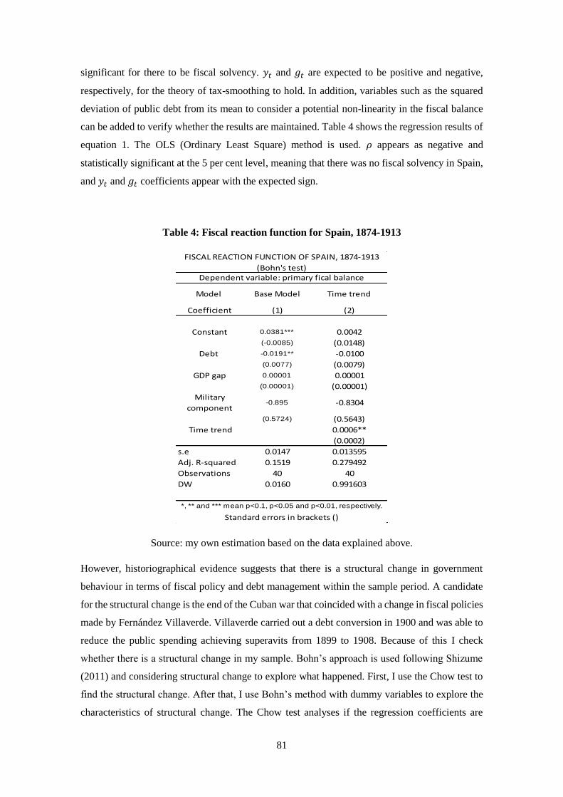
81
significant for there to be fiscal solvency. 𝑦𝑡 and 𝑔𝑡 are expected to be positive and negative,
respectively, for the theory of tax-smoothing to hold. In addition, variables such as the squared
deviation of public debt from its mean to consider a potential non-linearity in the fiscal balance
can be added to verify whether the results are maintained. Table 4 shows the regression results of
equation 1. The OLS (Ordinary Least Square) method is used. 𝜌 appears as negative and
statistically significant at the 5 per cent level, meaning that there was no fiscal solvency in Spain,
and 𝑦𝑡 and 𝑔𝑡 coefficients appear with the expected sign.
Table 4: Fiscal reaction function for Spain, 1874-1913
Source: my own estimation based on the data explained above.
However, historiographical evidence suggests that there is a structural change in government
behaviour in terms of fiscal policy and debt management within the sample period. A candidate
for the structural change is the end of the Cuban war that coincided with a change in fiscal policies
made by Fernández Villaverde. Villaverde carried out a debt conversion in 1900 and was able to
reduce the public spending achieving superavits from 1899 to 1908. Because of this I check
whether there is a structural change in my sample. Bohn’s approach is used following Shizume
(2011) and considering structural change to explore what happened. First, I use the Chow test to
find the structural change. After that, I use Bohn’s method with dummy variables to explore the
characteristics of structural change. The Chow test analyses if the regression coefficients are
Model Base Model Time trend
Coefficient (1) (2)
Constant 0.0381*** 0.0042
(-0.0085) (0.0148)
Debt -0.0191** -0.0100
(0.0077) (0.0079)
GDP gap 0.00001 0.00001
(0.00001) (0.00001)
Military
component-0.895 -0.8304
(0.5724) (0.5643)
Time trend 0.0006**
(0.0002)
s.e 0.0147 0.013595
Adj. R-squared 0.1519 0.279492
Observations 40 40
DW 0.0160 0.991603
Standard errors in brackets ()
FISCAL REACTION FUNCTION OF SPAIN, 1874-1913
(Bohn's test)Dependent variable: primary fical balance
*, ** and *** mean p<0.1, p<0.05 and p<0.01, respectively.

82
different for split data sets. Basically, it tests whether one regression line or two separate
regression lines best fit a split set of data. The result of the Chow test on equation (1) indicates a
structural change in 1903.39 Figure 5 shows the results of the Chow test. I find a structural change
after with the end of Cuban war, coinciding with the change in fiscal policies run by Fernández
Villaverde.
Figure 5. Chow test of equation 1
Source: own calculation
Following Shizume (2007), the equation of Bohn’s approach for testing debt sustainability with
structural change is as follows.
𝑠𝑡 = 𝛼0 + (𝜌1𝑑𝑡 + 𝜌2𝑑𝑡𝐷𝑡) + (𝛼1𝑔𝑡 + 𝛼2𝑔𝑡𝐷𝑡) + 𝑒𝑡 (2)
𝐷𝑡 has a value of zero before 1903 and one starting with 1903. 𝜌1, 𝜌2, 𝛼1 and 𝛼2 are the regression
coefficients. I exclude the output component in the main model because it is insignificant and I
need as many degrees of freedom as possible. When I run the regression with output component,
the results do not change.
39 Structural change is found in 1903 even when we consider seigniorage.
0
1
2
3
4
5
6
7
8
9
18
96
18
97
18
98
18
99
19
00
19
01
19
02
19
03
19
04
19
05
19
06
19
07
19
08
F-st
atis
tic
Chow testDependent variable: primary fiscal balance
Significant at 5 percent level (2.67)
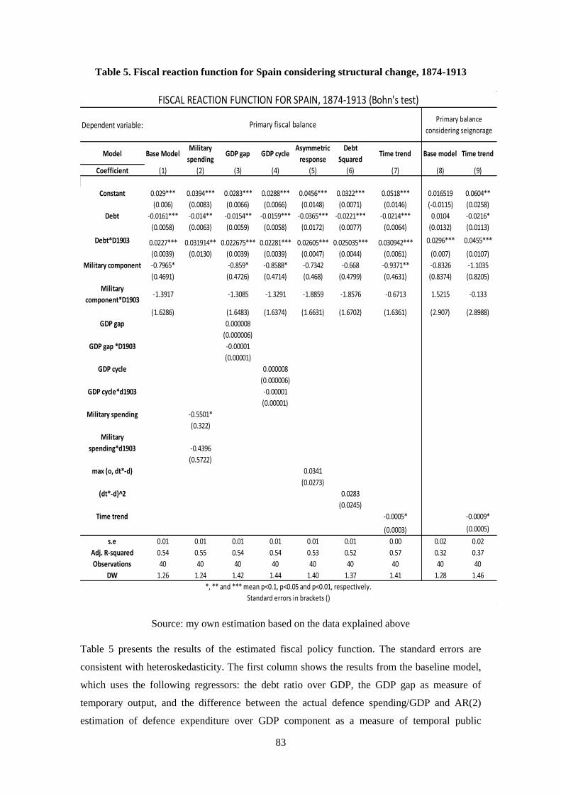
83
Table 5. Fiscal reaction function for Spain considering structural change, 1874-1913
Source: my own estimation based on the data explained above
Table 5 presents the results of the estimated fiscal policy function. The standard errors are
consistent with heteroskedasticity. The first column shows the results from the baseline model,
which uses the following regressors: the debt ratio over GDP, the GDP gap as measure of
temporary output, and the difference between the actual defence spending/GDP and AR(2)
estimation of defence expenditure over GDP component as a measure of temporal public
Dependent variable:
Model Base ModelMilitary
spendingGDP gap GDP cycle
Asymmetric
response
Debt
SquaredTime trend Base model Time trend
Coefficient (1) (2) (3) (4) (5) (6) (7) (8) (9)
Constant 0.029*** 0.0394*** 0.0283*** 0.0288*** 0.0456*** 0.0322*** 0.0518*** 0.016519 0.0604**
(0.006) (0.0083) (0.0066) (0.0066) (0.0148) (0.0071) (0.0146) (-0.0115) (0.0258)
Debt -0.0161*** -0.014** -0.0154** -0.0159*** -0.0365*** -0.0221*** -0.0214*** 0.0104 -0.0216*
(0.0058) (0.0063) (0.0059) (0.0058) (0.0172) (0.0077) (0.0064) (0.0132) (0.0113)
Debt*D1903 0.0227*** 0.031914** 0.022675*** 0.02281*** 0.02605*** 0.025035*** 0.030942*** 0.0296*** 0.0455***
(0.0039) (0.0130) (0.0039) (0.0039) (0.0047) (0.0044) (0.0061) (0.007) (0.0107)
Military component -0.7965* -0.859* -0.8588* -0.7342 -0.668 -0.9371** -0.8326 -1.1035
(0.4691) (0.4726) (0.4714) (0.468) (0.4799) (0.4631) (0.8374) (0.8205)
Military
component*D1903-1.3917 -1.3085 -1.3291 -1.8859 -1.8576 -0.6713 1.5215 -0.133
(1.6286) (1.6483) (1.6374) (1.6631) (1.6702) (1.6361) (2.907) (2.8988)
GDP gap 0.000008
(0.000006)
GDP gap *D1903 -0.00001
(0.00001)
GDP cycle 0.000008
(0.000006)
GDP cycle*d1903 -0.00001
(0.00001)
Military spending -0.5501*
(0.322)
Military
spending*d1903 -0.4396
(0.5722)
max (o, dt*-d) 0.0341
(0.0273)
(dt*-d)^2 0.0283
(0.0245)
Time trend -0.0005* -0.0009*
(0.0003) (0.0005)
s.e 0.01 0.01 0.01 0.01 0.01 0.01 0.00 0.02 0.02
Adj. R-squared 0.54 0.55 0.54 0.54 0.53 0.52 0.57 0.32 0.37
Observations 40 40 40 40 40 40 40 40 40
DW 1.26 1.24 1.42 1.44 1.40 1.37 1.41 1.28 1.46
Primary fiscal balance Primary balance
considering seignorage
FISCAL REACTION FUNCTION FOR SPAIN, 1874-1913 (Bohn's test)
*, ** and *** mean p<0.1, p<0.05 and p<0.01, respectively.
Standard errors in brackets ()

84
expenditure (Bohn, 2007).40 The second column estimates the same model taking the military
spending/GDP instead of the main measure for this variable. The third column runs the estimation
adding GDP as another control variable. The fourth column uses the cyclical GDP component as
a temporal output, obtaining the same results. Following D’Erasmo et al. (2016), the fifth column
introduces a spline coefficient when the debt is greater than the mean.41 The sixth column adds
the squares mean deviation of the debt ratio. The seventh column adds the time trend to the main
regression. The eighth column lays out the regression of the first column but considering
seigniorage since 1874, i.e., removing the Banco de España’s transfers to the Treasury. In this
way, it is possible to check whether the debt was sustainable thanks to seigniorage or not. This
has been done in order to take seigniorage into account later on.42 Thus, the eighth column uses
the same variables as the main model taking as a dependent variable the deficit that considers
seigniorage instead of the official deficit. Lastly, the ninth column adds time trend to the eighth
column.
When negative, this 𝑝 coefficient indicates there is no debt sustainability. 𝑝1 , the coefficient for
public debt between 1874 and 1902, is always negative and significant in all regressions, showing
the lack of fiscal solvency during those years even considering seigniorage. The hypothesis of the
sustainability of Spain’s fiscal policy can therefore be rejected. These results are in line with the
historiography. Three debt restructurings were made in those forty years, those of Salaverría,
Camacho and Villaverde. If the three conversions had not been made, the debt could not have
been sustained, leading the country to default. Therefore, not even seigniorage allowed the debt
to be sustainable. Despite monetization, Spain had to restructure the debt in order to move
forward. The results found corroborate what it is shown in figures 1 to 4. The temporary
expenditure component and GDP gap component have the expected signs, negative and positive
respectively. Temporary expenditure appears as a significant variable for the period 1874-1903
when seigniorage is not considered except for the debt squared and asymmetric response cases;
in other cases, they are insignificant, in agreement with the tax smoothing theory.
Otherwise, Spanish debt became sustainable at some point due to the policies adopted by
Fernández Villaverde. Independently of whether we consider seigniorage, the values of 𝑝2 are
always positive and statistically significant, implying a structural change in the year indicated by
Chow test. The coefficient for the public debt is positive and significant, which means that the
debt is sustainable. The change from the 𝑝1 to 𝑝2 coefficient shows a change in government’s
40 I estimate an AR(2) for the fitted values as Bohn (2007) does. Results do not change if I use Comin
(2005) data on military expenditure. 41 More on its construction in D’Erasmo et al. (2015). 42 We estimate the equation excluding seigniorage with different measures of expenditure and considering
different variables and the yields are the same.
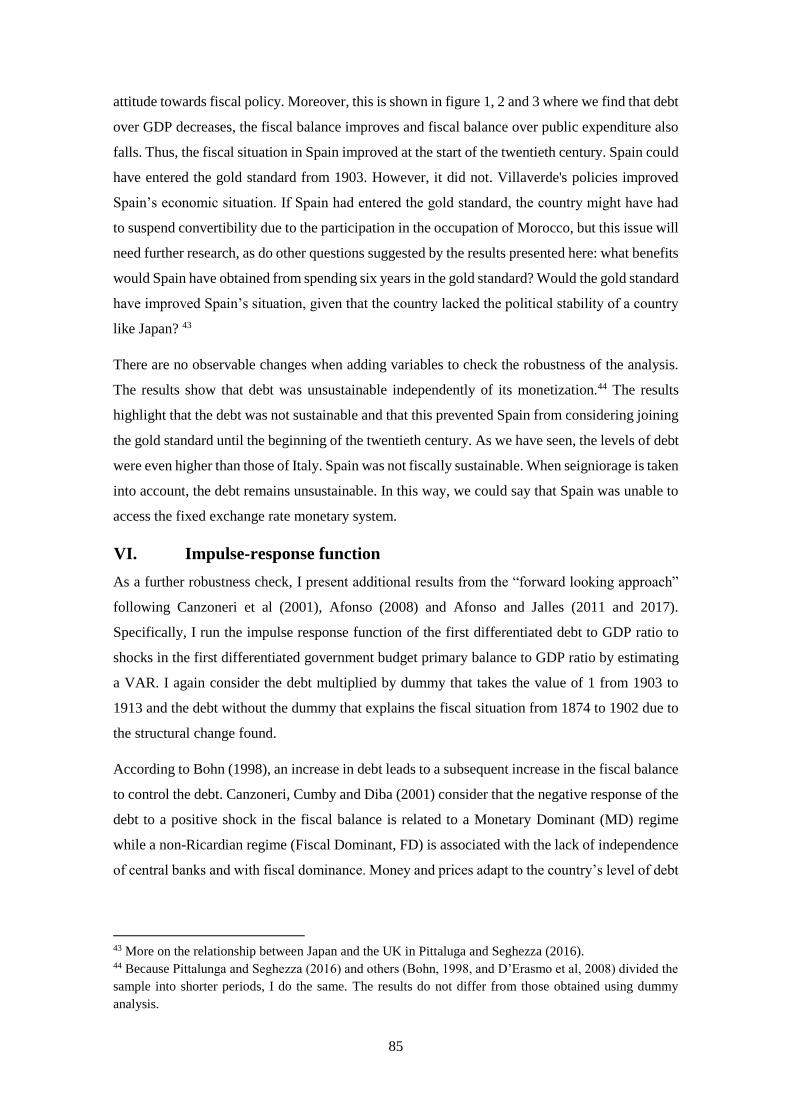
85
attitude towards fiscal policy. Moreover, this is shown in figure 1, 2 and 3 where we find that debt
over GDP decreases, the fiscal balance improves and fiscal balance over public expenditure also
falls. Thus, the fiscal situation in Spain improved at the start of the twentieth century. Spain could
have entered the gold standard from 1903. However, it did not. Villaverde's policies improved
Spain’s economic situation. If Spain had entered the gold standard, the country might have had
to suspend convertibility due to the participation in the occupation of Morocco, but this issue will
need further research, as do other questions suggested by the results presented here: what benefits
would Spain have obtained from spending six years in the gold standard? Would the gold standard
have improved Spain’s situation, given that the country lacked the political stability of a country
like Japan? 43
There are no observable changes when adding variables to check the robustness of the analysis.
The results show that debt was unsustainable independently of its monetization.44 The results
highlight that the debt was not sustainable and that this prevented Spain from considering joining
the gold standard until the beginning of the twentieth century. As we have seen, the levels of debt
were even higher than those of Italy. Spain was not fiscally sustainable. When seigniorage is taken
into account, the debt remains unsustainable. In this way, we could say that Spain was unable to
access the fixed exchange rate monetary system.
VI. Impulse-response function
As a further robustness check, I present additional results from the “forward looking approach”
following Canzoneri et al (2001), Afonso (2008) and Afonso and Jalles (2011 and 2017).
Specifically, I run the impulse response function of the first differentiated debt to GDP ratio to
shocks in the first differentiated government budget primary balance to GDP ratio by estimating
a VAR. I again consider the debt multiplied by dummy that takes the value of 1 from 1903 to
1913 and the debt without the dummy that explains the fiscal situation from 1874 to 1902 due to
the structural change found.
According to Bohn (1998), an increase in debt leads to a subsequent increase in the fiscal balance
to control the debt. Canzoneri, Cumby and Diba (2001) consider that the negative response of the
debt to a positive shock in the fiscal balance is related to a Monetary Dominant (MD) regime
while a non-Ricardian regime (Fiscal Dominant, FD) is associated with the lack of independence
of central banks and with fiscal dominance. Money and prices adapt to the country’s level of debt
43 More on the relationship between Japan and the UK in Pittaluga and Seghezza (2016). 44 Because Pittalunga and Seghezza (2016) and others (Bohn, 1998, and D’Erasmo et al, 2008) divided the
sample into shorter periods, I do the same. The results do not differ from those obtained using dummy
analysis.
86
in order to sustain fiscal policy. My hypothesis is that Spain had a non-Ricardian regime, in view
of the articles on fiscal dominance (Sabaté et al., 2006, Escario et al., 2012 and Sabate et al., 2019)
Due to the number of observations, I estimate the local impulse response function following Jordà
(2005). This section lays out the local impulse-response function of the debt-to-GDP ratio (dt) to
shocks on the ratio of the budget balance to GDP (st). The dotted red lines indicate error bands
that correspond to two standard deviations. The dotted (red) lines are the error bands. I use
conditional error bands for local impulse response because they help to remove the variability
caused by serial correlation. Following, Jordà (2009), error bands are consistent with the joint
null of significance and they are more sensitive to the significance of individual responses. If there
is no correlation between the impulse response coefficients, conditional and marginal bands
would be similar. As can be seen in figure 6, the debt-to-GDP ratio exhibits a negative and
significant response following a shock in the primary balance ratio from 1874 to 1902 and a
positive and significant shock in the budget balance response from 1903 to 1913. This approach,
therefore, would also say that an FD regime has prevailed through the years under study.
However, when seigniorage is considered (figure 7), the results do not change. A rise (an
innovation) in debt-to-GDP ratio generates a decrease in the budget balance from 1874 to 1902,
which runs counter to a Ricardian system and fits a system where the monetary policy is passive,
fiscal dominance exists and the debt generates larger deficits (first graph in figure 6 and 7).
Therefore, there is no response from the government. Otherwise, between 1903 and 1913, the
response of primary balance to a shock in debt-to-GDP ratio is positive. This result is related to
the results obtained in the previous section in the calculation of the fiscal response function.
Figure 6. Local impulse response function (blue) for primary balance.
-.006-.004-.002.000.002.004.006.008
0 1 2 3 4 5 6 7 8 9 10
Response of primary balance to an increase in debt over GDP until 1903
-.008
-.004
.000
.004
.008
0 1 2 3 4 5 6 7 8 9 10
Response of primary balance to an increase in debt over GDP from 1903
-.10
-.06
-.02
.02
.06
0 1 2 3 4 5 6 7 8 9 10
Response of debt over GDP to an increase in primary balance until 1903
-.3
-.2
-.1
.0
.1
.2
0 1 2 3 4 5 6 7 8 9 10
Response of debt over GDP to an increase in primary balance from 1903
Source: My own estimation from the data explained above.

87
Figure 7. Local impulse response function (blue) for primary balance considering
seigniorage.
-.015-.010-.005.000.005.010.015.020
0 1 2 3 4 5 6 7 8 9 10
Response of primary balance considering seignorage to an increase in debt over GDP until 1903
-.015-.010-.005.000.005.010.015
0 1 2 3 4 5 6 7 8 9 10
Response of primary balance considering seignorage to an increase in debt over GDP from 1903
-.08-.06-.04-.02.00.02.04.06
0 1 2 3 4 5 6 7 8 9 10
Response of debt over GDP to an increase in primary balance considering seignorage until 1903
-.2
-.1
.0
.1
.2
.3
0 1 2 3 4 5 6 7 8 9 10
Response of debt over GDP to an increase in primary balance considering seignorage from 1903
Source: My own estimation from the data explained above
VII. Conclusion
This paper is the first study on fiscal sustainability in Spain for the period 1874-1913, when the
dominant monetary system was the gold standard. The results leave no room for doubt that
Spain’s debt was unsustainable until 1903. This would explain why the country was not able to
adopt the gold standard and why it experienced greater instability than its European neighbours
until the beginning of the twentieth century. This quantitative study shows that Spain’s public
debt became sustainable around 1903 due to the new fiscal policies introduced by Villaverde; at
this point, Spain was in a position to join the gold standard. This change in 1903 has not been
reported previously. Moreover, the evidence shows that seigniorage was not as important as could
be expected. The sustainability or unsustainability of the debt did not depend on seigniorage
between 1874 and 1913. More research is needed into the causes of Spain’s failure to adopt the
gold standard. New quantitative research on Spanish debt and the impact of the policies adopted
by Villaverde on the real economy would also be useful. Finally, the socioeconomic impact of
this unsustainable debt should be analysed.

88
89
Chapter 3: “Spain and the classical gold standard. short- and
long-term analyses”.*
Abstract
This paper seeks to link the two theories put forward to explain the consequences of Spain’s non
adoption of the gold standard in the late nineteenth century, and does so by comparing the
outcomes of short- and long-run approaches. The empirical results obtained from applying an
autoregressive distributed lag model (ARDL) framework are reported. This ARDL analysis
reveals that the expansionary monetary policies implemented had a positive impact on Spain’s
output in the long-run. Exchange rate had a positive impact on Spanish output in the short-run but
not in the long-run. This paper provides new empirical evidence for the core-periphery debate
through an analysis of the impact of being or not being in the gold standard by dividing the
analysis between the short- and the long-run. Thus, it sheds new light on the developments in
Spain at the time of the classical gold standard.
Key words: Classical Gold Standard, Spain, Exchange Rate, ARDL, Monetary Policy
JEL codes: E42, E52, E63
* I wish to thank Francisco Comín for sharing his data with me. I would like to express my gratitude to
Professor Jordi Catalan and Matthias Morys. I am also grateful to my department colleagues and specially
those who are in my research project. This paper has been presented in different workshops, seminars and
conferences. I would like to thank the following scholars for their comments: Rui Esteves, Isabel Sanz,
Marcela Sabaté, José María Serrano Sanz, Alejandro Ayuso, Masato Shizume, Jonas Ljunberng, Anders
Orgen, This article has received funding from the Ministry of Economics and Competitiveness and from
FEDER trough research project HAR2015-64769-P. Naturally, I am responsible for the remaining errors.

90
“(...) in no way does the fall of the peseta seem to me synonymous with
weakness. The freedom to allow a certain moderate slackening in the
exchange rate in times of general depression affecting the rest of the
world can be a valuable measure to maintain internal stability, which
would otherwise be impossible.”
J. M. Keynes, interviewed in El Sol by
Luís de Olariaga, 10 June 1930
I. Introduction
Interest in the gold standard has grown in recent years because of the parallels that can be drawn
with the euro crisis and the questions that have been raised by relinquishing monetary sovereignty
(Stiglitz, 2016, p. 12). Indeed, the euro has generated the same rigidities in Europe that the gold
standard once imposed on the world (Bordo and James, 2014), when the countries in Europe’s
southern periphery were unable to remain in that monetary system1. These are the same countries
that today are struggling to overcome the recent economic crisis that has been played out against
the broader background of the single currency (Eichengreen, 2014, pp. 12, 13 and 93).
According to Bordo and Rockoff (1996, p. 394), adherence to the gold standard was a very
difficult objective to achieve for the countries of southern Europe; their experiences were
characterised by higher rates of growth of the money supply, fiscal deficits, and higher inflation
than other countries. Outside the gold standard, however, they were able to use fluctuations in
the exchange rate to cushion the impact of economic shocks (Bordo and Rockoff, 1996, p. 416).
The differences between the north and the south (core and periphery) in fiscal and monetary terms
may have affected the adherence to the gold standard (Bordo and Schwartz, 1986).2 Those authors
found that southern European and South American economies suffered from higher demand
shocks, and that as a result they used more discretionary fiscal and monetary policies.
The gold standard was actually less rigid than believed (Bloomfield, 1959; Dutton, 1984;
Pippenger, 1984; Giovaninni, 1986; Davutyan and Parke, 1995; Jeanne, 1995 and Reis, 2007).
According to Martín Aceña et al. (2011), although it is known that many economies were on the
gold standard without introducing money convertibility, they were nevertheless able to maintain
the stability of their exchange rates. In contrast, a large proportion of the countries on the
periphery experienced major exchange rate fluctuations and instability (Triffin, 1985, p. 128).
1 For the Italian case, see Fratianni and Spinelli (1984), Cipolla (1995), Tattara (2000 and 2003), Bordo
(1999, p. 328) and Fratianni and Spinelli (2012). For the Portuguese case, see Mata (1987), Reis (1996,
2000 and 2007), Valerio (1998) and Bordo (1999, p. 329). 2 More about core and periphery in Bordo and Flandreau (2003).
91
The exchange rate of the peseta fluctuated against gold and against other currencies. Moreover,
the balance of payments deficits made it difficult to remain in the international monetary system.
This paper covers the period known as the classical gold standard era, during which Spain
operated a de jure bimetallic standard. Having said that, in the late 1880s, the country is regarded
as operating a de facto fiduciary system, insofar as the real value of silver was lower than its face
value and there was a constant outflow of gold.
The debate on Spain’s decision not to adopt the gold standard is far from being resolved.3 Some
economists and economic historians claim that policies that the country was able to apply because
it was off the gold standard served to stimulate the economy. It is stressed that adherence to the
gold standard would have tied the government’s hands and prevented it from taking any monetary,
fiscal or exchange rate actions.4 The main proponent of this school of thought, the “classical
thesis”, is Joan Sardà. I consider that its arguments are more short-term than long-term
explanations.5 According to Sarda (1987, pp. 196-198), the favourable evolution of the Spanish
economy during the final years of the nineteenth century was largely due to the country’s absence
from the gold standard.6 Solé Villalonga (1967) and Tortella (1981 and 1994a) support Sardà's
position with arguments that are more sensitive to the long term. Sardà (1987, pp. 196-98 and
252), Solé Villalonga (1967, pp. 41-43) and Tortella (1970 and 1994b) consider the non-
convertibility of the peseta to have been positive for the Spanish economy: having a flexible
exchange rate and applying expansionary monetary and fiscal policies had a positive effect on
Spanish GDP.
More recently, this belief has been supported by Cubel et al. (1998), Catalan et al. (2001), Cubel
(2001), Llona (2001), Ródenas et al. (2001), Sabaté et al. (2001), Carreras and Tafunell (2004,
pp. 219-20), Serrano (2004) and Ródenas and Bru (2006).7 Despite this, the results of previous
work, published in Peseta y Protección (Sudrià and Tirado, 2001) are not conclusive. Before of
these studies, Herranz and Tirado (1996, p. 28) stress the difficulties Spain would have had by
keeping a fixed exchange rate. Serrano et al. (1998) consider that the use of the interest rate was
3 A summary of different positions can be found in Roldan (2017). 4 For example, following Sardà (1987, p. 176), the situation in 1883 could only be resisted by increasing
the money stock thanks to a fiduciary system. Moreover, the monetary expansion eased the impact of the
international depression and made it possible to finance the exaggerated deficits of the Spanish economy
while paying lower interest rates than those that would have been applied by foreign lenders. 5 According to the methodology used in this paper, short run is what happens between two years and long
run is what happens until Spain reaches the equilibrium (the cointegration relationship). For more details,
see methodology section. 6 Moreover, Tortella (1994a, pp. 323-24) equated the advantages of the gold standard with those later
associated with the European Monetary System, highlighting that with these monetary systems no
corrective measures could be taken and this forced to accept undesired situations such as gold outflows. 7 More about rigidity in Morys (2007).

92
not enough to maintain gold convertibility. It should have had an impact on the money supply,
which would have caused a notable recession. Moreover, the interest rate of the peseta when it
was convertible was higher than when it was not convertible. Serrano et al. (1998, p. 85), point
out that Spain's unique monetary option had no effect on long-term trade flows. Finally, Llona
(2001, pp. 164-169) points out that having maintained a stable exchange rate bolstered the level
of economic activity by reducing the price of non-tradable goods.
Pablo Martín Aceña (1981, 1985, 1993, 1997, 2000 and 2017) questions the validity of this thesis
and his works seem to adopt a long-term analysis. Martín Aceña upholds a “critical thesis”,
considering it a mistake on the part of the Spanish government not to have adopted the gold
standard. He considers that having a fiduciary system harmed the Spanish economy, causing the
isolation of international capital flows and reducing investments. Martín Aceña claims that the
country’s growth would have been much greater under the gold standard. In his view, the flexible
exchange rate, the application of an expansionary monetary policy and the lack of fiscal discipline
had a negative impact on Spanish economy (Martín Aceña, 1981, p. 267). At this point, it is
important to ask whether all countries were equal and had the same needs or, whether the effects
of the monetary system differed from country to country. Fraile (1991), Tena (1992), and Prados
de la Escosura (1997) all highlight the negative consequences of Spanish protectionism and the
depreciation of the peseta for the allocation of resources in the long term. Martín Aceña et al
(2011), Martínez Ruíz and Nogués Marco (2014), and Martinez-Ruiz and Nogués Marco (2018)
stress that the Banco de España (Bank of Spain) was responsible for the country’s absence from
the gold standard.
In my view, while the classical thesis focuses on the short-run, the critical thesis analysis is
characterised by what is primarily a long-run approach. I intend to test it. The effects, both positive
and negative, of Spain’s absence from the gold standard depend largely on the time scale of the
analysis. Thus, while the impact of certain instruments of economic policy may be null or negative
in the long term, they may be significant and positive in the short term. Hence, the results of my
analysis will depend on whether we focus on the long run or on the short run.
Martín Aceña (1981 and 1993) also thinks that movements in the exchange rate were mainly due
to changes in expectations. However, researchers closer to the classical thesis (Sabaté et al., 2006)
defend that Spain suffered fiscal dominance. Could the exchange rate have been affected by the
increase in the money supply? Or was the exchange rate caused, or explained, by changes in
expectations due to constant deficits and huge debt accumulation? This paper also aims to answer
these questions.
In the light of the above, my aim in this study is to test and compare the critical and the classical
theories in order to determine which theory provides a more faithful reflection of the

93
repercussions of not adopting the gold standard, considering a new perspective. In so doing, I
study the short-term and the long-term separately in an effort to establish a point of union between
the two theories. Finally, I aim to examine causality between the three macroeconomic policies
under study. This will allow me to understand if the path followed by exchange rate was due to
expectations, due to the monetary policy among other explanations. Moreover, I will be able to
check in different way what was underlined by Sabaté et al. (2006), Escario et al. (2011), Escario
et al. (2012) and Sabaté et al. (2014). This paper is also part of the debate on the positive or
negative effects of depreciation in the long term.8 To do this I use time series methodology that
permits me to distinguish between the short and the long term: ARDL (autoregressive distributed
lag) model.
Spain was the only western country that never joined the gold standard. There are no quantitative
or empirical studies of the impact of being outside the gold standard on Spain’s economic output
at the end of the nineteenth century and the beginning of the twentieth. This is what I intend to
provide in this paper, by unifying the two existing theories on the matter. The importance of this
research topic has been underlined by various economic historians, among them Martín Aceña et
al. (2000, p. 3), who state that “the debate on the feasibility and the costs and benefits for
peripheral economies of being on the gold standard is still far from closed”, Serrano (2004, p.
20) highlighting that it is necessary to study “the effect that the monetary strategy adopted by
Spain could have had on development during the Restoration (…)” and Pedro Lains (2006, p.
185). For García-Iglesias (2005), neither theory can be confirmed or rejected. Martín Aceña et al.
(2011) underline that the cost of having a different monetary system needs further research.
Recent papers and books on the subject include Martín Aceña (2017 and 2018) and Martínez Ruiz
and Nogués Marco (2018). For example, Martín Aceña (2018) says that the non-adoption of the
gold standard was negative unless the opposite can be demonstrated, thus leaving the door open
to further research.
The study confirms how adjustments to the exchange rate played a prominent short-run role in
Spain’s economic development. However, in the long run, the exchange rate had non-significant
impact or negative and significant effect on Spanish GDP, depending on the specification. Thus,
both theories seem correct if a distinction is made between the long and the short term. It is
important to stress that it is not my purpose to analyse if it was better to adopt the gold standard
or not. I only intend to analyse what happened, and to assess the impact of the presence of a
fiduciary system (thus, of having a flexible exchange rate) on the Spanish economy, in both the
short and the long run.
8 More in discussion section.
94
The rest of the paper is organised as follows: section 2 describes the historical context; section 3
presents the theoretical framework and the methodology employed; section 4 explains the data;
section 5 reports the empirical results and the robustness check; section 6 discusses these results
in relation to the previous literature; and, finally, section 7 offers my conclusions.
II. The Spanish economy during the classical gold standard
The decree of October 19, 1868, with Laureano Figuerola as finance minister, unified the
monetary system. The peseta was chosen as the official currency of Spain because of its similarity
to the franc. The objective was to align the national system with that of the countries with which
Spain maintained the greatest volume of trade. Spain adopted the operating requirements of the
Latin Monetary Union, but never formed part of it. The Echegaray Decree of March 19, 1874
granted the monopoly of the Banco de España's issuance of notes due to the treasury’s financial
difficulties at the time. From 1874, the state was able to increase the number of banknotes in
circulation (Figure 1) to solve its treasury problems (Sardà, 1987, p. 180).
There was certainly an interest in Spain in adopting the gold standard. The possibility was
officially raised in 1876 by the Consultative Board of the Currency (Serrano, 2004). At the
beginning of the twentieth century a further attempt was made. However, there was a constant
fear that the country would not be strong enough to stay on the gold standard and, together with
problems concerning the budget balance and the balance of payments, this led to not adopting the
monetary system. A wait-and-see policy was applied (Serrano, 2004) or, in the words of García-
Iglesias (2005), a policy of low risk and low profitability. Spain defended the wait-and-see policy,
using two main arguments. First, it was difficult to predict the international monetary scenario.
On the other hand, during the 1880s the value of the peseta was maintained with respect to the
lira. In this way, the stability of the exchange rate offered some respectability (Serrano, 2004,
p.67). The government did not demand any guarantee of convertibility. For its part, considering
that the conversion was an exclusively internal matter, the Banco de España rationed the cash it
had in its coffers (Serrano, 2004). The bank never had an obligation to convert banknotes into
gold; in fact, it never had to give explanations to anyone (Serrano, 2004).
The issue of banknotes increased notably after 1879 (Sarda, 1987, p. 175 and Tortella, 1994a, p.
177). In 1882, the Finance Minister Camacho converted the Spanish debt, due to the impossibility
of facing payments (Comin and Martorell, 2006, pp. 389-391). The Banque de Lyon et de la Loire
collapsed in 1882 and the Spanish banks were exposed to cash withdrawals, outright failure, and
dwindling gold reserves. The crisis in France affected Spain, draining the gold reserves and
precluding the conversion of Spanish banknotes into gold (Sardà, 1987, p. 179; Martín Aceña,
1993, pp. 135, 137 and 189; Tortella, 1994a, pp. 139, 177 and 480-481; Bordo and Schwartz,
1999, p. 32; Martín Aceña et al., 2011, p. 3 and Catalan and Sánchez, 2013, p. 96). There were

95
also constant outflows of gold (Martín Aceña, 2017). In 1883, Spain had a de facto fiduciary
system with a flexible exchange rate. The effect of Gresham's law left the Spanish economy
without any gold: between 1891 and 1892, gold disappeared from circulation (Sarda, 1987, p.
183). Martínez Ruiz and Nogués (2014, p. 24) considered that Spain was in the shadow of the
gold standard until the early 1890s, despite its de facto fiduciary system. At that point, a flotation
stage began. The exchange rate broke the band of gold points in 1889 and began a more
pronounced upward trend in 1891.9 Due to insufficient resources rather than to a lack of will, the
peseta became a floating currency (Serrano, 2004); the floating exchange rate was an automatic
mechanism for correcting economic cycles. Moreover, the agricultural depression compounded
the financial slump and made the crisis the longest one of the period.
The decree of July 14 1891 raised the limit on the issue of banknotes to 1500 million pesetas
(Sardà, 1987, p. 180). In 1891, the peseta depreciated, coinciding with the application of the
Cánovas tariff and improving the economic situation (Carreras et al., 2005, p. 1341). In 1892,
with the earlier crisis still not entirely overcome, a new economic crisis emerged: the Cuban
insurrection again increased the deficits from 1895, causing debt to rise from 800 million to 3000
million pesetas. This debt was monetized, thus increasing the money supply in circulation.
Between 1893 and 1898, the depreciation of the peseta was the highest in the period (Figure 1)
because of the constant deficits and the strong increase in debt. Subsequently, in 1898, the issue
limit was again increased, this time to 2500 million pesetas10. This was an economic crisis of
considerable breadth (Sardà, 1987, p. 223). Until 1896, the slight growth of the money supply
acted in a preventive manner against further depreciation (Martín Aceña, 1993, p. 141). Moreover,
the Méline tariff levied by the French placed insurmountable entry conditions on alcoholic
beverages from the Iberian Peninsula, curtailing all wine exports (Serrano, 2011, p. 641). The
loss of the French market intensified the slump, and the outbreak of phylloxera throughout the
Iberian Peninsula exacerbated the situation still further. Sardà (1987, pp. 196-98) thinks that the
favourable evolution of the Spanish economy in the final decade of the nineteenth century was,
in part, thanks to the fact that the country stayed off the gold standard.
With the approval of the Law of budgets of 1899-1900, the situation of the Treasury was restored
until 1909 and the limit on the issue of banknotes was lowered. These measures achieved a budget
surplus and for a few years the State was able to finance itself without having to issue
banknotes. Finally, in a last attempt to improve the price of the peseta on the international market
and reduce public debt, the limit was lowered to 2000 million pesetas because of a more
9 Martín Aceña (1993, p. 140) underlines that there was not depreciation after 1883 and peseta’s value
remained stable during some years. 10 The Cuban uprising forced the Ministry of Overseas Territories to resort to the issue of banknotes, Sardà
(1987, p. 190).

96
contractionary monetary policy than in the preceding years11. Between 1902 and 1906 Spain
entered another period of crisis, when pc GDP fell twice as a consequence of swingeing budget
adjustments. The effects of this restrictive policy can be judged as positive even though the
economy showed symptoms of depression (Sardà, 1987, p. 207). In this period it could have
entered into the gold standard but did not do so, because it wanted to return to the parity of 1868
instead of entering at a depreciated parity (Serrano, 2004).
Figure 1. The evolution of Spanish economy.
Source: see main text.
Martín Aceña (1993, p. 160), thinks that the authorities took the wrong decision at a crucial
moment; in his view, the only way to fully benefit from the expansion in world trade and
international investment of the late nineteenth and early twentieth centuries was to be on the gold
standard. The authorities did not like the floating exchange rate, but they did not carry out an
independent monetary policy either. According to Olariaga (1977, p. 133), monetary policy
11 These tighter policies are associated with Raimundo Fernández Villaverde, finance minister in 1899-
1900 and 1902-1903 and later prime minister in 1903 and 1905. His policies involved financial restructuring
to put the system on a sound footing again and to halt the depreciation of the currency. In 1908, these
policies were abandoned when signs of domestic slump appeared (Sardà, 1987, p. 202).

97
consisted of an ad hoc policy rather than a conscious control aimed at regulating the economic
cycle and the volume of credit. Tortella (1994a, p. 175), also supports this idea considering that
it was a series of measures that related to the fiscal sphere. The money supply expanded and
contracted depending on the position of the Treasury with the Banco de España, which depended
on the size of the budget deficit (Martín Aceña, 1993, p. 150).
The monetary policy of this period was characterized by a lack of national objectives and a
constant tension between the government and the Banco de España (Martínez Ruiz and Nogués
Marco, 2014, p. 21). It was unclear which of the two institutions was in charge of exercising the
functions of monetary authority. According to Sardà, the monetary policy was not as expansive
as might be imagined since in part the outflows of gold were replaced by banknotes. Despite
having a fiduciary system, governments endeavoured to maintain a certain discipline in
macroeconomic policy. For Tortella (1994a, p. 177), these were years of slow but steady growth
in the Spanish economy.
III. Data
Due to the absence of quarterly or monthly data for some of the variables, I draw on a sample of
annual data between 1870 and 1913.12 The data come from secondary sources as follows: the
𝑦𝑝𝑐𝑟𝑡 is real pc GDP measured using GDP calculations from Prados de la Escosura (2003) and
population statistics from Nicolau (2005) deflated by GDP deflator (Prados de la Escosura, 2003),
𝑓𝑡 is the fiscal balance obtained from Comín (2017)13 and deflated by GDP deflator from Prados
de la Escosura (2003), 𝑙𝑚𝑠𝑛𝑡 is the money supply measured by Martín Aceña (2018) and
𝑙𝑟𝑒𝑒𝑟𝑡 is the real effective exchange rate calculated by me. Here all the variables have been
converted into logarithms except for the fiscal balance.14 𝑙 is the logarithm of the variables.
The real effective exchange rate considers the average weight of the exchange rate against the
pound sterling, the French franc and the US dollar. I have calculated real effective exchange rate
as follows. The calculation of the real effective exchange rate draws on the GDP deflator reported
by Prados de la Escosura (2003) for Spain, the deflators reported by Toutain (1987) for France,
Balke and Gordon (1989) for the US and Thomas and Dimsdale (2017) for the UK, and the peseta
exchange rate from Martín Aceña and Pons (2005) and Martínez Ruiz and Nogués Marco
(2014).15 The series of real effective exchange rates calculated both using CPI and GDP deflator
12 I can start on 1870 thanks to the work done by Martín Aceña (2018) who constructed a new money supply
series for the years before the Banco de España monopoly of issuing. 13 I am extremely grateful to Francisco Comín who has shared his data with me improving the quality of
this analysis and making possible compare the results obtained with the two existent series for fiscal
balance. 14 This is the same procedure followed by Shibamoto and Shizume (2014). Because the fiscal balance has
negative values, it cannot be converted into logarithms. As a result, the variable is used without conversion. 15 I use GDP deflator from Prados de la Escosura as Serrano et al. (2017) did.

98
can be found in Annex 1. Results do not change if we use CPI from Maluquer (2013) and CPI
from Mitchell (2007) instead of GDP deflator (see Annex 2, figure 3). The weight of foreign trade
to the respective countries is obtained from Prados de la Escosura (1982, p. 42), using fixed
weightings updated every five years. The weightings account for more than 60% of total foreign
trade over the entire period.
IV. Theoretical framework and methodology
Different studies have used similar methodologies with similar goals. To test my hypothesis, I
will follow the theoretical approach developed in Kandil and Mirzaie (2002) and Bahmani-
Oskooee and Kandil (2010).16 The cited papers find that real output depends on movements in the
exchange rate, money supply and government spending.17 But, instead of using government
spending as a dependent variable I opt to use the fiscal balance.18 First, because while a state may
have high expenditure, its taxes may also be high, yet by only considering public spending, we
cannot take into consideration the whole of the state’s fiscal policy. Second, by focusing on fiscal
policy it will be possible to verify the causalities between macroeconomic policies that have been
studied elsewhere in the literature (most notably by Sabaté et al., 2006, pp. 310, 321 and 328 and
by Escario et al., 2011, pp. 271-272, Sabaté et al., 2019).
Following Kandil and Mirzaie (2002), Bahmani-Oskooee and Kandil (2010) and Shibamoto and
Shizume (2014), I employ four macroeconomic variables: pc GDP, budget balance, money supply
(M1) and real effective exchange rate. Real output is 𝑙𝑦𝑝𝑐𝑟 which varies according to the three
policy types. The money supply is 𝑙𝑚𝑠𝑛𝑡 and this approximates the monetary policy. Fiscal
policy, 𝑓𝑡, is measured by the fiscal balance and the real effective exchange rate is denoted by
𝑙𝑟𝑒𝑒𝑟𝑡. An increment in the exchange rate results in depreciation. If the exchange rate coefficient
presents a positive sign, depreciation helps raise GDP. Otherwise, if the effect is contractionary,
the sign is negative.19
The econometric tools used are also in line with Bahmani-Oskooee and Kandil (2010), who
analyse the effect of exchange rate fluctuations on real output growth, controlling for monetary
and fiscal policies for the case of Iran using a vector error correction (VEC) framework that
16 This approach is used today to understand the role of exchange rate on developing economies. I think
Spain during the end of the nineteenth century can be considered as a developing country. 17 One can find all the theoretical development in the two references quoted. 18 My results do not change if I use the government expenditure instead of the fiscal balance. 19 For more about the impact of exchange rates see Alexander (1952), Dornsbusch, Krugman and Cooper
(1976, p. 551), Krugman and Taylor (1978), Bahmani-Oskooee and Anker (2001), Bahmani-Oskooee and
Kandil (2010). For the effects of monetary policy, see Mishkin (1995). Taylor (1995) emphasizes the
importance of the exchange rate channel of monetary transmission. Taylor (1995) stresses the effects of
monetary policy on the economy (Mishkin, 1995, p. 5). For fiscal effects on economic growth, see
Blanchard and Perotti (2002).

99
distinguishes between the short and the long run.20 We can find more papers using the similar
time series methodology. Matesinni and Quintieri (1997) analyse the impact of macroeconomic
policies on Italian GDP to understand the recovery from the Great Depression through a VAR.
Cha (2003) conducts the same analysis for Japan, using a structural vector autoregressive (S-
VAR). Shibamoto and Shizume (2014) study how three macroeconomic policies (monetary, fiscal
stimulus and exchange rate adjustment) and expected inflation affected Japanse GDP during the
Great Depression. De Castro and Fernández-Caballero (2011) analyse the impact of fiscal shocks
on the Spanish effective exchange rate over the period 1981-2008 using a similar methodology.
Choudhary and Chaudry (2007) study whether a devaluation of the currency affects output
positively or negatively through a VECM for Pakistan between 1975 and 2005.21
The main objective of this paper is to distinguish between the short and the long run. As such, my
paper seeks to verify the respective claims of Martín Aceña (1981, 1993, 2000 and 2017) and
Sardà (1948). Due to the number of observations, I run an ARDL model. I compare the short
results obtained from ARDL model with those shown by local projections. ARDL is a time series
model that allows the adoption of a similar approach to that of the VEC model by analysing the
two different temporal approaches while obtaining better results for a small sample, in this
instance 44 observations. The ARDL model uses a single equation (Pesaran and Shin, 1995).22 It
does not deal with problems of endogeneity. It is unlikely that this problem will arise as long as
the errors are not serially correlated because regressors tend to be lagged in levels or differences.23
If there is cointegration, OLS is a consistent estimation. One can expect significant correlation
among variables if you use non-stationary series. However, ARDL is a robust and dynamic
method designed for that purpose and can therefore deal with these cases successfully. A further
advantage of ARDL is that the variables can be I(0) or I(1): they do not have to be integrated of
order 1.
20 Similar studies can be found in Bahmani-Oskooee et al. (2002), Kalyoncu et al. (2008), Bahmani-
Oskooee and Kutan (2008), Narayan and Narayan (2011), Bahmani-Oskooee and Gelan (2013) and
Bahmani-Oskooee et al. (2016). 21 There are diferent studies concerned about the effect of having a flexible exchange rate on output.
Nowadays, these studies are focused on developing countries. My point of view is that analysing an
economy such as Spain during the 19th century is close to what means today analysing a developing
country. Considering this, I decided to use similar methodologies. Other economic historians like
Shibamoto and Shizume (2014) also decided to use VAR models in order to study the impact of
macroeconomic policies (including exchange rate adjustments) on output using similar theoretical
approach. 22 Simple equation methods, such as fully modified and dynamic ordinary least squares (FMOLS and
DOLS), have been used to analyse the long term and cointegration between variables, producing similar
results. Here, the results of ARDL, DOLS and FMOLS were also very similar. 23 Moreover, I have lagged values of the variables on the right-hand side of (1).

100
The bound test procedure developed by Pesaran et al. (2001) is based on the estimation of the
unrestricted error correction model (ECM) by OLS, which can be applied to regressors with I(0)
or I(1). To implement the bounds testing procedure the following ARDL model is estimated.
(1) ∆𝑙𝑦𝑝𝑐𝑟𝑡 = 𝛼0 + ∑ 𝜙𝑖∆𝑙𝑦𝑝𝑐𝑟𝑡−𝑖 + ∑ 𝜗𝑖∆𝑓𝑡−𝑖 +𝑝𝑖=1
𝑛𝑖=1 ∑ 𝜕𝑖∆𝑙𝑚𝑠𝑛𝑡−𝑖 +𝑙
𝑖=1
∑ 𝜑𝑖∆𝑙𝑟𝑒𝑒𝑟𝑡−𝑖 + 𝑚𝑖=1 λ1𝑙𝑦𝑝𝑐𝑟𝑡−1 + + λ2𝑓𝑡−1 + λ3𝑙𝑚𝑠𝑛𝑡−1 + λ4𝑙𝑟𝑒𝑒𝑟𝑡−1 + 𝑒𝑡
where all variables are as previously defined, Δ is the difference operator and 𝑒𝑡 is the error term.
The next step involves estimations of the long-run relationship coefficients and of the error
correction term of the ARDL model, determining the speed of adjustment to equilibrium. ECT is
the residual obtained from the estimated cointegration model of equation 2. ECT is the residual
of λ1𝑙𝑦𝑝𝑐𝑟𝑡 − λ2𝑓𝑡 − λ3𝑙𝑚𝑠𝑛𝑡 − λ4𝑙𝑟𝑒𝑒𝑟𝑡, the long-term component of eq. (1). If the null
hypothesis of no cointegration is rejected, we can estimate the following short run ARDL error
correction model. For the specification above, the error correction versions of the ARDL model
in the variables 𝑦𝑝𝑐𝑟𝑡 , 𝑓𝑡, 𝑚𝑠𝑛𝑡 and 𝑟𝑒𝑒𝑟𝑡 are given by:
(2) ∆𝑙𝑦𝑝𝑐𝑟𝑡 = 𝛼0 + ∑ 𝜙𝑖∆𝑙𝑦𝑝𝑐𝑟𝑡−𝑖 + ∑ 𝜗𝑖∆𝑓𝑡−𝑖 +𝑝𝑖=1
𝑛𝑖=1 ∑ 𝜕𝑖∆𝑙𝑚𝑠𝑛𝑡−𝑖 +𝑙
𝑖=1
∑ 𝜑𝑖∆𝑙𝑟𝑒𝑒𝑟𝑡−𝑖 + + 𝑚𝑖=1 𝛿𝐸𝐶𝑇𝑡−1 + 𝜇𝑡
The cointegration coefficients characterize long-run relationships between levels and variables,
and the ECM coefficients describe changes that help to restore an equilibrium position. After
estimating the ARDL model, Toda and Yamamoto (1995)’s approach to the Granger causality
test is carried out. The Granger causality test presents problems when the series integrated are of
different orders (as happens in this study). Toda and Yamamoto (1995)’s approach to Granger
causality does not depend on the order of integration or on cointegration properties, but is based
on the Granger non-causality equation. Their procedure consists in estimating an augmented VAR
model (𝑘 + 𝑑𝑚𝑎𝑥) where 𝑘 is the optimal lag on the first VAR model and 𝑑𝑚𝑎𝑥 is the maximum
integrated order of the variables. Thus, the number of lags should be increased by the maximum
order of integration of the variables for Toda and Yamamoto’s causality testing procedure. After
that, the augmented VAR is estimated. The asymptotic distribution of the Wald statistic is
guaranteed. The lag length, considering the Akaike Information Criterion (AIC), is determined to
be 2.
V. Empirical results
This section describes the results obtained from the estimation of the ARDL. I proceed in three
stages. The first considers the order of integration of the variables; the second examines whether
the variables are cointegrated and studies the short- and long-term approaches; and the third
carries out the Toda and Yamamoto causality test.

101
Unit root test
The first step is to test the stationarity of the variables, considering both the Augmented Dickey-
Fuller (ADF) and Kwiatkowski-Phillips-Schmidt-Shin (KPSS) tests. Many economists consider
that unit root tests are problematic, and for this reason stationarity tests such as the KPSS have
been developed (Kwiatkowski et al., 1992). KPSS can be used to test the null hypothesis of
stationarity against the alternative of non-stationarity. Kwiatkowski et al. (1992) underlines that
their test aims to complement the unit root test. They stress that “(…) we can distinguish between
series that appear to be stationary, series that appear to have unit root, and series for which the
data (or the tests) are not sufficiently informative to be sure whether they are stationary or
integrated”. Thus, the KPSS test helps to complement unit root tests such as the Dickey–Fuller
tests. The ADF null hypothesis to determine the maximum order of integration is non-stationarity,
while the KPSS null hypothesis is stationarity. These two tests permit the assessment of the order
of integration from two different perspectives. As shown in Table 1, the variables of real effective
exchange rate and money supply tested with constant are non-stationary at levels for both tests,
but stationary at first difference.24 The null hypothesis of having a unit root is not rejected in the
ADF test (probability over 10%) and the null hypothesis of being stationary is rejected in the
KPSS test (probability under 10%). However, money supply seems to be I(1) for ADF and I(0)
for KPSS test when trend is considered. Exchange rate remains non stationary when it is tested
with trend. pc GDP is stationary except when it is tested with constant using KPSS. According to
economic theory, the variable fiscal balance should be stationary. The results obtained from the
KPSS tests suggest that it is stationary with constant and constant and trend while the ADF test
evidences that the series is not stationary with trend but stationary with constant.
24 According to the theoretical framework, the budget balance and the exchange rate should be stationary
variables, This can be attributable to the fact that Spain was a country with a tendency to budgetary deficits
during the entire period studied, only achieving a period of surplus during the first years of the twentieth
century. The exchange rate suffered a general depreciation (increase) after 1883 and specially from 1891,
reaching a maximum in 1898, depreciating by around 40%.
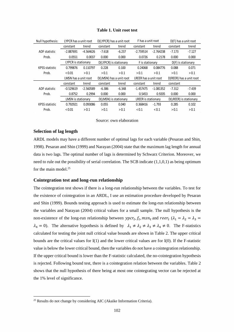
102
Table 1. Unit root test
Source: own elaboration
Selection of lag length
ARDL models may have a different number of optimal lags for each variable (Pesaran and Shin,
1998). Pesaran and Shin (1999) and Narayan (2004) state that the maximum lag length for annual
data is two lags. The optimal number of lags is determined by Schwarz Criterion. Moreover, we
need to rule out the possibility of serial correlation. The SCB indicate (1,1,0,1) as being optimum
for the main model.25
Cointegration test and long-run relationship
The cointegration test shows if there is a long-run relationship between the variables. To test for
the existence of cointegration in an ARDL, I use an estimation procedure developed by Pesaran
and Shin (1999). Bounds testing approach is used to estimate the long-run relationship between
the variables and Narayan (2004) critical values for a small sample. The null hypothesis is the
non-existence of the long-run relationship between 𝑦𝑝𝑐𝑟𝑡 , 𝑓𝑡, 𝑚𝑠𝑛𝑡 and 𝑟𝑒𝑒𝑟𝑡 (𝜆1 = 𝜆2 = 𝜆3 =
𝜆4 = 0). The alternative hypothesis is defined by 𝜆1 ≠ 𝜆2 ≠ 𝜆3 ≠ 𝜆4 ≠ 0. The F-statistics
calculated for testing the joint null critical value bounds are shown in Table 2. The upper critical
bounds are the critical values for I(1) and the lower critical values are for I(0). If the F-statistic
value is below the lower critical bound, then the variables do not have a cointegration relationship.
If the upper critical bound is lower than the F-statistic calculated, the no-cointegration hypothesis
is rejected. Following bound test, there is a cointegration relation between the variables. Table 2
shows that the null hypothesis of there being at most one cointegrating vector can be rejected at
the 1% level of significance.
25 Results do not change by considering AIC (Akaike Information Criteria).
Null hypothesis:
constant trend constant trend constant trend constant trend
ADF statistic -2.887691 -4.564626 -7.618 -6.237 -2.759514 -2.764238 -7.173 -7.127
Prob. 0.0551 0.0037 0.000 0.000 0.0726 0.2178 0.000 0.000
KPSS statistic 0.799876 0.110797 0.228 0.100 0.24068 0.084776 0.088 0.071
Prob. < 0.01 > 0.1 > 0.1 > 0.1 > 0.1 > 0.1 > 0.1 > 0.1
constant trend constant trend constant trend constant
ADF statistic -0.529619 -2.560589 -6.386 -6.348 -1.457475 -1.081352 -7.312 -7.439
Prob. 0.8752 0.2994 0.000 0.000 0.5453 0.9205 0.000 0.000
KPSS statistic 0.792921 0.093086 0.055 0.040 0.368416 -1.793 0.285 0.102
Prob. < 0.01 > 0.1 > 0.1 > 0.1 < 0.1 < 0.1 > 0.1 > 0.1
F is stationary D(F) is stationary
LMSN is stationary D(LMSN) is stationary LREER is stationary D(LREER) is stationary
LYPCR has a unit root D(LYPCR) has a unit root F has a unit root D(F) has a unit root
LMSN has a unit root D(LMSN) has a unit root LREER has a unit root D(REER) has a unit root
LYPCR is stationary D(LYPCR) is stationary

103
Table 2. Cointegration test
Source: own elaboration
Having established that an ARDL long-run cointegration relationship exists, the next stage of the
procedure is to examine the coefficients of the long-run relationship among the variables. The
long-run coefficients are shown in Table 3.
The exchange rate had a non-significant impact in the long run on GDP while monetary policy
and fiscal policy had a positive and significant effect. Exchange rate appears as negative and
significant in the long-run when old data on fiscal balance (Comín and Díaz, 2005) is used. This
would mean a depreciation of the currency had negative effect on Spanish GDP in the long run.
When estimation is run by using nominal effective exchange rate, fiscal balance and money
supply shows positive sign and it is significant in the long-run (see Annex 2, figure 1). Exchange
rate variable remains as non-significant. The exchange rate is negative and significant when the
estimation is run considering fiscal balance data, based on Comín and Díaz (2005) (Annex 2,
figure 2).
Table 3. Long-run relationship
Source: own elaboration
Actual Sample Size n=43 Signif. I(0) I(1)
Finite Sample: n=45 10% 3.74 4.78
5% 4.45 5.56
1% 6.053 7.458
Finite Sample: n=40 10% 3.76 4.795
5% 4.51 5.643
1% 6.238 7.74
F-Bounds Test
Null Hypothesis: No levels relationship
F-statistic = 9.634846
EC = LYPCR - (0.0001*FCR + 0.3897*LMSN2 -0.1065*LERDEFL1 )
LYPCR
F 0.0001
[0.0001]
LMSN 0.3897***
[0.0591]
LREER -0.1065
[0.0886]
Levels Equation
Std. Errior in [ ]*, **, *** are probability
of 10, 5 and 1%,
ARDL

104
One of ways a currency depreciation can have a negative effect on GDP is the following. The
effect of currency depreciation on the cost of production results in a decrease in real growth in
the long run. This means that there is an increase in import costs in the long term. We will discuss
more in section VI. The estimation passes the different diagnostic tests. The absence of serial
correlation is reported in Table 6. As such, the ARDL estimations are reliable.
Short-run relationship
To further confirm the long-run relationship, I estimate the error correction model. The error
correction coefficient presents the expected negative sign and is highly significant. Hence,
cointegration is further confirmed. The existence of a long-term stable relationship is further
confirmed if the error correction term is highly significant. The ECM coefficient is -0.4032 which
implies that deviation from the long-term growth rate in GDP is corrected by 40.32% after 1 year.
In Table 4 significant coefficients for the differenced values indicates that the real effective
exchange rate was an important determinant of fluctuations in real per capita output. Depreciation
of the real effective exchange rate has a positive effect on real output in the short-run. It is
possible, that producers (in the short-run) take advantage of the real depreciation reflected in the
increase in profits in domestic currency and so have greater incentives to produce and promote
exports. Transitory currency depreciation increases the output in the short run. Results remain
when estimation is done with old data on fiscal balance (Comín, 2005). Results for different
specifications can be found in Annex 2.
Table 4. Short run relationship
Source: own elaboration
Variable Coefficient
C 0.769***
[0.116]
Trend -0.0022***
[0.0005]
D(F) -0.00003
[0.00004]
D(LREER) 0.1334**
[0.0651]
CointEq(-1)* -0.4032***
[0.0623]
Adjusted R-squared 0.55
Durbin-Watson 2.08
ECM Regression
Std. Errior in [ ]
*, **, *** are probability of 10, 5 and
1%, respectively
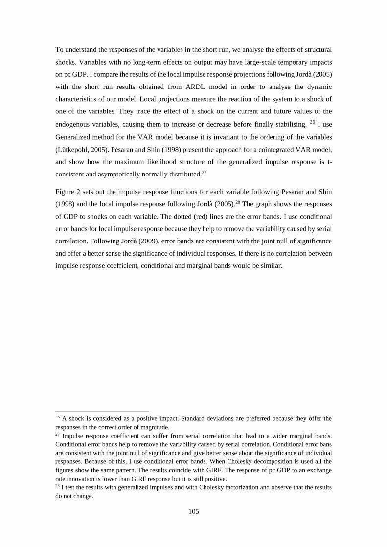
105
To understand the responses of the variables in the short run, we analyse the effects of structural
shocks. Variables with no long-term effects on output may have large-scale temporary impacts
on pc GDP. I compare the results of the local impulse response projections following Jordà (2005)
with the short run results obtained from ARDL model in order to analyse the dynamic
characteristics of our model. Local projections measure the reaction of the system to a shock of
one of the variables. They trace the effect of a shock on the current and future values of the
endogenous variables, causing them to increase or decrease before finally stabilising. 26 I use
Generalized method for the VAR model because it is invariant to the ordering of the variables
(Lütkepohl, 2005). Pesaran and Shin (1998) present the approach for a cointegrated VAR model,
and show how the maximum likelihood structure of the generalized impulse response is t-
consistent and asymptotically normally distributed.27
Figure 2 sets out the impulse response functions for each variable following Pesaran and Shin
(1998) and the local impulse response following Jordà (2005).28 The graph shows the responses
of GDP to shocks on each variable. The dotted (red) lines are the error bands. I use conditional
error bands for local impulse response because they help to remove the variability caused by serial
correlation. Following Jordà (2009), error bands are consistent with the joint null of significance
and offer a better sense the significance of individual responses. If there is no correlation between
impulse response coefficient, conditional and marginal bands would be similar.
26 A shock is considered as a positive impact. Standard deviations are preferred because they offer the
responses in the correct order of magnitude. 27 Impulse response coefficient can suffer from serial correlation that lead to a wider marginal bands.
Conditional error bands help to remove the variability caused by serial correlation. Conditional error bans
are consistent with the joint null of significance and give better sense about the significance of individual
responses. Because of this, I use conditional error bands. When Cholesky decomposition is used all the
figures show the same pattern. The results coincide with GIRF. The response of pc GDP to an exchange
rate innovation is lower than GIRF response but it is still positive. 28 I test the results with generalized impulses and with Cholesky factorization and observe that the results
do not change.

106
Figure 2. Local projection estimation
-.01
.00
.01
.02
.03
.04
.05
0 1 2 3 4 5 6 7 8 9 10 11
Response of pc GDP to pc GDP shock
-.03
-.02
-.01
.00
.01
.02
0 1 2 3 4 5 6 7 8 9 10 11
Response of pc GDP to fiscal balance shock
-.005
.000
.005
.010
.015
.020
.025
0 1 2 3 4 5 6 7 8 9 10 11
Response of pc GDP to money supply shock
-.010-.005.000.005.010.015.020.025.030
0 1 2 3 4 5 6 7 8 9 10 11
Response of pc GDP to real effective exchange rate
Response to Generalized One S.D. Innovations 95.0% Conditional confidence bands
Source: own elaboration
According to the local projections, both monetary policies and exchange rate had a positive and
significant effect on GDP. With an expansionary monetary policy, GDP rose.29 A depreciating
exchange rate implied an increase in pc GDP. When the budget balance decreased, the GDP rose
according to local projections results. According to this, when the fiscal balance improves, the
GDP decreased a little and after that, it increases again.
Toda and Yamamoto approach to Granger causality
The causal link between the variables is examined using Toda and Yamamoto (1995) causality
test as has been explained before. Correlation is not an indication of causality, which is why the
Toda and Yamamoto causality test is estimated. If X helps in the prediction of Y, then Y is said
to be caused by X (that is, the coefficients of the backward estimation are statistically significant).
The null hypothesis is that X does not cause Y. In the specific case of the Spanish economy, we
expect monetary policy to respond to fiscal needs (Escario et al., 2011, pp. 271-272 and Sabaté et
al., 2006).
29 Peripheral countries used depreciation recurrently in order to overcome crises. Matthias Morys (2013, p.
221), shows that these countries paid little attention to variations in the exchange rate and a great deal of
attention to the bank coverage ratio.

107
The estimation results of Toda and Yamamoto causality test are presented in Table 5. Causality
runs one-way from the money supply to pc GDP at the 5% level of significance. Thus past values
of monetary policy help to explain the present values of output. There is causal relationship
between money supply and fiscal balance at the 10% level of significance from money supply to
fiscal balance and at 10% from fiscal balance to money supply. The Granger causality analysis of
the variables shows, monetary policy accommodate the state’s fiscal needs (Escario et al., 2011,
pp. 271-272 and Sabaté et al., 2006, pp. 310, 321 and 328). In short, there was fiscal dominance
and, so, Spain’s monetary policy was affected by the fiscal needs of its government. Causality
runs from GDP to money supply at 5% level of significance underlining the relationship between
Spanish economy (government) and the increases in money supply.
When we estimate the Toda and Yamamoto causality test with the nominal effective exchange
rate or the real effective exchange rate estimated through CPI, we find similar results. The fiscal
policy seems to cause nominal exchange rate (see Annex 2, table 1). Thus, changes in the
expectations that the different fiscal decisions generated did appears as important as it was said
by Martin Aceña (1981, 1987,1993, 2000 and 2017). Thus, the past values of fiscal balance did
not affect the present values of nominal effective exchange rate. Nevertheless, the relationship
between fiscal behaviour, expectations and exchange rate will need further research; the present
study is merely an initial approach to the discussion.
Table 5. Toda and Yamamoto causality test
Source: own elaboration
ARDL robustness check
ARDL was subjected to several diagnostic tests. The diagnostic test in Table 6 shows that there
is no evidence of autocorrelation in the model. The null hypothesis of no correlation in the
Breusch-Godfrey test cannot be rejected. The equations are in their correct functional form
(Ramsey RESET test).
Excluded Chi-sq Prob. Excluded Chi-sq Prob.
F 0.291 0.864 LYPCR 6.369 0.041
LMSN 6.656 0.036 F 4.722 0.094
LREER 3.053 0.217 LREER 0.509 0.775
All 11.481 0.075 All 11.725 0.068
Excluded Chi-sq Prob. Excluded Chi-sq Prob.
LYPCR 1.670 0.434 LYPCR 2.254 0.324
LMSN 5.146 0.076 F 0.980 0.613
LREER 0.607 0.738 LMSN 2.232 0.328
All 5.994 0.424 All 4.394 0.624
Dependent variable: LYPCR Dependent variable: LMSN
Dependent variable: F Dependent variable: LREER
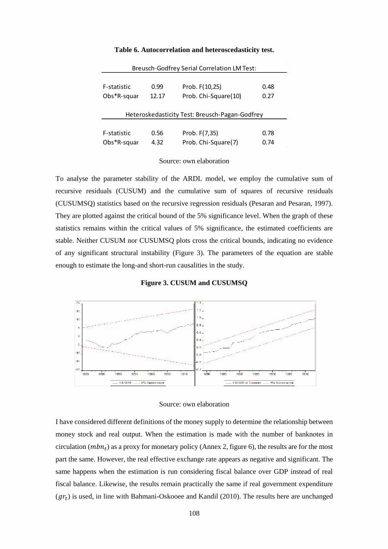
108
Table 6. Autocorrelation and heteroscedasticity test.
Source: own elaboration
To analyse the parameter stability of the ARDL model, we employ the cumulative sum of
recursive residuals (CUSUM) and the cumulative sum of squares of recursive residuals
(CUSUMSQ) statistics based on the recursive regression residuals (Pesaran and Pesaran, 1997).
They are plotted against the critical bound of the 5% significance level. When the graph of these
statistics remains within the critical values of 5% significance, the estimated coefficients are
stable. Neither CUSUM nor CUSUMSQ plots cross the critical bounds, indicating no evidence
of any significant structural instability (Figure 3). The parameters of the equation are stable
enough to estimate the long-and short-run causalities in the study.
Figure 3. CUSUM and CUSUMSQ
Source: own elaboration
I have considered different definitions of the money supply to determine the relationship between
money stock and real output. When the estimation is made with the number of banknotes in
circulation (𝑚𝑏𝑛𝑡) as a proxy for monetary policy (Annex 2, figure 6), the results are for the most
part the same. However, the real effective exchange rate appears as negative and significant. The
same happens when the estimation is run considering fiscal balance over GDP instead of real
fiscal balance. Likewise, the results remain practically the same if real government expenditure
(𝑔𝑟𝑡) is used, in line with Bahmani-Oskooee and Kandil (2010). The results here are unchanged
F-statistic 0.99 Prob. F(10,25) 0.48
Obs*R-squared 12.17 Prob. Chi-Square(10) 0.27
F-statistic 0.56 Prob. F(7,35) 0.78
Obs*R-squared 4.32 Prob. Chi-Square(7) 0.74
Breusch-Godfrey Serial Correlation LM Test:
Heteroskedasticity Test: Breusch-Pagan-Godfrey

109
when estimating the model with total GDP. The signs of my results do not change when plotting
the following four measures of the exchange rate: the real effective exchange rate (𝑟𝑒𝑒𝑟𝑡) using
CPI (Maluquer, 2013) and the nominal effective exchange rate (𝑛𝑒𝑒𝑟𝑡).30 The results also still the
same when real exchange rate is calculated with WPI from Sardà (1948, pp. 302-305). More
details can be found in Annex 2.
The results obtained by Cha (2003) and Shibamoto and Shizume (2014) vary depending on
whether or not the dynamics of prices are included in the SVAR model. For this reason, the same
analysis has been repeated with the prices variable (CPI from Maluquer, 2013) in order to observe
whether any changes occur. Prices responded positively to a output shock. Price shocks had a
positive impact on GDP following ARDL. The main findings of this study were not altered by
the addition of the variable prices (for more information, see Annex 2 (figure 4).
Running the estimation with the addition of the capital flows variable, the significance and signs
of the coefficients do not change. All the coefficients remain with the same sign and the exchange
rate remain significant and positive in the short run. The coefficient of capital flows variable
appears as negative and significant in the long-run analysis. We stress that at the start of the 20th
century, Spain received capital flows while outside the gold standard. Studies by Clemens and
Williamson (2000) considered that the gold standard was not the key variable for explaining UK
investments during the classical gold standard era. In this regard, Carreras and Tafunell (2004)
find it difficult to believe that Spain would have received more investment in the gold standard
because it had received too much in the years before.31 For more information on the capital flow
results, see Annex 2 (figure 5).
VI. Discussion
In the period under study, the gold standard was linked to prosperity. As such, the system was not
readily applicable to countries on the southern periphery of Europe, such as Spain. One of the
main causes of the internal instability experienced up to 1913 in these countries under the classical
gold standard was largely a result, therefore, of the subordination of their economic policies to
external objectives. Spain was never in the gold standard. Therefore, its policies did not depend
on the stability of the exchange rate. Spanish policies in the late nineteenth and early twentieth
centuries were not devised strategically, but were adjusted in accordance with circumstances32.
Martín Aceña stresses that using an expansionary monetary policy has no long-term implications,
since changes in the quantity of money have insignificant effects on long-term real income
30 Results can be found in Annex 2. 31 More in Roldan (2017). 32 Olariaga (1933/1977, p. 137) takes the view that Spain’s policy was ad hoc rather than consciously
designed to regulate the economic cycle.

110
growth.33 It is found that the monetary policy applied in this period had a positive effect on GDP.
According to the results, the role played by the monetary policy is not the one described by Martín
Aceña, and is more closely in line with the thesis defended by Sardà. According to Sardà (1987,
p. 218), the fiduciary expansion brought about by pressure from the Spanish treasury was able to
sustain the country’s economic progress. Monetary policy was one of the most powerful tools to
affect the real economy. The positive coefficient obtained for monetary policy shows that this
policy helped increase Spanish output in the long run.34 As Sabaté et al. (2006), Escario et al.
(2012), Sabaté et al. (2019) and my results stress, there was fiscal dominance. I have found that
money supply was caused by the fiscal balance. Thus, the positive sign in the long run could be
explained by seignorage. It seems that Spanish growth was sustained by monetary policy, which
was the Treasury’s response to the economic problems that arose. This, in turn, could affect the
exchange rate. Exchange rate shows a long-term non-significant impact with the new fiscal data
(table 3). However, the effect is negative and significant when data from Comín and Díaz (2005)
is used (figure 2 in Annex 2). There were also financial innovations during the late 19th century.
As it was said by Castañeda and Tafunell (1993) and Castañeda (2001) comparing the volume of
transfers with respect to the Spanish GDP, this importance is highlighted. In 1885, transfers
accounted for 6% of GDP and in 1900, for 31% of GDP when the estimation uses. Moreover, it
is said that moderate inflation can cause wealth redistribution.35 Monetary policy measured in
terms of the number of banknotes in circulation (Martín Aceña, 2018), it is also positive and
significant, which reinforces the results obtained (see Annex 2).
Local projections evidence a positive impact in the short term as well. It is expected that monetary
policy will positively affect real GDP because an increase in the amount of real money causes an
increase in equilibrium output through a variety of mechanisms such as the exchange rate, through
which monetary policy could have an effect on the real economy. That is we have found in the
local projections and in the ARDL long-run relationship. It should be stressed that the positive
impact of money supply on the pc GDP in the impulse response function and long term ARDL
coefficient can be explained by Sarda (1987).
In contrast, Martín Aceña (1881, 1887 and 1993) could be right to say that having a flexible
exchange rate could have damaged the Spanish economy. Martín Aceña (1981) rightly considered
that the effects of a depreciation would not be long-term effects. My results show how the
fluctuations of the exchange rate had non-significant long-term impact on pc GDP (main model).
When the estimation is run considering old data on the fiscal balance, the results show a negative
and significant impact of a depreciation in pc GDP (Figure 2, Annex 2). My result of a non-
33 Martín Aceña (1981, pp. 284-285), in an argument based on Friedman (1970, p. 217). 34 That is, when we dispose of sufficient lags to study the coefficients. 35 For example there is a study by Doepke and Schneider (2006).
111
significant or significant and negative impact of a depreciation was also found by Upadhyaya
(1999) who found a non-significant long-run effect for four out of six Asian economies and a
contractionary impact for the other two; by Bahmani-Oskooee (1998) who found no long-run
effect for their sample; by Bahmani-Oskooee et al. (2002) who underlined that depreciation had
a negative impact for many Asian countries, and by Christopoulos (2004) who found both positive
and negative effects in their sample. Therefore, the debate on contractionary effects of a
depreciation is still open.
While depreciation increases exports, it also raises production costs by increasing import prices.
Depending on the effects of these two actions on the economy, depreciation will have either a
positive or negative impact. A depreciation is considered successful when it succeeds in
modifying demand and quantity in the right direction (Guitian, 1976; Dornbusch, 1988). Its
success also depends on the ability of the economy to meet additional demand by producing more
goods. There have been many studies on the topic from different perspectives, such as Meade
(1951) and Dornbusch (1978). The structuralist school emphasizes the contractionary effects of
devaluation (Meade, 1951). The article written by Alexander (1952) changed the theory of the
effects of the exchange rate on a country’s economy. The classic history about the depreciation
underlines that a devaluation increases the price of foreign goods relative to domestic goods and
raises domestic demand. Most scholars agree that the immediate impact of devaluation is to raise
the demand for domestic goods; the disagreement lies in how the economy reacts to this increase
in demand. However, some studies such as Cooper (1971a and 1971b) and Díaz-Alejandro (1963)
suggest that a devaluation can reduce the aggregate demand. It is true that devaluation can
redistribute income from wages to profits. Nevertheless, a contractionary effect is more frequent
than one might expect (Dornbusch & Krugman, 1976; Krugman and Taylor, 1978; Kamin, 1988;
Edwards, 1989 and Lizondo and Montiel, 1989). Dornbusch and Krugman (1976) considers that
when there is trade deficit, devaluation can be contractionary. When foreign currency expenditure
surpasses foreign currency revenues, the prices of traded goods increase while domestic real
income is reduced. It is said that the greater the trade deficit, the greater the contractionary effect.
As Spain had problems in its balance of payments and suffered trade deficits, Krugman’s (1976)
argument appears to fit my results. In the short term, the exchange rate coefficient was positive
and significant, meaning that a depreciation could generate an increase in domestic income. In
the long run, the impact was negative and significant when the estimation is run considering
Comín (2005)’s data on the fiscal balance. This may be consistent with some of the literature
focusing on the contractionary effects of devaluation. Krugman (1976) also stresses that this is
more frequent in less developed countries. From the supply side, depreciation can be
contractionary when the economy is semi-industrialized and inputs are basically imported. Then,
manufacturers’ costs increase after a depreciation. Several recent studies have tested whether the

112
impact on the economy was positive or negative (Gylfason and Schmid, 1983; Gylfason and
Risager, 1984; Bahmani-Oskooee et al., 2002; Kalyoncu et al., 2008; Bahmani-Oskooee and
Kutan, 2008; Narayan and Narayan, 2013; Bahmani-Oskooee and Gelan, 2013 and Bahmani-
Oskooee and Mohammadian, 2016)
However in the short run, a flexible exchange rate helped the economy. The flexible exchange
rate is an important element of transmission of monetary policy. Taylor (1995) and Taylor (2001)
emphasize the importance of the exchange rate channel of monetary transmission. The positive
and significant impact of exchange rate remained the same when estimation is done with old data
on fiscal balance (Comín and Díaz, 2005). Serrano (2004, p. 163) concludes that “the exchange
rate acted as an occasional alarm by exerting an impulse towards moderation and a return to
equilibrium that prevented great divergences”. Cubel (2001, p. 187) indicates that not being on
the gold standard allowed Spain to reduce the disturbances in its economy; the cost of staying on
the gold standard would have been too high for a backward country (in the short-run). Llona
(2001, p. 172) stresses that the Spanish authorities were forced to adopt a flexible exchange rate
that would accelerate the adjustment to equilibrium. Martín Aceña (1981) accepts that the
depreciation of the peseta between 1890 and 1905 could have improved the terms of trade in a
way that would have encouraged exports and accelerated the process of import substitution. In
this way the independence of the gold standard would have had its compensations. The
depreciation of the peseta seems to be crucial in increasing output in the short run during the
period under study.36
The accumulation of deficits had a negative impact on Spanish economy in the long run, and
fiscal discipline had a positive effect on pc GDP, as Martín Aceña had underlined (1981, 1993
and 2000). An improvement in the budget balance represented an increase of GDP, while a
worsening of the budget balance generated a decline in output in the long-run. However, looking
at local projection estimations, a negative (but non-significant) sign can be seen in short-run
estimations and a negative impact on pc GDP. Thus, fiscal policy may have a countercyclical
effect in the short run but not in the long run, when fiscal discipline matters.
The Spanish Treasury obtained the financing it needed by monetising public debt (Sardà, 1987,
pp. 186, 190 and 199; Escario et al., 2011, pp. 271-272 and Sabaté et al., 2006, pp. 310, 321 and
328). The causality between fiscal and monetary policy is not only shown by the real effective
exchange rate results of the Toda and Yamamoto causality analysis but also by the nominal
effective exchange rate (see Annex 2, table 1). As the impulse response function shows, this
36 For more on the Spanish case, see Olariaga, (1933), Tortella (1974), Sardà (1987), Martín Aceña (1981,
1993, 1997 and 2000), Catalan et al. (2001) and Catalan and Sánchez (2013). For other cases, see Temin
(1995), Eichengreen and Temin (2010), Bordo and Rockoff (1996), Shibamoto and Shizume (2014),
Eichengreen and Sachs (1986).

113
policy accommodated the state’s fiscal needs (Escario, Gadea and Sabaté, 2011, pp. 271-272 and
Sabaté et al., 2006, pp. 310, 321 and 328). These scholars stress that seigniorage was essential to
safeguarding the state’s long-term solvency . The Spanish treasury was in need of money, which
it obtained by monetising public debt (Sardà, 1987, pp. 186, 190 and 199). We do not find that
the past values of macroeconomic policies in the model helped to explain the present values of
the real effective exchange rate. However, nominal effective exchange was caused by fiscal policy
underlining what was highlighted by Martín Aceña (1981 and 1993). He considered that exchange
rate was affected by expectations and those expectations could be explained by our lack of fiscal
discipline. This result should be considered as preliminary and the determinants of both nominal
and real exchange rates will need further research.
VII. Conclusion
The paper analyses the Spanish economy between 1870 and 1913. By conducting both short- and
long-run analyses, I have been able to combine the classical and critical theories, even though
they appear to be incompatible. The ARDL analysis reported here shows that exchange rate
adjustments played an important role in the short run. This suggests that the real exchange rate
was a useful policy tool in the short term, as Sardà claimed in 1948. However, the results obtained
support Martín Aceña’s proposals that having a flexible exchange rate could have had a negative
impact on long-term output. The study also finds a link between monetary policy and fiscal
policies. I show how the past values of fiscal policy were able to affect the present values of
nominal effective exchange rate, probably due to the lack of fiscal discipline. The results
presented in this paper provide new empirical evidence for the debates on the core-periphery
relationship and the effects of depreciation on output at the time of the classical gold standard.
Both schools of thought are therefore correct if we consider the temporal approaches taken: the
tools of macroeconomic policy were positive for the Spanish economy in the short term, but they
may have had detrimental effects in the long run.

114

115
Chapter 4: “Did the non-adoption of the gold standard benefit
or harm Spanish economy? A counterfactual analysis between
1870-1913”. *†
Abstract
This paper is an attempt to draw an overall picture of what would have happened if Spain had kept its
exchange rate stable (and if there had been no exchange rate shocks affecting economic growth) between
1870 and 1913. It is said that in the face of dramatic economic shocks, the rigidities of the monetary system
inhibited recovery, particularly in countries on the periphery. Would the impact of business cycles on Spain
have been much greater if the country had kept its exchange rate stable? To answer this question, I present
a counterfactual analysis based on the SVAR framework. The study also intends to highlight the importance
of macroeconomic policies (run outside the gold standard) to explain economic growth fluctuations. Via an
analysis of the historical decomposition of the variables I aim to identify the ones that helped to increase
growth and the ones that harmed the economy. My analysis sheds new light on the discussion of Spain’s
non-adoption of the classical gold standard. Having a fixed exchange rate would have made growth declines
deeper until the beginning of the 20th century; from that point on, the adoption of the gold standard would
have been a good decision. The results presented in this paper provide new empirical evidence for the core-
periphery debate addressing the period of the classical gold standard.
Key words: Classical Gold Standard, Spain, Exchange Rate, Counterfactual, SVAR.
JEL codes: E42, E52, E63, N10
* Earlier versions of this article were presented at Economic History Society Conference in the Royal
Holloway (2017), Iberometrics (2017), Workshop on Exchange Rate History at Lund University (2017),
Economic History PhD seminar at the University of Barcelona (2017) and Congreso Internacional de la
AEHE (2017). I wish to thank the participants for their feedback. I am also immensely grateful to Rui
Esteves, Matthias Morys, Marcela Sabaté, José Luís Peña, Lluís Castañeda, Masato Shizume, Jonas
Ljunberg, Daniel Tirado and Germán Forero for their comments on an earlier version of the manuscript. I
am also thankful to my research project colleagues at the University of Barcelona (Jordi Catalan, Ramon
Ramon, Alejandro Sánchez, Josep Maria Benaul, Miquel Gutiérrez, Marc Prat and Montserrat Carbonell).
I would also like to show my gratitude to José Antonio Miranda for their help and support every day. This
research was supported by HAR2015-64769-P (Ministry of Economy and Competitiveness) and my FPU
scholarship. I thank 4 anonymous reviewers for their so-called insights. Any errors are my own and should
not tarnish the reputations of these esteemed persons. † This chapter has been Ramon Carande prize (Asociación Española de Historia Económica) and published
in Investigaciones de Historia Económica – Economic History Research.

116
“(…) nothing could be farther from the truth than the idea that the
economists of that period as a body worshipped the golden calf—and,
second, that these opinions received but qualified support from those
leaders of scientific economics who actually worked in the field. As we
shall see, neither Jevons, nor Walras, nor Marshall, nor Wicksell, nor
Wieser, nor Fisher can, without qualification, be called either theoretical
or practical gold monometallists.”
Schumpeter (1954, p. 1040)
I. Introduction
The aim of this study is to understand what would have happened if Spain would not have suffered
from exchange rate shocks. This paper explores how would have been Spanish economic growth
if exchange rate would have been fixed. As far as I know, for the Spanish case, this type of study
(focus on estimating a counterfactual analysis) has no precedents for the period spanning the late
nineteenth and early twentieth century’s.1 I find this analysis extremely useful considering the
recent euro crisis. During the classical gold standard, Spain did not suffer the “golden fetters” and
broke them when it was necessary to increase its money supply and to overcome economic
shocks. Otherwise, Spain decided to be part of the euro and nowadays it is linked to “paper fetters”
(no possibility of running fiscal and monetary policies).2
I find very relevant to understand what would have happened in Spain’s economy if it would have
kept the exchange rate stable. Moreover, the two periods with higher average of crises depth
(understood as a cumulative loss of GDP) are the two globalization periods, 1880-1913 and 1973-
2000, (Betrán and Pons, 2013). It seems very interesting for me to focus on the first period.
Serrano (2004, p. 16) stresses that "Examining the monetary issue at that time also places us in a
particularly interesting perspective (...) the politics of money has multiple facets: ideological
arguments and power relations, economic conditions and external reflexes. The results are not
only sensitive to the economy, but also to the very fate of society, so that we are facing an
objectively "greater" issue ". Martín Aceña et al. (2011) underline that “Spain’s historic
detachment from the world monetary system cost the country dearly in terms of both its debt
burden and GDP growth, two questions that warrant further research”. This paper focuses on the
second question. There is a need of a counterfactual study following Martín Aceña (2017, p. 35):
“Remaining outside the gold standard was unwise, to say the least, unless it could be proven that
1 There are some counterfactual analysis for other cases such as Shibamoto and Shizume (2014) for Japan
or Bordo, Lane and Redish (2004) for the US among others. 2 More about golden fetters and paper fetters can be found in Eichengreen (1992) and Eichengreen and
Temin (2010).
117
its adoption would have been catastrophic for the national economy (…).” This article shows the
first counterfactual analysis to this never ending debate.
One of the successes of the gold standard was to preserve stability across much of the world and
to generate economic growth. The advanced economies were benefited from this monetary system
while many countries on the periphery experienced major exchange rate fluctuations and
instability3. Southern European economies did not succeed in remaining within the rules of the
classical gold standard.4 When the economies of the periphery joined the gold standard, they
were required to make a sacrifice to adjust their economies. The structural problems of their
economies prevented them from bringing their money supply under control and keeping their
exchange rate stable. There were many countries that did not follow the rules of the game
(Bloomfield, 1959). However, they were committed to long-term gold standard objectives.
According to Keynes (1913), the monetary regime called the gold standard comprised multiple
national variants. It was difficult to establish who was and who was not and when.
The adoption of a system of fixed exchange rates and free movement of capital causes the loss of
monetary autonomy (Obstfeld et al., 2005). Countries outside the gold standard used fluctuations
in the exchange rate to cushion the impact of economic shocks (Bordo and Rockoff, 1996, p. 416
and Bordo and Flandreau, 2003, p. 419). There is no consensus over whether the non-adoption of
the gold standard benefited or harmed Spain’s economic growth.5 The proponents of a fixed
3 For the core-periphery discussion, see De Cecco (1974), Hallwood et al. (1996), Bordo and Flandreau
(2003, p. 420), Morys (2013, p. 205) and Mitchener and Weidenmier (2015, p. 54). More on this can also
be found in Triffin (1985, p. 128), Braga de Macedo (1996, p. 243), Martín Aceña et al. (2000, p. 2) and
Sabaté et al. (2019).. More on speculative attacks to currencies in Eichengreen (1996, pp. 46-49), Bordo
and Jonung (2001, p. 14), and Bernanke (2015, p. 26). For withdrawals effects, see De Cecco (1974), Temin
(1995, p. 28), and Bordo and Flandreau (2003, p. 420). More about credibility and interest rates during the
gold standard can be found in Hallwood et al. (1996, p. 129), Bordo and Flandreau (2003, p. 446), Bordo
and MacDonald (2005, p. 326) and Mitchener et al. (2010, p. 54). For trade benefits, see Lopez-Cordova
and Meissner (2003). For additional information on the main characteristics of the gold standard, see, for
example, Eichengreen (1992), Temin (1995, p. 25), Officer (1996), Eichengreen and Flandreau (1997) or
Bordo (1999). 4 For Italy, see Fratianni and Spinelli (1984), Cipolla (1995), Tattara and Volpe (1997), Tattara (2000 and
2003), Bordo (1999, p. 328) and Frattiani and Spinelli (2012). For Portugal, see Mata (1987), Reis (1996,
2000 and 2007), Valerio (1998) and Bordo (1999, p. 329). 5 On one hand, Sardà (1987), Solé Villalonga (1964 and 1967) and Tortella (1981 and 1994a) defended a
position contrary to the gold standard. Their argument is based on the impossibility of taking monetary and
fiscal policy actions under the gold standard. More recently, this stance has been defended by Cubel et al
(1998); Catalan et al. (2001); Cubel (2001); Llona (2001); Ródenas, Brú and Almenar (2001); and Sabaté
et al. (2001), Carreras and Tafunell (2004, pp. 219-20), Serrano (2004) and Ródenas and Bru (2006). This
school of thought is called the “classical thesis” and is associated with Professor Joan Sardà. On the other
hand, Martín Aceña (1981, 1993, 1997, 2000, 2017) defends the critical thesis, viewing it as a mistake not
to have adopted the gold standard. Martín Aceña, professor at the University of Alcalá, holds that Spanish
growth would have been greater under the gold standard. In an intermediate position in the debate, we can
find García Iglesias (2005) and Prados de la Escosura (2003). A summary can be found in Roldan (2017).

118
exchange rate stress that growth would have been greater under the gold standard keeping the
exchange rate stable and bringing the fiscal policy under control. However, keeping a flexible
exchange rate and running fiscal and monetary policies could succeed in dampening the economic
fluctuations by making them less deep during the classical gold standard.
For this reason, the main purpose of the present study is to establish what would have been better
for Spanish economy. Spain made several attempts to adopt the monetary system. What would
have happened if one of these attempts had succeeded? The case of the Spanish economy offers
an opportunity to estimate a counterfactual analysis in a country that never adopted the gold
standard.6 Because of this, I run a counterfactual analysis of what would have happened if Spain
had kept its exchange rate stable like other European economies. To do this, I construct an SVAR
(structural vector autoregression)7. This study also sets out to assess the importance of the
instruments of monetary and fiscal policy and the exchange rate in explaining Spain’s economic
growth.
The paper shows a counterfactual analysis on the effects of the non-adoption of the gold standard
for Spanish economic growth between 1870 and 1913, distinguishing between a stage where the
depreciation of the exchange rate had positive effects making the crises less profound and the
decade before the Great War where it would have been possible for the economy to incorporate
the peseta into the gold standard. The article shows the growth gains and losses due to the flexible
exchange system.
It is found that exchange rate adjustments were important to explain the evolution of economic
growth. Following the results, having a flexible exchange rate seems to be significant to make
crises less deep until the beginning of the twentieth century. Before the 20th century, fixed
exchange rate would have generated bigger falls in GDP than flexible exchange rate.
Expansionary monetary policy was another policy that helped more to understand pc GDP
behaviour. The effects of fiscal policy were not very relevant. It can be said that, after the
beginning of the 20th century, membership of the gold standard was a possibility for Spain and
the counterfactual analysis suggests that its economic growth would have been higher under a
fixed exchange rate system. Considering results from counterfactual analysis, had the peseta
exchange rate not been permitted to separate from its historical parity, the Spanish growth would
have outpaced the actual growth at the beginning of the 20th century.
6 Sardà (1987), Martín Aceña (1981, p. 267), Martín Aceña (1993, p. 135), Tortella (1994a, p. 323), Serrano
(2004, p. 155), García Iglesias (2005, p. 62), Sabaté, Gadea and Escario (2006, p. 310), Martín Aceña et al.
(2011, p. 3), Martínez Ruíz and Nogués (2014, pp. 9 and 19), Martín Aceña (2017), Sabaté et al. (2019). 7 A formal explanation of SVAR can be found in Sims (1986).
119
In order to do this, I show the attempts to join the gold standard. Then, we see if having a flexible
exchange rate damaged Spain’s economy. Thus, if Spain should have been adopted the gold
standard or not. After that, we will study the importance of macroeconomic policies on economic
growth. Thereby, how much of economic growth fluctuations is explained by each policy shocks
and how change this effect along the years.
The paper is organised as follows: section 2 reviews the main features of the Spanish economy
and the attempts to adopt the gold standard; section 3 describes the methodology and data; section
4 presents the empirical results; section 5 offers a discussion of the results in relation to the
historical evidence and the previous literature; and, lastly, section 6 concludes.
II. The Spanish economy between 1870 and 1913: Attempts to adopt the
gold standard, policies and strategies.
The paper covers the period known as the classical gold standard. Spain had a de jure bimetallic
standard over the period. Nevertheless, during the eighties, the country is regarded to have had a
de facto fiduciary system.
In the nineteenth century the frequency of financial crises in Spain was well above the global
average (11.1%, according to Betrán et al. (2013), vs 4.9% worldwide,according to Bordo et al.
(2001). However, although the crises were quite severe in Spain, they were less severe than in the
rest of the world (Betrán and Pons, 2019).8 Would they have been deeper if the country had
adopted a fixed exchange rate (the gold standard)? According to Betrán and Pons (2019), financial
crisis were due to foreign capital entries, railway and mining booms, sudden stops, banking
expansion, increasing credit, public budget deficits, and current account imbalances.
8 More on Spanish crisis in Betrán et al. (2012) and Maixé and Iglesias (2018).

120
Figure 1. Evolution of pc GDP and nominal exchange rate (pesetas/pound).
350
400
450
500
550
600
650
700
16
20
24
28
32
36
40
44
1870 1875 1880 1885 1890 1895 1900 1905 1910
pc GDP in pesetas (left)Nominal exchange rate in pesetas/pound (right)
a b c d e
a. Attempt to adopt the gold standardb. Wait-and-see policy (shading area)c. Attempt to adopt the gold standard
d. Minor attempt to adopt the gold standarde. Minor attempt to adopt the gold standard
Source: main text.
Serrano (2004) considers the years before 1898 as years in which there was a wait-and-see policy.
The policymakers had an attitude of prudence waiting to see how the monetary system was
defined at the international level. In the first years of the Restoration it seemed that the peseta was
heading towards gold. The will of Spain was, once overcome the difficulties, to be part of the
international monetary system. However, soon, the apparent lack of definition of the international
monetary panorama provided a perfect excuse to opt for comfort.
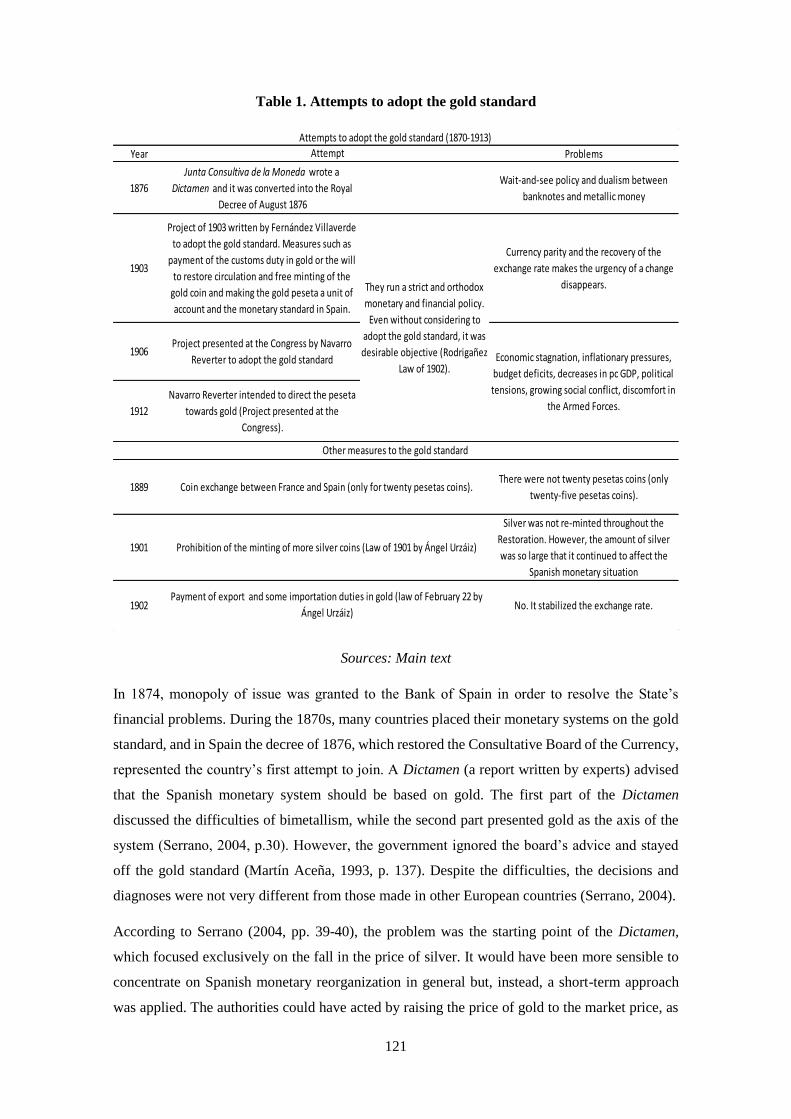
121
Table 1. Attempts to adopt the gold standard
Sources: Main text
In 1874, monopoly of issue was granted to the Bank of Spain in order to resolve the State’s
financial problems. During the 1870s, many countries placed their monetary systems on the gold
standard, and in Spain the decree of 1876, which restored the Consultative Board of the Currency,
represented the country’s first attempt to join. A Dictamen (a report written by experts) advised
that the Spanish monetary system should be based on gold. The first part of the Dictamen
discussed the difficulties of bimetallism, while the second part presented gold as the axis of the
system (Serrano, 2004, p.30). However, the government ignored the board’s advice and stayed
off the gold standard (Martín Aceña, 1993, p. 137). Despite the difficulties, the decisions and
diagnoses were not very different from those made in other European countries (Serrano, 2004).
According to Serrano (2004, pp. 39-40), the problem was the starting point of the Dictamen,
which focused exclusively on the fall in the price of silver. It would have been more sensible to
concentrate on Spanish monetary reorganization in general but, instead, a short-term approach
was applied. The authorities could have acted by raising the price of gold to the market price, as
Year Problems
1876
Junta Consultiva de la Moneda wrote a
Dictamen and it was converted into the Royal
Decree of August 1876
Wait-and-see policy and dualism between
banknotes and metallic money
1903
Project of 1903 written by Fernández Villaverde
to adopt the gold standard. Measures such as
payment of the customs duty in gold or the will
to restore circulation and free minting of the
gold coin and making the gold peseta a unit of
account and the monetary standard in Spain.
Currency parity and the recovery of the
exchange rate makes the urgency of a change
disappears.
1906Project presented at the Congress by Navarro
Reverter to adopt the gold standard
1912
Navarro Reverter intended to direct the peseta
towards gold (Project presented at the
Congress).
1889There were not twenty pesetas coins (only
twenty-five pesetas coins).
1901
Silver was not re-minted throughout the
Restoration. However, the amount of silver
was so large that it continued to affect the
Spanish monetary situation
1902 No. It stabilized the exchange rate.Payment of export and some importation duties in gold (law of February 22 by
Ángel Urzáiz)
They run a strict and orthodox
monetary and financial policy.
Even without considering to
adopt the gold standard, it was
desirable objective (Rodrigañez
Law of 1902).
Attempt
Economic stagnation, inflationary pressures,
budget deficits, decreases in pc GDP, political
tensions, growing social conflict, discomfort in
the Armed Forces.
Attempts to adopt the gold standard (1870-1913)
Other measures to the gold standard
Coin exchange between France and Spain (only for twenty pesetas coins).
Prohibition of the minting of more silver coins (Law of 1901 by Ángel Urzáiz)

122
recommended by the Consultative Board of the Currency, and by demonetizing the silver coinage.
The supply of money could have been restricted, because the reserves were dwindling and interest
rates were high (Martín Aceña, 1993, p. 139). However, Tortella (1994a, p. 480) considers that
trying to conserve the stock of gold at all costs would have imposed an intolerable and
unnecessary discipline on the country, given its problems with the balance of payments.
Spain went on to have a unique monetary regime, fully fiduciary in its internal circulation and
with a fluctuating exchange rate. Serrano (2004, p. 67) highlights that "(…) The monetary regime
was flotation, in the strictest sense of the term. This singularity confers a very special interest on
the peseta in contemporary monetary history, since it turned out to be the European currency
with the longest period of stable flotation, until the crisis of the 1930s”. Later Spanish
governments, less interested in monetary orthodoxy, saw in seigniorage an additional source of
income for improving the state of the public treasury. Thus, the purchase of gold was no longer
financed. Finally, the deficits became more serious and nobody supported a circulation full of
silver (a de facto fiduciary system). The time to join the gold standard had passed, and the question
of whether or not to apply for membership would not be posed again until 1898.
According to Tortella (1994a, p. 177), despite the rushed nature of the government’s decision not
to adopt the gold standard, it was in fact the best possible alternative, or at least the least bad. The
survival of the system of full metallic weight could have been an obstacle to growth (Tortella,
1994a, p. 177). The 1929 Dictamen considered it very doubtful that the gold standard system in
Spain could have been maintained in the long term (Tortella, 1994a, p. 325). Sardà (1987) states
that, although it was not the idea of the monetary authorities, the country was favoured by not
adopting the gold standard; its decision not to join protected the Spanish economy from the
fluctuations in income and prices that faced the rest of the economies and the international
depression of the last quarter of the nineteenth century.
Gold remained an option for economic policy, but the Spanish currency was never committed to
the rules of convertibility, capital-compensating movements, the use of the interest rate as an
instrument of adjustment, or fiscal discipline. The peseta was never integrated into the gold
standard because of a dualism in Spanish monetary organization (Serrano, 2004, p. 155). Neither
the decree of 1868, which regulated coin circulation, mentioned banknotes, nor did the decree of
1874, which regulated banknotes, refer to coin circulation. The Bank of Spain dealt with the
fiduciary circulation and had the power to convert, while the Treasury dealt with the coin
circulation. The precariousness of the Spanish Treasury prevented it from devoting the necessary
resources to improve economic situation, or submitting to fiscal discipline. This problem persisted
in the Dictamen of 1876 and the Royal Decree of August 1876. The declaration of convertibility

123
could have eliminated the problem, but convertibility was never in fact established (Serrano,
2004).
In 1889, France and Spain agreed to accept reciprocally twenty-peseta coins. The Bank of Spain
concurred, but no twenty-peseta coins were available because, in 1876, they had issued a twenty-
five peseta coin. Therefore, twenty-peseta coins had to be minted; as the numbers made were
insufficient, the agreement fell through.
The exchange rate remained stable for the most part until the late 1880s and early 1890s, though
with a tendency towards depreciation. In the early 1890s there was a currency crisis due to the
enduring effects of the financial problems of the late 1880s, the Baring crisis and the law of 1891
that increased the limit of issuing banknotes (Serrano, 2004). Betrán and Pons (2019) associate
the crash of 1890-92 with the international crisis, and they explain how the financial structure was
damaged. Referring to the period of the first large depreciation of the peseta in 1891, the finance
minister Raimundo Fernández Villaverde (1893, p. 563), considered that membership of the gold
standard required major sacrifices and concluded that it was not a valid solution for Spain at that
time. Between the end of the 1870s and the beginning of the 1890s there were those who defended
monometallism, others bimetallism, and others who maintained ambiguous or eclectic positions
(Serrano, 2004). It did not seem clear which monetary standard option was better, either in
practice or in theory. Schumpeter (1971, p. 1168) noted that the bimetallic argument could have
won the controversy, even without the support offered by several top-level scholars.
The change began in 1898. This was a turning point in Spanish monetary history, at least in the
field of ideas. The wait-and-see policy came to an end and the gold standard was always a possible
remedy (Serrano, 2004, p. 85). Fernández Villaverde made specific proposals for adopting the
gold standard. Fernández-Villaverde (1900, p. 69, 84 and 106), considered that the problem
should not be resolved abruptly because a sudden reduction of the monetary circulation would
cause a crisis and be an evil in itself Moreover, his diagnosis of the defects of the Spanish
monetary organization was fairly accurate – for example, the continuation of the minting of silver,
the financial indiscipline of the Treasury, and the perverse relations of the government with the
Bank of Spain (Serrano, 2004, p. 95).
On November 28, 1901, a further step was taken toward gold when the minting of silver was
prohibited. Nonetheless, the demonetization of silver proved difficult. Even though no more silver
was minted, the amount already in existence did not disappear. With the laws of December 26,
1899 and November 28, 1901, the government adopted provisions that favoured the restoration
of the circulation and the minting of gold coins. The best moment to adopt the gold standard was
1903 (Serrano, 2004). In that year, Fernández Villaverde, who had been President of the Council

124
during the previous year, proposed legislation to regularize and improve the exchange rate. He
was seeking to restore circulation and the free minting of gold coins and to establish the date when
the gold standard would be adopted by Spain.
The project of 1903 had to be carried out within the monetary system created by the decree-law
of October 19, 1868.9 This implied, according to Villaverde, that banknotes should be convertible
to the historical equivalent of 100 pesetas/29 grams of gold. The project of 1903 consisted of
returning to the parity of 25.22 pesetas per pound, something that was difficult to achieve. To
accomplish this, national prices had to be controlled (Serrano, 2004, pp. 106 and 109), which
would have implied the control of relative prices. The proposal included the generalization of the
payment in gold of customs duties as a way to obtain gold. Budget discipline and the amount of
gold obtained via customs duties achieved some monetary stability. The reduction of the
depreciation of the peseta in 1906 and the economic stability achieved meant that adopting the
gold standard was no longer such an urgent necessity (Serrano, 2004).
After 1903, two subsequent attempts were made to adopt the gold standard, in 1906 and 1912.
According to Juan Velarde (2004), the latter failed due to problems of social conflict, discontent
among the military during the Moroccan War, and economic stagnation. Until the 1930s there
were several moments when the political situation in Spanish encouraged entry, and the foreign
scenario was positive (Serrano, 2004, p. 159). But the adoption of the gold standard never
materialized. In the long term, this was a period of substantial stability (Carreras and Tafunell,
2004, Serrano, 2004 and García-Iglesias, 2005).
Martín Aceña (1993, p. 136), explains that Spain could and should have enjoyed the international
monetary system. The inconvertibility and the flexible exchange rate introduced risk in Spanish
international transactions, reducing trade and capital flows. However, since the first exchange
crisis of the peseta, at the beginning of the nineties, a powerful current of opinion held that the
Spanish economy had a restriction on its possibilities of committing itself to a monetary system
as demanding as gold in its difficulty in maintaining in equilibrium income and external payments
(Serrano, 2004). Protectionism or floating change was not seen as causes of the backwardness of
Spain, but as its inescapable results and appropriate defensive strategies for a backward country.
Even in the Dictamen there are echoes of these positions (Serrano, 2004, p. 61). Moreover, Martín
Aceña et al. (2011) consider that neither the Treasury nor the Banco de España were prepared to
take the necessary measures to choose the appropriate parity, balance the budget or follow an
orthodox fiscal policy to maintain the value of the exchange rate. For many, it was the situation
of the treasury that did not allow the gold standard to be implemented, since it required limiting
9 Fernández-Villaverde (1903).

125
the budget and indebtedness (Tortella, 1994a). If Spain did not implement the gold standard, it
was not because of a doctrinal principle, but because of the fear that its politicians and especially
the Banco de España harbored, that chronic deficits in the balance of trade and budget would
eventually cause a drain of gold that would make the project unviable (Tortella, 1994a).
III. Methodology and data
To this end, an SVAR (structural vector autoregression) model is constructed. The methodology
has been used by Cha (2003) and by Shibamoto and Shizume (2014) to capture the magnitudes
of the effects of macroeconomic policies in Japan, by Gordon and Krenn (2010) to measure the
same effects in the US, and by Mattesini and Quintieri (1997) in the Italian case, among others10.
Concretely, Shibamoto and Shizume (2014) have studied the impact of monetary, fiscal and
exchange rate policy in Japan economy during the inter-war period. As I do in this paper, Fackler
and Parker (1994a) use historical decomposition and counterfactual analysis to understand which
theory explains better the movements of GDP during the Great Depression and to understand if
some part of the depression could have been avoided by increasing the money stock in an
anticipated way. Bordo et al (2004) run an empirical analysis grounded by a VAR model of money
supply under the gold standard. They restrict themselves to business cycle frequencies because of
the short span of data available.
To estimate the importance of monetary, fiscal and exchange rate policy on real GDP, I construct
the following SVAR model using the variables of output (𝑦𝑝𝑐𝑟𝑡), fiscal balance (𝑓𝑡), money stock
(𝑚𝑡) and real effective exchange rate (𝑒𝑡):
𝐵(𝐿)𝑋𝑡 = 𝑏0 + ɛ𝑡
where 𝑋𝑡 = (𝑦𝑝𝑐𝑟𝑡 , 𝑓𝑡, 𝑚𝑡 , 𝑟𝑒𝑒𝑟𝑡), 𝑏0is the vector of the constant, 𝐵(𝐿) = 𝐵0 −
∑ 𝐵𝑝𝐿𝑝𝑝𝑗=1 where 𝐵0 is the contemporaneous relations between the variables making the system
overparametrized (Enders, 2004), 𝐿 denotes the lag and ɛ𝑡 = (ɛ𝑦𝑝𝑐𝑟𝑡, ɛ𝑓𝑡 , ɛ𝑚𝑡, ɛ𝑟𝑒𝑒𝑟𝑡) is a four-
by-one vector of serially uncorrelated structural disturbances with a mean zero and a covariance
matrix Σɛ. The vector ɛ𝑡 model random disturbances or white noise processes.
The reduced form baseline VAR is specified as follows:
𝐴(𝐿)𝑋𝑡 = 𝑎0 + 𝑢𝑡
where 𝑎0 is the vector of the constant, 𝑋𝑡 is is a vector of endogenous variables , A(L) is an
autoregressive lag-polynomial. The benchmark includes a constant. 𝐴(𝐿) = 𝐼 − ∑ 𝐴𝑝𝐿𝑝𝑝𝑗=1 is a
p-th order lag of matrix 𝐴𝑗 (𝑗 = 1, 2, … , 𝑝) , 𝐿 denotes the lag and 𝑢𝑡 = 𝑢𝑦𝑝𝑐𝑟𝑡 , 𝑢𝑓𝑡 , 𝑢𝑚𝑡, 𝑢𝑟𝑒𝑒𝑟𝑡
10 For the English case, see an analysis of monetary policy in Jeanne (1995).
126
is the a four-by-one vector of serially uncorrelated structural disturbances with a mean zero and
a covariance matrix Σ𝑢.The reduced form residuals which will present non zero cross correlations.
The model includes one lag of each endogenous variable. Generalized weights is used as an
identification of the reduced form covariance matrix Σ𝑢 is used to orthogonalize the reduced form
of innovations.
I model output, fiscal policy, monetary policy and exchange rate adjustments using the following
SVAR above.11 The SVAR is estimated in first differences because after considering the time
series properties of the data, all variables seem I(1).12 It is said that it is possible to lost information
when someone runs the model in first differences because long-run relations between levels can
be ignored. In this case is not an important problem. For example, differentiating pc GDP means
to have economic growth which is a variable of interest for the model. When the SVAR is
estimated on levels (Annex), the performance of the estimation is consistent even if each variable
is not stationary (Hamilton, 1994a, pp. 651-653 and Ramey, 2016). When I run my estimation in
levels, my results do not differ much from to those obtained in first differences (see Figure 4 in
the Annex to know more about results and differences with the main results).
As it is explained before, four macroeconomic variables are used in this analysis. I use the nominal
effective exchange rate and the real effective exchange rate to consider the value of the currency
due to reasons I explain later. The 𝑦𝑝𝑐𝑟𝑡 is real pc GDP measured using GDP from Prados de la
Escosura (2003) and population from Nicolau (2005) deflated by GDP deflator (Prados de la
Escosura, 2003), 𝑓𝑡 is the real fiscal balance as percentage of GDP obtained by Comín and Díaz
(2005), 𝑚𝑡 is the money supply measured from Martín Aceña, (2018), 𝑟𝑒𝑒𝑟𝑡 is the real effective
exchange rate, whose calculation is explained below, and 𝑛𝑒𝑒𝑟 is the nominal effective exchange
rate.13
To build the real effective exchange rate, I consider the average weight of the exchange rate
against the pound sterling, the French franc and the US dollar. The calculation of the exchange
rate makes use of the GDP deflator from Prados de la Escosura (2003) for Spain, the deflator
obtained by Toutain (1987) for France, Balke and Gordon (1989) and Mitchell (2007) for the US
and Thomas and Dimsdale (2017) for the UK.14 Results do not change if CPI (Consumer Price
Index) obtained by Maluquer (2013) for Spain and Mitchell (2007) for the other countries is used
to construct the real effective exchange rate. The peseta exchange rate is obtained from Martín
Aceña and Pons (2005) and Martínez Ruiz and Nogués (2014). The weight of foreign trade to the
11 VAR is estimated by OLS. 12 Based on KPSS (Kwiatkowski-Phillips-Schmidt-Shin, 1992) test considering constant. 13 I have chosen pc GDP because it is a better measure of economic growth since it takes into account the
population. 14 I use GDP deflator following Serrano et al. (2017).

127
respective countries is obtained from Prados de la Escosura (1982, p. 42), using fixed weightings
updated every five years.15 The weightings account for more than 60% of total foreign trade over
the entire period16.
The frequency of the data is annual. The sample runs from 1870 to 191317. All the variables have
been converted into logarithms with the exception of the fiscal balance.18 Fiscal balance is taken
in % of GDP. The available criteria for selecting the number of VAR lags (Akaike criteria,
Schwarz Criteria or Hannah Quinn Criteria) point to one lag as the optimal number to carry out
the SVAR estimation. Bordo, Landon and Redish (2004) have a comparable sample size and they
run a SVAR and historical decomposition and counterfactuals.
IV. Empirical results
Counterfactual analysis
In this section, I study what would have happened to output (economic growth) in the absence of
a flexible exchange rate (i.e., absence of exchange rate shocks) by using simulations in my VAR
model. The VAR is always estimated in first differences.19 Spain is the only country that allows
us to make this counterfactual analysis because it was not committed to the gold standard and had
no obligation to maintain its exchange rate fixed during the period of the classic gold standard.
SVAR allows us to carry out the counterfactual analysis that is inherent in our questions: how
would Spain’s output have evolved if had been on the gold standard? To do this, I estimate a
counterfactual analysis following Bordo et al. (2004) and Shibamoto and Shizume (2014). The
SVAR is estimated with the variables pc GDP, budget balance, money supply and effective
nominal exchange rate.20 Nominal effective exchange rate is used in the counterfactual analysis.
The nominal exchange rate is the one that shows the fluctuations as a consequence of having a
flexible exchange rate. The real exchange rate always fluctuates, since it depends on the
relationship between national and international prices. The results obtained using the real effective
exchange rate instead of the nominal can be found in the Annex.
When we estimate in first differences, we differentiate the logarithm of pc GDP obtaining pc GDP
growth; the difference between two values shows the increase or decrease from one year to the
15 Same data on foreign trade is used to calculate the nominal effective exchange rate. 16 See Aixala (1999) to know more about how real effective exchange rate can be constructed in the
Spanish case. 17 It is not possible to start the analysis earlier because of the lack of historical series of monetary
circulation prior to 1874. 18 Because the fiscal balance has negative values, it cannot be converted into logarithms. We will use the
budget balance over GDP. Money supply is M1. One can find it in Martín Aceña (2018) as “money supply”
in both estimations before and after 1874. 19 In Annex it can be found the results in levels as a robustness check. 20 See data section for more information.

128
next. In the same way, I consider the growth of the money supply and not stock of money or the
growth or decrease of the budget balance. As for the exchange rate, it reflects how much the
currency has appreciated or depreciated with respect to the previous year.
Figure 3 shows the results based on counterfactual simulations that switch off the shock response
of nominal effective exchange rate. The historical path of economic growth is shown by the solid
line, while the dotted line with dots shows the fictitious path of economic growth assuming that
the nominal exchange rate had been fixed at the initial value throughout the period. This means
there were no exogenous exchange rate shocks and no endogenous exchange rate responses to
fluctuations of other variables. We see the deepest falls in 1874, 1878, 1893 and 1896.
First of all, it can be seen that the falls in pc GDP were less marked with a flexible exchange rate.
In spite of this, the point that GDP growth finally reaches in 1913 does not seem to have depended
on the presence of a fixed or a flexible exchange rate.21 This result can reinforce the idea that the
exchange rate could have had a positive impact on economic growth in the short run but not in
the long run. Then, at the beginning of the 20th century, joining the gold standard would have been
a good decision because economic growth would have been higher. Thus, from 1903/1904
onwards, the greater stability in Europe at the turn of the century, together with the good economic
evolution of neighbouring countries such as Italy or France, meant that having a flexible exchange
rate would be negative and growth would have been greater with a fixed exchange rate at the
beginning of the 20th century. The following interpretation could also be given. The shock of the
exchange rate, which was appreciating sharply as a result of the enormous depreciation of
previous years, could have slowed down the economy. If the exchange rate had been kept fixed
throughout the period, the economic impacts until 1903 would have been more profound (see
figure 2 and table 2). However, Spain would not have suffered a sudden appreciation of the
currency and the consequent negative impact on economic growth during the first years of the
20th century.
21 The annex presents the counterfactual analysis in levels (figure 5). Figures for GDP in 1913 do not
differ much from those that would have been obtained under a fixed exchange rate regime.
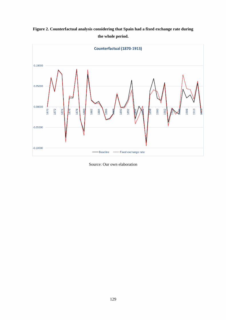
129
Figure 2. Counterfactual analysis considering that Spain had a fixed exchange rate during
the whole period.
Source: Our own elaboration
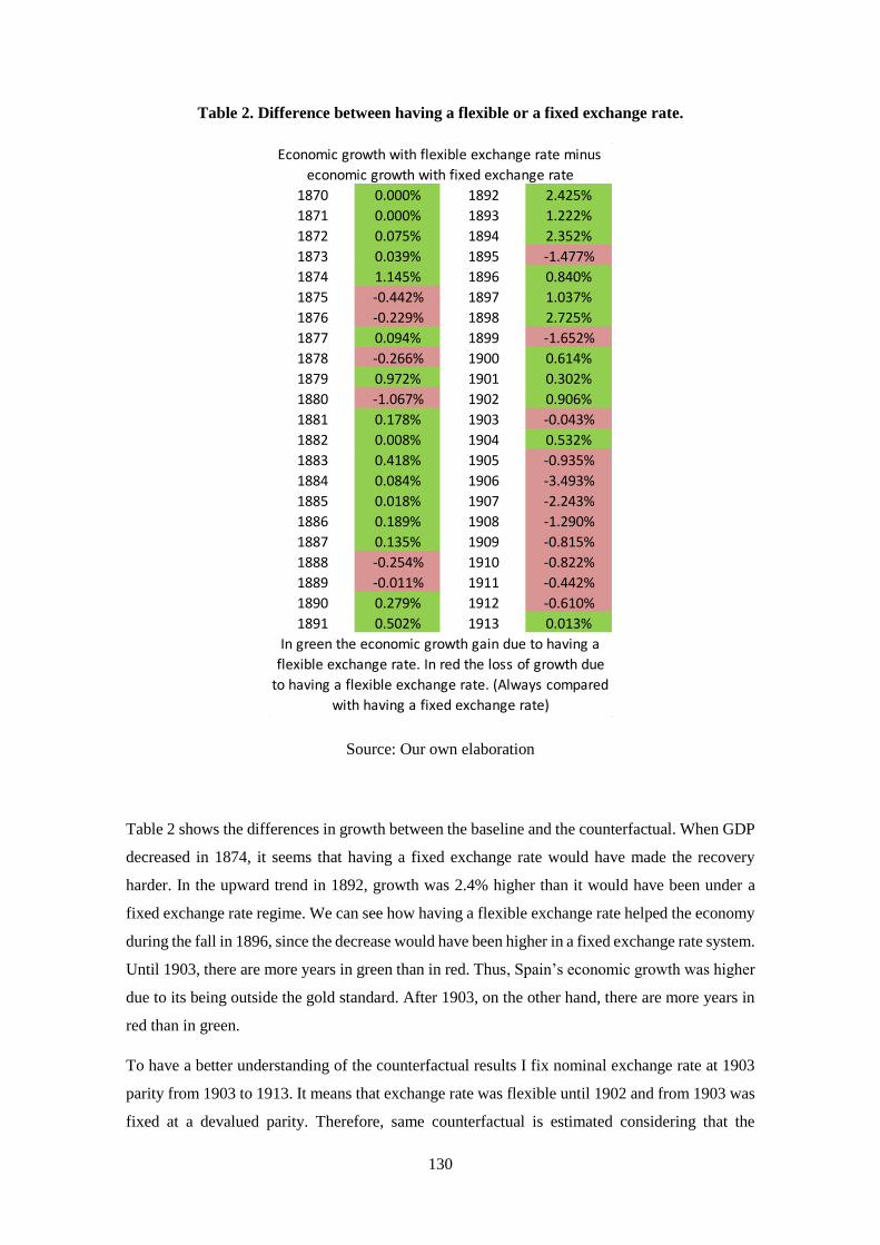
130
Table 2. Difference between having a flexible or a fixed exchange rate.
Source: Our own elaboration
Table 2 shows the differences in growth between the baseline and the counterfactual. When GDP
decreased in 1874, it seems that having a fixed exchange rate would have made the recovery
harder. In the upward trend in 1892, growth was 2.4% higher than it would have been under a
fixed exchange rate regime. We can see how having a flexible exchange rate helped the economy
during the fall in 1896, since the decrease would have been higher in a fixed exchange rate system.
Until 1903, there are more years in green than in red. Thus, Spain’s economic growth was higher
due to its being outside the gold standard. After 1903, on the other hand, there are more years in
red than in green.
To have a better understanding of the counterfactual results I fix nominal exchange rate at 1903
parity from 1903 to 1913. It means that exchange rate was flexible until 1902 and from 1903 was
fixed at a devalued parity. Therefore, same counterfactual is estimated considering that the
1870 0.000% 1892 2.425%
1871 0.000% 1893 1.222%
1872 0.075% 1894 2.352%
1873 0.039% 1895 -1.477%
1874 1.145% 1896 0.840%
1875 -0.442% 1897 1.037%
1876 -0.229% 1898 2.725%
1877 0.094% 1899 -1.652%
1878 -0.266% 1900 0.614%
1879 0.972% 1901 0.302%
1880 -1.067% 1902 0.906%
1881 0.178% 1903 -0.043%
1882 0.008% 1904 0.532%
1883 0.418% 1905 -0.935%
1884 0.084% 1906 -3.493%
1885 0.018% 1907 -2.243%
1886 0.189% 1908 -1.290%
1887 0.135% 1909 -0.815%
1888 -0.254% 1910 -0.822%
1889 -0.011% 1911 -0.442%
1890 0.279% 1912 -0.610%
1891 0.502% 1913 0.013%
Economic growth with flexible exchange rate minus
economic growth with fixed exchange rate
In green the economic growth gain due to having a
flexible exchange rate. In red the loss of growth due
to having a flexible exchange rate. (Always compared
with having a fixed exchange rate)
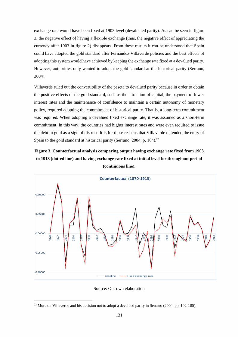
131
exchange rate would have been fixed at 1903 level (devaluated parity). As can be seen in figure
3, the negative effect of having a flexible exchange (thus, the negative effect of appreciating the
currency after 1903 in figure 2) disappears. From these results it can be understood that Spain
could have adopted the gold standard after Fernández Villaverde policies and the best effects of
adopting this system would have achieved by keeping the exchange rate fixed at a devalued parity.
However, authorities only wanted to adopt the gold standard at the historical parity (Serrano,
2004).
Villaverde ruled out the convertibility of the peseta to devalued parity because in order to obtain
the positive effects of the gold standard, such as the attraction of capital, the payment of lower
interest rates and the maintenance of confidence to maintain a certain autonomy of monetary
policy, required adopting the commitment of historical parity. That is, a long-term commitment
was required. When adopting a devalued fixed exchange rate, it was assumed as a short-term
commitment. In this way, the countries had higher interest rates and were even required to issue
the debt in gold as a sign of distrust. It is for these reasons that Villaverde defended the entry of
Spain to the gold standard at historical parity (Serrano, 2004, p. 104).22
Figure 3. Counterfactual analysis comparing output having exchange rate fixed from 1903
to 1913 (dotted line) and having exchange rate fixed at initial level for throughout period
(continuous line).
Source: Our own elaboration
22 More on Villaverde and his decision not to adopt a devalued parity in Serrano (2004, pp. 102-105).
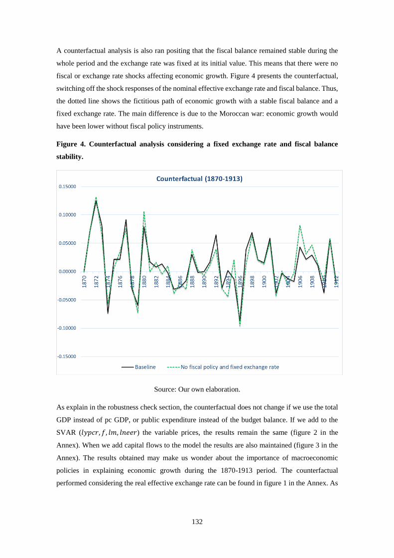
132
A counterfactual analysis is also ran positing that the fiscal balance remained stable during the
whole period and the exchange rate was fixed at its initial value. This means that there were no
fiscal or exchange rate shocks affecting economic growth. Figure 4 presents the counterfactual,
switching off the shock responses of the nominal effective exchange rate and fiscal balance. Thus,
the dotted line shows the fictitious path of economic growth with a stable fiscal balance and a
fixed exchange rate. The main difference is due to the Moroccan war: economic growth would
have been lower without fiscal policy instruments.
Figure 4. Counterfactual analysis considering a fixed exchange rate and fiscal balance
stability.
Source: Our own elaboration.
As explain in the robustness check section, the counterfactual does not change if we use the total
GDP instead of pc GDP, or public expenditure instead of the budget balance. If we add to the
SVAR (𝑙𝑦𝑝𝑐𝑟, 𝑓, 𝑙𝑚, 𝑙𝑛𝑒𝑒𝑟) the variable prices, the results remain the same (figure 2 in the
Annex). When we add capital flows to the model the results are also maintained (figure 3 in the
Annex). The results obtained may make us wonder about the importance of macroeconomic
policies in explaining economic growth during the 1870-1913 period. The counterfactual
performed considering the real effective exchange rate can be found in figure 1 in the Annex. As

133
can be seen, real effective exchange rate shocks were more important than nominal effective
exchange rate shocks.
Figure 5. Contribution of the components of GDP, 1870-1913
Source: Own elaboration based on Prados de la Escosura (2003).
Furthermore, focusing on the economic crisis of the late 1890s, the statistics on GDP point to the
importance of exports in the economic recovery (Figure 5). Figure 5 shows the GDP components:
consumption (C), government expenditure (G), investment (I), stock variation (SV), exports (X),
and imports (I), and indicates the proportion of GDP explained by the increase in exports. It also
helps to understand the potential importance of the exchange rate. As a proportion of GDP exports
increased by 44.5% between 1893 and 1898, second only to consumer spending. The proportion
of exports in GDP increased in the late 1880s and early 1890s. In the short run, thanks to its
flexible exchange rate, Spain barely noticed the cyclical downturn that affected the international
economy between 1890 and 1896 (Sardà, 1987, p. 197). Herranz and Tirado (1996) also highlight
how the different income elasticity of exports and imports hampered foreign payments, and
discouraged Spain from joining the gold standard, due to the effect on the price of the peseta.
Historical decomposition of the variables
Once we know what would have happened if we had had a fixed exchange rate, it would be
relevant to study the importance of macroeconomic policies to explain pc GDP growth during the
period of the classical gold standard (considering Spain had a flexible exchange rate). In order to
134
measure the importance of macroeconomic policies throughout the period, we will use the real
effective exchange rate and not nominal exchange rate. This will allow us to see the importance
that monetary policy and fiscal policy and exchange rate adjustments had on economic growth
(in the real economy). Thus, pc GDP, budget balance, money supply and the real effective
exchange rate are used.
First, I estimate a SVAR. In order to assess the driving forces of the dynamic evolution of the
economic growth, I run historical decomposition. For Burbidge and Harrison (1985), technique
of historical decomposition seems ideally suited as a vehicle for re-examination of money’s role
and other policies during the depression. It allows to assess the contribution of exchange rate
shocks and monetary and fiscal policy shocks to the observed output changes in busts and booms
over the period under study. Historical decomposition of each variable allows us to study how the
model interprets and describes the history. Thus, this analysis indicates the contribution of each
structural shock on the evolution of economic growth over time. Running this analysis is useful
to investigate the variables responsible of the falls and rises of one variable (output in our case).
The series of real pc GDP (or better said, economic growth) is decomposed into four components
that are explained by the four types of structural shocks, respectively: GDP, fiscal balance, money
supply and, exchange rate. In the figure 6 economic growth fluctuations is explained by four
different structural shock. The figures show the contributions of the individual shocks to
fluctuations of one variable (in our case, economic growth). Each panel contain the actual path
(the fluctuations of the variable) and the contribution of each structural shock to the fluctuations
of that variable. If the shock line follows the behaviour of the actual line, it shows that the isolated
shock accounts for the behaviour of the variable. If the shock line does not follow the pattern of
the first line, then the isolated shock had no effect on the variable. The bar chart shows the
fluctuations in GDP, and the continuous line shows the decomposition into the different structural
shocks.
The shocks in pc GDP account for the largest part of the fluctuations in economic growth during
the whole period. After shocks in GDP, the variable that follows the behaviour of the economic
growth fluctuations most closely is the real effective exchange rate. Real effective exchange rate
shocks are important in explaining economic growth fluctuations, especially between 1885 and
1905. The real exchange rate helps to improve economic growth after the pc GDP fall of the mid-
1880a (figure 1) and after the decrease in 1896. Thus, it explains the rise in economic growth
during the first two years after suffering a large fall. Indeed, the peseta’s greatest loss of value
occurred in 1898. Money supply also helps to explain the fluctuations of economic growth. It
follows the behaviour of economic growth before the 1880s and from 1891 to 1903. Changes in
the amount of money also explain the recovery of economic growth after 1896 (when Spain

135
suffered a large fall in GDP). Fiscal shocks have practically no effect on fluctuations in real GDP.
Fiscal policy shocks do not follow the movements of economic growth even when the model is
estimated considering total fiscal balance (rather than over GDP). They may have been important
in the decrease of 1896 and they seem to have had a countercyclical effect during the first years
of the twentieth century.
Figure 6. Historical decomposition of pc GDP
Historical Decomposition of economic growth using Generalized Weights
-.12
-.08-.04
.00
.04
.08
.12
.16
1880 1890 1900 1910
Due to economic growth shocks
-.12
-.08
-.04
.00
.04
.08
.12
1880 1890 1900 1910
Due to fiscal shocks
-.12
-.08
-.04
.00
.04
.08
.12
1880 1890 1900 1910
Due to money supply shocks
-.12
-.08
-.04
.00
.04
.08
.12
1880 1890 1900 1910
Economic growth fluctuationsVariable shocks
Due to exchange rate shocks
Source: own elaboration
Robustness check
In order to explore the robustness of our results we consider various alternative variable
definitions and add additional endogenous and exogenous variables to SVAR model. All of these
changes have only minor effects on the results obtained in the counterfactual and historical
decomposition analysis.
136
When I deflate the exchange rate by CPI from Maluquer (2013) and Mitchell (2007), results are
maintained. I also run the VAR considering the total GDP from Prados de la Escosura (2003)
instead of pc GDP, government expenditure from Comín and Diaz (2005) instead of budget
balance over GDP, budget balance deflated by GDP deflator (Prados de la Escosura, 2003) instead
of budget balance over GDP or banknotes in circulation from Martín Aceña (2017) instead of
money supply. In all cases results obtained are very similar. Moreover, I repit the analysis
considering the variable prices (in order to take into account inflation) without important changes
in my results (see Figure 2 in the annex).23 Finally, I add capital inflows from Prados de la
Escosura (2010) that can be considered important during that period and counterfactual and
historical decomposition analysis remain the same (see Figure 3 in the annex).24 New data on
fiscal balance have been estimated by Comin, though they have not yet been published.
Reestimating my results with these new data (Figure 4 in the annex), the results are maintained
and the main conclusions remain the same.
As Spain was affected by recurring armed conflicts in the period, the same model has also been
estimated with the addition of an exogenous dummy variable that takes a value of 1 for years in
which Spain was engaged in armed conflict and 0 for years in which it was not (Figure 6 in
Annex)25. The results does not change significantly. The counterfactual analysis is the same as
when we estimate the model without considering wars.26 The historical decomposition of output,
when taking wars into account, does not show changes compared to the main findings.27 There is
no heterokedascity or autocorrelation and the system is stable as can be shown in the Annex
(Figure 7 and Table 1).
V. Benefits and costs of being outside the gold standard
In the period under study, the maintenance of the gold standard was an important requirement for
prosperity. It was a system, however, that was hard to apply in countries on the southern periphery
of Europe like Spain. Floating exchange rates were and are a fast way to correct for shocks that
affect the equilibrium between domestic price levels and price levels abroad.28 The classical gold
23 Following Shibamoto and Shizume (2014), I add prices variable to check my results. 24 See more on this in Clemens and Williamson (2000). 25 Spain was engaged in the following armed conflicts: Third Carlist War (1872-1876), Ten Years’ War
(1868-1878), Little War (Cuba) (1879-1880), Cuban War of Independence (1895-1898), Spanish-American
War (1898), Philippine Revolution (1896-1898), Margallo War (1893-1894), Melilla War (1909-1913),
and Rif War, or Second Moroccan War (1911-1927). 26 The counterfactual analysis is always done with the nominal effective exchange rate, except when stated
otherwise (figure 1 in Annex). As has been stressed, being on the gold standard meant keeping the nominal
exchange rate stable. The real exchange rate cannot be fixed because it depends on prices. 27 The historical decomposition is always done with the real effective exchange rate because the aim iws to
capture the real impacts of exchange rate behaviour on Spanish economic growth. 28 “The classical gold standard is not appropriate in practice to overcome [such difficulties], simply because
it cannot produce a readjustment of domestic prices quickly enough” (Keynes, 1931/1988, p. 180).

137
standard did not permit this type of response and it undercut a country’s options to control its own
economy through the setting of exchange rates (Keynes, 1931/1988, pp. 173 and 180).29 Policies
in the late nineteenth century and early twentieth century run in accordance with circumstances.30
Some of these policy options could not have been pursued under the gold standard, which required
restrictive policies to be maintained over time.
Sardà (1987) states that although it was not the intention of the monetary authorities, the non-
adoption of the gold standard favoured Spain. It isolated the Spanish economy from the
fluctuations in income and prices that affected other countries and protected it from the
international depression of the last quarter-century. This is what we find in figure 2, table 2 and
figure 4, which show the benefits of being outside the gold standard during the final decades of
nineteenth century. These results also support Fernández Villaverde (1900)’s observation that the
end of the nineteenth century was not a good moment to adopt the gold standard.
As we see in figure 1, from 1903, GDP and exchange rate followed a different pattern. While the
exchange rate appreciated, GDP rose. This is consistent with the findings of the counterfactual
analysis, and also with Serrano (2004)’s view that the crucial moment to adopt the system was
1903. In figure 6, it can be found that exchange rate shocks were important for understanding the
behaviour of economic growth. The depreciation of the peseta may have helped to improve
exports and raise GDP, as we find in Table 2. The results suggest that the depreciation of the
peseta was relevant to increasing output, especially during the falls in 1886 and 1896 when
Spanish economy was badly hit. Without a flexible exchange rate, the impact of fluctuations on
the economic cycle would have been greater at the end of the nineteenth century. It is not
surprising that fiscal policy did not account for much of the conomic growth; Spain was a liberal
state that devoted a low percentage of its GDP to public expenditure. The result is consistent with
the historiography.
Therefore, Spain, despite not joining the gold standard, did not lose output. If the peseta exchange
rate had not been permitted to separate from its historical parity, the Spanish growth would have
outpaced the actual growth at the beginning of the 20th century. On the other hand, had it entered
in 1876, the economic shocks would have been greater and the economy would have been
negatively affected in the short term. We all know that the cost of a crisis is not just felt in the
loss in terms of GDP, but only in its effects on the level of employment and on people’s standard
of living. Therefore, future research should analyse the loss in the living standards that would
29 Keynes (1931) reproduced in Keynes (1988). 30 Olariaga (1977, p. 137) considers Spain’s policy was ad hoc. They did not regulate the economic cycle.

138
have have been caused by deeper crises (i.e, if a fixed exchange rate had been maintained until
1903).
VI. Conclusion
This paper presents a counterfactual analysis between 1870 and 1913 for Spain, in order to
consider whether having a fixed exchange rate would have improved the country’s economic
growth. This study is the first of its kind on this topic. The Spanish case is significant, because
the country did not adopt the classical gold standard. The main finding is that the depreciation of
the exchange rate had positive effects on the Spanish economy outside the gold standard,
alleviating the crises during the 1870-1903 period. As Villaverde wrote, it was not the moment to
adopt the gold standard. The historical decomposition analysis reveals that adjustments in
exchange rates and monetary policy were important to sustaining growth, and played an important
role in explaining the behaviour of economic growth before 1903. The exchange rate level helped
to improve the terms of trade, and promoted exports until the beginning of the twentieth century.
The effects of fiscal policy were less significant. After 1903, the adoption of the gold standard
would have been possible and it would not have damaged the economy; indeed, being on the gold
standard (keeping the exchange rate fixed) seems to have been the optimal option for increasing
the economic growth from around 1903. If the peseta exchange rate had not been permitted to
separate from its historical parity, the Spanish economic growth would have outpaced the actual
growth at the beginning of the 20th century. However, the economic shocks would have been
greater and the economy would have been negatively affected during the late 19th century. Finally,
the paper provides new empirical evidence for the core-periphery debate during the period of the
classical gold standard.

139

140
Concluding remarks
This study focuses on the rather unusual case of Spain and the classical gold standard. Spain never
adopted this monetary system and did not keep its exchange rate stable. For most of the period
under study, Spain experienced budget deficits and accumulation of public debt. Like other
countries on the Mediterranean periphery, it suffered the effects of the gold standard monetary
system and, in recent times, the effects of the euro crisis, also in a context of fixed exchange rates
among the eurozone countries. For this reason, it is important to analyse the potential costs and
benefits for Spain if the country had adopted the gold standard and the reasons why it was difficult
to do so (chapter 1); the causes of Spain’s decision to remain outside the gold standard and
whether this was a real problem (chapter 2); the consequences of not being on the gold standard
(chapter 3) and whether it was positive or negative for the Spanish economy to be outside the
fixed exchange rate system (by creating and studying a counterfactual scenario, chapter 4). To do
so, I aimed to determine whether the lack of fiscal discipline and the accumulation of debt
prevented the adoption of the gold standard, and to understand the role played by the different
macroeconomic policies in Spanish economic growth. My thesis sheds new light on the discussion
about the Spain’s non-adoption of the classical gold standard. It also shows new empirical
evidence for the core-periphery (north-south) debate during the late nineteenth and the early
twentieth centuries. Finally, the results obtained stress that the monetary system was not a cause
of the divergence experienced in Spain before the Great War.
Chapter 1 discusses the literature on the positive or negative effects that being outside the gold
standard could have had for Spanish economy. Spain wanted to join the gold standard, as
demonstrated by its attempt to become a member in 1876. This article shows the main problems
that could explain the Spain’s non-adoption of the gold standard: fiscal balance and balance of
payments deficits. Moreover, it can be found and explanation for gold reserves. The first part of
the article poses two questions presented in the introduction: Was there a desire to join the gold
standard? Was it even possible to do so? The paper underlines that an evaluation of the benefits
or costs of Spain’s non-adoption of the gold standard depends basically on the theoretical and
temporal perspective used. If the priority was the short term, having a flexible exchange rate could
be seen as being positive for the economy. On the other hand, if the most important aim is long
term stability (price stability), then having a fixed exchange rate would have been the best option.
The chapter also questionsd whether the long term perspective could be considered as a luxury
good for a backward country, such as Spain since the economy needed wealth for purposes other
than its circulation as a currency. Moreover, I argue that having a flexible exchange could have
protected the economy from economic cycle fluctuations. The chapter opens the door for the

141
analyses carried out in the other three chapters. So this article proposes the following introductory
questions: Why didn’t Spain adopt the gold standard? What were the costs and benefits of
maintaining flexible exchange rates (not adopting the gold standard) for a backward country like
Spain?
The second chapter focuses on the reasons that made the adoption of the gold standard difficult
for Spain. It provides an answer to the first question posed in introduction (Why didn’t Spain
adopt the gold standard?) As far as I know, it is also the first study of debt sustainability for Spain
at the end of the nineteenth century and the beginning of the twentieth. Previous studies have
assessed fiscal dominance . The main findings are that the primary balance responded negatively
to an increase in debt until the beginning of twentieth century, when the response started to be
positive. Therefore, debt was unsustainable until 1903 even when seigniorage is considered. Thus,
it was very difficult to be part of the gold standard due to this huge debt accumulation and the
weak political position until 1903. Seigniorage was not significant for the sustainability of the
debt, even though, as pointed by Joan Sardà, it was important to sustain economic growth. My
results suggest that the sustainability or unsustainability of debt depended on economic policies
such as the fiscal ones adopted by Raimundo Fernández Villaverde at the beginning of the
twentieth century to keep the budget balance under control. I detect a structural change in 1903
which has not previously been found in studies related to debt or fiscal dominance. This structural
change in 1903 is considered as a result of the policies carried out by Fernández Villaverde. It
was also in 1903 when Fernández Villaverde presented a draft bill to oversee the entry of Spain
into the gold standard; from 1903 membership would have been possible, since fiscal discipline
was maintained and the public debt became sustainable.
The third chapter is based on the different temporal approaches that can be considered to
understand what happened in Spain during the classical gold standard period and the beneficial
or detrimental effects that macroeconomic policies had on the Spanish economy. I attempt to
answer the following question: What was the effect on the Spanish economy of keeping the
exchange rate flexible (i.e., not adopting the gold standard)? The article establishes a point of
union between the two existing theses on Spain and the gold standard. As explained in chapter 1,
the positive or negative consequences of having a flexible exchange depend on the temporal
approach considered. ARDL analysis reveals that the expansionary monetary policies
implemented had a positive impact on Spain’s output in the long run. I find that monetary policy
helped to sustain economic growth in the long run. The explanation may lie in the connection
between fiscal policy and monetary policy throughout the period.
I also find that exchange rate had a positive impact on Spanish output in the short run but not in
the long run. Therefore, exchange rate adjustments seem to play an important short-run role in

142
Spain’s output. However, in the long run, the exchange rate had a non-significant impact on
Spanish output (tested with new data on fiscal balance) and a negative and significant effect on
Spanish GDP (tested with classical data on fiscal balance). This possible negative effect is
consistent with the findings of various scholars such as Krugman for backward economies with
trade balance deficits (see the discussion in chapter 3). Thus, both theories (Sardà and Martín-
Aceña) are correct: the exchange rate was able to help to overcome business cycle fluctuations
and to promote economic growth in the short run, but not in the long run. The Toda and Yamamoto
causality analysis of the variables carried out in this chapter shows that monetary policy
accommodates the state’s fiscal needs. Therefore, the results corroborate that there was also fiscal
dominance from 1870-1913, as other articles had underlined for a larger periods of time. This
article not only focuses on the never-ending debate on Spain and the classical gold standard but
is contributes to the broader discussion about the effects of exchange rate depreciation on output
carried out by economists such as Krugman, Alexander, Cooper among others. As far as I know,
no analysis of this kind has been carried out before for Spain for the period under study. Finally,
considering fiscal policy is positive and significant in the long-run main results and annex results,
my results supports the story that the size of the government debt is one of the two important
reasons why Spain did not join the Gold Standard. The accumulation of deficits (long run) had a
negative impact on Spanish economy while surpluses had the opposite effect.
Chapter 4 runs a counterfactual analysis to study the possible outcome for the Spanish economy
under a fixed exchange rate system. It answers the question posed in the introduction: what would
have happened if we had had a fixed exchange rate? This kind of analysis (never previously
applied to the Spanish case) can help to resolve the never-ending debate on the country’s non-
adoption of the gold standard. According to the results in chapter 4, the depreciation of the
currency helped the Spanish economy by cushioning the impact of business cycles at least until
the beginning of the twentieth century. It can be seen that under a fixed exchange rate system, the
falls would have been deeper. Before the early twentieth century, adopting the gold standard
would have been negative for Spain in terms of economic growth. However, after the Villaverde
reforms, Spain achieved budget surpluses and a certain level of fiscal discipline. This made the
debt sustainable (chapter 2) and from that moment onwards it would have been better to have a
fixed exchange rate than a flexible one. In fact, it is proven that, from 1903, if the exchange rate
had been maintained at the devalued level of 1903, economic growth would have been exactly
the same as the growth under exchange rate fixed at initial level (figure 3, chapter 4) and the
Spanish economy would have not suffered the appreciation experienced in the first years of the
twentieth century (figure 2, chapter 4). If the peseta exchange rate had remained around its
historical parity, Spanish growth at the beginning of the twentieth century would have been
higher. On the other hand, had it entered in 1876, the economic shocks would have been greater

143
and the economy would have been negatively affected in the short term. However, this study has
limitations and can only assess the economic part of the issue. it cannot calculate how different
countries and markets would have reacted to a commitment to devalued parity, or the
consequences that social level (living standards or inequality) might have had when the crises
were deeper. Also, based on a historical decomposition analysis I find that adjustments in
exchange rates and monetary policy were important for sustaining growth. They played a key role
in explaining the economic growth fluctuations especially before the beginning of twentieth
century. These findings are consistent with those presented in chapter 3. Significantly, even when
wars are considered, the results obtained remain similar.
This study offers the possibility of comparing the results obtained with the currently available
data on budgetary balance with those of the new data recently estimated by Francisco Comín.
Chapters 2 and 3 are mainly estimated with new data and the results for classic data can be found
in the respective annexes. Chapter 4 was awarded the Carande prize; because one of the
requirements was that the paper be published rapidly, the results with the new data were not
included and are now presented in the respective annex. As can be seen, the results are maintained
and in fact are even clearer, showing that the falls would have been much deeper in the last
decades of the nineteenth century in the light of the new fiscal balance data. This thesis also
provides an estimation of the real effective exchange rate constructed with the GDP deflator and
the CPI (Annex 1 in chapter 2).
As Villaverde suggested, and as shown by the results obtained in chapters 2 and 4, before the
beginning of the twentieth century the adoption of the gold standard would have been a mistake.
The exchange rate level helped to improve the terms of trade, and promoted exports (basically in
the short run) until the beginning of the twentieth century (chapters 3 and 4). The effects of fiscal
policy were less significant, as one would expect in a liberal state (chapters 3 and 4). At the
beginning of the twentieth century, the adoption of the gold standard would have been possible
(chapters 2 and 4). Keeping the exchange rate fixed at historical parity would have aggravated the
consequences of crises until the beginning of the twentieth century; however, after that time it
would have generated higher economic growth. Spain’s adoption of the gold standard would have
been positive for the economy if it had entered with devaluated parity (chapter 4). In this way, the
appreciation suffered by the exchange rate between 1902 and 1906 would not have negatively
affected the economy. Having a fixed exchange rate would not have damaged the economy during
the first years of the twentieth century, and in fact being on the gold standard would have been a
good option for the Spanish economy from around 1903.
These results are reflected in another way in chapter 3, where it is found that in the short term the
flexible exchange rate had a positive and significant impact on the economy. That is, in the short
144
term, the flexible exchange rate helps to cushion the economic cycle, while in the long term it is
not clear that it does not eventually have a negative effect. Again, the results corroborate the
findings of chapter 2. This shows how the public debt was sustainable between 1903 and 1913,
making it possible for Spain to join the gold standard thanks to having overcome one of the main
economic obstacles to entry. This is also consistent with the results of the counterfactuals studied
in chapter 4.
We stress that while there are fiscal problems and the economy suffers from recurring deficits and
the accumulation of public debt, it is better to have a flexible exchange rate. That is to say, with
greater macroeconomic problems, greater flexibility is needed to cushion the economic impacts.
This makes it possible to adapt quickly when there are falls, as can be seen in chapter 4. However,
when some of the problems affecting the economy are resolved, a fixed exchange rate system
does not have a negative impact on the economy, and it can allow a country to take advantage of
the benefits of its healthy economy. An exchange rate fixed at parity in 1870 would have given
good results from the beginning of the twentieth century, due to the stable economic situation of
Spain and its neighbours. However, it would have had a high cost before that date due to the need
for flexibility.
Finally, was the non-adoption of the gold standard one of the main causes of Spain’s
backwardness relative to the European average during that period?
The results show that the non-adoption of the gold standard cannot explain the divergence
experienced by Spain before the Great War. The results in chapter 2 show how debt became
sustainable ten years before this war. As can be seen in chapter 1, figure 1, between 1903 and
1913 Spain diverged continuously from the European countries. Therefore, achieving a
sustainable level of debt did not help to overcome the divergence pattern. However, the periods
with a slight convergence instead of the divergence pattern are similar to the years when the
exchange rate helped to explain the movements of pc GDP (figure 6 in chapter 4). The results in
chapter 3 are inconclusive. However, considering the new data on fiscal balance to be better than
the classical data, it seems that the flexible exchange rate did not have a real impact on Spanish
economy between 1870 and 1913. According to the results in chapter 3, the monetary policy does
not seem to have been a cause of the divergence experienced by Spain during the period under
study; it had a positive impact on GDP. The results in chapter 4 are clear: having an exchange
rate fixed at the initial level throughout the period would have permitted a higher economic
growth at the beginning of the twentieth century, but not during the last decades of the nineteenth
when the falls in times of crises would have been deeper.

145
146
References
Afonso, A. (2005). Fiscal sustainability: The unpleasant European case. FinanzArchiv: Public
Finance Analysis, 61(1), 19-44.
Afonso, A. (2008). Ricardian fiscal regimes in the European Union. Empirica, 35(3), 313-334.
Afonso, A., & Jalles, J. T. (2011). Appraising fiscal reaction functions. Economics Bulletin,
AccessEcon, vol. 31(4), 3320-3330.
Afonso, A., & Jalles, J. T. (2017). Sovereign debt composition and time-varying public finance
sustainability. The North American Journal of Economics and Finance, 42, 144-155.
Aixalá, J. (1999). La peseta y los precios: un análisis de largo plazo (1868-1995). Zaragoza: Prensas
Universitarias de Zaragoza.
Alexander, S.S. (1952). Effects of a Devaluation on a Trade Balance. IMF Staff Papers, 2, 263–278.
Anes, R. (1974a). Una serie de base monetaria (1874-1915). In Tortella, G. (dir.), La Banca española
en la Restauración, Vol. II: Datos para una historia económica. Madrid: Servicio de
Estudios del Banco de España, 199-209.
Anes, R. (1974b). Estimación de la moneda de plata existente en España entre 1874 y 1915. In
Tortella, G. (dir.), La Banca española en la Restauración, Vol. II: Datos para una historia
económica, Madrid: Servicio de Estudios del Banco de España, 99-116.
Arellano, C., & Bai, Y. (2017). Fiscal austerity during debt crises. Economic Theory, 64(4), 657-673.
Arestis, P., Cipollini, A., & Fattouh, B. (2004). Threshold effects in the US budget deficit. Economic
Inquiry, 42(2), 214-222.
Baffigi A. (2013). National Accounts 1861-2011. In Toniolo G. (Ed) The Oxford Handbook of the
Italian Economy since Unification. New York : Oxford University Press
Bahmani-Oskooee, M., & Anker, P. (2001). On the Relationship between the Value of the Mark and
German Production. Applied Economics, 33, 1525–1530.
Bahmani-Oskooee, M, Chomsisengphet, S and Kandil, M. (2002). Are devaluations contractionary
in Asia?. Journal of Post Keynesian Economics, 25, 69–81
Bahmani-Oskooee, M., Iqbal, J., & Salam, M. (2016). Short run and long run effects of exchange
rate volatility on commodity trade between Pakistan and Japan. Economic Analysis and
Policy, 52, 131-142.
147
Bahmani-Oskooee, M. & Kandil, M. (2010). Exchange Rate Fluctuations and Output in Oil-
Producing Countries: The Case of Iran. Emerging Markets Finance and Trade, 46(3), 23-
45.
Bahmani-Oskooee, M., & Kutan, A. M. (2008). Are devaluations contractionary in emerging
economies of Eastern Europe?. Economic Change and Restructuring, 41(1), 61-74.
Bahmani-Oskooee, M., & Gelan, A. (2013). Are devaluations contractionary in Africa?. Global
Economic Review, 42(1), 1-14.
Bahmani‐Oskooee, M., & Mohammadian, A. (2016). Asymmetry effects of exchange rate changes
on domestic production: evidence from nonlinear ARDL approach. Australian Economic
Papers, 55(3), 181-191.
Bajo-Rubio, O., Dıaz-Roldán, C., & Esteve, V. (2004). Searching for threshold effects in the
evolution of budget deficits: An application to the Spanish case. Economics Letters, 82(2),
239-243.
Bajo-Rubio, O., Díaz-Roldán, C., & Esteve, V. (2006). Is the budget deficit sustainable when fiscal
policy is non-linear? The case of Spain. Journal of Macroeconomics, 28(3), 596-608.
Bajo-Rubio, O., Diaz-Roldan, C., & Esteve, V. (2014). Deficit sustainability, and monetary versus
fiscal dominance: The case of Spain, 1850–2000. Journal of Policy Modeling, 36(5), 924-
937.
Balke, N. S., & Gordon, R. J. (1989). The estimation of prewar gross national product: Methodology
and new evidence. Journal of Political Economy, 97(1), 38-92.
Barciela, C., Giráldez, J., Grupo de Estudios de Historia Rural and López, I. (2005). Sector agrario
y pesca. In: Carreras, A. and Tafunell, X. (eds.). Estadísticas históricas de España: siglos
XIX-XX. Bilbao: Fundación BBVA, 245-356.
Barro, R. J. (1979). On the determination of the public debt. Journal of political Economy, 87(5, Part
1), 940-971.
Barro, R. J. (1986). US deficits since World War I. The Scandinavian Journal of Economics, 195-
222.
Berend, T. I., Ránki, G., Pálmai, É., & Ránki, G. (1982). The European periphery and
industrialization 1780-1914. Cambridge: Cambridge University Press.
Bernanke, B. (1995). The Macroeconomics of the Great Depression: A Comparative
Approach. Journal of Money, Credit & Banking, 27(1), 1.

148
Bernanke, B. (2015). Mis años en la Reserva Federal. Madrid: Deusto.
Betrán, C., Martín-Aceña, P., & Pons, M. A. (2012). Financial crises in Spain: lessons from the last
150 years. Revista de Historia Económica-Journal of Iberian and Latin American
economic History, 30(3), 417-446.
Betrán, C. & Pons, M. A. (2013). Understanding Spanish Financial crises, 1850-2000: What
determined their severity? EHES Working Paper, 48.
Betrán, C, Pons, M.A. (2019). Understanding Spanish financial crises severity, 1850–2015.
European Review of Economic History, 23 (2), 175-92.
Blanchard, O., & Perotti, R. (2002). An Empirical Characterization of the Dynamic Effects of
Changes in Government Spending and Taxes on Output. The Quarterly Journal of
Economics, 117(4), 1329-1368.
Blanchard, O. (1990), Suggestions for a New Set of Fiscal Indicators. OECD Economics Department
Working Papers, No. 79, OECD Publishing, Paris,
Bloomfield, A. I. (1959). Monetary policy under the international gold standard: 1880-1914. New
York: Federal Reserve Bank of New York
Bi, H., Shen, W., & Yang, S. C. S. (2016). Debt-dependent effects of fiscal expansions. European
Economic Review, 88, 142-157.
Bohn, H. (1991). Budget balance through revenue or spending adjustments?: Some historical
evidence for the United States. Journal of monetary economics, 27(3), 333-359.
Bohn, H. (1995). The sustainability of budget deficits in a stochastic economy. Journal of Money,
Credit and Banking, 27(1), 257-271.
Bohn, H. (1998). The behavior of US public debt and deficits. the Quarterly Journal of
economics, 113(3), 949-963.
Bohn, H. (2007). Are stationarity and cointegration restrictions really necessary for the intertemporal
budget constraint?. Journal of monetary Economics, 54(7), 1837-1847.
Bohn, H. (2008). The sustainability of fiscal policy in the United States. Sustainability of public debt,
15-49.
Bordo, M. D. (1981). The classical gold standard: Some lessons for today. Federal Reserve Bank of
St. Louis Review, 63(5), 2-17.
Bordo, M. D. (1990). The lender of last resort: alternative views and historical experience. FRB
Richmond Economic Review, 76(1), 18-29.
149
Bordo, M. D. (1999). The Gold Standard and Related Regimes. New York: Cambridge University
Press.
Bordo, M. D. (2005). The gold standard and related regimes: collected essays. Cambridge:
Cambridge University Press.
Bordo, M., Eichengreen, B., Klingebiel, D., & Martinez‐Peria, M. S. (2001). Is the crisis problem
growing more severe?. Economic policy, 16(32), 52-82.
Bordo, M. D., & James, H. (2008). A long term perspective on the euro (No. w13815). National
Bureau of Economic Research.
Bordo, J. & James, H., (2014) The European crisis in the context of the history of previous financial
crises. Journal of Macroeconomics, 39, 275-284.
Bordo, M. D., & Jonung, L. (2001). A return to the convertibility principle? Monetary and fiscal
regimes in historical perspective. In: Leijonhufvud, A. (Ed.), Monetary Theory as a Basis
for Monetary Policy (pp. 225-283). London: Palgrave.
Bordo, M. D., Lane, J. L., & Redish, A. (2004). Good versus bad deflation: lessons from the gold
standard era (w10329). National Bureau of Economic Research.
Bordo, M. D., & MacDonald, R. (2005). Interest rate interactions in the classical gold standard,
1880–1914: was there any monetary independence? Journal of Monetary Economics,
52(2), 307-327.
Bordo, M. & Schwartz, A. (1986). The operation of the specie standard: Evidence for core and
peripheral countries, 1880-1990. In Eichengreen, B., Reis, J., & de Macedo, J. B. (Eds.).
Currency convertibility: the gold standard and beyond. London: Routledge, ). The
operation of the specie standard: Evidence for core and peripheral countries, 238-317.
Bordo, M. D., & Schwartz, A. J. (1999). Monetary policy regimes and economic performance: the
historical record. Handbook of macroeconomics, 1, 149-234.
Braga de Macedo, J. (1996). Converging towards a European currency standard-Convertibility and
stability in 1990s and beyond. In: Eichengreen, B., Reis, J., & de Macedo, J. B. (Eds.).
Currency convertibility: the gold standard and beyond (pp.243-68). New York: Routledge.
Broder, A. (1976). Les investissements étrangers en Espagne au XIX e siècle: méthodologie et
quantification. Revue d'histoire économique et sociale, 54(1), 29-63.
Broder, A. (1993). L'économie française au XIXe siècle. París: Editions Ophrys.
Buiter, W. H. (1985). A guide to public sector debt and deficits. Economic policy, 1(1), 13-61.
150
Burbidge, J., & Harrison, A. (1985). An historical decomposition of the great depression to determine
the role of money. Journal of Monetary Economics, 16(1), 45-54.
Bustelo, F., & Tortella-Casares, G. (1976). Monetary Inflation in Spain 1800-1970. Journal of
European Economic History, 5(1), 141.
Canzoneri, M. B., Cumby, R. E., & Diba, B. T. (2001). Is the price level determined by the needs of
fiscal solvency?. American Economic Review, 91(5), 1221-1238.
Carreras, A. (2005). Industria. In: Carreras, A. y Tafunell, X.(Eds.). Estadísticas históricas de
España, siglos XIX-XX. Bilbao: Fundación BBVA, 357-454.
Carreras, A., Prados de la Escosura, L., & Rosés, J. R. (2005). Renta y riqueza. In Carreras, A. &
Tafunell X. (2005). Estadísticas históricas de España, siglos XIX-XX., Bilbao: Fundación
BBVA, 1297-1377
Carreras, A. & Tafunell X. (2004). Historia económica de la España contemporánea. Barcelona:
Crítica.
Carreras, A. & Tafunell X. (2005). Estadísticas históricas de España: siglos XIX-XX. Bilbao:
Fundación BBVA.
Castañeda, L. (2001). Esplendor y ocaso del mercado de letras de cambio en la Barcelona del siglo
XIX.
Castañeda, L., & Tafunell, X. (1993). Un nuevo indicador para la historia financiera española: la
cotización de las letras de cambio a corto plazo. Revista de Historia Economica-Journal of
Iberian and Latin American Economic History, 11(2), 367-383.
Catalan, J. (2002). Costes y beneficios del euro en la Europa periférica: España versus Suecia. Gaceta
Numismática, 145, 17-34.
Catalan, J., Sudrià, C. & Tirado, D., (2001). Peseta y protección: el debate historiográfico. In: Sudrià,
C. & Tirado, D. A. (eds.). Peseta y Protección. Comercio exterior, Moneda y Crecimiento
Económico en la España de la Restauración. Barcelona: Edicions de la Universitat de
Barcelona, 11-42.
Catalan, J. & Sánchez A. (2013). Cinco cisnes negros. Grandes depresiones en la industrialización
moderna y contemporánea, 1500-2012. In: Comín, F. & Hernández, M. (eds.). Crisis
económicas en España 1300-2012. Madrid: Alianza, 95-100.
Celasun, O., Ostry, J. D., & Debrun, X. (2006). Primary surplus behavior and risks to fiscal
sustainability in emerging market countries: A “Fan-chart” approach. IMF Staff
Papers, 53(3), 401-425.

151
Cha, M. S., (2003). Did Takahashi Korekiyo rescue Japan from the great depression? The Journal of
Economic History, 63(01), 127-144.
Chalk, M. N. A., & Hemming, M. R. (2000). Assessing fiscal sustainability in theory and
practice (No. 0-81). Working paper, International Monetary Fund.
Christopoulos, D. K. (2004). Currency devaluation and output growth: new evidence from panel data
analysis. Applied Economics Letters, 11(13), 809-813.
Choudhary, M. A., & Chaudhry, M. A. (2007). Effects of the exchange rate on output and price level:
evidence from the Pakistani economy. The Lahore Journal of Economics, 12(1), 49-77.
Cipolla, C. M. (1995). Storia facile dell'economia italiana dal Medioevo a oggi. Mondadori.
Clemens, M. A., & Williamson, J. G. (2000). Where did British foreign capital go? Fundamentals,
failures and the Lucas paradox: 1870-1913 (w8028). National Bureau of Economic
Research.
Comín, F. (1988). Hacienda y economía en la España contemporánea (1800-1936). Ministerio de
Hacienda. Centro de Publicaciones, Madrid.
Comín, F. (1985). La política fiscal en España entre 1874-1914: algunas precisiones. In Tuñón de
Lara, M. La España de la Restauración: política, economía, legislación y cultura: I
Coloquio de Segovia sobre Historia Contemporánea de España. Madrid: Siglo XXI de
España Editores, 189-214.
Comín, F. (1988). Evolución histórica del gasto público. Papeles de Economía Española, 37, 78-99.
Comín, F. (1989). Hacienda y Economia en la España Contemporanea, 2 vols. Madrid: Instituto de
Estudios Fiscales.
Comín, F. (1996). Historia de la hacienda pública: Europa. Barcelona: Crítica.
Comín, F. (1997). La Hacienda pública en España: una perspectiva histórica (siglos XIX y XX).
In Febrero, R. ¿ Qué es la economía? Madrid: Pirámide. 697-721
Comín, F. (1999). El desarrollo del Estado del bienestar en España. Historia y política: Ideas,
procesos y movimientos sociales, 2, 7-38.
Comín, F. & Martorell, M.A. (2003). Laureano Figuerola y el nacimiento de la peseta como unidad
monetaria, Miguel Angel Linares, Papeles y memorias de la Real Academia de Ciencias
Morales y Políticas, 11, 32-59.
Comín, F. (2004). La metamorfosis de la Hacienda (1808-1874). In Fontana, J., Historia: analisis
del pasado y proyecto social, Barcelona: Crítica. 31-102
152
Comín, F., & Díaz, D. (2005). Sector público administrativo y estado del bienestar. Estadísticas
Históricas de España: Siglos XIX y XX, 2nd edition edn. Bilbao: Fundación BBVA, 873-
964.
Comín, F. & Martorell, M. (2006). Laureano Figuerola: el ministro de Hacienda de la Revolución
Gloriosa. In Comín, F., Martín-Aceña, P. & Vallejo, R. (eds.). La Hacienda por sus
ministros. La etapa liberal de 1845 a 1899. Zaragoza: Publicaciones de la Universidad de
Zaragoza, 299-339.
Comín, F. (2013). Apuros, ahogos, arreglos y bancarrotas: las crisis de la deuda pública, 1504-2012.
In Crisis económicas en España: 1300-2012: lecciones de la historia. Madrid: Alianza,
169-201.
Comín, F. (2016). Las crisis de la deuda soberana en España (1500-2015). Madrid: Catarata.
Comín, F. (2017). Evaluating public debt series over two countries in Spain: from serial defaults to
responsible debt management. Unpublished paper.
Comín, F., & Martorell, M. (2006). Juan Francisco Camacho: un liberal templado. Comín, Martín
Aceña y Vallejo (eds.)(2006), 369-401.
Cooper, R. N. (1971). Currency devaluation in developing countries. Essays in International Finance
86. International Finance Section, Princeton University.
Corsetti, G., Dedola, L., Jarociński, M., Maćkowiak, B., & Schmidt, S. (2019). Macroeconomic
stabilization, monetary-fiscal interactions, and Europe's monetary union. European
Journal of Political Economy, 57, 22-33.
Cubel, A. (2001). Estabilidad e inestabilidad macroeconómica en España, 1880-1913: el coste del
abandono de la convertibilidad. In: Sudrià, C. and D. A. Tirado (eds.). Peseta and
protección. Comercio exterior, moneda and crecimiento económico en la España de la
Restauración. Edicions Universitat de Barcelona, Barcelona, 177-196.
Cubel, A., Palafox, J. & Sudrià, C. (1998). Public Deficit, Debt, Monetary Policy and External
Equilibrium. Spain, 1880-1930. In: Bovykine, V., A. Broder and R. Maranhao (orgs.).
Public debt, public finance, money and balance of payments in debtor countries 1890-
1932/33. Twelfth International Economic History Congress, Seville.
Davutyan, N. & Parke, W. (1995). The Operations of the Bank of England, 1890-1908: A Dynamic
Probit Approach. Journal of Money, Credit and Banking 27, 1099-112.
De Castro Fernández, F., & Fernández-Caballero, L. (2011). The effects of fiscal shocks on the
exchange rate in Spain (No. 1121). Madrid: Banco de España.
153
De Cecco, M. (1974). Money and empire, Blackwell and London, Oxford.
De Mattia, R. (1978). Storia del capitale della Banca d'Italia e degli istituti predecessori. Roma:
Banca d'italia.
D’Erasmo, P., Mendoza, E. G., & Zhang, J. (2016). What is a sustainable public debt?. In Handbook
of Macroeconomics (Vol. 2, pp. 2493-2597). Elsevier.
Díaz-Alejandro, C. F. (1963). A Note on the Impact of Devaluation and the Redistributive
Effect. Journal of Political Economy, 71(6), 577-580.
Dictamen de la Comisión nombrada por Real Orden de 9 de enero de 1929, para el estudio de la
implantación del patrón oro. Información Comercial Española, 318, 1960, 51-83.
Doepke, M., & Schneider, M. (2006). Inflation and the redistribution of nominal wealth. Journal of
Political Economy, 114(6), 1069-1097.
Domowitz, I., Glen, J., & Madhavan, A. (1998). International cross‐listing and order flow migration:
Evidence from an emerging market. The Journal of Finance, 53(6), 2001-2027.
Dornbusch, R. (1978) "Monetary Policy under Exchange Rate Flexibility," in Managed
ExchangeRate Flexibility: The Recent Experience. Federal Reserve Bank of Boston
Conference Series no. 20. Boston: Federal Reserve Bank of Boston.
Dornbusch, R. (1988). Real exchange rates and macroeconomics: a selective survey. NBER Working
Papers 2775, National Bureau of Economic Research, published as Dornbusch, R. (1989)
Real Exchange Rates and Macroeconomics: A Selective Survey. Scandinavian Journal of
Economics, vol. 91(2), 401-432.
Dornbusch, R. & Krugman, P. (1976). Flexible Exchange Rates in the Short Run, Brookings Papers
on Economic Activity, 3.
Dornbusch, R., Krugman, P., & Cooper, R. N. (1976). Flexible exchange rates in the short
run. Brookings Papers on Economic Activity, 1976(3), 537-584.
Dutton, J. (1984). The Bank of England and the Rules of the Game under the International Gold
Standard: New Evidence. In Bordo, M.D. & Schwartz, A.J. A Retrospective on the
Classical Gold Standard, 1821-1931, Chicago: Chicago University Press, 173-202
Edwards, S. (1989). Real exchange rates, devaluation, and adjustment: exchange rate policy in
developing countries (pp. 16-25). Cambridge, MA: MIT press.
Eichengreen, B. (1992). Golden Fetters: The Gold Standard and the Great Depression, 1919-1939.
Oxford: Oxford University Press.
154
Eichengreen, B. (1996) Globalizing Capital: A History of the International Monetary System,
published by Princeton University Press.
Eichengreen, B. J. (2000). La globalización del capital: historia del sistema monetario
internacional. Barcelona: Antoni Bosch Editor.
Eichengreen, B. (2014). Hall of mirrors: The great depression, the great recession, and the uses-and
misuses-of history. Oxford: Oxford University Press.
Eichengreen, B. J., & Flandreau, M. (Eds.). (1997). The gold standard in theory and history. New
York: Psychology Press.
Eichengreen, B., & Hausmann, R. (1999). Exchange rates and financial fragility (No. w7418).
National bureau of economic research.
Eichengreen, B., Reis, J., & de Macedo, J. B. (Eds.). (2005). Currency convertibility: the gold
standard and beyond. London: Routledge
Eichengreen, B. & Sachs, J. (1986). Competitive devaluation and the Great Depression: a theoretical
reassessment. Economics Letters, 22(1), 67-71.
Eichengreen, B. & Temin, P. (2010). Fetters of gold and paper. Oxford Review of Economic Policy,
26(3), 370-384.
Enders, W. (2004). Applied Econometric Times Series: And Rats Handbook for Econometric Time
Series, 2 Re. John Wiley & Sons.
Escario, R., Gadea, M. D., & Sabate, M. (2012). Multicointegration, seigniorage and fiscal
sustainability. Spain 1857–2000. Journal of Policy Modeling, 34(2), 270-283.
Escario, R., Sabaté, M., & Gadea, M. D. (2011). La sombra monetaria del déficit en la España de la
peseta. Investigaciones de Historia Económica, 7(1), 151-181.
Fackler, J. S., & Parker, R. E. (1994). Accounting for the Great Depression: a historical
decomposition. Journal of Macroeconomics, 16(2), 193-220.
Ferguson, N., & Schularick, M. (2006). The empire effect: the determinants of country risk in the
first age of globalization, 1880–1913. The Journal of Economic History, 66(2), 283-312.
Fernández-Villaverde, R. (1893). Sobre el estado anormal de los cambios. Reproduced in Serrano
Sanz, J. M. (2002).
Fernández-Villaverde, R. (1900). Una campaña parlamentaria: discursos pronunciados por el
Excmo. señor D. Raimundo Fernández Villaverde. Madrid: Suc. de Rivadeneyra.
155
Fernández-Villaverde, R. (1903). Proyecto de Ley para regularizar y mejorar el cambio exterior y
para procurar el restablecimiento de la circulación y de la libre acuñación de la moneda
de oro, Madrid: Imprenta de la sucesora de M. Minuesa de los Ríos
Flandreau, M. (1993). On the inflationary bias of common currencies: The Latin Union
puzzle. European Economic Review, 37(2-3), 501-506.
Flandreau, M. (1996). The French crime of 1873: An essay on the emergence of the international
gold standard, 1870–1880. The Journal of Economic History, 56(4), 862-897.
Flandreau, M., & Maurel, M. (2005). Monetary union, trade integration, and business cycles in 19th
century Europe. Open economies review, 16(2), 135-152.
Flandreau, M., Cacheux, J. L., & Zumer, F. (1998). Stability without a pact? Lessons from the
European gold standard, 1880—1914. Economic Policy, 13(26), 116-162.
Ford, A. G. (1962). The gold standard, 1880-1914: Britain and Argentina. Oxford: Clarendon Press.
Friedman, M., & Schwartz, A. J. (1982). The effect of term structure of interest rates on the demand
for money in the United States. Journal of Political economy, 90(1), 201-212.
Fraile, P. (1991). Industrialización y grupos de presión. La economía política de la protección en
España 1900-1950. Madrid: Alianza.
Friedman, M. (1970). A theoretical framework for monetary analysis. journal of Political
Economy, 78(2), 193-238.
Friedman, M. (1990). Bimetallism revisited. Journal of Economic Perspectives, 4(4), 85-104.
Friedman, M. (1997). The euro: Monetary unity to political disunity. Project Syndicate, 28.
Fratianni, M. & Spinelli, F. (1984). Italy in the gold standard period, 1861-1914. In Bordo, M. D., &
Schwartz, A. J. (Eds.).A Retrospective on the Classical Gold Standard, 1821-1931,
Chicago: University of Chicago Press, 405-454.
Frattiani, M. & Spinelli, F. (2001). Storia monetaria d'Italia: lira e politica monetaria dall'unità
all'Unione europea. Milano: Etas.
Fuentes Quintana, E. (1990). Las reformas tributarias en España. Teorıa, historia y propuestas.
Barcelona: Crıtica.
Gadea, Mª D., Serrano, J. M. & Sabaté, M. (1998). Tipo de cambio y protección. La peseta al margen
del patrón oro, 1883-1931. Revista de Historia Industrial, 13 83-112.

156
Gallarotti, G. M. (1995). The anatomy of an international monetary regime: the classical gold
standard, 1880-1914. Oxford: Oxford University Press.
Gallego, D. (2001). De los limitados efectos de la política arancelaria sobre las orientaciones
productivas del sector agrario español (1869-1914). In Sudriá, C. & Tirado, D. (eds.).
Peseta y protección. Comercio exterior, moneda y protección en la España de la
Restauración. Barcelona: Universidad de Barcelona, 45-70.
García-Iglesias, C. (1999). Interest rate risk and monetary union in the European periphery: Lessons
from the gold standard, 1880-1914. Working paper, European University Institute.
García-Iglesias, C. (2002). Interest rate risk premium and monetary union in lessons the european
periphery: New lessons from the gold standard. Scandinavian Economic History
Review, 50(2), 31-54.
García Iglesias, M. C. (2005). Ventajas y riesgos del patrón oro para la economía española (1850-
1913). Estudios de Historia Económica, 47. Madrid: Banco de España.
García Ruíz, J. L. (1992). Patrón oro, banca y crisis (1875-1936): una revisión desde la historia
económica. Cuadernos de estudios empresariales, (2), 57-86.
García Ruiz, J. L. (1996). Moneda y finanzas en España, 1845-1921. In Hernández Andreu, J.
(Coord.) Historia monetaria y financiera de España. Madrid: Síntesis, 123-188.
Ghatak, S., & Sánchez‐Fung, J. R. (2007). Is fiscal policy sustainable in developing
economies?. Review of Development Economics, 11(3), 518-530.
Ghosh, A. R., Kim, J. I., Mendoza, E. G., Ostry, J. D., & Qureshi, M. S. (2013). Fiscal fatigue, fiscal
space and debt sustainability in advanced economies. The Economic Journal, 123(566), F4-
F30.
Giovaninni, A. (1986). Rules of the Game' during the International Gold Standard: England and
Germany. Journal of International Money and Finance, 5, 467-83.
Gómez Mendoza, A. & San Román, E. (2005). Transportes y comunicaciones. In Carreras, A. &
Tafunell, X. (eds.). Estadísticas históricas de España: siglos XIX-XX. Bilbao: Fundación
BBVA, 509-572.
Gordon, R. J., & Krenn, R. (2010). The end of the great depression 1939-41: Policy contributions
and fiscal multipliers (w16380). National Bureau of Economic Research.
Gramm, M., & Gramm, P. (2004). The Free Silver Movement in America: A Reinterpretation. the
Journal of economic History, 64(4), 1108-1129.

157
Guitian, M. (1976). The effects of changes in the exchange rate on output, prices, and the balance of
payments. Journal of International Economics, 6, 65–74.
Gylfason, T., & Schmid, M. (1983). Does devaluation cause stagflation?. Canadian Journal of
Economics, 641-654.
Gylfason, T., & Risager, O. (1984). Does devaluation improve the current account?. European
Economic Review, 25(1), 37-64.
Hallwood, C. P., MacDonald, R., & Marsh, I. W. (1996). Credibility and fundamentals: were the
classical and interwar gold standards well-behaved target zones in: Bayoumi, T.
Eichengreen, B. & Taylor, M. P. (Eds.), Modern perspectives on the gold standard (pp.
129-61). Cambridge: Cambridge University Press.
Hakkio, C. S., & Rush, M. (1991). Is the budget deficit “too large?”. Economic inquiry, 29(3), 429-
445.
Hamilton, J. D. (1994). Time series analysis (Vol. 2). Princeton: Princeton University Press.
Hamilton, J. & Flavin, M. A. (1986). On the Limitations of Government Borrowing: A Framework
for EmpiricalTesting. American Economic Review, 76 (4), 808-19
Haug, A. A. (1991). Cointegration and government borrowing constraints: Evidence for the United
States. Journal of Business & Economic Statistics, 9(1), 97-101.
Herranz, A. & Tirado, D. (1996). La restricción exterior al crecimiento económico español (1870–
1913). Revista de Historia Económica, XIV, 1, 11-49.
Hoffmann, A. (2013). The euro as a proxy for the classical gold standard? Government debt financing
and political commitment in historical perspective. Journal des economistes et des etudes
humaines, 19(1), 41-61.
Ihori, T., Takero, D. and Kondo, H. (2001). Japanese fiscal reform: Fiscal reconstruction and fiscal
policy, Japan and the World Economy, 13, 351-370.
IMF, International Monetary Fund, 2003. “World Economic Outlook.” IMF Occasional Papers 21,
International Monetary Fund.
James, H. (2012). Making the European monetary union. Harvard University Press.
Jeanne, O. (1995). Monetary Policy in England 1893–1914: a structural VAR analysis. Explorations
in Economic History, 32, 302–326.
Jordà, Ò. (2005). Estimation and inference of impulse responses by local projections. American
economic review, 95(1), 161-182.
158
Jordà, Ò. (2009). Simultaneous confidence regions for impulse responses. The Review of Economics
and Statistics, 91(3), 629-647.
Kalyoncu, H., Artan, S., Tezekici, S., & Ozturk, I. (2008). Currency devaluation and output growth:
an empirical evidence from OECD countries. International Research Journal of Finance
and Economics, 14(2), 232-238.
Kamin, S. B. (1988). Devaluation, external balance, and macroeconomic performance: a look at the
numbers (No. 62). International Economics Section, Departement of Economics Princeton
University.
Kandil, M., & Mirzaie, A. (2002). Exchange Rate Fluctuations and Disaggregated Economic Activity
in the US: Theory and Evidence. Journal of International Money and Finance, 21, 1–31.
— (2005), The Effects of Exchange Rate Fluctuations on Output and Prices: Evidence from
Developing Countries. Journal of Developing Areas, 38, 189–219.
Keynes, J.M. (1913). Indian Currency and Finance, The Collected Writings, 1. London: MacMillan.
Keynes, J.M. (1931). Essays in Persuasion, The Collected Writings, vol. IX, MacMiIlan. It is cited
from Keynes (1988). Ensayos de persuasión. Barcelona: Critica Editorial.
Keynes, J.M. (1936). The General Theory of Employment, Interest and Money. New York: Harcourt
Brace
Krugman, P. R. (1991). Target zones and exchange rate dynamics. The Quarterly Journal of
Economics, 106(3), 669-682.
Krugman, P. & Taylor J. B. (1978). Contractionary effects of devaluation. Journal of International
Economics 8, 445–456.
Kwiatkowski, D., Phillips, P. C., Schmidt, P., & Shin, Y. (1992). Testing the null hypothesis of
stationarity against the alternative of a unit root: How sure are we that economic time series
have a unit root?. Journal of Econometrics, 54(1-3), 159-178.
Lains, P. (2006) Review of Prados de la Escosura, L. (2003). El progreso económico de España
(1850-2000). Investigaciones de Historia Económica, 5, 184-187.
Lévy-Leboyer, M. (1977). La position internationale de la France. Aspects économiques et
financiers XIXe-XXe siecles. Paris : Ecole des Hautes Etudes en Sciences Sociales.
Lizondo, J. S., & Montiel, P. J. (1989). Contractionary devaluation in developing countries: an
analytical overview. Staff Papers, 36(1), 182-227.

159
Llona, A., (2001). Flotar o hundirse: el dilema de la política de tipo de cambio en España entre 1850-
1913. In Sudrià, C. &Tirado, D. A. (eds.). Peseta y protección. Comercio exterior, moneda
y crecimiento económico en la España de la Restauración. Barcelona: Edicions Universitat
de Barcelona, 157-176.
Lopez-Cordova, J. E., & Meissner, C. M. (2003). Exchange-rate regimes and international trade:
Evidence from the classical gold standard era. The American Economic Review, 93(1), 344-
344.
Lucas, R. E. (1990). Why doesn’t capital flow from rich to poor countries?. American Economic
Review, 80(2), 92-96.
Lütkepohl, H. (2005): VAR Processes with Parameter Constraints. In H. Lütkepohl (Ed.), New
Introduction to Multiple Time Series Analysis. Heidelberg: Springer, 193‐231.
Maixé-Altés, J. C. & Iglesias, E.M. (2018). Banking, currency, stock market and debt crises in Spain,
1850–1995. Applied Economics, 50 (18), 2056-2069.
Maluquer de Motes, J. (2013). La inflación en España: un índice de precios de consumo, 1830-2012.
Madrid: Banco de España.
Martin, G. M. (2000). US Deficit Sustainability: A New Approach on Multiple Endogenous Breaks.
Journal of Applied Econometrics, 15, 83-105.
Martín-Aceña, P. (1981). España y el patrón oro, 1880-1913. Hacienda Pública Española, 69, 267-
290.
Martín-Aceña, P. (1985). Desarrollo y modernización del sistema financiero, 1844-1935. In La
modernización económica de España 1830-1930 ), Madrid: Alianza Editorial, 121-146.
Martín-Aceña, P. (1988): Una estimación de los principales agregados monetarios en España: 1940-
1962. Madrid: Banco de España.
Martín-Aceña, P. (1993). Spain during the Classical Gold Standard Years, 1880-1914. In Bordo, M.
D. & Capie, F. (eds.). Monetary Regimes in Transition. Cambridge: Cambridge University
Press, 135-172.
Martín-Aceña, P. (1997). El Banco de España: una visión histórica. Papeles de Economía, 73, 4-21.
Martín-Aceña, P. (2000). The Spanish Monetary Experience, 1848-1914. In Martín Aceña, P. & J.
REIS (eds.). Monetary Standards in the Periphery: Paper, Silver, and Gold, 1854-1933.
Houndmills: Palgrave Macmillan, 112-151.

160
Martín-Aceña, P. (2017). The Banco de España, 1782-2017. The history of a central bank. Estudios
de Historia Economica, 73. Madrid: Banco de España.
Martín-Aceña, P. (2018). Money in Spain. New historical statistics. 1830-1998, Working
Papers 1806 Banco de España..
Martín-Aceña, P., Martínez-Ruiz, E. & Nogues-Marco, P. (2011). Floating against the Tide: Spanish
Monetary Policy, 1870-1931, Working papers in Economic History Universidad Carlos III
de Madrid.
Martín-Aceña, P., Martínez-Ruiz, E., Nogues-Marco, P. (2012) Floating against the Tide: Spanish
Monetary Policy, 1870-1931. In: A. Ögren & L. F. Øksendal. The Gold Standard
Peripheries: Monetary Policy, Adjustment and Flexibility in a Global Setting. Basingstoke
: Palgrave Macmillan, 145-173.
Martín Aceña, P. & Pons, M. A. (2005). Sistema monetario y financiero. In: Carreras, A. & X.
Tafunell (eds.). Estadísticas históricas de España: siglo XIX-XX. Bilbao: Fundación
BBVA, 645-70.
Martín Aceña, P., Reis, J. & Llona, A. (2000). The Gold Standard in the periphery. In Martín Aceña,
P. & J. Reis (eds.). Monetary Standards in the Periphery: Paper, Silver, and Gold, 1854-
1933. Houndmills: Palgrave Macmillan, 1-17.
Martínez Ruíz, E., & Nogues, P. (2014). Crisis cambiarias y políticas de intervención en España,
1880-1975, Estudios de Historia Económica, 66. Madrid: Banco de España.
Martínez Ruíz, E., & Nogues, P. (2018). The political economy of exchange rate stability during the
gold standard. Spain, 1874-1914, Working Papers of the Hitotsubashi Institute for
Advanced Study, HIAS-E-73.
Martínez Vara, T. (1997). Una estimación del coste de la vida en Santander, 1800–1860. Revista de
Historia Económica-Journal of Iberian and Latin American Economic History, 15(1), 87-
124.
Mata, M. E. (1987). Câmbios e política cambial na economia portuguesa, 1891-1931. Lisboa:
Livraria Sá da Costa Editora (Cadernos da R.H.E.S., nº 8).
Mattesini, F., & Quintieri, B. (1997). Italy and the Great Depression: an analysis of the Italian
economy, 1929–1936. Explorations in Economic History, 34(3), 265-294.
Matthijs, M. (2014). Mediterranean blues: the crisis in Southern Europe. Journal of
Democracy, 25(1), 101-115.

161
Meade, J.E. (1951). The Theory of International Economic Policy, I: The Balance of Payment.
Oxford: Oxford University Press.
Mendoza, E. G., & Ostry, J. D. (2008). International evidence on fiscal solvency: Is fiscal policy
“responsible”?. Journal of Monetary Economics, 55(6), 1081-1093.
Mishkin, F. S. (1995). Symposium on the monetary transmission mechanism. Journal of Economic
perspectives, 9(4), 3-10.
Mitchell, B. R. 2007. International historical statistics: Europe, 1750-2005. Basingstoke: Palgrave
Macmillan.
Mitchell, B. R., & Deane, P. (1962). Abstract of British historical statistics. Cambridge: Cambridge
University Press.
Mitchell, B. R., McQuillin, F. J., Parker, D. G., & Stephenson, G. R. (1988). British historical
statistics. CUP Archive.
Mitchener, K. J., Shizume, M. and Weidenmier, M. D. (2010). Why did countries adopt the gold
standard? Lessons from Japan. The Journal of Economic History, 70, 1, 27-56.
Mitchener, K. J. & Weidenmier, M. D. (2015). Was the Classical Gold Standard Credible on the
Periphery? Evidence from Currency Risk, The Journal of Economic History, 75, 479-511.
Morellà, E. (1997). Un índice ponderado de precios industriales, 1874–1913. Revista de Historia
Economica-Journal of Iberian and Latin American Economic History, 15(3), 625-634.
Morys, M. (2007). Adjustment under the Classical Gold Standard (1870s-1914): How Costly did the
External Constraint Come to the European Periphery? In: The Experience of Exchange
Rate Regimes in South-Eastern Europe in Historical and Comparative Perspective,
Conference proceedings of the 2nd meeting of the South-Eastern European Monetary
History Network (12th and 13th April 2007). Vienna: Austrian National Bank, 50-79.
Morys M. (2013). Discount rate policy under the Classical Gold Standard: core versus periphery
(1870s -1914). Explorations in Economic History, 50, 205-226.
Nadal, J., & Sudrià, C. (1993). La controversia en torno al atraso económico español en la segunda
mitad del siglo XIX (1860-1913). Revista de Historia Industrial, (3), 199-224.
Nogues, P. (2007). Review of “El oro en la Restauración”. Discurso para la posesión de la plaza de
académico de la Real Academia de Ciencias Morales y Políticas, 4-mayo-2004 de J. M.
Serrano Sanz, 2004. RACMYP, Madrid. Investigaciones en Historia Económica, 8, 206-
208.
162
Narayan, P. K. (2004). Reformulating critical values for the bounds F-statistics approach to
cointegration: an application to the tourism demand model for Fiji, Department of
Economics Discussion Papers No. 02/04.
Narayan, P. K., & Narayan, S. (2013). The short-run relationship between the financial system and
economic growth: New evidence from regional panels. International Review of Financial
Analysis, 29, 70-78.
Neck, R., J. E. Sturm (2008), Sustainability of Public Debt: Introduction and Overview. In R. Neck,
J. E. Sturm (eds.), Sustainability of Public Debt. Cambridge: MIT press, 1-14.
Nicolau, R. (2005). Población, salud y actividad. In Carreras, A. & Tafunell X. (2005), Estadísticas
históricas de España: siglo XIX-XX. Bilbao: Fundación BBVA, 77-154
Obstfeld, M., Shambaugh, J.C. & Taylor, A.M. (2005). The Trilemma in History: Tradeoffs among
Exchange Rates, Monetary Policies, and Capital Mobility. Review of Economics and
Statistics 87, 423-38.
Obstfeld, M., & Taylor, A. M. (2003). Globalization and capital markets. In Williamson, J., Bordo,
M., & Taylor, A. M. Globalization in historical perspective. Chicago: University of
Chicago Press, 121-187.
Obstfeld, M., Shambaugh, J. C., & Taylor, A. M. (2010). Financial stability, the trilemma, and
international reserves. American Economic Journal: Macroeconomics, 2(2), 57-94.
Officer, L.H. (1996). Between the Dollar–Sterling Gold Points. Exchange Rates, Parity and Market
Behaviour. Cambridge University Press, Cambridge.
Olariaga, L. (1933). La política monetaria en España, Biblioteca de Ciencias Jurídicas, Madrid.
(Reprinted by Estudios de Banca Más Sarda, 1977)
Oppers, S. E. (1996). Was the worldwide shift to gold inevitable? An analysis of the end of
bimetallism. Journal of Monetary Economics, 37(1), 143-162.
O’Rourke, K. H. (2014). A tale of two trilemmas. In Brennan, L. Enacting Globalization. London:
Palgrave Macmillan, 287-297
Pesaran, M.H. & Shin, Y. (1995). An Autoregressive Distributed Lag Modelling Approach to
Cointegration Analysis. In: Strom, S. et al. (Eds). Centennial Volume of Rangar Frisch.
Cambridge: Cambridge University Press.
Pesaran, M. H. & Shin, Y. (1998). Generalized impulse response analysis in linear multivariate
models a, b, Economics Letters, 58 (1998), 17–29

163
Pesaran, M. H. & Shin, Y. (1999). An autoregressive distributed lag modelling approach to
cointegration analysis, in Econometrics and Economic Theory in the 20th Century: The
Ragnar Frisch Centennial Symposium, (Ed.) S. Storm. Cambridge: Cambridge University
Press, 1–33.
Pesaran, M. H., Shin, Y., & Smith, R. J. (2001). Bounds testing approaches to the analysis of level
relationships. Journal of applied econometrics, 16(3), 289-326.
Pippenger, J. (1984). Bank of England Operations, 1893-1913. In Bordo, M.D. and Schwartz, A.J. A
Retrospective on the Classical Gold Standard, 1821-1931, Chicago: University of Chicago
Press, 203-32.
Pittaluga, G. B., & Seghezza, E. (2016). How Japan remained on the Gold Standard despite
unsustainable external debt. Explorations in Economic History, 59, 40-54.
Pollard, S. (1985). Capital exports, 1870-1914: Harmful or beneficial?. Economic History Review,
489-514.
Powell, A., & Tavella, P. (2012). Capital inflow surges in emerging economies: How worried should
LAC be?. DB Working Paper Series, No. IDB-WP-326
Prados De La Escosura, L. (1988). De imperio a nación: crecimiento y atraso económico en España
(1780-1930). Madrid: Alianza.
Prados de la Escosura, L. (1995). Spain´ s gross domestic product, 1850-1993: Quantitative
conjectures (No. 3898). UC3M Working Paper. Economics. Universidad Carlos III de
Madrid. Departamento de Economía.
Prados de la Escosura, L. (1982). Comercio exterior y crecimiento económico en España, 1826-
1913: tendencias a largo plazo. Madrid: Banco de España
Prados de la Escosura, L. (2010). Política económica liberal y crecimiento en la España
contemporánea: un argumento contrafactual.
Prados de la Escosura, L. (2003). El progreso económico de España (1850-2000). Madrid: Fundación
BBVA.
Quintos, C. E. (1995). Sustainability of the deficit process with structural shifts. Journal of Business
& Economic Statistics, 13( 4), 409-417.
Ramey, V. A. (2016): Macroeconomic Shocks and Their Propagation. In: Taylor, J. B. Handbook of
Macroeconomics (1) (pp. 71–162), Elsevier.
164
Reinhart, C. M., & Reinhart, V. R. (2008). Capital flow bonanzas: an encompassing view of the past
and present (No. w14321). National Bureau of Economic Research.
Reinhart, C. M., & Rogoff, K. S. (2008). This time is different: A panoramic view of eight centuries
of financial crises (No. w13882). National Bureau of Economic Research.
Reis, J. (1996). First to join the gold standard, 1854. In: Currency Convertibility: The Gold Standard
and Beyond, 159-81.
Reis, J (2000). The gold standard in Portugal, 1854-1891. In Aceña, P. M., & Reis, J. (Eds.).
Monetary Standards in the Periphery: Paper, Silver, and Gold, 1854-1933. New York: St.
Martin’s Press, 69-111.
Reis, J (2007). An “art” and not a science? Central bank management in Portugal under the gold
standard, 1863–1887. The Economic History Review, 60, 712–741.
Ródenas, C. & Bru, S. (2006). La convertibilidad de la peseta en el siglo XIX. Revista de Historia
Económica, XXIV, 3, pp. 555-578.
Ródenas, C., S. Brú & Almenar, S. (2001). De plata y oro. Una reinterpretación del bimetalismo en
España durante la Restauración. In Sudrià, C. & Tirado, D. A. (eds.), Peseta y protección.
Comercio exterior, moneda y crecimiento económico en la España de la Restauración.
Barcelona: Edicions Universitat de Barcelona, 121-141.
Roldan, A. (2017). Costes y beneficios de la no entrada de España en el patrón oro (1874-1914): una
revisión. Investigaciones de Historia Económica - Economic History Research, 13, 69-80.
Roldan de Montaud, I. (2006). Joaquín López Puigcerver: un hacendista liberal en épocas de crisis
(1841-1906). In Comín, F., Martín-Aceña, P. & Vallejo, R. (eds.). La hacienda por sus
ministros: la etapa liberal de 1845 a 1899. Zaragoza: Prensas Universitarias de Zaragoza,
437-480.
Sabaté Sort, M. (1993). Tipos de cambio y protección en la economía española de principios de
siglo. Revista de Economía Aplicada, 1(1), 67-86.
Sabaté, M. (2000). El patrón oro en el horizonte, 1868-1918. In Serrano Sanz, J. M., & García
Delgado, J. L. Del real al euro. Una historia de la peseta. Barcelona: Servicio de
Publicaciones de La Caixa, 45-67.
Sabaté, O. (2016). New Quantitative Estimates of Long-Term Military Spending in Spain (1850–
2009). In Research in Economic History (pp. 225-276). Emerald Group Publishing
Limited.

165
Sabaté, M., Escario, R., & Gadea, M. D. (2014). Fighting fiscal dominance. The case of Spain, 1874–
1998. European Review of Economic History, 19(1), 23-43.
Sabaté, M., Fillat, C., & Gracia, A. B. (2011). The peripheral protectionist backlash in the First
Globalization: Spain (1870-1913). Revista de Historia Economica-Journal of Iberian and
Latin American Economic History, 29(1), 95-121.
Sabaté, M., Fillat, C. & Escario, R. (2019). Budget deficits and money creation: Exploring their
relation before Bretton Woods. Explorations in Economic History, 72, 38-56.
Sabaté, M., Gadea, M. D. & Serrano Sanz, J. M. (2001). Cambios, precios, balanza y expectativas.
In: Sudrià, C. & Tirado, D. A. (eds.). Peseta y protección. Comercio exterior, moneda y
crecimiento económico en la España de la Restauración. Barcelona: Edicions Universitat
de Barcelona, 143-156
Sabaté, M., Gadea, M. D., & Escario, R. (2006). Does fiscal policy influence monetary policy? The
case of Spain, 1874–1935. Explorations in Economic History, 43(2), 309-331.
Sánchez Alonso, B. (1995). Las causas de la emigración española, 1880-1930. Madrid: Alianza.
Sardà, J. (1948). La política monetaria y las fluctuaciones de la economía española en el siglo XIX.
Madrid: CSIC, 1948 (reedited in Barcelona: Ariel, 1970; in Madrid: Banco de España,
1987; and in Barcelona: Alta Fulla, 1998).
Sardà, J. (1987). Escritos (1948-1980), Madrid: Banco de España
Segura, A. (1983). El mercat de cereals i llegums a Barcelona, 1814-1868. Recerques: història,
economia, cultura, (14), 177-212.
Serrano Sanz, J. M. (2004). El oro en la Restauración. Madrid: Real Academia de Ciencias Morales
y Políticas.
Serrano Sanz, J. M. (2011). De la crisis económica en España y sus remedios, Universidad de
Zaragoza.
Serrano Sanz, J. M., Gadea, M. D & Sabaté, M. (1998).Tipo de cambio y protección. La peseta al
margen del patrón oro, 1883-1931. Revista de Historia Industrial 13 (1998), 83-112.
Serrano Sanz, J. M., Gadea, M. D. & Sabaté, M. (2017). Gone with the euro: a reappraisal of the
peseta’s adjustment mechanism (1870-1998). Revista de Historia Económica, 35(2), 207-
239
166
Shibamoto, M. & Shizume, M. (2014). Exchange rate adjustment, monetary policy and fiscal
stimulus in Japan's escape from the Great Depression, Explorations in Economic History,
53, 1-18.
Shizume, M. (2011). Sustainability of public debt: evidence from Japan before the Second World
War. The Economic History Review, 64(4), 1113-1143.
Sims, C. A. (1986). Are forecasting models usable for policy analysis? Federal Reserve Bank of
Minneapolis Quarterly Review, 10(1), 2-16.
Shizume, M. (2007). Sustainability of Public Debt: Evidence from Pre-World War II Japan (No.
201)
Solé Villalonga, G. (1967). La reforma fiscal de Villaverde, 1899-1900. Madrid: Editorial de
Derecho Financiero.
Stiglitz, J. E. (2016). The euro: How a common currency threatens the future of Europe. Ciudad WW
Norton & Company.
Sudrià, C. & Tirado, D. (2001). Peseta y Protección. Comercio exterior, Moneda y Crecimiento
Económico en la España de la Restauración. Barcelona: Edicions de la Universitat de
Barcelona, 11-42.
Sussman, N., & Yafeh, Y. (2000). Institutions, reforms, and country risk: lessons from Japanese
government debt in the Meiji era. The Journal of Economic History, 60(2), 442-467.
Svensson, L. E. (1994). Why exchange rate bands?: Monetary independence in spite of fixed
exchange rates. Journal of Monetary Economics, 33(1), 157-199.
Tattara, G. (2000). Was Italy ever on gold?, MPRA Paper 37160, University Library of Munich.
Tattara, G. (2003). Paper money but a gold debt: Italy on the gold standard. Explorations in Economic
History, vol. 40(2), 122-142.
Tattara, G. & Volpe, M. (1997). Italy, the fiscal dominance model, and the gold standard age. MPRA,
Paper 37155.
Taylor, J. B. (1995). The monetary transmission mechanism: an empirical framework. Journal of
Economic Perspectives, 9(4), 11-26.
Taylor, J. B. (2001). The role of the exchange rate in monetary-policy rules. American Economic
Review, 91(2), 263-267.
Temin, P. (1995). Lecciones de la Gran Depresión. Madrid: Alianza Editorial.

167
Tena, A. (1992). Las estadísticas históricas del comercio internacional: fiabilidad y comparabilidad
(1890-1960). Madrid: Servicio de Estudios del Banco de España.
Thomas, R and Dimsdale, N. (2017). A Millennium of UK Data, Bank of England OBRA dataset,
http://www.bankofengland.co.uk/research/Pages/onebank/threecenturies.aspx
Toda, H. Y., & Yamamoto, T. (1995). Statistical inference in vector autoregressions with possibly
integrated processes. Journal of econometrics, 66(1-2), 225-250.
Tortella, G. (1970). La evolución del sistema financiero español de 1856 a 1868, in Schwartz, P.
(ed.), Ensayos sobre la economía española a mediados del siglo XIX. Madrid: Ariel.
Tortella, G. (1981). La economía española, 1830-1900. In Tuñón de Lara, M. (dir.), Revolución
burguesa, oligarquía y constitucionalismo (1834-1923). Barcelona: Labor, 9-167.
Tortella, G. (1994a). El desarrollo de la España contemporánea. Historia económica de los siglos
XIX y XX, Madrid: Alianza Editorial.
Tortella, G. (1994b). Patterns of Economic Retardation and Recovery in South-Western Europe in
the Nineteenth and Twentieth Centuries. Economic History Review, 47, 1-21.
Toutain J. C. (1987). Le produit intérieur brut de la France de 1789 à 1982. Cahiers de l'ISMEA, 15.
Triffin, R. (1964). The evolution of the international monetary system: Historical reappraisal and
future perspectives. Princeton Studies in International Finance, n. 18.
Triffin, R. (1985). The myth and realities of the so-called gold standard. In Eichengreen B, The gold
standard in theory and history. London: Methuen & Co. Ltd.
Trehan, B., & Walsh, C. E. (1988). Common trends, the government's budget constraint, and revenue
smoothing. Journal of Economic Dynamics and Control, 12(2-3), 425-444.
Trehan, B. & Walsh, C. E. (1991). Testing Intertemporal Budget Constraints: Theory and
Applications to U.S. Federal Budget and Current Account Deficits. Journal of Money,
Credit, and Banking, 23, 206–223.
Valerio, N. (1998). Recent Developments on Portuguese. Retrospective National Accounts (No.
1998/12). ISEG-School of Economics and Management, GHES-Social and Economic
History Research Unit, University of Lisbon.
Velarde, J. (2004). Discurso de contestación. In Serrano (2004), El oro en la Restauración: discurso
de recepción del Académico de Número Excmo. Sr. D. José María Serrano Sanz: Sesión
del 4 de mayo de 2004. Madrid. Real Academia de Ciencias Morales y Políticas, 179-97.
168
Wieser, F. V. (1893). Resumption of Specie Payments in Austria-Hungary. Journal of Political
Economy, 1(3), 380-405.
Wilcox, D. W. (1989). The sustainability of government deficits: Implications of the present-value
borrowing constraint. Journal of Money, credit and Banking, 21(3), 291-306.

169

170
Annexes
Annex chapter 1.
Tabla 1. Costes y beneficios de la no entrada de España en el patrón oro.
Auto
rAñ
oCo
mer
cio
exte
rior
Estim
ació
n
cuan
titat
iva
Cost
ePr
ecio
sEs
timac
ión
cuan
titat
iva
Cost
eTi
pos d
e
inte
rés
Estim
ació
n
cuan
titat
iva
Cost
e R
iesg
oEs
timac
ión
cuan
titat
iva
Cost
e
Cata
lan,
J., C
. Sud
rià, Y
D. T
irado
2001
xN
oN
ox
No
No
xN
oN
ox
No
No
Cata
lan,
J., Y
A. S
ánch
ez20
12Ca
rrer
as, A
., Y
X. T
afun
ell
2004
xN
oSí
Cube
l, A.
, J. P
alaf
ox Y
C. S
udrià
1998
Cube
l, A.
2001
xSí
Síx
SíSí
Dict
amen
1929
xN
oSí
Galle
go M
artín
ez, D
.20
01x
No
No
Garc
ía-Ig
lesia
s, M
. C.
1999
xSí
Síx
SíSí
Garc
ía-Ig
lesia
s, M
. C.
2002
xSí
Sí
Garc
ía-Ig
lesia
s, M
. C.
2005
Garc
ía R
uíz,
J. L.
1992
Herr
anz,
A. Y
Tira
do, D
.19
96
Llon
a, A
.20
01x
SíN
o
Mal
uque
r De
Mot
es, J
.20
13x
No
No
Mar
tín A
ceña
, P.
1981
xN
oSí
xN
oSí
xN
oSí
xN
oSí
Mar
tín A
ceña
, P.
1993
xN
oSí
xN
oSí
xN
oSí
xN
oSí
Mar
tín A
ceña
, P.
1997
xN
oSí
xN
oSí
xN
oSí
xN
oSí
Mar
tín A
ceña
, P.
2000
Mar
tín A
ceña
, P.,
J. Re
is y
A. L
lona
2000
xN
oSí
Mar
tínez
Ruí
z, E.
, y N
ogue
s, P.
20
14
Nad
al, J
. Y S
udria
, C.
1993
xN
oN
o
Prad
os D
e La
Esc
osur
a, L
.19
82x
No
Sí
Prad
os D
e La
Esc
osur
a, L
.19
88x
No
Síx
No
Síx
No
Sí
Róde
nas,
C., S
. Brú
Y S
. Alm
enar
20
01x
No
No
xN
oN
o
Saba
té, M
.19
93
Saba
té, M
.20
00
Saba
té, M
., M
. D. G
adea
Y J.
M. S
erra
no S
anz
2001
xSí
No
Saba
te, M
., Ga
dea,
M. D
. Y E
scar
io, R
.20
06
Saba
té, M
., C.
Fill
at y
A. B
. Gra
cia
2011
xSí
No
Sánc
hez A
lons
o, B
.19
95x
No
Sí
Sard
à, J.
1987
Serr
ano
Sanz
, J. M
.20
04
Serr
ano
Sanz
, J. M
., M
. D. G
adea
, Y M
. Sab
até
1998
xSí
Sí
Solé
Vill
alon
ga, G
.19
64
Tort
ella
, G.
1974
Tort
ella
, G.
1981
xN
oSi
Tort
ella
, G.
1994
xN
oSí
xN
o Sí
COST
ES D
E LA
NO
ADO
PCIÓ
N D
EL P
ATRÓ
N O
RO E
N E
SPAÑ
A
Com
erci
o ex
terio
rAi
slam
ient
o in
tern
acio
nal
May
ores
niv
eles
de
riesg
o

171
Auto
rAñ
oIn
vers
ión
Estim
ació
n
cuan
titat
iva
Cost
eDi
scip
lina
fisca
l
Estim
ació
n
cuan
titat
iva
Cost
eIn
tegr
ació
n
euro
pea
Estim
ació
n
cuan
titat
iva
Cost
e
Crec
imie
n
to
econ
ómic
o
Estim
ació
n
cuan
titat
iva
Cost
e
Cata
lan,
J., C
. Sud
rià, Y
D. T
irado
2001
xNo
Nox
NoNo
xNo
No
Cata
lan,
J., Y
A. S
ánch
ez20
12x
NoNo
Carr
eras
, A.,
Y X.
Taf
unel
l20
04x
NoNo
xNo
No h
ay co
nclu
sión
Cube
l, A.
, J. P
alaf
ox Y
C. S
udrià
1998
Cube
l, A.
2001
Dict
amen
19
29x
NoNo
xNo
No
Galle
go M
artín
ez, D
.20
01
Garc
ía-Ig
lesia
s, M
. C.
1999
Garc
ía-Ig
lesia
s, M
. C.
2002
Garc
ía-Ig
lesia
s, M
. C.
2005
xNo
Síx
NoSí
xSí
No
Garc
ía R
uíz,
J. L.
1992
xNo
No
Herr
anz,
A. Y
Tira
do, D
.19
96
Llona
, A.
2001
Mal
uque
r De
Mot
es, J
.20
13
Mar
tín A
ceña
, P.
1981
xNo
Síx
NoSí
xNo
Síx
NoSí
Mar
tín A
ceña
, P.
1993
xNo
Síx
NoSí
xNo
Sí
Mar
tín A
ceña
, P.
1997
xNo
Síx
NoSí
xNo
Sí
Mar
tín A
ceña
, P.
2000
Mar
tín A
ceña
, P.,
J. Re
is y
A. Ll
ona
2000
xNo
Nox
NoNo
Mar
tínez
Ruí
z, E.
, y N
ogue
s, P.
20
14
Nada
l, J.
Y Su
dria
, C.
1993
Prad
os D
e La
Esc
osur
a, L.
1982
Prad
os D
e La
Esc
osur
a, L.
1988
Róde
nas,
C., S
. Brú
Y S
. Alm
enar
20
01x
NoNo
Saba
té, M
.19
93
Saba
té, M
.20
00x
NoNo
Saba
té, M
., M
. D. G
adea
Y J.
M. S
erra
no S
anz
2001
xNo
No
Saba
te, M
., Ga
dea,
M. D
. Y E
scar
io, R
.20
06
Saba
té, M
., C.
Filla
t y A
. B. G
racia
2011
Sánc
hez A
lons
o, B
.19
95
Sard
à, J.
1987
xNo
Nox
NoNo
Serr
ano
Sanz
, J. M
.20
04
Serr
ano
Sanz
, J. M
., M
. D. G
adea
, Y M
. Sab
até
1998
xNo
No
Solé
Vill
alon
ga, G
.19
64
Tort
ella
, G.
1974
xNo
No
Tort
ella
, G.
1981
Tort
ella
, G.
1994
Men
ores
niv
eles
de
inve
rsió
nM
enor
disc
iplin
a fisc
alDi
sfru
tar d
e lo
s ben
efici
os d
e la
inte
grac
ión
May
or cr
ecim
ient
o ec
onóm
ico

172
Aut
or
Año
Polít
ica
Mon
etar
ia
y Fi
scal
Esti
mac
ión
cuan
tita
tiva
Be
nefi
cio
Evit
ar
defl
ació
n
Esti
amci
ón
Cuan
tita
tiva
Bene
fici
oEs
tabi
lizad
or
auto
mát
ico
Esti
mac
ión
Cuan
tita
tiva
Bene
fici
o
Man
tene
r
el
bien
esta
r
gene
ral
Esti
mac
ión
cuan
tita
tiva
Bene
fici
o
Cata
lan,
J., C
. Sud
rià,
Y D
. Tir
ado
2001
xN
oSí
x N
oSí
xN
oSí
xN
oSí
Cata
lan,
J., Y
A. S
ánch
ez20
12x
No
Síx
No
Si
Carr
eras
, A.,
Y X.
Taf
unel
l20
04x
No
Síx
No
Sí
Cube
l, A
., J.
Pal
afox
Y C
. Sud
rià
1998
xN
oSí
Cube
l, A
.20
01x
Sí
Síx
SíSí
xSí
Sí
Dic
tam
en
1929
xSí
Sí
Gal
lego
Mar
tíne
z, D
.20
01
Gar
cía-
Igle
sias
, M. C
.19
99
Gar
cía-
Igle
sias
, M. C
.20
02
Gar
cía-
Igle
sias
, M. C
.20
05x
No
Síx
No
Sí
Gar
cía
Ruíz
, J. L
.19
92
Her
ranz
, A. Y
Tir
ado,
D.
1996
xSí
Sí
Llon
a, A
.20
01x
Sí
Síx
SíSí
Mal
uque
r D
e M
otes
, J.
2013
Mar
tín
Ace
ña, P
.19
81x
No
Síx
No
Síx
No
Sí
Mar
tín
Ace
ña, P
.19
93x
No
Síx
No
Sí
Mar
tín
Ace
ña, P
.19
97
Mar
tín
Ace
ña, P
.20
00
Mar
tín
Ace
ña, P
., J.
Reis
y A
. Llo
na20
00x
No
SÍ
Mar
tíne
z Ru
íz, E
., y
Nog
ues,
P.
2014
x N
oSí
Nad
al, J
. Y S
udri
a, C
.19
93
Prad
os D
e La
Esc
osur
a, L
.19
82
Prad
os D
e La
Esc
osur
a, L
.19
88
Róde
nas,
C.,
S. B
rú Y
S. A
lmen
ar
2001
xN
oSí
xN
oSí
xN
oSí
xN
oSí
Saba
té, M
.19
93
Saba
té, M
.20
00x
No
Síx
No
Sí
Saba
té, M
., M
. D. G
adea
Y J.
M. S
erra
no S
anz
2001
Saba
te, M
., G
adea
, M. D
. Y E
scar
io, R
.20
06x
No
Sí
Saba
té, M
., C.
Fill
at y
A. B
. Gra
cia
2011
xSí
Sí
Sánc
hez
Alo
nso,
B.
1995
Sard
à, J.
1987
x N
oSí
xN
oSí
xN
oSí
xN
oSí
Serr
ano
Sanz
, J. M
.20
04x
No
Síx
No
Síx
No
Sí
Serr
ano
Sanz
, J. M
., M
. D. G
adea
, Y M
. Sab
até
1998
xN
oSí
Solé
Vill
alon
ga, G
.19
64x
No
Síx
No
Sí
Tort
ella
, G.
1974
xN
oSí
xN
oSí
xN
oSí
Tort
ella
, G.
1994
xN
oSí
xN
oSí
BEN
EFIC
IOS
DE
LA N
O A
DO
PCIÓ
N D
EL P
ATR
ÓN
ORO
EN
ESP
AÑ
A
Aut
onom
ía d
e la
pol
ític
a ec
onóm
ica
Evit
ar la
def
laci
ón in
tern
acio
nal
Tipo
de
cam
bio
com
o es
tabi
lizad
or a
utom
átic
oEv
itar
gra
ndes
con
trac
cion
es

173

174
Annex chapter 2
If we look at the number of times that the constitution was changed in the nineteenth century,
we will see that political stability was very weak until the 1970s.
Table 1. Constitutions and years of duration
Constitution Years of duration
1808 6
18121 6
1834 2
1837 8
1845 24
1852 Non nata
1856 Non nata
1869 5
1873 Non nata
18762 48
Source: Paredes (2010)
On the other hand, the liberal reforms that were developed in the years before 1874 made possible
the stability experienced at the end of the nineteenth century, being the basis of the subsequent
economy (see Apogeo del liberalismo en "La Gloriosa": la reforma económica en el sexenio
liberal (1868-1874) by Antón Costas)
References
Paredes, J. (2010). Historia de España contemporánea. Barcelona: Ariel
Costas, A. (1988). Apogeo del liberalismo en "La Gloriosa": la reforma económica en el sexenio
liberal (1868-1874). Madrid: Siglo XXI de España.
1 1812-1814 and 1820-1823 2 1876-1923 and 1930-1931

175
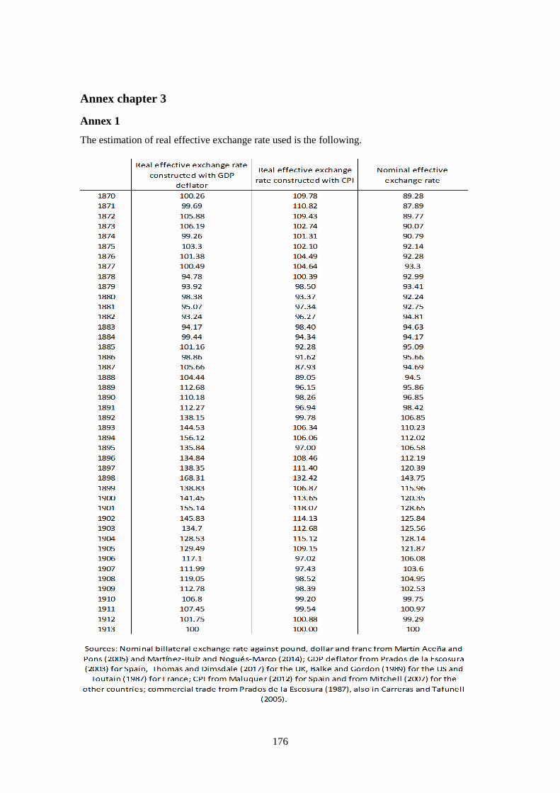
176
Annex chapter 3
Annex 1
The estimation of real effective exchange rate used is the following.
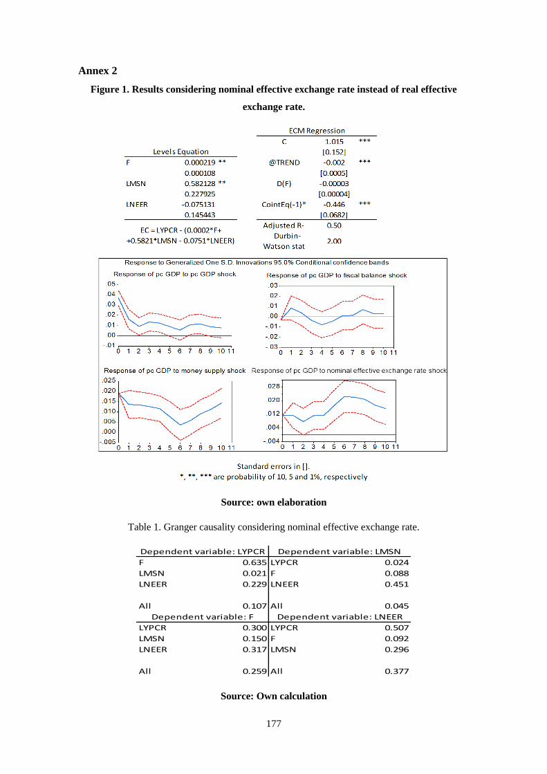
177
Annex 2
Figure 1. Results considering nominal effective exchange rate instead of real effective
exchange rate.
Source: own elaboration
Table 1. Granger causality considering nominal effective exchange rate.
Source: Own calculation
F 0.635 LYPCR 0.024
LMSN 0.021 F 0.088
LNEER 0.229 LNEER 0.451
All 0.107 All 0.045
LYPCR 0.300 LYPCR 0.507
LMSN 0.150 F 0.092
LNEER 0.317 LMSN 0.296
All 0.259 All 0.377
Dependent variable: LYPCR Dependent variable: LMSN
Dependent variable: F Dependent variable: LNEER

178
Figure 2. Results considering old data on fiscal balance (Comín and Díaz, 2005) instead of
the new one (Comín, unpublished).
Source: own elaboration
Table 2. Unit root test for fiscal data from Comín and Díaz (2005)
Source: own elaboration
Null hypothesis:
constant trend constant trend
ADF statistic -4.06845 -4.006867 -6.277 -6.833
Prob. 0.0027 0.0158 0.000 0.000
KPSS statistic 0.540 0.124 0.335 0.081
Prob. < 0.05 <0.01 > 0.1 > 0.1
F has a unit root D(F) has a unit root
F is stationary D(F) is stationary
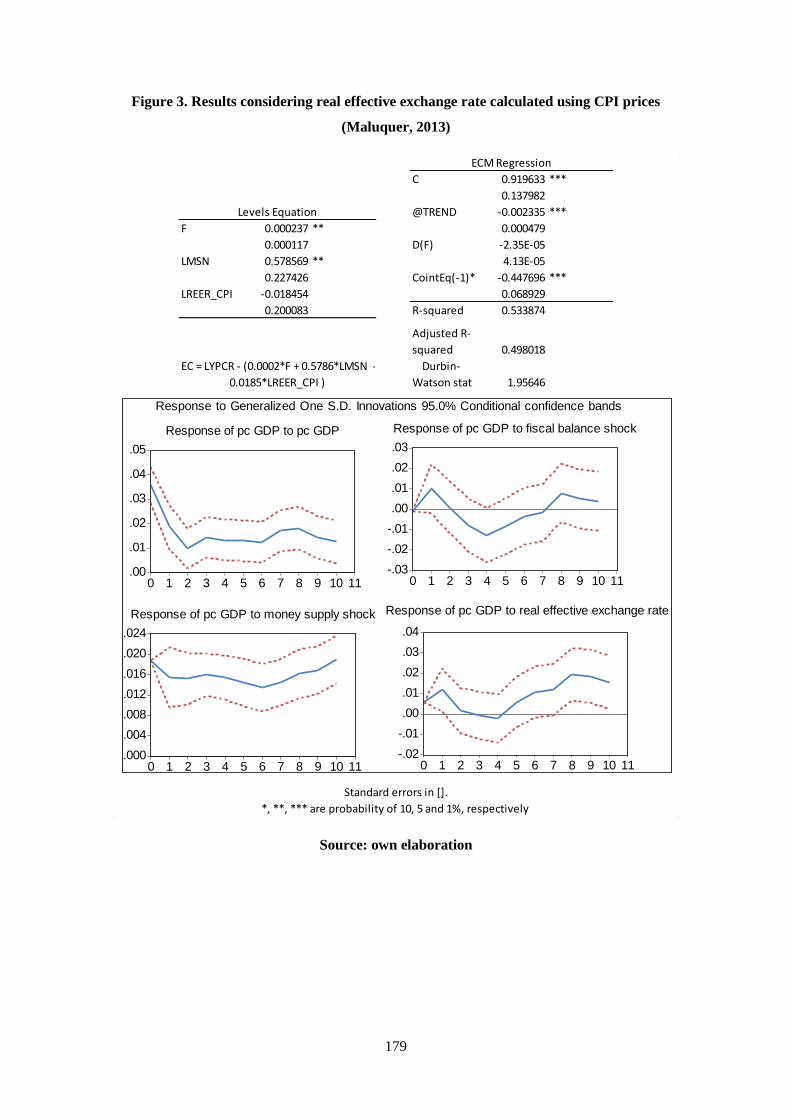
179
Figure 3. Results considering real effective exchange rate calculated using CPI prices
(Maluquer, 2013)
Source: own elaboration
C 0.919633 ***
0.137982
@TREND -0.002335 ***
F 0.000237 ** 0.000479
0.000117 D(F) -2.35E-05
LMSN 0.578569 ** 4.13E-05
0.227426 CointEq(-1)* -0.447696 ***
LREER_CPI -0.018454 0.068929
0.200083 R-squared 0.533874
Adjusted R-
squared 0.498018
Durbin-
Watson stat 1.95646
EC = LYPCR - (0.0002*F + 0.5786*LMSN -
0.0185*LREER_CPI )
*, **, *** are probability of 10, 5 and 1%, respectively
Standard errors in [].
Levels Equation
ECM Regression
.00
.01
.02
.03
.04
.05
0 1 2 3 4 5 6 7 8 9 10 11
Response of pc GDP to pc GDP
-.03
-.02
-.01
.00
.01
.02
.03
0 1 2 3 4 5 6 7 8 9 10 11
Response of pc GDP to fiscal balance shock
.000
.004
.008
.012
.016
.020
.024
0 1 2 3 4 5 6 7 8 9 10 11
Response of pc GDP to money supply shock
-.02
-.01
.00
.01
.02
.03
.04
0 1 2 3 4 5 6 7 8 9 10 11
Response of pc GDP to real effective exchange rate
Response to Generalized One S.D. Innovations 95.0% Conditional confidence bands
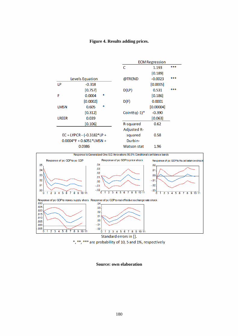
180
Figure 4. Results adding prices.
Source: own elaboration

181
Figure 5. Results adding capital flows.
Source: own elaboration

182
Figure 6. Results considering banknotes in circulation instead of money supply.
Source: Own calculation

183
Figure 7. Results considering fiscal balance over GDP instead of real fiscal balance.
Source: Own calculation
C 3.526 ***
[0.439]
@TREND 0.0011 ***
[0.0004]
F_GDP 1.98 *** D(F_GDP) -0.0632
[0.587] [0.222]
LMSN 0.311 *** D(F_GDP(-1)) -0.93 ***
[0.112] [0.26]
LREER -0.199 *** D(LREER) 0.105
[0.0485] [0.0632]
D(LREER(-1)) 0.2430 ***
[0.0664]
CointEq(-1)* -0.731 ***
[0.0914]
R-squared 0.70
Adjusted R-squared0.65
Durbin-Watson stat1.74
ECM Regression
Levels Equation
EC = LYPCR - (1.9830*FC +
0.3110*LMSN2 -0.1994*LERDEFL1 )
Standard errors in [].
*, **, *** are probability of 10, 5 and 1%, respectively
-.02-.01
.00
.01
.02
.03
.04
.05
0 1 2 3 4 5 6 7 8 9 10 11
Response of pc GDP to pc GDP shock
-.02
-.01
.00
.01
.02
.03
0 1 2 3 4 5 6 7 8 9 10 11
Response of pc GDP to fiscal balance shock
-.010
-.005
.000
.005
.010
.015
.020
.025
0 1 2 3 4 5 6 7 8 9 10 11
Response of pc GDP to money supply shock
-.02
-.01
.00
.01
.02
.03
0 1 2 3 4 5 6 7 8 9 10 11
Response of pc GDP to real effective exchange rate shock
Response to Generalized One S.D. Innovations 95.0% Conditional confidence bands
-.04
-.02
.00
.02
.04
.06
.08
0 1 2 3 4 5 6 7 8 9 10 11
Response of D(LYPCR) to D(LYPCR)
(Joint: 0.000 Cumulative: 0.047)
-.03
-.02
-.01
.00
.01
.02
.03
0 1 2 3 4 5 6 7 8 9 10 11
Response of D(LYPCR) to D(FC)
(Joint: 0.928 Cumulative: 0.520)
-.04
-.03
-.02
-.01
.00
.01
.02
.03
0 1 2 3 4 5 6 7 8 9 10 11
Response of D(LYPCR) to D(LMSN2)
(Joint: 0.985 Cumulative: 0.194)
-.04
-.03
-.02
-.01
.00
.01
.02
.03
0 1 2 3 4 5 6 7 8 9 10 11
Response of D(LYPCR) to D(LERDEFL1)
(Joint: 0.775 Cumulative: 0.472)
Response to Generalized One S.D. Innovations 95.0% Conditional confidence bands

184
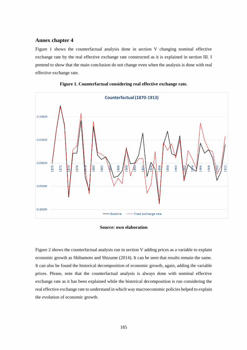
185
Annex chapter 4
Figure 1 shows the counterfactual analysis done in section V changing nominal effective
exchange rate by the real effective exchange rate constructed as it is explained in section III. I
pretend to show that the main conclusion do not change even when the analysis is done with real
effective exchange rate.
Figure 1. Counterfactual considering real effective exchange rate.
Source: own elaboration
Figure 2 shows the counterfactual analysis run in section V adding prices as a variable to explain
economic growth as Shibamoto and Shizume (2014). It can be seen that results remain the same.
It can also be found the historical decomposition of economic growth, again, adding the variable
prices. Please, note that the counterfactual analysis is always done with nominal effective
exchange rate as it has been explained while the historical decomposition is run considering the
real effective exchange rate to understand in which way macroeconomic policies helped to explain
the evolution of economic growth.
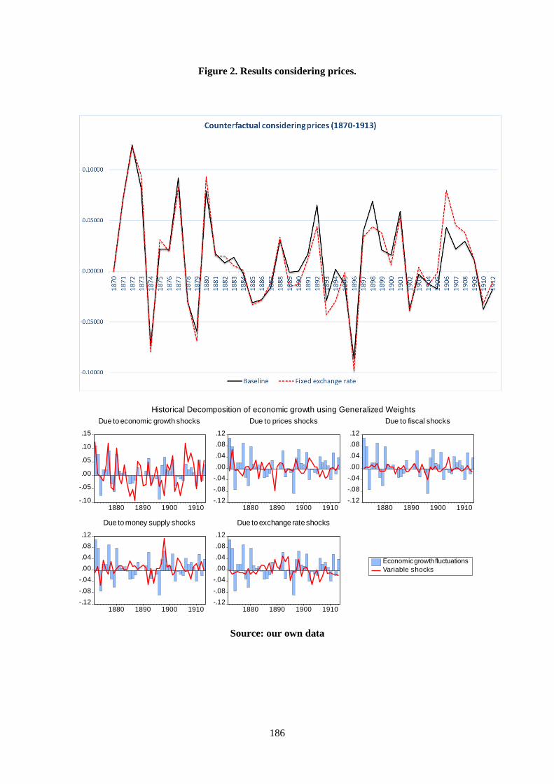
186
Figure 2. Results considering prices.
Historical Decomposition of economic growth using Generalized Weights
-.10
-.05
.00
.05
.10
.15
1880 1890 1900 1910
Due to economic growth shocks
-.12
-.08
-.04
.00
.04
.08
.12
1880 1890 1900 1910
Due to prices shocks
-.12
-.08
-.04
.00
.04
.08
.12
1880 1890 1900 1910
Due to fiscal shocks
-.12
-.08
-.04
.00
.04
.08
.12
1880 1890 1900 1910
Due to money supply shocks
-.12
-.08
-.04
.00
.04
.08
.12
1880 1890 1900 1910
Economic growth fluctuationsVariable shocks
Due to exchange rate shocks
Source: our own data
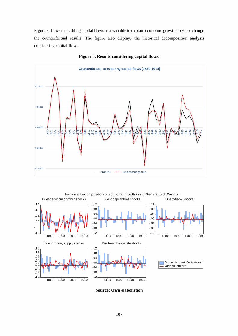
187
Figure 3 shows that adding capital flows as a variable to explain economic growth does not change
the counterfactual results. The figure also displays the historical decomposition analysis
considering capital flows.
Figure 3. Results considering capital flows.
Historical Decomposition of economic growth using Generalized Weights
-.10
-.05
.00
.05
.10
.15
1880 1890 1900 1910
Due to economic growth shocks
-.12
-.08
-.04
.00
.04
.08
.12
1880 1890 1900 1910
Due to capital flows shocks
-.12
-.08
-.04
.00
.04
.08
.12
1880 1890 1900 1910
Due to fiscal shocks
-.12-.08-.04.00.04.08.12.16
1880 1890 1900 1910
Due to money supply shocks
-.12
-.08
-.04
.00
.04
.08
.12
1880 1890 1900 1910
Economic growth fluctuationsVariable shocks
Due to exchange rate shocks
Source: Own elaboration
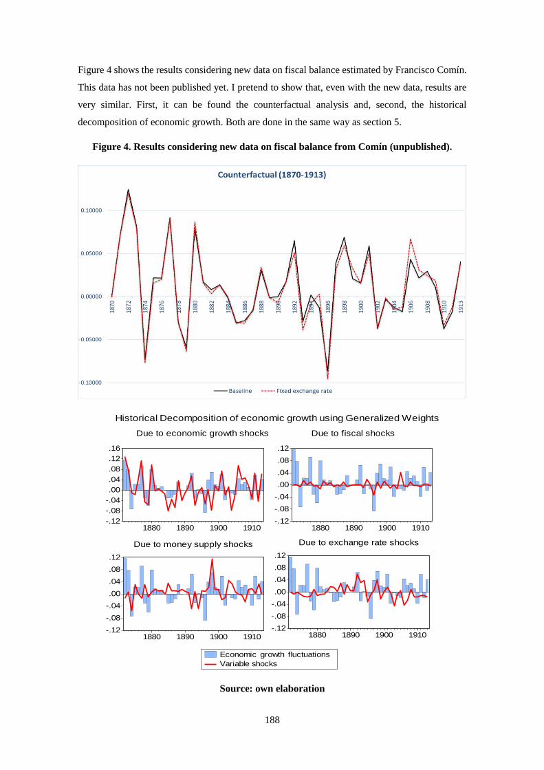
188
Figure 4 shows the results considering new data on fiscal balance estimated by Francisco Comín.
This data has not been published yet. I pretend to show that, even with the new data, results are
very similar. First, it can be found the counterfactual analysis and, second, the historical
decomposition of economic growth. Both are done in the same way as section 5.
Figure 4. Results considering new data on fiscal balance from Comín (unpublished).
Historical Decomposition of economic growth using Generalized Weights
-.12
-.08
-.04.00
.04
.08
.12
.16
1880 1890 1900 1910
Due to economic growth shocks
-.12
-.08
-.04
.00
.04
.08
.12
1880 1890 1900 1910
Due to fiscal shocks
-.12
-.08
-.04
.00
.04
.08
.12
1880 1890 1900 1910
Due to money supply shocks
-.12
-.08
-.04
.00
.04
.08
.12
1880 1890 1900 1910
Economic growth fluctuations Variable shocks
Due to exchange rate shocks
Source: own elaboration
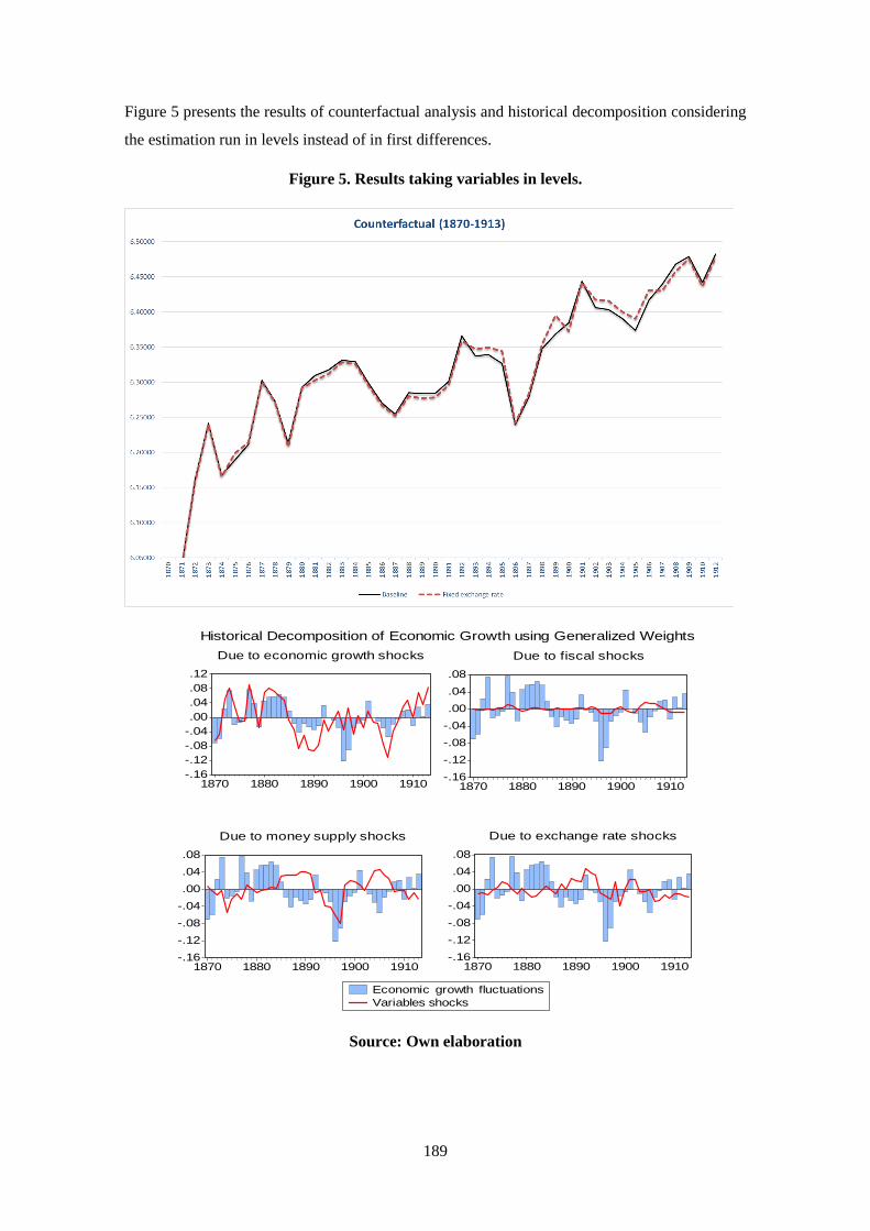
189
Figure 5 presents the results of counterfactual analysis and historical decomposition considering
the estimation run in levels instead of in first differences.
Figure 5. Results taking variables in levels.
Historical Decomposition of Economic Growth using Generalized Weights
-.16-.12-.08-.04.00.04.08.12
1870 1880 1890 1900 1910
Economic growth fluctuationsVariables shocks
Due to economic growth shocks
-.16
-.12
-.08
-.04
.00
.04
.08
1870 1880 1890 1900 1910
Due to fiscal shocks
-.16
-.12
-.08
-.04
.00
.04
.08
1870 1880 1890 1900 1910
Due to money supply shocks
-.16
-.12
-.08
-.04
.00
.04
.08
1870 1880 1890 1900 1910
Due to exchange rate shocks
Source: Own elaboration

190
Figure 6 shows the counterfactual analysis adding a dummy variable to consider wars experienced
by Spain during that period. It can also be found that the historical decomposition of economic
growth do not change when wars dummy is added to the estimation.
Figure 6. Counterfactual analysis and historical decomposition considering wars.
Historical Decomposition of economic growth using Generalized Weights
-.12
-.08
-.04
.00
.04
.08
.12
1880 1890 1900 1910
Due to economic growth shocks
-.12
-.08
-.04
.00
.04
.08
.12
1880 1890 1900 1910
Due to fiscal shocks
-.12
-.08
-.04
.00
.04
.08
.12
1880 1890 1900 1910
Due to money supply shocks
-.12
-.08
-.04
.00
.04
.08
.12
1880 1890 1900 1910
Economic growth fluctuationsVariable shocks
Due to exchange rate shocks
Source: Own elaboration
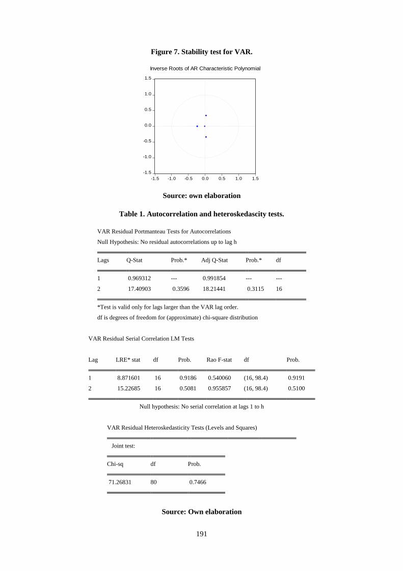
191
Figure 7. Stability test for VAR.
-1.5
-1.0
-0.5
0.0
0.5
1.0
1.5
-1.5 -1.0 -0.5 0.0 0.5 1.0 1.5
Inverse Roots of AR Characteristic Polynomial
Source: own elaboration
Table 1. Autocorrelation and heteroskedascity tests.
VAR Residual Portmanteau Tests for Autocorrelations
Null Hypothesis: No residual autocorrelations up to lag h
Lags Q-Stat Prob.* Adj Q-Stat Prob.* df
1 0.969312 --- 0.991854 --- ---
2 17.40903 0.3596 18.21441 0.3115 16
*Test is valid only for lags larger than the VAR lag order.
df is degrees of freedom for (approximate) chi-square distribution
VAR Residual Serial Correlation LM Tests
Lag LRE* stat df Prob. Rao F-stat df Prob.
1 8.871601 16 0.9186 0.540060 (16, 98.4) 0.9191
2 15.22685 16 0.5081 0.955857 (16, 98.4) 0.5100
Null hypothesis: No serial correlation at lags 1 to h
VAR Residual Heteroskedasticity Tests (Levels and Squares)
Joint test:
Chi-sq df Prob.
71.26831 80 0.7466
Source: Own elaboration

192