the chase procedure and its applications in data exchange

The Chase Procedure and its Applicationsin Data ExchangeAdrian Onet

Concordia UniversityMontreal, [email protected]

AbstractThe initial and basic role of the chase procedure was to test logical implication between sets ofdependencies in order to determine equivalence of database instances known to satisfy a givenset of dependencies and to determine query equivalence under database constrains. Recently thechase procedure has experienced a revival due to its application in data exchange. In this chapterwe review the chase algorithm and its properties as well as its application in data exchange.

1998 ACM Subject Classification H.2.5 [Heterogeneous Databases]: Data translation

Keywords and phrases chase, chase termination, data exchange, incomplete information

Digital Object Identifier 10.4230/DFU.Vol5.10452.1

1 Introduction

The main focus of this chapter is an introduction to the chase procedure and its importancein data exchange, as it is already announced in the title. A retrospective look at theevolution of the chase procedure proves with no doubt its importance and effectiveness insolving several data related problems. Originally, the chase was developed for testing logicalimplication between sets of embedded dependencies [36]. In fact, the logical implicationproblem tests whether all databases satisfying a set of dependencies must also satisfy anothergiven dependency. Later, the chase was reformulated for other types of dependencies suchas functional, join and multivalued dependencies [37, 49]. Beeri and Vardi [10] proposed aunified treatment for the implication problem by introducing the chase for tuple-generatingand equality-generating dependencies, classes of dependencies large enough to express all theprevious classes. Moreover, the chase procedure was also shown to be useful for determiningif two database instances (that may contain nulls) represent the same set of possible instancesunder a set of dependencies [43]. Finally, the chase was also used for testing query equivalenceand containment under database constraints [3, 31].

More recently, the chase procedure has gained a lot of attention due to its usefulnessin: data integration [33, 11], ontologies [14, 13], inconsistent databases and data repairs[5, 2, 23], data exchange [19], query optimization [17, 42], peer data exchange [9], anddata correspondence [23]. In this chapter we will focus on the advantages of using thechase procedure in data exchange. We will show that the chase can be used to computerepresentative target solutions in data exchange. Intuitively, the data exchange problemconsists of transforming a source database into a target one according to a set of sourceto target dependencies describing the mapping between the source and the target. The setof dependencies may also include target dependencies, that is constraints over the targetdatabase. It is important to mention that the source and the target schemata are consideredto be distinct. To be more precise: given a source instance I and a set Σ of source-to-target

© Adrian Onet;licensed under Creative Commons License CC-BY

Data Exchange, Integration, and Streams. Dagstuhl Follow-Ups, Volume 5, ISBN 978-3-939897-61-3.Editors: Phokion G. Kolaitis, Maurizio Lenzerini, and Nicole Schweikardt; pp. 1–37

Dagstuhl PublishingSchloss Dagstuhl – Leibniz-Zentrum für Informatik, Germany

http://dx.doi.org/10.4230/DFU.Vol5.10452.1

http://creativecommons.org/licenses/by/3.0/

http://www.dagstuhl.de/dagpub/978-3-939897-61-3

2 The Chase Procedure and its Applications in Data Exchange

and target dependencies, an instance J over the target schema is said to be a data-exchangesolution (or simply solution) for I and Σ, if I ∪ J satisfies all dependencies in Σ. One of themost important representation for this (usually infinite) set of solutions was introduced byFagin et al. [19]. They considered the finite instance obtained by chasing the initial sourceinstance with the set of dependencies. Such an instance, if it exists, was called a universalsolution. In their paper, Fagin et al. showed that the universal solution is a good candidateto be materialized on the target. In particular, the universal solution can be used to computecertain answers to (unions of) conjunctive queries over the target instance.

Even though not exhaustive, this chapter investigates the chase procedure when appliedagainst a set of tuple-generating and equality generating dependencies. We also investigatedifferent chase variations proposed for data exchange and review their properties. Section 3is devoted to the chase procedure and to some of its variations when the constraints arespecified by sets of tuple-generating and equality generating dependencies. This section itis not only focused on mapping constraints (i.e. source-to-target and target dependencies)but also general constraints giving us a full picture for the chase termination problem. Inthe same Section 3, we will also see that each of the chase variation presented computesinstances that are homomorphically equivalent and thus any of this chase variations can beused in computing universal solutions. Even more, to the best of our knowledge, there existsonly one chase variation which is complete in finding universal solutions. It is known thatthe chase procedure might not terminate for some input instances; even more, it was shownthat it is undecidable to test if a chase procedure terminates for a given set of dependenciesand a given input instance. Given this, there was tremendous work in finding classes ofdependencies that ensure the chase termination for all input instances. Section 4 presentssome of the main such classes and reviews the subset relationship and complexity of testingthe membership problem for these classes. In Section 5 we review the role played by thechase procedure in data exchange. Finally, Section 6 presents an extension of the chaseprocess that deals with larger classes of dependencies including inequalities, disjunctions andnegations. All the proofs presented in this chapter are only sketches, the complete proofscan be found in the mentioned literature.

2 Preliminaries

For basic definitions and concepts we refer to [1]. We will consider the complexity classesPTIME, NP, coNP, DP, RE, coRE, and first few levels of the polynomial hierarchy. Fordefinitions of these classes we refer to [45].

Let us start with some preliminary notions. A schema R is a finite set {R1, . . . , Rn} ofrelation names, each Ri having a fixed arity, arity(Ri). Let Const be a countably infinite setof constants, Null be a countably infinite set of labeled nulls and Var be a countable infiniteset of variables, such that the sets are pairwise disjoint. From the domain Dom = Const∪Nulland the finite set R we build up a Herbrand structure consisting of all expressions of theform R(a1, a2, . . . , ak), where R is a k-ary relation name from R and ai’s are values in Dom.Such an expression is called a tuple. A database instance I is then simply a finite set oftuples. We denote the set of values occurring in an instance I by dom(I). An instance I,such that dom(I) ⊆ Const, is called a ground instance.

Let then I and J be instances over a schema R. A homomorphism h from I to J is afunction on Const∪Null, that is identity on Const, extended to tuples, relations and instancesin the natural way, such that h(I) ⊆ J . We write I → J in case there exists a homomorphismfrom I to J . By I ↔ J we denote the fact that I → J and J → I. A homomorphism from I

A. Onet 3

to J is said to be full if h(I) = J . A full injective homomorphism is called embedding. Ahomomorphism h from I to J is said to be a retraction if h is identity on dom(J). In thiscase J is called a retract of I. An instance J is said to be a proper retract of instance I, if Jis a retract of I and J ⊂ I. An instance I is said to be a core if it does not have any properretract. An instance J is said to be a core of I if J is a retract of I and it is also a core. Thecores of an instance I are unique up to isomorphism and therefore we can talk about thecore of an instance I and denote it core(I).

A relational atom is an expression of the form R(x), where R is a relational symbol from aschema R and x ∈ (Const∪Var)arity(R). For an easier representation, by x we also representthe sets of elements in x and we denote by |x| the cardinality of such set. A conjunctivequery ϕ(x) over a schema R is a conjunction of relational atoms from R, where x denotesthe variables of the atoms in ϕ. CQ identifies the class of conjunctive queries and UCQthe class of unions of conjunctive queries. The class CQ 6= denotes all conjunctive queriesthat also allow the inequality atom (similarly is defined the class UCQ 6=). The extensionof previous classes by allowing negation gives CQ¬,UCQ¬, CQ¬, 6= and UCQ¬,6=. Given aformula α : R1(x1)∧R2(x2)∧ . . .∧Rn(xn) and a mapping h : (Const∪Var)→ (Const∪Null),identity on Const, by h(α) we denote the instance {R1(h(x1)), R2(h(x2)), . . . , Rn(h(xn))}.

Finally, a tuple generating dependency (tgd) is a first order sentence ξ of the form:∀x, y

(α(x, y)→ ∃z β(x, z)

), where α (the body) and β (the head) are conjunctive queries,

x and y denote the universally quantified variables, and z the existentially quantified ones.We denote by body(ξ) the set of all atoms in the body and by head(ξ) the set of all atoms inthe head. An equality generating dependency (egd) is a first order sentence ξ of the form∀x(α(x) → x1 = x2

). An egd is like a tgd, except that the consequent is an equality

between the variables x1 and x2 that also are part of x. For simplicity for these types offormulae, we will omit the universal quantifiers; also the conjunction between atoms willbe denoted by comma. Thus, the tgd ∀x, y

(R(x, y) ∧ R(y, x) → ∃z T (x, z) ∧ S(z)

)will

be simply denoted as R(x, y), R(y, x) → ∃z T (x, z), S(z). A full tgd is a tgd that has noexistentially quantified variables. A LAV tgd is a tgd with only one atom in the body. Letξ be a tgd of the form α(x, y)→ ∃z β(x, z), and a ∈ (Const)|x|+|y|. We denote by ξ(a) thefirst order sentence obtained from ξ by replacing the universal quantified variables with thecorresponding constants in a. An instance I is said to satisfy a set of dependencies, denotedI |= Σ, if I satisfies Σ in the theoretic standard model sense.

3 The chase procedure

The importance of the chase procedure in data exchange was first brought to the forefrontby Fagin, Kolaitis, Miller and Popa in their seminal paper [19], where the chase was used asa tool for constructing a "general" solution to the data-exchange problem. In their approachthe chase procedure applies at each iteration a chase step, that either adds a new tupleor changes the instance to model some equality generating dependency, or fails when theinstance could not be changed to satisfy an equality generating dependency. Based on thischase procedure, several variations were proposed [12, 16, 38, 24]. To differentiate them,we will call the chase procedure presented by Fagin et al. [19] the standard chase. Sincemost of the practical database constraints (such as key and inclusion dependencies) can berepresented as sets of tuple generating (tgd) and equality generating (egd) dependencies, inthis section we will present the chase procedure applied on such dependencies. Later on,more precisely in Section 6, we will introduce a variation of the chase procedure that alsodeals with dependencies containing inequalities and disjunctions. For an ease of notation,

Chapte r 01


through this section if not mentioned otherwise, we will use the notation I to represent anarbitrary instance over a given schema and Σ to refer to an arbitrary set of tgds and egdsover a schema explicitly mentioned if it does not follow directly from the context.

3.1 The chase stepThe chase procedure is a repetitive application of a chase step. Each chase step “applies” atgd or egd, on a subset of the instance.

The tgd chase step. Let I be an instance and ξ be the tgd α(x, y) → ∃z β(x, z) bothover a schema R. A pair (ξ, h) is said to be a trigger for I, if h is a homomorphism such thath(α(x, y)) ⊆ I. In case we also have that there is no extension h of h such that h(β(x, z)) ⊆ I,then (ξ, h) is said to be an active trigger for I. The tgd ξ is said to be applicable to I withhomomorphism h if (ξ, h) is a trigger (active or not) for I.

To fire the trigger (ξ, h) means to transform I into the instance J = I ∪ h(β(x, z)),where h is a distinct extension of h, i.e. an extension of h that assigns new fresh nulls tothe existential variables in β. By “new fresh” we mean the next unused element in somefixed enumeration of the nulls. We call this transformation as an oblivious-chase step anddenote it I ∗,(ξ,h)−−−−→ J . In case (ξ, h) is an active trigger for I, the transformation is calledstandard-chase step and is denoted I (ξ,h)−−−→ J . Clearly any standard-chase step is also anoblivious-chase step but the converse does not always hold.

I Example 1. Let us consider instance I = {R(a, b), R(b, a), S(b, c)} and tgd ξ:

R(x, y), R(y, x)→ ∃z S(x, z).

Homomorphism h = {x/a, y/b} maps the body of ξ to I and there is no extension of h thatmaps the head of ξ into I. That is, the trigger (ξ, h) is active for I and I (ξ,h)−−−→ J , whereJ = I ∪{S(a,X)} and h(z) = X. On the other hand, for the homomorphism h′ = {x/b, y/a}the pair (ξ, h′) is a trigger for I, but it is not an active trigger. In this case I ∗,(ξ,h

′)−−−−−→ J ′,where J ′ = I ∪ {S(b,X)}.

The complexity of testing if there exists a trigger (active trigger) for a given instance Iand a fixed (or given) tgd ξ is given by the following theorem:

I Theorem 2. [26] Let ξ be a tgd and I an instance. Then1. for a fixed ξ, testing whether there exists a trigger or an active trigger on a given I is

polynomial;2. testing whether there exists a trigger for a given ξ on a given I is NP-complete;3. testing whether there exists an active trigger for a given ξ and a given I is Σp2-complete.

Proof. Let us consider ξ to be a tgd of the form α(x, y)→ ∃z β(z). The polynomial casescan be verified by checking all homomorphisms from the body of the dependency into theinstance. We also need to consider for the active trigger problem if it has for each suchhomomorphism an extension that maps the head of the dependency into the instance. Thesetasks can be carried out in O(n|α|) and O(n|α|+|β|) time, respectively.

It is easy to see that the trigger existence problem is NP-complete in combined complexity,as the problem is equivalent to testing whether there exists a homomorphism between twoinstances (in our case α and I); a problem known to be NP-complete.

A. Onet 5

Regarding the combined complexity of the active trigger existence problem, we observethat it is in ΣP2 , since one may guess a homomorphism h from α into I, and then use an NPoracle to verify that there is no extension h′ of h, such that h′(β) ⊆ I. In the case of thelower bound, we will reduce the following problem to the active trigger existence problem.Let φ(x, y) be a Boolean formula in 3CNF over the variables in x and y. Is the formula∃x ¬

(∃y φ(x, y)

)true? The problem is a variation of the standard ∃∀-QBF problem [48] and

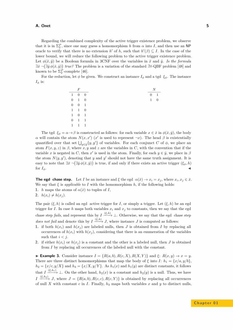
known to be ΣP2 -complete [46].For the reduction, let φ be given. We construct an instance Iφ and a tgd ξφ. The instance

Iφ is:

F

1 0 00 1 00 0 11 1 01 0 10 1 11 1 1

N

0 11 0

The tgd ξφ = α→β is constructed as follows: for each variable x ∈ x in φ(x, y), the bodyα will contain the atom N(x, x′) (x′ is used to represent ¬x). The head β is existentiallyquantified over that set

⋃y∈y{y, y′} of variables. For each conjunct C of φ, we place an

atom F (x, y, z) in β, where x, y and z are the variables in C, with the convention that if thevariable x is negated in C, then x′ is used in the atom. Finally, for each y ∈ y, we place in βthe atom N(y, y′), denoting that y and y′ should not have the same truth assignment. It iseasy to note that ∃x ¬

(∃y φ(x, y)

)is true, if and only if there exists an active trigger (ξφ, h)

for Iφ. J

The egd chase step. Let I be an instance and ξ the egd α(x)→ xi = xj , where xi, xj ∈ x.We say that ξ is applicable to I with the homomorphism h, if the following holds:1. h maps the atoms of α(x) to tuples of I,2. h(xi) 6= h(xj).

The pair (ξ, h) is called an egd active trigger for I, or simply a trigger. Let (ξ, h) be an egdtrigger for I. In case h maps both variables xi and xj to constants, then we say that the egdchase step fails, and represent this by I (ξ,h)−−−→ ⊥. Otherwise, we say that the egd chase stepdoes not fail and denote this by I (ξ,h)−−−→ J , where instance J is computed as follows:1. if both h(xi) and h(xj) are labeled nulls, then J is obtained from I by replacing all

occurrences of h(xi) with h(xj), considering that there is an enumeration of the variablessuch that i < j.

2. if either h(xi) or h(xj) is a constant and the other is a labeled null, then J is obtainedfrom I by replacing all occurrences of the labeled null with the constant.

I Example 3. Consider instance I = {R(a, b), R(c,X), R(X,Y )} and ξ: R(x, y) → x = y.There are three distinct homomorphisms that map the body of ξ into I: h1 = {x/a, y/b},h2 = {x/c, y/X} and h3 = {x/X, y/Y }. As h1(x) and h1(y) are distinct constants, it followsthat I (ξ,h1)−−−−→ ⊥. On the other hand, h2(x) is a constant and h2(y) is a null. Thus, we haveI

(ξ,h2)−−−−→ J , where J = {R(a, b), R(c, c), R(c, Y )} is obtained by replacing all occurrencesof null X with constant c in I. Finally, h3 maps both variables x and y to distinct nulls,

Chapte r 01


making the egd ξ applicable on I with the homomorphism h3. Hence I (ξ,h3)−−−−→ J ′, whereJ ′ = {R(a, b), R(c, Y ), R(Y, Y )} is obtained from I by replacing X with Y , considering thaty follows x in the variable enumeration.

Similarly to the tgd chase step, we have the following complexity results for the egdtrigger-existence problem. Note that for egds the trigger and active trigger notions coincide.

I Theorem 4. Let ξ be an egd and I an instance. Then1. for a fixed ξ, testing whether there exists a trigger on a given I is polynomial, and2. testing whether there exists a trigger for a given ξ on a given I is NP-complete.

Proof. Similar with the proof of Theorem 2. J

3.2 The chase algorithmUsing the previously introduced chase steps, we are now ready to present the standard-chasealgorithm. This algorithm can be described as an iterative application of the standard-chasesteps. In case one of the egd chase steps fails, then the algorithm will fail. If the algorithmdoes not fail, it nondeterministically chooses another active trigger, tgd or egd, and proceedswith the corresponding standard-chase step. The algorithm terminates when either oneof the egd chase step fails or when there are no other active triggers. More formally, thestandard-chase algorithm can be described as follows:

STANDARD-CHASE(I,Σ)1 I0 := I; i := 0;2 if exists active trigger (ξ, h) for Ii3 then4 if Ii

(ξ,h)−−−→ ⊥5 then return FAIL6 else Ii

(ξ,h)−−−→ Ii+1; i := i+ 17 else return Ii8 goto 2

Note that the previous algorithm introduces a nondeterministic step at line 2, inducedby the trigger choice. This makes the chase process to be viewed as a tree, where leveli in the tree represents the i-th step in the chase algorithm, and where to each node anew edge is added for each of the applicable active trigger. Each path from the root ofthe tree to a leaf node represents an execution branch, or simply a branch, similarly tothe nondeterministic finite automata. Thus the algorithm may return different instancesdepending on the considered branch. There are cases when, for some branches, the algorithmfails while it does not fail for other branches, as it is shown in Example 6. This happens byexhaustively choosing the same dependencies in the nondeterministic step.

Moreover, the standard-chase algorithm stops if it either fails, due to an egd trigger atstep 4, or there are no other active triggers to be applied. As the tgds are adding new tuplesto the instance, it may be that the chase algorithm never terminates as in Example 5.

Fagin et al. [19] showed that in case the standard-chase algorithm fails on one executionbranch, then it will fail on all finite branches.

For the branches for which the algorithm does not fail, a standard-chase sequence isa finite or infinite sequence (I0, I1, I2, . . . , In, . . .) such that I0 = I and Ii

(ξ,h)−−−→ Ii+1, for

A. Onet 7

some i ≥ 0 and some active trigger (ξ, h). If for some branch the algorithm terminates inthe finite, then there exists a positive integer n such that for the standard-chase sequence(I0, I1, I2, . . . , In) there is no active trigger for In.

As shown in the following example, a standard chase sequence may be finite or infinite,for the same set of tgds and the for same input instance.

I Example 5. Consider instance I = {R(a, b)} and tgds:

ξ1 = R(x, y)→ R(y, x), andξ2 = R(x, y)→ ∃z R(y, z).

If first we chose the tgd trigger (ξ1, {x/a, y/b}), the tuple R(b, a) is added to the instanceI forming an instance I ′ = I ∪{R(b, a)}. It can be easily noticed that there is no other activetrigger on I ′ involving either ξ1 or ξ2. From this it follows that the sequence (I, I ′) is a finitestandard-chase sequence. On the other hand, if in the standard-chase algorithm we chosefirst the active trigger (ξ2, {x/a, y/b}), and from there on only chose active triggers over ξ2,we get the following infinite chase sequence:

I0 = I

R

a b

(ξ2,h1)−−−−→ I1

R

a b

b X1

(ξ2,h2)−−−−→ . . .(ξ2,hn)−−−−→ In

R

a b

b X1

X1 X2

. . .

Xn−1 Xn

(ξ2,hn+1)−−−−−−→ . . .

The next example shows a case when the standard-chase algorithm fails on some branchesand does not terminate (implicitly does not fail) on others.

I Example 6. Let us now consider a slightly changed set of dependencies from the previousexample:

ξ1 = R(x, y)→ T (y, x);ξ2 = T (x, y)→ x = y; andξ3 = R(x, y)→ ∃z R(y, z).

Consider the instance I = {R(a, b)}. If applying an active trigger (ξ1, {x/a, y/b}), it willadd the tuple T (a, b) to I. Next, when applying the active trigger (ξ2, {x/a, y/b}) thestandard-chase algorithm will fail. However, if the chosen branch uses only the triggers overξ3, the standard-chase algorithm will not terminate, as previously shown.

In the previous example the standard-chase algorithm did not fail because we exhaustivelyapplied active triggers over the same dependency. To avoid such cases, the chase algorithmis required to be fair, defined as follows:

I Definition 7. Let I0 be an instance and Σ a set of tgds and egds. A standard-chasesequence (I0, I1, . . .) is said to be fair if for all i and for all active triggers (ξ, h) for Ii, whereξ ∈ Σ, there exists j such that either Ij

(ξ,h)−−−→ Ij+1 or the trigger (ξ, h) is not active for Ij .A standard-chase algorithm is said to be fair, if it only produces fair chase sequences.

In the rest of this chapter we will consider, if not mentioned otherwise, all the chasealgorithms to be fair.

Chapte r 01


Let us now turn our attention to standard-chase algorithms that terminate in a finitenumber of steps. The following proposition shows the relationship between the finite instancesreturned by the algorithm.I Proposition 8. [19] If K and J are two finite instances returned by the standard-chasealgorithm on two distinct execution branches, with input I and Σ, then K and J arehomomorphically equivalent, that is K ↔ J .

Based on the homomorphic equivalence class, if there exists an execution branch forwhich the standard-chase algorithm with input I and Σ terminates in the finite and doesnot fail, then we denote by chasestd

Σ(I) one representative of the equivalence class for theresulting finite instances. If the standard chase fails or if it does not terminate in the finiteon all branches, then we set chasestd

Σ(I) = ⊥. With the instance I and the dependencies Σdefined in Example 5, we have chasestd

Σ(I) = {R(a, b), R(b, a)}. On the other hand, withthe input instance and the dependencies defined in Example 6 we have chasestd

Σ(I) = ⊥.The following theorem, developed by Fagin et. al, states one of the main properties of thestandard-chase algorithm. As seen later in this section, this property also holds for the otherchase variations.

I Theorem 9. [19] If chasestdΣ(I) 6= ⊥, then chasestd

Σ(I) |= Σ and I → chasestdΣ(I).

Let us now turn our attention to the problem defined as the termination of standard-chasealgorithm. It is easy to see that the cause of non-termination lies in the existentially quantifiedvariables in the head of tgds. Thus, for simplicity, for the following classes we omitted egds.

I Definition 10. Given an instance I, by CTstdI,∀ we denote the class of tgd sets such that

Σ ∈ CTstdI,∀ iff all standard-chase sequences for I and Σ are finite. We denote by CTstd

I,∃ theclass of tgd sets such that Σ ∈ CTstd

I,∃ iff there exist some standard-chase sequences for I andΣ that are finite.

The previous notations are extended to classes of tgd sets for which the standard chaseterminates on all input instances as follows:

I Definition 11. We denote by CTstd∀∀ the class of tgd sets such that Σ ∈ CTstd

∀∀ iff for allinstances I all standard-chase sequences of I with Σ are finite. We denote by CTstd

∀∃ the classof tgd sets such that Σ ∈ CTstd

∀∃ iff for all instances I there exists at least one standard-chasesequence of I and Σ that is finite.

From the termination classes definition it is clear that CTstd∀∀ ⊆ CTstd

∀∃. Also from the setof dependencies presented in Example 5, it follows that the inclusion is strict.

Deutsch, Nash and Remmel in [16] showed that, given I and Σ, the problems of testingwhether Σ ∈ CTstd

I,∀ or Σ ∈ CTstdI,∃ are undecidable in general. More recently, Grahne

and O. [26] extended this undecidability result to the CTstd∀∃ class too. That is for a given

Σ, the problem of testing if Σ ∈ CTstd∀∃ is coRE-complete. In case we allow a single denial

constraint, then the class CTstd∀∀ is coRE-complete as well. Where a denial constraint is a tgd

of the form α(x)→ ⊥, which is satisfied by an instance I only if there is no homomorphismh such that h(α(a)) ⊆ I,

Given the previous result, the next best hope is to find large decidable classes of de-pendencies included in CTstd

∀∀. One such class is the one of full tgds, that is tgds withoutexistential quantifiers. In Section 4 we review other decidable classes of dependency sets thatare known to be in CTstd

∀∀.Before ending this section we need to reiterate that the termination classes are defined

over tgds. Even if the egds do not introduce new nulls, they still may play an importantrole in the standard-chase termination problem, as shown in the next example.

A. Onet 9

I Example 12. Let Σ = {ξ1, ξ2, ξ3}, where:

ξ1 = R(x, y)→ ∃z S(y, z);ξ2 = S(x, x)→ ∃z R(x, z); andξ3 = S(x, y)→ x = y.

Let I = {R(a, b)}. It is easy to see that the standard-chase algorithm converges to the infiniteinstance J = {R(a, b), R(b,X1), . . . , R(Xn−1, Xn), . . . , S(b, b), S(X1, X1), . . . , S(Xn, Xn), . . .}.On the other hand, Σ′ = {ξ1, ξ2} ∈ CTstd

∀∀, that is without the egd ξ3 the standard chasealgorithm terminates on all execution branches with any input instance.

3.3 Chase variationsAfter the standard chase was presented as a method of computing "general" solutions indata exchange [19], many variations of the standard-chase algorithm were proposed in theliterature [12, 16, 38, 24] . In the remaining part of this section, dedicated to the chasealgorithm, we try to differentiate between the main chase variations by highlighting theirtermination properties.

3.3.1 The oblivious chaseThis focuses on one of the simplest variations of the standard chase named the obliviouschase (also known as naïve chase). This procedure is based on the relaxation of the chasestep. The oblivious chase presented here differs from the one described by Cali et al. [12] bynot relying on any order. As we will see, this does not affect the finite instance returned bythe chase algorithm.

The oblivious-chase algorithm is an iterative application of the oblivious-chase step, thatis at each iteration all triggers are considered, and not only the active ones as in the standard-chase algorithm. Recall that for the trigger (ξ, h) and the instance I the oblivious-chasestep is denoted as I ∗,(ξ,h)−−−−→ J , where instance J is constructed the same way as in thestandard-chase step. Note that if (ξ, h) is a trigger for I, then (ξ, h) will also be a trigger forJ , where I ∗,(ξ,h)−−−−→ J . To avoid such infinite loops, the oblivious-chase algorithm applies eachtrigger only once.

I Example 13. Consider the instance I = {R(a, b), R(b, a), S(b, c)} and the tgd ξ defined asR(x, y), R(y, x)→ ∃z S(x, z) as in Example 1. The homomorphism h = {x/a, y/b} maps thebody of ξ to I, and there is no extension of h that maps the head of ξ into I. This makes (ξ, h)both a standard and an oblivious-chase trigger. However, the homomorphism h1 = {x/b, y/a}also maps the body of ξ to I, but there exists the extension h1 = {x/b, y/a, z/c} of h1,such that h1 maps the head of ξ into I. Hence (ξ, h1) is a trigger but not an active triggerfor I. The instance J is obtained by applying the oblivious-chase step I ∗,(ξ,h1)−−−−−→ J , whereJ = I ∪ {S(b, Y )} and Y is a new labeled null.

Because of the nondeterministic way the oblivious-chase algorithm selects the triggersat each iteration, we may have different execution branches. Similarly to the terminationclasses defined for the standard chase, we introduce corresponding termination classes of tgdsets for the oblivious chase: CTobl

I,∃, CToblI,∀, CTobl

∀∀ and CTobl∀∃.

The following proposition shows that the termination classes are not affected by thenondeterministic nature of the algorithm.

Chapte r 01


I Proposition 14. Let I be an instance. Then CToblI,∀ = CTobl

I,∃ and CTobl∀∀ = CTobl

∀∃.

Proof. The proof follows from the observation that for the oblivious-chase algorithm, whenthe input set of dependencies are only tgds, the set of triggers applied on each branch is thesame, up to isomorphism. Thus, if the oblivious chase terminates on one execution branch,then it will terminate on all branches. J

From the previous proof it also follows that in case the oblivious chase terminates forinstance I and set of tgds Σ, then the returned on all execution branches are isomorphicallyequivalent. As we will see in the following example, if we allow egds, the instances returnedare not guaranteed to be isomorphically equivalent. Still, using the same proof techniques asthe one used to prove Theorem 9, it can be shown that in this case, if the chase terminatesand does not fail, the instances returned are homomorphically equivalent. Thus, if theoblivious chase terminates with input I and Σ (containing both tgds and egds), then wedenote by chaseobl

Σ(I) one representative instance of the homomorphic equivalence class. Ifthe oblivious chase fails or if it does not terminate, we set chaseobl

Σ(I) = ⊥.

I Example 15. Let Σ = {ξ1, ξ2, ξ3}, where:

ξ1 = S(x)→ ∃y R(x, y);ξ2 = R(x, y)→ ∃z T (y, z); andξ3 = R(x, y)→ x = y.

Let us now consider the instance I = {S(a)}. If we apply the dependencies in the order ξ1,ξ2, ξ3 and then ξ2 again, we get the following instance J0 = {S(a), R(a, a), T (a,X1), T (a,X2)}.But, if we apply the dependencies in the order ξ1, ξ3 and finally ξ2, the instance returnedby the oblivious-chase algorithm is J1 = {S(a), R(a, a), T (a, Y1)}. Clearly J0 and J1 are notisomorphically equivalent but they are homomorphically equivalent.

From the observation that all active triggers are also triggers, it follows that:I Proposition 16. CTobl

∀∀ ⊂ CTstd∀∀.

Proof. The inclusion follows directly from the definition of the trigger and the active trigger.For the strict inclusion part consider dependency set from Example 17. J

I Example 17. Consider Σ = {R(x, y)→ ∃z R(x, z)}. Clearly there is no active trigger onΣ for any instance I. On the other hand, for I = {R(a, b)} the oblivious-chase algorithm willcreate the following infinite chase sequence:

I0 = I

R

a b

∗,(ξ,h1)−−−−−→ I1

R

a b

a X1

∗,(ξ,h2)−−−−−→ . . .∗,(ξ,hn)−−−−−→ In

R

a b

a X1

a X2

. . .

a Xn

∗,(ξ,hn+1)−−−−−−−→ . . .

In order to relate termination of the standard and the oblivious algorithms, we introducea transformation called enrichment that takes a tgd ξ = α(x, y)→ ∃z β(x, z) over a schemaR, and converts it into the tgd ξ = α(x, y)→ ∃z β(x, z), H(x, y), where H is a new relationalsymbol that does not appear in R. For a set Σ of tgds defined on schema R, the transformedset is Σ = {ξ : ξ ∈ Σ}. Using the enrichment notion, we can present the relation between thestandard and oblivious-chase terminations.

A. Onet 11

I Theorem 18. [25] Let Σ be a set of tgds and I an instance. Then we have:1. Σ ∈ CTobl

I,∀ if and only if Σ ∈ CTstdI,∀, and

2. Σ ∈ CTobl∀∀ if and only if Σ ∈ CTstd

∀∀.

Proof. It follows from the observation that for any instance I if (ξ, h) is a trigger for I, then(ξ, h) is also an active trigger for I. J

Cali et al. showed in [12] that it is undecidable if the oblivious chase terminates for agiven input I and given set of tgds Σ. The same result applies for the class CTobl

∀∀ if we allowat least one denial constraint [26]. It remains an open problem if the class CTobl

∀∀ remainsundecidable when considering only sets of tgds.

We close the presentation of the oblivious-chase algorithm by linking together the finiteinstances resulting from both chase algorithms.

I Theorem 19. [12] Let I be an instance and let Σ be a set of tgds and egds, such thatchaseobl

Σ(I) 6= ⊥. Then chasestdΣ(I)↔ chaseobl

Σ(I) and chaseoblΣ(I) |= Σ.

3.3.2 The semi-oblivious chaseThe semi-oblivious-chase method was first introduced by Marnette in [38]. For this, let ξ bea tgd α(x, y) → ∃z β(x, z); then the triggers (ξ, h) and (ξ, g) are considered equivalent ifh(x) = g(x). The semi-oblivious chase works as the oblivious one, except that exactly onetrigger from each such equivalence class is fired in a branch.

For a better differentiation between the chase algorithms presented so far consider thefollowing example:

I Example 20. Let Σ = {ξ} contain the tgd ∀x, y R(x, y)→ ∃z T (x, z), and consider theinstance I = {R(a, b), R(a, c), R(d, e), T (a, a)}. In this case there exist only three triggersτ1 = (ξ, {x/a, y/b}), τ2 = (ξ, {x/a, y/c}) and τ3 = (ξ, {x/d, y/e}). From these triggers onlyτ3 is an active trigger for I. Thus, there is only one step to be executed for the standardchase: I τ3−→ Jstd, where Jstd = I ∪{T (d,X1)}. Because the homomorphism from the triggerτ1 maps x to value a as the homomorphism from the trigger τ2, it follows that τ1 is equivalentwith τ2. That is in the semi-oblivious chase only two triggers are applied: the active triggerτ3 and the representative of the equivalence class for τ1 and τ2. Hence, the resulted instanceis Jsobl = I ∪ {T (d,X2)} ∪ {T (a,X3)}. Finally, the oblivious chase will apply all triggersreturning instance Jobl. Bellow are the tabular representations of the instances resultedby applying the standard, semi-oblivious and oblivious-chase algorithms. The instances arerestricted to relation T :

Jstd

T

a a

d X1

Jsobl

T

a a

d X2

a X3

Jobl

T

a a

d X4

a X5

a X6

Similarly to the previous chase algorithms, we define termination classes over sets of tgds:CTsobl

I,∃ ,CTsoblI,∀ , CTsobl

∀∃ and CTsobl∀∀ for the semi-oblivious algorithm. The following proposition

shows that the nondeterministic behavior of the semi-oblivious-chase algorithm does notinfluence the termination for different execution branches.

Chapte r 01


I Proposition 21. Let I be an instance. Then CTsoblI,∀ = CTsobl

I,∃ and CTsobl∀∀ = CTsobl

∀∃ .

Proof. It follows from the observation that the set of representative trigger for each equival-ence classes is the same for all execution branches. J

Similarly to the oblivious chase case, it can be shown that in case the semi-oblivious-chasealgorithm terminates and not fails with the input instance I and the set of tgds Σ, thenthe instances returned by each execution branch are isomorphically equivalent. In case weallow egds in Σ, then the returned instances will be homomorphically equivalent. In thiscase we denote by chasesobl

Σ(I) one representative instance of the homomorphic equivalenceclass for the instances computed on each execution branch. In case the semi-oblivious-chasealgorithm fails or it is non-terminating, we set chasesobl

Σ(I) = ⊥.The same as for the oblivious chase case, we can find a rewriting of the dependencies such

that we can relate the termination of the semi-oblivious-chase algorithm to the terminationof the standard-chase algorithm. We introduce a transformation, called semi-enrichment,that takes a tgd ξ = α(x, y) → ∃z β(x, z) over a schema R, and converts it into the tgdξ = α(x, y) → ∃z β(x, z), H(x), where H is a new relational symbol that does not appearin R. For a set Σ of tgds defined on schema R, the transformed set is Σ = {ξ : ξ ∈ Σ}. Usingthe semi-enrichment notion, the relation between the standard and semi-oblivious-chaseterminations can be presented as follows.

I Theorem 22. [26] Let Σ be a set of tgds and I an instance. Then we have:1. Σ ∈ CTsobl

I,∀ if and only if Σ ∈ CTstdI,∀, and

2. Σ ∈ CTsobl∀∀ if and only if Σ ∈ CTstd

∀∀.

The following theorem relates the instances returned by the semi-oblivious chase and theinstances returned by the standard-chase algorithm.

I Theorem 23. [38] Let I be and instance and let Σ be a set of tgds and egds, such thatchasesobl

Σ(I) 6= ⊥. Then chasestdΣ(I)↔ chasesobl

Σ(I) and chasesoblΣ(I) |= Σ.

Similarly to the standard chase algorithm, the problem of testing if the semi-obliviouschase is terminating for a given instance and a given set of tgds is undecidable [38]. Thesame result applies for the class CTsobl

∀∀ , if we allow at least one denial constraint [26]. Itremains an open problem if the class CTsobl

∀∀ remains undecidable when considering only setsof tgds.

The proposition below shows the set relationship between termination classes for thechase variations presented so far.

I Proposition 24. [26] CTobl∀∀ ⊂ CTsobl

∀∀ ⊂ CTstd∀∀ ⊂ CTstd

∀∃.

Proof. The inclusions are clear from the definition of the corresponding chase steps. For thefirst strict inclusion consider Σ1 = {R(x, y)→ ∃z R(x, z)}. From Example 17, we know thatΣ1 /∈ CTobl

∀∀. On the other hand, it is easy to see that for any instance I only a maximum of|I| triggers will be applied on each execution branch by the semi-oblivious chase. For thesecond strict inclusion consider Σ2 = {ξ1, ξ2}, where:

ξ1 = R(x)→ ∃z S(z), T (z, x), andξ2 = S(x)→ ∃z R(z), T (x, z).

It is easy to check that the standard chase terminates for Σ2 with any input instance I.Additionally, the semi-oblivious chase does not terminate for Σ2 and instance I = {R(a)}. J

A. Onet 13

3.3.3 The core chaseThe class of chase algorithms is enriched by the core chase algorithm introduced by Deutschet al. in [16]. We need to clarify from the very beginning that the core chase differs fromthe other variations by executing in parallel all applicable standard tgd chase steps andalso computing the core of the unified instance. Note that we may only apply the standardtgd chase steps in parallel but not the egd chase steps, as the latter may modify the giveninstance by equating existing labeled nulls to constants or to other labeled nulls.

For a better understanding, we slightly changed the algorithm from [16] by applying allthe egd triggers before applying in parallel all the active tgd triggers. This modificationdoes not change however the result or the complexity of the given algorithm.

CORE-CHASE(I,Σ)1 I0 := I; i := 0;2 if exists a standard egd trigger (ξ, h) for Ii3 then4 if Ii

(ξ,h)−−−→ ⊥5 then return FAIL6 else Ii

(ξ,h)−−−→ Ii+1; i := i+ 1 goto 27 if exists a standard tgd trigger for Ii8 then9 For all active trigger (ξ, h) for Ii, compute in parallel Ii

ξ,h−−→ Jj10 Ii+1 := Core(

⋃j Jj); i := i+ 1

11 else12 return Ii13 goto 2

By applying all the triggers in parallel, the core-chase algorithm eliminates the non-deterministic part introduced by the standard-chase algorithm. In case the core-chasealgorithm terminates in the finite and does not fail for input I and Σ, we denote the returnedinstance by chasecore

Σ(I) . In case the core chase fails or it is non-terminating, we setchasecore

Σ(I) = ⊥.Similarly to the other chase variations, for the core chase we introduce classes of tgd

sets CTcoreI,∀ , CTcore

I,∃ , CTcore∀∀ and CTcore

∀∃ . Because the core chase is deterministic, it follows thatCTcore

I,∀ = CTcoreI,∃ for any instance I and that CTcore

∀∀ = CTcore∀∃ .

I Theorem 25. [16] Let I be an instance. Then CTstdI,∃ ⊂ CTcore

I,∀ and CTstd∀∃ ⊂ CTcore

∀∀ .

Proof. For the second strict inclusion consider Σ = {R(x) → ∃y R(y), S(x)}. Clearly thestandard chase does not terminate on any branch with I = {R(a)} and Σ, that is Σ /∈ CTstd

∀∃ .On the other hand, for any instance I, the core chase will terminate in maximum |IR| steps,where IR is instance I restricted to tuple over relation R. J

In [16] it is shown that the membership problem for the class CTcoreI,∀ for a given instance

I is RE-complete. To this, it was shown most recently [26] that the membership problem forthe class CTcore

∀∀ is coRE-complete.It may be noted that at line 10 the core-chase algorithm does not simply compute the

union between all the instances computed at line 9, but it also computes its core. This givesthe following link between the core chase and standard-chase algorithms:

Chapte r 01


Figure 1 Termination classes for different chase variations.

I Theorem 26. Let I be and instance and let Σ be a set of tgds and egds, such thatchasestd

Σ(I) 6= ⊥. Then chasestdΣ(I) ↔ chasecore

Σ(I) and chasecoreΣ(I) |= Σ, even

more, Core(chasestdΣ(I)) = chasecore

Σ(I).

Before ending this section about chase variations, let us summarize the differences betweenthe presented chase algorithms. First we saw that in case the algorithm terminates anddoes not fail with input I and Σ, then the instances returned by all of the presented chasevariations are homomorphically equivalent. We also saw that the complexity of testing theexistence of a trigger is slightly easier than testing the existence of an active trigger. Fromthis it follows that the oblivious and semi-oblivious-chase steps are less expensive than thestandard-chase step that is also less expensive than the core-chase step. On the other hand,a set of dependencies is more likely to terminate for the core chase than any of the otherchase variations. Figure 1 shows the set inclusion relationship between different terminationclasses.

4 Sufficient conditions for the chase termination

In the previous section we saw that it is undecidable to test for all the chase variations if thechase will terminate for a given instance and a given set of dependencies. This motivatedthe research community to find large classes of tgd sets that ensure termination of thestandard-chase algorithm for all instances. In this section some of these classes of tgd setswill be presented for which it is known that the standard chase terminates on all executionbranches for all input instances. We also investigate here if these classes are sufficient toguarantee the chase termination for other chase variations beside the standard chase. Forthis, we will say that a class of sets of tgds C is closed under enrichment if Σ ∈ C impliesΣ ∈ C. Similarly, the class C is closed under semi-enrichment if Σ ∈ C implies Σ ∈ C. FromTheorems 18 and 22 it directly follows:

I Corollary 27. Let C ⊆ CTstd∀∀.

1. if C is closed under enrichment, then C ⊆ CTobl∀∀.

2. if C is closed under semi-enrichment, then C ⊆ CTsobl∀∀ .

We will use the previous corollary to show that the termination classes presented herenot only guarantee the termination for the standard-chase algorithm but also for the semi-oblivious-chase algorithm.

A. Onet 15

Figure 2 Extended dependency graphs associated with dependencies from Example 30.

4.1 Rich acyclicityThe class of richly acyclic set of dependencies was introduced by Hernich and Schweikardt in[30] in a different context, and it was shown in [25] that this class guarantees termination forthe oblivious chase on any input instance.

I Definition 28. [19, 12] For a given database schema R define a position in R to be a pair(R, k), where R is a relation symbol in R and k a natural number with 1 ≤ k ≤ arity(R),such that k identifies the k-th element in R.

The notion of extended-dependency graph is defined as follows:

I Definition 29. [30] Let Σ be a set of tgds over schema R. The extended-dependencygraph associated with Σ is a directed edge-labeled graph GEΣ = (V,E), such that each vertexrepresents a position in R and ((R, i), (S, j)) ∈ E, if there exists a tgd ξ ∈ Σ of the formα(x, y)→ ∃z β(x, z), and if one of the following holds:1. x ∈ x and x occurs in α on position (R, i) and in β on position (S, j). In this case the

edge is labeled as universal;2. x ∈ x ∪ y and x occurs in α on position (R, i) and variable z ∈ z that occurs in β on

position (S, j). In this case the edge is labeled as existential.

The following example illustrates the previous definitions:

I Example 30. Consider database schema R = {S,R}, with arity(S) = 1 and arity(R) = 2.The set {(S, 1), (R, 1), (R, 2)} represents all positions in R. Let Σ1 contain the followingdependency over R:

ξ11 = S(x)→ ∃y R(x, y)

let Σ2 contain the following dependencies:

ξ21 = S(x)→ ∃y R(x, y), andξ22 = R(x, y)→ ∃z R(x, z)

and, finally, let Σ3 be a slight modification of Σ2:

ξ31 = S(x)→ ∃y R(x, y), andξ32 = R(x, y)→ ∃z R(y, z).

Figure 2 captures the extended dependency graphs associated with Σ1, Σ2 and Σ3 (notethat the existential edges are represented as dotted lines).

Chapte r 01


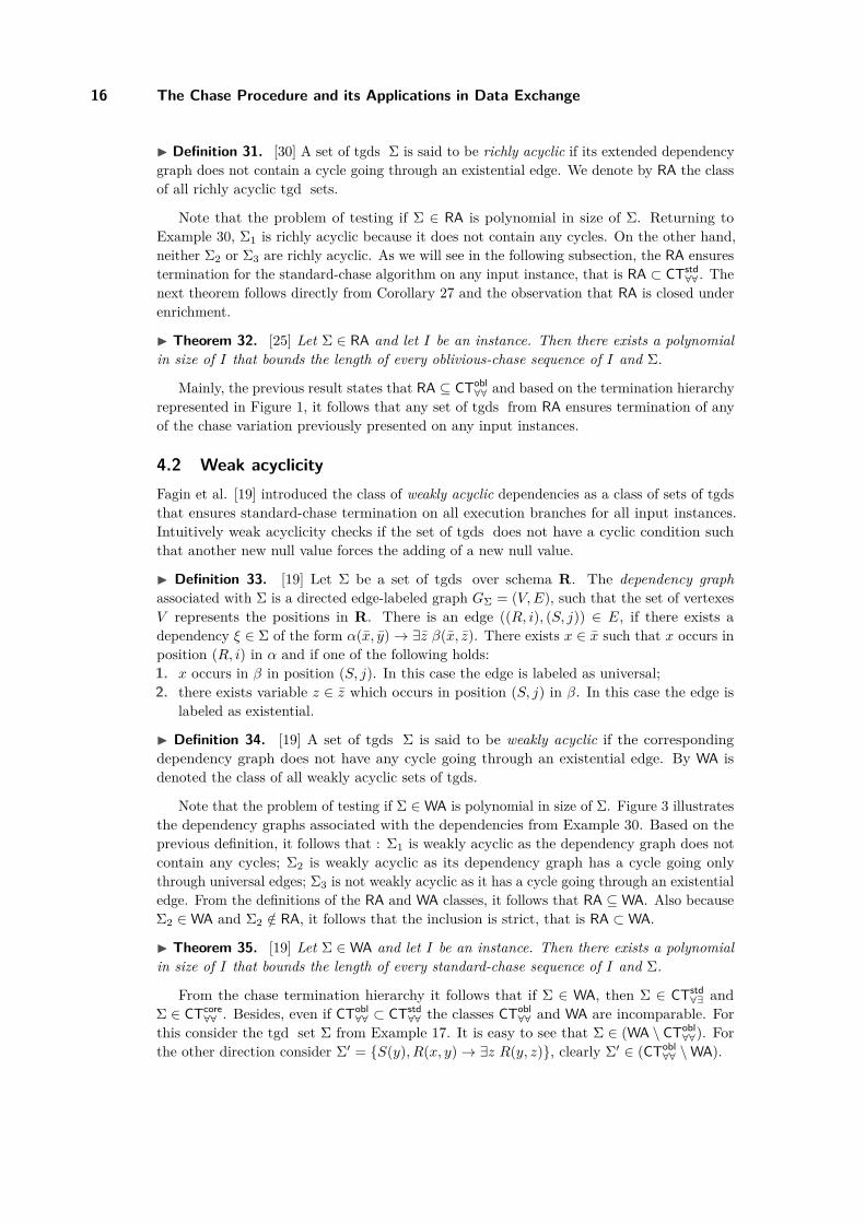
I Definition 31. [30] A set of tgds Σ is said to be richly acyclic if its extended dependencygraph does not contain a cycle going through an existential edge. We denote by RA the classof all richly acyclic tgd sets.

Note that the problem of testing if Σ ∈ RA is polynomial in size of Σ. Returning toExample 30, Σ1 is richly acyclic because it does not contain any cycles. On the other hand,neither Σ2 or Σ3 are richly acyclic. As we will see in the following subsection, the RA ensurestermination for the standard-chase algorithm on any input instance, that is RA ⊂ CTstd

∀∀ . Thenext theorem follows directly from Corollary 27 and the observation that RA is closed underenrichment.

I Theorem 32. [25] Let Σ ∈ RA and let I be an instance. Then there exists a polynomialin size of I that bounds the length of every oblivious-chase sequence of I and Σ.

Mainly, the previous result states that RA ⊆ CTobl∀∀ and based on the termination hierarchy

represented in Figure 1, it follows that any set of tgds from RA ensures termination of anyof the chase variation previously presented on any input instances.

4.2 Weak acyclicityFagin et al. [19] introduced the class of weakly acyclic dependencies as a class of sets of tgdsthat ensures standard-chase termination on all execution branches for all input instances.Intuitively weak acyclicity checks if the set of tgds does not have a cyclic condition suchthat another new null value forces the adding of a new null value.

I Definition 33. [19] Let Σ be a set of tgds over schema R. The dependency graphassociated with Σ is a directed edge-labeled graph GΣ = (V,E), such that the set of vertexesV represents the positions in R. There is an edge ((R, i), (S, j)) ∈ E, if there exists adependency ξ ∈ Σ of the form α(x, y)→ ∃z β(x, z). There exists x ∈ x such that x occurs inposition (R, i) in α and if one of the following holds:1. x occurs in β in position (S, j). In this case the edge is labeled as universal;2. there exists variable z ∈ z which occurs in position (S, j) in β. In this case the edge is

labeled as existential.

I Definition 34. [19] A set of tgds Σ is said to be weakly acyclic if the correspondingdependency graph does not have any cycle going through an existential edge. By WA isdenoted the class of all weakly acyclic sets of tgds.

Note that the problem of testing if Σ ∈WA is polynomial in size of Σ. Figure 3 illustratesthe dependency graphs associated with the dependencies from Example 30. Based on theprevious definition, it follows that : Σ1 is weakly acyclic as the dependency graph does notcontain any cycles; Σ2 is weakly acyclic as its dependency graph has a cycle going onlythrough universal edges; Σ3 is not weakly acyclic as it has a cycle going through an existentialedge. From the definitions of the RA and WA classes, it follows that RA ⊆WA. Also becauseΣ2 ∈WA and Σ2 /∈ RA, it follows that the inclusion is strict, that is RA ⊂WA.

I Theorem 35. [19] Let Σ ∈WA and let I be an instance. Then there exists a polynomialin size of I that bounds the length of every standard-chase sequence of I and Σ.

From the chase termination hierarchy it follows that if Σ ∈ WA, then Σ ∈ CTstd∀∃ and

Σ ∈ CTcore∀∀ . Besides, even if CTobl

∀∀ ⊂ CTstd∀∀ the classes CTobl

∀∀ and WA are incomparable. Forthis consider the tgd set Σ from Example 17. It is easy to see that Σ ∈ (WA \ CTobl

∀∀). Forthe other direction consider Σ′ = {S(y), R(x, y)→ ∃z R(y, z)}, clearly Σ′ ∈ (CTobl

∀∀ \WA).

A. Onet 17

Figure 3 Dependency graphs associated with dependencies from Example 30.

From the observation that the class WA is closed under semi-enrichment, Theorem 35and Corollary 27, it follows:

I Theorem 36. WA ⊂ CTsobl∀∀ .

Proof. For the strict inclusion part of this theorem consider the same set of dependenciesΣ′ = {S(y), R(x, y)→ ∃z R(y, z)}. J

4.3 Safe dependenciesMeier, Schmidt and Lausen [41] observed that the weak acyclicity condition takes into accountnulls that may not create infinite standard-chase sequences. For example, consider the setΣ = {ξ} [41] where:

ξ = R(x, y, z), S(y)→ ∃w R(y, w, x).

Figure 4a) represents the corresponding dependency graph with cycles going through exist-ential edges involving position (R, 2). Thus, the dependency is not weakly acyclic. On theother hand, the newly created null in position (R, 2) may create new null values only if thesame null also appears in position (S, 1). Based on the given dependency, new nulls cannotbe generated in position the (S, 1). Hence, this dependency can not cyclically create newnulls.

In order to introduce the notion of safe dependencies, we first need to define the followingconcept.

I Definition 37. [12] The affected positions associated with a set of tgds Σ is the set aff (Σ)defined as follows. For all positions (R, i) that occur in the head of some tgd ξ ∈ Σ, then1. if an existential variable appears in position (R, i) in ξ, then (R, i) ∈ aff (Σ);2. if universally quantified variable x appears in position (R, i) in the head and x appears

only in affected positions in the body, then (R, i) ∈ aff (Σ).

Intuitively, the affected positions are those where new null values can occur duringthe chase process. For example, the set of affected positions associated with the set ofdependencies Σ = {R(x, y, z), S(y)→ ∃w R(y, w, x)} is aff (Σ) = {(R, 2)}.

I Definition 38. [41] The propagation graph for a set of tgds Σ is a directed edge labeledgraph PΣ = (aff (Σ), E). Where ((R, i), (S, j)) ∈ E if there exists a dependency ξ ∈ Σ ofthe form α(x, y)→ ∃z β(x, z), there exists a variable x that occurs in α in position (R, i), xoccurs only in affected positions in α and one of the following holds:

Chapte r 01


Figure 4 a) Dependency graph, b) Propagation graph for {R(x, y, z), S(y) → ∃w R(y, w, x)}.

1. x appears in β in affected position (S, j). In this case the edge is labeled as universal;2. there exists variable z ∈ z which occurs in position (S, j) in β. In this case the edge is

labeled existential.

Considering the same dependency set Σ = {R(x, y, z), S(y)→ ∃w R(y, w, x)}, Figure 4a)represents the corresponding dependency graph and Figure 4b) the corresponding propagationgraph. Note that the propagation graph contains only one node, corresponding to the affectedposition (R, 2). Because y appears in the head in a non-affected position (S, 1), it followsthat there are no edges in the propagation graph.

I Definition 39. [41] A set of tgds Σ is called safe if its propagation graph PΣ does nothave a cycle going through an existential edge. By SD is denoted the class of all safe sets oftgds.

Note that the problem of testing if Σ ∈ SD is polynomial in size of Σ. In our example,the dependency graph did not contain any edges (see Figure 4b)), hence Σ ∈ SD.

I Theorem 40. [41] Let Σ ∈ SD. Then there exists a polynomial in size of I that boundsthe length of every standard-chase sequence of I and Σ.

From our running example in this subsection and from the definition of the SD class, itfollows that WA ⊂ SD. Also, similarly to the weakly acyclic class it can be shown that SD isclosed under semi-enrichment. Thus, because the previous theorem states that SD ⊂ CTstd

∀∀,it follows that actually SD ⊂ CTsobl

∀∀ ⊂ CTstd∀∀. This means that given a set of tgds which is

safe, one may use the semi-oblivious chase to compute an instance which is (see previoussection) homomorphically equivalent to any instance returned by the standard chase withthe same input. Finally, it can be easily noted that, even if SD is bigger than WA, it does notcontain the termination class CTobl

∀∀. For this consider Σ = {R(x, x)→ ∃z R(x, y)}, clearlyΣ ∈ (CTobl

∀∀ \ SD).

4.4 Super weak acyclicityThe following class of sets of tgds properly extends the class of safe sets of tgds andconsequently the class of weakly acyclic and richly acyclic sets of tgds. The new class ofdependencies, introduced by Marnette [38], beside omitting the nulls that can’t generateinfinite chase sequences, as in the case of safe dependencies, also takes into account therepeating variables. For a more uniform presentation of the sufficient classes, we will slightlychange the notations used in [38].

A. Onet 19

In this subsection we assume that the set of dependencies Σ has distinct variable namesin each tgd. We also assume that there exists a total order between the atoms in eachdependency. With this, we can now define the atom position to be a triple (ξ,R, i), where ξis a dependency in Σ, R is a relation name that occurs in ξ, i a positive integer i ≤ n, wheren is the maximum number of occurrences of R in ξ, given by the total order between theatoms in the tgd. Clearly each atom position uniquely identifies an atom in Σ. Similarlyto the notion of position, a place can be defined to be a pair ((ξ,R, i), k), where (ξ,R, i) isan atom position and 1 ≤ k ≤ arity(R). Intuitively, the place identifies the variable thatappears in the k-th attribute in the atom represented by (ξ,R, i).

Let V ar(ξ) denote the set of variables that occurs in dependency ξ. As mentioned, for anytwo distinct dependencies ξ1 and ξ2 from Σ, we have V ar(ξ1) ∩ V ar(ξ2) = ∅. The mappingV ar is extended in the natural way to a set of dependencies Σ, V ar(Σ) = ∪ξ∈Σ V ar(ξ).Similarly, we define the mappings V ar∃ and V ar∀ that map each dependency ξ to the setof existentially quantified variables in ξ and to the universally quantified variables in ξ,respectively. Clearly for each dependency ξ, V ar∃(ξ) and V ar∀(ξ) represent a partition ofV ar(ξ).

Given a tgd ξ and y ∈ V ar∃(ξ), Out(ξ, y) is defined to be the set of places in the head ofξ where y occurs. Given a set a tgd ξ and x ∈ V ar∀(ξ), In(ξ, x) is defined to be the set ofplaces in the body of ξ where x occurs. Intuitively, Out(ξ, y) represents the places wherevariable y is “exported” when applying tgd ξ. Similarly, In(ξ, x) represents the places thatneed to be “filled” for variable x in order for ξ to be applied.

Given an atom position (ξ,R, i), a substitution θ is a function that maps each variable xthat occurs in the atom (ξ,R, i) to a constant if x ∈ V ar∀(ξ) and to a fresh new constant,if x ∈ V ar∃(ξ), where by “new fresh” we mean the next unused element in some fixedenumeration of the constants. The atom resulted by replacing each variable in the atomgiven by (ξ,R, i) with the substitution θ is denoted by θ(ξ,R, i). Two atoms (ξ1, R, i1)and (ξ2, R, i2) are said to be unifiable if there exist substitutions θ1 and θ2 such thatθ1(ξ1, R, i1) = θ2(ξ2, R, i2). Two places p1 = ((ξ1, R, i1), k1) and p2 = ((ξ2, R, i2), k2) are saidto be unifiable if k1 = k2 and (ξ1, R, i1) is unifiable with (ξ2, R, i2). By p1 ∼ p2 it is denotedthat p1 and p2 are unifiable. Let us define ΓΣ to be a function that maps each variable x tothe set of places where x occurs in Σ. ΓHΣ represents the function that maps each variablex to the set of places from the head of some dependency where x occurs. Similarly, thefunction ΓBΣ maps each variable x to the set of places from the body of some dependencywhere x occurs.

For a better understanding of the previous notions, let us consider the example:

I Example 41. [47] Let Σ = {ξ1, ξ2}, where:

ξ1 = R(x)→ ∃y, z S(x, y, z), andξ2 = S(v, w,w)→ R(w).

The atom positions for Σ are: (ξ1, R, 1), corresponding with the atom R(x); (ξ1, S, 1),corresponding with the atom S(x, y, z); (ξ2, S, 1), corresponding with the atom S(v, w,w);and (ξ2, R, 1), corresponding with the atom R(w). We have V ar∀(Σ) = {x, v, w} andV ar∃(Σ) = {y, z}. Clearly (ξ1, R, 1) is unifiable with (ξ2, R, 1), consider for example unifiersθ1 = {x/a} and θ2 = {w/a} where both variables x and w are in V ar∀(Σ). On the other hand,the atom positions (ξ1, S, 1) and (ξ2, S, 1) are not unifiable because y and z are existentiallyquantified variables and thus any unifier will map y and z to distinct constants (recallthat each existential variable is mapped to a new fresh constants). Hence, we only have

Chapte r 01


((ξ1, R, 1), 1) ∼ ((ξ2, R, 1), 1). For variable x the set ΓΣ(x) = {((ξ1, R, 1), 1), ((ξ1, S, 1), 1)},ΓBΣ (x) = {((ξ1, R, 1), 1)} and ΓHΣ (x) = {((ξ1, S, 1), 1)}.

Given two sets of places P and Q, we denote P v Q if for all p ∈ P there exists q ∈ Qsuch p ∼ q. Let us now define mapping Move(Σ, Q) that gives the smallest set of places Psuch that Q ⊆ P , and for all variables x that occurs in a body of some dependency ξ ∈ Σ ifΓBΣ(x) v P then ΓHΣ (x) ⊆ P . Intuitively, the Move(Σ, Q) returns the smallest set of placessuch that new atoms may be generated in those positions by chasing some atoms given bythe places in Q.

I Definition 42. [38] Given Σ a set of tgds and ξ1, ξ2 ∈ Σ, we say ξ1 triggers ξ2 in Σ, andit is denoted by ξ1 ;Σ ξ2, iff there exist a variable y ∈ V ar∃(ξ1) and a variable x ∈ V ar∀(ξ2)occurring in both the body and the head of ξ2 such that:

In(ξ2, x) v Move(Σ,Out(ξ1, y)).

I Definition 43. [38] A set of tgds Σ is said to be super-weakly acyclic iff the triggerrelation ;Σ is acyclic. We denote by SwA the set off all super-weakly acyclic tgd sets.

I Example 44. Let us consider the same set of dependencies Σ = {ξ1, ξ2} from Example 41.The place ((ξ1, S, 1), 1) is not unifiable with ((ξ2, S, 1), 1), thus In(ξ2,w) 6v Move(Σ,Out(ξ1, y)),that is ξ1 6;Σ ξ2. Similarly, ξ2 does not contain any existential variables and so it followsthat ξ2 6;Σ ξ1. As both dependencies do not share common relation names in the head andbody, it follows that ξ1 6;Σ ξ1 and ξ2 6;Σ ξ2. That is the relation ;Σ does not induce anycycle, following that Σ is super-weakly acyclic. Moreover, it can be seen that Σ is not safe asbetween the affected positions (R, 1) and (S, 2) there exists a cycle through an existentialedge in the corresponding propagation graph.

Marnette [38] showed that the membership problem Is Σ ∈ SwA? is polynomial in thesize of Σ. Spezzano and Greco [47] also proved that SD ⊂ SwA, that is the super-weak acyclicclass properly contains the safe dependencies. The class SwA is closed in adding atoms to thebody of dependencies. Thus given a set of tgds Σ, then any set of dependencies Σ′ obtainedfrom Σ by adding new atoms in the body of any dependency remains super-weakly acyclic.

I Theorem 45. [38] Let Σ ∈ SwA and let I be an instance. Then there exists a polynomialin the size of I that bounds the length of every semi-oblivious-chase sequence of I and Σ.Thus, Swa ⊂ CTsobl

∀∀ .

This concludes that the super-weakly acyclic class of tgd sets is sufficient for thetermination of the semi-oblivious, standard and core-chase algorithms for all input instances.

4.5 StratificationThe stratified model of dependencies was introduced by Deutsch et al. in [16]. This classrelaxes the condition imposed by weak acyclicity by stratifying the dependencies and checkfor weak acyclicity on each of these strata instead of checking for the entire set.

I Definition 46. [16] Let ξ1 and ξ2 be two tgds , we write ξ1 ≺ ξ2, if there exist the instancesI, J and a vector a ⊆ dom(J) such that:1. I |= ξ2(a), and2. there exists an active trigger (ξ1, h), such that I (ξ1,h)−−−−→ J , and3. J 6|= ξ2(a).

A. Onet 21

I Example 47. Consider Σ = {ξ1, ξ2}, where:

ξ1 = R(x, y)→ S(x), andξ2 = S(x)→ R(x, x).

With the instance I = {R(a, b)} and the vector a = (a) we have that I |= ξ2(a); and forthe homomorphism h = {x/a, y/b} we have I (ξ1,h)−−−−→ J , where J = {R(a, b), S(a)}. BecauseJ 6|= ξ2(a), it follows that ξ1 ≺ ξ2. On the other hand, ξ2 6≺ ξ1 because for any instance Iand vector of constants b such that I |= ξ1(b) and I (ξ2,h)−−−−→ J , for some active trigger (ξ2, h),it follows that J |= ξ2(b).

The authors of [16] claimed that testing if ξ1 ≺ ξ2 is in NP, as we will show next, thiscannot be true unless NP = coNP.

I Theorem 48. [26] Given two tgds ξ1 and ξ2, the problem of testing if ξ1 ≺ ξ2 is coNP-hard.

Proof. We will use a reduction from the graph 3-colorability problem that is known to beNP-complete. It is also known that a graph G is 3-colorable if and only if there exists ahomomorphism from G to K3, where K3 is the complete graph with 3 vertices.

A graph G = (V,E), where V = n and E = m, is identified with the sequenceG(x1, . . . , xn) = E(xi1 , yi1), . . . , E(xim , yim) and treat the elements in V as variables. Simil-arly, we identify the graph K3 with the sequence

K3(z1, z2, z3) = E(z1, z2), E(z2, z1), E(z1, z3), E(z3, z1), E(z2, z3), E(z3, z2)

where z1, z2, and z3 are variables. With these notations, given a graph G = (V,E), weconstruct tgd’s ξ1 and ξ2 as follows:

ξ1 = R(z)→ ∃z1, z2, z3 K3(z1, z2, z3), andξ2 = E(x, y)→ ∃x1, . . . , xn G(x1, . . . , xn).

Clearly the reduction is polynomial in the size of G. We will now show that ξ1 ≺ ξ2 iff Gis not 3-colorable.

First, suppose that ξ1 ≺ ξ2. Then there exists an instance I and homomorphisms h1

and h2, such that I |= h2(ξ2). Consider J , where I (ξ1,h1)−−−−→ J . Thus RI had to contain atleast one tuple, and EI had to be empty, because otherwise the monotonicity property ofthe chase we would imply that J |= h2(ξ2).

On the other hand, we have I (ξ1,h1)−−−−→ J , where J = I ∪ {K3(h′1(z1), h′1(z2), h′1(z3))},and h′1 is a distinct extension of h1. Since EI = ∅, and we assumed that J 6|= h2(ξ2), itfollows that there is no homomorphism from G into J , i.e. there is no homomorphism fromG(h′2(x1), . . . , h′2(xn)) to K3(h′1(z1), h′1(z2), h′1(z3)), where h′2 is a distinct extension of h2.Therefore the graph G is not 3-colorable.

For the other direction, let us suppose that graph G is not 3-colorable. This means thatclearly there is no homomorphism from G into K3. In fact, with these assumptions let usconsider I = {R(a)}, and the two homomorphisms h1 = {z/a} and h2 = {x/h′1(z1), y/h′1(z2)}.It is easy to verify that I, h1 and h2 satisfy the three conditions for ξ1 ≺ ξ2. J

The obvious upper bound for the problem ξ1 ≺ ξ2 is ΣP2 . In [26] it is shown that this

upper bound can be lowered to ∆P2 . To the best of our knowledge these are the tidiest

bounds found so far for the given problem.Given a set of tgds Σ, the chase graph associated with Σ is a directed graph G = (V,E),

where V = Σ and (ξ1, ξ2) ∈ E iff ξ1 ≺ ξ2.

Chapte r 01


I Definition 49. [16] A set of tgds Σ is said to be stratified if the set of dependencies inevery simple cycle in the corresponding chase graph is weakly acyclic. The set of all stratifiedtgd sets is denoted by Str.

In [26] it is shown that the complexity of testing if Σ ∈ Str, for a given Σ, is in ΠP2 .

Meier et al. [41] shown that Str 6⊆ CTstd∀∀ but actually Str ⊆ CTstd

∀∃, that is the stratificationguarantees the termination only on some standard-chase execution branches for all inputinstances.

I Example 50. [41] Consider Σ = {ξ1, ξ2, ξ3, ξ4}, where:

ξ1 = R(x)→ S(x, x);ξ2 = S(x, y)→ ∃z T (y, z);ξ3 = S(x, y)→ T (x, y), T (y, z); andξ4 = T (x, y), T (x, z), T (z, x)→ R(y).

We have Σ ∈ Str is stratified since ξ1 ≺ ξ2, ξ1 ≺ ξ3 ≺ ξ4 ≺ ξ1, and the set {ξ1, ξ3, ξ4}is weakly acyclic. Let I = {R(a)}. The standard-chase execution branch that triggersrepeatedly dependencies ξ1, ξ2, ξ3 and ξ4 never terminates. On the other hand, the chasesequences that never trigger ξ2 will terminate.

Meier et al. [41] changed the stratification definition in order to guarantee terminationon all execution branches for all instances.

I Definition 51. [41] Let ξ1 and ξ2 be two tgds we write ξ1 ≺c ξ2, if there exist instancesI, J and tuple a ⊆ dom(J), such that:1. I |= ξ2(a), and

2. there exists trigger (ξ1, h), such that I ∗,(ξ1,h)−−−−−→ J , and3. J 6|= ξ2(a).

Given a set of tgds Σ, the c-chase graph associated with Σ is a directed graph Gc = (V,E).With V = Σ and (ξ1, ξ2) ∈ E iff ξ1 ≺c ξ2. A set of tgds Σ is said to be c-stratified if the setof dependencies in every simple cycle in the c-chase graph is weakly acyclic. The set of allc-stratified tgd sets is denoted by CStr.

I Theorem 52. [41] Let Σ ∈ CStr and let I be an instance. Then there exists a polynomial,in size of I, that bounds the length of every standard chase sequence of I and Σ.

Using the same reduction as in Theorem 48, it can be shown that the problem of testingif ξ1 ≺c ξ2 is coNP-hard and it is in ∆P

2 . Also the problem of testing if Σ ∈ CStr, for a givenΣ, it is in ΠP

2 .Meier et al. [41] showed that WA ⊂ CStr and that SD ∦ CStr1. Also Spezzano and Greco

[47] proved that SwA ∦ CStr, that is the super-weakly acyclic class is not comparable with thec-stratified class. Also based on the observation that CStr is closed under semi-enrichment,it follows that CStr ⊂ CTsobl

∀∀ .

1 The notation A ∦ B is shorthand for A * B and A + B

A. Onet 23

4.6 Inductively restricted dependenciesAnother class of dependencies that guarantees the standard-chase termination is the in-ductively restricted set of tgds. Note that the stratification method lifts the weakly acyclicclass of dependencies to the class of c-stratified dependencies. The inductively restrictedclass generalizes the stratification method while still keeping the termination property forthe standard-chase algorithm. This generalization is done using the so-called restrictionsystems [41]. With the help of the restriction systems, Meier et al. [41] define the newsufficient condition called inductive restriction that guarantees the standard-chase algorithmtermination on all execution branches for all instances. From this condition a new hier-archy of classes of dependencies is revealed with the same termination property, called theT-hierarchy. Note that the inductive restriction condition presented here is given from theerratum (http://arxiv.org/abs/0906.4228) and not from [41], where the presented condition,as mentioned in the erratum, does not guarantee the standard-chase termination on allbranches for all instances.

Let Σ be a set of tgds, I an instance and A a set of nulls. The set of all positions (R, i)such that there exists a tuple in I that contains a variable from A in position (R, i) is denotedby null-pos(A, I).

Similarly to relation "≺" for the stratified dependencies, the binary relation "≺P " isdefined for the inductive restriction condition, where P is a set of positions.

I Definition 53. [41] Let Σ be a set of tgds and P a set of positions. Let ξ1, ξ2 be twodependencies in Σ. It is said that ξ1 ≺P ξ2 if there exist instances I,J and vector a ⊆ dom(J),such that:1. I |= ξ2(a), and2. there exists a trigger (ξ1, h), such that I ∗,(ξ1,h)−−−−−→ J , and3. J 6|= ξ2(a), and4. there exists X ∈ a ∩ Null in the head of ξ2(a), such that null-pos({X}, I) ⊆ P .

I Example 54. Consider Σ containing a single tgd ξ = R(x, y)→ ∃z R(y, z). In Section 3we saw that there are instances I such that standard-chase algorithm does not terminateon all branches for I and Σ. It is easy to see that with instances I = {R(a, b)} andJ = {R(a, b), R(b,X)}, and vector a = (b,X), conditions 1,2 and 3 from the previousdefinition are fulfilled. For the 4th condition, consider X ∈ a, then we have ξ(a) whichrepresents the formula R(a,X)→ ∃zR(X, z). Thus, X occurs in the head of ξ(a). On theother hand, null-pos({X}, I) = ∅, instance I does not contain any labeled nulls, hence forany set P , null-pos({X}, I) ⊆ P . Thus, ξ ≺P ξ, for any set of positions P .

I Definition 55. [41] Let P be a set of positions and ξ a tgd. By aff-cl(ξ, P ) is denoted theset of positions (R, i) from the head of ξ such that one of the following holds:1. for all x ∈ V ar∀(ξ)2, with x occurs in (R, i), x occurs in the body of ξ only in positions

from P , or2. position (R, i) contains a variable x ∈ V ar∃(ξ).

For the tgd in Example 54, we have aff-cl(ξ, P ) = {(R, 1), (R, 2)}, where P = {(R, 2)}.Given a set of dependencies Σ, the set of all positions in Σ is written as pos(Σ).

2 Recall that by V ar∀(ξ) we denote the set of all universally quantified variables in ξ and by V ar∃(ξ) theset of all existentially quantified variables in ξ.

Chapte r 01


I Definition 56. [41] A 2-restriction system is a pair (G(Σ), P ), where G(Σ) is a directedgraph (Σ, E) and P ⊆ pos(Σ) such that:1. for all (ξ1, ξ2) ∈ E, aff-cl(ξ1, P ) ∩ pos(Σ) ⊆ P and aff-cl(ξ2, P ) ∩ pos(Σ) ⊆ P , and2. for all ξ1 ≺P ξ2, (ξ1, ξ2) ∈ P .

A 2-restriction system is minimal if it is obtained from ((Σ, ∅), ∅) by a repeated applicationof constraints 1 and 2, from the previous definition, such that P is extended only by thosepositions that are required to satisfy condition 1. Let us denote by part(Σ, 2) the set thatcontains the sets of all strongly connected components in a minimal 2-restriction system.

I Example 57. Returning to our dependency from Example 54, the minimal 2-restrictionsystem is computed as follows. Consider pair (({ξ}, ∅), ∅). Previously we showed that ξ ≺P ξ,for any set of positions P , by particularization we have ξ ≺∅ ξ. Thus, we add edge (ξ, ξ) to E.Using condition 1 from Definition 56 we have aff-cl(ξ, ∅) = {(R, 2)}. That is we add position(R, 2) to P . By repeating this process once again with P = {(R, 2)}, we add to P the position(R, 1) too. Hence, the minimal 2-restriction system is ((Σ, {(ξ, ξ)), {(R, 1), (R, 2)}}). Theonly connected component in this restriction system is {ξ}.

In [41], Meier et al. provide a simple algorithm that computes the set part(Σ, 2).

I Definition 58. [41] A set Σ of tgds is called inductively restricted iff every Σ′ ∈ part(Σ, 2)is safe. The set of all inductively restricted tgd sets is denoted by IR.

Using the same reduction from the proof of Theorem 48, it can be shown that the problemof testing if ξ1 ≺P ξ2, for a given ξ1, ξ2 and P , is coNP-hard and it can be solved in ΣP

2 .Similarly to the stratification case it can be shown that the complexity of testing if Σ ∈ IR isin ΠP

3 . From the definition, it directly follows that SD ⊂ IR. To this Meier et al. [41] alsoshowed that Str ∦ IR and that CStr ⊂ IR. On the other hand, the classes SwA and IR areincomparable [47], that is SwA ∦ IR.

I Example 59. [41] Consider the following set of tgds Σ:

ξ1 = S(x), E(x, y)→ E(y, x), andξ2 = S(x), E(x, y)→ ∃z E(y, z), E(z, x).

It can be easily observed that Σ is neither stratified nor safe, but it is inductively restricted.

I Theorem 60. [41] Let Σ ∈ IR and let I be an instance. Then there exists a polynomial, insize of I, that bounds the length of every standard-chase sequence of I and Σ.

Meier, Schmidt and Lausen [41] observed that the inductive restriction criterion can beextended to form a hierarchy of classes that ensure the standard-chase termination on allbranches for all instances. Intuitively, the lowest level of this hierarchy, noted T [2], is theclass of inductively restricted dependencies. Level T [k], k > 2 is obtained by extending thebinary relation ≺P to a k-ary relation ≺k,P . Intuitively, ≺k,P (ξ1, . . . , ξk) means that thereexists a standard-chase sequence such that firing ξ1 will also cause ξ2 to fire. This in turnwill cause ξ3 to fire and so on until ξk. Based on this new relation, the set part(Σ, k) iscomputed similarly to part(Σ, 2). The algorithm that computes part(Σ, k) can be found in[41]. For all k ≤ 2, it is shown that T [k] ⊂ T [k + 1].

It is easy to check that the previous hierarchy is closed under semi-enrichment, followingfrom Corollary 27 that for any k we have T [k] ⊂ CTsobl

∀∀ . Also in [44] it is shown thatT [k] ∦ CTobl

∀∀. More recently, the T [k] hierarchy of classes was extended by Meier et al. [42]

A. Onet 25

Figure 5 Relationship between chase termination classes.

to the ∀∃ − T [k] hierarchy of classes that ensures the standard-chase termination on at leastone execution branch and it showed that T [k] ⊂ ∀∃ − T [k], for any k > 1.

Figure 5 illustrates, as a Hasse diagram, the subset relationship between the terminationclasses presented.

Before concluding this subsection, we need to mention that more recently Greco et al.[27] extended the classes of dependencies that ensure the standard-chase termination to newlarge classes based on a stratification based method called local stratification.

4.7 The rewriting approachSpezzano and Greco [47] noticed that all the previous classes may be extended by usinga rewriting technique. Intuitively, if T is one of the classes {WA,SD,SwA,Str,CStr}, theninstead of directly checking if a set of dependencies Σ ∈ T, we check if Adn(Σ) ∈ T, whereAdn(Σ) is an adornment based rewriting of Σ such that, if Adn(Σ) ∈ CTstd

∀∀, then Σ ∈ CTstd∀∀.

Where the adornment of a predicate p of arity m is a string of the length m over the alphabet{b, f }. An adorned atom is of the form pα1,α2,...,αm(x1, x2, . . . , xm); if αi = b, then variablexi is considered bounded, otherwise the variable is considered free.

Due to the space constraints we will present this method following a simple example.Consider the following set of dependencies Σ = {ξ1, ξ2} [47]:

ξ1 = N(x)→ ∃y E(x, y), andξ2 = S(x), E(x, y)→ N(y).

The affected positions in Σ are (E, 1),(E, 2) and (N, 1). As the corresponding propagationgraph contains a cycle, through an existential edge, involving positions (N, 1) and (E, 2), itfollows that Σ /∈ SD. Construct the set of dependencies Adn(Σ) as follows:

Chapte r 01


1. For all predicate symbols p of arity m in Σ add the tgd:

∀x1, x2, . . . , xm p(x1, x2, . . . , xm)→ pα1,α2,...,αm(x1, x2, . . . , xm)

where, for all positive i ≤ m, αi = b.In our example Σ contains the following predicate symbols {E,S,N}, that is we add toAdn(Σ) the following set of tgds:

ξ′1 = E(x, y)→ Eb b(x, y);

ξ′2 = N(x)→ Nb(x); and

ξ′3 = S(x)→ Sb(x).2. Repeat to create new adornment predicate symbols based on the existing dependencies,

until none can be added. That is, if a variable in the head is marked as bounded (free)and if it occurs only bounded (free) places in the body. All existential variables in thehead are marked as free.Returning to our example and using ξ1 from Σ and the new adornment Nb, we add thefollowing dependency to Adn(Σ):

ξ′4 = Nb(x)→ ∃y Eb f (x, y).Similarly, based on tgd ξ2 from Σ and new adornments Sb and Eb b, we add the followingdependency to Adn(Σ):

ξ′5 = Sb(x), Eb b(x, y)→ Nb(y).Repeating this process, we add the following tgds to Adn(Σ):

ξ′6 = Sb(x), Eb f (x, y)→ N f (y), and

ξ′7 = N f (x)→ ∃y Ef f (x, y).After this point no other adornments can be created.

3. Finally, for each of the adornment predicate pα in Adn(Σ), add a new dependency inAdn(Σ) that "copies" pα to a new p predicate symbol. In this example the following newdependencies are added:

ξ′8 = Nb(x)→ N(x);

ξ′9 = N f (x)→ N(x);

ξ′10 = Sb(x)→ S(x);

ξ′11 = Eb b(x, y)→ E(x, y);

ξ′12 = Eb f (x, y)→ E(x, y); and

ξ′13 = Ef f (x, y)→ E(x, y).

In [47], it is proved that Σ ∈ CTstd∀∀ if and only if Adn(Σ) ∈ CTstd

∀∀. Returning to ourexample, it can be noted that the set Adn(Σ) is safe. Thus, using the previous observation, itresults that even if the set Σ was not safe, the standard chase will terminate on all brancheson Σ with any instances.

I Theorem 61. [41] Let T be one of the classes {WA,SD,SwA,Str,CStr}, let Σ be a set oftgds and let I be an instance. Then, if Adn(Σ) ∈ T, there exists a polynomial, in size of I,that bounds the length of every standard-chase sequences of I and Σ.

Even more, Spezzano and Greco [47] proved that these rewritings strictly extend theclasses of dependencies.

I Theorem 62. [41] Let T be one of the classes {WA,SD,SwA,Str,CStr} and let denote byAdnT the set of all Σ such that Adn(Σ) ∈ T. Then, T ⊂ AdnT.

A. Onet 27

More recently, this rewriting method was further improved by Greco et al. [27] by indexingthe adornment used to specify the free positions. This method ensures that we may equateonly variables that have the adornment with the same index.

5 The chase and data exchange

The previous section was mainly focused on presenting different chase algorithms and theirtermination criteria. This section is dedicated to the instance returned by the chase algorithmand to how it can be used in the data-exchange problem. As we will see, the finite instancereturned by any chase variation is strongly related to the notion of universal model. Suchinstances represent a good candidate to be materialized under the target schema in dataexchange. Beside computing a general solution for the data-exchange problem, the chaseprocedure also plays an important role in some related problems as the inverse, recovery[18, 22, 8], and composition of schema mappings [21, 6].

For a complete and coherent introduction to the application of the chase procedure indata exchange, we first present the notion of universal models and its relation with thechase algorithm. Need to mention that the notion universal models [16] was introduced as ageneralization of universal solutions [19] in data exchange. This first part will be followedby a short review of the data-exchange problem and the link between universal models andquery answering in data exchange. In the final part of this section we will review the queryanswering problem in case there are no universal models.

5.1 Universal modelsBeside the data-exchange problem, universal models play an important role in many otherdatabase problems as: testing for conjunctive query containment under functional andinclusion dependencies [31], data integration [33], and query answering over ontologies [14].

I Definition 63. [16] Given an instance I and Σ a set of dependencies, a finite instance J issaid to be a model for I and Σ if J |= Σ, and I → J .

I Example 64. Consider I = {R(a, b), R(b, c)} and Σ = {R(x, y), R(y, z)→ R(x, z)}. Theinstance J = {R(a, b), R(b, c), R(a, c)} is a model of I and Σ, so is instance J1 = J∪{R(a,X)},with X a labeled null from Null. On the other hand, J2 = {R(a, b), R(a, c)} is not a modelof I and Σ, even if J2 |= Σ, since there is no homomorphism from I into J2.

The conclusion of this example is that, in general, there may be an infinite number ofmodels of I and Σ. Still, some of these models are more general than the others in the sensethat they have a homomorphism into all the other models. Such models are called, of course,universal models.

I Definition 65. [16] A finite instance U is said to be a weak universal model of I and Σif U is a model of I and Σ, and if for any finite model J of I and Σ, it is that U → J . IfU → J . Also for all infinite models J of I and Σ, then U is said to be a strong universalmodel or simply a universal model.

I Example 66. Considering the instance I and the dependency Σ from Example 64, itis clear that both instances J and J1 are strong universal models. Moreover, the modelJ3 = {R(a, b), R(b, c), R(a, c), R(a, a)} is neither a strong nor weak universal model as theredoes not exist a homomorphism from J3 to model J .

Chapte r 01


I Theorem 67. [19, 16] Let I be an instance and Σ a set of tgds and egds. Then any finiteinstance returned by the standard-chase algorithm is a universal model of I and Σ.

Intuitively, the theorem says that whenever the standard chase terminates and it doesnot fail, it gives a universal model of I and Σ. From this theorem, it follows that ifchasestd

Σ(I) 6= ⊥ then chasestdΣ(I) is a universal model for I and Σ. In the finite case, the

instance returned by the standard-chase algorithm is homomorphically equivalent with thefinite result of any chase variations. It follows that for any of the previously presented chasevariations, when they terminate and do not fail, they return a universal model.

I Corollary 68. Let I be an instance, Σ a set of tgds and egds, and ∗ ∈ {obl, sobl, core}.If chase∗Σ(I) 6= ⊥, then chase∗Σ(I) is a universal model of I and Σ.

This result ensures that the standard, oblivious, semi-oblivious and core chase are soundin finding universal models. Naturally the following question raises: Are these algorithmsalso complete in finding universal models? The following example shows that the standard,oblivious and semi-oblivious-chase algorithms are not complete.

I Example 69. Let us consider the same instance I = {R(a, b)} and set Σ = {ξ1, ξ2}, where:

ξ1 = R(x, y)→ ∃z R(y, z), andξ2 = R(x, y), R(y, z)→ R(y, y).

It is easy to see that there is no terminating branch for the standard chase for Σ and I.Similarly, the oblivious and semi-oblivious algorithms with the same input will not terminate.On the other hand, there exists universal model J = {R(a, b), R(b, b)} of I and Σ. Thus thestandard chase is not complete in finding universal models.

The result below shows that the core chase is complete in finding universal models.

I Theorem 70. [16] Let I be an instance and Σ a set of tgds and egds. Then there exists auniversal model of I and Σ iff the core-chase algorithm terminates and does not fail on inputI and Σ.

We know from the definition of the universal models that all universal models are alsoweak universal models. The following example shows that the converse does not hold.

I Example 71. [16] Let us consider instance I = {T (a)} and Σ = {ξ1, ξ2, ξ3}, where:

ξ1 = T (x)→ ∃y, z E(y, z);ξ2 = E(x, y)→ ∃z E(y, z); andξ3 = E(x, y), E(y, z)→ E(x, z).

Consider the relation E to contain the edges of a graph. Clearly all models have an infinitewalk. From this it follows that every finite model has a cycle in the corresponding graph.From this and ξ3, it also follows that any finite model has a self loop. Besides, the instanceJ = {T (a), E(X,X)} is a model of I and Σ containing a self loop. Consequently, J is a weakuniversal model of I and Σ. On the other hand, the transitive closure of an infinite path alsosatisfies Σ, however no finite instance with cycle has a homomorphism into it. This meansthat J is not a strong universal model of I and Σ.

Deutsch et al. [16] showed that it is undecidable to test if an instance U is a strong (weak)universal model for a given instance I and Σ a set of tgds. Even more, they demonstratedthat there is no complete chase based procedures for finding weak universal models.

A. Onet 29

5.2 Data exchangeData exchange is an old database problem that only recently earned more formal treatment.More precisely, it is the problem of transforming data structured under a source schemato data structured under a different target schema. Formally, a data-exchange setting isa quadruple (S,T,Σst,Σt), where S represents the source schema, T represents the targetschema, Σst is a set of constraints representing the relationship between the source and targetschema, and Σt represents a set of constraints over the target schema. Given a data-exchangesetting (S,T,Σst,Σt) and the instance I over the source schema S, the data-exchangeproblem is to find instances J over the target schema T, such that I ∪ J is a model for I andΣst ∪Σt. An instance J with the previous properties is called a solution to the data-exchangeproblem, or simply a solution. This problem was first formalized by Fagin et al. in [19].Most of the data-exchange problems consider Σst to be a set of tgds and Σt to be a set oftgds and egds. From now on, if not mentioned otherwise, we assume that the data-exchangesettings are of this format.

As there is an infinite number of solutions to the data-exchange problem, a naturalquestion raises: Which solution or finite set of solutions should be materialized on the target?There is no simple answer to this question as there may be different representations of thetarget depending on the semantics of the queries used over the target instance. The semanticsconsidered in this subsection, also most prominent in the literature, is the certain answersemantics for union of conjunctive queries (UCQ) over the target instance. This can beformalized by the following definition:

I Definition 72. Let σ = (S,T,Σst,Σt), let I be a source instance and Q a query in UCQover T. The certain answer of Q for I and σ is defined as

certσ(Q, I) =def ⋂J, I∪J|=Σst∪Σt

Q(J).

Fagin et al. [19] showed that the universal solution is a good candidate to be materializedin data-exchange problem under the certain UCQ answer semantics. Where the universalsolution for a data-exchange setting σ = (S,T,Σst,Σt) and the instance I is a universalmodel for I and Σst ∪ Σt restricted to schema T. We need to mention that Fagin et al.considered as solutions only finite instances which is the more important case in practice.This means that all results specified in Subsection 5.1 also hold for universal solutions. Inparticular, it means that the universal solution can be computed by the chase algorithms andthat it is undecidable if the universal solution exists for a given data-exchange setting and agiven source instance. Marnette [38] showed that it is undecidable to test if the obliviouschase will terminate for a given data-exchange setting for all input instances. This result canbe enhanced to all chase variations, including core chase. Thus, it is undecidable to test if,for a given data-exchange setting for all the input instances, there exists a universal solution.

In [19], Fagin et al. described a sufficient condition for the universal solution to not exist,as the following theorem shows it:

I Theorem 73. [19] Let σ = (S,T,Σst,Σt) be a data-exchange setting and I a sourceinstance such that there is a failing branch for the standard chase with input I and Σst ∪ Σt.Then there is no universal solution for I and σ.

In data exchange we may also have the case when there exists a solution but there is nouniversal solution. Let us consider the next example:

Chapte r 01


I Example 74. Consider the following data-exchange setting:

σ = ({S}, {R}, {S(x, y)→ R(x, y)}, {R(x, y)→ ∃z R(y, z)})

and the source instance I = {S(a, b)}. Clearly there is no universal solution for this setting,but there exists solution J = {R(a, b), R(b, b)}.

As shown by Kolaitis et al. in [32], it is undecidable to check for a given instance I and adata-exchange setting σ, if there exists a solution for I and σ.

Before presenting the computation of the certain answer for a data-exchange setting usinga universal model, we need to introduce the notion of naïve evaluation. Let I be an instance,possible with null values, and Q be a query. The Qnaïve(I) is defined by evaluating Q onI and by treating each null as a new distinct constants, and then by eliminating from theresult all the tuples with nulls.

I Theorem 75. [19] Let σ = (S,T,Σst,Σt) be a data-exchange setting and I an instanceover the source instance that does not contain nulls such that there exists a universal solutionJ for I and σ. Then, certσ(Q, I) = Qnaïve(J) for any Q ∈ UCQ.

In [35] Libkin showed that UCQ is the largest class of queries with the property that thecertain answers may be computed using the naïve evaluation. We conclude this subsection byreiterating the idea that within the infinite set of universal solutions there exists a universalsolution which is minimal in size. Such universal solution is called core and, as noted in [20],it is unique up to variable renaming. Hence, in case there exists a universal solution, thecore chase will terminate and return the core.

5.3 Data exchange beyond universal solutions

For the data-exchange setting and the source instance presented in Example 74 we knowthat there is no universal solution. On the other hand, when considering the query Q(x)←∃y R(x, y), the certain answers is the set of tuples {(a), (b)}. In [12], Cali, Gottlob and Kiferinvestigate the problem of conjunctive query answering when the universal solution is notguaranteed to exist. For this, the authors unravel two classes of tgds , namely guarded tuplegenerating dependencies (gtgd) and weakly guarded tuple generating dependencies (wgtgd),for which the problem of conjunctive query evaluation is decidable. Intuitively, a tgd isguarded if its body contains an atom called guard which covers all the variables in the body.Clearly LAV tgds are gtgds. A set of tgds is weakly guarded, if for each tgd, its bodycontains one atom which covers all the variables that appear in the affected position, that is,predicate positions that may contain new labeled nulls generated during the chase process.

I Example 76. Let us consider the following dependencies:

ξ1 = S(x), R(x, y)→ ∃z R(y, z), andξ2 = R(x, z), R(z, y)→ R(y, x).

In ξ1, the atom R(x, y) covers all the variables in the body, meaning that it is a gtgd. Clearly,ξ2 is not gtgd as there is no atom to cover all variables from the body. The affected positionin the set {ξ1, ξ2} is (R, 2), that is we may introduce new labeled nulls during the chaseprocess only in the second position of the predicate R. As in ξ2, the atom R(z, y) coversboth variables that appear in affected position in ξ2. It follows that ξ2 is a wgtgd.

A. Onet 31

Cali et al. [12] give complexity bounds for the conjunctive query answering problem, thatis: Does a tuple t belong to the certain answer? The complexity bounds discovered are thefollowing: (1) for a fixed set gtgds the conjunctive query answering problem is NP-complete;(2) for atomic queries the problem becomes polynomial; (3) in case the fixed dependenciesare wgtgds, the conjunctive query answering problem becomes EXPTIME-complete. Need tomention here that in [29] Hernich showed that if the data-exchange setting contains onlyguarded tgds, it is decidable if for the given setting and a given instance there exists auniversal solution.

In the certain answer semantics for UCQ queries over the target schema a universalsolution is enough to compute certain answer for any UCQ query. Therefore another questioncomes up naturally: Is this semantics also a good model for general queries? As shown in [4]and [34], this semantics is not suitable for general queries, as it may give unintuitive answerseven for simple copying data-exchange settings.

I Example 77. Let us consider a data-exchange setting σ = ({R}, {R′},Σst, ∅), where Σstsimply copies the source into target: R(x, y) → R′(x, y). Consider the source instanceI = {R(a, b)} and the query over the target schema Q(x, y)← R′(x, y) ∧ ¬R′(x, x). As oneof the solution is the instance J = {R′(a, b), R′(a, a)}, it follows that certσ(Q, I) = ∅. Now,when applying the same query on the source instance (by replacing relation name R′ withR), it returns the set of tuples {(a, b)}. Clearly this is not the expected behavior as thetarget instance is supposed to be a copy of the source instance.

To avoid such cases, Fagin et al. [20] proposed a new semantics for the certain answersto existential queries. Where existential queries Q(x) is a formula of the form ∃y ϕ(x, y),where ϕ is a safe quantifier-free formula. Under this semantics, instead of evaluating thequery on all solutions, the query is evaluated on universal solutions only.

I Definition 78. Let σ = (S,T,Σst,Σt), let I be a source instance and Q a query over theschema T. The u-certain answer of Q for I and σ is defined as

u-certσ(Q, I) =def ⋂{Q(J) : J universal solution for I and σ}.

Clearly certσ(Q, I) ⊆ u-certσ(Q, I), for any data-exchange setting σ, instance I andquery Q. Also, as shown in [20], certσ(Q, I) = u-certσ(Q, I) whenever Q ∈ UCQ. Theu-certain semantics is shown [20] to be adequate for existential queries. Even more, it isproved that in case J is a universal solution for data-exchange setting σ and instance I,and Q is an existential query, then the answer under u-certain semantics can be computedas: u-certσ(Q, I) = Qnaïve(core(J)). Returning to the previous example, the core universalsolution is J = {R(a, b)}, hence the certain answer to query Q will be the expected set oftuples {(a, b)}.

Later on new closed world semantics was proposed in order to deal with general queriesfor the data-exchange problem [34, 30, 28, 24]. Libkin [34] considered data-exchange settingswithout target dependencies and computed CWA-solutions which are used afterwards tocompute certain answers for FO queries. Hernich and Schweikardt [30] introduced a new chasebased algorithm, called the α-chase, to compute CWA-solutions when the data-exchangesetting also contains target dependencies. In [24] Grahne and O. introduce a chase algorithmon conditional tables in order to strongly represent a closed world semantics called theconstructible solutions. A similar chase process for conditional tables that considers onlysource to target dependencies was also introduced in [7].

Chapte r 01


6 Chase extensions

The chase algorithms presented in the previous sections considered only tgds and egds asconstraints. In this section we will describe extensions of the chase algorithms needed inorder to deal with negation disjunctive embedded dependencies (NDED). As we will see, thechase procedure on NDEDs helps finding universal solution sets which are used afterwards incomputing certain answers to more general queries such as UCQ¬, 6=. Disjunctive dependenciesare also investigated by Marnette and Geerts in [40].

Before introducing the chase process for NDEDs, we need to extend the universal solutionnotion to universal solution set. Given two instances I and J , we write I 99K J if there existsan embedding from I to J . Let I, J be two sets of instances, we write I 99K J if for allJ ∈ J there exists I ∈ I such that I 99K J .

I Definition 79. [16] A set I of finite instances is an emb-universal model set for a set ofinstances J if it satisfies the following conditions:1. I 99K J .2. I ⊆ J .3. I is finite.4. there is no I ′ ⊂ I such that I ′ 99K J .

Let us first review the extended chase step for disjunctive embedded dependencies. Adisjunctive embedded dependency (DED) [15] is a constraint of the form:

ξ : ∀x α(x)→∨

1≤i≤n∃zi βi(xi, zi)

where, xi ⊆ x, for every 1 ≤ i ≤ n. Formulae α and each βi are conjunctions of relationalsymbols and equality atoms. For each 1 ≤ i ≤ n, let us denote by ξi the dependency∀x α(x) → ∃zi βi(xi, zi). The extended chase step on DED is defined as follows [16]. LetI be an instance and a homomorphism h such that h(α(x)) ⊆ I. If I (ξi,h)−−−→ ⊥, for all1 ≤ i ≤ n, then we say that the extended chase step on I with (ξ, h) failed, and it is denotedas I (ξ,h)−−−→ ⊥. Otherwise, let J be the set containing all instances Ji, such that I (ξi,h)−−−→ Ji.If J is empty, it is said that the extended chase step on I with (ξ, h) is not applicable. Forconvenience we write this as I (ξi,h)−−−→ I. Finally, if J 6= ∅, then J is said to be obtained fromI in one extended chase step with (ξ, h) and denoted as I (ξ,h)−−−→ J

I Example 80. Consider the following DED:

ξ = R(x, y), R(y, z)→ R(x, z) ∨ x = y ∨ ∃v R(v, z).

Let I = {R(a, b), R(b, c)}. Let h = {x/a, y/b, z/c} be the homomorphism that maps thebody of ξ to I. The three disjuncts from the head of ξ give the following dependencies:

ξ1 = R(x, y), R(y, z)→ R(x, z);ξ2 = R(x, y), R(y, z)→ x = y; andξ3 = R(x, y), R(y, z)→ ∃v R(v, z).

For these dependencies, we have I (ξ1,h)−−−−→ J , where J = I ∪ {R(a, c)}, I (ξ2,h)−−−−→ ⊥ and I |= ξ3.Thus I (ξ,h)−−−→ J , where J = {J}.

A. Onet 33

A dependency ξ of the form α(x) → ⊥, where α is a conjunction of atoms, is calleddenial constraint or falsehood . If for an instance I there exists a homomorphism h, such thath(α(x)) ⊆ I, then it is said that the extended chase failed on I with (ξ, h) and it is denotedby I (ξ,h)−−−→ ⊥.

If we add inequalities to DEDs, we obtain DED6=s [15]. Let Σ be a set of DED 6=s overthe schema R. The set of dependencies Σ is replaced by Σ 6=, in which each inequality ofthe from x 6= y from Σ is replaced by the atom N(x, y), where N is a new predicate whichdoes not appear in Σ. Also in Σ6= are added the following dependencies: → x = y ∨N(x, y),and x = y ∧N(x, y)→ ⊥. It may be noticed that in the new schema, Σ6= contains one extrapredicate compared to the schema of Σ and also it contains two new dependencies.

Finally, by adding to DED 6=s negation we obtain NDEDs. Let Σ be a set of NDEDs overthe schema R. By Σ 6=,¬ is denoted the set of dependencies Σ 6= in which each negated literalof the form ¬R(x) is replaced by a new literal R(x), and also for each predicate R ∈ R thefollowing two dependencies are added in Σ6=,¬: R(x) ∨ R(x), and R(x) ∧ R(x)→ ⊥. It canbe noted that for any set Σ of NDED, Σ 6=,¬ is a set of DED.

I Example 81. Consider the following set of dependencies Σ = {ξ1, ξ2}, where:

ξ1 = R(x, y)→ x 6= y, andξ2 = R(x, y), S(x)→ ¬S(y).

The corresponding Σ 6=,¬ will contain the dependencies:

ξ1 = R(x, y)→ N(x, y);ξ2 = R(x, y), S(x)→ S(y);ξ3 = x = y ∨N(x, y);ξ4 = x = y ∧N(x, y)→ ⊥;ξ3 = R(x, y) ∨ R(x, y);ξ4 = R(x, y) ∧ R(x, y)→ ⊥;ξ5 = S(x) ∨ S(x); andξ6 = S(x) ∧ S(x)→ ⊥.

Using the previous notations we are now ready to present the extended-core-chase al-gorithm introduced by Deutsch, Nash and Remmel in [16] which has as input an instance Iand a set Σ of NDED.

EXTENDED-CORE-CHASE(I,Σ)1 L0 = {I}; i := 0;2 Compute in parallel for each instance J ∈ Li the set KJ

where K ∈ KJ iff J (ξ,h)−−−→ K for some ξ ∈ Σ 6=,¬ and homomorphism h

3 L′ =⋃J∈Li

⋃K∈KJ

{core(K)}4 compute Li+1 by removing from L′ all K such that ∃L ∈ L′, L→ K; i = i +1;5 if Li = Li−16 then return the set of instances from Li restricted to the schema of I7 else goto 2

I Example 82. Consider Σ = {T (x)→ R(x)} over the schema {R,S, T} and consider theinstance I = {T (a)} over the same schema. With this input, the value of L1 after executingstep 4 is L1 = {{T (a), R(a), S(a)}, {T (a), R(a), S(a)}}, thus the algorithm will return theset {{T (a), R(a), S(a)}, {T (a), R(a)}}.

Chapte r 01


Let us denote by Σ(I) the set of all models for I and Σ. The following theorem, due to[16], ensures that the returned set of instances, if it terminates, is an emb-universal modelset for the set of all models of I and Σ.

I Theorem 83. [16] Let Σ be a set of NDEDs over the schema R and let I be an instanceover the same schema, such that the extended-core-chase algorithm terminates with the inputI and Σ returning the set of instances L. Then L is an emb-universal model set for Σ(I).

As shown in [16], emb-universal model sets can be used to compute the certain answersto UCQ 6=,¬.

I Theorem 84. [16] Let U be a emb-universal model set for Σ(I), and let Q be a UCQ 6=,¬

query. Then certΣ(Q, I) =⋂J∈U Q(J).

Let us consider the dependencies and the instance from Example 82 and also consider thequery Q(x) ← R(x) ∧ ¬S(x). When computing query Q against the emb-universal modelset from Example 82, certΣ(Q, I) = ∅. The previous result does not hold for general FOqueries. For this consider the boolean query Q′ ← (∀x S(x)→ R(x)). In this case Q′(J) istrue for all instance J from the emb-universal model set. On the other hand, the instanceJ = {T (a), R(a), S(b)} is a model for I and Q(J) = false, that is certΣ(Q, I) = false. Inorder to cope with general FO queries in data exchange, several closed world semantics havebeen proposed [34, 30, 28, 24].

7 Conclusion

This chapter was intended to be a review of the chase based algorithms and also to highlighttheir use in data exchange. One of the main issues with the chase algorithms is the terminationproblem, that is:

Is there a branch for which the algorithm terminates for a given input I and Σ?Does the chase algorithm terminate on all branches for a given I and Σ?

As presented, both these problems are undecidable in general. We also saw that the problemof testing if the core chase terminates for all input instances is undecidable in general. Theundecidability result holds for the standard chase as well, in case we allow at least one denialconstraint. Testing if the standard chase terminates for a given set of tgds on all instancesremains however an open problem. Note that this problem is not the same as testing if thereexists a universal solution for a given data-exchange setting with all input instances that isknown to be an RE-complete problem [39].

Section 4 was dedicated to presenting large decidable classes of tgds for which it is knownthat the standard chase algorithm terminates on all branches for all input instances. Asshown, all these classes actually ensure the termination for the “less expensive“ (complexitybased) semi-oblivious-chase algorithm, making this chase variation a better choice whendealing with sets of dependencies from those classes.

In case the chase based algorithm terminates, the instance computed is guaranteed tobe homomorphic equivalent to any instance computed by any other chase variations. Thisproperty of the chase algorithms plays an important role in data exchange, especially inchoosing the right instance on the target which should be materialized. Under the certainanswers semantics for UCQ queries, the finite instances returned from any of the chasealgorithms presented in Section 3 are good candidates to be materialized on the target. Theseinstances, which are universal solutions, can be used together with the naïve evaluation toobtain the certain answers to any UCQ query over the target schema. In case a universal

A. Onet 35

solution exists, the certain answers computation for UCQ queries is polynomial. In [12] it isshown that for some special classes of tgds, even if the universal solution is not guaranteedto exist, we may compute the certain answers to conjunctive queries. In these cases thecomplexity of computing the certain answers may grow as high as EXPTIME-hard.

To the best of our knowledge, the only chase based algorithm known to be complete infinding universal solutions for the data-exchange problem is the core chase. However, thecore chase is the most expensive, complexity wise. This is because at each step it involvesfinding all the active triggers as well as computing the core of the produced instance. Asshown in [20], the core-identification problem (i.e. given instances I and J , Is I the core ofJ?) is DP-complete. This leaves us with the open question if there exist other, less complex,chase based algorithms which are complete in finding universal solutions.

In this chapter we only focused on the cases where the chase algorithms terminate. Thisis mainly because in data exchange the infinite chase is not so important. If one is interestedin the infinite chase, a good starting point would be [12].

References1 Serge Abiteboul, Richard Hull, and Victor Vianu. Foundations of Databases. Addison-

Wesley, 1995.2 Foto N. Afrati and Phokion G. Kolaitis. Repair checking in inconsistent databases: al-

gorithms and complexity. In ICDT, pages 31–41, 2009.3 A. V. Aho, C. Beeri, and J. D. Ullman. The theory of joins in relational databases. ACM

Trans. Database Syst., 4(3):297–314, 1979.4 Marcelo Arenas, Pablo Barceló, Ronald Fagin, and Leonid Libkin. Locally consistent trans-

formations and query answering in data exchange. In PODS, pages 229–240, 2004.5 Marcelo Arenas, Leopoldo E. Bertossi, and Jan Chomicki. Consistent query answers in

inconsistent databases. In PODS, pages 68–79, 1999.6 Marcelo Arenas, Ronald Fagin, and Alan Nash. Composition with target constraints. In

ICDT, pages 129–142, 2010.7 Marcelo Arenas, Jorge Pérez, and Juan L. Reutter. Data exchange beyond complete data.

In PODS, pages 83–94, 2011.8 Marcelo Arenas, Jorge Pérez, and Cristian Riveros. The recovery of a schema mapping:

bringing exchanged data back. In PODS, pages 13–22, 2008.9 Renée J. Miller Ariel Fuxman, Phokion G. Kolaitis and Wang Chiew Tan. Peer data

exchange. In PODS, pages 160–171, 2005.10 Catriel Beeri and Moshe Y. Vardi. A proof procedure for data dependencies. J. ACM,

31(4):718–741, 1984.11 Andrea Calì, Diego Calvanese, Giuseppe De Giacomo, and Maurizio Lenzerini. Data integ-

ration under integrity constraints. Inf. Syst., 29(2):147–163, 2004.12 Andrea Calì, Georg Gottlob, and Michael Kifer. Taming the infinite chase: Query answering

under expressive relational constraints. In KR, pages 70–80, 2008.13 Andrea Calì, Georg Gottlob, and Thomas Lukasiewicz. Datalog±: a unified approach to

ontologies and integrity constraints. In ICDT, pages 14–30, 2009.14 Andrea Calì, Georg Gottlob, and Thomas Lukasiewicz. A general datalog-based framework

for tractable query answering over ontologies. In PODS, pages 77–86, 2009.15 Alin Deutsch. Fol modeling of integrity constraints (dependencies). In Encyclopedia of

Database Systems, pages 1155–1161, 2009.16 Alin Deutsch, Alan Nash, and Jeffrey B. Remmel. The chase revisited. In PODS, pages

149–158, 2008.

Chapte r 01


17 Alin Deutsch, Lucian Popa, and Val Tannen. Query reformulation with constraints. SIG-MOD Record, 35(1):65–73, 2006.

18 Ronald Fagin. Inverting schema mappings. In PODS, pages 50–59, 2006.19 Ronald Fagin, Phokion G. Kolaitis, Renée J. Miller, and Lucian Popa. Data exchange:

Semantics and query answering. In ICDT, pages 207–224, 2003.20 Ronald Fagin, Phokion G. Kolaitis, and Lucian Popa. Data exchange: getting to the core.

ACM Trans. Database Syst., 30(1):174–210, 2005.21 Ronald Fagin, Phokion G. Kolaitis, Lucian Popa, and Wang Chiew Tan. Composing schema

mappings: Second-order dependencies to the rescue. In PODS, pages 83–94, 2004.22 Ronald Fagin, Phokion G. Kolaitis, Lucian Popa, and Wang Chiew Tan. Quasi-inverses of

schema mappings. In PODS, pages 123–132, 2007.23 Gösta Grahne and Adrian Onet. Data correspondence, exchange and repair. In ICDT,

pages 219–230, 2010.24 Gösta Grahne and Adrian Onet. Closed world chasing. In LID, pages 7–14, 2011.25 Gösta Grahne and Adrian Onet. On conditional chase termination. In AMW, 2011.26 Gösta Grahne and Adrian Onet. Anatomy of the chase. In to appear, 2013.27 Sergio Greco, Francesca Spezzano, and Irina Trubitsyna. Stratification criteria and rewrit-

ing techniques for checking chase termination. PVLDB, 4(11):1158–1168, 2011.28 André Hernich. Answering non-monotonic queries in relational data exchange. In ICDT,

pages 143–154, 2010.29 André Hernich. Computing universal models under guarded tgds. In ICDT, pages 222–235,

2012.30 André Hernich and Nicole Schweikardt. Cwa-solutions for data exchange settings with

target dependencies. In PODS, pages 113–122, 2007.31 David S. Johnson and Anthony C. Klug. Testing containment of conjunctive queries under

functional and inclusion dependencies. J. Comput. Syst. Sci., 28(1):167–189, 1984.32 Phokion G. Kolaitis, Jonathan Panttaja, and Wang Chiew Tan. The complexity of data

exchange. In PODS, pages 30–39, 2006.33 Maurizio Lenzerini. Data integration: A theoretical perspective. In PODS, pages 233–246,

2002.34 Leonid Libkin. Data exchange and incomplete information. In PODS, pages 60–69, 2006.35 Leonid Libkin. Incomplete information and certain answers in general data models. In

PODS, pages 59–70, 2011.36 David Maier, Alberto O. Mendelzon, and Yehoshua Sagiv. Testing implications of data

dependencies. ACM Trans. Database Syst., 4(4):455–469, 1979.37 David Maier, Alberto O. Mendelzon, and Yehoshua Sagiv. Testing implications of data

dependencies (abstract). In SIGMOD Conference, page 152, 1979.38 Bruno Marnette. Generalized schema-mappings: from termination to tractability. In PODS,

pages 13–22, 2009.39 Bruno Marnette. Tractable Schema Mappings Under Oblivious Termination. PhD thesis,

University of Oxford, 2010.40 Bruno Marnette and Floris Geerts. Static analysis of schema-mappings ensuring oblivious

termination. In ICDT, pages 183–195, 2010.41 Michael Meier, Michael Schmidt, and Georg Lausen. On chase termination beyond strati-

fication. PVLDB, 2(1):970–981, 2009.42 Michael Meier, Michael Schmidt, Fang Wei, and Georg Lausen. Semantic query optimiza-

tion in the presence of types. In PODS, pages 111–122, 2010.43 Alberto O. Mendelzon. Database states and their tableaux. In XP2 Workshop on Relational

Database Theory, 1981.

A. Onet 37

44 Adrian Onet. The chase procedure and its applications. PhD thesis, Concordia University,2012.

45 Christos H. Papadimitriou. Computational complexity. Addison-Wesley, 1994.46 V Rutenberg. Complexity of generalized graph coloring. In Proceedings of the 12th sym-

posium on Mathematical foundations of computer science 1986, pages 537–581, New York,NY, USA, 1986. Springer-Verlag New York, Inc.

47 Francesca Spezzano and Sergio Greco. Chase termination: A constraints rewriting approach.PVLDB, 3(1):93–104, 2010.

48 Larry J. Stockmeyer. The polynomial-time hierarchy. Theor. Comput. Sci., 3(1):1–22, 1976.49 Moshe Y. Vardi. Inferring multivalued dependencies from functional and join dependencies.

Acta Inf., 19:305–324, 1983.

Chapte r 01

the chase procedure and its applications in data exchange

Documents