The Carroll Round at Georgetown University

Box 571016 Washington, DC 20057

Tel: (202) 687-5696 Fax: (202) 687-1431

carrollround@georgetown.edu

http://carrollround.georgetown.edu

The Fifteenth Annual Carroll Round Steering Committee

Maryanne Zhao (Chair) Olivia Bisel Audrey Chambers Felicia Choo Alexandra Colyer Serena Gobbi Elizabeth Johnson Grace Kim Duy Mai Harry Rosner Kristen Skillman

Carroll Round Proceedings Copyright © 2016 The Carroll Round Georgetown University Washington, DC

http://carrollround.georgetown.edu

All rights reserved. No part of this publication may be reproduced or transmitted in any former by any means, electronic or mechanical, including photography, recording, or an information storage and retrieval system, without the written permission of the contributing authors. The Carroll Round reserves the copyright to the Carroll Round Proceedings volumes.

Original works included in this volume are printed by consent of the respective authors as established in the “Non-Exclusive Copyright Agreement.” The Carroll Round has received permission to copy, display, and distribute copies of the contributors’ works through the Carroll Round website (carrollround.georgetown.edu) and through the annual proceedings publication. The contributing authors, however, retain the copyright and all other rights including, without limitation, the right to copy, distribute, publish, display, or modify the copyright work, and to transfer, assign, or grant license of any such rights.

The views expressed in the enclosed papers are those of the authors and do not necessarily represent those of the Carroll Round or Georgetown University.

CARROLL ROUND PROCEEDINGS The Fourteenth Annual Carroll Round An Undergraduate Conference Focusing on Contemporary

International Economics Research and Policy VOLUME 11

Editor in Chief: Serena Gobbi

Associate Editors: Maryanne Zhao, Olivia Bisel,Audrey Chambers, Felicia Choo, Alexandra Colyer,Elizabeth Johnson, Grace Kim, Duy Mai, Harry Rosner, Kristen Skillman

A Carroll Round Publication The Fourteenth and Fifteenth Carroll Round Steering Committees

Georgetown University, Washington, DC 2016

i

CONTENTS

What is the Carroll Round? Notes on Paper Submissions and Conference Participation Notes on Published Papers Acknowledgements A Brief History of the Carroll Round Introduction: Why I Support the Carroll Round

Carroll Round Proceedings

Security Without Equity? The Effect of Secure Communities on Racial Profiling by Police Jack Willoughby Duke University

Joint-Liability In Microcredit: Evidence From Bangladesh Raees Chowdhury University of Warwick

HIV Prevalence in Sub-Sahara Africa: A Spatial Econometric Approach* Levi Boxell Taylor University

Cost And Efficacy Of Collective Action Clauses* Chenbo Fang University of California Berkley

Has The MFN Free-Rider Problem Gotten Worse: Evidence From The Doha Round JonathanMcClureGeorgetown University

Do U.S. Border Enforcement Operations Increase Human Smuggling Fees Along the U.S.- Mexico Border?* Su-Shien Ryan Goh University of California Berkley

China and India in Africa: Implications of New Private Sector Actors on Bribe Paying Incidence SankalpGowdaGeorgetown University

Bank Capital Requirements and Post-Crisis Monetary Policy Transmission* Aaron GoodmanDartmouth College

Incentives, Institutions and Investment in Private Agricultural Research in Asia Dora Heng

iv iv iv v

vii xvii

1

30

58

59

60

75

76

93

94

Cornell University * denotes abstracts only

iiVII

Table of Contents

Peer Effects in Football* Samuel Huang The London School of Economics

An Agent Based Model for Competitive Equilibrium in Electricity Markets Michael Lee The University of Texas at Austin

Impact of Russia’s 2014–2015 Crisis on the Dynamic Linkages between the Stock Markets of Russia, the EU and U.S. Karlis Locmelis & Daniel Mititel

Stockholm School of Economics in Riga

Copyright Extensions and the Availability of Music: Evidence from British Hits of the 1960’s John McKeon Boston University

Can Greater Bank Capital Lead to Less Bank Lending? An Analysis of the Bank-Level Evidence from Europe Virginia Minni

University of Warwick

Fiscal Multipliers in a Financially Globalized World Lea Rendell Vassar College

Dealing with Data: An Empirical Analysis of Bayesian Extensions to the Black-Litterman Model Daniel Eller Roeder Duke University

The Dynamic Link Between Inequality and Economic Growth: A Stochastic Approach Raphael Small Haverford University

Foreign Direct Investment and School Attendance: Evidence from Vietnam Nancy Wu Dartmouth College

International Business Cycle Transmissions and News Shocks Yingtong Xie Macalester College

101

102

116

131

141

158

159

171

183

195

* denotes abstracts only

iiiVII

Table of Contents

Maybe I’ll Save A Bit More: Isolating The Cause of Low Borrowing Rates Among Beijing’s Urban Micro-Enterprises

Thomas Christiansen Georgetown University

Do Inward FDI Spillovers Promote Internet Diffusion? – Evidence from Developing Countries Eve Lee Georgetown University

Why Do Women Cluster In The Workforce? Natalie Nah Georgetown University

Appendix A: Fifteenth Annual Carroll Round Presentation Schedule Appendix B: Past Speakers Appendix C: Former Carroll Round Steering Committees Appendix D: Members of the Advisory Panel Appendix E: Past Participants

199

211

226

244 246 248 251 252

* denotes abstracts only

iv

What is the Carroll Round?

The Carroll Round is an international economics conference for undergraduate stu- dents held annually at Georgetown University in Washington, D.C. It takes the format of a professional academic conference at which students present their original research in international economics (broadly defined) that are typically honors theses. The goal of the Carroll Round is to foster the exchange of ideas among the leading undergraduate econom- ics students by encouraging and supporting the pursuit of scholarly innovation. To date, around 500 students from universities and colleges in North America, Western and Eastern Europe, Asia, South America, and Australia have participated, making the Carroll Round the premier conference of its kind. The conference also provides opportunities for participants to interact with prominent academic and policy economists. Alumni have moved on to top Ph.D., J.D., M.B.A., and other graduate programs, positions at the Federal Reserve, World Bank, and other public institutions, and major private corporations.

Notes on Paper Submissions and Conference Participation

The Carroll Round Proceedings is a publication of synopses and full-length papers from the Carroll Round Undergraduate International Economics Conference at George- town University. We do not accept paper submissions from the general public. If you are interested in presenting at the conference, please log on to our website: http://carrollround. georgetown.edu. All undergraduate students who have written or are in the process of writ- ing original work in the field of international economics (broadly defined) are encouraged to apply.

Notes on Published Papers

The papers contained herein are not all full-length. Many have been shortened from the original, while some have been more substantially abridged.

v

Acknowledgments

The Carroll Round is uniquely Georgetown. This global ambition of a dedicated group of students was able to develop into its current prominence because of the intense cooperation of students, alumni, faculty, and administration over the past 15 years. Georgetown proved to be fertile ground for the Round, a natural extension of its commitment to the advancement of the frontiers of knowledge and the development of the students’ potential, for the purpose of the larger good.

The Carroll Round would like to acknowledge special individuals who have cared deeply about our cause. Alumna Marianne Keler and her spouse Michael Kershow have graced us with their support and presence every year for 15 generations of Carroll Round Steering Committee students. In addition to their annual support, the Carroll Round Endowed Program Fund that they created for us has now ripened to provide us with a perpetual income stream to partially fund the annual conference. We thank Ms. Keler and Mr. Kershow deeply for having been such an important part of the Carroll Round over all these years.

Our deepest gratitude will forever to go to alumnus Yunho Song, who has personally supported the Carroll Round from its very first year. The first committee had the privilege of sitting down with Mr. Song at the Tombs to convey our dreams. Mr. Song designated for us his endowment fund, which now partly finances the Carroll Round year after year.

Among the Carroll Round alumni, Mr. Scott Pedowitz has provided tremendous guardianship and support. Mr. Pedowitz was a member of the founding committee, and the Carroll Round was able to gain his support each and every year, in amounts that are not insignificant for anyone’s post-college income. This year, the committee was pleased to welcome him to one of our weekly evening meetings.

The Carroll Round would have not been possible without the support of many other individuals. We would like to recognize Mr. Mario Espinosa, Mr. Oleg Nodelman, Ms. Colleen Murphy, Mr. and Mrs. Kenneth Kunkel, Ms. Sarah Osborne, Mr. Jonathan Prin, Mr. Jon Skillman and Ms. Luanne Selk, Mr. Geoffrey Yu, and former Carroll Round Steering Committee members Mr. James Arnold, Mr. Stephen Brinkmann, Ms. Amanda Delp, Dr. Andrew Hayashi, and Mr. Shuo Tan. In addition, the Sallie Mae Corporation significantly funded the first five conferences, and we are most grateful for their foresight in supporting our conception and our growth into an established undergraduate research conference. Moreover, we express our gratitude to the Kanzanjian Foundation, which provided the startup funds without which it would have been impossible to develop the Carroll Round Proceedings.

Within Georgetown, the Carroll Round was helped by past and present members of the advancement office: Mr. Mohamed Abdel-Kader, Mr. Thomas Esch, Ms. Carma Fauntleroy, Ms. Elizabeth Franzino, Ms. Reema Ghazi, Ms. Gail Griffith, Mr. Richard Jacobs, Dr. Venilde Jeronimo, Ms. Katerina Kulagina, Ms. Christine Smith, and Ms. Cara Sodos.

We would also like to provide special recognition to all the former steering committee members, beyond those already mentioned, who have contributed very generously to help the Carroll Round. Among them, we would especially like to thank Ms. Meredith Ballotta, Ms. Stacey Droms, Mr. Brandon Feldman, Ms. Daphney Francois, Ms. Yasmine Fulena, Mr. Christopher Griffin, Mr. Edward Hedke, Ms. Rebecca Heide, Mr. Dennis Huggins, Ms.

vi

Cindy Jin, Mr. Michael Karno, Dr. Anna Klis, Mr. Michael Kunkel, Mr. Dan Leonard, Mr. J. Brendan Mullen, and Dr. Erica Yu.

Beyond the financial viability of the Carroll Round, the conference also enjoys the grace of many proponents on Georgetown University’s campus to ensure its continuing and vibrant existence. We deeply thank each of the successive deans of the School of Foreign Service: Robert Gallucci, Carol Lancaster, Jim Reardon-Anderson, and Joel Hellman. Administratively, the Carroll Round was helped by SFS Dean’s Office members Dean Kendra Billingslea, Ms. Denisse Bonilla-Chaoui, Mr. Beau Boughamer, Ms. Rebecca Ernest, Mr. Franz Hartl, Dr. Dan Powers, Mr. Michael Volk, and Mr. Benjamin Zimmerman.

The Carroll Round has been fortunate for the last fifteen years to enjoy the substantive quality of the brightest economics undergraduates from across the world. We are particularly grateful to those professors that steer their best students to the Carroll Round, especially Professor Nancy Marion of Dartmouth College, Professor Judith Shapiro of the London School of Economics, Professor Michael Seeborg of Illinois Wesleyan University, Dr. Gianna Boero of Warwick University, and Professor Ian Walker of Lancaster University.

We receive the professional experience and wisdom of some of the most respected economists in the field. For the Fourteenth Annual Carroll Round, we were particularly fortunate to have presentations from Nobel Laureate Dr. George Akerlof and former USAID Administrator Rajiv Shah. Also critical to the substantive development of the Carroll Round and our participants’ work are the session chairs who take the time to read participants’ papers and critique their presentations at the conference. We would like to thank the 2015 session chairs for their contributions to the conference: Professors Robert Cumby (Georgetown), Christopher Griffin (William & Mary), Shareen Joshi (Georgetown), Anna Maria Mayda (Georgetown), Olga Timoshenko (George Washington), Erwin Tiongson (Georgetown), Carol Rogers (Georgetown), and Charles Udomsaph (Georgetown).

We thank the past Carroll Round Steering Committees, which have shaped and directed the development of the conference into its current state today. Their names are all listed in the Appendix section. We are also indebted to the contributions of the Carroll Round Advisory Panel for their assistance in developing a long-term vision for the Carroll Round and for grounding where the next decade may take this institution.

Finally, though not least importantly, we would like to express our ever-growing gratitude to Dean Mitch Kaneda, the Carroll Round Faculty Advisor. Without his support, time, and passion, this endeavor would not be possible.

vii

A Brief History of the Carroll Round

(Revised March 2016)

Each year when April is on the horizon, I realize how the Carroll Round is at once completely recognizable as the successor to the first conference weekend and unlike anything my friends on the inaugural committee imagined. Accepted paper quality has increased exponentially, and the weekend’s highlights are the students’ masterful presentations as much as the keynote speeches. None of these advances would be possible without the extraordinary work of the Georgetown students who organize the Round and of course the global contingent that descends on the nation’s capital each year. Other alumni and I remain awestruck by the effort, dedication, and commitment of each successive participant group. Despite the need always to look ahead—as we inevitably do in celebration of the Carroll Round’s fifteenth anniversary—reviewing its origins is equally important. During the first year, the ingenuity and dedication of a stellar group of Georgetown students, combined with the contributions of remarkable young scholars from around the country, showed how strong undergraduate economics can be.

The conference’s birthplace, as many know by now, was an Oxford pub called the Radcliffe Arms. Even though that tale is completely true, the Carroll Round’s roots extend firmly to the Georgetown University campus. For it was there that an incredible team of friends and colleagues assembled and launched the event in 2001.

Throughout the 1999-2000 academic year, I had the great pleasure of meeting and learning alongside seven outstanding economics classmates. My first meaningful discussions about economics took place that year with fellow students Andrew Hayashi and Ryan Michaels. Andrew and I were both enrolled in Professor Mitch Kaneda’s International Trade class that semester, and Ryan suffered with me through Microeconomic Theory as well as the demanding Introduction to Political Economy. I remember feeling intimidated at first by their boundless knowledge of theory and their irrepressible enthusiasm for learning. Over time I realized the extent to which I was learning from them as much as our instructors; their insights often proved more valuable than the content of weekly lectures. I also became acquainted with a second group of classmates, including Bill Brady, Josh Harris, Kathryn Magee, Brendan Mullen, and Scott Pedowitz. By the spring, our paths all pointed to Europe: Bill, Kathryn, and Scott were on their way to the London School of Economics; Brendan had chosen the University of Bristol; and Josh was destined for Poland and Hungary. Andrew, Ryan, and I planned to spend our year abroad at the University of Oxford studying a mixture of philosophy, politics, and economics. Before departing in October 2000, I knew our shared plans were not the product of mere coincidence. Something special would emerge from the experience.

Having established initial ties at Georgetown, the three of us began meeting on a regular basis to discuss our latest tutorial sessions, grueling problem sets, the future of macroeconomics and, occasionally, the latest gossip about luminaries in the field. Whereas C.S. Lewis, J.R.R. Tolkien, and the other Inklings made The Eagle and Child pub theirintellectual home away from home, we adopted the Radcliffe Arms as our haven. Overpints and pub food, Andrew’s twin passions for game theory and philosophy emerged.

viii

History

The future of monetary policy and development began to vex Ryan’s thoughts, while I hoped to better understand the mechanisms of cooperation, and conflict, underlying international trade institutions.

Meanwhile at Pembroke College, I encountered a group of students from universities across the country also spending their junior years at Oxford. I naturally befriended the other economists in our contingent, but I also developed close relationships with physicists, biologists, literary scholars, and art historians. In the Junior Common Room, a student lounge of sorts for undergraduates, or over traditional English dinners in the dining hall, we shared stories about life at our respective universities and the latest research we were conducting at Oxford. As thesis and postgraduate plans matured during these conversations, I appreciated ever more my exposure to alternative experiences and approaches to scholarship. The year eventually came to an end, and I worried that these exciting connections would dissolve upon return to the United States.

One evening at the start of my final term in Oxford, I thought about the importance of this dialogue and my commitment to the study of international economics. I had a distressing feeling that undergraduates, especially in economics, were not afforded adequate opportunities to present their work in a serious setting. After all, I always felt privileged when Andrew, Ryan, and my fellow Pembrokians shared their original ideas with me. I thought that undergraduate economists from around the country deserved an event at which they could interact significantly with each other and the professional academic community. In March 2001, I composed a memo that outlined my solution: the Carroll Round. The following paragraph from that proposal captures my motivating thoughts:

One evening at the start of my final term in Oxford, I thought about the importance of this dialogue and my commitment to the study of international economics. I had a distressing feeling that undergraduates, especially in economics, were not afforded adequate opportunities to present their work in a serious setting. After all, I always felt privileged when Andrew, Ryan, and my fellow Pembrokians shared their original ideas with me. I thought that undergraduate economists from around the country deserved an event at which they could interact significantly with each other and the professional academic community. In March 2001, I composed a memo that outlined my solution: the Carroll Round. The following paragraph from that proposal captures my motivating thoughts:

I invited Andrew and Ryan to join me in this endeavor over pints at the Radcliffe Arms even though there was no guarantee they would think it a good idea. I was confident that if such rising stars believed in the concept, other students would join in time. Having worked out more substantive ideas over the summer, I finally was prepared to call upon the other economics celebrities in my class to collaborate on the project. Bill, Josh, Kathryn, Brendan, and Scott fortunately signed on and completed the senior circle. A few months later we welcomed four more students: Cullen Drescher, Mark Longstreth, Waheed Sheikh, and future Chair Meredith Gilbert to encourage younger students and ensure continuity for the future.

ix

History

With the unflagging assistance of then-John Carroll Scholars Program Director John Glavin, the proposal was circulated among university administrators. After gaining their initial support, I asked Mitch Kaneda, my most influential undergraduate teacher and a newly appointed Associate Dean of the School of Foreign Service, to review the proposal. Without hesitation—and somewhat to my surprise—he offered his assistance, embarking on an indefinite and irreplaceable stewardship of the Carroll Round. Former Dean Robert Gallucci and his staff also extended moral and financial support, which cemented our institutional place at Georgetown.

The first Carroll Round Steering Committee struggled through many difficult decisions regarding conference content, format, and funding. Should submitted papers be limited to topics in international economics? What elements must be included in submissions and presentations? How do we ensure that financial constraints do not prevent the best students from attending? Over marathon sessions in Healy Hall and at the Tombs, we developed a model for the Carroll Round that has largely remained intact. Development Officers shared our ideas with generous alumni who responded favorably and pledged individual donations. Little by little, our initial concepts materialized into reality. When School of Foreign Service alumna Marianne Keler (’76) convinced the Sallie Mae Fund to contribute $10,000 to the Carroll Round, we both gained a lead sponsor and secured the long-term future of the conference. Since that year, Marianne has been gracious in her support and instrumental in expanding our reach to new global partners, including the American University in Bulgaria.

After distributing colorful brochures, contacting the top departments in the country, and preparing the Hilltop for the event, applications streamed in during the spring. By late March, we had narrowed our list of invited students to thirty-two. Seniors traveled to Washington from as near as the University of Virginia and as far as Stanford University. The Committee was stunned by the participants’ and their home departments’ enthusiasm. Among the more notable responses, Illinois-Wesleyan University sent four young economists to the conference and soon after published a special Carroll Round edition of their undergraduate economics journal.

The first Carroll Round officially began on Friday April 5, 2002, and the proceedings came to a close two days later. Participants enjoyed an exclusive audience with Director of the National Economic Council Lawrence B. Lindsey in the beautiful Riggs Library before hurrying to the Federal Reserve for another private meeting with former Vice Chairmen Roger W. Ferguson and Donald L. Kohn. The two monetary policy experts shared candid stories about the effects of September 11, 2001 on the nation’s banking system and the various roles that the Federal Reserve plays in American economic activity. Dr. John Williamson of the Institute for International Economics spoke about development issues over a splendid dinner at Cafe Milano, and Dr. Edwin M. Truman, former Assistant Secretary of the U.S. Treasury for International Affairs, closed the conference with words of wisdom to students considering careers in academia and policymaking.

xi

History

A total of twenty-eight papers were presented over the weekend, showcasing the impressive work of men and women now at the forefront of academia, law, and business. Georgetown professors who served as panel discussants later remarked that the quality of some presentations met or surpassed the sophistication of recent graduate-level dissertations. Judging by their comments, the conference brought together some of the best young prospects in economics as they approached the frontiers of research.

I never imagined in March 2001 that the first Carroll Round would attain the heights realized one year later, or for that matter even exist. The event has grown since then in size and scope beyond my initial hopes. The participation of Nobel Laureates from John F. Nash, Jr., in 2004 to George Akerlof in 2015, as well as Susan Athey, the first female recipient of the John Bates Clark Medal, in 2008 mark special peaks in the evolution of the conference. Indeed, this historic slate of speakers could not be more finely tuned to the spirit of the Carroll Round. The groundbreaking work that each has contributed to the study of international economics, including numerous articles and books designed to influence lay readers and public policy decision-makers, serve as exemplars for other scholars and practitioners.

Looking to the Carroll Round’s future, I still hope that students from the developing world eventually will be able to attend. Regardless of their home institutions, I continue to enjoy meeting participants and learning about their research interests. As they share in the excitement of presenting their work and the occasional trepidation of fielding questions, I feel humbled to be among such gifted individuals. In fact, alumni from previous years have advanced to graduate study at Berkeley, Chicago, Cornell, Duke, MIT, Michigan, Minnesota, Northwestern, Oxford, Princeton, Yale, and Wisconsin as well as top government and finance positions around the country. Past participants now are tenure-track members of economics, law, and public policy faculties. The cadre of former conference participants truly has grown into a professional and academic network unlike any other for young economists.

As always, I thank the Kazanjian Foundation for their generous support, which makes annual publication of the Carroll Round Proceedings possible. I also would like to extend my unwavering gratitude to the members of the inaugural Carroll Round Steering Committee without whom this history would have remained fiction. I have great respect and admiration for successor Chairs from Seth Kundrot in 2003 to MaryAnne Zhao in 2015. Those leaders, and all in between, ensure the success of the Carroll Round each year and deserve our appreciation.

The Carroll Round received a donation several years ago, much like the original Sallie Mae Fund contribution, which created an endowment for the conference thanks to the largesse of School of Foreign Service alumnus Yunho Song ‘86. I distinctly remember meeting with him and some of my closest friends at the Tombs to discuss our fledgling project, uncertain that fall semester in 2001 whether it would ever see the light of day. He was instrumental then in making the Carroll Round a reality, and he now has solidified its place within the fabric of Georgetown and the School of Foreign Service.

xi

History

For that, all of us who have watched the conference grow extend our heartfelt gratitude. The spirit of his gift, though, should live on through us. Support from alumni, not just of the financial variety, maintains the conference’s vibrancy long after the proceedings conclude. I encourage each of you to return to Georgetown in April and to consider making any donations to the Carroll Round fund when possible.

Finally, and as always, I must thank Mitch Kaneda who has miraculously preserved my vision for the Carroll Round over the years and watched over past Committees as they built upon its initial success and joined the ranks of distinguished alumni. With his continued collaboration and the eagerness of future Georgetown students, the Carroll Round’s future will dwarf the accomplishments of its past, creating even more exciting opportunities for undergraduate economists to learn from the best in the field and, more importantly, from each other.

Christopher L. Griffin, Jr. Georgetown Class of 2002 Carroll Round Founder

xvii

Introduction Why I support the Carroll Round

I once interviewed for a position as a junior associate at a large law firm in Manhattan. I sat down with a partner in their tax group and, after some pleasantries, he asked me: “what is a Nash equilibrium”?

This is not the sort of question that one expects at a law firm interview. Afterwards, he explained to me that tax lawyers engage in technical analysis of an area of the law that is littered with impenetrable jargon. That analysis must also be conveyed to clients who have no familiarity with tax law. Thus, in his view, conveying technical concepts to non-technical audiences was an essential skill for someone working in his practice area.

I think he’s right. I also think that it is a skill that is generally not acquired by college students who concentrate in the sciences (social or otherwise). Many universities do a good job of teaching students how to analyze and critique, and how to diagnose defects in analytic reasoning. Some also do a good job teaching students how to craft their own arguments. Rare is the school that also teaches students how to be teachers. And because of this, there are significant benefits (rents!) to be gained by the researcher who can both perform sophisticated analysis and communicate it to laypersons.

Enter the Carroll Round. The Round is not just an opportunity to exhibit economics research, but a forum to discuss and communicate it. From its inception, the Round has recognized excellent research but also rewarded active participation and clear communication of technical analysis. And so, this is one reason why I support the Carroll Round: it compels students to think about how to make their arguments accessible and persuasive, as well as sound, and it places Georgetown at the forefront of this important mission.

Second, in encouraging and rewarding undergraduate research in economics, the Carroll Round helps to right an imbalance in higher education that can emphasizes passive receptivity and unthinking regurgitation over risk-taking and intellectual adventure. Most good students know what it’s like to get a high grade in a class that made no difference in how they think about the world. Too few students know the fear, excitement, and hard but immensely rewarding work of original research. Doing this work requires leaving a world in which questions are posed to you and the methods of answering them are known, to another world where both the questions and the tools must be chosen. It is hard and often disorienting work to identify a question that is both important and answerable, and to figure out (or invent) the tools needed to shed light on that question. But getting to this place is a mark of intellectual maturity, and a great joy. It opens up the entire world for investigation.

My reasons for supporting the Carroll Round have grown in number, over time. I’ve described two of the reasons that I support the Carroll Round today, and they are based on the experiences of someone who is now on the “other side” of the lectern and

xviii

what I’ve observed from this vantage point. They have to do with gaining for oneself a real education. I suspect that Mitch Kaneda knew all about these things when he placed his considerable energies behind the Carroll Round in its early years, and every year since, and it is a great source of satisfaction for me to reflect on how the benefits of the Carroll Round just seem to multiply as I become more aware of them.

The other reasons do not diminish. The warm friendships I have with Round participants endure. I treasure my memories of speaking with John Nash and other renowned economists who gave keynote addresses. The research that is celebrated at the conference seems to get better and better every year. But I have two new reasons for supporting the Round and so, since this is a dedication after all, I would like to dedicate this fifteenth edition of the Carroll Round Proceedings to the student participants. They have taken the courageous step of venturing away from problem sets and into the world of original research, and whose intellectual curiosity and maturity have led them to produce and communicate the fine work included in this volume. Andrew T. Hayashi Associate Professor of Law, University of Virginia Georgetown University School of Foreign Service 2002

CARROLL ROUND PROCEEDINGS The Fourteenth Annual Carroll Round

An Undergraduate Conference Focusing on Contemporary International Economics Research and

Policy

1

Security Without Equity? The Effect of Secure Communities on Racial Profiling by

Police Jack Willoughby∗

Adviser: Frank Sloan June 29, 2015

Abstract Anecdotal and circumstantial evidence suggest that the implementation of Secure Communities, a federal program that allows police officers to more easily identify illegal immigrants, has increased racial bias by police. The goal of this analysis is to empirically evaluate the effect of Secure Communities on racial bias by police using motor vehicle stop and search data from the North Carolina State Bureau of Investigation. This objective differs from most previous research, which has largely attempted to quantify racial profiling for a moment in time rather than looking at how an event influences racial profiling. I examine the effects of Secure Communities on police treatment of Hispanics vs. whites with an expanded difference-in-difference approach that looks at outcomes in motor vehicle search success rate, search rate conditional on a police stop, and police action conditional on stop. Statistical analyses yield no evidence that the ratification of Secure Communities increased racial profiling against Hispanics by police. This finding is at odds with the anecdotal and circumstantial evidence that has led many to believe that the ratification of Secure Communities led to a widespread increase in racial profiling by police, a discrepancy that should caution policy makers about making decisions driven by stories and summary statistics.

∗Jack graduated Duke University in May, 2015, with a B.S. in Economics with distinction and a B.S. in Statistics.He currently attends The Ohio State University where he is pursuing a Master’s degree in Economics, after which he will work for McKinsey & Co. in New York City. He can be reached at jjwilloughby95@gmail.com.

2

1 Introduction

Secure Communities, a federal program that allows local police to quickly and easily identify illegal immigrants, has come under intense scrutiny since its inception in 2008. Under Secure Communities, all arrested individuals who receive a criminal background check are cross- referenced against a Department of Homeland Security database to identify if they have violated immigration laws. In response, critics have argued that police may be arbitrarily arresting individuals whom they suspect to be illegal immigrants in order to initiate deportation proceedings. The idea that police may be engaging in racial profiling against Hispanics is reinforced by anecdotal and circumstantial evidence. For example, Latinos comprise 93% of all people arrested through Secure Communities while they only make up 77% of the U.S. undocumented population (Kohli et. al, 2011). While these arguments are effective at generating national attention, they lack the statistical robustness necessary to assert that Secure Communities has, in fact, precipitated an increase in racial profiling against Hispanics by police. This analysis will attempt to empirically test the effect of Secure Communities on racial profiling.

Previous literature related to the economic analysis of racial profiling has overwhelmingly attempted to quantify racial profiling at a given moment in time, rather than to evaluate how an event may have influenced racial profiling. The theory developed in this paper builds on literature that attempts to differentiate justifiable statistical discrimination from unproductive racial bias in its development of a model to identify the effects of Secure Communities on racial profiling. The resulting models indicate what inferences of racial profiling can be drawn from differential changes in three outcome variables associated with motor vehicle stops: the change for whites vs. Hispanics from before to after the implementation of Secure Communities in 1) rate of possession of contraband conditional on search, 2) rate of search conditional on stop, and 3) police action taken against stopped motorists. The empirical analysis will build on previous work in two subsets of the existing literature. First, it will utilize an expanded difference-in-difference methodology similar to two previous empirical attempts to determine how events affected racial profiling. Second, it will employ empirical tests developed in the subset of previous studies that also had access to microdata, rather than merely summary data. The models will be fit with data from the North Carolina State Bureau of Investigation to quantify the effect of Secure Communities on racial profiling. Statistical analyses yield no evidence that the ratification of Secure Communities increased racial profiling against Hispanics by police.

The results are significant in two ways. First, this paper fills a current void in the critical evaluation of Secure Communities. With immigration law and policy a pressing issue in present day America, Secure Communities has been and will continue to be widely scrutinized. Many people have argued for its repeal, in part because of their belief in the program’s tendency to increase racial bias by police against His- panics. In its empirical investigation of the effect of Secure Communities on racial bias by police, this analysis should contribute to any thorough assessment of the true value of Secure Communities. Secondly, this analysis should warn policy makers to limit the extent to which they allow anecdotal and circumstantial evidence to enter into their decision-making. This paper’s finding that Secure Communities has not increased racial bias by police is at odds with the prevailing anecdotal and circumstantial evidence that has, to

3

this point, predominantly shaped opinions about the program. Such a discrepancy should serve as a reminder that stories often do not tell the entire story of a policy’s impact, and that without proper context, summary statistics can be misleading. This analysis, however, does not attempt to answer the question of absolute levels of racial bias: It could be the case that police are racially biased, but that their bias is unaffected by Secure Communities. If anecdotes and circumstantial evidence compel policy makers to limit Secure Communities, communities may feel like they have addressed the problem causing racial bias by police when they actually have not, which would disadvantage the people whom police are biased against. Such was likely the case in Alamance County, NC, which repealed 287g due to statistically suspect claims of its exacerbating influence on racial bias by police.

With nearly 4 million observations in the data, the analysis is well representative of the state of North Carolina. One potential limitation, however, is its generalizability to the rest of the USA. According to the US Census Bureau, North Carolina is the ninth largest state in the USA and is similar to the rest of the USA in age and gender composition and education levels, with its average income just slightly lower than the rest of the nation. However, North Carolina has a smaller population of Hispanics than the national average: its ratio of Hispanics to whites is about 1:8.1, while in the USA as a whole it is about 1:4.5. Removing California, Florida, and Texas from the calculation, the ratio of Hispanics to whites in the USA drops to 1:7.4, which is roughly comparable to North Carolina’s demographic. Similarly, 7.6% of North Carolina’s population is foreign born, while 12.9% of the population of the USA is foreign born; after removing California, Florida, and Texas, the share of the US population that is foreign born drops to just 9.3%, which is still higher but satisfyingly similar to North Carolina’s share of foreign born persons. Results may therefore not be generalizable to states with large shares of Hispanics in their population, such as those on the southern border of the USA, but are conceivably generalizable to the rest of the nation.

The study proceeds as follows: Section 2 discusses relevant background information, Section 3 provides a brief summary of background literature, section 4 builds a theoretical model, section 5 introduces the data used, section 6 explains the empirical model, section 7 describes the results of analysis, and section 8 concludes.

2 Background Information

Secure Communities is a federal program designed to involve local police in the Department of Homeland Security’s (DHS) fight against immigration violations. Prior to its implementation the identification of illegal immigrants was time and resource intensive, and usually required on-site interviews by federal Immigration and Customs Enforcement (ICE) officers.1 When police arrest individuals, standard procedure is to take the fingerprint of the arrestee and submit it to the Federal Bureau of Investigation (FBI) for a criminal background check; Secure Communities mandates that all fingerprints sent to the FBI for criminal background checks are forwarded to the DHS, where they are run through a database that flags known violators of immigration laws. A

1 This and the following descriptions of Secure Communities and 287(g) come from http://www.ice.gov, the subset of the DHS website devoted to ICE.

4

flagged individual’s identity is then sent to ICE for review, after which ICE determines whether it wants to issue a detainer on the arrestee. Detainers result in the arrestee being held in jail for up to 48 hours, during which an ICE officer will interview the individual and determine if he or she will be deported. The individual does not need to be found guilty of the crime for which he or she was arrested in order to be deported, and deportation verdicts are often found prior to the conclusion of parallel proceedings through the criminal justice system; through May 2013, 63,665 of the 306,662 people (21%) deported under secure communities had a spotless criminal record (Immigration and Customs Enforcement, 2013). If ICE deems the individual deportable, he or she is placed in a detaining facility until the event of his or her deportation. Secure Communities was gradually rolled out in all local police jurisdictions in the USA from 2008 to 2013.

Prior to the implementation of Secure Communities, local police officers from select jurisdictions could aid in immigration enforcement through provisions outlined in section 287(g) of the Immigration and Nationality Act enacted in 1996 (287g). Under 287g, local police jurisdictions and the Federal Government may enter agreements that allow police officers, after a baseline level of training and under the supervision of trained ICE officers, to identify and detain illegal immigrants they encounter while on duty. Jurisdictions that had previously enacted 287g were still mandated to implement Secure Communities, but the ease with which they could identify illegal immigrants increased less than in jurisdictions that had not previously enacted 287g. While considerable literature exists on the effect of Secure Communities and 287g on crime, citizens’ rights, and police relations with their local community (Kohli et. al, 2011; Weinstein, 2012; Kang, 2012; Gill, 2013; Cox et. al, 2014), to my knowledge, no formal economic model has been built to quantify the effect of Secure Communities on racial bias police.

3 Literature Review

Two prevailing, competing definitions of racial discrimination have emerged in previous literature: 1) racial discrimination is the use of race as an input in police’ decisions, and 2) racial discrimination is the use of race as an input in police’ decisions that results in suboptimal decision-making. There is a subtle but important distinction between the two, which lies in the acknowledgment of statistical discrimination as a positive force. Under the assumption that racial discrimination is undesirable, the first definition advocates that police should be color-blind at all times, regardless of its effect on their ability to do their jobs, while the second advocates that police do their jobs to the best of their abilities independent of race. This analysis will subscribe to the second definition, which parallels the notion of taste-based discrimination first introduced by Becker (1957). This will allow for statistical discrimination in which police can use information about race as they would other signals, like age, gender, type of car being driven, location, etc., to improve their performance as police officers.

The absence of racial discrimination yields an equilibrium in which the marginal motorist of all races should have an equal probability of being guilty, which here is defined as carrying contraband, conditional on being searched. Unfortunately, data only provide each race’s average probability of carrying contraband conditional on search, which is known as its “hit rate.” The

5

challenge that most relevant previous literature attempts to address is how to extrapolate from average to marginal hit rates, which is known as the “infra-marginality problem.” Knowles, Persico, & Todd (2001) address this problem with a model that describes an equilibrium in which all motorists will have the same probability of carrying contraband. This work paved the way for continued research that attempts to differentiate between statistical and taste-based discrimination, similar to the model built in this paper. While this analysis will rely on a theoretical model that parallels and builds on Knowles, Persico & Todd (2001), it will not be subject to their key assumptions, because the goal of this analysis differs from most previous literature. Previous literature has overwhelmingly focused on identifying the presence of racial discrimination by police at a given moment in time, but this analysis seeks to identify how an event affected racial discrimination by police.2

At least two other studies, to my knowledge, have similarly attempted to determine how an event effects racial profiling rather than to assess the existence of racial profiling at a given point in time. Warren & Tomaskovic-Devey (2009) sought to determine if increased social and political scrutiny of racial profiling affected racial profiling levels of police. Using data from the North Carolina Highway Traffic Study, Warren & Tomaskovic-Devey examined whether the timing of changes in search and hit rates is correlated with media references and legislative changes. They do not, however, include a control group, which subjects their analysis to potential confounding.

Heaton (2010) extends their study to assess the effects of police agency or government programs aimed at reducing racial bias by police. Heaton focuses on the state police department of New Jersey, which experienced a racial profiling scandal in 1998-9 in which white police officers shot four African-American and Hispanic motorists on the NJ Turnpike. The scandal precipitated an investigation that identified racial profiling by NJ state police officers and implemented reforms to decrease racial profiling. Heaton uses an expanded difference-in- difference specification that controls for location and crime type in its evaluation of how motor vehicle crime rates changed for whites vs. minorities from before to after the scandal. He uses data from neighboring states as a control to evaluate changes in racial profiling specific to New Jersey. While Heaton’s methodology provides a good starting point, he only has access to summary data that provide yearly averages of crimes by race and location, and therefore cannot control for individual level observables, like gender and time of day, that are available in microdata.

Another aspect of previous literature that relates to the current study is empirical research based on microdata rather than summary data. Pickerill, Mosher, & Pratt (2009) provide a good explanation of the importance of using microdata in quantifying racial bias. They argue that the outcomes that suggest racial inequality may not be indicative of intentional racial bias if there exist observable signals, like gender or time of day of the stop, that correlate with the race of a motorist and a police officer’s decision to stop or search the person. Many studies fail to account

2 For generalizations and extensions of the Knowles, Persico & Todd (2001) model, see Hernández-Murillo & Knowles (2004), Dharmapala & Ross (2004), Dominitz & Knowles (2006), Anwar & Fang (2006), Persico & Todd (2006), Bjerk (2007), Antonovics & Knight (2009), and Sanga (2009).

6

for these signals in their use of summary data. Pickerill, Mosher, & Pratt use micro- data from the state of Washington to control for observable motorist characteristics and attempt to isolate the racial bias that is truly due to race. They control for characteristics of the driver, police officer, and the stop in general. Importantly, they differentiate between the amount of discretion that officers have in different types of stops and searches, arguing that searches precipitated by a high level of police discretion are more prone to intentional racially motivated bias than those in which the police officer has no choice in whether or not to make the search. This analysis will borrow the insight of Pickerill, Mosher, & Pratt (2009) and incorporate the discretion level of a search into its empirical model.

Grogger & Ridgeway (2006) similarly argue that intentional racially motivated bias will be more prevalent during daylight hours when police can more easily identify the race of a motorist. They test their hypothesis by examining the difference in discrepancies in the rate at which police stop whites vs. blacks for stops that occur during the day vs. after sundown. While this analysis will not infer racial bias from stop rates, it will control for daylight for completeness. Finally, Antonovics & Knight (2009) recognize that if racial inequality is due purely to statistical discrimination, then levels of racial inequality should not vary depending on the race of the police officer for a given group of motorists (e.g., white police officers should search black motorists at the same success rate as black police officers search black motorists). Unfortunately, the data used in this analysis does not contain information on the race of the police officer, so this test is not presently feasible, which is a limitation in the analysis.

4 Theoretical Methodology

Overall Theory and Assumptions

Convergence of Expected Value of Making a Search From 2004 to 2012, North Carolina police searched roughly 7% of stopped motorists; police determine which stopped motorists to search by attempting to maximize the expected value of their searches under the stated goal of protecting and serving the citizens in their jurisdiction. Let {contraband = C, search = S, punishment = P, race = R, white = W , and Hispanic = H}. The expected value of a search is the product of the probability of the searched motorist carrying contraband and its value conditional on the carrying of contraband:

E[S | R] = Pr(C | S,R) ×E[P | C,R]

The probability that a motorist is carrying contraband is inferred by the police officer based on the signals he or she observes when stopping a motorist. Some of these observed signals are known to the data analyst and the police officer, like the gender, race and age of the driver, or the time of day, while others are known only to the officer, like the shiftiness of the drivers eyes or the smell of the car. All probabilities used in building theory will be conditional on the signals observable to the police officer unless otherwise noted.

7

Assume that prior to a search, police cannot perceive which searches would be of higher expected value conditional on finding contraband:3

E[P | C, W ] = E[P | C, H] (1) Assumption 1 implies that the expected value of a search is proportional to the probability that a motorist is carrying contraband:

E[S | R] ∝ Pr (C | S, R) To maximize the expected value of their searches, police search the motorists with the highest perceived probability of carrying contraband, and then proceed to search motorists in descending order of probability up to some break-even threshold. The break-even perceived search probability, above which police search motorists and be- low which they do not, would vary by police officer depending on his/her individual- specific value of wrongly searching innocent motorists vs. failing to search guilty ones, but its value would be the same for whites and Hispanics for non-racially biased police officers. Thus, absent racial profiling and on the margin, the probability of finding contraband, which can be defined as the “hit rate,” will converge across races for every police officer, and therefore for police as awhole:

Pr (C | S, W) = Pr (C | S, H) (2)

Expected value of carrying contraband The expected profit of carrying contraband (π) to a motorist depends on the motorist’s expected benefit if not caught with contraband (b); the cost (c), which is a sum of financial costs (e.g., gas, tolls), opportunity costs (e.g., forgone wages at a legitimate job), and the mental anguish associated with transporting contraband; and the expected value of the penalty of being caught. The expected penalty of being caught while carrying contraband equals the product of the probability of being searched (p1), the probability of a police officer finding contraband conditional on search and its presence (p2), and the expected penalty conditional on being searched and contraband found. The expected penalty conditional on being caught with contraband is a weighted average of expected penalty issued by the criminal justice system conditional on a finding of contraband and no deportation (j), which includes fines and jail time, and the negative value placed on being deported conditional on deportation (d), weighted by the probability of being deported conditional on contraband being found (q | C). For U.S. citizens, (q | C) = 0. The expected value of committing a crime is:

π = (1 − p1 × p2) × b − c − p1 × p2 × ((1 − (q | C)) × j+ (q | C) × d) (3) After implementation of Secure Communities, the expected value of carrying contraband would change:

∆π =∆((1 −p1 ×p2) ×b) −∆c−∆(p1 ×p2 ×(j +(q | C) ×(d−j))) (4) Assume that for the subset of crimes included in the analysis, which is confined to the presence of contraband in a motor vehicle, deportation is viewed by illegal immigrants as worse than

3 This assumption could break down if increased racial bias led to increased deportation, and deporting criminals is better for society than imprisoning them, then this assumption could wrongly accuse detected racial bias as unjustified. Since no increased racial bias is detected, exploration of this possibility is not necessary. That probabilities of a search yielding contraband conditional on its presence and search costs may vary by race do not harm the model since the model employs difference-in-difference, as described in Section 4.2.

8

prosecution through the judicial system, so that d− j> 0. Also assume that the implementation of Secure Communities does not affect the expected benefit or costs associated with carrying contraband, the probability of a search finding contraband conditional on its presence, or the expected judiciary outcome or negative value people place on deportation conditional on the presence of contraband.4 Therefore, ∆b = ∆c = ∆p2 = ∆j= ∆d = 0. Equation 4 simplifies to:

∆π = −b ×p2 ×∆p1 −p2 ×(d−j)×∆(p1 ×(q | C)) −j×p2 ×∆p1 = −(b +j) ×p2 ×∆p1 −p2 ×(d−j) ×∆(p1 ×(q | C))

Since 0 ≤ p2 ≤ 1; 0 ≤ min{b, c, d, j}, the values of p2, d, b, c, and j affect the magnitude of the change in motorists’ incentives to commit crimes, but the values cannot change its sign. Decomposing by whites (W) and Hispanics (H), the theoretical changes in propensity to commit a crime are:

∆πW = −[γ ×∆pW + δ ×∆ pW ×(q | C W ))]1 1

∆πH = −[γ ×∆pH + δ ×∆ pH ×(q | C H ))]1 1

where γ = (b + j)×p2 and δ = p2 ×(d − j) are positive constants. The primary effect of Secure Communities is to increase the probability of being deported conditional on contraband being found, or ∆ (q | C) > 0. Since there is a much higher fraction of Hispanics than whites who are in

the USA illegally,5 ∆ (q | C)H > ∆ (q | C)W. Next, police would require some time, even if onlya very brief amount, to realize that Hispanics are no longer committing as many crimes and to update their statistical discrimination.Therefore, the most likely change in pR that may result fromthe implementation of Secure Communities is a perceived increase in expected value of punishment conditional on finding contraband by searching more Hispanics, so that ∆pH ≥ 0.Taken together, theory indicates that ∆πH < 0, ∆πH < ∆πW , and that ∆πW is theoreticallyambiguous since there is a small effect on punishment W ∆ (q | C) > 0 which may be counteracted by a shift in police resources from searching whites to Hispanics, or ∆pW < 0. Inplain language, the implementation of Secure Communities yields an equilibrium in which Hispanics are incentivized to commit fewer crimes, both absolutely and relative to whites.

4 The validity of this assumption is a potential limitation of the study. It is conceivable that after the ratification of Secure Communities, the contraband carrying market will adjust and a new general equilibrium will arise in which carrying contraband is costlier to illegal immigrants but more well compensated due to the increased risk, so that the the value of carrying contraband increases, or ∆b > 0. For simplicity, assume that there is an inelastic enough supply of contraband carriers that their compensation does not change after the ratification of Secure Communities. 5 Pew Hispanic Center (2006) estimates that approximately 78% of undocumented people in the U.S. are Hispanic, while the CIA Fact Book estimates that the total population of the U.S. is only 15.1% Hispanic.

9

Methods and method specific theory

Method 1: Hit rates As explained in section 4.1, part A, when the expected value conditional on finding contraband is equal for both races of motorists, the marginal searched white and Hispanic motorists will have the same probability of carrying contraband, or hit rates of marginal motorists will be equal:

Pr (C | S, W) = Pr (C | S, H) This marginal rate is unknown to the data analyst, however, since only the average hit rate is deducible from recorded statistics. Furthermore, looking simply at the observed average hit rates fails to account for the infra-marginality problem, which acknowledges the potential difference between average and marginal hit rates. While hit rates should be equal across races on the margin, if there exist strong signals that indicate the presence of contraband more reliably for one race compared to another, so that the probability of carrying contraband is higher for non- marginal individuals of one race, then the average hit rates will not be equal absent racial profiling. As the goal of this analysis is to determine how an exogenous event affects racial profiling, rather than to quantify the level of racial discrimination in a community at a point in time, it has the unique ability to use difference-in-difference to remedy the infra- marginality problem without requiring stronger claims about the convergence of behavior at equilibrium.

Police officers’ searches can be ordered by their perceived probability of success, which is known by the police but not by the analyst, in order to establish which searches should be considered "on the margin." Define that the α percentile of searches with the lowest perceived success rate are on the margin, and the (1 – α) percentile of searches with the highest probability are not on the margin, with (1 − α) >> α. The average success rate for the non-marginal searches is θ, and the average success rate for the marginal searches is λ, with θ ≥ λ. The observed contraband hit rate, X, for race R is a weighted average of θ and λ:

XR = (1 − α) × θR + α × λR The difference in marginal probability of carrying contraband conditional on search between Hispanics, H, and whites, W, must be calculated using data that contain only the difference in average hit rates:

XH −XW = (1 −α) ×θH + α ×λH − (1 −α) ×θW + α ×λW

= (1 − α) × θH − θW + α × λH −λWNext, the difference-in-difference is calculated by subtracting the difference in hit rates for Hispanics vs. whites from before to after implementation of Secure Com- munities. The percentile at which "the margin" has been defined is held constant, so ∆α = 0. The difference-in- difference of hit rates will be:

∆ XH − XW= (1 −α) × ∆θH −∆θW + α× ∆λH −∆λWTo assert that Secure Communities increased racial bias by police against Hispanics requires

determination that ∆λW − ∆λH > 0. Section 4.1, part B, showed that∆θH < ∆θW , and by definition 0 < α < (1 − α) < 1. The above relationship can be rewritten:

∆ XH −XW = α × ∆λH − ∆λW + τwhere τ = (1 − α) × ∆θH − ∆θW > 0. Racial profiling exists against Hispanics only if the marginal searched Hispanic motorist is of lower probability of success than the marginal

10

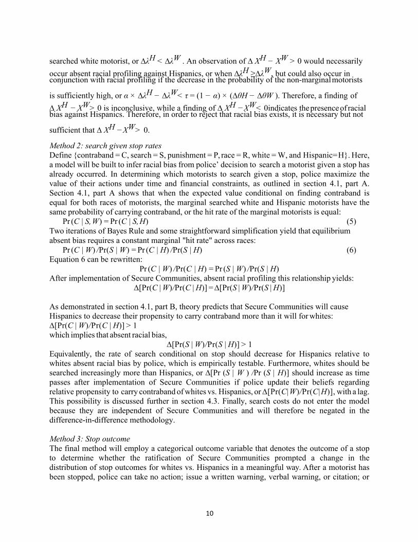
searched white motorist, or ∆λH < ∆λW . An observation of ∆ XH − XW > 0 would necessarilyoccur absent racial profiling against Hispanics, or when ∆λH ≥∆λW, but could also occur in conjunction with racial profiling if the decrease in the probability of the non-marginal motorists

is sufficiently high, or α × ∆λH − ∆λW< τ = (1 − α) × (∆θH − ∆θW ). Therefore, a finding of∆ XH − XW> 0 is inconclusive, while a finding of ∆ XH −XW< 0indicates the presence of racial bias against Hispanics. Therefore, in order to reject that racial bias exists, it is necessary but not

sufficient that ∆ XH −XW> 0.

Method 2: search given stop rates Define {contraband = C, search = S, punishment = P, race = R, white = W, and Hispanic= H}. Here, a model will be built to infer racial bias from police’ decision to search a motorist given a stop has already occurred. In determining which motorists to search given a stop, police maximize the value of their actions under time and financial constraints, as outlined in section 4.1, part A. Section 4.1, part A shows that when the expected value conditional on finding contraband is equal for both races of motorists, the marginal searched white and Hispanic motorists have the same probability of carrying contraband, or the hit rate of the marginal motorists is equal:

Pr (C | S, W) = Pr (C | S, H) (5) Two iterations of Bayes Rule and some straightforward simplification yield that equilibrium absent bias requires a constant marginal "hit rate" across races:

Pr (C | W) /Pr(S | W) = Pr (C | H) /Pr(S | H) (6) Equation 6 can be rewritten:

Pr (C | W) /Pr(C | H) = Pr (S | W) /Pr(S | H) After implementation of Secure Communities, absent racial profiling this relationship yields:

∆[Pr(C | W)/Pr(C | H)] = ∆[Pr(S | W)/Pr(S | H)]

As demonstrated in section 4.1, part B, theory predicts that Secure Communities will cause Hispanics to decrease their propensity to carry contraband more than it will for whites: ∆[Pr(C | W)/Pr(C | H)] > 1 which implies that absent racial bias,

∆[Pr(S | W)/Pr(S | H)] > 1 Equivalently, the rate of search conditional on stop should decrease for Hispanics relative to whites absent racial bias by police, which is empirically testable. Furthermore, whites should be searched increasingly more than Hispanics, or ∆[Pr (S | W ) /Pr (S | H)] should increase as time passes after implementation of Secure Communities if police update their beliefs regarding relative propensity to carry contraband of whites vs. Hispanics, or ∆[Pr(C|W)/Pr(C|H)], with a lag. This possibility is discussed further in section 4.3. Finally, search costs do not enter the model because they are independent of Secure Communities and will therefore be negated in the difference-in-difference methodology.

Method 3: Stop outcome The final method will employ a categorical outcome variable that denotes the outcome of a stop to determine whether the ratification of Secure Communities prompted a change in the distribution of stop outcomes for whites vs. Hispanics in a meaningful way. After a motorist has been stopped, police can take no action; issue a written warning, verbal warning, or citation; or

11

arrest the stopped motorist. In parallel with the model of taste based discrimination developed by Becker (1957), the utility of a police officer is a function of the action they take against the stopped motorist, or decision d, and the race of the motorist, which for this purpose is either white or Hispanic, R = {W, H}. Assume police receive utility from doing their job well, Uj (d), and from their treatment of people depending on their race.

The decision that maximizes the quality with which a police officer does his or her job is defined as d∗. Therefore, a police officer’s full utility function is:

U(d|R, d∗) = α ×[Uj (d) −Uj (d∗)] + U(d|H) × (R = H)With α > 0 and

1 (R = H) = 1 if R = H

0 if R = W

The outcome space for police officers can be reduced to three decisions for simplicity: arrest (d = a), citation (d = c), or no action (d = n), where n also includes both verbal and written warnings. Therefore a police officer chooses between three actions to maximize his/her utility:

U(a|R,d∗) = α×[Uj (a) −Uj (d∗)] + U(a|H) ×(1 | R = H)

U(c|R,d∗) = α×[Uj (c) −Uj (d∗)] + U(c|H) ×(1 | R = H)

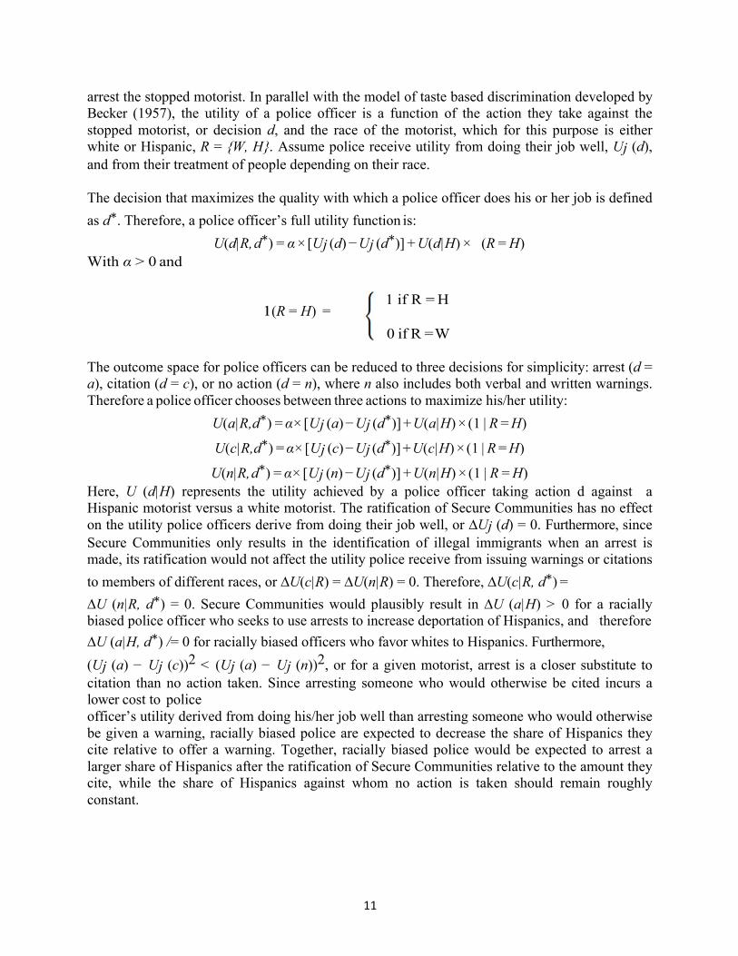
U(n|R, d∗) = α×[Uj (n) −Uj (d∗)] + U(n|H) ×(1 | R = H)Here, U (d|H) represents the utility achieved by a police officer taking action d against a Hispanic motorist versus a white motorist. The ratification of Secure Communities has no effect on the utility police officers derive from doing their job well, or ∆Uj (d) = 0. Furthermore, since Secure Communities only results in the identification of illegal immigrants when an arrest is made, its ratification would not affect the utility police receive from issuing warnings or citations to members of different races, or ∆U(c|R) = ∆U(n|R) = 0. Therefore, ∆U(c|R, d∗) =∆U (n|R, d∗) = 0. Secure Communities would plausibly result in ∆U (a|H) > 0 for a raciallybiased police officer who seeks to use arrests to increase deportation of Hispanics, and therefore ∆U (a|H, d∗) /= 0 for racially biased officers who favor whites to Hispanics. Furthermore,(Uj (a) − Uj (c))2 < (Uj (a) − Uj (n))2, or for a given motorist, arrest is a closer substitute tocitation than no action taken. Since arresting someone who would otherwise be cited incurs a lower cost to police officer’s utility derived from doing his/her job well than arresting someone who would otherwise be given a warning, racially biased police are expected to decrease the share of Hispanics they cite relative to offer a warning. Together, racially biased police would be expected to arrest a larger share of Hispanics after the ratification of Secure Communities relative to the amount they cite, while the share of Hispanics against whom no action is taken should remain roughly constant.

12

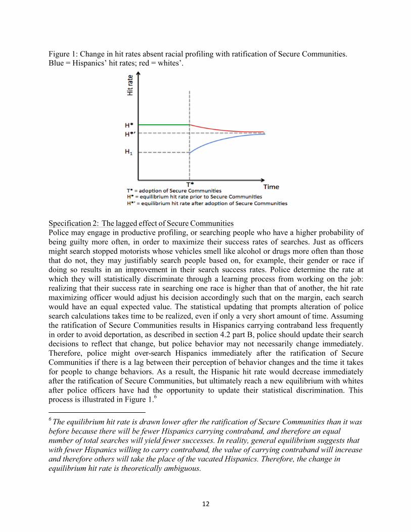
Figure 1: Change in hit rates absent racial profiling with ratification of Secure Communities. Blue = Hispanics’ hit rates; red = whites’.

Specification 2: The lagged effect of Secure Communities Police may engage in productive profiling, or searching people who have a higher probability of being guilty more often, in order to maximize their success rates of searches. Just as officers might search stopped motorists whose vehicles smell like alcohol or drugs more often than those that do not, they may justifiably search people based on, for example, their gender or race if doing so results in an improvement in their search success rates. Police determine the rate at which they will statistically discriminate through a learning process from working on the job: realizing that their success rate in searching one race is higher than that of another, the hit rate maximizing officer would adjust his decision accordingly such that on the margin, each search would have an equal expected value. The statistical updating that prompts alteration of police search calculations takes time to be realized, even if only a very short amount of time. Assuming the ratification of Secure Communities results in Hispanics carrying contraband less frequently in order to avoid deportation, as described in section 4.2 part B, police should update their search decisions to reflect that change, but police behavior may not necessarily change immediately. Therefore, police might over-search Hispanics immediately after the ratification of Secure Communities if there is a lag between their perception of behavior changes and the time it takes for people to change behaviors. As a result, the Hispanic hit rate would decrease immediately after the ratification of Secure Communities, but ultimately reach a new equilibrium with whites after police officers have had the opportunity to update their statistical discrimination. This process is illustrated in Figure 1.6

6 The equilibrium hit rate is drawn lower after the ratification of Secure Communities than it was before because there will be fewer Hispanics carrying contraband, and therefore an equal number of total searches will yield fewer successes. In reality, general equilibrium suggests that with fewer Hispanics willing to carry contraband, the value of carrying contraband will increase and therefore others will take the place of the vacated Hispanics. Therefore, the change in equilibrium hit rate is theoretically ambiguous.

13

To investigate the presence of potential statistical updating, the Secure Communities binary ratification variable was broken into a categorical variable that reflects how long prior to or after Secure Communities’ ratification a police stop takes place. These timing variables are described in the data section. While average hit rates might decrease for Hispanics after the ratification of Secure Communities, this might not be an indication of racial bias if the decreased average is caused by an immediate decrease in hit rate that later returns to equilibrium, as illustrated in Figure 1. The timing variables will help identify how racial profiling reacts to the ratification of Secure Communities and how long, if not instantaneously, police take to complete the statistical updating necessary for continued hit rate maximization.

5 Data

The data used come from Stop, Search, and Contraband datasets collected by the North Carolina State Bureau of Investigation, and include all motor vehicle stops in the state of North Carolina between January 1, 2004 and December 31, 2012. I restricted the data to observations with either a coded race of White or ethnicity of Hispanic. People who are listed as both white and Hispanic are considered Hispanic in the analysis, so the only people considered White are those who are both white and non-Hispanic. All people who are neither white nor Hispanic are excluded from analysis.

The SC, or Secure Communities, variable indicates the timing of the stop relative to the local implementation of Secure Communities. In specification 1, the Secure Communities variable, SC, indicates whether a stop takes place in a jurisdiction that has previously ratified Secure Communities at the time of the stop: 1

SC = 1 if stop occurs in county that has previously ratified Secure Communities

0 otherwise

In specification 2, Secure Communities will be categorical rather than binary and will reflect the time that has passed since Secure Communities was ratified in the jurisdiction where the stop was made. For these specifications, SecureCommunities implies that the stop took place during the stated 6 month interval after the ratification of Secure Communities, with stops in the control group taking place before the ratification of Secure Communities. The final Secure Communities timing variable uses data confined to stops within a period of three months prior to Secure Communities and 6 months after its ratification, and indicates the month in which the stop occurred. Relatedly, the variable 287g will mark whether the jurisdiction in which a stop takes place has previously adopted 287g, a provision that, as described in the background information section, allows local police involvement in immigration enforcement.

The level of discretion that the police have in making a search is reflected in the data by the type for the search, with higher discretion searches denoted by the binary variable HighDiscSearch. Following Pickerill, Mosher, and Pratt (2009), searches are marked as high discretion if their search type is consent or protective frisk, and low discretion if the type is due

14

to a search warrant, probable cause, or a search incident to arrest.

The time of a stop is marked at night if it is between the hours of 20:00 and 5:00. Additionally, 99 binary variables were created to add fixed effects for the 100 counties in which stops take place, and year fixed effects were added to the empirical model. The data also contains information on the age and gender of the motorist. The data is confined to stops made by local police within a named county, because the ratification date of Secure Communities is unclear for highway stops not made within county lines. The purpose of a stop is also recorded and will be controlled for:

The level of discretion for a stop is not reliably able to be inferred from its stated purpose, and there is therefore no measure of discretion for stops. All other variables will be used without manipulation. There are 3,837,247 motor vehicle stops and 268,372 motorist searches in the final dataset.

6 Empirical Methodology

As outlined in the theory section, three methods will be used to jointly determine whether the implementation of Secure Communities increased racial bias by police. Each method will use an extended difference-in-difference approach to isolate the effect of Secure Communities on the policing of whites vs. Hispanics. The methods will be distinguished by the unique outcome variable that each employs, and they will largely share covariates and controls in the difference-in- differences; each model will include available covariates to prevent confoundedness to the extent possible. There will likely still exist signals observable to the police but not the data analyst, like the smell of the car or the shiftiness of its driver’s eyes, but assuming these signals are not

15

correlated with both the outcome variable and the race/ethnicity of the driver, these omitted variables will not bias the results. Covariates used include the age, gender, and ethnicity of the driver; the county, time of day, and year of the stop; whether the stop was made in a jurisdiction that previously ratified 287g; whether the stop was before or after the implementation of Secure Communities (and in Specification 2 how long before or after the ratification of Secure Communities it was made); and the level of discretion associated with the search. The potential existence of omitted signals that correlate with both the outcome variable and race is a natural limitation of this analysis.

Method 1: Hit rates The first model will measure hit rates, which is the proportion of motor vehicle searches that yield contraband findings. To do so, it will employ a binary dependent variable of search outcome that indicates whether the motor vehicle search successfully uncoveredcontraband: 1

Contraband = 1 if contraband is found in a motor vehicle search

0 if no contraband is found

Since the outcome variable is whether or not police find contraband in a search, the data used to fit this model will be confined to the subset of stopped motorists who are searched.

The model will be fitted using a difference-in-difference-in-difference-in-difference (DDDD) methodology to attempt to isolate the effect of Secure Communities on the hit rates of whites vs. Hispanics. The first difference is whether the search occurs before vs. after the implementation of Secure Communities. By differencing before and after Secure Communities, pre-existing, baseline variation in the propensity of whites vs. Hispanics to carry contraband can be controlled for to isolate the effect of the implementation. The next difference will be Hispanics vs. whites. This difference prevents the influence of exogenous changes that affect the entire population over time (e.g., police budget cuts), and allows determination of how police behavior changed toward Hispanics relative to whites.

The third difference is whether the search occurred in jurisdictions that had previously ratified 287g vs. those that had not. Prior to the implementation of Secure Communities, 287g jurisdictions already provided local police the ability to aid in immigration enforcement and initiate the deportation process for illegal immigrants, so the ratification of Secure Communities in those jurisdictions did not change police incentives as much as in non-287g jurisdictions. Therefore, non-287g jurisdictions in which police incentives changed more dramatically are expected to experience greater effects of racial bias stemming from Secure Communities. The adoption of 287g requires an agreement between ICE and a local police jurisdiction, and is therefore self-selected by police jurisdictions, making it prone to confounding. It is likely that the jurisdictions that enacted 287g were, if anything, more predisposed to racial profiling against Hispanics, and therefore using them as a control group would, if anything, understate the effect that Secure Communities would have had on increasing racial bias in police absent the existence of 287g. This is another potential limitation of the analysis. The final difference used will be the discretion level of a search, as employed in Pickerill, Mosher, & Pratt (2009):

16

Police will be more able to exhibit racial bias in searches associated with higher discretion levels, so the effect of Secure Communities on racial bias should be more apparent for high relative to low discretion searches. The results of high and low discretion searches will be differenced to determine if this holds empirically.

Racial bias will be determined by the subset of variables that contain the inter- action Hispanic:SC, which is the effect of Secure Communities on search success rates of Hispanics relative to whites, controlling for the presence of 287g, search discretion, and available covariates.

Method 2: Search rates The second model will measure the rate at which motorists of different ethnicities are searched conditional on their being stopped. To do so, it will use a binary outcome variable for whether someone is searched:

Search = 1 if a stopped motorist is searched

0 if a stopped motorist is not searched

Since the outcome variable is whether or not police search a vehicle conditional on stop, the data used to fit this model will include all stopped motorists. The DDD methodology used in Method 2 is similar to that described in Method 1, but search discretion cannot be used since the outcome variable predicts search, and only searched motorists have a value of search discretion. Stop purpose will be controlled for but different purposes are not reliably correlated with police discretion.

Again, racial bias will be determined by the subset of variables that contain the interaction Hispanic:SC, which is the effect of Secure Communities on police propensity to search Hispanics relative to whites, controlling for the presence of 287g and available covariates.

Method 3: Stop outcome The fourth model will measure the change in probability of different stop out- comes for whites

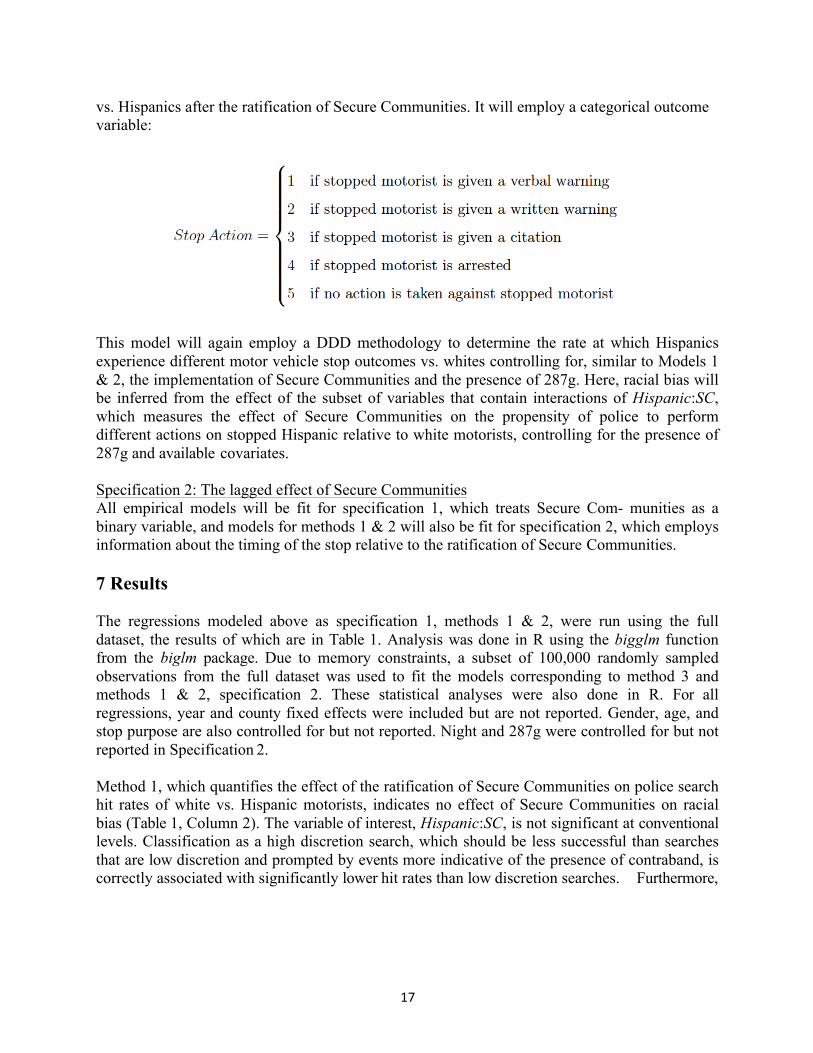
17

vs. Hispanics after the ratification of Secure Communities. It will employ a categorical outcome variable:

This model will again employ a DDD methodology to determine the rate at which Hispanics experience different motor vehicle stop outcomes vs. whites controlling for, similar to Models 1 & 2, the implementation of Secure Communities and the presence of 287g. Here, racial bias will be inferred from the effect of the subset of variables that contain interactions of Hispanic:SC, which measures the effect of Secure Communities on the propensity of police to perform different actions on stopped Hispanic relative to white motorists, controlling for the presence of 287g and available covariates.

Specification 2: The lagged effect of Secure Communities All empirical models will be fit for specification 1, which treats Secure Com- munities as a binary variable, and models for methods 1 & 2 will also be fit for specification 2, which employs information about the timing of the stop relative to the ratification of Secure Communities.

7 Results

The regressions modeled above as specification 1, methods 1 & 2, were run using the full dataset, the results of which are in Table 1. Analysis was done in R using the bigglm function from the biglm package. Due to memory constraints, a subset of 100,000 randomly sampled observations from the full dataset was used to fit the models corresponding to method 3 and methods 1 & 2, specification 2. These statistical analyses were also done in R. For all regressions, year and county fixed effects were included but are not reported. Gender, age, and stop purpose are also controlled for but not reported. Night and 287g were controlled for but not reported in Specification 2.

Method 1, which quantifies the effect of the ratification of Secure Communities on police search hit rates of white vs. Hispanic motorists, indicates no effect of Secure Communities on racial bias (Table 1, Column 2). The variable of interest, Hispanic:SC, is not significant at conventional levels. Classification as a high discretion search, which should be less successful than searches that are low discretion and prompted by events more indicative of the presence of contraband, is correctly associated with significantly lower hit rates than low discretion searches. Furthermore,

18

Hispanics are searched with higher probability in high discretion searches vs. low discretion searches after the ratification of Secure Communities, further rejecting increased racial bias due to Secure Communities. Similarly, 287g was found to be associated with higher hit rates for Hispanics vs. whites, indicating that it also did not prompt increased racial bias by police. There was no significant difference in the effect of Secure Communities in areas that had and had not previously adopted 287g. With 268,372 observations, any lack of significance is not due to a lack of precision or power in the analysis, but rather a lack of measurable effect.

Method 2, which quantifies the effect of ratification of Secure Communities on the rate at which Hispanics vs. whites are searched conditional on being stopped, also provides no evidence that Secure Communities affected racial bias by police (Table 1, Column 1). The variable of interest, Hispanic:SC, is significantly negative, indicating that fewer Hispanics were searched conditional on being stopped after the ratification of Secure Communities. Therefore, while Hispanics may be searched significantly more in general, this disparity is not exacerbated by Secure Communities. The decrease in search rate that occurs after ratification of Secure Communities is partially reversed for stops made in areas that had previously adopted 287g, but the net effect of Secure Communities still does not suggest an increase in racial bias.

Method 3, which assesses the propensity of police to take different actions against stopped motorists, the results of which are presented in Table 2, also suggests no evidence of racial bias by police. There is no significant effect of Secure Communities on the rate at which Hispanics versus whites are arrested, relative to given warnings or cited. Hispanics are arrested relatively more after the ratification of Secure Communities in places that had previously adopted 287g, but less at night, the aggregation of which yield no evidence that Secure Communities caused an increase in racial bias by police.

The regressions fit to model Methods 1 & 2 were re-run with Secure Communities timing indicator variables to assess the existence of a lagged effect of Secure Communities, the results of which are included in tables 3-4. The month indicators do not help to tell a story that indicates racial bias or updating of statistical discrimination as outlined in section 4.3. There are no discernible trends of the measured effect of the ratification of Secure Communities on racial bias of police against Hispanics versus whites. This result provides compelling evidence against the theory that Secure Communities led to increased racial bias by police. The results also suggest that either there was no change in the behavior of whites versus Hispanics after the implementation of Secure Communities, or that police behavior adjusted instantaneously in response to any changes in the behavior of Hispanics versus whites.

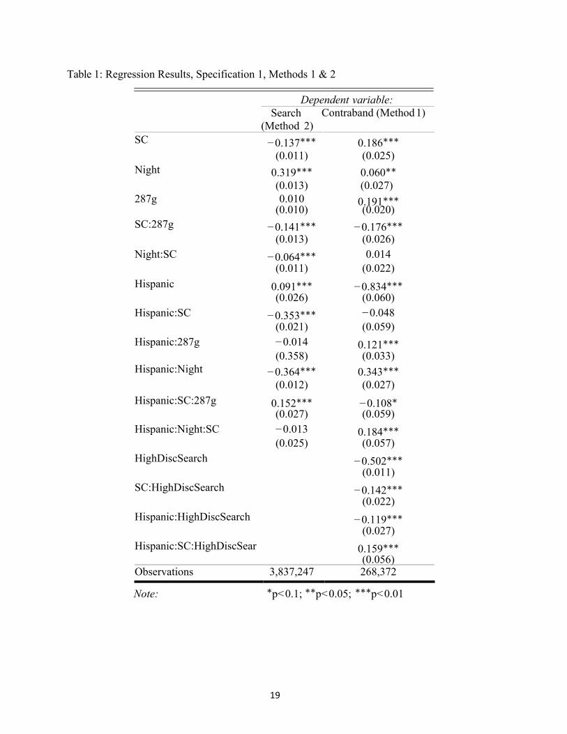
19

Table 1: Regression Results, Specification 1, Methods 1 & 2

Dependent variable: Search

(Method 2) Contraband (Method 1)

SC −0.137∗∗∗ 0.186∗∗∗ (0.011) (0.025)

Night 0.319∗∗∗ 0.060∗∗ (0.013) (0.027)

287g 0.010 0.191∗∗∗ (0.010) (0.020)

SC:287g −0.141∗∗∗ −0.176∗∗∗ (0.013) (0.026)

Night:SC −0.064∗∗∗ 0.014 (0.011) (0.022)

Hispanic 0.091∗∗∗ −0.834∗∗∗ (0.026) (0.060)

Hispanic:SC −0.353∗∗∗ −0.048 (0.021) (0.059)

Hispanic:287g −0.014 0.121∗∗∗ (0.358) (0.033)

Hispanic:Night −0.364∗∗∗ 0.343∗∗∗ (0.012) (0.027)

Hispanic:SC:287g 0.152∗∗∗ −0.108∗ (0.027) (0.059)

Hispanic:Night:SC −0.013 0.184∗∗∗ (0.025) (0.057)

HighDiscSearch −0.502∗∗∗ (0.011)

SC:HighDiscSearch −0.142∗∗∗ (0.022)

Hispanic:HighDiscSearch −0.119∗∗∗ (0.027)

Hispanic:SC:HighDiscSear 0.159∗∗∗ (0.056) Observations 3,837,247 268,372

Note: ∗p<0.1; ∗∗p<0.05; ∗∗∗p<0.01

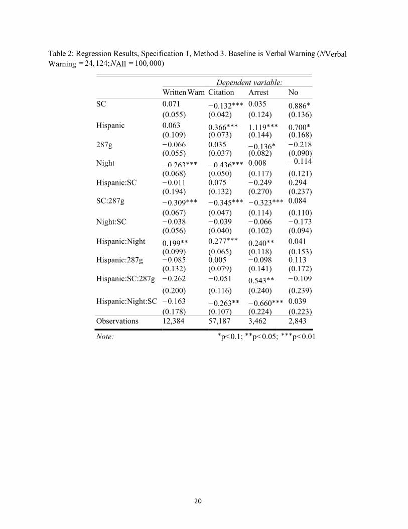
20

Table 2: Regression Results, Specification 1, Method 3. Baseline is Verbal Warning (NVerbal Warning = 24, 124; NAll = 100, 000)

Dependent variable:

Written Warn Citation Arrest No

SC 0.071 −0.132∗∗∗ 0.035 0.886∗ (0.055) (0.042) (0.124) (0.136)

Hispanic 0.063 0.366∗∗∗ 1.119∗∗∗ 0.700∗ (0.109) (0.073) (0.144) (0.168)

287g −0.066 0.035 −0.136∗ −0.218 (0.055) (0.037) (0.082) (0.090)

Night −0.263∗∗∗ −0.436∗∗∗ 0.008 −0.114 (0.068) (0.050) (0.117) (0.121) Hispanic:SC −0.011 0.075 −0.249 0.294 (0.194) (0.132) (0.270) (0.237) SC:287g −0.309∗∗∗ −0.345∗∗∗ −0.323∗∗∗ 0.084 (0.067) (0.047) (0.114) (0.110) Night:SC −0.038 −0.039 −0.066 −0.173 (0.056) (0.040) (0.102) (0.094) Hispanic:Night 0.199∗∗ 0.277∗∗∗ 0.240∗∗ 0.041 (0.099) (0.065) (0.118) (0.153) Hispanic:287g −0.085 0.005 −0.098 0.113 (0.132) (0.079) (0.141) (0.172) Hispanic:SC:287g −0.262 −0.051 0.543∗∗ −0.109

(0.200) (0.116) (0.240) (0.239) Hispanic:Night:SC −0.163 −0.263∗∗ −0.660∗∗∗ 0.039 (0.178) (0.107) (0.224) (0.223) Observations 12,384 57,187 3,462 2,843

Note: ∗p<0.1; ∗∗p<0.05; ∗∗∗p<0.01

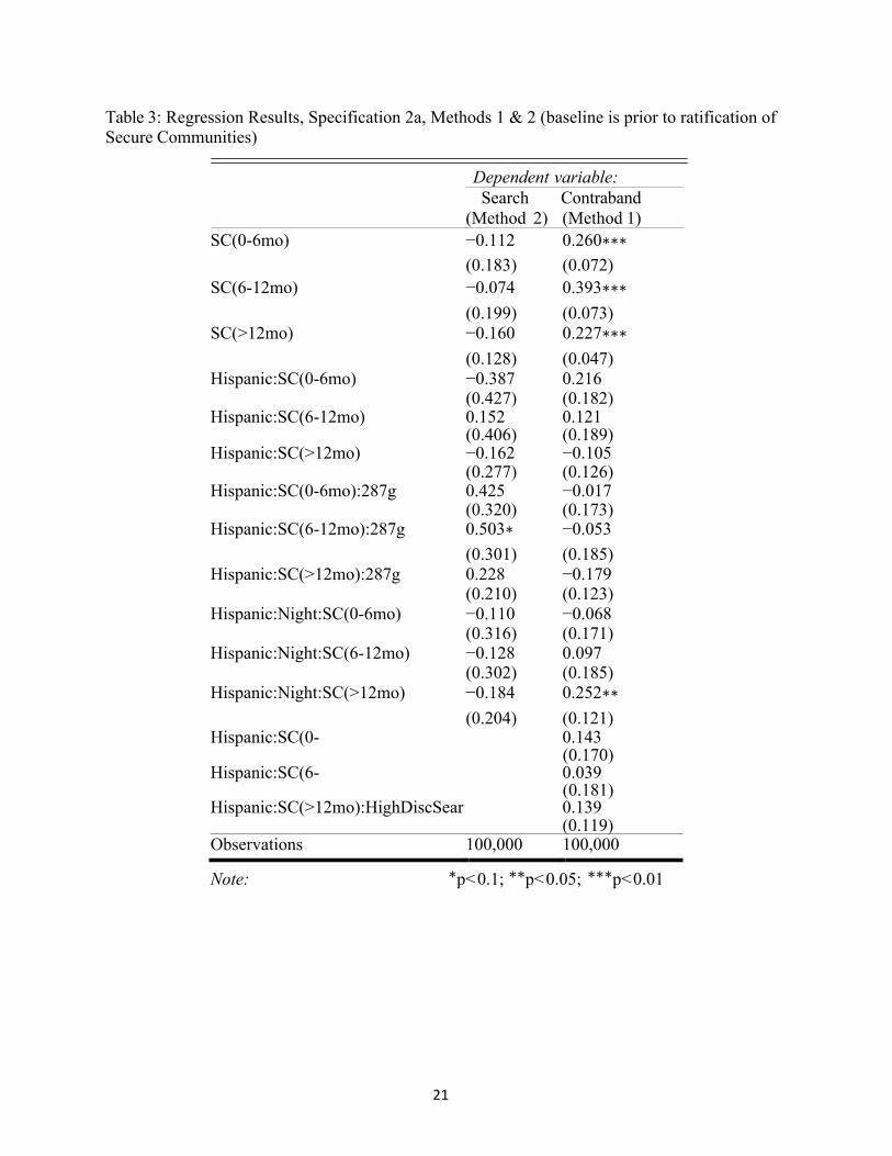
21

Table 3: Regression Results, Specification 2a, Methods 1 & 2 (baseline is prior to ratification of Secure Communities)

Dependent variable: Search

(Method 2) Contraband (Method 1)

SC(0-6mo) −0.112 0.260∗∗∗ (0.183) (0.072)

SC(6-12mo) −0.074 0.393∗∗∗ (0.199) (0.073)

SC(>12mo) −0.160 0.227∗∗∗ (0.128) (0.047)

Hispanic:SC(0-6mo) −0.387 0.216 (0.427) (0.182)

Hispanic:SC(6-12mo) 0.152 0.121 (0.406) (0.189)

Hispanic:SC(>12mo) −0.162 −0.105 (0.277) (0.126)

Hispanic:SC(0-6mo):287g 0.425 −0.017 (0.320) (0.173)

Hispanic:SC(6-12mo):287g 0.503∗ −0.053 (0.301) (0.185)

Hispanic:SC(>12mo):287g 0.228 −0.179 (0.210) (0.123)

Hispanic:Night:SC(0-6mo) −0.110 −0.068 (0.316) (0.171)

Hispanic:Night:SC(6-12mo) −0.128 0.097 (0.302) (0.185)

Hispanic:Night:SC(>12mo) −0.184 0.252∗∗ (0.204) (0.121)

Hispanic:SC(0- 0.143 (0.170)

Hispanic:SC(6- 0.039 (0.181)

Hispanic:SC(>12mo):HighDiscSear 0.139 (0.119) Observations 100,000 100,000

Note: ∗p<0.1; ∗∗p<0.05; ∗∗∗p<0.01

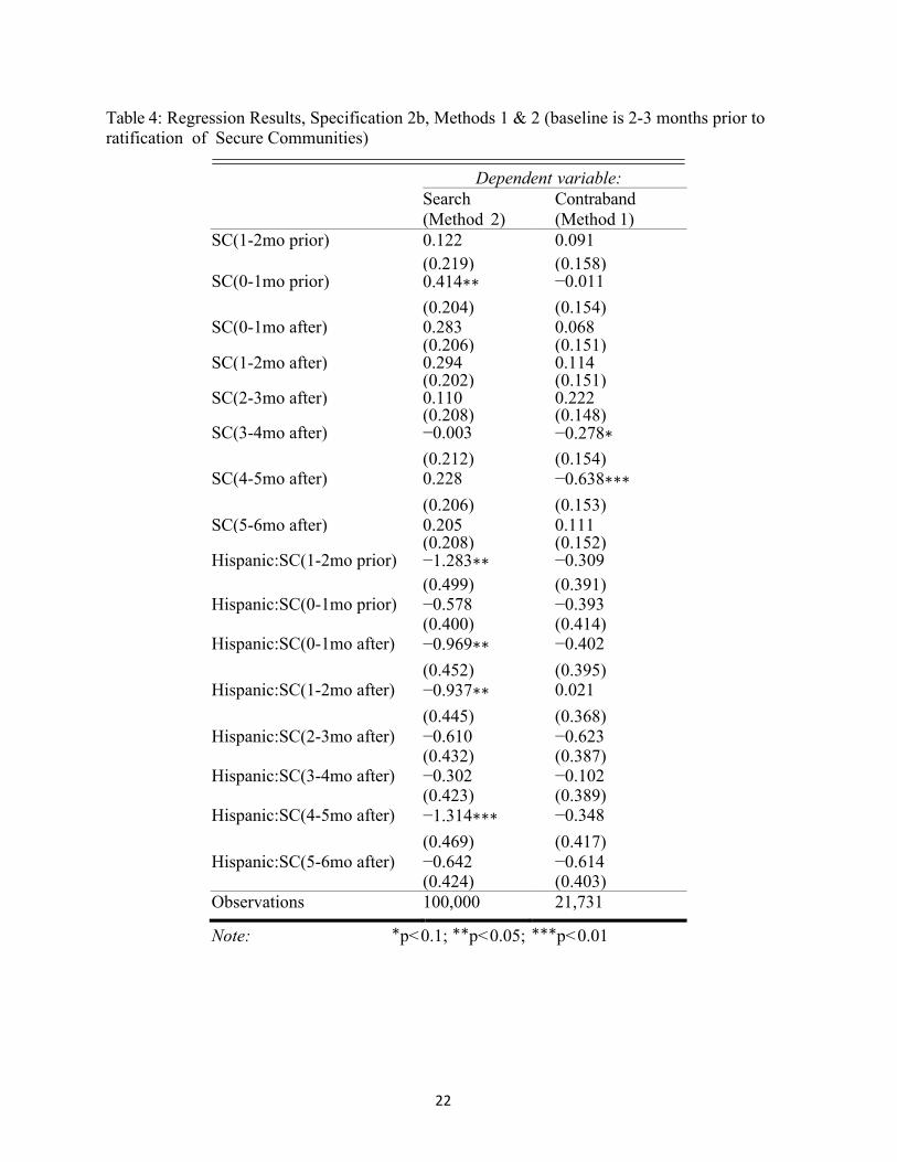
22

Table 4: Regression Results, Specification 2b, Methods 1 & 2 (baseline is 2-3 months prior to ratification of Secure Communities)

Dependent variable: Search

(Method 2) Contraband (Method 1)

SC(1-2mo prior) 0.122 0.091 (0.219) (0.158) SC(0-1mo prior) 0.414∗∗ −0.011 (0.204) (0.154) SC(0-1mo after) 0.283 0.068 (0.206) (0.151) SC(1-2mo after) 0.294 0.114 (0.202) (0.151) SC(2-3mo after) 0.110 0.222 (0.208) (0.148) SC(3-4mo after) −0.003 −0.278∗ (0.212) (0.154) SC(4-5mo after) 0.228 −0.638∗∗∗ (0.206) (0.153) SC(5-6mo after) 0.205 0.111 (0.208) (0.152) Hispanic:SC(1-2mo prior) −1.283∗∗ −0.309 (0.499) (0.391) Hispanic:SC(0-1mo prior) −0.578 −0.393 (0.400) (0.414) Hispanic:SC(0-1mo after) −0.969∗∗ −0.402 (0.452) (0.395) Hispanic:SC(1-2mo after) −0.937∗∗ 0.021 (0.445) (0.368) Hispanic:SC(2-3mo after) −0.610 −0.623 (0.432) (0.387) Hispanic:SC(3-4mo after) −0.302 −0.102 (0.423) (0.389) Hispanic:SC(4-5mo after) −1.314∗∗∗ −0.348 (0.469) (0.417) Hispanic:SC(5-6mo after) −0.642 −0.614 (0.424) (0.403) Observations 100,000 21,731

Note: ∗p<0.1; ∗∗p<0.05; ∗∗∗p<0.01

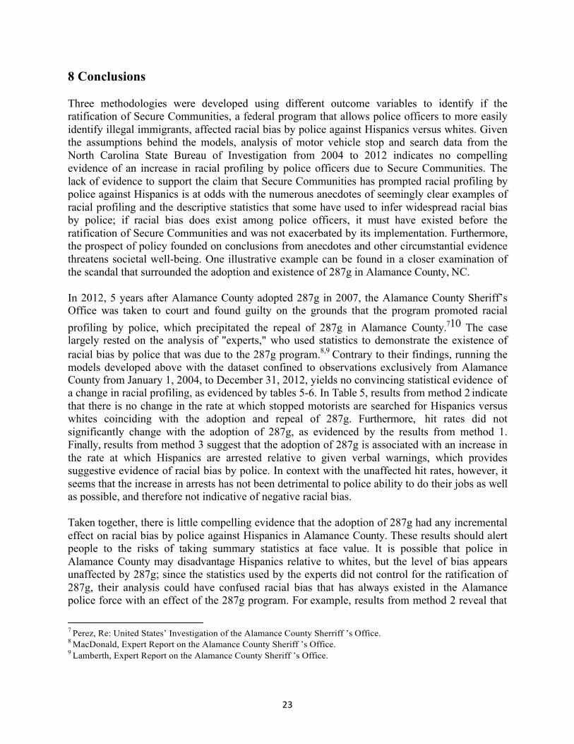
23

8 Conclusions

Three methodologies were developed using different outcome variables to identify if the ratification of Secure Communities, a federal program that allows police officers to more easily identify illegal immigrants, affected racial bias by police against Hispanics versus whites. Given the assumptions behind the models, analysis of motor vehicle stop and search data from the North Carolina State Bureau of Investigation from 2004 to 2012 indicates no compelling evidence of an increase in racial profiling by police officers due to Secure Communities. The lack of evidence to support the claim that Secure Communities has prompted racial profiling by police against Hispanics is at odds with the numerous anecdotes of seemingly clear examples of racial profiling and the descriptive statistics that some have used to infer widespread racial bias by police; if racial bias does exist among police officers, it must have existed before the ratification of Secure Communities and was not exacerbated by its implementation. Furthermore, the prospect of policy founded on conclusions from anecdotes and other circumstantial evidence threatens societal well-being. One illustrative example can be found in a closer examination of the scandal that surrounded the adoption and existence of 287g in Alamance County, NC.

In 2012, 5 years after Alamance County adopted 287g in 2007, the Alamance County Sheriff’s Office was taken to court and found guilty on the grounds that the program promoted racial profiling by police, which precipitated the repeal of 287g in Alamance County.710 The case largely rested on the analysis of "experts," who used statistics to demonstrate the existence of racial bias by police that was due to the 287g program.8,9 Contrary to their findings, running the models developed above with the dataset confined to observations exclusively from Alamance County from January 1, 2004, to December 31, 2012, yields no convincing statistical evidence of a change in racial profiling, as evidenced by tables 5-6. In Table 5, results from method 2 indicate that there is no change in the rate at which stopped motorists are searched for Hispanics versus whites coinciding with the adoption and repeal of 287g. Furthermore, hit rates did not significantly change with the adoption of 287g, as evidenced by the results from method 1. Finally, results from method 3 suggest that the adoption of 287g is associated with an increase in the rate at which Hispanics are arrested relative to given verbal warnings, which provides suggestive evidence of racial bias by police. In context with the unaffected hit rates, however, it seems that the increase in arrests has not been detrimental to police ability to do their jobs as well as possible, and therefore not indicative of negative racial bias.

Taken together, there is little compelling evidence that the adoption of 287g had any incremental effect on racial bias by police against Hispanics in Alamance County. These results should alert people to the risks of taking summary statistics at face value. It is possible that police in Alamance County may disadvantage Hispanics relative to whites, but the level of bias appears unaffected by 287g; since the statistics used by the experts did not control for the ratification of 287g, their analysis could have confused racial bias that has always existed in the Alamance police force with an effect of the 287g program. For example, results from method 2 reveal that

7 Perez, Re: United States’ Investigation of the Alamance County Sherriff ’s Office. 8 MacDonald, Expert Report on the Alamance County Sheriff ’s Office. 9 Lamberth, Expert Report on the Alamance County Sheriff ’s Office.

24

Hispanics in Alamance County are significantly more likely to be searched conditional on stop relative to whites, and results from method 3 indicate that police are significantly more likely to arrest or give a citation to a stopped Hispanic motorist relative to a white motorist. If this illustrative conjecture is true, citizens may be appeased by the repeal of 287g, but it would not actually solve the problem of racial bias in Alamance County. A better policy would allow 287g to continue but attempt to decrease racial bias in the Alamance County Police by putting officers through training programs, hiring a more diverse police force, or relieving the officers with the most severe record of bias of their duties.

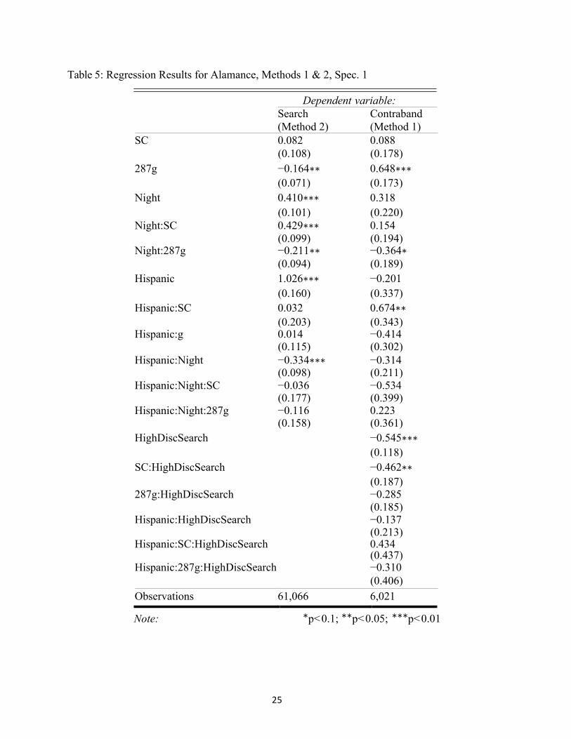
25

Table 5: Regression Results for Alamance, Methods 1 & 2, Spec. 1

Dependent variable: Search (Method 2)

Contraband (Method 1)

SC 0.082 0.088 (0.108) (0.178)

287g −0.164∗∗ 0.648∗∗∗ (0.071) (0.173)

Night 0.410∗∗∗ 0.318 (0.101) (0.220)

Night:SC 0.429∗∗∗ 0.154 (0.099) (0.194)

Night:287g −0.211∗∗ −0.364∗ (0.094) (0.189)

Hispanic 1.026∗∗∗ −0.201 (0.160) (0.337)

Hispanic:SC 0.032 0.674∗∗ (0.203) (0.343)

Hispanic:g 0.014 −0.414 (0.115) (0.302)

Hispanic:Night −0.334∗∗∗ −0.314 (0.098) (0.211)

Hispanic:Night:SC −0.036 −0.534 (0.177) (0.399)

Hispanic:Night:287g −0.116 0.223 (0.158) (0.361)

HighDiscSearch −0.545∗∗∗ (0.118)

SC:HighDiscSearch −0.462∗∗ (0.187)

287g:HighDiscSearch −0.285 (0.185)

Hispanic:HighDiscSearch −0.137 (0.213)

Hispanic:SC:HighDiscSearch 0.434 (0.437)

Hispanic:287g:HighDiscSearch −0.310 (0.406)

Observations 61,066 6,021

Note: ∗p<0.1; ∗∗p<0.05; ∗∗∗p<0.01

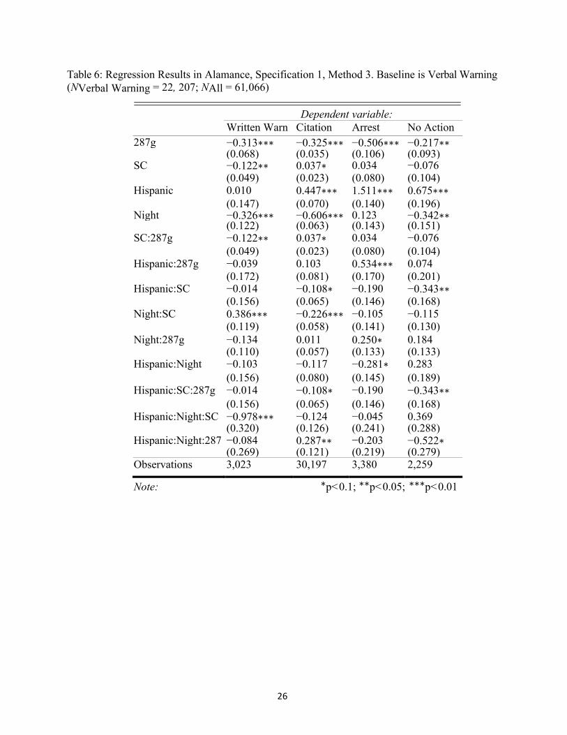
26

Table 6: Regression Results in Alamance, Specification 1, Method 3. Baseline is Verbal Warning (NVerbal Warning = 22, 207; NAll = 61,066)

Dependent variable:

Note: ∗p<0.1; ∗∗p<0.05; ∗∗∗p<0.01

Written Warn Citation Arrest No Action 287g −0.313∗∗∗ −0.325∗∗∗ −0.506∗∗∗ −0.217∗∗ (0.068) (0.035) (0.106) (0.093) SC −0.122∗∗ 0.037∗ 0.034 −0.076 (0.049) (0.023) (0.080) (0.104) Hispanic 0.010 0.447∗∗∗ 1.511∗∗∗ 0.675∗∗∗ (0.147) (0.070) (0.140) (0.196) Night −0.326∗∗∗ −0.606∗∗∗ 0.123 −0.342∗∗ (0.122) (0.063) (0.143) (0.151) SC:287g −0.122∗∗ 0.037∗ 0.034 −0.076 (0.049) (0.023) (0.080) (0.104) Hispanic:287g −0.039 0.103 0.534∗∗∗ 0.074 (0.172) (0.081) (0.170) (0.201) Hispanic:SC −0.014 −0.108∗ −0.190 −0.343∗∗ (0.156) (0.065) (0.146) (0.168) Night:SC 0.386∗∗∗ −0.226∗∗∗ −0.105 −0.115 (0.119) (0.058) (0.141) (0.130) Night:287g −0.134 0.011 0.250∗ 0.184 (0.110) (0.057) (0.133) (0.133) Hispanic:Night −0.103 −0.117 −0.281∗ 0.283 (0.156) (0.080) (0.145) (0.189) Hispanic:SC:287g −0.014 −0.108∗ −0.190 −0.343∗∗ (0.156) (0.065) (0.146) (0.168) Hispanic:Night:SC −0.978∗∗∗ −0.124 −0.045 0.369 (0.320) (0.126) (0.241) (0.288) Hispanic:Night:287 −0.084 0.287∗∗ −0.203 −0.522∗ (0.269) (0.121) (0.219) (0.279) Observations 3,023 30,197 3,380 2,259

27

Bibliography

Albert, Jared I. “ How Secure is Secure Communities? The Future of One of ICE’s most Controversial Programs”. In: Georgetown Immigration Law Journal (2011). Antonovics, Kate and Brian G. Knight. “ A New Look at Racial Profiling: Evidence from the Boston Police Department”. In: Review of Economics and Statistics 91.1 (2009), pp. 163–177. url: http://dx.doi.org/10.1162/rest.91.1.163.

Anwar, Shamena and Hanming Fang. “ An Alternative Test of Racial Prejudice in Motor Vehicle Searches: Theory

and Evidence”. In: National Bureau of Economic Research Working Paper Series No. 11264 (2005). url: http://www.nber.org/ papers/w11264;%20http://www.nber.org/papers/w11264.pdf.

Becker, Gary S. The Economics of Discrimination. Chicago: Univ. Chicago Press, 1957.

Bjerk, David. “ Racial Profiling, Statistical Discrimination, and the Effect of a Col- orblind Policy on the Crime

Rate”. In: Journal of Public Economic Theory 9.3 (2007), pp.521–545.

Brock, William A. et al. “ On the observational implications of taste-based discrim- ination in racial profiling”. In: Journal of Econometrics 166.1 (2012), pp. 66– 78.

Bunzel, Helle and Philippe Marcoul. “Can racially unbiased police perpetuate long- run discrimination?” In: Journal

of Economic Behavior & Organization 68.1 (2008), pp. 36–47.

Charles, Kerwin Kofi and Jonathan Guryan. “ Studying Discrimination: Fundamen- tal Challenges and Recent Progress”. In: National Bureau of Economic Research Working Paper Series No. 17156 (2011). url: http://www.nber.org/papers/ w17156;%20http://www.nber.org/papers/w17156.pdf.

Coleman, Mathew. “ The Local Migration State: The Site-Specific Devolution of Immigration Enforcement in the

U.S. South”. In: Law & Policy 34.2 (2012), pp. 159–190. url: http://dx.doi.org/10.1111/j.1467- 9930.2011.00358.x. Cox, Adam B. and Thomas J. Miles. “ Does Immigration Enforcement Reduce Crime? Evidence from Secure Communities”. In: Forthcoming The Journal of Law and Economics (2014).

— “ Policing Immigration”. In: The University of Chicago Law Review Vol. 80 (2012). url:

http://ssrn.com/abstract=2109820.

Dhammika, Dharmapala and L. Ross Stephen. “ Racial Bias in Motor Vehicle Searches: Additional Theory and Evidence”. In: The B.E.Journal of Economic Analysis & Policy 3.1 (2004), pp. 1–23. url: http://ideas.repec.org/a/bpj/bejeap/ vcontributions.3y2004i1n12.html.

Dominitz, Jeff and John Knowles. “ Crime minimisation and racial bias: what can we learn from police search

data?” In: The Economic Journal 116.515 (2006), pp. 368–384.

Donohue III, John J. and Steven D. Levitt. “ The Impact of Race on Policing and Arrests”. English. In: Journal of Law and Economics 44.2 (2001), pp. 367–394. url: http://www.jstor.org/stable/10.1086/322810.

Durlauf, Steven N. “ Assessing Racial Profiling”. English. In: The Economic Journal 116.515 (2006), pp. 402–426. url: http://www.jstor.org/stable/4121927.

Gill, Lindsey J. “ Secure Communities: Burdening Local Law Enforcement and Undermining the U Visa”. In:

William & Mary Law Review (2013). 54 Wm. & Mary L. Rev. 2055; 14209 words.

Glaser, Jack. “ The Efficacy and Effect of Racial Profiling: A Mathematical Simula- tion Approach”. English. In: Journal of Policy Analysis and Management 25.2 (2006), pp. 395–416. url: http://www.jstor.org/stable/30162726.

28

Grogger, Jeffrey and Greg Ridgeway. “ Testing for Racial Profiling in Traffic Stops From Behind a Veil of Darkness”. In: Journal of the American Statistical Associ- ation 101 (2006), pp. 878–887. url:

http://ideas.repec.org/a/bes/jnlasa/ v101y2006p878-887.html.

Hanson, Gordon H. “ Illegal Migration from Mexico to the United States”. English. In: Journal of Economic Literature 44.4 (2006), pp. 869–924. url: http://www. jstor.org/stable/30032389.

Heaton, Paul. “ Understanding the Effects of Antiprofiling Policies”. English. In: Journal of Law and Economics

53.1 (Feb. 2010), pp. 29–64. url: http://www. jstor.org/stable/10.1086/649645.

Hernandez-Murillo, Rubin and John Knowles. “ Racial Profiling Or Racist Polic- ing? Bounds Tests in Aggregate Data”. In: International Economic Review 45.3 (2004), pp.959–989.

Immigration and Customs Enforcement. “ Delegation of Immigration Authority Sec- tion 287(g) Immigration and

Nationality Act”. In: U.S. Department of Homeland Security (2014).

Immigration and Customs Enforcement. “ Secure Communities”. In: U.S. Department of Homeland Security(2014).

— “ Secure Communities Monthly Statistics through May 31, 2013”. In: U.S. De- partment of Homeland Security. (2013).

Kang, Stephanie. “ A Rose by Any Other Name: The Chilling Effect of ICE’s "Se- cure" Communities Program”. In:

Hastings Race & Poverty Law Journal (2012). 9 Hastings Race & Poverty L.J. 83; 13457 words.

Knowles, John, Nicola Persico, and Petra Todd. “ Racial Bias in Motor Vehicle Searches: Theory and Evidence”. In: National Bureau of Economic Research Working Paper Series No. 7449 (1999). url: http://www.nber.org/papers/ w7449;%20http://www.nber.org/papers/w7449.pdf.

Kohli, Aarti, Peter L. Markowitz, and Lisa Chavez. “ Secure Communities by the Numbers: An Analysis of

Demographics and Due Process”. In:(2011).

Persico, Nicola. “ Racial Profiling? Detecting Bias Using Statistical Evidence”. In: Annual Review of Economics 1.1 (2009). doi: 10.1146/annurev.economics.050708.143307; 03, pp. 229–254. url: http:// dx. doi. org/ 10 . 1146 / annurev.economics. 050708.143307.

Persico, Nicola and Petra Todd. “ Generalising the Hit Rates Test for Racial Bias in Law Enforcement, With an

Application to Vehicle Searches in Wichita*”. In: The Economic Journal 116.515 (2006), F351–F367.

Petrocelli, Matthew, Alex R. Piquero, and Michael R. Smith. “ Conflict theory and racial profiling: An empirical analysis of police traffic stop data”. In: Journal of Criminal Justice 31.1 (2003), pp. 1–11.

Pickerill, J. Mitchell, Clayton Mosher, and Travis Pratt. “ Search and Seizure, Racial Profiling, and Traffic Stops: A

Disparate Impact Framework”. In: Law & Policy 31.1 (2009), pp. 1–30.

Ridgeway, Greg. Analysis of Racial Disparities in the New York Police Department’s Stop, Question, and Frisk Practices. Santa Monica, CA: RAND Corporation, 2007. url: http://www.rand.org/pubs/technical_reports/TR534.

Ridgeway, Greg and John M. MacDonald. “ Doubly Robust Internal Benchmarking and False Discovery Rates for

Detecting Racial Bias in Police Stops”. In: Journal of the American Statistical Association 104.486 (2009). doi: 10.1198/jasa.2009.0034; 03, pp. 661–668. url: http://dx.doi.org/10.1198/jasa.2009.0034.

29

Sanga, Sarath. “ Reconsidering Racial Bias in Motor Vehicle Searches: Theory and Evidence”. English. In: Journal of Political Economy 117.6 (2009), pp. 1155– 1159. url: http://www.jstor.org/stable/10.1086/649800.

Smith, Michael R. and Matthew Petrocelli. “ Racial Profiling? A Multivariate Analysis of Police Traffic Stop Data”.

In: Police Quarterly 4.1 (2001), pp. 4–27.

Tomic, Aleksandar and Jahn K. Hakes. “ Case Dismissed: Police Discretion and Racial Differences in Dismissals of Felony Charges”. In: American Law and Eco- nomics Review 10.1 (2008), pp. 110–141.

Warren, Patricia Y. and Donald Tomaskovic-Devey. “ Racial profiling and searches: Did the politics of racial

profiling change police behavior?” In: Criminology & Public Policy 8.2 (2009), pp. 343–369.

Weinstein, Hannah. “ S-Comm: Shattering Communities”. In: Cardozo Public Law, Policy & Ethics Journal (2012). 10 Cardozo Pub. L. Pol’y & Ethics J. 395; 18613 words.

30

JOINT-LIABILITY IN MICROCREDIT: EVIDENCE FROM BANGLADESH

HAMEEM RAEES CHOWDHURY †

MARCH 22, 2015

SUPERVISED BY DR. ROBERT AKERLOF*

ABSTRACT

The joint-liability lending model in microcredit predicts social ties between groups of borrowers to incentivise repayment; however it also promotes free riding behaviour. Repeated experimental games conducted in Bangladesh1 are used to empirically analyse key theoretical hypothesise predicted under joint- liability; treated groups of microcredit borrowers are compared to control groups of non-microcredit borrowers alongside questionnaire findings. Results show treated groups to more likely repay loans and subsequently play more rounds compared to control groups in the games. Treated individuals forego short-run gains from non-repayment and benefit from higher long-run gains from progressing onto further rounds. The paper also finds that treated individuals are significantly less likely to free ride and more likely to shoulder for their partner compared to control individuals. Optimal individual and group characteristics to maximise repayment under joint-liability are then identified.

Keywords: microcredit, joint-liability, social ties, free riding, repeated games JEL Classification: O16, G21, D21

Give a man a fish and he will eat for a day. Give a woman microcredit, and she, her husband, her children, and her extended family will eat for a lifetime.

But who feeds (repays) the lender?

†University of Warwick, H.R.Chowdhury@warwick.ac.uk *I am indebted to Dr. Robert Akerlof for his support and comments as supervisor, Dr. Jeremy Smith for his knowledge on empirical techniques, Dr. Md. Kayes Samim Polash of Proshikar with whom I conducted the field experiments, Dr. Robert Akerlof and Dr. Gianna Boero for nominating this paper for the Carroll Round (for which it earned Outstanding Participation) and British Conference of Undergraduate Research, Mr. Shakhawat Hossain of Jai Jai Din for bringing media attention to my field work, and numerous others. Any remaining errors are my own. 1 Repeated experimental games are conducted by the author on the field in Manikganj, Dhaka, Bangladesh (Dec 2014).

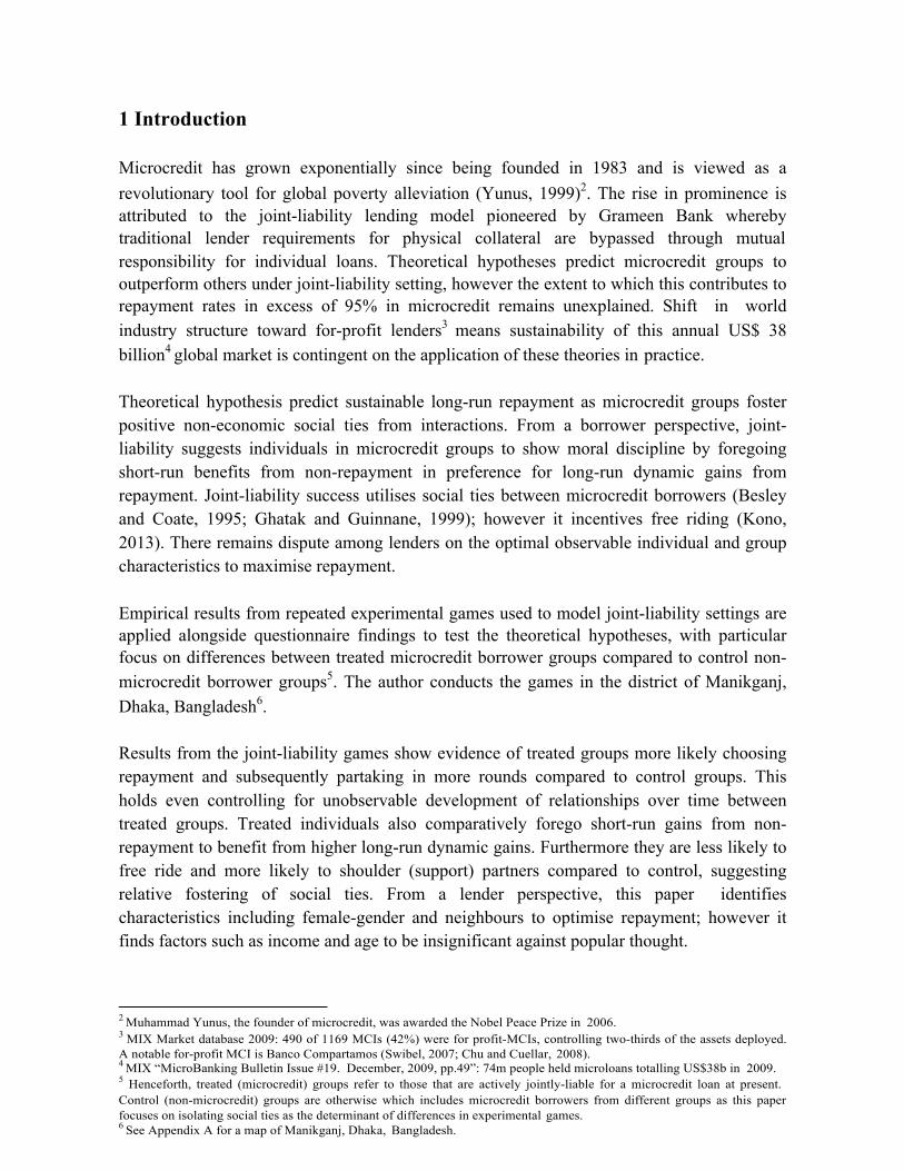
31

1 Introduction Microcredit has grown exponentially since being founded in 1983 and is viewed as a revolutionary tool for global poverty alleviation (Yunus, 1999)2. The rise in prominence is attributed to the joint-liability lending model pioneered by Grameen Bank whereby traditional lender requirements for physical collateral are bypassed through mutual responsibility for individual loans. Theoretical hypotheses predict microcredit groups to outperform others under joint-liability setting, however the extent to which this contributes to repayment rates in excess of 95% in microcredit remains unexplained. Shift in world industry structure toward for-profit lenders3 means sustainability of this annual US$ 38 billion4 global market is contingent on the application of these theories in practice.

Theoretical hypothesis predict sustainable long-run repayment as microcredit groups foster positive non-economic social ties from interactions. From a borrower perspective, joint- liability suggests individuals in microcredit groups to show moral discipline by foregoing short-run benefits from non-repayment in preference for long-run dynamic gains from repayment. Joint-liability success utilises social ties between microcredit borrowers (Besley and Coate, 1995; Ghatak and Guinnane, 1999); however it incentives free riding (Kono, 2013). There remains dispute among lenders on the optimal observable individual and group characteristics to maximise repayment.

Empirical results from repeated experimental games used to model joint-liability settings are applied alongside questionnaire findings to test the theoretical hypotheses, with particular focus on differences between treated microcredit borrower groups compared to control non- microcredit borrower groups5. The author conducts the games in the district of Manikganj, Dhaka, Bangladesh6.

Results from the joint-liability games show evidence of treated groups more likely choosing repayment and subsequently partaking in more rounds compared to control groups. This holds even controlling for unobservable development of relationships over time between treated groups. Treated individuals also comparatively forego short-run gains from non- repayment to benefit from higher long-run dynamic gains. Furthermore they are less likely to free ride and more likely to shoulder (support) partners compared to control, suggesting relative fostering of social ties. From a lender perspective, this paper identifies characteristics including female-gender and neighbours to optimise repayment; however it finds factors such as income and age to be insignificant against popular thought.

2 Muhammad Yunus, the founder of microcredit, was awarded the Nobel Peace Prize in 2006. 3 MIX Market database 2009: 490 of 1169 MCIs (42%) were for profit-MCIs, controlling two-thirds of the assets deployed. A notable for-profit MCI is Banco Compartamos (Swibel, 2007; Chu and Cuellar, 2008). 4 MIX “MicroBanking Bulletin Issue #19. December, 2009, pp.49”: 74m people held microloans totalling US$38b in 2009. 5 Henceforth, treated (microcredit) groups refer to those that are actively jointly-liable for a microcredit loan at present. Control (non-microcredit) groups are otherwise which includes microcredit borrowers from different groups as this paper focuses on isolating social ties as the determinant of differences in experimental games. 6 See Appendix A for a map of Manikganj, Dhaka, Bangladesh.

32

2 Related Literature

Microcredit gained traction subsequent to implementation of joint-liability lending7; between 1997 and 2005 the number of clients increased by 740% and institutions by 406%8. Higher market concentrations and transition toward for-profit lenders demand repayment rates in excess of 95% for sustainability (Hossein, 1988; Morduch, 1999)9. Theoretically, joint- liability success revolves around social ties within groups which counteract three key problems10: moral hazard11 (Banerjee et al., 1994; Laffont and Rey, 2003), adverse selection12 (Ghatak, 1999, 2000; Gangopadhyay et al., 2005), and free riding13 (Besley and Coate, 1995; Wydick, 2001; Bhole and Ogden, 2010). This paper isolates free riding, extending games by Kono (2013) by setting income exogenously and randomly selecting participants to control for moral hazard and adverse selection respectively.

Focusing therefore on social ties14 as solution to free riding, Besley and Coate (1995) and Ghatak and Guinnane (1999) theoretically prove high social ties deters group members shirking on repayments15. The former model defines benefits from repaying through dynamic incentives16 of future loans and avoiding social punishment; the latter uses historic and contemporary examples as proof, although there is ambiguity on the extent social ties explains the increased repayment.

Cason et al. (2009) and Zeller (1998) empirically show stronger social ties lead to improved repayment rates and lender profitability if it exceeds monitoring costs; and Abbink et.al (2006) finds group-lending to outperform individual-lending, although curiously self-selected groups show a higher yet less stable willingness to repay. This variance can be explained by contagion, a sub-set of group free riding where dominant strategy for individuals is to default should they observe high likelihood of default by the group. Contagion in joint-liability is evident in Mexico (Allen, 2012), Pakistan (Korusaki, 2012) and India (Breza, 2012). Abbink et.al (2006) provides evidence that the larger the loans, the bigger the incentive to free ride although the less lender and group tolerance toward defaulters. Inability to control 7 Joint-liability lending is interchangeable with group lending; it applies to 68% of all borrowers (Lapenu and Zeller, 2001). 8 See Daley-Harris, 2012; Mannan, 2014; for statistics on growth of MCIs. 9 Government credit programs have less than 25% repayment rate (Adams and Vogel, 1986; Braverman and Guasch, 1984). 10 See Frexias and Rochet, 1997; for the key problems for lenders of capital. 11 See Stiglitz, 1990; Varian (1990) for further theory on moral hazard. 12 See Akerlof, 1970 for further theory on adverse selection. 13 See Olson, 1965; for further theory on free-riding. 14 Social ties is interchangeable with the term social capital, defined as “features of social organisation such as trust, norms, and networks that can improve efficiency of society by facilitating co-ordinated actions” (Putnam et al. 1994). 15 Future inability to access loans should the group collectively be unable to repay their liabilities is an effective dynamic incentive device (Stiglitz and Weiss, 1983). The threat of future retaliation induces cooperative behaviour (Bo, 2005). 16 In reality many MCIs (e.g. Grameen Bank) do not impose future participation punishments (Todd, 1996; Rahman, 1999)

33

behavioural endogeneity which positively influences social ties and repayment is persistent across empirics. The counter-hypothesis is social ties reduce repayment through forgiveness toward defaults (Guinnane, 1994). Empirical study by Wydick (1999) and Cassar et al. (2007) applying games by Abbink et al. (2006) in Guatemala, South Africa, and Armenia respectively emphasise no significant gains from social ties, particularly for the latter comparing acquaintances groups against strangers17. The unobservable social ties are however measured by weakly correlated proxy dependant variables in the game structure which invalidate findings.

Theoretical research into changes from joint-liability to individual-liability hypothesise decreases in repayment ceteris paribus for groups with sufficient social ties (Banerjee et al., 1994), empirical examples being Peru where there is positive correlation between intra-group trustworthiness and strong social ties with higher repayment rates (Karlan, 2005; Karlan, 2007). In contrast other experiments show no difference after change from joint to individual liability (Gine and Yang, 2009; Gine and Karlan, 2009). Against popular literature the later deems excessive pressure of joint-liability to discourage good borrowers. The consensus however supports social ties, alongside features such as dynamic incentives and frequent instalment as important drivers of repayment rather than joint-liability itself (Armendariz de Aghion and Morduch, 2010). Townsend (2003) describes under theories of selection the ambiguity of Pareto optimal regimes subject to exogenous environmental characteristics; joint-liability as cure to free riding cannot be exemplified through one theory.

Comparing alternative game structures, findings in Malawi suggest no difference in repayment between joint and individual-liability (Schaefer-Kehnert, 1982). Kono (2006) counter-intuitively finds Vietnamese borrowers have lower repayment rate under joint- liability, even with peer monitoring and punishments through social ties. Thai microcredit programs show similar patterns of negative effects on repayment from social ties; positive gains to repayment are found to be possible only through high local sanctions and correlated returns (Ahlin and Townsend; 2007). Critically however the empirics did not control for other lending characteristics and endogenous selection of borrowers, and questions are raised at the excess regional variability. Kono (2013) bypasses endogeneity problems in conducting framed joint-liability experiments in Vietnam. His empirical findings conclude free-riding exceeds players helping group members, resulting in relative underperformance of joint- liability.

To the author’s knowledge, this paper is the first to investigate differences in repayment decisions between treated groups of microcredit borrowers against control groups of non- microcredit borrowers in identical joint-liability settings. Attanasio et al. (2001) and Banerjee et al. (2013) pioneered comparisons with treated groups; however the studies focus on poverty alleviation for women and development effects respectively.

17 This contradicts Gine et al. (2010) who suggested the opposite.

34

3 Model This paper models joint-liability settings through repeated experimental games to compare actions of treated microcredit groups against control non-microcredit groups, and in particular identifies the role of social ties versus free riding. The methodology used extends the model of repayment decisions utilised by Kono (2013).

The game is designed where at the beginning of each round each player i is allocated a stochastic income gi ∈[0, gi ] which is i.i.d. over individuals and rounds, representing exogenous investment returns funded by the loans18. Players in an n -person group are required to pay a repayment sum of nB collectively. Player i first chooses the action ri of whether to repay personal liability, B . If yes ( ri = B ), then player i is given the choice to shoulder (repay) di toward any remaining group liabilities. Repayment is dynamically incentivised as participation in the next round is contingent on full group repayment such that

n n

• ri + • di = nB ; otherwise all members in the group are eliminated. This represents i=1 i=1

borrowers only being able to access further loans subject to full group repayment under joint- liability irrespective of individual repayment decisions19. The discount factor, ⎣ is applied between periods to replicate a finite time horizon to the games where irrespective of outcome the game may end with probability 1/6 after each round ( ⎣ = 5/6) 20. Utility for player i of not receiving loans (thus inability to invest) is 0 .

The model assumes for two-player groups ( n = 2 ) that all players are unable to engage in any strategic interaction within groups outside of the experiment21, and that each stage is independent from the previous (players cannot save income from past periods). In contrast to prior experiments, imperfect monitoring is assumed whereby players cannot observe their group members’ income levels and decisions, and can only observe personal income, gi , and personal decisions ri and di ; hence players are unable to determine with certainty if group

n n

members are free riding. Note that if the group defaults where • ri + i=1 22

•di i=1

<nB , player i

loses ri +di as the lender does not return an individual’s repayment . Lender terms are not considered23 and assumed to be homogenous as it does not contribute to the paper’s focus on individual choice in a joint-liability setting.

18 Moral hazard is excluded as player incomes (returns on investment), g , are independent of their actions. 19 Inability for individuals to access future loans should the group default is an effective dynamic incentive device (Stiglitz and Weiss, 1983). The threat of future retaliation induces cooperative behaviour (Bo, 2005). 20 Assume ⎣ E ( g ) < 2B to exclude players having a dominant strategy of always repaying regardless. 21 Unrealistic as borrowers of microcredit live in the same community; to control for this experiments decisions are made face-to-face (Kono, 2014). Borrowers cannot enter binding contracts and outcomes are from repeated interactions. 22 Applies in reality assuming no strategic interaction between players such that players are unable to interact and agree on their decisions prior to repayment (contrary to model by Besley and Coate, 1995). 23 In practice lenders offer different terms to borrowers based on profit-seeking, past reputation, characteristics, risk etc.

35

The order of the decisions in round t can be summarised as follows:

1.Players i = 1, 2 are allocated stochastic income gi and simultaneously choose their repayment amount, ri , where i = 1, 2. The decisions (ri , rj ) are observed by both players.

2a.If ri =rj =B then both players have met group repayment conditions for the round.

2b.If ri = B but rj < B, j ↑ i , then player i has the option of shouldering (paying) di = B − rj for

the deficit of player j . By joint-liability, both players meet group repayment conditions for the round only in the scenario where player i pays the full deficit of player j . Vice versa if rj = B but ri < B, j ↑ i.

2c.

3.

If ri , rj < B , both players have not met group repayment conditions for the round (group default) and are eliminated. Given that both players have met group repayment conditions for the round where

n n

• ri + •di = nB , progression onto the next round is conditional on discount factor ⎣ =

4.

i=1

5/6. i=1

Both players in groups that progress participate in a further repetition in round t +1 .

Experimental Procedures The repeated experimental game is conducted in five rural villages in Manikganj, Bangladesh in December 2014. The experiments are conducted in village centres on random groups of n = 2 players, sampling 10% of the population from each village. Participating players first complete a verbal questionnaire24 before an explanation on taking part in the game25. This includes information on variables including if the group is a treated microcredit or control non-microcredit group26.

The repeated game is then administered; stochastic income for each player at the start of each period is privately allocated through the sum of the points of three randomly allocated cards, each representing either 10 points or 0 points forming three possible income values: g ∈{0,10, 20}27. The probability distribution of g is determined by q = (q , q , q )where

given q

g =Pr(gi =g ) , i 0 10 20

let q =(25%, 25%, 50%). Each player then simultaneously submits a card face down to represent repayment (10 ) or default ( 0 ). Should player i default, player j is then given the option of shouldering and must submit a further card face down to shoulder on their behalf ( 10 ) or otherwise ( 0 ). Players have satisfied group liabilities upon total group repayment of

24 See Appendix B for a copy of the questionnaire. 25 Questionnaire is done prior to game as otherwise game outcomes may affect questionnaire answers (Kono 2014). 26 microcredit is the key independent dummy variable of note. See Appendix C for definitions of all variables. 27 Minimum income is 0 (three cards of 0 points) and maximum income is 20 (two cards of 10 points, one card of 0 points).

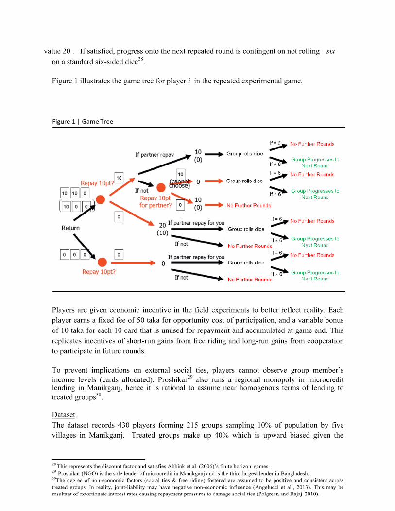
36

value 20 . If satisfied, progress onto the next repeated round is contingent on not rolling six on a standard six-sided dice28.

Figure 1 illustrates the game tree for player i in the repeated experimental game.

Players are given economic incentive in the field experiments to better reflect reality. Each player earns a fixed fee of 50 taka for opportunity cost of participation, and a variable bonus of 10 taka for each 10 card that is unused for repayment and accumulated at game end. This replicates incentives of short-run gains from free riding and long-run gains from cooperation to participate in future rounds.

To prevent implications on external social ties, players cannot observe group member’s income levels (cards allocated). Proshikar29 also runs a regional monopoly in microcredit lending in Manikganj, hence it is rational to assume near homogenous terms of lending to treated groups30.

Dataset The dataset records 430 players forming 215 groups sampling 10% of population by five villages in Manikganj. Treated groups make up 40% which is upward biased given the

28 This represents the discount factor and satisfies Abbink et al. (2006)’s finite horizon games. 29 Proshikar (NGO) is the sole lender of microcredit in Manikganj and is the third largest lender in Bangladesh. 30The degree of non-economic factors (social ties & free riding) fostered are assumed to be positive and consistent across treated groups. In reality, joint-liability may have negative non-economic influence (Angelucci et al., 2013). This may be resultant of extortionate interest rates causing repayment pressures to damage social ties (Polgreen and Bajaj 2010).

Figure1|GameTree

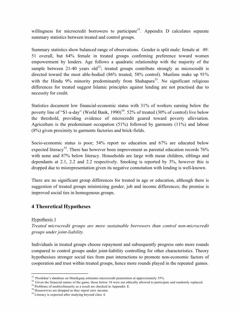
37

willingness for microcredit borrowers to participate31. Appendix D calculates separate summary statistics between treated and control groups.

Summary statistics show balanced range of observations. Gender is split male: female at 49: 51 overall, but 64% female in treated groups confirming preference toward women empowerment by lenders. Age follows a quadratic relationship with the majority of the sample between 21-40 years old32; treated groups contribute strongly as microcredit is directed toward the most able-bodied (86% treated, 58% control). Muslims make up 91% with the Hindu 9% minority predominantly from Shahapara33. No significant religious differences for treated suggest Islamic principles against lending are not practised due to necessity for credit.

Statistics document low financial-economic status with 31% of workers earning below the poverty line of “$1-a-day” (World Bank, 1990)34. 52% of treated (30% of control) live below the threshold, providing evidence of microcredit geared toward poverty alleviation. Agriculture is the predominant occupation (51%) followed by garments (11%) and labour (8%) given proximity to garments factories and brick-fields.

Socio-economic status is poor; 54% report no education and 67% are educated below expected literacy35. There has however been improvement as parental education records 76% with none and 87% below literacy. Households are large with mean children, siblings and dependants at 2.1, 2.2 and 2.2 respectively. Smoking is reported by 3%, however this is dropped due to misrepresentation given its negative connotation with lending is well-known.

There are no significant group differences for treated in age or education, although there is suggestion of treated groups minimizing gender, job and income differences; the premise is improved social ties in homogenous groups.

4 Theoretical Hypotheses

Hypothesis 1 Treated microcredit groups are more sustainable borrowers than control non-microcredit groups under joint-liability.

Individuals in treated groups choose repayment and subsequently progress onto more rounds compared to control groups under joint-liability controlling for other characteristics. Theory hypothesises stronger social ties from past interactions to promote non-economic factors of cooperation and trust within treated groups, hence more rounds played in the repeated games.

31 Proshikar’s database on Manikganj estimates microcredit penetration at approximately 35%. 32 Given the financial nature of the game, those below 18 were not ethically allowed to participate and randomly replaced. 33 Problems of multicolinearity as a result are checked in Appendix E. 34 Housewives are dropped as they report zero income. 35 Literacy is expected after studying beyond class 4.

38

This effect is forecasted to increase positively with the number of years the group has been together.

Hypothesis 2 Treated microcredit groups forego short-run gains from non-repayment in preference for long-run dynamic gains compared to control non-microcredit groups under joint-liability.

Treated group individuals are predicted to earn less income in the short-run given rounds played as they choose repayment, but dynamic gains from participation in more total rounds as a consequence leads to higher total income overall compared to control groups. Theory anticipates treated groups to show moral discipline; they forego short-run gains in preference for longer-term gains from future loans. The hypothesis also expects mutual gains from lending to treated groups: lenders are more likely repaid and treated borrowers make higher long-run gains.

Hypothesis 3 Developments in non-economic factors foster social ties which encourage shouldering and discourage free riding within treated microcredit groups compared to control non- microcredit groups.

Treated groups show significant development of social ties which promote shouldering (supporting partners) and deter free riding as a consequence of non-economic factors increasing cooperation and relationships. Theoretically treated groups are significantly more likely to shoulder (support) their partner and less likely to free ride compared to control groups under joint-liability (Besley and Coate, 1995; Ghatak and Guinnane, 1999).

Hypothesis 4 Lenders can maximise repayment rates under joint-liability by selecting individuals/groups that meet optimal characteristics.

Theory suggests various observable characteristics of individuals and groups that can maximise repayment decisions; controlling for differences between treated and control groups, there are optimal physical, individual, relational, and group characteristics36.

Literature on physical characteristics support female lending as they are risk averse with loan investment (Armendariz de Aghion and Morduch, 2010) and are genetically dutiful with payments (D’Espallier et al., 2011). Lenders also choose to lend to the able-bodied aged 20 to 30, who are most likely to earn repayment returns and to seize the initiative for future loans.

36 The objective of questionnaire used by MCIs to decide borrowers is to determine eligibility against expected optimal characteristics for repayment. Recall that this paper bases its questions (variables) on those used by Proshikar.

39

From a relational perspective, blood relatives and neighbours likely have strongest social ties, albeit at marginal risk that they anticipate a partner’s bad repayment behaviour. Inconclusive evidence suggests of mentality toward group support increasing with marriage, children, siblings, and dependants. There is also the reverse that emotional constraints may prevent willingness to support additional others. Popular thought is higher parental education is positively correlated toward childhood teachings on right-and-wrong, and that village differences affect social ties. Predictions for individual attributes are uncertain; increased education increases repayment from the strong positive correlation with good behaviour, however educated players may attempt to ‘cheat the system’. Similarly higher incomes and savings mean relative repayments are less of a burden, but also diminish the dynamic incentive for future loans. Optimal job guidelines are broad, allowing for any alongside which loan investment can be made into self-employment schemes.

Maximum repayment is anticipated from homogenous groups on the premise they show improved social ties as group members build stronger relationship when related in age, education and gender. Similar lifestyles and challenges from equal income, occupation and marital status also positively impact group repayment.

5 Empirical Results

Empirical findings from the questionnaire and repeated experimental games are recorded and analysed. The field experiments are used to empirically test the four key theoretical hypotheses proposed in Section 4. The cross-sectional data is econometrically analysed by OLS (Ordinary Least Squares) Regressions and MLE (Maximum Likelihood Estimation) Binary Estimation.

The key dependant variables analysed are as follows: rounds measures sustainability of joint- liability, counting the number of rounds the group plays having repaid. Points represent total earnings by the individual in the duration of the game (number of 10 cards accumulated and unused for repayment). Binary variables shoul and free determine whether an individual chose to shoulder or free ride respectively throughout the duration of the game37.

Preliminary Findings Preliminary analyses illustrated in Figure 2 suggest treated groups perform differently to control groups as hypothesised. Treated groups have a 91% higher mean rounds played at 4.18 rounds versus 2.20 rounds for control groups. They also score 53% more points on average (1.90 versus 1.24 points) throughout the duration of the game. This provides evidence treated groups comparatively play more rounds and score more total points.

37 See Appendix C for detailed definitions of all variables.

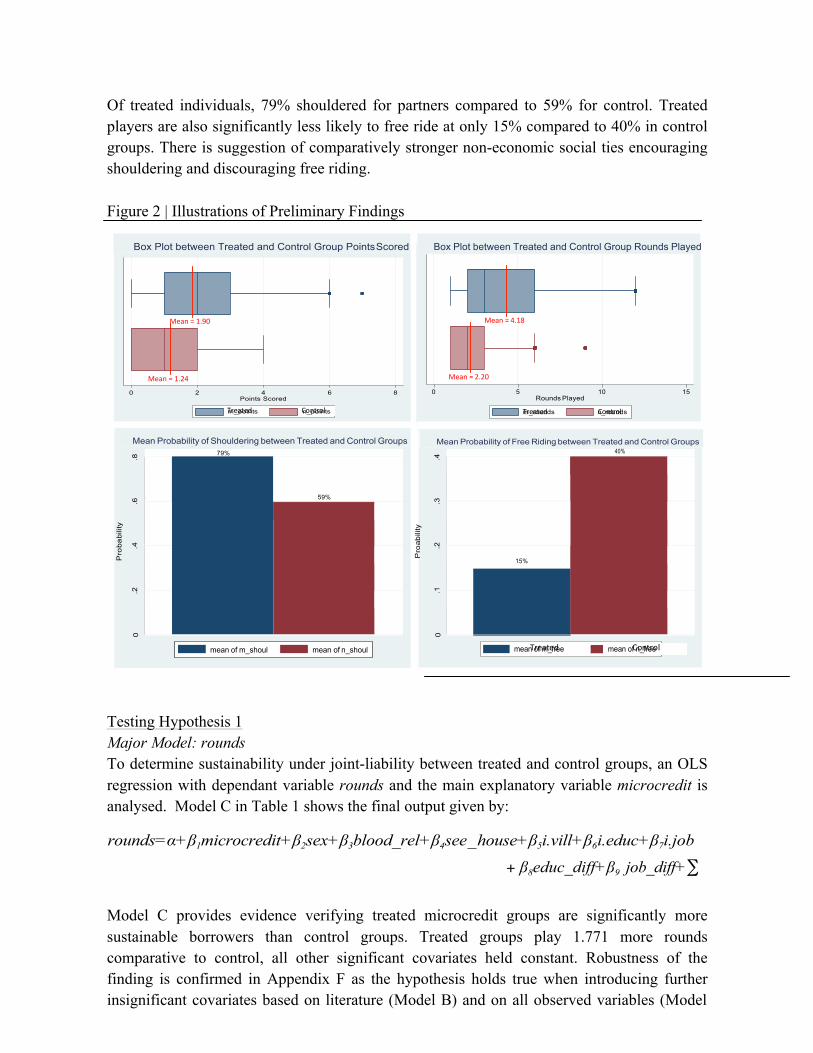
40

Mean & Deviation Comparison between Microcredit and Non-Microcredit Rounds Played

Mean & Deviation Comparison betweem Microcredit and Non-Microcredit Points Scored

Probabilities of Free-Riding between Microcredit and Non-Microcredit

Probability of Shouldering between Microcredit and Non-Microcredit Mean Probability of Shouldering between Treated and Control Groups

79%

mean of m_shoul mean of n_shoul

Mean Probability of Free Riding between Treated and Control Groups 40%

meanToref mat_efrdee mean ofCno_nfrtereol

Pro

abili

ty

.1

.2

.3

.4

0

Of treated individuals, 79% shouldered for partners compared to 59% for control. Treated players are also significantly less likely to free ride at only 15% compared to 40% in control groups. There is suggestion of comparatively stronger non-economic social ties encouraging shouldering and discouraging free riding.

Figure 2 | Illustrations of Preliminary Findings

Testing Hypothesis 1 Major Model: rounds To determine sustainability under joint-liability between treated and control groups, an OLS regression with dependant variable rounds and the main explanatory variable microcredit is analysed. Model C in Table 1 shows the final output given by:

rounds=α+β1microcredit+β2 sex+β3blood_rel+β4 see _ house+β5i.vill+β6 i.educ+β7i.job

+ β8educ_diff+β9 job_diff+∑

Model C provides evidence verifying treated microcredit groups are significantly more sustainable borrowers than control groups. Treated groups play 1.771 more rounds comparative to control, all other significant covariates held constant. Robustness of the finding is confirmed in Appendix F as the hypothesis holds true when introducing further insignificant covariates based on literature (Model B) and on all observed variables (Model

Box Plot between Treated and Control Group Points Scored

Mean=1.90

Mean=1.24

0 2 4 Points Scored

Tmre_aptoeidnts

6 8

Cno_nptorionlts Tmr_eraotuendds nC_ornoturnodls

Box Plot between Treated and Control Group Rounds Played

Mean=4.18

Mean=2.20

0 5 10 15 Rounds Played

59%

15%

Pro

babi

lity

.2

.4

.6

.8

0

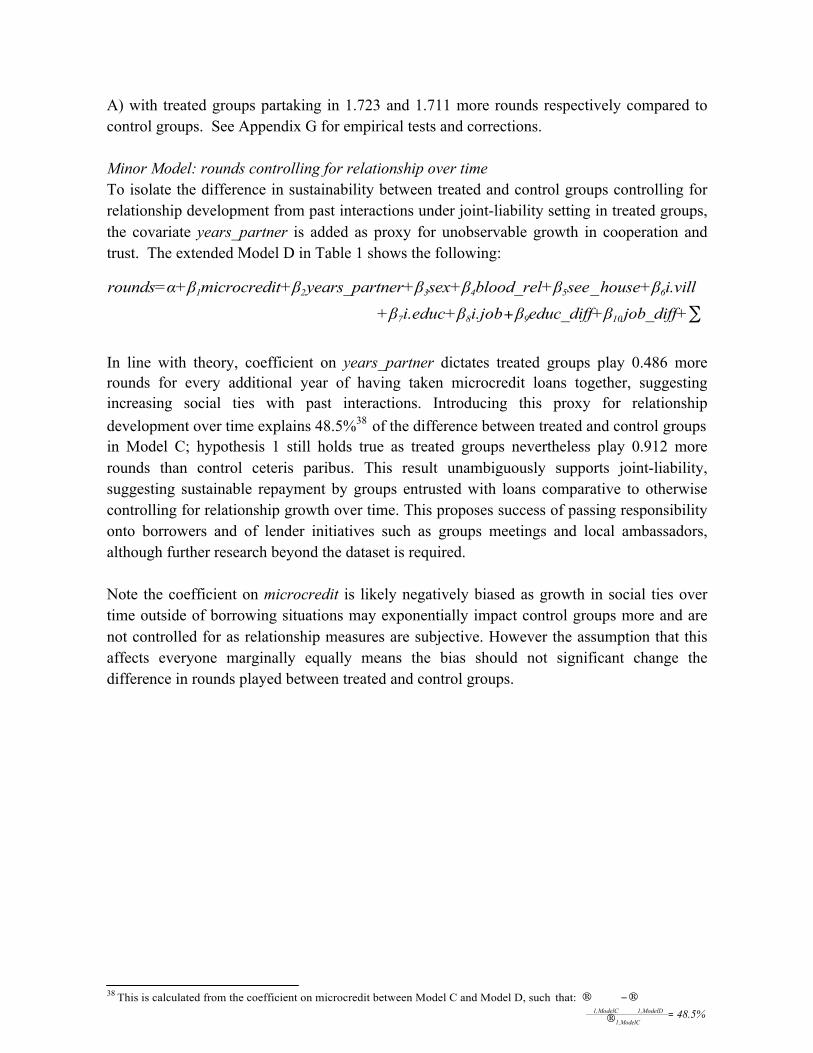
41

A) with treated groups partaking in 1.723 and 1.711 more rounds respectively compared to control groups. See Appendix G for empirical tests and corrections.

Minor Model: rounds controlling for relationship over time To isolate the difference in sustainability between treated and control groups controlling for relationship development from past interactions under joint-liability setting in treated groups, the covariate years_partner is added as proxy for unobservable growth in cooperation and trust. The extended Model D in Table 1 shows the following:

rounds=α+β1microcredit+β2 years_partner+β3sex+β4blood_rel+β5 see _ house+β6i.vill

+β7i.educ+β8i.job + β9educ_diff+β10 job_diff+∑

In line with theory, coefficient on years_partner dictates treated groups play 0.486 more rounds for every additional year of having taken microcredit loans together, suggesting increasing social ties with past interactions. Introducing this proxy for relationship development over time explains 48.5%38 of the difference between treated and control groups in Model C; hypothesis 1 still holds true as treated groups nevertheless play 0.912 more rounds than control ceteris paribus. This result unambiguously supports joint-liability, suggesting sustainable repayment by groups entrusted with loans comparative to otherwise controlling for relationship growth over time. This proposes success of passing responsibility onto borrowers and of lender initiatives such as groups meetings and local ambassadors, although further research beyond the dataset is required.

Note the coefficient on microcredit is likely negatively biased as growth in social ties over time outside of borrowing situations may exponentially impact control groups more and are not controlled for as relationship measures are subjective. However the assumption that this affects everyone marginally equally means the bias should not significant change the difference in rounds played between treated and control groups.

38 This is calculated from the coefficient on microcredit between Model C and Model D, such that: ® − ® 1,ModelC 1,ModelD =48.5%

®1,ModelC

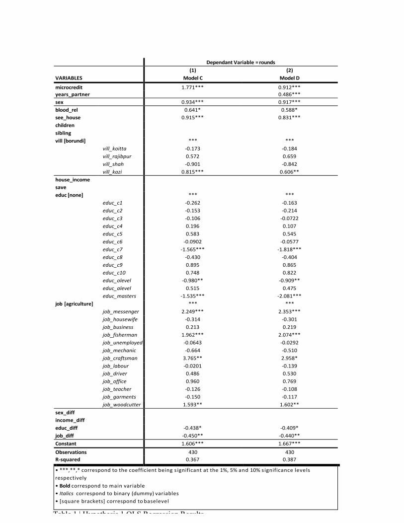
42

DependantVariable=rounds

VARIABLES

(1)ModelC

(2)ModelD

microcredit 1.771*** 0.912***years_partner 0.486***sex 0.934*** 0.917***blood_rel 0.641* 0.588*see_house 0.915*** 0.831***children sibling vill[borundi] *** ***

vill_koitta -0.173 -0.184

vill_rajibpur 0.572 0.659

vill_shah -0.901 -0.842

vill_kazi 0.815*** 0.606**house_income save educ[none] *** ***

educ_c1 -0.262 -0.163

educ_c2 -0.153 -0.214

educ_c3 -0.106 -0.0722

educ_c4 0.196 0.107

educ_c5 0.583 0.545

educ_c6 -0.0902 -0.0577

educ_c7 -1.565*** -1.818***

educ_c8 -0.430 -0.404

educ_c9 0.895 0.865

educ_c10 0.748 0.822

educ_olevel -0.980** -0.909**

educ_alevel 0.515 0.475

educ_masters -1.535*** -2.081***job [agriculture] *** ***

job_messenger 2.249*** 2.353***

job_housewife -0.314 -0.301

job_business 0.213 0.219

job_fisherman 1.962*** 2.074***

job_unemployed -0.0643 -0.0292

job_mechanic -0.664 -0.510

job_craftsman 3.765** 2.958*

job_labour -0.0201 -0.139

job_driver 0.486 0.530

job_office 0.960 0.769

job_teacher -0.126 -0.108

job_garments -0.150 -0.117

job_woodcutter 1.593** 1.602**sex_diff income_diff educ_diff -0.438* -0.409*job_diff -0.450** -0.440**Constant 1.606*** 1.667***Observations 430 430R-squared 0.367 0.387

•***,**,*correspondtothecoefficientbeingsignificantatthe1%,5%and10%significancelevelsrespectively•Boldcorrespondtomainvariable•Italicscorrespondtobinary(dummy)variables•[squarebrackets]correspondtobaselevel

Table 1 | Hypothesis 1 OLS Regression Results

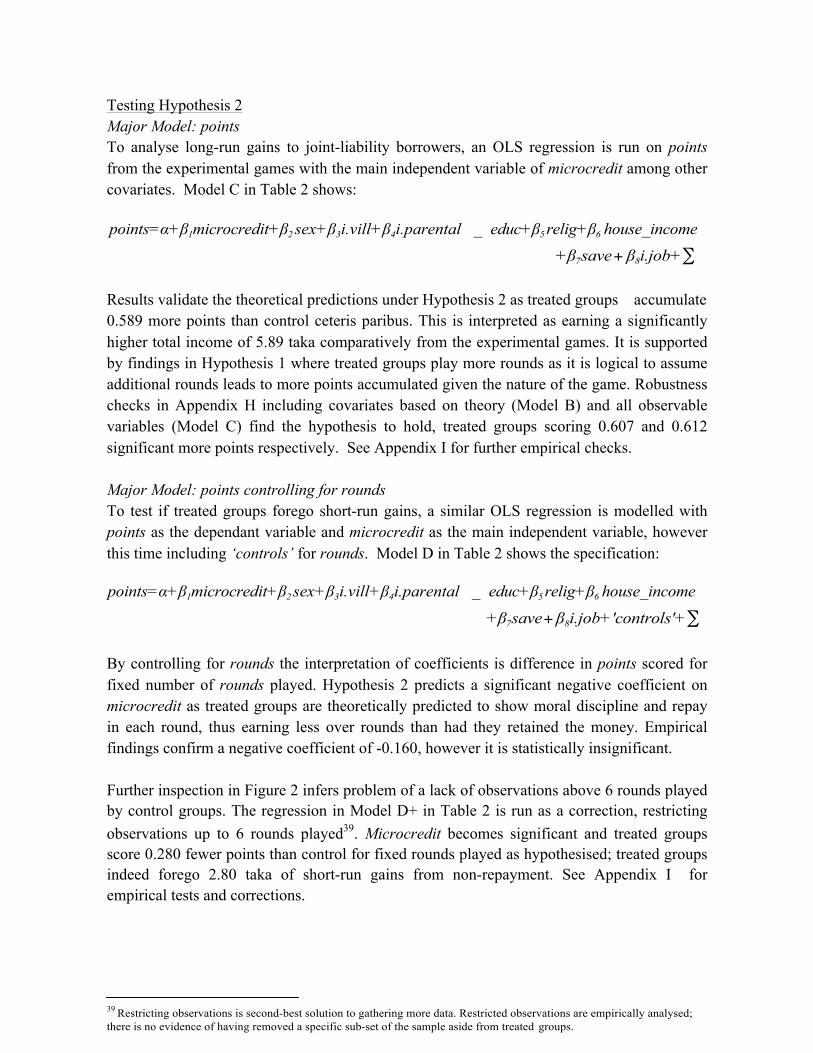
43

Testing Hypothesis 2 Major Model: points To analyse long-run gains to joint-liability borrowers, an OLS regression is run on points from the experimental games with the main independent variable of microcredit among other covariates. Model C in Table 2 shows:

points=α+β1microcredit+β2 sex+β3i.vill+β4i.parental _ educ+β5 relig+β6 house_income

+β7 save + β8i.job+∑

Results validate the theoretical predictions under Hypothesis 2 as treated groups accumulate 0.589 more points than control ceteris paribus. This is interpreted as earning a significantly higher total income of 5.89 taka comparatively from the experimental games. It is supported by findings in Hypothesis 1 where treated groups play more rounds as it is logical to assume additional rounds leads to more points accumulated given the nature of the game. Robustness checks in Appendix H including covariates based on theory (Model B) and all observable variables (Model C) find the hypothesis to hold, treated groups scoring 0.607 and 0.612 significant more points respectively. See Appendix I for further empirical checks.

Major Model: points controlling for rounds To test if treated groups forego short-run gains, a similar OLS regression is modelled with points as the dependant variable and microcredit as the main independent variable, however this time including ‘controls’ for rounds. Model D in Table 2 shows the specification:

points=α+β1microcredit+β2 sex+β3i.vill+β4i.parental _ educ+β5 relig+β6 house_income

+β7 save + β8i.job+'controls'+∑ By controlling for rounds the interpretation of coefficients is difference in points scored for fixed number of rounds played. Hypothesis 2 predicts a significant negative coefficient on microcredit as treated groups are theoretically predicted to show moral discipline and repay in each round, thus earning less over rounds than had they retained the money. Empirical findings confirm a negative coefficient of -0.160, however it is statistically insignificant.

Further inspection in Figure 2 infers problem of a lack of observations above 6 rounds played by control groups. The regression in Model D+ in Table 2 is run as a correction, restricting observations up to 6 rounds played39. Microcredit becomes significant and treated groups score 0.280 fewer points than control for fixed rounds played as hypothesised; treated groups indeed forego 2.80 taka of short-run gains from non-repayment. See Appendix I for empirical tests and corrections.

39 Restricting observations is second-best solution to gathering more data. Restricted observations are empirically analysed; there is no evidence of having removed a specific sub-set of the sample aside from treated groups.

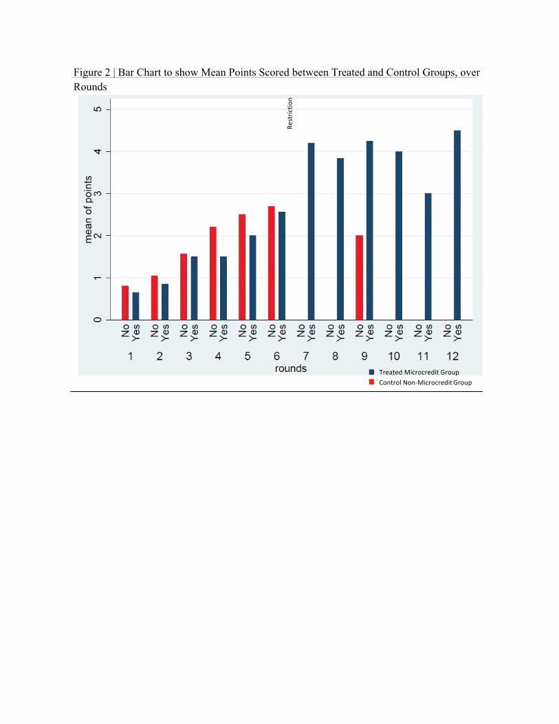
44

Figure 2 | Bar Chart to show Mean Points Scored between Treated and Control Groups, over Rounds

TreatedMicrocreditGroupControlNon-MicrocreditGroup

Restrictio

n

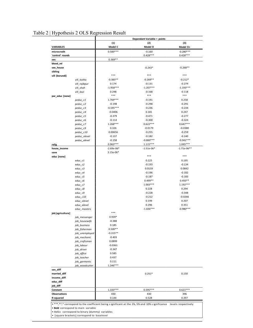
45

Table 2 | Hypothesis 2 OLS Regression Result DependantVariable= points

VARIABLES

(1)ModelC

(2)ModelD

(3)

ModelD+

microcredit 0.589*** -0.160 -0.280***'control' rounds 0.428*** 0.428***sex 0.369**blood_relsee_housesiblingvill [borundi] par_educ [none]

relig

vill_koittavill_rajibpurvill_shahvill_kazi

peduc_c1peduc_c2peduc_c3peduc_c4peduc_c5peduc_c6peduc_c7peduc_c9peduc_c10peduc_olevelpeduc_alevel

-0.243*

-0.268**

*** ***

***-0.383** -0.269** -0.212*0.174 -0.131 -0.274

-1.958*** -1.207*** -1.193***0.248 -0.168 -0.118*** *** ***

1.769*** -0.191 0.258-0.198 -0.298 -0.291

-0.595*** -0.236 -0.234-0.0406 0.181 0.247-0.379 -0.471 -0.277-0.114 -0.300 -0.324

1.268*** 0.622*** 0.647***0.326 -0.0179 -0.0380

0.00656 -0.255 -0.259-0.137 -0.182 -0.140-0.158 -0.860*** -0.941***

0.963*** 1.115*** 1.045***house_incomesaveeduc [none] job[agriculture]

educ_c1educ_c2educ_c3educ_c4educ_c5educ_c6educ_c7educ_c8educ_c9educ_c10educ_oleveleduc_aleveleduc_masters

job_messengerjob_housewifejob_businessjob_fishermanjob_unemployedjob_mechanicjob_craftsmanjob_labourjob_driverjob_officejob_teacherjob_garmentsjob_woodcutter

-2.69e-06* -1.51e-06* -1.71e-06**3.15e-06*

*** ***

0.225 0.195

-0.193 -0.134

0.0159 0.0842

-0.196 -0.182

-0.187 -0.183

0.499** 0.450**

1.003*** 1.192***

0.228 0.294

-0.228 -0.348

-0.212 -0.0266

0.199 0.207

0.296 0.351

-1.026*** -0.980******

0.939*

-0.388

0.185

0.500**

-0.315**

-0.403

0.0899

-0.0361

-0.347

0.585

0.437

0.111

1.346*** sex_diffmarried_diffincome_diffeduc_diffjob_diff

0.251*

0.150

Constant 1.333*** 0.595*** 0.621***Observations 430 430 396R-squared 0.144 0.528 0.397

•***,**,*correspondtothecoefficientbeingsignificantatthe1%,5%and10%significance levelsrespectively•Boldcorrespondtomain variable•Italicscorrespondtobinary(dummy) variables•[squarebrackets]correspondto baselevel

46

Testing Hypothesis 3 Major Model: shouldering Maximum Likelihood Estimation is used focusing on probit40 binary estimation results for the variable shoul to test if treated groups show higher likelihood of shouldering compared to control groups. The main independent variable is microcredit as in Probit C in Table 3:

shoul=α+β1microcredit+β2age+β3 sex+β4 see_house+β5children+β6 i.vill+β7 relig+β8i.job

+β9 school_diff+∑ Relatively stronger social ties in treated groups predict fostering of non-economic factors toward shouldering for a partner’s repayment. Empirically, treated groups are indeed 26.6% more likely to shoulder comparative to control groups ceteris paribus. Results are consistent and significant applying alternative estimation methods of logit estimation (Logit C) and linear probability model (LPM C) with output at 25.7% and 22.9% more likely for treated respectively. Robustness checks are confirmed on Probit A and Probit B models. See Appendix L, followed by tests in Appendix M.

Major Model: free riding Econometric techniques are next applied to the variable free for which the hypothesis anticipates microcredit to have a significant negative coefficient, interpreted as treated groups have a lower likelihood of free riding comparative to control groups. As in Probit C in Table 3:

free=α+β1microcredit+β2 sex+β3blood_rel+β4i.vill+β5house_income+β6i.job+∑

Results show individuals in treated groups are 27.4% significant less likely to free ride on their partner relatively as hypothesised. This provides evidence toward stronger social ties within treated groups, and is further confirmed by consistent findings when applying alternative estimation methods of logit (Logit C) and linear probability model (LPM C) which give output of 25.8% and 26.2% less likely respectively shown in Appendix J (including robustness checks on Probit A and Probit B models). See Appendix K for empirical tests.

Interpretation of Independent Variables for shouldering and free riding Different factors variably influence non-economic social tie drivers of shouldering and free riding when comparing significance of covariates41 holding constant differences between treated and control groups.

Physically, females are 17.3% more likely to shoulder and 10.1% less likely to free ride than male counterparts as reconciled by gender economics (D’Espallier et al., 2011). Each

40 Probit estimation is chosen as adjudged by past literature; the assumptions of normally distributed error terms are made. 41 See Table 3. Comparisons are distinguished from respective significant covariates in Probit C Models for shoul and free.

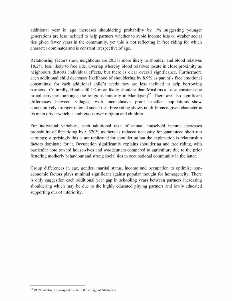
47

additional year in age increases shouldering probability by 1% suggesting younger generations are less inclined to help partners whether to avoid income loss or weaker social ties given fewer years in the community, yet this is not reflecting in free riding for which character dominates and is constant irrespective of age.

Relationship factors show neighbours are 20.3% more likely to shoulder and blood relatives 18.2%; less likely to free ride. Overlap whereby blood relatives locate in close proximity as neighbours distorts individual effects, but there is clear overall significance. Furthermore each additional child decreases likelihood of shouldering by 8.9% as parent’s face emotional constraints; for each additional child’s needs they are less inclined to help borrowing partners. Culturally, Hindus 40.2% more likely shoulder than Muslims all else constant due to collectiveness amongst the religious minority in Manikganj42. There are also significant differences between villages, with inconclusive proof smaller populations show comparatively stronger internal social ties. Free riding shows no difference given character is its main driver which is ambiguous over religion and children.

For individual variables, each additional taka of annual household income decreases probability of free riding by 0.320% as there is reduced necessity for guaranteed short-run earnings; surprisingly this is not replicated for shouldering but the explanation is relationship factors dominate for it. Occupation significantly explains shouldering and free riding, with particular note toward housewives and woodcutters compared to agriculture due to the prior fostering motherly behaviour and strong social ties in occupational community in the latter.

Group differences in age, gender, marital status, income and occupation to optimise non- economic factors plays minimal significant against popular thought for homogeneity. There is only suggestion each additional year gap in schooling years between partners increasing shouldering which may be due to the highly educated pitying partners and lowly educated supporting our of inferiority.

42 89.5% of Hindu’s sampled reside in the village of Shahapara.

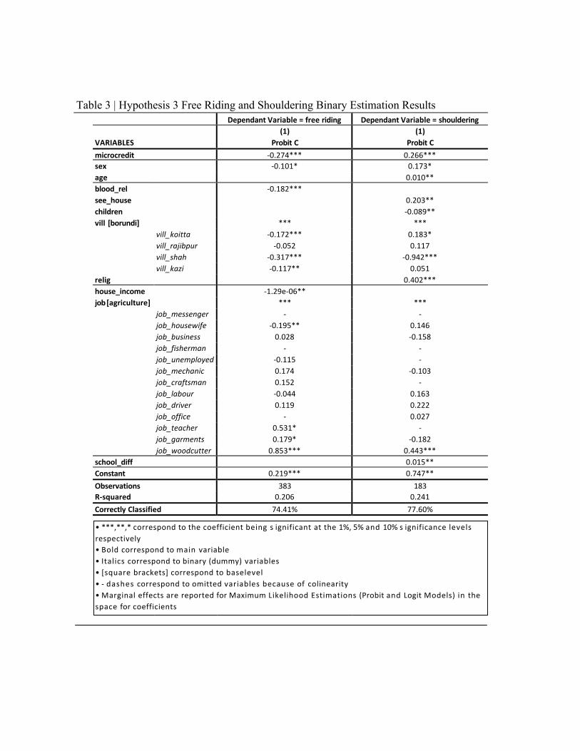
48

Table 3 | Hypothesis 3 Free Riding and Shouldering Binary Estimation Results DependantVariable=freeriding DependantVariable=shouldering

VARIABLES

(1)ProbitC

(1)ProbitC

microcredit -0.274*** 0.266***sex -0.101* 0.173*age 0.010**blood_rel -0.182*** see_house 0.203**children -0.089**vill[borundi] *** *** vill_koitta -0.172*** 0.183* vill_rajibpur -0.052 0.117 vill_shah -0.317*** -0.942*** vill_kazi -0.117** 0.051relig 0.402***house_income -1.29e-06** job[agriculture] *** *** job_messenger - - job_housewife -0.195** 0.146 job_business 0.028 -0.158 job_fisherman - - job_unemployed -0.115 - job_mechanic 0.174 -0.103 job_craftsman 0.152 - job_labour -0.044 0.163 job_driver 0.119 0.222 job_office - 0.027 job_teacher 0.531* - job_garments 0.179* -0.182 job_woodcutter 0.853*** 0.443***school_diff 0.015**Constant 0.219*** 0.747**Observations 383 183R-squared 0.206 0.241CorrectlyClassified 74.41% 77.60%

•***,**,*correspondtothecoefficientbeingsignificantatthe1%,5%and10%significancelevelsrespectively•Boldcorrespondtomainvariable•Italicscorrespondtobinary(dummy)variables•[squarebrackets]correspondtobaselevel•-dashescorrespondtoomittedvariablesbecauseof colinearity•MarginaleffectsarereportedforMaximumLikelihoodEstimations(ProbitandLogitModels)inthespaceforcoefficients

49

Testing Hypothesis 4 OLS regression specifications in Table 4 with rounds as dependant variable are used to identify optimal characteristics to maximise joint-liability repayment. Rounds are a measure of returns to lenders as further rounds are contingent on group repayment. Initial specifications on individual and group characteristics are refined in Appendix N for combination toward optimal characteristics43 specified below. Note microcredit is retained to control for differences between treated and control groups.

rounds=α+β1microcredit+β2 sex+β3blood_rel+β4 see _ house+β5i.vill+β6 i.educ+β7i.job

+ β8educ_diff+β9 job_diff+∑ The physical optimum in favour of women empowerment is to lend to females who are more sustainable borrowers, playing 0.934 more rounds than male counterparts. Age is not seen to impact repayment choice, disproving the notion of young workers having stronger motivation to repay for future loans to escape poverty. However this overlooks age affecting ability to work and generate income for repayment as game income is set exogenously independent of productivity.

Based on relationships, lenders maximise repayment from blood relatives and neighbours whom depict strong social ties as hypothesised, playing 0.641 and 0.915 more rounds than otherwise. Cooperation is higher and there is significant opportunity cost of punishment from losing trust in these groups. The data also finds no significant evidence to select borrowers based on children, siblings, dependants or upbringing based on parental education affecting helping mentality. There is however significant varying strength of cultural relationships between village groups, although further research is required to pinpoint its drivers44.

Focusing on the individual, lower education promotes repayment, confirming theory that better educated players attempt to ‘cheat the system’ by not repaying; significant levels are at Class 7, O-Level and Masters who participate in 1.565, 0.980 and 1.535 rounds less than baselevel no education respectively. Financial variables of income and savings are insignificant in influencing repayment; the story may be increases in income/savings lead to less repayment burden but also less dynamic incentive for future loans which trade-off perfectly in equilibrium. More likely however is by setting income exogenously and not incorporating possibility of financial losses, borrowers do not act realistically based on financials. Against acceptance of a broad remit on jobs, analysis finds more significance should be placed on occupation. There are higher long-run repayments from workers in predominantly niche forms of employment that form small work-communities as they better cooperate: messengers (+2.245), fisherman (+1.962), craftsman (+3.765) and woodcutters (+1.593) play more rounds than baseline agriculture workers that make up 51% of sampled treated borrowers.

43 Notice the Optimal Characteristics specification is the same as Model C in Table 1, as expected. 44 Banerjee et al. (2013) indeed find evidence of MCIs targeting borrower groups based on village of residence.

50

Optimal group criteria says same sex groups perform better by 0.483 rounds compared to otherwise however it is inconclusive when controlling for individual characteristics. Robustness checks confirm repayment differences due to individual gender explain majority of variation in group gender. Age difference is insignificant disproving less cooperation for bigger age gaps between partners. Partners with different education play 0.450 less rounds than identically educated; highly educated players chose non-repayment to attempt to cheat lenders and their partners, particularly if education differences exist with the latter. Group income disparity shows no significance which can be explained by similar lifestyles over range of incomes observed. Negative non-economic factors such as jealousy are not problematic as the population have 90,413 taka mean annual household income with 48,058 standard deviation45; the availability of goods for conspicuous consumption is constrained and anyone with high income re-locates away from rural villages. Moreover homogenous job groups outperform those otherwise by 0.450 rounds, placing importance on relationships within work communities. See Appendix N for robustness checks and extensions.

45 Augsburg et al, 2014 finds no income gains to microcredit borrowers in Bosnia suggesting no social jealousy toward them.

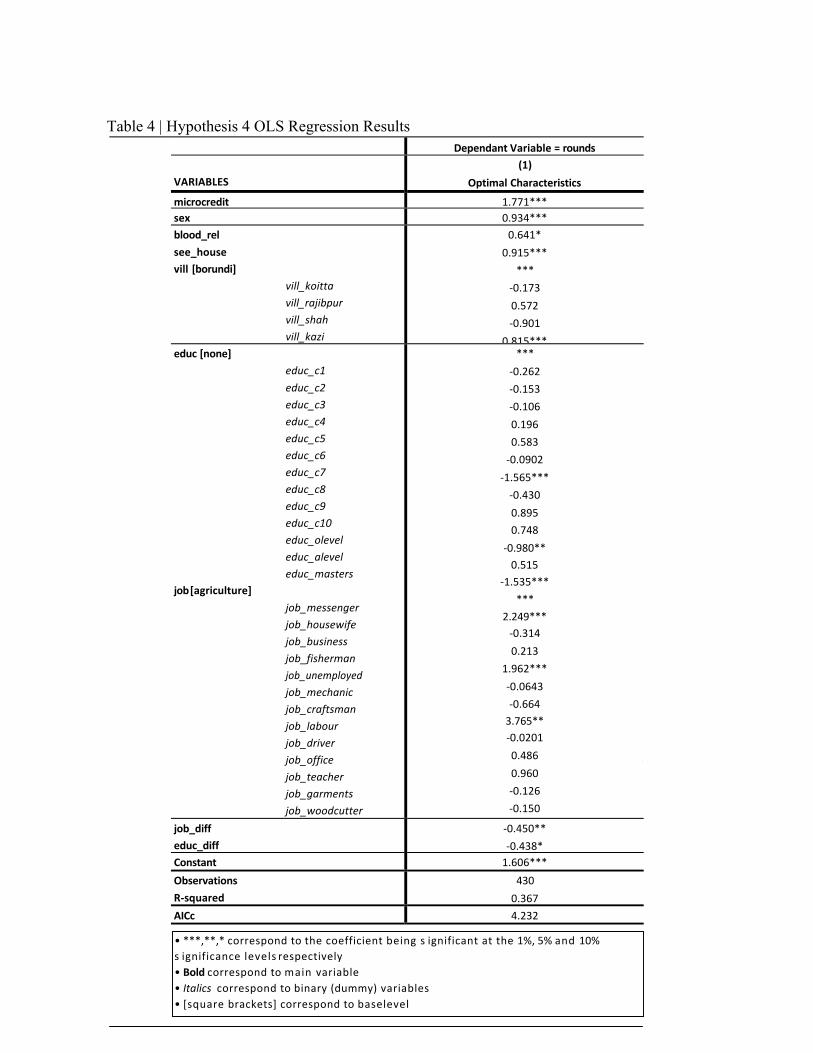
51

Table 4 | Hypothesis 4 OLS Regression Results DependantVariable=rounds

VARIABLES

(1)

OptimalCharacteristics

microcredit 1.771***sex 0.934***blood_relsee_housevill[borundi]

vill_koittavill_rajibpurvill_shahvill_kazi

0.641*

0.915***

***

-0.173

0.572

-0.901

0.815***educ[none]

educ_c1educ_c2educ_c3educ_c4educ_c5educ_c6educ_c7educ_c8educ_c9educ_c10educ_oleveleduc_aleveleduc_masters

job[agriculture]job_messengerjob_housewifejob_businessjob_fishermanjob_unemployedjob_mechanicjob_craftsmanjob_labourjob_driverjob_officejob_teacherjob_garmentsjob_woodcutter

***

-0.262

-0.153

-0.106

0.196

0.583

-0.0902

-1.565***

-0.430

0.895

0.748

-0.980**0.515

-1.535***

***2.249***-0.314

0.213

1.962***

-0.0643

-0.6643.765**-0.0201

0.486

0.960

-0.126

-0.1501.593**job_diff

educ_diff-0.450**

-0.438*Constant 1.606***ObservationsR-squared

430

0.367AICc 4.232

•***,**,*correspondtothecoefficientbeingsignificantatthe1%,5%and10%significancelevelsrespectively•Boldcorrespondtomainvariable•Italicscorrespondtobinary(dummy)variables•[squarebrackets]correspondtobaselevel

52

6 Concluding Remarks Pioneering repeated experimental games are modelled to evaluate social ties and free riding under practical joint-liability microcredit borrowing in Bangladesh; focus is given to repayment decisions by treated microcredit borrower-groups compared to control non- microcredit groups. The paper hypothesises and empirically challenges key theories.

Empirical evidence supports theoretical predictions of more sustainable treated groups likely repaying loans and participating in more rounds compared to control groups. Treated groups foster positive non-economic social ties from repeated interactions. This holds controlling for past joint-liability interactions over time, however relationship growth outside of this are assumed to equally affect all groups. Partial solutions would be to measure years’ groups have known each other or to include subjective measures of relationship strength.

Treated individuals in the experiments show moral discipline as hypothesised, foregoing short-run gains from non-repayment to benefit from higher dynamic long-run total earnings. Second-best policy of restricting rounds is however essential to conclude significant lower short-run earnings for treated group. First-best policy would be to expand the dataset to sampling 20% of all populations or exploring more villages, particularly because of multicolinearity problems from the Hindu village of Shahapara.

Hypothesis 3 states stronger social ties in treated groups to encourage shouldering and discourage free riding compared to control groups. Empirically this is well-proven with treated groups 26.6% more likely to shoulder and 27.4% less likely to free ride compared to control groups all else constant. In extension different observable characteristics impact likelihood of shouldering or free riding different; findings of shouldering being sensitive to physical and relational characteristics and free riding to individuals’ situation are suggested.

The story for lenders when selecting optimal borrowers in joint-liability is to choose predominantly women that are blood relatives and neighbours. To maximise repayments lenders must select those educated below Class 7 and in niche forms of employment so they benefit from stronger work-community social ties. Homogenous groups in sex, education and occupation should be formed. Optimum based on income and village is uncertain because of exogenously setting income outside of the loss domain and inability to identify cultural differences between villages respectively.

Contemporary game theoretical application to joint-liability microcredit lending is novel; there remains expansive scope for future literature. Extension to this paper include but are not limited to allowing observation of groups incomes to a degree of certainty to better replicate signals of repayment ability46, and finding proxy variables to measure unobservable

46 This however raises ethical concerns, hence why it was avoided in this paper.

53

behavioural characteristics which limit all empirical research in microcredit47. Alternative application of the experimental games can be made to test social ties in solving moral hazard by setting income endogenously or in solving adverse selection by comparing microcredit borrowers to those only deterred by high interest rates. Experimental games can also be adapted to model comparisons between joint-liability and other lending models such as individual-liability.

The paper finds significant evidence supporting theoretical hypotheses in joint-liability microcredit lending. Nevertheless whether joint-liability is the optimal lending model for alleviating world poverty remains undetermined48.

47 At best 38.7% of the variability (R-squared) through observable characteristics for sustainability is explained (rounds). 48 Recent studies have shown variations on joint an individual liability to differing degrees of success (Maitra et al., 2013).

54

Bibliography

Abbink, K., Irlenbusch, B., & Renner, E. (2006). Group size and social ties in microfinance institutions. Economic Inquiry, 44(4), 614-628.

Adams, D. W., & Vogel, R. C. (1986). Rural financial markets in low-income countries: Recent controversies

and lessons. World development, 14(4), 477-487.

Ahlin, C., & Townsend, R. M. (2007). Using Repayment Data to Test Across Models of Joint-liability Lending. The Economic Journal, 117(517), F11-F51.

Akerlof, G. A. (1970). The market for" lemons": Quality uncertainty and the market mechanism. The quarterly

journal of economics, 488-500.

Allen, T. (2012). Optimal (Partial) Group Liability in Microfinance Lending. mimeo.

Angelucci, M., Karlan, D., & Zinman, J. (2013). Win some lose some? Evidence from a randomized microcredit program placement experiment by Compartamos Banco (No. w19119). National Bureau of Economic Research.

Armendáriz de Aghion, B., & Morduch, J. (2000). Microfinance beyond group lending. Economics of

transition, 8(2), 401-420.

Armendáriz, B., & Morduch, J. (2010). The economics of microfinance. MIT press.

Attanasio, O., Augsburg, B., De Haas, R., Fitzsimons, E., & Harmgart, H. (2001). The Impacts of Microfinance: Evidence from Joint-Liability Lending in Mongolia. American Economic Journal: Applied Economics, 7(1), 90-122.

Banco, C. (2014). Microcredit Impacts: Evidence from a Randomized Microcredit Program Placement

Experiment by Compartamos Banco May 2014 Manuela Angelucci, Dean Karlan, and Jonathan Zinman.

Banerjee, A. V., Besley, T., & Guinnane, T. W. (1994). The neighbor's keeper: the design of a credit

cooperative with theory and a test. The Quarterly Journal of Economics, 109(2), 491-515.

Banerjee, A. V., Duflo, E., Glennerster, R., & Kinnan, C. (2013). The miracle of microfinance? Evidence from a randomized evaluation.

Barboza, G., & Trejos, S. (2009). Micro credit in Chiapas, México: Poverty reduction through group

lending. Journal of business ethics, 88(2), 283-299.

Besley, T., & Coate, S. (1995). Group lending, repayment incentives and social collateral. Journal of development economics, 46(1), 1-18.

Bhole, B., & Ogden, S. (2010). Group lending and individual lending with strategic default. Journal of Development Economics, 91(2), 348-363.

Bó, P. D. (2005). Cooperation under the shadow of the future: experimental evidence from infinitely repeated

games. American Economic Review, 1591-1604.

55

Braverman, A., & Guasch, J. L. (1986). Rural credit markets and institutions in developing countries: Lessons for policy analysis from practice and modern theory. World Development, 14(10), 1253-1267.

Breza, E. (2012). Peer effects and loan repayment: Evidence from the krishna default crisis. Job Market Paper MIT.

Casari, M., & Cason, T. N. (2009). The strategy method lowers measured trustworthy behavior. Economics

Letters, 103(3), 157-159.

Cassar, A., Crowley, L., & Wydick, B. (2007). The effect of social capital on group loan repayment: evidence from field experiments. The Economic Journal, 117(517), F85-F106.

Chu, M., & Cuellar, R. G. (2008). Banco Compartamos: Life after the IPO. Boston: Harvard Business.

D’Espallier, B., Guérin, I., & Mersland, R. (2011). Women and repayment in microfinance: A global

analysis. World Development, 39(5), 758-772.

Daley-Harris, S. (2012). State of the Microcredit Summit Campaign Report. Microcredit Summit Campaign.

Available at: http://stateofthecampaign.org/2012-data/ Web accessed on 31/11/14.

Freixas, X., & Rochet, J. C. (1997). Microeconomics of banking (Vol. 2). Cambridge, MA: MIT press. Gangopadhyay, S., Ghatak, M., & Lensink, R. (2005). Joint Liability Lending and the Peer Selection

Effect*. The Economic Journal, 115(506), 1005-1015.

Ghatak, M. (1999). Group lending, local information and peer selection. Journal of development Economics, 60(1), 27-50.

Ghatak, M., & Guinnane, T. W. (1999). The economics of lending with joint-liability: theory and

practice. Journal of development economics, 60(1), 195-228.

Giné, X., & Karlan, D. (2009). Group versus individual liability: Long term evidence from Philippine microcredit lending groups. Center Discussion Paper, Economic Growth Center.

Giné, X., & Yang, D. (2009). Insurance, credit, and technology adoption: Field experimental evidence from

Malawi. Journal of Development Economics, 89(1), 1-11.

Giné, X., Jakiela, P., Karlan, D., & Morduch, J. (2010). Microfinance games. American Economic Journal: Applied Economics, 2(3), 60-95.

Guinnane, T. W. (1994). A Failed Institutional Transplant: Raiffeisen′ s Credit Cooperatives in Ireland, 1894-

1914. Explorations in economic history, 31(1), 38-61.

Hossain, M. (1988). Credit for alleviation of rural poverty: The Grameen Bank in Bangladesh (No.65). International Food Policy Research Institute.

Karlan, D. S. (2005). Using experimental economics to measure social capital and predict financial

decisions. American Economic Review, 1688-1699.

Karlan, D. S. (2007). Social connections and group banking. The Economic Journal, 117(517), F52-F84.

Kono, H.(2006). Is Group Lending A Good Enforcement Scheme for Achieving High Repayment Rates?:

Evidence from Field Experiments in Vietnam (No. 61). IDE Discussion Paper.

56

Kono, H. (2013). Is Joint-liability a Good Enforcement Scheme for Achieving High Repayment Rates? : Evidence from Framed Field Experiments in Vietnam. Institute of Developing Economies: Mimeo.

Kono, H. (2014). Microcredit games with noisy signals: Contagion and free-riding. Journal of the Japanese and

International Economies, 96-113.

Kurosaki, T., & Khan, H. U. (2012). Vulnerability of microfinance to strategic default and covariate shocks:

evidence from Pakistan. The Developing Economies, 50(2), 81-115.

Laffont, J. J., & Rey, P. (2003). Moral hazard, collusion and group lending. IDEI Working Paper, 122.

Lapenu, C., & Zeller, M. (2001). Distribution, growth, and performance of microfinance institutions in Africa, Asia, and Latin America.

Maitra, P., Mitra, S., Mookherjee, D., Motta, A., & Visaria, S. (2013). Agent Intermediated Lending: A New

Approach to Microfinance (No. 16-13). Monash University, Department of Economics.

Mannan, M. (2014). Discussion. Independent University, Bangladesh. Discussion on 22/11/2014.

Morduch, J. (1999). The microfinance promise. Journal of economic literature, 1569-1614.

Olson, M. (1987). Collective action. The New Palgrave: A Dictionary of Economics, 1, 474-477.

Polgreen, L., & Bajaj, V. (2010). India microcredit faces collapse from defaults.New York Times, 18, A5.

Putnam, R. D., Leonardi, R., & Nanetti, R. Y. (1994). Making democracy work: Civic traditions in modern Italy. Princeton university press.

Rahman, A. (1999). Women and microcredit in rural Bangladesh: anthropological study of the rhetoric and

realities of Grameen Bank lending. Westview Press, Inc..

Ravallion, M., Chen, S., & Sangraula, P. (2009). Dollar a day revisited. The World Bank Economic Review, lhp007.

Schaefer-Kehnert, W. (1980). Success with group lending in Malawi. Quarterly Journal of International

Agriculture, 19(4), 331-337.

Stiglitz, J. E. (1990). Peer monitoring and credit markets. The world bank economic review, 4(3), 351-366.

Stiglitz, J. E., & Weiss, A. (1983). Incentive effects of terminations: Applications to the credit and labor

markets. The American Economic Review, 912-927.

Swibel, M. (2007). The world’s top 50 microfinance institutions. Forbes. Available at: http://www.forbes. com/2007/12/20/topphilanthropy-microfinance-biz-cz_1220land.html Web accessed on 31/11/14.

Todd, H. (1966). Women at the Centre. Boulder: Westview Press.

Townsend, R. M. (2003). Microcredit and mechanism design. Journal of the European Economic

Association, 1(2-3), 468-477.

Varian, H. R. (1990). Monitoring agents with other agents. Journal of Institutional and Theoretical Economics, 153-174.

57

Wydick, B. (1999). Can social cohesion be harnessed to repair market failures? Evidence from group lending in Guatemala. The Economic Journal, 109(457), 463-475.

Wydick, B. (2001). Group lending under dynamic incentives as a borrower discipline device. Review of

Development Economics, 5(3), 406-420.

Yunus, M. (1999). The Grameen Bank. Scientific American, 281(5), 114-119.

Zeller, M. (1998). Determinants of repayment performance in credit groups: the role of program design, intra-

group risk pooling and social cohesion. Economic Development and Cultural Change, 46(1), 599-620.

58

HIV Prevalence in Sub-Sahara Africa: A Spatial Econometric Approach

Levi Boxell Taylor University

Abstract The geographical dispersion of HIV in sub-Sahara Africa is a phenomenon that is little understood. I contribute to the literature of this occurrence by examining the spatial dependency of HIV prevalence. I introduce a simple model motivating the use of spatial econometric techniques. However, missing data is a common occurrence when dealing with developing nations and is often dealt with by listwise deletion. The problem in spatial econometrics is that listwise deletion gives biased estimates even for data missing completely at random, and there is no common solution for dealing with missing data. I develop a new class of missing data, denoted “Missing Spatially at Random,” that explains this occurrence. I then demonstrate a general method utilizing the EM-algorithm along with multiple imputation via chained equations that provide unbiased estimates of missing data in a wide variety of spatial econometric models. The unbiased nature of the estimates is confirmed via Monte Carlo simulations. Using this method for estimating a spatial autoregressive panel model with fixed effects, I estimate the spatial dependency of HIV prevalence in sub-Sahara Africa. Results suggest a statistically significant and positive coefficient for spatial dependency.

59

COST AND EFFICACY OF

COLLECTIVE ACTION CLAUSES

CHENBO FANG†‡

ABSTRACT

Recent developments in the sovereign capital market, such as the debt crises in the Eurozone, the massive restructuring by Greece, and the escalated tension between Argentina and its holdout creditors, have brought Collective Action Clauses (CACs) back to limelight. These clauses in sovereign bond contracts claim to address the coordination problem among creditors and thus enable a more orderly restructuring process, and previous researches have found little cost of carrying these “insurances” for debtor countries. In this research, I revisit the cost question through a replication method and new evidence made available by the Eurozone CACs mandate, and I examine the actual efficacy of CACs by surveying the 22 sovereign bond restructurings since 1970, on which there has been little empirical analysis that I am aware of. My analysis finds that Euro CACs with the aggregation feature are associated with little but positive addition to borrowing cost, and riskier investments with lower credit rating and longer maturity are subject to a higher CACs premium. At the same time, CACs have not significantly affected the outcome of restructurings after controlling for other factors such as creditor structure, haircut, and government coerciveness. This cost-benefit analysis leads me to conclude that although CACs do not lead to substantially higher borrowing costs -- even the “Super CACs” with the Aggregation Feature -- including them does not necessarily guarantee a more orderly restructuring, and thus more dramatic reforms may be necessary if further improvement in the restructuring process is desired.

Keywords: Sovereign Bond Restructuring, Collective Action Clauses (CACs), Aggregation Feature, Borrowing Cost, Participation Rate, Length of Negotiation, Litigation.

† Undergraduate student at University of California, Berkeley. Please contact fangchenbo@berkeley.edu for questions or comments. ‡ I would like to thank Professor Roger Craine for his guidance, support, and encouragement throughout the research process, without which I would not have been able to complete the present research. I am also indebted to Professor Christoph Trebesch for providing various data sources and suggestions, and Professor Barry Eichengreen, Professor Pierre-Olivier Gourinchas, and Professor Mitu Gulati for very helpful comments.

60

HAS THE MFN FREE-RIDER PROBLEM GOTTEN WORSE: EVIDENCE FROM THE DOHA ROUND

JONATHON C. F. MCCLURE

Georgetown University

ABSTRACT Previous analysis by Ludema and Mayda (2011) has shown that countries free-ride on MFN applied tariffs and that such tariffs are inefficiently high due to the inability of countries to internalize the terms-of-trade effects of trade liberalization. Developments in the global economic system throughout the Doha Round have impacted the ability of countries to internalize benefits through affecting exporter concentration. This paper examines the progression of the free rider problem from 1993 to 2012 through three causal channels: countries acceding to the WTO, the proliferation of PTAs, and the impact of emerging economies on trade flows. This study finds an average net increase in export concentration over these three channels, evidencing an implied tariff reduction and an amelioration of the free rider problem from 12%- 25% to 8%-12%. This effect is most pronounced on low-tech products that have been concentrated by emerging economies. Finally, the creation of predicted mega-FTAs or advancing customs unions encourage the internalization of terms-of-trade benefits and promote lower MFN tariffs.

61

1 Introduction

The past twenty years have resulted in tremendous changes to the international economic system presided over by the World Trade Organization (WTO) and its ability to foster multilateral trade liberalization. Three significant trends have occurred over this time period: the accession of new members, the rise of emerging economies, and the proliferation of preferential trade agreements (PTAs). The 2012 WTO had 157 members, 29 of which acceded since the WTO replaced the GATT in 1994.1 This group now includes two of Asia’s largest economies, the People’s Republic of China (acceded in 2001) and the Russian Federation (acceded in 2012). The second trend is the rise of “emerging” economies, most notably Brazil, Russia, India, and China (BRIC). The third trend is the tremendous expansion of trade flows under PTAs. With hundreds of PTAs being signed since the creation of the WTO, the majority of the world’s trade now flows between PTA partners and is not subject to WTO principles of nondiscrimination.2 This has led some to question the continuing relevance of the WTO system.

The Doha Round (2001-present) has been considered unsuccessful at making progress towards multilateral trade liberalization through WTO negotiations, leaving open the question of why the results failed to live up to expectations. Are any of the aforementioned trends responsible for the ineffectiveness of the Doha Round in promoting the liberalization of most-favored nation (MFN) tariffs? When considering these trends, is the WTO the appropriate institution for moving trade liberalization forward, and what are its prospects in the foreseeable future?

This paper attempts to examine the role of terms-of-trade effects in multilateral tariff negotiations to examine whether the free rider problem, written on extensively by Ludema and Mayda (2009, 2011) has been exacerbated or ameliorated by the three noted trends. This problem refers to the setting of inefficiently high tariffs as the terms-of-trade benefits of tariff cuts are not internalized by the liberalizing country due to the non-reciprocity of countries which benefit from the MFN tariff cut, but are not party to the negotiations and have no requirement to make the same cuts in return. This paper examines how exporter concentration has changed from 1993 to 2012 and thus contributed to an implied tariff cut or increase across countries and products through affecting the efficiency of negotiations. This paper hypothesizes that a net increase in the Herfindahl-Hirschmann Index (HHI) of countries’ imports has reduced implied tariffs and helped move the international economic system closer to an optimum negotiated tariff level, based on the model proposed by Ludema and Mayda (2011).

2 Review of Literature

The MFN free rider problem in economic literature can be established under the basic assumptions that there must be both free riders and an MFN externality. Johnson (1965) and Caplin and Krishna (1988) operated on these assumptions and demonstrated that the negotiated tariff rate would be higher than the efficient tariff. Alternatives to these assumptions have been raised in various forms. Viner (1931) argued that countries attempt to operate through loopholes in MFN by narrowly defining products. Bagwell and Staiger (2002) assert that the MFN externality can be minimized if participants adhere to norms of reciprocity in tariff negotiations, 1 WTO membership data for 1994 and 2012 are taken from WTO.org. 2 Over 50% of trade flows occur between PTA partners (an increasing trend, see Carpenter and Lendle, 2010) but a comparatively small amount (16% in 2011) actually receives preferential treatment (WTO. “Changing Face of Trade Pacts Requires Coherence with WTO, Report Says.” WTO, 20 July 2011.)

62

such that world prices are maintained and free riders are unable to benefit. Ludema (1991) showed that there may not be free riding even if the MFN externality exists, as countries engage in bargaining. Free riding countries trigger breakdowns in negotiations that effectively punish the behavior and incentivize participation.

Ludema and Mayda (2009) have argued that the above objections do not always hold in practice, noting that the harmonized classification system mitigates Viner’s theory of nonbinding MFN on narrowly-defined products. They also argue that reciprocity requires extensive information and a wide range of trade policy tools, many of which are not used or outright banned under the GATT. Furthermore, Finger et al. (2002) show that through the Uruguay Round, negotiators did not attempt to balance expected changes in trade flows. There is empirical evidence that suggests that tariff negotiations take the free rider problem into account and consider how to internalize the benefits. Using evidence from the first six GATT rounds (1947-1967), Finger (1979) shows that participation affected negotiated tariff concessions, concluding that tariff cuts were on selected goods that internalized benefits to participants.

The difficulty in coming to a definitive conclusion provided space for Ludema and Mayda (2009) to introduce an empirical investigation of the MFN free rider problem. They argue that the extent of free riding is determined by exporter concentration in the home import market, and the evidence strongly supports the persistence of the MFN free rider problem. Ludema and Mayday (2011) extended this paper through examining the problem in light of terms-of-trade effects on tariff negotiations, noting that the suggested inefficiency-correcting impact of the WTO suggested by Bagwell and Staiger (2002) did not seem to hold in practice. Ludema and Mayda (2011) applied prior analysis tariff schedules to MFN tariffs, noting that not all countries participate and thus the terms-of-trade effect is not explicitly internalized, raising the negotiated tariff. In order to estimate their model, Ludema and Mayda (2011) applied estimates from Broda, Greenfield, and Weinstein (2006) to measure importer market power, and generalized Ludema and Mayda (2009) to apply to multiple countries. They created a trade model based on the “competing exporters” framework introduced by Bagwell and Staiger (1998), which has seen extensive use in the literature on MFN.

The position of this paper in the literature is to build on Ludema and Mayda (2011) by examining the development of the three trends in the Doha Round: the proliferation of preferential trade agreements, the accession of new members to the WTO (most significantly China), and the change in trade flows resulting from emerging economies, such as Brazil, Russia, India, and China. Preferential trade agreements remove countries from MFN tariff negotiations with one another, theoretically concentrating the remaining exporters into a smaller set. The accession of new members is relevant as many non-WTO countries receive MFN benefits, yet have no requirement of reciprocity without being bound to MFN themselves. The emerging economies present the most interesting angle, as new, large exporters increase the multipolarity of global exports in some goods but concentrate them in others.

3 General Theory

As this paper is an extension to Ludema and Mayda (2011) in that it tests their hypotheses and model moving forward, the theory applied by the paper is broadly consistent with their previous literature. Section II notes that the underlying trade model is based on the “competing exporters” framework developed by Bagwell and Staiger (1998), which sees extensive use in the literature

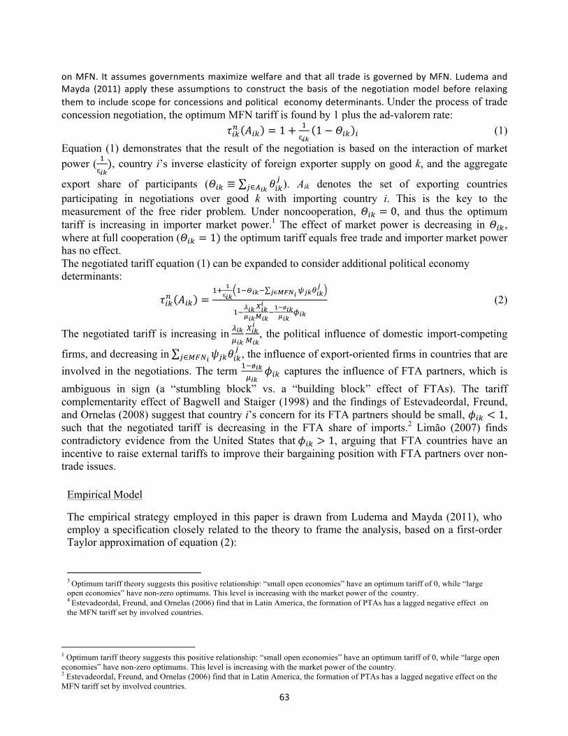
63

onMFN. Itassumesgovernmentsmaximizewelfareand thatall trade isgovernedbyMFN.LudemaandMayda (2011) apply these assumptions to construct the basis of the negotiationmodel before relaxingthemtoincludescopeforconcessionsandpolitical economydeterminants.Under the process of trade concession negotiation, the optimum MFN tariff is found by 1 plus the ad-valorem rate:

𝜏!"! 𝐴!" = 1+ !ᶓ!"

1− 𝛩!" ! (1) Equation (1) demonstrates that the result of the negotiation is based on the interaction of market power ( !

ᶓ!"), country i’s inverse elasticity of foreign exporter supply on good k, and the aggregate

export share of participants (𝛩!" ≡ 𝜃!"!

!∈!!" ). Aik denotes the set of exporting countries participating in negotiations over good k with importing country i. This is the key to the measurement of the free rider problem. Under noncooperation, 𝛩!! = 0, and thus the optimum tariff is increasing in importer market power.1 The effect of market power is decreasing in 𝛩!", where at full cooperation (𝛩!" = 1) the optimum tariff equals free trade and importer market power has no effect. The negotiated tariff equation (1) can be expanded to consider additional political economy determinants:

𝜏!"! 𝐴!" =!! !

ᶓ!"!!!!"! !!"!!"

!!∈!"!!

!!!!"!!"

!!"!

!!"!!!ø!"!!"

!!" (2)

The negotiated tariff is increasing in !!"!!"

!!"!

!!", the political influence of domestic import-competing

firms, and decreasing in 𝜓!"𝜃!"!

!∈!"!! , the influence of export-oriented firms in countries that are involved in the negotiations. The term !!ø!"

!!"𝜙!" captures the influence of FTA partners, which is

ambiguous in sign (a “stumbling block” vs. a “building block” effect of FTAs). The tariff complementarity effect of Bagwell and Staiger (1998) and the findings of Estevadeordal, Freund, and Ornelas (2008) suggest that country i’s concern for its FTA partners should be small, 𝜙!" < 1, such that the negotiated tariff is decreasing in the FTA share of imports.2 Limão (2007) finds contradictory evidence from the United States that 𝜙!" > 1, arguing that FTA countries have an incentive to raise external tariffs to improve their bargaining position with FTA partners over non-trade issues. Empirical Model

The empirical strategy employed in this paper is drawn from Ludema and Mayda (2011), who employ a specification closely related to the theory to frame the analysis, based on a first-order Taylor approximation of equation (2):

3 Optimum tariff theory suggests this positive relationship: “small open economies” have an optimum tariff of 0, while “large open economies” have non-zero optimums. This level is increasing with the market power of the country. 4 Estevadeordal, Freund, and Ornelas (2006) find that in Latin America, the formation of PTAs has a lagged negative effect on the MFN tariff set by involved countries.

1 Optimum tariff theory suggests this positive relationship: “small open economies” have an optimum tariff of 0, while “large open economies” have non-zero optimums. This level is increasing with the market power of the country.2 Estevadeordal, Freund, and Ornelas (2006) find that in Latin America, the formation of PTAs has a lagged negative effect on the MFN tariff set by involved countries.

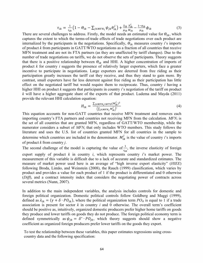
64

𝜏!" = !ᶓ!"

1− 𝛩!" − 𝜓!"𝜃!"!

!∈!"!! + !!"!!"

!!"!

!!"− !!ø!"

!!"𝜙!" (3)

There are several challenges to address. Firstly, the model needs an estimated value for 𝛩!", which captures the extent to which the terms-of-trade effects of trade negotiations over each product are internalized by the participants in the negotiations. Specifically, 𝛩!" measures country i’s imports of product k from participants in GATT/WTO negotiations as a fraction of all countries that receive MFN treatment and are not its FTA partners (as they are unaffected by tariff changes). Due to the number of trade negotiations on tariffs, we do not observe the sets of participants. Theory suggests that there is a positive relationship between 𝛩!" and HHI. A higher concentration of imports of product k for country i suggests the presence of relatively larger exporters, which face a greater incentive to participate in negotiations. Large exporters are deterred from free riding as their participation greatly increases the tariff cut they receive, and thus they stand to gain more. By contrast, small exporters have far less deterrent against free riding as their participation has little effect on the negotiated tariff but would require them to reciprocate. Thus, country i having a higher HHI on product k suggests that participants in country i’s negotiation of the tariff on product k will have a higher aggregate share of the exports of that product. Ludema and Mayda (2011) provide the relevant HHI calculation equation:

𝐻!" = (!!"

!!∈!"#!∩!"# )!

!!"!

!∈!"#!2 (4)

This equation accounts for non-GATT countries that receive MFN treatment and removes each importing country’s FTA partners and countries not receiving MFN from the calculation. MFNi is the set of all countries that are granted MFN, regardless of GATT/WTO membership, while the numerator considers a subset of MFNi that only includes WTO members. This study follows the literature and uses the U.S. list of countries granted MFN for all countries in the sample to determine which countries are included in the denominator. 𝑀!"

! is the value of country i’s imports of product k from country j. The second challenge of the model is capturing the value of !

ᶓ!", the inverse elasticity of foreign

export supply of product k in country i, which represents country i’s market power. The measurement of this variable is difficult due to a lack of accurate and standardized estimates. The measure of market power used here is an average of “high inverse export elasticity” (HIEE) following Broda, Limão, and Weinstein (2008), the Rauch (1999) classification, which varies by product and provides a value for each product of 1 if the product is differentiated and 0 otherwise (Diff), and a contract intensity index that considers the negotiating power of contracts across several metrics (Nunn, 2007). In addition to the main independent variables, the analysis includes controls for domestic and foreign political organization. Domestic political controls follow Goldberg and Maggi (1999), defined as 𝜆!" = 𝛾 + 𝛿 ∙ 𝑃𝑂!" , where the political organization term POik is equal to 1 if a trade association is present for sector k in country i and 0 otherwise. The overall term’s coefficient should be positive as, intuitively, organized domestic producers prefer higher home tariffs on goods they produce and lower tariffs on goods they do not produce. The foreign political economy term is defined symmetrically as 𝜓!" = 𝛿∗ ∙ 𝑃𝑂!", which theory suggests should show a negative coefficient as organized foreign producers prefer lower tariffs on the goods they export.

To test the relationship between these variables, this paper estimates regressions using cross- country data and the following specification:

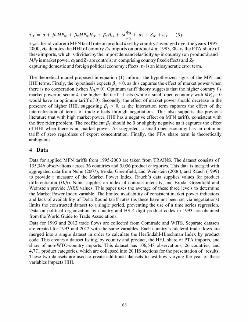
65

𝜏!" = 𝛼 + 𝛽!𝑀𝑃!! + 𝛽!𝑀𝑃!"𝐻!" + 𝛽!𝐻!" + 𝜔 Ф!"!!"

+ 𝛼! + 𝑍!" + 𝜀!" (5)

𝜏!"is the ad valorem MFN tariff rate on product k set by country i averaged over the years 1995- 2000, 𝐻!" denotes the HHI of country i’s imports on product k in 1993, Ф!" is the PTA share of these imports, which is divided by the import demand elasticity 𝜇!" in country i on product k, and 𝑀𝑃!" is market power. 𝛼! and 𝑍!" are controls: 𝛼! comprising country fixed effects and 𝑍!"

capturing domestic and foreign political economy effects. 𝜀!" is an idiosyncratic error term. The theoretical model proposed in equation (1) informs the hypothesized signs of the MPI and HHI terms. Firstly, the hypothesis expects 𝛽! > 0, as this captures the effect of market power when there is no cooperation (when 𝐻!"= 0). Optimum tariff theory suggests that the higher country i’s market power in sector k, the higher the tariff it sets (while a small open economy with 𝑀𝑃!"= 0 would have an optimum tariff of 0). Secondly, the effect of market power should decrease in the presence of higher HHI, suggesting 𝛽! < 0, as the interaction term captures the effect of the internalization of terms of trade effects through negotiations. This also supports the previous literature that with high market power, HHI has a negative effect on MFN tariffs, consistent with the free rider problem. The coefficient 𝛽! should be 0 or slightly negative as it captures the effect of HHI when there is no market power. As suggested, a small open economy has an optimum tariff of zero regardless of export concentration. Finally, the FTA share term is theoretically ambiguous.

4 Data

Data for applied MFN tariffs from 1995-2000 are taken from TRAINS. The dataset consists of 135,346 observations across 36 countries and 5,036 product categories. This data is merged with aggregated data from Nunn (2007), Broda, Greenfield, and Weinstein (2006), and Rauch (1999) to provide a measure of the Market Power Index. Rauch’s data supplies values for product differentiation (Diff). Nunn supplies an index of contract intensity, and Broda, Greenfield and Weinstein provide HIEE values. This paper uses the average of these three levels to determine the Market Power Index variable. The limited availability of consistent market power indicators and lack of availability of Doha Round tariff rates (as these have not been set via negotiations) limits the constructed dataset to a single period, preventing the use of a time series regression. Data on political organization by country and HS 4-digit product codes in 1993 are obtained from the World Guide to Trade Associations. Data for 1993 and 2012 trade flows are collected from Comtrade and WITS. Separate datasets are created for 1993 and 2012 with the same variables. Each country’s bilateral trade flows are merged into a single dataset in order to calculate the Herfindahl-Hirschman Index by product code. This creates a dataset listing, by country and product, the HHI, share of PTA imports, and share of non-WTO-country imports. This dataset has 106,548 observations, 26 countries, and 4,771 product categories, which are collapsed into 20 HS sections for the presentation of results. These two datasets are used to create additional datasets to test how varying the year of these variables impacts HHI.

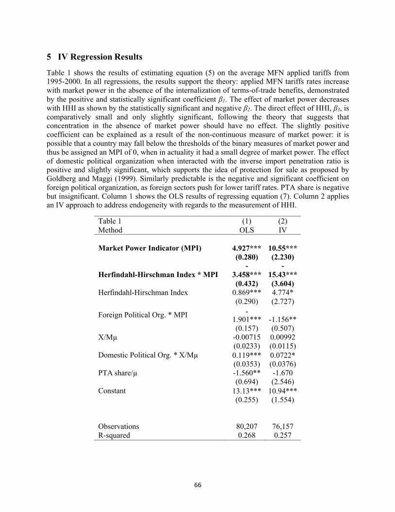
66

5 IV Regression Results

Table 1 shows the results of estimating equation (5) on the average MFN applied tariffs from 1995-2000. In all regressions, the results support the theory: applied MFN tariffs rates increase with market power in the absence of the internalization of terms-of-trade benefits, demonstrated by the positive and statistically significant coefficient β1. The effect of market power decreases with HHI as shown by the statistically significant and negative β2. The direct effect of HHI, β3, is comparatively small and only slightly significant, following the theory that suggests that concentration in the absence of market power should have no effect. The slightly positive coefficient can be explained as a result of the non-continuous measure of market power: it is possible that a country may fall below the thresholds of the binary measures of market power and thus be assigned an MPI of 0, when in actuality it had a small degree of market power. The effect of domestic political organization when interacted with the inverse import penetration ratio is positive and slightly significant, which supports the idea of protection for sale as proposed by Goldberg and Maggi (1999). Similarly predictable is the negative and significant coefficient on foreign political organization, as foreign sectors push for lower tariff rates. PTA share is negative but insignificant. Column 1 shows the OLS results of regressing equation (7). Column 2 applies an IV approach to address endogeneity with regards to the measurement of HHI.

Table 1 Method

(1) OLS

(2) IV

Market Power Indicator (MPI)

4.927*** (0.280)

10.55*** (2.230)

Herfindahl-Hirschman Index * MPI

- 3.458***

- 15.43***

Herfindahl-Hirschman Index

(0.432) 0.869***

(3.604) 4.774*

(0.290) (2.727)

Foreign Political Org. * MPI - 1.901*** (0.157)

-1.156** (0.507)

X/Mµ -0.00715 0.00992 (0.0233) (0.0115) Domestic Political Org. * X/Mµ 0.119***

(0.0353) 0.0722* (0.0376)

PTA share/µ -1.560** -1.670 (0.694) (2.546) Constant 13.13***

(0.255) 10.94*** (1.554)

Observations

80,207

76,157

R-squared 0.268 0.257

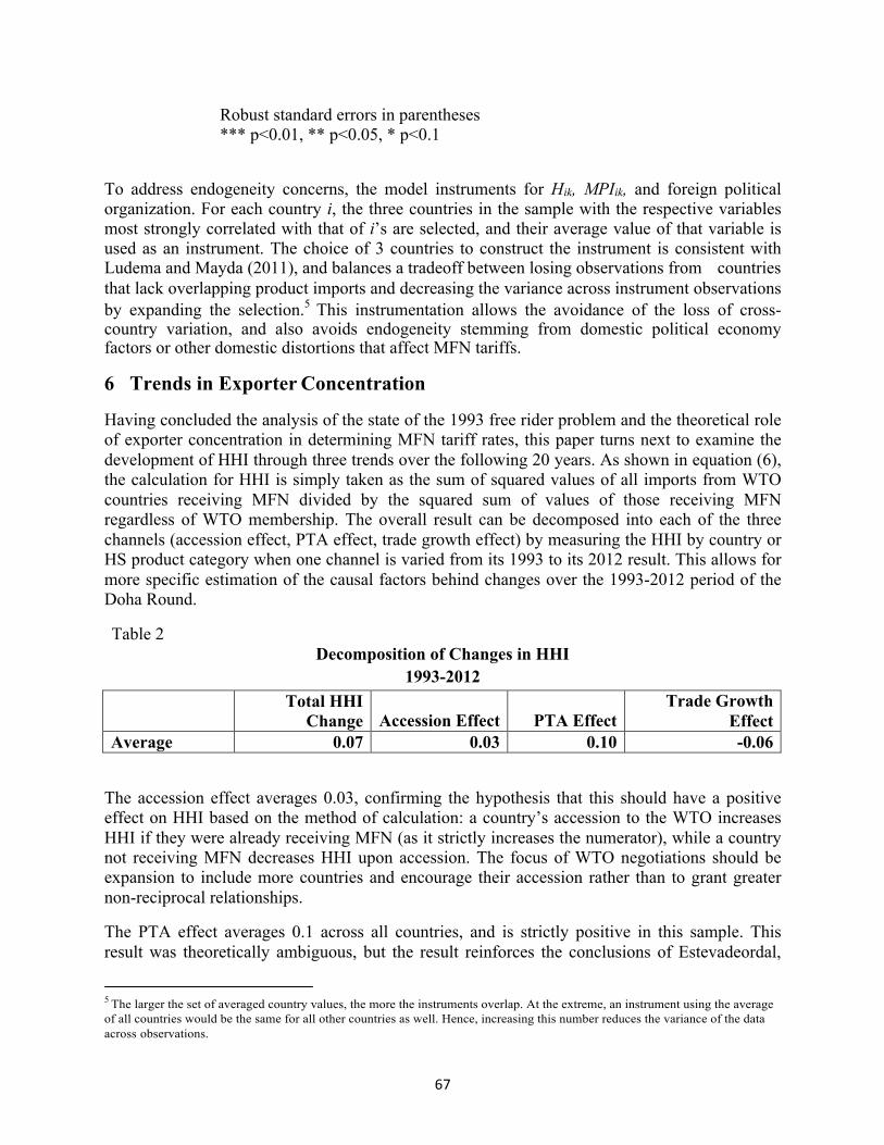
67

Robust standard errors in parentheses *** p<0.01, ** p<0.05, * p<0.1

To address endogeneity concerns, the model instruments for Hik, MPIik, and foreign political organization. For each country i, the three countries in the sample with the respective variables most strongly correlated with that of i’s are selected, and their average value of that variable is used as an instrument. The choice of 3 countries to construct the instrument is consistent with Ludema and Mayda (2011), and balances a tradeoff between losing observations from countries that lack overlapping product imports and decreasing the variance across instrument observations by expanding the selection.5 This instrumentation allows the avoidance of the loss of cross- country variation, and also avoids endogeneity stemming from domestic political economy factors or other domestic distortions that affect MFN tariffs.

6 Trends in Exporter Concentration

Having concluded the analysis of the state of the 1993 free rider problem and the theoretical role of exporter concentration in determining MFN tariff rates, this paper turns next to examine the development of HHI through three trends over the following 20 years. As shown in equation (6), the calculation for HHI is simply taken as the sum of squared values of all imports from WTO countries receiving MFN divided by the squared sum of values of those receiving MFN regardless of WTO membership. The overall result can be decomposed into each of the three channels (accession effect, PTA effect, trade growth effect) by measuring the HHI by country or HS product category when one channel is varied from its 1993 to its 2012 result. This allows for more specific estimation of the causal factors behind changes over the 1993-2012 period of the Doha Round.

Table 2 Decomposition of Changes in HHI

1993-2012 Total HHI

Change Accession Effect

PTA Effect

Trade Growth Effect

Average 0.07 0.03 0.10 -0.06 The accession effect averages 0.03, confirming the hypothesis that this should have a positive effect on HHI based on the method of calculation: a country’s accession to the WTO increases HHI if they were already receiving MFN (as it strictly increases the numerator), while a country not receiving MFN decreases HHI upon accession. The focus of WTO negotiations should be expansion to include more countries and encourage their accession rather than to grant greater non-reciprocal relationships.

The PTA effect averages 0.1 across all countries, and is strictly positive in this sample. This result was theoretically ambiguous, but the result reinforces the conclusions of Estevadeordal,

5 The larger the set of averaged country values, the more the instruments overlap. At the extreme, an instrument using the average of all countries would be the same for all other countries as well. Hence, increasing this number reduces the variance of the data across observations.

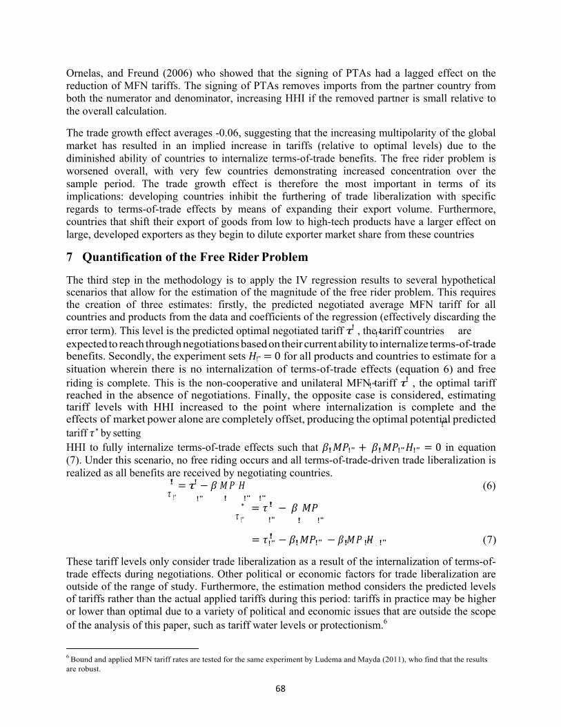
68

!"

!"

!"

!" ! !" ! !" !"

Ornelas, and Freund (2006) who showed that the signing of PTAs had a lagged effect on the reduction of MFN tariffs. The signing of PTAs removes imports from the partner country from both the numerator and denominator, increasing HHI if the removed partner is small relative to the overall calculation.

The trade growth effect averages -0.06, suggesting that the increasing multipolarity of the global market has resulted in an implied increase in tariffs (relative to optimal levels) due to the diminished ability of countries to internalize terms-of-trade benefits. The free rider problem is worsened overall, with very few countries demonstrating increased concentration over the sample period. The trade growth effect is therefore the most important in terms of its implications: developing countries inhibit the furthering of trade liberalization with specific regards to terms-of-trade effects by means of expanding their export volume. Furthermore, countries that shift their export of goods from low to high-tech products have a larger effect on large, developed exporters as they begin to dilute exporter market share from these countries

7 Quantification of the Free Rider Problem

The third step in the methodology is to apply the IV regression results to several hypothetical scenarios that allow for the estimation of the magnitude of the free rider problem. This requires the creation of three estimates: firstly, the predicted negotiated average MFN tariff for all countries and products from the data and coefficients of the regression (effectively discarding the error term). This level is the predicted optimal negotiated tariff 𝜏! , the tariff countries are expected to reach through negotiations based on their current ability to internalize terms-of-trade benefits. Secondly, the experiment sets 𝐻!" = 0 for all products and countries to estimate for a situation wherein there is no internalization of terms-of-trade effects (equation 6) and free riding is complete. This is the non-cooperative and unilateral MFN tariff 𝜏! , the optimal tariff reached in the absence of negotiations. Finally, the opposite case is considered, estimating tariff levels with HHI increased to the point where internalization is complete and the effects of market power alone are completely offset, producing the optimal potential predicted tariff 𝜏∗ by setting HHI to fully internalize terms-of-trade effects such that 𝛽!𝑀𝑃!" + 𝛽!𝑀𝑃!"𝐻!" = 0 in equation (7). Under this scenario, no free riding occurs and all terms-of-trade-driven trade liberalization is realized as all benefits are received by negotiating countries.

! = 𝜏! − 𝛽 𝑀𝑃 𝐻 (6) 𝜏 !" !" ! !" !"

∗ = 𝜏! − 𝛽 𝑀𝑃 𝜏 !" !" ! !"

= 𝜏! − 𝛽 𝑀𝑃 − 𝛽 𝑀𝑃 𝐻 (7)

These tariff levels only consider trade liberalization as a result of the internalization of terms-of- trade effects during negotiations. Other political or economic factors for trade liberalization are outside of the range of study. Furthermore, the estimation method considers the predicted levels of tariffs rather than the actual applied tariffs during this period: tariffs in practice may be higher or lower than optimal due to a variety of political and economic issues that are outside the scope of the analysis of this paper, such as tariff water levels or protectionism.6

6 Bound and applied MFN tariff rates are tested for the same experiment by Ludema and Mayda (2011), who find that the results are robust.

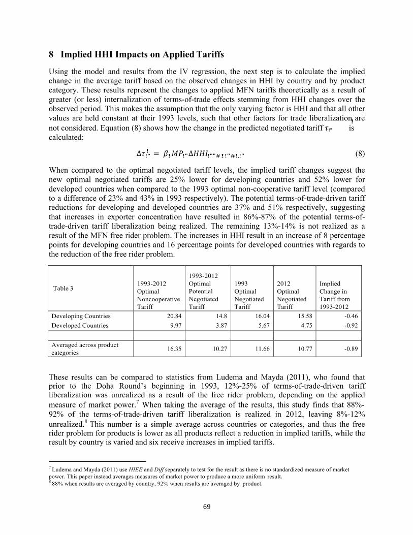
69

!" ! !" !""#!!"#!,!"

8 Implied HHI Impacts on Applied Tariffs

Using the model and results from the IV regression, the next step is to calculate the implied change in the average tariff based on the observed changes in HHI by country and by product category. These results represent the changes to applied MFN tariffs theoretically as a result of greater (or less) internalization of terms-of-trade effects stemming from HHI changes over the observed period. This makes the assumption that the only varying factor is HHI and that all other values are held constant at their 1993 levels, such that other factors for trade liberalization are ! not considered. Equation (8) shows how the change in the predicted negotiated tariff 𝜏!" is calculated:

∆𝜏! = 𝛽 𝑀𝑃 ∆𝐻𝐻𝐼 (8)

When compared to the optimal negotiated tariff levels, the implied tariff changes suggest the new optimal negotiated tariffs are 25% lower for developing countries and 52% lower for developed countries when compared to the 1993 optimal non-cooperative tariff level (compared to a difference of 23% and 43% in 1993 respectively). The potential terms-of-trade-driven tariff reductions for developing and developed countries are 37% and 51% respectively, suggesting that increases in exporter concentration have resulted in 86%-87% of the potential terms-of- trade-driven tariff liberalization being realized. The remaining 13%-14% is not realized as a result of the MFN free rider problem. The increases in HHI result in an increase of 8 percentage points for developing countries and 16 percentage points for developed countries with regards to the reduction of the free rider problem.

Table 3

1993-2012 Optimal Noncooperative Tariff

1993-2012 Optimal Potential Negotiated Tariff

1993 Optimal Negotiated Tariff

2012 Optimal Negotiated Tariff

Implied Change in Tariff from 1993-2012

Developing Countries 20.84 14.8 16.04 15.58 -0.46 Developed Countries 9.97 3.87 5.67 4.75 -0.92

Averaged across product categories 16.35 10.27 11.66 10.77 -0.89

These results can be compared to statistics from Ludema and Mayda (2011), who found that prior to the Doha Round’s beginning in 1993, 12%-25% of terms-of-trade-driven tariff liberalization was unrealized as a result of the free rider problem, depending on the applied measure of market power.7 When taking the average of the results, this study finds that 88%- 92% of the terms-of-trade-driven tariff liberalization is realized in 2012, leaving 8%-12% unrealized.8 This number is a simple average across countries or categories, and thus the free rider problem for products is lower as all products reflect a reduction in implied tariffs, while the result by country is varied and six receive increases in implied tariffs.

7 Ludema and Mayda (2011) use HIEE and Diff separately to test for the result as there is no standardized measure of market power. This paper instead averages measures of market power to produce a more uniform result. 8 88% when results are averaged by country, 92% when results are averaged by product.

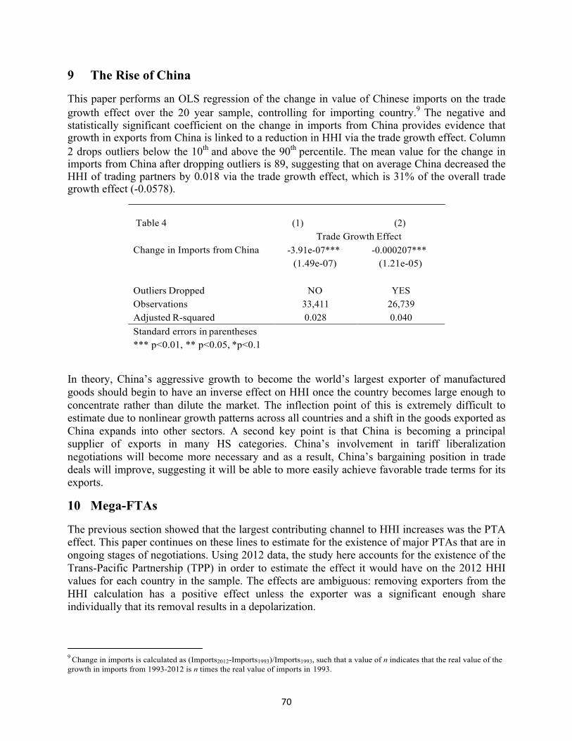
70

9 The Rise of China

This paper performs an OLS regression of the change in value of Chinese imports on the trade growth effect over the 20 year sample, controlling for importing country.9 The negative and statistically significant coefficient on the change in imports from China provides evidence that growth in exports from China is linked to a reduction in HHI via the trade growth effect. Column 2 drops outliers below the 10th and above the 90th percentile. The mean value for the change in imports from China after dropping outliers is 89, suggesting that on average China decreased the HHI of trading partners by 0.018 via the trade growth effect, which is 31% of the overall trade growth effect (-0.0578).

Table 4 (1) (2)

Trade Growth Effect Change in Imports from China -3.91e-07***

(1.49e-07) -0.000207***

(1.21e-05)

Outliers Dropped NO YES Observations 33,411 26,739 Adjusted R-squared 0.028 0.040 Standard errors in parentheses *** p<0.01, ** p<0.05, *p<0.1

In theory, China’s aggressive growth to become the world’s largest exporter of manufactured goods should begin to have an inverse effect on HHI once the country becomes large enough to concentrate rather than dilute the market. The inflection point of this is extremely difficult to estimate due to nonlinear growth patterns across all countries and a shift in the goods exported as China expands into other sectors. A second key point is that China is becoming a principal supplier of exports in many HS categories. China’s involvement in tariff liberalization negotiations will become more necessary and as a result, China’s bargaining position in trade deals will improve, suggesting it will be able to more easily achieve favorable trade terms for its exports.

10 Mega-FTAs

The previous section showed that the largest contributing channel to HHI increases was the PTA effect. This paper continues on these lines to estimate for the existence of major PTAs that are in ongoing stages of negotiations. Using 2012 data, the study here accounts for the existence of the Trans-Pacific Partnership (TPP) in order to estimate the effect it would have on the 2012 HHI values for each country in the sample. The effects are ambiguous: removing exporters from the HHI calculation has a positive effect unless the exporter was a significant enough share individually that its removal results in a depolarization.

9 Change in imports is calculated as (Imports2012-Imports1993)/Imports1993, such that a value of n indicates that the real value of the growth in imports from 1993-2012 is n times the real value of imports in 1993.

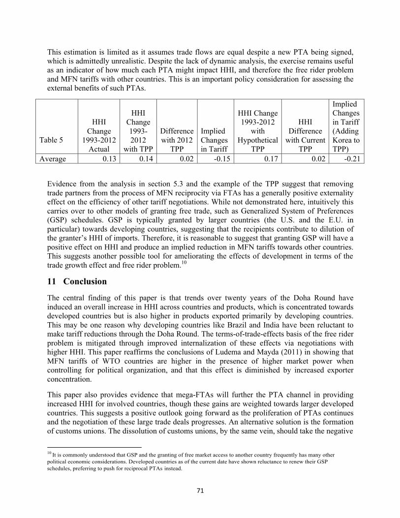
71

This estimation is limited as it assumes trade flows are equal despite a new PTA being signed, which is admittedly unrealistic. Despite the lack of dynamic analysis, the exercise remains useful as an indicator of how much each PTA might impact HHI, and therefore the free rider problem and MFN tariffs with other countries. This is an important policy consideration for assessing the external benefits of such PTAs.

Table 5

HHI Change

1993-2012 Actual

HHI

Change 1993- 2012

with TPP

Difference with 2012

TPP

Implied Changes in Tariff

HHI Change 1993-2012

with Hypothetical

TPP

HHI Difference

with Current TPP

Implied Changes in Tariff (Adding Korea to TPP)

Average 0.13 0.14 0.02 -0.15 0.17 0.02 -0.21

Evidence from the analysis in section 5.3 and the example of the TPP suggest that removing trade partners from the process of MFN reciprocity via FTAs has a generally positive externality effect on the efficiency of other tariff negotiations. While not demonstrated here, intuitively this carries over to other models of granting free trade, such as Generalized System of Preferences (GSP) schedules. GSP is typically granted by larger countries (the U.S. and the E.U. in particular) towards developing countries, suggesting that the recipients contribute to dilution of the granter’s HHI of imports. Therefore, it is reasonable to suggest that granting GSP will have a positive effect on HHI and produce an implied reduction in MFN tariffs towards other countries. This suggests another possible tool for ameliorating the effects of development in terms of the trade growth effect and free rider problem.10

11 Conclusion

The central finding of this paper is that trends over twenty years of the Doha Round have induced an overall increase in HHI across countries and products, which is concentrated towards developed countries but is also higher in products exported primarily by developing countries. This may be one reason why developing countries like Brazil and India have been reluctant to make tariff reductions through the Doha Round. The terms-of-trade-effects basis of the free rider problem is mitigated through improved internalization of these effects via negotiations with higher HHI. This paper reaffirms the conclusions of Ludema and Mayda (2011) in showing that MFN tariffs of WTO countries are higher in the presence of higher market power when controlling for political organization, and that this effect is diminished by increased exporter concentration.

This paper also provides evidence that mega-FTAs will further the PTA channel in providing increased HHI for involved countries, though these gains are weighted towards larger developed countries. This suggests a positive outlook going forward as the proliferation of PTAs continues and the negotiation of these large trade deals progresses. An alternative solution is the formation of customs unions. The dissolution of customs unions, by the same vein, should take the negative

10 It is commonly understood that GSP and the granting of free market access to another country frequently has many other political economic considerations. Developed countries as of the current date have shown reluctance to renew their GSP schedules, preferring to push for reciprocal PTAs instead.

72

effect it will have on terms-of-trade internalization into account as it will result in implied rises in future negotiated MFN tariffs. Finally, this paper highlights the impact developing countries have on terms-of-trade-driven tariff liberalization, as emerging economies dilute the export concentration of the major developed economies while raising the concentration of their own exported product types. This effect is most prominent with China, though as China grows and takes on more of a role as a principal supplier, its bargaining position in negotiations will also improve and the country will be able to push more seriously for tariff cuts.

The significance of these findings is that increasing the coverage of the WTO and of PTAs has a positive effect on reducing negotiated MFN tariffs to other countries. These effects have the capacity to outweigh the dilution effect of emerging economies, and creating PTAs with these countries can serve to remove their negative effects by eliminating the need for free-riding. The study concludes that from 1993-2012, unrealized potential liberalization on average decreased from a range of 12%-25% to a range of 8%-12%, and thus continued liberalization under the WTO should be an objective to further reduce the problem. The WTO and PTAs act as complements rather than substitutes in this process. This benefit can be augmented by grouping countries into customs unions that negotiate tariffs collectively and thus function as larger exporters, offsetting some of the losses resulting from economic development.

The decision for a country to create PTAs, grant GSP, or form customs unions has other important political and economic determinants, such as security, politics, and the political interests of employed constituents and national interests.11 The implications of this paper in providing evidence that the use of these tools increases the efficiency of MFN tariff negotiations are broadly that policymakers should take these benefits into account amongst their other concerns. A better understanding of the benefits of these policies allows a more informed decision that takes terms-of-trade internalization effects into consideration and sheds light on smoothing the difficult road towards trade liberalization.

12 Bibliography Abboushi, S. (2014). “Transatlantic trade and investment partnership - overview.” Competition Forum, 12(1), 107-

113.

Bagwell, Kyle, and Robert W. Staiger. “Regionalism and Multilateral Tariff Cooperation.” Working paper no. 5921. NBER Working Papers, 1998.

Bagwell, Kyle, and Robert W. Staiger. “The Economics of the World Trading System.” Cambridge, MA: MIT,

2002.

Bagwell, Kyle, and Robert W. Staiger. "What Do Trade Negotiators Negotiate About? Empirical Evidence from the World Trade Organization." American Economic Review 101.4 (2011): 1238-273.

Baldwin, R. E., and T. Murray. "MFN Tariff Reductions and Developing Country Trade Benefits Under the GSP." The Economic Journal 87.345 (1977): 30-46.

Bhagwati, Jagdish N. "The Selfish Hegemon Must Offer a New Deal on Trade." Financial Times. N.p., 19 Aug.

2008. Web.

11Busch, Marc L. and Reinhardt, Eric, "Industry Location and Protection: The Political and Economic Geography of U.S. Nontariff Barriers." American Journal of Political Science 43 (4) 1999: 1028-1050.

73

Blustein, Paul. “Misadventures of the Most Favored Nations: Clashing Egos, Inflated Ambitions, and the Great Shambles of the World Trade System.” New York: PublicAffairs, 2009.

Bown, Chad P. "The Economics of Trade Disputes, the GATT's Article XXIII, and the WTO's Dispute Settlement

Understanding." Economics and Politics 14.3 (2002): 283-323.

Bown, Chad P., and Meredith A. Crowley. "Self-Enforcing Trade Agreements: Evidence from Time-Varying Trade Policy." American Economic Review 103.2 (2013): 1071-090.

Broda, Christian, Nuno Limão, and David E. Weinstein. "Optimal Tariffs and Market Power: The Evidence."

American Economic Review 98.5 (2008): 2032-2065.

Bun, Maurice, and Harrison, Teresa. “OLS and IV Estimation of Regression Models Including Endogenous Interaction Terms.” Discussion paper, Amsterdam School of Economics. 2014.

Busch, Marc L. and Reinhardt, Eric, "Industry Location and Protection: The Political and Economic Geography of

U.S. Nontariff Barriers." American Journal of Political Science 43 (4) 1999: 1028-1050. Caplin, Andrew, and Kala Krishna. “Tariffs and the Most-Favored-Nation Clause.” Institute of Economics Research,

1988.

Carpenter, Theresa, and Andreas Lendle. “How Preferential Is World Trade?” Working paper no. 2010-32. Geneva: Center for Trade and Economic Integration, 2010.

Estevadeordal, A., Freund, C., Ornelas, E. “Does Regionalism Affect Trade Liberalization Towards Non-

Members?” Quarterly Journal of Economics, 123 (2008), 1531-1575.

FAO Trade and Markets Division. “World Statistical Compendium for Raw Hides and Skins, Leather and Leather Footwear 1993-2012.” Rep. Food and Agriculture Organization of the United Nations, 2013.

Fergusson, Ian F. “The World Trade Organization: The Non-Agricultural Market Access (NAMA) Negotiations.”

Rep.: Congressional Research Service, 2011.

Finger, J. Michael, and Julio J. Nogues. "The Unbalanced Uruguay Round Outcome: The New Areas in Future WTO Negotiations." The World Economy 25.3 (2002): 321-40.

Finger, J. M., and M. E. Kreinin. "A Measure of `Export Similarity' and Its Possible Uses." The Economic Journal

89.356 (1979): 905. Finger, J.M., Reincke, U, and Castro, A. “Market Access Bargaining in the Uruguay Round: How Tightly Does

Reciprocity Bind?” in On Going Alone: The Case for Relaxed Reciprocity in Freeing Trade, Jagdish N. Bhagwati, ed. (Cambridge MA: MIT Press, 2002).

Francois, Joseph and Ganeshan Wignaraja. “Economic Implications of Asian Integration.” Global Economy Journal

8, no. 3:1-46. 2008.

Johnson, H. “An economic theory of protectionism, tariff bargaining, and the formation of customs unions.” Journal of Political Economy 73, 256–283. 1965.

Jones, Vivian C. “Generalized System of Preferences: Background and Renewal Debate.” Rep.: Congressional

Research Service, Dec 16, 2014.

Goldberg, P.K. and G. Maggi. "Protection for Sale: An Empirical Investigation," American Economic Review 89, 5, pp. 1135-1155. 1999.

Grossman, G. and E. Helpman. "Protection for Sale," American Economic Review, 84, 4, pp. 833-850. 1994.

74

Helpman, Elhanan, “Politics and Trade Policy,” Advances in Economics and Econometrics: Theory and Applications, vol. 2, D. M. Kreps and K. F. Wallis, eds. (Cambridge: Cambridge University Press, 1997).

Hübner, Kurt. “Europe, Canada and the Comprehensive Economic and Trade Agreement.” Abingdon, Oxon: Routledge, 2011.

Kim, In---Song. “Political Cleavages within Industry: Firm Level Lobbying for Trade Liberalization.” Working Paper. Princeton University. Princeton. 2013.

Limão, N. “Are Preferential Trade Agreements with Non-Trade Objectives a Stumbling Block for Multilateral Liberalization?” Review of Economic Studies, 74 (2007), 821-855.

Ludema, R. "International Trade Bargaining And The Most-Favored-Nation Clause." Economics and Politics 3.1 (1991): 1-20.

Ludema, R. and A.M. Mayda, 2009. "Do Countries Free Ride on MFN?," Journal of International Economics, 77, 2, pp. 137-150.

Ludema, R. and A.M. Mayda, 2011. "Do terms-of-trade effects matter for trade agreements? Evidence from WTO countries," Quarterly Journal of Economics, 128, 4, pp. 1837-1893.

Nunn, N. "Relationship-Specificity, Incomplete Contracts, and the Pattern of Trade." The Quarterly Journal of Economics 122.2 (2007): 569-600.

O'Neill, Jim. “Building Better Global Economic BRICs,” Global Economics. no. 66. Goldman Sachs, 2001.

Petri, Peter A, Michael G. Plummer, and Fan Zhai. “The Trans-Pacific Partnership and Asia-Pacific Integration: A Quantitative Assessment.” Washington, DC: Peterson Institute for International Economics, 2012.

Preeg, Ernest H. “Traders and Diplomats; an Analysis of the Kennedy round of Negotiations under the General Agreement on Tariffs and Trade.” Washington: Brookings Institution, 1970.

Pregelj, Vladimir N. “Country Applicability of the U.S. Normal Trade Relations (Most-Favored-Nation) Status.” Rep.: Congressional Research Service, 2005.

Rauch, James E. “Networks versus Markets in International Trade,” Journal of International Economics, 48 (1999), 7-35.

Schott, Jeffrey J, Barbara Kotschwar, and Julia Muir. “Understanding the Trans-Pacific Partnership.” Washington, DC: Peterson Institute for International Economics, 2013.

WTO. “Changing Face of Trade Pacts Requires Coherence with WTO, Report Says.” WTO, 20 July 2011.

Viner, J. “The most-favored-national clause.” Index, Svenska Handelsbanken, Stockholm. Reprinted in: Viner, J., 1951. International Economics. Glencoe, IL, The Free Press. 1931.

75

Adjusting for Overconfidence

Using Partition Dependence Su-Shien Ryan Goh

University of California Berkeley

Abstract Overconfidence and the anchoring bias are two of the most common and robust biases to affect human decision-making. Overconfidence is the unsubstantiated belief that one attributes to himself and manifests in three different forms: overestimation of one’s own abilities, overplacement of self in a group, and overprecision in the belief of certainty of an outcome (Moore & Healy, 2008). The anchoring bias is the assimilation of beliefs to an uninformative, arbitrary point due to insufficient contrasting or over-assimilation (Mussweiler & Strack, 1999). The anchoring bias is extremely prevalent in elicitations of probability estimates, where people tend to equally assign probabilities across the probability state space, a phenomenon coined as partition dependence (Fox & Clemen, 2005).

In an attempt to study both of these biases, this paper proposes an innovative methodology to study the anchoring bias: using the normalized deviations of the median of fitted probability elicitations. The normalization allows the magnitude of the anchoring bias to be compared between different manipulations. We test for the effect of the anchoring bias and overprecision on each other and their effects on accuracy using experimental forecasting data from the Good Judgment Project.

Although there was no relationship found between the magnitude of the anchoring bias and overconfidence, results show that asking randomly-generated questions may have prompted participants to think more critically about their assumptions and improved the accuracy of their resulting probability estimates. Similar to previous studies, overconfidence was found to decrease accuracy.

Fox, C. R. and Clemen, R. T. (2005). Subjective Probability Assessment in Decision Analysis: Partition Dependence and Bias toward the Ignorance Prior.Management Science, 51(9): 1417–1432.

Moore, D. and Healy, P.J. (2008) The Trouble with Overconfidence.

Mussweiller, T. and Strack, F. Comparing is Believing: A Selective Accessibility Model of Judgmental Anchoring. European Review of Social Psy-chology, 10(1) (1999): 135–67.

76

China and India in Africa: Implications of New Private Sector Actors on Bribe

Paying Incidence Sankalp Gowda

Abstract

In recent years African nations have increasingly turned to Indian and Chinese firms to fill the investment gap left by Western countries in the wake of the global economic recession. While many have applauded these firms for boosting competition, providing access to new global supply chains, and producing learning effects through knowledge transfers, their reception within Africa has been mixed. This paper seeks to address one of the most common critiques of Asian firms doing business in Africa: that low levels of corporate governance and poor managerial practices have undermined anti-corruption efforts throughout the continent. The paper first details and analyzes the managerial practices of Indian and Chinese firms to distinguish what factors make these firms more likely to pay bribes. Next, it uses a combination of firm-level data from the 2006-2014 World Bank Enterprise Surveys and macro-level data on bilateral trade and FDI flows from UNCTAD, the IMF Direction of Trade Statistics, the World Bank Development Indicators, and the CEPII Gravity Dataset to empirically test the claim that the presence of Indian and Chinese firms has increased bribe-paying incidence in African countries. I find the result that firms operating in countries with large Indian and Chinese involvement are significantly less likely to engage in bribe paying. This is promising evidence against the “race to the bottom” scenario that many Western firms and governments have complained of in response to the growing Asian presence in Africa.

77

1 Introduction Over the course of the past decade, African nations have increasingly adopted a new view toward development that focuses on bolstering private sector growth through investment and trade. Driven by mounting criticism of the effectiveness of foreign aid dollars and cynicism toward the sustainability of development priorities set by Western nations, this move has coincided with the rise of India and China as global economic powers. Indian and Chinese firms have stepped in to fill the investment gap left in emerging economies by more cautious Western investors and have heavily prioritized building South-South relationships over the past several years. The economic significance of this trend is remarkable. The “global” south was responsible for 34% of all foreign direct investment to the developing world in 2010 and China’s outward FDI in the “south” alone totals over $1 trillion (Puri, 2010; World Bank, 2011, 23). Additionally, South- South exports grew to $4 trillion in 2011 and increased from 13% of world exports in 2001 to 25% in 2011 (UNCTAD, 2013, 1). Although not all of these flows have been directed at African nations, they undoubtedly played a significant role in contributing to the continent’s 4% growth rate in 2013, helping Africa top the global average of 3% (African Economic Outlook, 2014).

Understandably, this growth rate and these trends do not extend to all African nations, and Indian and Chinese involvement has been limited to a number of key countries. Primary among these are the oil and mineral rich Nigeria, Sudan, and Zambia that are critical to meeting Indian and Chinese demand for resources, but others include Botswana, Ethiopia, Kenya, Madagascar, Mauritius, Mozambique, Senegal, South Africa, and Uganda, where investment has extended into a much broader range of sectors (Broadman, 2008).

Although many applaud Indian and Chinese firms for boosting competition, providing access to new global supply chains, and producing learning effects through technology and knowledge transfers, the reception of these firms in these countries has been mixed. Common critiques of foreign firms from Asia include the undercutting of local wages/exclusion of the local labor market, quality concerns over working conditions and outputs, and the central focus of this paper: low levels of corporate governance that could undermine anticorruption efforts. This last view is well represented by Western donors and businesses. During a 2012 speech in Senegal, former Secretary of State Hillary Clinton took an indirect jab at India and China when she stated, "The USA stands for democracy and human rights, even when it's easier or more profitable to look away in order to secure resources" (Deutsche Welle, 2012). Business leaders echo this sentiment and point to anticorruption legislation such as the United States’ Foreign Corrupt Practices Act and the lack of similar legislation in India and China as an inherent disadvantage for Western firms (Wall Street Journal, 2014). The implication is clear: Indian and Chinese firms have been eclipsing Western investors through bribe paying and other corrupt practices. While India and China have been quick to refute such claims, they continue to cast a shadow over further investment efforts. Notably, much of this criticism has been directed toward Chinese firms while Indian firms have for the most part escaped relatively unscathed.

This paper seeks to deconstruct the impact of Indian and Chinese firms as new private sector actors on bribe paying incidence in the African region. Section 1 describes important differences in each nation’s approach to investing in Africa. Section 2 discusses how these differences may affect the supply-side of corruption through management practices that tolerate or even embrace

78

bribery. Section 3 summarizes literature regarding institutional drivers of corruption at the firm level that theoretically affect all firms operating in Africa. Section 4 outlines the data and methodology of my empirical analysis, and Section 5 presents my empirical findings. I conclude with policy implications and suggestions for areas of further research.

I first find preliminary evidence from the Enterprise Surveys supports the result that firms operating in countries with large Indian and Chinese involvement are significantly less likely to engage in bribe paying. I then use more detailed bilateral trade and FDI data measuring the China-Africa relationship – I exclude India from this analysis because of unreliable FDI statistics – to prove a causal relationship between Chinese FDI and lower corruption rates. To accomplish this, I treat for the endogenous relationship between investment climate and FDI by using an instrumental variables approach based on the gravity model of trade and investment. Although this evidence alone is not enough to exculpate all Indian and Chinese firms from any wrongdoing, it is certainly promising evidence against the “race to the bottom” hypothesis that has been raised against foreign firms operating in Africa.

2 The Indian vs. Chinese Approach to FDI in Africa

Of the two countries, China remains the dominant player in Africa, with approximately $119.7 billion dollars in FDI outflows to the continent between 2007 and 2012, compared with India’s $27.3 billion (Fortin, 2013, Ernst & Young, 2013). Although these numbers still lag far behind those of Western countries like the United States, the United Kingdom, and France, China has managed to become Africa’s largest trading partner, surpassing the United States in 2009. The majority of China’s investments are in resource intensive industries, particularly oil and natural gas, as it depends heavily on Africa for its energy needs (approximately one-third of its crude oil comes from Africa). Its investments in these industries have been accompanied by large-scale infrastructure projects in roads, ports, and buildings, adding to its visibility on the continent (Alessi & Hansion, 2012; Khare, 2013). The size of these contracts also means that the majority of these investments are made at the state-state level through state owned enterprises or sponsored by state agencies such as China’s ExIm Bank (The Economist, 2011). Starting in 2010, this trend has shifted toward a more diversified set of industries, with transportation, agriculture, and real estate investments eclipsing natural resource investment (Caulderwood, 2014). China’s centralized approach to investment on the continent has been backed by high- level visits from President Xi Jinping in 2013 as well as by former President Hu Jintao throughout the 2000s. As a result of its growth and heavy involvement in Africa’s capital- intensive industries, China has garnered more attention than any other investor in recent years.

India, on the other hand, operates by a different model. Although its state-owned energy companies pursue India’s interests in African resource markets in the same manner as China’s, the majority of its investment in Africa is led by the private sector (Jacobs, 2013). This is reflected by the fact that although India’s FDI outflows were only one-fifth of China’s, India was responsible for 56% more new FDI projects than China between 2007 and 2012 (Ernst & Young, 2013). These projects represent a far more diversified portfolio of smaller investments than China’s, and India is known for its presence in a broader range of sectors. These include agriculture, IT, telecommunications, and healthcare/medicine. Interestingly, these are sectors that avoid direct competition with Chinese investments in Africa, a product of private financing and a

79

more traditional program of risk assessment spurred by a lack of central state backing. Among the largest private sector actors in the Indian expansion into Africa are globally well-known and regarded firms such as the Tata Group, Godrej, and Bharti Airtel (Indo-African Business Magazine, 2011).

Indian and Chinese firms are further differentiated by their level of integration with local African economies (The Economist, 2013b). The Indian presence in East Africa has existed for more than a century, and the two regions are bound by a common colonial legacy. Furthermore, the strong, integrated Indian diaspora serves as a natural base to promote Indian interests in the region. This translates to a smaller language and culture barrier than that faced by Chinese firms. Additionally, a survey of Indian business leaders actively investing in Africa undertaken at the most recent WEF India Economic Summit in 2014 reported a hiring target for local employees of 90% and a new push to produce certain types of products in Africa instead of focusing on selling finished goods (Vanham, 2014). Chinese involvement has meanwhile been seen as the more foreign of the two and has at times evoked a xenophobic response from local populations. Some countries such as Malawi, Tanzania, Uganda, and Zambia have responded by restricting the sectors in which Chinese firms can operate. This suspicion is in part due to protectionism by African businesses, but it remains one of China’s biggest hurdles in Africa (The Economist, 2013a). Even more serious incidents such as recurring riots over working conditions in Zambian mines also continue to color popular perception of China as the continent’s new neocolonial power.

3 The Supply-Side of Corruption

It is clear that Indian and Chinese firms have vastly different approaches to doing business in Africa. Deconstructing these differences further could provide insight into how their management practices may affect the supply-side drivers of corruption. Given that the Western critique of Indian and Chinese firms is focused here, this is a subject worth exploring despite a paucity of existing literature.

In mainland China it is well documented that bribe paying and other forms of corruption are common business practice, reflected by China’s rank as 100th out of 175 countries on Transparency International’s Corruption Perceptions index (Transparency International, 2014). The business culture is reliant upon relationships and “gifts,” even in the private sector. Cai, et al. (2011) use a conceptual management theory of the Chinese firm to empirically show that entertainment and travel costs, a common category in most Chinese firms’ financials, is often used as a proxy for dollars spent on bribe paying or other similar activities (Cai, et al., 2011). Similarly, anecdotal evidence from Chinese firms in Africa supports the theory that these practices have been exported overseas. Chinese managers have been documented bribing union bosses with fake “study tours” to China to avoid censure over poor working conditions (The Economist, 2011). Additionally, there are numerous cases of Chinese SOEs like Nuctech Company – at one point managed by President Hu Jintao’s son – becoming the subject of both African and European anti-corruption probes (Gordon, et al., 2009). While the majority of these cases are on a smaller scale, a recent incident with Sicomines, a Chinese state-owned mining company, gives a better sense of the how much money can change hands in one of these transactions. The company recently signed a $6.5 billion deal with the Democratic Republic of

80

Congo that included a $350 million “signing bonus.” According to accountability NGO Global Watch, $24 million of this bonus made its way to secret bank accounts in the British Virgin Islands rather than into the DRC’s treasury (Kushner, 2013).

India, at 85th on Transparency International’s Corruption Perceptions Index, is not necessarily a much better contender for clean management practices in its own private sector (Transparency International, 2014). Aside from a more limited relationship with the state and a more traditional business perspective on risk management that may preclude firms from entering a corrupt market where costs are higher, there is little to indicate that Indian firms are less likely to engage in bribe paying than Chinese firms. Interestingly, however, a 2013 Transparency International study of BRICS firms operating in emerging markets ranked Indian firms first in transparency while Chinese firms ranked last. The rankings cited key Indian laws requiring publication of certain financial information as the driving force behind the relative transparency of Indian firms. Additionally, with more publically listed companies on the list, Indian firms performed better than other BRICS nations that had more state or private-owned firms. Publically listed companies are more accountable to shareholders and typically have more disclosure requirements. Tata Communications, the Indian firm that topped the list, also incorporated several additional measures into its corporate governance structure that included bribe reporting and whistleblower protection (Gayathri, 2013).

However, Transparency International’s rankings should not mask the fact that even Indian firms are far from perfect. Mining conglomerate Vedanta, which operates globally and has multiple investments in Africa, was found guilty of rampant corruption in India throughout the 2000s (Rankin, 2013). These practices may be replicated in Africa; as recently as 2011, Vedanta acquired a Liberian iron ore company that was being investigated by the Liberian anti-corruption committee. Such deals demonstrate the low emphasis that some Indian firms like Vedanta place on corruption in their risk assessment practices (Financial Times, 2011). Even Bharti Airtel, which ranked fourth on Transparency International’s list of most transparent firms, is currently facing charges of corruption in India over suspicious dealings with former Telecom Minister Andimuthu Raja. Since 2013, the chairman of Bharti Airtel has refused to answer his summons to testify in the case and has escalated the issue of his appearance to the Indian Supreme Court (Rautray, 2014). Although this evidence is only anecdotal, it is a good indication that management practices even among large publically traded Indian firms may mirror those of China’s state-owned enterprises.

From the supply-side perspective, both Indian and Chinese management practices appear to incorporate bribery and similar tactics in spite of numerous domestic anti-corruption laws. As two countries that rank relatively low on the Corruption Perception Index, this is not altogether surprising. However, in terms of how these practices transfer overseas, it is important to recognize that Indian and Chinese firms may not always perform worse than Western firms. Returning to the example of mining in the Democratic Republic of the Congo, the 2009 COMIDE deal is an example of how questionable circumstances led to the sale of the DRC’s 25% stake in a copper mining venture to a European multinational headquartered in London (Kushner, 2013). DRC officials who signed the deal failed to disclose the sale to the public, in violation of a conditional development loan from the International Monetary Fund. Ultimately, the IMF declined to renew its loan as a direct result of the COMIDE incident and the DRC

81

forfeited valuable development funds. Western firms may face greater regulation but this does not always translate to more reliable accountability.

4 Firm-level Determinants of Corruption

In addition to the supply-side determinants of corruption, bribery is also a result of the institutional investment climate in the countries where firms operate. Fitting within the traditional definition of corruption as public officials’ abuse of their office for private gain, the demand side of corruption allows us to identify firm-level characteristics for which firms are asked to pay bribes. In the empirical analysis that follows this section, these firm-level determinants will serve as a baseline to gauge which firms are more likely to pay bribes in Africa as a whole, and to provide a rough estimation of the potential supply-side impact of Chinese and Indian firms in the countries where they operate.

There are three primary hypotheses regarding firm-level determinants of corruption in the existing literature: the Control Rights hypothesis, the Bargaining Power hypothesis, and the Grease the Wheels hypothesis. Control Rights is based most heavily on the definition above, and focuses on public officials’ opportunity to extract bribes. A firm’s required dealings with the public sector for services such as water and electricity determine the firm’s dependency on public officials and its exposure to corruption risk (Svensson, 2003). By this logic, a firm that is more frequently in contact with the public sector is at increased risk of needing to pay a bribe. Bargaining Power refers to a firm’s position to refuse paying the bribe, quantifiable by its relative cost of exiting the market. If the cost of paying the bribe is greater than the firm’s cost of exiting, firms can more credibly refuse to pay the public officials (Svensson, 2003). This also holds in the opposite sense that stronger performing firms, i.e. those that are more profitable or solvent, will face more solicitation for bribes from savvy corrupt public officials. Lastly, Grease the Wheels refers to a mixed supply/demand explanation for bribe paying where firms bribe in order to circumvent or speed up procedures in an otherwise burdensome administrative environment (Alaimo, et al., 2009). Firms that are in this situation (e.g. our foreign Chinese and Indian firms) will pay bribes to gain an advantage over competitors or simply to respond to inefficient institutions in the operating country.

Because these institutional determinants of corruption theoretically extend to all private sector actors operating within the same industry and country/region, they serve as a good baseline lens through which to view corruption. The empirical evidence on each of these hypotheses is mixed and varies based on the level of analysis – country, regional, or global. Several key examples include Svensson (2003), Alaimo, et al. (2009), and Chen, et al (2008). Svensson (2003) tests the Control Rights and Bargaining Power hypotheses using survey data from Ugandan firms, and finds that both are powerful predictors of not only which firms pay bribes, but also how much they must pay. Alaimo, et al. (2009) test all three hypotheses at the regional level for Latin American firms and find support for Control Rights and Grease the Wheels, but do not find evidence in support of Bargaining Power. Chen, et al. (2008) conduct a cross-country analysis that incorporates the first two hypotheses (and implicitly the third) as well as several macro-level determinants of corruption. The authors find that certain firm characteristics, such as dependence on infrastructure, likelihood of going to an alternative authority, and number of competitors, are significant determinants of corruption that function similarly to the three hypotheses. They also

82

find that certain macro-level determinants such as British legal origin and average years of schooling are significantly correlated with lower levels of firm-level corruption, while population is a significant and positive determinant of corruption. The following empirical section will draw primarily on the techniques used by these authors as applied to the World Bank Enterprise Surveys Standardized dataset from 2006-2014.

5 Conceptual Framework, Data Description, and Empirical Specification

As discussed in the above studies (see Svensson, 2003 and Chen, et al., 2011), the factors that affect bribe payout by firms can be expressed as a function of several different factors:

Brij = f (Fj, Tj, Xj, ci, bi, gi, zi) (1) where Brij is the amount of bribes paid out by firm i in country j; F is a vector of country level attributes representing FDI flows and stock held by Chinese and Indian investors; T is a vector of country level attributes representing trade with India and China; X is a vector of country level attributes representing culture, legal systems, institutional and economic development, dependence on extractive industries, and trade openness; c is a vector of firm level characteristics representing Control Rights; b is a vector of firm level characteristics representing Bargaining Power; g is a vector of firm level characteristics representing Grease the Wheels; and z is a vector of other firm characteristics that may also lead to bribe paying. The first set of vectors is macro-level while the second set is focused at the firm level.

For the sake of this analysis, I will set aside the level of bribe payouts and instead look at bribe paying incidence – whether firms report having paid any bribes to a public official – as the dependent variable. This can be expressed as:

BDij = f (Fj, Tj, Xj, ci, bi, gi, zi) (2) where BD is a dummy variable equal to one if the firm reports paying a bribe, and zero otherwise. The dependent variable comes from several questions in the Enterprise Surveys which ask the respondent whether a “gift or informal payment” was expected or requested with regard to customs, taxes, licenses, regulation, public services, etc.

In addition to the dependent dummy variable, the other firm level variables also come from the Enterprise Surveys. The World Bank Enterprise Surveys provide a cross-sectional survey of industrial and service enterprises, with the data used in this analysis focusing on the Africa region between the years of 2006 and 2014. This dataset contains at least one country-year from 42 different African countries. Some countries were surveyed twice or three times and are also included for a total of 51 country-year surveys. Data collection efforts were led by the World Bank, which has been administering business environment surveys since the mid 1990s. The surveys focus on the manufacturing and services sectors and 100% state owned enterprises are not allowed to participate. Important for the purposes of this paper, the surveys do not include data from firms operating in extractive industries like oil or minerals. The surveys are administered through face-to-face interviews with business owners and top managers (World Bank, 2014).

The firm level vectors use variables constructed from responses to the Enterprise Surveys. The Control Rights vector is represented by the Government Help dummy variable, which is equal to 1 if a firm requested any public services in the past two years. According to the theory above,

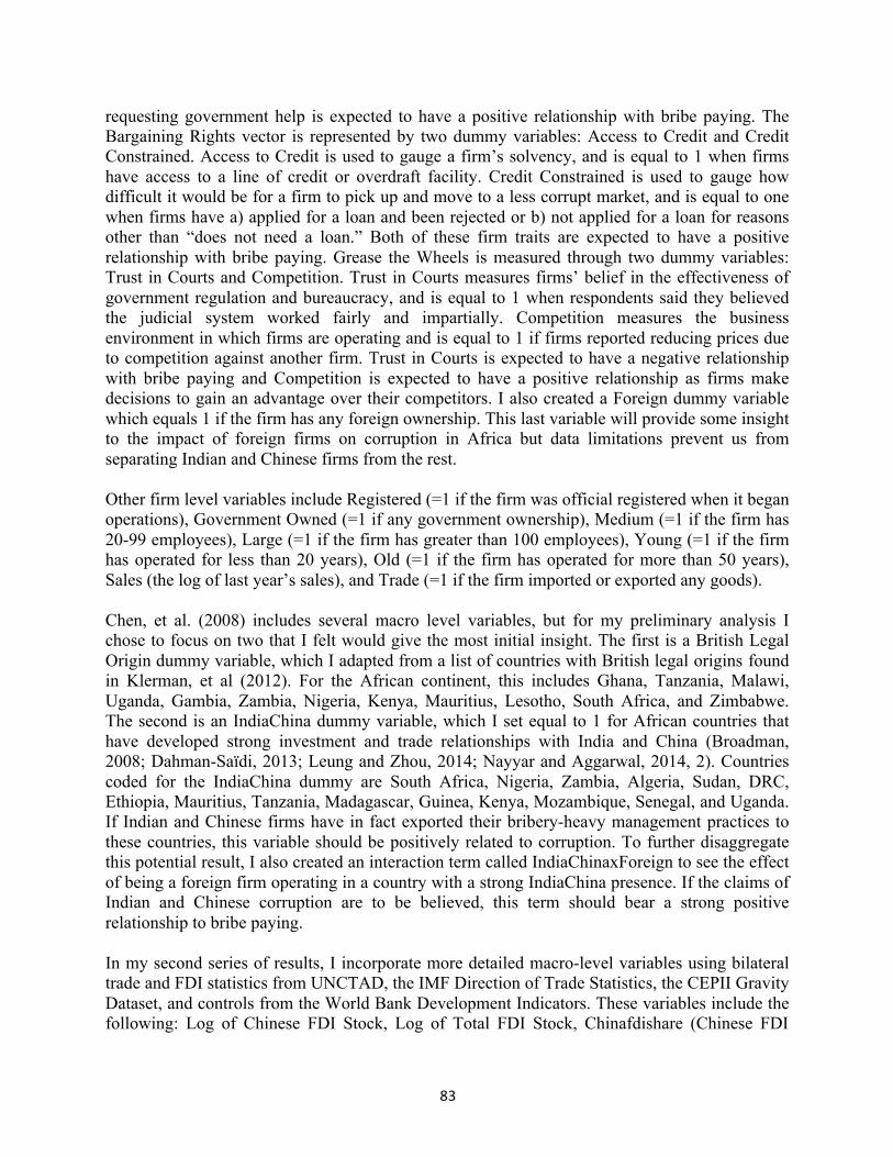
83

requesting government help is expected to have a positive relationship with bribe paying. The Bargaining Rights vector is represented by two dummy variables: Access to Credit and Credit Constrained. Access to Credit is used to gauge a firm’s solvency, and is equal to 1 when firms have access to a line of credit or overdraft facility. Credit Constrained is used to gauge how difficult it would be for a firm to pick up and move to a less corrupt market, and is equal to one when firms have a) applied for a loan and been rejected or b) not applied for a loan for reasons other than “does not need a loan.” Both of these firm traits are expected to have a positive relationship with bribe paying. Grease the Wheels is measured through two dummy variables: Trust in Courts and Competition. Trust in Courts measures firms’ belief in the effectiveness of government regulation and bureaucracy, and is equal to 1 when respondents said they believed the judicial system worked fairly and impartially. Competition measures the business environment in which firms are operating and is equal to 1 if firms reported reducing prices due to competition against another firm. Trust in Courts is expected to have a negative relationship with bribe paying and Competition is expected to have a positive relationship as firms make decisions to gain an advantage over their competitors. I also created a Foreign dummy variable which equals 1 if the firm has any foreign ownership. This last variable will provide some insight to the impact of foreign firms on corruption in Africa but data limitations prevent us from separating Indian and Chinese firms from the rest.

Other firm level variables include Registered (=1 if the firm was official registered when it began operations), Government Owned (=1 if any government ownership), Medium (=1 if the firm has 20-99 employees), Large (=1 if the firm has greater than 100 employees), Young (=1 if the firm has operated for less than 20 years), Old (=1 if the firm has operated for more than 50 years), Sales (the log of last year’s sales), and Trade (=1 if the firm imported or exported any goods).

Chen, et al. (2008) includes several macro level variables, but for my preliminary analysis I chose to focus on two that I felt would give the most initial insight. The first is a British Legal Origin dummy variable, which I adapted from a list of countries with British legal origins found in Klerman, et al (2012). For the African continent, this includes Ghana, Tanzania, Malawi, Uganda, Gambia, Zambia, Nigeria, Kenya, Mauritius, Lesotho, South Africa, and Zimbabwe. The second is an IndiaChina dummy variable, which I set equal to 1 for African countries that have developed strong investment and trade relationships with India and China (Broadman, 2008; Dahman-Saïdi, 2013; Leung and Zhou, 2014; Nayyar and Aggarwal, 2014, 2). Countries coded for the IndiaChina dummy are South Africa, Nigeria, Zambia, Algeria, Sudan, DRC, Ethiopia, Mauritius, Tanzania, Madagascar, Guinea, Kenya, Mozambique, Senegal, and Uganda. If Indian and Chinese firms have in fact exported their bribery-heavy management practices to these countries, this variable should be positively related to corruption. To further disaggregate this potential result, I also created an interaction term called IndiaChinaxForeign to see the effect of being a foreign firm operating in a country with a strong IndiaChina presence. If the claims of Indian and Chinese corruption are to be believed, this term should bear a strong positive relationship to bribe paying.

In my second series of results, I incorporate more detailed macro-level variables using bilateral trade and FDI statistics from UNCTAD, the IMF Direction of Trade Statistics, the CEPII Gravity Dataset, and controls from the World Bank Development Indicators. These variables include the following: Log of Chinese FDI Stock, Log of Total FDI Stock, Chinafdishare (Chinese FDI

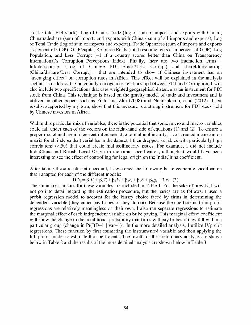
84

stock / total FDI stock), Log of China Trade (log of sum of imports and exports with China), Chinatradeshare (sum of imports and exports with China / sum of all imports and exports), Log of Total Trade (log of sum of imports and exports), Trade Openness (sum of imports and exports as percent of GDP), GDP/capita, Resource Rents (total resource rents as a percent of GDP), Log Population, and Less Corrupt (=1 if a country scores better than China on Transparency International’s Corruption Perceptions Index). Finally, there are two interaction terms – lnfdilesscorrupt (Log of Chinese FDI Stock*Less Corrupt) and sharefdilesscorrupt (Chinafdishare*Less Corrupt) – that are intended to show if Chinese investment has an “averaging effect” on corruption rates in Africa. This effect will be explained in the analysis section. To address the potentially endogenous relationship between FDI and Corruption, I will also include two specifications that uses weighted geographical distance as an instrument for FDI stock from China. This technique is based on the gravity model of trade and investment and is utilized in other papers such as Pinto and Zhu (2008) and Nunnenkamp, et al (2012). Their results, supported by my own, show that this measure is a strong instrument for FDI stock held by Chinese investors in Africa.

Within this particular mix of variables, there is the potential that some micro and macro variables could fall under each of the vectors on the right-hand side of equations (1) and (2). To ensure a proper model and avoid incorrect inferences due to multicollinearity, I constructed a correlation matrix for all independent variables in the dataset. I then dropped variables with particularly high correlations (>.50) that could create multicollinearity issues. For example, I did not include IndiaChina and British Legal Origin in the same specification, although it would have been interesting to see the effect of controlling for legal origin on the IndiaChina coefficient.

After taking these results into account, I developed the following basic economic specification that I adapted for each of the different models:

BDij = β1Fj + β2Tj + β3Xj + β4ci + β5bi + β6gi + β7zi (3) The summary statistics for these variables are included in Table 1. For the sake of brevity, I will not go into detail regarding the estimation procedure, but the basics are as follows. I used a probit regression model to account for the binary choice faced by firms in determining the dependent variable (they either pay bribes or they do not). Because the coefficients from probit regressions are relatively meaningless on their own, I also ran separate regressions to estimate the marginal effect of each independent variable on bribe paying. This marginal effect coefficient will show the change in the conditional probability that firms will pay bribes if they fall within a particular group (change in Pr(BD=1 | var=1)). In the more detailed analysis, I utilize IVprobit regressions. These function by first estimating the instrumented variable and then applying the full probit model to estimate the coefficients. The results of the preliminary analysis are shown below in Table 2 and the results of the more detailed analysis are shown below in Table 3.

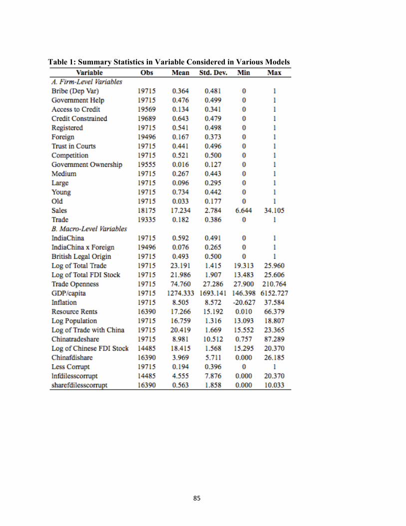
85

Table 1: Summary Statistics in Variable Considered in Various Models

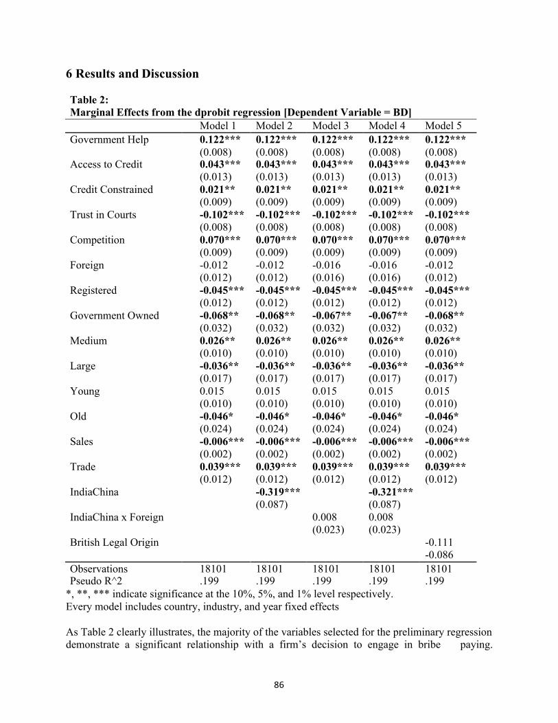
86

6 Results and Discussion

Table 2: Marginal Effects from the dprobit regression [Dependent Variable = BD] Model 1 Model 2 Model 3 Model 4 Model 5 Government Help 0.122***

(0.008) 0.122*** (0.008)

0.122*** (0.008)

0.122*** (0.008)

0.122*** (0.008)

Access to Credit 0.043*** (0.013)

0.043*** (0.013)

0.043*** (0.013)

0.043*** (0.013)

0.043*** (0.013)

Credit Constrained 0.021** (0.009)

0.021** (0.009)

0.021** (0.009)

0.021** (0.009)

0.021** (0.009)

Trust in Courts -0.102*** (0.008)

-0.102*** (0.008)

-0.102*** (0.008)

-0.102*** (0.008)

-0.102*** (0.008)

Competition 0.070*** (0.009)

0.070*** (0.009)

0.070*** (0.009)

0.070*** (0.009)

0.070*** (0.009)

Foreign -0.012 -0.012 -0.016 -0.016 -0.012 (0.012) (0.012) (0.016) (0.016) (0.012) Registered -0.045***

(0.012) -0.045*** (0.012)

-0.045*** (0.012)

-0.045*** (0.012)

-0.045*** (0.012)

Government Owned -0.068** (0.032)

-0.068** (0.032)

-0.067** (0.032)

-0.067** (0.032)

-0.068** (0.032)

Medium 0.026** (0.010)

0.026** (0.010)

0.026** (0.010)

0.026** (0.010)

0.026** (0.010)

Large -0.036** (0.017)

-0.036** (0.017)

-0.036** (0.017)

-0.036** (0.017)

-0.036** (0.017)

Young 0.015 0.015 0.015 0.015 0.015 (0.010) (0.010) (0.010) (0.010) (0.010) Old -0.046*

(0.024) -0.046* (0.024)

-0.046* (0.024)

-0.046* (0.024)

-0.046* (0.024)

Sales -0.006*** (0.002)

-0.006*** (0.002)

-0.006*** (0.002)

-0.006*** (0.002)

-0.006*** (0.002)

Trade 0.039*** (0.012)

0.039*** (0.012)

0.039*** (0.012)

0.039*** (0.012)

0.039*** (0.012)

IndiaChina -0.319*** (0.087)

-0.321*** (0.087)

IndiaChina x Foreign 0.008 0.008 (0.023) (0.023) British Legal Origin -0.111 -0.086 Observations 18101 18101 18101 18101 18101 Pseudo R^2 .199 .199 .199 .199 .199

*, **, *** indicate significance at the 10%, 5%, and 1% level respectively. Every model includes country, industry, and year fixed effects

As Table 2 clearly illustrates, the majority of the variables selected for the preliminary regression demonstrate a significant relationship with a firm’s decision to engage in bribe paying.

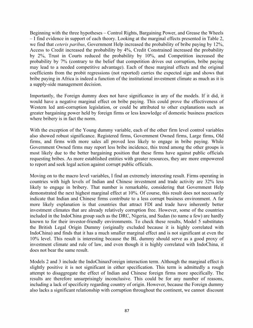
87

Beginning with the three hypotheses – Control Rights, Bargaining Power, and Grease the Wheels – I find evidence in support of each theory. Looking at the marginal effects presented in Table 2, we find that ceteris paribus, Government Help increased the probability of bribe paying by 12%, Access to Credit increased the probability by 4%, Credit Constrained increased the probability by 2%, Trust in Courts reduced the probability by 10%, and Competition increased the probability by 7% (contrary to the belief that competition drives out corruption, bribe paying may lead to a needed competitive advantage). Each of these marginal effects and the original coefficients from the probit regressions (not reported) carries the expected sign and shows that bribe paying in Africa is indeed a function of the institutional investment climate as much as it is a supply-side management decision.

Importantly, the Foreign dummy does not have significance in any of the models. If it did, it would have a negative marginal effect on bribe paying. This could prove the effectiveness of Western led anti-corruption legislation, or could be attributed to other explanations such as greater bargaining power held by foreign firms or less knowledge of domestic business practices where bribery is in fact the norm.

With the exception of the Young dummy variable, each of the other firm level control variables also showed robust significance. Registered firms, Government Owned firms, Large firms, Old firms, and firms with more sales all proved less likely to engage in bribe paying. While Government Owned firms may report less bribe incidence, this trend among the other groups is most likely due to the better bargaining position that these firms have against public officials requesting bribes. As more established entities with greater resources, they are more empowered to report and seek legal action against corrupt public officials.

Moving on to the macro level variables, I find an extremely interesting result. Firms operating in countries with high levels of Indian and Chinese investment and trade activity are 32% less likely to engage in bribery. That number is remarkable, considering that Government Help demonstrated the next highest marginal effect at 10%. Of course, this result does not necessarily indicate that Indian and Chinese firms contribute to a less corrupt business environment. A far more likely explanation is that countries that attract FDI and trade have inherently better investment climates that are already relatively corruption free. However, some of the countries included in the IndoChina group such as the DRC, Nigeria, and Sudan (to name a few) are hardly known to for their investor-friendly environments. To check these results, Model 5 substitutes the British Legal Origin Dummy (originally excluded because it is highly correlated with IndoChina) and finds that it has a much smaller marginal effect and is not significant at even the 10% level. This result is interesting because the BL dummy should serve as a good proxy of investment climate and rule of law, and even though it is highly correlated with IndoChina, it does not bear the same result.

Models 2 and 3 include the IndoChinaxForeign interaction term. Although the marginal effect is slightly positive it is not significant in either specification. This term is admittedly a rough attempt to disaggregate the effect of Indian and Chinese foreign firms more specifically. The results are therefore unsurprisingly inconclusive. This could be for any number of reasons, including a lack of specificity regarding country of origin. However, because the Foreign dummy also lacks a significant relationship with corruption throughout the continent, we cannot discount

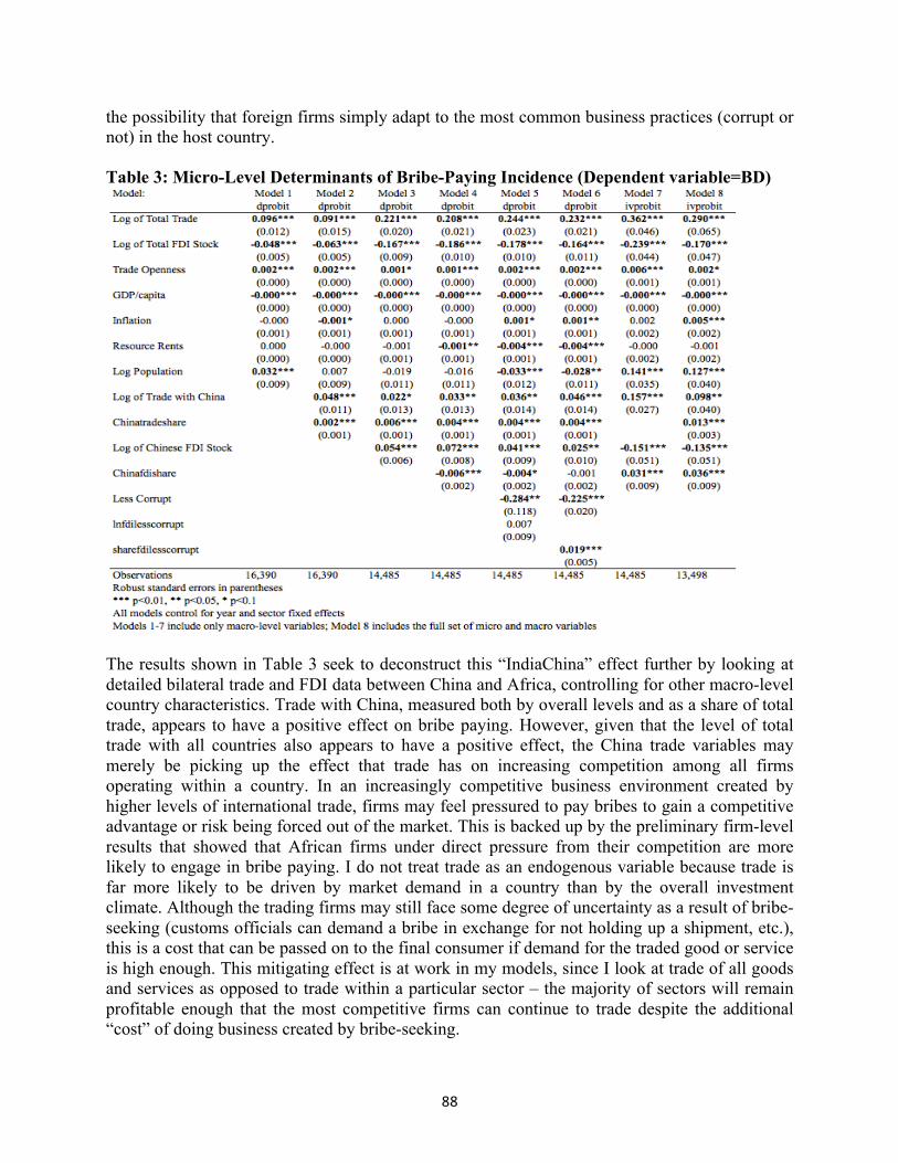
88

the possibility that foreign firms simply adapt to the most common business practices (corrupt or not) in the host country.

Table 3: Micro-Level Determinants of Bribe-Paying Incidence (Dependent variable=BD)

The results shown in Table 3 seek to deconstruct this “IndiaChina” effect further by looking at detailed bilateral trade and FDI data between China and Africa, controlling for other macro-level country characteristics. Trade with China, measured both by overall levels and as a share of total trade, appears to have a positive effect on bribe paying. However, given that the level of total trade with all countries also appears to have a positive effect, the China trade variables may merely be picking up the effect that trade has on increasing competition among all firms operating within a country. In an increasingly competitive business environment created by higher levels of international trade, firms may feel pressured to pay bribes to gain a competitive advantage or risk being forced out of the market. This is backed up by the preliminary firm-level results that showed that African firms under direct pressure from their competition are more likely to engage in bribe paying. I do not treat trade as an endogenous variable because trade is far more likely to be driven by market demand in a country than by the overall investment climate. Although the trading firms may still face some degree of uncertainty as a result of bribe- seeking (customs officials can demand a bribe in exchange for not holding up a shipment, etc.), this is a cost that can be passed on to the final consumer if demand for the traded good or service is high enough. This mitigating effect is at work in my models, since I look at trade of all goods and services as opposed to trade within a particular sector – the majority of sectors will remain profitable enough that the most competitive firms can continue to trade despite the additional “cost” of doing business created by bribe-seeking.

89

The coefficients for FDI on the other hand, yields a more interesting and substantive discussion. At first, and contrary to the preliminary results, higher levels of Chinese FDI appear to lead to higher rates of corruption (in non-instrumented Models 3-6). The share of FDI held by China, on the other hand, appears to have a slight negative effect on corruption rates. To see why this is the case, I turn to the “Less Corrupt” dummy variable (equal to one if a country scores better than China on Transparency International’s Corruption Perceptions Index). If a country is less corrupt than China, increased FDI should be responsible for a race to the bottom phenomenon as Chinese business culture and practices become more prevalent in the host country. When interacted with the log of Chinese FDI stock (lnfdilesscorrupt) and the share of FDI owned by China (sharefdilesscorrupt), it appears that only the share has a significant impact, this time in the opposite direction that we originally found in the results. As the share of FDI owned by China in “less corrupt” countries increases, so too does corruption in those countries. This result does not appear promising for China until we unpack why this is the case.

Performing a simple t-test on the difference in means for the Log of Chinese FDI Stock and Chinafdishare shows that both levels and share of FDI from China are more likely to be higher in “more corrupt” countries. This is likely the result of an “investment gap” left by Western firms in African countries that have poorer investment climates. As some of the literature claims, China may be stepping in to fill this gap as state-backing and existing trade relationships with these countries makes them attractive places to invest regardless of perceptions surrounding corruption (Cheung, et al, 2012). Although this investment gap theory needs to be explored further, it has the important implication that China may be exporting bad business practices to countries with good governance while simultaneously improving the business practices in countries with worse governance. In this case, as Chinese involvement on the continent expands, corruption could converge around some average level represented by the corruption rate in China.

This result and the “investment gap” theory behind it highlight the endogeneity issue between FDI and corruption. If corruption is in fact steering away Western investors and opening the door for Chinese investment, then these reported results may not actually demonstrate causality. To treat for this, I use the instrumental variables approach described in the empirical approach section in models (7) and (8). Model (7) includes only the macro-level variables, while Model (8) includes all the micro-level variables described in my previous paper, although these coefficients are not shown. In both of these models, higher amounts of FDI appear to have a negative effect on corruption. In models (7) and (8), the coefficient of Chinafdishare takes on a positive value, but because this variable can be considered to be endogenous, it is included for control purposes only and should not be taken to imply causality. Although the effect is not as strong as that of the IndiaChina dummy variable in the preliminary analysis, this is promising evidence in favor of Chinese investment efforts. Indeed, it provides further support for the “investment gap” theory as an explanation for the original contradictory results found in Models (3)-(6) and shows how this investment strategy may actually provide African countries with both more investment while promoting better governance.

90

7 Conclusion and Policy Implications The rise of India and China as global powers has changed the status quo in the private sectors of several key African economies. The Western response has been acute and critical; Secretary Clinton’s stark words in 2012 leave no confusion surrounding the West’s protectionist – not to be confused for altruistic – attitude. However, despite the West’s preferences, the sheer volume and trends in Indian and Chinese trade and investment in the continent show that they will remain major actors in the region for the foreseeable future. A 2014 report by McKinsey & Company predicts that Africa will become the fastest growing region in the next few decades and shows that Indian and Chinese involvement will be instrumental in leading that growth.

That said, Western concerns that imported Indian and Chinese management techniques will weaken governance are not entirely off the mark. Anecdotal evidence presented in this paper shows that even the “cleanest” Indian and Chinese firms have been caught up in corruption allegations at home, if not in Africa. Although these cases are far more common for large Chinese state owned enterprises with fewer accountability and transparency checks, Indian firms have had their own issues in recent years. However, it is important to remember that despite Western anti-corruption legislation, Western firms have also been found guilty of their own share of questionable deals in Africa. Legislation or not, bribe paying (and taking) remains a part of the business environment in virtually every African country. The empirical results support the idea that corruption is primarily driven by demand-side institutional factors that are met by supply- side firm practices.

The surprising finding that firms in countries with heavy Indian and Chinese involvement are 30% less likely to pay a bribe offers preliminary evidence that these new actors are not worsening the situation. The fact that this finding is further supported by more detailed macro- level data on the total amount and share of FDI/trade controlled by China, particularly after controlling for endogeneity, is even more promising. Contrary to Western claims of a “race to the bottom” scenario, this indicates an opposite trend in which an increased supply of investment funds gives African governments more bargaining power to strike better deals with more responsible corporate actors. Understandably, this process also creates greater opportunities for bribe taking, and anti-corruption efforts will need to continue at the country level.

Notably, these results include the caveat that the Enterprise Surveys do not include data from firms operating in extractive industries, where much of the criticism regarding the corrupt practices of Indian and Chinese firms has been focused. Functionally, this means that the findings of this paper could be skewed toward a more favorable representation of Indian and Chinese involvement on the African continent. However, as I note in the literature review, firms operating in these extractive industries have increasingly become the minority among Indian and Chinese companies interested in doing business in Africa. As business opportunities become more widespread in a larger variety of industries, the trends highlighted by this paper will likely become even more relevant.

Additionally, efforts to promote strong corporate governance should be undertaken at the firm level in order to solve the collective action problem of ending corruption in the private sector. Because refusing to pay a bribe can put a firm at a disadvantage to a direct competitor, it is

91

difficult to convince managers to maintain anti-corruption positions. Coordinated efforts like the UN Global Compact (which includes several Indian and Chinese firms) and the IFC’s Africa Corporate Governance Network represent promising first steps and should continue to be supported (United Nations, 2010; IFC, 2013).

As the Indian and Chinese presence in Africa continues to grow, there is room for further research regarding its impact on governance and corruption. The World Bank Enterprise Surveys have provided a good starting point, but a more detailed firm level dataset will be required to draw convincing conclusions in one direction or the other. Too much emphasis has been placed on the new East-West rivalry in Africa and the discussion has been colored by platitudes rather than by hard empirical evidence. However, as this data becomes increasingly available, firms – whether Indian, Chinese, European or American – and African government officials alike will hopefully be held more accountable for achieving positive governance outcomes in the region.

Bibliography

“Africa Corporate Governance Network Launches.” Oct. 16, 2013. Web. Dec. 12, 2014.

“African Economic Outlook - Measuring the pulse of Africa.” August 29, 2014. Web. Dec. 12, 2014.

Alaimo, V., & Fajnzylber, P. “Behind the Investment Climate: Back to Basics - Determinants of Corruption.” Does

the investment climate matter? Microeconomic foundations of growth in Latin America. Washington, DC: World Bank, 2009.

Alessi, C., & Hanson, S. “Expanding China-Africa Oil Ties.” Feb. 8, 2012. Web. Dec. 12, 2014.

Broadman, H. “China and India Go to Africa.” Apr. 1, 2008. Web. Dec. 12, 2014.

Cai, H., Fang, H., & Xu, L. “Eat, Drink, Firms, Government: An Investigation of Corruption from the Entertainment and Travel Costs of Chinese Firms.” Journal of Law and Economics, 54, 55-78. 2011.

Caulderwood, K. “Chinese Money In Africa Directed Away From Oil, Toward Other Sectors.” May 15, 2014. Web.

Dec. 12, 2014.

Chen, Y., Yaşar, M., & Rejesus, R. “Factors Influencing the Incidence of Bribery Payouts by Firms: A Cross- Country Analysis.” Journal of Business Ethics, 77(2), 231-244. 2008.

Cheung, Y., De Haan, J., Qian, X., & Yu, S. “China's Outward Direct Investment in Africa.” Review of International

Economics, 20(2), 201-220. 2012.

“China and India - Rivals in Africa | Asia | DW.DE | 09.10.2012.” Sep. 10, 2012. Web. Dec. 12, 2014

Dahman-Saïdi, M. “Chinese investment in Africa (part 1)”. Nov. 3, 2013. Web. Dec. 12, 2014

Dipietro, B. “FCPA Fears Hinder U.S. Companies Considering Africa.” July 23, 2014. Web. Dec. 12, 2014,

“Elephants and tigers.” Oct. 26, 2013. Web. Dec. 12, 2014

Fairclough, G., Childress, S., & Champion, M. “Probes Involve Firm Linked to China Leader's Son.” July 22, 2009. Web. Dec. 12, 2014.

92

“For African business, ending corruption is 'priority number one' | Africa Renewal Online.” Aug. 1, 2010. Web. Dec. 12, 2014.

Fortin, J. “Creeping Tiger: India's Presence In Africa Grows, Even As China Steals The Spotlight.” June 27, 2013.

Web. Dec. 12, 2014.

Gayathri, A. “Indian Companies Most Transparent Among Their BRICS Peers, While Chinese Firms Rank Last: Transparency International.” Oct. 7, 2013. Web. Dec. 12, 2014

“How corrupt is your country?” Jan. 1, 2014. Web. Dec. 12, 2014

“Indo-African Business.” Jan. 1, 2011. Web. Dec. 12, 2014.

Jacobs, S. “India-Africa trade: A unique relationship.” Jan. 1, 2013. Web. Dec. 12, 2014.

“Joining hands to unlock Africa’s potential: A new Indian industry-led approach to Africa.” Mar. 1, 2014. Web.

Dec. 12, 2014.

Khare, V. Aug. 4, 2013. Web. Dec. 12, 2014

Klerman, D., Mahoney, P., Spamann, H., & Weinstein, M. “Legal Origin or Colonial History?” Journal of Legal Analysis, 379-409. (2012).

Kushner, J. “Corruption in the Congo: How China Learnt from the West.” Oct. 3, 2013. Web. Dec. 12, 2014.

Leung, D., & Zhou, L. “Where Are Chinese Investments in Africa Headed?”. May 15, 2014. Web. Dec. 12, 2014

“More than minerals.” Mar. 23, 2013. Web. Dec. 12, 2014.

Nayyar, R., & Aggarwal, P. “AFRICA- INDIA’S NEW TRADE AND INVESTMENT PARTNER.” International Journal of Scientific and Research Publications, 4(3). 2014. Web. Dec. 12, 2014.

Nunnenkamp, P., Andres, M., Vadlamannati, K., & Waldkirch, A. “What Drives India's Outward FDI?” South Asian

Journal of Macroeconomics and Public Finance, 245-279. 2012.

Pinto, P., & Zhu, B. “Fortune or Evil? The Effects of Inward Foreign Direct Investment on Corruption.” Mar. 31, 2008. Web. Apr. 7, 2015.

Rankin, J. “Vedanta shares tumble on downgrade.” Oct. 9, 2013. Web. Dec. 12, 2014.

Rautray, S. “2G case: Bharti Airtel chairman Sunil Mittal urges SC to set aside court summons.” Nov. 27, 2014.

Web. Dec. 12, 2014.

“Survey Methodology.” (n.d.). Web. Dec. 12, 2014.

Svensson, J. “Who Must Pay Bribes and How Much? Evidence from a Cross Section of Firms.” The Quarterly Journal of Economics, 118(1), 207-230. 2003.

“Trying to pull together.” Apr. 23, 2011. Web. Dec. 12, 2014

Vanham, P. “Big dreams of India-Africa trade at Delhi forum.” Nov. 5, 2014. Web. Dec. 12, 2014.

“Vedanta to buy miner at centre of probe - FT.com.” Aug. 8, 2011. Web. Dec. 12, 2014.

93

Bank Capital Requirements and Post-Crisis Monetary Policy Transmission

Aaron Goodman Department of Economics Dartmouth College

aaron.s.goodman.15@dartmouth.edu 216-387-0583

20789 Shaker Blvd. Shaker Heights, OH 44122

July 29, 2015

Abstract

Using recent panel data for American commercial banks, I investigate whether regulatory capital requirements reduced the effectiveness of post-crisis monetary policy. Consistent with the “credit channel” literature, I find that banks’ lending response to monetary easing depends substantially on their capital position relative to regulatory requirements. The key bank-level results persist and have meaningful macroeconomic consequences when the data are aggregated geographically, as state- level variation in average bank capitalization predicts rates of aggregate lending and employment growth during the post-crisis period. These findings demonstrate the important implications of prudential banking regulations for the conduct of expansionary monetary policy after economic downturns.

94

INCENTIVES, INSTITUTIONS AND INVESTMENT IN PRIVATE AGRICULTURAL RESEARCH IN ASIA

DORA HENG

Cornell University

ABSTRACT Agricultural Research and Development (R&D) is critical to enhance agricultural productivity and, by extension, feed the world’s growing population. Despite the important role that research and innovation play, the trend of underinvestment in agricultural research is worrisome, especially given the decreasing fiscal ability of many national governments. Increasingly, governments are turning towards the private sector to step up investment.

The research presented in this paper explores the relationship between economic incentives, policies and institutional environment on private investment in agriculture R&D in the Asia- Pacific region. Both a descriptive analysis of key developments in the agricultural industry and the national innovation system and an empirical study quantifying the effects of the determinants on private investment are conducted. The study uses panel data with information on seven countries in the Asia-Pacific region from 1995-2003 to test the hypothesis that the expected market sizes for R&D outputs (including both domestic and external markets) and the appropriability of returns from innovation from institutional policies (which includes property rights and institutional environment) can induce greater private expenditure in agriculture R&D. Three linear regression models of private investment in agriculture R&D are built and tested.

Research findings indicate that size of agriculture markets and government effectives have a positive relationship with private investment in agricultural R&D, while economic openness and strength of Intellectual Property Regime (IPR) are found to be negatively correlated to private investment. The results for economic openness and IPR strength reveal that a minimum level of domestic technological capacity is required before developing countries can benefit from increased foreign private investment in R&D efforts.

95

Editor’s Note: Due to space limitations, the following is an abridged version of the original.

1 INTRODUCTION Agricultural Research and Development (R&D) is critical to enhance productivity and, by extension, to feed the world’s growing population. Despite the important role that research and innovation plays, there has been a worrying trend of underinvestment in agricultural research, especially with the decreasing fiscal capacity of many national governments. According to researchers Fan and Saurkar (2008), public expenditure to agriculture as a share of GDP has decreased from over 11% in 1980 to under 7% in 2002. Increasingly, policy-makers and governments are turning towards the private sector to step up investment. In this context, it is crucial for policymakers to understand the determinants influencing private investment in research to implement policies conducive towards incentivizing greater private sector involvement.

The Green Revolution of the 1960s was key in lifting many out of poverty in developing regions of the world. The use of modern technology and crop varieties catalyzed an increase in crop yields and productivity and was instrumental to this success. Thus, even the recent past provides evidence of the profound importance of agricultural R&D in not only enhancing agricultural productivity, but also in addressing pertinent issues of poverty reduction and food security. Further research has also been conducted to highlight the impact that agricultural technology and innovation has on improving livelihood outcomes such as higher income, increased crop yields and better nutrition (Meinzen-Dick, 2004).

However, despite the importance of R&D for agriculture, nations have been consistently underinvesting in agricultural research for decades (Alston et al., 2000). Research compiled by the public sector, typically the sector with the largest stake in R&D in most countries, is receiving stagnant or declining levels of funding, as evident by the global public agricultural research expenditures growth rate of 4.6% in 1976 tapering towards 1.7% in 1996 (Byerlee et al., 2002). Furthermore, public research institutions (especially in developing countries) tend to be run by ineffective bureaucracies and are unable to deliver high quality performance (Rukuni, Blackie, & Eicher, 1998).

Amidst the bleak outlook of declining public levels of investment in agricultural R&D, the private sector has emerged as an increasingly important player in the area of R&D financing. In 2000, the private sector contributed to 40% of total agricultural research expenditure globally (CGIAR, 2005). Furthermore, the growth trend is positive. A study conducted by Pray and Umali-Deininger (1998) of ten countries spanning both the developed and developing world showed that private R&D expenditure had a compounded at annual growth rate of around 3% from 1986 to 1996. From 1981 to 2000, among the Organization for Economic Cooperation and Development (OECD) countries, spending on private sector research has increased nearly three times as compared to the increase in public sector spending such that the private sector contributed 54% of total agricultural R&D expenditure in OECD countries (Fuglie, 2012). Private expenditure in agriculture research greatly exceeds public expenditure, particularly in the UK, USA, and the Netherlands, in part due to the presence of large pharmaceutical and pesticide industries in these countries (Alston et al., 2000). Private spending on agricultural R&D in

96

developing countries, despite comprising a very modest share of worldwide R&D expenditure, shows a similar upward trajectory of growth (Pardey et al., 2006).

There are several recent developments that may be influencing the participation of the private sector in agriculture research. First, there is a greater push for standardization in Intellectual Property Rights (IPR) regimes. The World Trade Organization coordinated the Trade-Related Aspects of Intellectual Property (TRIPs) agreement in 1994, which resulted in stronger international compliance to protect property rights for innovation. Secondly, many developing countries began privatizing their economies in the late 20th century and have adopted free market approaches to growth. The opening of national agricultural markets invited greater participation from the private sector to participate in agriculture research.

Experts assert that greater levels of private spending in agriculture R&D can increase national total expenditure on agriculture research to yield optimal expected returns (Pray,1983). However, challenges and limitations in the market systems of developing countries pose hindrances to galvanizing greater private sector support in financing research. These structural limitations come in the form of weak institutions, instability and high capital risks, smaller and less consolidated markets (Naseem et al., 2010).

Private sector involvement in the Asia-Pacific region is comparatively higher than it is in the rest of the developing world (Beintema, 2008). Concurrently, there exists great heterogeneity among Asian countries with regards to size and growth rates of private expenditure in agricultural research. According to a study by the United States Department of Agriculture (USDA), the country with the largest amount of private research in Asia is India with $55 million annually in the 1990s. In the middle tier level of spending, large to middle income countries such as Thailand, Malaysia and China fell into a similar band of $15 to $20 million per year, and at the bottom tier, mid-size low income countries such as Pakistan see spending of about $6 million (Pray and Fuglie, 2001). Countries such as India and China observed a rapid doubling of private research funding within the last decade of the 20th century, while Philippines and Thailand saw a modest but still impressive growth rate of 60-70%. The dynamic transformation that this region had witnessed in agriculture development makes this region a compelling case for analysis.

The key research goal of this study is to investigate factors and conditions that influenced greater private sector investment among countries in the Asia-Pacific region. In particular, this study seeks to establish the conceptual framework around the determinants of private investment in agricultural R&D, to examine the key trends and developments in the Asia-Pacific Region, to empirically quantify the impact of selected determinants on private agricultural R&D investment and finally to Explore implications on policy.

The findings of this paper will be useful in guiding policymakers’ decisions in identifying the range of policy options that can better incentivize private sector investment in agriculture R&D in developing countries.

97

2 CONCLUSION SUMMARY OF FINDINGSThis research has focused on the analysis of the complex interactions between economic incentives and intuitional factors and their influence on private R&D investment in agriculture in developing countries in Asia. With regards to economic incentives, the empirical findings show that private sector R&D investment responds favorably to size of the country’s agriculture market. However, it does not respond the same way to the openness of the economic market because agriculture technologies need to be localized. The size of the country’s agriculture market is shown to have the biggest effect on private sector R&D, indicating the importance of market demand in attracting R&D investment.

The findings showed that while government effectiveness matters, strength of IPR protection had a negative impact on private sector R&D investment, especially in developing countries with low technological capabilities. POLICY IMPLICATIONSWhen the empirical findings are seen in the light of the recent developments in the Asia-Pacific region, it becomes evident that the prerequisite conditions for private sector investment possess a progressive ordering of importance. This supports the argument that Pray and Fuglie (2001) makes, that sequencing of policies is necessary for effective private research development. Consequently, policymakers must understand that some conditions have primacy in building an environment for robust private-sector investment in agriculture R&D.

Placing undue emphasis on strengthening IPR regime in the absence of strong domestic market for agriculture R&D outputs will not effectively stimulate R&D activities. Rather, economic reforms and liberalization of the market, as witnessed by countries in Asia, are needed first to secure an established market among farmers and producers for private firms to supply technology to. Policies that incentivize the development of agriculture markets and reduce the distortion of government intervention are key. Institutions such as strong IPR regimes and effective governance can complement economic growth when these conditions are met. In the long run, a flourishing private sector requires adequate regulatory protection for firms to protect their innovation. Additionally, private sector firms will also benefit from working in collaboration with a complementary public research system.

This discussion of economic incentives and institutional quality in agriculture research ties in with the larger macro-perspective of economic growth and development. Endogenous growth theorists and developmental economists like Acemoglu (2001), Rodrik and Rodríguez (2000) also put forth the argument that institutions that provide market-oriented incentives and protect property rights help catalyze economic growth. However, they are also cognizant of the need for prescriptive and contextualized country diagnostics in determining effective policies. In the case of developing countries that do not have all the necessary preconditions for private sector involvement, embracing openness and harmonization with international IPR frameworks may result in the decline in economic performance. Policymakers in developing countries need to understand that strategic priorities differ among countries at different stages of economic growth. Ultimately, they should prioritize the importance of domestic capacity building, in terms of research capacity, secure markets and national innovation system, to accompany their policy reforms.

98

In summary, agriculture R&D and innovation are instrumental in helping developing countries to achieve agricultural productivity and growth. The private sector plays an important role in catalyzing innovation and development. Realizing the benefits of greater private sector involvement requires the right market conditions, complementary institutional design and public support. By undertaking suitable and germane measures to stimulate private investment, in a manner that is contextualized to location-specific constraints, developing countries will be able to attract sustainable sources of financing to nourish the growth in agriculture research.

Bibliography

Acemoglu, Daron, Simon Johnson, and James A. Robinson. “The colonial origins of comparative development: An

empirical investigation.” No. w7771. National Bureau of Economic Research, 2000.

Alston, Julian M., Philip G. Pardey, and Johannes Roseboom. "Financing agricultural research: international investment patterns and policy perspectives." World Development 26.6 (1998): 1057-1071.

Anandajayasekeram, Ponniah. "The role of agricultural R&D within the agricultural innovation systems framework." Report Prepared for the ASTI/IFPRI-FARA Conference. 2011.

Antons, Christoph. "Intellectual property law in Southeast Asia: Recent legislative and institutional developments." Journal of Information, Law & Technology 1.Special Issue (2006): 1-12.

Blakeney, Michael. “Trade related aspects of intellectual property rights: a concise guide to the TRIPs Agreement.” Sweet & Maxwell, 1996.

Boyle, Cara A. "US-Vietnam Bilateral Trade Agreement: How Vietnam's Efforts to Strengthen Its Trademark and Copyright Laws Signal Its Desire to Join the World Economy." Loy. Consumer L. Rev. 14 (2001): 4.

Briones, Roehlano M. “The Structure of Agricultural Trade Industry in Developing Countries.” No. DP 2013-15. 2013.

Byerlee, Derek, Gary Alex, and Ruben G. Echeverría. "The evolution of public research systems in developing countries: facing new challenges." Agricultural research policy in an era of privatization (2002): 19-34.

CGIAR Science Council. “Science for agricultural development: Changing contexts, new opportunities.” Rome: Science Council Secretariat, 2005

Chen, Yongmin, and Thitima Puttitanun. "Intellectual property rights and innovation in developing countries." Journal of development economics 78.2 (2005): 474-493.

Clayton, Elizabeth. "Survey Article: Agricultural Privatization in Transition Economies." Comparative Economic Studies 34.1 (1992): 86-92.

Diao, Xinshen, et al. The role of agriculture in development: Implications for Sub-Saharan Africa. Vol. 153. Intl Food Policy Res Inst, 2007.

Evenson, Robert and Larry Westphal. “Technological Change and Technology Strategy.” In Handbook of Development Economics, vol. 3, ed. T.N. Srinivasan and Jere Behrman (Amsterdam: New Holland), 2209- 2299, 1995

Fan, Shenggen, Bingxin Yu, and Anuja Saurkar. "Public spending in developing countries: trends, determination, and impact." Public expenditures, growth, and poverty (2008): 20-55.

Fuglie, Keith O., and Roley R. Piggott. "Indonesia: coping with economic and political instability." Agricultural R&D in the developing world: too little, too late? (2006): 65.

99

Fuglie, Keith, et al. "The contribution of private industry to agricultural innovation." Science 338.6110 (2012): 1031-1032.

Gerpacio, R. V. "The roles of public sector versus private sector in R&D and technology generation: The case of maize in Asia." Agricultural Economics29.3 (2003): 319-330.

Haggblade, Steven, Peter BR Hazell, and Thomas Anthony Reardon.Strategies for stimulating poverty-alleviating growth in the rural nonfarm economy in developing countries. International Food Policy Research Institute, Environmental and Production Technology Division, 2002.

Keller, W. "Geographic localization of international technology diffusion, American knowledge spillovers in Hungary." Acta Oeconomica 57 (2002): 1-20.

Koyek, D. "Intellectual property rights: Ultimate control of agricultural R&D in Asia." (2001).

MASTIC (Malaysian Science and Technology Information Centre). 2004. National Survey of Research and Development: 2004 report. Putrajaya.

McNeil Jr, Lawrence R. The international diffusion of technological knowledge: Industry-level evidence from ten developing economies. Diss. HOWARD UNIVERSITY, 2008.

Meinzen-Dick, Ruth. Science and poverty: An interdisciplinary assessment of the impact of agricultural research. Intl Food Policy Res Inst, 2004.

Morris, M. L. Maize in the developing world: Waiting for a green revolution. Maize Seed Industries in Developing Countries. No. 338.1731521 MOR. CIMMYT.. 1998.

Outlook, Continues Southeast Asian Economic. "Economic Outlook for Southeast Asia, China and India." (2014).

Palda, Kristian S., and Bohumir Pazderka. "International comparisons of R&D effort: The case of the Canadian pharmaceutical industry." Research Policy 11.4 (1982): 247-259..

Pardey, Philip G., et al. Agricultural Research: A growing global divide?. Vol. 17. Intl Food Policy Res Inst, 2006.

Payumo, Jane G. An Analysis of the Implications of Strengthened Intellectual Property Rights to Agriculture of Developing Countries and Responses of Selected Public Research Institutions in Southeast Asia. Diss. Washington State University, 2011.

Pray, Carl E. "Private agricultural research in Asia." Food Policy 8.2 (1983): 131-140.

Pray, Carl E., and Latha Nagarajan. "The transformation of the Indian agricultural input industry: has it increased agricultural R&D?." Agricultural Economics 45.S1 (2014): 145-156.

Qaim, M., and G. Traxler. ""Roundup Ready Soybeans in Argentina: Farm Level and Aggregate Welfare Effects."" Agricultural Economics 32(2005):73-86."

Reardon, Thomas, C. Peter Timmer, and Bart Minten. "Supermarket revolution in Asia and emerging development strategies to include small farmers."Proceedings of the National Academy of Sciences 109.31 (2012): 12332-12337.

Rodríguez, Francisco, and Dani Rodrik, ""Trade Policy and Economic Growth: A Skeptic's Guide to the Cross- National Literature,"" June 2000

Rodrik, Dani, Arvind Subramanian, and Francesco Trebbi. "Institutions rule: the primacy of institutions over geography and integration in economic development." Journal of economic growth 9.2 (2004): 131-165.

Rukuni, Mandivamba, Malcolm J. Blackie, and Carl K. Eicher. "Crafting smallholder-driven agricultural research systems in southern Africa." World Development 26.6 (1998): 1073-1087.

Spielman, David J., et al. "The seed and agricultural biotechnology industries in India: An analysis of industry structure, competition, and policy options." Food Policy 45 (2014): 88-100.

100

Than, Mya. "Economic Reforms in Transitional Economies of Mainland Southeast Asia'." International Conference on'System Transformation of the Transition Economies: Europe, Asia and North Korea', Institute for Korean Unification Studies, Seoul. Vol. 14. 1996.

Tripp, Robert, and Suresh Pal. "The private delivery of public crop varieties: Rice in Andhra Pradesh." World Development 29.1 (2001): 103-117.

Unctad. "World Investment Report 2009: Transnational Corporations, Agricultural Production and Development." (2009).

Van Donge, Jan Kees, David Henley, and Peter Lewis. "Tracking Development in South---East Asia and sub---Saharan Africa: The Primacy of Policy."Development Policy Review 30.s1 (2012): s5-s24.

Wooldridge, Jeffrey M. Econometric analysis of cross section and panel data. MIT press, 2010.

World Bank. Cultivating Knowledge and Skills to Grow African Agriculture. Washington, DC, 2007

101

Peer Effects in Football Huang Zhengbin Samuel∗

London School of Economics and Political Science

Abstract I study peer effects in football—how a football player's performance depends on the average productivity of his teammates. Using data on the English Premier League from the 2009/10 to the 2013/14 season, I find positive and significant spillovers from playing with teammates with higher inherent productivity. However, for a given player, peer effects experienced does not vary with his productivity. Spillovers between players with the same attacking or defensive roles are not significantly stronger than between players with different roles. Spillovers are stronger in teams with more at stake and when teammates are more experienced. I conclude that peer effects in the highly skilled team work environment of professional football are largely driven by peer pressure to win and not by contemporaneous skill spillovers.

∗ I would like to thank my supervisor, Dr Camille Landais for his support and guidance throughout the research project. I am also grateful to Dr Matthew Levy, Dr Judith Shapiro, Dr Matthew Gentry, Dr Guy Michaels, Professor Christopher Griffin and participants at the XIV Carroll Round conference for their helpful advice and suggestions. For the complete version of the paper or any other correspondence, please contact via email at samuelhzb@gmail.com.

102

An Agent Based Model for Competitive Equilibrium in Electricity Markets

Michael Lee

Advised by: Dr. Valerie Bencivenga∗ (2015)

Abstract

The research presented herein aims to computationally model participants in an electric utilities market. Utilizing an agent based (AB) approach, players are treated as uniquely intelligent, independent agents who seek to maximize utility via selective bidding in a marketplace. Agents must decide thier optimal output based on expectations of their opponent’s quantities supplied, the carbon make up of said supply, as well as expectations of future carbon tax rates. In making their decisions, agents are able to look back at historical quantity supplied, as well as look into their own cost structures in order to predict future outcomes. Agents are also able to invest and divest selectively from assets, giving them additional agency in affecting their outcomes.

Fundamental basis of the model come from various economic models, including oligopolis- tic competition– specifically Carnout competition– and Walrasian auctioning. The former denotes the market structure where firms decide independently on the output they will supply, while the later describes the mechanism by which competitors find equilibrium via repeated bidding.

The model is accomplished via a mix of computational tools, specifically python and its associated libraries. The prediction mechanism is achieved through multiple regression, while all optimization is performed via linear algebra toolkits. In order to increase efficiency in calculations, the model can be performed in parallel across many cores, assigning each agent and its associated properties to a single core for computation.

Results show that the speed in which agents reach a steady state is inversely proportional to the number of market participants, the decrease in consumer price per megawatt as the number of market participants increases, the the rate at which marginal taxes on carbon effect production on participants of different scales. These results are inline with the expectations put forth by optimization theory, Cornout competition, and Pigoviantaxes.

∗Senior Lecturer, Department of Economics, The University of Texas at Austin

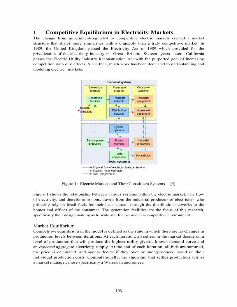
103

1 Competitive Equilibrium in Electricity Markets The change from government-regulated to competitive electric markets created a market structure that shares more similarities with a oligopoly than a truly competitive market. In 1989, the United Kingdom passed the Electricity Act of 1989 which provided for the privatization of the electricity industry in Great Britain. Sixteen years later, California passes the Electric Utility Industry Reconstruction Act with the purported goal of increasing competition with dire effects. Since then, much work has been dedicated to understanding and modeling electric markets.

Figure 1: Electric Markets and Their Constituent Systems [4]

Figure 1 shows the relationship between various systems within the electric market. The flow of electricity, and therefor emissions, travels from the industrial producers of electricity– who primarily rely on fossil fuels for their heat source– through the distribution networks to the homes and offices of the consumer. The generation facilities are the focus of this research, specifically their design making as to scale and fuel source in a competitive environment.

Market Equilibrium Competitive equilibrium in the model is defined as the state in which there are no changes in production levels between iterations. At each iteration, all sellers in the market decide on a level of production that will produce the highest utility given a known demand curve and an expected aggregate electricity supply. At the end of each iteration, all bids are summed, the price is calculated, and agents decide if they over or underproduced based on their individual production costs. Computationally, the algorithm that settles production acts as a market manager, more specifically a Walrasian auctioneer.

104

Each agent is treated as uniquely intelligent, using the output of previous rounds to adjust their expectations until a steady-state competitive equilibrium is reached. This process is a mirror of a Walrasian auction: instead of each agent calculating demand at all possible prices, all agents simultaneously submit bids for how much they are willing to produce at each possible price point. If after all bids have been submitted, and an agent’s market expectations are above the actualized quantities, it will subsequently lower its productions proportional to the difference between the two amounts. In the computational model, this process is performed via a negative feedback loop.1

The Asymmetric Information Problem One of the critical problems with modeling electric markets is the dependence on all parties of perfect information regarding their rivals cost structures. Since electricity markets are primarily a margins-driven business, producers can only operate when the cost per- megawatt is above their production costs. However, since production is sent to an ”electric pool”, where multiple producer’s output is amalgamated, the optimal production bundle of each agent is dependent on the summation of all bids in the market, and therefore the marginal costs of all producers. If agents cannot perfectly know all other participant’s cost structure, they will not be able to accurately predict the aggregate supply, and suboptimal production will result.

Market Structure: Competitive or Oligopolistic It has been argued that the competitive equilibrium model is only applicable in markets in which there are a large number of sellers. In small markets– like they one modeled here– each player’s production dramatically influences the market price. This market power to alter the price means that the market functions similar to an oligopoly.

The market modeled has properties similar to a Cournot oligopoly, namely: output is homogenous and chosen simultaneously across all firms, firms act independently, firms are price setters, and firms seek to maximize utility given opponent’s actions. Critically, the underlying assumption of the Cournot model is the ”not” conjecture, i.e. that the firm takes the output of its competitors as given and that its own production decision will not effect its competitor’s production outcomes.2

Potential Models Previous work into oligopolistic electricity markets have utilized the Cournot, Bertrand, Stackelberg, supply function equilibrium (SFE) and collusion models. Similar to the model presented herein, Hogan and Cardel et al use a Cournot quantity approach to a single period of market trading [8]. Building off this approach, Chen, Wong et al created a coevolutionary computational (CCEM) model in which two players evolve in the power ”ecosystem” based on their fitness, which in this case is a profit function[9].

1See fig. 3 2Figure 3 shows how this assumption is implemented in the computational model.

105

Agent-based computational economics (ACE) is a particularly well-suited platform for capturing the dynamic interaction between many different agents. In ACE, each market participant is modeled as an agent who is given a utility function that it seeks to maximize at each interval. One downside of this model however, is that that it its most basic form, the players cannot form any strategic ’thinking’ based on previous turns. ACE can be combined with other forms of computational modeling, specifically genetic algorithms (GA) to produce ”smart” models.

2 Model Formulation An agent based model is created in which multiple power providers independently select output based on expectations of future market conditions: including CO2 emissions, ag- gregate supply, and the regulatory environment. The market price per megawatt and effective tax rate are set via the value and composition of aggregate supply– meaning each producer must at every turn accurately predict the combined output and its associated carbon emissions in order to choose its own optimal production bundle. If the combined carbon output is greater than an exogenous, known threshold, then a marginal tax on carbon is enacted.

In the system, agents are aware of the market clearing price (MCP) and use thier own cost structure coupled with historical bids to estimate their opponet’s future bidding behavior. In this sense, agents are able to ”look back” and ”look in” in order to formulate their optimal bids for the next period3. Agents seek to optimize their utility for time period t + 1 by placing bids such that their utility– a combination of revenue, utilization rate and emissions–is maximized in the marketplace.

Agent Characteristics Each member of the class agent has the following unique attributes:

1. Quantity of various productionassets 2. Cost of production of each asset 3. Utility Coefficients 4. Available liquidity for investment 5. Damping coefficient

The characteristics listed above are variable for each agent and are initialized at the beginning of the simulation. All of the characteristics, except the utility coefficients, are dynamic and are updated as the simulation progresses. In the case where the above are identical for all agents, the quantities produced are the same for all agents and the steady state solution is immediately achieved 4.

3Or, to ”look forward”

106

Optimal Production At each turn, agents find the optimal production via a simple utility function given their expectations of future output. Where U is the total utility, R is the revenue, C is the carbon emissions, u is the utilization rate, and α, β, γ are the utility coefficients for each:

max Ui(R,C,u) = αiRi + βiCi + γiui (1) ∀q∈Q

Expected Revenue Expected revenue for each player, i, is calculated as a function of the cost per megawatt- hour for each production technology j, the quantity of each production technology supplied by player i, and the expected market price, P exp., for electricity– a function of aggregate supply, Sagg . In the model, a generic, linear demand curve is given, from which the market price is determined.

Where Qi is the total production for agent i, ci is the marginal cost of production for generation technology j, τ is the marginal tax rate, Ci is the agent’s carbon emissions, and q is the quantity of each generation technology produced by the agent. In the original and most simplified version of the model, the demand curve is exogenous, known, and static. Expected Carbon Emissions Similar to expected revenue, agents also calculate the expected carbon emissions for each turn. Since agents face a marginal tax rate if and only if total carbon emissions are above a predefined threshold, the optimal production bundle will be influenced by expected carbon emissions.

if Cagg. ≥ Cmax then tax =CCO2 ∗τi else tax = 0 end if Of the three different production technologies, only natural gas produces CO2 5. This implies that should an agent predict carbon emissions to be above the threshold, they will shift production towards clean technologies. Where κ is the amount of CO2 produced per megawatt-hour by burning natural gas:

CO2exp. = CO2exp. CO2

4This is derived from the fact that producers use their own cost structure to as their initial guess of opponent’s production.

107

In the expanded game, agents also predict whether the tax rate and threshold will changein the future, as they must plan investment into different power generation facilities. As the expectations that the carbon tax will increase, agents move capital away from natural gas facilities and towards renewable energies. Where τ is the carbon tax rate, T is the maximum amount of carbon allowable, p1 is the probability that the tax rate increases, p2is the probability that the tax rate is less than or equal to its current level, pa is probability that the threshold decreases, and pb is the probability that the threshold is greater than or equal to its current levels:

Egas[τ, T ] = P future ∗ Qgas − [p1τ (Qgas − paT ) + p2τ (Qgas − pbT )

+ p1τ (Qgas −pbT ) + p2τ (Qgas −paT )] (5)

Eq. 5 is the expected value operator for the agent’s investment decision. Thus, the future regulatory environment and the accuracy of which agents can know it have dramatic effects on the outcome of the game.

Utilization Rate The final component of agent’s utility is the utilization rate, defined as:

N

Where Aj is the total amount of asset j that the agent owns. The utilization rate is incorporated to ensure that agents are less inclined to disregard one asset type all together. In this sense, the utilization rate can be thought of as a minimum production diversification metric. Adding the utilization rate into the utility function also serves to keep agents from foregoing using their existing assets.

Cost Structure The costs of production vary with the type of generation technology used. However, in orderto mimic the benefits of scale, the marginal cost for all types decreases with the total amount of assets the producer has. Ergo the more gas plants an agent has, the lower the marginal cost of producing electricity from natural gas.

5Natural gas produces 117 lbs of CO2 per million BTU [1]

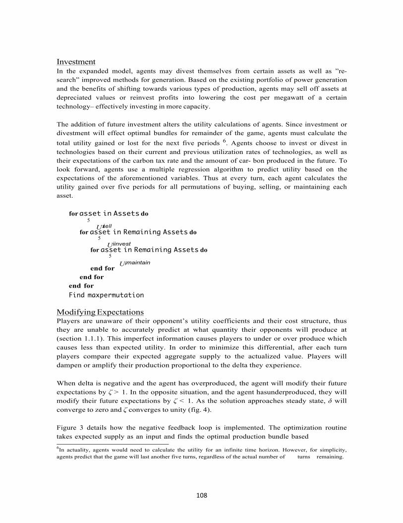
108

Investment In the expanded model, agents may divest themselves from certain assets as well as ”re- search” improved methods for generation. Based on the existing portfolio of power generation and the benefits of shifting towards various types of production, agents may sell off assets at depreciated values or reinvest profits into lowering the cost per megawatt of a certain technology– effectively investing in more capacity.

The addition of future investment alters the utility calculations of agents. Since investment or divestment will effect optimal bundles for remainder of the game, agents must calculate the total utility gained or lost for the next five periods 6. Agents choose to invest or divest in technologies based on their current and previous utilization rates of technologies, as well as their expectations of the carbon tax rate and the amount of car- bon produced in the future. To look forward, agents use a multiple regression algorithm to predict utility based on the expectations of the aforementioned variables. Thus at every turn, each agent calculates the utility gained over five periods for all permutations of buying, selling, or maintaining each asset.

for asset in Assets do

5 Usi ell

for asset in Remaining Assets do 5

Uiinvest for asset in Remaining Assets do

5

end for end for

end for

Uimaintain

Find maxpermutation Modifying Expectations Players are unaware of their opponent’s utility coefficients and their cost structure, thus they are unable to accurately predict at what quantity their opponents will produce at (section 1.1.1). This imperfect information causes players to under or over produce which causes less than expected utility. In order to minimize this differential, after each turn players compare their expected aggregate supply to the actualized value. Players will dampen or amplify their production proportional to the delta they experience.

When delta is negative and the agent has overproduced, the agent will modify their future expectations by ζ > 1. In the opposite situation, and the agent hasunderproduced, they will modify their future expectations by ζ < 1. As the solution approaches steady state, δ will converge to zero and ζ converges to unity (fig. 4).

Figure 3 details how the negative feedback loop is implemented. The optimization routine takes expected supply as an input and finds the optimal production bundle based

6In actuality, agents would need to calculate the utility for an infinite time horizon. However, for simplicity, agents predict that the game will last another five turns, regardless of the actual number of turns remaining.

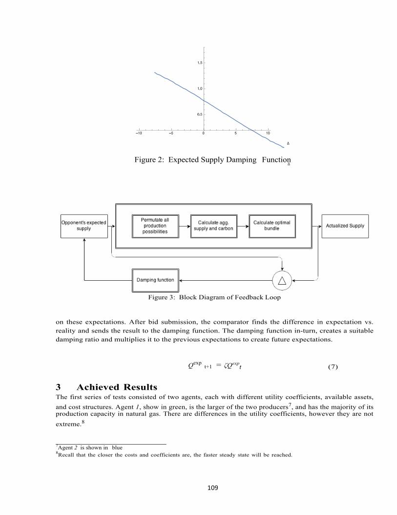
109

Figure 2: Expected Supply Damping Function

Figure 3: Block Diagram of Feedback Loop

on these expectations. After bid submission, the comparator finds the difference in expectation vs. reality and sends the result to the damping function. The damping function in-turn, creates a suitable damping ratio and multiplies it to the previous expectations to create future expectations.

Qexp t+1 = ζQexp

t (7)

3 Achieved Results The first series of tests consisted of two agents, each with different utility coefficients, available assets, and cost structures. Agent 1, show in green, is the larger of the two producers7, and has the majority of its production capacity in natural gas. There are differences in the utility coefficients, however they are not extreme.8

7Agent 2 is shown in blue 8Recall that the closer the costs and coefficients are, the faster steady state will be reached.

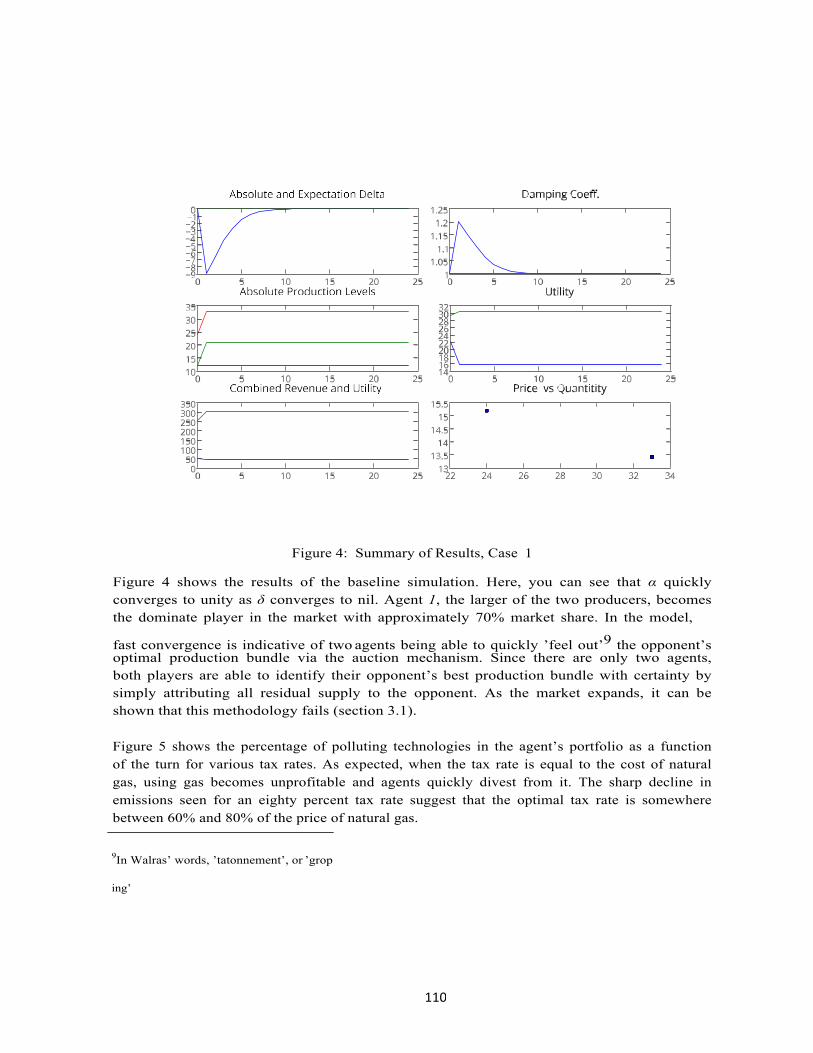
110

Figure 4: Summary of Results, Case 1

Figure 4 shows the results of the baseline simulation. Here, you can see that α quickly converges to unity as δ converges to nil. Agent 1, the larger of the two producers, becomes the dominate player in the market with approximately 70% market share. In the model,

fast convergence is indicative of two agents being able to quickly ’feel out’9 the opponent’soptimal production bundle via the auction mechanism. Since there are only two agents, both players are able to identify their opponent’s best production bundle with certainty by simply attributing all residual supply to the opponent. As the market expands, it can be shown that this methodology fails (section 3.1).

Figure 5 shows the percentage of polluting technologies in the agent’s portfolio as a function of the turn for various tax rates. As expected, when the tax rate is equal to the cost of natural gas, using gas becomes unprofitable and agents quickly divest from it. The sharp decline in emissions seen for an eighty percent tax rate suggest that the optimal tax rate is somewhere between 60% and 80% of the price of natural gas.

9In Walras’ words, ’tatonnement’, or ’grop

ing’

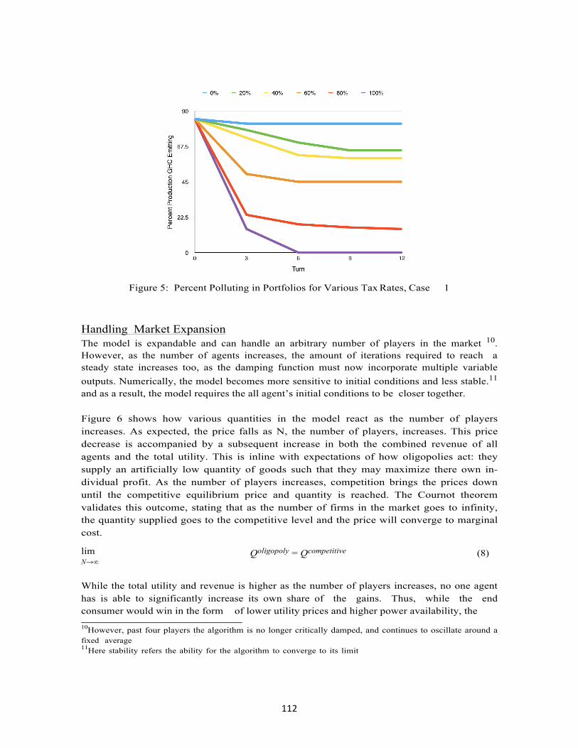
112

Figure 5: Percent Polluting in Portfolios for Various Tax Rates, Case 1

Handling Market Expansion The model is expandable and can handle an arbitrary number of players in the market 10. However, as the number of agents increases, the amount of iterations required to reach a steady state increases too, as the damping function must now incorporate multiple variable outputs. Numerically, the model becomes more sensitive to initial conditions and less stable.11

and as a result, the model requires the all agent’s initial conditions to be closer together.

Figure 6 shows how various quantities in the model react as the number of players increases. As expected, the price falls as N, the number of players, increases. This price decrease is accompanied by a subsequent increase in both the combined revenue of all agents and the total utility. This is inline with expectations of how oligopolies act: they supply an artificially low quantity of goods such that they may maximize there own in- dividual profit. As the number of players increases, competition brings the prices down until the competitive equilibrium price and quantity is reached. The Cournot theorem validates this outcome, stating that as the number of firms in the market goes to infinity, the quantity supplied goes to the competitive level and the price will converge to marginal cost.

lim N→∞

Qoligopoly = Qcompetitive (8)

While the total utility and revenue is higher as the number of players increases, no one agent has is able to significantly increase its own share of the gains. Thus, while the end consumer would win in the form of lower utility prices and higher power availability, the

10However, past four players the algorithm is no longer critically damped, and continues to oscillate around a fixed average 11Here stability refers the ability for the algorithm to converge to its limit

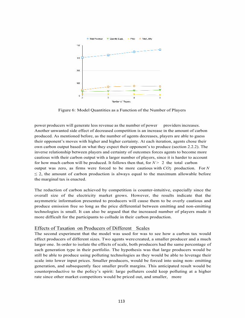
113

Figure 6: Model Quantities as a Function of the Number of Players

power producers will generate less revenue as the number of power providers increases. Another unwanted side effect of decreased competition is an increase in the amount of carbon produced. As mentioned before, as the number of agents decreases, players are able to guess their opponent’s moves with higher and higher certainty. At each iteration, agents chose their own carbon output based on what they expect their opponent’s to produce (section 2.2.2). The inverse relationship between players and certainty of outcomes forces agents to become more cautious with their carbon output with a larger number of players, since it is harder to account for how much carbon will be produced. It follows then that, for N > 2 the total carbon output was zero, as firms were forced to be more cautious with CO2 production. For N ≤ 2, the amount of carbon production is always equal to the maximum allowable before the marginal tax is enacted.

The reduction of carbon achieved by competition is counter-intuitive, especially since the overall size of the electricity market grows. However, the results indicate that the asymmetric information presented to producers will cause them to be overly cautious and produce emission free so long as the price differential between emitting and non-emitting technologies is small. It can also be argued that the increased number of players made it more difficult for the participants to collude in their carbon production.

Effects of Taxation on Producers of Different Scales The second experiment that the model was used for was to see how a carbon tax would effect producers of different sizes. Two agents were created, a smaller producer and a much larger one. In order to isolate the effects of scale, both producers had the same percentage of each generation type in their portfolio. The hypothesis was that large producers would be still be able to produce using polluting technologies as they would be able to leverage their scale into lower input prices. Smaller producers, would be forced into using non- emitting generation, and subsequently face smaller profit margins. This anticipated result would be counterproductive to the policy’s spirit: large polluters could keep polluting at a higher rate since other market competitors would be priced out, and smaller, more

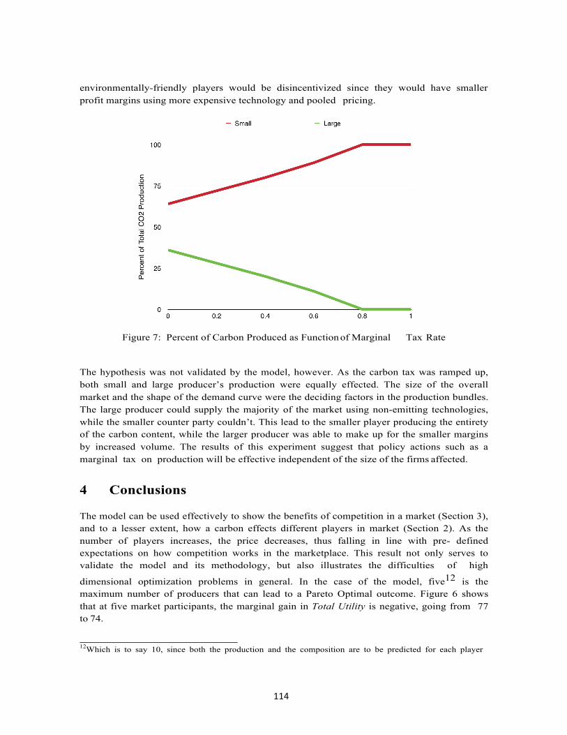
114

environmentally-friendly players would be disincentivized since they would have smaller profit margins using more expensive technology and pooled pricing.

Figure 7: Percent of Carbon Produced as Function of Marginal Tax Rate The hypothesis was not validated by the model, however. As the carbon tax was ramped up, both small and large producer’s production were equally effected. The size of the overall market and the shape of the demand curve were the deciding factors in the production bundles. The large producer could supply the majority of the market using non-emitting technologies, while the smaller counter party couldn’t. This lead to the smaller player producing the entirety of the carbon content, while the larger producer was able to make up for the smaller margins by increased volume. The results of this experiment suggest that policy actions such as a marginal tax on production will be effective independent of the size of the firms affected.

4 Conclusions The model can be used effectively to show the benefits of competition in a market (Section 3), and to a lesser extent, how a carbon effects different players in market (Section 2). As the number of players increases, the price decreases, thus falling in line with pre- defined expectations on how competition works in the marketplace. This result not only serves to validate the model and its methodology, but also illustrates the difficulties of high

dimensional optimization problems in general. In the case of the model, five12 is the maximum number of producers that can lead to a Pareto Optimal outcome. Figure 6 shows that at five market participants, the marginal gain in Total Utility is negative, going from 77 to 74.

12Which is to say 10, since both the production and the composition are to be predicted for each player

115

References

[1] EIA. How Much Carbon Dioxide (CO2) Is Produced hen Different Fuels Are Burned? U.S Energy Information Administration. U.S Energy Information Administration, n.d. Web. 9 Dec.2013.

[2] Osborne, Martin J. ”Competitive Equilibrium in an Exchange Economy.”

Economics UToronto. U Toronto, 1997. Web. 30 Nov. 2014. × <https://www.economics.utoronto.ca/osborne/2x3/tutorial/CEFRM.HTM >.

[3] Sandmo, Agnar (2008). ”Pigouvian taxes,” The New Palgrave Dictionary of Economics, 2nd Edition.

[4] Chappin, Dijkema (2007). ”An Agent Based Model of the System of Electricity Production Systems:

Exploring the Impact of CO2 Emission-Trading.”

[5] UCAR. ”How Much Has the Global Temperature Risen in the Last 100 Years?” University Corporation for Atmospheric Research. UCAR, n.d. Web. 9 Dec. 2013.

[6] Air quality board to fine Bay Area polluters, San Francisco Chronicle, May 22, 2008.

[7] Sarin, R., and F. Vahid, 2001. ”Predicting how People Play Games: A Simple Dynamic Model of Choice.” Games and Economic Behavior, 34, 104-122.

[8] W.W Hogan,”A market power model with strategic interaction in electricity networks,” Energy J. vol. 18, no. 5, pp. 107-141, 1997

[9] H. Chen, P. Wong et al,”Analyzing oligopolistic electricity market using coevolutionary

computation,” IEEE Transactions on Power Systems, vol. 21, no. 1, Feb. 2006

[10] Argonne National Laboratory. ”Electricity Market Complex Adaptive System.” Argonne National Laboratory. N.p., n.d. Web. 1 Feb. 2015. <http://www.dis.anl.gov/projects/emcas.html>.

[11] EPA. ”Overview of Greenhouse Gasses.” EPA. United States Environmental Protec- tion

Agency, n.d. Web. 9 Dec. 2013.

[12] Bunn, D.W and F.S Oliveira, 2001. ”Agent-based Simulation: An application to the New Electricity Trading Arrangments of England and Wales.” IEEE Transactions on Evoloutionary Computations 55:493-502

[13] Guerci, E., S. Ivaldi, S. Pastore, and S. Cincotti, 2005. ”Modeling and Implemen- tation of an

Artificial Electricity Market Using Agent-based Technology”. Physica A- Statistical Mechanics and Its Applications, 355 (1): 69-76.

[14] Pineau, P.-O., and P. Murto, 2003. ”An Oligopolistic Investment Model of the Finnish Electricity

Market.” Annalsof Operations Research,121, 123-148.

116

IMPACT OF RUSSIA’S 2014–2015 CRISIS ON THE DYNAMIC LINKAGES BETWEEN THE STOCK

MARKETS OF RUSSIA, THE EU AND U.S.

Kārlis Ločmelis, Daniel Mititel

Stockholm School of Economics in Riga One of the most recent turmoil periods of significant importance is the ongoing Russian financial crisis that started in 2014. Considering the openness of the Russian economy, it might be that this disruptive event could have had an impact on the linkages between Russian and other global stock markets. This paper analyses changes in the dynamic linkages between the U.S., EU and Russia's stock markets in the midst of the Russia’s 2014-2015 crisis. This study is particularly concerned with analyzing how short-run, long-run and volatility transmission linkages have changed due to the Russian crisis. We performed a structural break analysis to identify a period of tranquility in the Russian stock market and the date on which the crisis period started. Afterwards, we run cointegration, Granger-causality, and GARCH-BEKK tests to compare long- run, short-run, shock spillover, and volatility spillover linkages during the stable and the crisis periods.

We found that there are changes in the short-run, long-run and volatility linkages among the stock markets of the U.S., EU and Russia during the crisis period. Consistent with the idea that there is a financial crisis in Russia, return shocks in the Russian stock market are substantially higher during the crisis period than they were during the stable period. Also, during the crisis period stock market of Russia seems to be less sensitive to return shocks from the EU stock market and vice-versa. We consider that the bilateral sanctions between Russian and the EU might have contributed to the segregation of their stock markets. In addition, we discovered that there are greater short-run and long-run diversification benefits during the turmoil period. However, the results of the GARCH-BEKK model suggest that there is a contagion effect from the Russian stock market to the stock markets of the U.S. and the EU. Thus, investors should be aware of shock and volatility spillovers among these countries’ equity markets while assessing the risk of their portfolios. In addition, the results are robust even if the stable and the crisis periods are determined using historical, not implied volatility.

Keywords: Russia’s 2014-2015 crisis, returns spillover, volatility spillover, GARCH-BEKK

117

1 Introduction

Over the last few decades, dynamic linkages between international markets has been a hot topic, not only among academicians, but also among banks, international investors, hedge funds, and various other institutions. Particular interest in this topic was seen during the 2008 financial crisis, when a shock in the U.S. market brought down not only the domestic stock market, but also markets overseas and destabilized the Euro Zone which led to the European sovereign debt crisis (Fontaine, 2011). Thus, one should not underestimate the power of the information transmission mechanism among various markets.

How the 2014-15 Russian crisis has impacted the dynamic linkages across financial stock markets is an important research question for many reasons. First, to our knowledge, this paper is a pioneer in this field. Taking into account that previous research papers suggest that there is little evidence of contagion from the Russian equity market during recent crises (Claessens & Forbes, 2004) and that the Russian stock market is highly integrated, a substantial increase in the dependence between it and other markets is unlikely (Korhonen & Peresetsky, 2013), it is of interest for us to test the validity of these conclusions in the context of the current Russian crisis. Second, taking into account that the EU and the U.S. are two superpowers, which imposed most sanctions on Russia due to its military intervention in Ukraine in 2014, it is interesting for us to analyze the feedback effect coming from the plummeting stock market of Russia to the stock markets of the EU and the U.S. Third, this study will reveal information regarding equity market efficiency of the previously mentioned countries, since in an efficient market it is not possible to forecast returns by conditioning them on the lagged returns of other related markets. Fourth, knowledge of volatility interdependence may improve current estimates of conditional volatility, which is useful for the following financial applications: options pricing, value-at-risk (VaR) estimation, portfolio optimization, hedging, strategic asset allocation, and market selection. Last but not least, in the case that evidence of contagion is found, this study might be useful for government officials, investors and policymakers to strengthen individual economies and international financial systems in order to reduce the risk of contagion in the future by implementing better financial policies, by using improved investor strategies, or by creating stronger global frameworks.

Initially, we would like to define the main concepts of our study, namely interdependence, integration, and contagion. Interdependence can be considered as a stable state of dependence between capital markets (Trenca & Dezsi, 2013). In our paper we examine short-term (return) and long-term (price) interdependence among stock markets. The next two terms, namely integration and contagion, are related to shock and volatility spillover among equity markets. Integration can be defined as a high degree of dependence among equity markets that is not affected by an external shock. If two markets share a high degree of dependence during the periods of stability, and the co-movement between them after an external shock does not increase significantly, then this phenomenon is called integration rather than contagion. Forbes and Rigobon (2002) asserted that in case of a true contagion to take place, there should be no prior dependence between stock markets before the occurrence of a financial distress. Taking into account the considerable development of technology and the increased flow of capital between countries, which catalyzed the globalization process, it is almost impossible for stock markets to

118

be independent. Therefore, it is more appropriate to define contagion as an increase in shock and volatility dependence between equity markets during a financial distress period compared to their levels of dependence during a predefined stable period.

The rest of the paper is structured as follows. Section 2 outlines the literature on interdependence and contagion. Section 3 describes the methods used to answer the research questions. Section 4 specifies data gathering and section 5 provides and discusses the results, and we conclude the paper with section 6 that discusses the limitations of the study and suggest further research possibilities regarding the Russia’s 2014-2015 crisis and its impact on the dynamic linkages between stock markets.

2 Literature Review

Numerous studies have researched the dynamic linkages between stock markets. Tuluca and Zwick (2001) found that during the 1987 stock market crash short-term co-movements between the U.S. and the UK increased substantially. The same conclusion of increased short-run linkages during a crisis period is found by Jochum, Kirchgassner & Platek (1999) who studied Polish, Hungarian, Czech, Russian, and the U.S. stock markets during the Asian crisis in 1997 and during the subsequent Russian crisis in 1998. In addition, Gabriel and Manso (2014) investigated changes in the short-term linkages during the Dot-Com crisis and during the Global financial crisis and found that during both crises short-term linkages between twelve European and non- European equity markets increased.

Speaking about the long run linkages, Tuluca and Zwick (2001) found that the stock market crash in 1987 did not affect the long-term linkages between the U.S. and the UK. Also, Voronkova and Lucey (2005) did not find any long-run co-movement between Russia, UK, U.S., Hungary, and Poland stock markets before, during and after the Asian and the subsequent Russian crisis from 1998. Whereas, Inder (2014) suggested that Indian stock market has become more cointegrated with stock markets of other Asian countries after the subprime crisis. Similarly, Lee and Jeong (2014) advocated that the level of cointegration between the European and global stock markets had temporarily increased during the subprime crisis.

One can see that short-run and long-run linkages between various equity markets might change over time and that they are particularly susceptible to the turmoil periods.

It is of interest for us to analyze short-term and long-term dynamic linkages between the EU, U.S. and Russian stock markets prior to the recent 2014-2015 Russian crisis and whether this crisis has had any effect on those linkages. Thus we draw the following two research questions:

1. Have the long-run linkages between the stock markets of the U.S., Russia and the EU changed due to the Russia’s 2014-2015 financial crisis? 2. Has the short-run return transmission between the stock markets of the U.S., Russia and the EU changed due to the Russia’s 2014-15 financial crisis?

119

Volatility and shock transmission is high during periods of crises, because investors attempt to discover price changes in one market using observed fluctuations in other equity markets (Maghyereh and Awartani, 2012). Hamao, Masulis & Ng (1990) in their research concluded that volatility spilled over from New York to London stock exchange during the 1987 U.S. stock market crash. Kharchenko and Tzvetkov (2013) also observed this phenomenon during the 2008 financial crisis when volatility and shocks spilled from German and French stock markets to the Russian equity market and from Russian to the U.S. equity markets. A different view on the direction of the volatility and shock spillovers from Russia to the U.S. is presented by Khan (2010) who found a bidirectional link between both countries’ equity markets, whereas Dimitriou, Kenourgisos & Simos (2013) suggested that volatility was spilled from the U.S. to Russian equities, thus suggesting a third view about the volatility linkage between the U.S. and Russia during the sub-prime crisis in 2008. Despite the discussion on the direction of volatility and shock spillovers, Claessens and Forbes (2004) who analyzed financial crises in 1990s and the Argentinean and Turkish crises between 2001 and 2002 concludes that the contagion effect has become rare during financial crises as countries have employed better fiscal and monetary policies. The authors also state that there is little evidence of contagion effect from Argentinian and Turkish crisis. Furthermore, Korhonen and Peresetsky (2013) suggest that the Russian stock market is already highly integrated with the EU and the U.S. equity markets; thus, an increase in dependence through volatility and shock spillovers between Russia and other equity markets is unlikely.

Taking all of the above findings into account, we draw our third RQ:

3. Have the volatility transmission linkages between the stock markets of the U.S., Russia and the EU changed due to the Russia’s 2014-15 financial crisis? What is the direction of the shock and volatility spillovers?

In order to answer our research questions, we will analyze changes in price, return and volatility linkages among Russia, the U.S. and the EU. The latter two regions were chosen by the authors due to several reasons. The major reason is that they are the ones that have imposed most of the sanctions on Russia, because they considered its intervention in Ukraine unlawful (Klapper, 2014; Norman & White, 2014). Another reason why we chose to analyze the changes in volatility, price and return linkages with the EU and with the U.S. in the context of Russian crisis is that both of them are major superpowers in the world (Guttman, 2001; Herring, 2008); thus, it would be interesting for us to examine the effect of plummeting Russian stock market on such big world “players”. Moreover, the EU is not only the major trading partner of Russia, but it is also its most important investor. It is estimated that in 2013 around of 75% of FDI stocks in Russia came from the EU member states (European Commission, 2014). On the other hand, although the U.S. trade balance with Russia is much less, the Russian market still remains attractive for the U.S. companies, such as ExxonMobil, Boeing, Chevreon, Coca-Cola etc, which have invested more than $30 billion in the period from 1992-2011 (Borisov & Frye, 2011).

In sum, the purpose of this paper is to rigorously investigate the impact of the Russian financial crisis, which commenced in 2014, on the equity markets of two major world players, namely the United States and the European Union, by analyzing changes in the dynamic linkages among these stock markets.

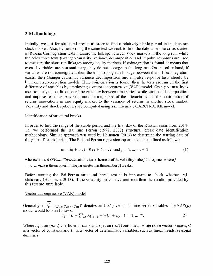
120

3 Methodology Initially, we test for structural breaks in order to find a relatively stable period in the Russian stock market. Also, by performing the same test we seek to find the date when the crisis started in Russia. Cointegration tests measure the linkage between stock markets in the long run, while the other three tests (Granger-causality, variance decomposition and impulse response) are used to measure the short-run linkages among equity markets. If cointegration is found, it means that even if variables are non-stationary, they do not diverge in the long run. On the other hand, if variables are not cointegrated, then there is no long-run linkage between them. If cointegration exists, then Granger-causality, variance decomposition and impulse response tests should be built on error-correction models. If no cointegration is found, then the tests are run on the first difference of variables by employing a vector autoregressive (VAR) model. Granger-causality is used to analyze the direction of the causality between time series, while variance decomposition and impulse response tests examine duration, speed of the interactions and the contribution of returns innovations in one equity market to the variance of returns in another stock market. Volatility and shock spillovers are computed using a multivariate GARCH-BEKK model.

Identification of structural breaks

In order to find the range of the stable period and the first day of the Russian crisis from 2014- 15, we performed the Bai and Perron (1998, 2003) structural break date identification methodology. Similar approach was used by Heinonen (2013) to determine the starting date of the global financial crisis. The Bai and Perron regression equation can be defined as follows:

𝜎! = 𝜃! + 𝜀!, t= 𝑇!!! + 1, … , 𝑇! and 𝑗 = 1, … , 𝑚 + 1 (1)

where 𝜎! is the RTS Volatility Index at time t, 𝜃! is the mean of the volatility in the 𝑗’𝑡ℎ regime, where 𝑗 = 0, … , 𝑚; 𝜀! is the error term. The parameter m is the number of breaks.

Before running the Bai-Perron structural break test it is important to check whether 𝜎!is stationary (Heinonen, 2013). If the volatility series have unit root then the results provided by this test are unreliable.

Vector autoregressive (VAR) model

Generally, if 𝑌! = (𝑦!! ,𝑦!! …𝑦!")′ denotes an (𝑛𝑥1) vector of time series variables, the 𝑉𝐴𝑅(𝑝) model would look as follows: 𝑌! = 𝐶 + 𝐴!𝑌!!!

!!!! +Ψ𝐷! + 𝜀! , 𝑡 = 1,… ,𝑇, (2)

Where 𝐴! is an (𝑛𝑥𝑛) coefficient matrix and 𝜀! is an (𝑛𝑥1) zero mean white noise vector process, C is a vector of constants and 𝐷! is a vector of deterministic variables, such as linear trends, seasonal dummies.

121

In a VAR model all variables should be stationary, but financial stock/index price series are usually non-stationary; therefore, the VAR model shall be transformed into Vector Error Correction Model (VECM), which drops out the requirement regarding the stationarity of the data.

To choose the optimal lag length we will rely on models that minimize information criteria. Particularly we will focus more on SBIC specification because it is more parsimonious, while the AIC will choose on average a model with too many lags.

Vector Error Correction Model (VECM)

Taking into account the 𝑉𝐴𝑅(𝑝) equation which we wrote in the previous sub-section (see equation 2), our VECM model looks as follows:

∆Y! = C+ Π Y!!! + Φ !∆Y!!!

!!!

!!!

+Ψ𝐷! + ε!

(3)

where Π=( 𝐴!!

!!! − 𝐼) and Φ ! = − 𝐴!!!!!!!

Cointegration test- Johansen approach

In order to investigate long-run relationship between variables in multivariate models, we will use the Johansen cointegration test (Johansen, 1991). The core of the Johansen method relies on testing for cointegration by looking at the rank of the ∠ matrix via its eigenvalues (characteristic roots).

Testing for the rank of ∠ matrix

The Johansen test analyzes whether the restrictions imposed on the rank of ∠ matrix can be rejected (Huyghebaert & Wang, 2010). The rank of the matrix is equal to the number of eigenvalues (𝜆!) that are different from 0. If the variables are not cointegrated, the rank of ∠ will be almost zero, i.e. 𝜆! ≈ 0.

To test for cointegration rank two likelihood tests can be used: trace statistics and maximum eigenvalue statistics. In this work we do not prefer one statistic over the other, but we will consider the results of both of them while drawing our conclusions.

Selection of the deterministic components in the Johansen test

Assuming that k=2 and 𝐷! = 𝑡 we can rewrite equation 3 as: ∆Y! = C+ 𝑎𝛽′Y!!! + Φ !∆Y!!! +Ψt+ ε! (4) where 𝑡 is a time trend variable. Following (Ahking, 2002), we can decompose C and Ψ into Ψ = 𝑎Ψ! + 𝑎!Ψ! (5)

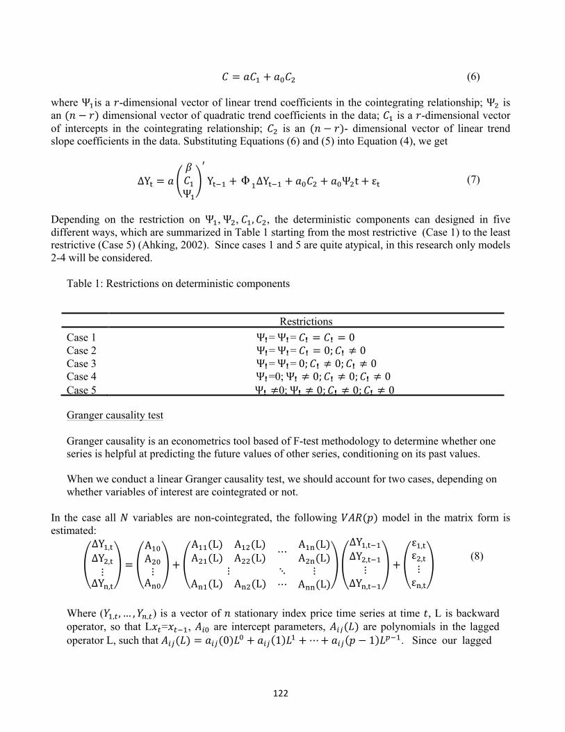
122

𝐶 = 𝑎𝐶! + 𝑎!𝐶! (6) where Ψ!is a 𝑟-dimensional vector of linear trend coefficients in the cointegrating relationship; Ψ! is an (𝑛 − 𝑟) dimensional vector of quadratic trend coefficients in the data; 𝐶! is a 𝑟-dimensional vector of intercepts in the cointegrating relationship; 𝐶! is an (𝑛 − 𝑟)- dimensional vector of linear trend slope coefficients in the data. Substituting Equations (6) and (5) into Equation (4), we get

∆Y! = 𝑎𝛽𝐶!Ψ!

!

Y!!! + Φ !∆Y!!! + 𝑎!𝐶! + 𝑎!Ψ!t+ ε!

(7)

Depending on the restriction on Ψ!, Ψ!, 𝐶!,𝐶!, the deterministic components can designed in five different ways, which are summarized in Table 1 starting from the most restrictive (Case 1) to the least restrictive (Case 5) (Ahking, 2002). Since cases 1 and 5 are quite atypical, in this research only models 2-4 will be considered.

Table 1: Restrictions on deterministic components

Restrictions

Case 1 Ψ!= Ψ!= 𝐶! = 𝐶! = 0 Case 2 Ψ!= Ψ!= 𝐶! = 0; 𝐶! ≠ 0 Case 3 Ψ!= Ψ!= 0; 𝐶! ≠ 0; 𝐶! ≠ 0 Case 4 Ψ!=0; Ψ! ≠ 0; 𝐶! ≠ 0; 𝐶! ≠ 0 Case 5 Ψ! ≠0; Ψ! ≠ 0; 𝐶! ≠ 0; 𝐶! ≠ 0

Granger causality test

Granger causality is an econometrics tool based of F-test methodology to determine whether one series is helpful at predicting the future values of other series, conditioning on its past values.

When we conduct a linear Granger causality test, we should account for two cases, depending on whether variables of interest are cointegrated or not.

In the case all 𝑁 variables are non-cointegrated, the following 𝑉𝐴𝑅(𝑝) model in the matrix form is estimated: ∆Y!,!

∆Y!,!⋮

∆Y!,!

=

A!"A!"⋮A!"

+

A!!(L) A!"(L)A!"(L) A!!(L)

⋯ A!"(L)A!"(L)

⋮ ⋱ ⋮A!"(L) A!"(L) ⋯ A!!(L)

∆Y!,!!!∆Y!,!!!⋮

∆Y!,!!!

+

ε!,!ε!,!⋮ε!,!

(8)

Where (𝑌!,! ,… ,𝑌!,!) is a vector of 𝑛 stationary index price time series at time 𝑡, L is backward operator, so that L𝑥!=𝑥!!!, 𝐴!! are intercept parameters, 𝐴!"(𝐿) are polynomials in the lagged operator L, such that 𝐴!"(𝐿) = 𝑎!"(0)𝐿! + 𝑎!" 1 𝐿! +⋯+ 𝑎!" 𝑝 − 1 𝐿!!!. Since our lagged

123

terms’ coefficient matrix is of size (𝑛𝑥𝑛), we have to test 𝑛(𝑛 − 1) null hypotheses of (non-) Granger causality.

If variables are cointegrated, Error Correction Mechanism (ECM) must be added to equation 8, therefore, the following model will be tested: ∆𝒀𝟏,𝒕

∆𝒀𝟐,𝒕⋮

∆𝒀𝒏,𝒕

=

𝑨𝟏𝟎𝑨𝟐𝟎⋮𝑨𝒏𝟎

+

𝑨𝟏𝟏 𝑳 𝑨𝟏𝟐 𝑳𝑨𝟐𝟏 𝑳 𝑨𝟐𝟐 𝑳

⋯ 𝑨𝟏𝒏 𝑳𝑨𝟐𝒏 𝑳

⋮ ⋱ ⋮𝑨𝒏𝟏 𝑳 𝑨𝒏𝟐 𝑳 ⋯ 𝑨𝒏𝒏 𝑳

∆𝒀𝟏,𝒕!𝟏∆𝒀𝟐,𝒕!𝟏

⋮∆𝒀𝒏,𝒕!𝟏

+

ℵ𝟎ℵ𝟏⋮ℵ𝒏

𝜺𝒕!𝟏 +

𝒖𝟏,𝒕𝒖𝟐,𝒕⋮𝒖𝒏,𝒕

(9)

In this case we only introduce lagged error terms from the previously mentioned 𝑉𝐴𝑅(𝑝) model. Multivariate GARCH In order to model the interactions between the volatility of two or more financial time series, a multivariate GARCH model must be used instead of a univariate one. In multivariate GARCH models, considering a vector of return series 𝑅! of the size (𝑁𝑥1), we can write: R! = 𝛼! + ΓR!!! + 𝜀! (10) where 𝑅!!! is an (𝑁𝑥1) vector of lagged returns, Γ is an (𝑁𝑥𝑁) matrix associated with these lagged returns; 𝛼!is an (𝑁𝑥1) vector of intercepts, 𝜀! is the innovation matrix (𝑁𝑥1) that stores the innovation term for each market. Further, the innovation matrix can be written as 𝜀! = H!

!!(θ)Z!

(11)

where H!!! θ is a positive definite matrix (𝑁𝑥𝑁) and Z! is assumed to be an (𝑁𝑥1) 𝑖. 𝑖.𝑑 vector,

with E(𝑍!)=0 and Var(𝑍!)=I!. H! is the variance-covariance matrix of R!. In case of a trivariate model the variance-covariance matrix of returns would look as follows:

H! =h!!,! h!",! h!",!h!",! h!!,! h!",!h!",! h!",! h!!,!

(12)

where ℎ!",! is the conditional covariance between country 𝑖 and country 𝑗 at time 𝑡.

In order to examine volatility spillovers we will employ the Baba, Engle, Kraft, and Kroner (BEKK) version of the multivariate GARCH model, whereby the conditional variance- covariance matrix is a function of the squared own and cross-product of innovation terms, 𝜀!, and

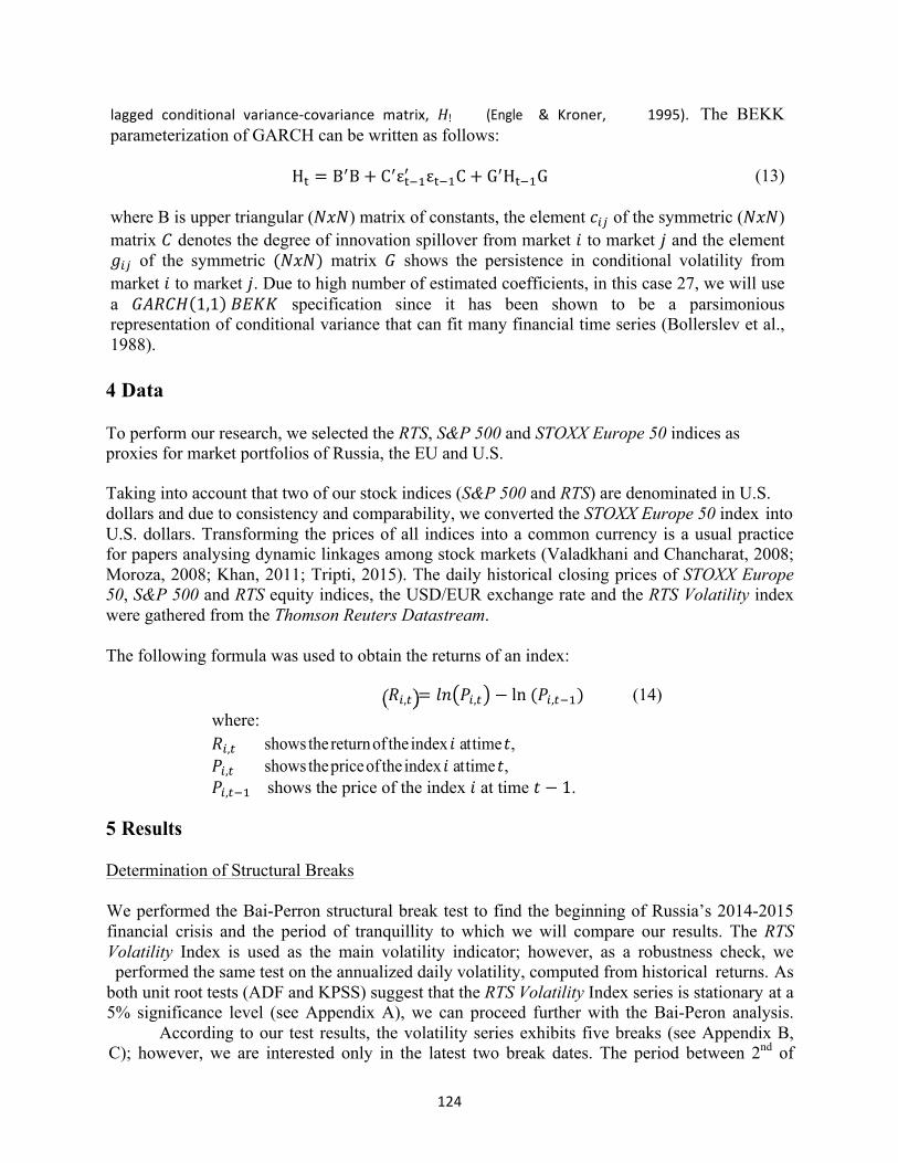
124

lagged conditional variance-covariance matrix, 𝐻! (Engle & Kroner, 1995). The BEKK parameterization of GARCH can be written as follows: H! = B!B+ C!ε!!!! ε!!!C+ G!H!!!G (13) where B is upper triangular (𝑁𝑥𝑁) matrix of constants, the element 𝑐!" of the symmetric (𝑁𝑥𝑁) matrix 𝐶 denotes the degree of innovation spillover from market 𝑖 to market 𝑗 and the element 𝑔!" of the symmetric (𝑁𝑥𝑁) matrix 𝐺 shows the persistence in conditional volatility from market 𝑖 to market 𝑗. Due to high number of estimated coefficients, in this case 27, we will use a 𝐺𝐴𝑅𝐶𝐻 1,1 𝐵𝐸𝐾𝐾 specification since it has been shown to be a parsimonious representation of conditional variance that can fit many financial time series (Bollerslev et al., 1988). 4 Data

To perform our research, we selected the RTS, S&P 500 and STOXX Europe 50 indices as proxies for market portfolios of Russia, the EU and U.S.

Taking into account that two of our stock indices (S&P 500 and RTS) are denominated in U.S. dollars and due to consistency and comparability, we converted the STOXX Europe 50 index into U.S. dollars. Transforming the prices of all indices into a common currency is a usual practice for papers analysing dynamic linkages among stock markets (Valadkhani and Chancharat, 2008; Moroza, 2008; Khan, 2011; Tripti, 2015). The daily historical closing prices of STOXX Europe 50, S&P 500 and RTS equity indices, the USD/EUR exchange rate and the RTS Volatility index were gathered from the Thomson Reuters Datastream.

The following formula was used to obtain the returns of an index:

where:

𝑅!,! = 𝑙𝑛 𝑃!,! − ln (𝑃!,!!!) (14)

5 Results

𝑅!,! shows the return of the index 𝑖 at time 𝑡, 𝑃!,! shows the price of the index 𝑖 at time 𝑡, 𝑃!,!!! shows the price of the index 𝑖 at time 𝑡 − 1.

Determination of Structural Breaks

We performed the Bai-Perron structural break test to find the beginning of Russia’s 2014-2015 financial crisis and the period of tranquillity to which we will compare our results. The RTS Volatility Index is used as the main volatility indicator; however, as a robustness check, we performed the same test on the annualized daily volatility, computed from historical returns. As

both unit root tests (ADF and KPSS) suggest that the RTS Volatility Index series is stationary at a 5% significance level (see Appendix A), we can proceed further with the Bai-Peron analysis.

According to our test results, the volatility series exhibits five breaks (see Appendix B, C); however, we are interested only in the latest two break dates. The period between 2nd of

125

October 2012 and 3rd of March 2014 exhibit the lowest average volatility, thus we consider it as our stable period. The crisis period, on the other hand, is considered to range between the 3rd of Mach 2014 till 3rd of March 2015. The latest break in volatility occurred one trading day before the Russian Foreign Ministry officially admitted that Russian forces had seized Crimea (Ensor & Merat, 2014; Hufbauer, Cimino & Moran, 2014). Overall, this gives us 369 observations before the crisis and 262 observations during the crisis. Furthermore, the robustness check, using historic instead of implied volatility, provided similar results.

Tests for Cointegration

Overall, the ADF and KPSS indicate that all level (price) series have a unit root and all return series are stationary during both the stable and the crisis periods. This means that all price series are integrated of order one, 𝐼(1). Thus, we can perform Johansen’s procedure to determine the number of cointegrating linkages among our variables. The number of lags in the VAR model is determined by SBIC information criteria and in both periods the test suggests to use two lags (see Appendix D). Regarding the parameter specification for Johansen’s test, we prefer model 4 over model 2 and 3 as all of our stock index price series have intercepts and that most of the series follow a clear trend.

The Johansen approach

The results of Johansen cointegration test (Appendix E) suggest that Russian, U.S. and European equity markets were more cointegrated before the crisis than they are afterwards. This is good news for investors because they can gain substantial long-run benefits due to diversification opportunities.

To determine which long-run associations between the U.S., EU and Russian equity markets that have vanished during the crisis period, we will implement Johansen’s cointegration test to each combination of two out of three stock markets.

After performing a similar analysis as in the trivariate case, we found that each stock index has a long-run association with other stock indices during the stable period. All cointegrated relationships are significant at a 10% significance level. This long-run association between the Russian and the U.S. equity markets during the stable period is consistent with the results of Zhang et al. (2013), Zhong et al. (2014) and Korhonen and Peresetsky (2013).

During the crisis period we found that there is a significant change in the long-run linkages among the three stock markets we analyze. According to the results of the Johansen test there is no bivariate long-run relationship among any of the stock markets we analyze. This indicates that the diversification benefits can be achieved during the crisis period by investing in any of the stock markets that our analysis is concerned with.

Short-term linkages

In this part, we present the results of statistical tests examining short-term linkages among the equity markets of Russia, the U.S. and EU during the stable and crisis periods. Initially, we

126

perform a Granger causality test during both periods to determine how the returns from one market influence the returns of other stock markets. The results of the Granger-causality test can also be interpreted as the degree of return spillover from one market to another. Next, we perform an impulse response analysis and a variance decomposition test during the stable and the crisis periods to provide more insights about changes in short-term dynamic linkages.

Return spillover effect: pairwise Granger causality tests

The SBIC suggest using a VAR and VECM model with one lag to perform Pairwise Granger causality tests during the stable and the crisis period (see Appendix F).

Appendix G presents the results of Granger causality tests among different stock markets during the stable period (Panel A) and during Russia’s 2014–2015 crisis (Panel B). During the stable period, returns of S&P 500 Granger caused returns of both RTS and STOXX Europe 50. Similarly, returns of STOXX Europe 50 have a statistically significant impact on the returns of other markets, namely on S&P 500 and RTS stock markets. On the other hand, RTS returns do not have any forecasting power at predicting returns of either S&P 500 or of STOXX Europe 50.

Multivariate GARCH-BEKK model

This paper uses a trivariate GARCH-BEKK model to quantify the effects of the lagged own and cross-innovations and lagged own and cross-volatility on the present own and cross volatility between the stock markets of Russia, the EU and the U.S. The estimated coefficients of the innovation and lagged variance-covariance parameters during the stable and the crisis periods are presented in the Appendix H.

According to our results, during Russia’s 2014-2015 crisis, there are more shock and volatility spillover linkages between the stock markets of countries that we analyze than there were during the stable period. In addition, all the linkages from the crisis period are more statistically significant than they were during the stable period (see Appendix H). In particular, shocks from Russia are unidirectional during the turmoil period and they seem to influence the volatility of all three stock markets and this impact is more statistically significant during the crisis than during the stable period. These results suggest that there were certain events in the Russian stock market, during the crisis that triggered higher volatility in the foreign markets. In addition, our results suggest that in comparison to the stable period, during the crisis period there was a bidirectional shock spillover between stock markets of the U.S. and the EU (see Appendix H, Panel A). The two-way shock spillover indicates a strong connection between the above-stated equity markets. Generally, bidirectional shock spillovers indicate that news about shocks in one stock exchange affects the volatility of another stock exchange and vice-versa. In this case, shocks from the U.S. equity market to the EU stock market and conversely might have started to be more significant determinants of volatility due to the fact that there was a rise in the foreign direct investments from the U.S. to the EU countries in comparison with the previous years, which strengthened the linkage between these two equity markets. In addition, there were some events that could have led to higher awareness in U.S. stock markets, for example Greek legislative elections from January 2015 and their expected negative impact on the Greek debt crisis (Kottasova, 2015) could have increased the awareness among U.S. investors.

127

Coefficients of lagged volatility linkages between stock markets that we analyze indicate that during the stable period there were own-volatility spillover linkages in the U.S. stock market, which suggests that past U.S. stock market volatility had a significant impact on its future values. On the other hand, the past volatility of the Russian stock market has a statistical significant impact on the volatility of the EU stock market and on the volatility of its own equity market during the crisis period.

The statistical significance of 𝑔(3,2) and the insignificance of 𝑔(2,3) during the crisis period (see Appendix H) indicate that the volatility spillover is unidirectional from the Russian stock market to the EU stock market. Additionally, we consider that we do not spot this volatility spillover linkage during the stable period due to the fact that the Russian equity market was relatively tranquil at that time (Appendix B). Thus, this channel of transmission of volatility could have been practically inactive

6 Conclusion

One of the most recent turmoil periods of major significance is the Russian financial crisis that started in 2014. It substantially undermined Russia’s economic stability and, given the openness of the Russian economy, we hypothesized that this disruptive period could have an impact on the linkages among global stock markets. In this paper, we analyzed the impact of this crisis on the dynamic linkages among the equity markets of Russia, the U.S. and EU. In particular, we studied the changes in long-term linkages, short term-linkages and the volatility transmission mechanism during the crisis.

(1) First, we performed a Bai-Perron structural break test, which suggested that, there was a significant increase in the average volatility in the Russian stock market in the following day after the Russian Foreign Ministry officially stated that Russian forces had seized Crimea. This is our proxy date for the beginning of the Russia’s 2014-15 Russian crisis. (2) Moreover, the same test allows us to identify a period of low volatility (a stable period) against which we compare our results from the crisis period. The stable period was found to be the period that immediately preceded the crisis period.

(3) Our results of the trivariate Johansen cointegration test suggest that there is no long-run association between the equity markets of the U.S., EU and Russia after the 2014-2015 Russian crisis started, despite the fact that there was a cointegrating linkage among all these markets prior to the crisis. (4) By performing a bivariate analysis, we found that there is no long-run linkage between any two of the three countries during the crisis. (5) These results suggest that there are long-run diversification benefits and can be reaped by investing in any of the three stock markets.

To analyze changes in the short-run linkages between the three stock markets we conducted the Granger-causality, Impulse response and Variance decomposition analyses.

(6) Our results from Granger-causality tests suggest that the EU stock market returns do not Granger-cause the returns of the U.S. equity market during the crisis period, despite the fact that

128

there was a Granger causality linkage during the stable period. (7) An implication of this result is that investors can better diversify their portfolios in the short-run by investing in the U.S. stock market. (8) Moreover, we found that during the crisis period Russian stock market returns have a higher statistical power at Granger-causing the returns of the EU and U.S. stock market than during the stable period. However, the existence of these linkages can still be rejected at conventional significance levels.

(10) Finally, the results of our GARCH-BEKK analysis suggest that during the Russian crisis shock spillovers intensified and new volatility spillovers appeared. Taking into account that the Russian crisis was transferred to other stock markets through variance channel by means of shock and volatility spillovers, we conclude that a contagion effect took place among the stock markets of the U.S. and EU during the Russia’s 2014-2015 crisis. Also, the results are robust even if the stable and the crisis periods are determined using historical, not implied volatility.

Bibliography Ahking, F., W. (2002). Model mis-specification and Johansen's co-integration analysis: An application to the US

money demand. Journal of Macroeconomics, 24.1, 51-66. doi:10.1016/S0164-0704(02)00017-4

Bai, J., & Perron, P. (1998). Estimating and testing linear models with multiple structural changes. Econometrica, 66(1), 47. doi:10.2307/2998540

Bai, J., & Perron, P. (2003). Computation and analysis of multiple structural change models. Journal of Applied

Econometrics, 18(1), 1-22. doi:10.1002/jae.659

Bollerslev, T., Engle, R., & Wooldridge, J. (1988). A capital asset pricing model with time-varying covariances. Journal of Political Economy, 96(1), 116. doi:10.1086/261527

Borisov, K., & Frye, T. (2011). Perspectives of Russian-American investment cooperation: tendencies, mechanisms

of support, recommendations. International Research & Exchanges Board, 1-8. Retrieved from http://www.irex.ru/assets/files/Gaidar%20Program/Borisov-Eng%28final%29.pdf

Claessens, S., & Forbes, K. (2004). International financial contagion. Boston: Kluwer Academic Publishers.

Dimitriou, D., Kenourgisos, D., & Simos, T. (2013). Global financial crisis and emerging stock market contagion: A multivariate FIAPARCH-DCC approach. International Review of Financial Analysis, 30, 46-56. doi:10.1016/j.irfa.2013.05.008

Engle, R., F., & Kroner, K., F. (1995). Multivariate simultaneous generalized ARCH. Econometric Theory, 11.01,

122. Retrieved from http://www.jstor.org/stable/3532933?seq=29#page_scan_tab_contents

Ensor, J., & Merat, A. (2014). Ukraine crisis live: President Barack Obama warns of 'costs' for any violation of Ukraine. Telegraph.co.uk. Retrieved 10 May 2015, from http://www.telegraph.co.uk/news/worldnews/europe/ukraine/10666893/Ukraine-crisis-live-President- Barack-Obama-warns-of-costs-for-any-violation-of-Ukraine.html

European Commission. (2014). Trading with Russia. European Commission. Retrieved 5 January, 2015, from http://ec.europa.eu/trade/policy/countries-and-regions/countries/russia/

Fontaine, P. (2011). Understanding the Euro crisis: How did the subprime crisis become a sovereign debt crisis in Europe?. Institute of Economic, Federean University of Rio de Janeiro. Retrieved 4 April, 2015, from http://www.akb.org.br/upload/130820121627034529_Patrick%20Fontaine.pdf

129

Forbes, K., & Rigobon, R. (2002). No contagion, only interdependence: Measuring stock market comovements.

Journal of Finance, 57(5), 2223-2261. doi:10.1111/0022-1082.00494

Gabriel, V., & Manso, J. (2014). Financial markets and stock markets linkages. Economic Review of Galicia, 23(4), 133-148.

Guttman, R. (2001). Europe in the new century. Boulder, CO: L. Rienner.

Hamao, Y., Masulis, R., & Ng, V. (1990). Correlations in price changes and volatility across international stock

markets. Review of Financial Studies, 3(2), 281-307. doi:10.1093/rfs/3.2.281

Heinonen, A. (2013). The fear gauge: VIX volatility index and the time-varying relationship between implied volatility and stock returns. University of Helsinki. Retrieve 11 March, 2015, from https://helda.helsinki.fi/bitstream/handle/10138/39870/Gradu_Heinonen_Anssi.pdf?sequence=2

Herring, G. (2008). From colony to superpower. New York: Oxford University Press.

Hufbauer, G., Cimino, C., & Moran, T. (2014). Ukraine-related sanctions (1st ed.). Peterson Institute for International Economics, 1. Retrieved from http://blogs.piie.com/realtime/files/2014/05/20140514tables- figures.pdf#page=2

Huyghebaert, N., & Wang, L. (2010). The co-movement of stock markets in East Asia. China Economic Review, 21(1), 98-112. doi:10.1016/j.chieco.2009.11.001

Inder, S. (2014) Interdependence between Indian stock market and other Asian markets: An empirical analysis.

Punjabi University. Retrieved 15 March, 2015, from http://utiicm.com/Faculty/pdf/arch1/shivani%20Chopra_JPascricha.pdf

Jochum C., Kirchgassner, G., & Platek, M. (1999). A long-run relationship between Eastern stock markets? Cointegration and the 1997–1998 crisis in emerging markets. Weltwirtschaftliches Archiv, 135, 454–479.

Johansen, S. (1991). Estimation and hypothesis testing of cointegration vectors in Gaussian vector autoregressive

models. The Econometric Society, 59(6), 1551-1580. Retrieved from http://www.jstor.org/stable/2938278?seq=1#page_scan_tab_contents.

Khan, S. (2010). Measuring volatility spillover in Russian equity market: A multivariate GARCH approach. SSRN. Retrieved from http://papers.ssrn.com/sol3/papers.cfm?abstract_id=1617714

Kharchenko, I., & Tzvetkov, P. (2013). Estimation of volatilities and spillover effects between developed and emerging market economies. Lund universitet. Retrieved 5 April, 2015, from http://lup.lub.lu.se/student- papers/record/3801343

Klapper, B. (2014). Obama condemns Russia for Ukraine violence; rules out U.S. military involvement | The rundown. PBS NewsHour. Retrieved 5 January, 2015, from http://www.pbs.org/newshour/rundown/u-s- condemns-russias-invasion-ukraine/

Korhonen, I., & Peresetsky, A. (2013). What determines stock market behavior in Russia and other emerging countries?. SSRN Journal. doi:10.2139/ssrn.2235072

Kottasova, I. (2015). Greek debt crisis: Who has most to lose?. CNNMoney. Retrieved 1 April, 2015, from

http://money.cnn.com/2015/01/28/investing/greek-debt-who-has-most-to-lose/

Lee, G., & Jeong, J. (2014). Global financial crisis and stock market integration between northeast Asia and Europe. RES, 6(1). doi:10.5539/res.v6n1p61

130

Maghyereh, A., & Awartani, B. (2012). Return and volatility spillovers between Dubai financial market and Abu Dhabi Stock Exchange in the UAE. Applied Financial Economics, 22(10), 837-848. doi:10.1080/09603107.2011.628292

Moroza, J. (2008). Dynamic linkages between Baltic and International stock markets. School of Economics and Management, Lund University, 22-23. Retrieved from http://lup.lub.lu.se/luur/download?func=downloadFile&recordOId=1334907&fileOId=1646555

Norman, L., & White, G. (2014). EU official raises prospect of reworking Ukraine trade pact. Wall Street Journal. Retrieved 5 January, 2015, from http://www.wsj.com/articles/petro-poroshenko-says-worst-of-war-in- ukraine-is-over-1411665603

Trenca, I., & Dezsi, E. (2013). Connections between the European stock markets. Review of Economic Studies and Research Virgil Madgearu, (2), 151-171.

Tripti, N. (2015). Financial integration between BRICS and developed stock markets. International Journal of

Business and Management Invention, 4(1), 65-71.

Tuluca S., A., & Zwick, B. 2001. The effects of the Asian crisis on global equity markets. Financial Review, 3,125– 142.

Valadkhani, A., & Chancharat, S. (2008). Dynamic linkages between Thai and international stock markets. Journal

of Economic Studies, 35(5), 425-441. doi:10.1108/01443580810903572

Voronkova, S., & Lucey, B., M. (2005). Russian equity market linkages before and after the 1998 crisis: Evidence from time-varying and stockhastic cointegration tests. Bank of Finland, Institure for Economies in Transition. Retrieved from http://www.suomenpankki.fi/pdf/120326.pdf

Zhang, B., Li, X., & Yu, H. (2013). Has recent financial crisis changed permanently the correlations between BRICS and developed stock markets?. The North American Journal of Economics and Finance, 26, 725- 738. doi:10.1016/j.najef.2013.05.003

Zhong, M., Chang, T., & Tzent, H.,W. (2014). International equity diversification between the United States and

BRICS countries. Romanian Journal of Economic Forecasting, 8(1), 123-38.

131

Copyright Extensions and the Availability of Music: Evidence from British Hits of the 1960’s

John McKeon Boston University

Abstract

This paper examines the effects of copyright protection on reissues of modern music. It specifically looks at the UK directive from 2011 commonly referred to as “Cliff’s Law” and its impact on top hits from the early 1960’s. We measure the availability of music using a count of the number of times each track was reissued in each year since its release, and ask whether tracks in the public domain are more likely to be reissued. Cliff’s Law allows one to compare the availability of similar tracks released within a narrow time window but with different copyright status. We find that copyright protection does cause a track to see significantly fewer reissues than when a similar track is in the public domain. We find copyright to lessen yearly reissues of a track by between 55% and 86%. Furthermore, copyright protection has an even greater and more significant impact on less popular artists as opposed to their more popular counterparts.

Acknowledgements

I would like to thank the Boston University Undergraduate Research Opportunities Program for funding. I would also like to thank Megan MacGarvie for sponsoring this research and providing guidance.

1 Introduction

Copyright gives the creator of a work exclusive monopoly rights over the work for a set period of time. This plays a key role in incentivizing the supply of new creative products. Though there has been some empirical analysis regarding the copyright of music of past generations, there is relatively little evidence on how copyright extensions affect the diffusion of modern music. Prior research on copyright of books finds that books published in the decade before 1923 (and therefore in the public domain today) are more likely to be in print in more editions, than books published in the ten years after 1923, which are currently protected by copyright (Heald 2008, Reimers 2013). This paper examines the impact of copyright on the availability of music, as measured by new reissues of music recorded in the early 1960s. If copyright protection suppresses the availability of music, as it does for new editions of books, then the implications for consumer welfare are potentially even more severe than those for books. This is because the technology used to consume recorded music when the albums of the early 1960s were recorded is essentially obsolete today, and if music is not reissued in digital format, most listeners will not hear it.

132

2 Aspects of Music Copyright The copyright of music is typically separated into two parts, each of which is protected separately. One facet of music protection is the “musical composition”, which is property of the composer or lyricist. This may be in the form of notated copy (i.e. sheet music) or phonorecord (i.e. CD) (United States Copyright Office 2012). It is, more specifically, the actual pattern of notes and lyrics published for the song. The musical composition is treated as a literary work in the UK and is protected separately. The second aspect is the “sound recording” which “results from the fixation of a series of musical, spoken, or other sounds” (United States Copyright Office 2012). The performer typically owns the rights to the sound recording, unless it is sold back to the record company. The sound recording can be thought of as ‘this’ specific way that the song is performed and recorded. There can be multiple different sound recordings copyrighted separately for the same song performed in different ways or by different artists. These two aspects of copyright law affect various artists and songs in different ways. Artists who chiefly write and compose their own songs will hold both the musical composition and sound recording rights to their music while others may only receive copyright royalties from the sound recording.

Publishing, or musical composition, is the main source of copyright income in the industry. The author gets paid whenever the song is played in public. In the UK, the copyright term is set at the author’s lifetime plus 70 years. However, artists who have others compose and write their music for them depend on sound recording rights for copyright income. Regardless of whether the artist holds both rights or just the sound recording rights, a third party must pay for both rights when reissuing music. This possible impact on the third parties has a major effect on the availability of the music to the public.

3 Cliff’s Law

In 2011 the UK enacted Directive 2011/77/EU, which extends the copyright of sound recordings from 50 years to 70 years. This Directive became known as “Cliff’s Law” since Cliff Richards, who didn’t hold the publishing rights to his songs, was a major advocate for the extension. This extension is a step towards what advocates were pushing for, but it is still a very short term compared to the United States which protects the copyright of sound recordings for the holder’s life plus 70 years. Cliff’s Law extends protection on songs first published in 1963 or later. Songs published in 1962 or earlier entered the public domain after 50 years.

The modern day music industry is a different market than the music of the early 20th century. The marketing, distribution, and popularity of music have changed, giving it the potential to be a very financially rewarding industry. The commercial availability of music from the past few decades is not something that was relevant before. There has been very limited analysis on the subject, as there is very little data on how copyright law impacts music of a more modern style in today’s large industry (Google Music Timeline).

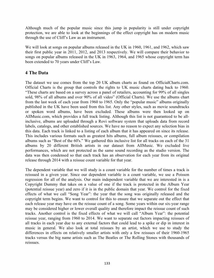
133

Although much of the popular music since this jump in popularity is still under copyright protection, we are able to look at the beginnings of the effect copyright has on modern music through the use of Cliff’s Law as an instrument.

We will look at songs on popular albums released in the UK in 1960, 1961, and 1962, which saw their first public year in 2011, 2012, and 2013 respectively. We will compare their behavior to songs on popular albums released in the UK in 1963, 1964, and 1965 whose copyright term has been extended to 70 years under Cliff’s Law.

4 The Data The dataset we use comes from the top 20 UK album charts as found on OfficialCharts.com. Official Charts is the group that controls the rights to UK music charts dating back to 1960. “These charts are based on a survey across a panel of retailers, accounting for 99% of all singles sold, 98% of all albums and over 90% of all video” (Official Charts). We use the albums chart from the last week of each year from 1960 to 1965. Only the “popular music” albums originally published in the UK have been used from this list. Any other styles, such as movie soundtracks or spoken word albums, have been excluded. These albums were then looked up on AllMusic.com, which provides a full track listing. Although this list is not guaranteed to be all- inclusive, albums are uploaded through a Rovi software system that uploads data from record labels, catalogs, and other established sources. We have no reason to expect any selection bias in this data. Each track is linked to a listing of each album that it has appeared on since its release. This includes various formats such as greatest hits albums, full album reissues, or compilation albums such as “Best of the 60's.” We gathered this inclusive list for all tracks on each of the 31 albums by 20 different British artists in our dataset from AllMusic. We excluded live performances, which are not protected as the same sound recording as the studio version. The data was then condensed so that each track has an observation for each year from its original release through 2014 with a reissue count variable for that year.

The dependent variable that we will study is a count variable for the number of times a track is reissued in a given year. Since our dependent variable is a count variable, we use a Poisson regression for all of the analysis. Our main independent variable that we are interested in is a Copyright Dummy that takes on a value of one if the track is protected in the Album Year (potential reissue year) and zero if it is in the public domain that year. We control for the fixed effects of what we call “Song Year”: the year that the song was originally released and the copyright term begins. We want to control for this to ensure that we separate out the effect that each release year may have on the reissue count of a song. Some years within our six-year range may be considered higher or lower overall quality and therefore impact the reissue count of such tracks. Another control is the fixed effects of what we will call “Album Year”: the potential reissue year, ranging from 1960 to 2014. We want to separate out factors impacting reissues of all tracks in each year due to any external factors that could lead to a spike or dip in interest in music in general. We also look at total reissues by an artist, which we use to study the differences in effects on relatively smaller artists with only a few reissues of their 1960-1965 tracks versus the big name artists such as The Beatles or The Rolling Stones with thousands of reissues.

134

The data consists of 26,339 observations, of which 9,541 are of songs released in 1962 or earlier and 16,798 are of songs released in 1963 or after. Song Year has a mean of 1962.9 and a median of 1963 while the mean Album Year is 1988.4 and the median is 1988. The mean of our dependent variable, reissue count, is 0.22 and ranges from 0 to 16 reissues. The total reissue count has a mean of 451.0 and a median of 371, which is what we will use as the barrier between small and large artists in our analysis. The Copyright dummy takes on a value of 1 in 25,825 observations and a value of 0 in 514 observations. Complete summary statistics for all relevant variables can be seen in Table 2. Naturally, there is a large difference between our quantity of data on copyrighted versus public songs since each track has an observation for each year of its existence, and has been protected for at least the first 50 years since its release.

5 Estimation and Results

Model In order to estimate the effect of copyright protection on the reissues of a song, we use the following model:

𝑟𝑒𝚤𝑠𝑠𝑢𝑒! = 𝐶𝑅 𝑏! + 𝑏!

!"#$

!!!"#$

+ 𝑏!

!"#$

!!!"#$

+ 𝑏!

!"

!!!

+ 𝑏! + 𝑒!

In this main regression equation, CR is a binary variable equal to one if the song is protected by copyright in year t and equal to zero if it is public in year t. 𝑏! captures the fixed effects of Album Year and 𝑏! captures the fixed effects of Song Year, as defined above. 𝑏! is the coefficient on artist fixed effects, representing the separate effect for each of the 20 artists in the data. We control for this to ensure that it is not a specific artist’s popularity or cultural influence that is chiefly influencing their reissue count.

Results Looking at the results from our main regression (Table 3; Regression 4), we see 𝑏! take on a value of -1.379, significant at the 1% level when we look at all observations. This shows us that a track’s copyright protection is estimated to have a very significant impact on its reissue count, holdingallothercontrolsconstant.

We will then apply this main regression to subsets of the data. We look at the significance of copyright protection on artists whose music during this six-year period was more popular than the median artist in our data. We want to see if there is a difference in copyright’s effect on the popular artists where there is likely more financial gain to be found from a reissue versus an artist who merely saw brief success in this period. We run this regression on artists who have seen less than the median total artist reissues of 371 and then on artists who have seen 371 or more total reissues of their tracks released in this period (Table 3; Regression 5 & 6).

When we look at only the smaller artists in relation to our results with the all-inclusive dataset, we see our copyright dummy has more of an impact, dropping to a value of -1.450 while still being significant at the 1% level. When we look at the more popular artists however, the copyright dummy seems to have less of an impact, taking on a value of -0.791. More interestingly, it is now significant only at the 10% level.

135

One way we can interpret these results is that for major artists, such as the Beatles or the Rolling Stones, the potential for large financial benefits that a third party may expect from a reissue may outweigh the cost of the rights of the sound recording, making the copyright status of these works less significant in its expected reissue count. For smaller artists, such as Manfred Mann or Lonnie Donegan, firms do not expect as much financial return from a reissue so they are strongly enticed by the ability to reissue a song without sound recording copyright expenses.

Additional Results When we begin with a regression of reissue count on only a copyright dummy, we see that the copyright dummy is significant at the 1% level. As we cumulatively add in Song Year fixed effects, Album Year fixed effects, and then Artist fixed effects (Table 3), the copyright dummy remains significant at the 1% level.

In order to test for bias in our Artist fixed effects, we run analyses with three dummy variables for various lists of Best British Artists of the 60’s (Table 4). We include lists from interestment.co.uk (“Top 20 Great British Bands”), Paste Magazine (“The 60 Best Albums of the 1960s”), and Radio Laurier (“The Top 10: The Most Influential British Bands”). A dummy variable is generated for each of these lists, equal to one if the artist appears on the list and zero if they do not. We do this to prove the validity of the Artist fixed effects variable in order to show that the reissue count results we are seeing in our main regression are not merely a result of artist popularity or influence. When we include all three list dummies with Song Year effects and Album Year effects (Regression 1), we see that they are all significant at the 1% level. The Copyright dummy is also significant at the 1% level, with a coefficient within 0.05 of our main regression.

We break this down further and look at artists above and below the median total reissues including the list dummies without the Artist fixed effects. When looking at less popular artists (Regression 2), the copyright dummy has a larger absolute value than with Artist fixed effects and is significant at the 1% level. However, for big artists (Regression 3), the copyright dummy is closer to zero and not significant at the 10% level with a t-stat of 1.25. This shows that our Artist fixed effects are correctly capturing the difference between the two subsets of artists. If anything, they may be underestimating the difference in impact of copyright on the two groups since we see more extreme coefficients and significance levels in Table 4.

Cohort-Period-Age Problem Another issue that has been addressed is the cohort, period, age problem. Our main regression includes cohort (Song Year) and period (Album Year) effects. We are unable to also include age effects not only because of collinearity but also because of its relationship to the 50 year barrier that copyright is capturing. To address these issues we regress reissue count on each of these effects separately and build up to a more inclusive model (Browning 2012).

When we run these regressions shown in Table 5, we see that the copyright dummy remains significant at the 1% level when we include cohort, period, and age individually. We include artist fixed effects for this process. This first level analysis shows us that it is not one of these effects, particularly the effect of age, which we have not previously looked at, that is shaping our results from Table 3.

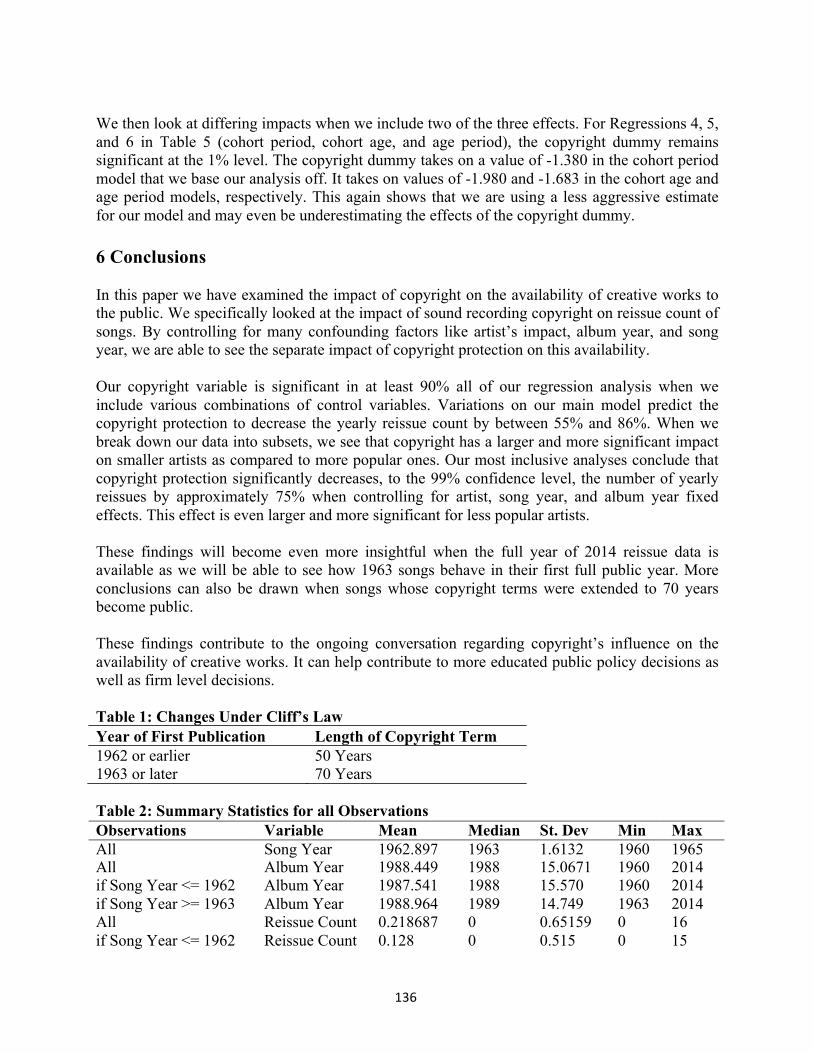
136

We then look at differing impacts when we include two of the three effects. For Regressions 4, 5, and 6 in Table 5 (cohort period, cohort age, and age period), the copyright dummy remains significant at the 1% level. The copyright dummy takes on a value of -1.380 in the cohort period model that we base our analysis off. It takes on values of -1.980 and -1.683 in the cohort age and age period models, respectively. This again shows that we are using a less aggressive estimate for our model and may even be underestimating the effects of the copyright dummy.

6 Conclusions

In this paper we have examined the impact of copyright on the availability of creative works to the public. We specifically looked at the impact of sound recording copyright on reissue count of songs. By controlling for many confounding factors like artist’s impact, album year, and song year, we are able to see the separate impact of copyright protection on this availability.

Our copyright variable is significant in at least 90% all of our regression analysis when we include various combinations of control variables. Variations on our main model predict the copyright protection to decrease the yearly reissue count by between 55% and 86%. When we break down our data into subsets, we see that copyright has a larger and more significant impact on smaller artists as compared to more popular ones. Our most inclusive analyses conclude that copyright protection significantly decreases, to the 99% confidence level, the number of yearly reissues by approximately 75% when controlling for artist, song year, and album year fixed effects. This effect is even larger and more significant for less popular artists.

These findings will become even more insightful when the full year of 2014 reissue data is available as we will be able to see how 1963 songs behave in their first full public year. More conclusions can also be drawn when songs whose copyright terms were extended to 70 years become public.

These findings contribute to the ongoing conversation regarding copyright’s influence on the availability of creative works. It can help contribute to more educated public policy decisions as well as firm level decisions.

Table 1: Changes Under Cliff’s Law

Year of First Publication Length of Copyright Term

1962 or earlier 50 Years 1963 or later 70 Years

Table 2: Summary Statistics for all Observations Observations Variable Mean Median St. Dev Min Max All Song Year 1962.897 1963 1.6132 1960 1965 All Album Year 1988.449 1988 15.0671 1960 2014 if Song Year <= 1962 Album Year 1987.541 1988 15.570 1960 2014 if Song Year >= 1963 Album Year 1988.964 1989 14.749 1963 2014 All Reissue Count 0.218687 0 0.65159 0 16 if Song Year <= 1962 Reissue Count 0.128 0 0.515 0 15

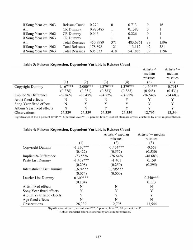
137

if Song Year >= 1963 Reissue Count 0.270 0 0.713 0 16 All CR Dummy 0.980485 1 0.1383 0 1 if Song Year <= 1962 CR Dummy 0.946 1 0.226 0 1 if Song Year >= 1963 CR Dummy 1 1 0 1 1 All Total Reissues 450.9989 371 483.6361 39 1596 if Song Year <= 1962 Total Reissues 178.898 121 113.112 42 381 if Song Year >= 1963 Total Reissues 605.633 418 541.885 39 1596

Table 3: Poisson Regression, Dependent Variable is Reissue Count Artists <

median Artists >=

median

(1)

(2)

(3)

(4) reissues

(5) reissues

(6) Copyright Dummy -1.167*** -2.000*** -1.379*** -1.379*** -1.450*** -0.791* (0.228) (0.251) (0.383) (0.383) (0.545) (0.431) Implied % Difference -68.86% -86.47% -74.82% -74.82% -76.54% -54.68% Artist fixed effects N N N Y Y Y Song Year fixed effects N Y Y Y Y Y Album Year fixed effects N N Y Y Y Y Observations 26,339 26,339 26,339 26,339 12,795 13,544

Significance at the 1 percent level***, 5 percent level**, 10 percent level*. Robust standard errors, clustered by artist in parentheses.

Table 4: Poisson Regression, Dependent Variable is Reissue Count Artists < median

reissues Artists >= median

reissues (1) (2) (3) Copyright Dummy -1.330*** -1.454*** -0.667 (0.422) (0.552) (0.530) Implied % Difference -73.55% -76.64% -48.68% Paste List Dummy -1.458*** -1.401 0.159 (0.208) (0.250) (0.295) Interestment List Dummy 1.674*** 1.796*** (0.074) (0.000) Laurier List Dummy 0.309*** 0.340*** (0.104) 0.113 Artist fixed effects N N N Song Year fixed effects Y Y Y Album Year fixed effects Y Y Y Age fixed effects N N N

Observations 26,339 12,795 13,544 Significance at the 1 percent level***, 5 percent level**, 10 percent level*.

Robust standard errors, clustered by artist in parentheses.

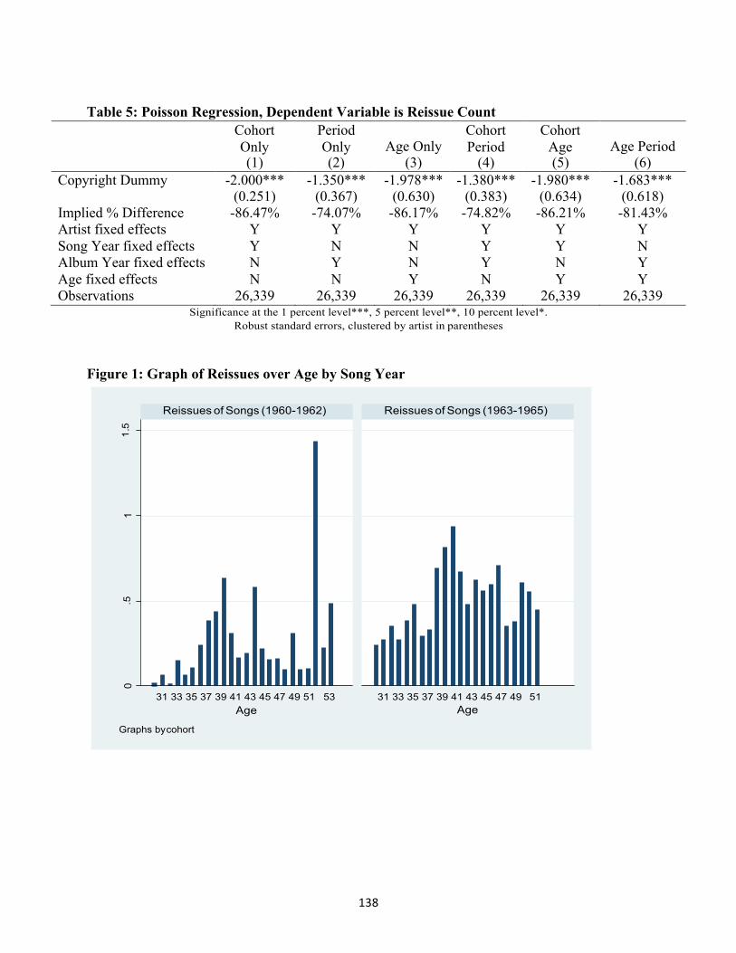
138

Table 5: Poisson Regression, Dependent Variable is Reissue Count Cohort

Only Period Only

Age Only

Cohort Period

Cohort Age

Age Period

(1) (2) (3) (4) (5) (6) Copyright Dummy -2.000*** -1.350*** -1.978*** -1.380*** -1.980*** -1.683*** (0.251) (0.367) (0.630) (0.383) (0.634) (0.618) Implied % Difference -86.47% -74.07% -86.17% -74.82% -86.21% -81.43% Artist fixed effects Y Y Y Y Y Y Song Year fixed effects Y N N Y Y N Album Year fixed effects N Y N Y N Y Age fixed effects N N Y N Y Y Observations 26,339 26,339 26,339 26,339 26,339 26,339

Significance at the 1 percent level***, 5 percent level**, 10 percent level*. Robust standard errors, clustered by artist in parentheses

Figure 1: Graph of Reissues over Age by Song Year

Reissues of Songs (1960-1962) Reissues of Songs (1963-1965)

31 33 35 37 39 41 43 45 47 49 51 53 Age

Graphs by cohort

31 33 35 37 39 41 43 45 47 49 51 Age

1.5

.5

0 1

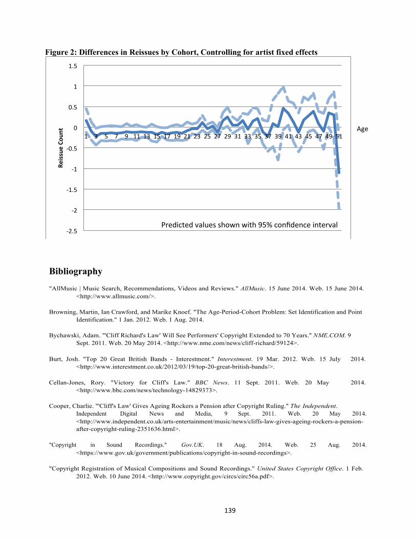
139

Figure 2: Differences in Reissues by Cohort, Controlling for artist fixed effects

Bibliography

"AllMusic | Music Search, Recommendations, Videos and Reviews." AllMusic. 15 June 2014. Web. 15 June 2014. <http://www.allmusic.com/>.

Browning, Martin, Ian Crawford, and Marike Knoef. "The Age-Period-Cohort Problem: Set Identification and Point

Identification." 1 Jan. 2012. Web. 1 Aug. 2014.

Bychawski, Adam. "'Cliff Richard's Law' Will See Performers' Copyright Extended to 70 Years." NME.COM. 9 Sept. 2011. Web. 20 May 2014. <http://www.nme.com/news/cliff-richard/59124>.

Burt, Josh. "Top 20 Great British Bands - Interestment." Interestment. 19 Mar. 2012. Web. 15 July 2014.

<http://www.interestment.co.uk/2012/03/19/top-20-great-british-bands/>.

Cellan-Jones, Rory. "Victory for Cliff's Law." BBC News. 11 Sept. 2011. Web. 20 May 2014. <http://www.bbc.com/news/technology-14829373>.

Cooper, Charlie. "'Cliff's Law' Gives Ageing Rockers a Pension after Copyright Ruling." The Independent.

Independent Digital News and Media, 9 Sept. 2011. Web. 20 May 2014. <http://www.independent.co.uk/arts-entertainment/music/news/cliffs-law-gives-ageing-rockers-a-pension- after-copyright-ruling-2351636.html>.

"Copyright in Sound Recordings." Gov.UK. 18 Aug. 2014. Web. 25 Aug. 2014.

<https://www.gov.uk/government/publications/copyright-in-sound-recordings>.

"Copyright Registration of Musical Compositions and Sound Recordings." United States Copyright Office. 1 Feb. 2012. Web. 10 June 2014. <http://www.copyright.gov/circs/circ56a.pdf>.

-2.5

-2

-1.5

-1

-0.5

0

0.5

1

1.5

1 3 5 7 9 11 13 15 17 19 21 23 25 27 29 31 33 35 37 39 41 43 45 47 49 51

ReissueCo

unt

Predictedvaluesshownwith95%confidenceinterval

Age

140

Daprato, Robin. "The Top 10: The Most Influential British Bands." Radio Laurier. 22 Nov. 2013. Web. 15 July 2014.<http://www.radiolaurier.com/shows/the-top-10-the-most-influential-british-bands/>.

"Future of Music Coalition." Public Performance Right for Sound Recordings. 5 Nov. 2013. Web. 29 May 2014.

<https://www.futureofmusic.org/article/fact-sheet/public-performance-right-sound-recordings>.

Heald, Paul. "Property Rights and the Efficient Exploitation of Copyrighted Works: An Empirical Analysis of Public Domain and Copyrighted Fiction Best Sellers." 9 Jan. 2007. Web. 1 June 2014. <http://papers.ssrn.com/sol3/papers.cfm?abstract_id=955954>.

"How Copyright Protects Your Work." - GOV.UK. 10 Apr. 2014. Web. 15 May 2014.

<https://www.gov.uk/copyright>.

"Music Timeline." Music Timeline. 15 May 2014. Web. 16 May 2014. <http://research.google.com/bigpicture/music/#POP>.

"Musicians Benefit from Extended Copyright Term for Sound Recordings." Gov.UK. 1 Nov. 2013. Web. 7 June

2014. <https://www.gov.uk/government/news/musicians-benefit-from-extended-copyright-term-for- sound-recordings>.

Reimers, Imke. "Copyright and Generic Entry in Book Publishing." 23 Jan. 2013. Web. 1 June 2014.

<http://imkereimers.weebly.com/uploads/2/7/9/9/2799121/mickey_dec4.pdf>.

Stanley, Bob. "Copyright Extension: Good for Cliff and the Beatles, Bad for the Little Guys?" 15 Sept. 2011. Web. 17 May 2014.<http://www.theguardian.com/music/2011/sep/15/copyright-extension-cliffs-law-beatles>.

Stiernberg, Bonnie. "The 60 Best Albums of the 1960s." Pastemagazine.com. 30 May 2012. Web. 15 July 2014.

<http://www.pastemagazine.com/blogs/lists/2012/05/the-60-best-albums-of-the-1960s.html?a=1>.

"The Official Charts Company | The UK Charts | Top 40." The Official Charts Company | The UK Charts | Top 40. 10 May 2014. Web. 15 May 2014. <http://www.officialcharts.com/>.

141

Can Greater Bank Capital Lead to Less Bank

Lending? An Analysis of the Bank-Level Evidence

from Europe

Virginia Magda Luisa Minni1

Research in Applied Economics

Department of Economics University of Warwick

Email: minnivirginia@gmail.com

Abstract This study focuses on the role of bank capital in the bank lending channel. Theoretically, higher capital should lead to higher loan growth. Yet, using a panel of European banks from 2004 to 2013, I show that this mechanism is impaired and higher capital tends to dampen bank lending. This is a novel result in the relevant literature and it is in line with the massive deleveraging by financial institutions observed since the deepening of the financial crisis. To tackle the endogeneity problem between bank lending and bank capital, I propose three different identification strategies: the simultaneous equation model using Indirect Least Squares (ILS), the instrumental variable method of Two-Stage Least Squares (2SLS) and the dynamic panel data model using the Generalised Methods of Moments (GMM) estimator. The research findings lend support to a countercyclical financial regulation highlighting a mutually reinforcing feedback between the financial system and the real economy.

Keywords: bank lending channel, bank capital, monetary policy, prudential regulation

JEL classification: E52, E44, G21, F

1 I am very grateful to Dr. Alexander Karalis Isaac for his support and encouragement, to Prof. Jeremy Smith for his suggestions and comments and to Dr. Alexander Karalis Isaac and Dr. Gianna

142

1 Introduction This study assesses the extent to which changes in bank capital exacerbate the cyclical behaviour of credit in the bank lending channel of monetary policy (henceforth, BLC). The BLC presumes that expansionary monetary policy directly affects bank loan supply, hence stimulating economic growth through greater investment. However, the current financial crisis has highlighted a number of weaknesses in the banking sector that could prevent the BLC to function properly. In particular, I focus on the role of bank capital in Europe.

The key question is whether higher bank capital, instead of triggering greater bank lending, can dampen loan growth. The financial crisis and its aftermath have shown that changes in bank capital may have pro-cyclical effects amplified by the Basel II risk-sensitive capital rules. More specifically, bank capital requirements are likely to rise with increasing risk in economic downturns, at a time when capital is more difficult to raise, which may result in a credit contraction and hence a deepening of recessions. If so, higher capital would not be able to dampen the losses during periods of economic stagnation and would rather amplify the risks of credit restrictions, thus contributing to worsening output fluctuations. The possibility of this scenario is of vital concern for scholars and policymakers as it can seriously hamper the prospect of faster economic recovery in Europe.

The contribution of this study to the existing literature is twofold. On the one hand, this study focuses on the role of bank capital in the BLC and challenges the underlying assumption that higher bank capital leads to higher bank lending. Besides, it directly addresses the source of the endogeneity between bank lending and bank capital, which has surprisingly been overlooked in the literature. As bank lending and bank capital are endogenously determined through the effect of financial and economic shocks, I investigate whether the endogeneity should be considered as simultaneity or as an omitted relevant variables problem.

For the empirical analysis, I use a panel dataset of European banks from 2004 to 2013. The choice to base this study on Europe is motivated by several reasons. First, particularly in Europe, the effectiveness of monetary policy depends on a well-functioning banking sector and policymakers have to pay particular attention to its developments (Praet, 2014). Secondly, ample evidence shows that credit is a fundamental factor for output growth in European countries (Rondorf, 2012). In addition, in contrast to findings for the United States, the role of bank capital in influencing loan supply has been largely downplayed in Europe (Ashcraft, 2006).

The findings of this paper shed new light on the functioning of the BLC. The methodology employed concludes that the endogeneity issue between bank lending and bank capital is not due to simultaneity but to some omitted relevant variables. This result informs on the choice of the most appropriate statistical models to conduct the empirical analysis. Secondly, I detect some changes in the monetary transmission via the BLC prior to and during the crisis. I find that higher bank capital suppresses bank lending: increases in capital lead to a slowdown in lending growth and potential detrimental effects on the economies concerned. Hence, future regulation should consider counter-cyclical capital requirements, which would explicitly take into account concerns about the procyclical behaviour of capital.

143

2 The Existing Literature

The Literature about the Bank Lending Channel According to the BLC thesis, contractionary monetary policy, by reducing available bank reserves, forces banks to create fewer reservable deposits. Banks must either replace the lost reserves with nonreservable liabilities or shrink their assets, such as loans and securities. The opposite case is that of an expansionary monetary policy that increases the quantity of loans available by increasing bank reserves and deposits (Gertler and Gilchrist, 1994; Ehrmann et al., 2003). However, recent research suggests that the traditional BLC transmission mechanism through reserves is becoming less important than a more direct mechanism operating via bank capital (Bernanke, 2007). There are two main ways through which capital impacts lending. From the banks’ perspectives, the presence of regulatory capital requirements acts as hard constraint on asset expansions (Peek and Rosengren 1995a, 1995b; Kashyap and Stein, 2004). Secondly, from the perspective of banks’ creditors, the amount of capital represents the extent to which losses can be cushioned and, thus, the banks’ levels of risk; in turn, this signal about banks’ creditworthiness influences the rate at which investors are willing to lend to banks and thus the cost of non-reservable funding (Hubbard, 1995; Guiso, 2003; Carlson et al., 2011). The Empirical Evidence Due to the difficulty of disentangling shifts in loan supply from shifts in loan demand, empirical research on the BLC at an aggregate level has not been very conclusive (Peek and Rosengren, 2013). However, panel data solves the identification problem since certain bank- specific characteristics, such as capitalization, size and liquidity only influence loan supply movements, while the demand for bank loans from borrowers is largely independent of them. Empirical work on the BLC has been focused predominantly on the USA and the evidence shows that banks might restrain from lending if they have low capital levels (Kishan and Opiela, 2000; Van den Heuvel, 2002, 2012). In Europe, evidence of the BLC is less extensive and more controversial. In particular, few papers focus on the impact of bank capital on bank lending. Ehrman et al. (2001) investigate the role of bank capital and liquidity in the BLC and find that, while the role of liquidity is important, the degree of bank capital is irrelevant for the way a bank adjusts its lending to monetary policy changes. Yet, it can be criticised that their measure of capitalisation is inadequate, as it does not capture the riskiness of banks: their capitalisation variable is derived directly from banks’ balance sheets without considering the structure of the loan portfolio or its risk characteristics. In fact, Gambacorta (2005), using Italian data and the GMM methodology, finds that, after a tightening of monetary policy, the impact on bank lending is greatest for less-capitalized banks since they are less able to raise uninsured funds. After a monetary tightening, lending decreases by -1.397% for less-capitalised banks versus -0.950% for well-capitalized banks. In the same way, in the presence of an easing of monetary policy, a bank facing a capital constraint may be unable to expand its assets. In this case, expansionary monetary policy is only effective in prompting the loan growth of high-capital banks while the channel is short- circuited for banks facing a binding capital constraint. These results on bank capital are confirmed by other studies such as Altunbas et al.(2009) and Cantero-Saiz et al.(2014).However, there are some limitations in their methodologies, as they do not explicitly take into account the endogeneity of bank capital.

144

While the literature has explored the possibility that the BLC may be inoperative for less- capitalized banks, much less attention has been directed to the possibility that, irrespective of the initial capitalization of the bank, increases in bank capital may negatively impact bank lending. Moreover, little scrutiny has been devoted to the identification strategy to tackle the endogeneity between bank lending and bank capital. Against this background, I investigate whether higher bank capital can decrease bank lending, what this means for the operation of the BLC and which modeling procedure may best tackle the endogeneity issues.

3 Methodology

The Endogeneity of Bank Capital Bank capital and bank lending are endogenous to each other as they are both impacted by the financial and economic shocks that go in the error term (Watanabe, 2007). An example clarifies this intrinsic endogeneity. If the aggregate economic environment worsens, the firms’ depressed sales performance can make them unable to repay back their existing loans. As a result, banks are hurt by the increasing number of non-performing loans, which affect the lender bank’s capital position through the loan loss provisions. Hence, banks are likely to reduce their future lending rates to shield from potential future losses and, at the same time, to increase their capital in order to avoid the risk of becoming insolvent. The same mechanism between bank capital and bank lending works in reverse. In an economic upturn, bank loan supply expands due to improved future prospects and higher profits of the banks increase their capital. Thus, the OLS estimator would be upward biased.

In overcoming the identification problem, the literature has proposed econometric techniques such as instrumental variable estimation using 2SLS and GMM. However, the nature of this endogeneity has never been explored: is it a simultaneity problem or an omitted relevant variables bias?

In the first case, it may be more effective to estimate a simultaneous equations model, where bank lending and bank capital are codetermined and each affects the other. In the second, the endogeneity of bank capital can be tackled using instrumental variable methods where bank lending is the outcome variable and bank capital is treated as an endogenous regressor.

Modelling Strategy: ILS The simultaneous equation model is appropriate in case of a simultaneity bias between bank lending and bank capital. The structural equation for bank lending growth is:

∆𝑙𝑛(𝑙𝑜𝑎𝑛𝑠)!" = 𝛼!! + 𝛼!𝑐𝑎𝑝𝑖𝑡𝑎𝑙!" + 𝛼!∆𝑖!" + 𝜐!!" Eq. (1) with 𝑖 = 1, … , 41 , 𝑚 = 1, … ,13 , 𝑡 = 1, … ,10 where i is the number of banks, m is the number of countries and t is the year. In the equation, 𝛼!! is a vector of fixed effects, ∆𝑙𝑛 (𝑙𝑜𝑎𝑛 𝑠 )!", is the change in the natural logarithm of aggregate loans, 𝑐 𝑎 𝑝 𝑖 𝑡 𝑎 𝑙 !", is thetotal regulatory capital ratio and ∆𝑖!", is the change in the monetary policy rate. The policy variable, ∆𝑖!", is considered as a predetermined variable, which is exogenous to the bank capital equation below (Eq. 2). The choice of the variables in Eq. (1) is motivated by the economic theory of the BLC and several authors, including Bernanke and Blinder

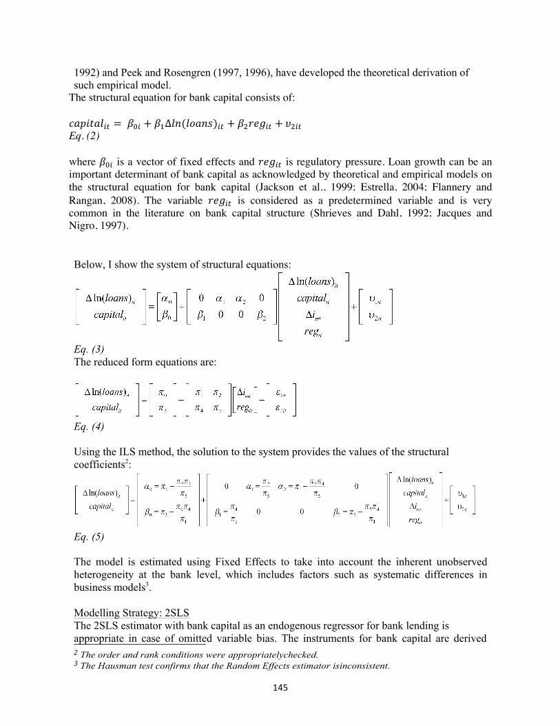
145

1992) and Peek and Rosengren (1997, 1996), have developed the theoretical derivation of such empirical model.

The structural equation for bank capital consists of: 𝑐𝑎𝑝𝑖𝑡𝑎𝑙!" = 𝛽!! + 𝛽!∆𝑙𝑛(𝑙𝑜𝑎𝑛𝑠)!" + 𝛽!𝑟𝑒𝑔!" + 𝜐!!" Eq. (2) where 𝛽!! is a vector of fixed effects and 𝑟𝑒𝑔!" is regulatory pressure. Loan growth can be an important determinant of bank capital as acknowledged by theoretical and empirical models on the structural equation for bank capital (Jackson et al., 1999; Estrella, 2004; Flannery and Rangan, 2008). The variable 𝑟𝑒𝑔!" is considered as a predetermined variable and is very common in the literature on bank capital structure (Shrieves and Dahl, 1992; Jacques and Nigro, 1997). Below, I show the system of structural equations:

Eq. (3) The reduced form equations are:

Eq. (4)

Using the ILS method, the solution to the system provides the values of the structural coefficients2:

Eq. (5)

The model is estimated using Fixed Effects to take into account the inherent unobserved heterogeneity at the bank level, which includes factors such as systematic differences in business models3.

Modelling Strategy: 2SLS The 2SLS estimator with bank capital as an endogenous regressor for bank lending is appropriate in case of omitted variable bias. The instruments for bank capital are derived

2 The order and rank conditions were appropriatelychecked. 3 The Hausman test confirms that the Random Effects estimator isinconsistent.

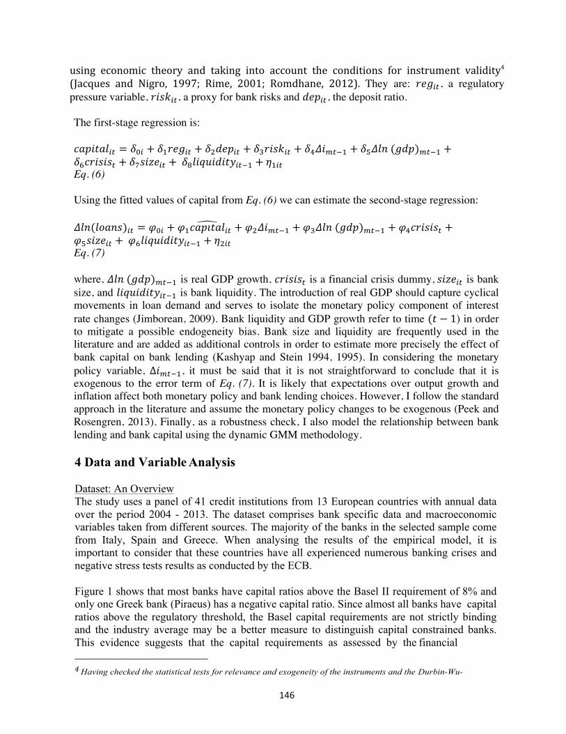
146

using economic theory and taking into account the conditions for instrument validity4(Jacques and Nigro, 1997; Rime, 2001; Romdhane, 2012). They are: 𝑟𝑒𝑔!", a regulatory pressure variable, 𝑟𝑖𝑠𝑘!", a proxy for bank risks and 𝑑𝑒𝑝!", the deposit ratio. The first-stage regression is: 𝑐𝑎𝑝𝑖𝑡𝑎𝑙!" = 𝛿!! + 𝛿!𝑟𝑒𝑔!" + 𝛿!𝑑𝑒𝑝!" + 𝛿!𝑟𝑖𝑠𝑘!" + 𝛿!𝛥𝑖!"!! + 𝛿!𝛥𝑙𝑛 (𝑔𝑑𝑝)!"!! +𝛿!𝑐𝑟𝑖𝑠𝑖𝑠! + 𝛿!𝑠𝑖𝑧𝑒!" + 𝛿!𝑙𝑖𝑞𝑢𝑖𝑑𝑖𝑡𝑦!"!! + 𝜂!!" Eq. (6) Using the fitted values of capital from Eq. (6) we can estimate the second-stage regression: 𝛥𝑙𝑛(𝑙𝑜𝑎𝑛𝑠)!" = 𝜑!! + 𝜑!𝑐𝑎𝑝𝚤𝑡𝑎𝑙!" + 𝜑!𝛥𝑖!"!! + 𝜑!𝛥𝑙𝑛 (𝑔𝑑𝑝)!"!! + 𝜑!𝑐𝑟𝑖𝑠𝑖𝑠! +𝜑!𝑠𝑖𝑧𝑒!" + 𝜑!𝑙𝑖𝑞𝑢𝑖𝑑𝑖𝑡𝑦!"!! + 𝜂!!" Eq. (7) where, 𝛥𝑙𝑛 (𝑔𝑑𝑝)!"!! is real GDP growth, 𝑐𝑟𝑖𝑠𝑖𝑠! is a financial crisis dummy, 𝑠𝑖𝑧𝑒!" is bank size, and 𝑙𝑖𝑞𝑢𝑖𝑑𝑖𝑡𝑦!"!! is bank liquidity. The introduction of real GDP should capture cyclical movements in loan demand and serves to isolate the monetary policy component of interest rate changes (Jimborean, 2009). Bank liquidity and GDP growth refer to time (𝑡 − 1) in order to mitigate a possible endogeneity bias. Bank size and liquidity are frequently used in the literature and are added as additional controls in order to estimate more precisely the effect of bank capital on bank lending (Kashyap and Stein 1994, 1995). In considering the monetary policy variable, ∆𝑖!"!!, it must be said that it is not straightforward to conclude that it is exogenous to the error term of Eq. (7). It is likely that expectations over output growth and inflation affect both monetary policy and bank lending choices. However, I follow the standard approach in the literature and assume the monetary policy changes to be exogenous (Peek and Rosengren, 2013). Finally, as a robustness check, I also model the relationship between bank lending and bank capital using the dynamic GMM methodology.

4 Data and Variable Analysis

Dataset: An Overview The study uses a panel of 41 credit institutions from 13 European countries with annual data over the period 2004 - 2013. The dataset comprises bank specific data and macroeconomic variables taken from different sources. The majority of the banks in the selected sample come from Italy, Spain and Greece. When analysing the results of the empirical model, it is important to consider that these countries have all experienced numerous banking crises and negative stress tests results as conducted by the ECB.

Figure 1 shows that most banks have capital ratios above the Basel II requirement of 8% and only one Greek bank (Piraeus) has a negative capital ratio. Since almost all banks have capital ratios above the regulatory threshold, the Basel capital requirements are not strictly binding and the industry average may be a better measure to distinguish capital constrained banks. This evidence suggests that the capital requirements as assessed by the financial

4Having checked the statistical tests for relevance and exogeneity of the instruments and the Durbin-Wu-

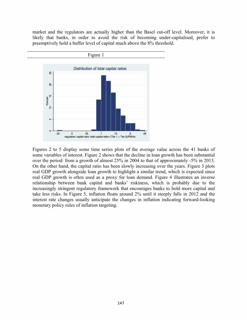
147

market and the regulators are actually higher than the Basel cut-off level. Moreover, it is likely that banks, in order to avoid the risk of becoming under-capitalised, prefer to preemptively hold a buffer level of capital much above the 8% threshold.

Figure 1

Figures 2 to 5 display some time series plots of the average value across the 41 banks of some variables of interest. Figure 2 shows that the decline in loan growth has been substantial over the period: from a growth of almost 25% in 2004 to that of approximately -5% in 2013. On the other hand, the capital ratio has been slowly increasing over the years. Figure 3 plots real GDP growth alongside loan growth to highlight a similar trend, which is expected since real GDP growth is often used as a proxy for loan demand. Figure 4 illustrates an inverse relationship between bank capital and banks’ riskiness, which is probably due to the increasingly stringent regulatory framework that encourages banks to hold more capital and take less risks. In Figure 5, inflation floats around 2% until it steeply falls in 2012 and the interest rate changes usually anticipate the changes in inflation indicating forward-looking monetary policy rules of inflation targeting.

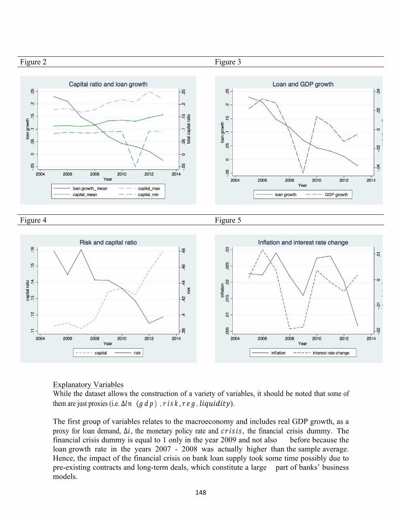
148

Figure 2 Figure 3

Figure 4 Figure 5

Explanatory Variables While the dataset allows the construction of a variety of variables, it should be noted that some of them are just proxies (i.e. ∆𝑙𝑛 (𝑔 𝑑 𝑝 ) , 𝑟 𝑖𝑠 𝑘 , 𝑟 𝑒𝑔 , 𝑙𝑖𝑞𝑢𝑖𝑑𝑖𝑡𝑦).

The first group of variables relates to the macroeconomy and includes real GDP growth, as a proxy for loan demand, ∆𝑖 , the monetary policy rate and 𝑐𝑟 𝑖𝑠 𝑖𝑠 , the financial crisis dummy. The financial crisis dummy is equal to 1 only in the year 2009 and not also before because the loan growth rate in the years 2007 - 2008 was actually higher than the sample average. Hence, the impact of the financial crisis on bank loan supply took some time possibly due to pre-existing contracts and long-term deals, which constitute a large part of banks’ business models.

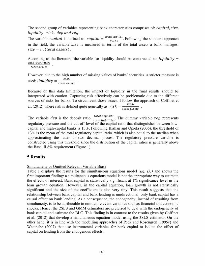
149

The second group of variables representing bank characteristics comprises of: 𝑐𝑎𝑝𝑖𝑡𝑎𝑙, 𝑠𝑖𝑧𝑒,𝑙𝑖𝑞𝑢𝑖𝑑𝑖𝑡𝑦, 𝑟𝑖𝑠𝑘, 𝑑𝑒𝑝 𝑎𝑛𝑑 𝑟𝑒𝑔. The variable 𝑐𝑎𝑝𝑖𝑡𝑎𝑙 is defined as: 𝑐𝑎𝑝𝑖𝑡𝑎𝑙 = !"!#$ !"#$%"&

!"#$. Following the standard approach

in the field, the variable 𝑠𝑖𝑧𝑒 is measured in terms of the total assets a bank manages: 𝑠𝑖𝑧𝑒 = 𝑙𝑛 (𝑡𝑜𝑡𝑎𝑙 𝑎𝑠𝑠𝑒𝑡𝑠) . According to the literature, the variable for liquidity should be constructed as: 𝑙𝑖𝑞𝑢𝑖𝑑𝑖𝑡𝑦 =!"#!!!"#$%&'&"!!"!#$ !""#$"

. However, due to the high number of missing values of banks’ securities, a stricter measure is used: 𝑙𝑖𝑞𝑢𝑖𝑑𝑖𝑡𝑦 = !"#!

!"!#$ !""#$" .

Because of this data limitation, the impact of liquidity in the final results should be interpreted with caution. Capturing risk effectively can be problematic due to the different sources of risks for banks. To circumvent those issues, I follow the approach of Coffinet et al. (2012) where risk is defined quite generally as: 𝑟𝑖𝑠𝑘 = !"#$

!"!#$ !""#$" .

The variable 𝑑𝑒𝑝 is the deposit ratio: !"!#$ !"#$%&'%

!"!#$ !"#$"!"%"&'. The dummy variable 𝑟𝑒𝑔 represents

regulatory pressure and the cut-off level of the capital ratio that distinguishes between low-capital and high-capital banks is 13%. Following Kishan and Opiela (2006), the threshold of 13% is the mean of the total regulatory capital ratio, which is also equal to the median when approximating the latter to two decimal places. The regulatory pressure variable is constructed using this threshold since the distribution of the capital ratios is generally above the Basel II 8% requirement (Figure 1).

5 Results

Simultaneity or Omitted Relevant Variable Bias? Table 1 displays the results for the simultaneous equations model (Eq. (3)) and shows the first important finding: a simultaneous equations model is not the appropriate way to estimate the effects of interest. Bank capital is statistically significant at 1% significance level in the loan growth equation. However, in the capital equation, loan growth is not statistically significant and the size of the coefficient is also very tiny. This result suggests that the relationship between bank capital and bank lending is unidirectional: only bank capital has a causal effect on bank lending. As a consequence, the endogeneity, instead of resulting from simultaneity, is to be attributable to omitted relevant variables such as financial and economic shocks. Hence, the 2SLS and GMM estimators are preferred to deal with the endogeneity of bank capital and estimate the BLC. This finding is in contrast to the results given by Coffinet et al. (2012) that develop a simultaneous equation model using the 3SLS estimator. On the other hand, it is in line with the modelling approaches of Peek and Rosengren (1995c) and Watanabe (2007) that use instrumental variables for bank capital to isolate the effect of capital on lending from the endogenous effects.

150

Table 1 The Simultaneous Equations Model Dependent variable: ∆𝑙𝑛(𝑙𝑜𝑎𝑛𝑠)!"

Dependent variable: 𝑐𝑎𝑝𝑖𝑡𝑎𝑙!"

𝑐𝑎𝑝𝑖𝑡𝑎𝑙!" -2.666963*** (.4620779)

∆𝑙𝑛(𝑙𝑜𝑎𝑛𝑠)!" .0196191 (.0484529)

∆𝑖!" 1.574942** (.649507)

𝑟𝑒𝑔!" -.0435053*** (.0058115)

No. of banks 41 No. of obs: 334 No. of banks 41 No. of obs: 334 The models are given by Equation 5 and are estimated using fixed effects and clustered standard errors. The following holds for Tables 1-3: -The coefficient for the constant is not reported because it is not relevant for the analysis. -The symbols *, **, and *** represent significance levels of 10 per cent, 5 per cent, and 1 per cent respectively. Empirical Findings The main finding of the study is that banks reduce their loan supply in the aftermath of an increase in their capital, after controlling for GDP growth as a proxy for loan demand and other bank characteristics. This is in contrast to what economic theory predicts and suggests that the traditional cycle between greater bank capitalisation and greater lending is impaired. Table 2 ILS, 2SLS Dependent variable: ∆𝑙𝑛(𝑙𝑜𝑎𝑛𝑠)!"

ILS 2SLS (1)

2SLS (2)

𝑐𝑎𝑝𝑖𝑡𝑎𝑙!" -2.666963*** (.4620779)

-2.460298*** (.6425895)

-2.847142*** (.9040812)

∆𝑖!" 1.574942** (.649507)

∆𝑖!"!! -3.861635* (1.984046)

-4.212526** (2.101361)

∆𝑙𝑛(𝑔𝑑𝑝)!"!! 1.558093** (.6171999)

1.738101** (.7004195)

𝑐𝑟𝑖𝑠𝑖𝑠! -.0543732** (.0276217)

-.0540782** (.0274429)

𝑠𝑖𝑧𝑒!" .1595252*

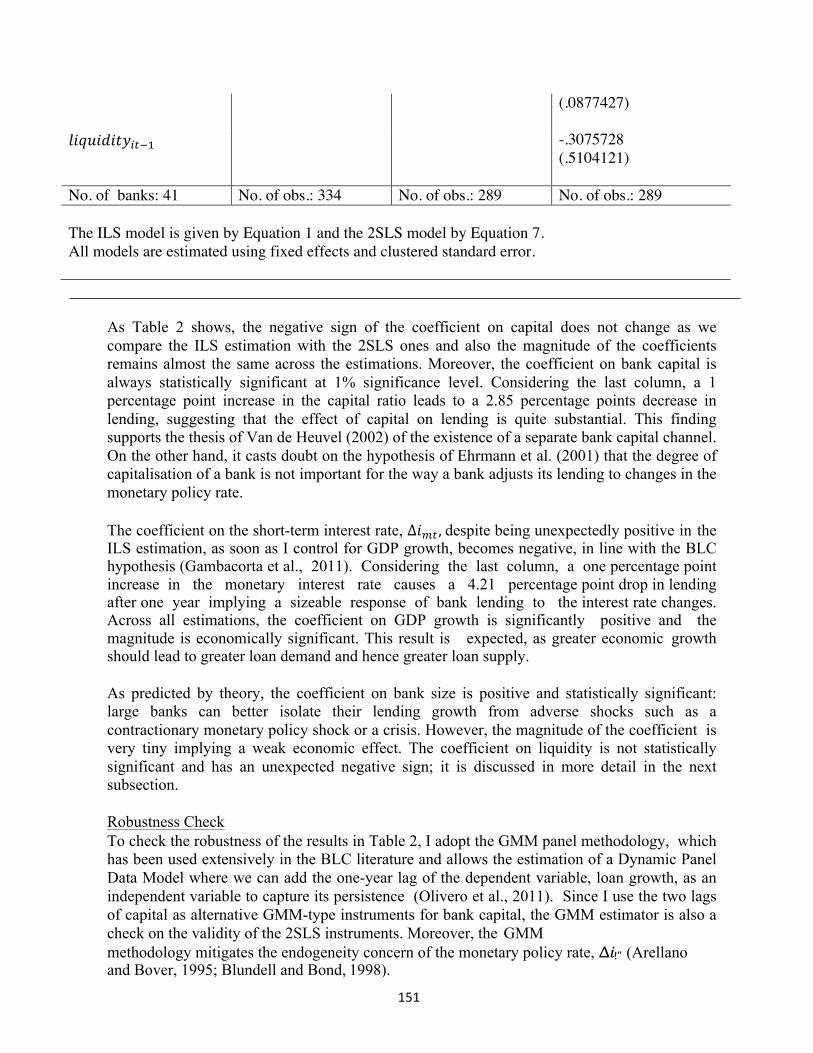
151

(.0877427)

𝑙𝑖𝑞𝑢𝑖𝑑𝑖𝑡𝑦!"!! -.3075728 (.5104121)

No. of banks: 41 No. of obs.: 334 No. of obs.: 289 No. of obs.: 289 The ILS model is given by Equation 1 and the 2SLS model by Equation 7. All models are estimated using fixed effects and clustered standard error.

As Table 2 shows, the negative sign of the coefficient on capital does not change as we compare the ILS estimation with the 2SLS ones and also the magnitude of the coefficients remains almost the same across the estimations. Moreover, the coefficient on bank capital is always statistically significant at 1% significance level. Considering the last column, a 1 percentage point increase in the capital ratio leads to a 2.85 percentage points decrease in lending, suggesting that the effect of capital on lending is quite substantial. This finding supports the thesis of Van de Heuvel (2002) of the existence of a separate bank capital channel. On the other hand, it casts doubt on the hypothesis of Ehrmann et al. (2001) that the degree of capitalisation of a bank is not important for the way a bank adjusts its lending to changes in the monetary policy rate.

The coefficient on the short-term interest rate, ∆𝑖!" , despite being unexpectedly positive in the ILS estimation, as soon as I control for GDP growth, becomes negative, in line with the BLC hypothesis (Gambacorta et al., 2011). Considering the last column, a one percentage point increase in the monetary interest rate causes a 4.21 percentage point drop in lending after one year implying a sizeable response of bank lending to the interest rate changes. Across all estimations, the coefficient on GDP growth is significantly positive and the magnitude is economically significant. This result is expected, as greater economic growth should lead to greater loan demand and hence greater loan supply.

As predicted by theory, the coefficient on bank size is positive and statistically significant: large banks can better isolate their lending growth from adverse shocks such as a contractionary monetary policy shock or a crisis. However, the magnitude of the coefficient is very tiny implying a weak economic effect. The coefficient on liquidity is not statistically significant and has an unexpected negative sign; it is discussed in more detail in the next subsection.

Robustness Check To check the robustness of the results in Table 2, I adopt the GMM panel methodology, which has been used extensively in the BLC literature and allows the estimation of a Dynamic Panel Data Model where we can add the one-year lag of the dependent variable, loan growth, as an independent variable to capture its persistence (Olivero et al., 2011). Since I use the two lags of capital as alternative GMM-type instruments for bank capital, the GMM estimator is also a check on the validity of the 2SLS instruments. Moreover, the GMM methodology mitigates the endogeneity concern of the monetary policy rate, ∆𝑖!" (Arellano and Bover, 1995; Blundell and Bond, 1998).

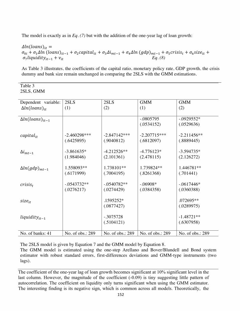
152

The model is exactly as in Eq. (7) but with the addition of the one-year lag of loan growth: 𝛥𝑙𝑛(𝑙𝑜𝑎𝑛𝑠)!" =𝜎!! + 𝜎!𝛥𝑙𝑛 (𝑙𝑜𝑎𝑛𝑠)!"!! + 𝜎!𝑐𝑎𝑝𝑖𝑡𝑎𝑙!" + 𝜎!𝛥𝑖!"!! + 𝜎!𝛥𝑙𝑛 (𝑔𝑑𝑝)!"!! + 𝜎!𝑐𝑟𝑖𝑠𝑖𝑠! + 𝜎!𝑠𝑖𝑧𝑒!" + 𝜎!𝑙𝑖𝑞𝑢𝑖𝑑𝑖𝑡𝑦!"!! + 𝜈!" Eq. (8) As Table 3 illustrates, the coefficients of the capital ratio, monetary policy rate, GDP growth, the crisis dummy and bank size remain unchanged in comparing the 2SLS with the GMM estimations.

Table 3 2SLS, GMM Dependent variable: ∆𝑙𝑛(𝑙𝑜𝑎𝑛𝑠)!"

2SLS (1)

2SLS (2)

GMM (1)

GMM (2)

∆𝑙𝑛(𝑙𝑜𝑎𝑛𝑠)!"!! -.0805795 (.0534152)

-.0929552* (.0529636)

𝑐𝑎𝑝𝑖𝑡𝑎𝑙!" -2.460298*** (.6425895)

-2.847142*** (.9040812)

-2.207715*** (.6812097)

-2.211456** (.8889445)

∆𝑖!"!! -3.861635* (1.984046)

-4.212526** (2.101361)

-4.776123* (2.478115)

-3.594735* (2.126272)

∆𝑙𝑛(𝑔𝑑𝑝)!"!! 1.558093** (.6171999)

1.738101** (.7004195)

1.739824** (.8261368)

1.446781** (.701441)

𝑐𝑟𝑖𝑠𝑖𝑠! -.0543732** (.0276217)

-.0540782** (.0274429)

-.06908* (.0384358)

-.0617446* (.0360388)

𝑠𝑖𝑧𝑒!" .1595252* (.0877427)

.072695** (.0289975)

𝑙𝑖𝑞𝑢𝑖𝑑𝑖𝑡𝑦!"!! -.3075728 (.5104121)

-1.48721** (.6307958)

No. of banks: 41 No. of obs.: 289 No. of obs.: 289 No. of obs.: 289 No. of obs.: 289 The 2SLS model is given by Equation 7 and the GMM model by Equation 8. The GMM model is estimated using the one-step Arellano and Bover/Blundell and Bond system estimator with robust standard errors, first-differences deviations and GMM-type instruments (two lags).

The coefficient of the one-year lag of loan growth becomes significant at 10% significant level in the last column. However, the magnitude of the coefficient (-0.09) is tiny suggesting little pattern of autocorrelation. The coefficient on liquidity only turns significant when using the GMM estimator. The interesting finding is its negative sign, which is common across all models. Theoretically, the

153

effect of bank liquidity on bank lending should be positive: in the event of shrinking deposits and/or reserves, liquid banks can draw on securities to replenish their loan portfolio (Kashyap and Stein, 2000). The negative sign in Table 3 questions the role of this indicator in capturing the effect of banks’ liquidity position on bank lending. For instance, the financial crisis has led European banks to hoard liquidity for precautionary purposes rather than lend it out (Cantero-Saiz et al., 2014). However, as highlighted in the Data Section, the missing data on securities makes the construction of the liquidity variable less reliable, further explaining the result. As the signs and magnitude of the coefficients do not change across the 2SLS and GMM estimations, it can be concluded that the model estimated is robust to alternative estimation methods.

6 Discussion, Policy Implications and Limitations

There are different mechanisms that might explain why an increase in the capital ratio leads to a decrease in bank lending. Firstly, holding capital, instead of investing it, is less profitable for a bank (Gropp and Heider, 2009; Shim, 2013). To make up for the expected reduced profits, banks engage in activities more lucrative than bank loans and, to get a higher return on their lending, they could also increase average credit spreads, leading to a decrease in the demand for loans.

An alternative explanation is that the capital ratio is increased by reducing the RWAs, rather than by injecting new capital into the banks’ balance sheet (𝑐𝑎𝑝𝑖𝑡𝑎𝑙 = !"!#$ !"#$%"&). Since

!"#$ loans constitute an important part of the RWAs, banks could be increasing the capital ratio by reducing the quantity of loans itself. This feedback cycle becomes more likely when raising new capital can be very costly, as in the financial crisis period (Carlson et al., 2011). For instance, Adrian and Shin (2010) document that the financial crisis has led to a significant pro-cyclical de-leveraging process in the banking sector. In order to restore their capital positions eroded by the burst of the subprime bubble, banks have been reducing their lending activities despite the extremely low interest rates and the non-standard policy measures aimed at increasing bank lending (Ciccarelli et al., 2010).

These results shed light on the effect of capital on lending growth and are interesting for the way macro-prudential policy is implemented in Europe. The rationale behind higher capital requirements goes along the lines of ensuring lower systemic risks and a healthier financial system through a reduced risk of bank failure. Yet, this paper shows that capital increases may lead to a slowdown in lending growth and potential detrimental effects on the economies concerned. Given this mutually reinforcing loop between the financial system and the real economy that amplifies financial and business cycles, future regulation should consider counter-cyclical capital requirements, which would explicitly take into account concerns about the procyclical 13ehavior of capital. Indeed, the recent developments of the Basel III standards go exactly towards this direction (Drehmann et al., 2010; BCBS, 2009, 2010).

The present study has limitations that future research in this field can overcome. Firstly, the construction of the variable liquidity can be improved using a dataset with more observations. Secondly, to take into account the endogeneity issue between bank lending and the monetary policy rate, the policy indicator should be extrapolated from the data and identified as an

154

exogenous monetary policy component using, for example, the narrative approach by Romer and Romer (2004) as done by Bluedorn et al. (2013). Moreover, as this study is one of the few that uses instrumental variable methods to estimate the BLC, more research should focus on a careful selection of the instruments for bank capital and should assess them in terms of their validity. In addition, data of higher frequency than this paper’s can be more effective in studies of short run adjustment. The number banks in the sample could also be increased so that the results can be considered more persuasive in terms of their external validity. Besides, the sample of banks considered is mostly made up of Italian, Greek and Spanish banks and these countries are not particularly representative of the whole of Europe given their economic woes following the financial crisis. Hence, studies using a more balanced sample of European banks could provide more conclusive results.

7 Concluding Remarks

Can higher bank capital lead to less bank lending? In contrast to earlier studies, I find evidence of a negative relationship between bank capital and bank lending. This counterintuitive result suggests that the effect of bank capital on bank lending is evolving along with changing economic circumstances leading to new dimensions of the BLC. From a policy perspective, the empirical examination feeds into the current debate on the new guidelines for capital and banking regulations drawn up by Basel III. In particular, this study’s results concur with the proposed creation of a counter-cyclical capital buffer.

Interesting avenues for future work include the extension of this study using richer datasets, additional empirical investigations across different countries to test whether the results hold outside Europe and further research on the implications of Basel III capital regulations for bank lending. Lastly, an important question is whether the changes detected in the transmission mechanism will persist in the near future or will disappear as the crisis subsides. The evidence presented in the paper is consistent with a scenario in which such changes cannot be considered as permanent but are likely to evolve over time. Hence, further analysis is needed to fully understand the role of bank capital in the monetary policy transmission mechanism.

Bibliography

Adrian, Tobias, Hyun Song Shin, “Financial Intermediaries and Monetary Economics,” Handbook of Monetary

Economics. Eds. Benjamin M. Friedman and Michael Woodford. New York: Elsevier B. V., 2010. 601-50. Web.

Altunbas, Yener, Leonardo Gambacorta, and David Marques-Ibanez, “Securitisation and the

Bank-Lending Channel,” European Economic Review 53 (2009): 996-1009. Web.

Arellano, Manuel and Olympia Bover, “Another Look and the Instrumental Variable Estimation of Error- Components Models,” Journal of Econometrics 68.1 (1995): 29-51. Web.

Ashcraft, Adam B., “New Evidence on the Lending Channel,” Journal of Money, Credit, and

Banking 38.3 (2006): 751-76. Web.

Basel Committee on Banking Supervision,“Strengthening the Resilience of the Banking Sector,” Basel: Bank for International Settlements, 2009. Web.

155

Basel Committee on Banking Supervision, “Group of Governors and Heads of Supervision Announces Higher Global Minimum Capital Standards,” Basel: Bank for International Settlements, 2010. Web.

Bernanke, Ben S., and Alan S. Blinder, “Credit, Money, and Aggregate Demand,” American

Economic Review 78.2 (1988): 435-439. Web.

Bernanke, Ben S., and Alan S. Blinder, “The Federal Funds Rate and the Channels of Monetary Transmission,” The American Economic Review 82 (1992): 901-921. Web.

Bernanke, Ben S. “The Financial Accelerator and the Credit Channel.” The Credit Channel of Monetary Policy

in the Twenty-First Century Conference. Federal Reserve Bank of Atlanta, Atlanta, GA. 15 Jun 2007. Speech.

Bluedorn, John C., Christopher Bowdler, and Christoffer Koch, “Heterogeneous Bank Lending Responses to

Monetary Policy: New Evidence from a Real-time Identification,” Washington: International Monetary Fund, 2013. Web. Working Paper No. 118.

Blundell, Richard and Stephen Bond, “Initial Conditions and Moment Restrictions in Dynamic Panel Data

Models,” Journal of Econometrics 87.2 (1998): 115–43. Web.

Cantero-Saiz, Maria, Sergio Sanfilippo-Azofra, Begoña Torre-Olmo, and Carlos López-Gutiérrez, “Sovereign risk and the bank lending channel in Europe,” Journal of International Money and Finance 47 (2014): 1-20. Web.

Carlson, Mark A., Thomas B. King, and Kurt B. Lewis, “Distress in the Financial Sector and

Economic Activity,” B.E. Journal of Economic Analysis and Policy 11.1 (2011): article 35. Web. Ciccarelli, Matteo, Angela Maddaloni, and Josè-Luis Pydro, “Trusting the Bankers: a New Look at the Credit

Channel of Monetary Policy,” Frankfurt: European Central Bank, 2010. Web. Working Paper No. 1228.

Coffinet, Jèrome, Virginie Coudert, Adrian Pop, and Cyril Pouvelle, “Two-Way Interplays Between Capital

Buffers and Credit Growth: Evidence from French banks,” Journal of International Financial Markets, Institutions and Money 22 (2012): 1110-1125. Web.

Drehmann Mathias, Claudio Borio, Leonardo Gambacorta, Gabriel Jimenez and Carlos Trucharte,

“Countercyclical Capital Buffers: Exploring Options,” Basel: Bank for International Settlements, 2010. Web. Working Paper No. 317.

Ehrmann, Michael, Leonardo Gambacorta, Jorge Martìnez-Pagés, Patrick Sevestre, and Andreas Worms,

“Financial Systems and the Role of Banks in Monetary Policy Transmission in the Euro Area,” Frankfurt: European Central Bank, 2001. Web. Working Paper No. 105.

Ehrmann, Michael, Leonardo Gambacorta, Jorge Martìnez-Pagés, Patrick Sevestre, and Andreas Worms, “The

Effects of Monetary Policy in the Euro Area,” Oxford Review of Economic Policy 19.1 (2003): 58-72. Web.

Estrella, Arturo, “The Cyclical Behaviour of Optimal Bank Capital,” Journal of Banking and Finance 28

(2004): 1469-1498. Web.

Flannery, Mark J. and Kasturi P. Rangan, “What Caused the Bank Capital Build-Up of the 1990s,” Review of Finance 12 (2008): 391–429. Web.

Friedman, Benjamin. Rev. of “The Credit Crunch,” by Ben S. Bernanke and Cara S. Lown. Brookings Papers

on Economic Activity 2 (1991): 240-7. Web.

Gambacorta, Leonardo “Inside the Bank Lending Channel,” European Economic Review 49 (2005): 1737-1759. Web.

156

Gambacorta, Leonardo, and David Marques-Ibanez, “The Bank Lending Channel: Lessons from the Crisis,” Basel: Bank for International Settlements, 2011. Web. Working Paper No. 345.

Gertler, Mark and Simon Gilchrist, “Monetary Policy, Business Cycles, and the Behaviour of Small

Manufacturing Firms,” Quarterly Journal of Economics 109.2 (1994): 309–340. Web.

Gropp, Rein and Florian Heider, “The Determinants of Bank Capital Structure,” Frankfurt: European Central Bank, 2009. Web. Working Paper No. 1096.

Guiso, Luigi, “Small Business Finance in Italy,” Luxembourg: European Investment Bank, 2003. Web. Papers

8.2: 120-49.

Gujarati, Damodar N. Basic Econometrics. 4th Edition. New York: McGraw-Hill, 2003. Print.

Hubbard, Glenn R., “Is there a ‘Credit Channel’ for Monetary Policy?” Federal Reserve Bank of St. Louis Review 77.3 (1995): 63-77. Web.

Jackson, Patricia, Craig Furfine, Hans Groeneveld, Diana Hancock, David Jones, William Perraudin, Lawrence

Radecki, and Masao Yoneyama, “Capital Requirements and Bank Behaviour: The Impact of the Basel Accord,” Basel: Basel Committee on Banking Supervision, 1999. Web. Working Paper No. 1.

Jacques, Kevin and Peter Nigro, “Risk-Based Capital, Portfolio Risk, and Bank Capital: a

Simultaneous Equations Approach,” Journal of Economics and Business 49 (1997): 533-547. Web.

Jimborean, Ramona, “The Role of Banks in the Monetary Policy Transmission in the New EU Member States,” Economic Systems 33 (2009): 360-375. Web.

Kashyap, Anil K. and Jeremy C. Stein, (1994) “The Impact of Monetary Policy on Bank Balance Sheets,”

Washington: National Bureau of Economic Research, 1994. Web. Working Paper 4821.

Kashyap, Anil K. and Jeremy C. Stein. “The Impact of Monetary Policy on Bank Balance Sheets.” Carnegie- Rochester Conference Series on Public Policy. New York: Elsevier B.V. 42 (1995): 151–95. Web.

Kashyap, Anil K. and Jeremy C. Stein, “What Do a Million Observations on Banks Say About the Transmission

of Monetary Policy?” The American Economic Review 90.3 (2000): 407-428. Web.

Kashyap, Anil K. and Jeremy C. Stein, “Cyclical Implications of the Basel II Capital Standard,” Federal Reserve Bank of Chicago Economic Perspectives (First Quarter 2004): 18-31. Web.

Kishan, Ruby P., and Timothy P. Opiela, “Banks Size, Bank Capital, and the Bank Lending

Channel,” Journal of Money, Credit, and Banking 32.1 (2000): 121-141. Web.

Kishan, Ruby P., and Timothy P. Opiela, “Bank Capital and Loan Asymmetry in the Transmission of Monetary Policy,” Journal of Banking and Finance 30.1 (2006): 259–285. Web.

Olivero, Maria Pia, Yuan Li, and Bang Nam Jeon, “Competition in Banking and the Lending Channel:

Evidence from Bank-Level Data in Asia and Latin America,” Journal of Banking and Finance 35.3 (2011): 560-571. Web.

Peek, Joe and Eric S. Rosengren, “The Capital Crunch: Neither a Borrower nor a Lender Be,” Journal of

Money, Credit and Banking 27.3 (1995): 625-638. Web.

Peek, Joe and Eric S. Rosengren, “Bank Regulation and the Credit Crunch,” Journal of Banking and Finance 19.3-4 (1995): 679-692. Web.

Peek, Joe and Eric S. Rosengren. “Bank Lending and the Transmission of Monetary Policy.” Is Bank Lending

Important for the Transmission of Monetary Policy? Eds. Joe Peek and Eric S. Rosengren. Boston: Federal Reserve Bank of Boston, 1995. Web.

157

Peek, Joe, and Eric S. Rosengren, “The International Transmission of Financial Shocks: The Case of Japan,” American Economic Review 87.4 (1997): 495–505. Web.

Peek, Joe and Eric S. Rosengren, (2013) “The Role of Banks in the Transmission of Monetary Policy,” Boston:

Federal Reserve Bank of Boston, 2013. Web. Public Policy Discussion Paper 13-5.

Praet, Peter. “Repairing the bank lending channel-the next steps.” European Macro Conference. Credit Suisse, London, UK. 17 Nov. 2014. Speech.

Rime, Bertrand, “Capital Requirements and Bank Behaviour: Empirical Evidence for Switzerland,” Journal of

Banking and Finance 25.4 (2001): 789-805. Web.

Romer, Christina D., and David H. Romer, “A New Measure of Monetary Shocks: Derivation and Implications,” American Economic Review 94.4 (2004): 1055–84. Web.

Romdhane, Mohamed, “The Determinants of Banks’ Capital Ratio in Developing Countries: Empirical

Evidence from Tunisia,” Research Journal of Finance and Accounting 3.1 (2012): 35-46. Web.

Rondorf, Ulrike, “Are Bank Loans Important for Output Growth?: a Panel Analysis of the Euro Area,” Journal of International Financial Markets, Institutions and Money 22.1 (2012): 103–119. Web.

Shim, Jeungbo, “Bank Capital Buffer and Portfolio Risk: The Influence of Business Cycle and Revenue

Diversification,” Journal of Banking & Finance 37 (2013): 761-772. Web.

Shrieves, Ronald E. and Drew Dahl, “The Relationship Between Risk and Capital in Commercial Banks,” Journal of Banking and Finance 16 (1992): 439-457. Web.

Van den Heuvel, Skander J., “Does Bank Capital Matter for Monetary Transmission?” Federal Reserve Bank of

New York Economic Policy Review (May 2002): 259-265. Web.

Van den Heuvel, Skander J., “Banking Conditions and the Effects of Monetary Policy: Evidence from U.S. States,” Journal of Macroeconomics: Advances in Macroeconomics 12.2 (2012): 1-29. Web.

Watanabe, Wako, “Prudential Regulation and the ‘Credit Crunch’: Evidence from Japan,” Journal of Money, Credit and Banking 39.2-3 (2007): 639-665. Web.

158

Fiscal Multipliers in a Financially Globalized World

By Lea Rendell

Vassar College

Abstract This paper establishes a relationship between levels of dollarization and the effectiveness of fiscal stimulus. Low dollarized economies experience an appreciation of currency from an increase in fiscal stimulus which causes a positive wealth effect. This change in wealth leads to an increase in output. In contrast, highly dollarized economies experience a decrease in output in response to increases in government spending. This suggests that fear of future depreciation of currency in highly dollarized economies stifles the response in output from fiscal stimulus. The results suggest that the effectiveness of fiscal stimulus depends on the level of dollarization in the economy.

159

Dealing with Data: An Empirical Analysis of Bayesian Extensions to the Black-Litterman

Model Daniel Eller Roeder∗

Professor Andrew Patton, Economics Faculty Advisor Professor Scott Schmidler, Statistical Science FacultyAdvisor

Duke University Durham, North

Carolina July 20, 2015

Abstract Portfolio Optimization is a common financial econometric application that draws on various types of statistical methods. The goal of portfolio optimization is to determine the ideal allocation of assets to a given set of possible investments. Many optimization models use classical statistical methods, which do not fully account for estimation risk in historical returns or the stochastic nature of future returns. By using a fully Bayesian analysis, however, this analysis is able to account for these aspects and also incorporate a complete information set as a basis for the investment decision. The information set is made up of the market equilibrium, an investor/expert’s personal views, and the historical data on the assets in question. All of these inputs are quantified and Bayesian methods are used to combine them into a succinct portfolio optimization model. For the empirical analysis, the model is tested using monthly re- turn data on stock indices from Australia, Canada, France, Germany, Japan, the U.K. and the U.S.

Keywords: Bayesian Analysis, Mean-Variance Portfolio Optimization, Global Markets

JEL Classification: C1, C11, C58, G111

1Daniel graduated from Duke University in 2015 with a B.S.in Economics with high distinction and a finance concentration as well as a B.S. in Statistics. He currently works at BlackRock, in the Corporate Development & Strategy group. Daniel can be reached at dan.roeder4@gmail.com

160

Editor’s Note: Due to space limitations, the following is an abridged version of the original.

1 Introduction Portfolio optimization is one of the fastest growing areas of research in financial econometrics. Only recently has computing power reached a level where analysis on numerous assets is even possible and in the post-crisis economy investors are looking for safer and more proven investment methods, which are exactly what financial models provide. Quantitative investment methods have already begun to take over the market and will only continue to rise in popularity as they become a prerequisite for investment profitability.

There are a number of portfolio optimization models used in financial econometrics and many of them build on aspects of previously defined models. The models defined in this paper combine insights from Markowitz (1952), Black and Litterman (1992) and Zhou (2009). Each of these papers use techniques from the previous one to specify and create a novel modeling technique.

The Markowitz model, often referred to as a mean-variance analysis, uses estimates of the next period’s mean return vector and covariance matrix to specify the investment portfolio. Markowitz (1952) uses the historical mean and covariance matrix to estimate these inputs. The model is quite sensitive to any changes in the data inputs and often advises extremely long or short positions in assets, which can be problematic for an investor.

The Black-Litterman (BL) model uses information from the market equilibrium and an investor’s personal views to estimate the mean and covariance matrix. Many investors make investment decisions based on how they view the market or a certain asset, so this extension is quite practical. Semi-Bayesian methods are employed by Black and Litterman (1992), but no historical data is used which makes the model inherently not Bayesian.

Bayesian statistical methods specify a few types of functions that are necessary to complete an analysis: the prior distribution, the likelihood function, and the posterior distribution. The prior distribution defines how one expects a certain variable to be distributed before viewing any data. The likelihood function describes the observed data in the study. The posterior distribution is the combination of the prior distribution with the likelihood function and defines the new distribution of a given variable under the prior and the likelihood. The prior is combined with the likelihood by using Bayes theorem, which multiplies the prior times the posterior and divides by the normalizing constant. Prior distributions can be of different weights in the posterior distribution depending on how confident one is in the prior. Bayesian analysis is an ideal method to use in a portfolio optimization problem because investors can estimate how the market will perform in the prior under their own beliefs, and then update those beliefs with actual information.

All of the necessary Bayesian components are incorporated in the model presented by Zhou (2009); the BL estimates act as a joint prior and the historical data defines the likelihood function. This strengthens the analysis by making it mostly consistent with Bayesian principles, though some aspects are still not met. The Zhou model uses the historical covariance matrix in each stage of the analysis (prior and likelihood), which is not a sound Bayesian application. The true next period covariance matrix is never observable to an

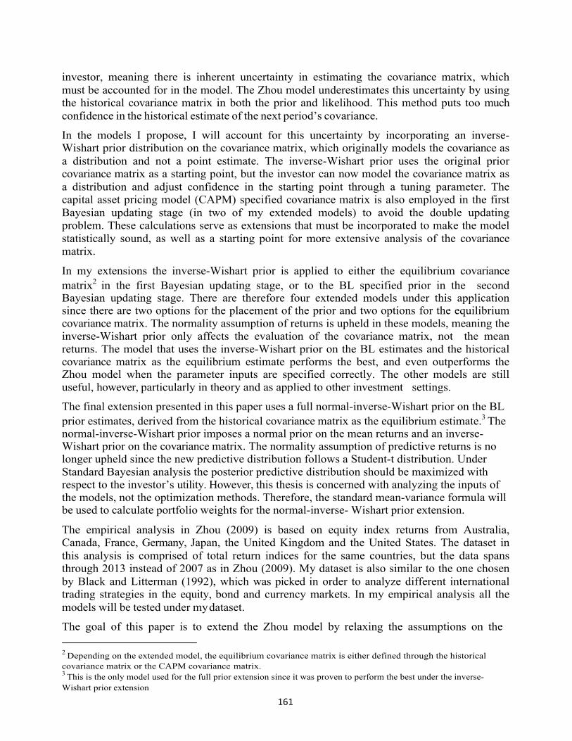
161

investor, meaning there is inherent uncertainty in estimating the covariance matrix, which must be accounted for in the model. The Zhou model underestimates this uncertainty by using the historical covariance matrix in both the prior and likelihood. This method puts too much confidence in the historical estimate of the next period’s covariance.

In the models I propose, I will account for this uncertainty by incorporating an inverse- Wishart prior distribution on the covariance matrix, which originally models the covariance as a distribution and not a point estimate. The inverse-Wishart prior uses the original prior covariance matrix as a starting point, but the investor can now model the covariance matrix as a distribution and adjust confidence in the starting point through a tuning parameter. The capital asset pricing model (CAPM) specified covariance matrix is also employed in the first Bayesian updating stage (in two of my extended models) to avoid the double updating problem. These calculations serve as extensions that must be incorporated to make the model statistically sound, as well as a starting point for more extensive analysis of the covariance matrix.

In my extensions the inverse-Wishart prior is applied to either the equilibrium covariance matrix2 in the first Bayesian updating stage, or to the BL specified prior in the second Bayesian updating stage. There are therefore four extended models under this application since there are two options for the placement of the prior and two options for the equilibrium covariance matrix. The normality assumption of returns is upheld in these models, meaning the inverse-Wishart prior only affects the evaluation of the covariance matrix, not the mean returns. The model that uses the inverse-Wishart prior on the BL estimates and the historical covariance matrix as the equilibrium estimate performs the best, and even outperforms the Zhou model when the parameter inputs are specified correctly. The other models are still useful, however, particularly in theory and as applied to other investment settings.

The final extension presented in this paper uses a full normal-inverse-Wishart prior on the BL prior estimates, derived from the historical covariance matrix as the equilibrium estimate.3 The normal-inverse-Wishart prior imposes a normal prior on the mean returns and an inverse- Wishart prior on the covariance matrix. The normality assumption of predictive returns is no longer upheld since the new predictive distribution follows a Student-t distribution. Under Standard Bayesian analysis the posterior predictive distribution should be maximized with respect to the investor’s utility. However, this thesis is concerned with analyzing the inputs of the models, not the optimization methods. Therefore, the standard mean-variance formula will be used to calculate portfolio weights for the normal-inverse- Wishart prior extension.

The empirical analysis in Zhou (2009) is based on equity index returns from Australia, Canada, France, Germany, Japan, the United Kingdom and the United States. The dataset in this analysis is comprised of total return indices for the same countries, but the data spans through 2013 instead of 2007 as in Zhou (2009). My dataset is also similar to the one chosen by Black and Litterman (1992), which was picked in order to analyze different international trading strategies in the equity, bond and currency markets. In my empirical analysis all the models will be tested under my dataset.

The goal of this paper is to extend the Zhou model by relaxing the assumptions on the

2 Depending on the extended model, the equilibrium covariance matrix is either defined through the historical covariance matrix or the CAPM covariance matrix. 3 This is the only model used for the full prior extension since it was proven to perform the best under the inverse- Wishart prior extension

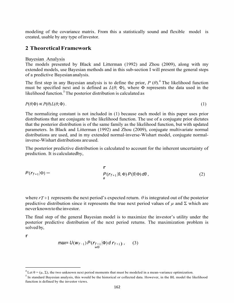
162

modeling of the covariance matrix. From this a statistically sound and flexible model is created, usable by any type of investor.

2 Theoretical Framework

Bayesian Analysis The models presented by Black and Litterman (1992) and Zhou (2009), along with my extended models, use Bayesian methods and in this sub-section I will present the general steps of a predictive Bayesian analysis.

The first step in any Bayesian analysis is to define the prior, P (θ).4 The likelihood function must be specified next and is defined as L(θ; Φ), where Φ represents the data used in the likelihood function.5 The posterior distribution is calculated as

P(θ|Φ) ∝ P(θ) L(θ; Φ) . (1)

The normalizing constant is not included in (1) because each model in this paper uses prior distributions that are conjugate to the likelihood function. The use of a conjugate prior dictates that the posterior distribution is of the same family as the likelihood function, but with updated parameters. In Black and Litterman (1992) and Zhou (2009), conjugate multivariate normal distributions are used, and in my extended normal-inverse-Wishart model, conjugate normal- inverse-Wishart distributions are used.

The posterior predictive distribution is calculated to account for the inherent uncertainty of prediction. It is calculatedby,

where rT +1 represents the next period’s expected return. θ is integrated out of the posterior predictive distribution since it represents the true next period values of µ and Σ which are never known to the investor.

The final step of the general Bayesian model is to maximize the investor’s utility under the posterior predictive distribution of the next period returns. The maximization problem is solved by,

4 Let θ = (µ, Σ), the two unknown next period moments that must be modeled in a mean-variance optimization. 5 In standard Bayesian analysis, this would be the historical or collected data. However, in the BL model the likelihood function is defined by the investor views.

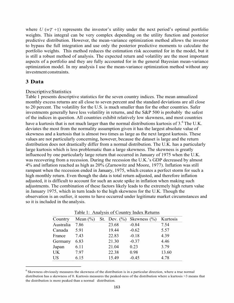
163

where U (wT +1) represents the investor’s utility under the next period’s optimal portfolio weights. This integral can be very complex depending on the utility function and posterior predictive distribution. However, the mean-variance optimization method allows the investor to bypass the full integration and use only the posterior predictive moments to calculate the portfolio weights. This method reduces the estimation risk accounted for in the model, but it is still a robust method of analysis. The expected return and volatility are the most important aspects of a portfolio and they are fully accounted for in the general Bayesian mean-variance optimization model. In my analysis I use the mean-variance optimization method without any investment constraints.

3 Data

Descriptive Statistics Table 1 presents descriptive statistics for the seven country indices. The mean annualized monthly excess returns are all close to seven percent and the standard deviations are all close to 20 percent. The volatility for the U.S. is much smaller than for the other countries. Safer investments generally have less volatility in returns, and the S&P 500 is probably the safest of the indices in question. All countries exhibit relatively low skewness, and most countries have a kurtosis that is not much larger than the normal distributions kurtosis of 3.6 The U.K. deviates the most from the normality assumption given it has the largest absolute value of skewness and a kurtosis that is almost two times as large as the next largest kurtosis. These values are not particularly concerning, however, because the dataset is large and the return distribution does not drastically differ from a normal distribution. The U.K. has a particularly large kurtosis which is less problematic than a large skewness. The skewness is greatly influenced by one particularly large return that occurred in January of 1975 when the U.K. was recovering from a recession. During the recession the U.K.’s GDP decreased by almost 4% and inflation reached as high as 20% (Zarnowitz and Moore, 1977). Inflation was still rampant when the recession ended in January, 1975, which creates a perfect storm for such a high monthly return. Even though the data is total return adjusted, and therefore inflation adjusted, it is difficult to account for such an acute spike in inflation when making such adjustments. The combination of these factors likely leads to the extremely high return value in January 1975, which in turn leads to the high skewness for the U.K. Though the observation is an outlier, it seems to have occurred under legitimate market circumstances and so it is included in the analysis.

Table 1: Analysis of Country Index Returns

Country Mean (%) St. Dev. (%) Skewness (%) Kurtosis Australia 7.86 23.68 -0.84 7.54 Canada 5.91 19.44 -0.62 5.57 France 7.43 22.83 -0.18 4.39 Germany 6.83 21.30 -0.37 4.46 Japan 6.11 21.04 0.23 3.79 UK 7.97 22.38 0.98 13.60 US 6.15 15.49 -0.45 4.78

6 Skewness obviously measures the skewness of the distribution is in a particular direction, where a true normal distribution has a skewness of 0. Kurtosis measures the peaked-ness of the distribution where a kurtosis >3 means that the distribution is more peaked than a normal distribution.

164

4 Model Implementation Rolling Window A predictive model is best tested under repeated conditions where a subset of the data is used as in-sample data to predict the out-of-sample optimal portfolio weights. For each iteration, only the in-sample data is used to calculate the next period’s weights. This simulates how a model would be implemented in a real investment setting since there is obviously no data incorporated in the model for the future prediction period. If the true returns of the predicted periods were included in the analysis, the predictive power of the model would be artificially increased.

In my analysis a 10-year rolling window is used as the in-sample data to predict the following month’s out-of-sample optimal portfolio weights. The first set of in-sample data is the first ten years of the data set, January, 1970 - December, 1980, and is used to predict the optimal asset weights for the following month, January 1981.7 The window then slides over one month and February, 1970 - January, 1981 is used to predict the optimal asset allocations for February, 1981. The dataset extends through 2013, giving 528 individual returns, and given the 10-year rolling window, 408 iterations of the model will be run.

The number of observations used in the in-sample dataset must be considerably larger than the number of parameters estimated by the data. In this analysis, there are 56 different parameters that must be estimated (49 in the 7x7 covariance matrix, and 7 historical mean returns). This ratio of data observations to estimated parameters is sufficient as there are many more observations than estimates. If a larger window were chosen there would be fewer calculated iterations of the models, in turn making the model testing procedure less robust. A 10-year rolling window is ideal to maximize iterations while also accounting for enough observations to estimate theparameters.

Another commonly used window is an expanding window, which starts at the beginning of the dataset and expands to include each successive month. One drawback of this method is that for each iteration, the early data points become increasingly far from the period they are predicting. In the final iteration of a model tested under an expanding window (under this dataset), data from 1970 would be used to estimate the optimal weights for December, 2013. This is not ideal because information on the market in 1970 is likely not useful in calculating portfolio weights for a period more than 40 years in the future. The expanding window also decreases the relative weight of each observation as the window expands, because as the number of observations in the in-sample data increases, each individual observation affects the results less and less. There is also less independence across iterations under an expanding window, since each new iteration contains the same in-sample data of the previous iteration, plus one more observation.

Under the rolling window it is quite simple to assess model performance since there is data on each realized return. For each iteration, the realized return of portfolio is calculated by multiplying each individual index’s calculated portfolio weight by its corresponding realized return. There are no investment constraints in the model so the amount invested in, or borrowed from, the risk-free rate must also be accounted for. The difference between the sum of all the calculated portfolio weights and 1 is the amount invested or borrowed from the risk-

7 The models in this paper are all one period models, so only the following month’s optimal weights are calculated.

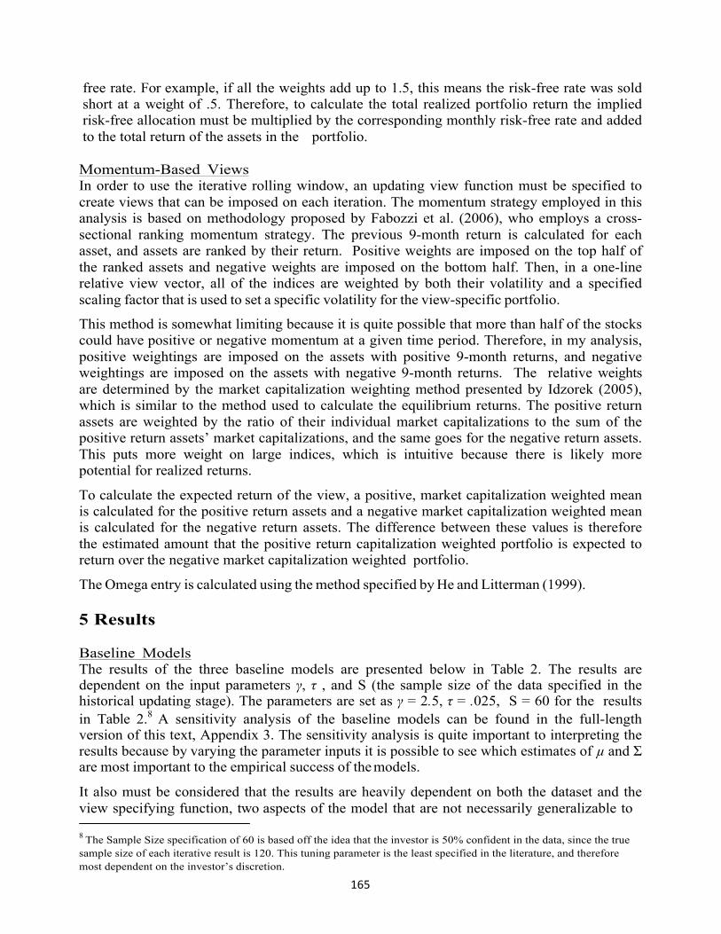
165

free rate. For example, if all the weights add up to 1.5, this means the risk-free rate was sold short at a weight of .5. Therefore, to calculate the total realized portfolio return the implied risk-free allocation must be multiplied by the corresponding monthly risk-free rate and added to the total return of the assets in the portfolio.

Momentum-Based Views In order to use the iterative rolling window, an updating view function must be specified to create views that can be imposed on each iteration. The momentum strategy employed in this analysis is based on methodology proposed by Fabozzi et al. (2006), who employs a cross- sectional ranking momentum strategy. The previous 9-month return is calculated for each asset, and assets are ranked by their return. Positive weights are imposed on the top half of the ranked assets and negative weights are imposed on the bottom half. Then, in a one-line relative view vector, all of the indices are weighted by both their volatility and a specified scaling factor that is used to set a specific volatility for the view-specific portfolio.

This method is somewhat limiting because it is quite possible that more than half of the stocks could have positive or negative momentum at a given time period. Therefore, in my analysis, positive weightings are imposed on the assets with positive 9-month returns, and negative weightings are imposed on the assets with negative 9-month returns. The relative weights are determined by the market capitalization weighting method presented by Idzorek (2005), which is similar to the method used to calculate the equilibrium returns. The positive return assets are weighted by the ratio of their individual market capitalizations to the sum of the positive return assets’ market capitalizations, and the same goes for the negative return assets. This puts more weight on large indices, which is intuitive because there is likely more potential for realized returns.

To calculate the expected return of the view, a positive, market capitalization weighted mean is calculated for the positive return assets and a negative market capitalization weighted mean is calculated for the negative return assets. The difference between these values is therefore the estimated amount that the positive return capitalization weighted portfolio is expected to return over the negative market capitalization weighted portfolio.

The Omega entry is calculated using the method specified by He and Litterman (1999). 5 Results

Baseline Models The results of the three baseline models are presented below in Table 2. The results are dependent on the input parameters γ, τ , and S (the sample size of the data specified in the historical updating stage). The parameters are set as γ = 2.5, τ = .025, S = 60 for the results in Table 2.8 A sensitivity analysis of the baseline models can be found in the full-length version of this text, Appendix 3. The sensitivity analysis is quite important to interpreting the results because by varying the parameter inputs it is possible to see which estimates of µ and Σ are most important to the empirical success of the models.

It also must be considered that the results are heavily dependent on both the dataset and the view specifying function, two aspects of the model that are not necessarily generalizable to

8 The Sample Size specification of 60 is based off the idea that the investor is 50% confident in the data, since the true sample size of each iterative result is 120. This tuning parameter is the least specified in the literature, and therefore most dependent on the investor’s discretion.

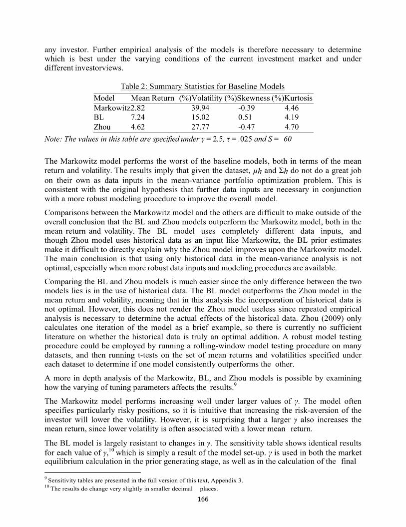
166

any investor. Further empirical analysis of the models is therefore necessary to determine which is best under the varying conditions of the current investment market and under different investorviews.

Table 2: Summary Statistics for Baseline Models

Model Mean Return (%)Volatility (%)Skewness (%)Kurtosis Markowitz2.82 39.94 -0.39 4.46 BL 7.24 15.02 0.51 4.19 Zhou 4.62 27.77 -0.47 4.70

Note: The values in this table are specified under γ = 2.5, τ = .025 and S = 60 The Markowitz model performs the worst of the baseline models, both in terms of the mean return and volatility. The results imply that given the dataset, µh and Σh do not do a great job on their own as data inputs in the mean-variance portfolio optimization problem. This is consistent with the original hypothesis that further data inputs are necessary in conjunction with a more robust modeling procedure to improve the overall model.

Comparisons between the Markowitz model and the others are difficult to make outside of the overall conclusion that the BL and Zhou models outperform the Markowitz model, both in the mean return and volatility. The BL model uses completely different data inputs, and though Zhou model uses historical data as an input like Markowitz, the BL prior estimates make it difficult to directly explain why the Zhou model improves upon the Markowitz model. The main conclusion is that using only historical data in the mean-variance analysis is not optimal, especially when more robust data inputs and modeling procedures are available.

Comparing the BL and Zhou models is much easier since the only difference between the two models lies is in the use of historical data. The BL model outperforms the Zhou model in the mean return and volatility, meaning that in this analysis the incorporation of historical data is not optimal. However, this does not render the Zhou model useless since repeated empirical analysis is necessary to determine the actual effects of the historical data. Zhou (2009) only calculates one iteration of the model as a brief example, so there is currently no sufficient literature on whether the historical data is truly an optimal addition. A robust model testing procedure could be employed by running a rolling-window model testing procedure on many datasets, and then running t-tests on the set of mean returns and volatilities specified under each dataset to determine if one model consistently outperforms the other.

A more in depth analysis of the Markowitz, BL, and Zhou models is possible by examining how the varying of tuning parameters affects the results.9

The Markowitz model performs increasing well under larger values of γ. The model often specifies particularly risky positions, so it is intuitive that increasing the risk-aversion of the investor will lower the volatility. However, it is surprising that a larger γ also increases the mean return, since lower volatility is often associated with a lower mean return.

The BL model is largely resistant to changes in γ. The sensitivity table shows identical results for each value of γ,10 which is simply a result of the model set-up. γ is used in both the market equilibrium calculation in the prior generating stage, as well as in the calculation of the final

9 Sensitivity tables are presented in the full version of this text, Appendix 3. 10 The results do change very slightly in smaller decimal places.

167

weights in the mean-variance optimization. This essentially wipes out the effect γ because the market equilibrium values are determined by γ, and the mean-variance optimization, which also uses γ, is calculated mostly through the equilibrium values.11

In the BL model τ specifies the investor’s confidence in the views, where a larger value is associated with less confidence. Increasing τ improves the model with respect to volatility, but not the mean return. When τ is increased from .01 to 1, the mean return is only slightly diminished while the volatility decreases by almost 50%. This is a great trade-off for almost any investor. These results imply that while the momentum strategy does work, it does not have enough predictive power to be used with complete confidence. This finding is in line with the literature on momentum, the momentum strategy is useful because momentum is a significant phenomenon in the market, but it is not robust enough to merit extreme confidence.

The results of the Zhou model are greatly affected by all three of the tuning parameters. Increasing values of γ are associated with an increasing mean return and a decreasing volatility. γ significantly affects the results of the Zhou model, unlike the BL model, because the parameter no longer has a similar affect across multiple stages of the model. γ is used in calculating the market equilibrium returns, µe, in the first stage, but is not used again in the model until after the historical data is incorporated. At this point the estimates are considerably changed from the equilibrium values so γ is not identically accounted for when used again in the mean-variance optimization. Larger values of γ improve the model both in the mean return and volatility which is consistent with the results of the Markowitz model. This consistency must occur because γ has the same affect across the use of the same historical data.

In the Zhou model τ is still used as the parameter that determines the relative confidence in the investor’s views, as compared to the equilibrium estimate, but its effect on the results is different due to the incorporation of historical data. When τ is increased, the model inherently puts more weight in both the equilibrium and the data. It has already been shown that the incorporation of historical data hurts the results in this empirical analysis, so by increasing the relative weight of the data by increasing τ it follows that the results are hurt both in the mean return and volatility.

Increasing values of S are associated with a decreasing mean return and an increasing volatility, which is expected in this empirical analysis because using the data does not improve the portfolio. This is now a direct effect since S specifically determines the weight of the data.

6 Extended Models

The results of the five proposed extended models are presented below in Table 3. There are four inverse-Wishart extensions that differ in their use of ΣCAPM or Σh in the equilibrium stage and in the location of the inverse-Wishart prior. The results are calculated using parameter inputs of γ = 2:5, τ = :025 and S = 60. For the models with the inverse-Wishart prior on the equilibrium estimate, the prior degrees of freedom (v0) is equal to N+231 and the posterior sample size on the views (SS) is equal to 1 (the investor's views have a weight of one observed data point). v0 is also equal to N+2 for the models with the inverse-Wishart prior on the BL covariance estimate. It must be noted that when CAPM is used as the

11The views seem to be playing a minimal role with respect to a changingγ.

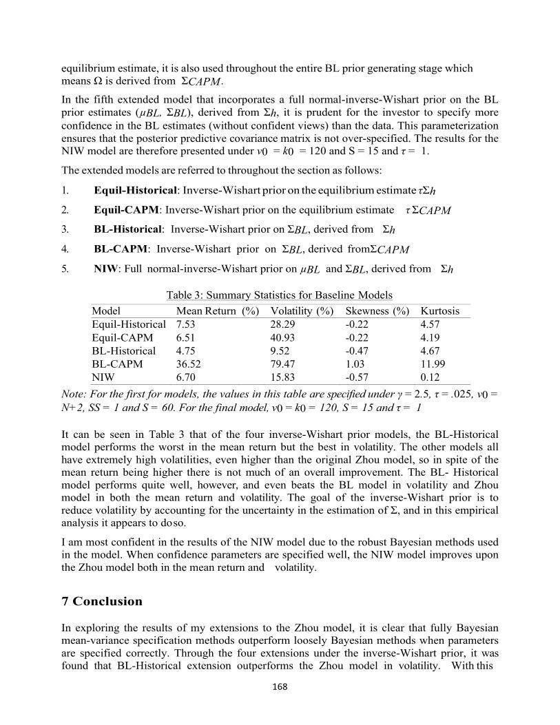
168

equilibrium estimate, it is also used throughout the entire BL prior generating stage which means Ω is derived from ΣCAPM . In the fifth extended model that incorporates a full normal-inverse-Wishart prior on the BL prior estimates (µBL, ΣBL), derived from Σh, it is prudent for the investor to specify more confidence in the BL estimates (without confident views) than the data. This parameterization ensures that the posterior predictive covariance matrix is not over-specified. The results for the NIW model are therefore presented under v0 = k0 = 120 and S = 15 and τ = 1.

The extended models are referred to throughout the section as follows:

1. Equil-Historical: Inverse-Wishart prior on the equilibrium estimate τΣh

2. Equil-CAPM: Inverse-Wishart prior on the equilibrium estimate τ ΣCAPM

3. BL-Historical: Inverse-Wishart prior on ΣBL, derived from Σh

4. BL-CAPM: Inverse-Wishart prior on ΣBL, derived fromΣCAPM

5. NIW: Full normal-inverse-Wishart prior on µBL and ΣBL, derived from Σh

Table 3: Summary Statistics for Baseline Models Model Mean Return (%) Volatility (%) Skewness (%) Kurtosis Equil-Historical 7.53 28.29 -0.22 4.57 Equil-CAPM 6.51 40.93 -0.22 4.19 BL-Historical 4.75 9.52 -0.47 4.67 BL-CAPM 36.52 79.47 1.03 11.99 NIW 6.70 15.83 -0.57 0.12

Note: For the first for models, the values in this table are specified under γ = 2.5, τ = .025, v0 = N+2, SS = 1 and S = 60. For the final model, v0 = k0 = 120, S = 15 and τ = 1

It can be seen in Table 3 that of the four inverse-Wishart prior models, the BL-Historical model performs the worst in the mean return but the best in volatility. The other models all have extremely high volatilities, even higher than the original Zhou model, so in spite of the mean return being higher there is not much of an overall improvement. The BL- Historical model performs quite well, however, and even beats the BL model in volatility and Zhou model in both the mean return and volatility. The goal of the inverse-Wishart prior is to reduce volatility by accounting for the uncertainty in the estimation of Σ, and in this empirical analysis it appears to do so.

I am most confident in the results of the NIW model due to the robust Bayesian methods used in the model. When confidence parameters are specified well, the NIW model improves upon the Zhou model both in the mean return and volatility.

7 Conclusion In exploring the results of my extensions to the Zhou model, it is clear that fully Bayesian mean-variance specification methods outperform loosely Bayesian methods when parameters are specified correctly. Through the four extensions under the inverse-Wishart prior, it was found that BL-Historical extension outperforms the Zhou model in volatility. With this

169

information in hand, a full normal-inverse-Wishart prior was used on the same prior estimates to create a robust and fully Bayesian mean-variance specification model.

The BL model, which is used as a joint prior in the Zhou and extended models, allows the investor to incorporate specific views on the market. The views can be determined in a one- off nature or by a complex function specifying an investment strategy. The former would likely be employed by an amateur, independent investor while the latter by a professional or investment team. All the models presented in this paper use a market capitalization weighted momentum strategy to specify the views in eachiteration.

The data updating stage of the Zhou model has similar flexibility in that the historical means, or a more complex data modeling mechanism, can be employed depending on the quantitative skills of the investor. The incorporation of a predictive model is a topic of further research that could significantly increase the profitability of the Bayesian model. However, this application would also greatly increase the complexity of the model. Asset return predictions models can also be incorporated in a much simpler manner through the use of absolute views on a specific asset.

The inverse-Wishart prior is used to model the uncertainty of predicting the next period’s covariance matrix, which is not fully accounted for in the original Zhou model. This method works well empirically in the BL-Historical model. The models that use the CAPM covariance matrix may be useful under large values of N, as the historical covariance matrix does a poor job estimating the next period’s covariance matrix in this setting. However, the CAPM covariance calculation is a simple method that is used as an example of other potential co- variance matrix specification methods. The study of additional covariance matrix inputs serves as another topic of further research within the general model.

The normal-inverse-Wishart prior is used in the NIW model to fully account for the uncertainty of estimating the mean and covariance matrix. This model is the most statistically robust given the fully Bayesian techniques used to estimate the mean-variance inputs. It also performs well empirically as it outperforms the Zhou model in returns and volatility under correct parameterization. To determine the parameters, the investor can run an iterative model on previous investment periods to see which parameter values are associated with investment profitability. This will give the investor a sense of which model inputs are most important in estimating the next period’s return and covariance matrix. This method is particularly important in determining S because the inclusion of historical data may not be optimal, as in my empirical analysis. If this is the case, the investor should set a small S or simply use the Black-Litterman model which does not incorporate historical data. Though these historical parameters will not perfectly specify the next period’s parameters, they give the investor a method of determining how the future returns are predicted by the various inputs.

The NIW model uses fully Bayesian methods to specify the mean and covariance matrix inputs, but the mean-variance method is still used to calculate the optimal portfolio weights instead of a fully Bayesian method. Bayesian optimization methods are still applicable to this analysis given that the posterior predictive t-distribution is fully calculated in the NIW model. In a fully Bayesian optimization model the investor would maximize investment utility with respect to the posterior predictive distribution. This application serves as a particularly important topic of further research within the realm of Bayesian portfolio optimization as there are many different investor utility functions that can be employed.

Through the use of a rolling window, the results presented in this paper give an idea of how

170

the models perform under repeated conditions. However, each iteration of the rolling window is very similar to the previous one given that all but one data point is identical. In order to confidently determine if one model outperforms another, it is necessary to do an empirical analysis on multiple datasets.

There are countless strategies within the Bayesian mean-variance model for both input specification (in an economic sense) and input combination (in a statistical sense). The importance of input specification is exemplified by the sub-optimal performance of the CAPM covariance matrix in the equilibrium model, while the importance of input combination is seen by the optimal performance of the NIW model. Through this Bayesian mean-variance specification model, the investor has a straightforward quantitative algorithm that can help improve investment success. Investors base their decisions off how they view the assets in the market, and by using this model they can greatly improve their chance of profitability by using robust methods of prediction outside of their views.

Bibliography

Asness, C., Liew, J., and Stevens, R. (1997). Parallels between the cross-sectional pre- dictability of stock and country returns. Journal of Portfolio Management, 23(3):79–87.

Berger, A., Ronen, I., and Moskowitz, T. (2009). The case for momentum investing.

Black, F. and Litterman, R. (1992). Global portfolio optimization. Financial Analysts Journal,

48(5):28.

Fabozzi, F., Focardi, S., and Kolm, P. (2006). Incorporating trading strategies in the black- litterman framework. CFA Digest, 36(4).

He, G. and Litterman, R. (1999). The intuition behind black-litterman model portfolios. Investment Management Research, Goldman Sachs and Co.

Idzorek, T. (2005). A step-by-step guide to the black-litterman model.

Jobson, J. D. and Korkie, B. (1981). Putting markowitz theory to work. Journal of Portfolio

Management, 7(4):70–74.

Lee, W. (2000). Advanced theory and methodology of tactical asset allocation. Markowitz, H. (1952). Portfolio selection. The Journal of Finance, 7(1):77.

Pogue, G. (1970). An extension of the markowitz portfolio selection model to include vari- able transactions’ costs, short sales, leverage polices and taxes. The Journal of Finance, 25(5):1005– 1027.

Satchell, S. and Scowcroft, A. (2000). A demystification of the black-litterman model: Man- aging

quantitative and traditional portfolio construction. Journal of Asset Management, 1(2):138– 150.

Zarnowitz, V. and Moore, G. (1977). The recession and recovery of 1973-1976. Explorations in Economic

Research,4(4):1–87.

Zhou, G. (2009). Beyond black-litterman: Letting the data speak. The Journal of Portfolio Management, 36(1):36.

171

The Dynamic Link Between Inequality and Economic Growth:

A Stochastic Approach

Raphael Small Senior Thesis

Department of Economics Haverford College

4/30/2015

Abstract

In this thesis I present a theoretical, neoclassical growth model with a rigorous microeconomic foundation that examines the dynamic link between inequality and economic growth. I take a standard Real Business Cycle model and augment the production function to incorporate human capital in accordance with the Mankiw, Romer, and Weil (1992) extension to the standard Solow Growth Model. My thesis contributes to the scope and detail of the existing literature, adding a spectrum of heterogeneous households differentiated in size, asset holdings, and stock of human capital. I utilize a Markov Transition Matrix to capture the stochastic and persistent nature of the business cycle and extend investment in human capital at the microeconomic level. I introduce two frictions to propagate inequality shocks from the microeconomic to the macroeconomic level: imperfect capital markets and discrete human capital. Results indicate that the relationship between inequality and growth is complex, but that stable growth occasionally decreases the income Gini Coefficient. The introduced frictions and nature of the model combine to generate patterns of investment shocks and capital depreciation that prevent the economy from reaching the steady-state achieved by the social planner or competitive markets, indicating that reducing the severity of frictions leads to economic stability and a Pareto Efficient improvement for the economy in the long-run. The paper presented here is an abridged version of the original; please contact me if interested in obtaining a full copy of the original.

172

1 Introduction

Inequality has become the center of an ongoing policy debate and has additionally fostered a great deal of interest due to its impact on long-term economic growth and broader macroeconomic consequences. Inequality is a highly nuanced and complex topic to study empirically; as such, there is a noticeable disagreement within the existing literature regarding the nature of its impact on long-term growth.

The pre-tax income Gini Coefficient has risen steadily with seasonally adjusted real GDP-per- capita over the past half-century. The correlation coefficient between both variables is 98% and is statistically significant at better than the 0.01% level. Over the past decade (2003-2013), the Gini Coefficient has risen from 0.464 to 0.477. The rise of inequality in recent years therefore is not too substantial.

To explore the relationship between inequality and growth, I model stochastic productivity shocks with a Markov Transition Matrix, adapting the production function to incorporate human capital in accordance with the Mankiw, Romer, and Weil (1992) extension of the Solow Growth Model. Accordingly, each household must also make utility maximization decisions with respect to human capital.

There are two primary frictions in this model that are used to propagate the impact of inequality from the microeconomic to the macroeconomic level: imperfect capital markets and discrete human capital. These frictions combine to form the poverty trap, in which poor households are unable to borrow in the imperfect capital markets to invest in human capital. Poor households are therefore unable to earn a skill premium, leaving them with only income from their unskilled labor. As human capital can only be purchased in discrete quantities, the poor are thus unable to acquire some marginal amount. The interaction of these frictions perpetuates the cycle of poverty, essentially creating the “poverty trap.”

2 Theoretical Model

Production I use the production function proposed by Mankiw, Romer, and Weil (1992) that adds human

capital to the Cobb-Douglas production function used in the standard Solow Growth Model:

In accordance with Real Business Cycle Theory, I assume that TFP experiences shocks are stochastic and exogenous to the production process. In order to capture these properties, I use a discrete Markov Process calibrated to US macroeconomic data to model productivity fluctuations. I use a neoclassical production function, with the usual constraints on the coefficients.

173

In this model I assume three states: boom, recession, and “normal” in an ordered productivity relationship.

The firm maximizes profit taking factor prices as given. The profit function is therefore:

Here is the rental cost of physical capital while and are wages. I distinguish the minimum

wage received from a worker with no human capital from , the skill premium that is earned for each unit of human capital held. Taking first-order-conditions yields

The Household and Utility I define a “dynasty” as an infinitively lived household that allocates resources between consumption and investment in order to dynamically optimize its infinite stream of discounted

utility, where the aggregate utility level is given by I use the CRRA utility function to allow for differing levels of risk-aversion. Households seek to maximize their own utility and must decide how to allocate their time and resources as such.

Thus the aggregate utility maximization problem is to maximize by dynamically setting consumption and investment. This is the social planner’s problem, in which economic resources are allocated in order to maximize total utility. When households decide to invest in education, there is a direct cost in terms of tuition and also an opportunity cost in terms of wages forgone. I

introduce the education decision variable to obtain the new labor income for a household of

size individuals:

is binary and takes on a value of one if the household decides to invest in human capital, and takes a zero otherwise. I assume that households either send all or none of their young to college.

The stock of human capital at the household level is given by This assumption embodies both the demographic and discrete human capital constraints.

Furthermore, households also derive income from returns on their wealth holdings . Thus the household obtains total income With a per-person exogenous cost of

education , the budget constraint becomes: I assume imperfect capital markets in the sense that they are nonexistent with respect to borrowing. While households are able to “lend” to the representative firm by investing in physical capital, they are unable to borrow against future income in order to obtain loans. A natural implication is that sufficiently poor households will be unable to invest in human capital because they cannot borrow to do so against the future returns to education. The law of motion

174

for human capital accumulation at the microeconomic level is therefore

where is the amount of human capital gained by receiving an education.

Thus for the ith household the utility maximization problem, knowing current prices and stocks

of human capital and assets, the goal is to maximize subject to the

budget constraint. In maximizing the average utility received per household member, this compensates for households of different sizes.

Endowments and Dynamics

I assume that the population is fixed, with births and deaths occurring at an equalized rate. This

rate is commonly referred to as the replacement rate, here denoted by . I also assume the population is exactly equal to the size of the available workforce so that the population consists

solely of eligible workers. I divide the population into those working, , and those involved in

education (improving their human capital) . Hence: . There are dynasties that

do not change in size, with population either or individuals such that .

Given the decisions of each of the households, I sum over the microeconomic variables in order to obtain the economy-wide aggregates. The “time” allocation at the macroeconomic level is illustrated by the size of the labor force and number of individuals in college:

and

From the budget constraint, I sum over consumption and investment in order to obtain the aggregates of consumption and investment.

By investing in education, households update the stock aggregate stock of human capital according to the aggregate law of motion for human capital accumulation:

Human capital accumulation is the aggregate of each

household’s investment decision, Physical capital, similarly, has a depreciation term , giving rise to the standard law of motion for physical capital accumulation:

I use the Gini Coefficient to measure of level of inequality in above defined three distributions: human capital, income, and physical assets.

General Equilibrium

To equalize supply and demand I must solve the following simultaneous equations in each time

period:

175

Since the economy enters each period with the stocks of capital and already determined as a result of investment and depreciation, the only macroeconomic variable I need to explicitly

solve for is the labor force which is determined by aggregate decisions of dynasties to invest in human capital.

Since this is a system of non-linear equations with two equations and three unknowns (the factor prices), I apply a non-linear least-squares approach in order to minimize the error associated with a set of general equilibrium prices with the constraint of positive prices.

The Social Planner’s Problem

The social planner seeks the savings rate across all time that will maximize the infinite stream of

discounted utility. Given the population and birth/death rate , exactly individuals remain in the next period. This is exactly the amount of old workers who are not eligible, by assumption, to pursue education.

At present, I assume that the social planner sends all of the young to receive an education. By sending all youth to college, the social planner obtains a labor force equivalent to the number of

remaining old workers in each period. The steady-state labor force is therefore: As

individuals are newly born and are thus eligible for education in each period, the steady-state

level of aggregate human capital is given implicitly by: This in turn yields

I define the steady-state level of physical capital by By

substituting in the steady-state level of physical capital, I obtain

In the steady-state, all of the aggregate macroeconomic variables are constant, hence the infinite

sum of discounted utility is defined by:

This is equivalent to maximizing consumption. Therefore I use the standard first-order-condition with respect to the savings rate and simplify to obtain the solution , which maximizes total discounted utility.

Factor Prices in the Competitive Steady-State

Suppose the parameter represents the fraction of households that have a smaller number of individuals . In equilibrium, I assume that the households collapse into two steady-state groups: rich and poor. I assume that the rich households are small and invest in human capital, while the

176

poor households are small do not invest in human capital, as they lack sufficient resources to do so.

I find that the steady-state level of human capital for a rich household is: and the

aggregate stock of human capital is: I note that the poor dynasties have zero human capital in equilibrium. This intuitively follows from their human capital continually depreciating without investment.

While solving for general equilibrium in the steady-state may seem daunting, I only extract the set of factor prices, and indeed, this greatly reduces the remaining work. First, given that I assume constant factor prices in the steady-state, it is helpful to rewrite the household income equations as:

Thus for the rich household, recalling the time subscripted budget, the utility maximization

problem is: I apply first-order-condition with respect to asset holdings and note that the asset term appears twice as a result of the time subscripting. Using the steady-state assumption of a constant stock of assets across all time, this simplification solves the utility maximization problem as follows:

This in turn yields the steady-state price of physical capital:

This result is similarly obtained through symmetry in the case of the poor household as a result

of the fact that labor income remains constant throughout the steady-state and independent of . Having obtained the steady-state price of physical capital, the equilibrium stock of physical capital is defined. This in turn yields the equilibrium level of output and therefore the steady- state prices.

Determining Optimal Household Behavior

Determining the exact optimal behavior of the households within a general equilibrium setting for this model is difficult because of the complexity and uncertainty regarding future prices. Naturally, the optimal utility-maximizing behavior of the households at a given time depends not only on the present realized prices, but also the stream of future prices as well. Thus, the behavior of the households depends on the set of future prices. However the behavior of the households also impacts those very same future prices as a result of their resource allocation choices under general equilibrium.

Suppose that the dynasties divide all of time into two periods: “now” and “later”. In the current period, prices are realized and are witnessed by the households without uncertainty. Regarding future prices, I assume there is a set of expected prices (the steady-state prices) upon which

177

households base their actions in the present. Households expect current prices to decay from their present level to their steady-state values at a specified rate.

Given their decay paths, the households now seek to maximize the infinite discounted stream of

utility The household therefore seeks a new optimal choice at each time in accordance with new factor prices and must continually decide whether to invest in education, and what fraction of income to allocate between consumption and assets in order to maximize utility subject to the poverty trap and imperfect capital markets friction.

I apply the standard first-order-condition, differentiating with respect to and simplify to obtain

the Euler Equation: This Euler Equation governs the optimal household allocation of resources in order to maximize the infinite stream of discounted utility.

The strength of this model, therefore, lies in the fact that the direction of inequality’s impact on growth is not predetermined through construction. To be sure, there are competing positive and negative effects, but the net impact depends on the specifics of the model itself.

3 Stochastic Simulations

Parameter Estimation and Calibration

Using the production function I estimate the level of TFP in each year by: I de-trend

the data so that productivity does not experience any long-run growth. Since the model assumes

a constant population, I define the population-weighted TFP by: I obtained data from Releast 8.0 of the Penn World Tables and from the FED Database maintained by the St. Louis

Federal Reserve Bank. I also use Acemoglu’s estimates for .

I apply the Hodrick-Prescott Filter to the FRED real GDP-per-capita in order to estimate the trend path of GDP-per-capita . I calculate the percentage trend deviation of GDP-per-capita To define the business cycle states I take the standard deviation of the percentage deviations and use it as the cutoff to define recessions, booms, and stagnant periods. I thus define the intervals:

• Boom:• Recession:• Stagnant:

I estimate by counting the number of times each state transitions to another state and rescaling the entries such that each column sums to one. I estimate the aggregate probabilities of each state occurring in the data by π(boom)=37.1%, π(stagnant)=35.5%, and π(recession)=27.4%

.

178

is diagonal

In calculating the eigenvalues of , I find that there are three distinct such numbers. As a result,

izable, hence there exists a real invertible matrix and real diagonal :

I take the limit as and define the matrix limit and find, by the steady-state probabilities, a boom occurs approximately 37.9% of the time, while recessions occur with a frequency of 26.1% and stagnant states with a frequency of 36.0%. These implied probabilities are quite similar to those empirically extracted and displayed in the aggregate probabilities.

Having classified each year within the data according to its productivity level, I use the estimates

of to calculate the average TFP for each state. After matching the TFP estimates to the business cycle states and taking the average over each, I obtain the following population-

weighted productivity levels: , and I define the

expected TFP as the that is featured extensively in the preceding sections.

4 Simulation Results and Discussion I explore several simulated economies, using slightly different parameter settings than those used in the “full” model. In Figures 1 and 2, I find that neither lowering the cost of education to zero nor eliminating productivity shocks diminished the severe GDP fluctuations. In Figure 3, I no longer impose the poverty trap in which poor households are forced to consume all of their income, and find that the economy collapses, with capital and output falling to zero.

The parameter choices used for the simulation show in Figure 4 result in a reasonably stable economy, although the productivity shocks in Figure 8.29 have little impact on what appear to be business cycle fluctuations. In Figures 5 and 6 it is clear the initial decade of rapid growth is fueled by large investment, primarily in physical capital, with most of the eligible youth attending college. These two figures also indicate that GDP shocks are driven by simultaneous investment by the households. Thus the initial period of growth was fueled by human capital accumulation, while subsequent growth is due to physical capital accumulation.

In examining capital accumulation in Figures 7-9 it is clear that both physical and human capital are far below their steady-states in the competitive equilibrium and the social planner’s equilibrium. This indicates that the introduced frictions lead to inefficiencies that degrade economic growth.

I additionally plot the deciles of the income distribution over time in Figure 10. While each income bracket appears to experience income changes in keeping with GDP fluctuations, the rich both gain and lose the most as a result of booms and recessions, respectively. In contrast, the income of the poor, defined by the first decile, spikes during booms but falls slowly during the time until the next trough.

179

By the definition of the poverty trap and imperfect capital markets, it is likely that the low income volatility of the poor is due to their diminished access to capital. The poor are unable to experience returns to human or physical capital, hence they only receive the minimum wage w. I examine the relationship between inequality and GDP growth. While the correlation coefficient between the human capital Gini Coefficient and GDP growth is 89.03% and significant above the 0.01% level, human capital quickly converges to a steady-state level of inequality that appears relatively independent from growth.

Lastly, I scatter inequality over GDP to examine the existence of the Kuznets Curve. In Figure 1, inequality rises initially and then falls as GDP continues to increase, giving rise to a semblance of a Kuznets Curve. The existence of a Kuznets Curve is most telling in Figures 11 and 12; there is a sustained increase in inequality during the initial period of growth that is followed by a rapid decline. Overall, however, it is difficult to discern the dynamics of the income distribution over time. While the income Gini Coefficient rises noticeably during booms, it also declines during smaller periods of growth while remaining constant during other periods of fluctuations. Thus income inequality does not appear to behave consistently with growth.

5 Conclusion

In examining the relationship between economic growth and inequality I find mixed results. The human capital Gini Coefficient rapidly declines after increasing during the initial decade of growth, regardless of GDP fluctuations; the income Gini Coefficient rises significantly during booms but declines in period of moderate growth. The inconsistent relationship between inequality and growth indicates that the model at hand agrees with Kuznets (1955) and Banerjee and Duflo (2003) in that it finds the link between inequality and growth to be highly nuanced.

In comparison to the social planner’s solution, markets do an ineffective job of developing the economy, as there is room for a Pareto Improvement of all agents. This improvement can be accomplished by alleviating the severity of imperfect credit markets through reducing the barriers that prevent poor households from acquiring loans to invest in capital. Human capital accumulation, according to Galor and Moav (2004), is degraded by inequality, thus financing access to educational opportunities for the poor may augment human capital accumulation and thus stimulate growth. Reducing the discrete nature of human capital by increasing the diversity of educational opportunities may diminish the discrete nature of human capital and improve the ability of poor households to acquire such capital.

I validate the existence of the Kuznets Curve, however the unstable nature of the simulations also serves to indicate why research in this area is so contested. In contrast with the highly volatility incomes of the rich, there is a sizable fraction of the population that remains poor even during periods of extreme growth. Thus capital market imperfections and discrete human capital are frictions that may cause such disparity and contribute to the poverty trap. The poverty trap also appears to be highly effective in motivating households to invest in capital and thus drive growth, although this may result from the programming of the model. As a result, this thesis is well situated within the literature as it embodies many of the themes discussed in the above literature review.

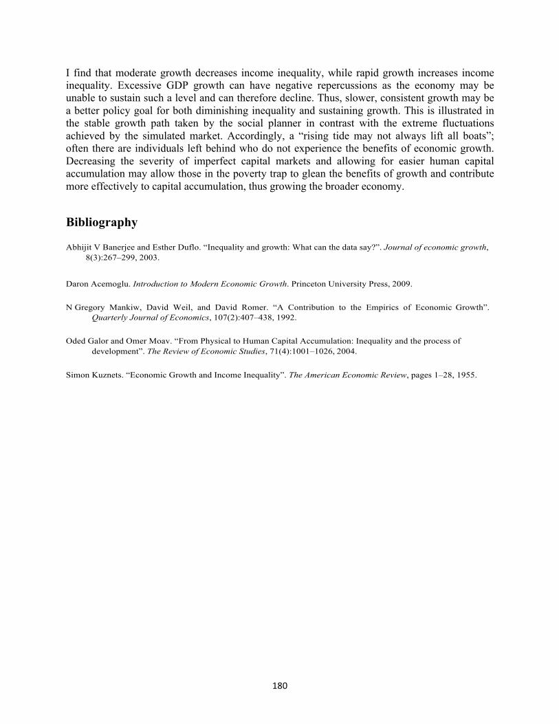
180

I find that moderate growth decreases income inequality, while rapid growth increases income inequality. Excessive GDP growth can have negative repercussions as the economy may be unable to sustain such a level and can therefore decline. Thus, slower, consistent growth may be a better policy goal for both diminishing inequality and sustaining growth. This is illustrated in the stable growth path taken by the social planner in contrast with the extreme fluctuations achieved by the simulated market. Accordingly, a “rising tide may not always lift all boats”; often there are individuals left behind who do not experience the benefits of economic growth. Decreasing the severity of imperfect capital markets and allowing for easier human capital accumulation may allow those in the poverty trap to glean the benefits of growth and contribute more effectively to capital accumulation, thus growing the broader economy.

Bibliography

Abhijit V Banerjee and Esther Duflo. “Inequality and growth: What can the data say?”. Journal of economic growth, 8(3):267–299, 2003.

Daron Acemoglu. Introduction to Modern Economic Growth. Princeton University Press, 2009.

N Gregory Mankiw, David Weil, and David Romer. “A Contribution to the Empirics of Economic Growth”. Quarterly Journal of Economics, 107(2):407–438, 1992.

Oded Galor and Omer Moav. “From Physical to Human Capital Accumulation: Inequality and the process of

development”. The Review of Economic Studies, 71(4):1001–1026, 2004.

Simon Kuznets. “Economic Growth and Income Inequality”. The American Economic Review, pages 1–28, 1955.

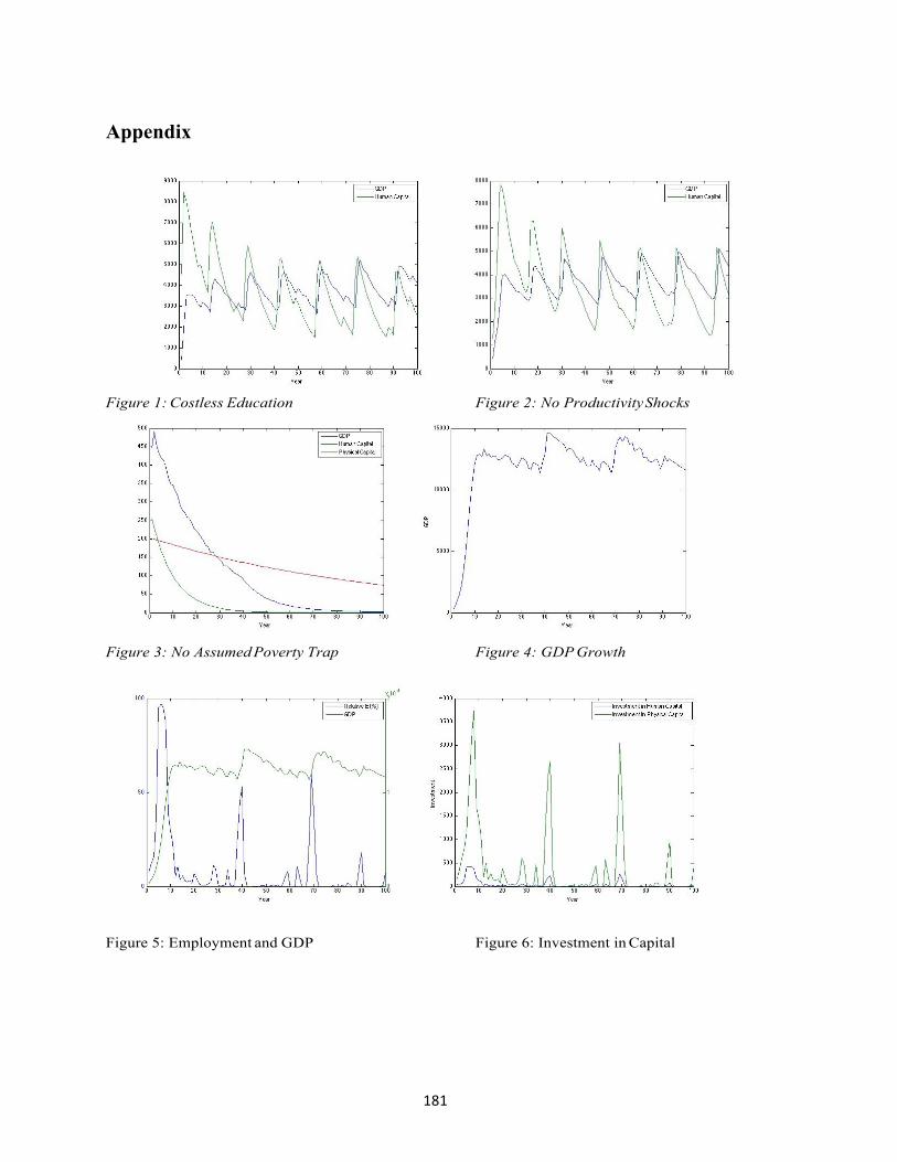
181

Appendix

Figure 1: Costless Education Figure 2: No Productivity Shocks

Figure 3: No Assumed Poverty Trap Figure 4: GDP Growth

Figure 5: Employment and GDP Figure 6: Investment in Capital

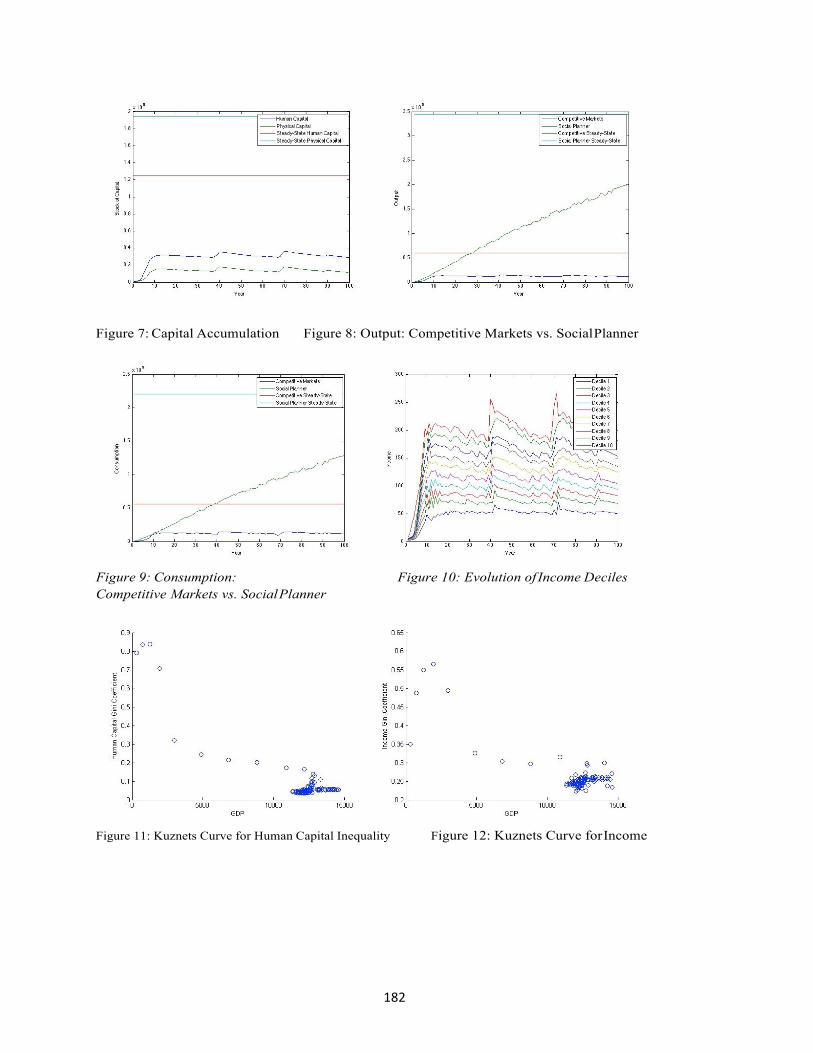
182

Figure 7: Capital Accumulation Figure 8: Output: Competitive Markets vs. Social Planner

Figure 9: Consumption: Figure 10: Evolution of Income Deciles Competitive Markets vs. Social Planner

Figure 11: Kuznets Curve for Human Capital Inequality Figure 12: Kuznets Curve for Income

183

Foreign Direct Investment and School Attendance: Evidence from Vietnam

NANCY F. WU

Dartmouth College

ABSTRACT

This paper uses the variation in the share of foreign direct investment jobs among provinces in Vietnam from 1999 to 2009 to examine the impact of increasing FDI jobs on school attendance in a low-income country. FDI jobs in Vietnam are more skill-intensive, on average, than non- FDI jobs within a given industry. I find evidence that an increase in the share of FDI jobs in a province leads to a decline in school attendance and an increase in the likelihood that a young adult works in a foreign sector job. These impacts are concentrated among young adults, ages 15 to 17, who are at the legal employment age but have not yet completed higher secondary schooling. These results are robust to controlling for changes in manufacturing jobs and education compositions within each province, and consistent within subgroups by gender, minority status, and spatial origin. These effects are driven by the FDI jobs requiring 9 years of education, which raises the opportunity cost of schooling for students at the key dropout margin of 15 to 17. Supplementary results suggest that exposure to FDI jobs also increases the likelihood that a cohort completes at least 9 years of schooling.

184

*The following is an abridged version of the original paper, not all tables will be included. 1 Introduction

Can jobs created by foreign direct investment (FDI) in a developing country impact a child’s decision to attend school? In the last thirty years, globalization has reshaped the employment opportunities available in developing countries. The existing literature has found that new jobs created due to globalization have impacted schooling either by increasing the skill premium and providing an incentive to attain more education (Oster and Steinberg 2013), or by increasing the wages of new lower skill jobs and increasing the opportunity cost of attending school (Atkin 2012). Unfortunately, there is little empirical work connecting FDI jobs, which vary in skill, to schooling. This paper aims to provide such a connection.

I use the variation in the share of FDI jobs among provinces in Vietnam from 1999 to 2009 to examine the impact of increasing FDI jobs on school attendance for individuals ages 15 to 25. Vietnam’s economic change in recent years provides a ripe context for studying the effects of globalization on schooling. In 1986, Vietnam initiated a collective set of economic reforms, known as Doi Moi, to create a regulated market economy from one that was centrally planned. Since these renovations, Vietnam has experienced spectacular growth rates, with real GDP increasing at an average annual rate of seven percent between 1986 and 2008 (McCaig and Pavcnik 2013). The year after reform, Vietnam opened its economy to foreign investors, leading to influxes in the number of foreign sector jobs and changing the employment landscape. Though the notion of expanding higher-wage job opportunities against a backdrop of economic growth is an appealing goal of globalization for both foreign investors and domestic policy makers, the potential opportunity costs that these jobs induce on education should also be considered.

To test the impact of an increase in the share of FDI jobs in a province on school attendance, I construct province-level characteristics through weighting shares of individual-level data by population. I find that a one-percentage point increase in the share of FDI jobs in a province is associated with a significant 0.3-percentage age points decline in school attendance. The magnitude of that decline increases to 0.8-percentage age points for secondary school aged children. These impacts are robust and even larger for females. The secondary school age cohort not attending school is more likely to work in the foreign sector than any sector in general.

I begin by reviewing the existing literature and laying out the theoretical framework through which FDI could impact schooling. Next, I introduce the data set. Section 4 discusses the empirical methodology. Section 5 analyzes the effects of new FDI jobs on school attendance. Section 6 presents robustness checks by breaking down groups by geography, gender, and minorities. This section also explores whether non-school attending children work in FDI jobs. Section 7 concludes with shortcomings, areas for future research, and policy implications.

2 Background: Literature Review and Theoretical Motivation

There is an abundant literature on the economic impacts of FDI in developing countries. Prior studies have found that FDI provides an external source of capital and income for developing countries that leads to economic growth, greater competition, technology transfer, new jobs, and the realization of competitive advantage (Freeman 2004; Nasser 2007). In Mexico, FDI led to the

185

doubling of wages in US dollars to workers in multinationals and a 50% increase in the number of FDI manufacturing jobs (Aizenman 2002). In Vietnam, FDI has contributed to overall macroeconomic growth and poverty reduction by generating new jobs, advanced technology, managerial skills and expertise, increased foreign exchange, and increased tax revenues (Freeman 2004).

However, fewer studies exist that explore globalization’s impacts on education or make the connection between FDI and schooling. Some prior literature has detailed how non-FDI channels of globalized production impact women and children. Many of these studies focus on Bangladesh, where textile export industries have expanded employment for young rural women. Hewett and Amin (2000) provide evidence that women employed in export-oriented textile manufacturing in Bangladesh rank better on quality of life measures that include housing conditions, agency over marriage and number of children, and consumption of jewelry and entertainment. Similar to the case of Bangladesh, trade liberalization in Mexico has led to a surge in female labor force participation in export-oriented manufacturing sectors. David Atkin (2011) has considered the role of factory openings that employ female labor on child health in Mexico. His research suggests that women whose first jobs are in manufacturing were induced to enter that field due to expansions in export-oriented manufacturing jobs and would not otherwise have chosen to do so. However, most research connecting FDI to education examines education level as an input rather than an output. Borensztein et al. (1998) and Wang and Wong (2011) have found that FDI only has a positive impact on economic growth given a certain threshold of quantity and quality of education, respectively.

The empirical section focuses on the impact of increased FDI jobs on school attendance. Thus, it is worth discussing some of the theoretical channels through which increased jobs through globalization could influence education. Atkin (2012) proposes a conceptual framework illustrating that new employment opportunities in developing countries have two offsetting effects. On the one hand, when new jobs are created, a student may drop out of school in order to take one of the abundant jobs—“the opportunity cost of schooling channel.” On the other hand, if the student expects that job opportunities will continue to be available and these jobs will reward higher education attainment, the student might choose to stay in school—“the return to schooling channel.” Atkin predicts that new job openings are most likely to reduce the aggregate schooling of a cohort “if the factory hires many unskilled workers at attractive wages, and many members of the cohort are of legal employment age and still attending school at the time of the factory arrival” (2012). Atkin’s study verified his predictions, finding that the arrivals of high- skill manufacturing jobs induce education acquisition, while low-skill arrivals induce school dropout. The dropout effects are even greater when the low-skill job arrivals pay a wage premium relative to existing jobs and there are many students in the region at the key school- leaving ages of 15 and 16—above the legal age to work but below the age of completing secondary school. Supporting Atkin’s framework for high-skill jobs, Emily Oster and M. Bryce Steinberg (2013) have also found that the opening of higher-skill and higher-wage business process outsourcing centers, in particular the Information Technology Enabled Services in India, lead to higher levels of school enrollment by increasing the local returns to schooling.

What effects would Atkin’s conceptual framework predict that FDI jobs should have on school attendance in Vietnam? First, it is reasonable to assume that Vietnam is relatively abundant in

186

unskilled labor. McCaig (2011) finds that goods created from unskilled labor, such as clothing, food and beverages, footwear, and furniture dominate Vietnam’s exports. These unskilled industries employed 61% of manufacturing workers in Vietnam in 1999 and would expand the most in terms of the number of jobs and employees. Second, McCaig and Pavcnik (2013) find that most FDI job opportunities in Vietnam occur in manufacturing, where unskilled industries dominate. In 2009, 22% of manufacturing workers were employed by the foreign sector, compared to 6.4% of workers in higher-skilled finance, insurance, real estate, and business services. Thus, an increase in the share of FDI jobs in a province would relatively increase the number of lower-skill, higher-wage jobs and lead to a drop in school attendance. However, part of this “opportunity cost of schooling” channel becomes offset when considering that FDI also creates higher-skill jobs. In addition, Atkin’s earlier paper (2011) found that higher-wage, low- skill manufacturing jobs encouraged higher investments in a child’s human capital, which suggests that parents could send children to school if FDI increases family income. Thus, I expect the impact of FDI jobs on school attendance to be negative or ambiguous.

I contribute to this prior literature by looking at the case of Vietnam from 1999 to 2009 in order to explore whether new FDI jobs created in a province influence a child’s school attendance. Vietnam is a suitable place to test Atkin’s conceptual framework. Due to the promulgation of the Foreign Investment Law of 1987 that liberalized Vietnam’s economy to encourage the entry of foreign owned firms and foreign investors, Vietnam has attracted significant foreign direct investment (FDI) in the 1990’s and 2000’s. Pavcnik and McCaig (2013) find that employment in the foreign sector increased by almost 1.5 million in the 2000’s. Like Atkin (2012) and Oster and Steinberg (2013), I will examine the school attendance of different school-aged cohorts. In addition, I expand upon existing literature by segregating my analysis by gender, spatial origin, and minority status. The situation of women in Vietnam is complex because gender roles expect women to both receive education and perform wage work (Priwitzer 2007). However, it is important to address gender because the largest FDI job expansion occurred in manufacturing, where women are more likely to work than men (Pavcnik and McCaig 2015). According to Atkin (2012), female job expansions should primarily affect schooling decisions of women and male job expansions should primarily affect schooling decisions of men. In addition, FDI jobs are often centered in urban locations, but over three-quarters of Vietnam is rural land, adding another layer of complexity. Urban or rural locations might also determine the distances of schools. Thus, I include urban and rural analyses because these subgroups may experience different exposure to both FDI jobs and education. Finally, since 90% of Vietnam’s ethnic minorities live in rural areas, I separately analyze geography and ethnicity to avoid conflating the two groups.

3 Data

I manipulate individual-level observations from one data source to explore the impact of an increase in the share of FDI jobs in a province on an individual’s school attendance using variation across provinces. My individual level data comes from a three percent subsample of the 1999 and 2009 Vietnam Population and Housing Census made available from IPUMS (Integrated Public Use Microdata Series). The data provides information on education attainment, school attendance, employment sector, industry, demographic traits, and various other individual characteristics. I restrict the sample to individuals ages 15 to 25, because 15 is

187

the legal working age in Vietnam and foreign firms would not be hiring illegal child labor. I cap my age group to 25 to represent the age range of individuals most likely to be attending secondary school or university. During my period of analysis, 1999-2009, the data covers about 3.5 million individuals. Table A provides the summary statistics on my individual data used: school attendance, spatial origin, ethnic minority status, gender, age, and age squared.

Since my empirical strategy relies on the variation in FDI jobs across provinces to identify the impact on school attendance, I manipulate my dataset of individual-level observations to create characteristics that vary at the province-level. The province is the first administrative subdivision in Vietnam. Based on existing literature by Brian McCaig (2011), the province is a good unit for the relevant labor market in Vietnam because annual inter-provincial migration rates appear to be very low, at one or two percent of the population, depending on the year. McCaig (2011) also finds that provinces vary in exposure to international trade flows, such as tariff levels, and macroeconomic shifts, such as poverty levels. According to McCaig and Pavcnik (2012), Vietnamese provinces differ in their extent of integration into foreign markets. Thus, in this paper, I use the province-level to capture variation in exposure to foreign sector jobs, industries, and skill levels in terms of education completion. I compute these shares using population weights, which I explain in more detail below. The summary statistics for these province characteristics are also provided in Table A. I observe the province in which surveyed individuals resided for 60 provinces, coded in three digits ranging from 110 to 892. I drop from my sample people residing abroad or whose provinces are unknown. The number of provinces in Vietnam grew between 1989 and 1999 and remained relatively stable between 1999 and 2009; therefore, I chose not to use 1989 census data even though it was also available to me.

My dependent variable is an indicator for the school attendance of individual i in province code j at year t, which I denote as 𝑎 𝑡𝑡𝑒𝑛𝑑 !"# . This indicator takes on the value 1 if the individual attends school and 0 if the individual does not currently attend school, having either attended in the past or never attended. My variable of interest is the share of FDI jobs among all jobs in province j at year t, denoted by 𝐹𝐷𝐼!". To create this variable, I calculate the share of foreign workers over total workers in a province, weighing each observation in the sample by the number of persons in the actual population the observation represents.

4 Empirical Strategy

My empirical model estimates the impact of FDI jobs on school attendance using an ordinary least squares estimator with various fixed effects. The basic equation is shown in Equation (1) below

𝑎𝑡𝑡𝑒𝑛𝑑!"# = 𝛼 + 𝛽!𝐹𝐷𝐼!" + 𝛾! + 2009! + 𝛿𝑋!"# + 𝜀!"# (1)

where the coefficient of interest is 𝛽!, which captures the effect of an increase in the share of FDI jobs in a province on an individual’s school attendance. This coefficient is identified through the variation in provinces receiving new FDI job openings. I use this coefficient to test my null hypothesis, that an increase in FDI share in a province has no effect on school attendance (𝛽! = 0), against the alternative that an increase in FDI share in a province does impact school attendance (𝛽! ≠ 0). 𝑋!"# is a vector of individual-level controls: gender, minority race, urban

188

residence, age, and age squared. I include these for the reasons described in section 2. This equation also includes province and time fixed effects. The inclusion of province fixed effects 𝛾!

controls for time-invariant province characteristics, such as geography, that may affect FDI share and school attendance. Since only two years—1999 and 2009—are represented in the data, 2009! is a year dummy that controls for macroeconomic shocks to all provinces over the time period. Throughout all my analyses, I cluster standard errors at the province level to account for heteroskedasticity and autocorrelation of outcomes at the province level.

A concern arises that there may be time-variant province characteristics, which province fixed effects do not capture, that affect both the share of FDI jobs in a province and school attendance. To address this issue, I include a set of province-level controls to the original equation using Equation (2) below.

𝑎𝑡𝑡𝑒𝑛𝑑!"# = 𝛼 + 𝛽!𝐹𝐷𝐼!" + 𝛾! + 2009! + 𝛿𝑋!"# + 𝜑𝑃!" + 𝜀!"# (2)

𝑃!" denotes a set of province-level controls measuring all, or a combination of the following: the share of manufacturing jobs over all jobs, the share of all individuals that have completed secondary education among all individuals ages 15 and above, and the share of all individuals that have completed university among all individuals ages 15 and above in province j at time t. Similarto𝐹𝐷𝐼!",Icomputetheaveragesharesusingpopulationweights.

5 Results: Impact of FDI Jobs on School Attendance

I begin by illustrating my results from my basic regression, Equation (1), for the impact of FDI jobs on school attendance in Table 1. To generate this table, I focus on four groups of students: (1) the full group of school age individuals (ages 15-25), (2) secondary school age individuals (ages 15-17), (3) a broader range of university age individuals that includes graduate school students (ages 18-25), and (4) a narrower range of undergraduate university age individuals (ages 18-21). The purpose of this disaggregation is to see whether FDI jobs impact schooling at different education levels. The key result is that there is no effect of changes in FDI shares on an individual’s school attendance for any of the age groups when only controlling for individual- level characteristics, year fixed effects, and province fixed effects. While all coefficients except the secondary school age group are positive, these coefficients are close to zero and statistically insignificant.

In Table 2, I include controls for province level characteristics by running different versions of Equation (2). All columns include a control for the time-variant share of manufacturing jobs in a province. This addresses Vietnam’s expansion in manufacturing employment between 1999 and 2009. In 1999, 87% of FDI workers were employed in manufacturing (McCaig and Pavcnik 2013). Thus, controlling for manufacturing share is highly important in all regressions because it allows us to use the variation of FDI on education while controlling for the share of manufacturing jobs.

In columns (1) through (3), I experiment with different combinations of time-variant province education shares for the full age group. Column (1) controls for the share of individuals within a province that have completed secondary education. This regression does not result in a

189

statistically significant impact of FDI on attendance. In contrast, column (2) includes a province control for the share of individuals with university completion and column (3) controls for both secondary and university completion, and both OLS estimates are statistically significant at the 5% level. Overall, a one-percentage point increase in the share of FDI jobs in a province leads to a 0.318% age-point decrease in school attendance in column (2), and a 0.305% age-point decrease in school attendance in column (3). The negative impact on attendance is consistent with Atkin’s prediction for the arrival of low-skill jobs, suggesting that lower-skill jobs dominate the types of FDI jobs introduced. The coefficients in all three estimates are similar, with the estimates of (2) and (3) being slightly higher than (1); however, the standard errors in (2) and (3) are significantly lower than the standard error of (1). This implies that including the share of university completion captures a significant amount of the variation in school attendance of children across provinces, thereby reducing the standard errors and producing significant results.

In columns (4) through (6), I limit my sample to secondary school age individuals and repeat the combinations of province level education controls from columns (1) through (3). With fewer observations, the standard errors among this set of individuals almost double over the aggregate sample, but all three regressions produce negative outcomes that are significant at the 1% level. A one-percentage point increase in the share of FDI jobs in a province leads to a 0.84% age-point decrease in school attendance. Given that 63% of the over 1 million secondary school age individuals in this sample attend school, this result is economically significant. This result is not surprising if it is true that new FDI jobs are mainly low-skill. If so, we would expect that FDI jobs would pull children out of school, and that this result will be accentuated among the key dropout cohort—the individuals who are at least the legal working age but have not yet completed secondary school—as Atkin (2012) predicts. All three coefficients and standard errors are similar, but coefficients in columns that include university share controls are more significant than the column that only controls for secondary share, showing that time-variant university- share controls remove some of the variation from school attendance of children across provinces. For all future regressions, including (7) and (8), I include all three province-level time-variant controls—manufacturing share, completed secondary share, and completed university share— like in columns (3) and (6).

Finally, regressions (7) and (8) limit the sample to a broader range of university age students and specifically undergraduate age students, respectively. Though both coefficients are negative, neither is statistically significant. This result is not surprising, since university students are at a higher skill-level than those who have not yet completed secondary school, and thus may not be as affected by the arrival of low-skill jobs. Again, the size of the standard errors reflects the sizes of each sample. Thus, the results from Table 2 conclude that province-level controls matter for finding the impact of FDI job share changes on school attendance, and most of the results from full age group are driven by the secondary school age group.

6 Robustness: Further Individual-Level Disaggregation and Interactions

In Table 3, I test the robustness of my estimates from Table 2 by using Equation (2) and restricting my sample using various individual characteristics. By disaggregating my results, I am able to show whether impacts on school attendance vary by geography, ethnicity, and gender in addition to school-level age. For reasons discussed in section 2, I expect women’s school

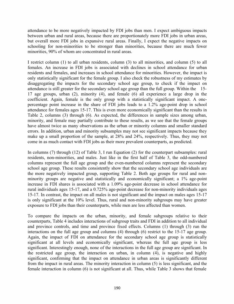
190

attendance to be more negatively impacted by FDI jobs than men. I expect ambiguous impacts between urban and rural areas, because there are proportionately more FDI jobs in urban areas, but overall more FDI jobs in expansive rural areas. Finally, I expect the negative impacts on schooling for non-minorities to be stronger than minorities, because there are much fewer minorities, 90% of whom are concentrated in rural areas.

I restrict column (1) to all urban residents, column (3) to all minorities, and column (5) to all females. An increase in FDI jobs is associated with declines in school attendance for urban residents and females, and increases in school attendance for minorities. However, the impact is only statistically significant for the female group. I also check the robustness of my estimates by disaggregating the impacts for the secondary school age group, to check if the impact on attendance is still greater for the secondary school age group than the full group. Within the 15- 17 age groups, urban (2), minority (4), and female (6) all experience a large drop in the coefficient. Again, female is the only group with a statistically significant impact. A one- percentage point increase in the share of FDI jobs leads to a 1.2% age-point drop in school attendance for females ages 15-17. This is even more economically significant than the results in Table 2, columns (3) through (6). As expected, the differences in sample sizes among urban, minority, and female may partially contribute to these results, as we see that the female groups have almost twice as many observations as the urban or minority columns and smaller standard errors. In addition, urban and minority subsamples may not see significant impacts because they make up a small proportion of the sample, at 28% and 24%, respectively. Thus, they may not come in as much contact with FDI jobs as their more prevalent counterparts, as predicted.

In columns (7) through (12) of Table 3, I run Equation (2) for the counterpart subsamples: rural residents, non-minorities, and males. Just like in the first half of Table 3, the odd-numbered columns represent the full age group and the even-numbered columns represent the secondary school age group. These results consistently show that the secondary school age individuals are the more negatively impacted group, supporting Table 2. Both age groups for rural and non- minority groups are negative and statistically and economically significant; a 1% age-point increase in FDI shares is associated with a 1.09% age-point decrease in school attendance for rural individuals ages 15-17, and a 0.725% age-point decrease for non-minority individuals ages 15-17. In contrast, the impact on all males is not significant and the impact on males ages 15-17 is only significant at the 10% level. Thus, rural and non-minority subgroups may have greater exposure to FDI jobs than their counterparts, while men are less affected than women.

To compare the impacts on the urban, minority, and female subgroups relative to their counterparts, Table 4 includes interactions of subgroup traits and FDI in addition to all individual and province controls, and time and province fixed effects. Columns (1) through (3) run the interactions on the full age group and columns (4) through (6) restrict to the 15-17 age group. Again, the impact of FDI on attendance for the secondary school age group is statistically significant at all levels and economically significant, whereas the full age group is less significant. Interestingly enough, none of the interactions in the full age group are significant. In the restricted age group, the interaction on urban, in column (4), is negative and highly significant, confirming that the impact on attendance in urban areas is significantly different from the impact in rural areas. The minority interaction in column (5) is less significant, and the female interaction in column (6) is not significant at all. Thus, while Table 3 shows that female

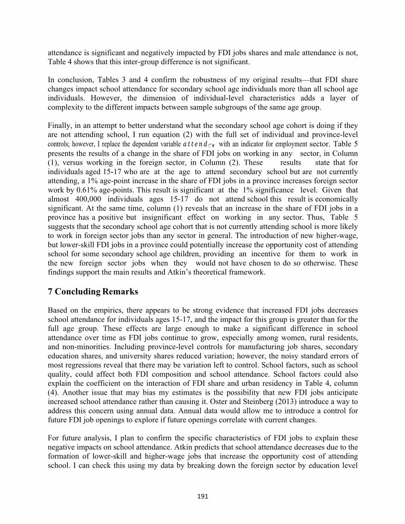
191

attendance is significant and negatively impacted by FDI jobs shares and male attendance is not, Table 4 shows that this inter-group difference is not significant.

In conclusion, Tables 3 and 4 confirm the robustness of my original results—that FDI share changes impact school attendance for secondary school age individuals more than all school age individuals. However, the dimension of individual-level characteristics adds a layer of complexity to the different impacts between sample subgroups of the same age group.

Finally, in an attempt to better understand what the secondary school age cohort is doing if they are not attending school, I run equation (2) with the full set of individual and province-level controls; however, I replace the dependent variable 𝑎 𝑡 𝑡𝑒𝑛 𝑑 !"# with an indicator for employment sector. Table 5 presents the results of a change in the share of FDI jobs on working in any sector, in Column (1), versus working in the foreign sector, in Column (2). These results state that for individuals aged 15-17 who are at the age to attend secondary school but are not currently attending, a 1% age-point increase in the share of FDI jobs in a province increases foreign sector work by 0.61% age-points. This result is significant at the 1% significance level. Given that almost 400,000 individuals ages 15-17 do not attend school this result is economically significant. At the same time, column (1) reveals that an increase in the share of FDI jobs in a province has a positive but insignificant effect on working in any sector. Thus, Table 5 suggests that the secondary school age cohort that is not currently attending school is more likely to work in foreign sector jobs than any sector in general. The introduction of new higher-wage, but lower-skill FDI jobs in a province could potentially increase the opportunity cost of attending school for some secondary school age children, providing an incentive for them to work in the new foreign sector jobs when they would not have chosen to do so otherwise. These findings support the main results and Atkin’s theoretical framework.

7 Concluding Remarks

Based on the empirics, there appears to be strong evidence that increased FDI jobs decreases school attendance for individuals ages 15-17, and the impact for this group is greater than for the full age group. These effects are large enough to make a significant difference in school attendance over time as FDI jobs continue to grow, especially among women, rural residents, and non-minorities. Including province-level controls for manufacturing job shares, secondary education shares, and university shares reduced variation; however, the noisy standard errors of most regressions reveal that there may be variation left to control. School factors, such as school quality, could affect both FDI composition and school attendance. School factors could also explain the coefficient on the interaction of FDI share and urban residency in Table 4, column (4). Another issue that may bias my estimates is the possibility that new FDI jobs anticipate increased school attendance rather than causing it. Oster and Steinberg (2013) introduce a way to address this concern using annual data. Annual data would allow me to introduce a control for future FDI job openings to explore if future openings correlate with current changes.

For future analysis, I plan to confirm the specific characteristics of FDI jobs to explain these negative impacts on school attendance. Atkin predicts that school attendance decreases due to the formation of lower-skill and higher-wage jobs that increase the opportunity cost of attending school. I can check this using my data by breaking down the foreign sector by education level

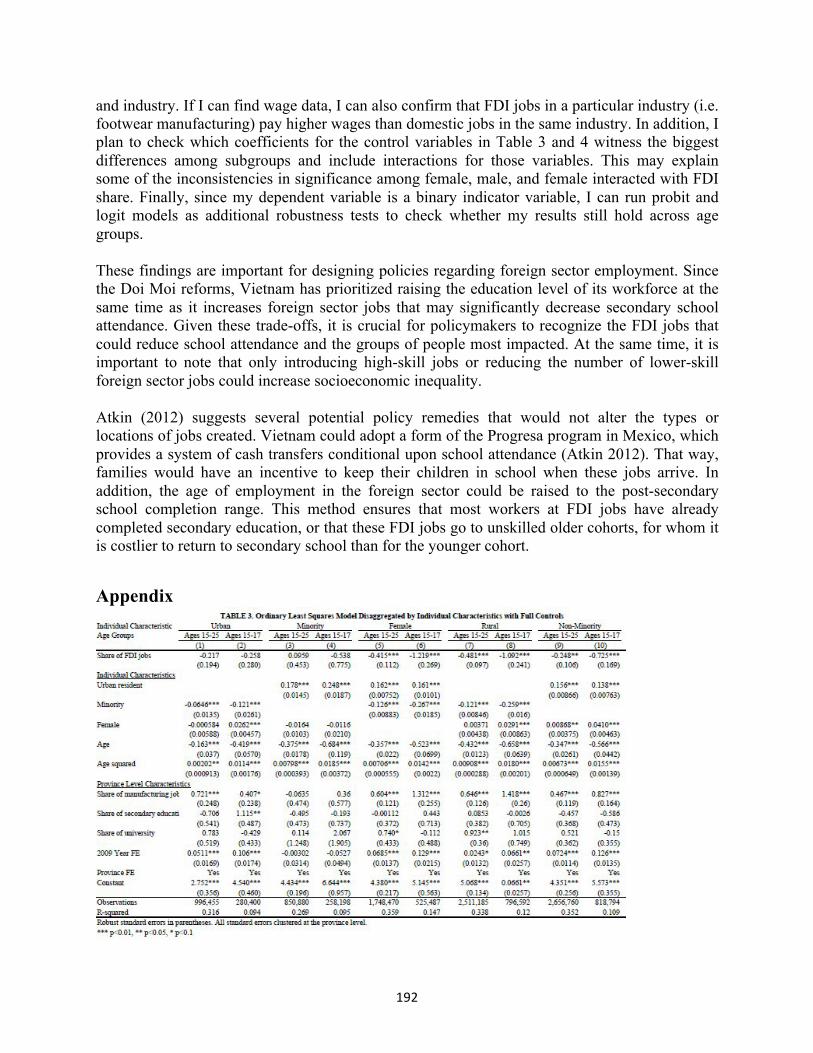
192

and industry. If I can find wage data, I can also confirm that FDI jobs in a particular industry (i.e. footwear manufacturing) pay higher wages than domestic jobs in the same industry. In addition, I plan to check which coefficients for the control variables in Table 3 and 4 witness the biggest differences among subgroups and include interactions for those variables. This may explain some of the inconsistencies in significance among female, male, and female interacted with FDI share. Finally, since my dependent variable is a binary indicator variable, I can run probit and logit models as additional robustness tests to check whether my results still hold across age groups.

These findings are important for designing policies regarding foreign sector employment. Since the Doi Moi reforms, Vietnam has prioritized raising the education level of its workforce at the same time as it increases foreign sector jobs that may significantly decrease secondary school attendance. Given these trade-offs, it is crucial for policymakers to recognize the FDI jobs that could reduce school attendance and the groups of people most impacted. At the same time, it is important to note that only introducing high-skill jobs or reducing the number of lower-skill foreign sector jobs could increase socioeconomic inequality.

Atkin (2012) suggests several potential policy remedies that would not alter the types or locations of jobs created. Vietnam could adopt a form of the Progresa program in Mexico, which provides a system of cash transfers conditional upon school attendance (Atkin 2012). That way, families would have an incentive to keep their children in school when these jobs arrive. In addition, the age of employment in the foreign sector could be raised to the post-secondary school completion range. This method ensures that most workers at FDI jobs have already completed secondary education, or that these FDI jobs go to unskilled older cohorts, for whom it is costlier to return to secondary school than for the younger cohort.

Appendix

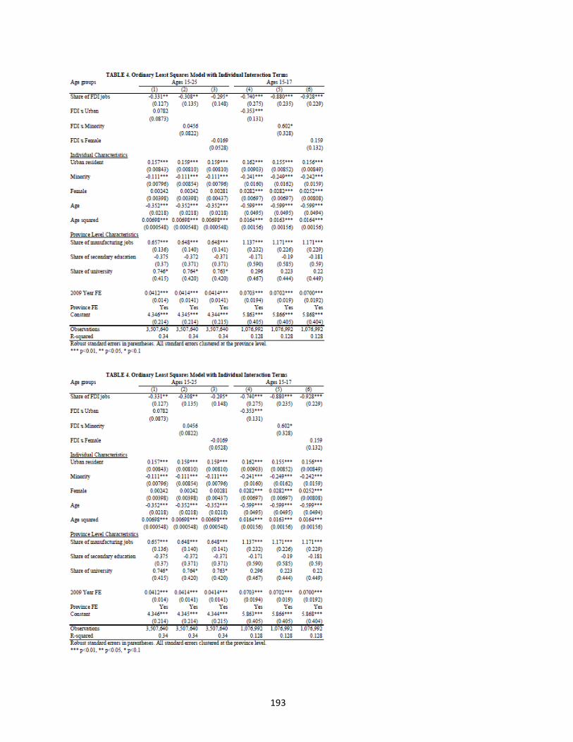
193

194

Bibliography

Aizenman, Joshua. “Volatility, Employment, and the Patterns of FDI in Emerging Markets” NBER Papers December 2002. Web.

Al Nasser, O. M. 2007, “The Determinants of the U.S. Foreign Direct Investment: Does the Region Matter?” Global

Economic Review 07 March 2007: 37-51. Web.

Atkin, David. 2011, “Working for the Future: Female Factory Work and Child Health in Mexico.” MIT April 2009. Web.

Atkin, David. “Endogenous Skill Acquisition and Export Manufacturing in Mexico.” MIT December 2015. Web.

Borensztein, E., De Gregorio, J., and Lee, J. W. “How Does Foreign Investment Affect Growth?”, Journal of International Economics 01 June 1998:115-135. Web.

Freeman, N. J.. “Harnessing Foreign Direct Investment for Economic Development and Poverty Reduction.”

Journal of the Asia Pacific Economy 04 June 2010: 209-222. Web.

Hewett, P., and Amin, S.. “Assessing the Impact of Garment Work on Quality of Life Measures.” Population Council 2000. Web.

Hoang, Thu Thi, Paitoon Wiboonchutikula, and Bangorn Tubtimtong. “Does Foreign Direct Investment Promote

Economic Growth in Vietnam?”.ASEAN Economic Bulletin 27.3 (2010): 295–311. Web.

McCaig, Brian and Pavcnik, Nina. “Moving Out of Agriculture: Structural Change in Vietnam.” NBER November 2013. Web.

McCaig, Brian and Pavcnik, Nina, 2015, “Informal Employment in a Growing and Globalizing Low-Income

Country,” American Economic Review May 2015: 545-550. American Economic Association. Web.

Oster, Emily and Millett, M. B.. “Do Call Centers Promote School Enrollment? Evidence from India.” Journal of Development Economics Sept 2013: 123-135. Web.

Priwitzer, Kerstin, 2007, “Gender Practices in Contemporary Vietnam.” International Quarterly for Asian Studies

2007: 206. Internationales Asien Forum. Web.

Wang, Miao and Wong, M.C.. “FDI, Education, and Economic Growth: Quality Matters.” International Atlantic Economic Society 2011: 103-115. Web.

195

International Business Cycle Transmissions and News Shocks

Yingtong Xie

Macalester College

Abstract

This paper examines how news shocks affect the business cycle comovements across countries. In the context of a dynamic stochastic general equilibrium model with Jaimovich-Rebelo (Jaimovich and Rebelo 2009) preferences, I use Bayesian estimation on data for the U.S. and Mexico from 1950 to 2010. The results show that there is evidence of comovements of business cycles across the two countries. While including news shocks appear to overestimate the aggregate fluctuations, it explains the across- country comovements better than the standard covariance matrix model. It implies that news shocks as a channel of business cycle transmissions deserves further investigation, possibly through modifications on the model and expanding estimations to other country pairs.

1 Introduction

The process of globalization has highlighted the interdependence among world economies. Economic fluctuations in one country can trigger those in another country—they can spill over to neighboring nations or even reach geographically distant places. This phenomenon is known as the international business cycle comovement or the synchronization of business cycles. One good example would be the Financial Crisis in 2008. The depression occurring in the U.S. greatly influenced the economies in Europe and spread around the world. It would be reasonable to consider that the resulting business cycle fluctuations across countries are dependent of each other.

During the 2008 financial crises, different agents’ anticipation also had an impact. Investors built their decisions on their anticipation which affected the capital flows across countries and potentially determined the future of certain financial institutions. Firms also have incentives to anticipate the market’s future demands. This is related to the studies on how news, or anticipated shocks, contribute to business cycle fluctuations. However, most of these studies concentrate in domestic environments.

In this paper, I take both streams of the literature and track whether news shocks work as transmission channels for business cycle comovements. In other words, I want to see how anticipation or beliefs on productivity shocks of a foreign country affect the domestic business cycle. The goal of this paper is to see the effects of news shocks on business cycle transmissions using the U.S. and Mexico as examples.

196

2 Estimation Results

To test the effects of news shocks on business cycles transmissions, I choose the country pair of the U.S. and Mexico from 1950 to 2010. Since this paper is only the first step to test the effect of news shocks on international business cycle transmission, I did not incorporate the trade effects, interest rates, or other frictions in the model.

Since quarterly per capita data are not available for Mexico, I used the annual data instead. This also implies a minor modification to our news shock equations: in our model, I assumed quarterly GDP data, which makes four periods of anticipated news shocks reasonable. With annual data, I adjusted to a simple, 1 period of anticipated news shock (implying that agents are only going to receive news at most for one year ahead in the current period).

I have implemented the log-linearized version of the model (where calculation process can be found in the appendix) which means that all observables are in percent deviations from steady state. The observables used in the estimations are percent deviations of real GDP per capita, corresponding consumption ratio, and per capita total hours worked ratio. All of them are accompanied by measurement error terms. Although the standard model presumed a mutual effect from news shocks, my particular country choice led me to think that the news shocks on Mexican economy are not going to affect the U.S. consumers’ behavior. Therefore, for this paper, the effect of news shocks only took on one direction as from the U.S. to Mexico, where

𝑧!!" = 1− 𝜌!" + 𝜌!"𝑧!!!!" + 𝜇!!" with

𝜇!!" = 𝐸!,!!,!" + 𝐸!,!!!

!,!" and

𝑧!!"# = 1− 𝜌!"# + 𝜌!"#𝑧!!!!"# + 𝜇!!"# with

𝜇!!"# = 𝐸!,!!,!"# + 𝐸!,!!!

!,!"# + 𝐸!,!!!!,!"

For estimation results, I ran 500,000 repetitions with 3 chains. Parameters such as α, β followed the majority of studies where α is set to be 0.64 and β = 0.99. Then the first pair of parameters was the depreciation rates. I kept the annual depreciation rate of capital in the U.S. to be 8% with standard deviation of 2% under a beta distribution. I also assumed that the Mexican capital depreciation rate is higher, which I set with an annual rate of 12%, 2% standard deviation under a beta distribution. The persistence of TFP, namely ρ, took on values of 0.95 for the U.S. and 0.90 for Mexico. For the other two pairs of parameters, ψ and θ, I followed the paper by Jaimovich and Rebelo (2009), so I set both ψ = 5.1755 and both θ = 1.4. The two σ are set to be 1.0001 to correspond to near logarithmic utility. The posterior mean for the depreciation rates came out to be 6.9% and 8.67%, respectively. The persistence of TFP for the US and Mexico has posterior mean of 0.438 and 0.496, respectively. Both values are much lower than my priors. The estimated values of ψ are very close to the calibrated value from Jaimovich—Rebelo (2009), which came out to be 5.184 and 5.172. On the other hands, the posterior means of two θs are much larger, with the U.S. to be 4.048 and Mexico to be 4.083.

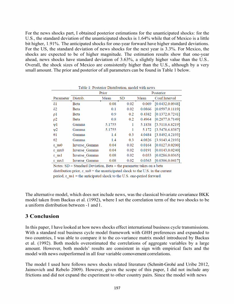
197

For the news shocks part, I obtained posterior estimations for the unanticipated shocks: for the U.S., the standard deviation of the unanticipated shocks is 1.64% while that of Mexico is a little bit higher, 1.91%. The anticipated shocks for one-year forward have higher standard deviations. For the US, the standard deviation of news shocks for the next year is 3.3%. For Mexico, the shocks are expected to be of higher magnitude. The estimation results show that one-year ahead, news shocks have standard deviation of 3.63%, a slightly higher value than the U.S.. Overall, the shock sizes of Mexico are consistently higher than the U.S., although by a very small amount. The prior and posterior of all parameters can be found in Table 1 below.

The alternative model, which does not include news, was the classical bivariate covariance BKK model taken from Backus et al. (1992), where I set the correlation term of the two shocks to be a uniform distribution between -1 and 1.

3 Conclusion

In this paper, I have looked at how news shocks effect international business cycle transmissions. With a standard real business cycle model framework with GHH preferences and expanded to two countries, I was able to compare it to the co-variance matrix model introduced by Backus et al. (1992). Both models overestimated the correlations of aggregate variables by a large amount. However, both models’ results are consistent in sign with empirical facts and the model with news outperformed in all four variable comovement correlations.

The model I used here follows news shocks related literature (Schmitt-Grohé and Uribe 2012, Jaimovich and Rebelo 2009). However, given the scope of this paper, I did not include any frictions and did not expand the experiment to other country pairs. Since the model with news

198

performed better, it is worth further pursuing through, for example, adding news shocks on growth or adding a government sector.

Another step could be to look for adding trade relations, based on recent literature. In other words, future research can add a trade element to consumption rule so that households from country A also consume goods from country B. In this way, we can test the effect of news shocks from a trade perspective, which could be more precise.

In general, the results from this paper are not conclusive, although I have shown that the news shock model is better than the simple BKK covariance matrix model in explaining international business cycle transmissions.

Bibliography

Backus, David K., Patrick J. Kehoe, and Finn E. Kydland. 1992. “International real business cycles”. Journal of

PoliticalEconomy. 100(1): 745-775.

Beaudry, Paul, Martial Dupaigne , and Franck Portier. 2008. “The International Propa- gation of News Shocks”. mimeo.1-37.

Beaudry, Paul, and Franck Portier. 2014. “News-driven business cycles: insights and challenges”. Journal of

EconomicLiterature.52(4): 993-1074.

Canova, Fabio. 2005. “The transmission of US shocks to Latin America”. Journal of Applied Econometrics.20(2): 229- 251.

Greenwood, Jeremy, Zvi Hercowitz and Gregory W. Huffman. 1988. “Investment, Capac- ity Utilization, and the Real

Business Cycle”. The American Economic Review. 78(3): 402-417.

Jaimovich, Nir and Sergio Rebelo. 2009. “Can News about the Future Drive the Business Cycle”. American Economic Review. 99(4): 1097-1118.

Kamber, Gunes, Konstantinos Theodoridis, and Christoph Thoenissen. 2014. “News-driven Business Cycles in Small

Open Economies”. CAMA Working Paper. 1-50.

Kandil, Magda. 2009. “Spillover Effects of U.S. Business Cycles on Latin America and the Caribbean”. Journal of Economic Issues. 43(4): 971-996.

Kose, M.Ayhan, and Kei-Mu Yi. 2005. “Can the Standard International Business Cycle Model Explain the Relation

between Trade and Comovement”. Journal of International Economics. 66:267-295.

Schmitt-Groh´e, Stephanie. 1997. “The international Transmission of Economic Fluc- tuations: Effects of U.S. Business Cycles on the Canadian Economy”. Journal of International Economics. 44: 257-287.

Schmitt-Groh´e, Stephanie and Martin Uribe. 2012. “What’s News in Business Cycles”.Econometrica. 80(6): 2733-

2764.

199

MAYBE I’LL SAVE A BIT MORE: ISOLATING THE CAUSE OF LOW BORROWING RATES

AMONG BEIJING’S URBAN MICRO-ENTERPRISES

THOMAS CHRISTIANSEN

Georgetown University

ABSTRACT

Historically, micro-enterprises in China’s urban areas have struggled to obtain capital through the formal financial system in part because these firms often lack the relational and reputational clout with banks that larger firms enjoy. Specifically, this paper hopes to evaluate whether bank reforms designed to help micro-enterprises beginning in 2010 have succeeded in penetrating into the micro-enterprise sector. This paper uses interview data collected by the author from 50 micro-enterprises in Beijing to evaluate why micro-enterprises do or do not apply for and/or receive bank loans, and where they go to find financing instead. From these analyses, this paper concludes that these reforms have largely failed—micro-enterprises still do not consider bank loans to be a viable source for investment capital, and many firms never even consider borrowing from banks at all. As a result, this paper concludes that more reforms are necessary at the bottom of the market in order to more fully empower China’s smallest shop owners.

200

1 Introduction Following the 2008 financial crisis, and in response to the growing threat that the informal banking sector posed to China’s macro economy (Hong 2014), the Chinese government introduced a series of banking reforms to financially include micro-enterprise and other borrowers (Sparreboom and Duflos 2012). These reforms have attempted to standardize the credit reporting system for micro-enterprises, provide lender’s insurance for certain types of loans, and develop new financial instruments for reducing risk in loans to smaller clients. These reforms coalesced in 2011 when China’s China Banking Regulatory Commission (CBRC)—that nation’s equivalent of the Federal Reserve—issued a series of rules, regulations, policies and suggestions to help overcome the formal banking barriers that have in part kept micro-enterprises from seeking capital through the banking sector (CBRC 2011b).

These reforms, however, only formally address one of four problems that prevent micro- enterprises from obtaining capital through the banking system—namely, they force banks to offer loan products and services suitable to micro-enterprises. This paper hopes to examine the degree to which these reforms actually impacted the reality of financial access for urban micro- enterprises: do these firms now obtain loans through the formal banking system, or are they still prevented from borrowing from banks for one or multiple of the following reasons: lack of social ties to banks, hukou registration status, or cultural stigmas against borrowing? This paper conducted 47 interviews with micro-enterprise owners in Beijing in 2013 in order to evaluate this question.

From those interviews, this paper concludes that micro-enterprise owners who might otherwise desire or benefit from a bank loan still largely do not obtain finance from banks because of lingering misperceptions about the banking system among micro-enterprise owners, especially among those that did not have Beijing hukou registration status. According to this study, a vast majority of those firms that might otherwise seek and qualify for bank loans do not even consider applying because they presume that their application will be denied. Among those firm owners that do not enjoy Beijing residency, these misperceptions are even stronger. Likewise, these trends particularly hold among the younger generation of business owners regardless of their hukou status. Finally, these results have two obvious policy implications: (1) the CBRC should relax restrictions on hukou status for obtaining major loans from banks, and (2) banks and their counterparts in the CBRC need to make a more concerted effort to not only change the formal procedures for obtaining loans from banks, but also change the perceptions that micro businesses maintain about the banking sector.

2 Literature Review

In China, most banks—both large and small—have historically overlooked micro-enterprises as viable loan candidates. Even those banks historically tasked with providing loans to urban micro- enterprises (as well as rural borrowers), such as the Agricultural Bank of China, have largely failed to do so (Geraci et al 2010). In most instances, then, micro-enterprises in China have struggled to contact the formal banking system or to obtain a satisfactory loan (in terms of loan size, payment schedule, or interest rate charged) from those banks (Sparreboom and Duflos 2012). Furthermore, throughout the 1990s and first years of the 21st Century, as larger

201

macroeconomic reforms transformed the banking industry, micro-enterprises continued to suffer from widespread credit rationing caused by a lack of collateral, available credit information, a lack of economies of scale, and political risks to lending to private micro-enterprises (Mu 2002). These barriers, furthermore, had a considerable deleterious impact throughout the Chinese economy during that period: as in most developing economies, a considerable proportion of China’s lower class—particularly in urban areas—are employed in micro-enterprises. Despite the importance of micro-enterprises from a development perspective, the China Banking Regulatory Commission (CBRC), China’s primary bank regulatory agency, devalued their importance throughout the first decade of the 20th Century, lumping micro-enterprises into the same category as Small and Medium Enterprises (SMEs) for the purposes of analysis and policy making (Sparreboom and Duflos 2012).

Despite initially ignoring micro-enterprises, increased pressure from development economists led the CBRC in 2011 implemented a series of reforms aimed at assisting micro-enterprises in obtaining greater access to banking services and financial markets (CBRC 2011b). These reforms began with the CBRC formally recognizing the existence of micro-enterprises as a meaningful economic category apart from SMEs. The CBRC went on to instruct China’s banks to give priority to distributing loans to small and micro-enterprises, improve financial service mechanisms for these firms, and promote favorable fiscal and tax policies for both these firms as well as those banks that successfully retool their loan products to cater to these firms’ unique needs (CBRC 2011b). Because these reforms took place relatively recently, however, little reliable data exists to determine their impact on loan provision to small and micro-enterprises. This paper hopes to fill this present gap in data relevant to this question by analyzing 47 interviews with micro-enterprise owners in Beijing conducted in Fall 2013.

These reforms have gone far in addressing many of the legal and bank institutional impediments to bank loan acquisition by micro-enterprises (Sparreboom and Duflos 2012). In addition to these barriers, however, micro-enterprises must also struggle with three other major obstacles: (1) informal social ties that they use to substitute for lack of social capital in the formal financial system, (2) hukou residency status that does not match the firm location, and (3) cultural stigmas to borrowing in China.

Guanxi, or “relationships,” has played a historically important role in Chinese business and politics. Emerging from Confucian concepts that emphasize the importance of hierarchical social relations founded in mutual respect and honor, guanxi has evolved to describe a complex network of interwoven social connections often founded on family or geographic ties and strengthened by frequent, mutual back scratching (Yu 2009). Guanxi, furthermore, has played a well-documented, prominent role in financial allocation in China. In the years following the 1978 reforms, most SOEs used social connections through the Communist Party to obtain cheap capital from China’s nationalized banking system (Naughton 2007). As recently as 2009, a majority of firms in China still reported obtaining capital primarily through these social connections (Hussain et al 2010). Micro-enterprise owners, however, rarely have the social connections necessary to obtain favorable conditions for bank loans (Bai 2010). For this reason, most micro-enterprises still either turn to friends and family (their own guanxi) for new capital or else they do not obtain capital at all (Bai 2010).

202

Hukou registration status likewise plays a critical role in preventing many urban micro- enterprises from obtaining loans from banks. China shares with North Korea the distinction of being one of only two countries on earth to maintain an internal registry system for citizens based on province and municipality type of their birth (Cai 2011). This hukou system identifies where an individual was born, whether Beijing or a village in Shaanxi province. More importantly, it determines whether an individual can receive certain social benefits such as full health care, priority access to public education, or entry into a municipality’s banking system (Liu 2010). Originally designed to slow and control China’s rapid rural-urban migration, this system now largely serves to block migrants from obtaining benefits enjoyed by life-long residents of China’s richest urban areas (Cai 2011). Furthermore, switching hukou can be both incredibly difficult and very costly—many migrants do not even attempt to switch (Cai 2011). Because migrants constitute a plurality of urban micro-entrepreneurs, they face this additional barrier to obtaining loans (Hu and Wu 2012).

Finally, Chinese cultural stigmas against borrowing often reduce a firm’s likelihood of seeking capital through formal financial channels (Turvey et al 2010). These stigmas emerge out of the perceived nefariousness of institutions charging usurious interest rates on loans and is strengthened by the perception that capital needs should be met through borrowing from friends and family (Turvey et al 2010). These stigmas reflect a broader distrust of impersonal institutions and the corollary reflexive reliance on the relationships that traditionally dominated Chinese society (Yu 2009). These stigmas have also contributed to the incredibly high volume of informal loans in China, with some studies indicating that loans among friends and family account for over 75% of all loans that take place in China (Huo and Qu 2005). Because these cultural stigmas are nebulous by definition and even more difficult to identify through data, this paper will attempt to use interviews to evaluate cultural biases against borrowing.

3 Interview Methodology

Interview Questions The claims I make in this paper find support from 50 long-form, open-ended interviews that I conducted with micro-entrepreneurs in Beijing in mid-October to mid-December, 2013. From these 50 interviews I removed three from final consideration because these firms evaded answering questions critical for addressing this paper’s research hypotheses, leaving me with 47 surveys to evaluate. Although 50 interviews far from constitute an ideal sample size for deductive approach that guides quantitative research, this sample size is roughly double the sample size recommended for most papers guided by inductive reasoning (Adler and Adler 2012). Furthermore, having 50 interviews provides more than enough support for the limited conclusions that this paper will draw about the availability of finance to micro-enterprises, as well as to the role that guanxi still plays in accessing finance for these firms.

In order to understand how guanxi influences micro-enterprises’ ability to obtain access to bank financing, respondents were asked questions in four categories: (1) firm and loan characteristics, (2) demographic characteristics of the firm owner, (3) awareness of alternative financial products, and (4) questions about firm owner willingness to participate in free business classes. First, and foremost, these interviews asked these owners a variety of questions concerning past and present business practices, current financial stability, their desires to invest in their business,

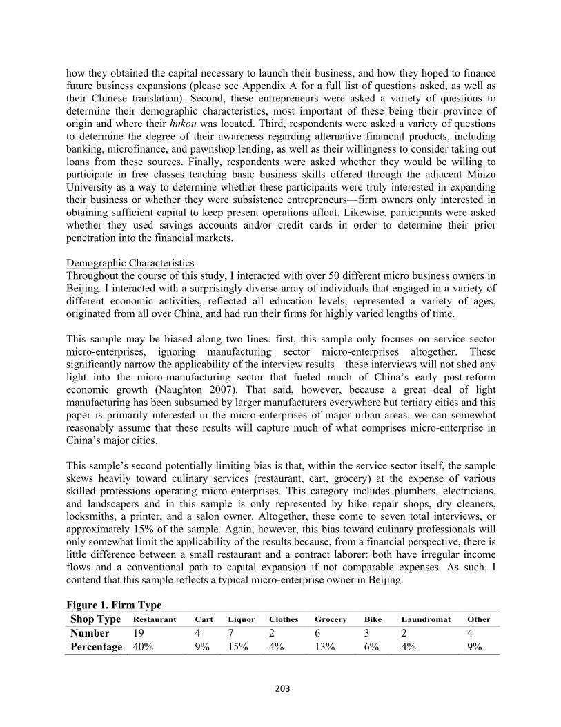
203

how they obtained the capital necessary to launch their business, and how they hoped to finance future business expansions (please see Appendix A for a full list of questions asked, as well as their Chinese translation). Second, these entrepreneurs were asked a variety of questions to determine their demographic characteristics, most important of these being their province of origin and where their hukou was located. Third, respondents were asked a variety of questions to determine the degree of their awareness regarding alternative financial products, including banking, microfinance, and pawnshop lending, as well as their willingness to consider taking out loans from these sources. Finally, respondents were asked whether they would be willing to participate in free classes teaching basic business skills offered through the adjacent Minzu University as a way to determine whether these participants were truly interested in expanding their business or whether they were subsistence entrepreneurs—firm owners only interested in obtaining sufficient capital to keep present operations afloat. Likewise, participants were asked whether they used savings accounts and/or credit cards in order to determine their prior penetration into the financial markets.

Demographic Characteristics Throughout the course of this study, I interacted with over 50 different micro business owners in Beijing. I interacted with a surprisingly diverse array of individuals that engaged in a variety of different economic activities, reflected all education levels, represented a variety of ages, originated from all over China, and had run their firms for highly varied lengths of time.

This sample may be biased along two lines: first, this sample only focuses on service sector micro-enterprises, ignoring manufacturing sector micro-enterprises altogether. These significantly narrow the applicability of the interview results—these interviews will not shed any light into the micro-manufacturing sector that fueled much of China’s early post-reform economic growth (Naughton 2007). That said, however, because a great deal of light manufacturing has been subsumed by larger manufacturers everywhere but tertiary cities and this paper is primarily interested in the micro-enterprises of major urban areas, we can somewhat reasonably assume that these results will capture much of what comprises micro-enterprise in China’s major cities.

This sample’s second potentially limiting bias is that, within the service sector itself, the sample skews heavily toward culinary services (restaurant, cart, grocery) at the expense of various skilled professions operating micro-enterprises. This category includes plumbers, electricians, and landscapers and in this sample is only represented by bike repair shops, dry cleaners, locksmiths, a printer, and a salon owner. Altogether, these come to seven total interviews, or approximately 15% of the sample. Again, however, this bias toward culinary professionals will only somewhat limit the applicability of the results because, from a financial perspective, there is little difference between a small restaurant and a contract laborer: both have irregular income flows and a conventional path to capital expansion if not comparable expenses. As such, I contend that this sample reflects a typical micro-enterprise owner in Beijing.

Figure 1. Firm Type Shop Type Restaurant Cart Liquor Clothes Grocery Bike Laundromat Other

Number 19 4 7 2 6 3 2 4 Percentage 40% 9% 15% 4% 13% 6% 4% 9%

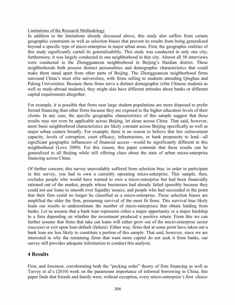
204

Limitations of the Research Methodology In addition to the limitations already discussed above, this study also suffers from certain geographic constraints as well as selection biases that prevent its results from being generalized beyond a specific type of micro-enterprise in major urban areas. First, the geographic realities of this study significantly curtail its generalizability. This study was conducted in only one city; furthermore, it was largely conducted in one neighborhood in that city. Almost all 50 interviews were conducted in the Zhongguancun neighborhood in Beijing’s Haidian district. These neighborhoods both possess distinct personalities and demographic characteristics that could make them stand apart from other parts of Beijing. The Zhongguancun neighborhood firms surround China’s most elite universities, with firms selling to students attending Qinghua and Peking Universities. Because these firms serve a distinct demographic (elite Chinese students as well as study-abroad students), they might also have different attitudes about banks or different capital requirements altogether.

For example, it is possible that firms near large student populations are more disposed to prefer formal financing than other firms because they are exposed to the higher education levels of their clients. In any case, the specific geographic characteristics of this sample suggest that these results may not even be applicable across Beijing, let alone across China. That said, however, more basic neighborhood characteristics are likely constant across Beijing specifically as well as major urban centers broadly. For example, there is no reason to believe that law enforcement capacity, levels of corruption, court efficacy, infrastructure, or bank propensity to lend—all significant geographic influencers of financial access—would be significantly different in this neighborhood (Love 2009). For this reason, this paper contends that these results can be generalized to all Beijing while still offering clues about the state of urban micro-enterprise financing across China.

Of further concern, this survey unavoidably suffered from selection bias: in order to participate in this survey, you had to own a currently operating micro-enterprise. This sample, then, excludes people who would have wanted to own a micro-enterprise but had been financially rationed out of the market, people whose businesses had already failed (possibly because they could not use loans to smooth over liquidity issues), and people who had succeeded to the point that their firm could no longer be classified as a micro-enterprise. These selection biases are amplified the older the firm, presuming survival of the most fit firms. This survival bias likely leads our results to underestimate the number of micro-enterprises that obtain lending from banks. Let us assume that a bank loan represents either a major opportunity or a major hardship to a firm depending on whether the investment produced a positive return. From this we can further assume that firms that take out loans will either grow out of the micro-enterprise sector (success) or exit upon loan default (failure). Either way, firms that at some point have taken out a bank loan are less likely to constitute a portion of this sample. That said, however, since we are interested in why the remaining firms that want more capital do not seek it from banks, our survey still provides adequate information to conduct this analysis.

4 Results

First, and foremost, corroborating both the “pecking order” theory of firm financing as well as Turvey et al’s (2010) work on the paramount importance of informal borrowing in China, this paper finds that friends and family were, without exception, every micro-enterprise’s first choice

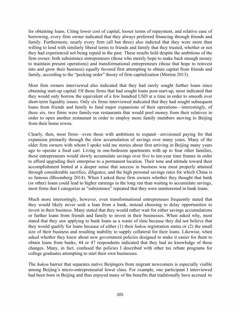
205

for obtaining loans. Citing lower cost of capital, looser terms of repayment, and relative ease of borrowing, every firm owner indicated that they always preferred financing through friends and family. Furthermore, nearly every firm (all but three) also indicted that they were more than willing to lend with similarly liberal terms to friends and family that they trusted, whether or not they had experienced not being repaid in the past. These results held despite the ambitions of the firm owner; both subsistence entrepreneurs (those who merely hope to make back enough money to maintain present operations) and transformational entrepreneurs (those that hope to reinvest into and grow their business) equally favored first attempting to obtain capital from friends and family, according to the “pecking order” theory of firm capitalization (Morton 2013).

Most firm owners interviewed also indicated that they had rarely sought further loans since obtaining start-up capital. Of those firms that had sought loans post-start-up, most indicated that they would only borrow the equivalent of a few hundred USD at a time in order to smooth over short-term liquidity issues. Only six firms interviewed indicated that they had sought subsequent loans from friends and family to fund major expansions of their operations—interestingly, of these six, two firms were family-run restaurants that would pool money from their relatives in order to open another restaurant in order to employ more family members moving to Beijing from their home towns.

Clearly, then, most firms—even those with ambitions to expand—envisioned paying for that expansion primarily through the slow accumulation of savings over many years. Many of the older firm owners with whom I spoke told me stories about first arriving in Beijing many years ago to operate a food cart. Living in one-bedroom apartments with up to four other families, these entrepreneurs would slowly accumulate savings over five to ten-year time frames in order to afford upgrading their enterprise to a permanent location. Their tone and attitude toward their accomplishment hinted at a deeper sense that success in business was most properly attained through considerable sacrifice, diligence, and the high personal savings rates for which China is so famous (Bloomberg 2014). When I asked these firm owners whether they thought that bank (or other) loans could lead to higher earnings in the long run than waiting to accumulate savings, most firms that I categorize as “subsistence” repeated that they were uninterested in bank loans.

Much more interestingly, however, even transformational entrepreneurs frequently stated that they would likely never seek a loan from a bank, instead choosing to delay opportunities to invest in their business. Many stated that they would rather wait for either savings accumulations or further loans from friends and family to invest in their businesses. When asked why, most stated that they saw applying to bank loans as a waste of time because they did not believe that they would qualify for loans because of either (1) their hukou registration status or (2) the small size of their business and resulting inability to supply collateral for their loans. Likewise, when asked whether they knew about new government policies designed to make it easier for them to obtain loans from banks, 44 or 47 respondents indicated that they had no knowledge of these changes. Many, in fact, confused the policies I described with other tax rebate programs for college graduates attempting to start their own businesses.

The hukou barrier that separates native Beijingers from migrant newcomers is especially visible among Beijing’s micro-entrepreneurial lower class. For example, one participant I interviewed had been born in Beijing and thus enjoyed many of the benefits that traditionally have accrued to

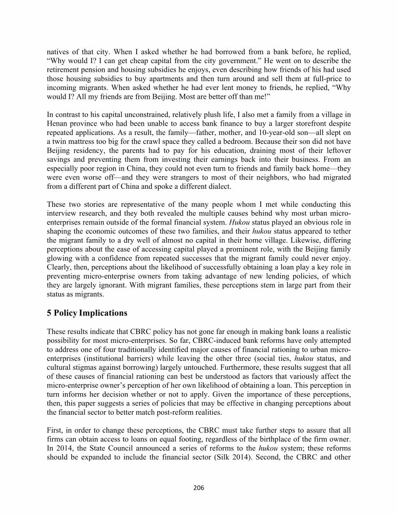
206

natives of that city. When I asked whether he had borrowed from a bank before, he replied, “Why would I? I can get cheap capital from the city government.” He went on to describe the retirement pension and housing subsidies he enjoys, even describing how friends of his had used those housing subsidies to buy apartments and then turn around and sell them at full-price to incoming migrants. When asked whether he had ever lent money to friends, he replied, “Why would I? All my friends are from Beijing. Most are better off than me!”

In contrast to his capital unconstrained, relatively plush life, I also met a family from a village in Henan province who had been unable to access bank finance to buy a larger storefront despite repeated applications. As a result, the family—father, mother, and 10-year-old son—all slept on a twin mattress too big for the crawl space they called a bedroom. Because their son did not have Beijing residency, the parents had to pay for his education, draining most of their leftover savings and preventing them from investing their earnings back into their business. From an especially poor region in China, they could not even turn to friends and family back home—they were even worse off—and they were strangers to most of their neighbors, who had migrated from a different part of China and spoke a different dialect.

These two stories are representative of the many people whom I met while conducting this interview research, and they both revealed the multiple causes behind why most urban micro- enterprises remain outside of the formal financial system. Hukou status played an obvious role in shaping the economic outcomes of these two families, and their hukou status appeared to tether the migrant family to a dry well of almost no capital in their home village. Likewise, differing perceptions about the ease of accessing capital played a prominent role, with the Beijing family glowing with a confidence from repeated successes that the migrant family could never enjoy. Clearly, then, perceptions about the likelihood of successfully obtaining a loan play a key role in preventing micro-enterprise owners from taking advantage of new lending policies, of which they are largely ignorant. With migrant families, these perceptions stem in large part from their status as migrants.

5 Policy Implications

These results indicate that CBRC policy has not gone far enough in making bank loans a realistic possibility for most micro-enterprises. So far, CBRC-induced bank reforms have only attempted to address one of four traditionally identified major causes of financial rationing to urban micro- enterprises (institutional barriers) while leaving the other three (social ties, hukou status, and cultural stigmas against borrowing) largely untouched. Furthermore, these results suggest that all of these causes of financial rationing can best be understood as factors that variously affect the micro-enterprise owner’s perception of her own likelihood of obtaining a loan. This perception in turn informs her decision whether or not to apply. Given the importance of these perceptions, then, this paper suggests a series of policies that may be effective in changing perceptions about the financial sector to better match post-reform realities.

First, in order to change these perceptions, the CBRC must take further steps to assure that all firms can obtain access to loans on equal footing, regardless of the birthplace of the firm owner. In 2014, the State Council announced a series of reforms to the hukou system; these reforms should be expanded to include the financial sector (Silk 2014). Second, the CBRC and other

207

banks must play a more proactive role in advertising newly available loan products to potential micro-enterprise customers, especially in urban areas.

As a final suggestion, the very small, migrant-owned micro-enterprises comprising this survey are generally underserved in the banking sector partially because they are not analyzed as a category separate from much larger “micro-enterprises.” At present, according to the CBRC, micro-enterprises are defined as firms with annual revenues less than 2 Million RMB (~$330,000 USD); the largest reported annual revenue for any firm contacted for this survey was 180,000 RMB (~$30,000 USD). Much smaller than even many “micro-enterprises,” and facing additional barriers to finance caused by hukou status, these firms largely exist outside the radar of banks and bank regulators. New research should be conducted to determine whether and how to appropriately evaluate this special class of low-income firms that often must operate on subsistence incomes because of their gross inability to access liquid capital. A welcoming first step would be to create a new analytical category for such firms.

6 Conclusions

This paper has asked a concrete question—did the CBRC’s 2011 reforms succeed in making bank finance available to micro-enterprises—and delivered a concrete answer. That answer, to repeat, is that these reforms failed because they only removed technical barriers to finance without attempting to convince micro-enterprise owners that applying for a bank loan would no longer be a waste of their time. In addition, hukou status sill bars most micro-enterprise owners from obtaining bank capital outside their home village. Ironically, then, those same owners actually do return to their villages in order to obtain necessary capital from friends and family, even many years after having left the village. Because these owners refuse to integrate into their new, relatively capital-rich urban environments, the lower ceiling on their borrowing power perennially cripples their growth prospects, with broader economic consequences for urban development.

208

7 Bibliography

Bai, Chengyu. “Chinese Microfinance Networks and Cooperation Patterns.” Microfinance in China. Edited by Pete Sparreboom and Vidhi Tambiah. World Microfinance Forum Geneva, 2010. http://www.microfinanceforum.org/wp-content/uploads/2012/03/ChinaCompendium-eVersion.pdf

Beck, Thorsten, and Asli Demirguc-Kunt. "Small and medium-size enterprises: Access to finance as a growth

constraint." Journal of Banking & Finance 30.11 (2006): 2931-2943.

Beck, Thorsten, Asli Demirgüç-Kunt, and Vojislav Maksimovic. "Financing patterns around the world: Are small firms different?." Journal of Financial Economics 89.3 (2008): 467-487.

Beck, Thorsten, Asli Demirguc-Kunt, and Vojislav Maksimovic. "Bank competition and access to finance:

International evidence." Journal of Money, Credit, and Banking 36.3 (2004): 627-648.

Beck, Thorsten, Asli Demirgüç-Kunt, and Ross Levine. "A New Database on the Structure and Development of the Financial Sector." The World Bank Economic Review 14.3 (2000): 597-605.

Cai, F. (2011), Hukou System Reform and Unification of Rural–urban Social Welfare. China & World Economy,

19: 33–48.

CBRC (China Banking Regulatory Commission). 2011b. “Annual Report 2010.” Beijing:

CBRC. http://www.cbrc.gov.cn/showannual.do.

Deininger, K., & Jin, S. (2009). Securing Property Rights in Transition: Lessons from Implementation of China's Rural Land Contracting Law. Journal of Economic Behavior & Organization, 70(1), 22-38.

Demirguc-Kunt, A., & Klapper, L. (2013). Measuring financial inclusion: Explaining variation in use of financial

services across and within countries. Brookings Papers on Economic Activity, 279-321.

Donaldson, Gordon. "Corporate Debt Capacity: A Study of Corporate Debt Capacity and the Determinants of Corporate Debt Capacity." (1961).

Du, Xiaoshan. The Current Situation and Future Prospects for Microfinance in China. Microfinance in China.

Edited by Pete Sparreboom and Vidhi Tambiah. World Microfinance Forum Geneva, 2010. http://www.microfinanceforum.org/wp-content/uploads/2012/03/ChinaCompendium-eVersion.pdf (accessed August 23, 2013).

Elliott, D. J., & Yan, K. (2013). The Chinese Financial System: An Introduction and Overview Brookings

Institution.

Geraci, Michele, Mengna Luan, and Chris Dixon, "Microcredit in China: Recommendations for Policy Makers," The Global Policy Institute Policy Paper, no. 15 (2010).

Guthrie, D. (1998). The Declining Significance of Guanxi in China's Economic Transition. The China Quarterly,

154, 254-282.

Hasan, I., Wachtel, P., & Zhou, M. (2009). Institutional Development, Financial Deepening and Economic Growth: Evidence from China. Journal of Banking & Finance, 33(1), 157-170.

Hu, F. and Wu, S. “Migration Experience of Village Leaders and Local Economic Development: Evidence from

Rural China.” China & World Economy, 20 (2012): 37–53.

209

Huo, X. and Qu, X. (2005), "Analysis on farmer's loan demand and supply in traditional agriculture area in West of China - investigation and thinking on lending to farmers in Weibei area of Shaanxi province", China Rural Economy, Vol. 8, pp. 58-67.

Hussain, Javed G., et al. "“Enter the dragoness”: firm growth, finance, guanxi, and gender in China." Gender in

Management: An International Journal 25.2 (2010): 137-156.

Khandker, Shahidur R. "Microfinance and Poverty: Evidence Using Panel Data from Bangladesh." The World Bank Economic Review. no. 2 (2005): 263-286.

Lee, Ming-Hsuan. "Migration and Children's Welfare in China: The Schooling and Health of Children Left

behind." The Journal of Developing Areas 44.2 (2011): 165-182.

Levine, R. (2005). Finance and growth: Theory and evidence. Handbook of Economic Growth, 1, 865-934.

Love, I. (2009). What are the Determinants of Financial Access in Latin America? In P. Fajnzylber, J. L. Guasch &

J. H. Lopez (Eds.), Does the Investment Climate Matter?: Microeconomic Foundations of Growth in Latin America (pp. 179). New York: World Bank.

Lovett, Steve, Lee C. Simmons, and Raja Kali. "Guanxi versus the market: Ethics and efficiency." Journal of

International Business Studies (1999): 231-247.

Liu, Y. and Zou, W. “Rural–urban Migration and Dynamics of Income Distribution in China: A Non–parametric

Approach.” China & World Economy, 19: 37–55. 201

Mu, Yibin. "Impediments to SME access to finance and credit guarantee schemes in China." The World Bank. Available at SSRN 486204 (2003).

Naughton, Barry. The Chinese Economy: Transitions and Growth. MIT press, 2007.

Park, A., & Ren, C. (2001). Microfinance with Chinese characteristics. World Development, 29(1), 39-62.

Park, A., Ren, C., & Wang, S. (2004). Microfinance, Poverty Alleviation, and Financial Reform in China.

Silk, Richard. “China’s Hukou Reform Plan Starts to Take Shape.” Wall Street Journal. August 4, 2014. http://blogs.wsj.com/chinarealtime/2014/08/04/chinas-hukou-reform-plan-starts-to-take-shape/

Sparreboom, Pete, and Eric Duflos, "Financial Inclusion in the People’s Republic of China," China Papers on

Inclusiveness, no. 7 (2012).

Turvey, Calum G., and Rong Kong. "Vulnerability, trust and microcredit: the case of China's rural poor." World Institute for Development Economics Research. no. 52 (2008).

Turvey, Calum G., Rong Kong, and Xuexi Huo. "Borrowing amongst friends: the economics of informal credit in

rural China." China Agricultural Economic Review. (2010): 133-147.

Tsai, K. S. (2004). Imperfect Substitutes: The Local Political Economy of Informal Finance and Microfinance in

Rural China and India. World Development, 32(9), 1487-1507.

Ulrich, Jing. “Perspectives on China’s Financial System Reforms.” Thought, 1Q 2014. J.P. Morgan online publication.

210

World Bank. (2014). Global Financial Development Report 2014: Financial inclusion. Washington, D.C.: World Bank. doi:10.1596/978-0-8213-9985-9

Yu, D. "Political Connections and Corporate Performance of Private Listed Companies: Government Intervention or

Guanxi?." Journal of Financial Research 11 (2009): 013.

Ed. Zheng Yisheng. Poverty Reduction and Sustainable Development in Rural China. Leyden: Brill, 2011. Review by John A. Donaldson. The Journal of Asian Studies, 2012, 71, pp 539-541.

211

Do Inward FDI Spillovers Promote Internet Diffusion? – Evidence from Developing Countries

Eve Shin-Yi Lee

Advisor: Dr. Erik Voeten

Teaching Assistant: David Tingle

Abstract Internet can be a force for development. In the information age we live in today, knowledge is power. The World Bank found that a ten percentage point increase in high-speed Internet connections boosts annual GDP growth in developing countries by 1.38 percentage points. Yet striking international differences in information and communication technology (ICT) still exist today. This article seeks to explain the distribution of the Internet. My main proposition is that the pattern of Internet adoption can be driven by the spillover effects of inward foreign direct investment (FDI) flows. My empirical results find a significant long-run positive contribution to Internet diffusion from inward foreign direct investment flows.

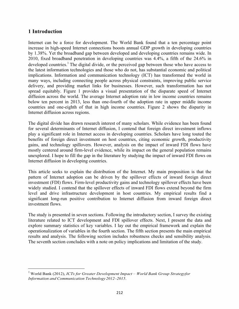
212

1 Introduction Internet can be a force for development. The World Bank found that a ten percentage point increase in high-speed Internet connections boosts annual GDP growth in developing countries by 1.38%. Yet the broadband gap between developed and developing countries remains wide. In 2010, fixed broadband penetration in developing countries was 4.4%, a fifth of the 24.6% in developed countries.1 The digital divide, or the perceived gap between those who have access to the latest information technologies and those who do not, has substantial economic and political implications. Information and communication technology (ICT) has transformed the world in many ways, including connecting people across physical constraints, improving public service delivery, and providing market links for businesses. However, such transformation has not spread equitably. Figure 1 provides a visual presentation of the disparate speed of Internet diffusion across the world. The average Internet adoption rate in low income countries remains below ten percent in 2013, less than one-fourth of the adoption rate in upper middle income countries and one-eighth of that in high income countries. Figure 2 shows the disparity in Internet diffusion across regions.

The digital divide has drawn research interest of many scholars. While evidence has been found for several determinants of Internet diffusion, I contend that foreign direct investment inflows play a significant role in Internet access in developing countries. Scholars have long touted the benefits of foreign direct investment on host countries, citing economic growth, productivity gains, and technology spillovers. However, analysis on the impact of inward FDI flows have mostly centered around firm-level evidence, while its impact on the general population remains unexplored. I hope to fill the gap in the literature by studying the impact of inward FDI flows on Internet diffusion in developing countries.

This article seeks to explain the distribution of the Internet. My main proposition is that the pattern of Internet adoption can be driven by the spillover effects of inward foreign direct investment (FDI) flows. Firm-level productivity gains and technology spillover effects have been widely studied. I contend that the spillover effects of inward FDI flows extend beyond the firm level and drive infrastructure development in host countries. My empirical results find a significant long-run positive contribution to Internet diffusion from inward foreign direct investment flows.

The study is presented in seven sections. Following the introductory section, I survey the existing literature related to ICT development and FDI spillover effects. Next, I present the data and explore summary statistics of key variables. I lay out the empirical framework and explain the operationalization of variables in the fourth section. The fifth section presents the main empirical results and analysis. The following section includes robustness checks and sensibility analysis. The seventh section concludes with a note on policy implications and limitation of the study.

1 World Bank (2012), ICTs for Greater Development Impact – World Bank Group Strategyfor Information and Communication Technology 2012–2015.

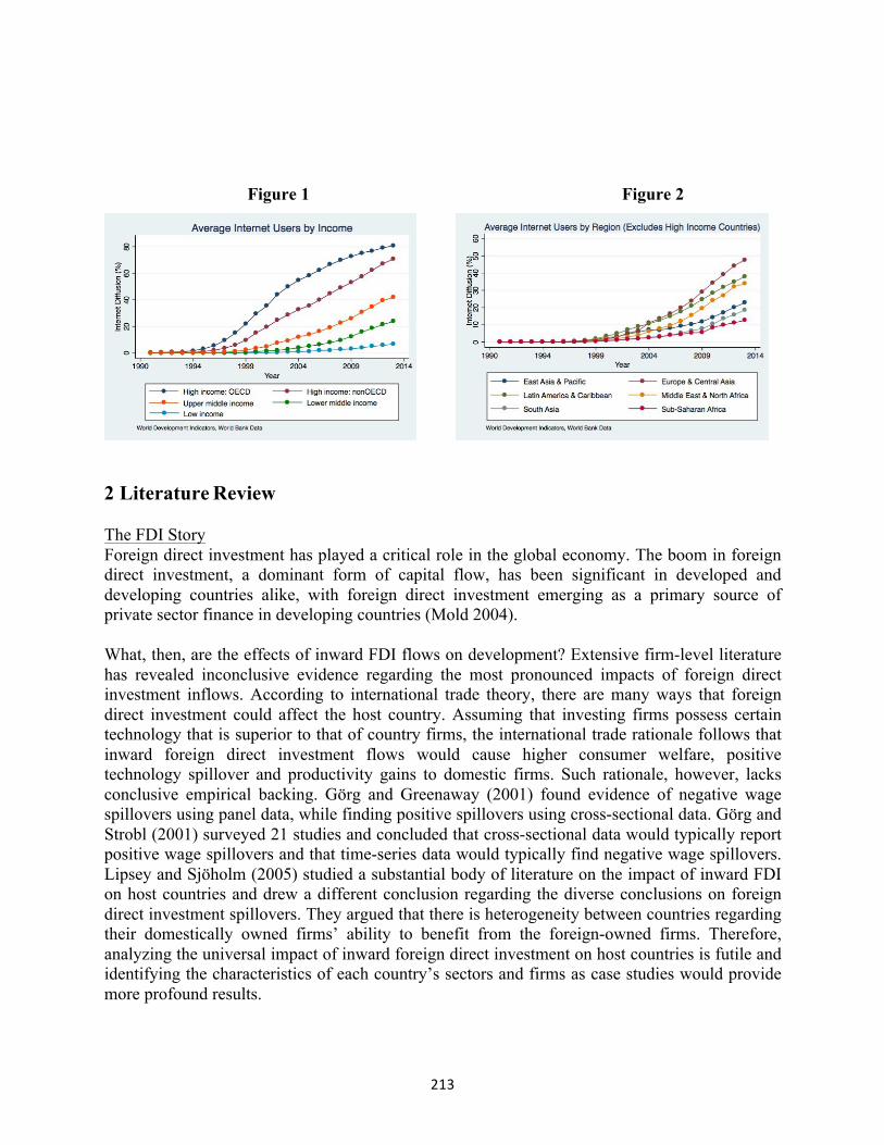
213

Figure 1 Figure 2

2 Literature Review

The FDI Story Foreign direct investment has played a critical role in the global economy. The boom in foreign direct investment, a dominant form of capital flow, has been significant in developed and developing countries alike, with foreign direct investment emerging as a primary source of private sector finance in developing countries (Mold 2004).

What, then, are the effects of inward FDI flows on development? Extensive firm-level literature has revealed inconclusive evidence regarding the most pronounced impacts of foreign direct investment inflows. According to international trade theory, there are many ways that foreign direct investment could affect the host country. Assuming that investing firms possess certain technology that is superior to that of country firms, the international trade rationale follows that inward foreign direct investment flows would cause higher consumer welfare, positive technology spillover and productivity gains to domestic firms. Such rationale, however, lacks conclusive empirical backing. Görg and Greenaway (2001) found evidence of negative wage spillovers using panel data, while finding positive spillovers using cross-sectional data. Görg and Strobl (2001) surveyed 21 studies and concluded that cross-sectional data would typically report positive wage spillovers and that time-series data would typically find negative wage spillovers. Lipsey and Sjöholm (2005) studied a substantial body of literature on the impact of inward FDI on host countries and drew a different conclusion regarding the diverse conclusions on foreign direct investment spillovers. They argued that there is heterogeneity between countries regarding their domestically owned firms’ ability to benefit from the foreign-owned firms. Therefore, analyzing the universal impact of inward foreign direct investment on host countries is futile and identifying the characteristics of each country’s sectors and firms as case studies would provide more profound results.

214

Turning away from cross-country analysis and focusing on within-country data, more conclusive empirical evidence has been found regarding the spillover effects of foreign direct investment. Focusing directly on the technology transfer externalities of foreign direct investment, data from Indonesian manufacturing firms found that foreign direct investment is a critical source of technology in developing countries (Blalock and Gertler 2005). In addition to horizontal technology transfers, Blalock and Gertler hypothesized that the benefit of technology transfer to suppliers accrues across sectors and to all consumers through the channel of increased competition. As a result, vertical technology transfer through supply chains not only benefits the foreign-owned firm, but also induces a Pareto welfare improvement.

More recent empirical techniques have also found more success in measuring the impact of foreign direct investment. Using a panel dataset of 37 countries for the period 1970-2002, Lee and Chang (2009) explored the directions of causality among foreign direct investment, level of financial development, and economic growth using panel cointegration and panel error correction models. They found convincing evidence of a strong, causal long-run relationship between foreign direct investment and economic growth and between financial development and economic growth. However, the panel causality tests revealed weak short-run relationship between foreign direct investment and economic growth. Their findings are consistent with previous literature which suggests that the host country’s level of financial development determines whether their economy realizes the benefits from foreign direct investment.

The Determinants of Internet Diffusion Similar to foreign direct investment, the digital divide has become a popular research interest in recent years. Many scholars have attempted to explain the cross-country disparities in ICT penetration. However, because of its relatively recent innovation, determinants of Internet use have been less studied. A study of 44 countries (including developed and developing countries) from 1990 to 1997 found inconclusive evidence because the sample period is quite early and many sampled countries still had low Internet adoption rates (Dasgupta, et al. 2001). Another study with a more recent sample, 1995-2000, found that the five-year growth in Internet adoption rates is associated with income, telephone access costs, and the average years of schooling (Kiiski and Pohjola 2002). Focusing on quantifying the relative importance of various determinants of Internet diffusion, a study surveying a panel of 161 countries over the period of 1999-2001 found that the global digital divide is mainly the result of disparate income levels (Chinn and Fairlie 2007). Other important contributing factors include regulatory quality, telephone density, education, and urbanization rate.

Beyond the economic determinants, recent studies also examine institutional factors that could contribute to the global digital divide. A study with data from about 190 countries from 1991 to 2001 found that democratic countries adopt Internet at a much faster rate than autocratic countries (Milner 2006). The article contends that the adoption of technology has clear political implications. In the case of Internet, autocracies are more likely to slow down the spread of Internet because it has the capacity to threaten their regime.

Linking Foreign Direct Investment and Infrastructure Despite the abundance of literature on the impact of foreign direct investment and the causes of the global digital divide, scarce scholarship has attempted to link foreign direct investment and

215

Internet diffusion. Rudra and Joshi (2011) contend that a study of the impacts of foreign direct investment on the well-being of the poor could benefit from evaluating the improvement or degradation to the provision of potable water. Exploring beyond the many touted benefits of inward foreign direct investment flows (economic related gains such as technology transfer, employment, and productivity), the authors studied whether and how foreign direct investment produces “real tangible improvements to the lives of the majority of citizens in the developing world.” They employed a cross-national sample of 103 developing countries, in addition to a case study on India, to evaluate the relationship between inward foreign direct investment flows and clean water access. Using ordinary least squared regressions with robust standard errors, they found that higher inward foreign direct investment flows are associated with slower improvements in access to clean water. Furthermore, they found empirical evidence that income inequality, combined with ethnic diversity, exacerbate the impact of foreign direct investment on access to potable water due to the collective action problem.

Gholami et al. (2006) investigate the causal relationship between information and communication technology and foreign direct investment inflows using the Granger causality test and time-series analysis and controlling for GDP growth and trade openness. Employing balanced panel data observed from 23 countries during the period 1976-1999, the results from least squares dummy variables and instrumental variable estimation methods indicate that there is inconclusive evidence of any long-run cointegration relationship between FDI and information communication technology (ICT). On the other hand, the results from the Granger causality test reflect that there is empirical short-run evidence that existing ICT infrastructure attracts foreign direct investment in developed countries while the direction of causality is reversed for developing countries. The authors contend that the direction of causality from inward foreign direct investment flows to ICT infrastructure in developing countries indicates that while ICT capacity must be fortified in order to attract foreign direct investment, the inflow of foreign investments causes further increases in ICT investment and infrastructure building in the host country.

3 Theory and Hypothesis

The reasoning behind my argument is two-fold. First, the FDI literature has shown some evidence of technology transfer spillovers at the firm level, and there is also empirical evidence for Pareto welfare gains (Blalock and Gertler 2005). I argue that inward FDI flows improve infrastructure development in the host country through the externality channel. Second, I contend that the impact on host country infrastructure improvement can be measured by Internet adoption in developing countries. Figure 3 summarizes the theoretical intuition regarding the impact of inward foreign direct investment flows on the host country’s rate of Internet diffusion.

The key assumption is that foreign-owned companies bring with them more sophisticated ICT technologies when they invest in the host country, and that they, in turn, invest in the ICT infrastructure of the host country in order to lower input costs and increase productivity. This process would create an externality to the host country infrastructure environment, with positive technology spillovers that benefit not only domestic firms, but also the general welfare of the society.

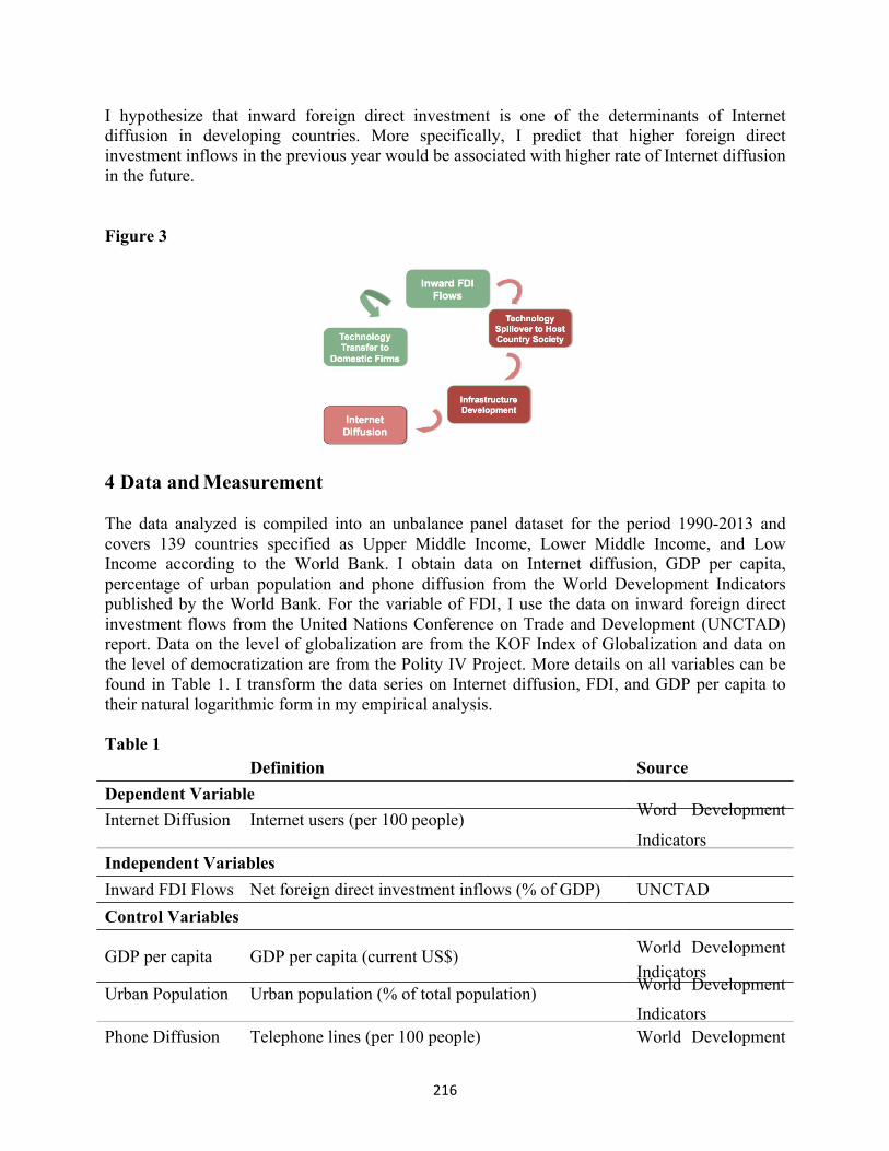
216

I hypothesize that inward foreign direct investment is one of the determinants of Internet diffusion in developing countries. More specifically, I predict that higher foreign direct investment inflows in the previous year would be associated with higher rate of Internet diffusion in the future.

Figure 3

4 Data and Measurement

The data analyzed is compiled into an unbalance panel dataset for the period 1990-2013 and covers 139 countries specified as Upper Middle Income, Lower Middle Income, and Low Income according to the World Bank. I obtain data on Internet diffusion, GDP per capita, percentage of urban population and phone diffusion from the World Development Indicators published by the World Bank. For the variable of FDI, I use the data on inward foreign direct investment flows from the United Nations Conference on Trade and Development (UNCTAD) report. Data on the level of globalization are from the KOF Index of Globalization and data on the level of democratization are from the Polity IV Project. More details on all variables can be found in Table 1. I transform the data series on Internet diffusion, FDI, and GDP per capita to their natural logarithmic form in my empirical analysis.

Table 1 Definition Source

Dependent Variable Internet Diffusion Internet users (per 100 people) Word Development

Indicators Independent Variables

Inward FDI Flows Net foreign direct investment inflows (% of GDP) UNCTAD

Control Variables

GDP per capita GDP per capita (current US$) World Development Indicators

Urban Population Urban population (% of total population) World Development Indicators Phone Diffusion Telephone lines (per 100 people) World Development

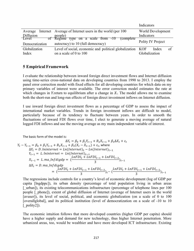
217

Average Internet Diffusion Level of

Average of Internet users in the world (per 100 people) Regime type on a scale from -10 (complete

Indicators World Development Indicators

Democratization autocracy) to 10 (full democracy) Polity IV Project Globalization Index

Level of social, economic and political globalization on a scale of 0 to 100

KOF Index of Globalization

5 Empirical Framework

I evaluate the relationship between inward foreign direct investment flows and Internet diffusion using time-series cross-national data on developing countries from 1990 to 2013. I employ the panel error correction model with fixed effects for all developing countries for which data on my primary variables of interest were available. The error correction model estimates the rate at which changes in 𝑌! return to equilibrium after a change in 𝑋!. The model allows me to examine both the short-run and long-run effects of foreign direct investment inflows on Internet diffusion.

I use inward foreign direct investment flows as a percentage of GDP to assess the impact of international market variables. Trends in foreign investment inflows are difficult to model, particularly because of its tendency to fluctuate between years. In order to smooth the fluctuations of inward FDI flows over time, I elect to generate a moving average of natural logged FDI inflows and use the moving average as my main independent variable of interest.

Thebasicformofthemodelis:∆𝑌! = 𝛽! + 𝛽!𝑌!!! + 𝐵!𝑋!!! + 𝛽!∆𝑋! + 𝜀!

𝑌! − 𝑌!!! = 𝛽! + 𝛽!𝑌!!! + 𝐵!𝑋!!! + 𝛽!(𝑋! − 𝑋!!!) + 𝜀!,where ∆𝑌! = 𝐷. 𝑙𝑛𝑖𝑛𝑡𝑒𝑟𝑛𝑒𝑡 = 𝐿𝑛(𝐼𝑛𝑡𝑒𝑟𝑛𝑒𝑡)! − 𝐿𝑛(𝐼𝑛𝑡𝑒𝑟𝑛𝑒𝑡)!!!

𝑌!!! = 𝐿. 𝑙𝑛𝑖𝑛𝑡𝑒𝑟𝑛𝑒𝑡 = 𝐿𝑛(𝐼𝑛𝑡𝑒𝑟𝑛𝑒𝑡)!!!

𝑋!!! = 𝐿.𝑚𝑎_𝑙𝑛𝑓𝑑𝑖𝑔𝑑𝑝 = (𝐿𝑛𝐹𝐷𝐼! + 𝐿𝑛𝐹𝐷𝐼!!! + 𝐿𝑛𝐹𝐷𝐼!!!

3)!!!

∆𝑋! = 𝐷.𝑚𝑎_𝑙𝑛𝑓𝑑𝑖𝑔𝑑𝑝

= (𝐿𝑛𝐹𝐷𝐼! + 𝐿𝑛𝐹𝐷𝐼!!! + 𝐿𝑛𝐹𝐷𝐼!!!

3)!− (

𝐿𝑛𝐹𝐷𝐼! + 𝐿𝑛𝐹𝐷𝐼!!! + 𝐿𝑛𝐹𝐷𝐼!!!3

)!!!

The regressions include controls for a country’s level of economic development (log of GDP per capita [lngdppc]), its urban density (percentage of total population living in urban areas [_urban]), its existing telecommunications infrastructure (percentage of telephone lines per 100 people [_phone]), extent of global diffusion of Internet (average of Internet users in the world [avuser]), its level of social, political, and economic globalization (on a scale of 0 to 100 [overallglobal], and its political institution (level of democratization on a scale of -10 to 10 [_polity2]).

The economic intuition follows that more developed countries (higher GDP per capita) should have a higher supply and demand for new technology, thus higher Internet penetration. More urbanized areas, too, would be wealthier and have more developed ICT infrastructure. Existing

218

telecommunications infrastructure and the extent of global diffusion of Internet are important controls because they capture the rate of technological advancement. These variables should reflect positive coefficients.

The political institution variables, level of democratization and level of globalization, are also important determinants for Internet diffusion and are therefore included in the model. Higher level of democratization should be associated with higher Internet penetration (Milner 2006). Countries that are more connected to the global political economy (higher globalization index) would also be more likely to demand and supply new technology, and therefore higher Internet adoption.

6 Main Empirical Results

Table 2 presents the results from estimating the error correction model with one-period lags. At the 1% significance level, there is strong evidence that inward FDI flows have a positive long- run effect on the increase in Internet access in the baseline model without control variables. A one percent increase in inward FDI flows is associated with a 3 percent increase in Internet diffusion. As expected, the coefficient of the lagged dependent variable is largely negative at the 99% confidence level. The level of Internet diffusion in the previous period should be strongly correlated with the level of diffusion in the current period, since individuals who have already been reached by the Internet in the previous year would not be counted in the following period. There is evidence of a long-run effect of inward FDI flows on Internet diffusion at the 5% significance level when control variables that capture the size of economy (GDP per capita), urban density, phone penetration, global average technological advancement (average Internet users in the world), level of globalization, and level of democratization are added in staggered groups. However, in the model with all control variables, significance on the long-run effect is lost, perhaps due to multi-collinearity. Notably, the results reflect a negative and significant association between foreign direct investment inflows and Internet diffusion when the political institution variables are included and when all of the control variables are included in the model.

Table 3 presents results with two-period lags. In the baseline model, a one percent increase in inward foreign direct investment is associated with a 4.5% increase in Internet diffusion with two-period lags at the 5% level of significance. The two-period lagged dependent variable continues to reflect negative and significant coefficients. The magnitude of the impact of inward foreign direct investment flows on Internet diffusion is higher in the long-run in both Model 1 and Model 2 at the 5% and 1% level of significance, respectively.

The results from one-period and two-period lags reveal similar results. Consistent to my hypothesis, there is empirical evidence of long-run benefits of foreign direct investment inflows on host country Internet diffusion. However, in the short-run, the results are either insignificant or negative. The disparity in findings could be the result of the heterogeneity in the type of foreign direct investment that entered the country. If the foreign-owned firm invested in a sector that does not require high-level ICT infrastructure, it would not promote nor create positive technology spillovers to the host country. However, in the long-run, regardless of the sector that the foreign firm invested in, the welfare benefits become more prominent and spillover effects could be observed.

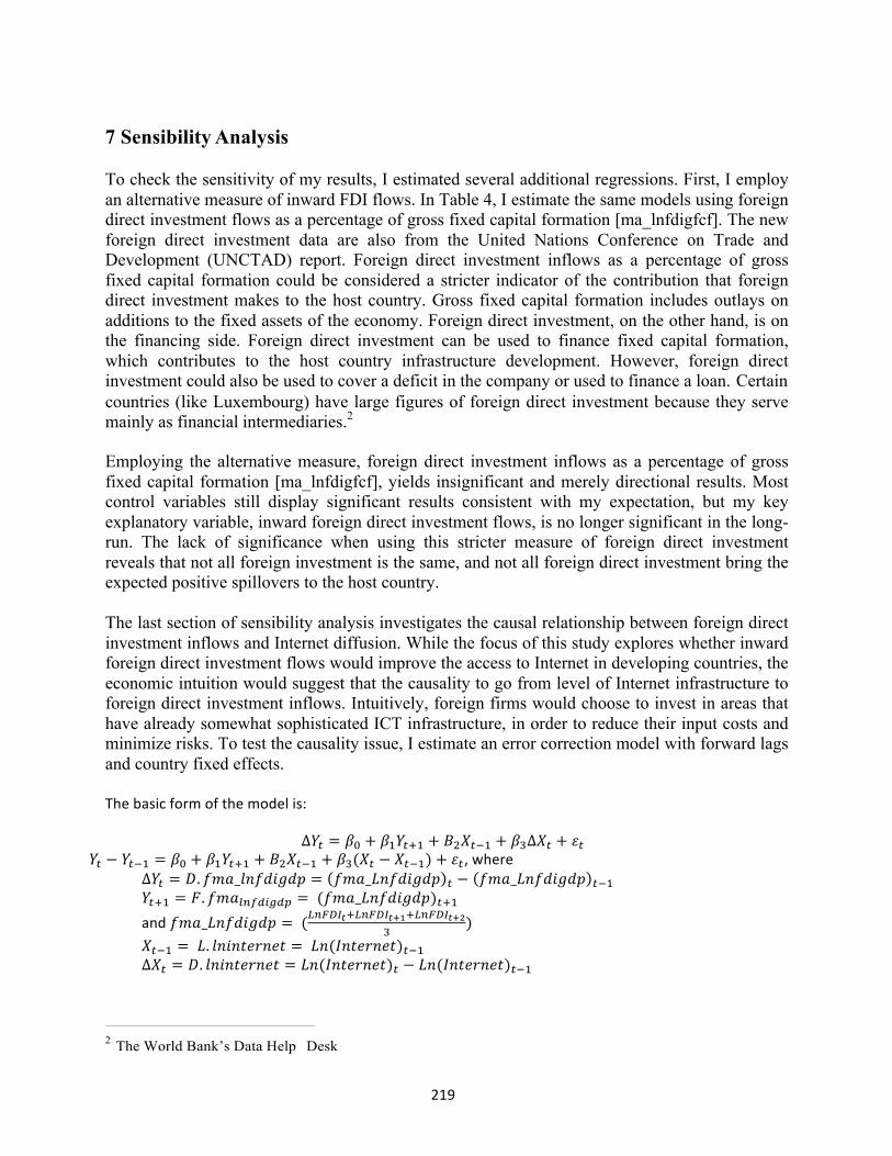
219

7 Sensibility Analysis

To check the sensitivity of my results, I estimated several additional regressions. First, I employ an alternative measure of inward FDI flows. In Table 4, I estimate the same models using foreign direct investment flows as a percentage of gross fixed capital formation [ma_lnfdigfcf]. The new foreign direct investment data are also from the United Nations Conference on Trade and Development (UNCTAD) report. Foreign direct investment inflows as a percentage of gross fixed capital formation could be considered a stricter indicator of the contribution that foreign direct investment makes to the host country. Gross fixed capital formation includes outlays on additions to the fixed assets of the economy. Foreign direct investment, on the other hand, is on the financing side. Foreign direct investment can be used to finance fixed capital formation, which contributes to the host country infrastructure development. However, foreign direct investment could also be used to cover a deficit in the company or used to finance a loan. Certain countries (like Luxembourg) have large figures of foreign direct investment because they serve mainly as financial intermediaries.2

Employing the alternative measure, foreign direct investment inflows as a percentage of gross fixed capital formation [ma_lnfdigfcf], yields insignificant and merely directional results. Most control variables still display significant results consistent with my expectation, but my key explanatory variable, inward foreign direct investment flows, is no longer significant in the long- run. The lack of significance when using this stricter measure of foreign direct investment reveals that not all foreign investment is the same, and not all foreign direct investment bring the expected positive spillovers to the host country.

The last section of sensibility analysis investigates the causal relationship between foreign direct investment inflows and Internet diffusion. While the focus of this study explores whether inward foreign direct investment flows would improve the access to Internet in developing countries, the economic intuition would suggest that the causality to go from level of Internet infrastructure to foreign direct investment inflows. Intuitively, foreign firms would choose to invest in areas that have already somewhat sophisticated ICT infrastructure, in order to reduce their input costs and minimize risks. To test the causality issue, I estimate an error correction model with forward lags and country fixed effects.

Thebasicformofthemodelis:

∆𝑌! = 𝛽! + 𝛽!𝑌!!! + 𝐵!𝑋!!! + 𝛽!∆𝑋! + 𝜀!𝑌! − 𝑌!!! = 𝛽! + 𝛽!𝑌!!! + 𝐵!𝑋!!! + 𝛽!(𝑋! − 𝑋!!!) + 𝜀!,where ∆𝑌! = 𝐷. 𝑓𝑚𝑎_𝑙𝑛𝑓𝑑𝑖𝑔𝑑𝑝 = 𝑓𝑚𝑎_𝐿𝑛𝑓𝑑𝑖𝑔𝑑𝑝 ! − 𝑓𝑚𝑎_𝐿𝑛𝑓𝑑𝑖𝑔𝑑𝑝 !!!

𝑌!!! = 𝐹. 𝑓𝑚𝑎!"#$%&$' = (𝑓𝑚𝑎_𝐿𝑛𝑓𝑑𝑖𝑔𝑑𝑝)!!!and𝑓𝑚𝑎_𝐿𝑛𝑓𝑑𝑖𝑔𝑑𝑝 = (!"#$%!!!"#$%!!!!!"#$%!!!

!)

𝑋!!! = 𝐿. 𝑙𝑛𝑖𝑛𝑡𝑒𝑟𝑛𝑒𝑡 = 𝐿𝑛(𝐼𝑛𝑡𝑒𝑟𝑛𝑒𝑡)!!!∆𝑋! = 𝐷. 𝑙𝑛𝑖𝑛𝑡𝑒𝑟𝑛𝑒𝑡 = 𝐿𝑛(𝐼𝑛𝑡𝑒𝑟𝑛𝑒𝑡)! − 𝐿𝑛(𝐼𝑛𝑡𝑒𝑟𝑛𝑒𝑡)!!!

2 The World Bank’s Data Help Desk

220

If there is a causal relationship from Internet adoption to inward foreign direct investment flows, the coefficient on [D.lninternet] and [L.lninternet] would be significant and positive. In Table 5, I estimate the above model with one-period lags. The empirical results with forward lags on inward foreign direct investment flows reveal either a negative or insignificant coefficient. Thus, I can inference that there is a weak but negative causal relationship. This allows me to conclude that there is not a serious endogeneity problem with my original model and hypothesis on the causal relationship from inward foreign direct investment flows to Internet diffusion. The results are also consistent with the findings in Gholami et al. (2006).

8 Conclusion

Estimating the error correction model yields some empirical evidence that inward FDI flows are correlated with increase in Internet diffusion in the long-run. Short-run effects are not significant at the 10% significance level. The sensitivity analyses confirmed that the causal relationship is consistent with my hypotheses and the reverse causality issue is not significant statistically.

The finding gives incentives for policy makers to consider formulating trade policies in a way that would attract foreign direct investment in order to promote technology spillover in the host country, in order to lead to greater Internet diffusion. The digital divide indicates that wealthier countries and regions enjoy better access to Internet and other ICT infrastructure. With the economic and social benefits that Internet connection brings, the disparity would only widen between those who have access to the Internet and those who do not.

However, this study does not account for heterogeneity in the types of inward foreign direct investment flows. The level of ICT requirement of the sector in which the foreign company invests would have heterogeneous effects on Internet diffusion. As evident in my alternative measure of foreign direct investment inflows as a percentage of gross fixed capital formation, not all foreign direct investment inflows would promote infrastructure development in the host country. Therefore, host countries should aim to formulate trade policies that would incentivize foreign firms to invest in fixed capital in the host country in order to promote the privatization and diffusion of ICT infrastructure.

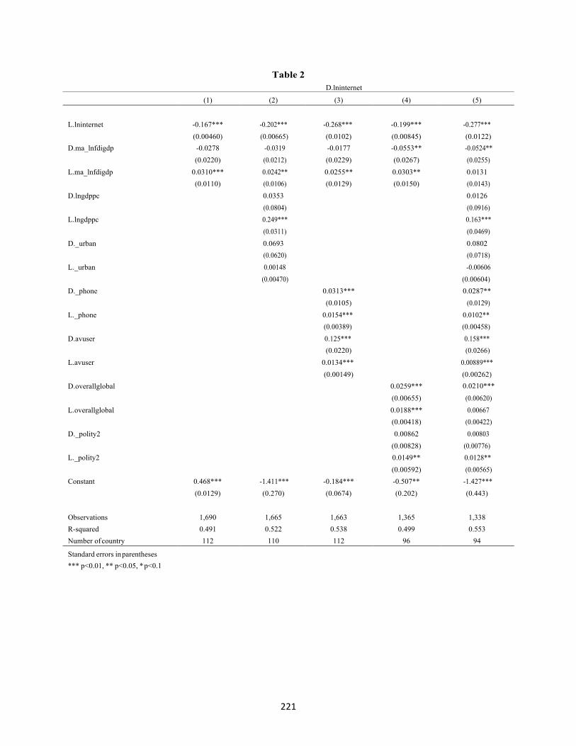
221

Table 2 D.lninternet

(1) (2) (3) (4) (5)

L.lninternet

-0.167*** (0.00460)

-0.202*** (0.00665)

-0.268*** (0.0102)

-0.199*** (0.00845)

-0.277*** (0.0122)

D.ma_lnfdigdp -0.0278 -0.0319 -0.0177 -0.0553** -0.0524**

(0.0220) (0.0212) (0.0229) (0.0267) (0.0255) L.ma_lnfdigdp 0.0310*** 0.0242** 0.0255** 0.0303** 0.0131

(0.0110) (0.0106) (0.0129) (0.0150) (0.0143) D.lngdppc 0.0353 0.0126

(0.0804) (0.0916) L.lngdppc 0.249*** 0.163***

(0.0311) (0.0469) D._urban 0.0693 0.0802

(0.0620) (0.0718) L._urban 0.00148 -0.00606

D._phone

(0.00470) 0.0313***

(0.00604) 0.0287**

(0.0105) (0.0129) L._phone 0.0154***

(0.00389) 0.0102**

(0.00458) D.avuser 0.125***

(0.0220) 0.158***

(0.0266) L.avuser 0.0134*** 0.00889***

D.overallglobal

(0.00149) 0.0259***

(0.00262) 0.0210***

(0.00655) (0.00620) L.overallglobal 0.0188*** 0.00667

(0.00418) (0.00422) D._polity2 0.00862 0.00803

L._polity2

(0.00828) 0.0149**

(0.00776) 0.0128**

(0.00592) (0.00565) Constant 0.468*** -1.411*** -0.184*** -0.507** -1.427***

(0.0129) (0.270) (0.0674) (0.202) (0.443)

Observations

1,690

1,665

1,663

1,365

1,338

R-squared 0.491 0.522 0.538 0.499 0.553 Number of country 112 110 112 96 94

Standard errors in parentheses *** p<0.01, ** p<0.05, * p<0.1

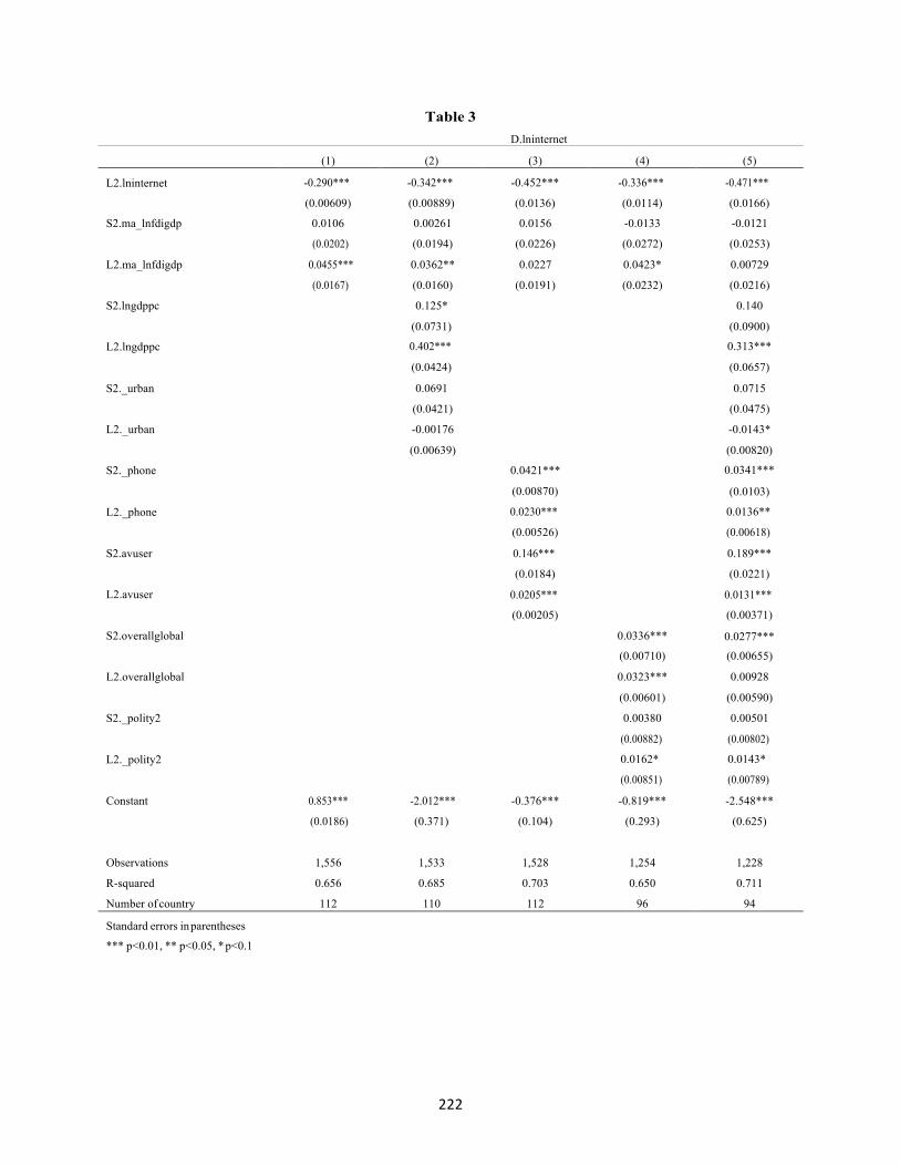
222

Table 3 D.lninternet

(1) (2) (3) (4) (5)

L2.lninternet -0.290***

(0.00609)

-0.342***

(0.00889)

-0.452***

(0.0136)

-0.336***

(0.0114)

-0.471***

(0.0166)

S2.ma_lnfdigdp 0.0106 0.00261 0.0156 -0.0133 -0.0121

(0.0202) (0.0194) (0.0226) (0.0272) (0.0253)

L2.ma_lnfdigdp 0.0455*** 0.0362** 0.0227 0.0423* 0.00729

(0.0167) (0.0160) (0.0191) (0.0232) (0.0216)

S2.lngdppc 0.125* 0.140

L2.lngdppc (0.0731)

0.402***

(0.0424)

(0.0900)

0.313***

(0.0657)

S2._urban 0.0691 0.0715

(0.0421) (0.0475)

L2._urban -0.00176 -0.0143*

S2._phone (0.00639)

0.0421*** (0.00820)

0.0341***

L2._phone

(0.00870)

0.0230***

(0.00526)

(0.0103)

0.0136**

(0.00618)

S2.avuser

L2.avuser

S2.overallglobal

0.146***

(0.0184)

0.0205***

(0.00205)

0.0336***

0.189***

(0.0221)

0.0131***

(0.00371)

0.0277***

(0.00710) (0.00655)

L2.overallglobal 0.0323*** 0.00928

(0.00601) (0.00590)

S2._polity2 0.00380 0.00501

L2._polity2 (0.00882)

0.0162*

(0.00851)

(0.00802)

0.0143*

(0.00789)

Constant 0.853***

(0.0186)

-2.012***

(0.371)

-0.376***

(0.104)

-0.819***

(0.293)

-2.548***

(0.625)

Observations

1,556

1,533

1,528

1,254

1,228

R-squared 0.656 0.685 0.703 0.650 0.711

Number of country 112 110 112 96 94

Standard errors in parentheses

*** p<0.01, ** p<0.05, * p<0.1

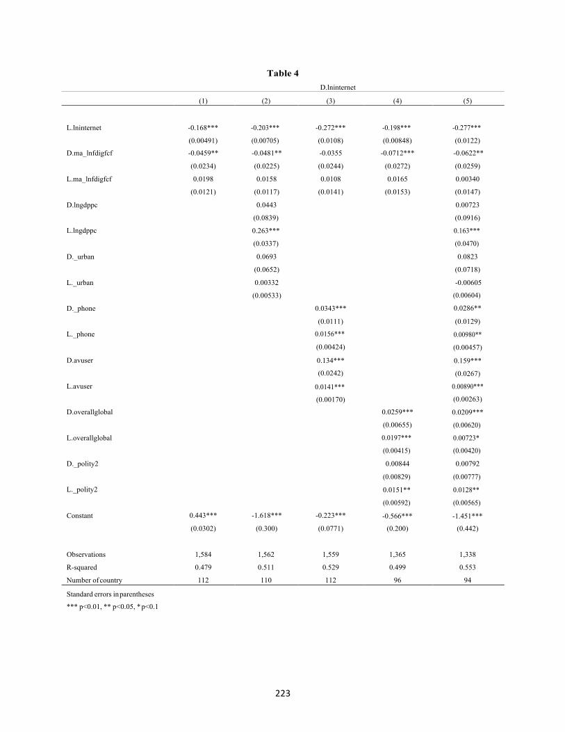
223

Table 4 D.lninternet

(1) (2) (3) (4) (5)

L.lninternet

-0.168***

(0.00491)

-0.203***

(0.00705)

-0.272***

(0.0108)

-0.198***

(0.00848)

-0.277***

(0.0122)

D.ma_lnfdigfcf -0.0459** -0.0481** -0.0355 -0.0712*** -0.0622**

(0.0234) (0.0225) (0.0244) (0.0272) (0.0259)

L.ma_lnfdigfcf 0.0198 0.0158 0.0108 0.0165 0.00340

(0.0121) (0.0117) (0.0141) (0.0153) (0.0147)

D.lngdppc 0.0443 0.00723

L.lngdppc (0.0839)

0.263***

(0.0337)

(0.0916)

0.163***

(0.0470)

D._urban 0.0693 0.0823

(0.0652) (0.0718)

L._urban 0.00332 -0.00605

D._phone (0.00533)

0.0343*** (0.00604)

0.0286**

L._phone

D.avuser

L.avuser

D.overallglobal

(0.0111)

0.0156***

(0.00424)

0.134***

(0.0242)

0.0141***

(0.00170)

0.0259***

(0.0129)

0.00980**

(0.00457)

0.159***

(0.0267)

0.00890***

(0.00263)

0.0209***

L.overallglobal

(0.00655)

0.0197***

(0.00415)

(0.00620)

0.00723*

(0.00420)

D._polity2 0.00844 0.00792

L._polity2

Constant

0.443***

-1.618***

-0.223***

(0.00829)

0.0151**

(0.00592)

-0.566***

(0.00777)

0.0128**

(0.00565)

-1.451***

(0.0302) (0.300) (0.0771) (0.200) (0.442)

Observations

1,584

1,562

1,559

1,365

1,338

R-squared 0.479 0.511 0.529 0.499 0.553

Number of country 112 110 112 96 94

Standard errors in parentheses

*** p<0.01, ** p<0.05, * p<0.1

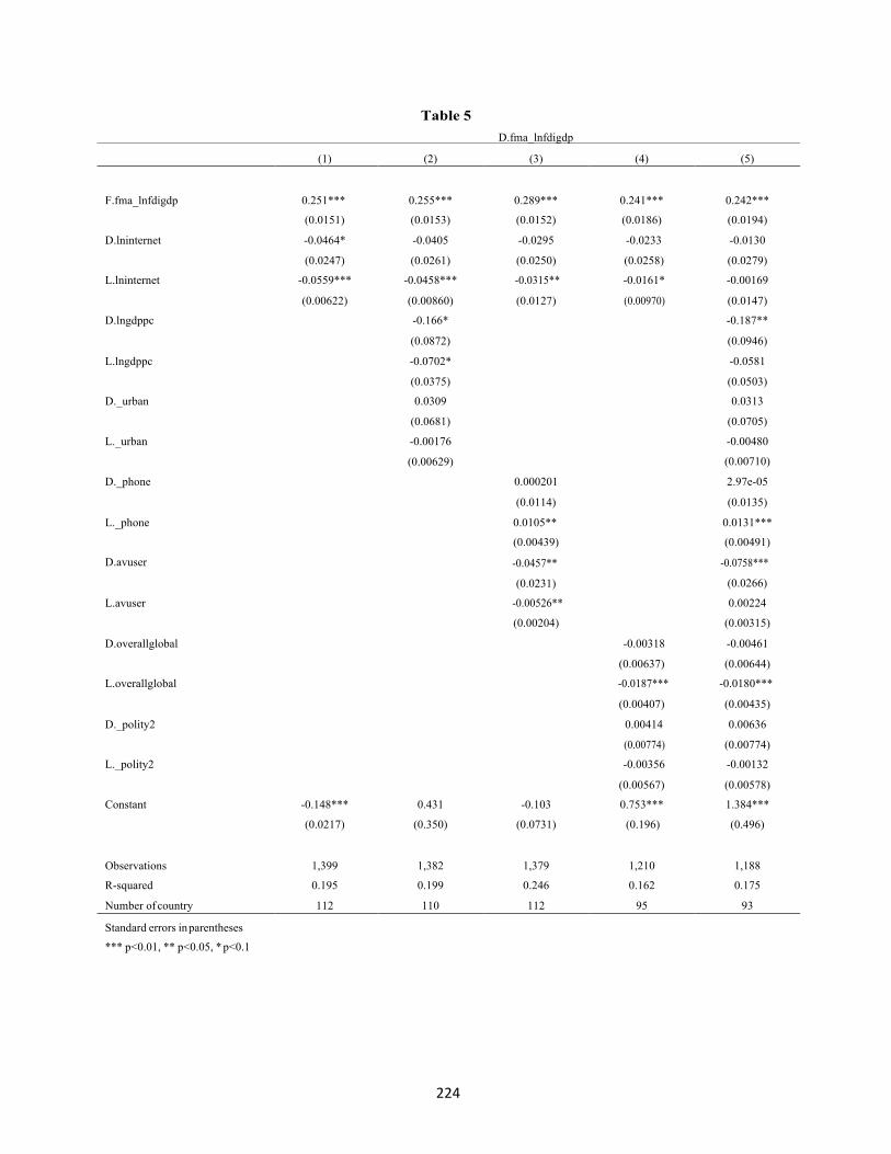
224

Table 5 D.fma_lnfdigdp

(1) (2) (3) (4) (5)

F.fma_lnfdigdp

0.251***

0.255***

0.289***

0.241***

0.242***

(0.0151) (0.0153) (0.0152) (0.0186) (0.0194)

D.lninternet -0.0464* -0.0405 -0.0295 -0.0233 -0.0130

(0.0247) (0.0261) (0.0250) (0.0258) (0.0279)

L.lninternet -0.0559*** -0.0458*** -0.0315** -0.0161* -0.00169

(0.00622) (0.00860) (0.0127) (0.00970) (0.0147)

D.lngdppc -0.166* -0.187**

(0.0872) (0.0946)

L.lngdppc -0.0702* -0.0581

(0.0375) (0.0503)

D._urban 0.0309 0.0313

(0.0681) (0.0705)

L._urban -0.00176 -0.00480

(0.00629) (0.00710)

D._phone 0.000201 2.97e-05

(0.0114) (0.0135)

L._phone 0.0105** 0.0131***

(0.00439) (0.00491)

D.avuser -0.0457**

(0.0231)

-0.0758***

(0.0266)

L.avuser -0.00526** 0.00224

(0.00204) (0.00315)

D.overallglobal -0.00318 -0.00461

(0.00637) (0.00644)

L.overallglobal -0.0187*** -0.0180***

(0.00407) (0.00435)

D._polity2 0.00414 0.00636

(0.00774) (0.00774)

L._polity2 -0.00356 -0.00132

(0.00567) (0.00578)

Constant -0.148*** 0.431 -0.103 0.753*** 1.384***

(0.0217) (0.350) (0.0731) (0.196) (0.496)

Observations

1,399

1,382

1,379

1,210

1,188

R-squared 0.195 0.199 0.246 0.162 0.175

Number of country 112 110 112 95 93

Standard errors in parentheses *** p<0.01, ** p<0.05, * p<0.1

225

Bibliography

Blalock, Garrick, and Paul J. Gertler. “Foreign Direct Investment and Externalities: The Case for Public Intervention.” Does Foreign Direct Investment Promote Development? ed., Theodore H. Moran, Edward M. Graham, and Magnus Blomström. Washington, D.C. Institute for International Economics. 73-106. Web. 2005.

Chinn, Menzie, and Robert W. Fairlie. “The determinants of the global digital divide: a cross-country analysis of

computer and internet penetration.” Oxford Economic Papers 59, 16-44. Web. 2007.

Dasgupta, S., Lall, S., and Wheeler, D. 2001. Policy reform, economic growth and the digital divide: an econometric analysis, Working Paper No. 2567, World Bank, Washington, DC.

Dreher, Axel “Does Globalization Affect Growth? Evidence from a new Index of Globalization” Applied Economics

38, 10: 1091-1110 2006. Web.

Gholami, Roghieh, Sang-Yong Tom Lee and Almas Heshmati. “The Causal Relationship Between Information and Communication Technology and Foreign Direct Investment.” United Nations University. 43-60. Web. 2006.

Görg, Holger, and David Greenaway. “Foreign Direct Investment and Intra-industry Spillovers: A Review of the

Literature.” Globalisation and Labor Markets Programme Research Paper No. 2001/37. Nottingham, UK: Leverhulme Centre for Research on Globalisation and Economic Policy. Web. 2001.

Görg, Holger, and Eric Strobl. “Multinational Companies and Productivity Spillovers. A Meta-analysis.” Economic

Journal 111, no.475 (November): F723-39. Web. 2001.

Lee, Chien-Chiang, and Chun-Ping Chang. “FDI, Financial Development, and Economic Growth: International Evidence.” Journal of Applied Economics. Vol XII, No.2, 249-271. Web. 2009.

Lipsey, Robert E. and Fredrik Sjöholm. “The Impact of Inward FDI on Host Countries: Why Such Different Answers?”

Does Foreign Direct Investment Promote Development?, ed., Theodore H. Moran, Edward M. Graham, and Magnus Blomström. Washington, D.C. Institute for International Economics. 23-43. Web. 2005.

Kiiski, S. and Pohjola, M. “Cross-country diffusion of the Internet”. Information Economics and Policy, 14, 297- 310.

Web. 2002.

Polity IV Individual Country Regime Trends, 1946-2013

Milner, Helen V. “The Digital Divide: The Role of Political Institutions in Technology Diffusion.” Comparative Political Studies. Volume 39, No.2, 176-199. Web. 2006.

Mold, Andrew. “FDI and Poverty Reduction: A Critical Appraisal of the Arguments”. Region et Developpment,

20. Web. 2004.

Rudra, Nita, and Siddharth Joshi. “Good for the Goose, Bad for the Flock? FDI in Developing Countries.” Working Paper. Web. 2011.

UNCTAD, United Nations Conference on Trade and Development.

World Bank, World Development Indicators (Washington, D.C.: World Bank).

226

Why Do Women Cluster In The Workforce?

Natalie Nah Georgetown University

Abstract Gender equality has been linked with many social, political, and economic benefits for women as well as the rest of society. This paper therefore looks at the issue of gender equality in the workforce of developing countries by examining the characteristics of firms women have a higher propensity of working in as well as the possible rationale behind such patterns. Using OLS regressions to test firm-level data, three theories (human capital, statistical discrimination, and feminist theories) were tested to explain the feminisation of such firms, with the results showing that the low education of women, statistical discrimination, and having female employers account for more of the variation in female hiring patterns.

I am greatly indebted to Professor George Shambugh, Professor Charles Udomsaph, and Professor Shareen Joshi for their invaluable guidance. Any mistakes are acknowledged as my own.

227

1 Introduction Global data shows correlation between gender equity in the workplace and economic growth. United Nations Development Program’s (UNDP) Gender Inequality Index (GII) shows a positive relationship when plotted against gross national income per capita. Using a more robust methodology, Klasen and Lamanna’s (2009) cross-country and panel regressions find that gender gaps in employment considerably reduce economic growth, with the reduction of economic growth differing between regions. These studies thus demonstrate that gender equity have a positive correlation with a nation’s income, growth, and competitiveness.

What explains the connection between employment inequality and growth on a microeconomic level? The simplest explanation is resulting inefficiency in labor markets. Undermining the employment opportunities for women may decrease the average productivity of the work force in absence of such inequality as it artificially reduces the pool of talent from which employers can draw, thereby reducing the average ability of the workforce (Esteve-Volart 2004). Moreover, if women cannot offer their labor services at competitive wages due to artificial barriers, this contributes to higher overall labor costs for the firms that do not hire women and hence lowers competitiveness for such firms (Koning 2000). According to the World Economic Forum, evidence also demonstrates that firms benefit by successfully integrating the female half of the available talent pool, women have a propensity for making more inclusive, informed decisions and engaging in less risky behavior, and gender-equal teams may be more successful (Hausmann, Tyson, and Zahidi 2012). Thus on both a global level and a firm level, evidence points to economic benefits of gender equality in the workplace. Besides that, there is a growing but still rather speculative and suggestive literature in its nascent stage of research that has found evidence that female employees, on average, appear to be less prone to corruption and nepotism compared to their male counterparts (World Bank 2001; Swamy, Azfar, Knack, and Lee 2001). If these findings prove to be robust, greater levels of women’s employment might be beneficial for economic performance in this sense as well.

Gender equity in the workplace not only enhances economic efficiency and is a possible determinant of economic growth in developing countries but also improves other development goals. Following Amartya Sen’s (1999) view, “gender equality matters in its own right,” development is seen as a process of expanding freedom equally for all people; thus gender equality is a core objective in itself. Restricting women’s participation is inconsistent with democratic values grounded on equal citizenship and rights. Based on a literature, women’s employment and earnings increase their bargaining power in the home (Sen 1990; Haddad, Hoddinott, and Alderman 1997; Thomas 1997; Klasen and Wink 2003; and King, Klasen, and Porter 2008). The promotion and maintenance of the welfare of female workers thus is a topic of interest. Inequity in terms of wages, occupational type (occupational concentration or segregation), and unequal treatment in the workplace by gender therefore require corrective action by policymakers.

The World Bank Development Report (2011) emphasizes the humanitarian significance of gender equality as it states that improving women’s relative and absolute status feeds other development outcomes, including those for their children. Greater bargaining power for women not only benefits the women concerned, but also has a range of growth-enhancing effects. These could include higher savings, as women and men differ in their savings behavior (Seguino, Floro, 2003), more

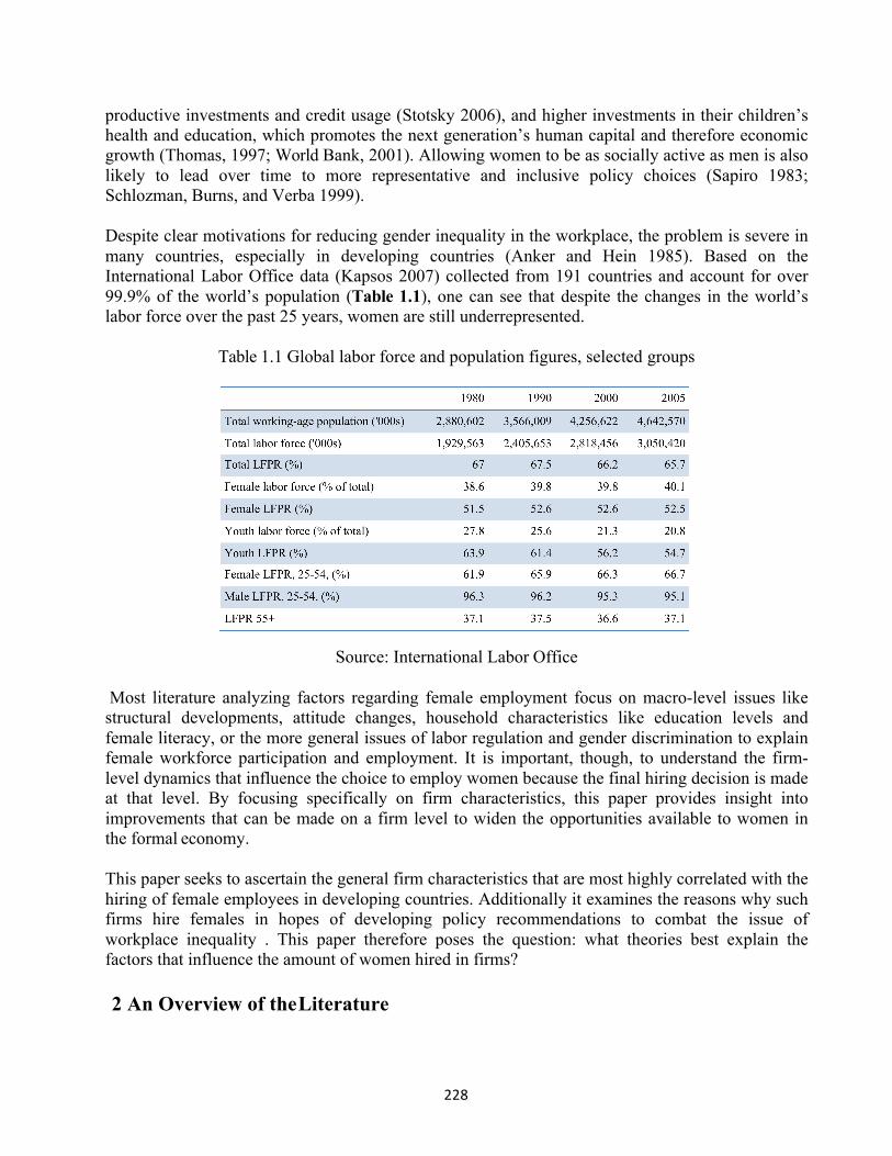
228

productive investments and credit usage (Stotsky 2006), and higher investments in their children’s health and education, which promotes the next generation’s human capital and therefore economic growth (Thomas, 1997; World Bank, 2001). Allowing women to be as socially active as men is also likely to lead over time to more representative and inclusive policy choices (Sapiro 1983; Schlozman, Burns, and Verba 1999).

Despite clear motivations for reducing gender inequality in the workplace, the problem is severe in many countries, especially in developing countries (Anker and Hein 1985). Based on the International Labor Office data (Kapsos 2007) collected from 191 countries and account for over 99.9% of the world’s population (Table 1.1), one can see that despite the changes in the world’s labor force over the past 25 years, women are still underrepresented.

Table 1.1 Global labor force and population figures, selected groups

Source: International Labor Office

Most literature analyzing factors regarding female employment focus on macro-level issues like structural developments, attitude changes, household characteristics like education levels and female literacy, or the more general issues of labor regulation and gender discrimination to explain female workforce participation and employment. It is important, though, to understand the firm- level dynamics that influence the choice to employ women because the final hiring decision is made at that level. By focusing specifically on firm characteristics, this paper provides insight into improvements that can be made on a firm level to widen the opportunities available to women in the formal economy.

This paper seeks to ascertain the general firm characteristics that are most highly correlated with the hiring of female employees in developing countries. Additionally it examines the reasons why such firms hire females in hopes of developing policy recommendations to combat the issue of workplace inequality . This paper therefore poses the question: what theories best explain the factors that influence the amount of women hired in firms?

2 An Overview of the Literature

229

In the book Gender and Jobs: Sex Segregation of Occupations in the World (1998), Richard Anker identifies the three major categories of employment gender gap. These hypotheses investigate the reasons why women choose (or not choose) to enter the workforce or prefer certain jobs over others as well as reasons why employers choose (or choose not) to hire women or prefer one gender over another for certain occupations. The categories are the neo-classical and human capital theory, institutional and labor market segmentation theory, and non-economic, feminist theories. Though Anker does not test these theories nor come up with methods to examine them empirically, his theories hold particular significance for this paper, as most of the independent variables were based off of these possible explanations for employment gender gaps.

The human capital theory emphasizes lower levels of female human capital in terms of what women bring to the labor market and what they acquire through their participation. Under this theory, firms seek to maximize their productivity and cut costs when making hiring decisions while workers seek to maximize their earnings, given the limitations set by their skill and experience endowments. In this theory, firms consider females to be less productive as women possess on average lower skill, education levels, and experience. Thus according to Anker (1998), jobs requiring higher levels of education, experience, or skill, are therefore more likely to be offered to men than women; however, Anker acknowledges that the relationship between women’s education and occupation is bi-directional as women may not choose particular occupations because they were not interested in or did not have access to the prerequisite education or experience. Therefore, in the long run, as women are generally discriminated against, they might obtain less education than men and to pursue careers that reinforce the current segregation.

Anker (1998) also theorizes that women are perceived as higher-cost workers because of indirect labor costs such as absenteeism, lateness due to familial obligations, and higher turnover rates. As families worldwide tend to make women responsible for housework and childcare, women rationally choose occupations with higher starting salary, low returns to experience, and flexible hours (Becker, 1985; Agrawa, 1997; Hoachschild, 1989). Through examining the situation from the perspective of the employee instead of the firm, Julie Gallaway and Alexandra Bernasek (2010) test the theory and found that for women, education and family responsibilities are important determinants of the decision to work. Specifically, women with lower levels of education have the highest probabilities of working at home or in the informal sector, whereas those with the highest levels of education have the lowest probabilities of working at home. Regarding household responsibilities, having an infant increases the probability the wife will work at home, and decreases the probabilities of paid informal or formal sector participation. For men, very few of the variables are significant; hence, unlike women, education and family responsibilities explain neither the labor force participation decision nor the decision between informal and formal sector employment well.

In order to try to level the playing field and reduce the burden of familial obligations on women, some governments mandated maternal benefits. Such legislation, however, may prove to be counterproductive as maternal benefits result in increased costs for employers. This might result in firms being less likely to hire women due to the possibility of having to absorb future maternal benefit costs. Sean Dougherty (2002) substantiates this theory as his study shows that obstacles like labor laws can contribute to this discrimination. Looking at the impact of employment protection legislation and related regulation on employment dynamics in the organized sector, Dougherty

230

(2002) finds that while reforms have taken some of the bite out of core labor laws, more comprehensive reforms are needed to address the distortions that have emerged.

The second major category of Anker’s theories, statistical discrimination theory, assumes there exists differences in the productivity, skills, and experience of groups of workers. This method makes more economic sense for jobs that do not require specialized skills as it decreases the hiring process’ efforst and costs. As women are generally found to have lesser education and experience than men, firms might make hiring decisions based on the assumption that a woman is statistically unlikely to have the characteristics sought in the firm as opposed to making the decision after assessing the characteristics of the individual. Additionally gender stereotyped personality traits may also be used in the hiring process. For example, there is a higher relative amount of women employed as nurses, teachers, maids, waitresses, and receptionists as they are seen to be “caring,” “honest”, and possessing “skills in household related work” as well as “manual dexterity” (Anker 1998).

Unfortunately, both the human capital theory and statistical discrimination theory fail to incorporate non-economic variables, which feminist theories do. The basic premise of gender theories is that women’s disadvantaged position in the labor market is a manifestation of patriarchy and women’s subordinate position in society and the family. Feminist theory thus states that societal view and restrictions also discourage women from participating in certain occupations, or the labor market in general. Feminists thus advocate for having more women in leadership positions in the workplace in order to influence the younger generation’s career aspirations and educational attainment, creating a role model effect. However, when Esther Duflo, Rohini Pande, and Petia Topalova (2012) tested this theory via a randomized natural experiment in India, they found that though the gender gap in adolescent educational attainment was erased and girls spent less time on household chores when villages had a female leader, there was no evidence of changes in young women’s labor market opportunities. This paper uses a similar theory but looks at the effect of having female employers and rationalizes that female employers influence employees and are more likely to be receptive towards hiring women.

This survey of literature therefore provides a helpful framework of analysis for the questions at hand. The comprehensive overview of different theories that explain gender segregation in employment will thus be used to analyze the situation. Aspects of each of Anker’s theory can be converted into independent variables to examine whether or not, within this specific dataset, such factors explain the likelihood of firms hiring women. Dougherty (2002), Gallaway and Bernasek (2002), and Duflo, Pande and Topalova (2012) provide additions to the literature by explaining the discrepancy in gender labor participation rates using empirical methods; however, these studies base their conclusions on individual, district, or state level data. Few studies have delved into whether firm-level data supports or refutes the widely held theories regarding trends in female employment in developing countries. Thus, this paper hopes to shed light on this phenomenon within a framework that focuses on firm-level reasoning for the discrepancies in female hiring in developing countries.

3 Data Analysis

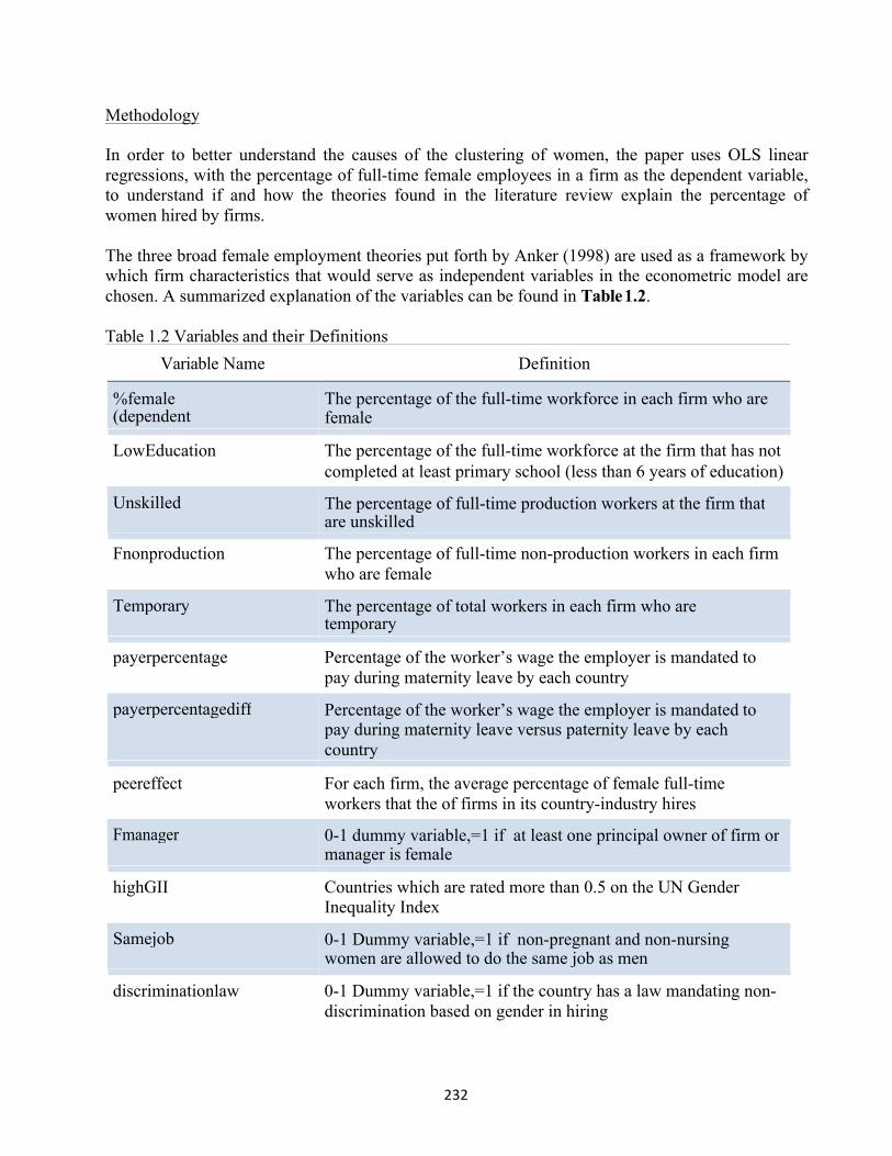
232

Methodology

In order to better understand the causes of the clustering of women, the paper uses OLS linear regressions, with the percentage of full-time female employees in a firm as the dependent variable, to understand if and how the theories found in the literature review explain the percentage of women hired by firms.

The three broad female employment theories put forth by Anker (1998) are used as a framework by which firm characteristics that would serve as independent variables in the econometric model are chosen. A summarized explanation of the variables can be found in Table 1.2.

Table 1.2 Variables and their Definitions

Variable Name Definition

LowEducation The percentage of the full-time workforce at the firm that has not

completed at least primary school (less than 6 years of education)

Fnonproduction The percentage of full-time non-production workers in each firm

who are female

payerpercentage Percentage of the worker’s wage the employer is mandated to

pay during maternity leave by each country

peereffect For each firm, the average percentage of female full-time

workers that the of firms in its country-industry hires

highGII Countries which are rated more than 0.5 on the UN Gender

Inequality Index

discriminationlaw 0-1 Dummy variable,=1 if the country has a law mandating non-

discrimination based on gender in hiring

%female (dependent variable)

The percentage of the full-time workforce in each firm who are female

Unskilled The percentage of full-time production workers at the firm that are unskilled

Temporary The percentage of total workers in each firm who are temporary workers

payerpercentagediff Percentage of the worker’s wage the employer is mandated to pay during maternity leave versus paternity leave by each country

Fmanager 0-1 dummy variable,=1 if at least one principal owner of firm or manager is female

Samejob 0-1 Dummy variable,=1 if non-pregnant and non-nursing women are allowed to do the same job as men

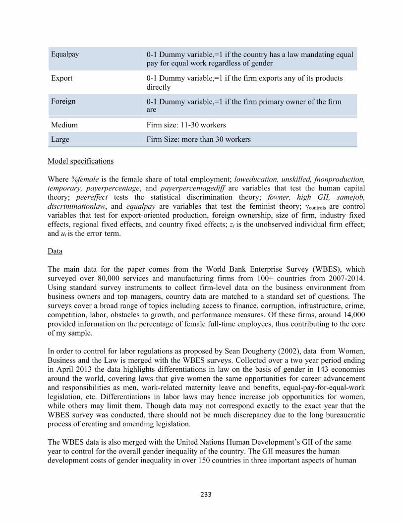
233

Export 0-1 Dummy variable,=1 if the firm exports any of its products

directly

Medium Firm size: 11-30 workers

Model specifications

Where %female is the female share of total employment; loweducation, unskilled, fnonproduction, temporary, payerpercentage, and payerpercentagediff are variables that test the human capital theory; peereffect tests the statistical discrimination theory; fowner, high GII, samejob, discriminationlaw, and equalpay are variables that test the feminist theory; γcontrols are control variables that test for export-oriented production, foreign ownership, size of firm, industry fixed effects, regional fixed effects, and country fixed effects; zi is the unobserved individual firm effect; and ui is the error term.

Data

The main data for the paper comes from the World Bank Enterprise Survey (WBES), which surveyed over 80,000 services and manufacturing firms from 100+ countries from 2007-2014. Using standard survey instruments to collect firm-level data on the business environment from business owners and top managers, country data are matched to a standard set of questions. The surveys cover a broad range of topics including access to finance, corruption, infrastructure, crime, competition, labor, obstacles to growth, and performance measures. Of these firms, around 14,000 provided information on the percentage of female full-time employees, thus contributing to the core of my sample.

In order to control for labor regulations as proposed by Sean Dougherty (2002), data from Women, Business and the Law is merged with the WBES surveys. Collected over a two year period ending in April 2013 the data highlights differentiations in law on the basis of gender in 143 economies around the world, covering laws that give women the same opportunities for career advancement and responsibilities as men, work-related maternity leave and benefits, equal-pay-for-equal-work legislation, etc. Differentiations in labor laws may hence increase job opportunities for women, while others may limit them. Though data may not correspond exactly to the exact year that the WBES survey was conducted, there should not be much discrepancy due to the long bureaucratic process of creating and amending legislation.

The WBES data is also merged with the United Nations Human Development’s GII of the same year to control for the overall gender inequality of the country. The GII measures the human development costs of gender inequality in over 150 countries in three important aspects of human

Equalpay 0-1 Dummy variable,=1 if the country has a law mandating equal pay for equal work regardless of gender

Foreign 0-1 Dummy variable,=1 if the firm primary owner of the firm are private foreign individuals, companies or organisations

Large Firm Size: more than 30 workers

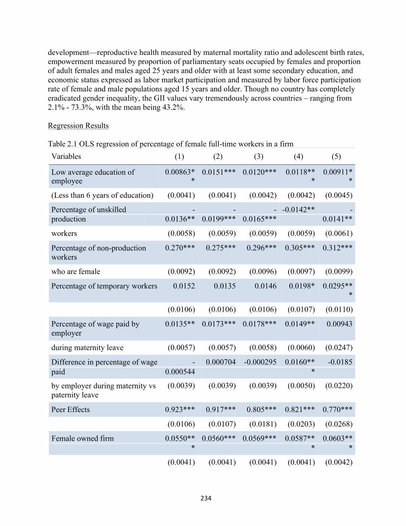
234

development—reproductive health measured by maternal mortality ratio and adolescent birth rates, empowerment measured by proportion of parliamentary seats occupied by females and proportion of adult females and males aged 25 years and older with at least some secondary education, and economic status expressed as labor market participation and measured by labor force participation rate of female and male populations aged 15 years and older. Though no country has completely eradicated gender inequality, the GII values vary tremendously across countries – ranging from 2.1% - 73.3%, with the mean being 43.2%.

Regression Results

Table 2.1 OLS regression of percentage of female full-time workers in a firm Variables (1) (2) (3) (4) (5)

Low average education of employee

0.00863* *

0.0151*** 0.0120*** 0.0118** *

0.00911* *

(Less than 6 years of education) (0.0041) (0.0041) (0.0042) (0.0042) (0.0045)

workers (0.0058) (0.0059) (0.0059) (0.0059) (0.0061)

Percentage of non-production workers

0.270*** 0.275*** 0.296*** 0.305*** 0.312***

who are female (0.0092) (0.0092) (0.0096) (0.0097) (0.0099)

Percentage of temporary workers 0.0152 0.0135 0.0146 0.0198* 0.0295** *

(0.0106) (0.0106) (0.0106) (0.0107) (0.0110)

Percentage of wage paid by 0.0135** 0.0173*** 0.0178*** 0.0149** 0.00943 employer

during maternity leave (0.0057) (0.0057) (0.0058) (0.0060) (0.0247)

by employer during maternity vs paternity leave

(0.0039) (0.0039) (0.0039) (0.0050) (0.0220)

Peer Effects 0.923*** 0.917*** 0.805*** 0.821*** 0.770*** (0.0106) (0.0107) (0.0181) (0.0203) (0.0268)

(0.0041) (0.0041) (0.0041) (0.0041) (0.0042)

Percentage of unskilled - - - -0.0142** - production 0.0136** 0.0199*** 0.0165*** 0.0141**

Difference in percentage of wage - 0.000704 -0.000295 0.0160** -0.0185 paid 0.000544 *

Female owned firm 0.0550** 0.0560*** 0.0569*** 0.0587** 0.0603** * * *

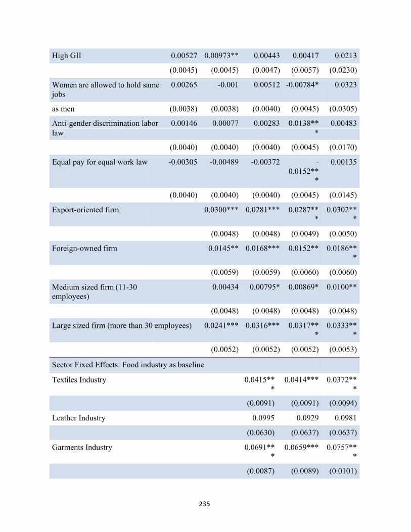
235

High GII 0.00527 0.00973** 0.00443 0.00417 0.0213 (0.0045) (0.0045) (0.0047) (0.0057) (0.0230)

Women are allowed to hold same jobs

0.00265 -0.001 0.00512 -0.00784* 0.0323

as men (0.0038) (0.0038) (0.0040) (0.0045) (0.0305) (0.0040) (0.0040) (0.0040) (0.0045) (0.0170)

Equal pay for equal work law -0.00305 -0.00489 -0.00372 - 0.0152**

*

0.00135

(0.0040) (0.0040) (0.0040) (0.0045) (0.0145)

Export-oriented firm 0.0300*** 0.0281*** 0.0287** *

0.0302** *

(0.0048) (0.0048) (0.0049) (0.0050)

Foreign-owned firm 0.0145** 0.0168*** 0.0152** 0.0186** *

(0.0059) (0.0059) (0.0060) (0.0060)

Medium sized firm (11-30 employees)

0.00434 0.00795* 0.00869* 0.0100**

(0.0048) (0.0048) (0.0048) (0.0048)

Large sized firm (more than 30 employees) 0.0241*** 0.0316*** 0.0317** *

0.0333** *

(0.0052) (0.0052) (0.0052) (0.0053)

Sector Fixed Effects: Food industry as baseline

Textiles Industry 0.0415** *

0.0414*** 0.0372** *

(0.0091) (0.0091) (0.0094)

Leather Industry 0.0995 0.0929 0.0981 (0.0630) (0.0637) (0.0637)

Garments Industry 0.0691** *

0.0659*** 0.0757** *

(0.0087) (0.0089) (0.0101)

Anti-gender discrimination labor 0.00146 0.00077 0.00283 0.0138** 0.00483 law *

236

Metals and Machinery Industry - 0.000082

-0.00208 -0.0143*

1

(0.0067) (0.0068) (0.0079)

Electronics Industry 0.00297 0.00238 -0.00128 (0.0158) (0.0159) (0.0161)

Chemicals and Pharmaceuticals Industry - 0.0158**

-0.0122* - 0.0210**

* (0.0070) (0.0071) (0.0073)

Wood and Furniture Industry 0.00127 0.00286 -0.0115 (0.0144) (0.0147) (0.0157)

Non-metallic and Plastic Materials Industry 0.0074 0.0106 - 0.000598 (0.0076) (0.0082) (0.0087)

Auto and Auto Components -0.0232* -0.0189 - Industry 0.0443** * (0.0130) (0.0132) (0.0161)

Other Manufacturing Industry 0.0039 0.00574 0.00216 (0.0056) (0.0056) (0.0063)

Retail and Wholesale Trade 0.0276 0.0277 0.0147 Industry

(0.0877) (0.0882) (0.0885)

Other Services Industry 0.0458** 0.0456** 0.0371* (0.0205) (0.0206) (0.0212)

Other Industry: Construction, Transportation, 0.0313 0.0202 -0.00708 etc.

(0.0236) (0.0239) (0.0247)

Regional Fixed Effects: Latin America and the Caribbean as baseline

East Asia and Pacific 0.0191** 0.0360** * * (0.0070) (0.0138)

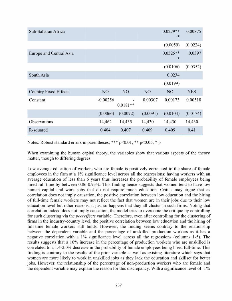
237

Sub-Saharan Africa 0.0279** *

0.00875

(0.0059) (0.0224)

Europe and Central Asia 0.0525** *

0.0397

(0.0106) (0.0352)

South Asia 0.0234

(0.0199)

Country Fixed Effects NO NO NO NO YES

Constant -0.00256 - 0.0181**

0.00307 0.00173 0.00518

(0.0066) (0.0072) (0.0091) (0.0104) (0.0174)

Observations 14,462 14,435 14,430 14,430 14,430

R-squared 0.404 0.407 0.409 0.409 0.41

Notes: Robust standard errors in parentheses; *** p<0.01, ** p<0.05, * p When examining the human capital theory, the variables show that various aspects of the theory matter, though to differing degrees.

Low average education of workers who are female is positively correlated to the share of female employees in the firm at a 1% significance level across all the regressions; having workers with an average education of less than 6 years thus increases the probability of female employees being hired full-time by between 0.86-0.93%. This finding hence suggests that women tend to have low human capital and work jobs that do not require much education. Critics may argue that as correlation does not imply causation, the positive correlation between low education and the hiring of full-time female workers may not reflect the fact that women are in their jobs due to their low education level but other reasons; it just so happens that they all cluster in such firms. Noting that correlation indeed does not imply causation, the model tries to overcome the critique by controlling for such clustering via the peereffects variable. Therefore, even after controlling for the clustering of firms in the industry-country level, the positive correlation between low education and the hiring of full-time female workers still holds. However, the finding seems contrary to the relationship between the dependent variable and the percentage of unskilled production workers as it has a negative correlation with a 1% significance level across all the regressions (columns 1-5). The results suggests that a 10% increase in the percentage of production workers who are unskilled is correlated to a 1.4-2.0% decrease in the probability of female employees being hired full-time. This finding is contrary to the results of the prior variable as well as existing literature which says that women are more likely to work in unskilled jobs as they lack the education and skillset for better jobs. However, the relationship of the percentage of non-production workers who are female and the dependent variable may explain the reason for this discrepancy. With a significance level of 1%

238

across all the regressions (columns 1-5), a 10% increase in the percentage of non-production workers who are female results in a 2.7-3.1% increase in the dependent variable. The interpretation of the finding hence suggests that women are more likely to be hired into administrative or clerical roles instead of production roles. Such jobs need not necessarily require employees with high levels of education and have been shown by existing literature to be typically female-dominant roles (Anker 1998), thus reconciling the results of the other two variables with regards to the human capital theory.

Besides testing the education and skill level of women, the regression also examined the cost of work flexibility. The relationship between the percentage of temporary workers and the dependent variable is shown to be positive but not significant till columns 4-5, with column 4 being significant only at the 10% level though column 5 is significant at the 1% level. The lack of sustained significance reduces the credibility of the findings, suggesting that either using the percentage of temporary worker is not a good proxy to measure the firm’s labor force flexibility or that contrary to Becker’s theory (1985), women do not value work flexibility more than men and are therefore just as likely as men to work in firms that are willing and able to provide that flexibility. The variables that measure the wages paid during paternal leave also tests for the cost of work flexibility though it looks at the employer’s considerations instead. The percentage of wage paid by employer during maternity leave was positive and significant at least the 5% level till the last column, when country fixed effects were added. The finding that a 10% increase in the percentage of wage the country mandates employers to pay during their employee’s maternity leave is associated with a 1.4-1.8% increase in the probability of female employees being hired full-time is contrary to the expectation that employers are likely to view maternity benefits as a cost and therefore not hire females in the first place in anticipation that they will have to give incur these costs in future. The difference in percentage of wage paid by employer during maternity versus paternity leave was insignificant. These results are thus contrary to the idea that mandated maternity leave might be a hiring disincentive to employers; however, one may also argue that there may be endogeneity between the variables as countries that are more likely to have such laws are more likely to have a populace, and firm owners, that view maternity leave less negatively. Such an argument may thus explain the loss of significance of the percentage of wage paid by employer during maternity leave when cross-country variations were taken into account. In view of that, the paper therefore shows that employers do not take the flexibility costs of hiring women into account when making hiring decisions.

When testing the statistical discrimination theory, the results show that peer effects is a large determinant of firm’s hiring of females. Based on the positive and significant results across all regressions (columns 1-5), a 10% increase in the mean percentage of full time female workers that other firms in same city and industry hired has a correlation of a 77% to 92% increase in the percentage of full time female workers that the tested firm hires. This result suggests that firms in the same industry of each country have pretty similar shares of women in their workforce. One might argue that this is an indicator of the characteristics that females possess. However, even with that hypothesis, after controlling for the human capital theories, the percentage of female hires across the firms seems too uniform. When hiring for lower waged jobs that require low education, firms may view the individual hiring process screening of each candidate as both too time consuming and costly. Firms therefore might have preconceived notions about the qualifications of women and therefore make hiring decisions based on the assumption that a woman is statistically

239

likely or unlikely to have the characteristics sought for the job instead of assessing the characteristics of the individual.

When looking at non-economic reasons, the variables tested suggest that besides the fact that female owned firms are shown to have a significant and positive correlation with the hiring of female full time employees, the feminist theory seem to lack significance. The results show that having at least one female owner in the firm increases the percentage of full time females hired by 5.5-6.0% at a 1% significance level. This finding might be due to the role model effect that they have as they serve as an inspiration to other women to join the workforce as their firm may be seen as being more “female-friendly.” It might also be more socially acceptable for employees to work for employers of the same gender. Having a female employer also provides employees an opportunity to interact with women in the workplace and “un-learn” the biases and preconceived notions that they previously had. However, the rest of the variables do not seem to produce significant results. When examining if the overall gender inequality of the country affects the hiring patterns of firms via the GII, the variable is unexpectedly positive, though it is significant - at the 5% level - only in the second column. The various variables that control for legislation against gender discriminatory labor practices are significant in the fourth column but all lose their significance when country fixed effects were added. When examining the significant finding (column 4), allowing women to hold the same jobs as men has a correlation of reducing the percentage of full time females hired by 0.78%. This result suggests that despite legislating against gender discrimination, firms still bar women from certain jobs. This finding, however, is significant only at the 10% level. Besides that, columns 1, 3, and 5 are insignificant and all have positive coefficients. Thus the validity of this result is questionable. Furthermore, though the variables testing for the presence of the anti-gender discrimination labor and equal pay for equal work laws have a significant result at the 1% level in column 4, it is the only column that has a significant result. Thus the variable does not show that anti-gender discrimination labor laws nor equal pay for equal work laws have an effect on the hiring decision of females. In light of such results, cultural biases against women in the workplace do not seem as rampant as previously expected.

When looking at the controls, one finds that export-oriented, foreign-owned, and firms that hire more employees all have a significant and positive relationship with the dependent variable. Looking at the industries, clothing-related sectors (i.e. textiles and garments) and the service industry, all are positively correlated with the dependent variable and are more female dominant. This finding is in line with existing literature (Anker 1998) stating that the service industry is more female dominant. Industries in the technology and manufacturing sectors (i.e. chemicals and pharmaceuticals, and auto and auto components), are significantly and negatively correlated with the dependent variable and are therefore more male dominant. However, industries that require employers with more “gender neutral” traits (hotels and restaurants as well as retail and wholesale trade) are also more male dominant as they are negatively and significantly correlated with the dependent variable.

Examining regional effects (columns 3 and 4), countries in East Asian and Pacific, Sub-Saharan Africa, and Europe and Central Asia were found to be more likely to hire females, with the significance of the result maintained and coefficient increased for countries in East Asian and Pacific when country fixed effects were taken into account (column 4).

240

The regressions therefore show that the human capital theory holds as female full-time employees tend to be hired into low education, non-production jobs. The statistical discrimination theory also has merit as firms in the same industry of each country have pretty similar shares of women in their workforce. The role model effect as outlined by feminist theory is also supported.

4 Policy Recommendations and Conclusion

In light of these findings, the government can enact the following policies to try to reduce the gender inequality in the workforce. As the human capital theory showed that women tend to work in firms that have a larger share of workers with a low average education, a way to increase the opportunities for women would be to try to improve their education level. Many countries provide conditional cash transfers to mothers when they ensure that their daughters are enrolled and attend school; however, the government should also try to increase the years of education attained by women. Besides encouraging education’s importance regardless of gender, governments should increase the number of higher education schools, provide scholarships and other monetary incentives, and create training programs for women to increase current and future female working generations’ skills.

The findings also show that even though employees tend to follow conventional gender stereotypes with women clustering in the clothing and service related industries and men in manufacturing industries, women tend to work in non-production areas of the firm regardless of industry. Unfortunately the data is limited and unable to examine what types of non-production jobs (administrative versus managerial roles) women tend to take. From the earlier finding that women tend to work in firms with low average education of employees, however, there is a higher probability that the female employees themselves have low education levels and therefore would be working in administrative and clerical roles rather than upper management. Increasing the education level of women would therefore provide them with the skills needed to rise up the career ladder and take on the higher waged, supervisory roles. Finding a dataset that allows for both an industrial and occupational analysis would help shed more light on this matter.

Increasing the education level of women can also help combat statistical discrimination in the long run. Gradually, firms would begin to realize that more women possess higher human capital and skills. Therefore they would change their views on women and be less likely to make hiring decisions based on the assumption that women are statistically unlikely to have the prerequisite education and skills. There, however is no guarantee for the change in this preconceived notion. Unfortunately the regressions are unable to parse out if the clustering of women is due to women choosing to interview for these roles or if firms disproportionally select females for these jobs. The paper’s finding that there is a positive correlation between female owned firms and the share of female full-time workers hired suggests that the discrimination might be more to do with the firm’s choices. A possible extension of this paper would be to separate the factors that affect the supply and demand of female workers. In the meantime, based on the paper’s results, imposing a quota, similar to that of Scandinavian countries, that mandate a certain percentage of women board members in publicly owned firms can also help to reduce the discrimination, statistical or otherwise; however, as can be seen from the insignificance of labor laws, legislation is ineffective if people are unwilling or cannot enforce it. The government could thus try to dispel industries’ gender stereotypes and promote the merits of diversity in the workforce via campaigns or incentives to

241

firms to have female board members or employ a higher than average number of females. It is important to note that these conclusions come with many assumptions and qualifications. The policy implications of this analysis are predicated on the accuracy of the data analysis, and limitations of the data analysis are mostly a result of the data set used. On a rudimentary level, the dataset had over 80,000 firms from over 100 countries, but due to the focus on countries with high gender inequality and incomplete data, the regressions ran on the smallest dataset took less than 20% of the firms surveyed into consideration. Besides that, data was not collected in each country for every year between 2007 and 2014. Therefore this cross-sectional data, unlike panel data, does not take changes in variables over time into account. In offering policy prescriptions, the paper thus assumes that the outcomes of this analysis can be applied more generally to the larger dataset and of developing countries. The weaknesses of the data therefore present opportunities for further research, some of which have been aforementioned.

Besides limitations in the data, a different methodology can be used to get a more accurate calculation of occupational segregation. The paper uses the percentage of full-time employees in a firm who are female as the dependent variable, allowing for the calculation of the extent to which the firm is feminised. However, it takes neither overall female and male population percentage nor female and male labor force participation rate into account. Therefore testing the data via a methodology that takes all these aspects into account would be helpful in understanding the factors that influence women to join the workforce and the specific occupations.

Data and econometric analysis therefore have their limitations, but the insight provided by this analysis still offers useful insight for policymakers. By focusing on the patterns and reasons behind the clustering of women in the workforce from a firm-level, some of which parallel contributing factors cited in the literature, this paper complements existing research as it acts as a bridge between the macro level and household/individual level analyses of female workforce participation and employment. It therefore provides insight into policies that can be enacted that affect firms directly in order to widen the opportunities available to women in the formal economy.

Bibliography

Agarwal, Bina. “Bargaining and Gender Relations: Within and Beyond the Household.” Feminist Economics 3.1

(1997).

Anker, Richard. “Gender and Jobs: Sex Segregation of Occupations in the World.” Geneva: International Labor Office (1998).

Anker, Richard and C. Hein. “Why Third World Urban Employment Usually Prefer Men.” International Labor Review.

Geneva: ILO. 12.1 (1985): 73-90.

Bagchi, Alaknanda. "Conflicting Nationalisms: The Voice of the Subaltern in Mahasweta Devi's Bashai Tudu." Tulsa Studies in Women's Literature 15.1 (1996): 41-50. Print.

Becker, Gary S. “Human Capital, Effort, and the Sexual Division of Labor” Jounral of Labor Economics 3.1.2 Trends in

Women’s Work, Education, and Family Building (January 1985): S33-S58 Blau, F. and Ferber, M. “Occupational Segregation by Gender: A Look at the 1980s”. Paper presented at the American

Economic Association Meeting. New York (December 1988).

242

Bradley, K. “The Incorporation of Women into Higher Education: Paradoxical Outcomes.” Sociology of Education 73 (2000): 1-18

Boulding, E. “Handbook of International Data on Women.” Beverly Hills, California (1976)

Cagatay, N. and Ozler, S. “Feminization of the Labor Force: The Effects of Long-Term Development and Structural Adjustment.” World Development 23 (1995).

Charles, M., and Grusky, D.B. “Occupational Ghettos: The Worldwide Segregation of Women and Men” Stanford:

Stanford University Press. 2004

Chen, Guifu and Hamori, Shigeyuki. "Bivariate Probit Analysis of Differences Between Male and Female Formal Employment in Urban China.” Journal of Asian Economics 21.5 (2010): 494-501. Print.

Chen, Martha Alter. “Women In The Informal Sector: A Global Picture, The Global Movement.” (2002).

Dougherty, Sean. “Labor Regulation and Employment Dynamics at the State Level in India.” OECD Economics Department Working Papers No. 624, OECD Publishing (2002).

Duncan, D. and B. Duncan. “A Methodological Analysis of Segregation Indices.” American Sociological Review No 20,

New York (1955): 210-217

Duflo, Esther, Rohini Pande, and Petia Topalova. “Female Leadership Raises Aspirations and Educational Attainment for Girls: A Policy Experimentin India.” Science (January 2012).

Esteve-Volart, Berta. “Gender Discrimination and Growth: Theory and Evidence from India.” Economic Organisation

and Public Policy Discussion Papers 42, Suntory and Toyota International Centres for Economics and Related Disciplines, LSE. (January 2004).

Gallaway, Julie; and Bernasek, Alexandra. "Gender and Informal Sector Employment in Indonesia." Journal of

Economic Issues 36.2 (2002): 313-21. Print.

Haddad, Lawrence James, Hoddinott, John, and Alderman, Harold. “Intrahousehold Resource Allocation in Developing Countries.” Baltimore: Johns Hopkins University Press (1997).

Hausmann, Ricardo, Tyson, and Laura D., and Zahidi, Saadia. “The Global Gender Gap Report 2012,” World Economic

Forum (July 2012).

Hochschild, Arlie. “The Second Shift: Working Parents and the Revolution.” The Second Shift (1989).

Joekes, Susan. “Influence of Trade Expansion on Women’s Work” Geneva: Interdepartmental Project on Equality for Women in Employment, International Labor Office.

Mazumdar, Dipak “The Urban Informal Sector” Employment and Rural Development Division, Development

Economics Department (October 1974).

Naila Kabeer “Gender Equality and Women's Empowerment: A Critical Analysis of the Third Millennium Development Goal.” Gender & Development 13.1 (2005): 13-24.

Kapsos, Steven. “World and Regional Trends in Labor Force Participation: Methodologies and Key Results.”

International Labor Office (2007).

King, Elizabeth M., Stephan Klasen, and Maria Porter. ‘‘Gender and Development Challenge Paper.’’ Paper Prepared for 2008 Round of Copenhagen Consensus Project. Mimeographed, Copenhagen Consensus Center (2008).

243

Klasen, Stephan and Francesca Lamanna. “The Impact of Gender Inequality in Education and Employment on Economic Growth: New Evidence for a Panel of Countries.” Feminist Economics, 15.3 (2009).

Klasen, Stephan and Claudia Wink.‘‘Missing Women: Revisiting the Debate.’’ Feminist Economics 9.2 (2003): 263– 299.

Koning, Juliette ed. “Women and Households in Indonesia: Cultural Notions and Social Practice”. Richmond, Surrey,

Curzon (2000).

Psacharopoulos, G. and Z. Tzannatos “Women’s Employment and Pay in Latin America: Overview and Methodology.”

Washington DC: The World Bank (1992).

Rajivan, Anuradha. “Power, Voice, and Rights: A Turning Point for Gender Equality in Asia and the Pacific.” Rep. UN Development Program (Feb. 2010). Web.

Ross. Michael. “Oil, Islam, and Women” American Political Science Review (2007).

Sapiro, Virginia. “The Political Integration of Women.” Urbana: University of Illinois Press (1983).

Schlozman, Kay Lehman, Nancy Burns Nancy, and Sidney Verba. "What Happened at Work Today?: A Multistage

Model of Gender, Employment, and Political Participation.” Journal of Politics 61 (February 1999): 29-53.

Sen, Amartya. “Development as Freedom.” New York: Alfred A. Knopf (1999).

Irene Tinker, ed. ‘‘Gender and Cooperative Conflicts,’’ Persistent Inequalities: Women and World Development, Oxford: Oxford University Press (1990): 123–49.

Seguino, Stephanie and Maria Sagrario Floro.‘‘Does Gender Have Any Effect on Aggregate Saving?’’ International

Review of Applied Economics 17.2 (2003): 147–66.

Stotsky, Janet. ‘‘Gender and its Relevance to Macroeconomic Policy: A Survey.’’ Working Paper WP/06/233, International Monetary Fund (2006).

Swamy, Anand, Omar Azfar, Stephen Knack, and Lee Young. “Gender and Corruption“. Journal of Development

Economics 64(1) The World Bank. (2001): 25-55.

Thomas, Duncan. ‘‘Incomes, Expenditures and Health Outcomes: Evidenceon Intrahousehold Resource Allocation.” Lawrence James Haddad, John Hoddinott, and Harold Alderman, eds. Intrahousehold Resource Allocation in Developing Countries, Baltimore: Johns Hopkins University Press (1997): 142– 64.

Weinberg, Daniel H., John Iceland, and Erika Steinmetz. “Measurement of Segregation by the U.S. Bureau of the Census in Racial and Ethnic Residential Segregation in the United States: 1980-2000.” Census 2002 Special Reports, U.S. Census Bureau (August 2002).

“Country and Lending Groups” The World Bank.Web. http://data.worldbank.org/about/country-and-lending-groups “Engendering Development” The World Bank. 2001.

“Gender Inequality Index (GII)” United Nations Development Programme Human Development Reports.

Web. http://hdr.undp.org/en/content/gender-inequality-index-gii “Getting a Job” Women Business and the Law. Web. http://wbl.worldbank.org/data/exploretopics/getting-a- job#parental-benefits

“World Development Report 2012: Gender Equality and Development.” The World Bank (2011). Web. http://siteresources.worldbank.org/INTWDR2012/Resources/7778105- 1299699968583/7786210- 1315936222006/Complete-Report.pdf

Appendix

243

APPENDIX A: Fourteenth Carroll Round Presentation Schedule

Session 1A Chair: Charles Udomsaph (Visiting Assistant Professor, Georgetown University) Natalie Nah (Georgetown University) Where and why do women cluster in the workforce? Discussant: Dora Heng Dora Heng (Cornell University) Incentives, institutions and investment in private agricultural research in Asia Discussant: Hameem Chowdhury Hameem Chowdhury (University of Warwick) Joint-Liability in Microcredit: Evidence from Bangladesh Discussant: Levi Boxell Levi Boxell (Taylor University) HIV Prevalence in sub-Sahara Africa: A Spatial Econometric Approach Discussant: Natalie Nah Session 1B Chair: Robert Cumby (Professor, Georgetown University) Thomas Christiansen (Georgetown University) It's Still Who You Know: The Lingering Effect of Guanxi On Access to Finance in China Discussant: Chenbo Fang Chenbo Fang (University of California, Berkley) Cost and Efficacy of Collective Action Clauses in Sovereign Bond Contracts Discussant: Virginia Minni Virginia Minni (University of Warwick) Can Greater Bank Capital Lead to Less Bank Lending? An Analysis of the Bank-Level Evidence from Europe Discussant: Aaron Goodman Aaron Goodman (Dartmouth College) Capital Requirements and Post-Crisis Monetary Policy Transmission

Discussant: Thomas Christiansen Session 2A Chair: Anna Maria Mayda (Associate Professor, Georgetown University) Lea Rendell (Vassar College) Fiscal Multipliers in a Financially Globalized World Discussant: Eve Lee Eve Lee (Georgetown University) Inward FDI Spillovers and Internet Diffusion Discussant: Lea Rendell Session 2B Chair: Shareen Joshi (Assistant Professor, Georgetown University) Ryan Go (University of California, Berkley) Adjusting for Overconfidence using Partition Dependence Discussant: Geeva Gopalkrishnan Geeva Gopalkrishnan (Georgetown University) Revisting the phenomenon of Missing Women in India: Household Air Pollutant as a Determinant Discussant: Ryan Go

Appendix

244

APPENDIX A: Fourteenth Carroll Round Presentation Schedule Session 3A Chair: Olga Timoshenko (Assistant Professor, George Washington University) Jonathan McClure (Georgetown University) Is the MFN Free Rider Problem Getting Worse? Evidence from the Doha Round Discussant: Nancy Wu Nancy Wu (Dartmouth College) Foreign Direct Investment Jobs and School Attendance: Evidence from Vietnam Discussant: Karlis Locmelis Karlis Locmelis (Stockholm School of Economics in Riga) The 2014-15 Russian crisis’ impact on the dynamic linkages between the stock markets of Russia, the EU and the U.S. Discussant: Daniel Roeder Daniel Roeder (Dartmouth College) Bayesian Portfolio Analysis: Analyzing the Global Investment Market Discussant: Jonathan McClure

Session 3B Chair: Carol Rogers (Associate Professor, Georgetown University) Mathison Clore and Michael McGrath (Georgetown University) The benefits of economic transparency for domestic investment Discussant: Emily Reeves Emily Reeves (Dartmouth College) Trade Liberalization and Deforestation Discussant: Michael Lee Michael Lee (University of Texas at Austin) An Agent Based Model for Competitive Equilibrium in Electricity Markets Discussant: Raphael Small

Raphael Small (Haverford College) The Dynamic Link between Inequality and Economic Growth: a Stochastic Approach Discussants: Mathison Clore and Michael McGrath

Session 4A Chair: Christopher Griffin (Assistant Professor, College of William and Mary) Kenan Jusufovic (London School of Economics) Platon's Republic: A Recipe for Economic Success? Discussant: Samuel Huang Samuel Huang (London School of Economics) Peer effects in football Discussant: Jack Willoughby Jack Willoughby (Duke University) Security Without Equity? The Effect of Secure Communities on Racial Profiling by Police Discussant: Shom Mazumder Shom Mazumder (Georgetown University) Dictators Embed: Preferential Trade Agreements, Regime Type and International Conflict Discussant: Kenan Jusufovic

Session 4B Chair: Erwin Tiongson (Professor in the Practice of International Affairs, Georgetown University) Yingtong Xie (Macalester College) International Business Cycle Transmissions and News Shocks Discussant: John McKeon John McKeon (Boston University) Copyright Extensions and the Availability of Music: Evidence from British Hits of the 1960’s Discussant: Thomas Gutierrez

Thomas Gutierrez (Harvard University) Demographics Influence on Global Current Account Imbalances in Advanced Economies Discussant: Sankalp Gowda Sankalp Gowda (Georgetown University) China and India in Africa: Implications of New Private Sector Actors on Bribe Paying Incidence Discussant: Yingtong Xie

Appendix

245

APPENDIX B: Past Speakers

First Annual Carroll Round (April 5-7, 2002) Roger W. Ferguson, Federal Reserve Board of Governors Donald L. Kohn, Federal Reserve Board of Governors Lawrence B. Lindsey, Assistant to the President and National Economic Council Edwin M. Truman, Institute for International Economics John Williamson, Institute for International Economics

Second Annual Carroll Round (April 11-13, 2003) R. Glenn Hubbard, Council of Economic Advisers and Columbia University Donald L. Kohn, Federal Reserve Board of Governors John Williamson, Institute for International Economics

Third Annual Carroll Round (April 15-18, 2004) Donald L. Kohn, Federal Reserve Board of Governors John F. Nash, Jr., Princeton University (1994 Nobel Laureate) Peter R. Orszag, The Brookings Institute

Fourth Annual Carroll Round (April 22-24, 2005) Ben S. Bernanke, Federal Reserve Board of Governors William Easterly, New York University Maurice Obstfeld, University of California at Berkeley Edwin M. Truman, Institute for International Economics

Fifth Annual Carroll Round (April 28-30, 2006) Kemal Dervis, United Nations Development Programme

Thomas C. Schelling, University of Maryland (2005 Nobel Laureate)

Sixth Annual Carroll Round (April 19-22, 2007) Grant D. Aldonas, Center for Strategic and International Studies François Bourguignon, Chief Economist and Senior Vice President of the World Bank Randall Kroszner, Federal Reserve Board of Governors

Seventh Annual Carroll Round (April 17-20, 2008) Susan C. Athey, Harvard University Philip I. Levy, American Enterprise Institute Steven Radelet, Senior Fellow at the Center for Global Development Eighth Annual Carroll Round (April 16-19, 2009) Eric S. Maskin, Princeton University (2007 Nobel Laureate) Nassim Nicholas Taleb, Universa Investments and New York University

Ninth Annual Carroll Round (April 22-25, 2010) Philip I. Levy, American Enterprise Institute Robert C. Merton, Harvard Business School (1997 Nobel Laureate) Lant Pritchett, Harvard Kennedy School

Tenth Annual Carroll Round (April 14-17, 2011) Jagdish Bhagwati, Columbia University Joseph Stiglitz, Columbia University (2001 Nobel Laureate)

Eleventh Annual Carroll Round (April 19-22, 2012) Jonathan Levin, Stanford University Gene Sperling, Director of the National Economic Council

Twelfth Annual Carroll Round (April 18-21, 2013) John Taylor, Stanford University Janet Currie, Princeton University

Appendix

246

APPENDIX B: Past Speakers Thirteenth Annual Carroll Round (April 10-13, 2014) Peter Diamond, Massachusetts Institute of Technology (2010 Nobel Laureate) Martin Ravallion, Georgetown University Fourteenth Annual Carroll Round (April 16-19, 2015) Rajiv Shah, United States Agency for International Development George Akerlof, Georgetown University (2001 Nobel Laureate)

Appendix

247

APPENDIX C: Former Carroll Round Steering Committees First Annual Carroll Round (April 5-7, 2002) Christopher L. Grifin, chair (SFS '02) William B. Brady (SFS '02) Cullen A. Drescher (COL'04) Meredith L. Gilbert (COL'04) Joshua M. Harris (SFS '02) Andrew T. Hayashi (SFS '02) Mark R. Longstreth (SFS '04) Kathryn E. Magee (SFS '02) Ryan F. Michaels (SFS '02) J. Brendan Mullen (SFS '02) Scott E. Pedowitz (SFS '02) Waheed A. Sheikh (SFS '04)

Second Annual Carroll Round (April 11-13, 2003) Seth M. Kundrot, chair (SFS '03) Nada M. Abdelnour (SFS '03) Maria M. Arhancet (SFS '04) Victoria E. Bembenista (SFS '03) Michael J. Callen (SFS '05) Eric M. Fischer (SFS '03) Daphney Francois (SFS/GRD '04) Meredith L. Gilbert (COL'04) Jeffrey M. Harris (COL'03) Robert S. Katz (COL'04) Marina Lafferriere (SFS '06) Lu Shi (SFS '03) Stacey H. Tsai (SFS '03) Robert T. Wrobel (SFS '03) Erica C. Yu (COL'05)

Third Annual Carroll Round (April 15-18, 2004) Meredith L. Gilbert, chair (COL'04) Heber M. Delgado-Medrano (SFS '06) Ryan V. Fraser (SFS '04) Tetyana V. Gaponenko (SFS '07) Yunjung Cindy Jin (SFS '05) Sarah H. Knupp (SFS '04) Robert S. Katz (COL'04) Marina Lafferriere (SFS '06) Alia F. Malik (SFS ’04) Susan M. Work (SFS ’04) Beatka J. Zakrzewski (SFS ’04)

Fourth Annual Carroll Round (April 22-24, 2005) Erica C. Yu, chair (COL ’05) Jasmina Beganovic (SFS ’05) Lucia Franzese (SFS ’07) Dennis L. Huggins (SFS ’07) Yunjung Cindy Jin (SFS ’05) Jonathan W. Kirschner (SFS ’05) Susan C. Kleiman (SFS '05) Yousif H. Mohammed (SFS '06) Amy M. Osekowsky (SFS '07) Daniel P. Schier (SFS '05)

Fifth Annual Carroll Round (April 27-30, 2006) Marina Lafferriere, chair (SFS '06) lrmak Bademli (SFS '06) Stephen Brinkmann (SFS '07) Heber Delgado (SFS '06) Lucia Franzese (SFS '07) Yasmine Fulena (SFS '08) Jen Hardy (SFS '06) Michael Kunkel (SFS '08) Yousif Mohammed (SFS '06) Emy Reimao (SFS '06) Tamar Tashjian (SFS '06)

Sixth Annual Carroll Round (April 19-22, 2007) Stephen A. Brinkmann, chair (SFS '07) Lucia Franzese (SFS ’07) Nicholas A. Hartman (SFS '07) lan P. Hinsdale (COL'09) Alexander P. Kostura (SFS ’09) Jennifer M. Noh (SFS '07) Amy M. Osekowsky (SFS ’07) Allison E. Phillips (SFS ’07) Sun Yi (SFS ’07)

Seventh Annual Carroll Round (April 17-20, 2008) Yasmine Fulena, chair (SFS '08) Sue Bai (SFS '08) Stacey Droms (COL '08) Brandon Feldman (COL '08) LiJia Gong (SFS '08 Kory Katenga (SFS ’10) Sung Kim (SFS '08) Michael Kunkel (SFS '08) Fuyang Zhang (SFS ’10)

Appendix

248

APPENDIX C: Former Carroll Round Steering Committees

Eighth Annual Carroll Round (April 16-19, 2009) Rebecca A. Heide, chair (SFS ’09) James O. Arnold (SFS ’11) Henry T. Gillam (SFS ’10) Tom J. Han (SFS ’10) Anna A. Klis (SFS ’10) Daniel T. Leonard (SFS ’09) Daniel Y. Lim (SFS ’11) Arjun B. Pant (SFS ’09) Benjamin D. Simmons (COL ’09) Ariell E. Zimran (SFS ’10)

Ninth Annual Carroll Round (April 22-25, 2010) Ariell E. Zimran, chair (SFS '10) Michael A. Counihan (SFS '11) Amanda B. Delp (SFS '12) Katherine E. Donato (SFS '10) Tom J. Han (SFS '10) Michael R. Karno (SFS '10) Allison T. Kern (SFS '10) Anna A. Klis (SFS '10) Daniel Y. Lim (SFS '11) H. Jess Seok (SFS '12) Matthew H. Shapiro (SFS '11)

Tenth Annual Carroll Round (April 14-17, 2011) Amanda Delp, chair (SFS '12) James Arnold (SFS '11) Albert Chiang (SFS '13) Malin Hu (SFS '11)

Katrina Koser (SFS '12) Nancy Lee (SFS '11) Doug Proctor (SFS '12) Vivek Sampathkumar (SFS '11) Monica Scheid (SFS '11) Matthew Shapiro (SFS '11) Eleventh Annual Carroll Round (April 19-22, 2012) Katrina Koser, Chair (SFS '12) Albert Chiang (SFS '13) Amanda Delp (SFS '12) Nhaca Le (SFS '12) Doug Proctor (SFS '12) Glenn Russo (COL '13) H. Jess Seok (SFS '12) Anusuya Sivaram (SFS '12) Meredith Strike (SFS '14) Shuo Yan Tan (SFS '12)

Twelfth Annual Carroll Round (April 18-21, 2013) Glenn Russo, chair (COL '13) Albert Chiang (SFS '13) Meredith Strike (SFS '14) Natalie Nah (SFS '15) Brian Goggin (SFS '14) Heather Hedges (SFS '14) Dawn Chan (SFS '14) Edward Hedke (SFS '13) Elena Malik (SFS '14) Stephen McDonald (SFS '13) Emily Oehlsen (SFS '13)

Appendix

249

APPENDIX C: Former Carroll Round Steering Committees Thirteenth Annual Carroll Round (April 10-13, 2014) Heather Hedges (SFS ’14) Brian Goggin (SFS ’14) Dawn Chan (SFS ’14) Elena Malik (SFS ’14) Natalie Nah (SFS ’15) Jill Ni (SFS ’14) Kristen Skillman (SFS ’16) Meredith Strike (SFS ’14) Christopher Stromeyer (SFS ’14) Rachel Szymanski (SFS ’14)

Fourteenth Annual Carroll Round (April 16-19, 2015) Natalie Nah (SFS ’15) Kristen Skillman (SFS ’16) Thomas Christiansen (SFS ’15) Geeva Gopalkrishnan (SFS ’15) Elle Kang (SFS ‘15) Grace Kim (SFS ‘17) Cheryl Lau (SFS ‘16) Eve Lee (SFS ‘15) Shom Mazumder (SFS ‘15) Morgan Snow (COL ‘16)

Maryanne Zhao (SFS ’16)

Appendix

250

APPENDIX D: Members of the Advisory Panel

Meredith L. Gilbert, The Chartis Group Christopher L. Grifin, College of William & Mary Andrew T. Hayashi, University of Virginia Mitch Kaneda, Georgetown University Robert S. Katz, Amazon J. Brendan Mullen, American College of Cariology Scott E. Pedowitz, Libby Garvey for Arlington County Board Erica Yu Wright, Bureau of Labor Statistics

Appendix

251

APPENDIX E: Past Participants

First Annual Carroll Round (April 5-7, 2002)

Azhar Adbul-Quader Columbia University Santosh Anagol Stanford University William Brady Georgetown University Daniel Braun Oberlin College Jacqueline Bueso University of Pennsylvania Karla Campbell University of Virginia Benn Eifert Stanford University Courtney Fretz University of Pennsylvania Carlos Galvez Stanford University Aniruddha Gopalakrishnan Duke University Christopher Grifin Georgetown University Casey Hanson Lehigh University Joshua Harris Georgetown University Andrew Hayashi Georgetown University Marco Hernandez Massachusetts Institute of Technology Katia Hristova Illinois-Wesleyan University Maria Jelescu Massachusetts Institute of Technology Fadi Kanaan Yale University Avinash Kaza Stanford University Vinay Kumar Duke University Anisha Madan Illinois-Wesleyan University Kathryn Magee Georgetown University Ryan Michaels Georgetown University Jack Moore Stanford University Brendan Mullen Georgetown University Andrei Muresianu Brown University Scott Orleck Duke University Scott Pedowitz Georgetown University Jonathan Prin University of Pennsylvania Jeremy Sandford Illinois-Wesleyan University Deborah Slezak Illinois-Wesleyan University Conan Wong Brown University

Second Annual Carroll Round (April 11-13, 2003)

Nada Abdelnour Georgetown University Amanda Barnett Emory University Andrea Bell Wellesley College Patrick Byrne University of Colorado David Chao Cornell University Sylvia Ciesluk Lehigh University Adam Doverspike Georgetown University

Appendix

252

APPENDIX E: Past Participants

Benn Eifert Stanford University Adam Engberg Georgetown University Alexandra Fiorillo Connecticut College Eric Fischer Georgetown University Zlata Hajro Wellesley College Samina Jain Georgetown University Avinash Kaza Stanford University Eric Kim The George Washington University Seth Kundrot Georgetown University Lada Kyi Rice University Lee Lockwood Northwestern University Sunil Mulani New York University Holly Presley Vanderbilt University Duncan Roberts University of California at Berkeley Lu Shi Georgetown University Shanaz Taber Barnard College Jiang Wei University of Michigan

Third Annual Carroll Round (April 15-18, 2004)

Jeffrey Arnold Dartmouth College Julia Berazneva Mt. Holyoke College Mehmet Cangul Georgetown University Richard Carew University of Virginia Ashley Coleman Vanderbilt University Dilyana Dimova Stanford University Fernando Galeana Stanford University M. Blair Garvey Emory University Meredith Gilbert Georgetown University Adam Greeney Oberlin College Asim Gunduz University of Virginia Marc Hafstead Northwestern University Andrew Hayashi University of California at Berkeley Katherine Howitt McGill University Sohini Kar Columbia University Josh Lewis McGill University Satish Lohani Illinois-Wesleyan University Alexis Manning Illinois-Wesleyan University Sara Menker Mt. Holyoke College Elizabeth Mielke Vanderbilt University Stratos Pahis Dartmouth College Alicja Pluta Georgetown University Adam Raymakers Dalhousie University Caroline Schmutte Dartmouth College

Appendix

253

APPENDIX E: Past Participants

Matt Sekerke Johns Hopkins University John Soleanicov Columbia University Kai Szakmary Columbia University Brandon Wall Yale University Kenneth Ward University of Chicago Susan Work Georgetown University

Fourth Annual Carroll Round (April 22-24, 2005)

Lidia Barabash Dartmouth College Jasmina Beganovic Georgetown University Xun Bian Illinois-Wesleyan University Michael Furchtgott Columbia University Michael Gechter Pomona College Kevin B. Goldstein Dartmouth College Michael Haase University of Copenhagen Dennis Huggins Georgetown University Michael Insel Claremont McKenna College Jonathan Kirschner Georgetown University Shiying Lee Duke University James Liao Dartmouth College Brian Lichter Washington University Wee Lee Loh Cornell University Alice Luo Duke University Katharine Mullock University of Western Ontario Jose Mustre del Rio The Ohio State University Leah Nelson Georgetown University Ee Cheng Ong Wellesley College Matthew Phan Columbia University Nina Rendelstein Washington University David Rogier Washington University Ana Maria Romero Illinois-Wesleyan University Nathan Saperia Dartmouth College Bogdan Tereshchenko Georgetown University Olga Timoshenko University of Western Ontario Tom Vogl Princeton University Kenneth Ward University of Chicago Jonathan Wolfson Washington University Suzanne Zurkiya Emory University

Fifth Annual Carroll Round (April 28-30, 2006)

Sarah Carroll Stanford University Ruth Coffman Georgetown University

Appendix

254

APPENDIX E: Past Participants

Dubravka Colic Wellesley College Pratik Dattani University of Warwick Jennifer Dawson Illinois-Wesleyan University Héber Delgado-Medrano Georgetown University Sherri Haas Illinois-Wesleyan University Jen Hardy Georgetown University Lauren Iacocca University of California at Los Angeles Salifou Issoufou University of Wisconsin at Madison Stella Klemperer Brown University Daniel Kurland Dartmouth College Corinne Low Duke University Shanthi Manian Georgetown University Michael Monteleone University of Chicago John Nesbitt Georgetown University Natasha Nguyen University of California at Berkeley Oyebanke Oyeyinka Carleton College Evgeniya Petrova Dartmouth College Emy Reimao Georgetown University Svetoslav Roussanov Columbia University Vikram Shankar Georgetown University Juan Carlos Suarez Trinity University Austin Vedder Dartmouth College David Wiczer Carleton College Geoffrey Yu Carleton College Xiaoti Zhang University of Warwick

Sixth Annual Carroll Round (April 19-22, 2007)

Matthew Adler Oberlin College Marion Aouad Princeton University Stephen Brinkmann Georgetown University Erik Eggum University of Warwick Lucia Franzese Georgetown University Tanja Groth University of St. Andrews Ashley Halpin Dartmouth College Nicholas Hartman Georgetown University Adrienna Huffman Washington University Abdulla Humaidan University of Warwick Mohammad Huq Georgetown University Nedko Kyuchukov Dartmouth College Zachary Mahone New York University R. Priya Mathew Washington University Yana Morgulis University of Chicago Jennifer Noh Georgetown University

Appendix

255

APPENDIX E: Past Participants

Andrew O’Brien Penney Georgetown University Jessica Oliveri Monash University Matthew Pech Dartmouth College Allison Phillips Georgetown University Angelica da Rocha University of Warwick Sören Radde University of Bayreuth Heleri Rande New York University Elena Spatoulas University of Michigan Yi Sun Georgetown University Bennett Surajat Carleton College Freddy Tsai University of British Columbia David Wolff Dartmouth College Jennifer Xi Dartmouth College Cynthia Yim Princeton University

Seventh Annual Carroll Round (April 17-20, 2008)

Karl Andres University of Warwick Cecil Ang University of Virginia Alaina Antonucci The Pennsylvania State University Sue Bai Georgetown University Marinella Boyadzhiev Oberlin College Quentin Brummet Illinois-Wesleyan University Brendan Cooper Carleton College Gerard DiPippo Dartmouth College Stacey Droms Georgetown University Varun Dutt Macalaster College Yasmine Fulena Georgetown University Amish Gandhi University of Warwick Katherine Gordon Mt. Holyoke College Yi Kang Wesleyan College Michael Kunkel Georgetown University Han Youp Lee Georgetown University Claudio LoCascio Dartmouth College Olivia Lynch Georgetown University Amr Moubarak The George Washington University Simone Nitsch University of Warwick Saurabh Pant New York University Carson Sherwood University of Western Ontario Tadashi Shirai University of Warwick Dominique Shure Georgetown University William Slater Vanderbilt University Shyam Sundaram Brown University Poh Lin Tan Princeton University Dorothy Voorhees Georgetown University Kris Walsh Georgetown University Monica Yu Dartmouth College

Appendix

256

APPENDIX E: Past Participants

Anders Jensen London School of Economics and Political Science William Kafoure The George Washington University Elira Kuka Wellesley College Daniel Leonard Georgetown University Chris Lim Dartmouth College Juan Ignacio Elorrieta Maira University of Chile Nick Marchio Macalester College Hekuran Neziri American University in Bulgaria Casey Oswald Georgetown University Arjun Pant Georgetown University Caitlin Pierce Dartmouth College Isra Salim Macalester College Keval Sangani University of Warwick Pronita Saxena University of California, Berkeley Benjamin Simmons Georgetown University Maximilian Sirianni Macalester College Seitaro Takarabe Wesleyan University Fabien Thayamballi Georgetown University Rachel Winograd Dartmouth College Woan Foong Wong Oberlin College

Eighth Annual Carroll Round (April 22-25, 2010)

Jennifer Cairns Calvin College David Childers Georgetown University Vaska Dimitrova American University in Bulgaria Rebecca Freeman Smith College Georg Graetz London School of Economics and Political Science Markus Gstoettner London School of Economics and Political Science Arpit Gupta University of Chicago Frederik Haney New York University Rebecca Heide Georgetown University Gregory Howard University of North Carolina at Chapel Hill Jacqueline Iwata The George Washington University Anders Jensen London School of Economics and Political Science William Kafoure The George Washington University Elira Kuka Wellesley College Daniel Leonard Georgetown University Chris Lim Dartmouth College Juan Ignacio Elorrieta Maira University of Chile Nick Marchio Macalester College Hekuran Neziri American University in Bulgaria Casey Oswald Georgetown University

Appendix

257

APPENDIX E: Past Participants

Ninth Annual Carroll Round (April 22-25, 2010)

Jorge Aponte Georgetown University Benjamin Arnold University of Michigan Courtney Blair Harvard University Vera Chau New York University Nick Chantraporn University of San Francisco Antonina Davydenko American University in Bulgaria Katherine Donato Georgetown University Yang Du Dartmouth College Siddharth George London School of Economics and Political Science Takuma Habu University of Warwick Kelsey Hample Illinois Wesleyan University Tom Han Georgetown University Rob Harris University of Warwick Sarah Hinkfuss Harvard University Peter Hull Wesleyan University Michael Karno Georgetown University Todd Kawakita Dartmouth College Allison Kern Georgetown University Anna Klis Georgetown University Birgit Leimer New York University Daniel Lim Georgetown University Berjamin Morley University of Warwick In Un Flora Ng Dartmouth College Katherine Ng University of San Francisco Hang Qian Dartmouth College Paul Unanue Princeton University Ahmad Wahdat Oberlin College Ariell Zimran Georgetown University

Appendix

258

APPENDIX E: Past Participants

Tenth Annual Carroll Round (April 14-17, 2011)

Dimitri Avramov American University in Bulgaria Daniel Boada Harvard College Gustavo Camilo New York University Daniel Chan United States Naval Academy Meryl Ching University of Warwick Kimberly Conlon University of Minnesota Tess DeLean Wellesley College Max Gelb Dartmouth College Ben Guttman-Kenney University of Warwick Malin Hu Georgetown University Kilian Huber London School of Economics and Political Science Tomas Jagelka Dartmouth College Shorena Kalanadarishvili Smith College Hideto Koizumi Soka University of America Krisjanis Krustins Stockholm School of Economics in Riga Benjamin Langworthy Macalester College Nancy Lee Georgetown University Daniel Lim Georgetown University Van Nguyen Washington and Lee University Nikita Orlov University of Warwick Anselm Rink London School of Economics and Political Science Vivek Sampathkumar Georgetown University Monica Scheid Georgetown University Markus Schwedeler Maastricht University Matthew Shapiro Georgetown University Zane Silina Stockholm School of Economics in Riga Anusuya Sivaram Georgetown University David Thomas University of Oxford Maximilian JC Thormann London School of Economics and Political Science

Eleventh Annual Carroll Round (April 19-22, 2012)

Madara Bogdane Stockholm School of Economics at Riga Paul Byatta Harvard College Nikhil Dugal New York University Vladimir Epuri American University in Bulgaria Samuel Evans University of Warwick Evan Friedman Brown University Fabian Gunzinger University of Bern

Appendix

259

APPENDIX E: Past Participants

Taras Ignashchenko Lancaster University Katrina Koser Georgetown University Nhaca Le Georgetown University Wanyi Li Macalester College Elitsa Nacheva American University in Bulgaria Anastasija Oleinika Stockholm School of Economics at Riga Carlo Pizzinelli Dartmouth College Thomas Preston University of Warwick Doug Proctor Georgetown University Julian Richers Columbia University Christopher Roth University of Warwick Andrea Ruiz George Washington University Kaivan Sattar New York University Mark Schmidt Georgetown University H. Jess Seok Georgetown University Kenichi Shimizu Soka University of America Anusuya Sivaram Georgetown University Shuo Yan Tan Georgetown University Anna Weber Georgetown University Edie Wu Dartmouth College Qianyi Yang Macalester College

Twelfth Annual Carroll Round (April 18-21, 2013)

Nikola Andreev American University in Bulgaria Matthew Bailey University of Warwick Albert Chiang Georgetown University Bayarkhuu Chinzorigt American University in Bulgaria Hadi Elzayn Columbia University Yi Jie Gwee London School of Economics Rosa Hayes Wesleyan University Asher Hecht-Bernstein Columbia University Edward Hedke Georgetown University Hannah Hill Georgetown University Sasha Indarte Macalester College Mohandass Kalaichelvan Dartmouth College Phoebe Kotlikoff United States Naval Academy Weiwen Leung Singapore Management University Shawn Lim University College London Michael Lopesciolo Georgetown University Sara Marcus Dartmouth College Stephen McDonald Georgetown University Leyla Mocan University of Pennsylvania Preston Mui Georgetown University Emily Oehlsen Georgetown University Igors Pasuks Stockholm School of Economics in Riga Nicolas Powidayko University of Brasilia

Appendix

260

APPENDIX E: Past Participants

Michael Reher Georgetown University Glenn Russo Georgetown University Eduards Sidorovics Stockholm School of Economics in Riga Fabian Trottner London School of Economics Ilyas Zhukenov University of Warwick Thirteenth Annual Carroll Round (April 10-13, 2014)

Eric Aldenhoff University of Maryland, College Park Russell Black Oxford University Thomas Bumberger University of Cambridge Dawn Chan Georgetown University Kyle Coombs Macalester College Rob Dent University of Virginia Brian Goggin Georgetown University Heather Hedges Georgetown University Alyssa Huberts Georgetown University Johnny Huynh Pomona College Nikhil Kalathil Oberlin College Matthew Klein University of Chicago Samsun Knight Oberlin College Vincent La Dartmouth College Nataliya Langburd Yale University Katherine Loosley London School of Economics Soumyajit Mazumder Georgetown University Russell Morton Princeton University Jill Ni Georgetown University Jonathan Pedde Dartmouth College Viktoria Pilinko Stockholm School of Economics in Riga Andrei Romancenco Stockholm School of Economics in Riga Saugata Sen London School of Economics Benjamin Shoesmith University of North Carolina Wilmington Meredith Strike Georgetown University Chris Stromeyer Georgetown University Rachel Syzmanski Georgetown University Josh Walker Lancaster University

Appendix

261

APPENDIX E: Past Participants

Fourteenth Annual Carroll Round (April 10-13, 2014)

Levi Boxell Hameem Raees Chowdhury Mathison Clore Chenbo Fang Ryan Su-Shien Go Aaron Goodman Sankalp Gowda Thomas Gutierrez Dora Heng Samuel Huang Kenan Jusufovic Michael Lee Karlis Locmelis Jonathan McClure Michael McGrath John McKeon Virginia Minni Emily Reeves Lea Rendell Daniel Roeder Raphael Small Jack Wiloughby Nancy Wu Yingtong Xie Thomas Christiansen Geeva Gopalkrishnan Eve Lee Shom Mazumder Natalie Nah

Taylor University University of Warwick Georgetown University University of California, Berkeley University of California, Berkeley Dartmouth College Georgetown University Harvard University Cornell University London School of Economics London School of Economics The University of Texas at Austin Stockholm School of Economics in Riga Georgetown University Georgetown University Boston University University of Warwick Dartmouth College Vassar College Duke University Haverford College Duke University Dartmouth College Macalester College Georgetown University Georgetown University Georgetown University Georgetown University Georgetown University