the association between accruals, economic value added

I

The Association between Accruals, Economic Value

Added, and Cash Value Added and the Market

Performance of UK and US Firms

Ahmed Mushref Al-Omush

A thesis submitted in Partial Fulfilment of the requirements

of the Faculty of Business and Law of the University of the

West of England, Bristol for the degree of

DOCTOR OF PHILOSOPHY

March 2014

I

DECLARATION

This work has not been previously accepted in substance for any degree and is not being

concurrently in candidature for any degree.

Signed.…………...…………… (Candidate)

Date.…………...……………...

STATEMENT 1

This thesis is the result of my own investigations except where otherwise stated. Other

sources are acknowledged by footnotes giving explicit references. A bibliography is

appended.


Date.…………...……………...

STATEMENT 2

I hereby consent for the thesis, if accepted, to be available for photocopying and inter-

library loan, for the title and summary to be available to outside organisations.


Date.…………...……………...

II

Abstract

The main purpose of this thesis is to provide statistical evidence on the value relevance

of a set of selected performance measures, to measure the performance of companies

according to the traditional accrual measures and value added measures, and finally, to

assess their information content and incremental information content. The study covers

a sample of 986 UK companies listed in the London Stock Exchange (LSE) with an

active share during the period 1990 to 2012.1 This thesis also provides evidence on the

long-term impact of adopting economic value added (EVA) by 89 US companies on a

set of important firm decisions, namely, the investing, financing and operating

decisions. The time horizon of this analysis spans the period 1960 -2012.

The empirical evidence indicates that all the performance measures used in this thesis

have a significant association with stock prices and returns. In addition, the results also

reveal that when applying the price model, cash flows from operation (CFO) has the

highest explanatory power among the variables considered. The remaining performance

measures regarding their value relevance are in the following order: earnings before

interest, tax, depreciation and amortization (EBITDA), earnings before interest and tax

(EBIT), net income (NI), earnings before extra ordinary items (EBEI), cash value added

(CVA) and EVA. Furthermore, the results show that EBITDA dominates other variables

when the return model is used.

With regard to the incremental information content, there is significant evidence of the

existence of incremental information content between paired measures. The best

combination was between CFO and EBITDA and the lowest exists when NI is paired

with EBEI. Furthermore, this study provides empirical evidence on the incremental

information content of EVA and NI components with regard to explaining the variation

in the annual stock return.

The final task involves the examination of the adoption of EVA as a performance

incentive scheme and management tool. The results show that EVA firms outperform

their matching firms and the market portfolio S&P500 index. In addition, it is found that

adopting EVA significantly affects the adopting firm’s potential investing and financing

and operating decisions. Several modifications to the model by Wallace (1997) are

proposed. However, the results obtained regarding the long-term effects of EVA

adoption are mixed regardless of the model applied. In particular, the new investment

decision is the only one in the direction of Wallace (1997).

1 The vast majority of the firms were from the Main Market (only 11 firms were from the Alternative

Investment Market).

III

DEDICATION

This work is dedicated to my Mother’s soul. She died in the middle of my writing-up

stage, for her constant encouragement as I began this process- may her soul rest in

peace.

IV

Acknowledgement

I would like to express my sincere thanks to my supervisor, Professor Cherif

Guermat for his dedicated supervision, positive advice, support, valuable

suggestions, constructive criticism, and continued encouragement that played a

crucial role in the completion of this thesis. Also, my appreciation goes to my

second supervisor Dr. Ismail Ufuk Misirlioglu for his thoughtful advice,

encouragement, and useful information that enhanced this thesis.

My special appreciation and thanks are due also to Professor Jon Tucker, Dr.

Salima Paul and Dr. Osman Yukselturk for their valuable suggestions and

guidance. Notably worth thanking are the staffs of the Faculty of Business and

Law at the University of the West of England. I am grateful to my colleagues for

their valuable help especially my best friend Vasco Vendrame. I am grateful to

all friends and colleagues especially Dr. Amer Al Shyshani, Dr. Fadi Al Shiyyab

and Dr. Adel Masarwah for their support and encouragement. In addition my

appreciation goes to Mr. Chris Foggin who helped me with the proofreading.

I would like to convey my special, deepest and honest appreciation to my

friend Nayif Al Gaber for his assistance and concern. I would also like to thank

my sponsor, The Hashemite University, for taking care of all my financial

needs.

I am indebted to my father, for his love, patience and encouragement. This

study would not have been completed without the support and encouragement

of all members of my extended family.

Last but not least, my gratitude goes to my wife and children for being there to

make this possible. Above all, I thank Allah, without Whom nothing is

possible.

V

List of Contents

Subject Page

Author’s Declaration ………………………………………………………… I

Abstract …………………………………………………………………….… II

Dedication ……………………………………….………………..……… III

Acknowledgements......………………………………………......................... IV

List of Contents ……………………………………………………………… V

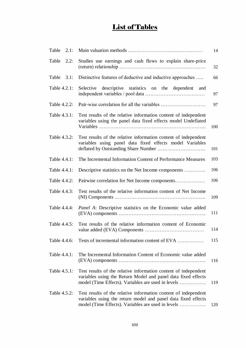
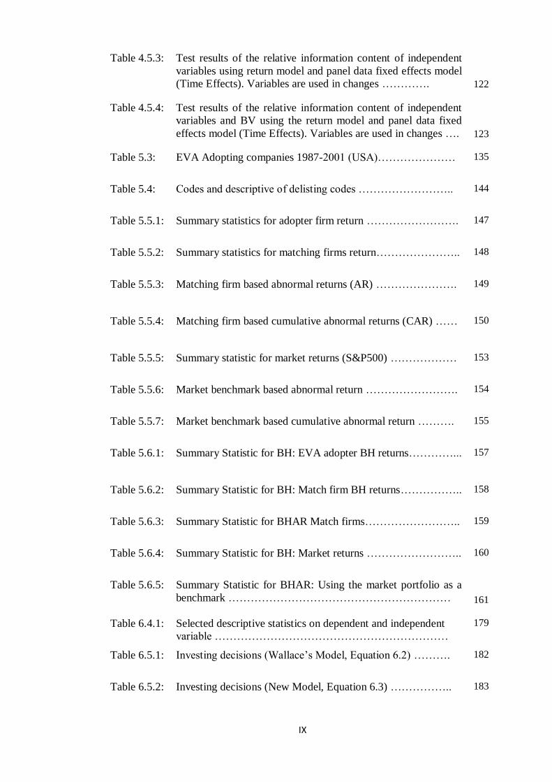
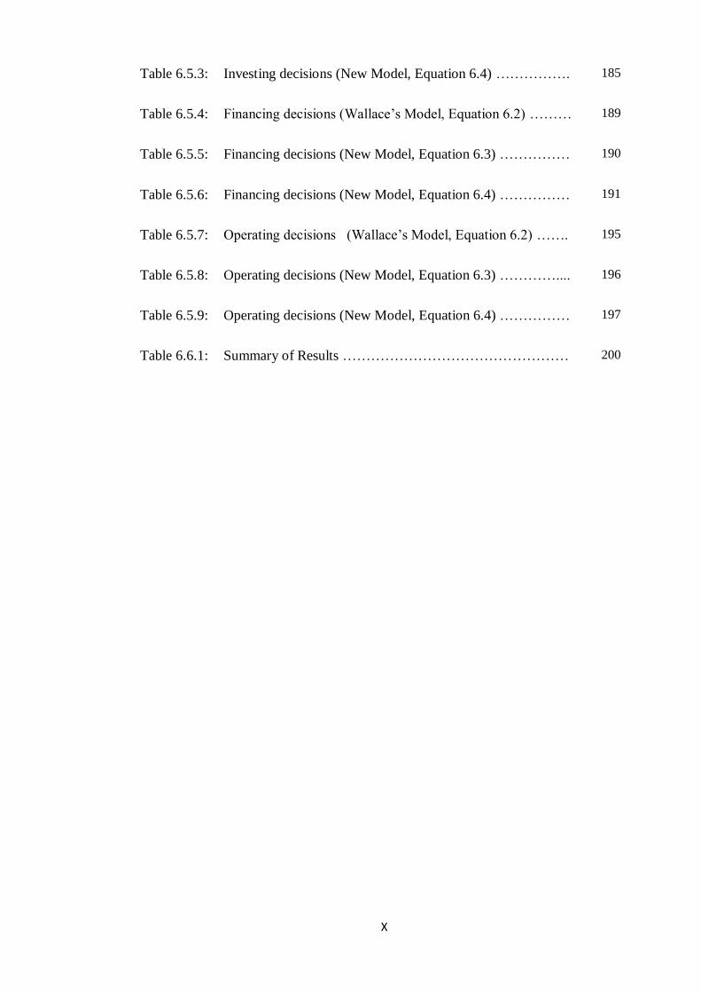
List of Tables ………………………………………………………………… VIII

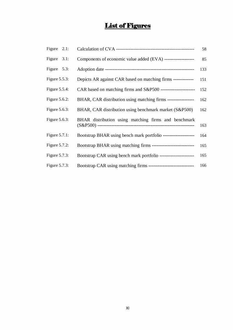
List of Figures ……………………………………………………………….. XI

List of Abbreviations ………………………………………………………… XII

List of Appendices …………………………………………………………… XVII

Chapter One: Introduction to the Research 1

1.1 Research Background ---------------------------------------------------------- 1

1.2 Motivation of the Research --------------------------------------------------- 6

1.3 Purpose of the Research ------------------------------------------------------ 7

1.4 Contribution of the Research ------------------------------------------------ 8

1.5 Scope of the Research -------------------------------------------------------- 9

1.6 Research Structure ------------------------------------------------------------ 9

Chapter Two: Literature Review 12

2.1 Introduction --------------------------------------------------------------------- 12

2.2 Theory of performance measure -------------------------------------------- 16

2.2.1 Theory of compensation -------------------------------------------- 17

2.2.2 Characteristics of performance measures ------------------------ 23

2.2.3 The information content theory ----------------------------------- 26

2.2.4 The incremental information content ---------------------------- 28

2.3 Previous studies --------------------------------------------------------------- 33

2.3.1 General overview of performance measures -------------------- 33

2.3.1.1 Reconciliation of performance measures -------------- 34

2.3.2 Accruals versus cash flows measure ----------------------------- 38

2.3.3 Value-based measure and residual income method ------------ 42

2.3.3.1 The validity of performance measure’s component--- 44

2.3.3.2 Performance measurement of productive activity ---- 47

2.3.3.3 Value-based measures versus traditional accounting method

------------------------------------------------------------------------- 48

VI

2.3.3.4 Modification of EVA as a performance measure ------- 53

2.3.3.5 Individual focus of value-based measures --------------- 55

2.3.3.6 Cash value added as a performance measure ------------ 57

2.3.3.6.1 CVA versus EVA -------------------------------- 61

2.4 Summary ------------------------------------------------------------------------- 63

Chapter Three: Research Design and Methodology 65

3.1 Introduction ---------------------------------------------------------------------- 65

3.2 Development of hypothesis ---------------------------------------------------- 65

3.2.1 Traditional measures versus cash flows and value added measures 71

3.2.1.1 The information content model---------------------------- 74

3.2.1.2 The incremental information content -------------------- 81

3.2.2 Earnings versus earnings’ components ---------------------------- 82

3.2.3 EVA versus EVA’s components ----------------------------------- 84

3.3 Hypotheses test------------------------------------------------------------------ 88

3.4 Variables measurement and definition -------------------------------------- 88

3.4.1 Controlling variables ------------------------------------------------- 91

3.5 Sample selection ---------------------------------------------------------------- 92

3.6 Summary ------------------------------------------------------------------------- 93

Chapter Four: The value Relevance of Performance Measures 94

4.1 Introduction --------------------------------------------------------------------- 94

4.2 Descriptive statistics ----------------------- ----------------------------------- 95

4.3 The relative information content of performance measures -------------- 98

4.4 The incremental information content of performance measures -------- 102

4.4.1 The incremental information content of net income components 105

4.4.2 The incremental information content of EVA components ---- 110

4.5 Empirical results of the return model --------------------------------------- 117

4.6 Conclusion ---------------------------------------------------------------------- 124

Chapter Five: The impacts of Adopting Economic Value Added

(EVA) on Stock performance 126

5.1 Introduction --------------------------------------------------------------------- 126

5.2 Previous studies ---------------------------------------------------------------- 128

5.3 sample --------------------------------------------------------------------------- 132

VII

5.4 Methodology ------------------------------------------------------------------ 138

5.5 Cumulative return results ----------------------------------------------------- 144

5.6 Buy and Hold Return Results ------------------------------------------------ 156

5.7 Testing the Aggregate Abnormal Returns ---------------------------- 163

5.8 Conclusion -------------------------------------------------------------------- 167

Chapter Six: The impacts of adopting Economic Value Added

(EVA) on adopters’ potential decisions 169

6.1 Introduction --------------------------------------------------------------- 169

6.2 The Wallace Study ----------------------------------------------------- 170

6.3 Sample Selection --------------------------------------------------------- 171

6.4 Methodology -------------------------------------------------------------- 172

6.4.1 The Wallace approach ------------------------------------------ 173

6.4.2 A modified Approach (MODIF 1) ---------------------------- 174

6.4.3 Test based on direct use of the control firms (MODIF 2) - 175

6.5 Empirical Results --------------------------------------------------------- 180

6.6 Conclusion ----------------------------------------------------------------- 198

Chapter Seven: Findings, Conclusion and Recommendation 203

7.1 Introduction --------------------------------------------------------------- 203

7.2 Main research findings -------------------------------------------------- 203

7.2.1 Findings for the value relevance and incremental information

content of performance measures ------------------------------- 204

7.2.2 Findings for the main components of NI and EVA ---------- 205

7.2.3 Findings for the effects of adopting EVA ---------------------- 206

7.3 Research conclusion ----------------------------------------------------- 208

7.4 Research contributions and recommendations ----------------------- 209

7.5 Research limitations ----------------------------------------------------- 210

7.6 Future research ----------------------------------------------------------- 212

Bibliography ------------------------------------------------------------------------ 213

Appendices---------------------------------------------------------------------------- 223

VIII

List of Tables

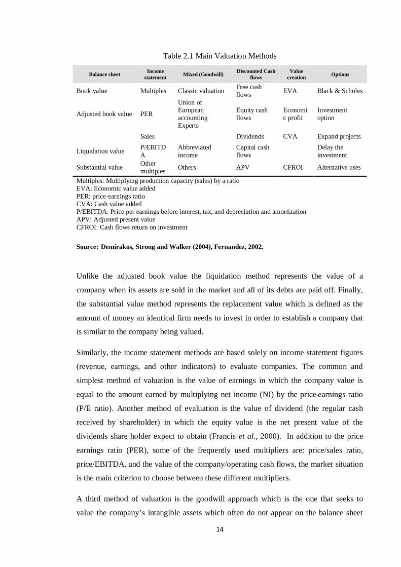
Table 2.1: Main valuation methods ……………………………………… 14

Table 2.2: Studies use earnings and cash flows to explain share-price

(return) relationship ……………………………………………. 32

Table 3.1: Distinctive features of deductive and inductive approaches ….. 66

Table 4.2.1: Selective descriptive statistics on the dependent and

independent variables / pool data ……………………………… 97

Table 4.2.2: Pair-wise correlation for all the variables ……………………… 97

Table 4.3.1: Test results of the relative information content of independent

variables using the panel data fixed effects model Undeflated

Variables ……………………………………………………….. 100


variables using panel data fixed effects model Variables

deflated by Outstanding Share Number ……………………….. 101

Table 4.4.1: The Incremental Information Content of Performance Measures 103

Table 4.4.1: Descriptive statistics on the Net Income components …………. 106

Table 4.4.2: Pairwise correlation for Net Income components……………… 106

Table 4.4.3: Test results of the relative information content of Net Income

(NI) Components ………………………………………………. 109

Table 4.4.4: Panel A: Descriptive statistics on the Economic value added

(EVA) components …………………………………………….. 111

Table 4.4.5: Test results of the relative information content of Economic

value added (EVA) Components ……………………………… 114

Table 4.4.6: Tests of incremental information content of EVA ……………. 115

Table 4.4.1: The Incremental Information Content of Economic value added

(EVA) components …………………………………………….. 116


variables using the Return Model and panel data fixed effects

model (Time Effects). Variables are used in levels ……………. 119


variables using the return model and panel data fixed effects

model (Time Effects). Variables are used in levels ……………. 120

IX


variables using return model and panel data fixed effects model

(Time Effects). Variables are used in changes …………. 122


variables and BV using the return model and panel data fixed

effects model (Time Effects). Variables are used in changes …. 123

Table 5.3: EVA Adopting companies 1987-2001 (USA)………………… 135

Table 5.4: Codes and descriptive of delisting codes …………………….. 144

Table 5.5.1: Summary statistics for adopter firm return ……………………. 147

Table 5.5.2: Summary statistics for matching firms return………………….. 148

Table 5.5.3: Matching firm based abnormal returns (AR) ………………….

149

Table 5.5.4: Matching firm based cumulative abnormal returns (CAR) ……

150

Table 5.5.5: Summary statistic for market returns (S&P500) ………………

153

Table 5.5.6: Market benchmark based abnormal return …………………….

154

Table 5.5.7: Market benchmark based cumulative abnormal return ……….

155

Table 5.6.1: Summary Statistic for BH: EVA adopter BH returns…………...

157

Table 5.6.2: Summary Statistic for BH: Match firm BH returns……………..

158

Table 5.6.3: Summary Statistic for BHAR Match firms……………………..

159

Table 5.6.4: Summary Statistic for BH: Market returns …………………….. 160

Table 5.6.5: Summary Statistic for BHAR: Using the market portfolio as a

benchmark ……………………………………………………

161

Table 6.4.1: Selected descriptive statistics on dependent and independent

variable ………………………………………………………

179

Table 6.5.1: Investing decisions (Wallace’s Model, Equation 6.2) ………. 182

Table 6.5.2: Investing decisions (New Model, Equation 6.3) …………….. 183

X

Table 6.5.3: Investing decisions (New Model, Equation 6.4) ……………. 185

Table 6.5.4: Financing decisions (Wallace’s Model, Equation 6.2) ……… 189

Table 6.5.5: Financing decisions (New Model, Equation 6.3) …………… 190

Table 6.5.6: Financing decisions (New Model, Equation 6.4) ……………

191

Table 6.5.7: Operating decisions (Wallace’s Model, Equation 6.2) ……. 195

Table 6.5.8: Operating decisions (New Model, Equation 6.3) ………….... 196

Table 6.5.9: Operating decisions (New Model, Equation 6.4) …………… 197

Table 6.6.1: Summary of Results ………………………………………… 200

XI

List of Figures

Figure 2.1: Calculation of CVA -------------------------------------------------- 58

Figure 3.1: Components of economic value added (EVA) ------------------- 85

Figure 5.3: Adoption date --------------------------------------------------------- 133

Figure 5.5.3: Depicts AR against CAR based on matching firms ------------- 151

Figure 5.5.4: CAR based on matching firms and S&P500 ---------------------- 152

Figure 5.6.2: BHAR, CAR distribution using matching firms ----------------- 162

Figure 5.6.3: BHAR, CAR distribution using benchmark market (S&P500) 162

Figure 5.6.3: BHAR distribution using matching firms and benchmark

(S&P500) -------------------------------------------------------------- 163

Figure 5.7.1: Bootstrap BHAR using bench mark portfolio -------------------- 164

Figure 5.7.2: Bootstrap BHAR using matching firms --------------------------- 165

Figure 5.7.3: Bootstrap CAR using bench mark portfolio ---------------------- 165

Figure 5.7.3: Bootstrap CAR using matching firms ----------------------------- 166

XII

List of Abbreviations

ACC Accruals

C Change in Cash and Short-term Marketable Securities

∆AP Changes in Accounts payable

∆AR Changes in Accounts Receivable

∆INV Changes in Inventory

ABC Activity-Based Costing System

AcctAdj Accounting adjustments

ADJ Adjustments

AMORT Amortisation

APV Adjusted Present Value

AR Abnormal Return

ATInt After Tax Interest

BHAR Buy and Hold Abnormal Return

BHR Buy Hold Return

BV Book Value

CA Current Asset

CAI Cash Flows After Investment

CAPCH Capital Charge

CAPM Capital Asset Pricing Method

CAR Cumulative Abnormal Return

CC Capital Charge

CEO Chief Executive Officer

XIII

CFAI Cash Flows after Investment

CFF Cash Flows from Financing Activities

CFI Cash Flows from Investing Activities

CFO Cash Flows from Operations

CFS Cash Flows Statement

CML Capital Market Line

CVA Cash Value Added

DCF Discounted Cash Flows

DD Dividends

DEP (DP) Depreciation

E Earnings

EARN Earnings

EBDIT Earnings Before Depreciation, Interest and Tax

EBEI Earnings Before Extraordinary Items

EBIT Earnings Before Interest and Tax

EBITDA Earnings Before Interest Tax Depreciation and Amortization

EBO Edward-Bell-Ohlson Model

ECF Equity Cash Flows Method

ED Economic Depreciation

EP Economic Profit

EPS Earnings per Share

EVA Economic Value Added

FASB Financial Accounting Standards Board

FCF Free Cash Flows Method

XIV

FEM Fixed Effects Model

FIFO First in First out Inventory Evaluation Method

FRS Financial Report Standards

GAAP General Accepted Accounting Principles

I Interest

IAS International Accounting Standards

IASB International Accounting Standard Board

IC Invested Capital

IFC International Financial Corporation

IFRS International Financial Reporting Standard

IPO Initial Public Offering

LIFO Last in First out Inventory Evaluation Method

LIM Linear Information Model

LSE London Stock Exchange

LSPD London Share Price Database

M Materials and Services Purchased

MAR Annual Stock Returns

MV Market Value

MVA Market Value Added

MVE Market Value of Equity

NCA Nun-Current Asset

NCF Net Cash Flows

NI Net Income

NIBIE Net Income Before Extra-Ordinary Items and Discontinued

Operations plus Depreciation

XV

NIDPR Net Income plus Depreciation and Amortisation

NOPAT Net Operating Profit after Tax

NPV Net Present Value

NVA Net Value Added

OCFD Operating Cash Flows Demand

OI Operating Income

OIADJ Operating Income Adjustment

OLS Ordinary Least Squares

OM1 Ohlson Model One

OM2 Ohlson Model Two

OP Operating Profit

OCF Cash Flows From Operations

OTHER Other Accruals

PER Price-Earnings Ratio

RE Retained Earnings

REVA Refined Economic Value Added

RI Residual Income

RIM Residual Income Method

ROA Return on Assets

ROE Return on Equity

ROI Return on Investment

ROS Return on Sales

S Sales

STSTADJ Stern Stewart Adjustments

XVI

T Tax

TA Total Assets

UCAI Unexpected Cash Flows After Investment

VA Value Added

VBM Value Based Measures

W Wages

WACC Weighted Average Cost of Capital

WCFO Working Capital from Operations

WCO Working Capital of Operations

XVII

List of Appendices

Page

Appendix 1 Full 60 months event period for all cases ----------- 223

Appendix 2 The full version of the bootstrap test tables -------- 231

1

Chapter 1

Introduction

1.1 Background

The measurement of a firm’s performance is a crucial issue to its stakeholders,

especially its shareholders, directors, managers and debtors. Changes in a firm’s

performance can be detrimental to its health, its profitability and ultimately its survival.

The concept of maximizing shareholder wealth has been one of the driving forces in the

change in current management practice. This is the wealth that is traditionally gauged

by either a standard accounting magnitude such as profits, earnings and cash flow from

operations or various financial statement ratios (e.g. earnings per share, returns on

assets, and investment and equity). Managers, shareholders and other interested parties

then use this financial statement information to assess and predict current and future

performance.

Over the past decades, considerable attention has been paid to the relationship between

accounting numbers and firm value. This attention to the relationship between

theoretical firm value and the performance stream has attracted considerable researcher

interest and resulted in a number of proprietary models being introduced. Ball and

Brown’s research in 1968 was the first to discuss the information content of accounting

numbers. They measured the association between annual earnings (cash flows from

operations) and the abnormal return using the operating earnings as proxy for operating

cash flows and they reported that earnings showed a higher correlation with abnormal

stock return than cash flows.

The work of Ball and Brown was replicated by sequences of empirical research using

various proxies for annual earnings (i.e. Beaver, 1968; Beaver and Dukes 1972; and

Pattel and Kaplan, 1977) to investigate the association between these performance

measures and the variation in the stock price (return). Unfortunately, the results

regarding the relevancy of the investigated measures are contradictory. This

contradiction in the result obtained by different market-based accounting research and

the criticisms which have arisen against the accruals (e.g. subjectivity and easily

manipulated), and the main components of traditional measures, means that increasing

2

attention has been paid to new financial performance measures as substitutes for

traditional accounting-based measures.

However, after the cash flow statements gained the attention of the International

Accounting Standard Board (IASB) more studies have been conducted to examine the

incremental information content of cash flows over earnings (Finger, 1994; Clubb,

1995; Barth et. al, 2001). These studies concluded that cash flows have information

content, but they reported mixed results regarding the incremental information content

of cash flows over earnings. However, these studies did not attempt to investigate the

role of aggregate accruals.

As there are no conclusive results regarding the usefulness of earnings and cash flow

items, neither the accrual earnings, nor the cash flow items, were perfect methods for

measuring management performance as an approach to evaluating the whole firm

(shareholder wealth) (Bowen et al., 1987; Charitou et al., 2001). Nevertheless the bulk

of empirical evidence indicates that the superiority of cash flow measures versus

earnings (as variously defined) has not been demonstrated.

Management decisions – particularly the investment, financing, and operating decisions

– affect shareholder value through their influence on such value drivers as value growth

duration profit margin for the cash flows from operations or the cost of capital. The

criterion has long persisted that in order for a company to create value and to generate

wealth it must earn more than it costs (cost of capital employed) by way of debt and

equity. The added value concept has been promoted strongly in performance

measurement literature. This notion is historically referred to as the residual income

(RI) method (a value added measure).

A long glance at the late 80s and early 90s, the dates when EVA spread widely among

firms, will enable the reader to attribute this diffusion to at least two factors. First, there

are the criticisms the traditional accounting measures faced as a result of their

subjectivity, depreciation methods, and inventory valuation (i.e., FIFO and LIFO

techniques). As a consequence, these measures can be easily manipulated by managers

and this will affect the profitability analysis. Second, financial markets went global and

experienced huge expansion. At the same time US firms found themselves competing

with foreign companies for a share of the market and faced tough competition from

other firms especially the Japanese. These factors imply that previous performance

3

measures that shareholders used over a long period to guide and evaluate their

investments are inefficient. This is a sufficient reason for shareholders and investors to

contemplate other performance metrics, ones which may be objective and not

manipulated. The best known example (at least from an EVA supporter’s viewpoint) is

perhaps the developed version of the residual income method: the Economic Value

Added or EVA model of Stern Stewart (1991).

EVA, as a periodic performance measure, was introduced by Stern and Stewart to

replace earnings and cash flows from operations as a measure of performance. Stewart

(1994, p.75) argued that ‘EVA stands well out from the crowd as the single best

measure of value creation on a continuous basis’. In addition to this he also remarks that

‘EVA is almost 50% better than its closest accounting-based competitor (i.e. earnings),

in explaining changes in shareholder wealth’ (p.75). EVA is defined as the profit earned

by the firm less the cost of financing the firm’s capital. It is similar to RI but adjusted

for net operating profit after tax (NOPAT) and invested capital where needed. It is also

referred to as net operating profits less a charge for the opportunity cost of invested

capital (West and Worthington, 2000).

Scholars have different points of view regarding the usefulness of economic value

added (EVA) measures in explaining the variation of stock price performance. Thus as

seen to date, the literature provides several studies questioning the claimed superiority

of EVA to earnings and other performance metrics. Biddle et al., (1997) claim that both

earnings before interest and tax (EBIT), and the residual income (RI) have the higher

adjusted and outperform EVA in explaining variation in stock performances.

Similarly, Lehn and Makhija (1997) argue that in spite of it having a higher correlation

with stock return among the other performance measures, EVA and market value added

(MVA) are not the most efficient metrics to evaluate a firm’s performance. Cahan et

al., (2002) contend that EVA is the best reward system as it better aligns the interests of

the manager and the firm. Furthermore, Anastassis and Kyriazis, 2007 assumed that the

value of EVA correlates better with market value (MV) than other accounting variables.

Recently, Mehdi and Iman (2011) investigated the relative and incremental information

content of EVA over traditional measures. They stated that stock return is highly

associated with return on assets (ROA), return on equity (ROE), and earnings per share

(EPS), while EVA appears to have little information content beyond that which exists in

other traditional accounting measures. Hence, the results do not support Stern and

4

Stewart’s claims that EVA is the only metric that best measures firms’ and manager

performance.

However, as a result of the criticisms the traditional and value added measures have

faced, particularly the earnings and economic value added (EVA). And also in response

to the arguments rose by Young (1999) towards the Stern and Stewart adjustment. The

adjustment that mainly intends to produce a modified version of the EVA measure that

probably has the ability to mitigate the drawbacks of accrual based measures and in its

essence is similar to cash flows measure, researchers have begun to rethink new

performance measures that can better capture the performance of firms and managers.

In response, Ottosson and Wiessenrider (1996) proposed a new performance measure

titled, cash value added (CVA)2 to replace the traditional accounting and value added

measures, specifically the periodic measure EVA. They defined CVA as the difference

between operating cash flows (OCF) and operating cash flows demand (OCFD). The

first component basically represents the earnings before depreciation, interest and tax

(EBDIT) adjusted for non-cash charges, working capital movements and non-strategic

investments. The second component refers to investors’ capital cost, which is mainly

the interest and dividends.

However, an empirical question arises here. Which measure has the better association

with the stock return/ price? Unfortunately, the empirical literature to date suggests that

there is no single accounting based measure upon which one can rely to explain changes

in shareholder wealth.

The question that has received much concern in market-based accounting research is the

relative information content of alternative performance measures (e. g. EVA, CVA,

earnings, EBITDA, and cash flows). In evaluating various performance metrics, the

criterion used must take into consideration the objective of a particular performance

measure (Kothari, 2001). An important purpose of cash flow statements is that cash

flow data are helpful in assessing the amount, timing, and uncertainty of future cash

flows.

2 This is a trademarked performance measure that was developed by the global management

consultant ‘Boston Consulting Group (BCG)’ a U.S company founded in 1963 and which

came to prominence in 1973.

5

The majority of prior empirical studies have used the association with share price or

stock return as the criterion to evaluate the different performance measures. Implicitly,

the main assumption of share price studies is that in an efficient market, share prices

reflect information about expected future cash flows (future benefits). However, this

assumption has been challenged by market "anomalies". For instance, the results of

Sloan (1996) indicate that investors appear to focus on earnings and investors were

incapable of considering the differential persistence of their cash flows and accruals

components. Thus, there is the opportunity that the share-price studies’ results may be

affected by the possibility that the market is concentrating on bottom line earnings (the

market is not efficient). In this context, Bernard (1995) described the limitation of

share-price studies: "Preclude from the outset the possibility that researchers could ever

discover something that was not already known by the market" (p. 735).

The value-relevance studies that investigate the empirical relation between stock market

values, changes in values and different accounting numbers are important disciplines for

accountant research. The price and return models are the most popular valuation

methods in accounting literature (Barth et al., 2001). According to Christie (1987) both

models are economically equivalent since they were derived from the same source

which is the linear information model introduced by Ohlson (1995). This implies that

the main inferences drawn from the two approaches should be the same- at least at the

theoretical level.

In practice, Kothari and Zimmerman (1995) claimed that even the return model suffers

fewer econometric problems than the price model where the estimations of earning

response coefficients are more biased than those of the price model. Barth et al. (2001)

found that when stock return is the dependent variable, earnings are better than cash

flows but when actual future cash flows is the dependent variable, cash flows turn out to

be better than earnings in explaining the variation in future cash flows. Thus, providing

evidence on the value relevance of different performance measures using only the stock-

return model is not enough to judge the usefulness of performance measures other than

earnings. There are many UK studies which had as their aim the comparison of various

performance measures on the basis of their association with stock return. However,

there has been no attempt to compare the different performance metrics on the basis of

their association with annual stock prices. Therefore, this study will try to bridge this

gap by investigating the association of different sets of performance measures with the

6

variation in stock price performances. These performance measures are net income

available to common shareholders (NI), earnings before interest, tax, depreciation and

amortization (EBITDA), earnings before interest and tax (EBIT), earnings before

extraordinary items (EBEI), net cash flows from operations (CFO), cash value added

(CVA) and economic value added (EVA).

1.2 Motivation of the Study

Each time researchers investigate the association between different performance

measures and the stock price (return) they arrive at different points of view regarding

the superiority and ability of these metrics in explaining the variations of stock price

(return) performances. However, they fell through because they could not assign the

optimal and perfect accounting measure that better gauges the performances of firms

and executive management (Lehn and Makhija, 1997; Barton et al, 2010).

Lee (1996, p. 32), for example, argues that ‘the search for a superior measure of firm

valuation is a, if not the, key feature of contemporary empirical finance: For years,

investors and corporate managers have been seeking a timely and reliable measurement

of shareholders’ wealth. With such a measure, investors could spot over or underpriced

stocks, lenders could gauge the security of their loans and managers could monitor the

profitability of their factories, divisions and firms’.

This relation between firm value and stock price return has been the focus of

voluminous empirical research for the past three decades. A primary motivation for this

research is to bridge an important gap in the UK literature relating to the information

and incremental information content of a set of chosen accounting performance

measures. While prior UK evidence (Board et al., 1989; Board and Day, 1989) is drawn

from return studies in which stock return is the main criterion in evaluating the value

relevance of accounting data, there are at present no UK stock price studies that

measure the information and incremental information content of accounting measures

by examining their ability to explain the variation in stock price performances.

Econometrically, the two evolutionary methods, price and return evaluation methods,

are different. Economically they are equivalent since they are derived from the same

source which is the linear information model (Ohslon, 1995). However, Rees (1999)

explains in his paper that there are some difficulties that can be expected in the return

model and these problems can be avoided by using the price models.

7

Another powerful motivation for this research is that it intends to be the first research

that utilises UK data to examine the value relevance of the new residual income method:

the cash value added (CVA), a title coined by the Boston consulting group, to provide

evidence on its ability to outperform other performance measures, namely the economic

value and traditional accounting metrics.

1.3 Purpose of the Research

The main objectives of the study are:

To empirically investigate the association between a comprehensive set of

performance measures and the stock price (return) performances to indicate

which of these measures are better at explaining the variation in stock

performance and have the ability to evaluate the management performances and

the whole company performances. These measures are the traditional accounting

measures: net income (NI); earnings before interest, tax, depreciation and

amortization (EBITDA); and earnings before extraordinary items (EBEI). There

is also the cash flows measure: cash flows from operation (CFO), the value

added measures (residual income method) economic value added (EVA), and

cash value added (CVA). This is achieved by employing a fixed effects model

and running six regressions against the selected metrics. The dependent variable

is the three month closing stock price following the reporting day and stock

return respectively. The set of independent variables is constructed from the

review of extant literature.

To empirically examine the incremental information content of the selected set

of performance measures.

To extend previous studies by decomposing the primary measure, namely

earnings and economic value added EVA, into their main components to test

whether these components contribute more to the association of the prime

measure with the stock (price) return.

8

To utilise the event study methodology to examine the impact of adopting EVA

as a compensation plan and management tool on the performance of US firms

after the adoption date. The BHAR and CAAR are the aggregation methods

used. This includes comparing the performance of event firms to that of both the

matching firms and benchmark portfolio index, the S&P500.

To extend the work of Wallace (1997) by proposing three econometric models

to investigate the long-terms effects of EVA adoption on US firms’ material

decisions. These are the investing, financing and operating decisions which it is

claimed would increase the value of the company.

1.4 Contribution of the Study

This research will contribute to prior UK studies in three major respects:

I. Unlike previous research, it will employ UK data for the selected period and

adopt a unified econometrics model to examine and test the association of a set

of performance measures, being the focus of past literature, and the variation in

annual stock price performances. From the research point of view, this will

eliminate the controversies embedded in the findings of previous UK and US

studies regarding the use of different samples and econometric models to

conduct their research (Garrod et al., 2000). Furthermore, this research will

extend its goal to test for the incremental information content of earnings and

EVA main components and examine whether any of these components has a

greater contribution to the association between the prime performance measures

and annual price performance.

II. As Rees (1999) explained in his paper, there are some difficulties to be

expected in the return model and these problems can be avoided by using the

price models. Hence, the stock price has become the most common value-

measure used in financial and accounting research. This research will use both

the stock price and the return as dependent variables instead of using the stock

return alone.

9

III. In response to the adjustments Stern and Stewart applied to NOPAT and the

capital employed, the main figures need to compute EVA, which aims to

produce a performance measure that is equivalent to cash flows and less subject

to the distortions of accrual accounting (Young, 1999). This research will

contribute and enhance the theoretical aspect of the research with a broad

empirical study of UK literature by using cash value added (CVA) as an

alternative performance measure (initially proposed by Ottosson and

Weissenrieder, 1997) and investigate its association with annual stock price

performance and test whether CVA contains more information content than

other performance measures.

IV. It will extend the work of Wallace (1997) by introducing three alternative

models that the current research expect will more effectively capture the long

term effects of adopting EVA as a compensation and management tool by

different US firms.

1.5 Scope of the Research

The current research uses the empirical approach to fulfil its aims. The sources of data

are DataStream, CRSP and Compustat. The data drawn from UK industrial companies

will be used to run the empirical test. This study will cover the period from 1990 to

2012.

Furthermore, in order to empirically test the impacts of adopting the EVA compensation

scheme on the treatment companies’ potential investment, a sample of 89 US firms over the

period from 1960 to 2012 were selected. The sources of data are Compustat and CRSP.

1.6 Research Structure

Apart from this introductory chapter the thesis is organized into six main chapters:

Chapter Two presents the literature review of different performance measures and their

association with stock price (return) performances and introduces the literature review

concerning the explanatory variables which will be examined in the current research and

provide a historical look at the debates these measures have encountered. This chapter is

10

also devoted to the discussion of certain economic theories in terms of its relation to the

topic under investigation. These are the compensation theory, the information content

theory and the incremental information content theory. Finally, this research will

discuss and review the literature which has already been conducted in terms of the

association between traditional measures, cash flows and value added measures and

variations in stock price (return) performances.

Chapter Three discusses the research methodology commencing with the review of the

research design which included identifying the hypothesis development process and

then addressing the research questions which follow the review of the literature.

Following this the models adopted in the research will be introduced. These are the

price model and the return model. The final part looks at the hypotheses of the research.

The research methodology chapter discusses the main research variables, including their

definitions and calculation.

The sample frame, the sample size, and the controlling variables are also discussed. In

addition, the chapter discusses the procedures of measuring and ascertaining the

reliability and relevancy of research variables. Finally, the chapter briefly discusses the

statistical analyses tests that will be used in the research and which are explained in-

depth in the next chapter.

Chapter Four develops tests for the hypotheses developed in Chapter Three and reports

on the main body of results for the study. The value relevancy and incremental

information content of performance measures will be evaluated by assessing their

ability in explaining the variation in stock performances.

The results for the fixed effects models are reported in this chapter. These results

provide evidence on the relative ability of net income (NI) versus the cash flows and

accrual components and the relative information content of Economic value added

(EVA) versus cash flows, accruals and other components.

Chapter Five describes the research design and the methodology that was used to

examine the EVA adoption event. It provides a historical look at the event study

literature and discusses and reviews the literature which has already been examined in

terms of the implications on firm value of firms adopting EVA as a performance and

management tool. The sample selection process and, the sample size are discussed as

well. The models which will be used in the research are then introduced. The CAR and

11

the BHAR aggregation approaches are used to conduct the event study test. Furthermore

it sheds light on the statistical properties of returns, abnormal returns and aggregate

abnormal returns, BHAR and CAR, and the empirical results obtained.

Chapter Six extends the empirical test begun in chapter five. It replicates the same

model applied by Wallace (1997). Three modifications were proposed to extend the

original work of Wallace. First it is modified by introducing the market return index

(S&P500) as a control variable to replace the change in ownership in Wallace’s original

model. Second, a model is proposed that uses levels rather than differences. Third, a

modified model is proposed that uses abnormal measures of dependent and independent

variables. It then describes the sources of data and the collection process in terms of the

set of variables used. Empirically, it tests the effects of adopting EVA on firms’

potential decisions taken to maximize the shareholders wealth, namely the investment,

financing and operating decisions.

Chapter Seven provides the main findings of the research, draws conclusions, research

contributions and implications, and indicates the research recommendations based on

the findings and conclusions. In addition, the chapter highlights the research limitations

and provides suggestions for future research.

12

Chapter 2

Literature Review

2.1 Introduction

The delegation of management from investors to executive managers is one of the most

important agency relationships in finance. Typically, the literature focuses on joint stock

corporations with a large number of shareholders who delegate power to managers.

These managers effectively control the company. Understandably, the appropriate

compensation for these managers is an important topic of debate among practitioners

and academics. On the other hand, there has been increasing pressure on managers to

maximise shareholders’ wealth (Sharma, 2010).

The evaluation of a company’s performance is considered one of the most important

challenges to researchers (Kaplan and Norton, 1992). This issue is becoming

increasingly important to shareholders, and has been the subject of heated debates. To

foster shareholders’ interest, managers adopt strategies to increase the value of their

organisation, which leads to maximising shareholder wealth through the optimum

allocation of resources. In order to assess whether managers are performing well,

researchers and practitioners need to use appropriate measurements. Scholars have

developed specific criteria relating to the validity, relevance, accountability, and

globalism of the performance measure(s) that are used to assess managers’ or

companies’ performance (Rappaport, 1986). Unfortunately, there is no general

agreement as to which criterion is most suitable and accurate as far as the evaluation of

the managers’ performance is concerned.

Rappaport argues that for any performance measure to succeed, certain fundamental

criteria should be met; the first and most important criterion being its validity. The

concern here is to show whether the inspected firms adopt the accepted accounting

standards prescribed by the various standard setting bodies such as the International

Accounting Standard Board (IASB) and its predecessor The International Accounting

Standard Committee (IASC); and the extent to which they comply with them. Second,

the performance measure should be verifiable. Hence, the adoption of any set of

accounting standards will force accountants to follow the same procedures in

accounting processes and that should lead to unbiased accounting numbers and support

13

the validity of the released accounting information used later by various parties to assess

the firm. Third, the selected performance measure should preserve accountability. This

means that managers and executives will be responsible for those activities and

investment decisions they have control over. The fourth criterion is the globalisation of

the performance measure. The idea is that a firm does not work in isolation from other

firms in the same industry or manufacturing segment. Consequently the performance

measure should be able to maintain comparability between competitive firms within the

same industry. Finally, the performance measure should be easily understandable by

internal and external parties. It should be understood by the managers that the

endorsement and selection of any performance measure means it will be used later to

assess their performances (Bouckaret et al., 2010).

Generally, any research design that aims to evaluate a firm’s performance should adopt

a valuation model that provides a better link between the firm’s value and the firm’s

specific characteristics. Of particular importance is the link between a firm’s value and

accounting figures. Researchers have used a wide diversity of valuation models, ranging

from the very simple to the most sophisticated (Ball and Brown, 1968; Patell and

Kaplan, 1977; Dechow, 1994, and Biddle et al., 1997). The main valuation models can

be classified into four groups as shown in Table 2.1: balance sheet based (book value of

equity); income statement based; value creation methods; and options (Fernandez,

2002). Obviously, there are practical considerations, such as the availability of

information that may constrain the decision maker’s choice of performance

measurement method.

The balance sheet methods basically assumed that the value of a company lies in its

balance sheet. These methods seek to determine the company’s value by estimating the

value of its assets. Some of these methods are the book value method in which the value

of the company is equivalent to its shareholder’ historical cost as presented in the

balance sheet statement. This method suffers from the subjectivity shortage that is

inherent in accounting procedures used to determine the value of balance sheet items

(Ohlson, 1995). Thus, the adjusted book value method tries to overcome this shortage

by evaluating the company’s assets and liabilities using the current market prices.

14

Table 2.1 Main Valuation Methods

Balance sheet Income

statement Mixed (Goodwill)

Discounted Cash

flows

Value

creation Options

Book value Multiples Classic valuation Free cash

flows EVA Black & Scholes

Adjusted book value PER

Union of European

accounting

Experts

Equity cash

flows

Economi

c profit

Investment

option

Sales Dividends CVA Expand projects

Liquidation value P/EBITD

A

Abbreviated

income

Capital cash

flows

Delay the

investment

Substantial value Other

multiples Others APV CFROI Alternative uses

Multiples: Multiplying production capacity (sales) by a ratio

EVA: Economic value added

PER: price-earnings ratio CVA: Cash value added

P/EBITDA: Price per earnings before interest, tax, and depreciation and amortization

APV: Adjusted present value

CFROI: Cash flows return on investment

Source: Demirakos, Strong and Walker (2004), Fernandez, 2002.

Unlike the adjusted book value the liquidation method represents the value of a

company when its assets are sold in the market and all of its debts are paid off. Finally,

the substantial value method represents the replacement value which is defined as the

amount of money an identical firm needs to invest in order to establish a company that

is similar to the company being valued.

Similarly, the income statement methods are based solely on income statement figures

(revenue, earnings, and other indicators) to evaluate companies. The common and

simplest method of valuation is the value of earnings in which the company value is

equal to the amount earned by multiplying net income (NI) by the price-earnings ratio

(P/E ratio). Another method of evaluation is the value of dividend (the regular cash

received by shareholder) in which the equity value is the net present value of the

dividends share holder expect to obtain (Francis et al., 2000). In addition to the price

earnings ratio (PER), some of the frequently used multipliers are: price/sales ratio,

price/EBITDA, and the value of the company/operating cash flows, the market situation

is the main criterion to choose between these different multipliers.

A third method of valuation is the goodwill approach which is the one that seeks to

value the company’s intangible assets which often do not appear on the balance sheet

15

(Ohlson, 1995). However, this method can be classified as follows: (i) the classical

method in which the company’s value is equal to its net assets plus the value of

goodwill, (ii) abbreviated income method where the firm’s value is equal to the firm

adjusted net worth plus the value of goodwill, and (iii) the Union of European

accounting expert method (UEC) where the company’s total value is equal to its net

assets plus the goodwill which, in turn, equals the excess of the cost of an acquired firm

over the net values set to assets acquired and liabilities assumed3.

Another way to evaluate companies is the cash flow discounted-based method in which

a firm’s value is determined by estimating future cash flows the company will generate

in the future and then discounting at a proper discount rate that takes into account the

risk and historic volatilities of future cash flows (Penman, 2001). According to this

method a firm’s future cash flows can be obtained by different methods, starting with

the free cash flow (FCF) which refers to the cash flow the company generates from

operations without taking into account financial debt and capital expenditures. Closely

related is the equity cash flow method (ECF) which is calculated by deducting the after

tax interest and principle paid to the debtors from the FCF and adding new debt

provided to the company. Thus, the capital cash flow method defines the future cash

flow as the sum of debt cash flow plus equity cash flow (Penman).

The fifth evaluation method, which is discussed in-depth in the current chapter, is the

value creation method that takes into their consideration the cost of capital used to

generate profit. These methods are: economic value added (EVA), cash value added

(CVA). All of these measures will be discussed later in this chapter.

Finally there is the real options method, the option that only exists when there are future

possibilities for action. There are different types of option: expanding option when the

company intended to expand its production facilities, and delay option depending on the

market’s future growth. Usually the net present values (NPV) were used to evaluate

these options. Basically, Black and Schole’s formula4 is the proper method to value the

financial option in which the value of a call on a share, with an exercise price K and

which can be exercised at time t, is the present value of its price at time t. The main

assumption of this formula is that the option can be replicated (El Karoui et al., 1998).

3 As mentioned in IFRS3. 4 An equation to value call and put option, named after its developers, Fischer Black and Myron Sholes.

16

The measurement of a firm’s performance is a crucial issue to its stakeholders,

especially its shareholders, directors, managers and debtors. Changes in a firm’s

performance can be detrimental to its health, its profitability and ultimately its survival

(Francis et al., 2003). Thus, valuation methods are tools that help identify the sources

of economic value creation and destruction within the specific company (Fernandez,

2002).

For many decades accounting earnings, the accrual performance measure, had been the

most popular approach to evaluate management performance. This seems to have been

superseded by evaluation models based on cash flow items (Board and Day, 1989).

Earnings, a traditional performance measure, has come under increasing attack over the

past few years because it relies heavily on historical cost concepts and ignores the cost

capital (Mehdi and Iman, 2011), and as an alternative, performance measures that take

into account the cost of capital and are used to generate value have received more

attention (Garvey and Milbouran, 2000; Stewart, 1991). This has encouraged

researchers to examine whether the residual income method and the value added method

are superior to, and more reliable than, traditional methods (Dechow et al., 1999; Rajan,

2000; Francis et al., 2003). This debate will be discussed in detail in the next section.

This chapter begins by highlighting, in Section 2.2, the main theories that have been

developed to explain the value relevance of accounting numbers. We also shed light on

the appropriate characteristics of a good performance measure. Section 2.3 will discuss

the main results of previous studies that have investigated the value relevance of

different performance measures and the association between traditional and value based

performance measures with annual stock price and return. Finally Section 2.4

summarises the chapter.

2.2 Theory of Performance Measures

The use of optimal performance measures has received much attention in accounting

and finance, but there is still no consensus regarding the appropriate specification. In the

accounting literature, the relationship between a firm’s accounting numbers and its

value is typically investigated using a number of different valuation models (Barth et

al., 2001). Price and return are the most widely used proxies for value nowadays.

17

2.2.1 Theory of Compensation

Managers’ interests, in some situations, are different from those of the company’s

shareholders. Furthermore, managers sometime conduct work operations and activities

in a manner that benefits their own interests, especially when their remuneration scheme

is linked to current earnings (short-run compensation schemes). One of the best ways of

inducing top management to adopt shareholder orientation is through a compensation

system tied to the shareholder value creation (Rappaport, 1986). Indeed, “the theory of

market economy is, after all, based in the individuals promoting their self interest via

market transaction to bring about an efficient allocation of resource” (Rappaport, p.3).

The split between the firm’s ownership and the firm’s management gives rise to a

variety of “principal-agent” relationship (Berle and Means, 1932). Theoretically,

shareholders, as owners of the firm, have a claim on the firm’s generated income even if

they do not run their firm by themselves. For example, investors or financiers

(principals) hire managers (agents) to operate the firm on their behalf as they need

managers (specialized human capital) to generate profit on their investments, and

managers may need the investors’ funds since they may not have enough capital of their

own to invest.

Agency theory reflects the conflict of interest between varying contracting parties and

resource holders. It is concerned with so-called agency conflicts of interest between

firm managers as agents and shareholders (principals), and the conflict between debt-

holders and stockholders (Jensen and Meckling, 1976). The voluminous agency theory

literature has produced (theoretically and empirically) several dimensions in explaining

the essence of agency conflicts and outlining a framework of the basic agency problem

between managers and shareholders. The agency relationship according to Jensen and

Meckling (1976: p308) is “a contract under which one or more persons (the principals)

engage another person (the agent) to perform some service on their behalf, which

involves delegating some decision making authority to the agent”. However, if both the

agent and the principal have different desires or interests and prefer different actions,

the agency problem will occur as the agents will always act in the best of their own

interest and not the interests of the principal. Because while the costs are borne by

owners (lower profit) the benefits of profit are enjoyed by managers, managers might

select decisions that would be more important from the owners’ point of view.

18

Furthermore, when an agency relationship exists, it also tends to give rise to agency

costs, which, as any other costs, reflects the value loss to shareholders, arising from

divergences of desires between shareholders and corporate managers. Overall, the

agency cost’s main components are the monitoring costs, bonding costs, residual loss

and any other expenses the firm has to incur in order to maintain an effective agency

relationship to promote managers to act in favour of the shareholders' interests (Jensen

and Meckling, 1976). Theoretically, there are more than one fundamental ways the

owners able to take in order to mitigate the agency problem. According to Jensen and

Meckling, the principal can restrict divergences from his interest by establishing

appropriate incentive schemes for the agent and paying monitoring costs designed to

limit the aberrant activities of the agent. In other words, a firm (owners) has to control

and monitor managers’ performance (behaviour) and reward them based upon the

performance they achieved. However, these methods are effective only if the key

actions taken by managers can be easily observed by shareholders; it is costly and a

hard task for the shareholder to verify what the managers are actually doing or whether

the managers have been behaved in proper way as assumed to be (Eisenhardt, 1989).

The key elements of agency theory lie on a set of mechanisms, called corporate

governance, adopted by a firm to minimize the inherent problems of agency. Corporate

governance has traditionally been associated with the agency problem and developed

many corporate governance mechanisms which, in turn, determine the effectiveness

with which the owner deals with the agency problem and encourages managers to act in

the shareholders' best interests. These mechanisms involve constraints, incentives and

punishments. The area of executive compensation has mainly laid on agency theory as it

focuses on the situation where a single owner (or principal) designs the optimal

incentive contract and offers it to the manager of his or her firm (his or her agent) on a

take-it-or-leave-it basis (Holmstrom and Milgrom, 1987). Alternatively, the literature of

the agency theory offers a variety of solutions, such as monitoring by both the large

shareholders and block-holders (Sloof and Praag, 2008), monitoring by debt holders

(John et al., 2010), monitoring by managerial ownership (inside ownership), monitoring

by the board of directors and their role in structuring the incentive compensations

contract (Jensen, 1983 and Datar et al., 2001), shareholder rights and takeover of the

firm, the regulation (Cooper, 2009), and auditor and institutional investors (Wright et

al., 2002).

19

Compensation is considered one of the most material cost categories in most

organisations. The efficiency with which this amount of compensation is allocated to

different executive managers and targeted employees will enhance the firm

performances and is likely to have a favourable impact on organisational behaviour

(Gomez et al., 2010). The critical question that has raised much concern is how the use

of compensation influences the behaviour of employees and decision makers, and what

would the implications be for a firm’s performance (Gomez-Mejia et al., 2010).

Traditionally, compensation, as an academic topic has attracted the interest of both

social psychology (motivation theories) and labour economics (labour market) (Gomez

et al).

The relationship between compensation and performance measures has been studied for

a long time (Stewart, 1989). As a result of the way incentive schemes affect value

creation within firms, many researchers (Stewart, 1991, 1994) target the heart of

management motivation with performance evaluation and compensation schemes that

are central to the value creation process. They contend that the most direct means of

linking management’s interests with those of shareholders is to design a compensation

system where the incentive portion is based on the market returns that shareholders

realise.

Closely related to the last point regarding a revised managerial compensation plan and

an amended internal benchmark for corporate performance, are material assumptions for

implementing Stern and Stewart’s compensation system. In this context, Lehn and

Makhija (1997) enrich this debate by raising the question as to which performance

measure best predicts the performance of executive officers (CEOs). They claim that

even though EVA appears to be a considerably more reliable indicator of CEO turnover

than traditional measures, EVA and MVA are not the relevant criteria.

From a different point of view, Rogerson (1997) investigates the relationship between

managerial investment incentives and the alternative allocation methods applied to the

cost of investment over the operating periods during which the benefits from these

investment decisions arise. Moreover, he contends that as managerial compensation

schemes in most companies are based on some accounting measure of income, the

allocation method that treats the cost of investment will have a number of effects on the

compensation incentive. A question which has arisen previously, regarding the conflicts

between managers’ and shareholders’ interests, is whether managers’ private incentives

20

(moral hazards) will lead them to choose those efficient investments that meet the

shareholder perspective.

Rogerson (1997) concludes that among the many alternative evaluation methods used to

allocate the cost of investment, the preferred approach that best allocates the cost of

investment and helps managers to choose the most efficient level of investment is the

adoption of the developed version of the residual income method (RI), the economic

value added EVA as a performance measure.

The concept of pay-for-performance is widely accepted by board members, top

management, compensation consultants, and stockholders (Jensen and Murphy, 1999).

However, firms may achieve their goals but at the same time suffer from declining stock

values which can be easily recognised as a mismatch between performance evaluation

and the measurement standards employed in the planning system. This lack of

association between shareholder returns and the compensation system has triggered

heated debate as to whether the performance measures adopted by the existing

compensation programmes motivate executives to adopt strategies that create economic

value for the shareholder.

In a related work, Gomez-Mejia et al., (2010) argue that when performance is used as a

basis to distribute rewards, payment is provided for individual or group contributions to

the firm’s value. “In general, a focus on performance to distribute rewards is most

appropriate when the organization’s culture and national or regional cultures emphasise

a performance ethos, competition among individuals and groups is encouraged” (p. 27).

Consistent with the above premise, a number of empirical studies (Wallace, 1997, 1998:

Kleiman 1999: Sharma and Kumar, 2010) investigated whether the inclusion of

traditional performance measures or new value-based measures such as the residual

income method (implicitly EVA) would add efficiency and reliability to the

compensation systems adopted and tried to show how to combine stock prices with

other performance measures (at least two) to produce an optimal compensation scheme.

Closely related to the last point, EVA has been the focus of two empirical studies

carried out by Wallace (1997, 1998). Wallace’s (1997) study is considered a major work

that addressed the changes in profitability a firm achieves when adopting EVA. He

investigated whether the use of value added, EVA or residual income bonus plans led to

the making of decisions consistent with the economic incentives embedded in those

21

plans. His findings are consistent with what Sharma and Kumar (2010) concluded

which is that in regard to the operating decisions, executive managers of a firm adopting

residual income method, mainly the EVA as a compensation and management tool, will

make the decisions that would increase the assets disposition and decrease the new

investment. As a result “Shareholders get what they pay for” (p.205).

Wallace (1998) provides survey evidence on firms that have adopted EVA-based

compensation systems. While he shows that such systems can change and enhance

managerial behaviour in general, he does not afford any indication of the individual

manager’s performance.

Dissatisfaction with traditional measures has triggered a heated debate among

researchers (Ittner and Larcker, 1998) as to whether EVA as an alternative to traditional

measures or earnings will better capture the managerial contribution to the firm’s value

and whether it has a significant association with the annual stock price. Academic

researchers have put potential weighting on different tools to test this association; these

tools are the correlation between these variables and annual stock return (Garvey and

Milbouran, 2000) and the variances of performance measures to gauge their relative

accuracy.

Generally, corporate governance describes the mechanisms that help align the interests

and actions of managers with shareholders’ interests and the performance-based

compensation system and is a critically important mechanism of such governance

(Jensen and Murphy, 1990; Rappaport, 1986). Opinions about how to design the

compensation contract differ widely among firms.

In this context, Garvey and Milbouran (2000) introduce a relatively standard principal-

agent model as a different approach to address the historical debate between traditional

and new performance measures. In this model the compensation scheme can be based

on any set of two accounting–based performance measures and stock price rather than

depending heavily on stock price alone as the optimal tool for compensation schemes.

Doing this will shed light on the exact information content of each performance

measure rather than on it is observable variability.

To conduct the empirical tests, Garvey and Milbouran begin by computing the value-

added of firms that add EVA to their existing compensation plans that depend only on

earnings and stock price to measure the performances. Following this the correlation

22

between these performance measures and stock return was examined. Accordingly, they

claimed that the most useful measure of value-added is the percentage reduction in

compensation variance when EVA is added to the wage contract. Garvey and Milbouran

have estimated this reduction and the relative for over 500 US companies for the

period 1986-1987 finding that EVA adds little or no value (consistent with Biddle et al.,

1997). He contends that a firm’s value is determined both by managers’ efforts and

choices and by other elements beyond managers’ control (randomness).

However, the model proposed by Garvey and Milbouran treat both EVA and earnings

as alternative performance measures regardless of how they treat the cost of capital.

Furthermore, Garvey and Milbouran introduce two unverifiable explanatory variables

that are “non-contractible but which are observed by capital market investors and

revealed indirectly through the stock price” (Garvey and Milbouran, 2000, p.217).

Garvey and Milbouran conclude that the accounting measure of performance (earnings)

continues to explain variances in compensation even when the stock return is included

as an explanatory variable and firms do not use exactly the same weightings as the stock

market in determining compensation. But what is important for companies is to know

the circumstances under which EVA beats earnings. Garvey and Milbouran’s paper

restrict attention to the use of EVA as a measure for compensation even though the

emphasis is at odds with the evidence that states that most firms use EVA for business

planning and financial management purposes rather than in incentive plans. Although

the contribution of Garvey and Milbouran enriched academic research with work on

new performance metrics, his findings have been criticised.

In line with the argument put forward by Garvey and Milbouran, Rajan, (2000) argues

that Garvey and Milbouran’s analysis mainly accommodates the assumption that the

shareholders observe other variables that are not contractible. This refers to the

sensitivity of the accounting metrics to changes in stock price. It is unclear how the

model would work if these parameters were not observed by the market since this

information is essential for specifying the weighting of the relevant contracting

variables for the purposes of compensation.

Correspondingly, Rajan criticises the way in which Garvey and Milbouran define his

variables, where the fundamental distinguishing feature of EVA as a performance

measure is the inclusion of capital cost against earnings to reflect the firm's cost of

capital. Moreover, the earnings number itself is subject to various transformations in

23

order to make it more representative of economic earnings. For example, R&D costs

might be capitalised in the EVA metric so as to capture the long-term nature of those

investments (Stern, 1991), while such costs are considered a burden when computing

earnings in accordance with GAAP. Garvey and Milbouran’s paper, however, makes no

effort to capture any of these key institutional features. There is also no modelling of the

process by which actions are transformed differentially into earnings numbers and EVA

numbers.

Earnings and EVA are simplistically viewed as equivalent linear signals of some

underlying component of value, with differential noise terms attached to them. In that

sense, this model is potentially guilty of a "naming fallacy": what the model calls EVA

could instead be expressed equivalently as “comprehensive income” or “earnings before

interest, tax, depreciation, and amortisation (EBITDA)” or any other metric that is

related to, yet distinct from, earnings.

Moreover, Rajan argues that Garvey and Milbouran (2000) do not actually resolve the

question he sets out to answer with regard to EVA versus earnings: that is ‘does it

matter which is more highly correlated with stock returns?’ In addition, as Garvey and

Milbouran assumed, it seems reasonable that a consultant implementing EVA in a firm

would have access to sufficient data about the metrics to obviate the need for

information. His message, then, appears most relevant for the (uninformed) researcher.

While this is an important constituency, it is perhaps a smaller audience than the one the

author had set out to target.

In conclusion, from the highest level (executive managers) to the lowest level (unskilled

hourly workers) in the pyramid, organisation members respond to how they are

rewarded, and hence, the design of the compensation system influences strategic

choices made by top executives as well as how those choices are eventually

implemented throughout the entire firm. Coupled with the fact that pay is the most

important single expense in most organisations, in the long run a firm’s performance

depends on whether or not compensation is used effectively.

2.2.2 Characteristics of the Performance Measures

Shareholders want to know whether executive managers are using the entity’s resources

efficiently in order to maximise their wealth. The separation between the interests of the

24

entity’s owners and the interests of shareholders, which are managed by professional

managers, (or are expected to be), are considered one of the main reasons for creating

performance measures.

Furthermore, shareholders try to prevent managers from using the entity’s resources for

the managers’ own benefit and this will be established from the point of view of

shareholders, through the creation of a performance measure which is used later for

establishing a compensation system.

According to Rappaport (1986), the best compensation system is the one that aligns

managers’ and shareholders’ interests. Unfortunately such alignment is difficult in the

real world because conflict often exists between them.

Lambert and Larcker (1985) list at least three main types of conflict between

shareholders’ interests and managers’ interests. First, managers and shareholders have

different attitudes toward risk. Managers, acting only as economic agents, have a lower

tolerance of risk than have shareholders. A second source of this conflict is the

difference in decision-making time-horizons of managers and shareholders. Sometimes

executive managers are evaluated by the board over a shorter time period than that used

by shareholders for evaluating the same investment decisions. This will encourage

managers to place emphasis on short term earnings rather than assess the value creation

potential over the full life of the investments. The third potential conflict stems from the

fact that shareholders focus on generating profit without paying any attention to costs

incurred while managers try to get a pecuniary advantage for the company’s benefit.

The performance measure is considered the most fundamental requirement for both

successful planning and performance evaluation, but before going through its

characteristics in depth, one fact in particular should be raised here: there are many

factors that affect the value of the whole company which are beyond the manager’s

control (Rappaport, 1986). The manager is held responsible for only those activities that

he /she can maintain control over.

For any performance measures to succeed, certain fundamental criteria must be met.

First and foremost is the validity of this measure, which means that in order to support

the validity of different accounting measures managers should apply and adopt

accounting standards and methods that make economic sense and which will lead to

unbiased reflection on the manager’s performance. Second, the performance measure

25

should be verified and computed from one set of true and clear numbers and therefore

not easily manipulated. Third, accountability, which is classified as the only activities

that managers have control over, should be used to assess their performance. Fourth, the

globalism of the performance measure: the company as a whole should be evaluated in

order to assess the executive performance and should be compared with the

performance of competitors within the same industry sector and similar accounting

standards used by accountants in different countries to calculate the value of the

performance measures. Furthermore, firms must cope with accounting standards that are

enforced by different international accounting bodies (e.g. IASB) in order to maintain

easy access to, and understanding of, its realised accounting and financial data by

different users of financial statements, while at the firm level doing this will make it an

easy task for executive managers to analyse the extent to which globalization of the

region in which a firm operates affects the firms’ performance. Finally, the performance

measure should be introduced in a manner that makes it easily understood by executives

and top management and easily communicated to external parties, particularly the

shareholders who can affect the election of the board of directors (Rappaport, 1986).

Stated equivalently, the performance metrics, in order to gain more value relevance,

should consider the following factors. First, a measure should be insensitive to the

choice of accounting approach- there should be free choice of accounting methods.

Regardless of the accounting treatment followed by the accountants in various countries

the performance measure must have the ability to accurately measure the performances

under investigation. Second, the performance metric should evaluate the firm’s current

decision in the light of the expected future results. Third, it should carefully consider the

inherent risk associated with the firm’s decision. Fourth, the performance metric should

neither penalize nor reward the decision maker for factors over which he or she has no

control.

The focus at this point is on how accounting numbers will affect the stock price

performances, and how these numbers can be used in establishing performance

standards and also whether the firms adopting EVA as a compensation plan will

enhance their operating, financing and investment decisions with regard to increasing

the wealth of the shareholders.

26

2.2.3 The Information Content Theory

Ball and Brown (1968, p.161) stated that “an observed revision of stock prices

associated with the release of the income report would thus provide evidence that the

information reflected in income numbers is useful.”

It is not easy to disclose all the information about a company and its activities in the

annual report. However, the IFRS (IASB) and stock markets regulations in adopting

countries force firms to release sufficient information in its annual reports (now on a

quarterly basis) to help external users of the financial statements, specifically the

shareholders and creditors to help decide whether or not to invest in, or lend to, a firm

(the general purpose financial report standard).

The IFRS (IASB) are firmly of the view that financial reporting is not an end in itself

but is intended to provide information that is useful for making business and economic

decisions (Ahmed, 2004).

Thus, financial reporting is intended to provide information to help investors, creditors

and other parties to assess the stewardship of the entity’s management and the amounts,

timing and uncertainty of prospective cash flows to the related enterprise. The financial

information released is considered to have information content if it is useful for

economic decision making and it has some impact on the firm’s share price. Hence,

unlike previous research, the current research will use the accounting figures needed to

investigate the association of performance measures with stock price and stock returns

as published in the financial lists rather than the use of proxies. The fact should be

raised here that it is quite difficult to understand the information content of the

accounting figures without considering the characteristics of the reliability and

relevancy of this accounting information. Financial information is said to be relevant if

it influences the economic decisions of users, which can be achieved by helping them to

evaluate past, present, and future which it does if it has predictive or confirmatory

value. Relevance and faithful representation are the key characteristics of useful

financial information. The faithful representation should be neutral, free from error and

complete.5

5 IASB, the Conceptual Framework of Financial Reporting, 2011

27

The information content is fundamentally linked to the efficient market hypothesis.

Under this hypothesis, especially the semi-strong form (where share prices are expected

to reflect all available accounting information including the present value of future cash

flows), accounting numbers have information content if security prices respond to

released data (Wolk et al., 2001).

Formally, information content, valuation relevance, and value relevance are the three

main approaches to have emerged in the last three decades for examining the effect of

accounting information on financial markets. Lo and Thomas (2000) show that

information content has remained constant while valuation relevance and value

relevance have both declined with respect to return volatility, and non-linearity of the

valuation models used (earnings composition model and the earnings expectation

model).

Historically, three primary approaches were used to investigate the implication of

accounting disclosures for security prices; the first are the information content studies

(Beaver, 1968). The second, based on Ball and Brown (1968), are the valuation

relevance studies. Third, based on association testing between prices and accounting

measures, are the value relevance studies. According to Beaver, an event

(announcement or disclosure) has information content if the price changes in excess of

the amount due to the passage of time (i.e., expected return) when such announcement

is released. Beaver compares the value of (the error term) in the announcement

period to the value of this function in the non-announcement period. He concludes that

the stock return variance is higher in the earnings announcement week.

Regarding the value added relevance studies, and consistent with the market efficiency

hypothesis, Ball and Brown (1968) assumed that capital markets are both efficient and

unbiased in that if information is useful in forming the capital asset price, then the latter

will immediately be adjusted by the market in the light of the released information

without leaving any possibility for abnormal gain. Since in the real world the efficient

market hypothesis does not operate and many other (weaker) forms such as semi-strong

or weak forms may, the findings of this research are undermined.

The focus of the valuation relevance approach (Ball and Brown, 1968) is on one or

more specific accounting summary measures. In the Ball and Brown research, it was the

earnings, and how these summary measures related to price changes. The summary

28

measures are said to be valuation relevant if the sign of this measure is positively related

to the changes in the stock price. Following this researchers used the magnitude of the

slope coefficient of a linear regression of returns on net income as a metric of the extent

to which earnings are less or more relevant in explaining returns (Collins and Kothari,

1989).

The value relevance approach discusses the association between market value and

accounting summary measures such as earnings and book value. Formally, this

approach requires that not only should the summary measure be identified by

researchers, but so should the valuation method that links this measure to prices. Under

this assumption a summary measure (performance measure) is said to be value relevant

if it connects to market values significantly enough (Holthausen and Watts, 2000).

Thus, this thesis aims mainly to investigate the association between a set of

performance measures and the stock price performances and to test whether any of the

measures examined is able to explain variation in stock price.

2.2.4 The Incremental Information Content

As discussed in the information content section, financial information is said to have

information content if it leads to a movement in share price, which means that the

released financial information/figures will have the ability to affect the economic

decision of the firm. On the other hand, if we have two accounting summaries (two

performance measures) both with a relative information content and with one (X)

containing more new information than the other (Y), we say that X has incremental

information content beyond that in Y.

Bowen et al. (1986) assessed the incremental information content of additional firm

disclosures made concurrently with annual earnings announcements. However, they did

not investigate the incremental information content for accruals and cash flows. They

therefore conducted further work in 1987, which extended the previous study by

comparing the ability of the accrual measures (net income and working capital from

operations (current assets – current liabilities)) and the cash flow measures (operating

cash flow and cash flows after investment) to explain the variation in the cumulative

abnormal return (CAR). More specifically they used the following model:

29

In addition, they used the random walk model to determine the unexpected part in each

variable except for operating cash flows where, instead, they used past working capital

from operation. They were relying on their previous conclusion that working capital

from operating (WCFO) is a better predictor of future cash flows than current cash

flows itself. In agreement, Dechow (1994) states that, as the working capital accruals

have the power to diminish the negative serial correlation in cash flows then changing

in past working capital from operation will have the ability to anticipate future operating

cash flows than current operating cash flows.

Ball and Brown (1987) concluded that cash flows from operations (CFO) have

incremental information content beyond that contained in earnings. Moreover, they

contain incremental information relative to that in accrual measures (WCFO, Earnings).

The results also reveal that the accrual measures jointly and separately have incremental

information content beyond that contained in cash flow measures whereas working

capital from operations has no incremental information beyond that contained in

earnings. Along similar lines, Ali and Pope (1994) and Clubb (1994) reported evidence

on the information content for cash flows. However the evidence on the incremental

information content for operating cash flows was weak and not enough to support the

usefulness of operating cash flows.

Board and Day’s (1989) study is considered the first in the UK to examine the

incremental information content of earnings components. Board and Day compared the

respective abilities of net income, working capital from operations and net cash flows to

explain the variations in stock return over the period 1961-1977. They declared that net

income and working capital from operations separately hold more information content

than net cash flows. They also extended their investigation to the incremental

information content for these variables. The results pointed out that with regard to the

incremental information content, net cash flow was the poorest of the measures

examined.

Arnold et al. (1991) held a different point of view reporting evidence on the information

content for cash flows, which was at odds with prior UK results. On a similar note, Ali

30

and Pope (1994) and Club (1995) reported evidence on the information content for cash

flows. However the evidence on the incremental information content for operating cash

flows was weak and not enough to support their usefulness.

In a closely related study, Ali (1994) extended the work of Bowen et al. (1987) by using

non-linear regression in addition to the linear regression used in prior studies. Based on

US data for the period 1974-88, he examined the incremental information content of

earnings, operating cash flows and working capital from operations. He even replicated

the same model used by Bowen et al., although the unexpected cash flows after

investment (UCAI) were excluded. Moreover, he used the change in the variables as

measures of the unexpected part (random walk model).

The results of the linear model were consistent with Bowen et al. except for the

following: (1) regarding the incremental information content, working capital from

operations out-performed earnings, and (2) cash flows from operations had no

incremental information content relative to earnings or to working capital from

operations. Ali (1994) suggested that the differences in the results were due to the

differences in the sample and the period of the study. In the non-linear model, he

divided the sample into two groups according to level of change in the absolute value

for earnings. The first group (high-change in earnings) contain the observations whose

absolute values lie above the median. The second group contained all the observations

whose absolute values lie below the median. The same method was used to divide the

sample according to the change in cash flows and to the change in working capital from

operations.

The results of Ali (1994) indicated that the incremental information content of earnings

(working capital from operation) was not a function of the change in earnings (working

capital from operations). Cash flows from operations have incremental information

content only in years with low change in operation cash flows. Ali also concluded that

the non-linear model more effectively specified the association between stock return

and the variables of the study.

In his seminal study, Wilson (1986) investigated the incremental information content

for earnings, fund flows (either cash flows or working capital from operations) and

accruals. His results show that fund flows have incremental information content beyond

that which exists in earnings. In addition, current accruals (short term accruals) have

incremental information content over that contained in cash flows whereas the long

31

terms accruals (non-current accruals) show no value added over that which exists in

working capital from operations. Livant and Zarown (1990) pointed out that

decomposing earnings into operating cash flows and accruals does not improve the

relationship with stock return. In the UK most studies used stock return as a proxy for

future cash flows.

In this context, Biddle et al. (1995) distinguished between the two concepts. They

contend that incremental information enquires whether one performance measure

provides more information content beyond that provided by another. On the other hand,

relative information enquires which performance measure has greater information

content and applies when intending to choose among alternatives or when ranking by

information content is required.

It is worth mentioning here that all prior UK and US studies reported different results

regarding the incremental information content for cash flows and the components of

accruals. This confusion in the results may be due to a number of reasons. Garrod et al.

(2000) attribute these confusions to differences in the definition of cash flows used in

different studies; to the diversity in the models used; to the variety in the time periods of

the study; and to the effect of contextual factors. The contextual factors include

differences between the economies of the countries where the studies have taken place.

In other words, we can expect different results from the same model if we change the

target market of the study. For instance, Board et al. (1989) used the same model for

both UK and US data and produced different results regarding the value relevance of

long-term accruals. Table 2.2 present a sample of US and UK studies that used

traditional and cash flow measures to explain the variation in stock return performances.

In view of the above discussion, this thesis will use UK data and price models in order

to examine the incremental information content of all the prime performance measures

over a specific period of time and extends its aims to test whether decomposing

earnings and EVA to their main components will contribute more to the association of

these prime measures in explaining changes in annual stock price.

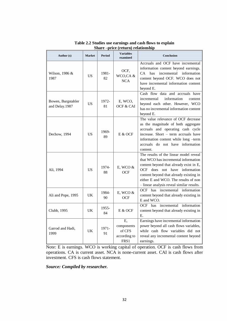
32

Table 2.2 Studies use earnings and cash flows to explain

Share –price (return) relationship

Author (s) Market Period Variables

examined Conclusion

Wilson, 1986 &

1987 US

1981-

82

OCF,

WCO,CA &

NCA

Accruals and OCF have incremental

information content beyond earnings.

CA has incremental information

content beyond OCF. WCO does not

have incremental information content

beyond E.

Bowen, Burgstahler

and Delay.1987 US

1972-

81

E, WCO,

OCF & CAI

Cash flow data and accruals have

incremental information content

beyond each other. However, WCO

has no incremental information content

beyond E.

Dechow, 1994 US 1969-

89 E & OCF

The value relevance of OCF decrease

as the magnitude of both aggregate

accruals and operating cash cycle

increase. Short – term accruals have

information content while long –term

accruals do not have information

content.

Ali, 1994 US 1974-

88

E, WCO &

OCF

The results of the linear model reveal

that WCO has incremental information

content beyond that already exist in E,

OCF does not have information

content beyond that already existing in

either E and WCO. The results of non

– linear analysis reveal similar results.

Ali and Pope, 1995 UK 1984-

90

E, WCO &

OCF

OCF has incremental information


E and WCO.

Clubb, 1995 UK 1955-

84 E & OCF

OCF has incremental information


E.

Garrod and Hadi,

1999 UK

1971-

91

E,

components

of CFS

according to

FRS1

Earnings have incremental information

power beyond all cash flows variables,

while cash flow variables did not

reveal any incremental content beyond

earnings.

Note: E is earnings. WCO is working capital of operation. OCF is cash flows from

operations. CA is current asset. NCA is none-current asset. CAI is cash flows after

investment. CFS is cash flows statement.

Source: Compiled by researcher.

33

2.3 Previous Studies

The relationship between accounting numbers (particularly earnings and cash flow) and

firm performance (measured by stock price or stock return) is one of the areas that have

been most exhaustively examined in previous research. In general these empirical

studies (Beaver, 1968; Dechow, 1994) have adopted different approaches to

investigating the questions raised about the relativity and superiority of different

performance measures. The following section will present a detailed description of the

debate surrounding them.

2.3.1 General Overview of Performance Measures

Accounting numbers represent a fertile area for the research that investigates the

empirical relationship between firm value and particular accounting numbers for the

purpose of assessing or providing a basis to assess a firm’s performance. It is well

known that the relevance of earnings (the after-tax profit available for stockholders) has

been investigated intensively since the issue was first raised by Beaver (1968).

Furthermore, many comparative accounting value relevance studies have focused on the

comparison between accounting earnings and cash flow (e.g. Dechow, 1994; Aharony et

al., 2003). The following are some popular performance measures used in different

articles to interpret the variation in annual stock price / return as a measure of a firm’s

value.

In this context, Ball and Brown (1968) investigated the association between earnings

and annual stock return, and they extended their study to test the incremental

information content of accruals, cash flows, working capital from operations, operations

cash flow, and cash flow measures. Furthermore they used the operating cash flows as a

proxy for annual earnings.

There have also been a number of studies concerned with the predictive ability of

earnings. Bowen et al. (1986) investigated the relationship between earnings and cash

flows, and used the following traditional definition of cash flows: net income before

extraordinary items and discontinued operations plus depreciation; and net income plus

depreciation, amortisation, and working capital from operations.

34

Along the same lines, Biddle et al. (1997) investigated whether the Economic Value

Added (EVA) has incremental information content beyond that of earnings. They then

extended their research to test whether EVA and the residual income (RI) method, and

earnings before interest and tax (EBIT) outperformed other performance measures

(earnings and operating cash flow) in explaining variation on annual stock return. EVA

is defined as the profit earned by the firm less the cost of financing the firm’s capital. It

is similar to RI but adjusted for net operating profit after tax (NOPAT) and invested

capital where needed. It is also referred to as net operating profits less a charge for the

opportunity cost of invested capital (West and Worthington, 2000).

In a related study, Francis et al., (2003) investigate the incremental information content

of earnings before interest, tax, depreciation, and amortisation (EBITDA), which refers

to an amount in which all interest, tax, depreciation and amortisation entries in the

income statement are reversed out from the bottom-line net income, and cash flows

from operations (CFO) which refer to the cash a company generates from its operation

activity presented in the cash flow statement.

The above mentioned performance measures will be discussed in depth in the following

sections.

2.3.1.1 Reconciliation of Performance Measures

As we have already noted, researchers have held different points of view regarding the

usefulness of earnings (accruals) and of cash flow items in explaining the variation in

stock price and there is no consensus on any one performance measure. This, together

with the criticisms of the previous performance measures (earnings, operating cash

flow, and residual income method) forced researchers to look for other measures that

amend the distortion of accruals measures and bring them closer to cash flow through

making certain necessary adjustments for the main items of the income statement,

specifically the net operating profit after tax (NOPAT).

In order to conduct this adjustment, analysts move upwards through the income

statement, starting with EBITDA which refers to an amount in which all interest, tax,

depreciation and amortization entries in the income statement are reversed out from the

bottom-line net income. EBITDA purports to measure cash earnings, cancelling the

35

effects of accrual accounting, tax-jurisdiction, and the effects of different capital

structures.

(1)

Where NOPAT is net operating profit after tax, DEP is depreciation and ATInt is after

tax interest. This construction of EBITDA differs from the operating cash flow in a cash

flow statement primarily by excluding payments for taxes or interest as well as changes

in working capital. EBITDA also differs from free cash flow (FCF) because it excludes

cash spent to acquire, to replace or to update physical assets such as buildings and

machinery (CAPEX).

In addition, free cash flows (FCF) refer to the cash available for distribution among all

the securities holders of an organization (equity holders, debt holders, preferred stock

holders, convertible security holders) which is equal to earnings before interest and tax

(EBIT) adjusted to accruals and changes in accruals and working capital. Thus, FCF is

equal to:

FCF = EBIT (1-Tax Rate) + Depreciation & Amortization

- Change in working capital – capital expenditure (2)

The first branch of this equation simply refers to net operating profit after tax (NOPAT)

which is the profit derived from a company’s operations after tax but before financing

costs and non-cash-book-keeping entries(Ross et al., 2010). In other words it is equal to

EBITDA less depreciation (DEP) and after tax interest (ATInt). Fundamentally, the first

branch represents the total pool of profits available to provide a cash return for those

who provide capital to the firm. The second branch of the equation is the invested

capital (IC) which represents the firm’s investment through the given period including

variation of working capital. Hence we can redefine FCF as (Penman, 2001):

FCF = NOPAT – ACCRUALS – IC (3)

or FCF = NOPAT – Increase in capital (4)

Similarly, Penman (2001) defined FCF as:

(5)

http://en.wikipedia.org/wiki/Cash_flow_statement

http://en.wikipedia.org/wiki/Cash_flow_statement

http://en.wikipedia.org/wiki/Working_capital

http://en.wikipedia.org/wiki/Free_cash_flow

http://en.wikipedia.org/wiki/Capex

36

From the previous definition, we note that by deducting the invested capital from

NOPAT we get FCF, but what happens if we deduct the cost of invested capital instead

of invested capital? The result is the residual income (RI) which is used to measure the

performance of management as a value added method so (Biddle et al., 1997):

RI = NOPAT – ( ×WACC) (6)

where WACC is the weighted average cost of capital. This basic formula in fact

represents the value created in excess of the required return to the company's

shareholders, which can be referred to simply as economic value added (EVA), that is

the profit earned by the firm less the cost of financing the firm’s capital (Stewart, 1991).

EVA = (EBITDA – DEP – ATInt) – IC × WACC6 (7)

where EBITDA-Depreciation and amortization is equal to earnings before interest and

tax (EBIT) and the EBIT × (1-tax) is equal to net operating income after tax (NOPAT).

This amount can be determined, among other ways, by making adjustments to GAAP

accounting, including deducting the opportunity cost of equity capital (Stern and

Stewart, 1991; Fernandez, 2002). Where EVA can be calculated after making certain

important adjustments to NOPAT and the invested capital (IC), these adjustments are:

Operating Income

+ Interest Income

± Equity income (Loss)7

+ Other investment income

-Income Tax

= Net Operating Profit after Tax (NOPAT)

Short term debt

+Long-term debt (Including bond)

+Other long-term liability (Deferred taxes and provision)

+Shareholder’s equity (Including minority interest)

= Invested capital (IC)

EVA= NOPAT – ( × WACC) (8)

6 Theoretically, the EVA equation is identical to the RI equation. Basically it is obtained after some

adjustment to NOPAT and the invested capital, debt and equity. 7 Equity income refers to income generated by existing assets (real estate, stocks). It usually refers to

dividend income which is a type of revenue available to shareholders that derives from the company’s

profit and is paid on a per-share basis.

http://en.wikipedia.org/wiki/Required_rate_of_return

http://en.wikipedia.org/wiki/Types_of_companies

http://en.wikipedia.org/wiki/Shareholder

http://en.wikipedia.org/wiki/GAAP

http://en.wikipedia.org/wiki/Opportunity_cost

37

Stern and Stewart (1991), the founders of EVA, argue that this method of performance

suffers from accruals distortions which mainly stem from the depreciation method

applied by different companies. Hence extra adjustments to EVA will bring it as close

as possible to the cash flow method (Young, 1998), where the cash value added (CVA)

metric (which is equal to the EVA adjusted for depreciation (DEP) and economic

depreciation (ED)), represents the best answer for this claim, and is defined as:

CVA = EVA + DEP – ED (9)

The economic depreciation represents the loss in the productive capacity of a physical

asset. It is the annuity depreciation expense (different from accounting depreciation

component as reported in the accounting reports) which, when capitalised at the cost of

capital (WACC), the assets’ value will accrue at the end of their useful life. This term

will create uniformity between firms and eliminate the effects of the depreciation

method that vary between entities. Using the NOPAT formula CVA can be verified to

be (Petravicius, 2008)8:

(10)

where RCF is the residual cash flows, NOPAT is the net operating profit after tax, DEP

is depreciation and amortization, ED is the economic depreciation and equal to

=

where RC is Gross fixed assets, or equal to (ROE – ) where

is debt book value, is equity’s book value and WACC is the weighted

average cost of capital. However, because of the difficulty we face while tracing the

useful life of different firms assets that are needed to calculate the economic

depreciation (ED), this research will use the simplified version of CVA, where CVA is

equal to cash flows from operations minus the cash flows demand, the dividends and

interest:

(11)

However, the inherent concern within the accounting community over the relationship

between market value and accounting numbers has led to the proposal of different

measures for assessing and evaluating the performance of companies as a whole, such

as value based measures (VBM) and other residual income methods (Ball and Brown,

8 As defined by Boston Consulting Group (BCG) or Frederik Weissenrieder Consulting.

38

1968; Patell and Kaplan, 1977; Stern and Stewart, 1991). The most commonly used

measures are the economic value added (EVA) framework founded by Stern and

Stewart Co., and the cash value added (CVA) introduced by the Boston Consulting

Group and Holt Value Associates (Malmi and Ikaheimo, 2003).

2.3.2 Accrual versus Cash flow measures

The majority of evaluation methods use income statement figures to build and compute

different forms of performance measures that help shareholders to evaluate those

companies in which they have invested and to measure the performance of managers

required to use this investment to maximise shareholders’ wealth.

Since 1968 an extensive amount of research has been conducted into the information

content of earnings’ components. Ball and Brown (1968) analysed a sample of firms

over the period 1944 – 1966 to test the information content of accounting numbers

(annual earnings) and investigate its association with abnormal returns. The approach

they adopted for this research relied on the assumption that the income of different firms

within a specific market has tended to move broadly together. The early findings of Ball

and Brown (1967) stated that 35 to 40 per cent of the variability in the level of an

average firm’s earnings per share (EPS) could be associated with economy-wide effects,

especially when income was defined as tax-adjusted return on capital employed.

They constructed two alternative models of what the market expected income to be and

then investigated the market’s reactions when its expectations proved false. A simple

linear regression was used to test the proposed association in which changes in firm i

income regressed against the change in the average income of firms in the market. This

showed that the information contained in the annual income number was useful in that it

is related to stock prices.

Ball and Brown’s research was the first to discuss the information content of accounting

numbers and has been replicated many times by different scholars (Beaver and Dukes,

1972; Bowen et al. 1986; Board and Day, 1989). They measured the association

between annual earnings (operating cash flows) and the abnormal return using the

operating earnings as proxy for operating cash flows and they reported that earnings

showed a higher correlation with abnormal stock return than cash flows.

39

However, the assumption of Ball and Brown is similar to that of CAPM (the capital

market is both efficient and unbiased). Hence, the assets price will rapidly adjust with

the release of information without leaving any chance of abnormal gain. This is actually

considered a criticism of their research, because in the real world the perfectly efficient

market may not exist although weaker forms of efficiency (semi-strong and weak form)

may hold in reality.

By using a different proxy for operating cash flows the seminal study of Beaver and

Dukes (1972) concluded that unexpected earnings, which they defined as earnings plus

depreciation, depletion and amortisation charge, and the change in deferred tax account,

were more highly associated with abnormal returns than unexpected operating cash

flows. In a related study, Patell and Kaplan (1977) examined the information content of

cash flows beyond that already existing in earnings. They calculated cash flows as

earnings after extraordinary items plus depreciation and deferred tax minus unremitted

earnings attributable to foreign consolidated industries plus other adjustments. They

pointed out that operating cash flows provided no information beyond that which

existed in earnings. As will be noted in earlier studies the operating cash flows showed

no information content beyond that which existed in earnings which may be due to the

naive method used in calculating the operating cash flows.

Correspondingly, Bowen et al. (1986) examined the relationship between accounting

earnings and cash flows for a sample of US data over the period 1971-1981. They used

the following traditional definitions of cash flows: net income before extra-ordinary

items and discontinued operations plus depreciation (NIBEI), net income plus

depreciation and amortisation (NIDPR), and working capital from operations (WCFO).

In addition, they employed three recently devised measures for cash flow: cash flow

from operations (CFO), cash flow after investment (CFAI), and change in cash and

short-term marketable securities (C).

Their aims were to answer the following questions:

1. Are the traditional cash flow measures used in prior studies highly

correlated with alternative measures of cash flows that have really

been advocated by academics and practitioners?

2. Are accrual accounting earnings and cash flow measures highly correlated?

3. Do earnings or cash flow variables best predict cash flows?

40

An empirical study by Bowen et al., (1986) concludes the following:

1. Measures of cash flows (NIBEI, WCFO) are poor proxies for cash flow.

2. Traditional measures of cash flows are more highly correlated with accrual earnings

than alternative measures (CFO, CFAI, and C).

3. The correlation between traditional measures and more recent measures is lower than

the correlation between traditional measures and accrual earnings.

4. The traditional measures of cash flow, WCFO and NIDPR, were better predictors of

future cash flow from operations than cash flows from operations themselves and from

net income before extraordinary items.

Their results were in contrast with the FASB 959 assertion that earnings are better

predictors for future cash flows than current cash flows.

The evaluation of the company’s performance is considered one of the greatest

challenges researchers have ever met. For many decades accounting earnings were the

most popular approach for evaluating management performance until the initiation of

the evaluation model that was based on cash flow items (Board and Day, 1989).

Board and Day (1989) examined the comparative ability of net income, working capital

from operations and net cash flow to explain the variation in stock return over the

period 1961-1977. They pointed out that net income and working capital from

operations have, separately, more information content than net cash flows. They also

investigated the incremental information content for these variables. Their results

indicate that net cash flows have the poorest incremental information content.

Based on UK data over the period 1985–1993, Charitou et al. (2001) investigated the

value relevance of operating cash flow and earnings under three contextual variables: (i)

earnings permanence, (ii) earnings growth, and (iii) firm size. The results revealed that

earnings had incremental information content over cash flow while operating cash flows

revealed incremental information content beyond earnings when pooled data were used.

The results also conveyed that prior operating cash flow was significantly positively

associated with stock return and indicated that firm size and market to book ratio (risk

9 Summary of statement No.95, Statement of cash flows (1987) updated to IAS7 Statement of cash flows.

41

proxies) improved the explanatory power of the model they adopted to conduct their

research.

Similarly, Francis et al. (2003) examined the relative and incremental information

content of earnings before interest, tax, depreciation, and amortization (EBITDA), cash

flow from operations (CFO) and earnings (EARN). Their sample covers 16 industrial

companies in the period 1990-2000. The Standard and Poor Index (S&P) published

reports were used to identify the most applicable performance metrics within different

industries and also to determine those industries to which the non-GAAP performance

metrics (i.e. not calculable from numbers reported in the audited financial statements).

The methodology applied by Francis et al. was to classify the industries according to the

claimed preferred performance metric applicable within the chosen industry, then assess

its ability in samples of industry where the non-GAAP performance metric is the

preferred metric in explaining the variability on stock return. Hence, the tested

hypothesis was whether the preferred GAAP metric outperformed the non-preferred

GAAP metrics in explaining returns.

The main contribution of the research by Francis et al. is the introduction of the non-

GAAP performance metric (non-earning, non-cash metric) and the assessment of the

usefulness of industry-specific performance measures in predicting either or both

earnings and revenues.

In summary, Francis et al. indicate that earnings significantly outperform both EBITDA

and CFO across industries using these preferred performance metrics. The findings also

show that EBITDA significantly outperforms CFO for the pooled and industry sample,

whereas Francis et al. show that EBITDA does not outperform EARN for any industry

even though it is considered the preferred metric within the chosen industry. This

finding holds within the industry level.

Turning to incremental power, the findings of Francis et al. reveal that all the GAAP

metrics show incremental power in the presence of other non-GAAP metrics within the

pooled data analysis, whereas the annual regression results show that EARN has highly

significant incremental explanatory power in comparison to both EBITDA and CFO for

each pooled and year regression. The research by Francis et al. provides consistent

evidence that each preferred metric has significant incremental explanatory power in its

42

preferred sample (Board and Day, 1989; Ali, 1994; Wilson, 1986, 1987; Chen and

Dodd, 1997: Forker and Powell, 2008).

Similarly, the findings of Francis et al. show that EARN has high explanatory power in

describing variation in stock return and outperforms the non-GAAP metric. The same is

found using EBITDA and CFO. The results also indicate that all the GAAP metrics

have incremental explanatory power compared to those that exist within non-GAAP

metrics (except for the homebuilding industry where the finding is that non GAAP

metrics add little incremental power to explain return). One interesting finding by

Rayburn (1986) is that the information contained in accrual components is what

explains and justifies the incremental information content of earnings beyond that

already existing in cash flow measures.

Because there are no conclusive results for the usefulness of earnings and cash flow

items, neither the accrual earnings, nor the cash flow items, was a perfect method for

measuring management performance as an approach to evaluating the whole firm

(shareholder wealth) (Bowen et al., 1987; Charitou et al., 2001). Nevertheless, the bulk

of empirical evidence indicates that the superiority of cash flow measures vis-à-vis

earnings (as variously defined) has not been demonstrated.

2.3.3 Value-Based Measures and Residual Income Method

The adage has long persisted that in order for a company to generate value and to create

wealth it must earn more than it costs by way of debt and equity. The added value

concept has been promoted strongly in performance measurement literature. This notion

is historically referred to as the residual income (RI) method (a value–based measure).

A periodic performance measure was introduced by Stern and Stewart (1991) to replace

earnings and cash flow from operations as a measure of performance. They called it

Economic Value Added (EVA). Stewart (1994, p.75) argues that ‘EVA stands well out

from the crowd as the single best measures of value creation on a continuous basis’. He

also remarked that ‘EVA is almost 50% better than its closest accounting-based

competitor (i.e. earnings) in explaining changes in shareholder wealth’ (p.75).

From a different point of view, Ball and Brown, (1968) and Patell and Kaplan, (1977)

highlight their contention that there is no single optimal accounting measure that

43

accurately explains the variability in shareholders’ wealth. A mass of empirical research

has been conducted to test the validity of the residual income model as an alternative to

the discounted cash flow model in equity evaluation, which specifies the relationship

between equity values and accounting variables such as earnings and book value

(Ohlson, 1995). Ohlson models a firms’ value as a linear function of earnings, book

value, and other unspecified information (Fundamental Value, ) that plays an

important role in linear information dynamics and proposes consensus analyst forecasts

as a proxy for .

However, some empirical research claims that even the traditional dividend discounting

model is the basis of the Ohlson model. The residual income model breaks new ground

on two fronts (Dechow, 1999). First, it has the ability to predict and explain stock prices

more effectively than the models based on discounting short-term forecasts of dividends

and cash flows. Second, it provides a more complete valuation approach than popular

alternatives because of the inclusion of non-GAAP metrics (Francis et al., 1997;

Frankel and Lee, 1998).

However, analyst forecasts depend in part on the information contained in current

earnings and book value. Analyst forecasts, therefore, not only reflect information about

future earnings beyond that conveyed by earnings and book value (the definition of ),

but also reflect, among other things, the ‘stale’ information concurrently conveyed by

the accounting fundamentals (Dechow et al., 1999).

Unfortunately, this empirical research ignores something essential to Ohlson’s model,

which is information dynamics. However, the results of both valuation models and

dividend discounted models appear identical regardless of whether earnings are

capitalised or forecast, ‘but make no appeal to book value or residual income’ (Dechow

et al., 1999, p. 2).

Correspondingly, Dechow et al. used the annual financial statement for the period 1976-

1995 to evaluate the empirical implications of Ohlson’s model. Unlike previous

research the information dynamics that link current information to future residual

income were incorporated. They stated that the Ohlson model was a restricted version of

the standard dividends discounted model that comprised three basic assumptions. First,

when the expected dividends are discounted to their present value the amount yielded is

equivalent to the price of shares. Second, the clean surplus accounting relationship is

44

maintained. The third assumption addresses the character of the relationship existing

between the present value of future dividends and the current information.

In their analysis Dechow et al. focus on the improvements provided by Ohlson’s model

over these simpler and more restrictive models, by imposing additional restrictions to

the dividends discount model. This restriction represents the ignorance of the other

information factors when analysing earnings forecasts. Dechow et al. contend that the

‘Ohlson model assumes that expectations of future abnormal earnings are based solely

on information in current abnormal earnings and that abnormal earnings are purely

transitory. Consequently, expected future abnormal earnings are zero and price is equal

to book value. This restricted version assumed that accounting earnings are used to

measure value creation' (p. 9).

After the empirical assessment of the residual income valuation model and the

imposition of the information dynamics that describe the formation of abnormal

earnings expectations, Dechow et al. conclude that models that simply capitalise

earnings forecasts in perpetuity outperform information dynamics models in explaining

stock prices. Furthermore, subsequent research showed that the superiority of the

simple capitalisation model over the information dynamics model stems from the fact

that investors are generally presumed to ‘overweight information in analysts’ earnings

forecasts and under-weight information in current earnings and book value ’ (Dechow et

al., 1999, p.32).

2.3.3.1 The Validity of the Performance Measure’s Components

Garrod et al. (2000) used the basic Edward-Bell-Ohlson (EBO) model to measure the

value relevance of earnings’ components. By adopting a cross-sectional analysis for UK

data over the period 1992-1996 they concluded that the disaggregation of earnings into

its prime components (i.e. cash flows and short and long term accruals) significantly

increased the explanatory power of the model. However, this increase in significance

mainly resulted from decomposing earnings into operating earnings and operating assets

rather than from decomposing earnings into its components i.e. cash flows and accruals.

They also investigated whether the value relevance for cash flows and earnings’

components was affected by the magnitude and the sign of the three following

contextual variables: (i) operating cash flows (ii) earnings and (iii) short term accruals.

The methodology they used are as follows. First, they divided the total sample into two

45

sub-samples according to the sign of the contextual variables. Then the positive sample

was divided into four groups according to the magnitude of the variable, the first group

containing the lowest values from the contextual variable and the fourth group

containing the highest.

The results of Garrod et al. (2000) supported the above conclusions that cash flows have

information content and that the cash flow model has the highest explanatory power for

the variation in price per share. They reported also that there was no value difference

between accruals and operating cash flows. However, long-term accruals were valued

differently in extreme cases where the contextual variables were negative or too

positive. Short term accruals were rarely valued differently. From the above results

Garrod et al. drew the conclusion that ‘the isolation of accruals from cash flows only

takes on valuation significance in conditions which are unusual and unlikely to persist’

(p.15).

Biddle et al. (1997) investigated whether EVA dominated and had incremental

information content beyond that of accrual earnings and also extended their

investigation to test whether any of EVA’s components had a higher association with

stock return and firm value.

Biddle et al. used a sample of 219 firms over the period 1984-1993 to test whether the

EVA and RI outperformed the mandated performance measures, earnings and operating

cash flow in explaining contemporaneous annual stock returns. These firms fell into two

main categories, those which adopted EVA as a performance measure and those which

did not. Moreover, they also tested whether the components unique to EVA and/or RI

contributed more to explain contemporaneous stock return beyond that explained by

CFO and earnings. They began their investigation by describing how the variables of

this study are linked to each other through a reconciliation process starting with

earnings before extraordinary items (EBIT) and ending with EVA.

The findings of Biddle et al. (1997) were that all the variables (EVA, RI, CFO, and

EBIT) were significant at a conventional level, and that both EBIT and RI have the

higher adjusted and outperformed EVA. Unlike Stern and Stewart (1991), this study

could not support the claim that EVA had greater information content than earnings. For

the incremental information, the results (based on F-statistic tests) indicated that both

CFO and Accrual had the highest incremental information content in explaining market-

adjusted returns, while the components of EVA (ATI, CC, Accrual ADJ) appeared to

46

make little contribution to the incremental information content. When combined with

the relative information content findings above, these results suggested that, ‘while

EVA components offer some incremental information content beyond earnings

components, their contributions to the information content of EVA are not sufficient for

EVA to provide greater relative information content than earnings’ (p.20).

In particular, the focus of Biddle et al. (1997) was on developing a statistical test for the

comparison of explanatory power, and the availability of data was the main criterion

used to select the sample for study in the proposed test. From the research perspective,

this raises concerns over subjectivity and prevents the results of Biddle et al. from being

globally compared to other research findings.

Furthermore, Forker and Powell (2008) criticised the findings of Biddle et al. They state

that Biddle et al.’s research design is ‘however, subject to the limitation that

shareholders’ return (an equity metric) is regressed on contemporaneous measures of

performance that are measured at the entity (operating) level of the firm. Restricting the

analysis to a single period contemporaneous association with firm values and returns

does not address the problem that one-period measures of residual income are not

necessarily associated with the shareholder changes in wealth reflected in security

returns. Also, an association between one-period returns and a charge for the cost of

capital is potentially mitigated by the charge having little variation across a sample of

large firms’ (p.6).

In a similar vein, West and Worthington’s (2000) study based on 110 Australian

companies over the period 1992 through to 1998, examined the association of EVA,

earnings, net cash flows, and residual income with annual stock return. In addition they

extended their research to test whether EVA had incremental information content and

outperformed conventional accounting-based measures. In their response to Stewart’s

(1991) claim that EVA is the best performance measure regarding its ability to capture

the true economic profit of a firm and to the recommendation of Biddle et al. , West and

Worthington examined which of the components of EVA and earnings were more likely

to contribute to, or subtract from, the information content.

West and Worthington used the same methodology as Biddle et al. , starting by

describing the linkages between the different competing measures of firms’

performances, except that, unlike the latter’s empirical research, they used the pooled-

time series, cross–sectional least squares regression to conduct their studies.

47

West and Worthington’s research indicates that (as with the Biddle et al. study) all the

performance measures have a significant association with adjusted annual stock return

variation, where earnings before extraordinary items (EBEI) were the most reliable

predictor, whereas EVA is the least reliable predictor of the four accounting measures.

For the incremental information content the results show that the most logical pairing of

information variables in explaining market return is EBEI and EVA.

The second phase of West and Worthington’s study is to examine the components of

EVA; the results convey that all the components are significant but that accrual (ACC)

has a greater explanatory power than the other variables in explaining variation in stock

return.

Conversely Worthington and West (2004) form different conclusions regarding the

superiority of EVA, based on Australian data. They contend that EVA is highly

associated with stock return and outperforms all other performance measures, namely

residual income, earnings and net cash flows.

2.3.3.2 Performance Measurement of Productive Activity

For any company to succeed in an increasingly competitive market, it has to know the

cost of its entire economic chain (productive activity) in order to maximise the

shareholders’ wealth. To do so a company should have the ability to manage the

economic cost of its entire production chain rather than its cost alone, so what it needs

to do is create value not control cost. To accomplish this aim a company needs

sufficient data on the total-factor productivity where EVA is designated as its best

measure (Drucker, 1995). Moreover, the transformation from traditional costing into the

activity-based costing system (ABC), within the complex high technology industry

sector encourages the adoption of EVA together with benchmarking to measure and

compare the performance of different companies to determine that of the best

performance within the sector (Drucker).

Essentially, what makes EVA superior to the other, traditional performance measures

(e.g. earnings, performance ratio), is its ability to incorporate the cost of invested capital

(IC) when measuring the value added or created by the company (Stern and Stewart,

1991; Fernandez, 2000) and also its ability to measure in effect the productivity of all

producing factors in a complex manufacturing unit (Drucker, 1995). In addition it has

48

the ability to indicate why a certain product or service does not add value; it shows what

the executive manager needs to find out and it identifies whether any remedial action is

needed in order for certain products and services to generate value.

The ccost of capital is thus the most important aspect of EVA. Under traditional

methods most companies appear to be profitable whereas in reality they are not (Stern

and Stewart, 1991). In a related note Drucker (1995) observes that “Until a business

returns a profit that is greater than its cost of capital, it operates at a loss. Never mind

that it pays taxes as if it had a genuine profit. The enterprise still returns less to the

economy than it devours in resources. It does not cover its full costs unless the reported

profit exceeds the cost of capital. Until then, it does not create wealth; it destroys it”

(p.59).

2.3.3.3 Value –Based Measures versus Traditional Accounting Measures

As a new concept of performance measurement EVA has aroused much concern,

especially in the advanced economies. In spite of its being widespread as a performance

measure, its implementation and validity has generated intense debate (Anastassis,

2007; Forker and Powell, 2008).

Historically, predictability and variability were used as the main criteria to gauge the

quality of earnings and, hence their usefulness to investor decisions. In this context,

Forker and Powell (2008) used these two criteria to test empirically the quality of EVA

relative to generally accepted accounting principles (GAAP) earnings, residual income,

cash flows, and other mandated metrics in the USA and the UK. Unlike Biddle et al.

(1997), Forker and Powel (p.1) were using a proxy ‘for accounting quality by applying

the long window- methodology to obtain hindsight valuation errors based on the

difference between ex ante actual market value and discounted ex post metrics as a

proxy for accounting quality’.

Forker and Powell’s focus in particular was on the value relevance embedded in the

recognition of the cost of capital, a factor noticeably absent from the issues under

consideration by the International Accounting Standard Board (IASB) in its quest to

improve financial reporting quality. Forker and Powell claim that, theoretically, EVA

outperforms earnings because it meets the requirements of the residual income method

as it strictly adopts the practice of clean surplus accounting that takes into account all

49

factors impacting on shareholder wealth when measuring income and because it

recognises the cost of equity capital (valuation of equity).

Forker and Powell (2008) conducted their test for valuation errors using three steps:

first by reporting the main cross-sectional valuation errors and the differences between

main paired valuation errors for each long-window; then by reporting the variability of

the individual valuation errors for all econometric measures; and lastly by providing the

actual cross-sectional errors and differences in errors across all windows and terminal

dates. Two sets of data were used to conduct this test: the USA data-set containing

1,000 firms for the 16 year period 1986 – 2001; and the UK data-set containing 500

firms for the 12 year period 1990 –2001.

The rule they applied here was that ‘the smaller the mean and variability statistics for

valuation errors the higher its accounting quality and decision usefulness in forecasting

future value’ (Forker and Powell, 2008. p.18). In addition, the t-test and Wilcoxon

signed test were used to examine the significance of different measures. Their results

showed that the best performance measure for all windows was the residual income

before exceptional and extraordinary items [RI (1), RI (2)].10

It is clear that the

exclusion of the cost of capital from conventional earnings is a direct source of error in

estimating intrinsic value.

However, in their study of the association between market returns and alternative

performance metrics, Forker and Powell find that residual-based metrics outperform the

GAAP-base metrics from which the non-cash cost of equity capital is excluded. In

terms of performance metrics’ forecasting powers the residual-based metrics have the

ability to outperform operating cash-flow-based metrics. Moreover, Forker and Powell’s

results show that the differences between EVA and residual-based measures are small, a

finding inconsistent with that of Francis et al. (2000). Further, unlike Biddle et al.

(1997), the key results reported that the residual income method (RI) and earnings

before interest and tax (EBIT) have the higher adjusted and outperform EVA.

However, the main paradigm of firms is to create and maximise shareholder wealth.

This is the wealth that is evaluated in terms of different performance measures and it

may be measured in terms of returns received on investment which could be in the form

10 Forker and Powell define RI (1): residual income before exceptional and extra-ordinary items with Stern and Stewart end of period capital employed. RI (2): residual income after exceptional and extra

ordinary-items with Stern and Stewart end of period capital employed.

50

of dividends, capital appreciation or both. But the crucial question here is what single

performance measure should be used by different interested parties to evaluate a firm.

Closely related to the last point, Anastassis and Kyriazis (2007) investigate the

explanatory power and the incremental information content of EVA against those of

traditional performance measures such as net income and operating income. They

contend that, unlike the traditional measures, EVA takes into consideration the cost of

the capital invested to generate profit, (recognising that a company is going to create

value only when, besides its various operating costs, it covers the cost of its invested

capital). Considering this, the only difference between EVA and Residual Income

method (RI) is the adjustment that Stewart (1991) suggests for the calculation of

invested capital and net operating profit (NOPAT). Supporters of the EVA performance

measure suggest more than one hundred adjustments for the NOPAT and the IC. The

most common and important adjustments are those for good will, operating lease,

research and development expenses, provisions and deferred taxes (Young, 1999).

Greek data for the period 1996–2003, (a time that witnessed the transformation of the

Greek stock market from an emerging and relatively weak form, to the developed and

more efficient one after year 2000) were used by Anastassis and Kyriazis to investigate

whether EVA would outperform other traditional performance measures. Furthermore,

they replicated the model introduced by Biddle et al. (1997) to test for the relative

information content of EVA.

Anastassis and Kyriazis used both panel regression and Cox pool regression (a test for

non-nested regression) to test for the relative information content and incremental

information content. The results reveal that with respect to abnormal stock returns

operating income (OI) has the highest explanatory power ( ), followed by net income

(NI) and then residual income (RI) whereas the explanatory power of EVA appears to

be the least. Regarding the incremental information content result their findings convey

that both EVA and OI are equivalent, and outperformed by both NI and RI. In addition,

the Wald test reveals that, for the EVA components, ‘both the capital charge (which is

also included in RI) and the Stern and Stewart (1991) adjustment do not have any value

relevant information additional to that which is already incorporated in the traditional

accounting variables’ (Anastassis and Kyriazis, 2007. p.15).

Contrary to previous regression results (abnormal return as dependent variable), EVA

outperforms all the other profitability measures when the regressions run against the

51

market value (MV). This is actually compatible with the theory behind EVA (time value

assumption), which states that the discounted value of all the EVAs the company

assumes it will achieve in the future, is equal to the current MV. Therefore, as assumed,

the value of EVA is better correlated with market value (MV) than accounting variables

(Anastassis and Kyriazis, 2007)

However, according to the Cox test, in spite of EVA having the highest (this

difference does not appear to be statistically significant), the finding of Anastasia and

Kyriazis ‘fails to provide adequate support for Stewart’s (1991) claim that EVA tracks

changes in MV better than any other performance measure, since it appears that the

other earnings measures are equally competent of explaining the variation in MV’

(p.23).

The results of Anastassis and Kyriazis’s model (2007) for the first difference (one year

lag) show statistically insignificant differences in the information content of RI, OI and

EVA. For the incremental content of EVA components the results indicate that NI is the

only one providing statistical significance whereas the changes in both operating

income adjustments and Stern and Stewart (1991) adjustments are of no importance to

the market. The Wald test also supports the evidence that ‘the first difference of

operating income adjustment, capital charge (CAPCH) and Stern Stewart adjustments

(ACCADJ) does not add any useful information to that already incorporated in the

change in net income (NI)’ (Anastassis and Kyriazis,2007, p. 18).

Along the same lines, Riahi (1993) investigated the relative and incremental

information content of certain variables (value added, earnings, and cash flows) using

the US data. In surveying the relative information content he concluded that value added

is a significant explanatory factor in stock return and, moreover, it has more power of

explanation in relation to general return of stocks. In surveying incremental information

content Riahi (1993) introduces the combination of value added and net profit as the

best explanation of stock return.

The association of earnings with stock return (price) and firm values has been the focus

of many accounting research studies (Ball and Brown, 1968; Beaver and Ducks, 1972)

for the past five decades, and many of these empirical studies have investigated the

information and incremental information content of earnings (accruals) beyond that

which already exists among different performance and evaluation methods. Further,

much of this research supported the finding that earnings outperform all other

52

performance measures that derive from discounted cash flow and residual income

(Pattel and Kaplan, 1977). Some have suggested that, in order to improve their

explanatory power, earnings should be deconstructed into their main components to

show whether these provide more information content than earnings itself (Bao and

Bao, 1998).

The study carried out by Bao and Bao (1998) investigated the association between

performance and value added and concluded that the latter was positively associated

with firm value in certain industries. EVA as a surrogate for abnormal economic

earnings has recently received much attention as another performance measure and

many researchers (Anastassis and Kyriazis, 2007; Forker and Powell, 2008) considered

it the best performance measure. It has even been predicted by different researchers

(Lehan and Makhija, 1997; Chen and Dodd, 1997; Erasmus, 2008) that EVA will

supersede earnings and earnings per share as the proper financial measures but this

claim has faced much controversy and the view that even if EVA has some merit it is

not as promising as its creators have claimed (Biddle et al., 1997).

Bao and Bao (1998) employ three types of analysis to examine the usefulness of

abnormal economic earnings and value added. These comprise a firm’s value analysis

(market value of equity) in which a firm’s value regress “against earnings and other

GAAP–related variables, levels studies regress prices/returns on earnings while changes

study regress prices/returns on changes in earnings” (p.5). Samples of 166 firms for the

two year period 1992 - 1993 were used to conduct the research.

The results of the firm value analyses reveal that for the year 1992, only EVA is

significant in explaining firm value, while the earnings add little value when paired with

value added. Furthermore, the sign of abnormal economic earnings coefficient always

comes against the forecasts (negative all the time). The results were the same for the

year 1993. For the incremental information analyses the results show that, consistent

with Riahi-Belkaoui (1993), value added has higher relative and incremental content

than earnings.

The results of Bao and Bao specify that for the level analysis shown, even though EVA

has the correct sign, it is not a statistically significant variable and has a lower power of

explanation than the other variables amongst which value added appears the most

highly significant. Furthermore, the change analysis results convey that while EVA

remains significant with higher explanatory power and the correct anticipated sign of

53

correlation (positive), the earnings and abnormal economic earnings are insignificant,

with a different sign of correlation than forecast.

When using the initial price of stock as a deflator the results reveal that contrary to the

level analysis finding all the explanatory variables of Bao and Bao’s study are

statistically significant. Consistently, EVA has greater explanatory power in comparison

to those of earnings and abnormal economic earnings.

Bao and Bao (1998) therefore conclude that “economic value added is not as promising

as Stern and Stewart have claimed, the usefulness of EVA as abnormal economic

earnings surrogate, therefore, is an empirical issue” (p.5).

More recently, Mehdi and Iman (2011) investigated the relativity and incremental

information content of EVA over traditional measures. They used the data from the

Iranian stock market for the period 2001 to 2008 to investigate the association between

EVA, traditional measures and the stock return. The results do not support Stern and

Stewart’s claims and reveal that stock return is highly associated with return on assets

(ROA), return on equity (ROE), and earnings per share (EPS), while EVA appears to

have little information content beyond that which exists in other traditional accounting

measures.

However, an empirical question arises here. Which measure has the better association

with stock return? Most interestingly, previous studies that have mainly used US data

consistently show superior relative value relevance (or information content) for value

added over income (Riahi-Belkaoui, 1993; Bao and Bao, 1998). ‘Because these studies

were limited to the few US companies which report the employee compensation data

needed to compute value added, it is possible that these results are influenced by self-

selection bias’ (Darcy, 2006, p.3).

2.3.3.4 Modification of EVA as A Performance Measure

Shareholder pressure on firms to maximise their wealth and to incentivise executive

managers to align their interests accurately with those of shareholders increased and

reached unprecedented levels (Rappaport, 1986; Young, 1997; Lovata and Costigan,

2002). Thus, managers’ compensation contracts should be designed to include the most

appropriate measure for evaluating their performance, and not necessarily the

historically dominant stock price measure. Furthermore, the stock price may not be an

54

efficient and proper contracting parameter because it is generally driven by many

factors beyond the control of the firm's managers (Bacidore et al. 1997).

Moreover, any selected performance measures to be used in managerial compensation

schemes must be highly correlated with changes in shareholder wealth and should not

be subject to all the essential randomness of an entity’s stock price (Bacidore et al.). As

Bacidore et al. 1997 have stated, ‘This dichotomy is the fundamental tension a good

performance measure must resolve’ (p.11). He also claimed that EVA as proposed by

Stewart (1991) would best resolve this tension as it has the creativity to secure better

linkage of the firm’s accounting data with its stock market performance.

Bacidore et al. present an empirical analysis to examine both the ability of EVA to

measure the abnormal return changes and the correlation between EVA and abnormal

return. Moreover, they claim that the most suitable performance measure should have

the ability to measure how the strategy of management can influence shareholder value.

This influence is measured by the risk-adjusted return on invested capital. Finally, the

performance measure should clarify how well the firm has generated operating profits,

given the amount of capital invested to produce those profits (Bacidore et al., 1997).

According to Bacidore et al. (1997), EVA is calculated as the net operating profit

(NOPAT) adjusted for the increase in bad debt and LIFO reserve; plus any increase in

net capitalised R&D; plus amortisation of goodwill; plus other operating income; minus

operating cash taxes; and minus the adjusted book value of net capital at the beginning

of the period (NA).

Bacidore et al. used a sample of 600 firms selected from the Stern and Stewart

performance 1000 database for the period 1982 through to 1992 to examine the

association between EVA and the abnormal stock return. After running the regression of

abnormal returns against the EVA as explanatory measures, the results showed that both

EVA is significantly associated with abnormal return. But, after the inclusion of lags as

explanatory variables to the regression, in order to test whether past realisation of EVA

has a significant effect on abnormal returns, the results convey that EVA is significantly

positively related to abnormal return whereas the lag EVA is significantly negatively

related to abnormal return.

Contrary to the claim of Bacidore et al. (1997) that REVA as a performance measure is

superior to EVA, Ferguson and Lestikow (1998) stated that EVA in reality is superior

55

to, and more widely spread, than REVA since its introduction by Stewart and Stern. The

key distinction between these two measures was that capital charge was based on the

firm’s market value instead of its net assets value. Thus, the main assumption of

Bacidore et al. is that an appropriate measure of operating performance must correlate

highly with abnormal stock return. This assumption seems plausible to Ferguson and

Lestikow (1998) who claim that management decisions that alter shareholder wealth

also cause a corresponding abnormal stock return. The theory suggests, however, that

no appropriate single-period measure of operating performance should be highly

correlated with abnormal stock return.

Accordingly, the main criticism of the work by Bacidore et al., is that the use of

abnormal stock return as a basis for rewarding management is likely to be inconsistent

with shareholder wealth maximisation. To this end, Ferguson and Lestikow (1998) used

the traditional dividend discount model to prove that EVA is more consistent than

REVA with finance theory and wealth maximisation.

2.3.3.5 Individuals Focus of Value -Based Measures

Most of the empirical research on economic value added focuses on the firm as a unit of

analysis whereas none of these studies focuses on individual managers or examines how

each individual will perform under different performance measures.

In terms of the assessment of the top management performance, Lehn and Makhija

(1997) (through the use of a sample of 452 entities during the period 1985-1994)

empirically examine the ability of EVA as a new performance measure, together with

return on sales (ROS), ROA, ROE, and market value added (MVA) to explain not only

the variation in stock return, but also the probability that a CEO will be dismissed for

poor performance. They claim that EVA appears to be a considerably more reliable

indicator of CEO turnover than profitability ratio measures (i.e. ROS, ROE). Lehn and

Makhija conclude that in spite of it having the higher correlation among the other

performance measures, EVA and MVA are not the most efficient criteria.

In their study of how managers perform under an EVA bonus scheme, Cahan et al.

(2002), examined whether the managers who are compensated using EVA-based bonus

plans outperform the managers who are compensated on traditional accounting-based

bonus plans. This system, they claim, can change managerial behaviour at the firm

56

level. However, they do not provide any evidence on the performance of the individual

manager. Cahan et al. (2002) contend that ‘one reason to expect better performance for

managers on EVA bonus plans is that an EVA-based reward system better aligns the

interests of the manager and the firm’ (p.8).

Based on the findings of Wallace (1998), there is evidence to suggest that EVA is hard

to understand and implement. Cahan et al. (2002) used a sample of 117 managers in

major international New Zealand Companies which included 52 on EVA bonus

schemes and 65 on traditional schemes.

Basically Cahan et al. were interested in the coefficient interactive term between the

budget type and the understanding of EVA, and expected it to be positive and

significant which means that the relationship between bonus type and performance

depends on the understanding of EVA. Moreover, they contend that managers with a

high understanding of EVA produce a higher performance when their firms adopt an

EVA–based bonus plan.

The result of Cahan after running the regression on the full model shows that ‘the high

EVA understanding has a quite dramatic positive effect on the performance of managers

on EVA reward systems while high EVA understanding actually has a slight negative

effect on managers on traditional reward systems’ (Cahan et al., 2002, p.19). Cahan et

al. attributed the negative effect of the latter to cognitive imbalance. Furthermore, when

accounting–based performance systems are used to evaluate those managers who best

understand EVA, their performance may experience cognitive conflict, and

consequently, may decline (Cahan et al.,).

For the reduced model adopted by Cahan et al. (interactive term excluded) the results

show that managers with EVA bonus plans and high EVA understanding outperformed

other managers in those areas in which manager have high EVA understanding and

traditional reward system. To sum up, the findings of Cahan et al. illustrate that there is

an interactive effect on overall performance between bonus plan types and the

understanding of EVA and demonstrate that, given differences in the delegation of

decision rights and strategic focus, EVA bonus plans might not be optimal in all areas

of operation. Finally, controversy to Stern and Stewart’s claim that EVA is easy to

understand by different managers’ level (high understanding) Cahan et al. (2002) state

that EVA understanding is not always high.

57

2.3.3.6 Cash Value Added (CVA) as a Performance Measure

Scholars have different points of view regarding the usefulness of traditional accounting

(earnings and accruals) and cash flow measures in explaining the variation of stock

price performance. However, the criticisms that the traditional and value added

measures have faced and the arguments raised by Young (1999) regarding the Stern and

Stewart adjustment (i.e. that the main aim of this adjustments is to produce a modified

version of the EVA that undermines the drawbacks of accrual based measures by

developing new performance measures that have the properties of cash flows (cash

value added metric)), all encourage researchers to develop new performance measures

that can better measure the performance of firms and managers.

In response to the above controversy, Ottosson and Wiessenrider (1996) proposed a new

performance measure entitled cash value added (CVA)11

- the surplus of cash flows - to

replace the traditional accounting and value added measures, specifically the periodic

measure EVA.

In this context, Ottosson and Wiessenrider argue that the focus of moderate

management, unlike traditional management accounting, should be on the strategic

investment (that creates value) and they should not waste valuable time on controlling

and evaluating non-strategic investment decisions. In addition, they claim that ‘the

fundamental difference between accounting and CVA method is that the CVA method

holds that managers are responsible for the evaluation of the CVA information’

(Ottosson and Wiessenrider, p.7).

According to Ottosson and Weissenrieder, the CVA is simply defined as the difference

between operating cash flow (OCF) and operating cash flow demand (OCFD). The first

part basically represents the earnings before depreciation, interest and tax (EBDIT)

adjusted for non-cash charges, working capital movements and non-strategic

investments; the secondary investment supports the main investment decision taken to

increase the wealth of shareholders. The second part refers to investors’ capital cost,

mainly the interest and dividends (see figure 2.1). Furthermore, the OCFD ‘represents

11

This is a trademarked performance measure that was developed by the global management consultant

‘Boston Consulting Group (BCG)’ a U.S company founded in 1963 and which came to prominence in

1973.

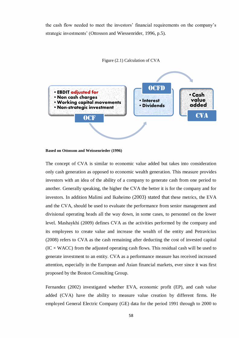
58

the cash flow needed to meet the investors’ financial requirements on the company’s

strategic investments’ (Ottosson and Wiessenrider, 1996, p.5).

Figure (2.1) Calculation of CVA

Based on Ottosson and Weissenrieder (1996)

The concept of CVA is similar to economic value added but takes into consideration

only cash generation as opposed to economic wealth generation. This measure provides

investors with an idea of the ability of a company to generate cash from one period to

another. Generally speaking, the higher the CVA the better it is for the company and for

investors. In addition Malimi and Ikaheimo (2003) stated that these metrics, the EVA

and the CVA, should be used to evaluate the performance from senior management and

divisional operating heads all the way down, in some cases, to personnel on the lower

level. Mashaykhi (2009) defines CVA as the activities performed by the company and

its employees to create value and increase the wealth of the entity and Petravicius

(2008) refers to CVA as the cash remaining after deducting the cost of invested capital

(IC × WACC) from the adjusted operating cash flows. This residual cash will be used to

generate investment to an entity. CVA as a performance measure has received increased

attention, especially in the European and Asian financial markets, ever since it was first

proposed by the Boston Consulting Group.

Fernandez (2002) investigated whether EVA, economic profit (EP), and cash value

added (CVA) have the ability to measure value creation by different firms. He

employed General Electric Company (GE) data for the period 1991 through to 2000 to

•EBDIT adjusted for •Non cash charges •Working capital movements •Non-strategic investment

OCF

•Interest •Dividends

OCFD

•Cash value added

CVA

59

run his regression model while Petravicius (2008) investigated how new performance

measures such as Market Value Added (MVA), Economic Value Added (EVA), Cash

Value Added (CVA), and Cash Flow Return on Investment (CFROI) will support the

effectiveness of traditional accounting numbers. Collectively, their results indicate that

new performance measures, the value added measure, are superior to the traditional

measures in evaluating the performance of executive managers and the company as

whole. This is attributed to the inclusion of the cost of invested capital when calculating

the value added measures.

Furthermore, Fernandez (2002) claims that cash value added (CVA) has an advantage

over EVA because the results of his research indicate that CVA, over the period of

study, makes more sense than EVA especially in those periods when the General

Electric Company (GE) appears to destroy value rather than create it. This claim arose

because the GE company began generating negative cash value added (CVA) in time of

destroying value while the economic value (EVA) generated remained positive all time.

He also claimed that CVA is more appropriate than book earnings for evaluating

executive performance.

Along the same lines, Mashaykhi (2009) used Iranian data from 408 companies listed

on the Tehran stock exchange for the period 1998 to 2003 to investigate the relevance

and the incremental information content of cash value added (CVA) and value added

(VA) beyond that which already exists in earnings (E) and cash flow from operating

(CFO). The OLS technique is used to test the relationship between the variables of this

study and the annual stock price.

Mashaykhi’s regression results indicate a significant relationship between value added

and a stock return. However, the cross-sectional regression shows an unstable

coefficient over time. For the purposes of the cash value added measure the results show

an insignificant relationship between cash value added (CVA) and annual stock return

on both pooled and cross-sectional data and the explanatory power is quite low. The

findings also show that earnings have the highest explanatory power among these

variables.

The results reveal that accrual measures have more information content beyond that

already contained in operating cash flow followed by value added and cash value added

respectively. The adjusted for the value added is greater than when cash value

60

added combines value added as an explanatory variable. Contrary to the above findings

the results indicate that the cash value added has incremental information content over

value added in 1998 and 1999. In addition, the results indicate that earnings have

incremental content beyond operating cash flow, but not vice versa.

Moreover, when all the variables are combined into one multi-regression model, the

result shows that for different periods through the cross-sectional level both value added

data and traditional data have incremental information content beyond each other,

whereas for the pooled data, value added data and traditional data have incremental

information content beyond each other (Mashaykhi, 2009).

Urbanczyk et al. (2005) used data from five large Polish companies for the period 1997

through to 2002 to investigate whether value added performance measures (EVA, CVA)

have the ability to outperform traditional accounting measures. They defined CVA as

the value a company creates over its cost of capital. They also considered CVA as a

developed version of Cash Flow Return on Investment (CFROI)12

which represents the

real cost of equity and gross investment that is defined as a gross cash flow a firm

creates over the invested capital. Urbanczyk et al. state that CVA is considered an

improved alternative to EVA because the latter ignores the impact of depreciation on

cash availability, while CVA includes the effects of depreciation on NOPAT and

invested capital, thus CVA is:

(10)

Where ROGA is the return on gross asset which is equal to gross operating profit after

tax divided by gross asset, WACC is the weighted average cost of capital, and Gross

Asset, asset plus depreciation, is the value of an asset before depreciation.

The results of Urbanczyk et al., show that all the selected Polish companies generate a

negative EVA and CVA which implies that they all generated net losses and destroyed

their shareholder wealth, whereas when applying the book value and traditional

performance measures these companies appear more profitable. Urbanczyk et al.

attributed the negative value of CVA and EVA to the privatisation process that was

taking place among Polish companies. Furthermore, they state that these companies

needed a long time to generate value after privatisation and the difficulty of calculating

12 CFROI was developed by the Swedish Company Boston Consulting Group as a performance measure

which is equivalent to NOPAT after adjusting for depreciation.

61

the cost of capital, and depending mainly on book value to estimate the weighted

average cost of capital, undermines their findings.

2.3.3.6.1 CVA versus EVA

Regardless of its matching and timing problems, CVA is considered the best alternative

to EVA for evaluating management performance and as a step in the process to evaluate

the whole firm and it seems to get its strength from the weakness of EVA (Escalona,

2003).

Fama and French (1996) argue that the cost of capital, one of the main figures in

calculating the EVA, is computed by using the capital asset pricing model (CAPM).

However, methodologically, EVA has structural difficulties in both the efficient and the

non–efficient capital markets, and its method has been criticised by both behavioural

and traditional approaches. The main criticism is that the CAPM is valid under the

assumption of strong and semi–strong efficient markets; but these two forms of

efficiency have not been evidenced by empirical research. Therefore, the EVA method

is considered to be an inefficient approach for evaluating and computing the cost of

capital.

If markets were efficient in the real world, all asset returns would be located on the

capital market line (CML). Among the main assumptions of CML is that the prices of

assets would be calculated in accordance with their intrinsic values. Another important

assumption is that the net present value will equal zero as the required rate of return is

equal to the internal rate of return (IRR). In this case EVA should be equal to zero

because in its simpler case it measures the differences between required rate of return

and internal rate of return. Therefore, EVA attempts numerical measurement in efficient

markets which do not exist in accordance with the definition, and consequently the

EVA is a financial fiction in the logic of efficient markets, and does not satisfy the

criteria as being a preferable evaluation model under these assumptions.

EVA, developed by Stern Stewart, is the difference between the firm’s after-tax return

on capital and its cost of capital. Stewart13

(1991) defined EVA as residual return that

subtracts the cost of invested capital from net operating profit after tax. EVA is equal to

13

Stewart III, G. B., 1991. The Quest for Value. Harper Business, New York.

62

the economic book value of the capital at the beginning of the year and the difference

between its return on capital and cost of capital.

EVA (Economic Value Added) is a model based on a company's accounting. Its

mechanism is therefore similar to accounting (Weissenrieder, 1997):

Sales

- Operating Expenses

- Tax

= Operating Profit

-Financial requirements

= EVA

The conclusion here is that the estimation of cost of capital is a great challenge as far as

EVA calculation for a company is concerned. Thus EVA is an undesirable method for

computing the cost of capital and we should not use it as a method of valuation.

Therefore the basic cost of capital computation, i.e. CAPM, has been rejected due to the

existence of a weak relationship between return and the systematic risk coefficient (β)

(Fama and French, 1996). But at the same time it does not mean that CVA is the perfect

method for evaluating the firm. Again EVA has a weak theoretical grounding and, just

like other accounting numbers, it is all too easy to manipulate.

Companies adopt EVA because it is easily understood by different levels of employees.

It can be implemented in the way most accounting systems can, the accounting reality,

whereas the implementation of CVA is an interactive process between the employee

active in the financial realities (top management, shareholder’s representatives) and the

ones active in the business reality (technicians, controllers). Thus, “the implementation

of CVA might therefore be perceived as being more difficult than implementing EVA

because it requires more attention from the organization. This attention is however the

attention necessary (and wanted) in order to reach the level of change in the

organization towards Shareholder Value” (Weissenrieder, 1997, p. 10).

63

2.4 Summary

The literature review discussed in this chapter shows that a large number of empirical

studies have investigated the association that exists between accounting performance

measures and stock return (Ball and Brown, 1968; Patell and Kaplan, 1977; Dechow

1994). Such work, from the viewpoint of market efficiency, ‘is useful since if a high

correlation exists between accounting-based information and market returns, then the

variable under consideration would provide an accurate indication of the firm’s value,

and therefore increasing firm value or identifying market under-pricings could be made

solely on that basis’ (West and Worthington, 2001, p.12).

Previously, the focus of empirical study has been on traditional accounting measures,

earnings and accruals, but in subsequent research value added measures have received

much attention (Beaver and Duck, 1972; Bowen et al., 1986). Furthermore, extra effort

has been directed toward examining the significance of the components of prime

performance measures, such as capital charges, accruals adjustment, and accounting

adjustments (Biddle et al., 1997).

It is worth noting here that the UK and US studies discussed in this chapter reported

different results regarding the information and incremental information content of the

different main performance measures (and their components). These mixed results may

have several explanations. Garrod et al. (2000) suggested a number of factors: (i)

differences in the definition of cash flow used in different studies, with different figures

being used as proxies for cash flows on some occasions; (ii) differences in the

econometric models used; and (iii) differences in the time periods examined in the

studies and the effect of contextual factors (e.g. national economic conditions). In other

words, we may get different results from the same model if we change the target market

of the study. For instance, Board et al. (1989) used the same model for both UK and US

data and found conflicting results regarding the value relevance of long-term accruals.

Responding to the controversies that exist in the field of performance literature and to

the criticism that Biddle et al. (1997) raised against EVA as the best alternative to the

traditional and other value added measures this research will uses UK data to introduce

evidence on the role of traditional accounting, cash flows, and value added measures in

explaining variations in stock prices. The methodology of this research is stimulated by

64

prior US and UK studies14

that provide a theoretical framework and empirical analysis

of the role of different performance measures, earnings and EVA components in

explaining annual price changes.

14

This study mainly benefits from the studies of Barth et al., and Biddle et al., who provide evidence of

the incremental information content for the main accruals and EVA components.

65

Chapter 3

Research Design and Methodology

3.1 Introduction

This chapter describes the main features of the research design approach adopted in this

study. It also provides a summary of the main methodological steps the researcher

intends to adopt. It presents and discusses the major methodological tools and concepts

employed as a means to achieve the objectives of the present research. In particular, two

major aims are worth noting. The first aim is to review the various performance

measures adopted in the literature. The second aim is to develop and present the main

hypotheses of this study.

This research will be based on a cross- sectional design to assess the association

between a set of performance measures and the annual stock price performance.

Performance measures will be classified into three categories: traditional accounting

measures, cash flow measures, and value added measures. These categories include: net

income (NI); earnings before interest, tax, depreciation and amortization (EBITDA);

earnings before extraordinary items (EBEI); cash flows from operations (CFO);

economic value added (EVA); and cash value added (CVA).

The plan of this chapter is as follows. Section 3.2 will discuss the main research

questions. The development of the main hypotheses of this study and the building of the

study’s models are discussed in sections 3.2.1, 3.2.2 and 3.2.3. Sections 3.3 and 3.3.1

provide a definition of the variables of the study and the deflator factors. Section 3.4

sheds light on the characteristics used to select the sample, and finally section 3.5

summarizes this chapter.

3.2 Development of Hypotheses

As far as our objectives are concerned, there are two main approaches to research

depending upon the objectives that the researcher is seeking to achieve. The following

are the two approaches used: positivism (quantitative or deductive approach) and the

phenomenological (qualitative or inductive approach) (Hussey, 1997).

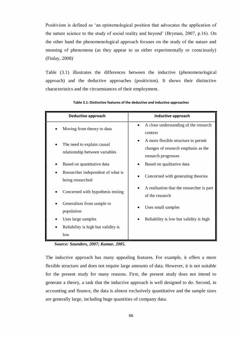
66

Positivism is defined as ‘an epistemological position that advocates the application of

the nature science to the study of social reality and beyond’ (Bryman, 2007, p.16). On

the other hand the phenomenological approach focuses on the study of the nature and

meaning of phenomena (as they appear to us either experimentally or consciously)

(Finlay, 2008).

Table (3.1) illustrates the differences between the inductive (phenomenological

approach) and the deductive approaches (positivism). It shows their distinctive

characteristics and the circumstances of their employment.

Table 3.1: Distinctive features of the deductive and inductive approaches

Deductive approach Inductive approach

Moving from theory to data A close understanding of the research

context

The need to explain causal

relationship between variables

A more flexible structure to permit

changes of research emphasis as the

research progresses

Based on quantitative data Based on qualitative data

Researcher independent of what is

being researched Concerned with generating theories

Concerned with hypothesis testing A realisation that the researcher is part

of the research

Generalises from sample to

population Uses small samples

Uses large samples Reliability is low but validity is high

Reliability is high but validity is

low

Source: Saunders, 2007; Kumar, 2005.

The inductive approach has many appealing features. For example, it offers a more

flexible structure and does not require large amounts of data. However, it is not suitable

for the present study for many reasons. First, the present study does not intend to

generate a theory, a task that the inductive approach is well designed to do. Second, in

accounting and finance, the data is almost exclusively quantitative and the sample sizes

are generally large, including huge quantities of company data.

67

Thus, given that this study is based on accounting data, and given that we are primarily

concerned with testing specific hypotheses and answering specific research questions,

the deductive approach seems more appropriate.

Therefore, to ensure conformity with the objectives of the present research the

quantitative approach will be employed. According to Kumar (2005) each method, tool

and technique has its unique strengths and weaknesses. In other words, there is an

expected trade-off between the various methodological choices regarding research

question setting, hypotheses development, data collection, and data analysis.

By using the deductive approach, which is based on addressing the research question

followed by the research hypotheses, Hussey (1997) and Kumar (2005) emphasised the

important role of hypotheses for ensuring clarity. Hence, I begin by addressing the

research questions that are consistent with the objectives of the research and stating the

questions as hypotheses. According to the deductive approach the hypotheses will

identify the independent variable(s) and the dependent variable (Hussey).

As will be shown, the dependent variable is the three month closing share price

following the reporting date; we allow three months for the accounting information to

be reflected in the stock’s price15

, while the independent variables are identified as

follows: net income (NI), earnings before interest, tax, depreciation and amortization

(EBITDA), earnings before non- recurring items (EBEI), cash flows from operations

activities (CFO), economic value added (EVA), and cash value added (CVA).

As was noted in Chapter 2 estimating the appropriate performance measure is the

concern of the market-based accounting researchers. Some researchers (Moehrle et al.,

2001; Charitou et al., 2001) claim that traditional accounting measures have the ability

to outperform any other performance measures in explaining variation in stock prices.

On the other hand, opponents of value based measures (VBM) (Stern and Stewart,

1991; Dechow et al., 1999; Francis et al., 2003) claim that measures that take into

account the cost of capital when evaluating the performance of companies/managers,

such as residual income method (RI), economic value added (EVA), and cash value

added (CVA) are better to explain stock return variances and outperform traditional

accounting (e.g. earnings, EBITDA, NOPAT) in explaining variation in the stock price.

15 This approach was used by Fama and French (1992). The purpose of this strategy is to avoid look-

ahead bias.

68

Moreover, other empirical studies claim that value added measures, that take into

account the cost of capital invested, are better than other performance measures and

have incremental information content beyond that which exists within traditional

performance measure cash flows in predicting future cash flows (West and Worth,

2000; Anastassis and Kyriazis, 2007).

Consistent with the objectives of the research and referring to the literature review on

performance measures as explanatory variables of the variation in annual stock prices,

and after selecting six performance measures, this research will attempt to address the

following questions:

1. Among the three performance measures (traditional measure;

cash flow measure; and value added measure), which one

provides the best explanation of variation in stock price

performance?

2. Does the decomposition of earnings into cash flows and accruals

components have incremental information content beyond

aggregate earnings?

3. Does the decomposition of EVA into its main components have

incremental information content beyond aggregate EVA?

4. Does a given performance measure provide more information

content beyond that provided by other performance measures?

5. Does the adoption of EVA as a compensation and management

tool enhance the overall performance of firms and encourage

manager to adopt decisions that are supposed to lead to

shareholders’ wealth maximization.

To provide answers to these questions, four hypotheses are developed in this section.

These hypotheses will be organized under the following headings: traditional measures

versus cash flows and value added measures, earnings versus earnings’ components

(cash flows and disaggregate accruals) and EVA versus EVA’s components. Chapters 5

and 6 will provide a detailed answer to question 5.

Before beginning the models’ construction processes, we will start by demonstrating

how both the price and return models are arrived at. The linear information model

(LIM) introduced by Ohlson (1995) is the model used to derive the popular type of the

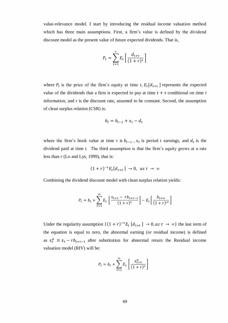
69

value-relevance model. I start by introducing the residual income valuation method

which has three main assumptions. First, a firm’s value is defined by the dividend

discount model as the present value of future expected dividends. That is,

where is the price of the firm’s equity at time t, represents the expected

value of the dividends that a firm is expected to pay at time conditional on time t

information, and r is the discount rate, assumed to be constant. Second, the assumption

of clean surplus relation (CSR) is:

where the firm’s book value at time t is , is period t earnings, and is the

dividend paid at time t. The third assumption is that the firm’s equity grows at a rate

less than r (Lo and Lys, 1999), that is:

Combining the dividend discount model with clean surplus relation yields:

Under the regularity assumption { } the last term of

the equation is equal to zero, the abnormal earning (or residual income) is defined

as after substitution for abnormal return the Residual income

valuation model (RIV) will be:

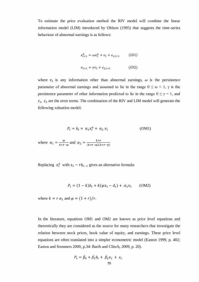
70

To estimate the price evaluation method the RIV model will combine the linear

information model (LIM) introduced by Ohlson (1995) that suggests the time-series

behaviour of abnormal earnings is as follows:

where is any information other than abnormal earnings, is the persistence

parameter of abnormal earnings and assumed to lie in the range 0 ≤ ω < 1, γ is the

persistence parameter of other information predicted to lie in the range 0 ≤ γ < 1, and

are the error terms. The combination of the RIV and LIM model will generate the

following valuation model:

(OM1)

where

and

Replacing with gives an alternative formula:

(OM2)

where and .

In the literature, equations OM1 and OM2 are known as price level equations and

theoretically they are considered as the source for many researchers that investigate the

relation between stock prices, book value of equity, and earnings. These price level

equations are often translated into a simpler econometric model (Easton 1999, p. 402;

Easton and Sommers 2000, p.34: Barth and Clinch, 2009, p. 20).

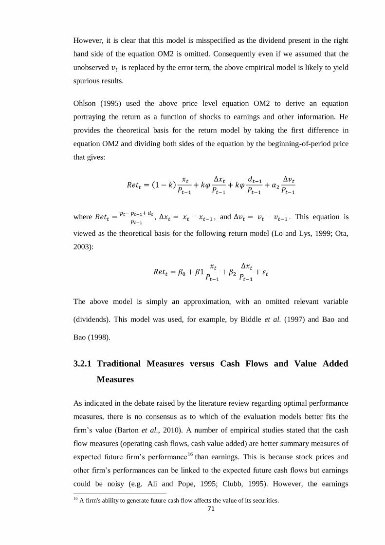
71

However, it is clear that this model is misspecified as the dividend present in the right

hand side of the equation OM2 is omitted. Consequently even if we assumed that the

unobserved is replaced by the error term, the above empirical model is likely to yield

spurious results.

Ohlson (1995) used the above price level equation OM2 to derive an equation

portraying the return as a function of shocks to earnings and other information. He

provides the theoretical basis for the return model by taking the first difference in

equation OM2 and dividing both sides of the equation by the beginning-of-period price

that gives:

where

, , and . This equation is

viewed as the theoretical basis for the following return model (Lo and Lys, 1999; Ota,

2003):

The above model is simply an approximation, with an omitted relevant variable

(dividends). This model was used, for example, by Biddle et al. (1997) and Bao and

Bao (1998).

3.2.1 Traditional Measures versus Cash Flows and Value Added

Measures

As indicated in the debate raised by the literature review regarding optimal performance

measures, there is no consensus as to which of the evaluation models better fits the

firm’s value (Barton et al., 2010). A number of empirical studies stated that the cash

flow measures (operating cash flows, cash value added) are better summary measures of

expected future firm’s performance16

than earnings. This is because stock prices and

other firm’s performances can be linked to the expected future cash flows but earnings

could be noisy (e.g. Ali and Pope, 1995; Clubb, 1995). However, the earnings 16 A firm's ability to generate future cash flow affects the value of its securities.

72

proponents suggest that stock prices and other firm’s performance measures are better

explained by current earnings than current operating cash flows (e.g. Moehrle et al.,

2001; Charitou et al., 2001). Other studies conclude that a combination of current cash

flow data and accruals data outperform earnings alone and cash flows alone in

predicting future cash flows (e.g. Barth et al., 2001). In contrast, Ottosson and

Wiessenrider (1996) introduce CVA as a new performance measure to replace accruals

and other cash flow measures.

The accounting earnings approach has faced severe criticism from many scholars

because it could easily be manipulated by both accountants and managers (Stern and

Stewart, 1991). Moreover, earnings reflect events that happened in the past and it is

difficult to judge whether its components will be permanent or recur in the future. This

shortcoming appears to cry out for proposals for new performance measures. Hence,

researchers and practitioners have proposed new methods to evaluate the management

performance such as residual income method (RIM)17

, economic value added (EVA)18

and operating income (OP) to interpret the stock price. Similarly, the residual and value

added methods have met with much debate from traditional method supporters. The

traditionalists claim that the cash flows and value added methods suffer from matching

and timing problems. One of the main aims of this thesis is to investigate the association

between the most important performance measures (discussed in chapter two) and the

annual stock price performance.

We will also discuss cash value added (CVA) as a value added performance measure

and will carry out a test to assess whether CVA has any association with annual stock

prices and whether it has any incremental information content beyond the other criteria

used to measure firms’ and managers’ performance.

As is well known, performance measurement is not always an easy task. The efficient

market hypothesis states that markets are unpredictable and that current prices fully

reflect all available information. A straightforward consequence of this is that

(historical) accounting measures have no added informational value. Another argument

is that prices are forward looking, in the sense that prices reflect what investors expect

to earn from their investments in the future. Thus, insofar as accounting information

cannot predict the future accounting or economic performance of a firm, all accounting

17 RIM involves discounting estimated future residual income over the entire life of the firm.

18 EVA is the difference between the firm’s after-tax return on capital and its cost of capital.

73

measures are likely to miss unobservable factors that are essential for predicting future

firm performance. Finally, as we have seen earlier, scholars are divided as to whether a

single accounting measure beats other measures in explaining stock prices. In summary,

the current wisdom is that it is unlikely to find a single accounting measure that

outperforms all alternative measures.

Based on the above, the following null hypotheses are proposed:

H01

: There is no significant statistical relationship between each of the

following three classes of accounting measures (traditional

accounting performance measures, cash flow measures and value

added measures) and annual stock prices.

H02

: Value added measures and cash flow measures provide no

incremental information content other than that already contained in

traditional accounting measures.

In order to test for the information content hypothesis, a simple OLS regression model

is used to examine the validity and the relevance of different performance measures.

These measures are divided into three groups, namely traditional accounting measures,

cash flow measures, measures and value added measures.

The price model and the return model are considered the most pervasive valuation

models (Barth et al., 2001). Theoretically, both price and return models are

economically equivalent since they are derived from the same source, which is the

Ohlson linear information model (Ota, 2001).

Researchers in accounting must often choose between return models in which returns

are regressed on a scaled earnings variable, namely earnings and earnings changes, and

price models, in which stock prices are regressed on earnings per share and book value.

The inherent problem in the price models is often referred to as ‘scale effects,19

and

those in the return models are termed ‘accounting recognition lag,20

and ‘transitory

19 A scale effect is a spurious relation in the price model regression that can be used by failing to control

scale that presumably exists among firms. 20 Value- relevant events observed by the market in the current period and reflected in the current returns

may not be recorded in the current earnings because of the accounting principles such as conservatism,

objectivity, and reliability.

74

earnings21

(Ota, 2003). However, we recognize that there is a trade-off. Returns are

stationary and are more likely to give less problematic estimations. The problem with

returns, however, is that they may not be economically meaningful. Returns are payoffs

to one unit of wealth and we therefore cannot differentiate between highly priced stock

and low priced stock.

Following on from this last point, Kothari and Zimmerman (1995) claim that ‘while

return and price models are economically equivalent (…) return models are

econometrically less problematic. Estimates of earnings response coefficients are more

biased when the return model is used as against the price and differenced–price models’

(p.2). Moreover, Kothari and Zimmerman (1995) claim that even though a return model

is preferred in general, the price models are ‘better specified in that the estimated slope

coefficients from price models, but not return models, are unbiased’ (p.1). Furthermore,

their results state that even the price model suffers more from econometric problems

than return models; the price models' earnings’ response coefficients are less biased. Ota

(2001) stated that although returns studies and levels studies are not econometrically

equivalent they are economically equivalent since they are derived from the same

source, which is the Ohlson (1995) linear information model. Furthermore, Rees (1999)

explains in his paper that there are some difficulties that can be expected in the return

model and these problems can be avoided by using the price models.

Previous studies have used mainly annual returns as a dependent variable (e.g. Biddle et

al., 1997: Barth et al., 2001; West and Worthington, 2000; Ismail, 2006). This research

will fill this gap and contribute to the debate by adopting both price and return models

in which price and return will be used as a dependent variable in the multivariate

regression model to examine the relevancy of investigated performance measures.

3.2.1.1 The Information Content Model

Following the descriptive analysis of previous literature this research progresses to the

next step which is the building of econometric models that will be used to test the

hypothesis of the current study. This is based on Biddle’s et al. (1997) model that

examines the association between selected performance measures and annual stock

returns.

21 Earnings contain transitory components such as special and extraordinary items.

75

Using a sample of 219 firms over the period 1984-1993, Biddle et al. (1997) test

whether EVA and residual income (RI) outperform earnings and operating cash flows in

explaining annual stock returns. They also try to test whether the components unique to

EVA and/or RI help explain contemporaneous stock returns beyond that explained by

operating cash flow (CFO) and earnings.

In order to test for the information content of the suggested performance measures,

Biddle et al. (1997) use the slope coefficient approach to examine the statistical

significance of their study variables in the following OLS regression:

(3.1)

where is the abnormal or unexpected returns for the time period t, and are the

intercept and the slope coefficient of the regression model respectively,

is the independent variable which represents the unexpected realization for a given

performance metric x (e.g., CFO, EBEI, RI or EVA), all the independent variables are

scaled by the market value of the firms’ equity at the beginning of the period; and is

the error term.

Biddle et al. extended their original model 1 by introducing the one-lag version (lagged

measure of accounting performance) for explanatory variables, which is considered ‘a

more convenient form that allows the slope coefficient to be observed directly rather

than being derived from separate coefficients on levels and change models’ (Biddle et

al., 1997, p.9).

(3.2)

Biddle et al. use to assess the relative information content. They build six pairwise

comparisons among the accounting performance measure and the test is constructed as a

comparison of of these pairwised sets.

The findings of Biddle et al. (1997) reveal that all the variables (EVA, RI, CFO, and

EBIT) are significant (in explaining returns) at conventional levels and both EBIT and

RI have the higher adjusted among other explanatory independent variables and

outperformed EVA in explaining variation in stock return. Thus, this study does not

76

support the Stern and Stewart (1991) claim that EVA has greater information content

than earnings.

Along the same lines, in a study based on a sample of 110 Australian companies over

the period 1992 to 1998, West and Worthington (2000) examined the association of

EVA, earnings, net cash flows, and residual income with annual stock return and

extended their research to test whether EVA has incremental information content and

outperformed conventional accounting-based measures. They adopt the same

methodology as Biddle et al. (1997) and examine the linkage between the competing

different measures of firm performance. However, unlike previous empirical research

they use the pooled time series and cross-sectional least squares regression to conduct

their research. They introduce the following model to test for the relative and

incremental information content of the competing measures:

(3.3)

where the dependent variable, is the three months compound annual stock

returns following the fiscal year end. The three months following the firm’s fiscal year

end is chosen to allow time for information contained in the annual report to be

impounded in market prices, is the intercept, is the economic value added,

is earning before non-recurring items, is operating cash flows, is

residual income, and is the error term. All the variables included in this model are

expressed per share.

The findings of West and Worthington (2000) indicate that, as with Biddle’s et al study,

all the performance measures have a significant association with the adjusted annual

stock return variation. It also indicates that EVA has the lowest association with the

variation in the adjusted stock return whereas EBEI outperforms the rest of the

accounting measures in explaining the variation.

Mashaykhi (2009) in an analysis of 408 Iranian companies’ data for the period 1998 to

2003 investigated the relevance and the incremental information content of cash value

added (CVA) and value added (VA) beyond that already existing on earnings (E) and

cash flow from operating (OPC). She used the OLS regression to test her study’s

hypothesis.

77

In the literature, value added is defined as the activities that are performed by the

company and its employees to create value and increase the wealth of the entity

shareholders. Thus, the value added is equal to sales less the cost of bought goods and

services (Riahi-Belkaoui, 1993). Accordingly this definition leads to two methods to

calculate the value added (VA): the descriptive (subtractive) and additive method:

The Descriptive Method: VA = S – M

The Additive Method: VA = W +I+ DP+ DD+ T+ RE

where S represents sales revenue; M, materials and services purchased from outside the

firm; W, wages; I, interest; DP, depreciation; DD, dividends; T is tax expense and RE,

retained earnings.

The above two methods illustrate that accrual items are included in the calculation of

value added. Hence, the new accounting concept introduced is called cash value added

(CVA) which represents the value added that was received or paid in cash.

CVA is computed by the same method used for the computation of value added:

The Subtractive Method: CVA = CS – CM

The Additive Method: CVA = WP +IP+ DDP+ TP+ OCF

where CS represents cash sales; CM, cash payment against material and service; WP,

wages paid; IP, interest paid; DDP, dividends paid; TP, tax payments; and OCF,

operating cash flow.

Biddle et al. (1995) state that there are two types of information contained in accounting

numbers: the incremental information content and the relative information content. The

relative information content describes the degree to which a specific measure has

greater information content than other measures and applies when intending to choose

among alternatives or when ranking by information content is required. Whereas the

incremental criterion asks whether a specific measure has more information content

than that already existing in other measures and applies when intending to assess

measures with regard to other measure incremental information content. This research

will apply the same methodology to test whether any of the investigated performance

measures has more information content than already exists in other performance

78

measures. In other words the incremental and relative information content of X, Y (any

two performance measures) can be depicted by:

Relative information content:

Information content of X Information content of Y

Incremental information content:

Information content of X, Y ≥ Information content of X

Information content of , ≥ Information content of Y

where X and Y refer to any paired performance measures of the set introduced by me,

that is: net income (NI), earnings before interest, tax, depreciation and amortization

(EBITDA), earnings before non-recurring items (EBEI), cash flows from operations

activities (CFO), economic value added (EVA), and cash value added (CVA).

Hejazi and Maleki (2007) used the cash value added (CVA) concept as it was defined

by the Boston Consulting Group where they considered CVA as an adjustment of cash

flow return on investment (CFROI), and in order to generate value, companies should

increase Cash Flow Return on Investment and grow the Gross Investment base. Hence,

the following method will be used to calculate CVA:

where CVA is cash value added. CFROI = (Gross Cash Flow- Economic Depreciation)/

Gross Investment. WACC is the weighted cost of capital. Gross Investment = Net

Current Assets + Historical initial cost.

Finally, owing to the scarcity of information available regarding CVA in Tehran’s stock

market (TSM), CVA added will be calculated according to:

After running the above regression (Hejazi and Maleki, 2007) concluded that both CVA

and P/E have a positive and significant relation to annual stock return at the 0.05 level

of significance. The significance relation also holds when the two variables are paired

together within one regression model. The findings of this research reveal that CVA is

79

better at explaining changes in stock returns than P/E, and it indicates that CVA has the

higher incremental information content. For the purposes of the current research CVA is

defined as:

where CVA is cash value added, OCF is the cash flows from operations, and OCFD is

operating cash flow demand equal to dividends and interest.

Similarly, Mashaykhi (2009) adopts the aforementioned distinction between relative

and incremental information content and used a linear valuation model in expressing the

relationship between change in price and earnings (E), operating cash flow (OCF), cash

value added (CVA) and value added (VA) where she introduced the following models:

(3.4)

where is the return adjusted for cash dividends, stock dividends, and new stock

offerings (the adjusted market return), the coefficient of determination, is the

change in independent variables (e.g., E, OCF, CVA , and VA), ( VA, CVA,

E, and OCF) is the technique used by Mashaykhi to test for the relative and

incremental information content of her study variables. The tool she used to rank the

investigated performance measures in regard to their relative information content is the

adjusted- . Thus, the higher the adjusted- is the higher the information content.

For the incremental information content purpose, the rule is that if the inclusion of a

new performance measure increases the old then the performance measure is said to

have more (incremental) information content beyond that already existing in the old

one. However, it should be pointed out here that it is well known that adding more

explanatory variables always results in an increase in . Therefore, a more appropriate

measure would be the adjusted which takes into account the number of additional

regressors.

Finally, Mashaykhi (2009) concludes that there is a significant relationship between

value added and annual stock returns where the cross–sectional regression shows

unstable coefficient overtime. For the cash value added the result shows an insignificant

relationship between cash value added (CVA) and annual stock returns on both pooled

and cross–sectional data. Moreover, the explanatory power is quite low.

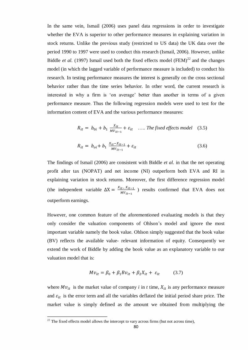
80

In the same vein, Ismail (2006) uses panel data regressions in order to investigate

whether the EVA is superior to other performance measures in explaining variation in

stock returns. Unlike the previous study (restricted to US data) the UK data over the

period 1990 to 1997 were used to conduct this research (Ismail, 2006). However, unlike

Biddle et al. (1997) Ismail used both the fixed effects model (FEM)22

and the changes

model (in which the lagged variable of performance measure is included) to conduct his

research. In testing performance measures the interest is generally on the cross sectional

behavior rather than the time series behavior. In other word, the current research is

interested in why a firm is ‘on average’ better than another in terms of a given

performance measure. Thus the following regression models were used to test for the

information content of EVA and the various performance measures:

….. The fixed effects model (3.5)

(3.6)

The findings of Ismail (2006) are consistent with Biddle et al. in that the net operating

profit after tax (NOPAT) and net income (NI) outperform both EVA and RI in

explaining variation in stock returns. Moreover, the first difference regression model

(the independent variable

) results confirmed that EVA does not

outperform earnings.

However, one common feature of the aforementioned evaluating models is that they

only consider the valuation components of Ohlson’s model and ignore the most

important variable namely the book value. Ohlson simply suggested that the book value

(BV) reflects the available value- relevant information of equity. Consequently we

extend the work of Biddle by adding the book value as an explanatory variable to our

valuation model that is:

(3.7)

where is the market value of company i in t time, is any performance measure

and is the error term and all the variables deflated the initial period share price. The

market value is simply defined as the amount we obtained from multiplying the

22 The fixed effects model allows the intercept to vary across firms (but not across time),

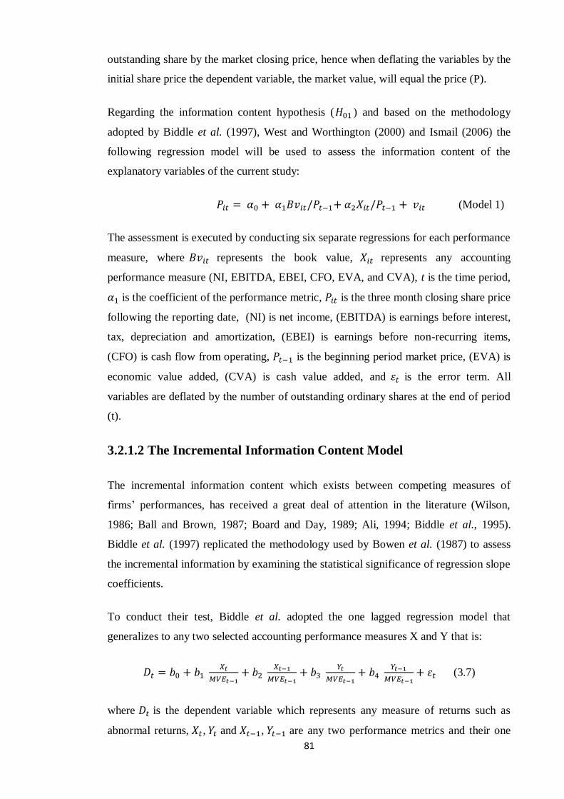
81

outstanding share by the market closing price, hence when deflating the variables by the

initial share price the dependent variable, the market value, will equal the price (P).

Regarding the information content hypothesis ( ) and based on the methodology

adopted by Biddle et al. (1997), West and Worthington (2000) and Ismail (2006) the

following regression model will be used to assess the information content of the

explanatory variables of the current study:

(Model 1)

The assessment is executed by conducting six separate regressions for each performance

measure, where represents the book value, represents any accounting

performance measure (NI, EBITDA, EBEI, CFO, EVA, and CVA), t is the time period,

is the coefficient of the performance metric, is the three month closing share price

following the reporting date, (NI) is net income, (EBITDA) is earnings before interest,

tax, depreciation and amortization, (EBEI) is earnings before non-recurring items,

(CFO) is cash flow from operating, is the beginning period market price, (EVA) is

economic value added, (CVA) is cash value added, and is the error term. All

variables are deflated by the number of outstanding ordinary shares at the end of period

(t).

3.2.1.2 The Incremental Information Content Model

The incremental information content which exists between competing measures of

firms’ performances, has received a great deal of attention in the literature (Wilson,

1986; Ball and Brown, 1987; Board and Day, 1989; Ali, 1994; Biddle et al., 1995).

Biddle et al. (1997) replicated the methodology used by Bowen et al. (1987) to assess

the incremental information by examining the statistical significance of regression slope

coefficients.

To conduct their test, Biddle et al. adopted the one lagged regression model that

generalizes to any two selected accounting performance measures X and Y that is:

(3.7)

where is the dependent variable which represents any measure of returns such as

abnormal returns, , and , are any two performance metrics and their one

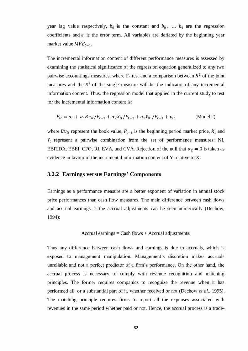
82

year lag value respectively, is the constant and , … are the regression

coefficients and is the error term. All variables are deflated by the beginning year

market value .

The incremental information content of different performance measures is assessed by

examining the statistical significance of the regression equation generalized to any two

pairwise accountings measures, where F- test and a comparison between of the joint

measures and the of the single measure will be the indicator of any incremental

information content. Thus, the regression model that applied in the current study to test

for the incremental information content is:

(Model 2)

where represent the book value, is the beginning period market price, and

represent a pairwise combination from the set of performance measures: NI,

EBITDA, EBEI, CFO, RI, EVA, and CVA. Rejection of the null that is taken as

evidence in favour of the incremental information content of Y relative to X.

3.2.2 Earnings versus Earnings’ Components

Earnings as a performance measure are a better exponent of variation in annual stock

price performances than cash flow measures. The main difference between cash flows

and accrual earnings is the accrual adjustments can be seen numerically (Dechow,

1994):

Accrual earnings = Cash flows + Accrual adjustments.

Thus any difference between cash flows and earnings is due to accruals, which is

exposed to management manipulation. Management’s discretion makes accruals

unreliable and not a perfect predictor of a firm’s performance. On the other hand, the

accrual process is necessary to comply with revenue recognition and matching

principles. The former requires companies to recognize the revenue when it has

performed all, or a substantial part of it, whether received or not (Dechow et al., 1995).

The matching principle requires firms to report all the expenses associated with

revenues in the same period whether paid or not. Hence, the accrual process is a trade-

83

off between reliability and relevance (Dechow, 1994, 1989; Watts and Zimmerman,

1986).

Cash flow measures avoid management manipulation but at the same time suffer from

matching and timing problems. However, other accounting conventions have restricted

management manipulation such as objectivity, verifiability and the use of historical cost

(Dechow, 1994; Watts and Zimmerman, 1986). Therefore, earnings suffer less from

management manipulation while cash flows still suffer from its inherent matching and

timing problems.

As shown in Chapter 2, there is no agreement on the performance of various accounting

measures. While some studies show that earnings are the best predictor for future cash

flows (Dechow, 1994; Dechow et al., 1998; Borad and Day, 1989; Ali and Pope, 1995;

Clubb, 1995), others provide evidence on the incremental information content for cash

flows (Bowen et al., 1986 and 1987; Barth et al., 2001).

Following Dechow (1994), Charitou and Clubb (1999) used UK data over the period

1985 to 1992 to examine the relationship between security returns, cash flows and

earnings. They assessed this relation using different intervals: one year, two years and

four years. They developed Dechow’s method by examining the incremental

information content of accounting earnings and cash flow measures. In addition, they

added new variables in their study. Using univariate models, they examined the

information content for earnings, operating cash flows, change in cash, and equity cash

earnings. Their results show that earnings had the highest propensity to explain the

variation in stock return. They also found that the operating cash flows and change in

cash had information content in explaining the variation in stock returns while the

equity cash earnings revealed a weak relation with stock returns. Moreover, their results

indicate that the adjusted increased as they extended the measurement interval which

is consistent with Dechow (1994).

Dechow et al. (1998) stated that ‘Since the difference between earnings and cash flows

is accruals, earnings’ forecasting power beyond cash flows is attributable to accruals’

(p. 152). Mcleay et al. (1997) analysed UK data and reported that the components of

accruals, namely the short and long term, have incremental information content beyond

that already existing in aggregate earnings. Therefore, the decomposition of earnings

84

into aggregate accruals and cash flows will unmask the information content in aggregate

accruals. This can be expressed in the following hypothesis:

: Earnings components have no statistically significant effect

on annual stock price performance.

This hypothesis is tested by looking at the restriction:

in model 3 below where earnings are equal to cash flows plus accruals (Barth et

al., 2001):

Earnings = CF+ Accrual

= CF + ∆AR + ∆INV- ∆AP- DEP-AMORT + OTHER

Biddle et al. (1997) in a study of the usefulness of EVA in the US context suggest that

“an avenue for future research suggested by the findings of this study is to examine

more closely which components of EVA and earnings contribute to, or subtract from,

information content” (p. 333). In addition Barth et al. (200l) state that earnings can be

disaggregated into the following major components: change in accounts receivable

(∆AR), change in accounts payable (∆AP), change in inventory (∆INV), depreciation

(DEP), amortization (AMORT) and other accruals (OTHER). This study will adopt the

following regression model that examines the information content of earnings

components:

where is the book value at the beginning of the operating year, CF is the cash flow

and other accruals = Earnings – (CF+ ∆AR + ∆INV- ∆AP- DEP-AMORT). This

decomposition is an attractive feature of earnings to reveal the source of changes in

stock return.

3.2.3 EVA versus EVA’s Components

As far as EVA versus EVA’s components are concerned, Biddle et al. (1997) extend

their research to investigate whether the economic value added (EVA) outperforms, and

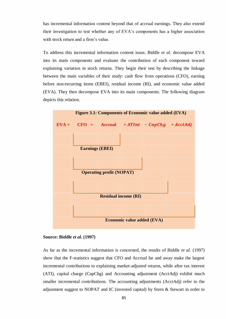
85

has incremental information content beyond that of accrual earnings. They also extend

their investigation to test whether any of EVA’s components has a higher association

with stock return and a firm’s value.

To address this incremental information content issue, Biddle et al. decompose EVA

into its main components and evaluate the contribution of each component toward

explaining variation in stock returns. They begin their test by describing the linkage

between the main variables of their study: cash flow from operations (CFO), earning

before non-recurring items (EBEI), residual income (RI), and economic value added

(EVA). They then decompose EVA into its main components. The following diagram

depicts this relation.

Figure 3.1: Components of Economic value added (EVA)

EVA = CFO + Accrual + +

Earnings (EBEI)

Operating profit (NOPAT)

Residual income (RI)

Economic value added (EVA)

Source: Biddle et al. (1997)

As far as the incremental information is concerned, the results of Biddle et al. (1997)

show that the F-statistics suggest that CFO and Accrual far and away make the largest

incremental contributions to explaining market-adjusted returns, while after tax interest

(ATI), capital charge (CapChg) and Accounting adjustment (AcctAdj) exhibit much

smaller incremental contributions. The accounting adjustments (AcctAdj) refer to the

adjustment suggest to NOPAT and IC (invested capital) by Stern & Stewart in order to

86

calculate the EVA. The main and common introduced adjustments are: the effects of

research and development expenses capitalisation, the effects of LIFO reserves, the

deferred taxes, the provision effects and the good will amortization (Young, 1999).

When combined with the relative information content findings, Biddle et al. suggest

that while EVA components offer some incremental information content beyond

earnings components, their contributions to the information content of EVA are not

sufficient for EVA to provide greater relative information content than earnings.

Building on the above, the following hypothesis is developed to test whether any of

EVA’s components contribute significantly to the association between EVA and stock

price performance.

: EVA components have no statistically significant effect on

stock price performance.

This hypothesis is tested by looking at the restriction:

in ‘model 4’ bellow where EVA is:

The incremental information content comparisons assess whether one measure provides

value-relevant data beyond that provided by another measure and whether they apply

when assessing the information content of a supplemental disclosure or the information

of a component measure (Bowen et al., 1987).

In their response to Stewart’s (1991) claim that EVA is the best performance measure

regarding its ability to capture the true economic profit of a firm and following the

recommendation of Biddle et al. (1997), West and Worthington examined which of the

components of EVA and earnings were more likely to contribute to, or subtract from,

the information content.

The second phase of West and Worthington’s study (the first phase was discussed in

Section 3.1.1.1) was to examine the components of EVA. Their results convey that all

the variables are significant where operating accruals (ACC) have greater explanatory

power among other variables. Further, the component in EVA that explains most

variation in stock returns is accrual. West and Worthington use the following model to

test for the incremental content between EVA’s components:

(3.8)

87

where is the compound annual return, CC is the cost of capital (Invested capital

at time t-1 (IC) × the firm’s weighted average cost of capital (WACC), ATI is the

interest after tax, ACC is the operating accruals (EBEI- NCF), ADJ is the accounting

adjustments and NCF is the net cash flows. For the incremental information content the

results show that the most logical pairing of information variables in explaining market

return is composed of EBEI and EVA.

To test for the incremental information content of EVA components and to evaluate

which components of EVA, if any, contribute to the association between EVA and stock

price performance, the Biddle et al. model is replicated. Biddle et al. (1997)

decomposed EVA into four major components: cash flows from operations (CFO), after

tax interest (ATI), operating accruals (ACC), capital charge (CC), and accounting

adjustments ( ). Hence, the regression model is:

(Model 4)

Unlike Biddle et al. (1997) the current study will use a panel data fixed effects model to

examine the association between EVA’s components and the stock price performance.

Various papers have analyzed the conceptual advantages and disadvantages of price and

return models. Gonedes and Dopuch (1974) claim that return models theoretically

outperform price models in the absence of well-developed theories of valuation. Lev

and Ohlson (1982) consider the two methods as complementary, whereas Landsman

and Magliolo (1988) argue that for specific applications price models are superior to

return models. Christie (1987) concludes that while return and price models are

economically the same, return models are econometrically less problematic.

Despite the criticism the price models have faced, they persist. The empirical result of

Kothari and Zimmerman (1995) confirm that the price models’ earnings’ response

coefficients are less biased. However, return models have less serious econometric

difficulties than price models. In some research contexts the combined use of both price

and return models may be useful and seem to be the best models to follow. In terms of

the results and methods used by Christie (1987), Kothari and Zimmerman, and Ota

(2003), the data from the UK stock market is used to compare the results obtained from

adopting price and return models as a tool to examine the information and incremental

information content of a set of different performance measures. The return models are:

88

(Model 5)

(Model 6)

where is the stock return, , are any two performance measures, and all the

independent variables are deflated by the market value of equity at the beginning of the

fiscal year

3.3 Hypothesis testing

The comparison between the ability of the four models in explaining the variation in

annual stock price and stock return is the basic approach to test the hypotheses of the

study. The models’ goodness of fit is considered the main criterion to distinguish

between any differences in explaining variation in annual stock prices. The increase in

adjusted is implied that the added variables have information content and vice versa.

In addition, the significance of the variables’ coefficient is taken into consideration to

formulate a judgment on variables’ usefulness.

3.4 Variable Measurement and Definition

In order to examine the ability of a set of performance measures in explaining changes

in stock price (return) performances, the variables used in the models of this research

are extracted from income statements and cash flow statements. These variables are

taken from the financial database, DataStream, FAME, and OSIRIS.

The dependent variable in all the models in this study is P, which is the three-month

share closing price following the reporting day. The annual return and abnormal return

have been extensively used to study the information content of different performance

measures (Biddle et al., 1997; West and Worthington, 2000; Ismail, 2006). In response

to the claims raised by Rees (1999), Kothari and Zimmerman (1995) and Christie

(1987) regarding the potential limitations of the return model, this research tries to

contribute to the existing UK literature by adopting the price model and the return

model to test for the information content and incremental information content of

performance measures.

89

The explanatory variable ( ) is the realization of certain performance measures over

the same period t, these independent variables are defined as follows23

:

NI or E: net income or earnings available to ordinary shareholders (WC01751).

EBITDA: earnings before interest, tax, depreciation, and amortization

(WC18198).

EBEI: earnings before extraordinary items (WC01551).

CFO: net cash provided by operating activities (WC04860).

EBIT: earnings before interest and tax (WC18191).

EVA: economic value added calculated as:

– × WACC (the firm’s cost of capital)

CVA: cash value added is calculated as: CFO – OCFD (operating cash flows

demand - dividends and interest (WC01251)).

∆AP: the annual change in annual accounts payable that shows the increase and

decrease in creditors during the year (WC03040).

∆INV: the annual change in inventories (WC02101).

∆AR: the annual change in accounts receivable (WC02051).

DEP: annual depreciation on tangible assets (WC01148).

OTHER: represents other accruals. It is defined as follows:

NI– (OCF+∆AR+∆INV-∆AP-DEP)

Accrual: operating accruals defined as: EBEI – CFO

ATI: the interest after tax computed as: interest expense (WC01251) × (1- Tax

rate) (WC08346).

CC: is calculated as: (invested capital) × WACC

IC: invested capital (capital employed) which is equal to the sum of the common

shareholders’ equity (WC03501) and long-term debt (WC03251).

NOPAT: is the net operating profit after tax calculated as net operating profit

(WC01250) × (1-Tax rate).

In order to calculate the economic value added (EVA), the cost of equity ( ), the cost of

debt ( ) and the weighted average cost of capital (WACC) should be estimated first.

The cost of equity is calculated using the capital pricing model (CAPM) where the cost

of equity is equal to:

23 Code between brackets represent the variables mnemonic ID used by DataStream database to trace

variables among different time horizons.

90

Where refers to the rate of the return expected by the shareholder, is the rate of

return for risk- free security, 24 represents risk of individual security and is

the market premium. The weighted average of the cost of capital is then calculated by

adopting the following formula:

WACC = ( E/V × ) + (D/V × )× (1- )

where E is equity, V is market value, is cost of equity, D is debt, is the cost of debt

which is calculated by dividing the interest and expenses the company incurred to

obtain loans by the total debt and is the tax rate.

For the purpose of the current research and to conduct the empirical analysis employed

here, earnings are defined as net income- the net income that is available to the common

shareholder. Specifically, this includes extraordinary items and income from

discontinued operations. This definition is inconsistent with the definition employed in

most US studies (e. g. Barth, et al., 2001). The question which may create some concern

is whether or not the general findings of such studies are unduly sensitive to earnings

definitions?

Dechow (1994) studied this issue and investigated the impact of one-off changes on the

relationship between earnings changes and stock returns. She found that the inclusion of

such one-off changes reduces the association, and therefore it makes sense for

extraordinary items and discontinued operations to be excluded from any earnings

definition employed here. However, it should also be noted that while Dechow finds

that variations in earnings definitions may have some impact on the strength of the

association it does not affect the direction (i.e. the sign) of the relationship. Hence,

positive associations are reported across all test periods.

In a similar vein, the UK study by Charitou, et al. (2001) examines the issue of the

earnings definition with regard to its association with stock returns. They defined

earnings as net income before extraordinary items, discontinued operations, and special

and non-operating items. Their main analysis employs a measure of operating earnings

from the Global Vantage database. However, they go on to note that “This earnings

24 I used the 60 days stock price method to calculate the missing companies’ Betas.

91

variable differs slightly from that used by ... [US researcher]. We re-ran several

regressions using an earnings before extraordinary items variable broadly comparable to

that used by ... [US researcher] and found no qualitative differences in our results” (p.

590).

In conclusion, Dechow (1994) and Charitou, et al. (2001) contend that minor

differences in earnings definitions do not materially affect the direction of associations

or the overall conclusions drawn from such studies.

3.4.1 Controlling Variables

It is useful to deflate some (or all) of the explanatory variables in the levels and returns

model by a measure of size such as outstanding shares, sales, market or book value

(Biddle et al.,1997; Dechow, 1999; Ismail, 2006). The stated objective of such deflation

typically is to control for size in the error term.

Most econometric issues are those raised as a result of dependencies between the

residuals (the error ε) in a regression equation and the included explanatory variables

since they lead to biased and inconsistent estimators. Other difficulties such as

Heteroscedasticity are efficiency issues. In this regard, problems related to the choice of

deflator represent obvious evidence of unresolved econometrics problems in both levels

(valuation) and return studies.

The correct deflator in the return model is the market value of equity at the beginning of

the period. The advantages of solving the deflator problem in the return study are that

the mismeasurement of expectations and the interpretation problems associated with

different deflators are eliminated (Christie, 1987). Christie (1987, p. 233) stated that

“there is no natural deflator in level models, but deflation by anything other than a

function of independent variables can generate specification errors’’.

Following prior research, all the independent variables of the current study are deflated

by the number of outstanding shares at the end of the operating year when share price is

the dependent variable (Garrod et al., 2000) and deflated by the market values at the

beginning of the period when the return model is adopted (Christie, 1987). The numbers

of outstanding ordinary shares are obtained from the balance sheet statement as

presented in the DataStream database.

92

3.5 Sample selection

The study sample consists of all non-financial UK companies listed on the London

stock exchange (LSE) with available data for the period 1991-2011 (see Appendix No,

1). The exclusion of financial companies is due to the variation between the components

of financial statements between financial and industrial firms. This exclusion is in line

with all prior market-based-research studies. Rees (1997) claims that this is

conventional as the relationship between accounting numbers and value is thought to be

very different for financial entities compared to industrial and other financial firms. The

data is not restricted to any firm size or fiscal year end date. Restricting the sample to

the December year end makes the sample biased towards larger firms (Strong and

Walker, 1993).

The empirical analysis of the current research uses both accounting and financial market

information. I collect data from three sources. First, I use the firms’ annual report where

the financial statement is prepared and issued according to the international accounting

standards (IAS). Thus, using the financial statement and the random selection of firms

will fulfil and enhance the reliability and validity criteria of our sample. Second, the

DataStream financial database is used to collect annual accounting information on this

research variable. Third, I have used the London Share Price Database (LSPD) to

collect data on monthly share prices and returns. Inclusion of entities in the sample

required satisfying underlying criteria. First, the annual accounting should be available

in the DataStream database for the selected period. Second, stock prices and returns

have to be available in LSPD. Finally, firms should have a positive book value (BV).

The exclusion of firms with negative a book value is due to the fact that firms with

negative BV have different approaches for valuation than those with a positive BV.

Overall, the negative BV will affect the value of the coefficient in the model used, thus,

the results will be biased in those firms. A third point could be that a negative BV

means that the firm is in distress, thus, the results will be affected by distress risk.

93

3.6 Summary

This chapter has described the research design and the methodology used to achieve the

research objectives. It has outlined the research design starting with performance

measurement practices in terms of classification, implementing the value-based model,

and how to measure the performance. There is a discussion of the research design of the

explanatory variables in terms of the research questions and how to define and measure

these measures.

The chapter has formulated the research hypotheses and the theoretical framework of

the research developed according to the literature and the research objectives. The

purpose of this research is to examine traditional and recently developed performance

measures and to compare these measures with the market’s assessment of market

performance, general talk, the stock’s price and return.

The main research instruments have been discussed, including their conceptual

advantages and disadvantages and two main valuation methods were used in this

research to test UK data, namely, the price and return models. The price methods in

which equity’s price are regressed against a set of performance measures. In terms of

the return model, the different performance measures are regressed against stock return.

94

Chapter 4

The Value Relevance of Performance Measures

4.1 Introduction

The purpose of this chapter is to report on the main body of results for the study. The

value relevance and incremental information content of performance measures will be

evaluated by assessing their ability to explain the variation in stocks performances.

Because of the superiority of net income (NI) among the traditional measures and the

heated debate around economic value added (EVA) this study will also examine the

relative explanatory power of both the EVA and NI components. Previous chapters

highlighted the theoretical background and provided the hypothesis for the current

research. This chapter will empirically test the hypothesis that was earlier developed in

chapter 3 on methodology.

The results I obtained show evidence that in the case of the UK the traditional

performance measures dominate and outperform value added measures. Similarly, cash

flows from operations (CFO), amortisation (AMORT), depreciation (DEP), changes in

accounts receivable (∆AR), changes in account payables (∆AP), changes in inventory

(∆Inv) and the other accruals (OTHER), the components of NI have provided more

information than NI alone. In addition to the results showing that net cash flows from

operations activity (CFO), accruals (ACCR), after tax interest (ATINT) and the capital

charge (CAPCHG), the EVA components contained more information than the EVA

itself.

The current chapter is divided into six main sections organised as follows: Section 4.2

describes the statistics. Section 4.3 provides empirical evidence on the relative

information content of performance measures. Section 4.4 provides evidence on the

incremental information content of performance measures and subsections 4.4.1 and

4.4.2 provide the results for the incremental information of NI and EVA components

respectively. Section 4.5 provides the empirical results of the return model. Finally, the

last section summarises the chapter.

95

4.2 Descriptive Statistics

In order to mitigate Heteroscedasticity and induce stationarity in the data, all

independent variables are deflated by the outstanding share price at the beginning of

each accounting period. Descriptive statistics of these deflated variables are provided in

Table 4.2.1. Earnings before extraordinary items (EBEI) and NI have the lowest

standard deviation among the seven performance measures. This is partially consistent

with Biddle et al. (1997) who claim that the lowest standard deviation of EBEI is

inconsistent with the “smoothing effects of accruals” (p.313). Market value (MV) and

book value (BV) have the highest standard deviation and mean (4.75 and 2.76

respectively). BV has the largest mean among the independent variables followed by

earnings before interest, tax, depreciation and amortization (EBITDA) and earnings

before interest and tax (EBIT). CFO has a higher mean and standard deviation than NI.

This is consistent with Dechow et al. (1998). The last two columns of Panel A show a

further characterisation of the data: the skewness and kurtosis of the different

performance metrics. After an examination of the results we notice that most of the

variables are skewed to the right (positive skewness) apart from cash value added

(CVA) and EVA which are skewed to the left. This is due to the long-run profitability

concept of CVA and EVA. Because these two measures involve the cost of capital they

are often negative when earnings are positive. In other words CVA and EVA reflect the

fact that firms can be value destroying, in which case the observations of EVA and

CVA take negative values. With regard to Kurtosis the results show that all measures

have a peaked distribution reflecting the fact that some firms have extreme

performances during the sample period.

Pair-wise correlation between variables is provided in Table 4.2.2. It is noticeable that

all the variables have a positive and significant correlation. BV and EBITDA have the

highest correlation with market value followed by EBIT and NI. CVA has the lowest

correlation with MV. The result also indicates a perfect correlation with r equal to one

between NI and EBEI. This is attributed to the fact that for most of the UK there have

been no significant extraordinary items for many years which means NI is equal, or

almost equal, to EBEI because the extraordinary items are too small to have a

discernible effect. More importantly, the economic profit measures, CVA and EVA,

have the lowest correlation with MV among the seven performance metrics. This is

96

inconsistent with Chen and Dodd (1997) and Ismail (2006), who refute the claims of the

EVA proponents that EVA is highly associated with a firm’s value.

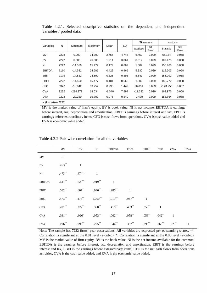
97

Table 4.2.1. Selected descriptive statistics on the dependent and independent

variables / pooled data.

Variables N Minimum Maximum Mean SD

Skewness Kurtosis

Statistic Std.

Error Statistic

Std.

Error

MV 7208 0.000 94.300 2.755 4.748 6.452 0.029 66.134 0.058

BV 7222 0.000 76.605 1.911 3.861 8.612 0.029 107.475 0.058

NI 7222 -14.550 15.477 0.179 0.667 1.507 0.029 155.965 0.058

EBITDA 7160 -14.532 24.687 0.429 0.965 5.230 0.029 119.203 0.058

EBIT 7179 -14.532 24.590 0.326 0.893 5.647 0.029 155.092 0.058

EBEI 7222 -14.550 15.477 0.181 0.668 1.502 0.029 155.772 0.058

CFO 5347 -18.042 83.757 0.296 1.442 36.831 0.033 2143.255 0.067

CVA 7222 -214.271 18.634 -1.040 7.894 -11.332 0.029 169.976 0.058

EVA 7222 -22.250 19.802 0.076 0.849 -0.439 0.029 155.864 0.058

N (List wise) 7222

MV is the market value of firm’s equity, BV is book value, NI is net income, EBITDA is earnings

before interest, tax, depreciation and amortization, EBIT is earnings before interest and tax, EBEI is

earnings before extraordinary items, CFO is cash flows from operations, CVA is cash value added and

EVA is economic value added.

Table 4.2.2 Pair-wise correlation for all the variables

MV BV NI EBITDA EBIT EBEI CFO CVA EVA

MV 1

BV .763** 1

NI .473** .474** 1

EBITDA .611** .620** .919** 1

EBIT .582** .607** .946** .986** 1

EBEI .473** .474** 1.000** .919** .947** 1

CFO .201** .222** .358** .416** .403** .358** 1

CVA .031** .026* .053** .062** .058** .053** .042** 1

EVA .196** .096** .295** .344** .337** .295** .366** .029* 1

Note: The sample has 7222 firms’ year observations. All variables are expressed per outstanding shares. **.

Correlation is significant at the 0.01 level (2-tailed). *. Correlation is significant at the 0.05 level (2-tailed).

MV is the market value of firm equity, BV is the book value, NI is the net income available for the common,

EBITDA is the earnings before interest, tax, depreciation and amortisation, EBIT is the earnings before

interest and tax, EBEI is the earnings before extraordinary items, CFO is the net cash flows from operations

activities, CVA is the cash value added, and EVA is the economic value added.

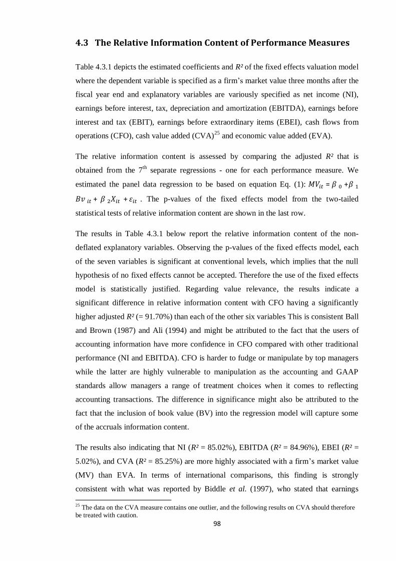
98

4.3 The Relative Information Content of Performance Measures

Table 4.3.1 depicts the estimated coefficients and R² of the fixed effects valuation model

where the dependent variable is specified as a firm’s market value three months after the

fiscal year end and explanatory variables are variously specified as net income (NI),

earnings before interest, tax, depreciation and amortization (EBITDA), earnings before

interest and tax (EBIT), earnings before extraordinary items (EBEI), cash flows from

operations (CFO), cash value added (CVA)25

and economic value added (EVA).

The relative information content is assessed by comparing the adjusted R² that is

obtained from the 7th

separate regressions - one for each performance measure. We

estimated the panel data regression to be based on equation Eq. (1): = +

+ + . The p-values of the fixed effects model from the two-tailed

statistical tests of relative information content are shown in the last row.

The results in Table 4.3.1 below report the relative information content of the non-

deflated explanatory variables. Observing the p-values of the fixed effects model, each

of the seven variables is significant at conventional levels, which implies that the null

hypothesis of no fixed effects cannot be accepted. Therefore the use of the fixed effects

model is statistically justified. Regarding value relevance, the results indicate a

significant difference in relative information content with CFO having a significantly

higher adjusted R² (= 91.70%) than each of the other six variables This is consistent Ball

and Brown (1987) and Ali (1994) and might be attributed to the fact that the users of

accounting information have more confidence in CFO compared with other traditional

performance (NI and EBITDA). CFO is harder to fudge or manipulate by top managers

while the latter are highly vulnerable to manipulation as the accounting and GAAP

standards allow managers a range of treatment choices when it comes to reflecting

accounting transactions. The difference in significance might also be attributed to the

fact that the inclusion of book value (BV) into the regression model will capture some

of the accruals information content.

The results also indicating that NI (R² = 85.02%), EBITDA (R² = 84.96%), EBEI (R² =

5.02%), and CVA (R² = 85.25%) are more highly associated with a firm’s market value

(MV) than EVA. In terms of international comparisons, this finding is strongly

consistent with what was reported by Biddle et al. (1997), who stated that earnings

25 The data on the CVA measure contains one outlier, and the following results on CVA should therefore

be treated with caution.

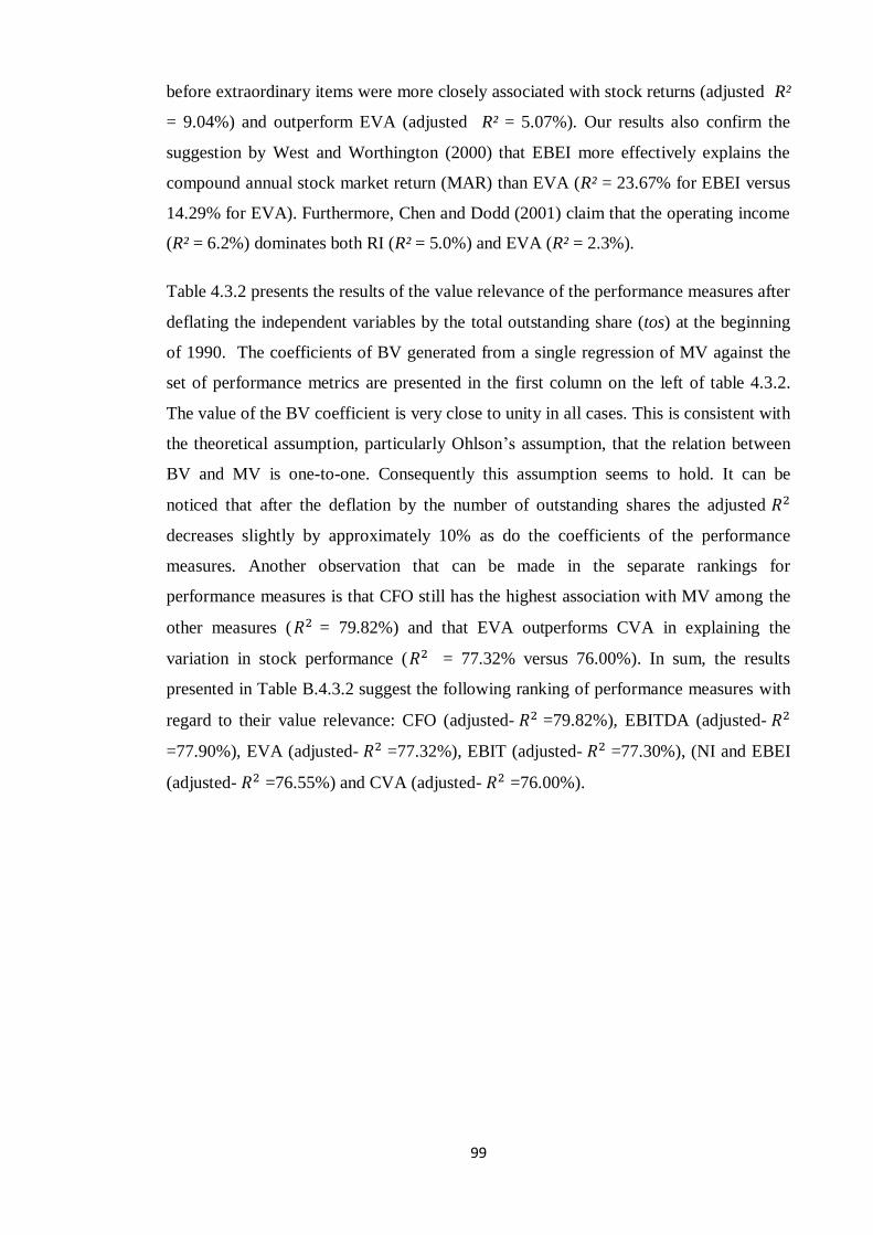
99

before extraordinary items were more closely associated with stock returns (adjusted R²

= 9.04%) and outperform EVA (adjusted R² = 5.07%). Our results also confirm the

suggestion by West and Worthington (2000) that EBEI more effectively explains the

compound annual stock market return (MAR) than EVA (R² = 23.67% for EBEI versus

14.29% for EVA). Furthermore, Chen and Dodd (2001) claim that the operating income

(R² = 6.2%) dominates both RI (R² = 5.0%) and EVA (R² = 2.3%).

Table 4.3.2 presents the results of the value relevance of the performance measures after

deflating the independent variables by the total outstanding share (tos) at the beginning

of 1990. The coefficients of BV generated from a single regression of MV against the

set of performance metrics are presented in the first column on the left of table 4.3.2.

The value of the BV coefficient is very close to unity in all cases. This is consistent with

the theoretical assumption, particularly Ohlson’s assumption, that the relation between

BV and MV is one-to-one. Consequently this assumption seems to hold. It can be

noticed that after the deflation by the number of outstanding shares the adjusted

decreases slightly by approximately 10% as do the coefficients of the performance

measures. Another observation that can be made in the separate rankings for

performance measures is that CFO still has the highest association with MV among the

other measures ( = 79.82%) and that EVA outperforms CVA in explaining the

variation in stock performance ( = 77.32% versus 76.00%). In sum, the results

presented in Table B.4.3.2 suggest the following ranking of performance measures with

regard to their value relevance: CFO (adjusted- =79.82%), EBITDA (adjusted-

=77.90%), EVA (adjusted- =77.32%), EBIT (adjusted- =77.30%), (NI and EBEI

(adjusted- =76.55%) and CVA (adjusted- =76.00%).

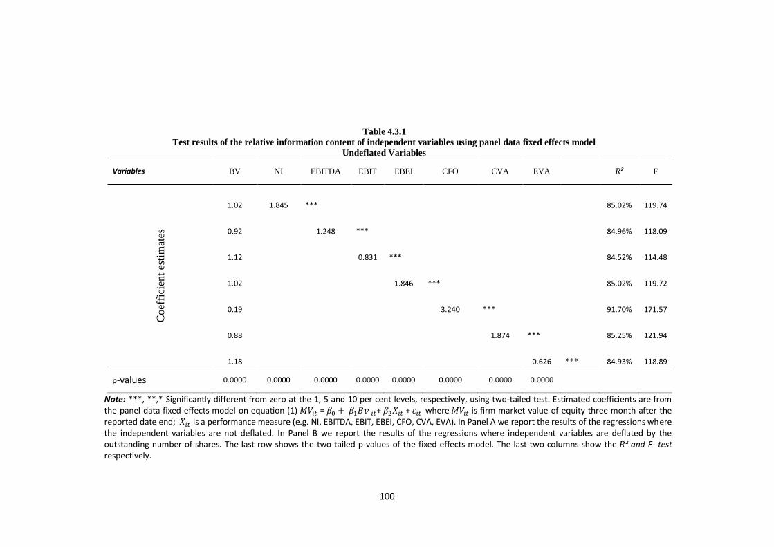
100

Table 4.3.1

Test results of the relative information content of independent variables using panel data fixed effects model

Undeflated Variables

Variables BV NI EBITDA EBIT EBEI CFO CVA EVA R² F

Coef

fici

ent

esti

mat

es

1.02 1.845 *** 85.02% 119.74

0.92 1.248 *** 84.96% 118.09

1.12 0.831 *** 84.52% 114.48

1.02 1.846 *** 85.02% 119.72

0.19 3.240 *** 91.70% 171.57

0.88 1.874 *** 85.25% 121.94

1.18 0.626 *** 84.93% 118.89

p-values 0.0000 0.0000 0.0000 0.0000 0.0000 0.0000 0.0000 0.0000

Note: ***, **,* Significantly different from zero at the 1, 5 and 10 per cent levels, respectively, using two-tailed test. Estimated coefficients are from the panel data fixed effects model on equation (1) = + + where is firm market value of equity three month after the reported date end; is a performance measure (e.g. NI, EBITDA, EBIT, EBEI, CFO, CVA, EVA). In Panel A we report the results of the regressions where the independent variables are not deflated. In Panel B we report the results of the regressions where independent variables are deflated by the outstanding number of shares. The last row shows the two-tailed p-values of the fixed effects model. The last two columns show the R² and F- test respectively.

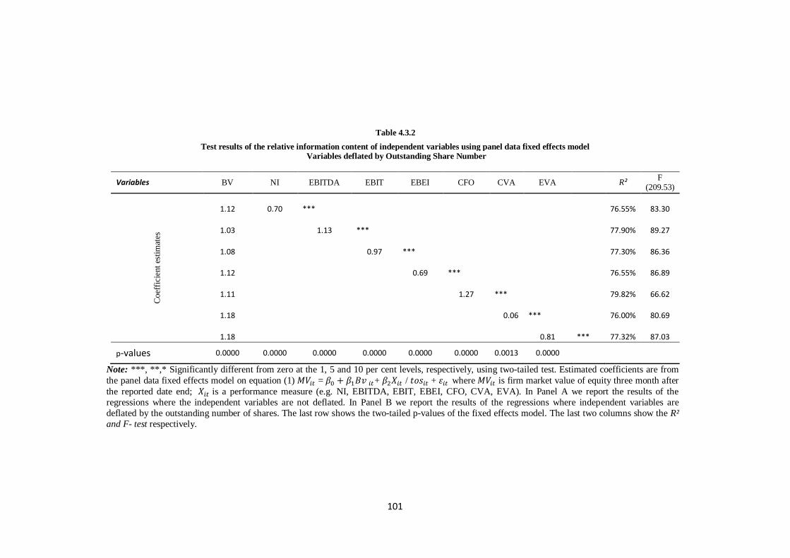
101

Table 4.3.2

Test results of the relative information content of independent variables using panel data fixed effects model Variables deflated by Outstanding Share Number

Variables BV NI EBITDA EBIT EBEI CFO CVA EVA R² F

(209.53)

Coef

fici

ent

esti

mat

es

1.12 0.70 *** 76.55% 83.30

1.03 1.13 *** 77.90% 89.27

1.08 0.97 *** 77.30% 86.36

1.12 0.69 *** 76.55% 86.89

1.11 1.27 *** 79.82% 66.62

1.18 0.06 *** 76.00% 80.69

1.18 0.81 *** 77.32% 87.03

p-values 0.0000 0.0000 0.0000 0.0000 0.0000 0.0000 0.0013 0.0000

Note: ***, **,* Significantly different from zero at the 1, 5 and 10 per cent levels, respectively, using two-tailed test. Estimated coefficients are from

the panel data fixed effects model on equation (1) = + / + where is firm market value of equity three month after

the reported date end; is a performance measure (e.g. NI, EBITDA, EBIT, EBEI, CFO, CVA, EVA). In Panel A we report the results of the

regressions where the independent variables are not deflated. In Panel B we report the results of the regressions where independent variables are

deflated by the outstanding number of shares. The last row shows the two-tailed p-values of the fixed effects model. The last two columns show the R²

and F- test respectively.

102

4.4 The Incremental Information Content of Performance Measures

The incremental criterion asks whether a specific measure has additional information

content over that already existing in other measures and is applicable when intending to

assess measures in regard to other performance measure’s information content. The

steps outlined by Biddle et al. (1995, 1997) and Charitou et al. (2001) were followed to

assess the incremental information content of the different performance metrics. It was

assessed by comparing the adjusted from a separate regression, one for each

performance measure, and the adjusted from a combination of two different

performance metrics.

Table 4.4.1 indicates that there is significant incremental information content existing

between pairwise measures. The p-values in the last row show that the fixed effects

model is more specified in favour of the random model and represents that in all cases

the null hypothesis that the pairwised variables are jointly insignificantly different from

zero (Biddle el al., 1995). The first row shows the adjusted from the single variable

regression for measure separately. For example, the first figure, 79.82%, is obtained

by regressing the deflated market value against CFO. Apart from NOPAT, CFO has the

highest explanatory power, which is consistent with Charitou et al. (2001) who used UK

data over the period 1985–1993 to investigate the value relevance of operating cash

flows and earnings where they claimed that operating cash flows revealed incremental

information content beyond earnings when pooled data were used.

The rest of Table 4.4.1 provides the adjusted obtained from various pairwise

combinations of performance measures. Each cell contains the adjusted from a

bivariate regression involving the row head and the column head. Under this figure a

smaller value is given in parenthesis. This is the increment in the adjusted obtained

by adding the second variable. For example, when we use CFO and EBITDA we obtain

an adjusted coefficient of determination of 80.73%. However adding EBITDA to CFO

increases the by 0.91%, while adding CFO to EBIDTA increases it by 2.83%.

Consistent with previous literature all the performance measures have, or contained

more, information than other performance measures except for EBIT as, when paired

with CVA, the adjusted decreased by 0.01.

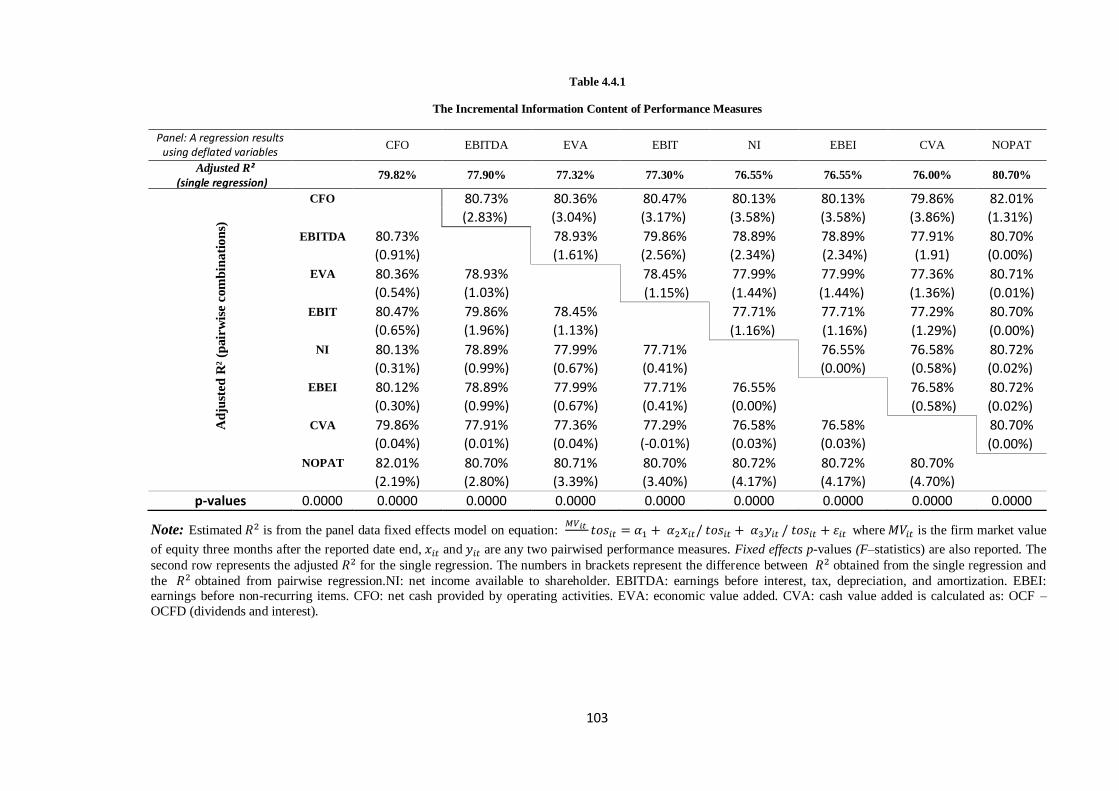
103

Table 4.4.1

The Incremental Information Content of Performance Measures

Panel: A regression results using deflated variables

CFO EBITDA EVA EBIT NI EBEI CVA NOPAT

Adjusted R² (single regression)

79.82% 77.90% 77.32% 77.30% 76.55% 76.55% 76.00% 80.70%

A

dju

sted

R²

(pair

wis

e com

bin

ati

on

s)

CFO 80.73% 80.36% 80.47% 80.13% 80.13% 79.86% 82.01% (2.83%) (3.04%) (3.17%) (3.58%) (3.58%) (3.86%) (1.31%)

EBITDA 80.73% 78.93% 79.86% 78.89% 78.89% 77.91% 80.70% (0.91%) (1.61%) (2.56%) (2.34%) (2.34%) (1.91) (0.00%)

EVA 80.36% 78.93% 78.45% 77.99% 77.99% 77.36% 80.71% (0.54%) (1.03%) (1.15%) (1.44%) (1.44%) (1.36%) (0.01%)

EBIT 80.47% 79.86% 78.45% 77.71% 77.71% 77.29% 80.70% (0.65%) (1.96%) (1.13%) (1.16%) (1.16%) (1.29%) (0.00%)

NI 80.13% 78.89% 77.99% 77.71% 76.55% 76.58% 80.72% (0.31%) (0.99%) (0.67%) (0.41%) (0.00%) (0.58%) (0.02%)

EBEI 80.12% 78.89% 77.99% 77.71% 76.55% 76.58% 80.72% (0.30%) (0.99%) (0.67%) (0.41%) (0.00%)

(0.58%) (0.02%)

CVA 79.86% 77.91% 77.36% 77.29% 76.58% 76.58% 80.70% (0.04%) (0.01%) (0.04%) (-0.01%) (0.03%) (0.03%)

(0.00%)

NOPAT 82.01% 80.70% 80.71% 80.70% 80.72% 80.72% 80.70%

(2.19%) (2.80%) (3.39%) (3.40%) (4.17%) (4.17%) (4.70%)

p-values 0.0000 0.0000 0.0000 0.0000 0.0000 0.0000 0.0000 0.0000 0.0000

Note: Estimated is from the panel data fixed effects model on equation: where is the firm market value

of equity three months after the reported date end, and are any two pairwised performance measures. Fixed effects p-values (F–statistics) are also reported. The

second row represents the adjusted for the single regression. The numbers in brackets represent the difference between obtained from the single regression and

the obtained from pairwise regression.NI: net income available to shareholder. EBITDA: earnings before interest, tax, depreciation, and amortization. EBEI: earnings before non-recurring items. CFO: net cash provided by operating activities. EVA: economic value added. CVA: cash value added is calculated as: OCF –

OCFD (dividends and interest).

104

The pairwise combinations of EBITDA and EBIT, EBIT and EVA, and EBITDA and

EVA, indicate that adjusted , the explanatory power, has increased by 1.96, 1.13, and

1.03 respectively over EBITDA and EBIT alone. Again the result also indicates that NI

has no incremental information content beyond EBEI (0.00 differences). This could be

attributed to what we have mentioned earlier which is that the reported NI and EBEI are

equal because there are no extraordinary circumstances which exist and even if they did

exist it was in small numbers and the descriptive statistics show that NI and EBEI are

perfectly correlated. Hence the net operating profit after tax (NOPAT) was introduced

to replace the EBEI as a performance measure. Moreover, the result indicates that NI

has increased the explanatory power of EVA by some 0.67%. This is inconsistent with

Bao and Bao (1998) who claimed that NI has a zero impact on EVA. Overall, the results

of Table 4.4.1 indicate that the net operating profit after tax (NOPAT) exhibits the

largest incremental information among the performance metrics, with an increase of

2.19 with CFO, 2.80 with EBITDA, 3.39 with EVA, 3.40 with EBIT, 4.17 with both NI

and EBEI, and 4.70 with CVA. Contrary to West and Worthington (2000) and

according to our results the most logical pairwise combination in explaining market

value (stock price) is therefore composed of CVA and NOPAT. However, consistent

with Biddle et al, (1997) our finding does not support the adage that EVA is the

dominant measure and superior to earnings and cash flow measures in its association

with the market value and annual stock return (price).

An interesting result is that the CFO has an incremental information content over the

rest of the performance measures When paired with EBITDA, EVA, EBIT, NI, EBEI,

CVA and NOPAT the adjusted increased by 2.83, 3.04, 3.17, 3.58, 3.58, 3.86 and

1.31 per cent respectively. This is in contradistinction to Board and Day’s (1989) claim

(they were the first in the UK to examine the incremental information content of

earnings components). They claimed that net income and working capital from

operations (WCFO) defined as the net income plus depreciation plus deferred tax

separately, hold more information content than net cash (quick) asset (NETQ) that is

defined as the net income plus depreciation plus deferred tax plus change in stock and

work in progress. In addition their results pointed out that with regard to the incremental

information content, net cash flow was the poorest of the measures examined. This

might be attributed to the proxies used for the cash flow figure as in that period 1961-

1977, the period of their study, the cash flow statement was not mandatory and the

companies voluntarily prepared the statement of cash flows. Arnold et al. (1991)

105

reported evidence on the information content for cash flows, which was at odds with the

results of prior UK studies. The differences in the results obtained by different studies

dealt with the information and incremental information content were due to the

differences in the sample and the period of the study. Notwithstanding, with regard to

the differences in performance measures and incremental information content, the best

combination (but not the most accurate) is when CFO composes NOPAT or EBITDA

where the adjusted is 82.01% or 80.73% in sequences, followed by NOPAT with NI

( = 80.72%) and NOPAT with CVA ( = 80.70%).

4.4.1 The Incremental Information Content of Net Income Components

As discussed in section 3.2.2 hypothesis states that net income (NI) components

have no statistically significant effect on annual stock price performance. The

hypothesis predicts that decomposing net income (NI) into its main components, cash

flows and aggregate accruals, is expected to increase the NI (earnings) ability to explain

the changes in annual stock performances. The assumption is that each component is

expected to reflect different information content (Dechow et al, 1998; Barth et al,

2001). The aforementioned hypothesis is examined by conducting the following panel

regression model under the fixed effects methodologies.

where is the firm market value three months after the fiscal year end; CFO is the

net cash flow from operating activity, ΔAP is the change in account payables; ΔAR is

the change in accounts receivable; ΔINV is the change in inventories, DEP is

depreciation, AMORT is amortization, and OTHER is other accruals. The values of

both dependent and explanatory variables have been deflated by the outstanding share

of each period consistent with Garrod et al. (2000).

Table 4.4.1.1 shows some descriptive statistics of NI components. First, CFO has the

larger mean among the other explanatory variables (0.29) with a standard deviation

(1.41). This value ranges from a minimum of -18.04 to a maximum of 83.76. This is

consistent, as expected, with the results obtained by Dechow et al. (1998) and Barth et

al. (2001). Second, while CFO has the larger standard deviation among NI components,

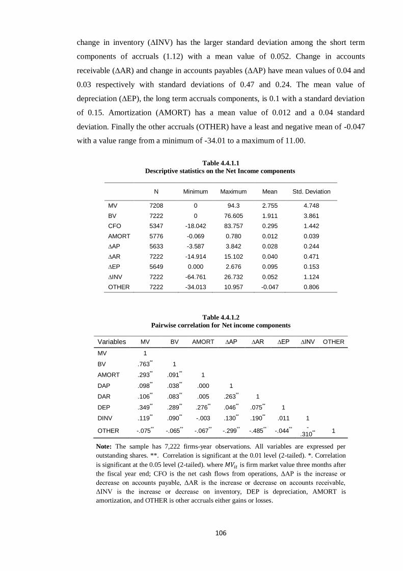
106

change in inventory (∆INV) has the larger standard deviation among the short term

components of accruals (1.12) with a mean value of 0.052. Change in accounts

receivable (∆AR) and change in accounts payables (∆AP) have mean values of 0.04 and

0.03 respectively with standard deviations of 0.47 and 0.24. The mean value of

depreciation (∆EP), the long term accruals components, is 0.1 with a standard deviation

of 0.15. Amortization (AMORT) has a mean value of 0.012 and a 0.04 standard

deviation. Finally the other accruals (OTHER) have a least and negative mean of -0.047

with a value range from a minimum of -34.01 to a maximum of 11.00.

Table 4.4.1.1

Descriptive statistics on the Net Income components

N Minimum Maximum Mean Std. Deviation

MV 7208 0 94.3 2.755 4.748

BV 7222 0 76.605 1.911 3.861

CFO 5347 -18.042 83.757 0.295 1.442

AMORT 5776 -0.069 0.780 0.012 0.039

∆AP 5633 -3.587 3.842 0.028 0.244

∆AR 7222 -14.914 15.102 0.040 0.471

∆EP 5649 0.000 2.676 0.095 0.153

∆INV 7222 -64.761 26.732 0.052 1.124

OTHER 7222 -34.013 10.957 -0.047 0.806

Table 4.4.1.2

Pairwise correlation for Net income components

Variables MV BV AMORT ∆AP ∆AR ∆EP ∆INV OTHER

MV 1

BV .763** 1

AMORT .293** .091

** 1

DAP .098** .038

** .000 1

DAR .106** .083

** .005 .263

** 1

DEP .349** .289

** .276

** .046

** .075

** 1

DINV .119** .090

** -.003 .130

** .190

** .011 1

OTHER -.075** -.065

** -.067

** -.299

** -.485

** -.044

**

-.310

**

1

Note: The sample has 7,222 firms-year observations. All variables are expressed per

outstanding shares. **. Correlation is significant at the 0.01 level (2-tailed). *. Correlation

is significant at the 0.05 level (2-tailed). where is firm market value three months after

the fiscal year end; CFO is the net cash flows from operations, ΔAP is the increase or

decrease on accounts payable, ΔAR is the increase or decrease on accounts receivable,

ΔINV is the increase or decrease on inventory, DEP is depreciation, AMORT is

amortization, and OTHER is other accruals either gains or losses.

107

Table 4.4.1.2 shows the correlation matrix for the set of NI components. The results

indicate that most correlations are positive and significant. However, the other accruals

(OTHER) correlations with the remaining components are all negative and significant.

The long term accruals components, BV, DEP and AMORT, have the highest

correlation with market value (0.763, 0.349 and 0.293 respectively), followed by the

change in inventory (0.119) then the change in accounts receivable (0.106) and then

change in accounts payables (0.098). Turning to the correlation between other variables,

the highest correlation exists between depreciation (DEP) and both book value (BV)

and amortisation (AMORT), at 0.289 and 0.276 respectively. Change in accounts

receivable (∆AR) and amortization have the lowest correlation (-0.49%). Table 4.4.1.2

also shows that all the correlation coefficients are less than 0.5.

Turning to the incremental information content of the NI components, Table 4.4.3

shows that all NI components are significant and positively associated with the share

price performances at the 0.05 level except for ΔAP, DEP and AMORT which has a

significant and negative sign. This is consistent with what Barth et al, (2001) reported.

They do not predict the sign of other accruals (OTHER) but their result shows a positive

and significant association which is consistent with what this study revealed.

Furthermore, the results reveal that the NI components have incremental information

content. The results show a higher when decomposing the NI into cash flows and

accruals at 82.70% while is equal to 76.55% when we run the regression against the

NI alone. The increase in by 6.15% indicates that cash flows and accruals

components jointly significantly outperform NI in explaining changes in price

performances. This is consistent with previous price-based studies. Wilson (1986 and

1987) and Garrod et al. (2000) claim that decomposing NI (earnings) into its main

components, the cash flows and accruals, will enhance the model’s ability to explain the

stock performance’s volatility.

Prior UK and USA price-based studies that examined the information content of

accruals decomposed total accruals into long and short term components, not individual

components, which raised difficulties when comparing our results with those which

previous studies predicted.

While results in Table 4.4.3 convey that both short-term accruals (e.g. ΔAP, ΔAR, and

ΔINV) and long-term accruals (e.g. DEP and AMORT) are relevant as explanatory

variables in explaining stock performance, previous studies contradicted each other

108

regarding the value relevance of long and short term accruals. There have been volumes

written that attempt to investigate the effects of both long and short term accruals. For

instance, Rayburn (1986) and Dechow (1994) claimed that short-term accruals have

information content but long term accruals have no information content. Contrary to

them, Garrod et al. (2000) reported that long term accruals contain information but short

term accruals have no information content. Along the same lines, McLeay et al. (1997)

analysed UK data and reported that the components of accruals, namely the short and long term,

have incremental information content beyond that already existing in aggregate earnings.

To conclude, the results in Table 4.4.3 provide empirical evidence on the usefulness of

decomposing earnings into operating cash flows and aggregate accruals. They also

provide empirical evidence on the usefulness of decomposing aggregate accruals into its

main components. Christie (1987) stated that there is no optimal deflator in levels

models, but deflation by anything other than a function of independent variable can lead

to some specification errors. To this end, all the variables are deflated by the

outstanding share at the beginning of each period.

109

Table (4.4.3) Test results of the relative information content of Net Income (NI) Components

Regression results

using deflated

variables

BV +

NI +

CFO +

ΔAP -

ΔAR +

ΔINV +

DEP -

AMORT -

OTHER ±

R² F

(209.533)

Coefficient estimates 1.12 0.70 76.55% 83.30

Fixed effects p-

values

0 .0000 ***

0.0000 ***

Coefficient estimates 0.90

2.2940 -0.6451 1.3820 1.4489 -3.9610 -8.4590 0.7055 82.70% F

(214.331)

p-values 0 .0000

0.0000 0.0000 0 .0000 0.0000 0 .0000 0.0000 0.0000 73.84

***

*** *** *** *** *** *** ***

Note: ***, **,* Significantly different from zero at the 1, 5 and 10 per cent levels, respectively, using two-tailed test. Estimated coefficients are

from the panel data fixed effects model on equation (Model 3):

where is firm market value of firm equity

three months after the reported date; CFO is the net cash flows from operations activity, ΔAP is the increase and decrease on accounts payable,

ΔAR is the increase and decrease on accounts receivable , ΔINV is the increase and decrease on inventories, DEP is depreciation, AMORT is

amortization, and OTHER is other accruals. We report the results of the regressions where all variables are deflated by the outstanding number

of shares. The last row shows the two-tailed p-values of the fixed effects model. The last two columns show the R² and F- test respectively.

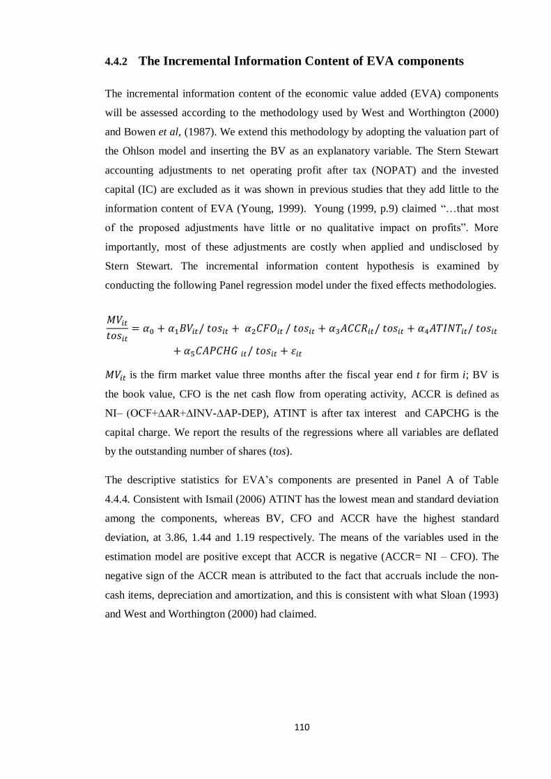
110

4.4.2 The Incremental Information Content of EVA components

The incremental information content of the economic value added (EVA) components

will be assessed according to the methodology used by West and Worthington (2000)

and Bowen et al, (1987). We extend this methodology by adopting the valuation part of

the Ohlson model and inserting the BV as an explanatory variable. The Stern Stewart

accounting adjustments to net operating profit after tax (NOPAT) and the invested

capital (IC) are excluded as it was shown in previous studies that they add little to the

information content of EVA (Young, 1999). Young (1999, p.9) claimed “…that most

of the proposed adjustments have little or no qualitative impact on profits”. More

importantly, most of these adjustments are costly when applied and undisclosed by

Stern Stewart. The incremental information content hypothesis is examined by

conducting the following Panel regression model under the fixed effects methodologies.

is the firm market value three months after the fiscal year end t for firm i; BV is

the book value, CFO is the net cash flow from operating activity, ACCR is defined as

NI– (OCF+∆AR+∆INV-∆AP-DEP), ATINT is after tax interest and CAPCHG is the

capital charge. We report the results of the regressions where all variables are deflated

by the outstanding number of shares (tos).

The descriptive statistics for EVA’s components are presented in Panel A of Table

4.4.4. Consistent with Ismail (2006) ATINT has the lowest mean and standard deviation

among the components, whereas BV, CFO and ACCR have the highest standard

deviation, at 3.86, 1.44 and 1.19 respectively. The means of the variables used in the

estimation model are positive except that ACCR is negative (ACCR= NI – CFO). The

negative sign of the ACCR mean is attributed to the fact that accruals include the non-

cash items, depreciation and amortization, and this is consistent with what Sloan (1993)

and West and Worthington (2000) had claimed.

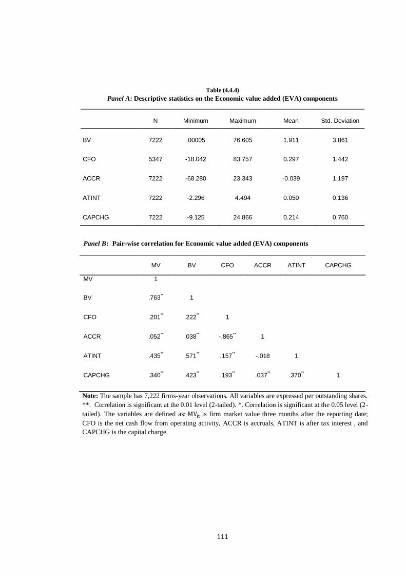
111

Table (4.4.4) Panel A: Descriptive statistics on the Economic value added (EVA) components

N Minimum Maximum Mean Std. Deviation

BV 7222 .00005 76.605 1.911 3.861

CFO 5347 -18.042 83.757 0.297 1.442

ACCR 7222 -68.280 23.343 -0.039 1.197

ATINT 7222 -2.296 4.494 0.050 0.136

CAPCHG 7222 -9.125 24.866 0.214 0.760

Panel B: Pair-wise correlation for Economic value added (EVA) components

MV BV CFO ACCR ATINT CAPCHG

MV 1

BV .763** 1

CFO .201** .222

** 1

ACCR .052** .038

** -.865

** 1

ATINT .435** .571

** .157

** -.018 1

CAPCHG .340** .423

** .193

** .037

** .370

** 1

Note: The sample has 7,222 firms-year observations. All variables are expressed per outstanding shares.

**. Correlation is significant at the 0.01 level (2-tailed). *. Correlation is significant at the 0.05 level (2-

tailed). The variables are defined as: is firm market value three months after the reporting date;

CFO is the net cash flow from operating activity, ACCR is accruals, ATINT is after tax interest , and

CAPCHG is the capital charge.

112

Panel B of Table 4.4.4, consistent with Biddle et al, (1997), reveals that CFO has a

negative significant correlation with ACCR. The correlations between CFO, ATINT

and CAPCHG are significant and positive, while our results report that the correlation

between ACCR and ATINT is negative and insignificant. Further, the negative

correlation between CFO and ACCR is consistent with the fact that “accrual process

smoothing earnings relative to the underlying operating cash flows” (Biddle et al, 1997,

p.316).

However, for the purposes of the current research, the accounting adjustments

(ACCTADJ) first introduced by Stern and Stewart (1991) were excluded from EVA’s

components. This exclusion was as a result of the fact that from the beginning I have

treated the EVA as it is mentioned in the economic theory, that is, similar in its essence

to the residual income (RI) concept mentioned in the literature centuries ago ( Drucker,

1995). Another important reason is that many researchers treat these adjustments as

cosmetic and adding little information content to EVA (Young, 1999). Finally, few UK

companies announced the adoption of EVA and the adoption period was brief. Hence,

EVA is defined as:

Table 4.4.5 provides results of the incremental information of the EVA components

from.

.

In this regression all the coefficients are significant at the 0.01 level of significance and

different from zero. The sign of the association (provided below the variables) is in line

with the literature except for ATINT which has an opposite sign.

The results show higher when decomposing the EVA into its main components

(80.23%) while is equal to 77.32% when we run the regression against the EVA

alone. The increase in by 2.91% indicates that EVA components together

significantly outperform EVA in explaining changes in price performances. This is

consistent with previous price-based studies (Biddle et al, 1997; West and Worthington,

2000). Biddle et al., claim that decomposing EVA into its main components will

enhance some of the model’s ability to explain the stock performance’s volatility.

113

Again, consistent with West and Worthington (2000) CFO and ATINT have the highest

positive coefficient among EVA components.

Table 4.4.6 provides the results of the pairwise regressions of the EVA components. All

the components are significant at conventional levels. The results indicate that in each

pairwise comparison, each component of EVA has an incremental information content

beyond that which already exists in other components. Based on the partial F-test all

pairwise between any two components are significantly different from one another and

this is consistent with the results revealed by Biddle et al., (1995), Biddle et al., (1997)

and Ismail, (2006). Moreover, the best pair of components is the one between the

ACCR, a component on NOPAT, and the CAPCHG (calculated as invested capital (IC)

× WACC), an EVA component, followed by ACCR and ATINT (calculated as Interest

expense (1- Tax rate)) where the pairwise partial F-tests are 81.81 and 81.79 respectively.

While CFO and ATINT have the highest coefficient estimates among the other

components (1.81, 1.90 respectively) when paired they had a low partial F-test (66.31).

The results also indicate that the EVA main components (e.g. CAPCHG and ATINT)

have added some information content when they were paired with other EVA

components. However, this contribution does not reach the level that makes EVA the

dominant performance measure. As seen in section 4.3, EVA has been positioned as the

third performance measure in its association with stock performances. The negative

association between CAPCHG, which is equal to (capital employed26

× WACC), and

market value corresponds with the literature and may be attributed to the size effect

theory where large firms earn low returns (Banz, 1981).

26 Capital employed refers to total equity plus non-current liabilities.

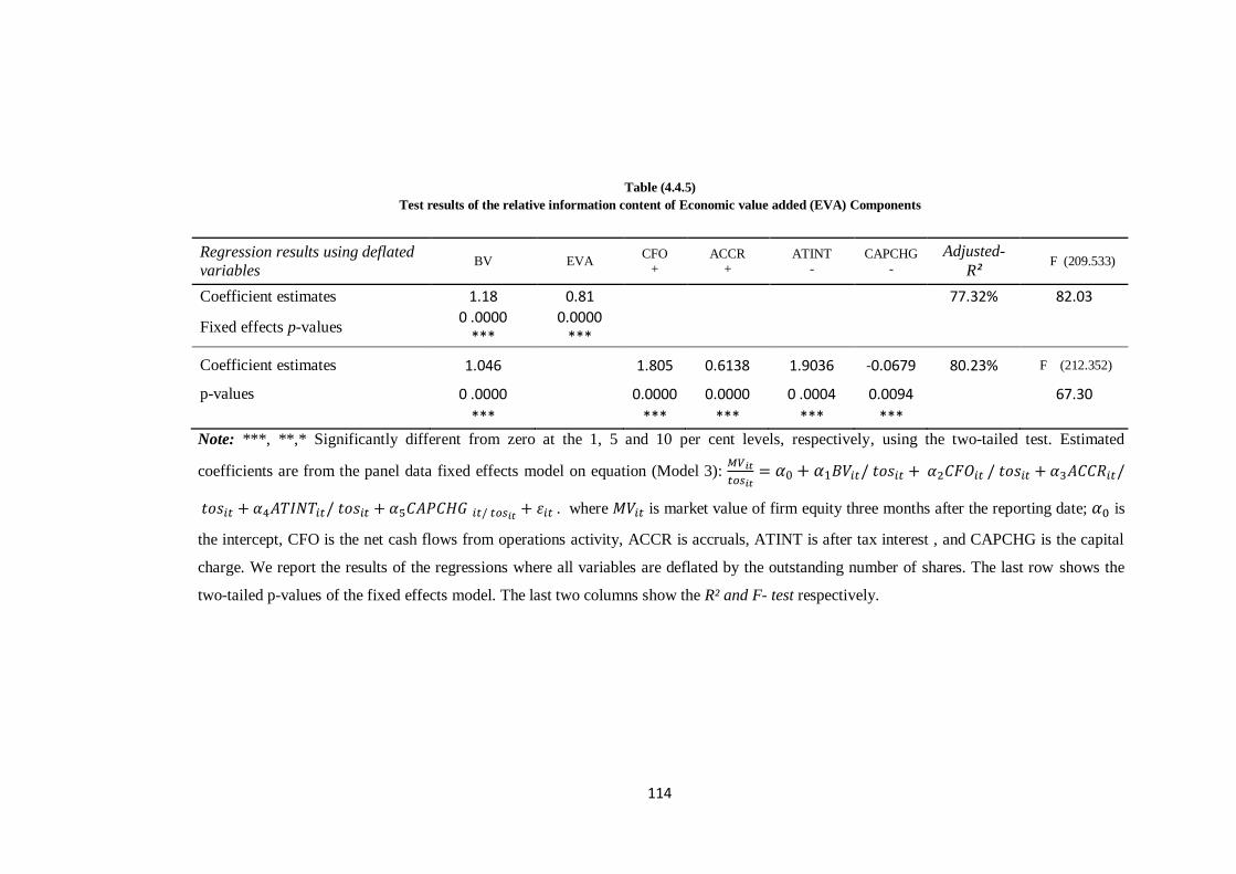
114

Table (4.4.5) Test results of the relative information content of Economic value added (EVA) Components

Regression results using deflated

variables BV EVA

CFO +

ACCR +

ATINT -

CAPCHG -

Adjusted-

R² F (209.533)

Coefficient estimates 1.18 0.81 77.32% 82.03

Fixed effects p-values 0 .0000

*** 0.0000

***

Coefficient estimates 1.046

1.805 0.6138 1.9036 -0.0679 80.23% F (212.352)

p-values 0 .0000

0.0000 0.0000 0 .0004 0.0094 67.30

***

*** *** *** ***

Note: ***, **,* Significantly different from zero at the 1, 5 and 10 per cent levels, respectively, using the two-tailed test. Estimated

coefficients are from the panel data fixed effects model on equation (Model 3):

. where is market value of firm equity three months after the reporting date; is

the intercept, CFO is the net cash flows from operations activity, ACCR is accruals, ATINT is after tax interest , and CAPCHG is the capital

charge. We report the results of the regressions where all variables are deflated by the outstanding number of shares. The last row shows the

two-tailed p-values of the fixed effects model. The last two columns show the R² and F- test respectively.

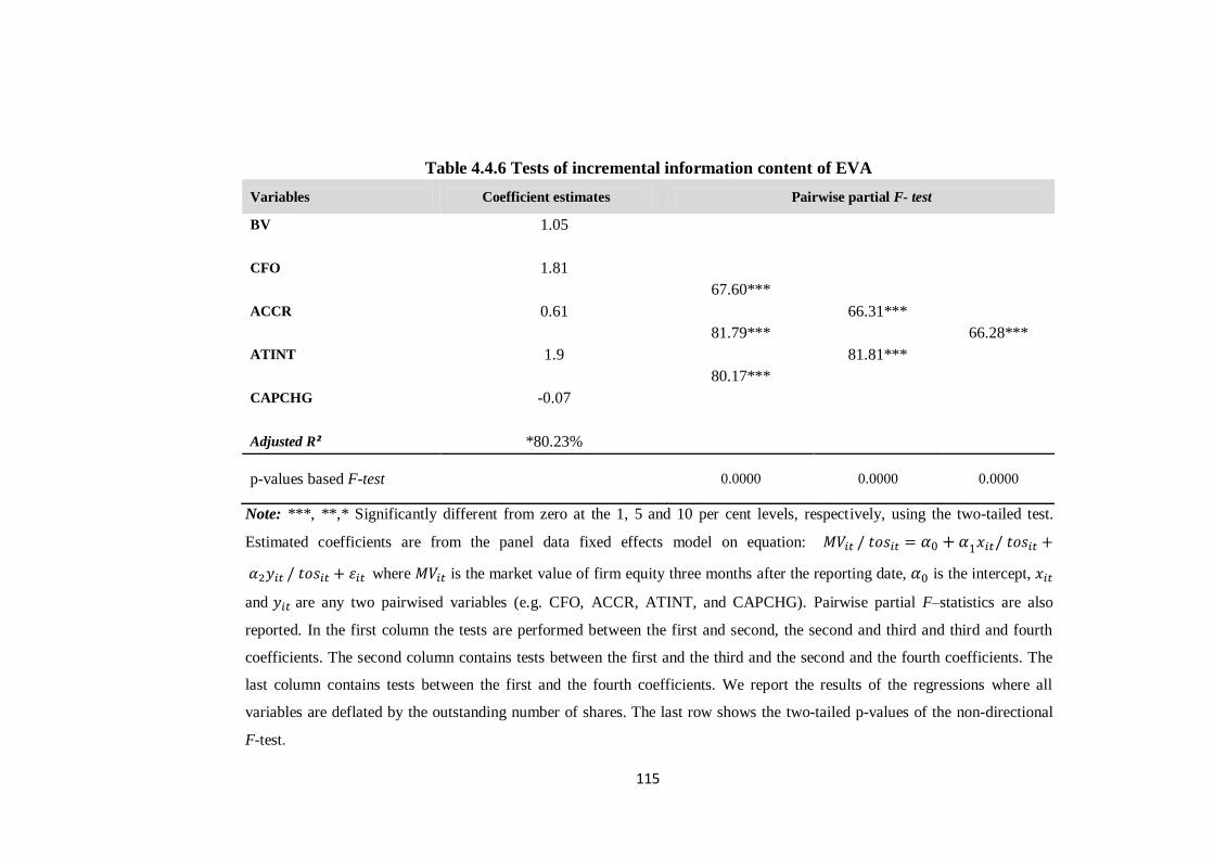
115

Table 4.4.6 Tests of incremental information content of EVA

Variables Coefficient estimates

Pairwise partial F- test

BV 1.05

CFO 1.81

67.60***

ACCR 0.61

66.31***

81.79***

66.28***

ATINT 1.9

81.81***

80.17***

CAPCHG -0.07

Adjusted R² *80.23%

p-values based F-test 0.0000 0.0000 0.0000

Note: ***, **,* Significantly different from zero at the 1, 5 and 10 per cent levels, respectively, using the two-tailed test.

Estimated coefficients are from the panel data fixed effects model on equation:

where is the market value of firm equity three months after the reporting date, is the intercept,

and are any two pairwised variables (e.g. CFO, ACCR, ATINT, and CAPCHG). Pairwise partial F–statistics are also

reported. In the first column the tests are performed between the first and second, the second and third and third and fourth

coefficients. The second column contains tests between the first and the third and the second and the fourth coefficients. The

last column contains tests between the first and the fourth coefficients. We report the results of the regressions where all

variables are deflated by the outstanding number of shares. The last row shows the two-tailed p-values of the non-directional

F-test.

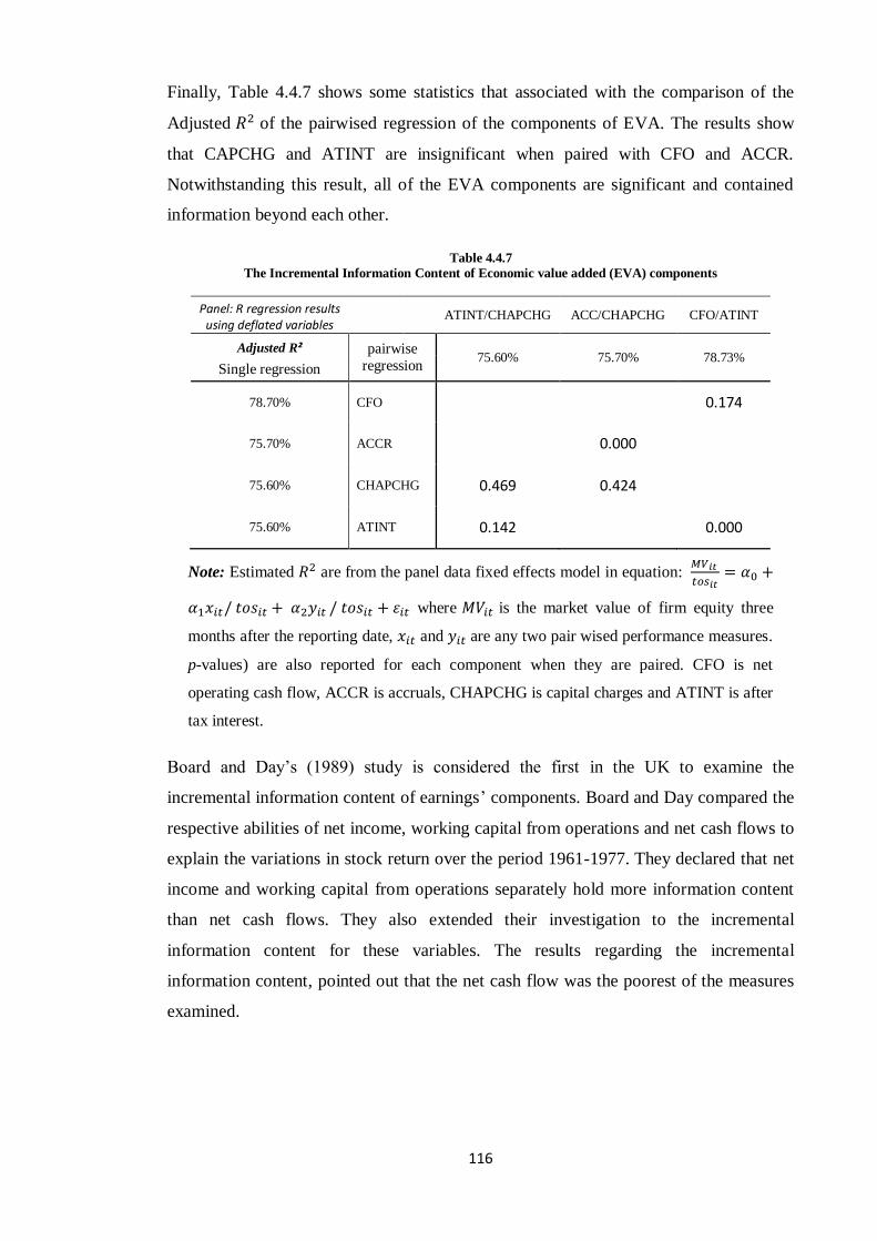
116

Finally, Table 4.4.7 shows some statistics that associated with the comparison of the

Adjusted of the pairwised regression of the components of EVA. The results show

that CAPCHG and ATINT are insignificant when paired with CFO and ACCR.

Notwithstanding this result, all of the EVA components are significant and contained

information beyond each other.

Table 4.4.7

The Incremental Information Content of Economic value added (EVA) components

Panel: R regression results using deflated variables

ATINT/CHAPCHG ACC/CHAPCHG CFO/ATINT

Adjusted R² pairwise

regression 75.60% 75.70% 78.73%

Single regression

78.70% CFO

0.174

75.70% ACCR

0.000

75.60% CHAPCHG 0.469 0.424

75.60% ATINT 0.142 0.000

Note: Estimated are from the panel data fixed effects model in equation:

where is the market value of firm equity three

months after the reporting date, and are any two pair wised performance measures.

p-values) are also reported for each component when they are paired. CFO is net

operating cash flow, ACCR is accruals, CHAPCHG is capital charges and ATINT is after

tax interest.

Board and Day’s (1989) study is considered the first in the UK to examine the

incremental information content of earnings’ components. Board and Day compared the

respective abilities of net income, working capital from operations and net cash flows to

explain the variations in stock return over the period 1961-1977. They declared that net

income and working capital from operations separately hold more information content

than net cash flows. They also extended their investigation to the incremental

information content for these variables. The results regarding the incremental

information content, pointed out that the net cash flow was the poorest of the measures

examined.

117

4.5 Empirical Results of the Return Model

Most of the past extant literature (e.g. Board and Day, 1989; Biddle et al. 1995, 1997;

Bao and Bao, 1998; West and Worthington, 2000; Ismail, 2006) adopted the return

model, the valuation component of the Ohlson model, to examine the value relevance

and incremental information content of a set of different accounting measures and also

test the association between these measures and the variation in annual stock. One

common feature of the aforementioned papers is that the ordinary least square (OLS)

regression was the technique applied for the set of cross-sectional and time series data to

obtain the results. This is the procedure that was sharply criticised by econometricians

because it might lead to biased and inaccurate estimates of the coefficients. Along the

same lines, Gujarati (2003) suggests applying panel data regression which takes into

consideration the specific characteristic of each cross-section as opposed to the OLS

regression.

We extend the previous work by introducing the book value (BV) in the valuation

model and treating it as an independent variable to be combined with the other

performance measures in a multivariate regression. Ohlson (1995) defines the stock

price as the combination of current BV, current abnormal earnings and other value

relevant information. Furthermore, we adopt the fixed effects model and allow the

intercept to vary across individuals but not across the time dimension. Finally, in terms

of comparison, we will report the results obtained from adopting both the traditional

valuation method and the one introduced by Ohlson (1995).

The results in Table 4.5.1 show the value relevance of the investigated performance

measures using the same model adopted by Biddle et al. (1997) and West and

Worthington (2000). The analysis shows that all the performance metrics are significant

and positively associated with the compound share return at the 0.05 level except for the

CVA which has a significant and negative sign. Moreover, the explanatory power for all

variables is significantly higher than that found in the study by Biddle et al., (1997).

The negative sign of the CVA is consistent with the profitability concept where

companies in the long run are less capable of generating high profits and accept the

level of return that is sufficient to cover its cost of capital which means firms will enter

into the value destroying phase rather than generating value. The explanatory power of

EBITDA is 15.13% higher than NI and both EVA and CVA. This is against the

118

unwritten rule that EVA has the ability to overshadow other performance measures.

Regardless of the low Adjusted of accounting–based measures, reported by Biddle

et al, (1997), our result is consistent with the claim that traditional performance

measures (i.e. EBITDA, EBIT, EBEI) have more information content than that of

value added measures (i.e. EVA and CVA). Moreover, NI stands on the fourth position

after EBITDA, EBIT and EBEI respectively. In terms of a comparison of our results

this is highly consistent with West and Worthington (2000) who estimated the value

relevance of EBEI, RI, NCF and EVA at 23.7%, 19.3%, 18.1% and 14.29%

respectively.

Table 4.5.2 presents results obtained after extending the Biddle model to include the

security book value BV into the valuation model, that is:

The inclusion of the book value of equity controls for possible size effect. It is well-

known that small firms earn abnormally larger returns even after controlling for risk.

Therefore, attempting to explain returns by a single performance measure might suffer

from an omitted variable bias. The omitted variables may vary, but it is believe that size

is a good proxy for other factors that might influence the firm’s return.

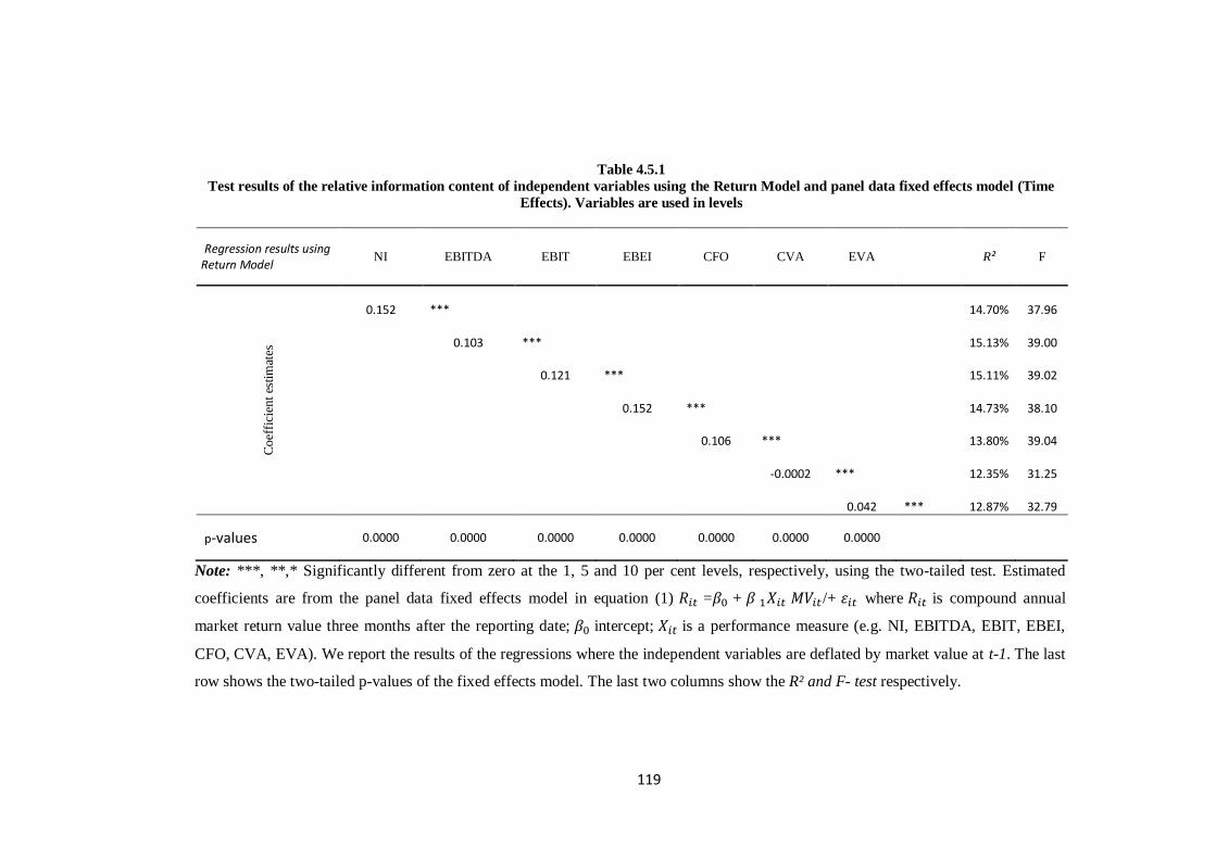
119

Table 4.5.1

Test results of the relative information content of independent variables using the Return Model and panel data fixed effects model (Time

Effects). Variables are used in levels

Regression results using Return Model

NI EBITDA EBIT EBEI CFO CVA EVA R² F C

oef

fici

ent

esti

mat

es

0.152 *** 14.70% 37.96

0.103 *** 15.13% 39.00

0.121 *** 15.11% 39.02

0.152 *** 14.73% 38.10

0.106 *** 13.80% 39.04

-0.0002 *** 12.35% 31.25

0.042 *** 12.87% 32.79

p-values 0.0000 0.0000 0.0000 0.0000 0.0000 0.0000 0.0000


coefficients are from the panel data fixed effects model in equation (1) = + /+ where is compound annual

market return value three months after the reporting date; intercept; is a performance measure (e.g. NI, EBITDA, EBIT, EBEI,

CFO, CVA, EVA). We report the results of the regressions where the independent variables are deflated by market value at t-1. The last

row shows the two-tailed p-values of the fixed effects model. The last two columns show the R² and F- test respectively.

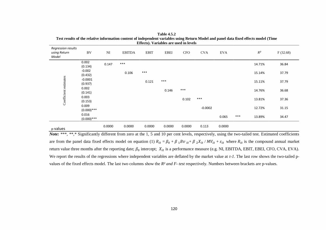
120

Table 4.5.2

Test results of the relative information content of independent variables using Return Model and panel data fixed effects model (Time

Effects). Variables are used in levels


BV NI EBITDA EBIT EBEI CFO CVA EVA R² F (32.68)

Coef

fici

ent

esti

mat

es

0.002 (0.134)

0.147 *** 14.71% 36.84

-0.002 (0.432)

0.106 *** 15.14% 37.79

-0.0001 (0.937)

0.121 *** 15.11% 37.79

0.002 (0.141)

0.146 *** 14.76% 36.68

0.003 (0.153)

0.102 *** 13.81% 37.36

0.009 (0.000)***

-0.0002

12.72% 31.15

0.016 (0.000)***

0.065 *** 13.89% 34.47

p-values 0.0000 0.0000 0.0000 0.0000 0.0000 0.113 0.0000

Note: ***, **,* Significantly different from zero at the 1, 5 and 10 per cent levels, respectively, using the two-tailed test. Estimated coefficients

are from the panel data fixed effects model on equation (1) = + + / + where is the compound annual market

return value three months after the reporting date; intercept; is a performance measure (e.g. NI, EBITDA, EBIT, EBEI, CFO, CVA, EVA).

We report the results of the regressions where independent variables are deflated by the market value at t-1. The last row shows the two-tailed p-

values of the fixed effects model. The last two columns show the R² and F- test respectively. Numbers between brackets are p-values.

121

Two observations from Table 4.5.2 are of special interest. First, by comparing the

results presented in Table 4.5.1 with 4.5.2, particularly the adjusted- , we discover

that the inclusion of BV into the valuation model has a significant effect with the

adjusted-R² barely changing. We also note that EVA has the highest increase in

explanatory power- adjusted-R² increased by 1.02 % for EVA (Table 4.5.2). We also

notice that all the variables, except for CVA, are significant at conventional levels. The

second observation we can make is that BV appears insignificant in all combinations

except when paired with the cash value added measures (CVA and EVA). This might

be attributed to the inherent characteristics of accrual that BV might contain important

information about stock returns and performances that already exist in other measures

(e.g. NI, EBITDA, EBIT, EBEI and CFO). The abovementioned results describe how

the explanatory variables behave in levels. Tables 4.5.3 show how the same variables

behave in changes in levels.

Looking at the results in Table 5.4.3 and 5.4.4 using the changes in variables, it can be

noticed that all of the explanatory variables are significant. For all variables the

Adjusted is slightly low. Again EVA and CVA, the value added measures, were still

dominated by the traditional and cash flow metrics. NI still has a higher explanatory

power than EVA. Consequently, despite the valuation model we use- the price or return

model- the claim that EVA is dominant among the performance measures is refuted.

The same results are obtained when applying the return model and including the BV

value as a dependent variable. ∆EBEI have the highest explanatory power (

) followed by ∆EBITDA and ∆EBIT where is 13.61% and 13.57%

respectively. CVA has the lowest adjusted (12.76%) and is negatively associated

with the stock return.

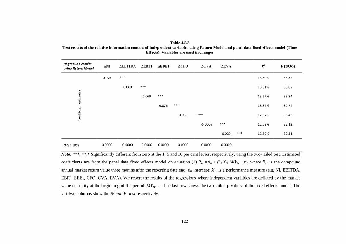
122

Table 4.5.3

Test results of the relative information content of independent variables using Return Model and panel data fixed effects model (Time

Effects). Variables are used in changes


∆NI ∆EBITDA ∆EBIT ∆EBEI ∆CFO ∆CVA ∆EVA R² F (30.65)

Coef

fici

ent

esti

mat

es

0.075 *** 13.30% 33.32

0.060 *** 13.61% 33.82

0.069 *** 13.57% 33.84

0.076 *** 13.37% 32.74

0.039 *** 12.87% 35.45

-0.0006 *** 12.62% 32.12

0.020 *** 12.69% 32.31

p-values 0.0000 0.0000 0.0000 0.0000 0.0000 0.0000 0.0000


coefficients are from the panel data fixed effects model on equation (1) = + / + where is the compound

annual market return value three months after the reporting date end; intercept; is a performance measure (e.g. NI, EBITDA,

EBIT, EBEI, CFO, CVA, EVA). We report the results of the regressions where independent variables are deflated by the market

value of equity at the beginning of the period . The last row shows the two-tailed p-values of the fixed effects model. The

last two columns show the R² and F- test respectively.

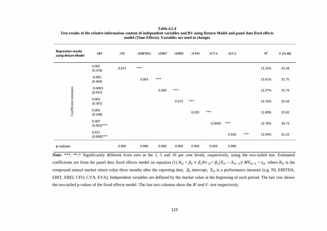
123

Table 4.5.4

Test results of the relative information content of independent variables and BV using Return Model and panel data fixed effects

model (Time Effects). Variables are used in changes


∆BV ∆NI ∆EBITDA ∆EBIT ∆EBEI ∆CFO ∆CVA ∆EVA R² F (21.48)

Coef

fici

ent

esti

mat

es

0.002 (0.376)

0.072 *** 13.32% 32.28

-0.002 (0.469)

0.063 *** 13.61% 32.75

-0.0003 (0.937)

0.069 *** 13.57% 32.74

0.002 (0.391)

0.073 *** 14.76% 32.44

0.003 (0.248)

0.035 *** 12.89% 33.82

0.007 (0.001)***

-0.0005 *** 12.76% 30.73

0.011 (0.000)***

0.026 *** 12.94% 31.22

p-values

0.000 0.000 0.000 0.000 0.000 0.003 0.000


coefficients are from the panel data fixed effects model on equation (1) = + )/ + where is the

compound annual market return value three months after the reporting date, intercept, is a performance measure (e.g. NI, EBITDA,

EBIT, EBEI, CFO, CVA, EVA). Independent variables are deflated by the market value at the beginning of each period. The last row shows

the two-tailed p-values of the fixed effects model. The last two columns show the R² and F- test respectively.

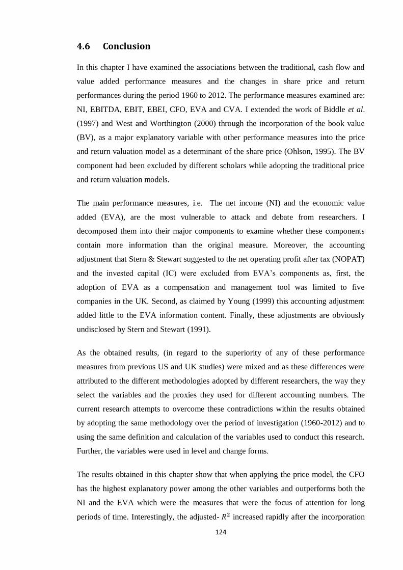
124

4.6 Conclusion

In this chapter I have examined the associations between the traditional, cash flow and

value added performance measures and the changes in share price and return

performances during the period 1960 to 2012. The performance measures examined are:

NI, EBITDA, EBIT, EBEI, CFO, EVA and CVA. I extended the work of Biddle et al.

(1997) and West and Worthington (2000) through the incorporation of the book value

(BV), as a major explanatory variable with other performance measures into the price

and return valuation model as a determinant of the share price (Ohlson, 1995). The BV

component had been excluded by different scholars while adopting the traditional price

and return valuation models.

The main performance measures, i.e. The net income (NI) and the economic value

added (EVA), are the most vulnerable to attack and debate from researchers. I

decomposed them into their major components to examine whether these components

contain more information than the original measure. Moreover, the accounting

adjustment that Stern & Stewart suggested to the net operating profit after tax (NOPAT)

and the invested capital (IC) were excluded from EVA’s components as, first, the

adoption of EVA as a compensation and management tool was limited to five

companies in the UK. Second, as claimed by Young (1999) this accounting adjustment

added little to the EVA information content. Finally, these adjustments are obviously

undisclosed by Stern and Stewart (1991).

As the obtained results, (in regard to the superiority of any of these performance

measures from previous US and UK studies) were mixed and as these differences were

attributed to the different methodologies adopted by different researchers, the way they

select the variables and the proxies they used for different accounting numbers. The

current research attempts to overcome these contradictions within the results obtained

by adopting the same methodology over the period of investigation (1960-2012) and to

using the same definition and calculation of the variables used to conduct this research.

Further, the variables were used in level and change forms.

The results obtained in this chapter show that when applying the price model, the CFO

has the highest explanatory power among the other variables and outperforms both the

NI and the EVA which were the measures that were the focus of attention for long

periods of time. Interestingly, the adjusted- increased rapidly after the incorporation

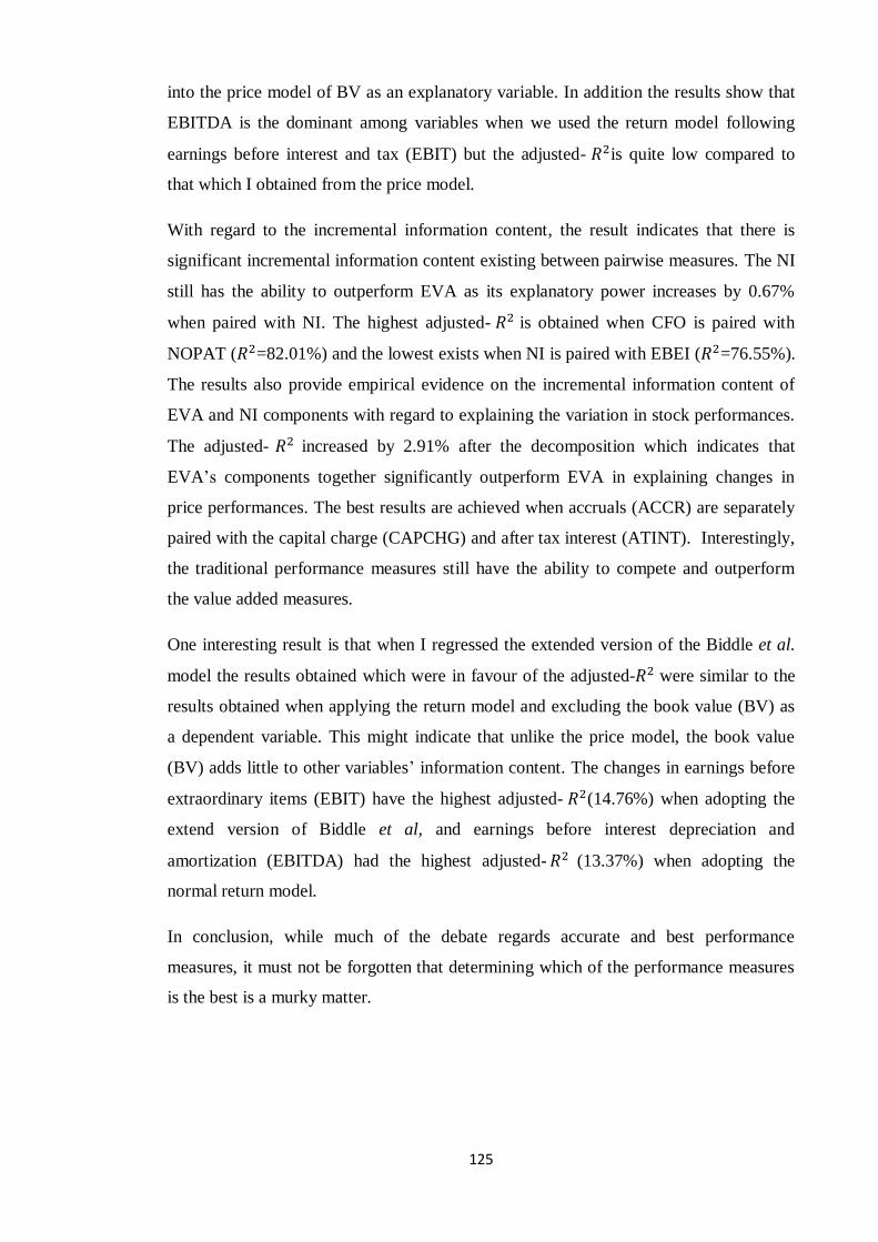
125

into the price model of BV as an explanatory variable. In addition the results show that

EBITDA is the dominant among variables when we used the return model following

earnings before interest and tax (EBIT) but the adjusted- is quite low compared to

that which I obtained from the price model.

With regard to the incremental information content, the result indicates that there is

significant incremental information content existing between pairwise measures. The NI

still has the ability to outperform EVA as its explanatory power increases by 0.67%

when paired with NI. The highest adjusted- is obtained when CFO is paired with

NOPAT ( =82.01%) and the lowest exists when NI is paired with EBEI ( =76.55%).

The results also provide empirical evidence on the incremental information content of

EVA and NI components with regard to explaining the variation in stock performances.

The adjusted- increased by 2.91% after the decomposition which indicates that

EVA’s components together significantly outperform EVA in explaining changes in

price performances. The best results are achieved when accruals (ACCR) are separately

paired with the capital charge (CAPCHG) and after tax interest (ATINT). Interestingly,

the traditional performance measures still have the ability to compete and outperform

the value added measures.

One interesting result is that when I regressed the extended version of the Biddle et al.

model the results obtained which were in favour of the adjusted- were similar to the

results obtained when applying the return model and excluding the book value (BV) as

a dependent variable. This might indicate that unlike the price model, the book value

(BV) adds little to other variables’ information content. The changes in earnings before

extraordinary items (EBIT) have the highest adjusted- (14.76%) when adopting the

extend version of Biddle et al, and earnings before interest depreciation and

amortization (EBITDA) had the highest adjusted- (13.37%) when adopting the

normal return model.

In conclusion, while much of the debate regards accurate and best performance

measures, it must not be forgotten that determining which of the performance measures

is the best is a murky matter.

126

Chapter 5

The Impact of Economic Value Added (EVA) Adoption

On Stock Performance

5.1 Introduction

It is generally accepted that the role of the executive manager is to maximize the firm’s

value (Wallace, 1997; Malmi and Ikaheimo, 2003). The shareholders of a business

enterprise are better off when its management chooses investment decisions that lead to

maximizing their wealth. Therefore, evaluating a manager’s performance on the basis of

whether it increases the stakeholder’s wealth is a proper approach. To this end, many

performance metrics have been advocated by researchers that examine how well a firm,

and particularly the executive manager of that firm, performs. These methods include:

(i) traditional methods such as accounting earnings or operating profit; (ii) profitability

measures such as return on asset (ROA) or return on investment (ROI); (iii) cash flow

measures; and (iv) value-based performance measures such as residual income (RI)

method and particularly economic value added (EVA) and cash value added (CVA).

Currently the advocated performance tools are the value-based management (VBM) that

takes into consideration the cost of invested capital (debt and equity) when calculating

the increase in wealth a firm generates as a result of this investment, such as the residual

income method (RI). One question that needs to be asked is why this issue has received

such attention? According to Drucker (1995, p.59) “until a business returns a profit that

is greater than its cost of capital, it does not create wealth; it destroys it.” The most

commonly used residual income performance measurement metrics are the economic

value added (EVA) first introduced by Stern & Stewart Co. in 1991, and the cash value

added (CVA) model by the Boston Consulting Group (Malmi and Ikaheimo, 2003).

The vast majority of research has examined whether the adoption of EVA’s incentive

compensation plan has any impact on managers’ investment behaviour (Wallace, 1997;

Kleiman, 1999; Hogan and Lewis, 2005). All of this empirical research has the common

assumption that the adoption of the EVA compensation system will rationalize a firm’s

investment decision and will lead to using the existing assets more efficiently to

generate more residual income and, hence, to maximize shareholders’ wealth as well.

127

The purpose of this chapter is to examine whether the adoption of the EVA framework

enhances the firm’s performance and to gauge the long-term effects of such an adoption

on the firm’s profitability. It also assesses whether the market reacts to the

announcement of the adoption of EVA as a compensation system. The event study

methodology initially introduced by Fama et al. (1969) will be used to assess the impact

of EVA’s adoption on a firm’s performance.

In a corporate context, the usefulness of event studies arises from the fact that the

magnitude of abnormal performance at the time of an event provides a measure of the

(unanticipated) impact of this type of event on the wealth of the firms’ shareholders.

Event studies start with a hypothesis on how a particular event is expected to affect the

value of a firm. The hypothesis that the value of the company has increased (decreased)

will be reflected in the stock showing an abnormal return. Coupled with the notion that

the information is readily contained in prices, the concept of abnormal returns (or

performance) is the key point of event study methods.

The efficient market hypothesis (EMH) states that stock prices fully reflect all publicly

available information and no information or analysis can provide investors with the

opportunity to outperform the market. As a result any news announcement concerning a

company is rapidly subsumed within its stock price and announcements will on average

not affect stock prices beyond a very short period of time. Departing from EMH, when

these announcements take place there might sometimes be an abnormal reaction in the

share prices of the underlying stocks. Such reactions can be measured using the event

study approach where the movement in stock prices around the event dates is analysed

to determine if the event in question has had an effect on the value of the underlying

stocks or not.

The most common approach of the event study involves three steps: (1) The

computation of the parameters in the estimation period; (2) The computing of the

forecast errors (and obtaining variance/covariance information) for a period, or over an

event window; aggregate across firms and infer the average effect; (3) Use the abnormal

returns in a cross –sectional regression against the relevant features of the stock which is

supposed to influence the impact of the event.

The use of the traded market EVA performance measure has grown rapidly since the

1990s in the USA and across different European countries. In the UK there are four

companies that reported the EVA as a performance and management tool. These

128

companies are Tate & Lyle, GSK, Hanson (now Heidelberg) and Diageo. While EVA

was implemented in the late 1990s and early 2000s, some companies may no longer be

using it.27

As a result the focus will be on the USA companies that have adopted EVA

as a management tool and as a compensation system.

The structure of this chapter is organized in the following way. Section 5.2 will discuss

the main results of the previous studies that have investigated the impact of EVA

adoption on a firm’s performance. Section 5.3 describes the sample and section 5.4 the

methodology used. Section 5.5 discusses the empirical results obtained and finally

section 5.6 summarises the main conclusions.

5.2 Previous studies

There is an underlying assumption that firms adopting the residual income method have

the ability to enhance their profitability and maximize shareholder’s wealth. This can be

achieved by increasing a firm’s ability to generate a large residual income and

encourage managers to invest in those projects that can earn more than the cost of the

capital invested. Furthermore, EVA’s proponents claim that the adoption of the EVA

framework will affect the manager’s behaviour and lead to the best alignment of

management interests with those of the shareholders (Stewart, 1991; Wallace, 1997). To

address this growing issue, several empirical studies were conducted to explore whether

the adoption of residual income-based performance incentives, namely the adoption of

the EVA framework, will lead to any differences in firms’ investment patterns (Wallace

1997: Kleiman, 1999; Sharma and Kumar, 2010). However, the results have been

mixed.

Wallace’s (1997) study is a seminal contribution that addressed the changes in

profitability that a firm achieves when adopting EVA. Wallace’s methodology has been

replicated by a number of scholars such as Kleiman (1999), Hogan and Lewis (2005)

and Balachandran (2006). Wallace (1997) compared a group of forty companies

adopting residual income (RI) as a compensation plan with the same number of control

firms to examine whether the adoption of RI, the investing decision, finance decision,

operating decision and shareholder wealth would increase or decrease within three post

27 Source: Stern Stewart Ltd. London Branch dated March 15, 2012.

129

adoption periods. Wallace’s methodology has been discussed in detail in chapter 6 of

the current study.

In a closely related study, Kleiman (1999) extended Wallace’s methodology by using a

sample of 71 firms adopting EVA as an incentive compensation system. Based on US

data for the period 1987-96, he examined the impacts of the adoption of EVA on

shareholders’ value. He also replicated the same method used by Wallace (1997) to

estimate the ‘closest-matched peer firm’ (the control firms). Unlike Wallace, the focus

was limited to those firms that adopted the EVA compensation plan rather than the RI-

based compensation plan and on the consequences of the EVA adoption on

shareholders’ value rather than on the improvement of firms’ operating performances.

The findings of Kleiman (1999) were that all the EVA adopters show a significant and

higher stock performance (return) than their competitors, the peer companies, while

before the adoption date they were equivalent with regard to their stock performances.

Turning to operating performance analysis, the findings of Kleiman contend that firms

were monitoring their working capital regardless of the incentive compensation plan

they adopted. Moreover, his results do not show any capital expenditure decline, the

manager’s behaviour has no obvious bias against new investment which is a finding

inconsistent with that of Wallace (1997). Further, consistent with theoretical arguments

and as Wallace (1997) reported, EVA-adopting companies significantly increase their

financial leverage. This increase is mostly achieved through extended share repurchases.

Finally, the results show substantial enhancement in both operating margins and

operating profits before depreciation.

Responding to the criticism that was raised against Wallace’s (1997) work, Hogan and

Lewis (2005) used a sample of 108 firms that chose to adopt the economic profit plans

(EPPs) as incentive compensation systems between 1983 and 1996 to examine whether

the adoption would affect these firms’ operating, organizational, financial and

compensation characteristics. Unlike Wallace and probably to account for the pre-

adoption performances they estimate a logistic regression model to select the optimal

control-matched firms. Accordingly, their control firms’ sample fall into four

categories: anticipated adopters, surprise adopters, anticipated non-adopters, and

surprise non-adopters. They then compare the performances of these categories to assess

whether adopting firms will outperform firms that are predicted to adopt EPPs but do

130

not. The focus of their research has been on analysing whether the adoption firms will

achieve the same increases in their performance if they chose to continue using

traditional performance-based compensation plans. Furthermore, they replicate the same

method used by Wallace (1997).

The findings of Hogan and Lewis (2005) reveal that all EPP adopter firms show a

significant enhancement in operating performance relative to their past performance

(pre-adoption period). In addition they show a significant difference in investment

behaviour, operating performance and value creation. This result is consistent with the

notion that an EPP-based compensation system encourages managers to choose

profitable projects that ultimately maximize shareholders’ wealth. Turning to the

control-matched firms’ categories and the comparison of the performance of anticipated

adopter firms to that of surprise non-adopters the findings of Hogan and Lewis reveal

that adopter firms used the operating asset more efficiently, improved their operating

performance, and maximized outstanding shareholder wealth. This is consistent with

Wallace’s findings (1997). However, their results fail to show a significant

improvement when compared with anticipated non-adopters and surprise adopter firms.

Similarly, Balachandran (2006) investigated whether switching from tradition

accounting-based performance plans, specifically earnings and returns on investment-

based compensation plans, to an EVA- based compensation incentive will affect the

investment motif. He used a sample of 181 firms that adopted the residual income (RI)-

based compensation incentive. These firms fell into two main categories: those which

previously adopted earnings as a compensation plan and then shifted to RI-based

compensation plan and those that adopted ROI-based compensation plan.

The criterion that Balachandran used to judge whether there is any difference in

investment patterns is the firm’s ability to generate more residual income after the

adoption (the delivered RI is likely to improve). Furthermore, he applied three

specifications to conduct his test. In the first and second specifications the firm used its

own controls but the control variables are different for each specification

(Balachandran, 2006. p.390). Finally, he used both the adopted firm and the matched

firm as a control variable.

Balachandran concludes that the results regarding the control variable used are mixed.

For the first specification the results show a significant difference in the investment

131

pattern when the firm switched from an earning-based compensation plan to an RI-

based compensation incentive; the second specification shows the same significant

difference for firms which switched from an ROI- based compensation plan while the

third specification shows no significant difference in investment pattern. Turning to the

delivered RI, the results show that the generated RI is increased when firms adopted the

RI-based compensation plan. Finally, his conclusion is consistent with Wallace’s (1997)

notion that “you get what you pay for”.

However, in Wallace’s and Balachandran’s (2006) analyses of the firms that adopted

the residual income-based compensation plan, they did not indicate whether these firms

specifically adopted the EVA framework. Thus, the findings of their research will not

only attribute to EVA a compensation technique but this advantage should be traced to

all residual income (RI) methods. Kleiman (1999) limited his sample to those firms that

adopted the EVA framework and discussed the impact of EVA’s adoption on the firm’s

ability to maximize shareholder value. This will more effectively indicate whether the

enhancement the companies have achieved regarding stock price performance could be

attributed directly to its ability to generate more operating income after adoption rather

than to the existing economic circumstances in the market where all these firms operate.

Hopefully, Kleiman’s finding will respond well to the question that has received much

attention in the literature: could “EVA and residual income prove effective in

motivating managers for shareholder wealth creation” (Sharma and Kumar, p. 205).

In a similar work, Lovata and Costigan (2002) used a sample of 115 US firms to

examine the characteristics of firms that have integrated EVA into an incentive

compensation system. The theory’s assumption is that the adoption of the EVA

framework will better align the managers’ interests with those of the shareholders which

would mitigate the moral hazard issue. Their claim was that firms which experience

high agency conflicts are more likely to adopt the EVA-based compensation plan.

Lovata and Costigan make a comparison between companies adopting EVA and

companies that have not in order to investigate whether the adoption of an EVA

compensation plan will alleviate the agency conflicts. They used the agency theory

variables such as the firm coefficient of risk Beta, institutional ownership, insider

ownership, and R&D/Sales ratio to test the implication of adopting EVA for

organizational behaviour and characteristics.

132

The results of Lovata and Costigan show that the EVA compensation system is suitable

for the companies that have the following characteristics: (i) less insider ownership, (ii)

high proportion of institutional investors, and (iii) companies that maintain a lower

R&D/Sales ratio. However firms where their current earnings have less power to predict

future success tend to use performance measures rather than the EVA metric.

Additionally, as the abovementioned studies point out, the EVA technique may be used

for two purposes. It is adopted as a decision making tool and used as a compensation

incentive plan. In the literature, firms usually first adopt the EVA framework as a

management tool and then introduce it as their incentive compensation scheme (Ittner

and Larcker, 1998) However, they claim that the majority of firms introduce the EVA

framework for decision making, rather than as an incentive compensation plan.

Previous tests have encountered several difficulties in addressing this argument. The

reason is simple: you cannot formally test different and unrelated samples. Our data on

the other hand enable testing across all available news types because they are from the

same sample. The sample selection processes will be explained in detail in section 5.3

below.

5.3 Sample

This chapter aimed to examine the consequences of adopting the EVA compensation

incentives plan. The sample comprises US firms that have chosen to adopt the EVA

compensation system. Consistent with Wallace, 1997 and Kleiman (1999) the first year

of the company announcing its adoption of EVA is defined as the event year, and for the

purpose of the current research we consider the month of December of that year as an

event date ( ). Initially, we start with Wallace’s 23 firms that adopted the EVA

compensation plan. This list of adopter firms was then updated by Kleiman and the

number of EVA adopters was increased to 71 firms. Then, we began our search using

various databases where the EVA-implementing firms may be identified. These

comprise the Stern Stewart & Co. brochure, Lexis-Nexis, Proxy Statement, 10-Q report

and Wall Street Journal. The majority of firms which adopted EVA have disclosed such

information in their official release. For example, RR Donnelley & Sons Co. states in its

10-Q report:

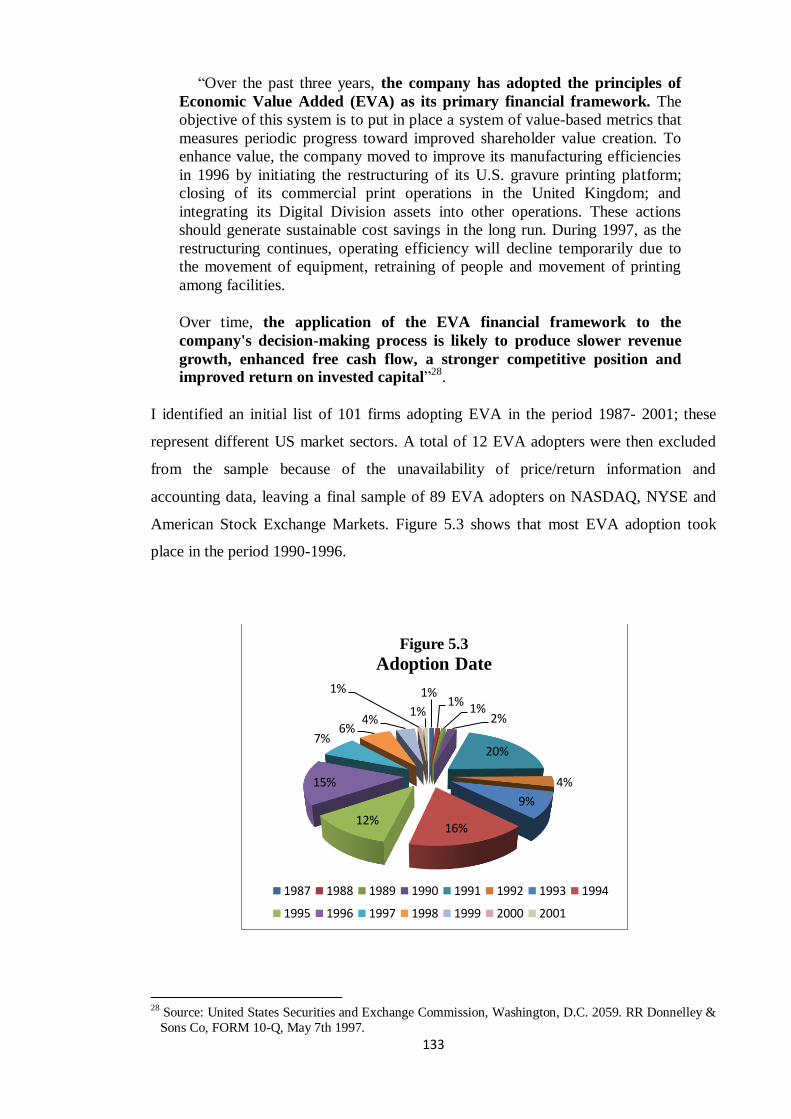
133

“Over the past three years, the company has adopted the principles of

Economic Value Added (EVA) as its primary financial framework. The

objective of this system is to put in place a system of value-based metrics that

measures periodic progress toward improved shareholder value creation. To

enhance value, the company moved to improve its manufacturing efficiencies

in 1996 by initiating the restructuring of its U.S. gravure printing platform;

closing of its commercial print operations in the United Kingdom; and

integrating its Digital Division assets into other operations. These actions

should generate sustainable cost savings in the long run. During 1997, as the

restructuring continues, operating efficiency will decline temporarily due to

the movement of equipment, retraining of people and movement of printing

among facilities.

Over time, the application of the EVA financial framework to the

company's decision-making process is likely to produce slower revenue

growth, enhanced free cash flow, a stronger competitive position and

improved return on invested capital”28

.

I identified an initial list of 101 firms adopting EVA in the period 1987- 2001; these

represent different US market sectors. A total of 12 EVA adopters were then excluded

from the sample because of the unavailability of price/return information and

accounting data, leaving a final sample of 89 EVA adopters on NASDAQ, NYSE and

American Stock Exchange Markets. Figure 5.3 shows that most EVA adoption took

place in the period 1990-1996.

28 Source: United States Securities and Exchange Commission, Washington, D.C. 2059. RR Donnelley &

Sons Co, FORM 10-Q, May 7th 1997.

1% 1%

1% 2%

20%

4%

9%

16% 12%

15%

7% 6%

4%

1%

1%

Figure 5.3

Adoption Date

1987 1988 1989 1990 1991 1992 1993 1994

1995 1996 1997 1998 1999 2000 2001

134

Assessing abnormal performance is tricky. Barber and Lyon (1996) favour the use of

control firms in calculating abnormal return that would alleviate the problems of the

misspecification that resulted from the bias occurring because of the inclusion of new

listed firms in the market index portfolio and the rebalancing process of market index

(portfolio). Given the advantages of the control firm approach, I followed in the steps of

Wallace (1997). I began by determining the Standard Industrial Classification (SIC)

code of adopter companies using the Centre for Research in Security Prices CRSP and

COMPUSTAT database. Subsequently, I selected a sample of the best matched

controlling firms that closely resembled the event firm to compare their performance.

The prices and returns data of both adopting and control firms that were used to analyse

the long-term effects of adoption were collected using CRSP. The selection processes of

the controlling firms were based on the following criteria:

1. The company should have the same 4-digits SIC code (Same industry sector). If

not, we chose the best matched company with a 3-digits SIC code.

2. Size: we used the total asset and number of outstanding common shares in the

year prior to the year of adoption to match adopters and control firms.

3. Time period: the control firm should have sufficient annual data and its

operating period should match that of the adopting firms’ operating period.

Table 5.3 provides a breakdown of firms adopting EVA and the year of adoption, the

main control firms and the SIC code respectively.

Another potential problem might be self-selection bias. This is mainly due to the

possibility that those firms that selected EVA belong to a certain class of performance.

Thus, comparing EVA adopters to non-EVA adopters might simply reflect their

inherent superior performance and not the effect of adopting EVA. Fortunately, this

concern is not justified for the simple reason that the control firms use residual income

and this latter is very similar to EVA. Given that the control firms are matched as

precisely as possible, the difference in performance, if any, can be relatively safely

attributed to the adoption of EVA.

135

Table (5.3) EVA Adopting Companies 1987-2001(USA)

NO. SAMPLE COMPANY ADOPTION

YEAR CONTROL COMPANY SIC CODE

1 COCA COLA 1987 PEPSICO INC 2080

2 CSX CORPORATION 1988 SANTA FE FINANCIAL CORP 6711

3 CILCORP 1989 ALLETE INC 4931

4 CRANE CO 1990 WHITTAKER CORP 3490/3494

5 BRIGGS & STRATTON 1990 STEWART & STEVENSON SVCS INC 3510/3519

6 QUAKER OATS 1991 RALSTON PURINA CO 2040/2043

7 BALL CORP 1992 CROWN HOLDINGS INC 3221

8 WHIRLPOOL CORP 1992 AKTIEBOLAGET ELECTROLUX 3630

9 AT&T 1992 G T E CORP 4813

10 SCHERER, R.P. 1992 FOREST LABS INC 2834

11 WELLMAN 1993 ASHLAND INC NEW 2824

12 GRAINGER, W.W. 1993 WAXMAN INDUSTRIES INC 5063

13 MANITOWOC CO 1993 ASTEC INDUSTRIES INC 3531

14 DIGITAL EQUIPMENT CORP 1993 APPLE INC 3573

15 FURON CORP. 1993 WYNNS INTERNATIONAL INC 3079

16 HARNISCHFEGER IND. INC. 1993 APPLIED MATERIALS INC 3536

17 HEWLETT PACKARD CO. 1993 HITACHI LIMITED 3571

18 RUBY TUESDAY INC. 1993 WORLDWIDE RESTAURANT CNCPTS INC

5812

19 SMITH INTERNATIONAL INC. 1993 CABOT CORP 3533

20 TRANSAMERICA CORP 1993 LOEWS CORP 6711

21 ACXIOM CORP 1994 MCGRAW HILL COS INC 7370

22 BOISE CASCADE CORP 1994 BT OFFICE PRODUCTS INTL INC 2421

23 FLEMING COMPANIES INC 1994 NASH FINCH COMPANY 5141

24 GEORGIAPACIFIC GROUP 1994 WEYERHAEUSER CO 2435

25 LILLY (ELI) & CO 1994 WYETH 2834

26 SPRINT FON GROUP 1994 CENTEL CORP 4813

27 CENTURA BANKS INC 1994 AMERICAN FLETCHER CORP 6036

28 CORE INDUSTRIES INC. 1994 WHITTAKER CORP 3429

29 DEERE & CO. 1994 KUBOTA CORP 3523

30 EASTMAN CHEMICAL CO. 1994 ROHM & HAAS CO 3861

136

Table (5.3) continued.


YEAR CONTROL COMPANY

SIC

CODE

31 GENCORP INC. 1994 LOCKHEED MARTIN CORP 3011

32 INCSTAR CORP. 1994 A M A G PHARMACEUTICALS INC 2830

33 INSTEEL INDUSTRIES 1994 NATIONAL STANDARD CO 3310

34 OHIO EDISON CO. 1994 NORTHEAST UTILITIES 4911

35 REYNOLDS METALS CO. 1994 KAISERTECH LTD 3353

36 TENNECO INC. 1994 CHAMPION PARTS INC 3714

37 WALLACE COMPUTER SERVICES 1994 MOORE WALLACE INC 2761

38 ZOLTEK COS. INC. 1994 WOODWARD INC 3620

39 ARMSTRONG HOLDINGS INC 1995 NEWELL RUBBERMAID INC 2511

40 BARD (C.R.) 1995 TELEFLEX INC 5086

41 PERKINELMER INC 1995 BIO RAD LABORATORIES INC 3823

42 SPX CORP 1995 GIDDINGS & LEWIS INC WIS 3540

43 AMERICAN PRECISION IND. 1995 FRANKLIN ELECTRIC INC 3443

44 ARMSTRONG WORLD INDUSTRIES INC.

1995 E G & G INC (VISKASE COMPANIES) 2511

45 BECKMAN INSTRUMENTS INC. 1995 PERKINELMER INC 5311

46 EMERSON ELECTRIC CO. 1995 PANASONIC CORP 3621/3823

47 IPALCO ENTERPRISES INC. 1995 TUCSON /U N S ENERGY CORP 4911

48 KAISER ALLUMINUM CORP. 1995 MAXXAM INC 3334

49 KNIGHT–RIDDER INC. 1995 NEW YORK TIMES CO 2711

50 NEW JERSEY RESOURCES 1995 ATMOS ENERGY CORP 4924

51 SEQUENT COMPUTER 1995 STRATUS COMPUTER INC 3570

52 ADC TELECOMMUNICATIONS INC 1996 TELLABS INC 3679

53 BAUSCH & LOMB INC 1996 CHIRON CORP 3861

54 BECTON DICKINSON & CO 1996 BARD C R INC 3841

55 DONNELLEY (R R) & SONS CO 1996 BOWNE & CO INC 3229

56 GUIDANT CORP 1996 MEDTRONIC INC 3841

57 KANSAS CITY POWER & LIGHT 1996 C M P GROUP INC 4911

58 OLIN CORP 1996 F M C CORP 2810

59 SILICON VY BANCSHARES 1996 AMSOUTH BANCORPORATION 6022/6710

60 TUPPERWARE CORP 1996 ENVIRODYNE INDUSTRIES INC 3089

137

Table (5.3) continued.


YEAR CONTROL COMPANY

SIC

CODE

61 MILLER HERMAN 1996 H N I CORP 2531

62 CINCINNATI MILACRON 1996 KENNAMETAL INC 3541

63 HACH CO. 1996 COHERENT INC 3820

64 KLLM TRANSPORT SERVICES 1996 MATLACK SYSTEMS INC 4210

65 NEW ENGLAND BUSINESS SERVICES 1996 ENNIS INC 2761

66 QUAKER STATE 1996 TESORO CORP 2911

67 STRATTEC SECURITY CORP 1996 F M C CORP 8740

68 TEKTRONIX 1996 SNAP ON INC 3825

69 CDI CORP 1997 ROBERT HALF INTL INC 3269

70 GC COMPANIES INC 1997 MARCUS CORP 7830

71 JOHNSON OUTDOORS INC 1997 ELECTRO SCIENTIFIC INDS INC 3940

72 MILLENNIUM CHEMICALS INC 1997 BIG THREE INDS INC 2813

73 PHARMACIA CORP 1997 BAUSCH & LOMB INC 2823

74 RYDER SYSTEM INC 1997 ROLLINS TRUCK LEASING CORP 6159

75 TENET HEALTHCARE CORP 1997 UNIVERSAL HEALTH SERVICES INC 8062

76 WEBSTER FINL CRP WATERBURY 1997 AMSOUTH BANCORPORATION 6035

77 FEDERALMOGUL CORP 1998 DANA HOLDING CORP 3562

78 MATERIAL SCIENCES CORP 1998 SHAW GROUP INC 3470

79 MONTANA POWER CO 1998 C H ENERGY GROUP INC 4911

80 PENNEY (J C) CO 1998 DILLARDS INC 5311

81 STANDARD MOTOR PRODS 1998 HARBINGER GROUP INC 3694

82 BRADLEY PHARMACEUTICALS 1998 BALCHEM CORP 2830/5120

83 BEST BUY CO INC 1998 RADIOSHACK CORP 5732

84 INTERNATIONAL MULTIFOODS 1999 RALSTON PURINA CO 2041

85 TOYS R US INC 1999 MICHAELS STORES INC 6711

86 GENESCO 1999 FOOT LOCKER INC 2341

87 MOLSON COORS 1999 ANHEUSER BUSCH COS INC 2082

88 SCHNITZER STEEL 2000 ENVIROSOURCE INC 3310

89 HARSCO 2001 DYNAMIC MATERIALS CORP 3446

Source: Wallace, 1997 and Kleiman (1999), Stern Stewart & Co. brochure, Lexis-Nexis, Proxy

Statement and 10-Q report and Wall Street Journal.

138

5.4 Methodology

Defenders of economic value added (EVA) claim that it helps to enhance the investment

activity that leads to a notable market reaction (Stewart, 1991). The object of the current

research is to examine whether the adoption of EVA has the predicted effects on

investment behaviour. If the market reacts to this claim we should observe some

enhancement in stock performance (abnormal return). In order to test this claim we use

the event study methodology. In practice event study methodology has been used for

two fundamental reasons: 1) to test the market efficiency, particularly testing the null

hypothesis that the market (price) incorporates all the public information efficiently and

2) to assess the impact of some event announcement on the firm’s wealth.

Fama et al. (1969) made two modifications to the event study methodology which have

later become standard. First, in their response to the market’s stationarity concern they

suggested five to seven years data as an optimal period for monthly observation studies.

Second, they stated that if the event date is included in the event’s window to estimate

the parameters, the estimation process will lead to a bias coefficient because the

disturbances are non-zero. This bias is in decline as long as the data periods matched

that of Fama et al. (1969).

The current research will use the same methodology as Wallace’s (1997) except that

while Wallace’s sample consists of those firms adopting a residual income-based

management system, this research uses only firms adopting EVA for incentive

compensation purposes. Moreover, while Wallace used a five-year return to conduct his

research, the current research uses the monthly market returns and focuses on long-term

abnormal stock return where we use statistics to detect monthly abnormal returns for the

period 1960-2012. In order to estimate the parameters of the return equation, our sample

includes observations since the 1960s prior to the adoption, the year of adoption, and up

to the year 2012 after the adoption. The estimated event study window is set between 30

months prior to the adoption date and 30 months after the adoption. However, as it is

difficult to determine the accurate date of EVA adoption we consider the month of

December, the earliest year the company released the adoption of EVA, as the event

date.

Many studies have discussed and examined the long-term financial performances after

the occurrences of certain events such as the IPO, mergers and acquisitions and the most

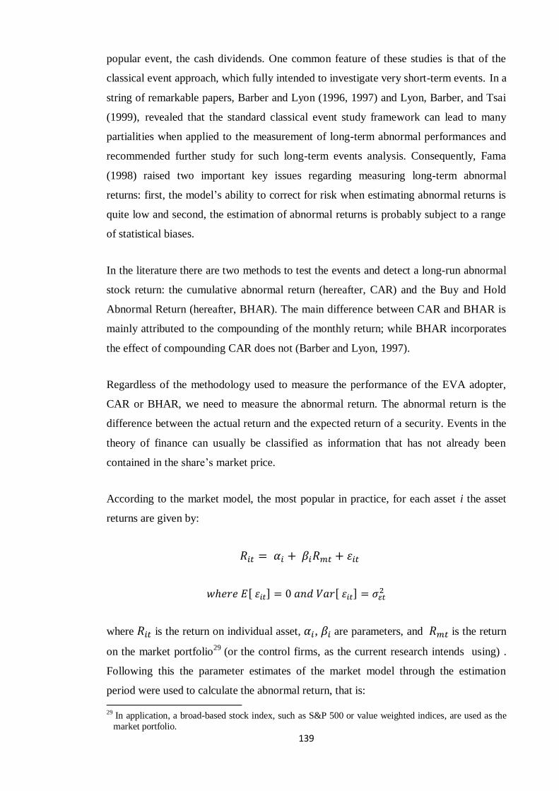
139

popular event, the cash dividends. One common feature of these studies is that of the

classical event approach, which fully intended to investigate very short-term events. In a

string of remarkable papers, Barber and Lyon (1996, 1997) and Lyon, Barber, and Tsai

(1999), revealed that the standard classical event study framework can lead to many

partialities when applied to the measurement of long-term abnormal performances and

recommended further study for such long-term events analysis. Consequently, Fama

(1998) raised two important key issues regarding measuring long-term abnormal

returns: first, the model’s ability to correct for risk when estimating abnormal returns is

quite low and second, the estimation of abnormal returns is probably subject to a range

of statistical biases.

In the literature there are two methods to test the events and detect a long-run abnormal

stock return: the cumulative abnormal return (hereafter, CAR) and the Buy and Hold

Abnormal Return (hereafter, BHAR). The main difference between CAR and BHAR is

mainly attributed to the compounding of the monthly return; while BHAR incorporates

the effect of compounding CAR does not (Barber and Lyon, 1997).

Regardless of the methodology used to measure the performance of the EVA adopter,

CAR or BHAR, we need to measure the abnormal return. The abnormal return is the

difference between the actual return and the expected return of a security. Events in the

theory of finance can usually be classified as information that has not already been

contained in the share’s market price.

According to the market model, the most popular in practice, for each asset i the asset

returns are given by:

where is the return on individual asset, , are parameters, and is the return

on the market portfolio29

(or the control firms, as the current research intends using) .

Following this the parameter estimates of the market model through the estimation

period were used to calculate the abnormal return, that is:

29 In application, a broad-based stock index, such as S&P 500 or value weighted indices, are used as the

market portfolio.

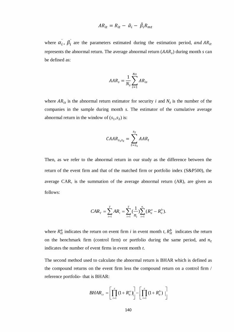
http://en.wikipedia.org/wiki/Financial_market

140

where ,

are the parameters estimated during the estimation period,

represents the abnormal return. The average abnormal return ( ) during month s can

be defined as:

where is the abnormal return estimator for security i and is the number of the

companies in the sample during month s. The estimator of the cumulative average

abnormal return in the window of ( , ) is:

Then, as we refer to the abnormal return in our study as the difference between the

return of the event firm and that of the matched firm or portfolio index (S&P500), the

average CAR, is the summation of the average abnormal return (AR), are given as

follows:

tn

t

b

it

a

it

T

t

T

t t

tT RRn

ARCAR11 1

).()1

(

where indicates the return on event firm i in event month t,

indicates the return

on the benchmark firm (control firm) or portfolio during the same period, and

indicates the number of event firms in event month t.

The second method used to calculate the abnormal return is BHAR which is defined as

the compound returns on the event firm less the compound return on a control firm /

reference portfolio- that is BHAR:

11

)1()1(t

b

it

t

a

iti RRBHAR

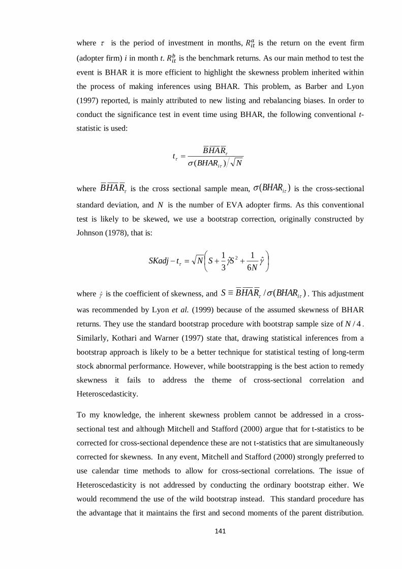
141

where is the period of investment in months, is the return on the event firm

(adopter firm) i in month t. is the benchmark returns. As our main method to test the

event is BHAR it is more efficient to highlight the skewness problem inherited within

the process of making inferences using BHAR. This problem, as Barber and Lyon

(1997) reported, is mainly attributed to new listing and rebalancing biases. In order to

conduct the significance test in event time using BHAR, the following conventional t-

statistic is used:

NBHAR

RAHBt

i )(

where RAHB is the cross sectional sample mean, )( iBHAR is the cross-sectional

standard deviation, and N is the number of EVA adopter firms. As this conventional

test is likely to be skewed, we use a bootstrap correction, originally constructed by

Johnson (1978), that is:

ˆ6

1ˆ

3

1 2

NSSNtSKadj

where is the coefficient of skewness, and )(/ iBHARRAHBS . This adjustment

was recommended by Lyon et al. (1999) because of the assumed skewness of BHAR

returns. They use the standard bootstrap procedure with bootstrap sample size of 4/N .

Similarly, Kothari and Warner (1997) state that, drawing statistical inferences from a

bootstrap approach is likely to be a better technique for statistical testing of long-term

stock abnormal performance. However, while bootstrapping is the best action to remedy

skewness it fails to address the theme of cross-sectional correlation and

Heteroscedasticity.

To my knowledge, the inherent skewness problem cannot be addressed in a cross-

sectional test and although Mitchell and Stafford (2000) argue that for t-statistics to be

corrected for cross-sectional dependence these are not t-statistics that are simultaneously

corrected for skewness. In any event, Mitchell and Stafford (2000) strongly preferred to

use calendar time methods to allow for cross-sectional correlations. The issue of

Heteroscedasticity is not addressed by conducting the ordinary bootstrap either. We

would recommend the use of the wild bootstrap instead. This standard procedure has

the advantage that it maintains the first and second moments of the parent distribution.

142

The difference between these corrections methods, the ordinary and wild bootstrap, is

simple. Assume that the residuals from a regression are i (in our case

RAHBBHARii ). In the regular ordinary bootstrap we resample by drawing

NN * residuals,*ˆi , with replacement from the series i . In the wild bootstrap we

produce the bootstrap residuals *ˆi as the product of the original residuals and an

independent random variable, i , with zero mean and unit variance. This ensures that

the bootstrap variance will be the same as that of the parent distribution. For example,

i can be standard normal and hence

0)ˆ()()ˆ( * iii EEE and )ˆ()ˆ()()ˆ( *

iiii VVVV

However, if the data is skewed, re-sampling based on the standard normal will yield

zero skewness since 0)( 3 iE . To preserve skewness, Liu (1988) and Mammen (1993)

suggest ways of obtaining 1)( 3 iE . One suggestion is:

ppw

ppw

i

1..2

51

52

15..

2

51

This will guarantee that 0)( iE , and 1)()( 32 ii EE . However, this scheme will

not preserve the kurtosis of the parent distribution since 2)( 4 iE . An alternative

scheme (see Davidson et al. (2007)) is to use

ppw

ppwi

1..12

1..1

This will preserve the mean, variance and kurtosis ( 0)( iE , and 1)()( 42 ii EE )

but not skewness ( 0)( 3 iE ). Accomplishing both preservations is not possible.

Davidson et al. (2007) recommend some combination that will achieve partial

refinement. However, here we advocate combining the skewness adjusted t-statistic

with the kurtosis preserving wild bootstrap. Providing the skewness adjustment of

Johnson (1978) is fairly accurate, the parent distribution of the adjusted statistic is

143

expected to be symmetric. Therefore, achieving 1)( 4 iE will be more important than

achieving 1)( 3 iE . Accordingly, we adopt this combined Skewness-Adjusted and

Kurtosis Preserving Bootstrap approach in our tests.

A further serious problem that we confront both in the EVA adopter sample and the

control firm sample is that of firms that de-list within the measurement period. Delisting

can result from acquisition, bankruptcy or going private. Liu and Strong (2006) replace

de-listed firm returns by either zero or the risk-free rate. They find similar results in

both cases. Lyon, Barber and Tsai (1999) and Mitchell and Stafford (2000, p.298)

replace all de-listed firms with the benchmark return. This has the potential to create an

upward bias in the estimated BHAR returns, since some of these de-listings are

bankruptcies. However, for the purpose of our study we use the following rules. If an

observation is missing within a valid set of observations we set the return equal to zero.

If the de-listings are due to bankruptcy we replace the missing return by -1. Finally, if

the delisting is due to a value preserving event such as a merger, we replace the return

by the benchmark return. We use CRSP description as a distinguishing feature of the

delisted firms. The Delisting Code is a 3-digit integer code. It either (1) indicates that a

security is still trading or (2) provides a specific reason for delisting. All delisting codes

are categorized by the first digit of the delisting code. The second and third digits of the

delisting codes provide further details of delisting events. Additional delisting codes,

specific to various delisting categories, have been created to indicate when an issue is

closed to further research, or if the issue is pending further research. The most important

codes are 241, 231, 233, 331, 251, 552 and 574. These categories of delisting are most

likely to be stocks that are either worthless or some distance from providing

shareholders with any terminal value, and consequently we treat these cases as if

investors lost all their investment. Table 5.4 describes these delisting codes.

It should be noted that benchmarking using the pre-event period from the same event

firm is not used in this thesis. Previous authors have warned against using this approach.

Specifically, Wallace (1997, p.281) states “Two major validity threats to the analysis of

an interrupted time series are the possibility that (1) some event other than the treatment

(a history threat), or (2) natural changes in a firm through time (a maturation threat) cause

the change in the time series (Cook and Campbell, 1979). The using of a properly selected

control group decreases these threats since both treatment and control firms are subject to

potential omitted variables and primarily differ based on the partitioning variable.”

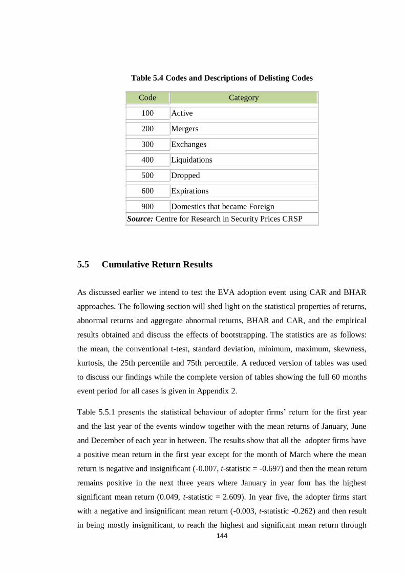
144

Table 5.4 Codes and Descriptions of Delisting Codes

Code Category

100 Active

200 Mergers

300 Exchanges

400 Liquidations

500 Dropped

600 Expirations

900 Domestics that became Foreign

Source: Centre for Research in Security Prices CRSP

5.5 Cumulative Return Results

As discussed earlier we intend to test the EVA adoption event using CAR and BHAR

approaches. The following section will shed light on the statistical properties of returns,

abnormal returns and aggregate abnormal returns, BHAR and CAR, and the empirical

results obtained and discuss the effects of bootstrapping. The statistics are as follows:

the mean, the conventional t-test, standard deviation, minimum, maximum, skewness,

kurtosis, the 25th percentile and 75th percentile. A reduced version of tables was used

to discuss our findings while the complete version of tables showing the full 60 months

event period for all cases is given in Appendix 2.

Table 5.5.1 presents the statistical behaviour of adopter firms’ return for the first year

and the last year of the events window together with the mean returns of January, June

and December of each year in between. The results show that all the adopter firms have

a positive mean return in the first year except for the month of March where the mean

return is negative and insignificant (-0.007, t-statistic = -0.697) and then the mean return

remains positive in the next three years where January in year four has the highest

significant mean return (0.049, t-statistic = 2.609). In year five, the adopter firms start

with a negative and insignificant mean return (-0.003, t-statistic -0.262) and then result

in being mostly insignificant, to reach the highest and significant mean return through

145

the five year window (0.052, t-statistic = 4.204). Subsequently, the mean return of

whole adopter firms decreases and continues to be insignificant. The last two months of

year five reveal a poor and insignificant increase in the mean return. The EVA adopter

firms exhibit lower skewness and kurtosis than matching firms. The result shows that

adopter firms have the highest skewness (3.270) and kurtosis (22.470) in month 25. One

important observation is that the adopter firms begin to generate a negative return

during the first three months after the adoption event.

Similarly, Table 5.5.2 describes the same descriptive statistics of matching firms

(control firms). The matching firms are notable for its positive mean return (few with

negative mean returns). The cross-sectional mean matching firms’ return fluctuates

from -0.003 to 0.028. Another notable feature of matching firms is that skewness and

kurtosis are relatively higher than in adopter firms and highly volatile, attaining a

maximum of 8.1 (skewness) and 71.74 (kurtosis) in month 42. However, the volatility

difference between the benchmark and the event asset may seriously distort the

performance of tests on CAR. Unlike the adoption firms, the match firm shows a

positive return during the three months following the adoption date.

Turning to the abnormal return (AR) which is obtained by subtracting the matching

firms’ return from EVA adopters’ returns, Table 5.5.3 shows that the whole adopter

firms’ performance varies from month to month. Month 11, 52 and 56 are the only

months that appear to be statistically significant where AR and t- Conventional are

(0.027, 2.337), (0.078, 4.579) and (-0.044, -2.641) respectively. It is common to find

adopter firms underperforming the matching firms in many months during the event

window. However, the matching firms showed some performance improvement during

the subsequent months of the date of the adoption. Put simply the matching firms

outperform adopting firms in most of the months that followed the adoption.

Table 5.5.4 reveals an interesting story about the overall performance, the cumulative

abnormal return (CAR) for the 10 years after the adoption date. Most of the CARs

appear to be positive but insignificant except for the months 27, 28, 29 and 30 which are

three years after the event date, where the mean return is positive and significant. The

result also shows up as positive but provides an insignificant performance following the

event date where the mean return increases dramatically for a few months after the

adoption released then the performance decreases in year 10 where the adopters

146

underperform the matching firms in the last 4 months in year 10. Figure 5.5.3 depicts

AR against CAR based on matching firms’ benchmarking.

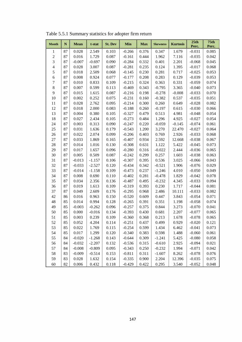
147

Table 5.5.1 Summary statistics for adopter firm return

Month N Mean t-stat St. Dev Min Max Skewness Kurtosis 25th

Perc.

75th

Perc.

1 87 0.028 2.549 0.103 -0.266 0.376 0.347 1.679 -0.031 0.085

2 87 0.016 1.729 0.087 -0.161 0.444 1.962 7.116 -0.035 0.042

3 87 -0.007 -0.697 0.090 -0.284 0.332 0.401 2.201 -0.068 0.045

4 87 0.028 3.007 0.087 -0.281 0.235 0.124 1.395 -0.017 0.068

5 87 0.018 2.509 0.068 -0.145 0.230 0.281 0.717 -0.025 0.053

6 87 0.008 0.924 0.077 -0.177 0.208 0.283 0.129 -0.039 0.053

7 87 0.010 0.833 0.109 -0.215 0.324 0.363 0.331 -0.059 0.074

8 87 0.007 0.599 0.113 -0.469 0.343 -0.795 3.365 -0.040 0.073

9 87 0.015 1.615 0.087 -0.216 0.198 -0.278 -0.008 -0.033 0.070

10 87 0.002 0.252 0.075 -0.231 0.160 -0.382 0.537 -0.035 0.051

11 87 0.028 2.762 0.095 -0.214 0.300 0.260 0.649 -0.028 0.082

12 87 0.018 2.000 0.083 -0.188 0.260 -0.197 0.615 -0.030 0.066

13 87 0.004 0.380 0.105 -0.327 0.479 0.513 4.981 -0.048 0.054

18 87 0.027 2.434 0.105 -0.273 0.484 1.296 4.925 -0.027 0.054

24 87 0.003 0.313 0.090 -0.247 0.220 -0.059 -0.145 -0.074 0.061

25 87 0.031 1.636 0.179 -0.543 1.200 3.270 22.470 -0.027 0.064

26 87 0.022 2.074 0.099 -0.206 0.403 0.769 2.926 -0.033 0.068

27 87 0.033 1.869 0.165 -0.407 0.934 2.592 12.668 -0.038 0.067

28 87 0.014 1.016 0.130 -0.308 0.631 1.122 5.422 -0.045 0.073

29 87 0.017 1.657 0.096 -0.280 0.316 -0.022 2.444 -0.036 0.065

30 87 0.005 0.509 0.087 -0.242 0.299 0.257 1.603 -0.038 0.063

31 87 -0.013 -1.157 0.106 -0.307 0.395 0.536 3.025 -0.066 0.043

32 87 -0.033 -2.527 0.120 -0.434 0.342 -0.521 1.906 -0.076 0.029

33 87 -0.014 -1.158 0.109 -0.473 0.237 -1.246 4.010 -0.050 0.049

34 87 0.008 0.690 0.110 -0.402 0.281 -0.478 1.829 -0.042 0.078

35 87 0.034 2.356 0.136 -0.487 0.495 -0.232 4.345 -0.033 0.094

36 87 0.019 1.613 0.109 -0.319 0.393 0.230 1.717 -0.044 0.081

37 87 0.049 2.609 0.176 -0.295 0.968 2.486 10.111 -0.033 0.082

42 86 0.016 0.963 0.150 -0.520 0.609 0.447 3.843 -0.054 0.071

48 85 0.014 0.994 0.128 -0.265 0.391 0.351 1.198 -0.058 0.074

49 85 -0.003 -0.262 0.096 -0.257 0.375 0.844 3.273 -0.070 0.041

50 85 0.000 -0.016 0.134 -0.393 0.430 0.681 2.207 -0.077 0.065

51 85 0.003 0.239 0.109 -0.360 0.368 0.213 1.678 -0.078 0.065

52 85 0.052 4.204 0.114 -0.251 0.437 0.499 0.929 -0.020 0.121

53 85 0.022 1.769 0.115 -0.254 0.599 1.434 6.462 -0.041 0.073

54 85 0.017 1.299 0.120 -0.340 0.383 0.598 1.488 -0.060 0.061

55 84 -0.020 -1.268 0.143 -0.644 0.309 -1.241 5.425 -0.080 0.058

56 84 -0.032 -2.207 0.132 -0.536 0.315 -0.610 2.925 -0.094 0.021

57 84 -0.008 -0.809 0.095 -0.343 0.250 -0.232 1.994 -0.071 0.042

58 83 -0.009 -0.514 0.153 -0.811 0.311 -1.607 8.262 -0.078 0.076

59 83 0.028 1.632 0.154 -0.335 0.900 2.204 12.396 -0.035 0.075

60 82 0.006 0.432 0.118 -0.429 0.422 0.295 3.540 -0.052 0.048

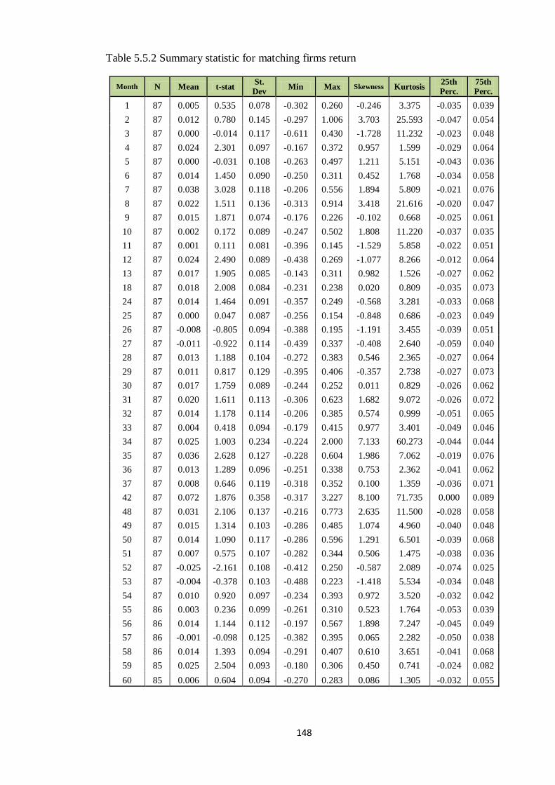
148

Table 5.5.2 Summary statistic for matching firms return

Month N Mean t-stat St.

Dev Min Max Skewness Kurtosis

25th

Perc.

75th

Perc.

1 87 0.005 0.535 0.078 -0.302 0.260 -0.246 3.375 -0.035 0.039

2 87 0.012 0.780 0.145 -0.297 1.006 3.703 25.593 -0.047 0.054

3 87 0.000 -0.014 0.117 -0.611 0.430 -1.728 11.232 -0.023 0.048

4 87 0.024 2.301 0.097 -0.167 0.372 0.957 1.599 -0.029 0.064

5 87 0.000 -0.031 0.108 -0.263 0.497 1.211 5.151 -0.043 0.036

6 87 0.014 1.450 0.090 -0.250 0.311 0.452 1.768 -0.034 0.058

7 87 0.038 3.028 0.118 -0.206 0.556 1.894 5.809 -0.021 0.076

8 87 0.022 1.511 0.136 -0.313 0.914 3.418 21.616 -0.020 0.047

9 87 0.015 1.871 0.074 -0.176 0.226 -0.102 0.668 -0.025 0.061

10 87 0.002 0.172 0.089 -0.247 0.502 1.808 11.220 -0.037 0.035

11 87 0.001 0.111 0.081 -0.396 0.145 -1.529 5.858 -0.022 0.051

12 87 0.024 2.490 0.089 -0.438 0.269 -1.077 8.266 -0.012 0.064

13 87 0.017 1.905 0.085 -0.143 0.311 0.982 1.526 -0.027 0.062

18 87 0.018 2.008 0.084 -0.231 0.238 0.020 0.809 -0.035 0.073

24 87 0.014 1.464 0.091 -0.357 0.249 -0.568 3.281 -0.033 0.068

25 87 0.000 0.047 0.087 -0.256 0.154 -0.848 0.686 -0.023 0.049

26 87 -0.008 -0.805 0.094 -0.388 0.195 -1.191 3.455 -0.039 0.051

27 87 -0.011 -0.922 0.114 -0.439 0.337 -0.408 2.640 -0.059 0.040

28 87 0.013 1.188 0.104 -0.272 0.383 0.546 2.365 -0.027 0.064

29 87 0.011 0.817 0.129 -0.395 0.406 -0.357 2.738 -0.027 0.073

30 87 0.017 1.759 0.089 -0.244 0.252 0.011 0.829 -0.026 0.062

31 87 0.020 1.611 0.113 -0.306 0.623 1.682 9.072 -0.026 0.072

32 87 0.014 1.178 0.114 -0.206 0.385 0.574 0.999 -0.051 0.065

33 87 0.004 0.418 0.094 -0.179 0.415 0.977 3.401 -0.049 0.046

34 87 0.025 1.003 0.234 -0.224 2.000 7.133 60.273 -0.044 0.044

35 87 0.036 2.628 0.127 -0.228 0.604 1.986 7.062 -0.019 0.076

36 87 0.013 1.289 0.096 -0.251 0.338 0.753 2.362 -0.041 0.062

37 87 0.008 0.646 0.119 -0.318 0.352 0.100 1.359 -0.036 0.071

42 87 0.072 1.876 0.358 -0.317 3.227 8.100 71.735 0.000 0.089

48 87 0.031 2.106 0.137 -0.216 0.773 2.635 11.500 -0.028 0.058

49 87 0.015 1.314 0.103 -0.286 0.485 1.074 4.960 -0.040 0.048

50 87 0.014 1.090 0.117 -0.286 0.596 1.291 6.501 -0.039 0.068

51 87 0.007 0.575 0.107 -0.282 0.344 0.506 1.475 -0.038 0.036

52 87 -0.025 -2.161 0.108 -0.412 0.250 -0.587 2.089 -0.074 0.025

53 87 -0.004 -0.378 0.103 -0.488 0.223 -1.418 5.534 -0.034 0.048

54 87 0.010 0.920 0.097 -0.234 0.393 0.972 3.520 -0.032 0.042

55 86 0.003 0.236 0.099 -0.261 0.310 0.523 1.764 -0.053 0.039

56 86 0.014 1.144 0.112 -0.197 0.567 1.898 7.247 -0.045 0.049

57 86 -0.001 -0.098 0.125 -0.382 0.395 0.065 2.282 -0.050 0.038

58 86 0.014 1.393 0.094 -0.291 0.407 0.610 3.651 -0.041 0.068

59 85 0.025 2.504 0.093 -0.180 0.306 0.450 0.741 -0.024 0.082

60 85 0.006 0.604 0.094 -0.270 0.283 0.086 1.305 -0.032 0.055

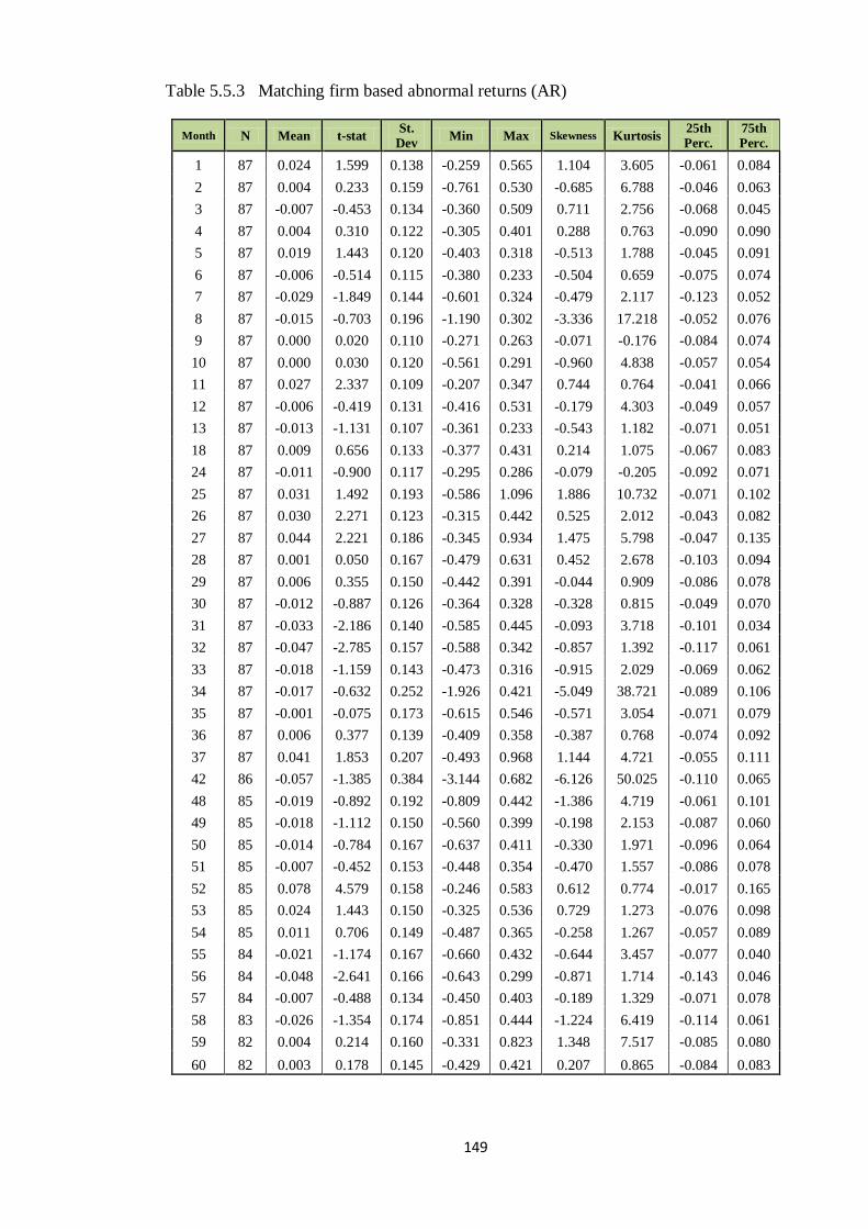
149

Table 5.5.3 Matching firm based abnormal returns (AR)



25th

Perc.

75th

Perc.

1 87 0.024 1.599 0.138 -0.259 0.565 1.104 3.605 -0.061 0.084

2 87 0.004 0.233 0.159 -0.761 0.530 -0.685 6.788 -0.046 0.063

3 87 -0.007 -0.453 0.134 -0.360 0.509 0.711 2.756 -0.068 0.045

4 87 0.004 0.310 0.122 -0.305 0.401 0.288 0.763 -0.090 0.090

5 87 0.019 1.443 0.120 -0.403 0.318 -0.513 1.788 -0.045 0.091

6 87 -0.006 -0.514 0.115 -0.380 0.233 -0.504 0.659 -0.075 0.074

7 87 -0.029 -1.849 0.144 -0.601 0.324 -0.479 2.117 -0.123 0.052

8 87 -0.015 -0.703 0.196 -1.190 0.302 -3.336 17.218 -0.052 0.076

9 87 0.000 0.020 0.110 -0.271 0.263 -0.071 -0.176 -0.084 0.074

10 87 0.000 0.030 0.120 -0.561 0.291 -0.960 4.838 -0.057 0.054

11 87 0.027 2.337 0.109 -0.207 0.347 0.744 0.764 -0.041 0.066

12 87 -0.006 -0.419 0.131 -0.416 0.531 -0.179 4.303 -0.049 0.057

13 87 -0.013 -1.131 0.107 -0.361 0.233 -0.543 1.182 -0.071 0.051

18 87 0.009 0.656 0.133 -0.377 0.431 0.214 1.075 -0.067 0.083

24 87 -0.011 -0.900 0.117 -0.295 0.286 -0.079 -0.205 -0.092 0.071

25 87 0.031 1.492 0.193 -0.586 1.096 1.886 10.732 -0.071 0.102

26 87 0.030 2.271 0.123 -0.315 0.442 0.525 2.012 -0.043 0.082

27 87 0.044 2.221 0.186 -0.345 0.934 1.475 5.798 -0.047 0.135

28 87 0.001 0.050 0.167 -0.479 0.631 0.452 2.678 -0.103 0.094

29 87 0.006 0.355 0.150 -0.442 0.391 -0.044 0.909 -0.086 0.078

30 87 -0.012 -0.887 0.126 -0.364 0.328 -0.328 0.815 -0.049 0.070

31 87 -0.033 -2.186 0.140 -0.585 0.445 -0.093 3.718 -0.101 0.034

32 87 -0.047 -2.785 0.157 -0.588 0.342 -0.857 1.392 -0.117 0.061

33 87 -0.018 -1.159 0.143 -0.473 0.316 -0.915 2.029 -0.069 0.062

34 87 -0.017 -0.632 0.252 -1.926 0.421 -5.049 38.721 -0.089 0.106

35 87 -0.001 -0.075 0.173 -0.615 0.546 -0.571 3.054 -0.071 0.079

36 87 0.006 0.377 0.139 -0.409 0.358 -0.387 0.768 -0.074 0.092

37 87 0.041 1.853 0.207 -0.493 0.968 1.144 4.721 -0.055 0.111

42 86 -0.057 -1.385 0.384 -3.144 0.682 -6.126 50.025 -0.110 0.065

48 85 -0.019 -0.892 0.192 -0.809 0.442 -1.386 4.719 -0.061 0.101

49 85 -0.018 -1.112 0.150 -0.560 0.399 -0.198 2.153 -0.087 0.060

50 85 -0.014 -0.784 0.167 -0.637 0.411 -0.330 1.971 -0.096 0.064

51 85 -0.007 -0.452 0.153 -0.448 0.354 -0.470 1.557 -0.086 0.078

52 85 0.078 4.579 0.158 -0.246 0.583 0.612 0.774 -0.017 0.165

53 85 0.024 1.443 0.150 -0.325 0.536 0.729 1.273 -0.076 0.098

54 85 0.011 0.706 0.149 -0.487 0.365 -0.258 1.267 -0.057 0.089

55 84 -0.021 -1.174 0.167 -0.660 0.432 -0.644 3.457 -0.077 0.040

56 84 -0.048 -2.641 0.166 -0.643 0.299 -0.871 1.714 -0.143 0.046

57 84 -0.007 -0.488 0.134 -0.450 0.403 -0.189 1.329 -0.071 0.078

58 83 -0.026 -1.354 0.174 -0.851 0.444 -1.224 6.419 -0.114 0.061

59 82 0.004 0.214 0.160 -0.331 0.823 1.348 7.517 -0.085 0.080

60 82 0.003 0.178 0.145 -0.429 0.421 0.207 0.865 -0.084 0.083

150

Table 5.5.4 Matching firm based cumulative abnormal returns (CAR)


Dev. Min Max Skewness Kurtosis

25th

Perc.

75th

Perc.

1 87 0.024 1.599 0.138 -0.259 0.565 1.104 3.605 -0.061 0.084 2 87 0.028 1.160 0.223 -0.968 0.980 0.037 7.417 -0.084 0.130 3 87 0.021 0.801 0.247 -0.624 0.932 0.711 2.073 -0.124 0.136 4 87 0.025 0.881 0.267 -0.615 1.055 0.588 2.004 -0.124 0.146 5 87 0.044 1.452 0.282 -0.657 0.799 0.310 0.567 -0.150 0.202 6 87 0.038 1.284 0.273 -0.768 0.900 0.180 1.042 -0.141 0.212 7 87 0.009 0.276 0.302 -0.705 0.983 0.206 1.239 -0.140 0.133 8 87 -0.006 -0.183 0.298 -0.768 0.752 -0.209 0.337 -0.165 0.173 9 87 -0.006 -0.180 0.290 -0.745 0.671 -0.311 0.146 -0.172 0.160

10 87 -0.005 -0.145 0.335 -0.915 0.808 -0.289 0.600 -0.191 0.196 11 87 0.022 0.595 0.345 -0.948 1.100 0.018 0.958 -0.183 0.227 12 87 0.016 0.388 0.388 -1.327 1.249 -0.336 1.909 -0.177 0.218 13 87 0.003 0.070 0.411 -1.352 1.416 -0.158 2.011 -0.195 0.211 14 87 0.046 1.058 0.408 -0.980 1.408 0.162 1.116 -0.160 0.246 15 87 0.069 1.526 0.420 -1.059 1.380 0.166 1.275 -0.163 0.277 16 87 0.059 1.303 0.420 -0.955 1.225 0.302 0.577 -0.188 0.294 17 87 0.065 1.429 0.426 -1.002 1.238 0.108 0.587 -0.184 0.319 18 87 0.075 1.502 0.463 -1.129 1.558 0.416 1.457 -0.192 0.285 19 87 0.072 1.319 0.508 -1.017 1.835 0.848 2.319 -0.246 0.346 20 87 0.079 1.454 0.505 -1.019 1.820 0.721 2.139 -0.254 0.334 21 87 0.033 0.674 0.460 -1.006 1.603 0.273 1.144 -0.306 0.290 22 87 0.026 0.527 0.459 -1.044 1.543 -0.023 0.814 -0.228 0.291 23 87 0.052 1.044 0.462 -1.094 1.446 -0.122 0.341 -0.261 0.356 24 87 0.040 0.754 0.500 -1.261 1.642 0.073 0.754 -0.292 0.369 25 87 0.071 1.272 0.523 -1.090 2.001 0.394 1.352 -0.355 0.345 26 87 0.101 1.708 0.554 -1.122 2.078 0.494 1.298 -0.235 0.371 27 87 0.146 2.157 0.630 -1.204 3.011 1.126 4.581 -0.252 0.414 28 87 0.147 2.070 0.661 -1.683 3.642 1.433 8.619 -0.189 0.450 29 87 0.152 2.104 0.675 -1.827 3.736 1.451 8.893 -0.225 0.392 30 87 0.140 1.984 0.659 -1.653 3.546 1.312 7.815 -0.206 0.451 31 87 0.108 1.480 0.678 -2.238 3.240 0.548 5.698 -0.229 0.430 32 87 0.061 0.819 0.690 -2.132 3.582 1.105 7.834 -0.355 0.365 33 87 0.043 0.541 0.739 -2.160 3.865 1.089 8.359 -0.344 0.381 34 87 0.026 0.312 0.770 -2.198 3.803 0.774 6.823 -0.391 0.397 35 87 0.024 0.279 0.817 -2.455 4.024 0.587 7.305 -0.366 0.454 36 87 0.030 0.343 0.818 -2.698 3.949 0.532 6.817 -0.376 0.442 37 87 0.071 0.847 0.783 -2.314 3.756 0.757 5.666 -0.342 0.468 38 87 0.084 1.022 0.771 -2.051 3.471 0.488 4.295 -0.288 0.455 39 87 0.098 1.173 0.776 -2.042 3.450 0.364 4.015 -0.272 0.469 40 87 0.122 1.424 0.800 -2.163 3.584 0.473 3.991 -0.249 0.527 41 87 0.150 1.757 0.796 -1.955 3.685 0.674 4.038 -0.287 0.607 42 86 0.080 0.821 0.903 -2.904 3.946 0.401 4.149 -0.365 0.621 43 86 0.060 0.585 0.945 -2.737 3.898 0.425 3.237 -0.421 0.650 44 86 0.033 0.314 0.984 -2.739 4.161 0.553 3.481 -0.464 0.583 45 86 0.020 0.171 1.071 -3.462 4.693 0.378 4.421 -0.472 0.605 46 85 0.014 0.116 1.099 -4.056 4.444 0.104 4.501 -0.495 0.535 47 85 0.033 0.280 1.101 -3.661 4.162 0.280 3.228 -0.500 0.523 48 85 0.015 0.119 1.146 -4.384 3.927 -0.023 3.568 -0.468 0.538 49 85 -0.003 -0.026 1.137 -4.288 4.037 0.117 3.556 -0.547 0.474 50 85 -0.017 -0.140 1.151 -4.287 4.277 0.233 3.597 -0.607 0.522 51 85 -0.025 -0.200 1.153 -4.242 4.371 0.181 3.441 -0.659 0.548 52 85 0.053 0.420 1.172 -4.424 4.365 0.049 3.528 -0.503 0.623 53 85 0.077 0.626 1.133 -4.291 4.290 0.103 3.763 -0.540 0.626 54 85 0.088 0.718 1.135 -4.519 3.803 -0.174 3.531 -0.493 0.666 55 84 0.052 0.408 1.171 -4.644 3.725 -0.301 3.115 -0.490 0.693 56 84 0.004 0.033 1.181 -4.931 3.412 -0.593 3.500 -0.542 0.635 57 84 -0.003 -0.022 1.186 -4.677 3.419 -0.424 2.862 -0.548 0.645 58 83 -0.037 -0.275 1.233 -4.787 3.553 -0.476 3.240 -0.511 0.628 59 82 -0.035 -0.262 1.215 -4.824 3.280 -0.465 3.126 -0.616 0.636 60 82 -0.032 -0.245 1.198 -4.538 3.115 -0.424 2.574 -0.581 0.655

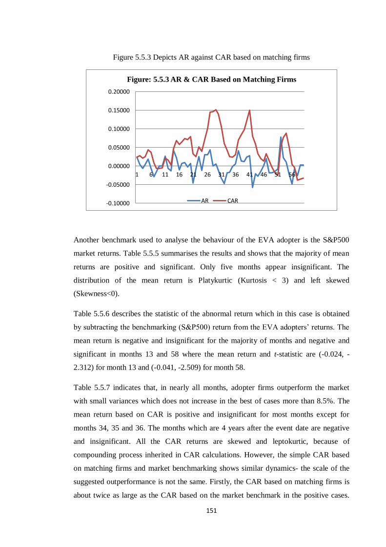
151

Figure 5.5.3 Depicts AR against CAR based on matching firms

Another benchmark used to analyse the behaviour of the EVA adopter is the S&P500

market returns. Table 5.5.5 summarises the results and shows that the majority of mean

returns are positive and significant. Only five months appear insignificant. The

distribution of the mean return is Platykurtic (Kurtosis < 3) and left skewed

(Skewness<0).

Table 5.5.6 describes the statistic of the abnormal return which in this case is obtained

by subtracting the benchmarking (S&P500) return from the EVA adopters’ returns. The

mean return is negative and insignificant for the majority of months and negative and

significant in months 13 and 58 where the mean return and t-statistic are (-0.024, -

2.312) for month 13 and (-0.041, -2.509) for month 58.

Table 5.5.7 indicates that, in nearly all months, adopter firms outperform the market

with small variances which does not increase in the best of cases more than 8.5%. The

mean return based on CAR is positive and insignificant for most months except for

months 34, 35 and 36. The months which are 4 years after the event date are negative

and insignificant. All the CAR returns are skewed and leptokurtic, because of

compounding process inherited in CAR calculations. However, the simple CAR based

on matching firms and market benchmarking shows similar dynamics- the scale of the

suggested outperformance is not the same. Firstly, the CAR based on matching firms is

about twice as large as the CAR based on the market benchmark in the positive cases.

-0.10000

-0.05000

0.00000

0.05000

0.10000

0.15000

0.20000

1 6 11 16 21 26 31 36 41 46 51 56

Figure: 5.5.3 AR & CAR Based on Matching Firms

AR CAR

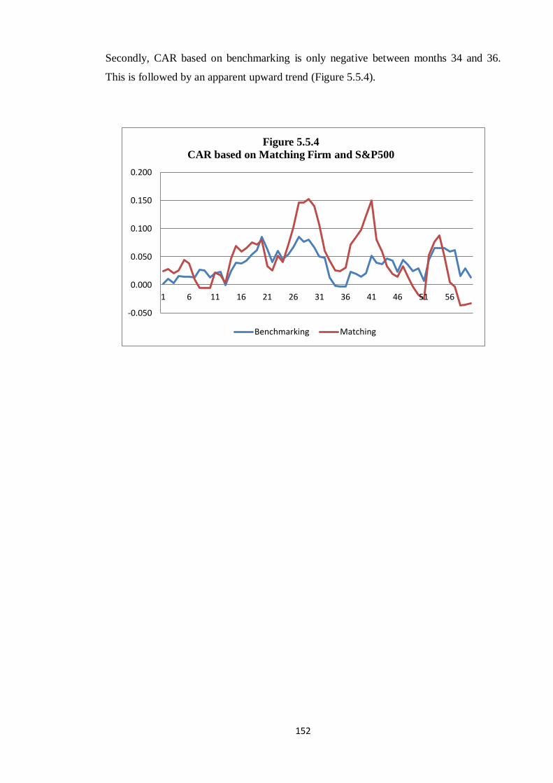
152

Secondly, CAR based on benchmarking is only negative between months 34 and 36.

This is followed by an apparent upward trend (Figure 5.5.4).

-0.050

0.000

0.050

0.100

0.150

0.200

1 6 11 16 21 26 31 36 41 46 51 56

Figure 5.5.4

CAR based on Matching Firm and S&P500

Benchmarking Matching

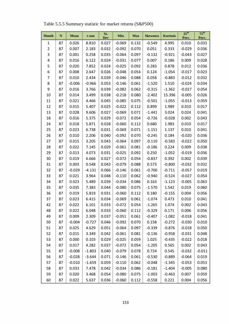
153

Table 5.5.5 Summary statistic for market returns (S&P500)



25th

Perc.

75th

Perc.

1 87 0.026 8.810 0.027 -0.069 0.132 -0.549 4.995 0.010 0.033

2 87 0.007 2.183 0.032 -0.092 0.070 0.051 0.333 -0.029 0.036

3 87 0.001 0.258 0.035 -0.064 0.097 -0.132 -0.921 -0.043 0.027

4 87 0.016 6.122 0.024 -0.031 0.077 0.007 0.186 0.009 0.028

5 87 0.020 7.852 0.024 -0.025 0.092 0.283 0.878 0.012 0.036

6 87 0.008 2.647 0.026 -0.048 0.054 0.124 -1.054 -0.017 0.023

7 87 0.010 2.434 0.039 -0.046 0.088 0.058 -0.883 -0.012 0.032

8 87 -0.006 -0.966 0.053 -0.146 0.061 -1.520 1.510 -0.024 0.034

9 87 0.016 3.766 0.039 -0.082 0.062 -0.315 -1.362 -0.027 0.054

10 87 0.014 3.499 0.038 -0.218 0.080 -2.402 15.396 -0.005 0.026

11 87 0.021 4.466 0.045 -0.085 0.075 -0.501 -1.055 -0.013 0.059

12 87 0.015 5.407 0.025 -0.022 0.112 0.899 1.989 0.010 0.017

13 87 0.028 9.606 0.027 -0.069 0.071 -1.441 3.024 0.024 0.041

18 87 0.016 5.375 0.029 -0.072 0.054 -0.726 -0.028 0.002 0.043

24 87 0.018 5.871 0.028 -0.060 0.112 0.680 1.983 0.010 0.017

25 87 0.023 6.738 0.031 -0.069 0.071 -1.151 1.137 0.010 0.041

26 87 0.010 2.206 0.040 -0.092 0.070 -0.245 0.184 -0.020 0.036

27 87 0.015 3.205 0.043 -0.064 0.097 -0.110 -0.583 -0.022 0.050

28 87 0.022 7.145 0.029 -0.061 0.081 -0.186 0.224 0.009 0.038

29 87 0.013 4.073 0.031 -0.025 0.092 0.250 -1.052 -0.019 0.036

30 87 0.019 6.666 0.027 -0.072 0.054 -0.837 0.392 0.002 0.039

31 87 0.003 0.548 0.043 -0.079 0.088 0.573 -0.800 -0.032 0.032

32 87 -0.029 -4.131 0.066 -0.146 0.061 -0.700 -0.711 -0.057 0.019

33 87 0.021 3.964 0.048 -0.110 0.062 -0.940 -0.524 -0.027 0.054

34 87 0.023 5.489 0.039 -0.034 0.086 0.163 -1.123 -0.005 0.063

35 87 0.035 7.383 0.044 -0.080 0.075 -1.570 1.542 0.019 0.060

36 87 0.019 5.819 0.031 -0.060 0.112 0.180 -0.155 0.004 0.056

37 87 0.023 6.415 0.034 -0.069 0.061 -1.074 0.473 0.010 0.041

42 87 0.022 6.101 0.033 -0.072 0.054 -1.265 1.074 0.002 0.043

48 87 0.022 6.048 0.033 -0.060 0.112 -0.329 0.171 0.006 0.056

49 87 0.009 2.309 0.037 -0.051 0.061 -0.407 -1.082 -0.018 0.041

50 87 -0.004 -0.727 0.046 -0.092 0.070 0.158 -0.272 -0.030 0.010

51 87 0.025 4.629 0.051 -0.064 0.097 -0.339 -0.876 -0.018 0.050

52 87 0.015 3.349 0.042 -0.061 0.081 -0.136 -0.958 -0.031 0.048

53 87 0.000 0.103 0.029 -0.025 0.059 1.025 -0.435 -0.022 0.018

54 87 0.017 4.282 0.037 -0.072 0.054 -1.205 0.565 0.002 0.043

55 87 -0.008 -1.803 0.040 -0.079 0.078 0.724 0.545 -0.032 -0.011

56 87 -0.028 -3.644 0.071 -0.146 0.061 -0.530 -0.889 -0.064 0.019

57 87 -0.010 -1.659 0.059 -0.110 0.062 -0.048 -1.345 -0.053 0.053

58 87 0.033 7.478 0.042 -0.034 0.086 -0.181 -1.404 -0.005 0.080

59 87 0.020 3.468 0.054 -0.080 0.075 -1.003 -0.463 0.007 0.059

60 87 0.022 5.637 0.036 -0.060 0.112 -0.558 0.221 0.004 0.056

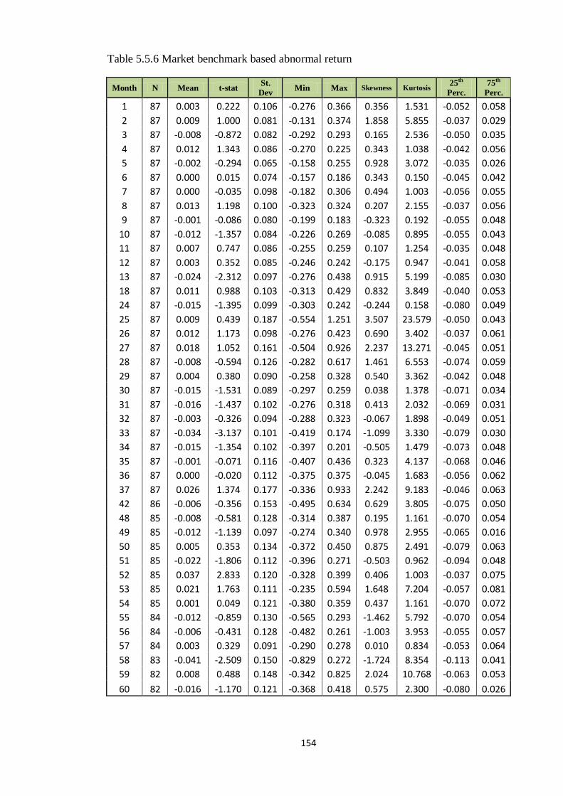
154

Table 5.5.6 Market benchmark based abnormal return



25th

Perc.

75th

Perc.

1 87 0.003 0.222 0.106 -0.276 0.366 0.356 1.531 -0.052 0.058

2 87 0.009 1.000 0.081 -0.131 0.374 1.858 5.855 -0.037 0.029

3 87 -0.008 -0.872 0.082 -0.292 0.293 0.165 2.536 -0.050 0.035

4 87 0.012 1.343 0.086 -0.270 0.225 0.343 1.038 -0.042 0.056

5 87 -0.002 -0.294 0.065 -0.158 0.255 0.928 3.072 -0.035 0.026

6 87 0.000 0.015 0.074 -0.157 0.186 0.343 0.150 -0.045 0.042

7 87 0.000 -0.035 0.098 -0.182 0.306 0.494 1.003 -0.056 0.055

8 87 0.013 1.198 0.100 -0.323 0.324 0.207 2.155 -0.037 0.056

9 87 -0.001 -0.086 0.080 -0.199 0.183 -0.323 0.192 -0.055 0.048

10 87 -0.012 -1.357 0.084 -0.226 0.269 -0.085 0.895 -0.055 0.043

11 87 0.007 0.747 0.086 -0.255 0.259 0.107 1.254 -0.035 0.048

12 87 0.003 0.352 0.085 -0.246 0.242 -0.175 0.947 -0.041 0.058

13 87 -0.024 -2.312 0.097 -0.276 0.438 0.915 5.199 -0.085 0.030

18 87 0.011 0.988 0.103 -0.313 0.429 0.832 3.849 -0.040 0.053

24 87 -0.015 -1.395 0.099 -0.303 0.242 -0.244 0.158 -0.080 0.049

25 87 0.009 0.439 0.187 -0.554 1.251 3.507 23.579 -0.050 0.043

26 87 0.012 1.173 0.098 -0.276 0.423 0.690 3.402 -0.037 0.061

27 87 0.018 1.052 0.161 -0.504 0.926 2.237 13.271 -0.045 0.051

28 87 -0.008 -0.594 0.126 -0.282 0.617 1.461 6.553 -0.074 0.059

29 87 0.004 0.380 0.090 -0.258 0.328 0.540 3.362 -0.042 0.048

30 87 -0.015 -1.531 0.089 -0.297 0.259 0.038 1.378 -0.071 0.034

31 87 -0.016 -1.437 0.102 -0.276 0.318 0.413 2.032 -0.069 0.031

32 87 -0.003 -0.326 0.094 -0.288 0.323 -0.067 1.898 -0.049 0.051

33 87 -0.034 -3.137 0.101 -0.419 0.174 -1.099 3.330 -0.079 0.030

34 87 -0.015 -1.354 0.102 -0.397 0.201 -0.505 1.479 -0.073 0.048

35 87 -0.001 -0.071 0.116 -0.407 0.436 0.323 4.137 -0.068 0.046

36 87 0.000 -0.020 0.112 -0.375 0.375 -0.045 1.683 -0.056 0.062

37 87 0.026 1.374 0.177 -0.336 0.933 2.242 9.183 -0.046 0.063

42 86 -0.006 -0.356 0.153 -0.495 0.634 0.629 3.805 -0.075 0.050

48 85 -0.008 -0.581 0.128 -0.314 0.387 0.195 1.161 -0.070 0.054

49 85 -0.012 -1.139 0.097 -0.274 0.340 0.978 2.955 -0.065 0.016

50 85 0.005 0.353 0.134 -0.372 0.450 0.875 2.491 -0.079 0.063

51 85 -0.022 -1.806 0.112 -0.396 0.271 -0.503 0.962 -0.094 0.048

52 85 0.037 2.833 0.120 -0.328 0.399 0.406 1.003 -0.037 0.075

53 85 0.021 1.763 0.111 -0.235 0.594 1.648 7.204 -0.057 0.081

54 85 0.001 0.049 0.121 -0.380 0.359 0.437 1.161 -0.070 0.072

55 84 -0.012 -0.859 0.130 -0.565 0.293 -1.462 5.792 -0.070 0.054

56 84 -0.006 -0.431 0.128 -0.482 0.261 -1.003 3.953 -0.055 0.057

57 84 0.003 0.329 0.091 -0.290 0.278 0.010 0.834 -0.053 0.064

58 83 -0.041 -2.509 0.150 -0.829 0.272 -1.724 8.354 -0.113 0.041

59 82 0.008 0.488 0.148 -0.342 0.825 2.024 10.768 -0.063 0.053

60 82 -0.016 -1.170 0.121 -0.368 0.418 0.575 2.300 -0.080 0.026

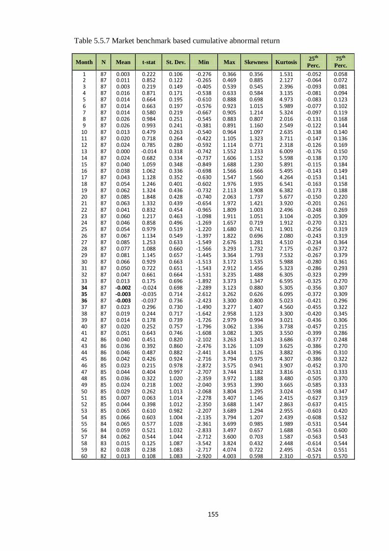
155

Table 5.5.7 Market benchmark based cumulative abnormal return

Month N Mean t-stat St. Dev. Min Max Skewness Kurtosis 25

th

Perc.

75th

Perc.

1 87 0.003 0.222 0.106 -0.276 0.366 0.356 1.531 -0.052 0.058 2 87 0.011 0.852 0.122 -0.265 0.469 0.885 2.127 -0.064 0.072 3 87 0.003 0.219 0.149 -0.405 0.539 0.545 2.396 -0.093 0.081 4 87 0.016 0.871 0.171 -0.538 0.633 0.584 3.135 -0.081 0.094 5 87 0.014 0.664 0.195 -0.610 0.888 0.698 4.973 -0.083 0.123 6 87 0.014 0.663 0.197 -0.576 0.923 1.015 5.989 -0.077 0.102 7 87 0.014 0.580 0.219 -0.667 0.905 1.214 5.324 -0.097 0.119 8 87 0.026 0.984 0.251 -0.545 0.883 0.807 2.016 -0.131 0.168 9 87 0.026 0.993 0.241 -0.381 0.891 1.160 2.549 -0.122 0.144

10 87 0.013 0.479 0.263 -0.540 0.964 1.097 2.635 -0.138 0.140 11 87 0.020 0.718 0.264 -0.422 1.105 1.323 3.711 -0.147 0.136 12 87 0.024 0.785 0.280 -0.592 1.114 0.771 2.318 -0.126 0.169 13 87 0.000 -0.014 0.318 -0.742 1.552 1.233 6.009 -0.176 0.150 14 87 0.024 0.682 0.334 -0.737 1.606 1.152 5.598 -0.138 0.170 15 87 0.040 1.059 0.348 -0.849 1.688 1.230 5.891 -0.115 0.184 16 87 0.038 1.062 0.336 -0.698 1.566 1.666 5.495 -0.143 0.149 17 87 0.043 1.128 0.352 -0.630 1.547 1.560 4.264 -0.153 0.141 18 87 0.054 1.246 0.401 -0.602 1.976 1.935 6.541 -0.163 0.158 19 87 0.062 1.324 0.436 -0.732 2.113 1.908 6.382 -0.173 0.188 20 87 0.085 1.848 0.428 -0.740 2.063 1.737 5.677 -0.150 0.220 21 87 0.063 1.332 0.439 -0.654 1.972 1.421 3.920 -0.201 0.261 22 87 0.041 0.832 0.454 -0.965 1.809 1.003 2.496 -0.248 0.269 23 87 0.060 1.217 0.463 -1.098 1.911 1.051 3.104 -0.205 0.309 24 87 0.046 0.858 0.496 -1.269 1.657 0.719 1.912 -0.270 0.321 25 87 0.054 0.979 0.519 -1.220 1.680 0.741 1.901 -0.256 0.319 26 87 0.067 1.134 0.549 -1.397 1.822 0.696 2.080 -0.243 0.319 27 87 0.085 1.253 0.633 -1.549 2.676 1.281 4.510 -0.234 0.364 28 87 0.077 1.088 0.660 -1.566 3.293 1.732 7.175 -0.267 0.372 29 87 0.081 1.145 0.657 -1.445 3.364 1.793 7.532 -0.267 0.379 30 87 0.066 0.929 0.663 -1.513 3.172 1.535 5.988 -0.280 0.361 31 87 0.050 0.722 0.651 -1.543 2.912 1.456 5.323 -0.286 0.293 32 87 0.047 0.661 0.664 -1.531 3.235 1.488 6.305 -0.323 0.299 33 87 0.013 0.175 0.696 -1.892 3.373 1.347 6.595 -0.325 0.270 34 87 -0.002 -0.024 0.698 -2.289 3.123 0.880 5.305 -0.356 0.307 35 87 -0.003 -0.035 0.714 -2.612 3.262 0.626 6.095 -0.372 0.309 36 87 -0.003 -0.037 0.736 -2.423 3.300 0.800 5.023 -0.421 0.296 37 87 0.023 0.296 0.730 -1.490 3.277 1.407 4.560 -0.455 0.322 38 87 0.019 0.244 0.717 -1.642 2.958 1.123 3.300 -0.420 0.345 39 87 0.014 0.178 0.739 -1.726 2.979 0.994 3.021 -0.436 0.306 40 87 0.020 0.252 0.757 -1.796 3.062 1.336 3.738 -0.457 0.215 41 87 0.051 0.643 0.746 -1.608 3.082 1.305 3.550 -0.399 0.286 42 86 0.040 0.451 0.820 -2.102 3.263 1.243 3.686 -0.377 0.248 43 86 0.036 0.392 0.860 -2.476 3.126 1.109 3.625 -0.386 0.270 44 86 0.046 0.487 0.882 -2.441 3.434 1.126 3.882 -0.396 0.310 45 86 0.042 0.426 0.924 -2.716 3.794 0.975 4.307 -0.386 0.322 46 85 0.023 0.215 0.978 -2.872 3.575 0.941 3.907 -0.452 0.370 47 85 0.044 0.404 0.997 -2.707 3.744 1.182 3.816 -0.531 0.333 48 85 0.036 0.322 1.020 -2.359 3.972 1.188 3.480 -0.505 0.370 49 85 0.024 0.218 1.002 -2.040 3.953 1.390 3.665 -0.585 0.333 50 85 0.029 0.262 1.013 -2.068 3.804 1.295 3.024 -0.598 0.347 51 85 0.007 0.063 1.014 -2.278 3.407 1.146 2.415 -0.627 0.319 52 85 0.044 0.398 1.012 -2.350 3.688 1.147 2.863 -0.637 0.415 53 85 0.065 0.610 0.982 -2.207 3.689 1.294 2.955 -0.603 0.420 54 85 0.066 0.603 1.004 -2.135 3.794 1.207 2.439 -0.608 0.532 55 84 0.065 0.577 1.028 -2.361 3.699 0.985 1.989 -0.531 0.544 56 84 0.059 0.521 1.032 -2.833 3.497 0.657 1.688 -0.563 0.600 57 84 0.062 0.544 1.044 -2.712 3.600 0.703 1.587 -0.563 0.543 58 83 0.015 0.125 1.087 -3.542 3.824 0.432 2.448 -0.614 0.544 59 82 0.028 0.238 1.083 -2.717 4.074 0.722 2.495 -0.524 0.551 60 82 0.013 0.108 1.083 -2.920 4.003 0.598 2.310 -0.571 0.570

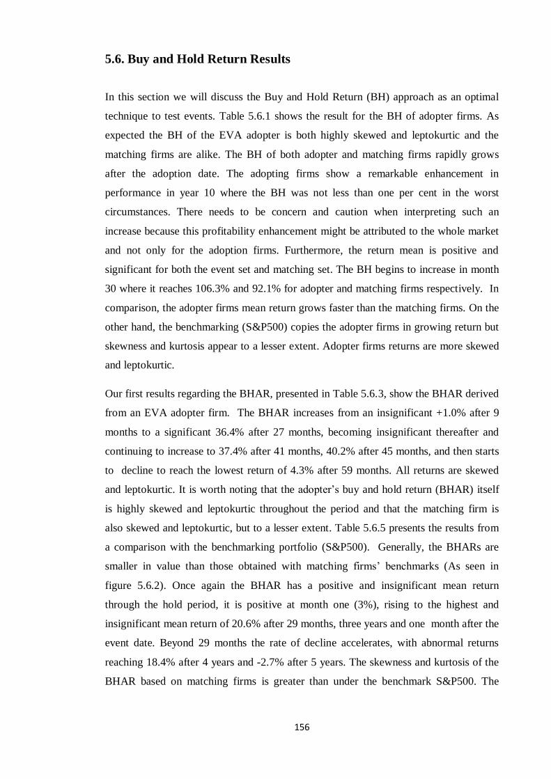
156

5.6. Buy and Hold Return Results

In this section we will discuss the Buy and Hold Return (BH) approach as an optimal

technique to test events. Table 5.6.1 shows the result for the BH of adopter firms. As

expected the BH of the EVA adopter is both highly skewed and leptokurtic and the

matching firms are alike. The BH of both adopter and matching firms rapidly grows

after the adoption date. The adopting firms show a remarkable enhancement in

performance in year 10 where the BH was not less than one per cent in the worst

circumstances. There needs to be concern and caution when interpreting such an

increase because this profitability enhancement might be attributed to the whole market

and not only for the adoption firms. Furthermore, the return mean is positive and

significant for both the event set and matching set. The BH begins to increase in month

30 where it reaches 106.3% and 92.1% for adopter and matching firms respectively. In

comparison, the adopter firms mean return grows faster than the matching firms. On the

other hand, the benchmarking (S&P500) copies the adopter firms in growing return but

skewness and kurtosis appear to a lesser extent. Adopter firms returns are more skewed

and leptokurtic.

Our first results regarding the BHAR, presented in Table 5.6.3, show the BHAR derived

from an EVA adopter firm. The BHAR increases from an insignificant +1.0% after 9

months to a significant 36.4% after 27 months, becoming insignificant thereafter and

continuing to increase to 37.4% after 41 months, 40.2% after 45 months, and then starts

to decline to reach the lowest return of 4.3% after 59 months. All returns are skewed

and leptokurtic. It is worth noting that the adopter’s buy and hold return (BHAR) itself

is highly skewed and leptokurtic throughout the period and that the matching firm is

also skewed and leptokurtic, but to a lesser extent. Table 5.6.5 presents the results from

a comparison with the benchmarking portfolio (S&P500). Generally, the BHARs are

smaller in value than those obtained with matching firms’ benchmarks (As seen in

figure 5.6.2). Once again the BHAR has a positive and insignificant mean return

through the hold period, it is positive at month one (3%), rising to the highest and

insignificant mean return of 20.6% after 29 months, three years and one month after the

event date. Beyond 29 months the rate of decline accelerates, with abnormal returns

reaching 18.4% after 4 years and -2.7% after 5 years. The skewness and kurtosis of the

BHAR based on matching firms is greater than under the benchmark S&P500. The

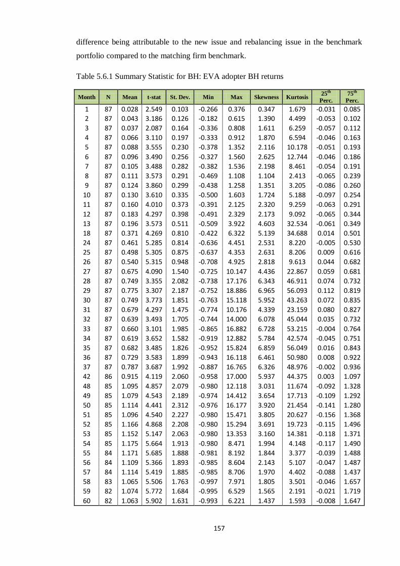
157

difference being attributable to the new issue and rebalancing issue in the benchmark

portfolio compared to the matching firm benchmark.

Table 5.6.1 Summary Statistic for BH: EVA adopter BH returns

Month N Mean t-stat St. Dev. Min Max Skewness Kurtosis 25

th

Perc.

75th

Perc.

1 87 0.028 2.549 0.103 -0.266 0.376 0.347 1.679 -0.031 0.085

2 87 0.043 3.186 0.126 -0.182 0.615 1.390 4.499 -0.053 0.102

3 87 0.037 2.087 0.164 -0.336 0.808 1.611 6.259 -0.057 0.112

4 87 0.066 3.110 0.197 -0.333 0.912 1.870 6.594 -0.046 0.163

5 87 0.088 3.555 0.230 -0.378 1.352 2.116 10.178 -0.051 0.193

6 87 0.096 3.490 0.256 -0.327 1.560 2.625 12.744 -0.046 0.186

7 87 0.105 3.488 0.282 -0.382 1.536 2.198 8.461 -0.054 0.191

8 87 0.111 3.573 0.291 -0.469 1.108 1.104 2.413 -0.065 0.239

9 87 0.124 3.860 0.299 -0.438 1.258 1.351 3.205 -0.086 0.260

10 87 0.130 3.610 0.335 -0.500 1.603 1.724 5.188 -0.097 0.254

11 87 0.160 4.010 0.373 -0.391 2.125 2.320 9.259 -0.063 0.291

12 87 0.183 4.297 0.398 -0.491 2.329 2.173 9.092 -0.065 0.344

13 87 0.196 3.573 0.511 -0.509 3.922 4.603 32.534 -0.061 0.349

18 87 0.371 4.269 0.810 -0.422 6.322 5.139 34.688 0.014 0.501

24 87 0.461 5.285 0.814 -0.636 4.451 2.531 8.220 -0.005 0.530

25 87 0.498 5.305 0.875 -0.637 4.353 2.631 8.206 0.009 0.616

26 87 0.540 5.315 0.948 -0.708 4.925 2.818 9.613 0.044 0.682

27 87 0.675 4.090 1.540 -0.725 10.147 4.436 22.867 0.059 0.681

28 87 0.749 3.355 2.082 -0.738 17.176 6.343 46.911 0.074 0.732

29 87 0.775 3.307 2.187 -0.752 18.886 6.965 56.093 0.112 0.819

30 87 0.749 3.773 1.851 -0.763 15.118 5.952 43.263 0.072 0.835

31 87 0.679 4.297 1.475 -0.774 10.176 4.339 23.159 0.080 0.827

32 87 0.639 3.493 1.705 -0.744 14.000 6.078 45.044 0.035 0.732

33 87 0.660 3.101 1.985 -0.865 16.882 6.728 53.215 -0.004 0.764

34 87 0.619 3.652 1.582 -0.919 12.882 5.784 42.574 -0.045 0.751

35 87 0.682 3.485 1.826 -0.952 15.824 6.859 56.049 0.016 0.843

36 87 0.729 3.583 1.899 -0.943 16.118 6.461 50.980 0.008 0.922

37 87 0.787 3.687 1.992 -0.887 16.765 6.326 48.976 -0.002 0.936

42 86 0.915 4.119 2.060 -0.958 17.000 5.937 44.375 0.003 1.097

48 85 1.095 4.857 2.079 -0.980 12.118 3.031 11.674 -0.092 1.328

49 85 1.079 4.543 2.189 -0.974 14.412 3.654 17.713 -0.109 1.292

50 85 1.114 4.441 2.312 -0.976 16.177 3.920 21.454 -0.141 1.280

51 85 1.096 4.540 2.227 -0.980 15.471 3.805 20.627 -0.156 1.368

52 85 1.166 4.868 2.208 -0.980 15.294 3.691 19.723 -0.115 1.496

53 85 1.152 5.147 2.063 -0.980 13.353 3.160 14.381 -0.118 1.371

54 85 1.175 5.664 1.913 -0.980 8.471 1.994 4.148 -0.117 1.490

55 84 1.171 5.685 1.888 -0.981 8.192 1.844 3.377 -0.039 1.488

56 84 1.109 5.366 1.893 -0.985 8.604 2.143 5.107 -0.047 1.487

57 84 1.114 5.419 1.885 -0.985 8.706 1.970 4.402 -0.088 1.437

58 83 1.065 5.506 1.763 -0.997 7.971 1.805 3.501 -0.046 1.657

59 82 1.074 5.772 1.684 -0.995 6.529 1.565 2.191 -0.021 1.719

60 82 1.063 5.902 1.631 -0.993 6.221 1.437 1.593 -0.008 1.647

158

Table 5.6.2 Summary Statistic for BH: Matching firm BH returns



25th

Perc.

75th

Perc.

1 87 0.005 0.535 0.078 -0.302 0.260 -0.246 3.375 -0.035 0.039

2 87 0.016 0.980 0.156 -0.510 0.888 1.691 11.473 -0.068 0.071

3 87 0.013 0.748 0.167 -0.671 0.386 -1.068 3.828 -0.044 0.111

4 87 0.041 1.796 0.211 -0.648 0.605 -0.362 1.706 -0.040 0.148

5 87 0.036 1.532 0.222 -0.607 0.683 -0.115 1.641 -0.051 0.159

6 87 0.046 1.944 0.221 -0.638 0.606 -0.150 1.135 -0.058 0.159

7 87 0.088 3.194 0.256 -0.673 0.753 -0.103 1.268 -0.011 0.219

8 87 0.097 3.626 0.248 -0.476 0.903 0.509 1.352 -0.011 0.238

9 87 0.113 4.007 0.263 -0.539 0.898 0.409 1.102 0.000 0.259

10 87 0.115 3.846 0.280 -0.584 1.019 0.406 1.120 0.000 0.258

11 87 0.116 3.782 0.286 -0.593 0.790 0.058 0.208 -0.014 0.249

12 87 0.148 4.267 0.323 -0.710 0.943 0.128 0.334 0.000 0.327

13 87 0.165 4.563 0.337 -0.661 1.255 0.317 0.744 0.000 0.354

18 87 0.231 4.931 0.436 -0.839 1.563 0.621 1.004 0.000 0.426

24 87 0.337 5.906 0.533 -0.742 1.976 0.693 0.644 0.000 0.596

25 87 0.337 5.775 0.545 -0.742 2.348 0.854 1.546 0.000 0.638

26 87 0.329 5.338 0.575 -0.742 3.000 1.296 4.377 0.000 0.642

27 87 0.311 4.946 0.587 -0.742 3.019 1.359 4.378 0.000 0.580

28 87 0.336 4.938 0.634 -0.742 2.952 1.334 3.094 0.000 0.635

29 87 0.351 4.994 0.655 -0.780 2.874 1.235 2.535 -0.004 0.653

30 87 0.376 5.216 0.673 -0.796 2.758 1.031 1.447 0.000 0.733

31 87 0.424 5.204 0.761 -0.845 3.082 1.136 1.425 -0.023 0.843

32 87 0.435 5.200 0.781 -0.832 3.107 1.170 1.283 0.000 0.757

33 87 0.449 5.105 0.820 -0.814 3.205 1.217 1.515 -0.050 0.832

34 87 0.465 5.156 0.841 -0.838 3.684 1.303 1.902 -0.049 0.812

35 87 0.516 5.347 0.900 -0.842 3.909 1.475 2.662 -0.025 0.999

36 87 0.510 5.574 0.853 -0.788 3.798 1.349 2.206 -0.030 1.032

37 87 0.515 5.738 0.837 -0.793 3.190 1.090 1.060 -0.037 1.139

42 87 0.561 5.790 0.903 -0.780 4.504 1.442 3.389 0.000 1.202

49 87 0.781 4.433 1.642 -0.742 12.989 5.077 35.541 0.000 1.221

50 87 0.816 4.277 1.780 -0.742 13.954 5.135 35.109 0.000 1.087

51 87 0.813 4.325 1.753 -0.742 13.600 5.011 33.571 0.000 1.044

52 87 0.793 3.944 1.876 -0.848 14.873 5.381 37.600 0.000 1.135

53 87 0.765 4.063 1.757 -0.848 14.056 5.320 38.137 0.000 1.038

54 87 0.787 3.719 1.973 -0.848 16.587 6.206 48.424 -0.026 1.060

55 86 0.871 3.378 2.392 -0.760 20.709 6.916 56.699 0.000 1.045

56 86 0.942 2.956 2.956 -0.742 26.357 7.675 65.914 0.000 1.080

57 86 0.886 3.171 2.590 -0.742 22.647 7.202 59.930 0.000 0.962

58 86 0.919 3.045 2.799 -0.742 24.881 7.582 64.746 0.000 1.023

59 85 0.994 3.043 3.013 -0.742 26.733 7.621 65.063 0.000 1.299

60 85 0.921 3.751 2.263 -0.742 19.239 6.512 51.889 0.000 1.255

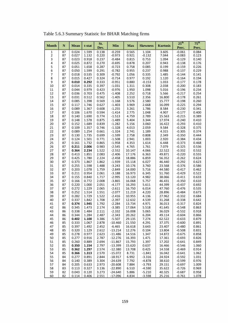
159

Table 5.6.3 Summary Statistic for BHAR Matching firms



25th

Perc.

75th

Perc.

1 87 0.024 1.599 0.138 -0.259 0.565 1.104 3.605 -0.061 0.084 2 87 0.027 1.132 0.220 -0.973 0.921 -0.132 7.044 -0.083 0.123 3 87 0.023 0.918 0.237 -0.484 0.815 0.753 1.094 -0.129 0.140 4 87 0.025 0.872 0.270 -0.695 0.878 0.207 0.943 -0.138 0.176 5 87 0.051 1.658 0.287 -0.723 0.758 0.085 0.199 -0.159 0.226 6 87 0.050 1.599 0.291 -0.782 0.955 0.237 0.988 -0.137 0.229 7 87 0.018 0.535 0.309 -0.792 1.056 0.335 1.485 -0.144 0.141 8 87 0.015 0.427 0.324 -0.714 0.977 0.192 1.120 -0.164 0.194 9 87 0.010 0.292 0.333 -0.951 0.880 -0.153 1.033 -0.177 0.178

10 87 0.014 0.335 0.397 -1.031 1.311 0.308 2.038 -0.200 0.183 11 87 0.044 0.979 0.423 -0.976 1.950 1.098 5.016 -0.196 0.234 12 87 0.036 0.703 0.475 -1.408 2.252 0.718 5.566 -0.217 0.254 13 87 0.031 0.512 0.562 -1.405 3.510 2.356 16.800 -0.178 0.261 14 87 0.085 1.398 0.569 -1.168 3.576 2.580 15.777 -0.198 0.260 15 87 0.117 1.746 0.627 -1.403 3.969 2.668 16.099 -0.225 0.294 16 87 0.089 1.367 0.608 -1.255 3.261 1.786 8.584 -0.230 0.341 17 87 0.106 1.670 0.594 -1.414 2.775 1.048 4.907 -0.177 0.400 18 87 0.140 1.690 0.774 -1.513 4.759 2.789 15.563 -0.215 0.389 19 87 0.148 1.578 0.875 -1.489 5.404 3.344 17.974 -0.240 0.410 20 87 0.152 1.689 0.839 -1.282 5.156 3.060 16.422 -0.293 0.410 21 87 0.109 1.357 0.746 -1.328 4.013 2.059 9.584 -0.328 0.375 22 87 0.089 1.254 0.661 -1.324 2.741 1.189 4.315 -0.305 0.374 23 87 0.130 1.735 0.699 -1.599 2.758 0.808 2.349 -0.350 0.444 24 87 0.124 1.501 0.771 -1.508 2.941 1.003 2.920 -0.384 0.434 25 87 0.161 1.732 0.865 -1.958 4.353 1.614 6.448 -0.373 0.468 26 87 0.211 2.006 0.983 -2.545 4.765 1.761 7.079 -0.325 0.536 27 87 0.364 2.234 1.522 -2.552 10.147 4.066 22.522 -0.332 0.532 28 87 0.413 1.851 2.083 -2.406 17.176 6.363 49.871 -0.220 0.555 29 87 0.425 1.780 2.224 -2.458 18.886 6.859 56.352 -0.262 0.624 30 87 0.373 1.867 1.862 -1.939 15.118 6.027 46.440 -0.292 0.623 31 87 0.255 1.598 1.488 -3.243 10.176 3.760 23.568 -0.376 0.586 32 87 0.203 1.078 1.759 -2.849 14.000 5.716 44.580 -0.417 0.462 33 87 0.211 0.954 2.061 -3.188 16.973 6.345 51.760 -0.429 0.522 34 87 0.155 0.840 1.717 -2.995 13.120 4.982 38.066 -0.411 0.633 35 87 0.166 0.772 2.008 -3.865 16.068 5.757 46.431 -0.350 0.610 36 87 0.220 1.000 2.051 -4.177 16.293 5.611 44.399 -0.437 0.692 37 87 0.272 1.229 2.065 -2.611 16.750 6.014 47.760 -0.476 0.535 38 87 0.252 1.514 1.551 -2.077 11.219 4.220 28.896 -0.484 0.673 39 87 0.282 1.729 1.522 -2.416 10.955 4.136 27.962 -0.332 0.684 40 87 0.337 1.842 1.708 -2.397 12.632 4.539 31.268 -0.338 0.642 41 87 0.374 1.945 1.792 -2.284 13.734 4.971 36.013 -0.317 0.824 42 86 0.345 1.473 2.174 -3.385 17.064 5.518 41.645 -0.548 0.863 43 86 0.338 1.484 2.111 -2.332 16.008 5.065 36.029 -0.532 0.918 44 86 0.344 1.284 2.487 -2.343 20.262 6.204 49.114 -0.604 0.866 45 86 0.402 1.100 3.386 -5.507 29.135 7.274 62.522 -0.633 0.879 46 85 0.333 1.067 2.878 -10.460 21.550 4.291 37.375 -0.600 0.891 47 85 0.397 1.492 2.452 -6.465 16.618 3.643 23.407 -0.480 0.861 48 85 0.320 1.129 2.612 -13.214 12.276 0.104 13.804 -0.508 0.831 49 85 0.278 0.977 2.623 -11.486 14.516 1.347 14.872 -0.675 0.858 50 85 0.277 0.916 2.787 -12.276 16.393 1.471 17.361 -0.693 0.826 51 85 0.260 0.889 2.694 -11.867 15.793 1.397 17.202 -0.641 0.849 52 85 0.350 1.154 2.797 -13.399 15.620 0.637 16.466 -0.546 1.060 53 85 0.362 1.297 2.574 -12.380 13.708 0.425 14.558 -0.469 0.914 54 85 0.366 1.313 2.570 -15.072 8.731 -1.841 16.042 -0.641 1.062 55 84 0.277 0.891 2.844 -18.917 6.992 -3.316 24.924 -0.592 1.031 56 84 0.140 0.389 3.304 -24.639 7.792 -4.878 38.610 -0.599 0.976 57 84 0.205 0.633 2.973 -20.608 7.884 -3.793 29.151 -0.697 1.009 58 83 0.113 0.327 3.136 -22.890 6.510 -4.590 35.622 -0.726 0.969 59 82 0.043 0.120 3.273 -24.640 5.886 -5.210 40.325 -0.687 0.958 60 82 0.114 0.406 2.551 -17.096 4.834 -3.598 25.216 -0.761 1.078

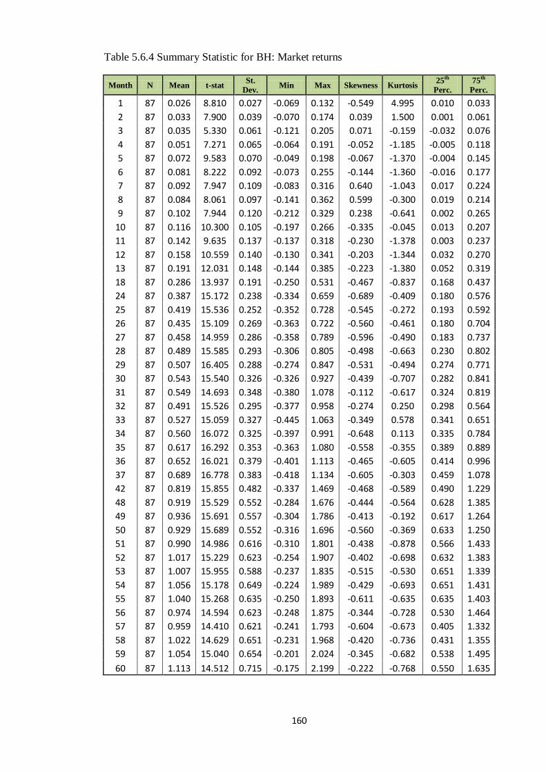
160

Table 5.6.4 Summary Statistic for BH: Market returns



25th

Perc.

75th

Perc.

1 87 0.026 8.810 0.027 -0.069 0.132 -0.549 4.995 0.010 0.033

2 87 0.033 7.900 0.039 -0.070 0.174 0.039 1.500 0.001 0.061

3 87 0.035 5.330 0.061 -0.121 0.205 0.071 -0.159 -0.032 0.076

4 87 0.051 7.271 0.065 -0.064 0.191 -0.052 -1.185 -0.005 0.118

5 87 0.072 9.583 0.070 -0.049 0.198 -0.067 -1.370 -0.004 0.145

6 87 0.081 8.222 0.092 -0.073 0.255 -0.144 -1.360 -0.016 0.177

7 87 0.092 7.947 0.109 -0.083 0.316 0.640 -1.043 0.017 0.224

8 87 0.084 8.061 0.097 -0.141 0.362 0.599 -0.300 0.019 0.214

9 87 0.102 7.944 0.120 -0.212 0.329 0.238 -0.641 0.002 0.265

10 87 0.116 10.300 0.105 -0.197 0.266 -0.335 -0.045 0.013 0.207

11 87 0.142 9.635 0.137 -0.137 0.318 -0.230 -1.378 0.003 0.237

12 87 0.158 10.559 0.140 -0.130 0.341 -0.203 -1.344 0.032 0.270

13 87 0.191 12.031 0.148 -0.144 0.385 -0.223 -1.380 0.052 0.319

18 87 0.286 13.937 0.191 -0.250 0.531 -0.467 -0.837 0.168 0.437

24 87 0.387 15.172 0.238 -0.334 0.659 -0.689 -0.409 0.180 0.576

25 87 0.419 15.536 0.252 -0.352 0.728 -0.545 -0.272 0.193 0.592

26 87 0.435 15.109 0.269 -0.363 0.722 -0.560 -0.461 0.180 0.704

27 87 0.458 14.959 0.286 -0.358 0.789 -0.596 -0.490 0.183 0.737

28 87 0.489 15.585 0.293 -0.306 0.805 -0.498 -0.663 0.230 0.802

29 87 0.507 16.405 0.288 -0.274 0.847 -0.531 -0.494 0.274 0.771

30 87 0.543 15.540 0.326 -0.326 0.927 -0.439 -0.707 0.282 0.841

31 87 0.549 14.693 0.348 -0.380 1.078 -0.112 -0.617 0.324 0.819

32 87 0.491 15.526 0.295 -0.377 0.958 -0.274 0.250 0.298 0.564

33 87 0.527 15.059 0.327 -0.445 1.063 -0.349 0.578 0.341 0.651

34 87 0.560 16.072 0.325 -0.397 0.991 -0.648 0.113 0.335 0.784

35 87 0.617 16.292 0.353 -0.363 1.080 -0.558 -0.355 0.389 0.889

36 87 0.652 16.021 0.379 -0.401 1.113 -0.465 -0.605 0.414 0.996

37 87 0.689 16.778 0.383 -0.418 1.134 -0.605 -0.303 0.459 1.078

42 87 0.819 15.855 0.482 -0.337 1.469 -0.468 -0.589 0.490 1.229

48 87 0.919 15.529 0.552 -0.284 1.676 -0.444 -0.564 0.628 1.385

49 87 0.936 15.691 0.557 -0.304 1.786 -0.413 -0.192 0.617 1.264

50 87 0.929 15.689 0.552 -0.316 1.696 -0.560 -0.369 0.633 1.250

51 87 0.990 14.986 0.616 -0.310 1.801 -0.438 -0.878 0.566 1.433

52 87 1.017 15.229 0.623 -0.254 1.907 -0.402 -0.698 0.632 1.383

53 87 1.007 15.955 0.588 -0.237 1.835 -0.515 -0.530 0.651 1.339

54 87 1.056 15.178 0.649 -0.224 1.989 -0.429 -0.693 0.651 1.431

55 87 1.040 15.268 0.635 -0.250 1.893 -0.611 -0.635 0.635 1.403

56 87 0.974 14.594 0.623 -0.248 1.875 -0.344 -0.728 0.530 1.464

57 87 0.959 14.410 0.621 -0.241 1.793 -0.604 -0.673 0.405 1.332

58 87 1.022 14.629 0.651 -0.231 1.968 -0.420 -0.736 0.431 1.355

59 87 1.054 15.040 0.654 -0.201 2.024 -0.345 -0.682 0.538 1.495

60 87 1.113 14.512 0.715 -0.175 2.199 -0.222 -0.768 0.550 1.635

161

Table 5.6.5 Summary Statistic for BHAR Using the market portfolio as a benchmark



25th

Perc.

75th

Perc.

1 87 0.003 0.222 0.106 -0.276 0.366 0.356 1.531 -0.052 0.058 2 87 0.010 0.731 0.127 -0.268 0.534 1.129 3.344 -0.064 0.066 3 87 0.002 0.125 0.160 -0.384 0.673 1.114 4.430 -0.101 0.072 4 87 0.015 0.735 0.192 -0.524 0.826 1.356 5.424 -0.094 0.093 5 87 0.016 0.645 0.226 -0.576 1.293 2.057 11.638 -0.092 0.115 6 87 0.015 0.561 0.243 -0.582 1.444 2.615 14.408 -0.088 0.104 7 87 0.013 0.446 0.269 -0.672 1.381 2.314 9.919 -0.126 0.118 8 87 0.028 0.891 0.288 -0.616 1.122 1.332 3.516 -0.138 0.162 9 87 0.021 0.683 0.290 -0.486 1.210 1.682 4.889 -0.146 0.140 10 87 0.014 0.395 0.326 -0.632 1.471 1.883 5.973 -0.160 0.142 11 87 0.019 0.492 0.356 -0.590 1.926 2.488 10.560 -0.179 0.132 12 87 0.025 0.633 0.376 -0.673 2.062 2.128 9.543 -0.177 0.156 13 87 0.005 0.092 0.497 -0.803 3.603 4.492 31.865 -0.228 0.149 14 87 0.034 0.608 0.528 -0.800 3.754 4.198 28.362 -0.206 0.179 15 87 0.058 0.906 0.594 -0.817 4.315 4.513 30.711 -0.186 0.172 16 87 0.043 0.704 0.566 -0.772 3.790 3.898 22.625 -0.213 0.131 17 87 0.049 0.791 0.579 -0.786 3.594 3.308 16.569 -0.221 0.134 18 87 0.085 0.979 0.810 -0.777 5.908 4.886 31.881 -0.283 0.145 19 87 0.115 1.135 0.941 -0.830 6.726 4.852 30.183 -0.282 0.164 20 87 0.140 1.476 0.887 -0.850 6.273 4.597 27.909 -0.240 0.263 21 87 0.101 1.150 0.819 -0.838 5.404 3.818 20.848 -0.311 0.223 22 87 0.065 0.787 0.776 -0.941 4.643 3.053 14.250 -0.357 0.305 23 87 0.089 0.987 0.845 -1.021 5.348 3.409 17.634 -0.330 0.349 24 87 0.074 0.828 0.834 -1.150 3.937 2.246 7.192 -0.409 0.300 25 87 0.078 0.810 0.901 -1.074 3.989 2.432 7.661 -0.443 0.293 26 87 0.105 1.012 0.973 -1.116 4.517 2.665 9.128 -0.410 0.296 27 87 0.217 1.300 1.560 -1.269 9.763 4.284 21.934 -0.440 0.319 28 87 0.260 1.150 2.105 -1.235 16.774 6.230 45.791 -0.516 0.329 29 87 0.268 1.133 2.208 -1.216 18.452 6.854 54.763 -0.570 0.381 30 87 0.206 1.023 1.882 -1.262 14.680 5.815 41.726 -0.615 0.330 31 87 0.130 0.805 1.512 -1.248 9.805 4.294 22.717 -0.619 0.265 32 87 0.147 0.793 1.729 -1.308 13.602 5.933 43.666 -0.591 0.304 33 87 0.133 0.618 1.999 -1.346 16.409 6.644 52.354 -0.689 0.291 34 87 0.059 0.345 1.605 -1.392 12.370 5.588 40.718 -0.667 0.279 35 87 0.065 0.332 1.837 -1.307 15.201 6.706 54.465 -0.697 0.305 36 87 0.078 0.378 1.921 -1.448 15.530 6.293 49.386 -0.773 0.280 37 87 0.098 0.454 2.016 -1.363 16.079 6.110 46.626 -0.809 0.241 38 87 0.024 0.149 1.502 -1.388 10.511 4.405 27.646 -0.739 0.238 39 87 0.011 0.065 1.517 -1.584 10.318 4.127 24.846 -0.742 0.233 40 87 0.027 0.147 1.690 -1.534 11.907 4.570 28.741 -0.795 0.187 41 87 0.071 0.378 1.742 -1.537 12.887 5.010 34.272 -0.806 0.239 42 86 0.097 0.426 2.107 -1.858 16.102 5.535 39.715 -0.738 0.228 43 86 0.101 0.460 2.035 -1.863 14.888 4.987 33.265 -0.804 0.277 44 86 0.172 0.666 2.399 -1.758 19.248 6.199 47.755 -0.707 0.336 45 86 0.261 0.752 3.220 -1.853 27.910 7.640 65.559 -0.706 0.328 46 85 0.184 0.658 2.581 -1.892 20.392 6.005 45.316 -0.797 0.400 47 85 0.206 0.816 2.325 -1.930 15.422 4.117 22.589 -0.891 0.401 48 85 0.180 0.760 2.184 -2.228 11.037 2.923 10.436 -0.937 0.428 49 85 0.146 0.591 2.280 -2.315 13.310 3.414 15.167 -0.989 0.345 50 85 0.193 0.752 2.362 -2.237 14.927 3.635 18.299 -1.014 0.262 51 85 0.115 0.466 2.279 -2.342 14.109 3.447 17.085 -0.983 0.376 52 85 0.157 0.643 2.256 -2.353 13.911 3.383 16.504 -1.066 0.258 53 85 0.153 0.669 2.113 -2.176 12.014 2.916 11.929 -1.065 0.253 54 85 0.128 0.595 1.978 -2.173 7.040 1.851 3.273 -1.068 0.291 55 84 0.144 0.679 1.941 -2.083 6.869 1.682 2.459 -1.100 0.346 56 84 0.142 0.683 1.906 -2.053 7.140 1.845 3.566 -0.981 0.419 57 84 0.165 0.799 1.896 -2.029 7.373 1.777 3.349 -1.007 0.601 58 83 0.051 0.259 1.809 -2.376 6.871 1.639 2.767 -1.010 0.369 59 82 0.041 0.206 1.785 -2.415 6.535 1.639 2.745 -1.013 0.441 60 82 -0.027 -0.143 1.736 -2.492 5.608 1.361 1.634 -1.124 0.395

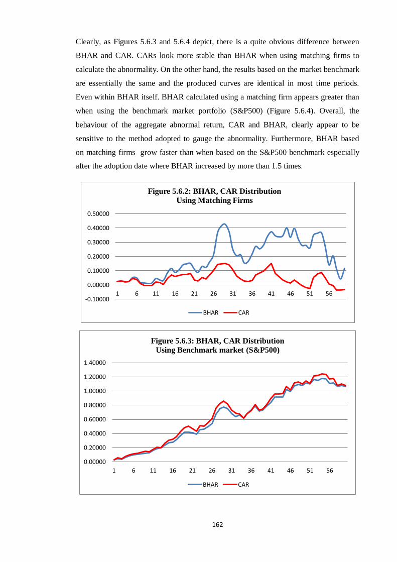
162

Clearly, as Figures 5.6.3 and 5.6.4 depict, there is a quite obvious difference between

BHAR and CAR. CARs look more stable than BHAR when using matching firms to

calculate the abnormality. On the other hand, the results based on the market benchmark

are essentially the same and the produced curves are identical in most time periods.

Even within BHAR itself. BHAR calculated using a matching firm appears greater than

when using the benchmark market portfolio (S&P500) (Figure 5.6.4). Overall, the

behaviour of the aggregate abnormal return, CAR and BHAR, clearly appear to be

sensitive to the method adopted to gauge the abnormality. Furthermore, BHAR based

on matching firms grow faster than when based on the S&P500 benchmark especially

after the adoption date where BHAR increased by more than 1.5 times.

-0.10000

0.00000

0.10000

0.20000

0.30000

0.40000

0.50000

1 6 11 16 21 26 31 36 41 46 51 56

Figure 5.6.2: BHAR, CAR Distribution

Using Matching Firms

BHAR CAR

0.00000

0.20000

0.40000

0.60000

0.80000

1.00000

1.20000

1.40000

1 6 11 16 21 26 31 36 41 46 51 56

Figure 5.6.3: BHAR, CAR Distribution

Using Benchmark market (S&P500)

BHAR CAR

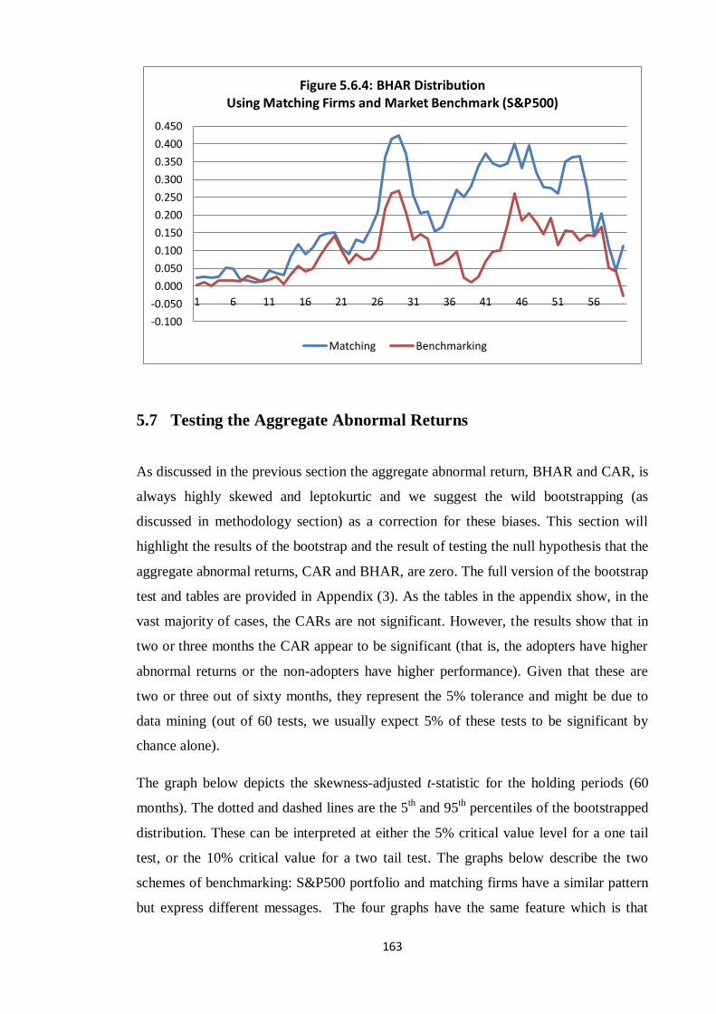
163

5.7 Testing the Aggregate Abnormal Returns

As discussed in the previous section the aggregate abnormal return, BHAR and CAR, is

always highly skewed and leptokurtic and we suggest the wild bootstrapping (as

discussed in methodology section) as a correction for these biases. This section will

highlight the results of the bootstrap and the result of testing the null hypothesis that the

aggregate abnormal returns, CAR and BHAR, are zero. The full version of the bootstrap

test and tables are provided in Appendix (3). As the tables in the appendix show, in the

vast majority of cases, the CARs are not significant. However, the results show that in

two or three months the CAR appear to be significant (that is, the adopters have higher

abnormal returns or the non-adopters have higher performance). Given that these are

two or three out of sixty months, they represent the 5% tolerance and might be due to

data mining (out of 60 tests, we usually expect 5% of these tests to be significant by

chance alone).

The graph below depicts the skewness-adjusted t-statistic for the holding periods (60

months). The dotted and dashed lines are the 5th and 95

th percentiles of the bootstrapped

distribution. These can be interpreted at either the 5% critical value level for a one tail

test, or the 10% critical value for a two tail test. The graphs below describe the two

schemes of benchmarking: S&P500 portfolio and matching firms have a similar pattern

but express different messages. The four graphs have the same feature which is that

-0.100

-0.050

0.000

0.050

0.100

0.150

0.200

0.250

0.300

0.350

0.400

0.450

1 6 11 16 21 26 31 36 41 46 51 56

Figure 5.6.4: BHAR Distribution Using Matching Firms and Market Benchmark (S&P500)

Matching Benchmarking

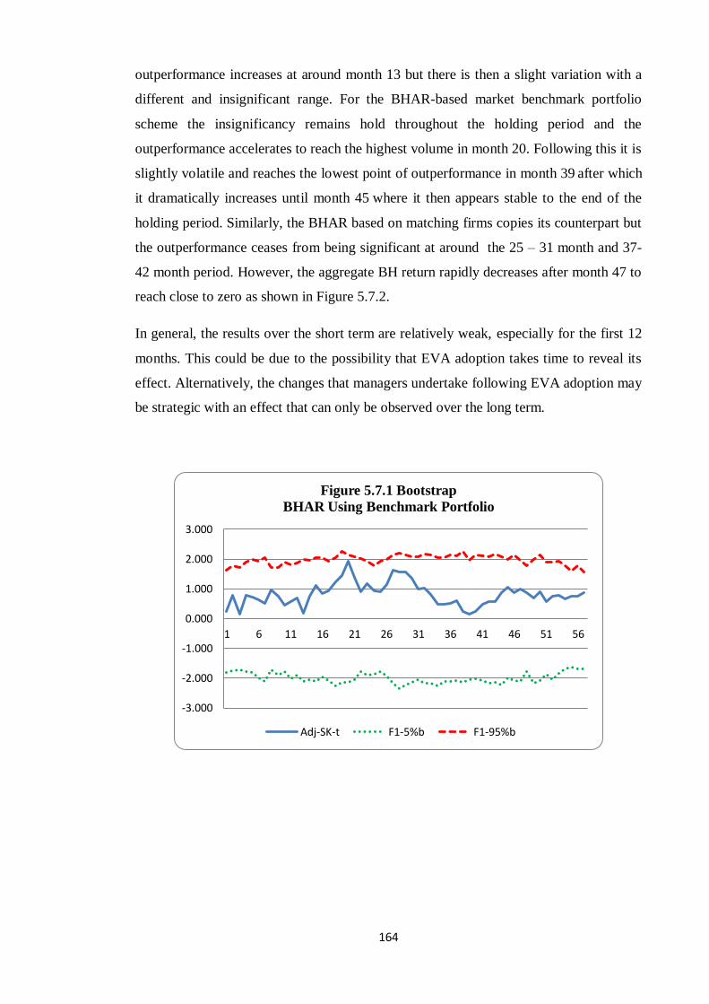
164

outperformance increases at around month 13 but there is then a slight variation with a

different and insignificant range. For the BHAR-based market benchmark portfolio

scheme the insignificancy remains hold throughout the holding period and the

outperformance accelerates to reach the highest volume in month 20. Following this it is

slightly volatile and reaches the lowest point of outperformance in month 39 after which

it dramatically increases until month 45 where it then appears stable to the end of the

holding period. Similarly, the BHAR based on matching firms copies its counterpart but

the outperformance ceases from being significant at around the 25 – 31 month and 37-

42 month period. However, the aggregate BH return rapidly decreases after month 47 to

reach close to zero as shown in Figure 5.7.2.

In general, the results over the short term are relatively weak, especially for the first 12

months. This could be due to the possibility that EVA adoption takes time to reveal its

effect. Alternatively, the changes that managers undertake following EVA adoption may

be strategic with an effect that can only be observed over the long term.

-3.000

-2.000

-1.000

0.000

1.000

2.000

3.000

1 6 11 16 21 26 31 36 41 46 51 56

Figure 5.7.1 Bootstrap

BHAR Using Benchmark Portfolio

Adj-SK-t F1-5%b F1-95%b

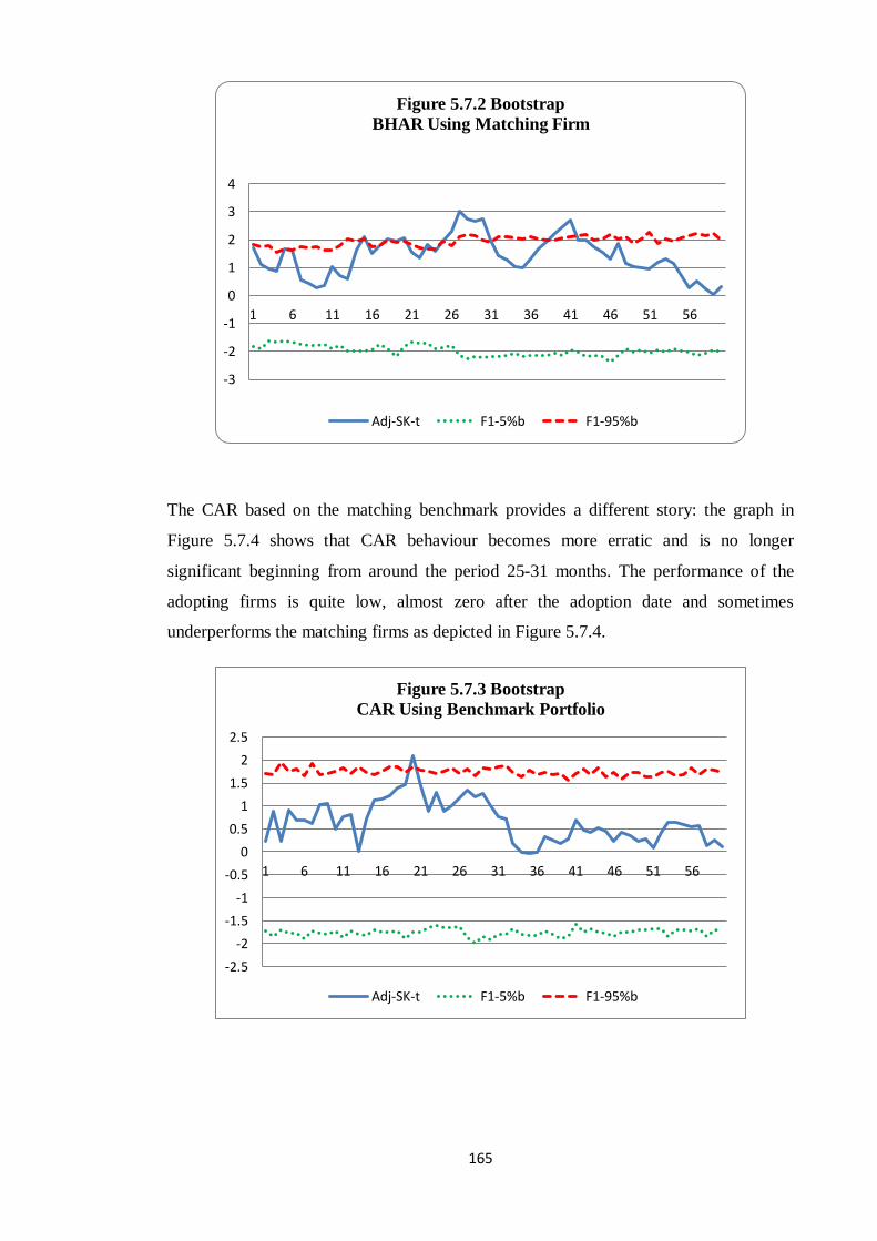
165

The CAR based on the matching benchmark provides a different story: the graph in

Figure 5.7.4 shows that CAR behaviour becomes more erratic and is no longer

significant beginning from around the period 25-31 months. The performance of the

adopting firms is quite low, almost zero after the adoption date and sometimes

underperforms the matching firms as depicted in Figure 5.7.4.

-3

-2

-1

0

1

2

3

4

1 6 11 16 21 26 31 36 41 46 51 56


BHAR Using Matching Firm


-2.5

-2

-1.5

-1

-0.5

0

0.5

1

1.5

2

2.5

1 6 11 16 21 26 31 36 41 46 51 56


CAR Using Benchmark Portfolio


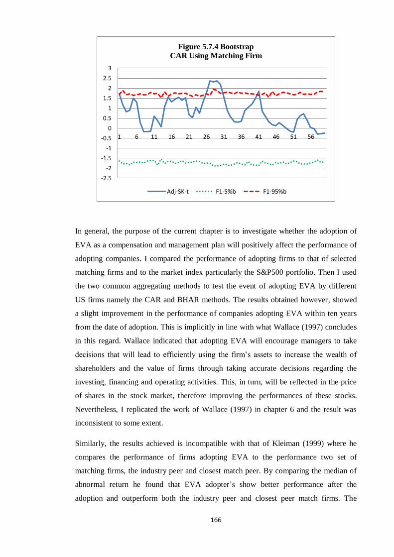
166

In general, the purpose of the current chapter is to investigate whether the adoption of

EVA as a compensation and management plan will positively affect the performance of

adopting companies. I compared the performance of adopting firms to that of selected

matching firms and to the market index particularly the S&P500 portfolio. Then I used

the two common aggregating methods to test the event of adopting EVA by different

US firms namely the CAR and BHAR methods. The results obtained however, showed

a slight improvement in the performance of companies adopting EVA within ten years

from the date of adoption. This is implicitly in line with what Wallace (1997) concludes

in this regard. Wallace indicated that adopting EVA will encourage managers to take

decisions that will lead to efficiently using the firm’s assets to increase the wealth of

shareholders and the value of firms through taking accurate decisions regarding the

investing, financing and operating activities. This, in turn, will be reflected in the price

of shares in the stock market, therefore improving the performances of these stocks.

Nevertheless, I replicated the work of Wallace (1997) in chapter 6 and the result was

inconsistent to some extent.

Similarly, the results achieved is incompatible with that of Kleiman (1999) where he

compares the performance of firms adopting EVA to the performance two set of

matching firms, the industry peer and closest match peer. By comparing the median of

abnormal return he found that EVA adopter’s show better performance after the

adoption and outperform both the industry peer and closest peer match firms. The

-2.5

-2

-1.5

-1

-0.5

0

0.5

1

1.5

2

2.5

3

1 6 11 16 21 26 31 36 41 46 51 56


CAR Using Matching Firm


167

adjusted market return increases from 2.8% to 28.8% through three year time period

after the adoption for the industry peer and from 2.6% to 7.8% for the closest match

peer. However, the increases in performance of the adopting firms are still quite low.

the current research used the mean of CAR and BHAR to compare the performances of

adopting firms to those matching firms and market benchmark portfolio (S&P500

index) and the result revealed that EVA’s firms outperform those matching and S&P500

portfolio and the CAR increases to reach 8.85% and 36.6% for matching firms and

benchmark index respectively and the BHAR increases to 6.6% and 26.8% for the same

order.

Contrary to Wallace’s and my findings, Tortella and Brusco (2003) used 65 EVA

adopter firms to analyse the market reaction to EVA adoption. They compared the daily

abnormal return of adopting firms to that of the equally weighted index (EW) and value

weighted index (VW) to test for any changes in performances after the adoption date.

However, he used a window of 30 days prior to the adoption and 100 days post the

adoption. For both the equally weighted and value weighted index the results indicated

that the daily cumulative average abnormal return (CAAR) is insignificant and negative

for 14 days after the adoption date. Furthermore, they conclude that the market does not

react properly to the evolution of EVA as a performance measure. In my opinion,

because the process of adoption of EVA as a performance and management tool is of a

long-term nature, it takes some years to complete the process, the daily stock price fails

to reflect this information and the daily CAAR appear insignificant for much of the

time.

5.8 Conclusion

This chapter has described the research design and the methodology that was used to

examine the EVA adoption event. Both the CAR and the BHAR approaches were

adopted to conduct our study. The previous research has been extended by increasing

the number of EVA adopter firms to 89 and the time horizon of the study to cover the

firms’ performance during the period 1960-2012 was also extended. In addition wild

bootstrapping and using the skewness adjusted t-statistic to enhance the statistical

reliability of the event test statistics was adopted. By doing this all three moments of the

parent distribution of the test statistic (Heteroscedasticity, skewness and kurtosis) were

taken into account. Furthermore, the criterion to select the matching firms was carefully

applied as was the problem of delisting.

168

The results obtained in this chapter are consistent with the previous studies’ results

discussed in section 5.2. Regardless of the methodology approach , CAR or BHAR, the

results of this chapter reveal that firms adopting EVA as a compensation plan and

management tool outperform the market (S&P500) and matching firms (same sector)

most of the time within holding period. The CAR results show that despite the

benchmarking used the majority of adopter firms positively outperform the matching

firms and the S&P500 portfolio and for a few months the adopter firms have a negative

performance mainly in year one and year five of the 10 year estimated period. In

general, CAR appears more stable and less skewed and leptokurtic.

Regarding the BHAR approach the findings reveal that the mean return of the adopter

firms is both positive and highly skewed and leptokurtic throughout the holding period.

Generally, the results obtained from a comparison against the benchmarking portfolio

(S&P500) are smaller in value than those obtained when compared to the matching

firms’ benchmark. One interesting finding is that CAR is almost the same as BHAR

when the S&P500 portfolio is used as a benchmark to calculate the aggregate returns.

To sum up, irrespective of the aggregation approach used to measure the abnormal

return, the adopter firms have a considerably low outperformance and this

outperformance increased as the hold period increased. However, even with the positive

performances most EVA adopter firms’ outperformance declines after the adoption and

takes some time to return to negative performance when matching benchmarks are used.

This might typically reflect the fact that the market might react poorly to the adoption

announcement. Finally, by analysing the adopter firms’ performance we recognize that

the adoption exists after a period of bad performances.

169

Chapter 6

The Long-Term Effect of Economic Value Added

Adoption on the Firm’s Business Decision

6.1 Introduction

The economic value added (EVA) metric has received considerable attention in the

literature as the best performance measure with the ability to align managers’ interests

with those of the shareholders. It is further claimed that adopting the EVA framework

(e.g. as a management system, or as a compensation system) will encourage managers

to use the firm’s resources more efficiently and make decisions that would help increase

the firm’s value (Wallace, 1997; Balachandran, 2006). However, one interesting aspect

of this new performance metric is that it is not all that new. Value added as a concept is

age-old. It has its origins in the notion of economic profit, first mentioned in the

literature a century ago.30

EVA, which specifically mentions residual income (RI), was

adopted by General Motors and Matsushita in the 1920s and 1930s respectively (Young,

1999). Officially, in the mid-1990s the American Institute of Certified Financial

Accountants (AICPA) recommended EVA as a type of measure that would enhance

internal decision-making and would replace earnings per share (EPS), the traditional

measure, in the regular stock and earnings report section (Zarowin, 1995).

This chapter will extend what was started in chapter 5 where the EVA adoption event

was tested using cumulative abnormal return (CAR) and buy-and-hold abnormal return

(BHAR). The results thereof reveal that firms adopting EVA as a management and

compensation system outperform the market portfolio, the S&P500 and the set of

matching firms. In this chapter Wallace’s (1997) work will be reconsidered. I will

investigate whether the adoption of EVA does indeed enhance the performance and the

quality of strategic decisions of the firm. Specifically, the strategic decisions that the

management will take in order to increase the value of the company and the wealth of

shareholders include asset dispositions, acquisitions and capital expenditure, share

repurchases, dividends and operating decisions.

30As Wallace (1997) stated, Alfred Marshall was the earliest to mention the residual income concept in

1890.

170

The structure of this chapter is as follows: Section 6.2 will discuss the work of Wallace

(1997) who investigated the impact of EVA adoption on a firm’s performance. Section

6.3 describes the data sources, sample selection and variable definitions. Section 6.4

describes the methodology, and Section 6.5 discusses the empirical results. Finally,

Section 5.6 summarises the main conclusions.

6.2 The Wallace Study

“You get what you pay for” (Wallace, 1997).

In his seminal work, Wallace (1997) addressed the changes in profitability which a firm

achieves when adopting EVA. He investigated whether the use of value added,

particularly residual income, and bonus plans leads to decisions that are consistent with

the economic incentives deeply embedded in those plans. Wallace claims that the

“compensation plans provide one method to mitigate agency conflicts by providing

incentives for managers to decisions that are in the best interest of the shareholders.” (p.

277)

Wallace (1997) used a sample of 40 firms that have adopted RI- based compensation

plans to test whether the adoption of the RI framework will enhance and increase the

action of these firms compared to the action of other selected firms still using traditional

accounting-based compensation plans. His approach is therefore based on contrasting

the adopters which he calls the treatment firms, with the non-adopters which he calls the

control firms. The period of investigation extends to five years prior to the adoption and

up to three years following the adoption date (event date); the majority of the

investigated firms adopted an RI- based compensation plan in 1993 and 1994.

Wallace begins his empirical research by discussing the consequences that a firm must

face when switching to a residual income-based incentive. The focus of his work was on

developing hypotheses to test investment decisions (e.g. asset dispositions, acquisition

and capital expenditure), financing decisions (e.g. share repurchase, dividends) and

operating decisions (e.g. asset turnover).

The findings of Wallace (1997) were that all the adopters of EVA as a compensation

plan show a significant increase in residual income. With respect to the decision

variables the results also show that firms adopting an RI-based compensation plan

171

encourage managers to increase dispositions of assets and increase their payments to

shareholders in the form of a repurchasing of shares and intensively utilize their assets.

The results also support the axiom that “you get what you measure and reward”

(Wallace, 1997, p.276). Finally, weak evidence suggests that the market does not appear

to react to EVA adoption.

The work of Wallace was replicated by many scholars (Kleiman, 1999, Lovata and

Costigan, 2002, Hogan and Lewis, 2005 and Balachandran, 2006). One common feature

of these papers is that they discuss the compensation and incentive plan from the agency

conflict’s point of view. However, even though they have replicated Wallace’s work

(1997) they have reached different conclusions. While Wallace claims that firms that

adopt EVA decrease new investment, Kleiman claims that the manager’s behaviour has

no obvious bias against new investment. Similarly, Hogan and Lewis find that firms that

anticipate converting to the EVA compensation system would likely change their

investment behaviour by reducing capital expenditure. Furthermore, to account for the

pre-adoption performances they construct their own logistic model to select the optimal

control-matched firms. Therefore, their control firms’ sample fall into four types:

anticipated adopters, surprise adopters, anticipated non-adopters, and surprise non-

adopters.

In this chapter, I show that Wallace’s approach needs to be reconsidered. I further

extend the time horizon of study to cover the period from 1960 until 2012, and, more

importantly, the number of sample firms is more than doubled to reach 89 EVA

adopters. Extending the sample in both the time and the cross section dimensions will

remove doubt that previous results may have been due to data limitation. However, a

more important contribution in this study are the modifications introduced to the

Wallace model, which are more appropriate in identifying the effect of EVA adoption

before and after the adoption decision date.

6.3 Sample selection

In order to examine the impact of adopting the economic value added (EVA) on the

performance of both the executive management and the company as a whole, a

comprehensive sample of US EVA adopter firms from January 1960 to December 2012

was collected using the Compustat and CRSP databases. The variables used in the

172

models in the current research were mainly extracted from balance sheets, income

statements and cash flow statements. The sample was composed of firms adopting EVA

during the period 1987-2001 as a compensation and management system. The selection

procedures of the sample set and matching firms are discussed briefly in Chapter 5. The

dependent variables are similar to that of Wallace (1997) and defined as described in the

Compustat data base:

- Dispositions: sale of plant, property and equipment (SPPE).31

- New investment: acquisitions (AQC) plus capital expenditures (CAPX).

- Purchases per share: purchases of common stock (PRSTKCC) divided by

Common Shares Outstanding (CSHO).

- Dividends per share: dividend available to common shareholders (DVC) divided

by Common Shares Outstanding (CSHO).

- Assets turnover: revenue (REVT) divided by average total assets (TA).

- Inventory turnover: Cost of Goods Sold (COGS) divided by average Inventories

total (INVT).

- Accounts receivable turnover: revenue (REVT) divided by average accounts

receivable total (AR).

- Account payable turnover: Cost of Goods Sold (COGS) divided by average

account payable trade (AP).

- ∆Leverage: changes in debt for firms between periods.

All the dependent variables are deflated by the initial total assets (TA) and used in

levels rather than differences.

6.4 Methodology

The current research will use the same methodology as Wallace’s (1997) except that

while Wallace’s sample consists of those firms adopting a residual income-based

management system, we use only firms adopting EVA for incentive compensation

purposes. Moreover, while Wallace used five-year returns to conduct his research, the

current research uses the annual accounting data for the period 1960-2012 and focuses

on the long-term effects of adopting EVA as management and compensation tools.

Further, I will begin with Wallace’s model, discussing its drawbacks and provide simple

31 An abbreviation between brackets stands for COMPUSTAT Mnemonic.

173

numerical examples to show that the set up used by Wallace may lead to spurious

results. Modifications that mitigate these problems are then proposed.

The estimated event window that was used to examine the adopter firms’ behaviour is

set between 30 months prior to the adoption date and 30 months after the adoption. As

discussed in chapter 5, it is difficult to determine an accurate date for EVA’s adoption. I

therefore consider the month of December in the earliest year that the company released

the adoption of EVA as the event date. This approach is also adopted by Wallace

(1997), Kleiman (1999) and Balachandran, 2006

6.4.1 The Wallace Approach

Wallace (1997) analysed the firms that adopted residual income-based compensation

plans. However, only 23 firms in his sample applied the EVA approach (the rest

adopted residual income plans). Thus, Wallace’s findings cannot be attributed to EVA

alone. Rather, the effect found by Wallace should be associated with all residual income

(RI) methods. Consequently it is not perfectly correct to generalize Wallace’s finding

that the motif detected in the selected sample would likely exist for any randomly

chosen firms to the EVA compensation scheme.

Another limitation in Wallace is that he did not account for the pre-adoption operating

performance. In other words, he compares the adopter firms with matching firms after

adoption but fails to compare the adopter firm before and after adoption. Barber and

Lyon (1996) show that the failure to capture past performance leads to biased test

statistics. It is true that Wallace considered the difference in variables between the pre-

and post-adoption years. However, this does not make the comparison of the two

periods (before and after adoption) explicit. Wallace’s (1997) approach stated that:

where refers to the difference between the mean of a particular variable before the

adoption date and the average of the same variables after (and including) the adoption

year. He uses increasing sample sizes for the pre- and post-adoption periods in order to

assess possible differences between the short and longer term effects. is an

indicator variable, it equals 1 for firms adopting EVA and 0 for the matching firm,

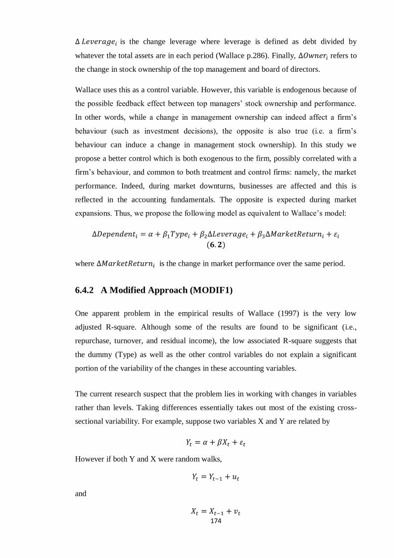
174

is the change leverage where leverage is defined as debt divided by

whatever the total assets are in each period (Wallace p.286). Finally, refers to

the change in stock ownership of the top management and board of directors.

Wallace uses this as a control variable. However, this variable is endogenous because of

the possible feedback effect between top managers’ stock ownership and performance.

In other words, while a change in management ownership can indeed affect a firm’s

behaviour (such as investment decisions), the opposite is also true (i.e. a firm’s

behaviour can induce a change in management stock ownership). In this study we

propose a better control which is both exogenous to the firm, possibly correlated with a

firm’s behaviour, and common to both treatment and control firms: namely, the market

performance. Indeed, during market downturns, businesses are affected and this is

reflected in the accounting fundamentals. The opposite is expected during market

expansions. Thus, we propose the following model as equivalent to Wallace’s model:

where is the change in market performance over the same period.

6.4.2 A Modified Approach (MODIF1)

One apparent problem in the empirical results of Wallace (1997) is the very low

adjusted R-square. Although some of the results are found to be significant (i.e.,

repurchase, turnover, and residual income), the low associated R-square suggests that

the dummy (Type) as well as the other control variables do not explain a significant

portion of the variability of the changes in these accounting variables.

The current research suspect that the problem lies in working with changes in variables

rather than levels. Taking differences essentially takes out most of the existing cross-

sectional variability. For example, suppose two variables X and Y are related by

However if both Y and X were random walks,

and

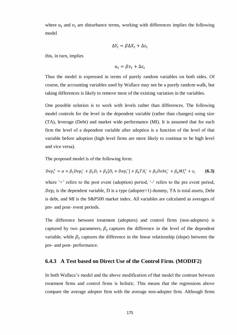
175

where and are disturbance terms, working with differences implies the following

model

this, in turn, implies

Thus the model is expressed in terms of purely random variables on both sides. Of

course, the accounting variables used by Wallace may not be a purely random walk, but

taking differences is likely to remove most of the existing variation in the variables.

One possible solution is to work with levels rather than differences. The following

model controls for the level in the dependent variable (rather than changes) using size

(TA), leverage (Debt) and market wide performance (MI). It is assumed that for each

firm the level of a dependent variable after adoption is a function of the level of that

variable before adoption (high level firms are more likely to continue to be high level

and vice versa).

The proposed model is of the following form:

(6.3)

where ‘+’ refers to the post event (adoption) period, ‘-‘ refers to the pre event period,

is the dependent variable, D is a type (adopter=1) dummy, TA is total assets, Debt

is debt, and MI is the S&P500 market index. All variables are calculated as averages of

pre- and post- event periods.

The difference between treatment (adopters) and control firms (non-adopters) is

captured by two parameters, captures the difference in the level of the dependent

variable, while captures the difference in the linear relationship (slope) between the

pre- and post- performance.

6.4.3 A Test based on Direct Use of the Control Firm. (MODIF2)

In both Wallace’s model and the above modification of that model the contrast between

treatment firms and control firms is holistic. This means that the regressions above

compare the average adopter firm with the average non-adopter firm. Although firms

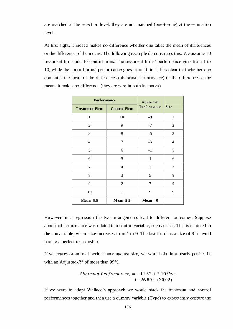
176

are matched at the selection level, they are not matched (one-to-one) at the estimation

level.

At first sight, it indeed makes no difference whether one takes the mean of differences

or the difference of the means. The following example demonstrates this. We assume 10

treatment firms and 10 control firms. The treatment firms’ performance goes from 1 to

10, while the control firms’ performance goes from 10 to 1. It is clear that whether one

computes the mean of the differences (abnormal performance) or the difference of the

means it makes no difference (they are zero in both instances).

Performance Abnormal

Performance

Size Treatment Firm Control Firm

1 10 -9 1

2 9 -7 2

3 8 -5 3

4 7 -3 4

5 6 -1 5

6 5 1 6

7 4 3 7

8 3 5 8

9 2 7 9

10 1 9 9

Mean=5.5 Mean=5.5 Mean = 0

However, in a regression the two arrangements lead to different outcomes. Suppose

abnormal performance was related to a control variable, such as size. This is depicted in

the above table, where size increases from 1 to 9. The last firm has a size of 9 to avoid

having a perfect relationship.

If we regress abnormal performance against size, we would obtain a nearly perfect fit

with an Adjusted- of more than 99%.

If we were to adopt Wallace’s approach we would stack the treatment and control

performances together and then use a dummy variable (Type) to expectantly capture the

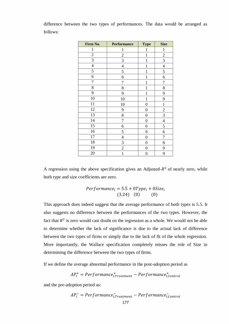
177

difference between the two types of performances. The data would be arranged as

follows:

Firm No. Performance Type Size

1 1 1 1

2 2 1 2

3 3 1 3

4 4 1 4

5 5 1 5

6 6 1 6

7 7 1 7

8 8 1 8

9 9 1 9

10 10 1 9

11 10 0 1

12 9 0 2

13 8 0 3

14 7 0 4

15 6 0 5

16 5 0 6

17 4 0 7

18 3 0 8

19 2 0 9

20 1 0 9

A regression using the above specification gives an Adjusted- of nearly zero, while

both type and size coefficients are zero.

This approach does indeed suggest that the average performance of both types is 5.5. It

also suggests no difference between the performances of the two types. However, the

fact that is zero would cast doubt on the regression as a whole. We would not be able

to determine whether the lack of significance is due to the actual lack of difference

between the two types of firms or simply due to the lack of fit of the whole regression.

More importantly, the Wallace specification completely misses the role of Size in

determining the difference between the two types of firms.

If we define the average abnormal performance in the post-adoption period as

and the pre-adoption period as:

178

Similarly, if I defines abnormal asset and abnormal debt as the difference between the

assets and debts between the treatment and control firms, respectively, that is,

and

Then we propose the following model:

If there is no effect resulting from the adoption, then the abnormal performance before

the event should be equal on average to the abnormal performance after the event. Any

possible change in abnormal performance could be due to the control variables

(abnormal TA and abnormal debt). Thus, the parameter of interest is , and the null

hypothesis of no effect is . However, we can operationalize the testing of this

hypothesis by subtracting from both sides of the equation to obtain

where . Thus, testing is equivalent to testing .

Table 6.4.1 presents summary statistics of the investigated potential investment

decisions (the dependent and independent/control variables employed in models (6.2),

(6.3) and (6.4)). The mean values of disposition per share for adopter firms are 27.581

and 27.739 for the matching firms. Reflecting overall expectations of negative

disposition per share after EVA adoption, standard deviation in particular for matching

firms is higher than the corresponding adopting firms. Interestingly, the mean new

investment is 344.580 for adopting firms, whereas the mean new investment is 266.953

for matching firms, which indicates that adopting firms operate with a considerable

balance of new investment rather than decreasing their expenditure on new projects. In

addition it is worth noting that both adopters and matching firms are operating with a

considerable leverage level. However, note that the distribution of all the potential

decisions is highly skewed to the right as indicated by the large standard deviations. For

most numbers the mean of adopting firms is even higher than the number for the

matching firms.

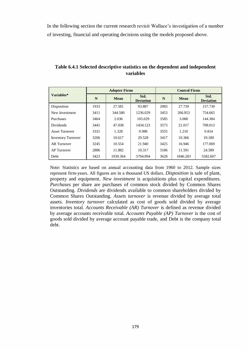
179

In the following section the current research revisit Wallace’s investigation of a number

of investing, financial and operating decisions using the models proposed above.

Table 6.4.1 Selected descriptive statistics on the dependent and independent

variables

Variables*

Adopter Firms Control Firms

N Mean Std.

Deviation N Mean

Std.

Deviation

Disposition 1933 27.581 93.887 2083 27.739 157.730

New Investment 3411 344.580 1236.029 3453 266.953 754.665

Purchases 3464 2.036 105.029 3585 3.068 144.384

Dividends 3441 47.038 1434.123 3573 21.017 708.013

Asset Turnover 3331 1.328 0.988 3555 1.210 0.814

Inventory Turnover 3206 10.617 29.528 3417 10.366 19.180

AR Turnover 3245 10.554 21.940 3425 16.946 177.069

AP Turnover 2886 11.882 10.317 3186 11.591 24.589

Debt 3423 1930.364 5704.894 3628 1846.283 5582.607

Note: Statistics are based on annual accounting data from 1960 to 2012. Sample sizes

represent firm-years. All figures are in a thousand US dollars. Disposition is sale of plant,

property and equipment. New investment is acquisitions plus capital expenditures.

Purchases per share are purchases of common stock divided by Common Shares

Outstanding. Dividends are dividends available to common shareholders divided by

Common Shares Outstanding. Assets turnover is revenue divided by average total

assets. Inventory turnover calculated as cost of goods sold divided by average

inventories total. Accounts Receivable (AR) Turnover is defined as revenue divided

by average accounts receivable total. Accounts Payable (AP) Turnover is the cost of

goods sold divided by average account payable trade, and Debt is the company total

debt.

180

6.5 Empirical Results

I began my analysis with the regression for equation (6.2), which is similar to that of

Wallace (1997) except that replaces as a control variable.

Table 6.5.1 summarises the results for dispositions and new investment decisions for the

period of five years before and five years after adoption (10 year window). The effect is

captured by the ‘Type’ coefficients. Contrary to Wallace’s finding, the adoption seems

to have no effect on dispositions and new investment; both coefficients (-0.001 and

0.005 respectively) are insignificant and of the opposite sign to those of Wallace. Thus,

over a ten-year window dispositions show no significant change, whereas in Wallace

they increased by 0.01 and were statistically significant. A similar insignificant effect is

found for new investment (a negative effect is found in Wallace although it is only

significant at the 10% level). Note that the adjusted- is only 2% for dispositions (9%

in Wallace) but 23% for new investment (1% in Wallace). This reversal of explanatory

power of Wallace’s specification seems erratic since extending the sample should

improve the coefficient of determination in both cases. This may well be due to the

possible spuriousness induced by used differences rather than levels as discussed

earlier. The difference cannot be attributed to the replacement of ‘ownership’ in

Wallace by ‘market return’ in this model. Both variables are insignificant in all cases.

However, the only significant variable is leverage, which seems to explain nearly 23%

of the variability of new investment (in Wallace leverage is insignificant). On the other

hand leverage is insignificant for disposition, which explained the low adjusted- (in

Wallace it is significant, explaining about 9% of the variability of new investment).

Table 6.5.2 shows the results of testing the modified version of Wallace (1997), which

uses levels rather than differences (see equation 6.3). Three noteworthy results emerge

from this table. First, the adjusted is quite high as predicted. It moves from 2% to

85% for disposition decisions and from 23.6% to 84.77% for new investment decisions.

This means that our modified model is better at capturing the variation of performances

between treatment and control firms than Wallace’s model. Second, the dummy variable

that is assumed to capture the difference in the level of the dependent variable is

insignificant for both the dispositions and new investment decisions.

However, this does not mean the absence of the adoption effect. Indeed, for

dispositions, the interaction variable is significant and has a positive coefficient. The

181

marginal effect is therefore obtained by taking partial derivatives of equation 6.3,

yielding,

Thus, adopter firms seem to increase dispositions (relative to control firms), but

interestingly this increase is not constant and is a multiple of the pre-event level of

disposition. In other words, firms with higher dispositions before adoption will increase

dispositions more than those with lower pre-event dispositions.

For new investments, the effect is totally absent. Neither the control, nor the dummy

variables are significant, indicating no difference between the treatment and control

firms. The high coefficient of determination is exclusively due to the lagged dependent

variable. The lagged dependent variable coefficient is highly significant and

considerably greater than unity (coefficient=1.346). This means that there has been an

overall increase in new investment by both adopter and non-adopter firms. However, in

contradistinction to dispositions, the interaction term is insignificant (coefficient=0.021,

p-value=0.822). This means that there is no difference in new investment decisions

between adopters and non-adopters. We can speculate that this positive trend in new

investment could be due either to economic growth or inflation (or both).

However, I think the new compensation plan that takes into account the time period

needed to repay managers their remuneration will encourage the management to rethink

of their investment strategy and start focusing more on positive projects regardless of

their cash inflow timing. Consequently, I think that the time- horizon agency cost

conflict is mitigated because it is already addressed by the new compensation system

where payment period extends to cover a few years following the investment decision.

Thus, managers will be more accountable for the quality of their decisions.

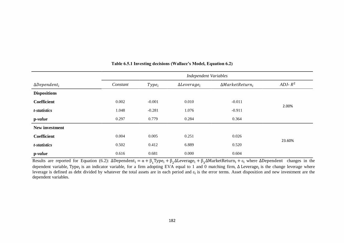
182

Table 6.5.1 Investing decisions (Wallace’s Model, Equation 6.2)

Independent Variables

Constant ADJ-

Dispositions

2.00% Coefficient 0.002 -0.001 0.010 -0.011

t-statistics 1.048 -0.281 1.076 -0.911

p-value 0.297 0.779 0.284 0.364

New investment

23.60% Coefficient 0.004 0.005 0.251 0.026

t-statistics 0.502 0.412 6.889 0.520

p-value 0.616 0.681 0.000 0.604

Results are reported for Equation (6.2):

ε where changes in the

dependent variable, is an indicator variable, for a firm adopting EVA equal to 1 and 0 matching firm, is the change leverage where

leverage is defined as debt divided by whatever the total assets are in each period and ε is the error terms. Asset disposition and new investment are the dependent variables.

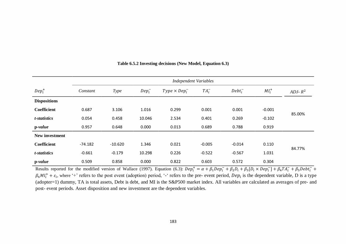
183

Table 6.5.2 Investing decisions (New Model, Equation 6.3)


Constant Type

ADJ-

Dispositions

85.00% Coefficient 0.687 3.106 1.016 0.299 0.001 0.001 -0.001

t-statistics 0.054 0.458 10.046 2.534 0.401 0.269 -0.102

p-value 0.957 0.648 0.000 0.013 0.689 0.788 0.919

New investment

84.77% Coefficient -74.182 -10.620 1.346 0.021 -0.005 -0.014 0.110

t-statistics -0.661 -0.179 10.298 0.226 -0.522 -0.567 1.031

p-value 0.509 0.858 0.000 0.822 0.603 0.572 0.304

Results reported for the modified version of Wallace (1997). Equation (6.3):

, where ‘+’ refers to the post event (adoption) period, ‘-‘ refers to the pre- event period, is the dependent variable, D is a type

(adopter=1) dummy, TA is total assets, Debt is debt, and MI is the S&P500 market index. All variables are calculated as averages of pre- and

post- event periods. Asset disposition and new investment are the dependent variables.

184

Table 6.5.3 shows the results obtained from running equation 6.4, which uses

abnormal dependent and independent variables. The models explain a fairly good

proportion of variability in abnormal dispositions and abnormal new investments

(the adjusted- are 30.62% and 48.34% respectively). As discussed earlier, the

coefficient of lagged performance is the parameter of interest and we are testing for

the null hypothesis that there is no effect ( : ) of adoption on firm

performance. The result shows that we fail to reject the null hypothesis for

dispositions. Consequently, the adoption of EVA, contrary to Wallace, has not

changed the disposition of assets (like with like, abnormal dispositions before

adoption are not different from abnormal dispositions after adoption). The growth or

decline in abnormal dispositions is mostly explained by the differential size and

differential leverage. In the first case, the coefficient of equals -0.035 and is

highly significant, implying that larger adopter firms have decreased dispositions.

On the other hand, more leveraged adopter firms have increased their dispositions

relative to non-adopters (the coefficient of is 0.065 and significant at the

1% level).

On the other hand, the current research reject the null hypothesis that there are no

effects of adoption on new investment decisions. The coefficient of lagged abnormal

new investment, equals -0.966 and is highly significant. This is clear evidence that

abnormal new investment has decreased significantly after adoption. This result is

much stronger statistically than Wallace’s negative impact which is found to be

weakly significant with a p-value of 0.09. The control variables are also significant

(but size is only weakly significant). First, while abnormal size has a negative impact

on dispositions, it has a positive effect on new investments. This is expected since

larger firms have greater ability to invest in absolute terms. However, abnormal

leverage has a significant coefficient but with an unexpected sign. Thus, while

abnormally high leveraged firms see higher abnormal dispositions they

(unexpectedly) also see higher abnormally new investment.

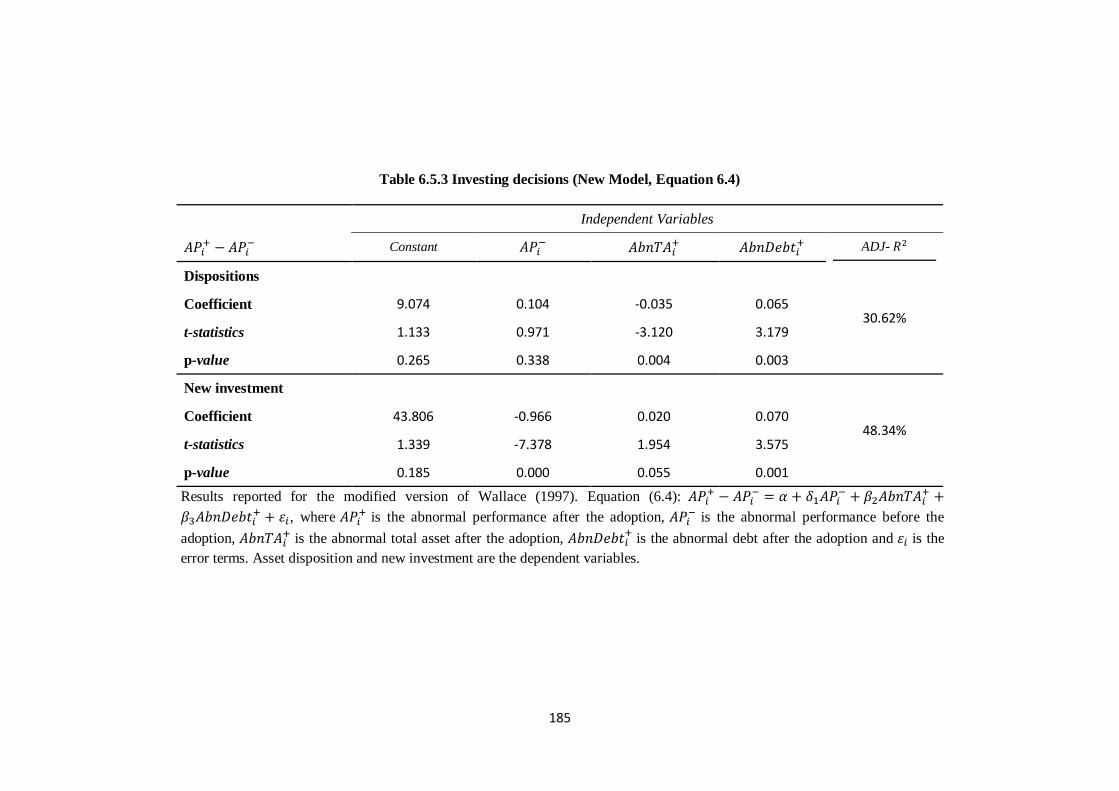
185

Table 6.5.3 Investing decisions (New Model, Equation 6.4)


Constant

ADJ-

Dispositions

30.62% Coefficient 9.074 0.104 -0.035 0.065

t-statistics 1.133 0.971 -3.120 3.179

p-value 0.265 0.338 0.004 0.003

New investment

48.34% Coefficient 43.806 -0.966 0.020 0.070

t-statistics 1.339 -7.378 1.954 3.575

p-value 0.185 0.000 0.055 0.001


, where

is the abnormal performance after the adoption, is the abnormal performance before the

adoption, is the abnormal total asset after the adoption,

is the abnormal debt after the adoption and is the

error terms. Asset disposition and new investment are the dependent variables.

186

Tables 6.5.4, 6.5.5 and 6.5.6 show the results for the Wallace model (equation 6.2),

the level model (equation 6.3), and the abnormal performance model (equation 6.4),

respectively. The tables show the results for repurchase and dividends decisions and

show different results regarding what happens to financing decisions after the

adoption of the EVA compensation plan over a ten-year window. Table 6.5.4 shows

a pattern similar to investment decision in Table 6.5.1. Contrary to Wallace’s

findings, the effect that is captured by the ‘type’ coefficient shows that EVA’s

adoption has no effect on repurchases and dividends decisions; the coefficients for

repurchases and dividends (0.0004 and -0.009 respectively) are both insignificant.

While the results of Table 6.5.4 suggest that no significant change in repurchases or

dividends is found after the adoption of EVA, Wallace reports a high and significant

increase in repurchase by 1.11. However, our result agrees with Wallace for

dividends (the coefficient in Wallace was 0.17 but statistically insignificant). The

adjusted- is quite low, only 2.39% for repurchase (8% in Wallace) and 1.88% for

dividends (-0.000 in Wallace). This confirms the inappropriateness of Wallace’s

specification. Like Wallace, neither of the other variables (

and ) are statistically significant on conventional levels.

Table 6.5.5 describes the results after running the modified version of Wallace

(1997) as given by equation 6.3. The effect of working with levels is quite clear. The

Adjusted- are much higher than in the Wallace model (increasing from 2.39% to

14.20% for repurchase decisions and from 1.88% to 64.06% for dividends

decisions). This means the new modified model is certainly an improvement on the

Wallace model.

For repurchases, two out of the three control variables are significant. The

performance of the market seems to play no role on repurchase behaviour. However,

Leverage reduces repurchases while size has the opposite effect. More importantly,

the dummy variables coefficient is positive and highly significant whereas the

interaction term is insignificant (although the coefficient seems large and negative at

-0.172, the p-value is very high). Since the interaction term is insignificant, the effect

of adoption on repurchases is fully reflected in the type dummy coefficient, that is,

EVA adopters on average increase their repurchases by 0.262 million dollars.

187

For dividends, the results are different. While size and leverage are significant and

have nearly identical effect, the market index is significant but negative, which

suggests that high markets see relatively lower levels of dividends. However, a more

interesting finding is that now both the type dummy and the interaction variables are

significant. However, while the dummy coefficient is positive (0.364), the interaction

coefficient is negative. Hence the adoption effect is complex. We can see this effect

through the marginal effect simply by taking partial derivatives of equation 6.3. This

yield

for dividends.

Thus the firms with relatively high dividends before adoption tend to reduce

dividends after adoption and vice versa. Specifically, those with pre-adoption

dividends of less than 0.734 tend to increase their dividends after adoption.

The above results for repurchases are consistent with Wallace (1997) and Kleiman

(1999). However, while Wallace reported insignificant effects for dividends, the

results of Table 6.5.5 show that the effect is significant but depends on the prior

dividend policy of the firm. This seems to be partly consistent with the agency

theory concept which states that a manager is not in favour of giving shareholders

any promises regarding the amount of the dividend they intend to pay in the future

because from the shareholders’ point of view any increase in the amount of the

dividend the manager promises to pay will become an obligation in the future. To

alleviate the consequences of minimizing dividends in their relation with

shareholders the manager will focus on the repurchasing of shares to enhance the

share prices movement in the stock market and as a result any shareholder seeking

extra cash can easily perform the selling of these shares at a better price. The results

so far only confirm the second conclusion relating to increasing repurchases by

managers. However, the first part of the theory, namely that managers are reluctant

to increase dividends, is not supported. Some managers (with low historical

dividends) may actually increase dividends after adopting EVA, while others (whose

historical dividends were high) will decrease them.

188

In the third model, the results in Table 6.5.6 are obtained from running equation 6.4.

The adjusted- is extremely high for dividends (=99.86%) and reasonably high for

repurchases (=32.14%). This means that the models explain a very good proportion

of variability in abnormal repurchases and abnormal dividends. The coefficient of

lagged performance, , is the parameter of interest. Contrary to Wallace, the results

show a fall in abnormal repurchase and dividends. The null hypotheses (

for repurchases and dividends are strongly rejected; both coefficients (-0.695 and -

0.998 respectively) are significant and negative, implying the reversal of the effect

found in Wallace. Thus, our result suggests that while repurchases seem to increase

in Wallace’s study, this study suggest the opposite. Furthermore, while EVA

adoption has no effect on dividends, this study finds strong and negative effect.

On the other hand, the coefficients of the control variable and

(0.00002, -0.00005 respectively) for repurchase are small and insignificant. This

implies that the difference in either size or leverage between adopter and control firm

does not explain the change in abnormal repurchases and abnormal dividends across

the pre- and post-adoption periods. The same conclusion applies to the dividends

case. The coefficients of the abnormal size and abnormal leverage are insignificant.

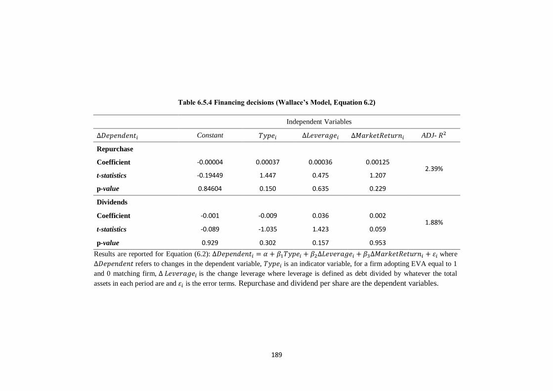
189

Table 6.5.4 Financing decisions (Wallace’s Model, Equation 6.2)


Constant ADJ-

Repurchase

2.39% Coefficient -0.00004 0.00037 0.00036 0.00125

t-statistics -0.19449 1.447 0.475 1.207

p-value 0.84604 0.150 0.635 0.229

Dividends

1.88% Coefficient -0.001 -0.009 0.036 0.002

t-statistics -0.089 -1.035 1.423 0.059

p-value 0.929 0.302 0.157 0.953

Results are reported for Equation (6.2): where

refers to changes in the dependent variable, is an indicator variable, for a firm adopting EVA equal to 1

and 0 matching firm, is the change leverage where leverage is defined as debt divided by whatever the total

assets in each period are and is the error terms. Repurchase and dividend per share are the dependent variables.

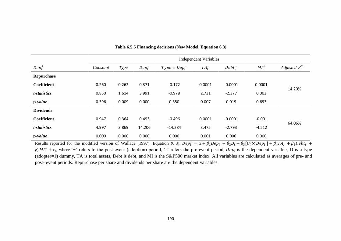
190

Table 6.5.5 Financing decisions (New Model, Equation 6.3)


Constant Type

Adjusted-

Repurchase

14.20% Coefficient 0.260 0.262 0.371 -0.172 0.0001 -0.0001 0.0001

t-statistics 0.850 1.614 3.991 -0.978 2.731 -2.377 0.003

p-value 0.396 0.009 0.000 0.350 0.007 0.019 0.693

Dividends

64.06% Coefficient 0.947 0.364 0.493 -0.496 0.0001 -0.0001 -0.001

t-statistics 4.997 3.869 14.206 -14.284 3.475 -2.793 -4.512

p-value 0.000 0.000 0.000 0.000 0.001 0.006 0.000


, where ‘+’ refers to the post-event (adoption) period, ‘-‘ refers the pre-event period, is the dependent variable, D is a type

(adopter=1) dummy, TA is total assets, Debt is debt, and MI is the S&P500 market index. All variables are calculated as averages of pre- and

post- event periods. Repurchase per share and dividends per share are the dependent variables.

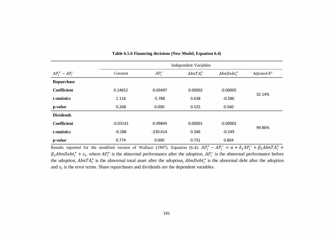
191

Table 6.5.6 Financing decisions (New Model, Equation 6.4)


Constant

Adjusted-

Repurchase

32.14% Coefficient 0.14652 -0.69497 0.00002 -0.00005

t-statistics 1.116 -5.788 0.638 -0.586

p-value 0.268 0.000 0.525 0.560

Dividends

99.86% Coefficient -0.03141 -0.99844 0.00001 -0.00002

t-statistics -0.288 -230.614 0.346 -0.249

p-value 0.774 0.000 0.731 0.804


, where

is the abnormal performance after the adoption, is the abnormal performance before

the adoption, is the abnormal total asset after the adoption,

is the abnormal debt after the adoption

and is the error terms. Share repurchases and dividends are the dependent variables.

192

Turning to operating decisions, Table 6.5.7 shows the result obtained from running

equation 6.2 in which is replaced by as a control

variable. The table shows the results for Asset, Inventory, Accounts Receivable, and

Accounts Payable turnovers.

The first note is that, similar to Wallace, the coefficients of determination are quite

low, suggesting overall inadequacy of the Wallace model. The only weakly

significant variable is the market return with a p-value of 7.5%. The remaining

variables are all insignificant including the ‘Type’ dummies, which are all highly

insignificant. In Wallace, the adoption has a positive effect for Asset turnover and

Accounts receivable (although both coefficients are only significant at the 10% level

respectively).

Thus, partly negating Wallace’s results and using the same model, we find no effect

of EVA adoption on the four operating decisions considered by Wallace, whereas he

finds increased asset turnover and accounts receivable turnover.

The change in operating decisions seems extremely hard to explain using Wallace’s

model. The most convincing explanation seems to be made by the change in market

return ( ), which seems to explain 2.84% of the variability of

assets turnover (in Wallace the adjusted- = 11%). The remaining coefficients of

determination are nearly zero (and all negative in Wallace), which confirms the

possibility that we are trying to estimate mainly random variation as discussed

previously.

When the model is modified, using levels rather than differences, the results change

substantially. First, the adjusted- for all dependent variables are high suggesting

that, the explanatory variables capture a good proportion of the variability in the

level of the four turnover variables. In all cases, none of the control variables is

significant, indicating that the explanatory power of the four models is due to a

lagged dependent variable and/or the type dummy.

The results of Wallace are reversed in three out of four cases. First, for asset

turnover, the coefficients of the type dummy and the interaction terms are both

insignificant. Thus, there seems to be no EVA effect for this type of operating

decisions (it is positive and significant in Wallace (Table 5, p.291)).

193

Second, for inventory turnover, Wallace finds no effect, whereas here the coefficient

of the interaction term is positive and significant (although the type dummy is

insignificant). This suggests a marginal effect of

In other words, the effect of EVA adoption is proportional to pre-adoption levels of

inventory turnovers. Thus high inventory turnover adopter firms will see their

inventory turnover increase by more than low pre-adoption inventory turnover firms.

Third, for A/R turnover, Wallace finds a positive effect (albeit weakly significant).

In this study, the results show strong statistical significance of both type dummy and

interaction variables. The marginal effect is

This suggests that the behaviour can vary from positive to negative, depending on

the level of pre-event AR turnover. For low turnover firms, there is a tendency to

increase AR turnover following adoption of EVA. On the other hand, if turnover is

more than 8.69 (=12.31/1.416) before adoption the firm will tend to reduce its AR

turnover after adoption and vice versa.

The final operating decision is accounts payable turnover. Here the results are in line

with Wallace as neither dummy nor interaction term coefficient is significant.

The results in Table 6.5.9 show a different story. In comparison to Wallace’s finding,

our modified version (equation 6.4) explains a very high proportion of variability in

abnormal asset turnover, inventory turnover, and AR turnover (the adjusted- are

54.66%, 38.19%, and 93.70% and 17.00% respectively), although the AP turnover

has a lower adjusted- (17%). As discussed earlier, , the coefficient of lagged

performance ( is the parameter of interest and we are testing for the null

hypothesis that there is no effect ( of EVA adoption on firm

performance. The result shows that we strongly reject the null hypothesis for all

turnovers. Thus the adoption of EVA has affected the operating decisions the

managers take in regard to turnovers. The effects are similar for asset turnover, AR

turnover and AP turnover. In these three operating decision variables, none of the

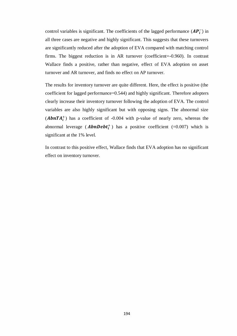
194

control variables is significant. The coefficients of the lagged performance ( in

all three cases are negative and highly significant. This suggests that these turnovers

are significantly reduced after the adoption of EVA compared with matching control

firms. The biggest reduction is in AR turnover (coefficient=-0.960). In contrast

Wallace finds a positive, rather than negative, effect of EVA adoption on asset

turnover and AR turnover, and finds no effect on AP turnover.

The results for inventory turnover are quite different. Here, the effect is positive (the

coefficient for lagged performance=0.544) and highly significant. Therefore adopters

clearly increase their inventory turnover following the adoption of EVA. The control

variables are also highly significant but with opposing signs. The abnormal size

( ) has a coefficient of -0.004 with p-value of nearly zero, whereas the

abnormal leverage ( ) has a positive coefficient (=0.007) which is

significant at the 1% level.

In contrast to this positive effect, Wallace finds that EVA adoption has no significant

effect on inventory turnover.

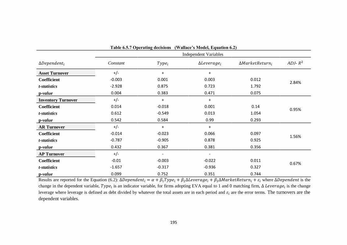
195

Table 6.5.7 Operating decisions (Wallace’s Model, Equation 6.2)


Constant ADJ-

Asset Turnover +/- + +

2.84% Coefficient -0.003 0.001 0.003 0.012

t-statistics -2.928 0.875 0.723 1.792

p-value 0.004 0.383 0.471 0.075

Inventory Turnover +/- + +

0.95% Coefficient 0.014 -0.018 0.001 0.14

t-statistics 0.612 -0.549 0.013 1.054

p-value 0.542 0.584 0.99 0.293

AR Turnover +/- + +

1.56% Coefficient -0.014 -0.023 0.066 0.097

t-statistics -0.787 -0.905 0.878 0.925

p-value 0.432 0.367 0.381 0.356

AP Turnover +/- - -

0.67% Coefficient -0.01 -0.003 -0.022 0.011

t-statistics -1.657 -0.317 -0.936 0.327

p-value 0.099 0.752 0.351 0.744

Results are reported for the Equation (6.2): where is the

change in the dependent variable, is an indicator variable, for firms adopting EVA equal to 1 and 0 matching firm, is the change

leverage where leverage is defined as debt divided by whatever the total assets are in each period and are the error terms. The turnovers are the

dependent variables.

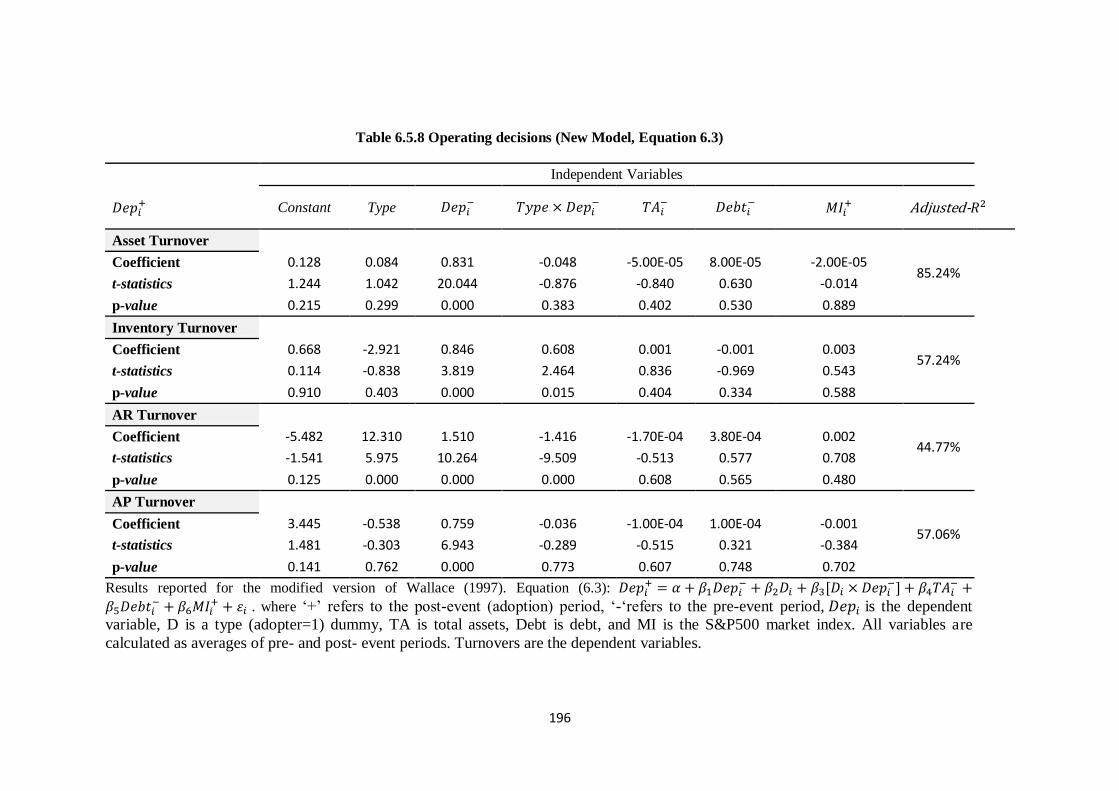
196

Table 6.5.8 Operating decisions (New Model, Equation 6.3)


Constant Type

Adjusted-

Asset Turnover

85.24% Coefficient 0.128 0.084 0.831 -0.048 -5.00E-05 8.00E-05 -2.00E-05

t-statistics 1.244 1.042 20.044 -0.876 -0.840 0.630 -0.014

p-value 0.215 0.299 0.000 0.383 0.402 0.530 0.889

Inventory Turnover

57.24% Coefficient 0.668 -2.921 0.846 0.608 0.001 -0.001 0.003

t-statistics 0.114 -0.838 3.819 2.464 0.836 -0.969 0.543

p-value 0.910 0.403 0.000 0.015 0.404 0.334 0.588

AR Turnover

44.77% Coefficient -5.482 12.310 1.510 -1.416 -1.70E-04 3.80E-04 0.002

t-statistics -1.541 5.975 10.264 -9.509 -0.513 0.577 0.708

p-value 0.125 0.000 0.000 0.000 0.608 0.565 0.480

AP Turnover

57.06% Coefficient 3.445 -0.538 0.759 -0.036 -1.00E-04 1.00E-04 -0.001

t-statistics 1.481 -0.303 6.943 -0.289 -0.515 0.321 -0.384

p-value 0.141 0.762 0.000 0.773 0.607 0.748 0.702


. where ‘+’ refers to the post-event (adoption) period, ‘-‘refers to the pre-event period, is the dependent

variable, D is a type (adopter=1) dummy, TA is total assets, Debt is debt, and MI is the S&P500 market index. All variables are

calculated as averages of pre- and post- event periods. Turnovers are the dependent variables.

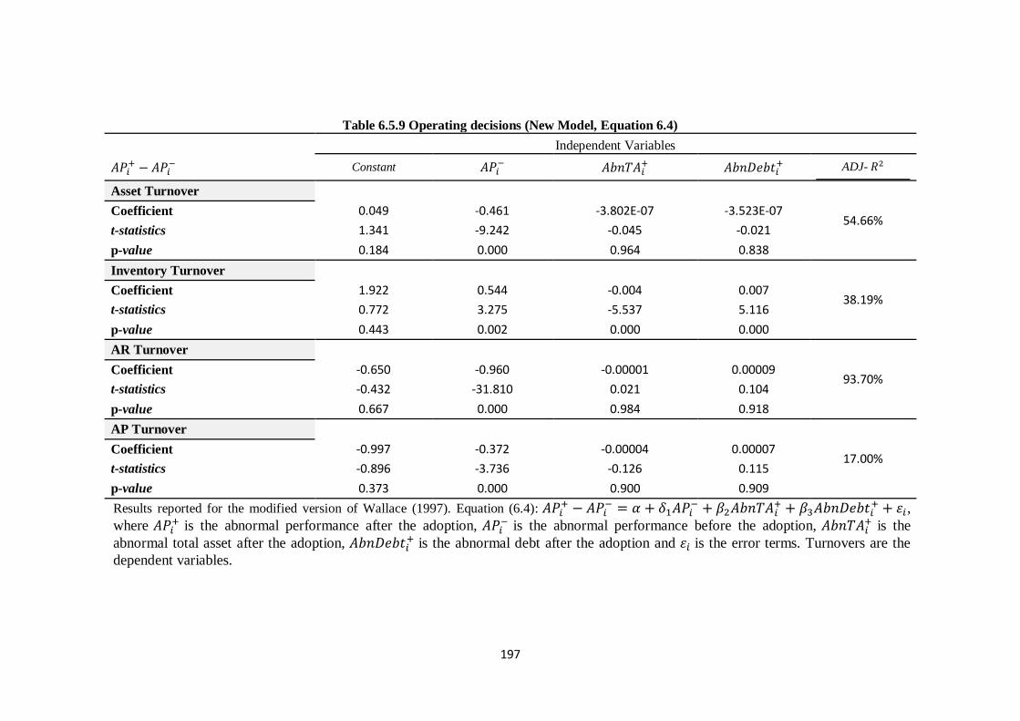
197

Table 6.5.9 Operating decisions (New Model, Equation 6.4)


Constant

ADJ-

Asset Turnover

54.66% Coefficient 0.049 -0.461 -3.802E-07 -3.523E-07

t-statistics 1.341 -9.242 -0.045 -0.021

p-value 0.184 0.000 0.964 0.838

Inventory Turnover

38.19% Coefficient 1.922 0.544 -0.004 0.007

t-statistics 0.772 3.275 -5.537 5.116

p-value 0.443 0.002 0.000 0.000

AR Turnover

93.70% Coefficient -0.650 -0.960 -0.00001 0.00009

t-statistics -0.432 -31.810 0.021 0.104

p-value 0.667 0.000 0.984 0.918

AP Turnover

17.00% Coefficient -0.997 -0.372 -0.00004 0.00007

t-statistics -0.896 -3.736 -0.126 0.115

p-value 0.373 0.000 0.900 0.909


,

where is the abnormal performance after the adoption,

is the abnormal performance before the adoption, is the

abnormal total asset after the adoption, is the abnormal debt after the adoption and is the error terms. Turnovers are the

dependent variables.

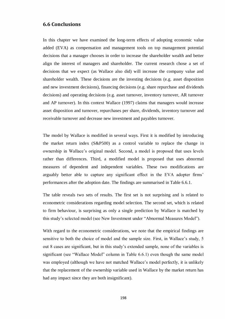
198

6.6 Conclusions

In this chapter we have examined the long-term effects of adopting economic value

added (EVA) as compensation and management tools on top management potential

decisions that a manager chooses in order to increase the shareholder wealth and better

align the interest of managers and shareholder. The current research chose a set of

decisions that we expect (as Wallace also did) will increase the company value and

shareholder wealth. These decisions are the investing decisions (e.g. asset disposition

and new investment decisions), financing decisions (e.g. share repurchase and dividends

decisions) and operating decisions (e.g. asset turnover, inventory turnover, AR turnover

and AP turnover). In this context Wallace (1997) claims that managers would increase

asset disposition and turnover, repurchases per share, dividends, inventory turnover and

receivable turnover and decrease new investment and payables turnover.

The model by Wallace is modified in several ways. First it is modified by introducing

the market return index (S&P500) as a control variable to replace the change in

ownership in Wallace’s original model. Second, a model is proposed that uses levels

rather than differences. Third, a modified model is proposed that uses abnormal

measures of dependent and independent variables. These two modifications are

arguably better able to capture any significant effect in the EVA adopter firms’

performances after the adoption date. The findings are summarised in Table 6.6.1.

The table reveals two sets of results. The first set is not surprising and is related to

econometric considerations regarding model selection. The second set, which is related

to firm behaviour, is surprising as only a single prediction by Wallace is matched by

this study’s selected model (see New Investment under “Abnormal Measures Model”).

With regard to the econometric considerations, we note that the empirical findings are

sensitive to both the choice of model and the sample size. First, in Wallace’s study, 5

out 8 cases are significant, but in this study’s extended sample, none of the variables is

significant (see “Wallace Model” column in Table 6.6.1) even though the same model

was employed (although we have not matched Wallace’s model perfectly, it is unlikely

that the replacement of the ownership variable used in Wallace by the market return has

had any impact since they are both insignificant).

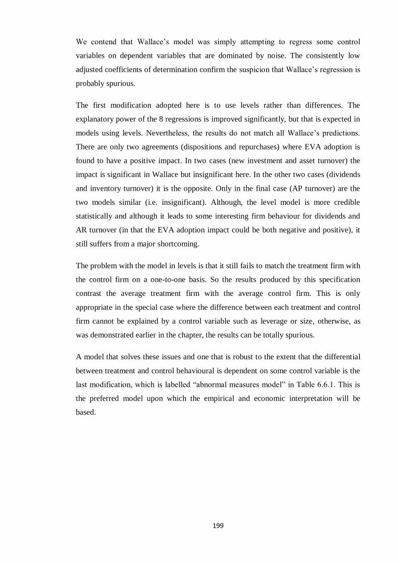
199

We contend that Wallace’s model was simply attempting to regress some control

variables on dependent variables that are dominated by noise. The consistently low

adjusted coefficients of determination confirm the suspicion that Wallace’s regression is

probably spurious.

The first modification adopted here is to use levels rather than differences. The

explanatory power of the 8 regressions is improved significantly, but that is expected in

models using levels. Nevertheless, the results do not match all Wallace’s predictions.

There are only two agreements (dispositions and repurchases) where EVA adoption is

found to have a positive impact. In two cases (new investment and asset turnover) the

impact is significant in Wallace but insignificant here. In the other two cases (dividends

and inventory turnover) it is the opposite. Only in the final case (AP turnover) are the

two models similar (i.e. insignificant). Although, the level model is more credible

statistically and although it leads to some interesting firm behaviour for dividends and

AR turnover (in that the EVA adoption impact could be both negative and positive), it

still suffers from a major shortcoming.

The problem with the model in levels is that it still fails to match the treatment firm with

the control firm on a one-to-one basis. So the results produced by this specification

contrast the average treatment firm with the average control firm. This is only

appropriate in the special case where the difference between each treatment and control

firm cannot be explained by a control variable such as leverage or size, otherwise, as

was demonstrated earlier in the chapter, the results can be totally spurious.

A model that solves these issues and one that is robust to the extent that the differential

between treatment and control behavioural is dependent on some control variable is the

last modification, which is labelled “abnormal measures model” in Table 6.6.1. This is

the preferred model upon which the empirical and economic interpretation will be

based.

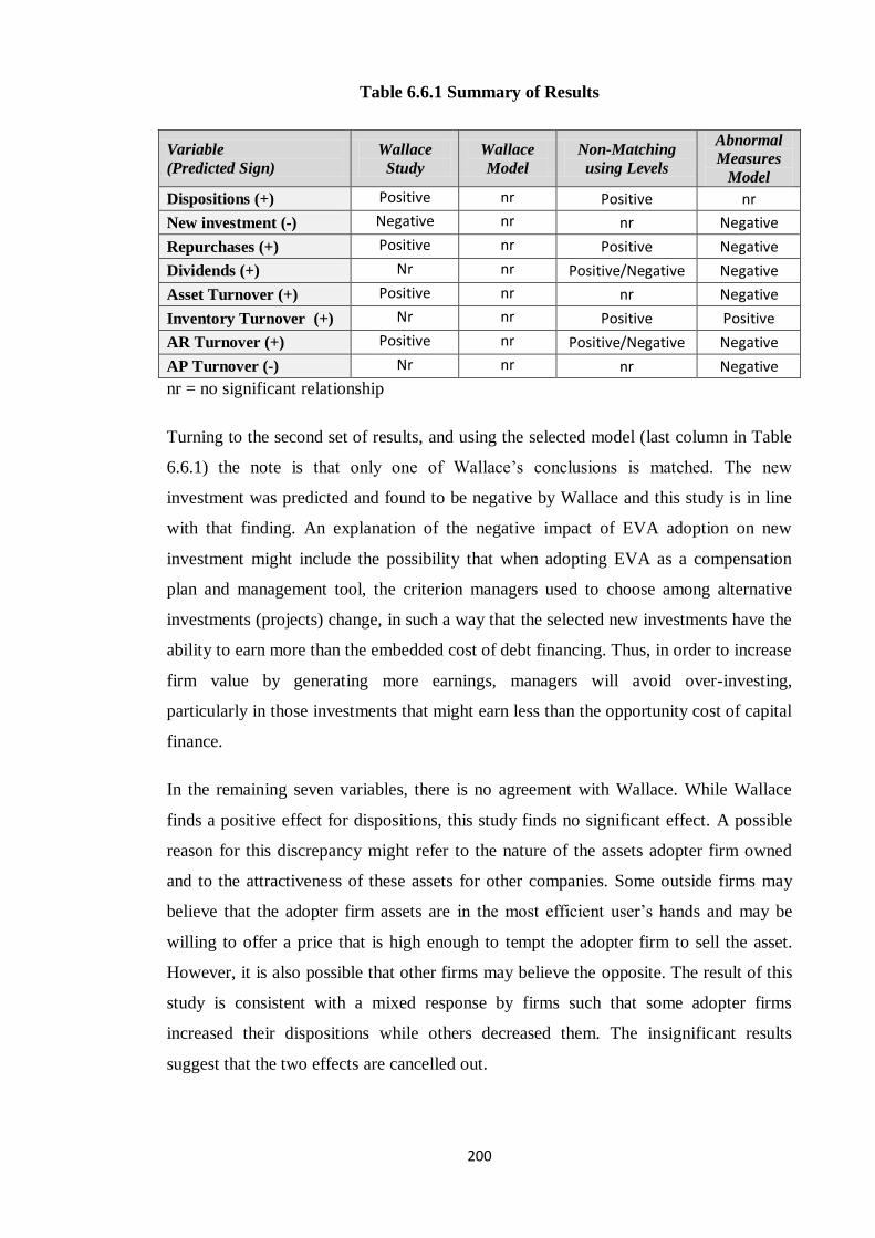
200

Table 6.6.1 Summary of Results

Variable

(Predicted Sign)

Wallace

Study

Wallace

Model

Non-Matching

using Levels

Abnormal

Measures

Model

Dispositions (+) Positive nr Positive nr

New investment (-) Negative nr nr Negative

Repurchases (+) Positive nr Positive Negative

Dividends (+) Nr nr Positive/Negative Negative

Asset Turnover (+) Positive nr nr Negative

Inventory Turnover (+) Nr nr Positive Positive

AR Turnover (+) Positive nr Positive/Negative Negative

AP Turnover (-) Nr nr nr Negative

nr = no significant relationship

Turning to the second set of results, and using the selected model (last column in Table

6.6.1) the note is that only one of Wallace’s conclusions is matched. The new

investment was predicted and found to be negative by Wallace and this study is in line

with that finding. An explanation of the negative impact of EVA adoption on new

investment might include the possibility that when adopting EVA as a compensation

plan and management tool, the criterion managers used to choose among alternative

investments (projects) change, in such a way that the selected new investments have the

ability to earn more than the embedded cost of debt financing. Thus, in order to increase

firm value by generating more earnings, managers will avoid over-investing,

particularly in those investments that might earn less than the opportunity cost of capital

finance.

In the remaining seven variables, there is no agreement with Wallace. While Wallace

finds a positive effect for dispositions, this study finds no significant effect. A possible

reason for this discrepancy might refer to the nature of the assets adopter firm owned

and to the attractiveness of these assets for other companies. Some outside firms may

believe that the adopter firm assets are in the most efficient user’s hands and may be

willing to offer a price that is high enough to tempt the adopter firm to sell the asset.

However, it is also possible that other firms may believe the opposite. The result of this

study is consistent with a mixed response by firms such that some adopter firms

increased their dispositions while others decreased them. The insignificant results

suggest that the two effects are cancelled out.

201

In repurchases and dividends, Wallace finds a positive effect while it is negative here. A

possible reason is that managers, in order to maximize their own personal benefit, begin

retaining free cash flows. One reason for this retention is to insulate the firm from the

capital market that serves as a monitoring instrument by subjecting any extra capital

needs of the firm to impartial scrutiny. To avoid capital market monitoring, managers

will only use the existing cash reserves that have been accumulated to finance new

projects (contrary to the results I achieved) rather than paying it out to shareholders

(Jensen, 1993). A possible, more interesting, reason for managers to avoid paying out

cash flow is the desire to maximize the firm size.32

Further, managers have more of a

tendency towards preventing shareholders from getting more cash than discouraging

them from redirecting capital to a more productive use. Moreover, firms are reluctant to

increase dividends payment particularly when they are unsure about the availability of

future free cash flows and whether they can sustain the same payout ratio (dividends are

sticky). Moreover, firms are more likely to prefer to finance share repurchases from the

excess cash they generate from non-recurring items rather than using the free cash flow

they generate from core activities (Miller and Rock, 1985). However, the stated purpose

of the long-term incentives scheme is to align the interests of managers with that of

shareholders. To the extent that these long-term compensation plans encourage

managers to develop growth opportunities, a significant fall in dividends (relative to

control firms) can only be accepted if it is accompanied by a significant increase in new

investments. Unfortunately, this is not the case. Both new investments and

dividends/repurchases have fallen in relative terms.

When examining the measures of turnovers, asset turnover, accounts receivable

turnover, and inventory turnover the result obtained showed decreases in asset turnover

and both the accounts receivable and account payables turnovers, and also showed an

increase in inventory turnover. Wallace found a positive accounts receivable and asset

turnover and a negative account payables turnover and reported a insignificant

relationship for inventory turnover. However, as discussed before, some managers have

some tendency to increase the firm size through accumulating sub-optimal assets, which

would lead to an increase in the asset base, asset turnover, and accounts receivable. At

the same time, we would expect accounts payable to decrease following the adoption.

32 Murphy (1985) documents a positive correlation between total management compensation

and firm size.

202

Overall, it is hard to choose between any of the proposed two models as a candidate for

detecting abnormal performance. While the Wallace-Level model has interesting

findings, it may be spurious. On the other hand, while the Abnormal-Measure model is

more robust statistically, the results are hard to explain.

Thus, there are both econometric and empirical implications. Econometrically, more

elaborate simulation studies may be required to establish the performance of matching

and non-matching models. Empirically, the results may be sensitive to several factors.

First, it is possible that an important factor is missing from the model. The models in

this study use size and leverage as firm characteristics and market return as a market

wide control factor. Other characteristics such as firm age and industry may be

influential. Second, the matching procedure may not produce accurate benchmarks.

Following previous studies, the SIC code was used here to match treatment and control

firms. This could possibly be improved by increasing the number of matching

characteristics to include firm characteristics such as size, leverage and systematic risk

(beta).

Elsewhere, the effective corporate governance suggests that boards should strive to

align executive and board remuneration with the longer-term interests of the company

and its shareholders and the long-term incentive schemes are alike. Recently,

compensation policies which emphasise long-term profitability only and bonus pay-outs

have been tied to the current performance with sufficient care for future risk and

revenue profiles. Thus, the focus of the firms’ manager is to increase the shareholder

wealth and to increase the firm value. To my knowledge I think this is the correct reason

for the bias in the returns obtained as indicated by the proposed models.

203

Chapter 7

Conclusions and Recommendations

7.1 Introduction

This chapter aims to highlight the main results and findings of the research, draw

conclusions and research contributions and implications. In addition, the chapter

highlights the research limitations and provides insight and direction for potential future

research.

7.2 Main research findings

The long-standing debate about the superiority of performance measures in explaining

the variation in stock price and stock return performances and what motivates

researchers and investors to select from these measures has by no means been resolved

through this study as further research is still called for. However, previous researchers

(i.e. US and UK studies) had attempted to use different methodologies and different

proxies for the accounting variables to explain the association between a selected

performance measure and stock return (price) performances. Furthermore, most of that

research replicates the work of Biddle et al., (1997) where the focus in methodology

were on the traditional evaluation components of the Ohlson (1995) model. Thus, the

results they obtained were mixed and contradictory regarding the superiority of

performance metrics.

The current research attempts to overcome these contradictions within the results

obtained utilising different research strategies by first, extending the methodology of

Biddle et al. by introducing the book value (BV) as a major explanatory variable with

other performance measures into the price and return valuation model as a determinate

of the share price (Ohlson, 1995). Second, applying the same methodology over the

extending period 1960 to 2012 and finally using the same definition and calculation of

the variables used to conduct this research. Further, I have adopted the most popular

evaluation method: the price and return model.

204

This study aimed to fill the apparent gaps in the literature. The overarching objective

was to examine the association of a set of performances, namely the net income

available to common (NI), earnings before interest, tax and amortization and

depreciation (EBIDA), earnings before interest and tax (EBIT), earnings before

extraordinary items (EBEI), net cash flows from operations (CFO), cash value added

(CVA) and economic value added (EVA), with stock price (return) performances. I then

extended the research to test for the incremental information of these variables.

Subsequently, the main performance measures, the net income (NI) and the economic

value added, were decomposed into the main components to examine whether the

components contained more value than the original measures.

The problem addressed in chapters 6 and 7 is “How will the adoption of economic value

added (EVA) affect the long-term performance of adopting firms regarding the

investing, financing and operating decisions?” In order to address this issue I used the

commonly used aggregation method, the cumulated average abnormal return (CAAR)

and buy-hold abnormal return (BHAR), to test for any changes in treatment firms’

performances after adoption. Then, in order to examine the long-term adoption effects, I

extended the work of Wallace (1997) in several ways. First it was modified by

introducing the market return index (S&P500) as a control variable to replace the

change in ownership in Wallace’s original model. Second, a model is proposed that uses

levels rather than differences. Third, a modified model is proposed that uses abnormal

measures of dependent and independent variables.

The key findings and related conclusions in response to research questions and

objectives as outlined in the introduction, literature, and methodology chapters can be

classified into three categories as presented below.

7.2.1 Findings for the value relevance and incremental information

content of performance measures

The result obtained with regard to value relevance showed that the adjusted- , the

criterion I used to gauge the value relevance of performance measures, increased rapidly

after the incorporation of BV into the price model as an explanatory variable. This

means that our extended model is better at capturing the variation of stock performances

than the Biddle et al. model (in Wallace it is significant, explaining about 9.04% of the

205

variability of stock performance in the best case where it is significant and explains

about 79.82% of the variability of stock performance when applying our extended

model). When applying the price model, the CFO has the highest explanatory power

among the other variables (adjusted- =79.82%). The remaining performance

measures are in the following order with regard to their value relevance: EBITDA

(adjusted- =77.90%), EVA (adjusted- =77.32%), EBIT (adjusted- =77.30%),

(NI and EBEI (adjusted- =76.55%) and CVA (adjusted- =76.00%).

In addition the results show that EBITDA (adjusted- =15.14%) is the dominant

variable when we used the return model following earnings before interest and tax

(EBIT) but the adjusted- is quite low compared to that obtained by the price model.

With regard to the incremental information content, the result indicates that there is

significant evidence regarding the incremental information content existing between

pairwise measures. The best combination exists between CFO and NOPAT (adjusted-

= 82.01%). The lowest exists when NI is paired with EBEI ( =76.55%). One

interesting result is that NI still has the ability to outperform EVA as its explanatory

power increases by 0.67% when paired with NI.

One interesting finding is that the adjusted- obtained from the original return model

by Biddle et al., is similar to that of the extended version of the return model where the

book value (BV) is introduced as a dependent variable. This might indicate that unlike

the price model, the book value (BV) adds little to other variables information content.

Moreover, the changes in earnings before extraordinary items (EBIT) have the highest

adjusted- (14.76%) when adopting the extended version of Biddle et al., and earnings

before interest depreciation and amortization (EBITDA) had the highest adjusted-

(13.37%) when adopting the normal return model.

7.2.2 Findings for the main components of NI and EVA

The results obtained provide empirical evidence on the incremental information content

of EVA and NI components with regard to explaining the variation in stock

performances. All NI components are significant and positively associated with the

share price performances at the 0.05 level except for ΔAP which has a significant and

negative sign. In support of the incremental information content of NI components,

there is strong evidence regarding the increases in adjusted- after decomposition into

206

cash flows and accruals. It increases from 76.55% (for NI alone) to 82.70% (after

decomposition). The increase in by 6.15% indicates that jointly, cash flow and

accrual components significantly outperform NI in explaining changes in price

performances. This is consistent with Wilson (1986 and 1987) and Garrod et al. (2000)

who claim that decomposing NI (earnings) into main components, the cash flows and

accruals, will enhance the model’s ability to explain the stock performance’s volatility.

Turning to EVA components the adjusted- has increased by 2.91% after the

decomposition which indicates that EVA’s components together significantly

outperform EVA in explaining changes in price performances. The best results are

achieved when accruals (ACCR) are separately paired with the capital charge

(CAPCHG) and after tax interest (ATINT). Interestingly, the traditional performance

measures still have the ability to compete and outperform the value added measures.

7.2.3 Findings for the effects of adopting economic value added (EVA)

The results that have been obtained after the application of the CAR and BHAR

aggregation method indicate that firms adopting EVA as a compensation plan and

management tool outperform the market (S&P500) and controlling firms (same sector)

most of the time within the hold period. The CAR results show that despite the

benchmarking used, the majority of adopter firms positively outperform the matching

firms and the S&P500 portfolio and after a few months the adopter firms have a

negative performance mainly in year one and year five of the ten year estimated period.

Regarding the BHAR approach the findings reveal that the results obtained from a

comparison against the benchmarking portfolio (S&P500) are smaller in value than

those obtained when compared to the matching firms’ benchmark. One interesting

finding is that CAR is almost the same as BHAR when the S&P500 portfolio is used as

a benchmark to calculate the aggregate returns.

To sum up, regardless of the aggregation approach used to measure the abnormal return,

the adopter firms have a considerably low outperformance and this outperformance

increased as the hold period increased. However, even with the positive performances

most EVA adopter firms’ outperformance declines after the adoption and takes some

time to return to negative performance when matching benchmarks are used. This might

207

typically reflect the fact that the market might react poorly to the adoption

announcement.

Although I have proposed three modified versions of Wallace (1997) to examine the

long-term effects of adopting economic value added (EVA) compensation plan on top

management investing decisions (e.g. asset disposition and new investment decisions),

financing decisions (e.g. share repurchase and dividends decisions) and operating

decisions (e.g. asset turnover, inventory turnover, AR turnover and AP turnover). The

result shows that the adjusted- , of the modified versions used is quite high. Thus, my

modified models are arguably better able to capture any significant effect in the EVA

adopter firms’ performances after the adoption date.

The results obtained from the Wallace model indicate that none of the firms’ potential

decisions is significantly affected by EVA adoption. In addition I contend that

Wallace’s model, where the market return index (S&P500) replaces the change in

ownership as a control variable in Wallace’s original model, was simply attempting to

regress some control variables on dependent variables that are dominated by noise. The

consistently low adjusted coefficients of determination confirm the suspicion that

Wallace’s regression is probably spurious.

For the second modified version, where variables are used in levels rather in

differences, the adjusted- is significantly improved for all decisions; only the new

investment and asset turnovers are insignificant, the disposition and repurchases are the

only decisions that are in agreement with Wallace’s original model. The remaining

variables, dividends and inventory decisions, are both significant and in opposite

directions. The AP turnover is insignificant in both the original and the extended

version model. Finally, the EVA adoption impact could be both negative and positive

on dividends and AR turnover decisions.

Turning to the third model result, when applying the abnormal measures model

(abnormal measures of dependent and independent variables) we expect the matching

problem inherent in the levels model (the second modification of Wallace model) will

be demolished. I note that the new investment decision is the only variable that matched

Wallace’s conclusion. The remaining decisions are significant but inconsistent with the

direction of the Wallace model. However, the only insignificant variable is the

disposition decision.

208

7.3 Research conclusion

With regard to the value relevance of selected performance measures, the general

conclusion is that all the selected performance measures (in whatever way the

evaluation model has been used) have a significant effect on the variation in stock return

(price) performances. The CFO and EBITDA are superior among the investigated

performance measures, particularly the value added measures (i.e. economic value

added (EVA) and cash value added (CVA)). Two results are worth noting. First, there is

strong UK evidence of the superiority of accruals in explaining changes in stock

performances and its ability to increase the value relevancy of NI when the latter is

decomposed into cash flows and main accruals components. Second, the cash value

added (CVA) (the performance measure that is used the first time to address the UK

data), is highly significant and has the ability to explain 76.0% of the variation in UK

stock performances.

Regarding the incremental information content, all the performance measures in this

research have incremental information beyond each other. The best compensation was

between CFO and NOPAT. To this end it is better to use a combination of performance

measures to examine firm performances.

In terms of decomposing, we conclude that decomposing NI into its main components,

the cash flows and accruals, increases the explanatory power of the former and

improves the quality of earnings. The increase in (6.15%) could be considered a

good indicator of the quality of the earnings released by the UK firm. Similarly, there

are some gains from decomposing EVA into its main components. The increases in

adjusted (the explanatory power) and all the EVA components are significant at the

conventional level.

In regard to the adoption of EVA as a performance incentive scheme and management

tool effect this research concludes that EVA firms have outperformed the matching

firms and the market portfolio S&P500 index through the holding periods but the

market was weak in its response to the adoption announcement. In addition, the current

research conclude that adopting EVA as a management tool significantly affects the

adopting firm’s potential investment, financial and operating decisions. The new

investment decision is the only one in the direction of Wallace (1997). In general, the

209

results obtained regarding the long-term effects of EVA adoption are mixed regardless

of the modified model applied.

7.4 Research contributions and recommendations

In order to draw attention to the main contributions of the current research, they were

divided into two main aspects: the contribution to the United Kingdom literature,

particularly the performance measures field, and the contribution to the US literature by

testing the consequences and the effects of adopting economic value added (EVA) as a

compensation scheme and as a management tool on firms’ performances and

management behaviour. Firstly, in the UK there is a lack of studies that examine the

association between performance measures and the variation in stock price (return)

performances in general. Therefore, this research will employ UK data for the period

1960 to 2012 and adopt a unified econometrics model to examine and test the

association of a set of performance measures, (being the focus of past literature), and the

variation in annual stock price performances. This, as intended, will eliminate the

controversies embedded in the findings of previous UK studies regarding the use of

different samples and econometric models in conducting their research.

In addition, the research will provide some statistical information about the value

relevance of cash value added (CVA), the performance measures that are being used for

the first time to examine UK data. Furthermore, the net income available to common

(NI) and economic value added (EVA), the measures that are most vulnerable to

criticism in the literature, are decomposed into their main items to test whether these

components can convey more information about a firm’s performance rather than the

original measures.

Secondly, there will be a contribution to the US literature in terms of the modification I

have done to Wallace’s (1997) model design. In order to test the impact of adopting

EVA as a performance incentive scheme and management tool on the performance of

adopter firms the current research modified Wallace’s work in three ways. First it is

modified by replacing the change in ownership in Wallace’s original model with the

market return index (S&P500) as a control variable. Second, I proposed a model that

uses variables in levels rather than differences. Third, a modified model is proposed that

uses abnormal measures of dependent and independent variables.

210

Finally, based on the results of running our test against the proposed models, this study

recommended that:

Firms and investors in the UK should be familiar with the logical meaning of the

economic value added (EVA) and cash value added (CVA) as new performance

measures to evaluate managers’ performances and the performances of firms

listed in the London Stock Exchange Market. As seen early in chapter 5 (EVA

adopter) there are five UK companies that have announced their adoption of the

EVA concept.

As different performance measures reveal incremental information beyond each

other, investors again should not rely heavily on one performance measure to

evaluate the top management and firm’s performance, and the probability of

there being no significant relationship holds between stock prices and what the

financial statement contains This might refer to the fact that investors are

unaware of the importance of these figures that are disclosed and what they

mean. Consequently this study suggests that we should do our best to steer

investor attentions towards the importance of these figures disclosed in financial

statements and their ability to provide us with the best indicator about the

intactness of firms’ performances.

7.5 Research limitations

This study, as with much research, has a number of limitations. These limitations

appeared during the different stages of the research. In the first stage, the stage of the

formulation of the research’s questions and its objectives, there was a scarcity of UK

academic studies that investigated the association between stock market performance

and different performance measures, and particularly studies that used the price model

to discuss the aforementioned association. Furthermore, none of these studies discussed

the association between cash value added (CVA) and stock price (return) performances.

In the second stage, that of data collection, there were many firms that had not released

accounting and financial information (i.e. share price and firms’ Betas) even though

they were listed on the London Stock Exchange (LSE) since the 1960s or even before

that.. Moreover, the mnemonic code that is used by the DataStream software engine as a

firms’ ID to trace all released accounting information in different time periods was

different to that used by the LSE and other databases. The most difficult problem to

211

address regarding the mnemonic code was that most firms (UK and US firms) have

different mnemonic codes within the same data software (e.g. DataStream, CRSP and

Compustat). The research attempted to deal with this limitation through the adoption of

a firm’s name (each time) to trace the accounting and financial information with a

miscellaneous database. In addition I manually calculated some variables that would

enable me to calculate the main variables of the study, such as the firm’s Beta.

To sum up, regardless of the aforementioned limitations the current research achieved

its objectives by providing a complete image of the value relevancy of the selected

performance measures and successfully designed a modification model that best

captures the consequences of adopting EVA regarding a managers’ and firms’

behaviour after the adoption.

Another possibly significant limitation is the change in the accounting standards that the

British system experienced. Due to time limitations, the possible effect of the

accounting standards change has not been addressed in this thesis. However, it would be

interesting to extend the present research to include the move of the accounting standard

from the UK-GAAP to IFRS.

This thesis focused on the US and the UK markets as case studies. This choice was

driven partly by the fact that these countries have similar financial and accounting

systems as well as being amongst the largest markets in the world. However, the results

may not be generalised to other countries that have different accounting systems.

Therefore, it may be useful to extend the present work to include other developed and

developing markets for the purpose of assessing the various accounting measures in

different accounting systems and financial environments.

One limitation related to the adoption of EVA by firms is the endogeneity inherent in

the adoption of EVA. Specifically, firms that adopt EVA also adopt other changes

within the firm. Therefore, the effect (or lack of it) of EVA adoption found in this study

could be only partially due to EVA. However, the use of control firms to contrast them

with the adopting or treatment firms has probably mitigated this effect.

212

7.6 Future research

Future studies should include replicating similar price and return evaluation models

using different UK sectors to see whether these results regarding the value relevance of

performance metrics continue to hold for UK data regardless of the sector in which the

company operates. As already noted, the economic value added (EVA) has been

calculated using the economic definition of EVA that is similar to the residual income

(RI) concept mentioned early in the literature and which ignored the accounting

adjustment recommended by Stern & Stewart Co. Therefore, in order to examine the

value relevance of these accounting adjustments, it is suggested that the same research

would likely apply to the UK accounting adjustments that have been applied to both net

operating profits after tax (NOPAT) and the invested capital (IC).

Finally, the three models I have proposed to replace Wallace’s (1997) original model

are considered to be a platform and a starting point for any research conducted in the

future into the impact of adopting EVA on managers’ and firms’ performances after the

adoption date.

213

Bibliography

Aharony, J., Falk, H. and Yehuda, N. (2003) Corporate Life Cycle and the Value

Relevance of Cash Flow versus Accrual Financial Information, Working Paper, Tel Aviv

University.

Ahmed, R. B. (2004) Accounting Theory: Fifth Edition. Thomson Learning, Great

Britain.

Ali, A. and Pope, F. Peter. (1995) The Incremental Information Content of Earnings,

Funds Flows and Cash Flow; the UK Evidence. Journal of Business Finance and

Accounting .22, pp. 9-34.

Anastassis, C. and Kyriazis, D. (2007) The Validity of the Economic Value Added

Approach: an Empirical Application. European Financial Management. 13(1), pp. 71-

100.

Arnold, A. J., Clubbs, C. D. B., Manson, S. and Wearing, R. T. (1991) The relation

between earnings, funds flows and cash flows: evidence for the UK. Accounting and

Business Research. 22 (85), pp. 13-19

Bacidore, M. J., Boquist, A. J., Milbourn, T. T, and Thakor, A.V. (1997) The search for

the best financial performance measure. Financial Analysts. 53(3), pp. 11-20.

Balachandran, S. (2006) How Does Income Affect Investment? The Role of Prior

Performance Measures. Management Science. 52(3), pp. 383-394.

Ball, R. and Brown, P. (1968) An empirical evaluation of accounting income numbers.

Journal of Accounting Research. 6 (2), pp.159-78.

Banz, R. W., (1981).The relationship between return and market value of common

stock. Journal of Financial Economics. 9, pp. 3-18.

Bao, B. H. and Bao, D. H. (1998) Usefulness of value Added and Abnormal Economic

Earnings: An Empirical examination. Journal of Business Finance and Accounting.

25(1-2), pp. 251-265.

Barber, B. and Lyon, J. (1997) ‘Detecting Abnormal Operating Performance: The

Empirical Power and Specification of Test Statistics’. Journal of Financial Economics.

41, pp. 359-399.

Barber, B. and Lyon, J. (1997) ‘Detecting Long-Run Abnormal Stock Returns: The

Empirical Power and Specification of Test Statistics’. Journal of Financial Economics.

43, pp. 341-372.

Barth, M. and Clinch. G. (2009) “Scale Effects in Capital Markets-Based Accounting

Research”. Journal of Business Finance and Accounting. 36(3-4), pp. 253-288.

214

Barth, M. Cram, D, and Nelson, K. (2001) Accruals and the Prediction of Future Cash

Flows. The Accounting Review. 76, pp.27-58.

Barton, J., Hansen, T.B. and Pownall, G. (2010) Which Performance Measures Do

Investors Around The World Value The Most – and Why? The Accounting review.

85(3), pp. 753-789.

Beaver, W.H., and Dukes, R. (1972) Interperiod Tax Allocation, Earnings, Expectation,

and the Behaviour of Security Prices. The Accounting Review. 48 (April), pp. 320-33.

Beaver, William. (1968) The information content of annual earnings announcements.

Journal of Accounting Research. 6 (Supplement), pp. 67-92.

Berle, A.A. and Means, G.C. (1932). The Modern Corporation and Private Property.

The Macmillan Company, New York, NY.

Bernard, V.L. (1995) The Feltham-Ohlson framework: implications for empiricists.

Contemporary Accounting Research. 11, pp. 733-747.

Biddle, G, Bowen, J., and Wallace, J. (1997) Does EVA beat Earnings? Evidence on

associations with stock returns and firm values. Journal of Accounting and Economics.

24, pp. 301-336.

Biddle, G, Seow, G., and Siegel, A. (1995) Relative Versus Information Content.


Board, J. L. G. and Day, J. F. S. (1989) The Information Content of Cash Flow Figures.

Accounting and Business Research. 20 (77), pp. 3-11.

Board, J. L. G., Day, J. F. S. and Walker, M. (1989) The Information Content of

Unexpected Accounting Income, Funds Flow and Cash Flow. Institute of Chartered

Accountants in England and Wales.

Bouckaret, G, Dooren, W. V. and Halligan, J. (2010) Performance Management in the

Public Sector: First Edition. Routledge. USA and Canada.

Bowen, R., Burgstahler, D., and Daley, L. A. (1987) The Incremental Information

Content of Accruals versus Cash flows. The Accounting Review. 62 (4), pp.723-47.

Brown, L. and Sivakumar, K. (2003) Comparing the Value Relevance of Two

Operating Income Measures. Review of Accounting Studies. 8, pp. 561-572.

Bryman, A. (2007) Business research methods, 2nd edition, Oxford: Oxford University

Press.

Cahan, S., Lal, M. and Riceman, S. (2002) Do managers perform better under EVA

bonus schemes?” European Accounting Review. 11(3), 537-72.

Chandra, U., and Ro, B. (2008) The Role of Revenue in Firm Valuation. Accounting

Horizon. 22(2), pp. 199-222.

215

Charitou, A., Clubb, C. and Andreou, A. (2001) The Effect of Earnings Permanence,

Growth and Firm Size on the Usefulness of Cash Flows and Earnings in Explaining

Security Returns: Empirical Evidence for the UK. Journal of Business Finance and

Accounting. 28 (5), pp. 563-94.

Chen, S. and Dodd, J. L. (1997) EVA: an empirical examination of a new corporate

performance measure. Journal of Managerial Issues. 9, pp. 318-333.

Christie, A., (1987) On Cross-Sectional Analysis In Accounting Research. Journal of

Accounting and Economics. 9, pp. 231-258.

Club, C. D. (1995) “An Empirical Study of the Information Content of Accounting

Income, Funds Flow, and Cash Flows in the UK”. Journal of Business Finance and

Accounting. 22, pp. 35-52.

Collins, Daniel W., and S.P. Kothari, (1989) An analysis of inter temporal and cross-

sectional Determinants of earnings response coefficients. Journal of Accounting and

Economics. 11, pp: 143-81.

Conyon M. and Freeman R. (2002) Shared Modes of Compensation and Firm

Performance: UK Evidence. Centre for Economic Performance. ISBN 0 7530 1599 4

Darcy. J. (2006) The Value Relevance of Value added and stakeholder Compensation

Across Business Culture. International Business & Economic Research Journal, 5(4),

pp. 29-44.

Datar, S., Klup, S. and Lambert, R., (2001) Balancing Performance Measures. Journal

of Accounting Research. 39(1), pp: 75-92.

Davidson, J., A. Monticini and Peel, D. (2007) ‘Implementing the Wild Bootstrap Using

a Two-Point Distribution’. Economics Letters. 96, pp. 309-315.

Dechow, M. P., Hutton, P.A. & Sloan, G. R. (1999) An empirical assessment of the

residual income valuation model. Journal of Accounting and Economics. 26(1-3), pp. 1-

34.

Dechow, M. P., Sloan, G. R. & Sweeney, P. A. (1995) Detecting Earnings

Management. The Accounting Review. 70(2), pp. 193-225.

Dechow, P.M. (1994) Accounting Earnings and Cash Flows as Measures of Firm

Performance; the role of Accounting Accruals. Journal of Accounting and Economics,

18, pp. 3-42.

Demirakos, E.G., Strong, N.C., Walker, M., (2004) What Valuation Models Do

Analysts Use? Accounting Horizons. 18, pp. 221-240.

Drucker, P.F. (1995) The information executives truly need. Harvard Business Review.

January- February, pp. 54-62.

216

Easton, P. and G. Sommers. (2003) “Scale and scale effects in market-based accounting

Research”, Journal of Business Finance and Accounting. 30(1-2), pp. 25-56.

Easton, P., (1999) Security returns and the value relevance of accounting data.

Accounting Horizons. 13, pp. 399-412.

El Karoui, N., M. Jeanblanc, P., and Shreve, S (1998) Robustness of the Black and

Scholes formula. Math. Finance. 8 (2), pp. 93–126.

Eisenhardt, K. M., (1989) Agency Theory: An assessment and review. Academy of

Management Journal, 14, pp: 57-74.

Erasmus, P.D. (2008) The Relative and Incremental Information Content of the Value

Based Financial Performance Measure Cash Value Added (CVA). Management

Dynamics. 17(1), pp.2-15.

Escalona, R. (2003) Analysis of EVA. Journal of Finance. 20, pp. 20-63.

Fama, E.F. (1998) ‘Market Efficiency, Long-Term Returns, and Behavioural Finance’.

Journal of Financial Economics. 49, pp. 283-306.

Fama, F., Fisher, L., Jenson, M. and Roll, R. (1969) The Adjustment of Stock Prices to

New information. International Economic Review. 10, pp. 1-21.

Ferguson, R. & Lestikow, D. (1998) Search for the Best Financial Performance

Measure: Basics Are Better. Financial Analysts Journal. 54(1), pp. 81-85.

Fernandez, P. (2002) Valuation Methods and Shareholder Value Creation, Academic

Press: San Diego, CA.

Finger, C. A. (1994) The Ability of Earnings to Predict Future Earnings and Cash Flow.

Journal of Accounting Research. 32 (2), pp. 210-23.

Finlay. L., (2008) A dance between the reduction and Reflexivity: Explicating the

‘Phenomenological Psychological Attitude’. Journal of Phenomenological Psychology.

39 (1), pp: 1-32.

Forker, J. and Powell, R. (2008) Comparison of error rates for EVA, residual income,

GAAP-earnings & other metrics using a long-window Valuation approach. European

Accounting Review. 17(3), pp. 471-502.

Francis, J., Schipper, K. and Vincent, L. (2003) The Relative and Incremental

Explanatory Power of Earnings and Alternative (to Earnings) Performance Measures for

Returns. Contemporary Accounting Research. 20 (1), pp. 121–164.

Frankel R., Lee, C.M.C., 1998. Accounting valuation, market expectation, and cross-

sectional stock returns. Journal of Accounting and Economics. 25(3), pp. 283-319.

217

Garrod, N., Giner, B, and Larrean, M. (2000) The Value Relevance of Earnings, Cash

Flows, and Accruals: The Impact of Diasggretion and Contingencies. Working Papers.

University of Glasgow.

Garvey, G. T. & Milbourn, T. T. (2000) EVA versus earnings: Does it matter which is

more highly correlated with stock returns? Journal of Accounting Research. 38, pp.

209-245.

Gomez-Mejia, L., Balkin, D., and Cardy, R., (2010) Managing Human Resources. New

York: Pearson –Prentice Hall.

Gonedes, N., & Dopuch, N. (1974) Capital market equilibrium, information production,

and selecting accounting techniques: theoretical framework and review of empirical

work. Journal of Accounting Research. 12, pp. 48–129.

Gujarati, D. N. (2003) Basic Econometrics. 4th ed. London: Mc Graw Hill Companies,

Inc.

Hejazi, R, and M. Maleki (2007) Studding of Relation Cash Value Added , P/E Ratio to

Future Stock Returns in The listed Production Companies in Tehran Stock Exchange

(TSE). Iranian Accounting Reviews. 14(47), pp.21-36.

Hogan, C.E., Lewis, C.M, (2005) Long-Run Investment Decisions, Operating

Performance, and Shareholder Value Creation Plans Based on Economic Profit. Journal

of Finance and Quantitative analysis. 40(4), pp: 721-745.

Holmstrom, B., and P. Milgrom., (1987) Aggregation and Linearity in the Provision of

Intertemporal Incentives. Econometrica. 55, pp: 303-328.

Holthausen, R, and Watts, R. (2001) The relevance of the value relevance literature for

financial accounting standard setting. Journal of Accounting and Economics. 31, pp. 3-

75.

Hussey, J., (1997) Business research: a practical guide for undergraduate and

postgraduate students London: MacMillan.

Ismail. A. (2006) Is Economic Value added More Associated with Stock Return than

Accounting Measures? The UK evidence. International Journal of Managerial Finance.

2(4), pp. 343-353.

Ittner, C. D. and D. F. Larcker, (1998) “Innovations in Performance Measurement:

Trends and Research Implications. Journal of Managerial Accounting Research. 10, pp.

205–238.

Jegadeesh, N., and Livant, J. (2006) Revenue surprises and stock returns. Journal of

Accounting and Economics. 41, pp. 47-171

218

Jensen, M., and Murphy, K. (1990) CEO Incentives-It's Not How Much You Pay, but

How. Journal of Applied Corporate Finance. (Fall), pp 36- 49.

Jensen, M.C., (1993) The modern industrial revolution, exit, and the failure of internal

control systems. The Journal of Finance. 48 (3), pp: 831-880.

Jensen, M. C., (1983) Separation of Ownership and Control, Journal of Law and

Economics, 26, pp: 301-325.

Jensen, M. C., and Meckling, W. H., (1976) Theory of the Firm, Managerial Behavior,

Agency costs and Ownership Structure, Journal of Financial Economics, 3: 305-360.

Johnson, N.J., (1978) Modified t test and confidence intervals for asymmetrical

population. Journal of the American Statistical Association. 73, pp. 536-544.

Kaplan, R.S. and Norton D.P., (1992) The Balanced Scorecard- Measures That Drive

Performance. Harvard Business Review. January and February, pp. 71-79.

Kleiman. T. R., (1999) Some New Evidence on EVA Companies. Journal of Applied

Corporate Finance. 12(2), pp. 80-91.

Kothari, S and Zimmerman, j. (1995) Price and Return model. Journal of Accounting

and Economics. 20(2), pp. 155-192.

Kothari, S.P. and Warner, J.B. (1997) ‘Measuring Long-Horizon Security Price

Performance. Journal of Financial Economics. 43, pp. 301-339.

Kumar, R., (2005) Research methodology: a step-by-step guide for beginners. 2nd

edition, London: Sage.

Lambert, R. and Larcker, D. (1985) ‘Executive Compensation, Corporate Decision –

Making and Shareholder Wealth: A Review of Evidence. Midland Corporate Finance

Journal, pp. 7-8.

Landsman,W. and Magliolo, J. (1988) Cross-sectional capital market research and

model specification. The Accounting Review. 64, pp. 586–604.

Lee, C., (1996) Measuring Wealth. The CPA Magazine. April, pp. 32-37.

Lehn, K. and Makhija, A. (1997) EVA, Accounting Profits, and CEO Turnover: An

Empirical Examination, 1985-1994. Journal of Applied Corporate Finance. 10 (2), pp.

90-97.

Lev, B., Ohlson, J. (1982) Market based empirical research in accounting: a review,

interpretations, and extensions. Journal of Accounting Research. 20 (Suppl.), pp. 249–

322.

219

Liu, R. Y., (1988) Bootstrap Procedure under Some non-I.I.D models. Journal of

Statistics. 16, pp. 1696-1708.

Liu, W. and Strong, N. (2006) Biases in Decomposing Holding Period Portfolio

Returns. Review of Financial Studies. 21(5), pp. 2243-2274.

Livant, J., and Zarowin, P. (1990) The Incremental Information Content of Cash- Flow

Components. Journal of Accounting and Economics. 13, pp. 25-46.

Lo, Kin. and Lys, Thomas, Z. (2000) The Ohlson Model: Contribution to Valuation

Theory, Limitations and Empirical Applications. Journal of Accounting, Auditing &

Finance. 15(3), pp. 337- 367.

Lo. K. and Thomas, Z. (2000) Bridging the Gap between Value Relevance and

Information Content. Sauder School of Business Working Paper. Available

http://dx.doi.org/10.2139/ssrn.253369.

Lovata, L.M and Costigan. M.L. (2002) Empirical analysis of adopters of economic

value added. Managerial Accounting Research. 13, pp, 215 – 228.

Lyon, J., Barber, B. and Tsai, C. (1999) Improved Methods for Tests of Long-Run

Abnormal Stock Returns. Journal of Finance. 54, pp. 165-201.

Malmi, T. and Ikaheimo, S. (2003) Value Based Management Practices - Some

Evidence from the Field. Management Accounting Research. 14(3), pp. 235-254.

Mammen, E. (1993) Bootstrap and Wild Bootstrap for High Dimensional Linear

Models. Annals of Statistics. 21, pp. 255-285.

Mashaykhi, B., (2009) Incremental Information content of Accrual Value, Value Added

and Cash value Added beyond Earning and Operating Cash flow: Case of Iran. Finance

India. 23(4), pp. 1231-1248.

McLeay, S., Kassab, J., and Helan, M. (1997) The Incremental Information Content of

Accruals: Evidence Based on the Exponential Smoothing of Levels and Trends in Pre-

tax Earnings, Funds Flow and Cash Flow. Journal of Business Finance and Accounting.

24 (7), pp. 1147-67.

Mehdi, A. and Iman, M. (2011) EVA or Traditional Accounting Measures; Empirical

Evidence from Iran. International Research Journal of Finance and Economics. (65),

pp. 51-58.

Milkovich, G.T., and Newman, J.M, (2009) Compensation, 8th

ed. Homewood.IL:

Irwin/McGraw-Hill.

Miller, M. and Rock, K. (1985) Dividend policy under asymmetric information. Journal

of Finance. 40 (4), pp. 1031-1051

http://dx.doi.org/10.2139/ssrn.253369

220

Mitchell, M.L. and Stafford, E. (2000) Managerial Decisions and Long-Term Stock

Price Performance. Journal of Business. 73, pp. 287-320.

Moehrle, S. R., Reynolds-Moehrle, J. A. and Wallace, J. S. (2001) How informative are

earnings number that exclude goodwill? Accounting Horizons. 15 (3), pp. 243-255.

Ohlson, J., (1995) Earnings, book values and dividends in security valuation.


Ota. K., (2003) The Impact of Price and Return Models on Value Relevance Studies in

Accounting: A review of Theory and Evidence. Accounting Research Journal. 16(1),

pp. 6-20.

Ottosson. E., and Wiessenrider, F. (1996) CVA: Cash Value Added- a new method for

measuring financial performance, http://ssrn.com.

Patell, J., and Kaplan, R. (1977) The Information Content of Cash Flow Data Relative

to Annual Earnings. Working paper. Stanford University (August).

Penman, Stephen. H. (2001) Financial Statement Analysis and Security Valuation. New

York: McGraw-Hill.

Petravicius, T. and Tamosiuniene, R. (2008) Corporate Performance and the measures

of Value added. Journal of Corporate Accounting and Finance. 23(3), pp.194-2001.

Rajan, M.V. (2000) Discussions of EVA versus earnings: does it matter which is more

highly correlated with stock returns? Journal of Accounting Research. 38, pp. 247-54.

Rappaport, A. (1986) Creating Shareholder Value, The new standard for Business

Performance, The Free Press, Collier Macmillan Publisher, London.

Rayburn, J. (1986) The Association of Operating Cash Flow and Accruals with Security

returns. Journal of Accounting research. 24, pp.112-133.

Rees, W. (1999) Influences in the Value Relevance of Equity and Net Income in the

UK. Working Paper. University of Glasgow.

Riahi-Belkaoui, A. (1993) The Information Content of Value added, Earnings and Cash

flow: US Evidence. International Journal of Accounting. (28), pp. 140- 146.

Rogerson, W.P., (1997) Intertemporal Cost Allocation and Managerial Investment

Incentives: A Theory Explaining the Use of Economic Value Added as a Performance

Measure. Journal of Political Economy. 105(4), pp. 770-795.

Rountree, B., Weston, J., and Allayannis, G., (2008) Do Investors value smooth

performance? Journal of Financial Economics. 90 (3), pp. 237-251.

Saunders, M., (2007) Research methods for business students. 4th ed. Harlow: Financial

Times Prentice Hall.

http://ssrn.com/

221

Sharma, A. and Kumar, S. (2010) Economic Value Added (EVA) - Literature Review

and Relevant Issues. International Journal of Economic and Finance. 2(2), pp. 200-220.

Sloan, R. G. (1993) Accounting Earnings and Top Executive Compensation. Journal of

Accounting and Economics (January-April-July), pp. 55-100.

Sloof, R., and Praag, C. M., (2008) Performance Measurement, Expectancy and Agency

Theory: An Experimental Study. Journal of Economic Behavior & Organization. 67,

pp: 794-809.

Stern, J.M, Stewart, G.B. & Chew, D.H., (1991) The EVA Financial Management

System. Journal of Applied Corporate Finance. 8(2), pp. 32-46.

Stewart, G. B., (1989) Performance Measurement and Management Incentive

Compensation, in Corporate Restructuring and Executive Compensation. Ballinger

Publishing Company, pp. 339-46.

Stewart, G.B., (1991) The Quest for Value. New York: Harper Collins Publishers.

Stewart, G.B., (1994) EVA: fact or fantasy? Journal of Applied Corporate Finance.

7(2), pp. 71-84.

Strong, N, and Walker, M. (1993) The Explanatory Power of Earnings for Stock

Returns. The Accounting Review. 68 (2), pp. 385-99.

Tortella, D. B. & Brusco, S. (2003). The Economic Value Added (EVA): an analysis of

market reaction. Advances in Accounting. 20, pp. 265–290.

Urbanczyk, E., Midoduchowska, J. E., and Szczesna, U. A., (2005) Economic value

added versus cash value added: The case of companies in transitional economy, Poland.

International Journal of Banking and Finance. 3(1), Article 8.

Wallace, J., (1997) Adopting residual income-based compensation plans: Do you get

what you pay for? Journal of Accounting and Economics. 24, pp. 275-300.

Wallace, J., (1998) EVA Financial systems: Management perspectives. Advances in

Management Accounting. 6, pp. 1-15.

Watts, R., and Zimmerman. (1986) Positive Accounting Theory: London: Prentice- Hall

International.

Weissenrieder, F. (1997) Value Based Management: Economic Value Added or Cash

Value Added? Working Paper. Gothenburg Studies in Financial Economics. Study NO.,

1997:3.

West, T., and Worthington, A. (2000) The Information Content of EVA: A comparative

analysis with earnings. cash flow and residual income. Journal of Finance.

http://elsevier.com.

West, T., and Worthington, A. (2001) Economic Value Added: A Review of the

Theoretical and Empirical Literature. Asian Review of Accounting. 9(1), pp. 67-68.

http://elsevier.com/

222

West, T., and Worthington, A. (2004) Australian Evidence Concerning the Information

Content of Economic Value- Added. Australian Journal of Management. 29(2), pp.

201-224.

Wilson, P. (1986) The Relative Information Content of Accruals and Cash Flows:

Combined Evidence at the Earnings Announcement and Annual Report Release Date.

Journal of Accounting Research. (Supplement), pp. 165-200.

Wolk, H. H., Tearney, M. G. and Dodd, J. L. (2001) Accounting Theory: A conceptual

and Institutional Approach. 5th ed. Ohio: South- Western College Publishing.

Young, D., (1997) Economic Value Added: A Primer for European Managers.

European management Journal. 15(2), pp. 335-343.

Young, S.D., (1999) Some Reflections on Accounting Adjustments and Economic

Value- Added. Journal of Financial Statement Analysis. 4(2), pp. 7-13.

Zarowin, S., (1995) The future of finance. Journal of Accountancy. 180, pp. 47-49.

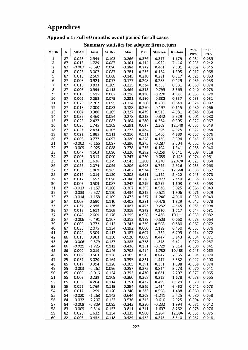
223

Appendices

Appendix 1: Full 60 months event period for all cases

Summary statistics for adopter firm return

Month N MEAN t-stat St. Dev. Min Max Skewness Kurtosis 25th

Perc.

75th

Perc.

1 87 0.028 2.549 0.103 -0.266 0.376 0.347 1.679 -0.031 0.085 2 87 0.016 1.729 0.087 -0.161 0.444 1.962 7.116 -0.035 0.042 3 87 -0.007 -0.697 0.090 -0.284 0.332 0.401 2.201 -0.068 0.045 4 87 0.028 3.007 0.087 -0.281 0.235 0.124 1.395 -0.017 0.068 5 87 0.018 2.509 0.068 -0.145 0.230 0.281 0.717 -0.025 0.053 6 87 0.008 0.924 0.077 -0.177 0.208 0.283 0.129 -0.039 0.053 7 87 0.010 0.833 0.109 -0.215 0.324 0.363 0.331 -0.059 0.074 8 87 0.007 0.599 0.113 -0.469 0.343 -0.795 3.365 -0.040 0.073 9 87 0.015 1.615 0.087 -0.216 0.198 -0.278 -0.008 -0.033 0.070

10 87 0.002 0.252 0.075 -0.231 0.160 -0.382 0.537 -0.035 0.051 11 87 0.028 2.762 0.095 -0.214 0.300 0.260 0.649 -0.028 0.082 12 87 0.018 2.000 0.083 -0.188 0.260 -0.197 0.615 -0.030 0.066 13 87 0.004 0.380 0.105 -0.327 0.479 0.513 4.981 -0.048 0.054 14 87 0.035 3.460 0.094 -0.278 0.333 -0.342 2.329 -0.001 0.080 15 87 0.022 2.427 0.083 -0.164 0.280 0.324 0.395 -0.027 0.067 16 87 0.020 1.745 0.109 -0.291 0.647 2.309 12.548 -0.035 0.049 18 87 0.027 2.434 0.105 -0.273 0.484 1.296 4.925 -0.027 0.054 19 87 0.022 1.885 0.111 -0.210 0.521 1.466 4.889 -0.037 0.076 20 87 0.008 0.777 0.097 -0.320 0.358 0.126 2.394 -0.045 0.059 21 87 -0.002 -0.166 0.097 -0.396 0.275 -0.287 2.704 -0.052 0.054 22 87 -0.009 -0.925 0.088 -0.278 0.235 0.104 1.341 -0.058 0.040 23 87 0.047 4.563 0.096 -0.226 0.292 -0.259 0.141 -0.009 0.118 24 87 0.003 0.313 0.090 -0.247 0.220 -0.059 -0.145 -0.074 0.061 25 87 0.031 1.636 0.179 -0.543 1.200 3.270 22.470 -0.027 0.064 26 87 0.022 2.074 0.099 -0.206 0.403 0.769 2.926 -0.033 0.068 27 87 0.033 1.869 0.165 -0.407 0.934 2.592 12.668 -0.038 0.067 28 87 0.014 1.016 0.130 -0.308 0.631 1.122 5.422 -0.045 0.073 29 87 0.017 1.657 0.096 -0.280 0.316 -0.022 2.444 -0.036 0.065 30 87 0.005 0.509 0.087 -0.242 0.299 0.257 1.603 -0.038 0.063 31 87 -0.013 -1.157 0.106 -0.307 0.395 0.536 3.025 -0.066 0.043 32 87 -0.033 -2.527 0.120 -0.434 0.342 -0.521 1.906 -0.076 0.029 33 87 -0.014 -1.158 0.109 -0.473 0.237 -1.246 4.010 -0.050 0.049 34 87 0.008 0.690 0.110 -0.402 0.281 -0.478 1.829 -0.042 0.078 35 87 0.034 2.356 0.136 -0.487 0.495 -0.232 4.345 -0.033 0.094 36 87 0.019 1.613 0.109 -0.319 0.393 0.230 1.717 -0.044 0.081 37 87 0.049 2.609 0.176 -0.295 0.968 2.486 10.111 -0.033 0.082 38 87 -0.006 -0.491 0.107 -0.313 0.189 -0.503 0.060 -0.073 0.064 39 87 0.009 0.772 0.112 -0.243 0.329 0.508 0.880 -0.067 0.072 40 87 0.030 2.075 0.134 -0.192 0.600 2.189 6.450 -0.037 0.076 41 87 0.040 3.309 0.113 -0.187 0.607 1.722 6.799 -0.014 0.072 42 86 0.016 0.963 0.150 -0.520 0.609 0.447 3.843 -0.054 0.071 43 86 -0.006 -0.379 0.137 -0.385 0.728 1.398 9.621 -0.070 0.057 44 86 -0.021 -1.725 0.112 -0.436 0.251 -0.729 2.314 -0.080 0.041 45 86 0.000 0.019 0.146 -0.798 0.414 -1.782 10.485 -0.045 0.069 46 85 0.008 0.563 0.136 -0.265 0.545 0.847 2.155 -0.084 0.079 47 85 0.054 3.020 0.164 -0.395 0.821 1.447 5.582 -0.027 0.100 48 85 0.014 0.994 0.128 -0.265 0.391 0.351 1.198 -0.058 0.074 49 85 -0.003 -0.262 0.096 -0.257 0.375 0.844 3.273 -0.070 0.041 50 85 0.000 -0.016 0.134 -0.393 0.430 0.681 2.207 -0.077 0.065 51 85 0.003 0.239 0.109 -0.360 0.368 0.213 1.678 -0.078 0.065 52 85 0.052 4.204 0.114 -0.251 0.437 0.499 0.929 -0.020 0.121 53 85 0.022 1.769 0.115 -0.254 0.599 1.434 6.462 -0.041 0.073 54 85 0.017 1.299 0.120 -0.340 0.383 0.598 1.488 -0.060 0.061 55 84 -0.020 -1.268 0.143 -0.644 0.309 -1.241 5.425 -0.080 0.058 56 84 -0.032 -2.207 0.132 -0.536 0.315 -0.610 2.925 -0.094 0.021 57 84 -0.008 -0.809 0.095 -0.343 0.250 -0.232 1.994 -0.071 0.042 58 83 -0.009 -0.514 0.153 -0.811 0.311 -1.607 8.262 -0.078 0.076 59 82 0.028 1.632 0.154 -0.335 0.900 2.204 12.396 -0.035 0.075 60 82 0.006 0.432 0.118 -0.429 0.422 0.295 3.540 -0.052 0.048

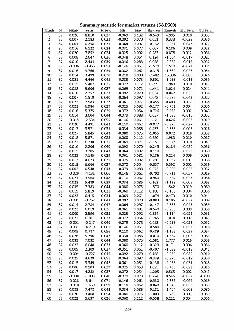
224

Summary statistic for market returns (S&P500) Month N MEAN t-stat St. Dev. Min Max Skewness Kurtosis 25th Perc. 75th Perc.

1 87 0.026 8.810 0.027 -0.069 0.132 -0.549 4.995 0.010 0.033 2 87 0.007 2.183 0.032 -0.092 0.070 0.051 0.333 -0.029 0.036 3 87 0.001 0.258 0.035 -0.064 0.097 -0.132 -0.921 -0.043 0.027 4 87 0.016 6.122 0.024 -0.031 0.077 0.007 0.186 0.009 0.028 5 87 0.020 7.852 0.024 -0.025 0.092 0.283 0.878 0.012 0.036 6 87 0.008 2.647 0.026 -0.048 0.054 0.124 -1.054 -0.017 0.023 7 87 0.010 2.434 0.039 -0.046 0.088 0.058 -0.883 -0.012 0.032 8 87 -0.006 -0.966 0.053 -0.146 0.061 -1.520 1.510 -0.024 0.034 9 87 0.016 3.766 0.039 -0.082 0.062 -0.315 -1.362 -0.027 0.054

10 87 0.014 3.499 0.038 -0.218 0.080 -2.402 15.396 -0.005 0.026 11 87 0.021 4.466 0.045 -0.085 0.075 -0.501 -1.055 -0.013 0.059 12 87 0.015 5.407 0.025 -0.022 0.112 0.899 1.989 0.010 0.017 13 87 0.028 9.606 0.027 -0.069 0.071 -1.441 3.024 0.024 0.041 14 87 0.010 2.757 0.033 -0.092 0.070 0.034 0.047 -0.020 0.036 15 87 0.007 1.519 0.040 -0.064 0.097 0.048 -0.686 -0.043 0.027 16 87 0.022 7.583 0.027 -0.061 0.077 -0.455 0.409 0.012 0.038 17 87 0.021 6.984 0.029 -0.025 0.092 -0.177 -0.751 0.004 0.036 18 87 0.016 5.375 0.029 -0.072 0.054 -0.726 -0.028 0.002 0.043 19 87 0.014 3.004 0.044 -0.079 0.088 0.037 -1.098 -0.016 0.032 20 87 -0.015 -2.534 0.055 -0.146 0.061 -1.121 0.626 -0.057 0.019 21 87 0.020 4.491 0.042 -0.110 0.062 -0.877 -0.375 -0.027 0.053 22 87 0.013 3.571 0.035 -0.034 0.086 0.453 -0.536 -0.005 0.026 23 87 0.027 5.845 0.043 -0.080 0.075 -1.055 0.072 0.018 0.059 24 87 0.018 5.871 0.028 -0.060 0.112 0.680 1.983 0.010 0.017 25 87 0.023 6.738 0.031 -0.069 0.071 -1.151 1.137 0.010 0.041 26 87 0.010 2.206 0.040 -0.092 0.070 -0.245 0.184 -0.020 0.036 27 87 0.015 3.205 0.043 -0.064 0.097 -0.110 -0.583 -0.022 0.050 28 87 0.022 7.145 0.029 -0.061 0.081 -0.186 0.224 0.009 0.038 29 87 0.013 4.073 0.031 -0.025 0.092 0.250 -1.052 -0.019 0.036 30 87 0.019 6.666 0.027 -0.072 0.054 -0.837 0.392 0.002 0.039 31 87 0.003 0.548 0.043 -0.079 0.088 0.573 -0.800 -0.032 0.032 32 87 -0.029 -4.131 0.066 -0.146 0.061 -0.700 -0.711 -0.057 0.019 33 87 0.021 3.964 0.048 -0.110 0.062 -0.940 -0.524 -0.027 0.054 34 87 0.023 5.489 0.039 -0.034 0.086 0.163 -1.123 -0.005 0.063 35 87 0.035 7.383 0.044 -0.080 0.075 -1.570 1.542 0.019 0.060 36 87 0.019 5.819 0.031 -0.060 0.112 0.180 -0.155 0.004 0.056 37 87 0.023 6.415 0.034 -0.069 0.061 -1.074 0.473 0.010 0.041 38 87 -0.001 -0.262 0.043 -0.092 0.070 -0.083 0.105 -0.032 0.009 39 87 0.014 2.784 0.047 -0.064 0.097 -0.147 -0.873 -0.043 0.039 40 87 0.023 6.019 0.036 -0.061 0.081 -0.540 -0.286 0.009 0.058 41 87 0.009 2.596 0.033 -0.025 0.092 0.534 -1.114 -0.022 0.036 42 87 0.022 6.101 0.033 -0.072 0.054 -1.265 1.074 0.002 0.043 43 87 -0.001 -0.247 0.046 -0.079 0.078 0.682 -0.599 -0.032 0.032 44 87 -0.031 -4.710 0.061 -0.146 0.061 -0.580 -0.486 -0.057 0.018 45 87 0.005 0.787 0.056 -0.110 0.062 -0.489 -1.166 -0.029 0.054 46 87 0.026 5.796 0.042 -0.034 0.086 -0.070 -1.354 -0.005 0.063 47 87 0.033 7.032 0.044 -0.080 0.075 -1.581 1.777 0.019 0.059 48 87 0.022 6.048 0.033 -0.060 0.112 -0.329 0.171 0.006 0.056 49 87 0.009 2.309 0.037 -0.051 0.061 -0.407 -1.082 -0.018 0.041 50 87 -0.004 -0.727 0.046 -0.092 0.070 0.158 -0.272 -0.030 0.010 51 87 0.025 4.629 0.051 -0.064 0.097 -0.339 -0.876 -0.018 0.050 52 87 0.015 3.349 0.042 -0.061 0.081 -0.136 -0.958 -0.031 0.048 53 87 0.000 0.103 0.029 -0.025 0.059 1.025 -0.435 -0.022 0.018 54 87 0.017 4.282 0.037 -0.072 0.054 -1.205 0.565 0.002 0.043 55 87 -0.008 -1.803 0.040 -0.079 0.078 0.724 0.545 -0.032 -0.011 56 87 -0.028 -3.644 0.071 -0.146 0.061 -0.530 -0.889 -0.064 0.019 57 87 -0.010 -1.659 0.059 -0.110 0.062 -0.048 -1.345 -0.053 0.053 58 87 0.033 7.478 0.042 -0.034 0.086 -0.181 -1.404 -0.005 0.080 59 87 0.020 3.468 0.054 -0.080 0.075 -1.003 -0.463 0.007 0.059 60 87 0.022 5.637 0.036 -0.060 0.112 -0.558 0.221 0.004 0.056

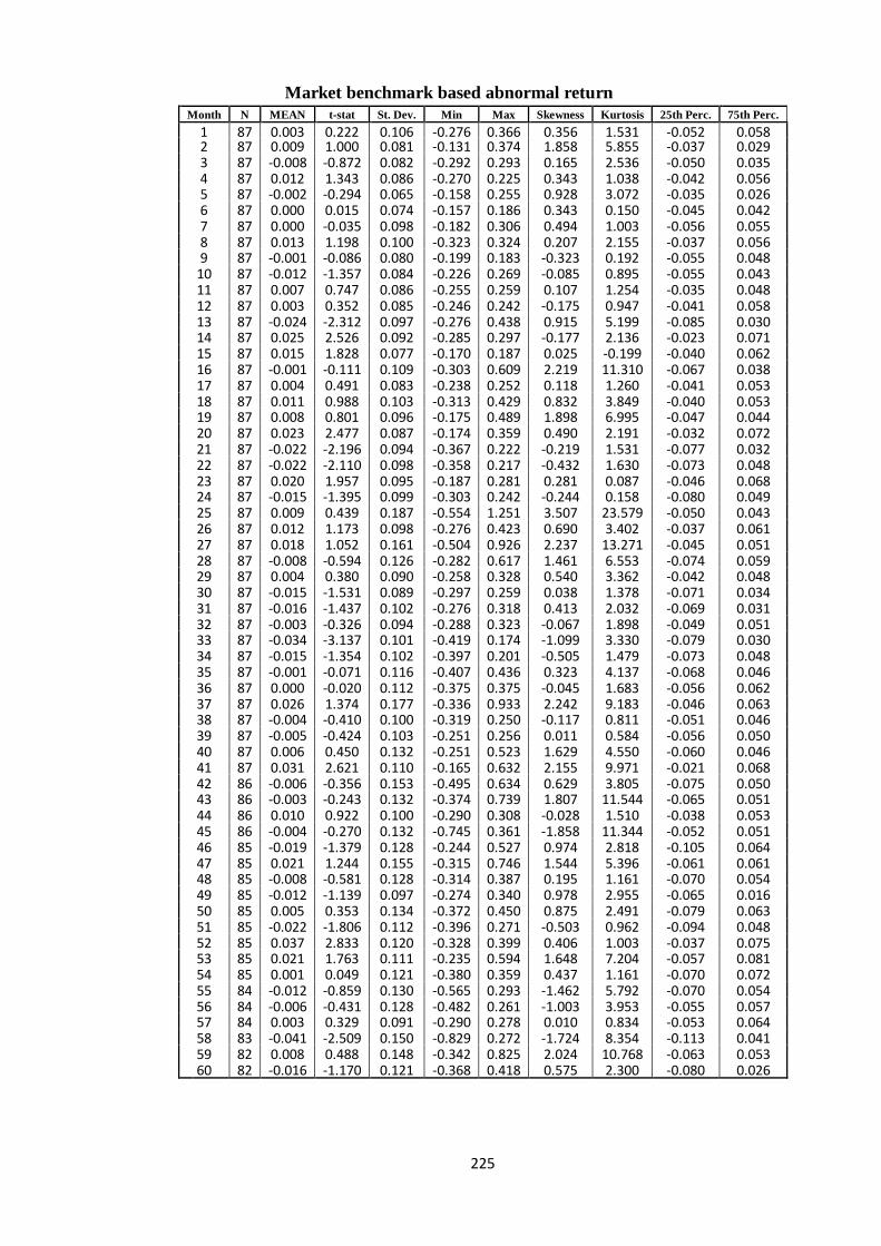
225

Market benchmark based abnormal return

Month N MEAN t-stat St. Dev. Min Max Skewness Kurtosis 25th Perc. 75th Perc.

1 87 0.003 0.222 0.106 -0.276 0.366 0.356 1.531 -0.052 0.058 2 87 0.009 1.000 0.081 -0.131 0.374 1.858 5.855 -0.037 0.029 3 87 -0.008 -0.872 0.082 -0.292 0.293 0.165 2.536 -0.050 0.035 4 87 0.012 1.343 0.086 -0.270 0.225 0.343 1.038 -0.042 0.056 5 87 -0.002 -0.294 0.065 -0.158 0.255 0.928 3.072 -0.035 0.026 6 87 0.000 0.015 0.074 -0.157 0.186 0.343 0.150 -0.045 0.042 7 87 0.000 -0.035 0.098 -0.182 0.306 0.494 1.003 -0.056 0.055 8 87 0.013 1.198 0.100 -0.323 0.324 0.207 2.155 -0.037 0.056 9 87 -0.001 -0.086 0.080 -0.199 0.183 -0.323 0.192 -0.055 0.048

10 87 -0.012 -1.357 0.084 -0.226 0.269 -0.085 0.895 -0.055 0.043 11 87 0.007 0.747 0.086 -0.255 0.259 0.107 1.254 -0.035 0.048 12 87 0.003 0.352 0.085 -0.246 0.242 -0.175 0.947 -0.041 0.058 13 87 -0.024 -2.312 0.097 -0.276 0.438 0.915 5.199 -0.085 0.030 14 87 0.025 2.526 0.092 -0.285 0.297 -0.177 2.136 -0.023 0.071 15 87 0.015 1.828 0.077 -0.170 0.187 0.025 -0.199 -0.040 0.062 16 87 -0.001 -0.111 0.109 -0.303 0.609 2.219 11.310 -0.067 0.038 17 87 0.004 0.491 0.083 -0.238 0.252 0.118 1.260 -0.041 0.053 18 87 0.011 0.988 0.103 -0.313 0.429 0.832 3.849 -0.040 0.053 19 87 0.008 0.801 0.096 -0.175 0.489 1.898 6.995 -0.047 0.044 20 87 0.023 2.477 0.087 -0.174 0.359 0.490 2.191 -0.032 0.072 21 87 -0.022 -2.196 0.094 -0.367 0.222 -0.219 1.531 -0.077 0.032 22 87 -0.022 -2.110 0.098 -0.358 0.217 -0.432 1.630 -0.073 0.048 23 87 0.020 1.957 0.095 -0.187 0.281 0.281 0.087 -0.046 0.068 24 87 -0.015 -1.395 0.099 -0.303 0.242 -0.244 0.158 -0.080 0.049 25 87 0.009 0.439 0.187 -0.554 1.251 3.507 23.579 -0.050 0.043 26 87 0.012 1.173 0.098 -0.276 0.423 0.690 3.402 -0.037 0.061 27 87 0.018 1.052 0.161 -0.504 0.926 2.237 13.271 -0.045 0.051 28 87 -0.008 -0.594 0.126 -0.282 0.617 1.461 6.553 -0.074 0.059 29 87 0.004 0.380 0.090 -0.258 0.328 0.540 3.362 -0.042 0.048 30 87 -0.015 -1.531 0.089 -0.297 0.259 0.038 1.378 -0.071 0.034 31 87 -0.016 -1.437 0.102 -0.276 0.318 0.413 2.032 -0.069 0.031 32 87 -0.003 -0.326 0.094 -0.288 0.323 -0.067 1.898 -0.049 0.051 33 87 -0.034 -3.137 0.101 -0.419 0.174 -1.099 3.330 -0.079 0.030 34 87 -0.015 -1.354 0.102 -0.397 0.201 -0.505 1.479 -0.073 0.048 35 87 -0.001 -0.071 0.116 -0.407 0.436 0.323 4.137 -0.068 0.046 36 87 0.000 -0.020 0.112 -0.375 0.375 -0.045 1.683 -0.056 0.062 37 87 0.026 1.374 0.177 -0.336 0.933 2.242 9.183 -0.046 0.063 38 87 -0.004 -0.410 0.100 -0.319 0.250 -0.117 0.811 -0.051 0.046 39 87 -0.005 -0.424 0.103 -0.251 0.256 0.011 0.584 -0.056 0.050 40 87 0.006 0.450 0.132 -0.251 0.523 1.629 4.550 -0.060 0.046 41 87 0.031 2.621 0.110 -0.165 0.632 2.155 9.971 -0.021 0.068 42 86 -0.006 -0.356 0.153 -0.495 0.634 0.629 3.805 -0.075 0.050 43 86 -0.003 -0.243 0.132 -0.374 0.739 1.807 11.544 -0.065 0.051 44 86 0.010 0.922 0.100 -0.290 0.308 -0.028 1.510 -0.038 0.053 45 86 -0.004 -0.270 0.132 -0.745 0.361 -1.858 11.344 -0.052 0.051 46 85 -0.019 -1.379 0.128 -0.244 0.527 0.974 2.818 -0.105 0.064 47 85 0.021 1.244 0.155 -0.315 0.746 1.544 5.396 -0.061 0.061 48 85 -0.008 -0.581 0.128 -0.314 0.387 0.195 1.161 -0.070 0.054 49 85 -0.012 -1.139 0.097 -0.274 0.340 0.978 2.955 -0.065 0.016 50 85 0.005 0.353 0.134 -0.372 0.450 0.875 2.491 -0.079 0.063 51 85 -0.022 -1.806 0.112 -0.396 0.271 -0.503 0.962 -0.094 0.048 52 85 0.037 2.833 0.120 -0.328 0.399 0.406 1.003 -0.037 0.075 53 85 0.021 1.763 0.111 -0.235 0.594 1.648 7.204 -0.057 0.081 54 85 0.001 0.049 0.121 -0.380 0.359 0.437 1.161 -0.070 0.072 55 84 -0.012 -0.859 0.130 -0.565 0.293 -1.462 5.792 -0.070 0.054 56 84 -0.006 -0.431 0.128 -0.482 0.261 -1.003 3.953 -0.055 0.057 57 84 0.003 0.329 0.091 -0.290 0.278 0.010 0.834 -0.053 0.064 58 83 -0.041 -2.509 0.150 -0.829 0.272 -1.724 8.354 -0.113 0.041 59 82 0.008 0.488 0.148 -0.342 0.825 2.024 10.768 -0.063 0.053 60 82 -0.016 -1.170 0.121 -0.368 0.418 0.575 2.300 -0.080 0.026

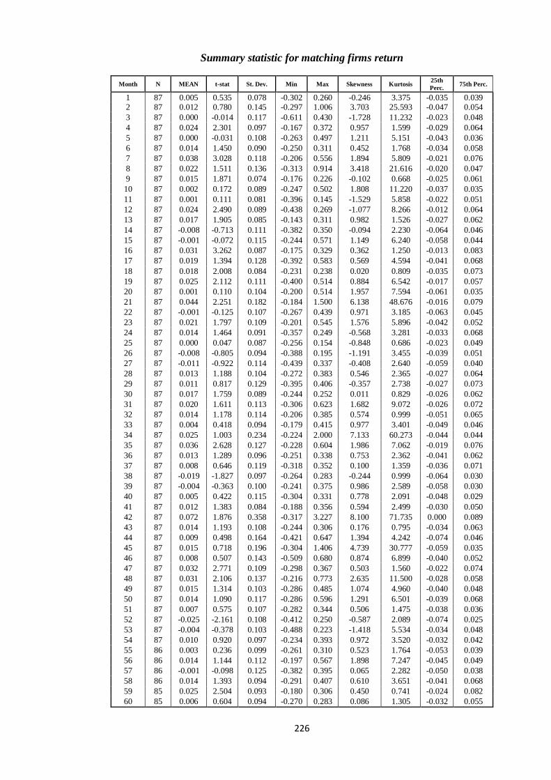
226

Summary statistic for matching firms return


Perc. 75th Perc.

1 87 0.005 0.535 0.078 -0.302 0.260 -0.246 3.375 -0.035 0.039 2 87 0.012 0.780 0.145 -0.297 1.006 3.703 25.593 -0.047 0.054

3 87 0.000 -0.014 0.117 -0.611 0.430 -1.728 11.232 -0.023 0.048

4 87 0.024 2.301 0.097 -0.167 0.372 0.957 1.599 -0.029 0.064

5 87 0.000 -0.031 0.108 -0.263 0.497 1.211 5.151 -0.043 0.036

6 87 0.014 1.450 0.090 -0.250 0.311 0.452 1.768 -0.034 0.058

7 87 0.038 3.028 0.118 -0.206 0.556 1.894 5.809 -0.021 0.076

8 87 0.022 1.511 0.136 -0.313 0.914 3.418 21.616 -0.020 0.047

9 87 0.015 1.871 0.074 -0.176 0.226 -0.102 0.668 -0.025 0.061

10 87 0.002 0.172 0.089 -0.247 0.502 1.808 11.220 -0.037 0.035

11 87 0.001 0.111 0.081 -0.396 0.145 -1.529 5.858 -0.022 0.051

12 87 0.024 2.490 0.089 -0.438 0.269 -1.077 8.266 -0.012 0.064

13 87 0.017 1.905 0.085 -0.143 0.311 0.982 1.526 -0.027 0.062

14 87 -0.008 -0.713 0.111 -0.382 0.350 -0.094 2.230 -0.064 0.046

15 87 -0.001 -0.072 0.115 -0.244 0.571 1.149 6.240 -0.058 0.044

16 87 0.031 3.262 0.087 -0.175 0.329 0.362 1.250 -0.013 0.083

17 87 0.019 1.394 0.128 -0.392 0.583 0.569 4.594 -0.041 0.068

18 87 0.018 2.008 0.084 -0.231 0.238 0.020 0.809 -0.035 0.073

19 87 0.025 2.112 0.111 -0.400 0.514 0.884 6.542 -0.017 0.057

20 87 0.001 0.110 0.104 -0.200 0.514 1.957 7.594 -0.061 0.035

21 87 0.044 2.251 0.182 -0.184 1.500 6.138 48.676 -0.016 0.079

22 87 -0.001 -0.125 0.107 -0.267 0.439 0.971 3.185 -0.063 0.045

23 87 0.021 1.797 0.109 -0.201 0.545 1.576 5.896 -0.042 0.052

24 87 0.014 1.464 0.091 -0.357 0.249 -0.568 3.281 -0.033 0.068

25 87 0.000 0.047 0.087 -0.256 0.154 -0.848 0.686 -0.023 0.049

26 87 -0.008 -0.805 0.094 -0.388 0.195 -1.191 3.455 -0.039 0.051

27 87 -0.011 -0.922 0.114 -0.439 0.337 -0.408 2.640 -0.059 0.040

28 87 0.013 1.188 0.104 -0.272 0.383 0.546 2.365 -0.027 0.064

29 87 0.011 0.817 0.129 -0.395 0.406 -0.357 2.738 -0.027 0.073

30 87 0.017 1.759 0.089 -0.244 0.252 0.011 0.829 -0.026 0.062

31 87 0.020 1.611 0.113 -0.306 0.623 1.682 9.072 -0.026 0.072

32 87 0.014 1.178 0.114 -0.206 0.385 0.574 0.999 -0.051 0.065

33 87 0.004 0.418 0.094 -0.179 0.415 0.977 3.401 -0.049 0.046

34 87 0.025 1.003 0.234 -0.224 2.000 7.133 60.273 -0.044 0.044

35 87 0.036 2.628 0.127 -0.228 0.604 1.986 7.062 -0.019 0.076

36 87 0.013 1.289 0.096 -0.251 0.338 0.753 2.362 -0.041 0.062

37 87 0.008 0.646 0.119 -0.318 0.352 0.100 1.359 -0.036 0.071

38 87 -0.019 -1.827 0.097 -0.264 0.283 -0.244 0.999 -0.064 0.030

39 87 -0.004 -0.363 0.100 -0.241 0.375 0.986 2.589 -0.058 0.030

40 87 0.005 0.422 0.115 -0.304 0.331 0.778 2.091 -0.048 0.029

41 87 0.012 1.383 0.084 -0.188 0.356 0.594 2.499 -0.030 0.050

42 87 0.072 1.876 0.358 -0.317 3.227 8.100 71.735 0.000 0.089

43 87 0.014 1.193 0.108 -0.244 0.306 0.176 0.795 -0.034 0.063

44 87 0.009 0.498 0.164 -0.421 0.647 1.394 4.242 -0.074 0.046

45 87 0.015 0.718 0.196 -0.304 1.406 4.739 30.777 -0.059 0.035

46 87 0.008 0.507 0.143 -0.509 0.680 0.874 6.899 -0.040 0.052

47 87 0.032 2.771 0.109 -0.298 0.367 0.503 1.560 -0.022 0.074

48 87 0.031 2.106 0.137 -0.216 0.773 2.635 11.500 -0.028 0.058

49 87 0.015 1.314 0.103 -0.286 0.485 1.074 4.960 -0.040 0.048

50 87 0.014 1.090 0.117 -0.286 0.596 1.291 6.501 -0.039 0.068

51 87 0.007 0.575 0.107 -0.282 0.344 0.506 1.475 -0.038 0.036

52 87 -0.025 -2.161 0.108 -0.412 0.250 -0.587 2.089 -0.074 0.025

53 87 -0.004 -0.378 0.103 -0.488 0.223 -1.418 5.534 -0.034 0.048

54 87 0.010 0.920 0.097 -0.234 0.393 0.972 3.520 -0.032 0.042

55 86 0.003 0.236 0.099 -0.261 0.310 0.523 1.764 -0.053 0.039

56 86 0.014 1.144 0.112 -0.197 0.567 1.898 7.247 -0.045 0.049

57 86 -0.001 -0.098 0.125 -0.382 0.395 0.065 2.282 -0.050 0.038

58 86 0.014 1.393 0.094 -0.291 0.407 0.610 3.651 -0.041 0.068

59 85 0.025 2.504 0.093 -0.180 0.306 0.450 0.741 -0.024 0.082

60 85 0.006 0.604 0.094 -0.270 0.283 0.086 1.305 -0.032 0.055

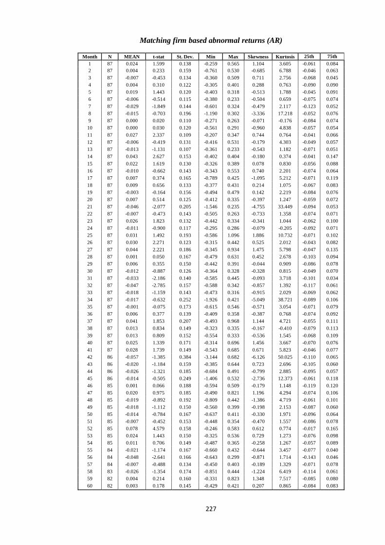
227

Matching firm based abnormal returns (AR)


Perc.

75th

Perc. 1 87 0.024 1.599 0.138 -0.259 0.565 1.104 3.605 -0.061 0.084

2 87 0.004 0.233 0.159 -0.761 0.530 -0.685 6.788 -0.046 0.063

3 87 -0.007 -0.453 0.134 -0.360 0.509 0.711 2.756 -0.068 0.045

4 87 0.004 0.310 0.122 -0.305 0.401 0.288 0.763 -0.090 0.090

5 87 0.019 1.443 0.120 -0.403 0.318 -0.513 1.788 -0.045 0.091

6 87 -0.006 -0.514 0.115 -0.380 0.233 -0.504 0.659 -0.075 0.074

7 87 -0.029 -1.849 0.144 -0.601 0.324 -0.479 2.117 -0.123 0.052

8 87 -0.015 -0.703 0.196 -1.190 0.302 -3.336 17.218 -0.052 0.076

9 87 0.000 0.020 0.110 -0.271 0.263 -0.071 -0.176 -0.084 0.074

10 87 0.000 0.030 0.120 -0.561 0.291 -0.960 4.838 -0.057 0.054

11 87 0.027 2.337 0.109 -0.207 0.347 0.744 0.764 -0.041 0.066

12 87 -0.006 -0.419 0.131 -0.416 0.531 -0.179 4.303 -0.049 0.057

13 87 -0.013 -1.131 0.107 -0.361 0.233 -0.543 1.182 -0.071 0.051

14 87 0.043 2.627 0.153 -0.402 0.404 -0.180 0.374 -0.041 0.147

15 87 0.022 1.619 0.130 -0.326 0.389 0.078 0.830 -0.056 0.088

16 87 -0.010 -0.662 0.143 -0.343 0.553 0.740 2.201 -0.074 0.064

17 87 0.007 0.374 0.165 -0.789 0.425 -1.095 5.212 -0.071 0.119

18 87 0.009 0.656 0.133 -0.377 0.431 0.214 1.075 -0.067 0.083

19 87 -0.003 -0.164 0.156 -0.494 0.479 0.142 2.219 -0.084 0.076

20 87 0.007 0.514 0.125 -0.412 0.335 -0.397 1.247 -0.059 0.072

21 87 -0.046 -2.077 0.205 -1.546 0.235 -4.755 33.449 -0.094 0.053

22 87 -0.007 -0.473 0.143 -0.505 0.263 -0.733 1.358 -0.074 0.071

23 87 0.026 1.823 0.132 -0.442 0.334 -0.341 1.044 -0.062 0.100

24 87 -0.011 -0.900 0.117 -0.295 0.286 -0.079 -0.205 -0.092 0.071

25 87 0.031 1.492 0.193 -0.586 1.096 1.886 10.732 -0.071 0.102

26 87 0.030 2.271 0.123 -0.315 0.442 0.525 2.012 -0.043 0.082

27 87 0.044 2.221 0.186 -0.345 0.934 1.475 5.798 -0.047 0.135

28 87 0.001 0.050 0.167 -0.479 0.631 0.452 2.678 -0.103 0.094

29 87 0.006 0.355 0.150 -0.442 0.391 -0.044 0.909 -0.086 0.078

30 87 -0.012 -0.887 0.126 -0.364 0.328 -0.328 0.815 -0.049 0.070

31 87 -0.033 -2.186 0.140 -0.585 0.445 -0.093 3.718 -0.101 0.034

32 87 -0.047 -2.785 0.157 -0.588 0.342 -0.857 1.392 -0.117 0.061

33 87 -0.018 -1.159 0.143 -0.473 0.316 -0.915 2.029 -0.069 0.062

34 87 -0.017 -0.632 0.252 -1.926 0.421 -5.049 38.721 -0.089 0.106

35 87 -0.001 -0.075 0.173 -0.615 0.546 -0.571 3.054 -0.071 0.079

36 87 0.006 0.377 0.139 -0.409 0.358 -0.387 0.768 -0.074 0.092

37 87 0.041 1.853 0.207 -0.493 0.968 1.144 4.721 -0.055 0.111

38 87 0.013 0.834 0.149 -0.323 0.335 -0.167 -0.410 -0.079 0.113

39 87 0.013 0.809 0.152 -0.554 0.333 -0.536 1.545 -0.068 0.109

40 87 0.025 1.339 0.171 -0.314 0.696 1.456 3.667 -0.070 0.076

41 87 0.028 1.739 0.149 -0.543 0.685 0.671 5.823 -0.046 0.077

42 86 -0.057 -1.385 0.384 -3.144 0.682 -6.126 50.025 -0.110 0.065

43 86 -0.020 -1.184 0.159 -0.385 0.644 0.723 2.696 -0.105 0.060

44 86 -0.026 -1.321 0.185 -0.684 0.491 -0.799 2.885 -0.095 0.057

45 86 -0.014 -0.505 0.249 -1.406 0.532 -2.736 12.373 -0.061 0.118

46 85 0.001 0.066 0.188 -0.594 0.509 -0.179 1.148 -0.119 0.120

47 85 0.020 0.975 0.185 -0.490 0.821 1.196 4.294 -0.074 0.106

48 85 -0.019 -0.892 0.192 -0.809 0.442 -1.386 4.719 -0.061 0.101

49 85 -0.018 -1.112 0.150 -0.560 0.399 -0.198 2.153 -0.087 0.060

50 85 -0.014 -0.784 0.167 -0.637 0.411 -0.330 1.971 -0.096 0.064

51 85 -0.007 -0.452 0.153 -0.448 0.354 -0.470 1.557 -0.086 0.078

52 85 0.078 4.579 0.158 -0.246 0.583 0.612 0.774 -0.017 0.165

53 85 0.024 1.443 0.150 -0.325 0.536 0.729 1.273 -0.076 0.098

54 85 0.011 0.706 0.149 -0.487 0.365 -0.258 1.267 -0.057 0.089

55 84 -0.021 -1.174 0.167 -0.660 0.432 -0.644 3.457 -0.077 0.040

56 84 -0.048 -2.641 0.166 -0.643 0.299 -0.871 1.714 -0.143 0.046

57 84 -0.007 -0.488 0.134 -0.450 0.403 -0.189 1.329 -0.071 0.078

58 83 -0.026 -1.354 0.174 -0.851 0.444 -1.224 6.419 -0.114 0.061

59 82 0.004 0.214 0.160 -0.331 0.823 1.348 7.517 -0.085 0.080

60 82 0.003 0.178 0.145 -0.429 0.421 0.207 0.865 -0.084 0.083

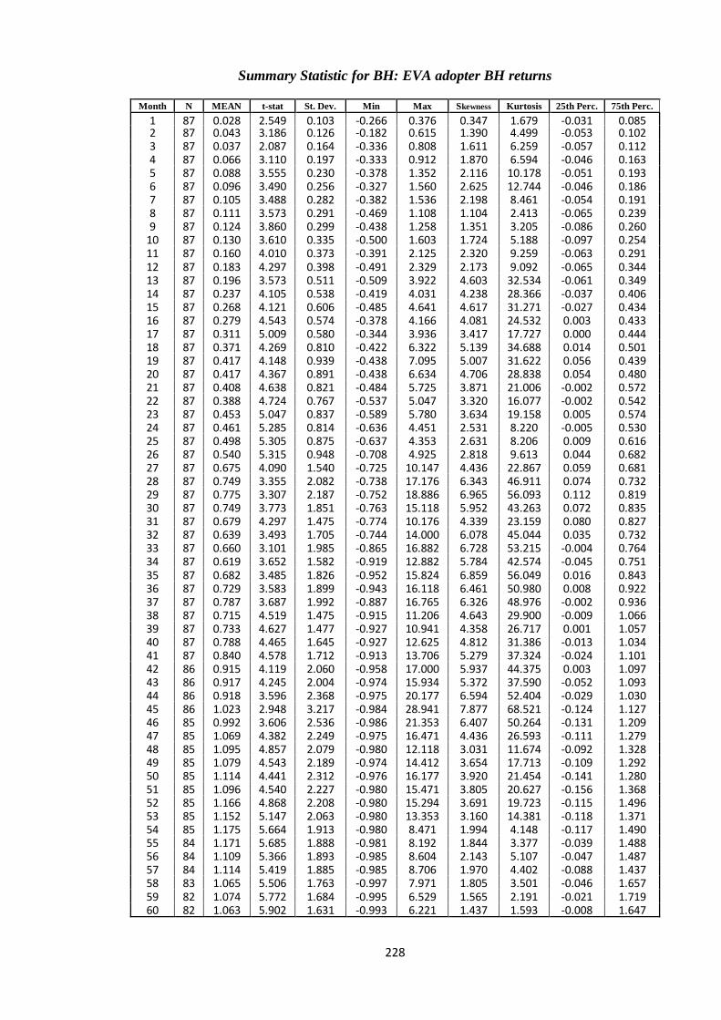
228

Summary Statistic for BH: EVA adopter BH returns

Month N MEAN t-stat St. Dev. Min Max Skewness Kurtosis 25th Perc. 75th Perc.

1 87 0.028 2.549 0.103 -0.266 0.376 0.347 1.679 -0.031 0.085 2 87 0.043 3.186 0.126 -0.182 0.615 1.390 4.499 -0.053 0.102 3 87 0.037 2.087 0.164 -0.336 0.808 1.611 6.259 -0.057 0.112 4 87 0.066 3.110 0.197 -0.333 0.912 1.870 6.594 -0.046 0.163 5 87 0.088 3.555 0.230 -0.378 1.352 2.116 10.178 -0.051 0.193 6 87 0.096 3.490 0.256 -0.327 1.560 2.625 12.744 -0.046 0.186 7 87 0.105 3.488 0.282 -0.382 1.536 2.198 8.461 -0.054 0.191 8 87 0.111 3.573 0.291 -0.469 1.108 1.104 2.413 -0.065 0.239 9 87 0.124 3.860 0.299 -0.438 1.258 1.351 3.205 -0.086 0.260

10 87 0.130 3.610 0.335 -0.500 1.603 1.724 5.188 -0.097 0.254 11 87 0.160 4.010 0.373 -0.391 2.125 2.320 9.259 -0.063 0.291 12 87 0.183 4.297 0.398 -0.491 2.329 2.173 9.092 -0.065 0.344 13 87 0.196 3.573 0.511 -0.509 3.922 4.603 32.534 -0.061 0.349 14 87 0.237 4.105 0.538 -0.419 4.031 4.238 28.366 -0.037 0.406 15 87 0.268 4.121 0.606 -0.485 4.641 4.617 31.271 -0.027 0.434 16 87 0.279 4.543 0.574 -0.378 4.166 4.081 24.532 0.003 0.433 17 87 0.311 5.009 0.580 -0.344 3.936 3.417 17.727 0.000 0.444 18 87 0.371 4.269 0.810 -0.422 6.322 5.139 34.688 0.014 0.501 19 87 0.417 4.148 0.939 -0.438 7.095 5.007 31.622 0.056 0.439 20 87 0.417 4.367 0.891 -0.438 6.634 4.706 28.838 0.054 0.480 21 87 0.408 4.638 0.821 -0.484 5.725 3.871 21.006 -0.002 0.572 22 87 0.388 4.724 0.767 -0.537 5.047 3.320 16.077 -0.002 0.542 23 87 0.453 5.047 0.837 -0.589 5.780 3.634 19.158 0.005 0.574 24 87 0.461 5.285 0.814 -0.636 4.451 2.531 8.220 -0.005 0.530 25 87 0.498 5.305 0.875 -0.637 4.353 2.631 8.206 0.009 0.616 26 87 0.540 5.315 0.948 -0.708 4.925 2.818 9.613 0.044 0.682 27 87 0.675 4.090 1.540 -0.725 10.147 4.436 22.867 0.059 0.681 28 87 0.749 3.355 2.082 -0.738 17.176 6.343 46.911 0.074 0.732 29 87 0.775 3.307 2.187 -0.752 18.886 6.965 56.093 0.112 0.819 30 87 0.749 3.773 1.851 -0.763 15.118 5.952 43.263 0.072 0.835 31 87 0.679 4.297 1.475 -0.774 10.176 4.339 23.159 0.080 0.827 32 87 0.639 3.493 1.705 -0.744 14.000 6.078 45.044 0.035 0.732 33 87 0.660 3.101 1.985 -0.865 16.882 6.728 53.215 -0.004 0.764 34 87 0.619 3.652 1.582 -0.919 12.882 5.784 42.574 -0.045 0.751 35 87 0.682 3.485 1.826 -0.952 15.824 6.859 56.049 0.016 0.843 36 87 0.729 3.583 1.899 -0.943 16.118 6.461 50.980 0.008 0.922 37 87 0.787 3.687 1.992 -0.887 16.765 6.326 48.976 -0.002 0.936 38 87 0.715 4.519 1.475 -0.915 11.206 4.643 29.900 -0.009 1.066 39 87 0.733 4.627 1.477 -0.927 10.941 4.358 26.717 0.001 1.057 40 87 0.788 4.465 1.645 -0.927 12.625 4.812 31.386 -0.013 1.034 41 87 0.840 4.578 1.712 -0.913 13.706 5.279 37.324 -0.024 1.101 42 86 0.915 4.119 2.060 -0.958 17.000 5.937 44.375 0.003 1.097 43 86 0.917 4.245 2.004 -0.974 15.934 5.372 37.590 -0.052 1.093 44 86 0.918 3.596 2.368 -0.975 20.177 6.594 52.404 -0.029 1.030 45 86 1.023 2.948 3.217 -0.984 28.941 7.877 68.521 -0.124 1.127 46 85 0.992 3.606 2.536 -0.986 21.353 6.407 50.264 -0.131 1.209 47 85 1.069 4.382 2.249 -0.975 16.471 4.436 26.593 -0.111 1.279 48 85 1.095 4.857 2.079 -0.980 12.118 3.031 11.674 -0.092 1.328 49 85 1.079 4.543 2.189 -0.974 14.412 3.654 17.713 -0.109 1.292 50 85 1.114 4.441 2.312 -0.976 16.177 3.920 21.454 -0.141 1.280 51 85 1.096 4.540 2.227 -0.980 15.471 3.805 20.627 -0.156 1.368 52 85 1.166 4.868 2.208 -0.980 15.294 3.691 19.723 -0.115 1.496 53 85 1.152 5.147 2.063 -0.980 13.353 3.160 14.381 -0.118 1.371 54 85 1.175 5.664 1.913 -0.980 8.471 1.994 4.148 -0.117 1.490 55 84 1.171 5.685 1.888 -0.981 8.192 1.844 3.377 -0.039 1.488 56 84 1.109 5.366 1.893 -0.985 8.604 2.143 5.107 -0.047 1.487 57 84 1.114 5.419 1.885 -0.985 8.706 1.970 4.402 -0.088 1.437 58 83 1.065 5.506 1.763 -0.997 7.971 1.805 3.501 -0.046 1.657 59 82 1.074 5.772 1.684 -0.995 6.529 1.565 2.191 -0.021 1.719 60 82 1.063 5.902 1.631 -0.993 6.221 1.437 1.593 -0.008 1.647

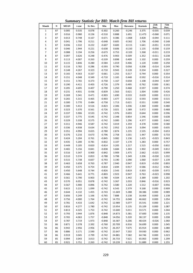
229

Summary Statistic for BH: Match firm BH returns


Perc.

75th

Perc.

1 87 0.005 0.535 0.078 -0.302 0.260 -0.246 3.375 -0.035 0.039

2 87 0.016 0.980 0.156 -0.510 0.888 1.691 11.473 -0.068 0.071

3 87 0.013 0.748 0.167 -0.671 0.386 -1.068 3.828 -0.044 0.111

4 87 0.041 1.796 0.211 -0.648 0.605 -0.362 1.706 -0.040 0.148

5 87 0.036 1.532 0.222 -0.607 0.683 -0.115 1.641 -0.051 0.159

6 87 0.046 1.944 0.221 -0.638 0.606 -0.150 1.135 -0.058 0.159

7 87 0.088 3.194 0.256 -0.673 0.753 -0.103 1.268 -0.011 0.219

8 87 0.097 3.626 0.248 -0.476 0.903 0.509 1.352 -0.011 0.238

9 87 0.113 4.007 0.263 -0.539 0.898 0.409 1.102 0.000 0.259

10 87 0.115 3.846 0.280 -0.584 1.019 0.406 1.120 0.000 0.258

11 87 0.116 3.782 0.286 -0.593 0.790 0.058 0.208 -0.014 0.249

12 87 0.148 4.267 0.323 -0.710 0.943 0.128 0.334 0.000 0.327

13 87 0.165 4.563 0.337 -0.661 1.255 0.317 0.744 0.000 0.354

14 87 0.151 4.048 0.349 -0.710 1.165 0.448 0.592 -0.016 0.314

15 87 0.151 3.765 0.373 -0.758 1.167 0.658 1.108 -0.044 0.307

16 87 0.190 4.411 0.403 -0.726 1.379 0.495 0.762 0.000 0.361

17 87 0.205 4.695 0.407 -0.790 1.250 0.468 0.597 0.000 0.374

18 87 0.231 4.931 0.436 -0.839 1.563 0.621 1.004 0.000 0.426

19 87 0.269 5.341 0.471 -0.903 1.690 0.533 0.639 0.000 0.513

20 87 0.265 5.315 0.465 -0.903 1.477 0.522 0.593 0.000 0.515

21 87 0.300 5.770 0.484 -0.758 1.713 0.621 0.551 0.000 0.540

22 87 0.300 5.413 0.516 -0.823 2.306 1.036 2.360 0.000 0.480

23 87 0.323 5.370 0.561 -0.726 3.021 1.589 5.472 0.000 0.468

24 87 0.337 5.906 0.533 -0.742 1.976 0.693 0.644 0.000 0.596

25 87 0.337 5.775 0.545 -0.742 2.348 0.854 1.546 0.000 0.638

26 87 0.329 5.338 0.575 -0.742 3.000 1.296 4.377 0.000 0.642

27 87 0.311 4.946 0.587 -0.742 3.019 1.359 4.378 0.000 0.580

28 87 0.336 4.938 0.634 -0.742 2.952 1.334 3.094 0.000 0.635

29 87 0.351 4.994 0.655 -0.780 2.874 1.235 2.535 -0.004 0.653

30 87 0.376 5.216 0.673 -0.796 2.758 1.031 1.447 0.000 0.733

31 87 0.424 5.204 0.761 -0.845 3.082 1.136 1.425 -0.023 0.843

32 87 0.435 5.200 0.781 -0.832 3.107 1.170 1.283 0.000 0.757

33 87 0.449 5.105 0.820 -0.814 3.205 1.217 1.515 -0.050 0.832

34 87 0.465 5.156 0.841 -0.838 3.684 1.303 1.902 -0.049 0.812

35 87 0.516 5.347 0.900 -0.842 3.909 1.475 2.662 -0.025 0.999

36 87 0.510 5.574 0.853 -0.788 3.798 1.349 2.206 -0.030 1.032

37 87 0.515 5.738 0.837 -0.793 3.190 1.090 1.060 -0.037 1.139

38 87 0.463 5.658 0.763 -0.787 2.940 0.947 0.819 -0.050 0.893

39 87 0.450 5.575 0.754 -0.810 2.694 0.917 0.586 -0.012 0.962

40 87 0.450 5.648 0.744 -0.826 2.543 0.819 0.303 -0.039 0.972

41 87 0.466 5.641 0.771 -0.803 2.923 0.947 0.763 -0.023 0.998

42 87 0.561 5.790 0.903 -0.780 4.504 1.442 3.389 0.000 1.202

43 87 0.570 6.051 0.878 -0.742 3.367 1.033 0.846 -0.016 0.923

44 87 0.567 5.900 0.896 -0.742 3.580 1.220 1.512 -0.007 0.956

45 87 0.615 5.215 1.099 -0.742 6.543 2.379 9.168 0.000 0.909

46 87 0.644 4.132 1.455 -0.743 11.669 5.288 38.386 0.000 0.989

47 87 0.656 5.249 1.166 -0.765 7.888 3.138 16.464 0.000 1.138

48 87 0.756 4.000 1.764 -0.742 14.755 6.048 46.662 0.000 1.054

49 87 0.781 4.433 1.642 -0.742 12.989 5.077 35.541 0.000 1.221

50 87 0.816 4.277 1.780 -0.742 13.954 5.135 35.109 0.000 1.087

51 87 0.813 4.325 1.753 -0.742 13.600 5.011 33.571 0.000 1.044

52 87 0.793 3.944 1.876 -0.848 14.873 5.381 37.600 0.000 1.135

53 87 0.765 4.063 1.757 -0.848 14.056 5.320 38.137 0.000 1.038

54 87 0.787 3.719 1.973 -0.848 16.587 6.206 48.424 -0.026 1.060

55 86 0.871 3.378 2.392 -0.760 20.709 6.916 56.699 0.000 1.045

56 86 0.942 2.956 2.956 -0.742 26.357 7.675 65.914 0.000 1.080

57 86 0.886 3.171 2.590 -0.742 22.647 7.202 59.930 0.000 0.962

58 86 0.919 3.045 2.799 -0.742 24.881 7.582 64.746 0.000 1.023

59 85 0.994 3.043 3.013 -0.742 26.733 7.621 65.063 0.000 1.299

60 85 0.921 3.751 2.263 -0.742 19.239 6.512 51.889 0.000 1.255

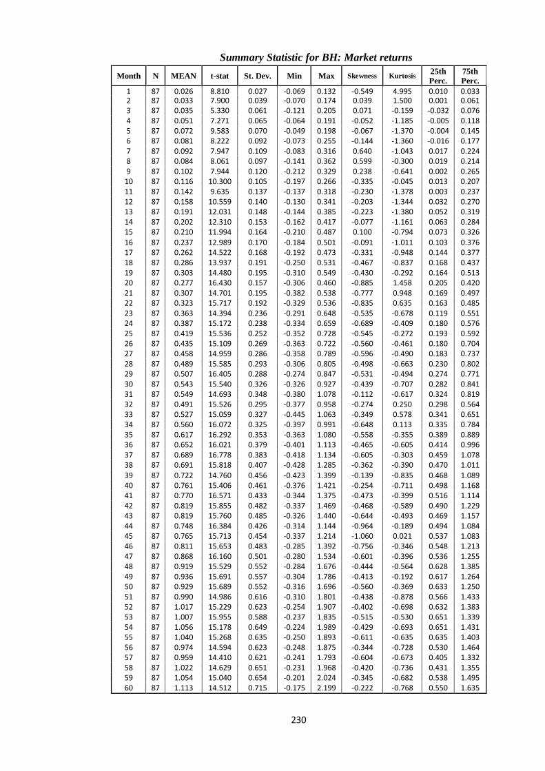
230

Summary Statistic for BH: Market returns


Perc.

75th

Perc.

1 87 0.026 8.810 0.027 -0.069 0.132 -0.549 4.995 0.010 0.033 2 87 0.033 7.900 0.039 -0.070 0.174 0.039 1.500 0.001 0.061 3 87 0.035 5.330 0.061 -0.121 0.205 0.071 -0.159 -0.032 0.076 4 87 0.051 7.271 0.065 -0.064 0.191 -0.052 -1.185 -0.005 0.118 5 87 0.072 9.583 0.070 -0.049 0.198 -0.067 -1.370 -0.004 0.145 6 87 0.081 8.222 0.092 -0.073 0.255 -0.144 -1.360 -0.016 0.177 7 87 0.092 7.947 0.109 -0.083 0.316 0.640 -1.043 0.017 0.224 8 87 0.084 8.061 0.097 -0.141 0.362 0.599 -0.300 0.019 0.214 9 87 0.102 7.944 0.120 -0.212 0.329 0.238 -0.641 0.002 0.265

10 87 0.116 10.300 0.105 -0.197 0.266 -0.335 -0.045 0.013 0.207 11 87 0.142 9.635 0.137 -0.137 0.318 -0.230 -1.378 0.003 0.237 12 87 0.158 10.559 0.140 -0.130 0.341 -0.203 -1.344 0.032 0.270 13 87 0.191 12.031 0.148 -0.144 0.385 -0.223 -1.380 0.052 0.319 14 87 0.202 12.310 0.153 -0.162 0.417 -0.077 -1.161 0.063 0.284 15 87 0.210 11.994 0.164 -0.210 0.487 0.100 -0.794 0.073 0.326 16 87 0.237 12.989 0.170 -0.184 0.501 -0.091 -1.011 0.103 0.376 17 87 0.262 14.522 0.168 -0.192 0.473 -0.331 -0.948 0.144 0.377 18 87 0.286 13.937 0.191 -0.250 0.531 -0.467 -0.837 0.168 0.437 19 87 0.303 14.480 0.195 -0.310 0.549 -0.430 -0.292 0.164 0.513 20 87 0.277 16.430 0.157 -0.306 0.460 -0.885 1.458 0.205 0.420 21 87 0.307 14.701 0.195 -0.382 0.538 -0.777 0.948 0.169 0.497 22 87 0.323 15.717 0.192 -0.329 0.536 -0.835 0.635 0.163 0.485 23 87 0.363 14.394 0.236 -0.291 0.648 -0.535 -0.678 0.119 0.551 24 87 0.387 15.172 0.238 -0.334 0.659 -0.689 -0.409 0.180 0.576 25 87 0.419 15.536 0.252 -0.352 0.728 -0.545 -0.272 0.193 0.592 26 87 0.435 15.109 0.269 -0.363 0.722 -0.560 -0.461 0.180 0.704 27 87 0.458 14.959 0.286 -0.358 0.789 -0.596 -0.490 0.183 0.737 28 87 0.489 15.585 0.293 -0.306 0.805 -0.498 -0.663 0.230 0.802 29 87 0.507 16.405 0.288 -0.274 0.847 -0.531 -0.494 0.274 0.771 30 87 0.543 15.540 0.326 -0.326 0.927 -0.439 -0.707 0.282 0.841 31 87 0.549 14.693 0.348 -0.380 1.078 -0.112 -0.617 0.324 0.819 32 87 0.491 15.526 0.295 -0.377 0.958 -0.274 0.250 0.298 0.564 33 87 0.527 15.059 0.327 -0.445 1.063 -0.349 0.578 0.341 0.651 34 87 0.560 16.072 0.325 -0.397 0.991 -0.648 0.113 0.335 0.784 35 87 0.617 16.292 0.353 -0.363 1.080 -0.558 -0.355 0.389 0.889 36 87 0.652 16.021 0.379 -0.401 1.113 -0.465 -0.605 0.414 0.996 37 87 0.689 16.778 0.383 -0.418 1.134 -0.605 -0.303 0.459 1.078 38 87 0.691 15.818 0.407 -0.428 1.285 -0.362 -0.390 0.470 1.011 39 87 0.722 14.760 0.456 -0.423 1.399 -0.139 -0.835 0.468 1.089 40 87 0.761 15.406 0.461 -0.376 1.421 -0.254 -0.711 0.498 1.168 41 87 0.770 16.571 0.433 -0.344 1.375 -0.473 -0.399 0.516 1.114 42 87 0.819 15.855 0.482 -0.337 1.469 -0.468 -0.589 0.490 1.229 43 87 0.819 15.760 0.485 -0.326 1.440 -0.644 -0.493 0.469 1.157 44 87 0.748 16.384 0.426 -0.314 1.144 -0.964 -0.189 0.494 1.084 45 87 0.765 15.713 0.454 -0.337 1.214 -1.060 0.021 0.537 1.083 46 87 0.811 15.653 0.483 -0.285 1.392 -0.756 -0.346 0.548 1.213 47 87 0.868 16.160 0.501 -0.280 1.534 -0.601 -0.396 0.536 1.255 48 87 0.919 15.529 0.552 -0.284 1.676 -0.444 -0.564 0.628 1.385 49 87 0.936 15.691 0.557 -0.304 1.786 -0.413 -0.192 0.617 1.264 50 87 0.929 15.689 0.552 -0.316 1.696 -0.560 -0.369 0.633 1.250 51 87 0.990 14.986 0.616 -0.310 1.801 -0.438 -0.878 0.566 1.433 52 87 1.017 15.229 0.623 -0.254 1.907 -0.402 -0.698 0.632 1.383 53 87 1.007 15.955 0.588 -0.237 1.835 -0.515 -0.530 0.651 1.339 54 87 1.056 15.178 0.649 -0.224 1.989 -0.429 -0.693 0.651 1.431 55 87 1.040 15.268 0.635 -0.250 1.893 -0.611 -0.635 0.635 1.403 56 87 0.974 14.594 0.623 -0.248 1.875 -0.344 -0.728 0.530 1.464 57 87 0.959 14.410 0.621 -0.241 1.793 -0.604 -0.673 0.405 1.332 58 87 1.022 14.629 0.651 -0.231 1.968 -0.420 -0.736 0.431 1.355 59 87 1.054 15.040 0.654 -0.201 2.024 -0.345 -0.682 0.538 1.495 60 87 1.113 14.512 0.715 -0.175 2.199 -0.222 -0.768 0.550 1.635

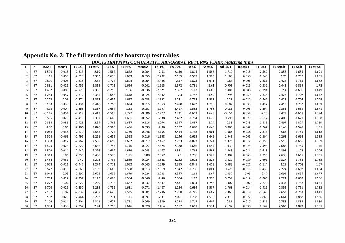
231

Appendix No. 2: The full version of the bootstrap test tables BOOTSTRAPPING CUMULATIVE ABNORMAL RETURNS (CAR): Matching firms

I N TSTAT mean1 F1-1% F1-99% F1-5% F1-95% Mean A FA-1% FA-99% FA-5% FA-95% Adj-SK-t mean1b F1-1%b F1-99%b F1-5%b F1-95%b

1 87 1.599 -0.016 -2.313 2.19 -1.584 1.622 0.004 -2.51 2.139 -1.814 1.598 1.719 -0.015 -2.562 2.358 -1.655 1.691

2 87 1.16 0.053 -2.319 2.362 -1.676 1.699 -0.055 -2.202 2.165 -1.589 1.523 1.163 0.058 -2.549 2.73 -1.797 1.891

3 87 0.801 0.006 -2.315 2.34 -1.724 1.604 -0.064 -2.445 2.17 -1.823 1.671 0.83 0.006 -2.381 2.422 -1.765 1.662

4 87 0.881 -0.025 -2.455 2.318 -1.772 1.654 -0.041 -2.523 2.372 -1.791 1.61 0.908 -0.025 -2.552 2.442 -1.835 1.72

5 87 1.452 0.006 -2.223 2.356 -1.715 1.66 -0.036 -2.621 2.357 -1.82 1.686 1.481 0.008 -2.294 2.4 -1.696 1.649

6 87 1.284 0.057 -2.312 2.385 -1.658 1.648 -0.024 -2.332 2.3 -1.752 1.59 1.298 0.059 -2.335 2.427 -1.707 1.672

7 87 0.276 -0.03 -2.374 2.367 -1.654 1.697 -0.033 -2.392 2.221 -1.758 1.583 0.28 -0.031 -2.462 2.423 -1.704 1.709

8 87 -0.183 0.033 -2.431 2.418 -1.718 1.674 0.015 -2.363 2.458 -1.672 1.739 -0.187 0.033 -2.427 2.419 -1.732 1.669

9 87 -0.18 -0.004 -2.365 2.337 -1.654 1.68 0.057 -2.197 2.497 -1.535 1.798 -0.186 -0.006 -2.394 2.351 -1.639 1.671

10 87 -0.145 0.054 -2.217 2.413 -1.595 1.777 -0.006 -2.277 2.221 -1.603 1.643 -0.151 0.054 -2.26 2.423 -1.618 1.794

11 87 0.595 0.028 -2.413 2.357 -1.608 1.681 -0.052 -2.38 2.482 -1.714 1.623 0.596 0.029 -2.512 2.406 -1.621 1.708

12 87 0.388 -0.086 -2.425 2.34 -1.768 1.667 0.116 -2.074 2.357 -1.487 1.74 0.38 -0.088 -2.536 2.497 -1.829 1.739

13 87 0.07 -0.06 -2.166 2.078 -1.508 1.486 0.033 -2.36 2.187 -1.678 1.643 0.068 -0.062 -2.267 2.146 -1.545 1.51

14 87 1.058 0.038 -2.279 2.582 -1.724 1.789 -0.046 -2.155 2.454 -1.738 1.601 1.068 0.038 -2.313 2.68 -1.755 1.818

15 87 1.526 -0.063 -2.495 2.261 -1.659 1.558 0.016 -2.368 2.146 -1.653 1.649 1.543 -0.065 -2.594 2.268 -1.668 1.585

16 87 1.303 0.012 -2.262 2.508 -1.659 1.682 -0.017 -2.462 2.293 -1.823 1.744 1.326 0.012 -2.258 2.516 -1.656 1.709

17 87 1.429 0.026 -2.522 2.656 -1.753 1.746 0.027 -2.524 2.388 -1.686 1.694 1.439 0.025 -2.495 2.688 -1.759 1.76

18 87 1.502 0.014 -2.442 2.296 -1.689 1.679 -0.043 -2.477 2.351 -1.768 1.591 1.543 0.014 -2.613 2.398 -1.72 1.706

19 87 1.319 0.06 -2.255 2.408 -1.575 1.71 -0.08 -2.357 2.1 -1.736 1.522 1.387 0.063 -2.396 2.638 -1.615 1.751

20 87 1.454 -0.031 -2.47 2.203 -1.732 1.669 -0.024 -2.368 2.262 -1.623 1.526 1.521 -0.029 -2.601 2.327 -1.753 1.735

21 87 0.674 -0.021 -2.442 2.274 -1.711 1.652 -0.045 -2.539 2.315 -1.845 1.623 0.683 -0.021 -2.514 2.29 -1.708 1.67

22 87 0.527 -0.013 -2.369 2.199 -1.666 1.568 0.013 -2.319 2.342 -1.736 1.801 0.526 -0.013 -2.433 2.224 -1.692 1.604

23 87 1.044 0.03 -2.397 2.622 -1.632 1.679 0.024 -2.283 2.347 -1.63 1.67 1.037 0.03 -2.47 2.695 -1.635 1.677

24 87 0.754 0.012 -2.257 2.143 -1.629 1.564 -0.046 -2.46 2.304 -1.62 1.575 0.757 0.012 -2.285 2.224 -1.659 1.596

25 87 1.272 0.02 -2.222 2.299 -1.716 1.627 -0.037 -2.547 2.431 -1.834 1.753 1.302 0.02 -2.229 2.437 -1.758 1.651

26 87 1.708 -0.025 -2.352 2.282 -1.755 1.681 -0.071 -2.487 2.234 -1.684 1.587 1.768 -0.024 -2.429 2.352 -1.751 1.712

27 87 2.157 -0.02 -2.337 2.457 -1.645 1.535 0.001 -2.286 2.268 -1.745 1.607 2.365 -0.019 -2.568 2.653 -1.753 1.641

28 87 2.07 0.023 -2.444 2.292 -1.731 1.71 -0.091 -2.31 2.051 -1.798 1.535 2.315 0.027 -2.863 2.661 -1.888 1.936

29 87 2.104 0.014 -2.504 2.341 -1.677 1.721 -0.069 -2.309 2.278 -1.715 1.607 2.36 0.017 -2.831 2.758 -1.885 1.889

30 87 1.984 -0.039 -2.257 2.24 -1.715 1.616 -0.028 -2.414 2.157 -1.681 1.571 2.192 -0.038 -2.562 2.563 -1.873 1.751

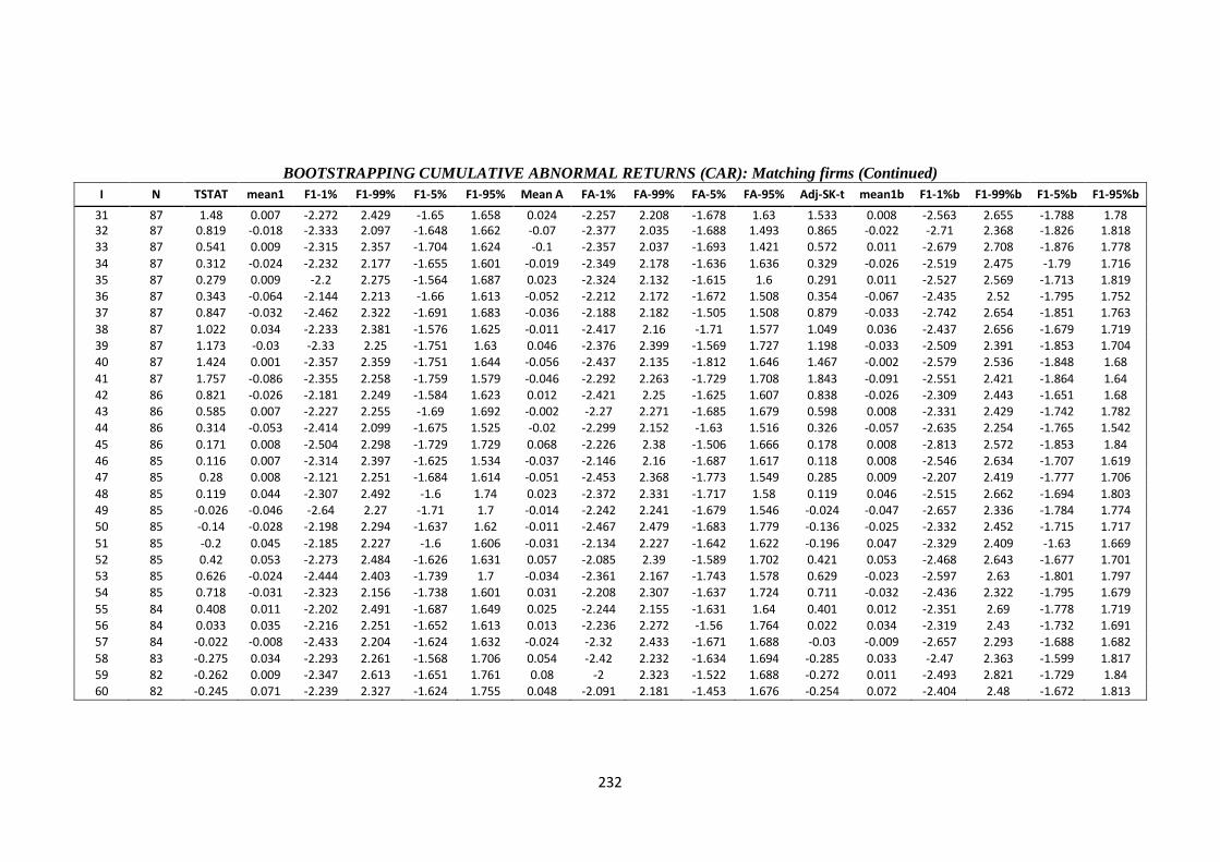
232

BOOTSTRAPPING CUMULATIVE ABNORMAL RETURNS (CAR): Matching firms (Continued)


31 87 1.48 0.007 -2.272 2.429 -1.65 1.658 0.024 -2.257 2.208 -1.678 1.63 1.533 0.008 -2.563 2.655 -1.788 1.78 32 87 0.819 -0.018 -2.333 2.097 -1.648 1.662 -0.07 -2.377 2.035 -1.688 1.493 0.865 -0.022 -2.71 2.368 -1.826 1.818 33 87 0.541 0.009 -2.315 2.357 -1.704 1.624 -0.1 -2.357 2.037 -1.693 1.421 0.572 0.011 -2.679 2.708 -1.876 1.778

34 87 0.312 -0.024 -2.232 2.177 -1.655 1.601 -0.019 -2.349 2.178 -1.636 1.636 0.329 -0.026 -2.519 2.475 -1.79 1.716 35 87 0.279 0.009 -2.2 2.275 -1.564 1.687 0.023 -2.324 2.132 -1.615 1.6 0.291 0.011 -2.527 2.569 -1.713 1.819 36 87 0.343 -0.064 -2.144 2.213 -1.66 1.613 -0.052 -2.212 2.172 -1.672 1.508 0.354 -0.067 -2.435 2.52 -1.795 1.752 37 87 0.847 -0.032 -2.462 2.322 -1.691 1.683 -0.036 -2.188 2.182 -1.505 1.508 0.879 -0.033 -2.742 2.654 -1.851 1.763

38 87 1.022 0.034 -2.233 2.381 -1.576 1.625 -0.011 -2.417 2.16 -1.71 1.577 1.049 0.036 -2.437 2.656 -1.679 1.719 39 87 1.173 -0.03 -2.33 2.25 -1.751 1.63 0.046 -2.376 2.399 -1.569 1.727 1.198 -0.033 -2.509 2.391 -1.853 1.704 40 87 1.424 0.001 -2.357 2.359 -1.751 1.644 -0.056 -2.437 2.135 -1.812 1.646 1.467 -0.002 -2.579 2.536 -1.848 1.68

41 87 1.757 -0.086 -2.355 2.258 -1.759 1.579 -0.046 -2.292 2.263 -1.729 1.708 1.843 -0.091 -2.551 2.421 -1.864 1.64 42 86 0.821 -0.026 -2.181 2.249 -1.584 1.623 0.012 -2.421 2.25 -1.625 1.607 0.838 -0.026 -2.309 2.443 -1.651 1.68 43 86 0.585 0.007 -2.227 2.255 -1.69 1.692 -0.002 -2.27 2.271 -1.685 1.679 0.598 0.008 -2.331 2.429 -1.742 1.782 44 86 0.314 -0.053 -2.414 2.099 -1.675 1.525 -0.02 -2.299 2.152 -1.63 1.516 0.326 -0.057 -2.635 2.254 -1.765 1.542

45 86 0.171 0.008 -2.504 2.298 -1.729 1.729 0.068 -2.226 2.38 -1.506 1.666 0.178 0.008 -2.813 2.572 -1.853 1.84 46 85 0.116 0.007 -2.314 2.397 -1.625 1.534 -0.037 -2.146 2.16 -1.687 1.617 0.118 0.008 -2.546 2.634 -1.707 1.619 47 85 0.28 0.008 -2.121 2.251 -1.684 1.614 -0.051 -2.453 2.368 -1.773 1.549 0.285 0.009 -2.207 2.419 -1.777 1.706

48 85 0.119 0.044 -2.307 2.492 -1.6 1.74 0.023 -2.372 2.331 -1.717 1.58 0.119 0.046 -2.515 2.662 -1.694 1.803 49 85 -0.026 -0.046 -2.64 2.27 -1.71 1.7 -0.014 -2.242 2.241 -1.679 1.546 -0.024 -0.047 -2.657 2.336 -1.784 1.774 50 85 -0.14 -0.028 -2.198 2.294 -1.637 1.62 -0.011 -2.467 2.479 -1.683 1.779 -0.136 -0.025 -2.332 2.452 -1.715 1.717

51 85 -0.2 0.045 -2.185 2.227 -1.6 1.606 -0.031 -2.134 2.227 -1.642 1.622 -0.196 0.047 -2.329 2.409 -1.63 1.669 52 85 0.42 0.053 -2.273 2.484 -1.626 1.631 0.057 -2.085 2.39 -1.589 1.702 0.421 0.053 -2.468 2.643 -1.677 1.701 53 85 0.626 -0.024 -2.444 2.403 -1.739 1.7 -0.034 -2.361 2.167 -1.743 1.578 0.629 -0.023 -2.597 2.63 -1.801 1.797 54 85 0.718 -0.031 -2.323 2.156 -1.738 1.601 0.031 -2.208 2.307 -1.637 1.724 0.711 -0.032 -2.436 2.322 -1.795 1.679

55 84 0.408 0.011 -2.202 2.491 -1.687 1.649 0.025 -2.244 2.155 -1.631 1.64 0.401 0.012 -2.351 2.69 -1.778 1.719 56 84 0.033 0.035 -2.216 2.251 -1.652 1.613 0.013 -2.236 2.272 -1.56 1.764 0.022 0.034 -2.319 2.43 -1.732 1.691 57 84 -0.022 -0.008 -2.433 2.204 -1.624 1.632 -0.024 -2.32 2.433 -1.671 1.688 -0.03 -0.009 -2.657 2.293 -1.688 1.682

58 83 -0.275 0.034 -2.293 2.261 -1.568 1.706 0.054 -2.42 2.232 -1.634 1.694 -0.285 0.033 -2.47 2.363 -1.599 1.817 59 82 -0.262 0.009 -2.347 2.613 -1.651 1.761 0.08 -2 2.323 -1.522 1.688 -0.272 0.011 -2.493 2.821 -1.729 1.84 60 82 -0.245 0.071 -2.239 2.327 -1.624 1.755 0.048 -2.091 2.181 -1.453 1.676 -0.254 0.072 -2.404 2.48 -1.672 1.813

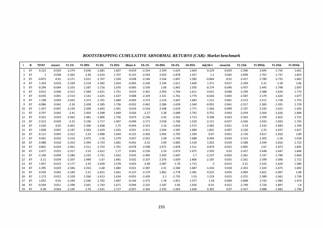
233

BOOTSTRAPPING CUMULATIVE ABNORMAL RETURNS (CAR): Market benchmark


1 87 0.222 -0.029 -2.274 2.636 -1.681 1.607 -0.019 -2.254 2.294 -1.624 1.664 0.229 -0.029 -2.396 2.695 -1.742 1.661

2 87 1 0.038 -2.365 2.46 -1.633 1.707 -0.125 -2.543 2.033 -1.878 1.427 1.1 0.045 -2.699 2.767 -1.737 1.853

3 87 -0.872 -0.01 -2.271 2.612 -1.707 1.594 0.038 -2.146 2.164 -1.607 1.582 -0.864 -0.01 -2.417 2.789 -1.735 1.662

4 87 1.343 0.016 -2.339 2.218 -1.582 1.654 -0.005 -2.246 2.194 -1.611 1.649 1.371 0.017 -2.359 2.31 -1.58 1.66

5 87 -0.294 -0.044 -2.333 2.287 -1.716 1.676 -0.083 -2.536 2.06 -1.842 1.505 -0.274 -0.046 -2.457 2.445 -1.798 1.697

6 87 0.015 0.046 -2.312 2.384 -1.621 1.751 0.019 -2.361 2.203 -1.704 1.611 0.021 0.048 -2.299 2.388 -1.634 1.773

7 87 -0.035 0.001 -2.514 2.142 -1.625 1.637 0.008 -2.329 2.321 -1.761 1.774 -0.026 0.003 -2.587 2.179 -1.626 1.677

8 87 1.198 0.059 -2.442 2.373 -1.701 1.684 -0.003 -2.273 2.216 -1.667 1.683 1.212 0.061 -2.573 2.511 -1.728 1.753

9 87 -0.086 0.041 -2.26 2.438 -1.585 1.736 -0.032 -2.462 2.286 -1.639 1.569 -0.091 0.041 -2.317 2.383 -1.591 1.729

10 87 -1.357 -0.007 -2.139 2.209 -1.603 1.501 0.019 -2.254 2.348 -1.619 1.771 -1.364 -0.009 -2.197 2.245 -1.615 1.503

11 87 0.747 0.042 -2.41 2.454 -1.598 1.669 0.026 -2.27 2.38 -1.689 1.742 0.751 0.043 -2.434 2.564 -1.626 1.684

12 87 0.352 0.033 -2.462 2.481 -1.806 1.736 0.073 -2.146 2.42 -1.562 1.713 0.348 0.033 -2.562 2.559 -1.822 1.731

13 87 -2.312 -0.029 -2.22 2.196 -1.717 1.607 -0.049 -2.171 2.018 -1.706 1.529 -2.121 -0.027 -2.426 2.433 -1.833 1.745

14 87 2.526 0.02 -2.401 2.396 -1.648 1.75 -0.044 -2.315 2.16 -1.654 1.572 2.483 0.021 -2.54 2.532 -1.683 1.764

15 87 1.828 0.007 -2.197 2.263 -1.629 1.625 0.031 -2.311 2.264 -1.587 1.689 1.831 0.007 -2.226 2.25 -1.637 1.627

16 87 -0.111 0.045 -2.312 2.23 -1.688 1.649 -0.125 -2.456 1.942 -1.795 1.509 -0.07 0.051 -2.726 2.617 -1.916 1.89

17 87 0.491 0.032 -2.216 2.475 -1.56 1.579 0.027 -2.422 2.38 -1.744 1.688 0.494 0.033 -2.315 2.503 -1.56 1.618

18 87 0.988 0.016 -2.353 2.394 -1.733 1.681 -0.041 -2.32 2.09 -1.685 1.519 1.032 0.019 -2.588 2.594 -1.816 1.722

19 87 0.801 -0.024 -2.461 2.311 -1.724 1.701 -0.078 -2.598 2.071 -1.878 1.511 0.879 -0.022 -2.805 2.67 -1.873 1.845

20 87 2.477 0.015 -2.317 2.53 -1.612 1.77 0.041 -2.256 2.24 -1.673 1.675 2.593 0.02 -2.427 2.648 -1.647 1.846

21 87 -2.196 -0.004 -2.286 2.235 -1.731 1.632 0.035 -2.485 2.293 -1.607 1.7 -2.237 -0.003 -2.361 2.197 -1.784 1.666

22 87 -2.11 0.034 -2.207 2.489 -1.67 1.681 0.032 -2.337 2.376 -1.639 1.806 -2.187 0.035 -2.261 2.599 -1.696 1.712

23 87 1.957 -0.013 -2.177 2.33 -1.639 1.578 0.025 -2.48 2.387 -1.76 1.715 2 -0.012 -2.21 2.325 -1.629 1.586

24 87 -1.395 0.019 -2.346 2.316 -1.68 1.684 0.021 -2.387 2.31 -1.584 1.687 -1.416 0.018 -2.353 2.324 -1.675 1.692

25 87 0.439 0.042 -2.183 2.21 -1.651 1.661 -0.137 -2.179 1.862 -1.778 1.381 0.525 0.054 -2.904 2.821 -2.067 2.08

26 87 1.173 0.012 -2.109 2.266 -1.613 1.634 -0.055 -2.426 2.1 -1.735 1.55 1.219 0.015 -2.255 2.389 -1.661 1.736

27 87 1.052 -0.01 -2.249 2.246 -1.702 1.687 -0.144 -2.375 1.78 -1.851 1.377 1.18 -0.009 -2.808 2.742 -1.982 1.974

28 87 -0.594 0.011 -2.398 2.441 -1.743 1.671 -0.094 -2.325 2.187 -1.83 1.456 -0.55 0.012 -2.749 2.726 -1.897 1.8

29 87 0.38 0.064 -2.195 2.76 -1.631 1.717 -0.057 -2.364 2.295 -1.603 1.646 0.392 0.07 -2.427 3.088 -1.682 1.796

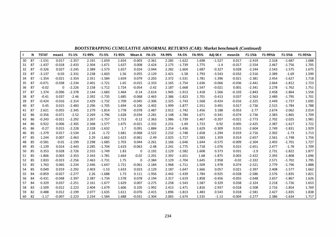
234

BOOTSTRAPPING CUMULATIVE ABNORMAL RETURNS (CAR): Market benchmark (Continued)


30 87 -1.531 0.017 -2.357 2.191 -1.659 1.654 -0.003 -2.361 2.285 -1.622 1.698 -1.527 0.017 -2.419 2.318 -1.687 1.688 31 87 -1.437 -0.018 -2.433 2.304 -1.671 1.637 0.008 -2.424 2.175 -1.739 1.775 -1.4 -0.017 -2.554 2.467 -1.756 1.705 32 87 -0.326 0.027 -2.245 2.389 -1.573 1.657 0.024 -2.044 2.282 -1.604 1.687 -0.327 0.028 -2.244 2.543 -1.575 1.675 33 87 -3.137 -0.03 -2.331 2.238 -1.603 1.56 0.055 -2.129 2.421 -1.58 1.793 -3.543 -0.032 -2.516 2.389 -1.69 1.599

34 87 -1.354 -0.021 -2.354 2.351 -1.584 1.659 0.079 -2.203 2.372 -1.531 1.781 -1.396 -0.021 -2.381 2.454 -1.627 1.718 35 87 -0.071 -0.038 -2.234 2.401 -1.721 1.65 -0.015 -2.333 2.165 -1.754 1.636 -0.066 -0.036 -2.441 2.664 -1.812 1.723 36 87 -0.02 0 -2.226 2.158 -1.712 1.724 -0.054 -2.42 2.187 -1.668 1.547 -0.021 0.001 -2.341 2.278 -1.762 1.751

37 87 1.374 -0.096 -2.378 2.144 -1.683 1.464 -0.14 -2.614 1.945 -1.913 1.418 1.566 -0.103 -2.843 2.458 -1.864 1.556 38 87 -0.41 0.037 -2.46 2.392 -1.735 1.685 -0.068 -2.463 2.386 -1.823 1.701 -0.413 0.037 -2.563 2.489 -1.795 1.701 39 87 -0.424 -0.016 -2.314 2.429 -1.732 1.709 -0.045 -2.306 2.325 -1.743 1.568 -0.424 -0.016 -2.325 2.449 -1.737 1.695 40 87 0.45 0.015 -2.483 2.296 -1.705 1.694 -0.106 -2.402 1.999 -1.877 1.551 0.491 0.017 -2.736 2.515 -1.784 1.788

41 87 2.621 -0.055 -2.345 2.279 -1.814 1.778 -0.078 -2.487 2.012 -1.742 1.456 3.188 -0.053 -2.77 2.674 -2.062 2.014 42 86 -0.356 -0.071 -2.52 2.269 -1.796 1.628 -0.034 -2.281 2.148 -1.784 1.671 -0.341 -0.074 -2.736 2.383 -1.865 1.709 43 86 -0.243 -0.021 -2.292 2.267 -1.757 1.713 -0.12 -2.363 1.986 -1.739 1.467 -0.207 -0.021 -2.773 2.702 -2.025 1.981

44 86 0.922 0.006 -2.305 2.368 -1.577 1.675 -0.021 -2.332 2.231 -1.69 1.723 0.92 0.005 -2.425 2.387 -1.617 1.722 45 86 -0.27 0.015 -2.228 2.328 -1.632 1.7 0.091 -1.884 2.254 -1.436 1.629 -0.309 0.015 -2.604 2.749 -1.831 1.929 46 85 -1.379 0.017 -2.534 2.16 -1.72 1.681 -0.068 -2.522 2.232 -1.748 1.658 -1.294 0.019 -2.716 2.302 -1.73 1.713

47 85 1.244 0.007 -2.463 2.29 -1.662 1.623 -0.061 -2.49 2.025 -1.717 1.583 1.359 0.014 -2.657 2.561 -1.748 1.756 48 85 -0.581 -0.01 -2.199 2.298 -1.685 1.703 0.044 -2.261 2.166 -1.646 1.644 -0.575 -0.009 -2.304 2.403 -1.701 1.727 49 85 -1.139 0.014 -2.443 2.285 -1.704 1.619 -0.063 -2.48 2.241 -1.775 1.718 -1.076 0.015 -2.651 2.477 -1.78 1.709 50 85 0.353 0.028 -2.726 2.555 -1.749 1.83 0 -2.192 2.129 -1.582 1.608 0.373 0.031 -2.9 2.731 -1.822 1.877

51 85 -1.806 0.003 -2.353 2.343 -1.781 1.664 -0.02 -2.201 2.392 -1.651 1.68 -1.875 0.003 -2.422 2.393 -1.808 1.696 52 85 2.833 -0.023 -2.256 2.463 -1.731 1.75 0 -2.384 2.129 -1.704 1.645 2.958 -0.02 -2.332 2.571 -1.702 1.795 53 85 1.763 0.065 -2.234 2.446 -1.647 1.721 -0.061 -2.184 1.968 -1.711 1.509 1.978 0.074 -2.521 2.779 -1.796 1.888

54 85 0.049 0.019 -2.292 2.403 -1.53 1.633 0.023 -2.129 2.187 -1.647 1.666 0.057 0.021 -2.397 2.408 -1.577 1.662 55 84 -0.859 -0.027 -2.277 2.26 -1.688 1.73 0.111 -1.956 2.442 -1.439 1.784 -0.925 -0.028 -2.586 2.576 -1.835 1.821 56 84 -0.431 -0.048 -2.397 2.387 -1.734 1.578 0.078 -2.194 2.317 -1.619 1.858 -0.456 -0.055 -2.648 2.657 -1.867 1.626 57 84 0.329 0.037 -2.251 2.161 -1.677 1.629 0.007 -2.275 2.258 -1.543 1.587 0.329 0.038 -2.324 2.218 -1.726 1.653

58 83 -2.509 -0.012 -2.223 2.404 -1.679 1.606 0.105 -1.992 2.413 -1.471 1.816 -2.937 -0.018 -2.508 2.716 -1.854 1.769 59 82 0.488 0.012 -2.199 2.077 -1.635 1.611 -0.076 -2.415 1.896 -1.813 1.483 0.543 0.018 -2.581 2.427 -1.835 1.838 60 82 -1.17 -0.007 -2.223 2.234 -1.584 1.688 -0.031 -2.304 2.065 -1.674 1.535 -1.13 -0.004 -2.277 2.386 -1.634 1.717

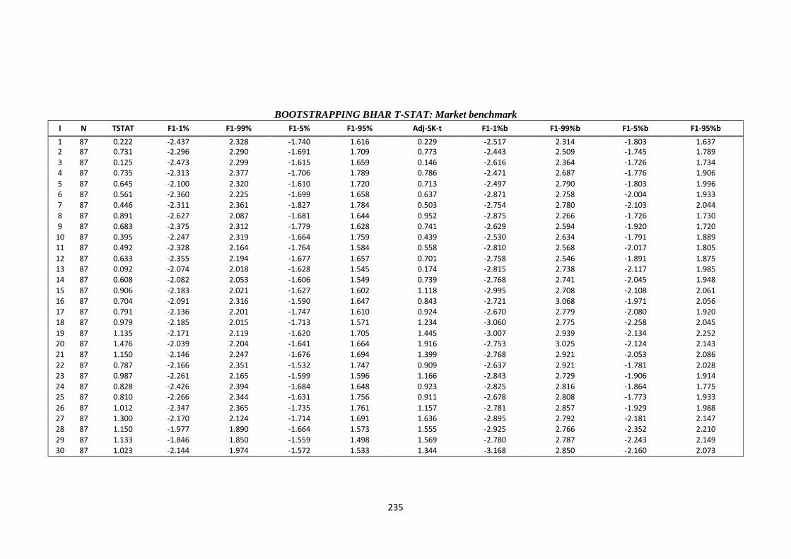
235

BOOTSTRAPPING BHAR T-STAT: Market benchmark

I N TSTAT F1-1% F1-99% F1-5% F1-95% Adj-SK-t F1-1%b F1-99%b F1-5%b F1-95%b

1 87 0.222 -2.437 2.328 -1.740 1.616 0.229 -2.517 2.314 -1.803 1.637 2 87 0.731 -2.296 2.290 -1.691 1.709 0.773 -2.443 2.509 -1.745 1.789 3 87 0.125 -2.473 2.299 -1.615 1.659 0.146 -2.616 2.364 -1.726 1.734 4 87 0.735 -2.313 2.377 -1.706 1.789 0.786 -2.471 2.687 -1.776 1.906

5 87 0.645 -2.100 2.320 -1.610 1.720 0.713 -2.497 2.790 -1.803 1.996 6 87 0.561 -2.360 2.225 -1.699 1.658 0.637 -2.871 2.758 -2.004 1.933 7 87 0.446 -2.311 2.361 -1.827 1.784 0.503 -2.754 2.780 -2.103 2.044

8 87 0.891 -2.627 2.087 -1.681 1.644 0.952 -2.875 2.266 -1.726 1.730 9 87 0.683 -2.375 2.312 -1.779 1.628 0.741 -2.629 2.594 -1.920 1.720

10 87 0.395 -2.247 2.319 -1.664 1.759 0.439 -2.530 2.634 -1.791 1.889 11 87 0.492 -2.328 2.164 -1.764 1.584 0.558 -2.810 2.568 -2.017 1.805

12 87 0.633 -2.355 2.194 -1.677 1.657 0.701 -2.758 2.546 -1.891 1.875 13 87 0.092 -2.074 2.018 -1.628 1.545 0.174 -2.815 2.738 -2.117 1.985 14 87 0.608 -2.082 2.053 -1.606 1.549 0.739 -2.768 2.741 -2.045 1.948

15 87 0.906 -2.183 2.021 -1.627 1.602 1.118 -2.995 2.708 -2.108 2.061 16 87 0.704 -2.091 2.316 -1.590 1.647 0.843 -2.721 3.068 -1.971 2.056 17 87 0.791 -2.136 2.201 -1.747 1.610 0.924 -2.670 2.779 -2.080 1.920 18 87 0.979 -2.185 2.015 -1.713 1.571 1.234 -3.060 2.775 -2.258 2.045

19 87 1.135 -2.171 2.119 -1.620 1.705 1.445 -3.007 2.939 -2.134 2.252 20 87 1.476 -2.039 2.204 -1.641 1.664 1.916 -2.753 3.025 -2.124 2.143 21 87 1.150 -2.146 2.247 -1.676 1.694 1.399 -2.768 2.921 -2.053 2.086

22 87 0.787 -2.166 2.351 -1.532 1.747 0.909 -2.637 2.921 -1.781 2.028 23 87 0.987 -2.261 2.165 -1.599 1.596 1.166 -2.843 2.729 -1.906 1.914 24 87 0.828 -2.426 2.394 -1.684 1.648 0.923 -2.825 2.816 -1.864 1.775 25 87 0.810 -2.266 2.344 -1.631 1.756 0.911 -2.678 2.808 -1.773 1.933

26 87 1.012 -2.347 2.365 -1.735 1.761 1.157 -2.781 2.857 -1.929 1.988 27 87 1.300 -2.170 2.124 -1.714 1.691 1.636 -2.895 2.792 -2.181 2.147 28 87 1.150 -1.977 1.890 -1.664 1.573 1.555 -2.925 2.766 -2.352 2.210

29 87 1.133 -1.846 1.850 -1.559 1.498 1.569 -2.780 2.787 -2.243 2.149 30 87 1.023 -2.144 1.974 -1.572 1.533 1.344 -3.168 2.850 -2.160 2.073

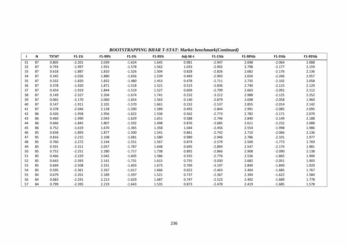
236

BOOTSTRAPPING BHAR T-STAT: Market benchmark(Continued)


31 87 0.805 -2.201 2.039 -1.624 1.645 0.981 -2.947 2.698 -2.064 2.088 32 87 0.793 -1.997 1.931 -1.578 1.562 1.033 -2.902 2.798 -2.177 2.159 33 87 0.618 -1.887 1.810 -1.526 1.504 0.828 -2.826 2.682 -2.176 2.136 34 87 0.345 -2.026 1.880 -1.656 1.539 0.469 -2.903 2.650 -2.266 2.057

35 87 0.332 -1.820 1.832 -1.480 1.453 0.478 -2.711 2.735 -2.102 2.058 36 87 0.378 -1.920 1.871 -1.518 1.521 0.523 -2.836 2.740 -2.115 2.129 37 87 0.454 -1.919 1.844 -1.519 1.527 0.609 -2.799 2.663 -2.091 2.112

38 87 0.149 -2.327 2.204 -1.674 1.741 0.232 -3.212 2.988 -2.125 2.252 39 87 0.065 -2.170 2.060 -1.654 1.563 0.140 -2.879 2.698 -2.058 1.960 40 87 0.147 -1.911 2.101 -1.570 1.661 0.232 -2.537 2.855 -2.014 2.142 41 87 0.378 -2.046 2.128 -1.590 1.589 0.493 -2.844 2.991 -2.085 2.095

42 86 0.426 -1.958 1.956 -1.622 1.536 0.562 -2.773 2.782 -2.171 2.070 43 86 0.460 -1.990 2.043 -1.629 1.651 0.588 -2.746 2.840 -2.149 2.188 44 86 0.666 -1.845 1.807 -1.592 1.498 0.876 -2.685 2.611 -2.232 2.088

45 86 0.752 -1.619 1.670 -1.365 1.358 1.044 -2.456 2.554 -1.998 1.986 46 85 0.658 -1.893 1.877 -1.500 1.541 0.861 -2.742 2.710 -2.066 2.136 47 85 0.816 -2.215 2.108 -1.681 1.580 0.989 -2.946 2.786 -2.101 1.977 48 85 0.760 -2.272 2.144 -1.551 1.567 0.874 -2.579 2.500 -1.773 1.769

49 85 0.591 -2.311 2.057 -1.787 1.648 0.695 -2.894 2.547 -2.174 1.981 50 85 0.752 -2.251 2.280 -1.717 1.738 0.892 -2.866 2.908 -2.090 2.138 51 85 0.466 -2.229 2.042 -1.605 1.586 0.555 -2.776 2.536 -1.865 1.900

52 85 0.643 -2.393 2.141 -1.731 1.615 0.755 -3.030 2.682 -2.051 1.903 53 85 0.669 -2.508 2.331 -1.603 1.673 0.769 -3.107 2.840 -1.840 1.920 54 85 0.595 -2.361 2.267 -1.617 1.666 0.652 -2.463 2.404 -1.685 1.767 55 84 0.679 -2.201 2.189 -1.597 1.521 0.737 -2.367 2.394 -1.622 1.584

56 84 0.683 -2.291 2.213 -1.629 1.687 0.747 -2.523 2.402 -1.689 1.778 57 84 0.799 -2.395 2.219 -1.643 1.535 0.873 -2.478 2.419 -1.685 1.578

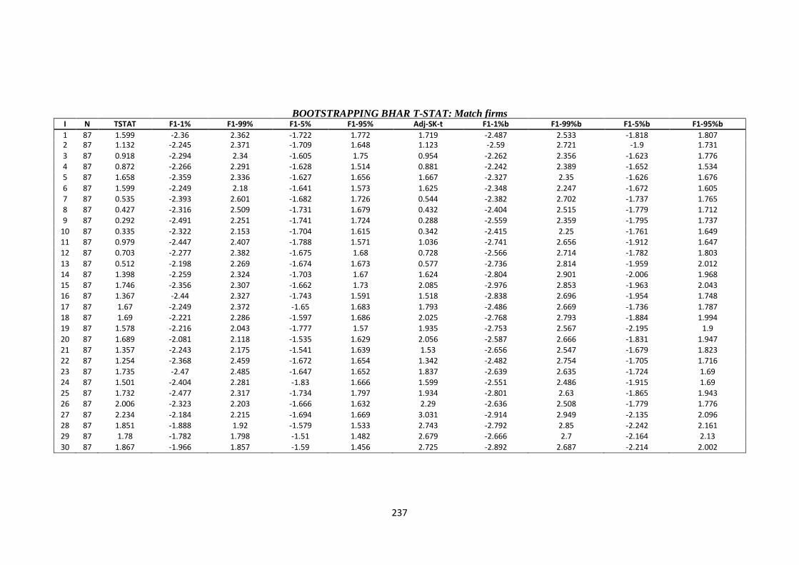
237

BOOTSTRAPPING BHAR T-STAT: Match firms I N TSTAT F1-1% F1-99% F1-5% F1-95% Adj-SK-t F1-1%b F1-99%b F1-5%b F1-95%b

1 87 1.599 -2.36 2.362 -1.722 1.772 1.719 -2.487 2.533 -1.818 1.807 2 87 1.132 -2.245 2.371 -1.709 1.648 1.123 -2.59 2.721 -1.9 1.731

3 87 0.918 -2.294 2.34 -1.605 1.75 0.954 -2.262 2.356 -1.623 1.776 4 87 0.872 -2.266 2.291 -1.628 1.514 0.881 -2.242 2.389 -1.652 1.534 5 87 1.658 -2.359 2.336 -1.627 1.656 1.667 -2.327 2.35 -1.626 1.676

6 87 1.599 -2.249 2.18 -1.641 1.573 1.625 -2.348 2.247 -1.672 1.605 7 87 0.535 -2.393 2.601 -1.682 1.726 0.544 -2.382 2.702 -1.737 1.765 8 87 0.427 -2.316 2.509 -1.731 1.679 0.432 -2.404 2.515 -1.779 1.712 9 87 0.292 -2.491 2.251 -1.741 1.724 0.288 -2.559 2.359 -1.795 1.737

10 87 0.335 -2.322 2.153 -1.704 1.615 0.342 -2.415 2.25 -1.761 1.649 11 87 0.979 -2.447 2.407 -1.788 1.571 1.036 -2.741 2.656 -1.912 1.647 12 87 0.703 -2.277 2.382 -1.675 1.68 0.728 -2.566 2.714 -1.782 1.803

13 87 0.512 -2.198 2.269 -1.674 1.673 0.577 -2.736 2.814 -1.959 2.012 14 87 1.398 -2.259 2.324 -1.703 1.67 1.624 -2.804 2.901 -2.006 1.968 15 87 1.746 -2.356 2.307 -1.662 1.73 2.085 -2.976 2.853 -1.963 2.043 16 87 1.367 -2.44 2.327 -1.743 1.591 1.518 -2.838 2.696 -1.954 1.748

17 87 1.67 -2.249 2.372 -1.65 1.683 1.793 -2.486 2.669 -1.736 1.787 18 87 1.69 -2.221 2.286 -1.597 1.686 2.025 -2.768 2.793 -1.884 1.994 19 87 1.578 -2.216 2.043 -1.777 1.57 1.935 -2.753 2.567 -2.195 1.9

20 87 1.689 -2.081 2.118 -1.535 1.629 2.056 -2.587 2.666 -1.831 1.947 21 87 1.357 -2.243 2.175 -1.541 1.639 1.53 -2.656 2.547 -1.679 1.823 22 87 1.254 -2.368 2.459 -1.672 1.654 1.342 -2.482 2.754 -1.705 1.716

23 87 1.735 -2.47 2.485 -1.647 1.652 1.837 -2.639 2.635 -1.724 1.69 24 87 1.501 -2.404 2.281 -1.83 1.666 1.599 -2.551 2.486 -1.915 1.69 25 87 1.732 -2.477 2.317 -1.734 1.797 1.934 -2.801 2.63 -1.865 1.943 26 87 2.006 -2.323 2.203 -1.666 1.632 2.29 -2.636 2.508 -1.779 1.776

27 87 2.234 -2.184 2.215 -1.694 1.669 3.031 -2.914 2.949 -2.135 2.096 28 87 1.851 -1.888 1.92 -1.579 1.533 2.743 -2.792 2.85 -2.242 2.161 29 87 1.78 -1.782 1.798 -1.51 1.482 2.679 -2.666 2.7 -2.164 2.13

30 87 1.867 -1.966 1.857 -1.59 1.456 2.725 -2.892 2.687 -2.214 2.002

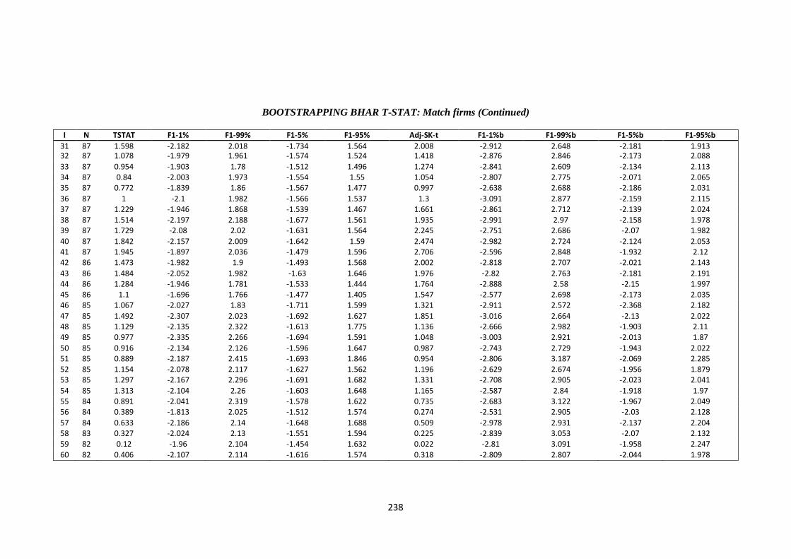
238

BOOTSTRAPPING BHAR T-STAT: Match firms (Continued)


31 87 1.598 -2.182 2.018 -1.734 1.564 2.008 -2.912 2.648 -2.181 1.913 32 87 1.078 -1.979 1.961 -1.574 1.524 1.418 -2.876 2.846 -2.173 2.088

33 87 0.954 -1.903 1.78 -1.512 1.496 1.274 -2.841 2.609 -2.134 2.113 34 87 0.84 -2.003 1.973 -1.554 1.55 1.054 -2.807 2.775 -2.071 2.065 35 87 0.772 -1.839 1.86 -1.567 1.477 0.997 -2.638 2.688 -2.186 2.031

36 87 1 -2.1 1.982 -1.566 1.537 1.3 -3.091 2.877 -2.159 2.115 37 87 1.229 -1.946 1.868 -1.539 1.467 1.661 -2.861 2.712 -2.139 2.024 38 87 1.514 -2.197 2.188 -1.677 1.561 1.935 -2.991 2.97 -2.158 1.978 39 87 1.729 -2.08 2.02 -1.631 1.564 2.245 -2.751 2.686 -2.07 1.982

40 87 1.842 -2.157 2.009 -1.642 1.59 2.474 -2.982 2.724 -2.124 2.053 41 87 1.945 -1.897 2.036 -1.479 1.596 2.706 -2.596 2.848 -1.932 2.12 42 86 1.473 -1.982 1.9 -1.493 1.568 2.002 -2.818 2.707 -2.021 2.143

43 86 1.484 -2.052 1.982 -1.63 1.646 1.976 -2.82 2.763 -2.181 2.191 44 86 1.284 -1.946 1.781 -1.533 1.444 1.764 -2.888 2.58 -2.15 1.997 45 86 1.1 -1.696 1.766 -1.477 1.405 1.547 -2.577 2.698 -2.173 2.035 46 85 1.067 -2.027 1.83 -1.711 1.599 1.321 -2.911 2.572 -2.368 2.182

47 85 1.492 -2.307 2.023 -1.692 1.627 1.851 -3.016 2.664 -2.13 2.022 48 85 1.129 -2.135 2.322 -1.613 1.775 1.136 -2.666 2.982 -1.903 2.11 49 85 0.977 -2.335 2.266 -1.694 1.591 1.048 -3.003 2.921 -2.013 1.87

50 85 0.916 -2.134 2.126 -1.596 1.647 0.987 -2.743 2.729 -1.943 2.022 51 85 0.889 -2.187 2.415 -1.693 1.846 0.954 -2.806 3.187 -2.069 2.285 52 85 1.154 -2.078 2.117 -1.627 1.562 1.196 -2.629 2.674 -1.956 1.879 53 85 1.297 -2.167 2.296 -1.691 1.682 1.331 -2.708 2.905 -2.023 2.041

54 85 1.313 -2.104 2.26 -1.603 1.648 1.165 -2.587 2.84 -1.918 1.97 55 84 0.891 -2.041 2.319 -1.578 1.622 0.735 -2.683 3.122 -1.967 2.049 56 84 0.389 -1.813 2.025 -1.512 1.574 0.274 -2.531 2.905 -2.03 2.128

57 84 0.633 -2.186 2.14 -1.648 1.688 0.509 -2.978 2.931 -2.137 2.204 58 83 0.327 -2.024 2.13 -1.551 1.594 0.225 -2.839 3.053 -2.07 2.132 59 82 0.12 -1.96 2.104 -1.454 1.632 0.022 -2.81 3.091 -1.958 2.247

60 82 0.406 -2.107 2.114 -1.616 1.574 0.318 -2.809 2.807 -2.044 1.978

the association between accruals, economic value added

Documents