the 2002 chesapeake bay eutrophication model
TRANSCRIPT
The 2002Chesapeake BayEutrophication ModelCarl F. Cerco Mark R. Noel
Three-D
imensio
nal Eutro
ph
ication M
od
el of C
hesap
eake Bay
JULY
2004
United StatesEnvironmental Protection Agency
Region IIIChesapeake BayProgram Office
U.S. Army Corps of EngineersEngineer Research & Development CenterEnvironmental Laboratory
EPA 903-R-04-004July 2004
July 2004
U.S. Environmental Protection AgencyRegion III
Chesapeake Bay Program OfficeAnnapolis, Maryland
1-800-YOUR-BAYand
U.S. Army Corps of EngineersEngineer Research and Development Center
Environmental LaboratoryVicksburg, Mississippi
The 2002 Chesapeake BayEutrophication Model
CARL F. CERCO and MARK R. NOEL U. S. Army Corps of EngineersWaterways Experiment Station3909 Halls Ferry RoadVicksburg, MS 39180
Prepared for: Chesapeake Bay Program OfficeU.S. Environmental Protection Agency410 Severn AvenueAnnapolis, MD 21401
EPA 903-R-04-004July 2004
This work was accomplished by ERDC through a cooperative agreement withthe U.S. Environmental Protection Agency Chesapeake Bay Program Office,which was administered by the Baltimore District U. S. Army Corps of Engineers.
Executive Summary . . . . . . . . . . . . . . . . . . . . . . . . . . . . . . . . . . . . . . . . . . . . viIntroduction . . . . . . . . . . . . . . . . . . . . . . . . . . . . . . . . . . . . . . . . . . . . . . . . . viCoupling with the Hydrodynamic Model . . . . . . . . . . . . . . . . . . . . . . . . .` viiBoundary Conditions . . . . . . . . . . . . . . . . . . . . . . . . . . . . . . . . . . . . . . . . . viiiHydrology and Loads . . . . . . . . . . . . . . . . . . . . . . . . . . . . . . . . . . . . . . . . . viiiKinetics . . . . . . . . . . . . . . . . . . . . . . . . . . . . . . . . . . . . . . . . . . . . . . . . . . . . xiFormat of Model-Data Comparisons . . . . . . . . . . . . . . . . . . . . . . . . . . . . . xivZooplankton . . . . . . . . . . . . . . . . . . . . . . . . . . . . . . . . . . . . . . . . . . . . . . . . xvEffects of Predation and Respiration on Primary Production . . . . . . . . . . xviProcess-Based Primary Production Model . . . . . . . . . . . . . . . . . . . . . . . . . xviiSuspended Solids and Light Attenuation . . . . . . . . . . . . . . . . . . . . . . . . . .xviiiTributary Dissolved Oxygen . . . . . . . . . . . . . . . . . . . . . . . . . . . . . . . . . . . xixModeling Processes at the Sediment-Water . . . . . . . . . . . . . . . . . . . . . . . . xixDissolved Phosphate . . . . . . . . . . . . . . . . . . . . . . . . . . . . . . . . . . . . . . . . . . xxiStatistical Summary of Calibration . . . . . . . . . . . . . . . . . . . . . . . . . . . . . . xxii
1 Introduction . . . . . . . . . . . . . . . . . . . . . . . . . . . . . . . . . . . . . . . . . . . . . . . . . 1The 2002 Chesapeake Bay Environmental Model Package . . . . . . . . . . . 3Expert Panels . . . . . . . . . . . . . . . . . . . . . . . . . . . . . . . . . . . . . . . . . . . . . . . 4This Report . . . . . . . . . . . . . . . . . . . . . . . . . . . . . . . . . . . . . . . . . . . . . . . . . 5Bibliography . . . . . . . . . . . . . . . . . . . . . . . . . . . . . . . . . . . . . . . . . . . . . . . . 5
2 Coupling with the Hydrodynamic ModelIntroduction . . . . . . . . . . . . . . . . . . . . . . . . . . . . . . . . . . . . . . . . . . . . . . . . . 7The Hydrodynamic Model . . . . . . . . . . . . . . . . . . . . . . . . . . . . . . . . . . . . . 7Linkage to the Water Quality Model . . . . . . . . . . . . . . . . . . . . . . . . . . . . . 10Vertical Diffusion . . . . . . . . . . . . . . . . . . . . . . . . . . . . . . . . . . . . . . . . . . . . 11References . . . . . . . . . . . . . . . . . . . . . . . . . . . . . . . . . . . . . . . . . . . . . . . . . . 20
– ii –
Contents
3 Boundary Conditions . . . . . . . . . . . . . . . . . . . . . . . . . . . . . . . . . . . . . . . 22Introduction . . . . . . . . . . . . . . . . . . . . . . . . . . . . . . . . . . . . . . . . . . . . . . . . . 22River Inflows . . . . . . . . . . . . . . . . . . . . . . . . . . . . . . . . . . . . . . . . . . . . . . . 22Lateral Inflows . . . . . . . . . . . . . . . . . . . . . . . . . . . . . . . . . . . . . . . . . . . . . . 25Ocean Boundary Conditions . . . . . . . . . . . . . . . . . . . . . . . . . . . . . . . . . . . . 26A Recommendation . . . . . . . . . . . . . . . . . . . . . . . . . . . . . . . . . . . . . . . . . . 37References . . . . . . . . . . . . . . . . . . . . . . . . . . . . . . . . . . . . . . . . . . . . . . . . . . 37
4 Hydrology and Loads . . . . . . . . . . . . . . . . . . . . . . . . . . . . . . . . . . . . . . . . 38Hydrology . . . . . . . . . . . . . . . . . . . . . . . . . . . . . . . . . . . . . . . . . . . . . . . . . . 38Loads . . . . . . . . . . . . . . . . . . . . . . . . . . . . . . . . . . . . . . . . . . . . . . . . . . . . . . 42Nonpoint-Source Loads . . . . . . . . . . . . . . . . . . . . . . . . . . . . . . . . . . . . . . . 42Point-Source Loads . . . . . . . . . . . . . . . . . . . . . . . . . . . . . . . . . . . . . . . . . . . 49Atmospheric Loads . . . . . . . . . . . . . . . . . . . . . . . . . . . . . . . . . . . . . . . . . . . 60Bank Loads . . . . . . . . . . . . . . . . . . . . . . . . . . . . . . . . . . . . . . . . . . . . . . . . . 62Wetlands Loads . . . . . . . . . . . . . . . . . . . . . . . . . . . . . . . . . . . . . . . . . . . . . . 71Summary of All Loads . . . . . . . . . . . . . . . . . . . . . . . . . . . . . . . . . . . . . . . . 77References . . . . . . . . . . . . . . . . . . . . . . . . . . . . . . . . . . . . . . . . . . . . . . . . . . 80
5 Linking in the Loads . . . . . . . . . . . . . . . . . . . . . . . . . . . . . . . . . . . . . . . . . 81Introduction . . . . . . . . . . . . . . . . . . . . . . . . . . . . . . . . . . . . . . . . . . . . . . . . . 81Nonpoint-Source Loads . . . . . . . . . . . . . . . . . . . . . . . . . . . . . . . . . . . . . . . 81Point-Source Loads . . . . . . . . . . . . . . . . . . . . . . . . . . . . . . . . . . . . . . . . . . . 89Other Loads . . . . . . . . . . . . . . . . . . . . . . . . . . . . . . . . . . . . . . . . . . . . . . . . 89References . . . . . . . . . . . . . . . . . . . . . . . . . . . . . . . . . . . . . . . . . . . . . . . . . . 90
6 Water Quality Model Formulation . . . . . . . . . . . . . . . . . . . . . . . . . . . . . 91Introduction . . . . . . . . . . . . . . . . . . . . . . . . . . . . . . . . . . . . . . . . . . . . . . . . . 91Conservation of Mass Equation . . . . . . . . . . . . . . . . . . . . . . . . . . . . . . . . . 91State Variables . . . . . . . . . . . . . . . . . . . . . . . . . . . . . . . . . . . . . . . . . . . . . . 92Algae . . . . . . . . . . . . . . . . . . . . . . . . . . . . . . . . . . . . . . . . . . . . . . . . . . . . . . 95Organic Carbon . . . . . . . . . . . . . . . . . . . . . . . . . . . . . . . . . . . . . . . . . . . . . . 105Phosphorus . . . . . . . . . . . . . . . . . . . . . . . . . . . . . . . . . . . . . . . . . . . . . . . . . 108Nitrogen . . . . . . . . . . . . . . . . . . . . . . . . . . . . . . . . . . . . . . . . . . . . . . . . . . . 112Silica . . . . . . . . . . . . . . . . . . . . . . . . . . . . . . . . . . . . . . . . . . . . . . . . . . . . . . 116Chemical Oxygen Demand . . . . . . . . . . . . . . . . . . . . . . . . . . . . . . . . . . . . . 117Dissolved Oxygen . . . . . . . . . . . . . . . . . . . . . . . . . . . . . . . . . . . . . . . . . . . . 118Temperature . . . . . . . . . . . . . . . . . . . . . . . . . . . . . . . . . . . . . . . . . . . . . . . . 120Inorganic (Fixed) Solids . . . . . . . . . . . . . . . . . . . . . . . . . . . . . . . . . . . . . . . 121Salinity . . . . . . . . . . . . . . . . . . . . . . . . . . . . . . . . . . . . . . . . . . . . . . . . . . . . 121Parameter Values . . . . . . . . . . . . . . . . . . . . . . . . . . . . . . . . . . . . . . . . . . . . 121References . . . . . . . . . . . . . . . . . . . . . . . . . . . . . . . . . . . . . . . . . . . . . . . . . . 126
7 Introduction to the Calibration . . . . . . . . . . . . . . . . . . . . . . . . . . . . . . . . 128The Monitoring Data Base . . . . . . . . . . . . . . . . . . . . . . . . . . . . . . . . . . . . . 128Comparison with the Model . . . . . . . . . . . . . . . . . . . . . . . . . . . . . . . . . . . . 131References . . . . . . . . . . . . . . . . . . . . . . . . . . . . . . . . . . . . . . . . . . . . . . . . . . 138
Chapter 4 • Hydrology and Loads
– iii –
8 The Zooplankton Model . . . . . . . . . . . . . . . . . . . . . . . . . . . . . . . . . . . . . . 139Introduction . . . . . . . . . . . . . . . . . . . . . . . . . . . . . . . . . . . . . . . . . . . . . . . . . 139Model Conceptualization . . . . . . . . . . . . . . . . . . . . . . . . . . . . . . . . . . . . . . 139Zooplankton Kinetics . . . . . . . . . . . . . . . . . . . . . . . . . . . . . . . . . . . . . . . . . 142Interfacing with the Eutrophication Model . . . . . . . . . . . . . . . . . . . . . . . . 145Parameter Evaluation . . . . . . . . . . . . . . . . . . . . . . . . . . . . . . . . . . . . . . . . . 148Observations . . . . . . . . . . . . . . . . . . . . . . . . . . . . . . . . . . . . . . . . . . . . . . . . 157Model Results . . . . . . . . . . . . . . . . . . . . . . . . . . . . . . . . . . . . . . . . . . . . . . . 157Recommendations for Improvement . . . . . . . . . . . . . . . . . . . . . . . . . . . . . 169References . . . . . . . . . . . . . . . . . . . . . . . . . . . . . . . . . . . . . . . . . . . . . . . . . . 170
9 Analysis of Predation and Respiration on Primary Production . . 172The N-P-Z Model . . . . . . . . . . . . . . . . . . . . . . . . . . . . . . . . . . . . . . . . . . . . 172Basic Parameter Set . . . . . . . . . . . . . . . . . . . . . . . . . . . . . . . . . . . . . . . . . . 173Phytoplankton with Respiration Only . . . . . . . . . . . . . . . . . . . . . . . . . . . . 174Phytoplankton with Zooplankton . . . . . . . . . . . . . . . . . . . . . . . . . . . . . . . . 176Phytoplankton with Quadratic Predation . . . . . . . . . . . . . . . . . . . . . . . . . . 178
10 Process-Based Primary Production Modeling in Chesapeake Bay . . . . . . . . . . . . . . . . . . . . . . . . . . . . . . . . . . . . . . . . . . . 180Introduction . . . . . . . . . . . . . . . . . . . . . . . . . . . . . . . . . . . . . . . . . . . . . . . . . 180Chesapeake Bay . . . . . . . . . . . . . . . . . . . . . . . . . . . . . . . . . . . . . . . . . . . . . 181The Chesapeake Bay Environmental Model Package (CBEMP) . . . . . . . 183Data Bases . . . . . . . . . . . . . . . . . . . . . . . . . . . . . . . . . . . . . . . . . . . . . . . . . 183Model Formulation . . . . . . . . . . . . . . . . . . . . . . . . . . . . . . . . . . . . . . . . . . . 186Primary Production Equations . . . . . . . . . . . . . . . . . . . . . . . . . . . . . . . . . . 192Parameter Evaluation . . . . . . . . . . . . . . . . . . . . . . . . . . . . . . . . . . . . . . . . . 193Results . . . . . . . . . . . . . . . . . . . . . . . . . . . . . . . . . . . . . . . . . . . . . . . . . . . . . 199Discussion . . . . . . . . . . . . . . . . . . . . . . . . . . . . . . . . . . . . . . . . . . . . . . . . . . 209In Conclusion . . . . . . . . . . . . . . . . . . . . . . . . . . . . . . . . . . . . . . . . . . . . . . . 215References . . . . . . . . . . . . . . . . . . . . . . . . . . . . . . . . . . . . . . . . . . . . . . . . . . 216
11 Suspended Solids and Light Attenuation . . . . . . . . . . . . . . . . . . . . 220Data Bases . . . . . . . . . . . . . . . . . . . . . . . . . . . . . . . . . . . . . . . . . . . . . . . . . 220The Light Attenuation Model . . . . . . . . . . . . . . . . . . . . . . . . . . . . . . . . . . . 225Solids Settling Velocities . . . . . . . . . . . . . . . . . . . . . . . . . . . . . . . . . . . . . . 228Model Results . . . . . . . . . . . . . . . . . . . . . . . . . . . . . . . . . . . . . . . . . . . . . . . 231References . . . . . . . . . . . . . . . . . . . . . . . . . . . . . . . . . . . . . . . . . . . . . . . . . . 246
12 Tributary Dissolved Oxygen . . . . . . . . . . . . . . . . . . . . . . . . . . . . . . . . . 247Introduction . . . . . . . . . . . . . . . . . . . . . . . . . . . . . . . . . . . . . . . . . . . . . . . . . 247Dissolved Organic Carbon Mineralization Rate . . . . . . . . . . . . . . . . . . . . 250Wetland Dissolved Oxygen Uptake . . . . . . . . . . . . . . . . . . . . . . . . . . . . . . 252Nonpoint-Source Carbon Loads . . . . . . . . . . . . . . . . . . . . . . . . . . . . . . . . . 252Spatially-Varying Dissolved Organic Carbon Mineralization Rate . . . . . . 255Reaeration Rate . . . . . . . . . . . . . . . . . . . . . . . . . . . . . . . . . . . . . . . . . . . . . . 258Sensitivity to G3 Carbon . . . . . . . . . . . . . . . . . . . . . . . . . . . . . . . . . . . . . . 258Sensitivity to Algal Predation Rate . . . . . . . . . . . . . . . . . . . . . . . . . . . . . . 260
Chapter 4 • Hydrology and Loads
– iv –
Sensitivity to Vertical Diffusion Coefficient . . . . . . . . . . . . . . . . . . . . . . . 262Discussion . . . . . . . . . . . . . . . . . . . . . . . . . . . . . . . . . . . . . . . . . . . . . . . . . . 265References . . . . . . . . . . . . . . . . . . . . . . . . . . . . . . . . . . . . . . . . . . . . . . . . . . 274
13 Modeling Processes at the Sediment-Water Interface . . . . . . . . . 275Introduction . . . . . . . . . . . . . . . . . . . . . . . . . . . . . . . . . . . . . . . . . . . . . . . . . 275Coupling With the Sediment Diagenesis Model . . . . . . . . . . . . . . . . . . . . 279Parameter Specification . . . . . . . . . . . . . . . . . . . . . . . . . . . . . . . . . . . . . . . 281Sediment Model Results . . . . . . . . . . . . . . . . . . . . . . . . . . . . . . . . . . . . . . . 283Benthos Model Results . . . . . . . . . . . . . . . . . . . . . . . . . . . . . . . . . . . . . . . . 301Results of the Submerged Aquatic Vegetation (SAV) Model . . . . . . . . . . 304Results from the Benthic Algal Model . . . . . . . . . . . . . . . . . . . . . . . . . . . . 307References . . . . . . . . . . . . . . . . . . . . . . . . . . . . . . . . . . . . . . . . . . . . . . . . . . 319
14 Dissolved Phosphate . . . . . . . . . . . . . . . . . . . . . . . . . . . . . . . . . . . . . . . 321Introduction . . . . . . . . . . . . . . . . . . . . . . . . . . . . . . . . . . . . . . . . . . . . . . . . . 321Dissolved Organic Phosphorus Mineralization . . . . . . . . . . . . . . . . . . . . . 322Sulfide Oxidizing Bacteria . . . . . . . . . . . . . . . . . . . . . . . . . . . . . . . . . . . . . 323Precipitation . . . . . . . . . . . . . . . . . . . . . . . . . . . . . . . . . . . . . . . . . . . . . . . . 324Summary . . . . . . . . . . . . . . . . . . . . . . . . . . . . . . . . . . . . . . . . . . . . . . . . . . . 326References . . . . . . . . . . . . . . . . . . . . . . . . . . . . . . . . . . . . . . . . . . . . . . . . . . 330
15 Statistical Summary of Calibration . . . . . . . . . . . . . . . . . . . . . . . . . . . 331Introduction . . . . . . . . . . . . . . . . . . . . . . . . . . . . . . . . . . . . . . . . . . . . . . . . . 331Methods . . . . . . . . . . . . . . . . . . . . . . . . . . . . . . . . . . . . . . . . . . . . . . . . . . . 331Statistics of Present Calibration . . . . . . . . . . . . . . . . . . . . . . . . . . . . . . . . . 333Statistics of Model Improvements . . . . . . . . . . . . . . . . . . . . . . . . . . . . . . . 335Comparison with Other Applications . . . . . . . . . . . . . . . . . . . . . . . . . . . . . 338Graphical Performance Summaries . . . . . . . . . . . . . . . . . . . . . . . . . . . . . . 340References . . . . . . . . . . . . . . . . . . . . . . . . . . . . . . . . . . . . . . . . . . . . . . . . . . 349
Chapter 4 • Hydrology and Loads
– v –
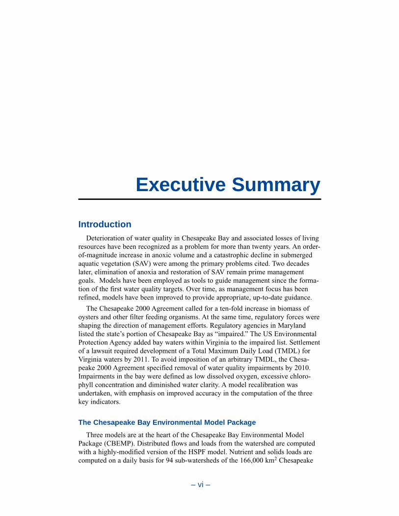
IntroductionDeterioration of water quality in Chesapeake Bay and associated losses of living
resources have been recognized as a problem for more than twenty years. An order-of-magnitude increase in anoxic volume and a catastrophic decline in submergedaquatic vegetation (SAV) were among the primary problems cited. Two decadeslater, elimination of anoxia and restoration of SAV remain prime managementgoals. Models have been employed as tools to guide management since the forma-tion of the first water quality targets. Over time, as management focus has beenrefined, models have been improved to provide appropriate, up-to-date guidance.
The Chesapeake 2000 Agreement called for a ten-fold increase in biomass ofoysters and other filter feeding organisms. At the same time, regulatory forces wereshaping the direction of management efforts. Regulatory agencies in Marylandlisted the state’s portion of Chesapeake Bay as “impaired.” The US EnvironmentalProtection Agency added bay waters within Virginia to the impaired list. Settlementof a lawsuit required development of a Total Maximum Daily Load (TMDL) forVirginia waters by 2011. To avoid imposition of an arbitrary TMDL, the Chesa-peake 2000 Agreement specified removal of water quality impairments by 2010.Impairments in the bay were defined as low dissolved oxygen, excessive chloro-phyll concentration and diminished water clarity. A model recalibration wasundertaken, with emphasis on improved accuracy in the computation of the threekey indicators.
The Chesapeake Bay Environmental Model Package
Three models are at the heart of the Chesapeake Bay Environmental ModelPackage (CBEMP). Distributed flows and loads from the watershed are computedwith a highly-modified version of the HSPF model. Nutrient and solids loads arecomputed on a daily basis for 94 sub-watersheds of the 166,000 km2 Chesapeake
– vi –
Executive Summary
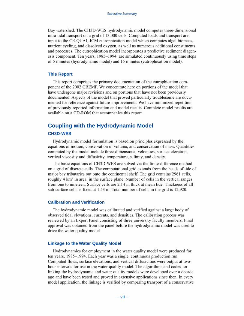
Bay watershed. The CH3D-WES hydrodynamic model computes three-dimensionalintra-tidal transport on a grid of 13,000 cells. Computed loads and transport areinput to the CE-QUAL-ICM eutrophication model which computes algal biomass,nutrient cycling, and dissolved oxygen, as well as numerous additional constituentsand processes. The eutrophication model incorporates a predictive sediment diagen-esis component. Ten years, 1985–1994, are simulated continuously using time stepsof 5 minutes (hydrodynamic model) and 15 minutes (eutrophication model).
This Report
This report comprises the primary documentation of the eutrophication com-ponent of the 2002 CBEMP. We concentrate here on portions of the model thathave undergone major revisions and on portions that have not been previouslydocumented. Aspects of the model that proved particularly troublesome are docu-mented for reference against future improvements. We have minimized repetition of previously-reported information and model results. Complete model results areavailable on a CD-ROM that accompanies this report.
Coupling with the Hydrodynamic ModelCH3D-WES
Hydrodynamic model formulation is based on principles expressed by theequations of motion, conservation of volume, and conservation of mass. Quantitiescomputed by the model include three-dimensional velocities, surface elevation,vertical viscosity and diffusivity, temperature, salinity, and density.
The basic equations of CH3D-WES are solved via the finite-difference methodon a grid of discrete cells. The computational grid extends from the heads of tide ofmajor bay tributaries out onto the continental shelf. The grid contains 2961 cells,roughly 4 km2 in area, in the surface plane. Number of cells in the vertical rangesfrom one to nineteen. Surface cells are 2.14 m thick at mean tide. Thickness of allsub-surface cells is fixed at 1.53 m. Total number of cells in the grid is 12,920.
Calibration and Verification
The hydrodynamic model was calibrated and verified against a large body ofobserved tidal elevations, currents, and densities. The calibration process wasreviewed by an Expert Panel consisting of three university faculty members. Finalapproval was obtained from the panel before the hydrodynamic model was used todrive the water quality model.
Linkage to the Water Quality Model
Hydrodynamics for employment in the water quality model were produced forten years, 1985–1994. Each year was a single, continuous production run.Computed flows, surface elevations, and vertical diffusivities were output at two-hour intervals for use in the water quality model. The algorithms and codes forlinking the hydrodynamic and water quality models were developed over a decadeago and have been tested and proved in extensive applications since then. In everymodel application, the linkage is verified by comparing transport of a conservative
Executive Summary
– vii –

substance computed in each model. For estuarine applications, the transport testscommonly take the form of comparing salinity computed by two models. In thepresent application, salinity comparisons verify that the hydrodynamic and waterquality models are correctly coupled and that transport processes in the two modelsare virtually identical.
Boundary ConditionsBoundary conditions must be specified at all open edges of the model grid.
These include river inflows, lateral flows, and the ocean interface.
Ocean Boundary Conditions
In the first version of the model, the open edge of the model grid was at theentrance to Chesapeake Bay. In the Tributary Refinements phase of model develop-ment, the grid was extended beyond the bay mouth, out onto the continental shelf.The primary objective was to ensure that boundary conditions specified at the edgeof the grid were beyond the influence of conditions within the bay. The grid exten-sion traded one set of problems for another. Model boundaries were moved from alocation with abundant observations to multiple locations at which little informa-tion was available. In the present phase of the model study, specification ofboundary conditions at the edge of the grid proved especially problematic. Thestrategy was developed in which conditions observed at the bay mouth wereextended to the edges of the grid. Kinetics were disabled outside the bay mouth toprevent substance transformations.
Our Recommendation
Extension of the grid onto the continental shelf had two objectives. The first wasto move nutrient boundary conditions to a location beyond the influence of loadswithin the bay. The second was to allow for coupling with a proposed continentalshelf model. The first objective was met, albeit with trade-offs. The proposed shelfmodel has been postponed indefinitely. The extension of the grid produced enor-mous difficulties for both the hydrodynamic and water quality modeling teams anddid not increase the accuracy of either model. Consequently, we recommend theboundary be restored to the mouth of the bay in future model efforts.
Hydrology and Loads
Hydrology
Major sources of freshwater to the Chesapeake Bay system are the SusquehannaRiver, to the north, and the Potomac and James Rivers to the west. Of these, theSusquehanna provides by far the largest flow fraction, followed by the Potomacand James. All tributaries exhibit similar seasonal flow patterns. Highest flowsoccur in winter (December–February) and spring (March–May). Lowest seasonalflows occur in summer (June–August) and fall (September–November) althoughtropical storms in these seasons can generate enormous flood events.
Executive Summary
– viii –
Loads
Loads to the system include distributed or nonpoint-source loads, point- sourceloads, atmospheric loads, bank loads, and wetlands loads. Nonpoint-source loadsenter the system at tributary fall lines and as runoff below the fall lines. Point-source loads are from industries and municipal wastewater treatment plants.Atmospheric loads are from the atmosphere directly to the water surface. Atmos-pheric loads to the watershed are incorporated in the distributed loads. Bank loadsoriginate with shoreline erosion. Wetland loads are materials created in andexported from wetlands.
Nonpoint-Source Loads
Nonpoint-source loads are from Phase IV of the EPA Chesapeake Bay Water-shed Model. Loads are provided on a daily basis, routed to surface cells on themodel grid. Routing is based on local watershed characteristics and on drainagearea contributing to the cell.
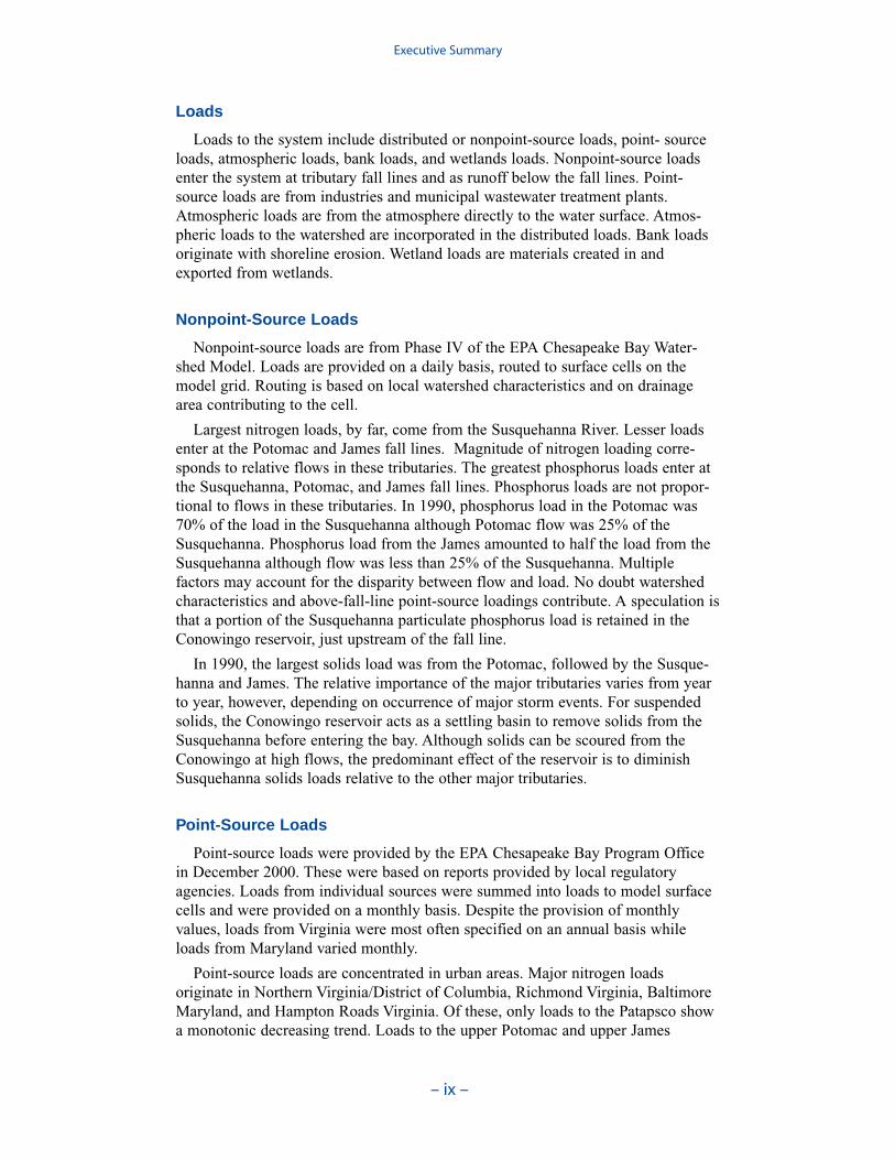
Largest nitrogen loads, by far, come from the Susquehanna River. Lesser loadsenter at the Potomac and James fall lines. Magnitude of nitrogen loading corre-sponds to relative flows in these tributaries. The greatest phosphorus loads enter atthe Susquehanna, Potomac, and James fall lines. Phosphorus loads are not propor-tional to flows in these tributaries. In 1990, phosphorus load in the Potomac was70% of the load in the Susquehanna although Potomac flow was 25% of theSusquehanna. Phosphorus load from the James amounted to half the load from theSusquehanna although flow was less than 25% of the Susquehanna. Multiplefactors may account for the disparity between flow and load. No doubt watershedcharacteristics and above-fall-line point-source loadings contribute. A speculation isthat a portion of the Susquehanna particulate phosphorus load is retained in theConowingo reservoir, just upstream of the fall line.
In 1990, the largest solids load was from the Potomac, followed by the Susque-hanna and James. The relative importance of the major tributaries varies from yearto year, however, depending on occurrence of major storm events. For suspendedsolids, the Conowingo reservoir acts as a settling basin to remove solids from theSusquehanna before entering the bay. Although solids can be scoured from theConowingo at high flows, the predominant effect of the reservoir is to diminishSusquehanna solids loads relative to the other major tributaries.
Point-Source Loads
Point-source loads were provided by the EPA Chesapeake Bay Program Officein December 2000. These were based on reports provided by local regulatoryagencies. Loads from individual sources were summed into loads to model surfacecells and were provided on a monthly basis. Despite the provision of monthlyvalues, loads from Virginia were most often specified on an annual basis whileloads from Maryland varied monthly.
Point-source loads are concentrated in urban areas. Major nitrogen loadsoriginate in Northern Virginia/District of Columbia, Richmond Virginia, BaltimoreMaryland, and Hampton Roads Virginia. Of these, only loads to the Patapsco showa monotonic decreasing trend. Loads to the upper Potomac and upper James
Executive Summary
– ix –
suggest a decrease after 1990. Point-source nitrogen loads to the Back River andthe lower James show no trend.
Point-source phosphorus loads are concentrated in the same urban areas asnitrogen although the relationship by size differs. In 1990, largest loads were fromHampton Roads and Richmond Virginia. Northern Virginia /District of Columbiacontributed the least phosphorus load of the major urban centers. The same areashowed the least reduction of phosphorus loads over the simulation period, possiblya consequence of load reductions prior to 1985. In the remaining urban areas,point-source phosphorus loads were halved from 1985 to 1994.
Atmospheric Loads
Daily atmospheric loads for each surface cell were computed by the EPA-Chesapeake Bay Program Office and provided in January 2000. Wet deposition ofammonium and nitrate was derived from National Atmospheric DepositionProgram observations. Dry deposition of nitrate was derived from wet depositionusing ratios calculated by the Regional Acid Deposition Model. Deposition oforganic and inorganic phosphorus was specified on a uniform, constant, areal basisderived from published values.
Bank Loads
Bank loads are the solids, carbon, and nutrient loads contributed to the watercolumn through shoreline erosion. Although erosion is episodic, bank loads can beestimated only as long-term averages. The volume of eroded material is commonlyquantified from comparison of topographic maps or aerial photos separated by timescales of years. Consequently, the erosion estimates are averaged over periods ofyears.
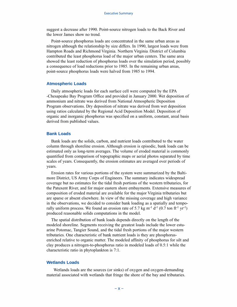
Erosion rates for various portions of the system were summarized by the Balti-more District, US Army Corps of Engineers. The summary indicates widespreadcoverage but no estimates for the tidal fresh portions of the western tributaries, forthe Patuxent River, and for major eastern shore embayments. Extensive measures ofcomposition of eroded material are available for the major Virginia tributaries butare sparse or absent elsewhere. In view of the missing coverage and high variancein the observations, we decided to consider bank loading as a spatially and tempo-rally uniform process. We found an erosion rate of 5.7 kg m-1 d-1 (0.7 ton ft-1 yr-1)produced reasonable solids computations in the model.
The spatial distribution of bank loads depends directly on the length of themodeled shoreline. Segments receiving the greatest loads include the lower estu-arine Potomac, Tangier Sound, and the tidal fresh portions of the major westerntributaries. One characteristic of bank nutrient loads is they are phosphorus-enriched relative to organic matter. The modeled affinity of phosphorus for silt andclay produces a nitrogen-to-phosphorus ratio in modeled loads of 0.5:1 while thecharacteristic ratio in phytoplankton is 7:1.
Wetlands Loads
Wetlands loads are the sources (or sinks) of oxygen and oxygen-demandingmaterial associated with wetlands that fringe the shore of the bay and tributaries.
Executive Summary
– x –

These loads are invoked primarily as an aid in calibration of tributary dissolvedoxygen. Wetlands areas adjacent to model surface cells were derived via GISanalysis and provided by the EPA Chesapeake Bay Program in November 2001.Loads to each cell were computed as the product of adjacent wetlands area andareal carbon export or oxygen consumption.
A uniform carbon export of 0.3 g C m-2 d-1 was employed. A uniform oxygendemand of 2 g O2 m-2 d-1 was employed. Segments receiving the largest carbonloads and subject to the greatest oxygen consumption include the mid-portion ofthe bay, Tangier Sound, several Eastern Shore tributaries, the middle and lowerJames River, the tidal fresh York River, and the York River mouth.
Loading Summary
Loads from all sources were compared by for 1990, a year central to the simula-tion period. Runoff in this year was moderate in the Susquehanna and James andlow in the Potomac.
Nonpoint sources dominated the nitrogen loads except in a few segments adja-cent to major urban areas. In these regions, point sources contributed a significantfraction of nitrogen loads. Atmospheric nitrogen loads were significant only in thelarge, open segments of the mainstem bay and in the lower Potomac. Bank loadswere negligibly small throughout.
Nonpoint sources usually comprised the largest fraction of phosphorus loads butwere not so predominant as for nitrogen. As with nitrogen, point-source loads weresignificant in urban areas and atmospheric loads contributed to substantially tolarge open-water segments. A major contrast with nitrogen was in bank loadingwhich equaled or exceed nonpoint-source phosphorus loads in segments distantfrom major inflows. These included the eastern embayments and the river-estuarinetransition segments of western tributaries.
Nonpoint sources dominate the solids loads in segments adjoining the inflows ofthe Susquehanna, Potomac, and James. Otherwise, bank loads are the dominantsource. For 1990, bank loads contribute more solids, system-wide, than nonpointsources. Of course, the relative contribution of bank loads depends on annualhydrology. In high-flow years, nonpoint sources may dominate. Still, the summaryindicates that control of bank erosion should be included in any solids managementplan.
KineticsThe foundation of CE-QUAL-ICM is the solution to the three-dimensional mass-
conservation equation for a control volume. Control volumes correspond to cells onthe hydrodynamic model grid. Solution is via a finite-difference scheme using theQUICKEST algorithm in the horizontal plane and a Crank-Nicolson scheme in thevertical direction. Discrete time steps, determined by computational stabilityrequirements, are 15 minutes.
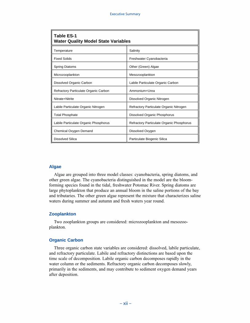
At present, the CE-QUAL-ICM model incorporates 24 state variables in the water column including physical variables, multiple algal groups, twozooplankton groups, and multiple forms of carbon, nitrogen, phosphorus and silica (Table ES-1).
Executive Summary
– xi –
Algae
Algae are grouped into three model classes: cyanobacteria, spring diatoms, andother green algae. The cyanobacteria distinguished in the model are the bloom-forming species found in the tidal, freshwater Potomac River. Spring diatoms arelarge phytoplankton that produce an annual bloom in the saline portions of the bayand tributaries. The other green algae represent the mixture that characterizes salinewaters during summer and autumn and fresh waters year round.
Zooplankton
Two zooplankton groups are considered: microzooplankton and mesozoo-plankton.
Organic Carbon
Three organic carbon state variables are considered: dissolved, labile particulate,and refractory particulate. Labile and refractory distinctions are based upon thetime scale of decomposition. Labile organic carbon decomposes rapidly in thewater column or the sediments. Refractory organic carbon decomposes slowly,primarily in the sediments, and may contribute to sediment oxygen demand yearsafter deposition.
Executive Summary
– xii –
Table ES-1 Water Quality Model State Variables
Temperature Salinity
Fixed Solids Freshwater Cyanobacteria
Spring Diatoms Other (Green) Algae
Microzooplankton Mesozooplankton
Dissolved Organic Carbon Labile Particulate Organic Carbon
Refractory Particulate Organic Carbon Ammonium+Urea
Nitrate+Nitrite Dissolved Organic Nitrogen
Labile Particulate Organic Nitrogen Refractory Particulate Organic Nitrogen
Total Phosphate Dissolved Organic Phosphorus
Labile Particulate Organic Phosphorus Refractory Particulate Organic Phosphorus
Chemical Oxygen Demand Dissolved Oxygen
Dissolved Silica Particulate Biogenic Silica

Nitrogen
Nitrogen is first divided into available and unavailable fractions. Available refersto employment in algal nutrition. Two available forms are considered: reduced andoxidized nitrogen. Reduced nitrogen includes ammonium and urea. Nitrate andnitrite comprise the oxidized nitrogen pool. Unavailable nitrogen state variables aredissolved organic nitrogen, labile particulate organic nitrogen, and refractory partic-ulate organic nitrogen.
Phosphorus
As with nitrogen, phosphorus is first divided into available and unavailable frac-tions. Only a single available form, dissolved phosphate, is considered. Three formsof unavailable phosphorus are considered: dissolved organic phosphorus, labileparticulate organic phosphorus, and refractory particulate organic phosphorus.
Silica
Silica is divided into two state variables: dissolved silica and particulate biogenicsilica. Dissolved silica is available to diatoms while particulate biogenic silicacannot be utilized.
Chemical Oxygen Demand
Chemical oxygen demand is the concentration of reduced substances that areoxidized by abiotic processes. The primary component of chemical oxygen demandis sulfide released from sediments. Oxidation of sulfide to sulfate may removesubstantial quantities of dissolved oxygen from the water column.
Dissolved Oxygen
Dissolved oxygen is required for the existence of higher life forms. Oxygenavailability determines the distribution of organisms and the flows of energy andnutrients in an ecosystem. Dissolved oxygen is a central component of the water-quality model.
Salinity
Salinity is a conservative tracer that provides verification of the transport com-ponent of the model and facilitates examination of conservation of mass. Salinityalso influences the dissolved oxygen saturation concentration and may be used inthe determination of kinetics constants that differ in saline and fresh water.
Temperature
Temperature is a primary determinant of the rate of biochemical reactions.Reaction rates increase as a function of temperature although extreme temperaturesmay result in the mortality of organisms and a decrease in kinetics rates.
Executive Summary
– xiii –

Fixed Solids
Fixed solids are the mineral fraction of total suspended solids. Solids are consid-ered primarily for their role in light attenuation.
Format of Model-Data ComparisonsThe Monitoring Data Base
The water quality model was applied to a ten-year time period, 1985–1994. Themonitoring data base maintained by the Chesapeake Bay Program was the principalsource of data for model calibration. Observations were collected at 49 stations inthe bay and 89 stations in major embayments and tributaries. Sampling wasconducted once or twice per month with more frequent sampling from Marchthrough October. Samples were collected during daylight hours with no attempt tocoincide with tide stage or flow. At each station, salinity, temperature, anddissolved oxygen were measured in situ at one- or two-meter intervals. Sampleswere collected one meter below the surface and one meter above the bottom forlaboratory analyses. At stations showing significant salinity stratification, additionalsamples were collected above and below the pycnocline. Analyses relevant to thisstudy are listed in Table ES-2. The listed parameters are either analyzed directly orderived from direct analyses.
Comparison with the Model
Time series comparisons of computations and observations were produced at 42locations. These were selected to provide coverage throughout the system. At leastone station was selected within each of the Chesapeake Bay Program Segmentsrepresented on the grid. Within the model code, daily-average concentrations werederived from computations at discrete time steps (15 minutes). These werecompared to individual observations, at surface and bottom.
The spatial distributions of observed and computed properties were compared ina series of plots along the axes of the bay and major tributaries. Three years wereselected for comparisons: 1985, 1990, and 1993. The year 1985 was a low-flowyear although the western tributaries were impacted by an enormous flood event inNovember. Flows in 1990 were characterized as average while major spring runoffoccurred in 1993.
Model results and observations were averaged into four seasons:
Winter—December through February
Spring—March through May
Summer—June through August
Fall–September through November
The mean and range of the observations, at surface and bottom, were comparedto the average and range of daily-average model results.
The vertical distributions of observed and computed properties were compared atselected stations in the bay and major tributaries. As with the longitudinal compar-isons, selection and aggregation were required to produce a manageable volume ofinformation. Comparisons were completed for three years and were subjected to
Executive Summary
– xiv –
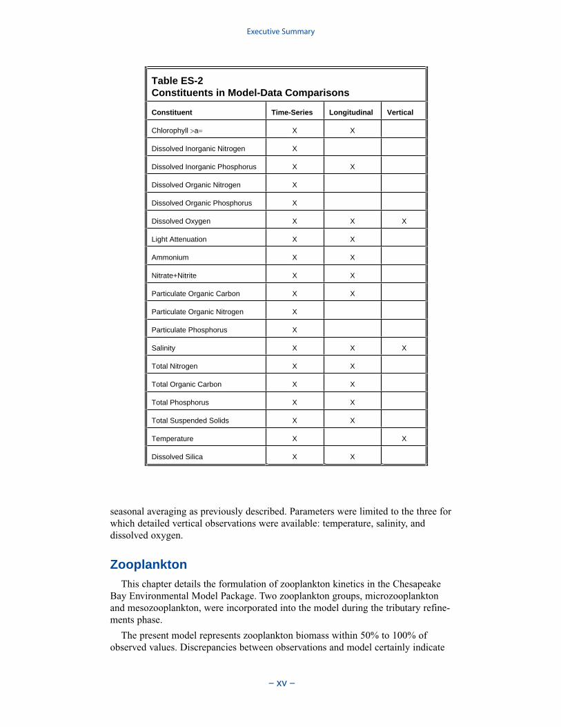
seasonal averaging as previously described. Parameters were limited to the three forwhich detailed vertical observations were available: temperature, salinity, anddissolved oxygen.
ZooplanktonThis chapter details the formulation of zooplankton kinetics in the Chesapeake
Bay Environmental Model Package. Two zooplankton groups, microzooplanktonand mesozooplankton, were incorporated into the model during the tributary refine-ments phase.
The present model represents zooplankton biomass within 50% to 100% ofobserved values. Discrepancies between observations and model certainly indicate
Executive Summary
– xv –
Table ES-2 Constituents in Model-Data Comparisons
Constituent Time-Series Longitudinal Vertical
Chlorophyll a X X
Dissolved Inorganic Nitrogen X
Dissolved Inorganic Phosphorus X X
Dissolved Organic Nitrogen X
Dissolved Organic Phosphorus X
Dissolved Oxygen X X X
Light Attenuation X X
Ammonium X X
Nitrate+Nitrite X X
Particulate Organic Carbon X X
Particulate Organic Nitrogen X
Particulate Phosphorus X
Salinity X X X
Total Nitrogen X X
Total Organic Carbon X X
Total Phosphorus X X
Total Suspended Solids X X
Temperature X X
Dissolved Silica X X
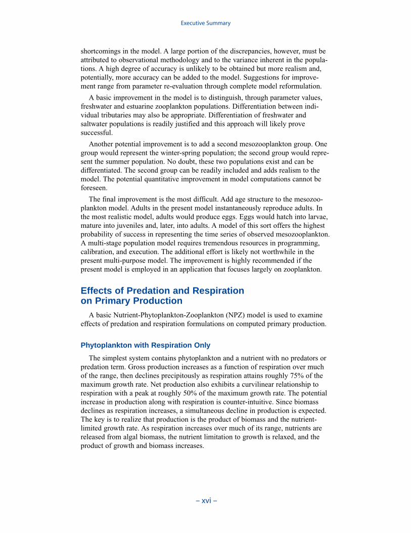
shortcomings in the model. A large portion of the discrepancies, however, must beattributed to observational methodology and to the variance inherent in the popula-tions. A high degree of accuracy is unlikely to be obtained but more realism and,potentially, more accuracy can be added to the model. Suggestions for improve-ment range from parameter re-evaluation through complete model reformulation.
A basic improvement in the model is to distinguish, through parameter values,freshwater and estuarine zooplankton populations. Differentiation between indi-vidual tributaries may also be appropriate. Differentiation of freshwater andsaltwater populations is readily justified and this approach will likely provesuccessful.
Another potential improvement is to add a second mesozooplankton group. Onegroup would represent the winter-spring population; the second group would repre-sent the summer population. No doubt, these two populations exist and can bedifferentiated. The second group can be readily included and adds realism to themodel. The potential quantitative improvement in model computations cannot beforeseen.
The final improvement is the most difficult. Add age structure to the mesozoo-plankton model. Adults in the present model instantaneously reproduce adults. Inthe most realistic model, adults would produce eggs. Eggs would hatch into larvae,mature into juveniles and, later, into adults. A model of this sort offers the highestprobability of success in representing the time series of observed mesozooplankton.A multi-stage population model requires tremendous resources in programming,calibration, and execution. The additional effort is likely not worthwhile in thepresent multi-purpose model. The improvement is highly recommended if thepresent model is employed in an application that focuses largely on zooplankton.
Effects of Predation and Respiration on Primary Production
A basic Nutrient-Phytoplankton-Zooplankton (NPZ) model is used to examineeffects of predation and respiration formulations on computed primary production.
Phytoplankton with Respiration Only
The simplest system contains phytoplankton and a nutrient with no predators orpredation term. Gross production increases as a function of respiration over muchof the range, then declines precipitously as respiration attains roughly 75% of themaximum growth rate. Net production also exhibits a curvilinear relationship torespiration with a peak at roughly 50% of the maximum growth rate. The potentialincrease in production along with respiration is counter-intuitive. Since biomassdeclines as respiration increases, a simultaneous decline in production is expected.The key is to realize that production is the product of biomass and the nutrient-limited growth rate. As respiration increases over much of its range, nutrients arereleased from algal biomass, the nutrient limitation to growth is relaxed, and theproduct of growth and biomass increases.
Executive Summary
– xvi –
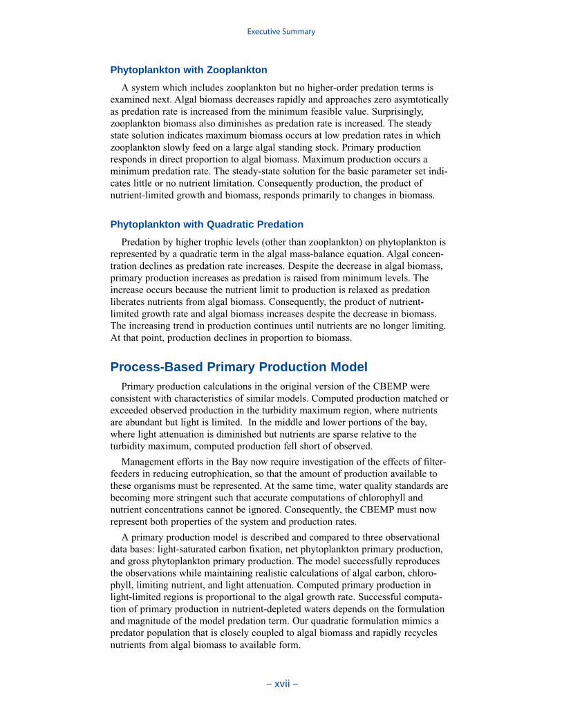
Phytoplankton with Zooplankton
A system which includes zooplankton but no higher-order predation terms isexamined next. Algal biomass decreases rapidly and approaches zero asymtoticallyas predation rate is increased from the minimum feasible value. Surprisingly,zooplankton biomass also diminishes as predation rate is increased. The steadystate solution indicates maximum biomass occurs at low predation rates in whichzooplankton slowly feed on a large algal standing stock. Primary productionresponds in direct proportion to algal biomass. Maximum production occurs aminimum predation rate. The steady-state solution for the basic parameter set indi-cates little or no nutrient limitation. Consequently production, the product ofnutrient-limited growth and biomass, responds primarily to changes in biomass.
Phytoplankton with Quadratic Predation
Predation by higher trophic levels (other than zooplankton) on phytoplankton isrepresented by a quadratic term in the algal mass-balance equation. Algal concen-tration declines as predation rate increases. Despite the decrease in algal biomass,primary production increases as predation is raised from minimum levels. Theincrease occurs because the nutrient limit to production is relaxed as predationliberates nutrients from algal biomass. Consequently, the product of nutrient-limited growth rate and algal biomass increases despite the decrease in biomass.The increasing trend in production continues until nutrients are no longer limiting.At that point, production declines in proportion to biomass.
Process-Based Primary Production ModelPrimary production calculations in the original version of the CBEMP were
consistent with characteristics of similar models. Computed production matched orexceeded observed production in the turbidity maximum region, where nutrientsare abundant but light is limited. In the middle and lower portions of the bay,where light attenuation is diminished but nutrients are sparse relative to theturbidity maximum, computed production fell short of observed.
Management efforts in the Bay now require investigation of the effects of filter-feeders in reducing eutrophication, so that the amount of production available tothese organisms must be represented. At the same time, water quality standards arebecoming more stringent such that accurate computations of chlorophyll andnutrient concentrations cannot be ignored. Consequently, the CBEMP must nowrepresent both properties of the system and production rates.
A primary production model is described and compared to three observationaldata bases: light-saturated carbon fixation, net phytoplankton primary production,and gross phytoplankton primary production. The model successfully reproducesthe observations while maintaining realistic calculations of algal carbon, chloro-phyll, limiting nutrient, and light attenuation. Computed primary production inlight-limited regions is proportional to the algal growth rate. Successful computa-tion of primary production in nutrient-depleted waters depends on the formulationand magnitude of the model predation term. Our quadratic formulation mimics apredator population that is closely coupled to algal biomass and rapidly recyclesnutrients from algal biomass to available form.
Executive Summary
– xvii –
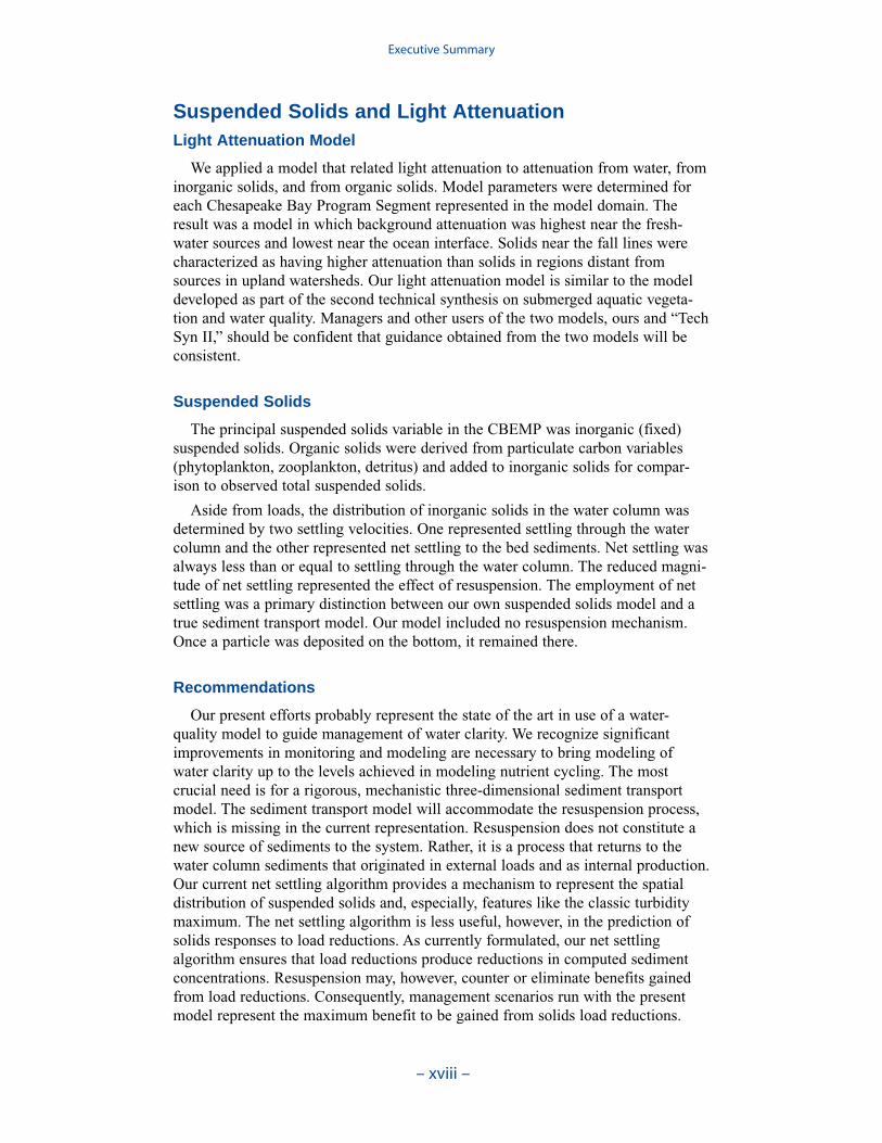
Suspended Solids and Light AttenuationLight Attenuation Model
We applied a model that related light attenuation to attenuation from water, frominorganic solids, and from organic solids. Model parameters were determined foreach Chesapeake Bay Program Segment represented in the model domain. Theresult was a model in which background attenuation was highest near the fresh-water sources and lowest near the ocean interface. Solids near the fall lines werecharacterized as having higher attenuation than solids in regions distant fromsources in upland watersheds. Our light attenuation model is similar to the modeldeveloped as part of the second technical synthesis on submerged aquatic vegeta-tion and water quality. Managers and other users of the two models, ours and “TechSyn II,” should be confident that guidance obtained from the two models will beconsistent.
Suspended Solids
The principal suspended solids variable in the CBEMP was inorganic (fixed)suspended solids. Organic solids were derived from particulate carbon variables(phytoplankton, zooplankton, detritus) and added to inorganic solids for compar-ison to observed total suspended solids.
Aside from loads, the distribution of inorganic solids in the water column wasdetermined by two settling velocities. One represented settling through the watercolumn and the other represented net settling to the bed sediments. Net settling wasalways less than or equal to settling through the water column. The reduced magni-tude of net settling represented the effect of resuspension. The employment of netsettling was a primary distinction between our own suspended solids model and atrue sediment transport model. Our model included no resuspension mechanism.Once a particle was deposited on the bottom, it remained there.
Recommendations
Our present efforts probably represent the state of the art in use of a water-quality model to guide management of water clarity. We recognize significantimprovements in monitoring and modeling are necessary to bring modeling ofwater clarity up to the levels achieved in modeling nutrient cycling. The mostcrucial need is for a rigorous, mechanistic three-dimensional sediment transportmodel. The sediment transport model will accommodate the resuspension process,which is missing in the current representation. Resuspension does not constitute anew source of sediments to the system. Rather, it is a process that returns to thewater column sediments that originated in external loads and as internal production.Our current net settling algorithm provides a mechanism to represent the spatialdistribution of suspended solids and, especially, features like the classic turbiditymaximum. The net settling algorithm is less useful, however, in the prediction ofsolids responses to load reductions. As currently formulated, our net settlingalgorithm ensures that load reductions produce reductions in computed sedimentconcentrations. Resuspension may, however, counter or eliminate benefits gainedfrom load reductions. Consequently, management scenarios run with the presentmodel represent the maximum benefit to be gained from solids load reductions.
Executive Summary
– xviii –
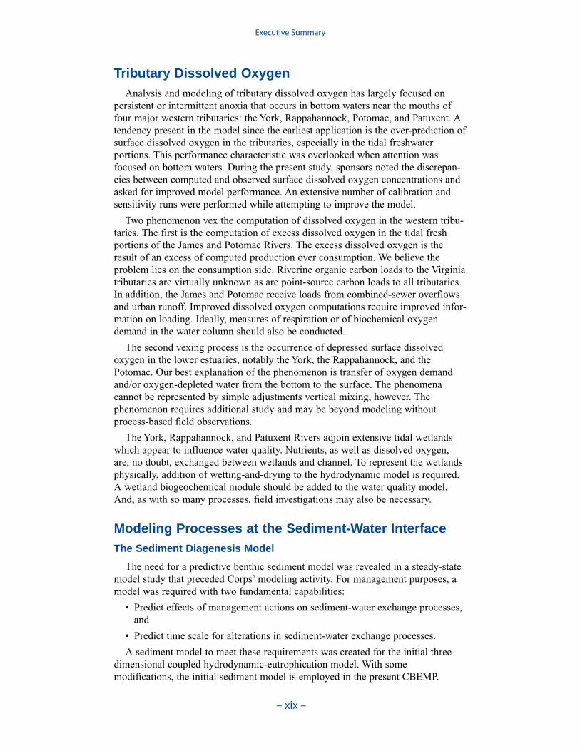
Tributary Dissolved OxygenAnalysis and modeling of tributary dissolved oxygen has largely focused on
persistent or intermittent anoxia that occurs in bottom waters near the mouths offour major western tributaries: the York, Rappahannock, Potomac, and Patuxent. Atendency present in the model since the earliest application is the over-prediction ofsurface dissolved oxygen in the tributaries, especially in the tidal freshwaterportions. This performance characteristic was overlooked when attention wasfocused on bottom waters. During the present study, sponsors noted the discrepan-cies between computed and observed surface dissolved oxygen concentrations andasked for improved model performance. An extensive number of calibration andsensitivity runs were performed while attempting to improve the model.
Two phenomenon vex the computation of dissolved oxygen in the western tribu-taries. The first is the computation of excess dissolved oxygen in the tidal freshportions of the James and Potomac Rivers. The excess dissolved oxygen is theresult of an excess of computed production over consumption. We believe theproblem lies on the consumption side. Riverine organic carbon loads to the Virginiatributaries are virtually unknown as are point-source carbon loads to all tributaries.In addition, the James and Potomac receive loads from combined-sewer overflowsand urban runoff. Improved dissolved oxygen computations require improved infor-mation on loading. Ideally, measures of respiration or of biochemical oxygendemand in the water column should also be conducted.
The second vexing process is the occurrence of depressed surface dissolvedoxygen in the lower estuaries, notably the York, the Rappahannock, and thePotomac. Our best explanation of the phenomenon is transfer of oxygen demandand/or oxygen-depleted water from the bottom to the surface. The phenomenacannot be represented by simple adjustments vertical mixing, however. Thephenomenon requires additional study and may be beyond modeling withoutprocess-based field observations.
The York, Rappahannock, and Patuxent Rivers adjoin extensive tidal wetlandswhich appear to influence water quality. Nutrients, as well as dissolved oxygen,are, no doubt, exchanged between wetlands and channel. To represent the wetlandsphysically, addition of wetting-and-drying to the hydrodynamic model is required.A wetland biogeochemical module should be added to the water quality model.And, as with so many processes, field investigations may also be necessary.
Modeling Processes at the Sediment-Water InterfaceThe Sediment Diagenesis Model
The need for a predictive benthic sediment model was revealed in a steady-statemodel study that preceded Corps’ modeling activity. For management purposes, amodel was required with two fundamental capabilities:
• Predict effects of management actions on sediment-water exchange processes,and
• Predict time scale for alterations in sediment-water exchange processes.
A sediment model to meet these requirements was created for the initial three-dimensional coupled hydrodynamic-eutrophication model. With somemodifications, the initial sediment model is employed in the present CBEMP.
Executive Summary
– xix –
Cumulative distributions were created for the population of Chesapeake Baysediment-water flux observations and for corresponding computations from thepresent model. Computed sediment oxygen demand exceeded observed throughoutthe distribution. Median computed demand exceeded observed by more than 0.5 g m-2 d-1. Observed sediment ammonium release exceeded computedthroughout the distribution. Median observed release exceeded modeled by 10 mgm-2 d-1. A number of explanations can be offered for these results. The excess ofsediment oxygen demand may be attributed to computed bottom dissolved oxygen.Computed bottom water dissolved oxygen does not match the lowest observationsat all locations. As a result, computed sediment oxygen demand exceeds observedbecause the model allows consumption of oxygen where no oxygen is present inthe bay. The excess of observed over computed ammonium release may indicatemore nitrogen should be deposited on the bottom. Or the occasional excess ofcomputed dissolved oxygen may be allowing more nitrification to take place in themodeled sediments than in the observations.
The preponderance of observed and computed sediment-water nitrate fluxes areessentially zero. Half the observed and computed sediment-water phosphate fluxesare less than or effectively zero. In the upper half of the distribution, the observa-tions show a gradual transition to sediment phosphorus release while the modelshows a much steeper gradient. Maximum phosphorus releases agree in both modeland observations. Observed sediment silica release greatly exceeds modeled. At the median, modeled release is essentially zero while median observed release is175 mg m-2 d-1. Maximum observed release exceeds 600 mg m-2 d-1 while themaximum modeled release is 100 mg m-2 d-1.
The Benthos Model
For the “Virginia Tributary Refinements” phase of the model activities, a deci-sion was made to initiate direct interactive simulation of three living resourcegroups: zooplankton, benthos, and SAV. Benthos were included in the modelbecause they are an important food source for crabs, finfish, and other economi-cally and ecologically significant biota. In addition, benthos can exert a substantialinfluence on water quality through their filtering of overlying water. Benthos withinthe model were divided into two groups: deposit feeders and filter feeders. Thedeposit-feeding group represents benthos which live within bottom sediments andfeed on deposited material. The filter-feeding group represents benthos which liveat the sediment surface and feed by filtering overlying water.
Examination of present model results indicates the computation of filter feedersclosely resembles the original application. Computed deposit feeders have, perhaps,increased since the original application. The increase in deposit feeders is inter-preted to have negligible impact on model computations. The resemblance ofresults between the present model and the Tributary Refinements model indicatesthe activity of the benthos, as originally calibrated, is maintained in the presentmodel.
Benthic Algae
Benthic algae are considered to occupy a thin layer between the water columnand benthic sediments. Biomass within the layer is determined by the balance
Executive Summary
– xx –
between production, respiration, and losses to predation. Nutrients from diageneticsediment production and from the overlying water are both available to the benthicalgae.
Computed benthic algal biomass ranges up to 3 g C m-2, in agreement withmeasures conducted in a variety of systems. The primary determinate of algaldensity is light. Algal biomass shows an inverse relationship to optical depth (totaldepth × light attenuation) at the sediment-water interface. No algae are computedabove optical depth 5. The highest densities of computed benthic algae are found inshallow water near the mouths of the lower western tributaries, along the lowereastern shore, and in eastern embayments. Lesser densities occur in tidal freshwaters and in other shoal areas.
Submerged Aquatic Vegetation (SAV)
An SAV submodel, which interacted with the main model of the water columnand with the sediment diagenesis submodel, was created for the “Virginia TributaryRefinements” phase of the model activities. Three state variables were modeled:shoots (above-ground biomass), roots (below-ground biomass), and epiphytes(attached growth). Three dominant SAV communities, Vallisneria americana,Ruppia maritima, or Zostera marina, were modeled.
When the phytoplankton production relationships and parameters in the presenteutrophication model were revised, corresponding changes were made to theepiphyte component of the SAV model. Examination of the SAV component of themodel revealed that these changes, and perhaps others, had a substantial, detri-mental, effect on computed SAV. Computed epiphytes overwhelmed the vegetation.As a consequence, a re-calibration of the SAV model was completed. We endeav-ored to bring epiphytes and SAV back into calibration while minimizing revisionsto the extensive model parameter suite. Changes were centered on the epiphyte lossterms and on the SAV production-irradiance relationships. The computations in thepresent model are consistent with, but not identical to, the original application. Theoriginal application obeyed light attenuation criteria listed in the first SAV Tech-nical Synthesis. During the re-calibration we verified that the present modelremains consistent with these criteria.
Dissolved PhosphateAn excess of computed dissolved phosphate, especially during summer, has been
a characteristic of the model since the original phase. While tuning the model toeffect an overall reduction in computed dissolved phosphate presents no problem,reducing phosphate in summer while maintaining sufficient phosphate to supportthe spring phytoplankton bloom is precarious.
We conducted an extensive number of sensitivity runs and process investigationsin order to calibrate dissolved phosphate in the present model. The final model cali-bration incorporates dissolved organic phosphorus mineralization, uptake by sulfideoxidizing bacteria, and precipitation. Introduction of the two uptake mechanisms aswell as alterations in multiple parameter values provided a reasonable representa-tion of summer-average phosphate in the surface of the bay, especially during years of dry to moderate hydrology. Considerable excess of computed phosphateremained present in a wet year.
Executive Summary
– xxi –
Phosphorus is a limiting nutrient in the mainstem bay in spring while nitrogen isthe primary limiting nutrient in summer. Consequently, our rough approach tomodeling dissolved phosphate in summer is acceptable. Still, a new phosphorusmodel seems appropriate, especially for management of freshwater segments wherephosphorus is the more important nutrient.
The first step in a new phosphate model is to explicitly recognize phosphateuptake by heterotrophic bacteria. Bacteria do not necessarily have to be incorpo-rated into the model as a state variable. One reviewer suggested relating phosphateuptake to organic carbon respiration, which is a bacterial process.
The second step in an improved phosphorus model is to explicitly differentiateparticulate inorganic phosphorus from particulate organic phosphorus through theaddition of a particulate inorganic phosphorus state variable.
A third step is to explore the utilization of dissolved organic phosphorus bybacteria and phytoplankton.
A concluding modification is to implement realistic sediment transportprocesses. No doubt, a distinct particulate inorganic phosphorus form exists and istransported along with the solids with which it is associated. Our ability to simulatesolids transport with the present model is limited, however. Consequently, correctrepresentation of total phosphorus is impossible when solids distributions cannot bereproduced.
Statistical Summary of CalibrationThe calibration of the model involved the comparison of hundreds of thousands
of observations with model results in various formats. Comparisons involvedconventional water quality data, process-oriented data, and living-resources obser-vations. The graphical comparisons produced thousands of plots which cannot beassimilated in their entirety. Evaluation of model performance requires statisticaland/or graphical summaries of results.
Examination of statistical summaries (Table ES-3) requires a good deal of judge-ment and interpretation. Generalizations and distinctions are not always possible. Oneclear pattern is that the model overestimates, on average, surface chlorophyll. Theoverestimation ranges from less than 1 mg m-3 to more than 2 mg m-3. The modelconsistently underestimates salinity although the mean error is always less than 1 ppt.For all systems except the Potomac, computed mean summer, bottom dissolvedoxygen is within 1 g m-3 of the observed average. In the Potomac, computed meansummer bottom dissolved oxygen is almost 2 g m-3 higher than observed. Carefulexamination of model results indicates the region of greatest computed excess is inthe tidal fresh portion of the river, where observed bottom dissolved oxygen exceeds5 g m-3. Excessive computed dissolved oxygen, surface and bottom, is a characteris-tics of the present model in most tidal freshwater regions. Except in the James, themodel underestimates mean total phosphorus concentration. Underestimation of totalphosphorus has been a characteristic of the model since the earliest application. Weoriginally attributed the shortfall to omission of bankloads. In this version we includebankloads of phosphorus but they are difficult to estimate accurately. The model alsoomits resuspension of particulate phosphorus and has difficulty reproducing theconcentration of particulate phosphorus in the turbidity maximums. In the James, weattribute the excess computed phosphorus to uncertainty in the large point-sourceand distributed loads to this tributary.
Executive Summary
– xxii –
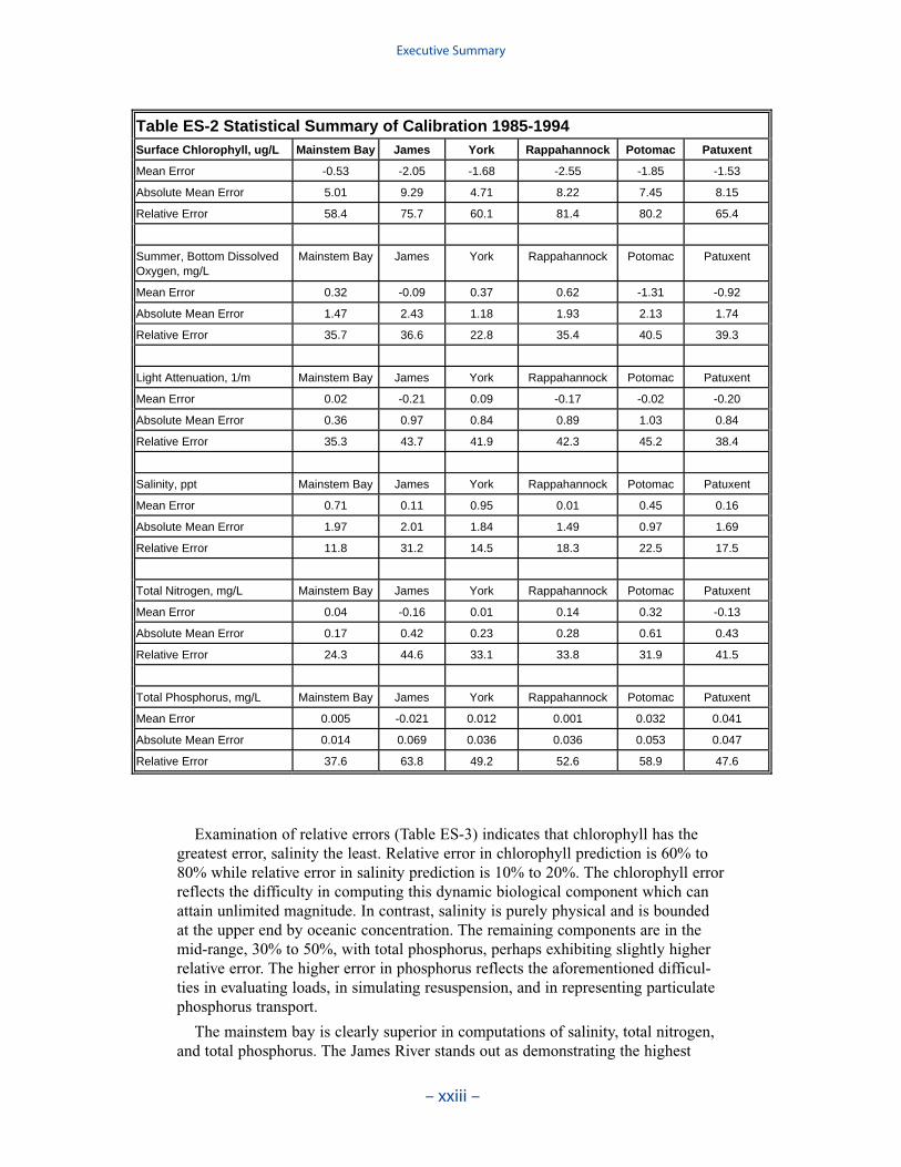
Examination of relative errors (Table ES-3) indicates that chlorophyll has thegreatest error, salinity the least. Relative error in chlorophyll prediction is 60% to80% while relative error in salinity prediction is 10% to 20%. The chlorophyll errorreflects the difficulty in computing this dynamic biological component which canattain unlimited magnitude. In contrast, salinity is purely physical and is boundedat the upper end by oceanic concentration. The remaining components are in themid-range, 30% to 50%, with total phosphorus, perhaps exhibiting slightly higherrelative error. The higher error in phosphorus reflects the aforementioned difficul-ties in evaluating loads, in simulating resuspension, and in representing particulatephosphorus transport.
The mainstem bay is clearly superior in computations of salinity, total nitrogen,and total phosphorus. The James River stands out as demonstrating the highest
Executive Summary
– xxiii –
Table ES-2 Statistical Summary of Calibration 1985-1994Surface Chlorophyll, ug/L Mainstem Bay James York Rappahannock Potomac Patuxent
Mean Error -0.53 -2.05 -1.68 -2.55 -1.85 -1.53
Absolute Mean Error 5.01 9.29 4.71 8.22 7.45 8.15
Relative Error 58.4 75.7 60.1 81.4 80.2 65.4
Summer, Bottom Dissolved Oxygen, mg/L
Mainstem Bay James York Rappahannock Potomac Patuxent
Mean Error 0.32 -0.09 0.37 0.62 -1.31 -0.92
Absolute Mean Error 1.47 2.43 1.18 1.93 2.13 1.74
Relative Error 35.7 36.6 22.8 35.4 40.5 39.3
Light Attenuation, 1/m Mainstem Bay James York Rappahannock Potomac Patuxent
Mean Error 0.02 -0.21 0.09 -0.17 -0.02 -0.20
Absolute Mean Error 0.36 0.97 0.84 0.89 1.03 0.84
Relative Error 35.3 43.7 41.9 42.3 45.2 38.4
Salinity, ppt Mainstem Bay James York Rappahannock Potomac Patuxent
Mean Error 0.71 0.11 0.95 0.01 0.45 0.16
Absolute Mean Error 1.97 2.01 1.84 1.49 0.97 1.69
Relative Error 11.8 31.2 14.5 18.3 22.5 17.5
Total Nitrogen, mg/L Mainstem Bay James York Rappahannock Potomac Patuxent
Mean Error 0.04 -0.16 0.01 0.14 0.32 -0.13
Absolute Mean Error 0.17 0.42 0.23 0.28 0.61 0.43
Relative Error 24.3 44.6 33.1 33.8 31.9 41.5
Total Phosphorus, mg/L Mainstem Bay James York Rappahannock Potomac Patuxent
Mean Error 0.005 -0.021 0.012 0.001 0.032 0.041
Absolute Mean Error 0.014 0.069 0.036 0.036 0.053 0.047
Relative Error 37.6 63.8 49.2 52.6 58.9 47.6

relative error in these components. We partially attribute the greater accuracy in themainstem to the relatively dense computational grid in this region. An additional,and probably more significant influence, is that the mainstem is dominated byinternal processes while the tributaries are strongly influenced by point-source anddistributed loads. The point-source loads are incompletely described, especially inthe early years of the simulation and in the Virginia tributaries. Below-fall-linedistributed loads cannot be measured; they can only be computed by the watershedmodel. We believe the uncertain loads, discharged into the constrained volumes ofthe tributaries, are the major reason for higher relative error in the tributaries. TheJames River stands out in this regard.
Executive Summary
– xxiv –

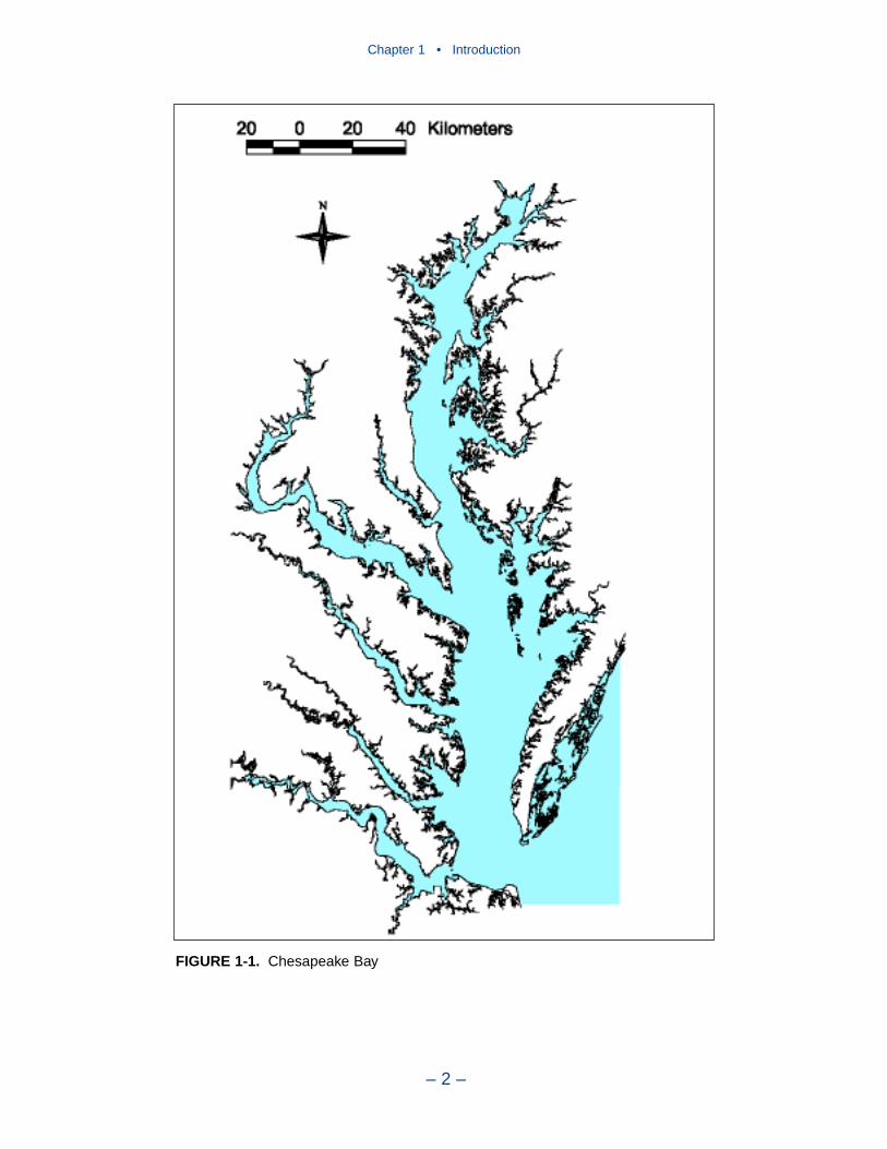
Deterioration of water quality in Chesapeake Bay (Figure 1-1) and associatedlosses of living resources have been recognized as problems for more than twentyyears (Flemer et al. 1983). An order-of-magnitude increase in anoxic volume and acatastrophic decline in submerged aquatic vegetation (SAV) were among theprimary problems cited. Two decades later, elimination of anoxia and restoration ofSAV remain prime management goals. Models have been employed as tools toguide management since the formation of the first water quality targets. Over time,as management focus has been refined, models have been improved to provideappropriate, up-to-date guidance.
Three models are at the heart of the Chesapeake Bay Environmental ModelPackage (CBEMP). Distributed flows and loads from the watershed are computedwith a highly-modified version of the HSPF model (Bicknell et al. 1996). Theseflows are input to the CH3D-WES hydrodynamic model (Johnson et al. 1993)which computes three-dimensional intra-tidal transport. Computed loads and trans-port are input to the CE-QUAL-ICM eutrophication model (Cerco and Cole 1993)which computes algal biomass, nutrient cycling, and dissolved oxygen, as well asnumerous additional constituents and processes. The eutrophication model incorpo-rates a predictive sediment diagenesis component (DiToro and Fitzpatrick 1993).The first coupling of these models simulated the period 1984-1986. Emphasis inthe model application was on examination of bottom-water anoxia. Results indi-cated a decision to reduce controllable nutrient input by 40% (Baliles et al. 1987)would reduce anoxic volume by 20%.
Circa 1992, management emphasis shifted from dissolved oxygen, a living-resource indicator, to living resources themselves. In response, the computationalgrid was refined to emphasize resource-rich areas (Wang and Johnson 2000) andliving resources including benthos (Meyers et al. 2000), zooplankton (Cerco andMeyers 2000), and submerged aquatic vegetation (Cerco and Moore 2001) wereadded to the model. The simulation period was extended from 1985 to 1994.
– 1 –
Introduction 1
Chapter 1 • Introduction
– 2 –
FIGURE 1-1. Chesapeake Bay
During this modeling phase, fixed solids were identified as major components oflight attenuation. Reductions in attenuation achieved solely through nutrientcontrols on phytoplankton could not restore submerged aquatic vegetation system-wide (Cerco and Moore 2001; Cerco et al. 2002).
In keeping with the emphasis on living resources, the Chesapeake 2000 Agree-ment (Gilmore et al. 2000) called for a ten-fold increase in biomass of oysters andother filter feeding organisms. In response, the computational grid was furtherrefined and plans were made to incorporate new living resources into the model. Atthe same time, regulatory forces were shaping the direction of management efforts.Regulatory agencies in Maryland listed the state’s portion of Chesapeake Bay as“impaired.” The US Environmental Protection Agency added bay waters withinVirginia to the impaired list. Settlement of a lawsuit required development of aTotal Maximum Daily Load (TMDL) for Virginia waters by 2011. To avoid imposi-tion of an arbitrary TMDL, the Chesapeake 2000 Agreement specified removal ofwater quality impairments by 2010. Impairments in the bay were defined as lowdissolved oxygen, excessive chlorophyll concentration and diminished water clarity.Management emphasis shifted from living resources back to living-resource indica-tors: dissolved oxygen, chlorophyll, and clarity. A model recalibration wasundertaken, with emphasis on improved accuracy in the computation of the threekey indicators.
The 2002 Chesapeake Bay Environmental Model Package
The framework of the original CBEMP remains intact although the componentshave been substantially modified and improved over fifteen years. The watershedmodel is now in Phase 4.3 (Linker et al. 2000). Documentation may be found maybe found on the Chesapeake Bay Program web sitehttp://www.chesapeakebay.net/modsc.htm. Nutrient and solids loads are computedon a daily basis for 94 sub-watersheds of the 166,000 km2 Chesapeake Bay water-shed and are routed to individual model cells based on local watershedcharacteristics and on drainage area contributing to the cell. The hydrodynamic andeutrophication models operate on a grid of 13,000 cells. The grid contains 2,900surface cells (4 km2) and employs non-orthogonal curvilinear coordinates in thehorizontal plane. Z coordinates are used in the vertical direction which is up to 19layers deep. Depth of the surface cells is 2.1 m at mean tide and varies as a func-tion of tide, wind, and other forcing functions. Depth of sub-surface cells is fixed at1.5 m. A band of littoral cells, 2.1 m deep at mean tide, adjoins the shorelinethroughout most of the system. Ten years, 1985-1994, are simulated continuouslyusing time steps of 5 minutes (hydrodynamic model) and 15 minutes (eutrophica-tion model).
Chapter 1 • Introduction
– 3 –
Expert Panels
Expert review has been part of the model activity since its commencement. Forthe present study, several “Expert Panels” were assembled to review various aspectsof the model application. These teams were:
Hydrodynamics Expert Panel
Dr. Richard GarvineCollege of Marine StudiesUniversity of Delaware, Newark DE
Dr. Albert Y. KuoVirginia Institute of Marine ScienceCollege of William and Mary, Gloucester Point, VA
Dr. Lawrence P. SanfordUniversity of Maryland Center for Environmental ScienceHorn Point Laboratory, Cambridge MD
Primary Production Expert Panel
Dr. Lawrence W. HardingUniversity of Maryland Center for Environmental ScienceHorn Point Laboratory, Cambridge MD
Dr. Raleigh HoodUniversity of Maryland Center for Environmental ScienceHorn Point Laboratory, Cambridge MD
Dr. W. Michael KempUniversity of Maryland Center for Environmental ScienceHorn Point Laboratory, Cambridge MD
Total Maximum Daily Load Expert Panel
Dr. Kevin FarleyDepartment of Environmental EngineeringManhattan College, Riverdale NY
Dr. Wu-Seng LungDepartment of Environmental EngineeringUniversity of Virginia, Charlottesville VA
We gratefully acknowledge the advice and assistance provided by our experts.Successful completion of this study would not have been possible without them.
Chapter 1 • Introduction
– 4 –

This Report
This report comprises the primary documentation of the eutrophication com-ponent of the 2002 CBEMP. The Chesapeake Bay model study has beenextensively documented since its earliest stages. We concentrate here on portions ofthe model that have undergone major revisions and on portions that have not beenpreviously documented. Aspects of the model that proved particularly troublesomeare documented for reference against future improvements. We have minimizedrepetition of previously-reported information and model results. The reader isreferred to the Bibliography, below, and to the EPA Chesapeake Bay Program website, http://www.chesapeakebay.net/modsc.htm, for additional information.
Bibliography
Baliles, G., Schaefer, W., Casey, R., Thomas, L., Barry, M., and Cole, K. (1987). “Chesa-peake Bay Agreement.” United States Environmental Protection Agency Chesapeake BayProgram, Annapolis MD.
Bicknell, B., Imhoff, J., Kittle, J., Donigian, A., Johanson, R., and Barnwell, T. (1996).“Hydrologic simulation program - FORTRAN user’s manual for release 11,” United StatesEnvironmental Protection Agency Environmental Research Laboratory, Athens GA.
Cerco, C., and Cole, T. (1993). “Three-dimensional eutrophication model of ChesapeakeBay,” Journal of Environmental Engineering, 119(6), 1006-10025.
Cerco, C., and Cole, T. (1994). “Three-dimensional eutrophication model of ChesapeakeBay,” Technical Report EL-94-4, US Army Engineer Waterways Experiment Station, Vicks-burg, MS.
Cerco, C. (1995a). “Simulation of long-term trends in Chesapeake Bay eutrophication,”Journal of Environmental Engineering, 121(4), 298-310.
Cerco, C. (1995b). “Response of Chesapeake Bay to nutrient load reductions,” Journal ofEnvironmental Engineering, 121(8), 549-557.
Cerco, C., and Cole, T. (1995). “User’s guide to the CE-QUAL-ICM three-dimensionaleutrophication model,” Technical Report EL-95-15, US Army Engineer Waterways Experi-ment Station, Vicksburg, MS.
Cerco, C. (2000). “Phytoplankton kinetics in the Chesapeake Bay model,” Water Qualityand Ecosystem Modeling, 1, 5-49.
Cerco, C., and Meyers, M. (2000). “Tributary refinements to the Chesapeake Bay Model,”Journal of Environmental Engineering, 126(2), 164-174.
Cerco, C., and Moore, K. (2001). “System-wide submerged aquatic vegetation model forChesapeake Bay,” Estuaries, 24(4), 522-534.
Cerco, C., Linker, L., Sweney, J., Shenk, G., and Butt, A. (2002). “Nutrient and solidscontrols in Virginia’s Chesapeake Bay tributaries,” Journal of Water Resources Planningand Management, 128(3), 179-189.
Cerco, C., Johnson, B., and Wang, H. (2002). “Tributary refinements to the Chesapeake Baymodel,” ERDC TR-02-4, US Army Engineer Research and Development Center, Vicksburg,MS.
Cerco, C., and Noel, M. (2003). “Managing for water clarity in Chesapeake Bay,” Journalof Environmental Engineering, in press.
Chapter 1 • Introduction
– 5 –
DiToro, D., and Fitzpatrick, J. (1993). “Chesapeake Bay sediment flux model,” ContractReport EL-93-2, US Army Engineer Waterways Experiment Station, Vicksburg, MS.
DiToro, D. (2001). Sediment Flux Modeling, John Wiley and Sons, New York.
Flemer, D., Mackiernan, G., Nehlsen, W., and Tippie, V. (1983). “Chesapeake Bay: Aprofile of environmental change,” U.S. Environmental Protection Agency, Region III,Philadelphia, PA.
Gillmore, J., Glendening, P., Ridge, T., Williams, A., Browner, C., and Bolling, B. (2000).“Chesapeake 2000 Agreement.” United States Environmental Protection Agency Chesa-peake Bay Program, Annapolis MD.
HydroQual Inc., (2000). “Development of a suspension feeding and deposit feeding benthosmodel for Chesapeake Bay,” Project No. USCE0410, HydroQual Inc., Mahwah NJ.
Johnson, B., Heath, R., Hsieh, B., Kim, K., and Butler, L. (1991). “Development and verifi-cation of a three-dimensional numerical hydrodynamic, salinity, and temperature model ofChesapeake Bay,” HL-91-7, US Army Engineer Waterways Experiment Station, Vicksburg,MS.
Johnson, B., Kim, K., Heath, R., Hsieh, B., and Butler, L. (1993). “Validation of a three-dimensional hydrodynamic model of Chesapeake Bay,” Journal of Hydraulic Engineering,199(1), 2-20.
Linker, L., Shenk, G., Dennis, R., and Sweeney, J. (2000). “Cross-media models of theChesapeake Bay watershed and airshed,” Water Quality and Ecosystem Modeling, 1(1-4),91-122.
Meyers, M., DiToro, D., and Lowe, S. (2000). “Coupling suspension feeders to the Chesa-peake Bay eutrophication model,” Water Quality and Ecosystem Modeling, 1(1-4), 123-140.
Wang, H., and Johnson, B. (2000). “Validation and application of the second-generationthree-dimensional hydrodynamic model of Chesapeake Bay,” Water Quality and EcosystemModeling, 1(1-4), 51-90.
Chapter 1 • Introduction
– 6 –

Introduction
Modeling the physics, chemistry, and biology of the Bay required a package ofmodels. Transport processes were modeled by a three-dimensional hydrodynamicmodel that operated independently of the water quality model. Transport informa-tion from the hydrodynamic model was processed and stored on-line forsubsequent use by the water quality model.
The Hydrodynamic ModelCH3D-WES
The CH3D-WES (Computational Hydrodynamics in Three Dimensions—Waterways Experiment Station) hydrodynamic model was a substantially revisedversion of the CH3D model originally developed by Sheng (1986). Model formula-tion was based on principles expressed by the equations of motion, conservation ofvolume, and conservation of mass. Quantities computed by the model includedthree-dimensional velocities, surface elevation, vertical viscosity and diffusivity,temperature, salinity, and density. Details of the model formulation and initialapplication to Chesapeake Bay were presented by Johnson et al. (1991).
Computational Grid
The basic equations of CH3D-WES were solved via the finite-differencemethod. The finite-difference solution algorithm replaced continuous derivatives inthe governing differential equations with ratios of discrete quantities. Solutions tothe hydrodynamics were obtained using five-minute intervals for the discrete timesteps. The spatial continuum of the Bay was divided into a grid of discrete cells. Toachieve close conformance of the grid to Bay geometry, cells were represented incurvilinear rather than rectangular coordinates. A z-plane grid was employed in
– 7 –
Coupling with theHydrodynamic Model 2
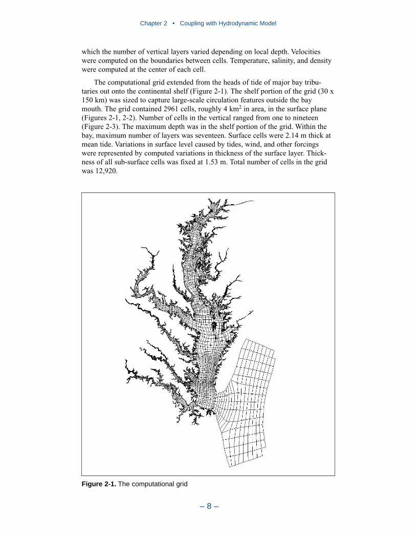
which the number of vertical layers varied depending on local depth. Velocitieswere computed on the boundaries between cells. Temperature, salinity, and densitywere computed at the center of each cell.
The computational grid extended from the heads of tide of major bay tribu-taries out onto the continental shelf (Figure 2-1). The shelf portion of the grid (30 x150 km) was sized to capture large-scale circulation features outside the baymouth. The grid contained 2961 cells, roughly 4 km2 in area, in the surface plane(Figures 2-1, 2-2). Number of cells in the vertical ranged from one to nineteen(Figure 2-3). The maximum depth was in the shelf portion of the grid. Within thebay, maximum number of layers was seventeen. Surface cells were 2.14 m thick atmean tide. Variations in surface level caused by tides, wind, and other forcingswere represented by computed variations in thickness of the surface layer. Thick-ness of all sub-surface cells was fixed at 1.53 m. Total number of cells in the gridwas 12,920.
Chapter 2 • Coupling with Hydrodynamic Model
– 8 –
Figure 2-1. The computational grid
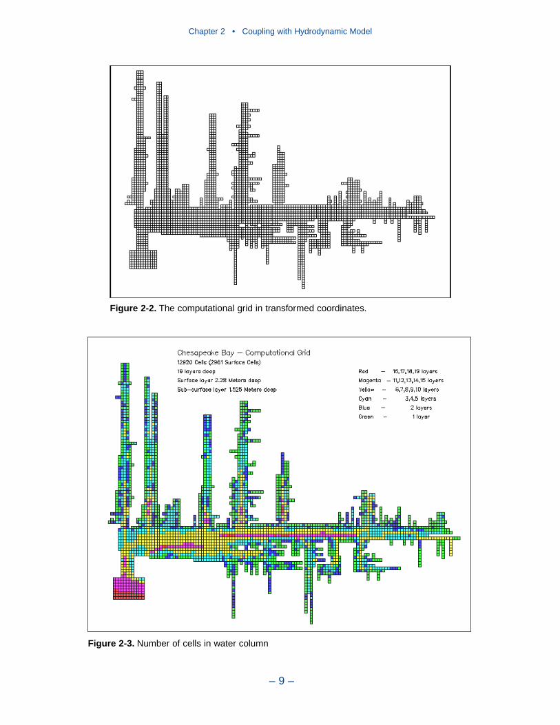
Chapter 2 • Coupling with Hydrodynamic Model
– 9 –
Figure 2-2. The computational grid in transformed coordinates.
Figure 2-3. Number of cells in water column
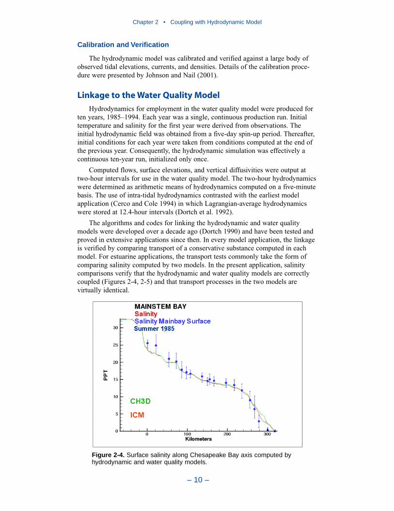
Chapter 2 • Coupling with Hydrodynamic Model
– 10 –
Calibration and Verification
The hydrodynamic model was calibrated and verified against a large body ofobserved tidal elevations, currents, and densities. Details of the calibration proce-dure were presented by Johnson and Nail (2001).
Linkage to the Water Quality Model
Hydrodynamics for employment in the water quality model were produced forten years, 1985–1994. Each year was a single, continuous production run. Initialtemperature and salinity for the first year were derived from observations. Theinitial hydrodynamic field was obtained from a five-day spin-up period. Thereafter,initial conditions for each year were taken from conditions computed at the end ofthe previous year. Consequently, the hydrodynamic simulation was effectively acontinuous ten-year run, initialized only once.
Computed flows, surface elevations, and vertical diffusivities were output attwo-hour intervals for use in the water quality model. The two-hour hydrodynamicswere determined as arithmetic means of hydrodynamics computed on a five-minutebasis. The use of intra-tidal hydrodynamics contrasted with the earliest modelapplication (Cerco and Cole 1994) in which Lagrangian-average hydrodynamicswere stored at 12.4-hour intervals (Dortch et al. 1992).
The algorithms and codes for linking the hydrodynamic and water qualitymodels were developed over a decade ago (Dortch 1990) and have been tested andproved in extensive applications since then. In every model application, the linkageis verified by comparing transport of a conservative substance computed in eachmodel. For estuarine applications, the transport tests commonly take the form ofcomparing salinity computed by two models. In the present application, salinitycomparisons verify that the hydrodynamic and water quality models are correctlycoupled (Figures 2-4, 2-5) and that transport processes in the two models arevirtually identical.
Figure 2-4. Surface salinity along Chesapeake Bay axis computed by hydrodynamic and water quality models.
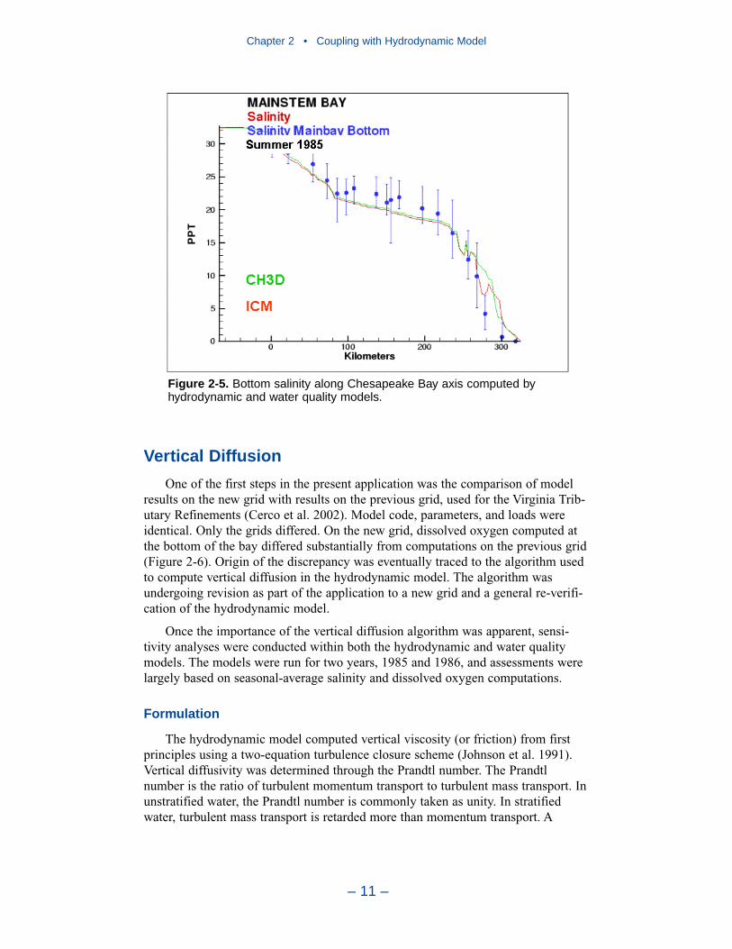
Vertical Diffusion
One of the first steps in the present application was the comparison of modelresults on the new grid with results on the previous grid, used for the Virginia Trib-utary Refinements (Cerco et al. 2002). Model code, parameters, and loads wereidentical. Only the grids differed. On the new grid, dissolved oxygen computed atthe bottom of the bay differed substantially from computations on the previous grid(Figure 2-6). Origin of the discrepancy was eventually traced to the algorithm usedto compute vertical diffusion in the hydrodynamic model. The algorithm wasundergoing revision as part of the application to a new grid and a general re-verifi-cation of the hydrodynamic model.
Once the importance of the vertical diffusion algorithm was apparent, sensi-tivity analyses were conducted within both the hydrodynamic and water qualitymodels. The models were run for two years, 1985 and 1986, and assessments werelargely based on seasonal-average salinity and dissolved oxygen computations.
Formulation
The hydrodynamic model computed vertical viscosity (or friction) from firstprinciples using a two-equation turbulence closure scheme (Johnson et al. 1991).Vertical diffusivity was determined through the Prandtl number. The Prandtlnumber is the ratio of turbulent momentum transport to turbulent mass transport. Inunstratified water, the Prandtl number is commonly taken as unity. In stratifiedwater, turbulent mass transport is retarded more than momentum transport. A
Chapter 2 • Coupling with Hydrodynamic Model
– 11 –
Figure 2-5. Bottom salinity along Chesapeake Bay axis computed byhydrodynamic and water quality models.
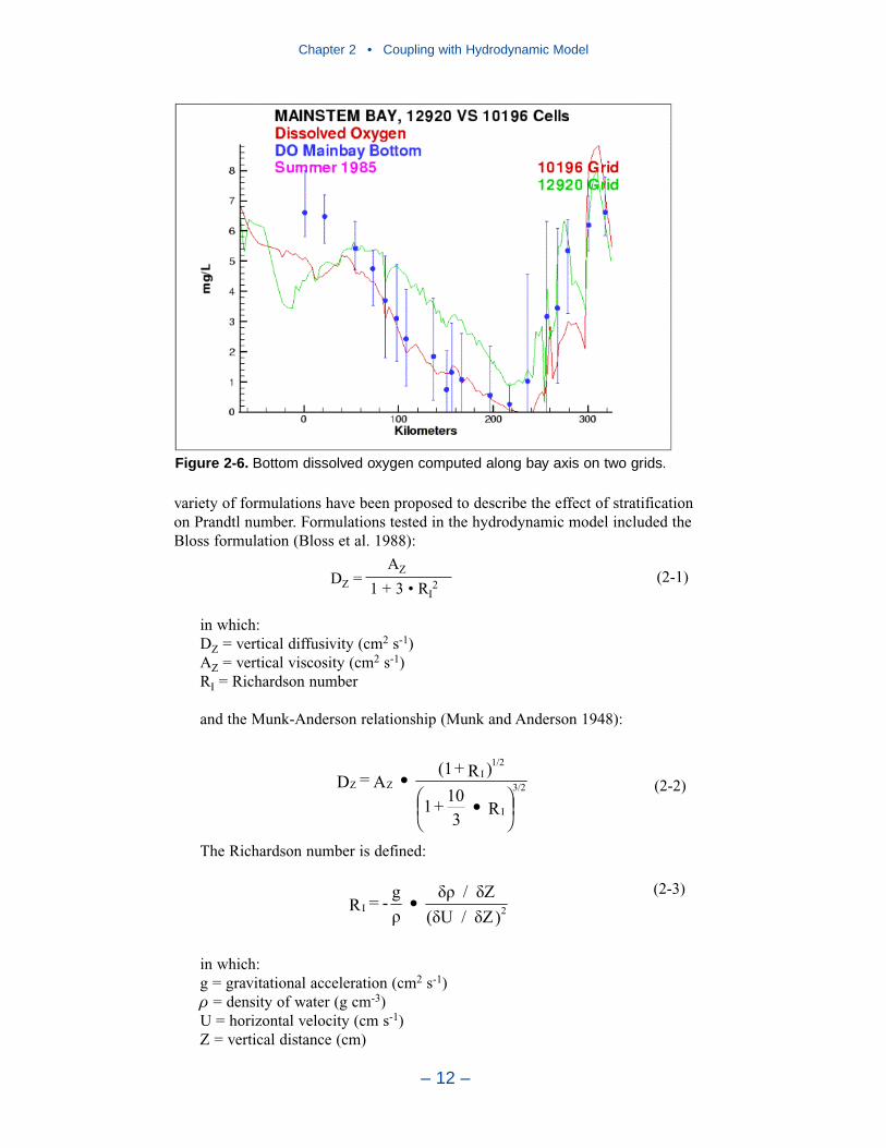
variety of formulations have been proposed to describe the effect of stratificationon Prandtl number. Formulations tested in the hydrodynamic model included theBloss formulation (Bloss et al. 1988):
DZ = AZ
1 + 3 • RI2
(2-1)
in which:DZ = vertical diffusivity (cm2 s-1)AZ = vertical viscosity (cm2 s-1)RI = Richardson number
and the Munk-Anderson relationship (Munk and Anderson 1948):
(2-2)
The Richardson number is defined:
(2-3)
in which:g = gravitational acceleration (cm2 s-1)ρ = density of water (g cm-3)U = horizontal velocity (cm s-1)Z = vertical distance (cm)
)Z /U(
Z /g-=R 2I •
•
•
R3
10+1
)R+(1A=D
I
3/2
1/2
IZZ
Chapter 2 • Coupling with Hydrodynamic Model
– 12 –
Figure 2-6. Bottom dissolved oxygen computed along bay axis on two grids.
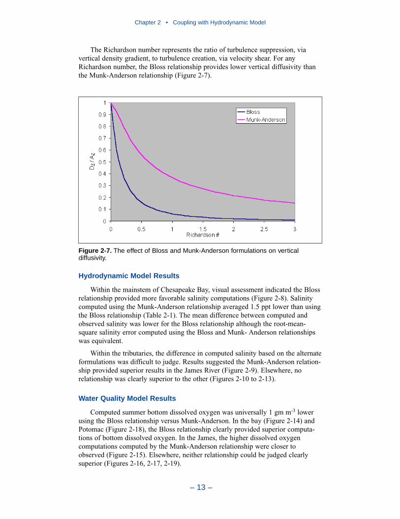
The Richardson number represents the ratio of turbulence suppression, viavertical density gradient, to turbulence creation, via velocity shear. For anyRichardson number, the Bloss relationship provides lower vertical diffusivity thanthe Munk-Anderson relationship (Figure 2-7).
Hydrodynamic Model Results
Within the mainstem of Chesapeake Bay, visual assessment indicated the Blossrelationship provided more favorable salinity computations (Figure 2-8). Salinitycomputed using the Munk-Anderson relationship averaged 1.5 ppt lower than usingthe Bloss relationship (Table 2-1). The mean difference between computed andobserved salinity was lower for the Bloss relationship although the root-mean-square salinity error computed using the Bloss and Munk- Anderson relationshipswas equivalent.
Within the tributaries, the difference in computed salinity based on the alternateformulations was difficult to judge. Results suggested the Munk-Anderson relation-ship provided superior results in the James River (Figure 2-9). Elsewhere, norelationship was clearly superior to the other (Figures 2-10 to 2-13).
Water Quality Model Results
Computed summer bottom dissolved oxygen was universally 1 gm m-3 lowerusing the Bloss relationship versus Munk-Anderson. In the bay (Figure 2-14) andPotomac (Figure 2-18), the Bloss relationship clearly provided superior computa-tions of bottom dissolved oxygen. In the James, the higher dissolved oxygencomputations computed by the Munk-Anderson relationship were closer toobserved (Figure 2-15). Elsewhere, neither relationship could be judged clearlysuperior (Figures 2-16, 2-17, 2-19).
Chapter 2 • Coupling with Hydrodynamic Model
– 13 –
Figure 2-7. The effect of Bloss and Munk-Anderson formulations on verticaldiffusivity.

Chapter 2 • Coupling with Hydrodynamic Model
– 14 –
Figure 2-8. Computed salinity along the axis of Chesapeake Bay, summer 1985,for the Bloss (left) and Munk-Anderson (right) relationships.
Table 2-1. Statistical Comparison of Computations on Different Grids and with Different Formulations for Prandtl Number
Salt, ppt DO, mg/L Temperature, C
Mean Error RMS Error Mean Error RMS Error Mean Error RMS Error
10,000 cell, VA Trib Refinements
-0.99 2.78 0.005 1.88 0.74 1.93
12,000 cell with Bloss scheme
-0.27 2.78 -0.057 1.97 0.69 1.77
12,000 cell withMunk-Andersonscheme
1.1 2.82 -0.45 1.9 0.67 1.65

Chapter 2 • Coupling with Hydrodynamic Model
– 15 –
Figure 2-10. Computed salinity along the York River axis, summer 1985, for theBloss (left) and Munk-Anderson (right) relationships.
Figure 2-9. Computed salinity along the James River axis, summer 1985, for theBloss (left) and Munk-Anderson (right) relationships.
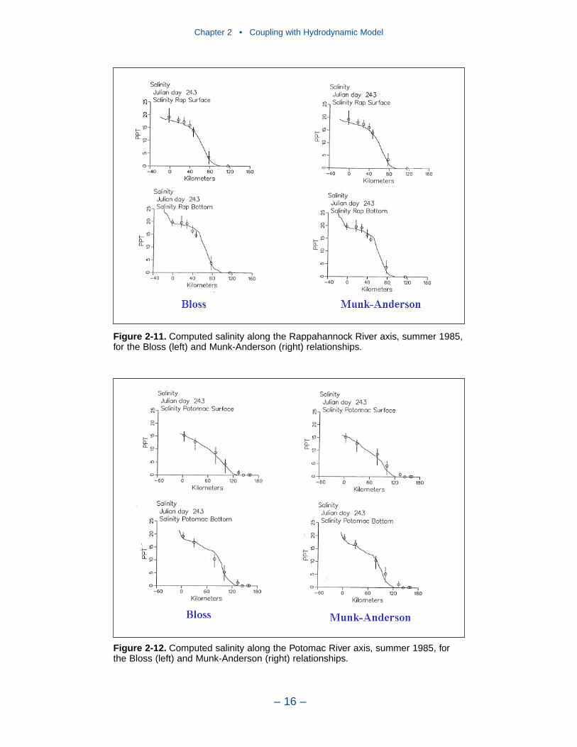
Chapter 2 • Coupling with Hydrodynamic Model
– 16 –
Figure 2-12. Computed salinity along the Potomac River axis, summer 1985, forthe Bloss (left) and Munk-Anderson (right) relationships.
Figure 2-11. Computed salinity along the Rappahannock River axis, summer 1985,for the Bloss (left) and Munk-Anderson (right) relationships.
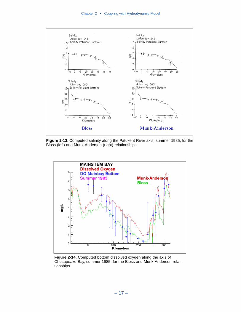
Chapter 2 • Coupling with Hydrodynamic Model
– 17 –
Figure 2-14. Computed bottom dissolved oxygen along the axis ofChesapeake Bay, summer 1985, for the Bloss and Munk-Anderson rela-tionships.
Figure 2-13. Computed salinity along the Patuxent River axis, summer 1985, for theBloss (left) and Munk-Anderson (right) relationships.
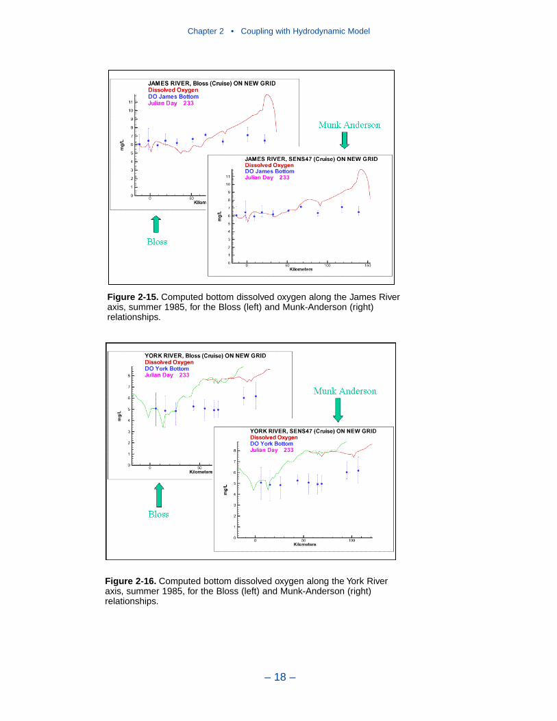
Chapter 2 • Coupling with Hydrodynamic Model
– 18 –
Figure 2-16. Computed bottom dissolved oxygen along the York Riveraxis, summer 1985, for the Bloss (left) and Munk-Anderson (right)relationships.
Figure 2-15. Computed bottom dissolved oxygen along the James Riveraxis, summer 1985, for the Bloss (left) and Munk-Anderson (right)relationships.
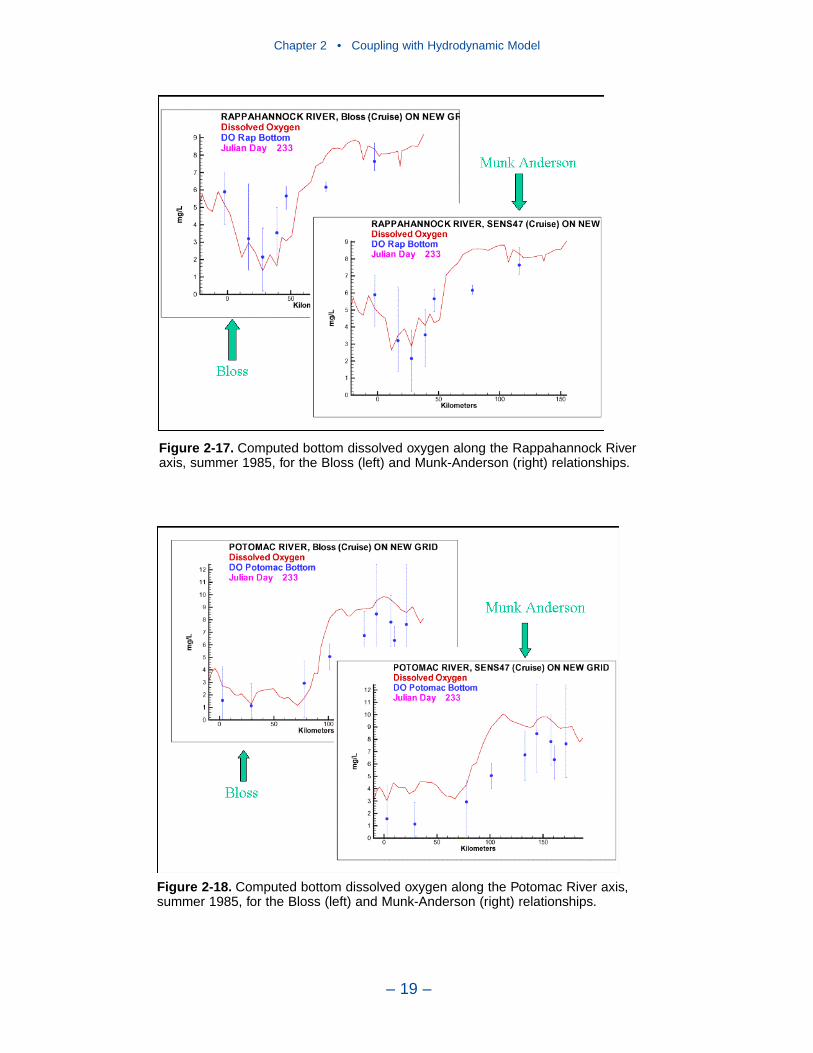
Chapter 2 • Coupling with Hydrodynamic Model
– 19 –
Figure 2-18. Computed bottom dissolved oxygen along the Potomac River axis,summer 1985, for the Bloss (left) and Munk-Anderson (right) relationships.
Figure 2-17. Computed bottom dissolved oxygen along the Rappahannock Riveraxis, summer 1985, for the Bloss (left) and Munk-Anderson (right) relationships.

The Decision
The model team proposed using a mixed scheme in which the Bloss and Munk-Anderson relationships were applied in the systems for which they provided thebest results. The first author’s opinion was (and remains) that the use of the mixedscheme was entirely appropriate. The existence of numerous relationships,including Bloss, Munk-Anderson and others, indicates that no one relationship hasuniversal applicability. The Hydrodynamics Expert Panel insisted that the mixedscheme should not be used. The Panel’s opinion was that one relationship must beapplied system-wide. Their recommendation was accepted and the Bloss schemewas selected for use. This scheme provided the best results in two systems, themainstem bay and the Potomac, for which computation of bottom-water anoxia wascrucial. Since dissolved oxygen was not a management issue in the James, theconsequences of employing the Bloss scheme there were considered acceptable.
References
Bloss, S., Lehfeldt, R., and Patterson, J. (1988). “Modeling turbulent transport in stratifiedestuary,” Journal of Hydraulic Engineering, 114(9), 1115-1133
Cerco, C., and Cole, T. (1994). “Three-dimensional eutrophication model of ChesapeakeBay,” Technical Report El-94-4, US Army Engineer Waterways Experiment Station, Vicks-burg MS.
Dortch, M. (1990). “Three-dimensional Lagrangian residual transport computed from anintratidal hydrodynamic model,” Technical Report EL-90-11, US Army Engineer Water-ways Experiment Station, Vicksburg MS.
Chapter 2 • Coupling with Hydrodynamic Model
– 20 –
Figure 2-19. Computed bottom dissolved oxygen along the Patuxent River axis, summer 1985, for the Bloss (left) and Munk-Anderson (right)relationships.

Dortch, M., Chapman, R., and Abt, S. (1992). “Application of three-dimensionalLagrangian residual transport,” Journal of Hydraulic Engineering, 118(6), 831-848
Johnson, B., Kim, K., Heath, R., and Butler, L. (1991). “Development and verification of athree-dimensional numerical hydrodynamic, salinity and temperature model of ChesapeakeBay,” Technical Report HL-91-7, US Army Engineer Waterways Experiment Station, Vicks-burg, MS.
Johnson, B., and Nail, G. (2001). “A 10-year (1985-1994) simulation with a refined three-dimensional numerical hydrodynamic, salinity, and temperature model of Chesapeake Bayand its tributaries,” June 2001 Draft Report, Coastal and Hydraulics Laboratory, US ArmyEngineer Research and Development Center, Vicksburg MS.
Munk, W., and Anderson, E. (1948). “Notes on the theory of the thermocline,” Journal ofMarine Research, 7, 276-295.
Sheng, P. (1986). “A three-dimensional mathematical model of coastal, estuarine and lakecurrents using boundary-fitted grid,” Report 585, ARAP Group of Titan Systems, PrincetonNJ.
Chapter 2 • Coupling with Hydrodynamic Model
– 21 –

Introduction
Boundary conditions must be specified at all open edges of the model grid.These include river inflows, lateral flows, and the ocean interface. Numerical treat-ment of all boundary conditions is identical. When flow across a boundary is out ofthe system, the concentration at the boundary is assigned the value computed at themodel cell immediately inside the boundary. When flow across a boundary is intothe system, concentration at the boundary is assigned a specified boundary value.Diffusion across the boundary is considered to be zero. The method of assigningboundary concentrations varies with the nature of the boundary.
River Inflows
Loads of carbon, nitrogen, phosphorus, and solids were specified at the riverinflows. Consequently, boundary concentrations of these substances were set tozero so that no material entered the system other than the specified loads. Boundaryconcentrations were required for substances not usually considered in the form ofloads. These included temperature, dissolved oxygen, phytoplankton, zooplankton,and silica. Boundary concentrations were specified as monthly values (Tables 3-1–3-7). Determination of the values depended on available observations.
Dissolved oxygen and temperature were based on mean monthly values in thefall-line monitoring program. Zooplankton was not monitored at the river inflows.Boundary conditions were based on nearby in-stream observations or adapted fromother rivers when no observations were available. Mean dissolved silica concentra-tions were based on fall-line observations. Particulate silica concentrations werederived from a 1994 observation program.
Limited chlorophyll observations were obtained from the fall-line data base.These were converted to algal carbon, the model state variable, using a carbon-to-chlorophyll ratio of 30. Phytoplankton in river inflows were assigned to the model
– 22 –
Boundary Conditions 3
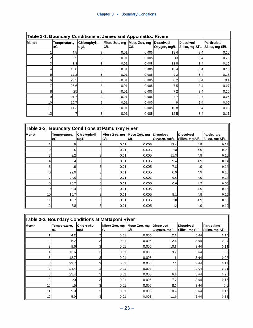
Chapter 3 • Boundary Conditions
– 23 –
Table 3-1. Boundary Conditions at James and Appomattox Rivers Month Temperature,
oCChlorophyll,ug/L
Micro Zoo, mg C/L
Meso Zoo, mg C/L
DissolvedOxygen, mg/L
DissolvedSilica, mg Si/L
ParticulateSilica, mg Si/L
1 4.8 3 0.01 0.005 13.4 3.4 0.16
2 5.5 3 0.01 0.005 13 3.4 0.26
3 8.8 3 0.01 0.005 11.8 3.4 0.19
4 13.8 3 0.01 0.005 10.4 3.4 0.15
5 19.2 3 0.01 0.005 9.2 3.4 0.18
6 23.5 3 0.01 0.005 8.2 3.4 0.1
7 25.6 3 0.01 0.005 7.5 3.4 0.07
8 25 3 0.01 0.005 7.2 3.4 0.15
9 21.7 3 0.01 0.005 7.7 3.4 0.04
10 16.7 3 0.01 0.005 9 3.4 0.05
11 11.3 3 0.01 0.005 10.8 3.4 0.08
12 7 3 0.01 0.005 12.5 3.4 0.11
Table 3-2. Boundary Conditions at Pamunkey River Month Temperature,
oCChlorophyll,ug/L
Micro Zoo, mg C/L
Meso Zoo, mg C/L
DissolvedOxygen, mg/L
DissolvedSilica, mg Si/L
ParticulateSilica, mg Si/L
1 5 3 0.01 0.005 13.4 4.9 0.19
2 6 3 0.01 0.005 13 4.9 0.26
3 9.2 3 0.01 0.005 11.3 4.9 0.16
4 14 3 0.01 0.005 9.4 4.9 0.14
5 19 3 0.01 0.005 7.8 4.9 0.14
6 22.9 3 0.01 0.005 6.9 4.9 0.15
7 24.6 3 0.01 0.005 6.6 4.9 0.14
8 23.7 3 0.01 0.005 6.6 4.9 0.36
9 20.4 3 0.01 0.005 7 4.9 0.13
10 15.7 3 0.01 0.005 8.1 4.9 0.15
11 10.7 3 0.01 0.005 10 4.9 0.18
12 6.8 3 0.01 0.005 12 4.9 0.19
Table 3-3. Boundary Conditions at Mattaponi River Month Temperature,
oCChlorophyll,ug/L
Micro Zoo, mg C/L
Meso Zoo, mg C/L
DissolvedOxygen, mg/L
DissolvedSilica, mg Si/L
ParticulateSilica, mg Si/L
1 4.2 3 0.01 0.005 12.9 3.64 0.17
2 5.2 3 0.01 0.005 12.4 3.64 0.29
3 8.6 3 0.01 0.005 10.8 3.64 0.14
4 13.6 3 0.01 0.005 9.2 3.64 0.1
5 18.7 3 0.01 0.005 8 3.64 0.07
6 22.7 3 0.01 0.005 7.3 3.64 0.12
7 24.4 3 0.01 0.005 7 3.64 0.04
8 23.4 3 0.01 0.005 6.9 3.64 0.26
9 20 3 0.01 0.005 7.2 3.64 0.12
10 15 3 0.01 0.005 8.3 3.64 0.1
11 9.9 3 0.01 0.005 10.4 3.64 0.12
12 5.9 3 0.01 0.005 11.9 3.64 0.18

Chapter 3 • Boundary Conditions
– 24 –
Table 3-4. Boundary Conditions at Rappahannock River Month Temperature,
oCChlorophyll,ug/L
Micro Zoo, mg C/L
Meso Zoo, mg C/L
DissolvedOxygen, mg/L
DissolvedSilica, mg Si/L
ParticulateSilica, mg Si/L
1 3.3 3 0.01 0.005 13.3 4.56 0.17
2 4.1 3 0.01 0.005 13 4.56 0.23
3 7.8 3 0.01 0.005 11.9 4.56 0.27
4 13.3 3 0.01 0.005 10.5 4.56 0.27
5 19.2 3 0.01 0.005 9 4.56 0.23
6 23.8 3 0.01 0.005 7.8 4.56 0.17
7 26.1 3 0.01 0.005 7.3 4.56 0.12
8 25.3 3 0.01 0.005 7.6 4.56 0.09
9 21.6 3 0.01 0.005 8.6 4.56 0.08
10 16.1 3 0.01 0.005 10 4.56 0.08
11 10.2 3 0.01 0.005 11.5 4.56 0.09
12 5.5 3 0.01 0.005 12.7 4.56 0.12
Table 3-5. Boundary Conditions at Potomac River Month Temperature,
oCChlorophyll,ug/L
Micro Zoo, mg C/L
Meso Zoo, mg C/L
DissolvedOxygen, mg/L
DissolvedSilica, mg Si/L
ParticulateSilica, mg Si/L
1 2.1 3 0.01 0.005 14.7 2 0.43
2 3.2 3 0.01 0.005 14.4 2 0.64
3 7.3 3 0.01 0.005 13.1 2 0.6
4 13.5 3 0.01 0.005 11.4 2 0.6
5 20 3 0.02 0.01 9.7 2 0.54
6 25.2 3 0.02 0.01 8.5 2 0.47
7 27.6 3 0.04 0.01 8.1 2 0.33
8 26.5 3 0.04 0.01 8.3 2 0.27
9 22.4 3 0.02 0.005 9.1 2 0.23
10 16.2 3 0.01 0.005 10.6 2 0.26
11 9.7 3 0.01 0.005 12.3 2 0.33
12 4.5 3 0.01 0.005 13.8 2 0.41
Table 3-6. Boundary Conditions at Patuxent River Month Temperature,
oCChlorophyll,ug/L
Micro Zoo, mg C/L
Meso Zoo, mg C/L
DissolvedOxygen, mg/L
DissolvedSilica, mg Si/L
ParticulateSilica, mg Si/L
1 3.8 3 0.02 0.01 11.9 3.7 0.65
2 4.6 3 0.02 0.01 12.1 3.7 0.65
3 7.8 3 0.02 0.01 11.1 3.7 0.65
4 12.6 3 0.02 0.01 9.2 3.7 0.65
5 17.7 3 0.05 0.01 7.2 3.7 0.65
6 21.7 3 0.05 0.01 5.7 3.7 0.65
7 23.6 3 0.05 0.01 5 3.7 0.65
8 22.8 3 0.05 0.01 5 3.7 0.65
9 19.6 3 0.05 0.01 5.6 3.7 0.65
10 14.8 3 0.04 0.01 6.7 3.7 0.65
11 9.7 3 0.04 0.01 8.4 3.7 0.65
12 5.7 3 0.02 0.01 10.2 3.7 0.65
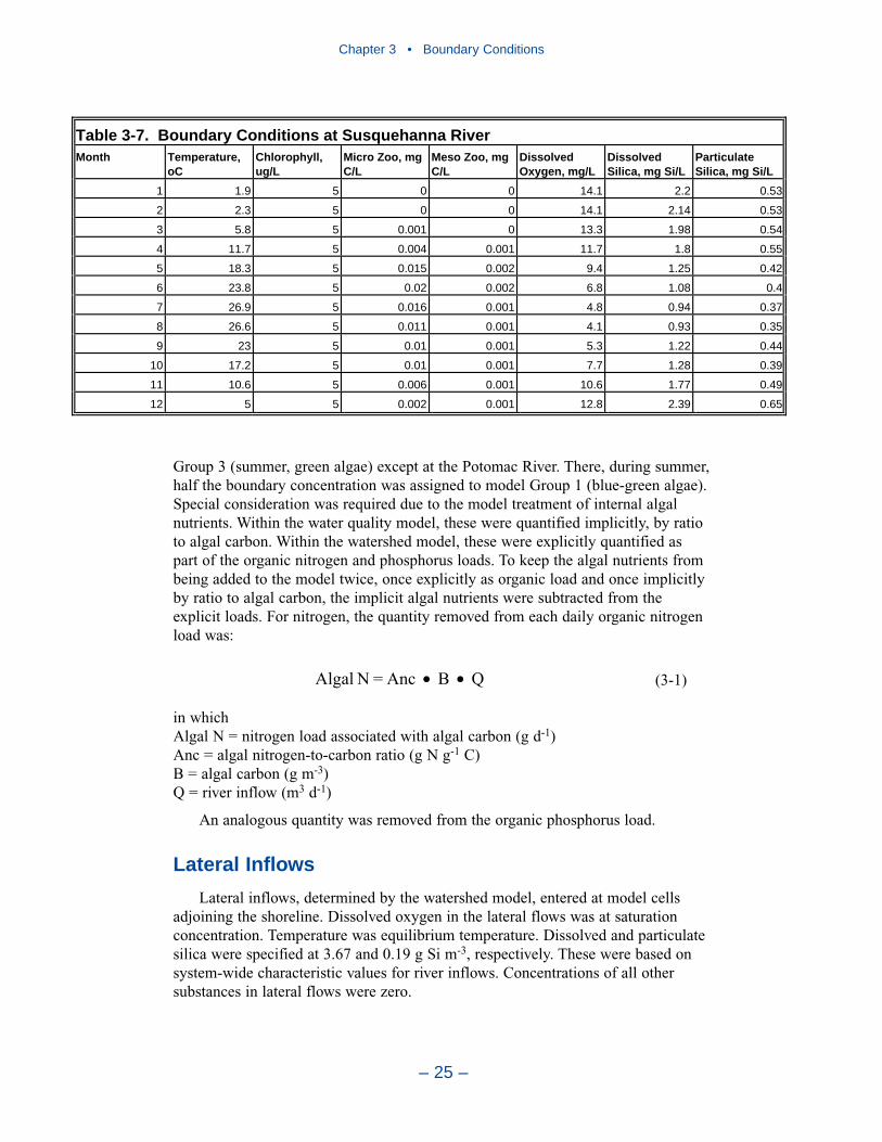
Group 3 (summer, green algae) except at the Potomac River. There, during summer,half the boundary concentration was assigned to model Group 1 (blue-green algae).Special consideration was required due to the model treatment of internal algalnutrients. Within the water quality model, these were quantified implicitly, by ratioto algal carbon. Within the watershed model, these were explicitly quantified aspart of the organic nitrogen and phosphorus loads. To keep the algal nutrients frombeing added to the model twice, once explicitly as organic load and once implicitlyby ratio to algal carbon, the implicit algal nutrients were subtracted from theexplicit loads. For nitrogen, the quantity removed from each daily organic nitrogenload was:
(3-1)
in whichAlgal N = nitrogen load associated with algal carbon (g d-1)Anc = algal nitrogen-to-carbon ratio (g N g-1 C)B = algal carbon (g m-3)Q = river inflow (m3 d-1)
An analogous quantity was removed from the organic phosphorus load.
Lateral Inflows
Lateral inflows, determined by the watershed model, entered at model cellsadjoining the shoreline. Dissolved oxygen in the lateral flows was at saturationconcentration. Temperature was equilibrium temperature. Dissolved and particulatesilica were specified at 3.67 and 0.19 g Si m-3, respectively. These were based onsystem-wide characteristic values for river inflows. Concentrations of all othersubstances in lateral flows were zero.
QBAnc=NAlgal ••
Chapter 3 • Boundary Conditions
– 25 –
Table 3-7. Boundary Conditions at Susquehanna River Month Temperature,
oCChlorophyll,ug/L
Micro Zoo, mg C/L
Meso Zoo, mg C/L
DissolvedOxygen, mg/L
DissolvedSilica, mg Si/L
ParticulateSilica, mg Si/L
1 1.9 5 0 0 14.1 2.2 0.53
2 2.3 5 0 0 14.1 2.14 0.53
3 5.8 5 0.001 0 13.3 1.98 0.54
4 11.7 5 0.004 0.001 11.7 1.8 0.55
5 18.3 5 0.015 0.002 9.4 1.25 0.42
6 23.8 5 0.02 0.002 6.8 1.08 0.4
7 26.9 5 0.016 0.001 4.8 0.94 0.37
8 26.6 5 0.011 0.001 4.1 0.93 0.35
9 23 5 0.01 0.001 5.3 1.22 0.44
10 17.2 5 0.01 0.001 7.7 1.28 0.39
11 10.6 5 0.006 0.001 10.6 1.77 0.49
12 5 5 0.002 0.001 12.8 2.39 0.65
Chapter 3 • Boundary Conditions
– 26 –
Ocean Boundary Conditions
Background
In the first version of the model (Cerco and Cole 1994), the open edge of themodel grid was at the entrance to Chesapeake Bay. Boundary concentrations wereinitially based on an array of Chesapeake Bay Program monitoring stations coinci-dent with the edge of the model grid. Inspection of the short record then availablesuggested nitrogen and phosphorus concentrations at the mouth were declining inresponse to load reductions within the bay. A requirement was imposed that themodel boundary conditions should respond to conditions within the bay. Conse-quently, “mass balance” boundary conditions were developed for nitrogen andphosphorus. The mass-balance boundary conditions determined the inflowingconcentrations of nitrogen and phosphorus as a weighted sum of outflowingconcentrations and concentrations in a hypothetical oceanic reservoir.
The mass-balance boundary conditions were successful but unnecessary. Sensi-tivity runs (Cerco and Cole 1994) indicated the inflowing nutrient concentrations atthe mouth declined by only 5% (phosphorus) to 10% (nitrogen) following loadreductions of 90%. Moreover, the apparent reduction in nitrogen concentration atthe mouth was attributed to changes in methodology. (The reduction in phosphorusremains unexplained to this day.)
In the Tributary Refinements phase of model development (Cerco et al. 2002),the grid was extended beyond the bay mouth, out onto the continental shelf. Theprimary objective was to ensure that boundary conditions specified at the edge ofthe grid were beyond the influence of conditions within the bay. The grid extensiontraded one set of problems for another. Model boundaries were moved from a loca-tion with abundant observations to multiple locations at which little informationwas available. Surveys conducted from May 1995 to August 1996 provided infor-mation on key water quality constituents but detailed boundary conditions for thesimulation period, 1985-1994, could not be reconstructed. Boundary conditions formajor nitrogen and phosphorus constituents were specified as constant concentra-tions throughout the simulation period. As a consequence, mean nitrogen andphosphorus concentrations at the mouth of the bay were well represented but thedynamics, especially of nitrogen, were not.
In the present phase of the model study, specification of boundary conditions atthe edge of the grid proved especially problematic. During the re-evaluation of thehydrodynamic model and refinement of water quality model kinetics, unpredictablebehavior occurred in the portion of the grid outside the bay mouth. Both modelswere in a transient state of development yet both models were expected to computedynamics in a region for which no data existed. Circulation and water qualitycomputed at the bay mouth were unsuited for calibration of the models within thebay. For the water quality model, the strategy was developed in which conditionsobserved at the bay mouth were extended to the edges of the grid. Kinetics weredisabled outside the bay mouth to prevent substance transformations. This strategycarried over into the final calibration of the present model.
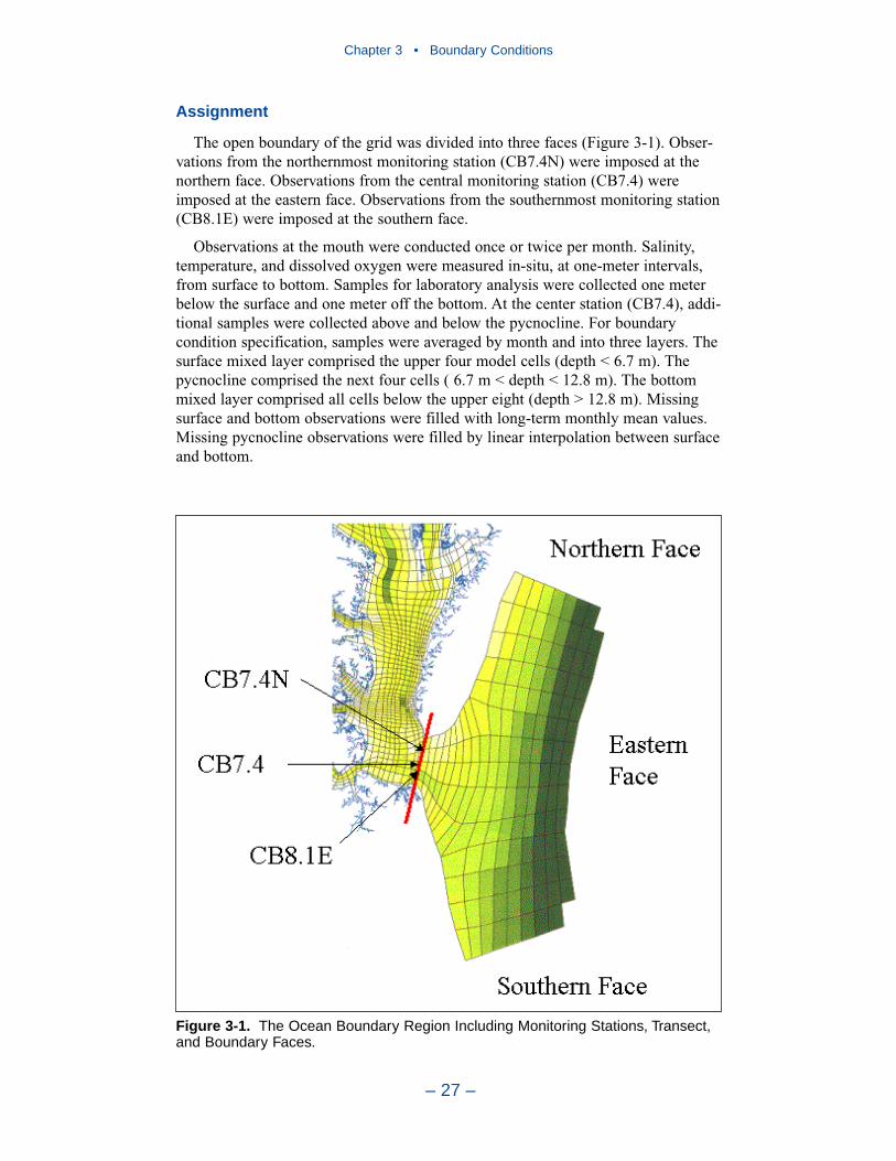
Assignment
The open boundary of the grid was divided into three faces (Figure 3-1). Obser-vations from the northernmost monitoring station (CB7.4N) were imposed at thenorthern face. Observations from the central monitoring station (CB7.4) wereimposed at the eastern face. Observations from the southernmost monitoring station(CB8.1E) were imposed at the southern face.
Observations at the mouth were conducted once or twice per month. Salinity,temperature, and dissolved oxygen were measured in-situ, at one-meter intervals,from surface to bottom. Samples for laboratory analysis were collected one meterbelow the surface and one meter off the bottom. At the center station (CB7.4), addi-tional samples were collected above and below the pycnocline. For boundarycondition specification, samples were averaged by month and into three layers. Thesurface mixed layer comprised the upper four model cells (depth < 6.7 m). Thepycnocline comprised the next four cells ( 6.7 m < depth < 12.8 m). The bottommixed layer comprised all cells below the upper eight (depth > 12.8 m). Missingsurface and bottom observations were filled with long-term monthly mean values.Missing pycnocline observations were filled by linear interpolation between surfaceand bottom.
Chapter 3 • Boundary Conditions
– 27 –
Figure 3-1. The Ocean Boundary Region Including Monitoring Stations, Transect,and Boundary Faces.
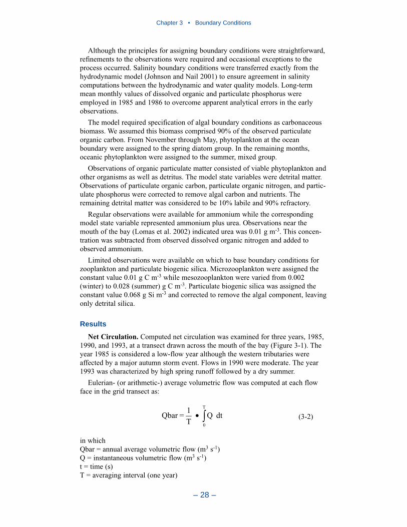
Chapter 3 • Boundary Conditions
– 28 –
Although the principles for assigning boundary conditions were straightforward,refinements to the observations were required and occasional exceptions to theprocess occurred. Salinity boundary conditions were transferred exactly from thehydrodynamic model (Johnson and Nail 2001) to ensure agreement in salinitycomputations between the hydrodynamic and water quality models. Long-termmean monthly values of dissolved organic and particulate phosphorus wereemployed in 1985 and 1986 to overcome apparent analytical errors in the earlyobservations.
The model required specification of algal boundary conditions as carbonaceousbiomass. We assumed this biomass comprised 90% of the observed particulateorganic carbon. From November through May, phytoplankton at the oceanboundary were assigned to the spring diatom group. In the remaining months,oceanic phytoplankton were assigned to the summer, mixed group.
Observations of organic particulate matter consisted of viable phytoplankton andother organisms as well as detritus. The model state variables were detrital matter.Observations of particulate organic carbon, particulate organic nitrogen, and partic-ulate phosphorus were corrected to remove algal carbon and nutrients. Theremaining detrital matter was considered to be 10% labile and 90% refractory.
Regular observations were available for ammonium while the correspondingmodel state variable represented ammonium plus urea. Observations near themouth of the bay (Lomas et al. 2002) indicated urea was 0.01 g m-3. This concen-tration was subtracted from observed dissolved organic nitrogen and added toobserved ammonium.
Limited observations were available on which to base boundary conditions forzooplankton and particulate biogenic silica. Microzooplankton were assigned theconstant value 0.01 g C m-3 while mesozooplankton were varied from 0.002(winter) to 0.028 (summer) g C m-3. Particulate biogenic silica was assigned theconstant value 0.068 g Si m-3 and corrected to remove the algal component, leavingonly detrital silica.
Results
Net Circulation. Computed net circulation was examined for three years, 1985,1990, and 1993, at a transect drawn across the mouth of the bay (Figure 3-1). Theyear 1985 is considered a low-flow year although the western tributaries wereaffected by a major autumn storm event. Flows in 1990 were moderate. The year1993 was characterized by high spring runoff followed by a dry summer.
Eulerian- (or arithmetic-) average volumetric flow was computed at each flowface in the grid transect as:
(3-2)
in whichQbar = annual average volumetric flow (m3 s-1)Q = instantaneous volumetric flow (m3 s-1)t = time (s)T = averaging interval (one year)
dtQT
1=Qbar
T
0
∫•

Results (Figures 3-2 to 3-4) conform to expectations. Net flows in the deepestportion of the transect, driven by a longitudinal density gradient, are into the bay.Flows out of the bay are confined to surface waters. Rotational effects tilt the levelof no net motion so that flows at the northern side of the transect tend to be into thebay at all depths. A small irregularity occasionally occurs at one depth on thenorthern side (Figures 3-3, 3-4). We cannot determine if this truly reflects a
Chapter 3 • Boundary Conditions
– 29 –
Figure 3-2. Net Volumetric Flows (m3 s-1) at the Mouth of the Bay for 1985. This view is intothe Bay from the Shelf. Positive flows are into the Bay.
Figure 3-4. Net Volumetric Flows (m3 s-1) atthe Mouth of the Bay for 1993. This view is intothe Bay from the Shelf. Positive flows are intothe Bay.
Figure 3-3. Net Volumetric Flows (m3 s-1) at the Mouth of the Bay for 1990. This view is intothe Bay from the Shelf. Positive flows are into the Bay.
complex circulation pattern or if this irregularity is an artifact of the grid and/orboundary conditions. Annual net flows in and out of the bay are roughly 3,000 and6,000 m3 s-1, respectively (Table 3-8). The computed flows are in reasonable agree-ment with net flows, 6,000 to 8,000 m3 s-1, measured during two months in 1971(Boicourt 1973).
Salinity Structure. Annual-mean computed salinity at the mouth (Figures 3-5 to3-7) is influenced by the effects of density, rotation, and boundary conditions. Therotational effects produce a tilting of the computed pycnocline. In the upper four orfive model layers (depth < 7 m), the water on the south side is fresher than wateron the north side at the same depth. This phenomenon is apparent in the observa-tions as well. The observations suggest the depth of the computed freshwater plumeshould be greater than the present representation but a more detailed analysis isrequired. The apparent disparity in plume depths may be an artifact of comparingaverages of discrete observations with continuous model results.
In deeper waters (depth > 7 m), salinity computed on the north side is less than onthe south side at the same depth. This phenomenon is also suggested in the observa-tions. The lower-salinity water originates in a plume that hugs the Delmarva peninsulaand enters the bay at the northern side of the mouth. Salinity boundary conditions onthe northern face, adjacent to the coast, were related to flow in the Delaware River(Cerco et al. 2002) and were lower than elsewhere on the grid perimeter.
Computed Concentrations at Bay Mouth. Selected comparisons of computedand observed concentrations for Station CB8.1E (Figure 3-1) are presented here.This station is in a channel (20 m) on the southern side of the bay mouth. At thislocation, net flow in the surface water (depth < 7 m) is usually out of the bay whilenet flow in deeper water is into the bay (Figures 3-2 to 3-4). Complete time seriescomparisons for all substances and stations across the mouth are included in anappendix to this report.
Chapter 3 • Boundary Conditions
– 30 –
Table 3-8. Volume and Mass Transport at Bay Mouth Flow,m3 sec-1
DIN,ton d-1
Total N,ton d-1
DIP,ton d-1
Total P,ton d-1
1985
In 3262 15 89 5.2 10.2
Out -5025 -54 -202 -4.3 -8.3
Net -1762 -38 -113 0.9 1.9
1990
In 3784 17 87 5.5 10.3
Out -6637 -40 -258 -4.7 -10.3
Net -2854 -23 -171 0.8 -0.0
1993
In 3707 15 91 4.1 9.7
Out -6564 -58 -277 -4.7 -9.5
Net -2857 -43 -186 -0.5 0.2

Chapter 3 • Boundary Conditions
– 31 –
Figure 3-5. Annual-Average Computedand Observed Salinity at the Mouth ofthe Bay for 1985. This View is into theBay from the Shelf. Observations(Circles) are Superimposed on ModelValues. Bottom observations werecollected in deep channels not entirelyrepresented by the model grid.
Figure 3-6. Annual-Average Computedand Observed Salinity at the Mouth ofthe Bay for 1990. This View is into theBay from the Shelf. Observations(Circles) are Superimposed on ModelValues. Bottom observations werecollected in deep channels not entirelyrepresented by the model grid.
Figure 3-7. Annual-Average Computedand Observed Salinity at the Mouth ofthe Bay for 1993. This View is into theBay from the Shelf. Observations(Circles) are Superimposed on ModelValues. Bottom observations werecollected in deep channels not entirelyrepresented by the model grid.
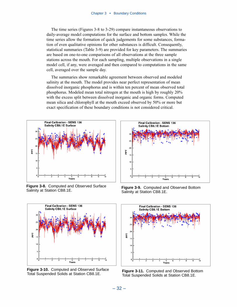
The time series (Figures 3-8 to 3-29) compare instantaneous observations todaily-average model computations for the surface and bottom samples. While thetime series allow the formation of quick judgements for some substances, forma-tion of even qualitative opinions for other substances is difficult. Consequently,statistical summaries (Table 3-9) are provided for key parameters. The summariesare based on one-to-one comparisons of all observations at the three samplestations across the mouth. For each sampling, multiple observations in a singlemodel cell, if any, were averaged and then compared to computations in the samecell, averaged over the sample day.
The summaries show remarkable agreement between observed and modeledsalinity at the mouth. The model provides near perfect representation of meandissolved inorganic phosphorus and is within ten percent of mean observed totalphosphorus. Modeled mean total nitrogen at the mouth is high by roughly 20%with the excess split between dissolved inorganic and organic forms. Computedmean silica and chlorophyll at the mouth exceed observed by 50% or more butexact specification of these boundary conditions is not considered critical.
Chapter 3 • Boundary Conditions
– 32 –
Figure 3-8. Computed and Observed SurfaceSalinity at Station CB8.1E.
Figure 3-9. Computed and Observed BottomSalinity at Station CB8.1E.
Figure 3-10. Computed and Observed SurfaceTotal Suspended Solids at Station CB8.1E.
Figure 3-11. Computed and Observed BottomTotal Suspended Solids at Station CB8.1E.
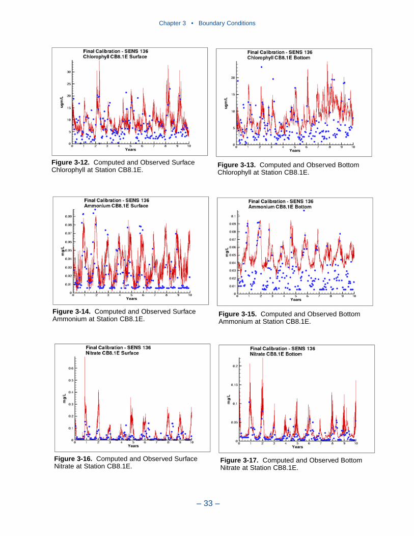
Chapter 3 • Boundary Conditions
– 33 –
Figure 3-12. Computed and Observed SurfaceChlorophyll at Station CB8.1E.
Figure 3-13. Computed and Observed BottomChlorophyll at Station CB8.1E.
Figure 3-14. Computed and Observed SurfaceAmmonium at Station CB8.1E.
Figure 3-15. Computed and Observed BottomAmmonium at Station CB8.1E.
Figure 3-16. Computed and Observed SurfaceNitrate at Station CB8.1E.
Figure 3-17. Computed and Observed BottomNitrate at Station CB8.1E.
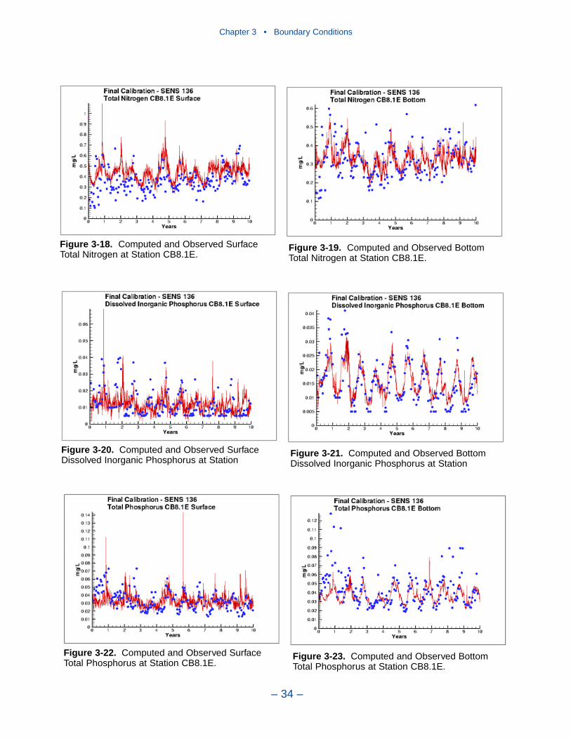
Chapter 3 • Boundary Conditions
– 34 –
Figure 3-18. Computed and Observed SurfaceTotal Nitrogen at Station CB8.1E.
Figure 3-19. Computed and Observed BottomTotal Nitrogen at Station CB8.1E.
Figure 3-20. Computed and Observed SurfaceDissolved Inorganic Phosphorus at Station
Figure 3-21. Computed and Observed BottomDissolved Inorganic Phosphorus at Station
Figure 3-22. Computed and Observed SurfaceTotal Phosphorus at Station CB8.1E.
Figure 3-23. Computed and Observed BottomTotal Phosphorus at Station CB8.1E.
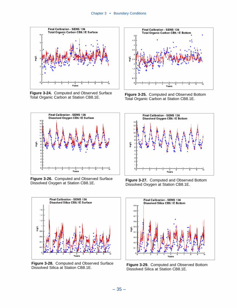
Chapter 3 • Boundary Conditions
– 35 –
Figure 3-24. Computed and Observed SurfaceTotal Organic Carbon at Station CB8.1E.
Figure 3-25. Computed and Observed BottomTotal Organic Carbon at Station CB8.1E.
Figure 3-26. Computed and Observed SurfaceDissolved Oxygen at Station CB8.1E.
Figure 3-27. Computed and Observed BottomDissolved Oxygen at Station CB8.1E.
Figure 3-28. Computed and Observed SurfaceDissolved Silica at Station CB8.1E.
Figure 3-29. Computed and Observed BottomDissolved Silica at Station CB8.1E.
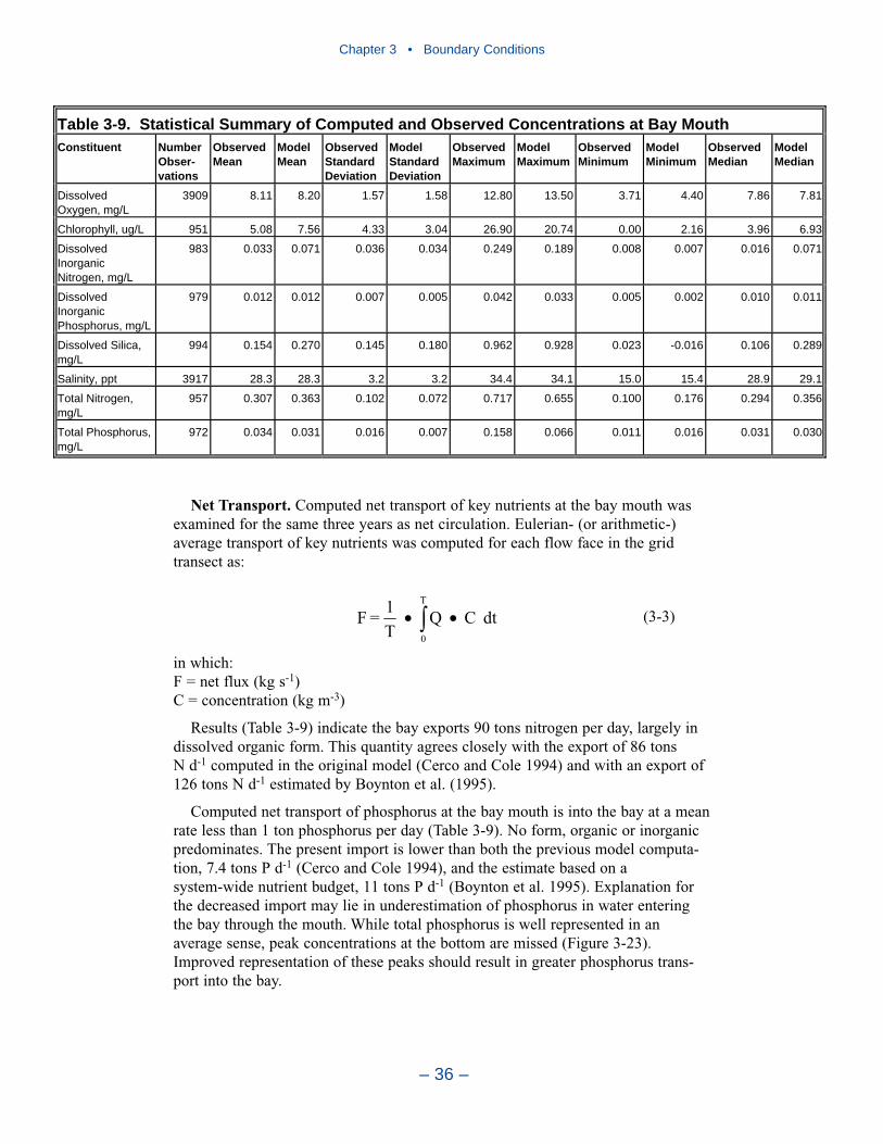
Net Transport. Computed net transport of key nutrients at the bay mouth wasexamined for the same three years as net circulation. Eulerian- (or arithmetic-)average transport of key nutrients was computed for each flow face in the gridtransect as:
(3-3)
in which:F = net flux (kg s-1)C = concentration (kg m-3)
Results (Table 3-9) indicate the bay exports 90 tons nitrogen per day, largely indissolved organic form. This quantity agrees closely with the export of 86 tons N d-1 computed in the original model (Cerco and Cole 1994) and with an export of126 tons N d-1 estimated by Boynton et al. (1995).
Computed net transport of phosphorus at the bay mouth is into the bay at a meanrate less than 1 ton phosphorus per day (Table 3-9). No form, organic or inorganicpredominates. The present import is lower than both the previous model computa-tion, 7.4 tons P d-1 (Cerco and Cole 1994), and the estimate based on asystem-wide nutrient budget, 11 tons P d-1 (Boynton et al. 1995). Explanation forthe decreased import may lie in underestimation of phosphorus in water enteringthe bay through the mouth. While total phosphorus is well represented in anaverage sense, peak concentrations at the bottom are missed (Figure 3-23).Improved representation of these peaks should result in greater phosphorus trans-port into the bay.
dtCQT
1=F
T
0
•• ∫
Chapter 3 • Boundary Conditions
– 36 –
Table 3-9. Statistical Summary of Computed and Observed Concentrations at Bay MouthConstituent Number
Obser-vations
ObservedMean
ModelMean
ObservedStandardDeviation
ModelStandardDeviation
ObservedMaximum
ModelMaximum
ObservedMinimum
ModelMinimum
ObservedMedian
ModelMedian
Dissolved Oxygen, mg/L
3909 8.11 8.20 1.57 1.58 12.80 13.50 3.71 4.40 7.86 7.81
Chlorophyll, ug/L 951 5.08 7.56 4.33 3.04 26.90 20.74 0.00 2.16 3.96 6.93
Dissolved InorganicNitrogen, mg/L
983 0.033 0.071 0.036 0.034 0.249 0.189 0.008 0.007 0.016 0.071
Dissolved InorganicPhosphorus, mg/L
979 0.012 0.012 0.007 0.005 0.042 0.033 0.005 0.002 0.010 0.011
Dissolved Silica, mg/L
994 0.154 0.270 0.145 0.180 0.962 0.928 0.023 -0.016 0.106 0.289
Salinity, ppt 3917 28.3 28.3 3.2 3.2 34.4 34.1 15.0 15.4 28.9 29.1
Total Nitrogen, mg/L
957 0.307 0.363 0.102 0.072 0.717 0.655 0.100 0.176 0.294 0.356
Total Phosphorus,mg/L
972 0.034 0.031 0.016 0.007 0.158 0.066 0.011 0.016 0.031 0.030
A Recommendation
Extension of the grid onto the continental shelf had two objectives. The first wasto move nutrient boundary conditions to a location beyond the influence of loadswithin the bay. The second was to allow for coupling with a proposed continentalshelf model. The first objective was met, albeit with trade-offs. The proposed shelfmodel has been postponed indefinitely.
In retrospect, extension of the boundaries to avoid influence of bay loads wasunnecessary. From 70% to 85% of the mix of water at the bay mouth originates inthe sea rather than in rivers, as evidenced by typical salinities of 25 to 30 ppt.Riverine and point-source loads are attenuated during transport such that a 90%load reduction results in only 5% to 10% concentration changes at the bay mouth(Cerco and Cole 1994). The extension of the grid produced enormous difficultiesfor both the hydrodynamic and water quality modeling teams and certainly did notincrease the accuracy of either model. Consequently, we recommend the boundarybe restored to the mouth of the bay in future model efforts.
Grid refinements also produce enormous difficulties. The present boundarycondition “works.” The grid should not be refined solely to alter the location of theboundaries. If future modeling requires grid changes, however, considerationshould be given to restoration of the boundary to the bay mouth.
References
Boicourt, W. (1973). “Circulation of water on the continental shelf from Chesapeake Bay toCape Hatteras,” Ph.D. diss., Johns Hopkins University, Baltimore, MD.
Boynton, W., Garber, J., Summers, R., and Kemp, W. (1995). “Inputs, transformations, andtransport of nitrogen and phosphorus in Chesapeake Bay and selected tributaries,”Estuaries, 18(1B), 285-314.
Cerco, C., and Cole, T. (1994). “Three-dimensional eutrophication model of ChesapeakeBay,” Technical Report El-94-4, US Army Engineer Waterways Experiment Station, Vicks-burg MS.
Cerco, C., Johnson, B., and Wang, H. (2002). “Tributary refinements to the Chesapeake Baymodel,” ERDC TR-02-4, US Army Engineer Research and Development Center, VicksburgMS.
Johnson, B., and Nail, G. (2001). “A 10-year (1985-1994) simulation with a refined three-dimensional numerical hydrodynamic, salinity, and temperature model of Chesapeake Bayand its tributaries,” June 2001 Draft Report, Coastal and Hydraulics Laboratory, US ArmyEngineer Research and Development Center, Vicksburg MS.
Lomas, M., Trice, T., Glibert, P., Bronk, D., and McCarthy, J. (2002). “Temporal and spatialdynamics of urea concentrations in Chesapeake Bay: biological versus physical forcing,”Estuaries, submitted.
Chapter 3 • Boundary Conditions
– 37 –
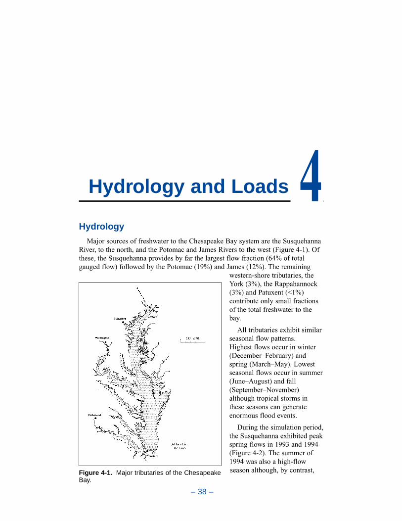
Hydrology
Major sources of freshwater to the Chesapeake Bay system are the SusquehannaRiver, to the north, and the Potomac and James Rivers to the west (Figure 4-1). Ofthese, the Susquehanna provides by far the largest flow fraction (64% of totalgauged flow) followed by the Potomac (19%) and James (12%). The remaining
western-shore tributaries, theYork (3%), the Rappahannock(3%) and Patuxent (<1%)contribute only small fractionsof the total freshwater to thebay.
All tributaries exhibit similarseasonal flow patterns. Highest flows occur in winter(December–February) andspring (March–May). Lowestseasonal flows occur in summer(June–August) and fall(September–November)although tropical storms inthese seasons can generateenormous flood events.
During the simulation period,the Susquehanna exhibited peakspring flows in 1993 and 1994(Figure 4-2). The summer of1994 was also a high-flowseason although, by contrast,
– 38 –
Hydrology and Loads 4
Figure 4-1. Major tributaries of the ChesapeakeBay.
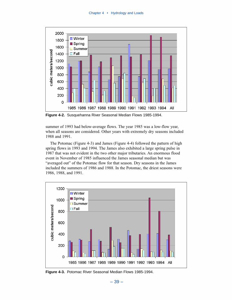
summer of 1993 had below-average flows. The year 1985 was a low-flow year,when all seasons are considered. Other years with extremely dry seasons included1988 and 1991.
The Potomac (Figure 4-3) and James (Figure 4-4) followed the pattern of highspring flows in 1993 and 1994. The James also exhibited a large spring pulse in1987 that was not evident in the two other major tributaries. An enormous floodevent in November of 1985 influenced the James seasonal median but was“averaged out” of the Potomac flow for that season. Dry seasons in the Jamesincluded the summers of 1986 and 1988. In the Potomac, the driest seasons were1986, 1988, and 1991.
Chapter 4 • Hydrology and Loads
– 39 –
Figure 4-2. Susquehanna River Seasonal Median Flows 1985-1994.
Figure 4-3. Potomac River Seasonal Median Flows 1985-1994.
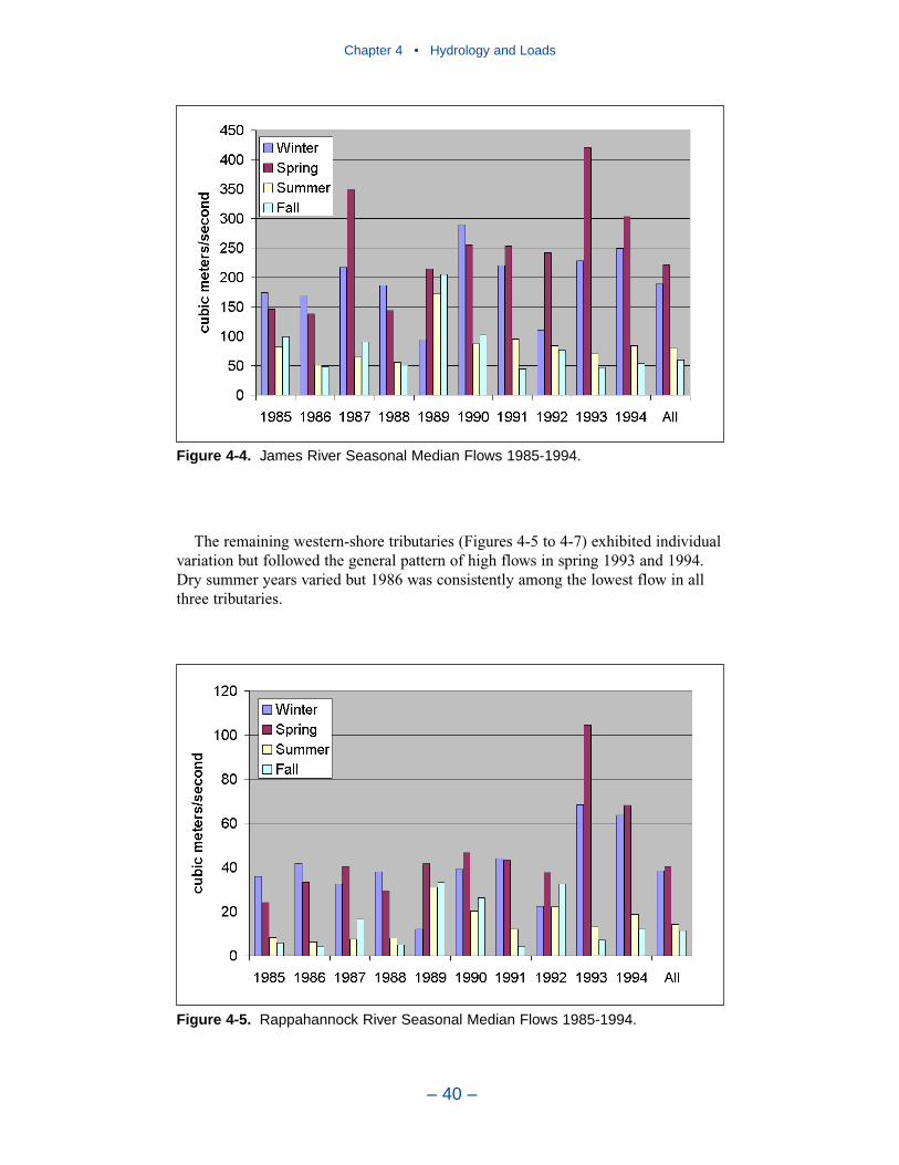
The remaining western-shore tributaries (Figures 4-5 to 4-7) exhibited individualvariation but followed the general pattern of high flows in spring 1993 and 1994.Dry summer years varied but 1986 was consistently among the lowest flow in allthree tributaries.
Chapter 4 • Hydrology and Loads
– 40 –
Figure 4-4. James River Seasonal Median Flows 1985-1994.
Figure 4-5. Rappahannock River Seasonal Median Flows 1985-1994.
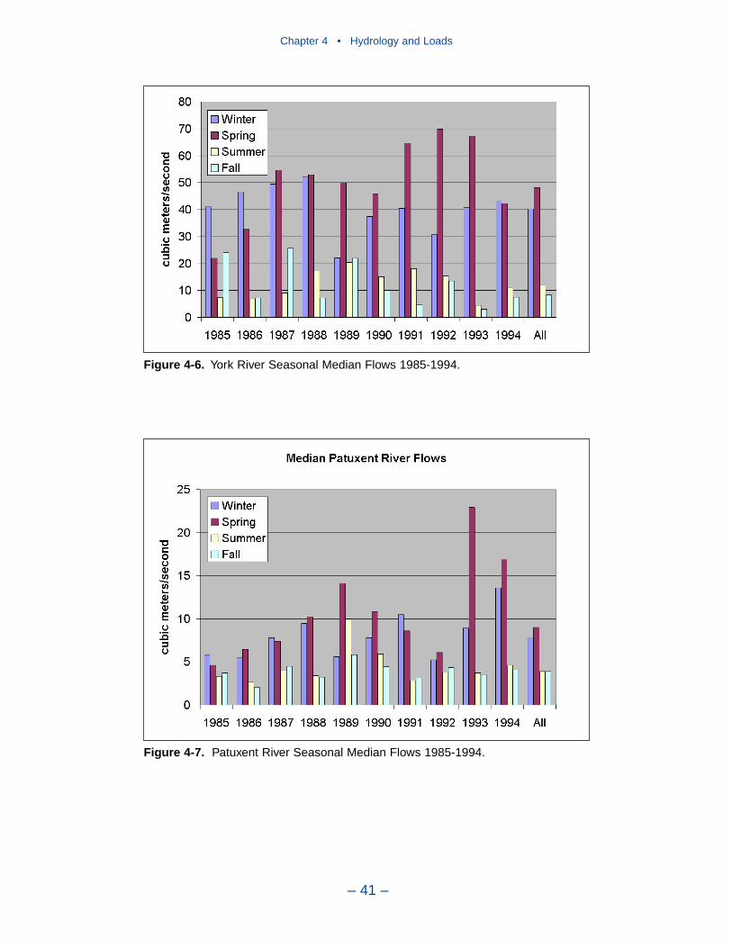
Chapter 4 • Hydrology and Loads
– 41 –
Figure 4-6. York River Seasonal Median Flows 1985-1994.
Figure 4-7. Patuxent River Seasonal Median Flows 1985-1994.
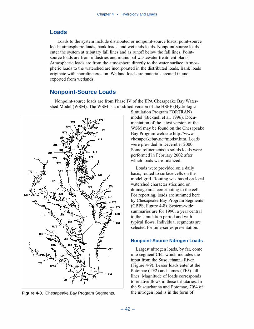
Chapter 4 • Hydrology and Loads
– 42 –
Loads
Loads to the system include distributed or nonpoint-source loads, point-sourceloads, atmospheric loads, bank loads, and wetlands loads. Nonpoint-source loadsenter the system at tributary fall lines and as runoff below the fall lines. Point-source loads are from industries and municipal wastewater treatment plants.Atmospheric loads are from the atmosphere directly to the water surface. Atmos-pheric loads to the watershed are incorporated in the distributed loads. Bank loadsoriginate with shoreline erosion. Wetland loads are materials created in andexported from wetlands.
Nonpoint-Source Loads
Nonpoint-source loads are from Phase IV of the EPA Chesapeake Bay Water-shed Model (WSM). The WSM is a modified version of the HSPF (Hydrologic
Simulation Program FORTRAN)model (Bicknell et al. 1996). Docu-mentation of the latest version of theWSM may be found on the ChesapeakeBay Program web site http://www.chesapeakebay.net/modsc.htm. Loadswere provided in December 2000.Some refinements to solids loads wereperformed in February 2002 afterwhich loads were finalized.
Loads were provided on a dailybasis, routed to surface cells on themodel grid. Routing was based on localwatershed characteristics and ondrainage area contributing to the cell.For reporting, loads are summed hereby Chesapeake Bay Program Segments(CBPS, Figure 4-8). System-widesummaries are for 1990, a year centralto the simulation period and withtypical flows. Individual segments areselected for time-series presentation.
Nonpoint-Source Nitrogen Loads
Largest nitrogen loads, by far, comeinto segment CB1 which includes theinput from the Susquehanna River(Figure 4-9). Lesser loads enter at thePotomac (TF2) and James (TF5) falllines. Magnitude of loads correspondsto relative flows in these tributaries. Inthe Susquehanna and Potomac, 70% ofthe nitrogen load is in the form ofFigure 4-8. Chesapeake Bay Program Segments.

nitrate while in the James 43% is nitrate. Segment ET6, on the lower EasternShore, receives the greatest load not associated with a fall line, of which 80% isnitrate.
Time series of major loads (Figures 4-10 to 4-13) demonstrate little correspon-dence to flows. Correspondence may be obscured by the comparison of annualmean loads with seasonal median flows. Above all, inspection indicates no trend innitrogen loading.
Chapter 4 • Hydrology and Loads
– 43 –
Figure 4-9. Nonpoint-Source Total Nitrogen by CBPS, 1990.
Figure 4-10. Annual Nonpoint-Source Nitrogen Loads in CB1, the SusquehannaFall Line
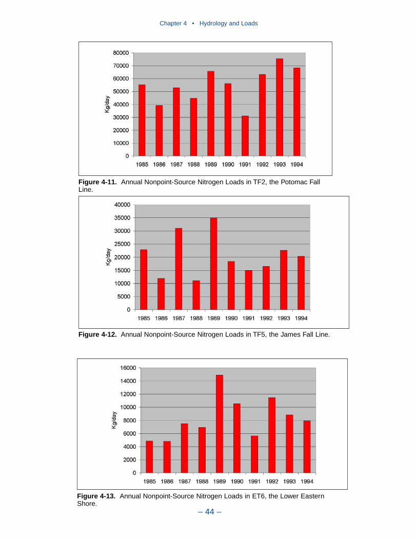
Chapter 4 • Hydrology and Loads
– 44 –
Figure 4-11. Annual Nonpoint-Source Nitrogen Loads in TF2, the Potomac FallLine.
Figure 4-12. Annual Nonpoint-Source Nitrogen Loads in TF5, the James Fall Line.
Figure 4-13. Annual Nonpoint-Source Nitrogen Loads in ET6, the Lower EasternShore.
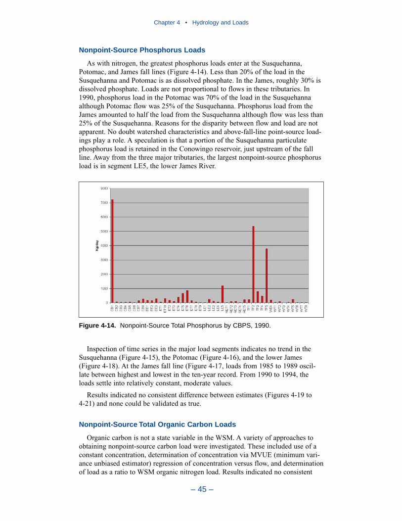
Nonpoint-Source Phosphorus Loads
As with nitrogen, the greatest phosphorus loads enter at the Susquehanna,Potomac, and James fall lines (Figure 4-14). Less than 20% of the load in theSusquehanna and Potomac is as dissolved phosphate. In the James, roughly 30% isdissolved phosphate. Loads are not proportional to flows in these tributaries. In1990, phosphorus load in the Potomac was 70% of the load in the Susquehannaalthough Potomac flow was 25% of the Susquehanna. Phosphorus load from theJames amounted to half the load from the Susquehanna although flow was less than25% of the Susquehanna. Reasons for the disparity between flow and load are notapparent. No doubt watershed characteristics and above-fall-line point-source load-ings play a role. A speculation is that a portion of the Susquehanna particulatephosphorus load is retained in the Conowingo reservoir, just upstream of the fallline. Away from the three major tributaries, the largest nonpoint-source phosphorusload is in segment LE5, the lower James River.
Inspection of time series in the major load segments indicates no trend in theSusquehanna (Figure 4-15), the Potomac (Figure 4-16), and the lower James(Figure 4-18). At the James fall line (Figure 4-17, loads from 1985 to 1989 oscil-late between highest and lowest in the ten-year record. From 1990 to 1994, theloads settle into relatively constant, moderate values.
Results indicated no consistent difference between estimates (Figures 4-19 to 4-21) and none could be validated as true.
Nonpoint-Source Total Organic Carbon Loads
Organic carbon is not a state variable in the WSM. A variety of approaches toobtaining nonpoint-source carbon load were investigated. These included use of aconstant concentration, determination of concentration via MVUE (minimum vari-ance unbiased estimator) regression of concentration versus flow, and determinationof load as a ratio to WSM organic nitrogen load. Results indicated no consistent
Chapter 4 • Hydrology and Loads
– 45 –
Figure 4-14. Nonpoint-Source Total Phosphorus by CBPS, 1990.
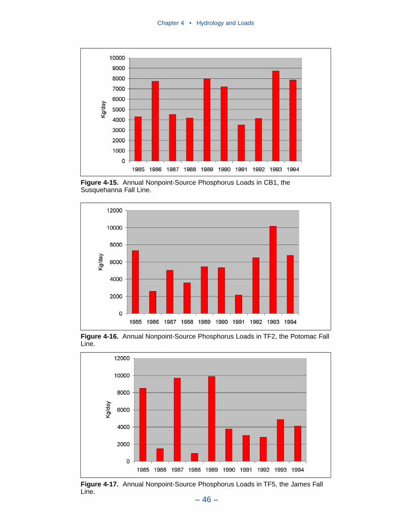
Chapter 4 • Hydrology and Loads
– 46 –
Figure 4-15. Annual Nonpoint-Source Phosphorus Loads in CB1, theSusquehanna Fall Line.
Figure 4-16. Annual Nonpoint-Source Phosphorus Loads in TF2, the Potomac FallLine.
Figure 4-17. Annual Nonpoint-Source Phosphorus Loads in TF5, the James FallLine.

Chapter 4 • Hydrology and Loads
– 47 –
Figure 4-18. Annual Nonpoint-Source Phosphorus Loads in LE5, the LowerJames River.
Figure 4-19. Susquehanna Total Organic Carbon Loads by Regression (MVUE),by Ratio to Watershed Model (WSM) and by Constant Concentration (Constant).
Figure 4-20. Potomac Total Organic Carbon Loads by Regression (MVUE), byRatio to Watershed Model (WSM) and by Constant Concentration (Constant).

difference between the estimates (Figures 4-19 to 4-21and none could be validatedas true. Ratio to the WSM was selected since this method allowed for computationof carbon load reductions in response to watershed management. Carbon-to-nitrogen ratios were obtained from fall-line observations posted by the USGSChesapeake Bay River Input Monitoring Program http://va.water.usgs.gov/chesbay/RIMP/). Observations were available for Maryland tributaries only. From these, acarbon-to-nitrogen ratio of 12 was specified system-wide except for the Potomacand Choptank. Ratios of 8 and 17.5 were specified for these fall lines, respectively.The distribution of nonpoint-source carbon loads across the system follows thepatterns of nitrogen and phosphorus; largest loads are at the Susquehanna,Potomac, and James fall lines (Figure 4-22).
Chapter 4 • Hydrology and Loads
– 48 –
Figure 4-21. James Total Organic Carbon Loads by Regression (MVUE), by Ratioto Watershed Model (WSM) and by Constant Concentration (Constant).
Figure 4-22. Nonpoint-Source Total Organic Carbon by CBPS, 1990.
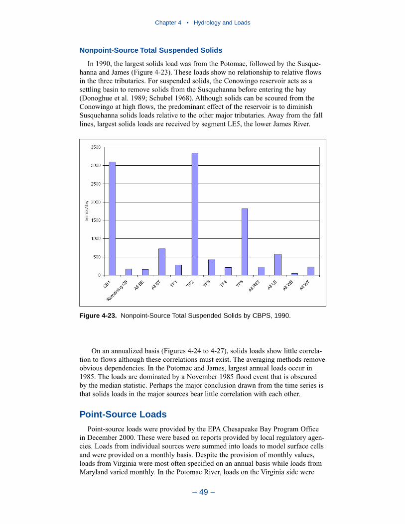
Nonpoint-Source Total Suspended Solids
In 1990, the largest solids load was from the Potomac, followed by the Susque-hanna and James (Figure 4-23). These loads show no relationship to relative flowsin the three tributaries. For suspended solids, the Conowingo reservoir acts as asettling basin to remove solids from the Susquehanna before entering the bay(Donoghue et al. 1989; Schubel 1968). Although solids can be scoured from theConowingo at high flows, the predominant effect of the reservoir is to diminishSusquehanna solids loads relative to the other major tributaries. Away from the falllines, largest solids loads are received by segment LE5, the lower James River.
On an annualized basis (Figures 4-24 to 4-27), solids loads show little correla-tion to flows although these correlations must exist. The averaging methods removeobvious dependencies. In the Potomac and James, largest annual loads occur in1985. The loads are dominated by a November 1985 flood event that is obscuredby the median statistic. Perhaps the major conclusion drawn from the time series isthat solids loads in the major sources bear little correlation with each other.
Point-Source Loads
Point-source loads were provided by the EPA Chesapeake Bay Program Officein December 2000. These were based on reports provided by local regulatory agen-cies. Loads from individual sources were summed into loads to model surface cellsand were provided on a monthly basis. Despite the provision of monthly values,loads from Virginia were most often specified on an annual basis while loads fromMaryland varied monthly. In the Potomac River, loads on the Virginia side were
Chapter 4 • Hydrology and Loads
– 49 –
Figure 4-23. Nonpoint-Source Total Suspended Solids by CBPS, 1990.
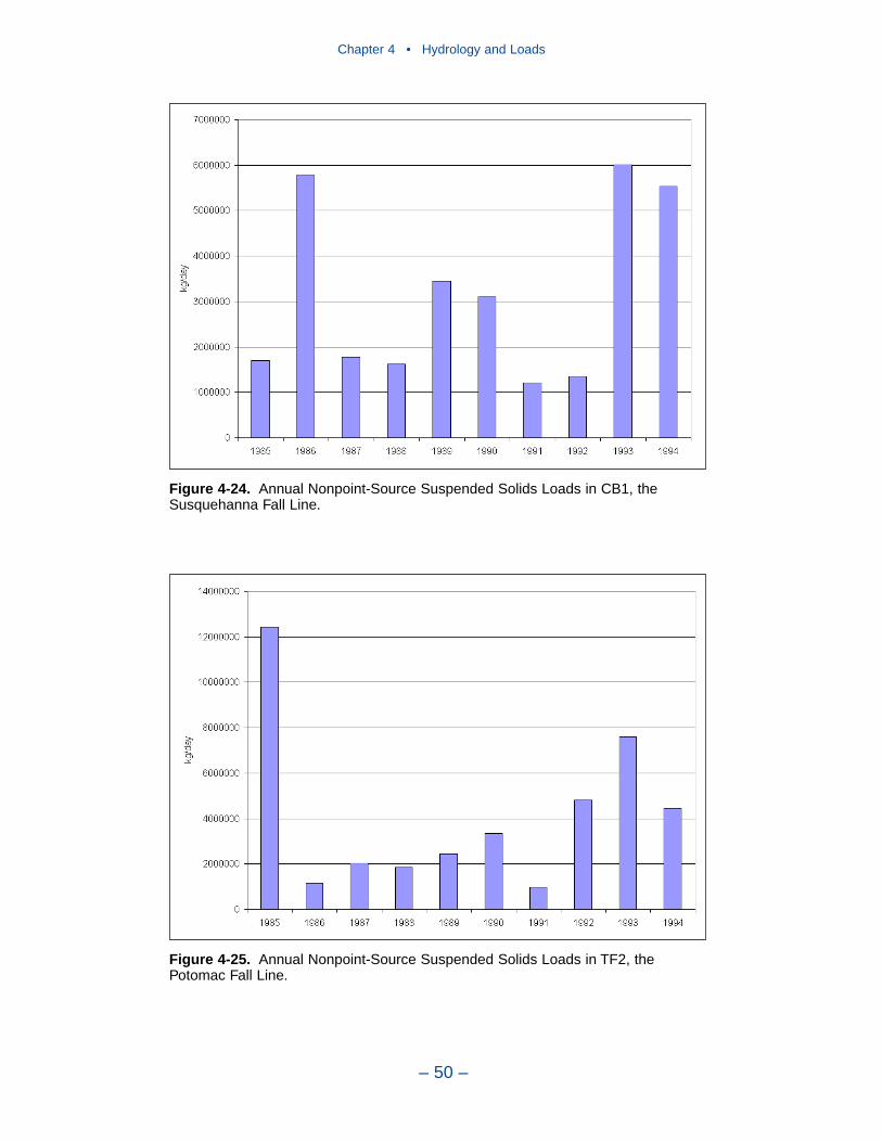
Chapter 4 • Hydrology and Loads
– 50 –
Figure 4-24. Annual Nonpoint-Source Suspended Solids Loads in CB1, theSusquehanna Fall Line.
Figure 4-25. Annual Nonpoint-Source Suspended Solids Loads in TF2, thePotomac Fall Line.
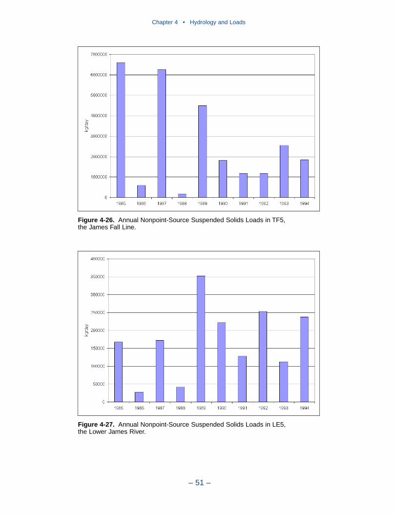
Chapter 4 • Hydrology and Loads
– 51 –
Figure 4-26. Annual Nonpoint-Source Suspended Solids Loads in TF5, the James Fall Line.
Figure 4-27. Annual Nonpoint-Source Suspended Solids Loads in LE5, the Lower James River.

annual loads while loads on the Maryland side were monthly loads. Examination ofthe Maryland loads indicates considerable variance (Figure 4-28) which is lackingin the specification of Virginia loads.
For reporting, loads are summed here by Chesapeake Bay Program Segments(CBPS, Figure 4-8). System-wide summaries are for 1990, a year central to thesimulation period. Individual segments are selected for time-series presentation.
Point-Source Nitrogen Loads
Point-source loads are concentrated in urban areas (Figure 4-29). Major nitrogenloads originate in Northern Virginia/District of Columbia (TF2), Richmond Virginia(TF5), Baltimore Maryland (WT5, WT4), and Hampton Roads Virginia (LE5). Ofthese, only loads to the Patapsco (WT5, Figure 4-32) show a monotonic decreasingtrend. Loads to the upper Potomac (TF2, Figure 4-30), and upper James (TF5,Figure 4-31) suggest a decrease after 1990. Point-source nitrogen loads to the BackRiver (WT4, Figure 4-33) and the lower James (LE5, Figure 4-34) show no trend.
Chapter 4 • Hydrology and Loads
– 52 –
Figure 4-28. Monthly (1994) Point-Source Phosphorus Loads to Model Cell 2846on the Maryland Shore of the Potomac River.
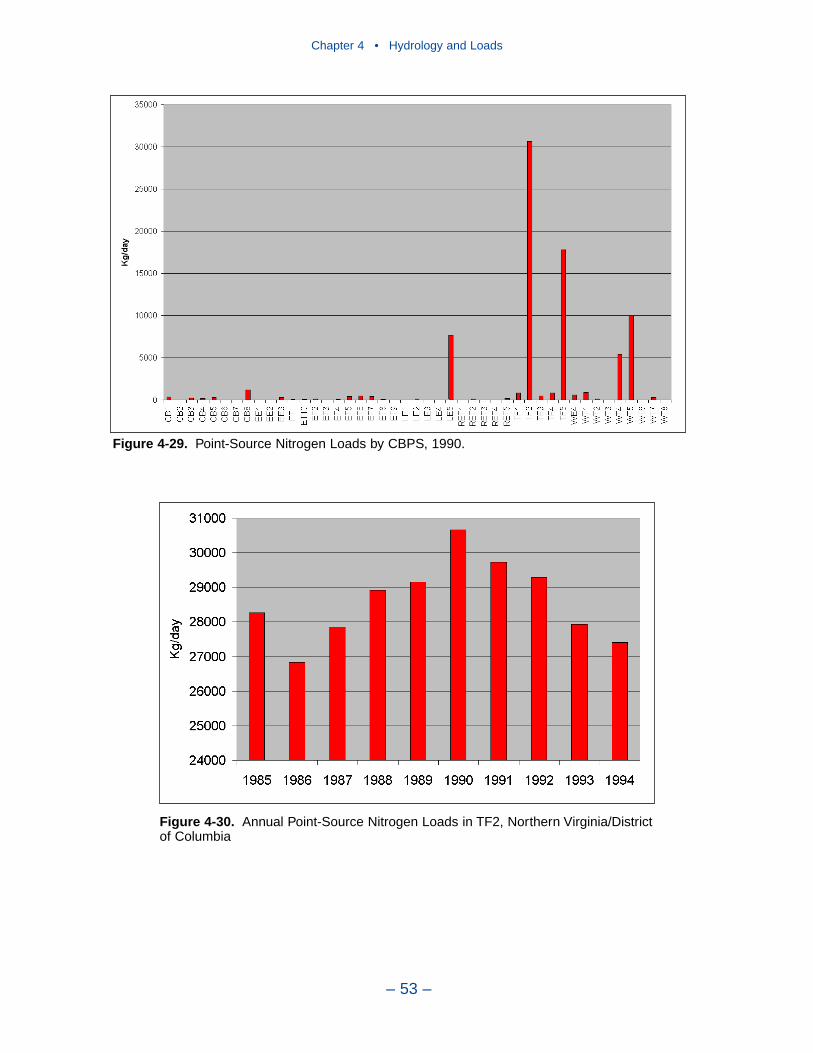
Chapter 4 • Hydrology and Loads
– 53 –
Figure 4-29. Point-Source Nitrogen Loads by CBPS, 1990.
Figure 4-30. Annual Point-Source Nitrogen Loads in TF2, Northern Virginia/Districtof Columbia
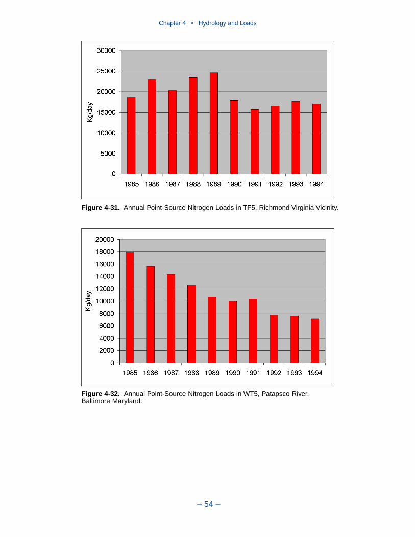
Chapter 4 • Hydrology and Loads
– 54 –
Figure 4-31. Annual Point-Source Nitrogen Loads in TF5, Richmond Virginia Vicinity.
Figure 4-32. Annual Point-Source Nitrogen Loads in WT5, Patapsco River,Baltimore Maryland.
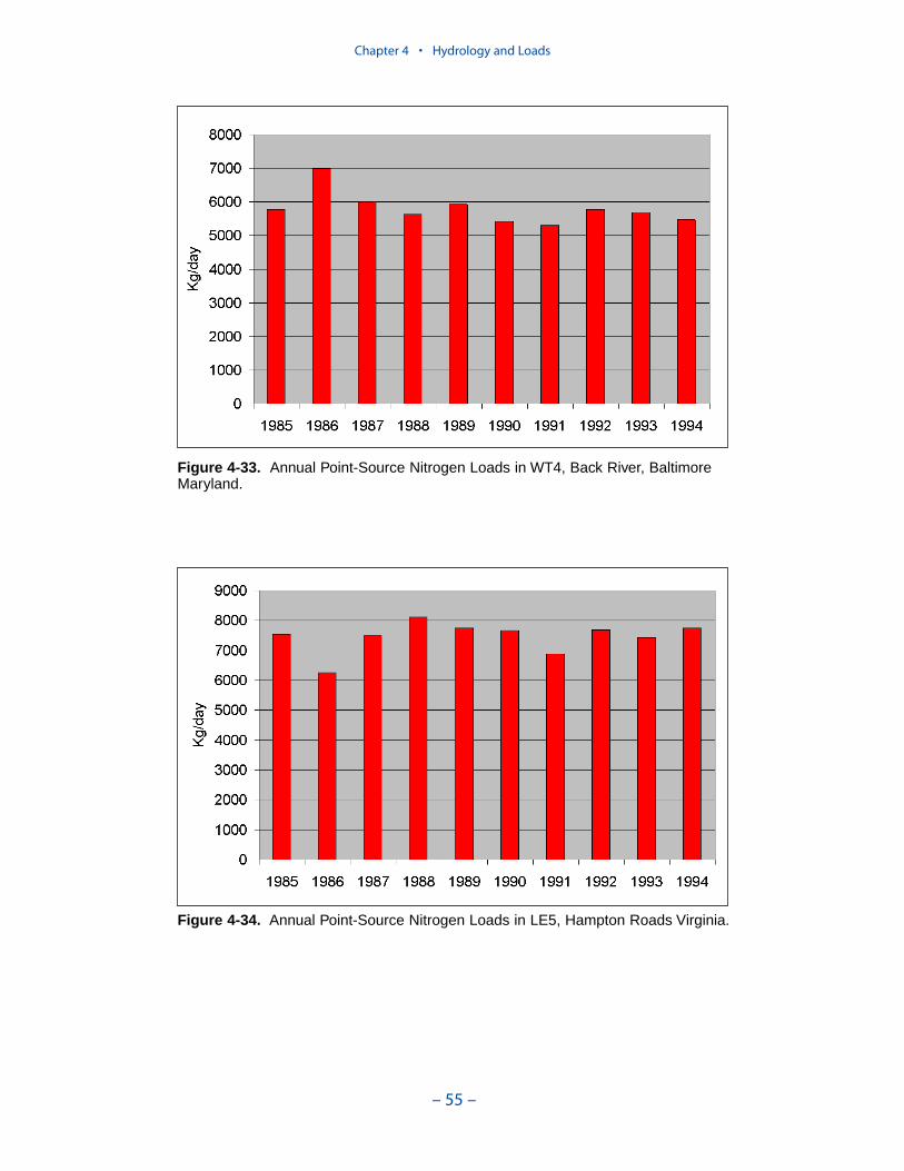
Chapter 4 • Hydrology and Loads
– 55 –
Figure 4-33. Annual Point-Source Nitrogen Loads in WT4, Back River, BaltimoreMaryland.
Figure 4-34. Annual Point-Source Nitrogen Loads in LE5, Hampton Roads Virginia.
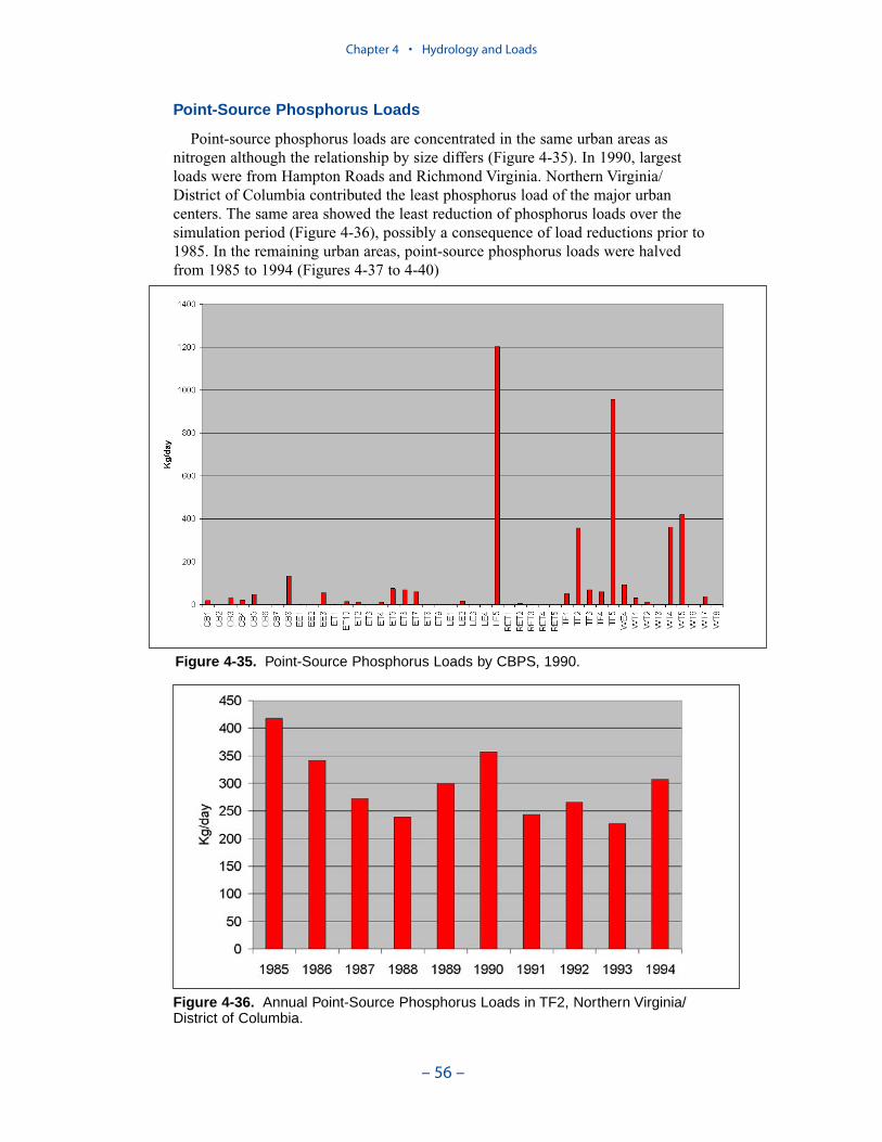
Point-Source Phosphorus Loads
Point-source phosphorus loads are concentrated in the same urban areas asnitrogen although the relationship by size differs (Figure 4-35). In 1990, largestloads were from Hampton Roads and Richmond Virginia. Northern Virginia/District of Columbia contributed the least phosphorus load of the major urbancenters. The same area showed the least reduction of phosphorus loads over thesimulation period (Figure 4-36), possibly a consequence of load reductions prior to1985. In the remaining urban areas, point-source phosphorus loads were halvedfrom 1985 to 1994 (Figures 4-37 to 4-40)
Chapter 4 • Hydrology and Loads
– 56 –
Figure 4-35. Point-Source Phosphorus Loads by CBPS, 1990.
Figure 4-36. Annual Point-Source Phosphorus Loads in TF2, Northern Virginia/District of Columbia.

Chapter 4 • Hydrology and Loads
– 57 –
Figure 4-37. Annual Point-Source Phosphorus Loads in TF5, Richmond Virginia Vicinity.
Figure 4-38. Annual Point-Source Phosphorus Loads in WT5, Patapsco River,Baltimore Maryland.
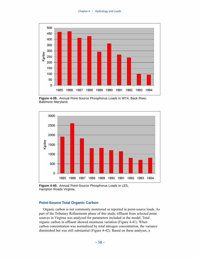
Point-Source Total Organic Carbon
Organic carbon is not commonly monitored or reported in point-source loads. Aspart of the Tributary Refinements phase of this study, effluent from selected pointsources in Virginia was analyzed for parameters included in the model. Totalorganic carbon in effluent showed enormous variation (Figure 4-41). When carbon concentration was normalized by total nitrogen concentration, the variancediminished but was still substantial (Figure 4-42). Based on these analyses, a
Chapter 4 • Hydrology and Loads
– 58 –
Figure 4-39. Annual Point-Source Phosphorus Loads in WT4, Back River, Baltimore Maryland.
Figure 4-40. Annual Point-Source Phosphorus Loads in LE5, Hampton Roads Virginia.

carbon-to-nitrogen ratio of 2:1 was utilized for point sources system-wide exceptfor the Chesapeake Corporation, located in the upper York River. Here, a ratio of10:1 was employed. Since carbon loads were obtained by simple ratio to nitrogenloads, the distribution of carbon loads (Figure 4-43) reflects the nitrogen load onwhich it is based.
Chapter 4 • Hydrology and Loads
– 59 –
Figure 4-41. Mean Total Organic Carbon Concentration in Virginia Point-SourceEffluent 1994-1995.
Figure 4-42. Carbon to Nitrogen Ratio in Virginia Point-Source Effluent 1994-1995.
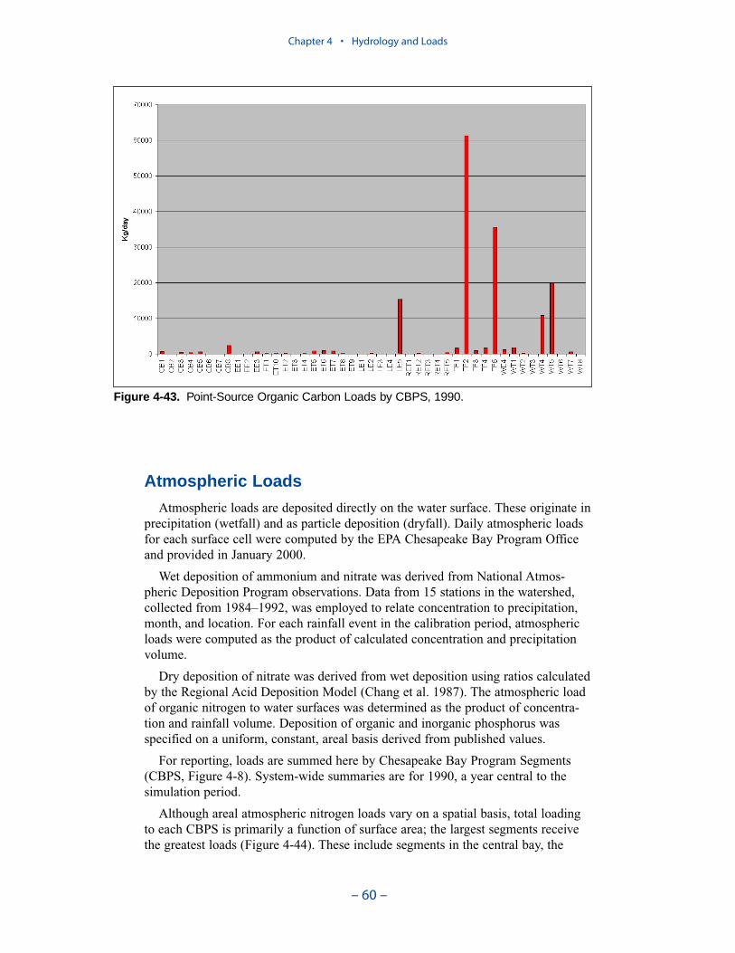
Atmospheric Loads
Atmospheric loads are deposited directly on the water surface. These originate inprecipitation (wetfall) and as particle deposition (dryfall). Daily atmospheric loadsfor each surface cell were computed by the EPA Chesapeake Bay Program Officeand provided in January 2000.
Wet deposition of ammonium and nitrate was derived from National Atmos-pheric Deposition Program observations. Data from 15 stations in the watershed,collected from 1984–1992, was employed to relate concentration to precipitation,month, and location. For each rainfall event in the calibration period, atmosphericloads were computed as the product of calculated concentration and precipitationvolume.
Dry deposition of nitrate was derived from wet deposition using ratios calculatedby the Regional Acid Deposition Model (Chang et al. 1987). The atmospheric loadof organic nitrogen to water surfaces was determined as the product of concentra-tion and rainfall volume. Deposition of organic and inorganic phosphorus wasspecified on a uniform, constant, areal basis derived from published values.
For reporting, loads are summed here by Chesapeake Bay Program Segments(CBPS, Figure 4-8). System-wide summaries are for 1990, a year central to thesimulation period.
Although areal atmospheric nitrogen loads vary on a spatial basis, total loadingto each CBPS is primarily a function of surface area; the largest segments receivethe greatest loads (Figure 4-44). These include segments in the central bay, the
Chapter 4 • Hydrology and Loads
– 60 –
Figure 4-43. Point-Source Organic Carbon Loads by CBPS, 1990.
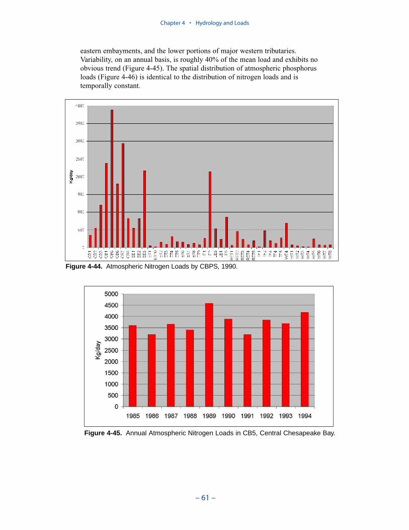
eastern embayments, and the lower portions of major western tributaries.Variability, on an annual basis, is roughly 40% of the mean load and exhibits noobvious trend (Figure 4-45). The spatial distribution of atmospheric phosphorusloads (Figure 4-46) is identical to the distribution of nitrogen loads and istemporally constant.
Chapter 4 • Hydrology and Loads
– 61 –
Figure 4-44. Atmospheric Nitrogen Loads by CBPS, 1990.
Figure 4-45. Annual Atmospheric Nitrogen Loads in CB5, Central Chesapeake Bay.
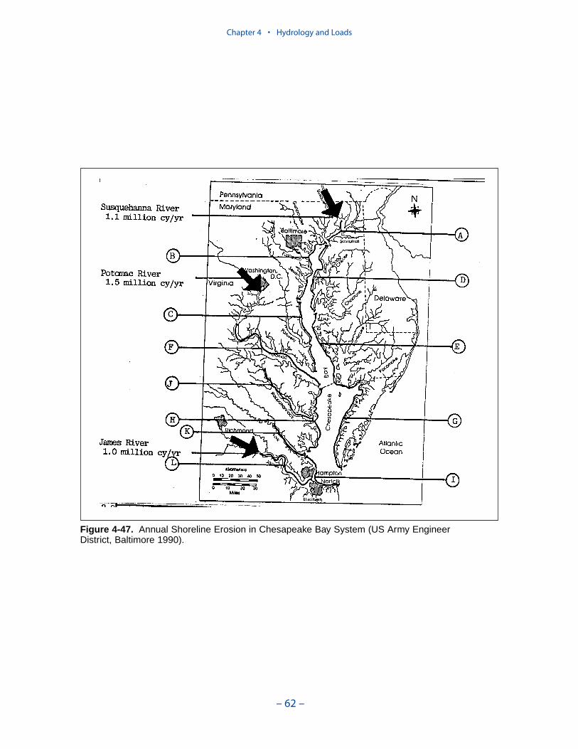
Chapter 4 • Hydrology and Loads
– 62 –
Figure 4-47. Annual Shoreline Erosion in Chesapeake Bay System (US Army EngineerDistrict, Baltimore 1990).
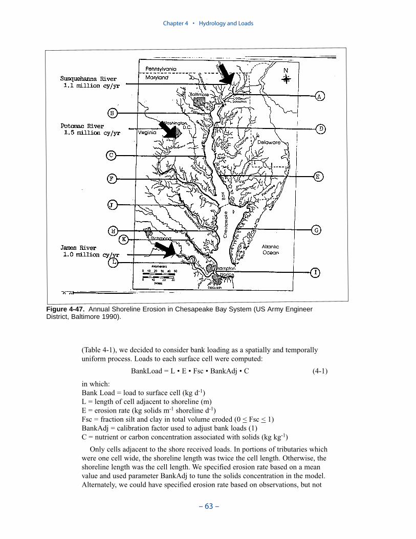
(Table 4-1), we decided to consider bank loading as a spatially and temporallyuniform process. Loads to each surface cell were computed:
BankLoad = L • E • Fsc • BankAdj • C (4-1)
in which:Bank Load = load to surface cell (kg d-1)L = length of cell adjacent to shoreline (m)E = erosion rate (kg solids m-1 shoreline d-1)Fsc = fraction silt and clay in total volume eroded (0 < Fsc < 1)BankAdj = calibration factor used to adjust bank loads (1)C = nutrient or carbon concentration associated with solids (kg kg-1)
Only cells adjacent to the shore received loads. In portions of tributaries whichwere one cell wide, the shoreline length was twice the cell length. Otherwise, theshoreline length was the cell length. We specified erosion rate based on a meanvalue and used parameter BankAdj to tune the solids concentration in the model.Alternately, we could have specified erosion rate based on observations, but not
Chapter 4 • Hydrology and Loads
– 63 –
Figure 4-47. Annual Shoreline Erosion in Chesapeake Bay System (US Army EngineerDistrict, Baltimore 1990).
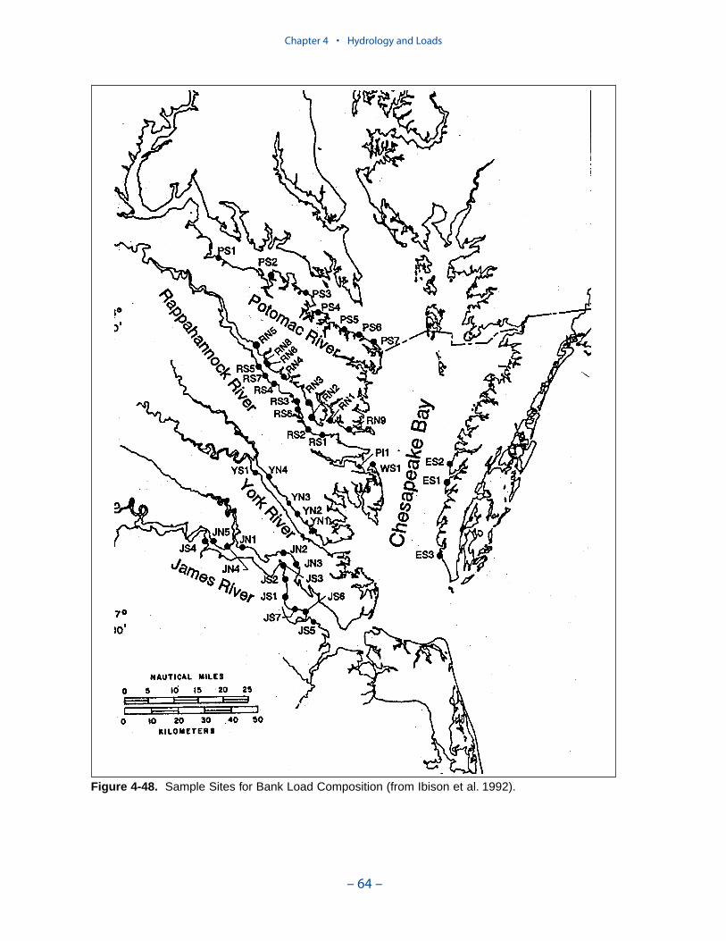
Chapter 4 • Hydrology and Loads
– 64 –
Figure 4-48. Sample Sites for Bank Load Composition (from Ibison et al. 1992).
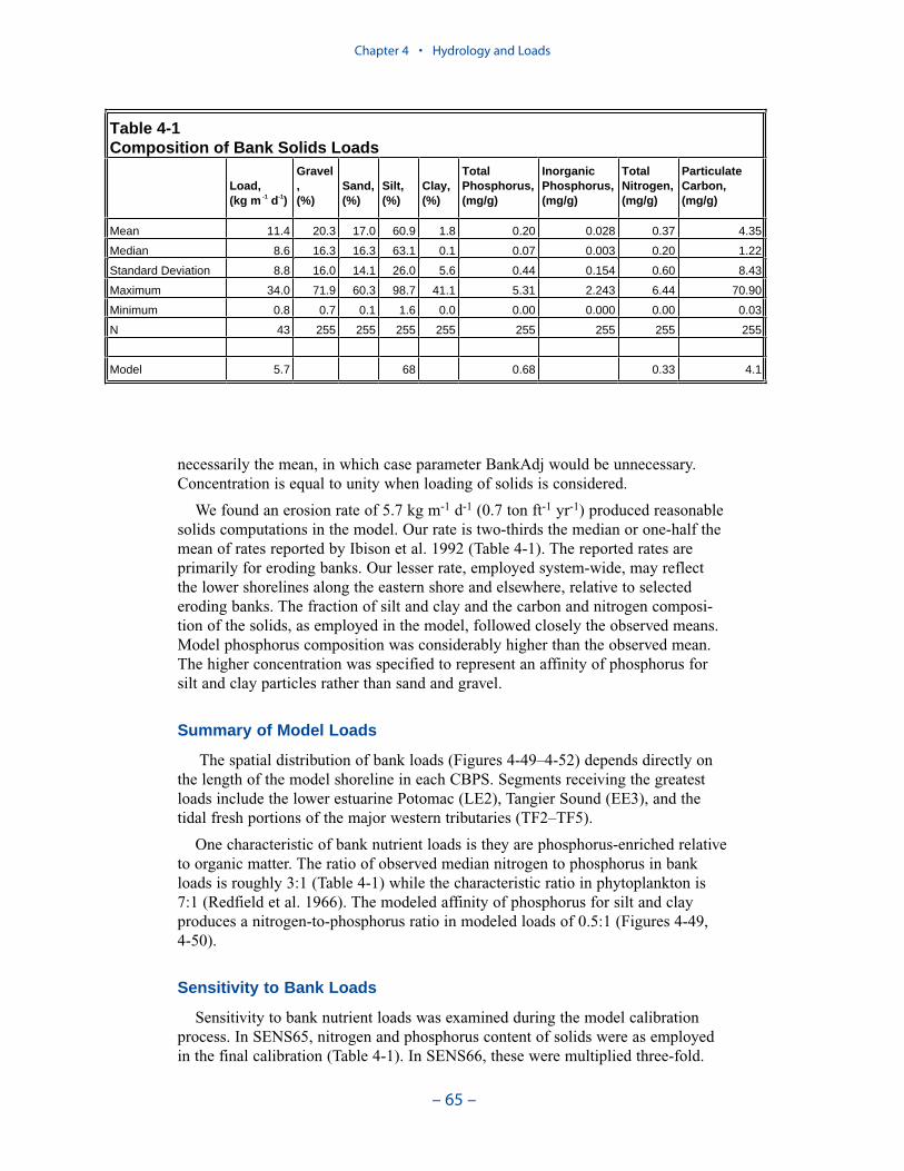
necessarily the mean, in which case parameter BankAdj would be unnecessary.Concentration is equal to unity when loading of solids is considered.
We found an erosion rate of 5.7 kg m-1 d-1 (0.7 ton ft-1 yr-1) produced reasonablesolids computations in the model. Our rate is two-thirds the median or one-half themean of rates reported by Ibison et al. 1992 (Table 4-1). The reported rates areprimarily for eroding banks. Our lesser rate, employed system-wide, may reflectthe lower shorelines along the eastern shore and elsewhere, relative to selectederoding banks. The fraction of silt and clay and the carbon and nitrogen composi-tion of the solids, as employed in the model, followed closely the observed means.Model phosphorus composition was considerably higher than the observed mean.The higher concentration was specified to represent an affinity of phosphorus forsilt and clay particles rather than sand and gravel.
Summary of Model Loads
The spatial distribution of bank loads (Figures 4-49–4-52) depends directly onthe length of the model shoreline in each CBPS. Segments receiving the greatestloads include the lower estuarine Potomac (LE2), Tangier Sound (EE3), and thetidal fresh portions of the major western tributaries (TF2–TF5).
One characteristic of bank nutrient loads is they are phosphorus-enriched relativeto organic matter. The ratio of observed median nitrogen to phosphorus in bankloads is roughly 3:1 (Table 4-1) while the characteristic ratio in phytoplankton is7:1 (Redfield et al. 1966). The modeled affinity of phosphorus for silt and clayproduces a nitrogen-to-phosphorus ratio in modeled loads of 0.5:1 (Figures 4-49,4-50).
Sensitivity to Bank Loads
Sensitivity to bank nutrient loads was examined during the model calibrationprocess. In SENS65, nitrogen and phosphorus content of solids were as employedin the final calibration (Table 4-1). In SENS66, these were multiplied three-fold.
Chapter 4 • Hydrology and Loads
– 65 –
Table 4-1 Composition of Bank Solids Loads
Load,(kg m -1 d-1)
Gravel,(%)
Sand,(%)
Silt,(%)
Clay,(%)
TotalPhosphorus,(mg/g)
InorganicPhosphorus,(mg/g)
TotalNitrogen,(mg/g)
ParticulateCarbon,(mg/g)
Mean 11.4 20.3 17.0 60.9 1.8 0.20 0.028 0.37 4.35
Median 8.6 16.3 16.3 63.1 0.1 0.07 0.003 0.20 1.22
Standard Deviation 8.8 16.0 14.1 26.0 5.6 0.44 0.154 0.60 8.43
Maximum 34.0 71.9 60.3 98.7 41.1 5.31 2.243 6.44 70.90
Minimum 0.8 0.7 0.1 1.6 0.0 0.00 0.000 0.00 0.03
N 43 255 255 255 255 255 255 255 255
Model 5.7 68 0.68 0.33 4.1

Chapter 4 • Hydrology and Loads
– 66 –
Figure 4-49. Total Nitrogen Bank Loads by CBPS
Figure 4-50. Total Phosphorus Bank Loads by CBPS
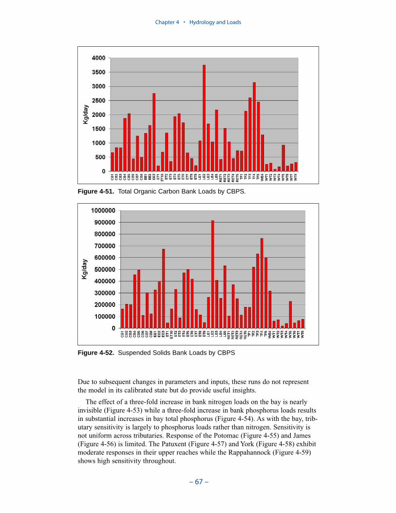
Due to subsequent changes in parameters and inputs, these runs do not representthe model in its calibrated state but do provide useful insights.
The effect of a three-fold increase in bank nitrogen loads on the bay is nearlyinvisible (Figure 4-53) while a three-fold increase in bank phosphorus loads resultsin substantial increases in bay total phosphorus (Figure 4-54). As with the bay, trib-utary sensitivity is largely to phosphorus loads rather than nitrogen. Sensitivity isnot uniform across tributaries. Response of the Potomac (Figure 4-55) and James(Figure 4-56) is limited. The Patuxent (Figure 4-57) and York (Figure 4-58) exhibitmoderate responses in their upper reaches while the Rappahannock (Figure 4-59)shows high sensitivity throughout.
Chapter 4 • Hydrology and Loads
– 67 –
Figure 4-51. Total Organic Carbon Bank Loads by CBPS.
Figure 4-52. Suspended Solids Bank Loads by CBPS
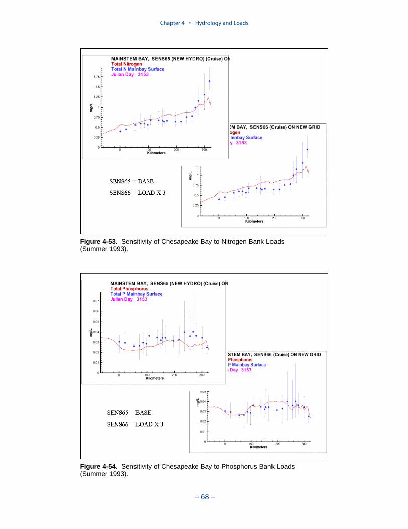
Chapter 4 • Hydrology and Loads
– 68 –
Figure 4-53. Sensitivity of Chesapeake Bay to Nitrogen Bank Loads (Summer 1993).
Figure 4-54. Sensitivity of Chesapeake Bay to Phosphorus Bank Loads (Summer 1993).
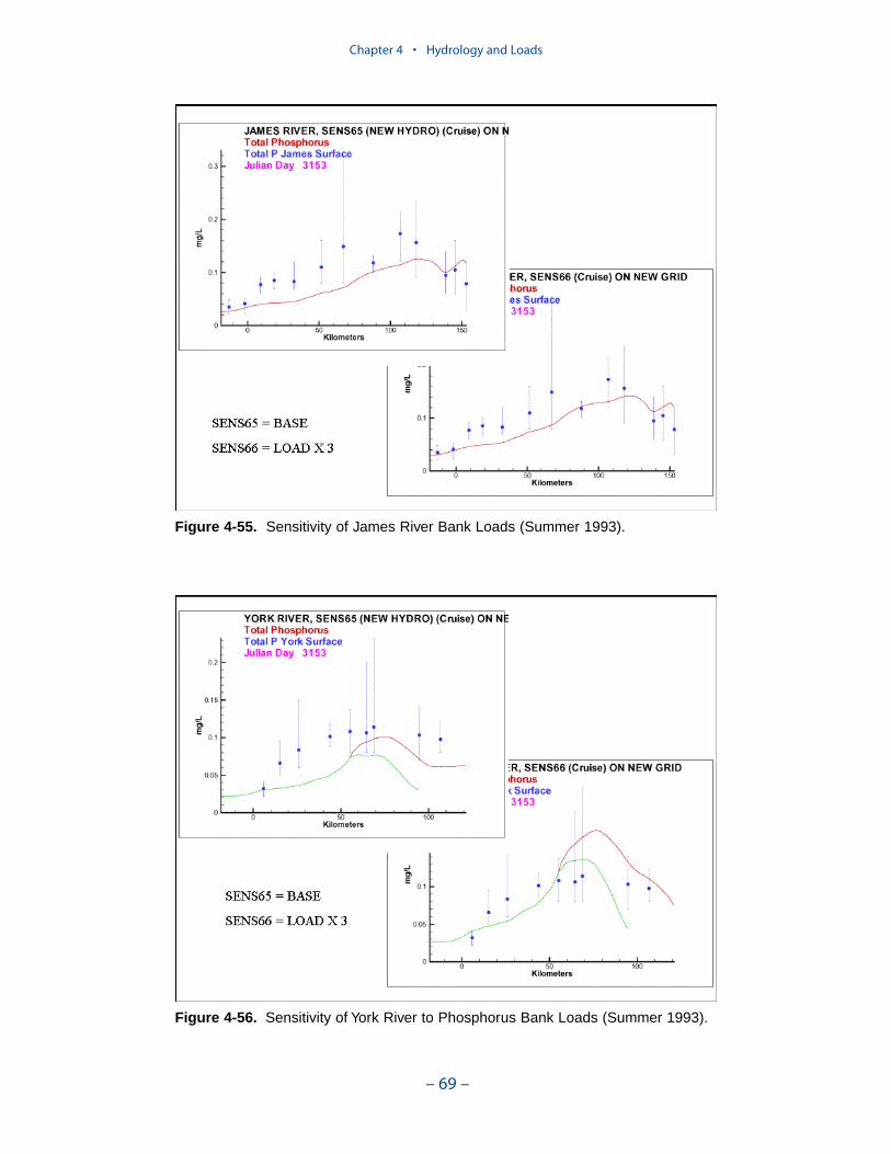
Chapter 4 • Hydrology and Loads
– 69 –
Figure 4-55. Sensitivity of James River Bank Loads (Summer 1993).
Figure 4-56. Sensitivity of York River to Phosphorus Bank Loads (Summer 1993).
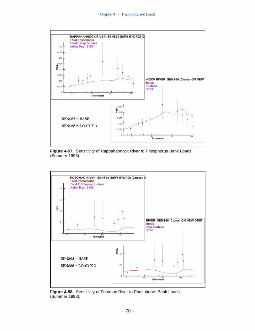
Chapter 4 • Hydrology and Loads
– 70 –
Figure 4-57. Sensitivity of Rappahannock River to Phosphorus Bank Loads(Summer 1993).
Figure 4-58. Sensitivity of Potomac River to Phosphorus Bank Loads (Summer 1993).

Chapter 4 • Hydrology and Loads
– 71 –
Figure 4-59. Sensitivity of Patuxent River to Phosphorus Bank Loads (Summer 1993).
Wetlands Loads
Wetlands loads are the sources (or sinks) of oxygen and oxygen-demandingmaterial associated with wetlands that fringe the shore of the bay and tributaries.These loads are invoked primarily as an aid in calibration of tributary dissolvedoxygen.
Quantifying the influence of wetlands on estuarine water quality has been aninterest of scientists and engineers for decades. New methodologies have providedimproved estimates but precise specification of wetlands effects remains impos-sible. The best that can be done is to bracket or “range” possible effects and thenselect values for use in the model from the range of potential values.
Neubauer et al. (2000) measured annual net macrophyte production of 1.4–2 g C m-2 d-1 in a tidal freshwater Pamunkey River marsh. Although episodic floodingor scouring of marshes may produce large loads, over long periods no more carboncan be exported from a marsh than is produced. Consequently, the Neubauer et al.study provides an upper range for marsh carbon export. Actual carbon exportshould be much less than annual net production due to burial; carbon import maybe necessary to balance combined effects of burial and respiration (Neubauer et al.2001). In the model, a uniform carbon export of 0.3 g C m-2 d-1 was employed.
Neubauer at al. (2000) calculated belowground marsh respiration of 516–723 gC m-2 yr-1—equivalent to 3.8–5.3 g oxygen equivalents m-2 d-1. Sediment oxygenconsumption should be less than total respiration due to gas evolution, burial ofsulfide, and other processes. A summary of sediment oxygen demand in the system
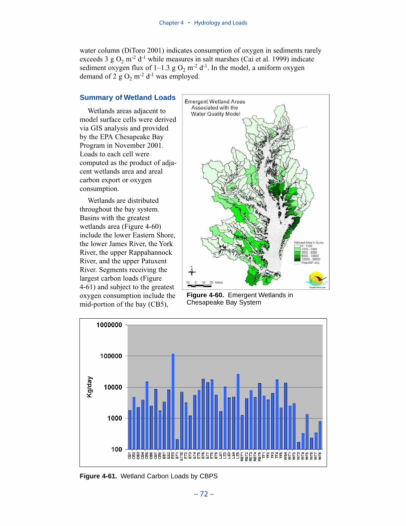
water column (DiToro 2001) indicates consumption of oxygen in sediments rarelyexceeds 3 g O2 m-2 d-1 while measures in salt marshes (Cai et al. 1999) indicatesediment oxygen flux of 1–1.3 g O2 m-2 d-1. In the model, a uniform oxygendemand of 2 g O2 m-2 d-1 was employed.
Summary of Wetland Loads
Wetlands areas adjacent tomodel surface cells were derivedvia GIS analysis and providedby the EPA Chesapeake BayProgram in November 2001.Loads to each cell werecomputed as the product of adja-cent wetlands area and arealcarbon export or oxygenconsumption.
Wetlands are distributedthroughout the bay system.Basins with the greatestwetlands area (Figure 4-60)include the lower Eastern Shore,the lower James River, the YorkRiver, the upper RappahannockRiver, and the upper PatuxentRiver. Segments receiving thelargest carbon loads (Figure 4-61) and subject to the greatestoxygen consumption include themid-portion of the bay (CB5),
Chapter 4 • Hydrology and Loads
– 72 –
Figure 4-60. Emergent Wetlands inChesapeake Bay System
Figure 4-61. Wetland Carbon Loads by CBPS
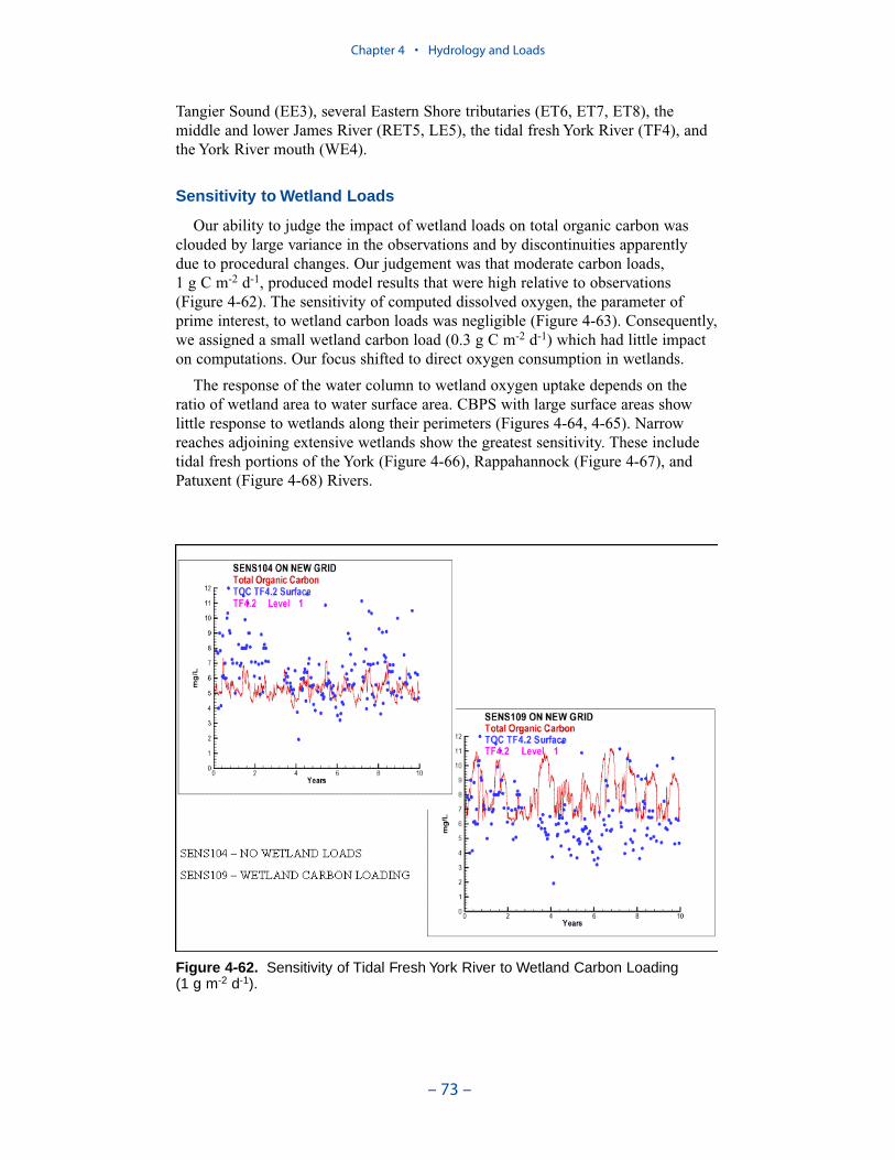
Tangier Sound (EE3), several Eastern Shore tributaries (ET6, ET7, ET8), themiddle and lower James River (RET5, LE5), the tidal fresh York River (TF4), andthe York River mouth (WE4).
Sensitivity to Wetland Loads
Our ability to judge the impact of wetland loads on total organic carbon wasclouded by large variance in the observations and by discontinuities apparently due to procedural changes. Our judgement was that moderate carbon loads,1 g C m-2 d-1, produced model results that were high relative to observations(Figure 4-62). The sensitivity of computed dissolved oxygen, the parameter ofprime interest, to wetland carbon loads was negligible (Figure 4-63). Consequently,we assigned a small wetland carbon load (0.3 g C m-2 d-1) which had little impacton computations. Our focus shifted to direct oxygen consumption in wetlands.
The response of the water column to wetland oxygen uptake depends on theratio of wetland area to water surface area. CBPS with large surface areas showlittle response to wetlands along their perimeters (Figures 4-64, 4-65). Narrowreaches adjoining extensive wetlands show the greatest sensitivity. These includetidal fresh portions of the York (Figure 4-66), Rappahannock (Figure 4-67), andPatuxent (Figure 4-68) Rivers.
Chapter 4 • Hydrology and Loads
– 73 –
Figure 4-62. Sensitivity of Tidal Fresh York River to Wetland Carbon Loading (1 g m-2 d-1).
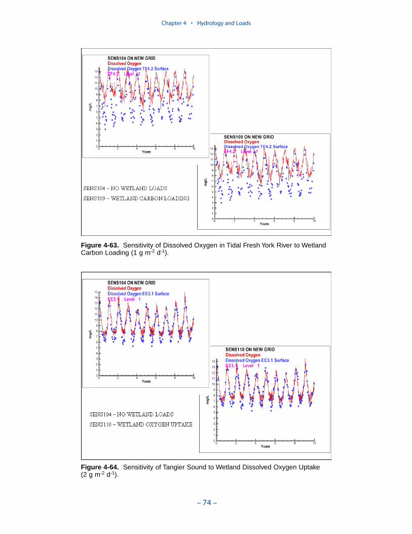
Chapter 4 • Hydrology and Loads
– 74 –
Figure 4-63. Sensitivity of Dissolved Oxygen in Tidal Fresh York River to WetlandCarbon Loading (1 g m-2 d-1).
Figure 4-64. Sensitivity of Tangier Sound to Wetland Dissolved Oxygen Uptake (2 g m-2 d-1).

Chapter 4 • Hydrology and Loads
– 75 –
Figure 4-65. Sensitivity of York River Mouth to Wetland Dissolved Oxygen Uptake(2 g m-2 d-1).
Figure 4-66. Sensitivity of Tidal Fresh York River to Wetland Dissolved OxygenUptake (2 g m-2 d-1).
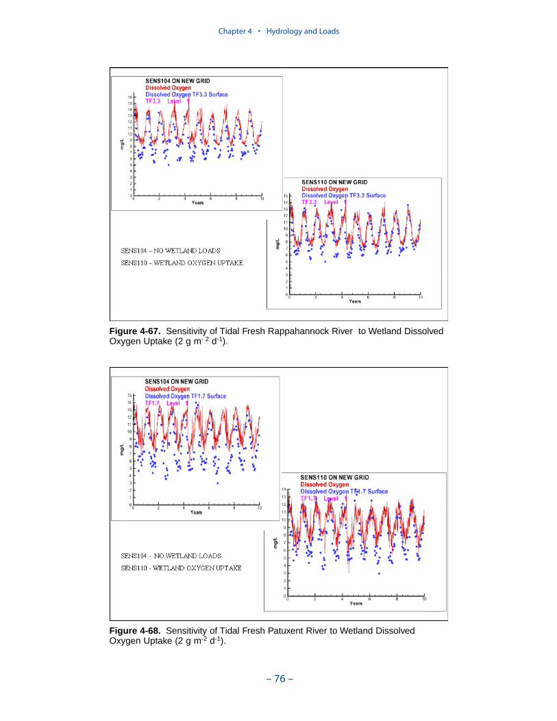
Chapter 4 • Hydrology and Loads
– 76 –
Figure 4-67. Sensitivity of Tidal Fresh Rappahannock River to Wetland DissolvedOxygen Uptake (2 g m- 2 d-1).
Figure 4-68. Sensitivity of Tidal Fresh Patuxent River to Wetland DissolvedOxygen Uptake (2 g m-2 d-1).

Summary of All Loads
Loads from all sources were compared by CBPS for 1990, a year central to thesimulation period. Runoff in this year was moderate in the Susquehanna and James(Figures 4-1, 4-3) and low in the Potomac (Figure 4-2).
Nonpoint sources dominated the nitrogen loads (Figure 4-69, Table 4-2) exceptin a few segments adjacent to major urban areas including Richmond (TF5),Hampton Roads (LE5), Washington (TF2), and Baltimore (WT4, WT5). In theseregions, point sources contributed a significant fraction of nitrogen loads. Atmos-pheric nitrogen loads were significant only in the large, open segments of themainstem bay (CB3–CB7, EE3) and in the lower Potomac (LE2). Bank loads werenegligibly small throughout.
Chapter 4 • Hydrology and Loads
– 77 –
Figure 4-69. Summary of Nitrogen Loads for the Year 1990.
Table 4-2 System-wide Load Summary, 1990
Point Source, (kg/day)
NonpointSource,(kg/day)
Atmosphere,(kg/day)
Bank Load, (kg/day)
Wetlands, (kg/day)
Nitrogen 80321 359506 26184 4218
Phosphorus 4245 24600 1927 8695
Carbon 160647 1014435 52424 1355742
Solids 11298430 12786991
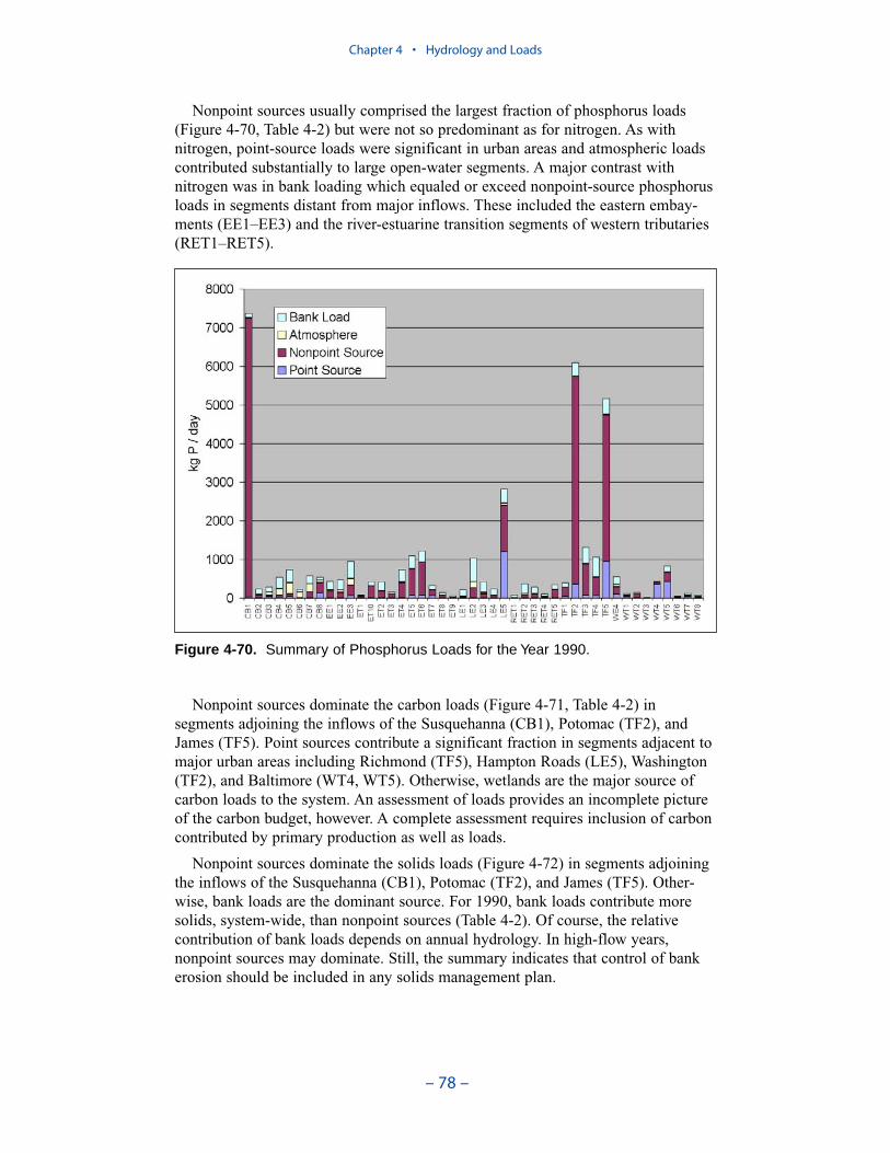
Nonpoint sources usually comprised the largest fraction of phosphorus loads(Figure 4-70, Table 4-2) but were not so predominant as for nitrogen. As withnitrogen, point-source loads were significant in urban areas and atmospheric loadscontributed substantially to large open-water segments. A major contrast withnitrogen was in bank loading which equaled or exceed nonpoint-source phosphorusloads in segments distant from major inflows. These included the eastern embay-ments (EE1–EE3) and the river-estuarine transition segments of western tributaries(RET1–RET5).
Nonpoint sources dominate the carbon loads (Figure 4-71, Table 4-2) insegments adjoining the inflows of the Susquehanna (CB1), Potomac (TF2), andJames (TF5). Point sources contribute a significant fraction in segments adjacent tomajor urban areas including Richmond (TF5), Hampton Roads (LE5), Washington(TF2), and Baltimore (WT4, WT5). Otherwise, wetlands are the major source ofcarbon loads to the system. An assessment of loads provides an incomplete pictureof the carbon budget, however. A complete assessment requires inclusion of carboncontributed by primary production as well as loads.
Nonpoint sources dominate the solids loads (Figure 4-72) in segments adjoiningthe inflows of the Susquehanna (CB1), Potomac (TF2), and James (TF5). Other-wise, bank loads are the dominant source. For 1990, bank loads contribute moresolids, system-wide, than nonpoint sources (Table 4-2). Of course, the relativecontribution of bank loads depends on annual hydrology. In high-flow years,nonpoint sources may dominate. Still, the summary indicates that control of bankerosion should be included in any solids management plan.
Chapter 4 • Hydrology and Loads
– 78 –
Figure 4-70. Summary of Phosphorus Loads for the Year 1990.
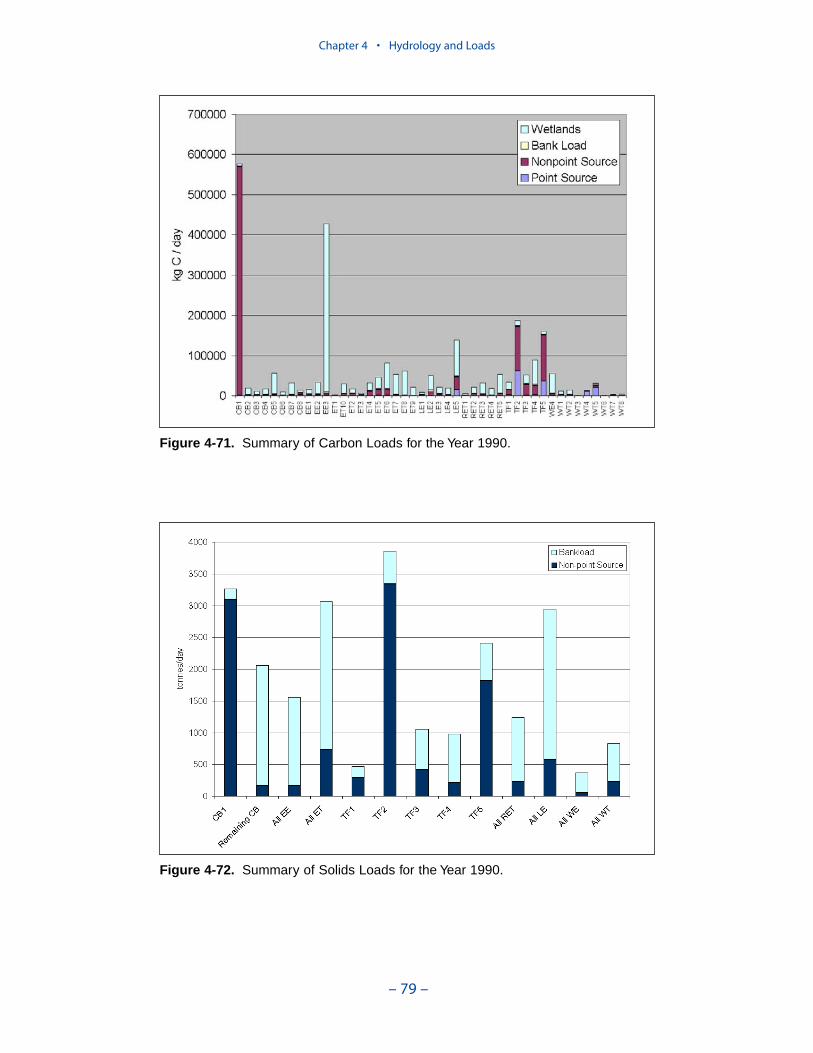
Chapter 4 • Hydrology and Loads
– 79 –
Figure 4-71. Summary of Carbon Loads for the Year 1990.
Figure 4-72. Summary of Solids Loads for the Year 1990.
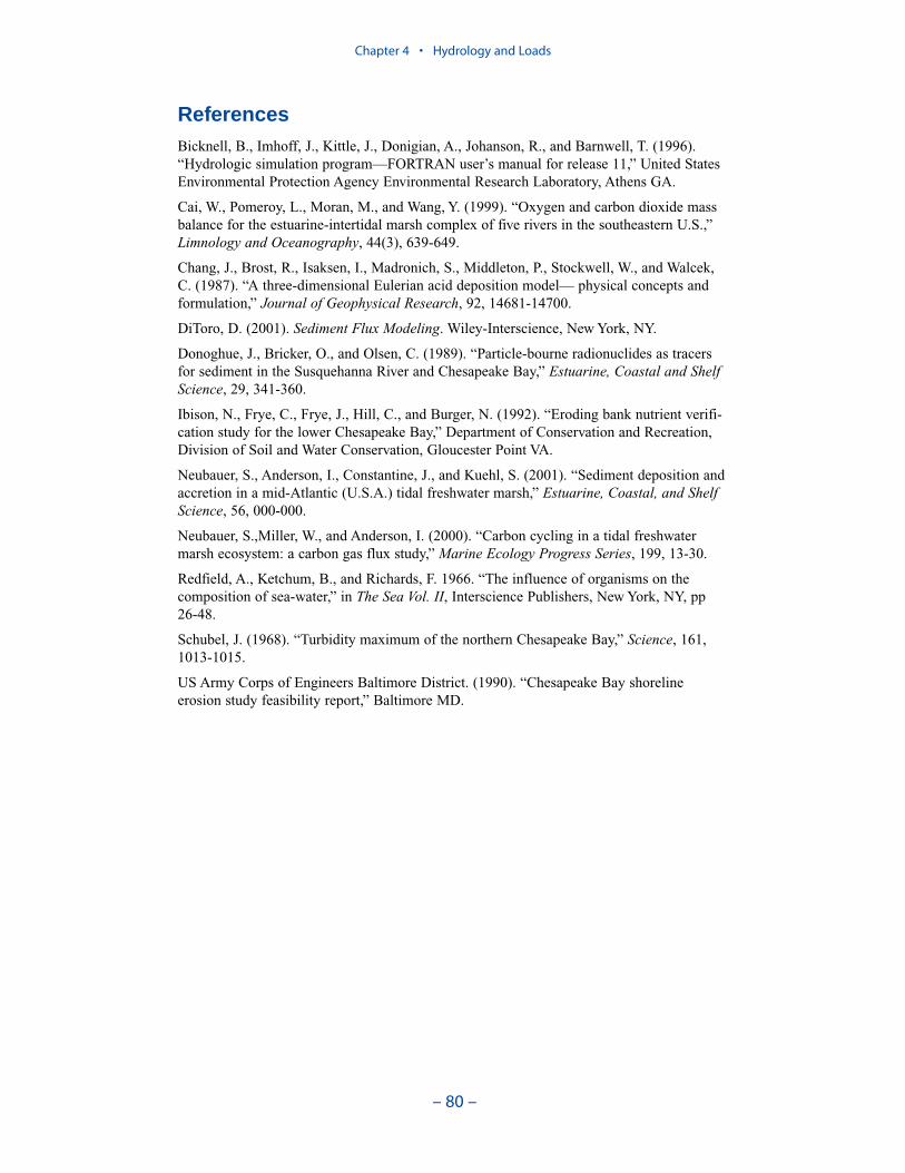
ReferencesBicknell, B., Imhoff, J., Kittle, J., Donigian, A., Johanson, R., and Barnwell, T. (1996).“Hydrologic simulation program—FORTRAN user’s manual for release 11,” United StatesEnvironmental Protection Agency Environmental Research Laboratory, Athens GA.
Cai, W., Pomeroy, L., Moran, M., and Wang, Y. (1999). “Oxygen and carbon dioxide massbalance for the estuarine-intertidal marsh complex of five rivers in the southeastern U.S.,”Limnology and Oceanography, 44(3), 639-649.
Chang, J., Brost, R., Isaksen, I., Madronich, S., Middleton, P., Stockwell, W., and Walcek,C. (1987). “A three-dimensional Eulerian acid deposition model— physical concepts andformulation,” Journal of Geophysical Research, 92, 14681-14700.
DiToro, D. (2001). Sediment Flux Modeling. Wiley-Interscience, New York, NY.
Donoghue, J., Bricker, O., and Olsen, C. (1989). “Particle-bourne radionuclides as tracersfor sediment in the Susquehanna River and Chesapeake Bay,” Estuarine, Coastal and ShelfScience, 29, 341-360.
Ibison, N., Frye, C., Frye, J., Hill, C., and Burger, N. (1992). “Eroding bank nutrient verifi-cation study for the lower Chesapeake Bay,” Department of Conservation and Recreation,Division of Soil and Water Conservation, Gloucester Point VA.
Neubauer, S., Anderson, I., Constantine, J., and Kuehl, S. (2001). “Sediment deposition andaccretion in a mid-Atlantic (U.S.A.) tidal freshwater marsh,” Estuarine, Coastal, and ShelfScience, 56, 000-000.
Neubauer, S.,Miller, W., and Anderson, I. (2000). “Carbon cycling in a tidal freshwatermarsh ecosystem: a carbon gas flux study,” Marine Ecology Progress Series, 199, 13-30.
Redfield, A., Ketchum, B., and Richards, F. 1966. “The influence of organisms on thecomposition of sea-water,” in The Sea Vol. II, Interscience Publishers, New York, NY, pp26-48.
Schubel, J. (1968). “Turbidity maximum of the northern Chesapeake Bay,” Science, 161,1013-1015.
US Army Corps of Engineers Baltimore District. (1990). “Chesapeake Bay shorelineerosion study feasibility report,” Baltimore MD.
Chapter 4 • Hydrology and Loads
– 80 –
Introduction
Major loads were mapped to model cells by the sponsor before they wereprovided to the model team. The linkage process between loads and modelconsisted of converting quantities in the loads into appropriate model state vari-ables. The present chapter describes development of conversion guidelines and listsparameter values employed in the conversions.
Nonpoint-Source Loads
Linking of watershed model loads focused on the nitrogen and phosphorusstate variables (Table 5-1). The watershed model loads distinguished particulateinorganic phosphorus from organic phosphorus. Discussion with the watershedmodel team indicated particulate inorganic phosphorus was utilized as a way ofmodeling scour from the bottom during high-flow intervals. No effort was made totruly distinguish particulate inorganic from organic phosphorus forms. The Tribu-tary Refinements phase of water quality model application (Cerco et al. 2002)distinguished particulate organic and particulate inorganic phosphorus forms. Thisdistinction was not carried forward into the present model. Consequently, thewatershed model particulate inorganic and organic phosphorus forms werecombined before mapping into water quality model variables. Since particulatephosphorus in the water quality model consists of both organic and inorganicforms, we have dropped the specification “organic” when referring to water qualitymodel particulate phosphorus.
The watershed model produced loads of total suspended solids. The corres-ponding water quality model variable was fixed (inorganic) solids. Linkage withthe watershed model required removal of the volatile (organic) solids from the totalsolids load. Volatile solids were still input to the water quality model but in theform of particulate organic carbon.
– 81 –
Linking in the Loads 5
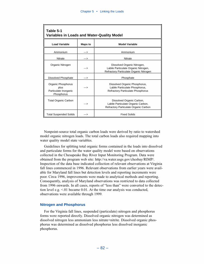
Nonpoint-source total organic carbon loads were derived by ratio to watershedmodel organic nitrogen loads. The total carbon loads also required mapping intowater quality model state variables.
Guidelines for splitting total organic forms contained in the loads into dissolvedand particulate forms for the water quality model were based on observationscollected in the Chesapeake Bay River Input Monitoring Program. Data wereobtained from the program web site: http://va.water.usgs.gov/chesbay/RIMP/.Inspection of the data base indicated collection of relevant observations at Virginiafall lines commenced in 1996. Relevant observations from earlier years were avail-able for Maryland fall lines but detection levels and reporting increments werepoor. Circa 1996, improvements were made to analytical methods and reporting.Consequently, analysis of Maryland observations was restricted to data collectedfrom 1996 onwards. In all cases, reports of “less than” were converted to the detec-tion level e.g. <.01 became 0.01. At the time our analysis was conducted,observations were available through 1999.
Nitrogen and Phosphorus
For the Virginia fall lines, suspended (particulate) nitrogen and phosphorusforms were reported directly. Dissolved organic nitrogen was determined asdissolved nitrogen less ammonium less nitrate+nitrite. Dissolved organic phos-phorus was determined as dissolved phosphorus less dissolved inorganicphosphorus.
Chapter 5 • Linking the Loads
– 82 –
Table 5-1 Variables in Loads and Water-Quality Model
Load Variable Maps to Model Variable
Ammonium ---> Ammonium
Nitrate ---> Nitrate
Organic Nitrogen --->
Dissolved Organic Nitrogen, Labile Particulate Organic Nitrogen,
Refractory Particulate Organic Nitrogen
Dissolved Phosphate ---> Phosphate
Organic Phosphorus plus
Particulate Inorganic Phosphorus
--->Dissolved Organic Phosphorus, Labile Particulate Phosphorus,
Refractory Particulate Phosphorus
Total Organic Carbon --->
Dissolved Organic Carbon, Labile Particulate Organic Carbon,
Refractory Particulate Organic Carbon
Total Suspended Solids ---> Fixed Solids
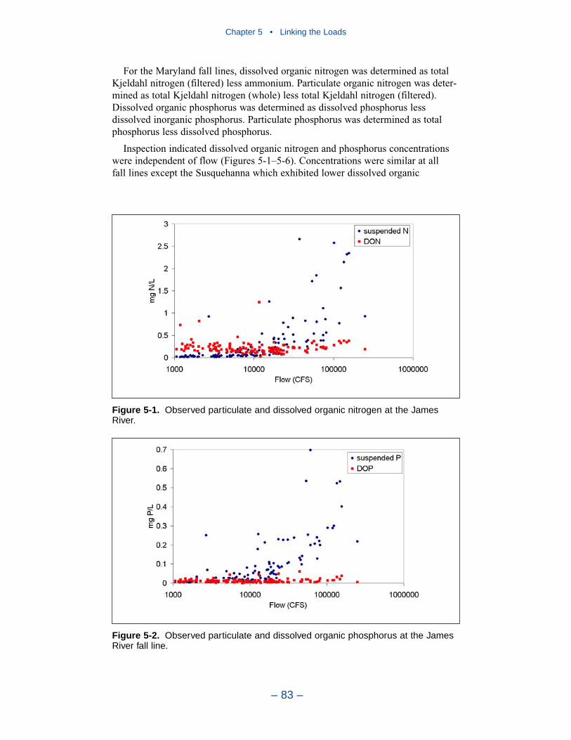
For the Maryland fall lines, dissolved organic nitrogen was determined as totalKjeldahl nitrogen (filtered) less ammonium. Particulate organic nitrogen was deter-mined as total Kjeldahl nitrogen (whole) less total Kjeldahl nitrogen (filtered).Dissolved organic phosphorus was determined as dissolved phosphorus lessdissolved inorganic phosphorus. Particulate phosphorus was determined as totalphosphorus less dissolved phosphorus.
Inspection indicated dissolved organic nitrogen and phosphorus concentrationswere independent of flow (Figures 5-1–5-6). Concentrations were similar at all fall lines except the Susquehanna which exhibited lower dissolved organic
Chapter 5 • Linking the Loads
– 83 –
Figure 5-1. Observed particulate and dissolved organic nitrogen at the JamesRiver.
Figure 5-2. Observed particulate and dissolved organic phosphorus at the JamesRiver fall line.
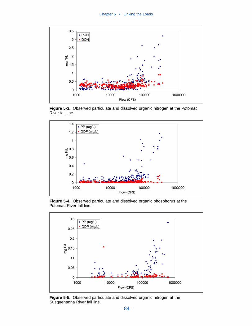
Chapter 5 • Linking the Loads
– 84 –
Figure 5-3. Observed particulate and dissolved organic nitrogen at the PotomacRiver fall line.
Figure 5-4. Observed particulate and dissolved organic phosphorus at thePotomac River fall line.
Figure 5-5. Observed particulate and dissolved organic nitrogen at theSusquehanna River fall line.
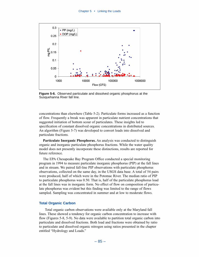
concentrations than elsewhere (Table 5-2). Particulate forms increased as a functionof flow. Frequently a break was apparent in particulate nutrient concentrations thatsuggested initiation of bottom scour of particulates. These insights led tospecification of constant dissolved organic concentrations in distributed sources. An algorithm (Figure 5-7) was developed to convert loads into dissolved andparticulate fractions.
Particulate Inorganic Phosphorus. An analysis was conducted to distinguishorganic and inorganic particulate phosphorus fractions. While the water qualitymodel does not presently incorporate these distinctions, results are reported forfuture reference.
The EPA Chesapeake Bay Program Office conducted a special monitoringprogram in 1994 to measure particulate inorganic phosphorus (PIP) at the fall linesand in stream. We paired fall-line PIP observations with particulate phosphorusobservations, collected on the same day, in the USGS data base. A total of 54 pairswere produced, half of which were in the Potomac River. The median ratio of PIPto particulate phosphorus was 0.50. That is, half of the particulate phosphorus loadat the fall lines was in inorganic form. No effect of flow on composition of particu-late phosphorus was evident but this finding was limited to the range of flowssampled. Sampling was concentrated in summer and at low to moderate flows.
Total Organic Carbon
Total organic carbon observations were available only at the Maryland falllines. These showed a tendency for organic carbon concentration to increase withflow (Figures 5-8, 5-9). No data were available to partition total organic carbon intoparticulate and dissolved fractions. Both load and fractions were obtained by ratioto particulate and dissolved organic nitrogen using ratios presented in the chapterentitled “Hydrology and Loads.”
Chapter 5 • Linking the Loads
– 85 –
Figure 5-6. Observed particulate and dissolved organic phosphorus at theSusquehanna River fall line.
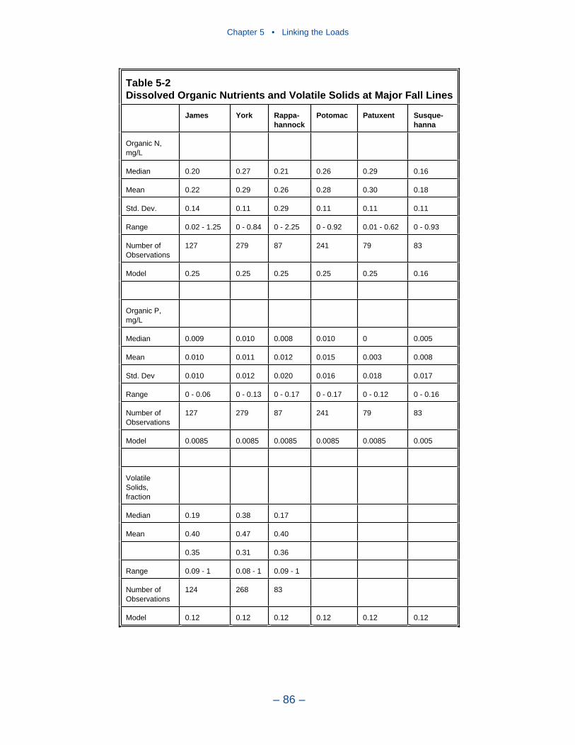
Chapter 5 • Linking the Loads
– 86 –
Table 5-2 Dissolved Organic Nutrients and Volatile Solids at Major Fall Lines
James York Rappa-hannock
Potomac Patuxent Susque-hanna
Organic N, mg/L
Median 0.20 0.27 0.21 0.26 0.29 0.16
Mean 0.22 0.29 0.26 0.28 0.30 0.18
Std. Dev. 0.14 0.11 0.29 0.11 0.11 0.11
Range 0.02 - 1.25 0 - 0.84 0 - 2.25 0 - 0.92 0.01 - 0.62 0 - 0.93
Number of Observations
127 279 87 241 79 83
Model 0.25 0.25 0.25 0.25 0.25 0.16
Organic P, mg/L
Median 0.009 0.010 0.008 0.010 0 0.005
Mean 0.010 0.011 0.012 0.015 0.003 0.008
Std. Dev 0.010 0.012 0.020 0.016 0.018 0.017
Range 0 - 0.06 0 - 0.13 0 - 0.17 0 - 0.17 0 - 0.12 0 - 0.16
Number of Observations
127 279 87 241 79 83
Model 0.0085 0.0085 0.0085 0.0085 0.0085 0.005
VolatileSolids, fraction
Median 0.19 0.38 0.17
Mean 0.40 0.47 0.40
0.35 0.31 0.36
Range 0.09 - 1 0.08 - 1 0.09 - 1
Number of Observations
124 268 83
Model 0.12 0.12 0.12 0.12 0.12 0.12
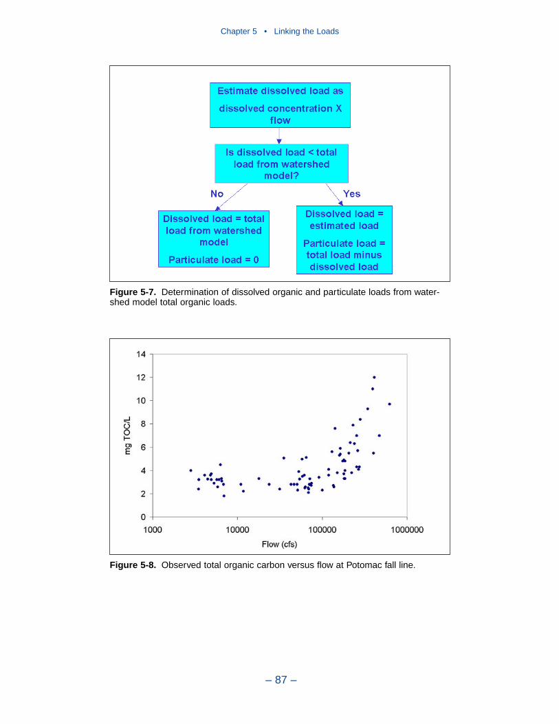
Chapter 5 • Linking the Loads
– 87 –
Figure 5-7. Determination of dissolved organic and particulate loads from water-shed model total organic loads.
Figure 5-8. Observed total organic carbon versus flow at Potomac fall line.
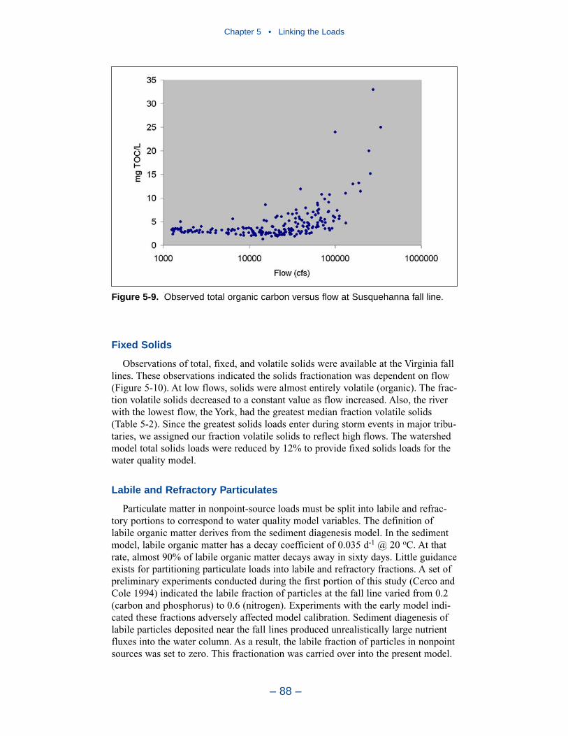
Fixed Solids
Observations of total, fixed, and volatile solids were available at the Virginia falllines. These observations indicated the solids fractionation was dependent on flow(Figure 5-10). At low flows, solids were almost entirely volatile (organic). The frac-tion volatile solids decreased to a constant value as flow increased. Also, the riverwith the lowest flow, the York, had the greatest median fraction volatile solids(Table 5-2). Since the greatest solids loads enter during storm events in major tribu-taries, we assigned our fraction volatile solids to reflect high flows. The watershedmodel total solids loads were reduced by 12% to provide fixed solids loads for thewater quality model.
Labile and Refractory Particulates
Particulate matter in nonpoint-source loads must be split into labile and refrac-tory portions to correspond to water quality model variables. The definition oflabile organic matter derives from the sediment diagenesis model. In the sedimentmodel, labile organic matter has a decay coefficient of 0.035 d-1 @ 20 oC. At thatrate, almost 90% of labile organic matter decays away in sixty days. Little guidanceexists for partitioning particulate loads into labile and refractory fractions. A set ofpreliminary experiments conducted during the first portion of this study (Cerco andCole 1994) indicated the labile fraction of particles at the fall line varied from 0.2(carbon and phosphorus) to 0.6 (nitrogen). Experiments with the early model indi-cated these fractions adversely affected model calibration. Sediment diagenesis oflabile particles deposited near the fall lines produced unrealistically large nutrientfluxes into the water column. As a result, the labile fraction of particles in nonpointsources was set to zero. This fractionation was carried over into the present model.
Chapter 5 • Linking the Loads
– 88 –
Figure 5-9. Observed total organic carbon versus flow at Susquehanna fall line.
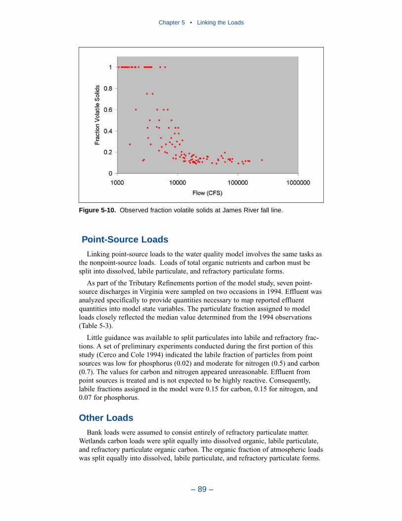
Point-Source Loads
Linking point-source loads to the water quality model involves the same tasks asthe nonpoint-source loads. Loads of total organic nutrients and carbon must besplit into dissolved, labile particulate, and refractory particulate forms.
As part of the Tributary Refinements portion of the model study, seven point-source discharges in Virginia were sampled on two occasions in 1994. Effluent wasanalyzed specifically to provide quantities necessary to map reported effluentquantities into model state variables. The particulate fraction assigned to modelloads closely reflected the median value determined from the 1994 observations(Table 5-3).
Little guidance was available to split particulates into labile and refractory frac-tions. A set of preliminary experiments conducted during the first portion of thisstudy (Cerco and Cole 1994) indicated the labile fraction of particles from pointsources was low for phosphorus (0.02) and moderate for nitrogen (0.5) and carbon(0.7). The values for carbon and nitrogen appeared unreasonable. Effluent frompoint sources is treated and is not expected to be highly reactive. Consequently,labile fractions assigned in the model were 0.15 for carbon, 0.15 for nitrogen, and0.07 for phosphorus.
Other Loads
Bank loads were assumed to consist entirely of refractory particulate matter.Wetlands carbon loads were split equally into dissolved organic, labile particulate,and refractory particulate organic carbon. The organic fraction of atmospheric loadswas split equally into dissolved, labile particulate, and refractory particulate forms.
Chapter 5 • Linking the Loads
– 89 –
Figure 5-10. Observed fraction volatile solids at James River fall line.
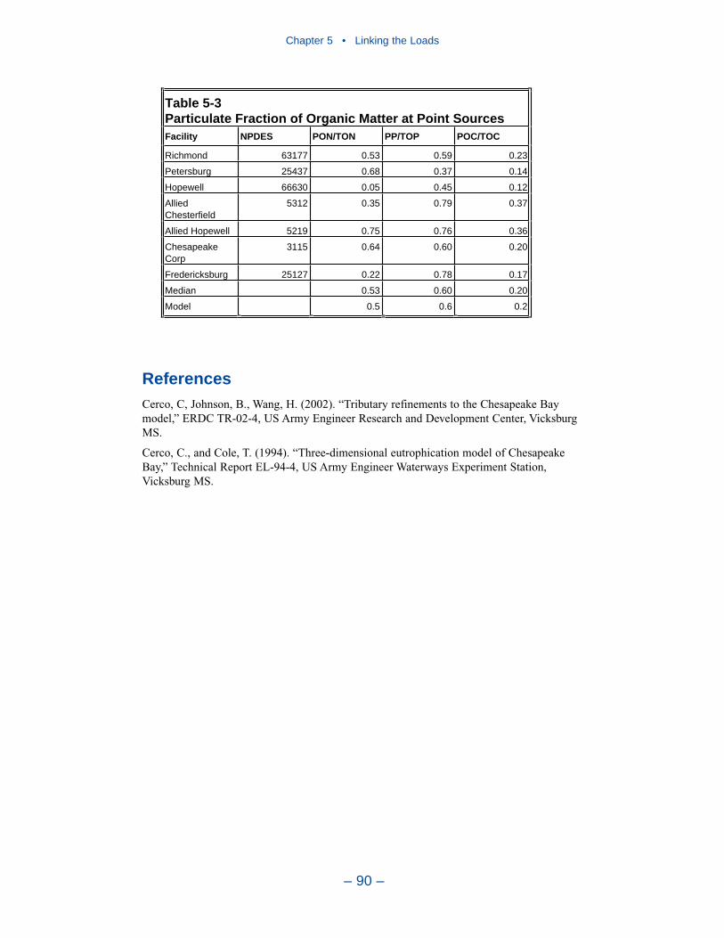
ReferencesCerco, C, Johnson, B., Wang, H. (2002). “Tributary refinements to the Chesapeake Baymodel,” ERDC TR-02-4, US Army Engineer Research and Development Center, VicksburgMS.
Cerco, C., and Cole, T. (1994). “Three-dimensional eutrophication model of ChesapeakeBay,” Technical Report EL-94-4, US Army Engineer Waterways Experiment Station,Vicksburg MS.
Chapter 5 • Linking the Loads
– 90 –
Table 5-3 Particulate Fraction of Organic Matter at Point Sources Facility NPDES PON/TON PP/TOP POC/TOC
Richmond 63177 0.53 0.59 0.23
Petersburg 25437 0.68 0.37 0.14
Hopewell 66630 0.05 0.45 0.12
AlliedChesterfield
5312 0.35 0.79 0.37
Allied Hopewell 5219 0.75 0.76 0.36
ChesapeakeCorp
3115 0.64 0.60 0.20
Fredericksburg 25127 0.22 0.78 0.17
Median 0.53 0.60 0.20
Model 0.5 0.6 0.2
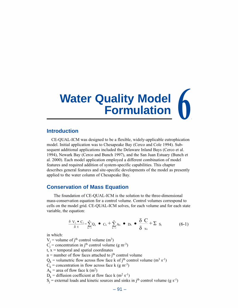
Introduction
CE-QUAL-ICM was designed to be a flexible, widely-applicable eutrophicationmodel. Initial application was to Chesapeake Bay (Cerco and Cole 1994). Sub-sequent additional applications included the Delaware Inland Bays (Cerco et al.1994), Newark Bay (Cerco and Bunch 1997), and the San Juan Estuary (Bunch etal. 2000). Each model application employed a different combination of modelfeatures and required addition of system-specific capabilities. This chapterdescribes general features and site-specific developments of the model as presentlyapplied to the water column of Chesapeake Bay.
Conservation of Mass Equation
The foundation of CE-QUAL-ICM is the solution to the three-dimensionalmass-conservation equation for a control volume. Control volumes correspond tocells on the model grid. CE-QUAL-ICM solves, for each volume and for each statevariable, the equation:
in which:Vj = volume of jth control volume (m3)Cj = concentration in jth control volume (g m-3)t, x = temporal and spatial coordinatesn = number of flow faces attached to jth control volumeQk = volumetric flow across flow face k of jth control volume (m3 s-1)Ck = concentration in flow across face k (g m-3)Ak = area of flow face k (m2)Dk = diffusion coefficient at flow face k (m2 s-1)Sj = external loads and kinetic sources and sinks in jth control volume (g s-1)
Sx
DACQ= t
CVj
k
kk
n
1=kkk
n
1=k
jj +C+ (6-1)
– 91 –
Water Quality ModelFormulation 6
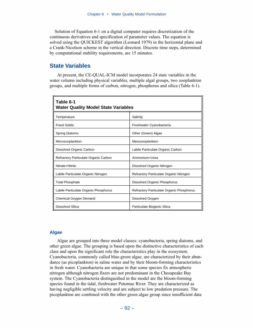
Solution of Equation 6-1 on a digital computer requires discretization of thecontinuous derivatives and specification of parameter values. The equation issolved using the QUICKEST algorithm (Leonard 1979) in the horizontal plane anda Crank-Nicolson scheme in the vertical direction. Discrete time steps, determinedby computational stability requirements, are 15 minutes.
State Variables
At present, the CE-QUAL-ICM model incorporates 24 state variables in thewater column including physical variables, multiple algal groups, two zooplanktongroups, and multiple forms of carbon, nitrogen, phosphorus and silica (Table 6-1).
Algae
Algae are grouped into three model classes: cyanobacteria, spring diatoms, andother green algae. The grouping is based upon the distinctive characteristics of eachclass and upon the significant role the characteristics play in the ecosystem.Cyanobacteria, commonly called blue-green algae, are characterized by their abun-dance (as picoplankton) in saline water and by their bloom-forming characteristicsin fresh water. Cyanobacteria are unique in that some species fix atmosphericnitrogen although nitrogen fixers are not predominant in the Chesapeake Baysystem. The Cyanobacteria distinguished in the model are the bloom-formingspecies found in the tidal, freshwater Potomac River. They are characterized ashaving negligible settling velocity and are subject to low predation pressure. Thepicoplankton are combined with the other green algae group since insufficient data
Chapter 6 • Water Quality Model Formulation
– 92 –
Table 6-1 Water Quality Model State Variables
Temperature Salinity
Fixed Solids Freshwater Cyanobacteria
Spring Diatoms Other (Green) Algae
Microzooplankton Mesozooplankton
Dissolved Organic Carbon Labile Particulate Organic Carbon
Refractory Particulate Organic Carbon Ammonium+Urea
Nitrate+Nitrite Dissolved Organic Nitrogen
Labile Particulate Organic Nitrogen Refractory Particulate Organic Nitrogen
Total Phosphate Dissolved Organic Phosphorus
Labile Particulate Organic Phosphorus Refractory Particulate Organic Phosphorus
Chemical Oxygen Demand Dissolved Oxygen
Dissolved Silica Particulate Biogenic Silica
exists to consider them separately. Spring diatoms are large phytoplankton thatproduce an annual bloom in the saline portions of the bay and tributaries. Settlingof spring diatom blooms to the sediments may be a significant source of carbon forsediment oxygen demand. Diatoms are distinguished by their requirement of silicaas a nutrient to form cell walls. Algae that do not fall into the preceding two groupsare lumped into the heading of green algae. The other green algae represent themixture that characterizes saline waters during summer and autumn and freshwaters year round. Non-bloom forming diatoms comprise a portion of this mixture.
Zooplankton
Two zooplankton groups are considered: microzooplankton and mesozoo-plankton. The microzooplankton can be important predators on phytoplankton andthey are one of the prey groups for mesozooplankton. Mesozooplankton consumephytoplankton and detritus as well as microzooplankton. The mesozooplankton arean important prey resource for carnivorous finfish such as Bay Anchovy.Zooplankton were included in the model as a first step towards computing theeffect of eutrophication management on top-level predators.
Organic Carbon
Three organic carbon state variables are considered: dissolved, labile particulate,and refractory particulate. Labile and refractory distinctions are based upon thetime scale of decomposition. Labile organic carbon decomposes on a time scale ofdays to weeks while refractory organic carbon requires more time. Labile organiccarbon decomposes rapidly in the water column or the sediments. Refractoryorganic carbon decomposes slowly, primarily in the sediments, and may contributeto sediment oxygen demand years after deposition.
Nitrogen
Nitrogen is first divided into available and unavailable fractions. Available refersto employment in algal nutrition. Two available forms are considered: reduced andoxidized nitrogen. Reduced nitrogen includes ammonium and urea. Nitrate andnitrite comprise the oxidized nitrogen pool. Both reduced and oxidized nitrogen areutilized to fulfill algal nutrient requirements. The primary reason for distinguishingthe two is that ammonium is oxidized by nitrifying bacteria into nitrite and, subse-quently, nitrate. This oxidation can be a significant sink of oxygen in the watercolumn and sediments.
Unavailable nitrogen state variables are dissolved organic nitrogen, labile partic-ulate organic nitrogen, and refractory particulate organic nitrogen. The dissolvedorganic nitrogen state variable excludes urea which is directly available as an algalnutrient.
Phosphorus
As with nitrogen, phosphorus is first divided into available and unavailablefractions. Only a single available form, dissolved phosphate, is considered. Themodel framework allows for exchange of phosphate between dissolved and
Chapter 6 • Water Quality Model Formulation
– 93 –
Chapter 6 • Water Quality Model Formulation
– 94 –
particulate (sorbed to solids) forms but this option is not implemented in thepresent application. Three forms of unavailable phosphorus are considered:dissolved organic phosphorus, labile particulate organic phosphorus, and refractoryparticulate organic phosphorus.
Silica
Silica is divided into two state variables: dissolved silica and particulate biogenicsilica. Dissolved silica is available to diatoms while particulate biogenic silicacannot be utilized. In the model, particulate biogenic silica is produced throughdiatom mortality. Particulate biogenic silica undergoes dissolution to availablesilica or else settles to the bottom sediments.
Chemical Oxygen Demand
Chemical oxygen demand is the concentration of reduced substances that areoxidized by abiotic processes. The primary component of chemical oxygen demandis sulfide released from sediments. Oxidation of sulfide to sulfate may removesubstantial quantities of dissolved oxygen from the water column.
Dissolved Oxygen
Dissolved oxygen is required for the existence of higher life forms. Oxygenavailability determines the distribution of organisms and the flows of energy andnutrients in an ecosystem. Dissolved oxygen is a central component of the water-quality model.
Salinity
Salinity is a conservative tracer that provides verification of the transport compo-nent of the model and facilitates examination of conservation of mass. Salinity alsoinfluences the dissolved oxygen saturation concentration and may be used in thedetermination of kinetics constants that differ in saline and fresh water.
Temperature
Temperature is a primary determinant of the rate of biochemical reactions. Reac-tion rates increase as a function of temperature although extreme temperatures mayresult in the mortality of organisms and a decrease in kinetics rates.
Fixed Solids
Fixed solids are the mineral fraction of total suspended solids. Solids are consid-ered primarily for their role in light attenuation.
The remainder of this chapter is devoted to detailing the kinetics sources andsinks and to reporting parameter values. For notational simplicity, the transportterms are dropped in the reporting of kinetics formulations.
Algae
Equations governing the three algal groups are largely the same. Differencesamong groups are expressed through the magnitudes of parameters in the equa-tions. Generic equations are presented below except when group-specificrelationships are required.
Algal sources and sinks in the conservation equation include production, metab-olism, predation, and settling. These are expressed:
in which:B = algal biomass, expressed as carbon (g C m-3)G = growth (d-1)BM = basal metabolism (d-1)Wa = algal settling velocity (m d-1)PR = predation (g C m-3 d-1)z = vertical coordinate
Production
Production by phytoplankton is determined by the intensity of light, by the avail-ability of nutrients, and by the ambient temperature.
Light
The influence of light on phytoplankton production is represented by a chloro-phyll-specific production equation (Jassby and Platt 1976):
in which:PB = photosynthetic rate (g C g-1 Chl d-1)PBm = maximum photosynthetic rate (g C g-1 Chl d-1)I = irradiance (E m-2 d-1)
Parameter Ik is defined as the irradiance at which the initial slope of the produc-tion vs. irradiance relationship (Figure 6-1) intersects the value of PBm
in which:α = initial slope of production vs. irradiance relationship (g C g-1 Chl (E m-2)-1)
mP=IkB
(6-4)
Ik+I
ImP=P22
BB(6-3)
PR-Bz
Wa-BM-G=B t (6-2)
Chapter 6 • Water Quality Model Formulation
– 95 –
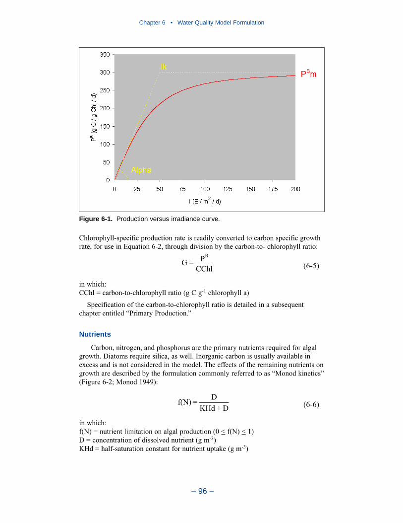
Chapter 6 • Water Quality Model Formulation
– 96 –
Chlorophyll-specific production rate is readily converted to carbon specific growthrate, for use in Equation 6-2, through division by the carbon-to- chlorophyll ratio:
in which:CChl = carbon-to-chlorophyll ratio (g C g-1 chlorophyll a)
Specification of the carbon-to-chlorophyll ratio is detailed in a subsequentchapter entitled “Primary Production.”
Nutrients
Carbon, nitrogen, and phosphorus are the primary nutrients required for algalgrowth. Diatoms require silica, as well. Inorganic carbon is usually available inexcess and is not considered in the model. The effects of the remaining nutrients ongrowth are described by the formulation commonly referred to as “Monod kinetics”(Figure 6-2; Monod 1949):
in which:f(N) = nutrient limitation on algal production (0 < f(N) < 1)D = concentration of dissolved nutrient (g m-3)KHd = half-saturation constant for nutrient uptake (g m-3)
D+KHdD=f(N) (6-6)
CChlP=G
B
(6-5)
Figure 6-1. Production versus irradiance curve.
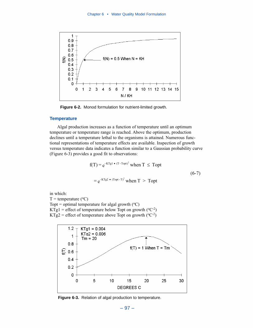
Chapter 6 • Water Quality Model Formulation
– 97 –
Figure 6-2. Monod formulation for nutrient-limited growth.
Temperature
Algal production increases as a function of temperature until an optimumtemperature or temperature range is reached. Above the optimum, productiondeclines until a temperature lethal to the organisms is attained. Numerous func-tional representations of temperature effects are available. Inspection of growthversus temperature data indicates a function similar to a Gaussian probability curve(Figure 6-3) provides a good fit to observations:
in which:T = temperature (oC)Topt = optimal temperature for algal growth (oC)KTg1 = effect of temperature below Topt on growth (oC-2)KTg2 = effect of temperature above Topt on growth (oC-2)
Topt>T when e=
ToptT when e=f(T)
)T-(ToptKTg2-
)Topt-(TKTg1-
2
2
(6-7)
Figure 6-3. Relation of algal production to temperature.
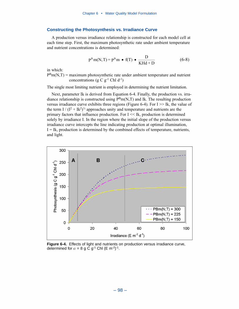
Constructing the Photosynthesis vs. Irradiance Curve
A production versus irradiance relationship is constructed for each model cell ateach time step. First, the maximum photosynthetic rate under ambient temperatureand nutrient concentrations is determined:
in which:PBm(N,T) = maximum photosynthetic rate under ambient temperature and nutrient
concentrations (g C g-1 Chl d-1)
The single most limiting nutrient is employed in determining the nutrient limitation.
Next, parameter Ik is derived from Equation 6-4. Finally, the production vs. irra-diance relationship is constructed using PBm(N,T) and Ik. The resulting productionversus irradiance curve exhibits three regions (Figure 6-4). For I >> Ik, the value ofthe term I / (I2 + Ik2)½ approaches unity and temperature and nutrients are theprimary factors that influence production. For I << Ik, production is determinedsolely by irradiance I. In the region where the initial slope of the production versusirradiance curve intercepts the line indicating production at optimal illumination,I = Ik, production is determined by the combined effects of temperature, nutrients,and light.
D+KHdDf(T)mP=T)m(N,P BB (6-8)
Chapter 6 • Water Quality Model Formulation
– 98 –
Figure 6-4. Effects of light and nutrients on production versus irradiance curve,determined for α = 8 g C g-1 Chl (E m-2)-1.
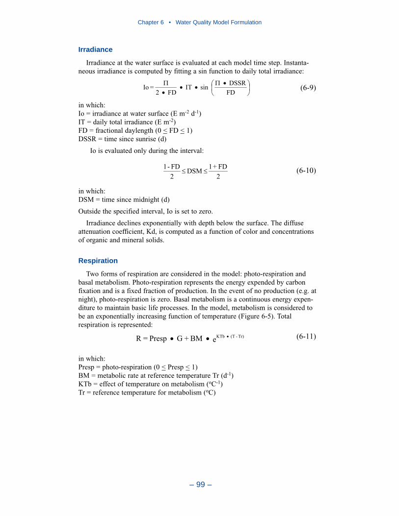
Irradiance
Irradiance at the water surface is evaluated at each model time step. Instanta-neous irradiance is computed by fitting a sin function to daily total irradiance:
in which:Io = irradiance at water surface (E m-2 d-1)IT = daily total irradiance (E m-2)FD = fractional daylength (0 < FD < 1)DSSR = time since sunrise (d)
Io is evaluated only during the interval:
in which:DSM = time since midnight (d)
Outside the specified interval, Io is set to zero.
Irradiance declines exponentially with depth below the surface. The diffuseattenuation coefficient, Kd, is computed as a function of color and concentrationsof organic and mineral solids.
Respiration
Two forms of respiration are considered in the model: photo-respiration andbasal metabolism. Photo-respiration represents the energy expended by carbonfixation and is a fixed fraction of production. In the event of no production (e.g. atnight), photo-respiration is zero. Basal metabolism is a continuous energy expen-diture to maintain basic life processes. In the model, metabolism is considered tobe an exponentially increasing function of temperature (Figure 6-5). Totalrespiration is represented:
in which:Presp = photo-respiration (0 < Presp < 1)BM = metabolic rate at reference temperature Tr (d-1)KTb = effect of temperature on metabolism (oC-1)Tr = reference temperature for metabolism (oC)
eBM+GPresp=R Tr)-(TKTb (6-11)
2FD+1DSM
2FD-1 (6-10)
FDDSSRsinIT
FD2=Io (6-9)
Chapter 6 • Water Quality Model Formulation
– 99 –
Chapter 6 • Water Quality Model Formulation
– 100 –
Figure 6-5. Exponential temperature relationship employed formetabolism and other processes.
Predation
The predation term includes the activity of zooplankton, filter-feeding benthos,and other pelagic filter feeders including planktivorous fish. Formulation andresults of the zooplankton computation appear elsewhere in this report. Details ofthe benthos computations may be found in HydroQual (2000) and athttp://www.chesapeakebay.net/model.htm. Predation by other planktivores ismodeled by assuming predators clear a specific volume of water per unit biomass:
F = filtration rate (m3 g-1 predator C d-1)M = planktivore biomass (g C m-3)
Detailed specification of the spatial and temporal distribution of the predatorpopulation is impossible. One approach is to assume predator biomass is propor-tional to algal biomass, M = γ B, in which case Equation 6-12 can be rewritten:
Since neither γ nor F are known precisely, the logical approach is to combinetheir product into a single unknown determined during the model calibration proce-dure. Effect of temperature on predation is represented with the same formulationas the effect of temperature on respiration. The final representation of predation,including zooplankton, is:
RMsz = microzooplankton maximum ration (g algal C g-1 zoo C d-1)SZ = microzooplankton biomass (g C m-3)KHsz = half saturation concentration for carbon uptake by microzooplankton
(g C m-3)
BPhtl+LZRMlzB+KHlz
B+
SZRMszB+KHsz
B=PR
2
(6-14)
BF=PR 2 (6-13)
MBF=PR (6-12)
RMlz = mesozooplankton maximum ration (g algal C g-1 zoo C d-1)LZ = mesozooplankton biomass (g C m-3)KHlz = half saturation concentration for carbon uptake by mesozooplankton
(g C m-3)Phtl = rate of predation by other planktivores (m3 g-1 C d-1)
Predation by filter-feeding benthos is represented as a loss term only in model cellsthat intersect the bottom.
Accounting for Algal Phosphorus
The amount of phosphorus incorporated in algal biomass is quantified througha stoichiometric ratio. Thus, total phosphorus in the model is expressed:
TotP = total phosphorus (g P m-3)PO4 = dissolved phosphate (g P m-3)Apc = algal phosphorus-to-carbon ratio (g P g-1 C)DOP = dissolved organic phosphorus (g P m-3)LPP = labile particulate organic phosphorus (g P m-3)RPP = refractory particulate organic phosphorus (g P m-3)
Algae take up dissolved phosphate during production and release dissolvedphosphate and organic phosphorus through respiration. The fate of phosphorusreleased by respiration is determined by empirical distribution coefficients. The fateof algal phosphorus recycled by predation is determined by a second set of distribu-tion parameters.
Accounting for Algal Nitrogen
Model nitrogen state variables include ammonium+urea, nitrate+nitrite,dissolved organic nitrogen, labile particulate organic nitrogen, and refractoryparticulate organic nitrogen. The amount of nitrogen incorporated in algal biomassis quantified through a stoichiometric ratio. Thus, total nitrogen in the model isexpressed:
TotN = total nitrogen (g N m-3)NH4-Urea = ammonium+urea (g N m-3)NO23 = nitrate+nitrite (g N m-3)Anc = algal nitrogen-to-carbon ratio (g N g-1 C)DON = dissolved organic nitrogen (g N m-3)LPON = labile particulate organic nitrogen (g N m-3)RPON = refractory particulate organic nitrogen (g N m-3)
As with phosphorus, the fate of algal nitrogen released by metabolism andpredation is represented by distribution coefficients.
RPON+LPON+DON+B_Anc+
NO+Urea-NH=TotN 234
(6-16)
RPOP+LPOP+DOP+B_Apc+PO=TotP 4 (6-15)
Chapter 6 • Water Quality Model Formulation
– 101 –
•
•
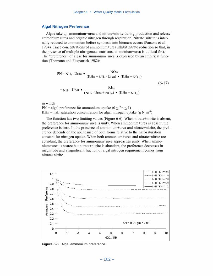
Algal Nitrogen Preference
Algae take up ammonium+urea and nitrate+nitrite during production and releaseammonium+urea and organic nitrogen through respiration. Nitrate+nitrite is inter-nally reduced to ammonium before synthesis into biomass occurs (Parsons et al.1984). Trace concentrations of ammonium+urea inhibit nitrate reduction so that, inthe presence of multiple nitrogenous nutrients, ammonium+urea is utilized first.The “preference” of algae for ammonium+urea is expressed by an empirical func-tion (Thomann and Fitzpatrick 1982):
in whichPN = algal preference for ammonium uptake (0 < Pn < 1)KHn = half saturation concentration for algal nitrogen uptake (g N m-3)
The function has two limiting values (Figure 6-6). When nitrate+nitrite is absent,the preference for ammonium+urea is unity. When ammonium+urea is absent, thepreference is zero. In the presence of ammonium+urea and nitrate+nitrite, the pref-erence depends on the abundance of both forms relative to the half-saturationconstant for nitrogen uptake. When both ammonium+urea and nitrate+nitrite areabundant, the preference for ammonium+urea approaches unity. When ammo-nium+urea is scarce but nitrate+nitrite is abundant, the preference decreases inmagnitude and a significant fraction of algal nitrogen requirement comes fromnitrate+nitrite.
)NO+(KHn)NO+Urea-NH(KHnUrea-NH+
)NO+(KHnUrea)-NH+(KHnNOUrea-NH=PN
232344
234
234
(6-17)
Chapter 6 • Water Quality Model Formulation
– 102 –
Figure 6-6. Algal ammonium preference.
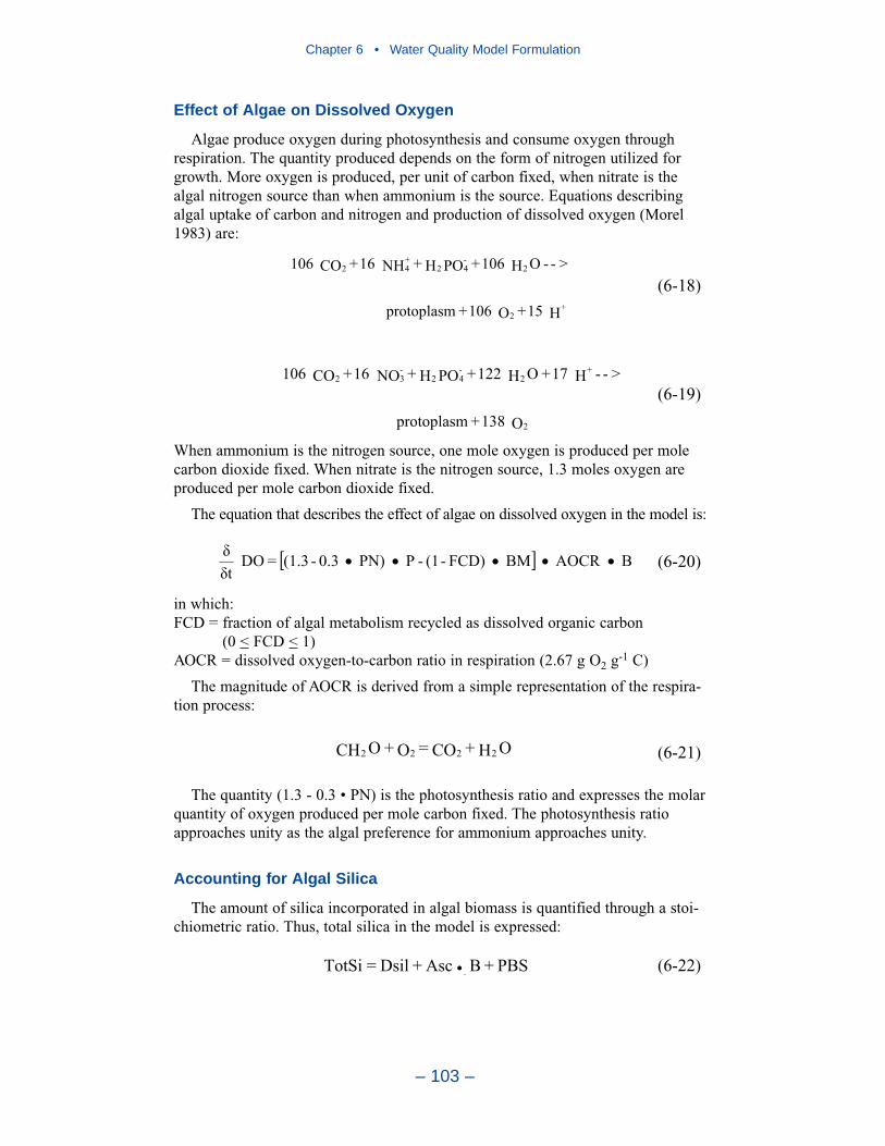
Chapter 6 • Water Quality Model Formulation
– 103 –
Effect of Algae on Dissolved Oxygen
Algae produce oxygen during photosynthesis and consume oxygen throughrespiration. The quantity produced depends on the form of nitrogen utilized forgrowth. More oxygen is produced, per unit of carbon fixed, when nitrate is thealgal nitrogen source than when ammonium is the source. Equations describingalgal uptake of carbon and nitrogen and production of dissolved oxygen (Morel1983) are:
When ammonium is the nitrogen source, one mole oxygen is produced per molecarbon dioxide fixed. When nitrate is the nitrogen source, 1.3 moles oxygen areproduced per mole carbon dioxide fixed.
The equation that describes the effect of algae on dissolved oxygen in the model is:
in which:FCD = fraction of algal metabolism recycled as dissolved organic carbon
(0 < FCD < 1)AOCR = dissolved oxygen-to-carbon ratio in respiration (2.67 g O2 g-1 C)
The magnitude of AOCR is derived from a simple representation of the respira-tion process:
The quantity (1.3 - 0.3 • PN) is the photosynthesis ratio and expresses the molarquantity of oxygen produced per mole carbon fixed. The photosynthesis ratioapproaches unity as the algal preference for ammonium approaches unity.
Accounting for Algal Silica
The amount of silica incorporated in algal biomass is quantified through a stoi-chiometric ratio. Thus, total silica in the model is expressed:
PBS+B_Asc+Dsil=TotSi (6-22)
OH+CO=O+OCH 2222 (6-21)
BAOCRBMFCD)-(1-PPN)0.3-(1.3=DOt
(6-20)
O138+protoplasm
>--H17+OH122+POH+NO16+CO106
2
+2
-42
-32
(6-19)
H15+O106+protoplasm
>--OH106+POH+NH16+CO106
+2
2-42
+42
(6-18)
•
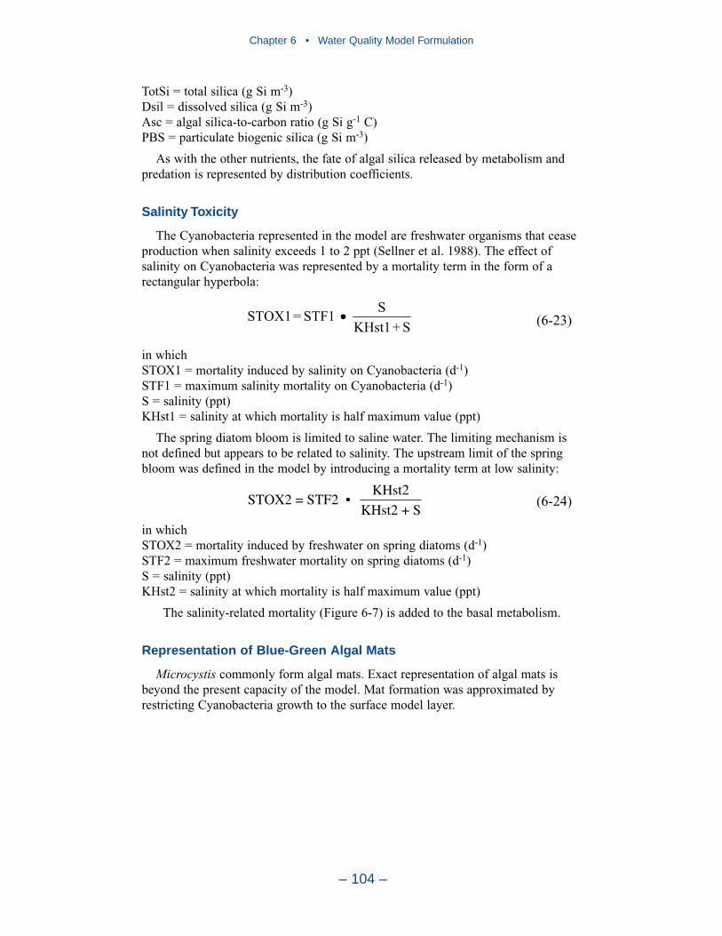
Chapter 6 • Water Quality Model Formulation
– 104 –
TotSi = total silica (g Si m-3)Dsil = dissolved silica (g Si m-3)Asc = algal silica-to-carbon ratio (g Si g-1 C)PBS = particulate biogenic silica (g Si m-3)
As with the other nutrients, the fate of algal silica released by metabolism andpredation is represented by distribution coefficients.
Salinity Toxicity
The Cyanobacteria represented in the model are freshwater organisms that ceaseproduction when salinity exceeds 1 to 2 ppt (Sellner et al. 1988). The effect ofsalinity on Cyanobacteria was represented by a mortality term in the form of arectangular hyperbola:
in whichSTOX1 = mortality induced by salinity on Cyanobacteria (d-1)STF1 = maximum salinity mortality on Cyanobacteria (d-1)S = salinity (ppt)KHst1 = salinity at which mortality is half maximum value (ppt)
The spring diatom bloom is limited to saline water. The limiting mechanism isnot defined but appears to be related to salinity. The upstream limit of the springbloom was defined in the model by introducing a mortality term at low salinity:
in whichSTOX2 = mortality induced by freshwater on spring diatoms (d-1)STF2 = maximum freshwater mortality on spring diatoms (d-1)S = salinity (ppt)KHst2 = salinity at which mortality is half maximum value (ppt)
The salinity-related mortality (Figure 6-7) is added to the basal metabolism.
Representation of Blue-Green Algal Mats
Microcystis commonly form algal mats. Exact representation of algal mats isbeyond the present capacity of the model. Mat formation was approximated byrestricting Cyanobacteria growth to the surface model layer.
KHst2STOX2 = STF2 •
KHst2 + S(6-24)
S+KHst1SSTF1=STOX1 (6-23)

Organic Carbon
Organic carbon undergoes innumerable transformations in the water column.The model carbon cycle (Figure 6-8) consists of the following elements:
• Phytoplankton production and excretion
• Zooplankton production and excretion
• Predation on phytoplankton
• Dissolution of particulate carbon
• Heterotrophic respiration
• Denitrification
• Settling
Algal production is the primary carbon source although carbon also enters thesystem through external loading. Predation on algae by zooplankton and otherorganisms releases particulate and dissolved organic carbon to the water column. Afraction of the particulate organic carbon undergoes first-order dissolution todissolved organic carbon. Dissolved organic carbon produced by excretion, bypredation, and by dissolution is respired at a first-order rate to inorganic carbon.Particulate organic carbon which does not undergo dissolution settles to the bottomsediments.
Zooplankton kinetics are detailed in a separate chapter. Kinetics of the organiccarbon state variables are described below.
Chapter 6 • Water Quality Model Formulation
– 105 –
Figure 6-7. Salinity toxicity relationship.

Dissolution and Respiration
Organic carbon dissolution and respiration are represented as first-orderprocesses in which the reaction rate is proportional to concentration of the reactant. An exponential function (Figure 6-5) relates dissolution and respiration to temperature.
In the model, a Monod-like function diminishes respiration as dissolved oxygenapproaches zero. As oxygen is depleted from natural systems, oxidation of organicmatter is effected by the reduction of alternate oxidants. The sequence in whichalternate oxidants are employed is determined by the thermodynamics of oxidation-reduction reactions. The first substance reduced in the absence of oxygen is nitrate.A representation of the denitrification reaction can be obtained by balancing stan-dard half-cell redox reactions (Stumm and Morgan 1981):
Equation 6-25 describes the stoichiometry of the denitrification reaction. Thekinetics of the reaction, represented in the model, are first-order. The dissolvedorganic carbon respiration rate, Kdoc, is modified so that significant decay viadenitrification occurs only when nitrate is freely available and dissolved oxygen isdepleted (Figure 6-9). A parameter is included so that the anoxic respiration rate isslower than oxic respiration:
CO5+OH7+N2>--OCH5+H4+NO4 2222+-
3 (6-25)
Chapter 6 • Water Quality Model Formulation
– 106 –
Figure 6-8. Model carbon cycle.
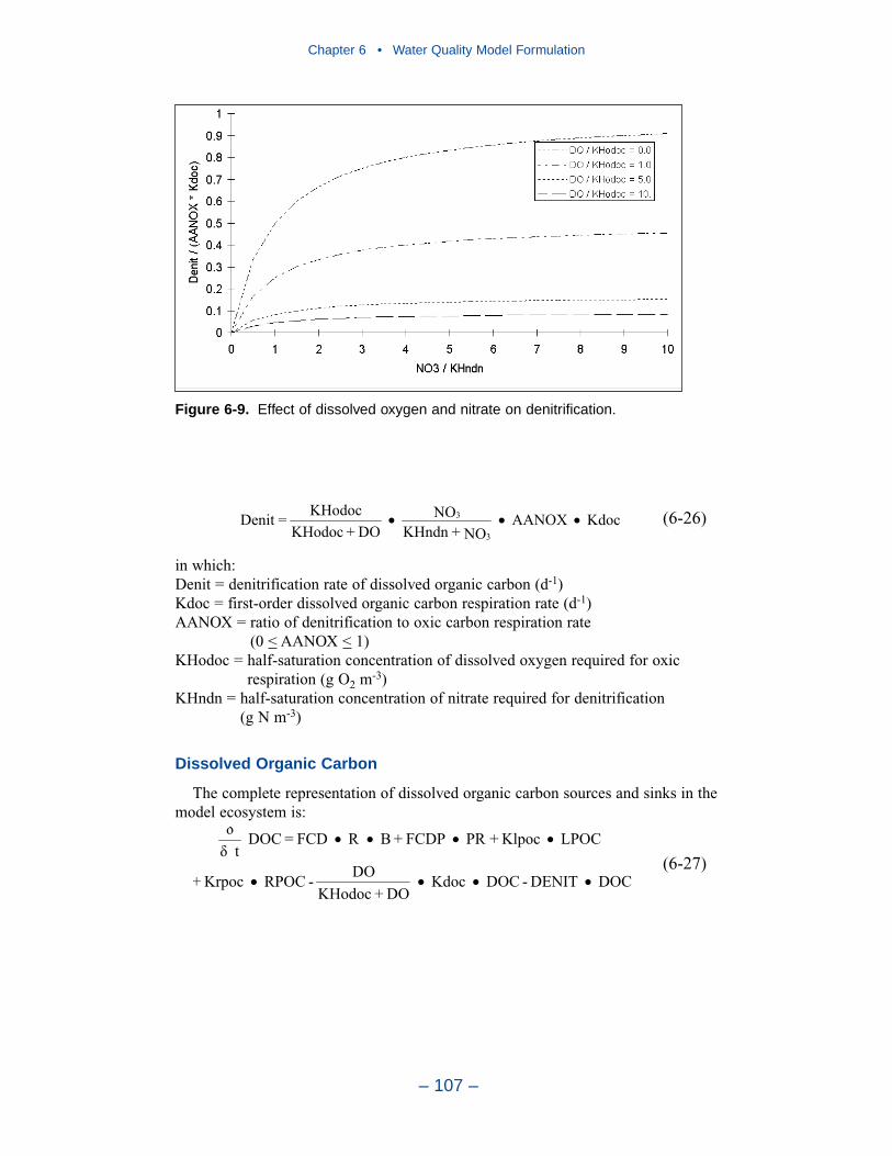
in which:Denit = denitrification rate of dissolved organic carbon (d-1)Kdoc = first-order dissolved organic carbon respiration rate (d-1)AANOX = ratio of denitrification to oxic carbon respiration rate
(0 < AANOX < 1)KHodoc = half-saturation concentration of dissolved oxygen required for oxic
respiration (g O2 m-3)KHndn = half-saturation concentration of nitrate required for denitrification
(g N m-3)
Dissolved Organic Carbon
The complete representation of dissolved organic carbon sources and sinks in themodel ecosystem is:
M d l F l ti 1
DOCDENIT-DOCKdocDO+KHodoc
DO-RPOCKrpoc+
LPOCKlpoc+PRFCDP+BRFCD=DOC t
(6-27)
KdocAANOXNO+KHndn
NODO+KHodoc
KHodoc=Denit3
3 (6-26)
Chapter 6 • Water Quality Model Formulation
– 107 –
Figure 6-9. Effect of dissolved oxygen and nitrate on denitrification.
in which:DOC = dissolved organic carbon (g m-3)LPOC = labile particulate organic carbon (g m-3)RPOC = refractory particulate organic carbon (g m-3)FCD = fraction of algal respiration released as DOC (0 < FCD < 1)FCDP = fraction of predation on algae released as DOC (0 < FCDP < 1)Klpoc = dissolution rate of LPOC (d-1)Krpoc = dissolution rate of RPOC (d-1)Kdoc = respiration rate of DOC (d-1)
Labile Particulate Organic Carbon
The complete representation of labile particulate organic carbon sources andsinks in the model ecosystem is:
in which:FCL = fraction of algal respiration released as LPOC (0 < FCL < 1)FCLP = fraction of predation on algae released as LPOC (0 < FCLP < 1)Wl = settling velocity of labile particles (m d-1)
Refractory Particulate Organic Carbon
The complete representation of refractory particulate organic carbon sourcesand sinks in the model ecosystem is:
in which:FCR = fraction of algal respiration released as RPOC (0 < FCR < 1) FCRP = fraction of predation on algae released as RPOC (0 < FCRP < 1)Wr = settling velocity of refractory particles (m d-1)
Phosphorus
The model phosphorus cycle (Figure 6-10) includes the following processes:
• Algal uptake and excretion
• Zooplankton excretion
• Predation
• Hydrolysis of particulate organic phosphorus
• Mineralization of dissolved organic phosphorus
• Settling and resuspension
RPOCz
Wr-
RPOCKrpoc-PRFCRP+BRFCR=RPOC t (6-29)
LPOCz
Wl-
LPOCKlpoc-PRFCLP+BRFCL=LPOC t (6-28)
Chapter 6 • Water Quality Model Formulation
– 108 –
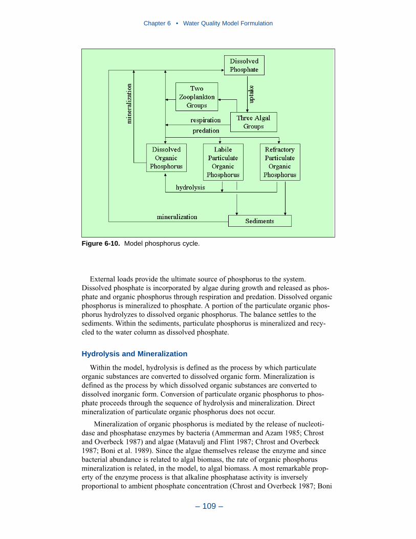
External loads provide the ultimate source of phosphorus to the system.Dissolved phosphate is incorporated by algae during growth and released as phos-phate and organic phosphorus through respiration and predation. Dissolved organicphosphorus is mineralized to phosphate. A portion of the particulate organic phos-phorus hydrolyzes to dissolved organic phosphorus. The balance settles to thesediments. Within the sediments, particulate phosphorus is mineralized and recy-cled to the water column as dissolved phosphate.
Hydrolysis and Mineralization
Within the model, hydrolysis is defined as the process by which particulateorganic substances are converted to dissolved organic form. Mineralization isdefined as the process by which dissolved organic substances are converted todissolved inorganic form. Conversion of particulate organic phosphorus to phos-phate proceeds through the sequence of hydrolysis and mineralization. Directmineralization of particulate organic phosphorus does not occur.
Mineralization of organic phosphorus is mediated by the release of nucleoti-dase and phosphatase enzymes by bacteria (Ammerman and Azam 1985; Chrostand Overbeck 1987) and algae (Matavulj and Flint 1987; Chrost and Overbeck1987; Boni et al. 1989). Since the algae themselves release the enzyme and sincebacterial abundance is related to algal biomass, the rate of organic phosphorusmineralization is related, in the model, to algal biomass. A most remarkable prop-erty of the enzyme process is that alkaline phosphatase activity is inverselyproportional to ambient phosphate concentration (Chrost and Overbeck 1987; Boni
Chapter 6 • Water Quality Model Formulation
– 109 –
Figure 6-10. Model phosphorus cycle.
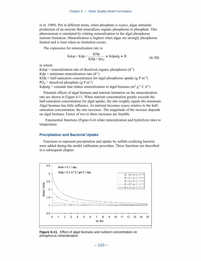
Chapter 6 • Water Quality Model Formulation
– 110 –
et al. 1989). Put in different terms, when phosphate is scarce, algae stimulateproduction of an enzyme that mineralizes organic phosphorus to phosphate. Thisphenomenon is simulated by relating mineralization to the algal phosphorusnutrient limitation. Mineralization is highest when algae are strongly phosphoruslimited and is least when no limitation occurs.
The expression for mineralization rate is:
in which:Kdop = mineralization rate of dissolved organic phosphorus (d-1)Kdp = minimum mineralization rate (d-1)KHp = half-saturation concentration for algal phosphorus uptake (g P m-3)PO4 = dissolved phosphate (g P m-3)Kdpalg = constant that relates mineralization to algal biomass (m3 g-1 C d-1)
Potential effects of algal biomass and nutrient limitation on the mineralizationrate are shown in Figure 6-11. When nutrient concentration greatly exceeds thehalf-saturation concentration for algal uptake, the rate roughly equals the minimum.Algal biomass has little influence. As nutrient becomes scarce relative to the half-saturation concentration, the rate increases. The magnitude of the increase dependson algal biomass. Factor of two to three increases are feasible.
Exponential functions (Figure 6-4) relate mineralization and hydrolysis rates totemperature.
Precipitation and Bacterial Uptake
Functions to represent precipitation and uptake by sulfide-oxidizing bacteriawere added during the model calibration procedure. These functions are describedin a subsequent chapter.
BKdpalgPO+KHp
KHp+Kdp=Kdop4
(6-30)
Figure 6-11. Effect of algal biomass and nutrient concentration on phosphorus mineralization.
Chapter 6 • Water Quality Model Formulation
– 111 –
Dissolved Phosphate
The mass-balance equation for dissolved phosphate is:
in which:FPI = fraction of algal metabolism released as dissolved phosphate (0 < FPI < 1)FPIP = fraction of predation released as dissolved phosphate (0 < FPIP < 1)
Dissolved Organic Phosphorus
The mass balance equation for dissolved organic phosphorus is:
in which:DOP = dissolved organic phosphorus (g P m-3)LPOP = labile particulate organic phosphorus (g P m-3)RPOP = refractory particulate organic phosphorus (g P m-3)FPD = fraction of algal metabolism released as DOP (0 < FPD < 1)FPDP = fraction of predation on algae released as DOP (0 < FPDP < 1)Klpop = hydrolysis rate of LPOP (d-1)Krpop = hydrolysis rate of RPOP (d-1)Kdop = mineralization rate of DOP (d-1)
Labile Particulate Organic Phosphorus
The mass balance equation for labile particulate organic phosphorus is:
in which:FPL = fraction of algal metabolism released as LPOP (0 < FPL < 1)FPLP = fraction of predation on algae released as LPOP (0 < FPLP < 1)
LPOPz
Wl-
LPOPKlpop-FPLP)PR+FPLB(BMAPC=LPOP t (6-33)
DOPKdop-RPOPKrpop+
LPOPKlpop+FPDP)PR+FPDB(BMAPC=DOP t (6-32)
PRFPIP+BBMFPIAPC+
BGAPC-DOPKdop=PO t 4 (6-31)
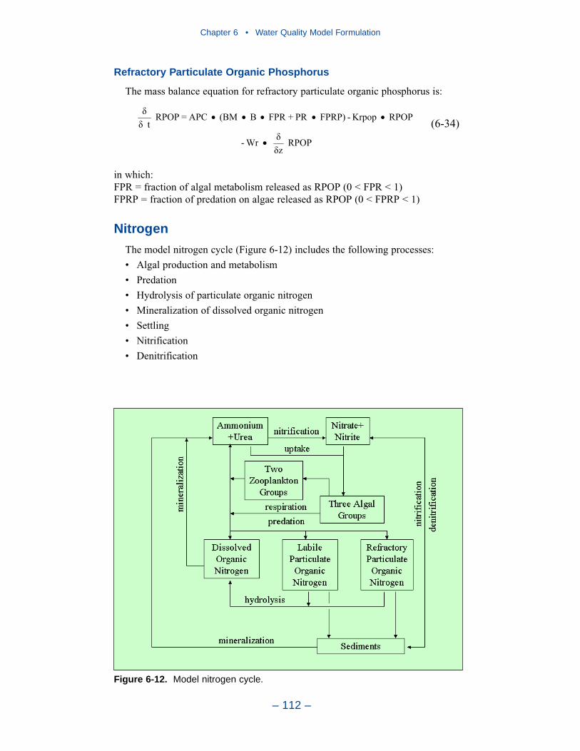
Refractory Particulate Organic Phosphorus
The mass balance equation for refractory particulate organic phosphorus is:
in which:FPR = fraction of algal metabolism released as RPOP (0 < FPR < 1)FPRP = fraction of predation on algae released as RPOP (0 < FPRP < 1)
Nitrogen
The model nitrogen cycle (Figure 6-12) includes the following processes:
• Algal production and metabolism
• Predation
• Hydrolysis of particulate organic nitrogen
• Mineralization of dissolved organic nitrogen
• Settling
• Nitrification
• Denitrification
RPOPz
Wr-
RPOPKrpop-FPRP)PR+FPRB(BMAPC=RPOP t (6-34)
Chapter 6 • Water Quality Model Formulation
– 112 –
Figure 6-12. Model nitrogen cycle.
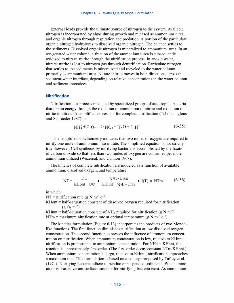
Chapter 6 • Water Quality Model Formulation
– 113 –
External loads provide the ultimate source of nitrogen to the system. Availablenitrogen is incorporated by algae during growth and released as ammonium+ureaand organic nitrogen through respiration and predation. A portion of the particulateorganic nitrogen hydrolyzes to dissolved organic nitrogen. The balance settles tothe sediments. Dissolved organic nitrogen is mineralized to ammonium+urea. In anoxygenated water column, a fraction of the ammonium+urea is subsequentlyoxidized to nitrate+nitrite through the nitrification process. In anoxic water,nitrate+nitrite is lost to nitrogen gas through denitrification. Particulate nitrogenthat settles to the sediments is mineralized and recycled to the water column,primarily as ammonium+urea. Nitrate+nitrite moves in both directions across thesediment-water interface, depending on relative concentrations in the water columnand sediment interstices.
Nitrification
Nitrification is a process mediated by specialized groups of autotrophic bacteriathat obtain energy through the oxidation of ammonium to nitrite and oxidation ofnitrite to nitrate. A simplified expression for complete nitrification (Tchobanoglousand Schroeder 1987) is:
The simplified stoichiometry indicates that two moles of oxygen are required tonitrify one mole of ammonium into nitrate. The simplified equation is not strictlytrue, however. Cell synthesis by nitrifying bacteria is accomplished by the fixationof carbon dioxide so that less than two moles of oxygen are consumed per moleammonium utilized (Wezernak and Gannon 1968).
The kinetics of complete nitrification are modeled as a function of availableammonium, dissolved oxygen, and temperature:
in which:NT = nitrification rate (g N m-3 d-1)KHont = half-saturation constant of dissolved oxygen required for nitrification
(g O2 m-3)KHnnt = half-saturation constant of NH4 required for nitrification (g N m-3)NTm = maximum nitrification rate at optimal temperature (g N m-3 d-1)
The kinetics formulation (Figure 6-13) incorporates the products of two Monod-like functions. The first function diminishes nitrification at low dissolved oxygenconcentration. The second function expresses the influence of ammonium concen-tration on nitrification. When ammonium concentration is low, relative to KHnnt,nitrification is proportional to ammonium concentration. For NH4 = KHnnt, thereaction is approximately first-order. (The first-order decay constant NTm/KHnnt.)When ammonium concentration is large, relative to KHnnt, nitrification approachesa maximum rate. This formulation is based on a concept proposed by Tuffey et al.(1974). Nitrifying bacteria adhere to benthic or suspended sediments. When ammo-nium is scarce, vacant surfaces suitable for nitrifying bacteria exist. As ammonium
NTmf(T)Urea-NH+KHnnt
Urea-NHDO+KHont
DO=NT4
4 (6-36)
H2+OH+NO>--O2+NH +2
-32
+4 (6-35)
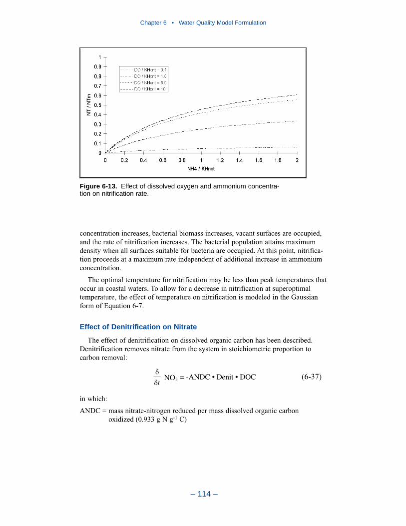
Chapter 6 • Water Quality Model Formulation
– 114 –
Figure 6-13. Effect of dissolved oxygen and ammonium concentra-tion on nitrification rate.
concentration increases, bacterial biomass increases, vacant surfaces are occupied,and the rate of nitrification increases. The bacterial population attains maximumdensity when all surfaces suitable for bacteria are occupied. At this point, nitrifica-tion proceeds at a maximum rate independent of additional increase in ammoniumconcentration.
The optimal temperature for nitrification may be less than peak temperatures thatoccur in coastal waters. To allow for a decrease in nitrification at superoptimaltemperature, the effect of temperature on nitrification is modeled in the Gaussianform of Equation 6-7.
Effect of Denitrification on Nitrate
The effect of denitrification on dissolved organic carbon has been described.Denitrification removes nitrate from the system in stoichiometric proportion tocarbon removal:
in which:
ANDC = mass nitrate-nitrogen reduced per mass dissolved organic carbonoxidized (0.933 g N g-1 C)
3 = -ANDC • Denit • DOCNOt
(6-37)
Chapter 6 • Water Quality Model Formulation
– 115 –
Nitrogen Mass Balance Equations
The mass-balance equation for nitrogen state variables are written by summingall previously-described sources and sinks:
Ammonium+Urea
in which:FNI = fraction of algal metabolism released as NH4 (0 < FNI < 1)PN = algal ammonium preference (0 < PN < 1)FNIP = fraction of predation released as NH4 (0 < FNIP < 1)
Nitrate+Nitrite
Dissolved Organic Nitrogen
in which:DON = dissolved organic nitrogen (g N m-3)LPON = labile particulate organic nitrogen (g N m-3)RPON = refractory particulate organic nitrogen (g N m-3)FND = fraction of algal metabolism released as DON (0 < FND < 1)FNDP = fraction of predation on algae released as DON (0 < FNDP < 1)Klpon = hydrolysis rate of LPON (d-1)Krpon = hydrolysis rate of RPON (d-1)Kdon = mineralization rate of DON (d-1)
Labile Particulate Organic Nitrogen
in which:FNL = fraction of algal metabolism released as LPON (0 < FNL < 1)FNLP = fraction of predation on algae released as LPON (0 < FNLP < 1)
LPONz
Wl-
LPONKlpon-FNLP)PR+FNLB(BMANC=LPON t (6-41)
DONKdon-RPONKrpon+
LPONKlpon+FNDP)PR+FNDB(BMANC=DON t (6-40)
DOCDenitANDC-
NT+BPPN)-(1ANC-=NO t 23 (6-39)
NT-DONKdon+
FNIPPR+BP)PN-FNI(BMANC=Urea-NH t 4 (6-38)
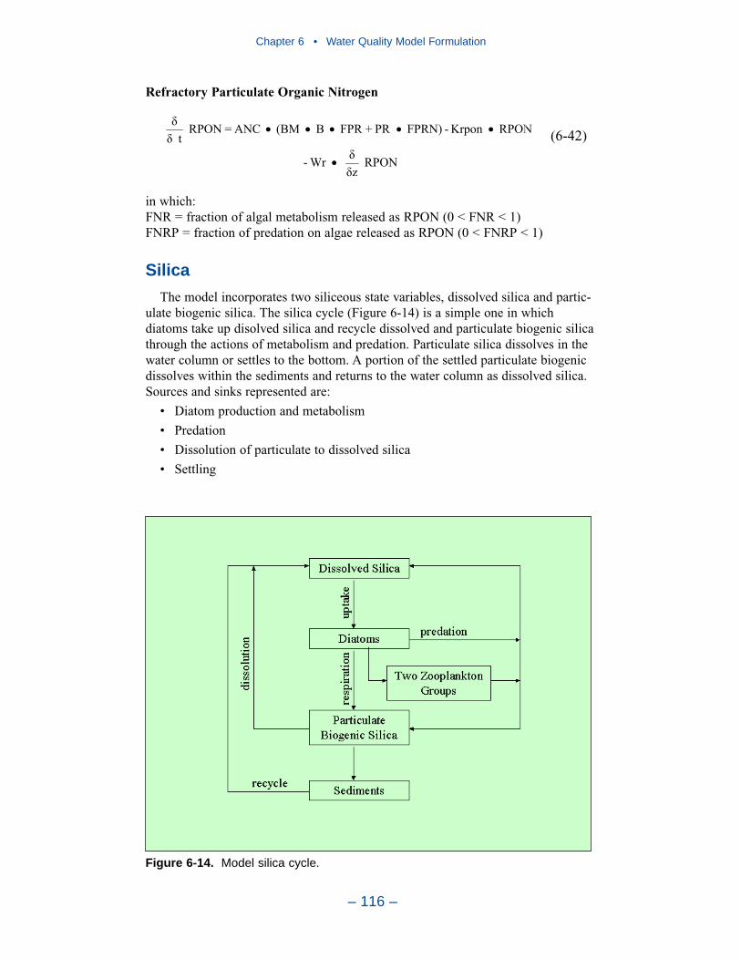
Refractory Particulate Organic Nitrogen
in which:FNR = fraction of algal metabolism released as RPON (0 < FNR < 1)FNRP = fraction of predation on algae released as RPON (0 < FNRP < 1)
Silica
The model incorporates two siliceous state variables, dissolved silica and partic-ulate biogenic silica. The silica cycle (Figure 6-14) is a simple one in whichdiatoms take up disolved silica and recycle dissolved and particulate biogenic silicathrough the actions of metabolism and predation. Particulate silica dissolves in thewater column or settles to the bottom. A portion of the settled particulate biogenicdissolves within the sediments and returns to the water column as dissolved silica.Sources and sinks represented are:
• Diatom production and metabolism
• Predation
• Dissolution of particulate to dissolved silica
• Settling
RPONz
Wr-
RPONKrpon-FPRN)PR+FPRB(BMANC=RPON t (6-42)
Chapter 6 • Water Quality Model Formulation
– 116 –
Figure 6-14. Model silica cycle.
Chapter 6 • Water Quality Model Formulation
– 117 –
Dissolved Silica
The kinetics equation for dissolved silica is:
in which:Dsil = dissolved silica (g Si m-3)PBS = particulate biogenic silica concentration (g Si m-3)FSAP = fraction of diatom silica made available by predation (0 < FSAP < 1)ASC = algal silica-to-carbon ratio (g Si g-1 C)Ksua = particulate silica dissolution rate (d-1)
Particulate Biogenic Silica
The kinetics equation for particulate biogenic silica is:
in which:Wpbs = biogenic silica settling rate (m d-1)
An exponential function (Figure 6-4) describes the effect of temperature onsilica dissolution.
Chemical Oxygen Demand
Chemical oxygen demand is the concentration of reduced substances that areoxidized through abiotic reactions. The source of chemical oxygen demand insaline water is sulfide released from sediments. A cycle occurs in which sulfate isreduced to sulfide in the sediments and reoxidized to sulfate in the water column.In freshwater, methane is released to the water column by the sediment model.Both sulfide and methane are quantified in units of oxygen demand and are treatedwith the same kinetics formulation:
in which:COD = chemical oxygen demand concentration (g oxygen-equivalents m-3)KHocod = half-saturation concentration of dissolved oxygen required for exertion
of chemical oxygen demand (g O2 m-3)Kcod = oxidation rate of chemical oxygen demand (d-1)
An exponential function (Figure 6-5) describes the effect of temperature onexertion of chemical oxygen demand.
CODKcodDO+KHocod
DO-=COD t
(6-45)
PBSKsua-PBSz
Wpbs-
BASCPRFSAP)-(1+BM=PBSt
(6-44)
PBSKsua+BASCP)-PR(FSAP=Dsilt (6-43)

Dissolved Oxygen
Sources and sinks of dissolved oxygen in the water column (Figure 6-15)include:
• Algal photosynthesis
• Atmospheric reaeration
• Algal respiration
• Heterotrophic respiration
• Nitrification
• Chemical oxygen demand
Reaeration
The rate of reaeration is proportional to the dissolved oxygen deficit in modelsegments that form the air-water interface:
in which:DO = dissolved oxygen concentration (g O2 m-3)Kr = reaeration coefficient (m d-1)DOs = dissolved oxygen saturation concentration (g O2 m-3)∆z = model layer thickness (m)
DO)-(DOsz
Kr=DO t (6-46)
Chapter 6 • Water Quality Model Formulation
– 118 –
Figure 6-15. Oxygen sources and sinks.

In freeflowing streams, the reaeration coefficient depends largely on turbulencegenerated by bottom shear stress (O’Connor and Dobbins 1958). In lakes andcoastal waters, however, wind effects may dominate the reaeration process(O’Connor 1983). For Chesapeake Bay, a relationship for wind-driven gasexchange (Hartman and Hammond 1985) was employed:
in which:Arear = empirical constant (0.1)Rυ = ratio of kinematic viscosity of pure water at 20 oC to kinematic viscosity of
water at specified temperature and salinityWms = wind speed measured at 10 m above water surface (m s-1)
Hartman and Hammond (1985) indicate Arear takes the value 0.157. In thepresent model, Arear is treated as a variable to allow for effects of wind sheltering,for differences in height of local wind observations, and for other factors.
An empirical function (Figure 6-16) that fits tabulated values of Rυ is:
in which:S = salinity (ppt)T = temperature (oC)
S0.0020-T0.0233+0.54=R (6-48)
WmsRArear=Kr 1.5 (6-47)
Chapter 6 • Water Quality Model Formulation
– 119 –
Figure 6-16. Computed and tabulated values of Rυ.

Saturation dissolved oxygen concentration diminishes as temperature andsalinity increase. An empirical formula that describes these effects (Genet et al.1974) is:
in which:CL = chloride concentration (= salinity/1.80655)
Mass Balance Equation for Dissolved Oxygen
in which:AOCR = oxygen-to-carbon mass ratio in production and respiration
(= 2.67 g O2 g-1 C)AONT = oxygen consumed per mass ammonium nitrified (= 4.33 g O2 g-1 N)
Temperature
Computation of temperature employs a conservation of internal energy equa-tion that is analogous to the conservation of mass equation. For practical purposes,the internal energy equation can be written as a conservation of temperature equa-tion. The only source or sink of temperature considered is exchange with theatmosphere. Atmospheric exchange is considered proportional to the temperaturedifference between the water surface and a theoretical equilibrium temperature(Edinger et al. 1974):
in which:T = water temperature (oC)Te = equilibrium temperature (oC)KT = Heat exchange coefficient (watt m-2 oC-1)Cp = specific heat of water (4200 watt s kg-1 oC-1)ρ = density of water (1000 kg m-3)
T)-(TeHCp
KT=T t (6-51)
DO)-(DOsHKr+CODKcod
DO+KHocodDO-
DOCKdocAOCRDO+KHodoc
DO-NTAONT-
BBMFCD)-(1-PPN)0.3-(1.3AOCR=DO t
(6-50)
×
2
-4 -6 -8 2
DOs = 14.5532 - 0.38217 • T + 0.0054258 • T
- CL • (1.665 × - 5.866 × • T + 9.796 • )10 10 10 T(6-49)
Chapter 6 • Water Quality Model Formulation
– 120 –
Chapter 6 • Water Quality Model Formulation
– 121 –
Inorganic (Fixed) Solids
The only kinetics transformation of fixed solids is settling:
in which:ISS = fixed solids concentration (g m-3)Wiss = solids settling velocity (m d-1)
Salinity
Salinity is modeled by the conservation of mass equation with no internalsources or sinks
Parameter Values
Model parameter evaluation is a recursive process. Parameters are selected froma range of feasible values, tested in the model, and adjusted until satisfactory agree-ment between predicted and observed variables is obtained. Ideally, the range offeasible values is determined by observation or experiment. For some parameters,however, no observations are available. Then, the feasible range is determined byparameter values employed in similar models or by the judgement of the modeler.A review of parameter values was included in documentation of the first applica-tion of this model (Cerco and Cole 1994). Parameters from the initial study wererefined, where necessary, for the Virginia Tributary Refinements (Cerco et al. 2002)and refined again for the present model. A complete set of parameter values isprovided in Table 6-2. Subsequent chapters describe derivation of parameters thatwere not in the original study.
ISSz
Wiss-=ISS t (6-52)

Chapter 6 • Water Quality Model Formulation
– 122 –
Table 6-2
Parameters in Kinetics Equations
Symbol Definition Value Units
AANOX ratio of anoxic to oxic respiration 0.5 0 < AANOX < 1
ANC nitrogen-to-carbon ratio of algae 0.135 (spring), 0.175 (other)
g N g-1 C
AOCR dissolved oxygen-to-carbon ratio in respiration
2.67 g O2 g-1 C
AONT mass dissolved oxygen consumed per mass ammonium nitrified
4.33 g O2 g-1 N
APC algal phosphorus-to-carbon ratio 0.0175 (green), 0.0125 (other)
g P g-1 C
Areaer empirical constant in reaeration equation 0.078
ASC algal silica-to-carbon ratio 0.0 (cyan), 0.4 (spring), 0.3 (green)
g Si g-1 C
BM basal metabolic rate of algae at reference temperature Tr
0.03 (cyan), 0.01 (spring), 0.02 (green)
d-1
FCD fraction of dissolved organic carbon produced by algal metabolism
0.0 0 < FCD < 1
FCDP fraction of dissolved organic carbon produced by predation
0.15 0 < FCDP < 1
FCL fraction of labile particulate carbon produced by algal metabolism
0.0 0 < FCL < 1
FCLP fraction of labile particulate carbon produced by predation
0.65 0 < FCLP < 1
FCR fraction of refractory particulate carbon produced by algal metabolism
0.0 0 < FCR < 1
FCRP fraction of refractory particulate carbon produced by predation
0.2 0 < FCRP < 1
FNI fraction of inorganic nitrogen produced by algal metabolism
0.55 0 < FNI < 1
FNIP fraction of inorganic nitrogen produced by predation
0.4 0 < FNIP < 1
FND fraction of dissolved organic nitrogen produced by algal metabolism
0.2 0 < FND < 1
continued
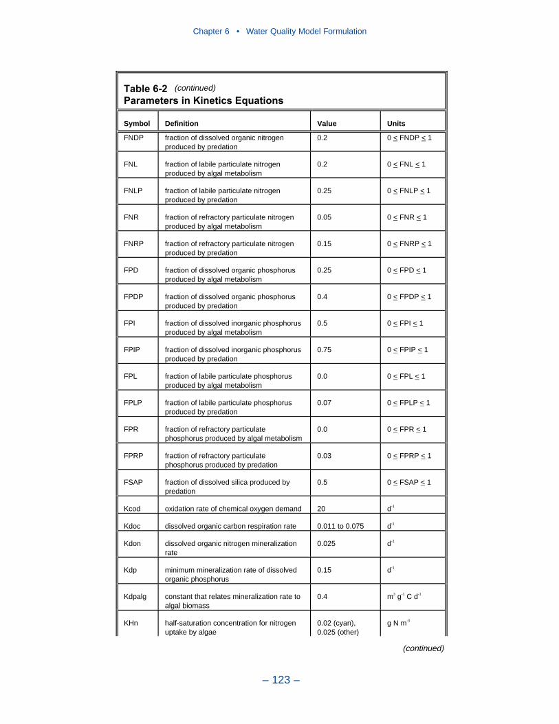
Chapter 6 • Water Quality Model Formulation
– 123 –
Table 6-2
Parameters in Kinetics Equations
Symbol Definition Value Units
FNDP fraction of dissolved organic nitrogen produced by predation
0.2 0 < FNDP < 1
FNL fraction of labile particulate nitrogen produced by algal metabolism
0.2 0 < FNL < 1
FNLP fraction of labile particulate nitrogen produced by predation
0.25 0 < FNLP < 1
FNR fraction of refractory particulate nitrogen produced by algal metabolism
0.05 0 < FNR < 1
FNRP fraction of refractory particulate nitrogen produced by predation
0.15 0 < FNRP < 1
FPD fraction of dissolved organic phosphorus produced by algal metabolism
0.25 0 < FPD < 1
FPDP fraction of dissolved organic phosphorus produced by predation
0.4 0 < FPDP < 1
FPI fraction of dissolved inorganic phosphorus produced by algal metabolism
0.5 0 < FPI < 1
FPIP fraction of dissolved inorganic phosphorus produced by predation
0.75 0 < FPIP < 1
FPL fraction of labile particulate phosphorus produced by algal metabolism
0.0 0 < FPL < 1
FPLP fraction of labile particulate phosphorus produced by predation
0.07 0 < FPLP < 1
FPR fraction of refractory particulate phosphorus produced by algal metabolism
0.0 0 < FPR < 1
FPRP fraction of refractory particulate phosphorus produced by predation
0.03 0 < FPRP < 1
FSAP fraction of dissolved silica produced by predation
0.5 0 < FSAP < 1
Kcod oxidation rate of chemical oxygen demand 20 d-1
Kdoc dissolved organic carbon respiration rate 0.011 to 0.075 d-1
Kdon dissolved organic nitrogen mineralization rate
0.025 d-1
Kdp minimum mineralization rate of dissolved organic phosphorus
0.15 d-1
Kdpalg constant that relates mineralization rate to algal biomass
0.4 m3 g-1 C d-1
KHn half-saturation concentration for nitrogen uptake by algae
0.02 (cyan), 0.025 (other)
g N m-3
(continued)
(continued)
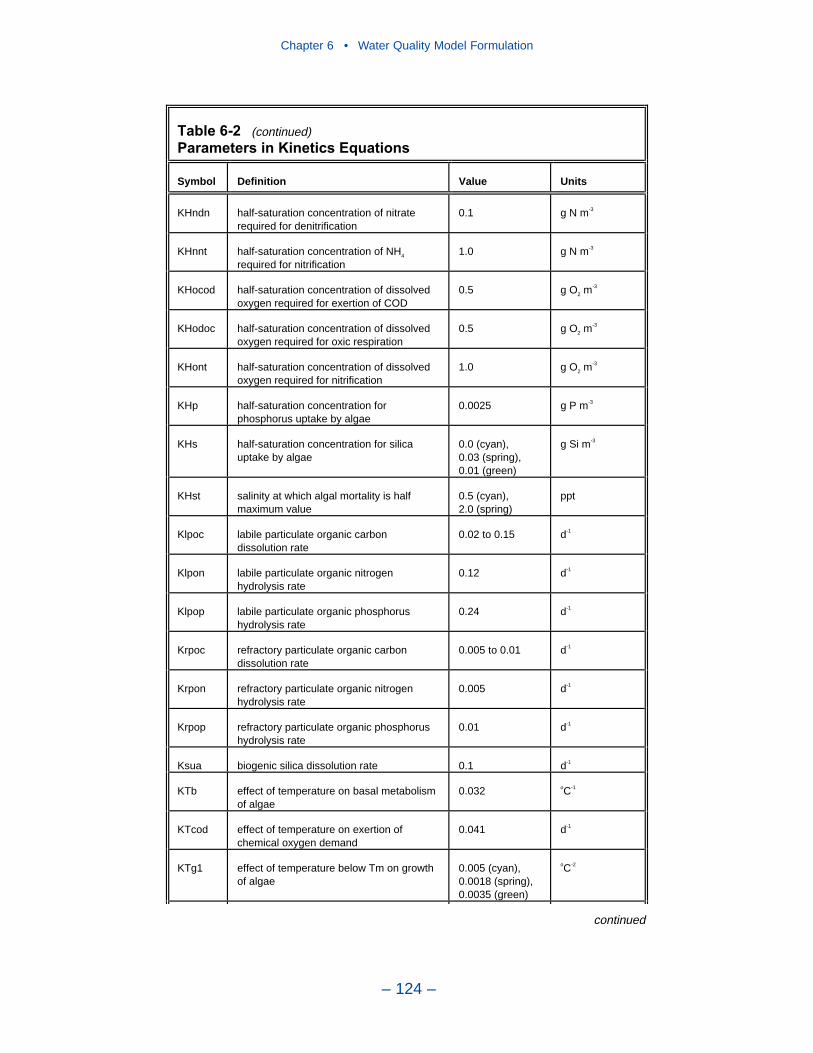
Chapter 6 • Water Quality Model Formulation
– 124 –
Table 6-2
Parameters in Kinetics Equations
Symbol Definition Value Units
KHndn half-saturation concentration of nitrate required for denitrification
0.1 g N m-3
KHnnt half-saturation concentration of NH4
required for nitrification 1.0 g N m-3
KHocod half-saturation concentration of dissolved oxygen required for exertion of COD
0.5 g O2 m-3
KHodoc half-saturation concentration of dissolved oxygen required for oxic respiration
0.5 g O2 m-3
KHont half-saturation concentration of dissolved oxygen required for nitrification
1.0 g O2 m-3
KHp half-saturation concentration for phosphorus uptake by algae
0.0025 g P m-3
KHs half-saturation concentration for silica uptake by algae
0.0 (cyan), 0.03 (spring), 0.01 (green)
g Si m-3
KHst salinity at which algal mortality is half maximum value
0.5 (cyan), 2.0 (spring)
ppt
Klpoc labile particulate organic carbon dissolution rate
0.02 to 0.15 d-1
Klpon labile particulate organic nitrogen hydrolysis rate
0.12 d-1
Klpop labile particulate organic phosphorus hydrolysis rate
0.24 d-1
Krpoc refractory particulate organic carbon dissolution rate
0.005 to 0.01 d-1
Krpon refractory particulate organic nitrogen hydrolysis rate
0.005 d-1
Krpop refractory particulate organic phosphorus hydrolysis rate
0.01 d-1
Ksua biogenic silica dissolution rate 0.1 d-1
KTb effect of temperature on basal metabolism of algae
0.032 oC-1
KTcod effect of temperature on exertion of chemical oxygen demand
0.041 d-1
KTg1 effect of temperature below Tm on growth of algae
0.005 (cyan), 0.0018 (spring), 0.0035 (green)
oC-2
continued
(continued)
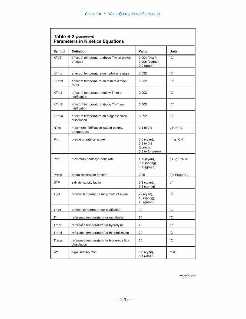
Chapter 6 • Water Quality Model Formulation
– 125 –
Parameters in Kinetics Equations
Symbol Definition Value Units
KTg2 effect of temperature above Tm on growth of algae
0.004 (cyan), 0.006 (spring), 0.0 (green)
oC-2
KThdr effect of temperature on hydrolysis rates 0.032 oC-1
KTmnl effect of temperature on mineralization rates
0.032 oC-1
KTnt1 effect of temperature below Tmnt on nitrification
0.003 oC-2
KTnt2 effect of temperature above Tmnt on nitrification
0.003 oC-2
KTsua effect of temperature on biogenic silica dissolution
0.092 oC-1
NTm maximum nitrification rate at optimal temperature
0.1 to 0.5 g N m-3 d-1
Phtl predation rate on algae 0.0 (cyan), 0.1 to 0.2 (spring),0.5 to 2 (green)
m3 g-1 C d-1
PmB maximum photosynthetic rate 100 (cyan), 300 (spring), 350 (green)
g C g-1 Chl d-1
Presp photo-respiration fraction 0.25 0 < Presp < 1
STF salinity toxicity factor 0.3 (cyan), 0.1 (spring)
d-1
Topt optimal temperature for growth of algae 29 (cyan), 16 (spring), 25 (green)
oC
Tmnt optimal temperature for nitrification 30 oC
Tr reference temperature for metabolism 20 oC
Trhdr reference temperature for hydrolysis 20 oC
Trmnl reference temperature for mineralization 20 oC
Trsua reference temperature for biogenic silica dissolution
20 oC
Wa algal settling rate 0.0 (cyan), 0.1 (other)
m d-1
continued
Table 6-2 (continued)
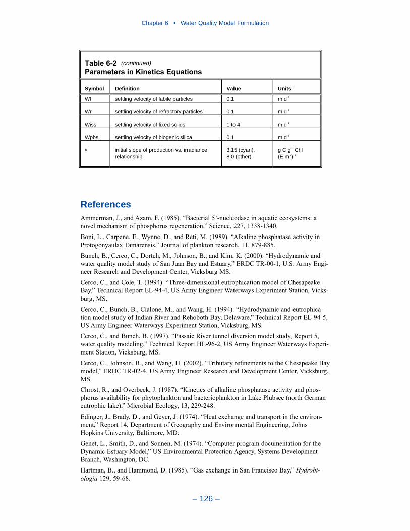
ReferencesAmmerman, J., and Azam, F. (1985). “Bacterial 5’-nucleodase in aquatic ecosystems: anovel mechanism of phosphorus regeneration,” Science, 227, 1338-1340.
Boni, L., Carpene, E., Wynne, D., and Reti, M. (1989). “Alkaline phosphatase activity inProtogonyaulax Tamarensis,” Journal of plankton research, 11, 879-885.
Bunch, B., Cerco, C., Dortch, M., Johnson, B., and Kim, K. (2000). “Hydrodynamic andwater quality model study of San Juan Bay and Estuary,” ERDC TR-00-1, U.S. Army Engi-neer Research and Development Center, Vicksburg MS.
Cerco, C., and Cole, T. (1994). “Three-dimensional eutrophication model of ChesapeakeBay,” Technical Report EL-94-4, US Army Engineer Waterways Experiment Station, Vicks-burg, MS.
Cerco, C., Bunch, B., Cialone, M., and Wang, H. (1994). “Hydrodynamic and eutrophica-tion model study of Indian River and Rehoboth Bay, Delaware,” Technical Report EL-94-5,US Army Engineer Waterways Experiment Station, Vicksburg, MS.
Cerco, C., and Bunch, B. (1997). “Passaic River tunnel diversion model study, Report 5,water quality modeling,” Technical Report HL-96-2, US Army Engineer Waterways Experi-ment Station, Vicksburg, MS.
Cerco, C., Johnson, B., and Wang, H. (2002). “Tributary refinements to the Chesapeake Baymodel,” ERDC TR-02-4, US Army Engineer Research and Development Center, Vicksburg,MS.
Chrost, R., and Overbeck, J. (1987). “Kinetics of alkaline phosphatase activity and phos-phorus availability for phytoplankton and bacterioplankton in Lake Plubsee (north Germaneutrophic lake),” Microbial Ecology, 13, 229-248.
Edinger, J., Brady, D., and Geyer, J. (1974). “Heat exchange and transport in the environ-ment,” Report 14, Department of Geography and Environmental Engineering, JohnsHopkins University, Baltimore, MD.
Genet, L., Smith, D., and Sonnen, M. (1974). “Computer program documentation for theDynamic Estuary Model,” US Environmental Protection Agency, Systems DevelopmentBranch, Washington, DC.
Hartman, B., and Hammond, D. (1985). “Gas exchange in San Francisco Bay,” Hydrobi-ologia 129, 59-68.
Chapter 6 • Water Quality Model Formulation
– 126 –
Table 6-2
Parameters in Kinetics Equations
Symbol Definition Value Units
Wl settling velocity of labile particles 0.1 m d-1
Wr settling velocity of refractory particles 0.1 m d-1
Wiss settling velocity of fixed solids 1 to 4 m d-1
Wpbs settling velocity of biogenic silica 0.1 m d-1
initial slope of production vs. irradiance relationship
3.15 (cyan), 8.0 (other)
g C g-1 Chl(E m-2)-1
(continued)

HydroQual (2000). “Development of a suspension feeding and deposit feeding benthosmodel for Chesapeake Bay,” Project USCE0410, prepared for US Army Engineer Researchand Development Center, Vicksburg MS.
Jassby, A., and Platt, T. (1976). “Mathematical formulation of the relationship betweenphotosynthesis and light for phytoplankton,” Limnology and Oceanography 21, 540-547.
Leonard, B. (1979). “A stable and accurate convection modelling procedure based on quad-ratic upstream interpolation,” Computer Methods in Applied Mechanics and Engineering,19, 59-98.
Matavulj, M., and Flint, K. (1987). “A model for acid and alkaline phosphatase activity in asmall pond,” Microbial Ecology, 13, 141-158.
Monod, J. (1949). “The growth of bacterial cultures,” Annual Review of Microbiology 3,371-394.
Morel, F. (1983). Principles of Aquatic Chemistry, John Wiley and Sons, New York, NY,150.
O’Connor, D., and Dobbins, W. (1958). “Mechanisms of reaeration in natural streams,”Transactions of the American Society of Civil Engineers, 123, 641-666.
O’Connor, D. (1983). “Wind effects on gas-liquid transfer coefficients,” Journal of the Envi-ronmental Engineering Division, 190, 731-752.
Parsons, T., Takahashi, M., and Hargrave, B. (1984). Biological oceanographic processes.3rd ed., Pergamon Press, Oxford.
Sellner, K., Lacoutre, R., and Parrish, C. (1988). “Effects of increasing salinity on aCyanobacteria bloom in the Potomac River Estuary,” Journal of Plankton Research, 10, 49-61.
Stumm, W., and Morgan, J. (1981). Aquatic chemistry. 2nd ed., Wiley- Interscience, NewYork.
Thomann, R., and Fitzpatrick, J. (1982). “Calibration and verification of a mathematicalmodel of the eutrophication of the Potomac Estuary,” HydroQual Inc., Mahwah, NJ.
Tchobanoglous, G., and Schroeder, E. (1987). Water quality, Addison Wesley, Reading,MA.
Tuffey, T., Hunter, J., and Matulewich, V. (1974). “Zones of nitrification”, Water ResourcesBulletin, 10, 555-564.
Wezernak, C., and Gannon, J. (1968). “Evaluation of nitrification in streams,” Journal of theSanitary Engineering Division, 94(SA5), 883-895.
Chapter 6 • Water Quality Model Formulation
– 127 –

The Monitoring Data Base
The water quality model was applied to a ten-year time period, 1985-1994. Themonitoring data base maintained by the Chesapeake Bay Program (ChesapeakeBay Program 1989, 1993) was the principal source of data for model calibration. Asummary of the monitoring program, as it operated from 1985 to 1994, is providedbelow. Details of the data base and information on the current program may befound at the Chesapeake Bay Program web sitehttp://www.chesapeakebay.net/data/index.htm.
Observations were collected at 49 stations in the bay and 89 stations in majorembayments and tributaries (Figure 7-1). Sampling was conducted once or twiceper month with more frequent sampling from March through October. Sampleswere collected during daylight hours with no attempt to coincide with tide stage orflow. Sampling periods were designated as “cruises.” Under ideal circumstances,cruises were completed in two to three days. Inclement weather or equipment fail-ures occasionally produced cruises as long as two weeks.
At each station, salinity, temperature, and dissolved oxygen were measured insitu at one- or two-meter intervals. Samples were collected one meter below thesurface and one meter above the bottom for laboratory analyses. At stationsshowing significant salinity stratification, additional samples were collected aboveand below the pycnocline. Analyses relevant to this study are listed in Table 7-1.The listed parameters are either analyzed directly or derived from direct analyses.
The major portion of the data base was obtained from the sponsor, in SAS trans-port format, in June 1996. Observations from 1991 through 1995 were updated in asecond transmission from the sponsor in June 1998. We discovered that observa-tions in the Potomac River and Maryland eastern shore were not complete. Thesewere provided by Maryland Department of Environment in March 1999. Additionalobservations were obtained from multiple sources. Descriptions are provided asthese observations are cited.
– 128 –
Introduction toCalibration 7
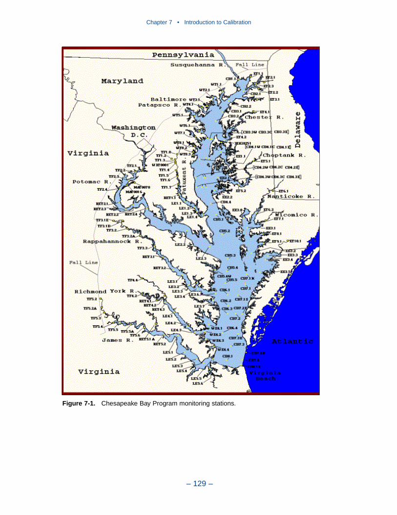
Chapter 7 • Introduction to Calibration
– 129 –
Figure 7-1. Chesapeake Bay Program monitoring stations.

Chapter 7 • Introduction to Calibration
– 130 –
Table 7-1 Direct or Derived Laboratory Analyses
Grouping Parameter Code
Total Phosphorus TP
Total Dissolved Phosphorus TDP
Particulate Phosphorus PHOSP
Orthophosphate PO4F
Dissolved Inorganic Phosphorus DIP
Phosphorus
Dissolve Organic Phosphorus DOP
Total Nitrogen TN
Total Dissolved Nitrogen TDN
Particulate Organic Nitrogen PON
Total Kjeldahl Nitrogen, Whole/Filtered TKNW, TKNF
Nitrate + Nitrite NO23
Ammonium NH4F
Dissolved Inorganic Nitrogen DIN
Dissolved Organic Nitrogen DON
Nitrogen
Total Organic Nitrogen TON
Total Organic Carbon TOC
Dissolved Organic Carbon DOC
Carbon
Particulate Organic Carbon POC
Silica, filtered SI
Total Suspended Solids TSS
Other
Chlorophyll a CHLA
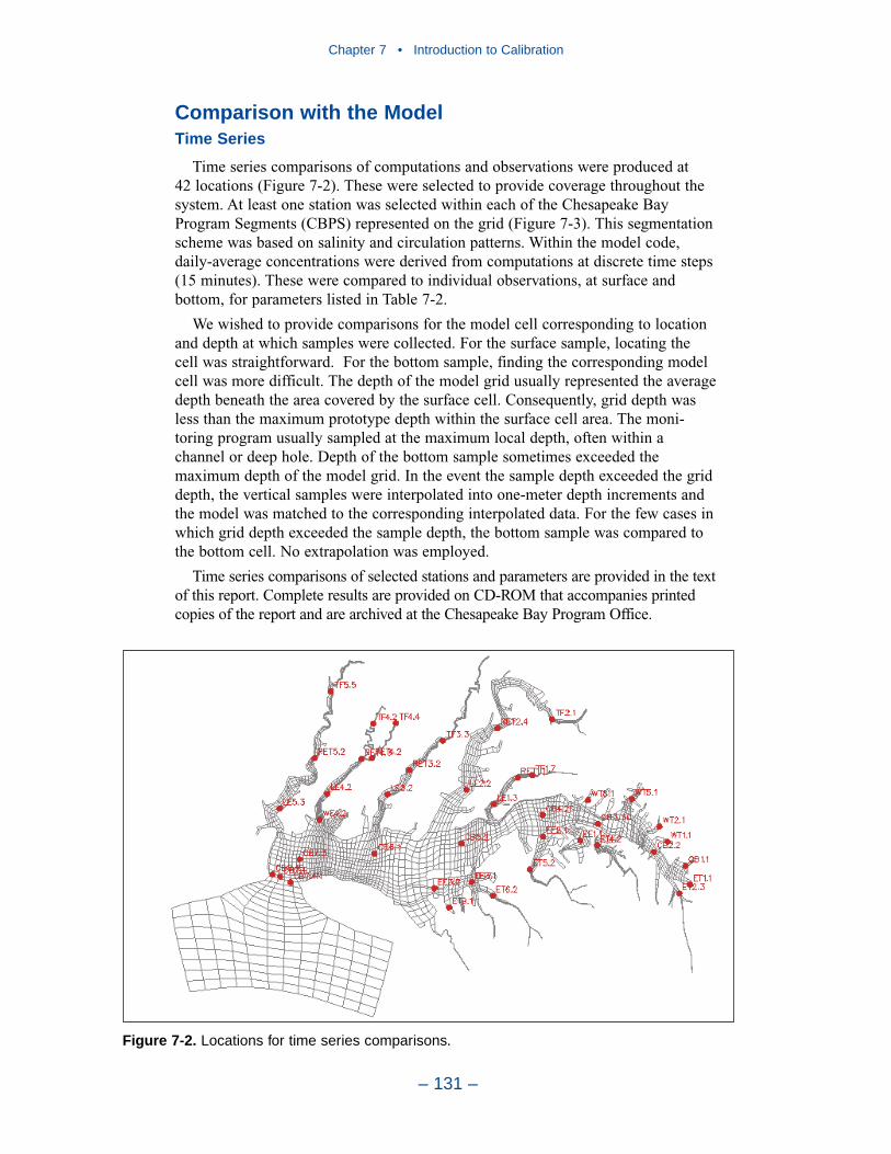
Comparison with the ModelTime Series
Time series comparisons of computations and observations were produced at 42 locations (Figure 7-2). These were selected to provide coverage throughout thesystem. At least one station was selected within each of the Chesapeake BayProgram Segments (CBPS) represented on the grid (Figure 7-3). This segmentationscheme was based on salinity and circulation patterns. Within the model code,daily-average concentrations were derived from computations at discrete time steps(15 minutes). These were compared to individual observations, at surface andbottom, for parameters listed in Table 7-2.
We wished to provide comparisons for the model cell corresponding to locationand depth at which samples were collected. For the surface sample, locating thecell was straightforward. For the bottom sample, finding the corresponding modelcell was more difficult. The depth of the model grid usually represented the averagedepth beneath the area covered by the surface cell. Consequently, grid depth wasless than the maximum prototype depth within the surface cell area. The moni-toring program usually sampled at the maximum local depth, often within achannel or deep hole. Depth of the bottom sample sometimes exceeded themaximum depth of the model grid. In the event the sample depth exceeded the griddepth, the vertical samples were interpolated into one-meter depth increments andthe model was matched to the corresponding interpolated data. For the few cases inwhich grid depth exceeded the sample depth, the bottom sample was compared tothe bottom cell. No extrapolation was employed.
Time series comparisons of selected stations and parameters are provided in the textof this report. Complete results are provided on CD-ROM that accompanies printedcopies of the report and are archived at the Chesapeake Bay Program Office.
Chapter 7 • Introduction to Calibration
– 131 –
Figure 7-2. Locations for time series comparisons.

Chapter 7 • Introduction to Calibration
– 132 –
Figure 7-3. Chesapeake Bay Program Segments.
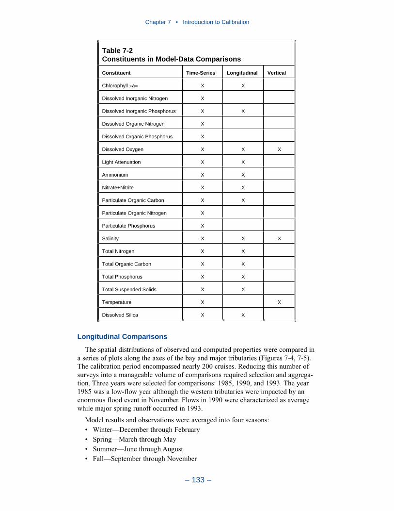
Longitudinal Comparisons
The spatial distributions of observed and computed properties were compared ina series of plots along the axes of the bay and major tributaries (Figures 7-4, 7-5).The calibration period encompassed nearly 200 cruises. Reducing this number ofsurveys into a manageable volume of comparisons required selection and aggrega-tion. Three years were selected for comparisons: 1985, 1990, and 1993. The year1985 was a low-flow year although the western tributaries were impacted by anenormous flood event in November. Flows in 1990 were characterized as averagewhile major spring runoff occurred in 1993.
Model results and observations were averaged into four seasons:• Winter—December through February• Spring—March through May• Summer—June through August• Fall—September through November
Chapter 7 • Introduction to Calibration
– 133 –
Table 7-2 Constituents in Model-Data Comparisons
Constituent Time-Series Longitudinal Vertical
Chlorophyll a X X
Dissolved Inorganic Nitrogen X
Dissolved Inorganic Phosphorus X X
Dissolved Organic Nitrogen X
Dissolved Organic Phosphorus X
Dissolved Oxygen X X X
Light Attenuation X X
Ammonium X X
Nitrate+Nitrite X X
Particulate Organic Carbon X X
Particulate Organic Nitrogen X
Particulate Phosphorus X
Salinity X X X
Total Nitrogen X X
Total Organic Carbon X X
Total Phosphorus X X
Total Suspended Solids X X
Temperature X X
Dissolved Silica X X
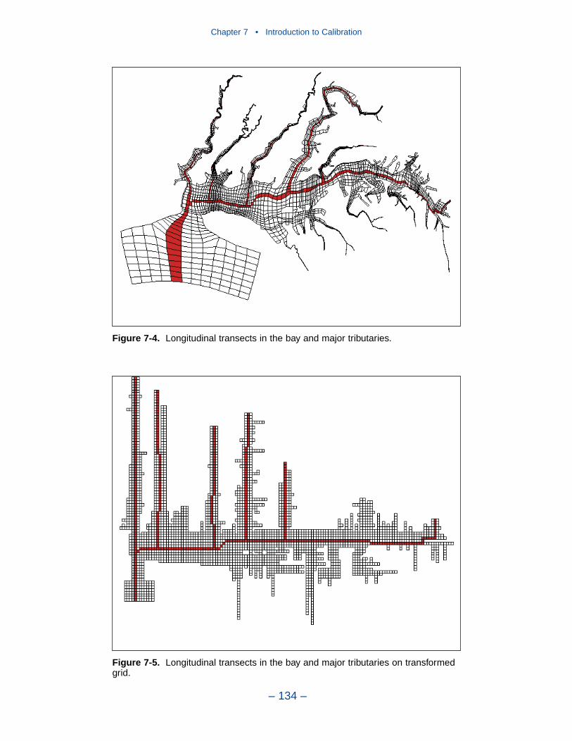
Chapter 7 • Introduction to Calibration
– 134 –
Figure 7-4. Longitudinal transects in the bay and major tributaries.
Figure 7-5. Longitudinal transects in the bay and major tributaries on transformed grid.
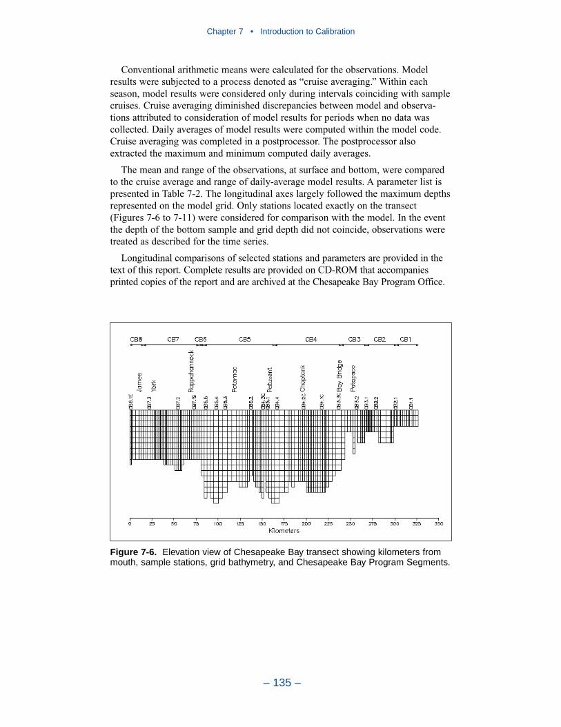
Conventional arithmetic means were calculated for the observations. Modelresults were subjected to a process denoted as “cruise averaging.” Within eachseason, model results were considered only during intervals coinciding with samplecruises. Cruise averaging diminished discrepancies between model and observa-tions attributed to consideration of model results for periods when no data wascollected. Daily averages of model results were computed within the model code.Cruise averaging was completed in a postprocessor. The postprocessor alsoextracted the maximum and minimum computed daily averages.
The mean and range of the observations, at surface and bottom, were comparedto the cruise average and range of daily-average model results. A parameter list ispresented in Table 7-2. The longitudinal axes largely followed the maximum depthsrepresented on the model grid. Only stations located exactly on the transect(Figures 7-6 to 7-11) were considered for comparison with the model. In the eventthe depth of the bottom sample and grid depth did not coincide, observations weretreated as described for the time series.
Longitudinal comparisons of selected stations and parameters are provided in thetext of this report. Complete results are provided on CD-ROM that accompaniesprinted copies of the report and are archived at the Chesapeake Bay Program Office.
Chapter 7 • Introduction to Calibration
– 135 –
Figure 7-6. Elevation view of Chesapeake Bay transect showing kilometers frommouth, sample stations, grid bathymetry, and Chesapeake Bay Program Segments.
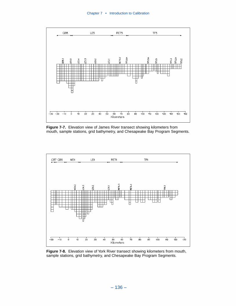
Chapter 7 • Introduction to Calibration
– 136 –
Figure 7-7. Elevation view of James River transect showing kilometers frommouth, sample stations, grid bathymetry, and Chesapeake Bay Program Segments.
Figure 7-8. Elevation view of York River transect showing kilometers from mouth,sample stations, grid bathymetry, and Chesapeake Bay Program Segments.

Chapter 7 • Introduction to Calibration
– 137 –
Figure 7-9. Elevation view of Rappahannock River transect showing kilometersfrom mouth, sample stations, grid bathymetry, and Chesapeake Bay Program.
Figure 7-10. Elevation view of Potomac River transect showing kilometers frommouth, sample stations, grid bathymetry, and Chesapeake Bay Program Segments.
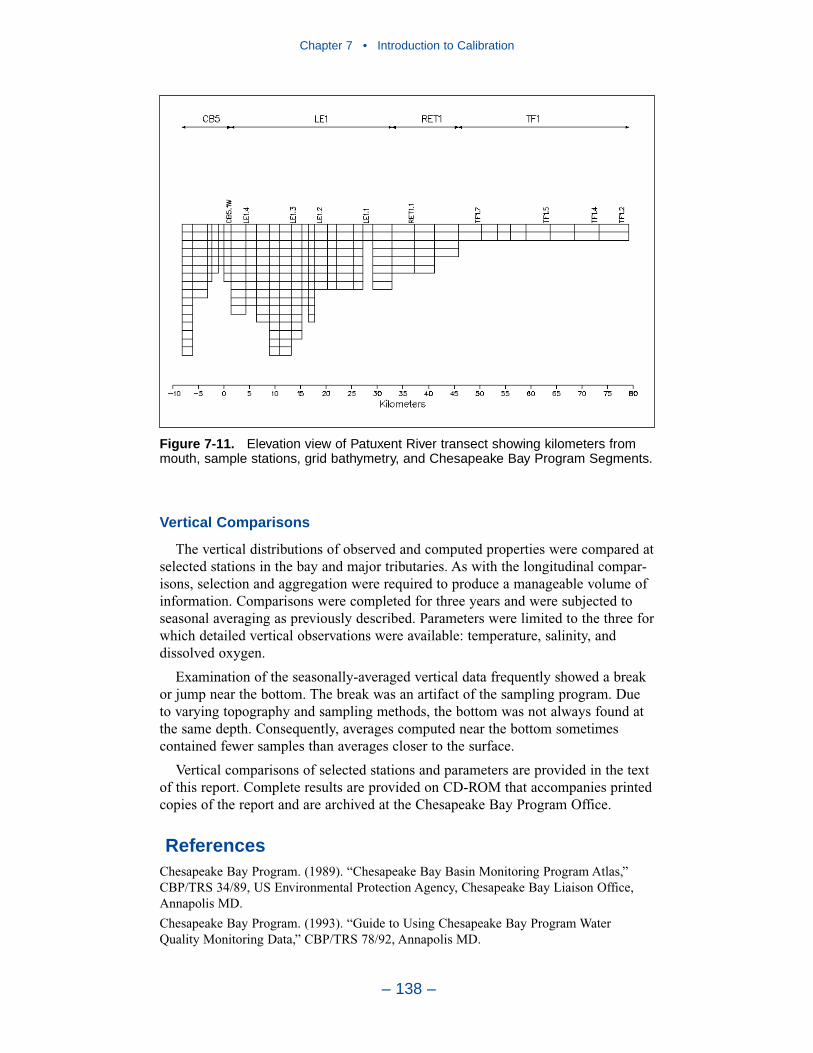
Vertical Comparisons
The vertical distributions of observed and computed properties were compared atselected stations in the bay and major tributaries. As with the longitudinal compar-isons, selection and aggregation were required to produce a manageable volume ofinformation. Comparisons were completed for three years and were subjected toseasonal averaging as previously described. Parameters were limited to the three forwhich detailed vertical observations were available: temperature, salinity, anddissolved oxygen.
Examination of the seasonally-averaged vertical data frequently showed a breakor jump near the bottom. The break was an artifact of the sampling program. Dueto varying topography and sampling methods, the bottom was not always found atthe same depth. Consequently, averages computed near the bottom sometimescontained fewer samples than averages closer to the surface.
Vertical comparisons of selected stations and parameters are provided in the textof this report. Complete results are provided on CD-ROM that accompanies printedcopies of the report and are archived at the Chesapeake Bay Program Office.
ReferencesChesapeake Bay Program. (1989). “Chesapeake Bay Basin Monitoring Program Atlas,”CBP/TRS 34/89, US Environmental Protection Agency, Chesapeake Bay Liaison Office,Annapolis MD.
Chesapeake Bay Program. (1993). “Guide to Using Chesapeake Bay Program WaterQuality Monitoring Data,” CBP/TRS 78/92, Annapolis MD.
Chapter 7 • Introduction to Calibration
– 138 –
Figure 7-11. Elevation view of Patuxent River transect showing kilometers frommouth, sample stations, grid bathymetry, and Chesapeake Bay Program Segments.
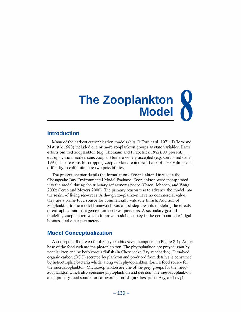
Introduction
Many of the earliest eutrophication models (e.g. DiToro et al. 1971; DiToro andMatystik 1980) included one or more zooplankton groups as state variables. Laterefforts omitted zooplankton (e.g. Thomann and Fitzpatrick 1982). At present,eutrophication models sans zooplankton are widely accepted (e.g. Cerco and Cole1993). The reasons for dropping zooplankton are unclear. Lack of observations anddifficulty in calibration are two possibilities.
The present chapter details the formulation of zooplankton kinetics in theChesapeake Bay Environmental Model Package. Zooplankton were incorporatedinto the model during the tributary refinements phase (Cerco, Johnson, and Wang2002; Cerco and Meyers 2000). The primary reason was to advance the model intothe realm of living resources. Although zooplankton have no commercial value,they are a prime food source for commercially-valuable finfish. Addition ofzooplankton to the model framework was a first step towards modeling the effectsof eutrophication management on top-level predators. A secondary goal ofmodeling zooplankton was to improve model accuracy in the computation of algalbiomass and other parameters.
Model Conceptualization
A conceptual food web for the bay exhibits seven components (Figure 8-1). At thebase of the food web are the phytoplankton. The phytoplankton are preyed upon byzooplankton and by herbivorous finfish (in Chesapeake Bay, menhaden). Dissolvedorganic carbon (DOC) secreted by plankton and produced from detritus is consumedby heterotrophic bacteria which, along with phytoplankton, form a food source forthe microzooplankton. Microzooplankton are one of the prey groups for the meso-zooplankton which also consume phytoplankton and detritus. The mesozooplanktonare a primary food source for carnivorous finfish (in Chesapeake Bay, anchovy).
– 139 –
The ZooplanktonModel 8
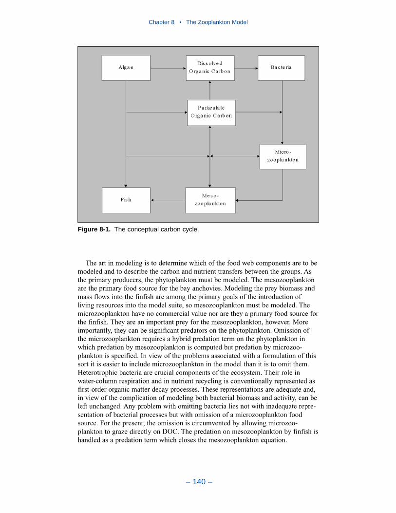
The art in modeling is to determine which of the food web components are to bemodeled and to describe the carbon and nutrient transfers between the groups. Asthe primary producers, the phytoplankton must be modeled. The mesozooplanktonare the primary food source for the bay anchovies. Modeling the prey biomass andmass flows into the finfish are among the primary goals of the introduction ofliving resources into the model suite, so mesozooplankton must be modeled. Themicrozooplankton have no commercial value nor are they a primary food source forthe finfish. They are an important prey for the mesozooplankton, however. Moreimportantly, they can be significant predators on the phytoplankton. Omission ofthe microzooplankton requires a hybrid predation term on the phytoplankton inwhich predation by mesozooplankton is computed but predation by microzoo-plankton is specified. In view of the problems associated with a formulation of thissort it is easier to include microzooplankton in the model than it is to omit them.Heterotrophic bacteria are crucial components of the ecosystem. Their role inwater-column respiration and in nutrient recycling is conventionally represented asfirst-order organic matter decay processes. These representations are adequate and,in view of the complication of modeling both bacterial biomass and activity, can beleft unchanged. Any problem with omitting bacteria lies not with inadequate repre-sentation of bacterial processes but with omission of a microzooplankton foodsource. For the present, the omission is circumvented by allowing microzoo-plankton to graze directly on DOC. The predation on mesozooplankton by finfish ishandled as a predation term which closes the mesozooplankton equation.
Chapter 8 • The Zooplankton Model
– 140 –
Figure 8-1. The conceptual carbon cycle.
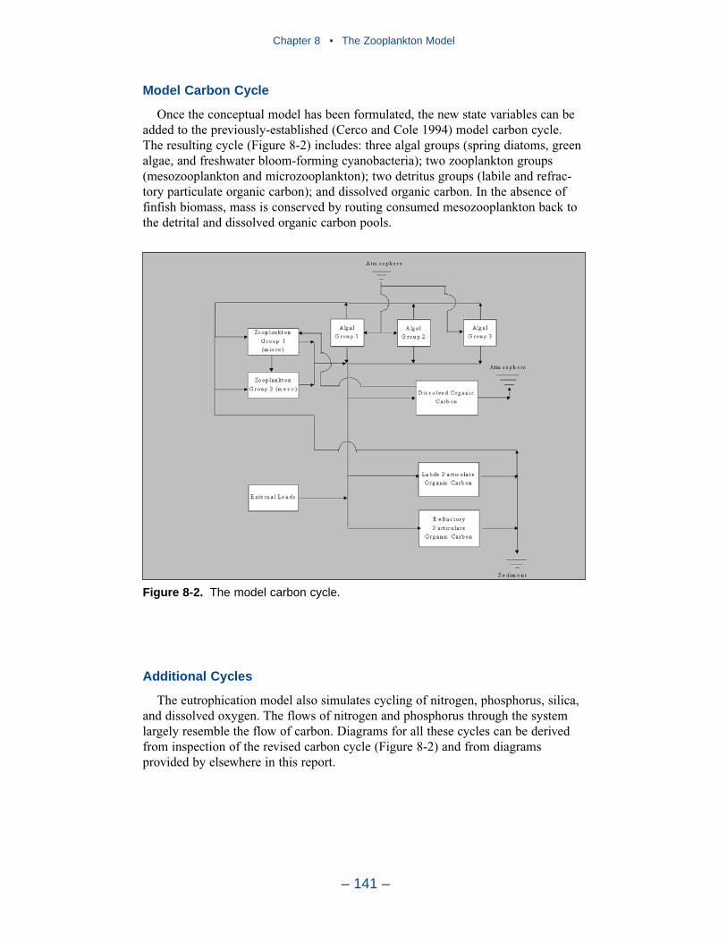
Model Carbon Cycle
Once the conceptual model has been formulated, the new state variables can beadded to the previously-established (Cerco and Cole 1994) model carbon cycle.The resulting cycle (Figure 8-2) includes: three algal groups (spring diatoms, greenalgae, and freshwater bloom-forming cyanobacteria); two zooplankton groups(mesozooplankton and microzooplankton); two detritus groups (labile and refrac-tory particulate organic carbon); and dissolved organic carbon. In the absence offinfish biomass, mass is conserved by routing consumed mesozooplankton back tothe detrital and dissolved organic carbon pools.
Additional Cycles
The eutrophication model also simulates cycling of nitrogen, phosphorus, silica,and dissolved oxygen. The flows of nitrogen and phosphorus through the systemlargely resemble the flow of carbon. Diagrams for all these cycles can be derivedfrom inspection of the revised carbon cycle (Figure 8-2) and from diagramsprovided by elsewhere in this report.
Chapter 8 • The Zooplankton Model
– 141 –
Figure 8-2. The model carbon cycle.
Chapter 8 • The Zooplankton Model
– 142 –
Zooplankton KineticsThe Algal Production Equation
Effects of zooplankton on phytoplankton are computed in the predation term ofthe algal production equation:
in which:Bx = biomass of algal group x (g C m-3)Gx = growth rate of algal group x (d-1)BMx = basal metabolic rate of algal group x (d-1)WSx = settling rate of algal group x (m d-1)PRx = predation on algal group x (g C m-3 d-1)z, t = vertical (m) and temporal (d) coordinates
Zooplankton Production Equation
Each zooplankton group is represented by an identical production equation. Thetwo groups are distinguished largely by parameter evaluation.
in which:Z = zooplankton biomass (g C m-3)Gz = growth rate of zooplankton group z (d-1)BMz = basal metabolic rate of zooplankton group z (d-1)Mz = mortality (d-1)PRz = predation on zooplankton group z (g C m-3 d-1)
Growth Rate
Grazing is represented by a maximum ration formulation equivalent to thefamiliar Monod formulation used to represent algal nutrient uptake. Grazing is notequivalent to growth, however. Not all prey grazed is assimilated. Grazing alsorequires effort which results in respiration above the basic metabolic rate. Therepresentation of growth rate which incorporates grazing, assimilation, andrespiratory loss is:
in which:PAz = prey available to zooplankton group z (g C m-3)KHCz = prey density at which grazing is halved (g C m-3)RMAXz = maximum ration of zooplankton group z
(g prey C g-1 zooplankton C d-1)Ez = assimilation efficiency of zooplankton group z (0 < E < 1)RFz = fraction of assimilated prey lost to respiration (0 < RF < 1)f(T) = effect of temperature on grazing
f(T)RFz)-(1EzRMAXzPAz+KHCz
PAz=Gz (8-3)
PRz- ZMz-BMz-Gz=t
Z(8-2)
PRx-Bxz
WSx-BMx-Gx= tBx
(8-1)
Available Prey
The computation of available prey incorporates two principles:
1) A constant, between zero and unity, determines the utilization of a prey groupby a predator,
2) A threshold density exists below which prey is not utilized.
The available portion of an algal group, for example, is determined:
in which:BAxz = The portion of algal group x available to zooplankton group z (g C m-3)CTz = The threshold concentration below which prey will not be utilized by
zooplankton group z (g C m-3)
Prey Available to Microzooplankton. Microzooplankton are conceived to grazeon dissolved organic carbon (a surrogate for bacteria), three algal groups, andorganic detritus. The total prey available to microzooplankton is:
in which:PA = prey available to microzooplankton (g C m-3)UDsz = utilization of dissolved organic carbon by microzooplanktonUBxsz = utilization of algal group x by microzooplanktonULsz = utilization of labile particulate organic carbon by microzooplanktonURsz = utilization of refractory particulate organic carbon by microzooplanktonDOCAsz = dissolved organic carbon available to microzooplankton (g C m-3)BAxsz = algal group x available to microzooplankton (g C m-3)LPOCAsz = labile particulate organic carbon available to microzooplankton
(g C m-3)RPOCAsz = refractory particulate organic carbon available to microzooplankton
(g C m-3)
Prey Available to Mesozooplankton. Mesozooplankton are conceived to graze onthree algal groups, microzooplankton, and organic detritus. The total prey availableto mesozooplankton is:
in which:SZ = microzooplankton biomass (g C m-3)
Definitions and notation for remaining terms largely follow those for microzoo-plankton.
M d lRPOCAlz URlz+LPOCAlz ULlz+
SZA USZlz+BAxlz UBxlz=PAlz(8-6)
RPOCAsz URsz+LPOCAsz ULsz+
BAxsz UBxsz+DOCAsz UDsz=PAsz(8-5)
0CTz,-BxMax=BAxz (8-4)
Chapter 8 • The Zooplankton Model
– 143 –
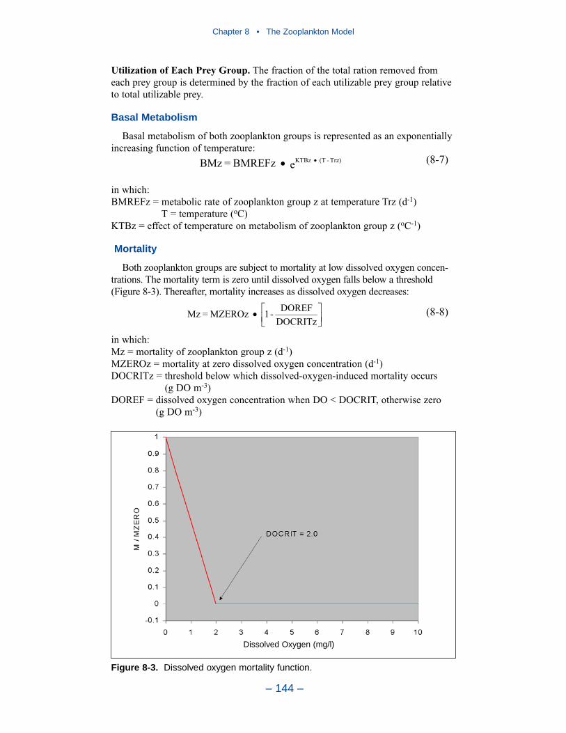
Chapter 8 • The Zooplankton Model
– 144 –
Utilization of Each Prey Group. The fraction of the total ration removed fromeach prey group is determined by the fraction of each utilizable prey group relativeto total utilizable prey.
Basal Metabolism
Basal metabolism of both zooplankton groups is represented as an exponentiallyincreasing function of temperature:
in which:BMREFz = metabolic rate of zooplankton group z at temperature Trz (d-1)
T = temperature (oC)KTBz = effect of temperature on metabolism of zooplankton group z (oC-1)
Mortality
Both zooplankton groups are subject to mortality at low dissolved oxygen concen-trations. The mortality term is zero until dissolved oxygen falls below a threshold(Figure 8-3). Thereafter, mortality increases as dissolved oxygen decreases:
in which:Mz = mortality of zooplankton group z (d-1)MZEROz = mortality at zero dissolved oxygen concentration (d-1)DOCRITz = threshold below which dissolved-oxygen-induced mortality occurs
(g DO m-3)DOREF = dissolved oxygen concentration when DO < DOCRIT, otherwise zero
(g DO m-3)
DOCRITzDOREF-1MZEROz=Mz (8-8)
eBMREFz=BMz Trz)-(TKTBz (8-7)
Figure 8-3. Dissolved oxygen mortality function.
Dissolved Oxygen (mg/l)
Predation on Zooplankton
Mesozooplankton graze on microzooplankton. In addition, grazing on mesozoo-plankton by organisms not represented in the model (jellyfish, finfish) isconsidered. Representation of predation by organisms that are not modeled is aclassic problem. Our approach results in a quadratic formulation that closes themesozooplankton system.
Assume the predators clear a specific volume of water per unit biomass. Thenpredation on zooplankton is the product of the clearance rate, prey abundance, andpredator abundance:
in which:F = clearance rate (m3 g-1 predator C d-1)LZ = mesozooplankton biomass (g C m-3)HTL = predator biomass (g C m-3)
In the absence of detailed data regarding the temporal and spatial predator distri-bution, a reasonable assumption is that predator biomass is proportional to preybiomass, HTL = α • LZ. In that case, Equation 8-9 can be re-written:
Since neither α nor F are known precisely, the logical approach is to combinetheir product into a single unknown, PHTlz, determined during the model calibra-tion procedure. In addition to closure, the quadratic predation term adds desirablestability to the potential oscillatory system represented by algae and zooplanktonalone.
Interfacing with the Eutrophication Model
The basic principles of the zooplankton model have been outlined above. Sincethis chapter is the first documentation of the zooplankton model, additional detailof the interfacing of the zooplankton component with the remaining model statevariables is presented here.
Effect of Zooplankton on Carbon
The rate of total carbon uptake by zooplankton is the product of the maximumration and biomass, modified by any existing food limitation:
in which:Rz = ration of zooplankton group z (g prey C g-1 zooplankton C d-1)
The rate at which carbon is recycled to the environment is determined by thefraction of the ration not assimilated, by the mortality, and by predation fromhigher trophic levels. The recycling of all zooplankton consumed by predators
f(T)RMAXzPAz+KHCz
PAz=Rz (8-11)
LZF=PRz 2 (8-10)
HTLLZF=PRlz (8-9)
Chapter 8 • The Zooplankton Model
– 145 –
Chapter 8 • The Zooplankton Model
– 146 –
enforces mass conservation on the system. Mass conservation implies thatzooplankton carbon permanently removed from the system due to harvest of preda-tors is negligibly small. The carbon recycle rate is:
in which:CRRATEz = rate of carbon recycling by zooplankton group z (g C m-3 d-1)
Once the total carbon uptake and recycle are defined, the uptake and release ofeach carbonaceous state variable can be obtained. The uptake is determined by theratio of utilization of a single component to total available carbon. The distributionof released carbon is determined by a set of empirical coefficients. The effect ofmicrozooplankton on dissolved organic carbon, for example, is:
in which:FDOCsz = fraction of carbon recycled to the dissolved organic pool by microzoo-
plankton (0 < FDOC < 1)
Effect of Zooplankton on Algae
Algae are a fraction of the total carbon uptake. No carbon is recycled to the algalpool, however. The effect of mesozooplankton on algal group 2, for example, is:
Effect of Zooplankton on Dissolved Oxygen
Zooplankton consume dissolved oxygen through the respiratory cost of assimi-lating food and through basal metabolism:
in which:Aocr = ratio of oxygen consumed to carbon metabolized (2.67 g DO g-1 C)
Effect of Zooplankton on Nitrogen
The computation of zooplankton effects on nutrients must account for differingcomposition of zooplankton and prey. An additional complication is that the modelconsiders organic nitrogen and phosphorus to exist independently from organiccarbon. In reality, these exist as organic matter composed of carbon, nitrogen, andphosphorus, among other elements. We consider that particulate organic nitrogenand phosphorus are consumed in proportion to detrital carbon.
ZAOCRBMz+RzRFzEz-= tDO
(8-15)
LZRlzPAlz
B2AlzUB2lz-=t
B2(8-14)
FDOCszCRRATEsz+SZRszPAsz
DOCAszUDsz-=t
DOC(8-13)
PRz+ ZMz+RzEz)-(1=CRRATEz (8-12)
First, evaluate the nitrogen-to-carbon ratio in the total prey consumed. For meso-zooplankton, this is:
in which:ANCPlz = nitrogen-to-carbon ratio in prey of mesozooplankton (g N g-1 C)ANCx = nitrogen-to-carbon ratio in algal group x (g N g-1 C)ANCsz = nitrogen-to-carbon ratio in microzooplankton group x (g N g-1 C)
Additional terms follow previous definitions and notation.
All nitrogen consumed is recycled except for the amount assimilated. Additionalnitrogen is recycled through respiration, mortality, and predation on zooplankton.For mesozooplankton, for example, the nitrogen recycle rate is:
in which:NRRATElz = nitrogen recycled by mesozooplankton (g N m-3 d-1)ANClz = nitrogen-to-carbon ratio of mesozooplankton (g N g-1 C)
Zooplankton do not take up dissolved organic nitrogen or ammonium. Recycleof these constituents is determined by the total recycle rate and empirical distribu-tion coefficients. Ammonium recycle by mesozooplankton, for example, is:
in which:FNH4lz = fraction of nitrogen recycled to the ammonium pool by mesozooplankton
(0 < FNH4lz < 1)
For particulate organic nitrogen, the recycle rate is the difference betweendetritus consumed and recycled. The effect of mesozooplankton on labile particu-late organic nitrogen, for example, is:
FLPONlzNRRATElz+
LZRlzLPOCLPONoverPAlzLPOCAlzULlz-=
tLPON
(8-19)
lzFNHNRRATElz=t
NH4
4(8-18)
ANClzPRlz+LZANClzMlz+BMlz+
LZRlzRFlz)-(1ElzANClz-ANCPlz
=NRRATElz
(8-17)
PAlz /RPOC
RPOCAlzRPONURlz+LPOC
LPOCAlzLPONULlz+
PAlz /SZAlz USZlzANCsz+BxAlz UBxlzANCx
=ANCPlz
(8-16)
Chapter 8 • The Zooplankton Model
– 147 –
ULlz • LPOCAlz
PAlz– •
Effect of Zooplankton on Phosphorus
The effect of zooplankton on phosphorus is analogous to the effects describedfor nitrogen.
Effect of Zooplankton on Silica
Zooplankton consume silica solely through the uptake of phytoplankton. Allsilica consumed is recycled. Computation of the effect of zooplankton on silicarequires summation of silica consumed and allocation to the two external silicapools. The effect of microzooplankton on dissolved silica, for example, is:
in which:ASCx = silica to carbon ratio of algal group x (g Si g-1 C)FRSAsz = fraction of silica recycled to dissolved pool by microzooplankton
(0 < FRSAsz < 1)
Parameter EvaluationParameters in the zooplankton model (Tables 8-1, 8-2) were adapted from
published values, when available, and adjusted to provide improved model results.Published values were not available for a number of empirical parameters whichwere evaluated largely through a recursive calibration procedure. The evaluationprocedure for significant parameters is detailed below.
Composition
The classic Redfield ratios for zooplankton (Redfield et al. 1963) indicate thefollowing ratios: nitrogen-to-carbon = 0.19 g N g-1 C; phosphorus to carbon = 0.025g P g-1 C. A summary by Parsons et al. (1984) indicates median values of 0.22 g Ng-1 C and 0.017 g P g-1 C for nitrogen-to-carbon and phosphorus-to-carbon. Modelcomposition for both zooplankton groups closely reflects these values.
Microzooplankton Ration
The microzooplankton community in the mainstem bay consists largely ofrotifers and tintinnids as well as juvenile forms of mesozooplankton and otherorganisms (Brownlee and Jacobs 1987). A survey of specific grazing rates (Table 8-3) indicates maximum rates in excess of 2 d-1 are observed.
The effect of temperature on grazing (Figure 8-4) was described with a functionof the form:
in which:T = temperature (oC)Topt = optimal temperature for grazing (oC)KTg1 = effect of temperature below optimal on grazing (oC-2)KTg2 = effect of temperature above optimal on grazing (oC-2)
ToptT when e=
ToptT when e=f(t)
)Topt-(TKTg2-
)Topt-(TKTg1-
2
2
(8-21)
FRSAszSZRszPAsz
BxAsz UBxszASCx= tSA
(8-20)
Chapter 8 • The Zooplankton Model
– 148 –

Chapter 8 • The Zooplankton Model
– 149 –
Table 8-1 Parameters in Microzooplankton Model
Parameter Description Value Units
ANCsz nitrogen to carbon ratio 0.2 g N g-1 C
AOCRsz ratio of oxygen consumed to carbon metabolized
2.67 g DO g-1 C
APCsz phosphorus to carbon ratio 0.02 g P g-1 C
BMREFsz basal metabolism at reference temperature 0.254 d-1
CTsz carbon threshold for grazing 0.01 g C m-3
DOCRITsz concentration below which dissolved oxygen mortality occurs
2.0 g DO m-3
Esz assimilation efficiency 0.3 0 < E < 1
FDOCsz fraction of carbon recycled to dissolved organic pool
0.25 0 < FDOC < 1
FDONsz fraction of nitrogen recycled to dissolved organic pool
0.20 0 < FDON < 1
FDOPsz fraction of phosphorus recycled to dissolved organic pool
0.40 0 < FDOP < 1
FLPOCsz fraction of carbon recycled to labile particulate organic pool
0.50 0 < FLPOC < 1
FLPONsz fraction of nitrogen recycled to labile particulate organic pool
0.25 0 < FLPON < 1
FLPOPsz fraction of phosphorus recycled to labile particulate organic pool
0.07 0 < FLPOP < 1
FNH4sz fraction of nitrogen recycled to dissolved inorganic pool
0.40 0 < FNH4 < 1
FPO4sz fraction of phosphorus recycled to dissolved inorganic pool
0.50 0 < FPO4 < 1
FRPOCsz fraction of carbon recycled to refractory particulate organic pool
0.25 0 < FRPOC < 1
FRPONsz fraction of nitrogen recycled to refractory particulate organic pool
0.15 0 < FRPON < 1
FRPOPsz fraction of phosphorus recycled to refractory particulate organic pool
0.03 0 < FRPOP < 1
FRSAsz fraction of silica recycled to dissolved pool 0.55 0 < FRSA < 1
KHCsz prey density at which grazing is halved 0.05 g C m-3
KTBGsz effect of temperature on basal metabolism 0.069 oC-1
KTGsz1 effect of sub-optimal temperature on grazing 0.0035 oC-2
continued
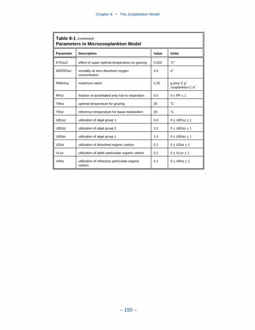
Chapter 8 • The Zooplankton Model
– 150 –
KTGsz2 effect of super-optimal temperature on grazing 0.025 oC-2
MZEROsz mortality at zero dissolved oxygen concentration
4.0 d-1
RMAXsz maximum ration 2.25 g prey C g-1
zooplankton C d-1
RFsz fraction of assimilated prey lost to respiration 0.5 0 < RF < 1
TMsz optimal temperature for grazing 25 oC
TRsz reference temperature for basal metabolism 20 oC
UB1sz utilization of algal group 1 0.0 0 < UB1sz < 1
UB2sz utilization of algal group 2 1.0 0 < UB2sz < 1
UB3sz utilization of algal group 1 1.0 0 < UB3sz < 1
UDsz utilization of dissolved organic carbon 0.1 0 < UDsz < 1
ULsz utilization of labile particulate organic carbon 0.1 0 < ULsz < 1
URsz utilization of refractory particulate organic carbon
0.1 0 < URsz < 1
Table 8-1 Parameters in Microzooplankton Model
Parameter Description Value Units
(continued)
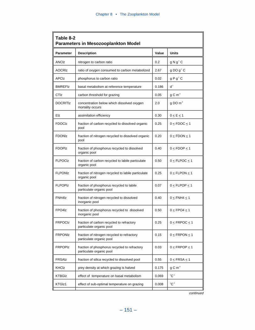
Chapter 8 • The Zooplankton Model
– 151 –
Table 8-2Parameters in Mesozooplankton Model
Parameter Description Value Units
ANClz nitrogen to carbon ratio 0.2 g N g-1 C
AOCRlz ratio of oxygen consumed to carbon metabolized 2.67 g DO g-1 C
APClz phosphorus to carbon ratio 0.02 g P g-1 C
BMREFlz basal metabolism at reference temperature 0.186 d-1
CTlz carbon threshold for grazing 0.05 g C m-3
DOCRITlz concentration below which dissolved oxygen mortality occurs
2.0 g DO m-3
Elz assimilation efficiency 0.30 0 < E < 1
FDOClz fraction of carbon recycled to dissolved organic pool
0.25 0 < FDOC < 1
FDONlz fraction of nitrogen recycled to dissolved organic pool
0.20 0 < FDON < 1
FDOPlz fraction of phosphorus recycled to dissolved organic pool
0.40 0 < FDOP < 1
FLPOClz fraction of carbon recycled to labile particulate organic pool
0.50 0 < FLPOC < 1
FLPONlz fraction of nitrogen recycled to labile particulate organic pool
0.25 0 < FLPON < 1
FLPOPlz fraction of phosphorus recycled to labile particulate organic pool
0.07 0 < FLPOP < 1
FNH4lz fraction of nitrogen recycled to dissolved inorganic pool
0.40 0 < FNH4 < 1
FPO4lz fraction of phosphorus recycled to dissolved inorganic pool
0.50 0 < FPO4 < 1
FRPOClz fraction of carbon recycled to refractory particulate organic pool
0.25 0 < FRPOC < 1
FRPONlz fraction of nitrogen recycled to refractory particulate organic pool
0.15 0 < FRPON < 1
FRPOPlz fraction of phosphorus recycled to refractory particulate organic pool
0.03 0 < FRPOP < 1
FRSAlz fraction of silica recycled to dissolved pool 0.55 0 < FRSA < 1
KHClz prey density at which grazing is halved 0.175 g C m-3
KTBGlz effect of temperature on basal metabolism 0.069 oC-1
KTGlz1 effect of sub-optimal temperature on grazing 0.008 oC-2
continued
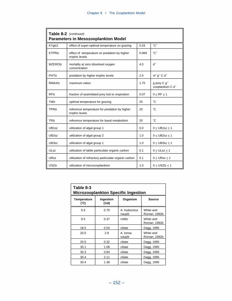
Chapter 8 • The Zooplankton Model
– 152 –
KTglz2 effect of super-optimal temperature on grazing 0.03 oC-2
KTPRlz effect of temperature on predation by higher trophic levels
0.069 oC-1
MZEROlz mortality at zero dissolved oxygen concentration
4.0 d-1
PHTlz predation by higher trophic levels 2.0 m3 g-1 C d-1
RMAXlz maximum ration 1.75 g prey C g-1
zooplankton C d-1
RFlz fraction of assimilated prey lost to respiration 0.07 0 < RF < 1
TMlz optimal temperature for grazing 25 oC
TPRlz reference temperature for predation by higher trophic levels
20 oC
TRlz reference temperature for basal metabolism 20 oC
UB1sz utilization of algal group 1 0.0 0 < UB1sz < 1
UB2sz utilization of algal group 2 1.0 0 < UB2sz < 1
UB3sz utilization of algal group 1 1.0 0 < UB3sz < 1
ULsz utilization of labile particulate organic carbon 0.1 0 < ULsz < 1
URsz utilization of refractory particulate organic carbon 0.1 0 < URsz < 1
USZlz utilization of microzooplankton 1.0 0 < USZlz < 1
Table 8-2Parameters in Mesozooplankton Model
(continued)
Table 8-3 Microzooplankton Specific Ingestion
Temperature(oC)
Ingestion(1/d)
Organism Source
5.5 0.79 A. hudsonica nauplii
White and Roman, 1992b
9.5 0.37 rotifer White and Roman, 1992b
18.5 0.54 ciliate Dagg, 1995
20.5 2.8 A. tonsa nauplii
White and Roman, 1992b
20.5 0.32 ciliate Dagg, 1995
30.1 1.08 ciliate Dagg, 1995
30.3 0.84 ciliate Dagg, 1995
30.4 2.11 ciliate Dagg, 1995
30.4 1.38 ciliate Dagg, 1995
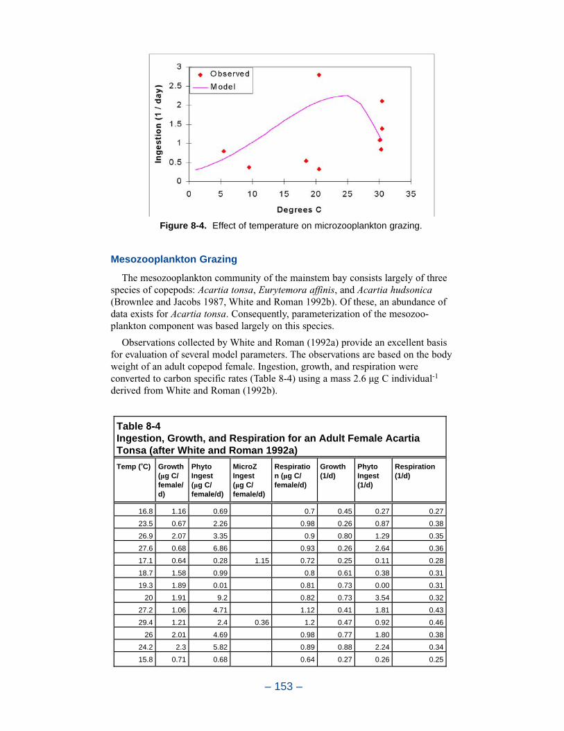
Mesozooplankton Grazing
The mesozooplankton community of the mainstem bay consists largely of threespecies of copepods: Acartia tonsa, Eurytemora affinis, and Acartia hudsonica(Brownlee and Jacobs 1987, White and Roman 1992b). Of these, an abundance ofdata exists for Acartia tonsa. Consequently, parameterization of the mesozoo-plankton component was based largely on this species.
Observations collected by White and Roman (1992a) provide an excellent basisfor evaluation of several model parameters. The observations are based on the bodyweight of an adult copepod female. Ingestion, growth, and respiration wereconverted to carbon specific rates (Table 8-4) using a mass 2.6 µg C individual-1
derived from White and Roman (1992b).
– 153 –
Table 8-4Ingestion, Growth, and Respiration for an Adult Female Acartia Tonsa (after White and Roman 1992a)
Temp (oC) Growth (µg C/ female/d)
PhytoIngest(µg C/ female/d)
MicroZIngest(µg C/ female/d)
Respiration (µg C/ female/d)
Growth (1/d)
PhytoIngest(1/d)
Respiration(1/d)
16.8 1.16 0.69 0.7 0.45 0.27 0.27
23.5 0.67 2.26 0.98 0.26 0.87 0.38
26.9 2.07 3.35 0.9 0.80 1.29 0.35
27.6 0.68 6.86 0.93 0.26 2.64 0.36
17.1 0.64 0.28 1.15 0.72 0.25 0.11 0.28
18.7 1.58 0.99 0.8 0.61 0.38 0.31
19.3 1.89 0.01 0.81 0.73 0.00 0.31
20 1.91 9.2 0.82 0.73 3.54 0.32
27.2 1.06 4.71 1.12 0.41 1.81 0.43
29.4 1.21 2.4 0.36 1.2 0.47 0.92 0.46
26 2.01 4.69 0.98 0.77 1.80 0.38
24.2 2.3 5.82 0.89 0.88 2.24 0.34
15.8 0.71 0.68 0.64 0.27 0.26 0.25
Figure 8-4. Effect of temperature on microzooplankton grazing.
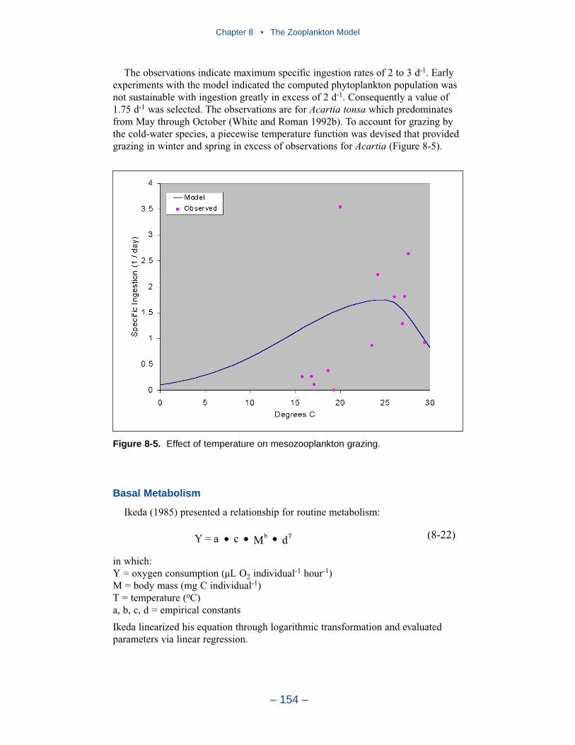
Chapter 8 • The Zooplankton Model
– 154 –
The observations indicate maximum specific ingestion rates of 2 to 3 d-1. Earlyexperiments with the model indicated the computed phytoplankton population wasnot sustainable with ingestion greatly in excess of 2 d-1. Consequently a value of1.75 d-1 was selected. The observations are for Acartia tonsa which predominatesfrom May through October (White and Roman 1992b). To account for grazing bythe cold-water species, a piecewise temperature function was devised that providedgrazing in winter and spring in excess of observations for Acartia (Figure 8-5).
Basal Metabolism
Ikeda (1985) presented a relationship for routine metabolism:
in which:Y = oxygen consumption (µL O2 individual-1 hour-1)M = body mass (mg C individual-1)T = temperature (oC)a, b, c, d = empirical constants
Ikeda linearized his equation through logarithmic transformation and evaluatedparameters via linear regression.
dMca=Y Tb (8-22)
Figure 8-5. Effect of temperature on mesozooplankton grazing.
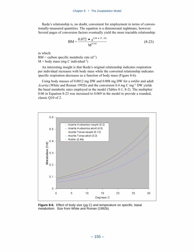
Ikeda’s relationship is, no doubt, convenient for employment in terms of conven-tionally-measured quantities. The equation is a dimensional nightmare, however.Several pages of conversion factors eventually yield the more tractable relationship:
in which:BM = carbon specific metabolic rate (d-1)M = body mass (mg C individual-1)
An interesting insight is that Ikeda’s original relationship indicates respirationper individual increases with body mass while the converted relationship indicatesspecific respiration decreases as a function of body mass (Figure 8-6).
Using body masses of 0.0012 mg DW and 0.008 mg DW for a rotifer and adultAcartia (White and Roman 1992b) and the conversion 0.4 mg C mg-1 DW yieldsthe basal metabolic rates employed in the model (Tables 8-1, 8-2). The multiplier0.06 in Equation 8-23 was increased to 0.069 in the model to provide a rounded,classic Q10 of 2.
Me0.072=BM0.165
20)-(T0.06
(8-23)
Chapter 8 • The Zooplankton Model
– 155 –
Figure 8-6. Effect of body size (µg C) and temperature on specific, basalmetabolism. Size from White and Roman (1992b).

Respiration Fraction and Efficiency
Data presented by White and Roman (1992a) indicates respiration accounts for40 to 50% of total microzooplankton and phytoplankton consumed by Acartia. Thisincludes both basal metabolism and the respiratory cost of feeding. Basal metabo-lism by Ikeda’s formula (0.185 d-1) is roughly half the specific respiration derivedfrom White and Roman’s data (Table 8-4). These proportions indicate the respira-tory fraction is the remaining half of specific respiration or 20 to 25% of preyconsumed. We found a lower fraction, 7% of prey consumed, provided reasonableresults when employed in the mesozooplankton computations. A higher value, 50%of prey consumed, was employed for microzooplankton to reflect the effect of bodysize on respiration.
The same observations indicate growth and respiration account for 87 to 95% oftotal ingestion. Roughly 10% of total ingestion is unaccounted for, indicating effi-ciency is roughly 90%. Modeled efficiencies are only one third of that value,however. While the observed efficiency seems high (White and Roman assume80%), the model values are unrealistically low. Reduced efficiencies were initiallyassigned to the model based on need. Efficiencies of 80 to 90% produced wideoscillations in computed populations and resulted in collapse of the phytoplanktonpopulation. Lower efficiencies resulted in damped oscillations and more stablecommunities.
Later insights indicated why lower efficiencies are appropriate. In the model,adult zooplankton instantaneously reproduce adult zooplankton. In reality, repro-duction is in the form of eggs. Eggs hatch into juvenile forms that eventuallymature into adults. The true growth process installs temporal lags in the system andreduces efficiency as eggs and juveniles are lost to predation and other processes.While the temporal lags are difficult to introduce into the present model, the lossesthat occur to eggs and juveniles are simulated though employment of relatively lowefficiencies.
Additional Parameters
Selection of the dissolved oxygen threshold for mortality was guided by theobservation that concentrations below 1 gm DO m-3 result in reduced survival ofcopepod adults and inhibited hatching of Acartia tonsa eggs (Roman et al. 1993).
Sellner et al. (1993) noted neither rotifers nor copepods grazed heavily onMicrocystis. Consequently, utilization of Group 1 algae, which represent cyanobac-teria in the tidal fresh Potomac River, was set to zero. White and Roman’s (1992a)observations indicate consumption of microzooplankton by mesozooplankton iscomparable to consumption of phytoplankton. Consequently utilization of micro-zooplankton was set to unity.
Selection of half-saturation and threshold concentrations for mesozooplanktonwas guided by interpretation of numerous studies (Table 8-5). Smaller concentra-tions were employed for microzooplankton to reflect their smaller body size.
Chapter 8 • The Zooplankton Model
– 156 –
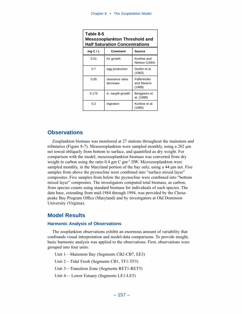
Observations
Zooplankton biomass was monitored at 27 stations throughout the mainstem andtributaries (Figure 8-7). Mesozooplankton were sampled monthly, using a 202 µmnet towed obliquely from bottom to surface, and quantified as dry weight. Forcomparison with the model, mesozooplankton biomass was converted from dryweight to carbon using the ratio 0.4 gm C gm-1 DW. Microzooplankton weresampled monthly, in the Maryland portion of the bay only, using a 44 µm net. Fivesamples from above the pycnocline were combined into “surface mixed layer”composites. Five samples from below the pycnocline were combined into “bottommixed layer” composites. The investigators computed total biomass, as carbon,from species counts using standard biomass for individuals of each species. Thedata base, extending from mid-1984 through 1994, was provided by the Chesa-peake Bay Program Office (Maryland) and by investigators at Old DominionUniversity (Virginia).
Model ResultsHarmonic Analysis of Observations
The zooplankton observations exhibit an enormous amount of variability thatconfounds visual interpretation and model-data comparisons. To provide insight,basic harmonic analysis was applied to the observations. First, observations weregrouped into four units:
Unit 1—Mainstem Bay (Segments CB2-CB7, EE3)
Unit 2—Tidal Fresh (Segments CB1, TF1-TF5)
Unit 3—Transition Zone (Segments RET1-RET5)
Unit 4— Lower Estuary (Segments LE1-LE5)
Chapter 8 • The Zooplankton Model
– 157 –
Table 8-5Mesozooplankton Threshold and Half Saturation Concentrations
mg C / L Comment Source
0.01 for growth Kiorboe and Nielson (1994)
0.7 egg production Durbin et al. (1983)
0.05 clearance rates decrease
Paffenhoferand Stearns (1988)
0.175 A. nauplii growth Berggreen et al. (1988)
0.2 ingestion Kiorboe et al. (1985)
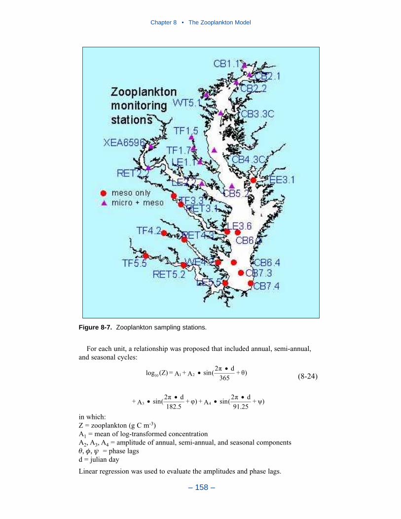
Chapter 8 • The Zooplankton Model
– 158 –
Figure 8-7. Zooplankton sampling stations.
For each unit, a relationship was proposed that included annual, semi-annual,and seasonal cycles:
in which:Z = zooplankton (g C m-3)A1 = mean of log-transformed concentrationA2, A3, A4 = amplitude of annual, semi-annual, and seasonal componentsθ, φ, ψ = phase lagsd = julian day
Linear regression was used to evaluate the amplitudes and phase lags.
)+91.25
d2(sinA+)+182.5
d2(sinA+
)+365
d2(sinA+A=(Z)log
43
2110 (8-24)
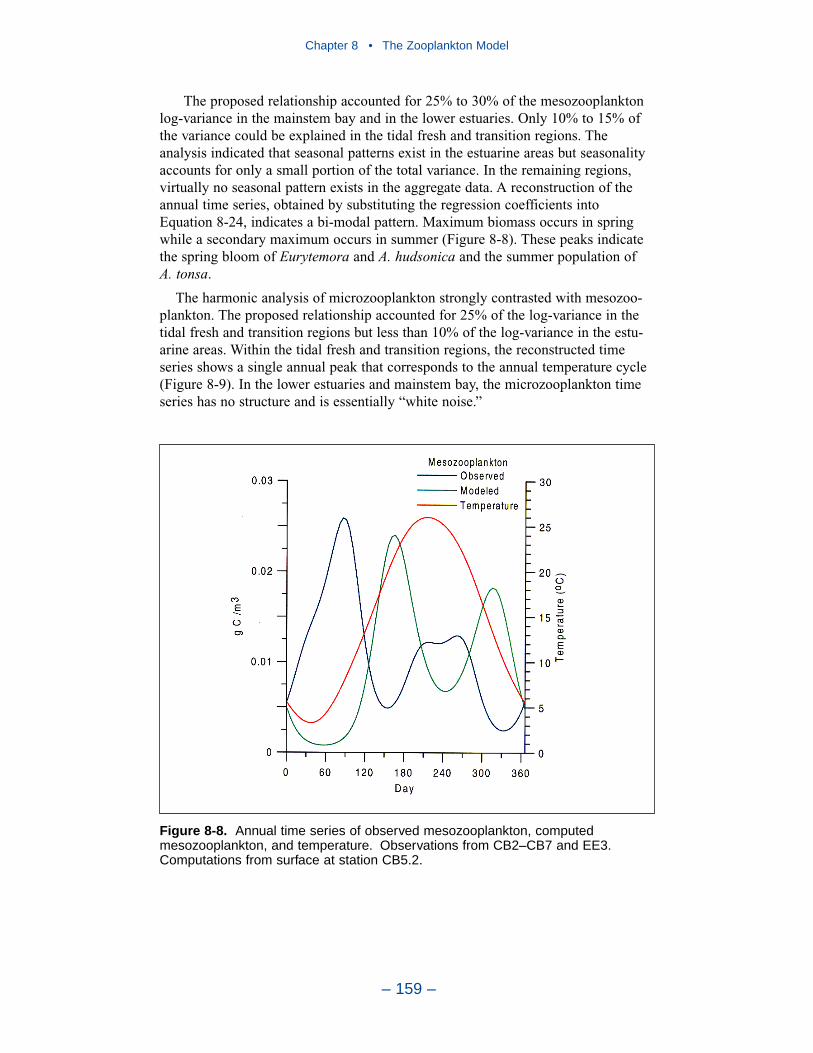
The proposed relationship accounted for 25% to 30% of the mesozooplanktonlog-variance in the mainstem bay and in the lower estuaries. Only 10% to 15% ofthe variance could be explained in the tidal fresh and transition regions. Theanalysis indicated that seasonal patterns exist in the estuarine areas but seasonalityaccounts for only a small portion of the total variance. In the remaining regions,virtually no seasonal pattern exists in the aggregate data. A reconstruction of theannual time series, obtained by substituting the regression coefficients intoEquation 8-24, indicates a bi-modal pattern. Maximum biomass occurs in springwhile a secondary maximum occurs in summer (Figure 8-8). These peaks indicatethe spring bloom of Eurytemora and A. hudsonica and the summer population of A. tonsa.
The harmonic analysis of microzooplankton strongly contrasted with mesozoo-plankton. The proposed relationship accounted for 25% of the log-variance in thetidal fresh and transition regions but less than 10% of the log-variance in the estu-arine areas. Within the tidal fresh and transition regions, the reconstructed timeseries shows a single annual peak that corresponds to the annual temperature cycle(Figure 8-9). In the lower estuaries and mainstem bay, the microzooplankton timeseries has no structure and is essentially “white noise.”
Chapter 8 • The Zooplankton Model
– 159 –
Figure 8-8. Annual time series of observed mesozooplankton, computedmesozooplankton, and temperature. Observations from CB2–CB7 and EE3.Computations from surface at station CB5.2.
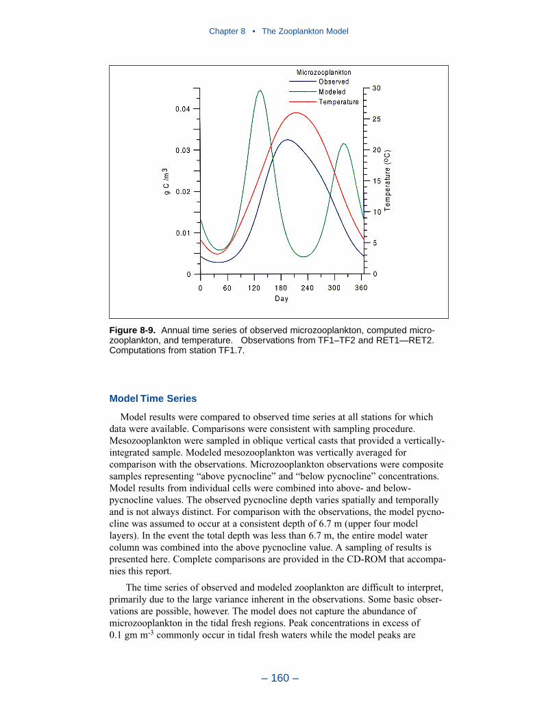
Model Time Series
Model results were compared to observed time series at all stations for whichdata were available. Comparisons were consistent with sampling procedure.Mesozooplankton were sampled in oblique vertical casts that provided a vertically-integrated sample. Modeled mesozooplankton was vertically averaged forcomparison with the observations. Microzooplankton observations were compositesamples representing “above pycnocline” and “below pycnocline” concentrations.Model results from individual cells were combined into above- and below-pycnocline values. The observed pycnocline depth varies spatially and temporallyand is not always distinct. For comparison with the observations, the model pycno-cline was assumed to occur at a consistent depth of 6.7 m (upper four modellayers). In the event the total depth was less than 6.7 m, the entire model watercolumn was combined into the above pycnocline value. A sampling of results ispresented here. Complete comparisons are provided in the CD-ROM that accompa-nies this report.
The time series of observed and modeled zooplankton are difficult to interpret,primarily due to the large variance inherent in the observations. Some basic obser-vations are possible, however. The model does not capture the abundance ofmicrozooplankton in the tidal fresh regions. Peak concentrations in excess of 0.1 gm m-3 commonly occur in tidal fresh waters while the model peaks are
Chapter 8 • The Zooplankton Model
– 160 –
Figure 8-9. Annual time series of observed microzooplankton, computed micro-zooplankton, and temperature. Observations from TF1–TF2 and RET1—RET2.Computations from station TF1.7.
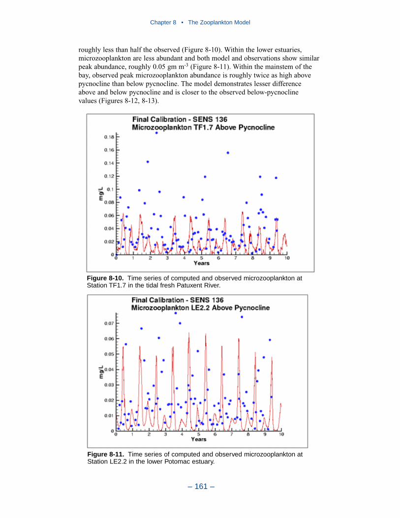
roughly less than half the observed (Figure 8-10). Within the lower estuaries,microzooplankton are less abundant and both model and observations show similarpeak abundance, roughly 0.05 gm m-3 (Figure 8-11). Within the mainstem of thebay, observed peak microzooplankton abundance is roughly twice as high abovepycnocline than below pycnocline. The model demonstrates lesser difference above and below pycnocline and is closer to the observed below-pycnocline values (Figures 8-12, 8-13).
Chapter 8 • The Zooplankton Model
– 161 –
Figure 8-10. Time series of computed and observed microzooplankton at Station TF1.7 in the tidal fresh Patuxent River.
Figure 8-11. Time series of computed and observed microzooplankton at Station LE2.2 in the lower Potomac estuary.
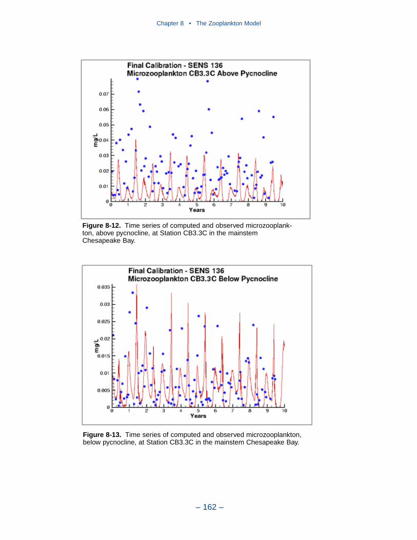
Chapter 8 • The Zooplankton Model
– 162 –
Figure 8-13. Time series of computed and observed microzooplankton,below pycnocline, at Station CB3.3C in the mainstem Chesapeake Bay.
Figure 8-12. Time series of computed and observed microzooplank-ton, above pycnocline, at Station CB3.3C in the mainstemChesapeake Bay.
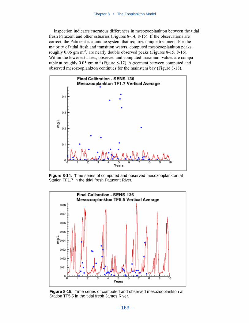
Inspection indicates enormous differences in mesozooplankton between the tidalfresh Patuxent and other estuaries (Figures 8-14, 8-15). If the observations arecorrect, the Patuxent is a unique system that requires unique treatment. For themajority of tidal fresh and transition waters, computed mesozooplankton peaks,roughly 0.06 gm m-3, are nearly double observed peaks (Figures 8-15, 8-16).Within the lower estuaries, observed and computed maximum values are compa-rable at roughly 0.05 gm m-3 (Figure 8-17). Agreement between computed andobserved mesozooplankton continues for the mainstem bay (Figure 8-18).
Chapter 8 • The Zooplankton Model
– 163 –
Figure 8-14. Time series of computed and observed mesozooplankton at Station TF1.7 in the tidal fresh Patuxent River.
Figure 8-15. Time series of computed and observed mesozooplankton at Station TF5.5 in the tidal fresh James River.
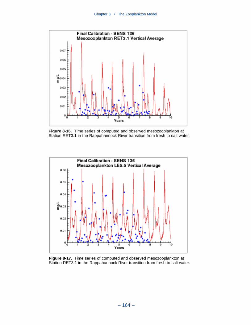
Chapter 8 • The Zooplankton Model
– 164 –
Figure 8-16. Time series of computed and observed mesozooplankton at Station RET3.1 in the Rappahannock River transition from fresh to salt water.
Figure 8-17. Time series of computed and observed mesozooplankton at Station RET3.1 in the Rappahannock River transition from fresh to salt water.
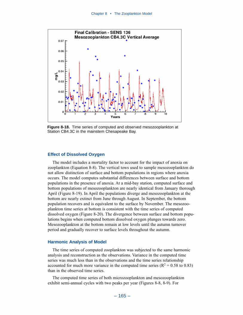
Effect of Dissolved Oxygen
The model includes a mortality factor to account for the impact of anoxia onzooplankton (Equation 8-8). The vertical tows used to sample mesozooplankton donot allow distinction of surface and bottom populations in regions where anoxiaoccurs. The model computes substantial differences between surface and bottompopulations in the presence of anoxia. At a mid-bay station, computed surface andbottom populations of mesozooplankton are nearly identical from January thoroughApril (Figure 8-19). In April the populations diverge and mesozooplankton at thebottom are nearly extinct from June through August. In September, the bottompopulation recovers and is equivalent to the surface by November. The mesozoo-plankton time series at bottom is consistent with the time series of computeddissolved oxygen (Figure 8-20). The divergence between surface and bottom popu-lations begins when computed bottom dissolved oxygen plunges towards zero.Mesozooplankton at the bottom remain at low levels until the autumn turnoverperiod and gradually recover to surface levels throughout the autumn.
Harmonic Analysis of Model
The time series of computed zooplankton was subjected to the same harmonicanalysis and reconstruction as the observations. Variance in the computed timeseries was much less than in the observations and the time series relationshipaccounted for much more variance in the computed time series (R2 = 0.58 to 0.83)than in the observed time series.
The computed time series of both microzooplankton and mesozooplanktonexhibit semi-annual cycles with two peaks per year (Figures 8-8, 8-9). For
Chapter 8 • The Zooplankton Model
– 165 –
Figure 8-18. Time series of computed and observed mesozooplankton atStation CB4.3C in the mainstem Chesapeake Bay.
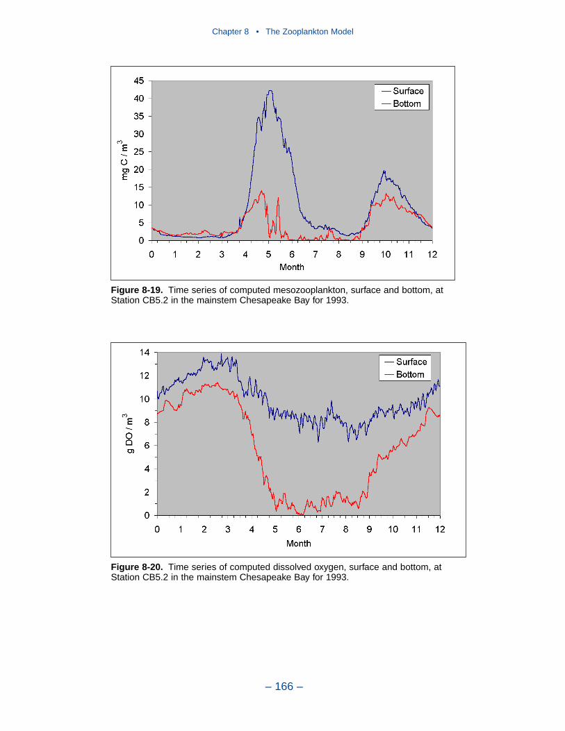
Chapter 8 • The Zooplankton Model
– 166 –
Figure 8-19. Time series of computed mesozooplankton, surface and bottom, atStation CB5.2 in the mainstem Chesapeake Bay for 1993.
Figure 8-20. Time series of computed dissolved oxygen, surface and bottom, atStation CB5.2 in the mainstem Chesapeake Bay for 1993.
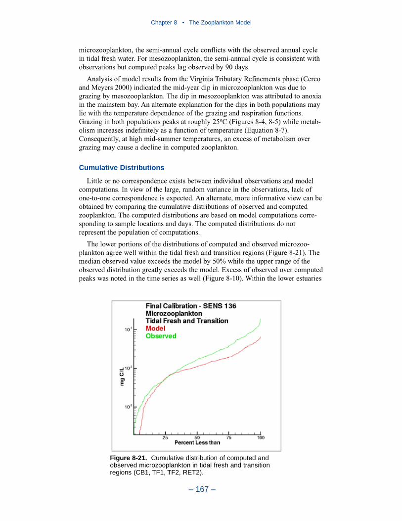
microzooplankton, the semi-annual cycle conflicts with the observed annual cyclein tidal fresh water. For mesozooplankton, the semi-annual cycle is consistent withobservations but computed peaks lag observed by 90 days.
Analysis of model results from the Virginia Tributary Refinements phase (Cercoand Meyers 2000) indicated the mid-year dip in microzooplankton was due tograzing by mesozooplankton. The dip in mesozooplankton was attributed to anoxiain the mainstem bay. An alternate explanation for the dips in both populations maylie with the temperature dependence of the grazing and respiration functions.Grazing in both populations peaks at roughly 25oC (Figures 8-4, 8-5) while metab-olism increases indefinitely as a function of temperature (Equation 8-7).Consequently, at high mid-summer temperatures, an excess of metabolism overgrazing may cause a decline in computed zooplankton.
Cumulative Distributions
Little or no correspondence exists between individual observations and modelcomputations. In view of the large, random variance in the observations, lack ofone-to-one correspondence is expected. An alternate, more informative view can beobtained by comparing the cumulative distributions of observed and computedzooplankton. The computed distributions are based on model computations corre-sponding to sample locations and days. The computed distributions do notrepresent the population of computations.
The lower portions of the distributions of computed and observed microzoo-plankton agree well within the tidal fresh and transition regions (Figure 8-21). Themedian observed value exceeds the model by 50% while the upper range of theobserved distribution greatly exceeds the model. Excess of observed over computedpeaks was noted in the time series as well (Figure 8-10). Within the lower estuaries
Chapter 8 • The Zooplankton Model
– 167 –
Figure 8-21. Cumulative distribution of computed and observed microzooplankton in tidal fresh and transition regions (CB1, TF1, TF2, RET2).
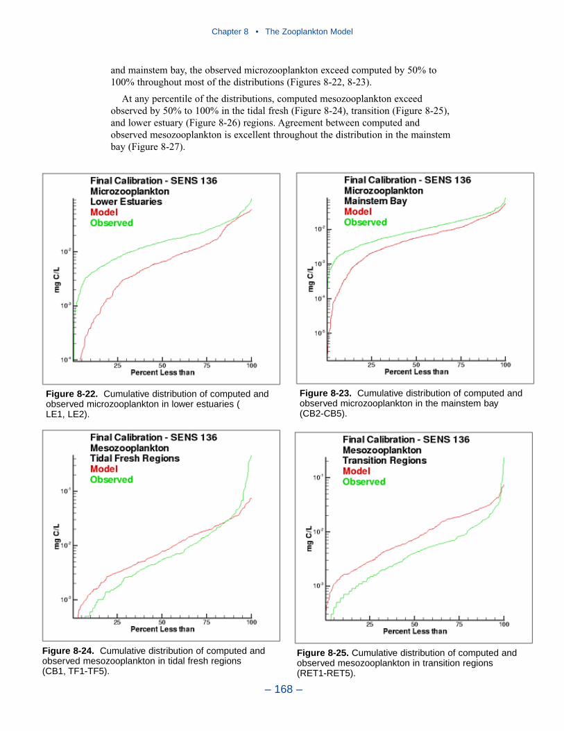
and mainstem bay, the observed microzooplankton exceed computed by 50% to100% throughout most of the distributions (Figures 8-22, 8-23).
At any percentile of the distributions, computed mesozooplankton exceedobserved by 50% to 100% in the tidal fresh (Figure 8-24), transition (Figure 8-25),and lower estuary (Figure 8-26) regions. Agreement between computed andobserved mesozooplankton is excellent throughout the distribution in the mainstembay (Figure 8-27).
Chapter 8 • The Zooplankton Model
– 168 –
Figure 8-22. Cumulative distribution of computed andobserved microzooplankton in lower estuaries (LE1, LE2).
Figure 8-23. Cumulative distribution of computed andobserved microzooplankton in the mainstem bay (CB2-CB5).
Figure 8-24. Cumulative distribution of computed andobserved mesozooplankton in tidal fresh regions (CB1, TF1-TF5).
Figure 8-25. Cumulative distribution of computed andobserved mesozooplankton in transition regions (RET1-RET5).
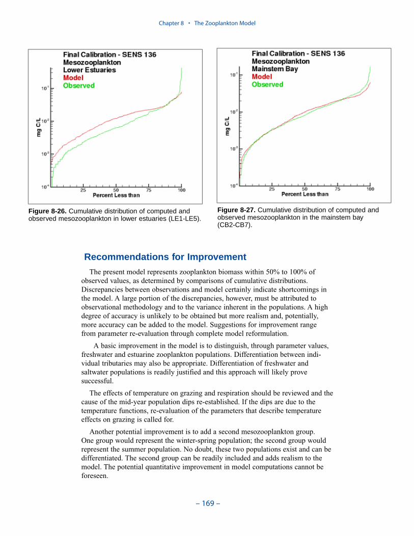
Recommendations for Improvement
The present model represents zooplankton biomass within 50% to 100% ofobserved values, as determined by comparisons of cumulative distributions.Discrepancies between observations and model certainly indicate shortcomings inthe model. A large portion of the discrepancies, however, must be attributed toobservational methodology and to the variance inherent in the populations. A highdegree of accuracy is unlikely to be obtained but more realism and, potentially,more accuracy can be added to the model. Suggestions for improvement rangefrom parameter re-evaluation through complete model reformulation.
A basic improvement in the model is to distinguish, through parameter values,freshwater and estuarine zooplankton populations. Differentiation between indi-vidual tributaries may also be appropriate. Differentiation of freshwater andsaltwater populations is readily justified and this approach will likely provesuccessful.
The effects of temperature on grazing and respiration should be reviewed and thecause of the mid-year population dips re-established. If the dips are due to thetemperature functions, re-evaluation of the parameters that describe temperatureeffects on grazing is called for.
Another potential improvement is to add a second mesozooplankton group. One group would represent the winter-spring population; the second group wouldrepresent the summer population. No doubt, these two populations exist and can bedifferentiated. The second group can be readily included and adds realism to themodel. The potential quantitative improvement in model computations cannot beforeseen.
Chapter 8 • The Zooplankton Model
– 169 –
Figure 8-26. Cumulative distribution of computed andobserved mesozooplankton in lower estuaries (LE1-LE5).
Figure 8-27. Cumulative distribution of computed andobserved mesozooplankton in the mainstem bay (CB2-CB7).
The final improvement is the most difficult. Add age structure to the mesozoo-plankton model. As previously noted, adults in the present model instantaneouslyreproduce adults. In the most realistic model, adults would produce eggs. Eggswould hatch into larvae, mature into juveniles and, later, into adults. A model ofthis sort offers the highest probability of success in representing the time series ofobserved mesozooplankton. A multi-stage population model requires tremendousresources in programming, calibration, and execution. The additional effort is likelynot worthwhile in the present multi-purpose model. The improvement is highlyrecommended if the present model is employed in an application that focuseslargely on zooplankton.
ReferencesBerggreen, U., Hansen, B. and Kiorboe, T. (1988). “Food size spectra, ingestion and growthof the copepod Acartia tonsa during development: implications for determination ofcopepod production,” Marine Biology, 99, 341-352.
Brownlee, D., and Jacobs, F. (1987). “Mesozooplankton and microzooplankton in theChesapeake Bay,” Contaminant Problems and Management of Living Chesapeake BayResources, Majumdar, S., Hall, L., and Austin, H., eds. The Pennsylvania Academy ofScience, Philadelphia.
Cerco, C., Johnson, B., and Wang, H. (2002). “Tributary refinements to the Chesapeake Baymodel,” ERDC TR-02-4, U.S. Army Engineer Research and Development Center, Vicks-burg, MS.
Cerco, C., and Meyers, M. (2000). “Tributary refinements to the Chesapeake Bay Model,”Journal of Environmental Engineering, 126(2), 164-174.
Cerco, C., and Cole, T. (1994). “Three-dimensional eutrophication model of ChesapeakeBay,” Technical Report EL-94-4, U.S. Army Engineer Waterways Experiment Station,Vicksburg, MS.
Cerco, C., and Cole, T. (1993). “Three-dimensional eutrophication model of ChesapeakeBay,” Journal of Environmental Engineering, 119(6), 1006- 10025.
Dagg, M. (1995). “Ingestion of phytoplankton by the micro- and mesozooplankton commu-nities in a productive subtropical estuary,” Journal of Plankton Research, 17(4), 845-857.
DiToro, D., and Matystik, W. (1980). “Mathematical models of water quality in large lakespart 1: Lake Huron and Saginaw Bay,” EPA-600/3-80-056, Environmental Research Labo-ratory, Office of Research and Development, US Environmental protection Agency, DuluthMN.
DiToro, D., O’Connor, S., and Thomann, R. (1971). “A dynamic model of the phyto-plankton population in the Sacramento-San Joaquin Delta,” Nonequilibrium systems inwater chemistry, American Chemical Society, Washington, DC, 131-180.
Durbin, E., Durbin, Ann G., Smayda, Thomas J., and Verity, Peter G. (1983). “Food limita-tion of production by adult Acartia tonsa in Naragansett Bay, Rhode Island,” Limnologyand Oceanography, 28(6), 1199-1213.
Ikeda, T. (1985). “Metabolic rates of epipelagic marine zooplankton as a function of bodymass and temperature,” Marine Biology 85, 1-11.
Kiorboe, T., and Neilson, T. (1994). “Regulation of zooplankton biomass and production ina temperate, coastal ecosystem. 1. Copepods,” Limnology and Oceanography, 39(3), 493-507.
Chapter 8 • The Zooplankton Model
– 170 –
Paffenhofer, G., and Stearns, D. (1988). “Why is Acartia tonsa (Copepoda: Calanoida)restricted to nearshore environments?,” Marine Ecology Progress Series, 42, 33-38.
Parsons, T., Takahashi, M., and Hargrave, B. (1984). Biological Oceanographic Processes,3rd ed., Pergamon Press, Oxford.
Redfield, A., Ketchum, B., and Richards, F. (1966). “The influence of organisms on thecomposition of sea-water.” The Sea Volume II. Interscience Publishers, New York, 26-48.
Roman, M., Gauzens, A., Rhinehart, W., and White, J. (1993). “Effects of low oxygenwaters on Chesapeake Bay zooplankton,” Limnology and Oceanography 38(8), 1603-1614.
Sellner, K., Brownlee, D., Bundy, M., Brownlee, S., and Braun, K. (1993). “Zooplanktongrazing in a Potomac River cyanobacteria bloom,” Estuaries 16(4), 859-872. White, J., andRoman M. (1992a). “Egg production by the calanoid copepod Acartia tonsa in the mesoha-line Chesapeake Bay: the importance of food resources and temperature,” Marine EcologyProgress Series 86, 239-249.
Thomann, R., and Fitzpatrick, J. (1982). “Calibration and verification of a mathematicalmodel of the eutrophication of the Potomac Estuary,” HydroQual Inc., Mahwah, NJ.
White, J., and Roman M. (1992b). “Seasonal study of grazing by metazoan zooplankton inthe mesohaline Chesapeake Bay,” Marine Ecology Progress Series 86, 251-261.
Chapter 8 • The Zooplankton Model
– 171 –
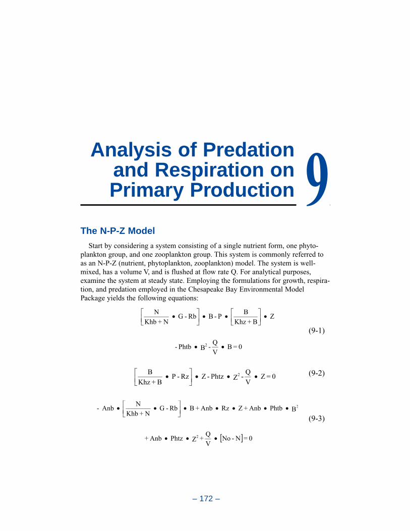
The N-P-Z Model
Start by considering a system consisting of a single nutrient form, one phyto-plankton group, and one zooplankton group. This system is commonly referred toas an N-P-Z (nutrient, phytoplankton, zooplankton) model. The system is well-mixed, has a volume V, and is flushed at flow rate Q. For analytical purposes,examine the system at steady state. Employing the formulations for growth, respira-tion, and predation employed in the Chesapeake Bay Environmental ModelPackage yields the following equations:
0=N-NoVQ+ZPhtzAnb+
BPhtbAnb+ ZRzAnb+BRb-GN+Khb
NAnb-
2
2
(9-3)
0= ZVQ-ZPhtz- ZRz-P
B+KhzB 2 (9-2)
0=BVQ-BPhtb-
ZB+Khz
BP-BRb-GN+Khb
N
2
(9-1)
– 172 –
Analysis of Predationand Respiration onPrimary Production 9
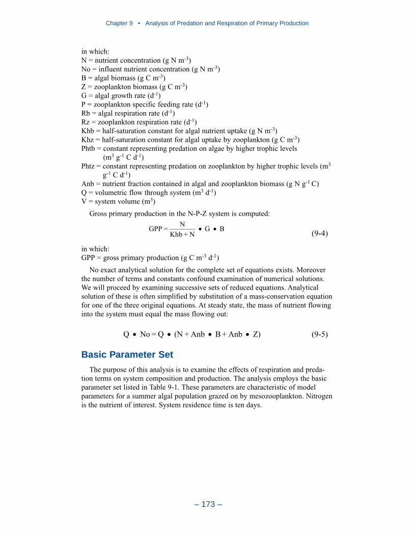
in which:N = nutrient concentration (g N m-3)No = influent nutrient concentration (g N m-3) B = algal biomass (g C m-3)Z = zooplankton biomass (g C m-3)G = algal growth rate (d-1)P = zooplankton specific feeding rate (d-1)Rb = algal respiration rate (d-1)Rz = zooplankton respiration rate (d-1)Khb = half-saturation constant for algal nutrient uptake (g N m-3)Khz = half-saturation constant for algal uptake by zooplankton (g C m-3)Phtb = constant representing predation on algae by higher trophic levels
(m3 g-1 C d-1)Phtz = constant representing predation on zooplankton by higher trophic levels (m3
g-1 C d-1)Anb = nutrient fraction contained in algal and zooplankton biomass (g N g-1 C) Q = volumetric flow through system (m3 d-1)V = system volume (m3)
Gross primary production in the N-P-Z system is computed:
in which:GPP = gross primary production (g C m-3 d-1)
No exact analytical solution for the complete set of equations exists. Moreoverthe number of terms and constants confound examination of numerical solutions.We will proceed by examining successive sets of reduced equations. Analyticalsolution of these is often simplified by substitution of a mass-conservation equationfor one of the three original equations. At steady state, the mass of nutrient flowinginto the system must equal the mass flowing out:
Basic Parameter Set
The purpose of this analysis is to examine the effects of respiration and preda-tion terms on system composition and production. The analysis employs the basicparameter set listed in Table 9-1. These parameters are characteristic of modelparameters for a summer algal population grazed on by mesozooplankton. Nitrogenis the nutrient of interest. System residence time is ten days.
Z)Anb+BAnb+(NQ=NoQ (9-5)
BGN+Khb
N=GPP(9-4)
Chapter 9 • Analysis of Predation and Respiration of Primary Production
– 173 –
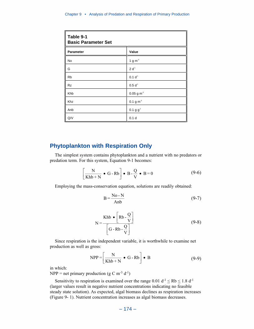
Chapter 9 • Analysis of Predation and Respiration of Primary Production
– 174 –
Table 9-1 Basic Parameter Set
Parameter Value
No 1 g m-3
G 2 d-1
Rb 0.1 d-1
Rz 0.5 d-1
Khb 0.05 g m-3
Khz 0.1 g m-3
Anb 0.1 g g-1
Q/V 0.1 d
Phytoplankton with Respiration Only
The simplest system contains phytoplankton and a nutrient with no predators orpredation term. For this system, Equation 9-1 becomes:
Employing the mass-conservation equation, solutions are readily obtained:
Since respiration is the independent variable, it is worthwhile to examine netproduction as well as gross:
in which:NPP = net primary production (g C m-3 d-1)
Sensitivity to respiration is examined over the range 0.01 d-1 < Rb < 1.8 d-1
(larger values result in negative nutrient concentrations indicating no feasiblesteady state solution). As expected, algal biomass declines as respiration increases(Figure 9- 1). Nutrient concentration increases as algal biomass decreases.
BRb-GN+Khb
N=NPP (9-9)
VQ-Rb-G
VQ-RbKhb
=N (9-8)
AnbN-No=B (9-7)
0=BVQ-BRb-G
N+KhbN (9-6)
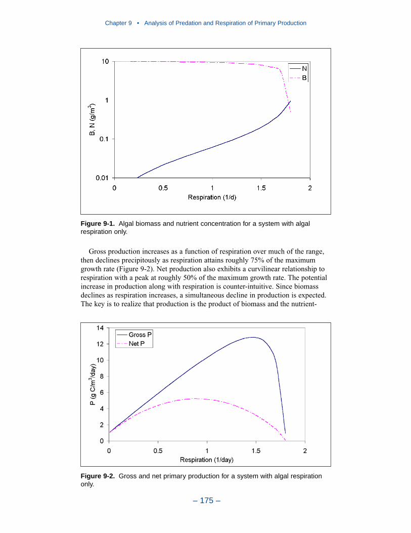
Gross production increases as a function of respiration over much of the range,then declines precipitously as respiration attains roughly 75% of the maximumgrowth rate (Figure 9-2). Net production also exhibits a curvilinear relationship torespiration with a peak at roughly 50% of the maximum growth rate. The potentialincrease in production along with respiration is counter-intuitive. Since biomassdeclines as respiration increases, a simultaneous decline in production is expected.The key is to realize that production is the product of biomass and the nutrient-
Chapter 9 • Analysis of Predation and Respiration of Primary Production
– 175 –
Figure 9-1. Algal biomass and nutrient concentration for a system with algalrespiration only.
Figure 9-2. Gross and net primary production for a system with algal respirationonly.
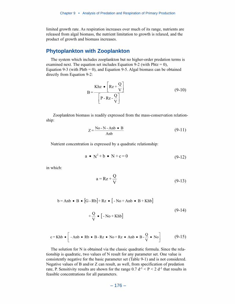
Chapter 9 • Analysis of Predation and Respiration of Primary Production
– 176 –
limited growth rate. As respiration increases over much of its range, nutrients arereleased from algal biomass, the nutrient limitation to growth is relaxed, and theproduct of growth and biomass increases.
Phytoplankton with Zooplankton
The system which includes zooplankton but no higher-order predation terms isexamined next. The equation set includes Equation 9-2 (with Phtz = 0),Equation 9-3 (with Phtb = 0), and Equation 9-5. Algal biomass can be obtaineddirectly from Equation 9-2:
Zooplankton biomass is readily expressed from the mass-conservation relation-ship:
Nutrient concentration is expressed by a quadratic relationship:
in which:
The solution for N is obtained via the classic quadratic formula. Since the rela-tionship is quadratic, two values of N result for any parameter set. One value isconsistently negative for the basic parameter set (Table 9-1) and is not considered.Negative values of B and/or Z can result, as well, from specification of predationrate, P. Sensitivity results are shown for the range 0.7 d-1 < P < 2 d-1 that results infeasible concentrations for all parameters.
NoVQ-BAnbRz+NoRz-BRbAnb-Khb=c (9-15)
Khb+No-VQ+
Khb+BAnb+No-Rz+Rb-GBAnb=b
(9-14)
VQ+Rz=a (9-13)
0=c+Nb+Na 2(9-12)
AnbBAnb-N-No=Z (9-11)
VQ-Rz-P
VQ+RzKhz
=B (9-10)

Algal biomass decreases rapidly and approaches zero asymtotically as predationrate is increased from the minimum feasible value (Figure 9-3). Surprisingly,zooplankton biomass also diminishes as predation rate is increased. The steadystate solution indicates maximum biomass occurs at low predation rates in whichzooplankton slowly feed on a large algal standing stock.
Primary production responds in direct proportion to algal biomass (Figure 9-4).Maximum production occurs a minimum predation rate. The steady-state solutionfor the basic parameter set indicates little or no nutrient limitation and the smallincrease in nutrient concentration at higher predation rates has little effect on
Chapter 9 • Analysis of Predation and Respiration of Primary Production
– 177 –
Figure 9-3. Algal biomass, zooplankton biomass, and nutrient concentration for asystem with algae, zooplankton, and a nutrient.
Figure 9-4. Gross primary production for a system with algae, zooplankton, and a nutrient.
Chapter 9 • Analysis of Predation and Respiration of Primary Production
– 178 –
growth. Consequently production, the product of nutrient-limited growth andbiomass, responds primarily to changes in biomass.
Phytoplankton with Quadratic Predation
Predation by higher trophic levels (other than zooplankton) on phytoplankton isrepresented by a quadratic term in the algal mass-balance equation. The quadraticformulation is derived by assuming the biomass of predators is linearly propor-tional to the biomass of prey. The proportionality constant and the specific feedingrate are lumped into the parameter Phtb.
The effect of the quadratic predation term is examined by solving a simplifiedalgal mass-balance equation:
and the mass-conservation equation.
The solution for algal biomass is quadratic with the following coefficients:
For the basic parameter set, one solution for B results in consistently negativenutrient concentrations. The second solution indicates an algal concentration thatdeclines as predation rate increases (Figure 9-5). Mass conservation dictatesnutrient concentration must increase as biomass decreases.
Despite the decrease in algal biomass, primary production increases as predationis raised from minimum levels (Figure 9-6). The increase occurs because thenutrient limit to production is relaxed as predation liberates nutrients from algalbiomass. Consequently, the product of nutrient-limited growth rate and algalbiomass increases despite the decrease in biomass. The increasing trend inproduction continues until nutrients are no longer limiting. That is, until N/(Khb +N) approaches unity. At that point, production declines in proportion to biomass.
VQ+RbNo+Khb-GNo=c (9-19)
VQAnb+No+KhbPhtb-R+G-Anb=b (9-18)
PhtbAnb=a (9-17)
0=BVQ-BPhtb-BRb-G
N+KhbN 2
(9-16)

Chapter 9 • Analysis of Predation and Respiration of Primary Production
– 179 –
Figure 9-6. Gross primary production for a system with quadratic predation and no zooplankton.
Figure 9-5. Algal biomass and nutrient concentration for a system with quadraticpredation and no zooplankton.
IntroductionPrimary production models may be placed in two categories. We call the first
category “observation based.” Observation-based models employ observations of aphotoadaptive variable, chlorophyll, and perhaps other quantities, to quantify depth-integrated production at the time and location of the observations. This class ofmodels has been extensively reviewed by Behrenfield and Falkowski (1997).
We call the second category “process based.” Process-based models quantifyproduction as a function of computed algal biomass and computed processes thatmay include growth (as affected by temperature, nutrients, and light), respiration,predation, and transport. Parameters in process-based models are commonlyassigned so that computations match one or more observed quantities. The assign-ment process is commonly denoted “calibration.”
We have noticed that process-based models frequently encounter difficulty insimultaneously matching observed biomass and production. Most commonly,process-based models provide reasonable representations of biomass but fall shortin computing production. Less commonly, the models adequately compute produc-tion but misrepresent biomass and/or growth-limiting nutrient concentration.
Doney et al. (1996) modeled phytoplankton, zooplankton, and nutrients in a sub-tropical region near Bermuda. They noted the model showed “skill in capturing themajor features of the annual chlorophyll field.” Computed primary production wasalmost always less than observed, however. Model performance was weakest“during late summer, when the model cannot supply enough nutrients to supportthe high production observed.”
McGillicuddy et al. (1995) showed computed and observed vertical profiles ofprimary production in the North Atlantic. In ten of thirteen cases, primary produc-tion was under-computed at the surface, where light is abundant and nutrients arescarce. In deeper waters, where light is attenuated and nutrients are more abundant,model-data comparisons were much improved.
Fasham et al. (1990) applied a model that included phytoplankton, zooplankton,bacteria and nutrients to ocean Station “S” near Bermuda. They calibrated their
– 180 –
Process-BasedPrimary Production
Modeling inChesapeake Bay10

Chapter 10 • Process-Based Primary Production Modeling in Chesapeake Bay
– 181 –
model to match observed primary production. During the summer, computed nitrateconcentrations were much less than observed. Their simulations “greatly overesti-mated the phytoplankton biomass in the summer and autumn.”
Moll (1998) simulated chlorophyll, phosphate, and primary production in theNorth Sea. Observed primary production was well-matched by the model. Atseveral stations, the computed phosphate agreed with observed while at otherstations computed exceeded observed by several hundred percent. At all stations,the computed concentration exceeded the specified half-saturation concentration bytwo to three times. Consequently, the effect of nutrient limitation on computedproduction was minimal.
Based on the cited studies, process-based models have the following characteris-tics. Observed production can be matched when light rather than nutrients appearsto limit production (the North Atlantic at depths greater than 20 to 30 m, the NorthSea as modeled). In regions where nutrients appear to be more limiting than light(North Atlantic surface waters, the sub-tropical Atlantic), observed productioncannot be computed without compromising computations of algal biomass andnutrients (Ocean Station “S”).
The objective of the present study is to create a process-based model of Chesa-peake Bay that simultaneously matches observations of phytoplankton biomass,limiting nutrient concentration, light attenuation, and primary production.
Chesapeake BayChesapeake Bay is an extensive estuarine system located on the east coast of the
United States of America (Figure 10-1). The mainstem of the bay extends 300 kmfrom the Susquehanna River, at the head, to the Atlantic Ocean, at the mouth. Meandepth of the mainstem bay is 8 m although a deep trench with depths to 50 m runsup the center. The Susquehanna provides the majority of freshwater flow (64 %)and nutrient loading (Malone et al. 1988, Boynton et al. 1995.) Virtually allremaining runoff and loads originate in several major western tributaries. The bayand major tributaries are classic examples of partially-mixed estuaries byPritchard’s (1967) classification.
The physics, chemistry, and biology of the bay have been extensively studied fordecades. Significant studies relative to primary production include nutrient(Boynton et al. 1995) and carbon budgets (Kemp et al. 1997), examinations ofnutrient limitations (Fisher et al. 1999, Malone et al. 1996, Fisher et al. 1992), andmeasures of primary production (Harding et al. 2002, Smith and Kemp 1995,Harding et al. 1986).
These studies describe a system in which maximum phytoplankton biomass andmaximum production are out of phase. Peak biomass occurs during the springbloom while peak production occurs concurrent with the summer temperaturemaximum (Malone et al. 1988, Smith and Kemp 1995, Malone et al. 1996, Hardinget al. 2002). During the spring bloom, phosphorus and silica tend to be the limitingnutrients while nitrogen is the primary limiting nutrient in summer (Fisher et al.1992, Malone et al. 1996, Fisher et al. 1999). Peak nitrogen loads delivered duringspring runoff are coupled to summer production through a nutrient trappingmechanism. Nitrogen present is spring runoff is taken up during the phytoplanktonbloom, deposited in bottom sediments, and recycled to the water column bytemperature-induced diagenesis (Malone et al. 1988).
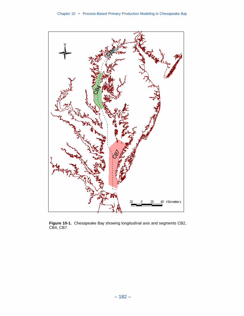
Chapter 10 • Process-Based Primary Production Modeling in Chesapeake Bay
– 182 –
Figure 10-1. Chesapeake Bay showing longitudinal axis and segments CB2,CB4, CB7.
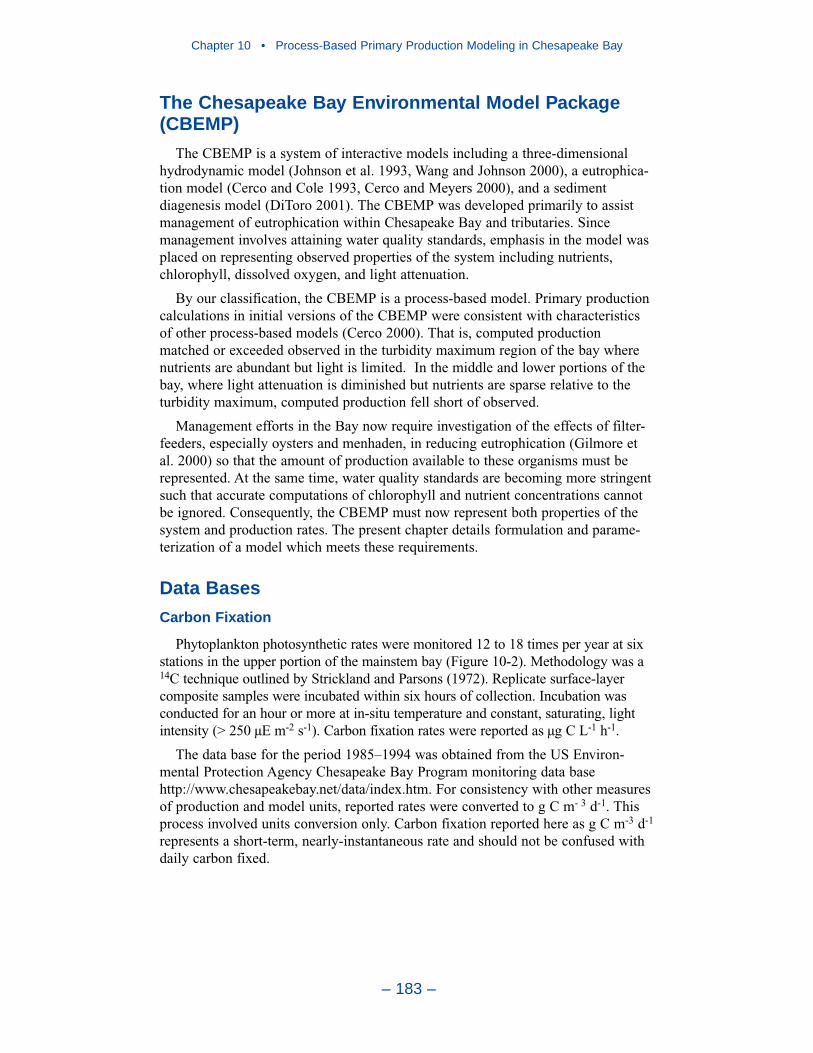
The Chesapeake Bay Environmental Model Package(CBEMP)
The CBEMP is a system of interactive models including a three-dimensionalhydrodynamic model (Johnson et al. 1993, Wang and Johnson 2000), a eutrophica-tion model (Cerco and Cole 1993, Cerco and Meyers 2000), and a sedimentdiagenesis model (DiToro 2001). The CBEMP was developed primarily to assistmanagement of eutrophication within Chesapeake Bay and tributaries. Sincemanagement involves attaining water quality standards, emphasis in the model wasplaced on representing observed properties of the system including nutrients,chlorophyll, dissolved oxygen, and light attenuation.
By our classification, the CBEMP is a process-based model. Primary productioncalculations in initial versions of the CBEMP were consistent with characteristicsof other process-based models (Cerco 2000). That is, computed productionmatched or exceeded observed in the turbidity maximum region of the bay wherenutrients are abundant but light is limited. In the middle and lower portions of thebay, where light attenuation is diminished but nutrients are sparse relative to theturbidity maximum, computed production fell short of observed.
Management efforts in the Bay now require investigation of the effects of filter-feeders, especially oysters and menhaden, in reducing eutrophication (Gilmore etal. 2000) so that the amount of production available to these organisms must berepresented. At the same time, water quality standards are becoming more stringentsuch that accurate computations of chlorophyll and nutrient concentrations cannotbe ignored. Consequently, the CBEMP must now represent both properties of thesystem and production rates. The present chapter details formulation and parame-terization of a model which meets these requirements.
Data Bases
Carbon Fixation
Phytoplankton photosynthetic rates were monitored 12 to 18 times per year at sixstations in the upper portion of the mainstem bay (Figure 10-2). Methodology was a14C technique outlined by Strickland and Parsons (1972). Replicate surface-layercomposite samples were incubated within six hours of collection. Incubation wasconducted for an hour or more at in-situ temperature and constant, saturating, lightintensity (> 250 µE m-2 s-1). Carbon fixation rates were reported as µg C L-1 h-1.
The data base for the period 1985–1994 was obtained from the US Environ-mental Protection Agency Chesapeake Bay Program monitoring data basehttp://www.chesapeakebay.net/data/index.htm. For consistency with other measuresof production and model units, reported rates were converted to g C m- 3 d-1. Thisprocess involved units conversion only. Carbon fixation reported here as g C m-3 d-1
represents a short-term, nearly-instantaneous rate and should not be confused withdaily carbon fixed.
Chapter 10 • Process-Based Primary Production Modeling in Chesapeake Bay
– 183 –
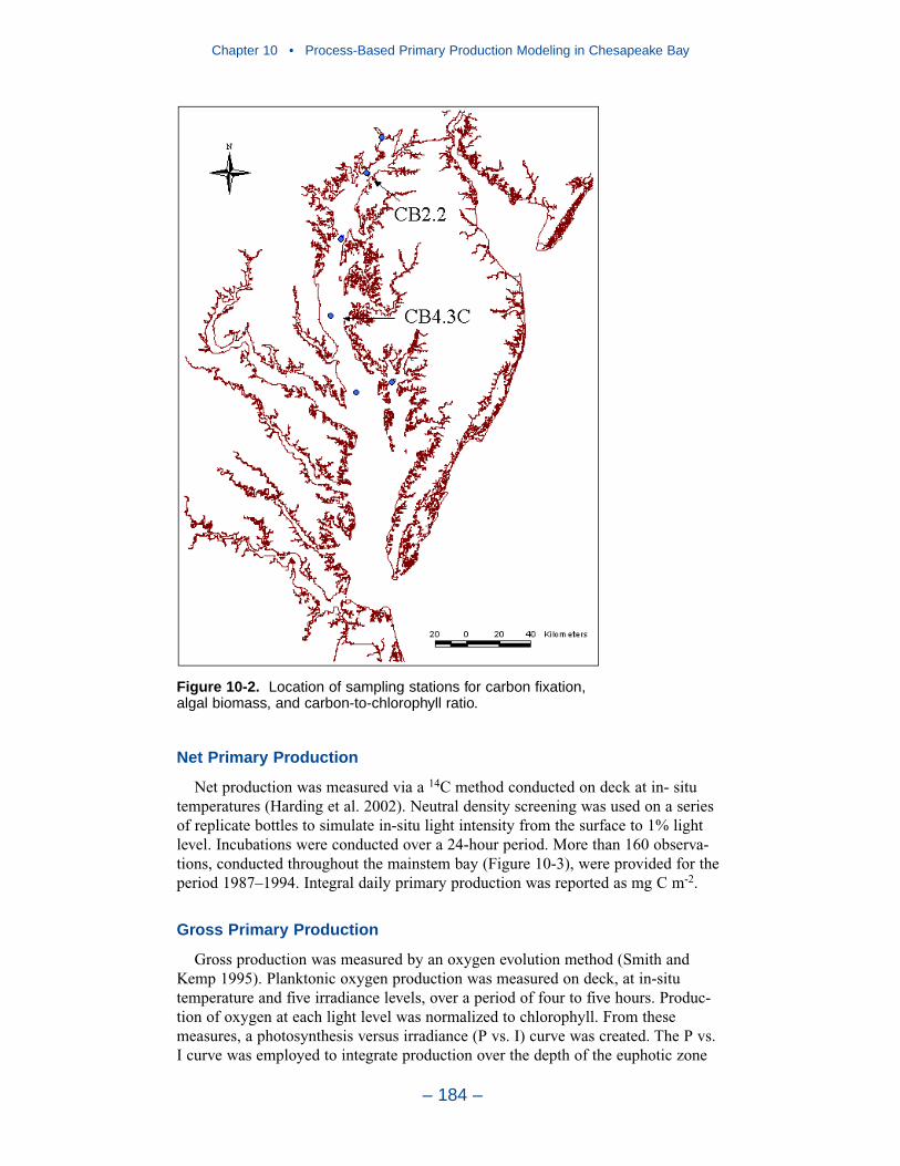
Net Primary Production
Net production was measured via a 14C method conducted on deck at in- situtemperatures (Harding et al. 2002). Neutral density screening was used on a seriesof replicate bottles to simulate in-situ light intensity from the surface to 1% lightlevel. Incubations were conducted over a 24-hour period. More than 160 observa-tions, conducted throughout the mainstem bay (Figure 10-3), were provided for theperiod 1987–1994. Integral daily primary production was reported as mg C m-2.
Gross Primary Production
Gross production was measured by an oxygen evolution method (Smith andKemp 1995). Planktonic oxygen production was measured on deck, at in-situtemperature and five irradiance levels, over a period of four to five hours. Produc-tion of oxygen at each light level was normalized to chlorophyll. From thesemeasures, a photosynthesis versus irradiance (P vs. I) curve was created. The P vs.I curve was employed to integrate production over the depth of the euphotic zone
Chapter 10 • Process-Based Primary Production Modeling in Chesapeake Bay
– 184 –
Figure 10-2. Location of sampling stations for carbon fixation, algal biomass, and carbon-to-chlorophyll ratio.

based on vertical attenuation of light and chlorophyll distribution. Daytime netproduction was estimated as the product of depth-integrated production (g O2 m-2
h-1) and number of daylight hours when incident light exceeded 100 µE m-2 s-1.
Respiration rates were measured as decreases in oxygen concentration in bottlesincubated for four to five hours in the dark at in-situ temperatures. Volumetric rateswere multiplied by depth to obtain vertically integrated respiration rates. Thesummed absolute values of net daytime production and daytime respiration resultedin estimates of daily gross production.
Roughly 60 measures, collected in the interval 1989–1992, were collected atthree stations (Figure 10-3). Daily gross production was reported as g O2 m-2. Forconsistency with other measures and with model units, gross production wasconverted to carbon equivalents using the relationship:
mCg=
CmolCg12
Omol1.4Cmol
Og32Omol
mOg
222
22
2
(10-1)
Chapter 10 • Process-Based Primary Production Modeling in Chesapeake Bay
– 185 –
Figure 10-3. Location of gross and net primary production stations.
The photosynthetic quotient was based on empirical comparisons of productionmeasured by 14C methods and by oxygen evolution (Harding et al. 2002).
Measures of light-saturated assimilation ratio, reported as µg O2 µg-1 Chl h-1,were produced in the course of the production measures. For consistency with othermeasures and with model units, the assimilation ratio was converted to carbonequivalents using the relationship:
Algal Biomass
Phytoplankton species counts and chlorophyll analyses were conducted atmonthly intervals on composite samples collected at six locations in the upper bay(Figure 10-2). Depending on the depth of the water column, the composites repre-sented “above pycnocline,” “below pycnocline,” or “water column.” Observationswere provided by the principal investigator (Richard Lacouture, Smithsonian Envi-ronmental Research Center). Prior to the data transfers, algal counts were convertedto carbon using published values of biomass per individual. Division of carbona-ceous biomass by chlorophyll concentration provided estimates of phytoplanktoncarbon-to-chlorophyll ratio.
Chlorophyll, Nutrients, and Associated Observations
The Chesapeake Bay Program conducted 12 to 18 sample cruises per year at 50stations throughout the mainstem bay. Chlorophyll, nutrient concentrations, andother observations for calibrating the model were obtained from an on-line database, http://www.chesapeakebay.net/data/index.htm. Methods and metadata areavailable at the same site.
Model Formulation
The eutrophication portion of the CBEMP considers three algal groups and twozooplankton groups. These groups interact with simulated cycles of carbon,nitrogen, phosphorus, and silica. Mass-balance equations for 24 state variables aresolved on a three-dimensional computational grid of over 12,000 cells. Detailsprovided here focus on recent developments required to simulate primary produc-tion. Additional descriptions of model formulation and applications may be foundelsewhere (Cerco and Cole 1993, Cerco and Meyers 2000).
Conservation of Mass Equation
The foundation of CE-QUAL-ICM is the solution to the three- dimensionalmass-conservation equation for a control volume. Control volumes correspond tocells on the model grid. CE-QUAL-ICM solves, for each volume and for each statevariable, the equation:
Sx
DACQ= t
CVj
k
kk
n
1=kkk
n
1=k
jj +C+ (10-3)
dChlgCg=
dh24
CmolCg12
Omol1.4Cmol
Og32Omol
hChlgµOgµ
22
22 (10-2)
Chapter 10 • Process-Based Primary Production Modeling in Chesapeake Bay
– 186 –
δ C
δ Xk
in which:Vj = volume of jth control volume (m3)Cj = concentration in jth control volume (g m-3)t, x = temporal and spatial coordinatesn = number of flow faces attached to jth control volumeQk = volumetric flow across flow face k of jth control volume (m3 s-1)Ck = concentration in flow across face k (g m-3)Ak = area of flow face k (m2)Dk = diffusion coefficient at flow face k (m2 s-1)Sj = external loads and kinetic sources and sinks in jth control volume (g s-1)
Solution to the mass-conservation equation is via the finite-difference method.For notational simplicity, the transport terms are dropped in the succeedingreporting of kinetics formulations.
Phytoplankton Kinetics
The model simulates three algal groups. The blue-green algal group representsthe Microcystis that are found only in the tidal freshwater portion of the PotomacRiver, one of the western tributaries. The spring algal group comprises the diatomsthat dominate saline waters from January to May. The summer algal group repre-sents the assemblage of flagellates, diatoms and other phytoplankton that dominatethe system from May to December. Each algal group is represented by identicalformulations. Differences between groups are determined by parameterspecifications.
Algal sources and sinks in the conservation equation include production, respira-tion, predation, and settling. These are expressed:
in which:B = algal biomass, expressed as carbon (g C m-3)G = growth (d-1)R = respiration (d-1)Wa = algal settling velocity (m d-1)PR = predation (g C m-3 d-1)
Production
Production by phytoplankton is determined by the intensity of light, by the avail-ability of nutrients, and by the ambient temperature.
Light
The influence of light on phytoplankton production is represented by achlorophyll-specific production equation (Jassby and Platt 1976):
Ik+I
ImP=P22
BB(10-5)
PR-Bz
Wa-R-G=B t
(10-4)
Chapter 10 • Process-Based Primary Production Modeling in Chesapeake Bay
– 187 –

in which:PB = production (g C g-1 Chl d-1)PBm = maximum photosynthetic rate (g C g-1 Chl d-1)I = irradiance (E m-2 d-1)
Parameter Ik is defined as the irradiance at which the initial slope of the produc-tion vs. irradiance relationship (Figure 10-4) intersects the value of PBm:
in which:α = initial slope of production vs. irradiance relationship (g C g-1 Chl (E m-2)-1)
Chlorophyll-specific production rate is readily converted to carbon-specificgrowth rate, for use in Equation 10-4, through division by the carbon-to-chlorophyll ratio:
in which:CChl = carbon-to-chlorophyll ratio (g C g-1 chlorophyll a)
CChlP=G
B
(10-7)
mP=IkB
(10-6)
Chapter 10 • Process-Based Primary Production Modeling in Chesapeake Bay
– 188 –
Figure 10-4. Production versus irradiance relationship showing regions of lightlimitation, nutrient limitation, and mixed limitations.
Nutrients
Carbon, nitrogen, and phosphorus are the primary nutrients required for algalgrowth. Diatoms require silica, as well. Inorganic carbon is usually available inexcess and is not considered in the model. The effects of the remaining nutrients ongrowth are described by the formulation commonly referred to as “Monod kinetics”(Monod 1949):
in which:f(N) = nutrient limitation on algal production (0 < f(N) < 1)D = concentration of dissolved nutrient (g m-3)KHd = half-saturation constant for nutrient uptake (g m-3)
Temperature
Algal production increases as a function of temperature until an optimumtemperature or temperature range is reached. Above the optimum, productiondeclines until a temperature lethal to the organisms is attained. Numerous func-tional representations of temperature effects are available. Inspection of growthversus temperature curves indicates a function similar to a Gaussian probabilitycurve provides a good fit to observations:
in which:T = temperature (oC)Topt = optimal temperature for algal growth (oC)KTg1 = effect of temperature below Topt on growth (oC-2)KTg2 = effect of temperature above Topt on growth (oC-2)
Constructing the Photosynthesis vs. Irradiance Curve
A production versus irradiance relationship is constructed for each model cell ateach time step. First, maximum photosynthetic rate under ambient temperature andnutrient concentrations is determined:
in which:PBm(N,T) = Maximum photosynthetic rate at ambient temperature and nutrient
concentrations (g C g-1 Chl d-1)
The single most limiting nutrient is employed in determining the nutrientlimitation.
D+KHdDf(T)mP=T)m(N,P BB (10-10)
Topt>T when e=
ToptT when e=f(T)
)T-(ToptKTg2-
)Topt-(TKTg1-
2
2
(10-9)
D+KHdD=f(N) (10-8)
Chapter 10 • Process-Based Primary Production Modeling in Chesapeake Bay
– 189 –
Next, parameter Ik is derived from Equation 10-6. Finally, the production vs.irradiance relationship is constructed using PBm(N,T) and Ik. The resulting produc-tion versus irradiance curve exhibits three regions (Figure 10-4). For I >> Ik, thevalue of the term I / (I2 + Ik2)½ approaches unity and temperature and nutrients arethe primary factors that influence production. For I << Ik, production is determinedsolely by and irradiance I. In the region where the initial slope of the productionversus irradiance curve intercepts the line indicating production at optimal illumi-nation, I Ik, production is determined by the combined effects of temperature,nutrients, and light.
Respiration
Two forms of respiration are considered in the model: photo-respiration andbasal metabolism. Photo-respiration represents the release or leakage of carbonfixed during the photosynthetic process (Goldsworthy 1970) and is represented as afixed fraction of production. Basal metabolism is the continuous energy expendi-ture to maintain basic life processes. In the model, metabolism is considered to be an exponentially increasing function of temperature. Total respiration isrepresented:
in which:Presp = photo-respiration (0 < Presp < 1)BMr = metabolic rate at reference temperature Tr (d-1)KTb = effect of temperature on metabolism (oC-1)Tr = reference temperature for metabolism (oC)
Predation
The predation term includes the activity of zooplankton, filter-feeding benthos,and other pelagic filter feeders including planktivorous fish. Formulation andresults of the zooplankton and benthos computations may be found in Cerco andMeyers (2000). Predation by other planktivores is modeled by assuming predatorsclear a specific volume of water per unit biomass:
in which:F = filtration rate (m3 g-1 predator C day-1)M = planktivore biomass (g C m-3)
Detailed specification of the spatial and temporal distribution of the predatorpopulation is impossible. One approach is to assume predator biomass is propor-tional to algal biomass, M = γB, in which case Equation 10-12 can be rewritten:
BF=PR 2(10-13)
MBF=PR (10-12)
eBMr+GPresp=R Tr)-(TKTb(10-11)
Chapter 10 • Process-Based Primary Production Modeling in Chesapeake Bay
– 190 –
Chapter 10 • Process-Based Primary Production Modeling in Chesapeake Bay
– 191 –
Since neither γ nor F are known precisely, the logical approach is to combinetheir product into a single unknown determined during the model calibration proce-dure. Effect of temperature on predation is represented with the same formulationas the effect of temperature on respiration. The final representation of predation,including zooplankton, is:
in which:RMsz = microzooplankton maximum ration (g algal C g-1 zoo C d-1)SZ = microzooplankton biomass (g C m-3)KHsz = half saturation concentration for carbon uptake by microzooplankton
(g C m-3)RMlz = mesozooplankton maximum ration (g algal C g-1 zoo C d-1)LZ = mesozooplankton biomass (g C m-3)KHlz = half saturation concentration for carbon uptake by mesozooplankton
(g C m-3)Phtl = rate of predation by other planktivores (m3 g-1 C d-1)
Predation by filter-feeding benthos is represented as a loss term only in model cellsthat intersect the bottom.
The Model Nitrogen Cycle
Nitrogen is first divided into available and unavailable fractions. Available refersto employment in algal nutrition. Two available forms are considered: reduced andoxidized nitrogen. Reduced nitrogen includes ammonium and urea. Nitrate andnitrite comprise the oxidized nitrogen pool. Both reduced and oxidized nitrogen areutilized to fulfill algal nutrient requirements. The primary reason for distinguishingthe two is that ammonium is oxidized by nitrifying bacteria into nitrite and, subse-quently, nitrate. This oxidation can be a significant sink of oxygen in the watercolumn and sediments.
In the presence of multiple nitrogenous nutrients, ammonium and urea areutilized first (McCarthy et al. 1977). In the model, the preference for reducednitrogen is expressed by an empirical function (Thomann and Fitzpatrick 1982)with two limiting values (Figure 10-5). When oxidized nitrogen is absent, the pref-erence for reduced nitrogen is unity. When reduced nitrogen is absent, thepreference is zero. In the presence of reduced and oxidized nitrogen, the preferencedepends on the abundance of both forms relative to the half-saturation constant fornitrogen uptake. When both forms are abundant, the preference for reducednitrogen approaches unity. When reduced nitrogen is scarce but oxidized nitrogen isabundant, the preference decreases in magnitude and a significant fraction of algalnitrogen requirement comes from oxidized nitrogen.
BPhtl+LZRMlzB+KHlz
B+
SZRMszB+KHsz
B=PR
2
(10-14)

Irradiance
Irradiance at the water surface is evaluated at each model time step by fitting asin function to daily total irradiance. Irradiance declines exponentially with depthbelow the surface. The diffuse attenuation coefficient, Kd, is computed as a func-tion of color and concentrations of organic and mineral solids (Cerco and Meyers2000).
Primary Production Equations
Computed production, for comparison with the observations, was derived fromthe model by three relationships.
Carbon Fixation
Carbon fixation measures were conducted at ambient temperature and nutrientconcentrations and saturating light intensity. The appropriate relationship forcomparison with the observations is:
in which:Cfix = carbon fixed (g C m-3 d-1)
Algal biomass, nutrient limitation, temperature effects, and carbon-to-chlorophyllratio are all based on model computations at the sample location.
BBMr(T)-Presp-1f(T)f(N)CChl
mP=CfixB
(10-15)
Chapter 10 • Process-Based Primary Production Modeling in Chesapeake Bay
– 192 –
Figure 10-5. Nitrogen preference function.
Gross Primary Production
The relationship for depth-integrated daily gross primary production is:
in which:GPP = daily gross primary production (g C m-2)D = daylength (1 day)Z1% = depth at which irradiance is 1% of surface irradiance (m)I(t) = time-varying irradiance (E m-2 d-1)
Algal biomass, nutrient limitation, temperature effects, irradiance, and carbon-to-chlorophyll ratio are all based on model computations at the sample location and at1.5 m depth increments.
Net Primary Production
The relationship for depth-integrated daily net primary production is:
in which:NPP = daily net primary production (g C m-2)
Algal biomass, nutrient limitation, temperature effects, irradiance, and carbon-to-chlorophyll ratio are all based on model computations at the sample location and at1.5 m depth increments.
Parameter Evaluation
Parameters are reported here for the spring and summer algal groups whichinhabit the mainstem of Chesapeake Bay. Model parameters are based on publishedvalues reported in a variety of units. For comparison with the model, reportedparameters are converted to model units of meter, gram, and day.
Algal Production Parameters
Maximum photosynthetic rates and their temperature dependence were based onobservations collected by Harding et al. (1986) and by Smith and Kemp (1995).The observed rates were subject to in-situ nutrient limitations. Since the maximumphotosynthetic rates employed by the model are for nutrient-unlimited situations,parameter values (Table 10-1) were specified at the upper range of reported rates(Figure 10-6) based on the assumption that lower observations represented nutrient-limited conditions.
( )
dtdzB
BMr(T)-Presp-1f(T)f(N)
Ik+)I(t
I(t)
CChl
mP
=NPP
22
BZ
0
D
0
1%
•••
•
•••∫∫ (10-17)
dtdzBf(T)f(N)Ik+)I(t
I(t)CChl
mP=GPP22
BZ
0
D
0
1%
(10-16)
Chapter 10 • Process-Based Primary Production Modeling in Chesapeake Bay
– 193 –
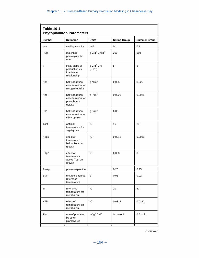
Chapter 10 • Process-Based Primary Production Modeling in Chesapeake Bay
– 194 –
Table 10-1 Phytoplankton Parameters
Symbol Definition Units Spring Group Summer Group
Wa settling velocity m d-1 0.1 0.1
PBm maximum photosyntheticrate
g C g-1 Chl d-1 300 350
initial slope of production vs. irradiancerelationship
g C g-1 Chl(E m-2)-1
8 8
Khn half-saturationconcentration for nitrogen uptake
g N m-3 0.025 0.025
Khp half-saturationconcentration for phosphorusuptake
g P m-3 0.0025 0.0025
Khs half-saturationconcentration for silica uptake
g S m-3 0.03
Topt optimaltemperature for algal growth
oC 16 25
KTg1 effect of temperaturebelow Topt on growth
oC-2 0.0018 0.0035
KTg2 effect of temperatureabove Topt on growth
oC-2 0.006 0
Presp photo-respiration 0.25 0.25
BMr metabolic rate at referencetemperature
d-1 0.01 0.02
Tr referencetemperature for metabolism
oC 20 20
KTb effect of temperature on metabolism
oC-1 0.0322 0.0322
Phtl rate of predation by other planktivores
m3 g-1 C d-1 0.1 to 0.2 0.5 to 2
continued
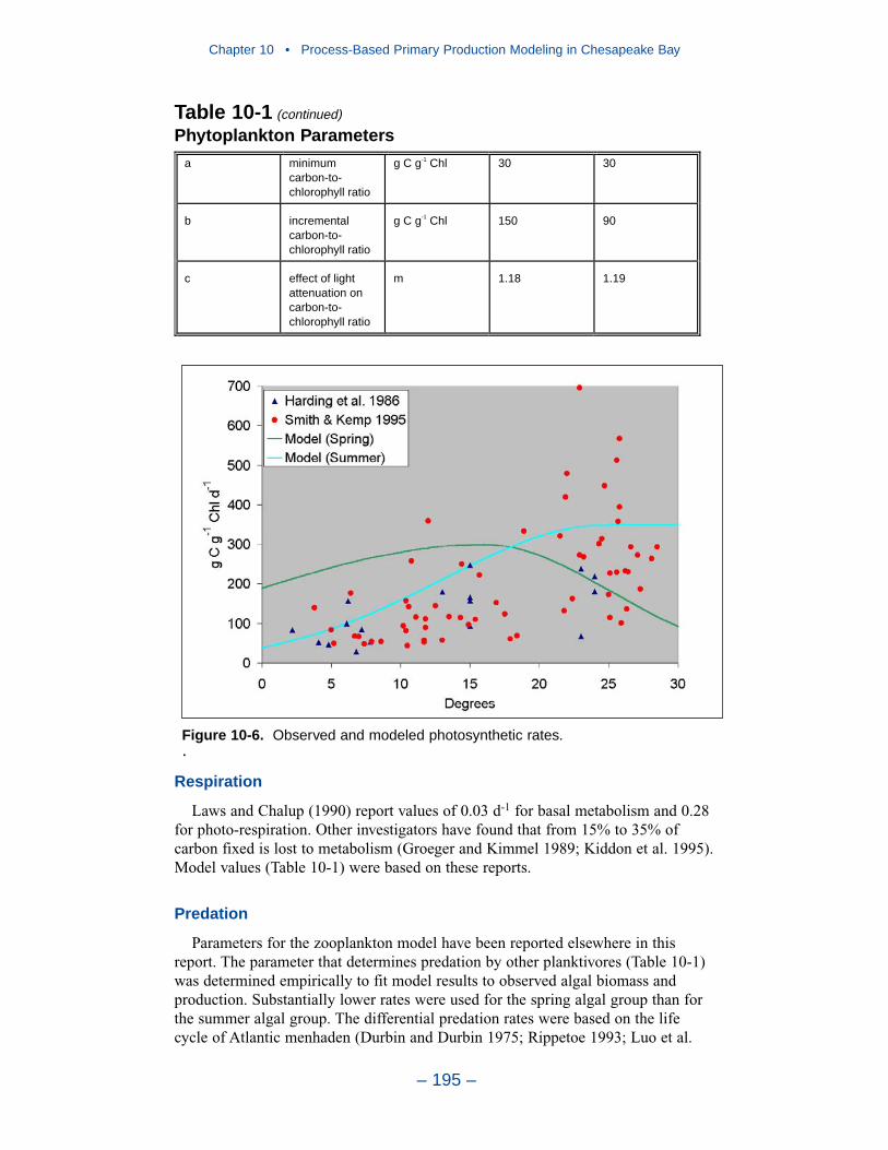
Respiration
Laws and Chalup (1990) report values of 0.03 d-1 for basal metabolism and 0.28for photo-respiration. Other investigators have found that from 15% to 35% ofcarbon fixed is lost to metabolism (Groeger and Kimmel 1989; Kiddon et al. 1995).Model values (Table 10-1) were based on these reports.
Predation
Parameters for the zooplankton model have been reported elsewhere in thisreport. The parameter that determines predation by other planktivores (Table 10-1)was determined empirically to fit model results to observed algal biomass andproduction. Substantially lower rates were used for the spring algal group than forthe summer algal group. The differential predation rates were based on the lifecycle of Atlantic menhaden (Durbin and Durbin 1975; Rippetoe 1993; Luo et al.
Chapter 10 • Process-Based Primary Production Modeling in Chesapeake Bay
– 195 –
a minimum carbon-to-chlorophyll ratio
g C g-1 Chl 30 30
b incrementalcarbon-to-chlorophyll ratio
g C g-1 Chl 150 90
c effect of light attenuation on carbon-to-chlorophyll ratio
m 1.18 1.19
Table 10-1 (continued)
Phytoplankton Parameters
Figure 10-6. Observed and modeled photosynthetic rates..
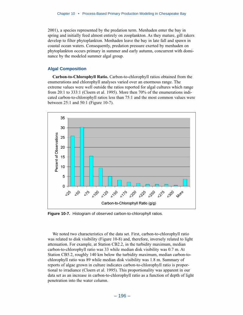
2001), a species represented by the predation term. Menhaden enter the bay inspring and initially feed almost entirely on zooplankton. As they mature, gill rakersdevelop to filter phytoplankton. Menhaden leave the bay in late fall and spawn incoastal ocean waters. Consequently, predation pressure exerted by menhaden onphytoplankton occurs primary in summer and early autumn, concurrent with domi-nance by the modeled summer algal group.
Algal Composition
Carbon-to-Chlorophyll Ratio. Carbon-to-chlorophyll ratios obtained from theenumerations and chlorophyll analyses varied over an enormous range. Theextreme values were well outside the ratios reported for algal cultures which rangefrom 20:1 to 333:1 (Cloern et al. 1995). More then 70% of the enumerations indi-cated carbon-to-chlorophyll ratios less than 75:1 and the most common values werebetween 25:1 and 50:1 (Figure 10-7).
We noted two characteristics of the data set. First, carbon-to-chlorophyll ratiowas related to disk visibility (Figure 10-8) and, therefore, inversely related to lightattenuation. For example, at Station CB2.2, in the turbidity maximum, mediancarbon-to-chlorophyll ratio was 33 while median disk visibility was 0.7 m. AtStation CB5.2, roughly 140 km below the turbidity maximum, median carbon-to-chlorophyll ratio was 89 while median disk visibility was 1.8 m. Summary ofreports of algae grown in culture indicates carbon-to-chlorophyll ratio is propor-tional to irradiance (Cloern et al. 1995). This proportionality was apparent in ourdata set as an increase in carbon-to-chlorophyll ratio as a function of depth of lightpenetration into the water column.
Chapter 10 • Process-Based Primary Production Modeling in Chesapeake Bay
– 196 –
Figure 10-7. Histogram of observed carbon-to-chlorophyll ratios.
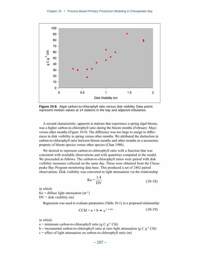
Chapter 10 • Process-Based Primary Production Modeling in Chesapeake Bay
– 197 –
A second characteristic, apparent at stations that experience a spring algal bloom,was a higher carbon-to-chlorophyll ratio during the bloom months (February–May)versus other months (Figure 10-9). The difference was too large to assign to differ-ences in disk visibility in spring versus other months. We attributed the distinction incarbon-to-chlorophyll ratio between bloom months and other months as a taxonomicproperty of bloom species versus other species (Chan 1980).
We desired to represent carbon-to-chlorophyll ratio with a function that wasconsistent with available observations and with quantities computed in the model.We proceeded as follows. The carbon-to-chlorophyll ratios were paired with diskvisibility measures collected on the same day. These were obtained from the Chesa-peake Bay Program monitoring data base. This produced a set of 2462 pairedobservations. Disk visibility was converted to light attenuation via the relationship:
in which:Ke = diffuse light attenuation (m-1)DV = disk visibility (m)
Regression was used to evaluate parameters (Table 10-1) in a proposed relationship:
in which:a = minimum carbon-to-chlorophyll ratio (g C g-1 Chl)b = incremental carbon-to-chlorophyll ratio at zero light attenuation (g C g-1 Chl)c = effect of light attenuation on carbon-to-chlorophyll ratio (m)
eb+a=CChl Kec- (10-19)
DV1.4=Ke (10-18)
Figure 10-8. Algal carbon-to-chlorophyll ratio versus disk visibility. Data pointsrepresent median values at 14 stations in the bay and adjacent tributaries.
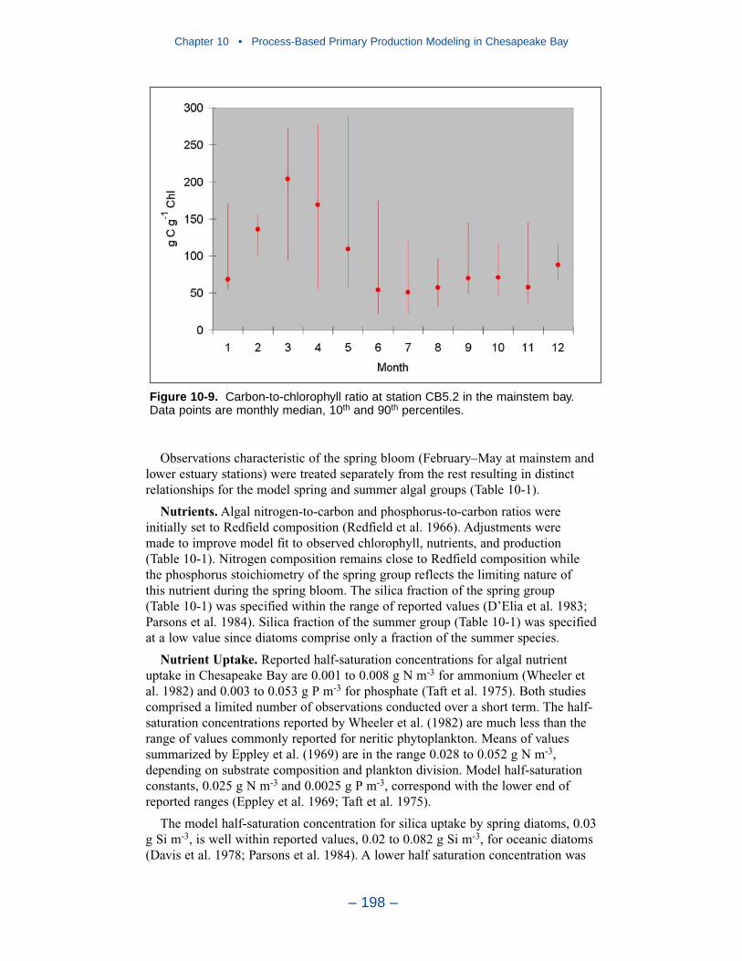
Observations characteristic of the spring bloom (February–May at mainstem andlower estuary stations) were treated separately from the rest resulting in distinctrelationships for the model spring and summer algal groups (Table 10-1).
Nutrients. Algal nitrogen-to-carbon and phosphorus-to-carbon ratios wereinitially set to Redfield composition (Redfield et al. 1966). Adjustments were made to improve model fit to observed chlorophyll, nutrients, and production(Table 10-1). Nitrogen composition remains close to Redfield composition whilethe phosphorus stoichiometry of the spring group reflects the limiting nature of this nutrient during the spring bloom. The silica fraction of the spring group (Table 10-1) was specified within the range of reported values (D’Elia et al. 1983;Parsons et al. 1984). Silica fraction of the summer group (Table 10-1) was specifiedat a low value since diatoms comprise only a fraction of the summer species.
Nutrient Uptake. Reported half-saturation concentrations for algal nutrientuptake in Chesapeake Bay are 0.001 to 0.008 g N m-3 for ammonium (Wheeler etal. 1982) and 0.003 to 0.053 g P m-3 for phosphate (Taft et al. 1975). Both studiescomprised a limited number of observations conducted over a short term. The half-saturation concentrations reported by Wheeler et al. (1982) are much less than therange of values commonly reported for neritic phytoplankton. Means of valuessummarized by Eppley et al. (1969) are in the range 0.028 to 0.052 g N m-3,depending on substrate composition and plankton division. Model half-saturationconstants, 0.025 g N m-3 and 0.0025 g P m-3, correspond with the lower end ofreported ranges (Eppley et al. 1969; Taft et al. 1975).
The model half-saturation concentration for silica uptake by spring diatoms, 0.03g Si m-3, is well within reported values, 0.02 to 0.082 g Si m-3, for oceanic diatoms(Davis et al. 1978; Parsons et al. 1984). A lower half saturation concentration was
Chapter 10 • Process-Based Primary Production Modeling in Chesapeake Bay
– 198 –
Figure 10-9. Carbon-to-chlorophyll ratio at station CB5.2 in the mainstem bay.Data points are monthly median, 10th and 90th percentiles.
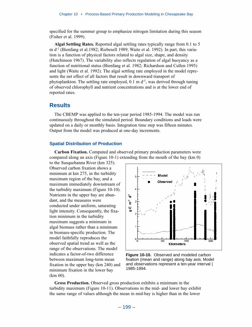
Chapter 10 • Process-Based Primary Production Modeling in Chesapeake Bay
– 199 –
specified for the summer group to emphasize nitrogen limitation during this season(Fisher et al. 1999).
Algal Settling Rates. Reported algal settling rates typically range from 0.1 to 5m d-1 (Bienfang et al.1982; Riebesell 1989; Waite et al. 1992). In part, this varia-tion is a function of physical factors related to algal size, shape, and density(Hutchinson 1967). The variability also reflects regulation of algal buoyancy as afunction of nutritional status (Bienfang et al. 1982; Richardson and Cullen 1995)and light (Waite et al. 1992). The algal settling rate employed in the model repre-sents the net effect of all factors that result in downward transport ofphytoplankton. The settling rate employed, 0.1 m d-1, was derived through tuningof observed chlorophyll and nutrient concentrations and is at the lower end ofreported rates.
Results
The CBEMP was applied to the ten-year period 1985-1994. The model was runcontinuously throughout the simulated period. Boundary conditions and loads wereupdated on a daily or monthly basis. Integration time step was fifteen minutes.Output from the model was produced at one-day increments.
Spatial Distribution of Production
Carbon Fixation. Computed and observed primary production parameters werecompared along an axis (Figure 10-1) extending from the mouth of the bay (km 0)to the Susquehanna River (km 325).Observed carbon fixation shows aminimum at km 275, in the turbiditymaximum region of the bay, and amaximum immediately downstream ofthe turbidity maximum (Figure 10-10).Nutrients in the upper bay are abun-dant, and the measures wereconducted under uniform, saturatinglight intensity. Consequently, the fixa-tion minimum in the turbiditymaximum suggests a minimum inalgal biomass rather than a minimumin biomass-specific production. Themodel faithfully reproduces theobserved spatial trend as well as therange of the observations. The modelindicates a factor-of-two differencebetween maximum long-term meanfixation in the upper bay (km 240) andminimum fixation in the lower bay(km 60).
Gross Production. Observed gross production exhibits a minimum in theturbidity maximum (Figure 10-11). Observations in the mid- and lower bay exhibitthe same range of values although the mean in mid-bay is higher than in the lower
Figure 10-10. Observed and modeled carbonfixation (mean and range) along bay axis. Model and observations represent a ten-year interval |1985-1994.

bay. The model reproduces theobserved spatial trend although themodel mean and range exceedobserved in the turbidity maximumstation. A factor-of- two separates thelong-term mean maximum productionat km 230 from production upstreamin the turbidity maximum.
Net Production. At first glance, theobserved net production exhibits apeculiar spatial distribution (Figure10-12). The apparent spatial distribu-tion is affected by non-uniformtemporal distribution of the sampling.At some transects, samples representup to 9 months of the calendar yearwhile at other locations, samplesrepresent as few two months. Modeledmean and range provide good agree-ment with the frequently-sampledtransects. The spatial distribution ofcomputed long-term mean net produc-tion matches the pattern of grossproduction. The maximum occursaround km 230 and is double produc-tion further upstream in the turbiditymaximum.
Temporal Distribution of Production
The temporal distribution of produc-tion parameters was examined at threelocations—one in the upper bay, one inthe mid-bay, and one in the lower bay.For carbon fixation, computations weredrawn from single model cells corre-sponding to the locations of stationsCB2.2 (upper bay) and CB4.3C (mid-bay). For gross production,computations were drawn from singlemodel cells corresponding to the loca-tions of stations NB (upper bay), MB(mid-bay), and SB (lower bay). For net production, daily spatial averages overregions CB2 (upper bay), CB4 (mid-bay), and CB7 (lower bay) were compared toall observations within these regions.
Carbon Fixation. Inspection of the observed and computed carbon fixation(Figures 10-13, 10-14) indicates a distinct seasonal pattern in which minimumfixation, near zero, takes place in winter and maximum fixation takes place in
Chapter 10 • Process-Based Primary Production Modeling in Chesapeake Bay
– 200 –
Figure 10-11. Observed and modeled gross primary production (mean and range) along bay axis.Observations from 1989-1992 are compared tomodel results from 1985-1994.
Figure 10-12. Observed and modeled net primaryproduction (mean and range) along bay axis.Observations from 1987-1992 are compared tomodel results from 1985-1994.
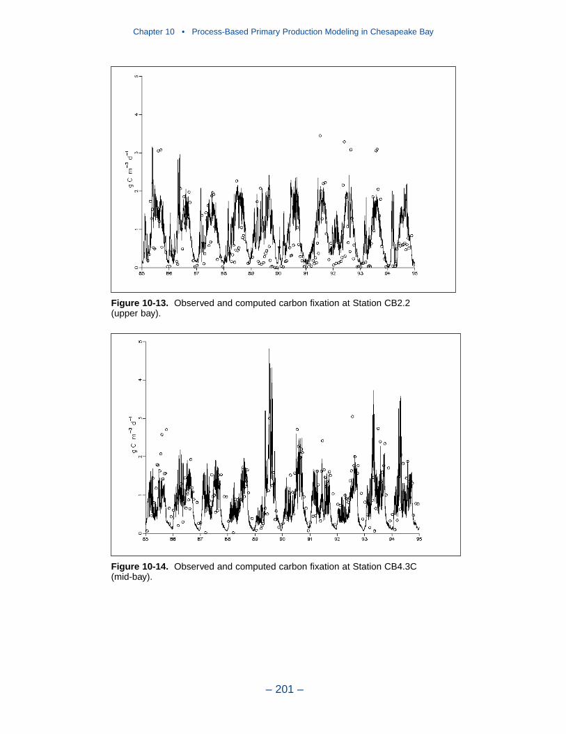
Chapter 10 • Process-Based Primary Production Modeling in Chesapeake Bay
– 201 –
Figure 10-13. Observed and computed carbon fixation at Station CB2.2 (upper bay).
Figure 10-14. Observed and computed carbon fixation at Station CB4.3C (mid-bay).
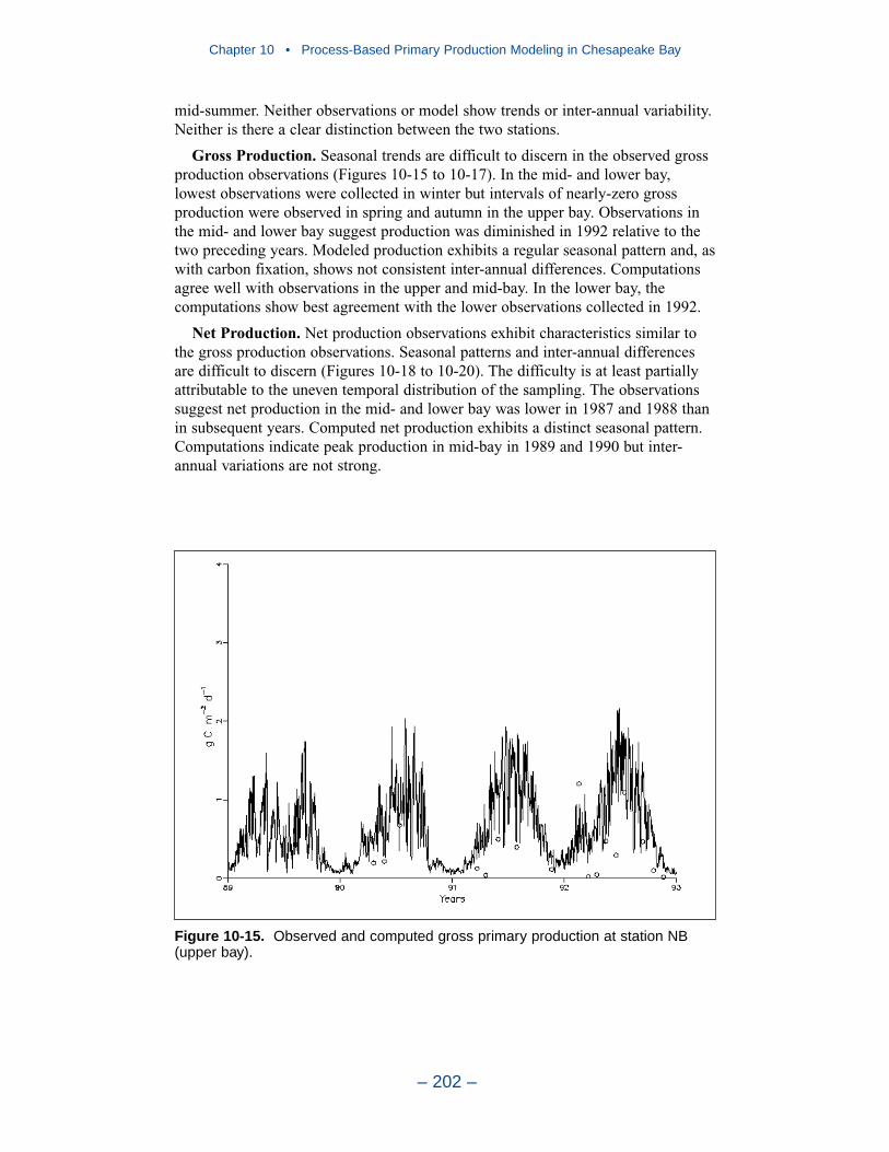
mid-summer. Neither observations or model show trends or inter-annual variability.Neither is there a clear distinction between the two stations.
Gross Production. Seasonal trends are difficult to discern in the observed grossproduction observations (Figures 10-15 to 10-17). In the mid- and lower bay,lowest observations were collected in winter but intervals of nearly-zero grossproduction were observed in spring and autumn in the upper bay. Observations inthe mid- and lower bay suggest production was diminished in 1992 relative to thetwo preceding years. Modeled production exhibits a regular seasonal pattern and, aswith carbon fixation, shows not consistent inter-annual differences. Computationsagree well with observations in the upper and mid-bay. In the lower bay, thecomputations show best agreement with the lower observations collected in 1992.
Net Production. Net production observations exhibit characteristics similar tothe gross production observations. Seasonal patterns and inter-annual differencesare difficult to discern (Figures 10-18 to 10-20). The difficulty is at least partiallyattributable to the uneven temporal distribution of the sampling. The observationssuggest net production in the mid- and lower bay was lower in 1987 and 1988 thanin subsequent years. Computed net production exhibits a distinct seasonal pattern.Computations indicate peak production in mid-bay in 1989 and 1990 but inter-annual variations are not strong.
Chapter 10 • Process-Based Primary Production Modeling in Chesapeake Bay
– 202 –
Figure 10-15. Observed and computed gross primary production at station NB(upper bay).
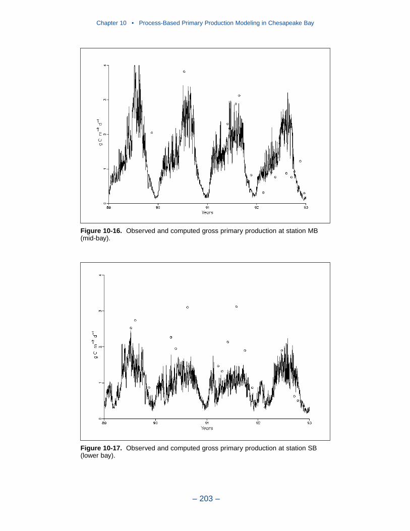
Chapter 10 • Process-Based Primary Production Modeling in Chesapeake Bay
– 203 –
Figure 10-16. Observed and computed gross primary production at station MB(mid-bay).
Figure 10-17. Observed and computed gross primary production at station SB(lower bay).
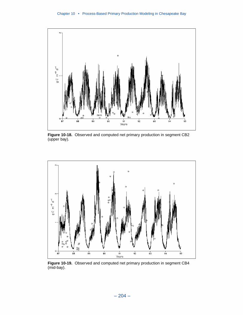
Chapter 10 • Process-Based Primary Production Modeling in Chesapeake Bay
– 204 –
Figure 10-18. Observed and computed net primary production in segment CB2(upper bay).
Figure 10-19. Observed and computed net primary production in segment CB4(mid-bay).
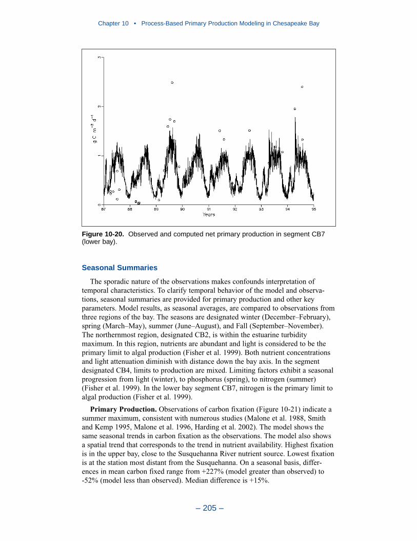
Seasonal Summaries
The sporadic nature of the observations makes confounds interpretation oftemporal characteristics. To clarify temporal behavior of the model and observa-tions, seasonal summaries are provided for primary production and other keyparameters. Model results, as seasonal averages, are compared to observations fromthree regions of the bay. The seasons are designated winter (December–February),spring (March–May), summer (June–August), and Fall (September–November).The northernmost region, designated CB2, is within the estuarine turbiditymaximum. In this region, nutrients are abundant and light is considered to be theprimary limit to algal production (Fisher et al. 1999). Both nutrient concentrationsand light attenuation diminish with distance down the bay axis. In the segmentdesignated CB4, limits to production are mixed. Limiting factors exhibit a seasonalprogression from light (winter), to phosphorus (spring), to nitrogen (summer)(Fisher et al. 1999). In the lower bay segment CB7, nitrogen is the primary limit toalgal production (Fisher et al. 1999).
Primary Production. Observations of carbon fixation (Figure 10-21) indicate asummer maximum, consistent with numerous studies (Malone et al. 1988, Smithand Kemp 1995, Malone et al. 1996, Harding et al. 2002). The model shows thesame seasonal trends in carbon fixation as the observations. The model also showsa spatial trend that corresponds to the trend in nutrient availability. Highest fixationis in the upper bay, close to the Susquehanna River nutrient source. Lowest fixationis at the station most distant from the Susquehanna. On a seasonal basis, differ-ences in mean carbon fixed range from +227% (model greater than observed) to-52% (model less than observed). Median difference is +15%.
Chapter 10 • Process-Based Primary Production Modeling in Chesapeake Bay
– 205 –
Figure 10-20. Observed and computed net primary production in segment CB7(lower bay).
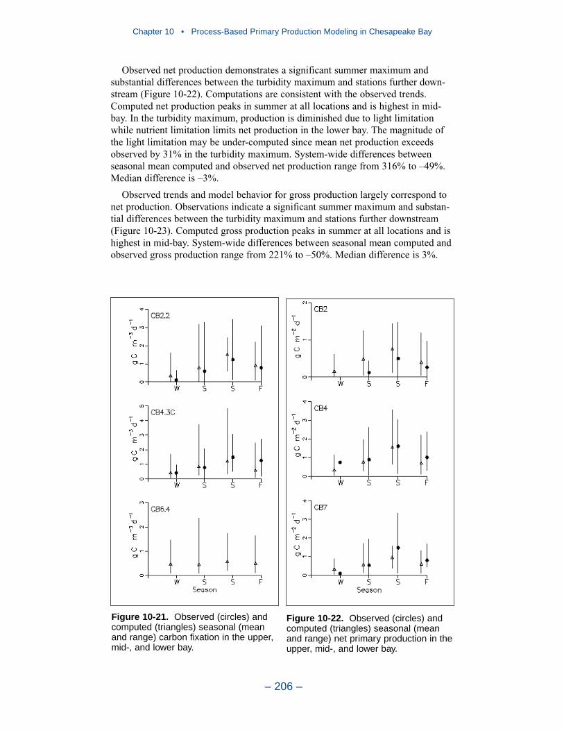
Observed net production demonstrates a significant summer maximum andsubstantial differences between the turbidity maximum and stations further down-stream (Figure 10-22). Computations are consistent with the observed trends.Computed net production peaks in summer at all locations and is highest in mid-bay. In the turbidity maximum, production is diminished due to light limitationwhile nutrient limitation limits net production in the lower bay. The magnitude ofthe light limitation may be under-computed since mean net production exceedsobserved by 31% in the turbidity maximum. System-wide differences betweenseasonal mean computed and observed net production range from 316% to –49%.Median difference is –3%.
Observed trends and model behavior for gross production largely correspond tonet production. Observations indicate a significant summer maximum and substan-tial differences between the turbidity maximum and stations further downstream(Figure 10-23). Computed gross production peaks in summer at all locations and ishighest in mid-bay. System-wide differences between seasonal mean computed andobserved gross production range from 221% to –50%. Median difference is 3%.
Chapter 10 • Process-Based Primary Production Modeling in Chesapeake Bay
– 206 –
Figure 10-21. Observed (circles) andcomputed (triangles) seasonal (meanand range) carbon fixation in the upper,mid-, and lower bay.
Figure 10-22. Observed (circles) andcomputed (triangles) seasonal (meanand range) net primary production in theupper, mid-, and lower bay.
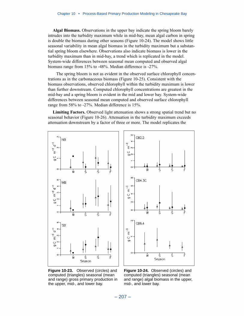
Algal Biomass. Observations in the upper bay indicate the spring bloom barelyintrudes into the turbidity maximum while in mid-bay, mean algal carbon in springis double the biomass during other seasons (Figure 10-24). The model shows littleseasonal variability in mean algal biomass in the turbidity maximum but a substan-tial spring bloom elsewhere. Observations also indicate biomass is lower in theturbidity maximum than in mid-bay, a trend which is replicated in the model.System-wide differences between seasonal mean computed and observed algalbiomass range from 15% to -48%. Median difference is -27%.
The spring bloom is not as evident in the observed surface chlorophyll concen-trations as in the carbonaceous biomass (Figure 10-25). Consistent with thebiomass observations, observed chlorophyll within the turbidity maximum is lowerthan further downstream. Computed chlorophyll concentrations are greatest in themid-bay and a spring bloom is evident in the mid and lower bay. System-widedifferences between seasonal mean computed and observed surface chlorophyllrange from 58% to -27%. Median difference is 15%.
Limiting Factors. Observed light attenuation shows a strong spatial trend but noseasonal behavior (Figure 10-26). Attenuation in the turbidity maximum exceedsattenuation downstream by a factor of three or more. The model replicates the
Chapter 10 • Process-Based Primary Production Modeling in Chesapeake Bay
– 207 –
Figure 10-23. Observed (circles) andcomputed (triangles) seasonal (meanand range) gross primary production inthe upper, mid-, and lower bay.
Figure 10-24. Observed (circles) andcomputed (triangles) seasonal (meanand range) algal biomass in the upper,mid-, and lower bay.
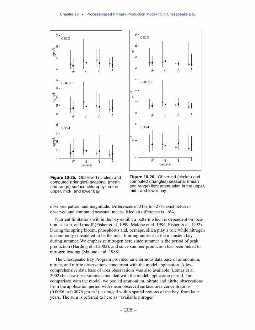
observed pattern and magnitude. Differences of 31% to –27% exist betweenobserved and computed seasonal means. Median difference is –6%.
Nutrient limitations within the bay exhibit a pattern which is dependent on loca-tion, season, and runoff (Fisher et al. 1999, Malone et al. 1996, Fisher et al. 1992).During the spring bloom, phosphorus and, perhaps, silica play a role while nitrogenis commonly considered to be the most limiting nutrient in the mainstem bayduring summer. We emphasize nitrogen here since summer is the period of peakproduction (Harding et al 2002), and since summer production has been linked tonitrogen loading (Malone et al. 1988).
The Chesapeake Bay Program provided an enormous data base of ammonium,nitrate, and nitrite observations concurrent with the model application. A lesscomprehensive data base of urea observations was also available (Lomas et al.2002) but few observations coincided with the model application period. Forcomparison with the model, we pooled ammonium, nitrate and nitrite observationsfrom the application period with mean observed surface urea concentrations(0.0056 to 0.0076 gm m-3), averaged within spatial regions of the bay, from lateryears. The sum is referred to here as “available nitrogen.”
Chapter 10 • Process-Based Primary Production Modeling in Chesapeake Bay
– 208 –
Figure 10-25. Observed (circles) andcomputed (triangles) seasonal (meanand range) surface chlorophyll in theupper, mid-, and lower bay.
Figure 10-26. Observed (circles) andcomputed (triangles) seasonal (meanand range) light attenuation in the upper,mid-, and lower bay.
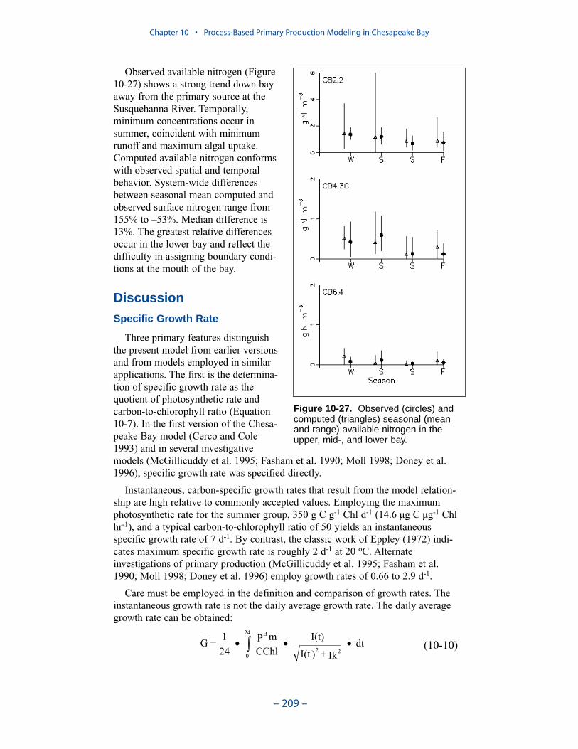
Observed available nitrogen (Figure10-27) shows a strong trend down bayaway from the primary source at theSusquehanna River. Temporally,minimum concentrations occur insummer, coincident with minimumrunoff and maximum algal uptake.Computed available nitrogen conformswith observed spatial and temporalbehavior. System-wide differencesbetween seasonal mean computed andobserved surface nitrogen range from155% to –53%. Median difference is13%. The greatest relative differencesoccur in the lower bay and reflect thedifficulty in assigning boundary condi-tions at the mouth of the bay.
Discussion
Specific Growth Rate
Three primary features distinguishthe present model from earlier versionsand from models employed in similarapplications. The first is the determina-tion of specific growth rate as thequotient of photosynthetic rate andcarbon-to-chlorophyll ratio (Equation10-7). In the first version of the Chesa-peake Bay model (Cerco and Cole1993) and in several investigativemodels (McGillicuddy et al. 1995; Fasham et al. 1990; Moll 1998; Doney et al.1996), specific growth rate was specified directly.
Instantaneous, carbon-specific growth rates that result from the model relation-ship are high relative to commonly accepted values. Employing the maximumphotosynthetic rate for the summer group, 350 g C g-1 Chl d-1 (14.6 µg C µg-1 Chlhr-1), and a typical carbon-to-chlorophyll ratio of 50 yields an instantaneousspecific growth rate of 7 d-1. By contrast, the classic work of Eppley (1972) indi-cates maximum specific growth rate is roughly 2 d-1 at 20 oC. Alternateinvestigations of primary production (McGillicuddy et al. 1995; Fasham et al.1990; Moll 1998; Doney et al. 1996) employ growth rates of 0.66 to 2.9 d-1.
Care must be employed in the definition and comparison of growth rates. Theinstantaneous growth rate is not the daily average growth rate. The daily averagegrowth rate can be obtained:
dtIk+)I(t
I(t)CChl
mP241=G
22
B24
0(10-10)
Chapter 10 • Process-Based Primary Production Modeling in Chesapeake Bay
– 209 –
Figure 10-27. Observed (circles) andcomputed (triangles) seasonal (meanand range) available nitrogen in theupper, mid-, and lower bay.
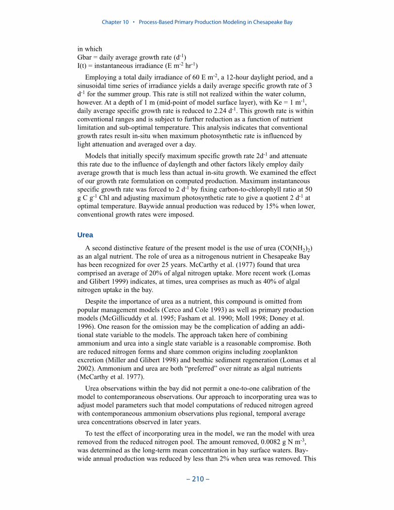
in whichGbar = daily average growth rate (d-1)I(t) = instantaneous irradiance (E m-2 hr-1)
Employing a total daily irradiance of 60 E m-2, a 12-hour daylight period, and asinusoidal time series of irradiance yields a daily average specific growth rate of 3d-1 for the summer group. This rate is still not realized within the water column,however. At a depth of 1 m (mid-point of model surface layer), with Ke = 1 m-1,daily average specific growth rate is reduced to 2.24 d-1. This growth rate is withinconventional ranges and is subject to further reduction as a function of nutrientlimitation and sub-optimal temperature. This analysis indicates that conventionalgrowth rates result in-situ when maximum photosynthetic rate is influenced bylight attenuation and averaged over a day.
Models that initially specify maximum specific growth rate 2d-1 and attenuatethis rate due to the influence of daylength and other factors likely employ dailyaverage growth that is much less than actual in-situ growth. We examined the effectof our growth rate formulation on computed production. Maximum instantaneousspecific growth rate was forced to 2 d-1 by fixing carbon-to-chlorophyll ratio at 50g C g-1 Chl and adjusting maximum photosynthetic rate to give a quotient 2 d-1 atoptimal temperature. Baywide annual production was reduced by 15% when lower,conventional growth rates were imposed.
Urea
A second distinctive feature of the present model is the use of urea (CO(NH2)2)as an algal nutrient. The role of urea as a nitrogenous nutrient in Chesapeake Bayhas been recognized for over 25 years. McCarthy et al. (1977) found that ureacomprised an average of 20% of algal nitrogen uptake. More recent work (Lomasand Glibert 1999) indicates, at times, urea comprises as much as 40% of algalnitrogen uptake in the bay.
Despite the importance of urea as a nutrient, this compound is omitted frompopular management models (Cerco and Cole 1993) as well as primary productionmodels (McGillicuddy et al. 1995; Fasham et al. 1990; Moll 1998; Doney et al.1996). One reason for the omission may be the complication of adding an addi-tional state variable to the models. The approach taken here of combiningammonium and urea into a single state variable is a reasonable compromise. Bothare reduced nitrogen forms and share common origins including zooplanktonexcretion (Miller and Glibert 1998) and benthic sediment regeneration (Lomas et al2002). Ammonium and urea are both “preferred” over nitrate as algal nutrients(McCarthy et al. 1977).
Urea observations within the bay did not permit a one-to-one calibration of themodel to contemporaneous observations. Our approach to incorporating urea was toadjust model parameters such that model computations of reduced nitrogen agreedwith contemporaneous ammonium observations plus regional, temporal averageurea concentrations observed in later years.
To test the effect of incorporating urea in the model, we ran the model with urearemoved from the reduced nitrogen pool. The amount removed, 0.0082 g N m-3,was determined as the long-term mean concentration in bay surface waters. Bay-wide annual production was reduced by less than 2% when urea was removed. This
Chapter 10 • Process-Based Primary Production Modeling in Chesapeake Bay
– 210 –
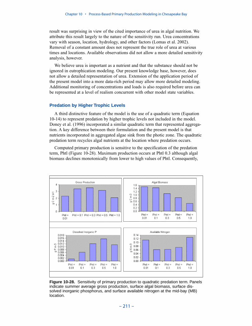
result was surprising in view of the cited importance of urea in algal nutrition. Weattribute this result largely to the nature of the sensitivity run. Urea concentrationsvary with season, location, hydrology, and other factors (Lomas et al. 2002).Removal of a constant amount does not represent the true role of urea at varioustimes and locations. Available observations did not allow a more detailed sensitivityanalysis, however.
We believe urea is important as a nutrient and that the substance should not beignored in eutrophication modeling. Our present knowledge base, however, doesnot allow a detailed representation of urea. Extension of the application period ofthe present model into a more data-rich period may allow more detailed modeling.Additional monitoring of concentrations and loads is also required before urea canbe represented at a level of realism concurrent with other model state variables.
Predation by Higher Trophic Levels
A third distinctive feature of the model is the use of a quadratic term (Equation10-14) to represent predation by higher trophic levels not included in the model.Doney et al. (1996) incorporated a similar quadratic term that represented aggrega-tion. A key difference between their formulation and the present model is thatnutrients incorporated in aggregated algae sink from the photic zone. The quadraticpredation term recycles algal nutrients at the location where predation occurs.
Computed primary production is sensitive to the specification of the predationterm, Phtl (Figure 10-28). Maximum production occurs at Phtl 0.3 although algalbiomass declines monotonically from lower to high values of Phtl. Consequently,
Chapter 10 • Process-Based Primary Production Modeling in Chesapeake Bay
– 211 –
Figure 10-28. Sensitivity of primary production to quadratic predation term. Panelsindicate summer average gross production, surface algal biomass, surface dis-solved inorganic phosphorus, and surface available nitrogen at the mid-bay (MB)location.
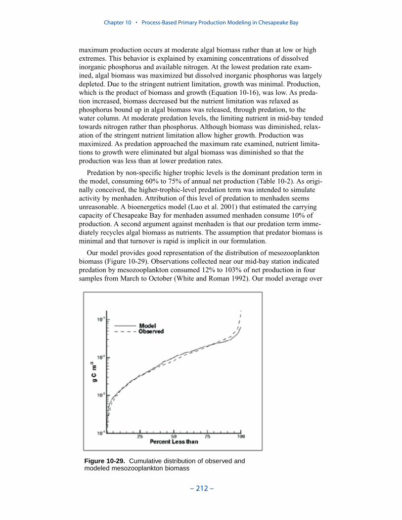
maximum production occurs at moderate algal biomass rather than at low or highextremes. This behavior is explained by examining concentrations of dissolvedinorganic phosphorus and available nitrogen. At the lowest predation rate exam-ined, algal biomass was maximized but dissolved inorganic phosphorus was largelydepleted. Due to the stringent nutrient limitation, growth was minimal. Production,which is the product of biomass and growth (Equation 10-16), was low. As preda-tion increased, biomass decreased but the nutrient limitation was relaxed asphosphorus bound up in algal biomass was released, through predation, to thewater column. At moderate predation levels, the limiting nutrient in mid-bay tendedtowards nitrogen rather than phosphorus. Although biomass was diminished, relax-ation of the stringent nutrient limitation allow higher growth. Production wasmaximized. As predation approached the maximum rate examined, nutrient limita-tions to growth were eliminated but algal biomass was diminished so that theproduction was less than at lower predation rates.
Predation by non-specific higher trophic levels is the dominant predation term inthe model, consuming 60% to 75% of annual net production (Table 10-2). As origi-nally conceived, the higher-trophic-level predation term was intended to simulateactivity by menhaden. Attribution of this level of predation to menhaden seemsunreasonable. A bioenergetics model (Luo et al. 2001) that estimated the carryingcapacity of Chesapeake Bay for menhaden assumed menhaden consume 10% ofproduction. A second argument against menhaden is that our predation term imme-diately recycles algal biomass as nutrients. The assumption that predator biomass isminimal and that turnover is rapid is implicit in our formulation.
Our model provides good representation of the distribution of mesozooplanktonbiomass (Figure 10-29). Observations collected near our mid-bay station indicatedpredation by mesozooplankton consumed 12% to 103% of net production in foursamples from March to October (White and Roman 1992). Our model average over
Chapter 10 • Process-Based Primary Production Modeling in Chesapeake Bay
– 212 –
Figure 10-29. Cumulative distribution of observed andmodeled mesozooplankton biomass

the same months indicates mesozooplankton consume 19% of net production.Interestingly, both the observations and our model indicate consumption can exceednet production, suggesting an import of phytoplankton to the mid-bay station.While the observations do not permit an exact determination of model performanceversus actual mesozooplankton grazing, comparison to available measures ofbiomass and grazing indicates performance is reasonable, at least.
Measures of microzooplankton grazing using the dilution technique (Gallegos1989) indicate microzoplankton potentially consume 45% to 105% of production inthe Rhode River, a Chesapeake Bay tributary. The same methodology applied toChesapeake Bay (McManus and Ederington-Cantrell 1992) indicated microzoo-plankton grazing rates averaged 57% of phytoplankton growth rates. Our annualestimates of microzooplankton consumption, 6% to 16% of net production, are lowby comparison to the measures. The computed distribution of microzooplanktonbiomass (Figure 10-30) is also low relative to observations. At the median,computed microzooplankton biomass is about half observed. Improvements to ourmicrozooplankton model to double the biomass might raise computed consumptionto 12 to 32% of net production.
Doubling the computed microzooplankton consumption still leaves a substantialfraction of non-specific predation. We attribute the remaining predation toheterotrophs not quantified in the microzooplankton observations. Microzoo-plankton sampling in the bay was conducted with a 44 µm net. Collection ofmicrozooplankton with nets is no longer recommended since soft-bodiedzooplankton may be destroyed by plankton mesh (Harris et al. 2000).Heterotrophic flagellates of size less than 44 µm will pass through the net entirely. In future applications, we may wish to re-parameterize the microzoo-plankton algorithm to increase computed biomass and compare results withimproved microzooplankton observations presently being collected.
Chapter 10 • Process-Based Primary Production Modeling in Chesapeake Bay
– 213 –
Figure 10-30. Cumulative distribution of observed andmodeled microzooplankton biomass
missing
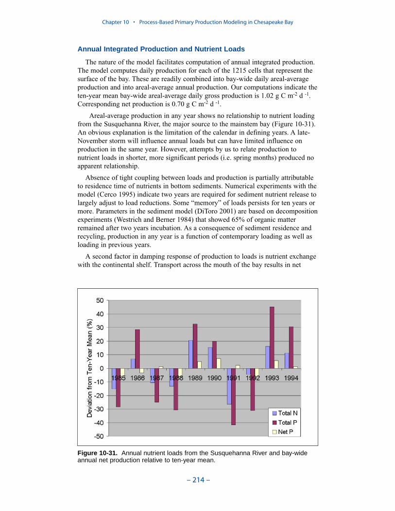
Annual Integrated Production and Nutrient Loads
The nature of the model facilitates computation of annual integrated production.The model computes daily production for each of the 1215 cells that represent thesurface of the bay. These are readily combined into bay-wide daily areal-averageproduction and into areal-average annual production. Our computations indicate theten-year mean bay-wide areal-average daily gross production is 1.02 g C m-2 d -1.Corresponding net production is 0.70 g C m-2 d -1.
Areal-average production in any year shows no relationship to nutrient loadingfrom the Susquehanna River, the major source to the mainstem bay (Figure 10-31).An obvious explanation is the limitation of the calendar in defining years. A late-November storm will influence annual loads but can have limited influence onproduction in the same year. However, attempts by us to relate production tonutrient loads in shorter, more significant periods (i.e. spring months) produced noapparent relationship.
Absence of tight coupling between loads and production is partially attributableto residence time of nutrients in bottom sediments. Numerical experiments with themodel (Cerco 1995) indicate two years are required for sediment nutrient release tolargely adjust to load reductions. Some “memory” of loads persists for ten years ormore. Parameters in the sediment model (DiToro 2001) are based on decompositionexperiments (Westrich and Berner 1984) that showed 65% of organic matterremained after two years incubation. As a consequence of sediment residence andrecycling, production in any year is a function of contemporary loading as well asloading in previous years.
A second factor in damping response of production to loads is nutrient exchangewith the continental shelf. Transport across the mouth of the bay results in net
Chapter 10 • Process-Based Primary Production Modeling in Chesapeake Bay
– 214 –
Figure 10-31. Annual nutrient loads from the Susquehanna River and bay-wideannual net production relative to ten-year mean.
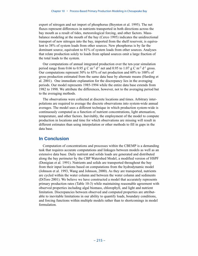
export of nitrogen and net import of phosphorus (Boynton et al. 1995). The netfluxes represent differences in nutrients transported in both directions across thebay mouth as a result of tides, meteorological forcing, and other factors. Mass-balance modeling at the mouth of the bay (Cerco 1995) indicates the unidirectionaltransport of new nitrogen into the bay, imported from the shelf reservoir, is equiva-lent to 38% of system loads from other sources. New phosphorus is by far thedominant source, equivalent to 81% of system loads from other sources. Analysesthat relate production solely to loads from upland sources omit a large fraction ofthe total loads to the system.
Our computations of annual integrated production over the ten-year simulationperiod range from 0.66 to 0.95 g C m-2 d-1 net and 0.95 to 1.07 g C m-2 d-1 gross.Our computations represent 50% to 85% of net production and 60% to 100% ofgross production estimated from the same data base by alternate means (Harding etal. 2001). One immediate explanation for the discrepancy lies in the averagingperiods. Our model represents 1985-1994 while the entire data base extends from1982 to 1998. We attribute the differences, however, not to the averaging period butto the averaging methods.
The observations were collected at discrete locations and times. Arbitrary inter-polations are required to average the discrete observations into system-wide annualaverages. The model uses a different technique in which production system-wide iscontinuously computed as a function of nutrient concentrations, light attenuation,temperature, and other factors. Inevitably, the employment of the model to computeproduction in locations and time for which observations are missing will result indifferent estimates than using interpolation or other methods to fill in gaps in thedata base.
In Conclusion
Computation of concentrations and processes within the CBEMP is a demandingtask that requires accurate computations and linkages between models as well as anextensive data base. Daily nutrient and solids loads are generated and distributedalong the bay perimeter by the CBP Watershed Model, a modified version of HSPF(Donigian et al. 1991). Nutrients and solids are transported throughout the bayfrom their input locations based on computations from the hydrodynamic model(Johnson et al. 1993, Wang and Johnson, 2000). As they are transported, nutrientsare cycled within the water column and between the water column and sediments(DiToro 2001). We believe we have constructed a model that accurately representsprimary production rates (Table 10-3) while maintaining reasonable agreement withobserved properties including algal biomass, chlorophyll, and light and nutrientlimitation. Discrepancies between observed and computed properties are attribut-able to inevitable limitations in our ability to quantify loads, boundary conditions,and forcing functions within multiple models rather than to shortcomings in modelformulation.
Chapter 10 • Process-Based Primary Production Modeling in Chesapeake Bay
– 215 –
ReferencesBehrenfield, M., and Falkowski, P. (1977). “A consumer’s guide to phytoplankton primaryproduction models,” Limnology and Oceanography, 42(7), 1479-1491.
Bienfang, P., Harrison, P., and Quarmby, L. (1982). “Sinking rate response to depletion ofnitrate, phosphate, and silicate in four marine diatoms,” Marine Biology, 67, 295-302.
Boynton, W., Garber, J., Summers, R., and Kemp, W. (1995). “Inputs, transformations, andtransport of nitrogen and phosphorus in Chesapeake Bay and selected tributaries,”Estuaries, 18, 285-314.
Cerco, C., and Cole, T. (1993). “Three-dimensional eutrophication model of ChesapeakeBay,” Journal of Environmental Engineering, 119(6), 1006-10025.
Cerco, C. (1995). “Response of Chesapeake Bay to nutrient load reductions,” Journal ofEnvironmental Engineering, 121(8), 549-557.
Cerco, C. (2000). “Phytoplankton kinetics in the Chesapeake Bay Eutrophication Model,”Journal of Water Quality and Ecosystem Modeling, 1, 5-49.
Cerco, C., and Meyers, M. (2000). “Tributary refinements to the Chesapeake Bay Model,”Journal of Environmental Engineering, 126(2), 164-174.
Chan, A. (1980). “Comparative physiological study of marine diatoms and dinoflagellatesin relation to irradiance and cell size. 2. Relationship between photosynthesis, growth, andcarbon/chlorophyll ratio. Journal of Phycology, 16, 428-432.
Cloern, J., Grenz, C., and Vidergar-Lucas, L. (1995). “An empirical model of the phyto-plankton chlorophyll:carbon ratio—the conversion factor between productivity and growthrate,” Limnology and Oceanography, 40(7), 1313-1321.
Davis, C., Breitner, N., and Harrison, P. (1978). “Continuous culture of marine diatomsunder silicon limitation. 3. a model of Si-limited diatom growth,” Limnology and Oceanog-raphy, 23, 41-52.
Chapter 10 • Process-Based Primary Production Modeling in Chesapeake Bay
– 216 –
Table 3 Statistical Summary of Modeled and Observed Production
Carbon Fixation,g C m-3 d-1
Gross Production,g C m-2 d-1
Net production, g C m-2 d-1
Observed Model Observed Model Observed Model
Mean 1.08 0.91 1.30 1.19 0.72 0.87
Median 0.93 0.79 0.91 1.01 0.41 0.82
Minimum 0.00 0.00 0.02 0.10 0.01 0
maximum 4.44 4.6 4.22 3.26 3.34 2.72
StandardDeviation
0.84 0.64 1.09 0.73 0.77 0.50
#Observed
876 64 166
Table 10-3
D’Elia, C., Nelson, D., and Boynton, W. 1983. “Chesapeake Bay Nutrient and PlanktonDynamics: III. The Annual Cycle of Silicon,” Geochimica et Cosmochimica Acta, 47:1945-1955.
DiToro, D. (2001). Sediment Flux Modeling, John Wiley and Sons, New York.
Doney, S., Glover, D., and Najjar, R. (1996). “A new coupled, one-dimensional biological-physical model for the upper ocean: Applications to the JGOFS Bermuda AtlanticTime-series Study (BATS) site,” Deep Sea Research II, 43(2- 3), 591-624.
Donigian, A., Bicknell, B., Patwardhan, A., Linker, L., Alegre, D., Chang, C., andReynolds, R. (1991). “Watershed model application to calculate bay nutrient loadings,”Chesapeake Bay Program Office, US Environmental Protection Agency, Annapolis MD.
Durbin, A., and Durgin, E. (1975). “Grazing rates of the Atlantic menhaden Brevoortiatyrannus as a function of particle size and concentration,” Marine Biology, 33, 265-277.
Eppley, R., Rogers, J., and McCarthy, J. (1969). “Half-saturation constants for uptake ofnitrate and ammonium by marine phytoplankton,” Limnology and Oceanography, 14(6),912-920.
Eppley, R. (1972). “Temperature and phytoplankton growth in the sea,” Fishery Bulletin,70(4), 1063-1085.
Fasham, M., Ducklow, H., and McKelvie, S. (1990). “A nitrogen-based model of planktondynamics in the oceanic mixed layer,” Journal of Marine Research, 48, 591-639.
Fisher, T., Gustafson, A., Sellner, K., Lacouture, R., Haas, L., Wetzel, R., Magnien, R.,Everitt, D., Michaels, B., and Karrh, R. (1999). “Spatial and temporal variation of resourcelimitation in Chesapeake Bay,” Marine Biology, 133, 763-778.
Fisher, T., Peele, E., Ammerman, J., and harding, L. (1992). “Nutrient limitation of phyto-plankton in Chesapeake Bay,” Marine Ecology Progress Series, 82, 51- 63.
Gallegos, C. (1989). “Microzooplankton grazing on phytoplankton in the Rhode River,maryland: nonlinear feeding kinetics,” Marine Ecology Progress Series, 57, 23-33.
Gilmore, J., Glendening, P., Ridgeway, T., Williams, A., Browner, C., and Bullaway, M.(2000). “Chesapeake 2000,” Chesapeake Bay Program, US Environmental ProtectionAgency, Annapolis MD.
Goldsworthy, A. (1970). “Photorespiration,” The Botanical Review, 36(4), 321- 340.
Groeger, A., and Kimmel, B. (1989). “Relationship between photosynthetic and respiratorycarbon metabolism in freshwater plankton,” Hydrobiologia, 173, 107-117.
Harding, L., Mallonee, M., and Perry, E. (2002). “Toward a predictive understanding ofprimary productivity in a temperature, partially stratified estuary,” Estuarine, Coastal andShelf Science, in press.
Harding, L., Meeson, B., and Fisher, T. (1986). “Phytoplankton in two east coast estuaries:photosynthesis-light curves and patterns of carbon assimilation,” Estuarine, Coastal andShelf Science, 23, 773-806.
Harris, R., Wiebe, P., Lenz, J., Skjodal, H., and Huntley, M. (2000). “Sampling, preserva-tion, enumeration and biomass of marine protozooplankton.” ICES zooplanktonmethodology manual. Academic Press, San Diego, 193-221.
Hutchinson, G. (1967). A treatise on limnology, Volume II, John Wiley and Sons, New York,245-305.
Jassby, A., and Platt, T. (1976). “Mathematical formulation of the relationship betweenphotosynthesis and light for phytoplankton,” Limnology and Oceanography, 21, 540-547.
Chapter 10 • Process-Based Primary Production Modeling in Chesapeake Bay
– 217 –
Johnson, B., Kim, K., Heath, R., Hsieh, B., and Butler, L. (1993). “Validation of a three-dimensional hydrodynamic model of Chesapeake Bay,” Journal of Hydraulic Engineering,199(1), 2-20.
Kemp, W., Smith, E., DiPasquale, M., and Boynton, W. (1997). “Organic carbon balanceand net ecosystem metabolism in Chesapeake Bay,” Marine Ecology Progress Series, 150,229-248.
Kiddon, J., Bender, M., and Marra, J. (1995). “Production and respiration in the 1989 NorthAtlantic spring bloom: an analysis of irradiance-dependent changes,” Deep-Sea Research,42(4), 553-576.
Laws, E., and Chalup, M. (1990). “A microalgal growth model,” Limnology and Oceanog-raphy, 35(3), 597-608.
Lomas, M., and Glibert, P. (1999). “Temperature regulation of nitrate uptake: A novelhypothesis about nitrate uptake and reduction in cool-water diatoms,” Limnology andOceanography, 44(3), 556-572.
Lomas, M., Trice, T., Glibert, P., Bronk, D., and McCarthy, J. (2002) “Temporal and spatialdynamics of urea concentrations in Chesapeake Bay: Biological versus physical forcing,”Estuaries, submitted.
Luo, J., Hartman, K., Brandt, S., Cerco, C., and Rippetoe, T. (2001). “A spatially-explicitapproach for estimating carrying capacity: an application for the Atlantic menhaden(Brevoortia tyrannus) in Chesapeake Bay,” Estuaries, 24(4), 545-556.
Malone, T., Crocker, L., Pike, S., and Wendler, B. (1988). “Influences of river flow on thedynamics of phytoplankton production in a partially stratified estuary,” Marine EcologyProgress Series, 48, 235-249.
Malone, T., Conley, D., Fisher, T., Glibert, P., Harding, and Sellner, K. (1996). “Scales ofnutrient-limited phytoplankton productivity in Chesapeake Bay,” Estuaries, 19, 371-385.
McCarthy, J., Taylor, W., and Taft, J. (1977). “Nitrogenous nutrition of the plankton in theChesapeake Bay. 1. Nutrient availability and phytoplankton preferences,” Limnology andOceanography, 22(6), 996-1011.
McGillicuddy, D., McCarthy, J., and Robinson, A. (1995). “Coupled physical and biologicalmodeling of the spring bloom in the North Atlantic (I): model formulation and one dimen-sional bloom processes,” Deep Sea Research I, 42(8), 1313-1357.
McManus, G., and Ederington-Cantrell, M. (1992). “Phytoplankton pigments and growthrates, and microzooplankton grazing in a large temperate estuary,” Marine Ecology ProgressSeries, 87, 77-85.
Miller, C., and Glibert, P. (1998). “Nitrogen excretion by the calanoid copepod Acartiatonsa: results of mesocosm experiments,” Journal of Plankton Research, 20(9), 1767-1780.
Moll, A. (1998). “Regional distribution of primary production in the North Sea simulatedby a three-dimensional model,” Journal of Marine Systems, 16, 151- 170.
Monod, J. (1949). “The growth of bacterial cultures,” Annual Review of Microbiology, 3,371-394.
Pritchard, D. (1967). “Observations of circulation in coastal plain estuaries.” Estuaries. G.Lauff ed., American Association for the Advancement of Science, Washington D.C., 37-44.
Parsons, T., Takahashi, M., and Hargrave, B. (1984). Biological Oceanographic Processes,Pergamon Press, Oxford.
Redfield, A., Ketchum, B., and Richards, F. (1966). “The influence of organisms on thecomposition of sea-water.” The Sea Volume II. Interscience Publishers, New York, 26-48.
Chapter 10 • Process-Based Primary Production Modeling in Chesapeake Bay
– 218 –

Richardson, T., and Cullen, J. (1995). “Changes in buoyancy and chemical compositionduring growth of a coastal marine diatom: ecological and biogeochemical consequences,”Marine Ecology Progress Series, 128, 77-90.
Riebesell, U. (1989). “Comparison of sinking and sedimentation rate measurements in adiatom winter/spring bloom,” Marine Ecology Progress Series, 54, 109-119.
Rippetoe, T. (1993). “Production and energetics of Atlantic menhaden in Chesapeake Bay,”M.S. Thesis, University of Maryland, College Park MD.
Smith, E., and Kemp, W. (1995). “Seasonal and regional variations in plankton communityproduction and respiration for Chesapeake Bay,” Marine Ecology Progress Series, 116, 217-231.
Strickland, J., and Parsons, T. (1972). “A practical handbook of seawater analysis,” Bulletinof the Fisheries Research Board of Canada,” 167, 310 pp.
Taft, J., Taylor, W., and McCarthy, J. (1975). “Uptake and release of phosphorus by phyto-plankton in the Chesapeake Bay estuary, USA,” Marine Biology, 33, 21- 32.
Thomann, R., and Fitzpatrick, J. (1982). “Calibration and verification of a mathematicalmodel of the eutrophication of the Potomac Estuary,” HydroQual Inc., Mahwah, NJ.
Waite, A., Thompson, P., and Harrison, P. (1992). “Does energy control the sinking rates ofmarine diatoms?.” Limnology and Oceanography, 37(3), 468- 477.
Wang, H., and Johnson, B. (2000). “Validation and application of the second-generation,three-dimensional hydrodynamic model of Chesapeake Bay,” Journal of Water Quality andEcosystem Modeling, 1, 51-90.
Westrich, J., and Berner, R. (1984). “The role of sedimentary organic matter in bacterialsulfate reduction: The G model tested,” Limnology and Oceanography, 29(2), 236-249.
Wheeler, P., Gilbert, P., and McCarthy, J. (1982). “Ammonium uptake and incorporation byChesapeake Bay phytoplankton: short-term uptake kinetics,” Limnology and Oceanography,27, 1113-1128.
White, J., and Roman, M. (1992). “Seasonal study of grazing by metazoan zooplankton inthe mesohaline Chesapeake Bay,” Marine Ecology Progress Series, 86, 251-261.
Chapter 10 • Process-Based Primary Production Modeling in Chesapeake Bay
– 219 –

Data Bases
Solids
Suspended solids observations in the monitoring data base included totalsuspended solids, fixed solids, volatile solids, and particulate organic carbon. (Forpractical purposes, fixed and volatile solids correspond to inorganic and organicsolids.) Direct analyses of organic solids were limited to stations in the Virginiatributaries (Table 11-1, Figure 11-1). The preponderance of organic solids observa-tions was in the form of particulate organic carbon. We converted particulateorganic carbon to organic solids through the relationship:
in which:VSS = organic solids concentration (g m-3)POC = particulate organic carbon concentration (g C m-3)
This commonly-employed relationship assumes organic matter is comprised of asimple carbohydrate CH2O. The total mass of this compound is 2.5 times thecarbonaceous mass. Organic solids were subtracted from total suspended solids toobtain inorganic solids concentration.
Examination of the system-wide solids distribution indicates that organic solidsrepresent a small fraction of the total suspended solids (Figures 11-2 to 11-4). Onlyin regions characterized by two stations, CB4.2C and CB5.2, do organic solidscomprise as much a half the total suspended solids. The observed solids com-position has significant implications for management activities in the bay system.Attempts to reduce organic solids concentrations, and thereby light attenuation,through nutrient controls address only a small fraction of the total suspended solidsin the water column. Analyses using the submerged aquatic vegetation model(Cerco and Moore 2001) indicate system-wide restoration of submerged aquaticvegetation through nutrient controls alone is impossible.
POC2.5=VSS (11-1)
– 220 –
Suspended Solidsand Light Attenuation 11
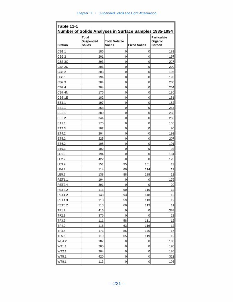
Chapter 11 • Suspended Solids and Light Attenuation
– 221 –
Table 11-1 Number of Solids Analyses in Surface Samples 1985-1994
Station
TotalSuspendedSolids
Total Volatile Solids Fixed Solids
ParticulateOrganicCarbon
CB1.1 186 0 0 181
CB2.2 201 0 0 197
CB3.3C 293 0 0 227
CB4.2C 206 0 0 200
CB5.2 208 0 0 196
CB6.1 194 0 0 193
CB7.3 204 0 0 208
CB7.4 204 0 0 204
CB7.4N 176 0 0 186
CB8.1E 182 0 0 181
EE1.1 197 0 0 182
EE2.1 268 0 0 254
EE3.1 380 0 0 288
EE3.2 344 0 0 253
ET1.1 176 0 0 155
ET2.3 102 0 0 90
ET4.2 204 0 0 191
ET5.2 225 0 0 207
ET6.2 108 0 0 101
ET9.1 102 0 0 93
LE1.3 194 0 0 181
LE2.2 422 0 0 123
LE3.2 151 95 151 12
LE4.2 114 60 114 12
LE5.3 138 88 138 11
RET1.1 194 0 0 179
RET2.4 391 0 0 20
RET3.2 116 60 116 12
RET4.2 148 93 148 12
RET4.3 113 59 113 12
RET5.2 113 60 113 11
TF1.7 415 0 0 388
TF2.1 376 0 0 23
TF3.3 111 58 111 12
TF4.2 116 63 116 12
TF4.4 176 86 176 17
TF5.5 119 65 119 12
WE4.2 187 0 0 186
WT1.1 205 0 0 190
WT2.1 204 0 0 186
WT5.1 420 0 0 322
WT8.1 113 0 0 103
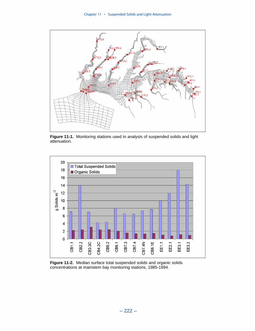
Chapter 11 • Suspended Solids and Light Attenuation
– 222 –
Figure 11-1. Monitoring stations used in analysis of suspended solids and lightattenuation.
Figure 11-2. Median surface total suspended solids and organic solidsconcentrations at mainstem bay monitoring stations, 1985-1994.
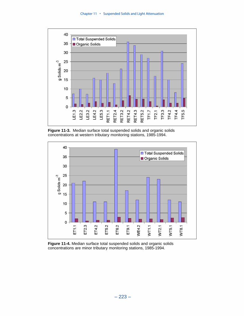
Chapter 11 • Suspended Solids and Light Attenuation
– 223 –
Figure 11-3. Median surface total suspended solids and organic solidsconcentrations at western tributary monitoring stations, 1985-1994.
Figure 11-4. Median surface total suspended solids and organic solidsconcentrations are minor tributary monitoring stations, 1985-1994.
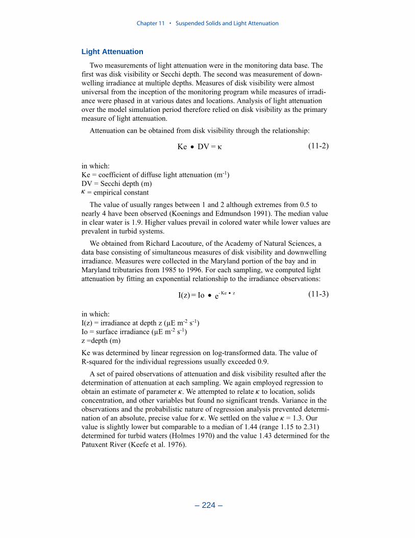
Light Attenuation
Two measurements of light attenuation were in the monitoring data base. Thefirst was disk visibility or Secchi depth. The second was measurement of down-welling irradiance at multiple depths. Measures of disk visibility were almostuniversal from the inception of the monitoring program while measures of irradi-ance were phased in at various dates and locations. Analysis of light attenuationover the model simulation period therefore relied on disk visibility as the primarymeasure of light attenuation.
Attenuation can be obtained from disk visibility through the relationship:
in which:Ke = coefficient of diffuse light attenuation (m-1)DV = Secchi depth (m)κ = empirical constant
The value of usually ranges between 1 and 2 although extremes from 0.5 tonearly 4 have been observed (Koenings and Edmundson 1991). The median valuein clear water is 1.9. Higher values prevail in colored water while lower values areprevalent in turbid systems.
We obtained from Richard Lacouture, of the Academy of Natural Sciences, adata base consisting of simultaneous measures of disk visibility and downwellingirradiance. Measures were collected in the Maryland portion of the bay and inMaryland tributaries from 1985 to 1996. For each sampling, we computed lightattenuation by fitting an exponential relationship to the irradiance observations:
in which:I(z) = irradiance at depth z (µE m-2 s-1)Io = surface irradiance (µE m-2 s-1)z =depth (m) Ke was determined by linear regression on log-transformed data. The value of R-squared for the individual regressions usually exceeded 0.9.
A set of paired observations of attenuation and disk visibility resulted after thedetermination of attenuation at each sampling. We again employed regression toobtain an estimate of parameter κ. We attempted to relate κ to location, solidsconcentration, and other variables but found no significant trends. Variance in theobservations and the probabilistic nature of regression analysis prevented determi-nation of an absolute, precise value for κ. We settled on the value κ = 1.3. Ourvalue is slightly lower but comparable to a median of 1.44 (range 1.15 to 2.31)determined for turbid waters (Holmes 1970) and the value 1.43 determined for thePatuxent River (Keefe et al. 1976).
eIo=I(z) zKe- (11-3)
=DVKe (11-2)
Chapter 11 • Suspended Solids and Light Attenuation
– 224 –
The Light Attenuation Model
We proposed a model that related light attenuation to attenuation from water,from inorganic suspended solids, from organic suspended solids, from dissolvedorganic matter, and from chlorophyll:
in which:a1 to a5 = empirical constantsISS = inorganic suspended solids concentration (g m-3)VSS = organic suspended solids concentration (g m-3)DOC = dissolved organic carbon (g C m-3)Chl = chlorophyll (mg m-3)We adopted dissolved organic carbon as a surrogate for the dissolved organicmatter that provides color in water.
Parameters in the model were determined through linear regression. Regressionwas performed for each sample station to allow for regional variations in parame-ters. We found no significant relationship of attenuation to dissolved organiccarbon. Various explanations for absence of a relationship may hold. The first isthat dissolved organic carbon is a poor surrogate for colored organic matter. Thesecond is that no significant spatial gradients of dissolved organic carbon exist. Thethird is that enormous variance is present in the analysis of dissolved organiccarbon and masks any relationship to attenuation. Likely all of these explanationshave validity.
We also found we could not distinguish attenuation from both chlorophyll andorganic solids. The two variables were too closely correlated for their properties tobe isolated by regression. We decided to drop chlorophyll from the model andretain organic solids. We reasoned we would like the model to distinguish potentialdifferences in attenuation between inorganic and organic solids. Since our parame-ters were determined by regression, attenuation by chlorophyll was included as partof the total attenuation by organic solids.
The resulting attenuation relationship had the form:
in which:a1 = background attenuation (m-1)a2 = attenuation by inorganic suspended solids (m2 g-1)a3 = attenuation by organic suspended solids (m2 g-1) The “background” attenuation term included attenuation from both water anddissolved organic matter.
Individual parameters were determined for each Chesapeake Bay ProgramSegment represented in the model domain (Figure 11-5). These were refined toprovide reasonable consistency in the parameterization. In a few cases, backgroundattenuation was adjusted to counter problems with the model solids computation.The result (Table 11-2) was a model in which background attenuation was highest
VSSa+ISSa+a=Ke 321(11-5)
Chla+DOCa+VSSa+ISSa+a=Ke 54321 (11-4)
Chapter 11 • Suspended Solids and Light Attenuation
– 225 –
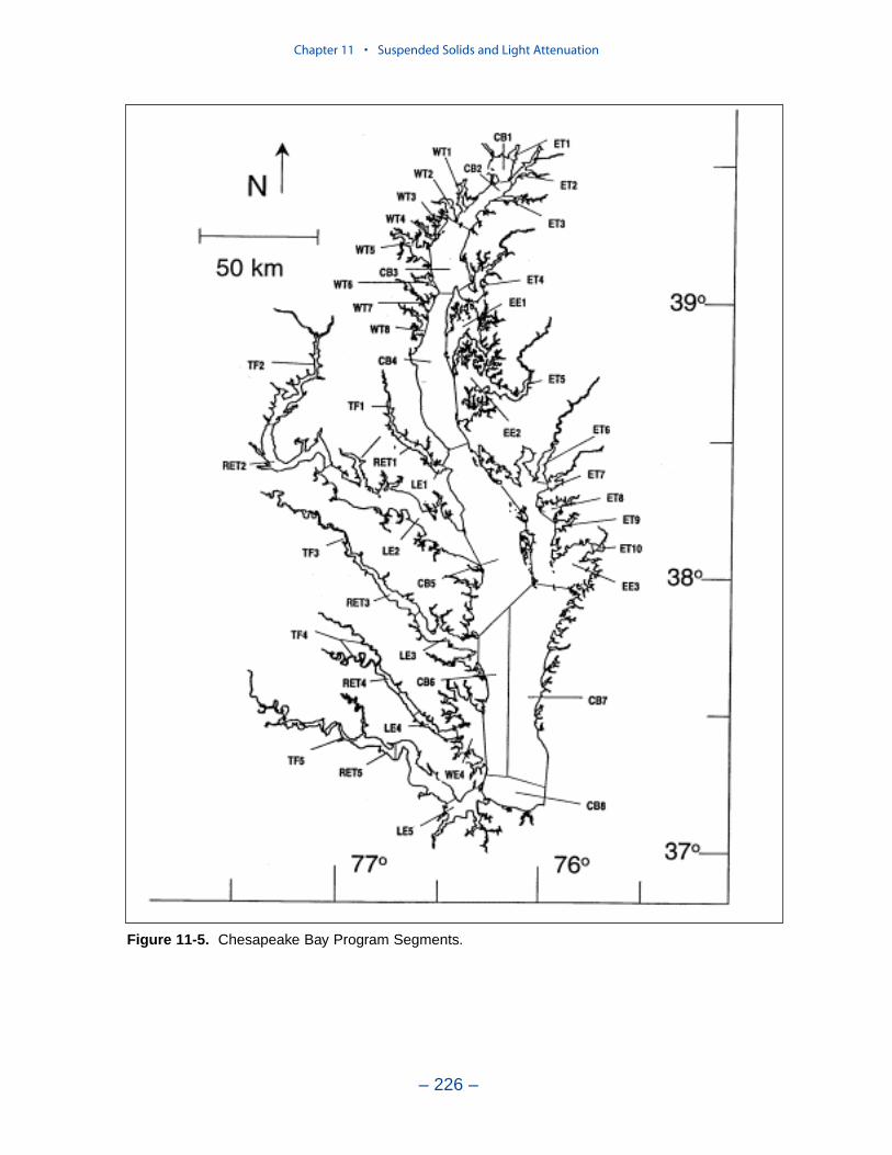
Chapter 11 • Suspended Solids and Light Attenuation
– 226 –
Figure 11-5. Chesapeake Bay Program Segments.
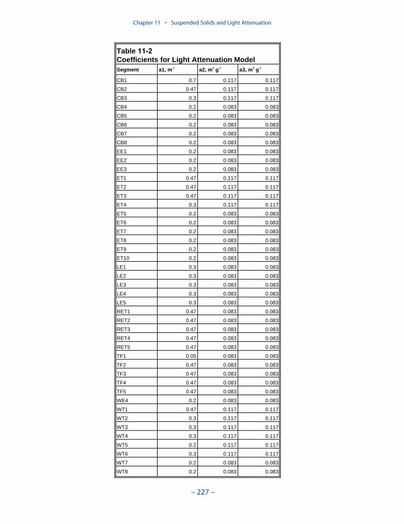
Chapter 11 • Suspended Solids and Light Attenuation
– 227 –
Table 11-2Coefficients for Light Attenuation Model Segment a1, m-1 a2, m2 g-1 a3, m2 g-1
CB1 0.7 0.117 0.117
CB2 0.47 0.117 0.117
CB3 0.3 0.117 0.117
CB4 0.2 0.083 0.083
CB5 0.2 0.083 0.083
CB6 0.2 0.083 0.083
CB7 0.2 0.083 0.083
CB8 0.2 0.083 0.083
EE1 0.2 0.083 0.083
EE2 0.2 0.083 0.083
EE3 0.2 0.083 0.083
ET1 0.47 0.117 0.117
ET2 0.47 0.117 0.117
ET3 0.47 0.117 0.117
ET4 0.3 0.117 0.117
ET5 0.2 0.083 0.083
ET6 0.2 0.083 0.083
ET7 0.2 0.083 0.083
ET8 0.2 0.083 0.083
ET9 0.2 0.083 0.083
ET10 0.2 0.083 0.083
LE1 0.3 0.083 0.083
LE2 0.3 0.083 0.083
LE3 0.3 0.083 0.083
LE4 0.3 0.083 0.083
LE5 0.3 0.083 0.083
RET1 0.47 0.083 0.083
RET2 0.47 0.083 0.083
RET3 0.47 0.083 0.083
RET4 0.47 0.083 0.083
RET5 0.47 0.083 0.083
TF1 0.05 0.083 0.083
TF2 0.47 0.083 0.083
TF3 0.47 0.083 0.083
TF4 0.47 0.083 0.083
TF5 0.47 0.083 0.083
WE4 0.2 0.083 0.083
WT1 0.47 0.117 0.117
WT2 0.3 0.117 0.117
WT3 0.3 0.117 0.117
WT4 0.3 0.117 0.117
WT5 0.2 0.117 0.117
WT6 0.3 0.117 0.117
WT7 0.2 0.083 0.083
WT8 0.2 0.083 0.083
near the freshwater sources and lowest near the ocean interface. This conceptual-ization was consistent with the observation that freshwater is more colored thanseawater (Kirk 1994). During the refinement, the distinction of coefficients forinorganic and organic solids was dropped but solids near the fall lines were charac-terized as having higher attenuation than solids in regions distant from sources inupland watersheds.
Comparison with the SAV Technical Synthesis II
An additive light attenuation model similar to our own was created as part of thesecond technical synthesis on submerged aquatic vegetation and water quality(Chesapeake Bay Program 2000). The model incorporated background attenuation,attenuation from total suspended solids, and attenuation from chlorophyll. As withour model, parameters were initially obtained from regression and then refined toimprove agreement with observations.
Regressions produced background attenuation in range 0.393 to 3.32 m-1. Thevalue 0.32 m-1 was recommended for use system-wide. This value is centrallylocated within the values 0.05 to 0.7 m-1 used in our model and is close to ourpredominant value of 0.2 m-1.
Regressions indicated the coefficient that related total suspended solids contribu-tion to light attenuation was in the range 0.013 to 0.101 m2 g-1. The coefficientrecommended for use system-wide was 0.094 m2 g-1. This value is nearly identicalto the average of the two values, 0.083 and 0.117 m2 g-1, used in our own model.
Fewer than half of the regressions conducted as part of the “Tech Syn II”resulted in significant relationships between chlorophyll and light attenuation.Several of the statistically significant relationships were negative, indicating aphysically-impossible relationship. These results echoed our own difficulty inisolating the effect of chlorophyll via regression. The attenuation coefficient ofchlorophyll is well-known, however (e.g. Pennock 1985). Consequently, the TechSyn II investigators elected to include chlorophyll attenuation, 0.016 m2 mg-1, intheir model. If we assume a carbon-to-chlorophyll ratio of 75 and utilize the ratioof 2.5 between solids and organic carbon, we find the chlorophyll attenuation usedin Tech Syn II is equivalent to 0.085 m2 g-1 organic solids, remarkably close to theprevailing value used in our own model.
We are relieved and reassured that the light attenuation relationships obtained inindependent investigations are equivalent. Managers and other users of the twomodels, ours and Tech Syn II, should be confident that guidance obtained from thetwo models will be consistent.
Solids Settling Velocities
The principal suspended solids variable in the CBEMP was inorganic (fixed)suspended solids. Organic solids were derived from particulate carbon variables(phytoplankton, zooplankton, detritus) and added to inorganic solids for compar-ison to observed total suspended solids.
No internal sources or sinks of inorganic solids were considered in the model.Aside from loads, the distribution of inorganic solids in the water column wasdetermined by two settling velocities. One represented settling through the water
Chapter 11 • Suspended Solids and Light Attenuation
– 228 –

column and the other represented net settling to the bed sediments. Within thewater column, the transport equation for inorganic solids was identical to the equa-tion for all other variables. A modification applied in cells that interfaced the bedsediments:
in which:C = solids concentration in cell adjoining bed sediments (g m-3)Cu = solids concentration two cells above bed sediments (g m-3)W = settling velocity in water column (m d-1)Wnet = settling velocity from water to bed sediments (m d-1)z = cell thickness (m)t = time (d)
Net settling was always less than or equal to settling through the water column.The reduced magnitude of net settling represented the net effect of resuspension.The ratio of net settling to settling through the water column may be viewed as thefraction of material deposited on the bed that remains in the bed. The employmentof net settling is a primary distinction between our own suspended solids modeland a true sediment transport model. Our model included no resuspension mecha-nism. Once a particle was deposited on the bottom, it remained there.
Settling and net settling were evaluated through a recursive calibration processbased on visual fitting of computed to observed solids. Settling velocities obtainedin this fashion were highest near the fall lines of several western tributaries and in afew minor Eastern Shore tributaries (Table 11-3). The high settling velocities in thewestern tributaries diminished with distance from the head of tide, perhaps indi-cating sorting out of large particles carried over the fall line. Our estimates ofloading from bank erosion were highly uncertain in the Eastern Shore embayments.The high settling velocities assigned in some tributaries there may reflect deposi-tional environments or may be a compensation for overestimated bank loads.Settling velocities assigned in the mainstem bay (Table 11-3) also diminished awayfrom the source in the Susquehanna River but were less than in several westerntributaries. The velocities assigned suggested particles with high settling velocitiessettled out in Conowingo Reservoir before reaching the bay.
Net settling velocities were five to ten percent of settling in the water column.(Table 11-3).
Net settling was enhanced in the presence of submerged aquatic vegetation(Cerco and Moore 2001) to represent the damping effect of vegetation on wavesand on resuspension.
Our model did not consider solids size classes. We found a modification toassigned settling velocities was required during major storm events. Storm eventswere defined as intervals in which inorganic solids concentration exceeded 100 g m-3. During storm events, the inorganic solids settling rate was specified as 5 m d-1 and no resuspension was allowed. This assignment simulated rapidsettling of large particles carried over the fall line during floods. If we did notassign rapid settling during storms, solids loads associated with storms remained inthe water column perpetually.
Cz
Wnet-Cuz
W+][transport=tC
(11-6)
Chapter 11 • Suspended Solids and Light Attenuation
– 229 –
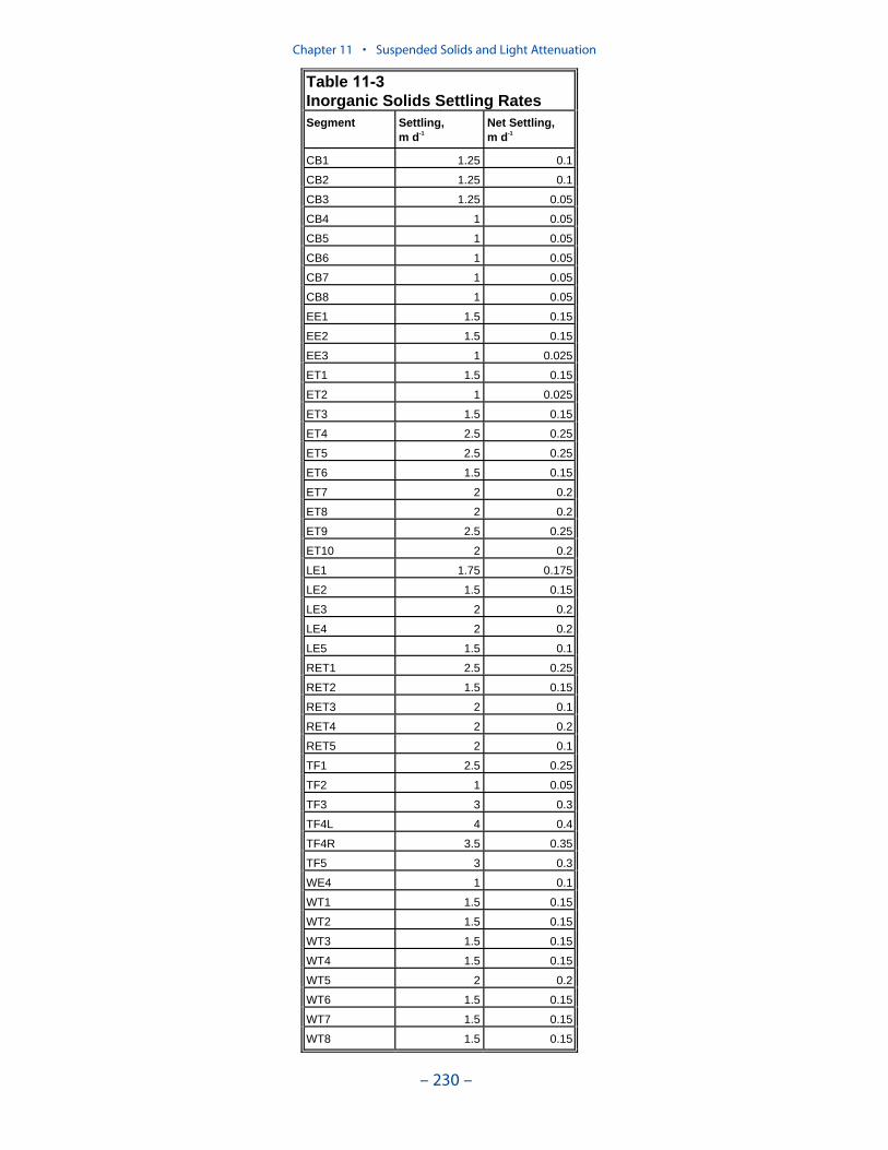
Chapter 11 • Suspended Solids and Light Attenuation
– 230 –
Table 11-3Inorganic Solids Settling Rates Segment Settling,
m d-1
Net Settling, m d-1
CB1 1.25 0.1
CB2 1.25 0.1
CB3 1.25 0.05
CB4 1 0.05
CB5 1 0.05
CB6 1 0.05
CB7 1 0.05
CB8 1 0.05
EE1 1.5 0.15
EE2 1.5 0.15
EE3 1 0.025
ET1 1.5 0.15
ET2 1 0.025
ET3 1.5 0.15
ET4 2.5 0.25
ET5 2.5 0.25
ET6 1.5 0.15
ET7 2 0.2
ET8 2 0.2
ET9 2.5 0.25
ET10 2 0.2
LE1 1.75 0.175
LE2 1.5 0.15
LE3 2 0.2
LE4 2 0.2
LE5 1.5 0.1
RET1 2.5 0.25
RET2 1.5 0.15
RET3 2 0.1
RET4 2 0.2
RET5 2 0.1
TF1 2.5 0.25
TF2 1 0.05
TF3 3 0.3
TF4L 4 0.4
TF4R 3.5 0.35
TF5 3 0.3
WE4 1 0.1
WT1 1.5 0.15
WT2 1.5 0.15
WT3 1.5 0.15
WT4 1.5 0.15
WT5 2 0.2
WT6 1.5 0.15
WT7 1.5 0.15
WT8 1.5 0.15
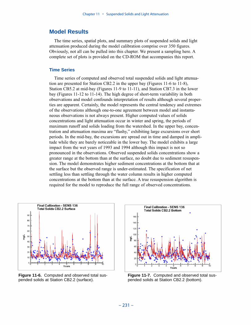
Model Results
The time series, spatial plots, and summary plots of suspended solids and lightattenuation produced during the model calibration comprise over 350 figures.Obviously, not all can be pulled into this chapter. We present a sampling here. Acomplete set of plots is provided on the CD-ROM that accompanies this report.
Time Series
Time series of computed and observed total suspended solids and light attenua-tion are presented for Station CB2.2 in the upper bay (Figures 11-6 to 11-8),Station CB5.2 at mid-bay (Figures 11-9 to 11-11), and Station CB7.3 in the lowerbay (Figures 11-12 to 11-14). The high degree of short-term variability in bothobservations and model confounds interpretation of results although several proper-ties are apparent. Certainly, the model represents the central tendency and extremesof the observations although one-to-one agreement between model and instanta-neous observations is not always present. Higher computed values of solidsconcentrations and light attenuation occur in winter and spring, the periods ofmaximum runoff and solids loading from the watershed. In the upper bay, concen-tration and attenuation maxima are “flashy,” exhibiting large excursions over shortperiods. In the mid-bay, the excursions are spread out in time and damped in ampli-tude while they are barely noticeable in the lower bay. The model exhibits a largeimpact from the wet years of 1993 and 1994 although this impact is not sopronounced in the observations. Observed suspended solids concentrations show agreater range at the bottom than at the surface, no doubt due to sediment resuspen-sion. The model demonstrates higher sediment concentrations at the bottom that atthe surface but the observed range is under-estimated. The specification of netsettling less than settling through the water column results in higher computedconcentrations at the bottom than at the surface. A true resuspension algorithm isrequired for the model to reproduce the full range of observed concentrations.
Chapter 11 • Suspended Solids and Light Attenuation
– 231 –
Figure 11-6. Computed and observed total sus-pended solids at Station CB2.2 (surface).
Figure 11-7. Computed and observed total sus-pended solids at Station CB2.2 (bottom).
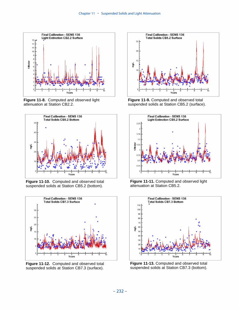
Chapter 11 • Suspended Solids and Light Attenuation
– 232 –
Figure 11-8. Computed and observed lightattenuation at Station CB2.2.
Figure 11-9. Computed and observed totalsuspended solids at Station CB5.2 (surface).
Figure 11-10. Computed and observed totalsuspended solids at Station CB5.2 (bottom).
Figure 11-11. Computed and observed lightattenuation at Station CB5.2.
Figure 11-12. Computed and observed totalsuspended solids at Station CB7.3 (surface).
Figure 11-13. Computed and observed totalsuspended solids at Station CB7.3 (bottom).
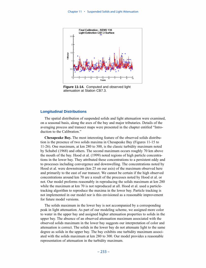
Longitudinal Distributions
The spatial distribution of suspended solids and light attenuation were examined,on a seasonal basis, along the axes of the bay and major tributaries. Details of theaveraging process and transect maps were presented in the chapter entitled “Intro-duction to the Calibration.”
Chesapeake Bay. The most interesting feature of the observed solids distribu-tion is the presence of two solids maxima in Chesapeake Bay (Figures 11-15 to11-26). One maximum, at km 280 to 300, is the classic turbidity maximum notedby Schubel (1968) and others. The second maximum occurs roughly 70 km abovethe mouth of the bay. Hood et al. (1999) noted regions of high particle concentra-tions in the lower bay. They attributed these concentrations to a persistent eddy andto processes including convergence and downwelling. The concentrations noted byHood et al. were downstream (km 25 on our axis) of the maximum observed hereand primarily to the east of our transect. We cannot be certain if the high observedconcentrations around km 70 are a result of the processes noted by Hood et al. ornot. Our model preforms reasonably in reproducing the solids maximum at km 280while the maximum at km 70 is not reproduced at all. Hood et al. used a particle-tracking algorithm to reproduce the maxima in the lower bay. Particle tracking isnot implemented in our model nor is this envisioned as a reasonable improvementfor future model versions.
The solids maximum in the lower bay is not accompanied by a correspondingpeak in light attenuation. As part of our modeling scheme, we assigned more colorto water in the upper bay and assigned higher attenuation properties to solids in theupper bay. The absence of an observed attenuation maximum associated with theobserved solids maximum in the lower bay suggests our interpretation of color andattenuation is correct. The solids in the lower bay do not attenuate light to the samedegree as solids in the upper bay. The bay exhibits one turbidity maximum associ-ated with the solids maximum at km 280 to 300. Our model provides a reasonablerepresentation of attenuation in the turbidity maximum.
Chapter 11 • Suspended Solids and Light Attenuation
– 233 –
Figure 11-14. Computed and observed lightattenuation at Station CB7.3.

Chapter 11 • Suspended Solids and Light Attenuation
– 234 –
Figure 11-15. Computed (mean and range) andobserved (mean and range) total suspended solidsalong Chesapeake Bay axis, winter 1990 (surface).
Figure 11-16. Computed (mean and range) andobserved (mean and range) total suspended solidsalong Chesapeake Bay axis, winter 1990 (surface).
Figure 11-17. Computed (mean and range) andobserved (mean and range) light attenuation alongChesapeake Bay axis, winter 1990.
Figure 11-18. Computed (mean and range) andobserved (mean and range) total suspended solidsalong Chesapeake Bay axis, spring 1990 (surface).
Figure 11-19. Computed (mean and range) andobserved (mean and range) total suspended solidsalong Chesapeake Bay axis, spring 1990 (bottom).
Figure 11-20. Computed (mean and range) andobserved (mean and range) light attenuation alongChesapeake Bay axis, spring 1990.

Chapter 11 • Suspended Solids and Light Attenuation
– 235 –
Figure 11-21. Computed (mean and range) andobserved (mean and range) total suspended solidsalong Chesapeake Bay axis, summer 1990 (surface).
Figure 11-22. Computed (mean and range) andobserved (mean and range) total suspended solidsalong Chesapeake Bay axis, summer 1990 (bottom).
Figure 11-23. Computed (mean and range) andobserved (mean and range) light attenuation alongChesapeake Bay axis, summer 1990.
Figure 11-24. Computed (mean and range) andobserved (mean and range) total suspended solidsalong Chesapeake Bay axis, fall 1990 (surface).
Figure 11-25. Computed (mean and range) andobserved (mean and range) total suspended solidsalong Chesapeake Bay axis, fall 1990 (bottom).
Figure 11-26. Computed (mean and range) andobserved (mean and range) light attenuation alongChesapeake Bay axis, fall 1990.
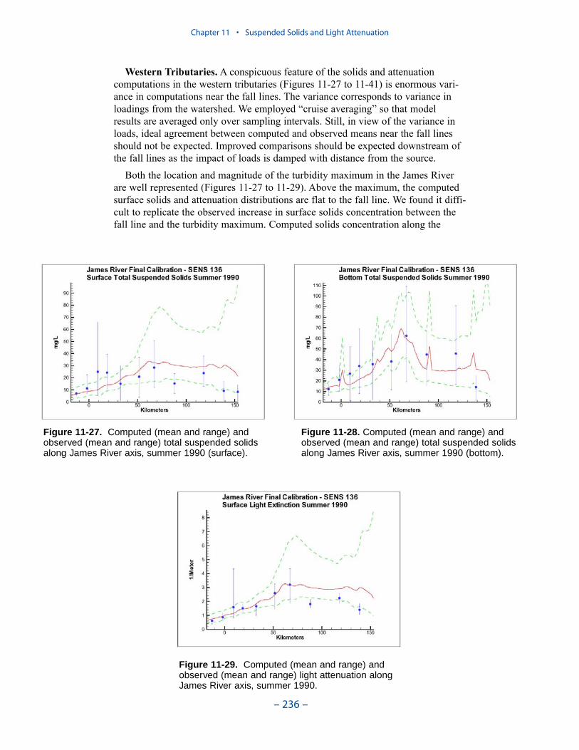
Western Tributaries. A conspicuous feature of the solids and attenuationcomputations in the western tributaries (Figures 11-27 to 11-41) is enormous vari-ance in computations near the fall lines. The variance corresponds to variance inloadings from the watershed. We employed “cruise averaging” so that modelresults are averaged only over sampling intervals. Still, in view of the variance inloads, ideal agreement between computed and observed means near the fall linesshould not be expected. Improved comparisons should be expected downstream ofthe fall lines as the impact of loads is damped with distance from the source.
Both the location and magnitude of the turbidity maximum in the James Riverare well represented (Figures 11-27 to 11-29). Above the maximum, the computedsurface solids and attenuation distributions are flat to the fall line. We found it diffi-cult to replicate the observed increase in surface solids concentration between thefall line and the turbidity maximum. Computed solids concentration along the
Chapter 11 • Suspended Solids and Light Attenuation
– 236 –
Figure 11-27. Computed (mean and range) andobserved (mean and range) total suspended solidsalong James River axis, summer 1990 (surface).
Figure 11-28. Computed (mean and range) andobserved (mean and range) total suspended solidsalong James River axis, summer 1990 (bottom).
Figure 11-29. Computed (mean and range) andobserved (mean and range) light attenuation alongJames River axis, summer 1990.

bottom provides a better approximation of the increase from the fall line to theturbidity maximum around km 70. Downstream of the turbidity maximum, themodel provides good representation of the solids concentration and excellent repre-sentation of light attenuation.
The observed turbidity maximum in the York River occurs around km 70(Figures 11-30 to 11-32). Computed solids concentration climbs from the intersec-tion with the bay (km 0) to around km 40. From km 40 to the fall line, computedsolids distribution is flat. Computed solids concentration in the turbidity maximumis underestimated. Computed light attenuation agrees well with observed through tokm 70. Above km 70, observations are sparse but the model tends to overestimatelight attenuation.
Chapter 11 • Suspended Solids and Light Attenuation
– 237 –
Figure 11-30. Computed (mean and range) andobserved (mean and range) total suspended solidsalong York River axis, summer 1993 (surface).
Figure 11-31. Computed (mean and range) andobserved (mean and range) total suspended solidsalong York River axis, summer 1993 (bottom).
Figure 11-32. Computed (mean and range) andobserved (mean and range) light attenuation along YorkRiver axis, summer 1993
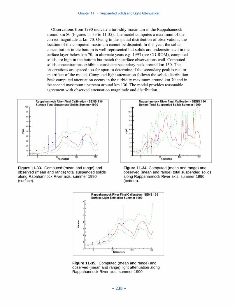
Observations from 1990 indicate a turbidity maximum in the Rappahannockaround km 80 (Figures 11-33 to 11-35). The model computes a maximum of thecorrect magnitude at km 70. Owing to the spatial distribution of observations, thelocation of the computed maximum cannot be disputed. In this year, the solidsconcentration in the bottom is well represented but solids are underestimated in thesurface layer below km 70. In alternate years e.g. 1993 (see CD-ROM), computedsolids are high in the bottom but match the surface observations well. Computedsolids concentrations exhibit a consistent secondary peak around km 130. Theobservations are spaced too far apart to determine if the secondary peak is real oran artifact of the model. Computed light attenuation follows the solids distribution.Peak computed attenuation occurs in the turbidity maximum around km 70 and inthe second maximum upstream around km 130. The model provides reasonableagreement with observed attenuation magnitude and distribution.
Chapter 11 • Suspended Solids and Light Attenuation
– 238 –
Figure 11-33. Computed (mean and range) andobserved (mean and range) total suspended solidsalong Rapahannock River axis, summer 1990(surface).
Figure 11-34. Computed (mean and range) andobserved (mean and range) total suspended solidsalong Rappahannock River axis, summer 1990(bottom).
Figure 11-35. Computed (mean and range) andobserved (mean and range) light attenuation alongRappahannock River axis, summer 1990.
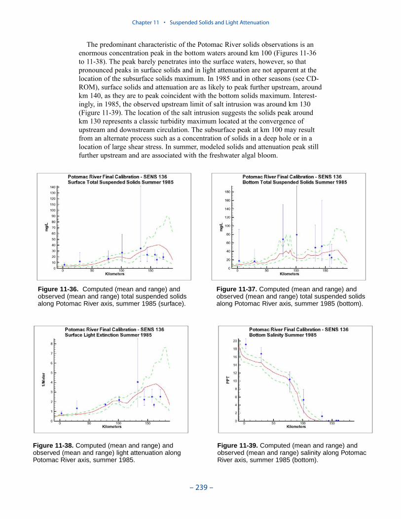
The predominant characteristic of the Potomac River solids observations is anenormous concentration peak in the bottom waters around km 100 (Figures 11-36to 11-38). The peak barely penetrates into the surface waters, however, so thatpronounced peaks in surface solids and in light attenuation are not apparent at thelocation of the subsurface solids maximum. In 1985 and in other seasons (see CD-ROM), surface solids and attenuation are as likely to peak further upstream, aroundkm 140, as they are to peak coincident with the bottom solids maximum. Interest-ingly, in 1985, the observed upstream limit of salt intrusion was around km 130(Figure 11-39). The location of the salt intrusion suggests the solids peak aroundkm 130 represents a classic turbidity maximum located at the convergence ofupstream and downstream circulation. The subsurface peak at km 100 may resultfrom an alternate process such as a concentration of solids in a deep hole or in alocation of large shear stress. In summer, modeled solids and attenuation peak stillfurther upstream and are associated with the freshwater algal bloom.
Chapter 11 • Suspended Solids and Light Attenuation
– 239 –
Figure 11-36. Computed (mean and range) andobserved (mean and range) total suspended solidsalong Potomac River axis, summer 1985 (surface).
Figure 11-37. Computed (mean and range) andobserved (mean and range) total suspended solidsalong Potomac River axis, summer 1985 (bottom).
Figure 11-38. Computed (mean and range) andobserved (mean and range) light attenuation alongPotomac River axis, summer 1985.
Figure 11-39. Computed (mean and range) andobserved (mean and range) salinity along PotomacRiver axis, summer 1985 (bottom).
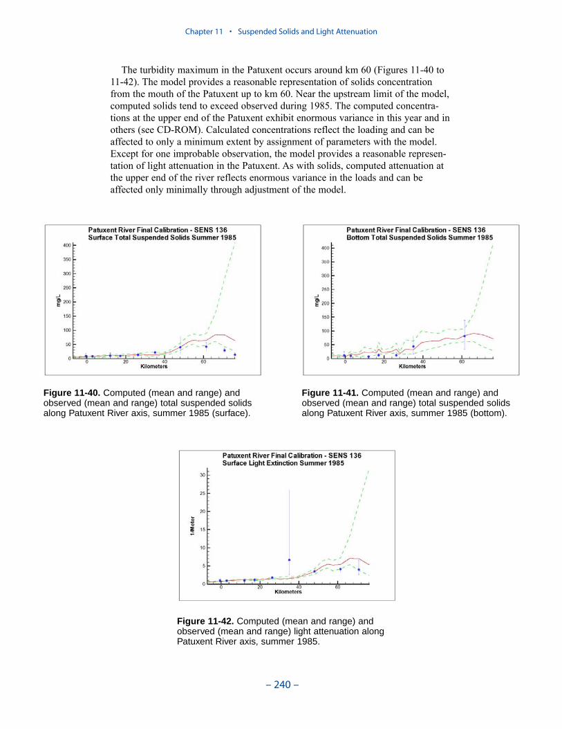
The turbidity maximum in the Patuxent occurs around km 60 (Figures 11-40 to11-42). The model provides a reasonable representation of solids concentrationfrom the mouth of the Patuxent up to km 60. Near the upstream limit of the model,computed solids tend to exceed observed during 1985. The computed concentra-tions at the upper end of the Patuxent exhibit enormous variance in this year and inothers (see CD-ROM). Calculated concentrations reflect the loading and can beaffected to only a minimum extent by assignment of parameters with the model.Except for one improbable observation, the model provides a reasonable represen-tation of light attenuation in the Patuxent. As with solids, computed attenuation atthe upper end of the river reflects enormous variance in the loads and can beaffected only minimally through adjustment of the model.
Chapter 11 • Suspended Solids and Light Attenuation
– 240 –
Figure 11-40. Computed (mean and range) andobserved (mean and range) total suspended solidsalong Patuxent River axis, summer 1985 (surface).
Figure 11-41. Computed (mean and range) andobserved (mean and range) total suspended solidsalong Patuxent River axis, summer 1985 (bottom).
Figure 11-42. Computed (mean and range) andobserved (mean and range) light attenuation alongPatuxent River axis, summer 1985.
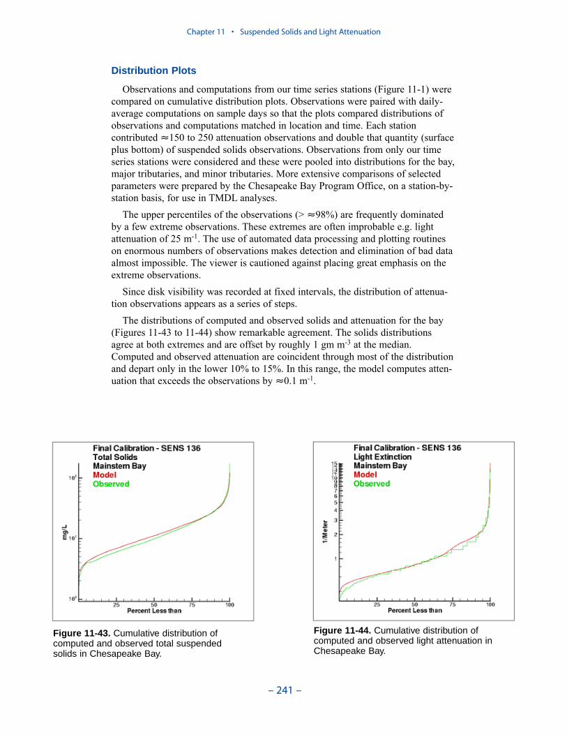
Distribution Plots
Observations and computations from our time series stations (Figure 11-1) werecompared on cumulative distribution plots. Observations were paired with daily-average computations on sample days so that the plots compared distributions ofobservations and computations matched in location and time. Each stationcontributed ≈150 to 250 attenuation observations and double that quantity (surfaceplus bottom) of suspended solids observations. Observations from only our timeseries stations were considered and these were pooled into distributions for the bay,major tributaries, and minor tributaries. More extensive comparisons of selectedparameters were prepared by the Chesapeake Bay Program Office, on a station-by-station basis, for use in TMDL analyses.
The upper percentiles of the observations (> ≈98%) are frequently dominatedby a few extreme observations. These extremes are often improbable e.g. lightattenuation of 25 m-1. The use of automated data processing and plotting routineson enormous numbers of observations makes detection and elimination of bad dataalmost impossible. The viewer is cautioned against placing great emphasis on theextreme observations.
Since disk visibility was recorded at fixed intervals, the distribution of attenua-tion observations appears as a series of steps.
The distributions of computed and observed solids and attenuation for the bay(Figures 11-43 to 11-44) show remarkable agreement. The solids distributionsagree at both extremes and are offset by roughly 1 gm m-3 at the median.Computed and observed attenuation are coincident through most of the distributionand depart only in the lower 10% to 15%. In this range, the model computes atten-uation that exceeds the observations by ≈0.1 m-1.
Chapter 11 • Suspended Solids and Light Attenuation
– 241 –
Figure 11-43. Cumulative distribution ofcomputed and observed total suspended solids in Chesapeake Bay.
Figure 11-44. Cumulative distribution ofcomputed and observed light attenuation inChesapeake Bay.

Computed and observed solids in the James River show reasonable agreementthough the lower half of the distribution but observed solids exceed computed inthe upper half (Figure 11-45). Inspection of the time-series plots indicates inabilityof the model to match extreme solids concentrations in the bottom waters of theturbidity maximum contributes substantially to the mis-match. The attenuationdistributions (Figure 11-46), which are based solely on surface solids, agree well.
The distributions of computed and observed solids and attenuation for the YorkRiver show good agreement (Figure 11-47) through the upper half of the distribu-tion. In the lower half, computed solids exceed observed by less than 5 g m-3.Computed and observed attenuation follow a similar pattern (Figure 11-48). Agree-ment is good in the upper half of the distribution but the model overestimates by≈0.2 m-1 in the lower half.
Chapter 11 • Suspended Solids and Light Attenuation
– 242 –
Figure 11-45. Cumulative distribution of computed and observed total suspended solids in James River.
Figure 11-46. Cumulative distribution ofcomputed and observed light attenuation in James River.
Figure 11-47. Cumulative distribution ofcomputed and observed total suspendedsolids in York River.
Figure 11-48. Cumulative distribution ofcomputed and observed light attenuation in York River.
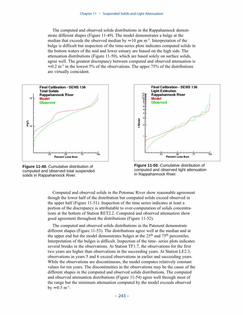
The computed and observed solids distributions in the Rappahannock demon-strate different shapes (Figure 11-49). The model demonstrates a bulge at themedian that exceeds the observed median by ≈10 gm m-3. Interpretation of thebulge is difficult but inspection of the time-series plots indicates computed solids inthe bottom waters of the mid and lower estuary are biased on the high side. Theattenuation distributions (Figure 11-50), which are based solely on surface solids,agree well. The greatest discrepancy between computed and observed attenuation is≈0.2 m-1 in the lowest 5% of the observations. The upper 75% of the distributionsare virtually coincident.
Computed and observed solids in the Potomac River show reasonable agreementthough the lower half of the distribution but computed solids exceed observed inthe upper half (Figure 11-51). Inspection of the time series indicates at least aportion of the discrepancy is attributable to over-computation of solids concentra-tions at the bottom of Station RET2.2. Computed and observed attenuation showgood agreement throughout the distributions (Figure 11-52).
The computed and observed solids distributions in the Patuxent demonstratedifferent shapes (Figure 11-53). The distributions agree well at the median and atthe upper end but the model demonstrates bulges at the 25th and 75th percentiles.Interpretation of the bulges is difficult. Inspection of the time- series plots indicatesseveral breaks in the observations. At Station TF1.7, the observations for the firsttwo years are higher than observations in the succeeding years. At Station LE2.3,observations in years 5 and 6 exceed observations in earlier and succeeding years.While the observations are discontinuous, the model computes relatively constantvalues for ten years. The discontinuities in the observations may be the cause of thedifferent shapes in the computed and observed solids distributions. The computedand observed attenuation distributions (Figure 11-54) agree well through most ofthe range but the minimum attenuation computed by the model exceeds observedby ≈0.5 m-1.
Chapter 11 • Suspended Solids and Light Attenuation
– 243 –
Figure 11-49. Cumulative distribution of computed and observed total suspended solids in Rappahannock River.
Figure 11-50. Cumulative distribution ofcomputed and observed light attenuation in Rappahannock River.
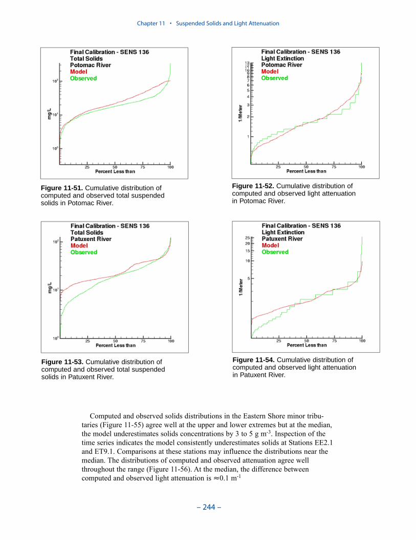
Computed and observed solids distributions in the Eastern Shore minor tribu-taries (Figure 11-55) agree well at the upper and lower extremes but at the median,the model underestimates solids concentrations by 3 to 5 g m-3. Inspection of thetime series indicates the model consistently underestimates solids at Stations EE2.1and ET9.1. Comparisons at these stations may influence the distributions near themedian. The distributions of computed and observed attenuation agree wellthroughout the range (Figure 11-56). At the median, the difference betweencomputed and observed light attenuation is ≈0.1 m-1
Chapter 11 • Suspended Solids and Light Attenuation
– 244 –
Figure 11-51. Cumulative distribution of computed and observed total suspended solids in Potomac River.
Figure 11-52. Cumulative distribution ofcomputed and observed light attenuationin Potomac River.
Figure 11-53. Cumulative distribution of computed and observed total suspended solids in Patuxent River.
Figure 11-54. Cumulative distribution ofcomputed and observed light attenuationin Patuxent River.
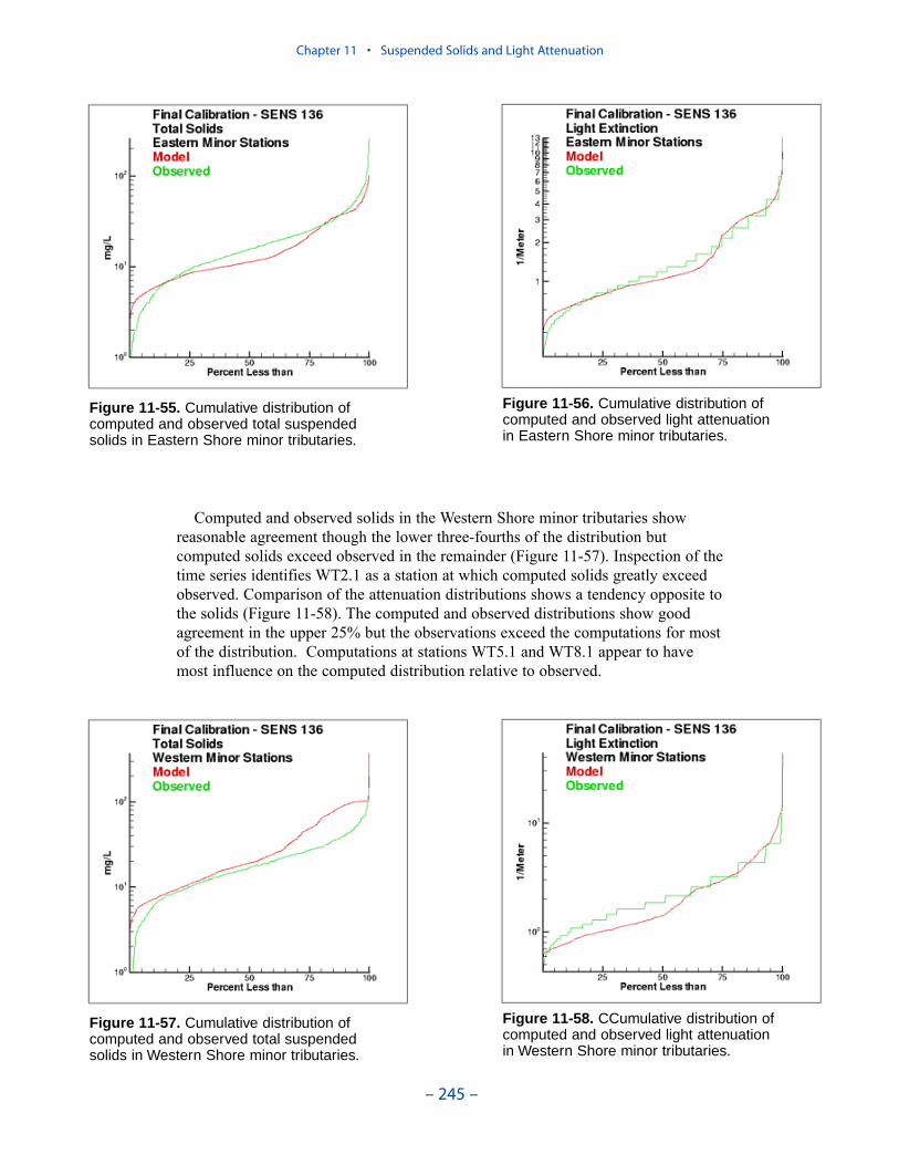
Computed and observed solids in the Western Shore minor tributaries showreasonable agreement though the lower three-fourths of the distribution butcomputed solids exceed observed in the remainder (Figure 11-57). Inspection of thetime series identifies WT2.1 as a station at which computed solids greatly exceedobserved. Comparison of the attenuation distributions shows a tendency opposite tothe solids (Figure 11-58). The computed and observed distributions show goodagreement in the upper 25% but the observations exceed the computations for mostof the distribution. Computations at stations WT5.1 and WT8.1 appear to havemost influence on the computed distribution relative to observed.
Chapter 11 • Suspended Solids and Light Attenuation
– 245 –
Figure 11-55. Cumulative distribution ofcomputed and observed total suspendedsolids in Eastern Shore minor tributaries.
Figure 11-56. Cumulative distribution ofcomputed and observed light attenuationin Eastern Shore minor tributaries.
Figure 11-57. Cumulative distribution ofcomputed and observed total suspendedsolids in Western Shore minor tributaries.
Figure 11-58. CCumulative distribution ofcomputed and observed light attenuationin Western Shore minor tributaries.
ReferencesCerco, C., and Moore, K. (2001). “System-wide submerged aquatic vegetation model forChesapeake Bay,” Estuaries, 24(4), 522-534.
Chesapeake Bay Program, United States Environmental Protection Agency. (2000).“Submerged aquatic vegetation water quality and habitat-based requirements for restorationtargets: A second technical synthesis,” CBP/TRS 245/00, EPA 903-R-00-014, AnnapolisMD.
Holmes, R. (1970). “The Secchi disk in turbid coastal waters,” Limnology and Oceanog-raphy, 15, 688-694.
Hood, R., Wang, H., Purcell, J., Houde, E., and Harding, L. (1999). “Modeling particles andpelagic organisms in Chesapeake Bay: Convergent features control plankton distributions,”Journal of Geophysical Research, 104(C1), 1223-1243.
Keefe, C., Flemer, D., and Hamilton, D. (1976). “Seston distribution in the Patuxent RiverEstuary,” Chesapeake Science, 17, 56-59.
Kirk, J. (1994). Light and photosynthesis in aquatic ecosystems. 2nd edition., CambridgeUniversity Press, Cambridge
Koenings, J., and Edmundson, J. (1991). “Secchi disk and photometer estimates of lightregimes in Alaskan lakes: Effects of yellow color and turbidity,” Limnology and Oceanog-raphy, 36(1), 91-105.
Pennock, J. (1985). “Chlorophyll distributions in the Delaware Estuary: Regulation by lightlimitation,” Estuarine, Coastal and Shelf Science, 21, 711- 725.
Schubel, J. (1968). “Turbidity maximum of the northern Chesapeake Bay,” Science, 161,1013-1015.
Chapter 11 • Suspended Solids and Light Attenuation
– 246 –
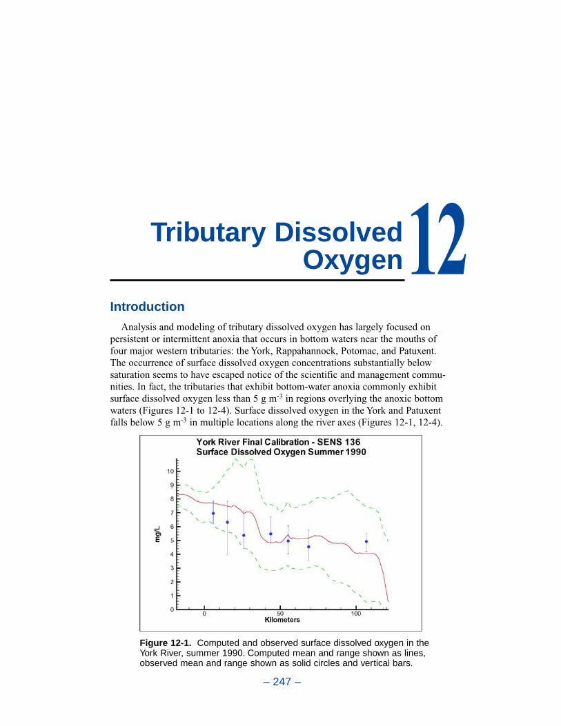
– 247 –
Tributary DissolvedOxygen12
Introduction
Analysis and modeling of tributary dissolved oxygen has largely focused onpersistent or intermittent anoxia that occurs in bottom waters near the mouths offour major western tributaries: the York, Rappahannock, Potomac, and Patuxent.The occurrence of surface dissolved oxygen concentrations substantially belowsaturation seems to have escaped notice of the scientific and management commu-nities. In fact, the tributaries that exhibit bottom-water anoxia commonly exhibitsurface dissolved oxygen less than 5 g m-3 in regions overlying the anoxic bottomwaters (Figures 12-1 to 12-4). Surface dissolved oxygen in the York and Patuxentfalls below 5 g m-3 in multiple locations along the river axes (Figures 12-1, 12-4).
Figure 12-1. Computed and observed surface dissolved oxygen in theYork River, summer 1990. Computed mean and range shown as lines,observed mean and range shown as solid circles and vertical bars.
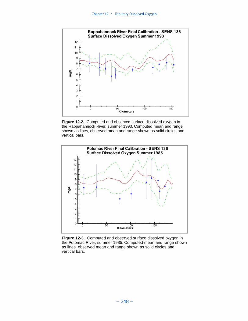
Chapter 12 • Tributary Dissolved Oxygen
– 248 –
Figure 12-2. Computed and observed surface dissolved oxygen in the Rappahannock River, summer 1993. Computed mean and rangeshown as lines, observed mean and range shown as solid circles andvertical bars.
Figure 12-3. Computed and observed surface dissolved oxygen inthe Potomac River, summer 1985. Computed mean and range shownas lines, observed mean and range shown as solid circles andvertical bars.
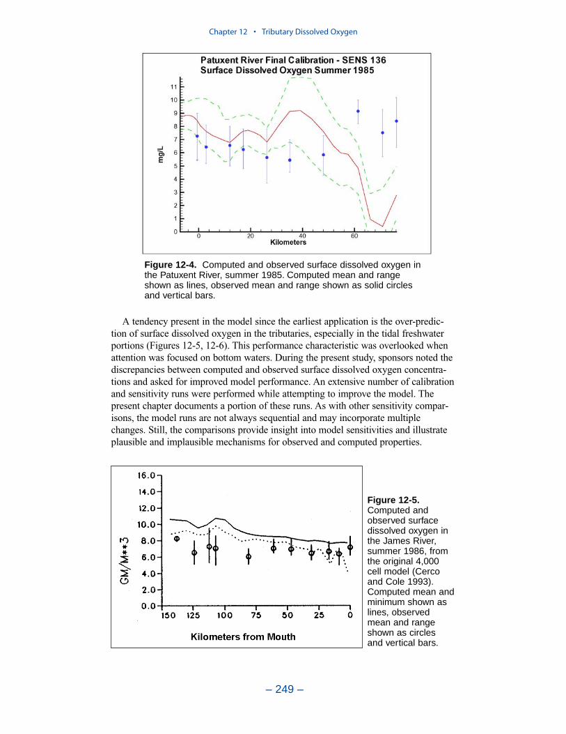
A tendency present in the model since the earliest application is the over-predic-tion of surface dissolved oxygen in the tributaries, especially in the tidal freshwaterportions (Figures 12-5, 12-6). This performance characteristic was overlooked whenattention was focused on bottom waters. During the present study, sponsors noted thediscrepancies between computed and observed surface dissolved oxygen concentra-tions and asked for improved model performance. An extensive number of calibrationand sensitivity runs were performed while attempting to improve the model. Thepresent chapter documents a portion of these runs. As with other sensitivity compar-isons, the model runs are not always sequential and may incorporate multiplechanges. Still, the comparisons provide insight into model sensitivities and illustrateplausible and implausible mechanisms for observed and computed properties.
Chapter 12 • Tributary Dissolved Oxygen
– 249 –
Figure 12-4. Computed and observed surface dissolved oxygen inthe Patuxent River, summer 1985. Computed mean and rangeshown as lines, observed mean and range shown as solid circlesand vertical bars.
Figure 12-5.Computed andobserved surfacedissolved oxygen inthe James River,summer 1986, fromthe original 4,000cell model (Cercoand Cole 1993).Computed mean andminimum shown aslines, observedmean and rangeshown as circles and vertical bars.

Dissolved Organic Carbon Mineralization Rate
The dissolved organic carbon mineralization (or respiration) rate is a key deter-minant of oxygen consumption in the water column. As a sensitivity test, wemultiplied the respiration rate by an order of magnitude, from 0.01 d-1 to 0.1 d-1 at20 oC. Major reaches of the tributaries were insensitive to an order-of- magnitudeincrease in the first-order rate (Figures 12-7, 12-8). Only reaches in the immediatevicinity of a carbon source, e.g. the Potomac below the District of Columbia,showed significant response to an increase in respiration rate. Lack of generalresponse indicated that oxygen consumption could not be increased without anincrease in oxygen-demanding material. An increase in first-order rate alone wouldnot suffice. In addition, the rate increase produced unacceptably low computationsof total organic carbon (Figures 12-9, 12-10).
Chapter 12 • Tributary Dissolved Oxygen
– 250 –
Figure 12-6.Computed andobserved surfacedissolved oxygen in the Potomac River,summer 1986, from the original 4,000 cellmodel (Cerco and Cole1993). Computed meanand minimum shown aslines, observed meanand range shown ascircles and verticalbars.
Figure 12-7. Sensitivity of Rappahannock River surface dissolved oxygen to dissolved organic carbon mineralization rate, summer 1990.
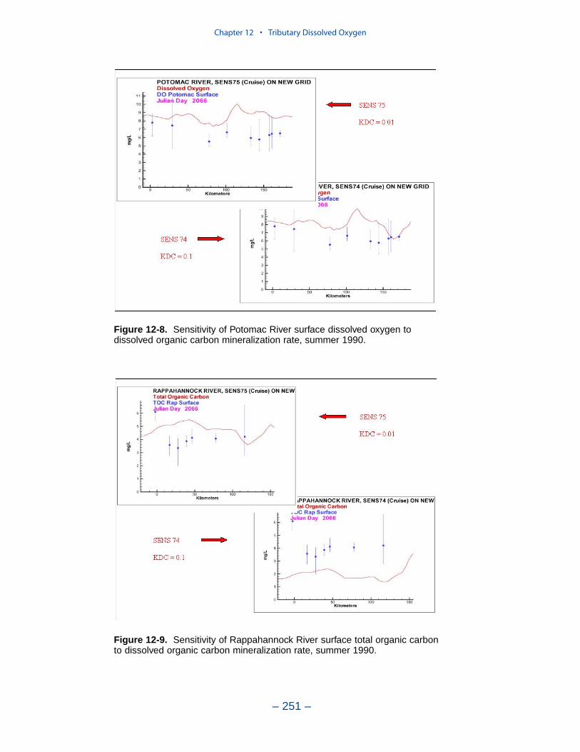
Chapter 12 • Tributary Dissolved Oxygen
– 251 –
Figure 12-8. Sensitivity of Potomac River surface dissolved oxygen to dissolved organic carbon mineralization rate, summer 1990.
Figure 12-9. Sensitivity of Rappahannock River surface total organic carbon to dissolved organic carbon mineralization rate, summer 1990.
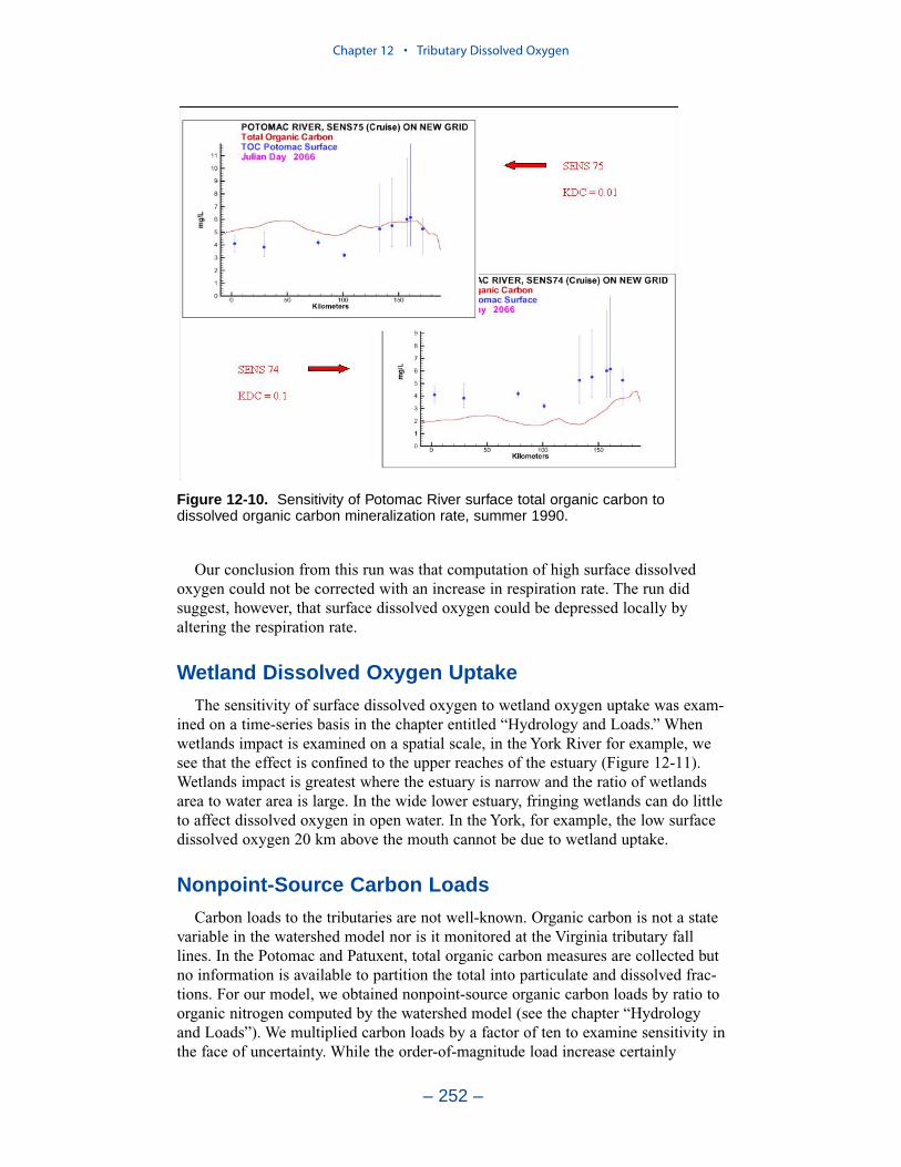
Our conclusion from this run was that computation of high surface dissolvedoxygen could not be corrected with an increase in respiration rate. The run didsuggest, however, that surface dissolved oxygen could be depressed locally byaltering the respiration rate.
Wetland Dissolved Oxygen Uptake
The sensitivity of surface dissolved oxygen to wetland oxygen uptake was exam-ined on a time-series basis in the chapter entitled “Hydrology and Loads.” Whenwetlands impact is examined on a spatial scale, in the York River for example, wesee that the effect is confined to the upper reaches of the estuary (Figure 12-11).Wetlands impact is greatest where the estuary is narrow and the ratio of wetlandsarea to water area is large. In the wide lower estuary, fringing wetlands can do littleto affect dissolved oxygen in open water. In the York, for example, the low surfacedissolved oxygen 20 km above the mouth cannot be due to wetland uptake.
Nonpoint-Source Carbon Loads
Carbon loads to the tributaries are not well-known. Organic carbon is not a statevariable in the watershed model nor is it monitored at the Virginia tributary falllines. In the Potomac and Patuxent, total organic carbon measures are collected butno information is available to partition the total into particulate and dissolved frac-tions. For our model, we obtained nonpoint-source organic carbon loads by ratio toorganic nitrogen computed by the watershed model (see the chapter “Hydrologyand Loads”). We multiplied carbon loads by a factor of ten to examine sensitivity inthe face of uncertainty. While the order-of-magnitude load increase certainly
Chapter 12 • Tributary Dissolved Oxygen
– 252 –
Figure 12-10. Sensitivity of Potomac River surface total organic carbon todissolved organic carbon mineralization rate, summer 1990.
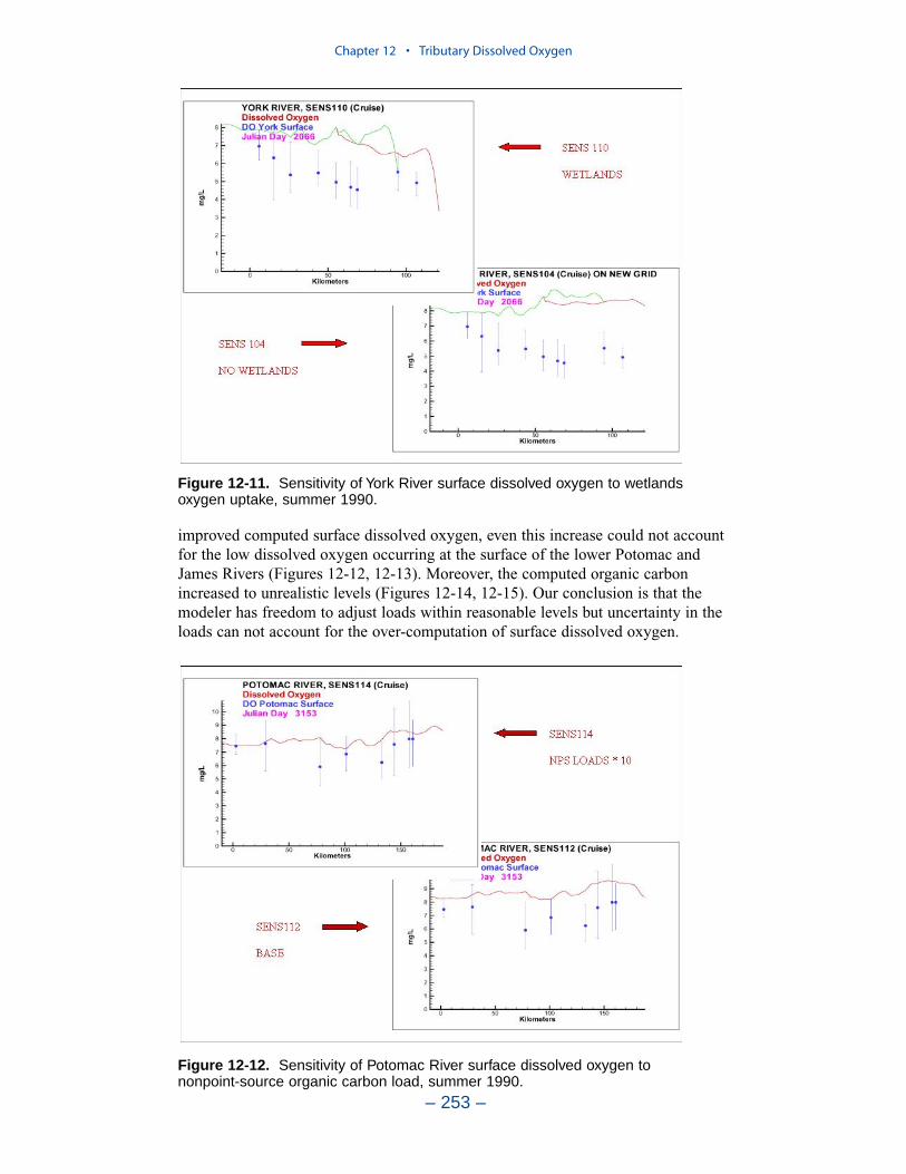
improved computed surface dissolved oxygen, even this increase could not accountfor the low dissolved oxygen occurring at the surface of the lower Potomac andJames Rivers (Figures 12-12, 12-13). Moreover, the computed organic carbonincreased to unrealistic levels (Figures 12-14, 12-15). Our conclusion is that themodeler has freedom to adjust loads within reasonable levels but uncertainty in theloads can not account for the over-computation of surface dissolved oxygen.
Chapter 12 • Tributary Dissolved Oxygen
– 253 –
Figure 12-11. Sensitivity of York River surface dissolved oxygen to wetlandsoxygen uptake, summer 1990.
Figure 12-12. Sensitivity of Potomac River surface dissolved oxygen to nonpoint-source organic carbon load, summer 1990.
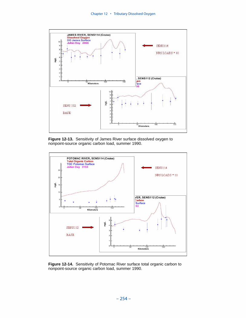
Chapter 12 • Tributary Dissolved Oxygen
– 254 –
Figure 12-13. Sensitivity of James River surface dissolved oxygen to nonpoint-source organic carbon load, summer 1990.
Figure 12-14. Sensitivity of Potomac River surface total organic carbon to nonpoint-source organic carbon load, summer 1990.
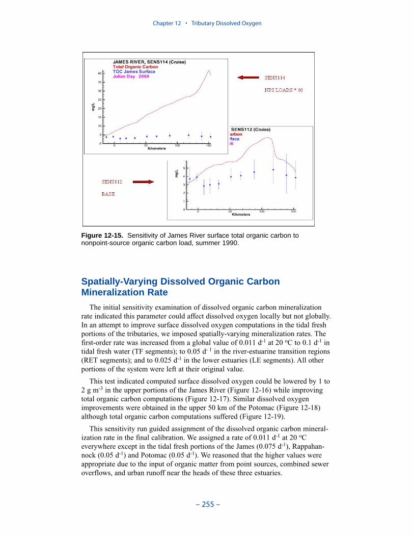
Spatially-Varying Dissolved Organic Carbon Mineralization Rate
The initial sensitivity examination of dissolved organic carbon mineralizationrate indicated this parameter could affect dissolved oxygen locally but not globally.In an attempt to improve surface dissolved oxygen computations in the tidal freshportions of the tributaries, we imposed spatially-varying mineralization rates. Thefirst-order rate was increased from a global value of 0.011 d-1 at 20 oC to 0.1 d-1 intidal fresh water (TF segments); to 0.05 d- 1 in the river-estuarine transition regions(RET segments); and to 0.025 d-1 in the lower estuaries (LE segments). All otherportions of the system were left at their original value.
This test indicated computed surface dissolved oxygen could be lowered by 1 to2 g m-3 in the upper portions of the James River (Figure 12-16) while improvingtotal organic carbon computations (Figure 12-17). Similar dissolved oxygenimprovements were obtained in the upper 50 km of the Potomac (Figure 12-18)although total organic carbon computations suffered (Figure 12-19).
This sensitivity run guided assignment of the dissolved organic carbon mineral-ization rate in the final calibration. We assigned a rate of 0.011 d-1 at 20 oCeverywhere except in the tidal fresh portions of the James (0.075 d-1), Rappahan-nock (0.05 d-1) and Potomac (0.05 d-1). We reasoned that the higher values wereappropriate due to the input of organic matter from point sources, combined seweroverflows, and urban runoff near the heads of these three estuaries.
Chapter 12 • Tributary Dissolved Oxygen
– 255 –
Figure 12-15. Sensitivity of James River surface total organic carbon to nonpoint-source organic carbon load, summer 1990.
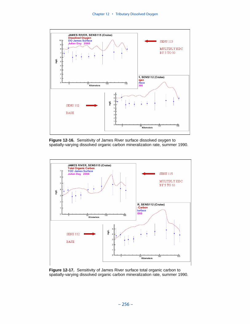
Chapter 12 • Tributary Dissolved Oxygen
– 256 –
Figure 12-16. Sensitivity of James River surface dissolved oxygen to spatially-varying dissolved organic carbon mineralization rate, summer 1990.
Figure 12-17. Sensitivity of James River surface total organic carbon to spatially-varying dissolved organic carbon mineralization rate, summer 1990.

Chapter 12 • Tributary Dissolved Oxygen
– 257 –
Figure 12-19. Sensitivity of Potomac River surface total organic carbon tospatially-varying dissolved organic carbon mineralization rate, summer 1990.
Figure 12-18 Sensitivity of Potomac River surface dissolved oxygen to spatially-varying dissolved organic carbon mineralization rate, summer 1990.
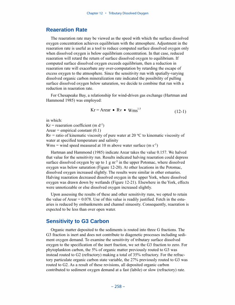
Chapter 12 • Tributary Dissolved Oxygen
– 258 –
Reaeration Rate
The reaeration rate may be viewed as the speed with which the surface dissolvedoxygen concentration achieves equilibrium with the atmosphere. Adjustment in thereaeration rate is useful as a tool to reduce computed surface dissolved oxygen onlywhen dissolved oxygen is below equilibrium concentration. In that case, reducedreaeration will retard the return of surface dissolved oxygen to equilibrium. Ifcomputed surface dissolved oxygen exceeds equilibrium, then a reduction inreaeration rate will exacerbate any over-computation by retarding the escape ofexcess oxygen to the atmosphere. Since the sensitivity run with spatially-varyingdissolved organic carbon mineralization rate indicated the possibility of pullingsurface dissolved oxygen below saturation, we decide to combine that run with areduction in reaeration rate.
For Chesapeake Bay, a relationship for wind-driven gas exchange (Hartman andHammond 1985) was employed:
in which:Kr = reaeration coefficient (m d-1)Arear = empirical constant (0.1)Rυ = ratio of kinematic viscosity of pure water at 20 oC to kinematic viscosity ofwater at specified temperature and salinityWms = wind speed measured at 10 m above water surface (m s-1)
Hartman and Hammond (1985) indicate Arear takes the value 0.157. We halvedthat value for the sensitivity run. Results indicated halving reaeration could depresssurface dissolved oxygen by up to 1 g m-3 in the upper Potomac, where dissolvedoxygen was below saturation (Figure 12-20). At other locations in the Potomac,dissolved oxygen increased slightly. The results were similar in other estuaries.Halving reaeration decreased dissolved oxygen in the upper York, where dissolvedoxygen was drawn down by wetlands (Figure 12-21). Elsewhere in the York, effectswere unnoticeable or else dissolved oxygen increased slightly.
Upon assessing the results of these and other sensitivity runs, we opted to retainthe value of Arear = 0.078. Use of this value is readily justified. Fetch in the estu-aries is reduced by embankments and channel sinuosity. Consequently, reaeration isexpected to be less than over open water.
Sensitivity to G3 Carbon
Organic matter deposited to the sediments is routed into three G fractions. TheG3 fraction is inert and does not contribute to diagenetic processes including sedi-ment oxygen demand. To examine the sensitivity of tributary surface dissolvedoxygen to the specification of the inert fraction, we set the G3 fraction to zero. Forphytoplankton carbon, the 5% of organic matter previously routed to G3 wasinstead routed to G2 (refractory) making a total of 35% refractory. For the refrac-tory particulate organic carbon state variable, the 27% previously routed to G3 wasrouted to G2. As a result of these revisions, all deposited organic carboncontributed to sediment oxygen demand at a fast (labile) or slow (refractory) rate.
WmsRArear=Kr 1.5(12-1)
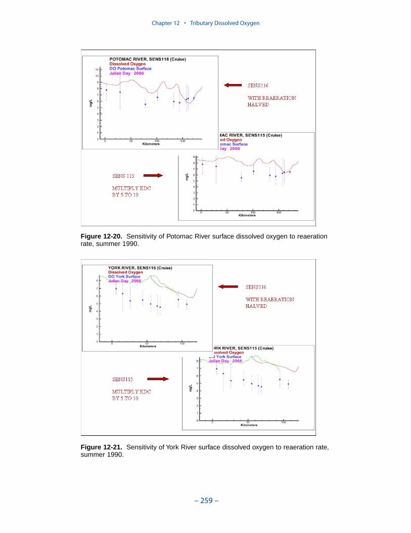
Chapter 12 • Tributary Dissolved Oxygen
– 259 –
Figure 12-20. Sensitivity of Potomac River surface dissolved oxygen to reaerationrate, summer 1990.
Figure 12-21. Sensitivity of York River surface dissolved oxygen to reaeration rate,summer 1990.
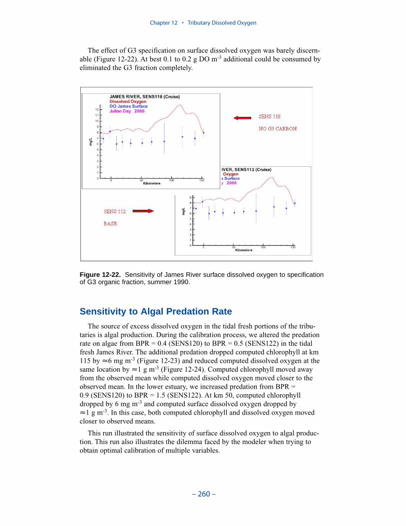
The effect of G3 specification on surface dissolved oxygen was barely discern-able (Figure 12-22). At best 0.1 to 0.2 g DO m-3 additional could be consumed byeliminated the G3 fraction completely.
Sensitivity to Algal Predation Rate
The source of excess dissolved oxygen in the tidal fresh portions of the tribu-taries is algal production. During the calibration process, we altered the predationrate on algae from BPR = 0.4 (SENS120) to BPR = 0.5 (SENS122) in the tidalfresh James River. The additional predation dropped computed chlorophyll at km115 by ≈6 mg m-3 (Figure 12-23) and reduced computed dissolved oxygen at thesame location by ≈1 g m-3 (Figure 12-24). Computed chlorophyll moved awayfrom the observed mean while computed dissolved oxygen moved closer to theobserved mean. In the lower estuary, we increased predation from BPR = 0.9 (SENS120) to BPR = 1.5 (SENS122). At km 50, computed chlorophyll dropped by 6 mg m-3 and computed surface dissolved oxygen dropped by ≈1 g m-3. In this case, both computed chlorophyll and dissolved oxygen movedcloser to observed means.
This run illustrated the sensitivity of surface dissolved oxygen to algal produc-tion. This run also illustrates the dilemma faced by the modeler when trying toobtain optimal calibration of multiple variables.
Chapter 12 • Tributary Dissolved Oxygen
– 260 –
Figure 12-22. Sensitivity of James River surface dissolved oxygen to specificationof G3 organic fraction, summer 1990.
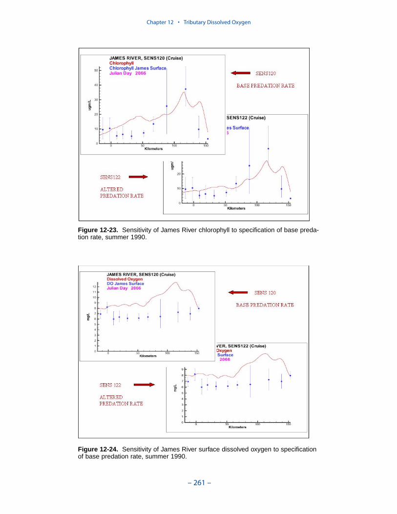
Chapter 12 • Tributary Dissolved Oxygen
– 261 –
Figure 12-23. Sensitivity of James River chlorophyll to specification of base preda-tion rate, summer 1990.
Figure 12-24. Sensitivity of James River surface dissolved oxygen to specificationof base predation rate, summer 1990.
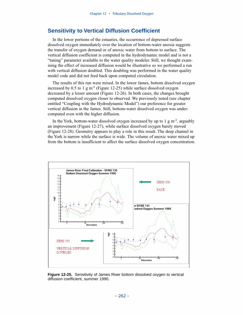
Sensitivity to Vertical Diffusion Coefficient
In the lower portions of the estuaries, the occurrence of depressed surfacedissolved oxygen immediately over the location of bottom-water anoxia suggeststhe transfer of oxygen demand or of anoxic water from bottom to surface. Thevertical diffusion coefficient is computed in the hydrodynamic model and is not a“tuning” parameter available to the water quality modeler. Still, we thought exam-ining the effect of increased diffusion would be illustrative so we performed a runwith vertical diffusion doubled. This doubling was performed in the water qualitymodel code and did not feed back upon computed circulation.
The results of this run were mixed. In the lower James, bottom dissolved oxygenincreased by 0.5 to 1 g m-3 (Figure 12-25) while surface dissolved oxygendecreased by a lesser amount (Figure 12-26). In both cases, the changes broughtcomputed dissolved oxygen closer to observed. We previously noted (see chapterentitled “Coupling with the Hydrodynamic Model”) our preference for greatervertical diffusion in the James. Still, bottom-water dissolved oxygen was under-computed even with the higher diffusion.
In the York, bottom-water dissolved oxygen increased by up to 1 g m-3, arguablyan improvement (Figure 12-27), while surface dissolved oxygen barely moved(Figure 12-28). Geometry appears to play a role in this result. The deep channel inthe York is narrow while the surface is wide. The volume of anoxic water mixed upfrom the bottom is insufficient to affect the surface dissolved oxygen concentration.
Chapter 12 • Tributary Dissolved Oxygen
– 262 –
Figure 12-25. Sensitivity of James River bottom dissolved oxygen to verticaldiffusion coefficient, summer 1990.
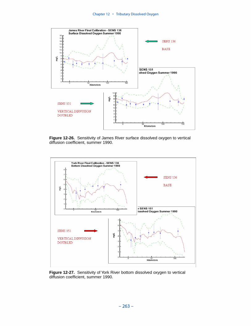
Chapter 12 • Tributary Dissolved Oxygen
– 263 –
Figure 12-26. Sensitivity of James River surface dissolved oxygen to verticaldiffusion coefficient, summer 1990.
Figure 12-27. Sensitivity of York River bottom dissolved oxygen to vertical diffusion coefficient, summer 1990.
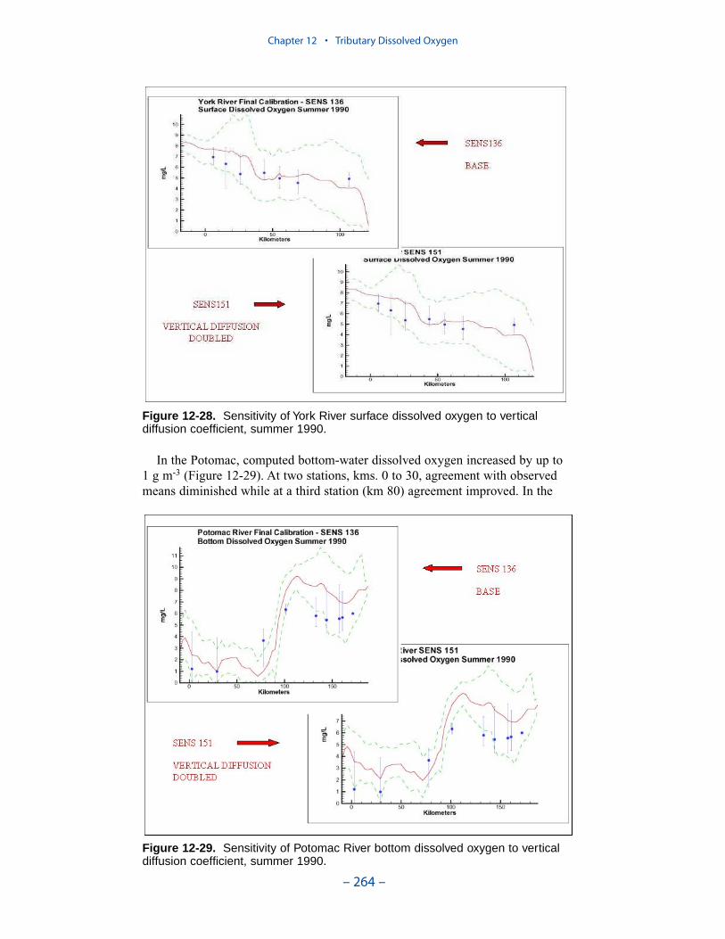
In the Potomac, computed bottom-water dissolved oxygen increased by up to 1 g m-3 (Figure 12-29). At two stations, kms. 0 to 30, agreement with observedmeans diminished while at a third station (km 80) agreement improved. In the
Chapter 12 • Tributary Dissolved Oxygen
– 264 –
Figure 12-28. Sensitivity of York River surface dissolved oxygen to verticaldiffusion coefficient, summer 1990.
Figure 12-29. Sensitivity of Potomac River bottom dissolved oxygen to verticaldiffusion coefficient, summer 1990.
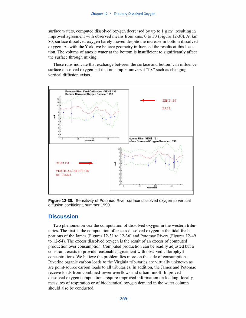
surface waters, computed dissolved oxygen decreased by up to 1 g m-3 resulting inimproved agreement with observed means from kms. 0 to 30 (Figure 12-30). At km80, surface dissolved oxygen barely moved despite the increase in bottom dissolvedoxygen. As with the York, we believe geometry influenced the results at this loca-tion. The volume of anoxic water at the bottom is insufficient to significantly affectthe surface through mixing.
These runs indicate that exchange between the surface and bottom can influencesurface dissolved oxygen but that no simple, universal “fix” such as changingvertical diffusion exists.
Discussion
Two phenomenon vex the computation of dissolved oxygen in the western tribu-taries. The first is the computation of excess dissolved oxygen in the tidal freshportions of the James (Figures 12-31 to 12-36) and Potomac Rivers (Figures 12-49to 12-54). The excess dissolved oxygen is the result of an excess of computedproduction over consumption. Computed production can be readily adjusted but aconstraint exists to provide reasonable agreement with observed chlorophyllconcentrations. We believe the problem lies more on the side of consumption.Riverine organic carbon loads to the Virginia tributaries are virtually unknown asare point-source carbon loads to all tributaries. In addition, the James and Potomacreceive loads from combined-sewer overflows and urban runoff. Improveddissolved oxygen computations require improved information on loading. Ideally,measures of respiration or of biochemical oxygen demand in the water columnshould also be conducted.
Chapter 12 • Tributary Dissolved Oxygen
– 265 –
Figure 12-30. Sensitivity of Potomac River surface dissolved oxygen to verticaldiffusion coefficient, summer 1990.

Chapter 12 • Tributary Dissolved Oxygen
– 266 –
Figure 12-31. Computed and observed surface dissolvedoxygen in the James River, summer 1985. Computed meanand range shown as lines, observed mean and rangeshown as solid circles and vertical bars.
Figure 12-32. Computed and observed bottom dissolvedoxygen in the James River, summer 1985. Computedmean and range shown as lines, observed mean andrange shown as solid circles and vertical bars.
Figure 12-33. Computed and observed surface dissolvedoxygen in the James River, summer 1990. Computed meanand range shown as lines, observed mean and rangeshown as solid circles and vertical bars.
Figure 12-34. Computed and observed bottom dissolvedoxygen in the James River, summer 1990. Computedmean and range shown as lines, observed mean andrange shown as solid circles and vertical bars.
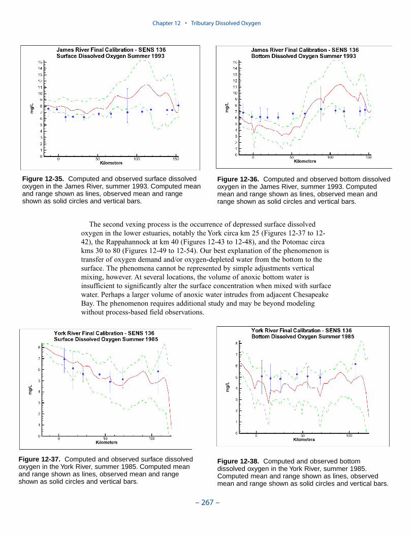
The second vexing process is the occurrence of depressed surface dissolvedoxygen in the lower estuaries, notably the York circa km 25 (Figures 12-37 to 12-42), the Rappahannock at km 40 (Figures 12-43 to 12-48), and the Potomac circakms 30 to 80 (Figures 12-49 to 12-54). Our best explanation of the phenomenon istransfer of oxygen demand and/or oxygen-depleted water from the bottom to thesurface. The phenomena cannot be represented by simple adjustments verticalmixing, however. At several locations, the volume of anoxic bottom water isinsufficient to significantly alter the surface concentration when mixed with surfacewater. Perhaps a larger volume of anoxic water intrudes from adjacent ChesapeakeBay. The phenomenon requires additional study and may be beyond modelingwithout process-based field observations.
Chapter 12 • Tributary Dissolved Oxygen
– 267 –
Figure 12-35. Computed and observed surface dissolvedoxygen in the James River, summer 1993. Computed meanand range shown as lines, observed mean and rangeshown as solid circles and vertical bars.
Figure 12-36. Computed and observed bottom dissolvedoxygen in the James River, summer 1993. Computedmean and range shown as lines, observed mean andrange shown as solid circles and vertical bars.
Figure 12-37. Computed and observed surface dissolvedoxygen in the York River, summer 1985. Computed meanand range shown as lines, observed mean and rangeshown as solid circles and vertical bars.
Figure 12-38. Computed and observed bottomdissolved oxygen in the York River, summer 1985.Computed mean and range shown as lines, observedmean and range shown as solid circles and vertical bars.
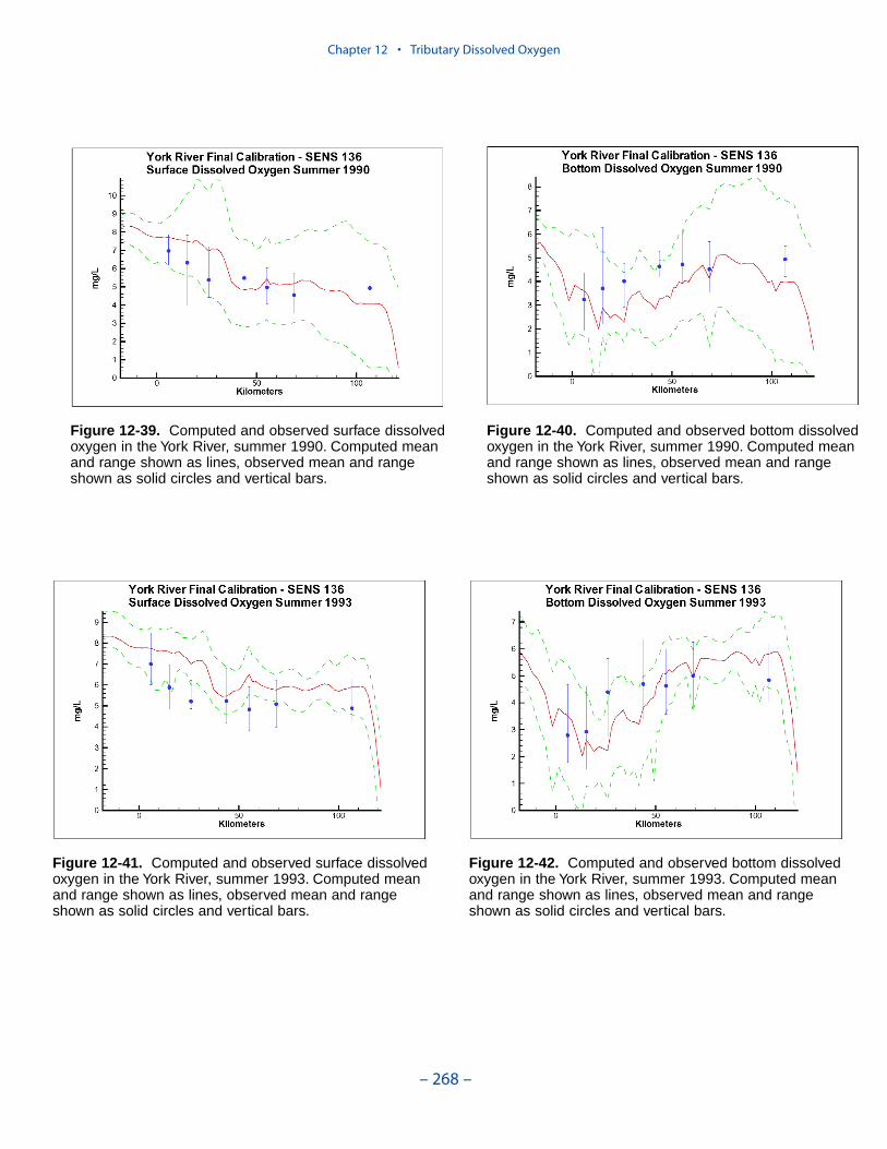
Chapter 12 • Tributary Dissolved Oxygen
– 268 –
Figure 12-39. Computed and observed surface dissolvedoxygen in the York River, summer 1990. Computed meanand range shown as lines, observed mean and rangeshown as solid circles and vertical bars.
Figure 12-40. Computed and observed bottom dissolvedoxygen in the York River, summer 1990. Computed meanand range shown as lines, observed mean and rangeshown as solid circles and vertical bars.
Figure 12-41. Computed and observed surface dissolvedoxygen in the York River, summer 1993. Computed meanand range shown as lines, observed mean and rangeshown as solid circles and vertical bars.
Figure 12-42. Computed and observed bottom dissolvedoxygen in the York River, summer 1993. Computed meanand range shown as lines, observed mean and rangeshown as solid circles and vertical bars.
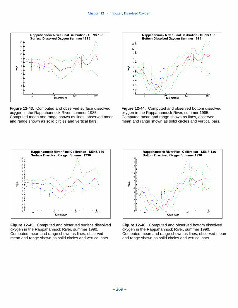
Chapter 12 • Tributary Dissolved Oxygen
– 269 –
Figure 12-43. Computed and observed surface dissolvedoxygen in the Rappahannock River, summer 1985.Computed mean and range shown as lines, observed meanand range shown as solid circles and vertical bars.
Figure 12-44. Computed and observed bottom dissolvedoxygen in the Rappahannock River, summer 1985.Computed mean and range shown as lines, observedmean and range shown as solid circles and vertical bars.
Figure 12-46. Computed and observed bottom dissolvedoxygen in the Rappahannock River, summer 1990.Computed mean and range shown as lines, observed meanand range shown as solid circles and vertical bars.
Figure 12-45. Computed and observed surface dissolvedoxygen in the Rappahannock River, summer 1990.Computed mean and range shown as lines, observedmean and range shown as solid circles and vertical bars.
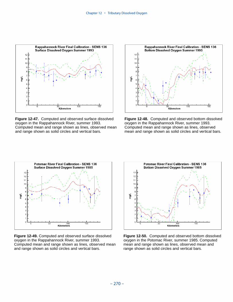
Chapter 12 • Tributary Dissolved Oxygen
– 270 –
Figure 12-47. Computed and observed surface dissolvedoxygen in the Rappahannock River, summer 1993.Computed mean and range shown as lines, observed meanand range shown as solid circles and vertical bars.
Figure 12-48. Computed and observed bottom dissolvedoxygen in the Rappahannock River, summer 1993.Computed mean and range shown as lines, observedmean and range shown as solid circles and vertical bars.
Figure 12-49. Computed and observed surface dissolvedoxygen in the Rappahannock River, summer 1993.Computed mean and range shown as lines, observed meanand range shown as solid circles and vertical bars.
Figure 12-50. Computed and observed bottom dissolvedoxygen in the Potomac River, summer 1985. Computedmean and range shown as lines, observed mean andrange shown as solid circles and vertical bars.
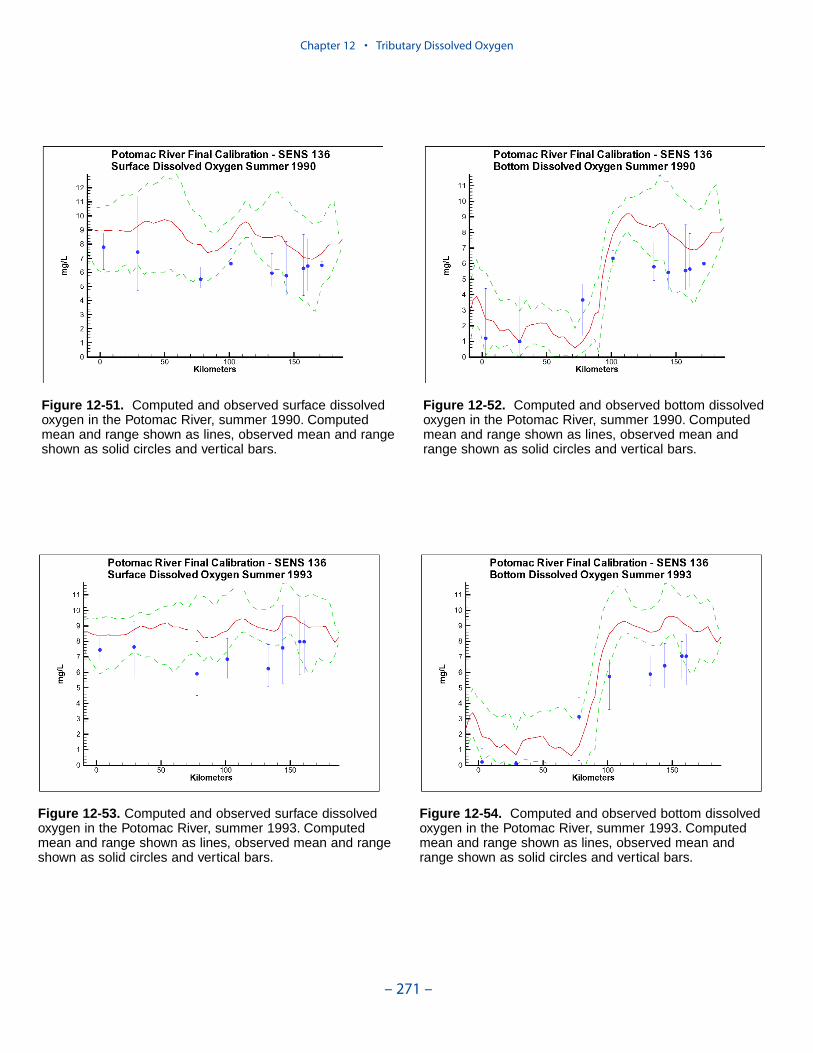
Chapter 12 • Tributary Dissolved Oxygen
– 271 –
Figure 12-51. Computed and observed surface dissolvedoxygen in the Potomac River, summer 1990. Computedmean and range shown as lines, observed mean and rangeshown as solid circles and vertical bars.
Figure 12-52. Computed and observed bottom dissolvedoxygen in the Potomac River, summer 1990. Computedmean and range shown as lines, observed mean andrange shown as solid circles and vertical bars.
Figure 12-53. Computed and observed surface dissolvedoxygen in the Potomac River, summer 1993. Computedmean and range shown as lines, observed mean and rangeshown as solid circles and vertical bars.
Figure 12-54. Computed and observed bottom dissolvedoxygen in the Potomac River, summer 1993. Computedmean and range shown as lines, observed mean andrange shown as solid circles and vertical bars.
Our model consistently under-computes dissolved oxygen in the bottom water ofthe lower James estuary (Figures 12-31 to 12-36). Here, an increase in verticalmixing is a fruitful approach to improving the computation. We did not adapt thisapproach since we were required to use a single formulation for vertical mixingsystem-wide. An alternative approach to improving dissolved oxygen in the Jamesmay be to increase longitudinal net circulation. Kuo and Neilson (1987) determineddissolved oxygen concentration in James River bottom water was maintained bystrong circulation; residence time in the bottom water was too short for anoxia todevelop. Increasing net circulation requires adjustments in the hydrodynamic modelrepresentations of viscosity and diffusivity. Whether simple adjustments in verticalmixing are made or whether more complex adjustments in circulation areattempted, refinement of the hydrodynamic model of the James is required beforeimprovements in the water quality model can result.
We have said little about the dissolved oxygen computation in the Patuxent River(Figures 12-55 to 12-60). Despite two increments in resolution since the originalmodel application (Cerco and Cole 1994), this tributary seems too coarsely griddedto provide more than a first-order representation of dissolved oxygen. Problems areespecially apparent in the upper river. The channel there is tortuous, the limit oftidal intrusion is indefinite, and extensive wetlands influence water quality. Surfacedissolved oxygen in the lower Patuxent is depressed, possibly for the same reasonsas depression in the lower York, Rappahannock, and Potomac.
Each western tributary possesses unique properties and each alone couldconsume as much study as the entire Chesapeake Bay. We note that an individualmodel of the Patuxent is underway and a model of the Potomac is in the planningstages.
Gridding of each western tributary should be sufficient to provide detailed repre-sentation of the complex geometry. This requirement calls for roughly the samenumber of cells as in the present representation of Chesapeake Bay. The tributarycells will, of course, be much smaller than the current bay cells. Once a detailedgrid is completed, careful model (and perhaps field) examination of circulation andmixing processes is required, with emphasis on the lower estuaries.
The York, Rappahannock, and Patuxent Rivers adjoin extensive tidal wetlandswhich appear to influence water quality. Nutrients, as well as dissolved oxygen,are, no doubt, exchanged between wetlands and channel. To represent the wetlandsphysically, addition of wetting-and-drying to the hydrodynamic model is required.A wetland biogeochemical module should be added to the water quality model.And, as with so many processes, field investigations may also be necessary.
Measures of loads of carbonaceous oxygen-demanding material to the tributariesare nearly unknown. Large-scale eutrophication modeling presupposes that algalproduction is the predominant source of oxygen demand. System-wide, thispremise is certainly true but in confined portions of the tributaries, in the presenceof inputs from multiple sources, external loads of oxygen-demanding materialcannot be ignored. Monitoring of inputs and, perhaps, addition of organic carbon tothe watershed model are recommended.
Chapter 12 • Tributary Dissolved Oxygen
– 272 –
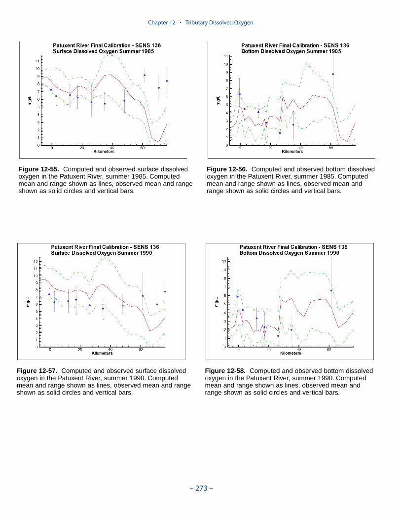
Chapter 12 • Tributary Dissolved Oxygen
– 273 –
Figure 12-55. Computed and observed surface dissolvedoxygen in the Patuxent River, summer 1985. Computedmean and range shown as lines, observed mean and rangeshown as solid circles and vertical bars.
Figure 12-56. Computed and observed bottom dissolvedoxygen in the Patuxent River, summer 1985. Computedmean and range shown as lines, observed mean andrange shown as solid circles and vertical bars.
Figure 12-57. Computed and observed surface dissolvedoxygen in the Patuxent River, summer 1990. Computedmean and range shown as lines, observed mean and rangeshown as solid circles and vertical bars.
Figure 12-58. Computed and observed bottom dissolvedoxygen in the Patuxent River, summer 1990. Computedmean and range shown as lines, observed mean andrange shown as solid circles and vertical bars.
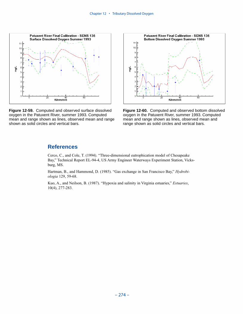
ReferencesCerco, C., and Cole, T. (1994). “Three-dimensional eutrophication model of ChesapeakeBay,” Technical Report EL-94-4, US Army Engineer Waterways Experiment Station, Vicks-burg, MS.
Hartman, B., and Hammond, D. (1985). “Gas exchange in San Francisco Bay,” Hydrobi-ologia 129, 59-68.
Kuo, A., and Neilson, B. (1987). “Hypoxia and salinity in Virginia estuaries,” Estuaries,10(4), 277-283.
Chapter 12 • Tributary Dissolved Oxygen
– 274 –
Figure 12-59. Computed and observed surface dissolvedoxygen in the Patuxent River, summer 1993. Computedmean and range shown as lines, observed mean and rangeshown as solid circles and vertical bars.
Figure 12-60. Computed and observed bottom dissolvedoxygen in the Patuxent River, summer 1993. Computedmean and range shown as lines, observed mean andrange shown as solid circles and vertical bars.
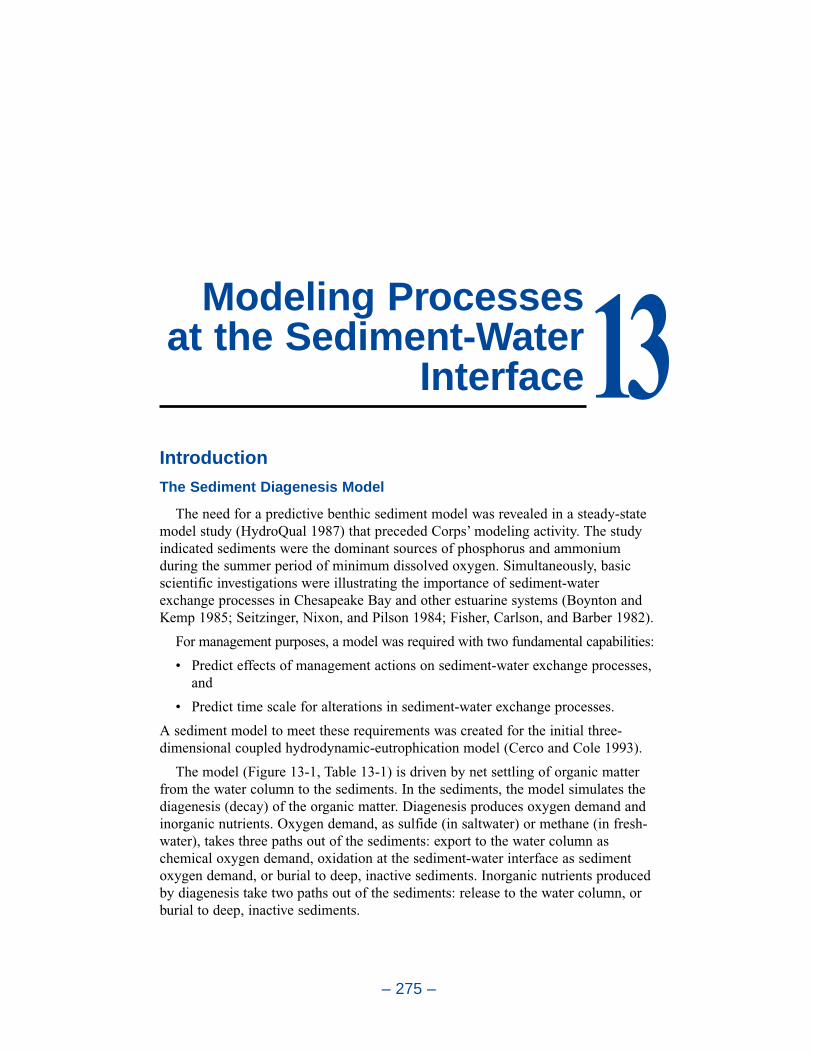
Introduction
The Sediment Diagenesis Model
The need for a predictive benthic sediment model was revealed in a steady-statemodel study (HydroQual 1987) that preceded Corps’ modeling activity. The studyindicated sediments were the dominant sources of phosphorus and ammoniumduring the summer period of minimum dissolved oxygen. Simultaneously, basicscientific investigations were illustrating the importance of sediment-waterexchange processes in Chesapeake Bay and other estuarine systems (Boynton andKemp 1985; Seitzinger, Nixon, and Pilson 1984; Fisher, Carlson, and Barber 1982).
For management purposes, a model was required with two fundamental capabilities:
• Predict effects of management actions on sediment-water exchange processes,and
• Predict time scale for alterations in sediment-water exchange processes.
A sediment model to meet these requirements was created for the initial three-dimensional coupled hydrodynamic-eutrophication model (Cerco and Cole 1993).
The model (Figure 13-1, Table 13-1) is driven by net settling of organic matterfrom the water column to the sediments. In the sediments, the model simulates thediagenesis (decay) of the organic matter. Diagenesis produces oxygen demand andinorganic nutrients. Oxygen demand, as sulfide (in saltwater) or methane (in fresh-water), takes three paths out of the sediments: export to the water column aschemical oxygen demand, oxidation at the sediment-water interface as sedimentoxygen demand, or burial to deep, inactive sediments. Inorganic nutrients producedby diagenesis take two paths out of the sediments: release to the water column, orburial to deep, inactive sediments.
– 275 –
Modeling Processesat the Sediment-Water
Interface13
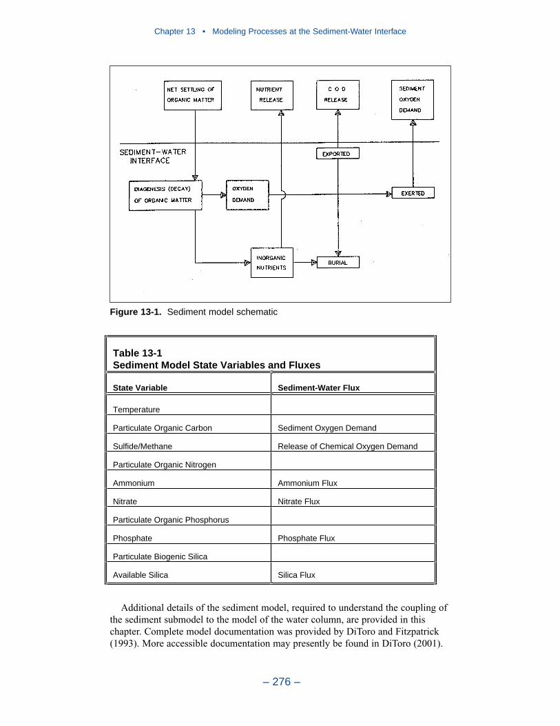
Additional details of the sediment model, required to understand the coupling ofthe sediment submodel to the model of the water column, are provided in thischapter. Complete model documentation was provided by DiToro and Fitzpatrick(1993). More accessible documentation may presently be found in DiToro (2001).
Chapter 13 • Modeling Processes at the Sediment-Water Interface
– 276 –
Figure 13-1. Sediment model schematic
Table 13-1 Sediment Model State Variables and Fluxes
State Variable Sediment-Water Flux
Temperature
Particulate Organic Carbon Sediment Oxygen Demand
Sulfide/Methane Release of Chemical Oxygen Demand
Particulate Organic Nitrogen
Ammonium Ammonium Flux
Nitrate Nitrate Flux
Particulate Organic Phosphorus
Phosphate Phosphate Flux
Particulate Biogenic Silica
Available Silica Silica Flux
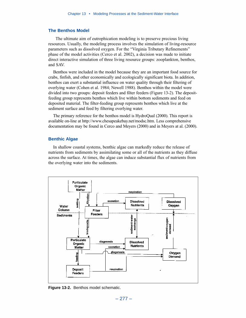
The Benthos Model
The ultimate aim of eutrophication modeling is to preserve precious livingresources. Usually, the modeling process involves the simulation of living-resourceparameters such as dissolved oxygen. For the “Virginia Tributary Refinements”phase of the model activities (Cerco et al. 2002), a decision was made to initiatedirect interactive simulation of three living resource groups: zooplankton, benthos,and SAV.
Benthos were included in the model because they are an important food source forcrabs, finfish, and other economically and ecologically significant biota. In addition,benthos can exert a substantial influence on water quality through their filtering ofoverlying water (Cohen et al. 1984; Newell 1988). Benthos within the model weredivided into two groups: deposit feeders and filter feeders (Figure 13-2). The deposit-feeding group represents benthos which live within bottom sediments and feed ondeposited material. The filter-feeding group represents benthos which live at thesediment surface and feed by filtering overlying water.
The primary reference for the benthos model is HydroQual (2000). This report isavailable on-line at http://www.chesapeakebay.net/modsc.htm. Less comprehensivedocumentation may be found in Cerco and Meyers (2000) and in Meyers at al. (2000).
Benthic Algae
In shallow coastal systems, benthic algae can markedly reduce the release ofnutrients from sediments by assimilating some or all of the nutrients as they diffuseacross the surface. At times, the algae can induce substantial flux of nutrients fromthe overlying water into the sediments.
Chapter 13 • Modeling Processes at the Sediment-Water Interface
– 277 –
Figure 13-2. Benthos model schematic.
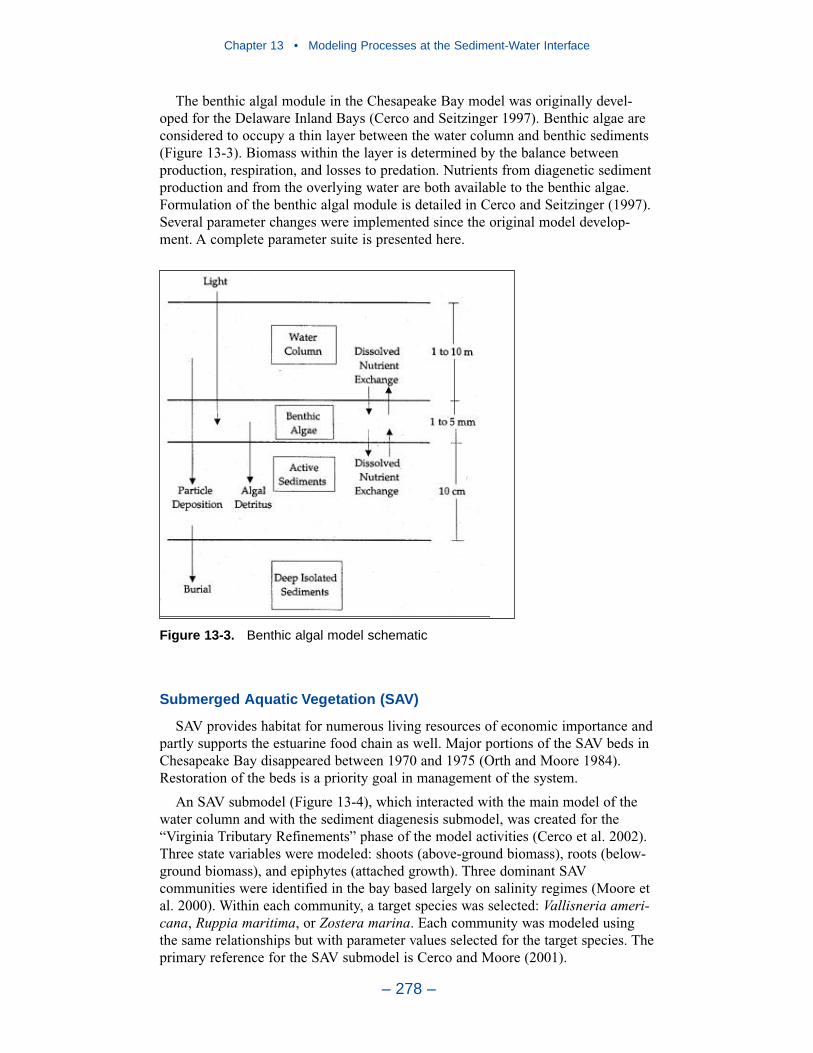
The benthic algal module in the Chesapeake Bay model was originally devel-oped for the Delaware Inland Bays (Cerco and Seitzinger 1997). Benthic algae areconsidered to occupy a thin layer between the water column and benthic sediments(Figure 13-3). Biomass within the layer is determined by the balance betweenproduction, respiration, and losses to predation. Nutrients from diagenetic sedimentproduction and from the overlying water are both available to the benthic algae.Formulation of the benthic algal module is detailed in Cerco and Seitzinger (1997).Several parameter changes were implemented since the original model develop-ment. A complete parameter suite is presented here.
Submerged Aquatic Vegetation (SAV)
SAV provides habitat for numerous living resources of economic importance andpartly supports the estuarine food chain as well. Major portions of the SAV beds inChesapeake Bay disappeared between 1970 and 1975 (Orth and Moore 1984).Restoration of the beds is a priority goal in management of the system.
An SAV submodel (Figure 13-4), which interacted with the main model of thewater column and with the sediment diagenesis submodel, was created for the“Virginia Tributary Refinements” phase of the model activities (Cerco et al. 2002).Three state variables were modeled: shoots (above-ground biomass), roots (below-ground biomass), and epiphytes (attached growth). Three dominant SAVcommunities were identified in the bay based largely on salinity regimes (Moore etal. 2000). Within each community, a target species was selected: Vallisneria ameri-cana, Ruppia maritima, or Zostera marina. Each community was modeled usingthe same relationships but with parameter values selected for the target species. Theprimary reference for the SAV submodel is Cerco and Moore (2001).
Chapter 13 • Modeling Processes at the Sediment-Water Interface
– 278 –
Figure 13-3. Benthic algal model schematic
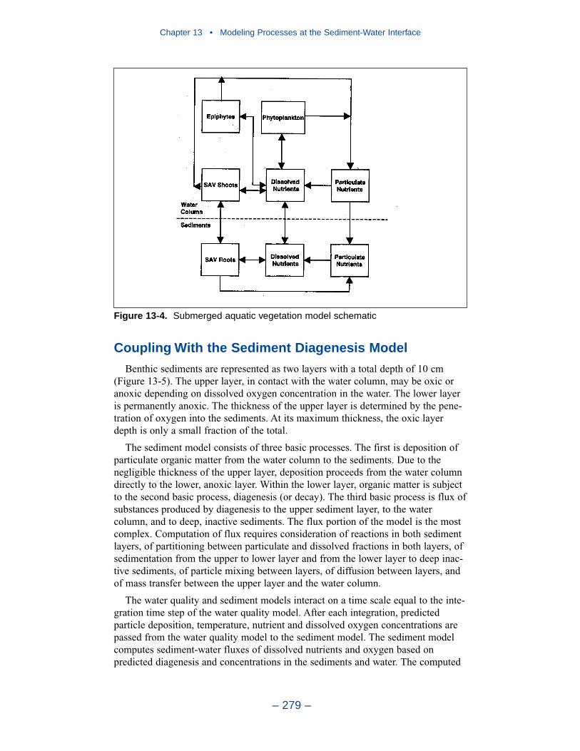
Chapter 13 • Modeling Processes at the Sediment-Water Interface
– 279 –
Figure 13-4. Submerged aquatic vegetation model schematic
Coupling With the Sediment Diagenesis Model
Benthic sediments are represented as two layers with a total depth of 10 cm(Figure 13-5). The upper layer, in contact with the water column, may be oxic oranoxic depending on dissolved oxygen concentration in the water. The lower layeris permanently anoxic. The thickness of the upper layer is determined by the pene-tration of oxygen into the sediments. At its maximum thickness, the oxic layerdepth is only a small fraction of the total.
The sediment model consists of three basic processes. The first is deposition ofparticulate organic matter from the water column to the sediments. Due to thenegligible thickness of the upper layer, deposition proceeds from the water columndirectly to the lower, anoxic layer. Within the lower layer, organic matter is subjectto the second basic process, diagenesis (or decay). The third basic process is flux ofsubstances produced by diagenesis to the upper sediment layer, to the watercolumn, and to deep, inactive sediments. The flux portion of the model is the mostcomplex. Computation of flux requires consideration of reactions in both sedimentlayers, of partitioning between particulate and dissolved fractions in both layers, ofsedimentation from the upper to lower layer and from the lower layer to deep inac-tive sediments, of particle mixing between layers, of diffusion between layers, andof mass transfer between the upper layer and the water column.
The water quality and sediment models interact on a time scale equal to the inte-gration time step of the water quality model. After each integration, predictedparticle deposition, temperature, nutrient and dissolved oxygen concentrations arepassed from the water quality model to the sediment model. The sediment modelcomputes sediment-water fluxes of dissolved nutrients and oxygen based onpredicted diagenesis and concentrations in the sediments and water. The computed
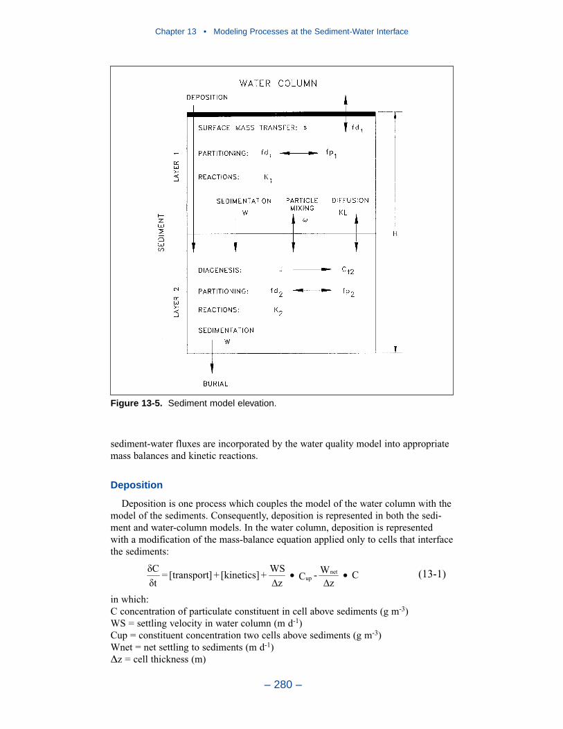
sediment-water fluxes are incorporated by the water quality model into appropriatemass balances and kinetic reactions.
Deposition
Deposition is one process which couples the model of the water column with themodel of the sediments. Consequently, deposition is represented in both the sedi-ment and water-column models. In the water column, deposition is representedwith a modification of the mass-balance equation applied only to cells that interfacethe sediments:
in which:C concentration of particulate constituent in cell above sediments (g m-3)WS = settling velocity in water column (m d-1)Cup = constituent concentration two cells above sediments (g m-3)Wnet = net settling to sediments (m d-1)∆z = cell thickness (m)
Cz
W-CzWS+[kinetics]+][transport=
tC net
up (13-1)
Chapter 13 • Modeling Processes at the Sediment-Water Interface
– 280 –
Figure 13-5. Sediment model elevation.
Chapter 13 • Modeling Processes at the Sediment-Water Interface
– 281 –
Net settling to the sediments may be less than or equal to settling in the watercolumn. Sediment resuspension is implied when settling to the sediments is lessthan settling through the water column.
Diagenesis
Organic matter in the sediments is divided into three G classes or fractions, inaccordance with principles established by Westrich and Berner (1984). Divisioninto G classes accounts for differential decay rates of organic matter fractions. TheG1, labile, fraction has a half life of 20 days. The G2, refractory, fraction has a halflife of one year. The G3, inert, fraction undergoes no significant decay before burial into deep, inactive sediments. Each G class has its own mass-conservationequation:
in which:H = total thickness of sediment layer (m)Gi = concentration organic matter in G class i (g m-3)fi = fraction of deposited organic matter assigned to G class iW = burial rate (m d-1)Ki = decay rate of G class i (d-1)θi = constant that expresses effect of temperature on decay of G class i
Since the G3 class is inert, K3 = 0.
Sediment-Water Flux
The exchange of dissolved substances between the sediments and water columnis driven by the concentration difference between the surface sediment layer andthe overlying water. Flux may be in either direction across the sediment-waterinterface, depending on concentration gradient. Sediment-water flux is computedwithin the diagenesis model as the product of concentration difference and an inter-nally-computed mass-transfer coefficient. In the water column, sediment-waterexchange of dissolved substances is represented with a modification of the mass-balance equation applied only to cells that interface with bottom sediments:
in which:BENFLX = sediment-water flux of dissolved substance (g m-2 d-1)
By convention, positive fluxes are from sediment to water. Negative fluxes,including sediment oxygen demand, are from water to sediments.
Parameter Specification
Coupling with the sediment model requires specification of net settling rates, ofthe G splits of organic matter, and of burial rates.
z
BENFLX+[kinetics]+][transport=
t
C(13-3)
GiKH-Gi W-CfW=t
GiH 20)-(Tiiinet
(13-2)
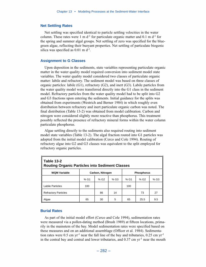
Net Settling Rates
Net settling was specified identical to particle settling velocities in the watercolumn. These rates were 1 m d-1 for particulate organic matter and 0.1 m d-1 forthe spring and summer algal groups. Net settling of zero was specified for the blue-green algae, reflecting their buoyant properties. Net settling of particulate biogenicsilica was specified as 0.01 m d-1.
Assignment to G Classes
Upon deposition in the sediments, state variables representing particulate organicmatter in the water quality model required conversion into sediment model statevariables. The water quality model considered two classes of particulate organicmatter: labile and refractory. The sediment model was based on three classes oforganic particles: labile (G1), refractory (G2), and inert (G3). Labile particles fromthe water quality model were transferred directly into the G1 class in the sedimentmodel. Refractory particles from the water quality model had to be split into G2and G3 fractions upon entering the sediments. Initial guidance for the splits wasobtained from experiments (Westrich and Berner 1984) in which roughly evendistribution between refractory and inert particulate organic carbon was noted. Thefinal distribution (Table 13-2) was obtained from model calibration. Carbon andnitrogen were considered slightly more reactive than phosphorus. This treatmentpossibly reflected the presence of refractory mineral forms within the water columnparticulate phosphorus.
Algae settling directly to the sediments also required routing into sedimentmodel state variables (Table 13-2). The algal fraction routed into G1 particles wasadopted from the initial model calibration (Cerco and Cole 1994). Routing ofrefractory algae into G2 and G3 classes was equivalent to the split employed forrefractory organic particles.
Burial Rates
As part of the initial model effort (Cerco and Cole 1994), sedimentation rateswere measured via a pollen-dating method (Brush 1989) at fifteen locations, prima-rily in the mainstem of the bay. Model sedimentation rates were specified based onthese measures and on an additional assemblage (Officer et al. 1984). Sedimenta-tion rates were 0.5 cm yr-1 near the fall line of the bay and tributaries, 0.25 cm yr-1
in the central bay and central and lower tributaries, and 0.37 cm yr-1 near the mouth
Chapter 13 • Modeling Processes at the Sediment-Water Interface
– 282 –
Table 13-2 Routing Organic Particles into Sediment Classes
WQM Variable Carbon, Nitrogen Phosphorus
% G1 % G2 % G3 % G1 % G2 % G3
Labile Particles 100 100
Refractory Particles 86 14 73 27
Algae 65 30 5 65 25.5 9.5
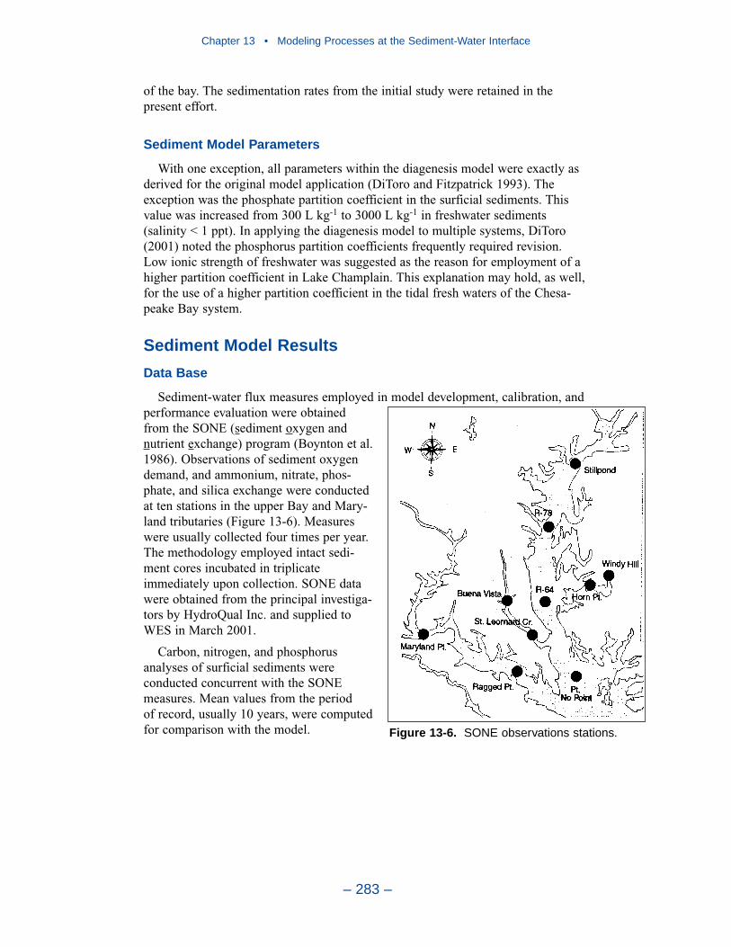
Chapter 13 • Modeling Processes at the Sediment-Water Interface
– 283 –
of the bay. The sedimentation rates from the initial study were retained in thepresent effort.
Sediment Model Parameters
With one exception, all parameters within the diagenesis model were exactly asderived for the original model application (DiToro and Fitzpatrick 1993). Theexception was the phosphate partition coefficient in the surficial sediments. Thisvalue was increased from 300 L kg-1 to 3000 L kg-1 in freshwater sediments(salinity < 1 ppt). In applying the diagenesis model to multiple systems, DiToro(2001) noted the phosphorus partition coefficients frequently required revision.Low ionic strength of freshwater was suggested as the reason for employment of ahigher partition coefficient in Lake Champlain. This explanation may hold, as well,for the use of a higher partition coefficient in the tidal fresh waters of the Chesa-peake Bay system.
Sediment Model Results
Data Base
Sediment-water flux measures employed in model development, calibration, andperformance evaluation were obtainedfrom the SONE (sediment oxygen andnutrient exchange) program (Boynton et al.1986). Observations of sediment oxygendemand, and ammonium, nitrate, phos-phate, and silica exchange were conductedat ten stations in the upper Bay and Mary-land tributaries (Figure 13-6). Measureswere usually collected four times per year.The methodology employed intact sedi-ment cores incubated in triplicateimmediately upon collection. SONE datawere obtained from the principal investiga-tors by HydroQual Inc. and supplied toWES in March 2001.
Carbon, nitrogen, and phosphorusanalyses of surficial sediments wereconducted concurrent with the SONEmeasures. Mean values from the period of record, usually 10 years, were computedfor comparison with the model. Figure 13-6. SONE observations stations.

Time Series
Time-series comparisons are presented for three stations: Still Pond, R- 64,and Point-No-Point (Figure 13-6). These stations are selected for their different bottom environments as characterized by dissolved oxygen concentration. Bottom dissolved oxygen at Still Pond rarely falls below 2 g m-3 (Figure 13-7). Complete anoxia is a regular occurrence during summer in bottom waters at R-64(Figure 13-8). At Point-No-Point, intermittent bottom-water anoxia occurs but theduration is not so severe as at R-64 (Figure 13-9).
Peak sediment oxygen demand of 2 to 2.5 g m-2 d-1 is observed at Still Pond(Figure 13-10). The model matches these observations well and occasionallycomputes sediment oxygen demand as high as 3 g m-2 d-1. Computed and observed
Chapter 13 • Modeling Processes at the Sediment-Water Interface
– 284 –
Figure 13-7. Computed and observed bottomdissolved oxygen at Station CB2.2, near Still Pond.
Figure 13-8. Computed and observed bottomdissolved oxygen at Station CB4.2C, near R-64.
Figure 13-9. Computed and observed bottomdissolved oxygen at Station CB5.2, near Point-No-Point.
Figure 13-10. Computed (daily) and observed(instantaneous) sediment oxygen demand at Still Pond.
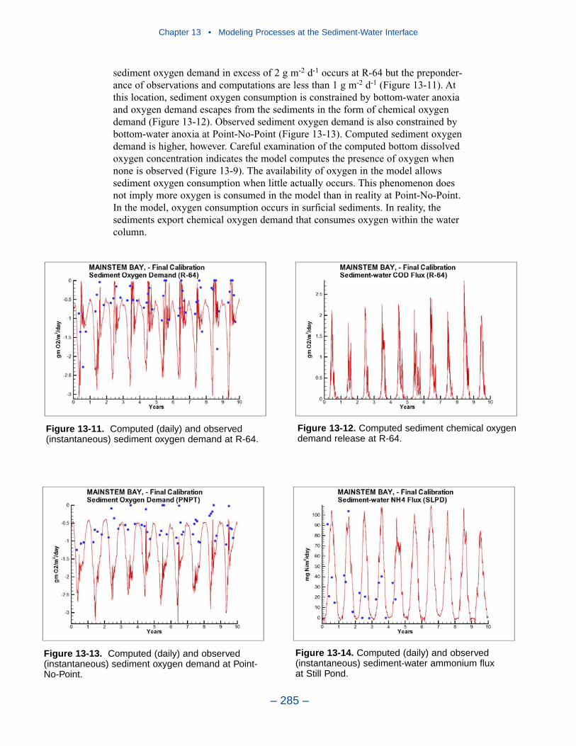
sediment oxygen demand in excess of 2 g m-2 d-1 occurs at R-64 but the preponder-ance of observations and computations are less than 1 g m-2 d-1 (Figure 13-11). Atthis location, sediment oxygen consumption is constrained by bottom-water anoxiaand oxygen demand escapes from the sediments in the form of chemical oxygendemand (Figure 13-12). Observed sediment oxygen demand is also constrained bybottom-water anoxia at Point-No-Point (Figure 13-13). Computed sediment oxygendemand is higher, however. Careful examination of the computed bottom dissolvedoxygen concentration indicates the model computes the presence of oxygen whennone is observed (Figure 13-9). The availability of oxygen in the model allowssediment oxygen consumption when little actually occurs. This phenomenon doesnot imply more oxygen is consumed in the model than in reality at Point-No-Point.In the model, oxygen consumption occurs in surficial sediments. In reality, thesediments export chemical oxygen demand that consumes oxygen within the watercolumn.
Chapter 13 • Modeling Processes at the Sediment-Water Interface
– 285 –
Figure 13-11. Computed (daily) and observed(instantaneous) sediment oxygen demand at R-64.
Figure 13-12. Computed sediment chemical oxygendemand release at R-64.
Figure 13-13. Computed (daily) and observed(instantaneous) sediment oxygen demand at Point-No-Point.
Figure 13-14. Computed (daily) and observed(instantaneous) sediment-water ammonium flux at Still Pond.
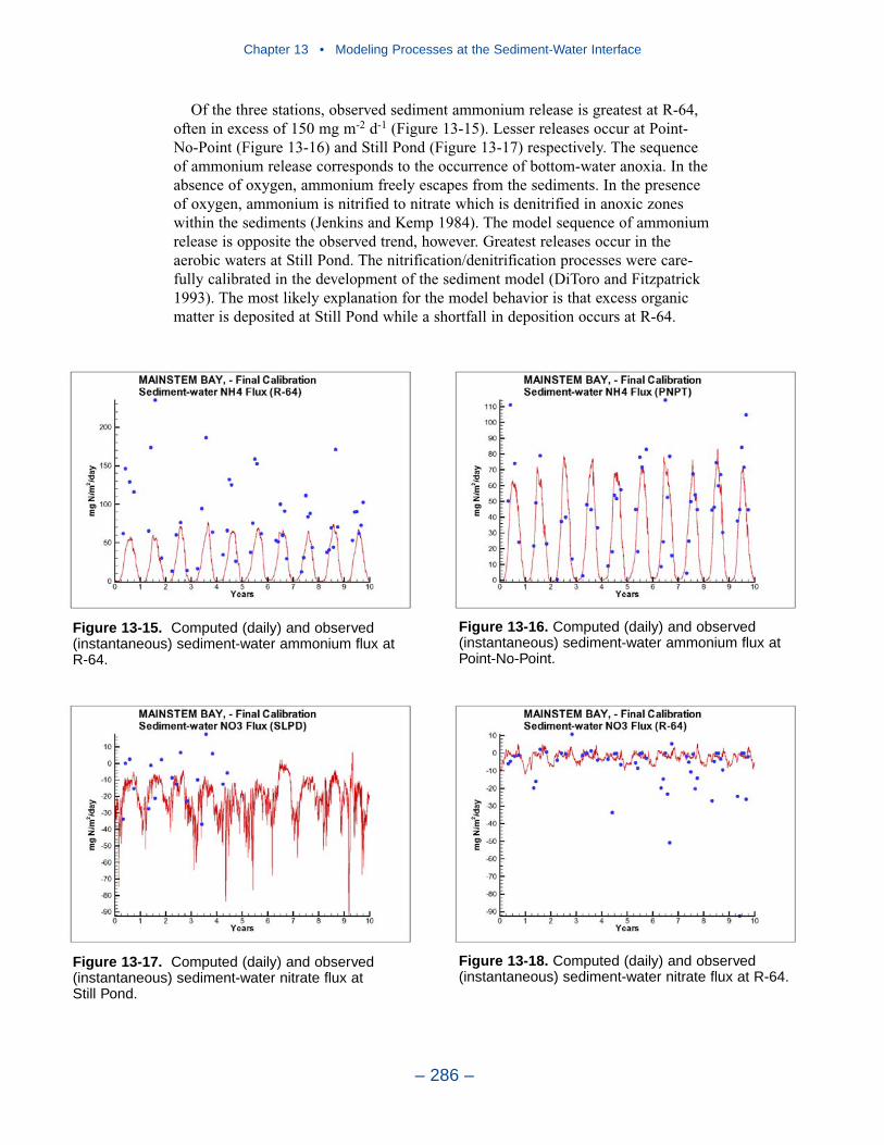
Of the three stations, observed sediment ammonium release is greatest at R-64,often in excess of 150 mg m-2 d-1 (Figure 13-15). Lesser releases occur at Point-No-Point (Figure 13-16) and Still Pond (Figure 13-17) respectively. The sequenceof ammonium release corresponds to the occurrence of bottom-water anoxia. In theabsence of oxygen, ammonium freely escapes from the sediments. In the presenceof oxygen, ammonium is nitrified to nitrate which is denitrified in anoxic zoneswithin the sediments (Jenkins and Kemp 1984). The model sequence of ammoniumrelease is opposite the observed trend, however. Greatest releases occur in theaerobic waters at Still Pond. The nitrification/denitrification processes were care-fully calibrated in the development of the sediment model (DiToro and Fitzpatrick1993). The most likely explanation for the model behavior is that excess organicmatter is deposited at Still Pond while a shortfall in deposition occurs at R-64.
Chapter 13 • Modeling Processes at the Sediment-Water Interface
– 286 –
Figure 13-15. Computed (daily) and observed(instantaneous) sediment-water ammonium flux at R-64.
Figure 13-16. Computed (daily) and observed(instantaneous) sediment-water ammonium flux atPoint-No-Point.
Figure 13-17. Computed (daily) and observed(instantaneous) sediment-water nitrate flux at Still Pond.
Figure 13-18. Computed (daily) and observed(instantaneous) sediment-water nitrate flux at R-64.
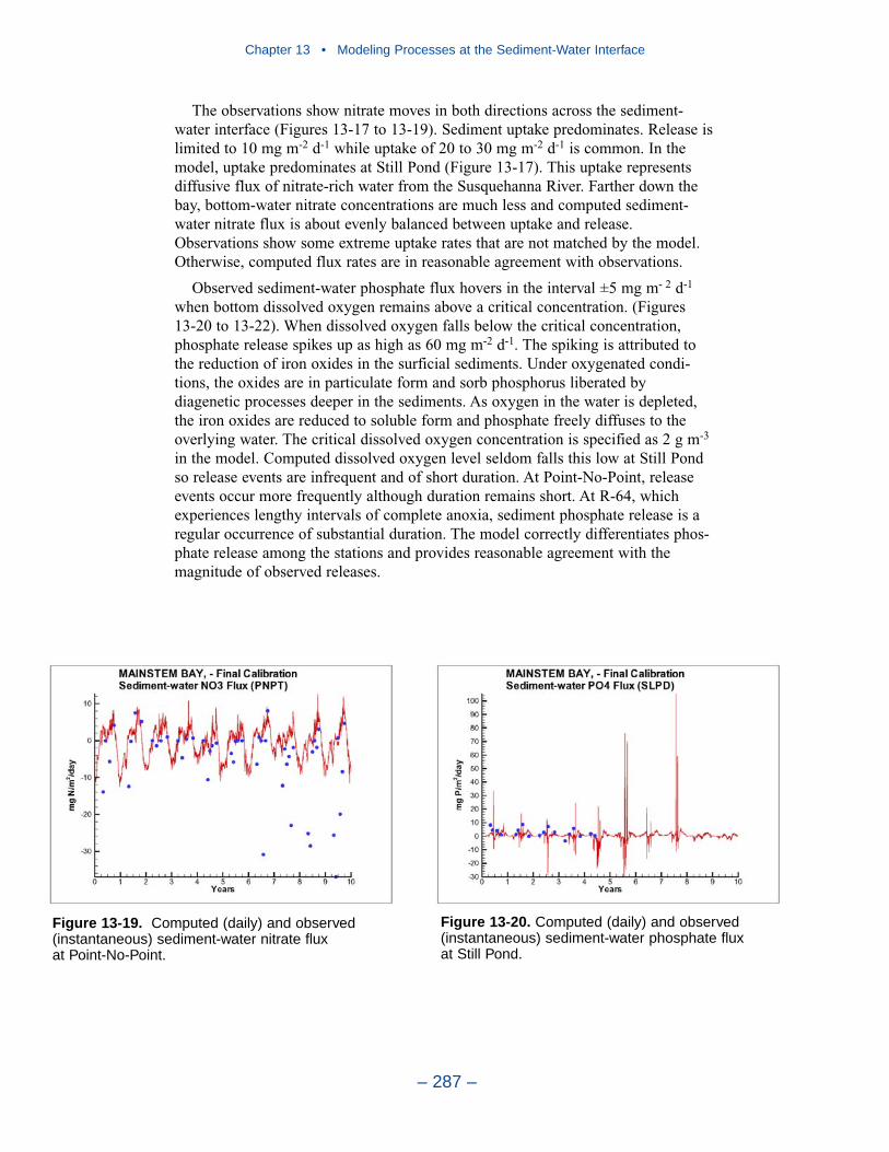
Chapter 13 • Modeling Processes at the Sediment-Water Interface
– 287 –
The observations show nitrate moves in both directions across the sediment-water interface (Figures 13-17 to 13-19). Sediment uptake predominates. Release islimited to 10 mg m-2 d-1 while uptake of 20 to 30 mg m-2 d-1 is common. In themodel, uptake predominates at Still Pond (Figure 13-17). This uptake representsdiffusive flux of nitrate-rich water from the Susquehanna River. Farther down thebay, bottom-water nitrate concentrations are much less and computed sediment-water nitrate flux is about evenly balanced between uptake and release.Observations show some extreme uptake rates that are not matched by the model.Otherwise, computed flux rates are in reasonable agreement with observations.
Observed sediment-water phosphate flux hovers in the interval ±5 mg m- 2 d-1
when bottom dissolved oxygen remains above a critical concentration. (Figures 13-20 to 13-22). When dissolved oxygen falls below the critical concentration,phosphate release spikes up as high as 60 mg m-2 d-1. The spiking is attributed tothe reduction of iron oxides in the surficial sediments. Under oxygenated condi-tions, the oxides are in particulate form and sorb phosphorus liberated bydiagenetic processes deeper in the sediments. As oxygen in the water is depleted,the iron oxides are reduced to soluble form and phosphate freely diffuses to theoverlying water. The critical dissolved oxygen concentration is specified as 2 g m-3
in the model. Computed dissolved oxygen level seldom falls this low at Still Pondso release events are infrequent and of short duration. At Point-No-Point, releaseevents occur more frequently although duration remains short. At R-64, whichexperiences lengthy intervals of complete anoxia, sediment phosphate release is aregular occurrence of substantial duration. The model correctly differentiates phos-phate release among the stations and provides reasonable agreement with themagnitude of observed releases.
Figure 13-19. Computed (daily) and observed(instantaneous) sediment-water nitrate flux at Point-No-Point.
Figure 13-20. Computed (daily) and observed(instantaneous) sediment-water phosphate flux at Still Pond.
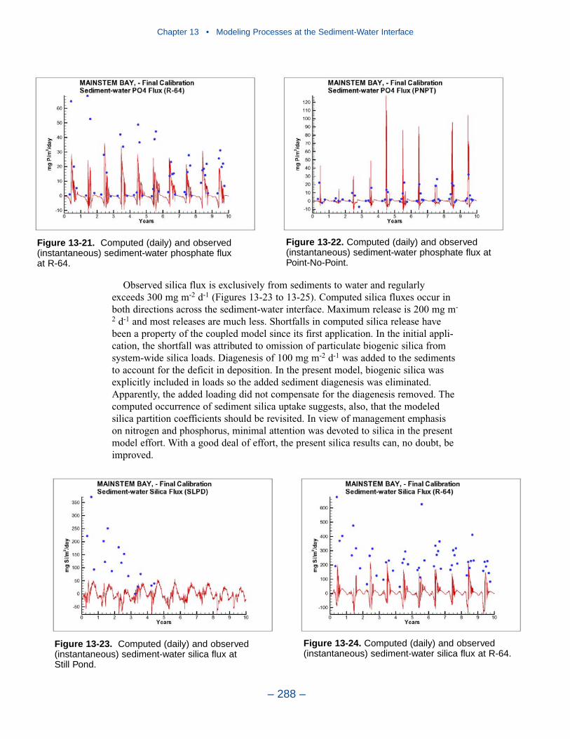
Chapter 13 • Modeling Processes at the Sediment-Water Interface
– 288 –
Observed silica flux is exclusively from sediments to water and regularlyexceeds 300 mg m-2 d-1 (Figures 13-23 to 13-25). Computed silica fluxes occur inboth directions across the sediment-water interface. Maximum release is 200 mg m-
2 d-1 and most releases are much less. Shortfalls in computed silica release havebeen a property of the coupled model since its first application. In the initial appli-cation, the shortfall was attributed to omission of particulate biogenic silica fromsystem-wide silica loads. Diagenesis of 100 mg m-2 d-1 was added to the sedimentsto account for the deficit in deposition. In the present model, biogenic silica wasexplicitly included in loads so the added sediment diagenesis was eliminated.Apparently, the added loading did not compensate for the diagenesis removed. Thecomputed occurrence of sediment silica uptake suggests, also, that the modeledsilica partition coefficients should be revisited. In view of management emphasison nitrogen and phosphorus, minimal attention was devoted to silica in the presentmodel effort. With a good deal of effort, the present silica results can, no doubt, beimproved.
Figure 13-21. Computed (daily) and observed(instantaneous) sediment-water phosphate flux at R-64.
Figure 13-22. Computed (daily) and observed(instantaneous) sediment-water phosphate flux atPoint-No-Point.
Figure 13-23. Computed (daily) and observed(instantaneous) sediment-water silica flux at Still Pond.
Figure 13-24. Computed (daily) and observed(instantaneous) sediment-water silica flux at R-64.
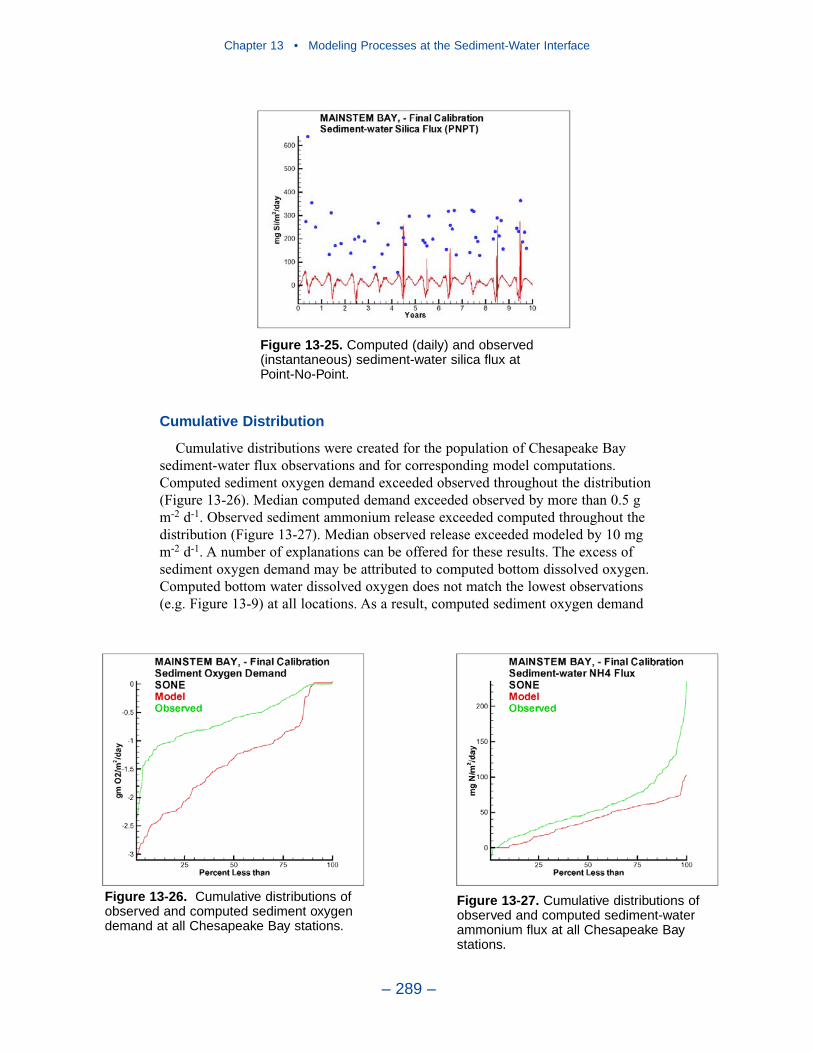
Cumulative Distribution
Cumulative distributions were created for the population of Chesapeake Baysediment-water flux observations and for corresponding model computations.Computed sediment oxygen demand exceeded observed throughout the distribution(Figure 13-26). Median computed demand exceeded observed by more than 0.5 gm-2 d-1. Observed sediment ammonium release exceeded computed throughout thedistribution (Figure 13-27). Median observed release exceeded modeled by 10 mgm-2 d-1. A number of explanations can be offered for these results. The excess ofsediment oxygen demand may be attributed to computed bottom dissolved oxygen.Computed bottom water dissolved oxygen does not match the lowest observations(e.g. Figure 13-9) at all locations. As a result, computed sediment oxygen demand
Chapter 13 • Modeling Processes at the Sediment-Water Interface
– 289 –
Figure 13-25. Computed (daily) and observed(instantaneous) sediment-water silica flux at Point-No-Point.
Figure 13-26. Cumulative distributions ofobserved and computed sediment oxygendemand at all Chesapeake Bay stations.
Figure 13-27. Cumulative distributions ofobserved and computed sediment-water ammonium flux at all Chesapeake Bay stations.
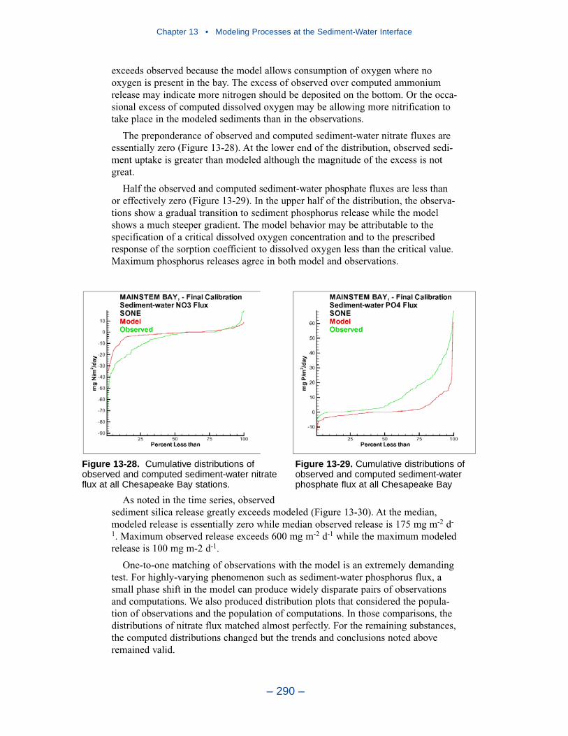
exceeds observed because the model allows consumption of oxygen where nooxygen is present in the bay. The excess of observed over computed ammoniumrelease may indicate more nitrogen should be deposited on the bottom. Or the occa-sional excess of computed dissolved oxygen may be allowing more nitrification totake place in the modeled sediments than in the observations.
The preponderance of observed and computed sediment-water nitrate fluxes areessentially zero (Figure 13-28). At the lower end of the distribution, observed sedi-ment uptake is greater than modeled although the magnitude of the excess is notgreat.
Half the observed and computed sediment-water phosphate fluxes are less thanor effectively zero (Figure 13-29). In the upper half of the distribution, the observa-tions show a gradual transition to sediment phosphorus release while the modelshows a much steeper gradient. The model behavior may be attributable to thespecification of a critical dissolved oxygen concentration and to the prescribedresponse of the sorption coefficient to dissolved oxygen less than the critical value.Maximum phosphorus releases agree in both model and observations.
As noted in the time series, observedsediment silica release greatly exceeds modeled (Figure 13-30). At the median,modeled release is essentially zero while median observed release is 175 mg m-2 d-
1. Maximum observed release exceeds 600 mg m-2 d-1 while the maximum modeledrelease is 100 mg m-2 d-1.
One-to-one matching of observations with the model is an extremely demandingtest. For highly-varying phenomenon such as sediment-water phosphorus flux, asmall phase shift in the model can produce widely disparate pairs of observationsand computations. We also produced distribution plots that considered the popula-tion of observations and the population of computations. In those comparisons, thedistributions of nitrate flux matched almost perfectly. For the remaining substances,the computed distributions changed but the trends and conclusions noted aboveremained valid.
Chapter 13 • Modeling Processes at the Sediment-Water Interface
– 290 –
Figure 13-28. Cumulative distributions ofobserved and computed sediment-water nitrateflux at all Chesapeake Bay stations.
Figure 13-29. Cumulative distributions ofobserved and computed sediment-waterphosphate flux at all Chesapeake Bay

Sediment Composition
The author of the sediment diagenesis model describes particulate organic matterin the sediment as the “ashes” of the diagenesis process. That is, the majority ofsediment organic matter is refractory or inert even though the majority of materialdeposited is labile (Figure 13-31). The labile material rapidly decays away leavingmostly ashes. Particulate carbon and nitrogen in the sediments is almost exclusivelyorganic; the end products of diagenesis escape to the water in dissolved or gaseousform. For phosphorus, however, a substantial amount of diagenetically-producedphosphate is trapped in the sediments in mineral form. Consequently, sedimentparticulate phosphorus is a mixture of organic and mineral substances.
Chapter 13 • Modeling Processes at the Sediment-Water Interface
– 291 –
Figure 13-30. Cumulative distributions ofobserved and computed sediment-water silica flux at all Chesapeake Bay stations.
Figure 13-31. Effect of sedimentation (burial) rate onsediment organic matter. Calculations based on depositionof 1 g m-2 d-1 and G1, G2, G3 splits of 0.65, 0.3, 0.05respectively.
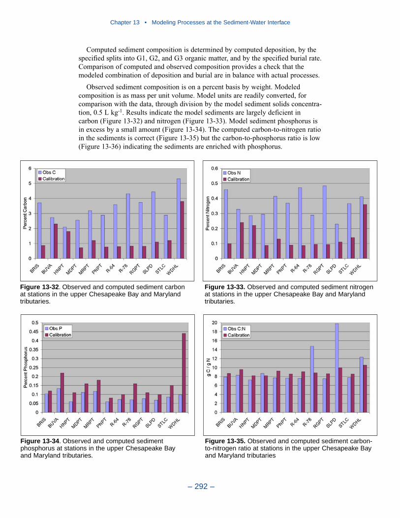
Computed sediment composition is determined by computed deposition, by thespecified splits into G1, G2, and G3 organic matter, and by the specified burial rate.Comparison of computed and observed composition provides a check that themodeled combination of deposition and burial are in balance with actual processes.
Observed sediment composition is on a percent basis by weight. Modeledcomposition is as mass per unit volume. Model units are readily converted, forcomparison with the data, through division by the model sediment solids concentra-tion, 0.5 L kg-1. Results indicate the model sediments are largely deficient incarbon (Figure 13-32) and nitrogen (Figure 13-33). Model sediment phosphorus isin excess by a small amount (Figure 13-34). The computed carbon-to-nitrogen ratioin the sediments is correct (Figure 13-35) but the carbon-to-phosphorus ratio is low(Figure 13-36) indicating the sediments are enriched with phosphorus.
Chapter 13 • Modeling Processes at the Sediment-Water Interface
– 292 –
Figure 13-32. Observed and computed sediment carbonat stations in the upper Chesapeake Bay and Marylandtributaries.
Figure 13-33. Observed and computed sediment nitrogenat stations in the upper Chesapeake Bay and Marylandtributaries.
Figure 13-34. Observed and computed sedimentphosphorus at stations in the upper Chesapeake Bay and Maryland tributaries.
Figure 13-35. Observed and computed sediment carbon-to-nitrogen ratio at stations in the upper Chesapeake Bayand Maryland tributaries
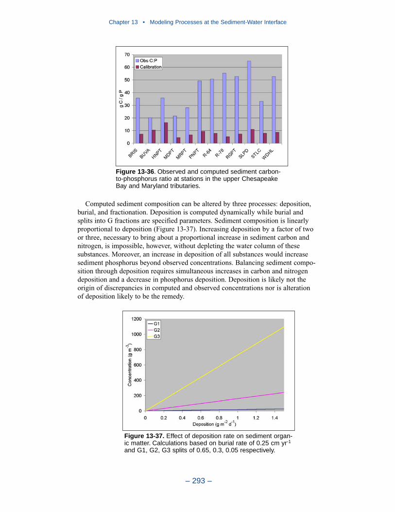
Computed sediment composition can be altered by three processes: deposition,burial, and fractionation. Deposition is computed dynamically while burial andsplits into G fractions are specified parameters. Sediment composition is linearlyproportional to deposition (Figure 13-37). Increasing deposition by a factor of twoor three, necessary to bring about a proportional increase in sediment carbon andnitrogen, is impossible, however, without depleting the water column of thesesubstances. Moreover, an increase in deposition of all substances would increasesediment phosphorus beyond observed concentrations. Balancing sediment compo-sition through deposition requires simultaneous increases in carbon and nitrogendeposition and a decrease in phosphorus deposition. Deposition is likely not theorigin of discrepancies in computed and observed concentrations nor is alterationof deposition likely to be the remedy.
Chapter 13 • Modeling Processes at the Sediment-Water Interface
– 293 –
Figure 13-36. Observed and computed sediment carbon-to-phosphorus ratio at stations in the upper ChesapeakeBay and Maryland tributaries.
Figure 13-37. Effect of deposition rate on sediment organ-ic matter. Calculations based on burial rate of 0.25 cm yr-1
and G1, G2, G3 splits of 0.65, 0.3, 0.05 respectively.
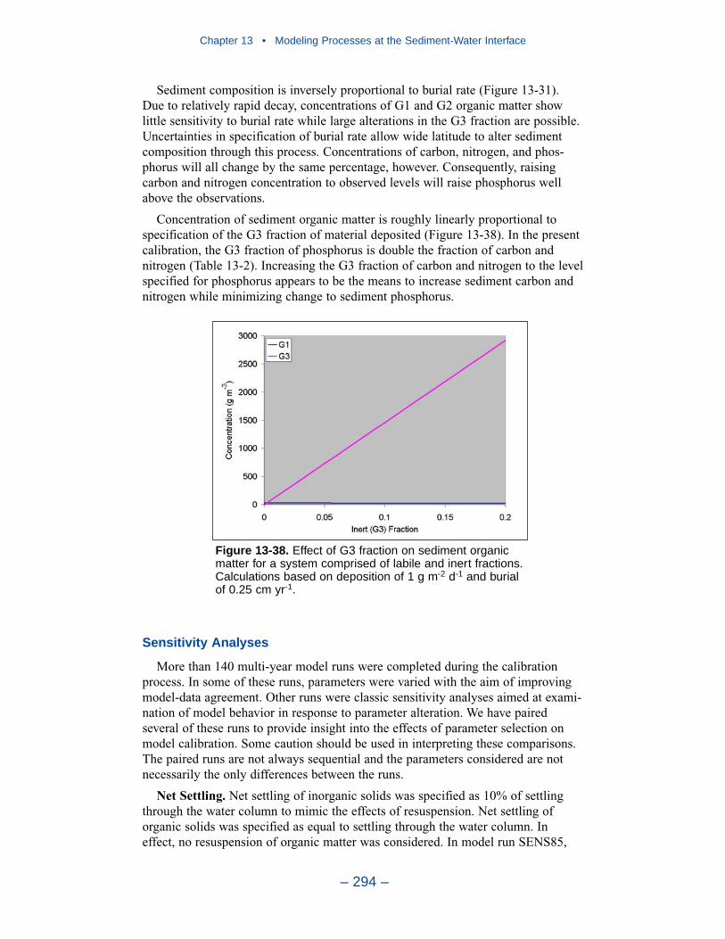
Sediment composition is inversely proportional to burial rate (Figure 13-31).Due to relatively rapid decay, concentrations of G1 and G2 organic matter showlittle sensitivity to burial rate while large alterations in the G3 fraction are possible.Uncertainties in specification of burial rate allow wide latitude to alter sedimentcomposition through this process. Concentrations of carbon, nitrogen, and phos-phorus will all change by the same percentage, however. Consequently, raisingcarbon and nitrogen concentration to observed levels will raise phosphorus wellabove the observations.
Concentration of sediment organic matter is roughly linearly proportional tospecification of the G3 fraction of material deposited (Figure 13-38). In the presentcalibration, the G3 fraction of phosphorus is double the fraction of carbon andnitrogen (Table 13-2). Increasing the G3 fraction of carbon and nitrogen to the levelspecified for phosphorus appears to be the means to increase sediment carbon andnitrogen while minimizing change to sediment phosphorus.
Sensitivity Analyses
More than 140 multi-year model runs were completed during the calibrationprocess. In some of these runs, parameters were varied with the aim of improvingmodel-data agreement. Other runs were classic sensitivity analyses aimed at exami-nation of model behavior in response to parameter alteration. We have pairedseveral of these runs to provide insight into the effects of parameter selection onmodel calibration. Some caution should be used in interpreting these comparisons.The paired runs are not always sequential and the parameters considered are notnecessarily the only differences between the runs.
Net Settling. Net settling of inorganic solids was specified as 10% of settlingthrough the water column to mimic the effects of resuspension. Net settling oforganic solids was specified as equal to settling through the water column. Ineffect, no resuspension of organic matter was considered. In model run SENS85,
Chapter 13 • Modeling Processes at the Sediment-Water Interface
– 294 –
Figure 13-38. Effect of G3 fraction on sediment organicmatter for a system comprised of labile and inert fractions.Calculations based on deposition of 1 g m-2 d-1 and burialof 0.25 cm yr-1.
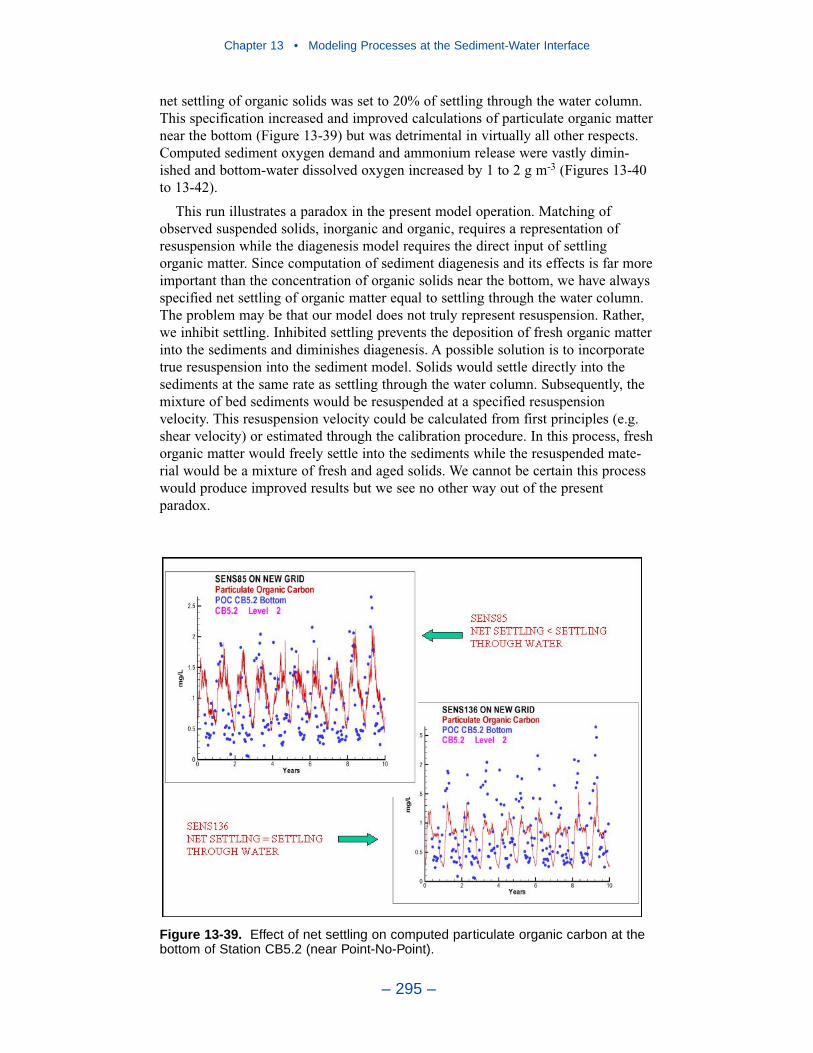
net settling of organic solids was set to 20% of settling through the water column.This specification increased and improved calculations of particulate organic matternear the bottom (Figure 13-39) but was detrimental in virtually all other respects.Computed sediment oxygen demand and ammonium release were vastly dimin-ished and bottom-water dissolved oxygen increased by 1 to 2 g m-3 (Figures 13-40to 13-42).
This run illustrates a paradox in the present model operation. Matching ofobserved suspended solids, inorganic and organic, requires a representation ofresuspension while the diagenesis model requires the direct input of settlingorganic matter. Since computation of sediment diagenesis and its effects is far moreimportant than the concentration of organic solids near the bottom, we have alwaysspecified net settling of organic matter equal to settling through the water column.The problem may be that our model does not truly represent resuspension. Rather,we inhibit settling. Inhibited settling prevents the deposition of fresh organic matterinto the sediments and diminishes diagenesis. A possible solution is to incorporatetrue resuspension into the sediment model. Solids would settle directly into thesediments at the same rate as settling through the water column. Subsequently, themixture of bed sediments would be resuspended at a specified resuspensionvelocity. This resuspension velocity could be calculated from first principles (e.g.shear velocity) or estimated through the calibration procedure. In this process, freshorganic matter would freely settle into the sediments while the resuspended mate-rial would be a mixture of fresh and aged solids. We cannot be certain this processwould produce improved results but we see no other way out of the presentparadox.
Chapter 13 • Modeling Processes at the Sediment-Water Interface
– 295 –
Figure 13-39. Effect of net settling on computed particulate organic carbon at thebottom of Station CB5.2 (near Point-No-Point).
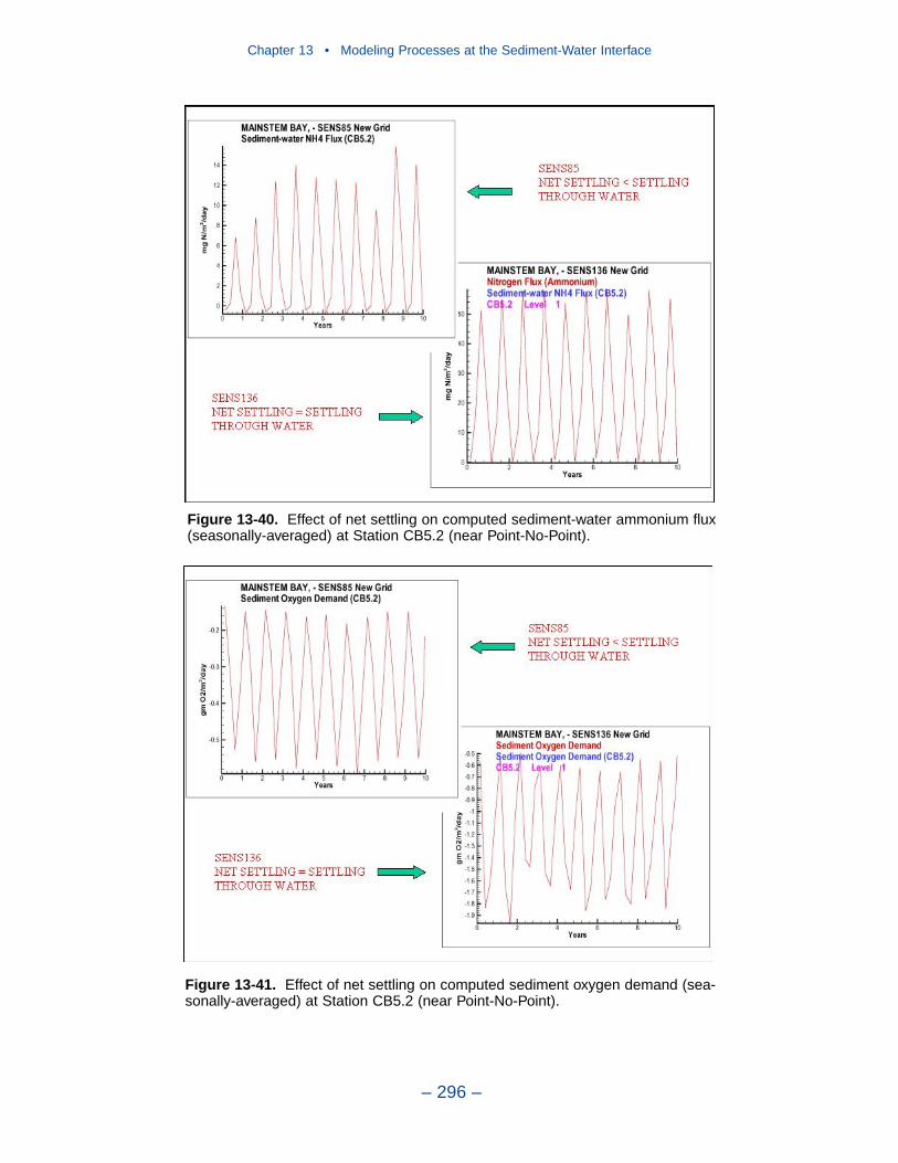
Chapter 13 • Modeling Processes at the Sediment-Water Interface
– 296 –
Figure 13-40. Effect of net settling on computed sediment-water ammonium flux(seasonally-averaged) at Station CB5.2 (near Point-No-Point).
Figure 13-41. Effect of net settling on computed sediment oxygen demand (sea-sonally-averaged) at Station CB5.2 (near Point-No-Point).
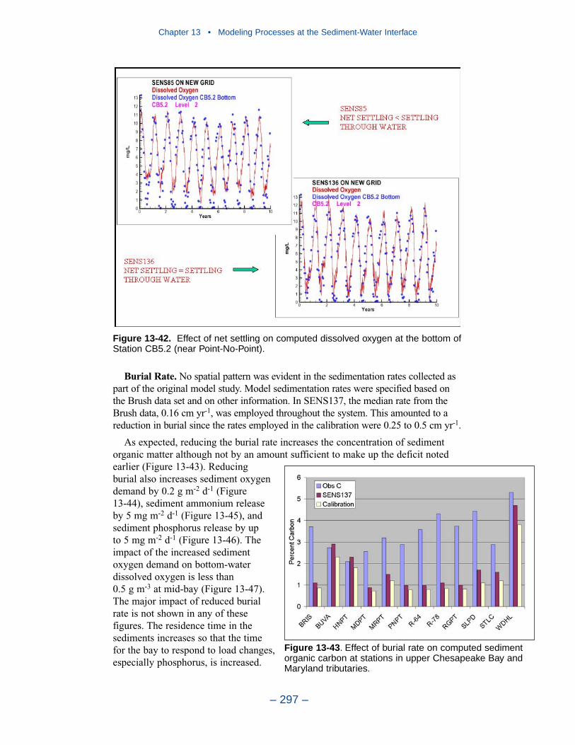
Burial Rate. No spatial pattern was evident in the sedimentation rates collected aspart of the original model study. Model sedimentation rates were specified based onthe Brush data set and on other information. In SENS137, the median rate from theBrush data, 0.16 cm yr-1, was employed throughout the system. This amounted to areduction in burial since the rates employed in the calibration were 0.25 to 0.5 cm yr-1.
As expected, reducing the burial rate increases the concentration of sedimentorganic matter although not by an amount sufficient to make up the deficit notedearlier (Figure 13-43). Reducingburial also increases sediment oxygendemand by 0.2 g m-2 d-1 (Figure 13-44), sediment ammonium releaseby 5 mg m-2 d-1 (Figure 13-45), andsediment phosphorus release by up to 5 mg m-2 d-1 (Figure 13-46). Theimpact of the increased sedimentoxygen demand on bottom-waterdissolved oxygen is less than 0.5 g m-3 at mid-bay (Figure 13-47).The major impact of reduced burialrate is not shown in any of thesefigures. The residence time in thesediments increases so that the timefor the bay to respond to load changes,especially phosphorus, is increased.
Chapter 13 • Modeling Processes at the Sediment-Water Interface
– 297 –
Figure 13-42. Effect of net settling on computed dissolved oxygen at the bottom ofStation CB5.2 (near Point-No-Point).
Figure 13-43. Effect of burial rate on computed sedimentorganic carbon at stations in upper Chesapeake Bay andMaryland tributaries.
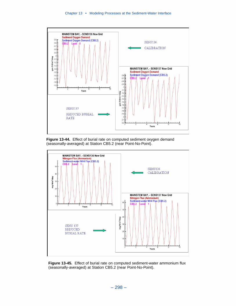
Chapter 13 • Modeling Processes at the Sediment-Water Interface
– 298 –
Figure 13-44. Effect of burial rate on computed sediment oxygen demand (seasonally-averaged) at Station CB5.2 (near Point-No-Point).
Figure 13-45. Effect of burial rate on computed sediment-water ammonium flux(seasonally-averaged) at Station CB5.2 (near Point-No-Point).
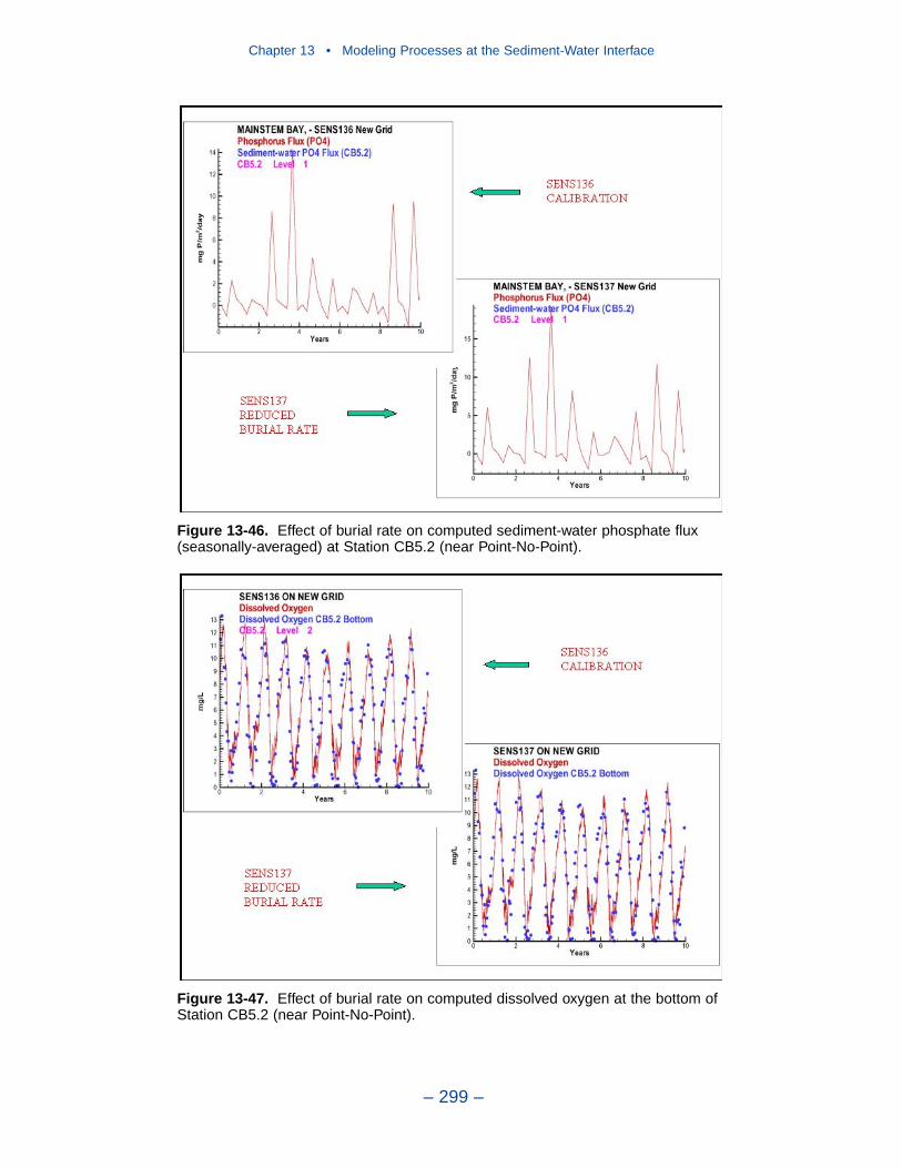
Chapter 13 • Modeling Processes at the Sediment-Water Interface
– 299 –
Figure 13-46. Effect of burial rate on computed sediment-water phosphate flux(seasonally-averaged) at Station CB5.2 (near Point-No-Point).
Figure 13-47. Effect of burial rate on computed dissolved oxygen at the bottom ofStation CB5.2 (near Point-No-Point).
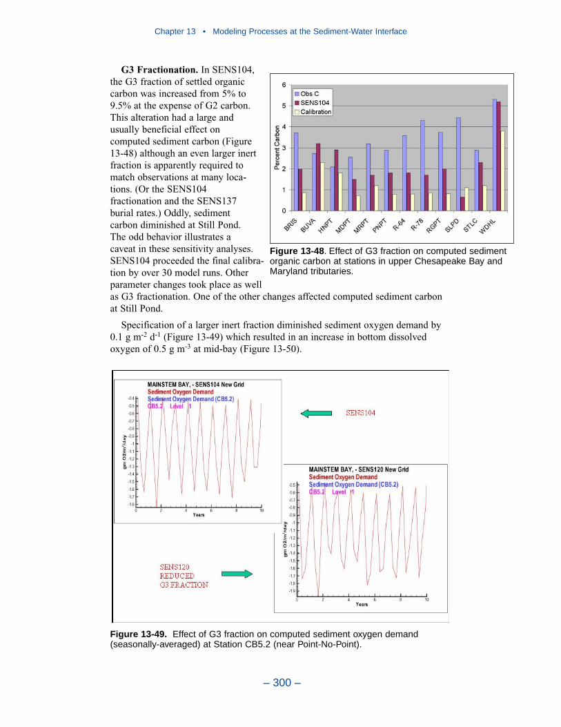
G3 Fractionation. In SENS104,the G3 fraction of settled organiccarbon was increased from 5% to9.5% at the expense of G2 carbon.This alteration had a large andusually beneficial effect oncomputed sediment carbon (Figure13-48) although an even larger inertfraction is apparently required tomatch observations at many loca-tions. (Or the SENS104fractionation and the SENS137burial rates.) Oddly, sedimentcarbon diminished at Still Pond.The odd behavior illustrates acaveat in these sensitivity analyses.SENS104 proceeded the final calibra-tion by over 30 model runs. Otherparameter changes took place as wellas G3 fractionation. One of the other changes affected computed sediment carbonat Still Pond.
Specification of a larger inert fraction diminished sediment oxygen demand by0.1 g m-2 d-1 (Figure 13-49) which resulted in an increase in bottom dissolvedoxygen of 0.5 g m-3 at mid-bay (Figure 13-50).
Chapter 13 • Modeling Processes at the Sediment-Water Interface
– 300 –
Figure 13-48. Effect of G3 fraction on computed sedimentorganic carbon at stations in upper Chesapeake Bay andMaryland tributaries.
Figure 13-49. Effect of G3 fraction on computed sediment oxygen demand (seasonally-averaged) at Station CB5.2 (near Point-No-Point).
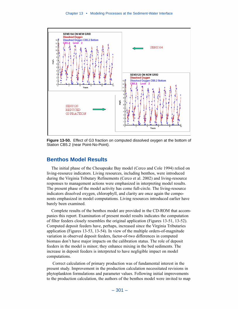
Benthos Model Results
The initial phase of the Chesapeake Bay model (Cerco and Cole 1994) relied onliving-resource indicators. Living resources, including benthos, were introducedduring the Virginia Tributary Refinements (Cerco et al. 2002) and living-resourceresponses to management actions were emphasized in interpreting model results.The present phase of the model activity has come full-circle. The living-resourceindicators dissolved oxygen, chlorophyll, and clarity are once again the compo-nents emphasized in model computations. Living resources introduced earlier havebarely been examined.
Complete results of the benthos model are provided in the CD-ROM that accom-panies this report. Examination of present model results indicates the computationof filter feeders closely resembles the original application (Figures 13-51, 13-52).Computed deposit feeders have, perhaps, increased since the Virginia Tributariesapplication (Figures 13-53, 13-54). In view of the multiple orders-of-magnitudevariation in observed deposit feeders, factor-of-two differences in computedbiomass don’t have major impacts on the calibration status. The role of depositfeeders in the model is minor; they enhance mixing in the bed sediments. Theincrease in deposit feeders is interpreted to have negligible impact on modelcomputations.
Correct calculation of primary production was of fundamental interest in thepresent study. Improvement in the production calculation necessitated revisions inphytoplankton formulations and parameter values. Following initial improvementsto the production calculation, the authors of the benthos model were invited to map
Chapter 13 • Modeling Processes at the Sediment-Water Interface
– 301 –
Figure 13-50. Effect of G3 fraction on computed dissolved oxygen at the bottom ofStation CB5.2 (near Point-No-Point).
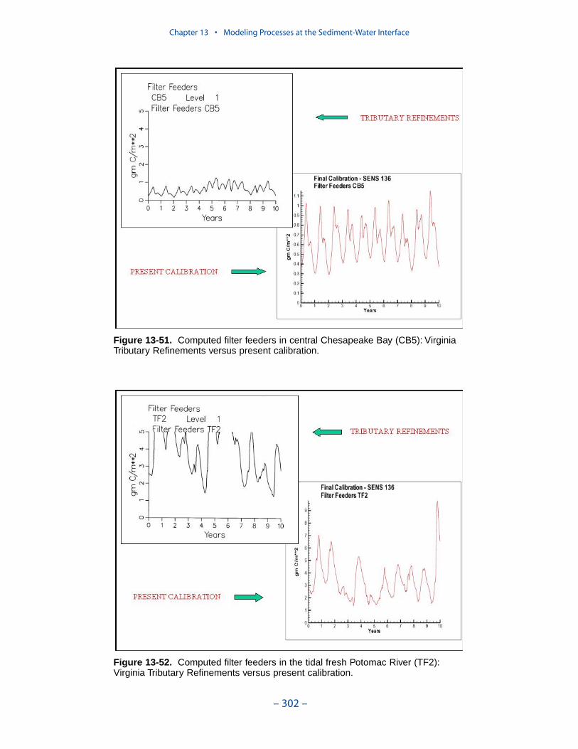
Chapter 13 • Modeling Processes at the Sediment-Water Interface
– 302 –
Figure 13-51. Computed filter feeders in central Chesapeake Bay (CB5): VirginiaTributary Refinements versus present calibration.
Figure 13-52. Computed filter feeders in the tidal fresh Potomac River (TF2):Virginia Tributary Refinements versus present calibration.
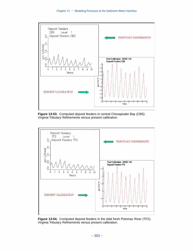
Chapter 13 • Modeling Processes at the Sediment-Water Interface
– 303 –
Figure 13-53. Computed deposit feeders in central Chesapeake Bay (CB5):Virginia Tributary Refinements versus present calibration.
Figure 13-54. Computed deposit feeders in the tidal fresh Potomac River (TF2):Virginia Tributary Refinements versus present calibration.
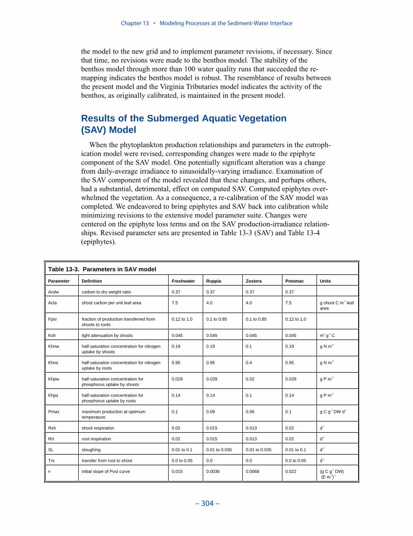
the model to the new grid and to implement parameter revisions, if necessary. Sincethat time, no revisions were made to the benthos model. The stability of thebenthos model through more than 100 water quality runs that succeeded the re-mapping indicates the benthos model is robust. The resemblance of results betweenthe present model and the Virginia Tributaries model indicates the activity of thebenthos, as originally calibrated, is maintained in the present model.
Results of the Submerged Aquatic Vegetation (SAV) Model
When the phytoplankton production relationships and parameters in the eutroph-ication model were revised, corresponding changes were made to the epiphytecomponent of the SAV model. One potentially significant alteration was a changefrom daily-average irradiance to sinusoidally-varying irradiance. Examination ofthe SAV component of the model revealed that these changes, and perhaps others,had a substantial, detrimental, effect on computed SAV. Computed epiphytes over-whelmed the vegetation. As a consequence, a re-calibration of the SAV model wascompleted. We endeavored to bring epiphytes and SAV back into calibration whileminimizing revisions to the extensive model parameter suite. Changes werecentered on the epiphyte loss terms and on the SAV production-irradiance relation-ships. Revised parameter sets are presented in Table 13-3 (SAV) and Table 13-4(epiphytes).
Chapter 13 • Modeling Processes at the Sediment-Water Interface
– 304 –
Table 13-3. Parameters in SAV model
Parameter Definition Freshwater Ruppia Zostera Potomac Units
Acdw carbon to dry weight ratio 0.37 0.37 0.37 0.37
Acla shoot carbon per unit leaf area 7.5 4.0 4.0 7.5 g shoot C m-2 leaf area
Fpsr fraction of production transferred from shoots to roots
0.12 to 1.0 0.1 to 0.85 0.1 to 0.85 0.12 to 1.0
Ksh light attenuation by shoots 0.045 0.045 0.045 0.045 m2 g-1 C
Khnw half-saturation concentration for nitrogen uptake by shoots
0.19 0.19 0.1 0.19 g N m-3
Khns half-saturation concentration for nitrogen uptake by roots
0.95 0.95 0.4 0.95 g N m-3
Khpw half-saturation concentration for phosphorus uptake by shoots
0.028 0.028 0.02 0.028 g P m-3
Khps half-saturation concentration for phosphorus uptake by roots
0.14 0.14 0.1 0.14 g P m-3
Pmax maximum production at optimum temperature
0.1 0.09 0.06 0.1 g C g-1 DW d-1
Rsh shoot respiration 0.02 0.015 0.013 0.02 d-1
Rrt root respiration 0.02 0.015 0.013 0.02 d-1
SL sloughing 0.01 to 0.1 0.01 to 0.035 0.01 to 0.035 0.01 to 0.1 d-1
Trs transfer from root to shoot 0.0 to 0.05 0.0 0.0 0.0 to 0.05 d-1
initial slope of PvsI curve 0.015 0.0036 0.0068 0.022 (g C g-1 DW) (E m-2)-1
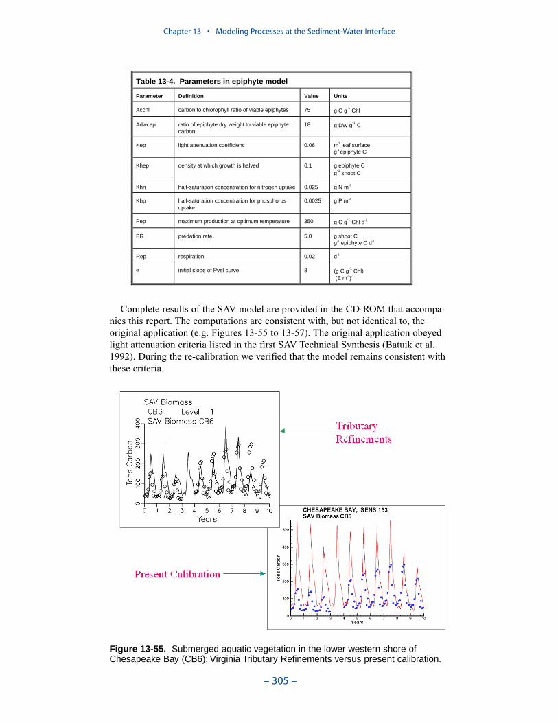
Complete results of the SAV model are provided in the CD-ROM that accompa-nies this report. The computations are consistent with, but not identical to, theoriginal application (e.g. Figures 13-55 to 13-57). The original application obeyedlight attenuation criteria listed in the first SAV Technical Synthesis (Batuik et al.1992). During the re-calibration we verified that the model remains consistent withthese criteria.
Chapter 13 • Modeling Processes at the Sediment-Water Interface
– 305 –
Table 13-4. Parameters in epiphyte model
Parameter Definition Value Units
Acchl carbon to chlorophyll ratio of viable epiphytes 75 g C g-1
Chl
Adwcep ratio of epiphyte dry weight to viable epiphyte carbon
18 g DW g-1
C
Kep light attenuation coefficient 0.06 m2 leaf surfaceg-1 epiphyte C
Khep density at which growth is halved 0.1 g epiphyte C g
-1 shoot C
Khn half-saturation concentration for nitrogen uptake 0.025 g N m-3
Khp half-saturation concentration for phosphorus uptake
0.0025 g P m-3
Pep maximum production at optimum temperature 350 g C g-1
Chl d-1
PR predation rate 5.0 g shoot Cg-1 epiphyte C d-1
Rep respiration 0.02 d-1
initial slope of PvsI curve 8 (g C g-1
Chl) (E m-2)-1
Figure 13-55. Submerged aquatic vegetation in the lower western shore ofChesapeake Bay (CB6): Virginia Tributary Refinements versus present calibration.
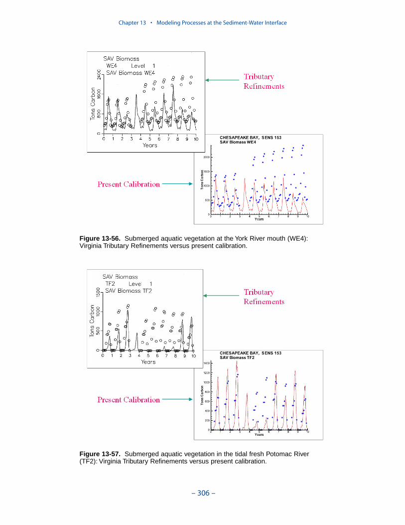
Chapter 13 • Modeling Processes at the Sediment-Water Interface
– 306 –
Figure 13-56. Submerged aquatic vegetation at the York River mouth (WE4):Virginia Tributary Refinements versus present calibration.
Figure 13-57. Submerged aquatic vegetation in the tidal fresh Potomac River(TF2): Virginia Tributary Refinements versus present calibration.
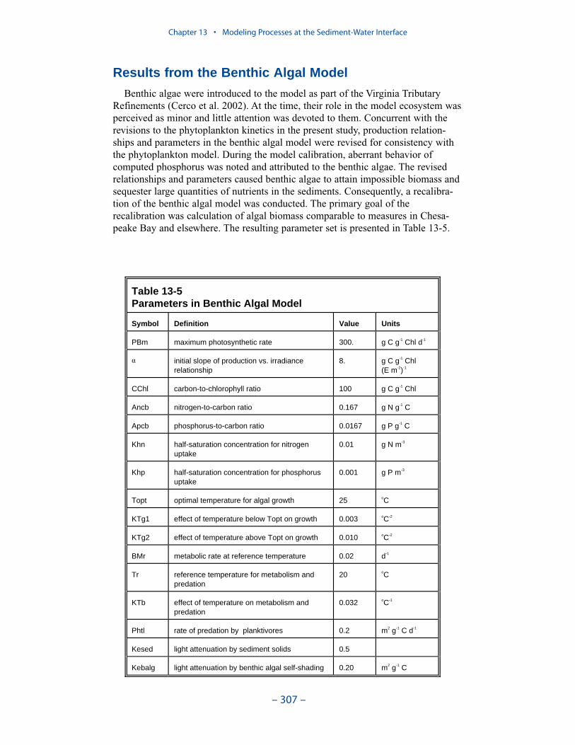
Results from the Benthic Algal Model
Benthic algae were introduced to the model as part of the Virginia TributaryRefinements (Cerco et al. 2002). At the time, their role in the model ecosystem wasperceived as minor and little attention was devoted to them. Concurrent with therevisions to the phytoplankton kinetics in the present study, production relation-ships and parameters in the benthic algal model were revised for consistency withthe phytoplankton model. During the model calibration, aberrant behavior ofcomputed phosphorus was noted and attributed to the benthic algae. The revisedrelationships and parameters caused benthic algae to attain impossible biomass andsequester large quantities of nutrients in the sediments. Consequently, a recalibra-tion of the benthic algal model was conducted. The primary goal of therecalibration was calculation of algal biomass comparable to measures in Chesa-peake Bay and elsewhere. The resulting parameter set is presented in Table 13-5.
Chapter 13 • Modeling Processes at the Sediment-Water Interface
– 307 –
Table 13-5 Parameters in Benthic Algal Model
Symbol Definition Value Units
PBm maximum photosynthetic rate 300. g C g-1 Chl d-1
initial slope of production vs. irradiance relationship
8. g C g-1 Chl(E m-2)-1
CChl carbon-to-chlorophyll ratio 100 g C g-1 Chl
Ancb nitrogen-to-carbon ratio 0.167 g N g-1 C
Apcb phosphorus-to-carbon ratio 0.0167 g P g-1 C
Khn half-saturation concentration for nitrogen uptake
0.01 g N m-3
Khp half-saturation concentration for phosphorus uptake
0.001 g P m-3
Topt optimal temperature for algal growth 25 oC
KTg1 effect of temperature below Topt on growth 0.003 oC-2
KTg2 effect of temperature above Topt on growth 0.010 oC-2
BMr metabolic rate at reference temperature 0.02 d-1
Tr reference temperature for metabolism and predation
20 oC
KTb effect of temperature on metabolism and predation
0.032 oC-1
Phtl rate of predation by planktivores 0.2 m2 g-1 C d-1
Kesed light attenuation by sediment solids 0.5
Kebalg light attenuation by benthic algal self-shading 0.20 m2 g-1 C
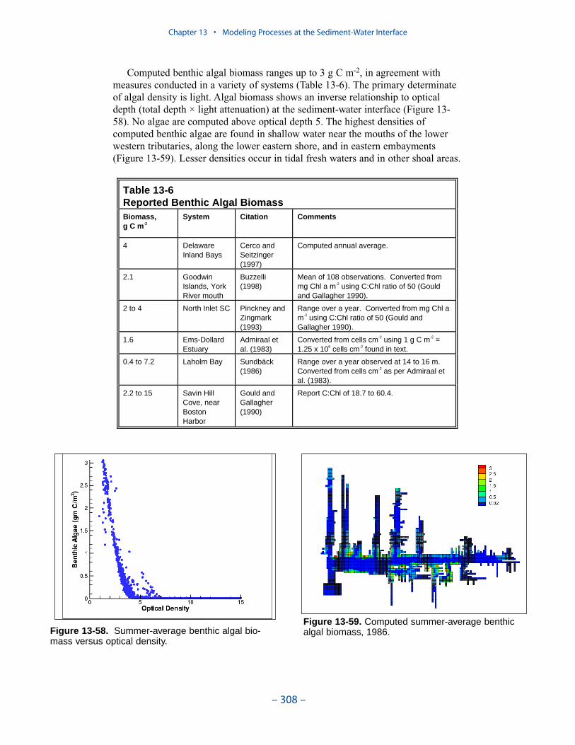
Computed benthic algal biomass ranges up to 3 g C m-2, in agreement withmeasures conducted in a variety of systems (Table 13-6). The primary determinateof algal density is light. Algal biomass shows an inverse relationship to opticaldepth (total depth × light attenuation) at the sediment-water interface (Figure 13-58). No algae are computed above optical depth 5. The highest densities ofcomputed benthic algae are found in shallow water near the mouths of the lowerwestern tributaries, along the lower eastern shore, and in eastern embayments(Figure 13-59). Lesser densities occur in tidal fresh waters and in other shoal areas.
Chapter 13 • Modeling Processes at the Sediment-Water Interface
– 308 –
Table 13-6 Reported Benthic Algal Biomass Biomass,g C m-2
System Citation Comments
4 DelawareInland Bays
Cerco and Seitzinger(1997)
Computed annual average.
2.1 GoodwinIslands, York River mouth
Buzzelli (1998)
Mean of 108 observations. Converted from mg Chl a m-2 using C:Chl ratio of 50 (Gould and Gallagher 1990).
2 to 4 North Inlet SC Pinckney and Zingmark(1993)
Range over a year. Converted from mg Chl a m-2 using C:Chl ratio of 50 (Gould and Gallagher 1990).
1.6 Ems-Dollard Estuary
Admiraal et al. (1983)
Converted from cells cm-2 using 1 g C m-2 = 1.25 x 10⁶ cells cm-2 found in text.
0.4 to 7.2 Laholm Bay Sundbäck(1986)
Range over a year observed at 14 to 16 m.Converted from cells cm-2 as per Admiraal et al. (1983).
2.2 to 15 Savin Hill Cove, near BostonHarbor
Gould and Gallagher(1990)
Report C:Chl of 18.7 to 60.4.
Figure 13-58. Summer-average benthic algal bio-mass versus optical density.
Figure 13-59. Computed summer-average benthicalgal biomass, 1986.
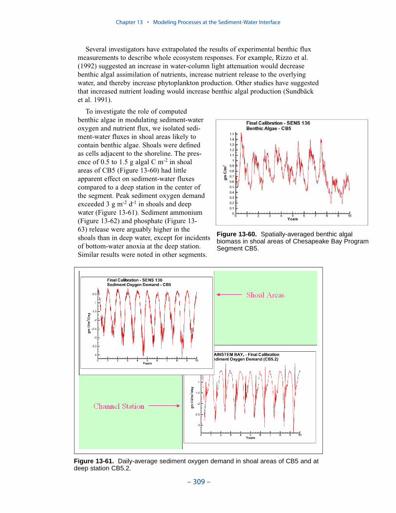
Several investigators have extrapolated the results of experimental benthic fluxmeasurements to describe whole ecosystem responses. For example, Rizzo et al.(1992) suggested an increase in water-column light attenuation would decreasebenthic algal assimilation of nutrients, increase nutrient release to the overlyingwater, and thereby increase phytoplankton production. Other studies have suggestedthat increased nutrient loading would increase benthic algal production (Sundbäcket al. 1991).
To investigate the role of computedbenthic algae in modulating sediment-wateroxygen and nutrient flux, we isolated sedi-ment-water fluxes in shoal areas likely tocontain benthic algae. Shoals were definedas cells adjacent to the shoreline. The pres-ence of 0.5 to 1.5 g algal C m-2 in shoalareas of CB5 (Figure 13-60) had littleapparent effect on sediment-water fluxescompared to a deep station in the center ofthe segment. Peak sediment oxygen demandexceeded 3 g m-2 d-1 in shoals and deepwater (Figure 13-61). Sediment ammonium(Figure 13-62) and phosphate (Figure 13-63) release were arguably higher in theshoals than in deep water, except for incidentsof bottom-water anoxia at the deep station.Similar results were noted in other segments.
Chapter 13 • Modeling Processes at the Sediment-Water Interface
– 309 –
Figure 13-60. Spatially-averaged benthic algalbiomass in shoal areas of Chesapeake Bay ProgramSegment CB5.
Figure 13-61. Daily-average sediment oxygen demand in shoal areas of CB5 and atdeep station CB5.2.

Chapter 13 • Modeling Processes at the Sediment-Water Interface
– 310 –
Figure 13-62. Daily-average sediment-water ammonium flux in shoal areas of CB5and at deep station CB5.2.
Figure 13-63. Daily-average sediment-water phosphate flux in shoal areas of CB5and at deep station CB5.2.
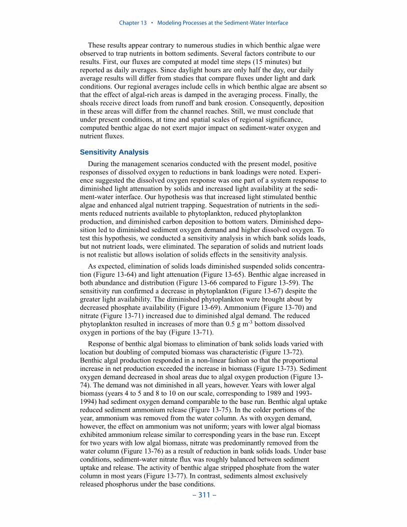
These results appear contrary to numerous studies in which benthic algae wereobserved to trap nutrients in bottom sediments. Several factors contribute to ourresults. First, our fluxes are computed at model time steps (15 minutes) butreported as daily averages. Since daylight hours are only half the day, our dailyaverage results will differ from studies that compare fluxes under light and darkconditions. Our regional averages include cells in which benthic algae are absent sothat the effect of algal-rich areas is damped in the averaging process. Finally, theshoals receive direct loads from runoff and bank erosion. Consequently, depositionin these areas will differ from the channel reaches. Still, we must conclude thatunder present conditions, at time and spatial scales of regional significance,computed benthic algae do not exert major impact on sediment-water oxygen andnutrient fluxes.
Sensitivity Analysis
During the management scenarios conducted with the present model, positiveresponses of dissolved oxygen to reductions in bank loadings were noted. Experi-ence suggested the dissolved oxygen response was one part of a system response todiminished light attenuation by solids and increased light availability at the sedi-ment-water interface. Our hypothesis was that increased light stimulated benthicalgae and enhanced algal nutrient trapping. Sequestration of nutrients in the sedi-ments reduced nutrients available to phytoplankton, reduced phytoplanktonproduction, and diminished carbon deposition to bottom waters. Diminished depo-sition led to diminished sediment oxygen demand and higher dissolved oxygen. Totest this hypothesis, we conducted a sensitivity analysis in which bank solids loads,but not nutrient loads, were eliminated. The separation of solids and nutrient loadsis not realistic but allows isolation of solids effects in the sensitivity analysis.
As expected, elimination of solids loads diminished suspended solids concentra-tion (Figure 13-64) and light attenuation (Figure 13-65). Benthic algae increased inboth abundance and distribution (Figure 13-66 compared to Figure 13-59). Thesensitivity run confirmed a decrease in phytoplankton (Figure 13-67) despite thegreater light availability. The diminished phytoplankton were brought about bydecreased phosphate availability (Figure 13-69). Ammonium (Figure 13-70) andnitrate (Figure 13-71) increased due to diminished algal demand. The reducedphytoplankton resulted in increases of more than 0.5 g m-3 bottom dissolvedoxygen in portions of the bay (Figure 13-71).
Response of benthic algal biomass to elimination of bank solids loads varied withlocation but doubling of computed biomass was characteristic (Figure 13-72).Benthic algal production responded in a non-linear fashion so that the proportionalincrease in net production exceeded the increase in biomass (Figure 13-73). Sedimentoxygen demand decreased in shoal areas due to algal oxygen production (Figure 13-74). The demand was not diminished in all years, however. Years with lower algalbiomass (years 4 to 5 and 8 to 10 on our scale, corresponding to 1989 and 1993-1994) had sediment oxygen demand comparable to the base run. Benthic algal uptakereduced sediment ammonium release (Figure 13-75). In the colder portions of theyear, ammonium was removed from the water column. As with oxygen demand,however, the effect on ammonium was not uniform; years with lower algal biomassexhibited ammonium release similar to corresponding years in the base run. Exceptfor two years with low algal biomass, nitrate was predominantly removed from thewater column (Figure 13-76) as a result of reduction in bank solids loads. Under baseconditions, sediment-water nitrate flux was roughly balanced between sedimentuptake and release. The activity of benthic algae stripped phosphate from the watercolumn in most years (Figure 13-77). In contrast, sediments almost exclusivelyreleased phosphorus under the base conditions.
Chapter 13 • Modeling Processes at the Sediment-Water Interface
– 311 –
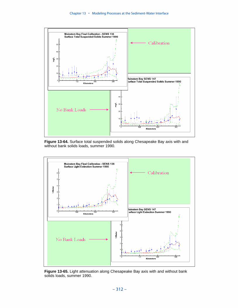
Chapter 13 • Modeling Processes at the Sediment-Water Interface
– 312 –
Figure 13-64. Surface total suspended solids along Chesapeake Bay axis with andwithout bank solids loads, summer 1990.
Figure 13-65. Light attenuation along Chesapeake Bay axis with and without banksolids loads, summer 1990.
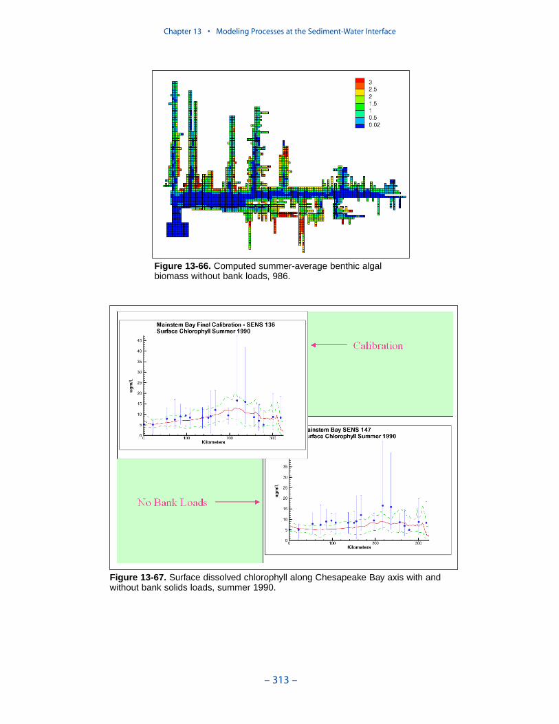
Chapter 13 • Modeling Processes at the Sediment-Water Interface
– 313 –
Figure 13-66. Computed summer-average benthic algalbiomass without bank loads, 986.
Figure 13-67. Surface dissolved chlorophyll along Chesapeake Bay axis with andwithout bank solids loads, summer 1990.
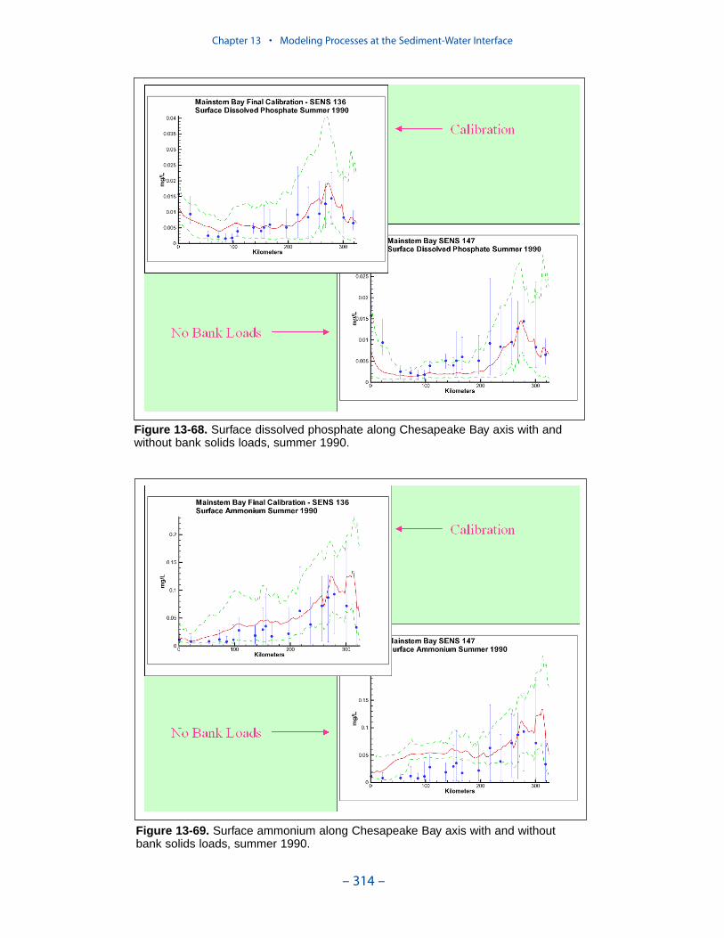
Chapter 13 • Modeling Processes at the Sediment-Water Interface
– 314 –
Figure 13-68. Surface dissolved phosphate along Chesapeake Bay axis with andwithout bank solids loads, summer 1990.
Figure 13-69. Surface ammonium along Chesapeake Bay axis with and withoutbank solids loads, summer 1990.
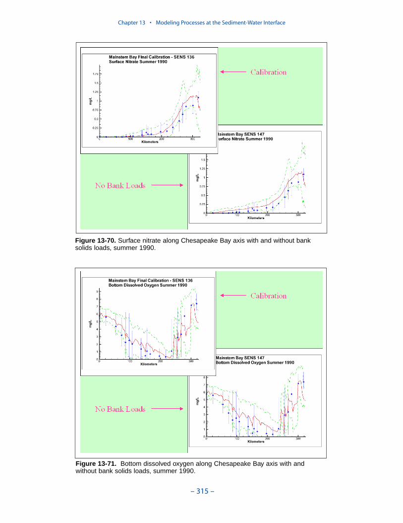
Chapter 13 • Modeling Processes at the Sediment-Water Interface
– 315 –
Figure 13-70. Surface nitrate along Chesapeake Bay axis with and without banksolids loads, summer 1990.
Figure 13-71. Bottom dissolved oxygen along Chesapeake Bay axis with and without bank solids loads, summer 1990.
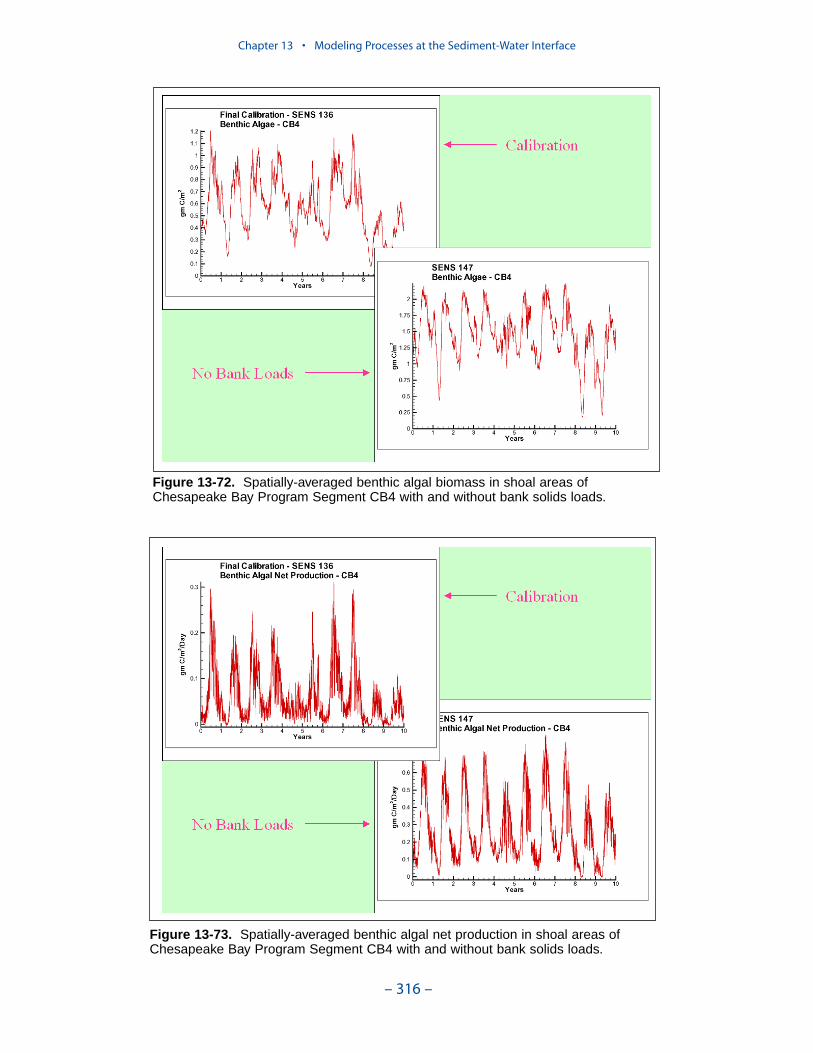
Chapter 13 • Modeling Processes at the Sediment-Water Interface
– 316 –
Figure 13-72. Spatially-averaged benthic algal biomass in shoal areas ofChesapeake Bay Program Segment CB4 with and without bank solids loads.
Figure 13-73. Spatially-averaged benthic algal net production in shoal areas ofChesapeake Bay Program Segment CB4 with and without bank solids loads.
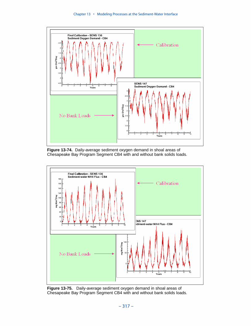
Chapter 13 • Modeling Processes at the Sediment-Water Interface
– 317 –
Figure 13-74. Daily-average sediment oxygen demand in shoal areas ofChesapeake Bay Program Segment CB4 with and without bank solids loads.
Figure 13-75. Daily-average sediment oxygen demand in shoal areas ofChesapeake Bay Program Segment CB4 with and without bank solids loads.
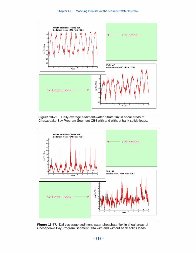
Chapter 13 • Modeling Processes at the Sediment-Water Interface
– 318 –
Figure 13-76. Daily-average sediment-water nitrate flux in shoal areas ofChesapeake Bay Program Segment CB4 with and without bank solids loads.
Figure 13-77. Daily-average sediment-water phosphate flux in shoal areas ofChesapeake Bay Program Segment CB4 with and without bank solids loads.
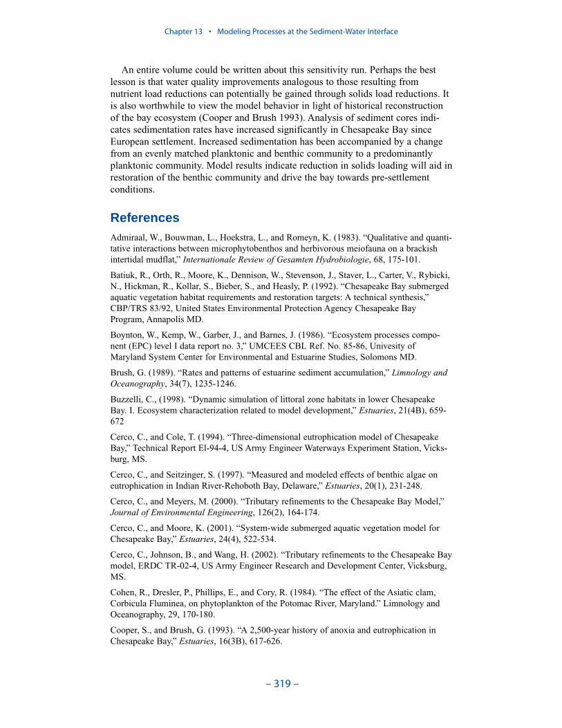
An entire volume could be written about this sensitivity run. Perhaps the bestlesson is that water quality improvements analogous to those resulting fromnutrient load reductions can potentially be gained through solids load reductions. Itis also worthwhile to view the model behavior in light of historical reconstructionof the bay ecosystem (Cooper and Brush 1993). Analysis of sediment cores indi-cates sedimentation rates have increased significantly in Chesapeake Bay sinceEuropean settlement. Increased sedimentation has been accompanied by a changefrom an evenly matched planktonic and benthic community to a predominantlyplanktonic community. Model results indicate reduction in solids loading will aid inrestoration of the benthic community and drive the bay towards pre-settlementconditions.
ReferencesAdmiraal, W., Bouwman, L., Hoekstra, L., and Romeyn, K. (1983). “Qualitative and quanti-tative interactions between microphytobenthos and herbivorous meiofauna on a brackishintertidal mudflat,” Internationale Review of Gesamten Hydrobiologie, 68, 175-101.
Batiuk, R., Orth, R., Moore, K., Dennison, W., Stevenson, J., Staver, L., Carter, V., Rybicki,N., Hickman, R., Kollar, S., Bieber, S., and Heasly, P. (1992). “Chesapeake Bay submergedaquatic vegetation habitat requirements and restoration targets: A technical synthesis,”CBP/TRS 83/92, United States Environmental Protection Agency Chesapeake BayProgram, Annapolis MD.
Boynton, W., Kemp, W., Garber, J., and Barnes, J. (1986). “Ecosystem processes compo-nent (EPC) level I data report no. 3,” UMCEES CBL Ref. No. 85-86, Univesity ofMaryland System Center for Environmental and Estuarine Studies, Solomons MD.
Brush, G. (1989). “Rates and patterns of estuarine sediment accumulation,” Limnology andOceanography, 34(7), 1235-1246.
Buzzelli, C., (1998). “Dynamic simulation of littoral zone habitats in lower ChesapeakeBay. I. Ecosystem characterization related to model development,” Estuaries, 21(4B), 659-672
Cerco, C., and Cole, T. (1994). “Three-dimensional eutrophication model of ChesapeakeBay,” Technical Report El-94-4, US Army Engineer Waterways Experiment Station, Vicks-burg, MS.
Cerco, C., and Seitzinger, S. (1997). “Measured and modeled effects of benthic algae oneutrophication in Indian River-Rehoboth Bay, Delaware,” Estuaries, 20(1), 231-248.
Cerco, C., and Meyers, M. (2000). “Tributary refinements to the Chesapeake Bay Model,”Journal of Environmental Engineering, 126(2), 164-174.
Cerco, C., and Moore, K. (2001). “System-wide submerged aquatic vegetation model forChesapeake Bay,” Estuaries, 24(4), 522-534.
Cerco, C., Johnson, B., and Wang, H. (2002). “Tributary refinements to the Chesapeake Baymodel, ERDC TR-02-4, US Army Engineer Research and Development Center, Vicksburg,MS.
Cohen, R., Dresler, P., Phillips, E., and Cory, R. (1984). “The effect of the Asiatic clam,Corbicula Fluminea, on phytoplankton of the Potomac River, Maryland.” Limnology andOceanography, 29, 170-180.
Cooper, S., and Brush, G. (1993). “A 2,500-year history of anoxia and eutrophication inChesapeake Bay,” Estuaries, 16(3B), 617-626.
Chapter 13 • Modeling Processes at the Sediment-Water Interface
– 319 –
DiToro, D., and Fitzpatrick, J. (1993). “Chesapeake Bay sediment flux model,” ContractReport EL-93-2, US Army Engineer Waterways Experiment Station, Vicksburg, MS.
DiToro, D. (2001). Sediment Flux Modeling, John Wiley and Sons, New York.
Fisher, T., Carlson, P., and Barber, R. (1982). “Sediment nutrient regeneration in threeNorth Carolina estuaries,” Estuarine, Coastal and Shelf Science, 4, 101- 116.
Gould, D., and Gallagher, E. (1990). “Field measurements of specific growth rate, biomass,and primary production of benthic diatoms of Savin Hill Cove, Boston,” Limnology andOceanography, 35, 1757-1770.
HydroQual. (1987). “A steady-state coupled hydrodynamic/water quality model of theeutrophication and anoxia process in Chesapeake Bay,” Final Report, HydroQual Inc.,Mahwah, NJ.
HydroQual. (2000). “Development of a suspension feeding and deposit feeding benthosmodel for Chesapeake Bay,” produced by HydroQual Inc. under contract to the U.S. ArmyEngineer Research and Development Center, Vicksburg MS.
Jenkins, M., and Kemp, W., (1984). “The coupling of nitrification and denitrification in twoestuarine sediments,” Limnology and Oceanography, 29(3), 609-619.
Meyers, M., DiToro, D., and Lowe, S. (2000). “Coupling suspension feeders to the Chesa-peake Bay eutrophication model,” Water Quality and Ecosystem Modeling, 1, 123-140.
Moore, K., Wilcox, D., Orth, R. (2000). “Analysis and abundance of submersed aquaticvegetation communities in the Chesapeake Bay,” Estuaries, 23, 115-127.
Officer, C., Lynch, D., Setlock, G., and Helz, G. (1984). “Recent sedimentation rates inChesapeake Bay,” The estuary as a filter. V. Kennedy, ed. Academic Press, Orlando FL,131-157.
Newell, R. (1988). “Ecological Changes in Chesapeake Bay: Are They the Results of Over-harvesting the American Oyster (Crassostrea Virginica)?” Understanding the Estuary:Advances in Chesapeake Bay Research. M Lynch and E Krome Eds., Chesapeake BayResearch Consortium Publication 129, Gloucester Point VA, 536-546
Orth, R., and Moore, K. (1984). “Distribution and abundance of submerged aquatic vegeta-tion in Chesapeake Bay: An historical perspective.” Estuaries (4B):531-540
Pinckney, J., and Zingmark, R. (1993). “Modeling the annual production of intertidalbenthic microalgae in estuarine ecosystems,” Journal of Phycology, 29, 396-407.
Rizzo, , W., Lackey, G., and Christian, R. (1992). “Significance of euphotic subtidal sedi-ments to oxygen and nutrient cycling in a temperate estuary,” Marine Ecology ProgressSeries, 85, 51-61.
Seitzinger, S., Nixon, S., and Pilson, M. (1984). “Denitrification and nitrous oxide produc-tion in a coastal marine ecosystem,” Limnology and Oceanography, 29(1), 73-83.
Sundbäck, K. (1986). “What are the benthic microalgae doing on the bottom of LanholmBay?,” Ophelia Supplement, 4, 273-286.
Sundbäck, K., Enoksson, V., Granéli, W., and Peterson, K. (1991). “Influence of sublittoralmicrophytobenthos on the oxygen and nutrient flux between sediment and water: A labora-tory continuous flow study,” Marine Ecology Progress Series, 74, 263-279
Westrich, J., and Berner, R. (1984). “The role of sedimentary organic matter in bacterialsulfate reduction: The G model tested,” Limnology and Oceanography, 29, 236-249.
Chapter 13 • Modeling Processes at the Sediment-Water Interface
– 320 –

Introduction
An excess of computed dissolved phosphate, especially during summer, has beena characteristic of the model since the earliest phase (Cerco and Cole 1994). Whiletuning the model to effect an overall reduction in computed dissolved phosphatepresents no problem, reducing phosphate in summer while maintaining sufficientphosphate to support the spring phytoplankton bloom is precarious.
The first-phase model employed two processes to reduce excess phosphate. Thefirst was variable algal stoichiometry. During periods of plentiful phosphate, thealgal phosphorus-to-carbon ratio increased so that more phosphate was stored asalgal biomass. During periods of phosphate depletion, the phosphorus-to-carbonratio decreased so that less phosphate was required to support algal growth.
The second process was co-precipitation of phosphate with iron and manganese.Iron and manganese are released in dissolved form by Chesapeake Bay sedimentsunder anoxic conditions. These metals precipitate at the interface between oxic andanoxic water and during the autumn aeration event. Dissolved phosphate isremoved from the water by sorption to the fresh precipitates.
The variable algal stoichiometry relied on an iterative bisection algorithm. Thealgorithm was time-consuming and numerically unstable. Consequently, wereverted to constant algal composition in the Virginia Tributary Refinements study(Cerco et al. 2002). Iron and manganese (together referred to as Total Active Metal,TAM) occupied a slot in the model code originally intended for fixed solids. Sincefixed solids were not modeled in the initial study, this variable was available forreprogramming as TAM. Fixed solids were modeled in the Virginia TributaryRefinements and in the present study so that TAM was dropped from the statevariable suite. As a result, in this study, we reverted to the original problem of anexcess of dissolved phosphate, especially during summer.
– 321 –
Dissolved Phosphate14

The present chapter outlines our efforts to bring dissolved phosphate into cali-bration. As with other sensitivity analyses, the runs compared are not necessarilysequential and may have multiple differences. Still, the results are illustrative of themagnitude and effects of various processes.
Dissolved Organic Phosphorus Mineralization
Dissolved phosphate is produced by multiple processes in the model ecosystem.A classic mechanism is the first-order mineralization of dissolved organic phos-phorus to dissolved phosphate. The sensitivity of dissolved phosphate tomineralization was tested by setting this process to zero. This was a reduction infirst-order rate from 0.15 d-1 to 0.0 d-1. Results indicated mineralization of 0.15 d-1
was responsible for 0.005 g PO4-P m-3 in surface waters of the bay during summer(Figure 14-1). Elimination of mineralization diminished phosphate uniformlyexcept at the system boundaries. In the central bay (km 100 to 200), computedphosphate changed from an excess to agreement with observations. In the upperbay (> km 250) computed phosphate that agreed with observed decreased to belowcomputed values. In portions of the lower bay (< km 100) computed phosphate washigh and remained high following elimination of mineralization. This run illus-trated the freedom the modeler has to alter phosphate via specification ofmineralization. The run also illustrated that mineralization rate alone cannot beused to tune the model unless spatially-variable rates are employed.
Chapter 14 • Dissolved Phosphate
– 322 –
Figure 14-1. Effect of mineralization rate on surface dissolved phosphate. Resultsare shown for summer 1990 along Chesapeake Bay axis.
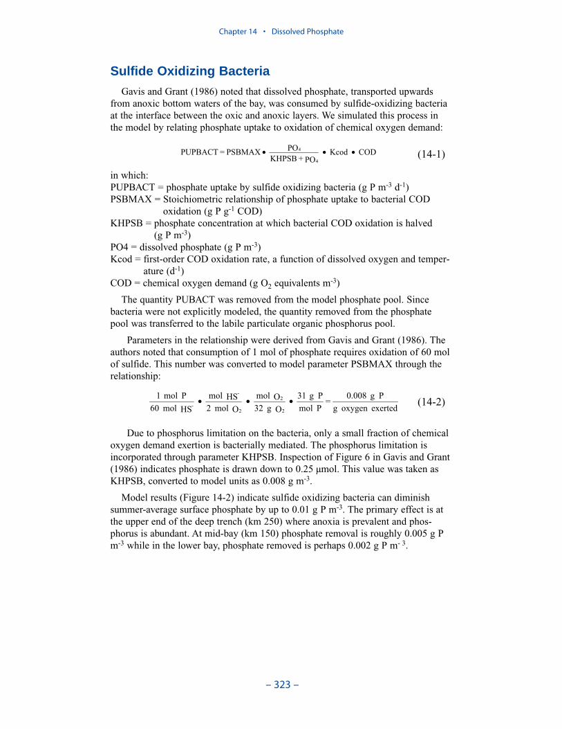
Chapter 14 • Dissolved Phosphate
– 323 –
Sulfide Oxidizing Bacteria
Gavis and Grant (1986) noted that dissolved phosphate, transported upwardsfrom anoxic bottom waters of the bay, was consumed by sulfide-oxidizing bacteriaat the interface between the oxic and anoxic layers. We simulated this process inthe model by relating phosphate uptake to oxidation of chemical oxygen demand:
in which:PUPBACT = phosphate uptake by sulfide oxidizing bacteria (g P m-3 d-1)PSBMAX = Stoichiometric relationship of phosphate uptake to bacterial COD
oxidation (g P g-1 COD)KHPSB = phosphate concentration at which bacterial COD oxidation is halved
(g P m-3)PO4 = dissolved phosphate (g P m-3)Kcod = first-order COD oxidation rate, a function of dissolved oxygen and temper-
ature (d-1)COD = chemical oxygen demand (g O2 equivalents m-3)
The quantity PUBACT was removed from the model phosphate pool. Sincebacteria were not explicitly modeled, the quantity removed from the phosphatepool was transferred to the labile particulate organic phosphorus pool.
Parameters in the relationship were derived from Gavis and Grant (1986). Theauthors noted that consumption of 1 mol of phosphate requires oxidation of 60 molof sulfide. This number was converted to model parameter PSBMAX through therelationship:
Due to phosphorus limitation on the bacteria, only a small fraction of chemicaloxygen demand exertion is bacterially mediated. The phosphorus limitation isincorporated through parameter KHPSB. Inspection of Figure 6 in Gavis and Grant(1986) indicates phosphate is drawn down to 0.25 µmol. This value was taken asKHPSB, converted to model units as 0.008 g m-3.
Model results (Figure 14-2) indicate sulfide oxidizing bacteria can diminishsummer-average surface phosphate by up to 0.01 g P m-3. The primary effect is atthe upper end of the deep trench (km 250) where anoxia is prevalent and phos-phorus is abundant. At mid-bay (km 150) phosphate removal is roughly 0.005 g Pm-3 while in the lower bay, phosphate removed is perhaps 0.002 g P m- 3.
exertedoxygeng
Pg0.008=
Pmol
Pg31
Og32
Omol
Omol2
HSmol
HSmol60
Pmol1
2
2
2
-
-••• (14-2)
CODKcodPO+KHPSB
POPSBMAX=PUPBACT
4
4 ••• (14-1)

Precipitation
We invoked precipitation in regions of the bay that experience anoxia (Table14-1). Phosphorus was routed from the phosphate pool to the refractory particulateorganic pool during the fall aeration period. Our relationship mimicked the resultsof precipitation although the approach was less mechanistic than the originalformulation involving TAM:
in which:PRECIP = precipitation rate (g P m-3 d-1)PCPMAX = first-order precipitation rate (d-1)KHPCP = phosphate concentration at which precipitation rate is halved (g P m-3)PCPDAY = a binary variable indicating the reaeration period (0 or 1)
Experience and inspection suggested PCPMAX = 0.1 to 0.2 d-1, KHPCP =0.0025 g P m-3, and a reaeration interval extending from mid-September to mid-December.
Results indicated daily precipitation of 10% to 20% of the phosphate pooleffected a tremendous improvement in late-summer and autumn phosphate (Figure 14-3). Precipitation in late summer did little to impact summer-averagephosphate concentration, however (Figure 14-4).
PCPDAYPO+KHPCP
POPCPMAXPO=PRECIP
4
44 ••• (14-3)
Chapter 14 • Dissolved Phosphate
– 324 –
Figure 14-2. Effect of sulfide oxidizing bacteria on surface dissolved phosphate.Results are shown for summer 1990 along Chesapeake Bay axis. Note change ofvertical scale.
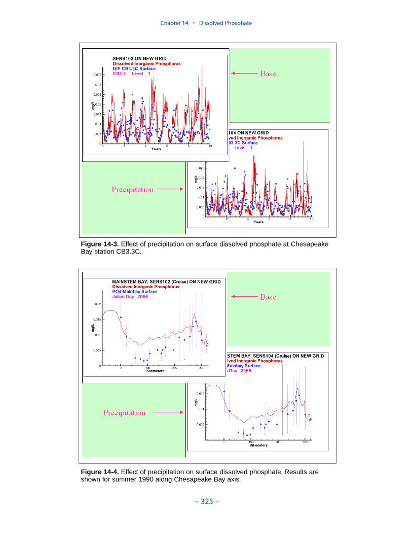
Chapter 14 • Dissolved Phosphate
– 325 –
Figure 14-3. Effect of precipitation on surface dissolved phosphate at ChesapeakeBay station CB3.3C.
Figure 14-4. Effect of precipitation on surface dissolved phosphate. Results areshown for summer 1990 along Chesapeake Bay axis.
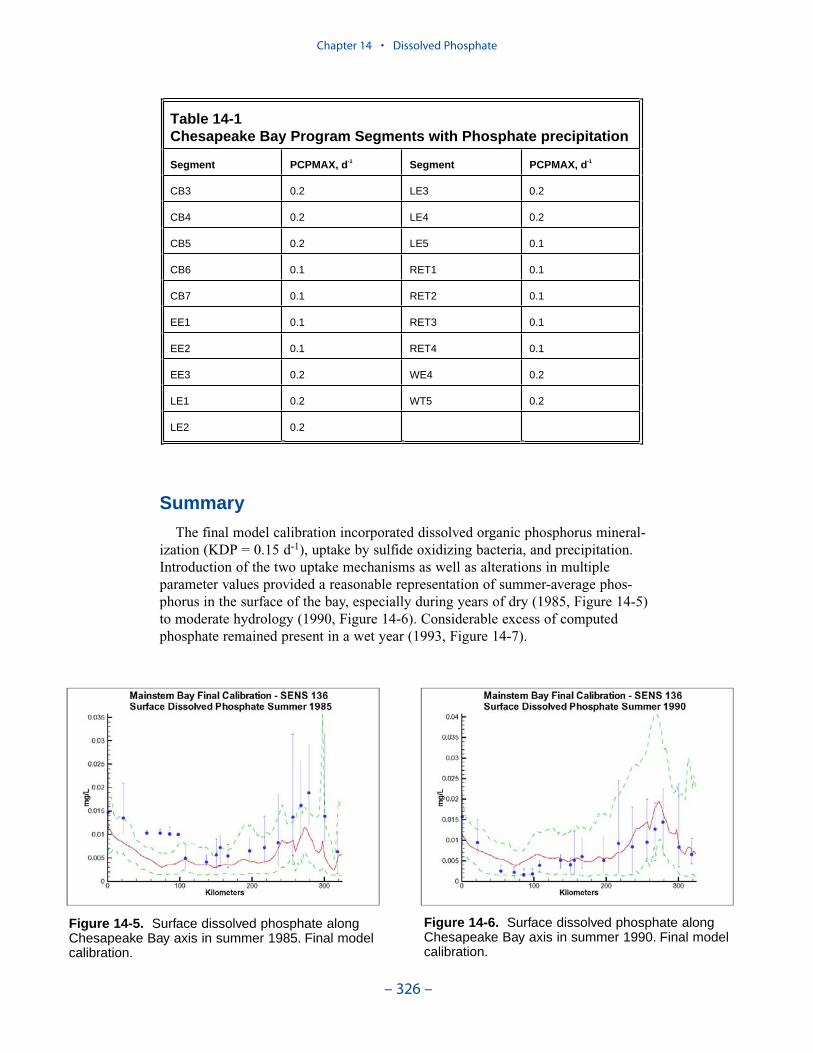
Summary
The final model calibration incorporated dissolved organic phosphorus mineral-ization (KDP = 0.15 d-1), uptake by sulfide oxidizing bacteria, and precipitation.Introduction of the two uptake mechanisms as well as alterations in multipleparameter values provided a reasonable representation of summer-average phos-phorus in the surface of the bay, especially during years of dry (1985, Figure 14-5)to moderate hydrology (1990, Figure 14-6). Considerable excess of computedphosphate remained present in a wet year (1993, Figure 14-7).
Chapter 14 • Dissolved Phosphate
– 326 –
Table 14-1 Chesapeake Bay Program Segments with Phosphate precipitation
Segment PCPMAX, d-1 Segment PCPMAX, d-1
CB3 0.2 LE3 0.2
CB4 0.2 LE4 0.2
CB5 0.2 LE5 0.1
CB6 0.1 RET1 0.1
CB7 0.1 RET2 0.1
EE1 0.1 RET3 0.1
EE2 0.1 RET4 0.1
EE3 0.2 WE4 0.2
LE1 0.2 WT5 0.2
LE2 0.2
Figure 14-5. Surface dissolved phosphate alongChesapeake Bay axis in summer 1985. Final modelcalibration.
Figure 14-6. Surface dissolved phosphate alongChesapeake Bay axis in summer 1990. Final modelcalibration.
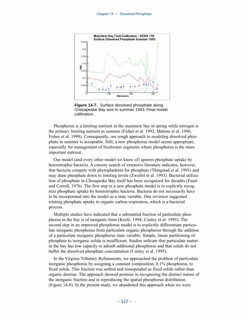
Phosphorus is a limiting nutrient in the mainstem bay in spring while nitrogen isthe primary limiting nutrient in summer (Fisher et al. 1992, Malone et al. 1996,Fisher et al. 1999). Consequently, our rough approach to modeling dissolved phos-phate in summer is acceptable. Still, a new phosphorus model seems appropriate,especially for management of freshwater segments where phosphorus is the moreimportant nutrient.
Our model (and every other model we know of) ignores phosphate uptake byheterotrophic bacteria. A cursory search of extensive literature indicates, however,that bacteria compete with phytoplankton for phosphate (Thingstad et al. 1993) andmay draw phosphate down to limiting levels (Zweifel et al. 1993). Bacterial utiliza-tion of phosphate in Chesapeake Bay itself has been recognized for decades (Faustand Correll, 1976). The first step in a new phosphate model is to explicitly recog-nize phosphate uptake by heterotrophic bacteria. Bacteria do not necessarily haveto be incorporated into the model as a state variable. One reviewer suggestedrelating phosphate uptake to organic carbon respiration, which is a bacterialprocess.
Multiple studies have indicated that a substantial fraction of particulate phos-phorus in the bay is of inorganic form (Keefe, 1994; Conley et al. 1995). Thesecond step in an improved phosphorus model is to explicitly differentiate particu-late inorganic phosphorus from particulate organic phosphorus through the additionof a particulate inorganic phosphorus state variable. Simple, linear partitioning ofphosphate to inorganic solids is insufficient. Studies indicate that particulate matterin the bay has low capacity to adsorb additional phosphorus and that solids do notbuffer the dissolved phosphate concentration (Conley et al. 1995).
In the Virginia Tributary Refinements, we approached the problem of particulateinorganic phosphorus by assigning a constant composition, 0.1% phosphorus, tofixed solids. This fraction was settled and resuspended as fixed solids rather thanorganic detritus. The approach showed promise in recognizing the distinct nature ofthe inorganic fraction and in reproducing the spatial phosphorus distribution(Figure 14-8). In the present study, we abandoned this approach when we were
Chapter 14 • Dissolved Phosphate
– 327 –
Figure 14-7. Surface dissolved phosphate alongChesapeake Bay axis in summer 1993. Final modelcalibration.
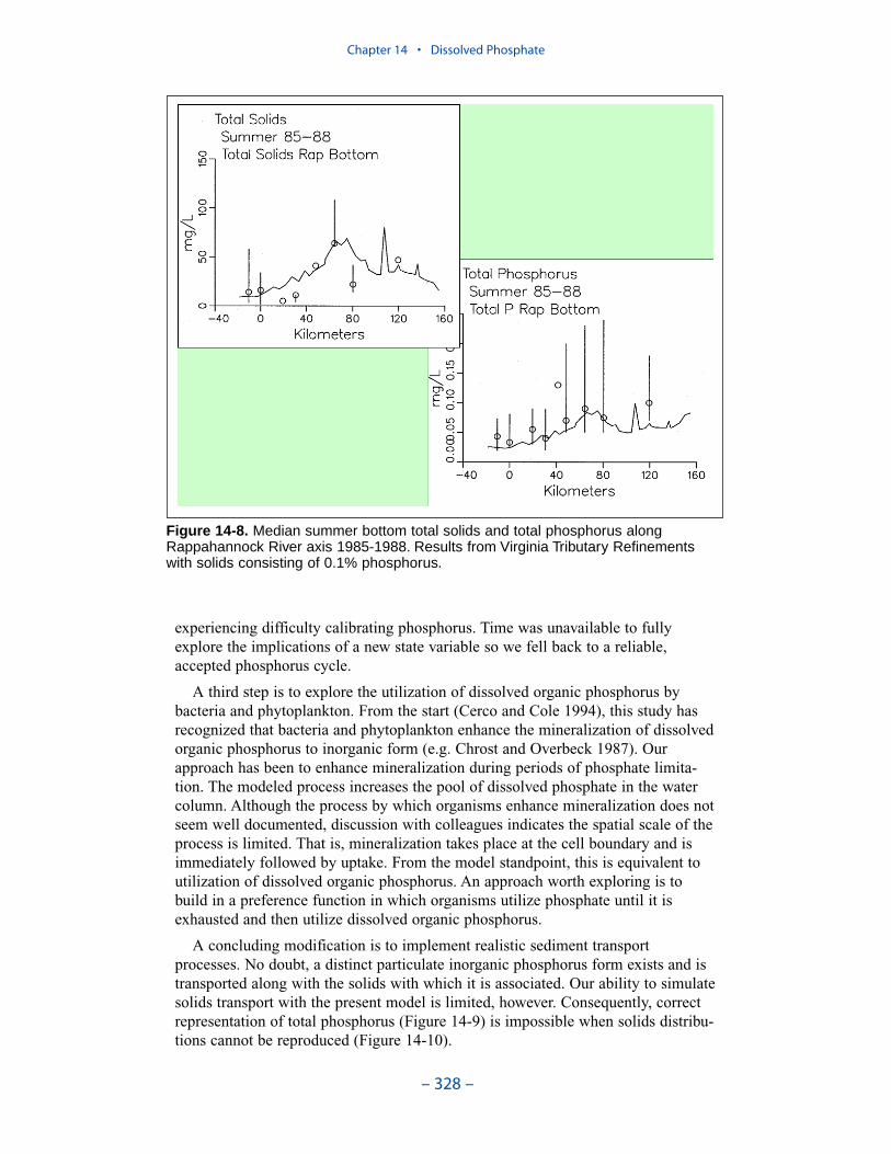
experiencing difficulty calibrating phosphorus. Time was unavailable to fullyexplore the implications of a new state variable so we fell back to a reliable,accepted phosphorus cycle.
A third step is to explore the utilization of dissolved organic phosphorus bybacteria and phytoplankton. From the start (Cerco and Cole 1994), this study hasrecognized that bacteria and phytoplankton enhance the mineralization of dissolvedorganic phosphorus to inorganic form (e.g. Chrost and Overbeck 1987). Ourapproach has been to enhance mineralization during periods of phosphate limita-tion. The modeled process increases the pool of dissolved phosphate in the watercolumn. Although the process by which organisms enhance mineralization does notseem well documented, discussion with colleagues indicates the spatial scale of theprocess is limited. That is, mineralization takes place at the cell boundary and isimmediately followed by uptake. From the model standpoint, this is equivalent toutilization of dissolved organic phosphorus. An approach worth exploring is tobuild in a preference function in which organisms utilize phosphate until it isexhausted and then utilize dissolved organic phosphorus.
A concluding modification is to implement realistic sediment transportprocesses. No doubt, a distinct particulate inorganic phosphorus form exists and istransported along with the solids with which it is associated. Our ability to simulatesolids transport with the present model is limited, however. Consequently, correctrepresentation of total phosphorus (Figure 14-9) is impossible when solids distribu-tions cannot be reproduced (Figure 14-10).
Chapter 14 • Dissolved Phosphate
– 328 –
Figure 14-8. Median summer bottom total solids and total phosphorus alongRappahannock River axis 1985-1988. Results from Virginia Tributary Refinementswith solids consisting of 0.1% phosphorus.
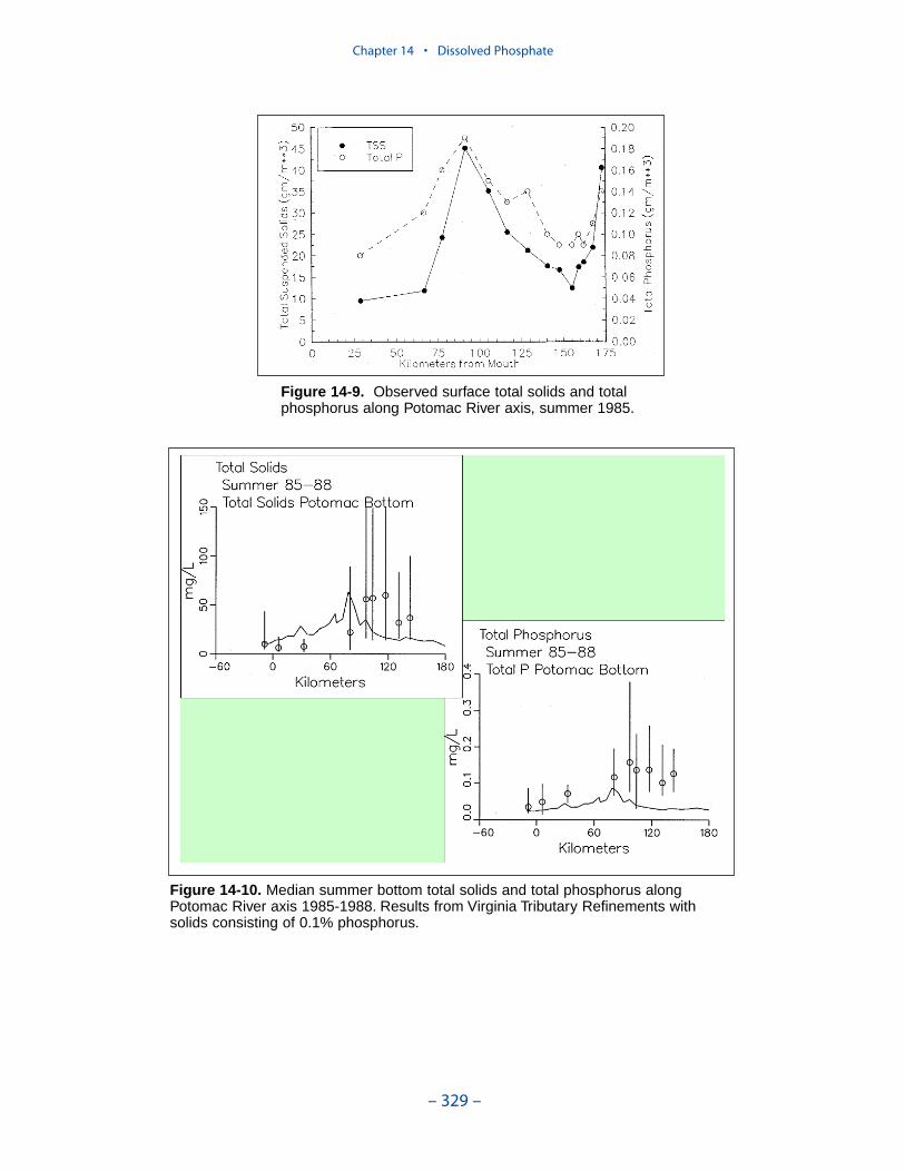
Chapter 14 • Dissolved Phosphate
– 329 –
Figure 14-9. Observed surface total solids and totalphosphorus along Potomac River axis, summer 1985.
Figure 14-10. Median summer bottom total solids and total phosphorus alongPotomac River axis 1985-1988. Results from Virginia Tributary Refinements withsolids consisting of 0.1% phosphorus.
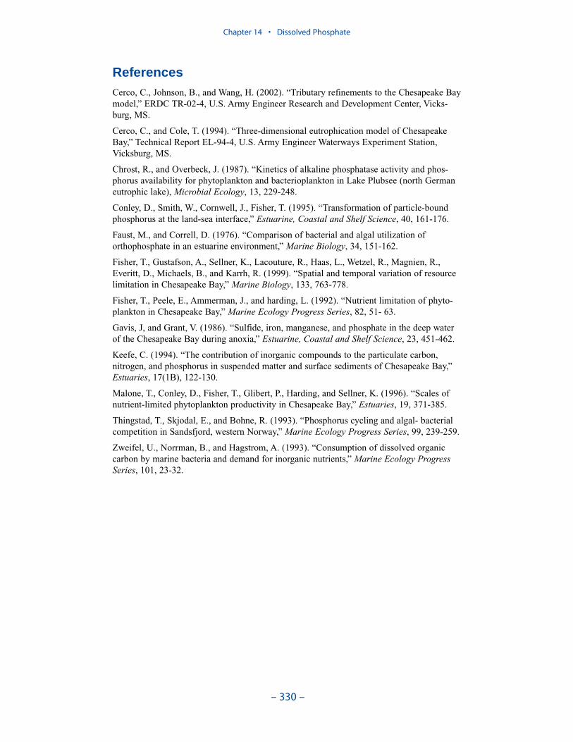
ReferencesCerco, C., Johnson, B., and Wang, H. (2002). “Tributary refinements to the Chesapeake Baymodel,” ERDC TR-02-4, U.S. Army Engineer Research and Development Center, Vicks-burg, MS.
Cerco, C., and Cole, T. (1994). “Three-dimensional eutrophication model of ChesapeakeBay,” Technical Report EL-94-4, U.S. Army Engineer Waterways Experiment Station,Vicksburg, MS.
Chrost, R., and Overbeck, J. (1987). “Kinetics of alkaline phosphatase activity and phos-phorus availability for phytoplankton and bacterioplankton in Lake Plubsee (north Germaneutrophic lake), Microbial Ecology, 13, 229-248.
Conley, D., Smith, W., Cornwell, J., Fisher, T. (1995). “Transformation of particle-boundphosphorus at the land-sea interface,” Estuarine, Coastal and Shelf Science, 40, 161-176.
Faust, M., and Correll, D. (1976). “Comparison of bacterial and algal utilization oforthophosphate in an estuarine environment,” Marine Biology, 34, 151-162.
Fisher, T., Gustafson, A., Sellner, K., Lacouture, R., Haas, L., Wetzel, R., Magnien, R.,Everitt, D., Michaels, B., and Karrh, R. (1999). “Spatial and temporal variation of resourcelimitation in Chesapeake Bay,” Marine Biology, 133, 763-778.
Fisher, T., Peele, E., Ammerman, J., and harding, L. (1992). “Nutrient limitation of phyto-plankton in Chesapeake Bay,” Marine Ecology Progress Series, 82, 51- 63.
Gavis, J, and Grant, V. (1986). “Sulfide, iron, manganese, and phosphate in the deep waterof the Chesapeake Bay during anoxia,” Estuarine, Coastal and Shelf Science, 23, 451-462.
Keefe, C. (1994). “The contribution of inorganic compounds to the particulate carbon,nitrogen, and phosphorus in suspended matter and surface sediments of Chesapeake Bay,”Estuaries, 17(1B), 122-130.
Malone, T., Conley, D., Fisher, T., Glibert, P., Harding, and Sellner, K. (1996). “Scales ofnutrient-limited phytoplankton productivity in Chesapeake Bay,” Estuaries, 19, 371-385.
Thingstad, T., Skjodal, E., and Bohne, R. (1993). “Phosphorus cycling and algal- bacterialcompetition in Sandsfjord, western Norway,” Marine Ecology Progress Series, 99, 239-259.
Zweifel, U., Norrman, B., and Hagstrom, A. (1993). “Consumption of dissolved organiccarbon by marine bacteria and demand for inorganic nutrients,” Marine Ecology ProgressSeries, 101, 23-32.
Chapter 14 • Dissolved Phosphate
– 330 –
Introduction
The calibration of the model involved the comparison of hundreds of thousandsof observations with model results in various formats. Comparisons involvedconventional water quality data, process-oriented data, and living-resources obser-vations. The graphical comparisons produced thousands of plots which cannot beassimilated in their entirety. Evaluation of model performance requires statisticaland/or graphical summaries of results. We present summaries here for major waterquality constituents in the mainstem bay and western tributaries. Additional graph-ical comparisons are available on the CD-ROM that accompanies this report.
Methods
No standard set of model performance statistics exists. We employ summarystatistics that were developed as part of our initial Chesapeake Bay model study(Cerco and Cole 1994). Use of a consistent set of statistics facilitates comparisonswith earlier model versions and with applications to other systems.
Statistics computed were mean error, absolute mean error, and relative error:
| O - P |RE = O
(15-3)
| O - P |AME = N
(15-2)
NP)-(O=ME (15-1)
– 331 –
Statistical Summaryof Calibration15
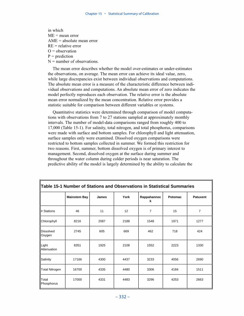
in which ME = mean errorAME = absolute mean errorRE = relative errorO = observationP = predictionN = number of observations.
The mean error describes whether the model over-estimates or under-estimatesthe observations, on average. The mean error can achieve its ideal value, zero,while large discrepancies exist between individual observations and computations.The absolute mean error is a measure of the characteristic difference between indi-vidual observations and computations. An absolute mean error of zero indicates themodel perfectly reproduces each observation. The relative error is the absolutemean error normalized by the mean concentration. Relative error provides astatistic suitable for comparison between different variables or systems.
Quantitative statistics were determined through comparison of model computa-tions with observations from 7 to 27 stations sampled at approximately monthlyintervals. The number of model-data comparisons ranged from roughly 400 to17,000 (Table 15-1). For salinity, total nitrogen, and total phosphorus, comparisonswere made with surface and bottom samples. For chlorophyll and light attenuation,surface samples only were examined. Dissolved oxygen comparisons wererestricted to bottom samples collected in summer. We formed this restriction fortwo reasons. First, summer, bottom dissolved oxygen is of primary interest tomanagement. Second, dissolved oxygen at the surface during summer andthroughout the water column during colder periods is near saturation. Thepredictive ability of the model is largely determined by the ability to calculate the
Chapter 15 • Statistical Summary of Calibration
– 332 –
Table 15-1 Number of Stations and Observations in Statistical Summaries
Mainstem Bay James York Rappahannock
Potomac Patuxent
# Stations 46 11 12 7 15 7
Chlorophyll 8216 2087 2188 1548 1971 1277
Dissolved Oxygen
2745 605 669 462 718 424
LightAttenuation
8351 1925 2108 1552 2223 1330
Salinity 17166 4300 4437 3233 4056 2690
Total Nitrogen 16700 4335 4480 3306 4184 1511
Total Phosphorus
17000 4331 4483 3296 4253 2663
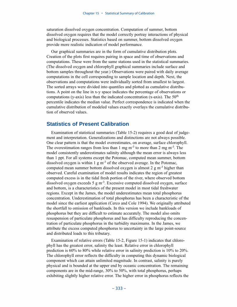
Chapter 15 • Statistical Summary of Calibration
– 333 –
saturation dissolved oxygen concentration. Computation of summer, bottomdissolved oxygen requires that the model correctly portray interactions of physicaland biological processes. Statistics based on summer, bottom dissolved oxygenprovide more realistic indication of model performance.
Our graphical summaries are in the form of cumulative distribution plots.Creation of the plots first requires pairing in space and time of observations andcomputations. These were from the same stations used in the statistical summaries.(The dissolved oxygen and chlorophyll graphical summaries include surface andbottom samples throughout the year.) Observations were paired with daily averagecomputations in the cell corresponding to sample location and depth. Next, theobservations and computations were individually sorted from smallest to largest.The sorted arrays were divided into quantiles and plotted as cumulative distribu-tions. A point on the line in x-y space indicates the percentage of observations orcomputations (y-axis) less than the indicated concentration (x-axis). The 50th
percentile indicates the median value. Perfect correspondence is indicated when thecumulative distribution of modeled values exactly overlays the cumulative distribu-tion of observed values.
Statistics of Present Calibration
Examination of statistical summaries (Table 15-2) requires a good deal of judge-ment and interpretation. Generalizations and distinctions are not always possible.One clear pattern is that the model overestimates, on average, surface chlorophyll.The overestimation ranges from less than 1 mg m-3 to more than 2 mg m-3. Themodel consistently underestimates salinity although the mean error is always lessthan 1 ppt. For all systems except the Potomac, computed mean summer, bottomdissolved oxygen is within 1 g m-3 of the observed average. In the Potomac,computed mean summer bottom dissolved oxygen is almost 2 g m-3 higher thanobserved. Careful examination of model results indicates the region of greatestcomputed excess is in the tidal fresh portion of the river, where observed bottomdissolved oxygen exceeds 5 g m-3. Excessive computed dissolved oxygen, surfaceand bottom, is a characteristics of the present model in most tidal freshwaterregions. Except in the James, the model underestimates mean total phosphorusconcentration. Underestimation of total phosphorus has been a characteristic of themodel since the earliest application (Cerco and Cole 1994). We originally attributedthe shortfall to omission of bankloads. In this version we include bankloads ofphosphorus but they are difficult to estimate accurately. The model also omitsresuspension of particulate phosphorus and has difficulty reproducing the concen-tration of particulate phosphorus in the turbidity maximums. In the James, weattribute the excess computed phosphorus to uncertainty in the large point-sourceand distributed loads to this tributary.
Examination of relative errors (Table 15-2, Figure 15-1) indicates that chloro-phyll has the greatest error, salinity the least. Relative error in chlorophyllprediction is 60% to 80% while relative error in salinity prediction is 10% to 20%.The chlorophyll error reflects the difficulty in computing this dynamic biologicalcomponent which can attain unlimited magnitude. In contrast, salinity is purelyphysical and is bounded at the upper end by oceanic concentration. The remainingcomponents are in the mid-range, 30% to 50%, with total phosphorus, perhapsexhibiting slightly higher relative error. The higher error in phosphorus reflects the
aforementioned difficulties in evaluating loads, in simulating resuspension, and inrepresenting particulate phosphorus transport.
The mainstem bay is clearly superior in computations of salinity, total nitrogen,and total phosphorus. The James River stands out as demonstrating the highest rela-tive error in these components. We partially attribute the greater accuracy in themainstem to the relatively dense computational grid in this region. An additional,and probably more significant influence, is that the mainstem is dominated byinternal processes while the tributaries are strongly influenced by point-source anddistributed loads. The point-source loads are incompletely described, especially inthe early years of the simulation and in the Virginia tributaries. Below-fall-linedistributed loads cannot be measured; they can only be computed by the watershed
Chapter 15 • Statistical Summary of Calibration
– 334 –
Table 15-2 Statistical Summary of Calibration 1985-1994Surface Chlorophyll, ug/L Mainstem Bay James York Rappahannock Potomac Patuxent
Mean Error -0.53 -2.05 -1.68 -2.55 -1.85 -1.53
Absolute Mean Error 5.01 9.29 4.71 8.22 7.45 8.15
Relative Error 58.4 75.7 60.1 81.4 80.2 65.4
Summer, Bottom Dissolved Oxygen, mg/L
Mainstem Bay James York Rappahannock Potomac Patuxent
Mean Error 0.32 -0.09 0.37 0.62 -1.31 -0.92
Absolute Mean Error 1.47 2.43 1.18 1.93 2.13 1.74
Relative Error 35.7 36.6 22.8 35.4 40.5 39.3
Light Attenuation, 1/m Mainstem Bay James York Rappahannock Potomac Patuxent
Mean Error 0.02 -0.21 0.09 -0.17 -0.02 -0.20
Absolute Mean Error 0.36 0.97 0.84 0.89 1.03 0.84
Relative Error 35.3 43.7 41.9 42.3 45.2 38.4
Salinity, ppt Mainstem Bay James York Rappahannock Potomac Patuxent
Mean Error 0.71 0.11 0.95 0.01 0.45 0.16
Absolute Mean Error 1.97 2.01 1.84 1.49 0.97 1.69
Relative Error 11.8 31.2 14.5 18.3 22.5 17.5
Total Nitrogen, mg/L Mainstem Bay James York Rappahannock Potomac Patuxent
Mean Error 0.04 -0.16 0.01 0.14 0.32 -0.13
Absolute Mean Error 0.17 0.42 0.23 0.28 0.61 0.43
Relative Error 24.3 44.6 33.1 33.8 31.9 41.5
Total Phosphorus, mg/L Mainstem Bay James York Rappahannock Potomac Patuxent
Mean Error 0.005 -0.021 0.012 0.001 0.032 0.041
Absolute Mean Error 0.014 0.069 0.036 0.036 0.053 0.047
Relative Error 37.6 63.8 49.2 52.6 58.9 47.6
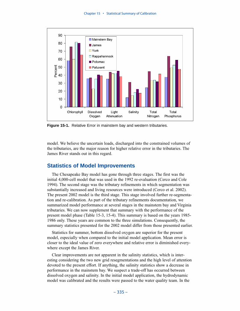
model. We believe the uncertain loads, discharged into the constrained volumes ofthe tributaries, are the major reason for higher relative error in the tributaries. TheJames River stands out in this regard.
Statistics of Model Improvements
The Chesapeake Bay model has gone through three stages. The first was theinitial 4,000-cell model that was used in the 1992 re-evaluation (Cerco and Cole1994). The second stage was the tributary refinements in which segmentation wassubstantially increased and living resources were introduced (Cerco et al. 2002).The present 2002 model is the third stage. This stage involved further re-segmenta-tion and re-calibration. As part of the tributary refinements documentation, wesummarized model performance at several stages in the mainstem bay and Virginiatributaries. We can now supplement that summary with the performance of thepresent model phase (Table 15-3, 15-4). This summary is based on the years 1985-1986 only. These years are common to the three simulations. Consequently, thesummary statistics presented for the 2002 model differ from those presented earlier.
Statistics for summer, bottom dissolved oxygen are superior for the presentmodel, especially when compared to the initial model application. Mean error iscloser to the ideal value of zero everywhere and relative error is diminished every-where except the James River.
Clear improvements are not apparent in the salinity statistics, which is inter-esting considering the two new grid resegmentations and the high level of attentiondevoted to the present effort. If anything, the salinity statistics show a decrease inperformance in the mainstem bay. We suspect a trade-off has occurred betweendissolved oxygen and salinity. In the initial model application, the hydrodynamicmodel was calibrated and the results were passed to the water quality team. In the
Chapter 15 • Statistical Summary of Calibration
– 335 –
Figure 15-1. Relative Error in mainstem bay and western tributaries.

Chapter 15 • Statistical Summary of Calibration
– 336 –
Table 15-3 Mean Errors in Three Model Phases
Salinity Mainstem James Rappahannock York
4000 Cell -0.06 -0.95 2.43 0.08
VA Tribs -0.62 0.55 -1.64 -0.94
2002 Model 1.69 0.32 1.14 1.68
SurfaceChlorophyll
Mainstem James Rappahannock York
4000 Cell -1.59 0.24 0.54 -1.19
VA Tribs -1.19 -4.84 2.25 -1.66
2002 Model -0.32 -2.47 -0.14 -1.46
LightAttenuation
Mainstem James Rappahannock York
4000 Cell -0.146 -0.329 -0.169 0.021
VA Tribs -0.206 -0.425 -0.599 0.222
2002 Model 0.065 0.009 0.135 0.125
Total Nitrogen Mainstem James Rappahannock York
4000 Cell -0.003 0.108 0.197 0.057
VA Tribs 0.011 -0.174 0.128 0.092
2002 Model 0.025 -0.205 0.098 0.004
TotalPhosphorus
Mainstem James Rappahannock York
4000 Cell 0.012 -0.0077 0.0265 0.0146
VA Tribs 0.0091 -0.0456 0.0043 0.0149
2002 Model 0.0115 -0.0534 -0.0008 -0.0025
Summer,Bottom,
DissolvedOxygen
Mainstem James Rappahannock York
4000 Cell -0.89 -1.88 -2.96 -0.48
VA Tribs 0.58 0.26 0.81 -0.08
2002 Model -0.03 -0.53 0.72 0.40
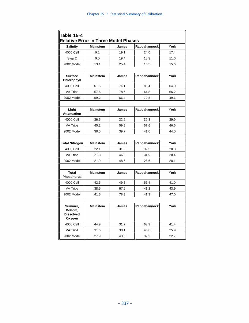
Chapter 15 • Statistical Summary of Calibration
– 337 –
Table 14-4 Relative Error in Three Model Phases
Salinity Mainstem James Rappahannock York
4000 Cell 9.1 19.1 24.0 17.4
Step 2 9.5 19.4 18.3 11.6
2002 Model 13.1 25.4 16.5 15.6
SurfaceChlorophyll
Mainstem James Rappahannock York
4000 Cell 61.6 74.1 83.4 64.0
VA Tribs 57.6 78.6 64.8 66.2
2002 Model 59.2 66.4 70.8 49.1
LightAttenuation
Mainstem James Rappahannock York
4000 Cell 36.5 32.6 32.8 39.9
VA Tribs 45.2 59.8 57.6 46.6
2002 Model 38.5 39.7 41.0 44.0
Total Nitrogen Mainstem James Rappahannock York
4000 Cell 22.1 31.9 32.5 20.8
VA Tribs 21.3 46.0 31.9 20.4
2002 Model 21.9 48.5 28.6 28.1
TotalPhosphorus
Mainstem James Rappahannock York
4000 Cell 42.5 49.3 53.4 41.0
VA Tribs 38.5 67.9 41.2 43.9
2002 Model 41.5 78.3 41.3 47.0
Summer,Bottom,
DissolvedOxygen
Mainstem James Rappahannock York
4000 Cell 44.9 31.7 63.9 41.4
VA Tribs 31.6 38.1 46.6 25.9
2002 Model 27.9 40.5 32.2 22.7
15-4
present application, the hydrodynamic and water quality models were calibratedinteractively. The salinity computation in the hydrodynamic model was weighedagainst the dissolved oxygen computation in the water quality model. We placedgreat emphasis on the dissolved oxygen computations. Apparently the devotion todissolved oxygen diminished the performance of the model with regard to salinity.
The performance of the model with regard to light attenuation deteriorated fromthe initial application to the Virginia Tributary application. In the initial application,regression was used to specify attenuation as a function of location and runoff.(Runoff was used as a surrogate for sediment load). This specification was highlyaccurate, if not predictive. In the Virginia Tributaries phase, we made the firstattempt to compute attenuation as a function of computed solids concentration.This model was intended to compute response to management control actions. Thepredictive model initially was less accurate than the regression model. In thepresent phase, we lavished attention on the solids calculation with the result thatattenuation was computed at levels comparable to or better than a regression model.
Consistent montonic changes in chlorophyll, total nitrogen, and total phosphorusare difficult to discern. Mean and relative errors have varied but are now essentiallywhere they were in the earlier model stages.
The statistical analysis that accompanied the Tributary Refinements examinedmultiple stages of model calibration. We noted then that clear, monotonic improve-ments in model representations of nitrogen, phosphorus, and chlorophyll weredifficult to discern. We declared that model revisions contributed realism and confi-dence rather than quantitative improvements. Our conclusions then remain validnow. Improvements that have been made to the model over 15 years include:
• Increasing resolution from a grid of 4,000 cells to a grid of 13,000 cells
• Improved vertical resolution in shallow-water areas
• Incorporation of living resources including submerged aquatic vegetation,zooplankton, and benthos
• Accurate modeling of primary production
• Modeling of suspended solids
• Predictive modeling of light attenuation
We have no doubt the model is of more use to management than it has ever beenalthough we may have reached a plateau in terms of quantitative modelperformance.
Comparison with Other Applications
No standard criteria exist for judging acceptable model performance. Oneapproach is to compare performance with similar statistics from other model appli-cations. Statistics comparable to other systems at least indicate the model is in theperformance mainstream. We compared relative error in the 2002 Chesapeake Bayapplication with two recent model applications, Florida Bay (Cerco et al. 2000) andthe lower St. Johns River, Florida (Tillman et al. 2003). Florida Bay is a shallowsub-tropical lagoon. The St. Johns is a partially- to well-mixed estuary with asubstantial tidal freshwater extent.
Chapter 15 • Statistical Summary of Calibration
– 338 –
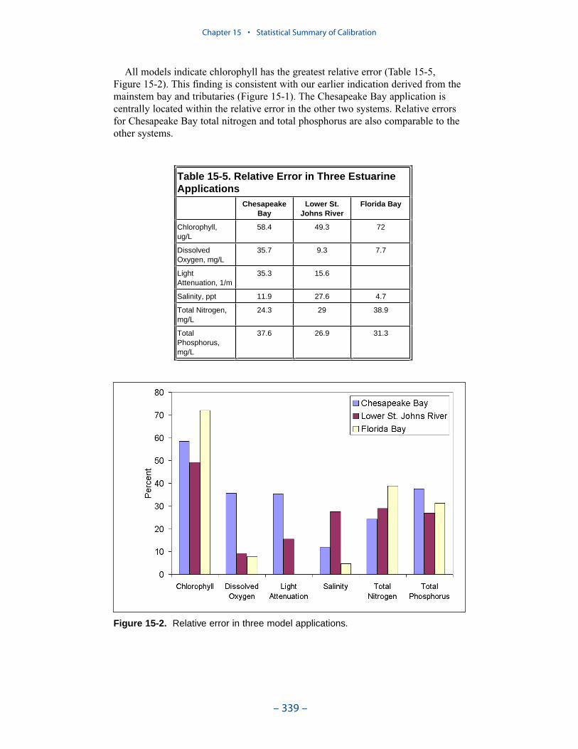
All models indicate chlorophyll has the greatest relative error (Table 15-5,Figure 15-2). This finding is consistent with our earlier indication derived from themainstem bay and tributaries (Figure 15-1). The Chesapeake Bay application iscentrally located within the relative error in the other two systems. Relative errorsfor Chesapeake Bay total nitrogen and total phosphorus are also comparable to theother systems.
Chapter 15 • Statistical Summary of Calibration
– 339 –
Table 15-5. Relative Error in Three Estuarine Applications
ChesapeakeBay
Lower St. Johns River
Florida Bay
Chlorophyll,ug/L
58.4 49.3 72
Dissolved Oxygen, mg/L
35.7 9.3 7.7
LightAttenuation, 1/m
35.3 15.6
Salinity, ppt 11.9 27.6 4.7
Total Nitrogen, mg/L
24.3 29 38.9
Total Phosphorus,mg/L
37.6 26.9 31.3
Figure 15-2. Relative error in three model applications.
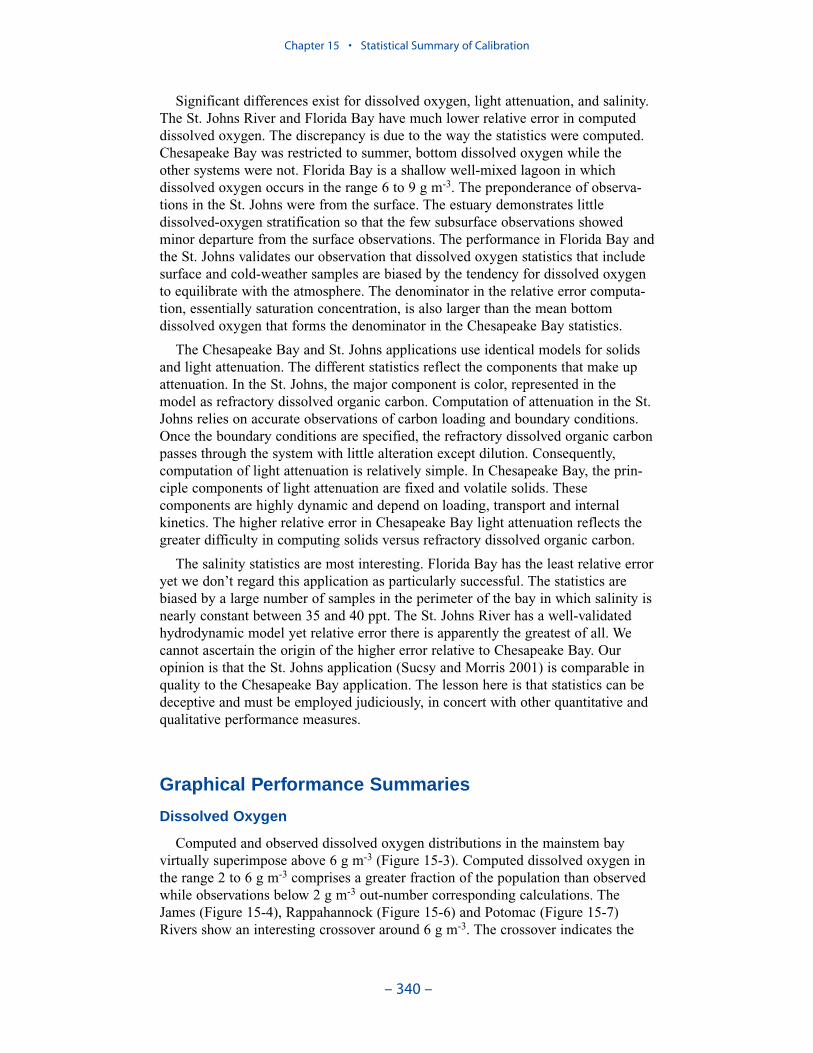
Significant differences exist for dissolved oxygen, light attenuation, and salinity.The St. Johns River and Florida Bay have much lower relative error in computeddissolved oxygen. The discrepancy is due to the way the statistics were computed.Chesapeake Bay was restricted to summer, bottom dissolved oxygen while theother systems were not. Florida Bay is a shallow well-mixed lagoon in whichdissolved oxygen occurs in the range 6 to 9 g m-3. The preponderance of observa-tions in the St. Johns were from the surface. The estuary demonstrates littledissolved-oxygen stratification so that the few subsurface observations showedminor departure from the surface observations. The performance in Florida Bay andthe St. Johns validates our observation that dissolved oxygen statistics that includesurface and cold-weather samples are biased by the tendency for dissolved oxygento equilibrate with the atmosphere. The denominator in the relative error computa-tion, essentially saturation concentration, is also larger than the mean bottomdissolved oxygen that forms the denominator in the Chesapeake Bay statistics.
The Chesapeake Bay and St. Johns applications use identical models for solidsand light attenuation. The different statistics reflect the components that make upattenuation. In the St. Johns, the major component is color, represented in themodel as refractory dissolved organic carbon. Computation of attenuation in the St.Johns relies on accurate observations of carbon loading and boundary conditions.Once the boundary conditions are specified, the refractory dissolved organic carbonpasses through the system with little alteration except dilution. Consequently,computation of light attenuation is relatively simple. In Chesapeake Bay, the prin-ciple components of light attenuation are fixed and volatile solids. Thesecomponents are highly dynamic and depend on loading, transport and internalkinetics. The higher relative error in Chesapeake Bay light attenuation reflects thegreater difficulty in computing solids versus refractory dissolved organic carbon.
The salinity statistics are most interesting. Florida Bay has the least relative erroryet we don’t regard this application as particularly successful. The statistics arebiased by a large number of samples in the perimeter of the bay in which salinity isnearly constant between 35 and 40 ppt. The St. Johns River has a well-validatedhydrodynamic model yet relative error there is apparently the greatest of all. Wecannot ascertain the origin of the higher error relative to Chesapeake Bay. Ouropinion is that the St. Johns application (Sucsy and Morris 2001) is comparable inquality to the Chesapeake Bay application. The lesson here is that statistics can bedeceptive and must be employed judiciously, in concert with other quantitative andqualitative performance measures.
Graphical Performance Summaries
Dissolved Oxygen
Computed and observed dissolved oxygen distributions in the mainstem bayvirtually superimpose above 6 g m-3 (Figure 15-3). Computed dissolved oxygen inthe range 2 to 6 g m-3 comprises a greater fraction of the population than observedwhile observations below 2 g m-3 out-number corresponding calculations. TheJames (Figure 15-4), Rappahannock (Figure 15-6) and Potomac (Figure 15-7)Rivers show an interesting crossover around 6 g m-3. The crossover indicates the
Chapter 15 • Statistical Summary of Calibration
– 340 –
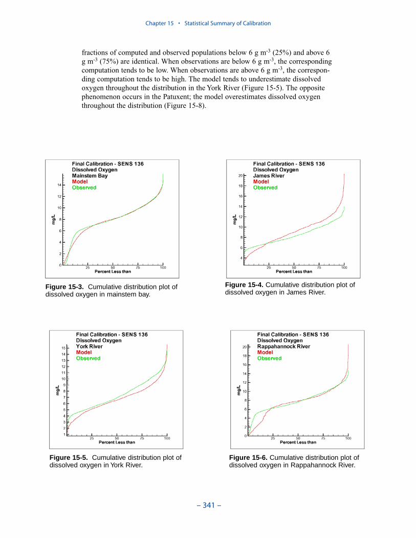
fractions of computed and observed populations below 6 g m-3 (25%) and above 6g m-3 (75%) are identical. When observations are below 6 g m-3, the correspondingcomputation tends to be low. When observations are above 6 g m-3, the correspon-ding computation tends to be high. The model tends to underestimate dissolvedoxygen throughout the distribution in the York River (Figure 15-5). The oppositephenomenon occurs in the Patuxent; the model overestimates dissolved oxygenthroughout the distribution (Figure 15-8).
Chapter 15 • Statistical Summary of Calibration
– 341 –
Figure 15-3. Cumulative distribution plot ofdissolved oxygen in mainstem bay.
Figure 15-4. Cumulative distribution plot ofdissolved oxygen in James River.
Figure 15-5. Cumulative distribution plot ofdissolved oxygen in York River.
Figure 15-6. Cumulative distribution plot ofdissolved oxygen in Rappahannock River.

Salinity
The graphical distributions indicate excellent representations of salinity in themainstem bay (Figure 15-9) and Potomac River (Figure 15-13). We believe thelarger number of grid elements and major role of gauged runoff versus ungaugedbelow-fall-line flow contribute to the computed accuracy in these systems. Salinitycomputations in the James (Figure 15-10), York (Figure 15-11), Rappahannock(Figure 15-12) and Patuxent Rivers are less accurate. This characteristic has beenwith the model since the earliest stages and remains after two grid re-segmenta-tions. Further re-segmentation should be of benefit but we have to recognize therole of local processes and effects that may never be represented in a system-widemodel.
Chapter 15 • Statistical Summary of Calibration
– 342 –
Figure 15-7. Cumulative distribution plot ofdissolved oxygen in Potomac River.
Figure 15-8. Cumulative distribution plot ofdissolved oxygen in Patuxent River.
Figure 15-9. Cumulative distribution plot ofsalinity in mainstem bay.
Figure 15-10. Cumulative distribution plot ofsalinity in James River.
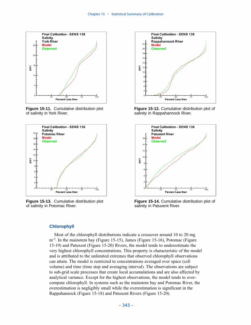
Chlorophyll
Most of the chlorophyll distributions indicate a crossover around 10 to 20 mg m-3. In the mainstem bay (Figure 15-15), James (Figure 15-16), Potomac (Figure15-19) and Patuxent (Figure 15-20) Rivers, the model tends to underestimate thevery highest chlorophyll concentrations. This property is characteristic of the modeland is attributed to the unlimited extremes that observed chlorophyll observationscan attain. The model is restricted to concentrations averaged over space (cellvolume) and time (time step and averaging interval). The observations are subjectto sub-grid scale processes that create local accumulations and are also affected byanalytical variance. Except for the highest observations, the model tends to over-compute chlorophyll. In systems such as the mainstem bay and Potomac River, theoverestimation is negligibly small while the overestimation is significant in theRappahannock (Figure 15-18) and Patuxent Rivers (Figure 15-20).
Chapter 15 • Statistical Summary of Calibration
– 343 –
Figure 15-11. Cumulative distribution plotof salinity in York River.
Figure 15-12. Cumulative distribution plot ofsalinity in Rappahannock River.
Figure 15-13. Cumulative distribution plotof salinity in Potomac River.
Figure 15-14. Cumulative distribution plot ofsalinity in Patuxent River.
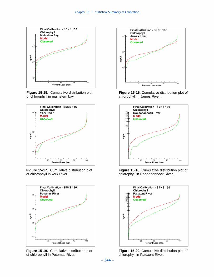
Chapter 15 • Statistical Summary of Calibration
– 344 –
Figure 15-15. Cumulative distribution plotof chlorophyll in mainstem bay.
Figure 15-16. Cumulative distribution plot ofchlorophyll in James River.
Figure 15-17. Cumulative distribution plotof chlorophyll in York River.
Figure 15-18. Cumulative distribution plot ofchlorophyll in Rappahannock River.
Figure 15-19. Cumulative distribution plotof chlorophyll in Potomac River.
Figure 15-20. Cumulative distribution plot ofchlorophyll in Patuxent River.
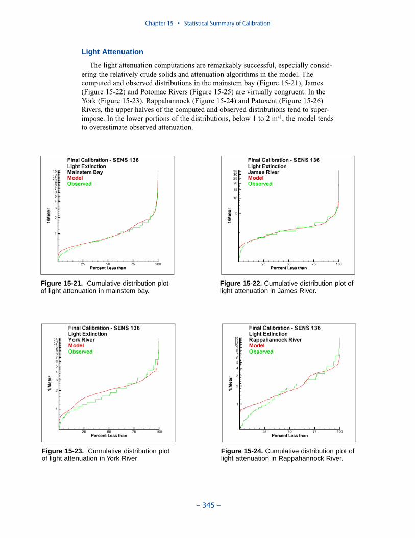
Light Attenuation
The light attenuation computations are remarkably successful, especially consid-ering the relatively crude solids and attenuation algorithms in the model. Thecomputed and observed distributions in the mainstem bay (Figure 15-21), James(Figure 15-22) and Potomac Rivers (Figure 15-25) are virtually congruent. In theYork (Figure 15-23), Rappahannock (Figure 15-24) and Patuxent (Figure 15-26)Rivers, the upper halves of the computed and observed distributions tend to super-impose. In the lower portions of the distributions, below 1 to 2 m-1, the model tendsto overestimate observed attenuation.
Chapter 15 • Statistical Summary of Calibration
– 345 –
Figure 15-21. Cumulative distribution plotof light attenuation in mainstem bay.
Figure 15-22. Cumulative distribution plot oflight attenuation in James River.
Figure 15-23. Cumulative distribution plotof light attenuation in York River
Figure 15-24. Cumulative distribution plot oflight attenuation in Rappahannock River.

Total Nitrogen
The James (Figure 15-28), York (Figure 15-29) and Patuxent (Figure 15-32)Rivers exhibit the familiar crossover pattern. In these tributaries, the model tends tooverestimate the highest nitrogen concentrations and underestimate the lowerconcentrations. The crossover occurs around 0.8 g m-3. We suspect this behavior isattributable to occasional enormous concentrations that are computed near the falllines during storm events. The water quality and hydrodynamic models use gaugedflows while the watershed model uses its own computed flow. Discrepanciesbetween gauged and computed flows can cause wild fluctuations during the largeloadings associated with storm events. The mainstem bay (Figure 15-27) andPotomac River (Figure 15-31) exhibit two crossovers. As with the preceding threetributaries, the model exceeds the very highest observed concentrations. The modelalso exceeds the lowest observations, less than about 0.6 g m-3. In the portions ofthe distributions between the extremes, observations tend to exceed modeledconcentrations. The Rappahannock River (Figure 15-30) stands out as one in whichtotal nitrogen is under-computed throughout the distribution.
Chapter 15 • Statistical Summary of Calibration
– 346 –
Figure 15-25. Cumulative distribution plotof light attenuation in Potomac River.
Figure 15-26. Cumulative distribution plot oflight attenuation in Patuxent River.
Figure 15-27. Cumulative distribution plotof total nitrogen in mainstem bay.
Figure 15-28. Cumulative distribution plot oftotal nitrogen in James River.
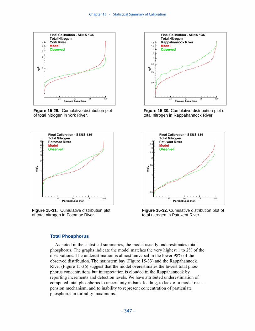
Total Phosphorus
As noted in the statistical summaries, the model usually underestimates totalphosphorus. The graphs indicate the model matches the very highest 1 to 2% of theobservations. The underestimation is almost universal in the lower 98% of theobserved distribution. The mainstem bay (Figure 15-33) and the RappahannockRiver (Figure 15-36) suggest that the model overestimates the lowest total phos-phorus concentrations but interpretation is clouded in the Rappahannock byreporting increments and detection levels. We have attributed underestimation ofcomputed total phosphorus to uncertainty in bank loading, to lack of a model resus-pension mechanism, and to inability to represent concentration of particulatephosphorus in turbidity maximums.
Chapter 15 • Statistical Summary of Calibration
– 347 –
Figure 15-29. Cumulative distribution plotof total nitrogen in York River.
Figure 15-30. Cumulative distribution plot oftotal nitrogen in Rappahannock River.
Figure 15-31. Cumulative distribution plotof total nitrogen in Potomac River.
Figure 15-32. Cumulative distribution plot oftotal nitrogen in Patuxent River.
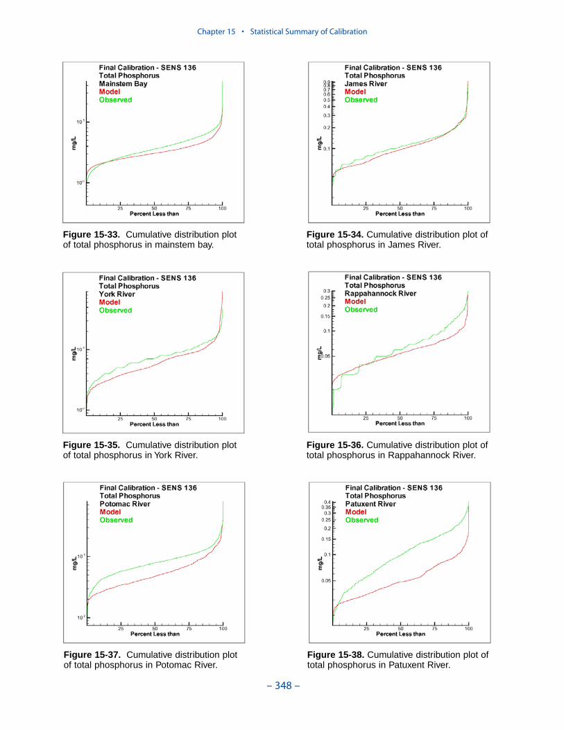
Chapter 15 • Statistical Summary of Calibration
– 348 –
Figure 15-33. Cumulative distribution plotof total phosphorus in mainstem bay.
Figure 15-34. Cumulative distribution plot oftotal phosphorus in James River.
Figure 15-35. Cumulative distribution plotof total phosphorus in York River.
Figure 15-36. Cumulative distribution plot oftotal phosphorus in Rappahannock River.
Figure 15-37. Cumulative distribution plotof total phosphorus in Potomac River.
Figure 15-38. Cumulative distribution plot oftotal phosphorus in Patuxent River.

ReferencesCerco, C., and Cole, T. (1994). “Three-dimensional eutrophication model of ChesapeakeBay,” TR EL-94-4, US Army Engineer Waterways Experiment Station, Vicksburg MS.
Cerco, C., Bunch, B., Teeter, A., and Dortch, M. (2000). “Water quality model of FloridaBay,” ERDC TR-00-10, US Army Engineer Research and Development Center, VicksburgMS.
Cerco, C., Johnson, B., and Wang, H. (2002). “Tributary refinements to the Chesapeake Baymodel,” ERDC TR-02-4, US Army Engineer Research and Development Center, VicksburgMS.
Sucsy, P., and Morris, F. (2001). “Salinity intrusion in the St. Johns River, Florida.” Estu-arine and Coastal Modeling, Proceedings of the Seventh International Conference. M.L.Spaulding ed., American Society of Civil Engineers, Reston VA, 120-139.
Tillman, D., Cerco, C., Noel, M., Martin, J., and Hamrick, J. (2003). “Three-dimensionaleutrophication model of the lower St. Johns River, Florida,” ERDC TR-03EL353, US ArmyEngineer Research and Development Center, Vicksburg MS.
Chapter 15 • Statistical Summary of Calibration
– 349 –