Energy Economics 79 (2019) 21–31

Contents lists available at ScienceDirect

Energy Economics

j ourna l homepage: www.e lsev ie r .com/ locate /eneco

Testing persistence of WTI and Brent long-run relationship after theshale oil supply shock�

Massimiliano Caporina, Fulvio Fontinib,*, Elham Talebbeydokhtib

aDepartment of Statistical Sciences, University of Padua, ItalybDepartment of Economics and Management, University of Padua, Italy

A R T I C L E I N F O

Article history:Received 10 April 2017Received in revised form 12 May 2018Accepted 23 August 2018Available online 24 October 2018

JEL classification:C01C32Q30Q31Q40Q41

Keywords:WTIBrentShale oilCointegrationVector Error Correction ModelGeneralized Impulse Response Function

A B S T R A C T

In the paper, we study the long-run relationship in the WTI-Brent oil time series, taking into account theoccurrence of two relevant events: the rise of shale oil production, in early 2011, and the widening and clos-ing of the WTI-Brent price spread, from 2011 to 2014. Monthly data of WTI and Brent crude oil prices, aswell as US shale oil quantities from January 2000 to December 2017 is used for the analyses. The empiricalresults of the cointegration tests with structural breaks show that two structural break occurs, in Febru-ary 2011 and in October 2014. We then estimate a Vector Error Correction Model (VECM), considering thestructural break suggested by the cointegration test results, the timing of the rise in shale oil productionand the dynamics of the WTI-Brent price spread. Our analysis reveals that WTI and Brent crude oil priceshave had a long-run relationship up to 2011; no cointegration existed during the period of widening of thespread; again, a new long-run relationship arises after the closing of the gap, which includes the shale oilproduction. In the last period, the cross price elasticity of Brent on WTI slightly reduces compared to thepre-2011 era, whilst the shale oil production increases its importance in explaining the long-run relation-ship between WTI and Brent fivefold. Using the Generalized Impulse Response Functions (GIRFs) we finallystudy the impact of exogenous shocks on the variables, showing that in the first period, with limited shaleoil production, oil prices reacted to shale oil and not vice versa. After October 2014, the opposite becomestrue and shale oil production follows changes in both WTI and Brent prices.

© 2018 Elsevier B.V. All rights reserved.

1. Introduction

There exist various types of internationally traded crude oils,each one with different qualities and characteristics, expressedby density (light to heavy) as well as acidity and sulphur con-tent (sweet, which refers to low sulphur content, and sour, whichrefers to high sulphur content). The two dominant oil referenceprices are the West Texas Intermediate (WTI)1 and the Brent crude

� This paper has been presented at the first AIEE Energy Symposium, Currentand Future challenges to Energy Security Conference, Milan, Italy, 30 November–2December 2016 and at Energy Finance Italia, II, University of Padua, Padua, Italy, 5–6December 2016.

* Corresponding author at: DSEA, University of Padua, Via del Santo 33, 35123, Italy.E-mail address: fulvio.fontini@unipd.it (F. Fontini).

1 WTI is the main oil benchmark in the US (Fattouh, 2010). It refers to oil extractedfrom wells in the US and sent via pipeline to Cushing, Oklahoma. For over threedecades, Cushing has been a major oil supply hub connecting oil suppliers to the GulfCoast, and, therefore it is the price settlement point for WTI. WTI is traded on the NewYork Mercantile Exchange (NYMEX) for delivery at Cushing.

oil.2 WTI and Brent crude are classified as sweet, light crude oil-sweet because of their low sulphur content and light because oftheir relatively low density-thus making them ideal for refiningdiesel fuel, gasoline and other high-demand products. However,Brent crude is not as sweet and light as WTI is.

The arbitrage principle applied to almost homogeneous prod-ucts such as WTI and Brent needs to reduce their price differentials;however, there are factors that can limit arbitrage, such as theirintrinsic quality, on the one hand, and/or external factors such astransportation constraints and costs, on the other hand.

2 Brent is a European benchmark related to oil extracted from the North Sea. Brentis composed of four crude blends: Brent, Forties, Oseberg, and Ekofisk (BFOE). TheBrent and Forties blends are produced offshore in the waters of the UK, and the Ekofiskand Oseberg blends are mainly produced offshore in the waters of Norway (EnergyInformation Administration, EIA (2016). In recent years, Brent has been used to pricetwo third of the world’s internationally traded crude oil supplies. Brent is traded onthe Intercontinental Exchange (ICE) for delivery at Sullom Voe.

https://doi.org/10.1016/j.eneco.2018.08.0220140-9883/© 2018 Elsevier B.V. All rights reserved.

22 M. Caporin et al. / Energy Economics 79 (2019) 21–31

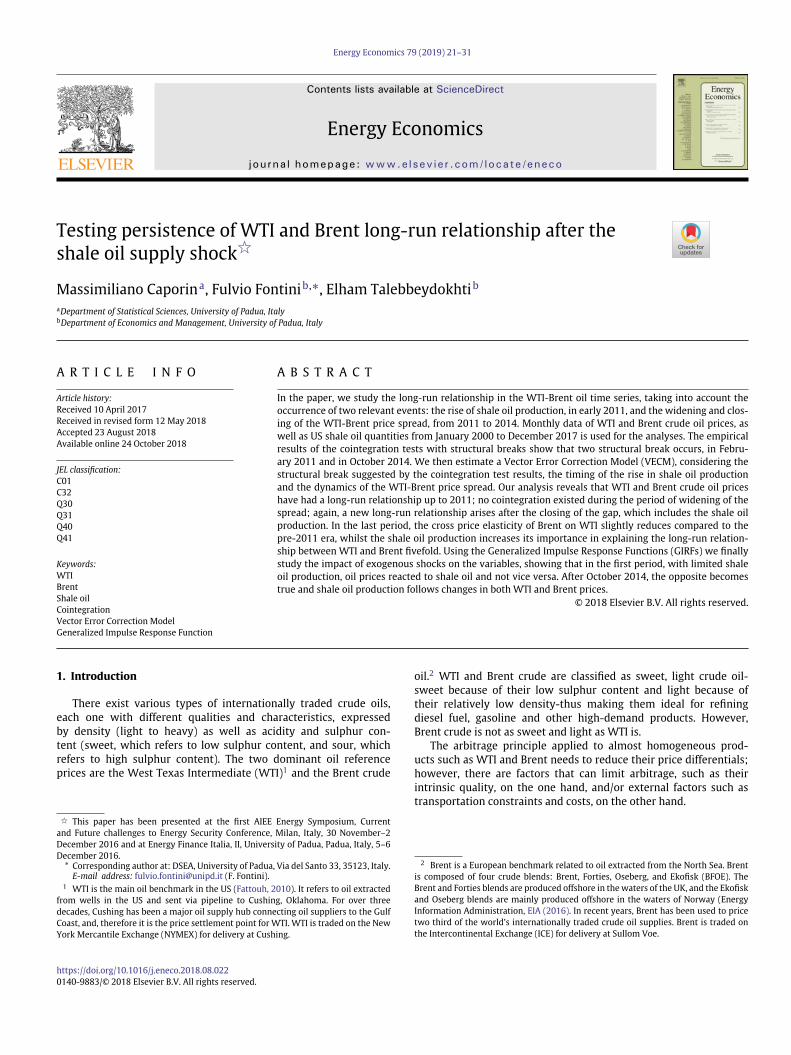
Several scholars have studied the crude oil price differentials(Fattouh, 2007, 2010; Kao and Wan, 2012; Borenstein et al., 2014).Historically, Brent and WTI crude oil prices have been tracked closely,with a price difference per barrel of ± 3 USD/bbl and with WTI usuallypriced higher than Brent, as shown in Fig. 1. This pattern of price dif-ferential probably denotes that arbitrage opportunities were kept ata minimum, with the price premium of WTI depending on its sweetercontent. The rather stable behaviour of the spread also denotes thatWTI and Brent were linked by a long-run equilibrium relationship.However, evidence from previous studies investigating whether WTIand Brent are integrated is mixed. Reboredo (2011) suggests thatcrude oil prices are linked with the same intensity during bull andbear markets, thus supporting the hypothesis that the oil market is asingle pool, in contrast with the hypothesis stating that the oil mar-ket is regionalised. Gülen (1999) argues that market segmentationgenerates market inefficiencies and gives rise to arbitrage opportuni-ties. Likewise, oil market co-movements have potentially importantimplications for portfolio allocation and hedging strategies involv-ing spot and future oil contracts. Hammoudeh et al. (2008), Liao etal. (2014) and Wilmot (2013) support the idea of the globalisationhypothesis. On the other hand, Weiner (1991) claim that the worldoil market is far from being completely united. (Kim et al., 2013) hasfound that the long-run relationships among WTI, Brent and Dubaicrude oil prices hold from January 1997 to July 2012, even when theeffects of the breaks are considered. Aruga (2015) claims that WTI nolonger has a long-run relationship with the Brent and Dubai crudeoil markets. Büyüksahin et al. (2013) find that a structural breakin the long-term relationship between WTI and Brent occurred in2008 and 2010. (Coronado et al., 2016) find a double causality pat-terns between Brent and WTI, includes also the Argus Sour CrudeIndex. In early 2011, the longstanding relationship between WTI andBrent prices began to change; Brent crude oil started to be pricedmuch higher than WTI was. The discrepancy between WTI and Brentprices resulted from exogenous factors. Whilst the WTI productionwas rising, limited transportation facilities impeded moving the WTIstockpiles at their delivery point at Cushing, Oklahoma, to refinerieslocated in the Gulf Coast. The spread rose to 27 USD/bbl in September2011. Eventually, the expansion of the transportation and refiningcapacity, including the addition of new pipelines at Cushing, allowedpushing back the price spread: in late 2014, the Brent-WTI spreadwas narrowed considerably.3

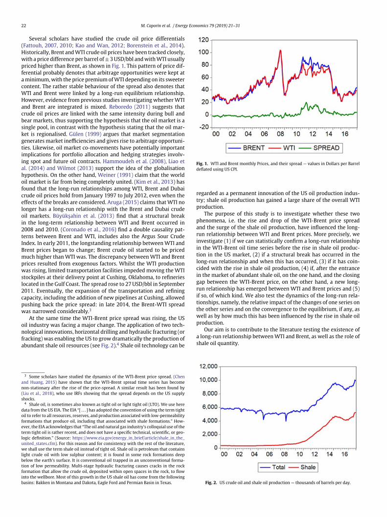
At the same time the WTI-Brent price spread was rising, the USoil industry was facing a major change. The application of two tech-nological innovations, horizontal drilling and hydraulic fracturing (orfracking) was enabling the US to grow dramatically the production ofabundant shale oil resources (see Fig. 2).4 Shale oil technology can be

3 Some scholars have studied the dynamics of the WTI-Brent price spread. (Chenand Huang, 2015) have shown that the WTI-Brent spread time series has becomenon-stationary after the rise of the price-spread. A similar result has been found by(Liu et al., 2018), who use IRFs showing that the spread depends on the US supplyshocks.

4 Shale oil, is sometimes also known as tight oil or light tight oil (LTO). We use heredata from the US EIA. The EIA “[ . . . ] has adopted the convention of using the term tightoil to refer to all resources, reserves, and production associated with low-permeabilityformations that produce oil, including that associated with shale formations.” How-ever, the EIA acknowledges that “The oil and natural gas industry’s colloquial use of theterm tight oil is rather recent, and does not have a specific technical, scientific, or geo-logic definition.” (Source: https://www.eia.gov/energy_in_brief/article/shale_in_the_united_states.cfm). For this reason and for consistency with the rest of the literature,we shall use the term shale oil instead of tight oil. Shale oil is petroleum that containslight crude oil with low sulphur content; it is found in some rock formations deepbelow the earth’s surface. It is conventional oil trapped in an unconventional forma-tion of low permeability. Multi-stage hydraulic fracturing causes cracks in the rockformation that allow the crude oil, deposited within open spaces in the rock, to flowinto the wellbore. Most of this growth in the US shale oil has come from the followingbasins: Bakken in Montana and Dakota, Eagle Ford and Permian Basin in Texas.

Fig. 1. WTI and Brent monthly Prices, and their spread — values in Dollars per Barreldeflated using US CPI.

regarded as a permanent innovation of the US oil production indus-try; shale oil production has gained a large share of the overall WTIproduction.

The purpose of this study is to investigate whether these twophenomena, i.e. the rise and drop of the WTI-Brent price spreadand the surge of the shale oil production, have influenced the long-run relationship between WTI and Brent prices. More precisely, weinvestigate (1) if we can statistically confirm a long-run relationshipin the WTI-Brent oil time series before the rise in shale oil produc-tion in the US market, (2) if a structural break has occurred in thelong-run relationship and when this has occurred, (3) if it has coin-cided with the rise in shale oil production, (4) if, after the entrancein the market of abundant shale oil, on the one hand, and the closinggap between the WTI-Brent price, on the other hand, a new long-run relationship has emerged between WTI and Brent prices and (5)if so, of which kind. We also test the dynamics of the long-run rela-tionships, namely, the relative impact of the changes of one series onthe other series and on the convergence to the equilibrium, if any, aswell as by how much this has been influenced by the rise in shale oilproduction.

Our aim is to contribute to the literature testing the existence ofa long-run relationship between WTI and Brent, as well as the role ofshale oil quantity.

Fig. 2. US crude oil and shale oil production — thousands of barrels per day.

M. Caporin et al. / Energy Economics 79 (2019) 21–31 23

The rest of the paper is structured as follows. Section 2 outlinesthe methodologies used for the cointegration analysis. Section 3describes the data. Section 4 provides all the empirical results.Finally, Section 5 presents the conclusions, and the references follow.

2. Methodology

From a statistical viewpoint, the time series of energy commodi-ties’ prices behave like the time series of financial instruments’prices, and they are usually non-stationary. Therefore, a simple ordi-nary least squares regression between two commodity prices wouldpotentially lead to a spurious regression. Such an event does notrealise if the series of interest share a common trend and are linearlyrelated by an equilibrium condition. To deal with this issue, we firstassess whether the variables under consideration are non-stationaryor characterised by a unit root, i.e. integrated of order one, or I(1). Wemight use traditional unit root tests, such as the Augmented Dickey-Fuller (ADF) test, but we are aware that our time series might becontaminated by a structural break because of the shale oil supplyshock. Therefore, we need to consider the possible existence of abreak in each time series, either in the intercept, in the trend or inboth the intercept and the trend. Consequently, we apply the Perron(1997) unit root test that allows for a break at an unknown locationand enables the evaluation of the null hypothesis of integration andthe identification of the break location. Notably, the identification ofthe break date comes from the evaluation of the minimum of the teststatistic for a number of possible break dates.

If the series are integrated, despite being possibly affected by astructural break, we are allowed to test the existence of cointegra-tion, i.e. to verify the existence of a long-run relationship betweenthe series of interest. We follow here the Gregory and Hansen (1996)cointegration analysis because again, we need to deal with the pos-sible presence of structural breaks. The approach of Gregory andHansen (1996) allows verifying the existence of cointegration in thepresence of a structural break of an unknown location.

Considering a simple model,

y1t = l + dt + ay2t + et , t = 1, . . . , n (1)

where y1t and y2t are the two variables of interest, both I(1), t is a timetrend, and et is a stationary innovation term; the structural breaksmight be of different forms. In fact, we might have a structural breakin the intercept, i.e. only l changes after the break date, with differentbehaviours of the test statistic depending on the presence or absenceof the deterministic trend component. Alternatively, we might havea structural break leading to changes in both the intercept and thecointegration parameters, i.e. both l and a change after the breakdate.

In all cases, the test of the null hypothesis of no cointegrationis residual based. In other words, we can regard y1t and y2t asbeing cointegrated by examining whether the residuals et do nothave a unit root. Gregory and Hansen (1996) constructed threestatistics for those tests: Z∗

a , Z∗t and ADF∗. The test statistics Z∗

a andZ∗

t build upon the Philips-Perron test statistics, whilst ADF∗ is basedon the Augmented Dickey-Fuller (ADF) statistics. The null hypothesisis rejected if the statistic, either ADF∗, Z∗

a or Z∗t , is smaller than

the corresponding critical value. In all cases, the critical values aretabulated as the test statistics do not follow a standard density.

If the tests proposed by Gregory and Hansen (1996) showevidence in favour of cointegration, a Vector Error Correction Model(VECM) can be specified to identify both the long-run relationshipsbetween the variables of interest and, at the same time, to accountfor the structural break.

The VECM can lead to a better understanding of the nature oflong-run and short-run relationships among the modelled variables.In our case, the model allows evaluating the existence of long-runrelationships across three variables, namely, WTI and Brent pricesand the shale oil quantity. To identity the number of cointegratingrelations, we rely on the tests of Johansen (1988, 1995). However, toaccount for the presence of structural breaks, we use the Johansenet al. (2000) and Giles and Godwin (2012) critical values. In its mostgeneral representation, the VECM model takes the following form:

DXt = PXt−1 +p∑

j=1

0jDXt−j + dDt + 4t , (2)

where Xt is the vector of the modelled variables (in logs), D identifiesthe first difference of the variables (i.e. the growth rates), thesummation monitors the short-run dynamics of the series growthrates, and, finally, Dt contains a set of deterministic variables, namelya constant and a linear trend, and might include terms needed toaccount for the structural break (see Johansen et al., 2000).

In the presence of cointegrating relationships, the matrix P mightbe decomposed as P = ab′, where the product b′Xt−1 contains dise-quilibrium errors, the matrix b provides the cointegration coefficient,i.e. the coefficient of the long-run relationship between variables,and the vector a contains the adjustment coefficients for the pastdisequilibrium.

In our setting, we expect to identify a long-run (cointegrating)relationship. In fact, with a stable relationship over time assumed,the link between Brent and WTI prices (thus excluding the shale oilquantity for the moment) would read as follows:

WTIt − l − b1Brentt = 4t , (3)

where WTIt denotes the WTI real log-price, Brentt is the Brent reallog-price, and 4t is the stationary error term. If the two oil prices havea stable and long-run link, we expect the coefficient b1 to be statisti-cally significant and close to one, suggesting that movements in theBrent (WTI) price are replicated in the WTI (Brent) price. Moreover,shocks to one of the two prices might lead to adjustments towardsthe equilibrium by means of the VECM specification, as governed bythe adjustment coefficients and the lag structure.

With the surge in shale oil production, shale oil quantity can alsoplay a role in the long-run equilibrium relation. In this case, the singleequilibrium relation would not only link the two prices, as above, butwill also allow shale oil quantity to play a role. The latter term wouldact as a possible driver of the diverging behaviour among prices. Infact, if we denote with ShaleQt the shale oil total quantity (in logs),the equilibrium relation becomes

WTIt − l − b1Brentt − b2ShaleQt = 4t. (4)

The coefficient b1 should be again statistically significant andclose to 1; deviations from the equilibrium because of a shock on,say, the Brent price might lead to an adjustment on both the WTIprice and the shale quantity, thus having a possible effect also onthe spread. Similarly, shocks on the shale oil quantity might have aneffect on the prices. The shale oil quantity has a significant role onlyif the coefficient b2 is statistically significant. In the case of cointegra-tion between the three variables, the coefficients b1 in Eqs. (3) and

24 M. Caporin et al. / Energy Economics 79 (2019) 21–31

(4) might not be identical, even though we expect them to be veryclose, and the shale oil quantity might not to be predominant.

Finally, we note that, because the variables are expressed in logs,the coefficients b1 and b2 represent the cross-price elasticity and theelasticity of the WTI price w.r.t. shale oil quantity, respectively.

Once the VECM has been estimated, short-run dynamics and theadjustment because of disequilibrium in the long-run relationshipcan be examined by considering the impulse response functions(IRFs). These functions measure the time profile of the effect of ashock, or impulse, on the (endogenous) variables of interest. A crucialelement is given by the chosen approach to orthogonalise the shocks.The most common one uses a Cholesky decomposition of the inno-vation’s covariance of the VECM model. However, the resulting IRFswould depend on the variables ordering. In our case, the two prices,Brent and WTI, are highly correlated, and we expect a high correla-tion even among the VECM model innovations. This characteristicsmakes the choice of any ordering questionable. Moreover, when weintroduce the shale oil quantity, choosing the proper variables order-ing is even more challenging. Consequently, we opt for the moreflexible Generalized IRF (GIRF) of Pesaran and Shin (1998). The GIRFsare independent from the variables ordering and correspond to thereaction of a target variable to a unit shock on one endogenousinnovation. We note that in the VECM model, the effect of shockswill lead to movements in the endogenous variables both throughthe disequilibrium that the shocks generate (from the impact ofthe error correction term, as measured from the adjustment coeffi-cients), as well as from the dynamic interaction among growth rates(i.e. through the lags of the VECM model, involving the variables’ firstdifference). In the empirical analysis we focus on GIRFs up to 24 lags(two years) and compute bootstrap confidence intervals.

In the following sections, we proceed to the analysis of the Brentand WTI prices, together with shale oil production. To evaluate theexistence of long-run relationships among these variables, we havethe following steps. Firstly, we analyse the series for the presence ofunit roots, a pre-requisite for cointegration. In this step, we allow thepresence of breaks in the series. Secondly, given the results of theunit root test, we focus on cointegration testing, again allowing thepresence of breaks. Finally, we move to the estimation of the VECMmodel and the derivation of the GIRF. All steps will be properly dis-cussed from an economic viewpoint; the results obtained from thebivariate system including prices only and from the trivariate systemincluding also the shale oil quantity will be compared.

3. Data analysis

We use the monthly real spot prices of WTI and Brent crudeoil (dollars per barrel) and the monthly tight oil quantities and UScrude oil production (thousand barrels per day) from the US EnergyInformation Administration. The observation period is from January2000 to December 2017, which yields a sample size of 216 observa-tions. Table 1 gives the summary statistics for the monthly growthrates of crude oil prices and quantities. We use logarithmic growthrates, which allow us to interpret the coefficients of the linear mod-els estimated as elasticities. Considering the significant rise in shaleoil production starting on February 2011, we divide the full-sampleperiod into two sub-samples. The growth rate of the two prices is, onaverage, negative in the second sub-sample, whereas the US crudeoil production (WTI quantity) increases from February 2011 onward,mostly caused by the increase in shale oil production. The tableincludes additional sub-samples; we discuss the criteria for theiridentification in the following section.

Note that the second sub-sample period saw the rise and fall ofthe WTI-Brent price spread, as shown in Fig. 1. As mentioned before,the crucial factor determining it was the bottleneck in US refinery andtransport infrastructures, coupled with the rise in shale production,

that impeded the arbitrage between WTI and imports. By 2015, theexpansion of transportation infrastructure eliminated the bottleneck,allowing light crude oil that was landlocked in the centre of the USto reach refineries (Borenstein et al., 2014; Kilian, 2016).5

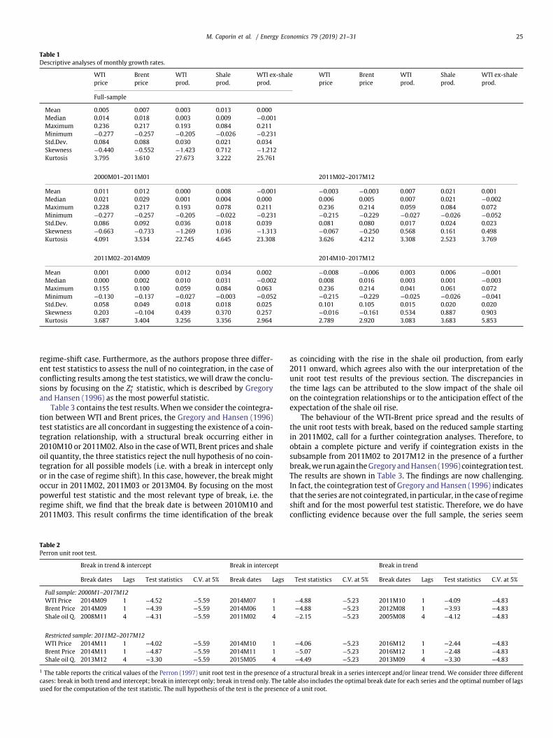
We then assess the stationarity property of WTI and Brent pricesand shale oil quantity before performing the analysis of cointegra-tion. Table 2 reports the results for the Perron (1997) test for unitroots in the presence of structural breaks. Notably, in all cases weaccept the null hypothesis, i.e. the presence of a unit root. Withrespect to the break date, we observe some heterogeneity in it. Infact, the break date oscillates from 2008 to 2014, with some preva-lence of dates around the 2011 and 2014. If we look at the plots forthe test statistic computed for various candidate break dates6, weobserve that the test statistic has, in many cases, a somewhat flatpattern from 2011 up to the end of 2014. This feature challengesthe proper identification of the break date from purely statisticaltools. Therefore, given the empirical evidence of the increase in theshale oil production at the beginning of 2011 and the contempora-neous amplification of the spread between Brent and WTI prices, wedecided to fix a first break date between January and February 2011.Furthermore, given our previous comments on the pattern of theWTI-Brent price spread and the existence of the transportation bot-tleneck, we expect a possible break date in the last months of 2014.We then proceed to a second set of tests based on the restricted sam-ple starting in February 2011 and ending in December 2017. Table 2presents the results. We find a confirmation of the non-stationarityof the series; all tests provide evidence in favour of the null hypothe-sis, i.e. the presence of a unit root. Notably, we found for both prices abreak in the last months of 2014, which is consistent with the graph-ical evidence of the spread. Considering the test outcomes of the fulltable, we do have evidence of a second break data in the last quarterof 2014, which we set between September 2014 and October 2014.Summarising, by combining the graphical evidence, the results of thetest statistics, and the exogenous elements affecting the oil market,we believe that the long-run relation among our variables of interestmight be affected by two possible break dates. The first was at thebeginning of 2011, associated with the rise in shale oil productionand the widening of the Brent-WTI spread (because of exogenouselements), and the second was at the end of 2014, associated withthe narrowing of the spread (the transportation bottleneck leadingto the spread was removed) and the start of the shale oil productionstabilisation.

4. Long-run relationships between oil prices and shale quantity

As the unit root test of Perron (1997) suggests that the WTI andBrent prices and shale oil quantity are I(1), we proceed to the eval-uation of the possible presence of cointegration between WTI andBrent prices by using the methodology introduced by Gregory andHansen (1996). Then, we replicate the analysis including also shaleoil quantity. We are reminded that the most interesting case, fromour viewpoint, is the presence of a structural change in the coin-tegrating vector, identified by Gregory and Hansen (1996) as the

5 We test for the relevance of other external factors in explaining the WTI-Brentprice spread. In particular, we check whether external control variables explain theprice spread. We consider three possible drivers of the spread: the trade-weightedvalue of the US dollar against a basket of major currencies, as a proxy of the US dollarstrength; the US Economic Policy Uncertainty index of Baker et al. (2016), as a measureof economic policy instability in the US market; and the Industrial Production Index,in order to track the US business cycle. The very limited R-squared of the regressionand the limited significance of the controls (either contemporaneous and/or lagged)show that these external factors cannot explain the spread. The results are availablefrom the authors upon request.

6 Plots available upon request.

M. Caporin et al. / Energy Economics 79 (2019) 21–31 25

Table 1Descriptive analyses of monthly growth rates.

WTI Brent WTI Shale WTI ex-shale WTI Brent WTI Shale WTI ex-shaleprice price prod. prod. prod. price price prod. prod. prod.

Full-sample

Mean 0.005 0.007 0.003 0.013 0.000Median 0.014 0.018 0.003 0.009 −0.001Maximum 0.236 0.217 0.193 0.084 0.211Minimum −0.277 −0.257 −0.205 −0.026 −0.231Std.Dev. 0.084 0.088 0.030 0.021 0.034Skewness −0.440 −0.552 −1.423 0.712 −1.212Kurtosis 3.795 3.610 27.673 3.222 25.761

2000M01–2011M01 2011M02–2017M12

Mean 0.011 0.012 0.000 0.008 −0.001 −0.003 −0.003 0.007 0.021 0.001Median 0.021 0.029 0.001 0.004 0.000 0.006 0.005 0.007 0.021 −0.002Maximum 0.228 0.217 0.193 0.078 0.211 0.236 0.214 0.059 0.084 0.072Minimum −0.277 −0.257 −0.205 −0.022 −0.231 −0.215 −0.229 −0.027 −0.026 −0.052Std.Dev. 0.086 0.092 0.036 0.018 0.039 0.081 0.080 0.017 0.024 0.023Skewness −0.663 −0.733 −1.269 1.036 −1.313 −0.067 −0.250 0.568 0.161 0.498Kurtosis 4.091 3.534 22.745 4.645 23.308 3.626 4.212 3.308 2.523 3.769

2011M02–2014M09 2014M10–2017M12

Mean 0.001 0.000 0.012 0.034 0.002 −0.008 −0.006 0.003 0.006 −0.001Median 0.000 0.002 0.010 0.031 −0.002 0.008 0.016 0.003 0.001 −0.003Maximum 0.155 0.100 0.059 0.084 0.063 0.236 0.214 0.041 0.061 0.072Minimum −0.130 −0.137 −0.027 −0.003 −0.052 −0.215 −0.229 −0.025 −0.026 −0.041Std.Dev. 0.058 0.049 0.018 0.018 0.025 0.101 0.105 0.015 0.020 0.020Skewness 0.203 −0.104 0.439 0.370 0.257 −0.016 −0.161 0.534 0.887 0.903Kurtosis 3.687 3.404 3.256 3.356 2.964 2.789 2.920 3.083 3.683 5.853

regime-shift case. Furthermore, as the authors propose three differ-ent test statistics to assess the null of no cointegration, in the case ofconflicting results among the test statistics, we will draw the conclu-sions by focusing on the Z∗

t statistic, which is described by Gregoryand Hansen (1996) as the most powerful statistic.

Table 3 contains the test results. When we consider the cointegra-tion between WTI and Brent prices, the Gregory and Hansen (1996)test statistics are all concordant in suggesting the existence of a coin-tegration relationship, with a structural break occurring either in2010M10 or 2011M02. Also in the case of WTI, Brent prices and shaleoil quantity, the three statistics reject the null hypothesis of no coin-tegration for all possible models (i.e. with a break in intercept onlyor in the case of regime shift). In this case, however, the break mightoccur in 2011M02, 2011M03 or 2013M04. By focusing on the mostpowerful test statistic and the most relevant type of break, i.e. theregime shift, we find that the break date is between 2010M10 and2011M03. This result confirms the time identification of the break

as coinciding with the rise in the shale oil production, from early2011 onward, which agrees also with the our interpretation of theunit root test results of the previous section. The discrepancies inthe time lags can be attributed to the slow impact of the shale oilon the cointegration relationships or to the anticipation effect of theexpectation of the shale oil rise.

The behaviour of the WTI-Brent price spread and the results ofthe unit root tests with break, based on the reduced sample startingin 2011M02, call for a further cointegration analyses. Therefore, toobtain a complete picture and verify if cointegration exists in thesubsample from 2011M02 to 2017M12 in the presence of a furtherbreak, we run again the Gregory and Hansen (1996) cointegration test.The results are shown in Table 3. The findings are now challenging.In fact, the cointegration test of Gregory and Hansen (1996) indicatesthat the series are not cointegrated, in particular, in the case of regimeshift and for the most powerful test statistic. Therefore, we do haveconflicting evidence because over the full sample, the series seem

Table 2Perron unit root test.

Break in trend & intercept Break in intercept Break in trend

Break dates Lags Test statistics C.V. at 5% Break dates Lags Test statistics C.V. at 5% Break dates Lags Test statistics C.V. at 5%

Full sample: 2000M1–2017M12WTI Price 2014M09 1 −4.52 −5.59 2014M07 1 −4.88 −5.23 2011M10 1 −4.09 −4.83Brent Price 2014M09 1 −4.39 −5.59 2014M06 1 −4.88 −5.23 2012M08 1 −3.93 −4.83Shale oil Q. 2008M11 4 −4.31 −5.59 2011M02 4 −2.15 −5.23 2005M08 4 −4.12 −4.83

Restricted sample: 2011M2–2017M12WTI Price 2014M11 1 −4.02 −5.59 2014M10 1 −4.06 −5.23 2016M12 1 −2.44 −4.83Brent Price 2014M11 1 −4.87 −5.59 2014M11 1 −5.07 −5.23 2016M12 1 −2.48 −4.83Shale oil Q. 2013M12 4 −3.30 −5.59 2015M05 4 −4.49 −5.23 2013M09 4 −3.30 −4.83

1 The table reports the critical values of the Perron (1997) unit root test in the presence of a structural break in a series intercept and/or linear trend. We consider three differentcases: break in both trend and intercept; break in intercept only; break in trend only. The table also includes the optimal break date for each series and the optimal number of lagsused for the computation of the test statistic. The null hypothesis of the test is the presence of a unit root.

26 M. Caporin et al. / Energy Economics 79 (2019) 21–31

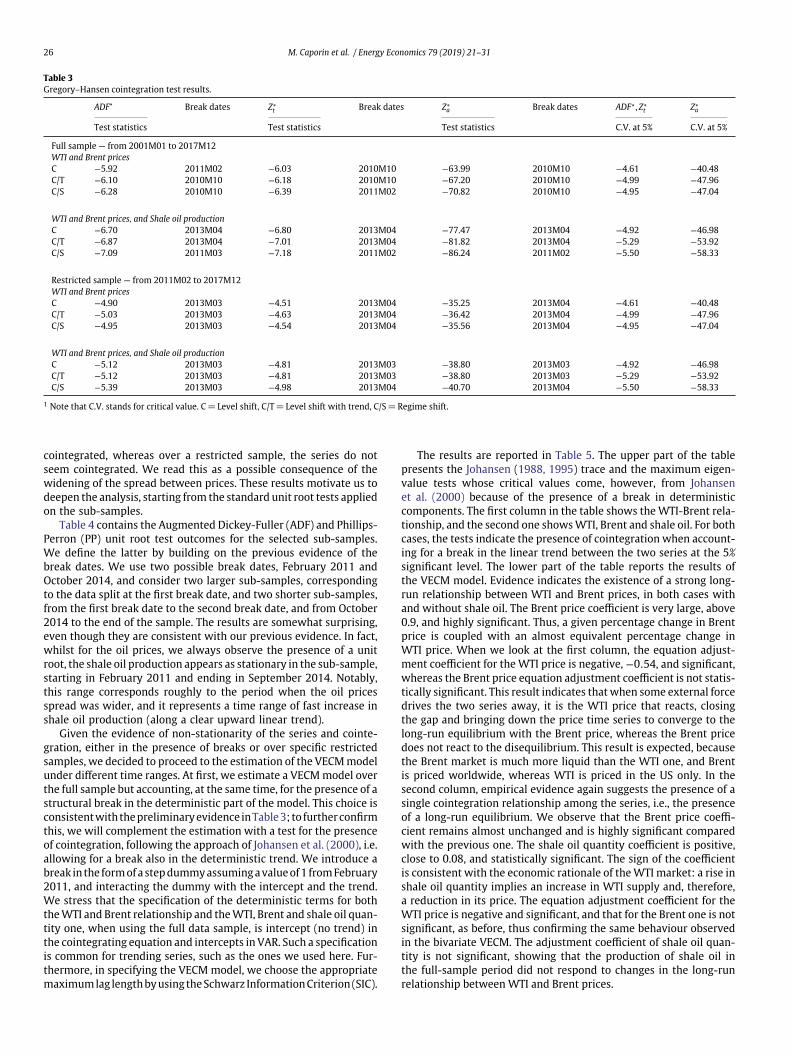
Table 3Gregory–Hansen cointegration test results.

ADF∗ Break dates Z∗t Break dates Z∗

a Break dates ADF∗ , Z∗t Z∗

a

Test statistics Test statistics Test statistics C.V. at 5% C.V. at 5%

Full sample — from 2001M01 to 2017M12WTI and Brent pricesC −5.92 2011M02 −6.03 2010M10 −63.99 2010M10 −4.61 −40.48C/T −6.10 2010M10 −6.18 2010M10 −67.20 2010M10 −4.99 −47.96C/S −6.28 2010M10 −6.39 2011M02 −70.82 2010M10 −4.95 −47.04

WTI and Brent prices, and Shale oil productionC −6.70 2013M04 −6.80 2013M04 −77.47 2013M04 −4.92 −46.98C/T −6.87 2013M04 −7.01 2013M04 −81.82 2013M04 −5.29 −53.92C/S −7.09 2011M03 −7.18 2011M02 −86.24 2011M02 −5.50 −58.33

Restricted sample — from 2011M02 to 2017M12WTI and Brent pricesC −4.90 2013M03 −4.51 2013M04 −35.25 2013M04 −4.61 −40.48C/T −5.03 2013M03 −4.63 2013M04 −36.42 2013M04 −4.99 −47.96C/S −4.95 2013M03 −4.54 2013M04 −35.56 2013M04 −4.95 −47.04

WTI and Brent prices, and Shale oil productionC −5.12 2013M03 −4.81 2013M03 −38.80 2013M03 −4.92 −46.98C/T −5.12 2013M03 −4.81 2013M03 −38.80 2013M03 −5.29 −53.92C/S −5.39 2013M03 −4.98 2013M04 −40.70 2013M04 −5.50 −58.33

1 Note that C.V. stands for critical value. C = Level shift, C/T = Level shift with trend, C/S = Regime shift.

cointegrated, whereas over a restricted sample, the series do notseem cointegrated. We read this as a possible consequence of thewidening of the spread between prices. These results motivate us todeepen the analysis, starting from the standard unit root tests appliedon the sub-samples.

Table 4 contains the Augmented Dickey-Fuller (ADF) and Phillips-Perron (PP) unit root test outcomes for the selected sub-samples.We define the latter by building on the previous evidence of thebreak dates. We use two possible break dates, February 2011 andOctober 2014, and consider two larger sub-samples, correspondingto the data split at the first break date, and two shorter sub-samples,from the first break date to the second break date, and from October2014 to the end of the sample. The results are somewhat surprising,even though they are consistent with our previous evidence. In fact,whilst for the oil prices, we always observe the presence of a unitroot, the shale oil production appears as stationary in the sub-sample,starting in February 2011 and ending in September 2014. Notably,this range corresponds roughly to the period when the oil pricesspread was wider, and it represents a time range of fast increase inshale oil production (along a clear upward linear trend).

Given the evidence of non-stationarity of the series and cointe-gration, either in the presence of breaks or over specific restrictedsamples, we decided to proceed to the estimation of the VECM modelunder different time ranges. At first, we estimate a VECM model overthe full sample but accounting, at the same time, for the presence of astructural break in the deterministic part of the model. This choice isconsistent with the preliminary evidence in Table 3; to further confirmthis, we will complement the estimation with a test for the presenceof cointegration, following the approach of Johansen et al. (2000), i.e.allowing for a break also in the deterministic trend. We introduce abreak in the form of a step dummy assuming a value of 1 from February2011, and interacting the dummy with the intercept and the trend.We stress that the specification of the deterministic terms for boththe WTI and Brent relationship and the WTI, Brent and shale oil quan-tity one, when using the full data sample, is intercept (no trend) inthe cointegrating equation and intercepts in VAR. Such a specificationis common for trending series, such as the ones we used here. Fur-thermore, in specifying the VECM model, we choose the appropriatemaximum lag length by using the Schwarz Information Criterion (SIC).

The results are reported in Table 5. The upper part of the tablepresents the Johansen (1988, 1995) trace and the maximum eigen-value tests whose critical values come, however, from Johansenet al. (2000) because of the presence of a break in deterministiccomponents. The first column in the table shows the WTI-Brent rela-tionship, and the second one shows WTI, Brent and shale oil. For bothcases, the tests indicate the presence of cointegration when account-ing for a break in the linear trend between the two series at the 5%significant level. The lower part of the table reports the results ofthe VECM model. Evidence indicates the existence of a strong long-run relationship between WTI and Brent prices, in both cases withand without shale oil. The Brent price coefficient is very large, above0.9, and highly significant. Thus, a given percentage change in Brentprice is coupled with an almost equivalent percentage change inWTI price. When we look at the first column, the equation adjust-ment coefficient for the WTI price is negative, −0.54, and significant,whereas the Brent price equation adjustment coefficient is not statis-tically significant. This result indicates that when some external forcedrives the two series away, it is the WTI price that reacts, closingthe gap and bringing down the price time series to converge to thelong-run equilibrium with the Brent price, whereas the Brent pricedoes not react to the disequilibrium. This result is expected, becausethe Brent market is much more liquid than the WTI one, and Brentis priced worldwide, whereas WTI is priced in the US only. In thesecond column, empirical evidence again suggests the presence of asingle cointegration relationship among the series, i.e., the presenceof a long-run equilibrium. We observe that the Brent price coeffi-cient remains almost unchanged and is highly significant comparedwith the previous one. The shale oil quantity coefficient is positive,close to 0.08, and statistically significant. The sign of the coefficientis consistent with the economic rationale of the WTI market: a rise inshale oil quantity implies an increase in WTI supply and, therefore,a reduction in its price. The equation adjustment coefficient for theWTI price is negative and significant, and that for the Brent one is notsignificant, as before, thus confirming the same behaviour observedin the bivariate VECM. The adjustment coefficient of shale oil quan-tity is not significant, showing that the production of shale oil inthe full-sample period did not respond to changes in the long-runrelationship between WTI and Brent prices.

M. Caporin et al. / Energy Economics 79 (2019) 21–31 27

Table 4Unit root tests on sub-samples.

Sample/Variables WTI price Brent price Shale quantity WTI price Brent price Shale quantity

Test ADF PP

2000/1–2017/12 0.316 0.231 0.532 0.332 0.273 0.5212000/1–2011/1 0.174 0.065 0.999 0.204 0.209 0.9992011/2–2017/12 0.533 0.412 0.004 0.691 0.642 0.0012011/2–2014/9 0.598 0.639 0.013 0.559 0.625 0.0022014/10–2017/12 0.419 0.154 0.805 0.422 0.251 0.946

1 The table reports the ADF and PP unit root tests p-values. We use automatic selection criteria for the specification of the test equation (in terms of deterministic componentsand lags structure.

We then consider the existence of a break in the structural rela-tion, as suggested by the Gregory-Hansen test results and the abruptincrease in shale oil production in 2011, in order to assess therole played by the rise in shale oil production before and after thestructural break. Therefore, we replicate the analysis for the twosub-samples. We test the existence of cointegration relationshipsin the first sub-sample from January 2000 to January 2011, andthen for the second sub-sample from February 2011 to December2017, between WTI and Brent prices. Through this process, we canascertain whether the long-run relationship between WTI and Brentprices has changed after a structural break. We also consider the pos-sible presence of cointegration between the two prices over the splitof the second sub-sample in October 2014, thus separating the time

Table 5Full-sample cointegration estimation.

Included Variables WTI price WTI price

Brent price Brent price

Shale oil quantity

Lags 2 2No. of cointegration 1 1Trace 41.06∗∗∗ 87.19∗∗∗

Critical value at 1% 41.98 64.57Critical value at 5% 36.06 57.43Max. Eig. 37.37∗∗∗ 47.15∗∗

Critical value at 1% 31.26 49.57Critical value at 5% 26.10 43.22Deterministic IC, IV IC, IVExogenous D11, D11*T D11, D11*T

Cointegration equation:WTIt − l − b1Brentt − b2ShaleQt = 4t

WTI price 1 1Shale oil quantity 0.078∗∗∗

(0.032)Brent price −0.937∗∗∗ −0.938∗∗∗

(0.016) (0.019)

Adjustment coefficients:WTI price −0.543∗∗∗ −0.456∗∗∗

(0.161) (0.159)Shale oil quantity 0.057

(0.032)Brent price −0.234 −0.117

(0.176) (0.172)

1 The first panel includes the cointegration test on the full-sample, and indicates thestructure of the VECM model in terms of lags and deterministic and exogenous com-ponents, including intercept in the cointegration equation (IC) and test VAR (IV), stepdummy from February 2011 (D11) and interaction between the step dummy and a lin-ear trend. Star denotes rejections of the null hypotheses under the appropriate criticalvalues reported below the test statistic (see Johansen et al., 2000; Giles and Godwin,2012 for details). The table also reports estimated coefficients, the standard errors (inparentheses).∗∗∗ Denotes the significant level at 1%.∗∗ Denotes significant level at 5%.

range associated with a widening of the spread from the most recentyears when the spread reverted back to more usual levels.

Finally, we discuss the cointegration between WTI and Brentprices and shale oil quantity. However, in this case, we must considerthe evidence shown in Table 4, suggesting that shale oil quantity isstationary from February 2011 to December 2017, as well as in thereduced sample starting in February 2011 and ending in September2014. Therefore, for the three-variate VECM, we consider only twosamples.

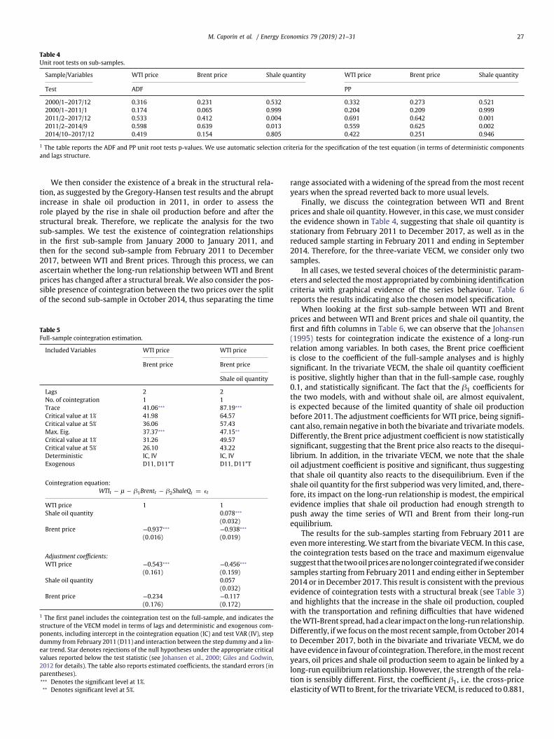
In all cases, we tested several choices of the deterministic param-eters and selected the most appropriated by combining identificationcriteria with graphical evidence of the series behaviour. Table 6reports the results indicating also the chosen model specification.

When looking at the first sub-sample between WTI and Brentprices and between WTI and Brent prices and shale oil quantity, thefirst and fifth columns in Table 6, we can observe that the Johansen(1995) tests for cointegration indicate the existence of a long-runrelation among variables. In both cases, the Brent price coefficientis close to the coefficient of the full-sample analyses and is highlysignificant. In the trivariate VECM, the shale oil quantity coefficientis positive, slightly higher than that in the full-sample case, roughly0.1, and statistically significant. The fact that the b1 coefficients forthe two models, with and without shale oil, are almost equivalent,is expected because of the limited quantity of shale oil productionbefore 2011. The adjustment coefficients for WTI price, being signifi-cant also, remain negative in both the bivariate and trivariate models.Differently, the Brent price adjustment coefficient is now statisticallysignificant, suggesting that the Brent price also reacts to the disequi-librium. In addition, in the trivariate VECM, we note that the shaleoil adjustment coefficient is positive and significant, thus suggestingthat shale oil quantity also reacts to the disequilibrium. Even if theshale oil quantity for the first subperiod was very limited, and, there-fore, its impact on the long-run relationship is modest, the empiricalevidence implies that shale oil production had enough strength topush away the time series of WTI and Brent from their long-runequilibrium.

The results for the sub-samples starting from February 2011 areeven more interesting. We start from the bivariate VECM. In this case,the cointegration tests based on the trace and maximum eigenvaluesuggest that thetwooilpricesarenolongercointegratedifweconsidersamples starting from February 2011 and ending either in September2014 or in December 2017. This result is consistent with the previousevidence of cointegration tests with a structural break (see Table 3)and highlights that the increase in the shale oil production, coupledwith the transportation and refining difficulties that have widenedthe WTI-Brent spread, had a clear impact on the long-run relationship.Differently, if we focus on the most recent sample, from October 2014to December 2017, both in the bivariate and trivariate VECM, we dohave evidence in favour of cointegration. Therefore, in the most recentyears, oil prices and shale oil production seem to again be linked by along-run equilibrium relationship. However, the strength of the rela-tion is sensibly different. First, the coefficient b1, i.e. the cross-priceelasticity of WTI to Brent, for the trivariate VECM, is reduced to 0.881,

28 M. Caporin et al. / Energy Economics 79 (2019) 21–31

Table 6Selected sub-samples cointegration estimation.

Included Variables WTI price WTI price WTI price WTI price WTI price WTI price

Brent price Brent price Brent price Brent price Brent price Brent price

Shale oil quantity Shale oil quantity

Sample 2000M01–2011M01 2011M02–2017M12 2011M02–2014M09 2014M10–2017M12 2000M01–2011M01 2014M10–2017M12Lags 2 2 1 2 2 2No. of cointegration 1 0 0 1 1 1Trace 25.59∗∗∗ 13.89 6.08 15.49∗∗ 43.73∗∗∗ 44.97∗∗∗

Critical value at 1% 19.94 19.94 19.94 19.94 41.08 41.08Critical value at 5% 15.49 15.49 15.49 15.49 35.01 35.01Max. Eig. 24.27∗∗∗ 12.74 6.03 14.26* 30.70∗∗∗ 33.19∗∗∗

Critical value at 1% 18.52 18.52 18.52 18.52 29.26 29.26Critical value at 5% 14.26 14.26 14.26 14.26 24.25 24.25Deterministic IC, IV IC, IV, TC IC IC IC, IV, TC IC, IV

Cointegration equation:WTIt − l − b1Brentt − b2ShaleQt = 4t

WTI price 1 1 1 1Shale oil quantity 0.103∗∗∗ 0.547∗∗∗

(0.038) (0.061)Brent price −0.937∗∗∗ −0.721∗∗∗ −0.941∗∗∗ −0.881∗∗∗

(0.013) (0.067) (0.021) (0.014)

Adjustment coefficients:WTI price −0.817∗∗∗ −0.861∗∗∗ −0.718∗∗∗ −3.003∗∗∗

(0.262) (0.242) (0.259) (0.712)Shale oil quantity 0.109∗∗ 0.326*

(0.049) (0.173)Brent price −0.527* −0.792∗∗∗ -0.375 −2.242∗∗∗

(0.293) (0.277) (0.311) (0.896)

1 The panel includes the cointegration test on the selected sub-samples, and indicates the structure of the VECM model in terms of lags and deterministic components, includinglinear trend in the cointegration equation (TC), intercept in the cointegration equation (IC) and test VAR (IV). The table then reports estimated coefficients, the standard errors (inparentheses).∗∗∗ Denotes the significant level at 1%.∗∗ Denotes significant level at 5%.∗ Denotes significant level at 10%.

compared with the value in the first sub-sample, 0.941 (or to the valuein the full-sample, 0.937). The same occurs for the bivariate VECM.This is an interesting results. The increase in shale oil production hassomehow lowered the WTI price response to the world oil price, asproxied by Brent. We conjecture that this might be because of thehigher resilience of the shale oil industry (WTI-based) to price change.It could be attributed to the shorter time-to-market and smaller scaleof the shale-oil production compared to traditional oil extraction.However, this point requires further investigation. Nevertheless, thehigher importance played by the shale industry in WTI price is con-firmed by the coefficient b2, linking the shale oil production to theWTI price. In the period from October 2014 onward, it remains posi-tive and statistically significant, rising more than five times from thevalue observed in the first sub-sample, i.e. going up to 0.547 fromthe previous value of 0.103. Thus, in the new long-run relationshipbetween WTI and Brent, from October 2014 onward, the shale oil pro-duction has become crucial: a 10% change in shale oil quantity has a5% impact on the WTI price (if the Brent price does not move).

The adjustment coefficients in all cases have now become larger(in absolute terms) than those of the first sub-sample. Notably, inboth models (bivariate and trivariate), all adjustment coefficientsappear statistically significant (for the shale quantity, only at the 10%level). The adjustment coefficients for the prices are larger than 1in modulus. This aspect might signal instability in the VECM model.However, the roots of the characteristic polynomial are all smallerthan 1 in modulus, with the exception of the two roots that mustbe equal to 1; this confirms that the VECM model is stationary.The large value of two adjustment coefficients likely depends onthe normalisation used to recover their point value, and might alsobe affected by the reduced sample size. In addition, the observed

point values do not lead to instability and divergence patterns of themodel; the impulse response functions confirm this aspect. Finally,the large value of the adjustment coefficients implies a fast speed ofconvergence to the equilibrium.7

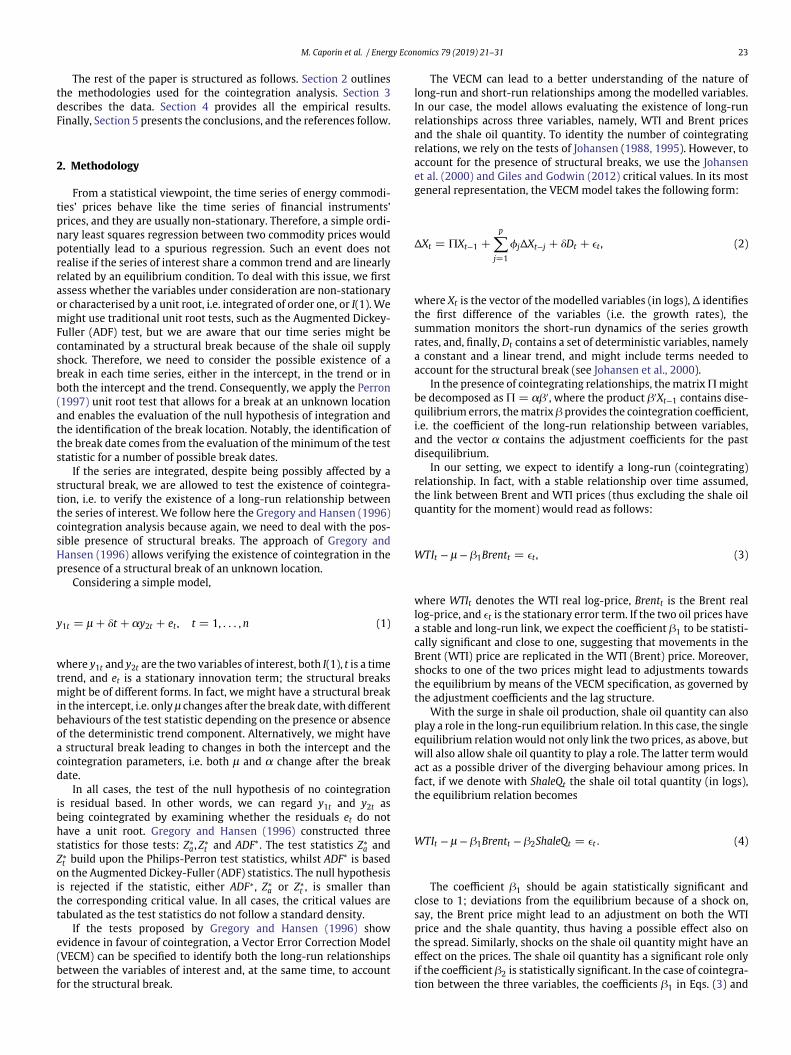
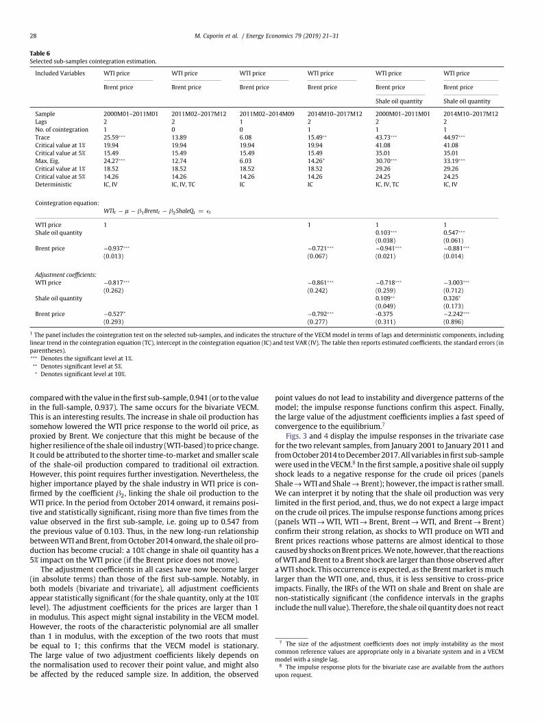
Figs. 3 and 4 display the impulse responses in the trivariate casefor the two relevant samples, from January 2001 to January 2011 andfrom October 2014 to December 2017. All variables in first sub-samplewere used in the VECM.8 In the first sample, a positive shale oil supplyshock leads to a negative response for the crude oil prices (panelsShale → WTI and Shale → Brent); however, the impact is rather small.We can interpret it by noting that the shale oil production was verylimited in the first period, and, thus, we do not expect a large impacton the crude oil prices. The impulse response functions among prices(panels WTI → WTI, WTI → Brent, Brent → WTI, and Brent → Brent)confirm their strong relation, as shocks to WTI produce on WTI andBrent prices reactions whose patterns are almost identical to thosecaused by shocks on Brent prices. We note, however, that the reactionsof WTI and Brent to a Brent shock are larger than those observed aftera WTI shock. This occurrence is expected, as the Brent market is muchlarger than the WTI one, and, thus, it is less sensitive to cross-priceimpacts. Finally, the IRFs of the WTI on shale and Brent on shale arenon-statistically significant (the confidence intervals in the graphsinclude the null value). Therefore, the shale oil quantity does not react

7 The size of the adjustment coefficients does not imply instability as the mostcommon reference values are appropriate only in a bivariate system and in a VECMmodel with a single lag.

8 The impulse response plots for the bivariate case are available from the authorsupon request.

M. Caporin et al. / Energy Economics 79 (2019) 21–31 29

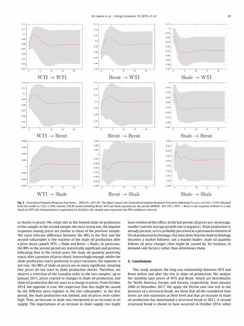
Fig. 3. Generalized Impulse Response Functions — 2001/01–2011/01. The figure reports the Generalized Impulse Response Functions following Pesaran and Shin (1998) obtainedfrom the model in Table 6, fifth column (VECM model including Brent, WTI and Shale quantity for the period 2000/01–2011/01); WTI → Brent is the response of Brent to a unitshock on WTI (the interpretation is equivalent for all plots); the shaded area represents the 90% confidence interval.

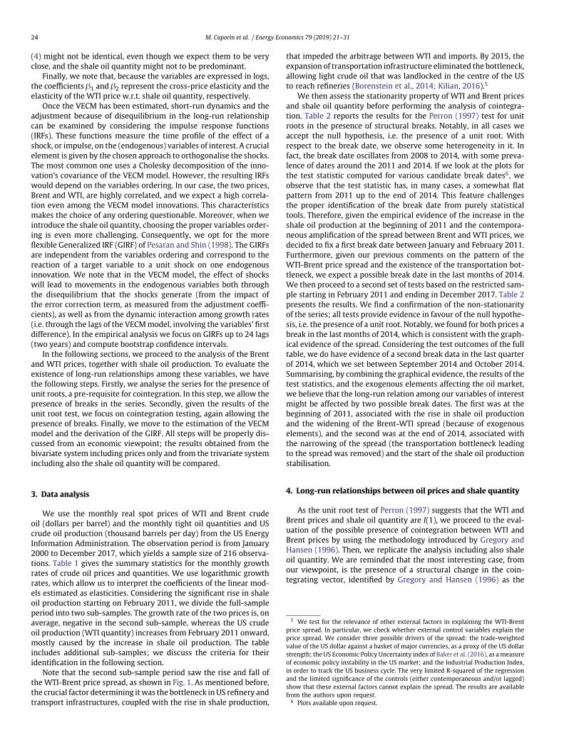
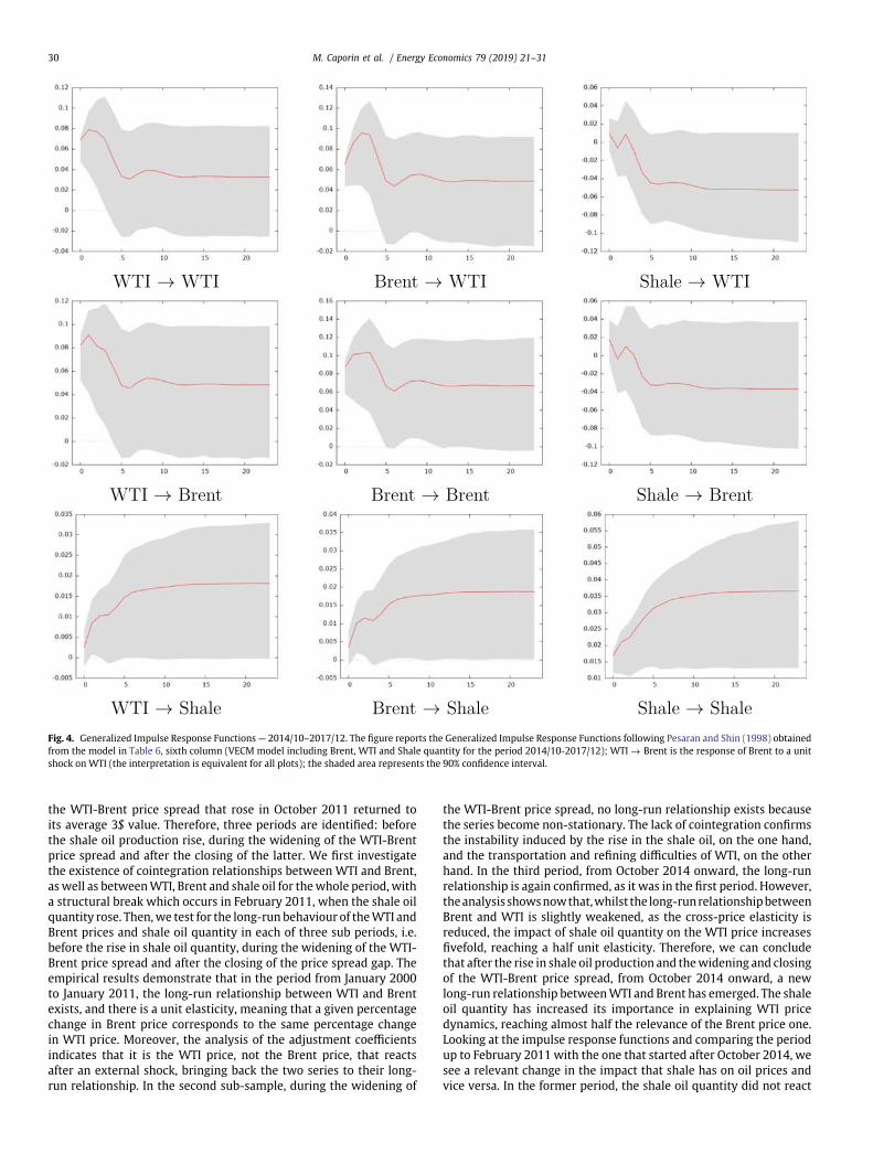
to shocks to prices. We relate this to the limited shale oil productionin this sample. In the second sample, the most recent one, the impulseresponses among prices are similar to those of the previous sample.The most relevant difference between the IRFs in the first and thesecond subsamples is the reaction of the shale oil production aftera price shock (panels WTI → Shale and Brent → Shale). In particular,the IRFs in the second period are statistically significant and positive,indicating that in the recent years the shale oil quantity positivelyreacts after a positive oil price shock. Interestingly enough, whilst theshale production reacts positively to price increases, the opposite isnot true: the IRFs of shale on prices are no more significant, meaningthat prices do not react to shale production shocks. Therefore, weobserve a reversion of the causality order in the two samples: up toJanuary 2011, prices reacted to changes in shale oil production, andshale oil production did not react to a change in prices. From October2014, the opposite is true. We conjecture that this might be causedby the different price regimes in the two subsamples: in the firstperiod, the shale production was limited, and oil prices were ratherhigh. Thus, an increase in shale was interpreted as an increase in oilsupply. The expectations of an increase in shale supply rise might

have reinforced this effect. In the last period, oil prices are, on average,smaller (and the average growth rate is negative). Shale production isalready present, so it is probably perceived as a permanent element ofUS oil production technology. Our data show that the shale technologybecomes a market follower, not a market leader: shale oil quantityfollows oil price changes (that might be caused by, for instance, todemand-side factors) rather than determines them.

5. Conclusions

This study analyses the long-run relationship between WTI andBrent before and after the rise in shale oil production. We analysethe monthly spot prices of WTI and Brent, which are benchmarksfor North America, Europe and Eurasia, respectively, from January2000 to December 2017. We apply the Perron unit root test in thepresence of a structural break; we show that all the considered timeseries are non-stationary at their level and that an increase in shaleoil production has determined a structural break in 2011. A secondstructural break is shown to have occurred in October 2014, when

30 M. Caporin et al. / Energy Economics 79 (2019) 21–31

Fig. 4. Generalized Impulse Response Functions — 2014/10–2017/12. The figure reports the Generalized Impulse Response Functions following Pesaran and Shin (1998) obtainedfrom the model in Table 6, sixth column (VECM model including Brent, WTI and Shale quantity for the period 2014/10-2017/12); WTI → Brent is the response of Brent to a unitshock on WTI (the interpretation is equivalent for all plots); the shaded area represents the 90% confidence interval.

the WTI-Brent price spread that rose in October 2011 returned toits average 3$ value. Therefore, three periods are identified: beforethe shale oil production rise, during the widening of the WTI-Brentprice spread and after the closing of the latter. We first investigatethe existence of cointegration relationships between WTI and Brent,as well as between WTI, Brent and shale oil for the whole period, witha structural break which occurs in February 2011, when the shale oilquantity rose. Then, we test for the long-run behaviour of the WTI andBrent prices and shale oil quantity in each of three sub periods, i.e.before the rise in shale oil quantity, during the widening of the WTI-Brent price spread and after the closing of the price spread gap. Theempirical results demonstrate that in the period from January 2000to January 2011, the long-run relationship between WTI and Brentexists, and there is a unit elasticity, meaning that a given percentagechange in Brent price corresponds to the same percentage changein WTI price. Moreover, the analysis of the adjustment coefficientsindicates that it is the WTI price, not the Brent price, that reactsafter an external shock, bringing back the two series to their long-run relationship. In the second sub-sample, during the widening of

the WTI-Brent price spread, no long-run relationship exists becausethe series become non-stationary. The lack of cointegration confirmsthe instability induced by the rise in the shale oil, on the one hand,and the transportation and refining difficulties of WTI, on the otherhand. In the third period, from October 2014 onward, the long-runrelationship is again confirmed, as it was in the first period. However,the analysis shows now that, whilst the long-run relationship betweenBrent and WTI is slightly weakened, as the cross-price elasticity isreduced, the impact of shale oil quantity on the WTI price increasesfivefold, reaching a half unit elasticity. Therefore, we can concludethat after the rise in shale oil production and the widening and closingof the WTI-Brent price spread, from October 2014 onward, a newlong-run relationship between WTI and Brent has emerged. The shaleoil quantity has increased its importance in explaining WTI pricedynamics, reaching almost half the relevance of the Brent price one.Looking at the impulse response functions and comparing the periodup to February 2011 with the one that started after October 2014, wesee a relevant change in the impact that shale has on oil prices andvice versa. In the former period, the shale oil quantity did not react

M. Caporin et al. / Energy Economics 79 (2019) 21–31 31

to the change in price, whilst the price was negatively affected bythe positive supply shocks of shale. In the second period, the shaleoil quantity reacts to price increases, whilst the opposite does notoccur anymore. We interpret this as a signal of a change in the shale-oil price relationships: in the first period, prices were high and theshale quantity was low, so an increase in the shale oil quantity wasperceived as a positive supply shock. In the last period, the oil priceswere low and the shale quantity was high, so the shale quantityfollowed the change in prices, which were not determined anymoreby supply shocks.

Appendix A. Supplementary data

Supplementary data to this article can be found online at https://doi.org/10.1016/j.eneco.2018.08.022.

References

Aruga, K., 2015. Testing the international crude oil market integration with structuralbreaks. Econ. Bull. 35, 641–649.

Baker, S., Bloom, N., Davis, S., 2016. Measuring economic policy uncertainty. Q. J. Econ.131, 1593–1636.

Borenstein, S., Kellogg, R., et al. 2014. The incidence of an oil glut: who benefits fromcheap crude oil in the Midwest? Energy J. 35 (1), 15–33.

Büyüksahin, B., Lee, T., Moser, J., Robe, M., 2013. Physical market conditions, papermarket activity, and the WTI-Brent spread. Energy J. 34 (3).

Chen, W., Huang, Z., 2015. Is there a structural change in the persistence of WTI-Brentoil price spreads in the post-2010 period? Econ. Model. 50, 64–71.

Coronado, S., Fullerton, T., Rojas, O., 2016. Causality patterns for brent, WTI, and argusoil prices. Appl. Econ. Lett. 24, 982–986.

EIA, 2016. Short-term Energy Outlook: Market Prices and Uncertainty Report. USEnergy Information Administration.

Fattouh, B., 2007. WTI benchmark temporarily breaks down: is it really a big deal.Middle East Econ. Surv. 50 (20), 7.

Fattouh, B., 2010. The dynamics of crude oil price differentials. Energy Econ. 32 (2),334–342.

Giles, D.E., Godwin, R.T., 2012. Testing for multivariate cointegration in the presenceof structural breaks: p-values and critical values. Appl. Econ. Lett. 19 (16),1561–1565.

Gregory, A.W., Hansen, B.E., 1996. Residual-based tests for cointegration in modelswith regime shifts. J. Econ. 70 (1), 99–126.

Gülen, S.G., 1999. Regionalization in the world crude oil market: further evidence.Energy J. 125–139.

Hammoudeh, S.M., Ewing, B.T., Thompson, M.A., 2008. Threshold cointegrationanalysis of crude oil benchmarks. Energy J. 79–95.

Johansen, S., 1988. Statistical analysis of cointegration vectors. J. Econ. Dyn. Control.12 (2-3), 231–254.

Johansen, S., 1995. Likelihood-based Inference in Cointegrated Vector AutoregressiveModels. Oxford University Press. https://doi.org/10.1093/0198774508.001.0001.

Johansen, S., Mosconi, R., Nielsen, B., 2000. Cointegration analysis in the presence ofstructural breaks in the deterministic trend. Econ. J. 3 (2), 216–249.

Kao, C.-W., Wan, J.-Y., 2012. Price discount, inventories and the distortion of WTIbenchmark. Energy Econ. 34 (1), 117–124.

Kilian, L., 2016. The impact of the shale oil revolution on us oil and gasoline prices.Rev. Environ. Econ. Policy 10 (2), 185–205.

Kim, J., Kim, J., Heo, E., 2013. Evolution of the international crude oil marketmechanism. Geosyst. Eng. 16, 265–274.

Liao, H., Lin, S., Huang, H., 2014. Are crude oil markets globalized or regionalized?Evidence from WTI and Brent. Appl. Econ. Lett. 21, 235–241.

Liu, P., Stevens, R., Vedenov, D., 2018. The physical market and the WTI/Brent pricespread. OPEC Energy Rev. 42, 55–73.

Perron, P., 1997. Further evidence on breaking trend functions in macroeconomicvariables. J. Econ. 80 (2), 355–385.

Pesaran, H.H., Shin, Y., 1998. Generalized impulse response analysis in linear multi-variate models. Econ. Lett. 58 (1), 17–29.

Reboredo, J.C., 2011. How do crude oil prices co-move?: A copula approach. EnergyEcon. 33 (5), 948–955.

Weiner, R., 1991. Is the world oil market ‘one great pool’? Energy J. 12, 95–107.Wilmot, N.A., 2013. Cointegration in the oil market among regional blends. Int. J.

Energy Econ. Policy 3 (4), 424.