temporal analysis of honey bee interaction networks based

Master Thesis, Institute of Computer Science, Freie Universitat Berlin

Biorobotics Lab, Intelligent Systems and Robotics

Temporal Analysis ofHoney Bee Interaction Networks

Based on Spatial Proximity

Alexa Schlegel

Supervisor: Prof. Dr. Tim Landgraf, Freie Universitat Berlin

Second Supervisor: Dr. Philipp Hovel, Technische Universitat Berlin

Berlin, April 20, 2017

Eidesstattliche Erklarung

Ich versichere hiermit an Eides Statt, dass diese Arbeit von niemand anderemals meiner Person verfasst worden ist. Alle verwendeten Hilfsmittel wie Berichte,Bucher, Internetseiten oder ahnliches sind im Literaturverzeichnis angegeben, Zitateaus fremden Arbeiten sind als solche kenntlich gemacht. Die Arbeit wurde bisherin gleicher oder ahnlicher Form keiner anderen Prufungskommission vorgelegt undauch nicht veroffentlicht.

Berlin, den 20. April 2017

Alexa Schlegel

Abstract

The BeesBook system provides high-resolution data about bee movements withina single colony by automatically tracking individual honey bees inside a hive overtheir entire life. This thesis focuses on the process of designing and implementing anetwork pipeline to extract interaction networks from this data. Spatial proximity isused as an indicator for interactions between bees. Social network analysis methodswere applied to investigate the static and dynamic properties of the resulting socialnetworks of honey bees on a global, intermediate and local level. The resultingnetworks were characterized by a low hierarchical structure and a high density. Theglobal structure of the colony seems to be stable over time. The local structureis highly dynamic, as bees change communities as they age. Communities in thehoney bee network are formed by age groups that show a high spatial fidelity. Thefindings are in line with the established state of research that colonies are organizedaround age-based task division. The results of the analysis validate the implementedpipeline and the inferred networks. Consequently, this work provides an excellentfoundation for future research focusing on temporal network analysis.

Keywords – social insects, spatial proximity network, interaction network, Apismellifera, community detection, social network analysis

Contents

1 Introduction 11.1 Motivation . . . . . . . . . . . . . . . . . . . . . . . . . . . . . . . . . 21.2 Research Goal and Method . . . . . . . . . . . . . . . . . . . . . . . . 21.3 Outline . . . . . . . . . . . . . . . . . . . . . . . . . . . . . . . . . . . 3

2 Theoretical Background for Network Analysis of Insect Colonies 42.1 Social Network Analysis . . . . . . . . . . . . . . . . . . . . . . . . . 4

2.1.1 Network Measures and Metrics . . . . . . . . . . . . . . . . . 52.1.2 Community Detection . . . . . . . . . . . . . . . . . . . . . . 62.1.3 Temporal Networks . . . . . . . . . . . . . . . . . . . . . . . . 8

2.2 Related Studies . . . . . . . . . . . . . . . . . . . . . . . . . . . . . . 92.2.1 Static Network Analysis of Honey Bee Colonies . . . . . . . . 92.2.2 Temporal Network Analysis of Insect Colonies . . . . . . . . . 10

3 Methodology 123.1 The Experimental Setup and Dataset . . . . . . . . . . . . . . . . . . 123.2 Data Quality and Data Cleansing . . . . . . . . . . . . . . . . . . . . 13

3.2.1 Data Scheme . . . . . . . . . . . . . . . . . . . . . . . . . . . 133.2.2 ID Probabilities, Confidence Level, and Quality . . . . . . . . 143.2.3 Detection Frequency Filter . . . . . . . . . . . . . . . . . . . . 153.2.4 Time Series of Bees and Bee Pairs . . . . . . . . . . . . . . . . 16

3.3 Inferring Spatial Proximity Networks . . . . . . . . . . . . . . . . . . 173.3.1 Defining the Network and its Parameters . . . . . . . . . . . . 173.3.2 Choosing Parameter Values for Network Analysis . . . . . . . 183.3.3 Summary . . . . . . . . . . . . . . . . . . . . . . . . . . . . . 19

3.4 Methods for Analyzing Spatial Proximity Networks . . . . . . . . . . 203.4.1 Investigating the Topology and Network Characteristics . . . . 203.4.2 Detecting Communities . . . . . . . . . . . . . . . . . . . . . . 223.4.3 Development of Community Members . . . . . . . . . . . . . . 25

4 Results of Network Analysis 264.1 Static Perspectives of Honey Bee Networks . . . . . . . . . . . . . . . 26

4.1.1 Properties of the Bee Colony . . . . . . . . . . . . . . . . . . . 274.1.2 Characteristics of Bees . . . . . . . . . . . . . . . . . . . . . . 274.1.3 Functional Groups within the Colony . . . . . . . . . . . . . . 30

4.2 Temporal Perspectives of Honey Bee Networks . . . . . . . . . . . . . 334.2.1 Stability of Functional Groups . . . . . . . . . . . . . . . . . . 334.2.2 Dynamic of Individual Bees . . . . . . . . . . . . . . . . . . . 34

iv

4.3 Discussion of Results . . . . . . . . . . . . . . . . . . . . . . . . . . . 354.3.1 Network Topology and Properties of Honey Bee Colonies . . . 354.3.2 Characterization of Functional Groups and its Dynamics . . . 37

5 Conclusions 395.1 Limitations . . . . . . . . . . . . . . . . . . . . . . . . . . . . . . . . 395.2 Recommendations . . . . . . . . . . . . . . . . . . . . . . . . . . . . . 405.3 Outlook . . . . . . . . . . . . . . . . . . . . . . . . . . . . . . . . . . 415.4 Closing Remarks . . . . . . . . . . . . . . . . . . . . . . . . . . . . . 42

Bibliography 43

List of Figures 46

List of Tables 48

A Literatur Review 49

B Additional Information about the Dataset 53

C Network Analysis 55

Chapter 1

Introduction

A social insect society is formed by thousands of individuals that continuously in-teract with each other inside a dark nest. Honey bees are organized in colonies,which are a complex and dynamic system. Observing individual honey bees andtheir interactions with each other is vital for understanding collective behavior andthe organization of tasks within the colony.

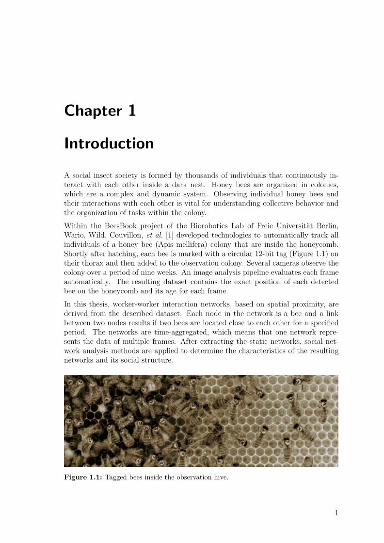
Within the BeesBook project of the Biorobotics Lab of Freie Universitat Berlin,Wario, Wild, Couvillon, et al. [1] developed technologies to automatically track allindividuals of a honey bee (Apis mellifera) colony that are inside the honeycomb.Shortly after hatching, each bee is marked with a circular 12-bit tag (Figure 1.1) ontheir thorax and then added to the observation colony. Several cameras observe thecolony over a period of nine weeks. An image analysis pipeline evaluates each frameautomatically. The resulting dataset contains the exact position of each detectedbee on the honeycomb and its age for each frame.

In this thesis, worker-worker interaction networks, based on spatial proximity, arederived from the described dataset. Each node in the network is a bee and a linkbetween two nodes results if two bees are located close to each other for a specifiedperiod. The networks are time-aggregated, which means that one network repre-sents the data of multiple frames. After extracting the static networks, social net-work analysis methods are applied to determine the characteristics of the resultingnetworks and its social structure.

Figure 1.1: Tagged bees inside the observation hive.

1

1.2. Research Goal and Method

1.1 Motivation

Manual insect tagging and tracking are widely applied in the behavioral sciences.Insects are marked using colored paint or numbered tags to distinguish individuals,and then they are observed using a video recorder or by taking photos. The interac-tion data is obtained by repeatedly watching the video files and manually extractingevents. Labeling only a small group of the colonies’ individuals, short observationperiods, a low sampling resolution, or limiting the observation to only a small areaof the hive is very common.

Consequently, most insect related studies, in the field of animal social network analy-sis, examine only a limited subset of the life of a colony. Due to technical limitations,the majority of social insect interaction network studies focus on static aspects. Re-cently, automated tracking of insects has become technically feasible [1]–[3]. Usingautomated high resolution tracking data, which includes all individuals of the en-tire hive over an extended period, allows for more advanced analysis focusing ontemporal dynamics.

Automatic tracking data of ant colonies [4] has already been investigated with net-work analysis methods. Mersch, Crespi, and Keller [4] used a dataset, obtainedby long-term observation of six ant colonies including all individuals, to investigatetemporal aspects of the ants’ social network. Their study was able to provide newinsights into the dynamics of the colonies’ functional units.

Applying network analysis methods on data that was obtained by automatic trackingof honey bees offers the possibility to investigate temporal aspects of bees’ socialnetworks. Therefore it holds the potential to reveal new insights in the area ofbehavioral sciences. My work contributes to lay the foundation for following thisnew path of research.

1.2 Research Goal and Method

The aim of this thesis is to investigate whether the BeesBook data of tracked honeybees is useful for creating worker-worker interaction networks using spatial proximityas an indicator for interactions between bees. Thus, I will implement a pipeline toextract networks out of the given data. Furthermore, I will investigate if the resultingnetworks are suitable for social network analysis.

I want to achieve my research goals by answering the following questions:

1. Is it possible to infer temporal networks with the provided honey bee tracking

data?

What challenges and limitations arise from using this data?What pipeline parameters are necessary?

2. What kind of worker-worker interaction networks emerge and how are they

structured?

What is their topology?

2

1.3. Outline

What are the properties of the networks and how do they differ from randomlygenerated networks?

3. Does the network display a meaningful community structure?

How are the identified communities characterized?Do they reflect already known colony behavior concerning age and spatialdistribution?

4. How do these communities develop over time?

Do the communities have stable properties?How do members move between communities?

This work is meant to establish the foundation for future research using a networkscience approach to study the complex system of honey bee colonies and their col-lective behavior.

The methodology of this work consists of two parts, described in detail in Chapter 3.The first part details the approach to infer and define spatial proximity networks us-ing the honey bee tracking data. The second part analyzes properties, communities,and the development of the identified networks.

1.3 Outline

This thesis is organized as follows. Chapter 2 is a short introduction to socialnetwork analysis. I define network measures, terms, and algorithms used throughoutthis work and provide a brief summary of the current state of research concerningsocial insect networks, temporal networks and community detection in animal socialnetworks. In Chapter 3, I describe my research approach in general and how thepipeline infers networks out of the given dataset, what steps are needed and whatparameters it uses. Also, I explain and justify what decisions I took during thenetwork analyses and community detection process. In Chapter 4, I report theresults of the network analysis and the characteristics of the extracted communities.Finally, in chapter 5, I summarize the results, discuss limitations and conclude withdirections for future work.

3

Chapter 2

Theoretical Background for NetworkAnalysis of Insect Colonies

The following chapter gives a short introduction into social network analysis (SNA)and introduces social insect interaction networks, as a specific type of a biologicalnetwork. It defines terms and concepts used throughout this work and explains theapplied network metrics and algorithms. I also provide a summary of the most rele-vant studies that use a network analysis approach to investigate interaction networksof social insect colonies.

2.1 Social Network Analysis

A social network is a representation of a social structure comprising actors suchas individuals, affiliations, as well as their social interactions. The network modelconceptualizes social, economic, or political structures as lasting patterns of inter-actions between actors [5]. In mathematical terms, networks are graphs and thusconsist of nodes (vertices, representing individuals), and links (edges, relationshipsor interactions). Social network analysis provides a set of methods, measures, andtheories, borrowed from network and graph theory, to investigate social structuresand their dynamics.

This work focuses on the special case of social insect networks, where individuals arenodes and links represent interaction events between individuals. Those networksare called interaction networks or association networks. According to Charbonneau,Blonder, and Dornhaus [6], the interactions used as a link can be of four differ-ent types when looking at social insect networks: spatial proximity, physical contact(usually with antennae, “antennation”), a food exchange event (trophallaxis), or spe-cific communication signals. Trophallaxis is the directed mouth-to-mouth transferof fluids and is used by social insects to exchange information and food.

Links can be directed or undirected and weighted or unweighted. The link weightsrepresent the strength of the relationship; commonly the number or duration ofinteractions is used [7].

In the course of this work I use the term frequency to refer to the total number ofoccurences (absolute frequency), as opposed to the use of this term in physics.

4

2.1. Social Network Analysis

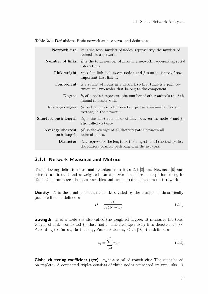
Table 2.1: Definitions Basic network science terms and definitions.

Network size N is the total number of nodes, representing the number ofanimals in a network.

Number of links L is the total number of links in a network, representing socialinteractions.

Link weight wij of an link lij between node i and j is an indicator of howimportant that link is.

Component is a subnet of nodes in a network so that there is a path be-tween any two nodes that belong to the component.

Degree ki of a node i represents the number of other animals the i-thanimal interacts with.

Average degree 〈k〉 is the number of interaction partners an animal has, onaverage, in the network.

Shortest path length dij is the shortest number of links between the nodes i and j,also called distance.

Average shortest 〈d〉 is the average of all shortest paths between allpath length pairs of nodes.

Diameter dmax represents the length of the longest of all shortest paths,the longest possible path length in the network.

2.1.1 Network Measures and Metrics

The following definitions are mainly taken from Barabasi [8] and Newman [9] andrefer to undirected and unweighted static network measures, except for strength.Table 2.1 summarizes the basic variables and terms used in the course of this work.

Density D is the number of realized links divided by the number of theoreticallypossible links is defined as

D =2L

N(N − 1). (2.1)

Strength si of a node i is also called the weighted degree. It measures the totalweight of links connected to that node. The average strength is denoted as 〈s〉.According to Barrat, Barthelemy, Pastor-Satorras, et al. [10] it is defined as

si =N∑

j=1

wij. (2.2)

Global clustering coefficient (gcc) c∆ is also called transitivity. The gcc is basedon triplets. A connected triplet consists of three nodes connected by two links. A

5


triangle consists of three connected triplets. According to Wasserman and Faust [5]the gcc is defined as

c∆ =(number of triangles)× 3

(number of connected triples). (2.3)

Local clustering coefficient (lcc) ci of a node i quantifies how close the node’sneighborhood is to beeing a complete subgraph and is defined as

ci =(number of pairs of neighbors of i that are connected)

(number of pairs of neighbors of i). (2.4)

Centrality When looking at the node level structure of a network, it is possible toidentify nodes, which are important or central to different aspects of the network.This concept is called centrality and measures the influence of a node in a network.

Degree Centrality C iD is the normalized degree ki of a node i in relation to the

whole network. It is calculated as

C iD =

ki

N − 1. (2.5)

Closeness Centrality C iC of a node i measures how close this node is to all other

nodes in the network. It is the average length of shortest paths between node i andall other nodes in the network and is calculated as

C iC =

N∑

j dij. (2.6)

Betweenness Centrality C iB of a node i measures the extent to which a node lies

on shortest paths between other nodes. Nodes that occur on many shortest pathsbetween other nodes have a higher betweenness that those that do not.

2.1.2 Community Detection

To understand the large-scale structure of networks, one can look at the network’scommunity structure. Communities are naturally occurring groups within a network,usually also called clusters, cohesive groups or modules and have no widely accepted,unique definition [11]. For my work, I adapt the definition according to Barabasi[8, p. 322]: “In network science, we call a community a group of nodes that have ahigher likelihood of connecting to each other than to nodes from other communities.”

6


In contrast to a simple graph partition, the number and size of communities is notpredetermined or set in advance.

In animal social networks, communities refer to groups of individuals that are asso-ciated more with each other than they are with the rest of the population. Thesecommunities reflect an intermediate level of social organization, which is locatedbetween the individual and population level [12].

There are a lot of different approaches and algorithms that address the detectionof communities. Fortunato [13] gives an extensive overview of the various types ofcommunity detection algorithms. Explaining any of those would be beyond the scopeof this work. For example, traditional methods include algorithms based on graphpartitioning, hierarchical clustering, and spectral clustering. There are also divisiveand agglomerative algorithms. The algorithms used in this work are described inthe following sections and include the leading eigenvector [14] and walktrap [15]algorithm.

Modularity

Modularity is a quantity that measures the quality of a partitioning. It can be usedto compare one community partition to another and to decide which is the betterone. Modularity optimization is also used for community detection algorithms. Ahigh modularity of a network indicates more connections between nodes within acommunity and fewer connections between nodes of different communities. Thebasic idea is: If the fraction of links inside the community is higher than expectedin the same community of a corresponding random graph with the same degreedistribution, then it is a community in the sense of modularity. This difference issummed up and normalized.

Fewer links inside the community than expected result in a negative value, morelinks positive. If all nodes fall into one community, the modularity is zero.

Leading Eigenvector and Walktrap

The leading eigenvector algorithm was proposed by Newman [14]. It uses the eigen-vectors of matrices for finding community structures in networks. It is a top-downhierarchical approach that optimizes modularity. The algorithm starts with all nodesinside one community (modularity is 0). In each step, the network is split into twoparts, so that the modularity of the new separation increases. The splitting is doneby first calculating the leading eigenvector of the modularity matrix and then split-ting the network in a way that maximizes the modularity improvement based onthe leading eigenvector. The algorithm stops if the modularity does not furtherincrease.

The walktrap algorithm by Pons and Latapy [15] is based on random walks. Theauthors use random walks as a tool to calculate the similarity between nodes of anetwork. The algorithm uses a bottom-up hierarchical approach, which means the

7


algorithm starts with each node in a single community. The basic idea of walktrapis that short distance random walks (the step size is a parameter) tend to stay in thesame community because there are only a few links that lead outside a given com-munity. The results of these random walks are used to merge separate communities.Again modularity can be used to cut the dendrogram at an optimal place.

2.1.3 Temporal Networks

When modeling temporal or dynamic networks, two main approaches exist: (1) time-aggregated (discrete), where the data is aggregated either in a disjoint, overlappingor cumulative snapshot; and (2) the time-ordered (continuous) approach, with in-teractions having a start and end timestamp [16]–[18].

The time-aggregated approach cumulates the data for each snapshot and reduces theavailable information per link. In contrast, the time-ordered approach retains theinformation about when interactions occurred and how long they lasted. It providesa detailed insight when timing and order of interactions are important. It can beused to model the topological flow of information through a network.

Choosing a suitable time interval for data aggregation is challenging [17], but manymethods for analyzing time-aggregated networks already exists, whereas, for time-ordered networks, only a limited toolset is available. To model nodes and linkweights in time-aggregated networks can be challenging, when since interactions,which occurred earlier or later in time, should be weighted accordingly.

8

2.2. Related Studies

2.2 Related Studies

Studies using a network analysis approach focusing on interaction networks to inves-tigate the behavior of social insects, especially honey bees are relevant for my work. Imainly reviewed studies mentioned in the survey papers of Pinter-Wollman, Hobson,Smith, et al. [17], Krause, James, Franks, et al. [19, Chapter 15] and Charbonneau,Blonder, and Dornhaus [6].

The most relevant studies were classified by:

• Type of analysis

temporal or static analysis using automated or manual tracking over a long orshort term

• Studied species

honey bees or other social insects

I reviewed the limitations of the studies in regards to time, space, and the number oftracked individuals. Table A.2 (Appendix A) summarizes the selected studies andthe characteristics of: duration of study, observation period, sampling resolution,the number of colonies, the number of marked individuals, and space limitations. Ialso recorded whether the studies included age cohorts in their analysis and listedthe software tools used for network analysis.

Within the scope of my literature review, I found a lot of studies in the field ofstatic network analysis of ants [20]–[25], wasps [26] and bumblebees [27], but only afew related to honey bees [28]–[31]. I did not find any studies focused on temporalaspects of honey bee colonies, but I did find several studies focused on temporalaspects of ant colonies [4], [32], [33].

2.2.1 Static Network Analysis of Honey Bee Colonies

The most advanced work studying honey bees using a network science approach is byBaracchi and Cini [28]. Their study revealed a highly compartmentalized structureinside the honey bee colony: Bees organize by age groups, which occupy separateareas of the comb and perform different tasks. There is limited contact betweenthese groups.

Generally, the theory that bees change tasks over the course of their lifetime, startingas nurses in the nest and ending as foragers outside, termed as temporal polyethism,is widely accepted and has been studied for a long time [34]–[36]. Johnson [35] ob-served two groups of within-nest bees: young bees responsible for the brood care andmiddle-aged bees specialized on nectar processing and nest maintenance. Seeley [34]observes four age subcastes among worker bees besides the queen cast: cell cleaning,brood nest, food storage, forager.Lindauer [36] defined certain tasks a bee can perform at any given age. Also, a beecan perform several different tasks per day. The bee is flexible and responds to thegiven needs of the hive. Young bees mostly clean cells and old bees mainly forage,

9


instead middle-aged bees perform several tasks. [36]

Baracchi and Cini [28] use the frequency of interactions between bees as link weightsin an undirected worker-worker interaction network. The body length of a bee definesthe radius of spatial proximity. Baracchi and Cini use the node level measuresstrength (weighted degree), closeness and eigenvector centrality to investigate thenetworks. They also perform a cluster analysis using as similarity the local networkmeasures. The main shortcomings of their work are sample size and observationfrequency. They studied one colony with 4,000 individuals, marking only 211 beesfrom three predefined age cohorts, and observed only one side of the observationhive for ten hours by capturing with a low resolution of one frame per minute.

Scholl and Naug [30] investigated the mechanism behind the emergence of organi-zational immunity of honey bee colonies by using unweighted, undirected physicalcontact and trophallaxis networks. They observed one hour per day, with threedays of observation spread over three weeks. In the field of network analysis, theyinvestigated the interactions between three predefined age cohorts.

Naug [29] inspects the network structure of weighted, directed trophallaxis networksusing four age cohorts. He evaluates the changes in transmission dynamics producedby experimental manipulation. The dataset is limited to one hour of observationand only first- and second-order trophallaxis interactions are considered. The foodtransfer from the forager to a worker bee is called first level interaction, the foodtransfer from that worker bee to other bees is called second-order.

2.2.2 Temporal Network Analysis of Insect Colonies

Mersch, Crespi, and Keller [4] apply similar methods to my work. They automat-ically tracked all individuals of six ant colonies over a period of 41 days using aresolution of two frames per second. For each observation day, the authors ex-tracted time-aggregated weighted contact networks per colony, using antennation asthe physical contact event. They applied the Infomap community detection algo-rithm to each daily network and revealed three distinct and robust groups. Eachgroup represents a functional behavioral unit, with ants changing groups as theyage. Except for community detection, they did not use any other network sciencemethods to investigate the network properties.

Jeanson [33] also used automatic tracking. His work is focused on the investigationof the temporal stability of spatial proximity networks in four ant colonies over threeweeks. Here, proximity is defined as 4/3 of an ant’s body length. Per week and percolony they generated weighted time-aggregated networks, using the total durationof interaction as the link weights. They investigated the strength, betweenness andcloseness centrality and found that the networks are stable over time, without thequeen contributing to the network structure. Also they state that individuals withlong lasting interactions seem to have a reduced tendency to move, while mobileants interact homogeneously with their nestmates. The observed colonies ranged insize from 55 to 58 individuals.

10


In these studies, each of the observed ant colonies contained a maximum of 200individuals. This number is relatively small compared to the size of honey beecolonies used in the static analysis approaches.

11

Chapter 3

Methodology

In this chapter, I outline the methodology I applied to reach my research goals. In thefirst section, I describe the data and the experimental setup. In the second section, Ishare my findings concerning data quality and the steps needed to obtain a reliabledataset. Then I describe my approach to infer networks. The last section explainsthe methods I used to analyze the properties, communities, and development of theresulting networks.

3.1 The Experimental Setup and Dataset

The dataset is derived from high-resolution video files that capture tagged honeybees of one colony in a single frame observation hive. The bees are uniquely taggedwith circular 12-bit markers (Figure 1.1, section 1). Two cameras per side filmed thecomplete honeycomb. Figure 3.1 illustrates the camera setup. The recording period

lasted nine weeks (63 days), from July 19, 2016 until September 19, 2016, with someinterruptions due to maintenance work and technical failures. An overview aboutthe complete recording period is given in Figure B.2.

All four cameras, each with a resolution of 4000×3000 pixel, recorded 3.5 frames persecond. An image analysis pipeline [1] detects all bees in each frame. The resultingdetection data is stored in a binary file format. A python library1 provides a frame-level access to those binary files. The size of the dataset is 470 GB, about 7.5 GBof binary data per day.

The 67 day tagging period began on June 28, 2016 and lasted until September 2, 2016,resulting in 3,191 tagged bees. Bees were already tagged three weeks before theobservation started. The young bees, which were raised in a separate incubator,were tagged and then added to the observation hive at noon each day. Figure B.1shows the frequency of tagged bees per day. The hatching day for each bee isdocumented and therefore the age of each bee at a particular point in time can becalculated. The life expectancy of a honey bee during summer ranges from 30 to 60days, according to Menzel and Eckoldt [37, p. 27] The maximum number of presentbees in the hive is about 1,600.

1The library is called bb-binary and is created by the Biorobotics Lab. It can be found on GitHub:https://github.com/BioroboticsLab/bb binary; Last accessed: February 16, 2016; 4:28 p.m.

12

https://github.com/BioroboticsLab/bb_binary

3.2. Data Quality and Data Cleansing

Camera 2

Camera 3

Camera 1

Camera

Side B Side A

Ho

neyc

om

b

Exit to the outdoor

0

Camera 2 Camera 3 Camera 0 Camera 1

Figure 3.1: Observation setup Each side of the honeycomb is filmed by two cameras.The two cameras per side overlap, so bees inside this area are detected from both cameras.

3.2 Data Quality and Data Cleansing

In this section, I describe the data scheme and investigate the quality of the trackingdata and completeness of bee tracks. I propose a way to filter invalid detections togain a cleaned and valid dataset, which can be used to infer networks. Frequentlyused terms are listed in Table 3.1.

3.2.1 Data Scheme

The data is organized in frame containers. Each frame container corresponds to onevideo file from a particular camera and contains aproximately 1,024 frames. Eachframe contains a list of bees, which were detected by the image analysis pipeline. Abee detection includes following attributes:

x pos x coordinate of bee with respect to the image in pixel

y pos y coordinate of bee with respect to the image in pixel

decoded ID decoded 12-bit ID

cam ID ID of the camera: 0, 1, 2, 3

timestamp unix timestamp with milliseconds

13


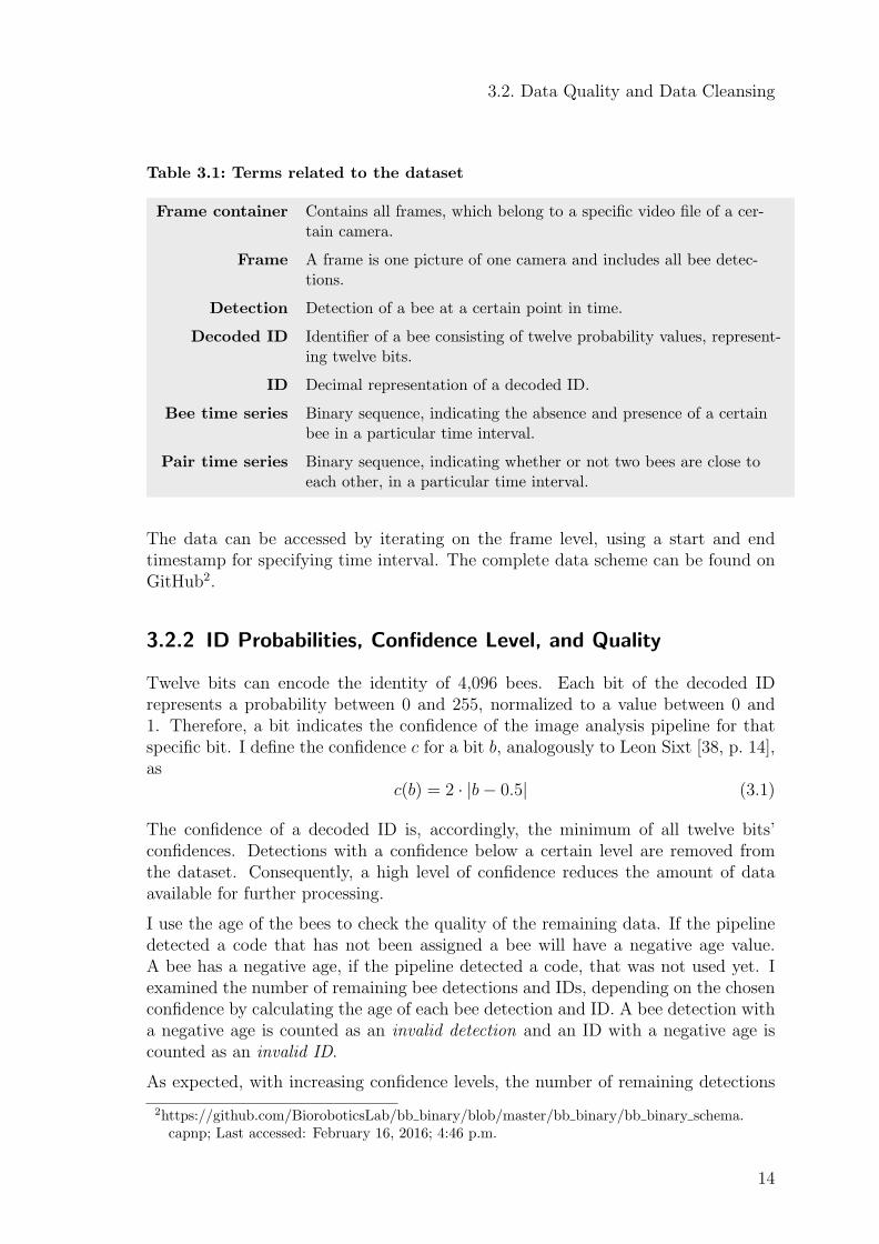
Table 3.1: Terms related to the dataset

Frame container Contains all frames, which belong to a specific video file of a cer-tain camera.

Frame A frame is one picture of one camera and includes all bee detec-tions.

Detection Detection of a bee at a certain point in time.

Decoded ID Identifier of a bee consisting of twelve probability values, represent-ing twelve bits.

ID Decimal representation of a decoded ID.

Bee time series Binary sequence, indicating the absence and presence of a certainbee in a particular time interval.

Pair time series Binary sequence, indicating whether or not two bees are close toeach other, in a particular time interval.

The data can be accessed by iterating on the frame level, using a start and endtimestamp for specifying time interval. The complete data scheme can be found onGitHub2.

3.2.2 ID Probabilities, Confidence Level, and Quality

Twelve bits can encode the identity of 4,096 bees. Each bit of the decoded IDrepresents a probability between 0 and 255, normalized to a value between 0 and1. Therefore, a bit indicates the confidence of the image analysis pipeline for thatspecific bit. I define the confidence c for a bit b, analogously to Leon Sixt [38, p. 14],as

c(b) = 2 · |b− 0.5| (3.1)

The confidence of a decoded ID is, accordingly, the minimum of all twelve bits’confidences. Detections with a confidence below a certain level are removed fromthe dataset. Consequently, a high level of confidence reduces the amount of dataavailable for further processing.

I use the age of the bees to check the quality of the remaining data. If the pipelinedetected a code that has not been assigned a bee will have a negative age value.A bee has a negative age, if the pipeline detected a code, that was not used yet. Iexamined the number of remaining bee detections and IDs, depending on the chosenconfidence by calculating the age of each bee detection and ID. A bee detection witha negative age is counted as an invalid detection and an ID with a negative age iscounted as an invalid ID.

As expected, with increasing confidence levels, the number of remaining detections

2https://github.com/BioroboticsLab/bb binary/blob/master/bb binary/bb binary schema.capnp; Last accessed: February 16, 2016; 4:46 p.m.

14

https://github.com/BioroboticsLab/bb_binary/blob/master/bb_binary/bb_binary_schema.capnp

https://github.com/BioroboticsLab/bb_binary/blob/master/bb_binary/bb_binary_schema.capnp


10 20 30 40 50 60 70 80 90 100

Confidence level in %

0

20

40

60

80

100

Am

ount

of d

etec

tions

in %

InvalidRemaining

(a) Detections

10 20 30 40 50 60 70 80 90 100

Confidence level in %

0

20

40

60

80

100

Am

ount

of I

Ds

in %

InvalidRemaining

(b) IDs

Figure 3.2: Quality of detections and IDs Light green represents the number ofremaining data and dark green indicates the fraction of invalid data. (a) Proportion ofremaining and invalid detections. (b) IDs, that are detected at least once, in relation toinvalid IDs. [Dataset: ten minutes; four cameras; July 26, 2016; 4 p.m.]

and IDs decreases (Figure 3.2), as does the fraction of invalid detections and IDs.With a confidence level of 100%, the fraction of invalid detections reaches 2.5%.However, the fraction of invalid IDs detected during a time interval of ten minutesremains at the high value of 30.2%. Consequently, selecting a high level of confidenceis not sufficient. To obtain a more reliable dataset, invalid detections need to befiltered out.

3.2.3 Detection Frequency Filter

A good indicator if a bee detection represents a real bee on the comb is the detectionfrequency of its ID. Individuals with a very low detection rate may be detectionerrors. To check this hypothesis, I investigate the correlation between the detectionfrequency of bees and their age. Figure 3.3 shows that bees with a negative age areobserved less often than bees with a positive age.

During my analysis, I noticed the existence of a group of bees with a negative age anda high detection frequency. I inspected the corresponding photos and confirmed thatthose bee detections correspond to living individuals and are not artifacts. This re-sults likely from a mistake in the reported hatching date for each bee. Consequently,these bess were excluded from the analysis. Also I excluded bees (n = 10), whoseage is unknown.

For each analysis day, the number of detections per ID is calculated, excludingthe mentioned IDs. To obtain a reliable dataset, I filtered invalid detections, bydiscarding all detections with an ID frequency below the 99th percentile of thenegative IDs.

15


0 25 50 75 100 125 150 175 200

Detection frequency ×103

103

102

0

102

103N

umbe

r of

bee

s P99

Negative agePositive age

Figure 3.3: Detection frequency of IDs Orange corresponds to bees with a negativeage and green displays bees with a positive age. The gray line represents the 99th per-centile of bees with a negative age. [Dataset: August 20, 2016; 24 hours, number of totalframes: 302,400]

3.2.4 Time Series of Bees and Bee Pairs

I investigated the quality of the initial data regarding its completeness of bee tracks.A bee track represents the movement of an individual over time. I transformed theinitial dataset into binary bee time series, depicted in Figure 3.4 left and middle. Abee time series, similar to a track, represents the absence and presence of a bee overa specified sequence of frames. For further processing I use the bee time series toextract pair time series of bees that are spatially close (Figure 3.4, right). A oneindicates that a pair of bees is detected and both bees are spatially close in a certainframe.

Detections: ID1, ID2, ID3, ...

Detections: ID2, ...

Detections: ID1, ID3, ...

...

Frame 3

Fram

e 1

Fram

e 2

Fram

e 3

ID1 1 0 1

ID2 1 1 0 …

ID3 1 0 1

Binary bee time series

...

Fram

e 1

Fram

e 2

Fram

e 3

ID1, ID2 1 0 0

ID1, ID3 1 0 1 …

ID2, ID3 1 0 0

...

Binary pair time series

Frame 2

Frame 1

Figure 3.4: Structure of dataset Left : original dataset - containing a sequence offrames with bee detections; Middle: binary bee time series - zero and one indicate absenceand presence of a bee; Right: binary pairs time series - zero and one indicate the absenceand presence of two bees in the same frame.

By analyzing the resulting pair time series, I noticed that detection sequences wereoften interrupted by short intervals without valid detections. As stated before, thehigher the level of confidence, the more data is discarded. This data reduction leadsto more zeroes (gaps) in both time series. Gaps in the pair time series frequently

16

3.3. Inferring Spatial Proximity Networks

correspond to gaps in one or both bee time series and are thus the result of missingdetections of the required confidence and do not represent any meaningful behaviorof the bees. Bees are not able to approach each other and move apart within asecond because they simply do not move that fast. Therefore, I concluded, thatthose gaps originate from detection errors and consequently need to be treated inan appropriate way during further data processing.

3.3 Inferring Spatial Proximity Networks

The network interference was driven by a combination of an exploratory data anal-ysis and an iterative pipeline development process. It serves as a prerequisite forthe network analysis part of this thesis. To generate functional and non-functionalrequirements of the pipeline, I conducted an analysis of the tracking data and a lit-erature review, presented in Section 2.2. The analysis led to a general understandingof the data, its structure, characteristics and an estimation of its quality. The pur-pose of the literature review was to get an overview of the common methods andapproaches regarding network analysis in the field behavioral insect studies.

Both results are then used to select a network type and to define its nodes and links.Furthermore, I inferred specific pipeline parameters and decided for the procedureof network extraction. The pipeline was developed, tested and refined in an iterativeprocess. Accordingly, the results of the evaluation lead to new or changing functionalrequirements. The evaluation is conducted by reviewing the pipeline parameters’effects on network properties and checking the validity and quality of the networksby investigating the age of bees in the resulting network.

3.3.1 Defining the Network and its Parameters

As this work constitutes the first step towards network analysis using this trackingdata I chose to infer a time-aggregated spatial proximity network. Accordingly, theinteractions are undirected but weighted. Methods for analyzing static networks arewidely established. Static tools and algorithms are already implemented and used bya large community. The results of the network analysis are easy to understand andinterpret. Additionally, static networks are the precondition for applying traditionalcommunity detection algorithms. My choice also establishes the comparability withMersch, Crespi, and Keller [4].

Each node in the network represents a bee, identified by an ID. The network consistsonly of bees that interact with other bees at least once, during the specified timeinterval. Two bees are associated (spatially close to each other) if their distance issmaller than a maximum distance. Using only this criterion leads to many interac-tions, resulting in a very dense network, because an interaction could only last for0.33 seconds. Therefore, an additional parameter, the minimum contact duration,is introduced. It specifies the minimum time two bees have to spend close to eachother to be called associated. Links are assigned two attributes. The first one is the

17


frequency of contacts, meaning how often they share a close position. The secondparameter refers to the total duration of all contacts.

The network pipeline takes two types of parameters. The first set of parametersdefines the resulting network and the exact type of spatial proximity. The secondset relates to the given data. Both parameter types are described below.

Pipeline parameters for network

Maximum distance Level of closeness between to individual bees. (in pixel)

Minimum The number of frames two individuals need to spend close.contact duration to each other to count it as an interaction (in frames)

Start timestamp Starting point of the network aggregation. (as UTC string)

Window size Size of time window for aggregating the network. (in minutes)

Pipeline parameters for data

Confidence Level of confidence, as described in Section 3.2.2. (in percent)

Valid IDs List of valid IDs within a specified time interval, as described inSection 3.2.3. (in CSV file format)

Gap Size Gaps in time series of bee pairs are assumed to be the result ofmissing detections. Gaps of this size are filled up. (in frames)

Number of CPUs Number of used CPUs for parallelization.

Year Calculate bee IDs and stitching of camera images according tothe observation period. (2015 or 2016)

3.3.2 Choosing Parameter Values for Network Analysis

For network analysis, I chose three days: August 20, August 22, and August 24, 2016.These days were selected because bees from a wide range of age groups were presentand older bees, which are likely to be foragers, were more represented in the hiveduring these days. Additionally, no data is missing due to camera failures. Thefollowing values are chosen according to biological constraints and similar to otherstudies, for better comparability.

I chose the length of a bee body, according to Baracchi and Cini [28], as the maximumdistance between two bees (Figure 3.5). The average bee length of 212px (±16px)was determined by manually measuring the length of all bees (n = 337) in imagesfrom the four cameras using the tool ImageJ3. The minimum contact duration is setto three frames (one second). This value corresponds to Mersch, Crespi, and Keller[4], as they also exclude interactions below one second. The networks are aggregatedfor ten hours during daylight; this corresponds to the biological rhythm of bees.

3http://imagej.net/Welcome; Last accessed: February 22, 2016; 12:34 p.m.

18

http://imagej.net/Welcome


Table 3.2: Parameters chosen for network analysis The maximum distance corre-sponds to the length of a bee body and the minimum contact duration is about one second.The networks are aggregated for ten hours.

Parameter Value Unit

Maximum distance 212 pxMinimum contact duration 3 frames

Window size 600 minutes

Confidence 95 percentGap size 2 frames

The confidence level is set to 95%, which will keep about 60% of the data. The gapsize is set to two frames. This value corresponds to the median gap length in thetime series of bee pairs.

3.3.3 Summary

The goal, as mentioned in 1.2, was to answer the question whether it is possible toinfer temporal networks with the provided honey bee tracking data and to work outchallenges and limitations regarding the provided dataset. Furthermore, it was agoal to identify the parameters necessary for the pipeline.

Pipeline Parameters

This analysis results in two types of pipeline parameters. The first category specifiesthe resulting network, concerning the definition of spatial proximity, duration ofinteraction and size of the aggregated time window. The second type representsparameters resulting out of the characteristics of the dataset.

(a) Body length of a bee (b) Contact radius

Figure 3.5: Maximum distance of bees: A length of a bee body is chosen as themaximum distance between two bees.

19

3.4. Methods for Analyzing Spatial Proximity Networks

1. Pipeline parameters for network

maximum distance, minimum contact duration, start timestamp, window size

2. Pipeline parameters for data

confidence, list of valid IDs, gap size, number of CPUs, year

Limitations

It is possible to infer networks, but a complex preprocessing of the dataset is essentialwith two major steps:

1. Reduction of data

Reduce the amount of data to obtain a reliable dataset, by filtering out detec-tions with a low confidence value or by IDs with a low detection frequency.

2. Combine camera data

This step consist of the time synchronization of each of the two cameras andthe joining of the data per frame.

A tradeoff exists between the remaining amount of data that can be used for networkinference and the data’s. A high confidence value reduces the amount of data andproduces gaps. The gap size parameter tries to fix this problem.

It is also possible to infer time-aggregated networks, but with restrictions. Whenlimiting the window size for network aggregation to the biological rhythms of dayand night, only a small amount of useful analysis days remain due to a large num-ber of interruptions. Any other window size entails the inclusion of the duration ofbiological processes related to honey bees, I would need to know beforehand. Alter-natively, I would need to apply a method to infer an appropriate window size out ofthe given data, this it out of scope.

3.4 Methods for Analyzing Spatial Proximity

Networks

This section outlines the methods I used to investigate the networks on a global,intermediate and local level. I present the choice of network measures used for theglobal analysis and explain the decision to use a community detection algorithm. Iillustrate the methods to examine the segregation of communities by age and spatialdistribution. Furthermore, I describe the approach used to study the developmentof communities.

3.4.1 Investigating the Topology and Network Characteristics

I summarized the network analysis methods of the reviewed studies (Chapter 2.2)to gain an overview of established procedures in the field of social insect networks.I grouped the methods by global measures, node level measures and other network

20


50 100 150 200 250 300

Number of interactions

2000

4000

6000

8000

10000D

urat

ion

of in

tera

ctio

ns

Figure 3.6: Frequency and total duration of interaction The two link weight valuesshow a strong positive correlation. The data of the three snapshots is aggregated.

analysis methods. Table A.3 summarizes the network analysis methods applied bythe reviewed studies. The network measures I chose for the global and node levelanalysis are listed in Table 3.3 and were defined in Chapter 2.1.1.

Each link in the network is attributed with the frequency of interactions and totalduration of interactions between the two individuals. Figure 3.6 shows a strongpositive correlation between those two values. For further analysis I decided to usethe frequency of interactions as the weight for links, analogously to [4], [28].

The degree of a bee represents the number of other bees this focal animal interactswith. Bees with a high number of interaction partners have a high degree. Thismeasure was chosen because it reveals a lot about the general topology of a network.The strength of a bee is the sum of its link weights. A high strength refers eitherto a large number of interaction partners with a low link weight or a low numberof interaction partners with high link weights. Especially for aggregated networksthis measure accumulates valuable information regarding the interaction activity ofbees. The local clustering coefficient (lcc) of a bee indicates how close its interactionpartners are to form a complete subgraph. A large lcc shows that most of its inter-action partners interact with each other. A low lcc indicates the absence of thoseinteractions. It is a good indicator for the embeddedness of single bees.

The betweenness of a bee measures the number of shortest paths between two otherbees that go through that bee. A bee with a high betweenness would be importantfor the information flow of the network. Removing this bee from the hive wouldlead to the breakdown of information or food flow and would negatively affect therobustness of the network. The closeness of a bee measures how fast this bee canreach all others in the network. A high closeness would indicate a very short pathto every other bee. A bee with high closeness can spread information to all otherbees very quickly.

I examined all node level measures concerning the age of bees and their detectionfrequency. The global network measures are compared to an Erdos-Renyi randomnetwork, by averaging over 100 runs.

21


Table 3.3: Measures used for analysis Each measure is explained in Chapter 2.1.1

Global level measures Node level measures

Number of nodes N and links E Degree k

Average degree 〈k〉 Strength s

Average strength 〈s〉 Local clustering coefficient cDensity D Closeness centrality CC

Diameter dmax Betweenness centrality CB

Number of componentsGlobal clustering coefficient c∆Average shortest path length 〈d〉Link weights w

3.4.2 Detecting Communities

For finding an appropriate community detection algorithm, I checked the reviewedstudies for applicable methods and scanned papers that compare various communitydetection algorithms. I identified a subset of algorithms as suitable and checkedthem.

The reviewed studies only include one examples of community detection and oneexample of cluster analysis. Mersch, Crespi, and Keller [4] used the infomap [39],[40] algorithm. According to the authors, this algorithm only works with sparsenetworks and is therefore not applicable in my case of densely connected spatialproximity networks. Baracchi and Cini [28] use a hierarchical clustering to infergroups of bees within the network that are similar in strength, eigenvector, andbetweenness centrality. In contrast to the resulting groups of community detec-tion, groups identified by hierarchical clustering do not automatically refer to densesubgraphs of the network.

Abundant literature on the comparative analysis of community detection algorithmsexists, e.g. [41], [42]. Some studies seem to be promising for choosing an appropriatealgorithm, but assume either a power law degree distribution or evaluate networkswith a low density, which is not applicable here. Thererfore, I tested communitydetection algorithms, implemented in python, to find an algorithm that works wellfor animal social networks. The three most common python libraries for networkanalysis were reviewed: NetworkX4, igraph5, and graph-tool6. The algorithm needsto fulfill the following criteria: support for large ((N = 1000) and dense (D > 50%)networks, support for weighted links, as well as a fast runtime.

Table 3.4 gives an overview about the algorithms reviewed. Five algorithms did notterminate after 15 minutes and were therefore excluded from further investigations.Infomap and label propagation tend to partition all nodes into a single community,

4https://networkx.github.io/; Last accessed: March 16, 2016; 6:36 p.m.5http://igraph.org/python/; Last accessed: March 16, 2016; 6:38 p.m.6https://graph-tool.skewed.de/; Last accessed: March 16, 2016; 6:39 p.m.

22

https://networkx.github.io/

http://igraph.org/python/

https://graph-tool.skewed.de/


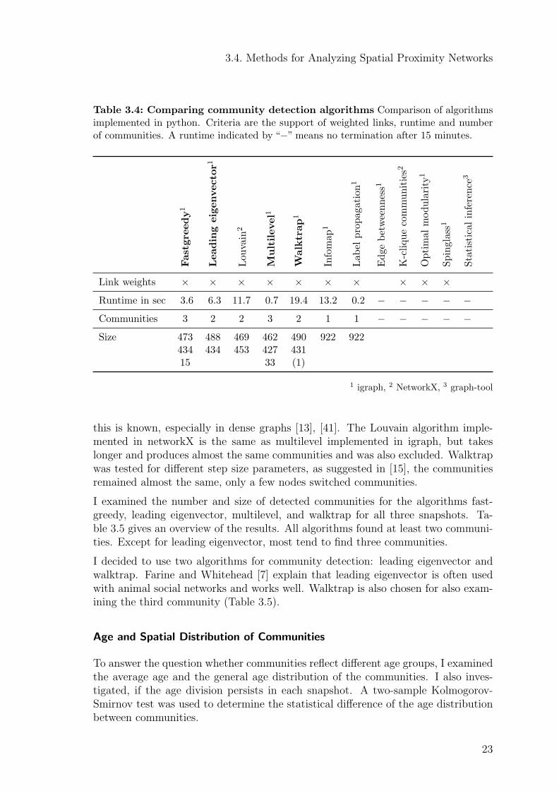
Table 3.4: Comparing community detection algorithms Comparison of algorithmsimplemented in python. Criteria are the support of weighted links, runtime and numberof communities. A runtime indicated by “−” means no termination after 15 minutes.

Fastgreedy1

Leadingeigenvecto

r1

Lou

vain

2

Multilevel1

Walktrap1

Infomap

1

Lab

elpropag

ation1

Edge

betweenness1

K-cliquecommunities2

Optimal

modularity

1

Spinglass1

Statistical

inference

3

Link weights × × × × × × × × × ×

Runtime in sec 3.6 6.3 11.7 0.7 19.4 13.2 0.2 − − − − −

Communities 3 2 2 3 2 1 1 − − − − −

Size 473 488 469 462 490 922 922434 434 453 427 43115 33 (1)

1 igraph, 2 NetworkX, 3 graph-tool

this is known, especially in dense graphs [13], [41]. The Louvain algorithm imple-mented in networkX is the same as multilevel implemented in igraph, but takeslonger and produces almost the same communities and was also excluded. Walktrapwas tested for different step size parameters, as suggested in [15], the communitiesremained almost the same, only a few nodes switched communities.

I examined the number and size of detected communities for the algorithms fast-greedy, leading eigenvector, multilevel, and walktrap for all three snapshots. Ta-ble 3.5 gives an overview of the results. All algorithms found at least two communi-ties. Except for leading eigenvector, most tend to find three communities.

I decided to use two algorithms for community detection: leading eigenvector andwalktrap. Farine and Whitehead [7] explain that leading eigenvector is often usedwith animal social networks and works well. Walktrap is also chosen for also exam-ining the third community (Table 3.5).

Age and Spatial Distribution of Communities

To answer the question whether communities reflect different age groups, I examinedthe average age and the general age distribution of the communities. I also inves-tigated, if the age division persists in each snapshot. A two-sample Kolmogorov-Smirnov test was used to determine the statistical difference of the age distributionbetween communities.

23


Table 3.5: Number of community members per algorithm and snapshot Fouralgorithms were tested and compared regarding the number of detected communities andthe size of the communities.

Fastgreedy

Leadingeigenvecto

r

Multilevel

Walktrap

Snapshot 1 473 488 462 490434 434 427 43115 33 (1)

Snapshot 2 504 503 481 372467 475 439 3117 58 294

(1)

Snapshot 3 534 537 505 310388 385 415 390

(2) 231

24


To investigate whether communities reflect groups of bees working in different areasof the comb, I used heat maps to determine the core regions per group. I stored thepositions of all bees present within the ten hour time windows in an SQLite databasefor faster access to the data and to eliminate the time-consuming parsing.

3.4.3 Development of Community Members

According to Aynaud, Fleury, Guillaume, et al. [43] and Brodka, Saganowski, andKazienko [44], there are three main approaches for community detection in tem-poral networks (sometimes referred to as community tracking): (1) using a staticcommunity detection algorithm on several snapshots and then solving a matchingproblem, (2) using algorithms that are directly suited for temporal networks and (3)using incremental or online algorithms when processing data streams. For each ofthe three approaches, several methods already exist. As community tracking is notthe main focus of this work, I chose to apply the most natural method: detectingstatic communities for each snapshot and then matching those communities usingset theory.

Two communities at successive times are matched if they share enough nodes. Thematch value between two communities C and D according to Hopcroft et al. [45] isdefined as

match(C,D) = min

(

|C ∩D|

|C|,|C ∩D|

|D|

)

. (3.2)

This value is between 0 and 1. A high match value occurs, if two communitiesshare many nodes and are of a similar size. Communities with high match valuesrepresent the same community at different points in time. The author suggestsapplying a threshold to more precisely define what “share enough nodes” means.Otherwise, communities with only 0.1% of nodes overlapping could be matched.

To investigate the total number of bees that remain in the network over the threesnapshots, I inspected the match value of bees in consecutive snapshots. I alsocalculated all match values between communities in consecutive snapshots and thenumber of intersecting bees. I visualize the dynamic movement of bees betweengroups of different snapshots with a flowchart diagram using the JavaScript libraryD3.js7.

7https://d3js.org/; Last accessed: April 19, 2016; 3:18 p.m.

25

https://d3js.org/

Chapter 4

Results of Network Analysis

This chapter summarizes the results of the analysis of the temporal, spatial proximitynetwork of honey bees, consisting of three consecutive time-aggregated snapshots.Section 4.1 describes static aspects of the network and Section 4.2 focuses on thetemporal network aspects. The last section of this chapter summarizes the mainresults and discusses the findings.

4.1 Static Perspectives of Honey Bee Networks

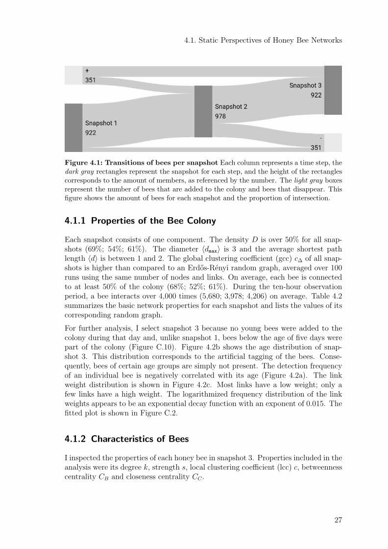
The networks are examined on three levels. First, I examine the network’s globalstructure and derive properties of the overall colony (global level). Next, I study thecharacteristics of individual bees (local level) and the relation of the characteristicsto detection frequency and age. Finally, I investigate the intermediate level of thecolonies social organization by detecting communities and inspecting their practicalmeaning. I analyzed a temporal network, consisting of three time-aggregated snap-shots; these are referred to below as snapshot 1 (N = 922), snapshot 2 (N = 978) andsnapshot 3 (N = 922). The snapshots are aggregated for ten hours (108,000 frames)starting at 8 a.m. and lasting until 6 p.m. See Table 4.1 for details about thebees added each day. Figure 4.1 shows the proportion of intersecting bees betweenconsecutive snapshots. This figure illustrates the stability of the network size.

Table 4.1: Sampling period Overview of the chosen aggregated daily snapshots includ-ing the number of added bees and the time they were added to the hive.

8/20/2016 8/21/2016 8/22/2016 8/23/2016 8/24/2016

Snapshot ID 1 − 2 − 3Number of bees added 0 0 110 60 0

Time added − − 2 p.m. 6 p.m. −

26

4.1. Static Perspectives of Honey Bee Networks

Figure 4.1: Transitions of bees per snapshot Each column represents a time step, thedark gray rectangles represent the snapshot for each step, and the height of the rectanglescorresponds to the amount of members, as referenced by the number. The light gray boxesrepresent the number of bees that are added to the colony and bees that disappear. Thisfigure shows the amount of bees for each snapshot and the proportion of intersection.

4.1.1 Properties of the Bee Colony

Each snapshot consists of one component. The density D is over 50% for all snap-shots (69%; 54%; 61%). The diameter 〈d

max〉 is 3 and the average shortest path

length 〈d〉 is between 1 and 2. The global clustering coefficient (gcc) c∆ of all snap-shots is higher than compared to an Erdos-Renyi random graph, averaged over 100runs using the same number of nodes and links. On average, each bee is connectedto at least 50% of the colony (68%; 52%; 61%). During the ten-hour observationperiod, a bee interacts over 4,000 times (5,680; 3,978; 4,206) on average. Table 4.2summarizes the basic network properties for each snapshot and lists the values of itscorresponding random graph.

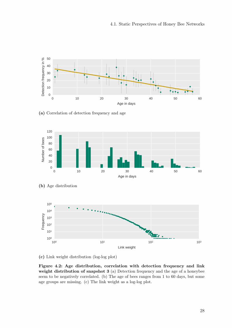
For further analysis, I select snapshot 3 because no young bees were added to thecolony during that day and, unlike snapshot 1, bees below the age of five days werepart of the colony (Figure C.10). Figure 4.2b shows the age distribution of snap-shot 3. This distribution corresponds to the artificial tagging of the bees. Conse-quently, bees of certain age groups are simply not present. The detection frequencyof an individual bee is negatively correlated with its age (Figure 4.2a). The linkweight distribution is shown in Figure 4.2c. Most links have a low weight; only afew links have a high weight. The logarithmized frequency distribution of the linkweights appears to be an exponential decay function with an exponent of 0.015. Thefitted plot is shown in Figure C.2.

4.1.2 Characteristics of Bees

I inspected the properties of each honey bee in snapshot 3. Properties included in theanalysis were its degree k, strength s, local clustering coefficient (lcc) c, betweennesscentrality CB and closeness centrality CC .

27


0 10 20 30 40 50 60

Age in days

0

10

20

30

40

50

Det

ectio

n fr

eque

ncy

in %

(a) Correlation of detection frequency and age

0 10 20 30 40 50 60

Age in days

0

20

40

60

80

100

120

Num

ber

of b

ees

(b) Age distribution

100 101 102 103

Link weight

100

101

102

103

104

105

Fre

quen

cy

(c) Link weight distribution (log-log plot)

Figure 4.2: Age distribution, correlation with detection frequency and linkweight distribution of snapshot 3 (a) Detection frequency and the age of a honeybeeseem to be negatively correlated. (b) The age of bees ranges from 1 to 60 days, but someage groups are missing. (c) The link weight as a log-log plot.

28


Table 4.2: Global network properties N number of nodes, L number of links, D

diameter, 〈dmax〉 average path length, 〈d〉 diameter, c∆ global clustering coefficient, 〈k〉average degree and 〈s〉 represents the average strength, as introduced in Section 2.1.1.

N L D 〈dmax〉〈d〉 c∆ 〈k〉〈s〉

Snapshot 1 922 291,179 0.69 3 1.32 0.79 631.62 5,680.17Random 1 922 291,179 0.69 2 1.31 0.69 631.62 -

Snapshot 2 978 256,066 0.54 3 1.46 0.72 523.65 3,977.94Random 2 978 256,066 0.54 2 1.46 0.54 523.65 -

Snapshot 3 922 259,421 0.61 3 1.39 0.75 562.74 4,205.99Random 3 922 259,421 0.61 2 1.39 0.61 562.74 -

Low Hierarchical Structure

The degree is normally distributed (panel (a) in Figure 4.3). Therefore most beeshave the same high number of interaction partners. The absence of hubs, a smallnumber of highly connected bees, indicates a low hierarchical structure of the net-work. Strength and lcc are also normally distributed (panel (d) and (g) in Fig-ure 4.3). That also shows the absence of extreme values and confirms that beesare similar to each other regarding those properties. Closeness and betweennesscentrality (panel (j) and (m) in Figure 4.3) also follow a normal distribution. Thisdistribution leads to the assumption that no central or important bees exist. How-ever, this could be a consequence of the definition of interaction (spatial proximity).All bees are similarly close to all other bees in the network, and every bee canreach any other bee with a few steps. That also corresponds to the low averagepath length, and the small diameter of the network described in Section 4.1.1. Theabsence of bees with a high betweenness suggests that the colonies functionality isrobust concerning the disappearance of single individuals.

Local Network Measures and Detection Frequency

Degree, strength, closeness and betweenness (panel (b), (e), (k), and (n) in Fig-ure 4.3) are positively correlated with the detection frequency. A low value corre-sponds to a low detection frequency. In contrast, the lcc (panel (h) in Figure 4.3)and detection frequency are negatively correlated.

Local Network Measures and Age of Bees

The histograms of degree, strength, betweenness, and closeness show a normal distri-bution with a tendency for bimodality. The lcc distribution is instead right skewed,with one peak at 0.75.

There is no sharp border between the two modes in the degree distribution plot (a),

29


but a value around 0.4 can be estimated. The strength histogram (d) seems to havea border at 1,000. For closeness (j) and betweenness (m), a border can be seen at 0.6and 0.0001. All distributions indicate a small group (100 bees) and a second largergroup containing the rest of the colony. The correlation between all measures isdepicted in the scatter plot in Figure C.9.

The first small group interacts on average with 20% of the colony and has a very lowstrength (number of total interactions below 250). The closeness value is comparedto the second group smaller but still over 0.5. The betweenness has a small range andis close to 0 for the first smaller group. The second group interacts with about 80%of the colony with an average strength of 5,000. A high strength can result fromlots of neighbors with low link weights or a few neighbors with high link weights.As only a few links with high weights exist (Figure 4.2c), the second option can beexcluded. The second group is characterized by a very high closeness (0.75) and astill very low betweenness but higher than the first group (0.0005).

All age-correlation plots show a seperate group of bees older than 45 days, corre-sponding to the first smaller group of bees described above. This older group ischaracterized by a low degree, a low strength, and low closeness and betweenness.In contrast, a high lcc, compared to the younger group is noticeable. The youngergroup has a high degree and strength, as well as a high betweeness and closenesscompared to the first group, but a lower lcc. The high lcc of the older group indicateshigh connectivity within the younger group and less connectivity between bees ofthe older group.

4.1.3 Functional Groups within the Colony

The leading eigenvector (LE) community detection algorithms revealed two commu-nities with a similar size (modularity score of 0.25). The walktrap algorithm (WT)discovered three communities instead, also evenly distributed (modularity scoreof 0.23). Table 4.3 lists the precise number of members per community and algorithmfor snapshot 3.

For both algorithms the communities correspond to different age groups. For LE,the average age of the young community is 13.2 days and the average age of theold community is 28.7 days. For WT, the average age of the young communityis 6.6 days and 29.3 days for the older commmunity. The average age of the thirdmiddle-aged community of WT is 25.1 days. The age distribution for each algorithmis represented in Figure 4.4a and 4.4b. The two sample Kolmogorov-Smirnov testconfirmed that the age distributions per community are significantly different. Thecorresponding p-values are listed in Table 4.4.

Each community occupies a different region of the comb. Figure 4.4 shows that theyoung communities spend the most time in the comb center and the old communitiescloser to the hive exit. The middle-aged community is positioned between the youngand old community and in the periphery of the comb.

30


0.0 0.2 0.4 0.6 0.8 1.00

1020304050607080

Num

ber

of b

ees

a

0.0 0.2 0.4 0.6 0.8 1.0

Degree k

0.0

0.2

0.4

0.6

0.8

1.0

Det

ectio

n fr

eque

ncy

b

0.0 0.2 0.4 0.6 0.8 1.00

102030405060

Age

in d

ays c

0.0

0.2

0.4

0.6

0.8

1.0

×104

0102030405060

Num

ber

of b

ees

d

0.0

0.2

0.4

0.6

0.8

1.0

Strength s ×104

0.0

0.2

0.4

0.6

0.8

1.0D

etec

tion

freq

uenc

ye

0.0

0.2

0.4

0.6

0.8

1.0

×104

0102030405060

Age

in d

ays f

0.4 0.5 0.6 0.7 0.8 0.9 1.00

20406080

100120140

Num

ber

of b

ees

g

0.5 0.6 0.7 0.8 0.9 1.0

Local clustering coefficient c

0.0

0.2

0.4

0.6

0.8

1.0

Det

ectio

n fr

eque

ncy

h

0.5 0.6 0.7 0.8 0.9 1.00

102030405060

Age

in d

ays i

0.4 0.5 0.6 0.7 0.8 0.9 1.00

20

40

60

80

100

Num

ber

of b

ees j

0.4 0.5 0.6 0.7 0.8 0.9 1.0

Closeness CC

0.0

0.2

0.4

0.6

0.8

1.0

Det

ectio

n fr

eque

ncy

k

0.4 0.5 0.6 0.7 0.8 0.9 1.00

102030405060

Age

in d

ays l

0.0

0.2

0.4

0.6

0.8

1.0

1.2

1.4

1.6

×10 3

0

20

40

60

80

100

Num

ber

of b

ees

m

0.0

0.2

0.4

0.6

0.8

1.0

1.2

1.4

Betweenness CB×10 3

0.0

0.2

0.4

0.6

0.8

1.0

Det

ectio

n fr

eque

ncy

n

0.0

0.2

0.4

0.6

0.8

1.0

1.2

1.4

×10 3

0102030405060

Age

in d

ays o

Figure 4.3: Local measures of snapshot 3

31


(a) Leading eigenvector (LE) communities

(b) Walktrap (WT) communities

Figure 4.4: Age and spatial distribution of communities Green represents theyoung community occupying the center area of the comb and orange the old community,which is situated closer to the hive access. For WT, the gray middle-aged community ispositioned between the other to and in the periphery of the comb.

32

4.2. Temporal Perspectives of Honey Bee Networks

Table 4.3: Communities per algorithm Communities marked with * contain thequeen. Age and standard deviation (SD) are measured in days. The queen and ninebees with a negative age are excluded from this analysis.

Community ID Members Proportion Age SD

LE CY ∗381 41.78% 13.15 ±13.50CO 531 58.22% 28.70 ±11.67

WT CY ∗229 25.11% 6.55 ±10.36CM 298 32.68% 25.08 ±11.97CO 385 42.21% 29.29 ±11.44

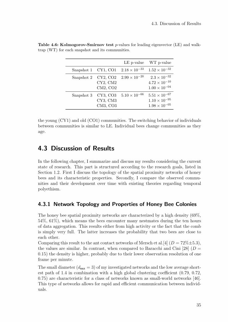
Table 4.4: Kolmogorov-Smirnov test p-values for leading eigenvector (LE) and walk-trap (WT)

Communities LE p-value WT p-value

CY, CO 5.10× 10−66 5.51× 10−67

CY, CM 1.10× 10−95

CM, CO 1.98× 10−05

4.2 Temporal Perspectives of Honey Bee Networks

I investigate the stability of local and global properties, as well as the stability of ageand spatial distribution of functional groups of bees. Furthermore, the dynamics ofindividual bees’ group membership over time are examined.

For all three snapshots, the same link weights distribution can be seen in Figure C.1.The analysis of snapshot 1 and 2 showed that the same characteristic distributionof degree, strength, lcc, betweenness, and closeness for snapshot 1 (Figure C.7)and snapshot 2 (Figure C.8) exists. They also follow a normal distribution. Thecorrelation between the local measure and detection frequency and age remains.All of this shows that the characteristics described in Section 4.1.2 apply for allthree snapshots and are therefore stable for the investigated time interval. A lowhierarchical structure and the correlation with age and detection frequency seem tobe global properties of the colony.

4.2.1 Stability of Functional Groups

Table 4.5 lists the exact number of bees per community for each algorithm andsnapshot. For each snapshot, LE detected two communities with about the samenumber of bees. The first communities CY(1,2,3) contain the queen and on averageyounger bees than the second communities CO(1,2,3).

In comparison, WT identified three communities in snapshot 2 and 3 but only two

33

4.2. Temporal Perspectives of Honey Bee Networks

Table 4.5: Overview about communities per snapshot Communities marked with* contain the queen. Age and standard deviation (SD) are measured in days. For eachnetwork the queen and bees with a negative age are excluded: snapshot 1: 12 bees,snapshot 2: 119 bees, snapshot 3: 10 bees.

ID Members Proportion Age SD

Leading eigenvector (LE)

Snapshot 1 CY1 ∗430 47.25% 17.12 ±10.97CO1 480 52.75% 27.24 ±10.96

Snapshot 2 CY2 ∗392 45.63% 20.24 ±12.01CO2 467 54.37% 28.10 ±10.88

Snapshot 3 CY3 ∗381 41.78% 13.15 ±13.50CO3 531 58.22% 28.70 ±11.67

Walktrap (WT)

Snapshot 1 CY1 ∗427 46.92% 17.07 ±10.92CO1 482 52.97% 27.23 ±11.00

Snapshot 2 CY2 ∗263 30.62% 18.23 ±11.46CM2 305 35.51% 25.20 ±11.47CO2 291 33.88% 29.47 ±10.06

Snapshot 3 CY3 ∗229 25.11% 6.55 ±10.36CM3 298 32.68% 25.08 ±11.97CO3 385 42.21% 29.29 ±11.44

communities in snapshot 1. The first communities CY(1,2,3) consist of the queen andon average younger bees than the second CM(2,3) and third communities CO(1,2,3).The bees in CM2 and CM3 are on average younger than the bees in CO2 and CO3.Figure C.5 and C.6 depicts the age distribution for each community and snapshot.

A two-sample Kolmogorov–Smirnov test showed that the age distributions are sig-nificantly different (p < 0.001) for both algorithms. The spatial segregation of thecommunities is very similar in all three snapshots. For further reference see the heatmaps in C.4 and C.3. The detected communities seem to differ in their respectiveage and occupy different areas of the comb, but remain stable over this inpectedtime interval.

4.2.2 Dynamic of Individual Bees

Figure 4.5a (LE) and Figure 4.5b (WT) show the flow of bees between consecutivesnapshots and communities. For LE communities, the majority of bees stay in theirage group, and a small fraction of bees switch to older communities. Only a fewbees change to younger communities.

The new middle-aged communities (CM2) of WT are formed equally by members of

34

4.3. Discussion of Results

Table 4.6: Kolmogorov-Smirnov test p-values for leading eigenvector (LE) and walk-trap (WT) for each snapshot and its communities.

LE p-value WT p-value

Snapshot 1 CY1, CO1 2.18× 10−33 1.52× 10−32

Snapshot 2 CY2, CO2 2.99× 10−20 2.3× 10−32

CY2, CM2 4.72× 10−10

CM2, CO2 1.00× 10−04

Snapshot 3 CY3, CO3 5.10× 10−66 5.51× 10−67

CY3, CM3 1.10× 10−95

CM3, CO3 1.98× 10−05

the young (CY1) and old (CO1) communities. The switching behavior of individualsbetween communities is similar to LE. Individual bees change communities as theyage.

4.3 Discussion of Results

In the following chapter, I summarize and discuss my results considering the currentstate of research. This part is structured according to the research goals, listed inSection 1.2. First I discuss the topology of the spatial proximity networks of honeybees and its characteristic properties. Secondly, I compare the observed commu-nities and their development over time with existing theories regarding temporalpolyethism.

4.3.1 Network Topology and Properties of Honey Bee Colonies

The honey bee spatial proximity networks are characterized by a high density (69%,54%, 61%), which means the bees encounter many nestmates during the ten hoursof data aggregation. This results either from high activity or the fact that the combis simply very full. The latter increases the probability that two bees are close toeach other.Comparing this result to the ant contact networks of Mersch et al.[4] (D = 72%±5.3),the values are similar. In contrast, when compared to Baracchi and Cini [28] (D =0.15) the density is higher, probably due to their lower observation resolution of oneframe per minute.

The small diameter (dmax

= 3) of my investigated networks and the low average short-est path of 1.4 in combination with a high global clustering coefficient (0.79, 0.72,0.75) are characteristic for a class of networks known as small-world networks [46].This type of networks allows for rapid and efficient communication between individ-uals.

35


(a) Leading eigenvector (LE) communities

(b) Walktrap (WT) communities

Figure 4.5: Dynamics of bees Each column represents a time step, the colored rectan-gles represent the communities for each step, and the height of the rectangles correspondsto the amount of its community members, as referenced by the number. Green indicatesthe community containing young bees and the queen, gray represents the community con-taining middle-aged bees (only for WT), and orange the community containing old bees.This figure shows that the major part of the bees either stays in the same aged communityor switches to an older group. The light gray boxes represent the number of bees that areadded to the colony and bees that disappear.

36


Charbonneau, Blonder, and Dornhaus [6] state that it is assumed that many biolog-ical networks, including insect colonies, approximate scale-free networks. For someof them, the scale-free property has been shown, but for social insect networks thisquestion remains open. Investigated social insect colonies are often small and there-fore the methods for the recognition of scale-free phenomena are limited. They donot specify the type of social insect networks, whether the inference of interactionsis based on spatial proximity, physical contacts, or food transfer events.The network I explored is large compared to past studies (Section 2.2). The degreedistribution of the investigated spatial proximity network of honey bees does not fol-low a power-law; the absence of hubs and a non-hierarchical structure characterizesthis network. This result corresponds to the decentralized structure of a honey beecolony, and the absence of a central authority described by Seeley [47].

I noticed bimodal degree, strength, closeness and betweenness distributions and aright skewed lcc distribution, corresponding mainly to bees older than 45 days. Whileinspecting this group of bees, I found that this group has a very low detection rateand is not part of any other following snapshot. Probably this group of bees diesduring that day. Bees who are present in the hive earlier that day and are thenabsent for the rest of the day have very low network measure values. The totalnumber of old bees is relatively small compared to other age groups. Consequently,low network measure values strongly affect the mean of that old group and shouldbe excluded in future studies.

Generally, I observed a correlation between the detection frequency of a bee, its age,and its corresponding network measure value. Older bees are detected less oftenthan younger bees and therefore differ in their network measures. The age-basedtask division of bees in a colony observed by Seeley [48] might be an explanation;namely, old bees are foragers, the middle-aged bees conduct several tasks inside thehive but mainly they store resources, and young bees are primarily nursing. Baracchiand Cini [28] also assumed that the time which bees spend outside the hive probablyaffects their connectedness within the interaction network.

4.3.2 Characterization of Functional Groups and its Dynamics

According to the definition of communities in Section 2.1.2, I found two to threecommunities, depending on the algorithm applied.

The algorithms (LE and WT) detected communities, despite a high network densityand without thresholding links of low values, as opposed to Mersch, Crespi, andKeller [4]. The authors reduced the network’s density artificially to 25% to applythe infomap algorithm.

I also examined the spatial fidelity of the revealed communities and their age com-position, similar to Baracchi and Cini [28]. I found that younger bees are locatedclose to the brood (upper center of the comb); older bees are situated closer to thehive exit, and middle-aged bees are placed between the two groups and around thebrood, where the cells for honey storage are located.

37


I inspected three snapshots over a period of five days and found that the detectedcommunities are stable over time. Age-division and spatial fidelity can be observedin all the snapshots. Bees from younger communities move to older communities asthey age. Only a few bees changed from older to younger communities.

It is surprising that my results align with Baracchi and Cini [28], because they didnot use a community detection algorithm. The authors conducted a hierarchicalclustering based on the network measures strength, eigenvector and betweennesscentrality of individual bees. Moreover, their colony contained bees of three prede-termined age cohorts, instead of representing all age groups ranging from 0 to 60days, as in my study.

The communities I detected are similar to the groups of bees formed by temporalpolyethism. The old bees positioned closer to the hive exit may be the foragers,the middle-aged group spatially close to the storage cells may be the food storagebees and the group of young bees may be the cell cleaning and brood care beesbecause they are located close to the brood. My findings are very close to the onesof Baracchi and Cini [28].

The two approaches discovered the same functional groups of the bee colony, onthe one hand by node level network measures (hierarchical clustering) and on theother hand by a higher than expected density of nodes (community detection). Thatacknowledges the existence of the age-based division of labor in honey bee coloniesas well as the higher communication frequency within groups than between groups.Nevertheless, the low modularity score indicates that the segregation of groups isnot that obvious and strict; therefore a lot of interaction between groups exists.

Mersch, Crespi, and Keller [4] revealed that the behavioral maturation of ants is aslow and noisy process. Instead of investigating the transition of individuals daywise, they grouped 41 days in four periods. For each period they assigned each antto a community if it was found in this community 70% of the time. It seems thathoney bee transitions are in contrast to ants faster and smoother.

38

Chapter 5

Conclusions

The purpose of this thesis was to investigate worker-worker interaction networks ofa honey bee colony. To achieve this, I implemented a pipeline for the extractionof time-aggregated networks using high-resolution honey bee tracking data. Thetopology, community structures and development of community members were ex-amined from the resulting weighted, undirected, spatial proximity networks of threeconsecutive time steps.

As opposed to most real-world networks, the examined honey bee interaction net-works are not scale-free. They are characterized by a non-hierarchical topology anda decentralized structure. The small-world characteristic of honey bee networks al-lows for efficient communication within the bee colony. The observed communitieswithin the honey bee colony, are formed of age-based functional groups with a spatialfidelity towards different areas of the comb. There are different types of cells (e.g.brood, honey, and pollen) and honeybees occupying different areas have distincttasks.

The global network structure of the honey bee colony is stable over time, but itslocal structure is highly dynamic. Individual bees change communities as they age.My results are in agreement with the established state of the research: the absence ofa central authority and the decentralized organization of honey bee colonies shapedby temporal polyethism.

My network analysis results verify the network pipeline, my definition of spatial prox-imity networks and the initially chosen parameters. The network pipeline providesan excellent foundation for further investigations.

5.1 Limitations

The following section outlines limitations concerning the accuracy and quality ofthe resulting networks. Especially, consequences of the networks’ high density arepointed out.

Despite a complex preprocessing procedure, several shortcomings concerning the thequality of the extracted networks still exist. I filtered out erroneous detections beforenetwork generation; however a few individuals remain in the extracted networks thatshould not exist according to the tagging and hatching documentation. Besides this,

39

5.2. Recommendations

bees which are dying at some point during the aggregation period, are part of thenetwork. This fact needs to be considered depending on the research context.

The prefiltering of detections, as well as the synchronization of four cameras, reducesthe amount of data that remains for the extraction of interactions. The gap sizeparameter was an attempt to compensate for this shortcoming of the data but doesnot perfectly solve the problem. I believe that some observed interactions are shorterthan they are in reality, which distorts the networks.

Spatial proximity is an indicator for interaction but it does not capture actual inter-actions. The definition of spatial proximity by a maximal distance and a minimumcontact duration is very loose, especially on a honeycomb with limited space. It leadsto many links and a high density of the network resulting in high noise. This noisecreates a blurred image of real interactions between bees. My choice of aggregatingthe networks for ten hours fosters this noisiness, resulting in a global state of thecolony, rather than capturing finer granular dynamics.

In this context, the network property strength is the only measure, that profits fromthe aggregation. All other measures are less meaningful. Due to the high density andsize of the network, the methods I can apply for community detection are limited.The selection of an algorithm for detecting communities is restricted to algorithmsfinding only non-overlapping structures.

5.2 Recommendations

This sections list recommendations for improving the applied methods. I am focusingon concepts to reduce the noise within the network.

More Dynamic and Temporal Analysis Lowering the window size of the aggre-gated network and investigating different granularities could allow more dynamicanalysis of the networks. Instead of using time-aggregated networks, one could shifttowards the use of time-ordered networks by using time-stamped interactions.

Focusing on Important Interactions The space on the honeycomb is limited andcrowded. For reducing the number of link to only meaningful interactions, I seethree main approaches. For the time being, it is an option to fine tune the pipelineparameters by lowering the size of the maximum distance and by raising the numberof frames for minimum contact duration. Instead of keeping the definition of spatialproximity, I would recommend extracting contact events (e.g. by including an angle,so bees facing each other) or trophallaxis events for defining the links, especially whenusing those networks to investigating more specific biological research questions.

Using the Potential of Weighted Links A simple global threshold for excludinglinks below a certain value could be used. Instead of applying a global threshold

40

5.3. Outlook

to reduce the density, a network reduction algorithm could be implemented to ex-tract the backbone structure of the network. Serrano, Boguna, and Vespignani [49]propose a disparity filter algorithm, which seems promising but needs further in-vestigation. The disparity measure characterizes the level of local heterogeneity oflinks [50]. For all network measures utilized in this work, weighted versions exist.The weighted measures (e.g., closeness and betweenness) implemented in igraph andnetworkX favor link weights over the number of links and simply apply Dijkstra [51]for calculating the shortest paths. Opsahl, Agneessens, and Skvoretz [52] proposeweighted network measures by providing a generalized degree and shortest path al-gorithm. The tuning parameter, Opsahl et al. introduce, has to be chosen. Thisparameter defines whether to emphasize the number of links or the weights of linksand must be selected according to a predefined research question.

Normalizing by the Detection Frequency of Individuals Depending on the topicsof further research a normalization of the networks regarding the detection rate ofindividuals could be useful. I propose two options: either normalize the link weightby applying the simple ratio index1 (SRI) [23] or normalize the particular node levelmeasure by taking the detection frequency of that focal individual into account.

Random Geometric Graph Instead of comparing the honeybee network to anErdos-Renyi graph a new model could be implemented. As the starting point, arandom geometric graph [53] can be used. In each frame, the nodes could be placednot completely randomly, preferably by modeling the behavior of a bee as a randomwalker. The direction of movement could be chosen randomly, but the distance of astep might be selected according to the average speed of bees.

5.3 Outlook

To fine tune the pipeline parameters for the network, one should systematically in-vestigate the parameters effects on network properties. I started to analyze this, butonly for a few combinations of values and for window sizes up to one hour. Simi-larly, the robustness of the detected communities regarding the pipeline parametersis worthy of further study. In addition, the provided dataset facilitates the inves-tigation of seasonal change in honey bee colonies using network analysis methods.Long-term dynamics offer a high potential for further studies. It would be interest-ing to compare my network analysis results of domesticated honey bees to the socialnetworks of wild honey bees, to discover differences regarding individual behaviorand global colony organization.

1Dividing the link weight by the proportion of times two individuals were seen together out ofthe total number of times those individuals were observed.

41

5.4. Closing Remarks

5.4 Closing Remarks

My work was an important first step to gain trust in the honey bee tracking datagenerated by the BeesBook system. It identifies limitations, pinpoints scope forimproving the system and lays the foundations for further network analysis.

Studying non-human animal data in an explorative way that fosters the framing ofnovel biological hypotheses demands a profound domain knowledge or the constantsupport of experts of the studied species. The process of manual data collection byobserving the animals face to face creates valuable information which is beneficial fordata analysis and understanding the context of research. An automatic observationprocess veils this part and therefore increases the abstraction level and encouragesalienation between the researchers and observed animals.

The automatic tracking of a vast number of animals over an extended observationperiod with a high sampling resolution leads to an enormous amount of data. Ap-plying network analysis methods to novel datasets, which were not collected for aspecific study, opens the space to investigate the data in an explorative way and todiscover the unexpected. However, it also carries the risk of either simply describ-ing network structures of various species or leading to the restating of well-knownfacts.

Framing biological research questions that benefit from network science methods orthe development of new techniques in the field of network analysis with the help ofthis unique dataset should be the overall goal.

42

Bibliography

[1] F. Wario et al., “Automatic methods for long-term tracking and the detectionand decoding of communication dances in honeybees”, Frontiers in Ecology

and Evolution, vol. 3, p. 103, 2015.

[2] J. D. Crall et al., “BEEtag: A low-cost, image-based tracking system for thestudy of animal behavior and locomotion”, PLOS ONE, vol. 10, no. 9, 2015.

[3] M. Fiala, “Comparing artag and artoolkit plus fiducial marker systems”, in2005 IEEE International Workshop on Haptic Audio Visual Environments

and their Applications, IEEE, 2005, pp. 6–13.

[4] D. P. Mersch et al., “Tracking individuals shows spatial fidelity is a key reg-ulator of ant social organization”, Science, vol. 340, no. 6136, pp. 1090–1093,2013.

[5] S. Wasserman and K. Faust, Social network analysis: Methods and applications.Cambridge University Press, 1994, vol. 8.

[6] D. Charbonneau et al., “Social insects: A model system for network dynamics”,in Temporal Networks, Springer, 2013, pp. 217–244.

[7] D. R. Farine and H. Whitehead, “Constructing, conducting and interpretinganimal social network analysis”, Journal of Animal Ecology, vol. 84, no. 5,pp. 1144–1163, 2015.

[8] A.-L. Barabasi, Network science. Cambridge University Press, 2016.

[9] M. E. J. Newman, Networks: An Introduction. Oxford University Press, 2010.

[10] A. Barrat et al., “The architecture of complex weighted networks”, Proceedingsof the National Academy of Sciences, vol. 101, no. 11, pp. 3747–3752, 2004.

[11] G. Palla et al., “Uncovering the overlapping community structure of complexnetworks in nature and society”, Nature, vol. 435, no. 7043, pp. 814–818, 2005.

[12] D. P. Croft et al., Exploring animal social networks. Princeton UniversityPress, 2008.

[13] S. Fortunato, “Community detection in graphs”, Physics Reports, vol. 486, no.3, pp. 75–174, 2010.

[14] M. E. Newman, “Finding community structure in networks using the eigenvec-tors of matrices”, Physical Review E, vol. 74, no. 3, p. 036 104, 2006.

[15] P. Pons and M. Latapy, “Computing communities in large networks usingrandom walks”, in International Symposium on Computer and Information

Sciences, Springer, 2005, pp. 284–293.

43

Bibliography

[16] J. Moody et al., “Dynamic network visualization 1”, American Journal of So-

ciology, vol. 110, no. 4, pp. 1206–1241, 2005.

[17] N. Pinter-Wollman et al., “The dynamics of animal social networks: Analytical,conceptual, and theoretical advances”, Behavioral Ecology, vol. 25, no. 2, p. 242,2014.

[18] B. Blonder et al., “Temporal dynamics and network analysis”, Methods in

Ecology and Evolution, vol. 3, no. 6, pp. 958–972, 2012.

[19] J. Krause et al., Animal social networks. Oxford University Press, 2014.

[20] E. Greenwald et al., “Ant trophallactic networks: Simultaneous measurementof interaction patterns and food dissemination”, Scientific Reports, vol. 5, 2015.

[21] N. Pinter-Wollman et al., “The effect of individual variation on the structureand function of interaction networks in harvester ants”, Journal of the Royal

Society Interface, vol. 8, no. 64, pp. 1562–1573, 2011.

[22] L. E. Quevillon et al., “Social, spatial, and temporal organization in a complexinsect society”, Scientific Reports, vol. 5, 2015.

[23] V. A. Formica et al., “Fitness consequences of social network position in awild population of forked fungus beetles (bolitotherus cornutus)”, Journal ofEvolutionary Biology, vol. 25, no. 1, pp. 130–137, 2012.

[24] J. S. Waters and J. H. Fewell, “Information processing in social insect net-works”, PLOS ONE, vol. 7, no. 7, e40337, 2012.

[25] A. B. Sendova-Franks et al., “Emergency networking: Famine relief in antcolonies”, Animal Behaviour, vol. 79, no. 2, pp. 473–485, 2010.

[26] D. Naug, “Structure and resilience of the social network in an insect colony asa function of colony size”, Behavioral Ecology and Sociobiology, vol. 63, no. 7,pp. 1023–1028, 2009.

[27] M. C. Otterstatter and J. D. Thomson, “Contact networks and transmission ofan intestinal pathogen in bumble bee (bombus impatiens) colonies”, Oecologia,vol. 154, no. 2, pp. 411–421, 2007.

[28] D. Baracchi and A. Cini, “A socio-spatial combined approach confirms a highlycompartmentalised structure in honeybees”, Ethology, vol. 120, no. 12, pp. 1167–1176, 2014.

[29] D. Naug, “Structure of the social network and its influence on transmissiondynamics in a honeybee colony”, Behavioral Ecology and Sociobiology, vol. 62,no. 11, pp. 1719–1725, 2008.

[30] J. Scholl and D. Naug, “Olfactory discrimination of age-specific hydrocarbonsgenerates behavioral segregation in a honeybee colony”, Behavioral Ecologyand Sociobiology, vol. 65, no. 10, p. 1967, 2011.

[31] D. Naug and B. Smith, “Experimentally induced change in infectious periodaffects transmission dynamics in a social group”, Proceedings of the Royal So-

ciety of London B: Biological Sciences, vol. 274, no. 1606, pp. 61–65, 2007.

44

Bibliography

[32] B. Blonder and A. Dornhaus, “Time-ordered networks reveal limitations toinformation flow in ant colonies”, PLOS ONE, vol. 6, no. 5, e20298, 2011.

[33] R. Jeanson, “Long-term dynamics in proximity networks in ants”, Animal Be-

haviour, vol. 83, no. 4, pp. 915–923, 2012.

[34] T. D. Seeley,“Adaptive significance of the age polyethism schedule in honeybeecolonies”, Behavioral Ecology and Sociobiology, vol. 11, no. 4, pp. 287–293,1982.

[35] B. R. Johnson,“Within-nest temporal polyethism in the honey bee”, BehavioralEcology and Sociobiology, vol. 62, no. 5, pp. 777–784, 2008.

[36] M. Lindauer,“Ein beitrag zur frage der arbeitsteilung im bienenstaat”, Journalof Comparative Physiology A, vol. 34, no. 4, pp. 299–345, 1952.

[37] R. Menzel and M. Eckoldt, Die Intelligenz der Bienen: Wie sie denken, planen,

fuhlen und was wir daraus lernen konnen. Knaus Albrecht, 2016.

[38] L. Sixt, “Rendergan: Generating realistic labeled data - with an application ondecoding bee tags”, Aug. 2016, unpublished thesis.

[39] M. Rosvall et al., “The map equation”, The European Physical Journal Special

Topics, vol. 178, no. 1, pp. 13–23, 2009.

[40] M. Rosvall and C. T. Bergstrom, “An information-theoretic framework for re-solving community structure in complex networks”, Proceedings of the NationalAcademy of Sciences, vol. 104, no. 18, pp. 7327–7331, 2007.

[41] Z. Yang et al., “A comparative analysis of community detection algorithms onartificial networks”, Scientific Reports, vol. 6, 2016.

[42] S. Harenberg et al., “Community detection in large-scale networks: A sur-vey and empirical evaluation”,Wiley Interdisciplinary Reviews: Computational

Statistics, vol. 6, no. 6, pp. 426–439, 2014.

[43] T. Aynaud et al., “Communities in evolving networks: Definitions, detection,and analysis techniques”, in Dynamics On and Of Complex Networks, Volume

2, Springer, 2013, pp. 159–200.

[44] P. Brodka et al.,“Community evolution”, Encyclopedia of Social Network Anal-

ysis and Mining, pp. 220–232, 2014.

[45] J. Hopcroft et al., “Tracking evolving communities in large linked networks”,Proceedings of the National Academy of Sciences, vol. 101, no. suppl 1, pp. 5249–5253, 2004.

[46] Q. K. Telesford et al., “The ubiquity of small-world networks”, Brain connec-

tivity, vol. 1, no. 5, pp. 367–375, 2011.

[47] T. D. Seeley, “The honey bee colony as a superorganism”, American Scientist,vol. 77, no. 6, pp. 546–553, 1989.

[48] ——, “Social foraging in honey bees: How nectar foragers assess their colony’snutritional status”, Behavioral Ecology and Sociobiology, vol. 24, no. 3, pp. 181–199, 1989.

45

Bibliography

[49] M. A. Serrano et al., “Extracting the multiscale backbone of complex weightednetworks”, Proceedings of the National Academy of Sciences, vol. 106, no. 16,pp. 6483–6488, 2009.

[50] M. Barthelemy et al., “Spatial structure of the internet traffic”, Physica A:

Statistical Mechanics and its Applications, vol. 319, pp. 633–642, 2003.

[51] E. W. Dijkstra, “A note on two problems in connexion with graphs”, Nu-

merische Mathematik, vol. 1, no. 1, pp. 269–271, 1959.

[52] T. Opsahl et al., “Node centrality in weighted networks: Generalizing degreeand shortest paths”, Social networks, vol. 32, no. 3, pp. 245–251, 2010.

[53] J. Dall and M. Christensen, “Random geometric graphs”, Physical Review E,vol. 66, p. 016 121, 1 Jul. 2002.

46

List of Figures

1.1 Tagged bees inside the observation hive. . . . . . . . . . . . . . . . . 1

3.1 Observation setup . . . . . . . . . . . . . . . . . . . . . . . . . . . . . 133.2 Quality of detections and IDs . . . . . . . . . . . . . . . . . . . . . . 153.3 Detection frequency of IDs . . . . . . . . . . . . . . . . . . . . . . . . 163.4 Structure of dataset . . . . . . . . . . . . . . . . . . . . . . . . . . . . 163.5 Maximum distance of bees . . . . . . . . . . . . . . . . . . . . . . . . 193.6 Frequency and total duration of interaction . . . . . . . . . . . . . . . 21

4.1 Transitions of bees per snapshot . . . . . . . . . . . . . . . . . . . . . 274.2 Age distribution, correlation with detection frequency and link weight

distribution of snapshot 3 . . . . . . . . . . . . . . . . . . . . . . . . 284.3 Local measures of snapshot 3 . . . . . . . . . . . . . . . . . . . . . . 314.4 Age and spatial distribution of communities . . . . . . . . . . . . . . 324.5 Dynamics of bees . . . . . . . . . . . . . . . . . . . . . . . . . . . . . 36

B.1 Tagging frequency . . . . . . . . . . . . . . . . . . . . . . . . . . . . . 53B.2 Recording season with maintainance and failures . . . . . . . . . . . . 54

C.1 Link weight distribution for all snapshots . . . . . . . . . . . . . . . . 55C.2 Link weight fit . . . . . . . . . . . . . . . . . . . . . . . . . . . . . . . 55C.3 Communities per network for LE . . . . . . . . . . . . . . . . . . . . 56C.4 Communities per network for WT . . . . . . . . . . . . . . . . . . . . 57C.5 Age distribution for LE . . . . . . . . . . . . . . . . . . . . . . . . . . 58C.6 Age distribution per snapshot for WT . . . . . . . . . . . . . . . . . . 59C.7 Snapshot 1: Local measures in relation to age and detection frequency 60C.8 Snapshot 2: Local measures in relation to age and detection frequency 61C.9 Snapshot 3: Scatter plot for node level measure . . . . . . . . . . . . 62C.10 Age distribution per snapshot . . . . . . . . . . . . . . . . . . . . . . 63

47

List of Tables

2.1 Definitions . . . . . . . . . . . . . . . . . . . . . . . . . . . . . . . . . 5

3.1 Terms related to the dataset . . . . . . . . . . . . . . . . . . . . . . . 143.2 Parameters chosen for network analysis . . . . . . . . . . . . . . . . . 193.3 Measures used for analysis . . . . . . . . . . . . . . . . . . . . . . . . 223.4 Compairing community detection algorithms . . . . . . . . . . . . . . 233.5 Number of community members per algorithm and snapshot . . . . . 24

4.1 Sampling period . . . . . . . . . . . . . . . . . . . . . . . . . . . . . . 264.2 Global network properties . . . . . . . . . . . . . . . . . . . . . . . . 294.3 Communities per algorithm . . . . . . . . . . . . . . . . . . . . . . . 334.4 Kolmogorov-Smirnov test . . . . . . . . . . . . . . . . . . . . . . . . . 334.5 Overview about communities . . . . . . . . . . . . . . . . . . . . . . 344.6 Kolmogorov-Smirnov test . . . . . . . . . . . . . . . . . . . . . . . . . 35

A.1 Type of network . . . . . . . . . . . . . . . . . . . . . . . . . . . . . . 50A.2 Properties of studies . . . . . . . . . . . . . . . . . . . . . . . . . . . 51A.3 Network measures . . . . . . . . . . . . . . . . . . . . . . . . . . . . . 52

48

Appendix A

Literatur Review

49

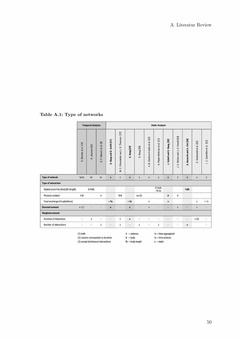
A. Literatur Review

Table A.1: Type of networks

50

A. Literatur Review

Table A.2: Properties of studies

51

A. Literatur Review

Table A.3: Network measures

52

Appendix B

Additional Information about theDataset

Figure B.1: Tagging frequency The bees were primarily tagged during the week. Onaverage 48 bees were tagged each day, considering only tagging days, the average is about91.

53

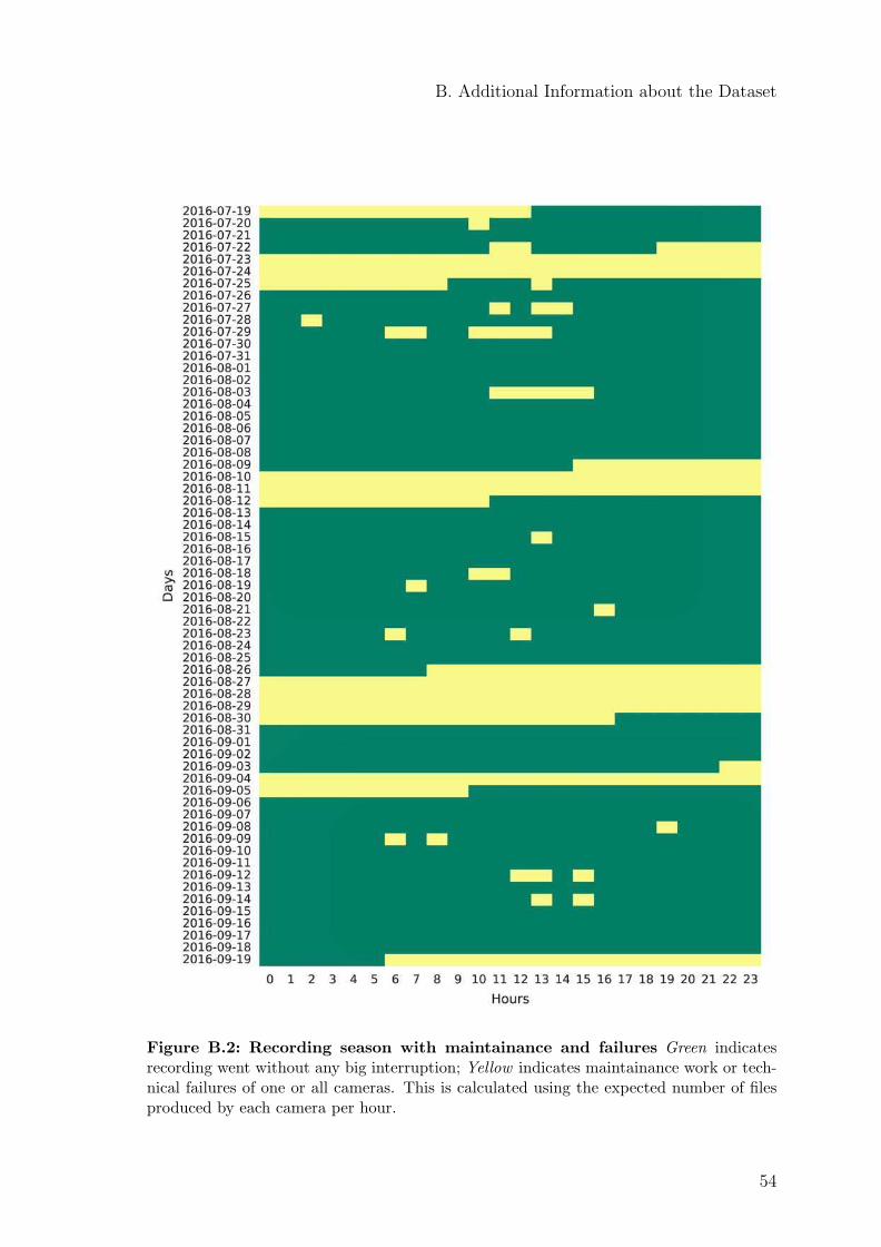
B. Additional Information about the Dataset

Figure B.2: Recording season with maintainance and failures Green indicatesrecording went without any big interruption; Yellow indicates maintainance work or tech-nical failures of one or all cameras. This is calculated using the expected number of filesproduced by each camera per hour.

54

Appendix C

Network Analysis

100 101 102 103

Link weight

100

101

102

103

104

105

106

Fre

quen

cy

Figure C.1: Link weight distribution for all snapshots

0 50 100 150 200 250 300 350

Link weights

2

0

2

4

6

8

10

12

Fre

quen

cy (

log)

Link weights

Fit. func: f(x) = 11. 509e0. 015x − 0. 831

Figure C.2: Link weight fit

55

C. Network Analysis

(a) Snapshot 1

(b) Snapshot 2

(c) Snapshot 3

Figure C.3: Communities per network for LE The green colour represents theyounger community, containing the queen. The orange color represents the older com-munity. The hive exit on side A is on the bottom right and on side B on the bottom left.The data is aggredated for the complete timeframe of ten hours.

56

C. Network Analysis

(a) Snapshot 1

(b) Snapshot 2

(c) Snapshot 3

Figure C.4: Communities per network for WT The green colour represents theyounger community, containing the queen. The orange color represents the older commu-nity. The gray represents the middle-age community. The hive exit on side A is on thebottom right and on side B on the bottom left. The data is aggredated for the completetimeframe of ten hours.

57

C. Network Analysis

0 10 20 30 40 50

Age in days

020406080

100120140

Num

ber

of b

ees

0 10 20 30 40 50

Age in days

020406080

100120140

Num

ber

of b

ees

Figure C.5: Age distribution for LE

58

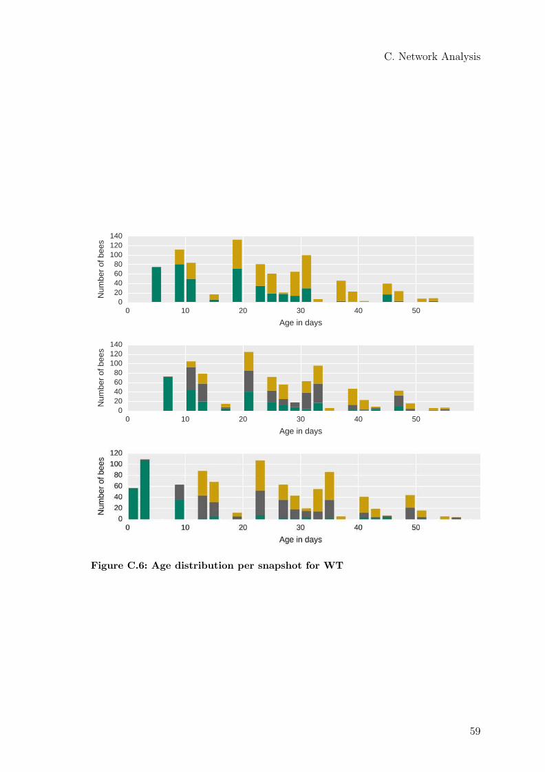
C. Network Analysis

0 10 20 30 40 50

Age in days

020406080

100120140

Num

ber

of b

ees

0 10 20 30 40 50

Age in days

020406080

100120140

Num

ber

of b

ees

Figure C.6: Age distribution per snapshot for WT

59

C. Network Analysis

0.0 0.2 0.4 0.6 0.8 1.00

20

40

60

80

100N

umbe

r of

bee

s

a

0.0 0.2 0.4 0.6 0.8 1.0

Degree k

0.0

0.2

0.4

0.6

0.8

1.0

Det

ectio

n fr

eque

ncy

b

0.0 0.2 0.4 0.6 0.8 1.00

102030405060

Age

in d

ays c

0.0

0.2

0.4

0.6

0.8

1.0

1.2

1.4

1.6

×104

01020304050607080

Num

ber

of b

ees

d

0.0

0.2

0.4

0.6

0.8

1.0

1.2

1.4

Strength s ×104

0.0

0.2

0.4

0.6

0.8

1.0D

etec

tion

freq

uenc

ye

0.0

0.2

0.4

0.6

0.8

1.0

1.2

1.4

×104

0102030405060

Age

in d

ays f

0.4 0.5 0.6 0.7 0.8 0.9 1.00

50

100

150

200

Num

ber

of b

ees

g

0.5 0.6 0.7 0.8 0.9 1.0


0.0

0.2

0.4

0.6

0.8

1.0

Det

ectio

n fr

eque

ncy

h

0.5 0.6 0.7 0.8 0.9 1.00

102030405060

Age

in d

ays i

0.4 0.5 0.6 0.7 0.8 0.9 1.00

20

40

60

80

100

Num

ber

of b

ees j

0.4 0.5 0.6 0.7 0.8 0.9 1.0

Closeness CC

0.0

0.2

0.4

0.6

0.8

1.0

Det

ectio

n fr

eque

ncy

k

0.4 0.5 0.6 0.7 0.8 0.9 1.00

102030405060

Age

in d

ays l

0.0

0.2

0.4

0.6

0.8

1.0

1.2

1.4

1.6

×10 3

020406080

100120

Num

ber

of b

ees

m

0.0

0.2

0.4

0.6

0.8

1.0

1.2

1.4


0.0

0.2

0.4

0.6

0.8

1.0

Det

ectio

n fr

eque

ncy

n

0.0

0.2

0.4

0.6

0.8

1.0

1.2

1.4

×10 3

0102030405060

Age

in d

ays o

Figure C.7: Snapshot 1: Local measures in relation to age and detection fre-quency

60

C. Network Analysis

0.0 0.2 0.4 0.6 0.8 1.00

20

40

60

80

100N

umbe

r of

bee

s

a

0.0 0.2 0.4 0.6 0.8 1.0

Degree k

0.0

0.2

0.4

0.6

0.8

1.0

Det

ectio

n fr

eque

ncy

b

0.0 0.2 0.4 0.6 0.8 1.00

102030405060

Age

in d

ays c

0.0

0.2

0.4

0.6

0.8

1.0

1.2

1.4

1.6

×104

01020304050607080

Num

ber

of b

ees

d

0.0

0.2

0.4

0.6

0.8

1.0

1.2

1.4

Strength s ×104

0.0

0.2

0.4

0.6

0.8

1.0D

etec

tion

freq

uenc

ye

0.0

0.2

0.4

0.6

0.8

1.0

1.2

1.4

×104

0102030405060

Age

in d

ays f

0.4 0.5 0.6 0.7 0.8 0.9 1.00

50

100

150

200

Num

ber

of b

ees

g

0.5 0.6 0.7 0.8 0.9 1.0


0.0

0.2

0.4

0.6

0.8

1.0

Det

ectio

n fr

eque

ncy

h

0.5 0.6 0.7 0.8 0.9 1.00

102030405060

Age

in d

ays i

0.4 0.5 0.6 0.7 0.8 0.9 1.00

20

40

60

80

100

Num

ber

of b

ees j

0.4 0.5 0.6 0.7 0.8 0.9 1.0

Closeness CC

0.0

0.2

0.4

0.6

0.8

1.0

Det

ectio

n fr

eque

ncy

k

0.4 0.5 0.6 0.7 0.8 0.9 1.00

102030405060

Age

in d

ays l

0.0

0.2

0.4

0.6

0.8

1.0

1.2

1.4

1.6

×10 3

020406080

100120

Num

ber

of b

ees

m

0.0

0.2

0.4

0.6

0.8

1.0

1.2

1.4


0.0

0.2

0.4

0.6

0.8

1.0

Det

ectio

n fr

eque

ncy

n

0.0

0.2

0.4

0.6

0.8

1.0

1.2

1.4

×10 3

0102030405060

Age

in d

ays o

Figure C.8: Snapshot 2: Local measures in relation to age and detection fre-quency

61

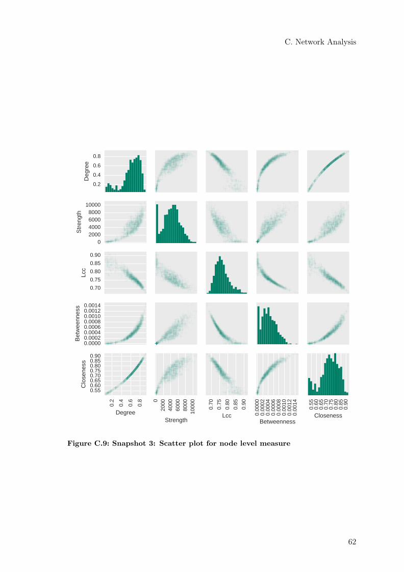
C. Network Analysis

0.2

0.4

0.6

0.8

Deg

ree

02000400060008000

10000

Stren

gth

0.700.750.800.850.90

Lcc

0.00000.00020.00040.00060.00080.00100.00120.0014

Betwee

nness

0.2

0.4

0.6

0.8

Degree

0.550.600.650.700.750.800.850.90

Closene

ss

020

0040

0060

0080

0010

000

Strength

0.70

0.75

0.80

0.85

0.90

Lcc 0.00

000.00

020.00

040.00

060.00

080.00

100.00

120.00

14

Betweenness

0.55

0.60

0.65

0.70

0.75

0.80

0.85

0.90

Closeness

Figure C.9: Snapshot 3: Scatter plot for node level measure

62

C. Network Analysis

0 10 20 30 40 50 60

Age in days

0

20

40

60

80

100

120

Num

ber

of b

ees

0 10 20 30 40 50 60

Age in days

0

20

40

60

80

100

120

Num

ber

of b

ees

0 10 20 30 40 50 60

Age in days

0

20

40

60

80

100

120

Num

ber

of b

ees

Figure C.10: Age distribution per snapshot

63

temporal analysis of honey bee interaction networks based

Documents