telecommunications infrastructure sharing.pdf - repositório
TRANSCRIPT
Universidade de Aveiro
2015
Departamento de Eletrónica,
Telecomunicações e Informática
David José Miranda
Teixeira
Partilha de Infraestruturas de Telecomunicações
Telecommunications Infrastructure Sharing

Universidade de Aveiro
2015
Departamento de Eletrónica,
Telecomunicações e Informática
David José Miranda
Teixeira
Partilha de Infraestruturas de Telecomunicações
Telecommunications Infrastructure Sharing
Dissertação apresentada à Universidade de Aveiro para cumprimento
dos requisitos necessários à obtenção do grau de Mestre em
Engenharia Eletrónica e Telecomunicações, realizada sob a orientação
científica do Professor Doutor Aníbal Manuel de Oliveira Duarte,
Professor Catedrático do Departamento de Eletrónica,
Telecomunicações e Informática da Universidade de Aveiro.

O Júri
Presidente Professor Doutor José Carlos da Silva Neves
Professor Catedrático do Departamento de Engenharia Eletrónica, Telecomunicações e
Informática da Universidade de Aveiro
Vogal - Arguente Principal Mestre Ricardo Jorge Moreira Ferreira
Gestor, PT Inovação e Sistemas
Vogal - Orientador Professor Doutor Aníbal Manuel de Oliveira Duarte
Professor Catedrático do Departamento de Engenharia Eletrónica, Telecomunicações e
Informática da Universidade de Aveiro

Agradecimentos
Em primeiro lugar, quero agradecer ao Professor Manuel de Oliveira
Duarte, pelo apoio, disponibilidade e orientação ao longo da realização
deste trabalho.
Quero agradecer também ao Eng.º Hugo Félix, Eng.º Pedro Ramos,
Eng.º António Alves e Eng.º Manuel Baptista pela ajuda prestada na
elaboração deste trabalho.
Agradeço também à Sandra dos Santos pela leitura e correção do texto
deste trabalho.
A todos os meus colegas e amigos que me apoiaram e ajudaram
durante todo o meu percurso académico, o meu muito obrigado.
Por último, agradeço à minha família por me ter dado todas as
condições e apoio incondicional nos meus estudos.

Palavras-chave
Partilha de Infraestruturas, Operador Neutro, Redes Móveis, Mercados
Emergentes, GSM, UMTS, LTE, Planeamento de Redes, Redes de Acesso.
Resumo
As telecomunicações móveis têm enfrentado enormes desafios em todo
o mundo, com especial ênfase nos países emergentes. A sua crescente
importância para o crescimento das economias dos países tornam a
sua presença essencial num mundo cada vez mais global e
tecnológico.
A partilha de infraestruturas de telecomunicações torna a
implementação de comunicações móveis numa dada região ou país
mais facilitada. No caso de Moçambique, que é dos países mais pobres
do mundo, a partilha seria uma estratégia interessante de forma a
permitir um rápido crescimento dos serviços de telecomunicações.
Neste projeto, foi desenvolvida uma ferramenta que auxilia o estudo
tecno-económico de cenários de partilha de infraestruturas de
telecomunicações. Esta ferramenta permitiu assim criar cenários para a
realidade Moçambicana.
Esta dissertação pretende contribuir para o desenvolvimento da área
das telecomunicações em mercados emergentes.

Keywords
Infrastructure Sharing, Neutral Operator, Mobile Networks, Emerging Markets,
GSM, UMTS, LTE, Network Planning, Access Network
Abstract
Mobile telecommunications have been facing a vast number of
challenges across the globe, with special emphasis on emerging
countries. Their increasing importance for economic growth of countries
make the presence of infrastructure essential in a progressively more
global and technological world.
Sharing telecommunication infrastructures can facilitate the
implementation of mobile communications in a giving region or country.
In the case of Mozambique, one of the poorest country of the world, a
sharing strategy could potentially allow for a rapid expansion of
telecommunication services.
In this work project, a tool that supports the techno-economic study of
scenarios of telecommunication infrastructure sharing was developed.
Through this mechanism, scenarios that consider the Mozambican’s
reality have been set up.
This dissertation aims then to contribute to the development of the
telecommunications sector in emerging markets.

Contents
Universidade de Aveiro I
Contents
LIST OF ABBREVIATIONS ....................................................................................................................... V
LIST OF SYMBOLS ..................................................................................................................................IX
LIST OF FIGURES ................................................................................................................................. XIII
LIST OF TABLES ................................................................................................................................. XVII
LIST OF CHARTS.................................................................................................................................. XIX
LIST OF EQUATIONS ........................................................................................................................... XXI
1. INTRODUCTION ............................................................................................................................. 1
1.1. MOTIVATION .................................................................................................................................. 1
1.2. TELECOMMUNICATION AND SOCIO-ECONOMIC DEVELOPMENT .................................................................. 2
1.3. OBJECTIVES..................................................................................................................................... 3
1.4. METHODOLOGY ............................................................................................................................... 3
1.5. DOCUMENT STRUCTURE .................................................................................................................... 4
2. MOBILE COMMUNICATION TECHNOLOGIES .................................................................................. 5
2.1. OVERVIEW OF MOBILE COMMUNICATION .............................................................................................. 5
2.2. CELLULAR NETWORKS FUNDAMENTALS ................................................................................................ 8
2.2.1. Hexagonal shape ................................................................................................................ 9
2.2.2. Clusters ............................................................................................................................. 10
2.2.3. Propagation Losses ........................................................................................................... 13
2.2.4. Interferences .................................................................................................................... 14
2.2.4.1. Co-channel interference .............................................................................................. 14
2.2.4.2. Adjacent-channel interference .................................................................................... 14
2.2.4.3. Internal Interferences .................................................................................................. 15
2.2.5. Cell Sectoring .................................................................................................................... 16
2.2.6. Antennas .......................................................................................................................... 17
2.2.6.1. Sector Antennas ........................................................................................................... 17
2.2.6.2. Advanced Systems ....................................................................................................... 18 2.2.6.2.1. Diversity scheme ................................................................................................................... 18 2.2.6.2.2. Adaptive method .................................................................................................................. 19 2.2.6.2.3. MIMO method ...................................................................................................................... 19
2.2.7. Handover/Handoff ........................................................................................................... 20
2.2.8. Roaming ........................................................................................................................... 21
2.2.9. Multiple Access Techniques ............................................................................................. 23
2.2.10. Frequency and Transmission modes ................................................................................ 28
2.3. NETWORK TOPOLOGIES ................................................................................................................... 33
2.4. UMTS ......................................................................................................................................... 35
2.4.1. Characteristics .................................................................................................................. 35
2.4.2. Standardization ................................................................................................................ 36
2.4.3. Structure and architecture ............................................................................................... 37
2.5. LTE ............................................................................................................................................. 45
2.5.1. Architecture ..................................................................................................................... 46
2.5.2. Physical Layer ................................................................................................................... 47

Telecommunication Infrastructure Sharing
II Departamento de Eletrónica, Telecomunicações e Informática
2.5.3. SON (Self Organizing Networks) ....................................................................................... 49
2.6. GSM VS. UMTS ........................................................................................................................... 50
2.7. UMTS VS. LTE ............................................................................................................................. 52
2.8. SUMMARY .................................................................................................................................... 53
3. BUSINESS MODELS ISSUES ........................................................................................................... 55
3.1. INFRASTRUCTURE SHARING .............................................................................................................. 55
3.1.1. Passive Sharing ................................................................................................................. 56
3.1.1.1. Site Sharing .................................................................................................................. 56
3.1.1.2. Mast Sharing ................................................................................................................ 58
3.1.2. Active Sharing ................................................................................................................... 61
3.1.2.1. Core Network Sharing .................................................................................................. 61
3.1.2.2. RAN Sharing ................................................................................................................. 62
3.2. BUSINESS MODELS ......................................................................................................................... 64
3.2.1. Mobile Virtual Network Operator (MVNO) ...................................................................... 64
3.2.2. Neutral Operator (NO) ..................................................................................................... 65
3.3. SUMMARY .................................................................................................................................... 67
4. NETWORK DIMENSIONING .......................................................................................................... 69
4.1. SITE DIMENSIONING ....................................................................................................................... 69
4.1.1. Site Coverage Dimensioning ............................................................................................. 70
4.1.2. Site Capacity Dimensioning .............................................................................................. 72
4.2. RNC DIMENSIONING ...................................................................................................................... 73
4.3. CORE NETWORK DIMENSIONING ....................................................................................................... 74
4.4. TECHNOLOGY ADOPTION – NUMBER OF USERS .................................................................................... 76
4.5. TECHNO-ECONOMIC ANALYSIS .......................................................................................................... 78
4.5.1. CAPEX ............................................................................................................................... 79
4.5.2. OPEX ................................................................................................................................. 79
4.5.3. Revenues .......................................................................................................................... 79
4.5.4. Annual Cash Flow and Cash Balance ................................................................................ 79
4.5.5. Net Present Value (NPV) .................................................................................................. 80
4.5.6. Internal Rate Return (IRR) ................................................................................................ 80
4.5.7. Payback Period ................................................................................................................. 81
4.6. TECHNO-ECONOMIC TOOL FOR NEUTRAL OPERATOR ............................................................................ 82
4.6.1. Customize Parameters ..................................................................................................... 82
4.6.2. Technology adoption ........................................................................................................ 85
4.6.3. Market .............................................................................................................................. 87
4.6.4. Cost Elements ................................................................................................................... 87
4.6.4.1. Base Station ................................................................................................................. 89
4.6.4.2. Radio Link ..................................................................................................................... 90
4.6.4.3. Core Network ............................................................................................................... 91
4.6.5. Granularity of network elements ..................................................................................... 91
4.6.5.1. Sites granularity ........................................................................................................... 91
4.6.5.2. GSM ............................................................................................................................. 94
4.6.5.3. UMTS ........................................................................................................................... 96
4.6.5.4. LTE ................................................................................................................................ 98
4.6.5.5. Core Network ............................................................................................................... 98
4.6.6. CAPEX ............................................................................................................................... 99
Contents
Universidade de Aveiro III
4.6.7. OPEX ............................................................................................................................... 101
4.6.8. Revenues ........................................................................................................................ 102
4.6.9. Economic Results ........................................................................................................... 104
4.7. SUMMARY .................................................................................................................................. 104
5. CASE STUDY ............................................................................................................................... 105
5.1. CONTEXTUALIZATION .................................................................................................................... 105
5.2. MOZAMBIQUE............................................................................................................................. 105
5.3. GEOGRAPHICAL AND DEMOGRAPHIC OVERVIEW OF MOZAMBIQUE ........................................................ 107
5.3.1. Maputo ........................................................................................................................... 110
5.4. CURRENT MOBILE TELECOMMUNICATION SCENARIO IN MOZAMBIQUE .................................................. 111
5.5. REGULATION OF THE MOZAMBICAN TELECOMMUNICATIONS MARKET ................................................... 113
5.6. MOZAMBIQUE BUSINESS MODEL .................................................................................................... 115
5.6.1. Mobile Virtual Network Operator (MVNO) .................................................................... 115
5.6.2. Neutral Operator ............................................................................................................ 115
5.6.3. Scenarios ........................................................................................................................ 116
5.6.3.1. Scenario A .................................................................................................................. 116
5.6.3.2. Scenario B .................................................................................................................. 117
5.6.3.3. Scenario C .................................................................................................................. 117
5.7. SCENARIO A ................................................................................................................................ 119
5.7.1. Technology adoption ...................................................................................................... 122
5.7.2. Market ............................................................................................................................ 122
5.7.2.1. Market GSM ............................................................................................................... 123
5.7.2.2. Market UMTS ............................................................................................................. 123
5.7.2.3. Market LTE ................................................................................................................. 124
5.7.3. Granularity of network elements ................................................................................... 124
5.7.3.1. Number of Sites ......................................................................................................... 124
5.7.3.2. GSM ........................................................................................................................... 127
5.7.3.3. UMTS ......................................................................................................................... 129
5.7.3.4. LTE .............................................................................................................................. 130
5.7.4. Evolution of network elements over the years .............................................................. 131
5.7.5. CAPEX ............................................................................................................................. 134
5.7.6. OPEX ............................................................................................................................... 134
5.7.7. Revenues ........................................................................................................................ 135
5.7.8. Economic Results ........................................................................................................... 135
5.8. SCENARIO B ................................................................................................................................ 138
5.8.1. Technology adoption ...................................................................................................... 140
5.8.2. Market ............................................................................................................................ 141
5.8.2.1. Market GSM ............................................................................................................... 142
5.8.2.2. Market UMTS ............................................................................................................. 142
5.8.2.3. Market LTE ................................................................................................................. 143
5.8.3. Granularity of network elements ................................................................................... 143
5.8.3.1. Number of Sites ......................................................................................................... 143
5.8.3.2. GSM ........................................................................................................................... 145
5.8.3.3. UMTS ......................................................................................................................... 146
5.8.3.4. LTE .............................................................................................................................. 146
5.8.4. Evolution of network elements over the year ............................................................... 146
5.8.5. CAPEX ............................................................................................................................. 148
Telecommunication Infrastructure Sharing
IV Departamento de Eletrónica, Telecomunicações e Informática
5.8.6. OPEX ............................................................................................................................... 149
5.8.7. Revenues ........................................................................................................................ 150
5.8.8. Economic Results ........................................................................................................... 150
5.9. SCENARIO C ................................................................................................................................ 153
5.9.1. Technology adoption ...................................................................................................... 154
5.9.2. Market ............................................................................................................................ 155
5.9.2.1. Market GSM ............................................................................................................... 155
5.9.2.2. Market UMTS ............................................................................................................. 156
5.9.2.3. Market LTE ................................................................................................................. 156
5.9.3. Granularity of network elements ................................................................................... 157
5.9.3.1. Number of Sites ......................................................................................................... 157
5.9.3.2. GSM ........................................................................................................................... 158
5.9.3.3. UMTS ......................................................................................................................... 159
5.9.3.4. LTE .............................................................................................................................. 159
5.9.4. Evolution of network elements over the years .............................................................. 160
5.9.5. CAPEX ............................................................................................................................. 162
5.9.6. OPEX ............................................................................................................................... 162
5.9.7. Revenues ........................................................................................................................ 163
5.9.8. Economic Results ........................................................................................................... 163
5.10. SUMMARY .................................................................................................................................. 165
6. FINAL CONSIDERATIONS ............................................................................................................ 167
6.1. CONCLUSIONS ............................................................................................................................. 167
6.2. FUTURE WORK ............................................................................................................................. 169
REFERENCES ....................................................................................................................................... 171
APPENDICES ............................................................................................................................................ I
APPENDIX A – GSM ARCHITECTURE .................................................................................................................. I
APPENDIX B – GSM INTERFACES ..................................................................................................................... II
APPENDIX C – UMTS ARCHITECTURE AND INTERFACES ....................................................................................... III
APPENDIX D – UMTS CIRCUIT-SWITCHED ........................................................................................................ IV
APPENDIX E – UMTS PACKET-SWITCHED ......................................................................................................... VI
APPENDIX F – ERLANG ................................................................................................................................... X
APPENDIX G – LINK BUDGET EXPLANATION ....................................................................................................... XI
APPENDIX H – PASSIVE TELECOMMUNICATION INFRASTRUCTURE SHARING REGULATION ........................................ XIV
List of Abbreviations
Universidade de Aveiro V
List of Abbreviations
3D Three dimensions 1G First Generation of Mobile Telecommunication Technology 2G Second Generation of Mobile Telecommunication Technology 2.5G 2.5 Generation of Mobile Telecommunication Technology 2.75G 2.75 Generation of Mobile Telecommunication Technology 3G Third Generation of Mobile Telecommunication Technology 3.5G 3.5 Generation of Mobile Telecommunication Technology 3GPP Third Generation Partnership Project 4G Fourth Generation of Mobile Telecommunication Technology AAA Authentication, Authorization and Accounting ACK Acknowledge Admin. Administration ADSL Asymmetric Digital Subscriber Line AMPS Advanced Mobile Phone System APN Access Point Name Approx. approximately ARPU Average Revenue Per User AuC Authentication Center BH Busy Hour BHCA Busy Hour Call Attempts BS Base Station BSC Base Station Controller BSS Base Station System BTS Base Transceiver Station CAPEX Capital Expenditures CATT China Academy of Telecommunication Technology CD Compact Disc CDMA Code Division Multiplexing Access CDMA IS-96 Code Division Multiplexing Access Interim Standard - 96 CDR Call Detail Records CG Charging Gateway CMI Chr. Michelsen Institute CN Core Network CP Costumer Premises CS Circuit Switched domain CSFB Circuit Switched Fall Back DHCP Dynamic Host Configuration Protocol DL Downlink DNS Domain Name System DTE Data Terminal Equipment DVB Digital Video Broadcasting E-UTRAN Evolved Universal Terrestrial Radio Access EC Echo Canceller EDGE Enhanced Data for GSM Evolution eICIC/IC enhanced Inter-Cell Interference Coordination/Interference Cancellation EIR Equipment Identity Register EIRP Equivalent Isotropic Radiated Power
Telecommunication Infrastructure Sharing
VI Departamento de Eletrónica, Telecomunicações e Informática
eNB E-UTRAN Node B eMBMS evolved Multimedia Broadcast Multicast Service EPC Evolved Packet Core ETSI European Telecommunication Standards Institute EV-DO Evolution Data Optimized EUR Euro FDD Frequency Division Duplexing FDMA Frequency Division Multiple Access FeICIC/IC Further enhanced Inter-Cell Interference Coordination/Interference
Cancellation FDI Foreign Direct Investment FM Frequency Modulation FTP File Transfer Protocol GDP Gross Domestic Product GERAN GSM EDGE Radio Access Network GGSN Gateway GPRS Support Node GMSC Gateway MSC GoS Grade of Service GPRS General Packet Radio Service GSM Global System for Mobile Communications GTP GPRS Tunneling Protocol GW Gateway HDTV High-Definition Television HetNets Heterogeneous Networks HLR Home Location Register HSDPA High Speed Downlink Packet Access HSPA High Speed Packet Access HSS Home Subscriber Server ID Identification iDEN Integrated Digital Enhanced Network IEEE Institute of Electrical and Electronics Engineers IMEI International Mobile Equipment Identity IMS IP Multimedia Subsystem IMSI International Mobile Subscriber Identity IMT-2000 International Mobile Telecommunication at 2.000 Mhz IMT-Advanced International Mobile Telecommunication Advanced INCM National Communications Institute of Mozambique (Instituto Nacional das
Comunicações de Moçambique) INE National Statistics Institute (Instituto Nacional de Estatística) IP Internet Protocol IPTV Internet Protocol Television IRR Internal Rate Return ISDN Integrated Services Digital Network ITU International Telecommunication Union IWF Interworking Function LAI Location Area Identity LTE Long Term Evolution LTE-A Long Term Evolution Advanced MAC Media Access Control max. maximum
List of Abbreviations
Universidade de Aveiro VII
MC-CDMA Multi-Carrier Code Division Multiple Access MD Mobile Device ME Mobile Equipment MGW Media Gateway MIMO Multiple-Input Multi-Output min. minute MME Mobile Management Entity MMS Multimedia Messaging Service MS Mobile Station MSC Mobile service Switching Center MSRN Mobile Station Roaming Number MT Metical MVNE Mobile Virtual Network Enabler MVNO Mobile Virtual Network Operator MZN Mozambican Metical NMT Nordic Mobile Telephone NO Neutral Operator Norad Norwegian Agency for Development Cooperation NPV Net Present Value NRT Non Real Time NSN Nokia Siemens Network NSS Network Switching System NTT Nippon Telegraph and Telephone OA&M Operation, Administrative and Maintenance OCS Online Charging System OFDMA Orthogonal Frequency-Division Multiple Access OMC Operations and Maintenance Center OMS Operations and Maintenance System OPEX Operational Expenditures P2P Ponit-to-Point PAPR Peak to Average Power Ratio PDC Personal Digital Cellular PDN Public Data Network PDP Packet Data Protocol PCRF Policy Control and Charging Rules Function PHS Personal Handyphon System PLMN Public Land Mobile Network PS Packet Switching PSS Primary Synchronization Signal PSTN Public Switched Telephone Network QAM Quadrature Amplitude Modulation QoS Quality of Service QPSK Quadrature Phase Shift Keying R&D Research and Development RADIUS Remote Authentication Dial in User Service RAN Radio Access Network Revs A&B Revision A and B RNC Radio Network Controller RNS Radio Network Subsystem ROI Return on Investment
Telecommunication Infrastructure Sharing
VIII Departamento de Eletrónica, Telecomunicações e Informática
RRM Radio Resource Management RT Real Time RTMS Radio Mobile Telephone Systems RTT Radio Transmission Technology SAE System Architecture Evolution SDMA Space Division Multiple Access SC Service Center SCDMA Synchronous Code Division Multiple Access SGSN Serving GPRS Support Node SIM Subscriber Identity Module SME Short Message Entity SMS Short Message Service SMS-GMSC Gateway MSC for Short Message Service SMS-IWMSC Interworking MSC for Short Message Service SMS-SC SMS Service Center SNR Signal-to-Noise Ratio SON Self-Organizing Networks TACS Total Access Communications System TDD Time Division Duplex TD-SCDMA Time Division Synchronous Code Division Multiple Access TDM Telecomunicações de Moçambique TDMA Time Division Multiplexing Access TDMA IS-54 Time Division Multiplexing Access Interim Standard - 54 TMSI Temporary Mobile Subscriber Identity TRAU Transcoding Rate and Adaptation Unit TRX Transceiver TV Television UE User equipment UL Uplink Um User mobile UMB Ultra Mobile Broadband UMTS Universal Mobile Telecommunication System UMTS900 Universal Mobile Telecommunication System at 900 MHz UMTS2100 Universal Mobile Telecommunication System at 2.100 MHz UNDP United Nations Development Program USD United States Dollar USIM UMTS Subscriber Identity Module UTRA Universal Terrestrial Radio Access UTRAN Universal Terrestrial Radio Access Network US/USA United Sates of America VAT Value Added Tax VCR Video Cassette Recording VLR Visitor Location Register VMSC Visited Mobile Switching Center VoIP Voice over Internet Protocol VoLTE Voice over LTE W-CDMA Wideband Code Division Multiple Access WiFi synonym to Wireless local area network (WLAN) WiMax Worldwide interoperability for Microwave Access WLAN Wireless Local Area Network
List of Symbols
Universidade de Aveiro IX
List of Symbols
λ Call arrival ° degree € Euro / per or or % Percentage %SOF Percentage of sites with optical fiber connection %SRL Percentage of sites with radio link connection Δ power margin μ One hour (3.600s) τi Initial instant the wave of technology appears on the market (time in years) A Interface between an BSC and a MSC Control parameter for market start moment Abis Interface between an BTS and a BSC B Interface between an MSC and a VLR or Control parameter for speed of market start C Interface between an MSC and a HRL or Costs or codes C1 CAPEX in year 1 CCN1 Cost to implement the Core Network in year 1 CCN_R_n Cost to implement the Core Network in remaining years CConst Number of sites x Cost per site construction CGGSN Cost per GGSN CHLR Cost per HLR CM1 Cost of equipment in year 1 to implement the first mobile communication
technology CMSC Cost per MSC/VLR CM_R_n Cost of implementation per year of mobile communication technologies COF Cost per km of Optical Fiber passed and tested CPCN Cost of Packet Core Network CPCN_upg Cost of Packet Core Network upgrade CR_n CAPEX in remaining years CRNC Cost per RNC CS Cost per site CSGSN Cost per SGSN CTRX Cost per TRX Cupg Cost of technologies upgrade C-450 Cellular radio system (C – third national public mobile network) CF Cash Flow Cu Interface between USIM and a ME D Interface between an HLR and a VLR d Reuse distance DCN Average site distance to Core Network dB decibel dBi dB isotropic
Telecommunication Infrastructure Sharing
X Departamento de Eletrónica, Telecomunicações e Informática
dBm dB milliwatt E Interface between an MSC and a MSW E/Erl Erlang or Total traffic offered to group in Erlang Eb/No Energy per bit to noise power spectral density ratio f frequency F Interface between an MSC and a EIR G Interface between an VLR and a VLR Ga Interface between a GGSN/SGSN and an OCS Gb Interface between an SGSN and a Base Station System (BSS) Gc Interface between a GGSN and an HLR Gd Interface between an SGSN and an SMS-GMSC/IWMSC Gf Interface between an SGSN and an EIR GHz Gigahertz Gi Reference point between GPRS and an external packet data network Gn Interface between two GSNs within the same PLMN Gp Interface between two GSNs in different PLMNs. The Gp interface allows
support of GPRS network services across areas served by the co-operating GPRS PLMNs
Gr Interfacebetween an SGSN and an HLR Gs Interface between an SGSN and an MSC GB Giga Byte Gbps Giga bit per second GBps Giga Byte per second Gx Interface between an S-GW and an UTRAN H Interface between an AuC and an HLR h Average call length or holding time hB Base Station (BS) antenna height in meters hnm transmission hM User Equipment (UE) antenna in meters Hz Hertz Iu Interface between the RNC and the Core Network (MSC or SGSN) Iub Interface between an RNC and a Node B Iu-CS Interface between an RNC and a MGC Iu-PS Interface between an RNC and a SGSN IuPS Interface between an RNC and a SGSN Iur Interface between RNCs K cluster size kbit/s or kbps kilo bit per second kBps kilo Bytes per second km kilometer km2 or km2 square kilometer LTE-Uu Interface Between an eNode B and an MS m meter or milli or number of identical parallel channel m1 potential market served by the first technology wave m2 potential market served by the second technology wave m3 potential market served by the third technology wave
List of Symbols
Universidade de Aveiro XI
mi potential market served by each technology wave, treated here as a percentage, although it may be in the number of customers
Mb Mega bit Mbit/s or Mbps Mega bit per second MB Mega Byte mE mili Erlang MHz Megahertz ms millisecond Nº Number NGGSN Number of GGSN NGGSN_upg Number of GGSN upgrade NHLR Number of HLR NHLR_upg Number of HLR upgrade NMSC Number of MSC/VLR NMSC_upg Number of MSC/VLR upgrade NRNC Number of RNCs NRNC_upg Number of RNC upgrade NS Number of Sites NS_upg Number of site upgrade NSGSN Number of SGSN NSGSN_upg Number of SGSN upgrade NTRX Number of TRXs NTRX_upg Number of TRX upgrade OPEXSITE OPEX per site P0 Starting Level p10 Starting Level in p1 equation p1f Saturation Level in p1 equation p20 Starting Level in p2 equation p2f Saturation Level in p2 equation p30 Starting Level in p3 equation p3f Saturation Level in p3 equation Pb Blocking Probability Pf Saturation Level pi(t) Function that characterizes the share of each wave of technology in the
Market Threshold level
Minimum signal level for reasonable voice quality
Q Quality factor R Interface between an MS and a DTE or Distance between BS and UE in km (site range) or Revenues r cell radius or discount rate RX Receiver Rx Interface between a PCRF and operators IP services s second S Space Si Function that characterizes the actual conduct of each technology wave,
affected by the behavior of other S1-MME Interface between an eNode B and an MME
Telecommunication Infrastructure Sharing
XII Departamento de Eletrónica, Telecomunicações e Informática
S1-U Interface between an eNode B and an S-GW S10 Control interface between MMEs S11 Interface between an S-GW and an MME S12 Interface between an S-GW and an UTRAN S3 Interface between an MME and an SGSN S4 Interface between an S-GW and a GERAN S5 Interface between an S-GW and a PDN-GW S6a Interface between an MME and an HSS SGi Interface between an a PDN-GW and operator IP services t time (in years) T Time period of the project TX transmitter Um Interface between a BTS and an MS Uu Air interface between a UE and Node B W Watt X2 Interface between neighboring Node B
List of Figures
Universidade de Aveiro XIII
List of Figures
Figure 1 – Technology evolution [36] [37] .................................................................................... 7
Figure 2 – Cell concept (adapted from [94]) ................................................................................. 8
Figure 3 – Cell representation [97]................................................................................................ 9
Figure 4 – Hexagons and Circles cellular system [97] ................................................................... 9
Figure 5 – Site representation [97] ............................................................................................. 10
Figure 6 – Cell Clusters [27] ......................................................................................................... 10
Figure 7 – Cluster K=4 [106] ........................................................................................................ 11
Figure 8 – Cluster K=7 [106] ........................................................................................................ 11
Figure 9 – Cluster K=12 [106] ...................................................................................................... 11
Figure 10 – Find co-channel neighbors [106] .............................................................................. 12
Figure 11 – Cluster [106] ............................................................................................................. 12
Figure 12 – Co-channel interference [27] ................................................................................... 14
Figure 13 – Example of frequencies attribution [94] .................................................................. 15
Figure 14 – Multipath Interference [27] ..................................................................................... 15
Figure 15 – Cell Sectoring [109] .................................................................................................. 16
Figure 16 – 120º Sectoring [110] ................................................................................................. 17
Figure 17 – Radiation diagram of sectorized antenna [61] ......................................................... 18
Figure 18 – General Outline of MIMO system [130] ................................................................... 19
Figure 19 – Handover scenario at two adjacent cell boundary (adapted from [111]) ............... 20
Figure 20 – Overview of international roaming technology and operations [112] .................... 21
Figure 21 – Commercial links required for international mobile roaming [112] ........................ 21
Figure 22 – Existing resources in the access technique [36] [39] ............................................... 23
Figure 23 – FDMA scheme [39] ................................................................................................... 23
Figure 24 – TDMA scheme [39] ................................................................................................... 24
Figure 25 – GSM scheme (TDMA with “frequency hopping”) [39] ............................................. 24
Figure 26 – CDMA scheme [39] ................................................................................................... 25
Figure 27 – UMTS transmission [38] ........................................................................................... 26
Figure 28 – FDD and TDD Scheme [84] ....................................................................................... 28
Figure 29 – FDD and TDD [83] ..................................................................................................... 30
Figure 30 – Frequencies for different equipments [85] .............................................................. 30
Figure 31 – GSM Frequencies [85] .............................................................................................. 30
Figure 32 – UMTS Frequencies [85] ............................................................................................ 31
Figure 33 – DL and UP frequencies for different operators [85] ................................................ 32
Figure 34 – Network Structure (adapted from [139]) ................................................................. 33
Figure 35 – Basic network topology configuration for RAN ........................................................ 33
Figure 36 – RAN network topology example (adapted from [139]) ........................................... 34
Figure 37 – World standards [38] ................................................................................................ 36
Figure 38 – Generic view of a UMTS network [139] ................................................................... 37
Figure 39 – UMTS network elements and interfaces architecture (adapted from [139]) .......... 37
Figure 40 – UMTS architecture (adapted from [11] [28] [29]) .................................................... 38
Telecommunication Infrastructure Sharing
XIV Departamento de Eletrónica, Telecomunicações e Informática
Figure 41 – Interfaces in GERAN core network [38] ................................................................... 42
Figure 42 – Interfaces in UTRAN core network [38] ................................................................... 42
Figure 43 – LTE Architecture (data only) (adapted from [27]) .................................................... 45
Figure 44 – LTE architecture (LTE over GSM) (adapted from [27]) ............................................. 46
Figure 45 – LTE Evolution [46] ..................................................................................................... 46
Figure 46 – LTE architecture [32] ................................................................................................ 47
Figure 47 – Physical Layer of LTE technology [59] ...................................................................... 48
Figure 48 – LTE Access scheme [87][86] ..................................................................................... 53
Figure 49 – Site constitution [10] ................................................................................................ 57
Figure 50 – Site Sharing [15] ....................................................................................................... 57
Figure 51 – Site sharing [119] ...................................................................................................... 58
Figure 52 – Mast sharing global scheme [119] ........................................................................... 59
Figure 53 – Mast sharing [119].................................................................................................... 59
Figure 54 – Mobile Communication Masts in Mira, Portugal ..................................................... 60
Figure 55 – Core Network [23] .................................................................................................... 61
Figure 56 – RAN sharing .............................................................................................................. 62
Figure 57 – Four model proposal for infrastructure sharing [131] ............................................. 66
Figure 58 – Number of sites calculation scheme [90] ................................................................. 69
Figure 59 – Hexagonal site templates ......................................................................................... 70
Figure 60 – Number of sites calculation scheme (coverage dimensioning) [90] ........................ 70
Figure 61 – Number of sites calculation scheme (capacity dim.) (adapted from [90] [145]) ..... 72
Figure 62 – Number of RNCs calculation scheme (adapted from [145]) .................................... 73
Figure 63 – Core Network calculation ......................................................................................... 74
Figure 64 – Core Network (adapted from Appendix C and [8]) .................................................. 75
Figure 65 – Technology adoption ................................................................................................ 78
Figure 66 – Techno-economic Analysis scheme .......................................................................... 78
Figure 67 – Techno-economic Tool flowchart ............................................................................. 82
Figure 68 – Network elements (adapted from [85]) ................................................................... 88
Figure 69 – Base Station architecture [26] .................................................................................. 89
Figure 70 – a) Antenna angle - 60° and b) Antenna angle - 120° (adapted from [27]) ............... 90
Figure 71 – Radio Link architecture [27] ..................................................................................... 90
Figure 72 – 18-sector site [77] .................................................................................................... 96
Figure 73 – Map of Mozambique [24] ....................................................................................... 107
Figure 74 – Population density [78] .......................................................................................... 108
Figure 75 – Maputo map [92] ................................................................................................... 110
Figure 76 – Current reality of telecommunication in Mozambique.......................................... 113
Figure 77 – Mozambique Scenario A ........................................................................................ 119
Figure 78 – Infrastructure of Scenario A ................................................................................... 120
Figure 79 – Economic Results for Scenario A (Best case scenario) ........................................... 136
Figure 80 – Economic Results for Scenario A (Worst case scenario) ........................................ 137
Figure 81 – Mozambique Scenario B ......................................................................................... 138
Figure 82 – Infrastructure of Scenario B ................................................................................... 139
Figure 83 – Infrastructure of Scenario C ................................................................................... 153
Figure 84 – GSM architecture (adapted from [11] [12]) ................................................................ I
List of Figures
Universidade de Aveiro XV
Figure 85 – GSM interfaces [22] .................................................................................................... II
Figure 86 – Basic UMTS network architecture [23] ..................................................................... III
Figure 87 – Voice call (circuit-switched) – Part I [36] ................................................................... IV
Figure 88 – Voice call (circuit-switched) – Part II [36] ................................................................... V
Figure 89 – Messaging in packet switched (Part I) [36] [40] [41] ................................................. VI
Figure 90 – Messaging in packet switched (Part II) [36] [40] [41] ............................................... VII
Figure 91 –Messaging flow [36] [40] [41] [43] ........................................................................... VIII
Figure 92 – Network elements and messages exchange [36] [40] [41] ....................................... IX
Figure 93 – Messages exchange between network elements [36] [40] [41] ............................... IX
Figure 94 – Calculation of site range R [77] ............................................................................... XIII
Telecommunication Infrastructure Sharing
XVI Departamento de Eletrónica, Telecomunicações e Informática
List of Tables
Universidade de Aveiro XVII
List of Tables
Table 1 – Overview of mobile technologies [36]........................................................................... 7
Table 2 – Comparison of different types of access [39] .............................................................. 27
Table 3 – FDD vs TDD [84] ........................................................................................................... 29
Table 4 – Frequencies in different world regions [85] ................................................................ 31
Table 5 – Bandwidth ranges in LTE [59] ...................................................................................... 48
Table 6 – Year of Project ............................................................................................................. 82
Table 7 – Users section................................................................................................................ 83
Table 8 – Price paid per user per month ..................................................................................... 83
Table 9 – Neutral Operator sharing section ................................................................................ 84
Table 10 – Region Characteristic section .................................................................................... 84
Table 11 – Civil Engineering section ............................................................................................ 84
Table 12 – Wireless Technology section ..................................................................................... 84
Table 13 – Financial Parameters ................................................................................................. 84
Table 14 – Total parameters ....................................................................................................... 85
Table 15 – GSM parameters ........................................................................................................ 85
Table 16 – UMTS parameters ...................................................................................................... 85
Table 17 – LTE parameters .......................................................................................................... 85
Table 18 – m1, m2 and m3 parameters ...................................................................................... 86
Table 19 – p’s parameters ........................................................................................................... 86
Table 20 – Cost elements ............................................................................................................ 88
Table 21 – Erlang B table [58] ..................................................................................................... 95
Table 22 – Configuration to 17mE/user [10] ............................................................................... 95
Table 23 - OPEX ......................................................................................................................... 102
Table 24 – Base case scenario ................................................................................................... 104
Table 25 – Distribution of Mozambique population per Province [67] .................................... 108
Table 26 – Geo-type distribution .............................................................................................. 116
Table 27 – Scenario A summary ................................................................................................ 117
Table 28 – Scenario B summary ................................................................................................ 117
Table 29 – Scenario C summary ................................................................................................ 118
Table 30 – Scenario A ................................................................................................................ 121
Table 31 – Vodacom monthly mobile tariffs [102] ................................................................... 121
Table 32 – Parameters tables for Scenario A ............................................................................ 122
Table 33 – Link budget calculations based on 12,2 kbps voice service [72] ............................. 126
Table 34 – Configuration to 25 mE/user ................................................................................... 128
Table 35 – Data needed for different internet activities [91] ................................................... 129
Table 36 – Method of estimated values [91] ............................................................................ 130
Table 37 – Typical user’s Profile [90]......................................................................................... 130
Table 38 – NPV, IRR and Payback period for Scenario A (Base case scenario) ......................... 135
Table 39 – NPV, IRR and Payback period for Scenario A (Best case scenario) .......................... 136
Table 40 – NPV, IRR and Payback period for Scenario A (Worst case scenario) ....................... 137
Telecommunication Infrastructure Sharing
XVIII Departamento de Eletrónica, Telecomunicações e Informática
Table 41 – Scenario B ................................................................................................................ 140
Table 42 – Parameters tables for Scenario B ............................................................................ 141
Table 43 – Percentage increase in coverage area [72] ............................................................. 143
Table 44 – Configuration to 25 mE/user ................................................................................... 145
Table 45 – NPV, IRR and Payback period for Scenario B (Base case scenario) ......................... 150
Table 46 – NPV, IRR and Payback period for Scenario B (Best case scenario) .......................... 151
Table 47 – NPV, IRR and Payback period for Scenario B (Worst case scenario) ....................... 152
Table 48 – Scenario C ................................................................................................................ 154
Table 49 – Parameters tables for Scenario C ............................................................................ 155
Table 50 – Configuration to 17mE/user .................................................................................... 158
Table 51 – NPV, IRR and Payback period for Scenario C (Base case scenario) ......................... 163
Table 52 – NPV, IRR and Payback period for Scenario C (Best case scenario) .......................... 164
Table 53 – NPV, IRR and Payback period for Scenario C (Worst case scenario) ....................... 164
Table 54 – Summary of uplink Eb/N0 (source: OVUM) [72] ......................................................... XII
Table 55 – Summary of downlink Eb/N0 (source: OVUM) [72] .................................................... XII
List of Charts
Universidade de Aveiro XIX
List of Charts
Chart 1 – Mobile cellular subscriptions per 100 inhabitants [2] ................................................... 1
Chart 2 – Examples of Consumer Adoptions [14] ....................................................................... 77
Chart 3 – Technologies adoption ................................................................................................ 86
Chart 4 – Total users per year ..................................................................................................... 87
Chart 5 – CAPEX example .......................................................................................................... 101
Chart 6 – OPEX example ............................................................................................................ 102
Chart 7 – Revenues example ..................................................................................................... 103
Chart 8 – Economic Results in Base case scenario .................................................................... 104
Chart 9 – Population pyramid [4] .............................................................................................. 109
Chart 10 – Mobile cellular subscriptions in Portugal and Mozambique [7] .............................. 112
Chart 11 – Business Volume of telecommunication in Mozambique [70] ................................ 112
Chart 12 – Technology adoption for Scenario A ....................................................................... 122
Chart 13 – Total users for Scenario A ........................................................................................ 123
Chart 14 – GSM users for Scenario A ........................................................................................ 123
Chart 15 – UMTS users for Scenario A ...................................................................................... 124
Chart 16 – LTE users for Scenario A .......................................................................................... 124
Chart 17 – TRXs for Scenario A .................................................................................................. 128
Chart 18 – Sites for Scenario A .................................................................................................. 132
Chart 19 – RNCs for Scenario A ................................................................................................. 132
Chart 20 – Core Network elements for Scenario A (Base case scenario) ................................. 133
Chart 21 – Core Network elements for Scenario A (Best case scenario) .................................. 133
Chart 22 – Core Network elements for Scenario A (Worst case scenario) ............................... 133
Chart 23- CAPEX for Scenario A ................................................................................................. 134
Chart 24 – OPEX for Scenario A ................................................................................................. 134
Chart 25 – Revenues for Scenario A .......................................................................................... 135
Chart 26 – Economic Results for Scenario A (Base case scenario) ............................................ 136
Chart 27 – Technology adoption for Scenario B ....................................................................... 140
Chart 28 – Total user for Scenario B ......................................................................................... 141
Chart 29 – GSM users for Scenario B ........................................................................................ 142
Chart 30 – UMTS users for Scenario B ...................................................................................... 142
Chart 31 – LTE users for Scenario B ........................................................................................... 143
Chart 32 – TRXs for Scenario B .................................................................................................. 145
Chart 33 – Sites for Scenario B .................................................................................................. 146
Chart 34 – RNCs for Scenario B ................................................................................................. 147
Chart 35 – Core Network elements for Scenario B (Base case scenario) .................................. 147
Chart 36 – Core Network elements for Scenario B (Best case scenario) .................................. 147
Chart 37 – Core Network elements for Scenario B (Worst case scenario) ............................... 148
Chart 38 – CAPEX for Scenario B ............................................................................................... 148
Chart 39 – CAPEX for Scenario B (between year 10 to 14) ....................................................... 149
Chart 40 – OPEX for Scenario B ................................................................................................. 149
Telecommunication Infrastructure Sharing
XX Departamento de Eletrónica, Telecomunicações e Informática
Chart 41 – Revenues for Scenario B .......................................................................................... 150
Chart 42 – Economic Results for Scenario B (Base case scenario) ............................................ 151
Chart 43 – Economic Results for Scenario B (Best case scenario) ............................................ 151
Chart 44 – Economic Results for Scenario B (Worst case scenario) .......................................... 152
Chart 45 – Technology adoption for Scenario C........................................................................ 154
Chart 46 – Total users for Scenario C ........................................................................................ 155
Chart 47 – GSM users for Scenario C ........................................................................................ 156
Chart 48 – UMTS users for Scenario C ...................................................................................... 156
Chart 49 – LTE users for Scenario C ........................................................................................... 157
Chart 50 – TRXs for Scenario C .................................................................................................. 158
Chart 51 – Sites for Scenario C .................................................................................................. 160
Chart 52 – RNCs for Scenario C ................................................................................................. 160
Chart 53 – Core Network elements for Scenario C (Base case scenario) .................................. 161
Chart 54 – Core Network elements for Scenario C (Best case scenario) .................................. 161
Chart 55 – Core Network elements for Scenario C (Worst case scenario) ............................... 161
Chart 56 – CAPEX for Scenario C ............................................................................................... 162
Chart 57 – OPEX for Scenario C ................................................................................................. 162
Chart 58 – Revenues for Scenario C .......................................................................................... 163
Chart 59 – Economic Results for Scenario C (Base case scenario) ............................................ 163
Chart 60 – Economic Results for Scenario C (Best case scenario)............................................. 164
Chart 61 – Economic Results for Scenario C (Worst case scenario) .......................................... 165
List of Equations
Universidade de Aveiro XXI
List of Equations
Equation 1 – Cluster size [106] .................................................................................................... 10
Equation 2 – Reuse Distance [106] ............................................................................................. 12
Equation 3 – Co-channel reuse ratio [106] ................................................................................. 12
Equation 4 – Power margin ......................................................................................................... 20
Equation 5 – Propagation model urban environments ............................................................... 71
Equation 6 – a(hM) ....................................................................................................................... 71
Equation 7 – Propagation path loss in dB urban environments ................................................. 71
Equation 8 – Propagation model suburban environments ......................................................... 71
Equation 9 – Propagation path loss in dB in suburban environments ........................................ 71
Equation 10 – Propagation model rural environment ................................................................ 71
Equation 11 – Propagation path loss in dB in rural environment for UMTS900 [82] ................. 71
Equation 12 – Site area [72] ........................................................................................................ 71
Equation 13 – Number of sites .................................................................................................... 72
Equation 14 – Total traffic Busy Hour ......................................................................................... 72
Equation 15 – Number of sites .................................................................................................... 72
Equation 16 – Number of RNCs ................................................................................................... 73
Equation 17 – Voice traffic per user BH ...................................................................................... 73
Equation 18 – Data traffic per user BH ....................................................................................... 73
Equation 19 – Network total traffic in Busy Hour ....................................................................... 74
Equation 20 – Number of RNCs ................................................................................................... 74
Equation 21 – MSC/VLR calculation ............................................................................................ 75
Equation 22 – HLR calculation ..................................................................................................... 75
Equation 23 – SGSN calculation .................................................................................................. 75
Equation 24 – GGSN calculation .................................................................................................. 75
Equation 25 – Global Market Evolution ...................................................................................... 76
Equation 26 – Individual Technological Evolution ...................................................................... 77
Equation 27 – Equation of the first technology in the market.................................................... 77
Equation 28 – Equation of the second technology in the market .............................................. 77
Equation 29 – Equation of the third technology in the market .................................................. 77
Equation 30 – Sum of the coefficients ........................................................................................ 78
Equation 31 - Formula for the calculation of Cash Flow [136] .................................................... 79
Equation 32 – Formula for the calculation of Cash Balance [136] .............................................. 80
Equation 33 – Formula for the calculation of NPV ...................................................................... 80
Equation 34 – TOTAL ................................................................................................................... 85
Equation 35 – GSM ...................................................................................................................... 85
Equation 36 – UMTS .................................................................................................................... 85
Equation 37 – LTE ........................................................................................................................ 85
Equation 38 –p1(t)....................................................................................................................... 86
Equation 39 –p2(t – τ2) ................................................................................................................ 86
Equation 40 –p3(t – τ3) ................................................................................................................ 86
Telecommunication Infrastructure Sharing
XXII Departamento de Eletrónica, Telecomunicações e Informática
Equation 41 – Users per site ....................................................................................................... 95
Equation 42 – First technology costs in year 1 .......................................................................... 100
Equation 43 – Core Network costs in year 1 ............................................................................. 100
Equation 44 – CAPEX in year 1 .................................................................................................. 100
Equation 45 – Remaining years costs ........................................................................................ 100
Equation 46 – Core Network costs in remaining years ............................................................. 100
Equation 47 – Upgrade costs .................................................................................................... 101
Equation 48 – CAPEX in remaining years .................................................................................. 101
Equation 49 – OPEX per site ...................................................................................................... 101
Equation 50 – OPEX ................................................................................................................... 101
Equation 51 – Revenue ............................................................................................................. 103
Equation 52 – Operators revenue ............................................................................................. 103
Equation 53 – Revenue ............................................................................................................. 103
Equation 54 – Erlang equation [64] ............................................................................................... X
Equation 55 – Erlang B equation [10] ........................................................................................... X
Equation 56 – Erlang per user in BH [10] ...................................................................................... X
Introduction
Universidade de Aveiro 1
1. Introduction
1.1. Motivation
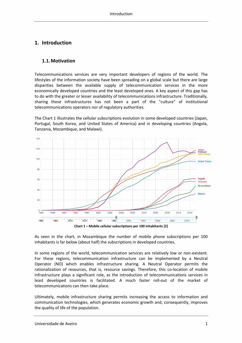
Telecommunications services are very important developers of regions of the world. The lifestyles of the information society have been spreading on a global scale but there are large disparities between the available supply of telecommunication services in the more economically developed countries and the least developed ones. A key aspect of this gap has to do with the greater or lesser availability of telecommunications infrastructure. Traditionally, sharing these infrastructures has not been a part of the "culture" of institutional telecommunications operators nor of regulatory authorities. The Chart 1 illustrates the cellular subscriptions evolution in some developed countries (Japan, Portugal, South Korea, and United States of America) and in developing countries (Angola, Tanzania, Mozambique, and Malawi).
Chart 1 – Mobile cellular subscriptions per 100 inhabitants [2]
As seen in the chart, in Mozambique the number of mobile phone subscriptions per 100 inhabitants is far below (about half) the subscriptions in developed countries. In some regions of the world, telecommunication services are relatively low or non-existent. For these regions, telecommunication infrastructure can be implemented by a Neutral Operator (NO) which enables infrastructure sharing. A Neutral Operator permits the rationalization of resources, that is, resource savings. Therefore, this co-location of mobile infrastructure plays a significant role, as the introduction of telecommunications services in least developed countries is facilitated. A much faster roll-out of the market of telecommunications can then take place. Ultimately, mobile infrastructure sharing permits increasing the access to information and communication technologies, which generates economic growth and, consequently, improves the quality of life of the population.
Telecommunication Infrastructure Sharing
2 Departamento de Eletrónica, Telecomunicações e Informática
1.2. Telecommunication and socio-economic development
Telecommunication infrastructure is not only important for domestic growth but also to connect domestic market of commodities and financial markets, which helps develop the foreign direct investment, among others. [99] Telecommunication infrastructures have a positive impact on the overall productivity of an economy, and, as a consequence, influence significantly and positively economic growth in the long term and contribute to a decline in income inequality, especially in developing countries. [5] [99] According to Qiang (2009) in a recent World Bank analysis to test the impact of telecommunications penetration on economic growth rates, it was demonstrated that for every 10% point increase in the penetration of mobile phones, there is an increase in economic growth of 0,81% points in developing countries. [144] According to a study conducted by Deloitte for Telenor, the mobile communications industry contributes to between 3,7% and 6,2% of GDP1 in the Telenor markets (Bangladesh, Malaysia, Pakistan, Thailand, Serbia and Ukraine)2. [128] [129] The mobile industry is, hence, crucial to the economic growth of developing nations:
It contributes to employment creation as it promotes business;
It attracts FDI which in turn generate high earning job opportunities, increase in demand for skilled labor, increase trade, among others;
And it allows the economy to develop further since the telecommunication sector indirectly establishes a more competitive labor market as firms can connect to each other more easily at a national and international levels, and since it enhances the growth of other sectors – agriculture, education, industry, health, banking, defense, transportation and tourism. [99] [128]
Furthermore, the telecommunication sector also contributes to social welfare, for instance through connecting people in remote areas to basic utilities such as banking and health care, and by making it easier for people to communicate with friends and family in distant locations. [128]
1 Gross Domestic Product is defined by the Organization for Economic Co-operation and Development
(OCDE) as “an aggregate measure of production equal to the sum of the gross values added of all resident, institutional units engaged in production (plus any taxes, and minus any subsidies, on products not included in the value of their outputs)” [127] 2 All numbers are based on a study undertaken by Deloitte for the Telenor Group in 2008. [129]
Introduction
Universidade de Aveiro 3
1.3. Objectives
The main goals of this work project can be defined as:
Contribute to a better understanding of the technological, economic and regulatory challenges associated with the sharing of telecommunications infrastructure.
Identify and analyze solutions for Telecommunications Infrastructure Sharing both in technical and economical terms
Develop methodologies and planning tools for Telecommunications Infrastructure Sharing.
Apply the methodology and tools developed to a concrete case study in Mozambique.
1.4. Methodology
The methodology used in this project work is:
Familiarization with the Telecommunication Infrastructure Sharing.
Familiarization with the state of art of the technologies (GSM, UMTS and LTE architectures).
Familiarization with the complexity and granularity of these technologies and identification of critical elements and functions.
Construction and development tools for the techno-economic analysis of Telecommunications Infrastructure Sharing.
Construction of the scenarios (Case Study) - Socio-geographic - Network scenarios
Technological solutions and business models for sharing of telecommunications infrastructure.
Technical and economic assessment of the modeled study scenarios.
Interpretation of results.
Presentation of conclusions of the work.
Presentation of recommendations.
Telecommunication Infrastructure Sharing
4 Departamento de Eletrónica, Telecomunicações e Informática
1.5. Document Structure
This Section provides a brief description of the contents and purposes of each one of the 6 Chapters that comprise this dissertation:
Chapter 1, “Introduction”: A brief exposition on the motivation, the importance and impact of telecommunications in emerging economies, objectives and methodology of this work.
Chapter 2, “Mobile Communication Technologies”: Gives a brief description of the history, current developments, main areas of applications, concerns and opportunities of telecommunications networks.
Chapter 3, “Business Models Issues”: Explanation of infrastructures sharing and business models of its implementation.
Chapter 4, “Network Dimensioning”: This chapter presents a explanation of network dimensioning and an analysis technological and economic. A techno-economic tool for Neutral Operator was also developed. This tool was built with the objective of developing scenarios and provides techno-economic results of a network infrastructure implementation.
Chapter 5, “Case Study”: Case study of three scenarios developed for Mozambique, demonstrating the usability and usefulness of the tool presented on chapter 4. This Case Study is a continuation of previous work projects developed by the Department of Electronics, Telecommunications and Informatics (DETI) of University of Aveiro (UA).
Chapter 6, “Final Considerations”: Conclusions on the legitimacy of the hypothesis, models and tools developed over the course of this work, and on the results achieved by the case study. Future developments and improvements on the proposed sharing model and on the tool are suggested.

Mobile Communication Technologies
Universidade de Aveiro 5
2. Mobile Communication Technologies
In this chapter, a brief overview of Mobile Communication Technologies is firstly presented, focusing on the evolution of technologies. Further on, definitions of telecommunications concepts are made and communication technologies are compared between them.
2.1. Overview of mobile communication
1G: The first mobile communication system (1G) to be created was the Advanced Mobile Phone System (AMPS). The AMPS allowed only voice calls through continuous waves. This system had several limitations as the analog system did not support any type of information encryption and had poor sound quality and a low transfer speed (was around 9.6 kbps). The first Generation employed the Frequency Division Multiple Access (FDMA), which was adopted by several countries in Europe, such as Total Access Communications System (TACS) in the United Kingdom, Italy, Spain, Austria and Ireland and the C-450 in Portugal and France. Due to the diversity of systems, as each had its own pattern and did allow for interconnection, an incompatibility between them arose. In addition, the existence bands did not support the extensive number of calls. Therefore, to respond to this demand for increasing capacity, the 2G was created. [36] 2G: The 2G Global System for Mobile Communications (GSM) replaced the analog broadcasts by digital. The quality, robustness/reliability, safety, efficient use of spectrum and the support for low-speed data services were the most important features that characterized the development of this generation (2G). Whit this Generation came a feature that is now trivial: send and receive SMS. [1] The technologies used by the second generation were based on the Time Division Multiplexing Access systems (TDMA) and Code Division Multiplexing Access (CDMA), and were the following:
Integrated Digital Enhanced Network (iDEN), the property Nextel network in the United States and Telus Mobility in Canada;
TDMA IS-54, American system, is a further development of AMPS and it amplifies the capacity of the system (in each analog channel 3 digital channels TDMA were included);
The Personal Handyphon System (PHS), originally used by NTT DoCoMo company in Japan, had a standard more focused on data transfer than the rest 2G standards;
Personal Digital Cellular (PDC) based on TDMA and used exclusively in Japan;
CDMA IS-96, was adopted in North America and in some countries in South America and Asia, and used the same frequency as the analog AMPS and was not compatible with the TDMA IS-54;
Global System for Mobile Communications (GSM) standard was created in Europe and recognized by all European countries in order to substitute incompatible analog systems. This system operated initially in the range of 900 MHz, but shortly after began to operate in the 1800 MHz band in Europe. The United States, on the other hand, used bands of 850 MHz and 1900 MHz. The GSM became, therefore, a worldwide standard being adopted throughout Europe, in several countries in Asia and in Canada, among others. [1] [8] [36] [49]
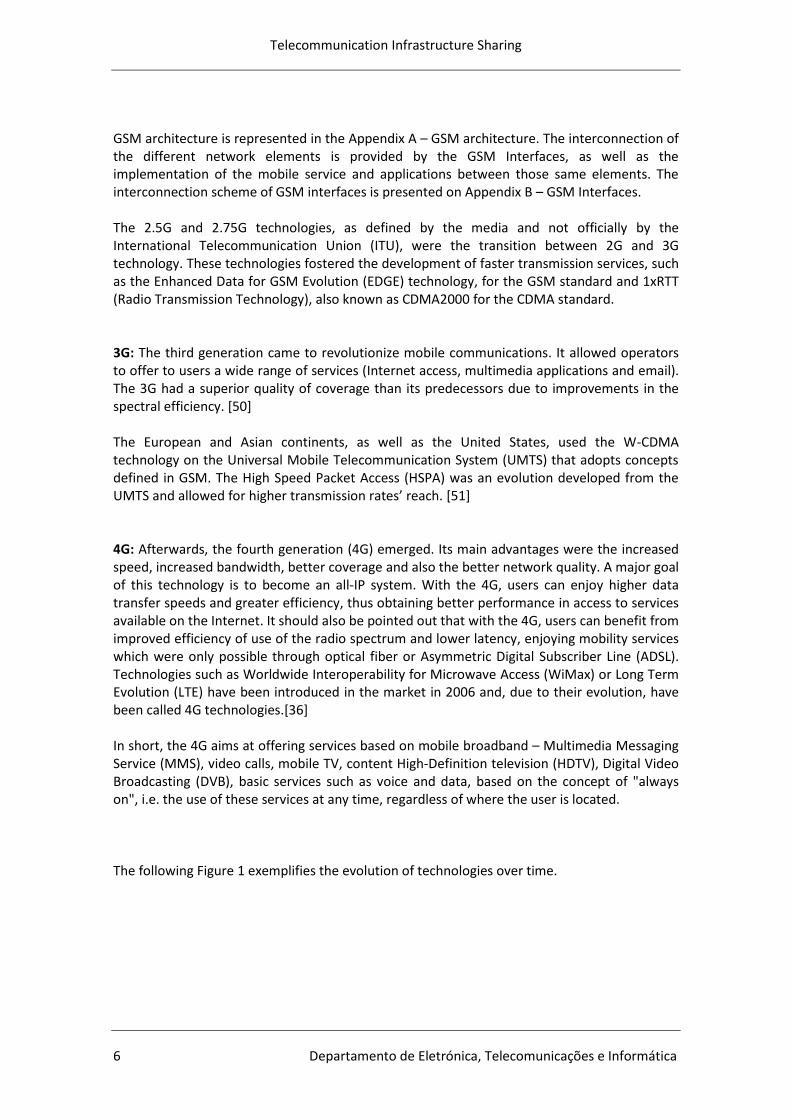
Telecommunication Infrastructure Sharing
6 Departamento de Eletrónica, Telecomunicações e Informática
GSM architecture is represented in the Appendix A – GSM architecture. The interconnection of the different network elements is provided by the GSM Interfaces, as well as the implementation of the mobile service and applications between those same elements. The interconnection scheme of GSM interfaces is presented on Appendix B – GSM Interfaces. The 2.5G and 2.75G technologies, as defined by the media and not officially by the International Telecommunication Union (ITU), were the transition between 2G and 3G technology. These technologies fostered the development of faster transmission services, such as the Enhanced Data for GSM Evolution (EDGE) technology, for the GSM standard and 1xRTT (Radio Transmission Technology), also known as CDMA2000 for the CDMA standard. 3G: The third generation came to revolutionize mobile communications. It allowed operators to offer to users a wide range of services (Internet access, multimedia applications and email). The 3G had a superior quality of coverage than its predecessors due to improvements in the spectral efficiency. [50] The European and Asian continents, as well as the United States, used the W-CDMA technology on the Universal Mobile Telecommunication System (UMTS) that adopts concepts defined in GSM. The High Speed Packet Access (HSPA) was an evolution developed from the UMTS and allowed for higher transmission rates’ reach. [51] 4G: Afterwards, the fourth generation (4G) emerged. Its main advantages were the increased speed, increased bandwidth, better coverage and also the better network quality. A major goal of this technology is to become an all-IP system. With the 4G, users can enjoy higher data transfer speeds and greater efficiency, thus obtaining better performance in access to services available on the Internet. It should also be pointed out that with the 4G, users can benefit from improved efficiency of use of the radio spectrum and lower latency, enjoying mobility services which were only possible through optical fiber or Asymmetric Digital Subscriber Line (ADSL). Technologies such as Worldwide Interoperability for Microwave Access (WiMax) or Long Term Evolution (LTE) have been introduced in the market in 2006 and, due to their evolution, have been called 4G technologies.[36] In short, the 4G aims at offering services based on mobile broadband – Multimedia Messaging Service (MMS), video calls, mobile TV, content High-Definition television (HDTV), Digital Video Broadcasting (DVB), basic services such as voice and data, based on the concept of "always on", i.e. the use of these services at any time, regardless of where the user is located. The following Figure 1 exemplifies the evolution of technologies over time.
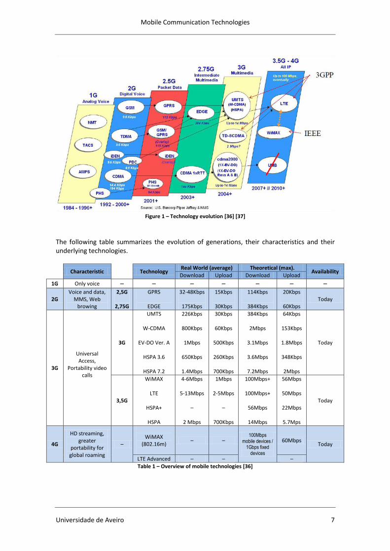
Mobile Communication Technologies
Universidade de Aveiro 7
Figure 1 – Technology evolution [36] [37]
The following table summarizes the evolution of generations, their characteristics and their underlying technologies.
Characteristic Technology Real World (average) Theoretical (max).
Availability Download Upload Download Upload
1G Only voice – – – – – – –
2G Voice and data,
MMS, Web browing
2,5G
2,75G
GPRS
EDGE
32-48Kbps
175Kbps
15Kbps
30Kbps
114Kbps
384Kbps
20Kbps
60Kbps Today
3G
Universal Access,
Portability video calls
3G
UMTS
W-CDMA
EV-DO Ver. A
HSPA 3.6
HSPA 7.2
226Kbps
800Kbps
1Mbps
650Kbps
1.4Mbps
30Kbps
60Kbps
500Kbps
260Kbps
700Kbps
384Kbps
2Mbps
3.1Mbps
3.6Mbps
7.2Mbps
64Kbps
153Kbps
1.8Mbps
348Kbps
2Mbps
Today
3,5G
WiMAX
LTE
HSPA+
HSPA
4-6Mbps
5-13Mbps
–
2 Mbps
1Mbps
2-5Mbps
–
700Kbps
100Mbps+
100Mbps+
56Mbps
14Mbps
56Mbps
50Mbps
22Mbps
5.7Mps
Today
4G
HD streaming, greater
portability for global roaming
–
WiMAX
(802.16m)
– – 100Mbps
mobile devices / 1Gbps fixed
devices
60Mbps Today
LTE Advanced – – –
Table 1 – Overview of mobile technologies [36]
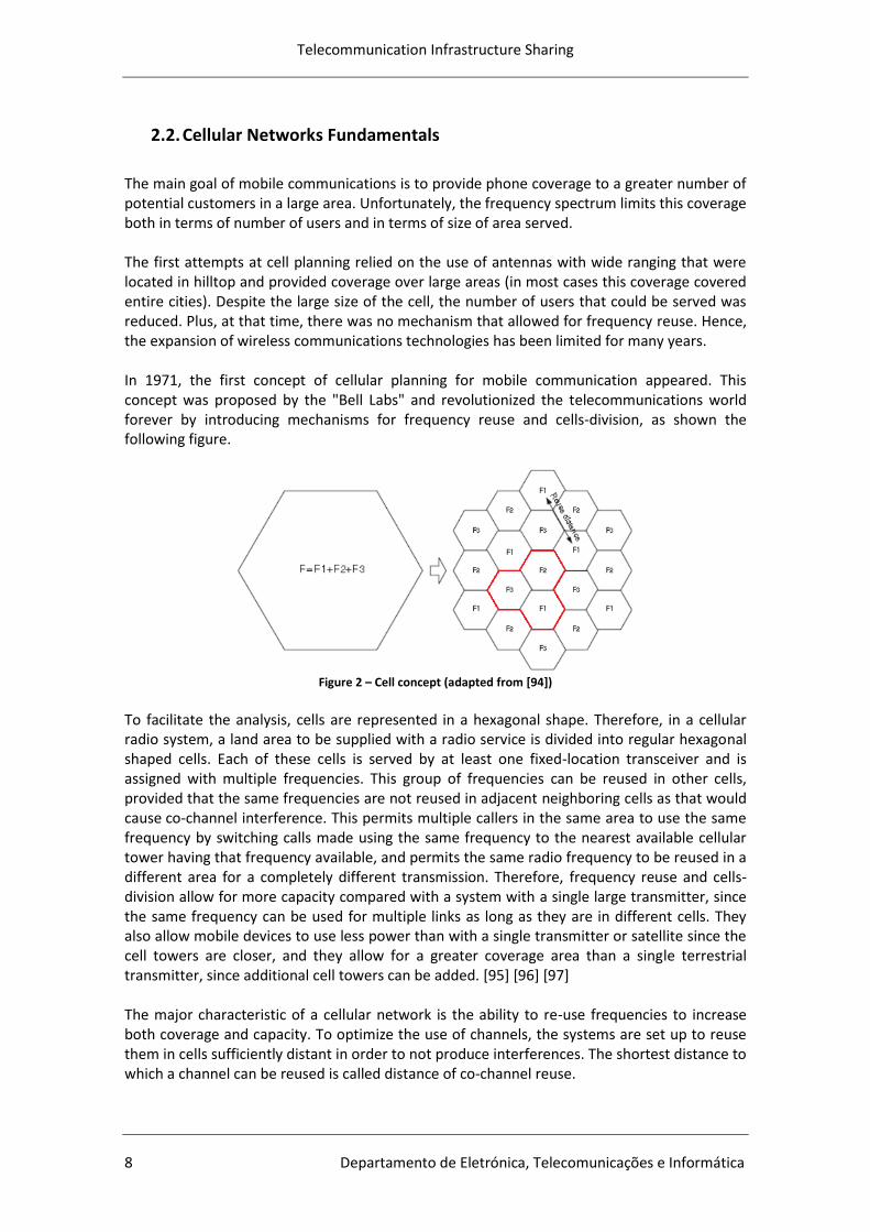
Telecommunication Infrastructure Sharing
8 Departamento de Eletrónica, Telecomunicações e Informática
2.2. Cellular Networks Fundamentals
The main goal of mobile communications is to provide phone coverage to a greater number of potential customers in a large area. Unfortunately, the frequency spectrum limits this coverage both in terms of number of users and in terms of size of area served. The first attempts at cell planning relied on the use of antennas with wide ranging that were located in hilltop and provided coverage over large areas (in most cases this coverage covered entire cities). Despite the large size of the cell, the number of users that could be served was reduced. Plus, at that time, there was no mechanism that allowed for frequency reuse. Hence, the expansion of wireless communications technologies has been limited for many years. In 1971, the first concept of cellular planning for mobile communication appeared. This concept was proposed by the "Bell Labs" and revolutionized the telecommunications world forever by introducing mechanisms for frequency reuse and cells-division, as shown the following figure.
Figure 2 – Cell concept (adapted from [94])
To facilitate the analysis, cells are represented in a hexagonal shape. Therefore, in a cellular radio system, a land area to be supplied with a radio service is divided into regular hexagonal shaped cells. Each of these cells is served by at least one fixed-location transceiver and is assigned with multiple frequencies. This group of frequencies can be reused in other cells, provided that the same frequencies are not reused in adjacent neighboring cells as that would cause co-channel interference. This permits multiple callers in the same area to use the same frequency by switching calls made using the same frequency to the nearest available cellular tower having that frequency available, and permits the same radio frequency to be reused in a different area for a completely different transmission. Therefore, frequency reuse and cells-division allow for more capacity compared with a system with a single large transmitter, since the same frequency can be used for multiple links as long as they are in different cells. They also allow mobile devices to use less power than with a single transmitter or satellite since the cell towers are closer, and they allow for a greater coverage area than a single terrestrial transmitter, since additional cell towers can be added. [95] [96] [97] The major characteristic of a cellular network is the ability to re-use frequencies to increase both coverage and capacity. To optimize the use of channels, the systems are set up to reuse them in cells sufficiently distant in order to not produce interferences. The shortest distance to which a channel can be reused is called distance of co-channel reuse.
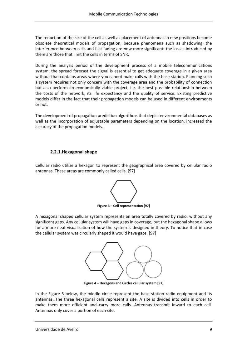
Mobile Communication Technologies
Universidade de Aveiro 9
The reduction of the size of the cell as well as placement of antennas in new positions become obsolete theoretical models of propagation, because phenomena such as shadowing, the interference between cells and fast fading are now more significant: the losses introduced by them are those that limit the cells in terms of SNR. During the analysis period of the development process of a mobile telecommunications system, the spread forecast the signal is essential to get adequate coverage in a given area without that contains areas where you cannot make calls with the base station. Planning such a system requires not only concern with the coverage area and the probability of connection but also perform an economically viable project, i.e. the best possible relationship between the costs of the network, its life expectancy and the quality of service. Existing predictive models differ in the fact that their propagation models can be used in different environments or not. The development of propagation prediction algorithms that depict environmental databases as well as the incorporation of adjustable parameters depending on the location, increased the accuracy of the propagation models.
2.2.1.Hexagonal shape
Cellular radio utilize a hexagon to represent the geographical area covered by cellular radio antennas. These areas are commonly called cells. [97]
Figure 3 – Cell representation [97]
A hexagonal shaped cellular system represents an area totally covered by radio, without any significant gaps. Any cellular system will have gaps in coverage, but the hexagonal shape allows for a more neat visualization of how the system is designed in theory. To notice that in case the cellular system was circularly shaped it would have gaps. [97]
Figure 4 – Hexagons and Circles cellular system [97]
In the Figure 5 below, the middle circle represent the base station radio equipment and its antennas. The three hexagonal cells represent a site. A site is divided into cells in order to make them more efficient and carry more calls. Antennas transmit inward to each cell. Antennas only cover a portion of each site.
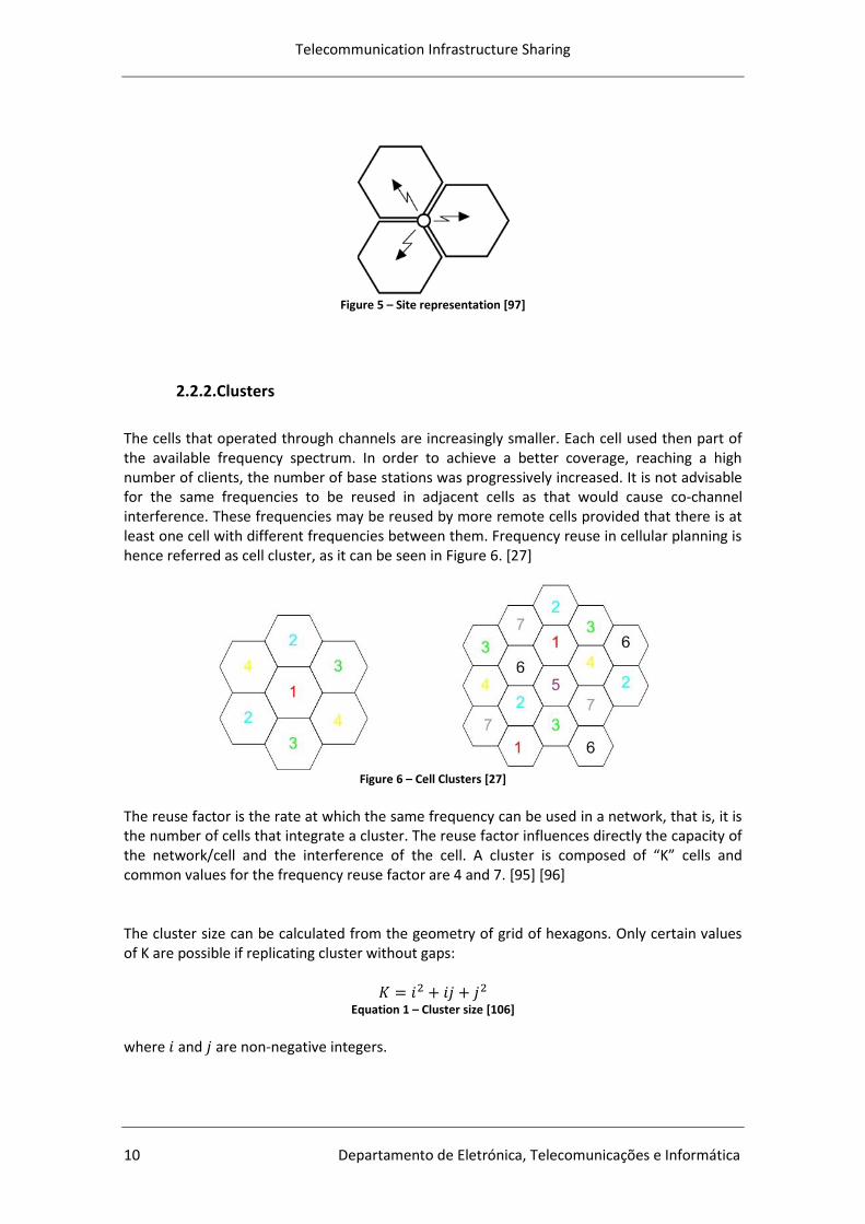
Telecommunication Infrastructure Sharing
10 Departamento de Eletrónica, Telecomunicações e Informática
Figure 5 – Site representation [97]
2.2.2.Clusters
The cells that operated through channels are increasingly smaller. Each cell used then part of the available frequency spectrum. In order to achieve a better coverage, reaching a high number of clients, the number of base stations was progressively increased. It is not advisable for the same frequencies to be reused in adjacent cells as that would cause co-channel interference. These frequencies may be reused by more remote cells provided that there is at least one cell with different frequencies between them. Frequency reuse in cellular planning is hence referred as cell cluster, as it can be seen in Figure 6. [27]
Figure 6 – Cell Clusters [27]
The reuse factor is the rate at which the same frequency can be used in a network, that is, it is the number of cells that integrate a cluster. The reuse factor influences directly the capacity of the network/cell and the interference of the cell. A cluster is composed of “K” cells and common values for the frequency reuse factor are 4 and 7. [95] [96] The cluster size can be calculated from the geometry of grid of hexagons. Only certain values of K are possible if replicating cluster without gaps:
Equation 1 – Cluster size [106]
where and are non-negative integers.
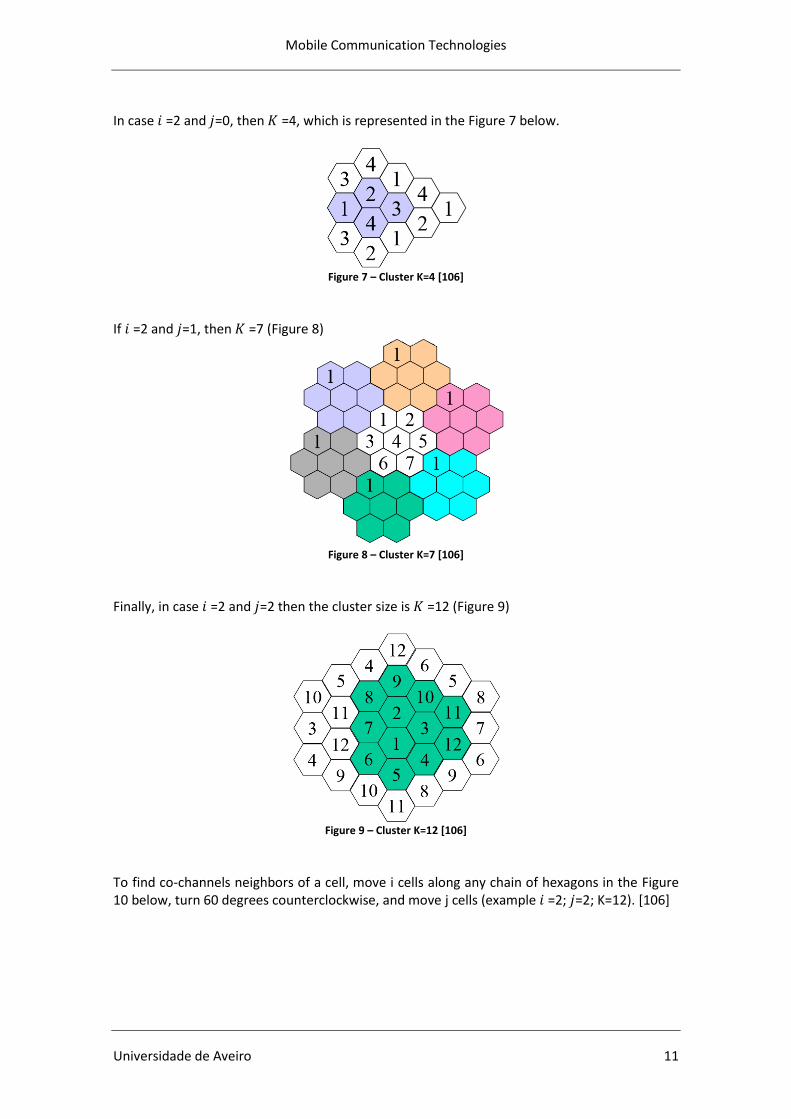
Mobile Communication Technologies
Universidade de Aveiro 11
In case =2 and =0, then =4, which is represented in the Figure 7 below.
Figure 7 – Cluster K=4 [106]
If =2 and =1, then =7 (Figure 8)
Figure 8 – Cluster K=7 [106]
Finally, in case =2 and =2 then the cluster size is =12 (Figure 9)
Figure 9 – Cluster K=12 [106]
To find co-channels neighbors of a cell, move i cells along any chain of hexagons in the Figure 10 below, turn 60 degrees counterclockwise, and move j cells (example =2; =2; K=12). [106]
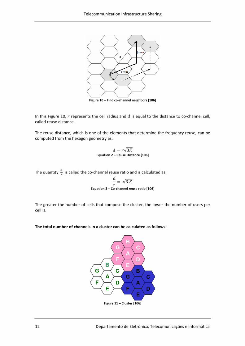
Telecommunication Infrastructure Sharing
12 Departamento de Eletrónica, Telecomunicações e Informática
Figure 10 – Find co-channel neighbors [106]
In this Figure 10, represents the cell radius and is equal to the distance to co-channel cell, called reuse distance. The reuse distance, which is one of the elements that determine the frequency reuse, can be computed from the hexagon geometry as:
Equation 2 – Reuse Distance [106]
The quantity
is called the co-channel reuse ratio and is calculated as:
Equation 3 – Co-channel reuse ratio [106]
The greater the number of cells that compose the cluster, the lower the number of users per cell is. The total number of channels in a cluster can be calculated as follows:
Figure 11 – Cluster [106]
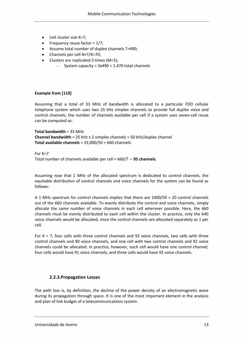
Mobile Communication Technologies
Universidade de Aveiro 13
Cell cluster size K=7;
Frequency reuse factor = 1/7;
Assume total number of duplex channels T=490;
Channels per cell N=T/K=70;
Clusters are replicated 3 times (M=3); - System capacity = 3x490 = 1.470 total channels
Example from [110] Assuming that a total of 33 MHz of bandwidth is allocated to a particular FDD cellular telephone system which uses two 25 kHz simplex channels to provide full duplex voice and control channels, the number of channels available per cell if a system uses seven-cell reuse can be computed as: Total bandwidth = 33 MHz Channel bandwidth = 25 kHz x 2 simplex channels = 50 kHz/duplex channel Total available channels = 33,000/50 = 660 channels For K=7 Total number of channels available per cell = 660/7 95 channels. Assuming now that 1 MHz of the allocated spectrum is dedicated to control channels, the equitable distribution of control channels and voice channels for the system can be found as follows: A 1 MHz spectrum for control channels implies that there are 1000/50 = 20 control channels out of the 660 channels available. To evenly distribute the control and voice channels, simply allocate the same number of voice channels in each cell wherever possible. Here, the 660 channels must be evenly distributed to each cell within the cluster. In practice, only the 640 voice channels would be allocated, since the control channels are allocated separately as 1 per cell. For K = 7, four cells with three control channels and 92 voice channels, two cells with three control channels and 90 voice channels, and one cell with two control channels and 92 voice channels could be allocated. In practice, however, each cell would have one control channel, four cells would have 91 voice channels, and three cells would have 92 voice channels.
2.2.3.Propagation Losses
The path loss is, by definition, the decline of the power density of an electromagnetic wave during its propagation through space. It is one of the most important element in the analysis and plan of link budget of a telecommunications system.
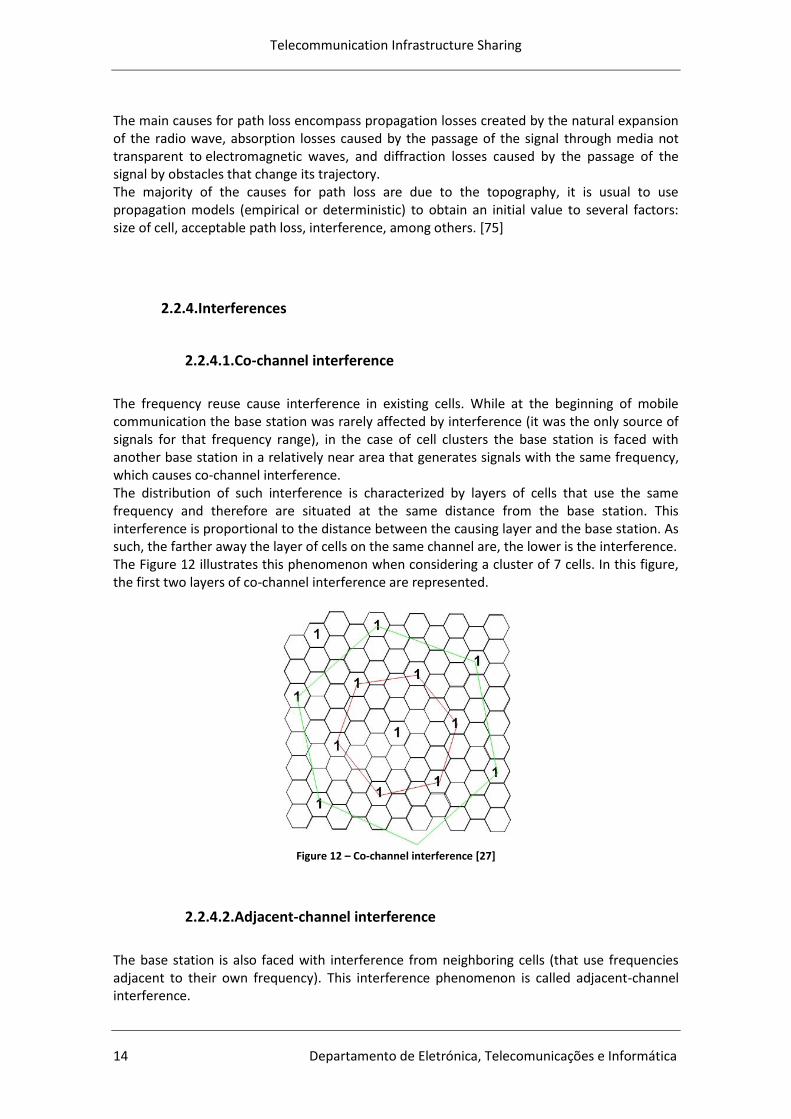
Telecommunication Infrastructure Sharing
14 Departamento de Eletrónica, Telecomunicações e Informática
The main causes for path loss encompass propagation losses created by the natural expansion of the radio wave, absorption losses caused by the passage of the signal through media not transparent to electromagnetic waves, and diffraction losses caused by the passage of the signal by obstacles that change its trajectory. The majority of the causes for path loss are due to the topography, it is usual to use propagation models (empirical or deterministic) to obtain an initial value to several factors: size of cell, acceptable path loss, interference, among others. [75]
2.2.4.Interferences
2.2.4.1.Co-channel interference
The frequency reuse cause interference in existing cells. While at the beginning of mobile communication the base station was rarely affected by interference (it was the only source of signals for that frequency range), in the case of cell clusters the base station is faced with another base station in a relatively near area that generates signals with the same frequency, which causes co-channel interference. The distribution of such interference is characterized by layers of cells that use the same frequency and therefore are situated at the same distance from the base station. This interference is proportional to the distance between the causing layer and the base station. As such, the farther away the layer of cells on the same channel are, the lower is the interference. The Figure 12 illustrates this phenomenon when considering a cluster of 7 cells. In this figure, the first two layers of co-channel interference are represented.
Figure 12 – Co-channel interference [27]
2.2.4.2.Adjacent-channel interference
The base station is also faced with interference from neighboring cells (that use frequencies adjacent to their own frequency). This interference phenomenon is called adjacent-channel interference.

Mobile Communication Technologies
Universidade de Aveiro 15
The main causes for adjacent-channel interference are:
Attribution of adjacent frequencies in the same cell;
Inadequate filtering in the recpetor;
Near-far effect;
Nonlinearities of spectrum reuse. [107] There are several methods to minimize the adjacent-channel interference, but none can entirely eliminate it. The main reduction methods used are to license carefully the frequency of cell (taking account the frequencies used by neighboring cells), use filters in the receptors with higher quality factor Q, control dynamically the power of the base station, among others. In the following Figure 13, two examples of adjacent-channel interference management are presented. The first figure is an example of bad licensing of adjacent-channel interference, while in the second case the attribution of adjacent-channel interference was done more carefully.
Figure 13 – Example of frequencies attribution [94]
2.2.4.3.Internal Interferences
There are also internal interferences worth mentioning. This one can be of two types: multipath interference and multiple access interference. The multipath interference is present in all communications systems that are near the surface. It is the interference caused by the reflections of the transmitted signal since, if the reflected signals roam different distances, they can reach the destination with a different amplitude and a different phase. This phenomenon can be observed in Figure 14. The multiple-access interference occurs in systems whose modulation works with CDMA as a base. A good example is the UMTS because in such systems the cell receives a power that grows according to the number of connected users.
Figure 14 – Multipath Interference [27]
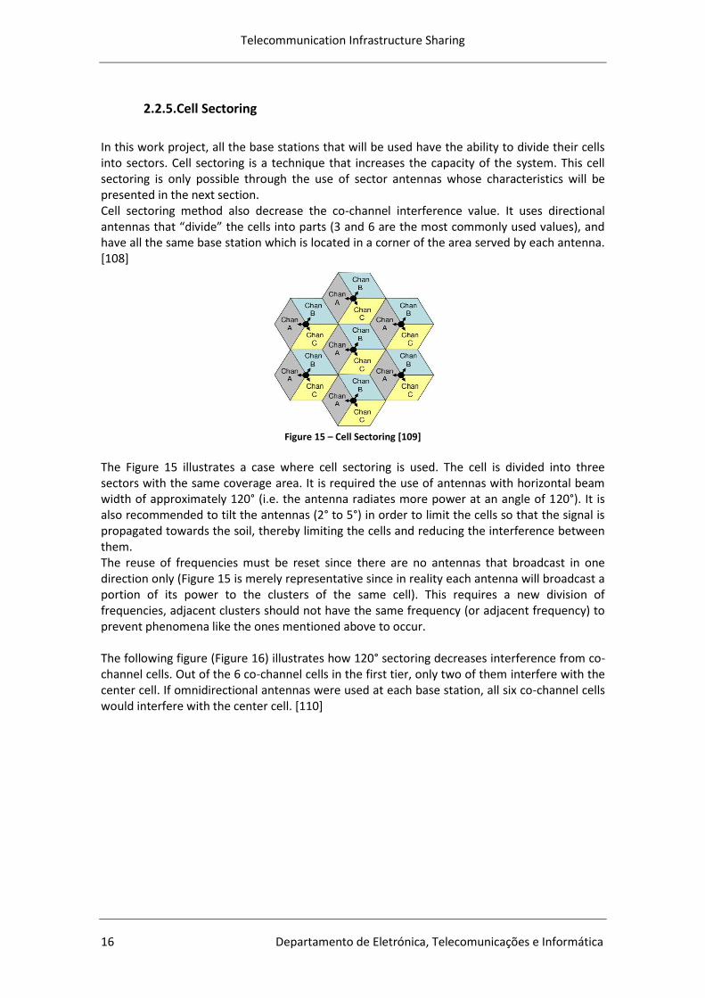
Telecommunication Infrastructure Sharing
16 Departamento de Eletrónica, Telecomunicações e Informática
2.2.5.Cell Sectoring
In this work project, all the base stations that will be used have the ability to divide their cells into sectors. Cell sectoring is a technique that increases the capacity of the system. This cell sectoring is only possible through the use of sector antennas whose characteristics will be presented in the next section. Cell sectoring method also decrease the co-channel interference value. It uses directional antennas that “divide” the cells into parts (3 and 6 are the most commonly used values), and have all the same base station which is located in a corner of the area served by each antenna. [108]
Figure 15 – Cell Sectoring [109]
The Figure 15 illustrates a case where cell sectoring is used. The cell is divided into three sectors with the same coverage area. It is required the use of antennas with horizontal beam width of approximately 120° (i.e. the antenna radiates more power at an angle of 120°). It is also recommended to tilt the antennas (2° to 5°) in order to limit the cells so that the signal is propagated towards the soil, thereby limiting the cells and reducing the interference between them. The reuse of frequencies must be reset since there are no antennas that broadcast in one direction only (Figure 15 is merely representative since in reality each antenna will broadcast a portion of its power to the clusters of the same cell). This requires a new division of frequencies, adjacent clusters should not have the same frequency (or adjacent frequency) to prevent phenomena like the ones mentioned above to occur. The following figure (Figure 16) illustrates how 120° sectoring decreases interference from co-channel cells. Out of the 6 co-channel cells in the first tier, only two of them interfere with the center cell. If omnidirectional antennas were used at each base station, all six co-channel cells would interfere with the center cell. [110]

Mobile Communication Technologies
Universidade de Aveiro 17
Figure 16 – 120º Sectoring [110]
2.2.6.Antennas
The choice over an adequate antenna is critical for all wireless communications. This choice should consider a number of parameters, namely:
Operating Frequency: all antennas are designed to operate at a certain frequency. The operating frequency will determine the size of the antenna, and the frequency at which the antenna will achieve the highest performance (although the antenna might operate at another frequency than the operating frequency).
Directivity: it is the antenna's ability to transmit signals in a given direction or to reject the signals coming from another direction. It is also called beam angle, antennas only radiate at a certain angle, neglecting all the remaining space.
Gain: this parameter is more commonly used by manufacturers and describes how much power is transmitted in a certain direction (if the power input of the antenna is known). Gain is usually presented in dBi (it shows the comparison between the antenna and the isotropic antenna). [114]
Bandwidth: it is the range of frequencies over which the antenna can properly receive or radiate. [115]
Polarization: this parameter describes the direction of the electric field of electromagnetic waves. Polarization can either be linear (vertical or horizontal), circular, or elliptical. Each of these types has it own radition characterisitics. [116]
2.2.6.1.Sector Antennas
As mentioned, the base stations of the technologies have the ability to divide their cells into sectors. This sectoring is only possible through the use of sector antennas. One of the main
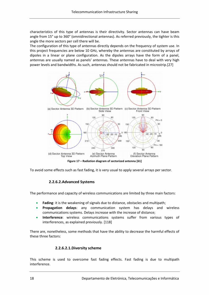
Telecommunication Infrastructure Sharing
18 Departamento de Eletrónica, Telecomunicações e Informática
characteristics of this type of antennas is their directivity. Sector antennas can have beam angle from 15° up to 360° (omnidirectional antennas). As referred previously, the tighter is this angle the more sectors per cell there will be. The configuration of this type of antennas directly depends on the frequency of system use. In this project frequencies are below 10 GHz, whereby the antennas are constituted by arrays of dipoles in a linear or plane configuration. As the dipoles arrays have the form of a panel, antennas are usually named as panels’ antennas. These antennas have to deal with very high power levels and bandwidths. As such, antennas should not be fabricated in microstrip.[27]
Figure 17 – Radiation diagram of sectorized antenna [61]
To avoid some effects such as fast fading, it is very usual to apply several arrays per sector.
2.2.6.2.Advanced Systems
The performance and capacity of wireless communications are limited by three main factors:
Fading: it is the weakening of signals due to distance, obstacles and multipath;
Propagation delays: any communication system has delays and wireless communications systems. Delays increase with the increase of distance;
Interference: wireless communications systems suffer from various types of interferences, as explained previously. [118]
There are, nonetheless, some methods that have the ability to decrease the harmful effects of these three factors:
2.2.6.2.1.Diversity scheme
This scheme is used to overcome fast fading effects. Fast fading is due to multipath interference.
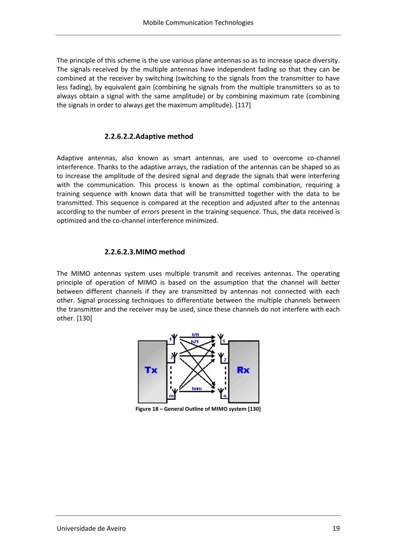
Mobile Communication Technologies
Universidade de Aveiro 19
The principle of this scheme is the use various plane antennas so as to increase space diversity. The signals received by the multiple antennas have independent fading so that they can be combined at the receiver by switching (switching to the signals from the transmitter to have less fading), by equivalent gain (combining he signals from the multiple transmitters so as to always obtain a signal with the same amplitude) or by combining maximum rate (combining the signals in order to always get the maximum amplitude). [117]
2.2.6.2.2.Adaptive method
Adaptive antennas, also known as smart antennas, are used to overcome co-channel interference. Thanks to the adaptive arrays, the radiation of the antennas can be shaped so as to increase the amplitude of the desired signal and degrade the signals that were interfering with the communication. This process is known as the optimal combination, requiring a training sequence with known data that will be transmitted together with the data to be transmitted. This sequence is compared at the reception and adjusted after to the antennas according to the number of errors present in the training sequence. Thus, the data received is optimized and the co-channel interference minimized.
2.2.6.2.3.MIMO method
The MIMO antennas system uses multiple transmit and receives antennas. The operating principle of operation of MIMO is based on the assumption that the channel will better between different channels if they are transmitted by antennas not connected with each other. Signal processing techniques to differentiate between the multiple channels between the transmitter and the receiver may be used, since these channels do not interfere with each other. [130]
Figure 18 – General Outline of MIMO system [130]
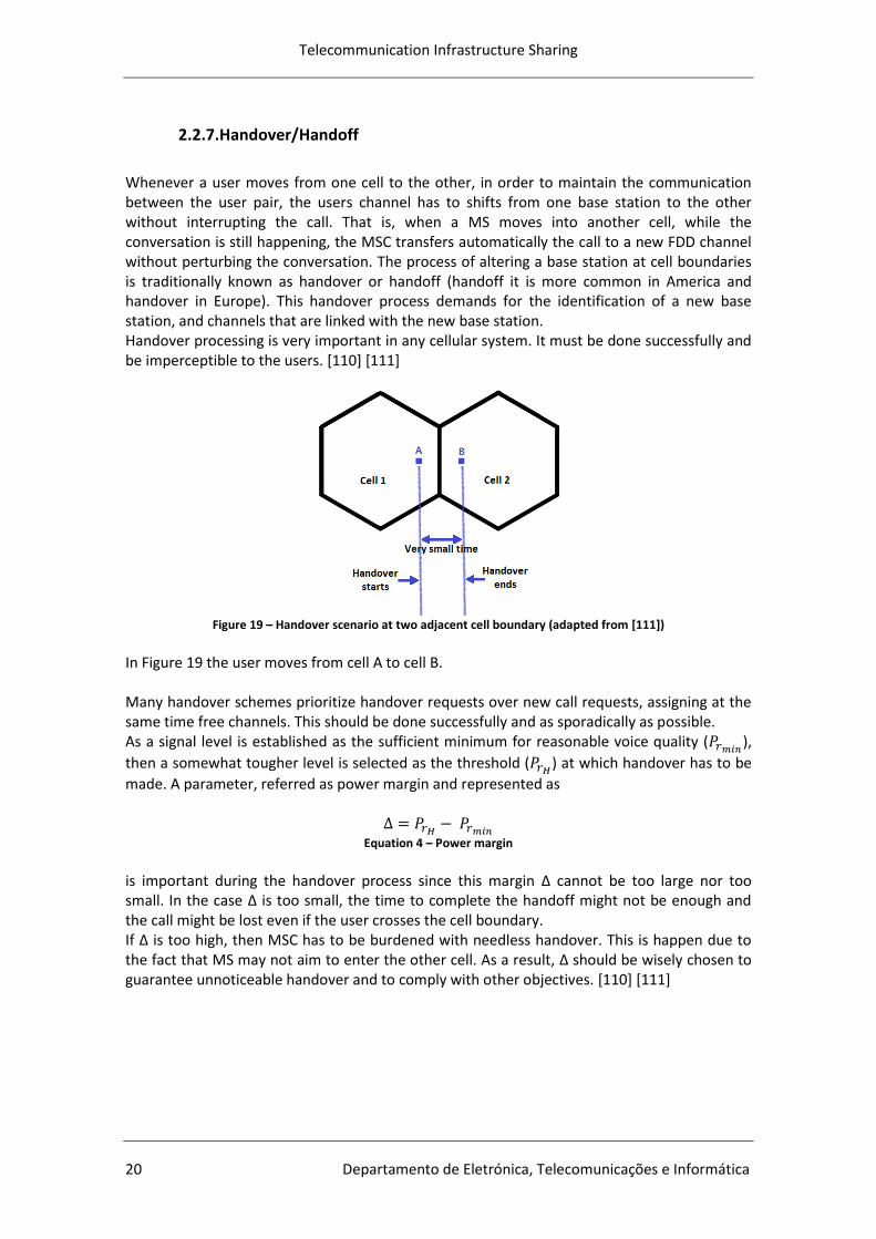
Telecommunication Infrastructure Sharing
20 Departamento de Eletrónica, Telecomunicações e Informática
2.2.7.Handover/Handoff
Whenever a user moves from one cell to the other, in order to maintain the communication between the user pair, the users channel has to shifts from one base station to the other without interrupting the call. That is, when a MS moves into another cell, while the conversation is still happening, the MSC transfers automatically the call to a new FDD channel without perturbing the conversation. The process of altering a base station at cell boundaries is traditionally known as handover or handoff (handoff it is more common in America and handover in Europe). This handover process demands for the identification of a new base station, and channels that are linked with the new base station. Handover processing is very important in any cellular system. It must be done successfully and be imperceptible to the users. [110] [111]
Figure 19 – Handover scenario at two adjacent cell boundary (adapted from [111])
In Figure 19 the user moves from cell A to cell B. Many handover schemes prioritize handover requests over new call requests, assigning at the same time free channels. This should be done successfully and as sporadically as possible. As a signal level is established as the sufficient minimum for reasonable voice quality (
),
then a somewhat tougher level is selected as the threshold ( ) at which handover has to be
made. A parameter, referred as power margin and represented as
Equation 4 – Power margin
is important during the handover process since this margin Δ cannot be too large nor too small. In the case Δ is too small, the time to complete the handoff might not be enough and the call might be lost even if the user crosses the cell boundary. If Δ is too high, then MSC has to be burdened with needless handover. This is happen due to the fact that MS may not aim to enter the other cell. As a result, Δ should be wisely chosen to guarantee unnoticeable handover and to comply with other objectives. [110] [111]
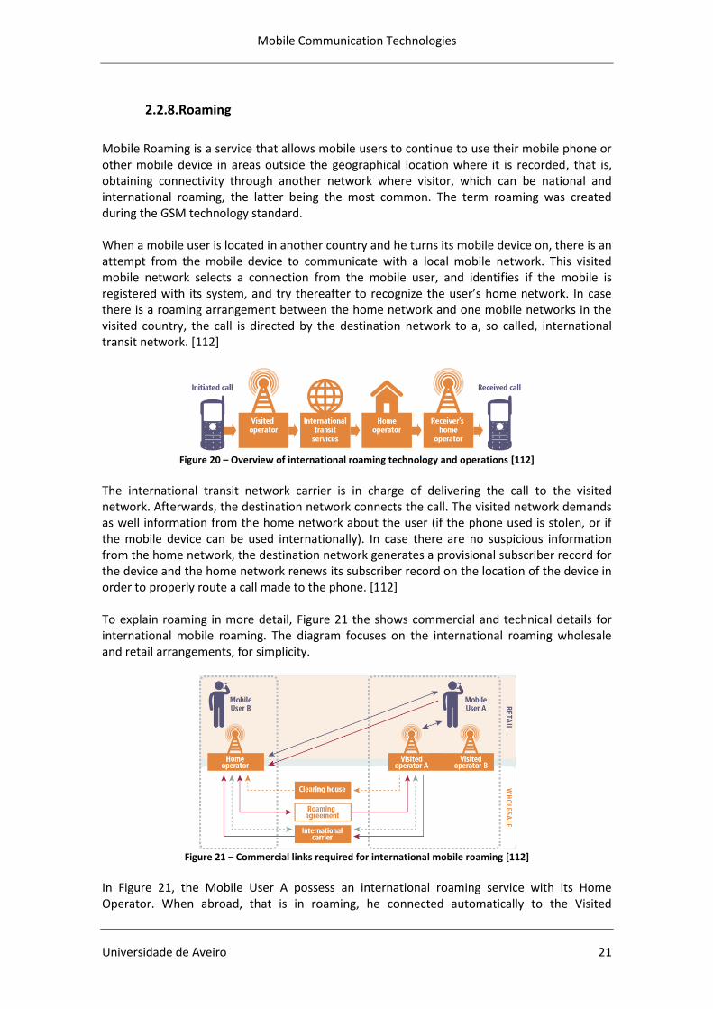
Mobile Communication Technologies
Universidade de Aveiro 21
2.2.8.Roaming
Mobile Roaming is a service that allows mobile users to continue to use their mobile phone or other mobile device in areas outside the geographical location where it is recorded, that is, obtaining connectivity through another network where visitor, which can be national and international roaming, the latter being the most common. The term roaming was created during the GSM technology standard. When a mobile user is located in another country and he turns its mobile device on, there is an attempt from the mobile device to communicate with a local mobile network. This visited mobile network selects a connection from the mobile user, and identifies if the mobile is registered with its system, and try thereafter to recognize the user’s home network. In case there is a roaming arrangement between the home network and one mobile networks in the visited country, the call is directed by the destination network to a, so called, international transit network. [112]
Figure 20 – Overview of international roaming technology and operations [112]
The international transit network carrier is in charge of delivering the call to the visited network. Afterwards, the destination network connects the call. The visited network demands as well information from the home network about the user (if the phone used is stolen, or if the mobile device can be used internationally). In case there are no suspicious information from the home network, the destination network generates a provisional subscriber record for the device and the home network renews its subscriber record on the location of the device in order to properly route a call made to the phone. [112] To explain roaming in more detail, Figure 21 the shows commercial and technical details for international mobile roaming. The diagram focuses on the international roaming wholesale and retail arrangements, for simplicity.
Figure 21 – Commercial links required for international mobile roaming [112]
In Figure 21, the Mobile User A possess an international roaming service with its Home Operator. When abroad, that is in roaming, he connected automatically to the Visited
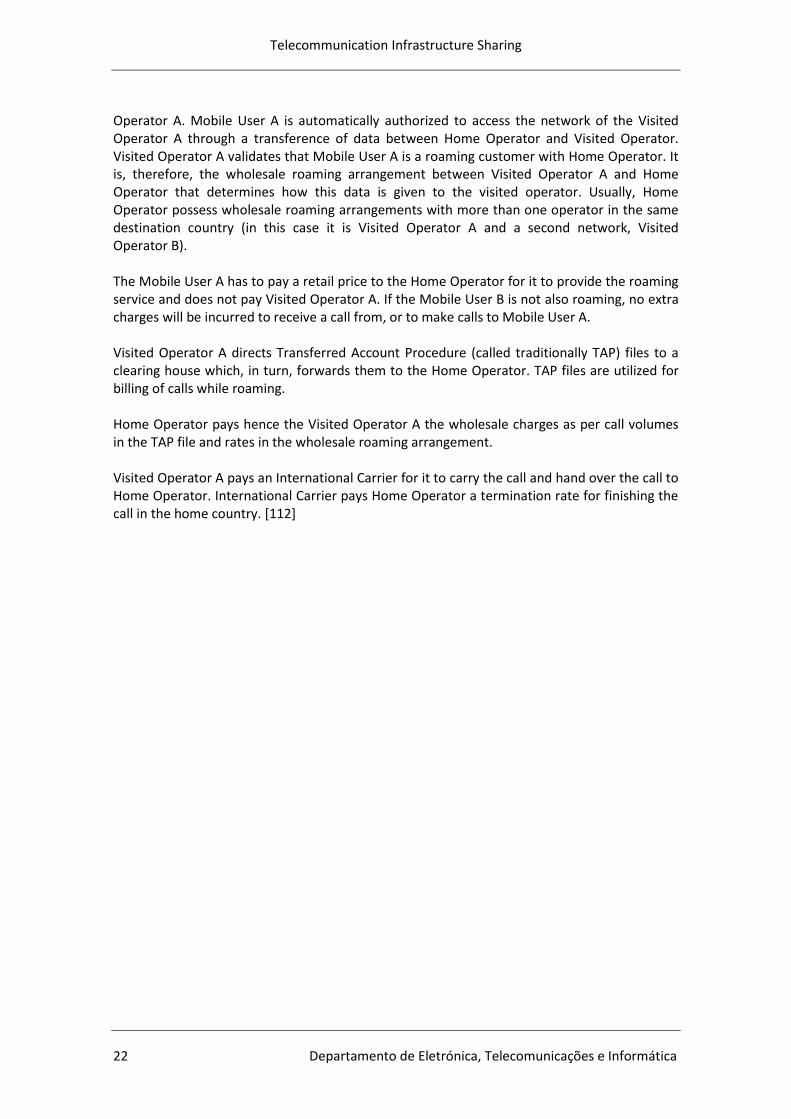
Telecommunication Infrastructure Sharing
22 Departamento de Eletrónica, Telecomunicações e Informática
Operator A. Mobile User A is automatically authorized to access the network of the Visited Operator A through a transference of data between Home Operator and Visited Operator. Visited Operator A validates that Mobile User A is a roaming customer with Home Operator. It is, therefore, the wholesale roaming arrangement between Visited Operator A and Home Operator that determines how this data is given to the visited operator. Usually, Home Operator possess wholesale roaming arrangements with more than one operator in the same destination country (in this case it is Visited Operator A and a second network, Visited Operator B). The Mobile User A has to pay a retail price to the Home Operator for it to provide the roaming service and does not pay Visited Operator A. If the Mobile User B is not also roaming, no extra charges will be incurred to receive a call from, or to make calls to Mobile User A. Visited Operator A directs Transferred Account Procedure (called traditionally TAP) files to a clearing house which, in turn, forwards them to the Home Operator. TAP files are utilized for billing of calls while roaming. Home Operator pays hence the Visited Operator A the wholesale charges as per call volumes in the TAP file and rates in the wholesale roaming arrangement. Visited Operator A pays an International Carrier for it to carry the call and hand over the call to Home Operator. International Carrier pays Home Operator a termination rate for finishing the call in the home country. [112]

Mobile Communication Technologies
Universidade de Aveiro 23
2.2.9.Multiple Access Techniques
The resources of access of the medium are the space and the spectrum (or time), however, by sharing the space (S), time (t), frequency (f) and codes (c) (see Figure 22) three access schemes emerge:
Frequency Division Multiple Access (FDMA).
Time Division Multiple Access (TDMA).
Code Division Multiple Access (CDMA).
Figure 22 – Existing resources in the access technique [36] [39]
In the FDMA a channel uses a certain band of the spectrum and different channels use different bands. That is, each call is assigned with its own frequency band during its length of action, with the entire frequency band divided in small individual channels for users to access. FDMA gives each user a different frequency, each user has its own frequency. One of the mostly known systems that work with FDMA are the FM radios where each radio station receives a certain frequency that belongs exclusively to that station. [36]
Figure 23 – FDMA scheme [39]
In TDMA the users share the same frequency band. To each call transmission a different timeslot is allocated. This principle is widely used in GSM mobile networks, where a GSM radio channel can be used by eight users. One of these users can be on air in a short period of time
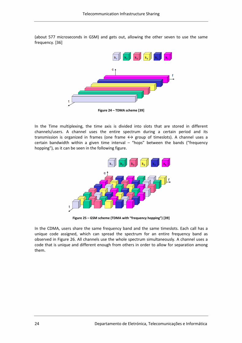
Telecommunication Infrastructure Sharing
24 Departamento de Eletrónica, Telecomunicações e Informática
(about 577 microseconds in GSM) and gets out, allowing the other seven to use the same frequency. [36]
Figure 24 – TDMA scheme [39]
In the Time multiplexing, the time axis is divided into slots that are stored in different channels/users. A channel uses the entire spectrum during a certain period and its transmission is organized in frames (one frame ↔ group of timeslots). A channel uses a certain bandwidth within a given time interval – “hops” between the bands ("frequency hopping"), as it can be seen in the following figure.
Figure 25 – GSM scheme (TDMA with “frequency hopping”) [39]
In the CDMA, users share the same frequency band and the same timeslots. Each call has a unique code assigned, which can spread the spectrum for an entire frequency band as observed in Figure 26. All channels use the whole spectrum simultaneously. A channel uses a code that is unique and different enough from others in order to allow for separation among them.
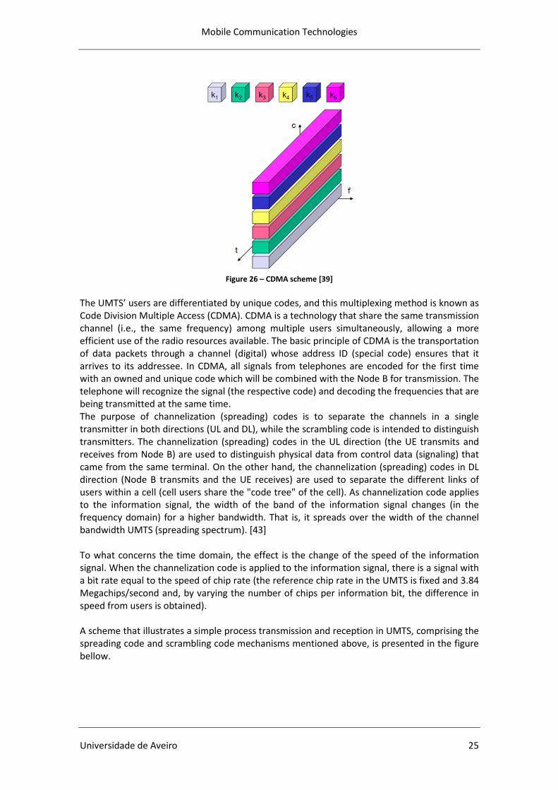
Mobile Communication Technologies
Universidade de Aveiro 25
Figure 26 – CDMA scheme [39]
The UMTS’ users are differentiated by unique codes, and this multiplexing method is known as Code Division Multiple Access (CDMA). CDMA is a technology that share the same transmission channel (i.e., the same frequency) among multiple users simultaneously, allowing a more efficient use of the radio resources available. The basic principle of CDMA is the transportation of data packets through a channel (digital) whose address ID (special code) ensures that it arrives to its addressee. In CDMA, all signals from telephones are encoded for the first time with an owned and unique code which will be combined with the Node B for transmission. The telephone will recognize the signal (the respective code) and decoding the frequencies that are being transmitted at the same time. The purpose of channelization (spreading) codes is to separate the channels in a single transmitter in both directions (UL and DL), while the scrambling code is intended to distinguish transmitters. The channelization (spreading) codes in the UL direction (the UE transmits and receives from Node B) are used to distinguish physical data from control data (signaling) that came from the same terminal. On the other hand, the channelization (spreading) codes in DL direction (Node B transmits and the UE receives) are used to separate the different links of users within a cell (cell users share the "code tree" of the cell). As channelization code applies to the information signal, the width of the band of the information signal changes (in the frequency domain) for a higher bandwidth. That is, it spreads over the width of the channel bandwidth UMTS (spreading spectrum). [43] To what concerns the time domain, the effect is the change of the speed of the information signal. When the channelization code is applied to the information signal, there is a signal with a bit rate equal to the speed of chip rate (the reference chip rate in the UMTS is fixed and 3.84 Megachips/second and, by varying the number of chips per information bit, the difference in speed from users is obtained). A scheme that illustrates a simple process transmission and reception in UMTS, comprising the spreading code and scrambling code mechanisms mentioned above, is presented in the figure bellow.
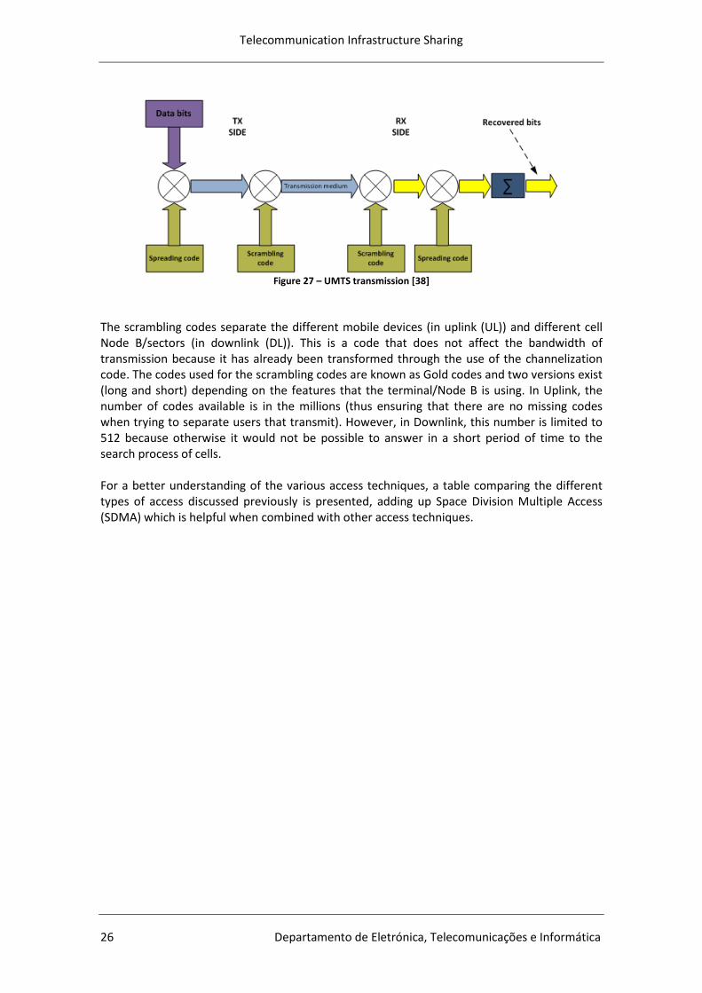
Telecommunication Infrastructure Sharing
26 Departamento de Eletrónica, Telecomunicações e Informática
Figure 27 – UMTS transmission [38]
The scrambling codes separate the different mobile devices (in uplink (UL)) and different cell Node B/sectors (in downlink (DL)). This is a code that does not affect the bandwidth of transmission because it has already been transformed through the use of the channelization code. The codes used for the scrambling codes are known as Gold codes and two versions exist (long and short) depending on the features that the terminal/Node B is using. In Uplink, the number of codes available is in the millions (thus ensuring that there are no missing codes when trying to separate users that transmit). However, in Downlink, this number is limited to 512 because otherwise it would not be possible to answer in a short period of time to the search process of cells. For a better understanding of the various access techniques, a table comparing the different types of access discussed previously is presented, adding up Space Division Multiple Access (SDMA) which is helpful when combined with other access techniques.
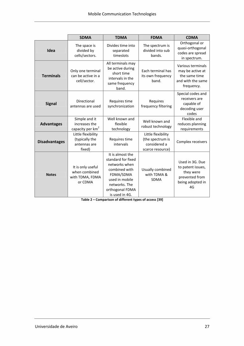
Mobile Communication Technologies
Universidade de Aveiro 27
SDMA TDMA FDMA CDMA
Idea The space is divided by
cells/sectors.
Divides time into separated timeslots
The spectrum is divided into sub
bands.
Orthogonal or quasi-orthogonal codes are spread
in spectrum.
Terminals Only one terminal can be active in a
cell/sector.
All terminals may be active during
short time intervals in the same frequency
band.
Each terminal has its own frequency
band.
Various terminals may be active at the same time
and with the same frequency.
Signal Directional
antennas are used Requires time
synchronization Requires
frequency filtering
Special codes and receivers are
capable of decoding user
codes
Advantages Simple and it increases the
capacity per km2
Well known and flexible
technology
Well known and robust technology
Flexible and reduces planning
requirements
Disadvantages
Little flexibility (typically the antennas are
fixed)
Requires time intervals
Little flexibility (the spectrum is
considered a scarce resource)
Complex receivers
Notes
It is only useful when combined
with TDMA, FDMA or CDMA
It is almost the standard for fixed
networks when combined with FDMA/SDMA
used in mobile networks. The
orthogonal FDMA is used in 4G.
Usually combined with TDMA &
SDMA
Used in 3G. Due to patent issues,
they were prevented from
being adopted in 4G
Table 2 – Comparison of different types of access [39]
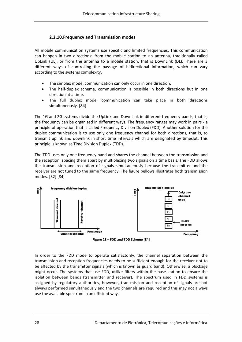
Telecommunication Infrastructure Sharing
28 Departamento de Eletrónica, Telecomunicações e Informática
2.2.10.Frequency and Transmission modes
All mobile communication systems use specific and limited frequencies. This communication can happen in two directions: from the mobile station to an antenna, traditionally called UpLink (UL), or from the antenna to a mobile station, that is DownLink (DL). There are 3 different ways of controlling the passage of bidirectional information, which can vary according to the systems complexity.
The simplex mode, communication can only occur in one direction.
The half-duplex scheme, communication is possible in both directions but in one direction at a time.
The full duplex mode, communication can take place in both directions simultaneously. [84]
The 1G and 2G systems divide the UpLink and DownLink in different frequency bands, that is, the frequency can be organized in different ways. The frequency ranges may work in pairs - a principle of operation that is called Frequency Division Duplex (FDD). Another solution for the duplex communication is to use only one frequency channel for both directions, that is, to transmit uplink and downlink in short time intervals which are designated by timeslot. This principle is known as Time Division Duplex (TDD). The TDD uses only one frequency band and shares the channel between the transmission and the reception, spacing them apart by multiplexing two signals on a time basis. The FDD allows the transmission and reception of signals simultaneously because the transmitter and the receiver are not tuned to the same frequency. The figure bellows illustrates both transmission modes. [52] [84]
Figure 28 – FDD and TDD Scheme [84]
In order to the FDD mode to operate satisfactorily, the channel separation between the transmission and reception frequencies needs to be sufficient enough for the receiver not to be affected by the transmitter signals (which is known as guard band). Otherwise, a blockage might occur. The systems that use FDD, utilize filters within the base station to ensure the isolation between bands (transmitter and receiver). The spectrum used in FDD systems is assigned by regulatory authorities, however, transmission and reception of signals are not always performed simultaneously and the two channels are required and this may not always use the available spectrum in an efficient way.
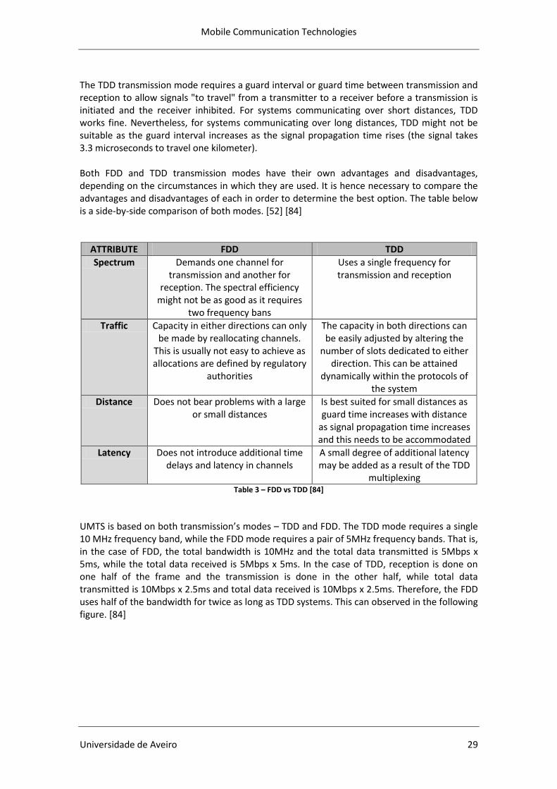
Mobile Communication Technologies
Universidade de Aveiro 29
The TDD transmission mode requires a guard interval or guard time between transmission and reception to allow signals "to travel" from a transmitter to a receiver before a transmission is initiated and the receiver inhibited. For systems communicating over short distances, TDD works fine. Nevertheless, for systems communicating over long distances, TDD might not be suitable as the guard interval increases as the signal propagation time rises (the signal takes 3.3 microseconds to travel one kilometer). Both FDD and TDD transmission modes have their own advantages and disadvantages, depending on the circumstances in which they are used. It is hence necessary to compare the advantages and disadvantages of each in order to determine the best option. The table below is a side-by-side comparison of both modes. [52] [84]
ATTRIBUTE FDD TDD
Spectrum Demands one channel for transmission and another for
reception. The spectral efficiency might not be as good as it requires
two frequency bans
Uses a single frequency for transmission and reception
Traffic Capacity in either directions can only be made by reallocating channels.
This is usually not easy to achieve as allocations are defined by regulatory
authorities
The capacity in both directions can be easily adjusted by altering the
number of slots dedicated to either direction. This can be attained
dynamically within the protocols of the system
Distance Does not bear problems with a large or small distances
Is best suited for small distances as guard time increases with distance
as signal propagation time increases and this needs to be accommodated
Latency Does not introduce additional time delays and latency in channels
A small degree of additional latency may be added as a result of the TDD
multiplexing Table 3 – FDD vs TDD [84]
UMTS is based on both transmission’s modes – TDD and FDD. The TDD mode requires a single 10 MHz frequency band, while the FDD mode requires a pair of 5MHz frequency bands. That is, in the case of FDD, the total bandwidth is 10MHz and the total data transmitted is 5Mbps x 5ms, while the total data received is 5Mbps x 5ms. In the case of TDD, reception is done on one half of the frame and the transmission is done in the other half, while total data transmitted is 10Mbps x 2.5ms and total data received is 10Mbps x 2.5ms. Therefore, the FDD uses half of the bandwidth for twice as long as TDD systems. This can observed in the following figure. [84]
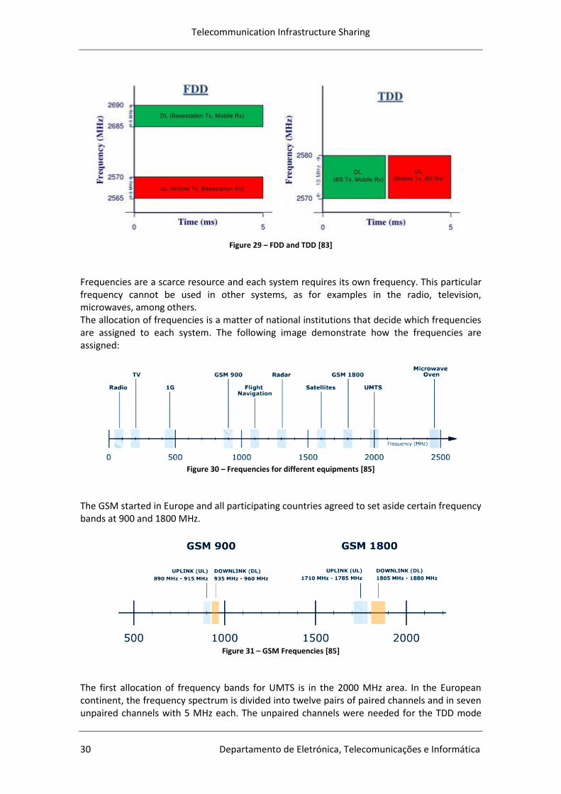
Telecommunication Infrastructure Sharing
30 Departamento de Eletrónica, Telecomunicações e Informática
Figure 29 – FDD and TDD [83]
Frequencies are a scarce resource and each system requires its own frequency. This particular frequency cannot be used in other systems, as for examples in the radio, television, microwaves, among others. The allocation of frequencies is a matter of national institutions that decide which frequencies are assigned to each system. The following image demonstrate how the frequencies are assigned:
Figure 30 – Frequencies for different equipments [85]
The GSM started in Europe and all participating countries agreed to set aside certain frequency bands at 900 and 1800 MHz.
Figure 31 – GSM Frequencies [85]
The first allocation of frequency bands for UMTS is in the 2000 MHz area. In the European continent, the frequency spectrum is divided into twelve pairs of paired channels and in seven unpaired channels with 5 MHz each. The unpaired channels were needed for the TDD mode
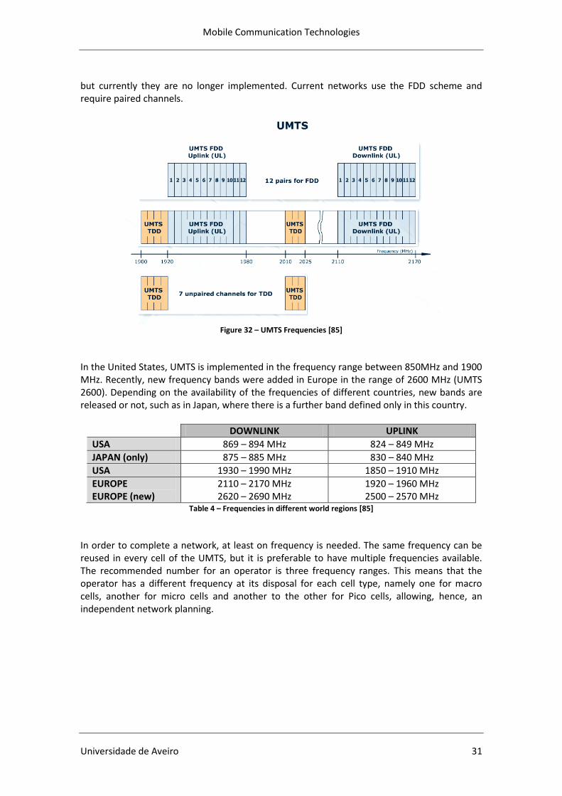
Mobile Communication Technologies
Universidade de Aveiro 31
but currently they are no longer implemented. Current networks use the FDD scheme and require paired channels.
Figure 32 – UMTS Frequencies [85]
In the United States, UMTS is implemented in the frequency range between 850MHz and 1900 MHz. Recently, new frequency bands were added in Europe in the range of 2600 MHz (UMTS 2600). Depending on the availability of the frequencies of different countries, new bands are released or not, such as in Japan, where there is a further band defined only in this country.
DOWNLINK UPLINK
USA 869 – 894 MHz 824 – 849 MHz
JAPAN (only) 875 – 885 MHz 830 – 840 MHz
USA 1930 – 1990 MHz 1850 – 1910 MHz
EUROPE EUROPE (new)
2110 – 2170 MHz 2620 – 2690 MHz
1920 – 1960 MHz 2500 – 2570 MHz
Table 4 – Frequencies in different world regions [85]
In order to complete a network, at least on frequency is needed. The same frequency can be reused in every cell of the UMTS, but it is preferable to have multiple frequencies available. The recommended number for an operator is three frequency ranges. This means that the operator has a different frequency at its disposal for each cell type, namely one for macro cells, another for micro cells and another to the other for Pico cells, allowing, hence, an independent network planning.
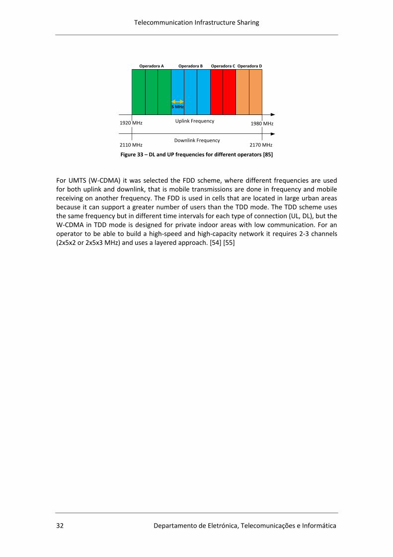
Telecommunication Infrastructure Sharing
32 Departamento de Eletrónica, Telecomunicações e Informática
1920 MHz
2170 MHz2110 MHz
1980 MHzUplink Frequency
Downlink Frequency
5 MHz
Operadora A Operadora B Operadora C Operadora D
Figure 33 – DL and UP frequencies for different operators [85]
For UMTS (W-CDMA) it was selected the FDD scheme, where different frequencies are used for both uplink and downlink, that is mobile transmissions are done in frequency and mobile receiving on another frequency. The FDD is used in cells that are located in large urban areas because it can support a greater number of users than the TDD mode. The TDD scheme uses the same frequency but in different time intervals for each type of connection (UL, DL), but the W-CDMA in TDD mode is designed for private indoor areas with low communication. For an operator to be able to build a high-speed and high-capacity network it requires 2-3 channels (2x5x2 or 2x5x3 MHz) and uses a layered approach. [54] [55]
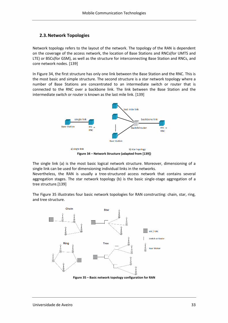
Mobile Communication Technologies
Universidade de Aveiro 33
2.3. Network Topologies
Network topology refers to the layout of the network. The topology of the RAN is dependent on the coverage of the access network, the location of Base Stations and RNCs(for UMTS and LTE) or BSCs(for GSM), as well as the structure for interconnecting Base Station and RNCs, and core network nodes. [139] In Figure 34, the first structure has only one link between the Base Station and the RNC. This is the most basic and simple structure. The second structure is a star network topology where a number of Base Stations are concentrated to an intermediate switch or router that is connected to the RNC over a backbone link. The link between the Base Station and the intermediate switch or router is known as the last mile link. [139]
Figure 34 – Network Structure (adapted from [139])
The single link (a) is the most basic logical network structure. Moreover, dimensioning of a single link can be used for dimensioning individual links in the networks. Nevertheless, the RAN is usually a tree-structured access network that contains several aggregation stages. The star network topology (b) is the basic single-stage aggregation of a tree structure.[139] The Figure 35 illustrates four basic network topologies for RAN constructing: chain, star, ring, and tree structure.
Figure 35 – Basic network topology configuration for RAN

Telecommunication Infrastructure Sharing
34 Departamento de Eletrónica, Telecomunicações e Informática
Usually the network is designed as a mixture of the above topologies. Figure 36 shows an example of a RAN network topology. A Base Station can either be directly connected to the RNC, or act as a traffic concentrator for a set of Base Stations, or it can be connected to an intermediate router or switch. An intermediate router or switch can be utilized to attain a higher degree of traffic aggregation, which might be used to connect several Base Stations to a common and distant RNC, or to aggregate the traffic between groups of RNCs and the core network. [139]
Figure 36 – RAN network topology example (adapted from [139])
Selecting an appropriate network topology is important as it has a great impact on the traffic patterns in the network and, as a consequence, affects the allocation of the link capacities, link costs and total network costs. Different network topologies indicate different degrees of traffic concentration, and hence the resultant multiplexing gain and cost savings differ from one another. For example, the star topology can achieve high multiplexing gain as a result of high concentration of traffic on the backbone link, i.e. the link between RNC and the switch or router which connects all Base Stations. [139]
Mobile Communication Technologies
Universidade de Aveiro 35
2.4. UMTS
Universal Mobile Telecommunication System (UMTS) is a third generation (3G) mobile cellular system and its architecture is based on GSM technology. UMTS was developed within 3GPP (Third Generation Partnership Project) and was created to enhance voice capacity and support more data applications with higher QoS (Quality of Service).[8] [51] One of the key factors for the arrival of UMTS was the great need for mobile services and applications with higher speeds of internet access than the existing ones. The mobile communications market is very different from user to user, as some are not willing to wait for making downloads, access emails, carry out payment services or even watch TV. The UMTS appears hence to address many of these needs.[47]
2.4.1.Characteristics
UMTS presents several features that seek to build and increase the capacity of cellular networks in order to provide higher quality and speed of data transfer and improve access via radio offering higher bandwidth and better geographic reach. During the design of the 3G standards, different requirements have been defined in the data rates for different environments.
Pico cells are designed for indoor coverage (hot spots), with data rates up to 1.92 Mbit/s.
Micro cells are designed for urban areas (with a few hundred meters), with data rates up to 384 kbit/s.
Macro cells to urban areas (between 500m and 5km), with data rates up to 384 kbit/s. In rural areas (between 5 and 20 km) - with data rates up 144 kbit/s. [56]
Nonetheless, higher data rates are needed for downloading services such as music or video. The existing 3G networks were improved to 3.5G with only minor modifications in order to provide higher data rates, to use frequencies more efficiently, to increase the capacity and coverage as well as to reduce costs. In the 3G, an antenna sends a signal to all users within a given area, without any distinction between users. The 3.5G implemented antennas with a sign that targets users with low bit rate and another sign that focuses on users with high bit rate. By removing high-bit users of the common signal, more coverage and capacity for all other users are available. One of the major advantages that can be observed in the 3.5G system is the packet-switching that allows for costs reductions. To make the frequency system more efficient and provide higher data rates, the 3G network supports the HSDPA (High Speed Downlink Packet Access). Contrary to the actual 384 kbit/s of downlink of UMTS speed, HSDPA offers to users about 1.5 to 2 Mbit/s, which is enough for high quality video or high resolution interactive games. The users of the UMTS and HSDPA are served simultaneously in the same site and the same antenna. New applications, such as broadcast TV and Video On Demand, require an even higher performance, which is why a high data rate is a critical requirement in 4G systems. This high data rate should be attained in 4G
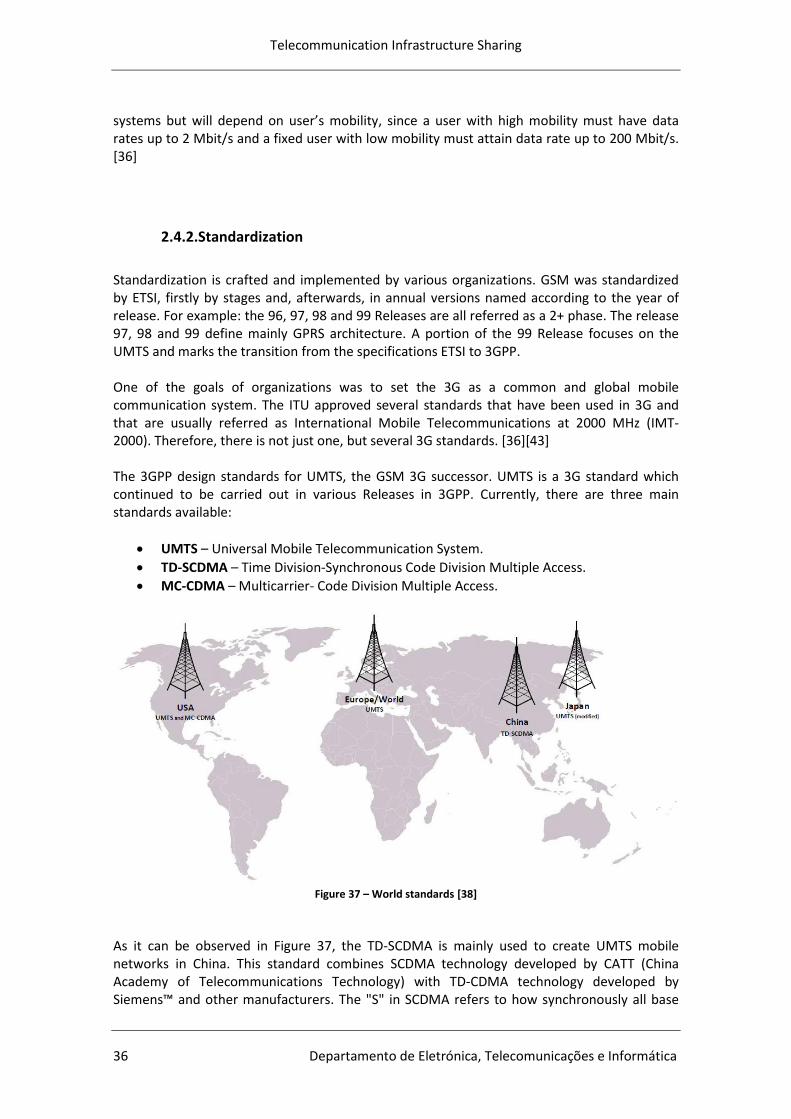
Telecommunication Infrastructure Sharing
36 Departamento de Eletrónica, Telecomunicações e Informática
systems but will depend on user’s mobility, since a user with high mobility must have data rates up to 2 Mbit/s and a fixed user with low mobility must attain data rate up to 200 Mbit/s. [36]
2.4.2.Standardization
Standardization is crafted and implemented by various organizations. GSM was standardized by ETSI, firstly by stages and, afterwards, in annual versions named according to the year of release. For example: the 96, 97, 98 and 99 Releases are all referred as a 2+ phase. The release 97, 98 and 99 define mainly GPRS architecture. A portion of the 99 Release focuses on the UMTS and marks the transition from the specifications ETSI to 3GPP. One of the goals of organizations was to set the 3G as a common and global mobile communication system. The ITU approved several standards that have been used in 3G and that are usually referred as International Mobile Telecommunications at 2000 MHz (IMT-2000). Therefore, there is not just one, but several 3G standards. [36][43] The 3GPP design standards for UMTS, the GSM 3G successor. UMTS is a 3G standard which continued to be carried out in various Releases in 3GPP. Currently, there are three main standards available:
UMTS – Universal Mobile Telecommunication System.
TD-SCDMA – Time Division-Synchronous Code Division Multiple Access.
MC-CDMA – Multicarrier- Code Division Multiple Access.
Figure 37 – World standards [38]
As it can be observed in Figure 37, the TD-SCDMA is mainly used to create UMTS mobile networks in China. This standard combines SCDMA technology developed by CATT (China Academy of Telecommunications Technology) with TD-CDMA technology developed by Siemens™ and other manufacturers. The "S" in SCDMA refers to how synchronously all base
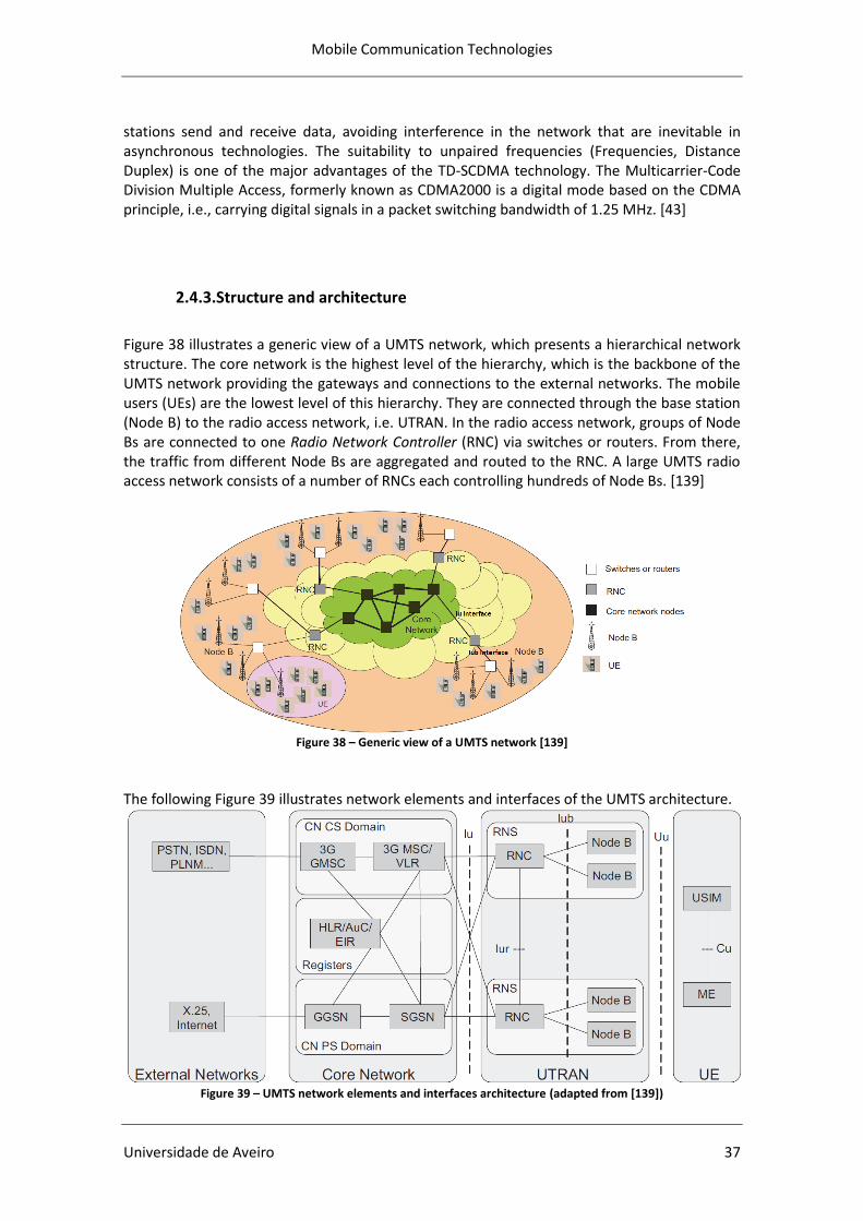
Mobile Communication Technologies
Universidade de Aveiro 37
stations send and receive data, avoiding interference in the network that are inevitable in asynchronous technologies. The suitability to unpaired frequencies (Frequencies, Distance Duplex) is one of the major advantages of the TD-SCDMA technology. The Multicarrier-Code Division Multiple Access, formerly known as CDMA2000 is a digital mode based on the CDMA principle, i.e., carrying digital signals in a packet switching bandwidth of 1.25 MHz. [43]
2.4.3.Structure and architecture
Figure 38 illustrates a generic view of a UMTS network, which presents a hierarchical network structure. The core network is the highest level of the hierarchy, which is the backbone of the UMTS network providing the gateways and connections to the external networks. The mobile users (UEs) are the lowest level of this hierarchy. They are connected through the base station (Node B) to the radio access network, i.e. UTRAN. In the radio access network, groups of Node Bs are connected to one Radio Network Controller (RNC) via switches or routers. From there, the traffic from different Node Bs are aggregated and routed to the RNC. A large UMTS radio access network consists of a number of RNCs each controlling hundreds of Node Bs. [139]
Figure 38 – Generic view of a UMTS network [139]
The following Figure 39 illustrates network elements and interfaces of the UMTS architecture.
Figure 39 – UMTS network elements and interfaces architecture (adapted from [139])
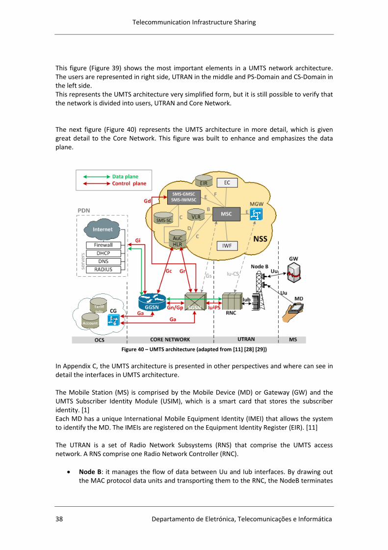
Telecommunication Infrastructure Sharing
38 Departamento de Eletrónica, Telecomunicações e Informática
This figure (Figure 39) shows the most important elements in a UMTS network architecture. The users are represented in right side, UTRAN in the middle and PS-Domain and CS-Domain in the left side. This represents the UMTS architecture very simplified form, but it is still possible to verify that the network is divided into users, UTRAN and Core Network. The next figure (Figure 40) represents the UMTS architecture in more detail, which is given great detail to the Core Network. This figure was built to enhance and emphasizes the data plane.
Figure 40 – UMTS architecture (adapted from [11] [28] [29])
In Appendix C, the UMTS architecture is presented in other perspectives and where can see in detail the interfaces in UMTS architecture. The Mobile Station (MS) is comprised by the Mobile Device (MD) or Gateway (GW) and the UMTS Subscriber Identity Module (USIM), which is a smart card that stores the subscriber identity. [1] Each MD has a unique International Mobile Equipment Identity (IMEI) that allows the system to identify the MD. The IMEIs are registered on the Equipment Identity Register (EIR). [11] The UTRAN is a set of Radio Network Subsystems (RNS) that comprise the UMTS access network. A RNS comprise one Radio Network Controller (RNC).
Node B: it manages the flow of data between Uu and Iub interfaces. By drawing out the MAC protocol data units and transporting them to the RNC, the NodeB terminates
Mobile Communication Technologies
Universidade de Aveiro 39
the physical layer. It is also a component of the radio resource management. [1] [22] [23]
RNC: it manages the radio resources of its domain. Its main operations are: - Control radio resources: the RNC incorporates an admission control module
which establishes if a voice call/data packet session is accepted and decides the radio resources that have to be allocated;
- Process radio signaling: the RNC handles all the radio signals that come from either the UE or the Core Network;
- Execute call setup and termination: the RNC transfers signaling from and to the NodeB, that in turn transfers the signals from and to the UE, so as to establish bearer service during the process of establishment of a communication session. It is also responsible for the opposite process;
- Carry out soft, intersystem and hard handoffs: the RNC determines (by utilizing radio signal measurements) when to command the UE to set up handovers;
- Give Operation, Administrative and Maintenance (OA&M) competences: the RNC transmits keep-alive messages through the numerous interfaces that connects it to other RNCs, NodeBs, and other access points for OA&M intents. [1] [23]
The Core Network (CN) is comprised of many interfaces and elements, namely:
The Authentication Centre (AuC): is the system held responsible for authentication and encryption operations. These operations are executed in the AuC and in the MS simultaneously. Their goal is to secure the system (advert cloning of MSs for example). The AuC communicates only with its associated HLR (H-interface), and is usually installed in the HLR hardware. [11] [23]
The Home Location Register (HLR): this register is in charge of administrating and controlling the data base of local users. It manages and keeps all changes made on a subscriber profile. The HLR data profiles are accessed in a remote way by the MSC and VLR. The essential data profile are: authentication key; International Mobile Subscriber Identity (IMSI); supplementary services associated to subscriber (and related information); current subscriber location in the VLR; subscriber status (attached/non-attached). [11] [23] [56]
The Echo Canceler (EC): mitigates the echo present in the MSC – PSTN connections. [11]
The Equipment Identity Register (EIR): The EIR is a data base that is responsible for
controlling the mobile equipment. It validates the IMEI number and the calls that are
done on a mobile network. The EIR holds the black, gray and white lists with
equipment numbers. Equipment in the Black List are not authorized to be used in the
network. Equipment in the Grey List are under observation, while equipment in the
white list are ready to be used in the network. The EIR is remotely accessed by the
MSC, which converts the IMEI on the EIR logic address. [11] [36] [55]
Telecommunication Infrastructure Sharing
40 Departamento de Eletrónica, Telecomunicações e Informática
The Interworking Function (IWF): it provides the GSM interface with other public and private networks. Its main responsibilities are data rate adaptation and protocol translation. [11] [23]
The Mobile services Switching Centre (MSC): it is the central element of the Network Switching System (NSS), and is responsible for switching and signaling functions (CS) for mobile stations. Its major functions comprise: call treating (establishment and termination of calls, handover between BSSs and between MSCs); inter-functioning (management of interfaces between GSM and other networks, e.g. PSTN or ISDN); operation, maintenance and supervision (data base management and traffic data measurement); and charging. [11] [55] [56]
The Service Centre (SC): The SC is responsible for transfer and store-and-forward a short message between a Short Message Entity3 (SME) and an MS. The SC is not a component of the GSM PLMN, however MSC and SC may be integrated. [29]
The Gateway MSC for Short Message Service (SMS-GMSC): It is a function of an MSC that receives short messages from an Service Centre (SC), interrogates an HLR for routing information and SMS info, and delivers the short message to the Visited Mobile Switching Centre (VMSC) of the recipient MS. [23] [29]
The Interworking MSC for Short Message Service (SMS-IWMSC): It is a function of an MSC that is capable of receiving a short message from within the PLMN and sending it to the recipient SC. [23] [29]
The Visitor Location Register (VLR): it is held responsible for keeping a copy of the users main profile data that are stored on the HLR in order to minimize the burden on the HLR. Examples of main profile data stored on the VLR are the MS state (e.g. available, busy, non-responsive); the Location Area Identity (LAI); the Temporary Mobile Subscriber Identity (TMSI); and the Mobile Station Roaming Number (MSRN). [23] [29] [56]
The Gateway GPRS Support Node (GGSN): it is a gateway between UMTS PS/GPRS
network and external data networks (e.g. Internet). The GGSN is responsible for
executing various functions such as, routing and data encapsulation between a MS and
external data networks, security control, network access control and network
management. Taking into consideration the UMTS PS/GPRS context, a MS picks out a
GGSN as its routing device between itself and the external network in the activation
process of a PDP4 context in which Access Point Name (APN) determines the access
point to destination data network. Considering the external network, the GGSN is a
router able to address all MS IPs in UMTS PS/GPRS network. [1] [23] [30]
The GGSN upholds the following functions:
- GPRS Tunneling Protocol (GTP);
3 SME: an entity that sends or receives Short Messages. The SME may be located in a fixed network, an
MS, or an SC. 4 PDP: network protocol used by an external packet data network interfacing to GPRS.
Mobile Communication Technologies
Universidade de Aveiro 41
- Lawful Interception5;
- Route resolve through HLR interaction;
- Static/Dynamic IP address assignment;
- Packet data routing;
- Authentication, Authorization, and Accounting (AAA);
- Traffic management and control (e.g. rejection of irrelevant packets and
congestion control);
- Service performance measurements. [1] [23] [30] [55]
The Serving GPRS Support Node (SGSN): the SGSN holds the function of delivering the
data packet from and to MSs within its serving area. Packet routing and transfer,
mobility management (attach/detach and location management), logical link
management authentication, and charging functions are some of SGSN fundamental
tasks. [23][30]
Hence, it supports functions such as:
- MS registration with its HLR;
- MS authentication;
- Authorization and admission control of packet services for a subscriber;
- Packet session establishment, maintenance, and termination;
- PDP context activations;
- Packet switching/routing for UMTS/GPRS packet services;
- Maintenance of a database of users currently being served;
- GPRS attach processes;
- GPRS Tunneling Protocol (GTP);
- Collection of charging data. [1] [23] [56]
Clusters of SGSNs can be connected to regional GGSNs. A trade-off must be achieved between the cost of equipment and the cost of transport in order to define the number of clusters that should be implemented and the way they should be configured.
Media Gateway (MGW): it is a translation device or service responsible of converting digital media streams between disparate telecommunications networks.
Charging Gateway (CG): is the billing unit for Packet Switched (PS) domain. It collects, merges, filters and stores the Call Detail Records (CDR) – and other charging information from the GGSN and the SGSN. It communicates with the billing center, and afterwards, transmits the sorted CDR to the billing center. The CG can be connected with the SGSN. [23] [29] [30]
Regarding the Core Network (CN), various options are accepted by the ITU taking into account that, due to standardization, an operator can choose any CN and combine it with any RAN. The
5 Lawful Interception: the process by which law enforcement agencies conduct electronic surveillance of
circuit and packet-mode communications as authorized by judicial or administrative order.

Telecommunication Infrastructure Sharing
42 Departamento de Eletrónica, Telecomunicações e Informática
radio access network differs from the UMTS to GSM, but the core network remains similar and interoperable between the two networks. The core equipment can be used for both technologies. In 2G, the GERAN has two interfaces in the core network: the Circuit-Switched Core Network interface (CS CN) and Packet-Switched Core Network (PS CN). The interface between GERAN and CS CN is known as the A interface (between BSS and MSC). The interface between GERAN and PS CN is a GPRS interface which is known as the Gb interface (between the BSS and the SGSN). [25] This can be observed in the Appendix C. [25] The Mobile Station (MS) communicates with the GERAN over the air interface and is defined as "A" (Mobile User) as it can be seen in Figure 41.
Figure 41 – Interfaces in GERAN core network [38]
According to the Release 99, the UTRAN is a network infrastructure that has the facilities that make the transmission over radio to and from the mobile users. The UTRAN has two components: the base station, which is called in UMTS Node B, and control nodes, which are called Radio Network Controller (RNC). The RNC is connected to the CN. The UE can make calls and send IP data, therefore the UTRAN has two different interfaces in the Core Network: IuCS and IuPS. The air interface is called UMTS User (Uu). Voice and video calls are traffic in Real Time (RT) and is handled by CS CN while all other traffic is called the traffic in Non Real Time (NRT) which is handled by PS CN. This can be observed in Figure 40, Figure 42 and in Appendix C. [8] [36]
Figure 42 – Interfaces in UTRAN core network [38]
Mobile Communication Technologies
Universidade de Aveiro 43
In the Appendix D and Appendix E two different mechanisms operating in the core network that covers the circuit-switched a voice call and the packet-switched data access in a web browser are presented. In case of failures in a certain equipment from the network, this one should behave similarly
when there are no errors as most of the equipment should present redundancy. Redundancy
can be done locally or another geographic point can be used for the resolution of the existing
failure.
Concerning the physical and / or logical connections, there are almost always two or more
protections (main and spare) because if case of a failure in a connection there is always a
backup connection which can ensure the normal operation of the network. [36]
In the core network, most of the equipment (SGSN, GGSN, MSC, HLR, EIR, VLR, AuC) also
present redundancy, which means that if there is a problem, there must be other equipment
that will support / replicate its functions. However, when certain failures occurs in certain
equipment, such as in the HLR, VLR or EIR, there is a risk of losing some information or some
records that can no longer be accessed. If the SGSN fails, the packet data exchange in the
system can be lost. On the other hand, if the GGSN breaks down the interface with the
external packet network (Internet) may be lost, that is, this equipment will no longer convert
the GPRS packets coming from the SGSN to the appropriate PDP format and will not send the
packets to the appropriate external network. [36]
If a problem occurs in the RNC, such as a card problem, there should always be another card
that assures the continuity of its normal operation. It is crucial to monitor constantly the
operation of this equipment (24 hours for 7 days a week) so that the functioning is always
continuous. If there is problem in the site (Node B), its performance can be usually ensured by
neighboring sites which create handovers, depending on the network planning and the
operator options as costs can increase significantly.
When there is a creation, exclusion or modification of network elements, the operator must
ensure that there is not an uncontrollable impact on the network. For this to happen, the
operator should always take into account security aspects and network configuration changes
should only be performed by authorized personnel. [36]
Regarding the messages exchanged between the network elements presented above (CS voice
call and access to a web browser), these messages operate based on timeouts. When a
message is sent, the issuer initiates a count and awaits confirmation of the recipient. If this
information is correctly received, the recipient sends an Acknowledge (ACK) to confirm its
receipt. If the recipient does not send an ACK and counter exceeds the expected time, the
sender resends the message, taking into account that there is a limit to the number of times
the message may be sent. If the limit number of times the message can be sent is reached, the
process is interrupted and the message is discarded. [36] [55]
Telecommunication Infrastructure Sharing
44 Departamento de Eletrónica, Telecomunicações e Informática
It is crucial that an operator is able to make changes and fix problems quickly with minimal
efforts and, if possible, without affecting user services.
The life cycle of a network may be divided into three phases:
1. Network installation and commissioning;
2. Network modification in order to meet some requirements. These modifications can
disturb the stability of the network and an optimization of the network may be needed
again;
3. Based on the network performance, this one is set to meet long-term needs taking
into account the capacity and the number of users. [36]
The operator must be able to solve any immediate problems that may arise, as for example,
reset the parameters of the network elements and/or adapt to day-to-day requirements. [36]
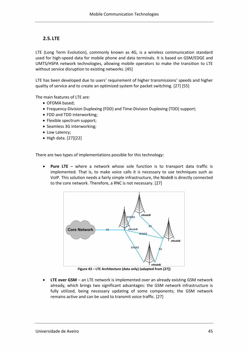
Mobile Communication Technologies
Universidade de Aveiro 45
2.5. LTE
LTE (Long Term Evolution), commonly known as 4G, is a wireless communication standard used for high-speed data for mobile phone and data terminals. It is based on GSM/EDGE and UMTS/HSPA network technologies, allowing mobile operators to make the transition to LTE without service disruption to existing networks. [45] LTE has been developed due to users’ requirement of higher transmissions’ speeds and higher quality of service and to create an optimized system for packet switching. [27] [55] The main features of LTE are:
OFDMA based;
Frequency-Division Duplexing (FDD) and Time-Division Duplexing (TDD) support;
FDD and TDD interworking;
Flexible spectrum support;
Seamless 3G interworking;
Low Latency;
High data. [27][22] There are two types of implementations possible for this technology:
Pure LTE – where a network whose sole function is to transport data traffic is implemented. That is, to make voice calls it is necessary to use techniques such as VoIP. This solution needs a fairly simple infrastructure, the NodeB is directly connected to the core network. Therefore, a RNC is not necessary. [27]
Figure 43 – LTE Architecture (data only) (adapted from [27])
LTE over GSM – an LTE network is implemented over an already existing GSM network already, which brings two significant advantages: the GSM network infrastructure is fully utilized, being necessary updating of some components; the GSM network remains active and can be used to transmit voice traffic. [27]
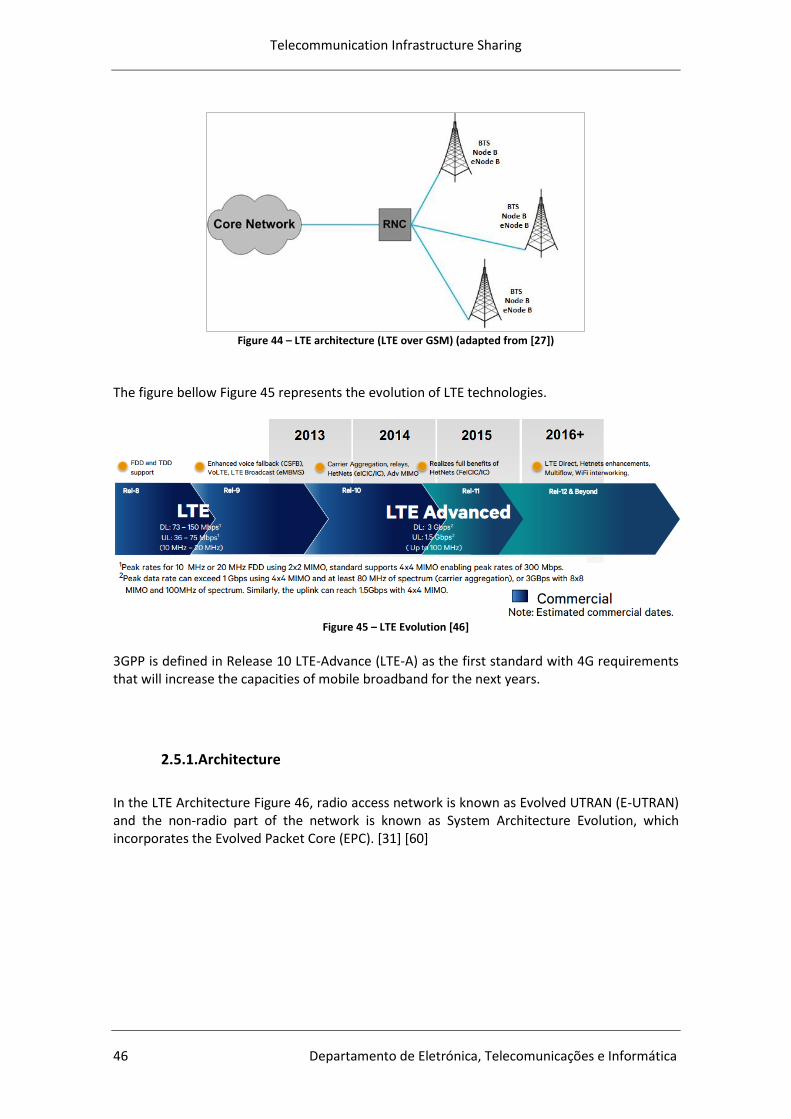
Telecommunication Infrastructure Sharing
46 Departamento de Eletrónica, Telecomunicações e Informática
Figure 44 – LTE architecture (LTE over GSM) (adapted from [27])
The figure bellow Figure 45 represents the evolution of LTE technologies.
Figure 45 – LTE Evolution [46]
3GPP is defined in Release 10 LTE-Advance (LTE-A) as the first standard with 4G requirements that will increase the capacities of mobile broadband for the next years.
2.5.1.Architecture
In the LTE Architecture Figure 46, radio access network is known as Evolved UTRAN (E-UTRAN) and the non-radio part of the network is known as System Architecture Evolution, which incorporates the Evolved Packet Core (EPC). [31] [60]
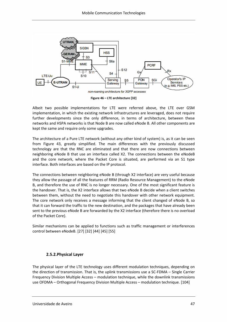
Mobile Communication Technologies
Universidade de Aveiro 47
Figure 46 – LTE architecture [32]
Albeit two possible implementations for LTE were referred above, the LTE over GSM implementation, in which the existing network infrastructures are leveraged, does not require further developments since the only difference, in terms of architecture, between these networks and HSPA networks is that Node B are now called eNode B. All other components are kept the same and require only some upgrades. The architecture of a Pure LTE network (without any other kind of system) is, as it can be seen from Figure 43, greatly simplified. The main differences with the previously discussed technology are that the RNC are eliminated and that there are now connections between neighboring eNode B that use an interface called X2. The connections between the eNodeB and the core network, where the Packet Core is situated, are performed via an S1 type interface. Both interfaces are based on the IP protocol. The connections between neighboring eNode B (through X2 interface) are very useful because they allow the passage of all the features of RRM (Radio Resource Management) to the eNode B, and therefore the use of RNC is no longer necessary. One of the most significant feature is the handover. That is, the X2 interface allows that two eNode B decide when a client switches between them, without the need to negotiate this handover with other network equipment. The core network only receives a message informing that the client changed of eNode B, so that it can forward the traffic to the new destination, and the packages that have already been sent to the previous eNode B are forwarded by the X2 interface (therefore there is no overload of the Packet Core). Similar mechanisms can be applied to functions such as traffic management or interferences control between eNodeB. [27] [32] [44] [45] [55]
2.5.2.Physical Layer
The physical layer of the LTE technology uses different modulation techniques, depending on the direction of transmission. That is, the uplink transmissions use a SC-FDMA – Single Carrier Frequency Division Multiple Access – modulation technique, while the downlink transmissions use OFDMA – Orthogonal Frequency Division Multiple Access – modulation technique. [104]

Telecommunication Infrastructure Sharing
48 Departamento de Eletrónica, Telecomunicações e Informática
Concerning downlink channels, the OFDMA modulation technique allows data to be transmitted on sub-carriers close to each other but mutually orthogonal in the frequency domain. In order to provide access to different users, users are assigned with subsets (not necessarily adjacent) of OFDM symbols. This is illustrated in Figure 47. The least amount of resources that can be assigned to a user, one Resource Block, has a size of 180 kHz (in the frequency domain) or of 1 ms (in the time domain). Individual Resource Blocks may have different coding and modulation (even if they belong to the same user) which allow this technology to adapt to frequencies selected for the links, and thus optimize coding and modulation (according to the frequency response of the channels). Uplink transmissions employ the SC-FDMA modulation technique. The major difference between the OFDMA and SC-FDMA is that this last one holds a continuous profile in the frequency domain. The principal objective of using SC-FDMA technique in Uplink transmission is to reduce the costs of the amplifiers of terminal equipment, since this technique has a PAPR (Peack to Average Power Ratio) lower than the modulation technique used in Downlink. [27] [60] [66][66] Nevertheless, these two modulation techniques (SC-FDMA and OFDMA) have many similarities in terms of signal processing, which makes it possible to harmonize at maximum properties of each signal sent/received.
Figure 47 – Physical Layer of LTE technology [59]
A significant property of LTE is the concept of flexible bandwidth. This concept, that comes from OFDM techniques, support changes in the bandwidth of the system through reductions (or increases) in the number of sub-carriers. There are six possible ranges, from 1.4 to 20 MHz, with different numbers of sub-carriers, as it can be observed in the Table 5. [60] [66]
Bandwidth (MHz) 1,4 3 5 10 15 20
Number of subcarriers 6 15 25 50 75 100 Table 5 – Bandwidth ranges in LTE [59]
As expected, the capacity of the system depends directly on the number of sub-carriers at its disposal. Besides, this flexibility allows LTE technology to adapt to different bands of the frequency spectrum. That is, thanks to this property, LTE technology can gradually be introduced in bands that are currently used in other technologies (GSM, UMTS, analog television, etc.). The introduction of MIMO techniques is, contrarily to what happened with HSPA technology, an integral part of the first Release for LTE technology. This implies that all terminal equipment have to be able to integrate MIMO systems (although it is not required that they support multiplexing techniques in space). Another difference between MIMO techniques used in LTE
Mobile Communication Technologies
Universidade de Aveiro 49
and HSPA is that, in LTE, it is possible to use four antennas in both the transmitters and receivers. [27] [60] [66]
2.5.3.SON (Self Organizing Networks)
One of the goals of operators when developing LTE technology was to create standard features that would decrease network operating costs. Nowadays, there is a significant effort to configure and optimize existing 2G and 3G networks. There is also a greater difficulty and complexity as operators want to have all (or at least some) of these technologies operating simultaneously. Therefore, the concept of networks SON (Self Organizing Networks) was developed with the purpose of transforming certain tasks currently done manually by operators into automated tasks, enabling hence the network to adjust its operating parameters dynamically. SON networks have two major types of processes:
Self-configuration: which are automatic configuration processes. When a new eNodeB is installed, its configuration is done automatically through an installation procedure that will introduce the basic settings required for the system to operate optimally.
Self-optimization – which are optimization processes that automatically and continuously adjust the operating parameters in order to maximize the system performance.
It is important to mention that the 3GPP does not define any default implementation of SON networks’ features. The 3GPP defines only some guidelines on terminal equipment, as well as the behavior of the X2 interface considered necessary to fulfill some practical cases, such as: [27]
Optimize the list of neighboring cells;
Coordinate interferences;
Optimize the coverage and capacity;
Optimize mobility’ robustness. [27]
Telecommunication Infrastructure Sharing
50 Departamento de Eletrónica, Telecomunicações e Informática
2.6. GSM vs. UMTS
The Global System for Mobile communication (GSM) is the most successful 2G system as it
provides advanced features as well as complementary services. It allows call forwarding,
Internet access, text message sending, and it displays who is calling. To increase the data
speed, the GSM network is reinforced by the General Packet Radio Service (GPRS), which
results in a 2.5G network. The introduction of the 2.5G, allowed the new services to benefit
from much higher transfer rates as well as services’ evolution and new models of phones. The
2.5G systems introduced transfer packages in order to increase data rates. The Universal
Mobile Telecommunication System (UMTS), also known as 3G, integrated and improved the
quality of existing services and allowed for the implementation of new services with higher
flexibility. The 3G has been globally standardized and special considerations were adopted to
reduce costs on devices and on mobile networks. [36]
UMTS networks based on TDD and FDD schemes are currently implemented in Europe and
offer multimedia services (video calls, video conferencing and fast Internet access) as a result
of high data transfer rates and high performance. Furthermore, UMTS offers new services and
applications of considerably higher quality.
The GSM system is a narrowband and UMTS is a broadband system. The 3G system employs a
bandwidth channel greater on the air interface when compared to the GSM system. The 3G
uses a wide band of 5 MHz for each channel, while the GSM uses only 0.2 MHz per channel.
Concerning the services, the 3G system introduces a new concept - Bandwidth On Demand,
which enables users to request bandwidth at desired levels where and when they need it.
Therefore, bandwidth is not wasted and data rates are flexible (each user can get Internet
access up to 384 kbit/s). On the other hand, a voice user will have a bandwidth between 4.75
kbit/s and 12.2 kbit/s. [36]
When the UMTS system is used to carry a voice call, it is possible to have a connection to three
antennas, which permits a call of high quality, as if the connection to one antenna is lost, the
others will ensure the call. This means that whenever there is UMTS coverage, the user is
connected to the UMTS network. If no UMTS network is available, the GSM / GPRS network is
used. Upon entering the UMTS network, the call is transferred without interruption from GSM
to UMTS, in order to use the increased bandwidth of UMTS giving users complete mobility in
different regions. [36]
GSM was designed primarily for voice transport, from which comes the circuit switched, which
means that a fixed connection is established and is also fixed a reserved bandwidth during the
entire call. These resources cannot be used by different users and the maximum possible data
rate in GSM network without GPRS is 14.4 kbit/s. On the other hand, the GPRS reaches a
theoretical maximum data rate of 53.6 kbit/s. An important feature in UMTS are the high bit
rates. The combination of CDMA and the adoption of a relatively wide frequency band of 5
MHz allows bit rates up to 384 kbit/s. Due to the combination of CDMA and a very wide
frequency band, UMTS is often referred to as Wideband-CDMA (W-CDMA). The W-CDMA, also
Mobile Communication Technologies
Universidade de Aveiro 51
known as Frequency Division Duplex (FDD) is a radio transmission technology which is a
variation of the CDMA principle but with a large bandwidth. This is mainly used in Europe
when switching from GSM to UMTS. All UMTS phones are compatible with the UMTS radio
network and with the existing GSM/GPRS radio networks. [36]
In GSM, each mobile equipment keeps the connection to a single antenna and, when moving
to a coverage area of another antenna, this connection has to be transferred to a new
antenna. When connections suffer poor conditions in the radio interface or something goes
wrong during the process of change, a connection loss occurs. However, in the CDMA, all
mobile phones use the same frequency so that a connection can be assured by three antennas
at maximum. [36]
The UMTS and GSM assign resources in a different way to the users and connect multiple users
to a base station or Node B. The allocation of resources of a base station or Node B to multiple
users is a process called multiplexing. GSM uses a combination of TDMA and FDMA in which up
to eight users share a frequency divided in time and an antenna support up to twelve
frequencies. Each user is assigned with a particular timeslot on a particular frequency and this
combination represents the transmission channel of a user. For voice calls in GSM, each user is
accredited with an exclusive channel assigned for the duration of the call. The GPRS utilizes the
same GSM voice transmission channels for the transport of data, however, these transmission
channels are not assigned exclusively to one user but rather to several users if necessary. That
is, users share the transmission channels and GPRS achieves higher data rates than GSM, given
that multiple channels are combined for parallel transmission.
3G systems reuse and improve security features of 2G systems, including, for example, an
encoding that makes the algorithms used stronger, safer and more difficult to decipher. [36]
UMTS revolutionized mobile networks, in the same way that the Internet has transformed the
world of information technology. [36]
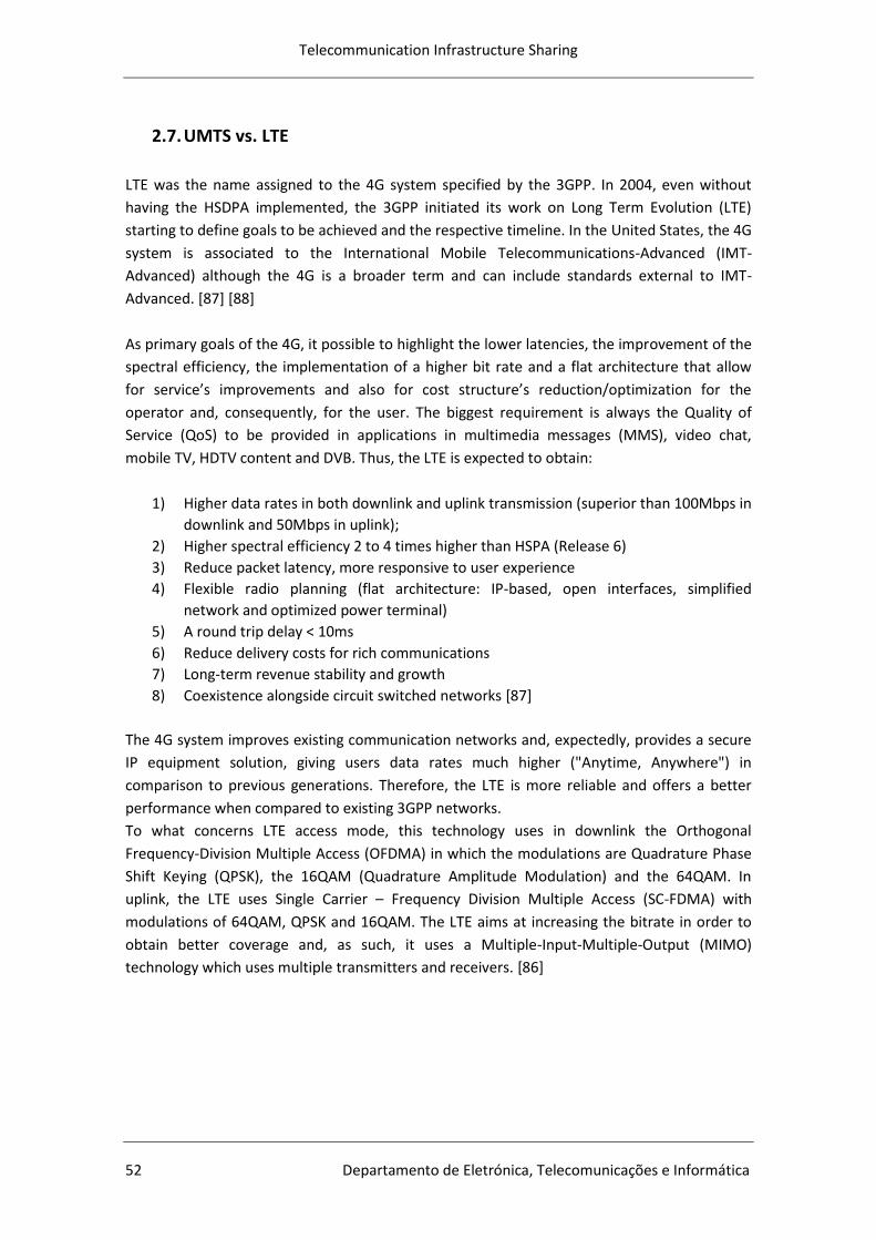
Telecommunication Infrastructure Sharing
52 Departamento de Eletrónica, Telecomunicações e Informática
2.7. UMTS vs. LTE
LTE was the name assigned to the 4G system specified by the 3GPP. In 2004, even without
having the HSDPA implemented, the 3GPP initiated its work on Long Term Evolution (LTE)
starting to define goals to be achieved and the respective timeline. In the United States, the 4G
system is associated to the International Mobile Telecommunications-Advanced (IMT-
Advanced) although the 4G is a broader term and can include standards external to IMT-
Advanced. [87] [88]
As primary goals of the 4G, it possible to highlight the lower latencies, the improvement of the
spectral efficiency, the implementation of a higher bit rate and a flat architecture that allow
for service’s improvements and also for cost structure’s reduction/optimization for the
operator and, consequently, for the user. The biggest requirement is always the Quality of
Service (QoS) to be provided in applications in multimedia messages (MMS), video chat,
mobile TV, HDTV content and DVB. Thus, the LTE is expected to obtain:
1) Higher data rates in both downlink and uplink transmission (superior than 100Mbps in
downlink and 50Mbps in uplink);
2) Higher spectral efficiency 2 to 4 times higher than HSPA (Release 6)
3) Reduce packet latency, more responsive to user experience
4) Flexible radio planning (flat architecture: IP-based, open interfaces, simplified
network and optimized power terminal)
5) A round trip delay < 10ms
6) Reduce delivery costs for rich communications
7) Long-term revenue stability and growth
8) Coexistence alongside circuit switched networks [87]
The 4G system improves existing communication networks and, expectedly, provides a secure
IP equipment solution, giving users data rates much higher ("Anytime, Anywhere") in
comparison to previous generations. Therefore, the LTE is more reliable and offers a better
performance when compared to existing 3GPP networks.
To what concerns LTE access mode, this technology uses in downlink the Orthogonal
Frequency-Division Multiple Access (OFDMA) in which the modulations are Quadrature Phase
Shift Keying (QPSK), the 16QAM (Quadrature Amplitude Modulation) and the 64QAM. In
uplink, the LTE uses Single Carrier – Frequency Division Multiple Access (SC-FDMA) with
modulations of 64QAM, QPSK and 16QAM. The LTE aims at increasing the bitrate in order to
obtain better coverage and, as such, it uses a Multiple-Input-Multiple-Output (MIMO)
technology which uses multiple transmitters and receivers. [86]
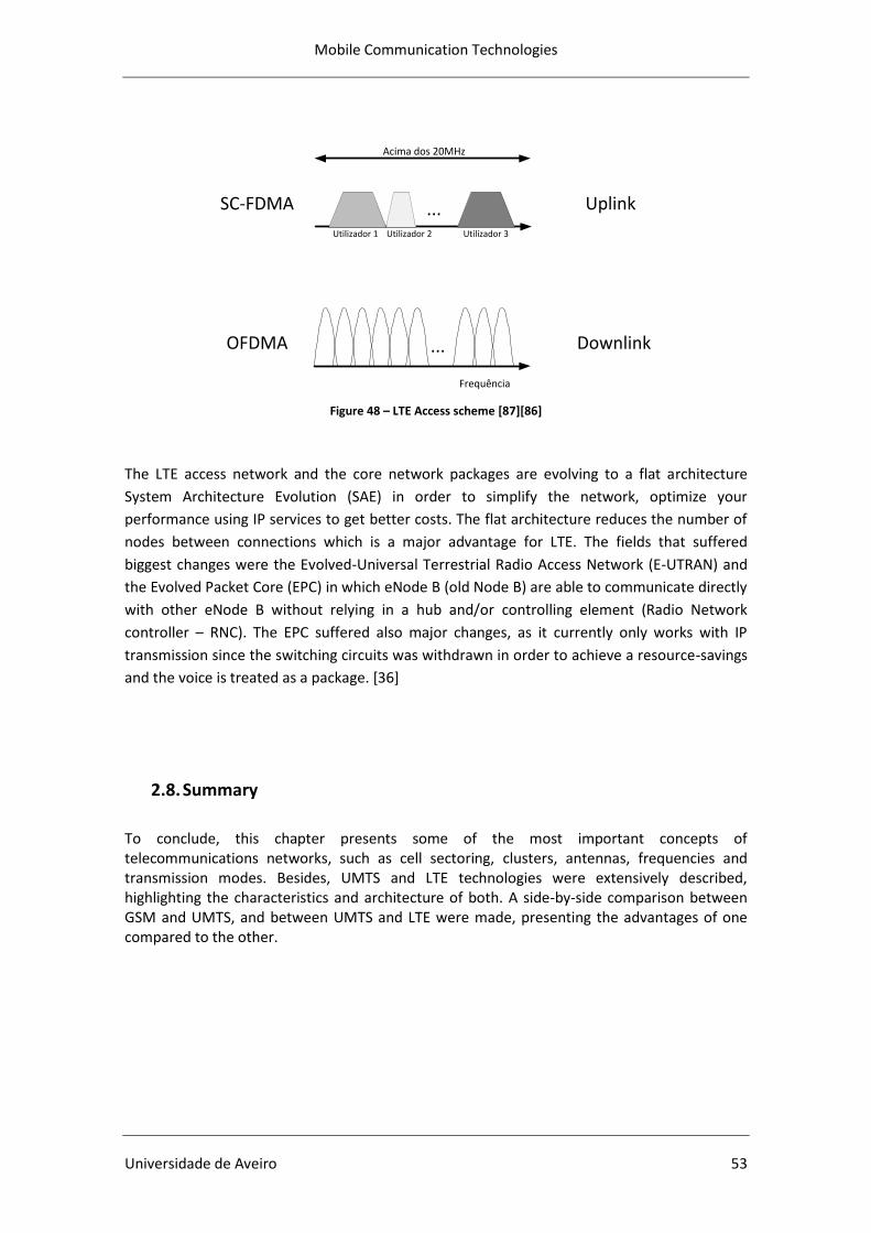
Mobile Communication Technologies
Universidade de Aveiro 53
...SC-FDMA
Downlink
Acima dos 20MHz
Uplink
OFDMA
Frequência
...
Utilizador 1 Utilizador 2 Utilizador 3
Figure 48 – LTE Access scheme [87][86]
The LTE access network and the core network packages are evolving to a flat architecture
System Architecture Evolution (SAE) in order to simplify the network, optimize your
performance using IP services to get better costs. The flat architecture reduces the number of
nodes between connections which is a major advantage for LTE. The fields that suffered
biggest changes were the Evolved-Universal Terrestrial Radio Access Network (E-UTRAN) and
the Evolved Packet Core (EPC) in which eNode B (old Node B) are able to communicate directly
with other eNode B without relying in a hub and/or controlling element (Radio Network
controller – RNC). The EPC suffered also major changes, as it currently only works with IP
transmission since the switching circuits was withdrawn in order to achieve a resource-savings
and the voice is treated as a package. [36]
2.8. Summary
To conclude, this chapter presents some of the most important concepts of telecommunications networks, such as cell sectoring, clusters, antennas, frequencies and transmission modes. Besides, UMTS and LTE technologies were extensively described, highlighting the characteristics and architecture of both. A side-by-side comparison between GSM and UMTS, and between UMTS and LTE were made, presenting the advantages of one compared to the other.

Telecommunication Infrastructure Sharing
54 Departamento de Eletrónica, Telecomunicações e Informática
Business Models Issues
Universidade de Aveiro 55
3. Business Models Issues
The conventional model of having a single mobile network operator that owns all the physical network elements and network layers is appearing to be outpaced. This is due to the rapid and complex technology migration combined with rigid regulatory requirements and increasing CAPEX. Compounding this with the growing competition, which led to a quick transformation of telecommunication equipment into simple commodities, as well as the increasing separation between network and service provision are driving operators to use multiple strategies. Network infrastructure sharing in the core and radio access networks emerge hence as progressive methods that can improve sustainability and network costs. [131] Developing countries and other emerging countries can now, thanks infrastructure sharing, exploit the technological, market and regulatory improvements that have make access to mobile and broadband services more affordable. At the same time, network operators that are entering or consolidating in emerging economies can have considerable savings on CAPEX and OPEX. [131]
3.1. Infrastructure Sharing
Infrastructure Sharing can be an economic alternative for operators to implement a network telecommunications in one region or in an entire country. Sharing network infrastructure has clear financial, environmental advantages and allows for timely implementation of networks. In fact, mobile infrastructure sharing encourages the adoption of newer technologies and the deployment of mobile broadband, which is more and more considered a viable method for turning broadband services accessible for a greater part of the world population. Mobile sharing can also bring more competition between mobile operators and service providers, at least where certain safeguards are used, without concerns for the appearance of anticompetitive behaviors. [20] There are two ways of sharing infrastructure in mobile networks: active and passive. Active Infrastructure Sharing is less used and in some countries is strongly regulated by the authorities. [19] In this form of infrastructure sharing, active elements of the network layer namely, antennas, base stations, transmission, operation and maintenance of base stations, the radio-electric planning, and, in some cases, frequency usage rights are divided among the operators. In a more general form it is primarily used national roaming, which can be implemented with great interest in rural areas. [19] [20] On the other hand, passive network sharing involves the elements with no electronic component such as mobile network sites, masts, cabinets or buildings, energy and air conditioning and security services. This is the most used form by operators. [19] Sharing telecommunications network infrastructure can create more efficient network coverage, since sites that have little coverage will be terminated and the savings generated are used to improve of networks with better coverage. This technique allows resource savings for operators.
Telecommunication Infrastructure Sharing
56 Departamento de Eletrónica, Telecomunicações e Informática
With infrastructure sharing, a further development of existing technologies may occur and they can be implemented in more remote areas, and in sparsely populated areas because the implementation costs will be shared by operators. [19] Regarding the impacts to the population, a sharing of infrastructure may be beneficial for them since there is a lower concentration of telecommunications equipment in the area, reducing not only the visual impact caused but also the exposure to electromagnetic waves. However, the sharing of infrastructure may cause telecom operators to reveal valuable information, such as costs and strategic plans, which can undermine their sustainability and market position. On the other hand, there may be a greater propensity for explicit or implicit collusive agreements, influencing negatively the competition and consequently the well-being of consumers. Nevertheless, in developing countries, infrastructure sharing is encouraged by governments and regulators of telecommunications as it stimulates the expansion of telecommunications networks. It also leads to a more efficient use of the existing resources, such as energy saving, which is a serious problem in remote areas (Appendix H). The most common and effective network sharing agreements are national roaming. These agreements can be limited for certain periods of time, for example one to two years, in order to avoid negative effects on competition between operators and to promote the development of the early stages of the construction of networks. [17] [18] [20] Another form of sharing refers to the virtual operator [Mobile Virtual Network Operator (MVNO)], which will be explained in more detail in section 3.2.1. This may be the aftermarket products and services to consumers, but using another brand, or purchasing data and minutes in large quantities and at low cost to other operators and reselling its users with specific plans of the brand. [18]
3.1.1.Passive Sharing
Passive sharing is the sharing of space in passive infrastructure, such as sites, building premises and masts. Passive sharing is usually a moderate form of network sharing, as there are still separate networks that just share physical space.
3.1.1.1.Site Sharing
The following figure (Figure 49) shows the basic elements for the construction of a mobile telecommunications site. The constituents are typically as demonstrated in the figure below:
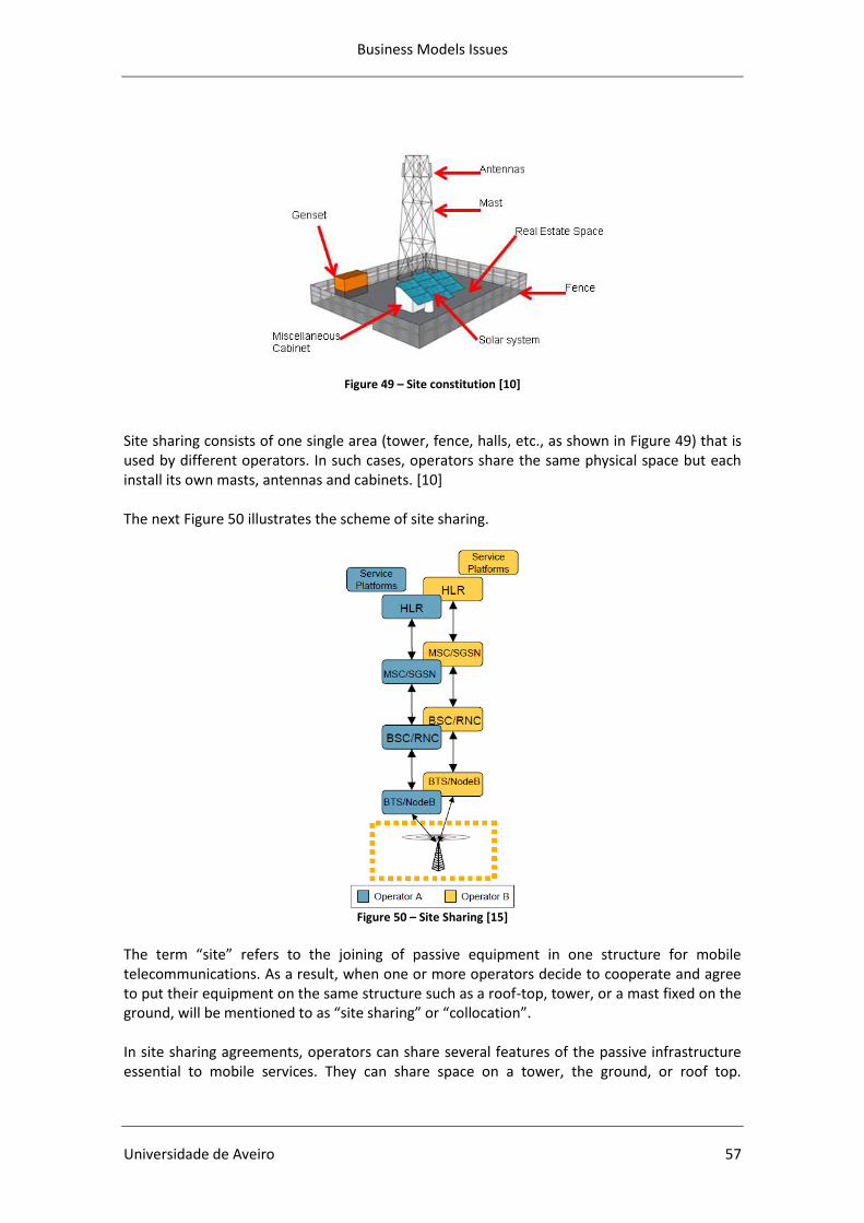
Business Models Issues
Universidade de Aveiro 57
Figure 49 – Site constitution [10]
Site sharing consists of one single area (tower, fence, halls, etc., as shown in Figure 49) that is used by different operators. In such cases, operators share the same physical space but each install its own masts, antennas and cabinets. [10] The next Figure 50 illustrates the scheme of site sharing.
Figure 50 – Site Sharing [15]
The term “site” refers to the joining of passive equipment in one structure for mobile telecommunications. As a result, when one or more operators decide to cooperate and agree to put their equipment on the same structure such as a roof-top, tower, or a mast fixed on the ground, will be mentioned to as “site sharing” or “collocation”. In site sharing agreements, operators can share several features of the passive infrastructure essential to mobile services. They can share space on a tower, the ground, or roof top.
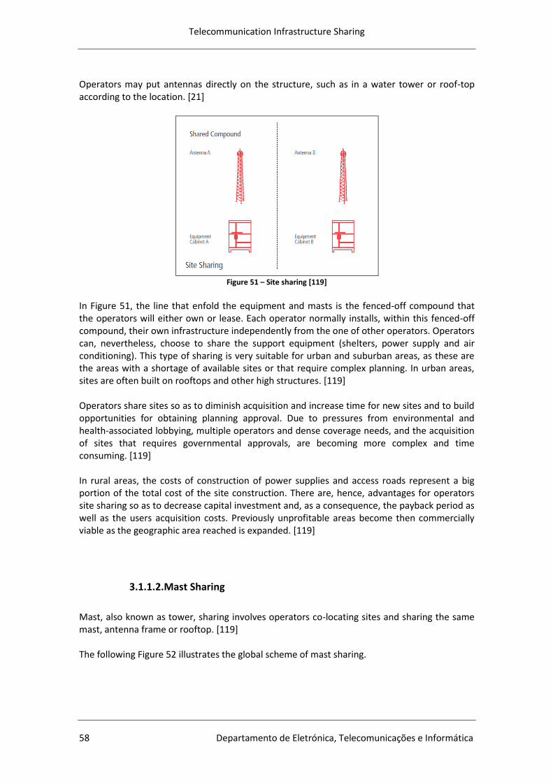
Telecommunication Infrastructure Sharing
58 Departamento de Eletrónica, Telecomunicações e Informática
Operators may put antennas directly on the structure, such as in a water tower or roof-top according to the location. [21]
Figure 51 – Site sharing [119]
In Figure 51, the line that enfold the equipment and masts is the fenced-off compound that the operators will either own or lease. Each operator normally installs, within this fenced-off compound, their own infrastructure independently from the one of other operators. Operators can, nevertheless, choose to share the support equipment (shelters, power supply and air conditioning). This type of sharing is very suitable for urban and suburban areas, as these are the areas with a shortage of available sites or that require complex planning. In urban areas, sites are often built on rooftops and other high structures. [119] Operators share sites so as to diminish acquisition and increase time for new sites and to build opportunities for obtaining planning approval. Due to pressures from environmental and health-associated lobbying, multiple operators and dense coverage needs, and the acquisition of sites that requires governmental approvals, are becoming more complex and time consuming. [119] In rural areas, the costs of construction of power supplies and access roads represent a big portion of the total cost of the site construction. There are, hence, advantages for operators site sharing so as to decrease capital investment and, as a consequence, the payback period as well as the users acquisition costs. Previously unprofitable areas become then commercially viable as the geographic area reached is expanded. [119]
3.1.1.2.Mast Sharing
Mast, also known as tower, sharing involves operators co-locating sites and sharing the same mast, antenna frame or rooftop. [119] The following Figure 52 illustrates the global scheme of mast sharing.
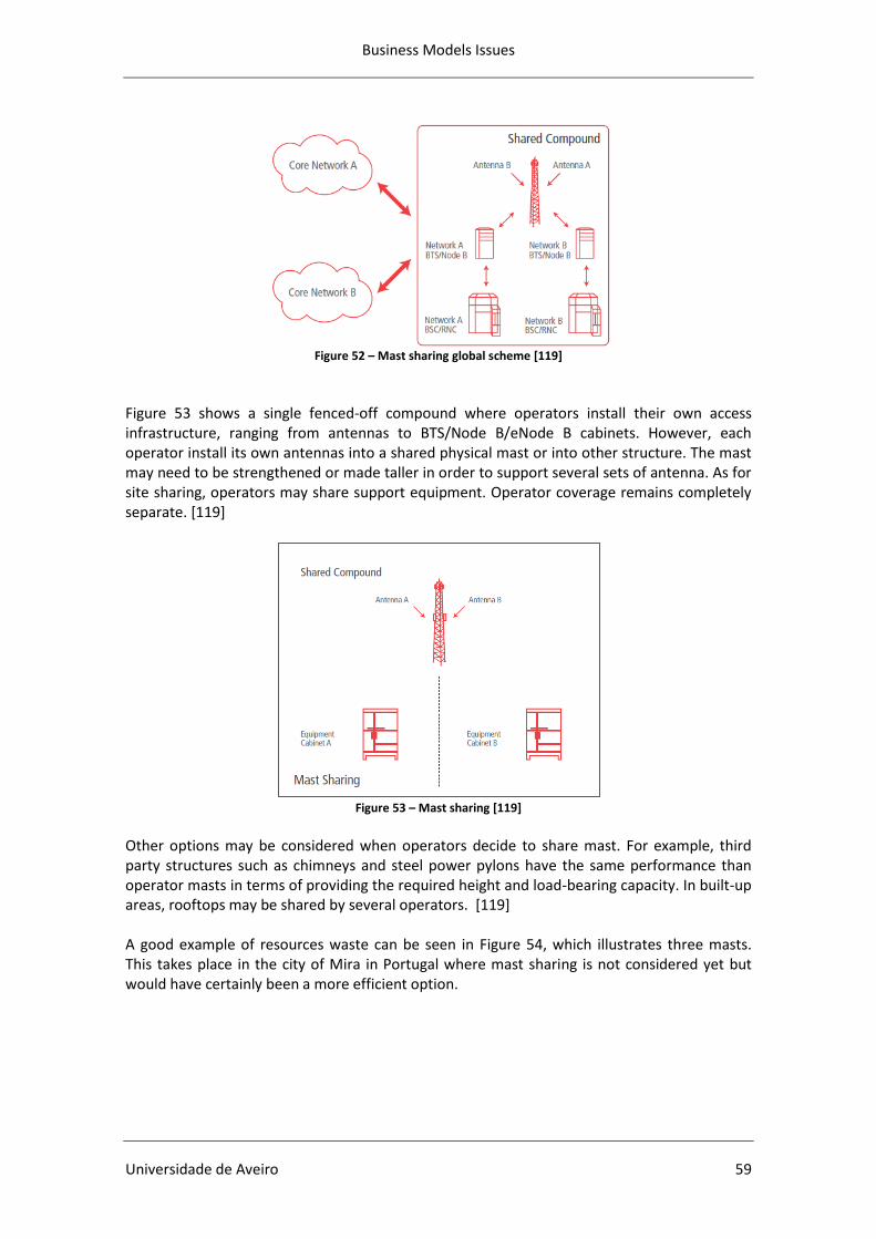
Business Models Issues
Universidade de Aveiro 59
Figure 52 – Mast sharing global scheme [119]
Figure 53 shows a single fenced-off compound where operators install their own access infrastructure, ranging from antennas to BTS/Node B/eNode B cabinets. However, each operator install its own antennas into a shared physical mast or into other structure. The mast may need to be strengthened or made taller in order to support several sets of antenna. As for site sharing, operators may share support equipment. Operator coverage remains completely separate. [119]
Figure 53 – Mast sharing [119]
Other options may be considered when operators decide to share mast. For example, third party structures such as chimneys and steel power pylons have the same performance than operator masts in terms of providing the required height and load-bearing capacity. In built-up areas, rooftops may be shared by several operators. [119] A good example of resources waste can be seen in Figure 54, which illustrates three masts. This takes place in the city of Mira in Portugal where mast sharing is not considered yet but would have certainly been a more efficient option.
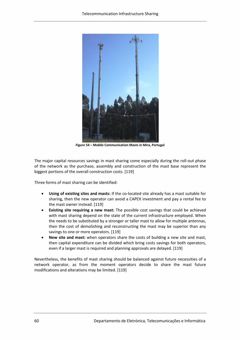
Telecommunication Infrastructure Sharing
60 Departamento de Eletrónica, Telecomunicações e Informática
Figure 54 – Mobile Communication Masts in Mira, Portugal
The major capital resources savings in mast sharing come especially during the roll-out phase of the network as the purchase, assembly and construction of the mast base represent the biggest portions of the overall construction costs. [119] Three forms of mast sharing can be identified:
Using of existing sites and masts: If the co-located site already has a mast suitable for sharing, then the new operator can avoid a CAPEX investment and pay a rental fee to the mast owner instead. [119]
Existing site requiring a new mast: The possible cost savings that could be achieved with mast sharing depend on the state of the current infrastructure employed. When the needs to be substituted by a stronger or taller mast to allow for multiple antennas, then the cost of demolishing and reconstructing the mast may be superior than any savings to one or more operators. [119]
New site and mast: when operators share the costs of building a new site and mast, then capital expenditure can be divided which bring costs savings for both operators, even if a larger mast is required and planning approvals are delayed. [119]
Nevertheless, the benefits of mast sharing should be balanced against future necessities of a network operator, as from the moment operators decide to share the mast future modifications and alterations may be limited. [119]
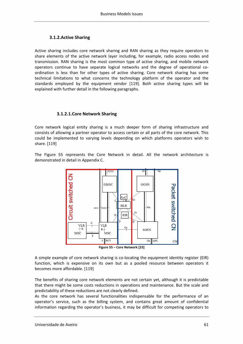
Business Models Issues
Universidade de Aveiro 61
3.1.2.Active Sharing
Active sharing includes core network sharing and RAN sharing as they require operators to share elements of the active network layer including, for example, radio access nodes and transmission. RAN sharing is the most common type of active sharing, and mobile network operators continue to have separate logical networks and the degree of operational co-ordination is less than for other types of active sharing. Core network sharing has some technical limitations to what concerns the technology platform of the operator and the standards employed by the equipment vendor [119]. Both active sharing types will be explained with further detail in the following paragraphs.
3.1.2.1.Core Network Sharing
Core network logical entity sharing is a much deeper form of sharing infrastructure and consists of allowing a partner operator to access certain or all parts of the core network. This could be implemented to varying levels depending on which platforms operators wish to share. [119] The Figure 55 represents the Core Network in detail. All the network architecture is demonstrated in detail in Appendix C.
Figure 55 – Core Network [23]
A simple example of core network sharing is co-locating the equipment identity register (EIR) function, which is expensive on its own but as a pooled resource between operators it becomes more affordable. [119] The benefits of sharing core network elements are not certain yet, although it is predictable that there might be some costs reductions in operations and maintenance. But the scale and predictability of these reductions are not clearly defined. As the core network has several functionalities indispensable for the performance of an operator’s service, such as the billing system, and contains great amount of confidential information regarding the operator’s business, it may be difficult for competing operators to
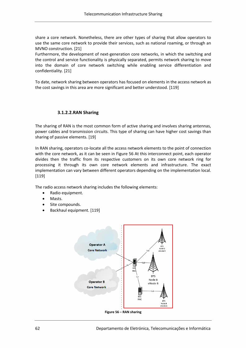
Telecommunication Infrastructure Sharing
62 Departamento de Eletrónica, Telecomunicações e Informática
share a core network. Nonetheless, there are other types of sharing that allow operators to use the same core network to provide their services, such as national roaming, or through an MVNO construction. [21] Furthermore, the development of next-generation core networks, in which the switching and the control and service functionality is physically separated, permits network sharing to move into the domain of core network switching while enabling service differentiation and confidentiality. [21] To date, network sharing between operators has focused on elements in the access network as the cost savings in this area are more significant and better understood. [119]
3.1.2.2.RAN Sharing
The sharing of RAN is the most common form of active sharing and involves sharing antennas, power cables and transmission circuits. This type of sharing can have higher cost savings than sharing of passive elements. [19] In RAN sharing, operators co-locate all the access network elements to the point of connection with the core network, as it can be seen in Figure 56 At this interconnect point, each operator divides then the traffic from its respective customers on its own core network ring for processing it through its own core network elements and infrastructure. The exact implementation can vary between different operators depending on the implementation local. [119] The radio access network sharing includes the following elements:
Radio equipment.
Masts.
Site compounds.
Backhaul equipment. [119]
Figure 56 – RAN sharing
Business Models Issues
Universidade de Aveiro 63
The sharing of antennas and supply cables, although technically viable, presents some technical problems. In the case of antennas sharing, it is difficult for operators to use different frequency bands or have different optimization’s network strategies. In the case of supply cables sharing, energy losses may happen and affect the coverage area of the services provided. [19] Offering services on the same network transmission (backhaul), namely the part of the network between Nodes B and RNCs, can reduce the operational costs of the leased lines and of the using rates of the microwave spectrum but it requires additional network elements at the ends of the connections6. [19] RAN sharing might eventually hamper competition, as operator have now a significant portion of costs in common, which can facilitate price coordination and make them more limited in their ability to differentiate when compared to passive sharing. There are nevertheless some practical cases of RAN co-locating. For example, in Denmark a joint venture between Telia Denmark and Telenor was made in order to jointly develop and control the RAN infrastructure, including masts and antennas. [19]
6 To mention that RAN sharing may involve more complex forms which require a network architecture in
which the RNC and Nodes B are divided between the parties. In this case, operators maintain independent control the parameters associated with the cells, although there are parameters shared at the sites level, in order to minimize the effects of sharing in terms of service differentiation and geographical coverage. In Nodes B, radio amplifiers and radio power remain physically independent, so that operators can use the frequencies which they have been assigned to. [19]

Telecommunication Infrastructure Sharing
64 Departamento de Eletrónica, Telecomunicações e Informática
3.2. Business Models
In this section two strategies are presented: the Mobile Virtual Network Operator (MVNO) and the Neutral Operator (NO). The MVNO to be implemented requires another operator to be in the market with a solid infrastructure already. The NO is the type of strategy that will be used in this work, and it is the operator that allows for infrastructure sharing. Although the MVNO will not be covered in this work, it may be important for telecommunication development when the Neutral Operator is implemented.
3.2.1.Mobile Virtual Network Operator (MVNO)
MVNOs typically lack of RAN and might not have spectrum usage rights. [19] They offer mobile telecom services to customers by reselling wholesale minutes that they have purchased from an existing infrastructure owner (a mobile network operator).[21] This infrastructure sharing varies according to the type of the MVNO and may be wholly or exclude, for example, certain parts of the core network. A MVNO can, hence, range from simple retail reseller (light MVNO) to an operator with its own network (full MVNO). The closer a MVNO is from a simple reseller, the lower is its capacity to differentiate services. [19] In general, the main distinguishing feature of a MVNO from network operators relates to the development of alternative business strategies focused on niche markets or to the smaller investment in the brand so as to guarantee the lowest prices. However, since the vast majority of its costs are related to the access tariffs negotiated with the network operator, the ability to differentiate the price is limited. [19] The number of MVNOs in Europe has increased significantly since the years 2002-2003. [21] Nevertheless, the degree of success of MVNOs and of their business models vary considerably from case to case and from country to country. [120] In the case of the United Kingdom, the number of successful MVNO’s is considerable, being the largest one Virgin Mobile with over 4 million users by 2006. [120] In the case of the Netherlands, there are approximately 50 MVNOs and other service providers without a network that are operating in the Dutch market and that represent together a market share of roughly 17%, with Debitel and Tele 2 being the largest ones. [121] In recent times, a new concept has been introduced in certain European countries called MVNE (Mobile Virtual Network Enabler). An MVNE provides administration, operation and infrastructure services to MVNOs or service providers, and does not have a direct relationship with the end user. [21] In spite of MVNOs possibly increase competition in certain markets, they are not a solution in markets where mobile networks have not been widely set. MVNOs depend on the existence of formerly set up networks so as to offer their services. Still, in case operators do not make use of their full capacity, giving access to MVNOs is appropriate option so as to put in the market more affordable services. In fact, in some countries MVNO access has been established by regulators. [122] To regulate MVNO access, a number of measures must be introduced to define, among others:
The type of access;
Pricing;
Transparency;

Business Models Issues
Universidade de Aveiro 65
Non-discrimination. Accordingly, regulators may facilitate the entry of MVNOs, whether or not through regulated access, in order to boost competition and make services more affordable.[21] In many cases where MVNO access has been introduced successfully, operators have entered into MVNO agreements on a voluntary basis. As mentioned, MVNO agreements may be beneficial when operators have spare capacity on their networks. In this case, operators have an incentive to offer this spare capacity to other operators and increase their revenues. Also, new entrants with a strong brand may also want to enter the mobile market. [21]
3.2.2.Neutral Operator (NO)
Neutral Operator (NO) is a relatively recent concept. It appeared in the beginning of the new century when the idea of Infrastructure Sharing started to become a more consolidated reality. Although infrastructure sharing has become a common solution for a number of growing challenges in the telecommunications market, the concept of NO has taken a little longer to be implemented, especially in the context of the emerging markets. This happens because an NO becomes an active agent in the economies where it is implemented. Therefore, the NO becomes more than a technological solution for telecommunication problems; it is an agent actively engaged in developing a sustainable and profitable form of overcoming the mobile telecommunications constraints. [10] A NO typically invest in infrastructure, namely in building base stations in more remote areas where other operators are usually unwilling to invest. A NO does not compete directly with other operators; instead, it creates the necessary conditions for those operators to penetrate an area perceived previously as less attractive from an investment perspective. In this case, the initially unappealing area becomes an opportunity for the incumbent and new entrants to provide services, without the unattractive investment usually required to cover such territorial extensions and the depressed Return on Investment (ROI). [10] The NO basically allows infrastructure sharing and, as such, it promotes competition in the different business sectors such as services and access networks. [143] NO is based on the following principles:
Neutrality, avoiding interference with potential business deals from the operators;
Non-discrimination among operators;
Transparency in both the access to wholesale and end-user offers;
Equity among all the operators interested in reaching final users within the network coverage. [142]
This new active agent, the NO, hold the role of a mediator within the telecommunications sector by setting up new dynamics between the government, operators, investors and the users. The NO becomes also an instrument and opportunity for new services development, for quality improvement of services and for better investment opportunities. [10] The NO model is based on a division of the network infrastructure and service provision. A new form of network operator, the Neutral Operator, is introduced, which acts as a coordinator
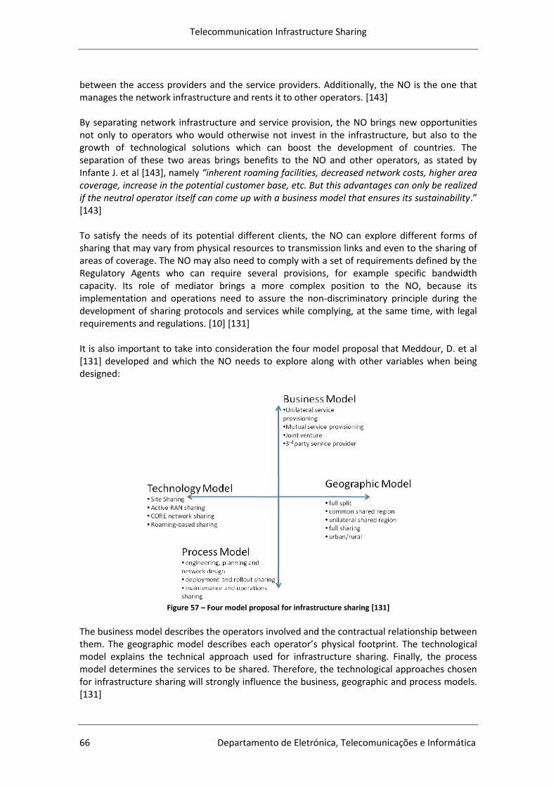
Telecommunication Infrastructure Sharing
66 Departamento de Eletrónica, Telecomunicações e Informática
between the access providers and the service providers. Additionally, the NO is the one that manages the network infrastructure and rents it to other operators. [143] By separating network infrastructure and service provision, the NO brings new opportunities not only to operators who would otherwise not invest in the infrastructure, but also to the growth of technological solutions which can boost the development of countries. The separation of these two areas brings benefits to the NO and other operators, as stated by Infante J. et al [143], namely “inherent roaming facilities, decreased network costs, higher area coverage, increase in the potential customer base, etc. But this advantages can only be realized if the neutral operator itself can come up with a business model that ensures its sustainability.” [143] To satisfy the needs of its potential different clients, the NO can explore different forms of sharing that may vary from physical resources to transmission links and even to the sharing of areas of coverage. The NO may also need to comply with a set of requirements defined by the Regulatory Agents who can require several provisions, for example specific bandwidth capacity. Its role of mediator brings a more complex position to the NO, because its implementation and operations need to assure the non-discriminatory principle during the development of sharing protocols and services while complying, at the same time, with legal requirements and regulations. [10] [131] It is also important to take into consideration the four model proposal that Meddour, D. et al [131] developed and which the NO needs to explore along with other variables when being designed:
Figure 57 – Four model proposal for infrastructure sharing [131]
The business model describes the operators involved and the contractual relationship between them. The geographic model describes each operator’s physical footprint. The technological model explains the technical approach used for infrastructure sharing. Finally, the process model determines the services to be shared. Therefore, the technological approaches chosen for infrastructure sharing will strongly influence the business, geographic and process models. [131]
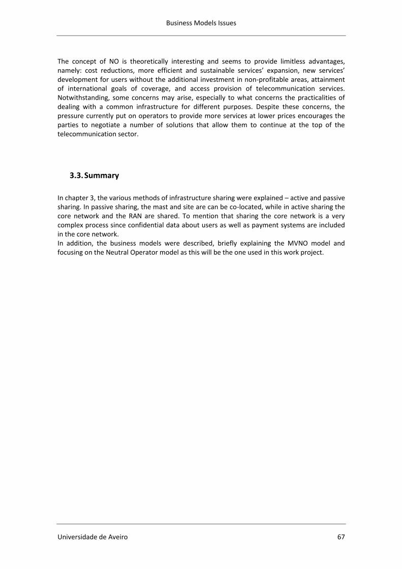
Business Models Issues
Universidade de Aveiro 67
The concept of NO is theoretically interesting and seems to provide limitless advantages, namely: cost reductions, more efficient and sustainable services’ expansion, new services’ development for users without the additional investment in non-profitable areas, attainment of international goals of coverage, and access provision of telecommunication services. Notwithstanding, some concerns may arise, especially to what concerns the practicalities of dealing with a common infrastructure for different purposes. Despite these concerns, the pressure currently put on operators to provide more services at lower prices encourages the parties to negotiate a number of solutions that allow them to continue at the top of the telecommunication sector.
3.3. Summary
In chapter 3, the various methods of infrastructure sharing were explained – active and passive sharing. In passive sharing, the mast and site are can be co-located, while in active sharing the core network and the RAN are shared. To mention that sharing the core network is a very complex process since confidential data about users as well as payment systems are included in the core network. In addition, the business models were described, briefly explaining the MVNO model and focusing on the Neutral Operator model as this will be the one used in this work project.

Telecommunication Infrastructure Sharing
68 Departamento de Eletrónica, Telecomunicações e Informática
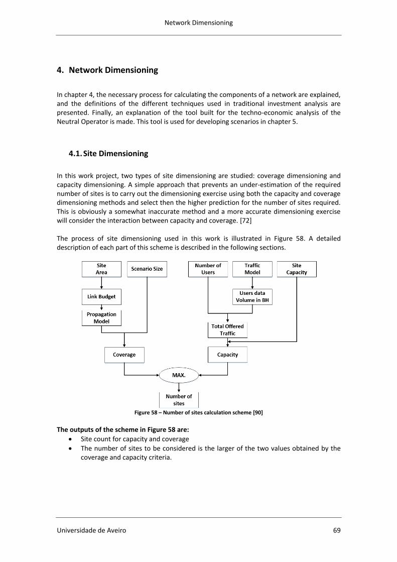
Network Dimensioning
Universidade de Aveiro 69
4. Network Dimensioning
In chapter 4, the necessary process for calculating the components of a network are explained, and the definitions of the different techniques used in traditional investment analysis are presented. Finally, an explanation of the tool built for the techno-economic analysis of the Neutral Operator is made. This tool is used for developing scenarios in chapter 5.
4.1. Site Dimensioning
In this work project, two types of site dimensioning are studied: coverage dimensioning and capacity dimensioning. A simple approach that prevents an under-estimation of the required number of sites is to carry out the dimensioning exercise using both the capacity and coverage dimensioning methods and select then the higher prediction for the number of sites required. This is obviously a somewhat inaccurate method and a more accurate dimensioning exercise will consider the interaction between capacity and coverage. [72] The process of site dimensioning used in this work is illustrated in Figure 58. A detailed description of each part of this scheme is described in the following sections.
Figure 58 – Number of sites calculation scheme [90]
The outputs of the scheme in Figure 58 are:
Site count for capacity and coverage
The number of sites to be considered is the larger of the two values obtained by the coverage and capacity criteria.
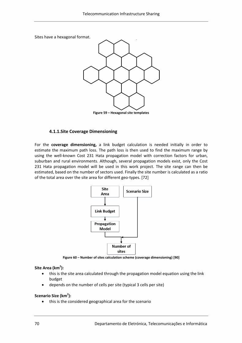
Telecommunication Infrastructure Sharing
70 Departamento de Eletrónica, Telecomunicações e Informática
Sites have a hexagonal format.
Figure 59 – Hexagonal site templates
4.1.1.Site Coverage Dimensioning
For the coverage dimensioning, a link budget calculation is needed initially in order to estimate the maximum path loss. The path loss is then used to find the maximum range by using the well-known Cost 231 Hata propagation model with correction factors for urban, suburban and rural environments. Although, several propagation models exist, only the Cost 231 Hata propagation model will be used in this work project. The site range can then be estimated, based on the number of sectors used. Finally the site number is calculated as a ratio of the total area over the site area for different geo-types. [72]
Figure 60 – Number of sites calculation scheme (coverage dimensioning) [90]
Site Area (km2):
this is the site area calculated through the propagation model equation using the link budget
depends on the number of cells per site (typical 3 cells per site) Scenario Size (km2):
this is the considered geographical area for the scenario

Network Dimensioning
Universidade de Aveiro 71
The following equations correspond to the Cost 231 Hata radio propagation model [82] to 900 MHz frequency band. For urban environments, the equation is:
Equation 5 – Propagation model urban environments
where
Equation 6 – a(hM)
and is the base station (BS) antenna height in meters, is the user equipment (UE) antenna height in meters, is the users frequency in MHz and R is the distance between BS and UE in km (site range). For some typical values, i.e. , , and , and so above formula is simplified to:
Equation 7 – Propagation path loss in dB urban environments
For suburban environments, the equation is
Equation 8 – Propagation model suburban environments
Therefore, for a typical value will be
Equation 9 – Propagation path loss in dB in suburban environments
In rural areas, the Cost 231 Hata propagation model equations is used to calculate the propagation path loss in decibel (dB) with corresponding correction factors for rural environment, as shown in Equation 10. [72] [82]
Equation 10 – Propagation model rural environment
Therefore for 920 MHz (UMTS900), the equation is
Equation 11 – Propagation path loss in dB in rural environment for UMTS900 [82]
The site range R is used to estimate the site area with three sectors, by using Equation 12 from Ovum Consulting [72]
Equation 12 – Site area [72]

Telecommunication Infrastructure Sharing
72 Departamento de Eletrónica, Telecomunicações e Informática
To calculate the number of sites the Equation 13 is used:
Equation 13 – Number of sites
4.1.2.Site Capacity Dimensioning
For the capacity dimensioning, the maximum capacity per carrier is initially calculated based on the pole capacity and the assumed noise rise. The overall (voice, SMS and data) offered traffic in busy hour per geo-type is then predicted. Finally the maximum number of sites per geo-type is calculated as a ratio of the offered traffic over the site capacity (that is, the carrier capacity times the carriers per site). [72]
Figure 61 – Number of sites calculation scheme (capacity dim.) (adapted from [90] [145])
Knowing the users data traffic in Busy Hour, the number of sites required is calculated in the following way:
Equation 14 – Total traffic Busy Hour
Equation 15 – Number of sites
In communication system, the Busy Hour happens because the calls bunch up. All traffic planning has to focus on peak periods. It is not acceptable to provide excellent service most of the time and terrible service just when the customers want to make calls. To calculate Busy Hour values, the most common approach is to take the busiest hour of each day for five or ten days during the busiest time of year, and then calculate the average of those hours traffic load. That “Average Busy Hour” is used to determine the maximum number of people needed. [74] [75]
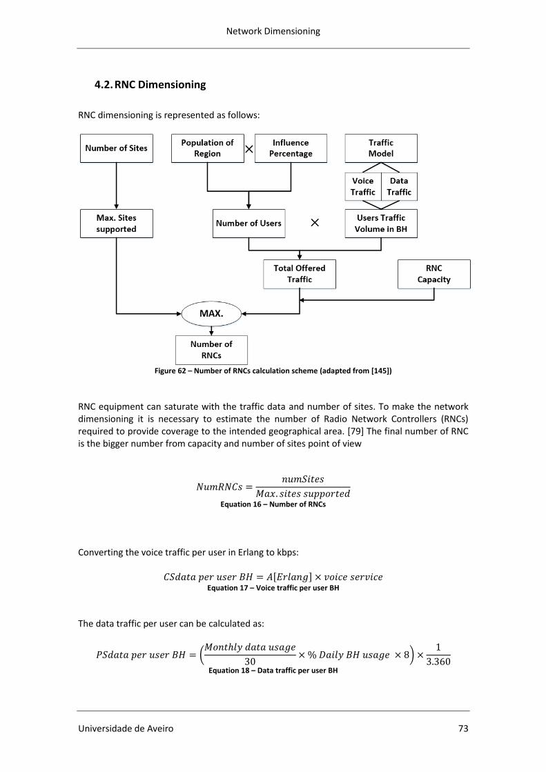
Network Dimensioning
Universidade de Aveiro 73
4.2. RNC Dimensioning
RNC dimensioning is represented as follows:
Figure 62 – Number of RNCs calculation scheme (adapted from [145])
RNC equipment can saturate with the traffic data and number of sites. To make the network dimensioning it is necessary to estimate the number of Radio Network Controllers (RNCs) required to provide coverage to the intended geographical area. [79] The final number of RNC is the bigger number from capacity and number of sites point of view
Equation 16 – Number of RNCs
Converting the voice traffic per user in Erlang to kbps:
Equation 17 – Voice traffic per user BH
The data traffic per user can be calculated as:
Equation 18 – Data traffic per user BH
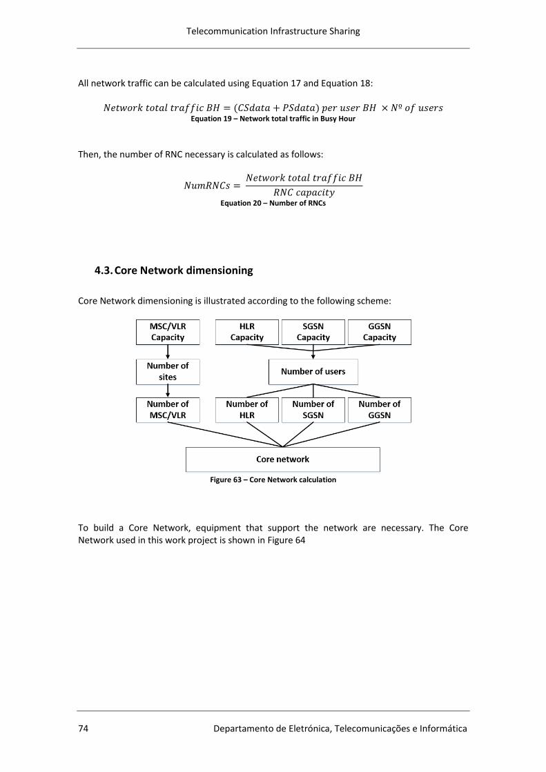
Telecommunication Infrastructure Sharing
74 Departamento de Eletrónica, Telecomunicações e Informática
All network traffic can be calculated using Equation 17 and Equation 18:
Equation 19 – Network total traffic in Busy Hour
Then, the number of RNC necessary is calculated as follows:
Equation 20 – Number of RNCs
4.3. Core Network dimensioning
Core Network dimensioning is illustrated according to the following scheme:
Figure 63 – Core Network calculation
To build a Core Network, equipment that support the network are necessary. The Core Network used in this work project is shown in Figure 64
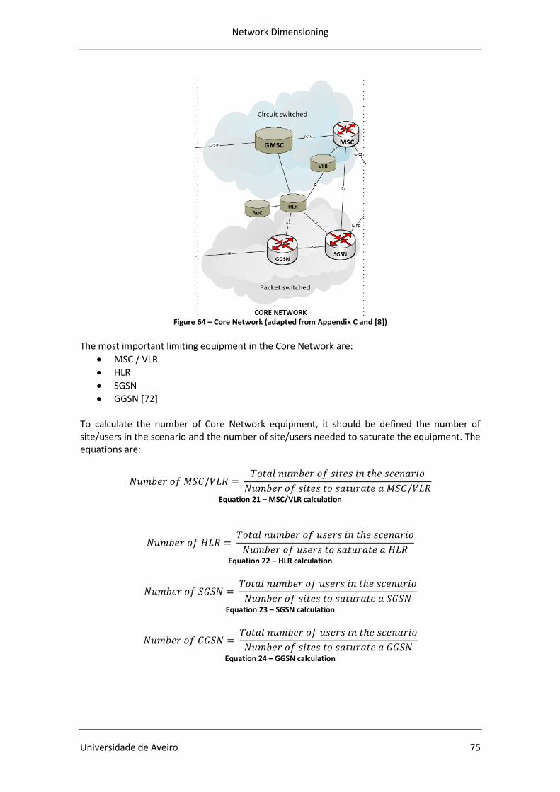
Network Dimensioning
Universidade de Aveiro 75
Figure 64 – Core Network (adapted from Appendix C and [8])
The most important limiting equipment in the Core Network are:
MSC / VLR
HLR
SGSN
GGSN [72] To calculate the number of Core Network equipment, it should be defined the number of site/users in the scenario and the number of site/users needed to saturate the equipment. The equations are:
Equation 21 – MSC/VLR calculation
Equation 22 – HLR calculation
Equation 23 – SGSN calculation
Equation 24 – GGSN calculation
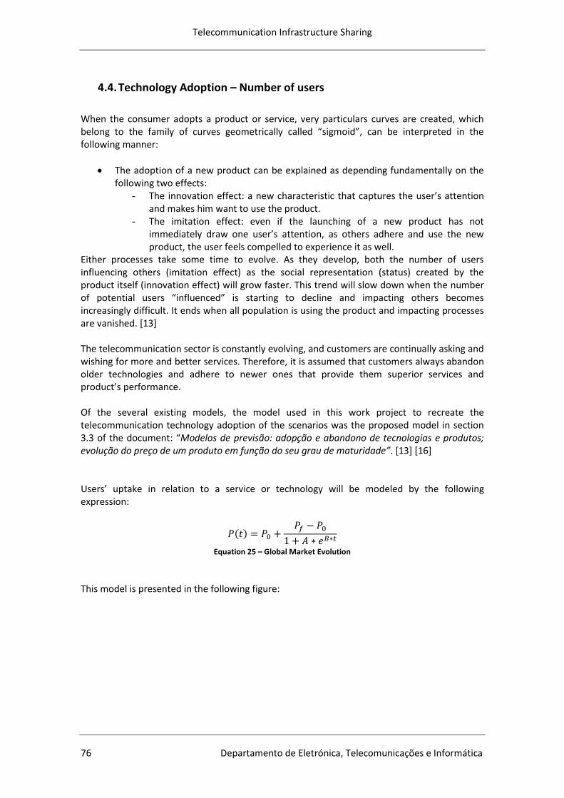
Telecommunication Infrastructure Sharing
76 Departamento de Eletrónica, Telecomunicações e Informática
4.4. Technology Adoption – Number of users
When the consumer adopts a product or service, very particulars curves are created, which belong to the family of curves geometrically called “sigmoid”, can be interpreted in the following manner:
The adoption of a new product can be explained as depending fundamentally on the following two effects:
- The innovation effect: a new characteristic that captures the user’s attention and makes him want to use the product.
- The imitation effect: even if the launching of a new product has not immediately draw one user’s attention, as others adhere and use the new product, the user feels compelled to experience it as well.
Either processes take some time to evolve. As they develop, both the number of users influencing others (imitation effect) as the social representation (status) created by the product itself (innovation effect) will grow faster. This trend will slow down when the number of potential users “influenced” is starting to decline and impacting others becomes increasingly difficult. It ends when all population is using the product and impacting processes are vanished. [13] The telecommunication sector is constantly evolving, and customers are continually asking and wishing for more and better services. Therefore, it is assumed that customers always abandon older technologies and adhere to newer ones that provide them superior services and product’s performance. Of the several existing models, the model used in this work project to recreate the telecommunication technology adoption of the scenarios was the proposed model in section 3.3 of the document: “Modelos de previsão: adopção e abandono de tecnologias e produtos; evolução do preço de um produto em função do seu grau de maturidade”. [13] [16] Users’ uptake in relation to a service or technology will be modeled by the following expression:
Equation 25 – Global Market Evolution
This model is presented in the following figure:
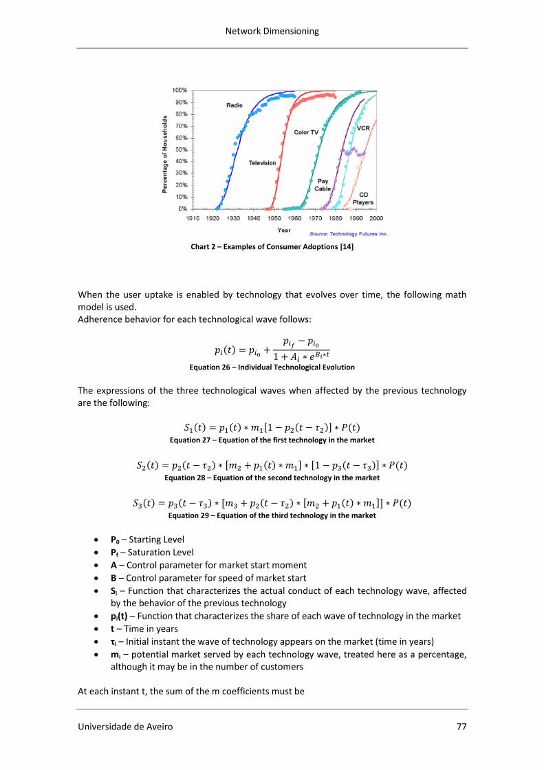
Network Dimensioning
Universidade de Aveiro 77
Chart 2 – Examples of Consumer Adoptions [14]
When the user uptake is enabled by technology that evolves over time, the following math model is used. Adherence behavior for each technological wave follows:
Equation 26 – Individual Technological Evolution
The expressions of the three technological waves when affected by the previous technology are the following:
Equation 27 – Equation of the first technology in the market
Equation 28 – Equation of the second technology in the market
Equation 29 – Equation of the third technology in the market
P0 – Starting Level
Pf – Saturation Level
A – Control parameter for market start moment
B – Control parameter for speed of market start
Si – Function that characterizes the actual conduct of each technology wave, affected by the behavior of the previous technology
pi(t) – Function that characterizes the share of each wave of technology in the market
t – Time in years
τi – Initial instant the wave of technology appears on the market (time in years)
mi – potential market served by each technology wave, treated here as a percentage, although it may be in the number of customers
At each instant t, the sum of the m coefficients must be
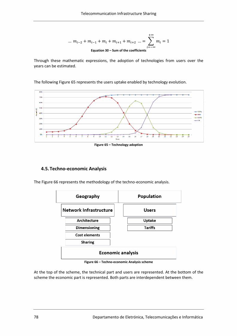
Telecommunication Infrastructure Sharing
78 Departamento de Eletrónica, Telecomunicações e Informática
Equation 30 – Sum of the coefficients
Through these mathematic expressions, the adoption of technologies from users over the years can be estimated. The following Figure 65 represents the users uptake enabled by technology evolution.
Figure 65 – Technology adoption
4.5. Techno-economic Analysis
The Figure 66 represents the methodology of the techno-economic analysis.
Figure 66 – Techno-economic Analysis scheme
At the top of the scheme, the technical part and users are represented. At the bottom of the scheme the economic part is represented. Both parts are interdependent between them.
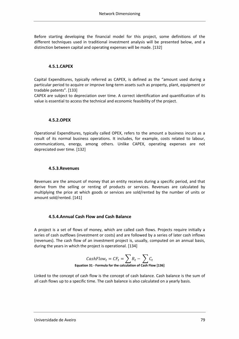
Network Dimensioning
Universidade de Aveiro 79
Before starting developing the financial model for this project, some definitions of the different techniques used in traditional investment analysis will be presented below, and a distinction between capital and operating expenses will be made. [132]
4.5.1.CAPEX
Capital Expenditures, typically referred as CAPEX, is defined as the “amount used during a particular period to acquire or improve long-term assets such as property, plant, equipment or tradable patents”. [133] CAPEX are subject to depreciation over time. A correct identification and quantification of its value is essential to access the technical and economic feasibility of the project.
4.5.2.OPEX
Operational Expenditures, typically called OPEX, refers to the amount a business incurs as a result of its normal business operations. It includes, for example, costs related to labour, communications, energy, among others. Unlike CAPEX, operating expenses are not depreciated over time. [132]
4.5.3.Revenues
Revenues are the amount of money that an entity receives during a specific period, and that derive from the selling or renting of products or services. Revenues are calculated by multiplying the price at which goods or services are sold/rented by the number of units or amount sold/rented. [141]
4.5.4.Annual Cash Flow and Cash Balance
A project is a set of flows of money, which are called cash flows. Projects require initially a series of cash outflows (investment or costs) and are followed by a series of later cash inflows (revenues). The cash flow of an investment project is, usually, computed on an annual basis, during the years in which the project is operational. [134]
Equation 31 - Formula for the calculation of Cash Flow [136]
Linked to the concept of cash flow is the concept of cash balance. Cash balance is the sum of all cash flows up to a specific time. The cash balance is also calculated on a yearly basis.

Telecommunication Infrastructure Sharing
80 Departamento de Eletrónica, Telecomunicações e Informática
Equation 32 – Formula for the calculation of Cash Balance [136]
Where corresponds to the time period of the project, which has a duration of 25 years on this case study, R is revenues and C is cost A common method used in the profitability of an investment project is the analysis of cash flows confronted, in turn, with different technological alternatives. Using the incremental approach in these cases is very common, where only costs directly related to the project are considered. The total costs are not usually taken into account in these studies. [10]
4.5.5.Net Present Value (NPV)
The Net Present Value (NPV) is considered the most important method for determining the value of the project. The NPV of an investment is the present value of all its future cash flows (all futures cash flows are translated into today’s cash flows). To convert future cash flow amount into its equivalent present value amount it is necessary to determine the discount factor ( ). Each annual Cash Flow is discounted by the corresponding rate , where is the discount rate and corresponds to the time period of the project, which has a duration of 25 years on this case study. The sum of all discounted cash flows is hence the net present value, which can be illustrated in the following equation:
Equation 33 – Formula for the calculation of NPV
Capital budgeting rules state that only positive NPV projects should be accepted. If the NPV is negative the project should be rejected, while if it is zero it does not matter. [135]
4.5.6.Internal Rate Return (IRR)
The Internal Rate of Return, referred as IRR, is another method used to determine the value of the project. This indicator is the maximum rate of profitability of the project and makes the NPV of all cash flows equal to zero. To determine the profitability of the project and its ability cover the capital invested, the IRR is compared to the cost of capital of the project itself. In case the IRR indicator value is higher than the cost of capital, then the project is economically profitable. On the other hand, if the IRR is lower than the cost of capital, the project is not financially viable and should be rejected. Nevertheless, the IRR has also some drawbacks. For instance, when a project has variable cash
Network Dimensioning
Universidade de Aveiro 81
flows, varying from positive to negative several times, numerous IRR can be identified, which make it hard to obtain the correct value of the IRR and can lead to wrong investment decisions. [132]
4.5.7.Payback Period
The Payback Period is the period at which revenues balance all investment costs. That is, it is the time span, in years usually, that the investment made is recovered making the cash balance become positive. The decision under the payback rule is to undertake the project with the shortest (best) payback period. Although it is a simple and practical indicator, taking it has the primary decision rule can lead to misleading choices as it does not take into consideration the behaviour of a project after its implementation. Therefore, the payback period should be used as an interesting side information for projects but other methods, such as the NPV and IRR, should be used for capital budgeting. [135]
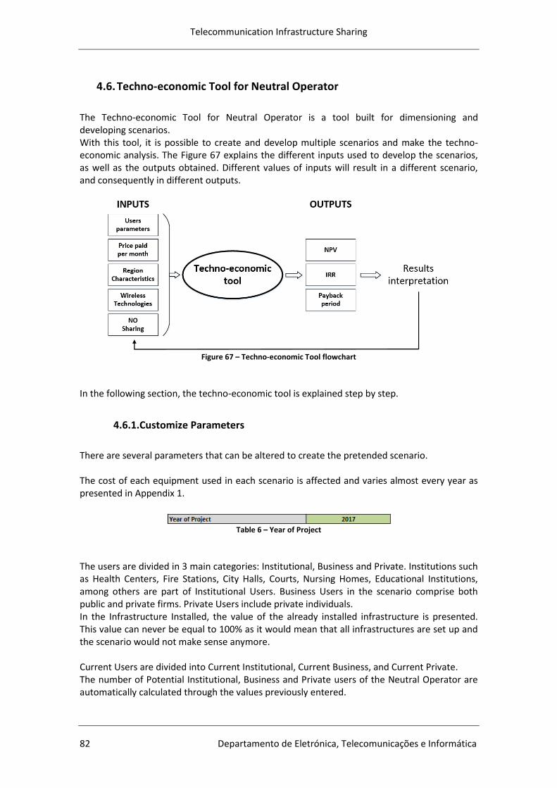
Telecommunication Infrastructure Sharing
82 Departamento de Eletrónica, Telecomunicações e Informática
4.6. Techno-economic Tool for Neutral Operator
The Techno-economic Tool for Neutral Operator is a tool built for dimensioning and developing scenarios. With this tool, it is possible to create and develop multiple scenarios and make the techno-economic analysis. The Figure 67 explains the different inputs used to develop the scenarios, as well as the outputs obtained. Different values of inputs will result in a different scenario, and consequently in different outputs.
Figure 67 – Techno-economic Tool flowchart
In the following section, the techno-economic tool is explained step by step.
4.6.1.Customize Parameters
There are several parameters that can be altered to create the pretended scenario. The cost of each equipment used in each scenario is affected and varies almost every year as presented in Appendix 1.
Table 6 – Year of Project
The users are divided in 3 main categories: Institutional, Business and Private. Institutions such as Health Centers, Fire Stations, City Halls, Courts, Nursing Homes, Educational Institutions, among others are part of Institutional Users. Business Users in the scenario comprise both public and private firms. Private Users include private individuals. In the Infrastructure Installed, the value of the already installed infrastructure is presented. This value can never be equal to 100% as it would mean that all infrastructures are set up and the scenario would not make sense anymore. Current Users are divided into Current Institutional, Current Business, and Current Private. The number of Potential Institutional, Business and Private users of the Neutral Operator are automatically calculated through the values previously entered.
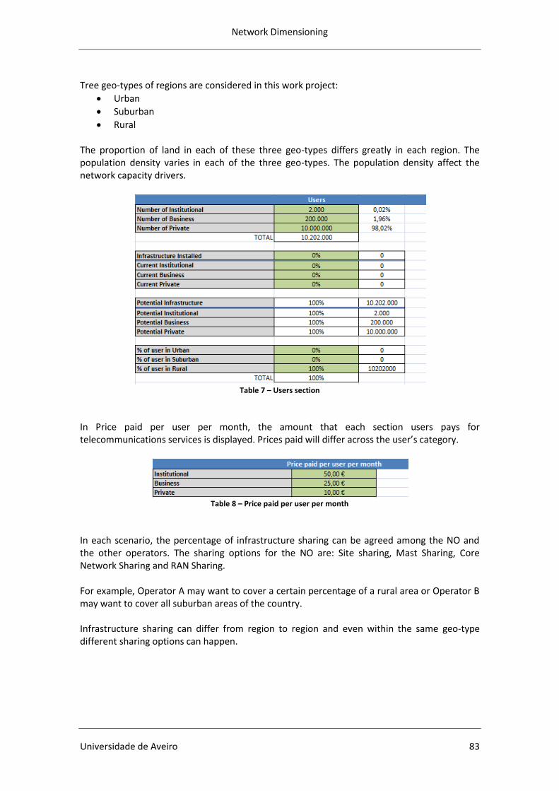
Network Dimensioning
Universidade de Aveiro 83
Tree geo-types of regions are considered in this work project:
Urban
Suburban
Rural The proportion of land in each of these three geo-types differs greatly in each region. The population density varies in each of the three geo-types. The population density affect the network capacity drivers.
Table 7 – Users section
In Price paid per user per month, the amount that each section users pays for telecommunications services is displayed. Prices paid will differ across the user’s category.
Table 8 – Price paid per user per month
In each scenario, the percentage of infrastructure sharing can be agreed among the NO and the other operators. The sharing options for the NO are: Site sharing, Mast Sharing, Core Network Sharing and RAN Sharing. For example, Operator A may want to cover a certain percentage of a rural area or Operator B may want to cover all suburban areas of the country. Infrastructure sharing can differ from region to region and even within the same geo-type different sharing options can happen.
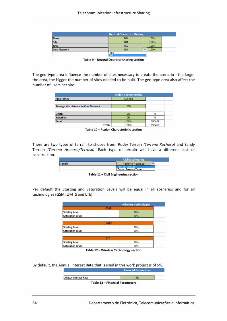
Telecommunication Infrastructure Sharing
84 Departamento de Eletrónica, Telecomunicações e Informática
Table 9 – Neutral Operator sharing section
The geo-type area influence the number of sites necessary to create the scenario - the larger the area, the bigger the number of sites needed to be built. The geo-type area also affect the number of users per site.
Table 10 – Region Characteristic section
There are two types of terrain to choose from: Rocky Terrain (Terreno Rochoso) and Sandy Terrain (Terreno Arenoso/Terroso). Each type of terrain will have a different cost of construction.
Table 11 – Civil Engineering section
Per default the Starting and Saturation Levels will be equal in all scenarios and for all technologies (GSM, UMTS and LTE)
Table 12 – Wireless Technology section
By default, the Annual Interest Rate that is used in this work project is of 5%.
Table 13 – Financial Parameters
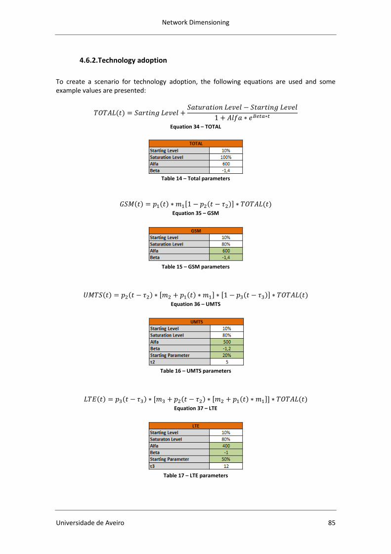
Network Dimensioning
Universidade de Aveiro 85
4.6.2.Technology adoption
To create a scenario for technology adoption, the following equations are used and some example values are presented:
Equation 34 – TOTAL
Table 14 – Total parameters
Equation 35 – GSM
Table 15 – GSM parameters
Equation 36 – UMTS
Table 16 – UMTS parameters
Equation 37 – LTE
Table 17 – LTE parameters

Telecommunication Infrastructure Sharing
86 Departamento de Eletrónica, Telecomunicações e Informática
Table 18 – m1, m2 and m3 parameters
Equation 38 –p1(t)
Equation 39 –p2(t – τ2)
Equation 40 –p3(t – τ3)
Table 19 – p’s parameters
All values (Alfa, Beta, Starting Parameter, τ2, τ3, p10, p1f, p20, p2f, p30 and p3f) were chosen by trial and error in order to achieve the desired technology adoption. The following chart is the growth rate of the adoption of the different technologies.
Chart 3 – Technologies adoption

Network Dimensioning
Universidade de Aveiro 87
4.6.3.Market
This section complements the previous one. In this section, the number of total users for all technologies (GSM, UMTS, LTE), as well as the total number of users per technology are calculated for three cases: base, best and worst cases. The base case works as the basis to perform a sensitivity analysis. This is useful to understand what can happen to the key decision criteria (NPV, IRR, Payback period) when one of the variables is changed. In this work project, sensitivity analysis investigates the impact due to changes (20% increase for the best case and 20% decrease for the worst case) in total number of users of telecommunication services. For example, in Chart 4, the total number of users per year are displayed in a random scenario.
Chart 4 – Total users per year
4.6.4.Cost Elements
It is important to define the cost of all equipment used to build the network. The values of costs were retrieved from Duarte, Manuel de Oliveira, 2015 “Ferramenta Agregação Wireless”; the Ovum Consulting, 2007, “Market Study for UMTS900” [72], and from José Pedro Ramos, 2014, “Telecommunication Infrastructure sharing in Mozambique”. [10]. In order to calculate the development costs of each scenario, it is needed the quantity of equipment and its associated costs. It is assumed that all equipment costs are equal for all technologies.
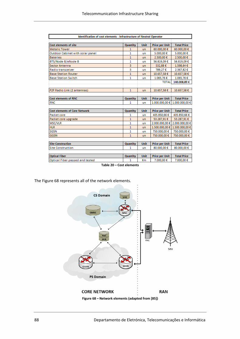
Telecommunication Infrastructure Sharing
88 Departamento de Eletrónica, Telecomunicações e Informática
Table 20 – Cost elements
The Figure 68 represents all of the network elements.
Figure 68 – Network elements (adapted from [85])
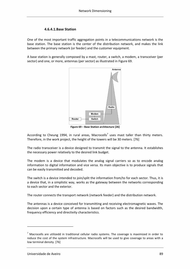
Network Dimensioning
Universidade de Aveiro 89
4.6.4.1.Base Station
One of the most important traffic aggregation points in a telecommunications network is the base station. The base station is the center of the distribution network, and makes the link between the primary network (or feeder) and the customer equipment. A base station is generally composed by a mast, router, a switch, a modem, a transceiver (per sector) and one, or more, antennas (per sector) as illustrated in Figure 69.
Figure 69 – Base Station architecture [26]
According to Cheung 1994, in rural areas, Macrocells7 uses mast taller than thirty meters. Therefore, in the work project, the height of the towers will be 30 meters. [76] The radio transceiver is a device designed to transmit the signal to the antenna. It establishes the necessary power relatively to the desired link budget. The modem is a device that modulates the analog signal carriers so as to encode analog information to digital information and vice versa. Its main objective is to produce signals that can be easily transmitted and decoded. The switch is a device intended to join/split the information from/to for each sector. Thus, it is a device that, in a simplistic way, works as the gateway between the networks corresponding to each sector and the exterior. The router connects the transport network (network feeder) and the distribution network. The antennas is a device conceived for transmitting and receiving electromagnetic waves. The decision upon a certain type of antenna is based on factors such as the desired bandwidth, frequency efficiency and directivity characteristics.
7 Macrocells are utilizedd in traditional cellular radio systems. The coverage is maximized in order to
reduce the cost of the system infrastructure. Macrocells will be used to give coverage to areas with a low terminal density. [76]

Telecommunication Infrastructure Sharing
90 Departamento de Eletrónica, Telecomunicações e Informática
Even though all solutions based on this type of technology have the same basic components, different architectures can be obtained by using different types of antennas. There are antennas with different angles beam, the most common are antennas with angle beam of 60° and 120°.
Figure 70 – a) Antenna angle - 60° and b) Antenna angle - 120° (adapted from [27])
From Figure 70 is it possible to observe that antennas with different angle beam generate sites formed by different amounts of sectors. The maximum range of a site is defined by the habitat in which it is located. This means that the use of antennas with tighter beam angle will only increase the total capacity of the same, increasing the number of sectors. Over the years, several propagation models were developed to determine, depending on the environment in which the system will be installed, the range of base stations for which the signal has a sufficiently high signal/noise ratio (SNR) to ensure communication between the customer equipment and the base station. [27]
4.6.4.2.Radio Link
A Radio Link is a primary network topology that uses two directional antennas and gives a link between two points that are separated by a few kilometers, given the condition that they have line of sight between them. These transmissions are generally used in areas where there is no core network and is used, in most cases, to connect the various points of the distribution network to a single point of aggregation. For this purpose, it may use several techniques, such as point-to-point, mesh, grid, among others. [27] Figure 71 demonstrates the architecture of Radio Link technology.
Figure 71 – Radio Link architecture [27]
Network Dimensioning
Universidade de Aveiro 91
The directional antennas (which have a very tight beam angle) and the radio transceivers are the main components of this technology.
Antennas make the connection between the two desired points, with signs operating frequency ranging between 15 and 38 GHz. [27]
Radio Transceivers modulate the signals so as to operate according to the desired protocol (it changes the signals according to the protocol of the next telecommunication system that will use them). [27]
With the arrival of high-speed wireless distribution technologies, this primary network topology became obsolete. Although radio link allows to make connections at a considerable distance, its capacity, as well as its limitation to several hundred of Mbps, is strongly weakened by distance and atmospheric conditions (for example, in adverse weather conditions, its capacity to traffic drops suddenly). [27] This radio link is used between sites which are located in very remote areas.
4.6.4.3.Core Network
The Core Network (Figure 64) is practically the same for all technologies (GSM, UMTS, LTE), but when a new technology is introduced an upgrade in the network is necessary in order to support the new technology. The most important and limiting equipment in the Core Network are:
MSC / VLR
HLR
SGSN
GGSN [72] The cost of the Packet core (Table 20) is the cost of the remaining equipment that are part of the core network, but that are not limiting the core network. The cost of the Packet core upgrade is considered when a new technology is introduced.
4.6.5.Granularity of network elements
To plan a network infrastructure it is necessary to select the desired network layout and the future expansion approach, to calculate the required equipment and to dimension all interfaces. In granularity of network elements, the RAN and the core network will be planned, as well as equipment needed for the technology evolution.
4.6.5.1.Sites granularity
It is assumed that the distribution of customers in each scenario is homogeneous and that there are three sectors per site.
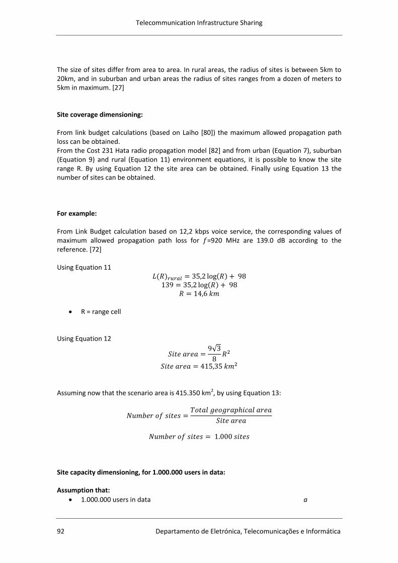
Telecommunication Infrastructure Sharing
92 Departamento de Eletrónica, Telecomunicações e Informática
The size of sites differ from area to area. In rural areas, the radius of sites is between 5km to 20km, and in suburban and urban areas the radius of sites ranges from a dozen of meters to 5km in maximum. [27] Site coverage dimensioning: From link budget calculations (based on Laiho [80]) the maximum allowed propagation path loss can be obtained. From the Cost 231 Hata radio propagation model [82] and from urban (Equation 7), suburban (Equation 9) and rural (Equation 11) environment equations, it is possible to know the site range R. By using Equation 12 the site area can be obtained. Finally using Equation 13 the number of sites can be obtained. For example: From Link Budget calculation based on 12,2 kbps voice service, the corresponding values of maximum allowed propagation path loss for =920 MHz are 139.0 dB according to the reference. [72] Using Equation 11
R = range cell Using Equation 12
Assuming now that the scenario area is 415.350 km2, by using Equation 13:
Site capacity dimensioning, for 1.000.000 users in data: Assumption that:
1.000.000 users in data a
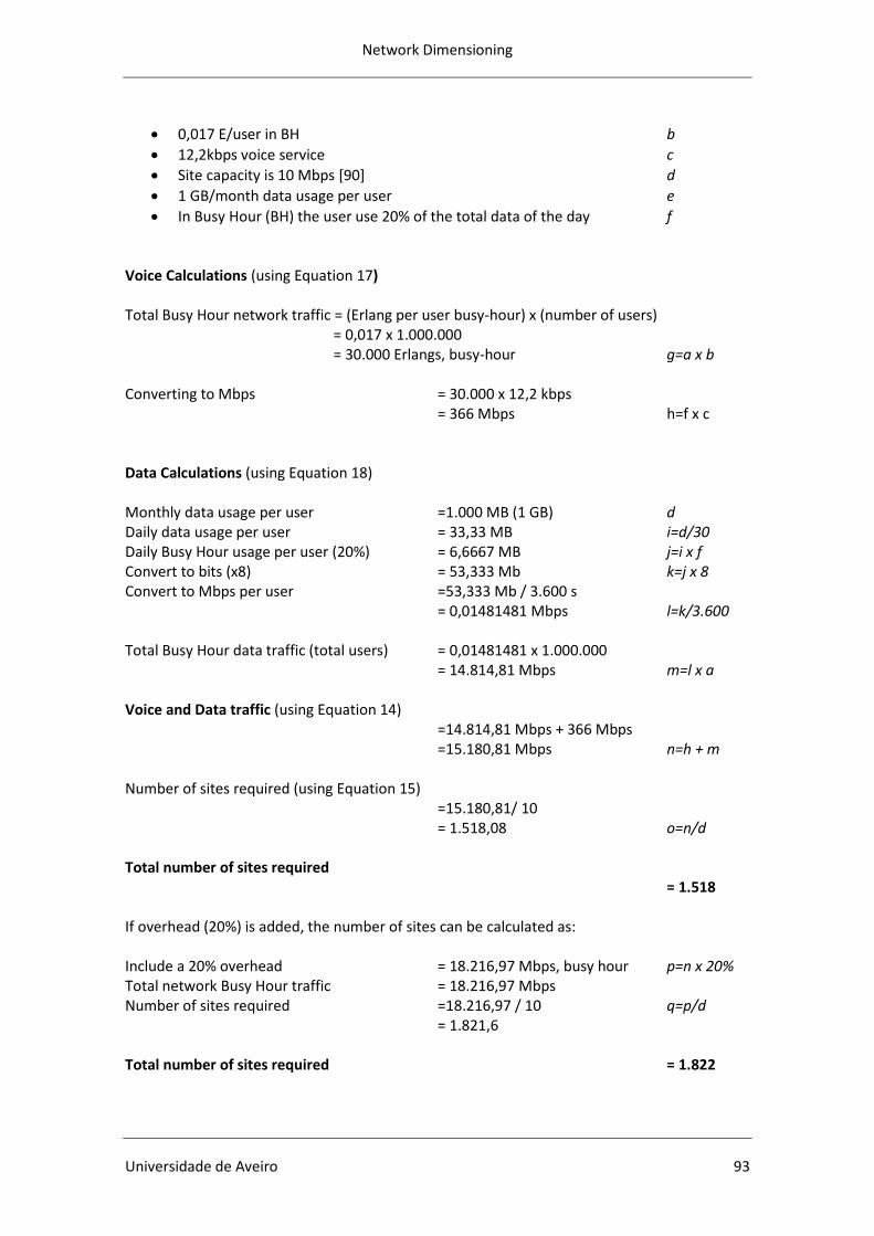
Network Dimensioning
Universidade de Aveiro 93
0,017 E/user in BH b
12,2kbps voice service c
Site capacity is 10 Mbps [90] d
1 GB/month data usage per user e
In Busy Hour (BH) the user use 20% of the total data of the day f Voice Calculations (using Equation 17) Total Busy Hour network traffic = (Erlang per user busy-hour) x (number of users)
= 0,017 x 1.000.000 = 30.000 Erlangs, busy-hour g=a x b
Converting to Mbps = 30.000 x 12,2 kbps
= 366 Mbps h=f x c Data Calculations (using Equation 18) Monthly data usage per user =1.000 MB (1 GB) d Daily data usage per user = 33,33 MB i=d/30 Daily Busy Hour usage per user (20%) = 6,6667 MB j=i x f Convert to bits (x8) = 53,333 Mb k=j x 8 Convert to Mbps per user =53,333 Mb / 3.600 s
= 0,01481481 Mbps l=k/3.600 Total Busy Hour data traffic (total users) = 0,01481481 x 1.000.000 = 14.814,81 Mbps m=l x a Voice and Data traffic (using Equation 14) =14.814,81 Mbps + 366 Mbps =15.180,81 Mbps n=h + m Number of sites required (using Equation 15) =15.180,81/ 10 = 1.518,08 o=n/d Total number of sites required = 1.518 If overhead (20%) is added, the number of sites can be calculated as: Include a 20% overhead = 18.216,97 Mbps, busy hour p=n x 20% Total network Busy Hour traffic = 18.216,97 Mbps Number of sites required =18.216,97 / 10 q=p/d = 1.821,6 Total number of sites required = 1.822
Telecommunication Infrastructure Sharing
94 Departamento de Eletrónica, Telecomunicações e Informática
In the next section, the calculations of equipment for each technology (GSM, UMTS and LTE) and for core network that constitute the scenario are explained.
4.6.5.2.GSM
To know the impact of users in the network, in the BTS configuration and to estimate the maximum number of users per site, some calculations need to be done. In GSM the limiting factor is the number of transceivers (TRX). The number of sites per scenario does not change over time. Admitting that:
In Busy Hour (μ, 3.600s) each user requires 60s of conversation (λ). Using Equation 56 (Appendix F):
There is 1% of Blocking Probability (Pb) In developed countries it is common to use a blocking probability between 0,1% and 1%.
Considering 2000 users, uniformly distributed by each one of the 3 sectors:
This means that there are 666 users per one sector.
Thus,
Blocking rate (GoS) = 1%
Traffic = 11,1E/sector

Network Dimensioning
Universidade de Aveiro 95
Table 21 – Erlang B table [58]
Based on Table 21, 19 channels are needed. Each TRX has 8 Channels, so 3 TRX/cell are needed, which in turn requires a S333 configuration.[49]
Equation 41 – Users per site
Resorting to calculations made previously (Equation 41), using 17 mE per user and knowing the relation between the site configuration and Erlang/site, the following table values is obtained:
Table 22 – Configuration to 17mE/user [10]
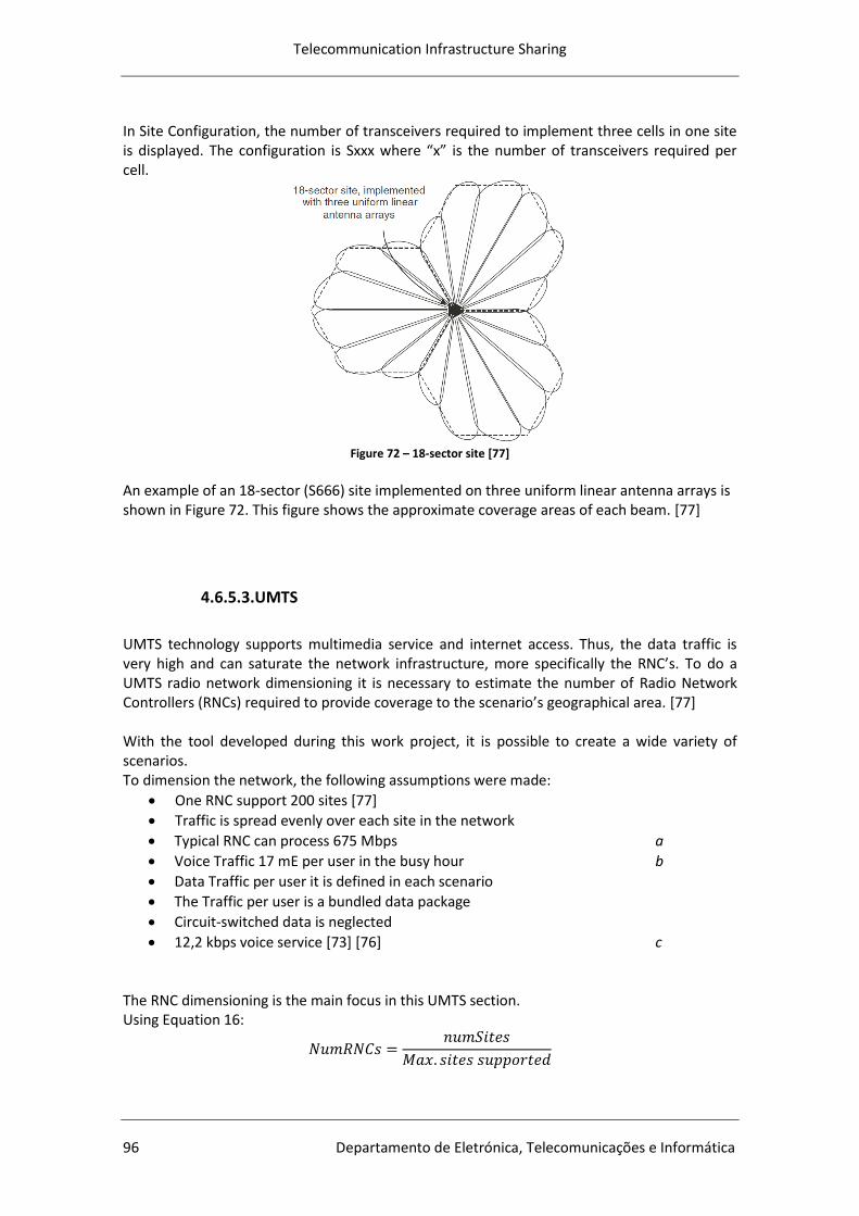
Telecommunication Infrastructure Sharing
96 Departamento de Eletrónica, Telecomunicações e Informática
In Site Configuration, the number of transceivers required to implement three cells in one site is displayed. The configuration is Sxxx where “x” is the number of transceivers required per cell.
Figure 72 – 18-sector site [77]
An example of an 18-sector (S666) site implemented on three uniform linear antenna arrays is shown in Figure 72. This figure shows the approximate coverage areas of each beam. [77]
4.6.5.3.UMTS
UMTS technology supports multimedia service and internet access. Thus, the data traffic is very high and can saturate the network infrastructure, more specifically the RNC’s. To do a UMTS radio network dimensioning it is necessary to estimate the number of Radio Network Controllers (RNCs) required to provide coverage to the scenario’s geographical area. [77] With the tool developed during this work project, it is possible to create a wide variety of scenarios. To dimension the network, the following assumptions were made:
One RNC support 200 sites [77]
Traffic is spread evenly over each site in the network
Typical RNC can process 675 Mbps a
Voice Traffic 17 mE per user in the busy hour b
Data Traffic per user it is defined in each scenario
The Traffic per user is a bundled data package
Circuit-switched data is neglected
12,2 kbps voice service [73] [76] c The RNC dimensioning is the main focus in this UMTS section. Using Equation 16:
Network Dimensioning
Universidade de Aveiro 97
Number of RNCs: 5 As it is assumed that all UMTS users use data traffic, a saturation of some sites might occur. Therefore, there must be build another site to alleviate the saturated sites. To ascertain if new sites construction are needed, the capacity dimensioning is done as explained in 4.6.5.1 Sites. The calculation for finding the number of RNCs needed is explained hereafter: UTRAN Dimensioning, for 2.000.000 users in voice and data: d Voice Dimensioning Calculations (using Equation 17) Total Busy Hour network traffic = (Erlang per user BH) x (number of users)
= 0,017 x 2.000.000 = 34.000 Erlangs, busy-hour e=b x d
Convert to Mbps = 34.000 x 12,2 kbps
= 414,8 Mbps f=e x c Data Dimensioning Calculations (using Equation 18) Monthly data usage per user =500 MB (0,5 GB) g Daily data usage per user = 16,6667 MB h=g/30 Daily Busy Hour usage per user (20%) = 3,3333 MB i=h x 20% Convert to bits (x8) = 26,666 Mb j=I x 8 Convert to Mbps per user =26,666 Mb / 3.600 s
= 7,4074 kbps k=j/3.600 Total Busy Hour data traffic (total users) = 7,4074 x 2.000.000 = 14.814,8 Mbps l=k x d Voice and Data Traffic Voice and Data BH = 414,8 Mbps + 14.814,8 Mbps = 15.229,61 Mbps, busy hour m=f + l Number of RNC’s required (using Equation 20) =15.229,61 / 675 = 22,6 n=m/a Total number of RNC’s required = 23
Telecommunication Infrastructure Sharing
98 Departamento de Eletrónica, Telecomunicações e Informática
If overhead (20%) is added, the number of sites can be calculated as: Include a 20% overhead = 18.275,54 Mbps, busy hour o=m x 20% Total network Busy Hour traffic = 18.275,54 Mbps Number of RNC’s required =18.275,54 / 675 = 27,1 p=o/a Total number of RNC’s required = 28 The maximum is 28 (5 and 28). Number of RNC is 28.
4.6.5.4.LTE
When the technology evolves from UMTS to LTE, an upgrade of the sites and Radio Access Network equipment are made in order to support LTE, using the technique demonstrated in Figure 44 (LTE over GSM). The initial upgrade will be over the older network until this one saturates. When these sites saturate, the upgrade will use pure LTE as shown in Figure 43 (do not have RNCs), the new sites will be connected directly to the core network. The limiting factor in LTE is the site capacity and the site capacity dimensioning is the main focus in this LTE section. Thanks to the other technologies (GSM and UMTS), the number of sites in the scenario and the number of users supported in the LTE technology with this number of sites are known. As the number of users and traffic grow, the equipment saturates and it is necessary to increase the number of sites in the scenario. The user density and user traffic profile are the main requirements for capacity dimensioning. Traffic forecast should be done by analyzing the offered Busy Hour traffic per user. To calculate the total number of sites, that is for capacity dimensioning, the computations made in 4.6.5.1 Sites are used.
4.6.5.5.Core Network
The Core Network used in this work project is shown in Figure 64. From Ovum Consulting, 2007, “Market Study for UMTS900” [72] and from Vilicom 2009, “UMTS Network Design & Cost” [73], the following factors will be assumed:
1 MSC / VLR per 400 sites
1 HLR per 1.000.000 users
1 SGSN per 1.000.000 users
1 GGSN per 1.000.000 users
Network Dimensioning
Universidade de Aveiro 99
4.6.6.CAPEX
All technologies (GSM, UMTS, LTE) require some CAPEX investment. In first year of the scenario, expenditures on GSM equipment and on the Core Network are needed so as the network to be functional. In remaining years, the CAPEX is the investment required when the network saturates and needs to be reinforced. Whenever there is a technology evolution, an upgrade in all sites and in the core network equipment is needed. It is assumed, for this work, that start of new technology occurs when the number of users reaches the minimum of ten users per site. It is also assumed that upgrade cost is the installation of new transceivers. To reach the value of CAPEX, the following calculations are made:
Year 1 Number of sites (NS) x Cost per site (CS) Number of sites x Cost per site construction (CConst) Number of sites x Average site distance to Core Network (DCN) x Cost
per km of Optical Fiber passed and tested (COF) x % of sites with optical fiber connection (%SOF)
Number of sites x Cost per radio link x % of sites with radio link connection (%SRL)
Number of RNCs (NRNC) x Cost per RNC (CRNC)
- GSM
Number of TRXs (NTRX) x Cost per TRX (CTRX)
- Core Network Cost of Packet Core Network (CPCN) Number of MSC/VLR (NMSC)x Cost per MSC/VLR (CMSC) Number of HLR (NHLR) x Cost per HLR (CHLR) Number of SGSN (NSGSN) x Cost per SGSN (CSGSN) Number of GGSN (NGGSN) x Cost per GGSN (CGGSN)
Remaining Years Number of site upgrade (NS_upg) x Cost per site Number of sites upgrade x Cost per site construction Number of sites upgrade x Average site distance to Core Network x
Cost per km of Optical Fiber passed and tested x % of sites with optical fiber connection
Number of sites upgrade x Cost per radio link x % of sites with radio link connection
Number of RNC upgrade (NRNC_upg) x Cost per RNC
- GSM Number of TRX upgrade (NTRX_upg) x Cost per TRX
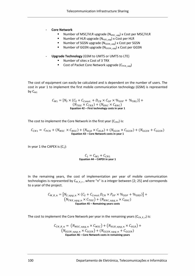
Telecommunication Infrastructure Sharing
100 Departamento de Eletrónica, Telecomunicações e Informática
- Core Network Number of MSC/VLR upgrade (NMSC_upg) x Cost per MSC/VLR Number of HLR upgrade (NHLR_upg) x Cost per HLR Number of SGSN upgrade (NSGSN_upg) x Cost per SGSN Number of GGSN upgrade (NGGSN_upg) x Cost per GGSN
- Upgrade Technology (GSM to UMTS or UMTS to LTE)
Number of sites x Cost of 3 TRX Cost of Packet Core Network upgrade (CPCN_upg)
The cost of equipment can easily be calculated and is dependent on the number of users. The cost in year 1 to implement the first mobile communication technology (GSM) is represented by CM1
Equation 42 – First technology costs in year 1
The cost to implement the Core Network in the first year (CCN1) is:
Equation 43 – Core Network costs in year 1
In year 1 the CAPEX is (C1):
Equation 44 – CAPEX in year 1
In the remaining years, the cost of implementation per year of mobile communication technologies is represented by CM_R_n , where “n” is a integer between [2; 25] and corresponds to a year of the project.
Equation 45 – Remaining years costs
The cost to implement the Core Network per year in the remaining years (CCN_R_n) is:
Equation 46 – Core Network costs in remaining years
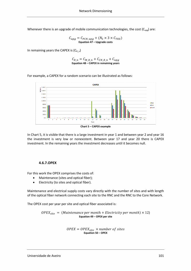
Network Dimensioning
Universidade de Aveiro 101
Whenever there is an upgrade of mobile communication technologies, the cost (Cupg) are:
Equation 47 – Upgrade costs
In remaining years the CAPEX is (CR_n)
Equation 48 – CAPEX in remaining years
For example, a CAPEX for a random scenario can be illustrated as follows:
Chart 5 – CAPEX example
In Chart 5, it is visible that there is a large investment in year 1 and between year 2 and year 16 the investment is very low or nonexistent. Between year 17 and year 20 there is CAPEX investment. In the remaining years the investment decreases until it becomes null.
4.6.7.OPEX
For this work the OPEX comprises the costs of:
Maintenance (sites and optical fiber);
Electricity (to sites and optical fiber). Maintenance and electrical supply costs vary directly with the number of sites and with length of the optical fiber network connecting each site to the RNC and the RNC to the Core Network. The OPEX cost per year per site and optical fiber associated is:
) Equation 49 – OPEX per site
Equation 50 – OPEX

Telecommunication Infrastructure Sharing
102 Departamento de Eletrónica, Telecomunicações e Informática
In the case of sites, only fixed costs will be considered, both for the electrical supply and the maintenance, which are then multiplied by the number of sites. Regarding the maintenance costs, it is admitted that a service technician will be needed for every 10 sites. Electrical supply costs are related with the number of active equipment, that is, of the existing equipment at the edges of each connection.
Table 23 - OPEX
The price of electricity per month is relatively low, because it takes into account that all base stations have their own power generating station via solar panels which provide much of the energy consumed by the equipment, and in the country of the case study (Mozambique ) the electricity tariffs are low (as specified in 5.2 Mozambique) The value obtained in Table 23 is assumed to be the average value for OPEX for a network infrastructure with 10 sites. The value obtained per year is then multiplied by the number of base stations and divided by 10. For example, a OPEX for a random scenario can be illustrated as follows:
Chart 6 – OPEX example
In Chart 6, it is visible that there is an increase in OPEX over the years in the three cases (Best, Base and Worst cases). This happens because the costs of equipment maintenance and of electricity rise due to increase of the number of users.
4.6.8.Revenues
Revenues are calculated by multiplying the number of users with the price paid by them per year. The price paid by users is calculated based on the price paid by private users. That is, the price paid by Business and Institutional users is divided by the price paid by private users in order to find the multiplication factor for the price and the capacity usage of the network.
Network Dimensioning
Universidade de Aveiro 103
Nevertheless, this methodology ignores any price advantage for Business and Institutional users since they usually need equipment with more features than private users.
Equation 51 – Revenue
In this work project, infrastructure is shared and each operator pays to use the network or some equipment. It is assumed that when the network infrastructure is shared, the price paid by operators is a percentage of the investments made to build the part of network infrastructure that is shared. In this project, this percentage of the investment to construct the network infrastructure that is shared is 10%. The revenues from operators are calculated as:
Equation 52 – Operators revenue
Therefore, total revenues are:
Equation 53 – Revenue
There are four types of sharing: mast, site, RAN and Core Network. Equipment may be shared as a whole or only a percentage of them can be shared. It may happen in some years that an operator does not pay the rent to the Neutral Operator. This is due to the fact that there are no investments made in the infrastructure by the Neutral Operator in that year. However, as the rental last for several years, at the end of the project the total rent paid to Neutral Operator is 10% of the investments. Revenues for a random scenario can be illustrated as follows:
Chart 7 – Revenues example

Telecommunication Infrastructure Sharing
104 Departamento de Eletrónica, Telecomunicações e Informática
4.6.9.Economic Results
The key decision criteria to determine the profitability of the investment are the NPV, the IRR and the Payback period. The amount of Annual Net Cash Flow and Cash Balanced are also analyzed in the techno-economic tool. The next figures (Table 24 and Chart 8) show the economic results for a random scenario in the Base Case.
Table 24 – Base case scenario
Chart 8 – Economic Results in Base case scenario
4.7. Summary
Through this chapter, the necessary steps for the dimensioning components of a network were presented: the number of sites was calculated using site coverage and site capacity, the number of RNCs was also calculated, as well as the most important equipment of Core Network. More specifically, for GSM technology it was also calculated the TRX necessary in order to give users support. Furthermore, it was explained how to make the economic analysis of the project.
Case Study
Universidade de Aveiro 105
5. Case Study
5.1. Contextualization
The case study of this dissertation will focus on the reality of the Mozambican telecommunication market. It aims to encourage the implementation of telecommunication services in the country by using infrastructure sharing. Possible scenarios to be implemented in the country will be discussed, so as to improve the sector making it more competitive and efficient. As mentioned in the Introduction, the Case Study is a continuation of a work project developed by José Pedro G. S. Ramos, entitled “Telecommunication Infrastructure Sharing in Mozambique”, of the Department of Electronics, Telecommunications and Informatics (DETI) of University of Aveiro (UA) [10].
5.2. Mozambique
Of all sub-Saharan countries, Mozambique has been the fastest growing economy over the last twenty years. After a post-conflict transition, its GDP has grown at an average annual rate of 7.4% since 1992. Various human development indicators have significantly progressed, such as GDP per capita, life expectancy and poverty headcount. This performance was due to the increasing efforts in implementing credible policies and structural reforms, a favorable external environment, donor support, and more recently due to the discovery and exploitation of natural resources. [5] However, challenges are still many. Mozambique’s GDP per capita stood at USD 567 in 2012, which is 40% less than the Sub-Saharan Africa average. Although the macroeconomic policies remain cautious, the structural reform agenda has still a long way ahead and capacity-building needs are extensive. The recent discovery and exploitation of natural resources have boost growth and Mozambique is expected to become one of the worlds’ biggest exporters of gas and coal in the next decade. Nevertheless, this discovery brings also the challenge to manage resources carefully while diversifying the economy and distributing gains evenly. [5] [63] In recent years, foreign investors were attracted by the generosity of fiscal incentives and the low-cost electricity. Therefore, the secondary sector (such as mining, electricity, manufacturing, and construction) has become to represent an important portion of GDP, growing continuously to 25% of GDP by 2004. To what concerns to agricultural sector, thanks to several large investments in commercial farms, the growth rate of the sector has exceed the growth rate of other sectors (in 2012, it represented 28% of Mozambique’s GDP). The tertiary sector (mainly transport, commerce, and public services) represented around 45% of GDP in 2012. [5] Investment, particularly in megaprojects which are foreign-owned and capital-intensive, encouraged growth and accounted for 2–4% in each year of construction. In the years following the war, investment was based on aid, but soon investment shifted to foreign direct
Telecommunication Infrastructure Sharing
106 Departamento de Eletrónica, Telecomunicações e Informática
investment destined to infrastructure projects (mainly the Cahora Bassa8, Mozal9 and Sasol10 projects). Since 2004 several mining projects were put in place, such as the recent successful gas exploration in the Rovuma basin in the northern shore of Mozambique. [5] The recent economic performance of Mozambique is mostly due to the sound macroeconomic and structural reforms, the favorable external environment, as well as donor support. While much has already been achieved, a lot still remains to be done to overcome the challenges the country is facing. As mentioned, the discovery of natural resources requires a profound transformation for Mozambique and adds challenges to managing the natural resource boom. But the biggest challenge is maintaining economic growth and make it more inclusive in order to achieve a long-lasting poverty reduction. [5]
8 Cahora Bassa is a dam in Mozambique.
9 Mozal is an aluminum smelter.
10 Gas pipeline linking to South Africa
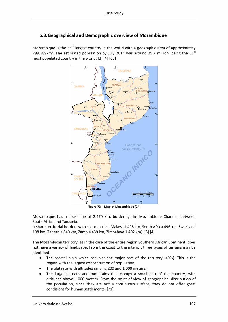
Case Study
Universidade de Aveiro 107
5.3. Geographical and Demographic overview of Mozambique
Mozambique is the 35th largest country in the world with a geographic area of approximately 799.389km2. The estimated population by July 2014 was around 25.7 million, being the 51st most populated country in the world. [3] [4] [63]
Figure 73 – Map of Mozambique [24]
Mozambique has a coast line of 2.470 km, bordering the Mozambique Channel, between South Africa and Tanzania. It share territorial borders with six countries (Malawi 1.498 km, South Africa 496 km, Swaziland 108 km, Tanzania 840 km, Zambia 439 km, Zimbabwe 1.402 km). [3] [4] The Mozambican territory, as in the case of the entire region Southern African Continent, does not have a variety of landscape. From the coast to the interior, three types of terrains may be identified:
The coastal plain which occupies the major part of the territory (40%). This is the region with the largest concentration of population;
The plateaus with altitudes ranging 200 and 1.000 meters;
The large plateaus and mountains that occupy a small part of the country, with altitudes above 1.000 meters. From the point of view of geographical distribution of the population, since they are not a continuous surface, they do not offer great conditions for human settlements. [71]
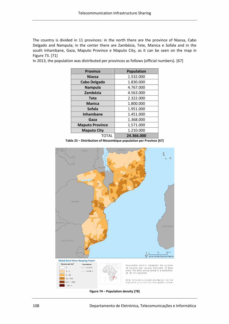
Telecommunication Infrastructure Sharing
108 Departamento de Eletrónica, Telecomunicações e Informática
The country is divided in 11 provinces: in the north there are the province of Niassa, Cabo Delgado and Nampula; in the center there are Zambézia, Tete, Manica e Sofala and in the south Inhambane, Gaza, Maputo Province e Maputo City, as it can be seen on the map in Figure 73. [71] In 2013, the population was distributed per provinces as follows (official numbers). [67]
Province Population
Niassa 1.532.000
Cabo Delgado 1.830.000
Nampula 4.767.000
Zambézia 4.563.000
Tete 2.322.000
Manica 1.800.000
Sofala 1.951.000
Inhambane 1.451.000
Gaza 1.368.000
Maputo Province 1.571.000
Maputo City 1.210.000
TOTAL 24.366.000 Table 25 – Distribution of Mozambique population per Province [67]
Figure 74 – Population density [78]

Case Study
Universidade de Aveiro 109
Population distribution: By 2015, the estimated population was of 25.727.911 and was distributed as follows:
Urban: 8.181.475 (31.8% of total population)
Rural: 17.546.436 (68,2% of total population) [63] [68] By 2020, the population forecast is of 29.310.000 inhabitants and will be distributed as follows:
Urban: 9.733.000 (33,2% of total population)
Rural: 19.577.000 (66,8% of total population) [68] As it can be seen in the population predictions for 2020, there is a decline of 1,4% in the population of rural areas, but it will still represent more than half of the Mozambican population. Age structure:
0–14 years: 45,3%
15–24 years: 21,3%
25–54 years: 27%
55–64 years: 3,5%
65 years and over: 2,9% [4]
Chart 9 – Population pyramid
11 [4]
11 A population pyramid shows the age and sex structures of a country's population. The population is
distributed along the horizontal axis, with males on the left and females shown on the right. The male and female populations are divided into 5 year age groups which are represented in horizontal bars along the vertical axis, with the youngest age groups at the bottom and the oldest at the top. The shape of the population pyramid gradually progresses over time according to fertility, mortality, and international migration trends. [4]
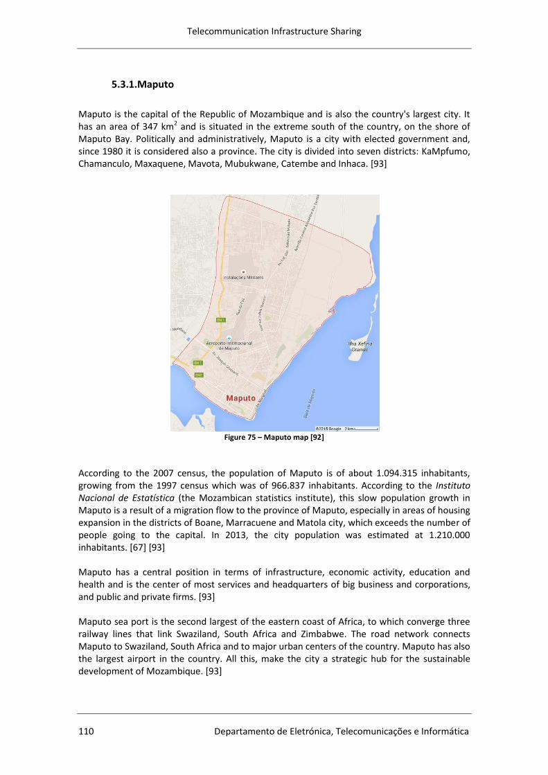
Telecommunication Infrastructure Sharing
110 Departamento de Eletrónica, Telecomunicações e Informática
5.3.1.Maputo
Maputo is the capital of the Republic of Mozambique and is also the country's largest city. It has an area of 347 km2 and is situated in the extreme south of the country, on the shore of Maputo Bay. Politically and administratively, Maputo is a city with elected government and, since 1980 it is considered also a province. The city is divided into seven districts: KaMpfumo, Chamanculo, Maxaquene, Mavota, Mubukwane, Catembe and Inhaca. [93]
Figure 75 – Maputo map [92]
According to the 2007 census, the population of Maputo is of about 1.094.315 inhabitants, growing from the 1997 census which was of 966.837 inhabitants. According to the Instituto Nacional de Estatística (the Mozambican statistics institute), this slow population growth in Maputo is a result of a migration flow to the province of Maputo, especially in areas of housing expansion in the districts of Boane, Marracuene and Matola city, which exceeds the number of people going to the capital. In 2013, the city population was estimated at 1.210.000 inhabitants. [67] [93] Maputo has a central position in terms of infrastructure, economic activity, education and health and is the center of most services and headquarters of big business and corporations, and public and private firms. [93] Maputo sea port is the second largest of the eastern coast of Africa, to which converge three railway lines that link Swaziland, South Africa and Zimbabwe. The road network connects Maputo to Swaziland, South Africa and to major urban centers of the country. Maputo has also the largest airport in the country. All this, make the city a strategic hub for the sustainable development of Mozambique. [93]

Case Study
Universidade de Aveiro 111
Although Maputo concentrates only 5,4% of the population, the city is responsible for 20,2% of Mozambique's GDP. The trade, transport and communications, and manufacturing sectors are the most important ones, contributing, respectively, to 29,6%, 29,5% and 12,4% of national production, according to the Relatório Nacional de Desenvolvimento Humano (National Human Development Report) (UNDP, 2006). [93]
5.4. Current Mobile Telecommunication Scenario in Mozambique
Mozambique is a relatively large country but has a small population density and suffers frequently harsh weather, especially during the rainy season when there is periodic flooding. In spite sustained and sizable government investments, infrastructures are still relatively insufficient to satisfy basic needs in the majority of the regions, namely in terms of access to networked electricity, clean water sources, roads, sanitation, Internet services, and telecommunication. The expansion of infrastructure networks, which is a part of the government agenda, is crucial for economic growth and poverty alleviation. The availability and reliability of infrastructure services are considered key to private sector growth. Regarding the access to basic infrastructure, there is a significant disparity between urban and rural areas. [5] The country was one of the first in the sub-Saharan Africa to reform its telecommunications sector, right after the end of the civil war in 1992. The mobile sub-sector has sustained significant growth rates following the opening to competition in 2003 between Vodacom Mozambique and mCel, the incumbent mobile entity of the national telecommunication TDM. [62] Nevertheless, market penetration is still below the African average. The introduction of Movitel as the third mobile operator in early 2012 was expected to boost the subscriber growth rate in the sector, as well as decrease the average revenue per user (ARPU) which stabilized following the introduction of mobile broadband services and higher tariffs. [62] To improve the telecommunication market competition the government is intent, but is hesitating, to privatize TDM. All other services are open to competition, subject to licensing by the industry regulator, INCM. [62] Internet usage in Mozambique has been restricted by the deficient fixed-line infrastructure and the high cost of international bandwidth. However, this market sector is now quickly increasing after the introduction of various types of broadband services including cable modems, ADSL, WiMAX and 3G mobile, and the presence of two international submarine fiber optic cables in the country (Seacom and EASSy). The lower cost of bandwidth has already contributed to expressive reductions in broadband retail prices. Further advancements are expected thanks to the ongoing rollout of a national fiber backbone network and plans for an alternative fiber infrastructure. [6] [62] The next chart compares the cellular subscriptions per 100 inhabitants in Portugal (developed country) and in Mozambique (developing country).
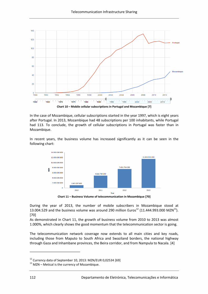
Telecommunication Infrastructure Sharing
112 Departamento de Eletrónica, Telecomunicações e Informática
Chart 10 – Mobile cellular subscriptions in Portugal and Mozambique [7]
In the case of Mozambique, cellular subscriptions started in the year 1997, which is eight years after Portugal. In 2013, Mozambique had 48 subscriptions per 100 inhabitants, while Portugal had 113. To conclude, the growth of cellular subscriptions in Portugal was faster than in Mozambique. In recent years, the business volume has increased significantly as it can be seen in the following chart:
Chart 11 – Business Volume of telecommunication in Mozambique [70]
During the year of 2013, the number of mobile subscribers in Mozambique stood at 13.004.529 and the business volume was around 290 million Euros12 (11.444.993.000 MZN13). [70] As demonstrated in Chart 11, the growth of business volume from 2010 to 2013 was almost 1.000%, which clearly shows the good momentum that the telecommunication sector is going. The telecommunication network coverage now extends to all main cities and key roads, including those from Maputo to South Africa and Swaziland borders, the national highway through Gaza and Inhambane provinces, the Beira corridor, and from Nampula to Nacala. [4]
12 Currency data of September 10, 2013: MZN/EUR 0,02534 [69]
13 MZN – Metical is the currency of Mozambique.
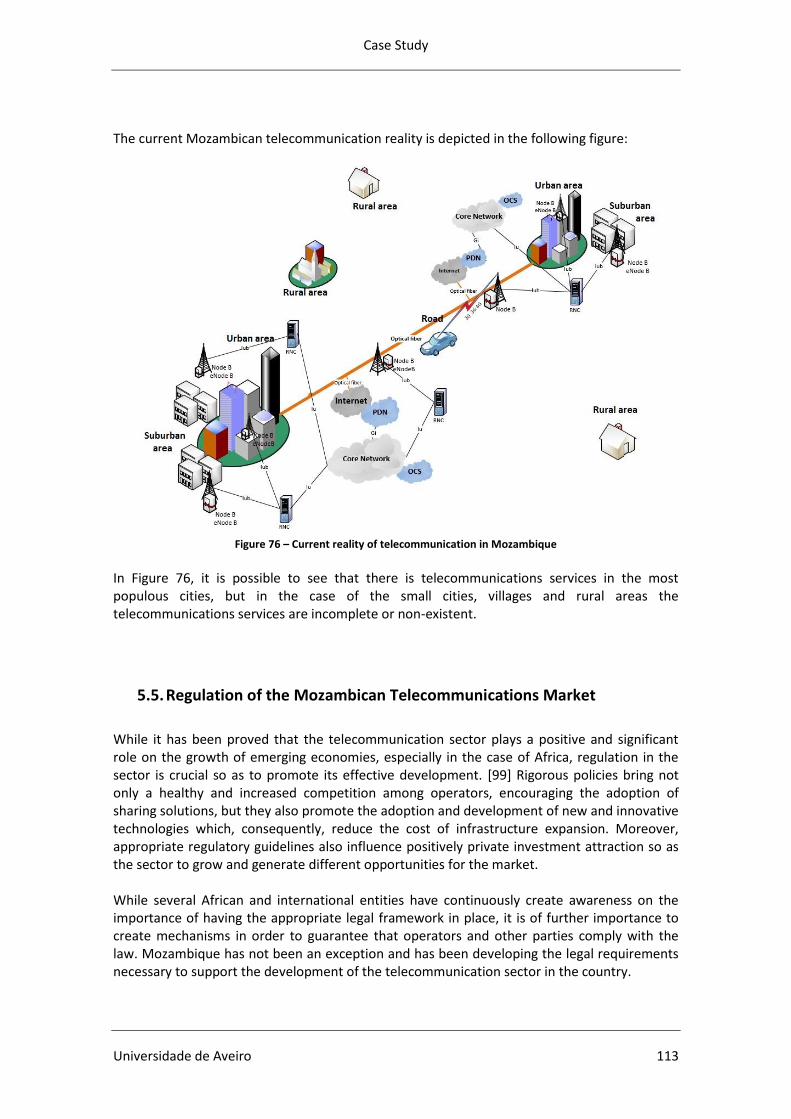
Case Study
Universidade de Aveiro 113
The current Mozambican telecommunication reality is depicted in the following figure:
Figure 76 – Current reality of telecommunication in Mozambique
In Figure 76, it is possible to see that there is telecommunications services in the most populous cities, but in the case of the small cities, villages and rural areas the telecommunications services are incomplete or non-existent.
5.5. Regulation of the Mozambican Telecommunications Market
While it has been proved that the telecommunication sector plays a positive and significant role on the growth of emerging economies, especially in the case of Africa, regulation in the sector is crucial so as to promote its effective development. [99] Rigorous policies bring not only a healthy and increased competition among operators, encouraging the adoption of sharing solutions, but they also promote the adoption and development of new and innovative technologies which, consequently, reduce the cost of infrastructure expansion. Moreover, appropriate regulatory guidelines also influence positively private investment attraction so as the sector to grow and generate different opportunities for the market. While several African and international entities have continuously create awareness on the importance of having the appropriate legal framework in place, it is of further importance to create mechanisms in order to guarantee that operators and other parties comply with the law. Mozambique has not been an exception and has been developing the legal requirements necessary to support the development of the telecommunication sector in the country.
Telecommunication Infrastructure Sharing
114 Departamento de Eletrónica, Telecomunicações e Informática
The Mozambican telecommunication market is regulated by decree-law 8/2004, July 21. [34] This decree-law defines the guidelines for the public and private telecommunications sector. It promotes technological innovation and progress in quality terms for telecommunication services, and it emphasizes the importance of ensuring coverage of these services across the country while guaranteeing the quality of the services provided. It also defines the conditions and preconditions for private investment. Furthermore, clauses 35, 44 and 45 highlight the general benefits of infrastructure sharing in terms of costs reduction and coverage area expansion. The public institution Instituto Nacional das Comunicações de Moçambique (INCM) (National Communications Institute of Mozambique) is the current Regulatory Authority for Telecommunications and Postal sectors, and has, therefore, regulation and supervision and representing powers of Postal and Telecommunications sectors. It is responsible as well as for managing the radio frequency spectrum. [35] The INCM was created by decree-law 22/92 in September 10. It is a state dependent entity supervised by the Ministry of Transports and Communication with administrative, financial and patrimonial autonomy. In fact, the decree-law 8/2004 results in part of the INCM’s efforts to strengthen regulation for an increasingly competitive telecommunication market. The decree-law 62/2010, December 27, (in Appendix H) points out the duties and responsibilities of the INCM. This decree also regulates the passive telecommunication infrastructure sharing. [33] The 62/2010 decree-law has as a main goal the promotion of telecommunication infrastructures sharing in general and, in particular, of passive telecommunication infrastructures sharing, taking into account the following:
The reduction of the replicated investments in passive telecommunication infrastructures and other network resources;
The protection of areas where the implementation of passive infrastructures and other network resources may evoke environmental and public concerns;
The benefits for the users in terms of quality, costs and availability of the services provided. (Appendix H)
According to the INCM website [98], to what concerns technical specifications for telecommunications the INCM is in charge of:
Planning, controlling and managing the radio spectrum and orbital positions;
Standardize, approve and certify telecommunication materials and equipment and define the conditions for their connection to the network, according to the legislation in force;
Design and manage the numbering plan and distribute to operators in an objective, transparent and non-discriminatory manner;
Coordinate the use of the radio-electric frequency at a regional and international level. The INCM is responsible for other areas of regulation, but the functions stated above are the essential ones that this entity will held during the implementation of a Neutral Operator model (NO) solution in Mozambique.
Case Study
Universidade de Aveiro 115
5.6. Mozambique Business Model
5.6.1.Mobile Virtual Network Operator (MVNO)
A Mobile Virtual Network Operator (MVNO) is a virtual system that offers mobile telecommunications services to the public, without being the holder of mobile frequencies or access network. That is, it sells communication minutes formerly bought from an infrastructure owner (such as a mobile network operator) to the public. There are many forms for a MVNO entity to put its business into practice. Nevertheless, to do so, it demands an already built mobile network. In the case of Mozambique, mobile networks are scattered across remote and rural regions. This can comprise the goal of finding a cost efficient solution for implementing MVNOs in the country. However, include Neutral Operator in the business model can greatly solve this problem, as it can provide services to MVNOs that need to broaden services in order to continue to be competitive and active agents in the market. [10] In spite the possibly slow consolidation of this reality due to the country specificities and political and economic characteristics, introducing a new cost efficient alternative for operators to scale to previously high risk areas will surely increase competition in a positive way. MVNOs present also a series of advantages. They actively solve technological/infrastructure limitations (for example, lack of capacity networks), and bring more services at more affordable prices to the Mozambican market that can perceive the benefits of mobile telephone services. The MVNO model complements hence the Neutral Operator model which will be discussed in the next topic. Nevertheless, MVNO model will not be used in this work project.
5.6.2.Neutral Operator
As mentioned, the NO is the single owner of all the network infrastructure and shares either the whole infrastructure or part of it with the other operators. This sharing network infrastructure is decided between Neutral Operator and the other operators. In this work project, a different type of infrastructure co-locating will be outlined for each scenario. In the case of Mozambique, the Neutral Operator will not be a traditional one. It will have a double role:
It will be a provider of shared infrastructure.
It will be a provider of user service. To mention that the NO will rent its equipment’s exceeding installed capacity to other operators. It is assumed that the network always have exceeding installed capacity, as when it
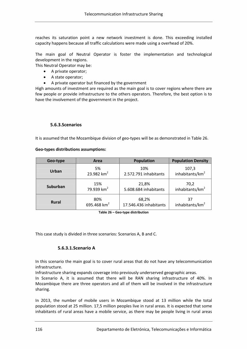
Telecommunication Infrastructure Sharing
116 Departamento de Eletrónica, Telecomunicações e Informática
reaches its saturation point a new network investment is done. This exceeding installed capacity happens because all traffic calculations were made using a overhead of 20%. The main goal of Neutral Operator is foster the implementation and technological development in the regions. This Neutral Operator may be:
A private operator;
A state operator;
A private operator but financed by the government High amounts of investment are required as the main goal is to cover regions where there are few people or provide infrastructure to the others operators. Therefore, the best option is to have the involvement of the government in the project.
5.6.3.Scenarios
It is assumed that the Mozambique division of geo-types will be as demonstrated in Table 26. Geo-types distributions assumptions:
Geo-type Area Population Population Density
Urban 5%
23.982 km2 10%
2.572.791 inhabitants 107,3
inhabitants/km2
Suburban 15%
79.939 km2 21,8%
5.608.684 inhabitants 70,2
inhabitants/km2
Rural 80%
695.468 km2 68,2%
17.546.436 inhabitants 37
inhabitants/km2
Table 26 – Geo-type distribution
This case study is divided in three scenarios: Scenarios A, B and C.
5.6.3.1.Scenario A
In this scenario the main goal is to cover rural areas that do not have any telecommunication infrastructure. Infrastructure sharing expands coverage into previously underserved geographic areas. In Scenario A, it is assumed that there will be RAN sharing infrastructure of 40%. In Mozambique there are three operators and all of them will be involved in the infrastructure sharing. In 2013, the number of mobile users in Mozambique stood at 13 million while the total population stood at 25 million. 17,5 million peoples live in rural areas. It is expected that some inhabitants of rural areas have a mobile service, as there may be people living in rural areas

Case Study
Universidade de Aveiro 117
and working in the city and so that can access to mobile services in city; or some rural areas close to major roads may receive mobile network coverage. Due to these factors, it is estimated that the Scenario A will have 10 million potential private users. The following table is a summary of Scenario A:
Urban Suburban Rural
Potential Private users 10.000.000
Area 695.468 km2
Site sharing X
Mast sharing X
Core Network sharing X
RAN sharing 40% Table 27 – Scenario A summary
5.6.3.2.Scenario B
In Scenario B, it is determined that the whole country is covered. This includes urban, suburban and rural areas The Neutral Operator will share 50% of the RAN and 20% of the Core Network. Assuming that 50% of the total population across the country does not have mobile service and that the percentage of people without mobile service is the same in all three geo-types areas, the potential private users is projected using the data from Table 26. The following table is a summary of Scenario B:
Urban Suburban Rural
Potential Private users 1.286.395 2.804.342 8.773.218
Area 23.982 km2 79.939 km2 695.468 km2
Site sharing X X X
Mast sharing X X X
Core Network sharing 20% 20% 20%
RAN sharing 50% 50% 50% Table 28 – Scenario B summary
The total number of users is 12.863.955.
5.6.3.3.Scenario C
In Scenario C, only one urban area is covered. Maputo City is the chosen city for this case study. The main goals in this scenario will be:
To reinforce the infrastructure for sharing purpose.
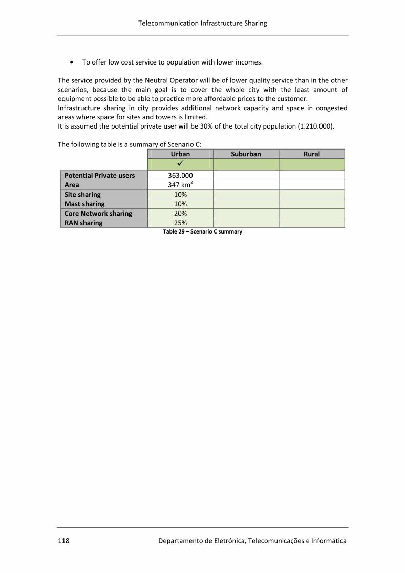
Telecommunication Infrastructure Sharing
118 Departamento de Eletrónica, Telecomunicações e Informática
To offer low cost service to population with lower incomes. The service provided by the Neutral Operator will be of lower quality service than in the other scenarios, because the main goal is to cover the whole city with the least amount of equipment possible to be able to practice more affordable prices to the customer. Infrastructure sharing in city provides additional network capacity and space in congested areas where space for sites and towers is limited. It is assumed the potential private user will be 30% of the total city population (1.210.000). The following table is a summary of Scenario C:
Urban Suburban Rural
Potential Private users 363.000
Area 347 km2
Site sharing 10%
Mast sharing 10%
Core Network sharing 20%
RAN sharing 25% Table 29 – Scenario C summary
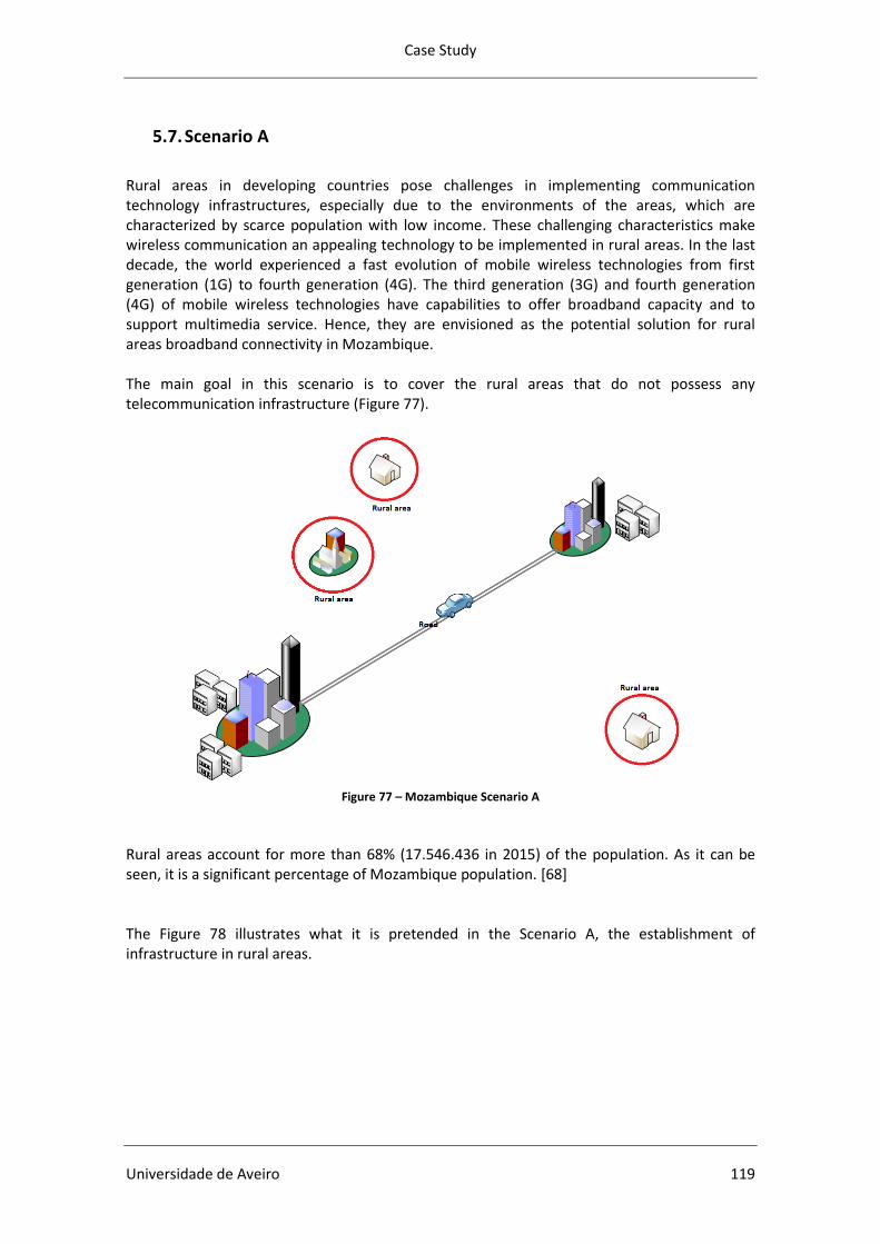
Case Study
Universidade de Aveiro 119
5.7. Scenario A
Rural areas in developing countries pose challenges in implementing communication technology infrastructures, especially due to the environments of the areas, which are characterized by scarce population with low income. These challenging characteristics make wireless communication an appealing technology to be implemented in rural areas. In the last decade, the world experienced a fast evolution of mobile wireless technologies from first generation (1G) to fourth generation (4G). The third generation (3G) and fourth generation (4G) of mobile wireless technologies have capabilities to offer broadband capacity and to support multimedia service. Hence, they are envisioned as the potential solution for rural areas broadband connectivity in Mozambique. The main goal in this scenario is to cover the rural areas that do not possess any telecommunication infrastructure (Figure 77).
Figure 77 – Mozambique Scenario A
Rural areas account for more than 68% (17.546.436 in 2015) of the population. As it can be seen, it is a significant percentage of Mozambique population. [68] The Figure 78 illustrates what it is pretended in the Scenario A, the establishment of infrastructure in rural areas.

Telecommunication Infrastructure Sharing
120 Departamento de Eletrónica, Telecomunicações e Informática
Figure 78 – Infrastructure of Scenario A
In Scenario A, the following assumptions were made:
The kick-off of project is 2017.
Only target rural areas - Telecommunications infrastructure is non-existent (0% infrastructure
installed).
The distribution of the users will be homogeneous.
In first year the number of users per site will never be enough to the point of having site saturation. But in the remaining years the site saturation will occur and the capacity dimensioning will be used.
All sites have three sectors.
It does not exist site distinction during the year, i.e. all sites will have the same size, same configuration and same number of users during the year. Only yearly sites actualizations are made.
12,2 kbps voice service
The evolution of the technology in Mozambique will follow the Portuguese evolution trend, but at a higher speed rate (GSM, UMTS and LTE).
Average distance per site to the Core Network is 45 km (distance between Site to RNC and RNC to Core Network).
The terrain is Sandy Terrain.
The technologies have a Starting Level at 5% and the Saturation Level at 75%.
Site to RNC connections will be 50% per optical fiber and 50% per radio link.
The Annual Interest Rate is 5%.
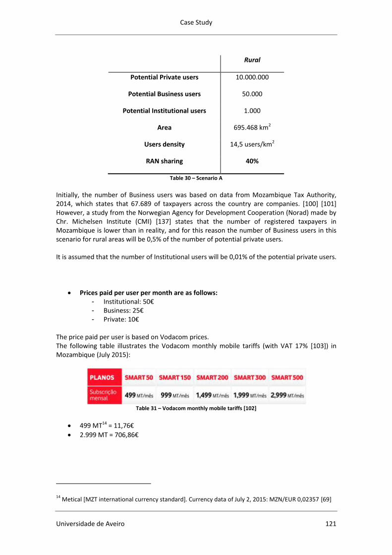
Case Study
Universidade de Aveiro 121
Rural
Potential Private users 10.000.000
Potential Business users 50.000
Potential Institutional users 1.000
Area 695.468 km2
Users density 14,5 users/km2
RAN sharing 40%
Table 30 – Scenario A
Initially, the number of Business users was based on data from Mozambique Tax Authority, 2014, which states that 67.689 of taxpayers across the country are companies. [100] [101] However, a study from the Norwegian Agency for Development Cooperation (Norad) made by Chr. Michelsen Institute (CMI) [137] states that the number of registered taxpayers in Mozambique is lower than in reality, and for this reason the number of Business users in this scenario for rural areas will be 0,5% of the number of potential private users. It is assumed that the number of Institutional users will be 0,01% of the potential private users.
Prices paid per user per month are as follows: - Institutional: 50€ - Business: 25€ - Private: 10€
The price paid per user is based on Vodacom prices. The following table illustrates the Vodacom monthly mobile tariffs (with VAT 17% [103]) in Mozambique (July 2015):
Table 31 – Vodacom monthly mobile tariffs [102]
499 MT14 = 11,76€
2.999 MT = 706,86€
14 Metical [MZT international currency standard]. Currency data of July 2, 2015: MZN/EUR 0,02357 [69]
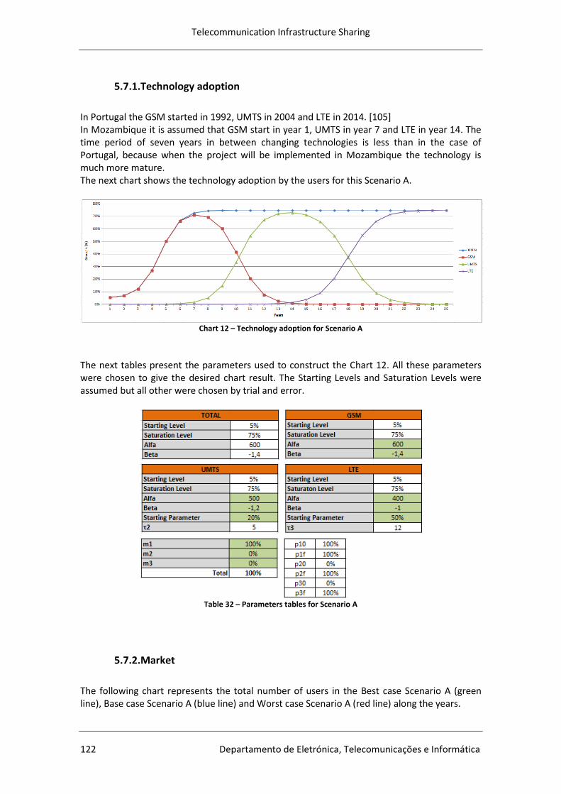
Telecommunication Infrastructure Sharing
122 Departamento de Eletrónica, Telecomunicações e Informática
5.7.1.Technology adoption
In Portugal the GSM started in 1992, UMTS in 2004 and LTE in 2014. [105] In Mozambique it is assumed that GSM start in year 1, UMTS in year 7 and LTE in year 14. The time period of seven years in between changing technologies is less than in the case of Portugal, because when the project will be implemented in Mozambique the technology is much more mature. The next chart shows the technology adoption by the users for this Scenario A.
Chart 12 – Technology adoption for Scenario A
The next tables present the parameters used to construct the Chart 12. All these parameters were chosen to give the desired chart result. The Starting Levels and Saturation Levels were assumed but all other were chosen by trial and error.
Table 32 – Parameters tables for Scenario A
5.7.2.Market
The following chart represents the total number of users in the Best case Scenario A (green line), Base case Scenario A (blue line) and Worst case Scenario A (red line) along the years.
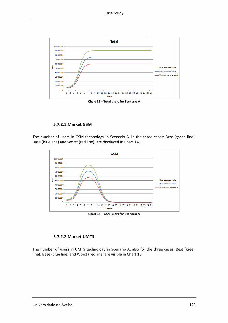
Case Study
Universidade de Aveiro 123
Chart 13 – Total users for Scenario A
5.7.2.1.Market GSM
The number of users in GSM technology in Scenario A, in the three cases: Best (green line), Base (blue line) and Worst (red line), are displayed in Chart 14.
Chart 14 – GSM users for Scenario A
5.7.2.2.Market UMTS
The number of users in UMTS technology in Scenario A, also for the three cases: Best (green line), Base (blue line) and Worst (red line, are visible in Chart 15.
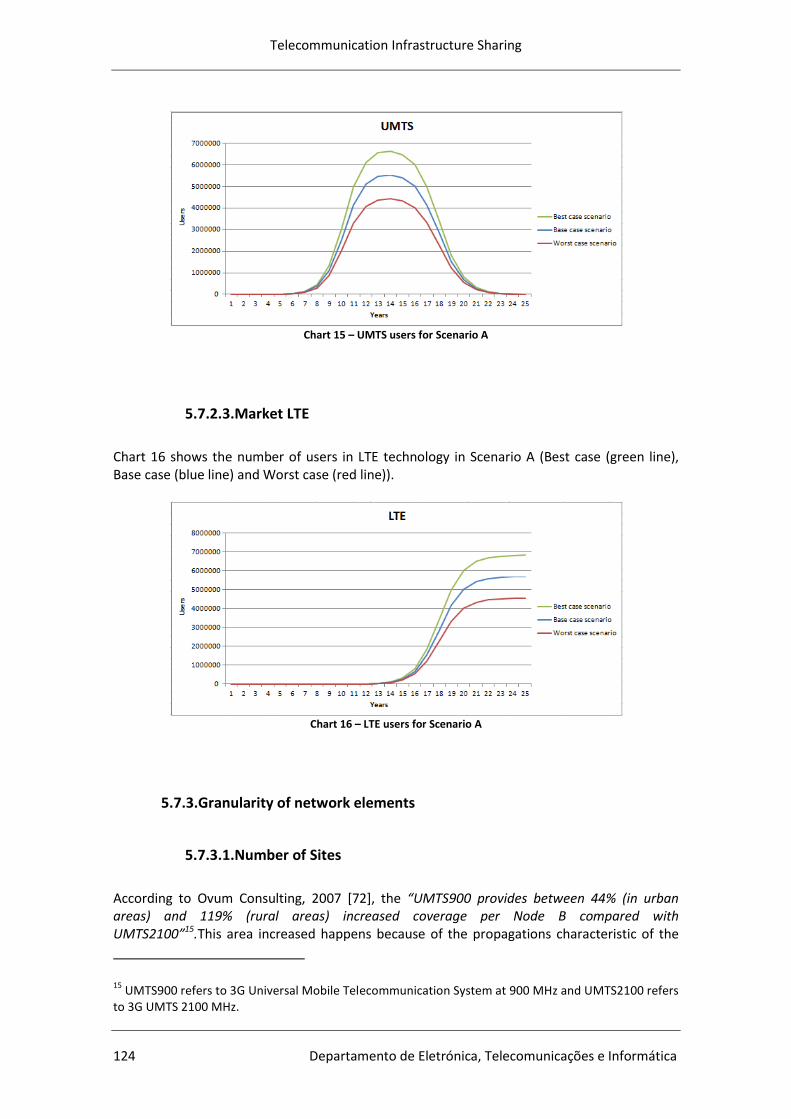
Telecommunication Infrastructure Sharing
124 Departamento de Eletrónica, Telecomunicações e Informática
Chart 15 – UMTS users for Scenario A
5.7.2.3.Market LTE
Chart 16 shows the number of users in LTE technology in Scenario A (Best case (green line), Base case (blue line) and Worst case (red line)).
Chart 16 – LTE users for Scenario A
5.7.3.Granularity of network elements
5.7.3.1.Number of Sites
According to Ovum Consulting, 2007 [72], the “UMTS900 provides between 44% (in urban areas) and 119% (rural areas) increased coverage per Node B compared with UMTS2100”15.This area increased happens because of the propagations characteristic of the
15 UMTS900 refers to 3G Universal Mobile Telecommunication System at 900 MHz and UMTS2100 refers
to 3G UMTS 2100 MHz.

Case Study
Universidade de Aveiro 125
lower frequency band. This brings benefits to the operator, because it directly lowers CAPEX and increases mobility benefits, providing a new option, with greater service capability for operators who may wish to replace their GSM networks. Also, 3G UMTS900 can be easier to implement as it reuses existing infrastructure of GSM. [72] [79] The improved NodeB coverage of UMTS900 technology decreases the number of sites in a region. This should reduce the potential number of gaps between sites, which will help overcome handover problems and hence make the customer experience better. [72] To maximize the benefits of UMTS900 (through lower equipment and device costs, and greater certainty of outcome) an international harmonization of the 900MHz band needs to set in order to allow UMTS900 use, which is one of the most used bands in the world. [72] In regions of the Sub Saharan Africa, using UMTS900 rather than UMTS2100 can reduce cumulative CAPEX by 41% over a five year period, and NPV improvements ranging from 40% - 55% can be attained. [72] There are practical examples of specific countries that illustrate the benefits of using UMTS900: Finland provides UMTS900 coverage for $700M less than with UMTS2100; in Saudi Arabia this reduction is $2.1bn; in South Africa $500M and in Sri Lanka $24M. [72] In Scenario A, it is assumed that only one frequency of 900 Mhz is used for all technologies (GSM, UMTS and LTE). The calculation tools used in this work project do not accept different sites sizes for different technologies - all sites have the same area. The site area is calculated for values of UMTS and the obtained area is used for all technologies. Link budget planning is part of the network planning process, which helps to dimension the required coverage, capacity and quality of service in the network. Link budget calculations were done based on 12,2 kbps voice service. [79] The link budget for mobile wireless networks are normally calculated (dimensioned) based on voice service, as the voice service is the most critical service. [77] [81] Uplink power budget will determine the maximum site range. A typical site range in rural areas will be several kilometers depending on the terrain. [89]
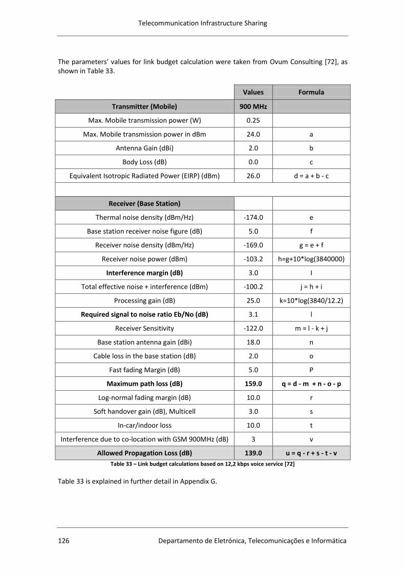
Telecommunication Infrastructure Sharing
126 Departamento de Eletrónica, Telecomunicações e Informática
The parameters’ values for link budget calculation were taken from Ovum Consulting [72], as shown in Table 33.
Values Formula
Transmitter (Mobile) 900 MHz
Max. Mobile transmission power (W) 0.25
Max. Mobile transmission power in dBm 24.0 a
Antenna Gain (dBi) 2.0 b
Body Loss (dB) 0.0 c
Equivalent Isotropic Radiated Power (EIRP) (dBm) 26.0 d = a + b - c
Receiver (Base Station)
Thermal noise density (dBm/Hz) -174.0 e
Base station receiver noise figure (dB) 5.0 f
Receiver noise density (dBm/Hz) -169.0 g = e + f
Receiver noise power (dBm) -103.2 h=g+10*log(3840000)
Interference margin (dB) 3.0 I
Total effective noise + interference (dBm) -100.2 j = h + i
Processing gain (dB) 25.0 k=10*log(3840/12.2)
Required signal to noise ratio Eb/No (dB) 3.1 l
Receiver Sensitivity -122.0 m = l - k + j
Base station antenna gain (dBi) 18.0 n
Cable loss in the base station (dB) 2.0 o
Fast fading Margin (dB) 5.0 P
Maximum path loss (dB) 159.0 q = d - m + n - o - p
Log-normal fading margin (dB) 10.0 r
Soft handover gain (dB), Multicell 3.0 s
In-car/indoor loss 10.0 t
Interference due to co-location with GSM 900MHz (dB) 3 v
Allowed Propagation Loss (dB) 139.0 u = q - r + s - t - v
Table 33 – Link budget calculations based on 12,2 kbps voice service [72] Table 33 is explained in further detail in Appendix G.
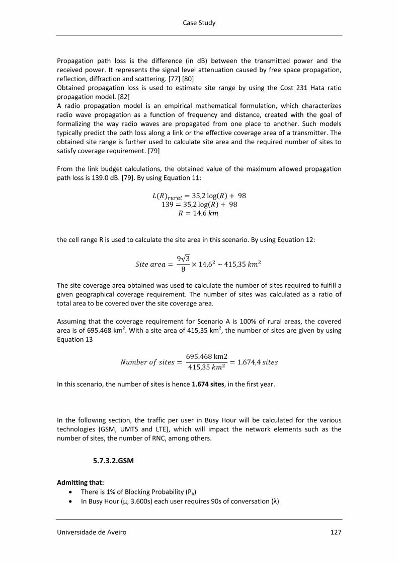
Case Study
Universidade de Aveiro 127
Propagation path loss is the difference (in dB) between the transmitted power and the received power. It represents the signal level attenuation caused by free space propagation, reflection, diffraction and scattering. [77] [80] Obtained propagation loss is used to estimate site range by using the Cost 231 Hata ratio propagation model. [82] A radio propagation model is an empirical mathematical formulation, which characterizes radio wave propagation as a function of frequency and distance, created with the goal of formalizing the way radio waves are propagated from one place to another. Such models typically predict the path loss along a link or the effective coverage area of a transmitter. The obtained site range is further used to calculate site area and the required number of sites to satisfy coverage requirement. [79] From the link budget calculations, the obtained value of the maximum allowed propagation path loss is 139.0 dB. [79]. By using Equation 11:
the cell range R is used to calculate the site area in this scenario. By using Equation 12:
The site coverage area obtained was used to calculate the number of sites required to fulfill a given geographical coverage requirement. The number of sites was calculated as a ratio of total area to be covered over the site coverage area. Assuming that the coverage requirement for Scenario A is 100% of rural areas, the covered area is of 695.468 km2. With a site area of 415,35 km2, the number of sites are given by using Equation 13
In this scenario, the number of sites is hence 1.674 sites, in the first year. In the following section, the traffic per user in Busy Hour will be calculated for the various technologies (GSM, UMTS and LTE), which will impact the network elements such as the number of sites, the number of RNC, among others.
5.7.3.2.GSM
Admitting that:
There is 1% of Blocking Probability (Pb)
In Busy Hour (μ, 3.600s) each user requires 90s of conversation (λ)
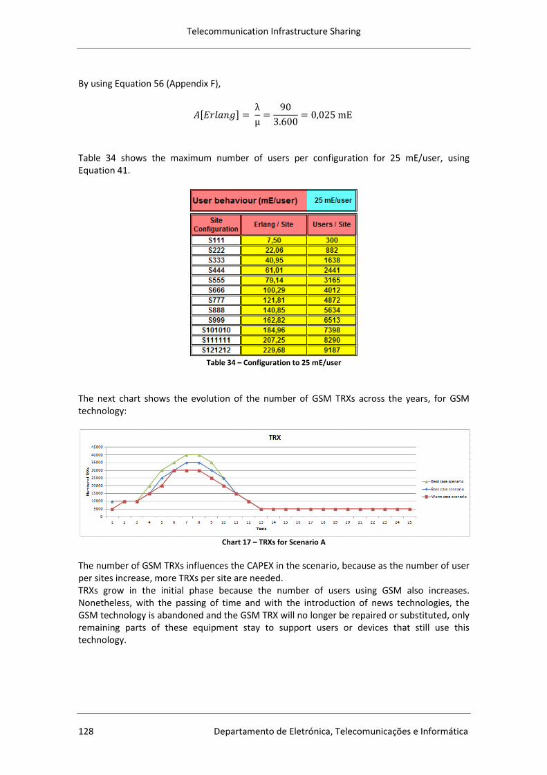
Telecommunication Infrastructure Sharing
128 Departamento de Eletrónica, Telecomunicações e Informática
By using Equation 56 (Appendix F),
Table 34 shows the maximum number of users per configuration for 25 mE/user, using Equation 41.
Table 34 – Configuration to 25 mE/user
The next chart shows the evolution of the number of GSM TRXs across the years, for GSM technology:
Chart 17 – TRXs for Scenario A
The number of GSM TRXs influences the CAPEX in the scenario, because as the number of user per sites increase, more TRXs per site are needed. TRXs grow in the initial phase because the number of users using GSM also increases. Nonetheless, with the passing of time and with the introduction of news technologies, the GSM technology is abandoned and the GSM TRX will no longer be repaired or substituted, only remaining parts of these equipment stay to support users or devices that still use this technology.
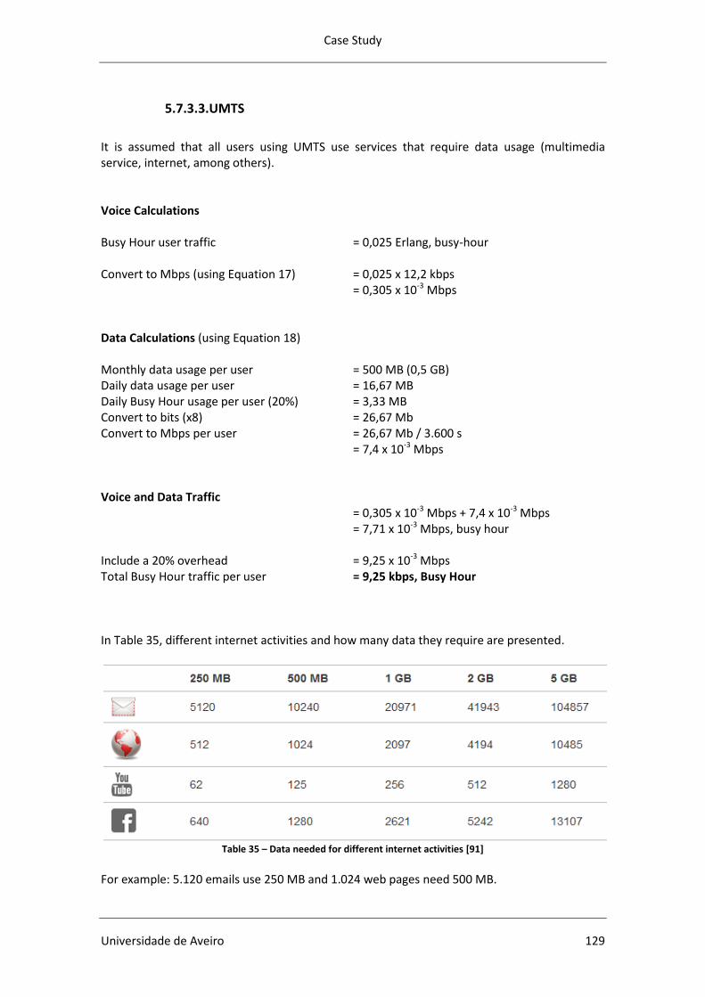
Case Study
Universidade de Aveiro 129
5.7.3.3.UMTS
It is assumed that all users using UMTS use services that require data usage (multimedia service, internet, among others). Voice Calculations Busy Hour user traffic = 0,025 Erlang, busy-hour Convert to Mbps (using Equation 17) = 0,025 x 12,2 kbps
= 0,305 x 10-3 Mbps Data Calculations (using Equation 18) Monthly data usage per user = 500 MB (0,5 GB) Daily data usage per user = 16,67 MB Daily Busy Hour usage per user (20%) = 3,33 MB Convert to bits (x8) = 26,67 Mb Convert to Mbps per user = 26,67 Mb / 3.600 s
= 7,4 x 10-3 Mbps Voice and Data Traffic = 0,305 x 10-3 Mbps + 7,4 x 10-3 Mbps = 7,71 x 10-3 Mbps, busy hour Include a 20% overhead = 9,25 x 10-3 Mbps Total Busy Hour traffic per user = 9,25 kbps, Busy Hour In Table 35, different internet activities and how many data they require are presented.
Table 35 – Data needed for different internet activities [91]
For example: 5.120 emails use 250 MB and 1.024 web pages need 500 MB.
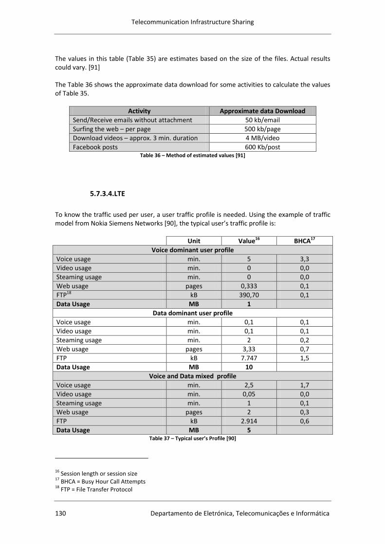
Telecommunication Infrastructure Sharing
130 Departamento de Eletrónica, Telecomunicações e Informática
The values in this table (Table 35) are estimates based on the size of the files. Actual results could vary. [91] The Table 36 shows the approximate data download for some activities to calculate the values of Table 35.
Activity Approximate data Download
Send/Receive emails without attachment 50 kb/email
Surfing the web – per page 500 kb/page
Download videos – approx. 3 min. duration 4 MB/video
Facebook posts 600 Kb/post Table 36 – Method of estimated values [91]
5.7.3.4.LTE
To know the traffic used per user, a user traffic profile is needed. Using the example of traffic model from Nokia Siemens Networks [90], the typical user’s traffic profile is:
Unit Value16 BHCA17
Voice dominant user profile
Voice usage min. 5 3,3
Video usage min. 0 0,0
Steaming usage min. 0 0,0
Web usage pages 0,333 0,1
FTP18 kB 390,70 0,1
Data Usage MB 1
Data dominant user profile
Voice usage min. 0,1 0,1
Video usage min. 0,1 0,1
Steaming usage min. 2 0,2
Web usage pages 3,33 0,7
FTP kB 7.747 1,5
Data Usage MB 10
Voice and Data mixed profile
Voice usage min. 2,5 1,7
Video usage min. 0,05 0,0
Steaming usage min. 1 0,1
Web usage pages 2 0,3
FTP kB 2.914 0,6
Data Usage MB 5 Table 37 – Typical user’s Profile [90]
16 Session length or session size
17 BHCA = Busy Hour Call Attempts
18 FTP = File Transfer Protocol
Case Study
Universidade de Aveiro 131
The main goal of the traffic model is to describe the average user behavior during the most loaded day period (the Busy Hour). In this example from Nokia Siemens Networks LTE, traffic model defines an application mix consisting of five services (VoIP, Video, Streaming, Web browsing & FTP). There are 3 user profiles each one mapped onto an application mix:
Voice Dominant
Data Dominant
Voice/Data The Average Data Volume per user per Busy Hour (BH) from the Nokia Siemens Networks Model [90], assuming the data dominant scenario, is 10,24 MB. Calculation of user traffic in Busy Hour: Busy Hour usage per user = 10,24 MB Convert to bits (x8) = 81,92 Mb Convert to Mbps per user = 81,92 Mb / 3.600 s
= 0,02275 Mbps Include a 20% overhead = 0,02731 Mbps Total Busy Hour traffic per user = 26,73 kbps, busy hour According to CelPlan, 2014 [138] the traffic per user in Busy Hour is 25,28 kbps. This number is very similar to the above calculated, which further proves that the value used is closer to the reality. Next, to know what monthly data traffic that Nokia Siemens Network estimates per user consumption, the following calculations were made (reverse engineering): Busy Hour usage per user = 10,24 MB Daily data usage per user = 51,2 MB Monthly data usage per user = 1.536 MB Approximately 1,5 GB
5.7.4.Evolution of network elements over the years
The users’ growth and the data traffic influence the number of network elements over the years. The next chart represents the evolution of the number of sites.
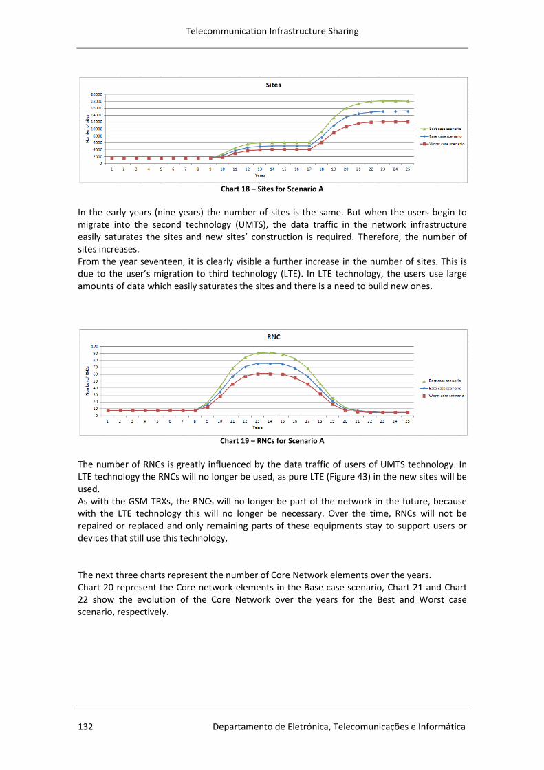
Telecommunication Infrastructure Sharing
132 Departamento de Eletrónica, Telecomunicações e Informática
Chart 18 – Sites for Scenario A
In the early years (nine years) the number of sites is the same. But when the users begin to migrate into the second technology (UMTS), the data traffic in the network infrastructure easily saturates the sites and new sites’ construction is required. Therefore, the number of sites increases. From the year seventeen, it is clearly visible a further increase in the number of sites. This is due to the user’s migration to third technology (LTE). In LTE technology, the users use large amounts of data which easily saturates the sites and there is a need to build new ones.
Chart 19 – RNCs for Scenario A
The number of RNCs is greatly influenced by the data traffic of users of UMTS technology. In LTE technology the RNCs will no longer be used, as pure LTE (Figure 43) in the new sites will be used. As with the GSM TRXs, the RNCs will no longer be part of the network in the future, because with the LTE technology this will no longer be necessary. Over the time, RNCs will not be repaired or replaced and only remaining parts of these equipments stay to support users or devices that still use this technology. The next three charts represent the number of Core Network elements over the years. Chart 20 represent the Core network elements in the Base case scenario, Chart 21 and Chart 22 show the evolution of the Core Network over the years for the Best and Worst case scenario, respectively.
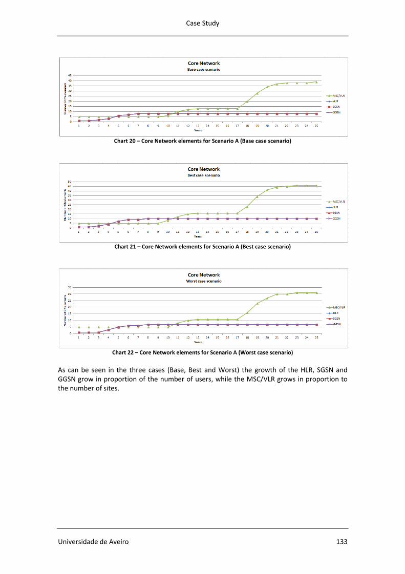
Case Study
Universidade de Aveiro 133
Chart 20 – Core Network elements for Scenario A (Base case scenario)
Chart 21 – Core Network elements for Scenario A (Best case scenario)
Chart 22 – Core Network elements for Scenario A (Worst case scenario)
As can be seen in the three cases (Base, Best and Worst) the growth of the HLR, SGSN and GGSN grow in proportion of the number of users, while the MSC/VLR grows in proportion to the number of sites.
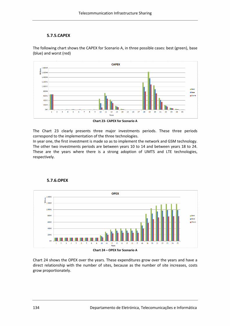
Telecommunication Infrastructure Sharing
134 Departamento de Eletrónica, Telecomunicações e Informática
5.7.5.CAPEX
The following chart shows the CAPEX for Scenario A, in three possible cases: best (green), base (blue) and worst (red)
Chart 23- CAPEX for Scenario A
The Chart 23 clearly presents three major investments periods. These three periods correspond to the implementation of the three technologies. In year one, the first investment is made so as to implement the network and GSM technology. The other two investments periods are between years 10 to 14 and between years 18 to 24. These are the years where there is a strong adoption of UMTS and LTE technologies, respectively.
5.7.6.OPEX
Chart 24 – OPEX for Scenario A
Chart 24 shows the OPEX over the years. These expenditures grow over the years and have a direct relationship with the number of sites, because as the number of site increases, costs grow proportionately.
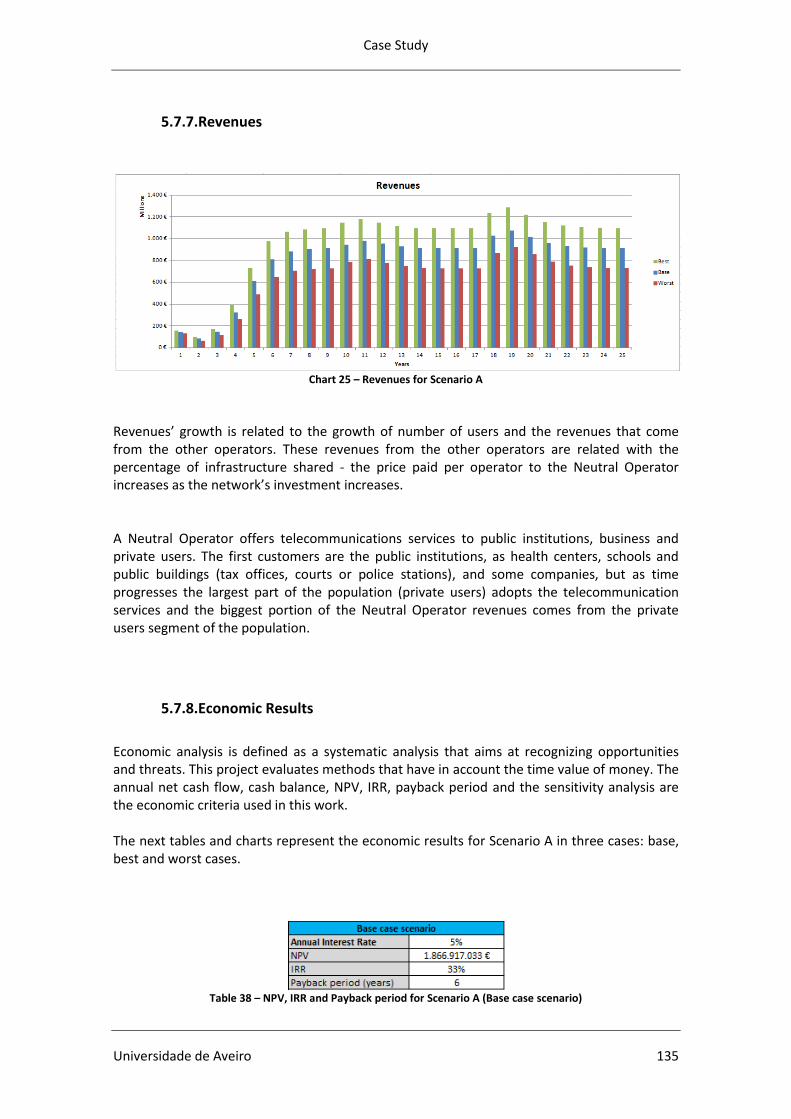
Case Study
Universidade de Aveiro 135
5.7.7.Revenues
Chart 25 – Revenues for Scenario A
Revenues’ growth is related to the growth of number of users and the revenues that come from the other operators. These revenues from the other operators are related with the percentage of infrastructure shared - the price paid per operator to the Neutral Operator increases as the network’s investment increases. A Neutral Operator offers telecommunications services to public institutions, business and private users. The first customers are the public institutions, as health centers, schools and public buildings (tax offices, courts or police stations), and some companies, but as time progresses the largest part of the population (private users) adopts the telecommunication services and the biggest portion of the Neutral Operator revenues comes from the private users segment of the population.
5.7.8.Economic Results
Economic analysis is defined as a systematic analysis that aims at recognizing opportunities and threats. This project evaluates methods that have in account the time value of money. The annual net cash flow, cash balance, NPV, IRR, payback period and the sensitivity analysis are the economic criteria used in this work. The next tables and charts represent the economic results for Scenario A in three cases: base, best and worst cases.
Table 38 – NPV, IRR and Payback period for Scenario A (Base case scenario)

Telecommunication Infrastructure Sharing
136 Departamento de Eletrónica, Telecomunicações e Informática
Chart 26 – Economic Results for Scenario A (Base case scenario)
The payback period, which is the numbers of years until revenues equal or exceed all investment costs, is 6 years for the base scenario. The NPV is positive, which means that investment is profitable. The IRR, which represents the maximum profitability rate of the project, is of 33% and is largely greater than the discount rate (5%) which reinforces the profitability of the investment.
Table 39 – NPV, IRR and Payback period for Scenario A (Best case scenario)
Figure 79 – Economic Results for Scenario A (Best case scenario)
Predictably, due to this being a more optimistic scenario, all economic results turn out to be better than in the base scenario. The payback period (5 years) is lower than in the base case, while the NPV and IRR are bigger.

Case Study
Universidade de Aveiro 137
Table 40 – NPV, IRR and Payback period for Scenario A (Worst case scenario)
Figure 80 – Economic Results for Scenario A (Worst case scenario)
Finally, the pessimistic case, the economic results are worse than in the other two cases, as expected, but still presents positive results. The payback period is 6 years, like in the base case scenario, while the NPV is of 1.369.345.644 Euros and IRR is of 26%. In summary, the predictions made for the Scenario A show that a possible investment can be successful and a good development engine for rural areas in Mozambique.
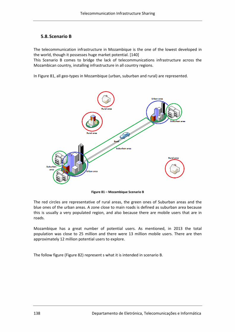
Telecommunication Infrastructure Sharing
138 Departamento de Eletrónica, Telecomunicações e Informática
5.8. Scenario B
The telecommunication infrastructure in Mozambique is the one of the lowest developed in the world, though it possesses huge market potential. [140] This Scenario B comes to bridge the lack of telecommunications infrastructure across the Mozambican country, installing infrastructure in all country regions. In Figure 81, all geo-types in Mozambique (urban, suburban and rural) are represented.
Figure 81 – Mozambique Scenario B
The red circles are representative of rural areas, the green ones of Suburban areas and the blue ones of the urban areas. A zone close to main roads is defined as suburban area because this is usually a very populated region, and also because there are mobile users that are in roads. Mozambique has a great number of potential users. As mentioned, in 2013 the total population was close to 25 million and there were 13 million mobile users. There are then approximately 12 million potential users to explore. The follow figure (Figure 82) represent s what it is intended in scenario B.
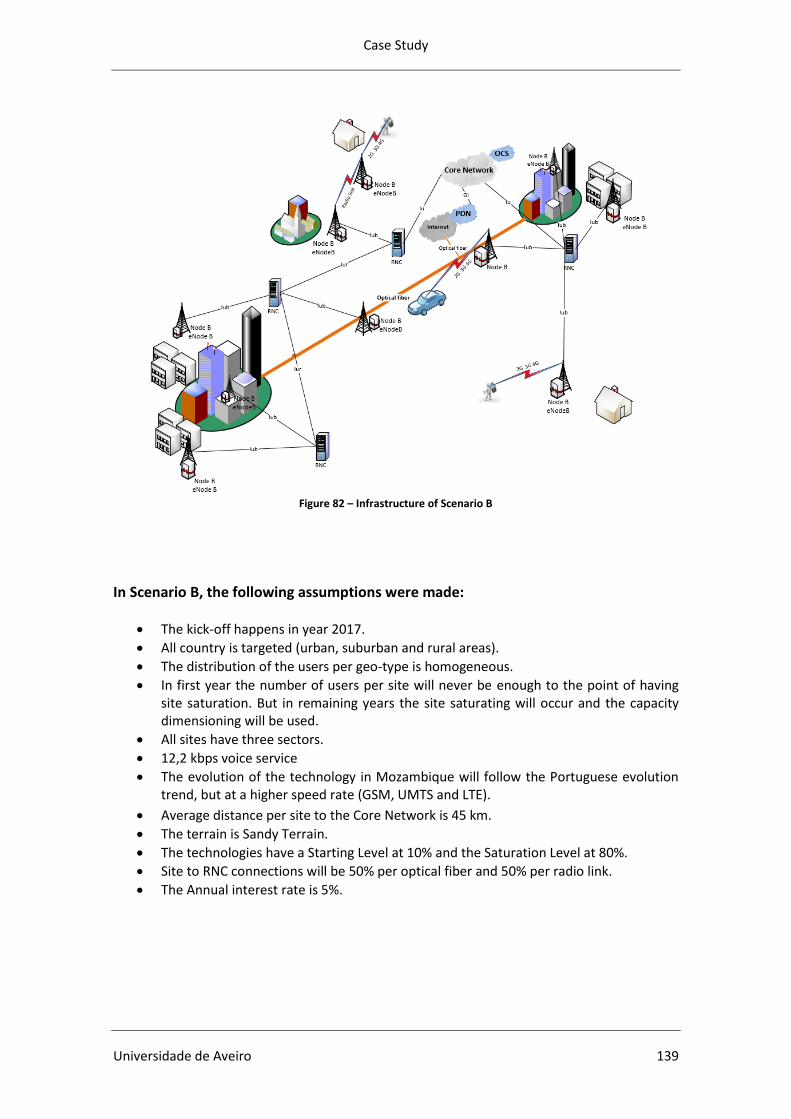
Case Study
Universidade de Aveiro 139
Figure 82 – Infrastructure of Scenario B
In Scenario B, the following assumptions were made:
The kick-off happens in year 2017.
All country is targeted (urban, suburban and rural areas).
The distribution of the users per geo-type is homogeneous.
In first year the number of users per site will never be enough to the point of having site saturation. But in remaining years the site saturating will occur and the capacity dimensioning will be used.
All sites have three sectors.
12,2 kbps voice service
The evolution of the technology in Mozambique will follow the Portuguese evolution trend, but at a higher speed rate (GSM, UMTS and LTE).
Average distance per site to the Core Network is 45 km.
The terrain is Sandy Terrain.
The technologies have a Starting Level at 10% and the Saturation Level at 80%.
Site to RNC connections will be 50% per optical fiber and 50% per radio link.
The Annual interest rate is 5%.
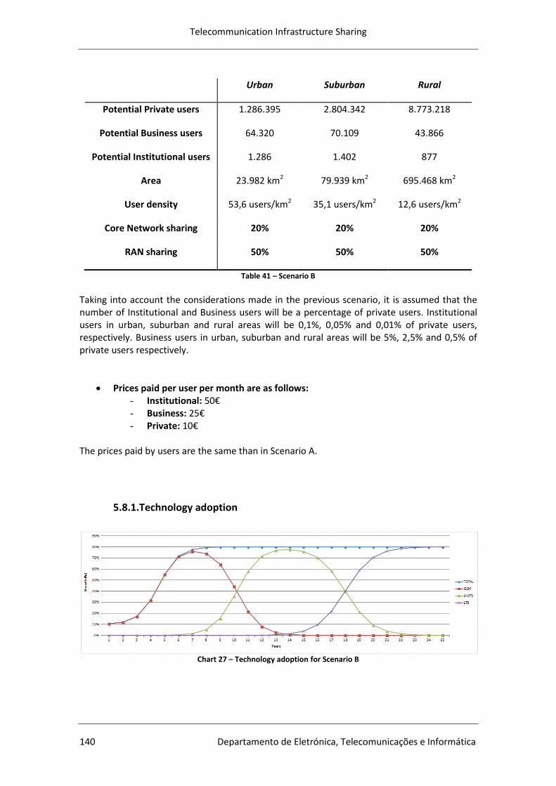
Telecommunication Infrastructure Sharing
140 Departamento de Eletrónica, Telecomunicações e Informática
Urban Suburban Rural
Potential Private users 1.286.395 2.804.342 8.773.218
Potential Business users 64.320 70.109 43.866
Potential Institutional users 1.286 1.402 877
Area 23.982 km2 79.939 km2 695.468 km2
User density 53,6 users/km2 35,1 users/km2 12,6 users/km2
Core Network sharing 20% 20% 20%
RAN sharing 50% 50% 50%
Table 41 – Scenario B
Taking into account the considerations made in the previous scenario, it is assumed that the number of Institutional and Business users will be a percentage of private users. Institutional users in urban, suburban and rural areas will be 0,1%, 0,05% and 0,01% of private users, respectively. Business users in urban, suburban and rural areas will be 5%, 2,5% and 0,5% of private users respectively.
Prices paid per user per month are as follows: - Institutional: 50€ - Business: 25€ - Private: 10€
The prices paid by users are the same than in Scenario A.
5.8.1.Technology adoption
Chart 27 – Technology adoption for Scenario B
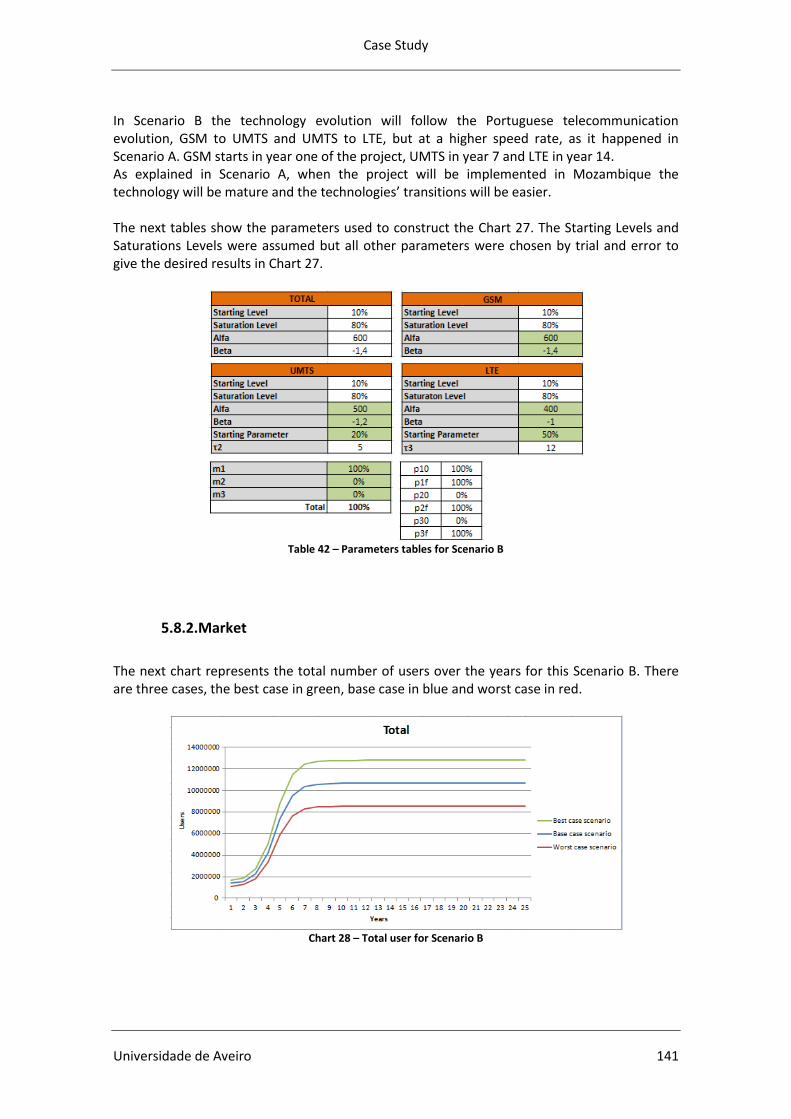
Case Study
Universidade de Aveiro 141
In Scenario B the technology evolution will follow the Portuguese telecommunication evolution, GSM to UMTS and UMTS to LTE, but at a higher speed rate, as it happened in Scenario A. GSM starts in year one of the project, UMTS in year 7 and LTE in year 14. As explained in Scenario A, when the project will be implemented in Mozambique the technology will be mature and the technologies’ transitions will be easier. The next tables show the parameters used to construct the Chart 27. The Starting Levels and Saturations Levels were assumed but all other parameters were chosen by trial and error to give the desired results in Chart 27.
Table 42 – Parameters tables for Scenario B
5.8.2.Market
The next chart represents the total number of users over the years for this Scenario B. There are three cases, the best case in green, base case in blue and worst case in red.
Chart 28 – Total user for Scenario B
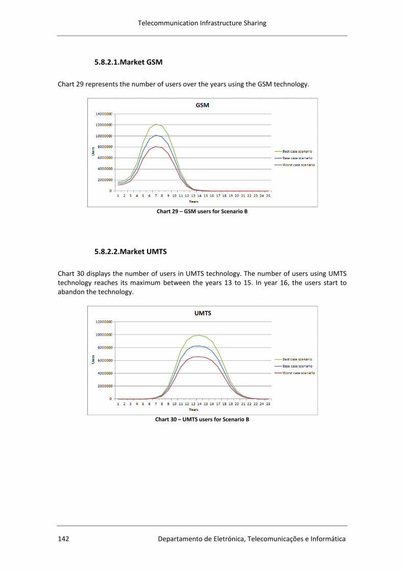
Telecommunication Infrastructure Sharing
142 Departamento de Eletrónica, Telecomunicações e Informática
5.8.2.1.Market GSM
Chart 29 represents the number of users over the years using the GSM technology.
Chart 29 – GSM users for Scenario B
5.8.2.2.Market UMTS
Chart 30 displays the number of users in UMTS technology. The number of users using UMTS technology reaches its maximum between the years 13 to 15. In year 16, the users start to abandon the technology.
Chart 30 – UMTS users for Scenario B

Case Study
Universidade de Aveiro 143
5.8.2.3.Market LTE
Chart 31 – LTE users for Scenario B
LTE technology is the last technology in this work. The Chart 31 demonstrates the number of users using LTE technology over the years.
5.8.3.Granularity of network elements
5.8.3.1.Number of Sites
Frequency Percentage increase in coverage area per Node-B (km2)
Urban Suburban Rural
900 MHz vs. 2.100 MHz 44% 60% 119%
Table 43 – Percentage increase in coverage area [72]
In the Table 43 shows very clearly that by using UMTS 900 MHz the coverage area per Node B increases when compared to UMTS 2100 MHz. According to Ovum Consulting, 2007, the improved Node B coverage of UMTS900 technology reduces the number of sites in a region. [72] In this work project, it will only be used UMTS 900Mhz to calculate site areas in the first year through coverage dimensioning. For the remaining years of the project, a yearly actualization will happen through capacity dimensioning. From the link budget calculations (Table 33), the obtained value for the maximum allowed propagation path loss is 139,0 dB. Therefore, for urban areas and by using Equation 7
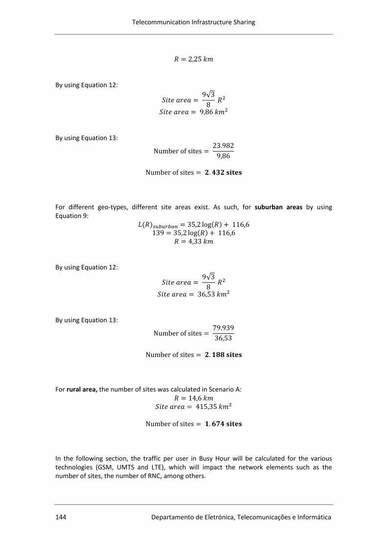
Telecommunication Infrastructure Sharing
144 Departamento de Eletrónica, Telecomunicações e Informática
By using Equation 12:
By using Equation 13:
For different geo-types, different site areas exist. As such, for suburban areas by using Equation 9:
By using Equation 12:
By using Equation 13:
For rural area, the number of sites was calculated in Scenario A:
In the following section, the traffic per user in Busy Hour will be calculated for the various technologies (GSM, UMTS and LTE), which will impact the network elements such as the number of sites, the number of RNC, among others.
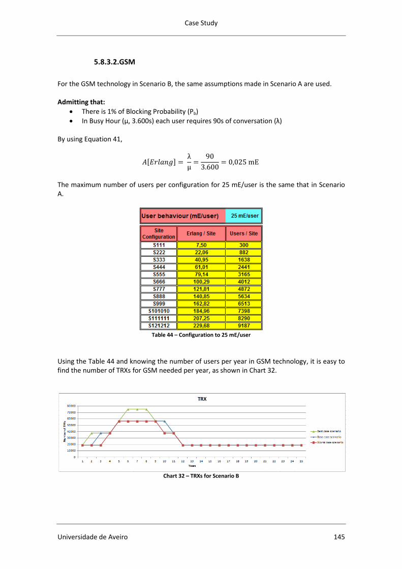
Case Study
Universidade de Aveiro 145
5.8.3.2.GSM
For the GSM technology in Scenario B, the same assumptions made in Scenario A are used. Admitting that:
There is 1% of Blocking Probability (Pb)
In Busy Hour (μ, 3.600s) each user requires 90s of conversation (λ) By using Equation 41,
The maximum number of users per configuration for 25 mE/user is the same that in Scenario A.
Table 44 – Configuration to 25 mE/user
Using the Table 44 and knowing the number of users per year in GSM technology, it is easy to find the number of TRXs for GSM needed per year, as shown in Chart 32.
Chart 32 – TRXs for Scenario B
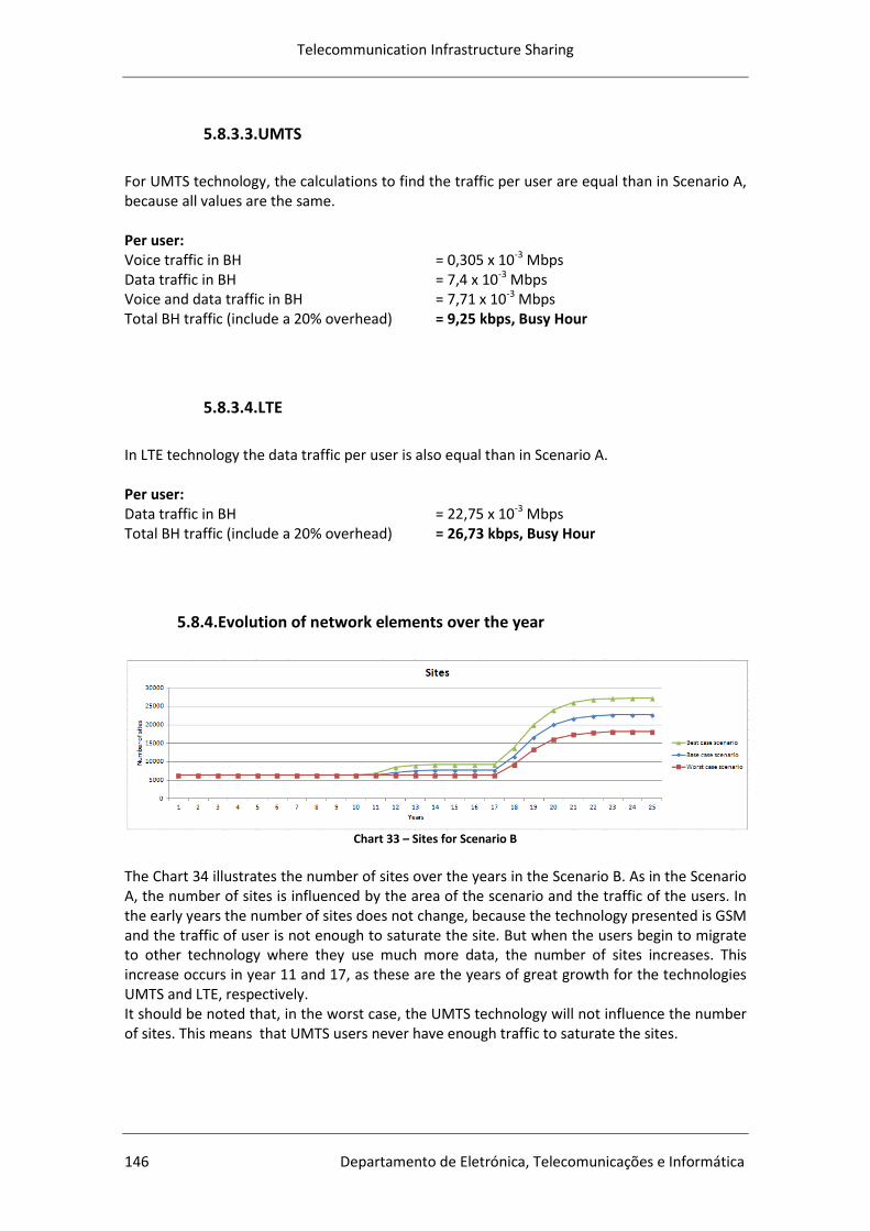
Telecommunication Infrastructure Sharing
146 Departamento de Eletrónica, Telecomunicações e Informática
5.8.3.3.UMTS
For UMTS technology, the calculations to find the traffic per user are equal than in Scenario A, because all values are the same. Per user: Voice traffic in BH = 0,305 x 10-3 Mbps Data traffic in BH = 7,4 x 10-3 Mbps Voice and data traffic in BH = 7,71 x 10-3 Mbps Total BH traffic (include a 20% overhead) = 9,25 kbps, Busy Hour
5.8.3.4.LTE
In LTE technology the data traffic per user is also equal than in Scenario A. Per user: Data traffic in BH = 22,75 x 10-3 Mbps Total BH traffic (include a 20% overhead) = 26,73 kbps, Busy Hour
5.8.4.Evolution of network elements over the year
Chart 33 – Sites for Scenario B
The Chart 34 illustrates the number of sites over the years in the Scenario B. As in the Scenario A, the number of sites is influenced by the area of the scenario and the traffic of the users. In the early years the number of sites does not change, because the technology presented is GSM and the traffic of user is not enough to saturate the site. But when the users begin to migrate to other technology where they use much more data, the number of sites increases. This increase occurs in year 11 and 17, as these are the years of great growth for the technologies UMTS and LTE, respectively. It should be noted that, in the worst case, the UMTS technology will not influence the number of sites. This means that UMTS users never have enough traffic to saturate the sites.
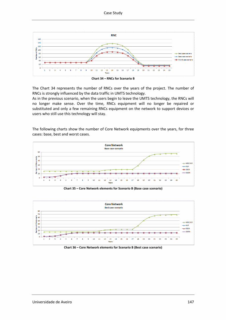
Case Study
Universidade de Aveiro 147
Chart 34 – RNCs for Scenario B
The Chart 34 represents the number of RNCs over the years of the project. The number of RNCs is strongly influenced by the data traffic in UMTS technology. As in the previous scenario, when the users begin to leave the UMTS technology, the RNCs will no longer make sense. Over the time, RNCs equipment will no longer be repaired or substituted and only a few remaining RNCs equipment on the network to support devices or users who still use this technology will stay. The following charts show the number of Core Network equipments over the years, for three cases: base, best and worst cases.
Chart 35 – Core Network elements for Scenario B (Base case scenario)
Chart 36 – Core Network elements for Scenario B (Best case scenario)
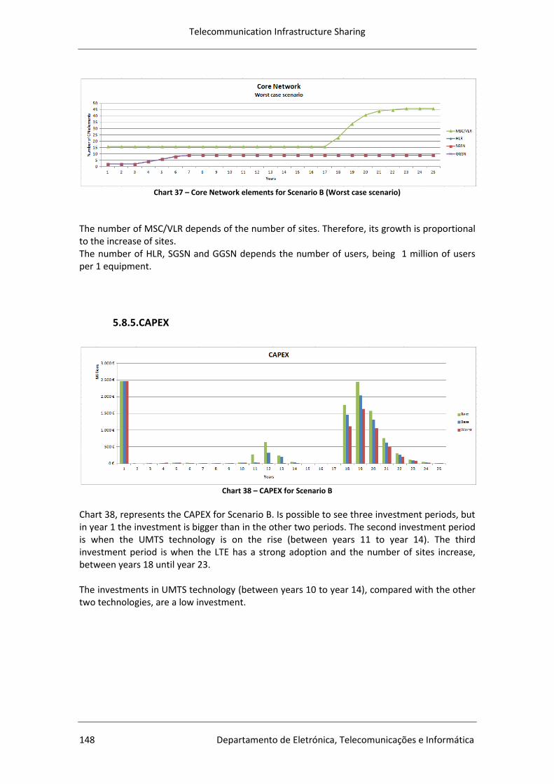
Telecommunication Infrastructure Sharing
148 Departamento de Eletrónica, Telecomunicações e Informática
Chart 37 – Core Network elements for Scenario B (Worst case scenario)
The number of MSC/VLR depends of the number of sites. Therefore, its growth is proportional to the increase of sites. The number of HLR, SGSN and GGSN depends the number of users, being 1 million of users per 1 equipment.
5.8.5.CAPEX
Chart 38 – CAPEX for Scenario B
Chart 38, represents the CAPEX for Scenario B. Is possible to see three investment periods, but in year 1 the investment is bigger than in the other two periods. The second investment period is when the UMTS technology is on the rise (between years 11 to year 14). The third investment period is when the LTE has a strong adoption and the number of sites increase, between years 18 until year 23. The investments in UMTS technology (between years 10 to year 14), compared with the other two technologies, are a low investment.
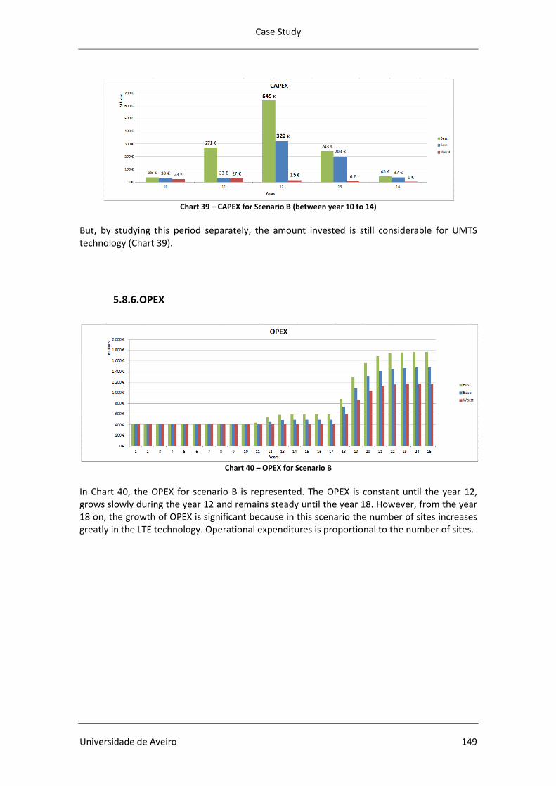
Case Study
Universidade de Aveiro 149
Chart 39 – CAPEX for Scenario B (between year 10 to 14)
But, by studying this period separately, the amount invested is still considerable for UMTS technology (Chart 39).
5.8.6.OPEX
Chart 40 – OPEX for Scenario B
In Chart 40, the OPEX for scenario B is represented. The OPEX is constant until the year 12, grows slowly during the year 12 and remains steady until the year 18. However, from the year 18 on, the growth of OPEX is significant because in this scenario the number of sites increases greatly in the LTE technology. Operational expenditures is proportional to the number of sites.
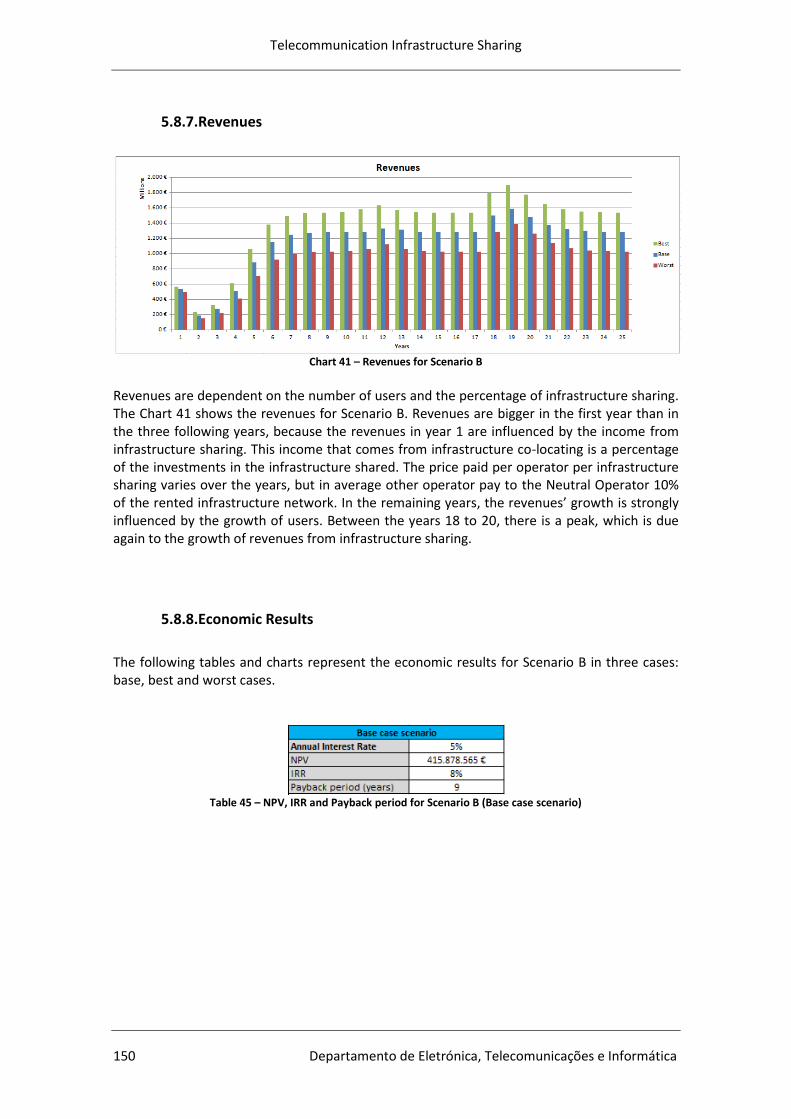
Telecommunication Infrastructure Sharing
150 Departamento de Eletrónica, Telecomunicações e Informática
5.8.7.Revenues
Chart 41 – Revenues for Scenario B
Revenues are dependent on the number of users and the percentage of infrastructure sharing. The Chart 41 shows the revenues for Scenario B. Revenues are bigger in the first year than in the three following years, because the revenues in year 1 are influenced by the income from infrastructure sharing. This income that comes from infrastructure co-locating is a percentage of the investments in the infrastructure shared. The price paid per operator per infrastructure sharing varies over the years, but in average other operator pay to the Neutral Operator 10% of the rented infrastructure network. In the remaining years, the revenues’ growth is strongly influenced by the growth of users. Between the years 18 to 20, there is a peak, which is due again to the growth of revenues from infrastructure sharing.
5.8.8.Economic Results
The following tables and charts represent the economic results for Scenario B in three cases: base, best and worst cases.
Table 45 – NPV, IRR and Payback period for Scenario B (Base case scenario)
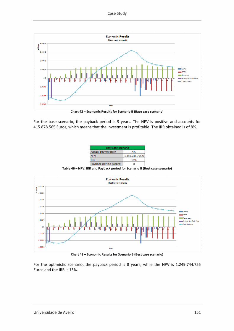
Case Study
Universidade de Aveiro 151
Chart 42 – Economic Results for Scenario B (Base case scenario)
For the base scenario, the payback period is 9 years. The NPV is positive and accounts for 415.878.565 Euros, which means that the investment is profitable. The IRR obtained is of 8%.
Table 46 – NPV, IRR and Payback period for Scenario B (Best case scenario)
Chart 43 – Economic Results for Scenario B (Best case scenario)
For the optimistic scenario, the payback period is 8 years, while the NPV is 1.249.744.755 Euros and the IRR is 13%.
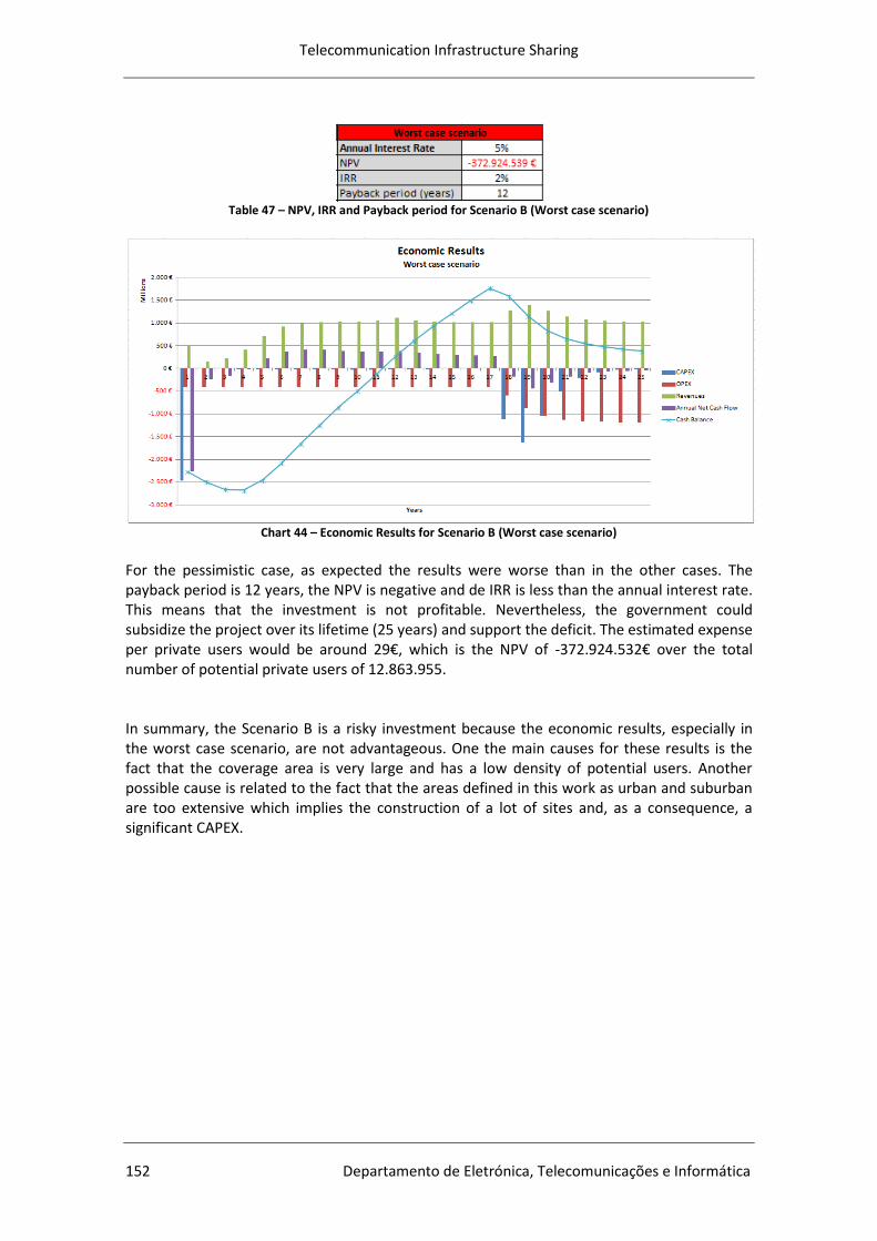
Telecommunication Infrastructure Sharing
152 Departamento de Eletrónica, Telecomunicações e Informática
Table 47 – NPV, IRR and Payback period for Scenario B (Worst case scenario)
Chart 44 – Economic Results for Scenario B (Worst case scenario)
For the pessimistic case, as expected the results were worse than in the other cases. The payback period is 12 years, the NPV is negative and de IRR is less than the annual interest rate. This means that the investment is not profitable. Nevertheless, the government could subsidize the project over its lifetime (25 years) and support the deficit. The estimated expense per private users would be around 29€, which is the NPV of -372.924.532€ over the total number of potential private users of 12.863.955. In summary, the Scenario B is a risky investment because the economic results, especially in the worst case scenario, are not advantageous. One the main causes for these results is the fact that the coverage area is very large and has a low density of potential users. Another possible cause is related to the fact that the areas defined in this work as urban and suburban are too extensive which implies the construction of a lot of sites and, as a consequence, a significant CAPEX.
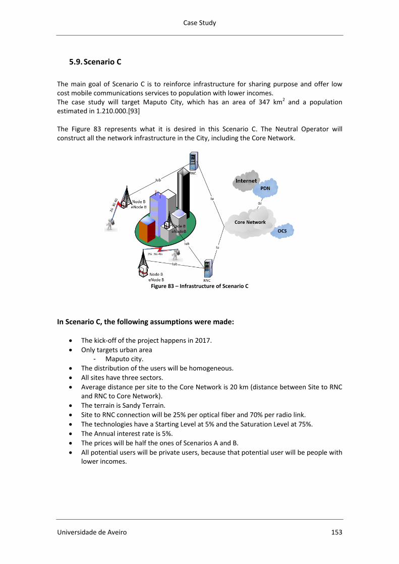
Case Study
Universidade de Aveiro 153
5.9. Scenario C
The main goal of Scenario C is to reinforce infrastructure for sharing purpose and offer low cost mobile communications services to population with lower incomes. The case study will target Maputo City, which has an area of 347 km2 and a population estimated in 1.210.000.[93] The Figure 83 represents what it is desired in this Scenario C. The Neutral Operator will construct all the network infrastructure in the City, including the Core Network.
Figure 83 – Infrastructure of Scenario C
In Scenario C, the following assumptions were made:
The kick-off of the project happens in 2017.
Only targets urban area - Maputo city.
The distribution of the users will be homogeneous.
All sites have three sectors.
Average distance per site to the Core Network is 20 km (distance between Site to RNC and RNC to Core Network).
The terrain is Sandy Terrain.
Site to RNC connection will be 25% per optical fiber and 70% per radio link.
The technologies have a Starting Level at 5% and the Saturation Level at 75%.
The Annual interest rate is 5%.
The prices will be half the ones of Scenarios A and B.
All potential users will be private users, because that potential user will be people with lower incomes.
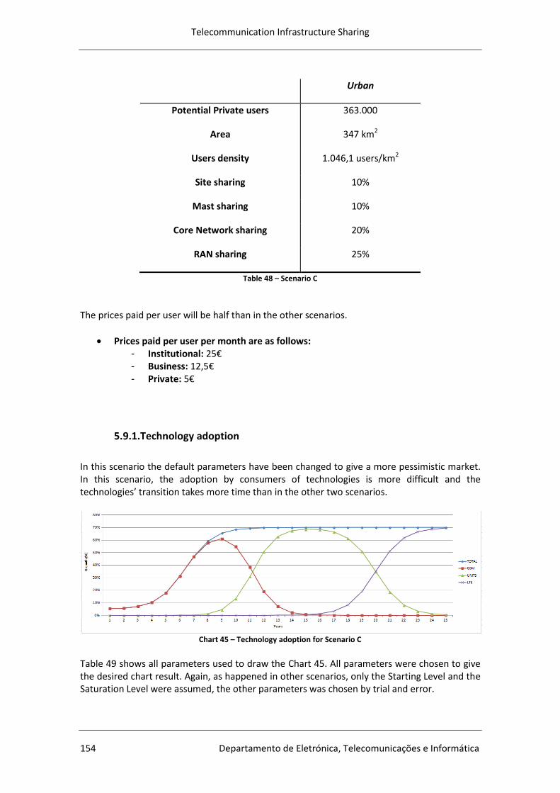
Telecommunication Infrastructure Sharing
154 Departamento de Eletrónica, Telecomunicações e Informática
Urban
Potential Private users 363.000
Area 347 km2
Users density 1.046,1 users/km2
Site sharing 10%
Mast sharing 10%
Core Network sharing 20%
RAN sharing 25%
Table 48 – Scenario C
The prices paid per user will be half than in the other scenarios.
Prices paid per user per month are as follows: - Institutional: 25€ - Business: 12,5€ - Private: 5€
5.9.1.Technology adoption
In this scenario the default parameters have been changed to give a more pessimistic market. In this scenario, the adoption by consumers of technologies is more difficult and the technologies’ transition takes more time than in the other two scenarios.
Chart 45 – Technology adoption for Scenario C
Table 49 shows all parameters used to draw the Chart 45. All parameters were chosen to give the desired chart result. Again, as happened in other scenarios, only the Starting Level and the Saturation Level were assumed, the other parameters was chosen by trial and error.
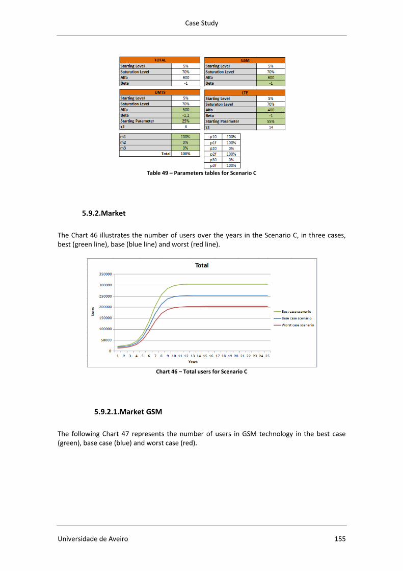
Case Study
Universidade de Aveiro 155
Table 49 – Parameters tables for Scenario C
5.9.2.Market
The Chart 46 illustrates the number of users over the years in the Scenario C, in three cases, best (green line), base (blue line) and worst (red line).
Chart 46 – Total users for Scenario C
5.9.2.1.Market GSM
The following Chart 47 represents the number of users in GSM technology in the best case (green), base case (blue) and worst case (red).
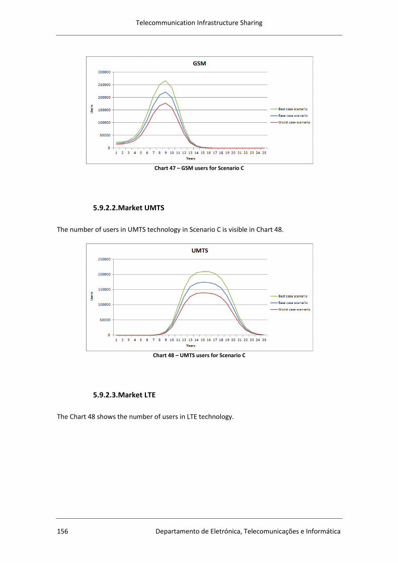
Telecommunication Infrastructure Sharing
156 Departamento de Eletrónica, Telecomunicações e Informática
Chart 47 – GSM users for Scenario C
5.9.2.2.Market UMTS
The number of users in UMTS technology in Scenario C is visible in Chart 48.
Chart 48 – UMTS users for Scenario C
5.9.2.3.Market LTE
The Chart 48 shows the number of users in LTE technology.
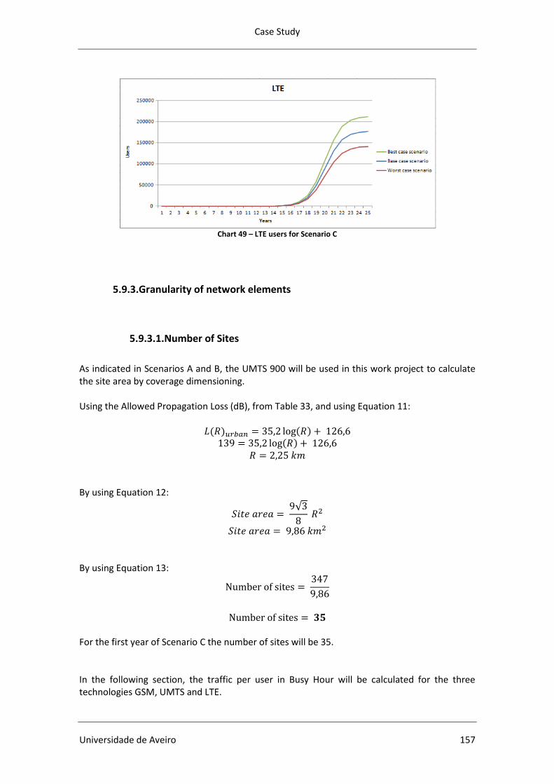
Case Study
Universidade de Aveiro 157
Chart 49 – LTE users for Scenario C
5.9.3.Granularity of network elements
5.9.3.1.Number of Sites
As indicated in Scenarios A and B, the UMTS 900 will be used in this work project to calculate the site area by coverage dimensioning. Using the Allowed Propagation Loss (dB), from Table 33, and using Equation 11:
By using Equation 12:
By using Equation 13:
For the first year of Scenario C the number of sites will be 35. In the following section, the traffic per user in Busy Hour will be calculated for the three technologies GSM, UMTS and LTE.
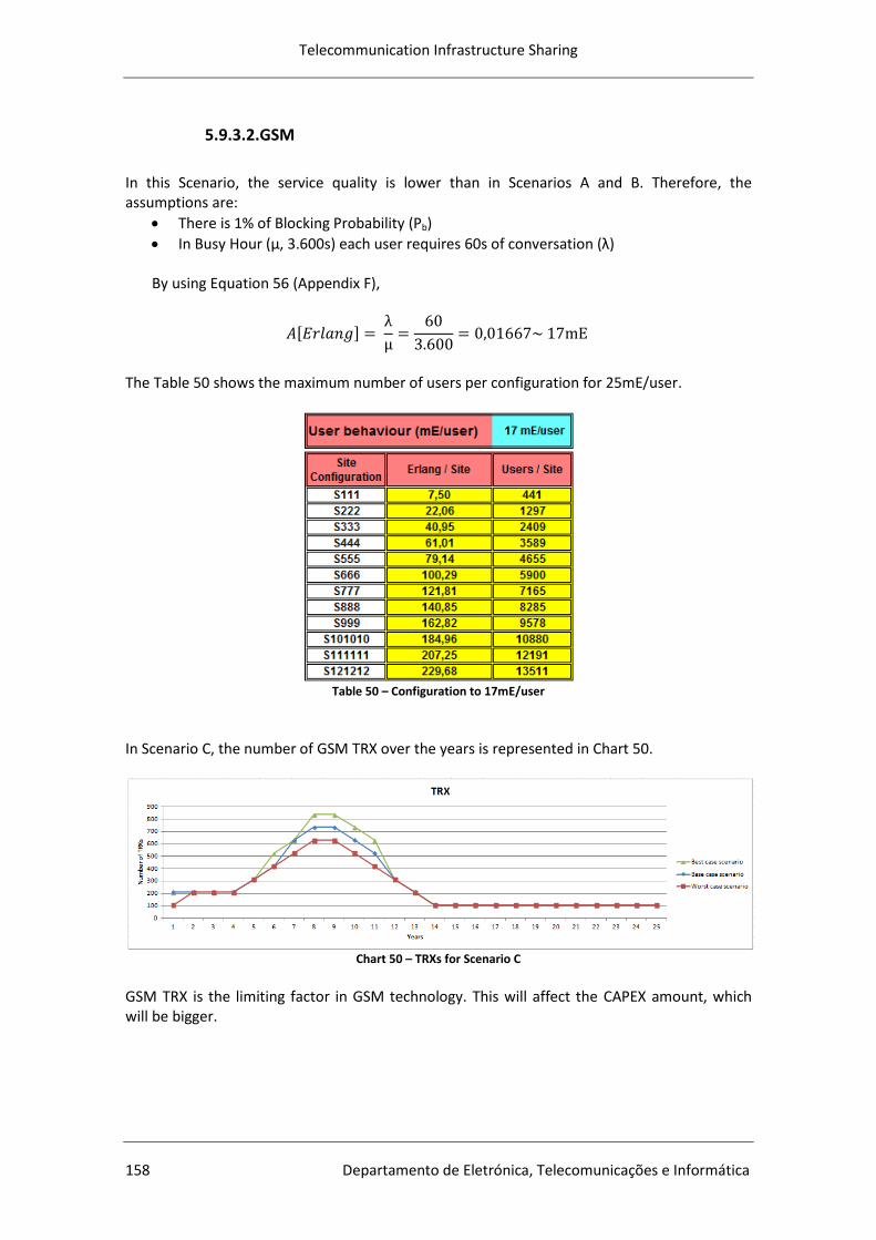
Telecommunication Infrastructure Sharing
158 Departamento de Eletrónica, Telecomunicações e Informática
5.9.3.2.GSM
In this Scenario, the service quality is lower than in Scenarios A and B. Therefore, the assumptions are:
There is 1% of Blocking Probability (Pb)
In Busy Hour (μ, 3.600s) each user requires 60s of conversation (λ) By using Equation 56 (Appendix F),
The Table 50 shows the maximum number of users per configuration for 25mE/user.
Table 50 – Configuration to 17mE/user
In Scenario C, the number of GSM TRX over the years is represented in Chart 50.
Chart 50 – TRXs for Scenario C
GSM TRX is the limiting factor in GSM technology. This will affect the CAPEX amount, which will be bigger.
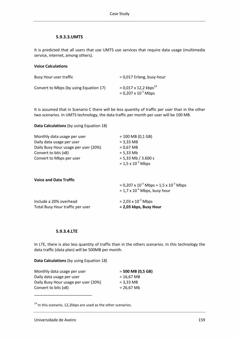
Case Study
Universidade de Aveiro 159
5.9.3.3.UMTS
It is predicted that all users that use UMTS use services that require data usage (multimedia service, internet, among others). Voice Calculations Busy Hour user traffic = 0,017 Erlang, busy-hour Convert to Mbps (by using Equation 17) = 0,017 x 12,2 kbps19
= 0,207 x 10-3 Mbps It is assumed that in Scenario C there will be less quantity of traffic per user than in the other two scenarios. In UMTS technology, the data traffic per month per user will be 100 MB. Data Calculations (by using Equation 18) Monthly data usage per user = 100 MB (0,1 GB) Daily data usage per user = 3,33 MB Daily Busy Hour usage per user (20%) = 0,67 MB Convert to bits (x8) = 5,33 Mb Convert to Mbps per user = 5,33 Mb / 3.600 s
= 1,5 x 10-3 Mbps Voice and Data Traffic = 0,207 x 10-3 Mbps + 1,5 x 10-3 Mbps = 1,7 x 10-3 Mbps, busy hour Include a 20% overhead = 2,03 x 10-3 Mbps Total Busy Hour traffic per user = 2,03 kbps, Busy Hour
5.9.3.4.LTE
In LTE, there is also less quantity of traffic than in the others scenarios. In this technology the data traffic (data plan) will be 500MB per month. Data Calculations (by using Equation 18) Monthly data usage per user = 500 MB (0,5 GB) Daily data usage per user = 16,67 MB Daily Busy Hour usage per user (20%) = 3,33 MB Convert to bits (x8) = 26,67 Mb
19 In this scenario, 12,2kbps are used as the other scenarios.
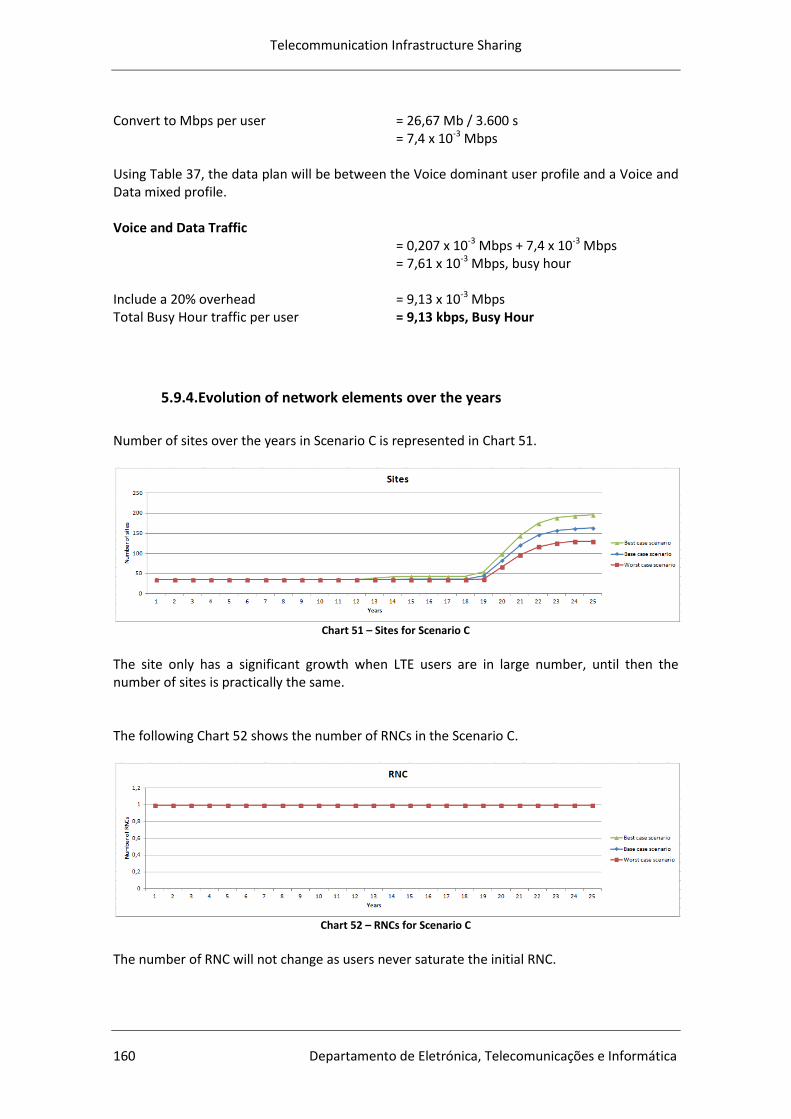
Telecommunication Infrastructure Sharing
160 Departamento de Eletrónica, Telecomunicações e Informática
Convert to Mbps per user = 26,67 Mb / 3.600 s = 7,4 x 10-3 Mbps
Using Table 37, the data plan will be between the Voice dominant user profile and a Voice and Data mixed profile. Voice and Data Traffic = 0,207 x 10-3 Mbps + 7,4 x 10-3 Mbps = 7,61 x 10-3 Mbps, busy hour Include a 20% overhead = 9,13 x 10-3 Mbps Total Busy Hour traffic per user = 9,13 kbps, Busy Hour
5.9.4.Evolution of network elements over the years
Number of sites over the years in Scenario C is represented in Chart 51.
Chart 51 – Sites for Scenario C
The site only has a significant growth when LTE users are in large number, until then the number of sites is practically the same. The following Chart 52 shows the number of RNCs in the Scenario C.
Chart 52 – RNCs for Scenario C
The number of RNC will not change as users never saturate the initial RNC.
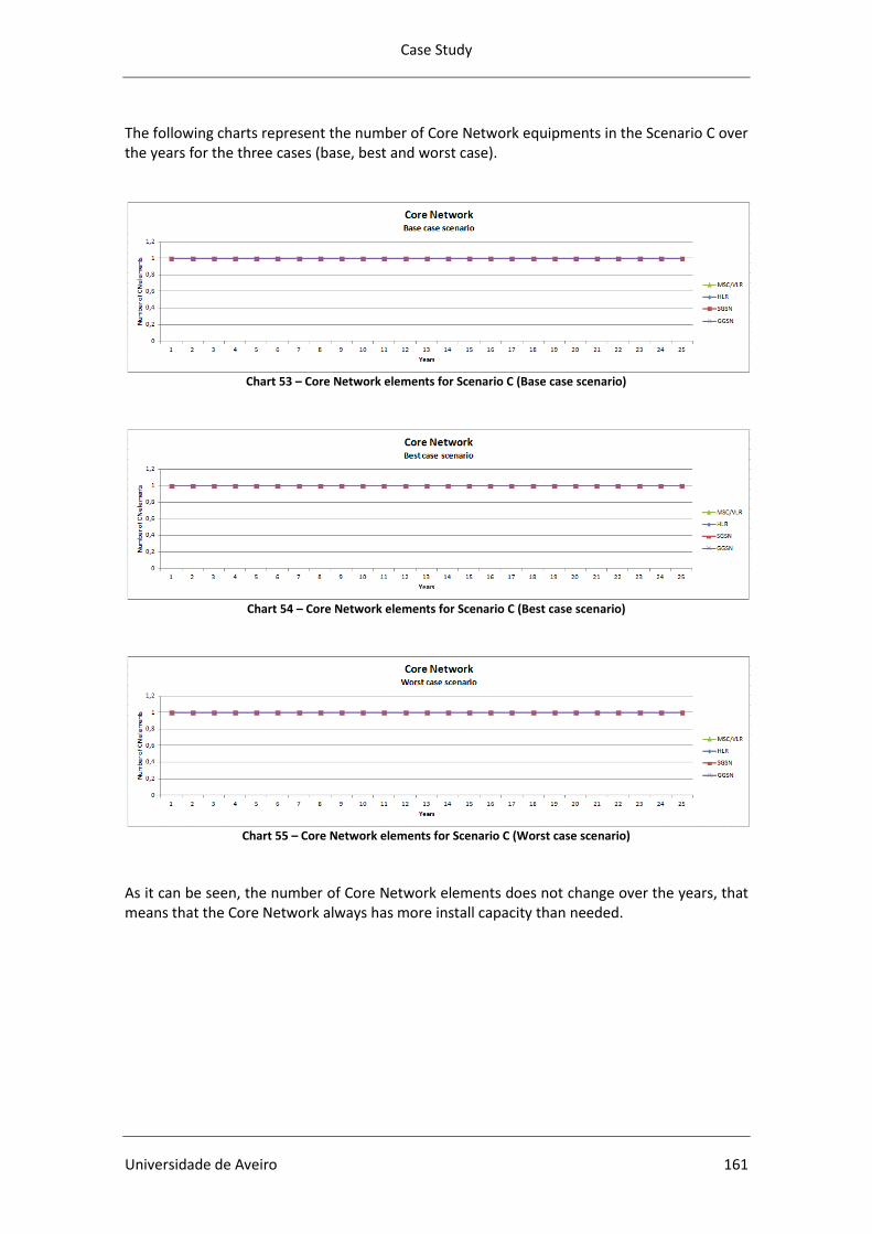
Case Study
Universidade de Aveiro 161
The following charts represent the number of Core Network equipments in the Scenario C over the years for the three cases (base, best and worst case).
Chart 53 – Core Network elements for Scenario C (Base case scenario)
Chart 54 – Core Network elements for Scenario C (Best case scenario)
Chart 55 – Core Network elements for Scenario C (Worst case scenario)
As it can be seen, the number of Core Network elements does not change over the years, that means that the Core Network always has more install capacity than needed.
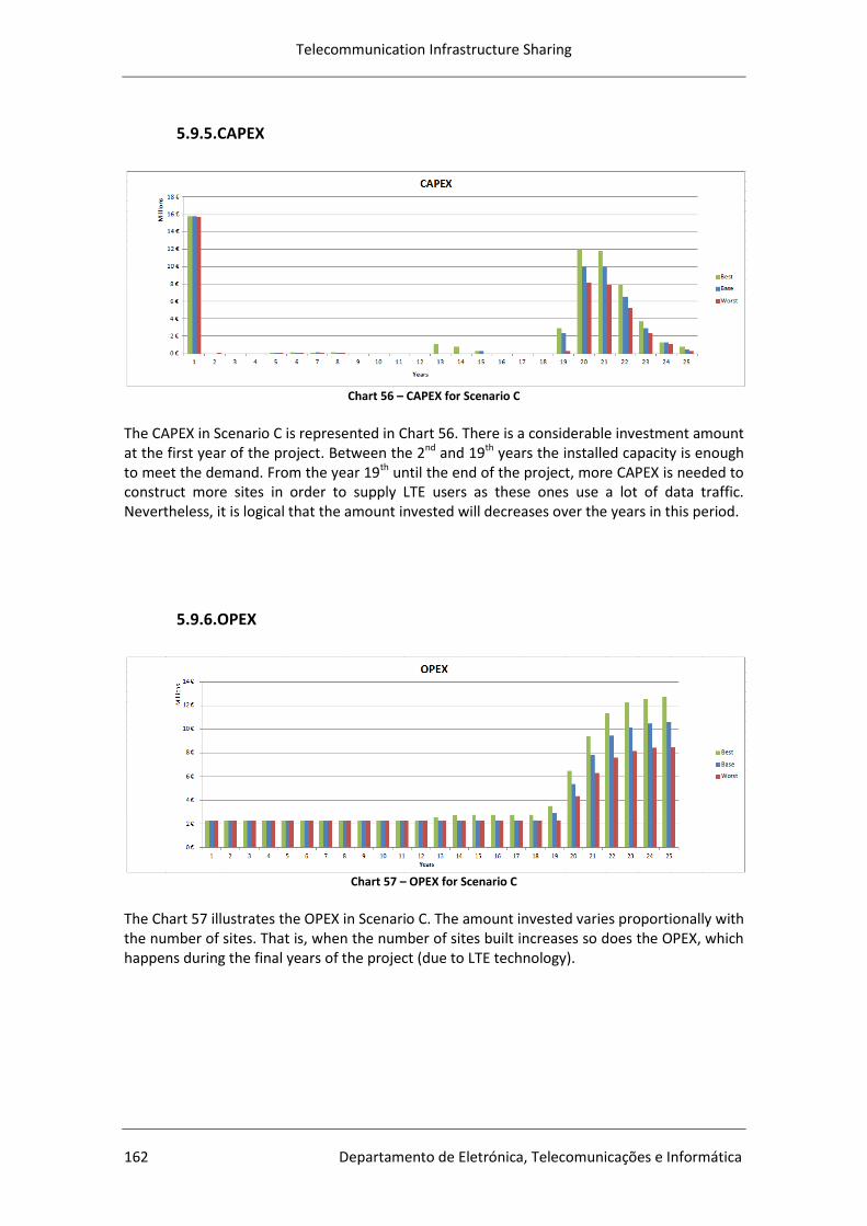
Telecommunication Infrastructure Sharing
162 Departamento de Eletrónica, Telecomunicações e Informática
5.9.5.CAPEX
Chart 56 – CAPEX for Scenario C
The CAPEX in Scenario C is represented in Chart 56. There is a considerable investment amount at the first year of the project. Between the 2nd and 19th years the installed capacity is enough to meet the demand. From the year 19th until the end of the project, more CAPEX is needed to construct more sites in order to supply LTE users as these ones use a lot of data traffic. Nevertheless, it is logical that the amount invested will decreases over the years in this period.
5.9.6.OPEX
Chart 57 – OPEX for Scenario C
The Chart 57 illustrates the OPEX in Scenario C. The amount invested varies proportionally with the number of sites. That is, when the number of sites built increases so does the OPEX, which happens during the final years of the project (due to LTE technology).
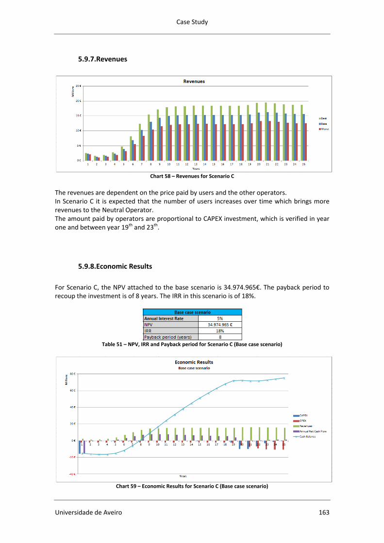
Case Study
Universidade de Aveiro 163
5.9.7.Revenues
Chart 58 – Revenues for Scenario C
The revenues are dependent on the price paid by users and the other operators. In Scenario C it is expected that the number of users increases over time which brings more revenues to the Neutral Operator. The amount paid by operators are proportional to CAPEX investment, which is verified in year one and between year 19th and 23th.
5.9.8.Economic Results
For Scenario C, the NPV attached to the base scenario is 34.974.965€. The payback period to recoup the investment is of 8 years. The IRR in this scenario is of 18%.
Table 51 – NPV, IRR and Payback period for Scenario C (Base case scenario)
Chart 59 – Economic Results for Scenario C (Base case scenario)
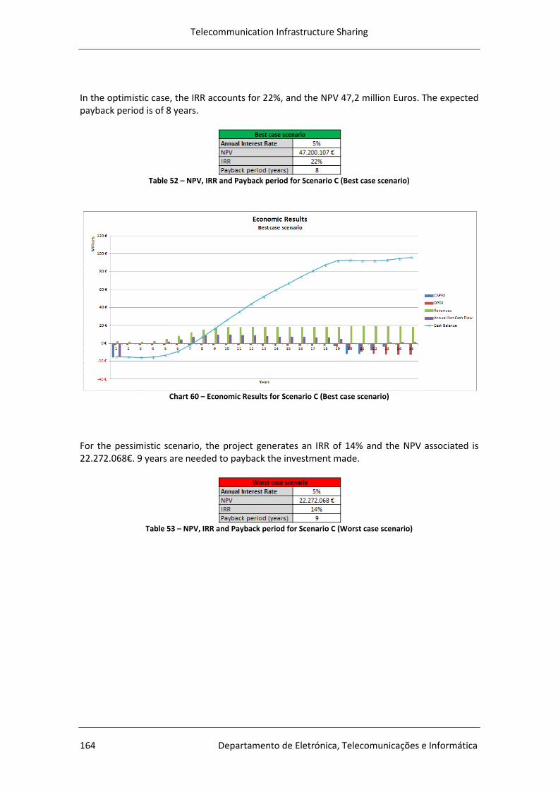
Telecommunication Infrastructure Sharing
164 Departamento de Eletrónica, Telecomunicações e Informática
In the optimistic case, the IRR accounts for 22%, and the NPV 47,2 million Euros. The expected payback period is of 8 years.
Table 52 – NPV, IRR and Payback period for Scenario C (Best case scenario)
Chart 60 – Economic Results for Scenario C (Best case scenario)
For the pessimistic scenario, the project generates an IRR of 14% and the NPV associated is 22.272.068€. 9 years are needed to payback the investment made.
Table 53 – NPV, IRR and Payback period for Scenario C (Worst case scenario)
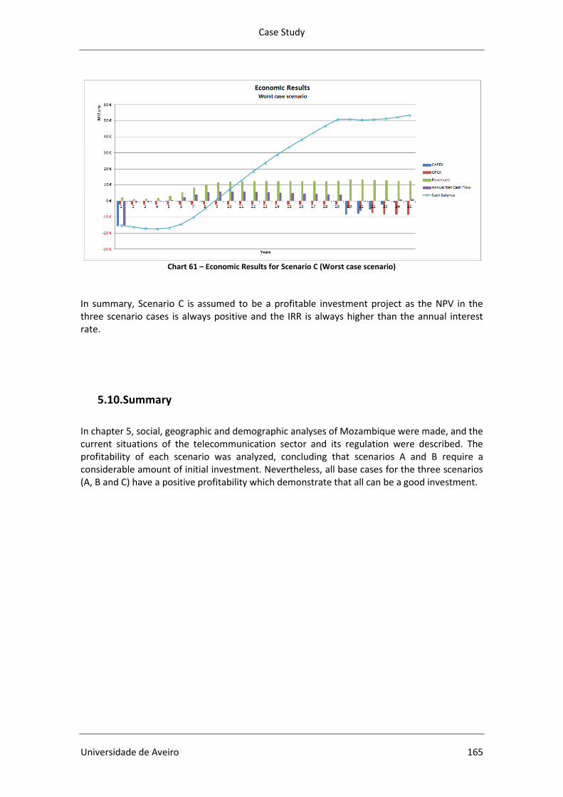
Case Study
Universidade de Aveiro 165
Chart 61 – Economic Results for Scenario C (Worst case scenario)
In summary, Scenario C is assumed to be a profitable investment project as the NPV in the three scenario cases is always positive and the IRR is always higher than the annual interest rate.
5.10.Summary
In chapter 5, social, geographic and demographic analyses of Mozambique were made, and the current situations of the telecommunication sector and its regulation were described. The profitability of each scenario was analyzed, concluding that scenarios A and B require a considerable amount of initial investment. Nevertheless, all base cases for the three scenarios (A, B and C) have a positive profitability which demonstrate that all can be a good investment.

Telecommunication Infrastructure Sharing
166 Departamento de Eletrónica, Telecomunicações e Informática

Final Considerations
Universidade de Aveiro 167
6. Final Considerations
6.1. Conclusions
There is a global growing tendency for infrastructure sharing of cellular networks by operators. This tendency is motivated by the financial benefits generated, especially, by risks sharing. As a result, consumers benefit from lower prices and higher quality services. Also, in underdeveloped areas, mobile networks infrastructure sharing may result in greater coverage areas and higher range for operators. Infrastructure co-locating is hence beneficial for the implementation of telecommunication networks in developing countries. However, infrastructure sharing may also have its downside effects. For instance, competition between operators might be hampered (possibility of price collusion for example), which might, in turn, harm consumers. Therefore, a greater control from competition authorities is required. The Mozambican case study considered in this work project takes into consideration the reality of the country, as well as the challenges faced by its telecommunication sector. One of the main challenges identified is the lack of communication coverage in rural and remote regions, which contributes to a demographic discrimination of communities spread over extensive areas. The development of a mobile sharing strategy enables the sector to overcome this problem. The selected solution of implementing a Neutral Operator can be quickly implemented and allows for immediate operation. This option is beneficial for Mozambique, not only because it brings quick mobile services to an underserved population, but also because it creates positive externalities to the population targeted (such as employment creation). Considering that implementing a Neutral Operator involves a considerable amount of investment and that several parties are included in the negotiation and operation, continuous adjustments on the sharing model and agreement should be done so as to improve the model. For instance, the agreements made among operators should be revised, and the government should benchmark the performance of the operators against stated agreements in order to ensure that they comply with them as well as with government policies. Therefore, the proposal of a Neutral Operator should be seen as an integrated model involving several parties’ interests. The large amount of investment required to implement a Neutral Operator solution, as well as the risks associated with the uncertainty of the viability of this solution and the risky profile of Mozambique, led to the necessity of developing three different scenarios that cover different geo-types areas: Scenario A covers all rural areas of the country, Scenario B covers the entire country, and Scenario C covers only Maputo city. In order to sustain the proposal of implementing a Neutral Operator in Mozambique and to validate the defended benefits that mobile infrastructure co-locating can bring to a potential investor and to the country in general, a strict financial analysis was conducted. The financial results obtained were encouraging. Based on the key decision criteria, an investment in NO has a positive NPV for in all three scenarios and the values for IRR are within the acceptable range,
Telecommunication Infrastructure Sharing
168 Departamento de Eletrónica, Telecomunicações e Informática
that is, above the reference value of the annual interest rate (the IRR is 33% for Scenario A, 8% for Scenario B, and 18% for Scenario C). The payback periods were reasonable and account for 6 years in Scenario A, 8 years in Scenario B, and 8 years in Scenario C. Furthermore, sensitivity analysis revealed that the investment in NO is still stable for Scenarios A and C. Scenario B was not profitable when a decrease of 20% in total users was made. Comparing the results obtained, Scenario A was predicted as the most profitable one. Hence, this investment should be considered by a potential investor, especially because it targets rural areas with poor telecommunication services and because the benefits for the population of an investment in these areas are higher than for the other two scenarios. Given the technical, social, and economic benefits of choosing a neutral operator as a form of covering the rural areas, of reinforcing the infrastructure in other geo-types areas and of complementing the other operators, it is argued that the implementation of the NO should include a public entity in order to guarantee the transparency principle and to bridge the high investment needed. Another alternative would be to develop a concession contract with a private entity operating under a concession contract supervised by the government.
Final Considerations
Universidade de Aveiro 169
6.2. Future work
It is acknowledged that this work project suffers from various limitations, especially because most of the work project is based on assumptions. Although the assumptions were reasonable, the uncertainty attached to them can never be entirely mitigated. Furthermore, and due to time constraints, additional topics should be analyzed in the future in order to refine the work project, namely:
A further study of interfaces and their capacity and saturation points.
Take into consideration the renewal of equipment.
Develop the project for LTE technology in more detail, since this work project focused on the UMTS technology.
A further study of sites in LTE technology and their cost.
In scenario B, the coverage of the whole country is not profitable. A further analysis should review this whole scenario and check in more detail the dimension of the geo-types in the country.
Take into account the users of other operators in the calculation of infrastructure sharing, as the only factor used during the calculations was the overhead in the users’ data traffic.
Conduct a study of the impact of the NO model on competition, since the NO shares the infrastructure and is a service provider (operator).
Develop a techno-economic tool that includes the competition.
Study the inclusion of new services provided by operators, such as the IPTV and/or OTT.

Telecommunication Infrastructure Sharing
170 Departamento de Eletrónica, Telecomunicações e Informática
References
Universidade de Aveiro 171
References
[1] Chuah, M. C. and Q. Zhang, “Design and performance of 3G wireless networks and
wireless lands”, Springer, 2006 [2] ICT Statistics Database, accessed Mar. 10, 2015. [3] Portal do Governo de Moçambique, accessed Mar. 25, 2015 [4] The World Factbook CIA, accessed Mar. 25, 2015 [5] Mozambique Rising Building a New Tomorrow, African Department, International
Monetary Fund , 2014 [6] World Economic Outlook, International Monetary Fund, April 2014 [7] ICT Statistics Database, accessed Apr. 13, 2015. [8] GSM, GSMA, accessed Nov. 26, 2014 [9] UMTS, rel99 Architecture Master Telecom Faster, accessed Dec. 10, 2014 [10] Ramos, José Pedro G. S., “Telecommunications Infrastructure Sharing in
Mozambique”, Department of Electronics, Telecommunications and Informatics, University of Aveiro, Aveiro, Portugal, 2014, pp. 12
[11] Sverzut, J. U., “Redes GSM, GPRS, EDGE e UMTS”, 1st ed. São Paulo, SP: Editora Érica, 2005, pp. 70-394
[12] Heine, G., “GSM Networks: Protocols, Terminology and Implementation”, Norwood, MA: Artech House, 1998, pp. 5-125.
[13] Duarte, A. M. de Oliveira e Hugo S. Félix, “Modelos de previsão: adopção e abandono de tecnologias e produtos; evolução do preço de um produto em função do seu grau de maturidade”, Departamento de Eletrónica, Telecomunicações e Informática, Universidade de Aveiro, Aveiro, versão preliminar de 25 de Julho de 2014
[14] Vanston, Lawrence K., “Residential Broadband Forecasts”, Technology Futures Inc, Austin, Texas, 2002
[15] Vornpuan, Panya, “Infrastructure Sharing in Practice: Sharing Mobile Networks”, Nokia Siemens, Setp 2, 2010
[16] Verbrugge, Sofie, Koen Casier, Jan Van Ooteghem and Bart Lannoo, “Practical steps in techno-economic evaluation of network deployment planning, White Paper” UGent/IBBT, Department of Information Technology (INTEC), 2009
[17] ICT Regulation Toolkit, accessed Jul. 01, 2014 [18] ITU – Mobile infrastructure sharing, accessed Jul. 01, 2014 [19] Autoridade da Concorrência, “Partilha de redes de comunicações eletrónicas”,
Dezembro de 2012 [20] ANACOM – Partilha de infraestruturas nas Rede Móveis 3G, accessed Jul. 01, 2014 [21] Lefèvre, Camila Borba, “Mobile Sharing”, ITU, February 2008 [22] Cruz, Bruno de Oliveira, “Impact of M2M Communications on Cellular
Telecommunications Networks”, Department of Electronics, Telecommunications and Informatics, University of Aveiro, Aveiro, Portugal, 2013, pp. Appendix A
[23] Waldhorst, O. and J. Mückenheim, “UMTS System Architecture and Protocol Architecture”, Oct, 2011.
[24] Moçambique, Wikipedia, accessed Mar. 25, 2015 [25] Dias, João Pedro S. V., “Gestão de Desempenho numa Rede Celular”, Department
of Electronics, Telecommunications and Informatics, University of Aveiro, Aveiro, Portugal, 2014
Telecommunication Infrastructure Sharing
172 Departamento de Eletrónica, Telecomunicações e Informática
[26] Smura, Timo, Techno-economic Analysis of IEEE 802.16a-Based Fixed Wireless Access Networks, Abril de 2004, Universidade de tecnologia de Helsínquia.
[27] Carrilho, David Coelho, “Redes Híbridas de Acesso Fixo sem Fios: Análise Tecno-Económica”, Department of Electronics, Telecommunications and Informatics, University of Aveiro, Aveiro, Portugal, 2010
[28] GSM 03.04, GSM/ETSI, Vers. 5.3.0, pp. 11-12, Jul, 1996. [29] Ouyang, Y. and M. H. Fallah, “An Analysis of Traffic and Throughput for UMTS
Packet Core Networks”, Howe School of Technology Management, Stevens Institute of Technology, Hoboken, NJ, USA.
[30] Ouyang, Y. and M. H. Fallah, “A Performance Analysis for UMTS Packet Switched Network based on Multivariate KPIs”, Howe School of Technology Management, Stevens Institute of Technology, Hoboken, NJ, USA.
[31] 3GPP TS 23.002, 3GPP, Vers. 10.2.0, Mar, 2011. [32] Flore, D., “LTE RAN architecture aspects”, IMT‐Advanced Evaluation, Beijing, P. R.
China, Dec 17‐18, 2009. [33] Imprensa Nacional de Moçambique, “Boletim da República – Decreto nº
62/2010”, Instituto Nacional das Comunicações de Moçambique, 27 de Dezembro de 2010
[34] Imprensa Nacional de Moçambique, “Boletim da República – Decreto nº 8/2004”, Instituto Nacional das Comunicações de Moçambique, 27 de Dezembro de 2010
[35] Instituto Nacional das Comunicações de Moçambique, accessed Apr. 2015 [36] Duarte, Manuel de Oliveira, “Redes Celulares – Notas de Estudo”, Department of
Electronics, Telecommunications and Informatics, University of Aveiro, Aveiro, Portugal, 2014 December
[37] Duarte, A. Manuel Oliveira, “Cellular Basic Concepts”, Department of Electronics, Telecommunications and Informatics, University of Aveiro, Aveiro, Portugal, 2011 December
[38] Training Nokia UMTS, “3G UMTS Network Solution”, 2013 [39] Duarte, A. Manuel Oliveira, “Cellular Networks Wireless LANs”, Department of
Electronics, Telecommunications and Informatics, University of Aveiro, Aveiro, Portugal, 2012-2013
[40] Chen, Xiaobao, Philippe Lucas, Martin Barkley Harris, “Packet radio network and method”, patent nº US 20090175215 A1
[41] Ahn, Hong-Jin, “Apparatus and method for performing traffic flow template packet filtering according to internet protocol versions in a mobile communication system”, patent nº US 20040205247 A1
[42] Duarte, Manuel de Oliveira, “IST-2000-25172 TONIC – Applications, QoS Classes and Resource Dimensioning in TONIC Business Cases”, Department of Electronics, Telecommunications and Informatics, University of Aveiro, Aveiro, Portugal, 2012 January
[43] Dias, João Pedro da Silva Valente, “Gestão de Desempenho numa Rede Celular”, Department of Electronics, Telecommunications and Informatics, University of Aveiro, Aveiro, Portugal, 2014
[44] LTE Protocols, Master Telecom Faster, accessed Jan. 25, 2015 [45] Gessner, C., A. Roessler, M. Kottkamp, “UMTS Long Term Evolution (LTE) –
Technology Introduction”, Rohde&Schwarz, July 2012 [46] “LTE – Qualcomm Leading the Global Success”, Qualcomm, August, 2013 [47] Kriaras, Ioannis N. et al “Third-Generation Mobile Network Architecture for the
Universal Mobile Telecommunication System (UMTS)”, Bell Labs Technical Journal, Summer 1997
References
Universidade de Aveiro 173
[48] Atkinson, G., S. Strickland and M. Chuah, “UMTS Packet Service Infrastructure: Distributed is Cheaper”, Networks 2002, Jun, 2002.
[49] Heine, Gunnar; “GSM Networks: Protocols, Terminology and Implementation” Artech House, Norwood, 1998
[50] Catarino, Helena I. B. M.,“UMTS versus DVB-SH na transmissão de sinais de vídeo”, Departamento de Engenharia de Eletrónica e Telecomunicações e de Computadores, Instituto Superior de Engenharia de Lisboa, Lisboa, Novembro de 2010
[51] Martins, Armanda M. P., “Evaluation of data applications quality of service over UMTS”, Instituto Superior Técnico, Universidade Técnica de Lisboa, Lisboa, Novembro 2012
[52] Soldani, David, “QoS MANAGEMENT IN UMTS TERRESTRIAL RADIO ACCESS FDD NETWORKS”, Communications Laboratory, Department of Electrical and Communications Engineering, Helsinki University of Technology, Espoo, Finland 2005
[53] Lopes, João M. C., “Performance Analysis of UMTS/HSDPA/HSUPA at the Cellular Level”, Instituto Superior Técnico, Universidade Técnica de Lisboa, Lisboa, March 2008
[54] “W-CDMA Technology” Technical Note, ANRITSU CORPORATION [55] Stasiak, Maciej et al, “Modeling and Dimensioning of Mobile Networks – From
GSM to LTE”, Wiley, United Kingdom, 2011 [56] Hamalainen, Jyri, “Cellular Network Planning and Optimization Part V: GSM”
Communication and Networking Department, Helsinki University of Technology, 2008
[57] Parkinson, R. “Traffic Engineering Techniques in Telecommunications” Infotel Systems Inc. Retrieved, 2005
[58] Traffic table, Wikimedia, accessed Jun. 08, 2015 [59] Bohagen, Frode and Jorgen Binningsbo, ”Future proof Mobile Broadband
Solutions”, Telektronikk1, 2010 [60] LTE, 3GPP, accessed Jun. 01, 2015 [61] Cisco, accessed Jun. 10, 2015 [62] “Mozambique, Country Profile”, KPMG Africa Region, KPMG, 2012/2013 [63] Instituto Nacional de Estatísticas de Moçambique, accessed Jun. 14, 2015 [64] Erlang, Westbay Engineers Limited, accessed Jun. 14, 2015 [65] “Global System for Mobile Communication (GSM), White Paper”, Tetcos
Engineering, 2010 [66] Zyren, Jim, “Overview of the 3GPP Long Term Evolution Physical Layer”, White
Paper, freescale, 07/2007 [67] “Mulheres e Homens em Moçambique, Indicadores Seleccionados de Género –
2011”, Instituto Nacional de Estatística, Moçambique, 2011 [68] “Estatísticas da CPLP 2012”, Instituto Nacional de Estatísticas, Portugal, 2013 [69] XE Currency Charts (MZN/EUR), accessed Jun.16, 2015 [70] “Estatísticas dos Transportes e Comunicações, 2013 – Moçambique”, Instituto
Nacional de Estatísticas, 2014 [71] “Moçambique, Inquérito Demográfico e de Saúde, 2011”, Instituto Nacional de
Estatística, Ministério da Saúde, Maputo, Moçambique, Março 2013 [72] “Market Study for UMTS900 – A report to GSMA”, Ovum Consulting, London,
February 2007 [73] “UMTS Network Design & Cost, Estimation for National UMTS900, UMTS1800 &
UMTS2100 Networks”, Vilicom, 15 January 2009
Telecommunication Infrastructure Sharing
174 Departamento de Eletrónica, Telecomunicações e Informática
[74] Angus, Ian, “An Introduction to Erlang B and Erlang C”, Telemanagement, Canada [75] Telecommunications: Glossary of Telecommunication Terms, Federal Standard
1037C, August 7, 1996 [76] Cheung, Joseph C. S. et al, “Network planning for third-generation mobile radio
systems”, IEEE Communications Magazine, December 1994 [77] Holma, Harri and Toskala, Antti, “WCDMA for UMTS, Radio Access For Third
Generation Mobile Communications”, John Wiley & Sons, England, 2004 [78] Population Density 2000, Mozambique, CIESIN, Columbia University, 2009 [79] Fatuma Simba, Lena Trojer, Nerey Mvungi, Bakari Mwinyiwiwa, Emmanuel
Mjema, “Techno-Economic Analysis of UMTS900 and UMTS2100 for Rural Connectivity in Tanzania”, 14th IEEE International Conference on Communication Technology (ICCT), 2012, Chengdu, China
[80] Laiho, J., Wacker, A. and Novosad, T, “Radio Network Planning” and Optimisation for UMTS John Wiley & Sons Ltd, 2006
[81] K.R. Chevallier, C., Brunner, C., Garavaglia, A., Murray, K.P And Baker, “WCDMA (UMTS) Deployment Handbook: Planning and Optimization Aspects”, John Wiley & Sons Ltd, 2006
[82] COST Action 231, “Digital mobile radio towards future generation system” Final report, Directorate-General Telecommunications, Information society, Information Market and Exploitation of Research, European Commission, 1999
[83] Dr. Darcy Poulin, “FDD vs TDD comparison: Why TDD LTE Improves Battery Life & Lower Costs”, October 15, 2009
[84] TDD FDD Duplex Schemes, Radio-Electronics.com, Resources and analysis for electronics engineers, accessed Mar. 13, 2015
[85] Training Nokia UMTS, “3G UMTS Network Solution”, 2013 [86] Holma, Harri and Toskala, Antti, “LTE for UMTS – OFDMA and SC-FDMA Based
Radio Access”, John Wiley & Sons, England, 2004 [87] Vuong, Khai, “UMTS vs. LTE: a comparison overview”, May, 2011 [88] Duarte, Arthur Delfino and Nunes, Daniel Andrade, “Comparação entre as redes
de pacotes dos padrões WCDMA/HSPA+ e LTE”, INCITEL, 2012 [89] WCDMA Link Budget, UMTS World, accessed Jun. 26, 2015 [90] Nokia Siemens Networks “LTE RPESS Radio Planning Capacity”,
RA41207EN20GLA0 NSN [91] Details Internet Additives, Vodafone Portugal, accessed Jun. 28, 2015 [92] Maputo, Google maps, accessed Jun. 29, 2015 [93] Maputo, União das Cidades Capitais de Língua Portuguesa, accessed Jun. 28, 2015 [94] “Planeamento de Comunicações Móveis”, Lecture notes 2009/2010, Universidade
de Aveiro, 2010 [95] Flood, J. E., “Telecommunication Networks”, Institution of Electrical Engineers,
London, UK, 1997, chapter 12 [96] Pauli, Volker, et al, “Heterogeneous LTE Networks and Inter-cell Interference
Coordination”, Nomor Research, Munich, Germany, December, 2010 [97] Cellular Telephone Basics, Privateline, accessed Jun. 30, 2015 [98] Licenciamento, Instituto Nacional das Comunicações de Moçambique, accessed
Jun. 30, 2015 [99] Ani, Wilson, et al, “Telecommunication Development and Regional Economic
Growth: Evidence from ITU ICT Development Index (IDI) Top Five Countries for African Region”, African Journal of Business and Economic Research, Volume 8, 2013, pp. 85-100
[100] Autoridade Tributária de Moçambique, accessed Jul. 02, 2015

References
Universidade de Aveiro 175
[101] Número de empresas registadas na Autoridade Tributária de Moçambique cresceu 19% em 2014, macauhub, accessed Jul. 02, 2015
[102] Tarifários, Vodacom, accessed Jul. 02, 2015 [103] Global Mobile Tax Review 2010/11, Deloite/GSMA, Geneva, September, 2011 [104] Pernes, David, et al, “Análise de Cobertura e Capacidade em Redes Móveis LTE de
Quarta Geração (4G)”, Área Departamental de Engenharia de Eletrónica e de Computadores (ADEETC), ISEL e Instituto de Telecomunicações (IT), Lisboa, Portugal
[105] ANACOM, accessed Jul. 02, 2015 [106] Tipper, David “Fundamentals of Cellular Networks”, Graduate Program in
Telecommunications and Networking, Slides 4, Telcom 2720, University of Pittsburgh
[107] Vieira, Carla, “Interferência no sistema WCDMA”, Escola de Engenharia, Universidade Federal Fluminense, Brasil, 2010, pp. 92
[108] Arokiamary, V. “Mobile Communications”, Technical Publications Pune, India, 2009, pp27
[109] Lopes, Bruno, “Technoeconomic study for a Mobile WiMAX solution in Luanda”, December, 2008
[110] “Wireless Communications: Principles and Practice, The Cellular Concept – System Design Fundamentals”, Second Edition, December, 2001, Chapter 3
[111] “The Cellular Engineering Fundamentals”, Chapter 3, Indian Institute of Technology Guwahati
[112] “International roaming explained, Africa”, GSMA [113] Bhawan, Mahanagar D. and Marg, Jawahar L. N., “Recommendations on
Infrastructure Sharing”, Telecom Regulatory Authority of India (TRAI), New Delhi, India, 2007
[114] Antenna Efficiency and Antenna Gain, Antenna Theory, accessed Jul.04, 2015 [115] Bandwidth, Antenna Theory, accessed Jul. 04, 2015 [116] Wallace, Richard, “Antenna Selection Guide”, Application Note AN058, Texas
Instruments, Texas [117] Wong, Kainam Thomas and Lai, Albert Kin-Yue, “Inexpensive Upgrade of Base-
Station Dumb Antennas by Two Magnetic Loops for “Blind” Adaptive Downlink Beamforming”, Department of Electrical & Computer Engineering, University of Waterloo, Canada and Department of Electronic Engineering, Chinese University of Hong Kong, Hong Kong
[118] Antenna Theory, accessed Jul. 04, 2015 [119] “Mobile Infrastructure Sharing”, GSMA, United Kingdom [120] Ofcom, “Interim Communication Report”, United Kingdom, February, 2006 [121] Decision of the European Commission of 20 August 2007, Case No. Comp/M.4748
– T-Mobile /Orange Netherlands [122] Notification of Adopted Measure pursuant to Article 7(5) of Directive 2002/21/EC,
Spain, CMT (Comision del Mercado de las Telecomunicaciones) [123] 3GPP TR 25.101, “User Equipment (UE) radio transmission and reception (FDD)” [124] 3GPP TR 25.104, “Base Station (BS) radio transmission and reception (FDD)” [125] Nawrocki, M. J., Dohler, M. and Aghvami, A. H., “Understanding UMTS Radio
Network Modeling Planning and Automated Optimization, Wiley, 2006 [126] ECC within CEPT, ECC Report 82, “Compatibility study for UMTS operating within
the GSM 900 and GSM 1800 frequency bands”, May 2006 [127] Glossary of statistical terms, OCDE, accessed Jul. 07, 2015 [128] Margareth Aske, “Mobile Industry Power Emerging Economies”, Telenor group
Telecommunication Infrastructure Sharing
176 Departamento de Eletrónica, Telecomunicações e Informática
[129] “Economic Contribution of Mobile Communication”, Telenor [130] LTE MIMO: Multiple Input Multiple Output Tutorial, Radio-Electronics.com,
accessed Jun. 7, 2015 [131] Meddour, Djamal-Eddine,Tinku Rasheed and Yvon Gourhant, “On the Role of
Infrastructure sharing for Mobile Network Operators in Emerging Markets”, France Telecom-Orange R&D, Lannion, France and CREATE-NET Research Center, Trento, Italy
[132] Verbrugge, Sofie et al, 2009, “White Paper: Practical Steps in Techno-Economic Evaluation of Network Deployment Planning”, Gent University
[133] Capital expenditures, Nasdaq, accessed Jul. 05, 2015 [134] Welch, Ivo, 2009, “Corporate Finance: An Introduction”, Prentice Hall, pp 3-4 [135] Welch, Ivo, 2009, “Corporate Finance: An Introduction”, Prentice Hall, pp 29-31 [136] Duarte, Manuel de Oliveira, “Techno-Economic Analysis of Engineering Projects,
DETI, Universidade de Aveiro, Portugal, 2013 [137] Fjeldstad, Odd-Helge and Heggstad, Kari K., “Building taxpayer culture in
Mozambique, Tanzania and Zambia: Achievements, challenges and policy recommendations”, Chr. Michelsen Institute (CMI), July 2012
[138] Korowajczuk, Leonhard,”How to Dimension User Traffic in 4G Networks , CelPlan International, Jun. 2014”
[139] Li, Xi, “Radio Access Network Dimensioning for 3G UMTS”, Communication Networks, University of Bremen, 2009
[140] Sala-i-Martín, Xavier, “The Global Competitiveness Report 2013-2014”, World Economic Forum, Geneva, 2013
[141] Revenue, Investopedia.com, accessed Jul. 14, 2015 [142] Neutral Operator, Aire networks, accessed Jul. 14, 2015 [143] Infante, Jorge, et al “Wi-Fi Neutral Operator: Promoting cooperation for network
and service growth”, Research Group on Networking Technology and Strategies, Universitat Pompeu Fabra
[144] Qiang, C. Z. W., Rossotto, C.M., “2009. Economic Impacts of Broadband, in Information and Communications for Development 2009: Extending Reach and Increasing Impact”, World Bank, Washington D.C. 35-50
[145] “Introduction to WCDMA and WCDMA Dimensioning for UMTS”, www.eaeee.ir, accessed Jul. 14, 2015
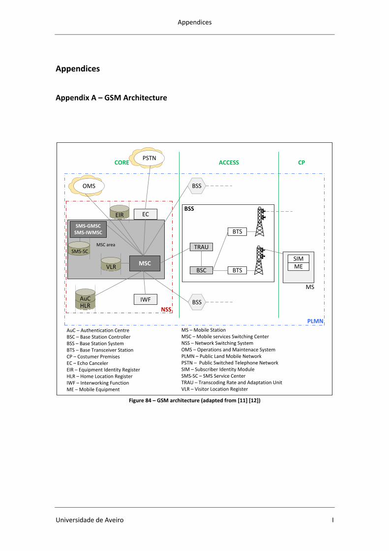
Appendices
Universidade de Aveiro I
Appendices
Appendix A – GSM Architecture
ME
MS
TRAU
BSC
BSS
BTSVLR
MSC
BSS
BSS
MSC area
HLRAuC IWF
ECEIR
NSS
OMS
PSTN
PLMN
BTS
AuC – Authentication CentreBSC – Base Station ControllerBSS – Base Station SystemBTS – Base Transceiver StationCP – Costumer PremisesEC – Echo CancelerEIR – Equipment Identity RegisterHLR – Home Location RegisterIWF – Interworking FunctionME – Mobile Equipment
MS – Mobile StationMSC – Mobile services Switching CenterNSS – Network Switching SystemOMS – Operations and Maintenace SystemPLMN – Public Land Mobile NetworkPSTN – Public Switched Telephone NetworkSIM – Subscriber Identity ModuleSMS-SC – SMS Service CenterTRAU – Transcoding Rate and Adaptation UnitVLR – Visitor Location Register
SIM
SMS-GMSCSMS-IWMSC
SMS-SC
CORE ACCESS CP
Figure 84 – GSM architecture (adapted from [11] [12])
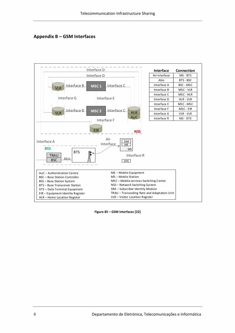
Telecommunication Infrastructure Sharing
II Departamento de Eletrónica, Telecomunicações e Informática
Appendix B – GSM Interfaces
MSC 1
VLR
VLR
Interface B
Interface B
Interface G
HLRAuC
Interface C
Interface C
Interface D
Interface D
EIR
Interface F
NSS
BTSTRAUBSC Abis
MSC 2
Interface A
BSS
SIMME
MS
Air Interface
DTE
Interface R
AuC – Authentication CentreBSC – Base Station ControllerBSS – Base Station SystemBTS – Base Transceiver StationDTE – Data Terminal EquipmentEIR – Equipment Identity RegisterHLR – Home Location Register
ME – Mobile Equipment MS – Mobile StationMSC – Mobile services Switching CenterNSS – Network Switching SystemSIM – Subscriber Identity ModuleTRAU – Transcoding Rate and Adaptation UnitVLR – Visitor Location Register
Interface ConnectionAir interface
Abis
Interface A
Interface B
Interface C
Interface D
Interface E
Interface F
Interface G
Interface R
MS - BTS
BTS - BSC
BSC - MSC
MSC - VLR
MSC - HLR
HLR - VLR
MSC - MSC
MSC - EIR
VLR - VLR
MS - DTE
Interface E
Figure 85 – GSM interfaces [22]
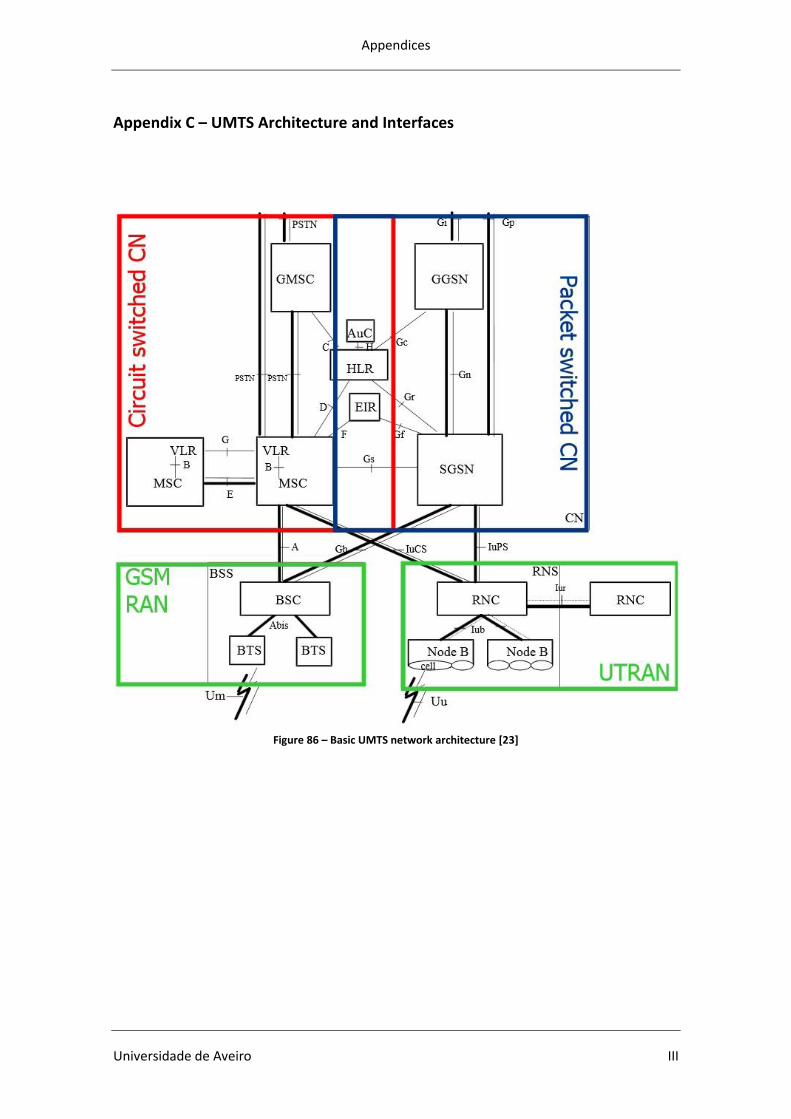
Appendices
Universidade de Aveiro III
Appendix C – UMTS Architecture and Interfaces
Figure 86 – Basic UMTS network architecture [23]
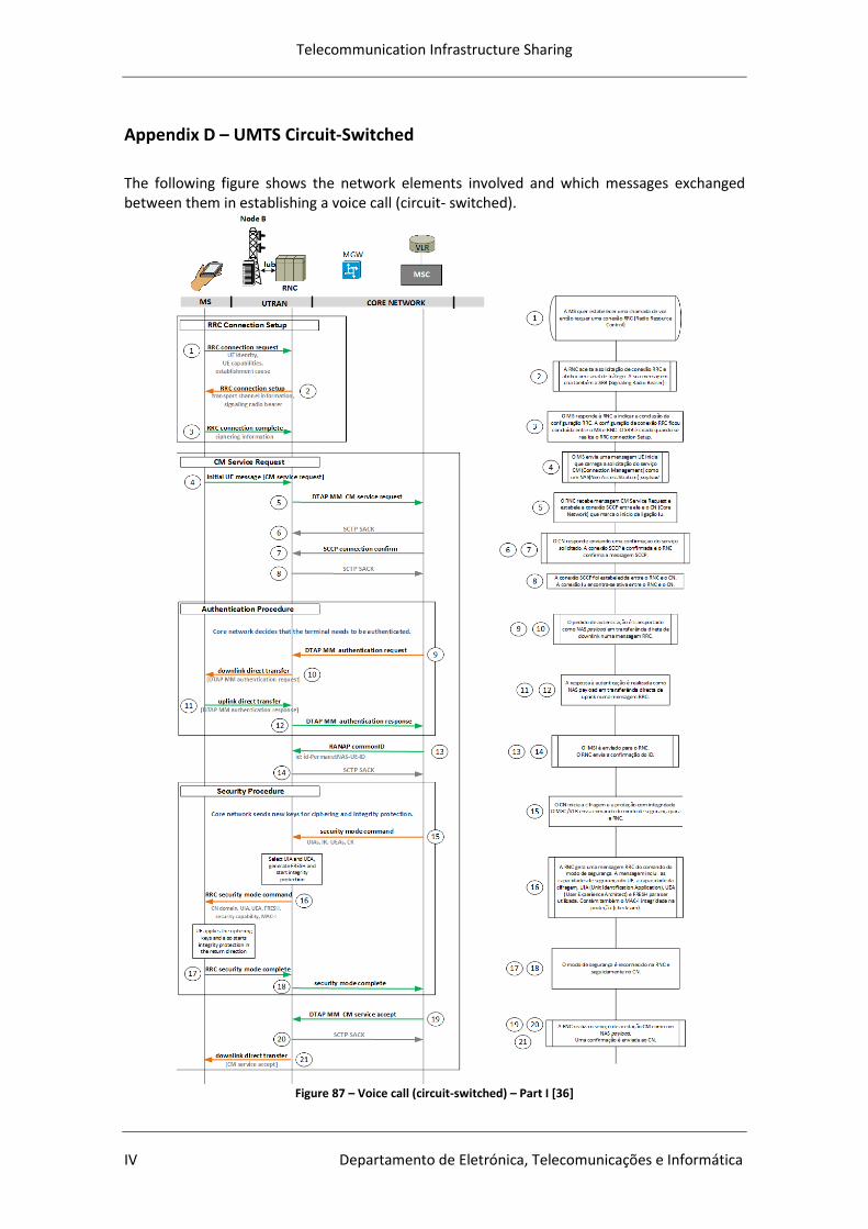
Telecommunication Infrastructure Sharing
IV Departamento de Eletrónica, Telecomunicações e Informática
Appendix D – UMTS Circuit-Switched
The following figure shows the network elements involved and which messages exchanged between them in establishing a voice call (circuit- switched).
Figure 87 – Voice call (circuit-switched) – Part I [36]
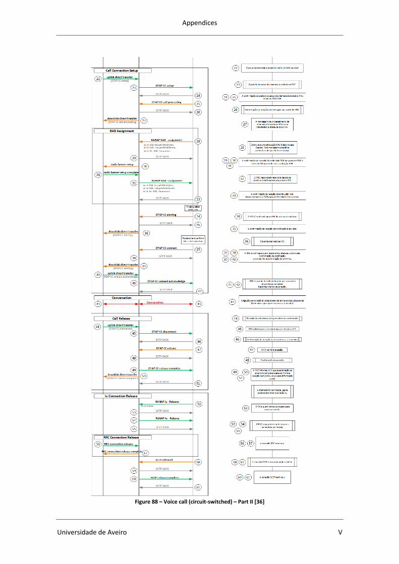
Appendices
Universidade de Aveiro V
Figure 88 – Voice call (circuit-switched) – Part II [36]

Telecommunication Infrastructure Sharing
VI Departamento de Eletrónica, Telecomunicações e Informática
Appendix E – UMTS Packet-Switched
Next will be presented a scheme that explains the exchange of messages in the packet-switched data access to a web browser, and also a flowchart that facilitates the understanding of the presented scheme.
Figure 89 – Messaging in packet switched (Part I) [36] [40] [41]
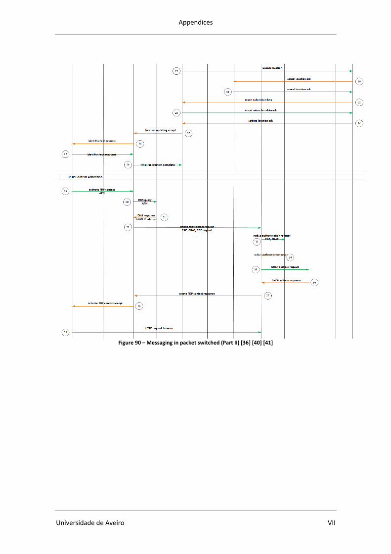
Appendices
Universidade de Aveiro VII
Figure 90 – Messaging in packet switched (Part II) [36] [40] [41]
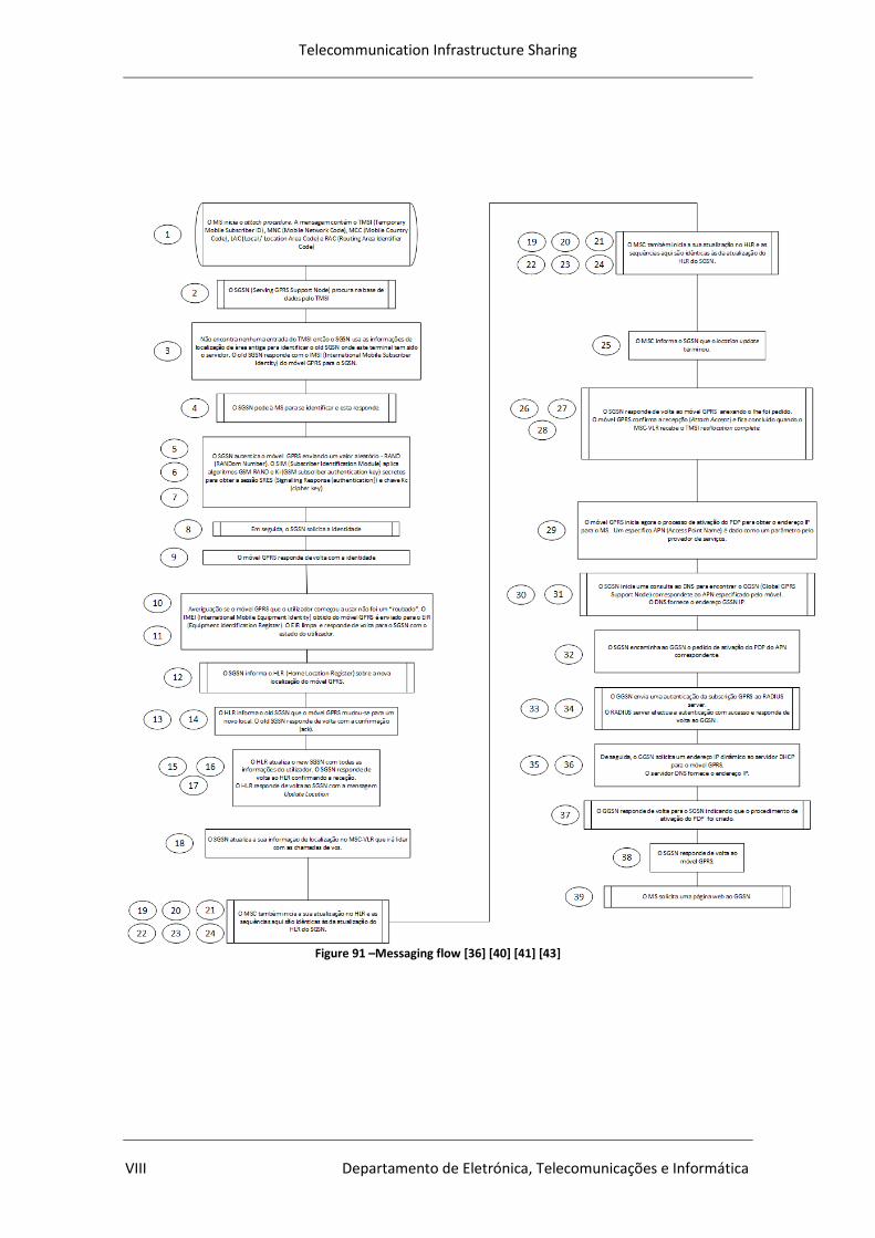
Telecommunication Infrastructure Sharing
VIII Departamento de Eletrónica, Telecomunicações e Informática
Figure 91 –Messaging flow [36] [40] [41] [43]
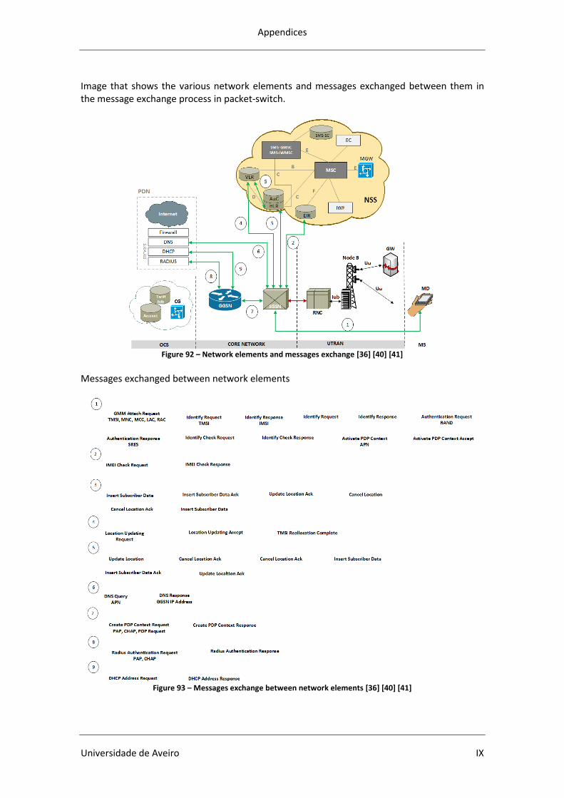
Appendices
Universidade de Aveiro IX
Image that shows the various network elements and messages exchanged between them in the message exchange process in packet-switch.
Figure 92 – Network elements and messages exchange [36] [40] [41]
Messages exchanged between network elements
Figure 93 – Messages exchange between network elements [36] [40] [41]
Telecommunication Infrastructure Sharing
X Departamento de Eletrónica, Telecomunicações e Informática
Appendix F – Erlang
The Erlang (symbol E) is a dimensionless unit of traffic intensity. It is used in telephony as a measure of offered load or carried load on service-providing elements such as telephone circuits or telephone switching equipment. [57] [65] One Erlang is usually defined as a single circuit and that uses continuously 60 minutes of calling in one hour. [74]
Equation 54 – Erlang equation [64]
λ is the call arrival rate h is the average call length or holding time Erlang B is a formula for the Blocking Probability that describes the probability of call losses for a group of parallel resources (circuits, traffic channels or equivalent).
Equation 55 – Erlang B equation [10]
Pb is the probability of blocking or Erlang B loss probability m is the number of identical parallel channel E is the total traffic offered to group in Erlang In Busy Hour each user requires λ seconds of conversation during one hour (μ, 3.600s). Therefore, Busy Hour can be calculated through the following equation:
Equation 56 – Erlang per user in BH [10]
Appendices
Universidade de Aveiro XI
Appendix G – Link Budget explanation
From OVUM, “Market Study for UMTS900”, report to GSMA, February, 2007, Annex A Model Description, A.4 Link Budget [72] Link budget explanation Brief description of all the values and formulas used in the link budget – (Uplink case). Maximum Transmission Power: 3GPP defines four classes for the mobile terminal with the following nominal power and tolerance values [123]:
1. Power Class 1: 33dBm (2W), +1/-3dB 2. Power Class 2: 27dBm (0.5W), +1/-3dB 3. Power Class 3: 24dBm (0.25W), +1/-3dB 4. Power Class 4: 21dBm (0.125W), +2/-2dB
We use Power Class 4 for voice (Power Class 3 for data). For the base station, 3GPP has defined upper limits for micro and pico base stations. This is for micro and for pico BS [124]. For the macro BS, there is no definition of an upper limit of output power; typically, it varies between 10 and 45 W ( tolerance), with the step of 5W, depending on manufacturer and product line. Antenna Gain: The gain on a mobile antenna depends mostly on its size and the application of the UE. In a typical handset application, such as voice, it is assumed that the antenna gain is equal to 0 dBi. UE used as data cards (PCMCIA) can contain an antenna with 2 dBi gain. For the BS antenna the gain depends on the directionality of the antenna. e.g. for 65o horizontal beam width the gain is 18 dBi. Body Loss: A body loss parameter is introduced due to the usage of the UE near the user’s body. It defines the additional loss in the transmitting and receiving path. Typical values are 2-3 dB on average for voice services and 0dB for data. Receiver: The receiver sensitivity level is mainly limited by thermal noise. The thermal noise power spectral density N0, normalized to 1 Hz bandwidth is -174dBm/Hz. This noise floor is further limited by the quality of internal components (Low Noise Amplifiers (LNA), filters, synthesizers, etc) which generates additive noise. This noise contribution is expressed as the receiver noise figure, F, and has typical values of 5 dB. The total noise power at the receiver is limited by its filter bandwidth (for UMTS, the chip-matched filter bandwidth B equals to the frequency band occupied by the scrambling code, i.e. approximately 3.84MHz, which owing to spectral side lobes, results in 5MHz carrier raster); thus the total receiver noise power in dBm is given by:
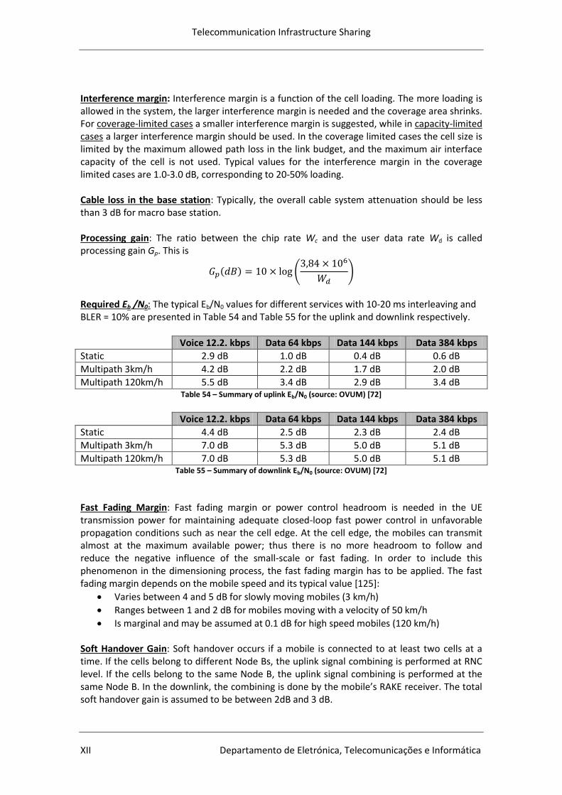
Telecommunication Infrastructure Sharing
XII Departamento de Eletrónica, Telecomunicações e Informática
Interference margin: Interference margin is a function of the cell loading. The more loading is allowed in the system, the larger interference margin is needed and the coverage area shrinks. For coverage-limited cases a smaller interference margin is suggested, while in capacity-limited cases a larger interference margin should be used. In the coverage limited cases the cell size is limited by the maximum allowed path loss in the link budget, and the maximum air interface capacity of the cell is not used. Typical values for the interference margin in the coverage limited cases are 1.0-3.0 dB, corresponding to 20-50% loading. Cable loss in the base station: Typically, the overall cable system attenuation should be less than 3 dB for macro base station. Processing gain: The ratio between the chip rate Wc and the user data rate Wd is called processing gain Gp. This is
Required Eb /N0: The typical Eb/N0 values for different services with 10-20 ms interleaving and BLER = 10% are presented in Table 54 and Table 55 for the uplink and downlink respectively.
Voice 12.2. kbps Data 64 kbps Data 144 kbps Data 384 kbps
Static 2.9 dB 1.0 dB 0.4 dB 0.6 dB
Multipath 3km/h 4.2 dB 2.2 dB 1.7 dB 2.0 dB
Multipath 120km/h 5.5 dB 3.4 dB 2.9 dB 3.4 dB Table 54 – Summary of uplink Eb/N0 (source: OVUM) [72]
Voice 12.2. kbps Data 64 kbps Data 144 kbps Data 384 kbps
Static 4.4 dB 2.5 dB 2.3 dB 2.4 dB
Multipath 3km/h 7.0 dB 5.3 dB 5.0 dB 5.1 dB
Multipath 120km/h 7.0 dB 5.3 dB 5.0 dB 5.1 dB Table 55 – Summary of downlink Eb/N0 (source: OVUM) [72]
Fast Fading Margin: Fast fading margin or power control headroom is needed in the UE transmission power for maintaining adequate closed-loop fast power control in unfavorable propagation conditions such as near the cell edge. At the cell edge, the mobiles can transmit almost at the maximum available power; thus there is no more headroom to follow and reduce the negative influence of the small-scale or fast fading. In order to include this phenomenon in the dimensioning process, the fast fading margin has to be applied. The fast fading margin depends on the mobile speed and its typical value [125]:
Varies between 4 and 5 dB for slowly moving mobiles (3 km/h)
Ranges between 1 and 2 dB for mobiles moving with a velocity of 50 km/h
Is marginal and may be assumed at 0.1 dB for high speed mobiles (120 km/h) Soft Handover Gain: Soft handover occurs if a mobile is connected to at least two cells at a time. If the cells belong to different Node Bs, the uplink signal combining is performed at RNC level. If the cells belong to the same Node B, the uplink signal combining is performed at the same Node B. In the downlink, the combining is done by the mobile’s RAKE receiver. The total soft handover gain is assumed to be between 2dB and 3 dB.
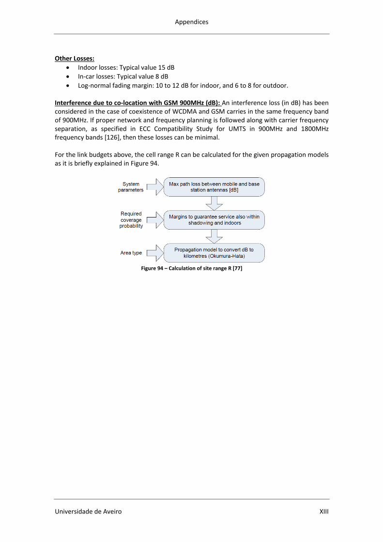
Appendices
Universidade de Aveiro XIII
Other Losses:
Indoor losses: Typical value 15 dB
In-car losses: Typical value 8 dB
Log-normal fading margin: 10 to 12 dB for indoor, and 6 to 8 for outdoor. Interference due to co-location with GSM 900MHz (dB): An interference loss (in dB) has been considered in the case of coexistence of WCDMA and GSM carries in the same frequency band of 900MHz. If proper network and frequency planning is followed along with carrier frequency separation, as specified in ECC Compatibility Study for UMTS in 900MHz and 1800MHz frequency bands [126], then these losses can be minimal. For the link budgets above, the cell range R can be calculated for the given propagation models as it is briefly explained in Figure 94.
Figure 94 – Calculation of site range R [77]
Telecommunication Infrastructure Sharing
XIV Departamento de Eletrónica, Telecomunicações e Informática
Appendix H – Passive Telecommunication Infrastructure Sharing Regulation
Infrastructure Sharing Regulation in Mozambique in next pages. Decree-Law nº62/2010 – Approves the Passive Telecommunication Infrastructure Sharing Regulation and other Network Resources, Monday, 2010 December 27. [33]