Computers in Biology and Medicine 40 (2010) 705–714

Contents lists available at ScienceDirect

Computers in Biology and Medicine

0010-48

doi:10.1

n Corr

E-m

(A.L.V.1 Po

journal homepage: www.elsevier.com/locate/cbm

Tackling EEG signal classification with least squares support vector machines:A sensitivity analysis study

Clodoaldo A.M. Lima a,1, Andre L.V. Coelho b,n, Marcio Eisencraft c

a Graduate Program in Electrical Engineering, School of Engineering, Mackenzie Presbyterian University, Rua da Consolac- ~ao, 896, 01302-907 S~ao Paulo, SP, Brazilb Graduate Program in Applied Informatics, Center of Technological Sciences, University of Fortaleza, Av. Washington Soares, 1321/J30, 60811-905 Fortaleza, CE, Brazilc Centro de Engenharia, Modelagem e Ciencias Sociais Aplicadas, Universidade Federal do ABC, Rua Santa Adelia, 166, 09210-170 Santo Andre, SP, Brazil

a r t i c l e i n f o

Article history:

Received 1 September 2009

Accepted 11 June 2010

Keywords:

Least squares support vector machines

Epilepsy

EEG signal classification

Sensitivity analysis

Kernel functions

25/$ - see front matter & 2010 Elsevier Ltd. A

016/j.compbiomed.2010.06.005

esponding author. Tel.: +55 11 2114 8833; fa

ail addresses: moraes@mackenzie.br (C.A.M. L

Coelho), marcio.eisencraft@ufabc.edu.br (M. E

st-publication contact author.

a b s t r a c t

The electroencephalogram (EEG) signal captures the electrical activity of the brain and is an important

source of information for studying neurological disorders. The proper analysis of this biological signal

plays an important role in the domain of brain–computer interface, which aims at the construction of

communication channels between human brain and computers. In this paper, we investigate the

application of least squares support vector machines (LS-SVM) to the task of epilepsy diagnosis through

automatic EEG signal classification. More specifically, we present a sensitivity analysis study by means

of which the performance levels exhibited by standard and least squares SVM classifiers are contrasted,

taking into account the setting of the kernel function and of its parameter value. Results of experiments

conducted over different types of features extracted from a benchmark EEG signal dataset evidence that

the sensitivity profiles of the kernel machines are qualitatively similar, both showing notable

performance in terms of accuracy and generalization. In addition, the performance accomplished by

optimally configured LS-SVM models is also quantitatively contrasted with that obtained by related

approaches for the same dataset.

& 2010 Elsevier Ltd. All rights reserved.

1. Introduction

In the last decades, the electroencephalogram (EEG) signal,which represents the electrical activity of the brain, has beenintensively studied. This is because it can convey valuable clinicalinformation about the current neurological conditions of patients,being widely used in the study of the nervous system properties,for monitoring sleep stages, and for the diagnosis of manydisorders such as epilepsy, sleep disorders, and dementia [1,2].Moreover, the analysis and processing of this type of biologicalsignal has played an important role in the domain of brain–computer interface [3], which aims at setting up communicationchannels between human brain and computers.

Temporary electrical disturbance of the brain can cause epilepticseizures. Sometimes seizures may go unnoticed, depending on theirstrength, and sometimes may be confused with other events, such asstrokes, which can also cause falls or migraines. Unfortunately, theoccurrence of an epileptic seizure seems unpredictable and itscourse of action is still very little understood [4]. So, more research is

ll rights reserved.

x: +55 11 2114 8600.

ima), acoelho@unifor.br

isencraft).

needed for a better understanding of the mechanisms causingepileptic disorders.

Despite rapid advances of neuroimaging techniques, EEGrecordings continue to play an important role in both thediagnosis of neurological diseases and the understanding ofpsychophysiological processes. In order to extract relevantinformation from recordings of brain electrical activity, a varietyof computerized-analysis methods have been developed. Most ofthem assume that the EEG signal is generated by a highly complexlinear system, which results in characteristic properties like non-stationarity and difficulty of prediction [5].

Recently, there has been a growing interest in applyingtechniques from the domains of nonlinear analysis and chaos theoryfor studying the behavior of experimental time series such as EEGsignals [5–9]. Moreover, many nonlinear classification methods havebeen proposed. Among them, we can mention artificial neuralnetworks [4,10–19] and support vector machines (SVM), either fortwo-class [3] or multiclass [20,21] EEG signal discrimination.

In particular, the application of SVM is justified for this type ofmachine learning (ML) technique has shown to be quitesuccessful in coping with a number of complex data analysisproblems. The SVM approach is based on the structural riskminimization principle, which asserts that the generalizationerror is delimited by the sum of the training error and a parcelthat depends on the Vapnik–Chervonenkis dimension [22,23]. By

C.A.M. Lima et al. / Computers in Biology and Medicine 40 (2010) 705–714706

minimizing this summation, high generalization performance canbe obtained. Besides, the number of free parameters in SVM doesnot explicitly depend upon the input dimensionality of theproblem at hand. Another important feature of the support vectorlearning approach is that the underlying optimization problemsare inherently convex and have no local minima, which comes asthe result of applying Mercer’s conditions on the characterizationof kernels [24].

In the literature, several derived formulations have beenproposed for SVM, seeking for advantages in terms of effective-ness or efficiency criteria. In particular, Suykens and Vandewalle[25], and Suykens et al. [26] have introduced the least squaresSVM (LS-SVM) classifier by modifying the standard formulation soas to obtain a system of linear equations in the dual space. This isdone by taking a least squares cost function, with equality insteadof inequality constraints. Despite the fact that LS-SVM havegained increased attention recently [27], our perception is thattheir application to the automatic analysis of nonlinear biomedi-cal signals has not been systematically investigated yet, with thework of Kemal et al. [28] over electrocardiogram (ECG) data beingone of the first in this context.

It is important to stress that, although considered as high-performance models, the efficiency and effectiveness underlyingthe induction of SVM and LS-SVM depend critically on theappropriate selection of values for some important hyperparameters[29]. The fact is that a bad specification of such parameters mayjeopardize the applicability of these kernel machines. Some workshave already provided solutions to this problem, ranging from thosebased on cross-validated model selection to those based onextensive grid search or heuristic optimization rules [30,31].

In this paper, we present a thorough analysis regarding theimpact of the choice of the kernel parameter value on theperformance exhibited by LS-SVM and SVM classifiers induced forEEG signal discrimination. Initially, we preprocess the dataset ofEEG signals [6,7] by extracting wavelet coefficients [10,13,16] andthen compute statistical metrics over the resultant data to createthe feature vectors. Such vectors serve as input to the kernelmachine (either SVM or LS-SVM), which provides the finalepilepsy/non-epilepsy decision. Several detailed graphs (referredto as sensitivity profiles) are presented here enabling one tovisually inspect, for each combination of kernel type, kernelparameter value and type of feature extracted, the accuracy/generalization levels achieved by the machines in terms ofmisclassification rate as well as sensitivity and specificity indices[13]. In addition, given that the EEG dataset used in this paper hasalso been explored by many researchers working in thebiomedical signal processing field [4,12–21], the classificationperformance achieved by optimally configured LS-SVM models isalso quantitatively contrasted with that produced by relatedapproaches as reported in the literature.

The remaining parts of the paper are organized as follows. Inthe next section, we describe the EEG benchmark data analyzedand the techniques used to preprocess it. Moreover, we presentthe mathematical formulations behind SVM and LS-SVM as wellas comment upon the importance underlying the choice of kernelfunctions and parameters. In Section 3, we discuss the empiricalresults achieved, showing the sensitivity profiles exhibited bythe machines and also providing a quantitative contrast, in termsof accuracy, with related work. Finally, Section 4 concludesthe paper.

2. Materials and methods

In this section, the sets of EEG signals used in the experimentsare described. Also, spectral analysis of the EEG signals using

discrete wavelet transform (DWT) is explained and the statisticalfeatures effectively extracted are presented. In a third part, themathematical formulations underlying the kernel machinesconsidered are given.

2.1. Dataset characterization

In this work, we have used the EEG data made publiclyavailable by Andrzejak et al. [6,7]. The complete dataset involvesfive sets (denoted A–E), each containing 100 single-channel EEGsegments. All EEG signals from this dataset were recorded withthe same amplifier system, using an average common reference.The data were digitized at 173.61 samples/s using 12 bitresolution. Bandpass filter settings were 0.53–40 Hz (12 dB/oct).Since in the experiments reported in Section 3 the kernelmachines investigated only discriminate between samples fromsets A and E, we focus on the description of these two sets in thesequel. The reader should refer to Refs. [6,7] for further details onthe data acquisition process.

Set A consists of segments taken from signals recordedextracranially during the relaxed state of healthy subjects witheyes open. That is, surface EEG recordings were carried out on fivehealthy volunteers using a standardized electrode placementscheme, namely the International 10–20 system [2]. Then,100 segments were selected and cut out from continuousmulti-channel EEG recordings (i.e., from all 20 electrodesused—refer to Fig. 1 of Ref. [6] for the anatomical disposition ofthese electrodes over the scalp) after visual inspection forartifacts, due, for example, to muscle activity or eye movements.

In contrast, set E originated from an EEG archive of pre-surgicaldiagnosis. That is, EEG time series recorded intracranially fromfive patients were selected, all of whom had achieved completeseizure control after resection of one of the hippocampalformations, which was therefore correctly diagnosed to be theseizure generating area. In this context, the implantation ofelectrodes was carried out to exactly localize this area, termed asthe epileptogenic zone. The 100 specific segments that composeset E were selected from all recording sites exhibiting ictal activity(i.e., actual epileptic seizures) [6].

2.2. Data pre-processing

Wavelet transform is a spectral estimation technique in whichany general function can be expressed as an infinite series ofwavelets [4,10]. The basic idea underlying wavelet analysisconsists of expressing a signal as a linear combination of aparticular set of functions (wavelet transform), obtained byshifting and dilating one single function called a mother wavelet.The decomposition of the signal leads to a set of coefficients calledwavelet coefficients. Therefore, the signal can be reconstructed asa linear combination of the wavelet functions weighted by thewavelet coefficients. In order to obtain an exact reconstruction ofthe signal, an adequate number of coefficients must be computed[13,16].

The key feature of wavelets is the time–frequency localization.It means that most of the energy of the wavelet is restricted to afinite time interval. Frequency localization means that the Fouriertransform is band limited. When compared to short-time Fouriertransform, the advantage of time–frequency localization is thatwavelet analysis varies the time–frequency aspect ratio, produ-cing good frequency localization at low frequencies (long timewindows), and good time localization at high frequencies (shorttime windows). This produces a segmentation or tiling of thetime–frequency plane that is appropriate for most physicalsignals, especially those of a transient nature. The wavelet

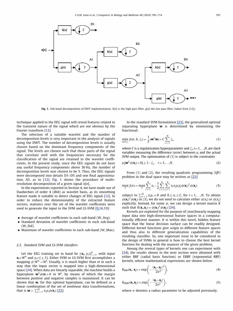
Fig. 1. Sub-band decomposition of DWT implementation; h[n] is the high-pass filter, g[n] the low-pass filter (taken from [12]).

C.A.M. Lima et al. / Computers in Biology and Medicine 40 (2010) 705–714 707

technique applied to the EEG signal will reveal features related tothe transient nature of the signal which are not obvious by theFourier transform [12].

The selection of a suitable wavelet and the number ofdecomposition levels is very important in the analysis of signalsusing the DWT. The number of decomposition levels is usuallychosen based on the dominant frequency components of thesignal. The levels are chosen such that those parts of the signalthat correlate well with the frequencies necessary for theclassification of the signal are retained in the wavelet coeffi-cients. In the present study, since the EEG signals do not haveany useful frequency components above 30 Hz, the number ofdecomposition levels was chosen to be 5. Thus, the EEG signalswere decomposed into details D1–D5 and one final approxima-tion, A5, as in [12]. Fig. 1 shows the procedure of multi-resolution decomposition of a given signal x[n].

In the experiments reported in Section 4, we have made use ofDaubechies of order 4 (db4) as wavelet basis, as its smoothingfeature made it suitable to detect changes of EEG signal [12]. Inorder to reduce the dimensionality of the extracted featurevectors, statistics over the set of the wavelet coefficients wereused to generate the input to the SVM and LS-SVM [9,16,19]:

�

Average of wavelet coefficients in each sub-band (W_Avg). � Standard deviation of wavelet coefficients in each sub-band

(W_Std).

� Maximum of wavelet coefficients in each sub-band (W_Max).

2.3. Standard SVM and LS-SVM classifiers

Let the EEG training set in hand be fðxi, yiÞgNi ¼ 1, with input

xiARm and yiA{71}. Either SVM or LS-SVM first accomplishes amapping f:Rm-Rn. Usually, n is much higher than m in such away that the input vector is mapped into a high-dimensionalspace [24]. When data are linearly separable, the machine builds ahyperplane wTfðxÞþb in Rn, by means of which the marginbetween positive and negative samples is maximized. It can beshown that w, for this optimal hyperplane, can be defined as alinear combination of the set of nonlinear data transformations,that is w¼

PNi ¼ 1 aiyifðxiÞ [22].

In the standard SVM formulation [23], the generalized optimalseparating hyperplane w is determined by minimizing thefunctional:

minw,b,xi

Jðw, b, xiÞ ¼1

2ðwT wÞþC

XN

i ¼ 1

xi, ð1Þ

where C is a regularization hyperparameter and xi, i¼1,y,N, are slackvariables measuring the difference (error) between yi and the actualSVM output. The optimization of (1) is subject to the constraints

yi½wTfðxiÞþb�Z1�xi, i¼ 1,. . .,N: ð2Þ

From (1) and (2), the resulting quadratic programming (QP)problem in the dual space may be written as [23]

maxa

JðaÞ ¼maxa

XN

i ¼ 1

ai�1

2

XN

i ¼ 1

XN

j ¼ 1

aiajyiyjfðxiÞTfðxjÞ ð3Þ

subject toPN

i ¼ 1 aiyi ¼ 0 and 0rairC, for i¼ 1,. . .,N. To obtainfðxiÞ

TfðxjÞ in (3), we do not need to calculate either f(xi) or f(xj)explicitly. Instead, for some f, we can design a kernel matrix K

such that Kðxi,xjÞ ¼fðxiÞTfðxjÞ [24].

Kernels are exploited for the purpose of (non)linearly mappinginput data into high-dimensional feature spaces in a computa-tionally efficient manner. It is within this novel, hidden featurespace that the linear decision surface can be readily designed.Different kernel functions give origin to different feature spacesand thus also to different generalization capabilities of theresulting classifier. So, one important issue to be considered inthe design of SVMs in general is how to choose the best kernelfunction for dealing with the nuances of the given problem.

Among the several types of kernels one can experiment with[24], the results shown in the next section were obtained witheither RBF (radial basis function) or ERBF (exponential RBF)kernels, whose mathematical expressions are shown below:

KRBFðxi, xjÞ ¼ exp �Jxi�xjJ

2

2s2

!, ð4Þ

KERBFðxi,xjÞ ¼ exp �Jxi�xjJ

2s2

� �, ð5Þ

where s denotes a radius parameter to be adjusted previously.

C.A.M. Lima et al. / Computers in Biology and Medicine 40 (2010) 705–714708

By resorting to kernels, (3) can be rewritten as

maxa

JðaÞ ¼maxa

XN

i ¼ 1

ai�1

2

XN

i ¼ 1

XN

j ¼ 1

aiajyiyjKðxi, xjÞ: ð6Þ

For the training samples along the decision boundary, thecorresponding ai’s are greater than zero, as ascertained by theKuhn–Tucker theorem [22]. These samples are known as supportvectors. The number of support vectors is generally much smallerthan N, being proportional to the generalization error of the

classifier [23]. A test vector xARm is then assigned to a given class

according to f ðxÞ ¼ sign½wTfðxÞþb� ¼ signPN

i ¼ 1 aiyiKðx,xiÞþb� �

.

In [25,26], a least squares type of SVM was introduced bymodifying the problem formulation so as to obtain a system oflinear equations in the dual space. This is done by taking a leastsquares cost function, with equality instead of inequalityconstraints. Hence, the parameters w and b of the hyperplanecan be obtained by solving the following alternative formulation:

minw,b,xi

Fðw, b, xiÞ ¼1

2ðwT wÞþ

C

2

XN

i ¼ 1

ðxiÞ2

ð7Þ

subject to equality constraints yi½wTfðxiÞþb� ¼ 1�xi, i¼ 1,. . .,N.

The Lagrangian defined in the LS-SVM dual space is written asfollows:

Lðw, b, xi; aiÞ ¼Fðw, b, xiÞ�XN

i ¼ 1

aifyi½wTfðxiÞþb��1þxig, ð8Þ

where aiAR, i¼1,y,N, are Lagrange multipliers, which can bepositive or negative due to the equality constraints, as followsfrom the Karush–Kuhn–Tucker (KKT) conditions [25,26].

The conditions for optimality:

@L

@w¼ 0-w¼

XN

i ¼ 1

aiyifðxiÞ,

@L

@b¼ 0-

XN

i ¼ 1

aiyi ¼ 0,

@L

@xi¼ 0-ai ¼ Cxi, 8i¼ 1,. . .,N,

@L

@ai¼ 0-yi wTfðxiÞþb

� ��1þxi ¼ 0, 8i¼ 1,. . .,N

8>>>>>>>>>>>>>><>>>>>>>>>>>>>>:

ð9Þ

can be written as the linear system

0 yT

y OþC�1I

" #b

a

" #¼

0

1

� ð10Þ

with y¼ ½y1,. . .,yN�T , a¼ ½a1,. . .,aN�

T , 1¼ ½1,. . .,1�T and I refers tothe identity matrix. Mercer’s conditions for kernels are embedded

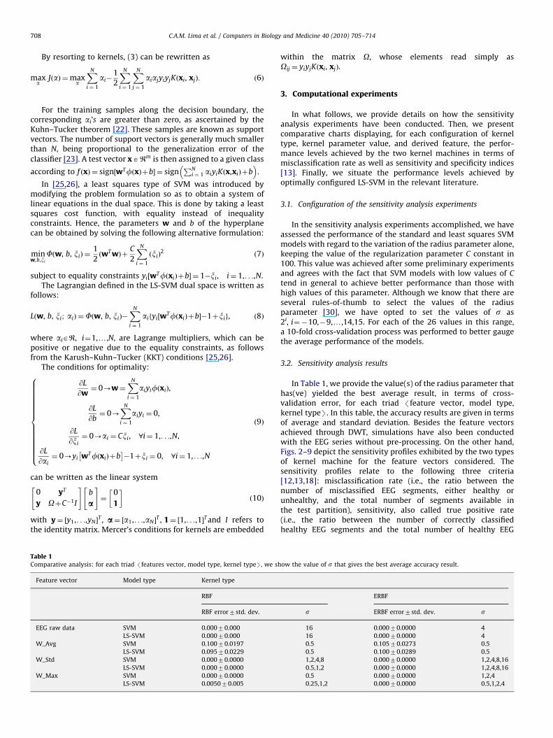
Table 1Comparative analysis: for each triad /features vector, model type, kernel typeS, we sh

Feature vector Model type Kernel type

RBF

RBF error7std. dev.

EEG raw data SVM 0.00070.000

LS-SVM 0.00070.000

W_Avg SVM 0.10070.0197

LS-SVM 0.09570.0229

W_Std SVM 0.00070.0000

LS-SVM 0.00070.0000

W_Max SVM 0.00070.0000

LS-SVM 0.005070.005

within the matrix O, whose elements read simply asOij ¼ yiyjKðxi, xjÞ.

3. Computational experiments

In what follows, we provide details on how the sensitivityanalysis experiments have been conducted. Then, we presentcomparative charts displaying, for each configuration of kerneltype, kernel parameter value, and derived feature, the perfor-mance levels achieved by the two kernel machines in terms ofmisclassification rate as well as sensitivity and specificity indices[13]. Finally, we situate the performance levels achieved byoptimally configured LS-SVM in the relevant literature.

3.1. Configuration of the sensitivity analysis experiments

In the sensitivity analysis experiments accomplished, we haveassessed the performance of the standard and least squares SVMmodels with regard to the variation of the radius parameter alone,keeping the value of the regularization parameter C constant in100. This value was achieved after some preliminary experimentsand agrees with the fact that SVM models with low values of C

tend in general to achieve better performance than those withhigh values of this parameter. Although we know that there areseveral rules-of-thumb to select the values of the radiusparameter [30], we have opted to set the values of s as2i, i¼�10,�9,y,14,15. For each of the 26 values in this range,a 10-fold cross-validation process was performed to better gaugethe average performance of the models.

3.2. Sensitivity analysis results

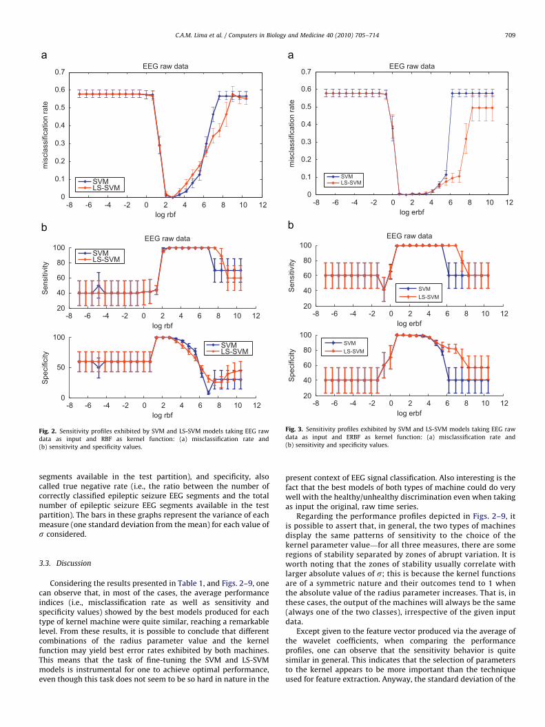
In Table 1, we provide the value(s) of the radius parameter thathas(ve) yielded the best average result, in terms of cross-validation error, for each triad /feature vector, model type,kernel typeS. In this table, the accuracy results are given in termsof average and standard deviation. Besides the feature vectorsachieved through DWT, simulations have also been conductedwith the EEG series without pre-processing. On the other hand,Figs. 2–9 depict the sensitivity profiles exhibited by the two typesof kernel machine for the feature vectors considered. Thesensitivity profiles relate to the following three criteria[12,13,18]: misclassification rate (i.e., the ratio between thenumber of misclassified EEG segments, either healthy orunhealthy, and the total number of segments available inthe test partition), sensitivity, also called true positive rate(i.e., the ratio between the number of correctly classifiedhealthy EEG segments and the total number of healthy EEG

ow the value of s that gives the best average accuracy result.

ERBF

s ERBF error7std. dev. s

16 0.00070.0000 4

16 0.00070.0000 4

0.5 0.10570.0273 0.5

0.5 0.10070.0289 0.5

1,2,4,8 0.00070.0000 1,2,4,8,16

0.5,1,2 0.00070.0000 1,2,4,8,16

0.5 0.00070.0000 1,2,4

0.25,1,2 0.00070.0000 0.5,1,2,4

-8 -6 -4 -2 0 2 4 6 8 10 120

0.1

0.2

0.3

0.4

0.5

0.6

0.7EEG raw data

log rbf

mis

clas

sific

atio

n ra

te

SVMLS-SVM

-8 -6 -4 -2 0 2 4 6 8 10 1220

40

60

80

100EEG raw data

log rbf

Sen

sitiv

ity

-8 -6 -4 -2 0 2 4 6 8 10 120

50

100

log rbf

Spe

cific

ity

SVMLS-SVM

SVMLS-SVM

Fig. 2. Sensitivity profiles exhibited by SVM and LS-SVM models taking EEG raw

data as input and RBF as kernel function: (a) misclassification rate and

(b) sensitivity and specificity values.

-8 -6 -4 -2 0 2 4 6 8 10 120

0.1

0.2

0.3

0.4

0.5

0.6

0.7EEG raw data

log erbf

mis

clas

sific

atio

n ra

te

SVMLS-SVM

-8 -6 -4 -2 0 2 4 6 8 10 1220

40

60

80

100EEG raw data

log erbf

Sen

sitiv

ity

-8 -6 -4 -2 0 2 4 6 8 10 1220

40

60

80

100

log erbf

Spe

cific

itySVMLS-SVM

SVMLS-SVM

Fig. 3. Sensitivity profiles exhibited by SVM and LS-SVM models taking EEG raw

data as input and ERBF as kernel function: (a) misclassification rate and

(b) sensitivity and specificity values.

C.A.M. Lima et al. / Computers in Biology and Medicine 40 (2010) 705–714 709

segments available in the test partition), and specificity, alsocalled true negative rate (i.e., the ratio between the number ofcorrectly classified epileptic seizure EEG segments and the totalnumber of epileptic seizure EEG segments available in the testpartition). The bars in these graphs represent the variance of eachmeasure (one standard deviation from the mean) for each value ofs considered.

3.3. Discussion

Considering the results presented in Table 1, and Figs. 2–9, onecan observe that, in most of the cases, the average performanceindices (i.e., misclassification rate as well as sensitivity andspecificity values) showed by the best models produced for eachtype of kernel machine were quite similar, reaching a remarkablelevel. From these results, it is possible to conclude that differentcombinations of the radius parameter value and the kernelfunction may yield best error rates exhibited by both machines.This means that the task of fine-tuning the SVM and LS-SVMmodels is instrumental for one to achieve optimal performance,even though this task does not seem to be so hard in nature in the

present context of EEG signal classification. Also interesting is thefact that the best models of both types of machine could do verywell with the healthy/unhealthy discrimination even when takingas input the original, raw time series.

Regarding the performance profiles depicted in Figs. 2–9, itis possible to assert that, in general, the two types of machinesdisplay the same patterns of sensitivity to the choice of thekernel parameter value—for all three measures, there are someregions of stability separated by zones of abrupt variation. It isworth noting that the zones of stability usually correlate withlarger absolute values of s; this is because the kernel functionsare of a symmetric nature and their outcomes tend to 1 whenthe absolute value of the radius parameter increases. That is, inthese cases, the output of the machines will always be the same(always one of the two classes), irrespective of the given inputdata.

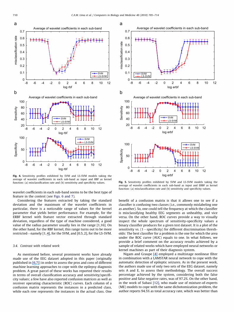
Except given to the feature vector produced via the average ofthe wavelet coefficients, when comparing the performanceprofiles, one can observe that the sensitivity behavior is quitesimilar in general. This indicates that the selection of parametersto the kernel appears to be more important than the techniqueused for feature extraction. Anyway, the standard deviation of the

-8 -6 -4 -2 0 2 4 6 8 10 120

0.1

0.2

0.3

0.4

0.5

0.6

0.7Average of wavelet coefficients in each sub-band

log rbf

mis

clas

sific

atio

n ra

te

SVMLS-SVM

-8 -6 -4 -2 0 2 4 6 8 10 1220

40

60

80

100Average of wavelet coefficients in each sub-band

log rbf

Sen

sitiv

ity

-8 -6 -4 -2 0 2 4 6 8 10 120

50

100

log rbf

Spe

cific

ity

SVMLS-SVM

SVMLS-SVM

Fig. 4. Sensitivity profiles exhibited by SVM and LS-SVM models taking the

average of wavelet coefficients in each sub-band as input and RBF as kernel

function: (a) misclassification rate and (b) sensitivity and specificity values.

-8 -6 -4 -2 0 2 4 6 8 10 120

0.1

0.2

0.3

0.4

0.5

0.6

0.7Average of wavelet coefficients in each sub-band

log erbf

mis

clas

sific

atio

n ra

te

SVMLS-SVM

-8 -6 -4 -2 0 2 4 6 8 10 1220

40

60

80

100Average of wavelet coefficients in each sub-band

log erbf

Sen

sitiv

ity

-8 -6 -4 -2 0 2 4 6 8 10 120

50

100

log erbf

Spe

cific

itySVMLS-SVM

SVMLS-SVM

Fig. 5. Sensitivity profiles exhibited by SVM and LS-SVM models taking the

average of wavelet coefficients in each sub-band as input and ERBF as kernel

function: (a) misclassification rate and (b) sensitivity and specificity values.

C.A.M. Lima et al. / Computers in Biology and Medicine 40 (2010) 705–714710

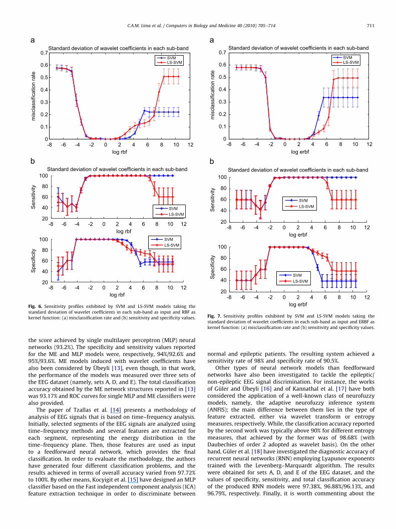
wavelet coefficients in each sub-band seems to be the best type offeature in the contest (see Figs. 6 and 7).

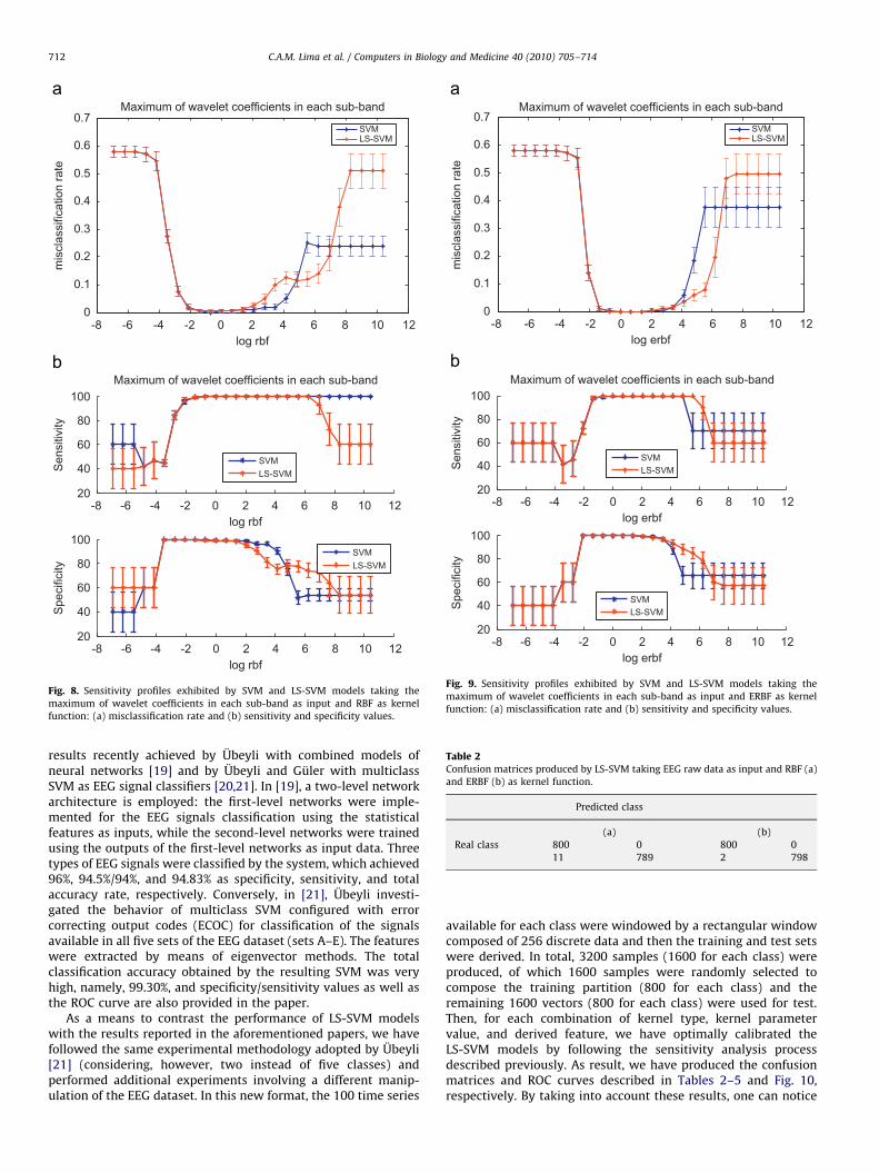
Considering the features extracted by taking the standarddeviation and the maximum of the wavelet coefficients inparticular, there is a noticeable range of values for the kernelparameter that yields better performance. For example, for theERBF kernel with feature vector extracted through standarddeviation, regardless of the type of machine considered, a goodvalue of the radius parameter usually lies in the range [1,16]. Onthe other hand, for the RBF kernel, this range turns out to be morerestricted—namely [1, 4], for the SVM, and [0.5, 2], for the LS-SVM.

3.4. Contrast with related work

As mentioned before, several prominent works have alreadymade use of the EEG dataset adopted in this paper (originallypublished in [6,7]) in order to assess the pros and cons of differentmachine learning approaches to cope with the epilepsy diagnosisproblem. A great parcel of these works has reported their resultsin terms of overall classification accuracy and sensitivity/specifi-city values; a few have also reported confusion matrices as well asreceiver operating characteristic (ROC) curves. Each column of aconfusion matrix represents the instances in a predicted class,while each row represents the instances in the actual class. One

benefit of a confusion matrix is that it allows one to see if aclassifier is confusing two classes (i.e., commonly mislabeling oneas another). So, one could tell the frequency at which the classifieris misclassifying healthy EEG segments as unhealthy, and viceversa. On the other hand, ROC curves provide a way to visuallyinspect the whole spectrum of sensitivity-specificity values abinary classifier produces for a given test dataset. It is a plot of thesensitivity vs. (1�specificity) for different discrimination thresh-olds: The best classifier for a problem is the one for which the areaunder the ROC curve (AUC) equals to one. In what follows, weprovide a brief comment on the accuracy results achieved by asample of related works which have employed neural networks orkernel machines as part of their diagnosis system.

Nigam and Graupe [4] employed a multistage nonlinear filterin combination with a LAMSTAR neural network to cope with theautomatic detection of epileptic seizures. As in the present work,the authors made use of only two sets of the EEG dataset, namelysets A and E, to assess their methodology. The overall successpercentage achieved by the system, considering both the falsepositive and false negative rates, was of 97.2%. On the other hand,in the work of Subasi [12], who made use of mixture-of-experts(ME) models to cope with the same dichotomization problem, theauthor reports 94.5% as total accuracy rate, which was better than

-8 -6 -4 -2 0 2 4 6 8 10 120

0.1

0.2

0.3

0.4

0.5

0.6

0.7Standard deviation of wavelet coefficients in each sub-band

log rbf

mis

clas

sific

atio

n ra

te

SVMLS-SVM

-8 -6 -4 -2 0 2 4 6 8 10 1220

40

60

80

100Standard deviation of wavelet coefficients in each sub-band

log rbf

Sen

sitiv

ity

-8 -6 -4 -2 0 2 4 6 8 10 1220

40

60

80

100

log rbf

Spe

cific

ity

SVMLS-SVM

SVMLS-SVM

Fig. 6. Sensitivity profiles exhibited by SVM and LS-SVM models taking the

standard deviation of wavelet coefficients in each sub-band as input and RBF as

kernel function: (a) misclassification rate and (b) sensitivity and specificity values.

-8 -6 -4 -2 0 2 4 6 8 10 120

0.1

0.2

0.3

0.4

0.5

0.6

0.7Standard deviation of wavelet coefficients in each sub-band

log erbf

mis

clas

sific

atio

n ra

te

SVMLS-SVM

-8 -6 -4 -2 0 2 4 6 8 10 1220

40

60

80

100Standard deviation of wavelet coefficients in each sub-band

log erbf

Sen

sitiv

ity

-8 -6 -4 -2 0 2 4 6 8 10 1220

40

60

80

100

log erbf

Spe

cific

ity

SVMLS-SVM

SVMLS-SVM

Fig. 7. Sensitivity profiles exhibited by SVM and LS-SVM models taking the

standard deviation of wavelet coefficients in each sub-band as input and ERBF as

kernel function: (a) misclassification rate and (b) sensitivity and specificity values.

C.A.M. Lima et al. / Computers in Biology and Medicine 40 (2010) 705–714 711

the score achieved by single multilayer perceptron (MLP) neuralnetworks (93.2%). The specificity and sensitivity values reportedfor the ME and MLP models were, respectively, 94%/92.6% and95%/93.6%. ME models induced with wavelet coefficients havealso been considered by Ubeyli [13], even though, in that work,the performance of the models was measured over three sets ofthe EEG dataset (namely, sets A, D, and E). The total classificationaccuracy obtained by the ME network structures reported in [13]was 93.17% and ROC curves for single MLP and ME classifiers werealso provided.

The paper of Tzallas et al. [14] presents a methodology ofanalysis of EEG signals that is based on time–frequency analysis.Initially, selected segments of the EEG signals are analyzed usingtime–frequency methods and several features are extracted foreach segment, representing the energy distribution in thetime–frequency plane. Then, those features are used as inputto a feedforward neural network, which provides the finalclassification. In order to evaluate the methodology, the authorshave generated four different classification problems, and theresults achieved in terms of overall accuracy varied from 97.72%to 100%. By other means, Kocyigit et al. [15] have designed an MLPclassifier based on the Fast independent component analysis (ICA)feature extraction technique in order to discriminate between

normal and epileptic patients. The resulting system achieved asensitivity rate of 98% and specificity rate of 90.5%.

Other types of neural network models than feedforwardnetworks have also been investigated to tackle the epileptic/non-epileptic EEG signal discrimination. For instance, the worksof Guler and Ubeyli [16] and of Kannathal et al. [17] have bothconsidered the application of a well-known class of neurofuzzymodels, namely, the adaptive neurofuzzy inference system(ANFIS); the main difference between them lies in the type offeature extracted, either via wavelet transform or entropymeasures, respectively. While, the classification accuracy reportedby the second work was typically above 90% for different entropymeasures, that achieved by the former was of 98.68% (withDaubechies of order 2 adopted as wavelet basis). On the otherhand, Guler et al. [18] have investigated the diagnostic accuracy ofrecurrent neural networks (RNN) employing Lyapunov exponentstrained with the Levenberg–Marquardt algorithm. The resultswere obtained for sets A, D, and E of the EEG dataset, and thevalues of specificity, sensitivity, and total classification accuracyof the produced RNN models were 97.38%, 96.88%/96.13%, and96.79%, respectively. Finally, it is worth commenting about the

-8 -6 -4 -2 0 2 4 6 8 10 120

0.1

0.2

0.3

0.4

0.5

0.6

0.7Maximum of wavelet coefficients in each sub-band

log rbf

mis

clas

sific

atio

n ra

te

SVMLS-SVM

-8 -6 -4 -2 0 2 4 6 8 10 1220

40

60

80

100Maximum of wavelet coefficients in each sub-band

log rbf

Sen

sitiv

ity

-8 -6 -4 -2 0 2 4 6 8 10 1220

40

60

80

100

log rbf

Spe

cific

ity

SVMLS-SVM

SVMLS-SVM

Fig. 8. Sensitivity profiles exhibited by SVM and LS-SVM models taking the

maximum of wavelet coefficients in each sub-band as input and RBF as kernel

function: (a) misclassification rate and (b) sensitivity and specificity values.

-8 -6 -4 -2 0 2 4 6 8 10 120

0.1

0.2

0.3

0.4

0.5

0.6

0.7Maximum of wavelet coefficients in each sub-band

log erbf

mis

clas

sific

atio

n ra

te

SVMLS-SVM

-8 -6 -4 -2 0 2 4 6 8 10 1220

40

60

80

100Maximum of wavelet coefficients in each sub-band

log erbf

Sen

sitiv

ity

-8 -6 -4 -2 0 2 4 6 8 10 1220

40

60

80

100

log erbf

Spe

cific

itySVMLS-SVM

SVMLS-SVM

Fig. 9. Sensitivity profiles exhibited by SVM and LS-SVM models taking the

maximum of wavelet coefficients in each sub-band as input and ERBF as kernel

function: (a) misclassification rate and (b) sensitivity and specificity values.

Table 2Confusion matrices produced by LS-SVM taking EEG raw data as input and RBF (a)

and ERBF (b) as kernel function.

Predicted class

(a) (b)

Real class 800 0 800 0

11 789 2 798

C.A.M. Lima et al. / Computers in Biology and Medicine 40 (2010) 705–714712

results recently achieved by Ubeyli with combined models ofneural networks [19] and by Ubeyli and Guler with multiclassSVM as EEG signal classifiers [20,21]. In [19], a two-level networkarchitecture is employed: the first-level networks were imple-mented for the EEG signals classification using the statisticalfeatures as inputs, while the second-level networks were trainedusing the outputs of the first-level networks as input data. Threetypes of EEG signals were classified by the system, which achieved96%, 94.5%/94%, and 94.83% as specificity, sensitivity, and totalaccuracy rate, respectively. Conversely, in [21], Ubeyli investi-gated the behavior of multiclass SVM configured with errorcorrecting output codes (ECOC) for classification of the signalsavailable in all five sets of the EEG dataset (sets A–E). The featureswere extracted by means of eigenvector methods. The totalclassification accuracy obtained by the resulting SVM was veryhigh, namely, 99.30%, and specificity/sensitivity values as well asthe ROC curve are also provided in the paper.

As a means to contrast the performance of LS-SVM modelswith the results reported in the aforementioned papers, we havefollowed the same experimental methodology adopted by Ubeyli[21] (considering, however, two instead of five classes) andperformed additional experiments involving a different manip-ulation of the EEG dataset. In this new format, the 100 time series

available for each class were windowed by a rectangular windowcomposed of 256 discrete data and then the training and test setswere derived. In total, 3200 samples (1600 for each class) wereproduced, of which 1600 samples were randomly selected tocompose the training partition (800 for each class) and theremaining 1600 vectors (800 for each class) were used for test.Then, for each combination of kernel type, kernel parametervalue, and derived feature, we have optimally calibrated theLS-SVM models by following the sensitivity analysis processdescribed previously. As result, we have produced the confusionmatrices and ROC curves described in Tables 2–5 and Fig. 10,respectively. By taking into account these results, one can notice

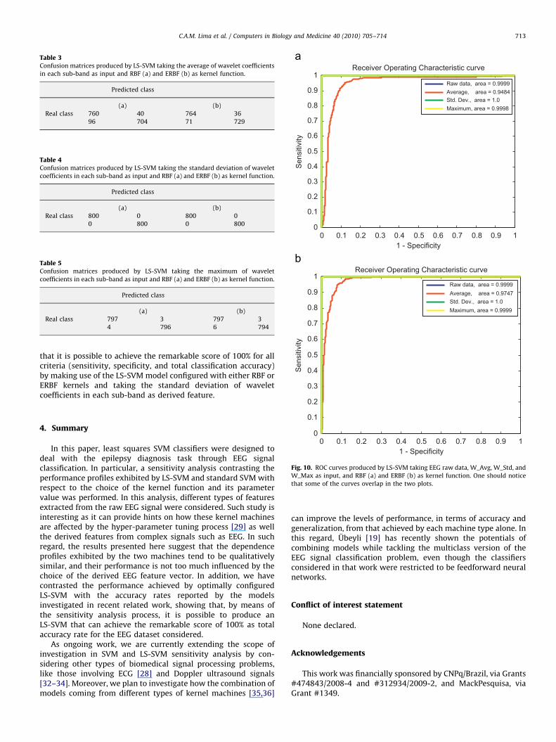
Table 4Confusion matrices produced by LS-SVM taking the standard deviation of wavelet

coefficients in each sub-band as input and RBF (a) and ERBF (b) as kernel function.

Predicted class

(a) (b)

Real class 800 0 800 0

0 800 0 800

Table 5Confusion matrices produced by LS-SVM taking the maximum of wavelet

coefficients in each sub-band as input and RBF (a) and ERBF (b) as kernel function.

Predicted class

(a) (b)

Real class 797 3 797 3

4 796 6 794

0 0.1 0.2 0.3 0.4 0.5 0.6 0.7 0.8 0.9 10

0.1

0.2

0.3

0.4

0.5

0.6

0.7

0.8

0.9

1Receiver Operating Characteristic curve

1 - Specificity

Sen

sitiv

ity

Raw data, area = 0.9999Average, area = 0.9484Std. Dev., area = 1.0Maximum, area = 0.9998

0.3

0.4

0.5

0.6

0.7

0.8

0.9

1Receiver Operating Characteristic curve

Sen

sitiv

ity

Raw data, area = 0.9999Average, area = 0.9747 Std. Dev., area = 1.0Maximum, area = 0.9999

Table 3Confusion matrices produced by LS-SVM taking the average of wavelet coefficients

in each sub-band as input and RBF (a) and ERBF (b) as kernel function.

Predicted class

(a) (b)

Real class 760 40 764 36

96 704 71 729

C.A.M. Lima et al. / Computers in Biology and Medicine 40 (2010) 705–714 713

that it is possible to achieve the remarkable score of 100% for allcriteria (sensitivity, specificity, and total classification accuracy)by making use of the LS-SVM model configured with either RBF orERBF kernels and taking the standard deviation of waveletcoefficients in each sub-band as derived feature.

0 0.1 0.2 0.3 0.4 0.5 0.6 0.7 0.8 0.9 10

0.1

0.2

1 - Specificity

Fig. 10. ROC curves produced by LS-SVM taking EEG raw data, W_Avg, W_Std, and

W_Max as input, and RBF (a) and ERBF (b) as kernel function. One should notice

that some of the curves overlap in the two plots.

4. Summary

In this paper, least squares SVM classifiers were designed todeal with the epilepsy diagnosis task through EEG signalclassification. In particular, a sensitivity analysis contrasting theperformance profiles exhibited by LS-SVM and standard SVM withrespect to the choice of the kernel function and its parametervalue was performed. In this analysis, different types of featuresextracted from the raw EEG signal were considered. Such study isinteresting as it can provide hints on how these kernel machinesare affected by the hyper-parameter tuning process [29] as wellthe derived features from complex signals such as EEG. In suchregard, the results presented here suggest that the dependenceprofiles exhibited by the two machines tend to be qualitativelysimilar, and their performance is not too much influenced by thechoice of the derived EEG feature vector. In addition, we havecontrasted the performance achieved by optimally configuredLS-SVM with the accuracy rates reported by the modelsinvestigated in recent related work, showing that, by means ofthe sensitivity analysis process, it is possible to produce anLS-SVM that can achieve the remarkable score of 100% as totalaccuracy rate for the EEG dataset considered.

As ongoing work, we are currently extending the scope ofinvestigation in SVM and LS-SVM sensitivity analysis by con-sidering other types of biomedical signal processing problems,like those involving ECG [28] and Doppler ultrasound signals[32–34]. Moreover, we plan to investigate how the combination ofmodels coming from different types of kernel machines [35,36]

can improve the levels of performance, in terms of accuracy andgeneralization, from that achieved by each machine type alone. Inthis regard, Ubeyli [19] has recently shown the potentials ofcombining models while tackling the multiclass version of theEEG signal classification problem, even though the classifiersconsidered in that work were restricted to be feedforward neuralnetworks.

Conflict of interest statement

None declared.

Acknowledgements

This work was financially sponsored by CNPq/Brazil, via Grants#474843/2008-4 and #312934/2009-2, and MackPesquisa, viaGrant #1349.

C.A.M. Lima et al. / Computers in Biology and Medicine 40 (2010) 705–714714

References

[1] L. Sornmo, P. Laguna, Bioelectrical Signal Processing in Cardiac andNeurological Applications, Elsevier, Amsterdam, 2005.

[2] E. Niedermeyer, F.L. da Silva, Electroencephalography: Basic Principles,Clinical Applications, and Related Fields, Lippincott Williams & Wilkins, 2004.

[3] X. Liao, Y. Yin, C. Li, D. Yao, Application of SVM framework for classification ofsingle trial EEG, in: J. Wang et al.(Ed.), Advances in Neural Networks—ISNN2006, Lecture Notes in Computer Science, vol. 3973, Springer 2006, pp. 548–553.

[4] V.P. Nigam, D. Graupe, A neural-network-based detection of epilepsy, Neurol.Res. 26 (2004) 55–60.

[5] K. Lehnertz, Non-linear time series analysis of intracranial EEG recordings inpatients with epilepsy—an overview, Int. J. Psychophysiol. 34 (1999) 45–52.

[6] R.G. Andrzejak, K. Lehnertz, F. Mormann, C. Rieke, P. David, C.E. Elger,Indications of nonlinear deterministic and finite dimensional structures intime series of brain electrical activity: dependence on recording region andbrain state, Phys. Rev. E 64 (2001) article ID 061907.

[7] R.G. Andrzejak, G Widman, K. Lehnertz, C. Rieke, P. David, C.E. Elger, Theepileptic process as nonlinear deterministic dynamics in a stochasticenvironment: an evaluation on mesial temporal lobe epilepsy, Epilepsy Res.44 (2001) 129–140.

[8] F.M. Alicata, C. Stefanini, M. Elia, R. Ferri, S. Del Gracco, S.A. Musumeci,Chaotic behavior of EEG slow-wave activity during sleep, Electron. Clin.Neurophysiol. 99 (1996) 539–543.

[9] E.D. Ubeyli, Statistics over features: EEG signals analysis, Comput. Biol. Med.39 (2009) 733–741.

[10] A. Subasi, Epileptic seizure detection using dynamic wavelet network, ExpertSyst. Appl. 28 (2005) 701–711.

[11] A. Subasi, E. Ercelebi, Classification of EEG signals using neural network andlogistic regression, Comput. Methods Prog. Biomed. 78 (2005) 87–99.

[12] A. Subasi, EEG signal classification using wavelet feature extraction and amixture of expert model, Expert Syst. Appl. 32 (2007) 1084–1093.

[13] E.D. Ubeyli, Wavelet/mixture of experts network structure for EEG signalsclassification, Expert Syst. Appl. 34 (2008) 1954–1962.

[14] A.T. Tzallas, M.G. Tsipouras, D.I. Fotiadis, Automatic seizure detection basedon time–frequency analysis and artificial neural networks, Comput. Intel.Neurosci. 2007 (2007) article ID 80510.

[15] Y. Kocyigit, A. Alkan, H. Erol, Classification of EEG recordings by using fastindependent component analysis and artificial neural network, J. Med. Syst.32 (2008) 17–20.

[16] _I. Guler, E.D. Ubeyli, Adaptive neuro-fuzzy inference system for classificationof EEG signals using wavelet coefficients, J. Neurosci. Methods 148 (2005)113–121.

[17] N. Kannathal, L.C. Min, U.R. Acharya, P.K. Sadasivan, Entropies for detection ofepilepsy in EEG, Comput. Methods Prog. Biomed. 80 (2005) 187–194.

[18] N.F. Guler, E.D. Ubeyli, _I. Guler, Recurrent neural networks employingLyapunov exponents for EEG signals classification, Expert Syst. Appl. 29(2005) 506–514.

[19] E.D. Ubeyli, Combined neural network model employing wavelet coefficientsfor EEG signals classification, Digital Signal Process 19 (2009) 297–308.

[20] I. Guler, E.D. Ubeyli, Multiclass support vector machines for EEG-signalsclassification, IEEE Trans. Inf. Technol. Biomed. 11 (2007) 117–126.

[21] E.D. Ubeyli, Analysis of EEG signals by combining eigenvector methods andmulticlass support vector machines, Comput. Biol. Med. 38 (2008) 14–22.

[22] N. Cristianini, J. Shawe-Taylor, An Introduction to Support Vector Machines,Cambridge University Press, London, 2000.

[23] V.N. Vapnik, Statistical Learning Theory, Wiley, New York, 1998.[24] B. Scholkopf, A. Smola, Learning with Kernels, The MIT Press, Cambridge,

2002.[25] J.A.K. Suykens, J. Vandewalle, Least squares support machine classifiers,

Neural Proc. Lett. 9 (1999) 293–300.

[26] J.A.K. Suykens, T. Van Gestel, J. De Brabanter, B. De Moor, J. Vandewalle, in:Least Squares Support Vector Machines, World Scientific Publishers,Singapore, 2002.

[27] T. Van Gestel, J.A.K. Suykens, B. Baesens, S. Viaene, J. Vanthienen, G. Dedene,B. De Moor, J. Vandewalle, Benchmarking least squares support machineclassifiers, Mach. Learn. 54 (2004) 5–32.

[28] P. Kemal, A. Bayram, S. Gunes-, Computer aided diagnosis of ECG data on theleast square support vector machine, Digital Signal Process. 18 (2008)25–32.

[29] O. Chapelle, V. Vapnik, O. Bousquet, S. Mukherjee, Choosing multipleparameters for support vector machines, Mach. Learn. 46 (2002) 131–159.

[30] V. Cherkassky, Y. Ma, Practical selection of SVM parameters and noiseestimation for SVM regression, Neural Networks 17 (2004) 113–126.

[31] F. Friedrichs, C. Igel, Evolutionary tuning of multiple SVM parameters,Neurocomputing 64 (2005) 107–117.

[32] E.D. Ubeyli, Probabilistic neural networks employing Lyapunov exponents foranalysis of Doppler ultrasound signals, Comput. Biol. Med. 38 (2008)82–89.

[33] E.D. Ubeyli, _I. Guler, Feature extraction from Doppler ultrasound signals forautomated diagnostic systems, Comput. Biol. Med. 35 (2005) 735–764.

[34] E.D. Ubeyli, Usage of eigenvector methods to improve reliable classifier forDoppler ultrasound signals, Comput. Biol. Med. 38 (2008) 563–573.

[35] C.A.M. Lima, A.L.V. Coelho, F.J. Von Zuben, Model selection based on VC-dimension for heterogeneous ensembles of support vector machines,Proceedings of the Fourth International Conference on Recent Advances inSoft Computing, Nottingham University Press, Nottingham, 2002pp. 459–464.

[36] C.A.M. Lima, W.J.P. Villanueva, E.P. dos Santos, F.J. Von Zuben, A multistageensemble of support vector machine variants, Proceedings of the FifthInternational Conference on Recent Advances in Soft Computing, Notting-ham, University Press, Nottingham, 2004, pp. 670–675.

Clodoaldo A.M. Lima received the B.Sc. degree (1997) in Electrical Engineeringfrom Federal University of Juiz de Fora (UFJF), Brazil, and M.Sc. (2000) and Ph.D.(2004) degrees in Computer Engineering from the State University of Campinas(Unicamp), Brazil. He was a post-doctoral fellow (from 2004 to 2006) and then aresearch collaborator (2007–2008) at the same university. Currently, he is with theGraduate Program in Electrical Engineering at Mackenzie Presbyterian University,S~ao Paulo, Brazil. His current research interests include multivariate analysis,machine learning, time series forecasting, and digital signal processing.

Andre L.V. Coelho received the B.Sc. degree in Computer Engineering in 1996, andearned the M.Sc. and Ph.D. degrees in Electrical Engineering in 1998 and 2004,respectively, all from the State University of Campinas (Unicamp), Brazil. He has arecord of publications related to the themes of machine learning, data mining,computational intelligence, metaheuristics, and multiagent systems. He is amember of ACM and has served as a reviewer for a number of scientificconferences and journals. Currently, he is an adjunct professor affiliated with theGraduate Program in Applied Informatics at the University of Fortaleza, Ceara,Brazil.

Marcio Eisencraft received the M.Sc. (2001) and Ph.D. (2006) degrees in ElectricalEngineering from the University of S~ao Paulo (USP), Brazil. From 2006 to 2010, hewas with the Graduate Program in Electrical Engineering at MackenziePresbyterian University. Currently, he is affiliated with the Federal University ofABC, S~ao Paulo, Brazil. His current research interests include digital signalprocessing, intermittent time series, and chaotic and nonlinear systems.