synchrosqueezed wave packet transforms and ... - arxiv
TRANSCRIPT
Synchrosqueezed wave packet transforms and diffeomorphism
based spectral analysis for 1D general mode decompositions
Haizhao Yang
Department of Mathematics, Stanford University
October 2013; revised April 2014
Abstract
This paper develops new theory and algorithms for 1D general mode decompositions.First, we introduce the 1D synchrosqueezed wave packet transform and prove thatit is able to estimate instantaneous information of well-separated modes from theirsuperposition accurately. The synchrosqueezed wave packet transform has a betterresolution than the synchrosqueezed wavelet transform in the time-frequency domainfor separating high frequency modes. Second, we present a new approach based ondiffeomorphisms for the spectral analysis of general shape functions. These two methodslead to a framework for general mode decompositions under a weak well-separationcondition and a well-different condition. Numerical examples of synthetic and real dataare provided to demonstrate the fruitful applications of these methods.
Keywords. Mode decomposition, general shape function, instantaneous, synchrosqueezedwave packet transform, diffeomorphism.
AMS subject classifications: 42A99 and 65T99.
1 Introduction
1.1 Problem statement
In signal processing, analyzing instantaneous properties (e.g., instantaneous frequencies,instantaneous amplitudes and instantaneous phases [1, 20]) of signals has been an importanttopic for over two decades. In many applications [3, 17, 27, 26, 33, 34], a signal would bea superposition of several components, for example, a complex signal
f(t) =K∑k=1
αk(t)e2πiNkφk(t), (1)
where αk(t) is the instantaneous amplitude, 2πNkφk(t) is the instantaneous phase andNkφ
′k(t) is the instantaneous frequency. One wishes to decompose the signal f(t) to obtain
each component αk(t)e2πiNkφk(t) and its corresponding instantaneous properties. This is
referred to as the mode decomposition problem.In spite of considerable successes of analyzing signals by decomposing them in the form
(1), a superposition of a few wave-like components belongs to a very limited class of os-cillatory patterns. Most of all, decompositions in the form (1) lose important physical
1
arX
iv:1
311.
4655
v2 [
mat
h.N
A]
1 A
pr 2
014
340365390
−100
10
−100
10
CO
2 C
on
ce
ntr
atio
ns (
pp
m)
−100
10
0 5 10 15 20 25 30340365390
Time (Year)
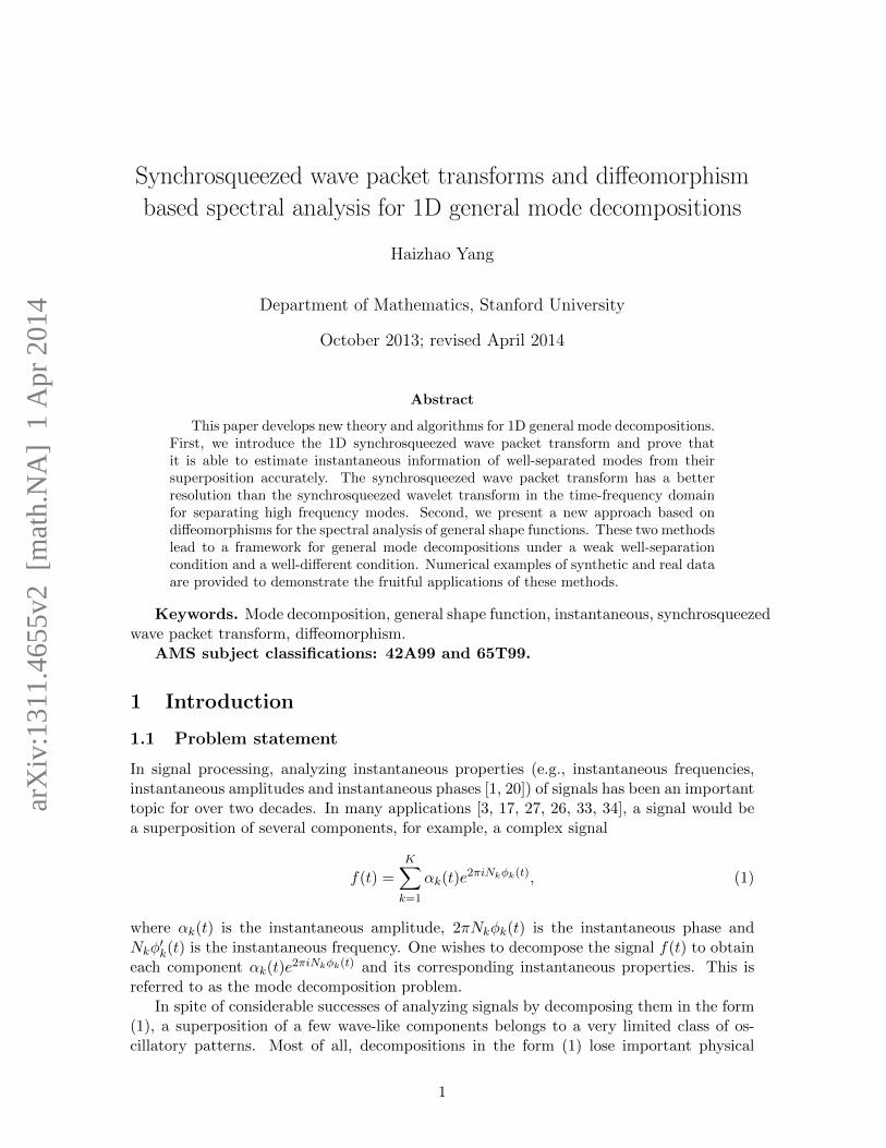
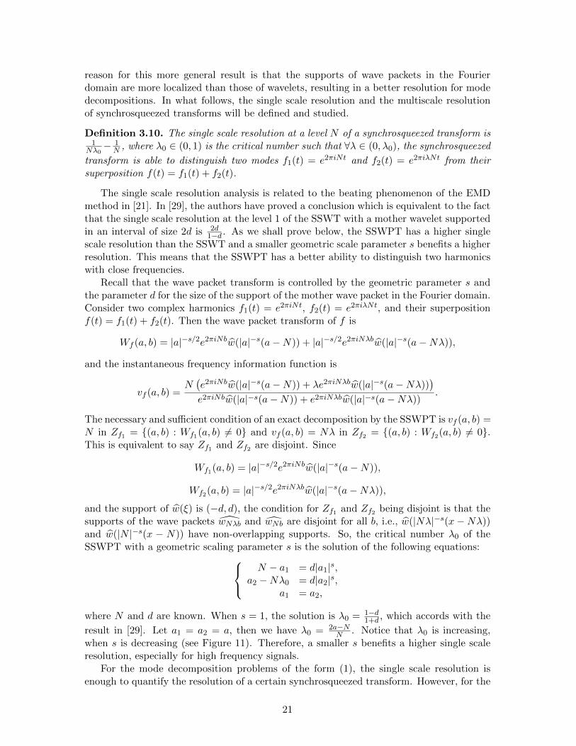
Figure 1: The top signal is the observed CO2 concentration of recent 31 years (1981-2011)at MLO. Below the original signal are the components provided by the wavelet transform.Only relevant components are separated and presented.
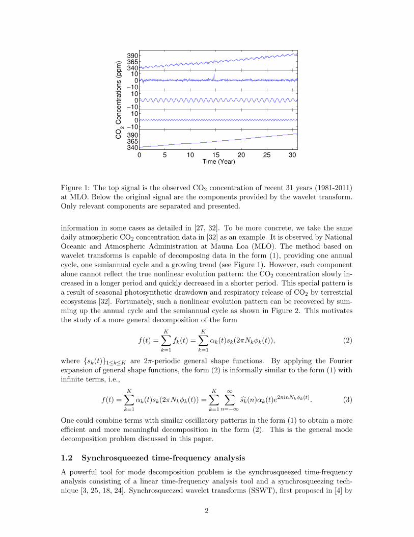
information in some cases as detailed in [27, 32]. To be more concrete, we take the samedaily atmospheric CO2 concentration data in [32] as an example. It is observed by NationalOceanic and Atmospheric Administration at Mauna Loa (MLO). The method based onwavelet transforms is capable of decomposing data in the form (1), providing one annualcycle, one semiannual cycle and a growing trend (see Figure 1). However, each componentalone cannot reflect the true nonlinear evolution pattern: the CO2 concentration slowly in-creased in a longer period and quickly decreased in a shorter period. This special pattern isa result of seasonal photosynthetic drawdown and respiratory release of CO2 by terrestrialecosystems [32]. Fortunately, such a nonlinear evolution pattern can be recovered by sum-ming up the annual cycle and the semiannual cycle as shown in Figure 2. This motivatesthe study of a more general decomposition of the form
f(t) =K∑k=1
fk(t) =K∑k=1
αk(t)sk(2πNkφk(t)), (2)
where sk(t)1≤k≤K are 2π-periodic general shape functions. By applying the Fourierexpansion of general shape functions, the form (2) is informally similar to the form (1) withinfinite terms, i.e.,
f(t) =K∑k=1
αk(t)sk(2πNkφk(t)) =K∑k=1
∞∑n=−∞
sk(n)αk(t)e2πinNkφk(t). (3)
One could combine terms with similar oscillatory patterns in the form (1) to obtain a moreefficient and more meaningful decomposition in the form (2). This is the general modedecomposition problem discussed in this paper.
1.2 Synchrosqueezed time-frequency analysis
A powerful tool for mode decomposition problem is the synchrosqueezed time-frequencyanalysis consisting of a linear time-frequency analysis tool and a synchrosqueezing tech-nique [3, 25, 18, 24]. Synchrosqueezed wavelet transforms (SSWT), first proposed in [4] by
2
0 0.2 0.4 0.6 0.8 1−4
−3
−2
−1
0
1
2
3
4
Time (Year)
CO
2 C
on
ce
ntr
atio
ns (
pp
m)
0 0.2 0.4 0.6 0.8 1−4
−3
−2
−1
0
1
2
3
4
Time (Year)
CO
2 C
on
ce
ntr
atio
ns (
pp
m)
0 0.2 0.4 0.6 0.8 1−4
−3
−2
−1
0
1
2
3
4
Time (Year)
CO
2 C
on
ce
ntr
atio
ns (
pp
m)
Figure 2: Wave shapes of relevant components provided by wavelet transform. Left: Annualwave shape. Middle: Semiannual wave shape. Right: Summation of the annual wave shapeand semiannual wave shape.
Daubechies et al., can accurately decompose a class of superpositions of wave-like compo-nents and estimate their instantaneous frequencies, as proved rigorously in [3]. Followingthis research line, a synchrosqueezed short-time Fourier transform (SSSTFT) and a general-ized synchrosqueezing transform have been proposed in [25] and [18], respectively. Stabilityproperties of these synchrosqueezing approaches have been studied in [24] recently. Withthese newly developed theories, these synchrosqueezing transforms have been applied toanalyze signals in the form (1) in many applications successfully [2, 10, 24, 28, 30].
In the analysis of existing synchrosqueezed transforms [3, 25], a key requirement toguarantee an accurate estimation of instantaneous properties and decompositions is thewell-separation condition for a class of superpositions of intrinsic mode type functions. Letus take the SSWT as an example. Since it is of significance to study the relation betweenthe magnitudes of instantaneous frequencies and the accuracy of instantaneous frequencyestimates, N and Nk are introduced in the following definitions.
Definition 1.1. (Intrinsic mode type function for the SSWT). A continuous function f :R → C, f ∈ L∞(R) is said to be intrinsic-mode-type (IMT) with accuracy ε > 0 if f(t) =a(t)e2πiNφ(t) with a(t) and φ(t) having the following properties:
a ∈ C1(R) ∩ L∞(R), φ ∈ C2(R)
inft∈R
φ′(t) > 0, supt∈R
φ′(t) <∞, supt∈R|φ′′(t)| <∞,
|a′(t)| ≤ ε|Nφ′(t)|, |φ′′(t)| ≤ ε|φ′(t)|, ∀t ∈ R.
Definition 1.2. (Superposition of well-separated intrinsic mode functions for the SSWT).A function f : R → C is said to be a superposition of well-separated intrinsic mode func-tions, up to accuracy ε, and with separation 4, if there exists a finite K, such that
f(t) =K∑k=1
fk(t) =K∑k=1
ak(t)e2πiNkφk(t),
where all the fk are IMT, and where moreover their respective phase functions φk satisfy
Nkφ′k(t) > Nk−1φ
′k−1(t) and |Nkφ
′k(t)−Nk−1φ
′k−1(t)| ≥ 4
[Nkφ
′k(t) +Nk−1φ
′k−1(t)
], ∀t ∈ R.
3
0 0.2 0.4 0.6 0.8 1−0.04
−0.02
0
0.02
0.04
0.06
0.08
0.1
0.12
0.14
0.16
t
s(t
)
−100 −50 0 50 1000
0.002
0.004
0.006
0.008
0.01
0.012
0.014
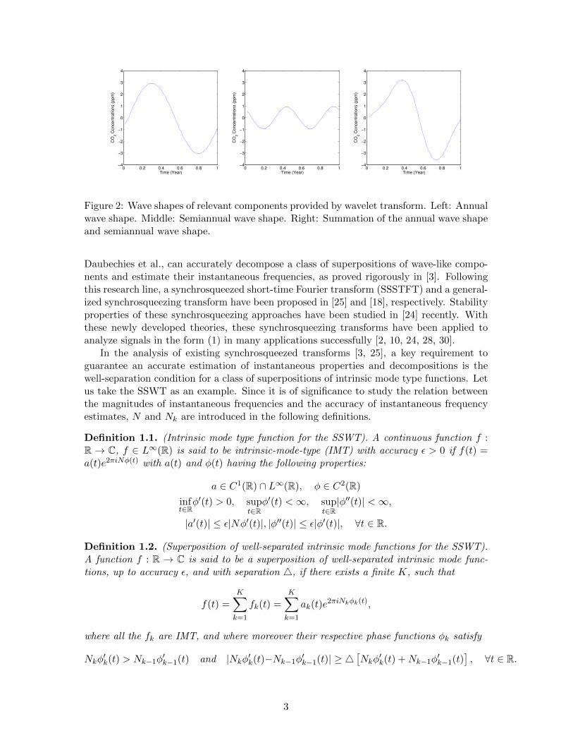
Figure 3: Left: The solid line plots a spike shape function s(t) of a real ECG signal and thedotted line is its band-limited approximation
∑|n|≤10 s(n)e2πint. The sum of a few Fourier
expansion terms cannot approximate the shape function accurately. Most importantly, thehighest peak, the key quantity called R-peak in [8], is smoothed and is hardly distinguished.Right: The Fourier power spectrum |s(ξ)| of s(t) is plotted. The energy in the Fourierdomain is spreading widely.
In [3], it is proved that the SSWT can estimate instantaneous frequencies of well-separated intrinsic mode functions from their superposition, using a mother wavelet sup-ported in [1−d, 1+d], with d < 4/(1+4). The well-separation condition can be essentiallyreferred to as the condition that the instantaneous frequencies Nkφ
′k(t) are not crossing over
the support of the same wavelet in the time-frequency domain.For the general mode decomposition problem, a straightforward question would be
whether the synchrosqueezed time-frequency representation can extract general modesαk(t)sk(2πNkφk(t))1≤k≤K , identify general shape functions sk(t)1≤k≤K and estimateinstantaneous properties. Recently, [27] shows that the SSWT can be used to solve thegeneral mode decomposition problem for a superposition of well-separated general modeswith analytic wave shape functions sk(t) sufficiently close to the exponential function eit,i.e., a few terms of the Fourier expansion of sk(t) are sufficient to approximate sk(t) well.However, this class of band-limited wave shape functions in [27] is still restrictive in somesituations, e.g., spike signals in neurons have shape functions with a wide Fourier band asshown in Figure 3. The SSWT would not be suitable to address the general mode decompo-sition problem in these circumstances because the well-separation condition for the SSWTis impractical for the following two reasons.
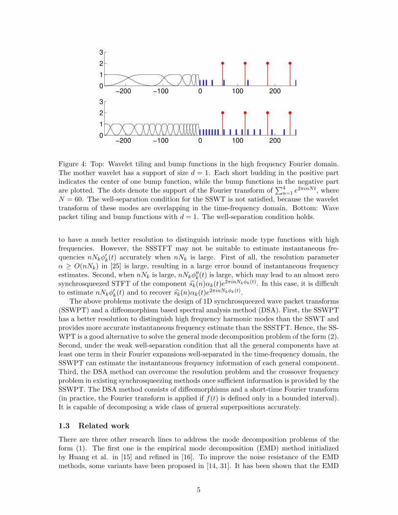
1. The superposition of two nearby Fourier expansion terms sk(n)αk(t)e2πinNkφk(t) and
sk(n+ 1)αk(t)e2πi(n+1)Nkφk(t) are not well-separated when n is large (see Figure 4 for
an example), due to the low resolution of wavelet transforms in the high frequencypart of the time-frequency domain.
2. For two different instantaneous frequencies Nkφ′k(t) and Njφ
′j(t), their multiples may
have crossover frequencies with high probability.
One possible idea to address the first problem might be to apply the SSSTFT in [25].The SSSTFT has a much weaker requirement for the well-separation condition and it seems
4
−200 −100 0 100 2000
1
2
3
−200 −100 0 100 2000
1
2
3
Figure 4: Top: Wavelet tiling and bump functions in the high frequency Fourier domain.The mother wavelet has a support of size d = 1. Each short budding in the positive partindicates the center of one bump function, while the bump functions in the negative partare plotted. The dots denote the support of the Fourier transform of
∑4n=1 e
2πinNt, whereN = 60. The well-separation condition for the SSWT is not satisfied, because the wavelettransform of these modes are overlapping in the time-frequency domain. Bottom: Wavepacket tiling and bump functions with d = 1. The well-separation condition holds.
to have a much better resolution to distinguish intrinsic mode type functions with highfrequencies. However, the SSSTFT may not be suitable to estimate instantaneous fre-quencies nNkφ
′k(t) accurately when nNk is large. First of all, the resolution parameter
α ≥ O(nNk) in [25] is large, resulting in a large error bound of instantaneous frequencyestimates. Second, when nNk is large, nNkφ
′′k(t) is large, which may lead to an almost zero
synchrosqueezed STFT of the component sk(n)αk(t)e2πinNkφk(t). In this case, it is difficult
to estimate nNkφ′k(t) and to recover sk(n)αk(t)e
2πinNkφk(t).The above problems motivate the design of 1D synchrosqueezed wave packet transforms
(SSWPT) and a diffeomorphism based spectral analysis method (DSA). First, the SSWPThas a better resolution to distinguish high frequency harmonic modes than the SSWT andprovides more accurate instantaneous frequency estimate than the SSSTFT. Hence, the SS-WPT is a good alternative to solve the general mode decomposition problem of the form (2).Second, under the weak well-separation condition that all the general components have atleast one term in their Fourier expansions well-separated in the time-frequency domain, theSSWPT can estimate the instantaneous frequency information of each general component.Third, the DSA method can overcome the resolution problem and the crossover frequencyproblem in existing synchrosqueezing methods once sufficient information is provided by theSSWPT. The DSA method consists of diffeomorphisms and a short-time Fourier transform(in practice, the Fourier transform is applied if f(t) is defined only in a bounded interval).It is capable of decomposing a wide class of general superpositions accurately.
1.3 Related work
There are three other research lines to address the mode decomposition problems of theform (1). The first one is the empirical mode decomposition (EMD) method initializedby Huang et al. in [15] and refined in [16]. To improve the noise resistance of the EMDmethods, some variants have been proposed in [14, 31]. It has been shown that the EMD
5
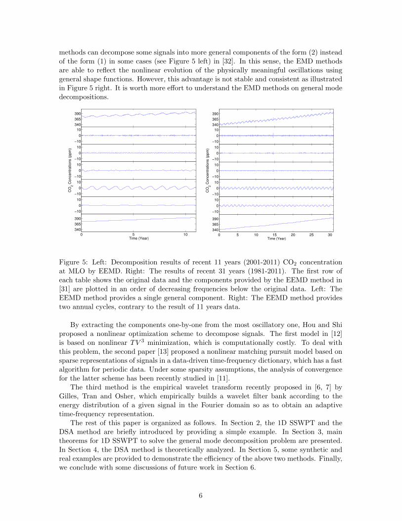
methods can decompose some signals into more general components of the form (2) insteadof the form (1) in some cases (see Figure 5 left) in [32]. In this sense, the EMD methodsare able to reflect the nonlinear evolution of the physically meaningful oscillations usinggeneral shape functions. However, this advantage is not stable and consistent as illustratedin Figure 5 right. It is worth more effort to understand the EMD methods on general modedecompositions.
340
365
390
−10
0
10
−10
0
10
−10
0
10
CO
2 C
on
ce
ntr
atio
ns (
pp
m)
−10
0
10
−10
0
10
0 5 10
340
365
390
Time (Year)
340
365
390
−10
0
10
−10
0
10
−10
0
10
CO
2 C
on
ce
ntr
atio
ns (
pp
m)
−10
0
10
−10
0
10
0 5 10 15 20 25 30
340
365
390
Time (Year)
Figure 5: Left: Decomposition results of recent 11 years (2001-2011) CO2 concentrationat MLO by EEMD. Right: The results of recent 31 years (1981-2011). The first row ofeach table shows the original data and the components provided by the EEMD method in[31] are plotted in an order of decreasing frequencies below the original data. Left: TheEEMD method provides a single general component. Right: The EEMD method providestwo annual cycles, contrary to the result of 11 years data.
By extracting the components one-by-one from the most oscillatory one, Hou and Shiproposed a nonlinear optimization scheme to decompose signals. The first model in [12]is based on nonlinear TV 3 minimization, which is computationally costly. To deal withthis problem, the second paper [13] proposed a nonlinear matching pursuit model based onsparse representations of signals in a data-driven time-frequency dictionary, which has a fastalgorithm for periodic data. Under some sparsity assumptions, the analysis of convergencefor the latter scheme has been recently studied in [11].
The third method is the empirical wavelet transform recently proposed in [6, 7] byGilles, Tran and Osher, which empirically builds a wavelet filter bank according to theenergy distribution of a given signal in the Fourier domain so as to obtain an adaptivetime-frequency representation.
The rest of this paper is organized as follows. In Section 2, the 1D SSWPT and theDSA method are briefly introduced by providing a simple example. In Section 3, maintheorems for 1D SSWPT to solve the general mode decomposition problem are presented.In Section 4, the DSA method is theoretically analyzed. In Section 5, some synthetic andreal examples are provided to demonstrate the efficiency of the above two methods. Finally,we conclude with some discussions of future work in Section 6.
6
2 Implementation of proposed methods
2.1 1D synchrosqueezed wave packet transforms (SSWPT)
In what follows, we briefly introduce the 1D SSWPT based on the 2D SSWPT in [34]. Letw(t) be a mother wave packet in the Schwartz class and the Fourier transform w(ξ) is areal-valued, non-negative, smooth function with a support equal to (−d, d) determined bya parameter d ≤ 1. We can use w(t) to define a family of wave packets through scaling,modulation, and translation, controlled by a geometric parameter s.
Definition 2.1. Given the mother wave packet w(t) and the parameter s ∈ (1/2, 1), thefamily of wave packets wab(t) : |a| ≥ 1, b ∈ R is defined as
wab(t) = |a|s/2w(|a|s(t− b))e2πi(t−b)a,
or equivalently, in the Fourier domain as
wab(ξ) = |a|−s/2e−2πibξw(|a|−s(ξ − a)).
Notice that if s were equal to 1, these functions would be qualitatively similar to thestandard wavelets. On the other hand, if s were equal to 1/2, we would obtain the waveatoms defined in [5]. But s ∈ (1/2, 1) is essential as we shall see in the main theorems.
The instantaneous frequency of the low frequency part is not well defined as discussedin [20]. For this reason, it is enough to consider the wave packets with |a| ≥ 1. The highfrequency modes can be identified and extracted independently of the low frequency partso that the low frequency part can be recovered by removing high frequency modes.
Definition 2.2. The 1D wave packet transform of a function f(t) is a function
Wf (a, b) = 〈wab, f〉 =
∫wab(t)f(t)dt (4)
= 〈wab, f〉 =
∫wab(ξ)f(ξ)dξ
for |a| ≥ 1, b ∈ R.
For f ∈ L2(R), if the Fourier transform f(ξ) vanishes for |ξ| < 1, it is easy to check thatthe L2 norms of Wf (a, b) and f(t) are equivalent, i.e., ∃c1 and c2 such that 0 < c1 < c2 <∞and
c1
∫|f(t)|2dt ≤
∫|Wf (a, b)|2dadb ≤ c2
∫|f(t)|2dt. (5)
Definition 2.3. Instantaneous frequency information function:Let f ∈ L∞(R). The instantaneous frequency information function of f is defined by
vf (a, b) =
∂bWf (a,b)2πiWf (a,b) , for |Wf (a, b)| > 0;
∞, otherwise.(6)
It will be proved that, for a class of wave-like functions f(t) = α(t)e2πiNφ(t), vf (a, b)precisely approximates Nφ′(b) independently of a as long as Wf (p, b) 6= 0. Hence, if wesqueeze the coefficients Wf (a, b) together based upon the same instantaneous frequencyinformation function vf (a, b), then we would obtain a sharpened time-frequency represen-tation of f(t). This motivates the definition of the synchrosqueezed energy distribution asfollows.
7
Definition 2.4. Given f(t), Wf (a, b), and vf (a, b), the synchrosqueezed energy distributionTf (v, b) is defined by
Tf (v, b) =
∫R|Wf (a, b)|2δ(<vf (a, b)− v)da (7)
for v, b ∈ R.
0 0.2 0.4 0.6 0.8 1−1.5
−1
−0.5
0
0.5
1
1.5
−50 0 500
0.1
0.2
0.3
0.4
0.5
0.6
0.7
0.8
0 0.2 0.4 0.6 0.8 1−2
−1.5
−1
−0.5
0
0.5
1
1.5
2
−50 0 500
0.1
0.2
0.3
0.4
0.5
0.6
0.7
0 0.2 0.4 0.6 0.8 1−5
0
5
Time (Second)
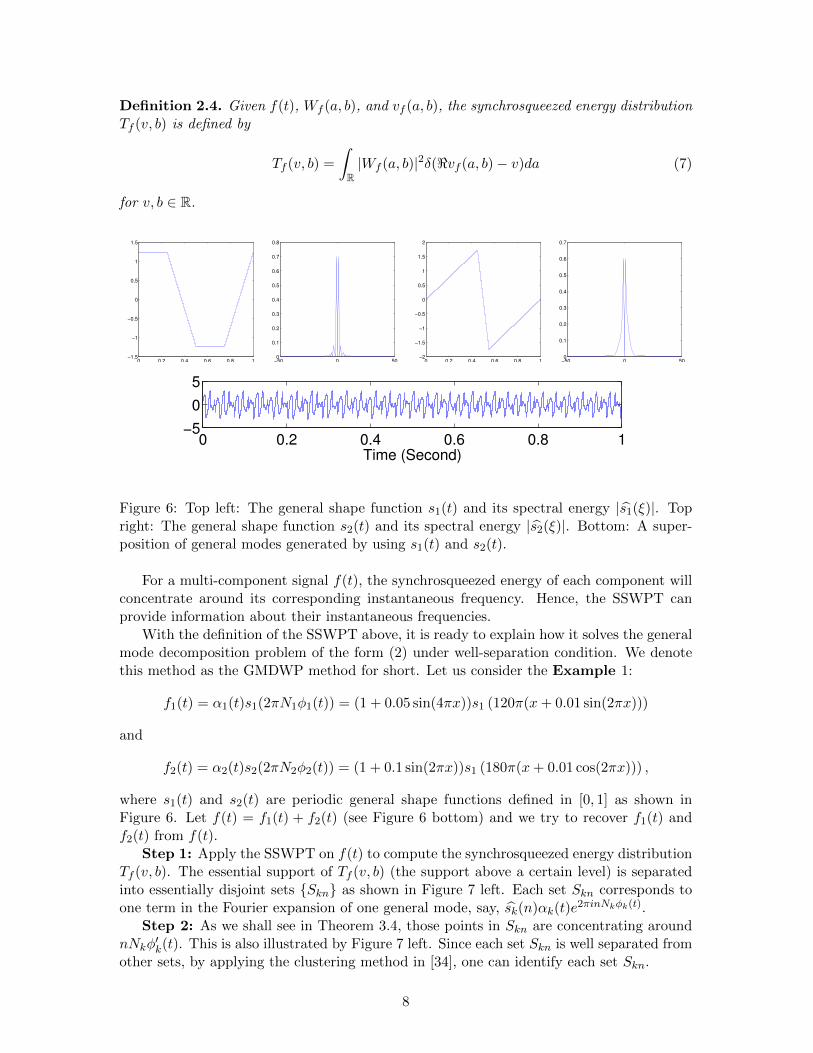
Figure 6: Top left: The general shape function s1(t) and its spectral energy |s1(ξ)|. Topright: The general shape function s2(t) and its spectral energy |s2(ξ)|. Bottom: A super-position of general modes generated by using s1(t) and s2(t).
For a multi-component signal f(t), the synchrosqueezed energy of each component willconcentrate around its corresponding instantaneous frequency. Hence, the SSWPT canprovide information about their instantaneous frequencies.
With the definition of the SSWPT above, it is ready to explain how it solves the generalmode decomposition problem of the form (2) under well-separation condition. We denotethis method as the GMDWP method for short. Let us consider the Example 1:
f1(t) = α1(t)s1(2πN1φ1(t)) = (1 + 0.05 sin(4πx))s1 (120π(x+ 0.01 sin(2πx)))
and
f2(t) = α2(t)s2(2πN2φ2(t)) = (1 + 0.1 sin(2πx))s1 (180π(x+ 0.01 cos(2πx))) ,
where s1(t) and s2(t) are periodic general shape functions defined in [0, 1] as shown inFigure 6. Let f(t) = f1(t) + f2(t) (see Figure 6 bottom) and we try to recover f1(t) andf2(t) from f(t).
Step 1: Apply the SSWPT on f(t) to compute the synchrosqueezed energy distributionTf (v, b). The essential support of Tf (v, b) (the support above a certain level) is separatedinto essentially disjoint sets Skn as shown in Figure 7 left. Each set Skn corresponds toone term in the Fourier expansion of one general mode, say, sk(n)αk(t)e
2πinNkφk(t).Step 2: As we shall see in Theorem 3.4, those points in Skn are concentrating around
nNkφ′k(t). This is also illustrated by Figure 7 left. Since each set Skn is well separated from
other sets, by applying the clustering method in [34], one can identify each set Skn.
8
Time (Second)
Fre
quency (
Hz)
0 0.2 0.4 0.6 0.8 10
100
200
300
400
500
600
0 0.2 0.4 0.6 0.8 10
100
200
300
400
500
600
Time (Second)
Fre
qu
en
cy (
Hz)
0 0.2 0.4 0.6 0.8 155
60
65
70
75
80
85
90
95
100
Time (Second)
Fre
qu
en
cy (
Hz)
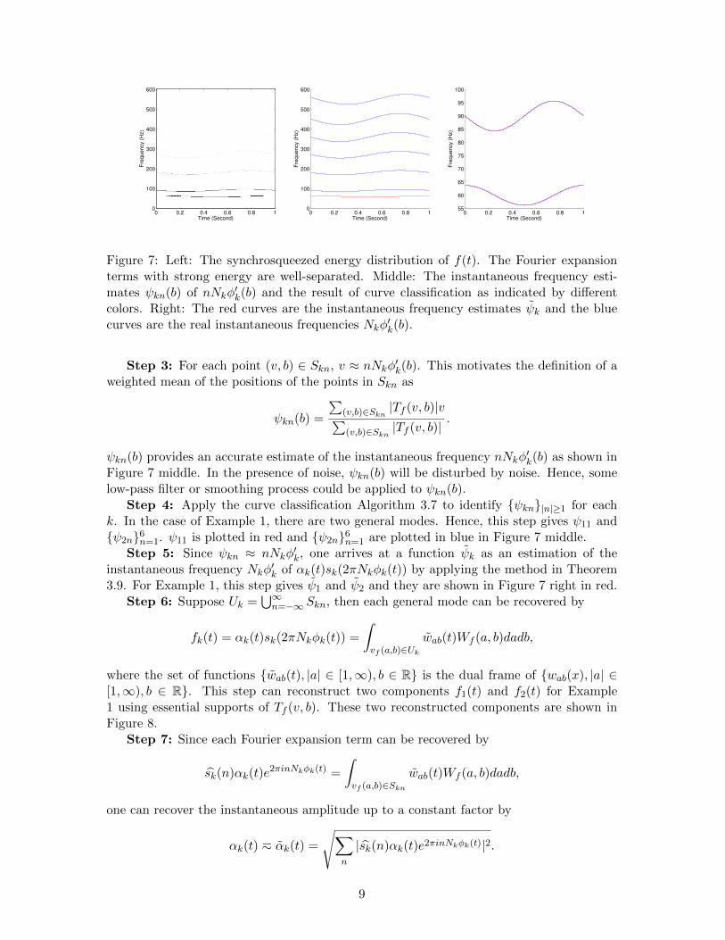
Figure 7: Left: The synchrosqueezed energy distribution of f(t). The Fourier expansionterms with strong energy are well-separated. Middle: The instantaneous frequency esti-mates ψkn(b) of nNkφ
′k(b) and the result of curve classification as indicated by different
colors. Right: The red curves are the instantaneous frequency estimates ψk and the bluecurves are the real instantaneous frequencies Nkφ
′k(b).
Step 3: For each point (v, b) ∈ Skn, v ≈ nNkφ′k(b). This motivates the definition of a
weighted mean of the positions of the points in Skn as
ψkn(b) =
∑(v,b)∈Skn |Tf (v, b)|v∑(v,b)∈Skn |Tf (v, b)|
.
ψkn(b) provides an accurate estimate of the instantaneous frequency nNkφ′k(b) as shown in
Figure 7 middle. In the presence of noise, ψkn(b) will be disturbed by noise. Hence, somelow-pass filter or smoothing process could be applied to ψkn(b).
Step 4: Apply the curve classification Algorithm 3.7 to identify ψkn|n|≥1 for eachk. In the case of Example 1, there are two general modes. Hence, this step gives ψ11 andψ2n6n=1. ψ11 is plotted in red and ψ2n6n=1 are plotted in blue in Figure 7 middle.
Step 5: Since ψkn ≈ nNkφ′k, one arrives at a function ψk as an estimation of the
instantaneous frequency Nkφ′k of αk(t)sk(2πNkφk(t)) by applying the method in Theorem
3.9. For Example 1, this step gives ψ1 and ψ2 and they are shown in Figure 7 right in red.Step 6: Suppose Uk =
⋃∞n=−∞ Skn, then each general mode can be recovered by
fk(t) = αk(t)sk(2πNkφk(t)) =
∫vf (a,b)∈Uk
wab(t)Wf (a, b)dadb,
where the set of functions wab(t), |a| ∈ [1,∞), b ∈ R is the dual frame of wab(x), |a| ∈[1,∞), b ∈ R. This step can reconstruct two components f1(t) and f2(t) for Example1 using essential supports of Tf (v, b). These two reconstructed components are shown inFigure 8.
Step 7: Since each Fourier expansion term can be recovered by
sk(n)αk(t)e2πinNkφk(t) =
∫vf (a,b)∈Skn
wab(t)Wf (a, b)dadb,
one can recover the instantaneous amplitude up to a constant factor by
αk(t) h αk(t) =
√∑n
|sk(n)αk(t)e2πinNkφk(t)|2.
9
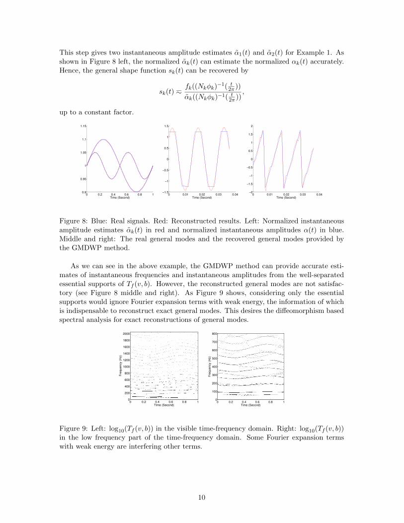
This step gives two instantaneous amplitude estimates α1(t) and α2(t) for Example 1. Asshown in Figure 8 left, the normalized αk(t) can estimate the normalized αk(t) accurately.Hence, the general shape function sk(t) can be recovered by
sk(t) hfk((Nkφk)
−1( t2π ))
αk((Nkφk)−1( t2π ))
,
up to a constant factor.
0 0.2 0.4 0.6 0.8 10.9
0.95
1
1.05
1.1
1.15
Time (Second)0 0.01 0.02 0.03 0.04
−1.5
−1
−0.5
0
0.5
1
1.5
Time (Second)0 0.01 0.02 0.03 0.04
−2
−1.5
−1
−0.5
0
0.5
1
1.5
2
Time (Second)
Figure 8: Blue: Real signals. Red: Reconstructed results. Left: Normalized instantaneousamplitude estimates αk(t) in red and normalized instantaneous amplitudes α(t) in blue.Middle and right: The real general modes and the recovered general modes provided bythe GMDWP method.
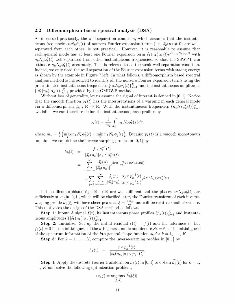
As we can see in the above example, the GMDWP method can provide accurate esti-mates of instantaneous frequencies and instantaneous amplitudes from the well-separatedessential supports of Tf (v, b). However, the reconstructed general modes are not satisfac-tory (see Figure 8 middle and right). As Figure 9 shows, considering only the essentialsupports would ignore Fourier expansion terms with weak energy, the information of whichis indispensable to reconstruct exact general modes. This desires the diffeomorphism basedspectral analysis for exact reconstructions of general modes.
Time (Second)
Fre
qu
en
cy (
Hz)
0 0.2 0.4 0.6 0.8 10
200
400
600
800
1000
1200
1400
1600
1800
2000
Time (Second)
Fre
qu
en
cy (
Hz)
0 0.2 0.4 0.6 0.8 10
100
200
300
400
500
600
700
800
Figure 9: Left: log10(Tf (v, b)) in the visible time-frequency domain. Right: log10(Tf (v, b))in the low frequency part of the time-frequency domain. Some Fourier expansion termswith weak energy are interfering other terms.
10
2.2 Diffeomorphism based spectral analysis (DSA)
As discussed previously, the well-separation condition, which assumes that the instanta-neous frequencies nNkφ
′k(t) of nonzero Fourier expansion terms (i.e. sk(n) 6= 0) are well-
separated from each other, is not practical. However, it is reasonable to assume thateach general mode has at least one Fourier expansion term sk(nk)αk(t)e
2πinkNkφk(t) withnkNkφ
′k(t) well-separated from other instantaneous frequencies, so that the SSWPT can
estimate nkNkφ′k(t) accurately. This is referred to as the weak well-separation condition.
Indeed, we only need the well-separation of the Fourier expansion terms with strong energyas shown by the example in Figure 7 left. In what follows, a diffeomorphism based spectralanalysis method is introduced to identify all the nonzero Fourier expansion terms using thepre-estimated instantaneous frequencies nkNkφ
′k(t)Kk=1 and the instantaneous amplitudes
|sk(nk)|αk(t)Kk=1 provided by the GMDWP method.Without loss of generality, let us assume the signal of interest is defined in [0, 1]. Notice
that the smooth function φk(t) has the interpretations of a warping in each general modevia a diffeomorphism φk : R → R. With the instantaneous frequencies nkNkφ
′k(t)Kk=1
available, we can therefore define the instantaneous phase profiles by
pk(t) =1
mk
∫ t
0nkNkφ
′k(x)dx,
where mk = 12
(maxtnkNkφ
′k(t) + min
tnkNkφ
′k(t)
). Because pk(t) is a smooth monotonous
function, we can define the inverse-warping profiles in [0, 1] by
hk(t) =f p−1
k (t)
|sk(nk)|αk p−1k (t)
=∞∑
n=−∞
sk(n)
|sk(nk)|e
2πi(nmknk
t+nNkφk(0))
+∑j 6=k
∞∑n=−∞
sj(n)
|sk(nk)|αj p−1
k (t)
αk p−1k (t)
e2πinNjφjp−1k (t).
If the diffeomorphisms φk : R → R are well different and the phases 2πNkφk(t) aresufficiently steep in [0, 1], which will be clarified later, the Fourier transform of each inverse-
warping profile hk(ξ) will have sheer peaks at ξ = nmknk
and will be relative small elsewhere.This motivates the design of the DSA method as follows.
Step 1: Input: A signal f(t), its instantaneous phase profiles pk(t)Kk=1 and instanta-neous amplitudes |sk(nk)|αk(t)Kk=1.
Step 2: Initialize: Set up the initial residual r(t) = f(t) and the tolerance ε. Letfk(t) = 0 be the initial guess of the kth general mode and denote Sk = ∅ as the initial guessof the spectrum information of the kth general shape function sk for k = 1, . . . , K.
Step 3: For k = 1, . . . , K, compute the inverse-warping profiles in [0, 1] by
hk(t) =r p−1
k (t)
|sk(nk)|αk p−1k (t)
.
Step 4: Apply the discrete Fourier transform on hk(t) in [0, 1] to obtain hk(ξ) for k = 1,. . . , K and solve the following optimization problem,
(τ, j) = arg max(ξ,k)
|hk(ξ)|.
11
Then τ ≈ nmjnj
for some n such that sj(n) 6= 0.
Step 5: Let g(t) = e2πiτt. Warp the harmonic g(t) with the jth instantaneousphase profile pj(t) and multiply the warped harmonic by the jth instantaneous amplitude|sj(nj)|αj(t) to obtain
|sj(nj)|αj(t)g pj(t) ≈ |sj(nj)|αj(t)e2πi
nmjnj
pj(t)
= |sj(nj)|αj(t)e2πinNj(φj(t)−φj(0))
= |sj(nj)|e−2πinNjφj(0)αj(t)e2πinNjφj(t).
Step 6: Solve the L2 minimization problem for a complex factor β ∈ C such that
β = arg minβ∈C
‖r(t)− β|sj(nj)|αj(t)g pj(t)‖L2 .
Thenβ|sj(nj)|αj(t)g pj(t) ≈ sj(n)αj(t)e
2πinNjφj(t),
which implies
|β| = |sj(n)||sj(nj)|
.
Step 7: Update: Compute the new residual
r(t) = r(t)− β|sj(nj)|αj(t)g pj(t).
Update the jth recovered general mode
fj(t) = fj(t) + β|sj(nj)|αj(t)g pj(t),
and the jth spectrum information set
Sj = Sj ∪ (τ, |β|).
Step 8: If ‖r(t)‖L2 > ε, repeat step 3-7. Otherwise, stop iterating and export thegeneral mode estimates fk and the spectrum information Sk for k = 1, . . . , K.
Notice that for each pair (τ, |β|) ∈ Sk, (τ, |β|) ≈ (nmknk, |sk(n)||sk(nk)|) for some n such that
sk(n) 6= 0. For each k, let
dk(ξ) =
|β|, for ξ = τ such that (τ, β) ∈ Sk0, otherwise.
Then
|sk(n)| ≈ |sk(nk)|dk(mkn
nk)⇒ dk(ξ) ≈
1
|sk(nk)|
∣∣∣∣sk( nkmkξ)
∣∣∣∣ .Hence, dk(ξ) is an approximation of the spectral energy |sk(ξ)| up to a constant factor anda scaling.
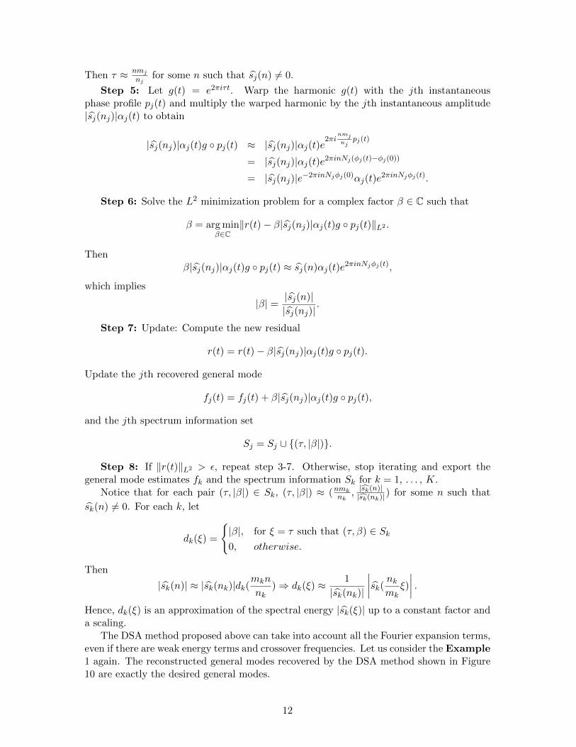
The DSA method proposed above can take into account all the Fourier expansion terms,even if there are weak energy terms and crossover frequencies. Let us consider the Example1 again. The reconstructed general modes recovered by the DSA method shown in Figure10 are exactly the desired general modes.
12
0 0.01 0.02 0.03 0.04−1.5
−1
−0.5
0
0.5
1
1.5
Time (Second)0 0.01 0.02 0.03 0.04
−2
−1.5
−1
−0.5
0
0.5
1
1.5
2
Time (Second)
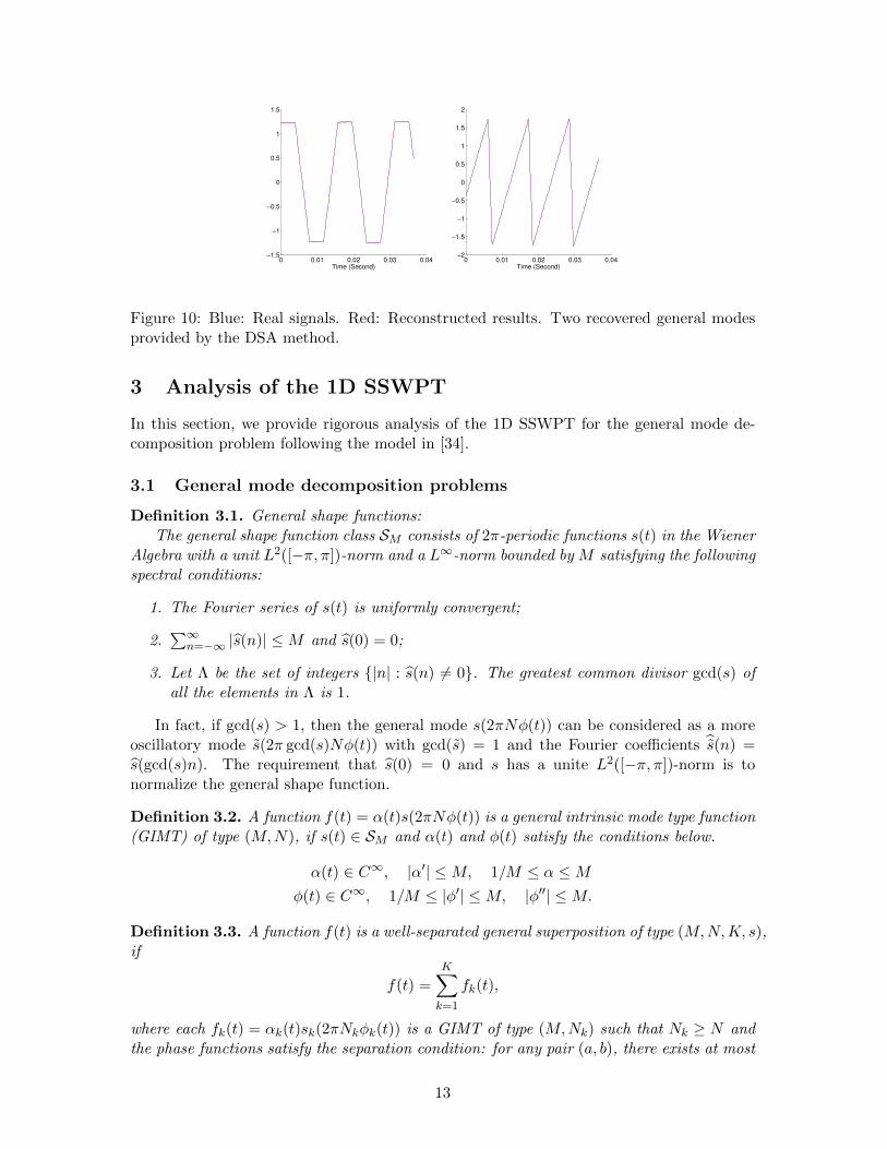
Figure 10: Blue: Real signals. Red: Reconstructed results. Two recovered general modesprovided by the DSA method.
3 Analysis of the 1D SSWPT
In this section, we provide rigorous analysis of the 1D SSWPT for the general mode de-composition problem following the model in [34].
3.1 General mode decomposition problems
Definition 3.1. General shape functions:The general shape function class SM consists of 2π-periodic functions s(t) in the Wiener
Algebra with a unit L2([−π, π])-norm and a L∞-norm bounded by M satisfying the followingspectral conditions:
1. The Fourier series of s(t) is uniformly convergent;
2.∑∞
n=−∞ |s(n)| ≤M and s(0) = 0;
3. Let Λ be the set of integers |n| : s(n) 6= 0. The greatest common divisor gcd(s) ofall the elements in Λ is 1.
In fact, if gcd(s) > 1, then the general mode s(2πNφ(t)) can be considered as a moreoscillatory mode s(2π gcd(s)Nφ(t)) with gcd(s) = 1 and the Fourier coefficients s(n) =s(gcd(s)n). The requirement that s(0) = 0 and s has a unite L2([−π, π])-norm is tonormalize the general shape function.
Definition 3.2. A function f(t) = α(t)s(2πNφ(t)) is a general intrinsic mode type function(GIMT) of type (M,N), if s(t) ∈ SM and α(t) and φ(t) satisfy the conditions below.
α(t) ∈ C∞, |α′| ≤M, 1/M ≤ α ≤Mφ(t) ∈ C∞, 1/M ≤ |φ′| ≤M, |φ′′| ≤M.
Definition 3.3. A function f(t) is a well-separated general superposition of type (M,N,K, s),if
f(t) =K∑k=1
fk(t),
where each fk(t) = αk(t)sk(2πNkφk(t)) is a GIMT of type (M,Nk) such that Nk ≥ N andthe phase functions satisfy the separation condition: for any pair (a, b), there exists at most
13
one pair (n, k) such that sk(n) 6= 0 and that
|a|−s|a− nNkφ′k(b)| < d.
We denote by GF (M,N,K, s) the set of all such functions.
Notice that the mode decomposition problem of the form (1) is a special case of thegeneral mode decomposition problem of the form (2). We therefore only analyze the 1DSSWPT for the general mode decomposition problem. Besides, the components are notnecessarily defined in the whole domain R, because the synchrosqueezed transforms arelocalized so as to capture the non-linear, non-stationary features of signals as illustrated in[3, 34]. For the sake of convenience, we omit the discussion of the data segments.
3.2 Instantaneous frequency estimates
With the definitions above, we are ready to present the theorems for the 1D SSWPT witha geometric scaling parameter s ∈ (1/2, 1). The estimates of the instantaneous frequenciesNkφ
′k(t)Kk=1 rely on Theorem 3.4, Algorithm 3.7, and Theorem 3.9 below.
Theorem 3.4. For a function f(t) and ε > 0, we define
Rε = (a, b) : |Wf (a, b)| ≥ |a|−s/2√ε
andZn,k = (a, b) : |a− nNkφ
′k(b)| ≤ d|a|s
for 1 ≤ k ≤ K and |n| ≥ 1. For fixed M and K, for any ε > 0, there exists a constantN0(M,K, s, ε) > 0 such that for any N > N0(M,K, s, ε) and f(t) ∈ GF (M,N,K, s) thefollowing statements hold.
(i) Zn,k : 1 ≤ k ≤ K, sk(n) 6= 0 are disjoint and Rε ⊂⋃
1≤k≤K⋃sk(n)6=0 Zn,k;
(ii) For any (a, b) ∈ Rε ∩ Zn,k,
|vf (a, b)− nNkφ′k(b)|
|nNkφ′k(b)|
.√ε.
The proof of Theorem 3.4 relies on two lemmas as follows to estimate the asymptoticbehavior of Wf (a, b) and ∂bWf (a, b) as N going to infinity. In what follows, when we writeO(·), ., or &, the implicit constants may depend on M and K.
Lemma 3.5. Suppose Ωa = (k, n) : a ∈ [nNk2M , 2MnNk]. Under the assumption of Theo-rem 3.4, for any ε > 0, we have
Wf (a, b) = |a|−s/2 ∑
(k,n)∈Ωa
sk(n)αk(b)e2πinNkφk(b)w
((a− nNkφ
′k(b)
)|a|−s
)+O(ε)
,
when N is sufficiently large.
14
Proof. Without loss of generality, we can simply assume Nk = N for all k and only provethe case for a > 1. Because w(t) decays rapidly, the wave packet transform Wf (a, b) iswell defined. By the uniform convergence of the Fourier series of sk(t) and the change ofvariables, we have
Wf (a, b) =
∫R
K∑k=1
αk(t)sk(2πNφk(t))as/2w(as(t− b))e−2πi(t−b)adt
= a−s/2K∑k=1
∑|n|≥1
sk(n)
∫Rαk(a
−sx+ b)w(x)e2πi(nNφk(a−sx+b)−a1−sx)dx.
Let us estimate Ikn = sk(n)∫R αk(a
−sx + b)w(x)e2πi(nNφk(a−sx+b)−a1−sx)dx. Let h(x) =sk(n)αk(a
−sx+ b)w(x) and g(x) = 2π(nNφk(a−sx+ b)− a1−sx), then
Ikn =
∫Rh(x)eig(x)dx,
andg′(x) = 2πa−s(nNφ′k(a
−sx+ b)− a).
If a < nN2M , then |g′(x)| & a−snN & (nN)1−s. If a > 2MnN , then |g′(x)| & a1−s & (nN)1−s.
So, if a /∈ [nN2M , 2MnN ], then |g′(x)| & (nN)1−s. For real smooth functions g(x), we definethe differential operator
L =1
i
∂xg′.
Because h(x) decays sufficiently fast at infinity, we perform integration by parts r times toget ∫
Rheigdx =
∫Rh(Lreig)dx =
∫R
((L∗)rh) eigdx,
where L∗ is the adjoint of L. A few algebraic calculation shows that L∗ contributes a factorof order 1
|g′| .1
(nN)1−s if a /∈ [nN2M , 2MnN ], and we therefore have
|Ikn| =∣∣∣∣∫
Reig ((L∗)rh) dx
∣∣∣∣ . |sk(n)|(nN)−(1−s)r . |sk(n)|ε.
Since s < 1 and∑∞
n=−∞ |sk(n)| ≤M , if N & ε−1
(1−s)r , then
a−s/2∑
(k,n)/∈Ωa
Ikn . a−s/2∑
(k,n)/∈Ωa
|sk(n)|O(ε) . a−s/2O(ε). (8)
Now let us estimate Ikn when a ∈ [nN2M , 2MnN ]. Recall that
Ikn = sk(n)
∫Rαk(a
−sx+ b)w(x)e2πi(nNφk(a−sx+b)−a1−sx)dx.
By Taylor expansion,αk(a
−sx+ b) = αk(b) + α′k(b∗)a−sx
and
φk(a−sx+ b) = φk(b) + φ′k(b)a
−sx+1
2φ′′k(b
∗∗)a−2sx2
15
for some b∗ and b∗∗. Notice that, if N & ε−1/s, then
|Ikn − sk(n)αk(b)
∫Rw(x)e2πi(nNφk(a−sx+b)−a1−sx)dx|
. |sk(n)|α′k(b∗)a−s∫R|x||w(x)|dx
. |sk(n)|O(ε).
This implies that
Ikn =
(sk(n)αk(b)
∫Rw(x)e2πi(nNφk(a−sx+b)−a1−sx)dx+ |sk(n)|O(ε)
)for a ∈ [nN2M , 2MnN ] and N & ε−1/s. Since |eix − 1| ≤ |x|, if N & ε−1/(2s−1), then we have
|Ikn − sk(n)αk(b)
∫Rw(x)e2πi(nNφk(b)+nNφ′k(b)a−sx−a1−sx)dx|
. |sk(n)|(O(ε) +
∣∣∣∣αk(b) ∫Rw(x)e2πi(nNφk(b)+nNφ′k(b)a−sx−a1−sx)
(e2πinN 1
2φ′′k(b∗∗)a−2sx2 − 1
)dx
∣∣∣∣). |sk(n)|
(O(ε) + nNa−2s
∫Rx2|w(x)|dx
). |sk(n)|O(ε).
Hence, it holds that
Ikn =(sk(n)αk(b)e
2πinNφk(b)w((a− nNφ′k(b))a−s
)+ |sk(n)|O(ε)
), (9)
if a ∈ [nN2M , 2MnN ] and N & maxε−1/s, ε−1/(2s−1) = ε−1/(2s−1).In sum, by (8) and (9), we arrive at
Wf (a, b) = a−s/2
∑(k,n)∈Ωa
Ikn +∑
(k,n)/∈Ωa
Ikn
= |a|−s/2
∑(k,n)∈Ωa
sk(n)αk(b)e2πinNφk(b)w
((a− nNφ′k(b)
)|a|−s
)+O(ε)
,
if N & maxε−1
(1−s)r , ε−1
2s−1 .Similar argument can prove the above conclusion for a < −1 and it is simple to generalize
it for different Nk to complete the proof.
The next lemma is to estimate ∂bWf (a, b) when Ωa = (k, n) : a ∈ [nNk2M , 2MnNk] isnot empty, i.e., when Wf (a, b) is relevant.
Lemma 3.6. Suppose Ωa = (k, n) : a ∈ [nNk2M , 2MnNk] is not empty. Under the assump-tion of Theorem 3.4, for any ε > 0, we have
∂bWf (a, b)
= |a|−s/2 ∑
(k,n)∈Ωa
2πinNksk(n)αk(b)φ′k(b)e
2πinNkφk(b)w((a− nNkφ
′k(b)
)|a|−s
)+ |a|O(ε)
,
when N is sufficiently large.
16
Proof. Similar to the proof of Lemma 3.5, we can assume Nk = N for all k and only needto prove the case when a > 1. By the definition of the wave packet transform, we have
∂bWf (a, b) =K∑k=1
2πia1+s/2
∫Rαk(t)sk(2πNφk(t))w(as(t− b))e−2πi(t−b)adt
−K∑k=1
a3s/2
∫Rαk(t)sk(2πNφk(t))w
′(as(t− b))e−2πi(t−b)adt.
Denote the first term by T1 and the second term by T2. By a similar discussion in the proofof Lemma 3.5, we have the following asymptotic estimates when N is sufficiently large.
T2 = −as/2K∑k=1
∑|n|≥1
sk(n)
∫Rαk(a
−sx+ b)w′(x)e2πi(nNφk(a−sx+b)−a1−sx)dx
= −as/2∑
(k,n)∈Ωa
∫Rsk(n)αk(a
−sx+ b)w′(x)e2πi(nNφk(a−sx+b)−a1−sx)dx+ as/2O(ε)
= as/2∑
(k,n)∈Ωa
∫Rsk(n)w(x)αk(a
−sx+ b)e2πi(nNφk(a−sx+b)−a1−sx)
(2πinNφ′k(a
−sx+ b)a−s − 2πia1−s) dx+ a−s/2∑
(k,n)∈Ωa
∫Rsk(n)w(x)
α′k(a−sx+ b)e2πi(nNφk(a−sx+b)−a1−s)dx+ as/2O(ε)
= a−s/2∑
(k,n)∈Ωa
2πinN
∫Rsk(n)φ′k(a
−sx+ b)αk(a−sx+ b)w(x)e2πi(nNφk(a−sx+b)−a1−sx)dx
−a1−s/2∑
(k,n)∈Ωa
2πi
∫Rsk(n)w(x)αk(a
−sx+ b)e2πi(nNφk(a−sx+b)−a1−sx)dx
+a−s/2O(1) + as/2O(ε)
= a−s/2∑
(k,n)∈Ωa
2πinN(sk(n)φ′k(b)αk(b)e
2πinNφk(b)w(a−s(a− nNφ′k(b))) + |sk(n)|O(ε))
−a1+s/2∑
(k,n)∈Ωa
sk(n)2πi
∫Rαk(t)w(as(t− b))e2πi(nNφk(t)−(t−b)a)dt
+a−s/2O(1) + as/2O(ε),
if N & maxε−1
(1−s)r , ε−1
2s−1 . The third equality holds by integration by parts and the lastequality holds by changing variables. Notice that
T1 = a1+s/2∑
(k,n)∈Ωa
sk(n)2πi
∫Rαk(t)w(as(t− b))e2πi(nNφk(t)−(t−b)a)dt
+∑
(k,n)/∈Ωa
2πia1−s/2sk(n)
∫Rαk(a
−sx+ b)w(x)e2πi(nNφk(a−sx+b)−a1−sx)dx
= a1+s/2∑
(k,n)∈Ωa
sk(n)2πi
∫Rαk(t)w(as(t− b))e2πi(nNφk(t)−(t−b)a)dt+ a1−s/2O(ε),
17
if N & ε−1
(1−s)r for any r >= 1. Hence T1 + T2 results in
∂bWf (a, b)
= a−s/2∑
(k,n)∈Ωa
2πinN(sk(n)φ′k(b)αk(b)e
2πinNφk(b)w(a−s(a− nNφ′k(b))) + |sk(n)|O(ε))
+a−s/2O(1) + as/2O(ε) + a1−s/2O(ε)
= |a|−s/2 ∑
(k,n)∈Ωa
2πinNsk(n)αk(b)φ′k(b)e
2πinNφk(b)w((a− nNφ′k(b)
)|a|−s
)+ |a|O(ε)
,
if N is sufficiently large. So, the Lemma 3.6 is proved.
We are now ready to prove Theorem 3.4 with Lemma 3.5 and Lemma 3.6.
Proof. Let us first consider (i). The well-separation condition implies that Zn,k : 1 ≤ k ≤K, sk(n) 6= 0 are disjoint. Let (a, b) be a point in Rε, then |Wf (a, b)| ≥ a−s/2
√ε, which
means that Ωa is not empty and ∃(k, n) ∈ Ωa such that w((a−nNkφ′k(b))a
−s) 6= 0. Becausethe support of w(ξ) is (−d, d), we know |a − nNkφ
′k(b)| ≤ asd, i.e., (a, b) ∈ Zn,k. Hence,
Rε ⊂⋃
1≤k≤K⋃sk(n)6=0 Zn,k.
To show (ii), let us recall that vf (a, b) is defined as
vf (a, b) =∂bWf (a, b)
2πiWf (a, b),
for Wf (a, b) 6= 0. If (a, b) ∈ Rε⋂Zn,k, then by Lemma 3.5
Wf (a, b) = |a|−s/2 ∑
(k,n)∈Ωa
sk(n)αk(b)e2πinNkφk(b)w
((a− nNkφ
′k(b)
)|a|−s
)+O(ε)
= |a|−s/2
(sk(n)αk(b)e
2πinNkφk(b)w((a− nNkφ
′k(b)
)|a|−s
)+O(ε)
),
as the other terms drop out, since Zn,k are disjoint. Similarly, by Lemma 3.6
∂bWf (a, b)
= |a|−s/2(
2πinNksk(n)αk(b)φ′k(b)e
2πinNkφk(b)w((a− nNkφ
′k(b)
)|a|−s
)+ |a|O(ε)
).
Let g denote the term sk(n)αk(b)e2πinNkφk(b)w ((a− nNkφ
′k(b)) |a|−s), then
vf (a, b) =nNkφ
′k(b)g + |a|O(ε)
g +O(ε)
=nNkφ
′k(b)(g +O(ε))
g +O(ε),
since a ∈ [nNk2M , 2MnNk]. Because |Wf (a, b)| ≥ a−s/2√ε for (a, b) ∈ Rε, then |g| &
√ε.
Therefore|vf (a, b)− nNkφ
′k(b)|
|nNkφ′k(b)|
.
∣∣∣∣ O(ε)
g +O(ε)
∣∣∣∣ . √ε.
18
Theorem 3.4 shows that the instantaneous frequency information function vf (a, b) canestimate nNkφ
′k(t) accurately for a class of superpositions of general mode functions if their
phases are sufficiently steep. This guarantees the well concentration of the synchrosqueezedenergy distribution Tf (v, b) around nNkφ
′k(t). Hence, ψkn(b) defined in the introduction
of the GMDWP method is an accurate estimate of nNkφ′k(b). Next, a curve classification
method and an instantaneous frequency identification method are introduced below.Let us reindex the functions ψkn : 1 ≤ k ≤ K, |n| ≥ 1 by ψj1≤j≤L. Our goal is
to obtain K index sets Λk1≤k≤K such that ψkn|n|≥1 = ψjj∈Λk . Becauseψkn1ψkn2
≈ n1n2
,
ψkn|n|≥1 can approximately be considered as a set in a one dimensional point set in ahigh dimensional space. Hence, the curve classification can be considered as a subspaceclustering problem studied in [22, 23]. This motivates the following method to classifyψj1≤j≤L. This method is similar to the method in [22] for subspace clustering.
Algorithm 3.7. Curve classification of ψj1≤j≤L1: For each pair (k, j) with k 6= j, let mk = ‖ψk‖L∞ and mj = ‖ψj‖L∞. Compute the
linear regression ofψkmjψjmk
and its residual rkj. Let R be the L × L matrix such that
Rkj = rkj.
2: Set up a variance parameter σ2 and define a Gaussian function g(x) = e−x2
2σ2 .3: Form the affinity graph G with nodes representing the L instantaneous frequencies and
edge weights given by g(Rkj) + g(Rjk).4: Compute the eighenvalues of the normalized Laplacian of G and sort them in descending
order σ1 ≥ σ2 ≥ · · · ≥ σL. Let
K = L− arg maxi=1,··· ,L−1
(σi − σi+1) .
5: Apply the spectral clustering method proposed in [19] and used in [34] to the affinitygraph using K as the number of curve class to divide the index set 1, . . . , L into Ksubsets Λk1≤k≤K .
6: Associate each index set Λk with a class of curves ψjj∈Λk .
If φ′k(t)1≤k≤K are not very similar, then the residual of the linear regression ofφ′k(t)
φ′j(t)
is large for k 6= j. By setting up a proper parameter σ, Algorithm 3.7 can classify ψkn :1 ≤ k ≤ K, |n| ≥ 1 accurately with high probability. In the case in which instantaneousfrequencies are disturbed by noise, robust subspace clustering techniques in [23] can beapplied.
Algorithm 3.7 results in K classes of curves ψjj∈Λk = ψkn|n|≥1 ≈ nNkφ′k|n|≥1
for 1 ≤ k ≤ K. The theorems below show how to estimate the instantaneous frequencyNkφ
′k(t) of the general mode αk(t)sk(2πNkφk(t)).
Theorem 3.8. Suppose α(t)s(2πN0φ(t)) is a general intrinsic mode function of type (M0, N0)and s(t) has some nonzero Fourier coefficients s(ni)1≤i≤N such that s(n) = 0 for n < |n1|and gcd(|n1|, . . . , |nN |) = 1. If we know ψi(t) = niN0φ
′(t) for 1 ≤ i ≤ N and
n0 = min
n : 1 ≤ n ≤M,
nψi(t)
ψ1(t)is a constant integer for 2 ≤ i ≤ N
, (10)
where M = M0 min |ψ1(t)|, then the instantaneous frequency N0φ′(t) of α(t)s(2πN0φ(t)) is
|ψ1(t)|n0
.
19
Proof.
nψi(t)
ψ1(t)is a constant integer for 2 ≤ i ≤ N ⇒ nni
n1is an integer for 2 ≤ i ≤ N
⇒ n1
gcd(n, n1)
∣∣ni for 2 ≤ i ≤ N ⇒ n1
gcd(n, n1)
∣∣ gcd(n2, . . . , nN )
⇒ gcd(n, n1) = n1 ⇒ n = k|n1| for some integer k ≥ 1.
Hence, |n1| = minn : 1 ≤ n ≤M, nψi(t)ψ1(t) is a constant integer for 2 ≤ i ≤ N
= n0, which
implies N0φ′(t) = |ψ1(t)|
n0.
Determining whether nψi(t)ψ1(t) is a constant integer is not practical unless the instantaneous
frequencies are exactly recovered. This motivates the design of the following method.
Theorem 3.9. Suppose the same condition of Theorem 3.8 holds and n0 is the solution ofthe following minimization problem,
n0 = min
(arg min1≤n≤M
1
N − 1
N∑i=2
‖nψi(t)ψ1(t)
− bnψi(t)ψ1(t)
+ 0.5c‖2L2
), (11)
where M = M0 min |ψ1(t)|. Then the instantaneous frequency N0φ′(t) of s(2πN0φ(t)) is
|ψ1(t)|n0
.
Proof. Let f(n) = 1N−1
∑Ni=2 ‖
nψi(t)ψ1(t) − b
nψi(t)ψ1(t) + 0.5c‖2L2 . Notice that
nψi(t)
ψ1(t)− bnψi(t)
ψ1(t)+ 0.5c =
nnin1− bnni
n1+ 0.5c.
If n = k|n1| for some integer k ≥ 1, then f(n) = 0.Otherwise, then by the proof of Theorem 3.8, ∃i, 2 ≤ i ≤ N such that nni
n1is not an
integer. Then
‖nψi(t)ψ1(t)
− bnψi(t)ψ1(t)
+ 0.5c‖2L2 > 0,
which implies f(n) > 0. So, |n1| = min
(arg min1≤n≤M
f(n)
). Therefore, N0φ
′(t) = |ψ1(t)|n0
.
Notice that the function g(x) = |x − bx + 0.5c| is absolutely continuous. If ψi(t) ≈niN0φ
′(t) is sufficiently accurate, the conclusion of Theorem 3.9 is still true.For each k, Theorem 3.9 estimates the instantaneous frequency of the general mode
αk(t)sk(2πNkφk(t)) using the result of Theorem 3.4 and Algorithm 3.7. This completes theestimates of the instantaneous frequencies of the general modes from a superposition of theform (2).
3.3 The analysis of spectral resolution
In Theorem 3.4, the lower bound s > 1/2 ensures that the wave packets is sufficientlylocalized in space so that it can reflect the second order properties of the phase functionsprecisely. The upper bound s < 1 enables the SSWPT to detect a more general classof shape functions compared to the wave shape functions defined in [27]. An intuitive
20
reason for this more general result is that the supports of wave packets in the Fourierdomain are more localized than those of wavelets, resulting in a better resolution for modedecompositions. In what follows, the single scale resolution and the multiscale resolutionof synchrosqueezed transforms will be defined and studied.
Definition 3.10. The single scale resolution at a level N of a synchrosqueezed transform is1
Nλ0− 1N , where λ0 ∈ (0, 1) is the critical number such that ∀λ ∈ (0, λ0), the synchrosqueezed
transform is able to distinguish two modes f1(t) = e2πiNt and f2(t) = e2πiλNt from theirsuperposition f(t) = f1(t) + f2(t).
The single scale resolution analysis is related to the beating phenomenon of the EMDmethod in [21]. In [29], the authors have proved a conclusion which is equivalent to the factthat the single scale resolution at the level 1 of the SSWT with a mother wavelet supportedin an interval of size 2d is 2d
1−d . As we shall prove below, the SSWPT has a higher singlescale resolution than the SSWT and a smaller geometric scale parameter s benefits a higherresolution. This means that the SSWPT has a better ability to distinguish two harmonicswith close frequencies.
Recall that the wave packet transform is controlled by the geometric parameter s andthe parameter d for the size of the support of the mother wave packet in the Fourier domain.Consider two complex harmonics f1(t) = e2πiNt, f2(t) = e2πiλNt, and their superpositionf(t) = f1(t) + f2(t). Then the wave packet transform of f is
Wf (a, b) = |a|−s/2e2πiNbw(|a|−s(a−N)) + |a|−s/2e2πiNλbw(|a|−s(a−Nλ)),
and the instantaneous frequency information function is
vf (a, b) =N(e2πiNbw(|a|−s(a−N)) + λe2πiNλbw(|a|−s(a−Nλ))
)e2πiNbw(|a|−s(a−N)) + e2πiNλbw(|a|−s(a−Nλ))
.
The necessary and sufficient condition of an exact decomposition by the SSWPT is vf (a, b) =N in Zf1 = (a, b) : Wf1(a, b) 6= 0 and vf (a, b) = Nλ in Zf2 = (a, b) : Wf2(a, b) 6= 0.This is equivalent to say Zf1 and Zf2 are disjoint. Since
Wf1(a, b) = |a|−s/2e2πiNbw(|a|−s(a−N)),
Wf2(a, b) = |a|−s/2e2πiNλbw(|a|−s(a−Nλ)),
and the support of w(ξ) is (−d, d), the condition for Zf1 and Zf2 being disjoint is that thesupports of the wave packets wNλb and wNb are disjoint for all b, i.e., w(|Nλ|−s(x−Nλ))and w(|N |−s(x − N)) have non-overlapping supports. So, the critical number λ0 of theSSWPT with a geometric scaling parameter s is the solution of the following equations:
N − a1 = d|a1|s,a2 −Nλ0 = d|a2|s,
a1 = a2,
where N and d are known. When s = 1, the solution is λ0 = 1−d1+d , which accords with the
result in [29]. Let a1 = a2 = a, then we have λ0 = 2a−NN . Notice that λ0 is increasing,
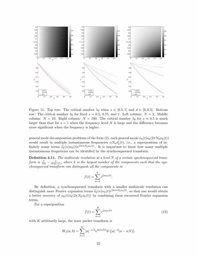
when s is decreasing (see Figure 11). Therefore, a smaller s benefits a higher single scaleresolution, especially for high frequency signals.
For the mode decomposition problems of the form (1), the single scale resolution isenough to quantify the resolution of a certain synchrosqueezed transform. However, for the
21
d
s
0 0.1 0.2 0.3 0.4 0.5
0.5
0.55
0.6
0.65
0.7
0.75
0.8
0.85
0.9
0.95
1
0.4
0.5
0.6
0.7
0.8
0.9
d
s
0 0.1 0.2 0.3 0.4 0.5
0.5
0.55
0.6
0.65
0.7
0.75
0.8
0.85
0.9
0.95
1
0.4
0.5
0.6
0.7
0.8
0.9
d
s
0 0.1 0.2 0.3 0.4 0.5
0.5
0.55
0.6
0.65
0.7
0.75
0.8
0.85
0.9
0.95
1
0.4
0.5
0.6
0.7
0.8
0.9
0 0.1 0.2 0.3 0.4 0.5
0.4
0.5
0.6
0.7
0.8
0.9
1
d
λ0
s=0.5
s=0.75
s=1
0 0.1 0.2 0.3 0.4 0.5
0.4
0.5
0.6
0.7
0.8
0.9
1
d
λ0
s=0.5
s=0.75
s=1
0 0.1 0.2 0.3 0.4 0.5
0.4
0.5
0.6
0.7
0.8
0.9
1
d
λ0
s=0.5
s=0.75
s=1
Figure 11: Top row: The critical number λ0 when s ∈ [0.5, 1] and d ∈ [0, 0.5]. Bottomrow: The critical number λ0 for fixed s = 0.5, 0.75, and 1. Left column: N = 2. Middlecolumn: N = 10. Right column: N = 100. The critical number λ0 for s ≈ 0.5 is muchlarger than that for s = 1 when the frequency level N is large and the difference becomesmore significant when the frequency is higher.
general mode decomposition problems of the form (2), each general mode αk(t)sk(2πNkφk(t))would result in multiple instantaneous frequencies nNkφ
′k(t), i.e., a superposition of in-
finitely many terms sk(n)αk(t)e2πinNkφk(t). It is important to know how many multiple
instantaneous frequencies can be identified by the synchrosqueezed transform.
Definition 3.11. The multiscale resolution at a level N of a certain synchrosqueezed trans-form is 1
Nk −1
N(k+1) , where k is the largest number of the components such that the syn-chrosqueezed transform can distinguish all the components in
f(t) =
k∑n=1
e2πinNt.
By definition, a synchrosqueezed transform with a smaller multiscale resolution candistinguish more Fourier expansion terms sk(n)αk(t)e
2πinNkφk(t), so that one would obtaina better recovery of αk(t)sk(2πNkφk(t)) by combining these recovered Fourier expansionterms.
For a superposition
f(t) =K∑n=1
e2πinNt (12)
with K arbitrarily large, the wave packet transform is
Wf (a, b) =K∑n=1
|a|−s/2e2πinNbw(|a|−2(a− nN)
)22
and the instantaneous frequency information function is
vf (a, b) =N∑K
n=1 ne2πinNbw (|a|−s(a− nN))∑K
n=1 e2πinNbw (|a|−s(a− nN))
.
Each term w (|a|−s(a− nN)) is supported in Zn = a : |a − nN | < d|a|s centered ata = nN . Similar to previous discussions, an exact recovery of the nth term is equivalentto Zn−1
⋂Zn = ∅ and Zn
⋂Zn+1 = ∅. Since the size of the interval Zn is monotonously
increasing as n increases and the space between their centers is fixed, one should identifyn0, the greatest n such that Zn
⋂Zn+1 = ∅, i.e., n0 = maxn ∈ Z+ : nN < a0, where
a0 =(N2d
)1/sis a solution of the following equations,
(n+ 1)N − a = d|a|s,a− nN = d|a|s.
Hence, n0 = b N1s−1
(2d)1/sc. Therefore, the multiscale resolution at the level N of the SSWPT
with a scaling parameter s and a mother wave packet supported in (−d, d) is
1
(n0 − 1)N− 1
n0N=
1
N(b N1s−1
(2d)1/sc − 1)b N
1s−1
(2d)1/sc≈ O(N1−2/s).
Notice that the synchrosqueezed wavelet transform (i.e., s = 1) can only distinguishO(1) terms in (12). This limits its application to general mode decompositions of the
form (2). However, the SSWPT is able to identify O(N1s−1) terms exactly in (12). This
motivates its application to the general mode decomposition problems of the form (2).Concrete examples will be presented to support this argument in Section 5.
4 Theory for the diffeomorphism based spectral analysis (DSA)
The analysis of the DSA method essentially consists of two main theorems. Theorem4.2 proves that the 1D SSWPT is able to provide accurate input instantaneous frequencyestimates if the weak well-separation condition defined below holds. Then Theorem 4.5proves that Step 4, the key idea of the DSA method, can provide precise spectral analysisfor general shape functions, if their corresponding phase functions are well-different andsteep enough. We omit the proof of the other steps in the DSA method to save space.
Definition 4.1. A function f(t) is a weak well-separated general superposition of type(M,N,K, s) if
f(t) =K∑k=1
fk(t)
where each fk(t) = αk(t)sk(2πNkφk(t)) is a GIMT of type (M,Nk) such that Nk ≥ N andthe phase functions satisfy the following weak well-separation conditions.
1. SupposeZnk =
(a, b) : |a− nNkφ
′k(b)| ≤ d|a|s
.
For each k, there exists nk such that sk(nk) 6= 0 and Znkk ∩ Znj = ∅ for all pairs(n, j) 6= (nk, k) and sj(n) 6= 0.
23
2. ∃K0 < ∞ such that ∀a ∈ R and ∀b ∈ R there exists at most K0 pairs of (n, k) suchthat (a, b) ∈ Znk.
We denote by wGF (M,N,K0,K, s) the set of all such functions. Note that wGF (M,N, 1,K, s) =GF (M,N,K, s).
In what follows, when we write O(·), ., or &, the implicit constants may depend onM , K and K0.
Theorem 4.2. For a function f(t) and ε > 0, we define
Rε = (a, b) : |Wf (a, b)| ≥ |a|−s/2√ε
andZn,k = (a, b) : |a− nNkφ
′k(b)| ≤ d|a|s
for 1 ≤ k ≤ K and |n| ≥ 1. For fixed M , K0, K and ∀ε > 0, there exists a constantN0(M,K0,K, s, ε) > 0 such that ∀N > N0 and f(t) ∈ wGF (M,N,K0,K, s) the followingstatements hold.
(i) For each j, there exists nj such that sj(nj) 6= 0 and Znjj ∩ Znk = ∅ for all pairs(n, k) 6= (nj , j) and sk(n) 6= 0;
(ii) For any (a, b) ∈ Rε ∩ Znj ,j,
|vf (a, b)− njNjφ′j(b)|
|njNjφ′j(b)|.√ε.
(iii) For each j, let
lnj (b) = mina : (a, b) ∈ Rε ∩ Znjj
, unj (b) = max
a : (a, b) ∈ Rε ∪ Znjj
.
Suppose vf (a, b) 6=∞. If a ≤ lnj (b), then vf (a, b) ≤ lnj (b)(1 +O(√ε)). If a ≥ unj (b),
then vf (a, b) ≥ unj (b)(1−O(√ε)).
Proof. The weak well-separation condition implies (i). (ii) is true by the same argumentof Theorem 3.4 (ii). We only need to prove (iii). Let us recall that
Ωa = (k, n) : a ∈ [nNk
2M, 2MnNk].
By Lemma 3.5
Wf (a, b) = |a|−s/2 ∑
(k,n)∈Ωa
sk(n)αk(b)e2πinNkφk(b)w
((a− nNkφ
′k(b)
)|a|−s
)+O(ε)
,
as the other terms drop out. Similarly, by Lemma 3.6
∂bWf (a, b)
= |a|−s/2 ∑
(k,n)∈Ωa
2πinNksk(n)αk(b)φ′k(b)e
2πinNkφk(b)w((a− nNkφ
′k(b)
)|a|−s
)+ |a|O(ε)
.
24
Let gn,k denote the term sk(n)αk(b)e2πinNkφk(b)w ((a− nNkφ
′k(b)) |a|−s), then
vf (a, b)− aa
=∂bWf (a, b)− 2πiaWf (a, b)
2πiaWf (a, b)
=
∑(k,n)∈Ωa
(nNkφ′k(b)− a)gn,k + |a|O(ε)
a|a|s/2Wf (a, b),
since a ∈ [nNk2M , 2MnNk] for (k, n) ∈ Ωa. Because f(t) ∈ wGF (M,N,K0,K, s), the number
of gn,k not vanishing is at most K0. Because |Wf (a, b)| ≥ |a|−s/2√ε for (a, b) ∈ Rε,
|a− nNkφ′k(b)| ≤ |a|sd for gn,k not vanishing, and |gn,k| . 1, then∣∣∣∣vf (a, b)− a
a
∣∣∣∣ . K0|a|sd+ |a|O(ε)
|a|√ε
.√ε,
if |a| & N & ε−11−s . Therefore, if a ≤ lnj (b), then
vf (a, b) ≤ a(1 +O(√ε)) ≤ lnj (b)(1 +O(
√ε))
for N sufficiently large. If a ≥ unj (b), then
vf (a, b) ≥ a(1−O(√ε)) ≥ unj (b)(1−O(
√ε))
for N large enough.
Theorem 4.2 (ii) shows that the instantaneous frequency information vf (a, b) can esti-mate instantaneous frequencies njNjφ
′j(t)Kj=1 of some well-separated Fourier expansion
terms accurately so that the energy of sj(nj)αj(t)e2πinjNjφj(t) is squeezed to sharpened
areas around njNjφ′j(t). Theorem 4.2 (iii) implies that the synchrosqueezed energy dis-
tribution Tf (a, b) has well-separated and sharp supports around njNjφ′j(t)Kj=1, each of
which only corresponds to sj(nj)αj(t)e2πinjNjφj(t). This guarantees the accurate estimate
of njNjφ′j(t) and the precise extraction of sj(nj)αj(t)e
2πinjNjφj(t).Next, Theorem 4.5 below shows that the DSA method with exact estimates of the
instantaneous frequencies is able to provide accurate spectral analysis of the general shapefunctions, if the phase functions are well-different and steep sufficiently.
Since f(t) is defined in R with non-vanishing amplitudes, we consider the followingshort-time Fourier transform with real-valued, non-negative and smooth window functionw1(t) compactly supported in (−1, 1) such that |w1| has a sheer peak around the origin andrapidly decays elsewhere.
Definition 4.3. Given the window function w1(t) and a parameter T > 1, the short-timeFourier transform of a function f(t) with a parameter T is a function
FT (f)(a, b) =
∫Rf(t)wT (t− b)e−2πiatdt
for a, b ∈ R, where wT (t) = w1(t/T ) and FT denote the short-time Fourier transformoperator with the parameter T .
Definition 4.4. For M > 0 and K > 0, the phase functions φk(t)1≤k≤K are well-differentof type (M,K) at b ∈ R, if they satisfy the following conditions.
25
1. For any T > 0, the number of extrema of φk φ−1j (t) in (b− T, b+ T ) is at most TM
for k 6= j.
2. For any T > 0 there exists η0 > 0, η1 > 0 and N0(M,K, T, b) such that ∀a ∈( 1
2M2 , 2M2) and ∀N > N0(M,K, T, b)
λ∗(
t :∣∣∣∂t (φk(φ−1
j (t)))− a∣∣∣ ≤ 1
N1−η0
∩ t : b− T ≤ t ≤ b+ T
). O(
1
Nη1)
for k 6= j, where λ∗(·) denotes the Lebesgue measure and . means the implicit constantmay depend on M , K, T and b.
The definition of well-different phase functions is crucial to general mode decomposi-tions. The difference of phase functions is the key feature for grouping the Fourier expansionterms of the general modes. If two phase functions are similar, their corresponding generalmodes would have similar evolution patterns. It is reasonable to combine them as onegeneral mode. On the other hand, the well-difference of phase functions guarantees thatthe key idea of the DSA method can provide accurate spectral information of general shapefunctions, as proved in the following theorem.
Theorem 4.5. Suppose f(t) =∑K
k=1 fk(t), where fk(t) = αk(t)sk(2πNkφk(t)) is a GIMTof type (M,Nk) with Nk ≥ N and the phase functions φk(t)1≤k≤K are well-different oftype (M,K) at b. Let s0 = max
(k,n)|sk(n)|. Define
hk(t) =f φ−1
k (t)
αk φ−1k (t)
for 1 ≤ k ≤ K. For fixed M , K, b, s0 and δ > 0, ∃T0(M,K, s0, δ, b), ∀T > T0,∃N0(M,K, s0, T, b) > 0 such that ∀N > N0 the solution of the following optimizationproblem
(a0, k0) = |(a,k)
arg maxFT (hk)(a, b)|
satisfies |a0 − nNk0 | < δ for some n such that sk0(n) 6= 0.
In what follows, when we write O(·), ., or &, the implicit constants may depend onM , K, T and b.
Proof. Notice that
hk(t) =f φ−1
k (t)
αk φ−1k (t)
=
∞∑n=−∞
sk(n)e2πinNkt +∑j 6=k
∞∑n=−∞
sj(n)αj φ−1
k (t)
αk φ−1k (t)
e2πinNjφjφ−1k (t),
then
FT (hk)(a, b) =
∞∑n=−∞
sk(n)
∫RwT (t− b)e2πi(nNk−a)tdt
+∑j 6=k
∞∑n=−∞
sj(n)
∫R
αj φ−1k (t)
αk φ−1k (t)
wT (t− b)e2πi(nNjφjφ−1k (t)−at)dt
26
by the uniform convergence of the Fourier series of sk(t). The first part of FT (hk)(a, b) is
I1(a, k) =
∞∑n=−∞
sk(n)
∫RwT (t− b)e2πi(nNk−a)tdt
=∞∑
n=−∞T sk(n)e2πib(nNk−a)
∫Rw1(x)e2πiT (nNk−a)xdx
=∞∑
n=−∞T sk(n)e2πib(nNk−a)w1 (T (a− nNk)) .
Hence, ∃T0(M,K, s0, δ, b) such that, if T > T0, then |I1(a, k)| has well-separated sheer
energy peaks at a = nNk of order T∣∣∣sk(n)
∣∣∣ and |I1(a, k)| < Ts03 if |a− nNk| ≥ δ for all n.
The estimate of the second part
I2(a, k) =∑j 6=k
∞∑n=−∞
sj(n)
∫R
αj φ−1k (t)
αk φ−1k (t)
wT (t− b)e2πi(nNjφjφ−1k (t)−at)dt
relies on the estimate of each term
Ijn = sj(n)
∫R
αj φ−1k (t)
αk φ−1k (t)
wT (t− b)e2πi(nNjφjφ−1k (t)−at)dt.
Notice thatαjφ−1
k (t)
αkφ−1k (t)
wT (t− b) and 2π(nNjφj φ−1k (t)− at) are real smooth functions and
wT (t − b) has a compact support in (b − T, b + T ). If ∂t(nNjφj φ−1k (t) − at) 6= 0 in
(b− T, b+ T ), a similar argument of the integration by parts in Lemma 3.5 shows that
|Ijn| . |sj(n)| 1∣∣nNj∂t(φj φ−1k )(t)− a
∣∣ .Therefore, the order of |Ijn| is determined by points t such that
∣∣nNj∂t(φj φ−1k )(t)− a
∣∣ isvanishing or relatively small.
If a /∈ (nNj2M2 , 2nNjM
2), then by the fact that ∂t(φj φ−1k )(t) ∈ [ 1
M2 ,M2], we have∣∣nNj∂t(φj φ−1
k )(t)− a∣∣ & nNj , which implies
|Ijn| .|sj(n)|nNj
.1
N. (13)
If a ∈ (nNj2M2 , 2nNjM
2), then anNj∈ ( 1
2M2 , 2M2). Let
A =
t :
∣∣∣∣∂t (φj φ−1k (t)
)− a
nNj
∣∣∣∣ ≤ 1
(nNj)1−η0
∩ t : b− T ≤ t ≤ b+ T .
Because the phase functions are well-different of type (M,K) at b, for fixed T there ex-ists η0 > 0, η1 > 0 and N1(M,K, T, b) such that for a
nNj∈ ( 1
2M2 , 2M2) and nNj >
N1(M,K, T, b), we have λ∗(A) . O( 1(nNj)η1
). This gives∣∣∣∣∣sj(n)
∫A
αj φ−1k (t)
αk φ−1k (t)
wT (t− b)e2πi(nNjφjφ−1k (t)−at)dt
∣∣∣∣∣ . O(|sj(n)|
(nNj)η1).
27
By the definition of well-difference of type (M,K), (R \A) ∩ (b− T, b+ T ) is a union of atmost O(TM) intervals. Hence, similar to the method of stationary phase, we have∣∣∣∣∣sj(n)
∫R\A
αj φ−1k (t)
αk φ−1k (t)
wT (t− b)e2πi(nNjφjφ−1k (t)−at)dt
∣∣∣∣∣ . O(|sj(n)|
(nNj)η0).
In sum,
|Ijn| ≤
∣∣∣∣∣sj(n)
∫R\A
αj φ−1k (t)
αk φ−1k (t)
wT (t− b)e2πi(nNjφjφ−1k (t)−at)dt
∣∣∣∣∣+
∣∣∣∣∣sj(n)
∫A
αj φ−1k (t)
αk φ−1k (t)
wT (t− b)e2πi(nNjφjφ−1k (t)−at)dt
∣∣∣∣∣. O(
|sj(n)|(nNj)η1
) +O(|sj(n)|
(nNj)η0).
Recall that Nk ≥ N and∞∑
n=−∞|sk(n)| ≤M for 1 ≤ k ≤ K. So, if N > N1(M,K, T, b)
|I2(a, k)| .∑j 6=k
∞∑n=−∞
(O(|sj(n)|
(nNj)η1) +O(
|sj(n)|(nNj)η0
)
). O(
(K − 1)M
Nη) . O(
1
Nη), (14)
where η = minη0, η1.
By (13) and (14), ∃N0 = max
N1(M,K, T, b),
(3Ts0
)1/η, 3Ts0
such that ∀N > N0, we
have |I2(a, k)| < Ts03 .
Let Ξk be the index set n : sk(n) 6= 0 and (n, k) = arg max(n,k)
|sk(n)|. Now suppose
N > N0. Let |FT (hk)(a, b)| take the maximum value at the pair (a0, k0). If there is non ∈ Ξk0 such that |a0 − nNk0 | < δ, then
|FT (hk0)(a0, b)| ≤ |I1(a0, k0)|+ |I2(a0, k0)| < 2Ts0
3.
However, for the pair (n, k), we have∣∣FT (hk)(n, b)∣∣ ≥ ∣∣∣I1(n, k)
∣∣∣− ∣∣∣I2(n, k)∣∣∣ > Ts0 −
Ts0
3>
2Ts0
3.
This conflicts with the fact that |FT (hk)(a, b)| takes the maximum value less than 2Ts03
at the pair (a0, k0). Hence, there exists n ∈ Ξk0 satisfying that |a0 − nNk0 | < δ. Thiscompletes the proof.
In practice, the signal f(t) is defined in a bounded interval, e.g., [0, 1] without loss ofgenerality. Applying the Fourier transform on f(t) in [0, 1] is equivalent to applying theshort-time Fourier transform on f(t) with a rectangle window function centered at t = 1
2 .In this sense, Theorem 4.5 implies that the DSA method can accurately decompose f(t)into GIMTs αk(t)sk(2πNkφk(t))Kk=1 and analyzes the spectra of general shape functionsαk(t)Kk=1 by extracting the Fourier expansion terms sk(n)αk(t)e
2πinNkφk(t) one by onefrom the one with highest energy.
28
5 Numerical examples
In this section, some numerical examples of synthetic and real data are provided to demon-strate the proposed properties of 1D SSWPT and the efficiency of the GMDWP methodand the DSA method in fruitful applications. In all of these examples, the 1D SSWPTis implemented using a fast algorithm similar to the one in [5, 34] and the complexity isO(L log(L)), where L is the number of sample points of a given signal. The mother wavepacket w(t) is constructed using the same method in [5] with a support parameter d = 1.The threshold parameter in the main theorems is ε = 10−6 and the scaling parameter s isequal to 2/3. For the purpose of convenience, the synthetic data is defined in [0, 1] and thenumber of samples is between 213 and 215.
5.1 The comparison of multiscale resolutions
Let us start by repeating the comparison of the resolutions of the SSWPT and the SSWT,since it is a fundamental issue in general mode decomposition problems. As we shall seein the following two examples, the SSWT would mix up high frequency terms and wouldprovide misleading high frequency information. However, the SSWPT can relieve muchof this trouble. In the following two examples, the mother wavelet and the mother wavepacket have the same size of supports d = 1 in the Fourier domain.
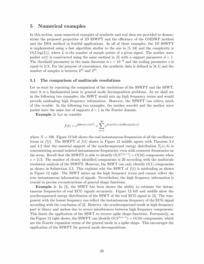
Example 2: Let us consider
f(t) = e200πi(x+5x2) +20∑n=1
e2πinN(x+0.005∗sin(2πx))
where N = 100. Figure 12 left shows the real instantaneous frequencies of all the oscillatoryterms in f(t). The SSWPT of f(t) shown in Figure 12 middle agrees with Theorem 3.4and 4.2 that the essential support of the synchrosqueezed energy distribution Tf (v, b) isconcentrating around isolated instantaneous frequencies, even with crossover frequencies onthe scene. Recall that the SSWPT is able to identify O(N1/s−1) = O(10) components whens = 2/3. The number of clearly identified components is 20 according with the multiscaleresolution analysis of the SSWPT. However, the SSWT can only identify O(1) componentsas shown in Subsection 3.3. This explains why the SSWT of f(t) is misleading as shownin Figure 12 right. The SSWT mixes up the high frequency terms and cannot reflect thetrue instantaneous information of signals. Nevertheless, the high frequency information iscrucial to precise reconstructions of general shape functions.
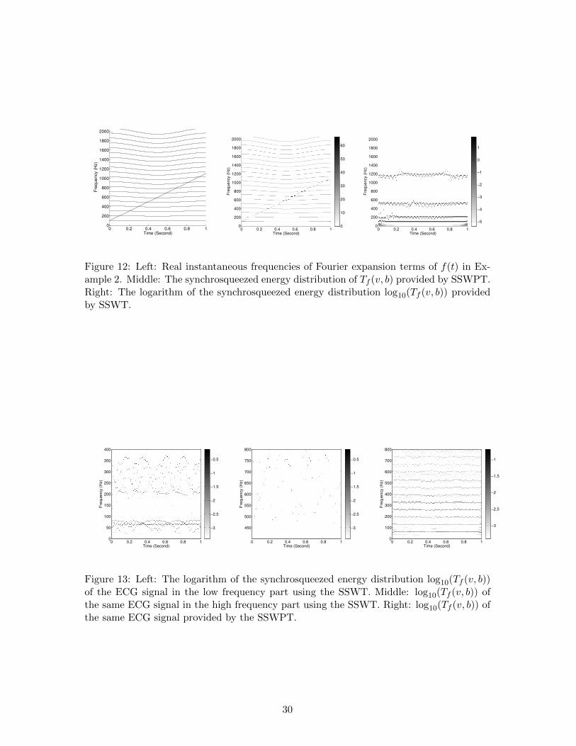
Example 3: In [3], the SSWT has been shown the ability to estimate the instan-taneous frequencies of real ECG signals accurately. Figure 13 left and middle show thesynchrosqueezed energy distribution of the SSWT of the real ECG signal in [3]. The com-ponent with the lowest frequency can reflect the instantaneous frequency of the ECG signalaccording with the conclusion of [3]. However, the synchrosqueezed result in high frequencypart is blurry and useless due to severe interferences between high frequency components.This limits the application of the SSWT to recover spike shape functions. Fortunately, asthe Figure 13 right shows, the SSWPT can identify O(N1/s−1) = O(10) components, whichare the Fourier expansion terms of the general mode in a spike shape. This encourages theapplication of the SSWPT for general mode decompositions.
29
0 0.2 0.4 0.6 0.8 10
200
400
600
800
1000
1200
1400
1600
1800
2000
Time (Second)
Fre
qu
en
cy (
Hz)
0 0.2 0.4 0.6 0.8 10
200
400
600
800
1000
1200
1400
1600
1800
2000
Time (Second)
Fre
qu
en
cy (
Hz)
0
10
20
30
40
50
60
0 0.2 0.4 0.6 0.8 10
200
400
600
800
1000
1200
1400
1600
1800
2000
Time (Second)
Fre
qu
en
cy (
Hz)
−5
−4
−3
−2
−1
0
1
Figure 12: Left: Real instantaneous frequencies of Fourier expansion terms of f(t) in Ex-ample 2. Middle: The synchrosqueezed energy distribution of Tf (v, b) provided by SSWPT.Right: The logarithm of the synchrosqueezed energy distribution log10(Tf (v, b)) providedby SSWT.
Time (Second)
Fre
qu
en
cy (
Hz)
0 0.2 0.4 0.6 0.8 10
50
100
150
200
250
300
350
400
−3
−2.5
−2
−1.5
−1
−0.5
Time (Second)
Fre
qu
en
cy (
Hz)
0 0.2 0.4 0.6 0.8 1
450
500
550
600
650
700
750
800
−3
−2.5
−2
−1.5
−1
−0.5
Time (Second)
Fre
qu
en
cy (
Hz)
0 0.2 0.4 0.6 0.8 10
100
200
300
400
500
600
700
800
−3
−2.5
−2
−1.5
−1
Figure 13: Left: The logarithm of the synchrosqueezed energy distribution log10(Tf (v, b))of the ECG signal in the low frequency part using the SSWT. Middle: log10(Tf (v, b)) ofthe same ECG signal in the high frequency part using the SSWT. Right: log10(Tf (v, b)) ofthe same ECG signal provided by the SSWPT.
30
5.2 General mode decompositions and the robustness
As we have seen in Example 1, the GMDWP method and the DSA method can exactlyrecover general modes. In what follows, we would study the robustness against noise andpresent some more examples of general shape functions. The shapes of general modes aredetermined by all the Fourier expansion terms, including those weak energy terms whichhave been concealed by noise. We will show the recovered results in noisy cases and thenpresent an example about denoising according to the feature of recovered modes. The noiseused here is a Gaussian random noise n(t) with zero mean and variance σ2. To quantifythe influence of the noise on each general mode, we introduce the following Signal-to-NoiseRatio (SNR)
SNR[dB] = min
10 log10
(‖fi‖L2
σ2
), 1 ≤ i ≤ K
,
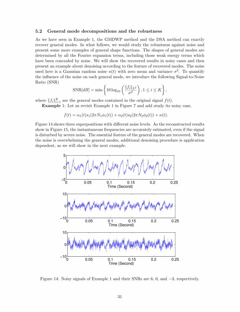
where fiKi=1 are the general modes contained in the original signal f(t).Example 1: Let us revisit Example 1 in Figure 7 and add study its noisy case,
f(t) = α1(t)s1(2πN1φ1(t)) + α2(t)s2(2πN2φ2(t)) + n(t).
Figure 14 shows three superpositions with different noise levels. As the reconstructed resultsshow in Figure 15, the instantaneous frequencies are accurately estimated, even if the signalis disturbed by severe noise. The essential feature of the general modes are recovered. Whenthe noise is overwhelming the general modes, additional denoising procedure is applicationdependent, as we will show in the next example.
0 0.05 0.1 0.15 0.2 0.25−5
0
5
Time (Second)
0 0.05 0.1 0.15 0.2 0.25−10
0
10
Time (Second)
0 0.05 0.1 0.15 0.2 0.25−10
0
10
Time (Second)
Figure 14: Noisy signals of Example 1 and their SNRs are 6, 0, and −3, respectively.
31
Time (Second)
Fre
quency (
Hz)
0 0.2 0.4 0.6 0.8 10
100
200
300
400
500
600
0 0.2 0.4 0.6 0.8 155
60
65
70
75
80
85
90
95
100
Time (Second)
Fre
quency (
Hz)
0 0.01 0.02 0.03 0.04−1.5
−1
−0.5
0
0.5
1
1.5
Time (Second)0 0.01 0.02 0.03 0.04
−2
−1.5
−1
−0.5
0
0.5
1
1.5
2
Time (Second)
Time (Second)
Fre
quency (
Hz)
0 0.2 0.4 0.6 0.8 10
100
200
300
400
500
600
0 0.2 0.4 0.6 0.8 155
60
65
70
75
80
85
90
95
100
Time (Second)
Fre
quency (
Hz)
0 0.01 0.02 0.03 0.04−1.5
−1
−0.5
0
0.5
1
1.5
Time (Second)0 0.01 0.02 0.03 0.04
−2
−1.5
−1
−0.5
0
0.5
1
1.5
2
2.5
Time (Second)
Time (Second)
Fre
quency (
Hz)
0 0.2 0.4 0.6 0.8 10
100
200
300
400
500
600
0 0.2 0.4 0.6 0.8 155
60
65
70
75
80
85
90
95
100
Time (Second)
Fre
quency (
Hz)
0 0.01 0.02 0.03 0.04−2
−1.5
−1
−0.5
0
0.5
1
1.5
2
Time (Second)0 0.01 0.02 0.03 0.04
−2.5
−2
−1.5
−1
−0.5
0
0.5
1
1.5
2
Time (Second)
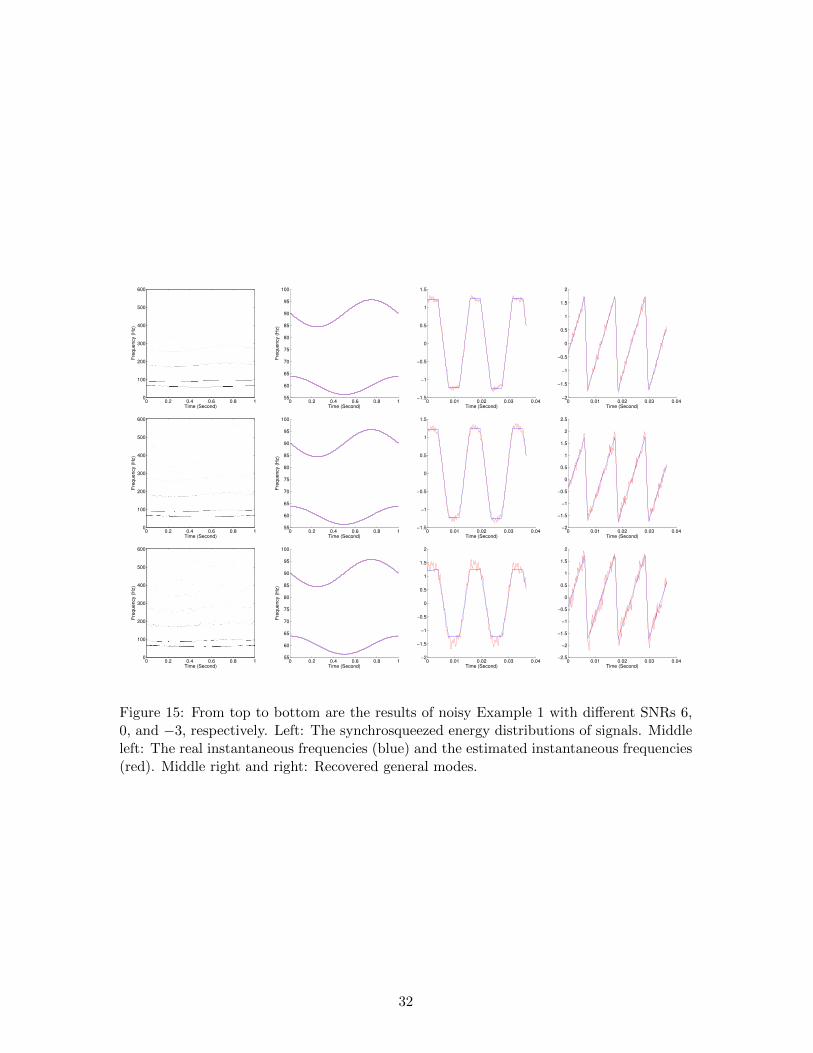
Figure 15: From top to bottom are the results of noisy Example 1 with different SNRs 6,0, and −3, respectively. Left: The synchrosqueezed energy distributions of signals. Middleleft: The real instantaneous frequencies (blue) and the estimated instantaneous frequencies(red). Middle right and right: Recovered general modes.
32
0 0.2 0.4 0.6 0.8 1−1.5
−1
−0.5
0
0.5
1
1.5
−50 0 500
0.1
0.2
0.3
0.4
0.5
0.6
0.7
0 0.2 0.4 0.6 0.8 1−1.5
−1
−0.5
0
0.5
1
1.5
−50 0 500
0.1
0.2
0.3
0.4
0.5
0.6
0.7
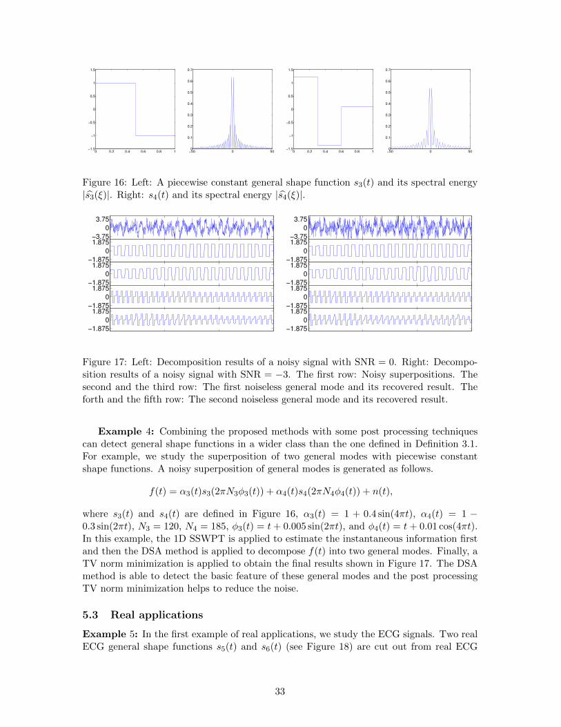
Figure 16: Left: A piecewise constant general shape function s3(t) and its spectral energy|s3(ξ)|. Right: s4(t) and its spectral energy |s4(ξ)|.
−3.75
0
3.75
−1.875
0
1.875
−1.875
0
1.875
−1.875
0
1.875
−1.875
0
1.875
−3.75
0
3.75
−1.875
0
1.875
−1.875
0
1.875
−1.875
0
1.875
−1.875
0
1.875
Figure 17: Left: Decomposition results of a noisy signal with SNR = 0. Right: Decompo-sition results of a noisy signal with SNR = −3. The first row: Noisy superpositions. Thesecond and the third row: The first noiseless general mode and its recovered result. Theforth and the fifth row: The second noiseless general mode and its recovered result.
Example 4: Combining the proposed methods with some post processing techniquescan detect general shape functions in a wider class than the one defined in Definition 3.1.For example, we study the superposition of two general modes with piecewise constantshape functions. A noisy superposition of general modes is generated as follows.
f(t) = α3(t)s3(2πN3φ3(t)) + α4(t)s4(2πN4φ4(t)) + n(t),
where s3(t) and s4(t) are defined in Figure 16, α3(t) = 1 + 0.4 sin(4πt), α4(t) = 1 −0.3 sin(2πt), N3 = 120, N4 = 185, φ3(t) = t+ 0.005 sin(2πt), and φ4(t) = t+ 0.01 cos(4πt).In this example, the 1D SSWPT is applied to estimate the instantaneous information firstand then the DSA method is applied to decompose f(t) into two general modes. Finally, aTV norm minimization is applied to obtain the final results shown in Figure 17. The DSAmethod is able to detect the basic feature of these general modes and the post processingTV norm minimization helps to reduce the noise.
5.3 Real applications
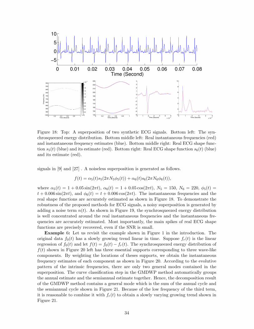
Example 5: In the first example of real applications, we study the ECG signals. Two realECG general shape functions s5(t) and s6(t) (see Figure 18) are cut out from real ECG
33
0 0.01 0.02 0.03 0.04 0.05 0.06 0.07 0.08
−5
0
5
10
Time (Second)
Time (Second)
Fre
qu
en
cy (
Hz)
0 0.2 0.4 0.6 0.8 1
500
550
600
650
700
750
800
850
900
950
1000 0
0.2
0.4
0.6
0.8
1
1.2
1.4
1.6
1.8
2
x 10−3
0 0.2 0.4 0.6 0.8 1140
150
160
170
180
190
200
210
220
230
Time (Second)0 1 2 3 4 5 6
x 10−3
−6
−5
−4
−3
−2
−1
0
1
2
3
4
Time (Second)0 1 2 3 4 5
x 10−3
−2
0
2
4
6
8
10
Time (Second)
Figure 18: Top: A superposition of two synthetic ECG signals. Bottom left: The syn-chrosqueezed energy distribution. Bottom middle left: Real instantaneous frequencies (red)and instantaneous frequency estimates (blue). Bottom middle right: Real ECG shape func-tion s5(t) (blue) and its estimate (red). Bottom right: Real ECG shape function s6(t) (blue)and its estimate (red).
signals in [9] and [27] . A noiseless superposition is generated as follows.
f(t) = α5(t)s5(2πN5φ5(t)) + α6(t)s6(2πN6φ6(t)),
where α5(t) = 1 + 0.05 sin(2πt), α6(t) = 1 + 0.05 cos(2πt), N5 = 150, N6 = 220, φ5(t) =t + 0.006 sin(2πt), and φ6(t) = t + 0.006 cos(2πt). The instantaneous frequencies and thereal shape functions are accurately estimated as shown in Figure 18. To demonstrate therobustness of the proposed methods for ECG signals, a noisy superposition is generated byadding a noise term n(t). As shown in Figure 19, the synchrosqueezed energy distributionis well concentrated around the real instantaneous frequencies and the instantaneous fre-quencies are accurately estimated. Most importantly, the main spikes of real ECG shapefunctions are precisely recovered, even if the SNR is small.
Example 6: Let us revisit the example shown in Figure 1 in the introduction. Theoriginal data f0(t) has a slowly growing trend linear in time. Suppose fr(t) is the linearregression of f0(t) and let f(t) = f0(t)− fr(t). The synchrosqueezed energy distribution off(t) shown in Figure 20 left has three essential supports corresponding to three wave-likecomponents. By weighting the locations of theses supports, we obtain the instantaneousfrequency estimates of each component as shown in Figure 20. According to the evolutivepattern of the intrinsic frequencies, there are only two general modes contained in thesuperposition. The curve classification step in the GMDWP method automatically groupsthe annual estimate and the semiannual estimate together. Hence, the decomposition resultof the GMDWP method contains a general mode which is the sum of the annual cycle andthe semiannual cycle shown in Figure 21. Because of the low frequency of the third term,it is reasonable to combine it with fr(t) to obtain a slowly varying growing trend shown inFigure 21.
34
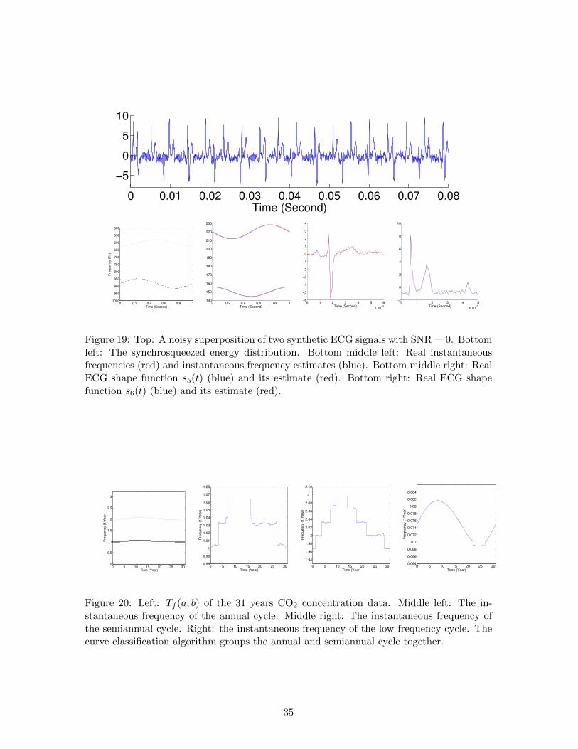
0 0.01 0.02 0.03 0.04 0.05 0.06 0.07 0.08
−5
0
5
10
Time (Second)
Time (Second)
Fre
qu
en
cy (
Hz)
0 0.2 0.4 0.6 0.8 1
500
550
600
650
700
750
800
850
900
950
10000 0.2 0.4 0.6 0.8 1
140
150
160
170
180
190
200
210
220
230
Time (Second)0 1 2 3 4 5 6
x 10−3
−6
−5
−4
−3
−2
−1
0
1
2
3
4
Time (Second)0 1 2 3 4 5
x 10−3
−2
0
2
4
6
8
10
Time (Second)
Figure 19: Top: A noisy superposition of two synthetic ECG signals with SNR = 0. Bottomleft: The synchrosqueezed energy distribution. Bottom middle left: Real instantaneousfrequencies (red) and instantaneous frequency estimates (blue). Bottom middle right: RealECG shape function s5(t) (blue) and its estimate (red). Bottom right: Real ECG shapefunction s6(t) (blue) and its estimate (red).
Time (Year)
Fre
qu
en
cy (
1/Y
ea
r)
0 5 10 15 20 25 300
0.5
1
1.5
2
2.5
3
0 5 10 15 20 25 300.98
0.99
1
1.01
1.02
1.03
1.04
1.05
1.06
1.07
1.08
Time (Year)
Fre
quency (
1/Y
ear)
0 5 10 15 20 25 30
1.94
1.96
1.98
2
2.02
2.04
2.06
2.08
2.1
2.12
Time (Year)
Fre
quency (
1/Y
ear)
0 5 10 15 20 25 300.064
0.066
0.068
0.07
0.072
0.074
0.076
0.078
0.08
0.082
0.084
Time (Year)
Fre
quency (
1/Y
ear)
Figure 20: Left: Tf (a, b) of the 31 years CO2 concentration data. Middle left: The in-stantaneous frequency of the annual cycle. Middle right: The instantaneous frequency ofthe semiannual cycle. Right: the instantaneous frequency of the low frequency cycle. Thecurve classification algorithm groups the annual and semiannual cycle together.
35
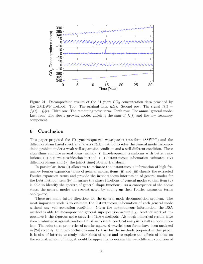
340365390
−100
10
−100
10C
O2 C
oncentr
ations (
ppm
)
−100
10
0 5 10 15 20 25 30340365390
Time (Year)
Figure 21: Decomposition results of the 31 years CO2 concentration data provided bythe GMDWP method. Top: The original data f0(t). Second row: The signal f(t) =f0(t)− fr(t). Third row: The remaining noise term. Forth row: The annual general mode.Last row: The slowly growing mode, which is the sum of fr(t) and the low frequencycomponent.
6 Conclusion
This paper proposed the 1D synchrosqueezed wave packet transform (SSWPT) and thediffeomorphism based spectral analysis (DSA) method to solve the general mode decompo-sition problem under a weak well-separation condition and a well-different condition. Thesealgorithms combine several ideas, namely (i) time-frequency transforms with better reso-lutions, (ii) a curve classification method, (iii) instantaneous information estimates, (iv)diffeomorphisms and (v) the (short time) Fourier transform.
In particular, item (i) allows us to estimate the instantaneous information of high fre-quency Fourier expansion terms of general modes; items (ii) and (iii) classify the extractedFourier expansion terms and provide the instantaneous information of general modes forthe DSA method; item (iv) linearizes the phase functions of general modes so that item (v)is able to identify the spectra of general shape functions. As a consequence of the abovesteps, the general modes are reconstructed by adding up their Fourier expansion termsone-by-one.
There are many future directions for the general mode decomposition problem. Themost important work is to estimate the instantaneous information of each general modewithout any well-separation condition. Given the instantaneous information, the DSAmethod is able to decompose the general superposition accurately. Another work of im-portance is the rigorous noise analysis of these methods. Although numerical results haveshown robustness against random Gaussian noise, theoretical analysis is still an open prob-lem. The robustness properties of synchrosqueezed wavelet transforms have been analyzedin [24] recently. Similar conclusions may be true for the methods proposed in this paper.It is also of interest to study other kinds of noise and to explore the effects of noise onthe reconstruction. Finally, it would be appealing to weaken the well-different condition of
36
phase functions in Theorem 4.5 and to classify the class of well-different phase functions.Acknowledgments. H.Y. was partially supported by NSF grant CDI-1027952. H.Y.
thanks Lexing Ying for comments on the manuscript.
References
[1] B. Boashash and S. Member. Estimating and interpreting the instantaneous frequencyof a signal. In Proceedings of the IEEE, pages 520–538, 1992.
[2] Y.-C. Chen, M.-Y. Cheng, and H.-T. Wu. Non-parametric and adaptive modelling ofdynamic periodicity and trend with heteroscedastic and dependent errors. Journal ofthe Royal Statistical Society: Series B (Statistical Methodology), pages n/a–n/a, 2013.
[3] I. Daubechies, J. Lu, and H.-T. Wu. Synchrosqueezed wavelet transforms: an empiricalmode decomposition-like tool. Appl. Comput. Harmon. Anal., 30(2):243–261, 2011.
[4] I. Daubechies and S. Maes. A nonlinear squeezing of the continuous wavelet transformbased on auditory nerve models. In Wavelets in Medicine and Biology, pages 527–546.CRC Press, 1996.
[5] L. Demanet and L. Ying. Wave atoms and sparsity of oscillatory patterns. Appl.Comput. Harmon. Anal., 23(3):368–387, 2007.
[6] J. Gilles. Empirical wavelet transform. IEEE TRANS. ON SIGNAL PROCESSING,to appear.
[7] J. Gilles, G. Tran, and S. Osher. 2d empirical transforms. wavelets, ridgelets andcurvelets revisited. submitted.
[8] A. Goldberger. Clinical Electrocardiography: A Simplified Approach. Mosby-Elsevier,7th edition, 2006.
[9] A. L. Goldberger, L. A. N. Amaral, L. Glass, J. M. Hausdorff, P. C. Ivanov, R. G.Mark, J. E. Mietus, G. B. Moody, C.-K. Peng, and H. E. Stanley. PhysioBank, Phys-ioToolkit, and PhysioNet: Components of a new research resource for complex physi-ologic signals. Circulation, 101(23):e215–e220, 2000 (June 13). Circulation ElectronicPages: http://circ.ahajournals.org/cgi/content/full/101/23/e215 PMID:1085218; doi:10.1161/01.CIR.101.23.e215.
[10] R. H. Herrera, J.-B. Tary, and M. van der Baan. Time-frequency representation ofmicroseismic signals using the synchrosqueezing transform. CoRR, abs/1301.1295,2013.
[11] T. Hou, Z. Shi, and P. Tavallali. Convergence of a data-driven time-frequency analysismethod. arXiv:1303.7048 [math.NA], 2013.
[12] T. Y. Hou and Z. Shi. Adaptive data analysis via sparse time-frequency representation.Adv. Adapt. Data Anal., 3(1-2):1–28, 2011.
[13] T. Y. Hou and Z. Shi. Data-driven timefrequency analysis. Applied and ComputationalHarmonic Analysis, 35(2):284 – 308, 2013.
37
[14] T. Y. Hou, M. P. Yan, and Z. Wu. A variant of the EMD method for multi-scale data.Adv. Adapt. Data Anal., 1(4):483–516, 2009.
[15] N. E. Huang, Z. Shen, S. R. Long, M. C. Wu, H. H. Shih, Q. Zheng, N.-C. Yen, C. C.Tung, and H. H. Liu. The empirical mode decomposition and the Hilbert spectrum fornonlinear and non-stationary time series analysis. R. Soc. Lond. Proc. Ser. A Math.Phys. Eng. Sci., 454(1971):903–995, 1998.
[16] N. E. Huang, Z. Wu, S. R. Long, K. C. Arnold, X. Chen, and K. Blank. On instanta-neous frequency. Adv. Adapt. Data Anal., 1(2):177–229, 2009.
[17] W. Huang, Z. Shen, N. E. Huang, and Y. C. Fung. Engineering analysis of biologicalvariables: An example of blood pressure over 1 day. Proc. Natl. Acad. Sci., 95, 1998.
[18] C. Li and M. Liang. A generalized synchrosqueezing transform for enhancing signaltimefrequency representation. Signal Processing, 92(9):2264 – 2274, 2012.
[19] A. Y. Ng, M. I. Jordan, and Y. Weiss. On spectral clustering: Analysis and analgorithm. Neural Information Processing Systems, 14, 2001.
[20] B. Picinbono. On instantaneous amplitude and phase of signals. IEEE Trans. SignalProcessing, pages 552–560, 1997.
[21] G. Rilling and P. Flandrin. One or two frequencies? The empirical mode decompositionanswers. IEEE Trans. Signal Process., 56(1):85–95, 2008.
[22] M. Soltanolkotabi and E. J. Cands. A geometric analysis of subspace clustering withoutliers. CoRR, abs/1112.4258, 2011.
[23] M. Soltanolkotabi, E. Elhamifar, and E. J. Candes. Robust subspace clustering. CoRR,abs/1301.2603, 2013.
[24] G. Thakur, E. Brevdo, N. S. Fuckar, and H.-T. Wu. The synchrosqueezing algorithmfor time-varying spectral analysis: robustness properties and new paleoclimate appli-cations. Signal Processing, 93(5):1079–1094, 2013.
[25] G. Thakur and H.-T. Wu. Synchrosqueezing-based recovery of instantaneous frequencyfrom nonuniform samples. SIAM J. Math. Analysis, 43(5):2078–2095, 2011.
[26] A. D. Veltcheva. Wave and group transformation by a hilbert spectrum. CoastalEngineering Journal, 44(4), 2002.
[27] H.-T. Wu. Instantaneous frequency and wave shape functions (i). Applied and Com-putational Harmonic Analysis, 35(2):181 – 199, 2013.
[28] H.-T. Wu, Y.-H. Chan, Y.-T. Lin, and Y.-H. Yeh. Using synchrosqueezing trans-form to discover breathing dynamics from ECG signals. Applied and ComputationalHarmonic Analysis, 36(2):354 – 359, 2014.
[29] H.-T. Wu, P. Flandrin, and I. Daubechies. One or two frequencies? The synchrosqueez-ing answers. Adv. Adapt. Data Anal., 3(1-2):29–39, 2011.
[30] H.-T. Wu, S.-S. Hseu, M.-Y. Bien, Y. R. Kou, and I. Daubechies. Evaluating physi-ological dynamics via synchrosqueezing: Prediction of ventilator weaning. BiomedicalEngineering, IEEE Transactions on, 61(3):736–744, March 2014.
38
[31] Z. Wu and N. E. Huang. Ensemble empirical mode decomposition: a noise-assisteddata analysis method. Advances in Adaptive Data Analysis, 01(01):1, 2009.
[32] Z. Wu, N. E. Huang, and X. Chen. Some considerations on physical analysis of data.Advances in Adaptive Data Analysis, 3(1-2):95–113, 2011.
[33] H. Yang and L. Ying. Synchrosqueezed curvelet transform for 2d mode decomposition.arXiv:1310.6079 [math.NA], 2013.
[34] H. Yang and L. Ying. Synchrosqueezed wave packet transform for 2d mode decompo-sition. SIAM Journal of Imaging Science, 2013.
39