Symbolic computation and

Mathematics with

the calculator HP Prime

Renée De Graeve Lecturer at Grenoble I

Translated from French by Jean-Michel Lecointre

2

© 2013 Renée De Graeve, renee.degraeve@wanadoo.fr Copy, translation and redistribution of this document on electronic support or paper are permitted for non-commercial purpose only. Use of this document for commercial purpose is forbidden without the written consent of the owner of the copyright. This documentation is provided “as is”, without warranty of any kind.The owner of the copyright shall not be held responsible in any case for any damage resulting from the use of this document. This document is available at the following Internet address: http://www-fourier.ujf-grenoble.fr/~parisse/hp-prime_cas.pdf ( link to be updated)

3

INDEX -, 40, 131, 293, 324 - inf, 196 - infinity, 196 _, 369, 371, 377 :=, 59, 499 :=, 44 !, 227 !=, 196, 513 .-, 293, 324 .*, 293, 325 ./, 294, 325 .ˆ, 326 .+, 292, 324 ‘’, 60 ’, 60, 225 ", 295 [[]], 295 [], 295 *, 40, 131, 324 /, 40, 133, 135 //, 497, 513 /laplace, 94 &*, 324 &&, 197 &ˆ, 325

, 499

%, 129, 208 %e, 196 %i, 196 %pi, 196 ^, 40 ˆ, 133, 325 →, 44, 59

∂, 60 +, 40, 130, 292, 296, 303, 324

+ infinity, 196 <, 196, 513 <=, 196, 197, 513 ≠, 196, 513 ==, 196, 513 =>, 371, 375, 499 >, 196, 513 >=, 196, 513 ||, 197 ≤, 196 ≥, 196 a2q, 103 abcuv, 149 about, 506 ABS, 210, 335 abscissa, 434 ACOS, 216 acos2asin, 113 acos2atan, 114 ACOSH, 221 ACOT, 219 ACSC, 217 ADDCOL, 316 additionally, 505 ADDROW, 322 affix, 435 algvar, 223 ALOG, 213 alog10, 213 altitude, 396 AMORT, 465 and, 197, 513 angle, 435 angleat, 427 angleatraw, 427 Ans, 508 ans(n), 508 append, 276 apply, 287 approx, 225 arc, 414 arcLen, 436 area, 438 areaat, 428 areaatraw, 428 ARG, 209 ASC, 297 ASEC, 218 ASIN, 216

4

asin2acos, 113 asin2atan, 113 ASINH, 220 assume, 502 ATAN, 217 atan2acos, 115 atan2asin, 115 ATANH, 221 atrig2ln, 116 barycenter, 384 basis, 329 Beta, 359 BINOMIAL, 239 BINOMIAL_CDF, 243 BINOMIAL_ICDF, 246 bisector, 397 bitand, 198 bitor, 198 bitxor, 198 bounded_function, 66 BREAK, 511 canonical_form, 151 CASE, 509 cat, 296 CEILING, 199 Celsius2Fahrenheit, 376 center, 395 cFactor, 53 CHAR, 298 charpoly, 327 CHECK, 517 chinrem, 149, 177 CHISQUARE, 238 CHISQUARE_CDF, 241 CHISQUARE_ICDF, 246 cholesky, 345 CHOOSE, 514 Ci, 366 circle, 413 circumcircle, 415 coeff, 155 col, 318 colDim, 316 collect, 49 COLNORM, 337 colSwap, 317 COMB, 227 comDenom, 55 comment, 497 common_perpendicular, 380 companion, 165 compare, 501 complexroot, 152 CONCAT, 274 COND, 339

conic, 105, 415 CONJ, 209 contains, 282 content, 170 CONTINUE, 510 convert, 371, 375 convexhull, 412 coordinates, 438 CopyVar, 499 correlation, 256 COS, 216 cos2sintan, 114 COSH, 220 COT, 218 count, 283 covariance, 255 covariance_correlation, 258 cpartfrac, 55 CROSS, 356 CSC, 217 cSolve, 89 cumSum, 291, 296 curl, 72 cyclotomic, 178 cZeros, 88, 90 degree, 168 DELCOL, 318 delcols, 318 DELROW, 319 delrows, 319 deltalist, 285 deSolve, 90 det, 136, 326 diag, 345 diff, 60 DIM, 278, 302, 315 Dirac, 367 distance, 441 distance2, 442 distanceat, 429 distanceatraw, 430 divergence, 73 divis, 140, 157 division_point, 393 divpc, 83 DOM_COMPLEX, 500 DOM_FLOAT, 500 DOM_IDENT, 500 DOM_INT, 500 DOM_LIST, 500 DOM_RAT, 500 DOM_STRING, 500 DOM_SYMBOLIC, 500 DOT, 356 DrawSlp, 395

5

e, 196 EDITMAT, 515 egcd, 148 Ei, 364 EIGENVAL, 342 eigenvals, 342 eigenvects, 343 EIGENVV, 343 eigVl, 344 element, 391 ellipse, 416 equation, 442 equilateral_triangle, 404 erf, 362 erfc, 363 euler, 125 euler_gamma, 196 eval, 224 evalc, 211 evalf, 225 even, 121 exact, 226 exbisector, 397 excircle, 417 EXP, 214 exp2pow, 110 exp2trig, 111 expand, 51 expexpand, 112 EXPM1, 214 exponential_regression, 261 expr, 299 extract_measure, 442 ezgcd, 146 f2nd, 56 factor, 52, 136, 139 factor_xn, 170 factorial, 227 factors, 157 fadeev, 328 Fahrenheit2Celsius, 376 false, 196 fcoeff, 162 fft, 86 FISHER, 239 FISHER_CDF, 242 FISHER_ICDF, 246 FLOOR, 200 fMax, 59 fMin, 59 FNROOT, 207 FOR, 519 FOR FROM TO DO END, 511 FOR FROM TO STEP DO END, 511 FP, 201 frac, 204

fracmod, 135 FREEZE, 514 froot, 153 fsolve, 101 function_diff, 60 Gamma, 360 gauss, 104 gbasis, 179 gcd, 122, 136, 144, 158 GETKEY, 514 GF, 137 grad, 73 gramschmidt, 104 greduce, 179 half_line, 397 halftan, 115 halftan_hyp2exp, 108 hamdist, 199 harmonic_conjugate, 394 harmonic_division, 393 has, 223 head, 304 Heaviside, 367 hermite, 179 hessenberg, 346 hessian, 73 hexagon, 410 hilbert, 334 histogram, 254 homothety, 421 hyp2exp, 112 hyperbola, 417 HypZ1mean, 466 HypZ2mean, 466 i, 196, 208 iabcuv, 123 ibasis, 329 ibpdv, 78 ibpu, 79 ichinrem, 128 id, 199 IDENMAT, 332 identity, 332 idivis, 121 iegcd, 123 IF, 508, 518 IF THEN ELSE END, 509 ifactor, 122 ifactors, 122 IFERR, 510 ifft, 86 IFTE, 508 igcd, 144 ihermite, 346

6

ilaplace, 94 IM, 209 image, 329 incircle, 418 inf, 196 infinity, 196 INPUT, 497, 515 InputStr, 497 INSTRING, 297, 301 int, 63 integrate, 75 inter, 388 interval2center, 58 inv, 135, 137, 199 inversion, 422 invlaplace, 84, 94 invztrans, 99 IP, 200 iPart, 204 iquo, 127 iquorem, 128 irem, 128 is_collinear, 446 is_concyclic, 446 is_conjugate, 446 is_coplanar, 447 is_element, 448 is_equilateral, 448 is_harmonic, 454 is_harmonic_circle_bundle, 455 is_harmonic_line_bundle, 454 is_isosceles, 449 is_orthogonal, 450 is_parallel, 450 is_parallelogram, 451 is_perpendicular, 452 is_rectangle, 452 is_rhombus, 453 is_square, 453 ISKEYDOWN, 514 ismith, 347 isobarycenter, 386 isopolygon, 410 isosceles_triangle, 406 isPrime, 124 ITERATE, 511 ithprime, 124 jacobi_symbol, 126 jordan, 344 JordanBlock, 333 ker, 329 l1norm, 290, 357 l2norm, 290, 357 lagrange, 180

laguerre, 184 laplace, 84 laplacian, 74 lcm, 123, 147, 159 lcoeff, 163, 169 left, 57, 281, 301 legendre, 184 legendre_symbol, 126 length, 278, 302 lgcd, 123 limit, 65, 67 lin, 107 line, 398, 399 linear_interpolate, 260 linear_regression, 261 LineHorz, 399 LineTan, 396 LineVert, 399 linsolve, 102 list2mat, 289 LN, 211 lname, 222 lncollect, 107 lnexpand, 107 LNP1, 215 locus, 418 log, 211, 212 log10, 212 logarithmic_regression, 262 logb, 213 logistic_regression, 265 LQ, 347 LSQ, 349 LU, 349, 350 lvar, 222 MAKELIST, 273 MAKEMAT, 331 MANT, 205 map, 287 mat2list, 290 matpow, 345 matrix, 332 MAX, 206 maxnorm, 290, 358 MAXREAL, 196 mean, 248, 267, 270, 465 median, 251, 267, 270 median_line, 401 member, 282 mid, 302 midpoint, 386 MIN, 206 MINREAL, 196 mkisom, 334 mksa, 372, 376 MOD, 206

7

modgcd, 146 mRow, 323 mRowAdd, 323 MSGBOX, 515 mult_c_conjugate, 211 mult_conjugate, 51 nDeriv, 62 neg, 199 nextprime, 124 norm, 290 normal, 50, 130, 131, 133 NORMALD, 238 NORMALD_CDF, 240 NORMALD_ICDF, 244 normalize, 291 not, 197, 513 nSolve, 101 NTHROOT, 207 numer, 56 odd, 121 odesolve, 97 ofnom, 56 open_polygon, 412 OR, 513 order_size, 83 ordinate, 443 orthocenter, 389 pa2b2, 127 pade, 69 parabola, 420 parallel, 401 parallelogram, 409 parameq, 444 partfrac, 54 pcoef, 156, 162 pcoeff, 156, 162 perimeter, 444 perimeterat, 431 perimeteratraw, 432 PERM, 228 perpen_bisector, 401 perpendicular, 402 Pi, 196 PIECEWISE, 47 pivot, 341 plotcontour, 192 plotdensity, 190 plotfield, 191 plotfunc, 187 plotimplicit, 189 plotlist, 193, 259 plotode, 193 plotparam, 188 plotpolar, 188

plotseq, 189 pmin, 164 point, 385 point2d, 387 POISSON, 240 POISSON_CDF, 244 POISSON_ICDF, 247 polar, 394 polar_coordinates, 441 polar_point, 387 pole, 394 poly2symb, 161 POLYCOEF, 305 polyEval, 163, 305 POLYFORM, 306 polygon, 412 polygonplot, 259 polygonscatterplot, 260 polynomial_regression, 263 POLYROOT, 308 POS, 277 potential, 74 pow2exp, 111 power_regression, 264 powerpc, 421 powexpand, 108 powmod, 129, 134 PredX, 466 PredY, 466 prepend, 277 preval, 64, 80 prevprime, 125 primpart, 170 print, 499, 515 product, 286 projection, 422 proot, 151 propfrac, 55 Psi, 361 ptayl, 153 purge, 507 q2a, 103 QR, 352 quadrilateral, 409 quantile, 253, 267, 270 quartile1, 252, 267 quartile3, 252, 267 quartiles, 251, 267, 270 quo, 131, 141, 166 quorem, 132, 143 QUOTE, 225, 295 radical_axis, 404 radius, 444 ramn, 333 rand, 229

8

randexp, 236 RANDINT, 229 RANDMAT, 333 randmatrix, 333 RANDNORM, 235 RANDOM, 228 randperm, 232 randpoly, 165 RANDSEED, 236 randvector, 232 RANK, 340 RE, 210 reciprocation, 395 rectangle, 407 rectangular_coordinates, 440 REDIM, 321 reduced_conic, 105 ref, 102 reflection, 423 regroup, 50 REGRS, 466 rem, 132, 142, 167 remove, 280 reorder, 165 REPEAT UNTIL, 511 REPLACE, 322 residue, 69 restart, 507 resultant, 174 REVERSE, 274 revlist, 278 rhombus, 406 right, 57, 281, 301 right_triangle, 405 romberg, 64 rootof, 154 rotate, 279, 302 rotation, 424 ROUND, 201 row, 318 rowAdd, 323 rowDim, 316 ROWNORM, 336 rowSwap, 317 rref, 137, 330 rsolve, 312 SCALE, 323 SCALEADD, 323 SCHUR, 352 SEC, 218 segment, 402 select, 285 seq, 512 seqsolve, 310 series, 68 shift, 279

shift_phase, 117 Si, 365 SIGN, 210 signature, 58 similarity, 425 simplify, 49 simult, 331 SIN, 216 sin2costan, 113 sincos, 111 single_inter, 387 SINH, 220 SIZE, 278, 302 slope, 445 slopeat, 432 slopeatraw, 433 snedecor, 239 snedecor_cdf, 242 snedecor_icdf, 246 solve, 87 SORT, 274 SPECNORM, 338 SPECRAD, 339 spline, 181 sq, 199 sqrfree, 53 sqrt, 199 square, 408 srand, 236 STARTVIEW, 517 STAT1, 465 stddev, 249, 267, 270 stddevp, 249, 267

Sto, 59

string, 299, 300 STUDENT, 238 STUDENT_CDF, 241 STUDENT_ICDF, 245 sturm, 171 sturmab, 171 sturmseq, 172 SUB, 320 subMat, 320 subst, 54 sum, 71, 286, 465 sum_riemann, 80 suppress, 280 surd, 207 SVD, 353 SVL, 355 SWAPCOL, 317 SWAPROW, 317 sylvester, 173 symb2poly, 161 table, 271 tail, 280, 304

9

TAN, 217 tan2sincos, 115 tan2sincos2, 114 tangent, 402 TANH, 221 taylor, 83 tchebyshev1, 185 tchebyshev2, 185 tcollect, 119 texpand, 108 time, 41 tlin, 117 TRACE, 341 translation, 426 transpose, 326 triangle, 404 trig2exp, 120 trigcos, 116 trigexpand, 119 trigsin, 116 trigtan, 117 TRN, 326 true, 196 trunc, 203 truncate, 156, 203 tsimplify, 112 TYPE, 500 ufactor, 372, 377 unapply, 44 UNCHECK, 517 usimplify, 373, 377

UTPC, 236 UTPF, 237 UTPN, 237 UTPT, 237 valuation, 169 vandermonde, 335 variance, 250, 267, 270 vector, 400 vertices, 390 vertices_abca, 390 vpotential, 75 WAIT, 515 when, 47 WHILE, 519 WHILE DO END, 511 xor, 197, 514 XPON, 205 zeros, 88 Zeta, 362 zip, 289 ztrans, 98 ΔLIST, 285 π, 196 ΠLIST, 286 ΣLIST, 286

10

Table of content

GETTING STARTED 31

Generalities 32

CAS and HOME keys 33

Reset and clear 35

Tactile screen 35

Keys 35

General settings 36

CAS settings: Shift CAS 36

Calculator settings: Shift HOME 36

Symbolic computation functions 36

MENU CAS OF THE TOOLBOX KEY 37

CHAPTER 1 GENERALITIES 39

1.1 Calculations in the CAS 39

1.2 Priority of operators 39

1.3 Implicit multiplication 39

1.4 Duration of a calculation: time 39

1.5 Lists and sequences in the CAS 40

1.6 Difference between expressions and functions 41 1.6.1 Defining a function by an expression 42 1.6.2 Definition of a function of one or several variables 43 1.6.3 To define a function by two expressions: when 45 1.6.4 Defining a function by n values: PIECEWISE piecewise 45 1.6.5 Exercise on expressions 46 1.6.6 Exercise on the functions (to be followed) 46

CHAPTER 2 MENU ALGEBRA 48

2.1 Simplifying an expression: simplify 48

2.2 Factorizing a polynomial on the integers: collect 48

2.3 Regrouping and simplifying: regroup 49

2.4 Expanding and simplifying: normal 49

11

2.5 Expanding an expression: expand 49

2.6 Multiply by the conjugate quantity: mult_conjugate 50

2.7 Factorizing an expression: factor 50

2.8 Factorization without square factor: sqrfree 51

2.9 Factorization in C: cFactor cfactor 52

2.10 Substituting a variable by a value: subst 53

2.11 Fractions 53 2.11.1 Decompose into simple elements: partfrac 53 2.11.2 Decomposition in simple elements on C: cpartfrac 53 2.11.3 Put to common denominator: comDenom 54 2.11.4 Integer part and fractional part: propfrac 54

2.12 Extract 55 2.12.1 Numerator of a fraction after simplifiation: numer 55 2.12.2 Denominator of a fraction after simplification: ofnom 55 2.12.3 Numerator and denominator: f2nd 55 2.12.4 Get the left member of an equation: left 56 2.12.5 Get the right member of an equation: right 56 2.12.6 Center of an interval: interval2center 56 2.12.7 Signature of a permutation: signature 57

CHAPTER 3 MENU CALCULUS 58

3.1 Definition of a function: := and →(Sto) 58

3.2 Maximum and minimum of an expression: fMax fMin 58

3.3 Differentiate 59 3.3.1 Derivative function of a function: function_diff 59 3.3.2 Differentiate : ∂ diff ’ ‘’ 59 3.3.3 Approximate calculation of the derivative number: nDeriv 61

3.4 Integration 62 3.4.1 Primitive: int 62 3.4.2 Evaluate a primitive: preval 63 3.4.3 Approximate calculation of integrals with the Romberg method: romberg 63

3.5 Limites: limit 63

3.6 Limit and integral 65

3.7 Series: series 67

3.8 Residue of an expression in a point: residue 67

3.9 Pade approximation: pade 68

3.10 Indexed finite and infinite sum and discrete primitive: sum 69

3.11 Differential 71

12

3.11.1 Rotational curl: curl 71 3.11.2 Divergence: divergence 71 3.11.3 Gradient: grad 71 3.11.4 Hessian matrix: hessian 72 3.11.5 Laplacian: laplacian 72 3.11.6 Potential: potential 73 3.11.7 Conservative vector field: vpotential 73

3.12 Integral 74 3.12.1 Primitive and definite integral: integrate 74 3.12.2 Integration by parts: ibpdv 76 3.12.3 Integration by parts: ibpu 77 3.12.4 Evaluate a primitive: preval 78

3.13 Limits 79 3.13.1 Riemann sum: sum_riemann 79 3.13.2 Series expansion: taylor 81 3.13.3 Division by increasing power order: divpc 82

3.14 Transform 82 3.14.1 Laplace transform: laplace 82 3.14.2 Laplace transform inverse: invlaplace 83 3.14.3 Fast Fourier transform: fft 84 3.14.4 inverse of the fast Fourier transform: ifft 84

CHAPTER 4 MENU SOLVE 86

4.1 Solve equations: solve 86

4.2 Zeros of an expression: zeros 87

4.3 Complex Zeros of an expression: cZeros 87

4.4 Solve equations in C: cSolve csolve 88

4.5 Complex zeros of an expression: cZeros 89

4.6 Differential equations 89 4.6.1 Solve differential equations: deSolve desolve 89 4.6.2 Laplace transform and inverse Laplace transform: /laplace ilaplace invlaplace 93

4.7 Approximate solution of y’ = f(t, y): odesolve 95

4.8 z transform and z inverse transform 97 4.8.1 z transform of a series: ztrans 97 4.8.2 z transform inverse of a rational fraction: invztrans 98

4.9 Solve numerical equations: nSolve 99

4.10 Solve equations with fsolve 99

4.11 Linear systems 100 4.11.1 Solve a linear system: linsolve 100 4.11.2 Gauss reduction of a matrix: ref 100

4.12 Quadratic forms 101

13

4.12.1 Matrix of a quadratic form: q2a 101 4.12.2 Transform a matrix in a quadratic form: a2q 102 4.12.3 Gauss method: gauss 102 4.12.4 Gramschmidt process: gramschmidt 102

4.13 Conics 103 4.13.1 Plot of a conic: conic 103 4.13.2 Reduction of a conic: reduced_conic 103

CHAPTER 5 MENU REWRITE 105

5.1 Collect the logarithms: lncollect 105

5.2 Expand the logarithms: lnexpand 105

5.3 Linearize the exponentials: lin 105

5.4 Transform a power in product of powers: powexpand 106

5.5 Transform the trigonometric and hyperbolic expressions in tan(x/2) and in ex: halftan_hyp2exp 106

5.6 Expand a transcendantal and trigonometric expression: texpand 106

5.7 Exp & Ln 108 5.7.1 Transform exp(n*ln(x)) in power: exp2pow 108 5.7.2 Transform a power into an exponential: pow2exp 109 5.7.3 Transform the complex exponentials into sin and cos: sincos exp2trig 109 5.7.4 Transform the functions hyperbolic in exponentials: hyp2exp 110 5.7.5 Write with complex exponentials: tsimplify 110 5.7.6 Expand the exponentials: expexpand 110

5.8 Sine 110 5.8.1 Transform the arcsin into arccos: asin2acos 110 5.8.2 Transform the arcsin in arctan: asin2atan 111 5.8.3 Transform sin(x) in cos(x)*tan(x): sin2costan 111

5.9 Cosine 111 5.9.1 Transform the arccos into arcsin: acos2asin 111 5.9.2 Transform the arccos into arctan: acos2atan 111 5.9.3 Transform cos(x) into sin(x)/tan(x): cos2sintan 112

5.10 Tangent 112 5.10.1 Transform tan(x) with sin(2x) and cos(2x): tan2sincos2 112 5.10.2 Transform the arctan into arcsin: atan2asin 112 5.10.3 Transform the arctan into arccos: atan2acos 113 5.10.4 Transform tan(x) into sin(x)/cos(x): tan2sincos 113 5.10.5 Transform a trigonometric expression in term of tan(x/2): halftan 113

5.11 Trigonometry 114 5.11.1 Simplify by privileging sine: trigsin 114 5.11.2 Simplify by privileging cosine: trigcos 114 5.11.3 Transform trigonometric inverse functions to logarithms: atrig2ln 114 5.11.4 Simplify by privileging tangent: trigtan 114 5.11.5 Linearize a trigonometric expression: tlin 115 5.11.6 Shift the phase by π2 in trigonometric expressions: shift_phase 115

14

5.11.7 Collect the sine and cosine of a same angle: tcollect 117 5.11.8 Expand a trigonometric expression: trigexpand 117 5.11.9 Transform a trigonometric expression into complex exponentials: trig2exp 117

CHAPTER 6 MENU INTEGER 118

6.1 Test of parity: even 118

6.2 Test of non parity: odd 118

6.3 Divisors of an integer: idivis 118

6.4 Prime factors decomposition of an integer: ifactor 119

6.5 List of prime factors and their multiplicity: ifactors 119

6.6 GCD of one or several integers: gcd 119 6.6.1 GCD of a list of integers: lgcd 119

6.7 LCM of one or several integers: lcm 120 6.7.1 Bezout identity: iegcd 120 6.7.2 Solve au + bv = c in Z: iabcuv 120

6.8 Primality 121 6.8.1 Check whether a number is prime: isPrime isprime 121 6.8.2 The N-th prime number: ithprime 121 6.8.3 nextprime 121 6.8.4 prevprime 122 6.8.5 Euler’s totient: euler 122 6.8.6 Legendre symbole: legendre_symbol 122 6.8.7 Jacobi symbol: jacobi_symbol 123 6.8.8 Solve a2 + ab2 = p in Z: pa2b2 124

6.9 Division 124 6.9.1 Quotient of the Euclidean division: iquo 124 6.9.2 Remainder of the Euclidean division: irem 124 6.9.3 Quotient and remainder of the Euclidean division: iquorem 125 6.9.4 Chinese remainder for integers: ichinrem 125 6.9.5 Calculation of an mod p: powmod 126

6.10 Modular calculus in Z /p Z or in Z /p Z [x] 126 6.10.1 Expand and factorise: normal 126 6.10.2 Addition in Z /p Z or in Z /pZ[x]: + 127 6.10.3 Substraction in Z /p Z or in Z /pZ[x]: - 127 6.10.4 Multiplication in Z /p Z or Z /p Z [x]: * 128 6.10.5 Quotient: quo 128 6.10.6 Remainder: rem 128 6.10.7 Quotient and remainder: quorem 129 6.10.8 Division in Z /p Z or Z /p Z [x]: / 129 6.10.9 Power in Z /p Z or Z /p Z [x]: ˆ 130 6.10.10 Calculation of an mod p or of A(x)n mod ¶(x), p: powmod 130 6.10.11 Inverse in Z /p Z: inv or / 131 6.10.12 Transform an integer into its fraction modulus p: fracmod 132 6.10.13 GCD in Z /p Z [x]: gcd 132 6.10.14 Factorization in Z /p Z [x]: factor 133 6.10.15 Determinant of a matrix of Z /p Z: det 133

15

6.10.16 Inverse of a matrix of Z /p Z: inv 133 6.10.17 Solve a linear system of Z /p Z: rref 133 6.10.18 Creation of a Galois field: GF 134 6.10.19 Factorization of a polynomial with coefficients in a Galois field: factor 136

6.11 Arithmetic of polynomials 136 6.11.1 List of divisors of a polynomial: divis 136 6.11.2 Euclidean quotient of two polynomials: quo 137 6.11.3 Euclidean remainder of two polynomials: rem 138 6.11.4 Quotient and Euclidean remainder: quorem 139 6.11.5 GCD of polynomials by Euclid’s algorithm: gcd igcd 140 6.11.6 Choose the algorithm of the GCD of two polynomials: ezgcd modgcd 142 6.11.7 LCM of two polynomials: lcm 143 6.11.8 Bezout identity: egcd 144 6.11.9 Solve polynomial of the form au + bv = c: abcuv 145 6.11.10 Chinese remainder: chinrem 145

CHAPTER 7 MENU POLYNOMIAL 147

7.1 Canonical form: canonical_form 147

7.2 Numerical roots of a polynomial: proot 147

7.3 Roots exact of a polynomial 148 7.3.1 Exact boundaries of complex roots of a polynomial: complexroot 148 7.3.2 Exact values of complex rational roots of a polynomial: crationalroot 148

7.4 Fraction rational, its roots and its exact poles 149 7.4.1 Roots and exact poles of a rational fraction: froot 149

7.5 Writing in powers of (x-a): ptayl 149

7.6 Calculation with the exact roots of a polynomial: rootof 150

7.7 Coefficients of a polynomial: coeff 151

7.8 Coefficients of a polynomial defined by its roots: pcoeff pcoef 152

7.9 Truncation of order n: truncate 152

7.10 List of divisors of a polynomial: divis 152

7.11 List of factors of a polynomial: factors 153

7.12 GCD of polynomials by Euclid’s algorithm: gcd 153

7.13 LCM of two polynomials: lcm 155

7.14 Create 156 7.14.1 Transform a polynomial into a list (internal recursive dense format): symb2poly 156 7.14.2 Transform the internal sparse distributed format of the polynomial into a polynomial writting: poly2symb 157 7.14.3 Coefficients of a polynomial defined by its roots: pcoeff pcoef 157 7.14.4 Coefficients of a rational fraction defined by its roots and its poles: fcoeff 158 7.14.5 Coefficients of the term of highest degree of a polynomial: lcoeff 158 7.14.6 Evaluation of a polynomial: polyEval 158

16

7.14.7 Minimal polynomial: pmin 159 7.14.8 Companion matrix of a polynomial: companion 160 7.14.9 Random polynomials: randpoly randPoly 160 7.14.10 Change the order of variables: reorder 161

7.15 Algebra 161 7.15.1 Euclidean quotient of two polynomials: quo 161 7.15.2 Euclidean remainder of two polynomials: rem 162 7.15.3 Degree of a polynomial: degree 163 7.15.4 Valuation of a polynomial: valuation 164 7.15.5 Coefficient of the term of highest degree of a polynomial: lcoeff 164 7.15.6 Put in factor of xn in a polynomial: factor_xn 165 7.15.7 GCD of coefficients of a polynomial: content 165 7.15.8 Primitive part of a polynomial: primpart 165 7.15.9 Sturm sequence and number of changes of the sign of P on ]a; b]: sturm 166 7.15.10 Number of changes of sign on ]a; b]: sturmab 166 7.15.11 Sequence of Sturm: sturmseq 167 7.15.12 Sylvester matrix of two polynomials: sylvester 168 7.15.13 Resultant of two polynomials: resultant 169 7.15.14 Chinese remainder: chinrem 172

7.16 Special 172 7.16.1 Cyclotomic polynomial: cyclotomic 172 7.16.2 Groebner basis: gbasis 173 7.16.3 Reduction according to a Groebner basis: greduce 174 7.16.4 Hermite polynomial: hermite 174 7.16.5 Lagrange interpolation: lagrange 175 7.16.6 Natural splines: spline 176 7.16.7 Laguerre polynomial: laguerre 178 7.16.8 Legendre polynomial: legendre 179 7.16.9 Tchebyshev polynomial of first kind: tchebyshev1 179 7.16.10 Tchebyshev polynomial of second kind: tchebyshev2 180

CHAPTER 8 MENU PLOT 181

8.1 Plot of a function: plotfunc 181

8.2 Parametric curve: plotparam 181

8.3 Polar curve: plotpolar 182

8.4 Plot of a recurrent sequence: plotseq 183

8.5 Implicit plot in 2D: plotimplicit 183

8.6 Plot of a function by colors levels: plotdensity 184

8.7 The field of tangents: plotfield 184

8.8 Level curves: plotcontour 186

8.9 Plot of solutions of a differential equation: plotode 186

8.10 Polygonal line ( translation to be checked): plotlist 187

THE MENU MATH OF THE TOOLBOX KEY 189

17

CHAPTER 9 FUNCTIONS ON REALS 190

9.1 HOME constants 190

9.2 The symbolic constants of the CAS: e pi i infinity inf euler_gamma 190

9.3 Booleans 190 9.3.1 Boolean values: true false 190 9.3.2 Tests: == != > >= < <= 190 9.3.3 Boolean operators: or xor and not 191

9.4 Bit to bit operators 192 9.4.1 operators bitor, bitxor, bitand 192 9.4.2 Bit to bit Hamming distance of: hamdist 193

9.5 Usual functions 193

9.6 The smallest integer greater than or equal to the argument: CEILING ceiling 193

9.7 Integer part of a real: FLOOR floor 194

9.8 Argument without its fractional part: IP 194

9.9 Fractional part: FP 195

9.10 Round a real or a complex to n decimal places: ROUND round 195

9.11 Truncate a real or a complex to n decimal places: TRUNCATE trunc 197

9.12 The fractional part of a real: frac 198

9.13 The real without its fractional part: iPart 198

9.14 Mantissa of a real: MANT 198

9.15 Integer part of the logarithm basis 10 of a real: XPON 199

CHAPTER 10 ARITHMETIC 200

10.1 Maximum of two or several values: MAX max 200

10.2 Minimum of two or several values: MIN min 200

10.3 MOD 200

10.4 FNROOT 201

10.5 N-th root: NTHROOT surd 201

10.6 % 202

10.7 Complex 202 10.7.1 The key i 202 10.7.2 Argument: ARG arg 203 10.7.3 Conjugate: CONJ conj 203 10.7.4 Imaginary part: IM im 203

18

10.7.5 Real part: RE re 203 10.7.6 Sign: SIGN sign 204 10.7.7 The key Shift +/−: ABS abs 204 10.7.8 Write of complex in the form of re(z) + i*im(z): evalc 204 10.7.9 Multiply by the complex conjugate: mult_c_conjugate 205

10.8 Exponential and Logarithms 205 10.8.1 Function neperian logarithm: LN ln log 205 10.8.2 Function logarithm basis 10: LOG log10 206 10.8.3 Function logarithm basis b: logb 206 10.8.4 Function antilogarithm: ALOG alog10 207 10.8.5 Function exponential: EXP exp 207 10.8.6 Function EXPM1 208 10.8.7 Function LNP1 208

CHAPTER 11 TRIGONOMETRIC FUNCTIONS 210

11.1 The keys of trigonometric functions 210

11.2 Cosecant: CSC csc 211

11.3 Arccosecant: ACSC acsc 211

11.4 Secant: SEC sec 212

11.5 Arcsecant: ASEC asec 212

11.6 Cotangent: COT cot 212

11.7 Arccotangent: ACOT acot 213

CHAPTER 12 HYPERBOLIC FUNCTIONS 214

12.1 Hyperbolic sine: SINH sinh 214

12.2 Hyperbolic arc sine: ASINH asinh 214

12.3 Hyperbolic cosine: COSH cosh 214

12.4 Hyperbolic arc cosine: ACOSH acosh 215

12.5 Hyperbolic tangent: TANH tanh 215

12.6 Hyperbolic arc tangent: ATANH atanh 215

12.7 Other functions 216 12.7.1 List of variables: lname 216 12.7.2 List of variables and expressions: lvar 216 12.7.3 List of variables and algebraic expressions: algvar 217 12.7.4 Testing the presence of a variable in an expression: has 217 12.7.5 Evaluate an expression: eval 218 12.7.6 Not evaluating an expression: QUOTE quote ’ 219 12.7.7 Numerical evaluation: evalf approx 219 12.7.8 Rational approximation: exact 220

19

CHAPTER 13 PROBABILITY FUNCTIONS 221

13.1 Factorial: factorial ! 221

13.2 Number of combinations of p objects among n: COMB comb 221

13.3 Number of permutations of p objects among n: PERM perm 221

13.4 Random numbers 222 13.4.1 Random number (real or integer): RANDOM 222 13.4.2 Random integer: RANDINT 223 13.4.3 Rand function of the CAS: rand 223 13.4.4 Random permutation: randperm 226 13.4.5 Generating a random list: randvector 226 13.4.6 Draw according to a multinomial law with programs 228 13.4.7 Draw according to a normal distribution: RANDNORM randNorm 229 13.4.8 Draw according to an exponential law: randexp 229 13.4.9 Initializing the series of random numbers: RANDSEED RandSeed srand 230 13.4.10 Function UTPC 230 13.4.11 Function UTPF 230 13.4.12 Function UTPN 230 13.4.13 Function UTPT 231

13.5 Density of probability 231 13.5.1 Density of probability of the normal distribution: NORMALD normald 231 13.5.2 Density of probability of the Student law: STUDENT student 232 13.5.3 Density of probability of the χ2: CHISQUARE chisquare 232 13.5.4 Density of probability of the Fisher law: FISHER fisher snedecor 232 13.5.5 Density of probability of the binomial law: BINOMIAL binomial 232 13.5.6 Density of probability of the Poisson law: POISSON poisson 233

13.6 Function of distribution 233 13.6.1 Function of distribution of the normal distribution: NORMALD_CDF normald_cdf 233 13.6.2 Function of distribution of the Student law: STUDENT_CDF student_cdf 234 13.6.3 Function of distribution of the χ2 law: CHISQUARE_CDF chisquare_cdf 235 13.6.4 The function of distribution of the Fisher-Snedecor law: FISHER_CDF fisher_cdf snedecor_cdf 235 13.6.5 Function of distribution of the binomial law: BINOMIAL_CDF binomial_cdf 236 13.6.6 Function of distribution of the Poisson law: POISSON_CDF poisson_cdf 237

13.7 Inverse distribution function 237 13.7.1 Inverse normal distribution function: NORMALD_ICDF normald_icdf 237 13.7.2 Inverse distribution Student’s function: STUDENT_ICDF student_icdf 238 13.7.3 Inverse function of the function of distribution of the χ2 law: CHISQUARE_ICDF chisquare_icdf 239 13.7.4 Inverse of the function of distribution of the Fisher-Snedecor law: FISHER_ICDF fisher_icdf snedecor_icdf 239 13.7.5 Inverse distribution function of the binomial law: BINOMIAL_ICDF binomial_icdf 239 13.7.6 Inverse distribution function of Poisson: POISSON_ICDF poisson_icdf 240

CHAPTER 14 STATISTICS FUNCTIONS 241

14.1 Statistics functions at one variable 241 14.1.1 The mean: mean 241 14.1.2 The standard deviation: stddev 242 14.1.3 The standard deviation of the population: stddevp stdDev 242

20

14.1.4 The variance: variance 243 14.1.5 The median: median 244 14.1.6 Different statistics values: quartiles 244 14.1.7 The first quartile: quartile1 245 14.1.8 The third quartile: quartile3 245 14.1.9 The quantile: quantile 245 14.1.10 The histogram: histogram 246 14.1.11 The covariance: covariance 247 14.1.12 The correlation: correlation 249 14.1.13 Covariance and correlation: covariance_correlation 250 14.1.14 Polygonal line: polygonplot 251 14.1.15 Polygonal line: plotlist 251 14.1.16 Polygonal line and cloud of plots: polygonscatterplot 252 14.1.17 Linear interpolation: linear_interpolate 252 14.1.18 Linear regression: linear_regression 253 14.1.19 Exponential regression: exponential_regression 254 14.1.20 Logarithmic regression: logarithmic_regression 254 14.1.21 Polynomial regression: polynomial_regression 256 14.1.22 Power regression: power_regression 256 14.1.23 Logistic regression: logistic_regression 257

CHAPTER 15 STATISTICS 260

15.1 Statistics functions on a list: mean, variance, stddev, stddevp, median, quantile, quartiles, quartile1, quartile3 260

15.1.1 Statistics functions on the columns of a matrix: mean, stddev, variance, median, quantile, quartiles 262

15.2 Tables indexed by two strings: table 264

CHAPTER 16 LISTS 266

16.1 Function MAKELIST makelist 266

16.2 Function SORT sort 267

16.3 Function REVERSE 267

16.4 Concatenate: CONCAT concat 267 16.4.1 Add an element at the end of a list: append 269 16.4.2 Add an element at the beginning of a list: prepend 269

16.5 Position in a list: POS 270

16.6 Function DIM dim SIZE size length 270 16.6.1 Get the reversed list: revlist 271 16.6.2 Get the list swapped starting from its n-th element: rotate 272 16.6.3 Get the list shifted starting from its n-th element: shift 272 16.6.4 Removing an element from a list: suppress 273 16.6.5 Get the list without its first element: tail 273 16.6.6 Removing elements from a list: remove 273 16.6.7 Right and left part straight of a list: right, left 274 16.6.8 Checking whether an element is in a list: member 274 16.6.9 Checkin whether an element is in a list: contains 275 16.6.10 Counting the elements of a list or of a matrix such as a property: count 275 16.6.11 Select elements of a list: select 277

21

16.7 List of differrences between consecutive terms: ΔLIST deltalist 278

16.8 Sum of the elements of a list: ΣLIST sum 278

16.9 Product of the elements of a list: ΠLIST product 279 16.9.1 Apply a function of one variable to the elements of a list: map apply 279 16.9.2 Apply a function of two variables to elements of two lists: zip 281

16.10 Convert a list to a matrix: list2mat 282

16.11 Convert a matrix to a list: mat2list 282

16.12 Useful functions for the lists and the components of a vector 282 16.12.1 Norms of a vector: maxnorm l1norm l2norm norm 282 16.12.2 Normalizing the components of a vector: normalize 283 16.12.3 Cumulated sums of the elements of a list: cumSum 284 16.12.4 Term by term sum of two lists: + .+ 284 16.12.5 Term by term difference of two lists: - .- 285 16.12.6 Term by term product of two lists: .* 286 16.12.7 Quotient term by term of two lists: ./ 286

CHAPTER 17 STRINGS OF CHARACTERS 287

17.1 Write a string or a character: " 287 17.1.1 To concatenate two numbers and strings: cat + 288 17.1.2 Concatenating a sequence of words: cumSum 288 17.1.3 Finding a character in a string: INSTRING inString 289

17.2 ASCII codes: ASC asc 289

17.3 Character from ASCII code: CHAR char 290 17.3.1 Converting a real or an integer into a string: string 290

17.4 Use a string as a number or a command: expr 291 17.4.1 Use a string as a number 291 17.4.2 Use a string as a command name 292

17.5 Evaluate an expression in the form of a string: string 292

17.6 inString 293

17.7 Left part of a string: left 293

17.8 Right part of a string: right 293

17.9 Mid part of a string: mid 294

17.10 Rotate last character: rotate 294

17.11 Length of a string: dim DIM size SIZE length 294

17.12 Concatenate two strings: + 295

17.13 Get the list or the string without its first element: tail 296

17.14 First element of a list or of a string: head 296

22

CHAPTER 18 POLYNOMIALS 297

18.1 Coefficients of a polynomial: POLYCOEF 297

18.2 Polynomial from coefficients: POLYEVAL 297

18.3 Expand a polynomial: POLYFORM 298

18.4 Roots of a polynomial from its coefficients: POLYROOT 300

CHAPTER 19 RECURRENT SEQUENCES 301

19.1 Values of a recurrent sequence or of a system of recurrent sequences: seqsolve 301

19.2 Values of a recurrent sequence or of a system of recurrent sequences: rsolve 303

CHAPTER 20 MATRICES 306

20.1 Generalities 306

20.2 Definition 306 20.2.1 Dimension of a matrix: dim 306 20.2.2 Number of rows: rowDim 307 20.2.3 Number of columns: colDim 307

20.3 Operations on rows and columns useful in programming 307 20.3.1 Add a column to a matrix: ADDCOL 307 20.3.2 Swap rows: SWAPROW rowSwap 308 20.3.3 Swap columns: SWAPCOL colSwap 308 20.3.4 Extract rows from a matrix: row 309 20.3.5 Extract columns from a matrix: col 309 20.3.6 Remove columns from a matrix: DELCOL delcols 309 20.3.7 Remove rows from a matrix: DELROW delrows 310 20.3.8 Extract a sub-matrix from a matrix: SUB subMat 311 20.3.9 Redimension a matrix or a vector: REDIM 312 20.3.10 Replace a portion of a matrix or of a vector: REPLACE 312 20.3.11 Add a row to a matrix: ADDROW 313 20.3.12 Add a row to another: rowAdd 313 20.3.13 Multiply a row by an expression: SCALE mRow 314 20.3.14 Add k times a row to another: SCALEADD mRowAdd 314

20.4 Creation and arithmetic of matrices 314 20.4.1 Addition and substraction of matrices: + - .+ .- 314 20.4.2 Multiplication of matrices: * &* 315 20.4.3 Rising a matrix to an integer power: ˆ &ˆ 315 20.4.4 Hadamard product (infix version): .* 316 20.4.5 Hadamard division (infix version): ./ 316 20.4.6 Hadamard power (infix version): .ˆ 316

20.5 Transpose matrix: transpose 316

20.6 Conjugate transpose matrix: TRN trn 316

20.7 Determinant: DET det 317 20.7.1 Characteristic polynomial: charpoly 317

23

20.8 Vectorial field and linear applications 319 20.8.1 Basis of a vectorial subspace: basis 319 20.8.2 Intersection basis of two vectorial subspaces: ibasis 319 20.8.3 Image of a linear application: image 319 20.8.4 Kernel of a linear application: ker 319

20.9 Solve a linear system: RREF rref 320 20.9.1 Solve of A*X = B: simult 321

20.10 Make matrices 322 20.10.1 Make a matrix from an expression: MAKEMAT makemat 322 20.10.2 Matrix of zeros: matrix 322 20.10.3 Matrix identity: IDENMAT identity 322 20.10.4 Matrix random: RANDMAT randMat randmatrix ramn 323 20.10.5 Jordan block: JordanBlock 324 20.10.6 N-th Hilbert matrix: hilbert 324 20.10.7 Matrix of an isometry: mkisom 324 20.10.8 Vandermonde matrix: vandermonde 325

20.11 Basics 325 20.11.1 Schur norm or Frobenius norm of a matrix: ABS 325 20.11.2 Maximum of the norms of the rows of a matrix: ROWNORM rownorm 326 20.11.3 Maximum of matrix norms of matrix columns of a matrix: COLNORM colnorm 327 20.11.4 Spectral norm of a matrix: SPECNORM 328 20.11.5 Spectral radius of a square matrix: SPECRAD 328 20.11.6 Condition number of an invertible square matrix: COND cond 329 20.11.7 Rank of a matrix: RANK rank 330 20.11.8 Step of the Gauss-Jordan reduction of a matrix: pivot 331 20.11.9 Trace of a square matrix: TRACE trace 331

20.12 Advanced 332 20.12.1 Eigenvalues: EIGENVAL eigenvals 332 20.12.2 Eigenvectors: EIGENVV eigenvects 333 20.12.3 Jordan matrix: eigVl 333 20.12.4 Jordan matrix and its transfer matrix: jordan 334 20.12.5 Power n of a square matrix: matpow 334 20.12.6 Diagonal matrix and its diagonal: diag 335 20.12.7 Cholesky matrix: cholesky 335 20.12.8 Hermite normal form of a matrix: ihermite 335 20.12.9 Matrix reduction to Hessenberg form: hessenberg 335 20.12.10 Smith normal form of a matrix: ismith 337

20.13 Factorization 337 20.13.1 LQ decomposition of a matrix: LQ 337 20.13.2 Minimal norm of the linear system A*X = B: LSQ 338 20.13.3 LU decomposition of a square matrix: LU 339 20.13.4 LU decomposition: lu 340 20.13.5 QR decomposition of a square matrix: QR qr 341 20.13.6 Matrix reduction to Hessenberg form: SCHUR schur 342 20.13.7 Singular value decomposition: SVD svd 342 20.13.8 Singular values: SVL svl 344

20.14 Vector 345 20.14.1 Cross product: CROSS cross 345 20.14.2 Dot product: DOT dot 345 20.14.3 Norm l2: l2norm 346 20.14.4 Norm l1: l1norm 346

24

20.14.5 Norm of the maximum: maxnorm 347

CHAPTER 21 SPECIAL FUNCTIONS 348

21.1 β function: Beta 348

21.2 Γ function: Gamma 349

21.3 Derivatives of the DiGamma function: Psi 350

21.4 The ζ function: Zeta 351

21.5 erf function: erf 351

21.6 erfc function: erfc 352

21.7 Exponential integral function: Ei 353

21.8 Sine integral function: Si 354

21.9 Cosine integral function: Ci 355

21.10 Heaviside function: Heaviside 355

21.11 Dirac distribution: Dirac 356

CHAPTER 22 CONSTANTS AND CALCULATIONS WITH UNITS 357

22.1 Shifted key Units 357

22.2 Units 357 22.2.1 Notation of units 357 22.2.2 Avalaible prefixes for units names 357 22.2.3 Calculations with units 358

22.3 Tools 359 22.3.1 Conversion of a unit object to another unit: convert => 359 22.3.2 Units conversion to MKSA units: mksa 360 22.3.3 Factorize a unit in a unit object: ufactor 360 22.3.4 Simplify a unit: usimplify 361

22.4 Physics constants 361

22.5 Units 361 22.5.1 Units notation 361 22.5.2 Calculations with units 361 22.5.3 Conversion of a unit object into another unit: convert => 362 22.5.4 Units conversion to MKSA units: mksa 364 22.5.5 Conversions between degree Celsius and Fahrenheit: Celsius2Fahrenheit Fahrenheit2Celsius 364 22.5.6 Factorization of a unit: ufactor 365 22.5.7 Simplify a unit: usimplify 365

22.6 Constants 365 22.6.1 Notation of chemical, physics or quantum mechanics constants. 365 22.6.2 Physics constants library 366

25

CHAPTER 23 FUNCTIONS OF 3D GEOMETRY 367

23.1 Common perpendicular to two 3D lines: common_perpendicular 367

THE APPLICATIONS AND THE APPS KEY 368

CHAPTER 24 THE MENU GEOMETRY 369

24.1 Generalities 369

24.2 Point 370 24.2.1 Point defined as barycenter of n points: barycenter 370 24.2.2 Point in geometry: point 371 24.2.3 Midpoint of a segment: midpoint 372 24.2.4 Isobarycenter of n points: isobarycenter 373 24.2.5 Randomly define a 2D point: point2d 373 24.2.6 Polar point in plane geometry: polar_point 374 24.2.7 One of the intersection points of two geometrical objects: single_inter 374 24.2.8 All intersection points of two geometrical objects: inter 375 24.2.9 Orthocenter of a triangle: orthocenter 376 24.2.10 Vertices of a polygon: vertices 376 24.2.11 Vertices of a polygon: vertices_abca 377 24.2.12 Point on a geometrical object: element 377 24.2.13 Point dividing a segment: division_point 379 24.2.14 Harmonic division: harmonic_division 380 24.2.15 Harmonic conjugate: harmonic_conjugate 380 24.2.16 Pole and polar: pole polar 381 24.2.17 Reciprocal polar: reciprocation 381 24.2.18 The center of a circle: center 381

24.3 Line 382 24.3.1 Line defined by a point and a slope: DrawSlp 382 24.3.2 Tangent to the curve of y = f(x) in x = a: LineTan 382 24.3.3 Altitude of a triangle: altitude 382 24.3.4 Internal bisector of a angle: bisector 383 24.3.5 External bisector of a angle: exbisector 383 24.3.6 Half line: half_line 383 24.3.7 Line and oriented line: line 384 24.3.8 Segment: Line 385 24.3.9 Plot of a 2D horizontal line: LineHorz 385 24.3.10 Plot of a 2D vertical line: LineVert 385 24.3.11 Vector in plane geometry: vector 386 24.3.12 Median line of a triangle: median_line 387 24.3.13 Parallel lines: parallel 387 24.3.14 Perpendicular bisector: perpen_bisector 387 24.3.15 Line perpendicular to a line: perpendicular 388 24.3.16 Segment: segment 388 24.3.17 Tangent to a geometrical object or tangent to a curv in a point: tangent 388 24.3.18 Radical axis of two circles: radical_axis 390

24.4 Polygon 390 24.4.1 Scalene triangle: triangle 390 24.4.2 Equilateral triangle: equilateral_triangle 390 24.4.3 Right triangle: right_triangle 391 24.4.4 Isosceles triangle: isosceles_triangle 392

26

24.4.5 Rhombus: rhombus 392 24.4.6 Rectangle: rectangle 393 24.4.7 Square: square 394 24.4.8 Quadrilateral: quadrilateral 395 24.4.9 Parallelogram: parallelogram 395 24.4.10 Isopolygon: isopolygon 396 24.4.11 Hexagon: hexagon 396 24.4.12 Polygon: polygon 397 24.4.13 Polygonal line: open_polygon 397 24.4.14 Convex hull of points of the plan: convexhull 398

24.5 Curves 398 24.5.1 Circle and arcs: circle 398 24.5.2 Arcs of circle: arc ARC 400 24.5.3 Circumcircle: circumcircle 400 24.5.4 Plot of a conic: conic 401 24.5.5 Ellipse: ellipse 401 24.5.6 Excircle: excircle 402 24.5.7 Hyperbola: hyperbola 402 24.5.8 Incircle: incircle 403 24.5.9 Locus and envelope: locus 403 24.5.10 Parabola: parabola 405 24.5.11 Power of a point according to a circle: powerpc 405

24.6 Transformation 406 24.6.1 Homothety: homothety 406 24.6.2 Inversion: inversion 406 24.6.3 Orthogonale projection: projection 407 24.6.4 Symmetry line and symmetry point: reflection 408 24.6.5 Rotation: rotation 409 24.6.6 Similarity: similarity 410 24.6.7 Translation: translation 410

24.7 Measure and graphics 411 24.7.1 Measure of a angle: angleat 411 24.7.2 Measure of a angle: angleatraw 412 24.7.3 Display of the area of a polygon: areaat 412 24.7.4 Area of a polygon: areaatraw 413 24.7.5 Length of a segment: distanceat 413 24.7.6 Length of a segment: distanceatraw 414 24.7.7 Perimeter of a polygon: perimeterat 415 24.7.8 Perimeter of a polygon: perimeteratraw 416 24.7.9 Slope of a line: slopeat 417 24.7.10 Slope of a line: slopeatraw 417

24.8 Measure 419 24.8.1 Abscissa of a point or of a vector: abscissa 419 24.8.2 Affix of a point or of a vector: affix 419 24.8.3 Measure of a angle: angle 420 24.8.4 Length of an arc of curve: arcLen 421 24.8.5 Area of a polygon: area 422 24.8.6 Coordinates of a point, a vector or a line: coordinates 422 24.8.7 Rectangular coordinates of a point: rectangular_coordinates 424 24.8.8 Polar coordinates of a point: polar_coordinates 425 24.8.9 Length of a segment and distance between two geometrical objects: distance 425 24.8.10 Square of the length of a segment: distance2 426 24.8.11 Cartesian equation of a geometrical object: equation 426

27

24.8.12 Get as answer the value of a measure displayed: extract_measure 426 24.8.13 Ordinate of a point or of a vector: ordinate 427 24.8.14 Parametric equation of a geometrical object: parameq 428 24.8.15 Perimeter of a polygon: perimeter 428 24.8.16 Radius of a circle: radius 428 24.8.17 Slope of a line: slope 429

24.9 Test 430 24.9.1 Check whether three points are collinear: is_collinear 430 24.9.2 Check whether four points are concyclic: is_concyclic 430 24.9.3 Check whether elements are conjugates: is_conjugate 430 24.9.4 Check whether points or/and lines are coplanar: is_coplanar 431 24.9.5 Check whether a point is on a geometrical object: is_element 432 24.9.6 Check whether a triangle is equilateral: is_equilateral 432 24.9.7 Check whether a triangle is isoscele: is_isosceles 433 24.9.8 Orthogonality of two lines or two circles: is_orthogonal 433 24.9.9 Check whether two lines are parallel: is_parallel 434 24.9.10 Check whether a polygon is a parallelogram: is_parallelogram 434 24.9.11 Check whether two lines are perpendicular: is_perpendicular 435 24.9.12 Check whether a triangle is right or a polygon is a rectangle: is_rectangle 436 24.9.13 Check whether a polygon is a rhombus: is_rhombus 436 24.9.14 Check whether a polygon is a square: is_square 437 24.9.15 Check whether 4 points form an harmonic division: is_harmonic 438 24.9.16 Check whether lines are in harmonic bundle: is_harmonic_line_bundle 438 24.9.17 Check whether circles are in harmonic bundle: is_harmonic_circle_bundle 438

24.10 Exercises of geometry 439 24.10.1 Transformations 439 24.10.2 Loci 439

24.11 Geometry activities 440

CHAPTER 25 THE SPREADSHEET 447

25.1 Generalities 447

25.2 Screen of the spreadsheet 447 25.2.1 Copy the content of a cell to another 447 25.2.2 Relative and absolute referencces 447

25.3 Functions of the spreadsheet 448 25.3.1 Function SUM 448 25.3.2 Function MEAN 448 25.3.3 Function AMORT 448 25.3.4 Function STAT1 448 25.3.5 Function REGRS 448 25.3.6 Functions PredY PredX 448 25.3.7 Functions HypZ1mean HypZ2mean 449

25.4 Use of the spreadsheet based on examples 449 25.4.1 Exercise 1 449 25.4.2 Exercise 2 450

CHAPTER 26 OTHER APPLICATIONS 453

26.1 Function application 453

28

26.2 Sequence application 453 26.2.1 Fibonnacci sequence 453 26.2.2 GCD 454 26.2.3 Bezout identity 454

26.3 Parametric application 455

26.4 Polar application 455

26.5 Solve application 456

26.6 Finance application 456

26.7 Linear Solver application 457

26.8 Triangle Solver application 458

26.9 1-Var Statistics 458

26.10 2-Var statistics 459 26.10.1 Exercises 460

26.11 Inference application 466 26.11.1 Frequency of a parameter and hypothesis based on samples 467 26.11.2 Samples extracted from a normal distribution 471 26.11.3 Samples extracted from a Student distribution 473

PROGRAMMING 475

CHAPTER 27 GENERALITIES 476

27.1 Syntax of HOME programs and CAS programs 476

27.2 Writing a program slightly different from an existing program 476

CHAPTER 28 PROGRAMMING INSTRUCTIONS 478

28.1 Variables 478 28.1.1 Variables names 478 28.1.2 Comments: comment // 478 28.1.3 Inputs: INPUT input InputStr 478 28.1.4 Outpouts: print 479

28.1.5 Assignment instruction: => := 480 28.1.6 Copy without evaluating the content of a variable: CopyVar 480 28.1.7 Function testing the type of its argument: TYPE type 481 28.1.8 Function testing the type of its argument: compare 482 28.1.9 Stating an assumption about a variable: assume 483 28.1.10 State an additional assumption about a variable: additionally 486 28.1.11 Know the assumptions stated about a variable: about 487 28.1.12 Delete the content of a variable: purge 487 28.1.13 Delete the content of all the variables: restart 488 28.1.14 Access to answers: Ans ans(n) 488

28.2 Conditionnal instructions 488

29

28.3 Loops 491 28.3.1 Instructions FOR FROM TO DO END and FOR FROM TO STEP DO END 491 28.3.2 Iterative loops: ITERATE 491 28.3.3 Instruction WHILE DO END 491 28.3.4 Instruction REPEAT UNTIL 491 28.3.5 Instruction BREAK 492 28.3.6 Function seq 492

28.4 Comments: // 493

28.5 Variables 493

28.6 Boolean operators: < <= == != > >= 493

28.7 Commands of applications 496

CHAPTER 29 HOW TO PROGRAM 498

29.1 Conditional instruction IF 498

29.2 FOR and WHILE loops 499 29.2.1 Make the calculator count by step of one and display the result 499 29.2.2 Make the calculator count by step of 1 by using a list or a sequence 500

29.3 Approximate value of the sum of a sequence 501 29.3.1 Sequence of general term un = 1n2 501 29.3.2 Sequence of general term vn = -1n + 1n 502 29.3.3 The sequence of general term wn = 1n is divergent 503

29.4 Decimal form of a fraction 504 29.4.1 With no program 504 29.4.2 With a CAS program 505

29.5 29.5 Newton method and Heron algorithm 506 29.5.1 29.5.1 Newton method 506 29.5.2 Newton algorithm 507 29.5.3 Heron algorithm 507

CHAPTER 30 EXAMPLE OF PROGRAMS 509

30.1 GCD and Bezout identity from Home 509 30.1.1 GCD 509 30.1.2 Bezout identity for A and B 509

30.2 GCD and Bezout identity from the CAS 511 30.2.1 GCD with the CAS with no program 511 30.2.2 GCD with a CAS program 511 30.2.3 Bezout identity with the CAS, with no program 511 30.2.4 Bezout identity with a CAS program 511

30

31

Getting started

32

Generalities

With the HP Prime calculator you have two calculators in one: one to do symbolic and exact computation (key CAS), the other to do approximate calculation (key HOME). This is the fruit of the union in the calculator of two softwares; Giac/Xcas for the CAS and the software developed by HP for their scientific and graphic calculators in HOME. These two logics are often contradictory, which

required a huge effort of consistency to allow the use of HOME data in the CAS and reciprocally, which effort being still continued up to today. Then, the logic of a symbolic computation software is to not have pre-assigned variable and to allow to store any kind of data in a variable which name is free (in particular a name of variable may be more than one letter long) whereas the logic of calculators HP38/39/40 was to have pre-assigned variables which name is a letter or a letter followed by a digit, and storing one kind only of data: A, B..Z for reals, Z0, ..Z9 for complex, L0, L1..L9 for lists, M0, M1..M9 for vectors or matrices etc., .... This has of course major consequences, if we write ab in the CAS, this designates a variable with a two-letter name, whereas AB in HOME designates the product (implicit multiplication) of variables A and B. To avoid confusion, it is advised to use names of variables in lower case in the CAS, names of CAS commands being in lower case (exceptions aside), while names of command in HOME are in upper case. This choice is eased by the lock of alphabetic keyboard in lower case in the CAS an in upper case in HOME. Many commands exist in the two versions (HOME in upper case, CAS in lower case), most of the time they do the same thing, but, unfortunately there are exceptions, for example size and SIZE (see below). Please also note that in HOME, there is a difference between the lists (L1:={1,2,3}) and the vectors (M1:=[1,2,3]) and the notion of sequence does not exist, whereas in the CAS there is no difference between lists and vectors (v:=[1,2,3] or v:={1,2,3}) and we may work with a sequence (s:=1,2,3). More to say, warning! The history does not always reflect what has been typed in, in the history of HOME the lower case letters are changed into upper case letters whereas in the history of CAS, it depends on whether Textbook is checked or not in General Setting (Shift (Settings)). Example: In HOME screen or in the CAS screen, we enter: SIZE(1,2,3) or size(1,2,3) We get in the history SIZE(1,2,3) and as a result: 3 In HOME screen, we enter: SIZE([1,2,3]) or size([1,2,3]) We get in the history SIZE([1,2,3]) and as a result: {3} In the CAS screen, we enter: SIZE([1,2,3]) or size([1,2,3]) We get in the history (if we did not check Textbook): SIZE([1,2,3]) or size([1,2,3]) and as a result: 3 In HOME screen, we enter: SIZE([[1,2,3],[4,5,6]]) or size([[1,2,3],[4,5,6]]) We get in the history SIZE([[1,2,3],[4,5,6]]) and as a result: {2,3} In the CAS screen, we enter: size([[1,2,3],[4,5,6]])

We get in the history (if we did not check Textbook): size([[1,2,3],[4,5,6]])

and as a result: 2 but if we enter in the CAS: SIZE([[1,2,3],[4,5,6]])

We get in the history (if we did not check Textbook): SIZE([[1,2,3],[4,5,6]]) and as a result: [2,3] ADVICE: make your choice: either you always work in HOME, either in the CAS because commands with same name not returning the same thing in HOME or in CAS quickly becomes a true brain teaser! Note for the users of Xcas: the getting started phase of the calculator mode CAS should be quick. However, please note what follows:

33

– some commands are not available, as HP did not wish to implement them (for example all the commands on permutations)

– some synonyms are not available, and unfortunately HP did not make the choice of Xcas native commands in lower case but the choice of mixte commands with a mixte name with an upper case letter in the middle of the command name.

– interface for the use of the programming language of Xcas is still perfectible (for example the alphabetic keyboard is locked in upper case even if we select a CAS program, the interface of the function of debugging debug is experimental...)

CAS and HOME keys

With the HP Prime calculator you can choose of working in exact mode or in approximate mode: there are two screens, one to do the exact calculation it is the CAS screen, the other to do the approximate calculation, it is the HOME screen. In CAS screen, we can also do approximate calculation for example 1/2 is an exact number and evalf(1/2)=0.5 is an approximate number. If in one expression there is an approximate number

the result will be approximate, for example: 1/2 + 1/3 returns 5/6 whereas 0.5 + 1/3 returns

0.833333333333. In CAS screen, commands are in lower case whereas they are in upper case in HOME screen. If you press on CAS, you work in exact mode, if you press on HOME you work in approximate mode. What does this change ?

For example, we will consider 2 sequences u and v defined by:

𝑢0 =2

3, 𝑢𝑛+1 = 2𝑢𝑛 −

2

3(𝑛 ≥ 0)

and

𝑣0 =2

3, 𝑣𝑛+1 = 2(𝑢𝑛 −

1

3)(𝑛 ≥ 0)

In the CAS screen

We press CAS and we enter to get the first terms of u: 2/3 then Enter and we get 2/3. We enter: 2*Ans-2/3 then Enter, Enter, ... and we get 2/3, 2/3, 2/3...

In exact mode, i.e. in the CAS screen, the sequence u is then stationnary and equals 2

3.

In this case the result is in accordance with the theoretical result.

Still in the CAS, to get the first terms of v, we enter: 2/3 then Enter and we get 2/3. We enter: 2*(Ans-1/3) then Enter,Enter... and we get 2/3, 2/3, 2/3...

In exact mode, i.e. in the CAS screen, the series v is then stationnary and equals 2

3.

The result, here, is still in accordance with the theoretical result. In HOME screen

Now we press HOME and to get the first terms of u, we enter the value of 𝑢0: 2/3 then Enter and we get 0.666666666667 then we enter: 2*Ans-2/3 then Enter, Enter, Enter... and we get 0.666666666663,0.666666666663... The result is here almost in accordance with the theoretical result. In approximate mode i.e. in HOME screen (key ), the sequence u is then stationary starting from n > 0

and equals 0.666666666663.

Still in HOME (key ), we enter to get the first terms of v: 2/3 then Enter and we get 0.666666666667. We enter: 2*(Ans-1/3) then Enter, Enter, Enter, ... and we get v1 =0.666666666668,

34

v2 =0.666666666670,

v3 =0.666666666674, then 0.666666666682,

0.666666666682,

0.666666666698,

0.666666666730,

0.666666666794,

0.666666666922

etc., ... and after having pressed Enter 51 or 52 times, we get: v40 = 1.76617829443 and v50 =2 252.46648036 etc.. In approximate mode, i.e. in HOME screen

(key ), the series v then tends to +∞. We clearly see that, in approximate mode, calculations errors accumulate themselves and that the results displayed are not always in accordance with the theroretical results! How the calculations are performed in HOME. In HOME, the real numbers are displayed with at most 12 significative digits but the calculations are

performed with more digits and then rounded to be displayed, for example: 1/3 will be represented by 0.333333333333 (with 12 times the digit 3)

2/3 will be represented by 0.666666666667 (with 11 times the digit 6 and a 7)

4/3 will be represented by 1.33333333333 (with 1 then 11 times the digit 3)

2*0.666666666667 or 2*0.666666666663 will be represented by 1.33333333333 (with 1 then 11 times the digit 3) For the calculation of u we enter u0: 2/3 we get 0.666666666667 then, 2*Ans-2/3 we get 1.33333333333-0.666666666667=0.666666666663 then,

2*Ans-2/3 we get because 1.33333333333-0.666666666667=0.666666666663

etc., ... The sequence u is then stationary for n > 0 and equals 0.666666666663.

For the sequence v the calculation is done once 2 has been put in factor. We enter v0: 2/3 we get 0.666666666667 then, 2*(Ans-1/3) in the different operations one always has 12 decimal places, we get: 2*(0.666666666667-0.333333333333)=2*0.333333333334=0.666666666668.

Then, we have:

If A:= 0.666666666666 and B:= 0.333333333333, we have A == 2 ∗ B and B ==A − B but, 2/3 = A + 10−12 and 1/3 = B Then, we have:

𝑣0 = 2

3 = 𝐴 + 10−12

𝑣1 = 2 ∗ ( 𝐴 + 10−12 − 𝐵) = 2 ∗ (𝐵 + 10−12) = 𝐴 + 2 ∗ 10−12

then

𝑣2 = 2 ∗ ( 𝐴 + 2 ∗ 10−12 − 𝐵) = 2 ∗ (𝐵 + 10−12) = 𝐴 + 22 ∗ 10−12

then...

𝑣38 = 𝐴 + 238 ∗ 10−12 = 0.94154457361

𝑣39 = 𝐴 + 239 ∗ 10−12 = 1.21642248055

𝑣40 = 𝐴 + 240 ∗ 10−12 = 1.76617829445

…

𝑣50 = 𝐴 + 250 ∗ 10−12 = 1126.56657351

𝑣51 = 𝐴 + 238 ∗ 10−12 = 2252.46648036

then the formula might not be true anymore due to rounding errors... If we use the command ITERATE which iterates, starting by the value 2/3, 90 times the function which to X matches 2*(X-1/3), we enter: ITERATE(2*(X-1/3),x,2/3,90) we get: 1.23794003934E15

and ITERATE(2*(X-1/3),x,2/3,91) we get: 2.4758800788=2*1.23794003934E15

35

So 𝑣𝑛 = 2𝑛−90 ∗ 𝑢90 and when n tends to the infinite 𝑣𝑛 = 2

𝑛−90 ∗ 𝑢90 tends to the infinite.

Reset and clear

To reset the calculator: – Press the keys F O C (not in ALPHA mode), – Perform a reset with a paper clip by keeping the keys pressed, – Release the keys then choose 4 FLS Utility, then 3 Format Disk C, then Esc then 9 Reset.

To clear: – the last character entered, press Del (the big black arrow). – the entry line, press ON – the last result or the last command of the history, press Shift-Del – all the history, press Shift-Esc (Clear).

Tactile screen

We notice that the menus at the bottom of the screen (here named push buttons) can only be accessed by touching with the finger: there are no soft keys F1...F6 anymore! The screen is tactile and this allows to easily copy a entry line or an answer to the history, or read or re-read a too long answer, to select a menu then a command of the key . For this:

– it is enough to look for the command or the answer to be copied by scrolling in the history with a finger, then to select the command or the answer to be copied still with a digit and press Copy on the push buttons when the line is hightlighted or to press twice quickly with the finger on the line to be copied,

– to read a too long answer it is enough to sweep the line of the answer with a finger – we open a menu with a finger or by its number, we do the same if there is a sub-menu, then

we select the function with a finger or with its number and that causes the function to be written at left of the entry line: all that is left is to enter the parameters of this function and to make with Enter . The result is then written at the right.

Keys

– CAS You must press the key CAS to do the symbolic computation. The letters in lower case can then be accessed in ALPHA mode and the key xtθn allows to directly get x.

– HOME You must press the key HOME to quit the symbolic computation and do numerical calculation.

– Apps You must press the key Apps to use the different Application which have, each one, 3 views: a Symbolic view which stores the commands that were called (key Symb ), a Plot view which executes the graphical commands (key Plot ) and a Numeric view for the numerical results (key Num).

– Menu The key Menu returns a specific menu depending on what we are doing. For instance, from the CAS or from HOME you can exchange data between the CAS screen and the HOME screen, from the Plot screen of the geometry application you can change the color of objects or do filled figures with the Options command (push buttons) or by filling with color, in the Symbolic view, the square located between the cell used to set and the name of the object (by touching this square one opens the color palet).

– Help The key Help gives help on the different commands that are in the Cmds menu (push buttons) or in the menu of the key: You must highlight this command with the arrows then press Help or we enter this command and we press Help.

– Esc The key Esc allows to cancel the command in progress

36

General settings

We opens the screen of the general setting with Shift-HOME. You can for example choose:

– to enter the commands in 2D (choose Entry: Textbook), – to get the answers in 2D (check Textbook Display), – to have the menus displaying the name of the commands rather than a theme (set Display

Menu), – to set the calculator in exam mode

CAS settings: Shift CAS

We enter: Shift CAS (Settings). To be in complex mode you must check i. To use of complex variables you must check Complex. For instance: solve(x^3+2*x^2+x+2=0,x) returns [-2] in real mode solve(x^3+2*x^2+x+2=0,x) returns [-2,-i,i] in complex mode To use square roots in a factorization you must check:

Use √ For instance:

factor(x^2+x-1) returns x^2+x-1 if Use √ is not checked factor(x^2+x-1) returns (x+(-(sqrt(5))+1)/2)*(x+(sqrt(5)+1)/2) if Use √ is checked

Calculator settings: Shift HOME

The key Shift HOME (Settings) allows to do the settings of the calculator. To get in the menus or the sub-menus the names of the commands, Display Menu must not be checked. If Display Menu is checked, the menus and the sub-menus describe the commands and returns the command when a menu or a sub-menu is selected.

Symbolic computation functions

We access functions of symbolic computation by pressing the key . These functions are sorted by category. Use Shift (Settings) and uncheck Display Menu to get the name of the functions and not the description of these functions.

37

Menu CAS of the Toolbox key

38

39

Chapter 1 Generalities

1.1 Calculations in the CAS

With the CAS, we do exact calculation. With the CAS we can use the variables of Home which have as a name one of the upper case letters and which have by default the value 0 but also variables which have as names a string of lower case letters or of digits starting by a lettre. These variables have by default no value: these variables are symbolic (without value) as long as we do not affect one to them. In CAS, the commands are in general in lower case, it is why the key ALPHA allows to enter a lower case and ALPHA, ALPHA locks the keyboard in lower case (no need to press Shift). With the CAS, the simplifications are not done automatically, only the useless parentheses are removed and the fractions are simplified. To get the simplified form of an expression, you must use the command simplify. We notice that the answer can be provided in an equation editor.

1.2 Priority of operators

The four following operations are infix operators. + designates the addition, - designates the substraction, * designates the multiplication, / designates the division. The raising to power is obtained with the key x^y and is written with ^ in the history. To do the calculations:

– we do the calculations between the parentheses, – we do the raising to powers, – we do the multiplications and the divitions in the order from left to right, – we do the additions and the substractions in the order from left to right.

1.3 Implicit multiplication

In CAS, to do a multiplication, the sign * can be omitted when we do the multiplication of a number by a variable. It is allowed to write 2x but you must write a*b to do the product of the variable a by b, because ab is also a name of variable. We can write for example: 2x+3i+4pi

We cannot write: (2)x, (2)(x+y), (2x+3)(x+y)

We must write: 2x or 2*(x+y) or (2x+3)*(x+y) Warning! x2 and xy designate the name of a variable and f(x+1) is the value of the function f at x+1.

1.4 Duration of a calculation: time

The evaluation of the duration of a long calculation is written in blue.

40

This evaluation of the duration is approximate, if you want more precision on the duration of your calculation, you must use the command time which returns the time taken for the evaluation in seconds. time takes as argument a command and returns the time counted in seconds. We enter:

time(factor(x^10-1))

We get in real mode:

0.0045

We enter:

time(factor(x^100-1))

We get in real mode:

0.0092

We enter:

time(factor(x^10-1))

We get in complex mode (set i in the CAS Settings):

0.272

We enter:

time(factor(x^100-1))

We get in complex mode:

29.794

1.5 Lists and sequences in the CAS

With the CAS, the lists (resp. the vectors) are put between brackets by { } or by [] and the indeces are put between brackets or between parentheses. All indices start at 1. For instance, we enter:

l:=[1,2,3,4];

ll:={1,2,3,4}; l[2] or ll[2] returns 2

l(2) or ll(2) returns 2

With the CAS, the type sequence is also available, which is a series of objects. The indices of a sequence also start at 1. For instance, we enter:

s:=1,2,3,4

s[2] or s(2) returns 2.

With this type sequence, the concatenation is easy. To define the emtpy sequence, we enter:

s:=NULL;

If we did not check Textbook or Algebraic in the general setting (Shift HOME), we get:

NULL

41

Then, we enter:

s:=s,1,2

We get:

seq[1,2]

We enter:

s[1])

We get:

2

Whereas with the type list, to define the emtpy list, we enter:

l:=[];

Then, we enter:

l:=concat(l,[1,2])

We get:

[1,2]

We enter:

l[1])

We get:

2

To transform a list into a sequence; we use the operator op. We enter:

op(l)

We get:

seq[1,2]

To transform a sequence into a list, it is enough to put the sequence between []. We enter:

[s])

We get:

[1,2]

1.6 Difference between expressions and functions

You must clearly distinguish expression and function. An expression is a series of terms separated by the sign of an operation. A term is a number, or a name of variable, or a product, or a pair of parentheses containing an expression.

42

Convention: the multiplication and the division have priority over the addition and the substraction. The sign ∗ is sometimes omitted in the writting, for example one writes: 2x instead of 2∗x. A real function f defined on I part of R is an application which at each number x of I maps an expression f(x). The value of the function in one point x is then given by an expression. Example With HP Prime we enter in the CAS: xpr:=3*x+2 We then define the expression xpr We enter:

f(x):=3*x+2

We then define the function f We enter:

subst(xpr,x=1) and we get 5

We enter:

f(1) and we get 5

We enter:

plotfunc(3*x+2) or, plotfunc(xpr) or, plotfunc(f(x))

we get one single graph which is the graph of the function f. Note: The plot of most of the commands starting by plot is working well from the CAS screen: then, it is better to use the geometry application to do the graphs related to these commands.

1.6.1 Defining a function by an expression

To define f(x) = x sin(x) we enter:

f(x):=x*sin(x)

We enter:

f(1)

We get:

sin(1)

but, take care, if we enter:

xpr:=x*sin(x)

then:

g(x):=xpr

this is not correct, because the variable x does not appear in xpr. You must enter:

g:=unapply(xpr,x)

We enter:

g(1)

We get:

sin(1)

43

The command unapply returns a function which is defined by an expression and a variable: for example here unapply(xpr,x) designates the function:

x → x ∗ sin(x)

1.6.2 Definition of a function of one or several variables

Definition of a function of ℝ𝒑 in ℝ

To define the function f(x) → x ∗ sin(x) : we enter:

f(x):=x*sin(x)

Or we enter:

f:=x->x*sin(x)

We get:

(x)->x*sin(x)

To define the function f ∶ (x, y) → x ∗ sin(y) we enter:

f(x,y):=x*sin(y)

Or we enter:

f:=(x,y)->x*sin(y)

We get:

(x,y)->x*sin(y)

Warning! What is after → is not evaluated. Definition of a function of ℝ𝒑 in ℝ𝒒

To define the function h ∶ (x, y) → (x ∗ cos(y), x ∗ sin(y)) : we enter:

h(x,y):=(x*cos(y),x*sin(y))

To define the function h ∶ (x, y) → [[x ∗ cos(y), x ∗ sin(y)]

we enter:

h(x,y):=[x*cos(y),x*sin(y)];

Or we enter:

h:=(x,y)->[x*cos(y),x*sin(y)];

Or we enter:

h(x,y):={[x*cos(y),x*sin(y)]};

Or we enter:

h:=(x,y)->return[x*cos(y),x*sin(y)];

44

Or we enter

h(x,y):={return [x*cos(y),x*sin(y)];}

We get:

(x,y)->{return([x*cos(y),x*sin(y)]);}

Warning! What is after → is not evaluated.

Definition of a function of ℝ𝒑−𝟏 in ℝ𝒒 from a function of ℝ𝒑 in ℝ𝒒

We define the function f ∶ (x, y) → x ∗ sin(y), then we want to define the family of functions depending

on the parameter t by 𝑔(𝑡)(𝑦):= 𝑓(𝑡, 𝑦). Since what is after → is not evaluated, we cannot define 𝑔(𝑡) by g(t):=y->f(t,y) and we must use the command unapply. To define the functions f(x, y) = x ∗ sin(y) and 𝑔(𝑡) = 𝑦 → 𝑓(𝑡, 𝑦), we enter:

f(x,y):=x*sin(y);g(t):=unapply(f(t,y),y)

We get:

((x,y)->x*sin(y), (t)->unapply(f(t,y),y))

We enter:

g(2)

We get:

y->2· sin(y)

We enter:

g(2)(1)

We get:

2·sin(1)

We define the function h ∶ (x, y) → (x ∗ cos(y), x ∗ sin(y)), then we want to define the family of

functions depending on the parameter t by 𝑘(𝑡)(𝑦): = ℎ(𝑡, 𝑦). Since what is after → is not evaluated, we cannot define k(t) by 𝑘(𝑡): = 𝑦 → ℎ(𝑥, 𝑦) and we must use the command unapply.

To define the function h(x, y), we enter:

h(x,y):=(x*cos(y),x*sin(y))

To define the function k(t), we enter:

k(t):=unapply(h(x,t),x)

We get:

(t)->unapply(h(x,t),x)

We enter:

k(2)

We get:

45

(x)->(x*cos(2),x*sin(2))

We enter:

k(2)(1)

We get:

(2*cos(1),2*sin(1))

Or else we define the function h ∶ (x, y) → [[x ∗ cos(y), x ∗ sin(y)], then we want to define the family of

functions depending on the parameter t by 𝑘(𝑡)(𝑦): = ℎ(𝑡, 𝑦). Since what is after → is not evaluated, we cannot define k(t) by 𝑘(𝑡): = 𝑦 → ℎ(𝑥, 𝑦) and we must use the command unapply.

To define the function h(x, y), we enter:

h(x,y):={[x*cos(y),x*sin(y)]}

To define the function k(t), we enter:

k(t):=unapply(h(x,t),x)

We get:

(t)->unapply(h(x,t),x)

We enter:

k(2)

We get:

(x)->{[x*cos(2),x*sin(2)];}

We enter:

k(2)(1)

We get:

[2· cos(1),2· sin(1)]

1.6.3 To define a function by two expressions: when

We enter: g(x):=when (x>0,x,-x)

g(-2) returns 2

g(-2) returns 2

1.6.4 Defining a function by n values: PIECEWISE piecewise

For instance, to define the function g which equals -1 if x < −1, 0 if −1 ≤ x ≤ 1 and 1 if x > 1, we enter:

g(x):=piecewise(x<-1,-1,x<=1,0,1)

piecewise uses pairs condition/value where value is returned if condition is true, which implies that the previous conditions are false. If the number of arguments is odd, the last value is the default value (as in switch). piecewise is the generalization of when.

46

To define the function f which equals -2 if x < −2, 3x + 4 if −2 ≤ x < −1, 1 if −1 ≤ x < 0 and x + 1 if x ≥ 0, we enter:

f(x):=piecewise(x<-2,-2,x<-1,3x+4,x<0,1,x+1)

Then, we can do the graph of f by entering:

plotfunc(f(x))

1.6.5 Exercise on expressions

Here are 6 expressions formed from T = 1 − x ∗ 2 + x by adding parentheses:

A = (1 − x) ∗ 2 + x

B = 1 − (x ∗ 2) + x

C = 1 − x ∗ (2 + x)

D = (1 − x ∗ 2) + x

F = 1 − (x ∗ 2 + x)

G = (1 − x) ∗ (2 + x)

1) Is there one (or several) expression(s) equals to T ? If so, why ?

2) Calculate the values of these expressions for 𝑥 = 1 and for 𝑥 = −1.

3) Among the expressions A, B, C, D, F, G: – Which are a sum of two terms? – Which are a difference of two terms? – Which are an algebraic sum of 3 terms? – Which are a product of two terms? – Which are equal?

4) Simplify the expressions A, B, C, D, F, G.

5) Write all the expressions formed from 𝑆 = 1 +𝑥

2∗𝑥 by adding parentheses.

Let us check with HP Prime. We enter:

T:=1-x*2+x

A:=(1-x)*2+x

B:=1-(x*2)+x

C:=1-x*(2+x)

D:=(1-x*2)+x

F:=1-(x*2+x)

G:=(1-x)*(2+x)

Then, we enter to check which expression equals T:

A==T, B==T, etc., ...

We find out that the answer to A==T is 0 which means that the expression A is different from T. We find out that the answer to B==T is 1 which means that the expression B is identical to T, etc., ...

1.6.6 Exercise on the functions (to be followed)

1) Define 6 functions having for respective values the expressions A, B, C, D, F, G. 2) Plot the graphs of these functions and look at them on the same graphical representation. 3) Among these graphs there are lines and parabolae. Recognize the graph of each function. Let

us check with HP Prime. To define the 6 functions, we enter:

a(x):=(1-x)*2+x

b(x):=1-(x*2)+x

c(x):=1-x*(2+x)

d(x):=(1-x*2)+x

47

f(x):=1-(x*2+x)

g(x):=(1-x)*(2+x)

Then, we enter to display the graphs:

plotfunc([a(x),b(x),c(x),d(x),f(x),g(x)])

We get only 5 curves of different colors. We can enter successively:

plotfunc([a(x)]), plotfunc([a(x),b(x)]), etc., ...

Then, we notice that: – the graph of a is the black line, – the graph of b is the red line, – the graph of c is the green parabola, – the graph of d is the yellow line which overlaps the red line, – the graph of f is the blue line, and – the graph of g is the green parabola.

48

Chapter 2 Menu Algebra

2.1 Simplifying an expression: simplify

simplify simplifies an expression in an automatic way. We enter:

simplify(x^5+1/((x-1)*4)+1/((x+1)*4)+1/((x+i)*4)+1/((x-i)*4))

We get:

(x^9-x^5+x^3)/(x^4-1)

We enter:

simplify(3-54*sqrt(1/162))

We get:

-3*sqrt(2)+3

Warning! simplify is more efficient when to simplify trigonometric expressions when being in radian: for this reason, we check radian in the CAS configuration. We enter:

simplify((sin(3*x)+sin(7*x))/sin(5*x))

We get:

4*(cos(x))^2-2

2.2 Factorizing a polynomial on the integers: collect

collect takes as parameter a polynomial or a list of polynomials and eventually sqrt(n). collect factors the polynomial (or the polynomials of the list) on the integers when the coefficients of

the polynomial are integers or one ℚ(√(𝑛)), if the coefficients of the polynomial are in ℚ(√(𝑛)) or if

sqrt(n) is the second argument. We enter:

collect(x^3-2*x^2+1)

We get:

(x-1)*(x^2-x-1)

We enter:

collect(x^3-2*x^2+1,sqrt(5))

We get:

(x+(-(sqrt(5))-1)/2)*(x-1)*(x+(sqrt(5)-1)/2)

49

See also factor depending on we have checked or not √ in the CAS configuration.

2.3 Regrouping and simplifying: regroup

regroup takes as parameter an expression. regroup does the obvious simplifications on an expression by grouping terms. We enter:

regroup(x+3*x+5*4/x)

We get:

20/x+4*x

2.4 Expanding and simplifying: normal

normal takes as parameter an expression. normal returns the developed and simplified expression. We enter:

normal(x+3*x+5*4/x)

We get:

(4*x^2+20)/x

We enter:

normal((x-1)*(x+1))

We get:

x^2-1

Warning! normal is less efficient than simplify and, sometimes, it might be necessary to invoque several times the command normal. We enter:

normal(3-54*sqrt(1/162))

We get:

(-9*sqrt(2)+9)/3

We enter:

normal((-9*sqrt(2)+9)/3)

We get:

-(3*sqrt(2))+3

2.5 Expanding an expression: expand

expand applies on an expression the distributive of the multiplication over the addition. We enter:

50

expand((x+1)*(x+2))

We get:

x^2+3*x+2

We enter:

expand((a+b)^5)

We get:

5*a^4*b+10*a^3*b^2+10*a^2*b^3+5*a*b^4+b^5+a^5

2.6 Multiply by the conjugate quantity: mult_conjugate

mult_conjugate takes as argument an expression with a denominator or a numerator comprising square roots:

– mult_conjugate takes as argument an expression with a denominator comprising square roots. mult_conjugate multiplies the numerator and the denominator of this expression by the conjugate quantity of the denominator.

– mult_conjugate takes as argument an expression with a denominator not comprising square roots. mult_conjugate multiplies the numerator and the denominator of this expression by the conjugate quantity of the numerator.

We enter:

mult_conjugate((2+sqrt(2))/(2+sqrt(3)))

We get:

(2+sqrt(2))*(2-sqrt(3))/((2+sqrt(3))*(2-sqrt(3)))

We enter:

mult_conjugate((2+sqrt(2))/(sqrt(2)+sqrt(3)))

We get:

(2+sqrt(2))*(-sqrt(2)+sqrt(3))/

((sqrt(2)+sqrt(3))*(-sqrt(2)+sqrt(3)))

We enter:

mult_conjugate((2+sqrt(2))/2)

We get:

(2+sqrt(2))*(2-sqrt(2))/(2*(2-sqrt(2)))

2.7 Factorizing an expression: factor

We enter:

factor(x^6-1)

We get in real mode:

51

(x-1)*(x+1)*(x^2-x+1)*(x^2+x+1)

We enter:

factor(x^6+1)

We get in real mode:

(x^2+1)*(x^4-x^2+1)

We get in complex mode with √ not checked:

(x+i)*(x-i)*(x^2+(i)*x-1)*(x^2+(-i)*x-1)

We get in complex mode with √ checked:

(x+i)*(x-i)*(x+(-(sqrt(3))-i)/2)*(x+(-(sqrt(3))+i)/2)*(x+(sqrt(3)-

i)/2)*(x+(sqrt(3)+i)/2)

We enter:

factor(x^6+1,sqrt(3))

We get in complex mode with √ checked or not:

(x+i)*(x-i)*(x+(-(sqrt(3))-i)/2)*(x+(-(sqrt(3))+i)/2)*(x+(sqrt(3)-

i)/2)*(x+(sqrt(3)+i)/2)

We enter:

factor(x^3-2*x^2+1)

We get, if we have not checked √ in the CAS configuration:

(x-1)*(x^2-x-1)

We enter:

factor(x^3-2*x^2+1)

We get, if we have checked √ in the CAS configuration:

(x+(-(sqrt(5))-1)/2)*(x-1)*(x+(sqrt(5)-1)/2)

We enter:

factor(expexpand(exp(5*x))-exp(x))

We get in complex mode:

exp(x)*(-1+exp(x))*(1+exp(x))*(i+exp(x))*(-i+exp(x))

2.8 Factorization without square factor: sqrfree

sqrfree takes as parameter a polynomial. sqrfree factors this polynomial by grouping the terms having the same exponent. We enter:

sqrfree((x^2-1)*(x-1)*(x+2))

52

We get:

(x^2+3*x+2)*(x-1)^2

We enter:

sqrfree((x^2-1)^2*(x-1)*(x+2)^2)

We get:

(x^2+3*x+2)*(x-1)^3

2.9 Factorization in ℂ: cFactor cfactor

cFactor or cfactor takes as parameter the expression we want to factor in the complex field without being in complex mode. When there are more than two variables, the factorization is performed on Gauss integers. Examples

1. Factorizing in ℂ:

𝑥4 − 1 We enter:

cFactor(x^4-1)

We get:

((x+-i)*((-i)*x+1)*((-i)*x+i)*(x+1))

2. Factorizing in ℂ: 𝑥4 + 1

We enter:

cfactor(x^4+1)

We get:

(x^2+i)*(x^2+-i)

Then, we enter:

cfactor(sqrt(2)*(x^2+i))*cFactor(sqrt(2)*(x^2+-i))

We get:

sqrt(2)*1/2*(sqrt(2)*x+1-i)*(sqrt(2)*x-

1+i)*sqrt(2)*1/2*(sqrt(2)*x+1+i)*(sqrt(2)*x-1-i)

but if we enter,:

cfactor(sqrt(2)*(x^4+1))

We get:

sqrt(2)*(x^2+sqrt(2)*x+1)*(x^2+(-(sqrt(2)))*x+1)

53

2.10 Substituting a variable by a value: subst

subst takes two or three arguments: an expression depending on a parameter and an equality (parameter=substitution value) or an expression depending on a parameter, the parameter and the substitution value. subst does the requested substitution in the expression provided that the parameter is not assigned because subst first evaluates the expression and then replaces the parameter (if it has been assigned) by its value without taking into account the substitution value supplied by the second parameter. We enter:

subst(a^2+1,a=3)

We get:

10

We enter:

a:=2;subst(a^2+1,a=3)

We get:

(2,5)

We enter:

a:=2;purge(a);subst(a^2+1,a=3)

We get:

(2,2,10)

2.11 Fractions

2.11.1 Decompose into simple elements: partfrac

partfrac takes as argument a rational fraction. partfrac returns its decomposition into simple elements. We enter:

partfrac(x^5+x^3/(x^4-1))

We get:

x^5+1/((x-1)*4)+1/((x+1)*4)+x/((x^2+1)*2)

We enter:

partfrac(x^5+x^3/(x^4-1))

We get:

x^5+1/((x-1)*4)+1/((x+1)*4)+1/((x+i)*4)+1/((x-i)*4)

2.11.2 Decomposition in simple elements on ℂ: cpartfrac

cpartfrac takes as argument a rational fraction.

54

cpartfrac returns its decomposition into simple elements on C be it in real mode or complex mode. Example: Decompose into simple elements the rational fraction:

𝑥5 − 2𝑥3 + 1

𝑥4 − 2𝑥3 + 2𝑥2 − 2𝑥 + 1

We use the command cpartfrac. We enter:

cpartfrac((x^5-2*x^3+1)/(x^4-2*x^3+2*x^2-2*x+1))

We get in real mode or in complex mode:

x+2+(-1+2*i)/((2-2*i)*((i)*x+1))+1/(2*(-x+1))+(-1-2*i)/((2-

2*i)*(x+i))

2.11.3 Put to common denominator: comDenom

comDenom takes as parameter a sum of rational fractions. comDenom returns this sum as a rational fraction, that is to say returns this sum once the rational fractions it is composed with have been put to common denominator. We enter:

comDenom(x-1/(x-1)-1/(x^2-1))

We get:

(x^3+-2*x-2)/(x^2-1)

2.11.4 Integer part and fractional part: propfrac

propfrac takes as argument a rational fraction. propfrac returns this rational fraction written in a way that brings out its integer part.

propfrac(A(x)/B(x)) writes the rational fraction 𝐴(𝑥)

𝐵(𝑥)

after simplification in the form of:

𝑄(𝑥) +𝑅(𝑥)

𝐵(𝑥)

with R(x) = 0 or 0 ≤ degree(R(x)) < degree(B(x)). We enter:

propfrac((5*x+3)*(x-1)/(x+2))

We get:

5*x-12+21/(x+2)

55

2.12 Extract

2.12.1 Numerator of a fraction after simplifiation: numer

numer takes as argument a fraction or a rational fraction and returns the numerator of this simplified fraction. We enter:

numer(42/12)

We get:

7

We enter:

numer(x^5+x^3/(x^4-1))

We get:

x^9-x^5+x^3

2.12.2 Denominator of a fraction after simplification: ofnom

denom takes as argument a fraction or a rational fraction and returns the denominator of this simplified fraction. We enter:

denom(42/12)

We get:

2

We enter:

denom(x^5+1/((x-1)*4)+1/((x+1)*4)+x/((x^2+1)*2))

We get:

x^4-1

2.12.3 Numerator and denominator: f2nd

f2nd takes as argument a fraction or a rational fraction and returns the list formed by the numerator and the denominator of this simplified fraction. We enter:

f2nd(42/12)

We get:

[7,2]

We enter:

f2nd((x^2-1)/(x-1))

56

We get:

[x+1,1]

We enter:

f2nd((x^2+2*x+1)/(x^2-1))

We get:

[x+1,x-1]

2.12.4 Get the left member of an equation: left

left takes as parameter an equation or an interval. left returns the left member of the equation or the left boundary of the interval. We enter:

left(a=3)

We get:

a

We enter:

left(a..2*a+1)

We get:

a

2.12.5 Get the right member of an equation: right

right takes as parameter an equation or an interval. right returns the right member of the equation or the right boundaryof the interval. We enter:

right(a=3)

We get:

3

We enter:

right(a..2*a+1)

We get:

2*a+1

2.12.6 Center of an interval: interval2center

interval2center takes as argument an interval or a list of intervals. interval2center returns the center of the interval or the list of centers of these intervals. We enter:

57

interval2center(3..5)

We get:

4

We enter:

interval2center([2..4,4..6,6..10])

We get:

[3,5,8]

2.12.7 Signature of a permutation: signature

signature takes as argument a permutation. signature returns the signature of the permutation supplied as argument. The signature of a permutation equals:

– 1 if it can be decomposed into an even product of transpositions, – -1 if it can be decomposed into an odd product of transpositions.

The signature of a cycle of order k is: (−1)𝑘+1. We enter:

signature(3,4,5,2,1)

We get:

-1

Indeed, this permutation is decomposed into the cycles: (1,3,5) and (2,4) that is to say in 3 transpositions: (1,3), (3,5) and (2,4).

58

Chapter 3 Menu Calculus

3.1 Definition of a function: := and →(Sto)

To define for example the function f which at x maps x^3+ln(x), we enter:

f:=x-> x^3+ln(x)

or we enter:

f(x):= x^3+ln(x)

3.2 Maximum and minimum of an expression: fMax fMin

fMax and fMin have as argument: an expression of one variable and the name of this variable (by default x). fMax returns the abscissa of the main solution of the maximum of the expression. fMin returns the abscissa of the main solution of the minimum of the expression. We enter:

fMax(sin(x),x)

Or we enter:

fMax(sin(x))

Or we enter:

fMax(sin(y),y)

We get:

pi/2

We enter:

fMin(sin(x),x)

Or we enter:

fMin(sin(x))

Or we enter:

fMin(sin(y),y)

We get:

-pi/2

We enter:

fMin(sin(x)^2,x)

59

We get:

0

3.3 Differentiate

3.3.1 Derivative function of a function: function_diff

function_diff takes as argument a function. function_diff returns the derivative function of this function. We enter:

function_diff(sin)

We get:

(‘ x‘)->cos(‘ x‘)

We enter:

function_diff(sin)(x)

We get:

cos(x)

We enter:

f(x):=x^2+x*cos(x)

function_diff(f)

We get:

(‘ x‘)->2*‘ x‘+cos(‘ x‘)+‘ x‘*(-(sin(‘ x‘)))

We enter:

function_diff(f)(x)

We get:

cos(x)+x*(-(sin(x)))+2*x

3.3.2 Differentiate : ∂ diff ’ ‘’

diff or ’ returns the derivative of an expression or of a function of a variable and returns also the partial derivatives of an expression of several variables. We can also use the key showing letter C and use: 𝜕

𝜕

and if we have checked the display configuration in Textbook mode (cf. Settings of HOME), it is enough to fill in the two .

– Derivative of an expression of one variable

We enter:

60

diff(x^3+ln(x))

Or we enter (’ is obtained with Shift-() (’’) by clearing a ’):

(x^3+ln(x))’

We get the expression of the derivative of x^3+ln(x) according to x:

3*x^2+1/x

We enter:

diff(y^3+ln(y),y)

Or we enter (’ is obtained with Shift-() (’’) by clearing a ’):

(y^3+ln(y),y)’

We get the expression of the derivative of y^3+ln(y) according to y:

3*y^2+1/y

– Second derivative (or Nth) of an expression of one variable We enter:

diff(diff(x^3+ln(x)))

Or we enter (’’ is obtained with Shift-()):

(x^3+ln(x))’’

We get the expression of the second derivative of x^3+ln(x) according to x:

3*2*x-1/x^2

We enter:

diff(diff(diff(diff(x^3+ln(x)))))

Or we enter (’’’’ is obtained with Shift-() Shift-()):

(x^3+ln(x))’’’’

We get the expression of the 4th derivative of x^3+ln(x) according to x:

-2*3/x^4

– Partial derivative of an expression of several variables. We enter:

diff(x*y*z,{x,y,z})

We get the expression of the partial derivative according to x, according to y and according to z, of x*y*z:

{y*z,x*z,x*y}

– Derivative of a function

61

To define the function f, we enter:

f(x):= x^3+ln(x)

We get:

(x)->x^3+ln(x)

We enter:

g:=diff(f)

Or we enter (’ is obtained with Shift-() (’’) by clearing a ’):

g:=f’

We get the function g which is the derivative function of f:

x->3*x^2+1/x

– Second derivative (or Nth) of a function To define the function f, we enter:

f(x):= x^3+ln(x)

We get

(x)->x^3+ln(x)

We enter:

h:=diff(diff(f))

Or we enter (’’ is obtained with Shift-()):

h:=f’’

We get the function h which is the second derivative function of f:

x->3*2*x-1/x^2

3.3.3 Approximate calculation of the derivative number: nDeriv

nDeriv takes as arguments: an expression Xpr, the name of the variable of this expression (by default x), and h (by default h=0.001). nDeriv(f(x),x,h) calculates, in an approximate way, the value of the derivative of the expression f(x) at point x and returns:

(f(x+h)-f(x+h))/2*h.

We enter:

nDeriv(x^ 2,x)

We get:

((x+0.001)^2-(x+-0.001)^2)*500.0

We enter:

62

subst(nDeriv(x^ 2,x),x=1)

We get:

2

3.4 Integration

3.4.1 Primitive: int

int allows to calculate a primitive of an expression or of a function or a definite integral. We can also use the key showing letter C and use:

∫ ∂

and if we have chosen the Textbook mode as display configuration (cf. Settings of HOME), it is enough to fill in the boxes.

– Primitive of an expression We enter:

int(x^3+ln(x))

We get a primitive of x^3+ln(x) according to x:

x*ln(x)-x+x^4/4

We enter:

int(y^3+ln(y),y)

We get a primitive of y^3+ln(y) according to y:

y*ln(y)-y+y^4/4

– Primitive of a function To define the function f, we enter:

f(x):= x^3+ln(x)

We get:

(x)->x^3+ln(x)

We enter:

g:=int(f)

We get the function g which is a primitive of f:

(x)->x*ln(x)-x+x^4/4

– Definite integral We enter:

int(x^3+ln(x),x,1,2)

Or we enter:

63

int(x^3+ln(x),x=1..2)

Or we enter:

int(y^3+ln(y),y=1..2)

Or we enter when f(x):= x^3+ln(x) and g:=int(f):

preval(g(x),1,2)

We get the value of ∫ 2

1x^3+ln(x)dx:

2*ln(2)-(-3/4

3.4.2 Evaluate a primitive: preval

preval has three parameters: an expression F(x) depending on the variable x, and two expressions a and b. preval does F(b)-F(a). preval is useful to calculate a definite integral by a primitive: we calculate a primitive, then one evaluates this primitive between the boundaries of the integral. We enter:

preval(x^2+x,2,3)

We get:

6

3.4.3 Approximate calculation of integrals with the Romberg method: romberg

romberg takes as arguments: an expression Xpr, the name of the variable of this expression (by default x), and two values a, b.

romberg(Xpr,x,a,b) returns the approximate integral ∫ 𝑋𝑝𝑟 𝑑𝑥𝑏

𝑎 by the Romberg method.

We enter:

romberg(exp(x^2),x,0,1)

We get:

1.46265174591

3.5 Limites: limit

Provided we are in radians, limit allows to calculate the limit of an expression in a finite point (or infinite). By means of an additional parameter, we can tell if we look for a limit by greater values or by lower values (1 to tell " by greater values " and -1 to tell " by lower values "). limit takes three or four arguments: an expression, the name of the variable (for example x), the limit point (for example a) and an optional argument which tells if the limit is unidirectional or bidirectional (by default 0). This argument equals -1 as left limit (x<a) or equals 1 as right limit (x>a) or equals 0 for a limit. The optional argument is then used when we want to calculate right limit (+1) or a left limit(-1). limit returns the requested limit (if any).

64

When we use limit from the menus and and if we have chosen the Textbook mode as display configuration (cf HOME Settings) it is diplayed on the entry line: lim

→ () and it is enough to fill in

the . For example, we get limit in the menu CAS CalculusLimit: limx→01 abs(x)/x

We get in the history:

limit(abs(x)/x,x,0,1)

and the answer:

1

We enter:

limit(sin(x)+ln(x))/x,x,1

We get:

sin(1)

We enter:

limit(1/x,x,0)

We get:

infinity

this means that abs(1/x) tends to +∞ when x tends to 0. We enter:

limit(1/x,x,0,1)

We get:

+infinity

We enter:

limit(1/x,x,0,-1)

We get:

-infinity

Note: if we enter limit((-1)^n,n=inf), then the CAS returns bounded_function(5) which means that the function is bounded but has no limit at the infinite. We enter:

limit(sin(x),x,inf)

We get:

bounded_function(2)

We enter:

65

limit(cos(x),x,inf)

We get:

bounded_function(7)

Exercises:

– Find for n > 2, the limit when x tends to 0 of: 𝑛 tan(𝑥) − tan(𝑛𝑥)

sin(𝑛𝑥) − 𝑛 sin(𝑥)

We enter:

limit((n*tan(x)-tan(n*x))/(sin(n*x)-n*sin(x)),x=0)

We get:

2

– Find the limit when x tends to +∞ of:

√𝑥 + √𝑥 + √𝑥 − √𝑥

We enter:

limit(sqrt(x+sqrt(x+sqrt(x)))-sqrt(x),x=+infinity)

We get:

1/2

– Find the limit when x tends to 0 of:

√1 + 𝑥 +𝑥2

2− 𝑒

𝑥2

(1 − cos(𝑥)) sin(𝑥)

We enter:

limit((sqrt(1+x+x^2/2)-exp(x/2))/((1-cos(x))*sin(x)),x,0)

We get:

-1/6

Sometimes, to calculate limits more easily, it can be judicious to quote the first argument. By example, we enter:

limit(’(2*x-1)*exp(1/(x-1))’,x=+infinity)

We notice that we have quoted here the first argument so that it is not evaluated, that is to say so that it is not simplified. We get:

+(infinity)

3.6 Limit and integral

We give here some examples:

– Determinate the limit when a tends to the infinite of:

66

∫1

𝑥2

𝑎

2

𝑑𝑥

We enter:

limit(int(1/(x^2),x,2,a),a,+(infinity))

We get (check that a is formal otherwise do purge(a)): 1/2

Indeed ∫1

𝑥2

𝑎

2𝑑𝑥 =

1

2−1

𝑎

Thus ∫1

𝑥2

𝑎

2𝑑𝑥 tends to

1

2 when a tends to the infinite.

– Determinate the limit when a tends to the infinite of:

∫ (𝑥

𝑥2 − 1+ ln (

𝑥 + 1

𝑥 − 1))

𝑎

2

𝑑𝑥

We enter:

limit(int(x/(x^2-1)+ln((x+1)/(x-1)),x,2,a), a,+(infinity))

We get (check that a is formal otherwise do purge(a)):

+(infinity)

Indeed:

∫𝑥

𝑥2 − 1

𝑎

2

𝑑𝑥 =1

2(ln(𝑎2 − 1) − ln(3))

and

∫ 𝑙𝑛 (𝑥 + 1

𝑥 − 1)𝑑𝑥 = ln(𝑎 + 1) + ln(𝑎 − 1) + 𝑎 ∗ ln (

𝑎 + 1

𝑎 − 1)

𝑎

2

− 3ln(3)

So when a tends to +∞ the integral tends to +∞.

– Determinate the limit when a tends to 0 of:

∫cos(𝑥)

𝑥

3𝑎

𝑎

𝑑𝑥

limit(int(cos(x)/x,x,a,3a),a,0)

We get (check that a is formal otherwise do purge(a)):

ln(3)

To find this limit, we boundarycos(𝑥)

𝑥 because we do not know the primitive of

cos(𝑥)

𝑥.

Knowing that:

1 − 2𝑠𝑖𝑛2𝑥

2= cos(𝑥) ≤ 1 and 𝑠𝑖𝑛2

𝑥

2≤𝑥2

4 thus,1 −

𝑥2

2= cos(𝑥) ≤ 1 and

1

𝑥−𝑥

2≤cos(𝑥)

𝑥≤1

𝑥

Thus:

∫ (1

𝑥−𝑥

2)

3𝑎

𝑎

𝑑𝑥 ≤ ∫cos(𝑥)

𝑥

3𝑎

𝑎

𝑑𝑥 ≤ ∫1

𝑥

3𝑎

𝑎

𝑑𝑥

ln(3) −9𝑎2

4+𝑎2

4≤ ∫

cos(𝑥)

𝑥

3𝑎

𝑎

𝑑𝑥 ≤ ln (3)

Thus ∫cos(𝑥)

𝑥

3𝑎

𝑎𝑑𝑥 tends to ln(3) when a tends to 0.

67

3.7 Series: series

series allows to do the series expansion of an expression of the variable Var in Var=0 (by default in x=0) at a supplied order (by default 5). We enter:

series(tan(x))

We get:

x+1/3*x^3+2/15*x^5+x^6*order_size(x)

order_size designates a function so that, regardless than r positive: x^r*order_size(x) tends to zero when x tends to zero. So, when we have in the answer (x-a)^n*order_size(x-a), this means that we have a series expansion at order n − 1 in the vicinity of x=a.

We enter:

series(tan(x),x=0,9)

We get:

x+1/3*x^3+2/15*x^5+17/315*x^7+62/2835*x^9+x^10*order_size(x)

We enter:

series(atan(x),x=+infinity,5)

We get:

1/2*pi-1/x+1/3*(1/x)^3-1/5*(1/x)^5+(1/x)^6*order_size(1/x)

here (1/x)^6*order_size(1/x) means that we have a series expansion at order 6 − 1 = 5 in the

vicinity of 1

𝑥= 0 i.e. in the vicinity of +∞

We enter:

series(atan(x),x=-infinity,5)

We get:

-1/2*pi-1/x-1/3*(-1/x)^3+1/5*(-1/x)^5+(-1/x)^6*order_size(-1/x)

here (-1/x)^6*order_size(-1/x) means that we have a series expansion at order 6 − 1 = 5 in

the vicinity of 1

𝑥= 0 i.e. in the vicinity of −∞

3.8 Residue of an expression in a point: residue

residue takes as argument an expression depending on a variable, the name of this variable and a complex a or else an expression depending on a variable and the equality: name_of_variable=a.

residue returns the residue of this expression at point a. We enter:

residue(cos(x)/x^3,x,0)

68

Or we enter:

residue(cos(x)/x^3,x=0)

We get:

(-1)/2

We enter:

int(exp(i*t)/(2*exp(i*t)-1),t=0..2*pi)

We get:

Searching int of 1/(2 ∗ t − 1) where t is on the unit circle, using residues

(2*pi)/2

We enter:

int(exp(2*i*t)/(2*exp(i*t)-1))^2,t=0..2*pi)

We get:

Searching int of t/(4 ∗ t2 − 4 ∗ t + 1) where t is on the unit circle, using residues

(2*pi)/4

3.9 Pade approximation: pade

pade has four arguments: – an expression, – the name of the used variable,

– an integer n or a polynomial N,

– an integer p. pade returns a rational fraction P/Q (with the order of P < p) which has, in the vicinity of 0, the same

Taylor series expansion at order n as the expression, or which equals the expression modulus 𝑥𝑛+1(resp. modulus N). We enter:

pade(exp(x),x,5,3)

Or we enter:

pade(exp(x),x,x^6,3)

We get:

(3*x^2+24*x+60)/(-x^3+9*x^2-36*x+60)

We check by entering:

taylor((3*x^2+24*x+60)/(-x^3+9*x^2-36*x+60))

We get:

1+x+1/2*x^2+1/6*x^3+1/24*x^4+1/120*x^5+x^6*order_size(x)

We recognize the Taylor series expansion at order 5 of exp(x) in the vicinity of 0.

69

We enter:

pade((x^15+x+1)/(x^12+1),x,12,3)

Or we enter:

pade((x^15+x+1)/(x^12+1),x,x^13,3)

We get:

x+1

We enter:

pade((x^15+x+1)/(x^12+1),x,14,4)

Or we enter:

pade((x^15+x+1)/(x^12+1),x,x^15,4)

We get:

(-2*x^3-1)/(-x^11+x^10-x^9+x^8-x^7+x^6-x^5+x^4-x^3-x^2+x-1)

We check by entering:

series(ans(),x=0,15)

We get:

1+x-x^12-x^13+2x^15+x^16*order_size(x)

then by entering:

series((x^15+x+1)/(x^12+1),x=0,15)

We get:

1+x-x^12-x^13+x^15+x^16*order_size(x)

Both expressions have the same Taylor series expansion at order 14 in the vicinity of 0.

3.10 Indexed finite and infinite sum and discrete primitive: sum

sum does the finite summation and infinite summation or returns the discrete primitive of an expression. sum also does the sum of the elements of a list (see 16.8).

– sum of a list or of a sequence We enter:

l:=[1,2,3,4,5,6,7,8]

Or we enter:

l:=1,2,3,4,5,6,7,8

Then, we enter:

70

sum(l)

We get the sum 1+2+..+8=8*9/2:

36

– indexed finite sum We enter:

sum(k,k=1..8)

Or we enter:

sum(k,k,1,8)

We get:

36

– indexed infinite sum We enter:

sum(1/2^k,k,0,inf)

We get:

2

– discrete primitive of an expression

The discrete primitive of the expression f(x) is the function G which makes: G(x + 1) − G(x) = f(x) Then sum has two arguments: an expression of one variable (for example f(x)) and the

variable (for example x): We enter:

sum(x,x)

We get:

(x^2-x)/2

Thus:

4 + 5 + ...19 = G(20) − G(4) = 190 − 6 = 184 Check that: sum(k,k=4..19) returns 184 We enter:

sum(1/(x*(x+1)),x)

We get:

-1/x

Thus:

1/(1 ∗ 2) + 1/(2 ∗ 3) + ...1/(9 ∗ 10) = −1/10 + 1 = 9/10

We check that: sum(seq(1/(k*(k+1)),k,1,9)) returns 9/10

71

3.11 Differential

3.11.1 Rotational curl: curl

curl has two parameters: an expression F depending on three real variables and a vector dimension 3 storing the name of these variables. curl designates the rotational curl of F. We enter:

curl([x*z,-y^2,2*x^y],[x,y,z])

We get:

[2*ln(x)*x^y,x-2*y*x^(y-1),0]

Indeed:

diff(2*x^y,y)-diff(-y^2,z) returns 2*ln(x)*x^y

diff(x*z,z)-diff(2*x^y,x) returns x-2*y*x^(y-1)

diff(-y^2,x)-diff(x*z,y) returns 0

We enter:

curl([x*y*z,-y^2,2*x],[x,y,z])

We get:

[0,x*y-2,-x*z]

3.11.2 Divergence: divergence

divergence has two parameters: an expression F depending on n real variables and a dimension n vector storing the name of these variables. divergence designates the divergence of F. We enter:

divergence([x^2+y,x+z+y,z^3+x^2],[x,y,z])

We get:

2*x+3*z^2+1

Indeed: diff(x^2+y,x)+diff(x+z+y,y)+diff(z^3+x^2,z) returns 2*x+1+3*z^2

3.11.3 Gradient: grad

grad has two parameters: an expression F depending on n real real variables and a dimension n vector storing the name of these variables. derive returns the gradient of F. We enter:

grad(2*x^2*y-x*z^3,[x,y,z])

We get:

[2*2*x*y-z^3,2*x^2,-x*3*z^2]

72

Indeed:

diff(2*x^2*y-x*z^3,x) returns 4*x*y-z^3

diff(2*x^2*y-x*z^3,y) returns 2*x^2

diff(2*x^2*y-x*z^3,z) returns -3*x*z^2

3.11.4 Hessian matrix: hessian

hessian has two parameters: an expression F depending on n real variables and a dimension n vector storing the name of these variables.

hessian returns the Hessian of F which is the matrix of derivatives of degree two namely diff(diff(F,[x,y,z]),[x,y,z]). We enter:

hessian(2*x^2*y-x*z,[x,y,z])

We get:

[[4*y,4*x,-1],[2*2*x,0,0],[-1,0,0]]

Indeed:

diff(diff(2*x^2*y-x*z,x),[x,y,z]) returns [4*y,4x,-1]

diff(diff(2*x^2*y-x*z,y),[x,y,z]) returns [4x,0,0]

diff(diff(2*x^2*y-x*z,z),[x,y,z]) returns [-1,0,0]

Note: To get the Hessian at critical points, we look for the critical points. We enter:

solve(diff(2*x^2*y-x*z^3,[x,y,z]),[x,y,z])

We get:

[[0,y,0]]

Then, we calculate the Hessian at these points. We enter:

subst([[4*y,4*x,-(3*z^2)],[2*2*x,0,0], [-

(3*z^2),0,6*x*z]],[x,y,z],[0,y,0])

We get:

[[4*y,4*0,-(3*0^2)],[4*0,0,0],[-(3*0^2),0,6*0*0]]

and after simplification:

[[4*y,0,0],[0,0,0],[0,0,0]]

3.11.5 Laplacian: laplacian

laplacian has two parameters: an expression F depending on n real variables and a dimension n vector storing the name of these variables.

73

laplacian returns the laplacian of 𝐹 (∇2(𝐹) =𝜕2𝐹

𝜕𝑥2+𝜕2𝐹

𝜕𝑦2+𝜕2𝐹

𝜕𝑧2 𝑖𝑓 𝑛 = 3).

Example

Determinate the laplacian of 𝐹(𝑥, 𝑦, 𝑧) = 2𝑥2𝑦 − 𝑥𝑧3. We enter:

laplacian(2*x^2*y-x*z^3,[x,y,z])

We get:

4*y+-6*x*z

3.11.6 Potential: potential

potential has two arguments: a vector �⃗� of ℝ𝑛 depending on n variables and the vector storing the name of these variables.

potential returns a function U so that 𝒢𝑟𝑎𝑑⃗⃗⃗⃗ ⃗⃗ ⃗⃗ ⃗⃗ (𝑈) = �⃗�

when possible. Then, we say that �⃗� issues from ( translation to be checked) the potential U. The general solution is the sum of a particular solution and a constant.

We know that a vector �⃗� is a gradient if and only if its rotational curl is null: in other words if curl(V)=0. potential is the reciprocal function of derive. We enter:

potential([2*x*y+3,x^2-4*z,-4*y],[x,y,z])

We get:

2*y*x^2/2+3*x+(x^2-4*z-2*x^2/2)*y

3.11.7 Conservative vector field: vpotential

vpotential has two arguments: a vector �⃗� of ℝ𝑛 depending on n variables and the vector storing the name of these variables.

vpotential returns a vector �⃗⃗� such as 𝑅𝑜𝑡⃗⃗⃗⃗⃗⃗ ⃗(�⃗⃗� ) = �⃗� when possible. Then, we say that �⃗� is a

conservative vector field or a solenoidal field. The general solution is the sum of a particular solution and the gradient of an arbitrary function, the calculator returns the particular solution vector whose first component is null.

One knows that a vector �⃗� is a rotational curl if and only if its divergence is null: in other words if divergence(V)=0. In electromagnetism science, we have:

�⃗� = �⃗� = the magnetic field and

�⃗⃗� = 𝐴 = the potential vector. vpotential is the reciprocal function of curl. We enter:

vpotential([2*x*y+3,x^2-4*z,-2*y*z],[x,y,z])

We get:

[0,(-(2*y))*z*x,-x^3/3-(-(4*z))*x+3*y]

74

3.12 Integral

3.12.1 Primitive and definite integral: integrate

integrate (or int) allows to calculate a primitive or a definite integral. We enter:

int(exp(x),x,0,1))

or

integrate(exp(x),x,0,1)

We get:

exp(1)-1)

We enter:

evalf(integrate(exp(x^2),x,0,1))

Or we enter:

evalf(int(exp(x^2),x,0,1))

We get:

1.46265174591

integrate (or int) has one, two or four arguments.

– with an argument which is an expression of the variable x, (resp. a function). integrate (or int) then returns an expression which is a primitive of the expression according to the variable x (resp. returns a primitive function of the function supplied as argument) We enter:

integrate(x^2)

We get:

x^3/3

We enter:

f(t):=t^2

g:=integrate(f)

We get:

(t)->t^3/3

– with two arguments which are: an expression and a variable, integrate (or int) then returns a primitive of the expression according to the variable supplied as second parameter. We enter:

75

integrate(x^2)

We get:

x^3/3

We enter:

integrate(t^2,t)

We get:

t^3/3

– with four arguments which are: an expression, a variable and the boundaries of the definite integral, integrate (or int) then returns the value of the definite integral. We enter:

integrate(x^2,x,1,2)

We get:

7/3

We enter:

integrate(1/(sin(x)+2),x,0,2*pi)

We get after simplification (thanks to simplify):

2*pi*sqrt(3)/3

Exercise 1 Let

𝑓(𝑥) =𝑥

𝑥2 − 1+ ln (

𝑥 + 1

𝑥 − 1)

Calculate a primitive of f. We enter:

int(x/(x^2-1)+ln((x+1)/(x-1)))

We find:

x*log((x+1)/(x-1))+log(x^2-1)+1/2*log(2*x^2/2-1)

Or else, we define the function f by entering:

f(x):=x/(x^2-1)+ln((x+1)/(x-1))

then we enter:

int(f(x))

We get, of course, the same result. Warning! In CAS, log is similar to ln (neperian logarithm), and log10 is the logarithm in basis 10. Exercise 2

76

Calculate:

∫2

𝑥6 + 2 ∙ 𝑥4 + 𝑥2𝑑𝑥

We enter:

int(2/(x^6+2*x^4+x^2))

We find:

2*((3*x^2+2)/(-(2*(x^3+x)))+-3/2*atan(x))

Exercise 3 Calculate:

∫1

sin(𝑥) + sin(2 ∙ 𝑥)𝑑𝑥

We enter:

integrate(1/(sin(x)+sin(2*x )))

We find:

(1/-3*log((tan(x/2))^2-3)+1/12*log((tan(x/2))^2))*2

3.12.2 Integration by parts: ibpdv

ibpdv allows to look for a primitive (or to calculate a definite integral) of an expression of the form 𝑢(𝑥) ∙ 𝑣′(𝑥). ibpdv has two parameters for the primitives and five parameters for the integrals defined:

– either an expression of the form 𝑢(𝑥) ∙ 𝑣′(𝑥) and 𝑣(𝑥) (or a list of two expressions [𝐹(𝑥), 𝑢(𝑥) ∗ 𝑣(𝑥)] and 𝑣(𝑥)),

– either an expression of the form g(x) and 0 (or a list of two expressions [𝐹(𝑥), 𝑔(𝑥)] and 0). – for the defined integrals, three other parameters must be added: the name of the variable and

the boundaries. Value returned by ibpdv depending on its parameters:

– ibpdv(u(x).v’(x),v(x)) (resp. ibpdv([F(x),u(x).v’(x)],v(x))) returns: if 𝑣(𝑥) ≠ 0, a list formed of 𝑢(𝑥). 𝑣(𝑥) and −𝑣(𝑥). 𝑢’(𝑥) (resp. a list formed of 𝐹(𝑥) + 𝑢(𝑥). 𝑣(𝑥) and −𝑣(𝑥). 𝑢’(𝑥)),

– ibpdv(g(x),0) (resp. ibpdv([F(x),g(x)],0)) returns: a primitive G(x) of g(x) (resp. 𝐹(𝑥) + 𝐺(𝑥)) where diff(G(x))=g(x).

– ibpdv(u(x)*v’(x),v(x),x,a,b) (resp. ibpdv([F(x),u(x)*v’(x)],v(x),x,a,b)) returns:

– if 𝑣(𝑥) ≠ 0, a list formed of 𝑢(𝑏). 𝑣(𝑏) − 𝑢(𝑎). 𝑣(𝑎) and −𝑣(𝑥). 𝑢’(𝑥) (resp. a list formed of 𝐹(𝑏) + 𝑢(𝑏). 𝑣(𝑏) − 𝐹(𝑎) − 𝑢(𝑎). 𝑣(𝑎) and −𝑣(𝑥). 𝑢’(𝑥)),

– if the second argument is null, ibpdv(g(x),0,x,a,b) returns: 𝐺(𝑏) − 𝐺(𝑎) where 𝐺(𝑥) is a primitive of the first argument 𝑔(𝑥) (resp. ibpdv([F(x),g(x)],0,x,a,b) returns 𝐹(𝑥) + 𝐺(𝑏) − 𝐺(𝑎) where 𝐺(𝑥) is a primitive of 𝑔(𝑥)).

We enter:

ibpdv(ln(x),x)

We get:

[x.ln(x),-1]

then we enter

ibpdv([x.ln(x),-1],0)

77

We get:

-x+x.ln(x)

We enter:

ibpdv(ln(x),x,x,1,2)

We get:

[2*ln(2),-1]

We enter:

ibpdv(ln(x),x,x,2,3)

We get:

[3*ln(3)-2*ln(2),-1]

then we enter:

ibpdv([3*ln(3)-2*ln(2),-1],0,x,2,3)

We get:

-1+3*ln(3)-2*ln(2)

3.12.3 Integration by parts: ibpu

ibpu allows to look for a primitive (or to calculate a definite integral) of an expression of the form 𝑢(𝑥). 𝑣’(𝑥). ibpu has two parameters for the primitives and five parameters for the integrals defined:

– either an expression of the form 𝑢(𝑥). 𝑣’(𝑥) and 𝑢(𝑥) (or a list of two expressions

[𝐹(𝑥), 𝑢(𝑥) ∗ 𝑣’(𝑥)] and 𝑢(𝑥)), – either an expression of the form 𝑔(𝑥) and 0 (or a list of expressions [𝐹(𝑥), 𝑔(𝑥)] and 0). – for the defined integrals, three other parameters must be added: the name of the variable and

the boundaries. Value returned by ibpu according to its parameters:

– ibpu(u(x).v’(x),u(x)) (resp. ibpu([F(x),u(x).v’(x)],u(x))) returns: if 𝑢(𝑥) ≠ 0, a list formed of 𝑢(𝑥). 𝑣(𝑥) and −𝑣(𝑥). 𝑢’(𝑥) (resp. a list formed of 𝐹(𝑥) + 𝑢(𝑥). 𝑣(𝑥) and −𝑣(𝑥). 𝑢’(𝑥)),

– ibpu(g(x),0) (resp. ibpu([F(x),g(x)],0)) returns: 𝐺(𝑥) a primitive of 𝑔(𝑥) (resp. 𝐹(𝑥) + 𝐺(𝑥) where diff(G(x))=g(x)).

– ibpu(u(x)*v’(x),u(x),x,a,b) (resp. ibpu([F(x),u(x)*v’(x)],u(x),x,a,b)) returns:

– if 𝑢(𝑥) ≠ 0, a list formed of 𝑢(𝑏). 𝑣(𝑏) − 𝑢(𝑎). 𝑣(𝑎) and −𝑣(𝑥). 𝑢’(𝑥) (resp. a list formed of 𝐹(𝑏) + 𝑢(𝑏). 𝑣(𝑏) − 𝐹(𝑎) − 𝑢(𝑎). 𝑣(𝑎) and −𝑣(𝑥). 𝑢’(𝑥)),

– if the second argument is null, ibpu(g(x),0,x,a,b) returns: 𝐺(𝑏) − 𝐺(𝑎) where 𝐺(𝑥) a primitive of 𝑔(𝑥) (resp. 𝐹(𝑥) + 𝐺(𝑏) − 𝐺(𝑎) where 𝐺(𝑥) is a primitive of 𝑔(𝑥)).

We enter:

ibpu(ln(x),ln(x))

We get:

[x.ln(x),-1]

78

then we enter:

ibpu([x.ln(x),-1],0)

We get:

-x+x.ln(x)

We enter:

ibpu(ln(x),ln(x),x,2,3)

We get:

[3*ln(3)-2*ln(2),-1]

then we enter:

ibpu([3*ln(3)-2*ln(2),-1],0,x,2,3)

We get:

-1+3*ln(3)-2*ln(2)

3.12.4 Evaluate a primitive: preval

preval has three parameters: an expression F(x) depending on the variable x, and two expressions a and b. preval does F(b)-F(a). preval is useful to calculate a definite integral by a primitive: we calculate a primitive, then one evaluates this primitive between the two boundaries of the integral. We enter:

preval(x^2+x,2,3)

We get:

6

We enter:

int(ln(x))

We get:

x*ln(x)-x

We enter:

preval(x*ln(x)-x,2,3)

We get:

3*ln(3)-3-2*ln(2)+2

79

3.13 Limits

3.13.1 Riemann sum: sum_riemann

sum_riemann has two arguments: an expression Xpr depending on two variables and the list of names of these two variables. sum_riemann(Xpr(n,k),[n,k]) returns an equivalent, in the vicinity of n =+∞, of ∑ 𝑋𝑝𝑟(𝑛, 𝑘)𝑛

𝑘=1

or of ∑ 𝑋𝑝𝑟(𝑛, 𝑘)𝑛−1𝑘=0 or of ∑ 𝑋𝑝𝑟(𝑛, 𝑘)𝑛−1

𝑘=1 , when the sum considered is a Riemann sum associated to a

function continuous on [0,1] or, when the search was unsucessfull, returns "This is probably not a Riemann sum" .( actual message to be checked) Let

𝑆𝑛 =∑𝑘2

𝑛3

𝑛

𝑘=1

Calculate

lim𝑛→+∞

𝑆𝑛

We enter:

sum_riemann(k^2/n^3,[n,k])

We get:

1/3

because:

∑𝑘2

𝑛3

𝑛

𝑘=1

=1

𝑛∑

𝑘2

𝑛2

𝑛

𝑘=1

is the Riemann sum associated to:

∫ 𝑥2𝑑𝑥 =1

3

1

0

Let

𝑆𝑛 =∑𝑘3

𝑛4

𝑛

𝑘=1

Calculate

lim𝑛→+∞

𝑆𝑛

We enter:

sum_riemann(k^3/n^4,[n,k])

We get:

1/4

because:

∑𝑘3

𝑛4

𝑛

𝑘=1

=1

𝑛∑

𝑘3

𝑛3

𝑛

𝑘=1

is the Riemann sum associated to:

∫ 𝑥3𝑑𝑥 =1

4

1

0

Let

80

𝑆𝑛 =∑32𝑛3

16𝑛4 − 𝑘4

𝑛

𝑘=1

Calculate

lim𝑛→+∞

𝑆𝑛

We enter:

sum_riemann(32*n^3/(16*n^4-k^4),[n,k])

We get:

2*atan(1/2)+log(3)

because:

∑32𝑛3

16𝑛4 − 𝑘4

𝑛

𝑘=1

=∑32

16 − (𝑘𝑛)4

𝑛

𝑘=1

is the Riemann sum associated to:

∫32

16 − 𝑥4𝑑𝑥 = ∫

1

𝑥 + 2−

1

𝑥 − 2

4

𝑥2 + 4

1

0

1

0

which then equals ln(3) − ln(2) + ln(2) − ln(1) + 2 atan (1/2) = ln(3) + 2 atan (1/2) Calculate

lim𝑛→+∞

(1

𝑛 + 1+

1

𝑛 + 2+⋯+

1

𝑛 + 𝑛)

We enter:

sum_riemann(1/(n+k),[n,k])

We get:

ln(2)

because:

∑1

𝑛 + 𝑘

𝑛

𝑘=1

=1

𝑛∑

1

1 + (𝑘𝑛)

𝑛

𝑘=1

is the Riemann sum associated to:

∫1

1 + 𝑥𝑑𝑥 = ln(1 + 1) = ln (2)

1

0

Calculate

lim𝑛→+∞

(𝑛

𝑛2 + 12+

𝑛

𝑛2 + 22+⋯+

𝑛

𝑛2 + 𝑛2)

We enter:

sum_riemann(n/(n^2+k^2),[n,k])

We get:

pi/4

because:

81

∑𝑛

𝑛2 − 𝑘2

𝑛

𝑘=1

=1

𝑛∑

1

1 + (𝑘𝑛)2

𝑛

𝑘=1

is the Riemann sum associated to:

∫1

1 − 𝑥2𝑑𝑥 = atan(1) =

𝜋

4

1

0

Calculate

lim𝑛→+∞

(1

√𝑛2 + 12+

1

√𝑛2 + 212+⋯+

1

√𝑛2 + 𝑛2)

We enter:

sum_riemann(1/sqrt(n^2+k^2),[n,k])

We get:

-ln(sqrt(2)-1)

because:

∑𝑛

√𝑛2 − 𝑘2

𝑛

𝑘=1

=1

𝑛∑

1

√1 + (𝑘𝑛)2

𝑛

𝑘=1

is the Riemann sum associated to:

∫1

√1 − 𝑥2𝑑𝑥 = ln (1 + √1 + 12)

1

0

− ln (0 + √1 + 02) = ln (1 + √2)

3.13.2 Series expansion: taylor

taylor has one to four parameters: the expression to be developped, x=a (by default x=0), the order of development (by default 5), or: the expression to be developped, x, the order of development (by default 5) and the point in the vicinity of which we want the development (by default 0). Note: we can also put x,a,n instead of x=a,n taylor returns a polynomial in x-a, plus a rest that the calculator writes: (x-a)^n*order_size(x-a)

This means that we have a series expansion at order n−1 (or at order p < n). Indeed, order_size designates a function so that, regardless r positive: x^r*order_size(x) tends to zero when x tends to zero. For instance, the constant functions, the log (or ln) function, are order_size functions. We enter:

taylor(sin(x),x=1,2)

Or we enter (mind the order of arguments!):

taylor(sin(x),x,2,1)

We get:

sin(1)+cos(1)*(x-1)-(sin(1)/2)*(x-1)^2+(x-1)^3*order_size(x-1)

82

3.13.3 Division by increasing power order: divpc

divpc has three arguments: two polynomials A(x), B(x) (with 𝐵(0) ≠ 0) and an integer n.

divpc returns the quotient Q(x) of the division of A(x) by B(x) by increasing power order with degree(𝑄) ≤ 𝑛 or 𝑄 = 0.

𝑄(𝑥) is then the series expansion order n of 𝐴(𝑥)

𝐵(𝑥) in the vicinity of 𝑥 = 0.

We enter:

divpc(1+x^2+x^3,1+x^2,5)

We get:

-x^5+x^3+1

Warning! This command does not work if the polynomials are written with the list of their coefficients.

3.14 Transform

3.14.1 Laplace transform: laplace

laplace has one, two or three arguments: the expression to be transformed and eventually the name of one or two variables.

The expression is an expression of the current variable (here x) or the expression to be transformed is an expression of the supplied variable as second argument. laplace is the Laplace transform of the expression supplied as argument . The result of laplace is an expression of variable: the third argument, or by default the second

argument, or by default x. We enter:

laplace(sin(x))

We get:

1/(x^2+1)

Or we enter:

laplace(sin(t),t)

We get:

1/(t^2+1)

Or we enter:

laplace(sin(x),x,t)

We get:

1/(t^2+1)

Or we enter:

laplace(sin(t),t,s)

We get:

83

1/(s^2+1)

3.14.2 Laplace transform inverse: invlaplace

invlaplace (or ilaplace) has one, two or three arguments: the expression to be transformed and eventually the name of one or two variables. The expression is an expression of the current variable (here x) or the expression to be transformed is an expression of the supplied variable as second argument. invlaplace is the inverse Laplace transform of the expression supplied as argument. The result of invlaplace is an expression of variable: the third argument, or by default the second argument, or by

default x. We enter:

invlaplace(1/(x^2+1))

We get:

sin(x)

Or we enter:

invlaplace(1/(t^2+1),t)

We get:

sin(t)

Or we enter:

invlaplace(1/(t^2+1),t,x)

We get:

sin(x)

Note: We use the Laplace transform (laplace) and the inverse Laplace transform (ilaplace or invlaplace) to solve differential equations linear at constant coefficients, for example:

𝑦’’ + 𝑝. 𝑦’ + 𝑞. 𝑦 = 𝑓(𝑥) 𝑦(0) = 𝑎 𝑦’(0) = 𝑏

By noting ℒ the Laplace transform, we have the following relations:

ℒ(𝑦)(𝑥) = ∫ 𝑒−𝑥.𝑢𝑦(𝑢)𝑑𝑢+∞

0

ℒ−1(𝑔)(𝑥) =1

2𝑖𝜋∫𝑒𝑧.𝑥𝑔(𝑧)𝑑𝑧

𝒞

where 𝒞 is a closed curve containing the poles of g. Example: Solve:

𝑦’’ − 6. 𝑦’ + 9. 𝑦 = 𝑥. 𝑒3.𝑥, 𝑦(0) = 𝑐0, 𝑦’(0) = 𝑐_1 Here, 𝑝 = −6, 𝑞 = 9. We enter:

laplace(x*exp(3*x))

84

We get:

1/(x^ 2-6*x+9)

We enter:

ilaplace((1/(x^2-6*x+9)+(x-6)*c_0+c_1)/(x^2-6*x+9))

We get

(216*x^3-3888*x*c_0+1296*x*c_1+1296*c_0)*exp(3*x)/1296

after simplification and factorization (command factor) the solution reads:

(-18*c_0*x+6*c_0+x^3+6*x*c_1)*exp(3*x)/6

One can, of course, press directly:

desolve(y’’-6*y’+9*y=x*exp(3*x),y)

We get:

exp(3*x)*(-18*c_0*x+6*c_0+x^3+6*x*c_1)/6

3.14.3 Fast Fourier transform: fft

fft takes as argument a list (or a sequence) [𝑎0, . . 𝑎𝑁−1 ] where N is a power of two.

fft returns the list [𝑏0, . . 𝑏𝑁−1 ] such as for k=0..N-1 such as: fft([a0, ..aN−1 ])[k]

= bk = ∑ 𝑥𝑗𝜔𝑁−𝑘.𝑗

𝑁−1

𝑗=0

with 𝜔𝑁 N-th root of the unity. We enter:

fft(0,1,1,0)

We get:

[2., -1-i, 0., -1+i]

Note: we can also work on a field ℤ /𝑝 ℤ, by giving an N-th primitive root of unity as second argument

and 𝑝 as third argument of fft.

3.14.4 inverse of the fast Fourier transform: ifft

ifft takes as argument a list or a sequence [𝑏0, . . 𝑏𝑁−1 ] where N is a power of two.

ifft returns the list [𝑎0, . . 𝑎𝑁−1 ] such as:

fft([𝑎0, . . 𝑎𝑁−1 ])= [𝑏0, . . 𝑏𝑁−1 ]. We enter:

ifft([2,-1-i,0,-1+i])

Or we enter:

ifft(2,-1-i,0,-1+i)

We get:

85

[0., 1., 1., 0.]

Note: we can also work on a field ℤ /𝑝 ℤ, by giving an N-th primitive root of unity as second argument

and 𝑝 as third argument of ifft.

86

Chapter 4 Menu Solve

4.1 Solve equations: solve

solve allows to solve an equation or a set of polynomial equations. solve takes one or two arguments which are an expression xpr in x or an expression

xpr of a variable var and the name of this variable var.

solve solves xpr = 0, the unknown value being x or var Warning! The second variable can specify an interval, for example 𝑥 = 𝑎. . 𝑏, to only have the

solutions in the interval [𝑎; 𝑏] but in this case the solutions will be numerical and solve is then similar to fsolve, for example: solve(t^2-2,t=0..2) or fsolve(t^2-2,t=0..2) returns [1.41421356237] whereas solve(t^2-2,t) returns [-(sqrt(2)),sqrt(2)]. We enter:

solve(x^2-3*x+2=0)

We get:

{1,2}

We enter:

solve(x^4-1=0)

We get:

{-sqrt(2),sqrt(2)}

We enter:

solve([x+y=3,x*y=2],[x,y])

Or we enter:

solve({x+y=3,x*y=2},{x,y})

We get:

{[1,2],[2,1]}

We enter:

solve([-x^2+y=2,x^2+y=0],[x,y])

Or we enter:

solve({-x^2+y=2,x^2+y=0},{x,y})

We get:

{}

87

4.2 Zeros of an expression: zeros

zeros takes as parameter an expression. zeros returns the list of elements which cause the expression to vanish. Depending on the chosen mode, if we are in real mode (complex_mode:=0 or if i is not checked in the CAS Settings) the zero will be real and if we are in complex mode (complex_mode:=1 or if i is checked in the CAS Settings)) the zero will be complex. We enter:

zeros(x^2-3*x+2)

We get:

[2,1]

We enter:

zeros(x^4-1)

We get:

[1,-1]

We enter:

zeros([x+y-3,x*y-2],[x,y])

Or we enter:

zeros({x+y-3,x*y-2},{x,y})

We get:

[[1,2],[2,1]]

We enter:

zeros([-x^2+y-2,x^2+y],[x,y])

Or we enter:

zeros({-x^2+y-2,x^2+y},{x,y})

We get:

[]

4.3 Complex Zeros of an expression: cZeros

cZeros takes as parameter an expression. cZeros returns the list of complex elements which make the expression equals zero. Note: Difference between zeros and cZeros: in complex mode, zeros returns the same result as cZeros (as far as cZeros is concerned, being in complex mode or real mode does not matter much). Thus, if we do not want that the result depends on the mode, it is better to use cZeros to get the complex solutions. We enter in real or complex mode:

88

cZeros(x^2+4)

We get:

[-2*i,2*i]

We enter:

cZeros(ln(x)^2-2)

We get:

[exp(sqrt(2)),exp(-(sqrt(2)))]

We enter:

cZeros(ln(y)^2-2,y)

We get:

[exp(sqrt(2)),exp(-(sqrt(2)))]

We enter:

cZeros(x*(exp(x))^2-2*x-2*(exp(x))^2+4)

We get:

[[log(sqrt(2)),log(-sqrt(2)),2]]

4.4 Solve equations in ℂ: cSolve csolve

cSolve or csolve solves an equation or a set of polynomial equations in ℂ without needing to be in complex mode. Note: Difference between solve and csolve: in complex mode solve returns the same result as csolve (as far as csolve is concerned, being in complex mode or real mode does not matter much). Thus, if we do not want that the result depends on the mode, for it is better to use csolve to get the complex solutions. We enter in real or complex mode:

cSolve(x^4-1=3)

or

csolve(x^4-1=3)

We get:

[sqrt(2),-sqrt(2),sqrt(2)*i,-sqrt(2)*i]

We enter:

cSolve([-x^2+y=2,x^2+y=0],[x,y])

Or we enter:

cSolve({-x^2+y=2,x^2+y=0},{x,y})

89

We get:

{[i,1],[-i,1]}

4.5 Complex zeros of an expression: cZeros

cZeros takes as parameter an expression. cZeros returns the list of complex elements which make the expression equals zero. Note: Difference between zeros and cZeros: in complex mode zeros returns the same result as cZeros (as far as cZeros is concerned, being in complex mode or real mode does not matter much). Thus, if we do not want that the result depends on the mode, it is better to use cZeros to get the complex solutions. We enter in real or complex mode:

cZeros(x^4-1)

We get:

[1,-1,-i,i]

We enter:

cZeros([-x^2+y-2,x^2+y],[x,y])

Or we enter:

cZeros({-x^2+y-2,x^2+y},{x,y})

We get:

[[-i,1],[i,1]]

4.6 Differential equations

For the numerical calculation of solutions of differential equations please refer to odesolve and for the graphical representation of solutions of differential equations please refer to plotfield, plotode.

4.6.1 Solve differential equations: deSolve desolve

deSolve or desolve allows to solve: – the linear differential equations with constant coefficients of order one or order two, – the linear differential equations of order one,

– the differential equations of order one incomplete in y,

– the differential equations of order one incomplete in x, – the differential equations of order one of separate variables, – the differential equations of order one homogeneous (𝑦’ = 𝐹(𝑦/𝑥)), – the differential equations of order one having an integrating ( translation to be checked)

factor, – the differential equations of Bernoulli (𝑎(𝑥)𝑦’ + 𝑏(𝑥)𝑦 = 𝑐(𝑥)𝑦𝑛),

– the differential equations of Clairaut (𝑦 = 𝑥 ∗ 𝑦’ + 𝑓(𝑦’)). Parameters of desolve:

– when the differential equation is of order one, the variable is x and the unknown value is y, the parameters are:

90

the differential equation or the differential equation followed by the list [𝑥0, 𝑦0] which sets as initial condition 𝑦(𝑥0) = 𝑦0.

– when the variable is x, the parameters are: the differential equation (or the list formed by the

differential equation and the initial conditions) and the unknown y.

In the differential equation y reads y, y’ reads y’, y” reads y”, because we derivate according to the variable x. For instance: desolve(y’’+2*y’+y,y) and desolve([y’’+2*y’+y,y(0)=1,y’(0)=0],y).

– when the variable is not x (for example t), the parameters are: the differential equation (or the

list formed by the differential equation and the initial conditions), the variable t and the unknown y or the unknown 𝑦(𝑡) (the variable is then 𝑡 and the unknown is 𝑦).

In the differential equation 𝑦 reads 𝑦(𝑡) and 𝑦’ reads diff(y(t),t), 𝑦’’ reads diff(y(t),t$2). For instance: deSolve(diff(y(t),t$2)+2*diff(y(t),t)+y(t),y(t)); or deSolve(diff(y(t),t$2)+2*diff(y(t),t)+y(t),t,y);

and deSolve([diff(y(t),t$2)+2*diff(y(t),t)+y(t), y(0)=1,y’(0)=0],y(t)); or deSolve([diff(y(t),t$2)+2*diff(y(t),t)+y(t), y(0)=1,y’(0)=0],t,y);

We enter (by pressing Shift-() for ”):

deSolve(y’’+y=cos(x),y)

or else:

deSolve((diff(diff(y))+y)=(cos(x)),y)

We find:

G_0*cos(x)+(x+2*G_1)/2*sin(x)

c_0, c_1 are the integration constants: y(0)=c_0 and y’(0)=c_1.

We enter, if we want the solutions that make 𝑦(0) = 1:

deSolve([y’’+y=cos(x),y(0)=1],y)

We get

[cos(x)+(x+2*c_1)/2*sin(x)]

the components of this vector are solutions (here we have one single component because we get one single solution depending on the constant c_1). Exercise Find the differentiable functions f which make:

𝑓’(𝑥) = 𝑓(−𝑥).

The function 𝑓’ is then differentiable and we have:

𝑓’’(𝑥) = −𝑓’(−𝑥) = −𝑓(𝑥).

𝑓 then makes the differential equation 𝑦’’ + 𝑦 = 0 which is easy to integrate.

So 𝑓 is solution of the differential equation: 𝑦’’ + 𝑦 = 0. We enter:

desolve(y’’+y=0)

We get:

c_0*cos(x)+c_1*sin(x)

So f(x) is of the form c_0*cos(x)+c_1*sin(x) Let us look for the values of c_0 and c_1 to get f’(x)-f(-x)=0 for all the values of x.

91

We enter:

f(x):=c_0*cos(x)+c_1*sin(x)

factor(f’(x)-f(-x))

We get:

(-sin(x)-cos(x))*(c_0-c_1)

So c_0=c_1 So the differentiable functions 𝑓 which make 𝑓’(𝑥) = 𝑓(−𝑥) are the functions equal to:

𝑐 ∗ (𝑐𝑜𝑠(𝑥) + 𝑠𝑖𝑛(𝑥)) where 𝑐 is an arbitrary constant.

Or 𝑓(𝑥) = 𝑘 𝑐𝑜𝑠(𝑥 − 𝜋/4) where 𝑘 is an arbitrary constant. We check by entering:

(cos(x)+sin(x))’-(cos(-x)+sin(-x))

or by entering

cos(x-pi/4)’-cos(-x-pi/4)

We get

0

Similar exercise Find the differentiable functions 𝑓 of ℝ+ in ℝ which make:

𝑓’(𝑥) = 𝑓(1/𝑥).

The function 𝑓’ of ℝ∗∗ in ℝ is then differentiable and we have:

𝑓’’(𝑥) = −𝑓’(1/𝑥)/𝑥2 = −𝑓(𝑥)/𝑥2

So 𝑓 then makes the differential equation 𝑥2𝑦’’ + 𝑦 = 0 which is more difficult to integrate. We enter:

factor(desolve(x^2*y’’+y=0))

We get:

sqrt(x)*(c_0*cos(2*sqrt(3)*ln(x)/4)+c_1*sin(2*sqrt(3)*ln(x)/4))

Let us look for the values of c_0 and c_1 so that 𝑓 makes:

f’(x)-f(1/x)=0 for all the values of x.

We enter:

f(x):=sqrt(x)*(c_0*cos(sqrt(3)*ln(x)/2)+c_1*sin(sqrt(3)*ln(x)/2))

factor(f’(x)-f(1/x))

We get:

sqrt(x)*(cos(sqrt(3)*ln(x)/2)+sqrt(3)*sin(sqrt(3)*ln(x)/2))*(-c_0-(-

(sqrt(3)))

So (-c_0-(-(sqrt(3)))*c_1)=0 that is to say -c_0=c_1*sqrt(3). So the differentiable functions 𝑓 which make 𝑓’(𝑥) = 𝑓(1/𝑥) are the functions equal to:

92

𝑐 ∗ (√3 cos(𝑥) + sin(𝑥)) where 𝑐 is an arbitrary constat. We check by entering:

f(x):=sqrt(x)*(sqrt(3)*cos(sqrt(3)*ln(x)/2)+sin(sqrt(3)*ln(x)/2))

Then, simplify(f’(x)-f(1/x)) returns 0. To do the integration by hand, we consider 𝑡 = 𝑙𝑛(𝑥) i.e. 𝑥 = 𝑒𝑡. We have:

𝑦𝑥′ = 𝑦𝑡

′/𝑥 and 𝑦𝑥′′ = 𝑦𝑡2

′′ /𝑥2 – 𝑦𝑡′/𝑥2 = 1/𝑥2(𝑦𝑡2

′′ – 𝑦𝑡′)

So 𝑔(𝑡) = 𝑓(𝑒𝑡) checks the differential equation:

𝑦𝑡2′′ – 𝑦𝑡

′ + 𝑦 = 0 whose characteristic equation is 𝑟2 − 𝑟 + 1 = 0. Thus 𝑔(𝑡) = 𝑓(𝑒𝑡) is of the form:

𝑒𝑡2 (𝑎 cos (

√3 ln(𝑥)

2) + 𝑏 sin (

√3 ln(𝑥)

2)

)

i.e. 𝑓(𝑥) is of the form:

𝑓(𝑥) = 𝑒ln (𝑥)2 (𝑎 cos (

√3 ln(𝑥)

2) + 𝑏 sin (

√3 ln(𝑥)

2)

)

Let us look for the values of a and b to get: 𝑓‘(𝑥) = 𝑓(1/𝑥).

𝑓‘(𝑥) = 𝑒ln (𝑥)2

(𝑎 (−√3 sin (√3 ln(𝑥)

2) + cos (

√3 ln(𝑥)2

)) + 𝑏 (sin (√3 ln(𝑥)

2)+√3cos (

√3 ln(𝑥)2

)))

2𝑥

and

𝑓’(𝑥) − 𝑓(1/𝑥) = 0 causes:

(−𝑎 + 𝑏√3) = 0 then 𝑎 = 𝑏√3.

If we look for the differentiable functions 𝑓 of ℝ∗ in ℝ which makes:

𝑓’(𝑥) = 𝑓(1/𝑥).

You must consider for 𝑥 < 0: 𝑥 = − exp(𝑡). We get the same differential equation but the relation 𝑦’(𝑥) = 𝑦(1/𝑥) gives as condition

𝑐1 = −𝑐0√3.

Then, we consider:

f(x):=exp(ln(abs(x))/2)*(sqrt(3)*cos(sqrt(3)/2*ln(abs(x)))+sin(sqrt(3)/2*ln

(abs(x))))

g(x):=exp(ln(abs(x))/2)*(cos(sqrt(3)/2*ln(abs(x)))-

sqrt(3)*sin(sqrt(3)/2*ln(abs(x))))

Then:

h(x):=ifte(x>0,f(x),g(x))

k(x):=ifte(x>0,f’(x),g’(x))

because if we enter k(x):=h’(x) we have as a result:

ifte: impossible to perform the test Error: Incorrect Argument Value.

or we enter: h(x):=when(x>0,f(x),g(x)) and k(x):=h’(x) because ifte performs the test, but not when, or the expression is evaluated to derivate. The functions c*h(x) where c is an arbitrary constant make c*h’(x)=c*k(x)= c*h(1/x)

We enter: plotfunc(h(x))

We get:

93

We notice that:

limit(f(x),x,0,1) returns 0 and

limit(g(x),x,0,-1) returns 0 so

h(0)=0 but h is not differentiable in 0 because limit(h(x)/x,x,0) equals the infinite. We enter:

plotfunc([k(x),h(1/x)])

We get one single curve:

4.6.2 Laplace transform and inverse Laplace transform: /laplace ilaplace invlaplace

laplace and ilaplace (or invlaplace) have one, two or three arguments: the expression to be transformed and eventually the name of two variables. The expression is an expression of the current variable (here x) or the expression that we transform is an expression of the supplied variable as second argument. laplace is the Laplace transform of the expression supplied as argument and ilaplace (or invlaplace) is the inverse Laplace transform of the expression supplied as argument . The result of laplace and ilaplace (or invlaplace) is an expression of variable the third argument, or by default the second argument, or by default x. Warning! The second argument is the name of the variable of the first argument and is also the name of the variable of the result when there is no third argument, by example: laplace(sin(x),t) returns sin(x)/t We use the Laplace transform (laplace) and the Laplace inverse transform (ilaplace or invlaplace) to solve linear differential equations at constant coefficients, for example:

𝑦’’ + 𝑝. 𝑦0 + 𝑞. 𝑦 = 𝑓(𝑥) 𝑦(0) = 𝑎 𝑦’(0) = 𝑏

By noting ℒ the Laplace transform, we have the following relations:

ℒ(𝑦)(𝑥) = ∫ 𝑒−𝑥.𝑢𝑦(𝑢)𝑑𝑢+∞

0

94

ℒ−1(𝑔)(𝑥) =1

2𝑖𝜋∫ 𝑒𝑧.𝑥𝑔(𝑧)𝑑𝑧𝒞

where 𝐶 is a closed curve containing the poles of g. laplace:

We enter:

laplace(sin(x))

here we do not specify the variable, then the expression to be transformed (here 𝑠𝑖𝑛(𝑥)) is an

expression of the current variable (here 𝑥) and the transform will also be a function of the variable 𝑥. We get:

1/(x^2+1)

Or we enter:

laplace(sin(t),t)

here we specify the name of the variable of the function to be transformed (here 𝑡) and this name of variable will be used for the Laplace transform. We get:

1/(t^2+1)

Or we enter:

laplace(sin(t),t,s)

here we specify the name of the variable of the function to be transformed (here 𝑡) and the name of

the variable that the we wish to get for the Laplace transform (here 𝑠). We get:

1/(s^2+1)

ilaplace or invlaplace: We enter:

ilaplace(1/(x^2+1))

We get:

sin(x)

We enter:

ilaplace(1/(t^2+1),t)

We get:

sin(t)

We enter:

ilaplace(1/(t^2+1),t,x)

95

We get:

sin(x)

We use the following properties:

ℒ(𝑦’)(𝑥) = −𝑦(0) + 𝑥. ℒ(𝑦)(𝑥)

ℒ(𝑦’’)(𝑥) = −𝑦’(0) + 𝑥. ℒ(𝑦0)(𝑥)

= −𝑦’(0) − 𝑥. 𝑦(0) + 𝑥2. ℒ(𝑦)(𝑥)

We have then if 𝑦’’(𝑥) + 𝑝. 𝑦’(𝑥) + 𝑞. 𝑦(𝑥) = 𝑓(𝑥):

ℒ(𝑓)(𝑥) = ℒ(𝑦’’ + 𝑝. 𝑦’ + 𝑞. 𝑦)(𝑥)

= −𝑦’(0) − 𝑥. 𝑦(0) + 𝑥2. ℒ(𝑦)(𝑥) − 𝑝. 𝑦(0) + 𝑝. 𝑥. ℒ(𝑦)(𝑥)) + 𝑞. ℒ(𝑦)(𝑥)

= (𝑥2 + 𝑝. 𝑥 + 𝑞). ℒ(𝑦)(𝑥) – 𝑦’(0) − (𝑥 + 𝑝). 𝑦(0)

soit, if 𝑎 = 𝑦(0) and 𝑏 = 𝑦’(0):

ℒ(𝑓)(𝑥) = (𝑥2 + 𝑝. 𝑥 + 𝑞). ℒ(𝑦)(𝑥) − (𝑥 + 𝑝). 𝑎 − 𝑏

The solution is then:

𝑦(𝑥) = ℒ−1((ℒ(𝑓)(𝑥) + (𝑥 + 𝑝). 𝑎 + 𝑏)/(𝑥2 + 𝑝. 𝑥 + 𝑞))

Example: Solve:

𝑦’’ − 6. 𝑦’ + 9. 𝑦 = 𝑥. 𝑒3. 𝑥, 𝑦(0) = 𝑐_0, 𝑦’(0) = 𝑐_1 Here, 𝑝 = −6, 𝑞 = 9. We enter:

laplace(x*exp(3*x))

We get:

1/(x^ 2-6*x+9)

We enter:

ilaplace((1/(x^2-6*x+9)+(x-6)*c_0+c_1)/(x^2-6*x+9))

We get

(216*x^3-3888*x*c_0+1296*x*c_1+1296*c_0)*exp(3*x)/1296

after simplification and factorization (command factor) the solution reads:

(-18*c_0*x+6*c_0+x^3+6*x*c_1)*exp(3*x)/6

We can, of course, press directly:

desolve(y’’-6*y’+9*y=x*exp(3*x),y)

We get:

exp(3*x)*(-18*c_0*x+6*c_0+x^3+6*x*c_1)/6

4.7 Approximate solution of 𝒚’ = 𝒇(𝒕, 𝒚): odesolve

Be 𝑓 a function of ℝ2 𝑦’ = 𝑓(𝑡, 𝑦) in ℝ . odesolve returns the approximate value 𝑦(𝑡1) of the solution of the differential equation 𝑦’ = 𝑓(𝑡, 𝑦) when 𝑦(𝑡0) = 𝑦0. odesolve takes as parameters:

96

– odesolve(f(t,y),[t,y],[t0,y0],t1) or odesolve(f(t,y),t=t0..t1,y,y0) or odesolve(t0..t1,f,y0) or odesolve(t0..t1,(t,y)->f(t,y),y0)

returns the approximate value of 𝑦(𝑡1) when 𝑦(𝑡) is the solution of 𝑦’(𝑡) = 𝑓(𝑡, 𝑦(𝑡)) which checks 𝑦(𝑡0) = 𝑦0. – We can add an optional parameter for tell the wished discretization in time (tstep=value). This value is not necessarily respected by the solver. – We can add curve as optional parameter to get the list of [𝑡, [𝑦(𝑡)]] calculated instead of the only

value of 𝑦(𝑡1). We enter:

odesolve(sin(t*y),[t,y],[0,1],2)

or:

odesolve(sin(t*y),t=0..2,y,1)

or:

odesolve(0..2,(t,y)->sin(t*y),1)

or else we define the function:

f(t,y):=sin(t*y)

and we enter:

odesolve(0..2,f,1)

We get:

[1.82241255674]

then we enter:

odesolve(0..2,f,1,tstep=0.3)

We get:

[1.82241255675]

We enter:

odesolve(sin(t*y),t=0..2,y,1,tstep=0.5)

We get:

[1.82241255675]

We enter:

odesolve(sin(t*y),t=0..2,y,1,tstep=0.5,curve)

We get:

[[0.0,[1.0]],[0.3906,[1.07811817892]],[0.760963058921,[1.30972370161]],

[1.07086790074,[1.60476137064]],[1.39334557444,[1.86417104883]],

[1.78645581533,[1.90374891395]],[2.0,[1.82241253071]]]

We enter:

97

odesolve(sin(t*y),t=0..2,y,1,curve)

Or we enter:

odesolve(sin(t*y),t=0..2,y,1,tstep=0.3,curve)

We get:

[[0.0,[1.0]],[0.3781,[1.07309655677]],[0.6781,[1.24392692452]],

[0.9781,[1.51224777765]],[1.2781,[1.7904830809]],[1.5781,[1.92164503333]],

[1.8781,[1.87481063533]],[2.0,[1.82241255617]]]

4.8 z transform and z inverse transform

4.8.1 𝒛 transform of a series: ztrans

ztrans has one or three arguments: – a sequence supplied by its general term 𝑎𝑥: the used variable to define the general term is 𝑥 and 𝑥 will also be the name of the used variable in the function returned by ztrans – a sequence supplied by its general term 𝑎𝑛, the name of the used variable to define this general

term (here 𝑛) and the name of the used variable in the function returned by ztrans (for example 𝑧). ztrans returns the z transform of the series supplied as argument. We have by definition: if 𝑓(𝑥) = 𝑧𝑡𝑟𝑎𝑛𝑠(𝑎𝑥) we have

𝑓(𝑥) = ∑𝑎𝑛𝑥𝑛

∞

𝑛=0

if 𝑓(𝑧) = 𝑧𝑡𝑟𝑎𝑛𝑠(𝑎𝑛, 𝑛, 𝑧) we have

𝑓(𝑧) = ∑𝑎𝑛𝑧𝑛

∞

𝑛=0

We enter:

ztrans(1)

We get:

x/(x-1)

We have indeed:

∑1

𝑥𝑛=

1

1 −1𝑥

=𝑥

𝑥 − 1

∞

𝑛=0

We enter:

ztrans(1,n,z)

We get:

z/(z-1)

We have indeed:

1 +1

𝑧+1

𝑧2+1

𝑧3+1

𝑧4+⋯ =∑

1

𝑧𝑛=

1

1 −1𝑧

=𝑧

𝑧 − 1

∞

𝑛=0

98

We enter:

ztrans(x)

We get:

x/(x^2-2*x+1)

We enter:

ztrans(n,n,z)

We get:

z/(z^2-2*z+1)

We have indeed:

1

𝑧 − 1= ∑

𝑛

𝑧𝑛−1

∞

𝑛=1

1

(𝑧 − 1)2= −(

1

𝑧 − 1) ′ = ∑

𝑛

𝑧𝑛−1

∞

𝑛=1

Thus

𝑧

(𝑧 − 1)2= ∑

𝑛

𝑧𝑛

∞

𝑛=1

4.8.2 z transform inverse of a rational fraction: invztrans

invztrans has one or three arguments:

– a rational fraction supplied by its expression by using the variable x and x will also be the name of the used variable in the function returned by ztrans,

– three arguments: a rational fraction supplied by its expression, the name of the used variable

to define this expression (for example the variable z), and the name of the used variable in the

function returned by invztrans (for example n). invztrans returns the z inverse transform of the rational fraction supplied as argument. We have by definition: if 𝑖𝑛𝑣𝑧𝑡𝑟𝑎𝑛𝑠(𝑅𝑥) = 𝑎𝑥 we have

𝑅𝑥 =∑𝑎𝑛𝑥𝑛

∞

𝑛=0

if 𝑎𝑛 = 𝑖𝑛𝑣𝑧𝑡𝑟𝑎𝑛𝑠(𝑅𝑧 , 𝑧, 𝑛) we have

𝑅𝑧 = ∑𝑎𝑛𝑧𝑛

∞

𝑛=0

We enter:

invztrans(x/(x-1))

We get:

1

We enter:

invztrans(z/(z-1),z,n)

99

We get:

1

We have indeed:

𝑧

𝑧 − 1=

1

1 −1𝑧

= 1 +1

𝑧+1

𝑧2+1

𝑧3+1

𝑧4+⋯ =∑

1

𝑧𝑛

∞

𝑛=0

We enter:

invztrans(x/(x-1)^2)

We get:

x

We enter:

invztrans(z/(z-1)^2,z,n)

We get:

n

4.9 Solve numerical equations: nSolve

nSolve allows to solve numerically non polynomial equations: 𝑓(𝑥) = 0 for 𝑥 ∈]𝑎, 𝑏[. The parameters of nSsolve are f(x)=0, x=x0 where x0 is a point of ]𝑎, 𝑏[. We enter:

nSolve(x^2-2=0,x=1)

We get:

1.41421356237

We enter:

nSolvex^2-2=0,x=-1)

We get:

-1.41421356237

4.10 Solve equations with fsolve

fsolve allows to solve numerically non polynomial equations: 𝑓(𝑥) = 0 for 𝑥 ∈]𝑎, 𝑏[. fsolve takes as arguments 𝑓(𝑥) = 0 and 𝑥 = 𝑎. . 𝑏 or 𝑓(𝑥) = 0, 𝑥 and 𝑎. . 𝑏. We enter:

fsolve(sin(x)=0,x=0..10)

100

Or we enter:

fsolve(sin(x)=0,x,0..10)

We get:

[0.0,3.14159265359,6.28318530718,9.42477796077]

We can add as last argument the value of the sample by specifying the value of xstep or the value of nstep (step of the interval ]𝑎, 𝑏[). We enter:

fsolve(sin(x)=0,x=0..10,xstep=1 )

We get:

[0.0,3.14159265359,6.28318530718,9.42477796077]

We enter:

fsolve(sin(x)=0,x=0..10,nstep=10)

We get:

[0.0,3.14159265359,6.28318530718,9.42477796077]

4.11 Linear systems

4.11.1 Solve a linear system: linsolve

linsolve allows to solve a linear equations system where each equation is of the form 𝑋𝑝𝑟 = 0

where 𝑋𝑝𝑟 is an expression. linsolve takes as parameters the list of equations and the list of variables. linsolve returns a list which is a solution of the equations system. linsolve allows to solve also a linear equations system in ℤ /𝑛 ℤ . We enter:

linsolve([2*x+y+z=1,x+y+2*z=1,x+2*y+z=4],[x,y,z])

We get:

[1/-2,5/2,1/-2]

so

𝑥 = −1

2, 𝑦 =

5

2, 𝑧 = −

1

2

is the solution of the linear system:

{

2x + y + z = 1x + y + 2z = 1x + 2y + z = 4

4.11.2 Gauss reduction of a matrix: ref

ref allows to solve a linear equations system that we write under matrix form:

A*X=B

101

The parameter of ref is the "expanded matrix" of the system (the one formed by the matrix A of the system and having as last column vector the second member B). The result is a matrix [A1,B1]: A1 has two zeros below its diagonal and the solutions of:

A1*X=B1

are the same as those of:

A*X=B

ref may work in ℤ /𝑝 ℤ . For instance, be the system in ℝ and in ℤ /5 ℤ to be solved:

{3𝑥 + 𝑦 = −23𝑥 + 2𝑦 = 2

To solve the system in ℝ, we enter:

ref([[3,1,-2],[3,2,2]])

We get:

[[1,1/3,-2/3],[0,1,4]]

so this means: 𝑦 = 4 and 𝑥 = −2 are solutions of the system. To solve the system in ℤ /5 ℤ, we enter:

ref([[3,1,-2],[3,2,2]]%5)

We get:

[[1 % 5,2 % 5,1 % 5],[0 % 5,1 % 5,-1 % 5]]

so this means: 𝑦 = −1%5 and 𝑥 = 3%5 are solutions of the system. Note: When the number of columns equals the number of lines +1 ref does not divide by the pivot of the last column, for example, we enter:

ref([[1,1,0,0,-a1],[0,1,1,0,-a2],[0,0,1,1,-a3],[1,0,0,1,-a4]])

We get:

[[1,1,0,0,-a1],[0,1,1,0,-a2],[0,0,1,1,-a3],[0,0,0,0,a1-a2+a3-a4]]

So one learns that if a1-a2+a3-a4 is not null, there is no solution.

4.12 Quadratic forms

4.12.1 Matrix of a quadratic form: q2a

q2a has two arguments: a quadratic form q and the vector whose components the used variables. q2a returns the matrix 𝐴 associated to 𝑞. We enter:

q2a(2*x*y,[x,y])

We get:

102

[[0,1],[1,0]]

4.12.2 Transform a matrix in a quadratic form: a2q

a2q has two arguments: a symmetric matrix 𝐴 representing a quadratic form q and the vector whose components are the used variables. a2q returns the quadratic form 𝑞. We enter:

a2q([[0,1],[1,0]],[x,y])

We get:

2*x*y

We enter:

a2q([[1,2],[2,4]],[x,y])

We get:

x^2+4*x*y+4*y^2

4.12.3 Gauss method: gauss

gauss has two arguments: a quadratic form 𝑞 and the vector whose components are the used variables. gauss returns the writting of 𝑞 under the form of a sum and difference of squares. We enter:

gauss(2*x*y,[x,y])

We get:

(y+x)^2/2+(-(y-x)^2)/2

4.12.4 Gramschmidt process: gramschmidt

gramschmidt has one or two parameters: – a matrix seen as a list of row vectors, the dot product of being the canonical scalar product, or – a vector containing the basis of a vector subspace and a function which defines a scalar

product. gramschmidt gives a orthonormal basis according to this scalar product. We enter:

normal(gramschmidt([[1,1,1],[0,0,1],[0,1,0]]))

Or we enter:

normal(gramschmidt([[1,1,1],[0,0,1],[0,1,0]],dot))

We get:

[[(sqrt(3))/3,(sqrt(3))/3,(sqrt(3))/3],

[(-(sqrt(6)))/6,(-(sqrt(6)))/6,(sqrt(6))/3],

103

[(-(sqrt(2)))/2,(sqrt(2))/2,0]]

Example

For the polynomials of degree < 𝑛, we consider the dot product defined by:

𝑃. 𝑄 = ∫ 𝑃(𝑥). 𝑄(𝑥)𝑑𝑥1

−1

We enter:

gramschmidt([1,1+x],(p,q)->integrate(p*q,x,-1,1))

Or we write the function p_scal, we enter:

p_scal(p,q):=integrate(p*q,x,-1,1)

and we enter:

gramschmidt([1,1+x],p_scal)

We get:

[1/(sqrt(2)),(1+x-1)/sqrt(2/3)]

4.13 Conics

4.13.1 Plot of a conic: conic

conic takes as argument the expression of a conic. conic plots the conic having for equation the argument equals zero. We enter:

conic(2*x^2+2*x*y+2*y^2+6*x)

We get:

the plot of the ellipse of center -2+i and equation

2*x^2+2*x*y+2*y^2+6*x=0

Note: Use reduced_conic to get the parametric equation of the conic.

4.13.2 Reduction of a conic: reduced_conic

reduced_conic takes one or two arguments: the expression of a conic and the vector whose components are the used variables if it is different from [𝑥, 𝑦]. reduced_conic returns a list of elements:

– the origin of the conic, – the matrix of a basis in which the conic is reduced, – 0 or 1 to tell whether the conic is degenerate or not, – the reduced equation of the conic in this basis, – a vector containing its parametric equation or its parametrics equations when the conic is

multi-napped. We enter:

reduced_conic(2*x^2+2*x*y+2*y^2+5*x+3,[x,y])

104

We get:

[[-5/3,5/6],[[-1/(sqrt(2)),1/(sqrt(2))],[-1/(sqrt(2)),

-1/(sqrt(2))]],1,3*x^2+y^2+-7/6,[[(-10+5*i)/6+(1/(sqrt(2))+

(i)/(sqrt(2)))*((sqrt(14)*cos(‘ t‘))/6+

((i)*sqrt(42)*sin(t))/6),t,0,2*pi,(2*pi)/60]]]

The conic is not degenerate and its reduced equation is:

3𝑥2 + 𝑦2 − 7

6 = 0

in the origin basis −5/3 + 5 ∗ 𝑖/6 and with axis parallel to vectors (−1, 1) and (−1,−1). Its parametric equation is:

−10 + 5 ∗ 𝑖

6+1 + 𝑖

√2∗√14 ∗ cos(𝑡) + 𝑖 ∗ √42 ∗ sin(𝑡)

6

and for the plot, the parameter 𝑡 varies from 0 to 2𝜋 by step tstep=2𝜋/60. Note: When the conic is degenerate in one or two line(s), each line is not supplied by its parametric equation but by the list constituted by a vector normal to the line and a point of the line. We enter:

reduced_conic(x^2-y^2+3*x+y+2)

We get:

[[(-3)/2,1/2],[[1,0],[0,1]],0,x^2-y^2, [[(-1+2*i)/(1-i),(1+2*i)/(1-

i)], [(-1+2*i)/(1-i),(-1)/(1-i)]]]

We get:

(2*sqrt(5*23297^2*126757^*21302293^2))/62906903119301897

That is to say:

2*sqrt(5)

We enter:

H1:=projection(D1,M)

length(M,F1)/length(M,H1)

We get:

(2^14*3*13*17*89*311*521*563*769*2609*

sqrt(2*3*49409^2*112249^2*126757^2*

21302293^2*568000439^2*6789838247809^2))/

(2^14*3^2*13*17*89*311*521*563*769*

2609*49409*112249*126757*21302293*568000439*6789838247809)

That is to say:

(sqrt(6))/3

105

Chapter 5 Menu Rewrite

5.1 Collect the logarithms: lncollect

lncollect takes as argument an expression containing logarithms. lncollect collects the terms in logarithms. It is better to use it on a factorized expression (by using factor). We enter:

lncollect(ln(x+1)+ln(x-1))

We get:

ln((x+1)*(x-1))

We enter:

lncollect(exp(ln(x+1)+ln(x-1)))

We get:

(x+1)*(x-1)

5.2 Expand the logarithms: lnexpand

lnexpand takes as argument an expression containing logarithms. lnexpand expands this expression. We enter:

lnexpand(ln(3*x^2)+ln(2*x+2))

We get:

ln(3)+2*ln(x)+ln(2)+ln(x+1)

5.3 Linearize the exponentials: lin

lin takes as argument an expression containing exponentials. lin linearizes this expression (rewrites it according to 𝑒𝑥𝑝(𝑛. 𝑥)). Examples

– We enter:

lin(sinh(x)^2)

We get:

1/4*exp(2*x)+1/-2+1/4*exp(-(2*x))

106

– We enter:

lin((exp(x)+1)^3)

We get:

exp(3*x)+3*exp(2*x)+3*exp(x)+1

5.4 Transform a power in product of powers: powexpand

powexpand allows to transformer a power in a product of powers. We enter:

powexpand(a^(x+y))

We get:

a^x*a^y

5.5 Transform the trigonometric and hyperbolic expressions in 𝐭𝐚𝐧(𝒙/𝟐) and

in 𝒆𝒙: halftan_hyp2exp

halftan_hyp2exp takes as argument a trigonometric or hyperbolic expression.

halftan_hyp2exp transforms the sin(𝑥), cos(𝑥) and tan(𝑥) of the expression in terms of tan (𝑥

2) and

𝑒𝑥. We enter:

halftan_hyp2exp(tan(x)+tanh(x))

We get:

(2*tan(x/2))/((1-(tan(x/2))^2))+(((exp(x))^2-1))/(((exp(x))^2+1))

We enter:

halftan_hyp2exp(sin(x)^2+cos(x)^2-sinh(x)^2+cosh(x)^2)

We get, after simplification with normal(ans():

2

5.6 Expand a transcendantal and trigonometric expression: texpand

texpand takes as argument a transcendantal and trigonometric expression. texpand is the generalization of expexpand, lnexpand and trigexpand because it expands the transcendantal and trigonometric expressions.

For example, txpand allows to transform ln(𝑥𝑛) in 𝑛 ln(𝑥), 𝑒𝑥𝑛 in 𝑒𝑛𝑥, and sin(2𝑥) in 2sin(𝑥) cos(𝑥).

– texpand takes as argument a transcendantal and trigonometric expression.

Example:

Expand exp(𝑥 + 𝑦) + cos(𝑥 + 𝑦) + ln(3𝑥2).

107

We enter:

texpand(exp(x+y)+cos(x+y)+ln(3*x^2))

We get:

cos(x)*cos(y)-sin(x)*sin(y)+exp(x)*exp(y)+ln(3)+2*ln(x)

– texpand takes as argument a trigonometric expression. texpand expands this expression in term of sin(𝑥) and cos(𝑥). Examples

1. Expand cos(𝑥 + 𝑦). We enter:

texpand(cos(x+y))

We get:

cos(x)*cos(y)-sin(x)*sin(y)

2. Expand cos(3𝑥). We enter:

texpand(cos(3*x))

We get:

4*(cos(x))^ 3-3*cos(x)

3. Expand sin(3 ∗ 𝑥) + sin(7 ∗ 𝑥)

sin(5 ∗ 𝑥).

We enter:

texpand((sin(3*x)+sin(7*x))/sin(5*x))

We get

(4*(cos(x))^2-1)*(sin(x)/(16*(cos(x))^4

-12*(cos(x))^2+1))/sin(x)+(64*(cos(x))^6

-80*(cos(x))^4+24*(cos(x))^2- 1)*sin(x)/

(16*(cos(x))^4-12*(cos(x))^2+1)/sin(x)

And, after simplification by entering simplify(Ans), we get:

4*(cos(x))^2-2

– texpand takes as argument a transcendantal expression. texpand expands this expression. Examples

1. Expand 𝑒𝑥𝑝(𝑥 + 𝑦). We enter:

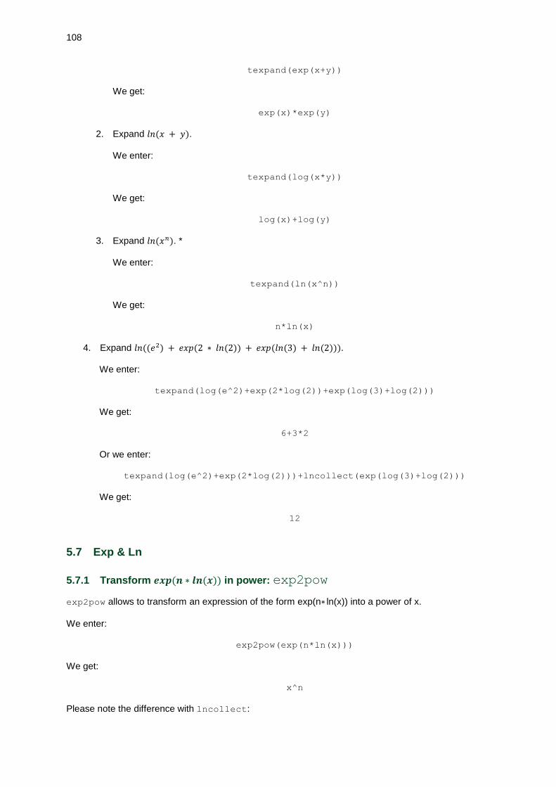
108

texpand(exp(x+y))

We get:

exp(x)*exp(y)

2. Expand 𝑙𝑛(𝑥 + 𝑦). We enter:

texpand(log(x*y))

We get:

log(x)+log(y)

3. Expand 𝑙𝑛(𝑥𝑛). * We enter:

texpand(ln(x^n))

We get:

n*ln(x)

4. Expand 𝑙𝑛((𝑒2) + 𝑒𝑥𝑝(2 ∗ 𝑙𝑛(2)) + 𝑒𝑥𝑝(𝑙𝑛(3) + 𝑙𝑛(2))). We enter:

texpand(log(e^2)+exp(2*log(2))+exp(log(3)+log(2)))

We get:

6+3*2

Or we enter:

texpand(log(e^2)+exp(2*log(2)))+lncollect(exp(log(3)+log(2)))

We get:

12

5.7 Exp & Ln

5.7.1 Transform 𝒆𝒙𝒑(𝒏 ∗ 𝒍𝒏(𝒙)) in power: exp2pow

exp2pow allows to transform an expression of the form exp(n∗ ln(x)) into a power of x.

We enter:

exp2pow(exp(n*ln(x)))

We get:

x^n

Please note the difference with lncollect:

109

lncollect(exp(n*ln(x))) = exp(n*ln(x))

lncollect(exp(2*ln(x))) = exp(2*ln(x))

exp2pow(exp(2*ln(x)))= x^2

But:

lncollect(exp(ln(x)+ln(x))) = x^2

exp2pow(exp(ln(x)+ln(x))) = x^(1+1)

5.7.2 Transform a power into an exponential: pow2exp

pow2exp allows to transform a power into exponential. We enter:

pow2exp(a^(x+y))

We get:

exp((x+y)*ln(a))

5.7.3 Transform the complex exponentials into sin and cos: sincos exp2trig

sincos or exp2trig takes as argument an expression containing complex exponentials. sincos or exp2trig transforms this expression in term of sin(𝑥) and cos(𝑥). We enter:

sincos(exp(i*x))

or

exp2trig(exp(i*x))

We get, if Complex is not checked in the CAS configuration (Shift-CAS):

cos(x)+i*sin(x)

We get, if Complex is checked in the CAS configuration:

exp(im(x))*(cos(re(x))+(i)*sin(re(x)))

We enter:

sincos(exp(i*x)+exp(-i*x))

or

exp2trig(exp(i*x)+exp(-i*x))

We get:

cos(x)+i*sin(x)+cos(x)-i*sin(x)

then we select this answer and we press simplify. We get:

2*cos(x)

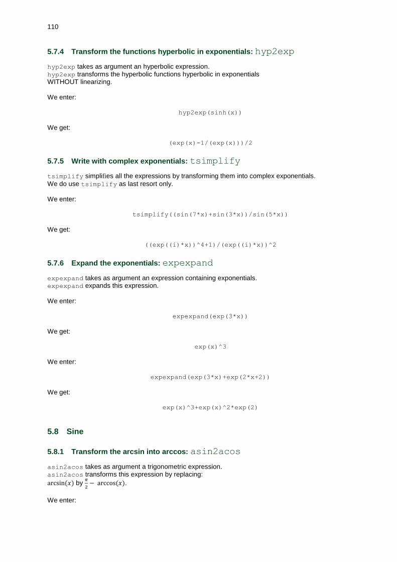
110

5.7.4 Transform the functions hyperbolic in exponentials: hyp2exp

hyp2exp takes as argument an hyperbolic expression. hyp2exp transforms the hyperbolic functions hyperbolic in exponentials WITHOUT linearizing. We enter:

hyp2exp(sinh(x))

We get:

(exp(x)-1/(exp(x)))/2

5.7.5 Write with complex exponentials: tsimplify

tsimplify simplifies all the expressions by transforming them into complex exponentials.

We do use tsimplify as last resort only. We enter:

tsimplify((sin(7*x)+sin(3*x))/sin(5*x))

We get:

((exp((i)*x))^4+1)/(exp((i)*x))^2

5.7.6 Expand the exponentials: expexpand

expexpand takes as argument an expression containing exponentials. expexpand expands this expression. We enter:

expexpand(exp(3*x))

We get:

exp(x)^3

We enter:

expexpand(exp(3*x)+exp(2*x+2))

We get:

exp(x)^3+exp(x)^2*exp(2)

5.8 Sine

5.8.1 Transform the arcsin into arccos: asin2acos

asin2acos takes as argument a trigonometric expression. asin2acos transforms this expression by replacing:

arcsin(𝑥) by 𝜋

2− arccos(𝑥).

We enter:

111

asin2acos(acos(x)+asin(x))

We get after simplification:

pi/2

5.8.2 Transform the arcsin in arctan: asin2atan

asin2atan takes as argument a trigonometric expression. asin2atan transforms this expression by replacing:

arcsin(𝑥) by arctan(𝑥

√1 – 𝑥2).

We enter:

asin2atan(asin(x))

We get:

atan(x/sqrt(1-x^2))

5.8.3 Transform sin(x) in cos(x)*tan(x): sin2costan

sin2costan takes as argument a trigonometric expression. sin2costan transforms this expression by replacing: sin(𝑥) by cos(𝑥) ∗ tan(𝑥). We enter:

sin2costan(sin(2*x))

We get:

cos(2*x)*tan(2*x)

5.9 Cosine

5.9.1 Transform the arccos into arcsin: acos2asin

acos2asin takes as argument a trigonometric expression. acos2asin transforms this expression by replacing:

arccos(𝑥) by 𝜋

2− arcsin(𝑥).

We enter:

acos2asin(acos(x)+asin(x))

We get after simplification:

pi/2

5.9.2 Transform the arccos into arctan: acos2atan

acos2atan takes as argument a trigonometric expression. acos2atan transforms this expression by replacing:

112

arccos(𝑥) by 𝜋

2− arctan (

𝑥

√1 – 𝑥2).

We enter:

acos2atan(acos(x))

We get:

pi/2-atan(x/sqrt(1-x^2))

5.9.3 Transform cos(x) into sin(x)/tan(x): cos2sintan

cos2sintan takes as argument a trigonometric expression. cos2sintan transforms this expression by replacing:

cos(𝑥) by sin(𝑥)

tan(𝑥).

We enter:

cos2sintan(cos(2*x))

We get:

sin(2*x)/tan(2*x)

5.10 Tangent

5.10.1 Transform tan(x) with sin(2x) and cos(2x): tan2sincos2

tan2sincos2 takes as argument a trigonometric expression. tan2sincos2 transforms this expression by replacing:

tan(𝑥) by sin(2.𝑥)

1+cos(2.𝑥).

We enter:

tan2sincos2(tan(x))

We get:

sin(2*x)/(1+cos(2*x))

5.10.2 Transform the arctan into arcsin: atan2asin

atan2asin takes as argument a trigonometric expression. atan2asin transforms this expression by replacing:

𝑎𝑟𝑐𝑡𝑎𝑛(𝑥) by arcsin (𝑥

√1+ 𝑥2).

We enter:

atan2asin(atan(x))

We get:

asin(x/sqrt(1+x^2))

113

5.10.3 Transform the arctan into arccos: atan2acos

atan2acos takes as argument a trigonometric expression. atan2acos transforms this expression by replacing:

arctan(𝑥) by 𝜋

2− arccos (

𝑥

√1+ 𝑥2).

We enter:

atan2acos(atan(x))

We get:

pi/2-acos(x/sqrt(1+x^2))

5.10.4 Transform tan(x) into sin(x)/cos(x): tan2sincos

tan2sincos takes as argument a trigonometric expression. tan2sincos transforms this expression by replacing:

tan(𝑥) by sin(𝑥)

cos(𝑥).

We enter:

tan2sincos(tan(2*x))

We get:

sin(2*x)/cos(2*x)

5.10.5 Transform a trigonometric expression in term of tan(x/2): halftan

halftan takes as argument a trigonometric expression.

halftan transforms the sin(𝑥), cos(𝑥) and tan(𝑥) of the expression in term of tan(𝑥

2).

We enter:

halftan(sin(x))

We get:

2*tan(x/2)/(1+tan(x/2)^2)

We enter:

halftan(sin(2*x)/(1+cos(2*x)))

We get:

2*tan(2*x/2)/((tan(2*x/2))^2+1)/(1+(1-

(tan(2*x/2))^2)/((tan(2*x/2))^2+1))

And, after simplification with simplify(Ans), we get:

tan(x)

114

5.11 Trigonometry

5.11.1 Simplify by privileging sine: trigsin

trigsin takes as argument a trigonometric expression. trigsin simplifies this expression using formulas:

sin(𝑥)2 + cos(𝑥)2 = 1, tan(𝑥) =sin(𝑥)

cos(𝑥) and by privileging sine.

We enter:

trigsin(cos(x)^2+1)

We get:

-sin(x)^2+2

5.11.2 Simplify by privileging cosine: trigcos

trigcos takes as argument a trigonometric expression. trigcos simplifies this expression using formulas:

sin(𝑥)2 + cos(𝑥)2 = 1, tan(𝑥) =sin(𝑥)

cos(𝑥) and by privileging cosine.

We enter:

trigcos(sin(x)^4+2)

We get:

cos(x)^4-2*cos(x)^2+3

5.11.3 Transform trigonometric inverse functions to logarithms: atrig2ln

atrig2ln rewrites the expression containing trigonometric inverse functions with logarithms. We enter:

atrig2ln(asin(x))

We get:

i*ln(x+sqrt(x^2-1))+pi/2

5.11.4 Simplify by privileging tangent: trigtan

trigtan takes as argument a trigonometric expression. trigtan simplifies this expression using formulas:

sin(𝑥)2 + cos(𝑥)2 = 1, tan(𝑥) =sin(𝑥)

cos(𝑥) and by privileging tangent.

We enter:

trigtan(sin(x)^4+cos(x)^2+1)

We get:

((tan(x))^2/(1+(tan(x))^2))^2+1/(1+(tan(x)^2)+1

and after simplification with simplify(Ans), we have:

115

(2*tan(x)^4+3*tan(x)^2+2)/(tan(x)^4+2*tan(x))^2+1)

5.11.5 Linearize a trigonometric expression: tlin

tlin takes as argument a trigonometric expression. tlin linearizes this expression in term of 𝑠𝑖𝑛(𝑛. 𝑥) 𝑎𝑛𝑑 𝑐𝑜𝑠(𝑛. 𝑥). Examples

– Linearize 𝑐𝑜𝑠(𝑥) ∗ 𝑐𝑜𝑠(𝑦). We enter:

tlin(cos(x)*cos(y))

We get:

1/2*cos(x-y)+1/2*cos(x+y)

– Linearize 𝑐𝑜𝑠(𝑥)3. We enter:

tlin(cos(x)^3)

We get:

3/4*cos(x)+1/4*cos(3*x)

– Linearize 4 𝑐𝑜𝑠(𝑥)2 − 2. We enter:

tlin(4*cos(x)^2-2)

We get:

2*cos(2*x)

5.11.6 Shift the phase by 𝝅

𝟐 in trigonometric expressions: shift_phase

shift_phase takes as argument a trigonometric expression.

shift_phase allows to shift the phase by 𝜋

2 in trigonometric expressions once the automatic

simplification has been performed. We enter:

shift_phase(x+sin(x))

We get:

x-cos((pi+2*x)/2)

We enter:

shift_phase(x+cos(x))

We get:

x-+sin((pi+2*x)/2)

116

We enter:

shift_phase(x+tan(x))

We get:

x+1/(tan((pi+2*x)/2))

Should the expression not be evaluated (i.e. no automatic simplification), just quote the argument. We enter:

shift_phase(’sin(x+pi/2)’)

We get:

-(cos(pi+x))

but if we enter without quoting the sine:

shift_phase(sin(x+pi/2))

We get:

sin((pi+2*x)/2)

because sin(x+pi/2) is evaluated (i.e. simplified) into cos(x) before the command shift_phase is called and then shift_phase(cos(x)) returns sin((pi+2*x)/2). Exercise Calculate

∑sin(𝑛 ∗ 𝑥)

𝑛

+∞

𝑛=1

We enter:

normal(sum((sin(n*x))/n,n=1..+infinity))

We get:

-atan((sin(x))/(cos(x)-1))

We enter:

normal(shift_phase(halftan(atan(sin(x)/(-cos(x)+1)))))

We get:

pi*floor(((pi+x)/2)/pi+1/2)+(-1)/2*pi+(-1)/2*x

if we enter:

tsimplify(atan((sin(x))/(-cos(x)+1)))

Because tsimplify is not rigorous with respect to 2𝑘𝜋, we get:

-1/2*pi-1/2*x

117

5.11.7 Collect the sine and cosine of a same angle: tcollect

tcollect takes as argument a trigonometric expression. tcollect linearizes this expression in term of sin(𝑛. 𝑥) and cos(𝑛. 𝑥) then collects the sine and cosine of same angle. We enter:

tcollect(sin(x)+cos(x))

We get:

sqrt(2)*cos(x-pi/4)

We enter:

tcollect(2*sin(x)*cos(x)+cos(2*x))

We get:

sqrt(2)*cos(2*x-pi/4)

5.11.8 Expand a trigonometric expression: trigexpand

trigexpand takes as argument a trigonometric expression. trigexpand expands this expression in term of sin(𝑥) and cos(𝑥). We enter:

trigexpand(cos(x+y))

We get:

cos(x)*cos(y)-sin(x)*sin(y)

5.11.9 Transform a trigonometric expression into complex exponentials: trig2exp

trig2exp takes as argument a trigonometric expression. trig2exp transforms the trigonometric functions into complex exponentials WITHOUT linearizing. We enter:

trig2exp(tan(x))

We get:

((exp((i)*x))^2-1)/((i)*((exp((i)*x))^2+1))

We enter:

trig2exp(sin(x))

We get:

(exp((i)*x)-1/(exp((i)*x)))/(2*i)

118

Chapter 6 Menu Integer

6.1 Test of parity: even

even takes as argument an integer n. even returns 1 if n is even and 0 if n is odd. We enter:

even(148)

We get:

1

We enter:

even(149)

We get:

0

6.2 Test of non parity: odd

odd takes as argument an integer n. odd returns 1 if n is odd and 0 if n is even. We enter:

odd(148)

We get:

0

We enter:

odd(149)

We get:

1

6.3 Divisors of an integer: idivis

idivis returns the vector whose components are the divisors of an integer. We enter:

idivis(45)

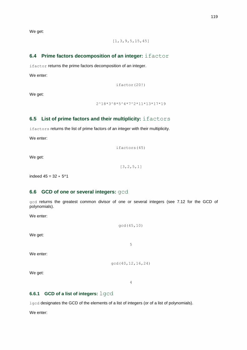
119

We get:

[1,3,9,5,15,45]

6.4 Prime factors decomposition of an integer: ifactor

ifactor returns the prime factors decomposition of an integer. We enter:

ifactor(20!)

We get:

2^18*3^8*5^4*7^2*11*13*17*19

6.5 List of prime factors and their multiplicity: ifactors

ifactors returns the list of prime factors of an integer with their multiplicity. We enter:

ifactors(45)

We get:

[3,2,5,1]

indeed 45 = 32 ∗ 5^1

6.6 GCD of one or several integers: gcd

gcd returns the greatest common divisor of one or several integers (see 7.12 for the GCD of polynomials). We enter:

gcd(45,10)

We get:

5

We enter:

gcd(40,12,16,24)

We get:

4

6.6.1 GCD of a list of integers: lgcd

lgcd designates the GCD of the elements of a list of integers (or of a list of polynomials). We enter:

120

lgcd([18,15,21,36])

We get:

3

6.7 LCM of one or several integers: lcm

lcm returns the lowest common multiple of two or several integers. We enter:

lcm(45,10)

We get:

90

We enter:

lcm(45,10,25,30)

We get:

450

6.7.1 Bezout identity: iegcd

iegcd(a,b) designates the extended GCD (Bezout identity ) of two integers. iegcd(a,b) returns [u,v,d] that make au+bv=d and such as d=gcd(a,b). We enter:

iegcd(48,30)

We get:

[2,-3,6]

Indeed:

2 · 48 + (−3) · 30 = 6

6.7.2 Solve 𝒂𝒖 + 𝒃𝒗 = 𝒄 in ℤ: iabcuv

iabcuv(a,b,c) gives [u,v] that make au+bv=c. Of course, c has to be a multiple of gcd(a,b) to get a solution. We enter:

iabcuv(48,30,18)

We get:

[6,-9]

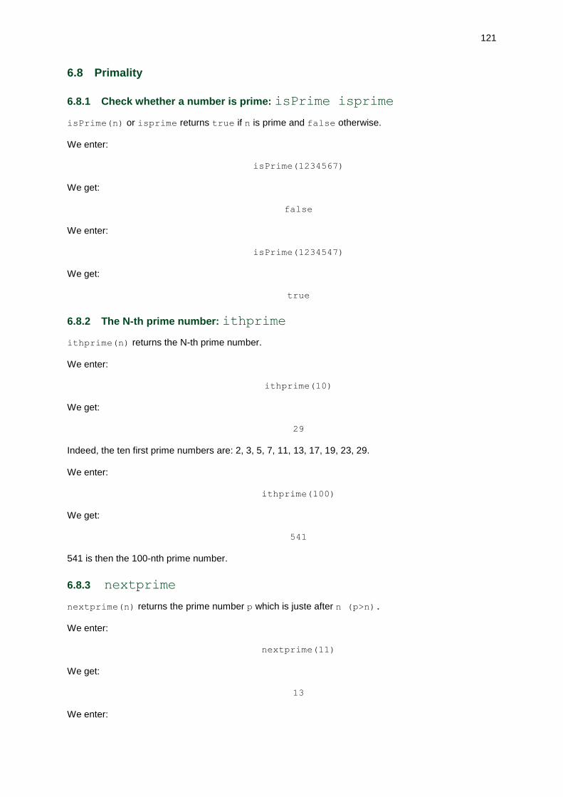
121

6.8 Primality

6.8.1 Check whether a number is prime: isPrime isprime

isPrime(n) or isprime returns true if n is prime and false otherwise. We enter:

isPrime(1234567)

We get:

false

We enter:

isPrime(1234547)

We get:

true

6.8.2 The N-th prime number: ithprime

ithprime(n) returns the N-th prime number. We enter:

ithprime(10)

We get:

29

Indeed, the ten first prime numbers are: 2, 3, 5, 7, 11, 13, 17, 19, 23, 29. We enter:

ithprime(100)

We get:

541

541 is then the 100-nth prime number.

6.8.3 nextprime

nextprime(n) returns the prime number p which is juste after n (p>n). We enter:

nextprime(11)

We get:

13

We enter:

122

nextprime(1234567)

We get:

1234577

6.8.4 prevprime

prevprime(n) returns the prime number p which is just before n (p<n). We enter:

prevprime(11)

We get:

7

We enter:

prevprime(1234567)

We get:

1234547

6.8.5 Euler’s totient: euler

euler(n) returns the cardinal of the set of numbers lower than n which are relatively prime to n. euler(n) designates then the Euler’s totient of the integer n. We enter:

euler(18)

We get:

6

Indeed, the set: 𝐸 = {5,7,11,13,15,17} corresponds to numbers lower than 18 which are prime to 18, and 𝐸 takes as

cardinal 6. With the euler function, we have the generalization of the Fermat’s theorem (which says that "if n is prime and if a is prime to n then 𝑎𝑛−1 = 1 𝑚𝑜𝑑 𝑛. ")

The generalization is (because if 𝑛 is prime, 𝑒𝑢𝑙𝑒𝑟(𝑛) = 𝑛 − 1):

𝑎𝑒𝑢𝑙𝑒𝑟(𝑛) = 1 𝑚𝑜𝑑 𝑛 if 𝑎 and 𝑛 are prime to each other. We enter:

powmod(5,6,18)

We get:

1

6.8.6 Legendre symbole: legendre_symbol

When 𝑛 is prime, we define the Legendre symbol of 𝑎 written (𝑎

𝑛) by:

123

(𝑎

𝑛) = {

0 if 𝑎 = 0 mod 𝑛 1 if 𝑎 ≠ 0 mod 𝑛 and if 𝑎 = b2 mod 𝑛−1 if 𝑎 ≠ 0 mod 𝑛 and if a ≠ b2 mod 𝑛

Some properties

– if 𝑛 is prime:

𝑎𝑛−12 = (

𝑎

𝑛) 𝑚𝑜𝑑 𝑛

– (𝑝

𝑞) . (

𝑞

𝑝) = (−1)

𝑝−1

2 . (−1)𝑞−1

2 if 𝑝 and 𝑞 are odd and positive

(2

𝑝) = (−1)

𝑝2−18

(−1

𝑝) = (−1)

𝑝−12

legendre_symbol has two parameters 𝑎 and 𝑛 and returns the Legendre symbol (𝑎

𝑛).

We enter:

legendre_symbol(26,17)

We get:

1

We enter:

legendre_symbol(27,17)

We get:

-1

We enter:

legendre_symbol(34,17)

We get:

0

6.8.7 Jacobi symbol: jacobi_symbol

When n is not prime, we define the Jacobi symbol of a, also written (𝑎

𝑛), from the Legendre symbol

and the decomposition of 𝑛 in prime factor. Let

𝑛 = 𝑝1𝛼1 . . 𝑝𝑘1

𝛼𝑘

where 𝑝𝑗 is prime and α𝑗 is an integer for 𝑗 = 1. . 𝑘. The Jacobi symbol of 𝑎 is defined by:

(𝑎

𝑛) = (

𝑎

𝑝1)𝛼1

. . (𝑎

𝑝𝑘)𝛼𝑘

jacobi_symbol has two parameters 𝑎 and 𝑛 and returns the symbol of Jacobi (𝑎

𝑛).

We enter:

jacobi_symbol(25,12)

We get:

1

124

We enter:

jacobi_symbol(35,12)

We get:

-1

We enter:

jacobi_symbol(33,12)

We get:

0

6.8.8 Solve 𝒂𝟐 + 𝒂𝒃𝟐 = 𝒑 in ℤ: pa2b2

pa2b2 decomposes a prime integer p, congruent to 1 modulus 4, in the sum of two squares: 𝑝 = 𝑎2 +𝑏2. The result is supplied as a list. We enter:

pa2b2(17)

We get:

[4,1]

indeed 17 = 42 + 12

6.9 Division

6.9.1 Quotient of the Euclidean division: iquo

iquo(a,b) returns the quotient of the Euclidean division of a by b when a and b are integers. We enter:

iquo(45,10)

We get:

4

indeed 45 = 4 ∗ 10 + 5

6.9.2 Remainder of the Euclidean division: irem

irem(a,b) returns the remainder of the Euclidean division of a by b when a and b are integers. We enter:

irem(45,10)

We get:

125

5

indeed 45 = 4 ∗ 10 + 5

6.9.3 Quotient and remainder of the Euclidean division: iquorem

iquorem gives the list of the quotient q and the integer remainder r of the Euclidean division of the integers a and b supplied as argument (𝑎 = 𝑏 ∗ 𝑞 + 𝑟 with 0 ≤ 𝑟 < 𝑏). We enter:

iquorem(148,5)

We get:

[29,3]

6.9.4 Chinese remainder for integers: ichinrem

ichinrem([a,n],[b,p]) returns the vector [c,lcm(p,q)] formed of two integers. The first number c is such as

∀𝑘 ∈ ℤ, 𝑑 = 𝑐 + 𝑘 × lcm(𝑝, 𝑞) 𝑙 checks

𝑑 = 𝑎 (mod 𝑝), 𝑑 = 𝑏 (mod 𝑞) If n and p are prime then there is always a solution and q=n*p Example: Find the solutions of:

{𝑥 = 3 (mod 5)𝑥 = 9 (mod 13)

We enter:

ichinrem([3,5],[9,13])

Or we enter:

ichinrem({[3,5},{9,13})

We get:

[-17,65]

So the solutions are x=-17+k*65 with 𝑘 ∈ ℤ . We have indeed −17 = −5 ∗ 4 + 3 = 3 mod 5 and −17 = −2 ∗ 13 + 9 = 9 mod 13 ichinrem returns the Chinese remainder for integers. We enter:

ichinrem({2,7},{3,5})

Or we enter:

ichinrem([2,7],[3,5])

We get:

[-12,35]

We do have −12 + 35𝑘 = 2 mod 7 and −12 + 35𝑘 = 3 mod 5 for 𝑘 ∈ ℤ

126

6.9.5 Calculation of 𝒂𝒏 𝐦𝐨𝐝 𝒑: powmod

powmod(a,n,p) returns 𝑎𝑛 modulus 𝑝 with the method of the fast exponentiation. We enter:

powmod(5,21,13)

We get:

5

52 = 25 = −1 𝑚𝑜𝑑 13 then 521 = 5 ∗ 520 = 5 mod 13 We enter:

powmod(37,25,11)

We get:

1

indeed 37 = 4 𝑚𝑜𝑑 11 and 45 = 42 ∗ 42 ∗ 4 = 25 ∗ 4 = 1 𝑚𝑜𝑑 11

6.10 Modular calculus in ℤ /𝒑 ℤ or in ℤ /𝒑 ℤ [𝒙]

We can perform calculations modulus p that is to say in ℤ /𝑝 ℤ or in ℤ /𝑝 ℤ [𝑥]. The numbers 𝑛 of ℤ /𝑝 ℤ are written n% p. Examples of notation

– an integer n of ℤ /13 ℤ n:=12% 13.

– a vector V of coordinates in ℤ /13 ℤ V:=[1,2,3]% 13 or V:=[1% 13,2% 13,3% 13].

– a matrix A of coefficients in ℤ /13 ℤ A:=[[1,2,3],[2,3,4]]% 13 or A:=[[1% 13,2% 13,3% 13],[2% 13,3% 13,4% 13]].

– a polynomial A of ℤ /13 ℤ [𝑥] in symbolic notation A:=(2*x^2+3*x-1)%13

or A:=2%13*x^2+3%13*x-1%13.

– a polynomial A of ℤ /13 ℤ [𝑥] represented with a list A:=poly1[1,2,3]%13

or A:=poly1[1%13,2%13,3%13].

To transform an object o of modular coefficients into an object of integer coefficients, press: o % 0. For instance, if we enter o:=4% 7 then o% 0, we get -3. Notes

– For some commands in ℤ /𝑝 ℤor in ℤ /𝑝 ℤ [𝑥], we have to choose a number p which is prime. – The chosen representation is the symmetrical representation:

11%13 = -2%13

6.10.1 Expand and factorise: normal

normal takes as argument a polynomial expression. normal expands and factors this expression in ℤ/𝑝ℤ[𝑥].

127

We enter:

normal(((2*x^2+12)*( 5*x-4))% 13)

We get:

(-3% 13)*x^3+(5% 13)*x^2+(-5%13)*x+4% 13

6.10.2 Addition in ℤ /𝒑 ℤ or in ℤ /𝒑ℤ[𝒙]: +

To perform an addition in ℤ/𝑝ℤ, we use the usual + and, for polynomials of ℤ/𝑝ℤ[𝑥], we use the usual + and the command normal to simplify. For the integers in ℤ/𝑝ℤ, we enter:

3% 13+10% 13

We get:

0%13

For the polynomials with coefficients in ℤ/𝑝ℤ, we enter:

normal(11% 13*x+5% 13+8% 13*x+6% 13)

or else

normal((11*x+5 )% 13+(8*x+6)% 13)

We get:

(6%13)*x+-2% 13

6.10.3 Substraction in ℤ /𝒑 ℤ or in ℤ /𝒑ℤ[𝒙]: -

To perform a substraction in ℤ/𝑝ℤ, we use the usual - and, for polynomials of ℤ/𝑝ℤ[𝑥], we use the usual - and the command normal to simplify. For the integers in ℤ/𝑝ℤ, we enter:

31% 13-10% 13

We get:

-5% 13

For the polynomials with coefficients in ℤ/𝑝ℤ, we enter:

normal(11% 13*x+5% 13-8% 13*x+6% 13)

or else

normal((11*x+5)% 13-(8*x+6)% 13)

We get:

(3% 13)*x+-1% 13

128

6.10.4 Multiplication in ℤ /𝒑 ℤ or ℤ /𝒑 ℤ [𝒙]: *

To perform a multiplication in ℤ/𝑝ℤ, we use the usual * and, for polynomials of ℤ/𝑝ℤ[𝑥], we use the usual * then the command normal to simplify. For the integers in ℤ/𝑝ℤ, we enter:

31% 13*10% 13

We get:

-2% 13

For the polynomials with coefficients in ℤ/𝑝ℤ, we enter:

normal((11% 13*x+5% 13)*(8% 13*x+6% 13))

or else we enter:

normal((11*x+5)% 13*(8*x+6 )% 13)

We get:

(-3% 13)*x^2+(2% 13)*x+4% 13

6.10.5 Quotient: quo

quo takes as arguments two polynomials 𝐴 and 𝐵 with coefficients in ℤ/𝑝ℤ. 𝐴 and 𝐵 may be supplied

by a symbolic polynomial expression (of 𝑥 or of the name of the variable supplied as third argument) or by the list of their coefficients.

quo returns the quotient of the Euclidean division of 𝐴 by 𝐵 in ℤ/𝑝ℤ[𝑥]. We enter:

quo((x^3+x^2+1)% 13,(2*x^2+4)% 13)

Or we enter:

quo((x^3+x^2+1,2*x^2+4)% 13)

We get:

(-6% 13)*x+-6% 13

indeed 𝑥3 + 𝑥2 + 1 = (2𝑥2 + 4) (𝑥 +1

2) +

5𝑥 –4

4

and −3 ∗ 4 = −6 ∗ 2 = 1 mod 13

6.10.6 Remainder: rem

rem takes as arguments two polynomials 𝐴 and 𝐵 with coefficients in ℤ/𝑝ℤ. 𝐴 and 𝐵

may be supplied by a symbolic polynomial expression (of 𝑥 or of the name of the variable supplied as third argument) or by the list of their coefficients. rem returns the remainder of the Euclidean division of 𝐴 by 𝐵 in ℤ/𝑝ℤ[𝑥]. We enter:

rem((x^3+x^2+1)% 13,(2*x^2+4)% 13)

Or we enter:

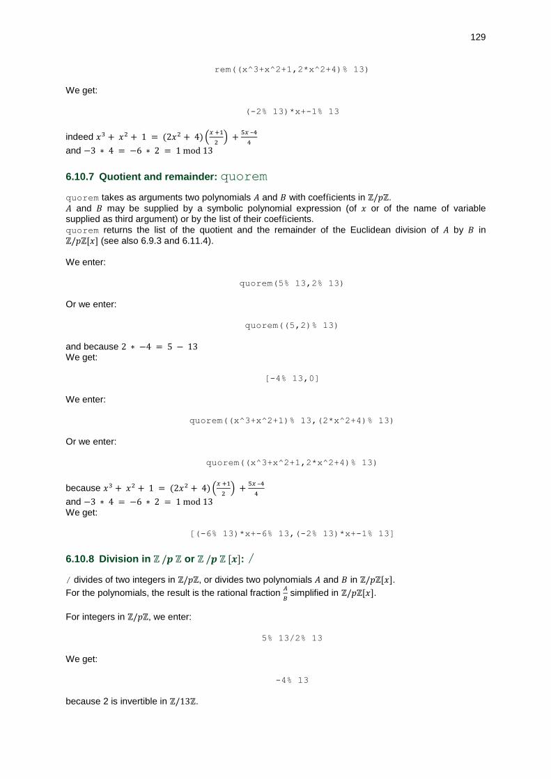
129

rem((x^3+x^2+1,2*x^2+4)% 13)

We get:

(-2% 13)*x+-1% 13

indeed 𝑥3 + 𝑥2 + 1 = (2𝑥2 + 4) (𝑥 +1

2) +

5𝑥 –4

4

and −3 ∗ 4 = −6 ∗ 2 = 1 mod 13

6.10.7 Quotient and remainder: quorem

quorem takes as arguments two polynomials 𝐴 and 𝐵 with coefficients in ℤ/𝑝ℤ.

𝐴 and 𝐵 may be supplied by a symbolic polynomial expression (of 𝑥 or of the name of variable supplied as third argument) or by the list of their coefficients.

quorem returns the list of the quotient and the remainder of the Euclidean division of 𝐴 by 𝐵 in

ℤ/𝑝ℤ[𝑥] (see also 6.9.3 and 6.11.4). We enter:

quorem(5% 13,2% 13)

Or we enter:

quorem((5,2)% 13)

and because 2 ∗ −4 = 5 − 13 We get:

[-4% 13,0]

We enter:

quorem((x^3+x^2+1)% 13,(2*x^2+4)% 13)

Or we enter:

quorem((x^3+x^2+1,2*x^2+4)% 13)

because 𝑥3 + 𝑥2 + 1 = (2𝑥2 + 4) (𝑥 +1

2) +

5𝑥 –4

4

and −3 ∗ 4 = −6 ∗ 2 = 1 mod 13 We get:

[(-6% 13)*x+-6% 13,(-2% 13)*x+-1% 13]

6.10.8 Division in ℤ /𝒑 ℤ or ℤ /𝒑 ℤ [𝒙]: /

/ divides of two integers in ℤ/𝑝ℤ, or divides two polynomials 𝐴 and 𝐵 in ℤ/𝑝ℤ[𝑥].

For the polynomials, the result is the rational fraction 𝐴

𝐵 simplified in ℤ/𝑝ℤ[𝑥].

For integers in ℤ/𝑝ℤ, we enter:

5% 13/2% 13

We get:

-4% 13

because 2 is invertible in ℤ/13ℤ.

130

For the polynomials with coefficients in ℤ/𝑝ℤ.

We enter:

(2*x^2+5)% 13/(5*x^2+2*x-3)% 13

We get:

((6% 13)*x+1% 13)/((2% 13)*x+2% 13)

6.10.9 Power in ℤ /𝒑 ℤ or ℤ /𝒑 ℤ [𝒙]: ˆ

To calculate a at the power n in ℤ/𝑝ℤ we use the operator ^. We enter:

(5% 13)^2)

We get:

-1% 13

To calculate A at the power n in ℤ/𝑝ℤ[𝑥] we use the operator ^ and the command normal. We enter:

normal(((2*x+1)% 13)^5)

We get:

(6% 13)*x^5+(2% 13)*x^4+(2% 13)*x^3+(1% 13)*x^2+(-3%13)*x+1% 13

because: 10 = −3 (mod 13) 40 = 1 (mod 13) 80 = 2 (mod 13) 32 = 6 (mod 13).

6.10.10 Calculation of 𝒂𝒏 𝐦𝐨𝐝 𝒑 or of 𝑨(𝒙)𝒏 𝒎𝒐𝒅 ¶(𝒙), 𝒑: powmod

– To calculate in [0; 𝑝 − 1] 𝑎𝑛 𝑚𝑜𝑑 𝑝 we use the command powmod or powermod with as

argument 𝑎, 𝑛, 𝑝.

We enter:

powmod(5,21,13)

We get:

5

We enter:

powmod(5,21,8)

We get:

5

– To calculate 𝐴(𝑥)𝑛 mod ¶(𝑥), 𝑝 with as a result a polynomial with coefficients in ℤ (which will

be symmetrical remainders of division by 𝑝), we use the command powmod or powermod with

as argument 𝐴(𝑥), 𝑛, 𝑝, 𝑃(𝑥). We enter:

131

powmod(x+1,17,5,x^4+x+1)

We get:

-x^3-x^2

We have indeed:

rem((x+1)^17,x^4+x+1)

which returns:

29144*x^3+36519*x^2+12270*x-4185

and

(29144*x^3+36519*x^2+12270*x-4185)% 5

which returns:

(-1 % 5)*x^3+(-1 % 5)*x^2

and

((-1 % 5)*x^3+(-1 % 5)*x^2)% 0

which returns:

-x^3-x^2

Note (cf section 6.10.9)

If we can calculate a power in ℤ /𝑝 ℤ we enter for example:

(5% 13)^21)

We get:

5% 13

We enter:

(5% 8)^21)

We get:

-3% 8

6.10.11 Inverse in ℤ /𝒑 ℤ: inv or /

We calculate the inverse of an integer n in ℤ /𝑝 ℤ by entering 1/n% p or inv(n%p) or inverse(n% p). We enter:

inv(3% 13)

We get:

-4% 13

Indeed: 3 × −4 = −12 = 1 (mod 13)

132

6.10.12 Transform an integer into its fraction modulus 𝒑: fracmod

fracmod has two arguments, an integer n (or an integer expression) and an integer p. fracmod returns a fraction a/b such as:

−√𝑝

2< 𝑎 ≤

√𝑝

2, 0 ≤ 𝑏 <

√𝑝

2, 𝑛 × 𝑏 = 𝑎 (mod 𝑝)

In other words 𝑛 = 𝑎

𝑏 (mod 𝑝).

We enter:

fracmod(3,13)

We get:

-1/4

Indeed: 3 ∗ −4 = −12 = 1 (mod 13) then 3 = −1/4% 13.

We enter:

fracmod(13,121)

We get:

-4/9

Indeed: 13 × −9 = −117 = 4 (mod 121) then 13 = −4/9% 13.

6.10.13 GCD in ℤ /𝒑 ℤ [𝒙]: gcd

When gcd has two polynomials with coefficients in ℤ /𝑝 ℤ as arguments (p must be prime), gcd

returns the GCD of the two polynomials in ℤ /𝑝 ℤ [𝑥] (see also 7.12 for polynomials with non modular coefficients). We enter:

gcd((2*x^2+5)% 13,(5*x^2+2*x-3)% 13)

We get:

(-4% 13)*x+5% 13

We enter:

gcd(x^2+2*x+1,x^2-1) mod 5

We get:

1

but if we enter:

gcd((x^2+2*x+1,x^2-1)) mod 5)

gcd is calculatedin ℤ [𝑥] then the modular calculus is performed, we get:

x% 5

133

6.10.14 Factorization in ℤ /𝒑 ℤ [𝒙]: factor

factor takes as argument a polynomial with coefficients in ℤ /𝑝 ℤ . factor factors this polynomial in ℤ /𝑝 ℤ [𝑥] (𝑝 must be prime). We enter:

factor((-3*x^3+5*x^2-5*x+4)% 13)

We get:

((1% 13)*x+-6% 13)*((-3% 13)*x^2+-5% 13)

6.10.15 Determinant of a matrix of ℤ /𝒑 ℤ: det

det takes as argument a matrix 𝐴 with coefficients in ℤ /𝑝 ℤ.

det returns the determinant of this matrix 𝐴. We enter:

det([[1,2,9]% 13,[3,10,0]% 13,[3,11,1]% 13])

Or we enter:

det([[1,2,9],[3,10,0],[3,11,1]]% 13)

We get:

5% 13

thus, in ℤ /13 ℤ, the determinant of the matrix 𝐴 = [[1, 2, 9], [3, 10, 0], [3, 11, 1]] is 5% 13 (on a det(A)=31).

6.10.16 Inverse of a matrix of ℤ /𝒑 ℤ: inv

inverse (or inv) takes as argument a matrix 𝐴 with coefficients in ℤ /𝑝 ℤ . inv returns the inverse of the matrix 𝐴 in ℤ /𝑝 ℤ. We enter:

inv([[1,2,9]% 13,[3,10,0]% 13,[3,11,1]% 13])

Or we enter:

inv([[1,2,9],[3,10,0],[3,11,1]]% 13)

We get:

[[2% 13,-4% 13,-5% 13],[2% 13,0% 13,-5% 13], [-2%13,-1% 13,6% 13]]

It is the inverse of the matrix 𝐴 = [[1, 2, 9], [3, 10, 0], [3, 11, 1]] in ℤ /13 ℤ.

6.10.17 Solve a linear system of ℤ /𝒑 ℤ: rref

rref allows to solve, in ℤ /𝑝 ℤ, a linear equations system of the form: 𝐴𝑥 = 𝐵 (see also 20.9).

The argument is a matrix formed by 𝐴 bordered ( translation to be checked) with 𝐵 as last column

vector. The result is a matrix formed of 𝐴1 and 𝐵1 where 𝐴1 has two zeros from either side of the diagonal, and where the system 𝐴1𝑥 = 𝐵1 is equivalent to 𝐴𝑥 = 𝐵.

Solve in ℤ /13 ℤ

134

{ 𝑥 + 2 · 𝑦 = 93 · 𝑥 + 10 · 𝑦 = 0

We enter:

rref([[1, 2, 9]% 13,[3,10,0]% 13])

Or we enter:

rref([[1, 2, 9],[3,10,0]])%13

We get:

[[1% 13,0% 13,3% 13],[0% 13,1% 13,3% 13]]

which means that x=3% 13 and y=3% 13.

6.10.18 Creation of a Galois field: GF

In its simplest form, GF takes as arguments a prime number 𝑝 and an integer 𝑛 > 1 or the power of a prime number 𝑝𝑛 and an optional argument which is the name of variable chosen for the generator of the field (the variable must be purged first). GF creates a Galois field of characteristic 𝑝 and having 𝑝𝑛 elements, the elements of the field are then

0 and the powers from 0 to 𝑝𝑛 − 2 of the generator. The field itself is stored in a free variable (by default 𝐾, this variable is displayed by the system, at the same time as the names of the generator

and the free variable, by default 𝑘, used to represent the elements of the field such as the quotient

ℤ /𝑝 ℤ [𝑘]/𝑃(𝑘) where 𝑃 is a irreducible polynomial and primitive). For instance:

– GF(3,5) or GF(3^5) creates a field having 35 elements whose generator is g (or h, ... if

g is assigned). We can create an element of the field by taking a polynomial in term of 𝑔, for

example 𝑔10 + 5𝑔 + 1.

– GF(2,8,a) creates a field having 28 elements, and uses the variable a to designate the generator (Warning, do purge(a) first if necessary).

– The command pmin allows knowing the minimal polynomial of an element of the field. We can then create polynomials or matrices having coefficients in the field, and handle them with the usual instructions + - * / inv, sqrt, quo, rem, quorem, diff, factor, gcd,

egcd,... for example: – GF(3,5,b); A:=[[1,b],[b,1]]; inv(A) returns the inverse of a matrix with

coefficients in the field of 35 elements – GF(5,3,c); p:=x^2-c-1; factor(p) factors the polynomial p as polynomial with

coefficients in the field at 53 elements, we deduce from it a value of square root of 𝑐 + 1. – p:=randpoly(x,5,g); q:=diff(p); gcd(p,q) generates a polynomial with random

coefficients, then returns its derivative and the GCD, which allows to know if p has multiples roots.

There are still limitations due to the incomplete implementation of some algorithms (for example factorization with several variables when the polynomial is not unitary). In its most comprehensive form (but more difficult to handle and less legible), the elements of this field and the field itself are represented by GF(...) where ... is a sequence composed of:

– the characteristic 𝑝 (𝑝𝑥 = 0), – the minimal irreducible polynomial (primitive if created by the CAS) generating an ideal 𝐼 in

ℤ /𝑝 ℤ [𝑋], the Galois field is then the quotient of ℤ /𝑝 ℤ [𝑋] by 𝐼, – the name of the variable of the polynomial, by default x, – a polynomial (a remainder modulus the minimal polynomial) to designate an element of the

field (These elements have an additive representation) or undef to designate the whole field which is the quotient of polynomials with coefficients in ℤ /𝑝 ℤ by 𝐼.

Usually, we give a name to the created field (for example G:=GF(p,n)), in order to build a particular element of the groupe from a polynomial of ℤ /𝑝 ℤ [𝑋], by writing for example G(x^3+x). Note that

135

G(x) is a generator of the multiplicative group 𝐺∗ when the minimal polynomial is generated by the CAS. We enter:

G:=GF(2,8)

We get (for example):

GF(2,k^8-k^7-k^6-k-1,k,undef)

The field 𝐺 has 28 = 256 elements and 𝑔 = 𝐺(𝑘) generates the multiplicative group of this field

({1, 𝑔, 𝑔2, . . . , 𝑔254}). We enter:

K(k^9)

We get:

g^6+g^2+1)

We enter:

K(k)^255

We get

1

As you notice on the previous examples, when we work with the same field, the answers content redundant informations. This is why the definition of a field may have a third argument: the name of the generator or a list containing two or three names of formal variables, (the name of the undetermined of the irreducible polynomial and the name of the Galois field that has to be quoted so that these variables are not evaluated as well as the name of the generator). This allows to get a more compact display of the elements of the field. We enter:

G:=GF(2,2,[’w’,’G’]):; G(w^2)

We get:

Done, G(w+1)

We enter:

G(w^3)

We get:

G(1)

The elements of GF(2,2) are then: 0,1,w,w^2=w+1. We can then tell which irreducible polynomial we wish to use, by mentioning it as second parameter (instead of n), for example:

G:=GF(2,w^8+w^6+w^3+w^2+1,[’w’,’G’])

If we give a non primitive irreducible polynomial, the calculator tells it and proposes a replacement by a primitive polynomial, for example:

136

G:=GF(2,w^8+w^7+w^5+w+1,[’w’,’G’])

We get:

G:=GF(2,w^8-w^6-w^3-w^2-1,[’w’,’G’],undef)

6.10.19 Factorization of a polynomial with coefficients in a Galois field:

factor

We can factorize a polynomial with coefficients in a Galois field with factor. By example, to get 𝐺 = 𝔽4, we enter:

GF(2,2,a)

We get:

GF(2,k^2+k+1,[k,K,a],undef)

By example, we enter:

factor(a^2*x^2+1))

We get:

(a+1)*(x+a+1)^2

6.11 Arithmetic of polynomials

Polynomials are represented by expressions or by the list of their coefficients listed with decreasing powers. In the first case the variable used by default is 𝑥. For the polynomials with coefficients in

ℤ /𝑛 ℤ, apply % n to the expression or to each coefficient of the list.

6.11.1 List of divisors of a polynomial: divis

divis takes as argument a symbolic polynomial (or a list of polynomials) and returns the list of divisors. We enter:

divis(x^2-1)

We get:

[1,x-1,x+1,(x-1)*(x+1)]

We enter:

divis(t^2-1)

We get:

[1,t-1,t+1,(t-1)*(t+1)]

We enter:

divis(x^4-1)

Or we enter:

137

divis(poly2symb([1,0,0,0,-1],x))

We get:

[1,x^2+1,x+1,(x^2+1)*(x+1),x-1,(x^2+1)*(x-1), (x+1)*(x-

1),(x^2+1)*(x+1)*(x-1)]

We enter:

divis([t^2,x^2-1])

We get:

[[1,t,t^2],[1,x+1,x-1,(x+1)*(x-1)]]

6.11.2 Euclidean quotient of two polynomials: quo

quo gives the quotient of the Euclidean division of polynomials (division by decreasing power order). We can enter the polynomials either by the list of their coefficients by decreasing power order, either under symbolic forms, and in this case the variable must be added as third argument (by default the variable is x). We enter:

quo(x^2+2x+1,x+3)

We get:

x-1

We enter:

quo(t^2+2t+1,t+3,t)

We get:

t-1

or we enter:

quo([1,2,1],[1,3])

We get:

[] 1,-1 []

that is to say the polynomial poly1[1,-1].

To get the quotient of 𝑥3 + 2𝑥 + 4 by 𝑥2 + 𝑥 + 2, we enter:

quo(x^3+2x+4,x^2+x+2)

We get:

x-1

Or we enter:

quo([1,0,2,4],[1,1,2])

We get:

138

[] 1,-1 []

that is to say the polynomial poly1[1,-1] or the polynomial x-1. We enter:

quo(t^3+2t+4,t^2+t+2,t)

We get:

t-1

If we do not put the variable 𝑡 as last argument, we enter:

quo(t^3+2t+4,t^2+t+2)

We get:

(t^3+2*t+4)/(t^2+t+2)

6.11.3 Euclidean remainder of two polynomials: rem

rem gives the remainder of the Euclidean division of two polynomials (division by decreasing power order). We can enter the polynomials either by the list of their coefficients by decreasing power order, either under symbolic forms, and in this case the variable must be added as third argument (by default the variable is x). We enter:

rem(x^3-1,x^2-1)

We get:

x-1

We enter:

rem(t^3-1,t^2-1,t)

We get:

t-1

We enter:

rem(x^2+2x+1,x+3)

Or we enter:

rem(t^2+2t+1,t+3,t)

We get:

4

or we enter:

rem([1,2,1],[1,3])

We get:

139

[] 4

that is to say the polynomial poly1[4] or else the polynomial 4.

To get the remainder of x, we enter 𝑥3 + 2𝑥 + 4 by 𝑥2 + 𝑥 + 2:

rem(x^3+2x+4,x^2+x+2)

We get:

x+6

Or we enter:

rem([1,0,2,4],[1,1,2])

We get:

[] 1,6[]

that is to say the polynomial poly1[1,6] or the polynomial x+6. We enter:

rem(t^3+2t+4,t^2+t+2,t)

We get:

t+6

We enter, if we do not put the variable 𝑡 as last argument:

rem(t^3+2t+4,t^2+t+2)

We get:

0

6.11.4 Quotient and Euclidean remainder: quorem

quorem (or divide) gives the list of the quotient and the remainder of the Euclidean division (by decreasing power order) of two polynomials. (See also 6.9.3 and 6.10.7). We can enter the polynomials either by the list of their coefficients by decreasing power order, either under symbolic forms, and in this case the variable must be added as third argument (by default the variable is x).

To get the quotient and the remainder of the division of 𝑥3 + 2𝑥 + 4 by 𝑥2 + 𝑥 + 2, we enter:

quorem(x^3+2x+4,x^2+x+2)

We get:

[x-1,x+6]

Or we enter:

quorem([1,0,2,4],[1,1,2])

We get:

[[1,-1],[1,6]]

that is to say the list of polynomials [poly1[1,-1],poly1[1,6]] then the quotient is the polynomial x-1 and the remainder is the polynomial x+6.

140

We enter:

quorem(t^3+2t+4,t^2+t+2,t)

We get:

[t-1,t+6]

We enter:

quorem(t^3+2t+4,t^2+t+2)

We get:

[(t^3+2*t+4)/(t^2+t+2),0]

We enter:

quorem(x^3-1,x^2-1)

We get:

[x,x-1]

We enter:

quorem(t^3-1,t^2-1,t)

We get:

[t,t-1]

6.11.5 GCD of polynomials by Euclid’s algorithm: gcd igcd

gcd or igcd designates the GCD (Greatest Common Divisor) of two polynomials which may have several variables and also the GCD of a list of polynomials, or of a sequence of polynomials which may have several variables (see 6.6 for the GCD of integers). We can also put as parameters two lists of same length (or a matrix of two lines), in this case gcd returns the greatest common divisor of elements of same index (or of same column). We enter:

gcd([x^2-4,x*y-y],[x^3-8,y^2-x^2*y])

Or we enter:

gcd([[x^2-4,x*y-y],[x^3-8,y^2-x^2*y]])

We get:

[x-2,y]

Examples We enter:

gcd(x^2+2*x+1,x^2-1)

We get:

x+1

141

We enter:

gcd(x^2-2*x+1,x^3-1,x^2-1,x^2+x-2)

or

gcd([x^2-2*x+1,x^3-1,x^2-1,x^2+x-2])

We get:

x-1

We enter:

A:=z^2+x^2*y^2*z^2+(-(y^2))*z^2+(-(x^2))*z^2

B:=x^3*y^3*z+(-(y^3))*z+x^3*z-z

C:=gcd(A,B)

We get:

z*x*y+z*x-z*y-z

We enter:

factor(A)

We get:

(y-1)*(y+1)*(x-1)*(x+1)*z^2

We enter:

factor(B)

We get:

(x^2+x+1)*(x-1)*(y+1)*(y^2-y+1)*z

We enter:

factor(C)

We get:

(y+1)*(x-1)*z

For the polynomials with modular coefficients, we enter for example:

gcd((x^2+2*x+2) mod 5,(x^2-1) mod 5)

We get:

(1 % 5)*x-1 % 5

but if we enter:

gcd(x^2+2*x+2,x^2-1) mod 5)

We get:

142

1%5

because the modular operation modular is done after the calculation of the GCD which has been calculated in ℤ [𝑋].

6.11.6 Choose the algorithm of the GCD of two polynomials: ezgcd modgcd

ezgcd and modgcd designate the GCD (Greatest Common Divisor) of two polynomials (or of a list of polynomials, or of a sequence of polynomials) of several variables. ezgcd is calculated with the algorithm ezgcd, modgcd is calculated with the modular algorithm. We enter:

gcd(x^2-2*x*y+y^2-1,x-y)

or

ezgcd(x^2-2*x*y+y^2-1,x-y)

or

modgcd(x^2-2*x*y+y^2-1,x-y)

We get:

1

We enter:

gcd((x+y-1)*(x+y+1),(x+y+1)^2)

or we enter:

ezgcd((x+y-1)*(x+y+1),(x+y+1)^2)

or

modgcd((x+y-1)*(x+y+1),(x+y+1)^2)

We get:

x+y+1

We enter:

ezgcd((x+1)^4-y^4,(x+1-y)^2)

We get:

"GCD not successfull Error: Bad Argument Value"

but if we enter:

gcd((x+1)^4-y^4,(x+1-y)^2)

or

modgcd((x+1)^4-y^4,(x+1-y)^2)

143

We get:

x-y+1

6.11.7 LCM of two polynomials: lcm

lcm designates the LCM (Lowest Common Multiple) of two polynomials which may have several variables and also the LCM of a list of polynomials or of a sequence of polynomials which may have several variables (see 6.7 for the LCM of integers). We enter:

lcm(x^2+2*x+1,x^2-1)

We get:

(x+1)*(x^2-1)

We enter:

lcm(x,x^2+2*x+1,x^2-1)

or

lcm([x,x^2+2*x+1,x^2-1])

We get:

(x^2+x)*(x^2-1)

We enter:

A:=z^2+x^2*y^2*z^2+(-(y^2))*z^2+(-(x^2))*z^2

B:=x^3*y^3*z+(-(y^3))*z+x^3*z-z

D:=lcm(A,B)

We get:

(x*y*z-x*z+y*z-z)*(x^3*y^3*z+(-(y^3))*z+x^3*z-z)

We enter:

factor(A)

We get:

(y-1)*(y+1)*(x-1)*(x+1)*z^2

We enter:

factor(B)

We get:

(x^2+x+1)*(x-1)*(y+1)*(y^2-y+1)*z

We enter:

factor(D)

144

We get:

(x-1)*(x+1)*(x^2+x+1)*(y-1)*(y+1)*(y^2-y+1)*z^2

6.11.8 Bezout identity: egcd

It is the Bezout identity for polynomials (Extended Greatest Common Divisor). egcd takes two or three arguments: the polynomials 𝐴 and 𝐵 which are either in the form of

expressions of one variable, (if the variable is not specified it is 𝑥), either supplied by the list of their coefficients by decreasing power order.

Given 2 polynomials 𝐴(𝑥), 𝐵(𝑥), egcd or gcdex returns 3 polynomials [U(x),V(x),D(x)] such as:

U(x)*A(x)+V(x)*B(x)=D(x)=GCD(A(x),B(x))

We enter:

egcd(x^2+2*x+1,x^2-1)

We get:

[1,-1,2*x+2]

We enter:

egcd([1,2,1],[1,0,-1])

We get:

[[1],[-1],[2,2]]

We enter:

egcd(t^2+2*t+1,t^2-1,t)

We get:

[1,-1,2*t+2]

We enter:

egcd(x^2-2*x+1,x^2-x+2)

We get:

[x-2,-x+3,4]

We enter:

egcd([1,-2,1],[1,-1,2])

We get:

[[1,-2],[-1,3],[4]]

We enter:

egcd(t^2-2*t+1,t^2-t+2,t)

We get:

145

[t-2,-t+3,4]

6.11.9 Solve polynomial of the form 𝒂𝒖 + 𝒃𝒗 = 𝒄: abcuv

It is still the Bezout identity. abcuv solves the polynomial equation

𝐶(𝑥) = 𝑈(𝑥) ∗ 𝐴(𝑥) + 𝑉 (𝑥) ∗ 𝐵(𝑥) in which the unknowns are the polynomials 𝑈 and 𝑉 and the parameters are the three polynomials, 𝐴, 𝐵, 𝐶 where 𝐶 must be a multiple of the GCD of 𝐴 and 𝐵.

abcuv takes as argument thre polynomials expressions 𝐴, 𝐵, 𝐶 and the name of their variable (by

default 𝑥) (resp. 3 lists representing the coefficients by decreasing power order of 3 polynomials 𝐴, 𝐵, 𝐶). abcuv returns the list of two polynomial expressions 𝑈 and 𝑉 (resp. of two lists which are the

coefficients by decreasing power order of 𝑈 and 𝑉 ). We enter:

abcuv(x^2+2*x+1,x^2-1,x+1)

We get:

[1/2,1/-2]

We enter:

abcuv(x^2+2*x+1,x^2-1,x^3+1)

We get:

[1/2*x^2+1/-2*x+1/2,-1/2*x^2-1/-2*x-1/2]

We enter:

abcuv([1,2,1],[1,0,-1],[1,0,0,1])

We get:

[poly1[1/2,1/-2,1/2],poly1[1/-2,1/2,1/-2]]

6.11.10 Chinese remainder: chinrem

chinrem takes as argument two lists having each as components two polynomials eventually supplied by the list of their coefficients by decreasing power order. chinrem returns a list of components of two polynomials. chinrem([A,R],[B,Q]) returns the list of polynomials P and S such as:

𝑆 = 𝑅. 𝑄, 𝑃 = 𝐴 (mod 𝑅), 𝑃 = 𝐵 (mod 𝑄)

There is always a solution 𝑃 if 𝑅 and 𝑄 are prime to each other, and all the solutions are congruent

modulus 𝑆 = 𝑅 ∗ 𝑄

Find the solutions 𝑃(𝑥) of:

{𝑃(𝑥) = 𝑥 mod (𝑥2 + 1)

𝑃(𝑥) = 𝑥 − 1 mod (𝑥2 − 1)

We enter:

chinrem([[1,0],[1,0,1]],[[1,-1],[1,0,-1]])

We get:

[[1/-2,1,1/-2],[1,0,0,0,-1]]

146

or we enter:

chinrem([x,x^2+1],[x-1,x^2-1])

We get:

[1/-2*x^2+x+1/-2,x^4-1]

so 𝑃(𝑥) = −𝑥2 − 2.𝑥 +1

2(𝑚𝑜𝑑 𝑥4 − 1)

Other example: We enter:

chinrem([[1,2],[1,0,1]],[[1,1],[1,1,1]])

We get:

[[-1,-1,0,1],[1,1,2,1,1]]

or we enter:

chinrem([x+2,x^2+1],[x+1,x^2+x+1])

We get:

[-x^3-x^2+1,x^4+x^3+2*x^2+x+1]

147

Chapter 7 Menu Polynomial

7.1 Canonical form: canonical_form

canonical_form takes as parameter a trinomial of the second degree that we want to put into the canonical form. Example: Transform into canonical form:

𝑥2 − 6𝑥 + 1 We enter:

canonical_form(x^2-6*x+1)

We find:

(x-3)^2-8

7.2 Numerical roots of a polynomial: proot

proot takes as argument a polynomial or the vector whose components are the coefficients of a polynomial (by decreasing order). proot returns a vector whose components are the numerical roots of the polynomial.

To find the numerical roots of 𝑃(𝑥) = 𝑥3 + 1, we enter:

proot([1,0,0,1])

or we enter:

proot(x^3+1)

We get:

[-1,0.5+0.866025403784*i,0.5-0.866025403784*i]

To get the numerical roots of 𝑥2 – 3, we enter:

proot([1,0,-3])

or:

proot(x^2-3)

We get:

[1.73205080757,-1.73205080757]

To find the numerical roots of 𝑃(𝑥) = 𝑥3 − 5 ∗ 𝑥2 + 8 ∗ 𝑥 − 4, we enter:

proot([1,-5,8,-4])

or we enter:

148

proot(x^3-5x^2+8x-4)

We get:

[1.,2.,2.]

7.3 Roots exact of a polynomial

7.3.1 Exact boundaries of complex roots of a polynomial: complexroot

complexroot has two or four arguments: a polynomial and a real number, and eventually two complex 𝛼, 𝛽.

– if complexroot has two arguments, complexroot returns the list of vectors of coordinates the value of complex and exact roots of the polynomial and their multiplicity, or of coordinates an interval (the boundaries of the interval are the opposite vertices of a rectangle with sides parallel to the axis and in which is a root complex of the polynomial) and the multiplicity of this root. If the interval is [𝑎1 + 𝑖𝑏1, 𝑎2 + 𝑖𝑏2] we have |𝑎1 − 𝑎2 | < and |𝑏1 − 𝑏2 | < ℰ and the root

𝑎 + 𝑖𝑏 checks 𝑎1 ≤ 𝑎 ≤ 𝑎2 and 𝑏1 ≤ 𝑏 ≤ 𝑏2. – if complexroot has four arguments, complexroot only returns the roots laying in the

rectangle with sides parallel to the axis and of opposite vertices 𝛼, 𝛽.

To get the roots of 𝑥3 + 1, we enter:

complexroot(x^3+1,0.1)

We get:

[[-1,1],[[(4-7*i)/8,(8-13*i)/16],1],[[(8+13*i)/16,(4+7*i)/8],1]]

So for 𝑥3 + 1: −1 is a root of multiplicity 1, 1/2𝑖 ∗ 𝑏 is a root of multiplicity 1 with −7/8 ≤ 𝑏 ≤ −13/16, 1/2𝑖 ∗ 𝑐 is root of multiplicity1 with 13/1 ≤ 𝑐 ≤ 7/8.

To get the roots of 𝑥3 + 1 in the rectangle of opposite vertices −1, 1 + 2 ∗ 𝐼, we enter:

complexroot(x^3+1,0.1,-1,1+2*i)

We get:

[[-1,1],[[(8+13*i)/16,(4+7*i)/8],1]]

7.3.2 Exact values of complex rational roots of a polynomial: crationalroot

crationalroot has one or three arguments: a polynomial and eventually two complex α, β. – if crationalroot has one argument, crationalroot returns the list of values of complex

roots rational of the polynomial without tell the multiplicity of these roots. – if crationalroot has three arguments, crationalroot only returns the complex rational

roots laying in the rectangle of opposite vertices [𝛼, 𝛽].

To get the roots rational and complex of (𝑥2 + 4) ∗ (2𝑥 − 3) = 2 ∗ 𝑥3 − 3 ∗ 𝑥2 + 8 ∗ 𝑥 − 12, we enter:

crationalroot(2*x^3-3*x^2+8*x-12)

We get:

[2*i,3/2,-2*i]

149

7.4 Fraction rational, its roots and its exact poles

7.4.1 Roots and exact poles of a rational fraction: froot

froot takes as argument a rational fraction 𝐹(𝑥). froot returns a vector whose components are the roots and the poles of 𝐹(𝑥) followed by their multiplicity. The calculator returns the exact values of these roots or poles when possible and otherwise returns their numerical values. We enter:

froot((x^5-2*x^4+x^3)/(x-2))

We get:

[1,2,0,3,2,-1]

so for 𝐹(𝑥) = 𝑥5 − 2𝑥4+𝑥3

𝑥– 2 :

1 is a double root, 0 is a triple root and 2 is a pole of order 1. We enter:

froot((x^3-2*x^2+1)/(x-2))

We get:

[1,1,(1+sqrt(5))/2,1,(1-sqrt(5))/2,1,2,-1]

Note: to get the roots and the complex poles, we must have checked Complex in the CAS configuration (key giving the status line). We enter:

froot((x^2+1)/(x-2))

We get:

[-i,1,i,1,2,-1]

7.5 Writing in powers of (𝒙 − 𝒂): ptayl

It is to write a polynomial 𝑃(𝑥) in powers of (𝑥 − 𝑎). ptayl has two parameters: a polynomial P supplied in symbolic form or by the list of its coefficients, and a number a. ptayl returns the polynomial 𝑄 such as 𝑄(𝑥 − 𝑎) = 𝑃(𝑥). We enter:

ptayl(x^2+2*x+1,2)

We get the polynomial 𝑄(𝑥):

x^2+6*x+9

We enter:

150

ptayl([1,2,1],2)

We get:

[1,6,9]

Warning! We have:

𝑃(𝑥) = 𝑄(𝑥 − 𝑎) that is to say for the example:

𝑥2 + 2𝑥 + 1 = (𝑥 − 2)2 + 6(𝑥 − 2) + 9

7.6 Calculation with the exact roots of a polynomial: rootof

Be 𝑃 and 𝑄 two polynomials supplied by the list of their coefficients, so rootof(P,Q) designates the

value 𝑃(𝛼) where 𝛼 is the "largest" root of 𝑄 (one first compares the real parts and in case of equality one compare the imaginary parts). Then, we can perform calculations with this value. We enter:

normal(rootof([1,0],[1,2,-3]))

We get:

1

indeed 𝑥2 + 2𝑥 − 3 = (𝑥 − 1)(𝑥 + 3) takes as largest root 1. Other example :

Be 𝛼 the largest root in norm of 𝑄(𝑥) = 𝑥4 + 10𝑥2 + 1.

– Calculate 1

𝛼

We enter:

normal(1/rootof([1,0],[1,0,10,0,1]))

because 𝑃(𝑥) = 𝑥 is represented by [1,0]. We get:

rootof([[-1,0,-10,0],[1,0,10,0,1]])

which means that: 1

𝛼= −(𝛼)3 − 10. 𝛼

– Calculate (𝛼)2. We enter:

normal(rootof([1,0],[1,0,10,0,1])^2)

We have 𝛼 =rootof([1,0],[1,0,10,0,1]) because 𝑃(𝑥) = 𝑥 is represented by [1,0], and to get 𝛼2, we raise 𝛼 to square. We get:

-5-2*sqrt(6)

or to get 𝛼2 directly, we enter:

151

normal(rootof([1,0,0],[1,0,10,0,1])^2)

because 𝑃(𝑥) = 𝑥2 is represented by [1,0,0]. We get:

-5-2*sqrt(6)

This result can be checked because we have a biquadratic equation of reduced discriminant 25 − 1 = 24 = 4 ∗ 6. We enter:

csolve(x^4+10x^2+1)

We get:

[(i)*sqrt(-2*sqrt(6)+5),

(-i)*sqrt(-2*sqrt(6)+5),

(i)*sqrt(2*sqrt(6)+5),

(-i)*sqrt(2*sqrt(6)+5)]

So 𝛼 = 𝑖 ∗ √2 ∗ √6 + 5 We enter:

((i)*sqrt(2*sqrt(6)+5))^2

We get:

-5-2*sqrt(6)

7.7 Coefficients of a polynomial: coeff

coeff has three arguments: the polynomial, the name of the variable (or the list of names of the variables) the order (or the list of orders of variables). coeff returns the coefficient of the polynomial of specified order. We enter:

coeff(x^3-5x^2+8x-4,2)

We get:

-5

We enter:

coeff(-x^4+3*x*y^2+x,y,2)

We get:

3*x

We enter:

coeff(-x^4+3*x*y^2+x,[x,y],[1,2])

We get:

152

3

7.8 Coefficients of a polynomial defined by its roots: pcoeff pcoef

pcoeff (or pcoef) takes as argument a list whose components are the roots of a polynomial P. pcoeff (or pcoef) returns a list of components the coefficients of the polynomial univariate P (by decreasing order). We enter:

pcoef([1,2,0,0,3])

We get:

[1,-6,11,-6,0,0]

that is to say (𝑥 − 1)(𝑥 − 2)(𝑥2)(𝑥 − 3) = 𝑥5 − 6𝑥4 + 11𝑥3 − 6𝑥2.

7.9 Truncation of order n: truncate

truncate allows to truncate a polynomial at a supplied order. truncate is useful when we do series expansions by hand, or to transform a series expansion into a polynomial. truncate has two arguments: a polynomial and an integer n. truncate returns the polynomial truncated at order n (no terms of order greater than or equal to n+1). We enter:

truncate((1+x+x^2/2)^3,4)

We get:

(9*x^4+16*x^3+18*x^2+12*x+4)/4

We enter:

truncate(series(sin(x)),4)

We get:

(-x^3-(-6)*x)/6

We notice that the returned polynomial is reduced to common denominator.

7.10 List of divisors of a polynomial: divis

divis takes as argument a symbolic polynomial (or a list of polynomials) and returns the list of divisors. We enter:

divis(x^2-1)

We get:

[1,x-1,x+1,(x-1)*(x+1)]

153

We enter:

divis(2t^2-2)

We get:

[1,2,t-1,2*(t-1),t+1,2*(t+1),(t-1)*(t+1),2*(t-1)*(t+1)]

We enter:

divis([t^2,x^2-1])

We get:

[[1,t,t^2],[1,x+1,x-1,(x-1)*(x+1)]]

7.11 List of factors of a polynomial: factors

factors takes as argument a polynomial or a list of polynomials. factors gives the list of factors of the polynomial with their multiplicity. We enter:

factors(x^2+2*x+1)

We get:

[x+1,2]

We enter:

factors(x^4-2*x^2+1)

We get:

[x-1,2,x+1,2]

We enter:

factors([x^3-2*x^2+1,x^2-x])

We get:

[[x-1,1,x^2-x-1,1],[x,1,x-1,1]]

We enter:

factors([x^2,x^2-1])

We get:

[[x,2],[x+1,1,x-1,1]]

7.12 GCD of polynomials by Euclid’s algorithm: gcd

gcd designates the GCD (Greatest Common Divisor) of two polynomials pou-vant get several variables and also the GCD of a list of polynomials or of a sequence of polynomials which may have several variables (see 6.6 for the GCD of integers).

154

We can also put as parameters two lists of same length (or a matrix of two lines), in this case gcd returns the greatest common divisor of elements of same index (or of a same column). We enter:

gcd(x^2+2*x+1,x^2-1)

We get:

x+1

We enter:

gcd([x^2-4,x*y-y],[x^3-8,y^2-x^2*y])

Or we enter:

gcd([[x^2-4,x*y-y],[x^3-8,y^2-x^2*y]])

We get:

[x-2,y]

We enter:

gcd(x^2-2*x+1,x^3-1,x^2-1,x^2+x-2)

or

gcd([x^2-2*x+1,x^3-1,x^2-1,x^2+x-2])

We get:

x-1

We enter:

A:=z^2+x^2*y^2*z^2+(-(y^2))*z^2+(-(x^2))*z^2

B:=x^3*y^3*z+(-(y^3))*z+x^3*z-z

C:=gcd(A,B)

We get:

z*x*y+z*x-z*y-z

We enter:

factor(A)

We get:

(y-1)*(y+1)*(x-1)*(x+1)*z^2

We enter:

factor(B)

We get:

155

(x^2+x+1)*(x-1)*(y+1)*(y^2-y+1)*z

We enter:

factor(C)

We get:

(y+1)*(x-1)*z

For the polynomials with modular coefficients, we enter, for example, because %% is there used to designate a modular number:

gcd((x^2+2*x+2) %% 5,(x^2-1) %% 5)

We get:

(1 %% 5)*x -1 %% 5

but if we enter:

gcd(x^2+2*x+2,x^2-1) %% 5

We get:

1 %% 5

because the modular operation is performed after the calculation of the GCD which has been calculated in Z [X].

7.13 LCM of two polynomials: lcm

lcm designates the LCM (lowest common multiple) of two polynomials which may have several variables and also the LCM of a list of polynomials or of a sequence of polynomials which may have several variables (see 6.7 for the LCM of integers). We enter:

lcm(x^2+2*x+1,x^2-1)

We get:

(x+1)*(x^2-1)

We enter:

lcm(x,x^2+2*x+1,x^2-1)

or

lcm([x,x^2+2*x+1,x^2-1])

We get:

(x^2+x)*(x^2-1)

We enter:

A:=z^2+x^2*y^2*z^2+(-(y^2))*z^2+(-(x^2))*z^2

156

B:=x^3*y^3*z+(-(y^3))*z+x^3*z-z

D:=lcm(A,B)

We get:

(x*y*z-x*z+y*z-z)*(x^3*y^3*z+(-(y^3))*z+x^3*z-z)

We enter:

factor(A)

We get:

(y-1)*(y+1)*(x-1)*(x+1)*z^2

We enter:

factor(B)

We get:

(x^2+x+1)*(x-1)*(y+1)*(y^2-y+1)*z

We enter:

factor(D)

We get:

(x-1)*(x+1)*(x^2+x+1)*(y-1)*(y+1)*(y^2-y+1)*z^2

7.14 Create

7.14.1 Transform a polynomial into a list (internal recursive dense format):

symb2poly

symb2poly takes as argument a polynomial, supplied with a polynomial writting, of a variable (resp. several variables), and the name of this formal variable (by default x) (resp. the sequence of names of these variables). symb2poly transforms this polynomial writting, into the list of coefficients by decreasing power order according to the name of the variable supplied as second argument (resp. the recursive writting of the list of coefficients by decreasing power order according to the names of variables supplied as second argument: the result is the list of coefficients of the first variable, coefficients which are itself polynomials which will be supplied in form of the list of coefficients of the second variable, etc., ...). Warning! If the second argument is a list, the result is the writting of the polynomial under internal format. We enter:

symb2poly(x^2-1)

Or we enter:

symb2poly(x^2-1,x)

Or we enter:

symb2poly(y^2-1,y)

157

We get:

[1,0,-1]

We enter:

symb2poly(x*y^2+2y-1,x)

We get:

[y^2,2y-1]

We enter:

symb2poly(x*y^2+2y-1,y)

We get:

[x,2,-1]

7.14.2 Transform the internal sparse distributed format of the polynomial into a

polynomial writting: poly2symb

poly2symb takes as argument the list of coefficients by decreasing power order of a polynomial and a name of formal variable (by default x) (resp. the internal sparse ( translation to be checked) distributed format of the polynomial that is to say the sum of monomials such as: %%%{c,[px,py,pz] %%%} and a list of formal variables such as [x,y,z] which represents the monomial 𝑐𝑥𝑝𝑥𝑦𝑝𝑦𝑧𝑝𝑧). poly2symb transforms the list of coefficients by decreasing power order of a polynomial (resp. the sum of %%%{c,[px,py,pz] %%%}), in its polynomial writting (according to Horner), by using the name of the variable supplied in second argument (resp. by using the list of variables supplied in second argument [x,y,z]). We enter:

poly2symb([1,0,-1])

Or we enter:

poly2symb([1,0,-1],x)

We get:

x*x-1

We enter:

poly2symb([1,0,-1],y)

We get:

y*y-1

7.14.3 Coefficients of a polynomial defined by its roots: pcoeff pcoef

pcoeff (or pcoef) takes as argument a list of components the roots of a polynomial P. pcoeff (or pcoef) returns a list of components the coefficients of the polynomial univariate P (by decreasing order). We enter:

158

pcoef([1,2,0,0,3])

We get:

[1,-6,11,-6,0,0]

that is to say (𝑥 − 1)(𝑥 − 2)(𝑥2)(𝑥 − 3) = 𝑥5 − 6𝑥4 + 11𝑥3 − 6𝑥2.

7.14.4 Coefficients of a rational fraction defined by its roots and its poles: fcoeff

fcoeff takes as argument a vector whose components are the roots and the poles of a rational fraction 𝐹(𝑥) followed by their multiplicity. fcoeff returns the rational fraction 𝐹(𝑥). We enter:

fcoeff([1,2,0,3,2,-1])

We get:

(x-1)^2*x^3*(x-2)^-1

7.14.5 Coefficients of the term of highest degree of a polynomial: lcoeff

lcoeff takes as argument a polynomial supplied in symbolic form or by the list of its coefficients. lcoeff returns the coefficient of highest degree of this polynomial (lcoeff=leading coefficient). We enter:

lcoeff([2,1,-1,0])

We get:

2

We enter:

lcoeff(3*x^2+5*x,x)

We get:

3

We enter:

lcoeff(3*x^2+5*x*y^2,y)

We get:

5*x

7.14.6 Evaluation of a polynomial: polyEval

polyEval takes as argument a polynomial p supplied by the list of its coefficients and a real a. polyEval returns the numerical or exact value of p(a). We enter:

polyEval([1,0,-1],sqrt(2))

159

We get:

sqrt(2)*sqrt(2)-1

Then:

normal(sqrt(2)*sqrt(2)-1)

We get:

1

We enter:

polyEval([1,0,-1],1.4)

We get:

0.96

7.14.7 Minimal polynomial: pmin

pmin has one (resp. two) argument(s). pmin takes as argument a matrix 𝐴 of degree 𝑛 (resp. a matrix 𝐴 of degree 𝑛 and a name of formal variable). pmin returns the minimal polynomial of 𝐴 written as a list of its coefficients (resp. the minimal

polynomial 𝑃 of 𝐴 written in symbolic form by using the name of variable supplied as argument). The minimal polynomial 𝑃 of 𝐴 is the polynomial of lowest degree which makes 𝐴 equals zero

(𝑃(𝐴) = 0). We enter:

pmin([[1,0],[0,1]])

We get:

[1,-1]

Or we enter:

pmin([[1,0],[0,1]],x)

We get:

x-1

So the minimal polynomial of [[1,0], [0,1]] is 𝑥 − 1. We enter:

pmin([[1,1,0],[0,1,1],[0,0,1]])

We get:

[1,-3,3,-1]

We enter:

pmin([[1,1,0],[0,1,1],[0,0,1]],x)

160

We get:

x^3-3*x^2+3*x-1

So the minimal polynomial of [[1,1,0], [0,1,1], [0,0,1]] is 𝑥3 − 3 ∗ 𝑥2 + 3 ∗ 𝑥 − 1. We enter:

pmin([[2,1,0],[0,2,0],[0,0,2]])

We get:

[1,-4,4]

We enter:

pmin([[2,1,0],[0,2,0],[0,0,2]],x)

We get:

x^2-4*x+4

So the minimal polynomial of [[2,1,0], [0,2,0], [0,0,2]] is 𝑥2 − 4𝑥 + 4.

7.14.8 Companion matrix of a polynomial: companion

companion takes as argument a univariate polynomial 𝑃 and the name of its variable.

companion returns the matrix which has for characteristic polynomial the polynomial 𝑃. If 𝑃(𝑥) = 𝑥 + 𝑎𝑛−1𝑥

𝑛−1+ . . . + 𝑎 − 1𝑥 + 𝑎0, this matrix equals the matrix unity of order 𝑛 − 1

bordered ( translation to be checked) by [0, 0. . , 0, −𝑎0] as first line, and by [−𝑎0, −𝑎1, . . . . , −𝑎𝑛−1] as last column. We enter:

companion(x^2+5x-7,x)

We get:

[[0,7],[1,-5]]

We enter:

companion(x^4+3x^3+2x^2+4x-1,x)

We get:

[[0,0,0,1],[1,0,0,-4],[0,1,0,-2],[0,0,1,-3]]

7.14.9 Random polynomials: randpoly randPoly

randpoly randPoly takes as parameter an integer n. randPoly returns the coefficients of a polynomial of degree n and whose coefficients are random integers equally distributed on −99. . +99. We enter in HOME or in the CAS:

randPoly(4)

or

161

randpoly(4)

We get for example:

[4,53,-45,80,-99)

7.14.10 Change the order of variables: reorder

reorder has two parameters: an expression and a list containing the names of variables in a certain order. reorder expands the expression by order of the variables supplied as second parameter. We enter:

reorder(x^2+2*x*a+a^2+z^2-x*z,[a,x,z])

We get:

a^2+2*a*x+x^2-x*z+z^2

Warning! The variables must not be assigned.

7.15 Algebra

7.15.1 Euclidean quotient of two polynomials: quo

quo gives the quotient of the Euclidean division of two polynomials (division by decreasing power order). We can give the polynomials either by the list of their coefficients by decreasing power order, either in symbolics forms, and in this case the variable must be added as third argument (by default the variable is x). We enter:

quo(x^2+2x+1,x+3)

We get:

x-1

We enter:

quo(t^2+2t+1,t+3,t)

We get:

t-1

or we enter:

quo([1,2,1],[1,3])

We get:

[ 1,-1]

that is to say the polynomial poly1[1,-1].

To get the quotient of 𝑥3 + 2𝑥 + 4 by 𝑥2 + 𝑥 + 2, we enter:

162

quo(x^3+2x+4,x^2+x+2)

We get:

x-1

Or we enter:

quo([1,0,2,4],[1,1,2])

We get:

[] 1,-1 []

that is to say the polynomial poly1[1,-1] or else the polynomial x-1. We enter:

quo(t^3+2t+4,t^2+t+2,t)

We get:

t-1

If we do not put the variable t as last argument, we enter:

quo(t^3+2t+4,t^2+t+2)

We get:

(t^3+2*t+4)/(t^2+t+2)

7.15.2 Euclidean remainder of two polynomials: rem

rem gives the remainder of the Euclidean division of two polynomials (division by decreasing power order). We can give the polynomials either by the list of their coefficients by decreasing power order, either in symbolic forms, and in this case the variable must be added as third argument (by default the variable is x). We enter:

rem(x^3-1,x^2-1)

We get:

x-1

We enter:

rem(t^3-1,t^2-1,t)

We get:

t-1

We enter:

rem(x^2+2x+1,x+3)

Or we enter:

163

rem(t^2+2t+1,t+3,t)

We get:

4

or we enter:

rem([1,2,1],[1,3])

We get:

[] 4

that is to say the polynomial poly1[4] or else the polynomial 4.

To get the remainder of 𝑥3 + 2𝑥 + 4 by 𝑥2 + 𝑥 + 2,we enter:

rem(x^3+2x+4,x^2+x+2)

We get:

x+6

Or we enter:

rem([1,0,2,4],[1,1,2])

We get:

[1,6]

that is to say the polynomial poly1[1,6] or else the polynomial x+6. We enter:

rem(t^3+2t+4,t^2+t+2,t)

We get:

t+6

If we do not put the variable 𝑡 as last argument, we enter:

rem(t^3+2t+4,t^2+t+2)

We get:

0

7.15.3 Degree of a polynomial: degree

degree takes as argument a polynomial supplied in symbolic form or by the list of its coefficients. degree returns the degree of this polynomial (degree of the monomial of highest degree). We enter:

degree(x^3+x)

We get:

164

3

We enter:

degree([1,0,1,0])

We get:

3

7.15.4 Valuation of a polynomial: valuation

valuation or ldegre takes as argument a polynomial supplied in symbolic form or by the list of its coefficients. valuation or ldegre returns the valuation of this polynomial, it is the degree of the monomial of lowest (ldegree=low degree). We enter:

valuation(x^3+x)

We get:

1

We enter:

valuation([1,0,1,0])

We get:

1

7.15.5 Coefficient of the term of highest degree of a polynomial: lcoeff

lcoeff takes as argument a polynomial supplied in symbolic form or by the list of its coefficients. lcoeff returns the coefficient of highest degree of this polynomial (lcoeff=leading coefficient). We enter:

lcoeff([2,1,-1,0])

We get:

2

We enter:

lcoeff(3*x^2+5*x,x)

We get:

3

We enter:

lcoeff(3*x^2+5*x*y^2,y)

We get:

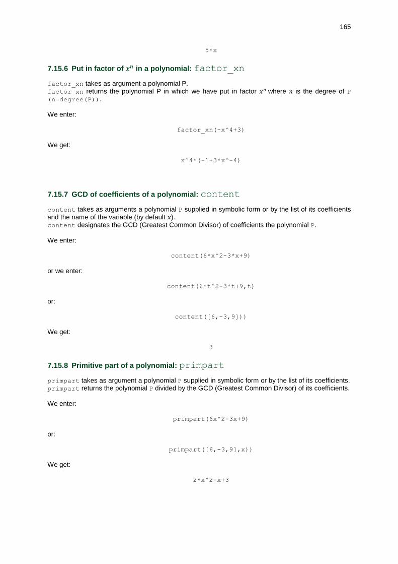
165

5*x

7.15.6 Put in factor of 𝒙𝒏 in a polynomial: factor_xn

factor_xn takes as argument a polynomial P. factor_xn returns the polynomial P in which we have put in factor 𝑥𝑛 where 𝑛 is the degree of P (n=degree(P)). We enter:

factor_xn(-x^4+3)

We get:

x^4*(-1+3*x^-4)

7.15.7 GCD of coefficients of a polynomial: content

content takes as arguments a polynomial P supplied in symbolic form or by the list of its coefficients and the name of the variable (by default 𝑥). content designates the GCD (Greatest Common Divisor) of coefficients the polynomial P. We enter:

content(6*x^2-3*x+9)

or we enter:

content(6*t^2-3*t+9,t)

or:

content([6,-3,9]))

We get:

3

7.15.8 Primitive part of a polynomial: primpart

primpart takes as argument a polynomial P supplied in symbolic form or by the list of its coefficients. primpart returns the polynomial P divided by the GCD (Greatest Common Divisor) of its coefficients. We enter:

primpart(6x^2-3x+9)

or:

primpart([6,-3,9],x))

We get:

2*x^2-x+3

166

7.15.9 Sturm sequence and number of changes of the sign of P on ]𝒂; 𝒃]: sturm

sturm has two or four parameters: a polynomial expression P, or a rational fraction 𝑃/𝑄, and the

name of the variable, or a polynomial expression 𝑃, the name of the variable and two numbers 𝑎 and 𝑏.

When there are two parameters, sturm returns the list of Sturm series and their multiplicity for 𝑃 or for

𝑃 and for 𝑄 (sturm is then similar to sturmseq). When there are four parameters, sturm behaves as sturmab:

– if 𝑎 and 𝑏 are reals, sturm returns the number of changes of sign of 𝑃 on ]𝑎; 𝑏] – if 𝑎 or 𝑏 is complex, sturm returns the number of complex roots laying inside the rectangle of

opposite vertices 𝑎 and 𝑏. We enter:

sturm(2*x^3+2,x)

We get:

[2,[[1,0,0,1],[3,0,0],-9],1]

We enter:

sturm((2*x^3+2)/(x+2),x)

We get:

[2,[[1,0,0,1],[3,0,0],-9],1,[[1,2],1]]

We enter:

sturm(x^2*(x^3+2),x,-2,0)

We get:

1

7.15.10 Number of changes of sign on ]𝒂; 𝒃]: sturmab

sturmab has four parameters: a polynomial expression 𝑃, the name of the variable and two numbers

𝑎 and 𝑏.

– if 𝑎 and 𝑏 are reals, sturmab returns either a strictly positive number which is the number of changes of sign of 𝑃 on ]𝑎; 𝑏], either 0 if 𝑃 remains of constant positive sign or null on ]𝑎; 𝑏], either −1 if 𝑃 remains of constant negative sign or null on ]𝑎; 𝑏]. Thus, sturmab let us know

the number of roots on [a, b[ of the polynomial 𝑃/𝐺 with 𝐺 = gcd(𝑃, diff(𝑃)). – if 𝑎 or 𝑏 is complex, the number of complex roots laying inside the rectangle of opposite

vertices 𝑎 and 𝑏. We enter:

sturmab(x^2*(x^3+2),x,-2,0)

We get:

1

We enter:

sturmab(x^3-1,x,-2-i,5+3i)

We get:

167

3

We enter:

sturmab(x^3-1,x,-i,5+3i)

We get:

1

Warning!

𝑃 must be supplied by its symbolic expression, and, if we enter:

sturmab([1,0,0,2,0,0],x,-2,0)

we get:

Bad argument type.

7.15.11 Sequence of Sturm: sturmseq

sturmseq takes as parameter a polynomial expression 𝑃 or a rational fraction 𝑃/𝑄.

sturmseq returns the list of Sturm series and their multiplicity for 𝑃, or for 𝑃 and 𝑄.

The series of sturm 𝑅1, 𝑅2, . .. is obtained from the factor 𝐹 without square of 𝑃. To get 𝐹 starting from

the decomposition of 𝑃 in prime factors, one removes the square terms and one transforms the odd powers in powers 1.

𝑅1 is the opposite of the remainder of the Euclidean division of 𝐹 by 𝐹′ then, 𝑅2 is the opposite of the

remainder of the Euclidean division of 𝐹′ by 𝑅1 .... and so on until 𝑅𝑘 = 0. We enter:

sturmseq(2*x^3+2)

or

sturmseq(2*y^3+2,y)

We get:

[2,[[1,0,0,1],[3,0,0],-9],1]

The first term gives the GCD of the coefficients of the numerator (here 2), the last term gives the

denominator (here 1). Between these two terms, we have the series of polynomials

[𝑥3 + 1, 3𝑥2, −9]. We enter:

sturmseq((12*x^3+4)/(6*x^2+3),x)

We get:

[4,[[3,0,0,1],[9,0,0],-81],3,[[2,0,1],[4,0],-16]]

The first term gives the GCD of the coefficients of the numerator (here 4), then the Sturm series of the numerator ([[3,0,0,1], [9,0,0], −81]), then the the GCD of the coefficient of the denominator (here 3),

and the Sturm series of the denominator ([[2,0,1], [4,0], −16]). We have the series of polynomials

[3𝑥3 + 1, 9𝑥2, −81] for the numerator and, [2𝑥2 + 1, 4𝑥, −16] for the denominator. We enter:

168

sturmseq((x^3+1)^2,x)

We get:

[1,1]

Indeed, the square terms are removed and 𝐹 = 1. We enter:

sturmseq(3*(3*x^3+1)/(2*x+2),x)

We get:

[3,[[3,0,0,1],[9,0,0],-81],2,[[1,1],1]]

The first term gives the GCD of the coefficients of the numerator (here 3), the second term gives the series of polynomials (here 3x^3+1, 9x^2, 81), the third term gives the GCD of the coefficients of

the denominator (here 2), the fourth term gives the series of polynomials of the denominator (x+1,1). Warning!

P must be supplied by its symbolic expression, and, if we enter:

sturmseq([1,0,0,1],x)

we get:

Bad argument type.

7.15.12 Sylvester matrix of two polynomials: sylvester

sylvester takes as arguments two polynomials. sylvester returns the Sylvester matrix S of two polynomials.

For two polynomials 𝐴(𝑥) = ∑ 𝑎𝑖𝑥𝑖𝑖=𝑛

𝑖=0 and 𝐵(𝑥) = ∑ 𝑏𝑖𝑥𝑖𝑖=𝑚

𝑖=0 , the Sylvester matrix S is a square matrix

of dimension m+n whose m=degree(B(x)first lines are composed of coefficients of 𝐴(𝑥):

(

𝑠11 = 𝑎𝑛 𝑠12 = 𝑎𝑛−1 ⋯ 𝑠1(𝑛+1) = 𝑎0 0 ⋯ 0

𝑠21 = 0 𝑠22 = 𝑎𝑛 ⋯ 𝑠2(𝑛+1) = 𝑎1 𝑠2(𝑛+2) = 𝑎0 ⋯ 0

⋮ ⋮ ⋮ ⋱ ⋮ ⋱ ⋮𝑠𝑚1 = 0 𝑠𝑚2 = 0 ⋯ 𝑠𝑚(𝑛+1) = 𝑎𝑚−1 𝑠𝑚(𝑛+2) = 𝑎𝑚−2 ⋯ 𝑎0)

and the n=degree(A(x)) following lines are composed the same way of coefficients of B(x):

(

𝑠(𝑚+1)1 = 𝑏𝑚 𝑠(𝑚+1)2 = 𝑏𝑚−1 ⋯

⋮ ⋮ ⋮𝑠(𝑚+𝑛)1 = 0 𝑠(𝑚+𝑛)2 = 0 ⋯

𝑠(𝑚+1)(𝑚+1) = 𝑏0 0 ⋯ 0

⋱ ⋮ ⋱ ⋮𝑠(𝑚+𝑛)(𝑚+1) = 𝑏𝑛−1 𝑏𝑛−2 ⋯ 𝑏0

)

We enter:

sylvester(x^3-p*x+q,3*x^2-p,x)

We get:

[[1,0,-p,q,0],[0,1,0,-p,q],[3,0,-p,0,0], [0,3,0,-p,0],[0,0,3,0,-p]]

We enter:

det([[1,0,-p,q,0],[0,1,0,-p,q],[3,0,-p,0,0], [0,3,0,-p,0],[0,0,3,0,-

p]])

We get:

-4*p^3-27*q^2

169

7.15.13 Resultant of two polynomials: resultant

resultant takes as arguments two polynomials. resultant returns the resultant of two polynomials. The resultant is the determinant of the Sylvester matrix S.

For the two polynomials (𝑥) = ∑ 𝑎𝑖𝑥𝑖𝑖=𝑛

𝑖=0 and 𝐵(𝑥) = ∑ 𝑏𝑖𝑥𝑖𝑖=𝑚

𝑖=0 , the Sylvester matrix S is a square

matrix of dimension 𝑚 + 𝑛 whose m first lines are composed of coefficients of 𝐴(𝑥):

(

𝑠00 = 𝑎𝑛 𝑠01 = 𝑎𝑛−1 ⋯ 𝑠0𝑛 = 𝑎0 0 ⋯ 0𝑠10 = 0 𝑠11 = 𝑎𝑛 ⋯ 𝑠1𝑛 = 𝑎1 𝑠1(𝑛+1) = 𝑎0 ⋯ 0

⋮ ⋮ ⋮ ⋱ ⋮ ⋱ ⋮𝑠(𝑚−1)0 = 0 𝑠(𝑚−1)1 = 0 ⋯ 𝑠(𝑚−1)𝑛 = 𝑎𝑚−1 𝑠(𝑚−1)(𝑛+1) = 𝑎𝑚−2 ⋯ 𝑎0

)

and the 𝑛 following lines are composed the same way of from coefficients of 𝐵(𝑥): We enter:

resultant(x^3-p*x+q,3*x^2-p,x)

We get:

-4*p^3-27*q^2

We look for two polynomials 𝑈(𝑥) = 𝛼 ∗ 𝑥 + 𝛽 (of degree 1) and 𝑉 (𝑥) = 𝛾 ∗ 𝑥2 + 𝛿 ∗ 𝑥 + 휀 (of

degree 2) so that 𝑈(𝑥) ∗ (𝑥3 − 𝑝 ∗ 𝑥 + 𝑞) + 𝑉 (𝑥) ∗ (3 ∗ 𝑥2 − 𝑝) = 1 Then, we must solve a linear system of five equations and five unknowns, which are 𝛼, . . . 𝛿, 𝜂

(Warning! 휀 = 10−10). We enter:

symb2poly((alpha*x+beta)*(x^3-p*x+q)+(gamma*x^2+delta*x+eta)*(3*x^2-

p),x)

We get:

poly1[alpha+3*gamma,beta+3*delta,-alpha*p-p*gamma+3*eta,

alpha*q-beta*p-p*delta,beta*q-p*eta]

The matrix A of this system is then:

𝐴 =

(

1 0 3 0 00 1 0 3 0−𝑝 0 −𝑝 0 3𝑞 −𝑝 0 −𝑝 00 𝑞 0 0 −𝑝)

the Sylvester matrix S is the transpose matrix of A:

𝑆 =

(

1 0 −𝑝 𝑞 00 1 0 −𝑝 𝑞3 0 −𝑝 0 00 3 0 −𝑝 00 0 3 0 −𝑝)

We have det(A)=det(S)=-4*p^3+27*q^2 In fact, we solve 𝑈𝑃 + 𝑉𝑄 = 𝐶 with any 𝐶 such as deg(𝐶) < deg(𝑃) + deg(𝑄) i.e. we look for U and V such as deg(𝑈) < deg(𝑄) and deg(𝑉 ) < deg(𝑃) (strict inequalities) which make

𝑈𝑃 + 𝑉 𝑄 = 1. When the system is a Cramer system, there is a unique solution and, arithmetically

speaking, it corresponds to 𝑃 and 𝑄 prime to each other (and reciprocally). So, if det(𝐴) = det(𝑆) is not null, 𝑈 and 𝑉 exist and are unique, so the two polynomials

𝑥3 − 𝑝 ∗ 𝑥 + 𝑞 and 3 ∗ 𝑥2 − 𝑝 are prime to each other and reciprocally if the two polynomials 𝑥3 − 𝑝 ∗ 𝑥 + 𝑞 and 3 ∗ 𝑥2 − 𝑝 are prime to each other 𝑈 and 𝑉 such as deg(𝑈) < deg(𝑄) and deg(𝑉 ) < deg(𝑃) exist and are unique so det(𝐴) = det(𝑆) is not null.

170

So if this determinant is null, the two polynomials 𝑥3 − 𝑝 ∗ 𝑥 + 𝑞 and 3 ∗ 𝑥2 − 𝑝 are not prime to each other. Note: We have: discriminant(P)=resultant(P,P’)/lcoeff(P). Example of the use of the resultant:

Be 𝐹1 and 𝐹2 two fixed points, and a variable point 𝐴 on the circle of center 𝐹1 and radius 2𝑎. We

want to find the cartesian equation of the locus of the points 𝑀, intersection of 𝐹1𝐴 and the perpendicular bisector of 𝐹2𝐴: we have 𝑀𝐹1 + 𝑀𝐹2 = 𝑀𝐹1 + 𝑀𝐴 = 𝐹1𝐴 = 2𝑎 then 𝑀 draws an

ellipse of foci 𝐹1 and 𝐹2 and major axis 2𝑎.

Let us choose as orthonormal basis the one of center 𝐹1 and axis 𝑂𝑥 of vector

𝐹1𝐹2⃗⃗⃗⃗ ⃗⃗ ⃗⃗ ⃗⃗ ⃗. We have:

𝐴 = (2𝑎 cos(𝜃); 2𝑎 sin(𝜃)) where 𝜃 is the angle (𝑂𝑥, 𝑂𝐴). We choose as parameter 𝑡 = tan(𝜃/2) so

that the coordinates of 𝐴 are a rational function of the parameter 𝑡. Then, we have:

𝐴 = (𝑎𝑥; 𝑎𝑦) = (2𝑎1 − 𝑡2

1 + 𝑡2; 2𝑎

2𝑡

1 + 𝑡2)

We consider 𝐹1𝐹2 = 2𝑐 and we note 𝐼 the midpoint of 𝐴𝐹2. We have: 𝐹2 = (2𝑐, 0) and

𝐼 = (𝑐 + 𝑎𝑥

2; 𝑎𝑦

2) = (𝑐 + 𝑎

1 − 𝑡2

1 + 𝑡2; 𝑎

2𝑡1 − 𝑡2

1 + 𝑡2)

𝐼𝑀 is perpendicular to 𝐴𝐹2 then 𝑀 = (𝑥; 𝑦) checks the equation 𝑒𝑞1 = 0 with:

𝑒𝑞1:= (𝑥 − 𝑖𝑥) ∗ (𝑎𝑥 − 2 ∗ 𝑐) + (𝑦 − 𝑖𝑦) ∗ 𝑎𝑦

𝑀 = (𝑥; 𝑦) is one 𝐹1𝐴 then 𝑀 checks the equation 𝑒𝑞2 = 0 with:

𝑒𝑞2:= 𝑦

𝑥 – 𝑎𝑦

𝑎𝑥

We have: resultant(eq1,eq2,t) is a polynomial 𝑒𝑞3 of 𝑥 and 𝑦, 𝑒𝑞3 is independant from 𝑡 and there are

polynomials of 𝑡, 𝑈 and 𝑉 such as: 𝑈(𝑡) ∗ 𝑒𝑞1 + 𝑉 (𝑡) ∗ 𝑒𝑞2 = 𝑒𝑞3. We enter:

ax:=2*a*(1-t^2)/(1+t^2);ay:=2*a*2*t/(1+t^2);

ix:=(ax+2*c)/2; iy:=(ay/2)

eq1:=(x-ix)*(ax-2*c)+(y-iy)*ay

eq2:=y/x-ay/ax

factor(resultant(eq1,eq2,t))

We get as resultant:

-(64·(x^2+y^2)·(x^2·a^2-x^2·c^2+-2·x·a^2·c+2·x·c^3-a^4+2·a^2·c^2+a^2· y^2-c^4))

The factor -64·(x^2+y^2) never vanishes, then the equation of the locus is:

𝑥2𝑎2 − 𝑥2𝑐2 + −2𝑥𝑎2𝑐 + 2𝑥𝑐3 − 𝑎4 + 2𝑎2𝑐2 + 𝑎2𝑦2 − 𝑐4 = 0 By taking as origin of the basis in 𝑂 midpoint of 𝐹1𝐹2, one finds back the cartesian equation of the ellipse. To do this change of of origin, we have

𝐹1𝑀⃗⃗⃗⃗ ⃗⃗ ⃗⃗ ⃗ = 𝐹1𝑂⃗⃗⃗⃗ ⃗⃗ ⃗⃗ + 𝑂𝑀⃗⃗ ⃗⃗ ⃗⃗ , so we enter:

normal(subst(x^2·a^2-x^2·c^2+-2· x·a^2·c+2·x·c^3-a^4+2·a^2·c^2+a^2·y^2-c^4,[x,y]=[c+X,Y]))

We get:

-c^2*X^2+c^2*a^2+X^2*a^2-a^4+a^2*Y^2

171

or else if we put 𝑏2 = 𝑎2 − 𝑐2

normal(subst(c^2*X^2+c^2*a^2+X^2*a^2-a^4+a^2*Y^2,c^2=a^2-b^2))

We get:

a^2*b^2+a^2*Y^2+b^2*X^2

that is to say after division by 𝑎2𝑏2, 𝑀 checks the equation:

𝑋2

𝑎2+𝑌2

𝑏2= 1

Another example of use of the resultant

Be 𝐹1 and 𝐹2 two fixed points and a variable point 𝐴 on the circle of center 𝐹1 and radius 2𝑎. We want

to find the cartesian equation of the envelop of the perpendicular bisector 𝐷 of 𝐹2𝐴 (we know that the

perpendicular bisector of 𝐹2𝐴 is tangent to the ellipse of foci 𝐹1 and 𝐹2 and major axis 2𝑎). Let us choose as orthonormal basis the one of center 𝐹1 and axis 𝑂𝑥 of vector

𝐹1𝐹2⃗⃗⃗⃗ ⃗⃗ ⃗⃗ ⃗⃗ ⃗. We have:

𝐴 = (2𝑎 cos(𝜃); 2𝑎 sin(𝜃)) where 𝜃 is the angle (𝑂𝑥, 𝑂𝐴). We choose as parameter 𝑡 = tan(𝜃/2) so

that the coordinates of 𝐴 are a rational function of parameter 𝑡. We have then:

𝐴 = (𝑎𝑥; 𝑎𝑦) = (2𝑎1 − 𝑡2

1 + 𝑡2; 2𝑎

2𝑡

1 + 𝑡2)

We consider 𝐹1𝐹2 = 2𝑐 and we note 𝐼 the midpoint of 𝐴𝐹2. We have:

𝐹2 = (2𝑐, 0) and

𝐼 = (𝑐 + 𝑎𝑥

2; 𝑎𝑦

2) = (𝑐 + 𝑎

1 − 𝑡2

1 + 𝑡2; 𝑎

2𝑡1 − 𝑡2

1 + 𝑡2)

𝐷 is perpendicular to 𝐴𝐹2 then 𝐷 has for equation: 𝑒𝑞1 = 0 with: 𝑒𝑞1:= (𝑥 − 𝑖𝑥) ∗ (𝑎𝑥 − 2 ∗ 𝑐) + (𝑦 − 𝑖𝑦) ∗ 𝑎𝑦

The envelop of 𝐷 is then the locus of 𝑀 intersection of 𝐷 and 𝐷’ of equation 𝑒𝑞2 = 0 with

𝑒𝑞2:= 𝑑𝑖𝑓𝑓(𝑒𝑞1, 𝑡). We enter:

ax:=2*a*(1-t^2)/(1+t^2);ay:=2*a*2*t/(1+t^2);

ix:=(ax+2*c)/2; iy:=(ay/2)

eq1:=normal((x-ix)*(ax-2*c)+(y-iy)*ay)

eq2:=normal(diff(eq1,t))

factor(resultant(eq1,eq2,t))

We get as resultant:

(-(64· a^2))·(x^2+y^2)·(x^2·a^2-x^2·c^2+-2·x·a^2·c+2·x·c^3

-a^4+2·a^2·c^2+a^2·y^2-c^4)

The factor -64·(x^2+y^2) never vanishes then the equation of the locus is:

𝑥2𝑎2 − 𝑥2𝑎𝑐2 + −2𝑥𝑎2𝑐 + 2𝑥𝑐3 − 𝑎4 + 2𝑎2𝑐2 + 𝑎2𝑐𝑦2 − 𝑐4 = 0 By taking as origin of the basis in 𝑂 midpoint of 𝐹1𝐹2, we find as previously the cartesian equation of the ellipse:

𝑋2

𝑎2+𝑌2

𝑏2= 1

172

7.15.14 Chinese remainder: chinrem

chinrem takes as argument two lists having each as components two polynomials eventually supplied by the list of their coefficients by decreasing power order. chinrem returns a list of components of two polynomials. chinrem([A,R],[B,Q]) returns the list of polynomials 𝑃 and 𝑆 such as:

𝑆 = 𝑅. 𝑄, 𝑃 = 𝐴 (𝑚𝑜𝑑 𝑅), 𝑃 = 𝐵 (𝑚𝑜𝑑 𝑄) There is always a solution 𝑃 if 𝑅 and 𝑄 are prime to each other, and all the solutions are congruent modulus 𝑆 = 𝑅 ∗ 𝑄

Find the solutions 𝑃(𝑥) of:

{𝑃(𝑥) = 𝑥 𝑚𝑜𝑑 (𝑥2 + 1)

𝑃(𝑥) = 𝑥 − 1 𝑚𝑜𝑑 (𝑥2 − 1)

We enter:

chinrem([[1,0],[1,0,1]],[[1,-1],[1,0,-1]])

We get:

[[1/-2,1,1/-2],[1,0,0,0,-1]]

or we enter:

chinrem([x,x^2+1],[x-1,x^2-1])

We get:

[-1/2*x^2+x-1/2,x^4-1]

so

𝑃(𝑥) = −𝑥2 – 2𝑥 +1

2(𝑚𝑜𝑑 𝑥4 − 1)

Other example: We enter:

chinrem([[1,2],[1,0,1]],[[1,1],[1,1,1]])

We get:

[[-1,-1,0,1],[1,1,2,1,1]]

or we enter:

chinrem([x+2,x^2+1],[x+1,x^2+x+1])

We get:

[-x^3-x^2+1,x^4+x^3+2*x^2+x+1]

7.16 Special

7.16.1 Cyclotomic polynomial: cyclotomic

cyclotomic takes as parameter an integer n. cyclotomic returns the list of coefficients of the cyclotomic polynomial of degree 𝑛. It is the polynomial whose zeros are all the n-th roots and primitives of the unity (an n-th root of the unity is primitive if its powers generate all the others n-th roots of the unity).

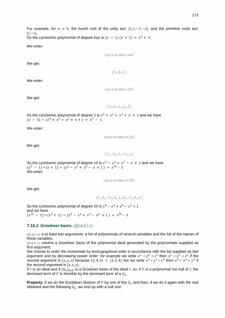
173

For example, for 𝑛 = 4, the fourth root of the unity are: {1, 𝑖, −1, −𝑖}, and the primitive roots are:

{𝑖, −𝑖}. So the cyclotomic polynomial of degree four is (𝑥 − 𝑖). (𝑥 + 𝑖) = 𝑥2 + 1. We enter:

cyclotomic(4)

We get:

[1,0,1]

We enter:

cyclotomic(5)

We get:

[1,1,1,1,1]

So the cyclotomic polynomial of degree 5 is 𝑥4 + 𝑥3 + 𝑥2 + 𝑥 + 1 and we have

(𝑥 − 1) ∗ (𝑥4 + 𝑥3 + 𝑥2 + 𝑥 + ) = 𝑥5 − 1. We enter:

cyclotomic(10)

We get:

[1,-1,1,-1,1]

So the cyclotomic polynomial of degree 10 is 𝑥4 − 𝑥3 + 𝑥2 − 𝑥 + 1 and we have (𝑥5 − 1) ∗ (𝑥 + 1) ∗ (𝑥4 − 𝑥3 + 𝑥2 − 𝑥 + 1 ) = 𝑥10 – 1 We enter:

cyclotomic(20)

We get:

[1,0,-1,0,1,0,-1,0,1]

So the cyclotomic polynomial of degree 20 is 𝑥8 − 𝑥6 + 𝑥4 − 𝑥2 + 1 and we have (𝑥10 − 1) ∗ (𝑥2 + 1) ∗ (𝑥8 − 𝑥6 + 𝑥4 − 𝑥2 + 1 ) = 𝑥20 – 1

7.16.2 Groebner basis: gbasis

gbasis a at least two arguments: a list of polynomials of several variables and the list of the names of these variables. gbasis returns a Groebner basis of the polynomial ideal generated by the polynomials supplied as first argument. We choose to order the monomials by lexicographical order in accordance with the list supplied as last

argument and by decreasing power order: for example we write 𝑥2 ∗ 𝑦4 ∗ 𝑧3 then 𝑥2 ∗ 𝑦3 ∗ 𝑧4 if the

second argument is [𝑥, 𝑦, 𝑧] because (2, 4, 3) > (2, 3, 4) but we write 𝑥2 ∗ 𝑦3 ∗ 𝑧4 then 𝑥2 ∗ 𝑦4 ∗ 𝑧3 if the second argument is [𝑥, 𝑧, 𝑦]. If 𝐼 is an ideal and if (𝐺𝑘)𝑘∈𝐾 is a Groebner basis of the ideal 𝐼, so, if 𝐹 is a polynomial not null of 𝐼, the

dominant term of 𝐹 is divisible by the dominant term of a 𝐺𝑘. Property: if we do the Euclidean division of 𝐹 by one of the 𝐺𝑘 and then, if we do it again with the rest

obtained and the following 𝐺𝑘, we end up with a null rest.

174

We enter:

gbasis([2*x*y-y^2,x^2-2*x*y],[x,y])

We get:

[y^3,x*y+(-1/2)*y^2,x^2-y^2]

7.16.3 Reduction according to a Groebner basis: greduce

greduce has three arguments: a polynomial of several variables, a list of polynomials forming a Groebner basis depending on the same variables and the list of the names of these variables. greduce returns the reduction (a multiplicative constant excepted) of the polynomial supplied as first argument according to the Groebner basis supplied as second argument. We enter:

greduce(x*y-1,[x^2-y^2,2*x*y-y^2,y^3],[x,y])

We get:

1/2*y^2-1

which means that 𝑥𝑦 – 1 =1

2(𝑦2– 2)mod 𝐼 where 𝐼 is the ideal generated by the Groebner basis

[𝑥2– 𝑦2, 2𝑥𝑦 – 𝑦2, 𝑦3], because 𝑦2 − 2 is the remainder of the Euclidean division of 2(𝑥𝑦 – 1) by

𝐺2 = 2𝑥𝑦 – 𝑦2. Note: The multiplicative constant can be determinated by looking at how the constant coefficient is transformed. In the example, the constant term -1 is transformed into the constant term -2, then the multiplicative coefficient is 1/2.

7.16.4 Hermite polynomial: hermite

hermite takes as argument an integer n and eventually the name of the variable (𝑥 by default).

hermite returns the Hermite polynomial of degree 𝑛.

The Hermite polynomial of degree 𝑛 written 𝑃(𝑛, 𝑥) checks the relations:

𝑃(0, 𝑥) = 1

𝑃(1, 𝑥) = 2𝑥

𝑃(𝑛, 𝑥) = 2𝑥𝑃(𝑛 − 1, 𝑥) − 2(𝑛 − 1)𝑃(𝑛 − 2, 𝑥)

These polynomials are orthogonal for the scalar product:

< 𝑓, 𝑔 > = ∫ 𝑓(𝑥)𝑔(𝑥)𝑒−𝑥2𝑑𝑥

+∞

−∞

We enter:

hermite(6)

We get:

64*x^6+-480*x^4+720*x^2-120

We enter:

hermite(6,y)

We get:

175

64*y^6+-480*y^4+720*y^2-120

7.16.5 Lagrange interpolation: lagrange

lagrange takes as argument two lists of length n or a matrix of two lines and n columns and eventually the name of the variable var (by default x): the first list (or line) corresponds to values of abscissa 𝑥𝑘, and the second list (or line) corresponds to

values of ordinates 𝑦𝑘 for k from 1 to n. lagrange returns a polynomial expression P(var) of degree n-1 such as

𝑃(𝑥𝑘) = 𝑦𝑘.

We enter:

lagrange([[1,3],[0,1]])

Or we enter:

lagrange([1,3],[0,1])

We get:

1/2*(x-1)

indeed for 𝑥 = 1 we have 𝑥−1

2= 0 and for 𝑥 = 3 we have

𝑥−1

2= 1.

We enter:

lagrange([1,3],[0,1],y)

We get:

1/2*(y-1)

Warning! lagrange([1,2],[3,4],y) does not return a function but an expression, but we can define a function by putting:

f(x):=lagrange([1,2],[3,4],x)

or

f(y):=lagrange([1,2],[3,4],y)

and so f(4) returns 6 because f(x)=x+2) Please note the difference between:

g(x):=lagrange([1,2],[3,4])

and

f(x):=lagrange([1,2],[3,4],x).

g(x):=lagrange([1,2],[3,4]) does not define a function, for example, g(2)=x-1+3 whereas f(2)=4. That said, the definition of f is not efficient because the polynomial will be recalculated from the beginning at each call of f (when we define a function the right member is not evaluated, the evaluation is made only when we call f). To be efficient, you must use unapply:

f:=unapply(lagrange([1,2],[3,4]),x)

176

or

f:=unapply(lagrange([1,2],[3,4],y),y)

Exercise:

Be 𝑓(𝑥) =1

𝑥, 𝑥0 = 2𝑥1 = 2.5 and 𝑥2 = 4. You are asked to calculate the polynomial 𝐿 of Lagrange

interpolation, and its value in 𝑥 = 3 and 𝑥 = 4.5. We enter:

f(x):=1/x

L:=unapply(normal(lagrange([2,2.5,4],[f(2),f(2.5),f(4)])),x)

We get:

x->0.05*x^2-0.425*x+1.15

We enter:

L(3),L(4.5)

We get:

0.325,0.25

7.16.6 Natural splines: spline

Definition

Be a subdivision 𝜎𝑛 of the interval [𝑎, 𝑏]: 𝑎 = 𝑥0, 𝑥1, … , 𝑥𝑛 = 𝑏

We say that 𝑠 is a spline function of degree 𝑙 if 𝑠 is an application of [𝑎, 𝑏] in ℝ such as:

– 𝑠 has continuous derivatives up to degree 𝑙 − 1, – 𝑠 restricted at each interval of the subdivision is a polynomial of degree lower than or equals 𝑙.

Theorem

The set of splines functions of degree 𝑙 on 𝜎𝑛 is a ℝ-vector field of dimension 𝑛 + 𝑙. Indeed: We [𝑎, 𝑥1], s is a polynomial 𝐴 of degree lower than or equals 𝑙, then on [𝑎, 𝑥1], 𝑠 = 𝐴(𝑥) = 𝑎0 + 𝑎1𝑥 + …𝑎𝑙𝑥

𝑙 and 𝐴 is a linear combination of 1, 𝑥, … 𝑥𝑙. We [𝑥1, 𝑥2], s is a polynomial 𝐵 of degree lower than or equals 𝑙, then on [𝑥1, 𝑥2], 𝑠 = 𝐵(𝑥) = 𝑏 − 0 + 𝑏 − 1 𝑥 + …𝑏𝑙𝑥

𝑙. Since 𝑠 has continuous derivatives up to degree 𝑙 − 1 we must have:

∀0 ≤ 𝑗 ≤ 𝑙 − 1, 𝐵(𝑗)(𝑥1)– 𝐴(𝑗)(𝑥1) = 0

so 𝐵(𝑥)– 𝐴(𝑥) = 𝛼1(𝑥 – 𝑥1)𝑙

or else 𝐵(𝑥) = 𝐴(𝑥) + 𝛼1(𝑥 – 𝑥1)𝑙.

Be the function:

𝑞1(𝑥) = { 0 on [𝑎, 𝑥1]

(𝑥 − 𝑥1)𝑙 on [𝑥1, 𝑏]

Thus:

𝑠| [𝑎, 𝑥2] = 𝑎0 + 𝑎1 𝑥 + … 𝑎𝑙 𝑥𝑙 + 𝛼1 𝑞1 (𝑥).

On [𝑥2, 𝑥3], 𝑠 is a polynomial 𝐶 of degree lower than or equal to 𝑙, then on [𝑥2, 𝑥3], 𝑠 = 𝐶(𝑥) = 𝑐0 + 𝑐1𝑥 + … 𝑐𝑙𝑥

𝑙. Since 𝑠 has continuous derivatives up to degree 𝑙 − 1 we must have:

∀0 ≤ 𝑗 ≤ 𝑙 − 1, 𝐶(𝑗)(𝑥2)– 𝐵(𝑗)(𝑥2) = 0

so 𝐶(𝑥)– 𝐵(𝑥) = 𝛼2(𝑥 – 𝑥2)𝑙

or else 𝐶(𝑥) = 𝐵(𝑥) + 𝛼2(𝑥 – 𝑥2)𝑙.

177

Be the function:

𝑞2(𝑥) = { 0 on [𝑎, 𝑥2]

(𝑥 − 𝑥2)𝑙 on [𝑥2, 𝑏]

Thus:

𝑠|[𝑎,𝑥3] = 𝑎0 + 𝑎1 𝑥 + … 𝑎𝑙 𝑥𝑙 + 𝛼1 𝑞1 (𝑥) + 𝛼2 𝑞2 (𝑥)

and so on, we define the functions: ∀1 ≤ 𝑗 ≤ 𝑛 − 1,

∀1 ≤ 𝑗 ≤ 𝑛 − 1, 𝑞𝑗(𝑥) = { 0 on [𝑎, 𝑥𝑗]

(𝑥 − 𝑥𝑗)𝑙 on [𝑥𝑗 , 𝑏]

thus,

𝑠|[𝑎,𝑏] = 𝑎0 + 𝑎1 𝑥 + … 𝑎𝑙 𝑥𝑙 + 𝛼1 𝑞1 (𝑥) + 𝛼𝑛−1 𝑞𝑛−1 (𝑥)

and 𝑠 is a linear combination of 𝑛 + 𝑙 independant functions 1, 𝑥, . . 𝑥𝑙 , 𝑞1, . . 𝑞𝑛−1. Interpolation with splines functions

We can ask to interpolate a function 𝑓 on 𝜎𝑛 by a spline function 𝑠 of degree 𝑙, which forces 𝑠 to check

𝑠(𝑥𝑘) = 𝑦𝑘 = 𝑓(𝑥𝑘) for all 0 ≥ 𝑘 ≥ 𝑛.

We have then 𝑛 + 1 conditions, then remain 𝑙 − 1 degrees of freedom. So can we still impose 𝑙 − 1 additional conditions which will be conditions on the derivatives of 𝑠 in 𝑎 and 𝑏. There are then three kinds of interpolation (Hermite interpolation, natural interpolation, periodic interpolation) which are obtained by adding three kind of constraints. We can show that for each of these kinds of interpolation the solution to the interpolation problem is unique. Let us assume 𝑙 odd, 𝑙 = 2𝑚 − 1, there are then 2𝑚 − 2 degrees of freedom. We add the following constraints:

– Hermite interpolation

∀1 ≤ 𝑗 ≤ 𝑚 − 1, 𝑠(𝑗)(𝑎) = 𝑓(𝑗)(𝑎), 𝑠(𝑗)(𝑏) = 𝑓(𝑗)(𝑏) – natural interpolation

∀𝑚 ≤ 𝑗 ≤ 2𝑚 − 2, 𝑠(𝑗)(𝑎) = 𝑠(𝑗)(𝑏) = 0 – periodic interpolation

∀1 ≤ 𝑗 ≤ 2𝑚 − 2, 𝑠(𝑗)(𝑎) = 𝑠(𝑗)(𝑏) Let us assume 𝑙 even, 𝑙 = 2𝑚, there are then 2𝑚 − 1 degrees of freedom. We add the following constraints:

– Hermite interpolation

∀1 ≤ 𝑗 ≤ 𝑚 − 1, 𝑠(𝑗)(𝑎) = 𝑓(𝑗)(𝑎), 𝑠(𝑗)(𝑏) = 𝑓(𝑗)(𝑏) and

𝑠(𝑚)(𝑎) = 𝑓(𝑚)(𝑎) – natural interpolation

∀𝑚 ≤ 𝑗 ≤ 2𝑚 − 2, 𝑠(𝑗)(𝑎) = 𝑠(𝑗)(𝑏) = 0 and

𝑠(2𝑚−1)(𝑎) = 0 – periodic interpolation

∀1 ≤ 𝑗 ≤ 2𝑚 − 1, 𝑠(𝑗)(𝑎) = 𝑠(𝑗)(𝑏) A natural spline of supplied degree passing by two supplied points is a spline function that makes the natural interpolation. The instruction spline returns a natural spline of supplied degree passing by points whose lists of abscissae by increasing order and ordinates are supplied has argument. It returns the spline function under the form of a list of polynomials, each polynomial being valide in an interval. We give the list of abscissae in increasing order, the list of ordinates, the names of variables wished for the polynomials, and the degree. For instance, we want a natural spline of degree 3, passing by the points

𝑥0 = 0, 𝑦0 = 1, 𝑥1 = 1, 𝑦1 = 3 and 𝑥2 = 2, 𝑦2 = 0. We enter:

spline([0,1,2],[1,3,0],x,3)

178

We get a list of two polynomials function of x:

[−5 ∗ 𝑥3

4+ 13 ∗ 𝑥

4+ 1,

5 ∗ (𝑥 − 1)3

4− 15 ∗ (𝑥 − 1)2

4+(𝑥 − 1)

− 2 + 3]

valid respectively on the intervals [0, 1] and [1, 2]. For instance, we want a natural spline of degree 4, passing by the points 𝑥0 = 0, 𝑦0 = 1, 𝑥1 = 1, 𝑦1 = 3, 𝑥2 = 2, 𝑦2 = 0 and 𝑥3 = 3, 𝑦3 = −1, we enter:

spline([0,1,2,3],[1,3,0,-1],x,4)

We get a list of three polynomials function of x:

[−62 ∗ 𝑥4 + 304 ∗ 𝑥

121+ 1,

201 ∗ (𝑥 − 1)4− 248 ∗ (𝑥 − 1)3− 372 ∗ (𝑥 − 1)2+ 56 ∗ (𝑥 − 1)

121+ 3,

−139 ∗ (𝑥 − 2)4+ 556 ∗ (𝑥 − 2)3+ 90 ∗ (𝑥 − 2)2 −628 ∗ (𝑥 − 2)

121]

valid respectively on the intervals [0, 1], [1, 2] and [2, 3].

For instance, to get the natural interpolation of cos on [0,𝜋

2,3𝜋

2]

We enter:

spline([0,pi/2,3*pi/2],cos([0,pi/2,3*pi/2]),x,3)

We get:

[(3𝜋3 + (−7𝜋2)𝑥 + 4𝑥3) (

13)

𝜋3,(15𝜋3 + (−46𝜋2) ∗ +36𝜋𝑥2 − 8𝑥3) (

112)

𝜋3]

7.16.7 Laguerre polynomial: laguerre

laguerre takes as argument an integer 𝑛 and eventually the name of the variable (𝑥 by default) and

the parameter (𝑎 by default).

laguerre returns the Laguerre polynomial of degree 𝑛 and parameter 𝑎. The Laguerre polynomial of degree 𝑛 of parameter 𝑎 written 𝐿(𝑛, 𝑎, 𝑥) checks the relations:

𝐿(0, 𝑎, 𝑥) = 1

𝐿(1, 𝑎, 𝑥) = 1 + 𝑎 − 𝑥

𝐿(𝑛, 𝑎, 𝑥) =2𝑛 + 𝑎 − 1 − 𝑥

𝑛𝐿(𝑛 − 1, 𝑎, 𝑥)–

𝑛 + 𝑎 − 1

𝑛𝐿(𝑛 − 2, 𝑎, 𝑥)

These polynomials are orthogonal for the scalar product:

< 𝑓, 𝑔 > = ∫ 𝑓(𝑥)𝑔(𝑥)𝑥𝑎𝑒−𝑥𝑑𝑥+∞

0

We enter:

laguerre(2)

We get:

1/2*a^2-a*x+3/2*a+1/2*x^2-2*x+1

We enter:

laguerre(2,y)

We get:

1/2*a^2-a*y+3/2*a+1/2*y^2-2*y+1)

b must be purged (b:=’b’), we enter:

179

laguerre(2,y,b)

We get:

1/2*b^2-b*y+3/2*b+1/2*y^2-2*y+1

7.16.8 Legendre polynomial: legendre

legendre takes as argument an integer 𝑛 and eventually the name of the variable (𝑥 by default).

legendre returns the Legendre polynomial of degree 𝑛: it is the polynomial, not null, solution of the differential equation:

(𝑥2 − 1). 𝑦’’ − 2. 𝑥. 𝑦’ − 𝑛(𝑛 + 1). 𝑦 = 0

The Legendre polynomial of degree 𝑛 written 𝑃(𝑛, 𝑥) checks the relations:

𝑃(0, 𝑥) = 1

𝑃(1, 𝑥) = 𝑥

𝑃(𝑛, 𝑥) =2𝑛 − 1

𝑛𝑥𝑃(𝑛 − 1, 𝑥)–

𝑛 − 1

𝑛𝑃(𝑛 − 2, 𝑥)

These polynomials are orthogonal for the scalar product:

< 𝑓, 𝑔 > = ∫ 𝑓(𝑥)𝑔(𝑥)𝑑𝑥+1

−1

We enter:

legendre(4)

We get:

35/8*x^4+-15/4*x^2+3/8

We enter:

legendre(4,y)

We get:

35/8*y^4+-15/4*y^2+3/8

7.16.9 Tchebyshev polynomial of first kind: tchebyshev1

tchebyshev1 takes as argument an integer n and eventually the name of the variable (𝑥 by default). tchebyshev1 returns the Tchebyshev polynomial of first kind, of degree 𝑛, written 𝑇(𝑛, 𝑥). We have:

𝑇(𝑛, 𝑥) = 𝑐𝑜𝑠(𝑛. 𝑎𝑟𝑐𝑐𝑜𝑠(𝑥)) 𝑇(𝑛, 𝑥) checks the relations:

𝑇(0, 𝑥) = 1

𝑇(1, 𝑥) = 𝑥

𝑇(𝑛, 𝑥) = 2𝑥𝑇(𝑛 − 1, 𝑥) − 𝑇(𝑛 − 2, 𝑥)

The polynomials 𝑇(𝑛, 𝑥) are orthogonal for the scalar product:

< 𝑓, 𝑔 ≥ ∫ 𝑓(𝑥)𝑔(𝑥)

√1 − 𝑥2𝑑𝑥

+1

−1

We enter:

tchebyshev1(4)

We get:

180

8*x^4-8*x^2+1

We enter:

tchebyshev1(4,y)

We get:

8*y^4-8*y^2+1

and we do have:

𝑐𝑜𝑠(4. 𝑥) = 𝑅𝑒((𝑐𝑜𝑠(𝑥) + 𝑖. sin (𝑥))4)

cos(4. 𝑥) = cos(𝑥)4 − 6. cos(𝑥)2 . (1 − cos(𝑥)2) + (1 − cos(𝑥)2)2

cos(4. 𝑥) = 𝑇(4, cos(𝑥))

7.16.10 Tchebyshev polynomial of second kind: tchebyshev2

tchebyshev2 takes as argument an integer 𝑛 and eventually the name of the variable (𝑥 by default).

tchebyshev2 returns the Tchebyshev polynomial of second kind, of degree 𝑛, written 𝑈(𝑛, 𝑥). We have:

𝑈(𝑛, 𝑥) =sin((𝑛 + 1). arccos(𝑥))

sin(arccos(𝑥))

or else

𝑠𝑖𝑛((𝑛 + 1)𝑥) = 𝑠𝑖𝑛(𝑥) ∗ 𝑈(𝑛, 𝑐𝑜𝑠(𝑥))

𝑈(𝑛, 𝑥) checks the relations:

𝑈(0, 𝑥) = 1

𝑈(1, 𝑥) = 2𝑥

𝑈(𝑛, 𝑥) = 2𝑥𝑈(𝑛 − 1, 𝑥) − 𝑈(𝑛 − 2, 𝑥)

Polynomials 𝑈(𝑛, 𝑥) are orthogonal for the scalar product:

< 𝑓, 𝑔 ≥ ∫ 𝑓(𝑥)𝑔(𝑥)√1 − 𝑥2𝑑𝑥+1

−1

We enter:

tchebyshev2(3)

We get:

8*x^3+-4*x

We enter:

tchebyshev2(3,y)

We get:

8*y^3+-4*y

indeed:

sin(4. 𝑥) = sin(𝑥) ∗ (8 ∗ cos(𝑥)3 − 4. cos(𝑥)) = sin(𝑥) ∗ 𝑈(3, cos(𝑥)).

181

Chapter 8 Menu Plot

Note: The plot of most of the commands starting by plot is not well done from the CAS screen: you will then preferably use the geometry application to do the plots corresponding to these commands.

8.1 Plot of a function: plotfunc

We open the geometry application and we press the key Plot. Then, we use Cmds of the push buttons. We choose 6 Plot then 1 Function. plotfunc( shows on the entry line and it is enough to fill up with the expression 𝑓(𝑥) which we want to get the plot of. The Symbolic view stores then an additional line containing the command entered for example: plotfunc(f(x)) plotfunc(f(x),x) plots the graphical representation of 𝑦 = 𝑓(𝑥) and plotfunc(f(x),x=a..b) plots the graphical representation of 𝑦 = 𝑓(𝑥) when 𝑎 ≤ 𝑥 ≤ 𝑏. We enter:

plotfunc(x^2-2)

or

plotfunc(a^2-2,a=-1..2)

We get:

the graphical representation of y=x^2-2

Or else, we enter:

gf:=plotfunc(x^2-2)

Then, in the Symbolic view of the geometry application (Symb), we press New, which displays, for example:

√GC:=

We fill up with

√GC:=gf

Then, we press the key Plot to get the Plot view of the geometry application, we get:

the plot of x^2-2

8.2 Parametric curve: plotparam

plotparam(f(t)+i*g(t),t) (resp. plotparam(f(t)+i*g(t),t=t1..t2)) plots the parametric representation of the curve defined by 𝑥 = 𝑓(𝑡), 𝑦 = 𝑔(𝑡) (resp. by 𝑥 = 𝑓(𝑡), 𝑦 = 𝑔(𝑡) and 𝑡1 ≥ 𝑡 ≥ 𝑡2).

182

We enter:

plotparam(cos(x)+i*sin(x),x)

or

plotparam([cos(x),sin(x)],x)

We get:

The plot of the circle unity

We can specify the boundaries of the interval of variation of the parameter. We enter:

plotparam(sin(t)+i*cos(t),t=-4..1)

or else:

plotparam(sin(x)+i*cos(x),x=-4..1)

Or we enter, if in the plot configuration t goes from -4 to 1:

plotparam(sin(t)+i*cos(t))

We get:

The plot of the arc of circle unity starting from -4 at 1

We can add a parameter to specify the step of sampling of the parameter t with tstep= , that is to say the step t we want to use to do the plot. We enter, if in the plot configuration t goes from −4 to 1:

plotparam(sin(t)+i*cos(t),t,tstep=0.5)

Or we enter:

plotparam(sin(t)+i*cos(t),t=-4..1,tstep=0.5)

We get:

The raw plot of the arc of circle unity starting from -4 to 1

8.3 Polar curve: plotpolar

plotpolar(f(t),t) plots the Polar representation of the curve defined by: 𝜌 = 𝑓(𝑡). We enter:

plotpolar(t,t=0..10)

We enter, if in the plot configuration t goes from 0 to 10:

plotpolar(t,t)

We get:

183

The spiral ρ=t is plotted

We can add a parameter to specify the step of sampling of the parameter t with tstep= , that is to say the step t we want to use to do the plot. We enter, if in the plot configuration t goes from 0 to 10:

plotpolar(t,t,tstep=1)

or:

plotpolar(t,t=0..10,tstep=1)

We get:

The spiral ρ=t is plotted roughly.

8.4 Plot of a recurrent sequence: plotseq

plotseq(f(x),a,n) or plotseq(f(t),t=a,n) allows to display the n first terms of a recurrent sequence defined by:

𝑢0 = 𝑎, 𝑎 = 𝑓(𝑢𝑛−1)

We enter:

plotseq(sqrt(1+x),3,5)

We get:

The plot of y=sqrt(1+x), of y=x and the five first terms

of the sequence u_0=3 and u_n=sqrt(1+u_(n-1))

8.5 Implicit plot in 2D: plotimplicit

plotimplicit allows to plot curves defined in an implicit way by an expression. In order to not have the calculator starting to factorize the expression, the command plotimplicit can be used with the option unfactored put as last parameter:

– with unfactored, the expression will not be modified, – without unfactored, the calculator factors the expression to the same denominator and then

tries to factorize the numerator. – plotimplicit(f(x,y),x,y) or plotimplicit(f(x,y),[x,y]) plots the graphical

representation of the curve defined implicitly by 𝑓(𝑥, 𝑦) = 0 when 𝑥 (resp. 𝑦) varies according to 𝑊𝑋 −, 𝑊𝑋 + (resp. 𝑊𝑌-, 𝑊𝑌 +) defined in cfg,

– plotimplicit(f(x,y),x=0..1,y=-1..1) or plotimplicit(f(x,y),[x=0..1,y=-1..1]) plots the graphical representation of the curve defined implicitly by 𝑓(𝑥, 𝑦) = 0 when 0 ≤ 𝑥 ≤ 1 and −1 ≤ 𝑦 ≤ 1 (set the boundaries slightly larger to avoid losing part of the plot!).

We enter:

plotimplicit(x^2+y^2-1,[x,y])

Or we enter:

184

plotimplicit(x^2+y^2-1,{x,y},unfactored)

Or we enter:

plotimplicit(x^2+y^2-1,x,y,unfactored)

We get:

circle(point(O,O),1)

We enter:

g:=plotimplicit(x^2+y^2-1,[x,y])

Then, in the Symbolic view of the geometry application (Symb), we press New, which displays, for example:

√GC:=

We fill up with

√GC:=g

Then, in the Plot view of the geometry application (Plot), we get:

the plot of the circle unity

8.6 Plot of a function by colors levels: plotdensity

plotdensity(f(x,y),[x,y]) plots the graph of 𝑧 = 𝑓(𝑥, 𝑦) in the plane by representing 𝑧 by one of the colors of the rainbow. We enter:

plotdensity(x^2-y^2,[x=-2..2,y=-2..2],xstep=0.1,ystep=0.1)

We get:

A 2D-plot representing, for each z, the hyperbola defined by x^2-

y^2=z

of one of the colors of the rainbow.

We notice that we have the color scale below the plot.

8.7 The field of tangents: plotfield

We can plot the field of tangents of the differential equation y’= f(t, y) or of the system of differential equations 𝑥’ = 𝑢(𝑥, 𝑦), 𝑦’ = 𝑣(𝑥, 𝑦) and we can specify the ranges of values of the parameters.

– Be 𝑓(𝑡, 𝑦) an expression depending on two variables 𝑡 and 𝑦, then

plotfield(f(t,y),[t,y]) plots the field of tangents of the differential equation 𝑦’ = 𝑓(𝑡, 𝑦) where 𝑦 represents a real variable and 𝑡 is represented in abscissa,

– Be 𝑉 = [𝑢(𝑥, 𝑦), 𝑣(𝑥, 𝑦)] a 2D-vector of coordinates two expressions depending on two

variables 𝑥, 𝑦, but not depending from the time, so plotfield(V,[x,y]) plots the field of tangents of the system [𝑥’(𝑡) = 𝑢(𝑥, 𝑦), 𝑦’(𝑡) = 𝑣(𝑥, 𝑦)],

185

– The ranges of values of 𝑡, 𝑦 or of 𝑥, 𝑦 can be specified by t=tmin..tmax, x=xmin..xmax, y=ymin..ymax instead of the name of the variable only.

– We can specify the plot view by putting, for example: plotfield(f(t,y),[t=tmin..tmax,y=ymin..ymax])

– We can specify that the field of tangents is, in an orthonormal basis, of norm 1 with the option normalize. Without the option normalize the contact point is the origin of the vector tangent, and with the option normalize, the contact point is located at the midpoint of the tangent lines.

– We can also specify the value of the step in t and in y with xstep=... and ystep=.... We enter:

plotfield(4*sin(t*y),[t=0..2,y=-3..7])

We get:

Segments of slope 4*sin(t*y) are plotted in different points.

These lines represent the vectors tangent oriented toward

the increasing t and whose origin is the point of contact.

We enter:

plotfield(4*sin(t*y),[t=0..2,y=-3..7],normalize,

xstep=0.7,ystep=0.7))

We get:

Segments of length 1 and slope 4*sin(t*y)

Representing the tangent lines at their midpoint.

These points are spaced of 0.7.

We enter:

plotfield(5*[-y,x],[x=-1..1,y=-1..1])

We get:

vectors [−y, x] are plotted at points (x, y).

These vectors represent vectors tangents at their origin to curves

solutions of the system x(t)0= −y, y(t)0= x.

They are orientated toward the increasing t.

We enter:

plotfield(5*[-y,x],[x=-1..1,y=-1..1],normalize)

We get:

Segments of length 1 and slope −y/x

representing the lines tangent at their midpoint

to curves solutions of the systemx(t)0= −y, y(t)0= x.

186

8.8 Level curves: plotcontour

plotcontour(f(x,y),[x,y]) plots the level curves 𝑧 = −10, 𝑧 = −8, . . , 𝑧 = 0, 𝑧 = 2, . . , 𝑧 = 10

of the surface defined by 𝑧 = 𝑓(𝑥, 𝑦). We enter:

g:=plotcontour(x^2+y^2,[x=-3..3,y=-3..3],[1,2,3],

display=[green,red,black]+[filled$3])

We get:

[polygon(point(....))..]

Then, in the Symbolic view of the geometry application (Symb), we press New, which displays, for example:

√GC:=

We fill up with

√GC:=g

Then, in the Plot view of the geometry application (Plot), we get:

the plot of three ellipses x^2-y^2=n for n=1,2,3;

the areas in between these ellipses are filled with the color green,red or black. We enter:

plotcontour(x^2-y^2,[x,y])

We get:

[polygon(point(-4.8,-5),point(-3.9,-4)....)]

Then, in the Symbolic view of the geometry application (Symb), we press New, which displays, for example:

√GC:=

We fill up with

√GC:=g

Then, in the Plot view of the geometry application (Plot), we get:

the plot of 11 hyperbolae x^2-y^2=n for n=-10,-8,..10

8.9 Plot of solutions of a differential equation: plotode

We can plot the solutions of the differential equation 𝑦’ = 𝑓(𝑡, 𝑦) or of the system of differential

equations 𝑥’ = 𝑢(𝑡, 𝑥, 𝑦), 𝑦’ = 𝑣(𝑡, 𝑥, 𝑦) and we can specify the ranges of values of the parameters. – plotode(f(t,y),[t,y],[t0,y0]) plots according to the time the solution y(t) of the

differential equation 𝑦’ = 𝑓(𝑡, 𝑦) passing by the point (t0,y0), where 𝑓(𝑡, 𝑦) designates an

expression depending on the time variable 𝑡 and the variable 𝑦.

– By default, 𝑡 varies along the two directions. We can specify the range of the time by the optional parameter t=tmin..tmax.

187

– When 𝑦 = (𝑋, 𝑌 ) is a vector of length 2 and 𝑓 has values in ℝ2, we can also represent in the space (𝑡, 𝑋, 𝑌) or in the plane (𝑋, 𝑌) the solution of a differential equation 𝑦’ = 𝑓(𝑡, 𝑦), that is to

say [𝑋’, 𝑌’] = [𝑓(𝑡, 𝑋, 𝑌 )]. For that, it is enough to replace 𝑦 by the names of variables 𝑋, 𝑌 and the initial value by the two initial values of the variables at time 𝑡0.

We enter:

plotode(sin(t*y),[t,y],[0,1])

We get:

The graph of the solution of y’=sin(t,y) passing by the point (0,1).

To display the values of the solution, please refer to section 4.7.

We enter:

plotfield(5*[-y,x],[x=-1..1,y=-1..1],normalize)

plotode(5*[-y,x],[t=0..1,x,y],[0,0.3,0.7],tstep=0.05,plan)

We get:

The graph of the solution of x’=-y,y’=x for t=0

passing by the point (0.3,0.7)

8.10 Polygonal line ( translation to be checked): plotlist

plotlist takes as argument a list l or a matrix of two columns. plotlist allows to display the segments connecting the cloud of dots having for abscissa [0,1,2...n] and for ordinate l, or for coordinates a line of the matrix. listplot or plotlist connects by two line segments the different points of the cloud, but without reorder the points unlike polygonplot which reorders the points according to their abscissa then connects them. We enter:

a:=plotlist([0,1,4,9,16])

Or we enter:

a:=plotlist([[0,0],[1,1],[2,4],[3,9],[4,16]])

Then, in the Symbolic view of the geometry application (Symb), we press New, which displays, for example:

√GD:=

We fill up with

√GD:=a

Then, in the Plot view of the geometry application (Plot), we get:

the plot of 5 points ((0,0),(1,1),...(4,16)) joined by 4 segments

Warning!

188

plotlist([0,1,2,3,4],[0,1,4,9,16])

or

plotlist([[0,1,2,3,4],[0,1,4,9,16]])

is not valid!

189

The menu MATH of the Toolbox key

190

Chapter 9 Functions on reals

9.1 HOME constants

– e for exp(1) – i for the complex number of modulus 1 and argument 𝜋/2 or (0,1) – MAXREAL it is +∞

– MINREAL it is 0

– Pi or pi or PI for 𝜋

9.2 The symbolic constants of the CAS: e pi i infinity inf

euler_gamma

e or %e designates the number exp(1); pi or %pi designates the number 𝜋;

infinity designates ∞. +infinity or inf designates +∞. -infinity or -inf designates −∞.

i or %i designates the complex number 𝑖. euler_gamma designates the Euler constant. We have:

euler_gamma=limit(sum(1/k,k,1,n)-ln(n),n,+infinity)

and

evalf(euler_gamma) returns 0.577215664902

9.3 Booleans

9.3.1 Boolean values: true false

A boolean takes as value true or false. We have the following synonyms: true or TRUE or 1 and, false or FALSE or 0. In HOME, TRUE is replaced in the history by 1, and FALSE by 0. The tests or the conditions are Boolean functions.

9.3.2 Tests: == != > >= < <=

==,!=, >, >=, <, <= are infix operators. >=, <=,!= are obtaineds with the keys ≥, ≤ and ≠. a==b tests the equality between a and b and returns 1 if a equals b and 0 otherwise. a!=b returns 1 if a is different from b and 0 otherwise. a>=b returns 1 if a is greater than or equals b and 0 otherwise. a>b returns 1 if a is strictly greater than b and 0 otherwise. a<=b returns 1 if a is lower than or equals b and 0 otherwise. a<b returns 1 if a is strictly lower than b and 0 otherwise. To define the boolean function which is true on ]0; +∞[ and false on ] − ∞; 0], we enter:

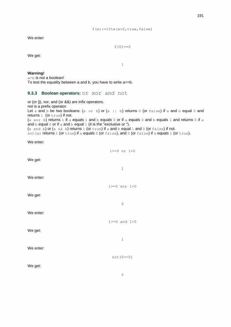
191

f(x):=ifte(x>0,true,false)

We enter:

f(0)==0

We get:

1

Warning! a=b is not a boolean! To test the equality between a and b, you have to write a==b.

9.3.3 Boolean operators: or xor and not

or (or ||), xor, and (or &&) are infix operators. not is a prefix operator. Let a and b be two booleans: (a or b) or (a || b) returns 0 (or false) if a and b equal 0 and returns 1 (or true) if not. (a xor b) returns 1 if a equals 1 and b equals 0 or if a equals 0 and b equals 1 and returns 0 if a and b equal 0 or if a and b equal 1 (it is the "exclusive or "). (a and b) or (a && b) returns 1 (or true) if a and b equal 1 and 0 (or false) if not. not(a) returns 1 (or true) if a equals 0 (or false), and 0 (or false) if a equals 1 (or true). We enter:

1>=0 or 1<0

We get:

1

We enter:

1>=0 xor 1>0

We get:

0

We enter:

1>=0 and 1>0

We get:

1

We enter:

not(0==0)

We get:

0

192

9.4 Bit to bit operators

9.4.1 operators bitor, bitxor, bitand

The integers can be entered with the notation 0x... in hexadecimal. By example, 0x1f represents 16 +15 = 31 in decimal. We can display the integers in hexadecimal (key of the status line of the CAS with the key Base (Integers)).

– bitor is the inclusive logic bit to bit or.

We enter:

bitor(0x12,0x38)

or we enter:

bitor(18,56)

We get:

58

indeed:

18 reads 0x12 in basis 16 and 0b010010 in basis 2,

56 reads 0x38 in basis 16 and 0b111000 in basis 2,

bitor(18,56) reads 0b111010 in basis 2 and then equals 58.

– bitxor is the logic exclusive bit to bit or.

We enter:

bitxor(0x12,0x38)

or we enter:

bitxor(18,56)

We get:

42

indeed:

18 reads 0x12 in basis 16 and 0b010010 in basis 2,

56 reads 0x38 in basis 16 and 0b111000 in basis 2,

bitxor(18,56) reads 0b101010 in basis 2 and then equals 42.

– bitand is the bit to bit logic and. We enter:

bitand(0x12,0x38)

or we enter:

bitand(18,56)

We get:

193

16

indeed:

18 reads 0x12 in basis 16 and 0b010010 in basis 2,

56 reads 0x38 in basis 16 and 0b111000 in basis 2,

bitand(18,56) reads 0b010000 in basis 2 and then equals 16.

9.4.2 Bit to bit Hamming distance of: hamdist

The bit to bit Hamming distance is the sum of absolute values of bit to bit differences between two numbers, that is to say the number of different bits. We enter:

hamdist(0x12,0x38)

or we enter

hamdist(18,56)

We get:

3

indeed:

18 reads 0x12 in basis 16 and 0b010010 in basis 2,

56 reads 0x38 in basis 16 and 0b111000 in basis 2,

hamdist(18,56) equals 1+0+1+0+1+0 and then equals 3.

9.5 Usual functions

The usual functions can be accessed by pressing the corresponding keys. We need their programming names, for example: id designates the function identity, sq designates the function square, sqrt designates the function square root, neg designates the function 𝑥 → −𝑥,

inv designates the function 𝑥 →1

𝑥.

9.6 The smallest integer greater than or equal to the argument: CEILING

ceiling

CEILING(a) or ceiling(a) returns the smallest integer greater than or equal to the argument 𝑎. We enter:

CEILING(45/8)

We get:

6

We enter:

CEILING(-45/8)

194

We get:

-5

We enter:

CEILING(2.5)

We get:

3

9.7 Integer part of a real: FLOOR floor

FLOOR(a) or floor(a) returns the greater integer lower than or equal to the argument 𝑎. We enter:

FLOOR(45/8)

We get:

5

We enter:

FLOOR(-45/8)

We get:

-6

We enter:

FLOOR(2.5)

We get:

2

9.8 Argument without its fractional part: IP

IP(a) returns the argument real 𝑎 without its fractional part. We enter:

IP(45/8)

We get:

5

We enter:

IP(-45/8)

We get:

195

-5

9.9 Fractional part: FP

FP(a) returns the fractional part of the real argument 𝑎. We enter in:

FP(45/8)

We get:

0.625

We enter in the CAS:

FP(45/8)

We get:

5/8

We enter in:

FP(-45/8)

We get:

-0.625

We enter in the CAS:

FP(-45/8)

We get:

-5/8

9.10 Round a real or a complex to 𝒏 decimal places: ROUND round

ROUND(a) or round(a) (resp. ROUND(a,n) or round(a,n)) rounds the real 𝑎 according to the closest integer (resp. the closest decimal number having 𝑛 decimal places).

ROUND(a) (resp. ROUND(a,n)) rounds the complex a according to the closest element of ℤ[𝑖], (resp.

with 𝑛 decimal places). We enter:

ROUND(45/8)

or

round(45/8)

We get:

6

We enter:

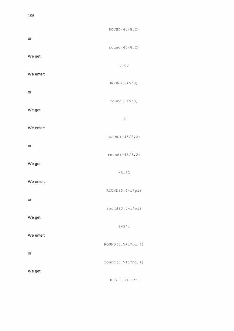
196

ROUND(45/8,2)

or

round(45/8,2)

We get:

5.63

We enter:

ROUND(-45/8)

or

round(-45/8)

We get:

-6

We enter:

ROUND(-45/8,2)

or

round(-45/8,2)

We get:

-5.62

We enter:

ROUND(0.5+i*pi)

or

round(0.5+i*pi)

We get:

1+3*i

We enter:

ROUND(0.5+i*pi,4)

or

round(0.5+i*pi,4)

We get:

0.5+3.1416*i

197

9.11 Truncate a real or a complex to 𝒏 decimal places: TRUNCATE trunc

TRUNCATE or trunc returns the argument truncated to 𝑛 decimal places (by default 𝑛 = 0) . We enter in HOME or in the CAS:

TRUNCATE(45/8)

or

trunc(45/8)

We get:

5

We enter in HOME or in the CAS:

TRUNCATE(45/8,2)

or

trunc(45/8,2)

We get:

5.62

We enter in HOME or in the CAS:

TRUNCATE(-45/8)

or

trunc(-45/8)

We get:

-5

We enter in HOME or in the CAS:

TRUNCATE(-45/8,2)

or

trunc(-45/8,2)

We get:

-5.63

We enter in HOME or in the CAS:

TRUNCATE(sqrt(2)+i*sqrt(5),4)

or

trunc(sqrt(2)+i*sqrt(5),4)

We get:

198

1.4142+2.236*i

Warning! In CAS, truncate(P,n) truncates the polynomial P at degree n. We enter:

truncate(x^5+x^4+x^2+x+1,2)

We get:

x^2+x+1

9.12 The fractional part of a real: frac

frac of a real returns its fractional part. We enter in the CAS or in HOME:

frac(22/7))

We get:

1/7

We enter in the CAS or in HOME:

frac(sqrt(2))

We get:

sqrt(2)-1

9.13 The real without its fractional part: iPart

iPart of a real returns a real which equals the real argument without its fractional part. We enter:

iPart(sqrt(2))

We get:

1.0

9.14 Mantissa of a real: MANT

MANT(a) returns |𝑎|/ 10𝑛 where the integer n checks:

10𝑛 ≤ |𝑎| < 10𝑛+1. MANT(a) then returns the mantissa of a real 𝑎, that is to say the significant digits of 𝑎. We enter:

MANT(45/8)

We get:

5.625

199

We enter:

MANT(-45/8)

We get:

5.625

9.15 Integer part of the logarithm basis 10 of a real: XPON

XPON(a) returns the integer n such as 10𝑛 ≤ |𝑎| < 10𝑛+1. We enter:

XPON(45/8)

We get:

0

We enter:

XPON(45000/8)

We get:

3

We enter:

XPON(1234*sqrt(2))

We get:

3

indeed 103 < 1234 ∗ √2 ≃ 1745.13953597 < 104

200

Chapter 10 Arithmetic

10.1 Maximum of two or several values: MAX max

MAX or max returns the maximum of elements of a sequence or of a list of reals. We enter:

MAX(4,5,8,2,6)

or

max(4,5,8,2,6)

We get:

8

10.2 Minimum of two or several values: MIN min

MIN or min returns the minimum of elements of a sequence or of a list of reals. We enter:

MIN(4,5,8,2,6)

or

min(4,5,8,2,6)

We get:

2

10.3 MOD

MOD is an infix function.

a MOD b returns the remainder of the Euclidean division of a by b. We enter:

22 MOD 5

We get:

2

201

10.4 FNROOT

FNROOT returns an approximate root of the expression supplied as first argument, for the variable supplied as second argument, and which is close to the third argument.

We enter in real mode (i not checked in the CAS Settings):

FNROOT(x^4+3x-4)

We get:

-1.74295920217,1.

We enter in real mode (i not checked in the CAS Settings):

FNROOT(x^4+3x-4,x,-2)

We get:

-1.74295920217

We enter in complex mode (i checked in the CAS Settings):

FNROOT(x^4+3x-4)

We get:

[-1.74295920217,0.371479601083+1.46865601291*i, 0.371479601083-

1.46865601291*i,1.0]

10.5 N-th root: NTHROOT surd

NTHROOT is an infix function whereas surd is a prefix command of the CAS .

NTHROOT comes with the shifted key √ n

(Shift 𝑥𝑦).

p NTHROOT n returns the value of 𝑛1/𝑝

surd(n,p) returns 𝑛1/𝑝

We enter in real mode in HOME (i not checked in the CAS Settings):

3 NTHROOT 8

We get:

2

We enter in complex mode in HOME (i checked in the CAS Settings):

3 NTHROOT -1+i

We get:

0.85502540378-0.5*i

We enter in real mode in the CAS (i not checked in the CAS Settings):

3 NTHROOT 8

or

202

surd(8,3)

We get:

2

We enter in complex mode in the CAS:

3 NTHROOT -1+i

or

surd(-1+i,3)

We get:

exp(ln(-1+i)/3)

10.6 %

%(a,b) returns 𝑎

100∗ 𝑏 (a percent of b).

We enter:

%(5,70)

We get:

3.5

We enter:

%(5,90)

We get:

4.5

10.7 Complex

10.7.1 The key i

The key i is a shifted key (Shift 2). i is the complex number of modulus 1 and argument 𝜋/2. We enter:

1+3*i

or

1+3i

We get:

1+3*i

203

10.7.2 Argument: ARG arg

ARG or arg returns the argument of the complex number supplied as argument (in degrees or in radians according to the chosen configuration). We enter in HOME:

ARG(2+6*i)

We get, if we are in radians:

1.2490457724

We get, if we are in degrees:

71.5650511771

We enter in the CAS:

ARG(2+6*i)

We get, if we are in radians:

atan(3)

We get, if we are in degrees:

71.5650511771

10.7.3 Conjugate: CONJ conj

CONJ or conj returns the conjugate of the complex number supplied as argument. We enter:

CONJ(1+3*i)

or

conj(1+3*i)

We get:

1-3*i

10.7.4 Imaginary part: IM im

IM or im returns the imaginary part of the complex number supplied as argument. We enter:

IM(1+3*i)

We get:

3

10.7.5 Real part: RE re

RE or re returns the real part of the complex number supplied as argument.

204

We enter:

RE(1+3*i)

We get:

1

10.7.6 Sign: SIGN sign

SIGN or sign returns the complex number supplied as argument divided by its modulus. We enter:

SIGN(1+3*i)

We get:

(1+3*i)/sqrt(10)

10.7.7 The key Shift +/−: ABS abs

The key |x| is a shifted key (Shift +/−). The key |x| returns ABS(x), which equals:

– the absolute value of a real, – the modulus of a complex number,

– the length of a vector 𝑣𝑗 ((∑ |𝑣𝑗|2𝑛

𝑗=1 )1/2

),

– the Schur norm or Frobenius norm of a matrix 𝑎𝑗,𝑘 ((∑ |𝑎𝑗,𝑘|2𝑛

𝑗,𝑘=1 )1/2

).

We enter:

ABS(1+3*i)

We get:

3.1622776602

We use the key |x| in the CAS:

ABS(1+3*i)

or we enter:

abs(1+3*i)

We get:

sqrt(10)

10.7.8 Write of complex in the form of 𝐫𝐞(𝒛) + 𝒊 ∗ 𝐢𝐦(𝒛): evalc

evalc takes as argument a complex number z. evalc returns this complex number, written in the form re(z)+i*im(z). We enter:

evalc(sqrt(2)*exp(i*pi/4))

205

We get:

1+i

10.7.9 Multiply by the complex conjugate: mult_c_conjugate

If an expression has a complex denominator, mult_c_conjugate multiplies the numerator and the denominator of this expression by the complex conjugate of the denominator. If an expression does not have a complex denominator, mult_c_conjugate multiplies the numerator and the denominator of this expression by the complex conjuguate of the numerator. We enter:

mult_c_conjugate((2+i)/(2+3*i))

We get:

(2+i)*(2+3*(-i))/((2+3*(i))*(2+3*(-i)))

We enter:

mult_c_conjugate((2+i)/2)

We get:

(2+i)*(2+-i)/(2*(2+-i))

10.8 Exponential and Logarithms

10.8.1 Function neperian logarithm: LN ln log

LN or ln or log designates the function neperian logarithm. LN (or ln in the CAS) is accessed with the key LN. Warning! The neperian log is LN in HOME, and ln or log in the CAS. We enter in HOME:

LN(e)

We get:

1

We enter:

LN(2)

We get:

0.69314718056

but in the CAS, we enter:

ln(e)

or

log(e)

206

We get:

1

We enter:

ln(2)

or

log(2)

We get:

ln(2)

10.8.2 Function logarithm basis 10: LOG log10

Warning! The log basis 10 is LOG in HOME and log10 in the CAS and log designates the neperian log. LOG or log10 designates the function logarithm basis ten, LOG (or log10 in the CAS) can be accessed with the key LOG. We enter in HOME:

LOG(10)

We get:

1

We enter:

LOG(7)

We get:

0.84509804001

We enter in the CAS:

log10(10)

We get:

1

We enter:

log10(7)

We get:

ln(7)/ln(10)

10.8.3 Function logarithm basis 𝒃: logb

logb designates the function logarithm with the basis supplied as second argument: We enter in the CAS:

207

logb(7,7)

We get:

1

We enter in the CAS:

logb(7,10)

We get:

ln(7)/ln(10)

logb(7,10)=log10(7)=log(7)/log(10)

10.8.4 Function antilogarithm: ALOG alog10

alog10 designates the function antilogarithm basis ten, it is the function: 𝑥 → 10𝑥. We enter in HOME:

ALOG(3/2)

We get:

31.6227766017

it is the approximate value of sqrt(10)*10 at the nearest 10−10. We enter in the CAS:

ALOG(3/2)

or

alog(3/2)

or we get:

sqrt(10)*10^1

We enter:

alog10(10)

We get:

10000000000

10.8.5 Function exponential: EXP exp

EXP or exp designates the function exponential. EXP (or exp in the CAS) can be accessed with the key EXP. We enter in HOME:

208

EXP(2)

We get:

7.38905609893

but in the CAS, we enter:

exp(2)

We get:

exp(2)

10.8.6 Function EXPM1

EXPM1 designates the function 𝑥 → 𝐸𝑋𝑃(𝑥) − 1. We enter:

EXPM1(4)

We get:

EXP(4)-1

We enter:

EXPM1(2.*10^-4)

We get:

0.00020002000133

BUT if we enter:

EXP(2.*10^-4)-1

We get:

0.00020002

10.8.7 Function LNP1

LNP1 designates the function 𝑥 → 𝐿𝑁(𝑥 + 1) We enter:

LNP1(4)

We get:

LN(5)

We enter:

LNP1(2.*10^-4)

We get:

209

1.99980002666E-4

210

Chapter 11 Trigonometric functions

11.1 The keys of trigonometric functions

– SIN or sin designates the function sine. We enter in the CAS:

SIN(pi/3)

or

sin(pi/3)

We get:

sqrt(3)/2

– ASIN or asin designates the function arc sine. We enter in the CAS:

ASIN(1/2)

or

asin(1/2)

We get:

pi/6

– COS or cos designates the function cosine. We enter in the CAS:

COS(pi/3)

or

cos(pi/3)

We get:

1/2

– ACOS or acos designates the function arc cosine. We enter in the CAS:

ACOS(1/2)

or

acos(1/2)

211

We get:

pi/3

– TAN or tan designates the function tangent. We enter in the CAS:

TAN(pi/3)

or

tan(pi/3)

We get:

sqrt(3)

– ATAN or atan designates the function arc tangent. We enter in the CAS:

ATAN(sqrt(3)/3)

or

atan(sqrt(3)/3)

We get:

pi/6

11.2 Cosecant: CSC csc

CSC(x) or csc returns 1/SIN(x): it is the function cosecant. We enter in the CAS:

CSC(pi/3)

or

csc(pi/3)

We get after simplification:

2*sqrt(3)/3

11.3 Arccosecant: ACSC acsc

ACSC(x) or acsc returns ASIN(1/x): it is the reciprocal function of the function cosecant. We enter in the CAS:

ACSC(sqrt(2))

or

212

acsc(sqrt(2))

We get after simplification:

pi/4

11.4 Secant: SEC sec

SEC(x) or sec returns 1/COS(x): it is the function secant. We enter in the CAS:

SEC(pi/3)

or

sec(pi/3)

We get:

2

11.5 Arcsecant: ASEC asec

ASEC(x) or asec returns ACOS(1/x): it is the reciprocal function of the function secant. We enter in the CAS:

ASEC(2)

or

asec(2)

We get:

1/3*pi

11.6 Cotangent: COT cot

COT(x) or cot returns COS(x)/SIN(x): it is the function cotangent. We enter in the CAS:

COT(pi/3)

or

cot(pi/3)

We get after simplification:

sqrt(3)/3

213

11.7 Arccotangent: ACOT acot

ACOT(x) or acot returns pi/2-ATAN(x): it is the reciprocal function of the function cotangent. We enter in the CAS:

ACOT(sqrt(3))

or

acot(sqrt(3))

We get after simplification:

pi/6

214

Chapter 12 Hyperbolic functions

12.1 Hyperbolic sine: SINH sinh

SINH(x) or sinh(x) returns: exp(𝑥) − exp(−𝑥)

2

it is the function hyperbolic sine We enter in the CAS:

hyp2exp(SINH(ln(2)))

We enter in the CAS:

hyp2exp(sinh(ln(2)))

We get:

3/4

Indeed, the command hyp2exp transforms the functions hyperbolic into exponentials.

12.2 Hyperbolic arc sine: ASINH asinh

ASINH or asinh is the reciprocal function of the function hyperbolic sine. We enter in the CAS:

ASINH(3/4)

or

asinh(3/4)

We get:

ln(2)

12.3 Hyperbolic cosine: COSH cosh

COSH(x) or cosh returns: exp(𝑥) + exp(−𝑥)

2

it is the function hyperbolic cosine. We enter in the CAS:

COSH(0)

or

215

cosh(0)

We get:

1

12.4 Hyperbolic arc cosine: ACOSH acosh

ACOSH or acosh is the reciprocal function of the function hyperbolic cosine. We enter in the CAS:

hyp2exp(ACOSH(1))

or

hyp2exp(acosh(1))

We get:

0

12.5 Hyperbolic tangent: TANH tanh

TANH(x) or tanh returns: exp(2𝑥) – 1

exp(2𝑥) + 1

it is the function hyperbolic tangent. We enter in the CAS:

hyp2exp(TANH(ln(3)))

or

hyp2exp(tanh(ln(3)))

We get:

4/5

Indeed, the command hyp2exp transforms the functions hyperbolic into exponentials.

12.6 Hyperbolic arc tangent: ATANH atanh

ATANH or atanh is the reciprocal function of the function hyperbolic tangent. We enter in the CAS:

ATANH(4/5)

or

atanh(4/5)

We get:

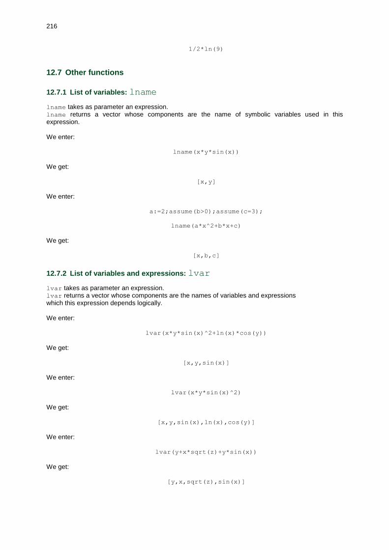
216

1/2*ln(9)

12.7 Other functions

12.7.1 List of variables: lname

lname takes as parameter an expression. lname returns a vector whose components are the name of symbolic variables used in this expression. We enter:

lname(x*y*sin(x))

We get:

[x,y]

We enter:

a:=2;assume(b>0);assume(c=3);

lname(a*x^2+b*x+c)

We get:

[x,b,c]

12.7.2 List of variables and expressions: lvar

lvar takes as parameter an expression. lvar returns a vector whose components are the names of variables and expressions which this expression depends logically. We enter:

lvar(x*y*sin(x)^2+ln(x)*cos(y))

We get:

[x,y,sin(x)]

We enter:

lvar(x*y*sin(x)^2)

We get:

[x,y,sin(x),ln(x),cos(y)]

We enter:

lvar(y+x*sqrt(z)+y*sin(x))

We get:

[y,x,sqrt(z),sin(x)]

217

12.7.3 List of variables and algebraic expressions: algvar

algvar takes as parameter an expression. algvar returns a vector whose components are the name of symbolic variables, by order of algebraic extension, used in this expression. We enter:

algvar(y+x*sqrt(z))

We get:

[[y,x],[z]]

We enter:

algvar(y*sqrt(x)*sqrt(z))

We get:

[[y],[z],[x]]

We enter:

algvar(y*sqrt(x*z))

We get:

[[y],[x,z]]

We enter:

algvar(y+x*sqrt(z)+y*sin(x))

We get:

[[x,y,sin(x)],[z]]

12.7.4 Testing the presence of a variable in an expression: has

has takes as parameter an expression and the name of a variable. has returns 1, or 0, depending on the variable is present , or not present , in the expression. We enter:

has(x*y*sin(x),y)

We get:

1

We enter:

has(x*y*sin(x),z)

We get:

0

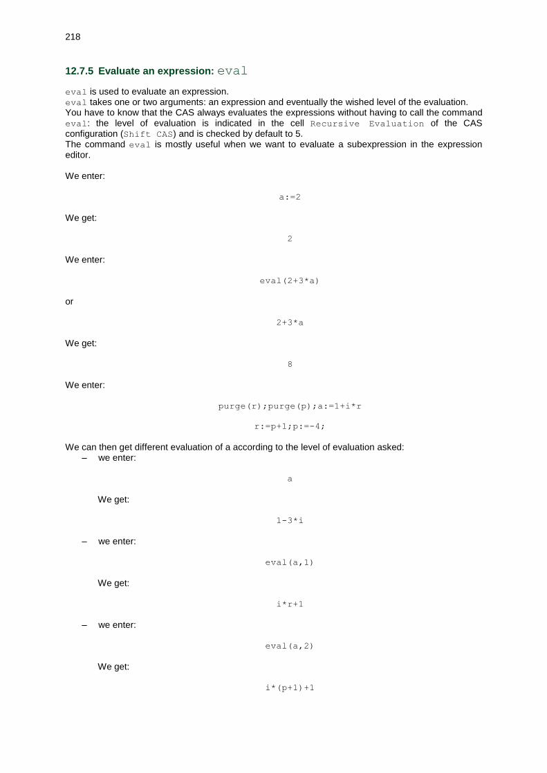
218

12.7.5 Evaluate an expression: eval

eval is used to evaluate an expression. eval takes one or two arguments: an expression and eventually the wished level of the evaluation. You have to know that the CAS always evaluates the expressions without having to call the command eval: the level of evaluation is indicated in the cell Recursive Evaluation of the CAS configuration (Shift CAS) and is checked by default to 5. The command eval is mostly useful when we want to evaluate a subexpression in the expression editor. We enter:

a:=2

We get:

2

We enter:

eval(2+3*a)

or

2+3*a

We get:

8

We enter:

purge(r);purge(p);a:=1+i*r

r:=p+1;p:=-4;

We can then get different evaluation of a according to the level of evaluation asked: – we enter:

a

We get:

1-3*i

– we enter:

eval(a,1)

We get:

i*r+1

– we enter:

eval(a,2)

We get:

i*(p+1)+1

219

– we enter:

eval(a,3)

We get:

1-3*i

12.7.6 Not evaluating an expression: QUOTE quote ’

If we do not want an expression to be evaluated in a calculation, we need to quote it, either with ’, either thanks to the function quote. Note When we enter for example a:=quote(a), this purges the variable a, and this instruction returns the value of this variable (or the assumptions made on this variable). So a:=quote(a) is synonymous of purge(a). We enter:

a:=2;quote(2+3*a)

or

a:=2;’2+3*a’

We get:

(2,2+3.a)

12.7.7 Numerical evaluation: evalf approx

evalf or approx takes as parameter a numerical expression or a matrix. evalf returns the numerical value of the expression or of the matrix. By adding a second argument n to evalf (or approx), we can specify the number of significant digits of the approximation. We enter:

evalf(sqrt(2))

We get:

1.41421356237

We enter:

evalf(sqrt(2),5)

We get:

1.4142

We enter:

evalf([[1,sqrt(2)],[0,1]])

We get:

[[1.0,1.41421356237],[0.0,1.0]]

220

We enter:

evalf([[1,sqrt(2)],[0,1]],5)

We get:

[[1.0,1.4142],[0.0,1.0]]

12.7.8 Rational approximation: exact

exact takes as parameter a real numerical expression. exact gives a rational approximation of all the decimal numbers r present which validate |𝑟 − exact(𝑟)| < 휀, where 휀 is defined by epsilon in the CAS configuration (key Shift CAS). We enter:

exact(1.5)

We get:

3/2

We enter:

exact(1.414)

We get:

707/500

We enter:

exact(1.41421356237^2)

We get:

2

221

Chapter 13 Probability functions

13.1 Factorial: factorial !

! is a postfix function whereas factorial is a prefix function.

n! or factorial(n) returns the factorial of n if n is n integer, and a! returns the value of the Gamma function for 𝑎 + 1 if 𝑎 is real. We enter in the CAS:

20!

or

factorial(20)

We get:

2432902008176640000

We enter:

5.2!

or

factorial(5.2)

We get:

169.406099462

13.2 Number of combinations of p objects among 𝒏: COMB comb

COMB(n,p) or comb(n,p) returns the number of combinations of p elements among n (n and p are integers). We have: COMB(n,p) returns

𝑛!

𝑝! (𝑛 − 𝑝)!

We enter:

COMB(5,2)

We get:

10

13.3 Number of permutations of p objects among n: PERM perm

PERM(n,p) or perm(n,p) returns the number of permutations of p elements among n (n and p are integers).

222

We have: PERM(n,p) returns 𝑛!

(𝑛 − 𝑝)!

We enter:

PERM(5,2)

We get:

20

13.4 Random numbers

13.4.1 Random number (real or integer): RANDOM

– To get a random real number between 0 and 1, we do not put any argument. We enter:

RANDOM

We get a real number of the range 0,1, for example:

0.291424166081

– To get a random integer a between 1 and n (1 ≤ 𝑎 ≤ 𝑛), we put n as argument without brackets. We enter:

RANDOM 3

We get 1, 2 or 3, for example:

1

– To get a random real number a between b and c (𝑏 ≤ 𝑎 ≤ 𝑐), we put b, c as arguments without brackets. We enter:

RANDOM 3,5

We get a real number of 3,5 for example:

4.81731227506

– To get k random integers a between p and n (𝑝 ≤ 𝑎 ≤ 𝑛) we put k, p, n as arguments without

brackets. We enter:

RANDOM 3,2,5

We get 3 integers between 2 and 5, for example:

[5,3,2]

223

13.4.2 Random integer: RANDINT

– To get a random integer a between 1 and n (1 ≤ 𝑎 ≤ 𝑛) we put n as argument. We enter:

RANDINT(4)

We get 0,1,2,3 or 4, for example:

2

– To get a random integer a between b and c (𝑏 ≤ 𝑎 ≤ 𝑐), we put b and c as arguments. We enter:

RANDINT(4,6)

We get 4,5 or 6, for example:

5

– To get k random integers a between p and n (𝑝 ≤ 𝑎 ≤ 𝑛) we put k, p and n as arguments. We enter:

RANDINT(4,2,6)

We get 4 numbers between 2 and 6, for example:

[2,6,2,6]

13.4.3 Rand function of the CAS: rand

Equally distributed draw on [0, 1[: rand()

rand() returns randomly, in an equiprobable manner, a real number of [0, 1[. We enter:

rand()

We get for example:

0.912569261115

To get, randomly, in an equiprobable manner, a number of [0; 1[, we can also use (see following paragraph):

rand(0,1)

We get:

0.391549611697

Equally distributed draw on the interval [𝒂; 𝒃[: rand(a,b)

If a and b are reals, rand(a,b) designates a random decimal number of the interval [𝑎; 𝑏[. Thus, rand(a,b) returns randomly, and in an equiprobable manner, a decimal number of [𝑎; 𝑏[. To get, randomly and in an equiprobable manner, a decimal number of [0; 1[, we enter:

rand(0,1)

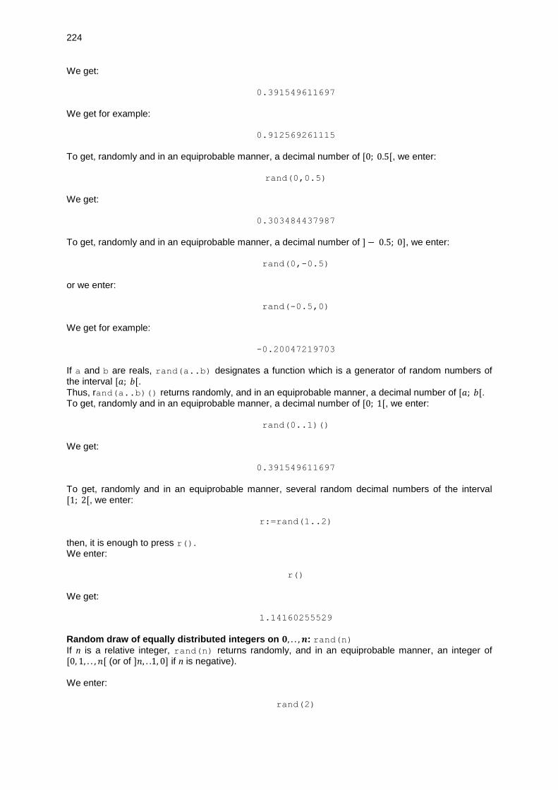
224

We get:

0.391549611697

We get for example:

0.912569261115

To get, randomly and in an equiprobable manner, a decimal number of [0; 0.5[, we enter:

rand(0,0.5)

We get:

0.303484437987

To get, randomly and in an equiprobable manner, a decimal number of ] − 0.5; 0], we enter:

rand(0,-0.5)

or we enter:

rand(-0.5,0)

We get for example:

-0.20047219703

If a and b are reals, rand(a..b) designates a function which is a generator of random numbers of the interval [𝑎; 𝑏[. Thus, rand(a..b)() returns randomly, and in an equiprobable manner, a decimal number of [𝑎; 𝑏[. To get, randomly and in an equiprobable manner, a decimal number of [0; 1[, we enter:

rand(0..1)()

We get:

0.391549611697

To get, randomly and in an equiprobable manner, several random decimal numbers of the interval [1; 2[, we enter:

r:=rand(1..2)

then, it is enough to press r(). We enter:

r()

We get:

1.14160255529

Random draw of equally distributed integers on 𝟎, . . , 𝒏: rand(n)

If n is a relative integer, rand(n) returns randomly, and in an equiprobable manner, an integer of [0, 1, . . , 𝑛[ (or of ]𝑛, . .1, 0] if n is negative). We enter:

rand(2)

225

We get:

1

or we get:

0

We enter:

rand(-2)

We get:

-1

or we get:

0

To get a random integer between 6 and 10, boundaries included, we enter:

6+rand(11-6)

We get for example:

8

Random draw without replacement of 𝒑 objects among 𝒏: rand rand has, in this case, either two, either three arguments. If rand has two arguments: the arguments are an integer p and a list L, then rand(p,L) returns, randomly, p elements of the list L. If rand has three arguments: the arguments are three integers p,min,max, then rand(p,min,max) returns, randomly, p integers of [min,..,max] We enter:

rand(3,["r","r","r","r","v","v","v"])

We get:

["r","r","v"]

We enter:

rand(2,1,10)

We get:

[3,7]

We enter:

rand(2,4,10)

We get:

[5,7]

226

13.4.4 Random permutation: randperm

randperm takes as argument an integer n. randperm returns a random permutation of [0. . 𝑛 − 1]. We enter:

randperm(3)

We get:

[2,0,1]

13.4.5 Generating a random list: randvector

randvector generates a list of random numbers.

randvector takes as argument an integer n and eventually a second argument, either an integer k, either the quoted or not quoted name of the distribution law of the random numbers of the list (see also 13.4.8, 13.5.4, 13.5.5 and 13.5.6). randvector returns a list of degree n constituted of random integers equally distributed between −99

and 99 (by default) or between 0 and 𝑘 − 1 or a list of degree n of random numbers distributed according to the quoted law or as parameter. When randvector takes as argument an integer n and a random law of the calculator you have to quote or not in this case, randvector returns a list of dimension n whose elements are taken randomly according to the function supplied as third argument. The functions supplied as second argument, which must be quoted or not, can be: ’rand(n)’

’binomial(n,p)’ or binomial,n,p or ’randbinomial(n,p)’ ’poisson(λ)’ or poisson, λ or ’randpoisson(λ)’ ’normald(µ,σ)’ or normald,µ,σ or ’randnorm(µ,σ)’

’exponential(a)’ or exponential,a or ’randexp(a)’ ’fisher(n,m)’ or fisher,n,m or ’randfisher(n,m)’ Warning! The syntax without quote suits to the laws, but not to the corresponding command rand..., then, for example, the commands randvector(3,normald,0,1) or randvector(3,’normald(0,1)’) or randvector(3,’randnorm(0,1)’) are valid but randvector(3,randnorm,0,1) is not valid. We enter:

randvector(3)

We get for example:

[-54,78,-29]

We enter:

randvector(3,5)

We enter:

randvector(3,’rand(5)’)

We get for example:

[1,2,4]

We enter:

227

randvector(3,normald,0,1)

Or we enter:

randvector(3,’normald(0,1)’)

We get for example:

[1.39091705476,-0.136794772167,0.187312440336]

We enter:

randvector(3,2..4)

We get for example:

[3.92450003885,3.50059241243,2.7322040787]

We enter:

randvector(6,binomial,4,0.2)

Or we enter:

randvector(6,’binomial(4,0.2)’)

We get for example:

[0,1,0,2,2,0]

We enter:

randvector(6,poisson,1.3)

Or we enter:

randvector(6,’poisson(1.3)’)

We get for example:

[1,0,1,1,1,1]

We enter:

randvector(4,exponential,1.2)

Or we enter:

randvector(4,’exponential(1.2)’)

We get for example:

[1.67683756526,0.192937941271,0.580820253805,0.709352619633]

We enter:

randvector(5,fisher,4,6)

Or we enter:

randvector(5,’fisher(4,6)’)

228

We get for example:

[0.17289703163,1.03709368317,0.161051043162,1.4407877128,0.3586901042

75]

13.4.6 Draw according to a multinomial law with programs

We write the programs randmult and randmultiname which simulate the multinomial law. randmult(n,P) chooses randomly n numbers among 1...k according to the multinomial law of probability P (k=size(P)). This means that we do a draw with replacement of n objects among k=size(P) objects. randmult(n,P) returns a list R of k=size(P) elements where R[j] is the number of objects of probability P[j] which have been drawn. We enter the program randmult:

(n,p)->BEGIN

local k,j,l,r,x,y;

k:=size(p);

x:=cumSum(p);

if x[k]!=1 then return "error"; end;

y:=makelist(0,1,k)

for j from 1 to n do

r:=rand(0,1);

l:=1;

while r>x[l] do

l:=l+1;

end;

y[l]:=y[l]+1

end;

return (y);

END;

We do six times the draw of an object among three objects (draw with replacement). Each object has a probability [1/2,1/3,1/6] to be drawn. To simulate a draw, we enter:

randmult(6,[1/2,1/3,1/6])

We get for example:

[3,2,1]

randmultinom(n,P,C) chooses randomly n objects among the elements of the list C. If k=size(C), the object C[j] has the probability P[j] to be drawn for (j=1..k). We must get k=size(C)=size(P) and sum(P)=1. randmultinom(n,P,C) returns the sequence of k lists constituted of the name of the objects and their number of occurence. We enter the program randmultinom:

(n,p,c)->BEGIN

local k,j,l,r,x,y;

k:=size(p);

if size(c)!=k then return "error"; end;

x:=cumSum(p);

if x[k]!=1 then return "error"; end;

y:=MAKELIST([c[j],0],j,1,k);

for j from 1 to n do

r:=rand(0,1);

l:=1;

while r>x[l] do

l:=l+1;

end;

y[l,2]:=y[l,2]+1

end;

229

return y;

END;

We do six times the draw of an object among three objects ["A","B","C"] (draw with replacement). Each object has the probability [1/2,1/3,1/6] to be drawn. To simulate a draw, we enter:

randmultinom(6,[1/2,1/3,1/6],["A","B","C"])

We get for example:

[["A",3],["B",1],["C",2]]]

13.4.7 Draw according to a normal distribution: RANDNORM randNorm

RANDNORM(mu,sigma) or randNorm(mu,sigma) returns a real randomly distributed according to the normal distribution 𝑁(𝑚𝑢, 𝑠𝑖𝑔𝑚𝑎) (by default 𝑚𝑢 = 0 and 𝑠𝑖𝑔𝑚𝑎 = 1). We enter:

RANDNORM()

Or we enter:

RANDNORM(0,1)

We get, for example:

1.2440525851

We enter:

RANDNORM(1,2)

We get, for example:

-1.8799815939

13.4.8 Draw according to an exponential law: randexp

randexp(a) returns numbers randomly distributed according to the exponential law of positive parameter a. The density of probability is proportional to 𝑒𝑥𝑝(−𝑎 ∗ 𝑡) and we have:

𝑃𝑟𝑜𝑏𝑎(𝑋 ≤ 𝑡) = 𝑎 ∫ 𝑒𝑥𝑝(−𝑎 ∗ 𝑢)𝑑𝑢𝑡

0.

We enter:

randexp(1)

We get for example:

0.310153677284

or we get for example:

0.776007926195

230

13.4.9 Initializing the series of random numbers: RANDSEED RandSeed srand

RANDSEED or RandSeed or srand initializes the series of random numbers supplied by RANDOM. If we do not put a parameter, RANDSEED uses the time value as parameter. We enter:

RANDSEED()

We get:

1

We enter:

RANDSEED(pi)

We get:

1

13.4.10 Function UTPC

UTPC(n,x0) returns the probability that a random Chisquare variable with n degrees of freedom be greater than x0. We enter:

UTPC(2,6.1)

We get:

0.0473589243911

13.4.11 Function UTPF

UTPF(n,m,x0) returns the probability that a random Fisher-Snedecor variable with n,m degrees of freedom be greater than x0. We enter:

UTPF(4,10,3.5)

We get:

0.0491881403249

13.4.12 Function UTPN

UTPN(mu,v,x0) returns the probability that a random Normal variable be greater than x0 with mu the mean and v the variance (by default 𝑚𝑢 = 0 and 𝑣 = 1). We enter:

UTPN(1.96) or UTPN(1,4,4.92)

We get:

0.0249978951482

231

indeed (𝑥 − 1)/√4 > 1.96 is equivalent to 𝑥 > 4.92. We enter:

UTPN(0.98)

or

UTPN(1,4,2.96)

We get:

0.163543059328

indeed (𝑥 − 1)/√4 > 0.98 is equivalent to 𝑥 > 2.96.

13.4.13 Function UTPT

UTPT(n,x0) returns the probability that a random Student variable with n degrees of freedom be greater than x0. We enter:

UTPT(3,2.35)

We get:

0.050152899407

We enter:

UTPT(3,-2.35)

We get:

0.949847100593

13.5 Density of probability

13.5.1 Density of probability of the normal distribution: NORMALD normald

NORMALD(x) or normald(x) is the density of probability of the normal reduced centered distribution (of mean 0 and standard deviation 1). NORMALD(µ, σ,x) or normald(µ, σ,x) is the density of probability of the normal distribution of

mean µ and standard deviation σ). We enter:

NORMALD(0.5)

Or we enter:

NORMALD(0,1,0.5)

We get:

0.352065326764

232

We enter:

NORMALD(1,2,0.5)

We get:

0.193334058401

13.5.2 Density of probability of the Student law: STUDENT student

STUDENT(n,x) or student(n,x) is the density of probability of the Student law having n degrees of freedom. We enter:

STUDENT(3,5.2)

We get:

0.00366574413491

13.5.3 Density of probability of the χ2: CHISQUARE chisquare

CHISQUARE(n,x) or chisquare(n,x) is the density of probability of the 𝜒2 law having n degrees of freedom. We enter:

CHISQUARE(2,3.2)

We get:

0.100948258997

13.5.4 Density of probability of the Fisher law: FISHER fisher snedecor

FISHER(n,m,x) or fisher(n,m,x) or snedecor(n,m,x) returns the density of probability in x of

the Fisher-Snedecor law (n and m are the numbers of degrees of freedom). We enter:

FISHER(4,10,2.1)

We get:

0.141167840452

13.5.5 Density of probability of the binomial law: BINOMIAL binomial

BINOMIAL(n,k,p) or binomial(n,k,p) returns COMB(𝑛, 𝑘) ∗ 𝑝𝑘 ∗ (1 − 𝑝)(𝑛 – 𝑘) and BINOMIAL(n,k) or binomial(n,k,p) returns COMB(𝑛, 𝑘) if there is no third argument. We enter:

BINOMIAL(4,2)

We get:

6

233

We enter:

BINOMIAL(4,2,0.5)

We get:

0.375

We enter in the CAS:

binomial(4,2)

We get:

6

We enter in the CAS:

binomial(4,2,1/2)

We get:

3/8

13.5.6 Density of probability of the Poisson law: POISSON poisson

The density of probability of the Poisson law of parameter mu, that is to say of mean mu and standard deviation mu is: POISSON(mu,k) or poisson(mu,k) returns

exp(−𝑚𝑢) ∗ 𝑚𝑢𝑘

𝑘!

We enter:

POISSON(0.5,2)

We get:

0.0758163324641

13.6 Function of distribution

13.6.1 Function of distribution of the normal distribution: NORMALD_CDF

normald_cdf

When a random variable X follows a normal reduced centered distribution, we have:

𝑃𝑟𝑜𝑏𝑎(𝑋 ≤ 𝑥) =NORMALD_CDF(x)=normald_cdf(x) and

𝑃𝑟𝑜𝑏𝑎(𝑥 ≤ 𝑋 ≤ 𝑦) =NORMALD_CDF(x,y)=normald_cdf(x,y).

When a random variable X follows a normal distribution of mean µ and standard deviation σ, we have:

𝑃𝑟𝑜𝑏𝑎(𝑋 ≤ 𝑥) =NORMALD_CDF(µ, 𝜎, 𝑥).

𝑃𝑟𝑜𝑏𝑎(𝑥 ≤ 𝑋 ≤ 𝑦) =NORMALD_CDF(µ, 𝜎, 𝑥, 𝑦).

We enter:

NORMALD_CDF(0.96)

Or we enter:

234

NORMALD_CDF(0,1,0.96)

We get:

0.831472392533

We enter:

NORMALD_CDF(1.96)

We get:

0.975002104852

We enter:

NORMALD_CDF(0,1.96)

We get:

0.475002104852

because NORMALD_CDF(0)=1/2 and 0.975002104852 − 0.5 = 0.475002104852 We enter:

NORMALD_CDF(1,2,1.96)

We get:

0.684386303484

We enter:

NORMALD_CDF(1,2,1.1,2.9)

We get:

0.309005067853

13.6.2 Function of distribution of the Student law: STUDENT_CDF student_cdf

When a random variable X follows a Student law having n degrees of freedom,we have:

𝑃𝑟𝑜𝑏𝑎(𝑋 ≤ 𝑥) =STUDENT_CDF(n,x)=student_cdf(n,x).

𝑃𝑟𝑜𝑏𝑎(𝑥 ≤ 𝑋 ≤ 𝑦) =STUDENT_CDF(n,x,y)=student_cdf(n,x,y).

We enter:

STUDENT_CDF(5,2)

We get:

0.949030260585

We enter:

STUDENT_CDF(5,-2)

We get:

235

0.0509697394149

13.6.3 Function of distribution of the 𝝌𝟐 law: CHISQUARE_CDF chisquare_cdf

When a random variable X follows a 𝜒2 law having n degrees of freedom, we have:

𝑃𝑟𝑜𝑏𝑎(𝑋 ≤ 𝑥) =CHISQUARE_CDF(n,x)=chisquare_cdf(n,x).

𝑃𝑟𝑜𝑏𝑎(𝑥 ≤ 𝑋 ≤ 𝑦) =CHISQUARE_CDF(n,x,y)=chisquare_cdf(n,x,y).

We enter:

CHISQUARE_CDF(5,11)

We get:

0.948620016517

We enter:

CHISQUARE_CDF(5,3)

We get:

0.300014164121

We enter:

CHISQUARE_CDF(5,3,11)

We get:

0.648605852396

because 0.948620016517 − 0.300014164121 = 0.648605852396

13.6.4 The function of distribution of the Fisher-Snedecor law: FISHER_CDF fisher_cdf snedecor_cdf

When a random variable X follows a Fisher-Snedecor law having as degrees of freedom n1, n2, we have:

𝑃𝑟𝑜𝑏𝑎(𝑋 ≤ 𝑥) =FISHER_CDF(n1,n2,x)=fisher_cdf(n1,n2,x).

𝑃𝑟𝑜𝑏𝑎(𝑥 ≤ 𝑋 ≤ 𝑦) =FISHER_CDF(n1,n2,x,y)=

fisher_cdf(n1,n2,x,y)=snedecor_cdf(n1,n2,x,y).

We enter:

FISHER_CDF(5,3,9)

We get:

0.949898927032

We enter:

FISHER_CDF(3,5,9.)

We get:

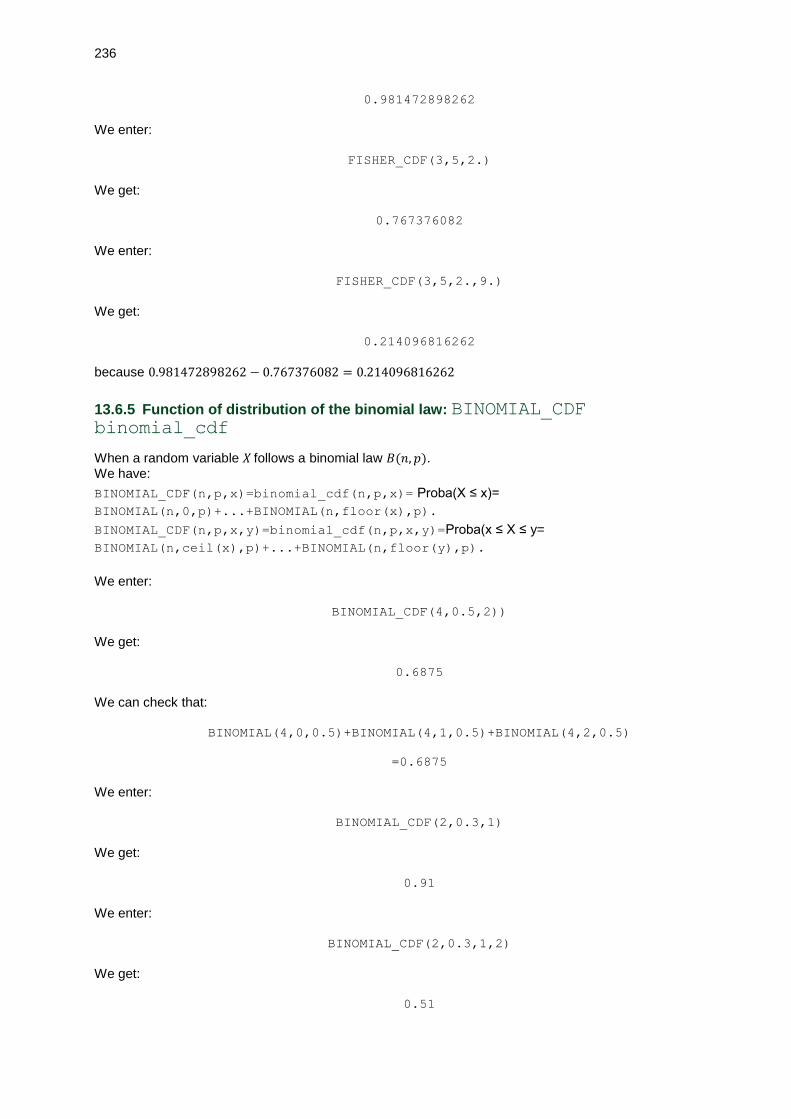
236

0.981472898262

We enter:

FISHER_CDF(3,5,2.)

We get:

0.767376082

We enter:

FISHER_CDF(3,5,2.,9.)

We get:

0.214096816262

because 0.981472898262 − 0.767376082 = 0.214096816262

13.6.5 Function of distribution of the binomial law: BINOMIAL_CDF binomial_cdf

When a random variable X follows a binomial law 𝐵(𝑛, 𝑝). We have:

BINOMIAL_CDF(n,p,x)=binomial_cdf(n,p,x)= Proba(X ≤ x)=

BINOMIAL(n,0,p)+...+BINOMIAL(n,floor(x),p).

BINOMIAL_CDF(n,p,x,y)=binomial_cdf(n,p,x,y)=Proba(x ≤ X ≤ y=

BINOMIAL(n,ceil(x),p)+...+BINOMIAL(n,floor(y),p).

We enter:

BINOMIAL_CDF(4,0.5,2))

We get:

0.6875

We can check that:

BINOMIAL(4,0,0.5)+BINOMIAL(4,1,0.5)+BINOMIAL(4,2,0.5)

=0.6875

We enter:

BINOMIAL_CDF(2,0.3,1)

We get:

0.91

We enter:

BINOMIAL_CDF(2,0.3,1,2)

We get:

0.51

237

We enter in the CAS:

binomial_cdf(4,1/2,2))

We get:

11/16

We enter:

binomial_cdf(2,3/10,1)

We get:

91/100

We enter:

binomial_cdf(2,3/10,1,2)

We get:

51/100

13.6.6 Function of distribution of the Poisson law: POISSON_CDF poisson_cdf

When a random variable X follows a Poisson law of parameter mu, of mean mu, we have:

𝑃𝑟𝑜𝑏𝑎(𝑋 ≤ 𝑥)=POISSON_CDF(mu,x)=poisson_cdf(mu,x) with 𝑋 ∈ 𝑃(𝑚𝑢). And

𝑃𝑟𝑜𝑏𝑎(𝑥 ≤ 𝑋 ≤ 𝑦) =POISSON_CDF(mu,x,y)=poisson_cdf(mu,x,y)

POISSON_CDF(mu,x) is the function of distribution of the Poisson law of parameter mu. We enter:

POISSON_CDF(10.0,3)

We get:

0.0103360506759

13.7 Inverse distribution function

13.7.1 Inverse normal distribution function: NORMALD_ICDF normald_icdf

When a random variable X follows a normal reduced centered distribution, if we have NORMALD_ICDF(x)=normald_icdf(x)=h ,it is what we have:

𝑃𝑟𝑜𝑏𝑎(𝑋 ≤ ℎ) =x=NORMALD_CDF(h)=normald_cdf(h).

When a random variable X follows a normal distribution of mean µ and standard deviation σ, if we have:

NORMALD_ICDF(µ, σ,x)=normald_icdf(µ, σ,x)=h

it is that we have:

𝑃𝑟𝑜𝑏𝑎(𝑋 ≤ ℎ) =x=NORMALD_CDF(µ, σ,h)=normald_cdf(µ, σ,h).

We enter:

NORMALD_ICDF(0.95)

238

Or we enter:

NORMALD_ICDF(0,1,0.95)

We get:

1.64485362695

We enter:

NORMALD_ICDF(0.975)

We get:

1.95996398454

We enter:

NORMALD_ICDF(1,2,0.495)

We get:

0.974933060984

We enter:

NORMALD_ICDF(1,2,NORMALD_CDF(1,2,0.975))

We get:

0.975

We enter:

NORMALD_CDF(1,2,NORMALD_ICDF(1,2,0.495))

We get:

0.495

We enter:

NORMALD_ICDF(1,2,2.96*sqrt(2))

We get:

0.944423950497

13.7.2 Inverse distribution Student’s function: STUDENT_ICDF student_icdf

When a random variable X follows a Student law having n degrees of freedom, if we have STUDENT_ICDF(n,x)=student_icdf(n,x)=h it is that:

𝑃𝑟𝑜𝑏𝑎(𝑋 ≤ ℎ) =x=STUDENT_CDF(n,h)=student_cdf(n,h).

We enter:

STUDENT_ICDF(5,0.95)

We get:

239

2.01504837333

13.7.3 Inverse function of the function of distribution of the 𝝌𝟐 law:

CHISQUARE_ICDF chisquare_icdf

When a random variable X follows a 𝜒2 law having n degrees of freedom, if we have CHISQUARE_ICD(n,x)=chisquare_icdf(n,x)=h it is that:

𝑃𝑟𝑜𝑏𝑎(𝑋 ≤ ℎ) =x= CHISQUARE_CDF(n,h)=chisquare_cdf(n,h).

We enter:

CHISQUARE_ICDF(5,0.95)

We get:

11.0704976935

13.7.4 Inverse of the function of distribution of the Fisher-Snedecor law:

FISHER_ICDF fisher_icdf snedecor_icdf

When a random variable X follows a Fisher-Snedecor law having as degrees of freedom 𝑛1, 𝑛2, if we have:

FISHER_ICDF(n1,n2,x)=fisher_icdf(n1,n2,x)=snedecor_icdf(n1,n2,x)=h

it is that:

𝑃𝑟𝑜𝑏𝑎(𝑋 ≤ ℎ)=x=FISHER_CDF(n1,n2,h)=fisher_cdf(n1,n2,h)= snedecor_cdf(n1,n2,h

We enter:

FISHER_ICDF(5,3,0.95)

We get:

9.01345516752

We enter:

1/FISHER_ICDF(3,5,0.05)

We get:

9.01345516752

Note: FISHER_ICDF(n1,n2,p)=1/FISHER_ICDF(n2,n1,1-p)

13.7.5 Inverse distribution function of the binomial law: BINOMIAL_ICDF binomial_icdf

When a random variable X follows a binomial law 𝐵(𝑛, 𝑝), if we have: BINOMIAL_ICDF(n,p,x)=binomial_icdf(n,p,x)=h it is that

𝑃𝑟𝑜𝑏𝑎(𝑋 ≤ ℎ) =x=BINOMIAL_ICDF(n,p,h)=binomial_cdf(n,p,h).

We enter:

BINOMIAL_ICDF(4,0.5,0.9)

We get:

240

3

We enter:

BINOMIAL_ICDF(2,0.3,0.95)

We get:

2

We enter in the CAS:

binomial_icdf(4,1/2,0.9)

We get:

3

We enter:

binomial_icdf(2,3/10,0.95)

We get:

2

13.7.6 Inverse distribution function of Poisson: POISSON_ICDF poisson_icdf

When a random variable X follows a Poisson law of parameter mu, of mean mu, we have: POISSON_ICDF(mu,t)=poisson_icdf(mu,t)= h is equivalent to 𝑃𝑟𝑜𝑏𝑎(𝑋 ≤ ℎ) =t= poisson_cdf(mu,h)=POISSON_CDF(mu,h) with 𝑋 ∈ 𝑃(𝑚𝑢). POISSON_ICDF(mu,t) is the inverse of the function of distribution of the Poisson law of parameter mu. We enter:

POISSON_ICDF(10.0,0.975)

We get:

0.125110035721

241

Chapter 14 Statistics functions

14.1 Statistics functions at one variable

We will describe the different statistics functions thanks to an example: with the list A:=[0,1,2,3,4,5,6,7,8,9,10,11]

– taking as statistical sequence of size 1 the list A1, or – taking as statistical sequence the list A1 with as size again the list A1.

We enter:

A1:=[0,1,2,3,4,5,6,7,8,9,10,11]

We can also refer to 15.1 when the arguments are lists and at 15.1.1 when the arguments are matrices.

14.1.1 The mean: mean

mean returns the numerical mean of the elements of a list (or of each column of a matrix). We enter:

A:=[0,1,2,3,4,5,6,7,8,9,10,11]

mean(A)

We get:

11/2

Indeed, (0 + 1+. . . +11) = 66 and 66/12 = 11/2 We enter:

mean([[1,2],[3,4]])

We get:

[2,3]

Indeed, (1 + 3)/2 = 2 and (2 + 4)/2 = 3. mean returns the numerical mean of the elements of a list (respectively of each column of a matrix) weighted by a list (respectively a matrix) of same size, supplied as second argument. We enter:

A:=[0,1,2,3,4,5,6,7,8,9,10,11]

mean(A,A)

We get:

23/3

242

Indeed: 1 ∗ 1 + 2 ∗ 2+. .11 ∗ 11 = 23 ∗ 12 ∗ 11/6 = 23 ∗ 2 ∗ 11 and 1 + 2+. .11 = 66 then:

mean(A,A)= 23 ∗ 2 ∗ 11/66 = 23/3 We enter:

mean([[1,2],[3,4]],[[1,2],[3,4]])

We get:

[5/2,10/3]

Indeed: (1 ∗ 1 + 3 ∗ 3)/(1 + 3) = 5/2 and (2 ∗ 2 + 4 ∗ 4)/(2 + 4) = 10/3

14.1.2 The standard deviation: stddev

stddev returns the numerical standard deviation of the elements of a list (or of each column of a matrix). We enter:

A:=[0,1,2,3,4,5,6,7,8,9,10,11]

stddev(A)

We get:

sqrt(143/12)

We enter:

stddev([[1,2],[3,4]])

We get:

[1,1]

stddev returns the numerical standard deviation of the elements of a list weighted by another list supplied as second argument. We enter:

A:=[0,1,2,3,4,5,6,7,8,9,10,11]

stddev(A,A)

We get:

sqrt(65/9)

14.1.3 The standard deviation of the population: stddevp stdDev

stddevp takes as argument a (or two) list(s): stddevp(l) returns an estimation of the numerical standard deviation of the population whose is issu the sample described by the elements of the list l, of length n, supplied as argument (size(l)=n and n must be large). We have: stddevp(l)^2=n/(n-1)* stddev(l)^2.

We enter:

A1:=[0,1,2,3,4,5,6,7,8,9,10,11]

243

stddevp(A1)

We get:

sqrt(13)

Indeed: n=size(A1)=12 and 12/11*stddev(A1)^2=12/11*143/12=13. We enter:

stddevp([[1,2],[3,4]])

We get:

[sqrt(2),sqrt(2)]

stddevp(l1,l2) returns the numerical standard deviation of the population whose is issu the sample described by the elements of a list l1 weighted by another list l2 supplied as second argument. We have: stddevp(l1,l2)^2=n/(n-1)* stddev(l1,l2)^2 if n is the size of the sample, that is to say if n is the sum of the list l2 (sum(l2)=n). We enter:

stddevp(A1,A1)

We get:

sqrt(22/3)

Indeed, sum(A1)=66 and 22

3=66

65∗65

9

Note stddev is the standard deviation after division by n (size of the sample) whereas stddevp is divided by n-1 and gives the non biased estimator of the standard deviation of a population from the standard deviation calculated with a sample (the division by n-1 allows to remove the bias). For the variance, we just give one command (division by n), but it is very easy to define a "variance of sample" by taking the square of the standard deviation stddevp.

14.1.4 The variance: variance

variance returns the numerical variance of the elements of a list. We enter:

A1:=[0,1,2,3,4,5,6,7,8,9,10,11]

variance(A1)

We get:

143/12

variance returns the numerical variance of the elements of a list weighted by another list supplied as second argument. We enter:

A1:=[0,1,2,3,4,5,6,7,8,9,10,11]

variance(A1,A1)

244

We get:

65/9

We enter:

variance([[1,2],[3,4]])

We get:

[1,1]

14.1.5 The median: median

median returns the median of the elements of a list. We enter:

A1:=[0,1,2,3,4,5,6,7,8,9,10,11]

median(A1)

We get:

5.0

median returns the numerical median of the elements of a list weighted by another list supplied as second argument. We enter:

A1:=[0,1,2,3,4,5,6,7,8,9,10,11]

median(A1,A1)

We get:

8

We have indeed: 1 + 2 + 3 + . . .7 = 28 and 9 + 10 + 11 = 30 there are then 28 elements before 8 and 30 elements after 8.

14.1.6 Different statistics values: quartiles

quartiles returns the matrix column formed by: the minimum, the first quartile, the median, the third quartile and the maximum of the elements of a list. We enter:

A1:=[0,1,2,3,4,5,6,7,8,9,10,11]

quartiles(A1)

We get:

[[0.0],[2.0],[5.0],[8.0],[11.0]]

We enter:

A1:=[0,1,2,3,4,5,6,7,8,9,10,11]

245

quartiles(A1,A1)

We get:

[1,6,8,10,11]

14.1.7 The first quartile: quartile1

quartile1 returns the first quartile of the elements of a list. We enter:

A1:=[0,1,2,3,4,5,6,7,8,9,10,11]

quartile1(A1)

We get the first quartile of A1:

2.0

quartile1 returns the first quartile of the elements of a list weighted by another list supplied as second argument. We enter:

quartile1(A1,A1)

We get the first quartile of A1 weighted by A1:

6

14.1.8 The third quartile: quartile3

quartile3 returns the third quartile of the elements of a list. We enter:

A1:=[0,1,2,3,4,5,6,7,8,9,10,11]

quartile3(A1)

We get the third quartile of A1:

8.0

quartile3 returns the third quartile of the elements of a list weighted by another list supplied as second argument. We enter:

quartile3(A1,A1)

We get the first quartile of A1 weighted by A1:

10

14.1.9 The quantile: quantile

quantile(L1,p) where L1 is the statistical sequence and p a real of [0,1[, tells the value of the character starting from which the cumulated frequency of L1 reaches or exceeds p. We enter:

246

A1:=[0,1,2,3,4,5,6,7,8,9,10,11]

quantile(A1,0.1)

We get the first quantile:

1.0

We enter:

quantile(A1,0.25)

We get the first quartile:

2.0

We enter:

quantile(A1,0.5)

We get the median:

5.0

We enter:

quantile(A1,0.75)

We get the third quartile:

8.0

We enter:

quantile(A1,0.9)

We get the ninth quantile:

10.0

quantile(l1,l2,p) returns the quantile specified by the last argument of the elements of the list l1 weighted by the list l2. We enter:

quantile(A1,A1,0.25)

We get the first quartile of the list A weighted by A:

6

14.1.10 The histogram: histogram

histogram plots the histogram of data. We can specify a list of numbers of items, or a number nc of classes, or the mimimum classmin of the classes and the size classsize of the classes. histogram allows to display the function density of frequencies: we put as abscissa the classes and as ordinate the density of frequency (if we have discret values, they are considered as being the center of the class). The histogram is then a stairs graph in which the frequency of different classes are represented by the areas of different rectangles located under the different steps.

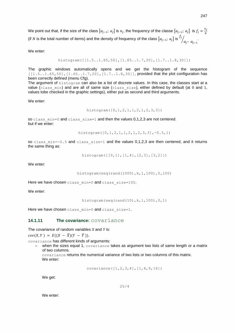
247

We point out that, if the size of the class [𝑎𝑗−1; 𝑎𝑗] is 𝑛𝑗, the frequency of the classe [𝑎𝑗−1; 𝑎𝑗] is 𝑓𝑗 =𝑛𝑗

𝑁

(if 𝑁 is the total number of items) and the density of frequency of the class [𝑎𝑗−1; 𝑎𝑗] is 𝑓𝑗𝑎𝑗– 𝑎𝑗−1⁄ .

We enter:

histogram([[1.5..1.65,50],[1.65..1.7,20],[1.7..1.8,30]])

The graphic windows automatically opens and we get the histogram of the sequence [[1.5..1.65,50],[1.65..1.7,20],[1.7..1.8,30]], provided that the plot configuration has been correctly defined (menu Cfg). The argument of histogram can also be a list of discrete values. In this case, the classes start at a

value (class_min) and are all of same size (class_size), either defined by default (at 0 and 1, values tobe checked in the graphic settings), either put as second and third arguments. We enter:

histogram([0,1,2,1,1,2,1,2,3,3])

so class_min=0 and class_size=1 and then the values 0,1,2,3 are not centered. but if we enter:

histogram([0,1,2,1,1,2,1,2,3,3],-0.5,1)

so class_min=-0.5 and class_size=1 and the values 0,1,2,3 are then centered, and it returns the same thing as:

histogram([[0,1],[1,4],[2,3],[3,2]])

We enter:

histogram(seq(rand(1000),k,1,100),0,100)

Here we have chosen class_min=0 and class_size=100. We enter:

histogram(seq(rand(10),k,1,100),0,1)

Here we have chosen class_min=0 and class_size=1.

14.1.11 The covariance: covariance

The covariance of random variables X and Y is:

𝑐𝑜𝑣(𝑋, 𝑌 ) = 𝐸((𝑋 − �̅�)(𝑌 − �̅� )).

covariance has different kinds of arguments: – when the sizes equal 1, covariance takes as argument two lists of same length or a matrix

of two columns. covariance returns the numerical variance of two lists or two columns of this matrix. We enter:

covariance([1,2,3,4],[1,4,9,16])

We get:

25/4

We enter:

248

covariance([[1,1],[2,4],[3,9],[4,16]])

We get:

25/4

Because we have:

1/4 ∗ (1 + 8 + 27 + 64) − 75/4 = 25/4

Provided that A1:=[0,1,2,3,4,5,6,7,8,9,10,11], we enter:

covariance(A1,A1^2)

We get:

1573/12

– when the sizes are different from 1:

if the paired values 𝑎[𝑗], 𝑏[𝑗] have as size 𝑛[𝑗] (𝑗 = 0. . 𝑝 − 1), covariance takes as argument three lists 𝑎, 𝑏, 𝑛 of same length 𝑝, or a matrix of three columns 𝑎, 𝑏, 𝑛 and 𝑝

lines [𝑎[𝑗], 𝑏[𝑗], 𝑛[𝑗]]. covariance returns the numerical variance of the two first lists weighted by the list supplied as last argument, or of the two columns of this matrix weighted by the third column. We enter:

covariance([1,2,3,4],[1,4,9,16],[3,1,5,2])

Or we enter:

covariance([[1,1,3],[2,4,1],[3,9,5],[4,16,2]])

We get:

662/121

if the paired values 𝑎[𝑗], 𝑏[𝑘] have for size 𝑁[𝑗, 𝑘] (𝑗 = 1. . 𝑝, 𝑘 = 1. . 𝑞), covariance takes as argument two lists 𝑎, 𝑏 of respective lengths 𝑝 and 𝑞, and a matrix 𝑁 of 𝑝 rows

and 𝑞 columns, or also, in order to write the data in a pleasant way in the table,

covariance can also have two arguments, a matrix 𝑀 and −1. 𝑀 is then a double entry table equal to:

𝑀 = [

𝑎 \ 𝑏 𝑏[1] ⋯ 𝑏[𝑞]

𝑎[1] 𝑁[1, 1] ⋯ 𝑁[1, 𝑞]⋮ ⋮ ⋱ ⋮

𝑎[𝑝] 𝑁[𝑝, 0] ⋯ 𝑁[𝑝, 𝑞]

]

covariance(a,b,N) or covariance(M,-1) returns the numerical covariance of paired values 𝑎[𝑗], 𝑏[𝑘] weighted by 𝑁𝑗,𝑘.

We enter:

covariance([1,2,3,4],[1,4,9,16],[[3,0,0,0],

[0,1,0,0],[0,0,5,0],[0,0,0,2]])

We get:

662/121

249

We enter:

covariance([[b\a,1,2,3,4],[1,3,0,0,0],

[4,0,1,0,0],[9,0,0,5,0],[16,0,0,0,2]],-1)

We get:

662/121

14.1.12 The correlation: correlation

The coefficient of linear correlation of two random variables X and Y is 𝜌 =𝑐𝑜𝑣(𝑋,𝑌)

𝜎(𝑋)𝜎(𝑌) where 𝜎(𝑋) (resp.

𝜎(𝑌)) designates the standard deviation of 𝑋 (resp. 𝑌). correlation has the same arguments a covariance. When the sizes equal 1, correlation takes as argument two lists of same length or a matrix of two columns. We enter:

correlation([1,2,3,4],[1,4,9,16])

We get:

100/(4*sqrt(645))

We enter:

correlation([[1,1],[2,4],[3,9],[4,16]])

We get:

100/(4*sqrt(645))

Provided that A1:=[0,1,2,3,4,5,6,7,8,9,10,11], we enter:

correlation(A1,A1^2)

We get:

18876/(572*sqrt(1173))

When the sizes are different from 1: – if the paired values 𝑎[𝑗], 𝑏[𝑗] have as size 𝑛[𝑗] (𝑗 = 0. . 𝑝 − 1), correlation takes as

argument three lists a, b, n of same length p, or a matrix of three columns 𝑎, 𝑏, 𝑛 and 𝑝 rows

[𝑎[𝑗], 𝑏[𝑗], 𝑛[𝑗]]. correlation returns the numerical correlation of the two first lists which are weighted by the list supplied as last argument or returns the numerical correlation of two columns of this matrix which are weighted by the third column. We enter:

correlation([1,2,3,4],[1,4,9,16],[3,1,5,2])

Or we enter:

correlation([[1,1,3],[2,4,1],[3,9,5],[4,16,2]])

We get:

662/(180*sqrt(14))

250

– if the paired values 𝑎[𝑗], 𝑏[𝑘] have for size 𝑁[𝑗, 𝑘] (𝑗 = 1. . 𝑝, 𝑘 = 1. . 𝑞), correlation takes

as argument two lists 𝑎, 𝑏 of respective lengths 𝑝 and 𝑞 and a matrix 𝑁 of 𝑝 rows and 𝑞 columns or else, in order to write the data in a pleasant way in the table, correlation can also get for argument, a matrix 𝑀 and −1. M is then a double entry table equal to:

𝑀 = [

𝑎 \ 𝑏 𝑏[1] ⋯ 𝑏[𝑞]

𝑎[0] 𝑁[1, 1] ⋯ 𝑁[1, 𝑞]⋮ ⋮ ⋱ ⋮

𝑎[𝑝] 𝑁[𝑝, 1] ⋯ 𝑁[𝑝, 𝑞]

]

correlation(a,b,N) or correlation(M,-1) returns the numerical correlation of paired values a[j], b[k] weighted by Nj,k. We enter:

correlation([1,2,3,4],[1,4,9,16],[[3,0,0,0],[0,1,0,0],

[0,0,5,0],[0,0,0,2]])

We get:

662/(180*sqrt(14))

We enter:

correlation([["b\a",1,2,3,4],[1,3,0,0,0],

[4,0,1,0,0],[9,0,0,5,0],[16,0,0,0,2]],-1)

We get:

662/(180*sqrt(14))

14.1.13 Covariance and correlation: covariance_correlation

covariance_correlation has the same arguments as covariance: if the sizes equal 1, covariance_correlation takes as argument two lists of same length or a matrix of two columns

representing two random variables X and Y and otherwise covariance_correlation takes as

argument three lists of same length, or a matrix of three columns representing two random variables X and Y and the weighting of their sizes or else a matrix M and -1, where M gives the weighting of X (the first column of M without 𝑀[0, 0]) and Y (the first line of M without 𝑀[0, 0]). covariance_correlation returns the list of the covariance 𝑐𝑜𝑣(𝑋, 𝑌) and the coefficient of linear

correlation ρ of two random variables X and Y.

We have 𝜌 =𝑐𝑜𝑣(𝑋,𝑌)

𝜎(𝑋)𝜎(𝑌) where 𝜎(𝑋) (resp. 𝜎(𝑌)) designates the standard deviation of X (resp. Y ).

We enter:

covariance_correlation([[1,1],[2,4],[3,9],[4,16]])

We get:

[25/4,100/(4*sqrt(645))]

Provided that A1:=[0,1,2,3,4,5,6,7,8,9,10,11], we enter:

covariance_correlation(A1,A1^2)

We get:

[1573/12,18876/(572*sqrt(1173))]

We enter:

251

covariance_correlation([1,2,3,4],[1,4,9,16],[3,1,5,2])

Or we enter:

covariance_correlation([[1,1,3],[2,4,1],[3,9,5],[4,16,2]])

We get:

[662/121,662/(180*sqrt(14))]

We enter:

covariance_correlation([1,2,3,4],[1,4,9,16],

[[3,0,0,0],[0,1,0,0],[0,0,5,0],[0,0,0,2]])

We get:

[662/121,662/(180*sqrt(14))]

We enter:

covariance_correlation([["b\a",1,2,3,4],[1,3,0,0,0],

[4,0,1,0,0],[9,0,0,5,0],[16,0,0,0,2]],-1)

We get:

[662/121,662/(180*sqrt(14))]

14.1.14 Polygonal line: polygonplot

polygonplot takes as arguments two lists or a matrix of two columns. polygonplot allows to display the line segments joining the different points of the cloud of dots defined by the argument and ordinates according to the increasing abscissae. If you want that the points are joined in the order supplied, you must use listplot. We enter:

polygonplot([[0,0],[1,1],[2,4],[3,9],[4,16]])

Or we enter, because the points will be ordered according to the increasing abscissae:

polygonplot([[2,4],[0,0],[3,9],[1,1],[4,16]])

Or we enter:

polygonplot([0,1,2,3,4],[0,1,4,9,16])

The graphic windows automatically opens and we get the plot of 4 segments joining the 5 points ((0,0), . . . (4,16)), provided that the plot configuration has been correctly defined (menu Cfg).

14.1.15 Polygonal line: plotlist

plotlist takes as argument a list l or a matrix of two columns. listplot or plotlist allows to display the segments joining the cloud of plots having for abscissa [0,1,2...n] and for ordinate l or for coordinates a line of the matrix. plotlist connects by two line segments the different points of the cloud, but without reordering the points, unlike polygonplot which reorders the points according to their abscissa, then connects them. We enter:

252

plotlist([0,1,4,9,16])

Or we enter:

plotlist([[0,0],[1,1],[2,4],[3,9],[4,16]])

The graphic windows automatically opens and we get, provided that the plot configuration has been correctly defined (menu Cfg):

the plot of 5 points ((0,0),(1,1),...(4,16)) connected by 4 segments

We enter, if A is a matrix of 5 rows and 2 columns:

A:=[[0,0],[1,1],[5,4],[3,9],[4,16]]

listplot(A[0..4,0..1])

The graphic windows automatically opens and we get:

The 5 points joined by 4 segments

Please note the difference between:

listplot([[0,0],[1,1],[5,4],[3,9],[4,16]])

polygonplot([[0,0],[1,1],[5,4],[3,9],[4,16]])

Warning! listplot([0,1,2,3,4],[0,1,4,9,16])

or listplot([[0,1,2,3,4],[0,1,4,9,16]])

is not valid!

14.1.16 Polygonal line and cloud of plots: polygonscatterplot

polygonscatterplot takes as arguments two lists or a matrix of two columns. polygonscatterplot allows to display the cloud of dots defined by the argument, by joining by line segments the different points of the cloud, ordering them according to the increasing abscissae . We enter:

polygonscatterplot([[0,0],[1,1],[2,4],[3,9],[4,16]])

Or we enter:

polygonscatterplot([0,1,2,3,4],[0,1,4,9,16])

The graphic windows automatically opens and we get the plot of 5 points ((0,0), . . . (4,16)) joined by 4 segments, provided that the plot configuration has been correctly defined (menu Cfg).

14.1.17 Linear interpolation: linear_interpolate

Considering a matrix of two lines giving points coordinates: once the abcissae of these points have been sorted, these points define a polygonal line. We want to get the points coordinates of this line regularly distributed. linear_interpolate has four arguments, a two line matrix A1 giving the coordinates of the points of a polygonal line, the minimum value of x (xmin), the maximum value of x (xmax), and the step (xstep). linear_interpolate returns the coordinates of the points of the polygonal line for x growing from xmin to xmax with a step of xstep.

253

Note: we must have xmin and xmax being in the interval [min(A1[0]);max(A1[0])]. We enter:

linear_interpolate([[1,2,6,9],[3,4,6,12]],1,9,1)

We get:

[[1.0,2.0,3.0,4.0,5.0,6.0,7.0,8.0,9.0],

[3.0,4.0,4.5,5.0,5.5,6.0,8.0,10.0,12.0]]

We enter:

linear_interpolate([[1,2,6,9],[3,4,6,12]],2,7,1)

We get:

[[2.0,3.0,4.0,5.0,6.0,7.0],[4.0,4.5,5.0,5.5,6.0,8.0]]

We enter:

linear_interpolate([[1,2,9,6],[3,4,6,12]],1,9,1)

We get:

[[1.0,2.0,3.0,4.0,5.0,6.0,7.0,8.0,9.0],

[3.0,4.0,6.0,8.0,10.0,12.0,10.0,8.0,6.0]]

14.1.18 Linear regression: linear_regression

To fit the data the best way by the line of the least squares having for equation 𝑦 = 𝑚𝑥 + 𝑏, we use

linear_regression which returns the paired value (𝑚, 𝑏). If the data are 𝑥𝑖, 𝑦𝑖 with 𝑖 = 1. . 𝑛, we have:

𝑚 =𝑐𝑜𝑣(𝑋,𝑌)

𝜎(𝑋)2 and 𝑏 = �̅� − 𝑚�̅�

because the sum of the squares of the distances 𝑑𝑖 = |𝑦𝑖– 𝑚𝑥𝑖– 𝑏𝑖| is minimal for these values and

this minimum (which is then the average vertical quadratic error) equals (1 – 𝜌2)𝜎(𝑌)2 where r is the

correlation coefficient (𝜌 =𝑐𝑜𝑣(𝑋,𝑌)

𝜎(𝑋)𝜎(𝑌)).

linear_regression has the same arguments as covariance. We enter:

linear_regression([[0,0],[1,1],[2,4],[3,9],[4,16]])

Or we enter:

linear_regression([0,1,2,3,4],[0,1,4,9,16])

We get:

4,-2

it is then the linear function equation 𝑦 = 4𝑥 − 2 which fits the data the best. We enter:

X1:=[0,1,2,3,4,5,6,7,8,9,10]

254

Y1:=[7.3,9.53,12.47,16.3,21.24,27.73,36.22, 47.31,61.78,80.68,105]

Z1:=log(Y1)

linear_regression(X1,Z1)

We get:

0.266729219953,1.98904252589

it is then the linear function equation 𝑧 = ln(𝑦) = 0.267𝑥 + 1.99 which fits the data the best.

14.1.19 Exponential regression: exponential_regression

To fit the data by an exponential function equation 𝑦 = 𝑏𝑒𝑚𝑥 = 𝑏𝑎𝑥, we use exponential_regression which returns the paired value (𝑎, 𝑏). exponential_regression has the same arguments as covariance. We enter:

evalf(exponential_regression([[1,1],[2,4],[3,9],[4,16]]))

Or we enter:

evalf(exponential_regression([1,2,3,4],[1,4,9,16]))

We get:

2.49146187923,0.5

it is then the exponential function of equation 𝑦 = 0.5 ∗ (2.49146187923)𝑥 which fits the data the best. We enter:

X1:=[0,1,2,3,4,5,6,7,8,9,10]

Y1:=[7.3,9.53,12.47,16.3,21.24,27.73,36.22,47.31, 61.78,80.68,105]

exponential_regression(X1,Y1)

We get:

1.30568684451,7.30853268031

it is then the function exponential of equation 𝑦 = 7.3 ∗ (1.3)𝑥 which fits the data the best. We check by entering:

e^[linear_regression(X1,ln(Y1))]

We get:

1.30568684451,7.30853268031

14.1.20 Logarithmic regression: logarithmic_regression

To fit the data by a logarithmic function equation 𝑦 = 𝑚ln(𝑥) + 𝑏, we use logarithmic_regression which returns the paired value (𝑚, 𝑏). logarithmic_regression has the same arguments as covariance.

255

We enter:

evalf(logarithmic_regression([[1,1],[2,4],[3,9],[4,16]]))

Or we enter:

evalf(logarithmic_regression([1,2,3,4],[1,4,9,16]))

We get:

10.1506450002,-0.564824055818

it is then the logarithmic function of equation 𝑦 = 10.15 𝑙𝑛(𝑥) − 0.565 which fits the data the best. We enter:

X1:=[1,1.5,2,2.5,3,3.5,4,4.5,5,5.5,6,6.5,7,7.5,8]

Y1:=[1.6,2.15,2.65,3.12,3.56,3.99,4.4,4.8,5.18,

5.58,5.92,6.27,6.62,7.06,7.3]

logarithmic_regression(X1,Y1)

We get:

2.83870854646,0.843078064152

it is then the logarithmic function of equation 𝑦 = 0.84 𝑙𝑛(𝑥) + 2.84 which fits the data the best. We check by entering:

linear_regression(ln(X1),Y1)

We get:

2.83870854646,0.843078064152

and the correlation coefficient is:

correlation(ln(X1),Y1)

We get:

0.977939822434

We can also enter to look for a better approximation:

logarithmic_regression(X1,log(Y1))

We get:

0.732351031846,0.467599676658

it is then the function logarithmique of equation 𝑧 = 𝑙𝑛(𝑦) = 0.73 𝑙𝑛(𝑥) + 0.47 which fits the data the best. We check by entering:

linear_regression(ln(X1),ln(Y1))

We get:

0.732351031846,0.467599676658

256

and the correlation coefficient is:

correlation(ln(X1),ln(Y1))

We get:

0.999969474543

14.1.21 Polynomial regression: polynomial_regression

To fit the data by a polynomial function of degree ≤ 𝑛 of equation 𝑦 = 𝑎0𝑥𝑛+. . +𝑎𝑛, we use, putting

the degree n as last parameter, polynomial_regression which returns the list [𝑎𝑛, . . 𝑎0]. polynomial_regression has the same first arguments as covariance, the last argument being the degree of the polynomial returned. We enter:

polynomial_regression([[1,1],[2,4],[3,9],[4,16]],3)

Or we enter:

polynomial_regression([1,2,3,4],[1,4,9,16],3)

We get:

[0,1,0,0]

it is then the polynomial function equation 𝑦 = 0 ∗ 𝑥3 + 𝑥2 + 0 ∗ 𝑥 + 0 = 𝑥2 which fits the data the best. Note: we will notice that the equation of the curve represented as well as the value of the correlation coefficient of data are written in blue. If we want to get the equation and/or the correlation coefficient on the plot we must add as last argument the option equation and/or correlation.

14.1.22 Power regression: power_regression

To fit the data by a function power equation 𝑦 = 𝑏𝑥𝑚, we use power_regression which returns the

paired value (𝑚, 𝑏). power_regression has the same arguments as covariance. We enter:

evalf(power_regression([[1,1],[2,4],[3,9],[4,16]]))

Or we enter:

evalf(power_regression([1,2,3,4],[1,4,9,16]))

We get:

(2.0,1.0)

so 𝑦 = 𝑥2 is the function power which fits the data the best. We enter:

X1:=[1,1.5,2,2.5,3,3.5,4,4.5,5,5.5,6,6.5,7,7.5,8]

Y1:=[1.6,2.15,2.65,3.12,3.56,3.99,4.4,4.8,5.18,

5.58,5.92,6.27,6.62,7.06,7.3]

257

power_regression(X,Y)

We get:

0.732351031846,1.59615829535

it is then the function power of of equation 𝑦 = 1.6 ∗ 𝑥0.73 which fits the data the best. We check by entering:

linear_regression(ln(X1),ln(Y1))

We get:

0.732351031846,0.467599676658

We do have:

e^0.467599676658=1.59615829535

so ln(𝑦) = ln(1.59615829535) + ln(𝑥) ∗ 0.732351031846 ln(𝑦) = 0.467599676659 + ln(𝑥) ∗ 0.732351031846 and the correlation coefficient is:

correlation(ln(X1),ln(Y1))

We get:

0.999969474543

14.1.23 Logistic regression: logistic_regression

The logistic curves are of curves whose equation 𝑦 = 𝑦(𝑥) are solutions of a differential equation of the form: 𝑦’/𝑦 = 𝑎 ∗ 𝑦 + 𝑏 and 𝑦0 = 𝑦(𝑥0) with 𝑎 < 0 and 𝑏 > 0.

The solutions are of the form: 𝑦(𝑥) = 𝐶/(1 + 𝑒𝑥𝑝(−𝛼(𝑥 – 𝑥_0 − 𝑘) with 𝐶 = −𝑏/𝑎, 𝛼 = −𝑏 and

𝑦0 = (−𝑏/𝑎)/(1 + exp(−𝑏 ∗ 𝑘)) thus 𝑘 = −1/𝑏 ∗ (𝑙𝑛(−((𝑎 ∗ 𝑦0 + 𝑏)/(𝑎 ∗ 𝑦0)))) To check, we can enter:

normal(desolve(y’/y=a*y+b)

We get:

(-b*exp(-(b*c_0-b*x)))/(a*exp(-(b*c_0-b*x))-1)

Then, we can enter to check:

normal(desolve([y’/y=a*y+b,y(x0)=y0],y)

We get:

[(-b*exp(b*x-b*x0+ln(y0/(a*y0+b))))/(a*exp(b*x-b*x0+ln(y0/(a*y0+b)))-

1)]

We have then: 𝑐0 = 𝑥0 − 𝑙𝑛(𝑦0/(𝑎 ∗ 𝑦0 + 𝑏))/𝑏

Thus, by multiplying the numerator and denominator of 𝑦(𝑥) by exp(𝑏 ∗ 𝑐0 − 𝑏 ∗ 𝑥), we have:

𝑦(𝑥) = (−𝑏/(𝑒𝑥𝑝(𝑏 ∗ 𝑐_0 − 𝑏 ∗ 𝑥) ∗ 𝑎 ∗ 𝑒𝑥𝑝(−(𝑏 ∗ 𝑐_0 − 𝑏 ∗ 𝑥)) − 1)

so 𝑦(𝑥) = −𝑏/(𝑎 − 𝑒𝑥𝑝(𝑏 ∗ (𝑥 – 𝑐0))) = (−𝑏/(𝑎 ∗ (1 − 𝑒𝑥𝑝(𝑏 ∗ (𝑥 – 𝑐0))/𝑎)) We have 1/𝑎 = − exp(−ln(−𝑎)) because 𝑎 < 0

then 𝑦(𝑥) = (−𝑏/𝑎) ∗ (1/(1 + 𝑒𝑥𝑝(𝑏 ∗ (𝑥 – 𝑐0) − 𝑙𝑛(−𝑎))) which is indeed the form announced.

258

When we know the values of 𝑓’ at 𝑥 = 𝑥0, 𝑥0 + 1… . 𝑥0 + 𝑛, we look for a logistic function 𝑦(𝑥) such as

𝑦’(𝑥) fits the different values of 𝑓’(𝑥) the best. logistic_regression takes as parameters:

– a list L1 which stores the values of 𝑦’ to 𝑥 = 𝑥0, 𝑥0 + 1… . 𝑥0 + 𝑛,

– the value x0 of 𝑥0 – the value y0 of 𝑦(𝑥0) when we know it, otherwise the calculator gets to estimate it...

logistic_regression(L1,x0,y0) returns the functions y(x) and y’(x), the constant C, y1M and xM with y1M is the value y’(xM) which is the maximum of 𝑦’ obtained in 𝑥 = 𝑥𝑀, and then the

linear correlation coefficient R of 𝑌 = 𝑦’/𝑦 function of y with the line 𝑌 = 𝑎 ∗ 𝑦 + 𝑏. From the list L1, the calculator returns the list Ly by using the formula 𝑦(𝑡 + 1) − 𝑦(𝑡) = 𝑦’(𝑡), thus, we have Ly=[y0,y0+y0’,y0+y0’+y1’,....]. Then, the CAS performs a linear regression of L/Ly in term of Ly to get the values of a and b (𝑦’/𝑦 = 𝑎 ∗ 𝑦 + 𝑏 and 𝑦0 = 𝑦(𝑥0)) then finds the solution of this differential equation. We enter:

logistic_regression([0.0,1.0,2.0,3.0,4.0],0,1)

We get, written in blue, the signification of the values returned:

[(-17.77)/(1+exp(-0.496893925384*x+2.82232341488+3.14159265359*i)),

(-2.48542227469)/(1+cosh(-

0.496893925384*x+2.82232341488+3.14159265359

-17.77,-1.24271113735,5.67993141131+6.32246138079*i, 0.307024935856]

We enter:

evalf(logistic_regression([1,2,4,6,8,7,5],0,2))

Or we enter:

logistic_regression(evalf([1,2,4,6,8,7,5]),0,2.0))

We get:

[64.8358166583/(1.0+exp(-0.551746244591*x+2.95837880348)),

14.4915280084/(1.0+cosh(-0.551746244591*x+2.95837880348)),

64.8358166583,7.24576400418,5.36184674112,-0.81176431297]

To retrieve the value −0.81176431297 of the correlation coefficient, we enter:

L:=[1,2,4,6,8,7,5];

y0:=2.0;

Ly:=makelist(y0,1,size(L))+cumSum(L)

We get:

[3,5,9,15,23,30,35]

then

correlation(L/Ly,Ly)

which returns

-0.81176431297

259

260

Chapter 15 Statistics

15.1 Statistics functions on a list: mean, variance, stddev,

stddevp, median, quantile, quartiles, quartile1,

quartile3

See also 15.1.1 and 14. Useful functions for statistics whose data are lists:

– mean to calculate the mean of the elements of a list. We enter:

mean([3,4,2])

We get:

3

We enter:

mean([1,0,1])

We get

2/3

– stddev to calculate the numerical standard deviation of the elements of a list. We enter:

stddev([3,4,2])

We get:

sqrt(2/3)

We have indeed the mean which equals 3 and the standard deviation which equals:

√(3 − 3)2 + (4 − 3)2 + (2 − 3)2

3 = √

2

3

– stddevp to calculate an estimation of the numerical standard deviation of the population from a sample whose elements are supplied in a list. We enter:

stddevp([3,4,2])

We get:

1

We have indeed the mean which equals 3 and the standard deviation which equals:

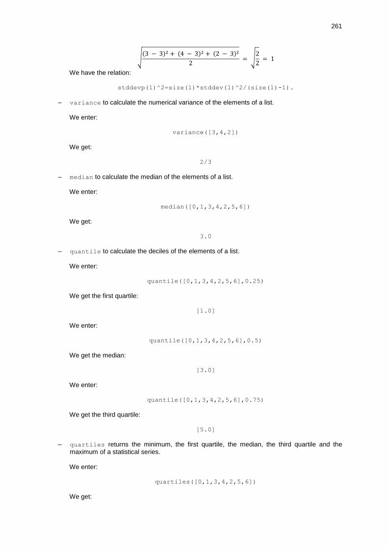
261

√(3 − 3)2 + (4 − 3)2 + (2 − 3)2

2 = √

2

2 = 1

We have the relation:

stddevp(l)^2=size(l)*stddev(l)^2/(size(l)-1).

– variance to calculate the numerical variance of the elements of a list. We enter:

variance([3,4,2])

We get:

2/3

– median to calculate the median of the elements of a list. We enter:

median([0,1,3,4,2,5,6])

We get:

3.0

– quantile to calculate the deciles of the elements of a list. We enter:

quantile([0,1,3,4,2,5,6],0.25)

We get the first quartile:

[1.0]

We enter:

quantile([0,1,3,4,2,5,6],0.5)

We get the median:

[3.0]

We enter:

quantile([0,1,3,4,2,5,6],0.75)

We get the third quartile:

[5.0]

– quartiles returns the minimum, the first quartile, the median, the third quartile and the maximum of a statistical series. We enter:

quartiles([0,1,3,4,2,5,6])

We get:

262

[[0.0],[1.0],[3.0],[5.0],[6.0]]

– quartile1 returns the first quartile of a statistical series. We enter:

quartile1([0,1,3,4,2,5,6])

We get:

1.0

– quartile3 returns the third quartile of a statistical series. We enter:

quartile3([0,1,3,4,2,5,6])

We get:

5.0

Be A the list [0,1,2,3,4,5,6,7,8,9,10,11]. We enter:

A:=[0,1,2,3,4,5,6,7,8,9,10,11]

We get:

11/2 for mean(A)

sqrt(143/12) for stddev(A)

0 for min(A)

[1.0] for quantile(A,0.1)

[2.0] for quantile(A,0.25)

[5.0] for median(A) or for quantile(A,0.5)

[8.0] for quantile(A,0.75)

[9.0] for quantile(A,0.9)

11 for max(A)

[[0.0],[2.0],[5.0],[8.0],[11.0]] for quartiles(A)

See also these functions for matrices at section 15.1.1 and for weighted lists at chapter 14.

15.1.1 Statistics functions on the columns of a matrix: mean, stddev, variance, median, quantile, quartiles

See also 15.1 and 14. Useful functions for statistics whose data are the columns of a matrix:

– mean to calculate the mean numerical of statistical series which are the columns of a matrix. We enter:

mean([[3,4,2],[1,2,6]])

263

We get a vector whose components are the mean of columns:

[2,3,4]

We enter:

mean([[1,0,0],[0,1,0],[0,0,1]])

We get

[1/3,1/3,1/3]

– stddev to calculate the numerical standard deviation of statistical series which are the columns of a matrix. We enter:

stddev([[3,4,2],[1,2,6]])

We get a vector whose components are the standard deviation of columns:

[1,1,2]

– variance to calculate the numerical variance of statistical series which are the columns of a matrix. We enter:

variance([[3,4,2],[1,2,6]])

We get a vector whose components are the variance of columns:

[1,1,4]

– median to calculate the median of statistical series which are the columns of a matrix. We enter:

median([[6,0,1,3,4,2,5],[0,1,3,4,2,5,6],[1,3,4,2,5,6,0],

[3,4,2,5,6,0,1],[4,2,5,6,0,1,3],[2,5,6,0,1,3,4]])

We get a vector whose components are the median of columns:

[2.0,2.0,3.0,3.0,2.0,2.0,3.0]

– quantile to calculate the decile according to the second argument, of statistical series which are the columns of a matrix. We enter:

quantile([[6,0,1,3,4,2,5],[0,1,3,4,2,5,6],[1,3,4,2,5,6,0],

[3,4,2,5,6,0,1],[4,2,5,6,0,1,3],[2,5,6,0,1,3,4]],0.25)

We get a vector whose components are the first quartile of columns:

[1.0,1.0,2.0,2.0,1.0,1.0,1.0]

We enter:

quantile([[6,0,1,3,4,2,5],[0,1,3,4,2,5,6],[1,3,4,2,5,6,0],

[3,4,2,5,6,0,1],[4,2,5,6,0,1,3],[2,5,6,0,1,3,4]],0.75)

264

We get a vector whose components are the third quartile of columns:

[4.0,4.0,5.0,5.0,5.0,5.0,5.0]

– quartiles to calculate the minimum, the first quartile, the median, the third quartile and the maximum of statistical series which are the columns of a matrix. We enter:

quartiles([[6,0,1,3,4,2,5],[0,1,3,4,2,5,6],[1,3,4,2,5,6,0],

[3,4,2,5,6,0,1], [4,2,5,6,0,1,3], [2,5,6,0,1,3,4]])

We get the matrix, of first line the minimum of each column, of second line the first quartile of each column, of third line the median of each column, of fourth line the third quartile of each column and last line the maximum of each column:

[[0.0,0.0,1.0,0.0,0.0,0.0,0.0],[1.0,1.0,2.0,2.0,1.0,1.0,1.0],

[2.0,2.0,3.0,3.0,2.0,2.0,3.0],[4.0,4.0,5.0,5.0,5.0,5.0,5.0],

[6.0,5.0,6.0,6.0,6.0,6.0,6.0]]

15.2 Tables indexed by two strings: table

A table is a list indexed by something more general than integers. A table can be used, for example, to store of telephone numbers indexed by two names. In CAS, the index of a table can be any objects of the CAS. The access is done by an algorithm which sorts by type then uses the order of each type (for example < for numerical type, lexicographical order for strings, etc., ...). table takes as argument a list or a sequence of equalities of the form: "index_name"=value_element.

table returns this table. We enter:

T:=table(3=-10,"a"=10,"b"=20,"c"=30,"d"=40)

We enter:

T["b"]

We get:

20

We enter:

T[3]

We get:

-10

Example

We want to encode the letters "a","b",.."z" by 1,2, . . . .26. We enter:

alphab:="abcdefghijklmnopqrstuvwxyz";

then:

265

code:=table(seq(alphab[j]=j+1,j=0..25));

We enter

code["c"]

We get

3

or we write a function:

Code(a):={

local code,alphab,j;

alphab:="abcdefghijklmnopqrstuvwxyz";

code:=table(seq(alphab[j]=j+1,j=0..25));

return code(a);

};

We enter

Code("c")

We get

3

Note: If we do an assignment of the type T[n]:= ... where T is the name of a variable and n an integer

– if the variable T stores a list or a sequence, then the n-th element of T is modified,

– if the variable T is not assigned, a table T is created with an entry (corresponding to the index 𝑛). Note that once this assignment is done, T is not a list, even though 𝑛 is an integer.

266

Chapter 16 Lists

16.1 Function MAKELIST makelist

In HOME, MAKELIST creates a list from a symbolic expression.

For instance, we create a list starting from 𝑋2 + 1, by having the variable X growing from 2 to 6 with a

step of 1 (1 can be omitted), we enter:

MAKELIST(X^2+1,X,2,6)

We get:

{5,10,17,26,37}

We enter:

MAKELIST(0,X,1,10)

We get:

{0,0,0,0,0,0,0,0,0,0}

We create a list starting from 𝑋2 + 1, by having the variable X growing from 2 to 6 with a step of 2, we enter:

MAKELIST(X^2+1,X,2,6,2)

We get:

{5,17,37}

In CAS, we can use MAKELIST and makelist. makelist has a function as first argument, the second argument represents the initilal value of the variable and the third argument represents its final value. We can put a fourth argument which represents the step of the variable. Warning! The index also starts at 1. We enter:

makelist(x->x^2,1,10)

We get:

[1,4,9,16,25,36,49,64,81,100]

We enter:

makelist(x->x^2,1,10,2)

We get:

[1,9,25,49,81]

267

16.2 Function SORT sort

SORT or sort sorts by increasing order the components of a list. We enter:

SORT([12,2,31,24,15])

We get:

[2,12,15,24,31]

We enter:

SORT({12,2,31,24,15})

We get:

{2,12,15,24,31}

16.3 Function REVERSE

REVERSE creates a list by reversing the order of the elements. We enter:

REVERSE([1,22,3,4,5])

We get:

[5,4,3,22,1]

We enter:

REVERSE({1,22,3,4,5})

We get:

{5,4,3,22,1}

16.4 Concatenate: CONCAT concat

CONCAT or concat concatenates two lists or two vectors or two strings of characters or two matrices (the two matrices must have the same number of rows, and will be concatenated line by line.) We enter:

CONCAT([1,2,3],[4,5])

We get:

[1,2,3,4,5]

We enter:

CONCAT({1,2,3},{4,5})

We get:

268

{1,2,3,4,5}

We enter:

CONCAT("HE","LLO")

We get:

"HELLO"

We enter:

2=>A

CONCAT([1,A,3],[4,5])

We get:

[1,2,3,4,5]

We enter:

CONCAT([[1,2],[3,4]],[[4,5,6],[6,7,8]])

We get:

[[1,2,4,5,6],[3,4,6,7,8]]

We enter:

2=>A

CONCAT({1,A,3},{4,5})

We get:

{1,2,3,4,5}

To concatenate a string and a list into a list we use CONCAT. We enter:

2=>A

CONCAT([1,A,3]),"L1"

We get:

[1,2,3,"L1"]

We enter:

2=>A

CONCAT("L1",[1,A,3])

We get:

["L1",1,2,3]

Warning!

269

To concatenate a string and a list into a string we use +. We enter:

2=>A

"L1="+[1,A,3]

We get:

"L1=[1,2,3]"

We enter:

2=>A

[1,A,3]+"L1="

We get:

"[1,2,3]L1="

We enter:

2=>A

"L1="+{1,A,3}

We get:

"L1={1,2,3}"

16.4.1 Add an element at the end of a list: append

append adds an element at the end of a list. We enter:

append([3,4,2],1)

We get:

[3,4,2,1]

We enter:

append([1,2],[3,4])

We get:

[1,2,[3,4]]

16.4.2 Add an element at the beginning of a list: prepend

prepend adds an element at the beginning of a list. We enter:

prepend([3,4,2],1)

270

We get:

[1,3,4,2]

We enter:

prepend([1,2],[3,4])

We get:

[[3,4],1,2]

16.5 Position in a list: POS

POS returns the position of an element in a list, that is to say POS returns the index of the first occurence of the element or 0 if the element is not in the list. We enter:

POS([4,3,1,2,3,4,5],4)

Or we enter:

POS({4,3,1,2,3,4,5},4)

We get:

1

We enter:

POS([4,3,1,2,3,4,5],2)

Or we enter:

POS({4,3,1,2,3,4,5},2)

We get:

4

We enter:

POS([4,3,1,2,3,4,5],6)

Or we enter:

POS({4,3,1,2,3,4,5},6)

We get:

0

16.6 Function DIM dim SIZE size length

SIZE or size or DIM or dim or length returns the length of the list (or of the strings) supplied as argument. Warning!

271

In HOME and in the CAS SIZE returns the dimension of a matrix whereas in the CAS size returns the number of line of a matrix. We enter in HOME:

SIZE({1,2,3})

We get:

3

We enter:

SIZE([[1,2,3],[4,5,6]])

We get:

{2,3}

We enter in the CAS:

size([1,2,3])

We get:

3

We enter:

size([[1,2,3],[4,5,6]])

We get:

2

Warning! We enter in the CAS:

SIZE([[1,2,3],[4,5,6]])

We get:

[2,3]

16.6.1 Get the reversed list: revlist

revlist takes as argument a list (resp. a sequence). revlist returns the list (resp. the sequence) in reversed order. We enter:

revlist([0,1,2,3,4])

We get:

[4,3,2,1,0]

We enter:

revlist([0,1,2,3,4],3)

272

We get:

3,[0,1,2,3,4]

16.6.2 Get the list swapped starting from its n-th element: rotate

rotate takes as argument a list and an relative integer (by default n=-1). rotate returns:

– if n>0: the list obtained by swapping the n first elements with the end of the list, – if n<0: the list obtained by swapping the -n last elements with the beginning of the list. By

default, n=-1 and we put the last element in first position. We enter:

rotate([0,1,2,3,4])

We get:

[4,0,1,2,3]

We enter:

rotate([0,1,2,3,4],2)

We get:

[2,3,4,0,1]

We enter:

rotate([0,1,2,3,4],-2)

We get:

[3,4,0,1,2]

16.6.3 Get the list shifted starting from its n-th element: shift

shift takes as argument a list and an relative integer (by default n=-1). shift returns:

– if n>0: the list obtained by replacing the n first elements of the list by undef, then by swapping these n first elements with the end of the list,

– if n<0: the list obtained by replacing the -n last elements of the list by undef, then by swapping the -n last elements with the beginning of the list. By default (n=-1) the first element equals undef and is followed by the list whose last element is removed.

We enter:

shift([0,1,2,3,4])

We get:

[undef,0,1,2,3]

We enter:

shift([0,1,2,3,4],2)

We get:

273

[2,3,4,undef,undef]

We enter:

shift([0,1,2,3,4],-2)

We get:

[undef,undef,0,1,2]

16.6.4 Removing an element from a list: suppress

suppress removes from a list the element of supplied index. Warning! The index of the first element is 0. We enter:

suppress([3,4,2],1)

We get:

[3,2]

16.6.5 Get the list without its first element: tail

tail returns the list without its first element. We enter:

tail([0,1,2,3])

We get:

[1,2,3]

l:=tail([0,1,2,3]) is equivalent to l:=suppress([0,1,2,3],0)

16.6.6 Removing elements from a list: remove

remove has two parameters: a boolean function f and a list l. remove removes the elements c from the list l, which checks f(c)=true. We enter:

remove(x->(x>=2),[0,1,2,3,4,5])

We get:

[0,1]

Note To do the same thing with a string of characters, for example, remove all the "a" from a string: We enter:

ord("a")

We get:

97

274

We enter:

f(chn):={local l:=length(chn); return

remove(x->(ord(x)==97),seq(chn[k],k,1,l));}

Then, we enter:

f("abracadabra")

We get:

["b","r","c","d","b","r"]

Then, we enter:

char(ord(["b","r","c","d","b","r"]))

We get:

"brcdbr"

16.6.7 Right and left part straight of a list: right, left

– right(l,n) returns the n last elements of a list l. We enter:

right([1,2,3,4,5,6],4)

We get:

[3,4,5,6]

– left(l,n) returns the n first elements of a list l. We enter:

left([1,2,3,4,5,6,7,8],3)

We get:

[1,2,3]

16.6.8 Checking whether an element is in a list: member

member has two parameters: an element c and a list (or a set) L. member is a function which checks whether the element c is in the list L. member returns 0 if c is not in L, and returns otherwise:

"the index of its first occurence".

Warning! For sake of compatibility, please mind the order of the parameters! We enter:

member(2,[1,2,3,4,2])

We get:

275

2

We enter:

member(2,% {1,2,3,4,2% })

We get:

2

16.6.9 Checkin whether an element is in a list: contains

contains has two parameters: a list (or a set) L and an element c. contains is a function which checks whether the element c is in the list L. contains returns 0 if c is not in L, and otherwise returns:

"the index of its first occurence".

Warning! For sake of compatibility, please mind the order of the parameters! We enter:

contains([1,2,3,4,2],2)

We get:

2

We enter:

contains(% {1,2,3,4,2% },2)

We get:

2

16.6.10 Counting the elements of a list or of a matrix such as a property:

count

Depending on its parameters, count is able to count in a list l the number of elements: – equal to a with count(x->x==a,l), – greather than a with count(x->x>a,l), – lower than a with count(x->x<a,l), – with count(x->1,l)

Indeed, count has one, two or three parameters: 1. a list of integers l 2. a real function f,

list l of length n or a matrix a of dimension p*q,

an optional argument row or col, in case of the second parameter is a matrix a. When count has:

– one parameter which is a list of integers l, count(l) counts the number of occurences by returning a matrix of first column the elements of the list l sorted, and second column the number of occurences of this element in the list.

– two parameters, count applies the function to the elements of the list (or of the matrix) and in returns the sum, that is to say, count(f,l) returns the number f(l[0])+f(l[1])+..f(l[n-1]) or count(f,a) returns the number f(a[0,0])+....+f(a[p-1,q-1]). If f is a boolean function, count returns the number of elements of the list (or of the matrix) for which the boolean function is true.

276

– three parameters, count applies the function to the elements of each line (resp. column) of the matrix a if the optional argument is row (resp. col) and returns a list of length p having as k-nth element:

f(a[k,0])+...f(a[k,q-1]) (resp. a list of length q having as k-nth element: f(a[0,k])+..f(a[p-1,k])).

We enter:

count([1,3,1,1,2,10,3])

We get:

[[1,3],[2,1],[3,2],[10,1]]

We enter:

count((x)->x,[2,12,45,3,7,78])

Or we enter:

count((x)->x,[[2,12,45],[3,7,78]])

We get:

147

because we have: 2 + 12 + 45 + 3 + 7 + 78 = 147. We enter:

count((x)->x,[[2,12,45],[3,7,78]],row)

We get:

[59,88]

because we have: 2 + 12 + 45 = 59 𝑎𝑛𝑑 3 + 7 + 78 = 88. We enter:

count((x)->x,[[2,12,45],[3,7,78]],col)

We get:

[5,19,123]

because we have: 2+3=5,12+7=10,45+78=123Tapez une équation ici.. We enter:

count((x)->x<12,[2,12,45,3,7,78])

We get:

3

Indeed, (𝑥) → 𝑥 < 12 is a boolean function which equals 1 if 𝑥 < 12 and 0 otherwise.

We have then 1 + 0 + 0 + 1 + 1 + 0 = 3. We enter:

277

count((x)->x==12,[2,12,45,3,7,78])

Or we enter:

count((x)->x==12,[[2,12,45],[3,7,78]])

We get:

1

Indeed, (𝑥)−> 𝑥 == 12 is a boolean function which equals 1 if 𝑥 == 12 and 0 otherwise.

We get then the number of terms equal to 12. Here it is 1. We enter:

count((x)->x>12,[2,12,45,3,7,78])

We get:

2

Indeed, (𝑥) → 𝑥 > 12 is a boolean function which equals 1 if 𝑥 > 12 and 0 otherwise.

We have then 0 + 0 + 1 + 0 + 0 + 1 = 2. We enter:

count(x->x^2,[3,5,1])

We get:

35

Indeed, we have: 32 + 52 + 11 = 35. We enter:

count(id,[3,5,1])

We get:

9

Indeed, id is the function identity and we have: 3 + 5 + 1 = 9. We enter:

count(1,[3,5,1])

We get:

3

Indeed, 1 is the constant function equal to 1 and we have: 1 + 1 + 1 = 3.

16.6.11 Select elements of a list: select

In CAS, select has two parameters: a boolean function f and a list L. select selects the elements c of the list L which checks f(c)=true. We enter:

278

select(x->(x>=2),[0,1,2,3,4,5])

We get:

[2,3,4,5]

16.7 List of differrences between consecutive terms: ΔLIST deltalist

In HOME, (resp. CAS), ΔLIST (resp. deltalist) returns the list of differerences between the

components of the list supplied as argument. We enter in HOME:

ΔLIST([1,21,34,41,52])

We get:

[20,13,7,11]

We enter in HOME:

ΔLIST({1,21,34,41,52})

We get:

{20,13,7,11}

We enter in the CAS:

deltalist([1,21,34,41,52])

We get:

[20,13,7,11]

16.8 Sum of the elements of a list: ΣLIST sum

In HOME, ΣLIST returns the sum of components of the list supplied as argument.

We enter:

ΣLIST([1,2,3,4,5])

We get:

15

We enter:

ΣLIST({1,2,3,4,5})

We get:

15

In CAS, sum returns the sum of the components of the list supplied as argument. We enter:

279

sum([1,2,3,4,5])

We get:

15

16.9 Product of the elements of a list: ΠLIST product

In HOME, ΠLIST returns the product of the components of the list supplied as argument.

We enter:

ΠLIST([1,2,3,4,5])

We get:

120

We enter:

ΠLIST({1,2,3,4,5})

We get:

120

In CAS, product returns the product of the components of the list supplied as argument. We enter:

product([1,2,3,4,5])

We get:

120

16.9.1 Apply a function of one variable to the elements of a list: map apply

map, or apply, is used to apply a function to the elements of a list, but these two instructions are not of synonymous. We have:

– apply has two parameters: a function f and a list L. apply(f,L) returns [f(L[0]),f(L[1]),...f(L[size(L)-1])]. Warning! apply answers [] if the second element is not a list.

– map has two parameters: an expression E or a list L, and a function f. map(E,f) returns f(E) and map(L,f) returns [f(L[0]),f(L[1]),...f(L[size(L)-1])].

Warning!, Please mind that, for sake of compatibility, the orders of the parameters are different for map and apply. When the list is a matrix and the function must apply to each element of a matrix, matrix must be put as optional argument to map.

We enter:

apply(x->x+1,[3,5,1])

or

map([3,5,1],x->x+1)

280

this adds 1 to each element of the list, and we get:

[4,6,2]

Example with a matrix We enter:

apply(x->x+1,[[3,5,1],[3,5,1],[3,5,1]])

or

map([[3,5,1],[3,5,1],[3,5,1]],x->x+1)

this adds 1 to each element of the list, that is to say to each line of the matrix and since [3,5,1]+1=[3,5,2], we get:

[[3,5,2],[3,5,2],[3,5,2]]

We enter:

map([[3,5,1],[3,5,1],[3,5,1]],x->x+1,matrix)

this adds 1 to each element of the matrix, and we get:

[[4,6,2],[4,6,2],[4,6,2]]

Other examples. We enter:

apply(x->x^2,[3,5,1])

or

map([3,5,1],x->x^2)

or we define the function ℎ(𝑥) = 𝑥^2 by entering:

h(x):=x^2

then

apply(h,[3,5,1])

or

map([3,5,1],h)

We get:

[9,25,1]

We enter:

apply(h,[[3,5,1],[3,5,1],[3,5,1]])

or

map([[3,5,1],[3,5,1],[3,5,1]],h)

or

281

map([[3,5,1],[3,5,1],[3,5,1]],h,matrix)

We get each element raised to square:

[[9,25,1],[9,25,1],[9,25,1]]

We define the function 𝑔(𝑥) = [𝑥, 𝑥2, 𝑥3] by entering:

g(x):=[x,x^2,x^3]

or

g:=(x)->[x,x^2,x^3]

then, we enter:

apply(g,[3,5,1])

or

map([3,5,1],g)

We make 𝑔 proceed on 3, on 5, then on 1, and we get:

[[3,9,27],[5,25,125],[1,1,1]]

Note: If l1,l2,l3 are lists:

sizes([l1,l2,l3])=map(size,[l1,l2,l3])

16.9.2 Apply a function of two variables to elements of two lists: zip

zip is used to apply a function of two variables to elements of two lists. We enter:

zip(’sum’,[a,b,c,d],[1,2,3,4])

We get:

[a+1,b+2,c+3,d+4]

We enter:

zip((x,y)->x^2+y^2,[4,2,1],[3,5,1])

Or we enter:

f:=(x,y)->x^2+y^2

then,

zip(f,[4,2,1],[3,5,1])

We get:

[25,29,2]

We enter:

282

f:=(x,y)->[x^2+y^2,x+y]

then,

zip(f,[4,2,1],[3,5,1])

We get:

[[25,7],[29,7],[2,2]]

16.10 Convert a list to a matrix: list2mat

list2mat allows to get the matrix of the terms of the list supplied as argument by splitting the list according to the number of columns specified. If terms are missing, the list is supplemented by zeros. We enter:

list2mat([5,8,1,9,5,6],2)

We get:

[[5,8],[1,9],[5,6]]

We enter:

list2mat([5,8,1,9],3)

We get:

[[5,8,1],[9,0,0]]

Note:

In the answer, the delimitors of a matrix are ⟦ and ⟧, whereas the delimitors of a list are [ and ] (the vertical line of the brackets is thicker for the matrices).

16.11 Convert a matrix to a list: mat2list

mat2list allows to get the list of the terms of the matrix supplied as argument. We enter:

mat2list([[5,8],[1,9]])

We get:

[5,8,1,9]

16.12 Useful functions for the lists and the components of a vector

16.12.1 Norms of a vector: maxnorm l1norm l2norm norm

See also 20.11.1 for the different instructions to get the norms of a matrix. The different instructions to get the norms of a vector are:

– maxnorm to calculate the norm 𝑙∞ of a vector: it is the maximum of the absolute values of its coordinates. We enter:

283

maxnorm([3,-4,2])

Or we enter:

maxnorm(vector(3,-4,2))

We get:

4

Indeed: 𝑥 = 3, 𝑦 = −4, 𝑧 = 2 and 4 = max(|𝑥|, |𝑦|, |𝑧|). – l1norm to calculate the norm 𝑙1 of a vector: it is the sum of the absolute values of its

coordinates. We enter:

l1norm([3,-4,2])

Or we enter:

l1norm(vector(3,-4,2))

We get:

9

Indeed: 𝑥 = 3, 𝑦 = −4, 𝑧 = 2 and 9 = |𝑥| + |𝑦| + |𝑧|. – norm or l2norm to calculate the norm 𝑙2 of a vector: it is the square root of the sum of the

squares of its coordinates. We enter:

norm([3,-4,2])

Or we enter:

norm(vector(3,-4,2))

We get:

sqrt(29)

Indeed: 𝑥 = 3, 𝑦 = −4, 𝑧 = 2 and 29 = |𝑥|2 + |𝑦|2 + |𝑧|2.

16.12.2 Normalizing the components of a vector: normalize

normalize normalizes the components of a vector and returns the components of a vector of norm 1

according to the norm 𝑙2 (the square root of the sum of the squares of its coordinates). We enter:

normalize([3,4,5])

We get:

[3/(5*sqrt(2)),4/(5*sqrt(2)),5/(5*sqrt(2))]

Indeed: 𝑥 = 3, 𝑦 = 4, 𝑧 = 5 and 50 = |𝑥|2 + |𝑦|2 + |𝑧|2.

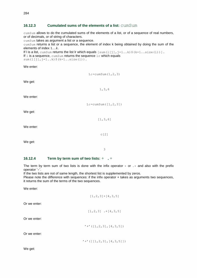
284

16.12.3 Cumulated sums of the elements of a list: cumSum

cumSum allows to do the cumulated sums of the elements of a list, or of a sequence of real numbers, or of decimals, or of string of characters. cumSum takes as argument a list or a sequence. cumSum returns a list or a sequence, the element of index k being obtained by doing the sum of the elements of index 1. . . 𝑘. If l is a list, cumSum returns the list lr which equals [sum(l[j],j=1..k)$(k=1..size(l))]. If l is a sequence, cumSum returns the sequence lr which equals sum(l[j],j=1..k)$(k=1..size(l)). We enter:

L:=cumSum(1,2,3)

We get:

1,3,6

We enter:

L:=cumSum([1,2,3])

We get:

[1,3,6]

We enter:

c[2]

We get:

3

16.12.4 Term by term sum of two lists: + .+

The term by term sum of two lists is done with the infix operator + or .+ and also with the prefix operator ’+’. If the two lists are not of same length, the shortest list is supplemented by zeros. Please note the difference with sequences: if the infix operator + takes as arguments two sequences, it returns the sum of the terms of the two sequences. We enter:

[1,2,3]+[4,3,5]

Or we enter:

[1,2,3] .+[4,3,5]

Or we enter:

’+’([1,2,3],[4,3,5])

Or we enter:

’+’([[1,2,3],[4,3,5]])

We get:

285

[5,5,8]

We enter:

[1,2,3,4,5,6]+[4,3,5]

Or we enter:

[1,2,3,4,5,6].+[4,3,5]

Or we enter:

’+’([[1,2,3,4,5,6],[4,3,5]])

Or we enter:

’+’([[1,2,3,4,5,6],[4,3,5]])

We get:

[5,5,8,4,5,6]

Warning! When the operator + is prefix, it must be quoted, that is to say written ’+’. If we enter:

[1,2,3,4,5,6]+4

We get, because the list is considered as the coefficients of a polynomial:

[1,2,3,4,5,10]

16.12.5 Term by term difference of two lists: - .-

The term by term difference of two lists is done with the infix operator - or .- and also with the prefix operator ’-’. If the two lists are not of same length, the shorted list is supplemented by zeros. Please note the difference with sequences: if the infix operator - takes as arguments two sequences, it returns the difference of the sums of the terms of each of the sequences. We enter:

[1,2,3]-[4,3,5]

Or we enter:

[1,2,3] .- [4,3,5]

Or we enter:

’-’([1,2,3],[4,3,5])

Or we enter:

’-’([[1,2,3],[4,3,5]])

We get:

[-3,-1,-2]

Warning!

286

When the operator - is prefix, it must be quoted, that is to say written ’-’.

16.12.6 Term by term product of two lists: .*

See also product for lists and matrices (cf 20.4.4 and ??) The term by term product of two lists of same length is done with the infix operator.*.

We enter:

[1,2,3] .* [4,3,5]

We get:

[4,6,15]

We enter:

[[1,2],[4,3]] .* [[4,3],[5,6]]

We get:

[[4,6],[20,18]]

16.12.7 Quotient term by term of two lists: ./

The quotient term by term of two lists of same length is done with the infix operator ./. We enter:

[1,2,3] ./ [4,3,5]

We get:

[1/4,2/3,3/5]

287

Chapter 17 Strings of characters

17.1 Write a string or a character: "

Strings of characters are written by using the quotes as delimitors (" " it is the key ALPHA 0). A character is a string of one character; indeed the delimitors ’ ’ or (quote key Shift ()) are used to specify that the variable put between the quotes must not be evaluated. Example: "a" is a character but ’a’ or quote(a) designates the variable a non evaluated. The characters of a string are designated by an index (as for the lists). To access an element of a string, we enter the index of this element between two brackets (the index which start at 1): [] [[]]. Example: We enter:

"hello"[2]

We get:

"e"

We enter:

"hello"[[2]]

We get:

"e"

Note: When we put a string of characters on the entry line, this generates an echo as a result. Example: We enter:

"hello"

We have "hello" written as a question and we get hello as answer. We enter:

"hello"+", how do you do?"

We get:

"hello, how do you do?"

288

17.1.1 To concatenate two numbers and strings: cat +

+ or cat evaluates the arguments and concatenates them in a string. This allows so to convert a real number into a string of characters. We enter:

"="+123

Or we enter:

cat("=",123)

We get:

"=123"

We enter:

a:=123

then,

"We get: "+a)

or

cat("We get: ",a)

We get:

"We get: 123"

17.1.2 Concatenating a sequence of words: cumSum

cumSum allows to do the concatenation of a list of strings. cumSum takes as argument a list of strings. cumSum returns a list of strings, the element of index 𝑘 being obtained by concatenating the strings

before it (i.e those of index 1. . . 𝑘 − 1) with the string of index 𝑘. If l is a list of 𝑘 strings, cumSum returns the list lr equal to [sum(l[j],j=1..k)$(k=1..size(l))] We enter:

c:=cumSum("Hello ","my ","friend")

We get:

" Hello "," Hello my "," Hello my friend"

We enter:

c[2]

We get:

" Hello my "

289

17.1.3 Finding a character in a string: INSTRING inString

inString has two parameters: a string of characters S and a character c. inString is a function which checks whether the character c is in the string of characters S. inString returns 0 if c is not in S and, otherwise, returns "the index of its first

occurence". We enter:

inString("abcded","d")

We get:

4

We enter:

inString("abcd","e")

We get:

0

17.2 ASCII codes: ASC asc

ASC or asc returns the list of ASCII codes of the characters of the string. We enter the " " thanks to the key ALPHA 0. We enter in HOME:

ASC("A")

We get:

[65]

We enter in HOME:

ASC("ABC")

We get:

[65,66,67]

We enter in the CAS:

asc("A")

We get:

[65]

We enter in the CAS:

asc("ABC")

We get:

[65,66,67]

290

17.3 Character from ASCII code: CHAR char

CHAR or char returns the string corresponding to the characters having as ASCII code those of the argument. We enter in HOME:

char(65)

or

char({65})

We get:

"A"

We enter:

char([65,66,67])

or

char({65,66,67})

We get:

"ABC"

We enter in the CAS:

char(65)

or

char([65])

or

char({65})

We get:

"A"

We enter:

char([65,66,67])

or

char({65,66,67})

We get:

"ABC"

17.3.1 Converting a real or an integer into a string: string

string evaluates its argument and converts it into a string of characters.

291

We enter:

string(1.32*10^20)

We get:

"1.23e+20"

We enter:

a:=1.32*10^4)

string(a+a)

We get:

"26400"

17.4 Use a string as a number or a command: expr

17.4.1 Use a string as a number

expr allows to use a string of digits without leading zero as an integer written in basis 10, or a string

of digits with a point as a decimal number written in basis 10. expr returns this integer. We enter:

expr("123")+1

We get:

124

We enter:

expr("45.67")+2.12

We get:

47.79

expr also allows to use a string of digits with no 8, nor 9, and with no leading zero as an integer written in basis 8. We enter:

expr("0123")

We get:

83

Indeed, 1 ∗ 82 + 2 ∗ 8 + 3 = 83 Note: If we enter expr("018"), we get the decimal number 18.0. expr allows to use a string containing digits and the letters a,b,c,d,e,f, and with the prefix 0x as an integer written in basis 16.

292

We enter:

expr("0x12f")

We get:

303

Indeed, 1 ∗ 162 + 2 ∗ 16 + 15 = 303

17.4.2 Use a string as a command name

expr allows to use a string of characters as a command. expr is mostly useful in a program. expr takes as argument a string of characters which can be interpreted as a command (or the name of a variable which stores a string or an expression returning a string). expr transforms the string in an expression, then evaluates this expression: to do an assignment, we should not write expr("a"):=2, but expr("a:=2") (see also expr 17.4) We enter:

expr("c:=1")

We get:

The variable c stores 1

We enter:

a:="ifactor(54)";expr(a)

or:

expr("ifactor(54)")

We get:

2*3^3

17.5 Evaluate an expression in the form of a string: string

string evaluates an expression and returns its value in the form of a string of characters. We can also use the concatenation of the expression with an emtpy string. We enter:

string(ifactor(6))

Or we enter:

ifactor(6)+""

Or we enter:

""+ifactor(6)

We get:

293

"2*3"

We enter:

string(’(ifactor(6)’))

We get:

"ifactor(6)"

17.6 inString

inString(l,c) checks whether c is in the string l and returns the index of 𝑐 or 0. We enter:

inString"ABCDEF","C"

We get:

3

We enter:

inString"ABCDEF","G"

We get:

0

17.7 Left part of a string: left

left(l,n) returns the left part of length 𝑛 of the string 𝑙. We enter:

left("ABCDEF",3)

We get:

"ABC"

17.8 Right part of a string: right

right(l,n) returns the right part of length 𝑛 of the string 𝑙. We enter:

right("ABCDEF",2)

We get:

"EF"

294

17.9 Mid part of a string: mid

mid(l,d,n) returns the string extracted from the string 𝑙, starting by the character of index 𝑑, and

length 𝑛 (by default 𝑛 = dim(𝑙) − 𝑑). We enter:

mid("ABCDEF",2,3)

We get:

"BCD"

We enter:

mid("ABCDEF",2)

We get:

"BCDEF"

17.10 Rotate last character: rotate

rotate returns the string obtained by turning the last character first. We enter:

rotate("ABC")

We get:

("CAB")

17.11 Length of a string: dim DIM size SIZE length

DIM (or dim or size or SIZE or length returns the length of the string (or of the list). We enter in HOME or in the CAS:

DIM("ABC")

We get:

3

We can also use SIZE We enter:

SIZE("ABC")

We get:

3

Note In HOME, DIM and SIZE are equivalent for matrices.

295

We enter in HOME:

DIM([[1,2,3],[4,5,6]])

We get:

{2,3}

We enter in HOME:

SIZE([[1,2,3],[4,5,6]])

We get:

{2,3}

In CAS, dim and size are not equivalent for matrices. dim returns the list giving the dimension of a matrix whereas size returns the length of the list. We enter in the CAS:

dim([[1,2,3],[4,5,6]])

We get:

[2,3]

We enter in the CAS:

size([[1,2,3],[4,5,6]])

We get:

2

17.12 Concatenate two strings: +

+ concatenates two strings. We enter:

"ABC"+"DEF"

We get:

"ABCDEF"

We can also use CONCAT We enter:

CONCAT("ABC","DEF")

We get:

"ABCDEF"

296

17.13 Get the list or the string without its first element: tail

tail(s) returns the list or the string s without its first element. We enter:

tail([0,1,2,3])

We get:

[1,2,3]

l:=tail([0,1,2,3]) is equivalent to l:=suppress([0,1,2,3],0) We enter:

tail("abcdef")

We get:

"bcdef"

l:=tail("abcdef") is equivalent to l:=suppress("abcdef","a")

17.14 First element of a list or of a string: head

head(s) returns the first element of the list s or the first character of the strings s. We enter:

head([0,1,2,3])

We get:

0

We enter:

head("abcdef")

We get:

"a"

297

Chapter 18 Polynomials

18.1 Coefficients of a polynomial: POLYCOEF

POLYCOEF returns the coefficients of a polynomial knowing its roots. We enter:

POLYCOEF([2,1])

or we enter:

POLYCOEF(2,1)

We get:

poly1[1,-3,2]

this represents the polynomial 𝑋2– 3𝑋 + 2 = (𝑋 – 2) ∗ (𝑋 – 1)

We enter:

POLYCOEF([2,-1,3,-4])

We get:

poly1[1,0,-15,10,24]

this represents the polynomial 𝑋4– 15𝑋2 + 10𝑋 + 24

18.2 Polynomial from coefficients: POLYEVAL

POLYEVAL returns the symbolic writting of a polynomial supplied by the list of its coefficients or POLYEVAL evaluates at a point a polynomial supplied by the list of its coefficients. We enter:

POLYEVAL({1,0,-15,10,24})

or we enter:

POLYEVAL([1,0,-15,10,24])

We get:

X^4-15*X^2+10*X+24

We enter:

POLYEVAL({1,0,-15,10,24},4)

or we enter:

POLYEVAL([1,0,-15,10,24],4)

298

We get:

80

because 44– 15 ∗ 42 + 10 ∗ 4 + 24 = 80

18.3 Expand a polynomial: POLYFORM

POLYFORM expands a polynomial supplied by an expression of one or several variables. POLYFORM also permits to factorize a polynomial of one or several variables and do the decomposition into simple elements of a rational fraction. We enter:

POLYFORM((X+2)^3+5)

or

POLYFORM((X+2)^3+5,X)

We get:

X^3+6*X^2+12*X+13

We enter:

POLYFORM((X+Y)^3+5)

or

POLYFORM((X+Y)^3+5,X,Y)

We get:

X^3+3*X^2*Y+3*X*Y^2+Y^3+5

We enter:

POLYFORM((X+Y)^3+5,Y,X)

We get:

Y^3+3*Y^2*X+3*Y*X^2+X^3+5

We enter:

POLYFORM((X+2)^2+5,X)

We get:

X^2+4*X+8

We enter:

POLYFORM((X+Y)^2+5)

We get:

X^2+2*X*Y+Y^2+5

299

We enter:

POLYFORM((X^2+2*X+1)*(X-1)))

We get:

X^3+X^2-X-1)

To factorize we enter:

POLYFORM(X^3+X^2-X-1,’*’)

We get:

(X-1)*(X+1)^2

We enter:

POLYFORM(X^2-Y^2,’*’)

We get:

(X-Y)*(X+Y)

We enter:

POLYFORM(1/(X^2-Y^2),’*’)

We get:

1/((X-Y)*(X+Y))

To perform the decomposition into simple elements of a rational fraction, we enter:

POLYFORM(1/(1-X^2)^2),’+’

We get:

-1/4/(X-1)^2-1/4/(X-1)+1/4/(X+1)^2+1/4/(X+1)

We enter:

POLYFORM(1/(X^2-Y^2)),’+’

We get:

1/(2*Y)/(X+Y)-1/(2*Y)/(X-Y)

Note: We can also use STO to get a rewritting of an expression:

– STO STO to evaluate formally an expression, – STO + to expand or to do a decomposition into simple elements ( translation to be checked) – STO * to factorize

We enter from Home:

X*SIN(X) STO STO

We get:

X*SIN(X)

300

We enter:

∂(X*SIN(X),X) STO STO

We get:

SIN(X)+X*COS(X)

We enter:

∫ (SIN(X),X) STO STO

We get:

-COS(X)

We enter:

(X+Y)^2+5 STO +

We get:

X^2+2*X*Y+Y^2+5

We enter:

1/(1-X^2)^2 STO +

We get:

-1/4/(X-1)^2-1/4/(X-1)+1/4/(X+1)^2+1/4/(X+1)

We enter:

X^3+X^2-X-1 STO *)

We get:

(X-1)*(X+1)^2

18.4 Roots of a polynomial from its coefficients: POLYROOT

POLYROOT returns the roots of a polynomial knowing its coefficients. We enter:

POLYROOT({1,0,-15,10,24})

Or we enter:

POLYROOT([1,0,-15,10,24])

We get:

[-1,2,3,-4]

which are the four roots of the polynomial 𝑋4– 15𝑋2 + 10𝑋 + 24

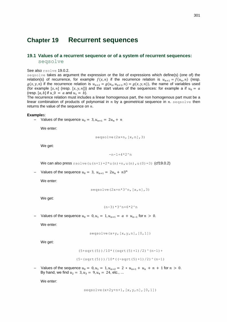
301

Chapter 19 Recurrent sequences

19.1 Values of a recurrent sequence or of a system of recurrent sequences:

seqsolve

See also rsolve 19.0.2. seqsolve takes as argument the expression or the list of expressions which define(s) (one of) the relation(s) of recurrence, for example 𝑓(𝑥, 𝑛) if the recurrence relation is 𝑢𝑛+1 = 𝑓(𝑢𝑛, 𝑛) (resp.

𝑔(𝑥, 𝑦, 𝑛) if the recurrence relation is 𝑢𝑛+2 = 𝑔(𝑢𝑛, 𝑢𝑛+1, 𝑛) = 𝑔(𝑥, 𝑦, 𝑛)), the name of variables used

(for example [𝑥, 𝑛] (resp. [𝑥, 𝑦, 𝑛])) and the start values of the sequences: for example a if 𝑢0 = 𝑎

(resp. [𝑎, 𝑏] if 𝑢_0 = 𝑎 and 𝑢1 = 𝑏). The recurrence relation must includes a linear homogenous part, the non homogenous part must be a linear combination of products of polynomial in 𝑛 by a geometrical sequence in 𝑛. seqsolve then

returns the value of the sequence on 𝑛. Examples:

– Values of the sequence 𝑢0 = 3, 𝑢𝑛+1 = 2𝑢𝑛 + 𝑛 We enter:

seqsolve(2x+n,[x,n],3)

We get:

-n-1+4*2^n

We can also press rsolve(u(n+1)=2*u(n)+n,u(n),u(0)=3) (cf19.0.2)

– Values of the sequence 𝑢0 = 3, 𝑢𝑛+1 = 2𝑢𝑛 + 𝑛3𝑛

We enter:

seqsolve(2x+n*3^n,[x,n],3)

We get:

(n-3)*3^n+6*2^n

– Values of the sequence 𝑢0 = 0, 𝑢1 = 1, 𝑢𝑛+1 = 𝑎 + 𝑢𝑛−1 for 𝑛 > 0. We enter:

seqsolve(x+y,[x,y,n],[0,1])

We get:

(5+sqrt(5))/10*((sqrt(5)+1)/2)^(n-1)+

(5-(sqrt(5)))/10*((-sqrt(5)+1)/2)^(n-1)

– Values of the sequence 𝑢0 = 0, 𝑢1 = 1, 𝑢𝑛+2 = 2 ∗ 𝑢𝑛+1 + 𝑢𝑛 + 𝑛 + 1 for 𝑛 > 0. By hand, we find 𝑢2 = 3, 𝑢3 = 9, 𝑢4 = 24, etc., ... We enter:

seqsolve(x+2y+n+1,[x,y,n],[0,1])

302

We get:

(-4*n-3*(-(sqrt(2)-1))^n*sqrt(2)+2*(-(sqrt(2)-1))^n+3*(sqrt(2)+1)^n

Check that n:=4 returns 24 Or we enter because we have 𝑢𝑛+1 = 2𝑢𝑛 + 𝑣𝑛 + 𝑛 and 𝑣𝑛+1 = 𝑢𝑛 (so 𝑣𝑛 = 𝑢𝑛−1) with 𝑢0 = 0 and 𝑢1 = 2𝑢0 + 𝑣0 + 0 = 1 then 𝑣0 = 1:

seqsolve([2x+y+n,x],[x,y,n],[0,1])

We get:

[(-1)/2-(-2-3*sqrt(2))/8*(sqrt(2)+1)^n-(-2+3*sqrt(2))/8*(-

sqrt(2)+1)^n-1/2*n, -(-4+sqrt(2))/8*(sqrt(2)+1)^n-(-4-sqrt(2))/8*(-

sqrt(2)+1)^n-1/2*n]

Check that n:=4 returns 24

– Values of the sequence 𝑢_0 = 0, 𝑣0 = 1, 𝑢𝑛+1 = 𝑢𝑛 + 2𝑣𝑛, 𝑣𝑛+1 = 𝑢𝑛 + 𝑛 + 1 for 𝑛 > 0. We enter:

seqsolve([x+2*y,n+1+x],[x,y,n],[0,1])

We get:

[(-2*n-(-1)^n+2^n*4-3)/2,((-1)^n+2*2^n-1)/2]

– Values of the sequence 𝑢0 = 0, 𝑣0 = 1, 𝑢𝑛+1 = 𝑢𝑛 + 2𝑣𝑛 + 𝑛 + 1, 𝑣𝑛 + 1 = 𝑢𝑛 for 𝑛 > 0. We enter:

seqsolve([x+2*y+n+1,x],[x,y,n],[0,1])

We get:

[(-2*n-(-1)^n*3+2^n*8-5)/4,(-2*n+(-1)^n*3+2^n*4-3)/4]

– Values of the sequence 𝑢0 = 0, 𝑣0 = 1, 𝑢𝑛+1 = 𝑢𝑛 + 𝑣𝑛 , 𝑣𝑛+1 = 𝑢𝑛 – 𝑣𝑛 for 𝑛 > 0. We enter:

seqsolve([x+y,x-y],[x,y,n],[0,1])

We get:

[(-4*n-3*(-(sqrt(2)-1))^n*sqrt(2)+

2*(-(sqrt(2)-1))^n+ 3*(sqrt(2)+1)^n*sqrt(2)+

2*(sqrt(2)+1)^n-4)/8, (-4*n+(-(sqrt(2)-1))^n*sqrt(2)+

4*(-(sqrt(2)-1))^n-(sqrt(2)+ 1)^n*sqrt(2)+

4*(sqrt(2)+1)^n)/8]

– Values of the sequence 𝑢0 = 2, 𝑣0 = 0, 𝑢𝑛+1 = 4 ∗ 𝑣𝑛 + 𝑛 + 1, 𝑣𝑛 + 1 = 𝑢𝑛, for 𝑛 > 0. We enter:

seqsolve([4y+n+1,x],[x,y,n],[2,0])

303

We get:

[(-8)/9+2*2^n-(-8)/9*(-1)^n*2^n-1/3*n,

(-5)/9+2^n-4/9*(-1)^n*2^n-1/3*n]

19.2 Values of a recurrent sequence or of a system of recurrent sequences:

rsolve

See also seqsolve 19.1. rsolve takes as argument the relation(s) of recurrence, the name of the variables used and the start value of the sequence. The recurrence relation is:

– either a linear homogenous part, the non homogenous part must be a linear combination of products of polynomial in 𝑛 by a geometrical sequence in 𝑛. For example, 𝑢𝑛+1 = 2𝑢𝑛 + 𝑛3

𝑛

– either an homographic function. For example, 𝑢𝑛+1 =𝑢𝑛 – 1

𝑢𝑛− 2

rsolve then returns a matrix whose rows are the values of the sequence in n. Notes Unlike seqsolve, rsolve is more flexible because with rsolve:

– starting the sequence by u(0) is not compulsory, – we can give several start values, for example u(0)^2=1, that is why rsolve returns a list, – we write the recurrence relation as in mathematics.

Examples:

– Values of the sequence 𝑢0 = 3, 𝑢𝑛+1 = 2𝑢𝑛 + 𝑛 We enter:

rsolve(u(n+1)=2u(n)+n,u(n),u(0)=3)

We get:

[-1+4*2^(n+1-1)-n]

– Values of the sequence 𝑢12 = 1, 𝑢𝑛+1 = 2𝑢𝑛 + 𝑛

We enter:

rsolve(u(n+1)=2u(n)+n,u(n),u(1)^2=1)

We get:

[[-1-(-3)/2*2^(n+1-1)-n, -1-(-1)/2*2^(n+1-1)-n]]

– Values of the sequence 𝑢0 = 3, 𝑢𝑛+1 = 2𝑢𝑛 + 𝑛3𝑛

We enter:

rsolve(u(n+1)=2u(n)+(n)*3^n,u(n),u(0)=3)

We get:

[-3*3^(n+1-1)+6*2^(n+1-1)+n*3^(n+1-1)]

– Values of the sequence 𝑢0 = 4, 𝑢𝑛+1 =𝑢𝑛 – 1

𝑢𝑛 – 2

We enter:

304

rsolve(u(n+1)=(u(n)-1)/(u(n)-2),u(n),u(0)=4)

We get:

[((10*sqrt(5)+30)*((sqrt(5)-3)/2)^n+30*sqrt(5)-70)/

(20*((sqrt(5)-3)/2)^n+10*sqrt(5)-30)]

– Values of the sequence 𝑢0 = 0, 𝑢1 = 1, 𝑢𝑛+1 = 𝑎 + 𝑢𝑛−1 for 𝑛 > 0. We enter:

rsolve(u(n+1)=u(n)+u(n-1),u(n),u(0)=0,u(1)=1)

We get:

[(5+sqrt(5))/10*((sqrt(5)+1)/2)^(n+1-1-1)+

(5-sqrt(5))/10*((-sqrt(5)+1)/2)^(n+1-1-1)]

– Values of the sequence 𝑢0 = 0, 𝑢1 = 1, 𝑢𝑛+1 = 2 ∗ 𝑎 + 𝑢𝑛−1 + 𝑛 for 𝑛 > 0. We enter:

rsolve(u(n+1)=2*u(n)+u(n-1)+n,u(n),u(0)=0,u(1)=1)

We get:

[(-1)/2-(-2-3*sqrt(2))/8*(sqrt(2)+1)^(n+1-1)-(-2+3*sqrt(2))/8*(-

sqrt(2)+1)^(n+1-1)-1/2*n]

Or we enter:

rsolve([u(n+1)=2*u(n)+v(n)+n,v(n+1)=u(n)], [u(n),v(n)],u(0)=0,v(0)=1)

We get:

[[(-1)/2-(-2-3*sqrt(2))/8*(sqrt(2)+1)^(n+1-1)-(-2+3*sqrt(2))/8*(-

sqrt(2)+1)^(n+1-1)-1/2*n, -(-4+sqrt(2))/8*(sqrt(2)+1)^(n+1-1)-(-4-

sqrt(2))/8*(-sqrt(2)+1)^(n+1-1)-1/2*n]]

– Values of the sequence 𝑢0 = 0, 𝑣0 = 1, 𝑢𝑛+1 = 𝑎 + 𝑣𝑛 , 𝑣𝑛+1 = 𝑎 – 𝑣𝑛. We enter:

rsolve([u(n+1)=u(n)+v(n),v(n+1)=u(n)-v(n)],

[u(n),v(n)],[u(0)=0,v(0)=1])

We get:

[[1/2*2^((n-1)/2)+1/2*(-(sqrt(2)))^(n-1), (-1+sqrt(2))/2*2^((n-1)/2)+

(-1-sqrt(2))/2*(-(sqrt(2)))^(n-1)]]

– Values of the sequence 𝑢0 = 2, 𝑣0 = 0, 𝑢𝑛+1 = 4 ∗ 𝑣𝑛 + 𝑛 + 1, 𝑣𝑛+1 = 𝑢𝑛. We enter:

rsolve([u(n+1)=4*v(n)+n+1,v(n+1)=u(n)], [u(n),v(n)],[u(0)=2,v(0)=0])

We get:

305

[[(-8)/9+2*2^(n+1-1)-(-8)/9*(-1)^(n+1-1)*2^(n+1-1)-1/3*n,

(-5)/9+2^(n+1-1)-4/9*(-1)^(n+1-1)*2^(n+1-1)-1/3*n]]

306

Chapter 20 Matrices

20.1 Generalities

To write a matrix, we put between two brackets a series of row vectors, for example: [[1,2], [3,4]]. The numerical matrices are stored in variables 𝑀0,𝑀1. . . 𝑀9. The index of rows and columns of a matrix start at 1, and we put the index between two brackets or parentheses.

20.2 Definition

To define the matrix 𝑀1 which equals [[1,2], [3,4]], we enter: [[1,2],[3,4]]=>M1 or we use the matrix editor (Shift 4 (Matrix)) We get:

[[1,2],[3,4]]

To define the matrix 𝑀2 which equals [[1,2], [3,4], [5,6]], we enter: [[1,2],[3,4],[5,6]]=>M2 or we use the matrix editor (Shift 4 (Matrix)) We get:

[[1,2],[3,4],[5,6]]

To get the element 3 of 𝑀2, located at the beginning of the second row: this will be the element on row

of index 2 and on column of index 1 if we designate it by M2[2,1] or M2(2,1). We enter:

M1[2,1]

We get:

3

We enter:

M1(2,1)

We get:

3

20.2.1 Dimension of a matrix: dim

dim takes as argument a matrix 𝐴.

dim returns the dimension of the matrix 𝐴 in the form of a list formed by its number of rows and number of columns. We enter:

dim([[1,2,3],[3,4,5]])

We get:

[2,3]

307

20.2.2 Number of rows: rowDim

rowDim takes as argument a matrix 𝐴.

rowDim returns the number of rows of the matrix 𝐴. We enter:

rowDim([[1,2,3],[3,4,5]])

We get:

2

20.2.3 Number of columns: colDim

colDim takes as argument a matrix 𝐴.

colDim returns the number of columns of the matrix 𝐴. We enter:

colDim([[1,2,3],[3,4,5]])

We get:

3

20.3 Operations on rows and columns useful in programming

20.3.1 Add a column to a matrix: ADDCOL

ADDCOL(M1,col,n) adds the column col which will be the column of index n of the matrix M1. We enter:

[[1,2],[3,4]]=>M1

ADDCOL(M1,[5,6],1)

We get the new matrix 𝑀1:

[[5,1,2],[6,3,4]]

We enter:

M1

We get the new matrix 𝑀1:

[[5,1,2],[6,3,4]]

To add a last column (which, in this case, will be the column of index 3) to the matrix M1, we enter:

[[1,2],[3,4]]=>M1

ADDCOL(M1,[5,6],3)

We get the new matrix 𝑀1:

[[1,2,5],[3,4,6]]

308

We enter:

M1

We get the new matrix 𝑀1:

[[1,2,5],[3,4,6]]

20.3.2 Swap rows: SWAPROW rowSwap

SWAPROW or rowSwap has three arguments: a matrix and two integers 𝑛1 and 𝑛2.

SWAPROW or rowSwap returns the matrix obtained by swapping the rows 𝑛1 and 𝑛2 in the matrix given as argument. We enter in HOME (the index starts at 1):

SWAPROW([[1,2],[3,4]],1,2)

We get:

[[3,4],[1,2]]

We enter in the CAS (the index also starts at 1):

SWAPROW([[1,2],[3,4]],1,2)

or

rowSwap([[1,2],[3,4]],1,2)

We get:

[[3,4],[1,2]]

20.3.3 Swap columns: SWAPCOL colSwap

SWAPCOL or colSwap has three arguments: a matrix and two integers 𝑛1 and 𝑛2. SWAPCOL or colSwap returns the matrix obtained by swapping the columns 𝑛1 and 𝑛2 in the matrix given as argument. We enter in HOME or in the CAS (the index starts at 1):

SWAPCOL([[1,2],[3,4]],1,2)

We get:

[[2,1],[4,3]]

We enter in the CAS

SWAPCOL([[1,2],[3,4],[5,6]],1,2)

or

colSwap([[1,2],[3,4],[5,6]],1,2)

We get:

[[2,1],[4,3],[6,5]]

309

20.3.4 Extract rows from a matrix: row

row allows to extract one or several rows from a matrix. row has two arguments: a matrix and an integer 𝑛 or an interval 𝑛1. . 𝑛2. row returns the row of index 𝑛 of the matrix supplied as argument, or the sequence of rows of index

starting from 𝑛1 to 𝑛2 of this matrix. We enter in HOME or in the CAS (the index starts at 1):

row([[1,2,3],[4,5,6],[7,8,9]],1)

We get:

[1,2,3]

We enter:

row([[1,2,3],[4,5,6],[7,8,9]],1..2)

We get:

[[1,2,3],[4,5,6]]

20.3.5 Extract columns from a matrix: col

col allows to extract one or several columns from a matrix. col has two arguments: a matrix, and an integer 𝑛 or an interval 𝑛1. . 𝑛2. col returns the column of index n of the matrix supplied as argument, or the sequence of columns of index starting from 𝑛1 to 𝑛2 of this matrix. We enter in HOME or danc CAS (the index starts at 1):

col([[1,2,3],[4,5,6],[7,8,9]],1)

We get:

[1,4,7]

We enter:

col([[1,2,3],[4,5,6],[7,8,9]],1..2)

We get:

([1,4,7],[2,5,8])

20.3.6 Remove columns from a matrix: DELCOL delcols

In HOME, DELCOL(M1,n) removes the column of index n from the matrix M1. In CAS, delcols has two arguments: a matrix 𝐴, and an integer 𝑛 or an interval 𝑛1. . 𝑛2.

delcols returns the matrix obtained by removing the column 𝑛 or the columns 𝑛1 up to 𝑛2 from the

matrix 𝐴. We enter:

[[1,2,5],[3,4,6]]=>M1

DELCOL(M1,2)

or

310

DELCOL(M1,2..2)

We get:

[[1,5],[3,6]]

To remove the columns of index 2 and 3 from the matrix 𝑀1, we enter:

[[1,2,5],[3,4,6]]=>M2

DELCOL(M1,2..3)

We get:

[[1],[3]]

We enter:

delcols([[1,2,3],[4,5,6],[7,8,9]],2)

We get:

[[1,3],[4,6],[7,9]]

We enter:

delcols([[1,2,3],[4,5,6],[7,8,9]],1..2)

We get:

[[3],[6],[9]]

20.3.7 Remove rows from a matrix: DELROW delrows

In HOME, DELROW(M1,n) removes the row of index n from the matrix M1 In CAS, delrows has two arguments: a matrix 𝐴, and an integer 𝑛 or an interval 𝑛1. . 𝑛2.

delrows returns the matrix obtained by removing the row 𝑛 or the rows 𝑛1 up to 𝑛2 from the matrix 𝐴. We enter:

[[1,2],[3,4],[5,6]]=>M1

DELROW(M1,2)

or

DELROW(M1,2..2)

We get the new matrix M1:

[[1,2],[5,6]]

To remove the rows of index 2 and 3 from the matrix 𝑀1, we enter:

[[1,2],[3,4],[5,6]]=>M1

DELROW(M1,2..3)

We get the new matrix 𝑀1:

[[1,2]]

311

We enter:

delrows([[1,2,3],[4,5,6],[7,8,9]],2)

We get:

[[1,2,3],[7,8,9]]

We enter:

delrows([[1,2,3],[4,5,6],[7,8,9]],1..2)

We get:

[[7,8,9]]

20.3.8 Extract a sub-matrix from a matrix: SUB subMat

In HOME, SUB has three arguments: a matrix 𝑀1, and two lists of indexs {𝑛𝑙1, 𝑛𝑐1}, {𝑛𝑙2, 𝑛𝑐2}. Warning! Indices starts at 1. These indices are: 𝑛𝑙1 index of the beginning of row,

𝑛𝑐1 index of the beginning of column, 𝑛𝑙2 index of end of row,

𝑛𝑐2 index of end of column.

SUB(M1,{nl1,nc1},{nl2,nc2}) extracts the sub-matrix from the matrix 𝐴 of first element A[nl1,nc1] and last element A[nl2,nc2]. We enter:

SUB([[3,4,5],[1,2,6]],{1,2},{2,3})

We get:

[[4,5],[2,6]]

In CAS, subMat has three arguments: a matrix A, and two lists of indexs [𝑛𝑙1, 𝑛𝑐1], [𝑛𝑙2, 𝑛𝑐2] or

{𝑛𝑙1, 𝑛𝑐1}, {𝑛𝑙2, 𝑛𝑐2}. Warning! Indices also start at 1. These indices are: 𝑛𝑙1 index the beginning of row,

𝑛𝑐1 index of the beginning of column,

𝑛𝑙2 index of end of row

𝑛𝑐2 index of end of column. subMat(A,nl1,nc1,nl2,nc2) extracts the sub-matrix from the matrix 𝐴 of first element A[nl1,nc1] and last element A[nl2,nc2]. To define the matrix 𝐴, we enter:

A:=[[1,2,3],[4,5,6],[7,8,9]]

We enter:

subMat(A,[1,2],[2,3])

We get:

[[2,3],[5,6]]

312

20.3.9 Redimension a matrix or a vector: REDIM

REDIM takes as argument a matrix 𝐴 (resp. a vector) and a list of two integers (resp. one integer).

REDIM redimension this matrix (resp. this vector) either by reducing it, either by filling it with 0. We enter:

REDIM([[4,1,-2],[1,2,-1]],[3,4])

We get:

[[4,1,-2,0],[1,2,-1,0],[0,0,0,0]]

We enter:

REDIM([[4,1,-2],[1,2,-1],[2,1,0]],[2,1])

We get:

[[4],[1]]

We enter:

REDIM([4,1,-2,1,2,-1],8)

We get:

[4,1,-2,1,2,-1,0,0]

We enter:

REDIM([4,1,-2,1,2,-1],3)

We get:

[4,1,-2]

20.3.10 Replace a portion of a matrix or of a vector: REPLACE

REPLACE takes as argument a matrix A (resp. a vector) and a list of two indices (resp. one integer) and the matrix (resp. the vector) which must be replaced starting from these two indices. REPLACE does this replacement by eventually reducing the matrix (resp. the vector) if it is oversized. We enter in HOME:

REPLACE([[1,2,3],[4,5,6]],{1,1},[[5,6],[7,8]])

Or we enter in the CAS:

REPLACE([[1,2,3],[4,5,6]],[1,1],[[5,6],[7,8]])

We get:

[[5,6,3],[7,8,6]]

We enter in HOME:

REPLACE([[1,2,3],[4,5,6]],{1,2},[[7,8],[9,0]])

Or we enter in the CAS:

313

REPLACE([[1,2,3],[4,5,6]],[1,2],[[7,8,10],[9,0,11]])

We get:

[[1,7,8],[4,9,0]]

We enter in HOME or in the CAS:

REPLACE([1,2,3,4],2,[5,6])

We get:

[1,5,6,4]

We enter in HOME or in the CAS:

REPLACE([1,2,3,4],2,[5,6,7,8])

We get:

[1,5,6,7]

20.3.11 Add a row to a matrix: ADDROW

ADDROW(M1,row,n) adds the row row which will be the row of index 𝑛 to the matrix 𝑀1. We enter:

[[1,2],[3,4]]=>M1

ADDROW(M1,[5,6],1)

We get the new matrix 𝑀1:

[[5,6],[1,2],[3,4]]

To add a last row (which will be here the row of index 3) to the matrix 𝑀1, we enter:

[[1,2],[3,4]]=>M1

ADDROW(M1,[5,6],3)

We get the new matrix 𝑀1:

[[1,2],[3,4],[5,6]]

20.3.12 Add a row to another: rowAdd

In CAS, rowAdd has three arguments: a matrix 𝐴 and two integers 𝑛1 and 𝑛2.

rowAdd returns the matrix obtained by replacing in 𝐴 the row 𝑛2 by the sum of rows 𝑛1 and 𝑛2. We enter:

rowAdd([[1,2],[3,4]],1,2)

We get:

[[1,2],[4,6]]

314

20.3.13 Multiply a row by an expression: SCALE mRow

Warning! SCALE and mRow do not have their arguments listed in the same order.

SCALE has three arguments: a matrix 𝐴, an expression and an integer 𝑛. mRow has three arguments: an expression, a matrix 𝐴 and an integer 𝑛.

SCALE or mRow returns the matrix obtained by replacing in 𝐴 the row 𝑛 by the multiplication of the row

𝑛 by the expression. We enter:

SCALE([[1,2],[3,4]],12,2)

Or we enter:

mRow(12,[[1,2],[3,4]],2)

We get:

[[1,2],[36,48]]

20.3.14 Add k times a row to another: SCALEADD mRowAdd

Warning! SCALEADD and mRowAdd do not have their arguments listed in the same order.

SCALEADD has four arguments: a matrix 𝐴, a real 𝑘 and two integers 𝑛1 and 𝑛2. mRowAdd has four arguments: a real 𝑘, a matrix 𝐴 and two integers 𝑛1 and 𝑛2.

mRowAdd returns the matrix obtained by replacing in 𝐴 the row 𝑛2 by the sum of the row 𝑛2 and 𝑘

times the row 𝑛1. We enter:

SCALEADD([[5,7],[3,4],[1,2]],1.1,2,3)

Or we enter:

mRowAdd(1.1,[[5,7],[3,4],[1,2]],2,3)

We get:

[[5,7],[3,4],[4.3,6.4]]

20.4 Creation and arithmetic of matrices

20.4.1 Addition and substraction of matrices: + - .+ .-

The addition (resp. the substraction) of matrices is done thanks to the infix operator + or .+ (resp. - or .-). We enter:

[[1,2],[3,4]] + [[5,6],[7,8]]

We get:

[[6,8],[10,12]]

We enter:

[[1,2],[3,4]] - [[5,6],[7,8]]

315

We get:

[[-4,-4],[-4,-4]]

Note: + can also be prefix, in this case it must be quoted. We enter:

’+’([[1,2],[3,4]],[[5,6],[7,8]],[[2,2],[3,3]])

We get:

[[8,10],[13,15]]

20.4.2 Multiplication of matrices: * &*

The multiplication of matrices is done thanks to the infix operator * (or &*). We enter:

[[1,2],[3,4]] * [[5,6],[7,8]]

Or we enter:

[[1,2],[3,4]] &* [[5,6],[7,8]]

We get:

[[19,22],[43,50]]

20.4.3 Rising a matrix to an integer power: ˆ &ˆ

The rising of a matrix to a power is done thanks to the infix operator ^ (or &^). We enter:

[[1,2],[3,4]] ^ 5

Or we enter:

[[1,2],[3,4]] &^ 5

We get:

[[1069,1558],[2337,3406]]

We enter:

normal([[1,2],[3,4]] ^ n)

Or we enter:

normal([[1,2],[3,4]] &^ n)

We get:

[[(11-sqrt(33))/22*((sqrt(33)+5)/2)^n+

(11+sqrt(33))/22*((-sqrt(33)+5)/2)^n,(2

316

20.4.4 Hadamard product (infix version): .*

See also 16.12.6 and ??. .* takes as arguments two matrices or two lists 𝐴 and 𝐵 of same order. .* is a infix operator which returns the matrix or the list constituted by the product terme at term of elements of 𝐴 and 𝐵. We enter:

[[1, 2],[3,4]] .* [[5, 6],[7, 8]]

We get:

[[5,12],[21,32]]

20.4.5 Hadamard division (infix version): ./

./ takes as arguments of matrices or two lists 𝐴 and 𝐵 of same degree.

./ is a infix operator which returns the matrix or the list constituted by the division term by term of elements of 𝐴 and 𝐵. We enter:

[[1, 2],[3,4]] ./ [[5, 6],[7, 8]]

We get:

[[1/5,1/3],[3/7,1/2]]

20.4.6 Hadamard power (infix version): .ˆ

.^ takes as arguments a matrix 𝐴 and a real number 𝑏.

.^ is an infix operator which returns the matrix constituted by each element of 𝐴 rised to the power 𝑏. We enter:

[[1, 2],[3,4]] .^ 2

We get:

[[1,4],[9,16]]

20.5 Transpose matrix: transpose

In CAS, transpose returns the transpose matrix of the matrix supplied as argument. We enter:

transpose([[i,2],[4,5-i]])

We get:

[[i,4],[2,5-i]]

20.6 Conjugate transpose matrix: TRN trn

In CAS, TRN returns the transpose of the conjugatee of the matrix supplied as argument.

317

We enter:

TRN([[i,2],[4,5-i]])

Or we enter:

trn([[i,2],[4,5-i]])

We get:

[[-i,4],[2,5+i]]

20.7 Determinant: DET det

In HOME, DET returns the determinant of a square matrix. We enter:

DET([[1/2,2,4],[4,5,6],[7,8,9]])

We get:

-1.5

In CAS, DET or det returns the determinant of a square matrix. We enter:

DET([[1/2,2,4],[4,5,6],[7,8,9]])

Or we enter:

det([[1,2,4],[4,5,6],[7,8,9]])

We get:

-3/2

20.7.1 Characteristic polynomial: charpoly

charpoly has one (resp. two) argument(s). charpoly takes as argument a matrix 𝐴 of order 𝑛 (resp. a matrix 𝐴 of order 𝑛 and a name of formal variable). charpoly returns the characteristic polynomial 𝑃 of 𝐴 written as a list of its coefficients (resp. the

characteristic polynomial 𝑃 of 𝐴 written in symbolic form by using the name of variable supplied as argument). The characteristic polynomial 𝑃 of 𝐴 is defined by

𝑃(𝑥) = det(𝑥. 𝐼 − 𝐴)

We enter:

charpoly([[4,1,-2],[1,2,-1],[2,1,0]])

We get:

[1,-6,12,-8]

So the characteristic polynomial of [[4,1, −2], [1,2, −1], [2,1,0]] is

318

𝑥3 − 6𝑥2 + 12𝑥 − 8

We can also get the symbolic form by entering:

normal(poly2symb([1,-6,12,-8]))).

We enter:

purge(x):;charpoly([[4,1,-2],[1,2,-1],[2,1,0]],x)

We get:

x^3-6*x^2+12*x-8

We can specify by an optional argument the algorithm used to do this calculations, among the following:

– lagrange: calculation by Lagrange interpolation, by giving to 𝑥 the values between 0 and the dimension. We enter:

pcar([[4,1,-2],[1,2,-1],[2,1,0]],lagrange)

We get:

x*((x-1)*(-x+5)-7)+8

and after simplification:

-x^3+6*x^2-12*x+8

– hessenberg: calculation by tridiagonal reduction, then recurrence formula, efficient on a finite field. We enter:

pcar([[4,1,-2],[1,2,-1],[2,1,0]],hessenberg)

We get:

[1,-6,12,-8]

– fadeev: simultaneous calculation of the characteristic polynomial and the comatrix of 𝑥𝐼 – 𝐴 We enter:

pcar([[4,1,-2],[1,2,-1],[2,1,0]],fadeev)

We get:

[1,-6,12,-8]

– pmin: calculation of the minimal polynomial relative to a randomly chosen vector. It is the characteristic polynomial if it is of maximal degree. We enter:

pcar([[4,1,-2],[1,2,-1],[2,1,0]],pmin)

We get:

319

[1,-6,12,-8]

For matrices with integer coefficients, the algorithm used by default is modular, we calculate the characteristic polynomial modulus several prime numbers, either by the minimal polynomial, either by Hessenberg, and we rebuild by the chinese remainders coefficient by coefficient. The stop condition is probabilistic, when the rebuilt polynomial does not vary anymore for prime numbers whose product is greater than the inverse of the value of proba_epsilon (which can be tuned in the CAS configuration). If proba_epsilon is null, the result is determinist (an increase a priori of the coefficients is then used). In all cases, the calculation time is of the range 𝑂(𝑛4 ln(𝑛)), but it is quicker with the probabilistic method.

20.8 Vectorial field and linear applications

20.8.1 Basis of a vectorial subspace: basis

basis takes as argument the list of components of the vectors which generate a vectorial subspace of ℝ𝑛. basis returns a list constituted of vectors of a basis of this vectorial subspace. We enter:

basis([[1,2,3],[1,1,1],[2,3,4]])

We get:

[[1,0,-1], [0,1,2]]

20.8.2 Intersection basis of two vectorial subspaces: ibasis

ibasis takes as argument two lists of vectors generating two vectorial subspaces of ℝ𝑛. ibasis returns a list constituted of vectors forming a basis of the intersection of these vectorial subspaces. We enter:

ibasis([[1,2]],[[2,4]])

We get:

[[1,2]]

20.8.3 Image of a linear application: image

image takes as argument the matrix of a linear application 𝑓 in the canonical basis.

image returns a list of vectors forming a basis of the image of 𝑓. We enter:

image([[1,1,2],[2,1,3],[3,1,4]])

We get:

[[-1,0,1],[0,-1,-2]]

20.8.4 Kernel of a linear application: ker

ker takes as argument the matrix of a linear application 𝑓 in the canonical basis.

320

ker returns a list of vectors forming a basis of the kernel of 𝑓. We enter:

ker([[1,1,2],[2,1,3],[3,1,4]])

We get:

[[1,1,-1]]

The kernel is then generated by the vector [1,1,-1].

20.9 Solve a linear system: RREF rref

In HOME, RREF allows to solve a linear system of matrix 𝑀1 and second member 𝑀3. ADDCOL(M1,M3)=>M2 and RREF(M2) returns the reduced row-echelon form of 𝑀2.

For instance, we want to solve the system: {3𝑥 + 𝑦 = 2, 3𝑥 + 2𝑦 = −2} with respect to 𝑥, 𝑦. We enter:

RREF([[3,1,2],[3,2,-2]])

We get:

[[1,0,2],[0,1,-4]]

and we deduce that 𝑥 = 2 and 𝑦 = −4. We want to solve the system: {𝑥 + 𝑦 − 𝑧 = 5, 2𝑥 − 𝑦 = 7, 𝑥 − 2𝑦 + 𝑧 = 2} with respect to 𝑥, 𝑦, 𝑧. We enter:

RREF([[1,1,-1,5],[2,-1,0,7],[1,-2,1,2]])

We get:

[[1,0,-0.333333333333,4],[0,1,-0.666666666667,1],[0,0,0,0]]

and we deduce that 𝑥 = 4 + 𝑧/3, 𝑦 = 1 + 2𝑧/3 and 𝑧 = 𝑧. In CAS, rref or RREF returns the reduced row-echelon form of the matrix supplied as argument. For instance, we want solve the system: {3𝑥 + 𝑦 = 2, 3𝑥 + 2𝑦 = −2} with respect to 𝑥, 𝑦. We enter:

rref([[3,1,2],[3,2,-2]])

Or we enter:

RREF([[3,1,2],[3,2,-2]])

We get:

[[1,0,2],[0,1,-4]]

and we deduce that 𝑥 = 2 and 𝑦 = −4. We want to solve the system: {𝑥 + 𝑦 − 𝑧 = 5, 2𝑥 − 𝑦 = 7, 𝑥 − 2𝑦 + 𝑧 = 2} with respect to 𝑥, 𝑦, 𝑧. We enter:

321

rref([[1,1,-1,5],[2,-1,0,7],[1,-2,1,2]])

Or we enter:

RREF([[1,1,-1,5],[2,-1,0,7],[1,-2,1,2]])

We get:

[[1,0,-1/3,4],[0,1,-2/3,1],[0,0,0,0]]

and we deduce that 𝑥 = 4 + 𝑧/3, 𝑦 = 1 + 2𝑧/3 and 𝑧 = 𝑧.

20.9.1 Solve of 𝑨 ∗ 𝑿 = 𝑩: simult

simult allows to solve a system of linear equations (resp. several systems of linear equations which differ by their second member only). We write the system(s) in matrix form (see also 6.10.17):

A*X=b (resp. A*X=B)

The parameters of simult are the matrix A of the system and the column vector b (i.e. a matrix of one column) formed by the second member of the system to be solved (resp. the matrix B whose columns are the vectors b of the second members of the systems to be solved). The result is a column vector solution of the system (resp. a matrix whose columns are the solutions of the different systems). For instance, be the following system to be solved:

{3𝑥 + 𝑦 = −23𝑥 + 2𝑦 = 2

We enter:

simult([[3,1],[3,2]],[[-2],[2]])

We get:

[[-2],[4]]

so this means: 𝑥 = −2 and 𝑦 = 4 are solutions of the system. We enter:

simult([[3,1],[3,2]],[[-2,1],[2,2]])

We get:

[[-2,0],[4,1]]

so this means that: 𝑥 = −2 and 𝑦 = 4 are solutions of the system

{3𝑥 + 𝑦 = −23𝑥 + 2𝑦 = 2

and that 𝑥 = 0 and 𝑦 = 1 are solutions of the system

{3𝑥 + 𝑦 = 13𝑥 + 2𝑦 = 2

322

20.10 Make matrices

20.10.1 Make a matrix from an expression: MAKEMAT makemat

In HOME, MAKEMAT(Expr(I,J),n,p) creates a matrix from an expression according to the variables 𝐼 and 𝐽. 𝐼 represents the index of rows and 𝐽 represents the index of columns and the index 𝐼 goes from 1 to 𝑛

and the index 𝐽 goes from 1 to 𝑝.

MAKEMAT(Expr(I,J),n,p) returns the matrix 𝑀𝐼, 𝐽 = 𝐸𝑥𝑝𝑟(𝐼, 𝐽) for 𝐼 = 1. . 𝑛 and 𝐽 = 1. . 𝑝. We enter:

MAKEMAT(I*J,2,3)

We get:

[[2,3,4],[3,4,5]]

In CAS, we can use MAKEMAT and makemat. makemat has a function as first argument: the first variable, the index of the row and the second variable, the index of the column. The second argument represents the number of rows and the third argument represents the number of columns. Warning! The indices also start at 1. We enter:

MAKEMAT((I+J),2,3)

Or we enter:

makemat((j,k)->(j+k),2,3)

We get:

[[0,1,2],[1,3,5]]

20.10.2 Matrix of zeros: matrix

matrix(n,p) returns the matrix of n rows and p columns formed by zeros. We enter:

matrix(4,3)

We get:

[[0,0,0],[0,0,0],[0,0,0],[0,0,0]]

20.10.3 Matrix identity: IDENMAT identity

In HOME, IDENMAT(n) creates the identity matrix of size 𝑛. We enter:

IDENMAT(3)

We get the identity matrix of size 3:

[[1,0,0],[0,1,0],[0,0,1]]

In CAS,IDENMAT(n) creates the identity matrix of size 𝑛.

323

We enter:

IDENMAT(3)

Or we enter:

identity(3)

We get the identity matrix of size 3:

[[1,0,0],[0,1,0],[0,0,1]]

20.10.4 Matrix random: RANDMAT randMat randmatrix ramn

In HOME, RANDMAT(M1,n,p) creates a random matrix 𝑀1 of 𝑛 rows and 𝑝 columns and formed of

integers between −99 and +99. We enter:

RANDMAT(M1,2,3)

We get:

[[-24.0,-67.0,38.0],[-73.0,-3.0,72.0]]

We enter:

M1

We get:

[[-24,-67,38],[-73,-3,72]]

In CAS, we have two arguments only: RANDMAT(n,p) creates a random matrix of 𝑛 rows and 𝑝

columns, and formed of integers between −99 and +99. We enter:

RANDMAT(2,3)

In CAS, or in HOME, randMat(n,p) or randmatrix or ranm(n,p) creates a random matrix of 𝑛

rows and 𝑝 columns, and formed of integers between −99 and +99. We enter:

randMat(2,3)

Or we enter:

randmatrix(2,3)

Or we enter:

ranm(2,3)

We get for example:

[[-57,17,39],[-61,23,4]]

324

20.10.5 Jordan block: JordanBlock

In HOME, we use it in the form of CAS.JordanBlock(a,n) because it is a CAS function. In CAS, JordanBlock(a,n) returns a square matrix of size 𝑛, filled with 𝑎 on the main diagonal, 1 above and 0 elsewhere. We enter:

JordanBlock(7,3)

We get:

[[7,1,0],[0,7,1],[0,0,7]]

20.10.6 N-th Hilbert matrix: hilbert

hilbert is used in the CAS (in HOME, use CAS.hilbert). hilbert(n) returns the 𝑛-th Hilbert matrix, that is to say:

𝐻𝑗,𝑘 =1

𝑗 + 𝑘 + 1 to 𝑗 = 1. . 𝑛 and 𝑘 = 1. . 𝑛.

We enter:

hilbert(3)

We get:

[[1,1/2,1/3],[1/2,1/3,1/4],[1/3,1/4,1/5]]

20.10.7 Matrix of an isometry: mkisom

mkisom is used in the CAS (in HOME, use CAS.mkisom). mkisom takes as argument:

– In dimension 3, the list of characteristic elements (axis direction, angle for a rotation or normal to the plane for a symmetry) and +1 or -1 for direct isometries or -1 indirect isometries).

– In dimension 2, the characteristic element (an angle or a vector) and +1 or -1 (+1 for direct isometries and -1 for indirect isometries).

mkisom returns the matrix of the isometry defined by the arguments. We enter:

mkisom([[-1,2,-1],pi],1)

We get the matrix of a rotation of axis [−1, 2, −1] and angle 𝜋:

[[-2/3,-2/3,1/3],[-2/3,1/3,-2/3],[1/3,-2/3,-2/3]]

We enter:

mkisom([pi],-1)

We get the matrix of a symmetry with respect to 𝑂:

[[-1,0,0],[0,-1,0],[0,0,-1]]

We enter:

mkisom([1,1,1],-1)

We get the matrix of a symmetry with respect to the plane 𝑥 + 𝑦 + 𝑧 = 0:

325

[[1/3,-2/3,-2/3],[-2/3,1/3,-2/3],[-2/3,-2/3,1/3]]

We enter:

mkisom([[1,1,1],pi/3],-1)

We get the matrix product of a rotation of axis [1, 1, 1] and angle 𝜋

3 and a symmetry with respect to the

plane 𝑥 + 𝑦 + 𝑧 = 0:

[[0,-1,0],[0,0,-1],[-1,0,0]]

We enter:

mkisom(pi/2,1)

We get the matrix, in dimension 2, of the plane rotation of angle 𝜋

2:

[[0,-1],[1,0]]

We enter:

mkisom([1,2],-1)

We get the matrix, in dimension 2, of the plane symmetry with respect to the line of equation

𝑥 + 2𝑦 = 0:

[[3/5,-4/5],[-4/5,-3/5]]

To get the matrix in dimension 2 of rotation center 𝑂 and angle 1, we enter:

mkisom(1,1)

We get:

[[cos(1),-sin(1)],[sin(1),cos(1)]]

20.10.8 Vandermonde matrix: vandermonde

vandermonde is used in the CAS (in HOME, use CAS.vandermonde). vandermonde takes as argument a vector whose components are 𝑥𝑗.

vandermonde returns the corresponding Vandermonde matrix: elle a for 𝑘-nth row the vector whose

components are 𝑥𝑗𝑘−1(𝑘 = 1. . 𝑛).

Warning!

The calculator numbers the rows and the columns starting from 1. We enter:

vandermonde([a,2,3])

We get (if a is not assigned):

[[1,1,1],[a,2,3],[a*a,4,9]]

20.11 Basics

20.11.1 Schur norm or Frobenius norm of a matrix: ABS

We point out that ABS let us get:

326

– the absolute value of a real, – the modulus of a complex number,

– the length of a vector 𝑣𝑗 ((∑ |𝑣𝑗 |2𝑛

𝑗=1 )

1

2),

– the Schur norm or Frobenius norm of a matrix 𝑎𝑗,𝑘 ∶ ((∑ |𝑎𝑗,𝑘 |2𝑛

𝑗,𝑘=1 )

1

2).

We enter:

ABS([[1,2],[3,4]])

We get:

sqrt(30)

indeed √1 + 4 + 9 + 16 = √30 We enter:

ABS([[1,2],[3,4],[5,11]])

We get:

4*sqrt(11)

indeed √1 + 4 + 9 + 16 + 25 + 121 = √176 = 4√11 In CAS, we enter:

abs([[i,2],[4,5+i]])

Or we enter || with the key on the right of the toolbox:

|[[i,2],[4,5+i]]|

We get:

sqrt(47)

because √1 + 4 + 16 + 25 + 1 = √47 In HOME, we enter:

ABS([[i,2],[4,5+i]])

Or we enter || with the key on the right of the toolbox:

|[[i,2],[4,5+i]]|

We get:

6.8556546004

because √1 + 4 + 16 + 25 + 1 = √47 ≃ 6.8556546004

20.11.2 Maximum of the norms of the rows of a matrix: ROWNORM rownorm

In HOME, ROWNORM takes as argument a matrix. ROWNORM returns the maximum of the norms of the rows of this matrix (the norm of a row being the sum of the absolute values of the components of the line). We enter:

327

ROWNORM([[1,-2,3],[4,5,-6]])

We get:

15

indeed we have 1 + 2 + 3 = 6 < 4 + 5 + 6 = 15 In CAS, ROWNORM or rownorm takes as argument a matrix. ROWNORM or rownorm returns the maximum of the norms of the rows of this matrix (the norm of a row being the sum of matrix absolute values of matrix components of the line). We enter:

ROWNORM([[1,-2,3],[4,5,-6]])

Or we enter:

rownorm([[1,-2,3],[4,5,-6]])

We get:

15

indeed we have 1 + 2 + 3 = 6 < 4 + 5 + 6 = 15

20.11.3 Maximum of matrix norms of matrix columns of a matrix: COLNORM

colnorm

In HOME, COLNORM takes as argument a matrix. COLNORM returns the maximum of the norms of the columns of this matrix (the norm of a column being the sum of the absolute values of the components of the column). We enter:

COLNORM([[1,-2,3],[4,5,-6]])

We get:

9

indeed we have 1 + 4 < 2 + 5 < 3 + 6 = 9 In CAS, COLNORM or colnorm takes as argument a matrix. COLNORM or colnorm returns the maximum of the norms of the columns of this matrix (the norm of a column being the sum of the absolute values of the components of the column). We enter:

COLNORM([[1,-2,3],[4,5,-6]])

Or we enter:

colnorm([[1,-2,3],[4,5,-6]])

We get:

9

indeed we have 1 + 4 < 2 + 5 < 3 + 6 = 9

328

20.11.4 Spectral norm of a matrix: SPECNORM

In HOME, SPECNORM is written CAS.SPECNORM and takes as argument a matrix 𝑀1.

SPECNORM returns the spectral norm of this matrix 𝑀1: it is the largest singular value of the matrix 𝑀1 i.e. the root of the largest eigenvalue of the symmetric matrix 𝑀1 ∗ TRN(𝑀1). We enter:

CAS.SPECNORM([[1,1],[0,2]])

We get:

2.28824561127

because

eigenvals([[1,1],[0,2]]*trn([[1,1],[0,2]]))=[sqrt(5)+3,-sqrt(5)+3]

EIGENVAL([[1,1],[0,2]]*TRN([[1,1],[0,2]]))

=[0.7639320225,5.2360679775]

and

SVL([[1,1],[0,2]])=[sqrt(sqrt(5)+3),sqrt(-sqrt(5)+3)]

and

√√5 + 3 ≃ 2.28824561127

In CAS, SPECNORM takes as argument a matrix 𝐴.

SPECNORM returns the spectral norm of this matrix 𝐴: it is the largest singular value of the matrix A i.e.

the root of the largest eigenvalue of the symmetric matrix 𝐴 ∗ TRAN(𝐴). We enter:

SPECNORM([[1,1],[0,2]])

We get:

2.28824561127

because

eigenvals([[1,1],[0,2]]*trn([[1,1],[0,2]]))=[sqrt(5)+3,-sqrt(5)+3]

EIGENVAL([[1,1],[0,2]]*TRN([[1,1],[0,2]]))=[0.7639320225,5.2360679775

]

and

SVL([[1,1],[0,2]])=[sqrt(sqrt(5)+3),sqrt(-sqrt(5)+3)]

and

√√5 + 3 ≃ 2.28824561127. Indeed, SVL(A)), returns the list of singular values (i.e. the positive square roots of the eigenvalues of 𝐴 ∗ trn(𝐴)) of the real numerical matrix 𝐴 supplied as argument.

20.11.5 Spectral radius of a square matrix: SPECRAD

In HOME, SPECRAD is written CAS.SPECRAD and takes as argument a square matrix.

329

SPECRAD returns the spectral radius of this square matrix: the spectral radius is the largest eigenvalue in absolute value. We enter:

CAS.SPECRAD([[1,1],[0,-2]])

We get:

2.

In CAS, SPECNORM takes as argument a matrix A. SPECNORM returns the spectral radius of this square matrix: the spectral radius is the largest eigenvalue in absolute value. We enter:

SPECRAD([[1,1],[0,-2]])

We get:

2.

20.11.6 Condition number of an invertible square matrix: COND cond

In HOME (resp. in the CAS), COND (resp. cond) takes as argument an invertible square matrix and as second argument 1, 2 or ∞ (obtained with Shift 9) (resp. 1, 2 or inf), by default 1, specifying the

norm used (𝑙1, 𝑙2 or 𝑙∞). COND returns the condition number of this invertible square matrix for the norm specified:

– if the second argument is 1, the condition number of an invertible square matrix is the product of the column norm (it is colnorm) of this matrix by the column norm of its inverse matrix. The column norm of 𝑀1 of dimension 𝑝, 𝑞 is:

𝑀𝐴𝑋(1≤𝑘≤𝑞)(∑𝐴𝐵𝑆(𝑀1[𝑗, 𝑘])

𝑝

𝑗=1

)

We enter:

COND([[1,2],[5,6]])

or

cond([[1,2],[5,6]])

We get:

22

We have indeed: Column norm of [[1, 2], [5, 6]] is 2 + 6 = 8

Column norm of [[1, 2], [3, −4]]−1= [[−1.5, 0.5], [1.25, −0.25]] is 1.5 + 1.25 = 2.75.

We do have 2.75 ∗ 8 = 22. – if the second argument is 2, the condition number of an invertible square matrix is the product

of the spectral norm (it is SPECNORM, and also max(SVL()) of this matrix by the spectral norm of its inverse matrix. We enter:

COND([[1,2],[3,-4]],2)

or

330

cond([[1,2],[3,-4]],2)

We get:

2.6180339888

We have indeed:

SPECNORM(INV([[1,2],[3,-4]]))=5.116672736

SPECNORM(INV([[1,2],[3,-4]]))=0.5116672736.

We do have 5.116672736 ∗ 0.5116672736 = 2.6180339888. – if the second argument is inf, the condition number of an invertible square matrix is the

product of the norm row (it is rownorm) of this matrix by the norm row of its inverse matrix. The norm row of 𝑀1 of dimension 𝑝, 𝑞 is:

𝑀𝐴𝑋(1≤𝑗≤𝑝) (∑𝐴𝐵𝑆(𝑀1[𝑗, 𝑘])

𝑞

𝑘=1

)

We enter:

COND([[1,2],[5,6]],inf)

or

cond([[1,2],[5,6]],inf)

We get:

22.0

We have indeed: Norm row of [[1, 2], [5, 6]] is 5 + 6 = 11

Norm row of [[1, 2], [3, −4]]−1= [[−1.5, 0.5], [1.25, −0.25]] is 1.5 + 0.5 = 2.

We do have 2 ∗ 11 = 22.

20.11.7 Rank of a matrix: RANK rank

In HOME, RANK returns the rank of the matrix supplied as argument. We enter:

RANK([[1,2,3],[4,5,6]])

We get:

2

In CAS, RANK or rank returns the rank of the matrix supplied as argument. We enter:

RANK([[1,2,3],[4,5,6]])

Or we enter:

rank([[1,2,3],[4,5,6]])

We get:

331

2

20.11.8 Step of the Gauss-Jordan reduction of a matrix: pivot

pivot is used in the CAS (in HOME, use CAS.pivot). pivot has three arguments: a matrix of 𝑛 rows and 𝑝 columns and two integers 𝑙 and 𝑐 such as: 0 ≤ 𝑙 < 𝑛 and 0 ≤ 𝑐 < 𝑝. pivot(A,l,c) returns the matrix obtained by putting zeros in the column c of A, with the method of Gauss-Jordan, using the element A[l,c] as pivot. We enter:

pivot([[1,2],[3,4],[5,6]],1,1)

We get:

[[-2,0],[3,4],[2,0]]

We enter:

pivot([[1,2],[3,4],[5,6]],0,1)

We get:

[[1,2],[2,0],[4,0]]

20.11.9 Trace of a square matrix: TRACE trace

In HOME, TRACE returns the trace of the square matrix supplied as argument. We enter:

TRACE([[1/2,2,3],[4,5,6],[7,8,9]])

We get:

14.5

We enter:

TRACE([[i,2],[4,5-i]])

We get:

5

In CAS, TRACE or trace returns the trace of the square matrix supplied as argument. We enter:

TRACE([[1/2,2,3],[4,5,6],[7,8,9]])

Or we enter:

trace([[1,2,3],[4,5,6],[7,8,9]])

We get:

29/2

332

We enter:

TRACE([[i,2],[4,5-i]])

Or we enter:

trace([[i,2],[4,5-i]])

We get:

5

20.12 Advanced

20.12.1 Eigenvalues: EIGENVAL eigenvals

In HOME, EIGENVAL returns the vector of the calculable eigenvalues of a diagonalizable numerical matrix. We enter:

EIGENVAL([[1,1],[0,2]])

We get:

[2,1]

In CAS, eigenvals returns the vector of the calculable eigenvalues of a matrix. We enter:

eigenvals([[1,1,2],[0,1,1],[0,0,1]])

We get:

[1,1,1]

We enter:

eigenvals([[1,1,2],[0,2,1],[0,0,3]])

We get:

[3,2,1]

We enter:

eigenvals([[1,1,2],[0,1,1],[0,0,1]])

We get:

[1,1,1]

We enter:

eigenvals([[1,1,2],[0,2,1],[0,0,3]])

We get:

333

[3,2,1]

20.12.2 Eigenvectors: EIGENVV eigenvects

In HOME, EIGENVV returns a list of two matrices: the one of eigenvectors and the one of the calculable eigenvalues of a numerical diagonalizable matrix. We enter:

EIGENVV([[1,1],[0,2]])

We get:

{[[0.707106781187,-1.41421356237],[0.707106781187,0]],[[2,0],[0,1]]}

In CAS, eigenvects or eigVc returns the matrix of eigenvectors of a diagonalizable matrix. We enter:

eigenvects([[1,1],[0,2]])

or

eigVc([[1,1],[0,2]])

We get:

[[1,-1],[1,0]]

We enter:

eigenvects([[1,1,2],[0,1,1],[0,0,1]])

or

eigVc([[1,1,2],[0,1,1],[0,0,1]])

We get:

"Low accuracy or not diagonalizable at some eigenvalue.

Try jordan if the matrix is exact."

We enter:

eigenvects([[1,1,2],[0,2,1],[0,0,3]])

or

eigVc([[1,1,2],[0,2,1],[0,0,3]])

We get:

[[3,-1,1],[2,-1,0],[2,0,0]],[[3,0,0],[0,2,0],[0,0,1]]

20.12.3 Jordan matrix: eigVl

eigVl takes as argument a matrix of size 𝑛. eigVl returns the matrix of Jordan associated to this matrix.

334

Note: if the matrix is symbolic, we can get as a numerical result eigenvalues because the CAS must formally factorize the characteristic polynomial! We enter:

egVl([[4,1,-2],[1,2,-1],[2,1,0]])

We get:

[[2,1,0],[0,2,1],[0,0,2]]

We enter:

egVl([[4,1,0],[1,2,-1],[2,1,0]])

We get:

[[0.324869129433,0,0],[0,4.21431974338,0],[0,0,1.46081112719]]

20.12.4 Jordan matrix and its transfer matrix: jordan

jordan is used in the CAS (in HOME, use CAS.jordan and the result will be exact). jordan returns the list formed by the transfer matrix and the Jordan form of a matrix. We enter:

jordan([[1,1,2],[0,2,1],[0,0,3]])

We get:

[[3,-1,1],[2,-1,0],[2,0,0]]

We enter:

jordan([[1,1,2],[0,1,1],[0,0,1]])

We get:

[[1,2,0],[0,1,0],[0,0,1]],[[1,1,0],[0,1,1],[0,0,1]]

If A=[[1,1,2],[0,1,1],[0,0,1]], P=[[1,2,0],[0,1,0],[0,0,1]] and B=[[1,1,0],[0,1,1],[0,0,1]], we have: inv(P)*A*P returns B.

20.12.5 Power n of a square matrix: matpow

matpow rises a square matrix to the power n by jordanization. We enter:

matpow([[1,2],[2,1]],n)

We get:

[[((-1)^n+3^n)/2,(-(-1)^n+3^n)/2],[(-(-1)^n+3^n)/2,((-1)^n+3^n)/2]]

We have indeed: jordan([[1,2],[2,1]]) returns:

[[1,-1],[1,1]],[[3,0],[0,-1]]

335

20.12.6 Diagonal matrix and its diagonal: diag

diag is used in the CAS (in HOME, use CAS.diag). When diag takes as argument a matrix, diag returns the vector formed by the elements of its diagonal. When diag takes as argument a vector, diag returns the diagonal matrix, of diagonal the elements of this vector. We enter:

diag([[1,0],[0,2]])

We get:

[1,2]

We enter:

diag([1,2])

We get:

[[1,0],[0,2]]

20.12.7 Cholesky matrix: cholesky

cholesky is used in the CAS (in HOME, use CAS.cholesky). cholesky takes as argument a symmetric matrix A. cholesky returns the matrix L such as A=L*tran(L) We enter:

cholesky([[3,1],[1,4]])

We get:

[[3/(sqrt(3)),0],[1/(sqrt(3)),(sqrt(33))/3]]

and we do have [[3/(sqrt(3)),0],[1/(sqrt(3)),(sqrt(33))/3]]* tran([[3/(sqrt(3)),0],[1/(sqrt(3)),(sqrt(33))/3]])

returns [[3,1],[1,1/3+11/3]]

20.12.8 Hermite normal form of a matrix: ihermite

ihermite returns the Hermite normal form of a matrix 𝐴 of integer coefficients.

ihermite returns 𝑈, 𝐵 such as 𝑈 is invertible in ℤ, 𝐵 is upper triangular and 𝐵 = 𝑈 ∗ 𝐴. We enter:

ihermite([[1,2],[2,3]])

We get:

[[-3,2],[2,-1]],[[1,0],[0,1]]

20.12.9 Matrix reduction to Hessenberg form: hessenberg

hessenberg is used in the CAS (in HOME, use CAS.hessenberg). hessenberg takes as first argument a matrix 𝐴 and as second argument 0,−1 or −2 or 𝑛 > 1 and 𝑛 prime.

336

hessenberg returns the transfer matrix 𝑃 and the matrix 𝐵 similar to 𝐴 whose coefficients sous-sous-

diagonaux are null. We say that 𝐵 is a Hessenberg matrix and we have 𝐵 = 𝑃−1𝐴𝑃 or 𝐵 ∼ 𝑃−1𝐴𝑃 according to the second argument.

– With one single argument or as second argument 0, calculations are exact.

– With as second argument −1, the calculations are approximate and the matrix 𝐵 is triangular.

– With as second argument −2, the calculations are approximate and the matrix 𝑃 is orthogonal and the matrix 𝐵 has its subdiagonal coefficients are null.

– With as second argument 𝑛 > 1 and 𝑛 prime, the calculations are given modulus 𝑛 and the

matrix 𝐵 is triangular. We enter:

hessenberg([[1,2,3],[4,5,6],[7,8,1]])

We get:

[[[1,0,0],[0,4/7,1],[0,1,0]], [[1,29/7,2],[7,39/7,8],[0,278/49,3/7]]]

We enter:

hessenberg([[1,2,3],[4,5,6],[7,8,1]],-1)

We get:

[[[-0.293737737475,0.802770468103,0.518919759814],

[-0.69005396727,-0.553745992027,0.466037443312],

[-0.661470833702,0.221189854777,-0.716611041155]],

[[12.4541647409,-2.25953233593,-4.26290461387],

[8.03071937292e-17,-0.379762185881,0.849798726727],

[4.52383345971e-20,-9.66694414605e-19,-5.07440255497]]]

We enter:

hessenberg([[1,2,3],[4,5,6],[7,8,1]],-2)

We get:

[[[1,0.0,0.0],

[0,0.496138938357,0.868243142124],

[0,0.868243142124,-0.496138938357]],

[[1.0,3.59700730309,0.248069469178],

[8.0622577483,8.01538461538,6.27692307692],

[0,4.27692307692,-2.01538461538]]]

We enter:

hessenberg([[1,2,3],[4,5,6],[7,8,1]],3)

We get:

[[[1,0,0],[0,1,0],[0,1,1]],[[1,-1,0],[1,-1,0],[0,1,1]]]

337

20.12.10 Smith normal form of a matrix: ismith

ismith is used in the CAS (in HOME, use CAS.ismith). ismith(A) returns the Smith normal form of the matrix 𝐴 with integer coefficients and returns the matrices 𝑈, 𝐵, 𝑉 with 𝑈 and 𝑉 invertible in ℤ and where 𝐵 is a diagonal matrix so that 𝐵[𝑗, 𝑗] is a divider

of 𝐵[𝑗 + 1, 𝑗 + 1] and 𝐵 = 𝑈 ∗ 𝐴 ∗ 𝑉 . We enter:

ismith([[1,2],[2,3]])

We get:

[[1,0],[2,-1]],[[1,0],[0,1]],[[1,-2],[0,1]]

We enter:

ismith([[9,-36,30],[-36,192,-180],[30,-180,180]])

We get:

[[-3,0,1],[6,4,3],[20,15,12]],[[3,0,0],[0,12,0],[0,0,60]],

[[1,24,-30],[0,1,0],[0,0,1]]

20.13 Factorization

20.13.1 LQ decomposition of a matrix: LQ

In HOME LQ(M1), (resp. in the CAS LQ(A)), returns the LQ decomposition of a numerical matrix 𝑀1

(resp. 𝐴) of dimension 𝑚 × 𝑛 in a lower triangular matrix 𝑀2 (resp. 𝐿) of dimension 𝑚 × 𝑛, an orthogonal matrix 𝑀3 (resp. 𝑄) of dimension 𝑛 × 𝑛 and a permutation matrix 𝑀4 (resp. 𝑃) of dimension

𝑛 × 𝑛 such as 𝑀4 ∗ 𝑀1 = 𝑀2 ∗ 𝑀3 (resp. 𝑃 ∗ 𝐴 = 𝐿 ∗ 𝑄). We enter:

LQ([[4,0,0],[8,-4,3]])

We get:

[[4.0,0,0],[8.0,5.0,0]],[[1,0,0],

[0,-0.8,0.6],[0,-0.6,-0.8]],[[1,0,],[0,1]]

We enter:

LQ([[0.8,0.6],[2.2,0.4]])

We get:

[[1.0,0],[2.0,-1.0]],[[0.8,0.6], [-0.6,0.8]],[[1,0],[0,1]]

We enter:

LQ([[4,3],[11,2]])

We get:

[[5.0,0],[10.0,-5.0]],[[0.8,0.6], [-0.6,0.8]],[[1,0],[0,1]]

338

We enter:

LQ([[1,2],[3,4]])

We get:

[[2.2360679775,0.],[4.9193495505,0.894427191]],

[[0.4472135955,0.894427191],[0.894427191,-0.4472135955]],

[[1,0],[0,1]]]

which means that:

[[1,2],[3,4]]=[[2.2360679775,0.0],[4.9193495505,0.894427191]]*

[[0.4472135955,0.894427191],[0.894427191,-0.4472135955]]

We enter:

[[1,2,3],[3,4,5],[5,6,7]]=>M3

LQ(M3)

We get:

[[3.74165738677,0,0],[6.94879228972,1.30930734142,0],

[10.1559271927,2.61861468283,1]],

[[0.267261241912,0.534522483825,0.801783725737],

[0.872871560944,0.218217890236,-0.436435780472],

[-9.09494701773e-13,-2.27373675443e-13,6.8212102633e-13]],

[[1,0,0], [0,1,0],[0,0,1]]

20.13.2 Minimal norm of the linear system 𝑨 ∗ 𝑿 = 𝑩: LSQ

LSQ(A,B) returns the minimal norm to the least squares method of the over or underdeterminated linear system A*X=B, to estimate the solution of a linear system A*X=B (if B is a vector) or of linear systems A*X=B (if B is a matrix) for:

– an overdeterminated system (more rows than columns) – if B is a vector: we look for X, of Euclidean norm minimal which minimizes the Euclidean norm

of (AX-B). – if B is a matrix: we look for Xj of Euclidean norm minimal among the solutions which minimize

the Euclidean norm of (AXj-Bj) – an underdeterminated system (most of the time: more columns than rows)

We look for X which minimizes the Frobenius norm of (AX-B) (the Frobenius norm of a matrix

𝑀 is √𝑃 |𝑀(𝑗, 𝑘)|2). – a system exactly determinated (the number of columns equals the number of rows and A is

invertible). We use inv(A)*B to get X which gives false results with approximate calculation if the matrix is baddly determinated (independant equations close one to the other)

We enter:

LSQ([[1,2],[3,4]],[[5,-1],[11,-1]])

We get:

[[1,1],[2,-1]]

We enter:

339

LSQ([[1,2]],[[5,-1]])

We get:

[[1,-1.2],[2,-0.4]]

We enter:

LSQ([[1,2],[3,4],[3,6]],[[5,-1],[11,-1],[15,-3]])

We get:

[[1,1],[2,-1]]

We enter:

LSQ([[1,2],[3,4],[3,6]],[[5,-1],[11,-1],[15,-1]])

We get:

[[1,-0.2],[2,-0.1]]

20.13.3 LU decomposition of a square matrix: LU

Warning! LU and lu do not return the same result. In HOME LU(M1), returns the 𝐿𝑈 decomposition of a square matrix 𝑀1 (resp. 𝐴1) in a lower triangular matrix 𝑀2 (resp. 𝐿) (of diagonal 1) and a upper triangular matrix 𝑀3 (resp. 𝑈) such as, if 𝑀4 (resp. 𝑃)

is a permutation matrix we have 𝑀4 ∗ 𝑀1 = 𝑀2 ∗ 𝑀3 (resp. 𝑃 ∗ 𝐴1 = 𝐿 ∗ 𝑈). We enter:

LU([[1,2],[1,4]])

We get:

{[[1,0],[1,1]],[[1,2],[0,2]],[[1,0],[0,1]]}

We enter:

LU([[1,2],[3,4]])

We get:

{[[1,0],[0.333333333333,1]],

[[3,4],[0,0.666666666667]],

[[0,1],[1,0]]}

because we have chosen to put 1 on the diagonal of 𝐿. This means that:

[[0,1],[1,0]]*[[1,2],[3,4]])= [[3,0],[1,0.666666]]*[[1,1.333333],[0,1]]

We enter:

LU([[1,2,4],[4,5,6],[7,8,9]])

We get:

340

[[[1,0,0],[4,1,0],[7,2,1]], [[1,2,4],[0,-3,-10],[0,0,1]],[0,1,2]]

which means that:

[[1,2,4],[4,5,6],[7,8,9]]=

[[1,0,0],[4,1,0],[7,2,1]]*[[1,2,4],[0,-3,-10],[0,0,1]]

because the matrix associated to the permutation [0,1,2] is the identity matrix of size 3. We enter:

LU([[6,12,18],[5,14,31],[3,8,18]])

We get:

[[[1,0,0],[2,1,0],[5/3,(-1)/6,1]],[[3,8,18],[0,-4,-18],[0,0,-

2]],[2,0,1]]

which means that:

[[0,0,1],[1,0,0],[0,1,0]]*[[6,12,18],[5,14,31],[3,8,18]]=

[[1,0,0],[2,1,0],[5/3,(-1)/6,1]]*[[3,8,18],[0,-4,-18],[0,0,-2]]

because the matrix associated to the permutation [2,0,1] is the matrix [[0,0,1], [1,0,0], [0,1,0]].

20.13.4 LU decomposition: lu

Warning! LU and lu do not return the same result. In HOME (resp. in the CAS) lu takes as argument a square matrix 𝑀1 (resp. 𝐴1) of size 𝑛 (numerical or symbolic). lu(M1) returns a permutation 𝑝 of 1. . 𝑛 (because in HOME the indices start at 1), a lower triangular

matrix 𝐿 with 1 on its diagonal and an upper triangular matrix 𝑈.

lu(A) returns a permutation 𝑝 of 1. . 𝑛 (because in the CAS the indices also start at 1), a lower

triangular matrix 𝐿 with 1 on its diagonal and an upper triangular matrix 𝑈. These matrices are such as:

– 𝑃 ∗ 𝑀1 = 𝐿 ∗ 𝑈 (resp. 𝑃 ∗ 𝐴1 = 𝐿 ∗ 𝑈), where 𝑃 is the permutation matrix associated to 𝑝 (that we can calculate in the CAS with P:=permu2mat(p)),

– the equation 𝐴 ∗ 𝑥 = 𝐵 equals:

𝐿 ∗ 𝑈 ∗ 𝑥 = 𝑃 ∗ 𝐵 = 𝑝(𝐵) where 𝑝(𝐵) = [𝑏𝑝(1), 𝑏𝑝(2). . 𝑏𝑝(𝑛)], 𝐵 = [𝑏1, 𝑏2. . 𝑏𝑛]

We can also define from p the permutation matrix 𝑃𝑛 by:

𝑃𝑛[𝑖, 𝑝(𝑖)] ≔ 1

and

𝑃𝑛[𝑖, 𝑗]: = 0 if 𝑗 ≠ 𝑝(𝑖).

It is the matrix obtained by permuting, according to permutation 𝑝, the rows of the matrix unity.

We can use the function permu2mat: permu2mat(p) returns the matrix 𝑃 of size 𝑛. We enter in HOME:

(p,L,U):=lu([[3,5],[4,5]])

We get:

[1,2],[[1,0],[1.3333333333,1]],[[4,5],[0,-1.6666666667]]

We enter in the CAS:

(p,L,U):=lu([[3,5],[4,5]])

We get:

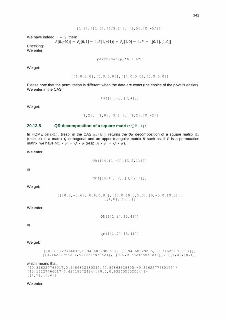
341

[1,2],[[1,0],[4/3,1]],[[3,5],[0,-5/3]]

We have indeed 𝑛 = 2, then:

𝑃[0, 𝑝(0)] = 𝑃2[0, 1] = 1, 𝑃[1, 𝑝(1)] = 𝑃2[1, 0] = 1, 𝑃 = [[0, 1], [1, 0]] Checking: We enter:

permu2mat(p)*A1; L*U

We get:

[[4.0,5.0],[3.0,5.0]],[[4.0,5.0],[3.0,5.0]]

Please note that the permutation is different when the data are exact (the choice of the pivot is easier). We enter in the CAS:

lu([[1,2],[3,4]])

We get:

[1,2],[[1,0],[3,1]],[[1,2],[0,-2]]

20.13.5 QR decomposition of a square matrix: QR qr

In HOME QR(M1), (resp. in the CAS qr(A)), returns the 𝑄𝑅 decomposition of a square matrix M1

(resp. A) in a matrix 𝑄 orthogonal and an upper triangular matrix 𝑅 such as, if 𝑃 is a permutation matrix, we have 𝑀1 ∗ 𝑃 = 𝑄 ∗ 𝑅 (resp. 𝐴 ∗ 𝑃 = 𝑄 ∗ 𝑅). We enter:

QR([[4,11,-2],[3,2,11]])

or

qr([[4,11,-2],[3,2,11]])

We get:

{[[0.8,-0.6],[0.6,0.8]],[[5.0,10.0,5.0],[0,-5.0,10.0]],

[[1,0],[0,1]]}

We enter:

QR([[1,2],[3,4]])

or

qr([[1,2],[3,4]])

We get:

[[0.316227766017,0.948683298051], [0.94868329805,-0.316227766017]],

[[3.16227766017,4.42718872424], [0.0,0.632455532034]], [[1,0],[0,1]]

which means that: [[0.316227766017,0.948683298051],[0.94868329805,-0.316227766017]]*

[[3.16227766017,4.42718872424],[0.0,0.632455532034]]=

[[1,2],[3,4]]

We enter:

342

QR([[1,2,4],[4,5,6],[7,8,9]])

We get:

[[[1,0,0],[4,1,0],[7,2,1]], [[1,2,4],[0,-3,-10],[0,0,1]],[0,1,2]]

which means that: [[1,2,4],[4,5,6],[7,8,9]]=

[[1,0,0],[4,1,0],[7,2,1]]*[[1,2,4],[0,-3,-10],[0,0,1]]

20.13.6 Matrix reduction to Hessenberg form: SCHUR schur

In HOME SCHUR(M1), (resp. in the CAS schur(A)), returns the numerical matrices [𝑃, 𝐵] such as

𝐵 = 𝑖𝑛𝑣(𝑃) ∗ 𝑀1 ∗ 𝑃 (resp. 𝐵 = inv(𝑃) ∗ 𝐴 ∗ 𝑃) with 𝐵 triangular. We have SCHUR(A)=hessenberg(A,-1). 𝐵 is the Hessenberg matrix similar to the matrix 𝑀1 (resp.

𝐴). We enter:

SCHUR([[1,2,3],[4,5,6],[-1,3,-2]])

We get two matrices P (orthogonal transfer matrix tran(P)=inv(P)) and B (triangular matrix similar to the argument):

[[[0.353452714748,-0.31069680265,0.882348386557],

[0.905760021954,-0.122092619725,-0.405822836763],

[0.23381608385,0.94263507734,0.238262774897]],

[[8.10977222864,3.79381095693,2.32899008373],

[0.0,-3.0,-3.03031411127],[0.0,0.0,-1.10977222865]]]

and we have:

B∼ inv(P)*[[1,2,3],[4,5,6],[-1,3,-2]]*P.

We enter:

SCHUR([[1,2,4],[4,5,6],[7,8,9]])

We get two matrices P (orthogonal transfer matrix tran(P)=inv(P)) and B (triangular matrix similar to the argument):

[[[-0.275726630766,-0.921788330317,-0.272545591008],

[-0.518148584403,-0.0962872203049,0.849853408352],

[-0.809627611663,0.375546329096,-0.451074367633]],

[[16.5037894003,3.99680014234,-0.803622341526],

[-4.55776517517e-20,-1.61625693617,0.616262731649],

[4.1752316389e-20,-2.72155736143e-15,0.112467535861]]]

and we have:

MB∼ inv(P)*[[1,2,3],[4,5,6],[-1,3,-2]]*P

20.13.7 Singular value decomposition: SVD svd

In HOME SVD(M1) returns 1 matrix M2, 1 vector M3, 1 matrix M4.

343

This gives the factorization of the rectangular numerical matrix real 𝑀1 (of size 𝑚 ∗ 𝑛) in

M2*diag(M3)*TRN(M4) where M2 is an orthogonal matrix 𝑚 ∗ 𝑚, M4 is an orthogonal matrix 𝑛 ∗ 𝑛, and diag(M3) is a diagonal matrix of dimension 𝑚 ∗ 𝑛 having as diagonal the singular values M3 of

𝑀1. In CAS, svd(A) returns 1 matrix U, 1 vector S, 1 matrix Q. This gives the factorization of the rectangular numerical matrix real 𝐴 (of size 𝑚 ∗ 𝑛) in

U*diag(S)*TRN(Q) where U is an orthogonal matrix m∗m, Q is an orthogonal matrix 𝑛 ∗ 𝑛, and

diag(S) is a matrix diagonal of size 𝑚 ∗ 𝑛 having as diagonal the singular values S of 𝐴. We enter in HOME:

M2,M3,M4:=SVD([[1,2],[2,1]])

We get:

{[[[0.707106781187,-0.707106781187],

[0.707106781187,0.707106781187]],

[3,1],

[[0.707106781187,0.707106781187],

[0.707106781187,-0.707106781187]]]}

and we have (here 𝑀4 is symmetrical): M2*diag(M3)*TRN(M4). We enter in the CAS:

U,S,Q:=SVD([[1,2],[2,1]])

Or we enter in the CAS:

U,S,Q:=svd([[1,2],[2,1]])

We get:

{[[[0.707106781187,-0.707106781187],

[0.707106781187,0.707106781187]],

[3.,1.],

[[0.707106781187,0.707106781187],

[0.707106781187,-0.707106781187]]]}

and we have (𝑄 is symmetrical): [[0.707106781187,-0.707106781187],[0.707106781187,0.707106781187]]*

[[3,0],[0,1]]*

[[0.707106781187,0.707106781187],[0.707106781187,-0.707106781187]]=

[[1,2],[2,1]]

We enter in the CAS:

SVD([[1,2],[3,4]])

Or we enter in the CAS:

svd([[1,2],[3,4]])

344

We get:

[[-0.404553584834,-0.914514295677],

[-0.914514295677,0.404553584834]],

[5.46498570422,0.365966190626]

[[-0.576048436767,0.81741556047],

[-0.81741556047,-0.576048436766]],

because

[[−0.404553584834, −0.914514295677], [−0.914514295677, 0.404553584834]]∗ [[5.46498570422, 0], [0, 0.365966190626]]∗ TRN([[−0.576048436767, 0.81741556047], [−0.81741556047, −0.576048436766]]) =

[[1.0, 2.0], [3.0, 4.0]]

20.13.8 Singular values: SVL svl

In HOME SVL(M1), (resp. in the CAS svl(A)), returns the list of singular values of the numerical real matrix 𝑀1 (resp. 𝐴) i.e. the positive square roots of the eigenvalues of the real symmetrical matrix

𝑀1 ∗ 𝑇𝑅𝑁(𝑀1) (resp(𝐴 ∗ 𝑇𝑅𝑁(𝐴)). We enter:

SVL([[1,4],[1,1]])

Ou:

svl([[1,4],[1,1]])

We get:

[4.30277563773,0.697224362268]

because eigenvals([[1,4],[1,1]]*[[1,1],[4,1]]) returns (5*sqrt(13)+19)/2,(-5*sqrt(13)+19)/2

and sqrt((5*sqrt(13)+19)/2.),sqrt((-5*sqrt(13)+19)/2.)

returns 4.30277563773,0.697224362268

We enter:

SVL([[1,2],[2,1]])

or

svl([[1,2],[2,1]])

We get:

[3,1]

because EIGENVAL([[1,2],[2,1]]*[[1,2],[2,1]])

returns [9,1].

We enter:

345

SVL([[1,2],[3,4]])

or

svl([[1,2],[3,4]])

We get:

[5.46498570422,0.365966190626]

because EIGENVAL([[1,2],[3,4]]*[[1,3],[2,4]])

returns [29.8660687473,0.133931252682]

which are the aproached values of √221 + 15 and – √221 + 15. We have:

√√221 + 15 ≃ 5.46498570422,√− √221 + 15 ≃ 0.365966190626

20.14 Vector

20.14.1 Cross product: CROSS cross

In HOME, CROSS returns the cross product of two vectors. We enter:

CROSS([1,2,3],[4,5,6])

or

CROSS({1,2,3},{4,5,6})

We get:

[-3,6,-3]

because 2 ∗ 6 − 5 ∗ 3 = −3, 4 ∗ 3 − 1 ∗ 6 = 6, 5 − 4 ∗ 2 = −3 In CAS, CROSS or cross returns the cross product of two vectors. We enter:

CROSS([1,2,3],[4,5,6])

or

cross([1,2,3],[4,5,6])

We get:

[-3,6,-3]

because 2 ∗ 6 − 5 ∗ 3 = −3, 4 ∗ 3 − 1 ∗ 6 = 6, 5 − 4 ∗ 2 = −3

20.14.2 Dot product: DOT dot

In HOME, DOT returns the dot product of two vectors. We enter:

346

DOT([1,2,3],[3,4,5])

We get:

26

because 1 ∗ 3 + 2 ∗ 4 + 3 ∗ 5 = 26

In CAS, DOT returns the dot product of two vectors. We enter:

DOT([1,2,3],[3,4,5])

Or we enter:

dot([1,2,3],[3,4,5])

We get:

26

because 1 ∗ 3 + 2 ∗ 4 + 3 ∗ 5 = 26

20.14.3 Norm l2: l2norm

l2norm is used in the CAS (in HOME, use CAS.l2norm and the answer will be exact).

l2norm returns the norm 𝑙2 of a vector: it is the square root of the sum of the squares of its coordinates. We enter:

l2norm([3,-4,2])

Or we enter:

l2norm(vector(3,-4,2))

We get:

sqrt(29)

Indeed: 𝑥 = 3, 𝑦 = −4, 𝑧 = 2 and 29 = |𝑥|2 + |𝑦|2 + |𝑧|2 .

20.14.4 Norm 𝒍𝟏: l1norm

l1norm is used in the CAS (in HOME, use CAS.l1norm and the answer will be exact). l1norm returns the norm 𝑙1 of a vector: it is the sum of absolute values of its coordinates. We enter:

l1norm([3,-4,2])

Or we enter:

l1norm(vector(3,-4,2))

We get:

9

347

Indeed: 𝑥 = 3, 𝑦 = −4, 𝑧 = 2 and 9 = |𝑥| + |𝑦| + |𝑧|.

20.14.5 Norm of the maximum: maxnorm

maxnorm is used in the CAS (in HOME, use CAS.maxnorm and the answer will be exact). maxnorm returns the norm 𝑙∞ of a vector: it is the maximum of absolute values of its coordinates. We enter:

maxnorm([3,-4,2])

Or we enter:

maxnorm(vector(3,-4,2))

We get:

4

Indeed: 𝑥 = 3, 𝑦 = −4, 𝑧 = 2 and 4 = 𝑚𝑎𝑥(|𝑥|, |𝑦|, |𝑧|).

348

Chapter 21 Special functions

21.1 𝜷 function: Beta

Beta is used in the CAS (in HOME, use CAS.Beta and the answer will be exact). Beta takes as argument two reals 𝑎, 𝑏, or three reals 𝑎, 𝑏, 𝑝, or three reals and 1: 𝑎, 𝑏, 𝑝, 1.

– with two arguments 𝑎, 𝑏, Beta returns the values of the function 𝛽 at the point 𝑎, 𝑏 of ℝ2. We have by definition:

𝛽(𝑥, 𝑦) =Γ(𝑥) ∗ Γ(𝑦)

Γ(𝑥 + 𝑦)

We have: 𝛽(1, 1) = 1

𝛽(𝑛, 1) =1

𝑛

and:

𝛽(𝑛, 2) =1

𝑛(𝑛 + 1)

We have:

Beta(a,b)= ∫ 𝑡𝑎−1 ∗ (1 – 𝑡)𝑏−1𝑑𝑡

1

0

Beta(a,b) is defined for 𝑎 and 𝑏 positive reals (so that the integral is convergent). We enter:

Beta(5,2)

We get:

1/30

We enter:

simplify(Beta(5,-3/2))

We get:

256/15

We enter:

Beta(x,y)

We get:

Gamma(x)*Gamma(y)/Gamma(x+y)

We enter:

Beta(5.1,2.2)

We get:

0.0242053671402

– with three arguments 𝑎, 𝑏, 𝑝 ,it is the incomplete Beta function for 𝑝 between 0 and 1, it is:

349

– Beta(a,b,p)= ∫ 𝑡𝑎−1 ∗ (1 – 𝑡)𝑏−1𝑑𝑡

𝑝

0, the integral goes from 0 to 𝑝 instead of 0 to 1 for the

Beta function. We enter:

Beta(5,2,0.5)

We get:

0.00364583333333

– with four arguments 𝑎, 𝑏, 𝑝, 1, if we put 1 as fourth argument, this returns the regularized incomplete beta function, i.e. the incomplete Beta function divided by Beta(a,b). We enter:

Beta(5,2,0.5,1)

We get:

0.109375

indeed Beta(5,2)=1/30 and 0.00364583333333*30=0.109375

21.2 𝚪 function: Gamma

Gamma is used in the CAS (in HOME, use CAS.Gamma and the answer will be exact). Gamma takes as argument a number a. Gamma returns the values of the function Γ at point a. We have by definition:

𝛤(𝑎) = ∫ 𝑒−𝑡𝑡𝑎−1𝑑𝑡,+∞

0

if 𝑎 > 0

and we use the formula: Γ(𝑎 + 1) = 𝑎 ∗ Γ(𝑎) if 𝑎 is not a negative integer Thus:

Γ(1) = 1

Γ(𝑎 + 1) = 𝑎 ∗ Γ(𝑎) and thus:

Γ(𝑛 + 1) = 𝑛! We enter:

Gamma(5)

We get:

24

We enter:

Gamma(1/2)

We get:

sqrt(pi)

We enter:

Gamma(0.7)

350

We get:

1.29805533265

We enter:

Gamma(-0.3)

We get:

-4.32685110883

Indeed: Gamma(0.7)=-0.3*Gamma(-0.3) We enter:

Gamma(-1.3)

We get:

3.32834700679

Indeed: Gamma(0.7)=-0.3*Gamma(-0.3)=(-0.3)*(-1.3)*Gamma(-1.3)

21.3 Derivatives of the DiGamma function: Psi

Psi is used in the CAS (in HOME, use CAS.Psi and the answer will be exact). Psi takes as arguments a real a and an integer n (by default 𝑛 = 0).

Psi is the value of the 𝑛-th derivative of the DiGamma function at point 𝑎. The DiGamma function is the derivative of ln (Γ(𝑥)). We enter:

Psi(3,1)

We get:

pi^2/6-5/4

We can omit the parameter 𝑛 when 𝑛 = 0.

When Psi takes as single parameter a number 𝑎, Psi returns the value of the DiGamma function at

point 𝑎: then we have Psi(a,0)=Psi(a). We enter:

Psi(3)

We get:

Psi(1)+3/2

We enter:

evalf(Psi(3))

We get:

.922784335098

351

21.4 The ζ function: Zeta

Zeta is used in the CAS (in HOME, use CAS.Zeta and the answer will be exact). Zeta takes as argument a real x. Zeta returns for 𝑥 > 1:

∑1

𝑛𝑥

+∞

𝑛=1

We enter:

Zeta(2)

We get:

pi^2/6

We enter:

Zeta(4)

We get:

pi^4/90

21.5 𝒆𝒓𝒇 function: erf

erf is used in the CAS (in HOME, use CAS.erf and the answer will be exact). erf takes as argument a number a. erf returns the values of the erf function at point 𝑎. We have by definition:

erf(x) =2

√π∫ 𝑒−𝑡

2𝑥

0

𝑑𝑡

We have: erf(+∞) = 1

erf(−∞) = −1 Indeed, we know that:

∫ 𝑒−𝑡2

+∞

0

𝑑𝑡 =√π

2

We enter:

erf(1)

We get:

0.84270079295

We enter:

erf(1/(sqrt(2)))*1/2+0.5

We get:

0.841344746069

Note: There is a relationship between the functions erf and normal_cdf:

normal_cdf(x) = 1

2 +

1

2erf (

𝑥

√2)

352

Indeed:

normal_cdf(x) = 1

2 +

1

√2π∫ e

−𝑡2

2𝑥

0𝑑𝑡

so with the change of variable 𝑡 = 𝑢 ∗ √2, we have:

normal_cdf(x) =1

2 +

1

√π∫ 𝑒−𝑢

2𝑥

√2

0𝑑𝑢 =

1

2 +

1

2erf (

𝑥

√2)

We check by entering:

normal_cdf(1)=0.841344746069

21.6 erfc function: erfc

erfc is used in the CAS (in HOME, use CAS.erfc and the answer will be exact). erfc takes as argument a number 𝑎.

erfc returns the values of the erfc functionc at point 𝑎. We have by definition:

erfc(𝑥) =2

√π∫ 𝑒−𝑡

2+∞

𝑥

𝑑𝑡 = 1 − erf(𝑥)

We have: 𝑒𝑟𝑓𝑐(0) = 1

𝑒𝑟𝑓𝑐() = −1 Indeed, we know that:

∫ e−𝑡2

+∞

𝑥

𝑑𝑡 =√π

2

We enter:

erfc(1)

We get:

0.15729920705

We enter:

1- erfc(1/(sqrt(2)))*1/2

We get:

0.841344746069

Note: There is a relationship between the functions erfc and normal_cdf:

normal_cdf(x) = 1 – 1

2 erfc (

𝑥

√2)

Indeed:

normal_cdf(x) =1

2 +

1

√2π∫ 𝑒

−𝑡2

2𝑥

0𝑑𝑡

so with the change of variable 𝑡 = 𝑢 ∗ √2

normal_cdf(x) = 1

2 +

1

√π∫ 𝑒−𝑢

2𝑥

√2

0𝑑𝑢 = 1 –

1

2 erfc (

𝑥

√2)

We check by entering:

normal_cdf(1)=0.841344746069

353

21.7 Exponential integral function: Ei

Ei is used in the CAS (in HOME, use CAS.Ei and the answer will be exact). Ei takes as argument a complex number 𝑎.

Ei returns the values of the Ei function at point 𝑎. We have by definition:

Ei(𝑥) = ∫𝑒𝑡

𝑡

𝑥

t=−∞

dt

For 𝑥 > 0, we extend by the principal value of the integral (the parts of 0− and 0+ compensate themselves). We have:

𝐸𝑖(0) = −∞, 𝐸𝑖(−∞) = 0

When we are close to 𝑥 = 0 we know that:

exp(𝑥)

𝑥=1

𝑥+ 1 +

𝑥

2!+𝑥2

3!+ … +

𝑥𝑛

(𝑛 − 1)!….

then we have for 𝑥 ∈ 𝐶 – ℝ+, (the function is discontinuous on ℝ+):

Ei(𝑥) = ln(−𝑥) + 𝛾 + 𝑥 +𝑥2

2.2!+𝑥3

3.3!+ …

where γ = Euler constant = 0.57721566490.. on the axis 𝑥 > 0 we take:

Ei(𝑥) = ln(𝑥) + 𝛾 + 𝑥 +𝑥2

2.2!+𝑥3

3.3!+ …

We enter:

Ei(1.)

We get:

1.89511781636

We enter:

Ei(-1.)

We get:

-0.219383934396

We enter:

Ei(1.)-Ei(-1.)

We get:

2.11450175075

We enter:

int((exp(x)-1)/x,x=-1..1.)

We get:

2.11450175075

We enter:

evalf(Ei(-1)-sum((-1)^n/n/n!,n=1..100))

We get the Euler constant γ:

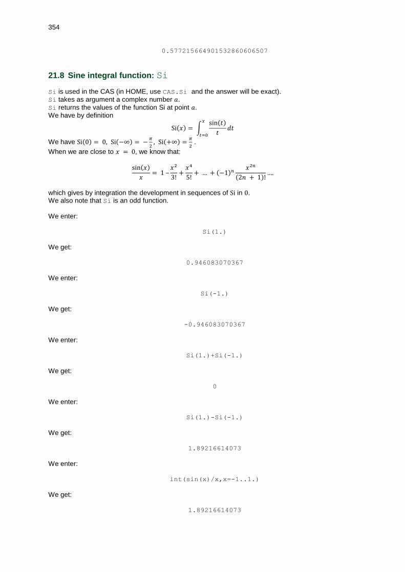
354

0.577215664901532860606507

21.8 Sine integral function: Si

Si is used in the CAS (in HOME, use CAS.Si and the answer will be exact). Si takes as argument a complex number 𝑎.

Si returns the values of the function Si at point 𝑎. We have by definition

Si(𝑥) = ∫sin(𝑡)

𝑡

𝑥

𝑡=0

𝑑𝑡

We have Si(0) = 0, Si(−∞) = −𝜋

2, Si(+∞) =

𝜋

2 .

When we are close to 𝑥 = 0, we know that:

sin(𝑥)

𝑥= 1 –

𝑥2

3!+𝑥4

5!+ … + (−1)𝑛

𝑥2𝑛

(2𝑛 + 1)!….

which gives by integration the development in sequences of Si in 0. We also note that Si is an odd function. We enter:

Si(1.)

We get:

0.946083070367

We enter:

Si(-1.)

We get:

-0.946083070367

We enter:

Si(1.)+Si(-1.)

We get:

0

We enter:

Si(1.)-Si(-1.)

We get:

1.89216614073

We enter:

int(sin(x)/x,x=-1..1.)

We get:

1.89216614073

355

21.9 Cosine integral function: Ci

Ci is used in the CAS (in HOME, use CAS.Ci and the answer will be exact). Ci takes as argument a complex number a. Ci returns the values of the function Ci at point a. We have by definition:

Ci(𝑥) = ∫cos(𝑡)

𝑡

𝑡=+∞

𝑥

𝑑𝑡 = ln(𝑥) + γ + ∫cos(𝑡) − 1

𝑡

𝑥

0

𝑑𝑡

We have: 𝐶𝑖(0) = −∞, 𝐶𝑖(−∞) = 𝑖𝜋, 𝐶𝑖(+∞) = 0.

When we are close to 𝑥 = 0 we know that

cos(𝑥)

𝑥= 1

𝑥 –𝑥

2+𝑥3

4!+ … + (−1)𝑛

𝑥2𝑛−1

(2𝑛)!….

which gives by integration the development in sequences of Ci. We enter:

Ci(1.)

We get:

0.337403922901

We enter:

Ci(-1.)

We get:

0.337403922901+3.14159265359*i

We enter:

Ci(1.)-Ci(-1.)

We get:

-3.14159265359*i

We enter:

int((cos(x)-1)/x,x=-1..1.)

We get:

-3.14159265359*i

21.10 𝑯𝒆𝒂𝒗𝒊𝒔𝒊𝒅𝒆 function: Heaviside

Heaviside takes as argument a number a. Heaviside returns the values of the Heaviside function at point a. We have by definition:

𝐻𝑒𝑎𝑣𝑖𝑠𝑖𝑑𝑒(𝑥) = 0 if 𝑥 < 0 and 1 otherwise We enter:

Heaviside(2)

We get:

356

1

We enter:

Heaviside(-4)

We get:

0

21.11 𝑫𝒊𝒓𝒂𝒄 distribution: Dirac

Dirac takes as argument a number 𝑎. Dirac is the Dirac distribution, it is the distribution associated to the function Heaviside. We have by definition:

𝐷𝑖𝑟𝑎𝑐(𝑥) = 0 if 𝑥 6 = 0 and ∞ otherwise

and if 𝑎 ≥ 0 and 𝑏 ≠ 0 we have:

∫ 𝐷𝑖𝑟𝑎𝑐(𝑥)𝑑𝑥𝑎

𝑏

= 1

∫ 𝐷𝑖𝑟𝑎𝑐(𝑥)𝑓(𝑥)𝑑𝑥𝑎

𝑏

= [𝐻𝑒𝑎𝑣𝑖𝑠𝑖𝑑𝑒(𝑥)𝑓(𝑥)]𝑏𝑎 −∫ 𝐻𝑒𝑎𝑣𝑖𝑠𝑖𝑑𝑒(𝑥)𝑓′(𝑥)𝑑𝑥 = 𝑓(0)

𝑎

𝑏

∫ 𝐷𝑖𝑟𝑎𝑐(𝑥) ∗ 𝑓(𝑥)𝑑𝑥+∞

−∞

= 𝑓(0)

We enter:

int(Dirac(x)*sin(x),x,-1,2)

We get:

sin(0)

We enter:

int(Dirac(x-1)*sin(x),x,-1,2)

We get:

sin(1)

357

Chapter 22 Constants and calculations with units

22.1 Shifted key Units

With the shifted key Units, and then Tools of the push buttons, we get the functions allowing to perform calculations with units: convert, mksa, ufactor, usimplify. With the shifted key Units, and then Units of the push buttons, we get the units sorted by category, in menu 1 the avalaible prefixes. With the shifted key Units, and then Const of the push buttons, we get the Mathematics, Chemistry, Physics and Quantum Mechanics constants.

22.2 Units

22.2.1 Notation of units

The names of units are prefixed with the symbol _ ("underscore"). For instance 2_m for 2 meters.

You can add a prefix ahead of the name of a unit meaning a multiplication by a power of 10. For

example, k or K for kilo (means multiplication by 103), D for deca (means multiplication by 10), d for deci (means multiplication by 10−1), etc.. When combining a real number with units, we create a unit object. We enter:

10.5_m

We get:

a unit object of 10.5 meters

We enter:

10.5_km

We get:

a unit object of 10.5 kilometers

22.2.2 Avalaible prefixes for units names

You can add prefixes ahead of the names of the units: each prefix corresponds to the name of the unit multiplied by a power of 10. Here are the different avalaible prefixes: Prefix Name (*10^) n Prefix Name (*10^) n Y yota 24 d deci -1 Z zeta 21 c cent -2 E exa 18 m mili -3 P peta 15 mu micro -6 T tera 12 n nano -9 G giga 9 p pico -12 M mega 6 f femto -15 k or K kilo 3 a atto -18 h or H hector 2 z zepto -21 D deca 1 y yocto -24

358

Note: You can of course not use a prefix with an integrated unit if this combination leads to another integrated unit. For instance, 1_a is an are and 1_Pa is a Pascal, and not 10^15_a.

22.2.3 Calculations with units

We can do the basic operations (+, -, *, /) with unit objects. In the operations, we can use different units (provided they are compatibles for + and -) and the result will be expressed according to the corresponding unit. For the multiplication and the division of two different units _u1 and _u2 the result unity reads _(u1*u2) or _(u1/u2) (Mind to not forget the parentheses!) We can also rise a unit object to an integer power: we get the corresponding unit object. Please note that, as far as the addition or substraction is concerned, the result will be expressed with the unit of the first term of the operation. We enter:

1_m+100_cm

We get:

2_m

We enter:

100_cm+1_m

We get:

200_cm

We enter:

1_m*100_cm

We get:

100_(cm*m)

We enter:

3_h +10_mn-(1_h+45_mn)

We get:

1.41666666667_h

We enter:

10_mn+3_h-(1_h+45_mn)

We get:

85.0_mn

359

22.3 Tools

22.3.1 Conversion of a unit object to another unit: convert =>

convert allows to get the conversion of a unit object into another unit given as second parameter. => is the infix version of convert. We enter:

convert(2_h+30_mn,_mn)

or else

2_h+30_mn=>_mn

We get:

150_mn

We enter:

convert(1_m*100_cm,_m^2)

or else

convert(100_(cm*m),_m^2)

or else

100_(cm*m)=>_m^2

We get:

1_m^2

We enter:

convert(1_h,_s)

Or we enter:

1_h=>_s

We get:

3600_s

We enter:

convert(60_mn,_h)

Or we enter:

60_mn=>_h

We get:

1.0_h

Note:

360

You must insert a space before the unit if the number of unit is stored in a variable or if it is a constant: We enter:

convert(pi _rad,_deg)

Or we enter:

pi _rad=>_deg

We get:

180.0_deg

We enter:

a:=180

convert(a _deg,_rad)

Or we enter:

a _deg=>_rad

We get:

3.14159265358_rad

22.3.2 Units conversion to MKSA units: mksa

mksa allows to get the conversion of a unit object into a unit object expressed in MKSA units. We enter:

mksa(15_C)

We get:

15_A*s

We enter:

mksa(1_Hz)

We get:

1_s^(-1)

22.3.3 Factorize a unit in a unit object: ufactor

ufactor allows to factorize the compound unit of a unit object to get a unit object expressed in constituent units (i.e. multiplied by the necessary MKSA units). We enter:

ufactor(3_J,_W)

We get:

3_(W*s)

361

We enter:

ufactor(3_W,_J)

We get:

3_(J/s)

22.3.4 Simplify a unit: usimplify

usimplify allows to simplify a unit in a unit object. We enter:

usimplify(3_(W*s))

We get:

3_J

22.4 Physics constants

With the shifted key Units then Const of the push buttons, then 3: Physics we get the physics constants sorted by category. With the shifted key Units then Unit of the push buttons, we get the units sorted by category. The physics constants, and the units sorted by category, are in the menu Physics.

22.5 Units

22.5.1 Units notation

The names of units are prefixed with the symbol _ ("underscore"). For instance 2_m for 2 meters. You can add a prefix ahead of the name of a unit meaning a multiplication by a power of 10. For

example, k or K for kilo (multiplication by 103), D for deca (means multiplication by 10), d for deci (means multiplication by 10−1) etc., ... When combining a real number with units, we create a unit object. We enter:

10.5_m

We get:

a unit object of 10.5 meters

We enter:

10.5_km

We get:

a unit object of 10.5 kilometers

22.5.2 Calculations with units

In the operations, we can use different units (provided they are compatibles for + and -) and the result will be expressed according to the corresponding unit. For the multiplication and the division of two

362

different units _u1 and _u2 the result unity reads _(u1*u2) or _(u1/u2) (Mind to not forget the parentheses!) We can also rise a unit object to an integer power: we get the corresponding unit object. Please note that, as far as the addition or substraction is concerned, the result will be expressed with the unit of the first term of the operation. We enter:

1_m+100_cm

We get:

2_m

We enter:

100_cm+1_m

We get:

200_cm

We enter:

1_m*100_cm

We get:

100_(cm*m)

We enter:

3_h +10_mn-(1_h+45_mn)

We get:

1.41666666667_h

We enter:

10_mn+3_h-(1_h+45_mn)

We get:

85.0_mn

22.5.3 Conversion of a unit object into another unit: convert =>

convert allows to get the conversion of a unit object into another unit given as second parameter. => is the infix version of convert. We enter:

convert(2_h+30_mn,_mn)

or else

2_h+30_mn=>_mn

We get:

363

150_mn

We enter:

convert(1_m*100_cm,_m^2)

or else

convert(100_(cm*m),_m^2)

or else

100_(cm*m)=>_m^2

We get:

1_m^2

We enter:

convert(1_h,_s)

Or we enter:

1_h=>_s

We get:

3600_s

We enter:

convert(60_mn,_h)

Or we enter:

60_mn=>_h

We get:

1.0_h

Note: You must insert a space before the unit if the numerical value of the unit is stored in a variable or if it is a constant: We enter:

convert(pi _rad,_deg)

Or we enter:

pi _rad=>_deg

We get:

180.0_deg

We enter:

a:=180

364

convert(a _deg,_rad)

Or we enter:

a _deg=>_rad

We get:

3.14159265358_rad

22.5.4 Units conversion to MKSA units: mksa

mksa allows to get the conversion of a unit object to a unit object expressed in MKSA units. We enter:

mksa(15_C)

We get:

15_A*s

We enter:

mksa(1_Hz)

We get:

1_s^(-1)

22.5.5 Conversions between degree Celsius and Fahrenheit:

Celsius2Fahrenheit Fahrenheit2Celsius

Celsius2Fahrenheit allows to convert the Celsius degrees into Fahrenheit degrees. We enter:

Celsius2Fahrenheit(a)

We get:

(a*9)/5+32

We enter:

Celsius2Fahrenheit(0)

We get:

32

Fahrenheit2Celsius allows to convert the Fahrenheit degrees into Celsius degrees. We enter:

Fahrenheit2Celsius(a)

We get:

((a-32)*5)/9

365

We enter:

Fahrenheit2Celsius(212))

We get:

100

22.5.6 Factorization of a unit: ufactor

ufactor allows to factorize the compound unit of a unit object to get a unit object expressed in constituent units (i.e. multiplied by the necessary MKSA units). We enter:

ufactor(3_J,_W)

We get:

3_(W*s)

We enter:

ufactor(3_W,_J)

We get:

3_(J/s)

22.5.7 Simplify a unit: usimplify

usimplify allows to simplify a unit in a unit object. We enter:

usimplify(3 _(W*s))

We get:

3 _J

22.6 Constants

22.6.1 Notation of chemical, physics or quantum mechanics constants.

The names of physics constants start and end by the character _ ("underscore"). Do no mix physics constants and symbolic constants. For example, 𝑒, 𝜋 are symbolic constants whereas _c_, _NA_ are physics or chemical constants. We enter:

_c_

We get the light speed in vacuum:

299792458_m*s^-1

We enter:

_NA_

366

We get the Avogadro number:

6.0221367e23_gmol^-1

22.6.2 Physics constants library

Here is the constants library: Name Description _NA_ Avogadro Number _k_ Boltzmann constant _Vm_ Molar volume of ideal gas _R_ Molar gas constant _StdT_ Standard temperature _StdP_ Standard pression _sigma_ tefan-Boltzmann constant _c_ Light speed _epsilon0_ Vacuum permittivity _mu0_ Vacuum permeability _g_ Acceleration of gravity _G_ Gravitation _h_ Planck constant _hbar_ Dirac constant _q_ Electronic charge _me_ Electron mass _qme_ q/me ratio (charge/mass of the electron) _mp_ Proton mass _mpme_ mp/me ratio (proton mass /electron mass) _alpha_ fine structure _phi_ Magnetic flux quantum _F_ Faraday constant _Rinfinity_ Rydberg constant _a0_ Bohr radius _muB_ Bohr magneton _muN_ Nuclear magneton _lambda0_ Photon wavelength _f0_ Photon frequency _lambdac_ Compton wavelength ! FOLLOWING CONSTANTS NON PRESENT IN THE CALCULATOR ! _rad_ 1 radian _twopi_ 2*pi radians _angl_ Angle of 180 degrees _c3_ Wien displacement law constant _kq_ k/q (Boltzmann/electronic charge) _epsilon0q_ epsilon0/q (permittivity/electronic charge) _qepsilon0_ q*epsilon0 (electronic charge*permittivity) _epsilonsi_ Silicium dielectric constant _epsilonox_ Silicium dioxyd dielectric constant _I0_ Sound reference intensity

367

Chapter 23 Functions of 3D geometry

23.1 Common perpendicular to two 3D lines: common_perpendicular

common_perpendicular takes as argument two lines D1 and D2. common_perpendicular(D1,D2) draws the common perpendicular of lines D1 and D2. We enter:

D1:=line([1,1,0],[0,1,1]);

D2:=line([0,-1,0],[1,-1,1]);

Then, we enter:

d:=common_perpendicular(D1,D2)

We get:

pnt([[1,0,-1],[-1/3,-2/3,-1/3]],0,d)

Which means that the common perpendicular to 𝐷1 and 𝐷2 passes through the points [1,0, −1] and

[−1/3, −2/3, −1/3]. Then, we enter:

equation(d)

We get:

[2/3-2*x/3+4*y/3=0,-4/3-8*x/9-4*y/9-20*z/9=0]

368

The Applications and the Apps key

369

Chapter 24 The menu Geometry

Warning! The documentation on the geometry application is subject to modification.

24.1 Generalities

We will describe here the Geometry application which allows to do interactive geometry. As all the Apps, the plane geometry application has three views: the Symbolic view, the Plot view and the Numeric view. Cmds, in the push buttons of these three views, lists the geometry commands, sorted by categories useful in each of the views: Point Line Polygon Curv Plot Transformation for the Symbolic view, Zoom Point Line Polygon Curv Plot Transformation, Cartesian, Measure,Tests for the Plot view, Cartesian, Measure,Tests for the Numeric view. Let us detail these three views with an example:

1. the key Symb opens the Symbolic view. Tap Edit or Insert in the push buttons, and fill in the cell GC:circle(1,2) For that:

– enter circle (spelt out) or tap Cmds in the push buttons (Cmds->Curv>Circle). If it is the first command you enter, it will be named GA. You can modify this name by selecting GA and editing it by tapping Edit in the push buttons. Change A for C and press Enter.

– directly plot a circle in the Plot view so that circle(point(GA),GB-GA) is written in GC, in

the Symbolic view. You can then modify the values of GA and GB − GA by point(1) and

Notes a. To have the command stored in GC executed, check the cell ahead of GC. b. To highlight a command line, use the cursor. c. To reorder the commands, use the arrows ↑ and ↓ of the push buttons: with them you can

move the highlighted line. d. To insert a new command, press Insert of the push buttons. e. To change the name of a variable in the Symbolic view, select this name, edit it with

Edit of the push buttons, modify it, and confirm with Enter. f. To delete a command line, highlight it, then press the delete key.

2. The key Plot opens the Plot view.

To directly plot a circle in the Plot view, use Cmds (push buttons) (Cmds->Curv>Circle), then designate with your finger the point which will be the center (you can then refine with the cursor), and press Enter to confirm your choice: the command point(2.375,1.24)(for example) has been automatically registered in GA in the Symbolic view. Then, directly with your finger a second point, this time on the circle (you can then refine with the cursor) and press Enter to confirm your choice. The command point(2.375,3.24) (for example) is then written in GB and the command circle(point(GA),GB-GA) is then written in GC in the Symbolic view. Once the circle is drawn, you can: a. change the color.

Put your finger close to the contour of the circle to have Options appear in the push buttons, then tap Options->Choose to choose a color and Enter. The color palette opens: select a color with your finger and confirm with Enter.

b. Fill it with color Put your finger close to the contour of the circle to have Options appear in the push buttons, then tap Options->Filled and Enter, which fills the circle with the chosen color.

c. Hide its name

370

Put your finger close to the contour of the circle to have Options appear in the push buttons, then tap Options->Hide Label: in case of ambiguity, the calculator will propose several choices.

d. Move it Put your finger close to the name of the circle (refine with the cursor) to have Options appear in the push buttons, then Enter. Then, you can dragg it anywhere with your finger or with the cursor. Confirm with Enter.

Note: Please note that the points or the geometrical objects directly created in the Plot view are written automatically: the geometrical objects are named and designated by A, B, C... then stored in the variables GA, GB, GC... variables also listed in the Symbolic view. Please note that the point F does not exist because GF is a CAS command.

3. the key Num opens the Numeric view.

If you want the equation of the circle previously defined, press: equation(GC) and you get:

(x-1.0)^2+y^2=4.0

The Numeric view allows to use the numerical commands in relationship with the graphic and to get numerical results. The commands giving a numerical result (points coordinates, lines equationsor of curves...) can be executed from the Num screen by using New, then Cmds (push buttons) of the Num screen.

When we are in the CAS or in the Geometry Application, the commands of geometry are sorted by category in the menu Apps-> Geometry of the key Toolbox. We find there the nine categories of the Cmds menu of each (push buttons) of the various views: Point, Line, Polygon, Curve, Plot, Transformation, Cartesian, Measure,

Tests.

Note: All the geometry functions can be executed from the CAS, but, in this case, the answer will be such as, for example: point(1,2), or line(x=1), but not a plot. Then, we can do 2D, or even 3D analytic geometry from the CAS. For example, let us enter from the CAS: g:=line(x=1) then add in the Symb screen GK:=g. Warning! We can retrieve the value of these variables in the Symbolic view , in the Numeric view, or in the CAS screen. If, for example, in the geometry application, we have: GA:=point(4.16+2.13*i) and in the CAS we enter GA:=5, GA will be equal to 5, as long as we have not used Plot of the geometry application, because, once we will have done this, we will have back GA:=point(4.16+2.13*i). For this reason, it is not safe to use the variables GA, GB, ... in the CAS.

24.2 Point

24.2.1 Point defined as barycenter of n points: barycenter

In plane geometry, barycenter takes as argument 𝑛 lists of length 2 (resp. a matrix of 𝑛 lines and two columns): the first element of the list 𝑗 (resp. the 𝑗-th element of the first column of the matrix) stores the point 𝐴𝑗

or the complex number aj representing the affix of this point, the second element of the list 𝑗 (resp. the

𝑗-th element of the second column) stores the real coefficient αj assigned to 𝐴𝑗.

barycenter returns and plots the point which is the barycenter of points 𝐴𝑗 of affixes 𝑎𝑗 assigned of

real coefficients 𝛼𝑗 when ∑αj ≠ 0.

If ∑αj = 0, barycenter returns an error.

371

We enter:

barycenter([1+i,1],[1-i,1])

Or we enter:

barycenter([point(1,1),1],[point(1,-1),1])

Or we enter:

barycenter([[1+i,1],[1-i,1]])

Or we enter:

barycenter([[point(1,1),1],[point(1,-1),1]])

We get in the geometry application:

The point of affix 1 is plotted with a cross and its label (name)

We get in the CAS:

point(1)

Warning! In the geometry application, if you want to get as answer a complex number, you have to ask for the affix of the barycenter, otherwise we get the plot of the barycenter point. We enter:

affix(barycenter([1+i,1],[1-i,1]))

Or we enter:

affix(barycenter([[1+i,1],[1-i,1]]))

We get:

1

In CAS screen, barycenter may also be used in 3D geometry and takes as argument 𝑛 lists of

length 2 (or a matrix of 𝑛 lines and two columns). The first element of the list 𝑗 (resp. the 𝑗-th element of the first column of the matrix) stores the point 𝐴𝑗, the second element of the list 𝑗 (resp. the 𝑗-nth

element of the second column) stores the real coefficient 𝛼𝑗 assigned to 𝐴𝑗.

barycenter returns point([a,b,c]), where [a,b,c] are the coordinates of the barycenter of these 𝑛 points. We enter:

barycenter([point(0,0,0),1],[point(3,3,3),2])

We get:

pnt(pn[(point[2,2,2],0)])

24.2.2 Point in geometry: point

In the Plot view, to get a point, it is enough to be in mode point (i.e. Point of the push buttons, then select Point and Enter) and locate the cursor at the wished place (with the finger or the arrows) then to confirm with Enter: a point is displayed as well as a label. This label is automatically generated: A, then B, etc., ... We can also use the command point:

372

point takes as argument a complex number or a paired value of two real numbers. Warning! If a,b is a paired value of two complex numbers whose one is non real, GK:=point(a,b) returns two points of same label (here K): one of affix a, the other of affix b. When a,b is a paired value of two real numbers, GA:=point(a,b) returns and plots the point having for affix a+ib. We enter:

GA:=point(1+i)

We get:

The point A of affix 1+i is plotted with a cross

We enter:

GB:=point(-2,1)

We get:

The point B of affix -2+i is plotted with a cross

We enter:

GC:=point(-2,i)

We get:

The two points of affix -2 and i are plotted with a cross and are

written C

Note When doing an assignment, for example GA:=point(-2+i), this stores the point(-2+i) in the variable GA, to plot the point with a cross and to assign it as a label the name on the left of := by omitting the letter G: here A. In the case we do several assignments with one single := sign, such as: GD,GE:=point(-2+i),point(2+i), the variable GD stores the point(-2+i), and GE the point(-2+i), but it will not be possible to move these points by pointing them. To avoid this, we must enter: GL:=point(-2+i),point(2+i):;GD:=L[0];GE:=L[1]

or

GL:=point(-2+i,2+i):;GD:=L[0];GE:=L[1] which defines the point D of affix −2 and the point E of affix i (because the affix of GD is not real!).

24.2.3 Midpoint of a segment: midpoint

In plane geometry, midpoint takes as argument two points or two complex numbers representing the affixes of these points (or else a list of two points or of two complex numbers). midpoint returns and plots the point midpoint of the segment defined by these two points. We enter:

midpoint(-1,1+i)

We get in the geometry application:

The point of affix i/2 is plotted with its label

In CAS screen, midpoint may also be used in 3D geometry and returns the point midpoint of the segment defined by two points.

373

We enter:

midpoint(point(0,0,0),point(2,2,2))

We get:

point(1,1,1)

24.2.4 Isobarycenter of n points: isobarycenter

isobarycenter takes as argument the list (or the sequence) of 𝑛 points or 𝑛 complex numbers representing the affixes of these points. isobarycenter returns and plots a point which is the isobarycenter of these 𝑛 points. We enter:

isobarycenter(0,2,2*i)

We get:

The point of affix 2/3+2*i/3 is plotted with a cross in the geometry

application

In CAS screen, isobarycenter may also be used in 3D geometry and takes as argument the list (or the sequence) of n points. isobarycenter returns point([a,b,c]) where [a,b,c] are the coordinates of the isobarycenter of these n points. We enter:

isobarycenter(point(0,0,0),point(3,3,3))

We get:

pnt(pn[(point[3/2,3/2,3/2],0]))

24.2.5 Randomly define a 2D point: point2d

point2d takes as argument a sequence of names of points. point2d randomly defines the integer coordinates (between −5 and +5) of the 2D points supplied as argument. We enter:

point2d(A,B,C)

Then, we enter:

triangle(A,B,C)

We get:

The plot of a triangle ABC

Warning! The points defined by the command point2d are fixed once and for all, and hence, they may not be moved.

374

24.2.6 Polar point in plane geometry: polar_point

polar_point(r,t) returns the 2D point of polar coordinates the arguments r and t, that is to say the point of affix r*exp(i*t). We enter:

polar_point(2,pi/4)

We get:

The plot of the point of affix 2*exp(i*pi/4)

24.2.7 One of the intersection points of two geometrical objects: single_inter

single_inter takes two or three arguments which are two geometrical objects and eventually a third argument which ,is either a point either a list of points. single_inter returns one of the intersection points of these two geometrical objects. If we have supplied a point GA (or its affixe) as third argument, single_inter returns the intersection point the closest to GA, and if we have supplied a list of points l (or a list of affixes), single_inter returns the intersection point which is not in the list l. We enter:

GA:=single_inter(line(0,1+i),line(1,i))

We get:

The point of affix 1/2+i/2 is plotted with a cross and is labeled A

We enter:

GB:=single_inter(circle(0,1),line(-1,i))

We get:

The point of affix i is plotted with a cross and is labeled B

We enter:

GB1:=single_inter(circle(0,1),line(-1,i),[i])

We get:

The point of affix -1 is plotted with a cross and is labeled B1

We enter:

GB2:=single_inter(circle(0,1),line(-1,1+2*i),1+2*i)

We get:

The point of affix i is plotted with a cross and is labeled B2

We enter:

GC:=single_inter(circle(1,sqrt(2)),circle(0,1))

We get:

The point of affix i is plotted with a cross and is labeled C

375

We enter:

GC1:=single_inter(circle(1,sqrt(2)),circle(0,1),[i])

We get:

The point of affix -i is plotted with a cross and is labeled C1

We enter:

GC2:=single_inter(circle(1,sqrt(2)),circle(0,1),i/2)

We get:

The point of affix i is plotted with a cross and is labeled C2

24.2.8 All intersection points of two geometrical objects: inter

inter takes two arguments or three arguments: – if inter is supplied with two geometrical objects as arguments, it returns the list of points of

intersection of these two geometrical objects. – if inter is supplied with two geometrical objects and a point as arguments, it returns the

intersection point of these two geometrical objects the closest of the point supplied as third argument.

We enter in geometry:

GA:=inter(line(0,1+i),line(1,i))[0]

We get:

The point of affix 1/2+i/2 is plotted with a cross and is labeled A

We enter in geometry:

GB:=inter(circle(0,1),line(1,i))[0]

GC:=inter(circle(0,1),line(1,i))[1]

We get:

The point of affix i is plotted with a cross and is labeled B

The point of affix 1 is plotted with a cross and is labeled C

We enter in the CAS:

inter(circle(0,1),line(1,i))

We get:

[point(1),point(i)]

We enter in geometry in the Symbolic view:

GL inter(circle(0,1),line(1,i))

We get in the Plot view:

The points of affix i and 1 are plotted with a cross and are written

L

376

We enter in plane geometry:

GD:=inter(circle(0,1),line(1,i),point(1/2))

We get:

The point of affix 1 is plotted with a cross and is labeled D

24.2.9 Orthocenter of a triangle: orthocenter

orthocenter takes as argument a triangle, or three points, or three complex numbers specifying the affix of three points. orthocenter plots and returns the point which is the orthocenter of the triangle, or of the triangle formed by these three points. We enter:

orthocentre(0,1+i,-1+i)

Or we enter:

orthocenter(triangle(0,1+i,-1+i))

We get:

The point of affix 0 is plotted with a cross

We enter in the Symbolic view of the geometry application:

GT triangle(-i,2+i,-1+i);GH orthocenter(T)

We get:

The triangle T and the point H of affix 0 are plotted

24.2.10 Vertices of a polygon: vertices

vertices takes as argument a polygon. vertices returns the list of the vertices of this polygon and plots them. Warning! If the polygon has n vertices the list will be of length n. We enter:

vertices(equilateral_triangle(0,2))

We get:

the points [pnt(0,0),pnt(2,0),pnt((2*(sqrt(3)*(i)+1))/2,0)] are

plotted with a cross

We enter:

GC:=vertices(equilateral_triangle(0,2))[2]

We get:

The point of affix 1 + 𝑖 ∗ √3 is plotted with a cross and is labeled C

Warning! If we enter:

377

GT:=equilateral_triangle(0,2,C);

We get:

the triangle T and the point C

Whereas, if we enter

GT:=equilateral_triangle(0,2,C):;vertices(GT[0])

We get:

the vertices of T plotted with a cross without label

24.2.11 Vertices of a polygon: vertices_abca

vertices_abca takes as argument the name of a polygon. vertices_abca returns the "closed" list of vertices of this polygon and plot them. Warning! If the polygon has n vertices the list will be of length 𝑛 + 1 because it starts and ends by the first vertex (“closed” list). We enter:

vertices_abca(equilateral_triangle(0,2))

We get:

[pnt(0,0),pnt(2,0),pnt((2*(sqrt(3)*(i)+1))/2,0),pnt(0,0)]

24.2.12 Point on a geometrical object: element

element may take different kind of arguments: 1. an interval a..b and two reals, the value and the step (by default the value equals (𝑎 + 𝑏)/2

and the step (𝑏 − 𝑎)/100). For example, we enter in the Symbolic view: GC:=element(-pi..pi) or GC:=element(-pi..pi,pi/2) or GC:=element(-pi..pi,pi/2,pi/100.0) this means that GC can take any value in the range [−𝜋; 𝜋], the second argument 𝜋/2 is the

start value of GC and 𝜋/100.0 is the chosen step. Then, in the Plot view:

– we have at the bottom-left the coordinates x1,y1 of the pointer. We enter C in Alpha mode,

– then we get at the bottom-right Pick GC; Press Enter to validate. – then pick C.

A line appears at the top of the Plot view: it is a cursor which allows to change the value of GC with the arrows (← and →) and at the bottom-right we have Move GC to the left of this line we have GC=xc (xc is the value of GC). The arrows ← and → allow to change the value xc of GC.

Example. We define GC as above: We enter in the Symbolic view:

GC:=element(-pi..pi,pi/2)

GD:=line(y+x*TAN(GC)-2*SIN(GC)=0)

GD is then a line of parameter GC. When we move the cursor GC, the line GD moves. We can keep the trace of this line GD by entering in the Symbolic view: trace(GD) or by using in the menu of the Plot view Point->Plus->trace, which allows to choose the name

378

of the object whose we want the trace of and thus trace(GD) reads automatically in the Symbolic view. Thus, we can see that the envelop of these lines is an astroid. Note: To delete the trace or to stop it, use the menu Point->Plus.

2. a geometrical object and a real (by default this real equals 1/2), for example:

GA:=element(circle(0,2),1) means that A is on the circle of center 0 and radius 2, and has as affix 2 ∗ 𝑒𝑥𝑝(𝑖) (because 2 ∗ 𝑒𝑥𝑝(𝑖 ∗ 𝑡) is the parametric equation of this circle and

the second argument 1 gives the value of the parameter 𝑡 to define GA).

For instance, GA:=element(circle(0,1)) means that A is on the circle of center 0 and radius 1, the point A will be plotted by having 𝑡 = 1/2 as value of the parameter of the

parametric equation of the geometrical object (here affix(GA)= 2 ∗ 𝑒𝑥𝑝(𝑖/2)). When moving A with the arrows, A will follow the outline of the geometrical object. Warning! It is the projection of the cursor on the circle which defines the point A: take care to move the cursor in the Plot view so that it defines a point A.

3. a geometrical object and a name of variable (for example GC) previously defined by the command element: for example GC:=element(0..pi). If we enter GD:=element(circle(0,2),GC), then GC is the variable of setting of the geometrical object defined by the first argument of element, that is to say that GD is on the circle of center 0 and radius 2, and GD has as affix 2 ∗ 𝑒𝑥𝑝(𝑖 ∗ 𝐺𝐶), because 2 ∗ 𝑒𝑥𝑝(𝑖 ∗ 𝑡) is the parametric equation of the circle(0,2). It is compulsory in this case to previously define the second argument (here GC) as being an element of an interval. By example, we enter:

GC:=element(0..pi)

then

GD:=element(circle(0,2),GC)

Then, we place the cursor on GC (Pointer GC), then Enter. As a result, we have at the top a cursor labelled GC that the we can move with the arrows (← and →) from 0 to 𝜋, with at the left

of this cursor a number equal to the value of the cursor. This cursor allows to move the point A on the top half-circle of the circle of center 0 and radius 1 (because 0 ≤ 𝑡 ≤ 𝜋) and this without plotting this half-circle. By example, we enter:

GA:=point(1);GB:=point(2+i)

GC:=element(0..2)

then

GD:=element(line(GA,GB),GC)

D is a point of the line AB and we have M=A+t*(B-A) i.e. M=(1-t)*A+t*B to follow the segment AB, you have to put GC:=element(0..1) or else GD:=element(segment(GA,GB),GC) which leaves D in A if 𝑡 < 0 and leave D in B if 𝑡 > 1.

4. a polygonal line GP and [floor(GC),frac(GC)] with GC previsouly defined by the command element: for example GC:=element(0..5) if GP has 5 sides. The sides of the polygonal line GP have as number: 0,1. ... If, for example, GP has 5 sides and as vertices S(0),...S(4),S(5)=S(0), we enter:

GC:=element(0..5)

GD:=element(GP,[floor(GC),frac(GC)])

Thus, according to the values of GC, D will follow the 5 sides of GP: D will be located on the side number n=floor(GC) and we will have: D=frac(GC)*S(n)+(1-frac(GC))*S(n+1).

For instance:

379

GA:=point(0);

GB:=point(4);

GC:=point(4*i);

Gd:=element(0..3);

GT:=triangle(A,B,C);

GM:=element(GT,[floor(GD),frac(GD)]);

Warning! If we add a complex a to a point 𝑀 of affix 𝑚, defined as element of a curve 𝐶, this defines a point 𝑁 of the curve 𝐶 which is the projection the point of affix 𝑚 + 𝑎 on 𝐶.

Par contre if a point M of affix m, defined as element of a curve 𝐶, we add a point 𝐴 of affix 𝑎, this

defines a point 𝑃 of affix 𝑚 + 𝑎. For instance, being supplied 3 points 𝑀,𝐴, 𝐵, if we want to define the point 𝑁 that makes for example:

𝑀𝑁⃗⃗⃗⃗⃗⃗ ⃗ = 𝐴𝐵⃗⃗⃗⃗ ⃗, We can enter: GN:=GM+(GB-GA) provided that 𝑀 is not defined as element of a curve 𝐶. Indeed, if we

have entered GM:=element(GC),we must define 𝑁 by entering: GN:=affix(GM)+GB-GA or GN:=GM+GB-GA (without parenthesis) because GN:=GM+GB-GA is interpreted as GN:=(GM+GB)-GA becausethere are no precedence rules for + and − whereas GN:=GM+(GB-GA)returns an element of the curve C which is the projection of N on C. Thus, if we enter:

GA:=point(-2,2);GB:=point(1,3);GC:=circle(0,1);

GM:=element(GC);GN:=affix(GM)+GB-GA;(or GN:=GM+GB-GA;)

GN is not on the curve C but if we enter:

GP:=GM+(GB-GA) (or GP:=projection(GC,GN);)

P is on the curve C.

24.2.13 Point dividing a segment: division_point

division_point takes three arguments: two points (or two complex numbers 𝑎 and 𝑏) and a

complex number 𝑘. division_point returns and plots the point of affix 𝑧 such as:

𝑧 − 𝑎

𝑧 − 𝑏= 𝑘

We enter:

GA:=division_point(i,2+i,3+i)

We get:

the point A of affix (5+4*i)/(2+i)

because csolve(z-i=(3+i)*(z-2-i),z) returns [(14+3*i)/5] and (5+4*i)/(2+i) returns (14+3*i)/5 We enter:

GB:=division_point(point(i),point(2+i),3)

We get:

the point B of affix 3+i

because csolve(z-i=3*(z-2-i),z) returns [3+i]

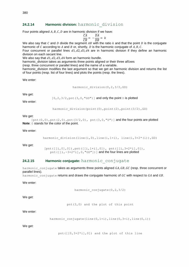
380

24.2.14 Harmonic division: harmonic_division

Four points aligned 𝐴, 𝐵, 𝐶, 𝐷 are in harmonic division if we have:

𝐶𝐴̅̅ ̅̅

𝐶𝐵̅̅ ̅̅= −

𝐷𝐴̅̅ ̅̅

𝐷𝐵̅̅ ̅̅= 𝑘

We also say that 𝐶 and 𝐷 divide the segment 𝐴𝐵 with the ratio 𝑘 and that the point 𝐷 is the conjugate

harmonic of 𝐶 according to 𝐴 and 𝐵 or, shortly, 𝐷 is the harmonic conjugate of 𝐴, 𝐵, 𝐶. Four concurrent or parallel lines 𝑑1, 𝑑2, 𝑑3, 𝑑4 are in harmonic division if they define an harmonic division on each secant line. We also say that 𝑑1, 𝑑2, 𝑑3, 𝑑4 form an harmonic bundle. harmonic_division takes as arguments three points aligned or their three affixes (resp. three concurrent or parallel lines) and the name of a variable. harmonic_division modifies the last argument so that we get an harmonic division and returns the list of four points (resp. list of four lines) and plots the points (resp. the lines). We enter:

harmonic_division(0,2,3/2,GD)

We get: [0,2,3/2,pnt(3,0,"GD")] and only the point D is plotted

We enter:

harmonic_division(point(0),point(2),point(3/2),GD)

We get: [pnt(0,0),pnt(2,0),pnt(3/2,0), pnt(3,0,"D")] and the four points are plotted

Note: 0 stands for the color of the point. We enter:

harmonic_division(line(i,0),line(i,1+i), line(i,3+2*(i)),GD)

We get: [pnt([[i,0],0]),pnt([[i,1+i],0]), pnt([[i,3+2*i],0]),

pnt([[i,-3+2*i],0,"GD"])] and the four lines are plotted

24.2.15 Harmonic conjugate: harmonic_conjugate

harmonic_conjugate takes as arguments three points aligned 𝐺𝐴, 𝐺𝐵, 𝐺𝐶 (resp. three concurrent or parallel lines). harmonic_conjugate returns and draws the conjugate harmonic of 𝐺𝐶 with respect to 𝐺𝐴 and 𝐺𝐵. We enter:

harmonic_conjugate(0,2,3/2)

We get:

pnt(3,0) and the plot of this point

We enter:

harmonic_conjugate(line(0,1+i),line(0,3+i),line(0,i))

We get:

pnt([[0,3+2*i],0]) and the plot of this line

381

24.2.16 Pole and polar: pole polar

polar takes as argument a circle 𝐺𝐶 and a point 𝐺𝐴 (or a complex number).

polar returns and draws the polar of the point 𝐺𝐴 with respect to the circle 𝐺𝐶: it is the line which is the locus of conjugates of 𝐺𝐴 with respect to the circle 𝐺𝐶.

pole takes as argument a circle 𝐺𝐶 and a line 𝐺𝑑.

pole returns and draws the pole of 𝐺𝑑 with respect to the circle 𝐺𝐶: it is the point 𝐺𝐴 having 𝐺𝑑 as polar according to 𝐺𝐶. We enter:

polaire(circle(0,1),(point(1+i))/2)

We get:

pnt([[2,2*i],0]) and the plot of this line

We enter:

pole(circle(0,1),line(i,1))

We get:

pnt(1+i,0) and the plot of this point

24.2.17 Reciprocal polar: reciprocation

reciprocation takes as argument a circle 𝐺𝐶 and a list of points and lines. reciprocation returns the list obtained by replacing in the list supplied as argument a point (resp. a line) by its polar (resp. its pole) with respect to the circle 𝐺𝐶. We enter:

reciprocation(circle(0,1),[point((1+i)/2), line(1,-1+i)])

We get:

the line of equation y = (−x + 2) and the point of affix 1+2i

24.2.18 The center of a circle: center

center takes as argument the name of a circle (see the definition of the circle ??). center returns and plots the center of this circle. We enter:

GC:=center(circle(0,point(2*i)))

We get:

The point of affix i is plotted with a cross and is labeled C

We enter:

GM:=center(circle(point(1+i),1))

We get:

The point of affix 1+i is plotted with a cross and is labeled M

382

24.3 Line

24.3.1 Line defined by a point and a slope: DrawSlp

DrawSlp(a,b,m) draws the line of slope 𝑚 passing by the point (𝑎, 𝑏) We enter:

DrawSlp(1,2,-1)

We get:

The line passing by the point of affix 1+2i and slope -1

24.3.2 Tangent to the curve of 𝒚 = 𝒇(𝒙) in 𝒙 = 𝒂: LineTan

LineTan(f(x),x=a) plots the tangent to the curve of 𝑦 = 𝑓(𝑥) in 𝑥 = 𝑎. We enter:

LineTan(sin(x),pi/6)

Or we enter:

LineTan(sin(t),t,pi/6)

We enter:

LineTan(sin(t),t=pi/6)

We get:

The plot of the tangent to the curve y = sin(x) at the point of

abscissa x = π/6)

24.3.3 Altitude of a triangle: altitude

altitude(GA,GB,GC) plots the altitude of the triangle 𝐴𝐵𝐶 through 𝐴. We enter:

altitude(1,0,1-i)

We get in the geometry application:

The plot of the altitude of the triangle (1, 0, 1 − i) through the point of affix 1

We enter:

altitude(0,1,2-i)

We get in the geometry application:

The plot of the altitude of the triangle (0, 1, 2 − i) through the point of affix 0

We enter in the CAS screen:

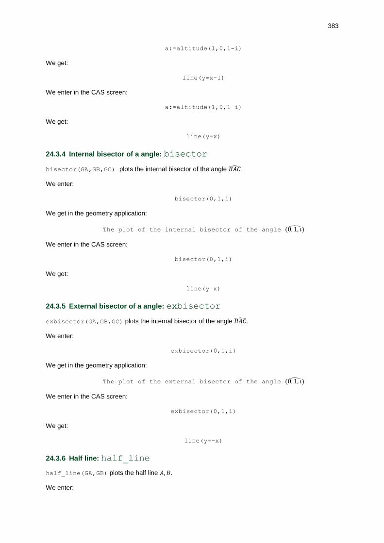
383

a:=altitude(1,0,1-i)

We get:

line(y=x-1)

We enter in the CAS screen:

a:=altitude(1,0,1-i)

We get:

line(y=x)

24.3.4 Internal bisector of a angle: bisector

bisector(GA,GB,GC) plots the internal bisector of the angle 𝐵𝐴�̂�. We enter:

bisector(0,1,i)

We get in the geometry application:

The plot of the internal bisector of the angle (0, 1, 𝑖)̂

We enter in the CAS screen:

bisector(0,1,i)

We get:

line(y=x)

24.3.5 External bisector of a angle: exbisector

exbisector(GA,GB,GC) plots the internal bisector of the angle 𝐵𝐴�̂�. We enter:

exbisector(0,1,i)

We get in the geometry application:

The plot of the external bisector of the angle (0, 1, 𝑖)̂

We enter in the CAS screen:

exbisector(0,1,i)

We get:

line(y=-x)

24.3.6 Half line: half_line

half_line(GA,GB) plots the half line 𝐴, 𝐵. We enter:

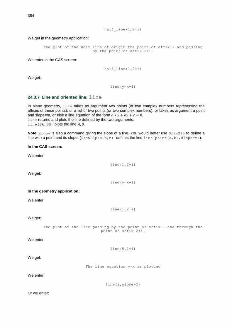
384

half_line(1,2+i)

We get in the geometry application:

The plot of the half-line of origin the point of affix 1 and passing

by the point of affix 2+i.

We enter in the CAS screen:

half_line(1,2+i)

We get:

line(y=x-1)

24.3.7 Line and oriented line: line

In plane geometry, line takes as argument two points (or two complex numbers representing the affixes of these points), or a list of two points (or two complex numbers), or takes as argument a point and slope=m, or else a line equation of the form 𝑎 ∗ 𝑥 + 𝑏𝑦 + 𝑐 = 0. line returns and plots the line defined by the two arguments. line(GA,GB) plots the line 𝐴, 𝐵. Note: slope is also a command giving the slope of a line. You would better use DrawSlp to define a line with a point and its slope. (DrawSlp(a,b,m) defines the line line(point(a,b),slope=m)). In the CAS screen: We enter:

line(1,2+i)

We get:

line(y=x-1)

In the geometry application: We enter:

line(1,2+i)

We get:

The plot of the line passing by the point of affix 1 and through the

point of affix 2+i.

We enter:

line(0,1+i)

We get:

The line equation y=x is plotted

We enter:

line(i,slope=2)

Or we enter:

385

DrawSlp(0,1,2)

We get:

The line equation y=2x+1 is plotted

We enter:

line(y-x=0)

We get:

The line equation y=x is plotted

Note: orientation of the line – When the line is defined by two points, its orientation is defined by the order n which the points

are supplied as argument. For example, line(GA,GB) defines a line oriented by the vector

𝐴𝐵⃗⃗⃗⃗ ⃗. – When the line is defined by an equation, we rewrite the equation in the form: "𝑙𝑒𝑓𝑡_𝑚𝑒𝑚𝑏𝑒𝑟 −

𝑟𝑖𝑔ℎ𝑡_𝑚𝑒𝑚𝑏𝑒𝑟 = 0" to get a line equation of the form 𝑎 ∗ 𝑥 + 𝑏𝑦 + 𝑐 = 0 and then the vector giving the orientation of the line is [𝑏, −𝑎], or else its orientation is defined by the 3D cross

product of its normal vector (third coordinate 0) and [0,0,1]. For instance, line(y=2*x) is

orientated by [1,2] because its equation is −2 ∗ 𝑥 + 𝑦 = 0 and cross([-2,1,0],

[0,0,1])=[1,2,0]. – When the line is defined by a point 𝐴 and its slope 𝑚, its orientation is defined by the vector

𝐴𝐵⃗⃗⃗⃗ ⃗ with 𝐵 = 𝐴 + 1 + 𝑖 ∗ 𝑚.

24.3.8 Segment: Line

Line takes as argument four real numbers giving the coordinates of two points. Line(a,b,c,d) returns and plots the segment defined by the two points 𝑎 + 𝑖 ∗ 𝑏 and 𝑐 + 𝑖 ∗ 𝑑. We enter:

Line(-1,1,2,-2)

We get:

The segment -1+i,2-2*i

24.3.9 Plot of a 2D horizontal line: LineHorz

LineHorz takes as argument an expression 𝑋𝑝𝑟. LineHorz plots the horizontal line 𝑦 = 𝑋𝑝𝑟. We enter:

LineHorz(1)

We get:

the plot of the line y=1

24.3.10 Plot of a 2D vertical line: LineVert

LineVert takes as arguments an expression 𝑋𝑝𝑟. LineVert plots the the vertical line 𝑥 = 𝑋𝑝𝑟. We enter:

LineVert(1)

386

We get:

the plot of the line x=1

24.3.11 Vector in plane geometry: vector

In plane geometry, vector takes as arguments: – either two points 𝐺𝐴 and 𝐺𝐵, or two complex numbers representing the affixes of these points,

or two lists of the points coordinates.

vector defines and draws the vector 𝐺𝐴𝐺𝐵⃗⃗⃗⃗ ⃗⃗ ⃗⃗ ⃗⃗ ⃗⃗ – either a point 𝐺𝐴 (or a complex number representing the affix of this point or a list representing

the coordinates of this point) and a vector 𝐺𝑉⃗⃗⃗⃗ ⃗ (recursive definition).

vector defines and draws the vector 𝐴𝐵 such as 𝐺𝐴𝐺𝐵⃗⃗⃗⃗ ⃗⃗ ⃗⃗ ⃗⃗ ⃗⃗ = 𝐺𝑉⃗⃗⃗⃗ ⃗.

If GW:=vector(GA,GV), so the point 𝐺𝐵⃗⃗⃗⃗ ⃗ such as 𝐺𝐴𝐺𝐵⃗⃗⃗⃗ ⃗⃗ ⃗⃗ ⃗⃗ ⃗⃗ = 𝐺𝑉⃗⃗⃗⃗ ⃗ is point(GW[1,1])or point(coordinates(GV)+coordinates(GA))or GA+(affix(V)[1]-affix(GV)[0]).

We enter:

vector(point(-1),point(i))

Or we enter:

vector(-1,i)

Or we enter:

vector([-1,0],[0,1])

We get:

The plot of the vector of origin -1 and end i

We enter:

GV:=vector(point(-1),point(i))

We enter:

vector(point(-1+i),GV)

Or we enter:

vector(-1+i,GV)

Or we enter:

vector([-1,1],GV)

We enter:

point([-1,1],coordinates(GV))

We get:

The plot of the vector of origin -1+i and end 2*i

We enter:

GD:=point([-1,1]+coordinates(GV))

387

We get:

GD the point(2*i)

Note: In symbolic computation, we work with the list of coordinates of the vectors that the we get thanks to the command coordinates (cf 24.8.6).

24.3.12 Median line of a triangle: median_line

median_line(GA,GB,GC) plots the median line of the triangle 𝐴𝐵𝐶 through 𝐴. We enter:

median_line(0,1,2+i)

We get in the geometry application:

The plot of the line passing by the point of affix 0 and through the

point of affix (3+i)/2 (midpoint of the segment (0,2+i))

We enter in the CAS screen:

median_line(0,1,2+i)

We get:

line(y=x/3)

24.3.13 Parallel lines: parallel

parallel(GA,GD) plots the line parallel to the line 𝐷 passing by 𝐴. We enter:

parallel(0, line(1,i))

We get in the geometry application:

the plot of the line equation y=-x

We enter in the CAS screen:

parallel(0, line(1,i))

We get:

line(y=(-x))

24.3.14 Perpendicular bisector: perpen_bisector

perpen_bisector(GA,GB) plots the perpendicular bisector of the segment 𝐴𝐵. We enter:

perpen_bisector(1,i)

We get in the geometry application:

the plot of the line equation y=x

We enter in the CAS screen:

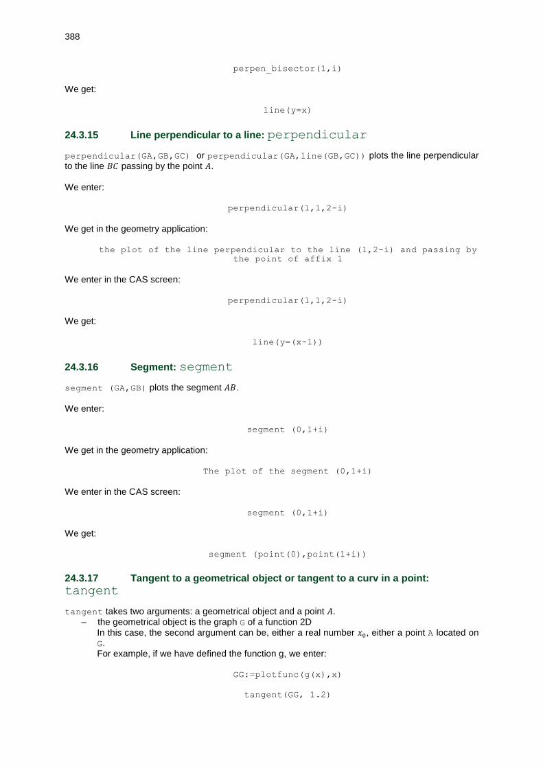
388

perpen_bisector(1,i)

We get:

line(y=x)

24.3.15 Line perpendicular to a line: perpendicular

perpendicular(GA,GB,GC) or perpendicular(GA,line(GB,GC)) plots the line perpendicular to the line 𝐵𝐶 passing by the point 𝐴. We enter:

perpendicular(1,1,2-i)

We get in the geometry application:

the plot of the line perpendicular to the line (1,2-i) and passing by

the point of affix 1

We enter in the CAS screen:

perpendicular(1,1,2-i)

We get:

line(y=(x-1))

24.3.16 Segment: segment

segment (GA,GB) plots the segment 𝐴𝐵. We enter:

segment (0,1+i)

We get in the geometry application:

The plot of the segment (0,1+i)

We enter in the CAS screen:

segment (0,1+i)

We get:

segment (point(0),point(1+i))

24.3.17 Tangent to a geometrical object or tangent to a curv in a point:

tangent

tangent takes two arguments: a geometrical object and a point 𝐴. – the geometrical object is the graph G of a function 2D

In this case, the second argument can be, either a real number 𝑥0, either a point A located on G. For example, if we have defined the function g, we enter:

GG:=plotfunc(g(x),x)

tangent(GG, 1.2)

389

plots the tangent to the graph G of the function g at point of abscissa x=1.2, or we enter:

GA:=point(1.2+i*g(1.2))

tangent(GG, GA)

plots the tangent to point A of the graph G of the function g.

For instance, to get the plot of the tangent to the curve of 𝑔(𝑥) = 𝑥2 at point of abscissa 𝑥0 = 1, we enter in the CAS:

g(x):=x^2

Then, in Symb, we enter:

GG:=plotfunc(g(x),x)

GT:=tangent(G,1)

or we enter:

GT:=tangent(G,point(1+i))

We get

The tangent to the curve of 𝑔(𝑥) = 𝑥2 at point 1+i

We get the equation of the tangent by entering in Num:

equation(GT)

– the geometrical object is not a graph

tangent may take as arguments: – either a geometrical object 𝐺 and a point 𝐴,

– either a point 𝐴 defined by element whose parameters are: a geometrical object 𝐺 and a real representing the value of the parameter of the parametric equation of 𝐺. tangent returns a list of lines and draws these lines which are the tan-gentes at this geometrical object 𝐺 and which passent through the point 𝐴. We enter:

tangent(circle(0,1),point(1+i))

We get:

The line equation x=1 and the line equation y=1

We enter:

tangent(element(circle(0,1),1))

We get:

The tangent to the circle of center 0 and radius 1, at point of affix

exp(i)

We enter:

tangent(circle(i,1+i),point((1+i*sqrt(3))*2))

We get:

390

2 tangents to the circle of center i and radius √2 through the point((1+i*sqrt(3))*2)

24.3.18 Radical axis of two circles: radical_axis

The radical axis of two circles 𝐶1 and 𝐶2 is the locus of points which have the same power with respect to 𝐶1 and at 𝐶2. We enter:

radical_axis(circle(0,1+i),circle(1,1+i)))

We get:

The plot of the line equation x = 1/2

Indeed: the line 𝑥 = 1/2 is the perpendicular bisector of the segment [0; 1]

24.4 Polygon

24.4.1 Scalene triangle: triangle

In plane geometry, triangle takes as arguments: three points (or three complex numbers representing the affixes of these points, or else a list of three points or of three complex numbers). triangle returns and plots the triangle having for vertices these three points. We enter:

triangle(-1,i,1+i)

We get:

The triangle of vertices -1, i, 1+i

24.4.2 Equilateral triangle: equilateral_triangle

In plane geometry, equilateral _triangle, takes two a or three arguments: – two arguments: two points or two complex numbers representing the affixes of these points

(or else a list of two points or of two complex numbers). equilateral_triangle(GA,GB) returns and plots the equilateral triangle direct ABC but without defining the point 𝐶. We enter:

equilateral_triangle(0,2)

We get:

the equilateral triangle of vertices the points of affix

0,2,1+i*sqrt(3)

To define the third vertex 𝐶, we can give the triangle a label (for example GT:=equilateral_triangle(0,2)) and use the command vertices(GT) which returns the list of vertices of 𝑇. Then, we will define GC:= vertices(GT)[2] but it is easier to add GC, name of the last vertex, as third argument.

– three arguments: the two previous arguments and as third argument the name of a variable to define and plot the third vertex with its label. We enter:

391

equilateral_triangle(0,2,GC)

We get:

the equilateral triangle of vertices the points of affix

0,2,1+i*sqrt(3)

We enter:

normal(affix(GC))

We get:

1+i*sqrt(3)

24.4.3 Right triangle: right_triangle

In plane geometry, right_triangle takes three or four arguments: – three arguments: two points 𝐴 and 𝐵 (or two complex numbers representing the affixes of

these points) and a real 𝑘 not null.

right_triangle(GA,GB,k) returns and plots the triangle 𝐴𝐵𝐶 right angled in 𝐴: this

triangle is direct if 𝑘 > 0, indirect if 𝑘 < 0 and is such as 𝐴𝐶 = |𝑘| ∗ 𝐴𝐵.

Thus, if the angle (𝐵𝐶⃗⃗⃗⃗ ⃗, 𝐵𝐴⃗⃗⃗⃗ ⃗) = 𝛽 radians (or degrees), we have 𝑡𝑎𝑛(𝛽) = 𝑘. We notice that if 𝐶 is the transform of 𝐵 in the similarity of center 𝐴 of ratio |𝑘| and angle

(𝑘/|𝑘|) ∗ 𝜋/2. We enter:

right_triangle(i,-i,2)

We get:

The right triangle of vertices i, -i, 4+i

We enter:

right_triangle(i,-i,-2)

We get:

The right triangle of vertices i, -i, -4+i

– four arguments: the three previous arguments and as last argument the name of a variable to define the third vertex. We enter:

right_triangle(i,-i,2,GD)

We get:

The right triangle of vertices i, -i, 4+i

We enter:

normal(affix(GD))

We get:

4+i

392

24.4.4 Isosceles triangle: isosceles_triangle

In plane geometry, isosceles_triangle takes three or four arguments: – three arguments: two points 𝐴 and 𝐵 (or two complex numbers representing the affixes of

these points) and a real which designates the measure in radians (or in degrees) of the angle

(𝐴𝐵⃗⃗⃗⃗ ⃗, 𝐴𝐶⃗⃗⃗⃗ ⃗). isosceles_triangle(GA,GB,c) returns and plots the isosceles triangle 𝐴𝐵𝐶 of vertex 𝐴

(𝐴𝐵 = 𝐴𝐶) and such as the angle (𝐴𝐵⃗⃗⃗⃗ ⃗, 𝐴𝐶⃗⃗⃗⃗ ⃗) = 𝑐 radians (or degrees), without defining the point 𝐶). We enter:

isosceles_triangle(i,1,-3*pi/4)

We get, if we have checked radian in the CAS configuration (Shift-CAS):

The isoscele triangle of vertices -1, i, −√2+i

– four arguments: the three previous arguments and as fourth argument the name of a variable to define the third vertex. We enter:

isosceles_triangle(i,1,-3*pi/4,GC)

We get, if we have checked radian in the CAS configuration (Shift-CAS):

The isoscele triangle of vertices -1, i, −√2+i

We enter:

normal(affix(GC))

We get:

-sqrt(2)+i

24.4.5 Rhombus: rhombus

In plane geometry, rhombus takes three to five arguments: – three arguments: two points or two complex numbers representing the affixes of these points

and a real number 𝑎.

rhombus(GA,GB,a) returns and plots the rhombus 𝐴𝐵𝐶𝐷 such as:

(𝐴𝐵⃗⃗⃗⃗ ⃗, 𝐴𝐷⃗⃗ ⃗⃗ ⃗) = 𝑎 radians (or degrees), but without defining the points 𝐶 and 𝐷.

We enter:

rhombus(-2*i,sqrt(3)-i,pi/3)

We get, if we have checked radian in the CAS or Home configuration (Shift-CAS or Shift-Home)

The rhombus of vertices −2 ∗ 𝑖, √3 − 𝑖, √3 + 𝑖, 0 – four (resp. five) arguments: the three previous arguments, the last parameter (resp. the two

last parameters) is (resp. are) the name(s) of a (resp. of the two) variable(s) which define(s) the penultimate vertex (resp. the two last vertices). We enter:

rhombus(-2*i,sqrt(3)-i,pi/3,E,F)

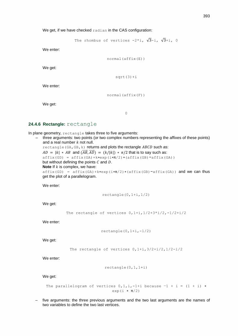
393

We get, if we have checked radian in the CAS configuration:

The rhombus of vertices -2*i, √3-i, √3+i, 0

We enter:

normal(affix(E))

We get:

sqrt(3)+i

We enter:

normal(affix(F))

We get:

0

24.4.6 Rectangle: rectangle

In plane geometry, rectangle takes three to five arguments: – three arguments: two points (or two complex numbers representing the affixes of these points)

and a real number 𝑘 not null.

rectangle(GA,GB,k) returns and plots the rectangle 𝐴𝐵𝐶𝐷 such as:

𝐴𝐷 = |𝑘| ∗ 𝐴𝐵 and (𝐴𝐵⃗⃗⃗⃗ ⃗, 𝐴𝐷⃗⃗ ⃗⃗ ⃗) = (𝑘/|𝑘|) ∗ 𝜋/2 that is to say such as:

affix(GD) = affix(GA)+k∗exp(i∗π/2)∗(affix(GB)−affix(GA))

but without defining the points 𝐶 and 𝐷.

Note If 𝑘 is complex, we have:

affix(GD) = affix(GA)+k∗exp(i∗π/2)∗(affix(GB)−affix(GA)) and we can thus

get the plot of a parallelogram. We enter:

rectangle(0,1+i,1/2)

We get:

The rectangle of vertices 0,1+i,1/2+3*i/2,-1/2+i/2

We enter:

rectangle(0,1+i,-1/2)

We get:

The rectangle of vertices 0,1+i,3/2+i/2,1/2-i/2

We enter:

rectangle(0,1,1+i)

We get:

The parallelogram of vertices 0,1,i,-1+i because −1 + i = (1 + i) ∗ exp(i ∗ π/2)

– five arguments: the three previous arguments and the two last arguments are the names of two variables to define the two last vertices.

394

We enter:

rectangle(0,1+i,-1/2,GG,GH)

We get:

The rectangle of vertices 0,1+i,3/2+i/2,1/2-i/2

We enter:

normal(affix(GG))

We get:

(3+i)/2

We enter:

normal(affix(GH))

We get:

(1-i)/2

24.4.7 Square: square

In plane geometry, square takes one to four arguments: – two arguments: two points or two complex numbers representing the affixes of these points (or

else a list of two points or of two complex numbers). square(GA,GB) returns and plots the square 𝐴𝐵𝐶𝐷 of direct direction, but without defining

the points 𝐷 and 𝐶. We enter:

square(0,1+i)

We get:

The square of vertices 0, 1+i, 2*i, -1+i

– three (resp. four) arguments: the two previous arguments followed by the the name of a (resp. two) variable(s) which define(s) the penultimate vertex (resp. the two other vertices). We enter:

square(0,1+i,GC,GD)

We get:

The square of vertices 0, 1+i, 2*i, -1+i

We enter:

affix(GC)

We get:

2*i

We enter:

395

affix(GD)

We get:

-1+i

24.4.8 Quadrilateral: quadrilateral

In plane geometry, quadrilateral(GA,GB,GC,GD), returns and plots the quadrilateral 𝐴𝐵𝐶𝐷. We enter:

quadrilateral(0,1,1+i,-1+2*i)

We get:

The "kite" of vertices 0, 1, 1+i, 1+2*i

24.4.9 Parallelogram: parallelogram

In plane geometry, parallelogram takes three arguments or four arguments: – three arguments: three points (or three complex numbers representing the affixes of these

points). parallelogram(GA,GB,GC) returns and plots the parallelogram 𝐴𝐵𝐶𝐷 such as:

𝐴𝐷⃗⃗ ⃗⃗ ⃗ = 𝐵𝐶⃗⃗⃗⃗ ⃗ but without defining the point 𝐷. We enter:

parallelogram(0,1,2+i)

We get:

The parallelogram of vertices 0,1,2+i,1+i

We enter:

parallelogram(1,0,-1+i)

We get:

The parallelogram of vertices 1,0,-1+i,i

– four arguments: the three previous arguments and as fourth argument the name of a variable which defines the missing vertex. We enter:

parallelogram(0,1,2+i,GF)

We get:

The parallelogram of vertices 0,1,2+i,1+i and the point F of affix

1+i

We enter:

normal(affix(GF))

We get:

396

1+i

24.4.10 Isopolygon: isopolygon

In plane geometry, isopolygon takes three arguments: – either two points or two complex numbers and a positive integer 𝑘

– either two points or two complex numbers and a negative integer 𝑘. When 𝑘 > 0, isopolygon plots the direct regular polygon of 𝑘 sides and consecutive vertices the two first arguments. We enter:

isopolygon(0,1,4)

We get:

The square of vertices 0,1,1+i,i

When 𝑘 < 0, isopolygon plots the direct regular polygon having – 𝑘 sides, as center the first argument, and as vertex the second argument. We enter:

isopolygon(0,1,-4)

We get:

square of vertices 1,i,-1,-i

24.4.11 Hexagon: hexagon

See also: ?? for 2D geometry. In plane geometry, hexagon may take from two to six arguments. Description of the arguments:

– two arguments: two points or two complex numbers representing the affixes of these points (or else a list of two points or of two complex numbers). hexagon(A,B) returns and plots the hexagon 𝐴𝐵𝐶𝐷𝐸𝐹 of direct orientation, but without

defining the points 𝐷, 𝐶, 𝐸 and 𝐹. We enter:

hexagon(0,1)

We get:

The hexagon of vertices

0,1,3/2+i*sqrt(3)/2,1+i*sqrt(3),i*sqrt(3),-1/2+i*sqrt(3)/2

– six arguments, the four last parameters are the name of two variables which define the two other vertices. We enter:

hexagon(0,1,C,D,E,F)

We get:

The hexagon of vertices

0,1,3/2+i*sqrt(3)/2,1+i*sqrt(3),i*sqrt(3),-1/2+i*sqrt(3)/2

397

We enter:

affix(C)

We get:

3/2+i*sqrt(3)/2

We enter:

affix(D)

We get:

1+i*sqrt(3)

We enter:

affix(E)

We get:

i*sqrt(3)

We enter:

affix(F)

We get:

-1/2+i*sqrt(3)/2

24.4.12 Polygon: polygon

In plane geometry, polygon takes as argument the list (or the sequence) of 𝑛 points or of 𝑛 complex numbers representing the affixes of these points. polygon returns and plots the polygon having for vertices these 𝑛 points. We enter:

polygon(-1,-1+i/2,i,1+i,-i)

We get:

The polygon of vertices -1,-1+i/2,i,1+i,-i

We enter:

polygon(makelist(x->exp(i*pi*x/3),0,5,1))

We get:

The hexagon of vertices 1, 𝑒𝑖𝜋

3 , 𝑒2𝑖𝜋

3 , . . , 𝑒5𝑖𝜋

3

24.4.13 Polygonal line: open_polygon

In plane geometry, open_polygon takes as argument the list (or the sequence) of 𝑛 points or of 𝑛 complex numbers representing the affixes of these points. open_polygon returns and plots the polygonal line having for vertices these 𝑛 points.

398

We enter:

open_polygon(-1,-1+i/2,i,1+i,-i)

We get:

The polygonal line of vertices -1,-1+i/2,i,1+i,-i

We enter:

open_polygon(makelist(x->exp(i*pi*x/3),0,5,1))

We get:

The polygonal line of vertices 1, 𝑒𝑖𝜋

3 , 𝑒2𝑖𝜋

3 , . . , 𝑒5𝑖𝜋

3

24.4.14 Convex hull of points of the plan: convexhull

The instruction convexhull returns the convex hull of a ensemble of points of the plane supplied by two points or of affixes of points, elle returns a list of complex affixes of vertices of the envelop convexe. The algorithm used ist the scan of Graham. We can use polygon on the result of convexhull to get the plot of the convexe envelop. We enter:

polygon(convexhull(0,1,1+i,1+2i,-1-i,1-3i,-2+i))

to get the convex hull of points of affixes (0,0), (1,0), (1,1), (1,2), (−1,−1), (1, −3), (−2,1).

24.5 Curves

24.5.1 Circle and arcs: circle

circle takes one or two arguments to draw a circle, and four to six arguments to draw an arc of circle:

– with one argument: the argument of circle is then the equation of the circle having as variables 𝑥 and 𝑦,

– with two arguments: The first argument of circle is a point or a complex number considered as the affix of a point. The second argument specifies which additional data is supplied to plot the circle: either the radius (as modulus of a complex number), either the diameter (specified by a point). Then:

– circle(GC,r) where GC is a point (or a complex number) and r a complex number, plots the circle of center C and radius the modulus of r. This is useful, for example, to get the circle of center A passing by B. We enter:

circle(GA,GB-GA).

– circle(GA,GB) where A is a point or a complex number and B a point, plots the circle

of diameter AB. We enter:

circle(x^2+y^2-2*x-2*y)

399

We get:

The circle of center 1+i and radius sqrt(2) is drawn.

We enter:

circle(-1,i)

We get:

The circle of center -1 and radius 1 is drawn.

We enter:

circle(-1, point(i))

We get:

The circle of diameter -1,i

– With four to six arguments: circle designates an arc of circle. In this case, the two first arguments determinate the circle which is the basis of the arc (see above) and the two following arguments are the angles at the center of the points which border the arc, and the two last arguments are the names of the variables storing the points which border the arc. The third and the fourth argument are the measures of the angles at the center of points which border the arc, these angles are measured in radians (or in degrees) starting from the axis defined by the two first arguments if the second argument is a point (definition of the circle by its diameter) or of the axis defined by its center 𝐶 and the point 𝐴 = 𝐶 + 𝑟 if the second argument is a complex equal to 𝑟 (definition of the circle by its centre and a complex whose modulus equals the radius). The fifth and the sixth argument are not mandatory and define the ends of the arc. We enter:

circle(-1,1,0,pi/4,A,B)

We get, if we have checked radian in the CAS configuration:

The arc AB (GA:=point(0) and GB:=point(−1+√2+𝑖∗√2

2)) of the circle of

center -1 and radius 1 is drawn.

Indeed, the angle is measured starting from the axis (−1,0) and then the angle 0 is the point (0). We enter:

circle(-1,i,0,pi/4,A,B)

We get, if we have checked radian in the CAS configuration:

The arc AB (GA:=point(-1+i) and GB:=point(−1−√2+𝑖∗√2

2)) of the circle of

center -1 and radius 1 is drawn.

Indeed, the angle is measured starting from the axis (−1, 𝑖 − 1) and then the angle 0 is the

point of affix 𝑖 − 1. We enter:

circle(-1, point(i),0,pi/4,A,B)

400

We get:

The arc AB (GA:=point(i) and GB:=point(−1+𝑖∗(1+√2)

2)) the circle of

diameter -1,i

Indeed, the angle is measured starting from the axis (−1, 𝑖) and then the angle 0 is the point of

affix 𝑖.

24.5.2 Arcs of circle: arc ARC

See also: 24.5.1 for circles and arcs of circle. arc takes three to five arguments: two points A,B (or two complex numbers a,b) and a real number 𝛼

representing the measure of the arc AB in radians (−2 ∗ 𝜋 ≤ 𝛼 ≤ 2 ∗ 𝜋). The fourth and the fifth arguments are not mandatory and are names of variables storing the center and the radius of the circle the arc is based on. The arc AB is then based on the circle of centre: (𝑎 + 𝑏)/2 + 𝑖 ∗ (𝑏 − 𝑎)/(2 ∗ 𝑡𝑎𝑛(𝛼/2)). arc(A,B,α) is the arc where we see the segment AB from, along the angle −𝜋 + 𝛼/2 if 2𝜋 > 𝛼 >0, or under the angle 𝜋 + 𝛼/2 if −2𝜋 < 𝛼 < 0. To get the arc capable AB of measure 𝛽 that is to say the arc of where the we see the segment AB

from, along the angle −𝜋 < 𝛽 < 𝜋, you have to enter:

arc(A,B,2*(-pi+β)) if 𝜋 > 𝛽 > 0 or arc(A,B,2*(pi+β)) if −𝜋 < 𝛽 < 0 .

Warning! The sign of α gives the direction of the arc AB. For example, arc(A,B,3*pi/2) and arc(A,B,-

pi/2) draw a full circle. We enter:

arc(1,i,pi/2)

We get:

The arc (1,i) of the circle of center 0 and radius 1

We enter:

arc(1,i,pi/2,C,r)

We get:

The arc (1,i) of the circle of center C=point(0) and radius r=1

We enter:

arc(2,2*i,pi,C,r)

We get:

The half-circle of center C=point(1+i) and radius r=sqrt(2), starting

from the point(2) to the point(2*i) in positive direction.

Note: When circle has four arguments, circle also draws an arc of circle (cf. ??).

24.5.3 Circumcircle: circumcircle

circumcircle takes three parameters defining the vertices of a triangle. circumcircle draws and returns the circumcircle of this triangle. We enter:

401

circumcircle(-1,i,1+i)

We get:

Circumcircle of the triangle(-1,i,1+i)

24.5.4 Plot of a conic: conic

conic takes as argument the expression of a conic. conic plots the conic having for equation argument=0. We enter:

conic(2*x^2+2*x*y+2*y^2+6*x)

We get:

the plot of the ellipse of center -2+i and equation

2*x^2+2*x*y+2*y^2+6*x=0

Note: Use reduced_conic to get the parametric equation of the conic. We enter:

reduced_conic(2*x^2+2*x*y+2*y^2+6*x)[4]

We get:

[-2+i+(1+i)*(cos(t)+sqrt(3)*i*sin(t)),t,0,2π,2π/60]

24.5.5 Ellipse: ellipse

In plane geometry, ellipse takes one or three parameters: – one parameter:

its equation of variables x and y. ellipse(p(x,y)) plots the conic equation 𝑝(𝑥, 𝑦) = 0 if

𝑝(𝑥, 𝑦) is a polynomial of degree 2. – three parameters: the two foci and a point on the ellipse (or its affix if this affix is not real) or its

two foci and a real (its half-major axis). ellipse(GF1,GF2,GA) plots the ellipse passing by A and of foci F1 and F2 or, ellipse(GF1,GF2,a) where a is a real number, plots the ellipse of foci F1 and F2 and half-major axis |a|.

We enter:

ellipse(-i,i,1+i)

We get:

The ellipse of foci -i, i and passing by 1+i

We enter:

ellipse(-i,i,sqrt(5)-1)

We get:

The ellipse of foci -i, i and half-major axis

sqrt(5)-1

402

We enter:

ellipse(x^2+2*y^2-1)

or we enter:

ellipse(sqrt(2)/2,-sqrt(2)/2,1)

We get:

The ellipse of center 0 and half-major axis 1 and foci sqrt(2)/2 and

-sqrt(2)/2

24.5.6 Excircle: excircle

excircle has three parameters defining the vertices of a triangle. excircle draws and returns the excircle in the inner angle of the first vertex of this triangle. We enter:

excircle(-1,i,1+i)

We get:

Excircle in the angle of vertex -1 the triangle(-1,i,1+i) is drawn.

24.5.7 Hyperbola: hyperbola

In plane geometry, hyperbola takes one or three parameters: – one parameter:

its equation of variables 𝑥 and 𝑦. hyperbola(p(x,y)) plots the conic equation 𝑝(𝑥, 𝑦) = 0 if

𝑝(𝑥, 𝑦) is a polynomial of degree 2. – three parameters:

its two foci and one of these points (or its affix if this affix is not real) or its two foci and a real (its half-major axis). hyperbola(GF1,GF2,GA) plots the hyperbola passing by A and of foci F1 and F2 or, hyperbola(GF1,GF2,a) where a is a real number, plots the hyperbola of foci F1 and F2 and half-major axis |a|.

We enter:

hyperbola(-i,i,1+i)

We get:

The hyperbola of foci -i, i and passing by 1+i

We enter:

hyperbola(-i,i,1/2)

We get:

The hyperbola of foci -i, i and half-major axis 1/2

We enter:

hyperbola(x^2+2*y^2-1)

or we enter:

403

hyperbola(sqrt(6)/2,-sqrt(6)/2,1)

We get:

The hyperbola of center 0 and half-major axis 1 and foci sqrt(6)/2

and -sqrt(6)/2

24.5.8 Incircle: incircle

incircle has three parameters defining the vertices of a triangle. incircle draws and returns the incircle of this triangle. We enter:

incircle(-1,i,1+i)

We get:

Incircle of the triangle(-1,i,1+i)

24.5.9 Locus and envelope: locus

locus allows to plot the locus of a point which depends on another point to be defined with the function element. locus also permits to plot the envelop of a line which depends on a point to be defined with the function element.

– locus of a point. locus takes two to four arguments. The two first argument are names of variables: the first argument is the name of the point (for example B) whose we want to know the locus, this point being function of the second argument, the second argument is the name of the point (for example A) which follows the curve C and to be defined by GA:=element(GC). We can eventually specify as third argument the interval in which is the parameter used for the setting of C when the second described argument C and specify as fourth argument the value of tstep. Note: Use the command parameq(C) to know the setting of the curve C. locus draws the locus of the first argument when the second argument moves as specified in the argument given to element. Tip:

Put as few instructions as possible between the definition of 𝑀 and the instruction locus.

To get the locus of the center of gravity 𝐵 of the triangle of vertices point(−1), point(1) and 𝐴,

when 𝐴 follows the line of equation 𝑦 = 1, we enter:

GA:=element(line(i,1+i))

GB:=isobarycenter(-1,1,GA)

GC:=locus(GB,GA)

We get:

The line parallel to the x axis passing by i/3

We enter in the Numeric view:

equation(GC)

We get:

404

equation(GC):y=1/3

– envelop of a line function of a point following a curve. locus takes as arguments two names of variables: the first argument is the name of the line we want to know the envelop of, and this line is function of the second argument. The second argument is the name of the point which moves, to be defined with the function element. locus draws the envelop of the first argument when the second argument moves according to what has been supplied as argument of element. To get the the envelop of the perpendicular bisector of 𝐹𝐻 when 𝐻 follows the line of equation

𝑥 = 0, we enter:

GF:=point(1)

GH:=element(line(x=0))

GD:=perpend_bisector(GF,GH)

locus(GD,GH)

We get:

The parabola of focus F and directrix line the y axis, whose equation

is 2*x-y^2-1=0

– envelop of a line supplied by an equation depending on a parameter. In this case, you have to specify that the parameter is the affix of a point of the line 𝑦 = 0.

For instance, envelop of a family of lines of equations 𝑦 + 𝑥 𝑡𝑎𝑛(𝑡) − 2 𝑠𝑖𝑛(𝑡) = 0

when 𝑡 ∈ ℝ . (cf. 1) We enter:

GH:=element(line(y=0));

GD:=line(y+x*tan(affix(M))-2*sin(affix(M)))

locus(GD,GH)

We get:

The astroid of parametric equation 2*cos(t)^3+2*i*sin(t)^3

To get the envelop when 𝑡 = 0. . 𝜋, we enter:

locus(GD,GH,t=0..pi)

We get:

The part above y = 0 of the astroid of parametric equation

2*cos(t)^3+2*i*sin(t)^3

We can also look for the intersection of GD and GE (detailed below) to get the parametric equation of the locus.

GD:=y+x*tan(t)-2*sin(t)

GE:=diff(GD,t)

GM:=linsolve([GD=0,GE=0],[x,y])

GP:=plotparam(affix(simplify(GM)),t)

We get:

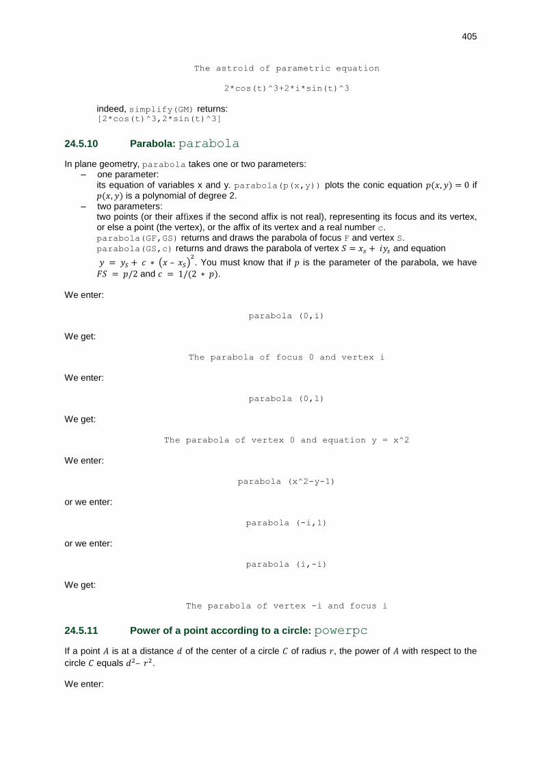
405

The astroid of parametric equation

2*cos(t)^3+2*i*sin(t)^3

indeed, simplify(GM) returns: [2*cos(t)^3,2*sin(t)^3]

24.5.10 Parabola: parabola

In plane geometry, parabola takes one or two parameters: – one parameter:

its equation of variables x and y. parabola(p(x,y)) plots the conic equation 𝑝(𝑥, 𝑦) = 0 if

𝑝(𝑥, 𝑦) is a polynomial of degree 2. – two parameters:

two points (or their affixes if the second affix is not real), representing its focus and its vertex, or else a point (the vertex), or the affix of its vertex and a real number c. parabola(GF,GS) returns and draws the parabola of focus F and vertex S. parabola(GS,c) returns and draws the parabola of vertex 𝑆 = 𝑥𝑠 + 𝑖𝑦𝑠 and equation

𝑦 = 𝑦𝑆 + 𝑐 ∗ (𝑥 – 𝑥𝑆)2. You must know that if 𝑝 is the parameter of the parabola, we have

𝐹𝑆 = 𝑝/2 and 𝑐 = 1/(2 ∗ 𝑝). We enter:

parabola (0,i)

We get:

The parabola of focus 0 and vertex i

We enter:

parabola (0,1)

We get:

The parabola of vertex 0 and equation y = x^2

We enter:

parabola (x^2-y-1)

or we enter:

parabola (-i,1)

or we enter:

parabola (i,-i)

We get:

The parabola of vertex -i and focus i

24.5.11 Power of a point according to a circle: powerpc

If a point 𝐴 is at a distance 𝑑 of the center of a circle 𝐶 of radius 𝑟, the power of 𝐴 with respect to the

circle 𝐶 equals 𝑑2– 𝑟2. We enter:

406

powerpc(circle(0,1+i),3+i)

We get:

8

Indeed: 𝑟 = √2 and 𝑑 = √10 then 𝑑2– 𝑟2 = 8

24.6 Transformation

24.6.1 Homothety: homothety

In plane geometry, homothety takes two or three arguments: a point (the center of the homothety), a real (the value of the ratio of the homothety) and eventually the geometrical object to be transformed. When homothety has two arguments, this function applies on a geometrical object. We enter:

h:=homothety(i,2)

Then:

h(1+i)

We get:

The point 2+i plotted as a black cross (x)

When homothety has three arguments, homothety draws and returns the transform of the third argument in the homothety of center the first argument and ratio the second argument. We enter:

homothety(i,2,1+i)

We get:

The point 2+i plotted as a black cross (x)

We enter:

homothety(i,2,circle(1+i,1))

We get:

The circle of center 2+i and radius 2

Note:

When the value of the homothety ratio is a non real complex number k, homothety(GA,k) is the similarity of center the point A, of ratio abs(k) and angle arg(k).

24.6.2 Inversion: inversion

In plane geometry, inversion takes two or three arguments: a point (the center of the inversion), a real (the value of the ratio of the inversion) and eventually the geometrical object to be transformed. When inversion has two arguments, this function applies on a geometrical object.

If GF:=inversion(GC,k) and GB:=GF(GA), we have 𝐶𝐴 ∗ 𝐶𝐵 = 𝑘. We enter:

407

GF:=inversion(i,2)

Then:

GF(circle(1+i,1))

We get:

The vertical line of equation x=1

We enter:

GF(circle(1+i,1/2))

We get:

The circle of center 8/3+i and radius 4/3 (passing by the point 4+i)

When inversion has three arguments, inversion draws and returns the transform of the third argument in the inversion of center the first argument and ratio the second argument.

If A1:=inversion(C,k,A) we have CA ∗ CA1 = k.

We enter:

inversion(i,2,circle(1+i,1))

We get:

The vertical line of equation x=1

We enter:

inversion(i,2,circle(1+i,1/2))

We get:

The circle of center 8/3+i and radius 4/3, passing by the point 4+i

24.6.3 Orthogonale projection: projection

In plane geometry, projection takes one or two arguments: a geometrical object and eventually a point. When projection has one argument, this function applies on a point and projects this point orthogonally on the geometrical object. We enter:

p1:=projection(line(-1,i))

Then:

p1(1+i)

We get:

The point 1/2+3/2*i shows as a black cross (x)

We enter:

p2:=projection(circle(-1,1))

408

p2(i)

We get:

The point of affix, sqrt(2)/2+(i)*sqrt(2)/2-1, shows as a black cross

(x)

When projection has two arguments, projection draws and returns the transform of the point supplied as second argument by the orthogonal projection on the first argument. We enter:

projection(line(-1,i),1+i)

We get:

The point 1/2+3/2*i shows as a black cross (x)

We enter:

projection(circle(-1,1),i)

We get:

The point of affix, -1+sqrt(2)/2+(i)*sqrt(2)/2, shows as a black

cross (x)

24.6.4 Symmetry line and symmetry point: reflection

In plane geometry, reflection takes one or two arguments: a point or a line, and eventually the geometrical object to be transformed. When reflection has one argument, this function applies on a geometrical object: when the first argument is a point (or a complex number), it is the symmetry with respect to this point (or with respect to point of affixe this complex number) and when the first argument is a line ,it is the symmetry with

respect to this line. We enter:

sp:=reflection(-1)

Then:

sp(1+i)

We get:

The point -3-i plotted as a black cross (x)

We enter:

sd:=reflection(line(-1,i))

Then:

sd(1+i)

We get:

The point 2*i plotted as a black cross (x)

409

When reflection has two arguments, reflection draws and returns the transform of the second argument in the symmetry defined by the first argument: when the first argument is a point (or a complex number) it is the symmetry with respect to this point (or with respect to point of affix this complex number) and when the first argument is a line ,it is the symmetry with respect to this line. We enter:

reflection(-1,1+i)

We get:

The point -3-i plotted as a black cross (x)

We enter:

reflection(line(-1,i),1+i)

We get:

The point 2*i plotted as a black cross (x)

24.6.5 Rotation: rotation

In plane geometry, rotation takes two or three arguments. When rotation has two arguments, these are: a point (the center of rotation) and a real (the measure of the rotation angle); this function applies on a geometrical object (point, line, etc., ...) We enter:

r:=rotation(i,-pi/2)

Then:

r(1+i)

We get, if we have checked radian in the CAS configuration:

The point 0 plotted as a black cross (x)

When rotation has three arguments, these are: a point (the center of rotation), a real (the measure of the rotation angle) and the geometrical object to be transformed; rotation draws and returns the transform of the third argument in the rotation of center the first argument and measure of rotation angle the second argument. We enter:

rotation(i,-pi/2,1+i)

We get, if we have checked radian in the CAS configuration:

The point 0 plotted as a black cross (x)

We enter:

rotation(i,-pi/2,line(1+i,-1))

We get, if we have checked radian in the CAS configuration:

The line passing by 0 and -1+2*i

410

24.6.6 Similarity: similarity

In plane geometry, similarity takes three or four arguments: a point (the center of rotation), a real (the value of the ratio 𝑘 of the similarity), a real (the measure 𝑎 of the rotation angle in radians (or degrees)) and eventually the geometrical object to be transformed. Note: if the ratio 𝑘 is negative, the angle of the similarity is then of measure −𝑎 radians (or degrees). When similarity has three arguments, this function applies on a geometrical object. We enter:

GS:=similarity(i,2,-pi/2)

Then:

GS(1+i)

We get, if we have chosen radian in the CAS configuration:

The point -i plotted as a black cross (x)

We enter:

GS(circle(1+i,1))

We get, if we have chosen radian in the CAS configuration:

The circle of center -i and radius 2

When similarity has four arguments, similarity draws and returns the transform of the fourth argument in the similarity of center the first argument, of ratio the second argument and angle the third argument. We enter:

similarity(i,2,-pi/2,1+i)

We get, if we have chosen radian in the CAS configuration:

The point -i plotted as a black cross (x)

We enter:

similarity(i,2,-pi/2,circle(1+i,1))

We get, if we have chosen radian in the CAS configuration:

The circle of center -i and radius 2

Note: In 2D, the similarity of center the point GA, ratio k and angle a results in: similarity(GA,k,a) or by homothety(GA,k*exp(i*a)).

24.6.7 Translation: translation

In plane geometry, translation takes one or two arguments: the vector of translation supplied by a geometrical vector, or by the list of its coordinates, or by its affix (difference between the coordinates of two points, or a complex number) and eventually the geometrical object to be transformed. When translation has one argument, this function applies on a geometrical object. We enter:

411

t:=translation(1+i)

Then:

t(-2)

We get:

The point -1+i plotted as a black cross (x)

When translation has two arguments, translation draws and returns the transform of the second argument in the translation of vector the first argument. We enter:

translation([1,1],-2)

Or we enter:

GA:=point(1);GB:=point(2+i);translation(vector(GA,GB),-2)

Or we enter:

translation(1+i,-2)

Or we enter:

GA:=point(1);GB:=point(2+i);translation(GB-GA,-2)

We get:

The point -1+i plotted as a black cross (x)

We enter:

translation(1+i,line(-2,-i))

We get:

The line passing by -1+i and 1

24.7 Measure and graphics

24.7.1 Measure of a angle: angleat

angleat takes as argument the name of three points and a point (or the affix of this point supplied as a complex number). Warning! Take care that the three first arguments are names. angleat returns the fourth point, calculates the measure (in radians or in degrees) of the oriented angle of vertex the first argument, the second argument is on the first side of the angle and the third argument on the second side, and this measure is displayed, along with a label, at the location of the fourth point. Thus, angleat(GA,GB,GC,GD) designates the measure of the angle in radians (or in degrees) of

(𝐴𝐵⃗⃗⃗⃗ ⃗, 𝐴𝐶⃗⃗⃗⃗ ⃗) and this measure will be displayed, preceded by 𝛼𝐴 =, at the location of point D. We enter this command in the Symbolic view. We enter:

GA:=point(-1);GB:=point(1+i);GC:=point(i);

412

segment(GA,GB); segment (GA,GC);

angleat(GA,GB,GC,0.2i)

We get, if we have checked radian in the CAS configuration (Shift-CAS):

αA=atan(1/3) is displayed at the point(0.4i)

24.7.2 Measure of a angle: angleatraw

angleatraw takes as argument four points (or the affixes of these points supplied as four complex numbers). angleatraw returns the fourth point, returns the measure (in radians or in degrees) of the oriented angle of vertex the first argument, the second point is on the first side of the angle, the third point on the second side and the measure is displayed, along with a label, close to the fourth point. Thus, angleatraw(GA,GB,GC,GD) designates the measure of the angle in radians (or in degrees)

of (𝐴𝐵⃗⃗⃗⃗ ⃗, 𝐴𝐶⃗⃗⃗⃗ ⃗) and this measure will be displayed at the location of point D. We enter:

GA:=point(-1);GB:=point(1+i);GC:=point(i);

segment (GA,GB); segment (GA,GC);

angleatraw(GA,GB,GC,0.2i)

We get, if we have checked radian in the CAS configuration (Shift-CAS):

atan(1/3) is displayed at the point(0.4i)

24.7.3 Display of the area of a polygon: areaat

areaat takes as arguments the name of a circle or of a polygon and a point (or the affix of a point supplied as a complex number). areaat returns the point, the area of the circle or polygon and displays this area at the location of the point with a label. Warning! Take care that the first argument is the name of a circle or of a polygon. We enter:

t:=triangle(0,1,i)

areaat(t,(1+i)/2)

We get:

1/2 is displayed at the point(1+i)/2 with the label

We enter:

cc:=circle(0,2)

areaat(cc,2.2)

We get:

4*pi is displayed at the point(2.2) with a label

We enter:

413

c:=square(0,2)

areaat(c,2.2)

We get:

4 is displayed at the point(2.2) with a label

We enter:

h:=hexagon(0,1)

areaat(h,1.2)

We get:

3*sqrt(3)/2 is displayed at the point(1.2) with a label

24.7.4 Area of a polygon: areaatraw

areaatraw takes as arguments a circle or a polygon and a point (or the affix of a point supplied as a complex number). areaatraw returns the point, the area of the circle or of the polygon and displays this area at the location of the point. We enter:

areaatraw(triangle(0,1,i),(1+i)/2)

We get:

1/2 is displayed at the point(1+i)/2

We enter:

areaatraw(circle(0,2),2.2)

We get:

4*pi is displayed at the point(2.2)

We enter:

areaatraw(square(0,2),2.2)

We get:

4 is displayed at the point(2.2)

We enter:

areaatraw(hexagon(0,1),1.2)

We get:

3*sqrt(3)/2 is displayed at the point(1.2)

24.7.5 Length of a segment: distanceat

distanceat is a command which allows to display at a point the length of a segment with a label.

414

We enter this command in the Symbolic view. distanceat takes three arguments: the name of two points and a point (or the affix of this point) or else the name of two geometrical objects and a point (or the affix of this point). Warning! Take care that the two first arguments are names of point. distanceat returns the point supplied in third argument, the length of the segment defined by the two fist points or the distance between the two geometrical objects and displays this length at the location of the third point, preceeded by a label. We enter (we must give the name of the objects):

GA:=point(-1);GB:=point(1+i);

distanceat(GA,GB,0.4i)

We get:

"GAB=sqrt(5)" is displayed at the point(0.4i)

We enter (you must give the name of the objects):

GC:=point(0);GD:=line(-1,1+i)

distanceat(GC,GD,i/2)

We get:

"GCD=sqrt(5)/5" is displayed at the point(i/2)

We enter (me must give the name of the objects):

GK:=circle(0,1); GL:=line(-2,1+3i)

distanceat(GK,GL,0)

We get:

"GKL=sqrt(2)-1" is displayed at the point(0)

24.7.6 Length of a segment: distanceatraw

distanceatraw is a command which allows to display at a point the length of a segment, but with no label. We enter this command in the Symbolic view. distanceatraw takes as argument three points (or two points and the affix of a point supplied as a complex number) or else two geometrical objects and a point (or the affix of this point). distanceatraw returns the point supplied in third argument, the length of the segment defined by the two fist points, or the distance between the two geometrical objects, and displays this length at the location of the third point. We enter:

GA:=point(-1);GB:=point(1+i);

distanceatraw(GA,GB,0.4i)

Or we enter directly:

distanceatraw(point(-1),point(1+i),0.4i)

We get:

415

sqrt(5) is displayed at the point(0.4i)

We enter:

GC:=point(0);GD:=line(-1,1+i)

distanceatraw(GC,GD,i/2)

Or we enter directly:

distanceatraw(point(0),line(-1,1+i),0.4i)

We get:

sqrt(5)/5 is displayed at the point(i/2)

We enter:

GK:=circle(0,1); GL:=line(-2,1+3i)

distanceatraw(GK,GL,0)

Or we enter directly:

distanceatraw(circle(0,1),line(-2,1+3i),0.4i)

We get:

sqrt(2)-1 is displayed at the point(0)

24.7.7 Perimeter of a polygon: perimeterat

perimeterat takes as argument the name of a circle or of a polygon and a point (or the affix of a point supplied as a complex number). perimeterat returns the point, the perimeter of the circle or of the polygon, and displays this perimeter at the location of the point with a label. We enter this command in the Symbolic view. Warning! Take care that the first argument is the name of a circle or of a polygon. We enter:

t:=triangle(0,1,i)

perimeterat(t,(1+i)/2)

We get:

2+sqrt(2) is displayed at the point((1+i)/2) with a label

We enter:

c:=square(0,2)

perimeterat(c,2.2)

We get:

8 is displayed at the point(2.2) with a label

We enter:

416

cc:=circle(0,2)

perimeterat(cc,2.2)

We get:

4*pi is displayed at the point(2.2) with a label

We enter:

h:=hexagon(0,1)

perimeterat(h,1.2)

We get:

6 is displayed at the point(1.2) with a label

24.7.8 Perimeter of a polygon: perimeteratraw

perimeteratraw takes as argument a circle or a polygon, and a point (or the affix of a point supplied as a complex number). perimeteratraw returns the point, the perimeter of the circle or of the polygon, and displays this perimeter at the location of the point. We enter this command in the Symbolic view. We enter:

perimeteratraw(triangle(0,1,i),(1+i)/2)

We get:

2+sqrt(2) is displayed at the point((1+i)/2)

We enter:

perimeteratraw(circle(0,2),2.2)

We get:

4*pi is displayed at the point(2.2)

We enter:

perimeteratraw(hexagon(0,1),1.2)

We get:

6 is displayed at the point(1.2)

We enter:

perimeteratraw(square(0,2),2.2)

We get:

8 is displayed at the point(2.2)

417

24.7.9 Slope of a line: slopeat

slopeat is a command which allows to display at a point the slope of a line, or of a segment, with a label. We enter this command in the Symbolic view. slopeat takes two arguments: the name of a line (or of a segment), and a point (or the affix of a point supplied as a complex number). slopeat returns the point, the slope of the line (or of the segment) and displays this slope at the location of the point, with a label. Warning! Take care that the first argument is the name of a line or of a segment. We enter:

GD:=line(1,2i)

Or we enter:

GD:= segment (1,2i),i)

slopeat(GD,i)

We get:

"sD=-2" is displayed at the point(i)

We enter:

GP:=line(2y-x=3),2*i)

slopeat(GP,2*i)

We get:

"sP=1/2" is displayed at the point(2*i)

We enter:

GT:=tangent(plotfunc(sin(x)),pi/4)

Or we enter:

GT:=LineTan(sin(x),pi/4)

Then:

slopeat(GT,i)

We get:

"sT=(sqrt(2))/2" is displayed at the point(i)

24.7.10 Slope of a line: slopeatraw

slopeatraw is a command which allows to display at a point the slope of a line or of a segment but with no label. We enter this command in the Symbolic view. slopeatraw takes two arguments: a line (or a segment) and a point (or the affix of a point supplied as a complex number). slopeatraw returns the point, the slope of the line (or of the segment), and displays this slope at the location of the point.

418

We enter:

GD:=line(1,2i)

slopeatraw(GD,i)

Or we enter directly:

slopeatraw(line(1,2i),i)

We get:

-2 is displayed at the point(i)

We enter:

GE:= segment (1,2i),i)

slopeatraw(GE,1)

Or we enter directly:

slopeatraw(segment (1,2i),1)

We get:

-2 is displayed at the point(1)

We enter:

GP:=line(2y-x=3,2*i)

slopeatraw(GP,2*i)

Or we enter directly:

slopeatraw(line(2y-x=3,2*i),2*i)

We get:

1/2 is displayed at the point(2*i)

We enter:

GT:=tangent(plotfunc(sin(x)),pi/4)

slopeat(GT,i)

Or we enter directly:

slopeatraw(tangent(plotfunc(sin(x)),pi/4),i)

We get:

(sqrt(2))/2 is displayed at the point(i)

419

24.8 Measure

24.8.1 Abscissa of a point or of a vector: abscissa

In plane geometry, abscissa takes as argument a point, a vector, or a complex number. abscissa returns the abscissa of the point or of the vector: - if the point A is of cartesian coordinates (𝑥𝐴, 𝑦𝐴), abscissa(GA) returns 𝑥𝐴,

- if the point B is of cartesian coordinates (𝑥𝐵 , 𝑦𝐵), abscissa(GA-GB) returns 𝑥𝐴– 𝑥𝐵 (because GA-

GB designates the vector 𝐵𝐴⃗⃗⃗⃗ ⃗. We enter:

abscissa(point(1+2*i))

We get:

1

We enter:

abscissa(point(i)-point(1+2*i))

We get:

-1

We enter:

abscissa(1+2*i)

We get:

1

We enter:

abscissa([1,2])

We get:

1

24.8.2 Affix of a point or of a vector: affix

affix takes as argument a point, a vector, or the coordinates of a point or of a 2D vector. affix returns the affix of the point or of the vector:

– if the point A is of cartesian coordinates (𝑥𝐴, 𝑦𝐴), affix(GA) returns 𝑥𝐴 + 𝑖 ∗ 𝑦𝐴 – if the point B is of cartesian coordinates (𝑥𝐵 , 𝑦𝐵), affix(GA-GB) or

affix(vector(GB,GA)) returns 𝑥𝐴– 𝑥𝐵 + 𝑖 ∗ (𝑦𝐴– 𝑦𝐵) (because GA-GB designates the

vector 𝐵𝐴⃗⃗⃗⃗ ⃗ and coordinates(vector(GB,GA))returns [𝑥𝐴 + 𝑖 ∗ 𝑦𝐴 , 𝑥𝐵 + 𝑖 ∗ 𝑦𝐵]. We enter:

affix(point(i))

We get:

i

420

We enter:

affix(point(i)-point(1+2*i))

We get:

-1-i

24.8.3 Measure of a angle: angle

angle takes as argument three points (or the affixes of these points supplied as three complex numbers) and eventually a string used as label along with the symbol of an arc of circle which represents the angle on the figure (the arc of circle is replaced by the symbol of the half of a square in

the case of the angle equals 𝜋/2 or −𝜋/2). angle returns the measure (in radians or in degrees) of the oriented angle of vertex the first argument, the second argument is on the first side of the angle and the third argument is on the second side. Then:

angle(GA,GB,GC) designates the measure of the angle in radians (or in degrees) of (𝐴𝐵⃗⃗⃗⃗ ⃗, 𝐴𝐶⃗⃗⃗⃗ ⃗).

angle(GA,GB,GC,"") plots the angle (𝐴𝐵⃗⃗⃗⃗ ⃗, 𝐴𝐶⃗⃗⃗⃗ ⃗) with as label a small oriented arc.

angle(GA,GB,GC,"a") plots the angle (𝐴𝐵⃗⃗⃗⃗ ⃗, 𝐴𝐶⃗⃗⃗⃗ ⃗) with as label a small oriented arc written a. angle(GA,GB,GC,"")[0] or angle(GA,GB,GC,"a")[0] designates the measure of the angle in

radians (or in degrees) of (𝐴𝐵⃗⃗⃗⃗ ⃗, 𝐴𝐶⃗⃗⃗⃗ ⃗). We enter:

angle(0,1,1+i)

We get, if we have chosen radian in the CAS configuration:

pi/4

We enter:

angle(0,1,1+i,"")

We get, if we have checked radian in the CAS configuration:

[pi/4,circle(point(0,0),1/5)] and the angle is designated by an arc

of circle without label.

We enter:

angle(0,1,1+i,"a")

We get, if we have checked radian in the CAS configuration:

[pi/4,circle(point(0,0),1/5)] and the angle is deisgnated by an arc

of circle with as label.

We enter:

angle(0,1,i,"a")

We get, if we have checked radian in the CAS configuration:

[pi/2,polygon(point(1/5,0),point(1/5,1/5),point(0,1/5),point(0,1/5))]

and the right angle is designated by an half of square with the label

a.

421

24.8.4 Length of an arc of curve: arcLen

arcLen takes one or four parameters. Warning! Take care to not be in complex mode.

– the parameter is either a circle or an arc of circle, either a polygon. We enter:

arcLen(circle(0,1,0,pi/2))

We get:

pi/4

We enter:

arcLen(hexagon(0,1))

We get:

6

– the four parameters are: an expression 𝑒𝑥𝑝𝑟 (resp. a list of two expressions [𝑒𝑥𝑝𝑟1, 𝑒𝑥𝑝𝑟2]), the name of a parameter and two values 𝑎 and 𝑏 of this parameter.

arcLen returns the length of the arc of curve defined by the equation 𝑦 = 𝑓(𝑥) = 𝑒𝑥𝑝𝑟 (resp. by 𝑥 = 𝑒𝑥𝑝𝑟1, 𝑦 = 𝑒𝑥𝑝𝑟2) for the values of the parameter between 𝑎 and 𝑏. We have then arcLen(f(x),x,a,b)=: integrate(sqrt(diff(f(x),x)^2+1),x,a,b) or integrate(sqrt(diff(x(t),t)^2+diff(y(t),t)^2),t,a,b).

Examples

– Calculate the length of the arc of circle 𝐴𝐵 (with 𝐴 = (0, 0) and 𝐵 = (0, 1)) and angle at

center 𝜋/2. We enter:

arcLen(arc(0,1,pi/2))

We get:

sqrt(2)*pi/4

– Calculate the perimeter of the triangle 𝐴𝐵𝐶 (with 𝐴 = (0, 0), 𝐵 = (0, 1) and 𝐶 = (1, 1)). We enter:

arcLen(triangle(0,1,1+i))

We get:

sqrt(2)+2

– Calculate the length of the arc of parabola 𝑦 = 𝑥2 to x from 0 to 𝑥 = 1. We enter:

arcLen(x^2,x,0,1)

or

422

arcLen([t,t^2],t,0,1)

We get:

(sqrt(5))/2-ln(sqrt(5)-2)/4

– Calculate the length of the arc of the curve 𝑦 = cosh(𝑥) for 𝑥 from 0 to 𝑥 = ln(2). We enter:

arcLen(cosh(x),x,0,log(2))

We get:

3/4

– Calculate the length of the arc of circle 𝑥 = 𝑐𝑜𝑠(𝑡), 𝑦 = 𝑠𝑖𝑛(𝑡) for 𝑡 from 0 to 𝑡 = 2 ∗ 𝜋. We enter:

arcLen([cos(t),sin(t)],t,0,2*pi)

We get:

2*pi

24.8.5 Area of a polygon: area

area returns the area of a circle or of a polygon. We enter:

area(triangle(0,1,i))

We get:

1/2

We enter:

area(square(0,2))

We get:

4

24.8.6 Coordinates of a point, a vector or a line: coordinates

In plane geometry, coordinates takes as argument a point, a complex number, a vector or a line. coordinates returns the list of the abscissa and the ordinate of the point, or the vector, or the list of affixes of two points of the oriented line.

– if the point A is of cartesian coordinates (𝑥𝐴, 𝑦𝐴), coordinates(GA) returns [𝑥𝐴 , 𝑦𝐴], – if the point B is of cartesian coordinates (𝑥𝐵 , 𝑦𝐵), coordinates(vector(GA,GB)) or

coordinates(GB-GA) returns [𝑥𝐵– 𝑥𝐴 , 𝑦𝐵– 𝑦𝐴] (whereas B-A returns (𝑥𝐵– 𝑥𝐴) + 𝑖 ∗

(𝑦𝐵– 𝑦𝐴) because B-A designates the affix of the vector AB in plane geometry),

– if the vector V is of cartesian coordinates (𝑥𝑉 , 𝑦𝑉), coordinates(GV) or

coordinates(vector(GA,GV)) returns [𝑥𝑉 , 𝑦𝑉], – if a line D is defined by two points A and B, coordinates(GD) returns

[affix(GA),affix(GB)]. If D is defined by its equation, coordinates(GD) returns

423

[affix(GA),affix(GB)] where A and B are two points of the line D, the vector AB having same orientation as d.

We enter:

coordinates(point(1+2*i))

Or we enter:

coordinates(1+2*i)

We get:

[1,2]

We enter:

coordinates(point(1+2*i)-point(i))

Or we enter:

coordinates(point(1+2*i)-point(i))

We get:

[1,1]

We enter:

coordinates(vector(point(i),point(1+2*i)))

Or we enter:

coordinates(vector(i,1+2*i))

Or we enter:

coordinates(vector([0,1],[1,2]))

We get:

[1,1]

We enter:

coordinates(1+2*i)

Or we enter:

coordinates(vector(1+2*i))

Or we enter:

coordinates(vector(point(i),vector(1+2*i)))

We get:

[1,2]

We enter:

424

coordinates(point(i),vector(1+2*i))

We get:

[1,2]

We enter:

d:=line(-1+i,1+2*i)

Or we enter

d:=line(point(-1,1),point(1,2))

Then,

coordinates(d)

We get:

[-1+i,1+2*i]

We enter:

d:=line(y=(1/2*x+3/2))

We get:

[(3*i)/2,1+2*i]

We enter:

d:=line(x-2*y+3=0)

We get:

[(3*i)/2,(-4+i)/2]

Warning! coordinates might also take as argument a sequence or a list of points. Then, coordinates returns the sequence or the list of lists of coordinates of these points, for example: coordinates(i,1+2*i) or coordinates(point(i),point(1+2*i)) returns the sequence: [0,1],[1,2] and coordinates([i,1+2*i]) or coordinates([point(i),point(1+2*i)]) returns the matrix: [[0,1],[1,2]] so coordinates([1,2]) returns the matrix: [[1,0],[2,0]] because [1,2] is considered as the list of two points of affix 1 and 2.

24.8.7 Rectangular coordinates of a point: rectangular_coordinates

rectangular_coordinates returns the list of the abscissa and the ordinate of a point supplied by the list of its polar coordinates. We enter:

rectangular_coordinates(2,pi/4)

Or we enter:

425

rectangular_coordinates(polar_point(2,pi/4))

We get:

[2/(sqrt(2)),2/(sqrt(2))]

24.8.8 Polar coordinates of a point: polar_coordinates

polar_coordinates returns the list of the modulus and the argument of the affixe of a point, of a

complex number, or of the list of rectangular coordinates. We enter:

polar_coordinates(1+i)

Or we enter:

polar_coordinates(point(1+i))

Or we enter:

polar_coordinates([1,1])

We get:

[sqrt(2),pi/4]

24.8.9 Length of a segment and distance between two geometrical objects:

distance

distance takes as argument two points (or the affixes of these points supplied as two complex numbers) or two geometrical objects. distance returns the length of the segment defined by these two points or the distance between the two geometrical objects. We enter:

distance(-1,1+i)

We get:

sqrt(5)

We enter:

distance(0,line(-1,1+i))

We get:

sqrt(5)/5

We enter:

distance(circle(0,1),line(-2,1+3i))

We get:

sqrt(2)-1

426

24.8.10 Square of the length of a segment: distance2

distance2 takes as argument two points (or two points and a the affix of a point supplied as a complex number). distance2 returns the square of the length of the segment defined by these two points. We enter:

distance2(-1,1+i)

We get:

5

24.8.11 Cartesian equation of a geometrical object: equation

equation allows to get the cartesian equation of a geometrical object. Warning! Prior to use equation, take care of purging the variables x and y by entering purge(x) and purge(y) or x:=’x’ and y:=’y’. We enter:

equation(line(point(0,1,0),point(1,2,3)))

We get:

(x-y+1=0,3*x+3*y-2*z=0)

We enter:

equation(sphere(point(0,1,0),2))

We get:

x^2+y^2+-2*y+z^2-3=0

which is the equation of the sphere of center (0,1,0) and radius 2.

24.8.12 Get as answer the value of a measure displayed:

extract_measure

extract_measure allows to get the value of a measure which has been displayed. extract_measure takes as argument the command which previously displayed this measure. We enter:

GA:=point(-1);GB:=point(1+i);GC:=segment(GA,GB)

extract_measure(distanceat(GA,GB,i))

We get:

sqrt(5)

We enter:

extract_measure(distanceatraw(GA,GB,i))

We get:

427

sqrt(5)

We enter:

extract_measure(slopeat(GC,i))

We get:

1/2

We enter:

extract_measure(slopeatraw(GC,i))

We get:

1/2

24.8.13 Ordinate of a point or of a vector: ordinate

In plane geometry, ordinate takes as argument a point, a vector, or a complex number. ordinate returns the ordinate of the point or of the vector:

– if the point A is of cartesian coordinates (𝑥𝐴, 𝑦𝐴), ordinate(GA) returns 𝑦𝐴,

– if the point B is of cartesian coordinates (𝑥𝐵 , 𝑦𝐵), ordinate(GA-GB) returns 𝑦𝐴– 𝑦𝐵

(A-B designates the vector 𝐵𝐴⃗⃗⃗⃗ ⃗).

We enter:

ordinate(point(1+2*i))

We get:

2

We enter:

ordinate(point(i)-point(1+2*i))

We get:

-1

We enter:

ordinate(1+2*i)

We get:

2

We enter:

ordinate([1,2])

We get:

2

428

24.8.14 Parametric equation of a geometrical object: parameq

In plane geometry, parameq allows to get the parametric equation of a geometrical object in the form of the complex number 𝑥(𝑡) + 𝑖 ∗ 𝑦(𝑡). Warning! Prior to use parameq, take care of purging the variable t by entering: purge(t) or t:=’t’. We enter:

parameq(line(-1,i))

We get:

-t+(1-t)*(i)

We enter:

parameq(circle(-1,i))

We get:

-1+exp(i*t)

We enter:

normal(parameq(ellipse(-1,1,i)))

We get:

sqrt(2)*cos(t)+(i)*sin(t)

24.8.15 Perimeter of a polygon: perimeter

perimeter returns the perimeter of a circle or of a polygon. See also the command arcLen. We enter:

perimeter(triangle(0,1,i))

We get:

2+sqrt(2)

We enter:

perimeter(square(0,2))

We get:

8

24.8.16 Radius of a circle: radius

radius takes as argument a circle. radius returns the length of the radius of this circle. We enter:

radius(circle(-1,i))

429

We get:

1

We enter:

radius(circle(-1,point(i)))

We get:

sqrt(2)/2

24.8.17 Slope of a line: slope

slope is either a command, either a parameter of the command line (See 24.3.7) When slope is a command, it takes argument a line, a segment, two points or two complex numbers. slope returns the slope of the line defined by the segment, the two points, or their affixes. We enter:

slope(line(1,2i))

Or we enter:

slope(segment (1,2i))

Or we enter:

slope(point(1),point(2i))

Or we enter:

slope(1,2i)

We get:

-2

We enter:

slope(line(2y-x=3))

We get:

1/2

We enter:

slope(tangent(plotfunc(sin(x)),pi/4))

Or we enter:

slope(LineTan(sin(x),pi/4))

We get:

(sqrt(2))/2

430

24.9 Test

24.9.1 Check whether three points are collinear: is_collinear

is_collinear is a boolean function and takes as argument a list or a sequence of points. is_collinear equals 1 if the points are collinear, 0 otherwise. We enter:

is_collinear(0,1+i,-1-i)

We get:

1

We enter:

is_collinear(i/100,1+i,-1-i)

We get:

0

24.9.2 Check whether four points are concyclic: is_concyclic

is_concyclic is a boolean function and takes as argument a list or a sequence of points. is_concyclic equals 1 if the points are concyclic, 0 otherwise. We enter:

is_concyclic(1+i,-1+i,-1-i,1-i)

We get:

1

We enter:

is_concyclic(i,-1+i,-1-i,1-i)

We get:

0

24.9.3 Check whether elements are conjugates: is_conjugate

is_conjugate allows to know if four points are conjugates, or if two points, two lines, or a line and a point are conjugates for a circle or for two lines. is_conjugate is a boolean function and takes as arguments two points (resp. two lines, or a circle) followed by two points, two lines, or a line and a point. is_conjugate equals 1 if the arguments are conjugates, 0 otherwise. We enter:

is_conjugate(circle(0,1+i),point(1-i),point(3+i))

We get:

1

431

We enter:

is_conjugate(circle(0,1),point((1+i)/2),line(1+i,2))

Or we enter:

is_conjugate(circle(0,1),line(1+i,2),point((1+i)/2))

We get:

1

We enter:

is_conjugate(circle(0,1),line(1+i,2), line((1+i)/2,0))

We get:

1

We enter:

is_conjugate(point(1+i),point(3+i),point(i),point(i+3/2))

We get:

1

We enter:

is_conjugate(line(0,1+i),line(2,3+i), line(3,4+i),line(3/2,5/2+i))

We get:

1

24.9.4 Check whether points or/and lines are coplanar: is_coplanar

is_coplanar checks whether a list, or a sequence of points, or of lines are coplanar. We enter:

is_coplanar([0,0,0],[1,2,-3],[1,1,-2],[2,1,-3])

We get:

1

We enter:

is_coplanar([-1,2,0],[1,2,-3],[1,1,-2],[2,1,-3])

We get:

0

We enter:

is_coplanar([0,0,0],[1,2,-3],line([1,1,-2],[2,1,-3]))

We get:

432

1

We enter:

is_coplanar(line([0,0,0],[1,2,-3]),line([1,1,-2],[2,1,-3]))

We get:

1

We enter:

is_coplanar(line([-1,2,0],[1,2,-3]), line([1,1,-2],[2,1,-3]))

We get:

0

24.9.5 Check whether a point is on a geometrical object: is_element

is_element is a boolean function and takes as argument a point and a geometrical object. is_element equals 1 if the point is on the geometrical object, 0 otherwise. We enter:

is_element(point(-1-i),line(0,1+i))

We get:

1

We enter:

is_element(point(i),line(0,1+i))

We get:

0

24.9.6 Check whether a triangle is equilateral: is_equilateral

is_equilateral is a boolean function and takes as argument three points or a geometrical object. is_equilateral equals 1 if the three points form an equilateral triangle, or if the geometrical object is an equilateral triangle, 0 otherwise. We enter:

is_equilateral(0,2,1+i*sqrt(3))

We get:

1

We enter:

GT:=equilateral_triangle(0,2,GC);is_equilateral(GT[0])

We get:

1

433

Indeed, GT[0] designates a triangle because GT is a list composed of the triangle and its vertex GC.

We enter affix(GC) and we get 1+i*sqrt(3)

We enter:

is_equilateral(1+i,-1+i,-1-i)

We get:

0

24.9.7 Check whether a triangle is isoscele: is_isosceles

is_isosceles is a boolean function and takes as argument three points or a geometrical object. is_isosceles equals 1 (resp. 2, 3) if the three points form an isosceles triangle or if the geometrical object is an isosceles triangle whose angle between the two equal sides is designated by the first (resp. second, third) argument, or equals 4 if the three points form an equilateral triangle, or if the geometrical object is an equilateral triangle, 0 otherwise. We enter:

is_isosceles(1,1+i,i)

We get:

2

We enter:

GT:=isosceles_triangle(0,1,pi/4);is_isoceles(GT)

We get:

1

We enter:

GT:=isosceles_triangle(0,1,pi/4,GC);is_isoceles(GT[0])

We get:

1

Indeed, GT[0] designates a triangle because GT is a list composed of the triangle and its vertex C.

We enter affix(GC) and we get (sqrt(2))/2+((i)*sqrt(2))/2

We enter:

is_isosceles(1+i,-1+i,-i)

We get:

3

24.9.8 Orthogonality of two lines or two circles: is_orthogonal

is_orthogonal is a boolean function and takes as argument two lines or two circles.

434

is_orthogonal equals 1 if the two lines or the two circles (i.e if the tangents at their cross points are orthogonal), 0 otherwise. We enter:

is_orthogonal(line(1,i), line(0,1+i))

We get:

1

We enter:

is_orthogonal(line(2,i), line(0,1+i))

We get:

0

We enter:

is_orthogonal(circle(0,1),circle(sqrt(2),1))

We get:

1

We enter:

is_orthogonal(circle(0,1),circle(2,1))

We get:

0

24.9.9 Check whether two lines are parallel: is_parallel

In plane geometry, is_parallel is a boolean function and takes as argument two lines. is_parallel equals 1 if the two lines are parallel, 0 otherwise. We enter:

is_parallel(line(0,1+i),line(i,-1))

We get:

1

We enter:

is_parallel(line(0,1+i),line(i,-1-i))

We get:

0

24.9.10 Check whether a polygon is a parallelogram: is_parallelogram

is_parallelogram is a boolean function and takes as argument four points or a geometrical object.

435

is_parallelogram equals 1 (resp. 2, 3, 4) if the four points form a parallelogram (resp. a rhombus, a rectangle, a square) or if the geometrical object is a parallelogram (resp. a rhombus, a rectangle, a square), 0 otherwise. We enter:

is_parallelogram(i,-1+i,-1-i,1-i)

We get:

0

We enter:

is_parallelogram(1+i,-1+i,-1-i,1-i)

We get:

1

We enter:

GQ:=quadrilateral(1+i,-1+i,-1-i,1-i);is_parallelogram(GQ)

We get:

4

Warning! We must enter:

GP:=parallelogram(-1-i,1-i,i,GD);is_parallelogram(GP[0])

To get:

1

Indeed, it is GP[0] which designates a parallelogram because GP is a list composed of a parallelogram and its last vertex D. If we enter affix(GD), we get -2+i.

24.9.11 Check whether two lines are perpendicular: is_perpendicular

In plane geometry, is_perpendicular is a boolean function having as argument two lines. is_perpendicular equals 1 if the two lines are perpendicular, and equals 0 otherwise. We enter:

is_perpendicular(line(0,1+i),line(i,1))

We get:

1

We enter:

is_perpendicular(line(0,1+i),line(1+i,1))

436

24.9.12 Check whether a triangle is right or a polygon is a rectangle:

is_rectangle

is_rectangle is a boolean function and takes as argument three or four points, or a geometrical object. is_rectangle equals 1 (resp. 2 or 3) if the three points form a right triangle, the right angle being specified in the first (resp. second, third) argument or if the geometrical object is a right triangle, is_rectangle equals 1 (resp. 2) if the four points form a rectangle (resp. a square) or if the geometrical object is a rectangle (resp. a square), 0 otherwise. We enter:

is_rectangle(1,1+i,i)

We get:

2

We enter:

is_rectangle(1+i,-2+i,-2-i,1-i)

We get:

1

We enter:

GR:=rectangle(-2-i,1-i,3,GC,GD);is_rectangle(GR[0])

We get:

1

Indeed, GR[0] designates a rectangle because GR is a list composed of the rectangle and its vertices C and D.

24.9.13 Check whether a polygon is a rhombus: is_rhombus

is_rhombus is a boolean function and takes as argument four points or a geometrical object. is_rhombus equals 1 (rep 2) if the four points form a rhombus (resp. a square) or if the geometrical object is a rhombus (resp. a square), 0 otherwise. We enter:

is_rhombus(1+i,-1+i,-1-i,1-i)

We get:

1

We enter:

GK:=rhombus(1+i,-1+i,pi/4);is_rhombus(GK)

We get:

1

We enter:

437

GK:=rhombus(1+i,-1+i,pi/4,GC,DD);is_rhombus(GK[0])

We get:

1

Indeed, GK[0] designates a rhombus because GK is a list composed of a rhombus and its vertices GC and GD. If we enter: normal(coordinates(GC,GD)), we get [-sqrt(2)-1,-sqrt(2)+1],[-

sqrt(2)+1,-sqrt(2)+1]. We enter:

is_rhombus(i,-1+i,-1-i,1-i)

We get:

0

24.9.14 Check whether a polygon is a square: is_square

is_square is a boolean function and takes as argument four points or a geometrical object. is_square equals 1 if the four points form a square or if the geometrical object is a square, 0 otherwise. We enter:

is_square(1+i,-1+i,-1-i,1-i)

We get:

1

We enter:

GK:=square(1+i,-1+i);is_square(GK)

We get:

1

We enter:

GK:=square(1+i,-1+i,C,D);is_square(GK[0])

We get:

1

Indeed, GK[0] designates a square because GK is a list composed of a square and ses vertices C and D. If we enter affix(GC,GD), we get -1-i,1-i. We enter:

is_square(i,-1+i,-1-i,1-i)

We get:

0

438

24.9.15 Check whether 4 points form an harmonic division: is_harmonic

is_harmonic allows to know if four points are in harmonic division. is_harmonic is a boolean function and takes as arguments four points. is_harmonic equals 1 if the four points are in harmonic division and 0 otherwise. We enter:

is_harmonic(0,2,3/2,3)

We get:

1

We enter:

is_harmonic(0,1+i,1,i)

We get:

0

24.9.16 Check whether lines are in harmonic bundle:

is_harmonic_line_bundle

is_harmonic_line_bundle takes as argument a list of lines. is_harmonic_line_bundle returns: 1 if these lines are concurrent in a point, 2 if they are parallel, 3 if they are overlapping, and 0 otherwise. We enter:

is_harmonic_line_bundle([line(0,1+i),line(0,2+i),

line(0,3+i),line(0,1)])

We get:

1

24.9.17 Check whether circles are in harmonic bundle:

is_harmonic_circle_bundle

is_harmonic_circle_bundle takes as argument a list of circles. is_harmonic_circle_bundle returns: 1 if these circles form a beam (that is to say if they have by pair the same radical axis), 2 if these circles are concentric, 3 if these circles are overlaping, and 0 otherwise. We enter:

is_harmonic_circle_bundle([circle(0,i),circle(4,i),

circle(0,point(1/2))])

We get:

1

439

24.10 Exercises of geometry

24.10.1 Transformations

– Translation Paving: any plane non crossed quadrilateral might form a pavement of the plane as a regular pattern. We define 4 points A,B,C,D randomly: menu Points->Free points->4 random point In Symb, we change the name of points so that the quadrilateral 𝐴, 𝐵, 𝐶, 𝐷 is not crossed. Then, we define the quadrilateral 𝐴, 𝐵, 𝐶, 𝐷 with the menu Lines->Polygons-

>Quadrilateral and this will be the basis pattern: GE:=quadrilateral(GA,GB,GC,GD) GA:=point()

GB:=point()

GC:=point()

GD:=point

GE:=quadrilateral(GA,GB,GC,GD)

GG:=segment(GA,GB)

GH:= segment (GB,GC)

GI:= segment (GC,GD)

GJ:= segment (GD,GA)

GK:=midpoint(GA,GB)

GL:=reflection(GK,GC)

GM:=reflection(GK,GD)

GN:=quadrilateral(GA,GB,GL,GM)

GO:= segment (GA,GB)

GP:= segment (GB,GL)

GQ:= segment (GL,GM)

GR:= segment (GM,GA)

translation(GB-GD,[GE,GN])

translation(GC-GA,[GE,GN])

– Inversion

The Peaucellier inverter GA:=element(-1.6..1.6,0.6)

GD:=circle(1,1)

GE:=point(1+EXP(i*GA)

GH:=circle(GE,2.)

GI:=circle(0,3.)

GJ:=inter(GH,GI)

GK:=reflection(GJ,GE)

GL:=locus(GK,GA)

GG:=quadrilateral(GE,GJ[0],GK,GJ[1])

GB:=segent(0,GJ[0])

GC:=segent(0,GJ[1])

24.10.2 Loci

Be a direct triangle 𝑂𝐴𝐵 right in 𝑂, with 𝑂𝐴 = 𝑎 and 𝑂𝐵 = 𝑏.

Be 𝐷 = 𝐴𝑡 a variable half line so that: (𝑂𝐴⃗⃗ ⃗⃗ ⃗, 𝐴𝑡⃗⃗⃗⃗ ) = 𝑐, 0 ≤ 𝑐 ≤ 𝜋/2.

Let 𝐴1 and 𝐵1 be the respective projections of 𝐴 and 𝐵 on 𝐷. What is the value of 𝑐 which causes 𝐴1 and 𝐵1 to be mixed in a point named 𝑃 ? Find the loci of 𝐴1

and 𝐵1 when 𝑐 varies.

Show that the triangle 𝑃𝐴1𝐵1 remains similar to the triangle 𝑂𝐴𝐵 when 𝑐 varies.

Find the locus of 𝑀 midpoint of 𝐴1𝐵1 when 𝑐 varies.

GA:=point(0.,3.)

GB:=point(5.,0.)

GC:=arc(1.5*i,1.5)

GD:=(inter(GC,line(GA,GB)))[0]

GE:=arc(1.5*i,-pi/2.,pi/2)

GG:=element(0..1.57,0.25)

GH:=line(y=TAN(GG)*x)

GI:=projection(GH,GA)

440

GJ:=projection(GH,GB)

GK:=triangle(GD,GI,GJ)

GL:=triangle(GD,2.5,1.5*i)

GM:=midpoint(GI,GJ)

GN:=trace(GM)

24.11 Geometry activities

– Perpendicular bisector of AB Create a segment AB. Draw the perpendicular bisector of AB, by using the same geometric construction as with a compass. Answer: We tap: Lines->Segment and we define with the cursor two points A and B and the segment C is automatically defined in Symb (GC:= segment (GA,GB)). perpen_bisector directly draws the perpendicular bisector of AB. To do the same geometric construction as with a compass: We tap: Curves->Circles->Circle We pick the center B (or we enter Alpha B), we confirm with Enter or with , then we pick the point A (or we enter Alpha A) . The following is then displayed below the figure: circle(GB,GA-GB) (it is the circle D of center B passing by A), we confirm with Enter (GD:=circle(GB,GA-GB) is automatically defined in Symb). Then, we pick the center A then the point B. The following is then displayed below the figure: circle(GA,GB-GA) (it is the circle E of center A passing by B), we confirm with Enter (GE:=circle(GA,GB-GA) is automatically defined in Symb). We can then enter in Symb: GG:=line(inter(GD,GE) to plot the line joigning the two points of the intersection of GD and GE (inter(GD,GE) is the list of intersection points). Or else, we define the intersection with Point->Inter and then, by designing the first intersection point, then the second one.

– Midpoint

Create a segment [AB]. Draw the midpoint of AB, either by using the coordinates, either by using the same geometric construction as with a compass. We enter: GI:=point(coordinates(GA)/2+coordinates(GB)/2) or we add to the construction of the perpendicular bisector (cf above): GI:=single_inter(GC,GG)

As an exercise of programming, we can also define the function Midpoint. (The first letter of the name of the function must be in upper case, because midpoint is a CAS command). We enter:

Midpoint(A,B):=point(coordinates(A)/2+coordinates(B)/2)

or else if we have defined the function Perpendicular_bissector:

Midpoint(A,B):=single_inter(segment

(A,B),Perpendicular_bissector(A,B))

– Isobarycenter

Create 4 points A,B,C,D. Define the isobarycenter of A,B,C,D, by using the coordinates.

441

Answer: We enter in Symb:

GE:=point((coordinates(GA)+coordinates(GB)+coordinates(GC)+

coordinates(GD))/4)

As an exercise of programming, we can define the function ISOBAR Warning! isobarycenter is an existing command. We enter as name of program ISOBAR and we check CAS. We enter (the variables must be in lower case):

(l)->BEGIN

LOCAL s,d;

d:=size(l);

s:=sum(l[k],k,1,d)/d;

RETURN s;

END;

By example, we enter:

ISOBAR(0,1,1+i,i)

We get:

(1+i)/2

– Barycenter Create 4 points A,B,C,D. To define the barycenter of [A,1],[B,-2],[C,1],[D,3], by using the coordinates. Answer: We enter:

GE:=point((coordinates(GA)-

2*coordinates(GB)+coordinates(GC)+3*coordinates(GD))/3)

As an exercise of programming, we can also define the function BARY

Warning! barycenter is an existing command which returns the barycenter of points 𝐴, 𝐵. .. weighted of coefficients 𝛼, 𝛽. ... We enter BARY as name of the program and we check CAS. We enter (the variables must be in lower case) and we assume that 𝑙 is the list

affix(𝐺𝐴),𝛼,affix𝐺𝐵, 𝛽...:

(l)->BEGIN

LOCAL s,d;

d:=size(l);

s:=sum(l[k],k,2,d,2);

IF s==0 THEN RETURN "not defined" END;

RETURN sum(L[k]*L[k+1],k,1,d,2)/s;

END;

By example, we enter:

ISOBAR(0,2,1,1

442

We get:

1/3

– Bissector of a angle Create a triangle ABC. Draw the bissector of the angle 𝐴 of the triangle 𝐴𝐵𝐶, by using the same geometric construction as with a compass and by using the instruction perpen_bissector which plots the perpendicular bisector of a segment. Answer: We tap: Lines->Triangle->Triangle and we define with the cursor three points A, B and C and then the triangle D as well as its sides are automatically defined in Symb

(GD:=triangle(GA,GB,GC)),

GE:= segment ([GA,GB]),

GG:= segment ([GB,GC]),

GH:= segment ([GC,GA]). We tap: Curves->Circles->Circle We assume that 𝐴𝐵 < 𝐴𝐶 so that the circle of center A passing by B intersects the segment H which is the segment AC. We pick the center A (or we enter Alpha A), we confirm with Enter or with , then we pick the point B (or we enter Alpha B) . The following is then displayed below the figure: circle(GA,GB-GA) which is the circle I of center A passing by B. We tap Points->Dep.points->Inter and we designate the circle I, then the segment H GJ:=inter(GI,GH) defines the intersection of the circle I with the segment H which is the segment AC. Then, we select perpen_bissector to plot the perpendicular bisector of BJ GK:=perpen_bissector(GB,GJ)

As an exercise of programming, we can also define the functions Bissector and Exbissector Warning! bissector and exbissector are existing commands. We enter, if we have defined the function Perpendicular_bissector: Perpendicular_bissector(GA,GB,GC):=perpen_bissector(single_inter(half

_line(GA,GB), circle(A,2)),single_inter(half_line(GA,GC),circle(GA,2)))

Exbissector (GA,GB,GC):={local GC1:=GA+(GA-GC);

Bissector (GA,GB,GC1)}

– Offset from a given length

Given three points A, B and C, we want to build a point D so that 𝐴𝐷 = 𝐵𝐶. We use the command circle and we enter: GD:= element(circle(GA,GB-GC))

The instruction distance(GB,GC) returns the length of the segment BC (units defined in Plot view). If we want to offset of this length in a given direction, we multiply this length by the unity vector of this direction. Example: Given three points A, B and C, build on the half-line 𝐴𝐵 a point 𝐷 such as 𝐴𝐷 = 𝐴𝐶. We enter:

GD:=GA+distance(GA,GC)*(GB-GA)/distance(GA,GB)

or else

443

GD:=single_inter(circle(GA,GC-GA),half_line(GA,GB))

– Offset from a given angle

Given two points A and B, we want to build C so that the angle (𝐴𝐵⃗⃗⃗⃗ ⃗, 𝐴𝐶⃗⃗⃗⃗ ⃗) let of measure

supplied for example 72 degrees or 2 ∗ 𝜋/5 radians. We enter, if we have checked radian in the CAS settings:

GD:=rotation(GA,2*pi/5,line(GA,GB))

or, if we are in degree (we did not check radian):

GD:=rotation(GA,72,line(GA,GB))

then we enter:

GC:=element(GD)

The instruction angle(GA,GB,GC) gives the measure in radians (or in degrees) of the angle

(𝐴𝐵⃗⃗⃗⃗ ⃗, 𝐴𝐶⃗⃗⃗⃗ ⃗), we can then check the construction requested.

Given two points A and B, we want to build C so that the angle (𝐴𝐵⃗⃗⃗⃗ ⃗, 𝐴𝐶⃗⃗⃗⃗ ⃗) is equal to the angle

(𝑂𝑀⃗⃗ ⃗⃗ ⃗⃗ , 𝑂𝑃⃗⃗⃗⃗ ⃗). We enter:

GD:=rotation(GA,angle(GO,GM,GP),line(GA,GB));

GC:=element(GD)

– Perpendicular to the line BC passing by A Create a point A and a line BC not passing by A. Draw the perpendicular to the line 𝐵𝐶 passing by 𝐴, by using the same geometric construction as with a compass. Answer: We tap: Points->Point and we define with the cursor the point A, then we tap Lines->Line and we define with the cursor the points B and C and the line D is automatically defined in Symb (GD:=line(GB,GC)). We tap: Curves->Circles->Circle We pick the center B (or we enter Alpha B), we confirm with Enter or with , then we pick the point A (or we enter Alpha A) . The following is then displayed below the figure: circle(GB,GA-GB) which is the circle E of center B passing by A. We pick the center C (or we enter Alpha C), we confirm with Enter or with , then we pick the point A (or we enter Alpha A) . The following is then displayed below the figure: circle(GC,GA-GC) which is the circle G of center C passing by A. We tap Points->Dep.points->Inter and we designate the first intersection point of circles E and G. This defines the point H, then we designate their second intersection point and this defines the point K. Then, we draw the line HK.

– Perpendicular to the line AB passing by A Draw the perpendicular to the line 𝐴𝐵 passing by 𝐴 by using the same geometric construction as with a compass. Answer: We tap:

444

Lines->Line and we define with the cursor the points A and B, and the line C is automatically defined in Symb (GC:=line(GA,GB)). We tap: Curves->Circles->Circle We pick the center A (or we enter Alpha A), we confirm with Enter or with , then we pick the point B (or we enter Alpha B) . The following is then displayed below the figure: circle(GA,GB-GA) which is the circle D of center A passing by B. We tap Points->Dep.points->inter and we designate the point of intersection (other than B) of the circle D with the line C. This defines the point E, then we plot the perpendicular bisector of BE. perpen_bissector(GB,GE) draws the perpendicular bisector of two points defined by inter(C3,line(GA,GB)), this perpendicular bisector passes by A and is perpendicular to AB. As an exercise of programming, we can also define the function PERP Warning! perpendicular is an existing command. We enter as name of program PERP and we check CAS. We enter (the variables must be in lower case or names of geometrical objects) and we assume that GA is a point and that GD is a line:

(GA,GD)->BEGIN

LOCAL GM,GE,GL;

GE:=element(GD);

IF is_element(GA,GD) THEN

GL:=inter(GD,circle(GA,1));

RETURN equation(perpen_bisector(GL));

END;

IF angle(GE,GA,GD)==pi/2 OR angle(GE,GA,GD)==-pi/2

RETURN equation(line(GA,GE)); END;

GM:=midpoint(op(inter(GD,circle(GA,GE-GA))));

RETURN equation(line(GA,GM));

END;

We enter:

PERP(point(i),line(0,1+i))

We get:

y=-3*x+1

We enter:

PERP(point(i),line(-2,2+2i))

We get:

y=-2*x+1

We enter:

PERP(point(1),line(0,1+i))

We get:

y=-x+1

We enter:

PERP(point(1),line(-2,1+i))

We get:

445

y=-3*x+3

– Parallel to a line passing by A

Create a point A and a segment BC not passing by A. Draw the parallel to the line BC passing by A by using the instruction perpendicular. Answer: We tap with the finger to create three point A, B and C, and the segment BC. We enter:

GD:=perpendicular(GA,line(GB,GC))

this plots the perpendicular to 𝐵𝐶 passing by 𝐴

GP:=perpendicular(GA,GD)

this plots the perpendicular to 𝐷 passing by 𝐴. As an exercise of programming, we can define the function PARAL which returns the equation of the line parallel to D passing by A (Take care to have the first letter of the name of the function in upper case, because parallel is an existing geometry command). We enter PARAL as name of program and we check CAS. We enter (variable names must be in lower case or names of geometrical objects) and we assume that GA is a point and GD is a line:

(GA,GD)->BEGIN

LOCAL GP:=line(PERP(GA,GD));

RETURN PERP(GA,GP);

};

We enter:

PARAL(point(i),line(0,1+i))

We get:

y=x+1 We enter:

PARAL(point(1),line(-2,2+i))

We get:

y=(1/4)*x-1/4

– Parallels to a line located at a distance 𝒅 of this line.

Create a point A and a segment BC not passing by A. Then, create a point D to define 𝑑=distance(A,D).

Draw the parallel to the line BC located at a distance 𝑑=distance(A,D) of BC. Answer: We pick on the screen to create three point A, B and C, the segment BC, then the point D (𝑑 = distance(A,D)). We enter: GD1:=perpendicular(GB,line(GB,GC));

GC1:=circle(GB,distance(GA,GD));

GI:=inter(GD1,GC1);

GE:=GI[0];

GF:=GI[1];

or we use the complex numbers to define GE and GF:

446

GE:=GB+i*(GC-GB)*distance(GA,GD)/distance(GB,GC) the point E is at a distance d = distance(A, D) of the line BC, GF:=GB-i*(GC-GB)*distance(GA,GD)/distance(GB,GC) the point F is at a distance d = distance(A,D) of the line BC (E and F are symmetrical with respect to BC), and then, parallel(GE,line(GB,GC)) draws a line parallel to the line BC located at a distance d = distance(A,D) of BC. parallel(GF,line(GB,GC)) draws the other line parallel to the line BC, located at a distance d = distance(A,D) of BC.

447

Chapter 25 The spreadsheet

25.1 Generalities

Once the Spreadsheet application is open, the Menu key gives access to the following functions: SUM MEAN AMORT STAT1 REGRS PredY PredX HypZ1mean HypZ2mean

The spreadsheet is a calculation sheet in the form of a grid, composed of rows and columns forming what are called the cells. Cells stores values, commands, or formulas referring to other cells.

25.2 Screen of the spreadsheet

The spreadsheet is a table composed of columns designated by two letters in upper case A,B,C,... or sometimes in lower case g,l,m, z, and rows numbered 1, 2, .3, ... Thus, A1 designates the first cell of the spreadsheet.

25.2.1 Copy the content of a cell to another

For instance: We enter 1 in A1 and we want to copy downward the formula =A1+1 valid in A2, to get 1,2,3,4,5 in the column A. There are three ways to do it: choose the one which suits you the most!

– first way: we tap select (push buttons) to select the block from A2 to A5, and we enter: =A1+1,

– second way: we enter =A1+1 in A2, copy, then select (push buttons) to select from A3 to A5, and paste, by choosing the formula among the expressions which are in the clipboard,

– third way: we put =A1+1 in A2, then we select from A2 to A5, then Edit and Enter

25.2.2 Relative and absolute referencces

In a cell, we can enter: – a string of characters, – an algebraic expression, – a formula refering to other cells. These references to the cell storing the formula can be either

absolute, either relative. Relative references become absolute by adding the symbol $ ahead of the letter of the column and/or ahead of the number of the line of the cell to refer to.

Relative references allow to designate the cells with respect to another: Thus, A0 entered in the cell B1 designates the cell located in the preceeding column and the preceeding row, and this is the information copied when we copying the formula downward or rightward. Examples: Given 1 in A1, we enter the following formula in B2:

– $A$1+2: the content of B2 is then 3, and if we copy this formula downward, we get 3’s in the column B because we copy the same formula $A$1+2 in all the cells of the column B. If we copy this formula rightward, we also get 3’s on the first row, because we copy in all the cells of the first line the same formula $A$1+2, since $A$1 is the absolute reference of the cell A1.

– $A1+2: the content of B2 is then 3, and if we copy this formula downward, it will become $A2+2 in B2, $A2+2 in B3. Then, the value of B2 depends on the value of A1, the value of B3 depends on the one of A2, etc., ... If we copy this formula rightward, it will become $A1+2 in C2, $A1+2 in D2 ...we get then a row of 3’s. $A0 always refer to the column A: A is an absolute reference but 0 designates here the preceeding line because $A1 is stored in B2.

448

– A$1+2: the content of B2 is then 3, and if we copy this formula downward, we get 3’s in column B, but if we copy this formula rightward, it will become B$1+2 in C2, C$1+2 in D2 etc., ...

– =A1+2: the content of B2 is then 3, and if we copy this formula downward, it will become =A2+2 in B3, =A3+2 in B4 etc.,.. If we copy this formula rightward, it will become =B1+1 in C2, =C1+1 in D2 etc., ...

25.3 Functions of the spreadsheet

25.3.1 Function SUM

SUM does the sum of the cells supplied as argument. For instance: SUM(A1:B3) does the sum A1+A2+A3+B1+B2+B3

25.3.2 Function MEAN

MEAN

25.3.3 Function AMORT

AMORT allows to calculate the amortization of a loan. The syntax is: AMORT(range,n,i,pv,pmt,[ppyr=12,cpyr=ppyr,Groupement=ppyr,beg=false,fix=cur

rent,),"Configuration")

where: range refers to cells in which one pourra lire the results, n is the number of periods of the loan (i.e. number of payments), i is the interest rate, pv is the remaining due sum (present value), pmt is the amount of each payment (per-period payment). For instance: but it seems easier to use the Finance application.

25.3.4 Function STAT1

STAT1 allows to do statistics at one variable. The syntax is: STAT1(range,[mode],["configuration"]). range is the source of data, for example: A1:B3 mode equals:

1 if each column is independent, 2 if the columns are used by pairs (data, frequencies), 3 if the columns are used by pairs (data, weight), 4, but it seems easier to use the application:

Stats-1Var.

25.3.5 Function REGRS

REGRS attempts to fit the input data to a specified function (default is linear). The syntax is: REGRS(range,[mode],["configuration"]). For instance: but it seems easier to use the commands linear_regression, exponential_regression, etc., ....

25.3.6 Functions PredY PredX

For instance:

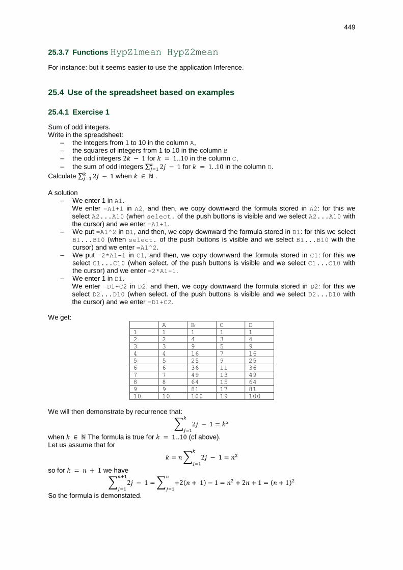
449

25.3.7 Functions HypZ1mean HypZ2mean

For instance: but it seems easier to use the application Inference.

25.4 Use of the spreadsheet based on examples

25.4.1 Exercise 1

Sum of odd integers. Write in the spreadsheet:

– the integers from 1 to 10 in the column A, – the squares of integers from 1 to 10 in the column B – the odd integers 2𝑘 − 1 for 𝑘 = 1. .10 in the column C,

– the sum of odd integers ∑ 2𝑗 − 1𝑘𝑗=1 for 𝑘 = 1. .10 in the column D.

Calculate ∑ 2𝑗 − 1𝑘𝑗=1 when 𝑘 ∈ ℕ .

A solution

– We enter 1 in A1. We enter =A1+1 in A2, and then, we copy downward the formula stored in A2: for this we select A2...A10 (when select. of the push buttons is visible and we select A2...A10 with the cursor) and we enter =A1+1.

– We put =A1^2 in B1, and then, we copy downward the formula stored in B1: for this we select B1...B10 (when select. of the push buttons is visible and we select B1...B10 with the cursor) and we enter =A1^2.

– We put =2*A1-1 in C1, and then, we copy downward the formula stored in C1: for this we select C1...C10 (when select. of the push buttons is visible and we select C1...C10 with the cursor) and we enter =2*A1-1.

– We enter 1 in D1. We enter =D1+C2 in D2, and then, we copy downward the formula stored in D2: for this we select D2...D10 (when select. of the push buttons is visible and we select D2...D10 with the cursor) and we enter =D1+C2.

We get:

A B C D

1 1 1 1 1

2 2 4 3 4

3 3 9 5 9

4 4 16 7 16

5 5 25 9 25

6 6 36 11 36

7 7 49 13 49

8 8 64 15 64

9 9 81 17 81

10 10 100 19 100

We will then demonstrate by recurrence that:

∑ 2𝑗 − 1𝑘

𝑗=1= 𝑘2

when 𝑘 ∈ ℕ The formula is true for 𝑘 = 1. .10 (cf above). Let us assume that for

𝑘 = 𝑛∑ 2𝑗 − 1𝑘

𝑗=1= 𝑛2

so for 𝑘 = 𝑛 + 1 we have

∑ 2𝑗 − 1𝑛+1

𝑗=1=∑ +2(𝑛 + 1) − 1 = 𝑛2 + 2𝑛 + 1 = (𝑛 + 1)2

𝑛

𝑗=1

So the formula is demonstated.

450

25.4.2 Exercise 2

The Pascal triangle and the Fibonacci sequence. The Fibonacci sequence

The Fibonacci sequence is the sequence 𝑢 defined by:

𝑢0 = 1 𝑢1 = 1

𝑢𝑛 = 𝑢𝑛−1 + 𝑢𝑛−2 for 𝑛 > 1 We want to find the 11 first terms of this sequence. We use the spreadsheet. We put: 1 in A1 1 in A2

We select the column A from 3 to 11 (commands Select. and Go↓ of the push buttons should be

displayed) and we enter: =A1+A2 We get in the column A: 1,1,2,3,5,8,13,21,34,55,89

Pascal triangle We want to use the spreadsheet to create the Pascal triangle from 0 to 10. For that, we use the relations for 𝑛 ∈ ℕ and 𝑝 ∈ ℕ:

𝐶𝑛0 = 1, 𝐶𝑛

𝑛 = 1, 𝐶𝑛𝑝= 0 if 𝑝 > 𝑛 and 𝐶𝑛

𝑝= 𝐶𝑛−1

𝑝+ 𝐶𝑛−1

𝑝−1 for 0 < 𝑝 ≤ 𝑛.

We check and enter:

simplify(comb(j-1,k-1)+comb(j-1,k)-comb(j,k))

We get:

0

To fill in the spreadsheet: We enter 1 in A1 then we copy A1 by pressing the keys Shift Copy, we tap Select (push buttons) (which becomes Sel.).

We choose Go↓ in the push buttons and we select the cells from 1 to 11, then we press the keys

Shift Paste: as a result, this puts 1’s in the column A. We enter 0’s in B1 then we copy B1 with the keys Shift Copy, we press Select (push buttons) (which becomes Sel.).

We choose Go→ in the push buttons and we select the columns from B to K, then we press the keys

Shift Paste: as a result, this put 0 in the line 1 starting from the column B. We enter =A1+B1 in B2 then we copy B2 with on the keys Shift Copy, we press Select (push buttons) (which becomes Sel.).

We choose Go→ in the push buttons and we select the columns from B to K, then we press the keys

Shift Paste: as a result, this puts 1 in B2 and 0 in the line 2 starting from the column C but this also copies the formulas =B1+C1 in C2, =C1+D1 in D2 etc., ..... Then, we also copy the formula =A1+B1 in the column B (with the keys Shift Copy, we press Select (push buttons) (which becomes Sel.).

We choose Go↓ in the push buttons and we select the cells from 2 to 11, then we press the keys

Shift Paste: as a result, this puts in the column B: 0,1,2,3,4..10 . Then, we also copy the formula =B1+C1 in the column C (with the keys Shift Copy, we press Select (push buttons) (which becomes Sel.).

We choose Go↓ in the push buttons and we select the cells from 2 to 11, then we press the keys

Shift Paste (first copy the formula and then choose 0→ Formula): as a result, this puts in the

column C: 0,0,1,3,6,10,15,21,28,36,45.

Likewise, we copy the formula located in D2 (resp. E2...K2) in the column D (resp. E...K). We get:

A B C D E F g H I J K

1 1 0 0 0 0 0 0 0 0 0 0

451

2 1 1 0 0 0 0 0 0 0 0 0

3 1 2 1 0 0 0 0 0 0 0 0

4 1 3 3 1 0 0 0 0 0 0 0

5 1 4 6 4 1 0 0 0 0 0 0

6 1 5 10 10 5 1 0 0 0 0 0

7 1 6 15 20 15 6 1 0 0 0 0

8 1 7 21 35 35 21 7 1 0 0 0

9 1 8 28 56 70 56 28 8 1 0 0

10 1 9 36 84 126 126 84 36 9 1 0

11 1 10 45 120 210 252 210 120 45 10 1

The Fibonacci sequence and the Pascal triangle When we do the sum of the diagonals of the Pascal triangle upward, we get the Fibonacci sequence. For instance:

(

1 = 1 = 2 = 3 = 5 = 8 = 13 =)

(

1 0 0 0 0 0 ↗ ↗ ↗ ↗ ↗ 1 1 0 0 0 0 ↗ ↗ ↗ ↗ ↗ 1 2 1 0 0 0 ↗ ↗ ↗ ↗ 1 3 3 1 0 0 ↗ ↗ ↗ 1 4 6 4 1 0 ↗ ↗ 18 5 10 5 5 1 ↗ 1 6 15 20 15 6)

We enter:

A:=makemat((j,k)->comb(j,k),11,11)

L:=sum(A[j-k, k],k=1..j-1)$(j=2..12)

We get:

1,1,2,3,5,8,13,21,34,55,89

We enter:

L1:=0,sum(A[j-k-1,k-1],k=2..j-2)$(j=3..12)

We get:

0,0,1,1,2,3,5,8,13,21,34

We enter:

L2:=1,sum(A[j-k-1,k],k=1..j-2)$(j=3..12)

We get:

1,1,1,2,3,5,8,13,21,34,55

We enter:

[L1]+[L2]

We get:

452

[1,1,2,3,5,8,13,21,34,55,89]

To show it, we use the relation for 𝑛 ∈ ℕ:

𝐶𝑛0 = 1, 𝐶𝑛

𝑛 = 1, 𝐶𝑛𝑝= 0 and 𝐶𝑛

𝑝= 𝐶𝑛−1

𝑝+ 𝐶𝑛−1

𝑝−1 for 0 < 𝑝 ≤ 𝑛.

Be an the series which equals the sum of the upward diagonals of the Pascal triangle. We have then: 𝑎0 = 1, 𝑎1 = 1 and for 𝑛 > 1:

𝑎𝑛 = ∑ comb(n – p, p)floor(

n2)

p=0= 1 +∑ comb(n – p, p)

floor(n2)

p=1

𝑎𝑛 = 1 +∑ comb(n – p − 1, p − 1)floor(

n2)

p=1+∑ comb(n – p − 1, p)

floor(n2)

p=1

We have for any 𝑛: floor (𝑛

2) − 1 = floor (

𝑛−2

2).

If 𝑛 = 2𝑘, we have floor(𝑛/2) = floor((𝑛 − 1)/2) + 1 = 𝑘:

1 +∑ comb(n – p − 1, p)floor(

n2)

p=1=∑ comb(n – 1 − p, p) + comb(2k– 1 − k, k)

floor(n−12)

p=0= 0

because comb(2𝑘 − 1 − 𝑘, 𝑘) = 0

∑ comb(n – p − 1, p)floor(

n2)

p=1=∑ comb(n – 1 − p, p)

floor(n−12)

p=0= 𝑎𝑛−1

∑ comb(n – p − 1, p − 1)floor(

n2)

p=1=∑ comb(n – 2 − p, p)

floor(n−22)

p=0= 𝑎𝑛−2

because floor (𝑛

2) − 1 = floor (

𝑛−2

2)

If 𝑛 = 2𝑘 + 1, then we have floor (𝑛

2) = floor (

𝑛 − 1

2) = 𝑘:

1 +∑ comb(n – p − 1, p)floor(

n2)

p=1=∑ comb(n – 1 − p, p)

floor(n−12)

p=0= 𝑎𝑛−1

∑ comb(n – p − 1, p − 1)floor(

n2)

p=1=∑ comb(n – 2 − p, p)

floor(n−22)

p=0= 𝑎𝑛−2

because 𝑓𝑙𝑜𝑜𝑟 (𝑛

2) − 1 = 𝑓𝑙𝑜𝑜𝑟 (

𝑛−2

2)

Thus: 𝑎0 = 1, 𝑎1 = 1 and for 𝑛 > 1 we have 𝑎𝑛 = 𝑎𝑛−1 + 𝑎𝑛−2 𝑎𝑛 is then the Fibonacci sequence.

453

Chapter 26 Other Applications

26.1 Function application

We enter in the Symbolic view of the Function application: F1(X)=SIN(2X)+X

F2(X)=∂(F1(A),A=X) We highlight ∂(F1(A),A=X) and we press EVAL of the push buttons. We get, if we are in Radians:

F2(X)=COS(2*X)*2+1

In HOME, we enter:

F1(1)

We get, if we are in Radians:

SIN(2)+1

In HOME, we enter:

F2(1)

We get, if we are in Radians:

COS(2)*2+1

In HOME, we enter:

∂(F1(X),X=1)

We get, if we are in Radians:

0.167706326906

26.2 Sequence application

26.2.1 Fibonnacci sequence

We enter:

U1(1)=1

U1(2)=1

U1(N)=U1(N-1)+U1(N-2)

We get by pressing Num:

the Fibonnacci sequence

We enter the sequence of the remainders:

U1(1)=1

454

U1(2)=1

U1(N)=U1(N-1)+U1(N-2)

We get by pressinge Num:

the Fibonnacci sequence

26.2.2 GCD

Here is an implementation of Euclid’s algorithm with the HPrime. Here is the description of this algorithm: We do successive euclidean divisions:

𝐴 = 𝐵 × 𝑄1 + 𝑅10 ≤ 𝑅1 < 𝐵 𝐵 = 𝑅_1 × 𝑄_2 + 𝑅_2 0 ≤ 𝑅_2 < 𝑅1 𝑅_1 = 𝑅_2 × 𝑄_3 + 𝑅_3 0 ≤ 𝑅_3 < 𝑅2

. . . . . . . 𝑅𝑛−2 = 𝑅𝑛−1 × 𝑄_𝑛 + 𝑅_𝑛 0 ≤ 𝑅_𝑛 < 𝑅𝑛−1

After a finite number of steps (at most 𝐵), there is an integer n such as: 𝑅𝑛 = 0. Then we have:

𝐺𝐶𝐷(𝐴, 𝐵) = 𝐺𝐶𝐷(𝐵, 𝑅1) = … . 𝐺𝐶𝐷(𝑅𝑛−1, 𝑅𝑛) = 𝐺𝐶𝐷(𝑅𝑛−1, 0) = 𝑅𝑛 − 1

Thanks to the Sequence application, we write the series of the remainders. We enter the series of remainders 𝑅:

U1(1)=76

U1(2)=56

U1(N)=irem(U1(N-2),U1(N-1))

We get by pressing Num: 76,56,20,16,4,0 then .... the GCD of 76 and 56 is 4

26.2.3 Bezout identity

The Euclid’s algorithm allows to trouver a paired value 𝑈, 𝑉 such as:

𝐴 × 𝑈 + 𝐵 × 𝑉 = 𝐺𝐶𝐷(𝐴, 𝐵) With the Sequence application, we will define "the sequence of remainders" 𝑅 and two sequences 𝑈

and 𝑉, so that at each step we have:

𝑅𝑛 = 𝑈𝑛 × 𝐴 + 𝑉𝑛 × 𝐵. If 𝑄 is "the sequence of quotients", 𝑄𝑛 = 𝑖𝑞𝑢𝑜(𝑅𝑛−2, 𝑅𝑛−1) because 𝑄_𝑛 is the integer quotient of 𝑅𝑛−2 by 𝑅𝑛−1 and we have:

𝑅𝑛 = 𝑖𝑟𝑒𝑚(𝑅𝑛−2, 𝑅𝑛−1) = 𝑅𝑛−2–𝑄𝑛 × 𝑅𝑛−1 because 𝑅𝑛−2 = 𝑅(𝑛−1)𝑄𝑛 + 𝑅𝑛𝑤𝑖𝑡ℎ 0 ≤ 𝑅𝑛 < 𝑅𝑛−1.

𝑈_𝑛 and 𝑉_𝑛 will then check the same relation of recurrence. We have at the beginning: 𝑅1 = 𝐴 𝑅2 = 𝐵 𝑈1 = 1 𝑈2 = 0 because 𝐴 = 1 × 𝐴 + 0 × 𝐵

𝑉1 = 0 𝑉2 = 1 because 𝐵 = 0 × 𝐴 + 1 × 𝐵 We enter in 𝑈1 the series of remainders 𝑅 for 𝐴 = 76 and 𝐵 = 56:

U1(1)=76

U1(2)=56

U1(N)=irem(U1(N-2),U1(N-1))

We enter the series of quotients 𝑄 in 𝑈2:

U2(1)=0

455

U2(2)=0

U2(N)=iquo(U1(N-2),U1(N-1))

We will put 𝑈 in 𝑈_3 and 𝑈_4 in 𝑉 so that at each step we have 76 ∗ 𝑈 + 56 ∗ 𝑉 = 𝑅.

Since 𝑅(𝑁) = 𝑅(𝑁 − 2) − 𝑅(𝑁 − 1) ∗ 𝑄(𝑁) and 𝑄(𝑁)iquo(𝑅(𝑁 − 2), 𝑅(𝑁 − 1)), if we have:

76 ∗ 𝑈(𝑁 − 2) + 56 ∗ 𝑉 (𝑁 − 2) = 𝑅(𝑁 – 2)(1)

and 76 ∗ 𝑈(𝑁 − 1) + 56 ∗ 𝑉 (𝑁 − 1) = 𝑅(𝑁 − 1)(2) By doing (1) − (2) ∗ 𝑄(𝑁), we have:

76 ∗ (𝑈(𝑁 − 2) − 𝑈(𝑁 − 1) ∗ 𝑄(𝑁)) + 56 ∗ (𝑉 (𝑁 − 2) − 𝑉 (𝑁 − 1) ∗ 𝑄(𝑁)) = 𝑅(𝑁 − 2) − 𝑅(𝑁 − 1) ∗ 𝑄(𝑁) = 𝑅(𝑁)

The recurrence relations are then: 𝑈(𝑁) = 𝑈(𝑁 − 2) − 𝑈(𝑁 − 1) ∗ 𝑄(𝑁) = 𝑈(𝑁 − 2) − 𝑈(𝑁 − 1) ∗ 𝑖𝑞𝑢𝑜(𝑅(𝑁 − 2), 𝑅(𝑁 − 1)) 𝑉 (𝑁) = 𝑉 (𝑁 − 2) − 𝑉 (𝑁 − 1) ∗ 𝑄(𝑁) = 𝑉 (𝑁 − 2) − 𝑉 (𝑁 − 1) ∗ 𝑖𝑞𝑢𝑜(𝑅(𝑁 − 2), 𝑅(𝑁 − 1))

We enter in U3 the sequence of 𝑈: U3(1)=1

U3(2)=0

U2(N)=U3(N-2)-U3(N-1)*iquo(U1(N-2),U1(N-1))

We enter in U4 the sequence of 𝑉: U4(1)=0

U4(2)=1

U4(N)=U4(N-2)-U4(N-1)*iquo(U1(N-2),U1(N-1))

Thus, for each N we have 76*U3(N)+56*U4(N)=U1(N) By pressing Num, we get:

76,0,1,0 (76 = 76 ∗ 1 + 56 ∗ 0)

56,0,0,1 (56 = 76 ∗ 0 + 56 ∗ 1)

20,1,1,-1 (20 = 76 ∗ 1 + 56 ∗ −1)

16,2,-2,3 (16 = 76 ∗ −2 + 56 ∗ 3)

4,1,3,-4 (4 = 76 ∗ 3 + 56 ∗ −4)

0,4,-14,19 (0 = 76 ∗ −14 + 56 ∗ 19)

so 76 ∗ 3 + 56 ∗ −4 = 4 =GCD of 76 and 56

26.3 Parametric application

We enter:

X1(T)=-COS(2T)

Y1(T)=SIN(3T)

We get:

the plot of a curve looking like an α

26.4 Polar application

We enter:

456

R1(θ)=COS(3θ)

We get:

the plot of a clover

26.5 Solve application

We enter in the Symbolic view of the Solve application:

COS(X)-X

By pressing Num: We enter:

1

To start the iteration, and then we press SOLVE (push buttons) to get:

0.739085133215

Then, we enter in HOME:

X

We get:

0.739085133215

the value obtained has been stored in X.

26.6 Finance application

We fill in all different fields but one, and we press SOLVE of the push buttons. For instance, we want to know the monthly payments of a 10-year loan of $ 100,000 at 4.6 % annual interest, we enter:

NbPmt 120 IPYR 4.6

PV 100,000 PPYR 12

PMT CPYR 12

FV 0.00 Fin Y

Group Size 12

We highlight PMT and we press SOLVE of the push buttons. We get the value of the monthly payment:

-1,041.21

The payments of this loan are then of $ 1,041.21 per month. Press AMORT of the push buttons. We get the amortization table by groups of 12 months: Princ gives the amount of the paid sums Inter gives the amount of the interest Balan gives the amount of the due sums For example, at the end of the second year, we have:

Princ=-16,505.07: we have then reimboursed $ 16,505.07 Inter=-8,484.0: we have paid $ 8,484 of interest Balan=83,494.9: $ 83,494.93 are to be reimbursed (100,000 − 16,505.07)

457

By pressing the key PLOT we get the amortization graph. We can read: 1-12 Principal 8,063.12 and Interest 4,431.41 and by using the right arrow 13-24 Principal 8,441.95 and Interest 4,052.59 Thus, we recover the previous values: 8,063.12+8,441.95=16,505.07 and 4,431.41+4,052.59=8,484.0. We returns in the application Finance by pressing the key Num. If the payments are quaterly, we change: NbPmt 40 and PPYR 4 and we leave CPYR 12. We highlight PMT and we press SOLVE of the push buttons. We get the value of the quarterly payments: -3,133.03

The payments of this loan are then of $ 3,133.03 by quarter.

26.7 Linear Solver application

This application allows to solve linear systems of two equations at two unknowns 𝑋, 𝑌, or of three

equations at three unknowns 𝑋, 𝑌, 𝑍. Note: To solve a linear system of two equations at two unknowns 𝑋, 𝑌, you have to set 2×2 in the push buttons. The fields of the system are displayed and we only need to enter the coefficients. The answer appears at the bottom of the screen. We enter:

1*X+1*Y+1*Z=3

2*X+(-2)*Y+1*Z=1

3*X+1*Y+1*Z=5

We get:

X:1,Y:1,Z:1

We enter:

1*X+1*Y+1*Z=3

2*X+2*Y+2*Z=1

3*X+1*Y+1*Z=5

We get:

No Solutions

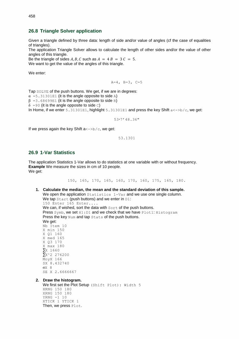
458

26.8 Triangle Solver application

Given a triangle defined by three data: length of side and/or value of angles (cf the case of equalities of triangles). The application Triangle Solver allows to calculate the length of other sides and/or the value of other angles of this triangle. Be the triangle of sides 𝐴, 𝐵, 𝐶 such as 𝐴 = 4 𝐵 = 3 𝐶 = 5. We want to get the value of the angles of this triangle. We enter:

A=4, B=3, C=5

Tap SOLVE of the push buttons. We get, if we are in degrees: α =5.31301E1 (it is the angle opposite to side A) β =3.68699E1 (it is the angle opposite to side B) δ =90 (it is the angle opposite to side C) In Home, if we enter 5.31301E1, highlight 5.31301E1 and press the key Shift a<->b/c, we get:

53◦7’48.36"

If we press again the key Shift a<->b/c, we get:

53.1301

26.9 1-Var Statistics

The application Statistics 1-Var allows to do statistics at one variable with or without frequency. Example We measure the sizes in cm of 10 people. We get:

150, 165, 170, 165, 160, 170, 160, 175, 165, 180.

1. Calculate the median, the mean and the standard deviation of this sample. We open the application Statistics 1-Var and we use one single column. We tap Start (push buttons) and we enter in D1: 150 Enter 165 Enter....

We can, if wished, sort the data with Sort of the push buttons. Press Symb, we set H1:D1 and we check that we have Plot1: Histogram Press the key Num and tap Stats of the push buttons. We get: Nb Item 10

X min 150

X Q1 160

X med 165

X Q3 170

X max 180

∑X 1660 ∑X^2 276200 MoyX 166

SX 8.432740

σX 8 SE X 2.6666667

2. Draw the histogram. We first set the Plot Setup (Shift Plot): Width 5 HRNG 150 180

XRNG 150 180

YRNG -1 10

XTICK 1 YTICK 1

Then, we press Plot.

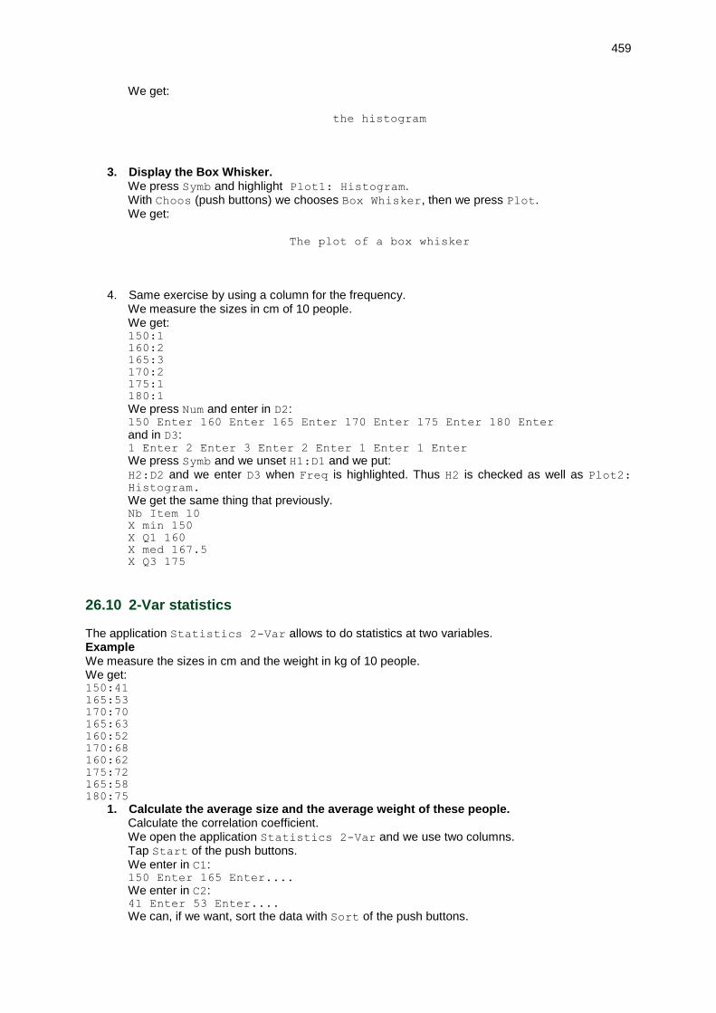
459

We get:

the histogram

3. Display the Box Whisker. We press Symb and highlight Plot1: Histogram. With Choos (push buttons) we chooses Box Whisker, then we press Plot. We get:

The plot of a box whisker

4. Same exercise by using a column for the frequency. We measure the sizes in cm of 10 people. We get: 150:1

160:2

165:3

170:2

175:1

180:1

We press Num and enter in D2: 150 Enter 160 Enter 165 Enter 170 Enter 175 Enter 180 Enter

and in D3: 1 Enter 2 Enter 3 Enter 2 Enter 1 Enter 1 Enter

We press Symb and we unset H1:D1 and we put: H2:D2 and we enter D3 when Freq is highlighted. Thus H2 is checked as well as Plot2: Histogram. We get the same thing that previously. Nb Item 10

X min 150

X Q1 160

X med 167.5

X Q3 175

26.10 2-Var statistics

The application Statistics 2-Var allows to do statistics at two variables. Example We measure the sizes in cm and the weight in kg of 10 people. We get: 150:41

165:53

170:70

165:63

160:52

170:68

160:62

175:72

165:58

180:75

1. Calculate the average size and the average weight of these people. Calculate the correlation coefficient. We open the application Statistics 2-Var and we use two columns. Tap Start of the push buttons. We enter in C1: 150 Enter 165 Enter....

We enter in C2: 41 Enter 53 Enter....

We can, if we want, sort the data with Sort of the push buttons.

460

Press Symb, we put S1:C1 C2, we set S1 and we check that we have: Type1:Linear

Fit1: m*X+b

Press the key Num and tap Stats of the push buttons. We get: Nb Item 10

Corr 0.91798

CoefDet 0.84269

SCov 81.7778

PCov 73.6

X max 180

P

XY 102660

By tapping X (push buttons) we have: MoyX 166

P

X 1660

P

X^2 276200

SX 8.432740

σX 8 SE X 2.6666667

By tapping Y (push buttons) we have: MoyY 61.4

P

Y 614

P

Y^2 38704

SY 10.5641

σY 10.0220 SE Y 3.340659

2. Plot the cloud of dots We first set the Plot Setup (Shift Plot): XRNG 145 185 YRNG 39 77

XTICK 5 YTICK 2

Then, we press Plot. We get:

the cloud of dots and the plot of the regression line

3. Determinate a line of linear regression by the least squares method. We get the equation of the line of linear regression by pressing Symb. We get:

Fit1:1.15*X+-129.5

26.10.1 Exercises

– The aim of this activity is the study of the size (in cm) of a sample of 250 basket players.

Size 173

174

175

176

177

178

179

180

181

182

183

184

185

186

187

Frequency

4 8 7 18 23 22 24 32 26 25 18 19 10 8 6

The activity starts by the calculation of statistic parameters and is followed by the plot of the correlated graphs: bar graph, histograms and polygon of cumulated increasing frequency. We enter:

Ts:=(173+j)$(j=0..14)

We get:

461

173,174,175,176,177,178,179,180,181,182,183,184,185,186,187

We enter:

Ef:=(4,8,7, 18, 23, 22, 24, 32, 26, 25, 18, 19, 10, 8, 6)

sum(Ef)

We get:

250

We enter:

histogram(tran([[Ts],[Ef]]))

We get:

We enter:

bar_plo([[T],[Ef]])

We get:

We enter: boxwhisker([T],[Ef])

We get:

462

We enter:

Efc:=(sum(Ef[j],j=1..k)/250.)$(k=1..size(Ef))

We get:

0.016,0.048,0.076,0.148,0.24,0.328,0.424,0.552,0.656,0.756,0.828,0.90

4,0.944,0.976,1.0

We enter:

scatterplot([[T],[Efc]]),cumulated_frequencies(trn([[T],[Ef]]))

We get:

We enter:

evalf(mean([T],[Ef]))

We get:

180.104

We enter:

evalf(sttdev([T],[Ef]))

We get:

3.27859482096

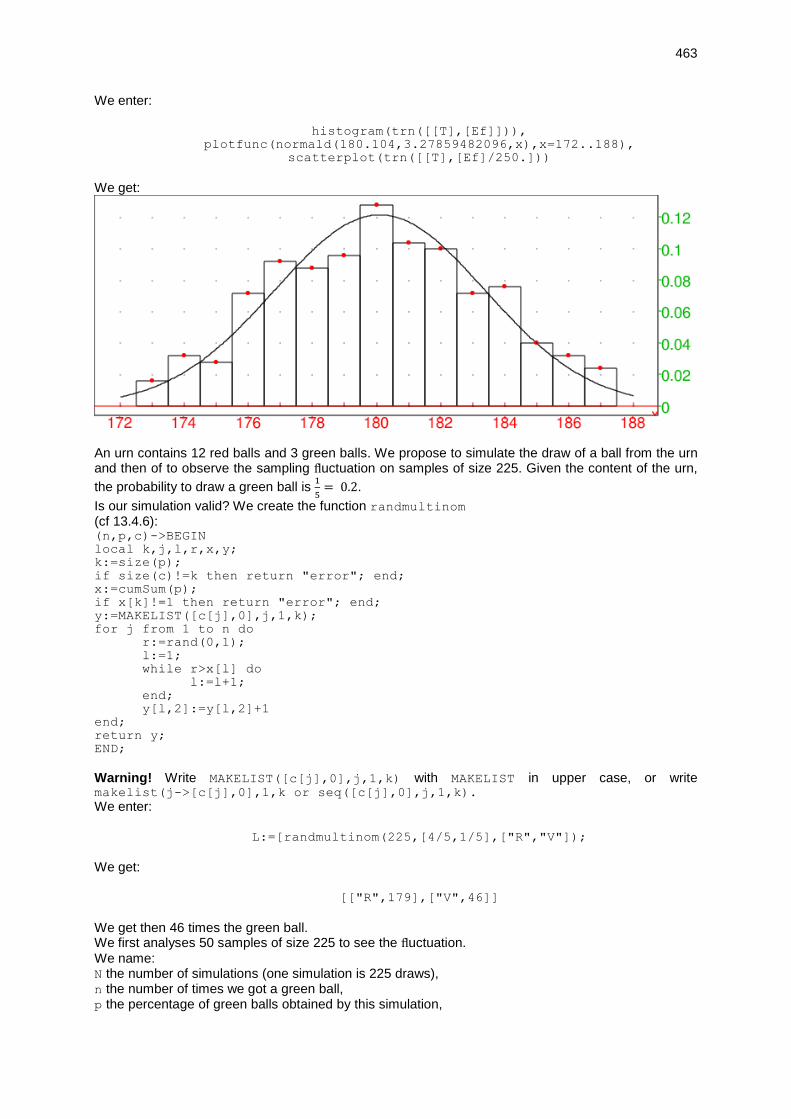
463

We enter:

histogram(trn([[T],[Ef]])),

plotfunc(normald(180.104,3.27859482096,x),x=172..188),

scatterplot(trn([[T],[Ef]/250.]))

We get:

An urn contains 12 red balls and 3 green balls. We propose to simulate the draw of a ball from the urn and then of to observe the sampling fluctuation on samples of size 225. Given the content of the urn,

the probability to draw a green ball is 1

5= 0.2.

Is our simulation valid? We create the function randmultinom (cf 13.4.6): (n,p,c)->BEGIN

local k,j,l,r,x,y;

k:=size(p);

if size(c)!=k then return "error"; end;

x:=cumSum(p);

if x[k]!=1 then return "error"; end;

y:=MAKELIST([c[j],0],j,1,k);

for j from 1 to n do

r:=rand(0,1);

l:=1;

while r>x[l] do

l:=l+1;

end;

y[l,2]:=y[l,2]+1

end;

return y;

END;

Warning! Write MAKELIST([c[j],0],j,1,k) with MAKELIST in upper case, or write makelist(j->[c[j],0],1,k or seq([c[j],0],j,1,k).

We enter:

L:=[randmultinom(225,[4/5,1/5],["R","V"]);

We get:

[["R",179],["V",46]]

We get then 46 times the green ball. We first analyses 50 samples of size 225 to see the fluctuation.

We name: N the number of simulations (one simulation is 225 draws), n the number of times we got a green ball, p the percentage of green balls obtained by this simulation,

464

Lp the sequence of percentages obtained. We enter: test0(N):={

local L,p,n,k,Lp;

Lp:=NULL;

for k from 1 to N do

L:=randmultinom(225,[4/5,1/5],["R","V"]);

n:=L[2,2])

p:=n/225.;

Lp:=Lp,p;

fpour;

return Lp;

}:;

Then:

plotlist(test0(50)),line(y=2/15),line(y=4/15)

We get:

We successively analyse 𝑡 samples of size 𝑛 = 225 for 𝑡 ∈ 10, 20, 50, 100, 200, 500. In our case, the

fluctuation interval at level of 95% is: 𝑝 –1

√𝑛𝑝 +

1

√𝑛 with 𝑝 =

1

5 and 𝑛 = 225 that is to say

2

15,4

15.

To check whether the simulation is correct or not, we write a program checking whether we do have or

not p laying in the interval 2

15,4

15 in 95% of the cases.

We note N the number of simulations (one simulation is 225 draws). For the k-nth simulation, (k=1..N), we name: L the list of 225 draws obtained, n the number of times we got a green ball, p the percentage of green balls obtained by this simulation, l s the number of draws such as 2/15<p<4/15 when we have done k simulations, sn the number of times we got a green ball when we have done k simulations. pcn the percentage of green balls obtained by these N*225 draws, which is then sn/(225*N) The number of times we have 2/15<p<4/15 is s, or else the percentage pc=s/N. We check then if pc>0.95

test0(N):={

local s,L,p,n,pc,sn,pcn,k,Le;

s:=0;sn:=0;

Le:=NULL;

for k from 1 to N do

L:=[randmultinom(225,[4/5,1/5],["R","V"])];

n:=L[2,2]

p:=n/225;

Le:=Le,p;

fpour;

465

returns Le;

}:;

test(N):={

local s,L,p,n,pc,sn,pcn,k,Le;

s:=0;sn:=0;

Le:=NULL;

for k from 1 to N do

L:=[randmultinom(225,[4/5,1/5],["R","V"])];

n:=L[2,2]

p:=n/225;

Le:=Le,p;

if p>2/15 and p<4/15 then s:=s+1; endif;

sn:=sn+n;

fpour;

pc:=evalf(s/N);

pcn:=evalf(sn/N/225);

if pc>0.95 then returns pcn,pc,"correct"; otherwise returns pcn,pc,’’not

correct’’; endif;

}:;

We enter:

test(10)

We get:

0.203111111111,1.0,"correct"

We enter:

test(20)

We get:

0.194888888889,0.95,’’not correct’’

We enter:

test(50)

We get:

0.194311111111,0.98,"correct"

We enter:

test(100)

We get:

0.198888888889,0.97,"correct"

We enter:

test(200)

We get:

0.193777777778,0.99,"correct"

test(500)

We get:

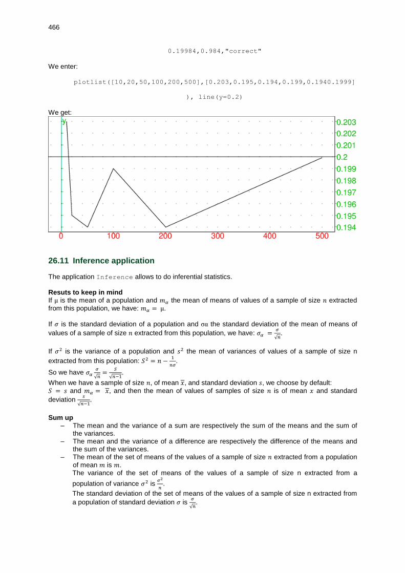
466

0.19984,0.984,"correct"

We enter:

plotlist([10,20,50,100,200,500],[0.203,0.195,0.194,0.199,0.1940.1999]

), line(y=0.2)

We get:

26.11 Inference application

The application Inference allows to do inferential statistics. Resuts to keep in mind If µ is the mean of a population and 𝑚𝛼 the mean of means of values of a sample of size 𝑛 extracted

from this population, we have: 𝑚𝛼 = µ. If 𝜎 is the standard deviation of a population and σα the standard deviation of the mean of means of

values of a sample of size 𝑛 extracted from this population, we have: 𝜎𝛼 =𝜎

√𝑛.

If 𝜎2 is the variance of a population and 𝑠2 the mean of variances of values of a sample of size n

extracted from this population: 𝑆2 = 𝑛 −1

𝑛𝜎.

So we have 𝜎𝛼𝜎

√𝑛=

𝑆

√𝑛−1.

When we have a sample of size 𝑛, of mean 𝑥, and standard deviation 𝑠, we choose by default:

𝑆 = 𝑠 and 𝑚𝛼 = 𝑥, and then the mean of values of samples of size 𝑛 is of mean 𝑥 and standard

deviation 𝑠

√𝑛−1.

Sum up

– The mean and the variance of a sum are respectively the sum of the means and the sum of the variances.

– The mean and the variance of a difference are respectively the difference of the means and the sum of the variances.

– The mean of the set of means of the values of a sample of size 𝑛 extracted from a population

of mean 𝑚 is 𝑚. The variance of the set of means of the values of a sample of size n extracted from a

population of variance 𝜎2 is 𝜎2

𝑛.

The standard deviation of the set of means of the values of a sample of size n extracted from

a population of standard deviation 𝜎 is 𝜎

√𝑛.

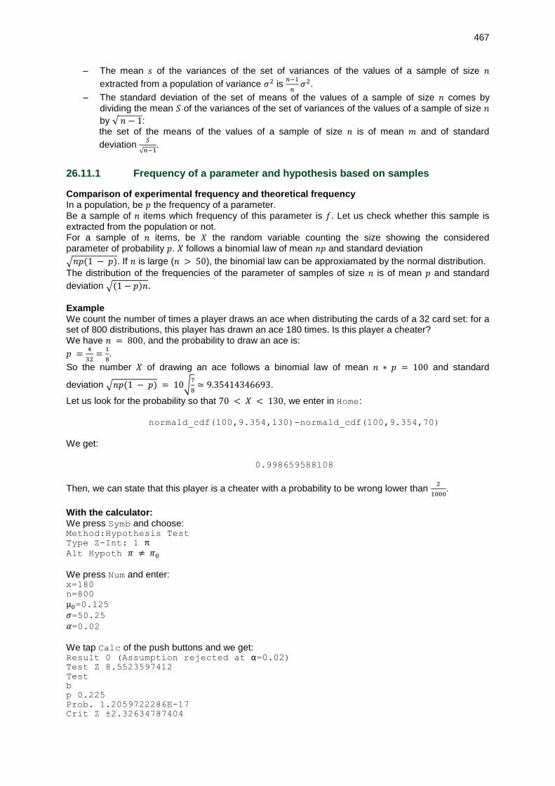
467

– The mean 𝑠 of the variances of the set of variances of the values of a sample of size 𝑛

extracted from a population of variance 𝜎2 is 𝑛−1

𝑛𝜎2.

– The standard deviation of the set of means of the values of a sample of size 𝑛 comes by dividing the mean 𝑆 of the variances of the set of variances of the values of a sample of size 𝑛

by √ 𝑛 − 1: the set of the means of the values of a sample of size 𝑛 is of mean 𝑚 and of standard

deviation 𝑆

√𝑛−1.

26.11.1 Frequency of a parameter and hypothesis based on samples

Comparison of experimental frequency and theoretical frequency In a population, be 𝑝 the frequency of a parameter.

Be a sample of 𝑛 items which frequency of this parameter is 𝑓. Let us check whether this sample is extracted from the population or not. For a sample of 𝑛 items, be 𝑋 the random variable counting the size showing the considered parameter of probability 𝑝. 𝑋 follows a binomial law of mean 𝑛𝑝 and standard deviation

√𝑛𝑝(1 − 𝑝). If 𝑛 is large (𝑛 > 50), the binomial law can be approxiamated by the normal distribution.

The distribution of the frequencies of the parameter of samples of size 𝑛 is of mean 𝑝 and standard

deviation √(1 − 𝑝)𝑛.

Example We count the number of times a player draws an ace when distributing the cards of a 32 card set: for a set of 800 distributions, this player has drawn an ace 180 times. Is this player a cheater? We have 𝑛 = 800, and the probability to draw an ace is:

𝑝 =4

32=1

8.

So the number 𝑋 of drawing an ace follows a binomial law of mean 𝑛 ∗ 𝑝 = 100 and standard

deviation √𝑛𝑝(1 − 𝑝) = 10√7

8≃ 9.35414346693.

Let us look for the probability so that 70 < 𝑋 < 130, we enter in Home:

normald_cdf(100,9.354,130)-normald_cdf(100,9.354,70)

We get:

0.998659588108

Then, we can state that this player is a cheater with a probability to be wrong lower than 2

1000.

With the calculator: We press Symb and choose: Method:Hypothesis Test

Type Z-Int: 1 π Alt Hypoth 𝜋 ≠ 𝜋0 We press Num and enter: x=180

n=800

µ0=0.125 𝜎=50.25 𝛼=0.02 We tap Calc of the push buttons and we get: Result 0 (Assumption rejected at α=0.02) Test Z 8.5523597412

Test

b

p 0.225

Prob. 1.2059722286E-17

Crit Z ±2.32634787404

468

Lower 0.0906543...

Upper 0.15934...

We enter in Home:

(180-100)/9.35414346693

We get:

8.5523597412

We enter in Home:

normald_icdf(100,9.35414346693,0.99)

We get:

121.760991768

We enter in Home:

(121.760991768-100)/9.35414346693

We get:

2.32634787407

We enter in Home for 𝛼 = 0.002:

normald_icdf(100,9.354,0.001), normald_icdf(100,9.354,0.999)

We get:

71.0939670081,128.906032992

Confidence interval of a proportion or a frequency How to evaluate the frequency 𝑝 of a parameter in a population au view of a sample of size 𝑛. Example We throw a dice 3,000 times and we have get 490 times the six. Can we state that the dice is regular ? We have:

𝑛 = 3000, 𝑓 =49

300≃ 0.163333333333, 1 − 𝑓 =

251

300≃ 0.836666666667

so 𝑚 = 𝑛𝑓 = 490 and 𝑠 = √𝑛𝑓(1 − 𝑓) ≃ 20.2476336066

At the level of 𝛼 = 0.002, we enter in Home:

normald_cdf(3000*49./300,sqrt(3000*49./300*251/300),500)-

normald_cdf(3000

We get:

0.378612513321

So the probability that 𝑝 is in the interval [480, 500] is 0.378612513321. We can reasonably admit that 𝑝 = 1/6, that is to say that the dice is regular, because, otherwise, the probability to be wrong would

be 1 − 0.378612513321 ≃ 0.621387486679 With the calculator: We press Symb and choose: Method: Confidence interval

469

Type: Z-Int: 1 𝜋 We press Num and enter: x=490

n=3000

µ0=0.166666666667 𝛼=0.05 We tap Calc of the push buttons and we get: C 0.95

Crit Z ± 1.95996398454

Lower 0.150105122453

Upper 0.176561544214...

With: C=0.38

We tap Calc of the push buttons and we get: C 0.38

Crit Z ± 0.495850347347

Lower 0.159986734614

Upper 0.166679932052

Comparison of the frequencies of two samples We have two samples of sizes 𝑛1 and 𝑛2 for which the frequencies of a parameter are 𝑓1 and 𝑓2. If 𝑓1 and 𝑓2 are different, how to know whether these two samples come from a same population or not ? If we do the hypothesis that the two samples come from of a same population, we can estimate the

frequency p of the entire population by grouping the two samples with 𝑝 =𝑛1𝑓1+𝑛2𝑓2

𝑛1+𝑛2.

The standard deviation of the distribution of the frequencies of the parameter of the sample 1 is

√𝑓1(1−𝑓1)

𝑛1 and the one of the sample 2 is √

𝑓2(1−𝑓2)

𝑛2.

We consider the distibution of the values of 𝑓1 − 𝑓2, if the two samples come from a same population:

the mean of 𝑓1 − 𝑓2 is 0 and the standard deviation 𝑠 of 𝑓1– 𝑓2 is √𝑝(1−𝑝)

𝑛1+𝑝(1−𝑝)

𝑛2

Example

Among the 40 class mates of class 𝐴, 23 have been admitted, and among the 40 of class 𝐵, 17 have

been. Are the class mates of classes 𝐴 and 𝐵 part of the same population ?

If they are, the distribution of frequencies 𝑓1– 𝑓2 follows a normal distribution:

of mean 𝑝 =40

80= 0.5

and standard deviation 𝑠 = √2∗0.5∗0.5

40≃ 0.111803398875

We know that 𝑓1 =23

40 ≃ 0.575 and 𝑓2 =

17

40≃ 0.425 then 𝑓1– 𝑓2 = 0.15 and

𝑓1–𝑓2

𝑠 ≃ 1.3416407865

We enter:

normal_cdf(0,0.111803398875,0.15)-normal_cdf(0,0.111803398875,-0.15)

or we enter:

normal_cdf(0,1,1.3416407865)-normal_cdf(0,1,-1.3416407865)

We get:

0.820287505121

We enter:

1-0.820287505121

We get:

0.179712494879

470

This means that the we can state that the two classes come from the same population, because if would state the contrary, the probability to be wrong would be 17.97 % We enter, if we want a result at te level of 5%:

normal_icdf(0,0.111803398875,0.025),normal_icdf(0,0.111803398875,0.97

5)

We get:

-0.219130635144,0.219130635144

We enter, if we want a result at the level of 5%:

normal_icdf(0,1,0.025),normal_icdf(0,1,0.975)

We get:

-1.95996398454,1.95996398454

As 0.15 is in the interval [−0.219130635144,0.219130635144], we can say that, at the level of 5%, the two classes come from the same population. With the Inference application: We press Symb and choose: Method: Hypothesis test

Type: Z-Int: 1 𝜋1 − 𝜋2 Alt Hypoth: 𝜋1 6= 𝜋2 We press Num and enter:

𝑥1=23 𝑥2=17 𝑛1=40 𝑛2=40 𝛼=0.05 We tap Calc of the push buttons and we get: Result 1 (𝐻0 not rejected at 𝛼=0.05) Test Z 1.3416407865

Test Δ�̂� 0.15 Prob. 0.179712494879

Crit Z ±1.95996398454

Lower -0.0666513904072

Upper 0.366651390407

We enter in Home:

normal_icdf(0.15,0.111803398875,0.025),normal_icdf(0.15,0.11180339887

5,

0.975)

We get:

-0.0691306351442,0.369130635144

The sample 1 has as mean:

𝑓1 =23

40= 0.575 and as variance:

𝑓1(1 − 𝑓1)

𝑛1=0.575 ∗ 0.425

40

The sample 2 has as mean:

𝑓1 =17

40= 0.425 and as variance:

471

𝑓2(1 − 𝑓2)

𝑛2=0.425 ∗ 0.575

40

We consider the distribution of frequencies 𝑓1– 𝑓2: we can say that it has as mean the difference of means, i.e.:

0.575 − 0.425 = 0.15 and as variance the sum of these two variances, i.e: 2 ∗ 0.425 ∗ 0.575

40

We enter in Home to get the standard deviation of the distribution of frequency 𝑓1– 𝑓2:

sqrt(2*0.575*0.425/40.)

We get:

0.1105384548472

normal_icdf(0.15,0.1105384548472,0.025),normal_icdf(0.15,0.1105384548

472,0.975)

We get the critical lower and upper:

-0.0666513904072,0.366651390407

26.11.2 Samples extracted from a normal distribution

Comparison of an experimental mean and a theoretical mean If the statistical series follows a normal distribution of mean 𝑚 and standard deviation σ, the

distribution of means 𝑚𝛼 of samples of size 𝑛 follows a normal law of mean 𝑚 and standard deviation

𝜎𝛼 =𝜎

√𝑛.

If 𝑆 is the mean of standard deviation of samples of size 𝑛 then we have 𝑆

√𝑛=

𝜎

√𝑛−1 and then σα =

𝑆

√𝑛−1

Example We weight 100 400 g-breads taken randomly in a bakery and we get a mean 𝑚1 of 390 g with a

standard deviation 𝑠1 of 50 g. Does the baker observe the weight of its 400 g breads at the significance level of 95 % ? Estimate the mean of the population starting from 𝑥 and standard deviation s of this sample.

– It is to compare an experimental mean 𝑚𝛼 = 𝑥 to a theoretical mean µ. The hypothesis (𝐻0) is that the difference between these 2 means is not significant i.e. (𝐻0): 𝑥 = µ. The alternate hypothesis (𝐻1) is then (𝐻1): 𝑥 ≠ µ. The standard deviation 𝑠 of the sample of 100 elements is 50, we estimate then the standard deviation of the population at:

50 ∗ √100

99 ≃ 50.25

Knowing that:

𝑈 = 𝑥 − µ𝜎

√𝑛

significantly follows a reduced centered law because 𝑛 = 100 > 30. Then, we consider:

𝑈 = 390 − 400

50

√99

≃ −1.98997487421

Given 𝛼, we look for 𝑢𝛼 such as:

𝑃𝑟𝑜𝑏(−𝑢𝛼 < 𝑈 < 𝑢𝛼) = 1 − 𝛼.

If 𝛼 = 0.05, we enter:

472

normald_icdf(0.975)

We get:

1.95996398454 ≃ 1.96

We enter:

normald_icdf(0.025)

We get:

-1.95996398454 ≃ -1.96

So 𝑃𝑟𝑜𝑏(−1.96 < 𝑈 < 1.96) = 0.975 − 0.025 = 0.95 = 1 − 0.05 and we have 𝑢𝛼 = 1.96.

As 𝑈 ∉] − 𝑢𝛼 , 𝑢𝛼[, the hypothesis (𝐻0) is rejected with a risk of error less than 5%. So, we can say with a risk of error less than 5%, that the baker does not respect the weight of 400 g of its breads.

With the calculator: We press Symb and we choose: Hypothesis test

Type Z-Int: 1 µ

Alt Hypoth µ ≠ µ0 We press Num and enter:

N=100

µ=400

σ=50.25 α=0.05 We tap Calc of the push buttons and we get: Result 0 (Hypothesis rejected at 𝛼=0.05) Test Z -1.99

Test x 390

Prob Z 0.0466

Crit Z ±1.9599

Lower 390.151

Upper 409.849

We enter in Home:

normald_icdf(400,5.025,0.025), normald_icdf(400,5.025,0.975)

We get:

390.151180978,409.848819022

– It is to find an interval at the level of 5%, of center 𝑥, in which 𝑚 is laying with a probability of 95 %. We choose by default: 𝑥 = 𝑚𝛼

𝑠 = 𝑠𝛼 = 𝜎 √𝑛−1

√𝑛 and 𝑠 = 𝜎𝛼 then the mean of means of samples of size 𝑛 follows a normal

distribution of mean 𝑥 and standard deviation 𝜎

√𝑛=

𝑠

√𝑛−1 Thus 𝜎 =

500

√99 ≃ 50.25.

With the calculator: We press Symb and we choose: Inter of Confidence

.Type Z-int: 1 µ

We press Num and enter:

x 390

N=100

𝜎=50.25 C=0.95

473

We tap Calc of the push buttons and we get: C 0.95

Crit.Z ± 1.96

Lower 380.1511...

Upper 399.8488...

We enter in Home:

normald_icdf(390,5.025,0.025), normald_icdf(390,5.025,0.975)

We get:

380.151180978,399.848819022

26.11.3 Samples extracted from a Student distribution

We use the Student law (mostly valid for small samples (𝑛 < 30)):

The variable 𝑇 =|𝑚𝛼 −𝑚|

𝑠√𝑛 follows a Student law of 𝑛 − 1 degrees of freedom.

Comparison of an experimental mean to a theoretical mean We can do the previous exercise with the Student law:

– We press Symb and we choose: Hypothesis test

Type T-Test: 1 µ

Alt Hypoth µ ≠ µ0 We press Num and enter: x=390

S=50

N=100

µ0=400

𝛼=0.05 We tap Calc of the push buttons and we get: Result 0 (Hypothesis rejected at 𝛼=0.05) Test T -2

Test x 390

Prob T 0.048239...

DF=99

Crit T ±1.9842...

Lower 390.0789

Upper 409.921

We enter in Home:

student_icdf(99,0.025),student_icdf(99,0.975)

We get:

-1.98421695159,1.98421695159

We enter in Home:

student_icdf(99,0.025)*50/sqrt(100)+400,

student_icdf(99,0.975)*50/sqrt(100)+400

We get:

390.078915242,409.921084758

– We press Symb and we choose: Inter of Confidence

474

Type T-int: 1 µ

We press Num and enter: x: 390

S:=50

N=100

C=0.95

We tap Calc of the push buttons and we get: C 0.95

DF=99

Crit T ±1.9842

Min Crit x 380.0789

Maxi Crit x 399.9210

We enter in Home:

student_icdf(99,0.025)*5+390, student_icdf(99,0.975)*5+390

We get:

380.078915242,399.921084758

475

Programming

476

Chapter 27 Generalities

27.1 Syntax of HOME programs and CAS programs

Following examples are programs using either only HOME commands, either both HOME and CAS commands. To enter the programming interface, we enter: Shift Program and then New. of the push buttons. We get a dialog box with Name and CAS. We check CAS to write a CAS program and we put ABC as name, by example, then OK and we enter the program. The syntax of a program is:

– For an HOME program of name ABC: EXPORT ABC(<name of parameters>)

BEGIN

LOCAL <name of local variables>;

<instructions>;

RETURN <result>;

END;

With Shift Program we get the list of valid programs among which ABC.

– For a CAS program of name ABC: (we notice that ABC is not shown in the program) (<name of parameters>)->BEGIN

LOCAL <name of local variables>;

<instructions>;

RETURN <result>;

END;

With Shift Program we get the list of valid programs among which ABC(CAS).

27.2 Writing a program slightly different from an existing program

You have already written a program and you want to write a slightly different program without rewriting all from scratch. For example, you have written the CAS program PERP returning the equation of the perpendicular to a line through a given point: (GA,GD)->BEGIN

LOCAL GM,GE,GL;

GE:=element(GD);

IF is_element(GA,GD) THEN

GL:=inter(GD,circle(GA,1));

RETURN equation(perpen_bisector(GL));

END;

IF angle(GE,GA,GD)==pi/2 OR angle(GE,GA,GD)==-pi/2

THEN RETURN equation(line(GA,GE)); END;

GM:=midpoint(op(inter(GD,circle(GA,GE-GA))));

RETURN equation(line(GA,GM));

END;

You want to get the program FOOTP returning the affix of the foot of this perpendicular. We enter in the CAS: FOOTP:=PERP

Then, Shift Program We see that FOOTP is in the program list. Then, it is enough to edit it and modify it as follows:

GA,GD)->BEGIN

LOCAL GM,GE,GL;

GE:=element(GD);

477

IF is_element(GA,GD) THEN

GL:=inter(GD,circle(GA,1));

RETURN affix(GA));

END;

IF angle(GE,GA,GD)==pi/2 OR angle(GE,GA,GD)==-pi/2

THEN RETURN affix(GE); END;

GM:=midpoint(op(inter(GD,circle(GA,GE-GA))));

RETURN affix(GM);

END;

We enter:

FOOTP(point(1),line(-2,2+2i))

We get:

2/5+6i/5

478

Chapter 28 Programming instructions

28.1 Variables

28.1.1 Variables names

In HOME, there are no symbolic variables and the names of the variables are predefined, such as: A..Z for real variables (default value 0), L0..L9 for lists (default value { }), M0..M9 for matrices (default value [[0]]). In CAS, apart the names of HOME variables, the names of the variables are strings composed of letters or digits, starting by a letter. Warning! All names are not valid, some are already used by the system. In CAS, all the variables are symbolics as long as they are not assigned. The variables defined in HOME are also valid in the CAS, and the assigned variables defined in the CAS are also valid in HOME.

28.1.2 Comments: comment //

comment takes as argument a string of characters (take care to use the ") whereas // does not require the " but must end by a carriage return character: this means that the argument of comment, or what is between // and the the carriage return character, is not taken into account by the program and that it is a comment. We enter the program in a program editor, then we validate it with OK:

f(x):={comment("f:R->R^2")

return [x+1,x-1];}

or:

f(x):={//f:R->R^2

return [x+1,x-1];}

We get:

the commented definition of the function f(x)=[x+1,x-1]

28.1.3 Inputs: INPUT input InputStr

input INPUT allow to enter expressions, InputStr allows to enter strings of characters. input, INPUT and InputStr take as argument the name of a variable (resp. a sequence of names of variables) or a string of characters (strings giving the user instructions on the value to be entered) and the name of a variable (resp. a sequence of strings of characters and a sequence of names of variables). input, INPUT and InputStr open a dialog box where we can enter the value of the variable supplied as argument and where is displayed, as label, the string of characters supplied as argument (if any). With input, INPUT, we can enter numbers or strings of characters (add "...") or names of variables (without "..."). With InputStr, we can enter only strings of characters, hence, the "..." are not needed.

479

We enter:

input(a)

or:

input("a=?",a)

We get:

a dialog box where we can enter the value of a

We enter: 12 in this dialog box, then OK then:

a+3

We get:

15

We enter:

input("polynomial",p,"value",a)

We get:

a dialog box where we can enter the values of p with the label

"polynomial" and a with the label "value"

We enter:

InputStr(a)

or:

InputStr("answer=",a)

We get:

a dialog box where we can enter the value of a

We enter: 12 in this dialog box, then OK then:

a+3

We get:

123

because a is the string of characters "12", and the "+" sign concatenates the two strings "12" and "3".

28.1.4 Outpouts: print

print takes as argument a sequence of string of characters or of names of variables. print displays the strings of characters and the content of variables on the screen before the answer.

480

We enter:

a:=12

then:

print("a=",a)

We get:

"a=",12 is displayed, and the answer is 1

28.1.5 Assignment instruction: => :=

To store an object in a variable, in HOME, we use Stoof the push buttons. I n HOME, we enter for example:

12 Sto A

as a result, this stores 12 in the variable A. In CAS, or in a CAS program, we enter for example:

12 => a

Or we enter

a:=12

as a result, this stores 12 in the variable a. In CAS, or in a CAS program, we can write: a,b:=12,34 or a,b:=[12,34] as a result, this put 12 in the variable a and 34 in the variable b. For instance, to put the quotient and the remainder of the Euclidean division respectively in q and r by using the CAS command iquorem, we enter: q,r:=iquorem(365,12)

as a result, this stores 30 in the variable q, and 5 in the variable r, because 365 = 30 ∗ 12 + 5.

Warning! You must use this carefully because these two assignments are done simultaneously. For example: a:=1;b:=2; a:=a+b;a:=1;b:=a-b; is equivalent to: a:=1;b:=2;c:=a;a:=a+b;b:=c-b;

so, after that, a equals 3 and b equals -1 (and not 1). BUT purge(a);a,b:=2,a+1 stores 2 in a and 3 in b.

28.1.6 Copy without evaluating the content of a variable: CopyVar

CopyVar takes as arguments the name of two variables. CopyVar copy, without evaluating it, the content of the first variable in the second variable. We enter (mind the order):

a:=c

c:=5

CopyVar(a,b)

b

481

We get:

c

then we enter:

c:=10

b

We get:

10

A modification of the content of c also modifies the content of b, because b stores c. We enter:

a:=d

b

We get:

10

We enter:

purge(c)

b

We get:

c

because b stores c.

28.1.7 Function testing the type of its argument: TYPE type

TYPE is an HOME function returning the type of the object supplied as argument. For example: TYPE(1)=TYPE(pi)=0, TYPE(i)=3, TYPE([1,2])=6, TYPE({1,2})=6.

type is a CAS function returning the type of the object supplied as argument. For example: DOM_FLOAT,DOM_INT,DOM_COMPLEX,..,DOM_IDENT,DOM_LIST,DOM_SYMBOLIC,DOM_RAT,..

,DOM_SYMBOLIC,DOM_STRING.

There are 20 different types, each one represented by an integer from 1 to 20. type allows to check for an input error. We enter:

type(3.14)

We get:

DOM_FLOAT

We enter:

type(3.14)+0

We get:

482

1

We enter:

type(3)

We get:

DOM_INT

We enter:

type(3)+0

We get:

2

We enter:

type(3% 5)

We get:

15

28.1.8 Function testing the type of its argument: compare

compare is a function of two arguments returning 1 if they are of different types, or if they are of same type and listed in increasing order of type, and 0 otherwise. We enter:

compare(1,2)

We get:

1

We enter:

compare(2,1)

We get:

0

We enter:

compare("3","a")

We get:

1

We enter:

compare("a",3)

We get:

483

0

We enter:

compare(3,"a")

We get:

1

We enter:

compare("a",3)

We get:

0

Indeed, we have: type(3)=DOM_INT=2 and type("a")=DOM_STRING=12

28.1.9 Stating an assumption about a variable: assume

assume allows to state an assumption on a variable. assume takes as argument a name of variable followed by an equality, or an inequality, representing the assumption stated, or else a name of variable followed by a comma and its type. We can put several assumptions, provided they are linked by and or or, depending on what we want to do. Though, you must use additionally as second argument of assume to specify the type of the variable and a range of values for this variable. assume returns the name of the variable about which we have stated the assumption, or the type of this variable. Warning! If we state another assumption with assume, the previous assumption is deleted: if you want to add another assumption, you must use the command additionally, or put additionally as second argument of assume. Notes This allows to do interactive geometry while doing symbolic computations at the same time. For instance, if we put in geometry: assume(a=2);assume(b=3); A:=point(a+i*b), the figure will be built with the values given to the variables, but the calculations will be performed with the symbolic variables a and b, because for all the graphic outputs, and these ones only, the variable is evaluated. We enter:

assume(a=2)

Or we enter directly:

assume(a=[2,-5,5,0.1])

We get:

a sliding bar allowing to make a vary

When we make a vary, the command assume(a=2) turns into assume(a=[2.1,-5.0,5.0,0.1]) and the following levels are evaluated. If there is nothing on the following level we will get undef as a result. This means that a may vary between -5 and 5 with a step of 0.1 and that a equals 2.1. If on the two following levels we have evalf(a+2) and evalf(a+3), the answers will evoluate according to the position of the cursor (cursor at 2.1: we have 4.1 and 5.1, then cursor at 2.2 we

484

have 4.2 and 5.2). but if on the two following levels we have a+2 and a+3, the answers will always be a+2 and a+3. To assume that the formal variable a is positive, we enter:

assume(a>0)

We get:

a

We enter:

assume(a)

We get:

assume[DOM_FLOAT,[line[0,+(infinity)]],[0]]

this means that a is a real variable laying in ]0;+∞[ and that 0 is excluded. We know the domain, the interval and the excluded values.

To assume that the formal variable a is in [2;4[∪]6;∞[, we enter:

assume((a>=2 and a<4) or a>6)

We get:

a

We enter:

assume(a)

We get:

assume[DOM_FLOAT,[[2,4],[6,+(infinity)]],[4,6]]

this means that a is a real variable laying in [2;4[ ∪ ]6;∞[ and that 4 and 6 are excluded. We know the domain, the interval, and the excluded values. We enter:

abs(1-a)

We get:

-1+a

We enter to tell that b is an integer:

assume(b,integer)

We get:

DOM_INT

We enter:

assume(b)

We get:

485

[DOM_INT]

To tell that b is an integer strictly greater than 5, we enter:

assume(b,integer);

assume(b>5,additionally)

We get:

DOM_INT

then

b

We enter:

assume(b)

We get:

[DOM_INT]

Note: When assume takes as argument one single equality and the command is entered from the entry line of the Geometry screen, as a result, this adds a small cursor at the top right of this screen. The name of the parameter is written at the right of the cursor. This cursor allows to change the value of the parameter, and this value will be written at the left of the cursor. By example, we enter: assume(a=[2,-10,10,0.1])

This means that all the calculations will be performed with any value of a, provided that the points have exact coordinates, but also that the figure will be plotted with a=2 and that we will be able to have this figure vary thanks to the small cursor according to a from -10 to +10, with a step of 0.1. If we put assume(a=[2,-5,5), a varies from -5 to +5 with a step of (5-(-5))/100), and if we put assume(a=2), a varies from WX- to WX+ and the step is ((WX+)-(WX-))/100. Warning! As far as geometry is concerned, you have to work with exact coordinates. For example:

A:=point(i);assume(b:=2); B:=point(b);

then we enter:

length(A,B);

We get:

sqrt((-b)^2+1)

But:

A:=point(0.0+i);assume(b:=2); B:=point(b);

then we enter:

length(A,B);

We get the approximate value of √1 + 4:

486

2.2360679775

Warning! A parameter defined by assume is evaluated for graphic outputs only, otherwise you must use evalf. Example. We enter: dr(m):=ifte(m==2,line(x=1),line(x+(m-2)*y-1)) then in a level of geometry, we enter: assume(a=[2.0,-5,5,0.1])

dr(evalf(a))

which returns line(x=2) when a:=2 and line(y=(-5*x+5)) when a:=2.2, whereas dr(a) returns line(y=(-1/(a-2)*x+1/(a-2))) whatever a is and this wil then lead to an error for a=2. Warning! Mind the difference between assume and element. If b:=element(0..3,1,0.1) is entered from the entry line of thea Geometry screen, this adds a small cursor at the top right of this screen with b=1 and we will be able to have b vary thanks to the small cursor from 0 to 3 with a step of 0.1, but the variable b is not formal! We enter:

a;b

We get:

(a,1)

28.1.10 State an additional assumption about a variable: additionally

additionally allows to state additional assumptions about a variable. Indeed, if we state another assumption with assume, the previous assumption is deleted. Thus, if you want to add a new assumption, you must use the command additionally or put additionally as second argument of assume. additionally has the same arguments as assume: a name of variable along with an equality or an inequality representing the assumption stated, or else the name and the type of a variable separated by a comma. Several assumptions may be suppled, provided that they are linked by and or or, depending on what we want to do. We must use additionally to specify the type and the range of values of a variable at the same time. To tell that b is an integer strictly greater than 5, we enter:

assume(b,integer);

additionally(b>5)

or else

assume(b,integer);

assume(b>5,additionally)

We get:

DOM_INT

then

b

We enter:

assume(b)

487

We get:

[DOM_INT]

28.1.11 Know the assumptions stated about a variable: about

about takes as argument a name of variable. about allows to know the assumptions stated about this variable. We enter:

assume(a,real);additionally(a>0)

or

assume(a,real);assume(a>0,additionally)

then,

about(a)

We get:

assume[DOM_FLOAT,[0,+(infinity)],[0]]

assume[ ] means that we have a list of a specific type.

The last 0 means that 0 is excluded from the interval [0,+(infinity)]. We enter:

assume(b,real);additionally(b>=0 and b<2)

or

assume(b,real);assume(b>=0 and b<2,additionally)

then,

about(b)

We get:

assume[DOM_FLOAT,[0,2],[2]]

The last 2 means that 2 is excluded from the interval [0,2[. We enter:

about(x)

We get:

x

which means that x is a formal variable.

28.1.12 Delete the content of a variable: purge

purge allows to delete the content of a variable or to cancel an assumption stated about this variable. We enter:

488

purge(a)

If a is not assigned, we get in direct mode "a not assigned", otherwise the previous value is returned (or the assumptions stated on this variable) and the variable turns back to formal with no assumption. We can also enter:

purge(a,b)

to delete the content of variables a and b.

28.1.13 Delete the content of all the variables: restart

restart allows to delete the content of all the variables and to cancel the assumptions stated about these variables. We enter:

A:=point(1+i);assume(n>0);

then

restart

We get:

[A,n]

if the variables [A,n] would have been the only assigned variables.

28.1.14 Access to answers: Ans ans(n)

Ans (Shift +) or Ans() designates the latest answer, ans must be used when working without modifying the lines already validated. Indeed, the questions and the answers are numbered starting from 0, and this number does not correspond to the entry lines numbers. Indeed, we can, for example, modify the first line after having already entered 4 other lines, and this modification will be numbered 4. If n ≥ 0, ans(n) designates the answer of number n + 1, and, if n < 0, ans(n) designates the (−𝑛)-nth previous answer. Then: ans(0) designates the first answer (the one corresponding to the first requested command). Warning! If you have deleted some levels, the answers of these levels are not deleted and are taken into account by ans(n).

28.2 Conditionnal instructions

– IF IF < 𝑐𝑜𝑛𝑑 > THEN < 𝑖𝑛𝑠𝑡1 > END

If the condition < 𝑐𝑜𝑛𝑑 > is true, the instructions < 𝑖𝑛𝑠𝑡1 > are executed, otherwise nothing is done. We enter: 3=>X

IF X>0 THEN X+1 END

or

IF X>0 THEN X+1;END

489

We get:

3

We enter: -3=>X

IF X>0 THEN X+1 END

or IF X>0 THEN X+1;END

We get: -3

– IFTE

IFTE(𝑐𝑜𝑛𝑑,𝑖𝑛𝑠𝑡1,𝑖𝑛𝑠𝑡2) If the condition supplied as first argument is true, the second argument is executed, otherwise the third argument is executed. We enter: 3=>X

IFTE(X>0,X+1,X-1)

We get: 4

To define the absolute value, we enter: -3=>X

IFTE(X>0,X,-X)

We get: 3

We enter: EXPORT TRIAL0(X,A)

BEGIN

RETURN IFTE(X<-ABS(A),-1,IFTE(X<ABS(A),0,1));

END;

Then, we enter: TRIAL0(-5,3)

We get: -1

We enter: TRIAL0(-2,3)

We get: 0

We enter: TRIAL0(5,3)

We get: 1

– IF THEN ELSE END

IF < 𝑐𝑜𝑛𝑑 >THEN < 𝑖𝑛𝑠𝑡1 > ELSE < 𝑖𝑛𝑠𝑡2 > END If the condition < 𝑐𝑜𝑛𝑑 > is true, the instructions < 𝑖𝑛𝑠𝑡1 > is executed, otherwise the

instructions < 𝑖𝑛𝑠𝑡2 > is executed. We enter: 3=>X

IF X>0 THEN X+1 ELSE X-1 END

or IF X>0 THEN X+1; ELSE X-1; END

We get: 3

We enter: -3=>X

IF X>0 THEN X+1 ELSE X-1 END

or IF X>0 THEN X+1; ELSE X-1; END

We get: -4

We enter: EXPORT TRIAL(X,A)

BEGIN

490

IF X<-ABS(A) THEN RETURN -1; END;

IF X<ABS(A) THEN RETURN 0; END;

RETURN 1;

END;

Then, we enter: TRIAL(-5,3)

We get: -1

We enter: TRIAL(-2,3)

We get: 0

We enter: TRIAL(5,3)

We get: 1

– CASE CASE ... END

CASE

IF < 𝑐𝑜𝑛𝑑1 > THEN < 𝑖𝑛𝑠𝑡1 > END; IF < 𝑐𝑜𝑛𝑑2 > THEN < 𝑖𝑛𝑠𝑡2 > END; IF < 𝑐𝑜𝑛𝑑3 > THEN < 𝑖𝑛𝑠𝑡3 > END; DEFAULT < 𝑖𝑛𝑠𝑡4 >; END

We use CASE to avoid using nested IF. < 𝑐𝑜𝑛𝑑1 > is evaluated:

– if < 𝑐𝑜𝑛𝑑1 > is true, the instructions < 𝑖𝑛𝑠𝑡1 > are executed, and we end CASE by doing the instructions following END of CASE.

– if < 𝑐𝑜𝑛𝑑1 > is false, then < 𝑐𝑜𝑛𝑑2 > is evaluated, if it is true the instructions < 𝑖𝑛𝑠𝑡2 > are executed and we end CASE by doing the instructions following END of CASE, etc., ... The instruction < 𝑖𝑛𝑠𝑡4 > is done if the three conditions < 𝑐𝑜𝑛𝑑1 >, < 𝑐𝑜𝑛𝑑2 >, < 𝑐𝑜𝑛𝑑3 > are false.

CASE

IF X<-1 THEN -1=>R; END;

IF X<1; THEN 0=>R; END;

IF X>=1 THEN 1=>R; END;

END;

R;

or else: CASE

IF X<-1 THEN -1=>R; END;

IF X<1 THEN 0=>R; END;

DEFAULT 1=>R;

END;

R;

– IFERR The syntax is: IFERR < 𝑖𝑛𝑠𝑡0 > THEN < 𝑖𝑛𝑠𝑡1 > ELSE < 𝑖𝑛𝑠𝑡2 > END

If an error is detected in the instructions < 𝑖𝑛𝑠𝑡0 >, the instructions < 𝑖𝑛𝑠𝑡1 > are executed,

otherwise the instructions < 𝑖𝑛𝑠𝑡2 > are executed. We enter (for example if we do not know the order of the arguments of the command POS):

IFERR(A:=POS(5,[1,3,5,2,4]); THEN

A:=POS([1,3,5,2,4],5); ELSE

A:=POS(5,[1,3,5,2,4]);

END

We get: 4

491

– CONTINUE When CONTINUE; is among instructions of an iteration, this leads to skip the instructions which follows it and go to the next iteration.

We enter to calculate 1 + 2 + 4 + 5 = ∑ 𝑗5𝑗≠3 𝑎𝑛𝑑 𝑗=1 :

A:=0;

FOR J FROM 1 TO 5 DO

IF J==3 THEN CONTINUE; END;

A:=A+J;

END;

We get: 12

28.3 Loops

28.3.1 Instructions FOR FROM TO DO END and FOR FROM TO STEP DO END

We enter: S:=0; FOR J FROM 1 TO 5 DO S:=S+J;END

We get: 15

because 1 + 2 + 3 + 4 + 5 = 15 We enter: S:=0; FOR J FROM 2 TO 10 STEP 2 DO S:=S+J;END

We get: 30

because 2 + 4 + 6 + 8 + 10 = 30

28.3.2 Iterative loops: ITERATE

To do an iteration, we enter: ITERATE(X^2,X,2,3)

this means that X:=2; FOR J FROM 1 TO 3 DO X^2=>X;END; We get: 256

because 𝑋 equals 2 then 22 = 4 then 42 = 16 then 162 = 256

28.3.3 Instruction WHILE DO END

We enter: A:=1; WHILE A<=1 DO A:=A+1; END;A;

We get: 2

We enter: S:=0;J:=1;WHILE J<=5 DO S:=S+J;J:=J+1; END;S

We get as value of S: 15

28.3.4 Instruction REPEAT UNTIL

We enter: A:=1; REPEAT A:=A+1 UNTIL A>1;A;

We get as value of A: 2

We enter: A:=1; REPEAT A:=A+1 UNTIL A>4;A;

We get as value of A: 5

492

28.3.5 Instruction BREAK

We enter: BREAK

We get: The exit from a loop

For example, to get the approximate value of the sum 6∑1

𝑗2∞𝑗=1 , we decide to not add the terms lower

than 𝑃 and to not do more than 100 additions. We enter: EXPORT PI2S6(P)

BEGIN

LOCAL J,S,U;

FOR J FROM 1 TO 100 DO

U:=1/J^2;

IF U<P THEN

BREAK;

END;

S:=S+U;

END;

RETURN S;

END;

We enter: PI2S6(0.001)

We get: 1.61319070033

We enter: PI2S6(0.0001)

We get: 1.63498390018

We enter: PI^2/6

We get: 1.64493406685

28.3.6 Function seq

seq is not an instruction but a function which allows to return the list constituted by the different values of the first argument when the second argument varies according to the values of following arguments: start value, end value, step (by default, step=1). seq(f(k),k,1,3)=[f(1),f(2),f(3)]

seq(f(k),k,1,5,2)=[f(1),f(3),f(5)]

The function seq is useful to plot a series of points on the Geometry screen. Example We want to represent the ten first terms of the sequence:

𝑢𝑛 = (1 +1

𝑛)𝑛

= 𝑓(𝑛) by the points 𝑛 + 𝑖 ∗ 𝑓(𝑛).

We open the Geometry application and we enter:

f(n):=(1+1/n)^n

seq(point(k+i*f(k)),k,1,10)

We get:

We see the points on this Geometry screen

If we enter:

for (k:=1;k<11;k++) {point(k+i*f(k));}

493

We get:

only the last point

but if if we enter:

L:=[];for (k:=1;k<11;k++)

{L:=append(L,point(k+i*f(k)));}:;L;

We get:

We see the points on the Geometry screen

28.4 Comments: //

// starts a line intended to be a comment.

28.5 Variables

In programming, the variables have as names a string of letters or numbers starting by a letter. The variables which are locals to the program will be declared by using the key word LOCAL, for example: LOCAL A,B,AB,x;. In this case, the variables are set to 0. To get a formal variable, we write: x:=’x’.

28.6 Boolean operators: < <= == != > >=

<,<=,>,>= are boolean infix operators checking for inequality. == is a boolean infix operator checking for equality. <> or != or ≠ is a boolean infix operator checking for non equality.

– AND and

AND or and is the boolean infix operator 𝑎𝑛𝑑. We enter: 1 AND 0

We get: 0

We enter: 1 AND 1

We get: 1

We enter: 0 AND 0

We get: 0

– NOT

NOT returns the logic inverse of the argument. We enter: NOT 1

We get: 0

We enter: NOT 0

We get: 1

494

– OR or

OR or or is the boolean infix operator 𝑜𝑟. We enter: 1 OR 0

We get: 1

We enter: 1 OR 1

We get: 1

We enter: 0 OR 0

We get: 0

– XOR

XOR is the boolean infix operator exclusive 𝑜𝑟. We enter: 1 XOR 0

We get: 1

We enter: 1 XOR 1

We get: 0

We enter: 0 XOR 0

We get: 0

Input commands

– CHOOSE To choose the value of A among the three values (1,2,3), we enter: CHOOSE(A,"TITLE:A=","ONE","TWO","THREE")

We get: A dialogue opens displaying three items:

if we pick on the first (resp. the second, the third) item, this

stores 1 (resp. 2, 3) in A

– FREEZE

We enter: FREEZE

We get: the screen freezes, we press a key to quit

– GETKEY

We enter: A:=GETKEY

We get, if we pressed .: 48

We enter: A:=GETKEY

We get, if we did not press any key: -1

– ISKEYDOWN

We enter: ISKEYDOWN(48)

We get, if we did not press the key .: 0

We enter: ISKEYDOWN(48)

We get, if we have pressed the key .: 1

495

– INPUT

We enter: INPUT(C,"TITLE:C=")

We get: A screen allowing to enter a value to be stored in the variable C

– MSGBOX

We enter: A:=3

MSGBOX(2*A)

or MSGBOX(2*A,0)

We get: 6 and OK in the push buttons

If we tap OK then MSGBOX(2*A) or MSGBOX(2*A,0) returns 1. We enter: A:=3

MSGBOX(2*A,1)

We get: 6 and CANCEL and OK in the push buttons

If we press CANCEL then MSGBOX(2*A,1) returns 0. If we press OK then MSGBOX(2*A,1) returns 1. We enter: A:=3

MSGBOX("A= "+A)

We get: "A= 3"

– PRINT

We enter: A:=3

PRINT(A)

We get: A:3

– WAIT

We enter: WAIT(5)

We get: A 5 seconde pause of the program

– EDITMAT

We enter: EDITMAT(M)

We get: A matrix editor opens to enter the matrix M

An example of use of GETKEY and ISKEYDOWN. The following program let us know the code of each key pressed and ends when pressing the key ..

EXPORT AA()

BEGIN

LOCAL A,L;

L:=[];

REPEAT

REPEAT

A:=GETKEY;

UNTIL A!=-1;

L:=CONCAT(L,A);

UNTIL ISKEYDOWN(48);

RETURN L;

END;

We enter:

496

AA() then Enter 1230. We get: [42,43,44,47,48]

We can also write the following program, which gives the same result: EXPORT AAA()

BEGIN

LOCAL A,L,N;

L:=[];

N:=0

WHILE N==0 DO

REPEAT

A:=GETKEY;

UNTIL A!=-1;

L:=CONCAT(L,A);

N:=ISKEYDOWN(48);

END;

RETURN L;

END;

We enter: AAA() then Enter 1230. We get: [42,43,44,47,48]

Example of a dice roll: two players A and B roll alternately two dices and keep their scores SA and SB, putting aside the score of some rolls (for example some giving at least one 6). They decide to stop playing after two minutes. The program will display the result of the roll of each of the two players. We notice that the display of the roll of player B: MSGBOX(N+1+":B="+B,1)) takes as second parameter 1. CANCEL and OK are displayed in the push buttons. If we press CANCEL, MSGBOX(N+1+":B="+B,1) returns 0 and otherwise MSGBOX(N+1+":B="+B,1) returns 1. So if we press CANCEL we cancel the play. To stop playing, it is enough to press OK (key 5). The program displays then the score and the list of the rolls. EXPORT TWODICES()

BEGIN

LOCAL SA,SB,A,B,C,N,L;

SA:=0;

SB:=0;

N:=0;

L:=[];

RANDSEED

WHILE ISKEYDOWN(5)==0 DO

A:=(RANDOM 6+RANDOM 6);

MSGBOX(N+1+":A="+A,0);

B:=(RANDOM 6+RANDOM 6);

C:=MSGBOX(N+1+":B="+B,1);

IF C==-1 THEN

L[N]:=[A,B];

N:=N+1;

IF A>B THEN

SA:=SA+1;

ELSE

SB:=SB+1;

END;

END;

END;

RETURN SA,SB,L;

END;

28.7 Commands of applications

– CHECK

497

If the current application is Function, we enter: F2(X):=COS(X)+X

CHECK(2)

We get: The definition of F2 in the Function application and the function F2

is checked

– UNCHECK

If the current application is Function, we enter: UNCHECK (2)

We get: The function F2 is unchecked

– STARTVIEW

We enter: STARTVIEW(1)

We get: black: 0

drak grey: 1

light grey: 2

white: 3

Symbolic: 0

Plot: 1

Numeric: 2

Symbolic Setup: 3

Plot Setup: 4

Numeric Setup: 5

First special view (Split Screen Plot Detail):6

Second special view (Split Screen Plot Table):7

Third special view (Autoscale): 8

Fourth special view (Decimal): 9

Fifth special view (Integer): 10

Sixth special view (Trig): 11

HomeScreen: -1

Home Modes: -2

Memory Manager: -3

APP Library: -4

Application Note Editor: -5

MatrixCatalog: -6

ListsCatalog: -8

ProgramCatalog: -10

Note Catalog: -12

498

Chapter 29 How to program

29.1 Conditional instruction IF

Three stores selling the same wools at the same unit price of $ 𝑝, decide to offer rebates. In the store 1, the conditions of the rebates are:

– 10 % rebate when buying over 5 to less than 10 balls of wool, – 20 % rebate when buying at least 10 balls.

In the store 2, the conditions of the rebates are:

– 1 ball free for 8 bought – 2 balls free for 13 bought.

In the store 3, the conditions of the rebates are:

– 10 % rebate when buying 5 balls, – 20 % rebate when buying 10 balls,

for example, if you buy 7 balls at $ p one, you get the rebate on 5 balls only and pay 2 ∗ p + 5

∗ 0.9 ∗ p = 6.5 ∗ p and if you buy 17 balls, you get the rebate on 10 balls only and on 5 balls

and you pay 2 ∗ p + 5 ∗ 0.9 ∗ p + 10 ∗ 0.8 ∗ p = 14.5 ∗ p.

You need 9 balls, which store do you choose? You need 15 balls, which store do you choose? Write the program price(n,p) for each store, returning the price to pay, the number of balls and the money spared thanks to the rebate, when buying n balls at a unit price p. The programs

– price1

(n,p)->BEGIN

LOCAL p1,p2,n1,n2,r1;

p1:=0.8*p;

p2:=0.9*p;

r1:=irem(n,10);

IF n<5 THEN return n*p,n,0;END;

IF 5<=n and n<10 THEN return n*p2,n,n*(p-p2);END;

IF n>10 THEN return n*p1,n, n*(p-p1);END;

END;

– price2

(n,p)->BEGIN:={

LOCAL r1,q1;

r1:= irem(n,13);

q1:=iquo(n,13);

IF r1>=8 THEN return n*p, n+2*q1+1, 2*q1*p+p; END;

IF r1<8 THEN return n*p, n+2*q1, 2*q1*p; END;

END;

– price3

(n,p)->BEGIN

LOCAL p1,p2,n1,n2,r1;

p1:=0.8*p;

p2:=0.9*p;

r1:=irem(n,10);

IF r1<5 THEN n1:=n-r1; return n1*p1+r1*p,n,(n-r1)*p-n1*p1;END;

IF r1>=5 THEN n1:=n-r1; return n1*p1+5*p2+(r1-5)*p,n,(n-r1+5)*p-

n1*p1-5

499

END;

29.2 FOR and WHILE loops

29.2.1 Make the calculator count by step of one and display the result

We want the calculator display: 0, then 1, then 2, etc., … When not in a program, we enter: n:=0;

then, Enter We enter: n:=n+1

then, Enter, Enter, etc., ... We get (each press of Enter displays the following number): 1, then 2, etc., ... With a CAS program

The FOR loop We name the program countf, and check CAS. In order to display the sequence 0,1,2..p, we enter a program using a FOR loop:

(p)->BEGIN

LOCAL n;

FOR n FROM 0 TO p DO

PRINT(n);

END;

RETURN n;

END;

We notice that: n is initialized by the value following FROM, and the value following TO is used to do the loop stop test. The instruction n:=n+1, and then the test n<=p is automatically done in a FOR loop. The loop stops when the first integer n strictly greater than p is reached. We enter in the CAS: countf(-1)

We get: 0, because the test n<=p is done at the beginning of the loop. We enter in the CAS: countf(4)

We get: 0

1

2

3

4, then 5, because 5 is the first integer strictly greater than p=4 Sum up FOR initializes the variable of the FOR, does the test, if true executes the body of the loop (i.e. all the instructions up to the END of the FOR), then the variable the FOR is incremented, then the test is done: if true executes the body of the loop etc..; and if false executes the instructions following the END of the FOR. The WHILE loop We name the program countw and we check CAS. In order to display the sequence 0,1,2..p, we enter a program using a WHILE loop: (p)->BEGIN

500

LOCAL n;

n:=0;

WHILE n <=p DO

PRINT(n);

n:=n+1;

END

RETURN n;

END;

We notice that: n must be initialized before the beginning of the loop, WHILE does the test n<=p: if the test is true it executes the body of the loop (i.e. all the instructions up to the END of the WHILE) but, be careful, you have to change in the body of the loop the value of at least one variable of the test, so that the test is false at a time, to avoid to get an infinite loop, in this case the instruction n:=n+1. Then, WHILE does the test n<=p, if true, executes the body of the loop, etc., ..., otherwise executes the instructions following the END of the WHILE. The loop stops when the first integer n strictly greater than p is reached. We enter in the CAS: countw(-1)

We get: 0, because the test n<=p is done at the beginning of the loop. We enter in the CAS: countw(4)

We get: 0

1

2

3

4

then 5, because 5 is the first integer strictly greater than p=4

29.2.2 Make the calculator count by step of 1 by using a list or a sequence

Rather than displaying the numbers with the command PRINT, we will put these numbers into a list or a sequence. With a list The emtpy list is [] and the command l:=append(l,a) adds the element a at the end of the list l. With a FOR loop We name the program countlf and we check CAS. In order to display the list [0,1,2..p], we enter the program using a FOR loop: (p)->BEGIN

LOCAL n,l;

l:=[];

FOR n FROM 0 TO p DO

l:=append(l,n);

END;

RETURN l;

END;

With a WHILE loop We name the program countlw and we check CAS. In order to display the list [0,1,2..p], we enter the program using a WHILE loop: (p)->BEGIN

LOCAL n,l;

l:=[];

n:=0;

WHILE n <=p DO

501

l:=append(l,n);

n:=n+1;

END

RETURN l;

END;

We enter: countlf(4) or countlw(4)

We get: [0,1,2,3,4]

With a sequence The emtpy sequence is NULL and the command l:=l,a adds the element a at the end of the sequence l. With a FOR loop We name the program countsf (or we modify the previous program) and we check CAS. In order to display the list [0,1,2..p], we enter the program using a FOR loop: (p)->BEGIN

LOCAL n,l;

l:=NULL;

FOR n FROM 0 TO p DO

l:=l,n;

END;

RETURN l;

END;

With a WHILE loop We name the program countsw (or we modify the previous program) and we check CAS. In order to display the list [0,1,2..p], we enter the program using a WHILE loop: (p)->BEGIN

LOCAL n,l;

l:=NULL;

n:=0;

WHILE n <=p DO

l:=l,n;

n:=n+1;

END;

RETURN l;

END;

We enter: countsf(4) or countsw(4)

We get: 0,1,2,3,4

29.3 Approximate value of the sum of a sequence

29.3.1 Sequence of general term 𝒖𝒏 =𝟏

𝒏𝟐

With no program We enter in the CAS: s:=0;n:=1;

Then, Enter We enter then: s:=s+1/n^2;n:=n+1

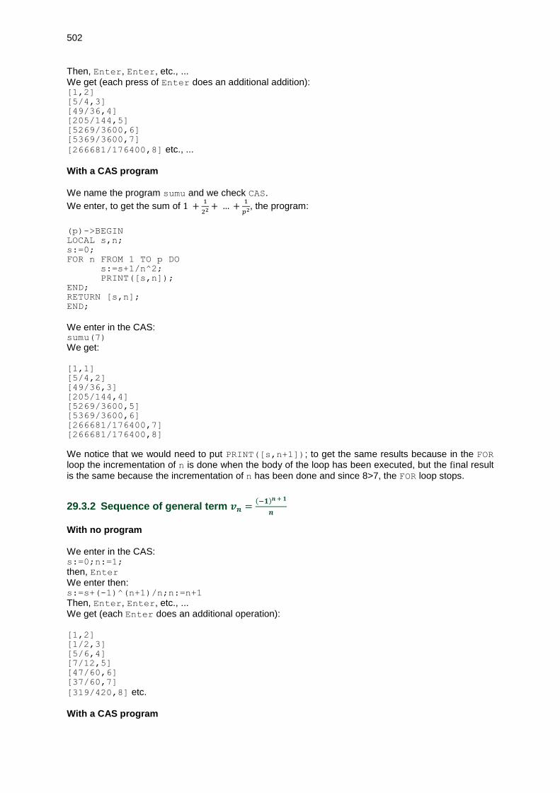
502

Then, Enter, Enter, etc., ... We get (each press of Enter does an additional addition): [1,2]

[5/4,3]

[49/36,4]

[205/144,5]

[5269/3600,6]

[5369/3600,7]

[266681/176400,8] etc., ... With a CAS program We name the program sumu and we check CAS.

We enter, to get the sum of 1 +1

22+ … +

1

𝑝2, the program:

(p)->BEGIN

LOCAL s,n;

s:=0;

FOR n FROM 1 TO p DO

s:=s+1/n^2;

PRINT([s,n]);

END;

RETURN [s,n];

END;

We enter in the CAS: sumu(7)

We get: [1,1]

[5/4,2]

[49/36,3]

[205/144,4]

[5269/3600,5]

[5369/3600,6]

[266681/176400,7]

[266681/176400,8]

We notice that we would need to put PRINT([s,n+1]); to get the same results because in the FOR loop the incrementation of n is done when the body of the loop has been executed, but the final result is the same because the incrementation of n has been done and since 8>7, the FOR loop stops.

29.3.2 Sequence of general term 𝒗𝒏 =(−𝟏)𝒏 + 𝟏

𝒏

With no program We enter in the CAS: s:=0;n:=1;

then, Enter We enter then: s:=s+(-1)^(n+1)/n;n:=n+1

Then, Enter, Enter, etc., ... We get (each Enter does an additional operation): [1,2]

[1/2,3]

[5/6,4]

[7/12,5]

[47/60,6]

[37/60,7]

[319/420,8] etc. With a CAS program

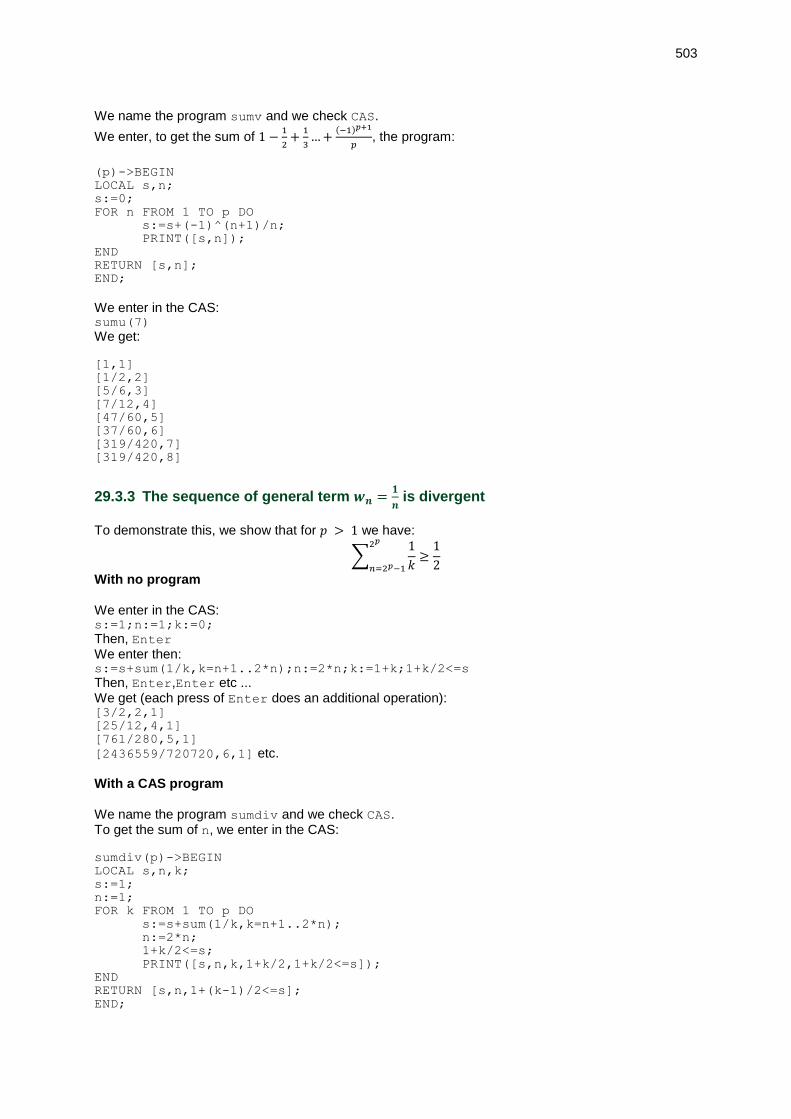
503

We name the program sumv and we check CAS.

We enter, to get the sum of 1 −1

2+1

3…+

(−1)𝑝+1

𝑝, the program:

(p)->BEGIN

LOCAL s,n;

s:=0;

FOR n FROM 1 TO p DO

s:=s+(-1)^(n+1)/n;

PRINT([s,n]);

END

RETURN [s,n];

END;

We enter in the CAS: sumu(7)

We get:

[1,1]

[1/2,2]

[5/6,3]

[7/12,4]

[47/60,5]

[37/60,6]

[319/420,7]

[319/420,8]

29.3.3 The sequence of general term 𝒘𝒏 =𝟏

𝒏 is divergent

To demonstrate this, we show that for 𝑝 > 1 we have:

∑1

𝑘

2𝑝

𝑛=2𝑝−1≥1

2

With no program We enter in the CAS: s:=1;n:=1;k:=0;

Then, Enter We enter then: s:=s+sum(1/k,k=n+1..2*n);n:=2*n;k:=1+k;1+k/2<=s

Then, Enter,Enter etc ... We get (each press of Enter does an additional operation): [3/2,2,1]

[25/12,4,1]

[761/280,5,1]

[2436559/720720,6,1] etc. With a CAS program We name the program sumdiv and we check CAS. To get the sum of n, we enter in the CAS:

sumdiv(p)->BEGIN

LOCAL s,n,k;

s:=1;

n:=1;

FOR k FROM 1 TO p DO

s:=s+sum(1/k,k=n+1..2*n);

n:=2*n;

1+k/2<=s;

PRINT([s,n,k,1+k/2,1+k/2<=s]);

END

RETURN [s,n,1+(k-1)/2<=s];

END;

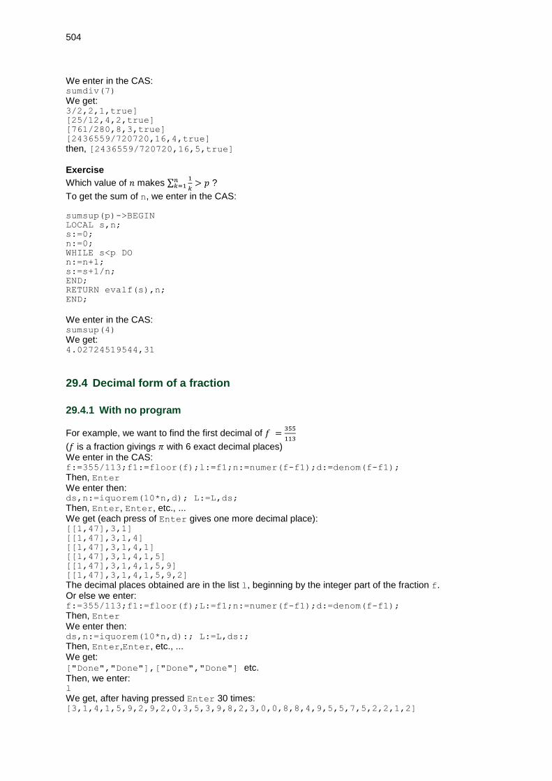
504

We enter in the CAS: sumdiv(7)

We get: 3/2,2,1,true]

[25/12,4,2,true]

[761/280,8,3,true]

[2436559/720720,16,4,true]

then, [2436559/720720,16,5,true] Exercise

Which value of 𝑛 makes ∑1

𝑘

𝑛𝑘=1 > 𝑝 ?

To get the sum of n, we enter in the CAS:

sumsup(p)->BEGIN

LOCAL s,n;

s:=0;

n:=0;

WHILE s<p DO

n:=n+1;

s:=s+1/n;

END;

RETURN evalf(s),n;

END;

We enter in the CAS: sumsup(4)

We get: 4.02724519544,31

29.4 Decimal form of a fraction

29.4.1 With no program

For example, we want to find the first decimal of 𝑓 =355

113

(𝑓 is a fraction givings 𝜋 with 6 exact decimal places) We enter in the CAS: f:=355/113;f1:=floor(f);l:=f1;n:=numer(f-f1);d:=denom(f-f1);

Then, Enter We enter then: ds,n:=iquorem(10*n,d); L:=L,ds;

Then, Enter, Enter, etc., ... We get (each press of Enter gives one more decimal place): [[1,47],3,1]

[[1,47],3,1,4]

[[1,47],3,1,4,1]

[[1,47],3,1,4,1,5]

[[1,47],3,1,4,1,5,9]

[[1,47],3,1,4,1,5,9,2]

The decimal places obtained are in the list l, beginning by the integer part of the fraction f. Or else we enter: f:=355/113;f1:=floor(f);L:=f1;n:=numer(f-f1);d:=denom(f-f1);

Then, Enter We enter then: ds,n:=iquorem(10*n,d):; L:=L,ds:;

Then, Enter,Enter, etc., ... We get: ["Done","Done"],["Done","Done"] etc. Then, we enter: l

We get, after having pressed Enter 30 times: [3,1,4,1,5,9,2,9,2,0,3,5,3,9,8,2,3,0,0,8,8,4,9,5,5,7,5,2,2,1,2]

505

As it is difficult to count the number of times we have pressed Enter, we can display, by example, five more decimal places each time we press Enter. The first Enter pressed displays the integer part followed by five decimal places. We may also wish or not to display 𝑑𝑠 and 𝑛. We enter: f:=355/113;f1:=floor(f);L:=f1;n:=numer(f-f1);d:=denom(f-f1);

Then, Enter and then, ds,n:=iquorem(105*n,d); l:=l*10^5+ds; or, if we do not want the values of ds and n: ds,n:=iquorem(10^5*n,d):; l:=l*10^5+ds;

We get after the first Enter: [14159 33],314159

(or ["Done","Done"],314159)

We notice that: 113 ∗ 314159 + 33 = 355 ∗ 105 If we press 8 times Enter we get a 41-digit number: the integer part 3, followed by the 40 decimal places of 355/113: [5309 83],31415929203539823008849557522123893805309

If we enter: l

We get: 31415929203539823008849557522123893805309

Note that 5309 has only 4 digits, so the last decimal places are: 05309 and we have:

113 ∗ 𝑙 + 83 = 355 ∗ 1040

29.4.2 With a CAS program

We name the program decimal and we check CAS. The program decimal returns a sequence l giving the integer part (f1) and the p first decimal places (ds) of a fraction f. We use the following functions: floor, which gives the integer part of a number, numer, which gives the numerator of a simplified fraction, denom, which gives the denominator of a simplified fraction, iquorem, which gives the quotient and the remainder of the Euclidean division ds,n:=iquorem(10*n,d); is equivalent to: ds:=iquo(10*n,d); (to get the quotient of 10*n by d) and n:=irem(10*n,d); (to get the remainder of 10*n by d). We enter, Shift Program, then New of the push buttons. We get a dialog box with Name and CAS. We check CAS and put as Name: decimal, then OK, and we enter the program which gives the integer part and the p decimal places, one by one, of the rationnal number f: (f,p)->BEGIN

LOCAL n,d,l,f1,j,ds;

f1:=floor(f);

l:=f1;

n:=numer(f-f1);

d:=denom(f-f1);

FOR j FROM 1 TO p DO

ds,n:=iquorem(10*n,d);

l:=l,ds;

END;

RETURN l;

END;

We enter in the CAS: decimal(355/311,20)

We get: 1,1,4,1,4,7,9,0,9,9,6,7,8,4,5,6,5,9,1,6,3

We enter in the CAS: decimal(355/113,20)

We get an approximation of 𝜋 to the next 3 ∗ 10−7: [3,1,4,1,5,9,2,9,2,0,3,5,3,9,8,2,3,0,0,8,8]

We have indeed: evalf(pi) wihich returns 3.1415926536

506

We can determinate the decimal places by 𝑝 groups of 𝑔 decimal places and return an integer 𝑙. The

decimal form of the fraction is then 𝑙 ∗ 10^( − 𝑝 ∗ 𝑔). We name the program decimalg and we check CAS (or we modify the program decimal): (f,p,g)->BEGIN

LOCAL n,d,l,f1,j,ds;

f1:=floor(f);

l:=f1;

n:=numer(f-f1);

d:=denom(f-f1);

FOR j FROM 1 TO p DO

ds,n:=iquorem(10^g*n,d);

l:=l*10^g+ds;

END;

RETURN l;

END;

We enter in the CAS: decimalg(355/311,8,5)

We get: 11414790996784565916398713826366559485530

We enter in the CAS: decimalg(355/113,8,5)

We get: 31415929203539823008849557522123893805309

29.5 29.5 Newton method and Heron algorithm

29.5.1 29.5.1 Newton method

Be 𝑓 two times differentiable, having one and only one zero 𝑟 in the interval [𝑎; 𝑏]. Let us additionally assume that 𝑓’ and 𝑓’’ has a constant sign on [𝑎; 𝑏]. The Newton method consist in

fit 𝑟 by the abscissa 𝑥1 of the point common to 𝑂𝑥 and the tangent at the point 𝑀0 to the graph of 𝑓. If

𝑀0 has for coordinates (𝑥0, 𝑓(𝑥0))(𝑥0 ∈ [𝑎; 𝑏]), the tangent in 𝑀0 has for equation:

𝑦 = 𝑓(𝑥0) + 𝑓’(𝑥0) ∗ (𝑥 – 𝑥0) and then we have:

𝑥1 = 𝑥0 −𝑓(𝑥0)

𝑓(𝑥0)

We can then reiterate the process, and we get a sequence 𝑥_𝑛 converging to 𝑟

– either by greater values, if 𝑓’ ∗ 𝑓’’ > 0 on [𝑎; 𝑏] (i.e. if 𝑓’(𝑟) > 0 and if 𝑓 is convex (𝑓’’ > 0 on [𝑎; 𝑏]) or if 𝑓’(𝑟) < 0 and if 𝑓 is concave (𝑓’’ < 0 𝑜𝑛 [𝑎; 𝑏]))

– either by lower values, if 𝑓’ ∗ 𝑓’’ < 0 on [𝑎; 𝑏] (i.e. if 𝑓’(𝑟) < 0 and if 𝑓 is convex (𝑓’’ > 0 on [𝑎; 𝑏]) or if 𝑓’(𝑟) > 0 and if 𝑓 is concave (𝑓’’ < 0 on [𝑎; 𝑏])).

The Heron algorithm is a specific case of the application of the Newton method to look for the

approximate values of √a for a integer. In this case

√a is a zero of 𝑓(𝑥) = 𝑥2 − 𝑎 and 𝑔(𝑥) = 𝑓’(𝑥) = 2𝑥 then the sequence of the iterations is supplied by:

𝑥𝑛 + 1 = 𝑥𝑛–𝑥𝑛2– 𝑎

2𝑥𝑛= 1

2(𝑥𝑛–

𝑎

𝑥𝑛)

507

29.5.2 Newton algorithm

The function newton_rac returns the approximate value, at the nearest 𝑝, of the root of 𝑓(𝑥) = 0 , starting the iteration with 𝑥0. We notice that the parameter 𝑓 is a function, and thus, that its derivative is the function g:=function_diff(f). We look for a approximate value, so we must write: x0:=evalf(x0) because if we do not put evalf, the calculations of the iteration we be done in the exact way, and hence, will be soon complicated. We check at the beginning if the sequence of 𝑥𝑖(𝑖 = 0. . 𝑛) is increasing or decreasing, starting from

𝑛 = 1, by comparing at the beginning 𝑥1 and 𝑥2. We name the program newton_rac and we check CAS. The program newton_rac gives a zero of f close to x0 at the nearest p. We enter the program: (f,x0,p)->BEGIN

LOCAL x1,h,g;

g:=function_diff(f)

x0:=evalf(x0);

x0:=x0-f(x0)/g(x0);

x1:=x0-f(x0)/g(x0);

IF (x1>x0) THEN

h:=p;

ELSE

h:=-p;

END;

WHILE (f(x1)*f(x1+h)>0) DO

x1:=x1-f(x1)/g(x1);

END;

RETURN x1;

END;

We enter in the CAS: f(x):=cos(x)-x

newtonrac(f,0.4,1e-10)

We get: 0.739085133215

We enter in the CAS: cos(0.739085133215)-0.739085133215

We get: 2.70006239589e-13

29.5.3 Heron algorithm

We name the program heron and we check CAS. The program heron gives a fraction approaching sqrt(a) at the nearest p when x0 is close to sqrt(a). We enter: (a,x0,p)->BEGIN

LOCAL b;

b:=x0-p;

WHILE b^2>a DO

x0:=(x0+a/x0)/2;

b:=x0-p;

END;

RETURN x0;

END;

We enter in the CAS: heron(2,3/2,10^-10)

We get:

508

66587/470832

We enter in the CAS: decimalg(66587/470832,2,5)

We get: 14142135623

We enter in the CAS: f:=heron(2,2,10^-40)

We get: 1572584048032918633353217/1111984844349868137938112

We enter in the CAS: r2:=decimalg(f,8,5)

We get: 14142135623730950488016887242096980785696

and √2 ≃ r2 ∗ 10−40 The library of long floating point numbers is not implemented in the HP Prime. We use the CAS to check. We enter in CAS: evalf(r2*10^-40,41)

We get: 1.4142135623730950488016887242096980785696

We enter in CAS: evalf(sqrt(2),41)

Because the CAS rounds off the last decimal place, we get: 14142135623730950488016887242096980785697

509

Chapter 30 Example of programs

30.1 GCD and Bezout identity from Home

30.1.1 GCD

We use Euclid’s algorithm. We enter: EXPORT GCD(A,B)

BEGIN

LOCAL R;

WHILE B<>0 DO

R:=A MOD B;

A:=B;

B:=R;

END;

RETURN A;

END;

Or else we use the function irem which returns the remainder of the Euclidean division: EXPORT GCD(A,B)

BEGIN

LOCAL R;

WHILE B<>0 DO

R:=CAS.irem(A,B);

A:=B;

B:=R;

END;

RETURN A;

END;

We enter: GCD(45,25)

We get: 5

30.1.2 Bezout identity for A and B

We use Euclid’s algorithm and the variables U,V,R which will vary so that at the step 𝑘 we have 𝐴 ∗ 𝑈𝑘 + 𝐵 ∗ 𝑉𝑘 = 𝑅𝑘 .

Thus, when 𝑅𝑝 is the GCD of 𝐴 and 𝐵, we will have:

𝐴 ∗ 𝑈𝑝 + 𝐵 ∗ 𝑉𝑝 = GCD(𝐴, 𝐵).

At the beginning, we have: (1) 𝐴 = 𝑈1 ∗ 𝐴 + 𝑉1 ∗ 𝐵 (𝑅1 = 𝐴, 𝑈1 = 1, 𝑉1 = 0) (2) 𝐵 = 𝑈2 ∗ 𝐴 + 𝑉2 ∗ 𝐵 (𝑅2 = 𝐵, 𝑈2 = 0, 𝑉2 = 1) We want to get: 𝑅3 = 𝑈3 ∗ 𝐴 + 𝑉3 ∗ 𝐵

since 𝑅3 = 𝐴 − 𝐵 ∗ 𝑄3 (with 𝑄3 integer quotient of 𝐴 = 𝑅1 by 𝐵 = 𝑅2) we find, by doing (1)– 𝑄3 ∗ (2):

𝑈3 = 𝑈1– 𝑄3 ∗ 𝑈2 and 𝑉3 = 𝑉1– 𝑄3 ∗ 𝑉2 and thus 𝑅3 = 𝑈3 ∗ 𝐴 + 𝑉3 ∗ 𝐵 and at each step we will have

𝑅𝑘 = 𝑈𝑘 ∗ 𝐴 + 𝑉𝑘 ∗ 𝐵 with the relations:

510

𝑈𝑘 = 𝑈𝑘−2 – 𝑄𝑘 ∗ 𝑈𝑘−1 and 𝑉𝑘 = 𝑉𝑘−2 – 𝑄𝑘 ∗ 𝑉𝑘−1. To write the program, we need 3 lists 𝐿1, 𝐿2, 𝐿3 which will be 3 successive steps of [𝑈𝑘 , 𝑉𝑘 , 𝑅𝑘]. At the beginning: 𝐿1 = 1, 0, 𝑅1 (𝑅1 = 𝐴) 𝐿2:= 0, 1, 𝑅2 (𝑅2 = 𝐵) We calculate 𝐿3: 𝐿3 is obtained from 𝐿1 and 𝐿2 and if 𝑄3, 𝑅3:=iquorem(R1,R2), on 𝑅3 = 𝑅1 − 𝑅2 ∗ 𝑄3 and then

𝐿3 = 𝐿1 − 𝑄3 ∗ 𝐿2.

Then, 𝑅1 takes the value of 𝑅2, 𝐿1 the value of 𝐿2, 𝑅2 the value of 𝑅3, 𝐿2 the value of 𝐿3, etc., ... We stop when 𝑅2 = 0 and then 𝑅1 = GCD(𝐴, 𝐵). We enter: EXPORT BEZOUT(A,B)

BEGIN

LOCAL L1,L2,L3,Q3,R1,R2,R3;

R1:=A;

R2:=B;

L1:={1,0,R1};

L2:={0,1,R2};

WHILE B<>0 DO

Q3,R3:=CAS.iquorem(R1,R2);

R1:=R2;

R2:=R3;

L3:=L1-Q3*L2;

L1:=L2;

L2:=L3;

END;

RETURN L1;

END;

We can reduce the number of variables: EXPORT BEZOUT(A,B)

BEGIN

LOCAL L1,L2,L3,Q;

L1:={1,0,A};

L2:={0,1,B};

WHILE L2(3)<>0 DO

//Q:=iquo(L1(3),L2(3));

Q:=(L1(3)-L1(3) MOD L2(3))/L2(3)

L3:=L1-Q*L2;

L1:=L2;

L2:=L3;

END;

RETURN L1;

END;

We enter: BEZOUT(45,10)

We get: 1,-4,5

Which means that 1 ∗ 45 − 4 ∗ 10 = 5 = GCD(45,25) We enter: BEZOUT(45,25)

We get: -1,2,5

Which means that −1 ∗ 45 + 2 ∗ 25 = 5 = GCD(45,25)

511

30.2 GCD and Bezout identity from the CAS

30.2.1 GCD with the CAS with no program

We can apply Euclid’s algorithm by using the key Enter of the calculator. We enter on the entry line: a:=72;b:=33; then we press Enter Then, we enter on the entry line: r:=irem(a,b);a:=b;b:=r; then we press Enter several times until the last value is null. When the last value is null,the GCD of a and b is the value 3 above the 0. We can check this thanks to the existing gcd command: gcd(72,33) returns 3.

30.2.2 GCD with a CAS program

We use the function irem to write the Euclid’s algorithm. We check CAS, and we name the program GCD, and we enter: (a,b)->

BEGIN

LOCAL r;

WHILE b<>0 DO

r:=irem(a,b);

a:=b;

b:=r;

END;

RETURN(a);

END;

We enter: GCD(45,25)

We get: 5

30.2.3 Bezout identity with the CAS, with no program

We can apply the algorithm giving the coefficients of the Bezout identity by using the Enter key of the calculator. We enter on the entry line: a:=72;b:=33;l1:=[1,0,a];l2:=[0,1,b] then we press Enter Then, we enter on the entry line: q:=iquo(l1(3),l2(3));l3:=l1-q*l2;l1:=l2;l2:=l3; then we press Enter several times until the last value of the last list is null. When this last value is null, the Bezout identity [-5,11,3] is the last list above the 0: this means that -5*72+11*33=3]. We can check this thanks to the existing iegcd command, giving the Bezout identity: iegcd(72,33) returns [-5,11,3].

30.2.4 Bezout identity with a CAS program

We use Euclid’s algorithm and the variables u,v,r which will vary so that at te step 𝑘 we have 𝑎 ∗ 𝑢_𝑘 + 𝑏 ∗ 𝑣_𝑘 = 𝑟_𝑘. Thus, when rp is the GCD of 𝑎 and 𝑏, we will have:

𝑎 ∗ 𝑢_𝑝 + 𝑏 ∗ 𝑣_𝑝 = 𝐺𝐶𝐷(𝑎, 𝑏). To write the program, we need 3 lists 𝐿1, 𝐿2, 𝐿3 which will be 3 successive steps of [𝑢_𝑘, 𝑣_𝑘, 𝑟_𝑘]. At the beginning:

𝐿1 = 1, 0, 𝑟1 (𝑟1 = 𝑎) 𝐿2:= 0, 1, 𝑟2 (𝑟2 = 𝑏)

We calculate 𝐿3: 𝐿3 is obtained from 𝐿1 and 𝐿2 and if q3, r3:=iquorem(r1, r2), we have: 𝑟3 = 𝑟1 − 𝑟2 ∗ 𝑞3

and then 𝐿3 = 𝐿1 − 𝑞3 ∗ 𝐿2.

Then, 𝑟1 takes the value of 𝑟2, 𝐿1 the value of 𝐿2, 𝑟2 takes the value of 𝑟3, 𝐿2 the value of 𝐿3, etc., ...

512

We stop when 𝑒2 = 0 and then 𝑟1 = 𝐺𝐶𝐷(𝑎, 𝑏). We enter: (a,b)->BEGIN

LOCAL l1,l2,l3,q;

l1:=[1,0,a];

l2:=[0,1,b];

WHILE l2(3)<>0 DO

q:=iquo(l1(3),l2(3));

l3:=l1-q*l2;

l1:=l2;

l2:=l3;

END;

RETURN l1;

END;

We enter: BEZOUT(45,10)

We get: 1,-4,5

Which means that 1*45-4*10=5=GCD(45,25) We enter: BEZOUT(45,25)

We get: -1,2,5

Which means that −1 ∗ 45 + 2 ∗ 25 = 5 = GCD(45,25)