Separable Data

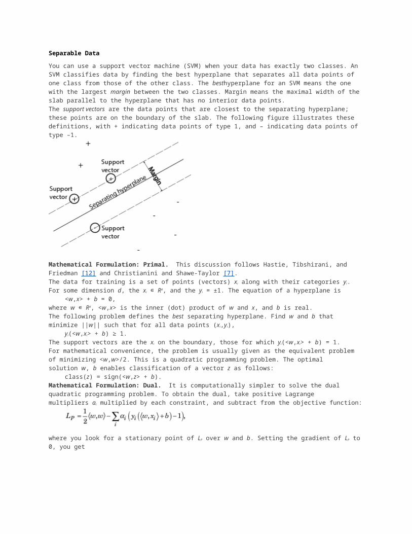
You can use a support vector machine (SVM) when your data has exactly two classes. An SVM classifies data by finding the best hyperplane that separates all data points of one class from those of the other class. The besthyperplane for an SVM means the one with the largest margin between the two classes. Margin means the maximal width of the slab parallel to the hyperplane that has no interior data points.The support vectors are the data points that are closest to the separating hyperplane; these points are on the boundary of the slab. The following figure illustrates these definitions, with + indicating data points of type 1, and – indicating data points of type –1.

Mathematical Formulation: Primal.  This discussion follows Hastie, Tibshirani, and Friedman [12] and Christianini and Shawe-Taylor [7].The data for training is a set of points (vectors) xi along with their categories yi. For some dimension d, the xi ∊ Rd, and the yi = ±1. The equation of a hyperplane is

<w,x> + b = 0,where w ∊ Rd, <w,x> is the inner (dot) product of w and x, and b is real.The following problem defines the best separating hyperplane. Find w and b that minimize ||w|| such that for all data points (xi,yi),

yi(<w,xi> + b) ≥ 1.The support vectors are the xi on the boundary, those for which yi(<w,xi> + b) = 1.For mathematical convenience, the problem is usually given as the equivalent problem of minimizing <w,w>/2. This is a quadratic programming problem. The optimal solution w, b enables classification of a vector z as follows:

class(z) = sign(<w,z> + b).Mathematical Formulation: Dual.  It is computationally simpler to solve the dual quadratic programming problem. To obtain the dual, take positive Lagrange multipliers αi multiplied by each constraint, and subtract from the objective function:

where you look for a stationary point of LP over w and b. Setting the gradient of LP to 0, you get

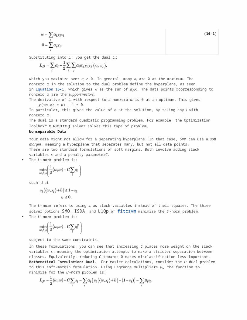
(16-1)

Substituting into LP, you get the dual LD:

which you maximize over αi ≥ 0. In general, many αi are 0 at the maximum. The nonzero αi in the solution to the dual problem define the hyperplane, as seen in Equation   16-1 , which gives w as the sum of αiyixi. The data points xicorresponding to nonzero αi are the support vectors.The derivative of LD with respect to a nonzero αi is 0 at an optimum. This gives

yi(<w,xi> + b) – 1 = 0.In particular, this gives the value of b at the solution, by taking any i with nonzero αi.The dual is a standard quadratic programming problem. For example, the Optimization Toolbox™ quadprog solver solves this type of problem.Nonseparable Data

Your data might not allow for a separating hyperplane. In that case, SVM can use a soft margin, meaning a hyperplane that separates many, but not all data points.There are two standard formulations of soft margins. Both involve adding slack variables si and a penalty parameterC.

The L1-norm problem is:

such that

The L1-norm refers to using si as slack variables instead of their squares. The three solver options SMO, ISDA, and L1Qp of fitcsvm minimize the L1-norm problem.

The L2-norm problem is:

subject to the same constraints.In these formulations, you can see that increasing C places more weight on the slack variables si, meaning the optimization attempts to make a stricter separation between classes. Equivalently, reducing C towards 0 makes misclassification less important.Mathematical Formulation: Dual.  For easier calculations, consider the L1 dual problem to this soft-margin formulation. Using Lagrange multipliers μi, the function to minimize for the L1-norm problem is:

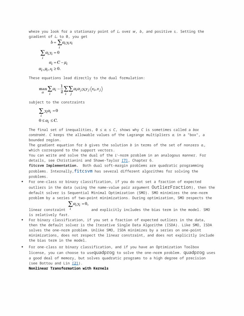
where you look for a stationary point of LP over w, b, and positive si. Setting the gradient of LP to 0, you get

These equations lead directly to the dual formulation:

subject to the constraints

The final set of inequalities, 0 ≤ αi ≤ C, shows why C is sometimes called a box constraint. C keeps the allowable values of the Lagrange multipliers αi in a "box", a bounded region.The gradient equation for b gives the solution b in terms of the set of nonzero αi, which correspond to the support vectors.You can write and solve the dual of the L2-norm problem in an analogous manner. For details, see Christianini and Shawe-Taylor [7], Chapter 6.fitcsvm Implementation.  Both dual soft-margin problems are quadratic programming problems. Internally,fitcsvm has several different algorithms for solving the problems.

For one-class or binary classification, if you do not set a fraction of expected outliers in the data (using the name-value pair argument OutlierFraction), then thedefault solver is Sequential Minimal Optimization (SMO). SMO minimizes the one-norm problem by a series of two-point minimizations. During optimization, SMO respects the

linear constraint   and explicitly includes the bias term in the model. SMO is relatively fast.

For binary classification, if you set a fraction of expected outliers in the data, then the default solver is the Iterative Single Data Algorithm (ISDA). Like SMO, ISDA solves the one-norm problem. Unlike SMO, ISDA minimizes by a series on one-point minimizations, does not respect the linear constraint, and does not explicitly includethe bias term in the model.

For one-class or binary classification, and if you have an Optimization Toolbox license, you can choose to usequadprog to solve the one-norm problem. quadprog usesa good deal of memory, but solves quadratic programs to a high degree of precision (see Bottou and Lin [2]).Nonlinear Transformation with Kernels

Some binary classification problems do not have a simple hyperplane as a useful separating criterion. For those problems, there is a variant of the mathematical approach that retains nearly all the simplicity of an SVM separating hyperplane.

This approach uses these results from the theory of reproducing kernels:

There is a class of functions K(x,y) with the following property. There is a linear space S and a function φmapping x to S such that

K(x,y) = <φ(x),φ(y)>.The dot product takes place in the space S.

This class of functions includes:o Polynomials: For some positive integer d,

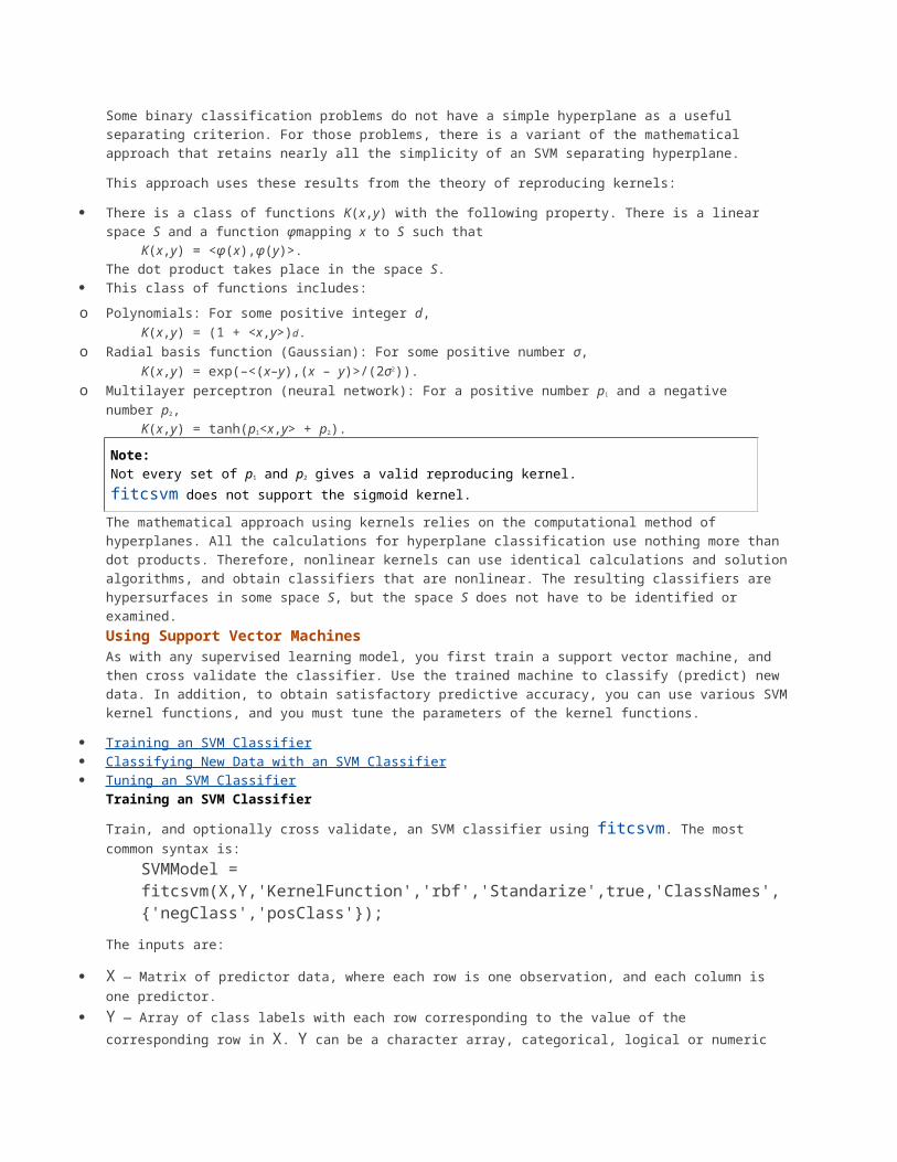
K(x,y) = (1 + <x,y>)d.o Radial basis function (Gaussian): For some positive number σ,

K(x,y) = exp(–<(x–y),(x – y)>/(2σ2)).o Multilayer perceptron (neural network): For a positive number p1 and a negative

number p2,K(x,y) = tanh(p1<x,y> + p2).

Note:  Not every set of p1 and p2 gives a valid reproducing kernel.fitcsvm does not support the sigmoid kernel.The mathematical approach using kernels relies on the computational method of hyperplanes. All the calculations for hyperplane classification use nothing more than dot products. Therefore, nonlinear kernels can use identical calculations and solutionalgorithms, and obtain classifiers that are nonlinear. The resulting classifiers are hypersurfaces in some space S, but the space S does not have to be identified or examined.Using Support Vector MachinesAs with any supervised learning model, you first train a support vector machine, and then cross validate the classifier. Use the trained machine to classify (predict) new data. In addition, to obtain satisfactory predictive accuracy, you can use various SVMkernel functions, and you must tune the parameters of the kernel functions.

Training an SVM Classifier Classifying New Data with an SVM Classifier Tuning an SVM Classifier

Training an SVM Classifier

Train, and optionally cross validate, an SVM classifier using fitcsvm. The most common syntax is:

SVMModel = fitcsvm(X,Y,'KernelFunction','rbf','Standarize',true,'ClassNames',{'negClass','posClass'});

The inputs are:

X — Matrix of predictor data, where each row is one observation, and each column is one predictor.

Y — Array of class labels with each row corresponding to the value of the corresponding row in X. Y can be a character array, categorical, logical or numeric

vector, or vector cell array of strings. Column vector with each row corresponding to the value of the corresponding row in X. Y can be a categorical or character array, logical or numeric vector, or cell array of strings.

KernelFunction — The default value is 'linear' for two-class learning, which separates the data by a hyperplane. The value 'rbf' is the default for one-class learning, and uses a Gaussian radial basis function. An important step to successfullytrain an SVM classifier is to choose an appropriate kernel function.

Standardize — Flag indicating whether the software should standardize the predictorsbefore training the classifier.

ClassNames — Cell array of strings indicating which class is the negative class, andwhich is the positive class. The negative class is in the first cell (negClass), andthe positive class is in the second cell (posClass). It is good practice to specify the class names, especially if you are comparing the performance of different classifiers.The resulting, trained model (SVMModel) contains the optimized parameters from the SVM algorithm, enabling you to classify new data.For more name-value pairs you can use to control the training, see the fitcsvm reference page.Classifying New Data with an SVM Classifier

Classify new data using predict. The syntax for classifying new data using a trained SVM classifier (SVMModel) is:

[label,score] = predict(SVMModel,newX);

The resulting vector, label, represents the classification of each row in X. score is an n-by-2 matrix of soft scores. Each row corresponds to a row in X, which is a new observation. The first column contains the scores for the observations being classified in the negative class, and the second column contains the scores observations being classified in the positive class.To estimate posterior probabilities rather than scores, first pass the trained SVM classifier (SVMModel) tofitPosterior, which fits a score-to-posterior-probability transformation function to the scores. The syntax is:

ScoreSVMModel = fitPosterior(SVMModel,X,Y);

The property ScoreTransform of the classifier ScoreSVMModel contains the optimaltransformation function. PassScoreSVMModel to predict. Rather than returning the scores, the output argument score contains the posterior probabilities of an observation being classified in the negative (column 1 of score) or positive (column 2 of score) class.Tuning an SVM Classifier

Try tuning parameters of your classifier according to this scheme:

1. Pass the data to fitcsvm, and set the name-value pair arguments 'KernelScale','auto'. Suppose that the trained SVM model is called SVMModel. The software uses a heuristic procedure to select the kernel scale. The heuristic procedure uses subsampling. Therefore, to reproduce results, set a random number seed usingrng before training the classifier.

2. Cross validate the classifier by passing it to crossval. By default, the softwareconducts 10-fold cross validation.

3. Pass the cross-validated SVM model to kFoldLoss to estimate and retain the classification error.

4. Retrain the SVM classifier, but adjust the 'KernelScale' and 'BoxConstraint' name-value pair arguments.

BoxConstraint — One strategy is to try a geometric sequence of the box constraint parameter. For example, take 11 values, from 1e-5 to 1e5 by a factor of 10. Increasing BoxConstraint might decrease the number of support vectors, but also might increase training time.

KernelScale — One strategy is to try a geometric sequence of the RBF sigma parameter scaled at the original kernel scale. Do this by:

1. Retrieving the original kernel scale, e.g., ks, using dot notation: ks = SVMModel.KernelParameters.Scale.

2. Use as new kernel scales factors of the original. For example, multiply ks by the 11 values 1e-5 to 1e5, increasing by a factor of 10.

Choose the model that yields the lowest classification error.

You might want to further refine your parameters to obtain better accuracy. Start withyour initial parameters and perform another cross-validation step, this time using a factor of 1.2. Alternatively, optimize your parameters withfminsearch, as shown in Train and Cross Validate SVM Classifiers.Train SVM Classifiers Using a Gaussian KernelThis example shows how to generate a nonlinear classifier with Gaussian kernel function. First, generate one class of points inside the unit disk in two dimensions, and another class of points in the annulus from radius 1 to radius 2. Then, generates a classifier based on the data with the Gaussian radial basis function kernel. The default linear classifier is obviously unsuitable for this problem, since the model iscircularly symmetric. Set the box constraint parameter to Inf to make a strict classification, meaning no misclassified training points. Other kernel functions mightnot work with this strict box constraint, since they might be unable to provide a strict classification. Even though the rbf classifier can separate the classes, the result can be overtrained.Generate 100 points uniformly distributed in the unit disk. To do so, generate a radius r as the square root of a uniform random variable, generate an angle t uniformlyin (0,   ), and put the point at (r cos( t ), r sin( t )).

rng(1); % For reproducibilityr = sqrt(rand(100,1)); % Radiust = 2*pi*rand(100,1); % Angledata1 = [r.*cos(t), r.*sin(t)]; % Points

Generate 100 points uniformly distributed in the annulus. The radius is again proportional to a square root, this time a square root of the uniform distribution from 1 through 4.

r2 = sqrt(3*rand(100,1)+1); % Radius

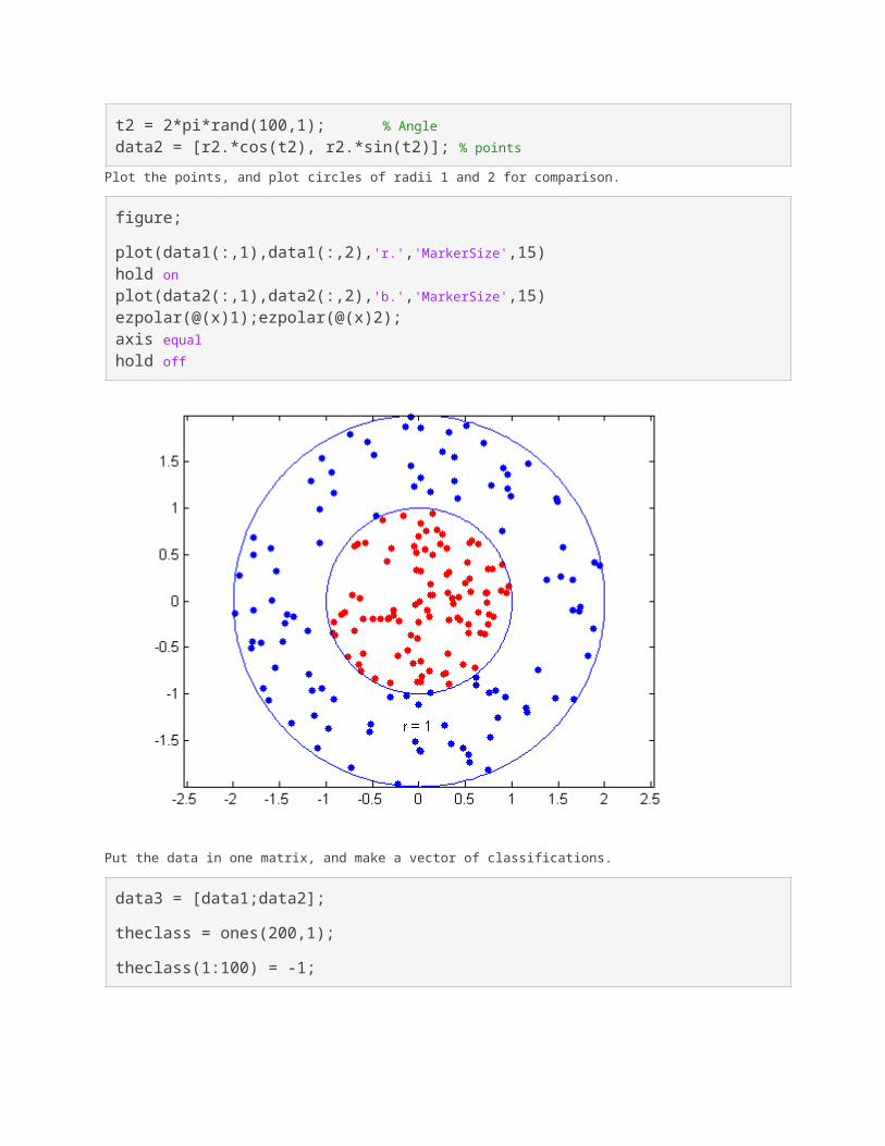
t2 = 2*pi*rand(100,1); % Angledata2 = [r2.*cos(t2), r2.*sin(t2)]; % points

Plot the points, and plot circles of radii 1 and 2 for comparison.

figure;

plot(data1(:,1),data1(:,2),'r.','MarkerSize',15)hold onplot(data2(:,1),data2(:,2),'b.','MarkerSize',15)ezpolar(@(x)1);ezpolar(@(x)2);axis equalhold off

Put the data in one matrix, and make a vector of classifications.

data3 = [data1;data2];

theclass = ones(200,1);

theclass(1:100) = -1;

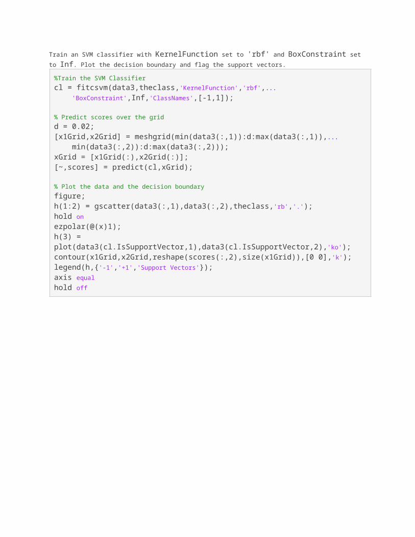
Train an SVM classifier with KernelFunction set to 'rbf' and BoxConstraint set to Inf. Plot the decision boundary and flag the support vectors.%Train the SVM Classifiercl = fitcsvm(data3,theclass,'KernelFunction','rbf',... 'BoxConstraint',Inf,'ClassNames',[-1,1]);

% Predict scores over the gridd = 0.02;[x1Grid,x2Grid] = meshgrid(min(data3(:,1)):d:max(data3(:,1)),... min(data3(:,2)):d:max(data3(:,2)));xGrid = [x1Grid(:),x2Grid(:)];[~,scores] = predict(cl,xGrid);

% Plot the data and the decision boundaryfigure;h(1:2) = gscatter(data3(:,1),data3(:,2),theclass,'rb','.');hold onezpolar(@(x)1);h(3) = plot(data3(cl.IsSupportVector,1),data3(cl.IsSupportVector,2),'ko');contour(x1Grid,x2Grid,reshape(scores(:,2),size(x1Grid)),[0 0],'k');legend(h,{'-1','+1','Support Vectors'});axis equalhold off

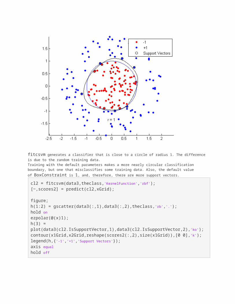
fitcsvm generates a classifier that is close to a circle of radius 1. The difference is due to the random training data.Training with the default parameters makes a more nearly circular classification boundary, but one that misclassifies some training data. Also, the default value of BoxConstraint is 1, and, therefore, there are more support vectors.cl2 = fitcsvm(data3,theclass,'KernelFunction','rbf');[~,scores2] = predict(cl2,xGrid);

figure;h(1:2) = gscatter(data3(:,1),data3(:,2),theclass,'rb','.');hold onezpolar(@(x)1);h(3) = plot(data3(cl2.IsSupportVector,1),data3(cl2.IsSupportVector,2),'ko');contour(x1Grid,x2Grid,reshape(scores2(:,2),size(x1Grid)),[0 0],'k');legend(h,{'-1','+1','Support Vectors'});axis equalhold off

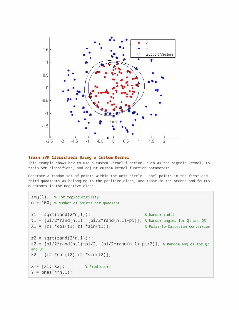
Train SVM Classifiers Using a Custom KernelThis example shows how to use a custom kernel function, such as the sigmoid kernel, totrain SVM classifiers, and adjust custom kernel function parameters.

Generate a random set of points within the unit circle. Label points in the first and third quadrants as belonging to the positive class, and those in the second and fourthquadrants in the negative class.

rng(1); % For reproducibilityn = 100; % Number of points per quadrant

r1 = sqrt(rand(2*n,1)); % Random radiit1 = [pi/2*rand(n,1); (pi/2*rand(n,1)+pi)]; % Random angles for Q1 and Q3X1 = [r1.*cos(t1) r1.*sin(t1)]; % Polar-to-Cartesian conversion

r2 = sqrt(rand(2*n,1));t2 = [pi/2*rand(n,1)+pi/2; (pi/2*rand(n,1)-pi/2)]; % Random angles for Q2and Q4X2 = [r2.*cos(t2) r2.*sin(t2)];

X = [X1; X2]; % Predictors Y = ones(4*n,1);

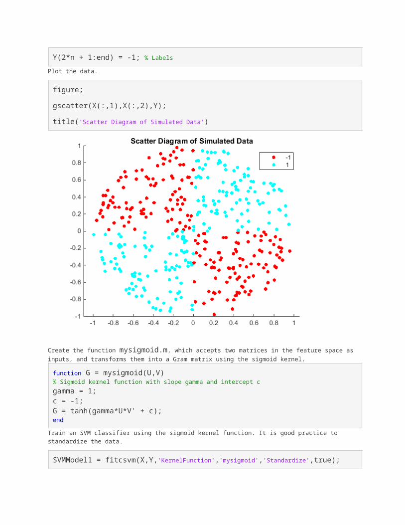
Y(2*n + 1:end) = -1; % LabelsPlot the data.

figure;

gscatter(X(:,1),X(:,2),Y);

title('Scatter Diagram of Simulated Data')

Create the function mysigmoid.m, which accepts two matrices in the feature space as inputs, and transforms them into a Gram matrix using the sigmoid kernel.

function G = mysigmoid(U,V)% Sigmoid kernel function with slope gamma and intercept cgamma = 1;c = -1;G = tanh(gamma*U*V' + c);end

Train an SVM classifier using the sigmoid kernel function. It is good practice to standardize the data.

SVMModel1 = fitcsvm(X,Y,'KernelFunction','mysigmoid','Standardize',true);

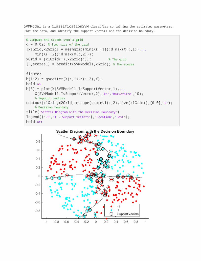
SVMModel is a ClassificationSVM classifier containing the estimated parameters.Plot the data, and identify the support vectors and the decision boundary.

% Compute the scores over a gridd = 0.02; % Step size of the grid[x1Grid,x2Grid] = meshgrid(min(X(:,1)):d:max(X(:,1)),... min(X(:,2)):d:max(X(:,2)));xGrid = [x1Grid(:),x2Grid(:)]; % The grid[~,scores1] = predict(SVMModel1,xGrid); % The scores

figure;h(1:2) = gscatter(X(:,1),X(:,2),Y);hold onh(3) = plot(X(SVMModel1.IsSupportVector,1),... X(SVMModel1.IsSupportVector,2),'ko','MarkerSize',10); % Support vectorscontour(x1Grid,x2Grid,reshape(scores1(:,2),size(x1Grid)),[0 0],'k'); % Decision boundarytitle('Scatter Diagram with the Decision Boundary')legend({'-1','1','Support Vectors'},'Location','Best');hold off

You can adjust the kernel parameters in an attempt to improve the shape of the decision boundary. This might also decrease the within-sample misclassification rate, but, you should first determine the out-of-sample misclassification rate.

Determine the out-of-sample misclassification rate by using 10-fold cross validation.

CVSVMModel1 = crossval(SVMModel1);

misclass1 = kfoldLoss(CVSVMModel1);

misclass1

misclass1 =

0.1350

The out-of-sample misclassification rate is 13.5%.

Set gamma = 0.5; within mysigmoid.m. Then, train an SVM classifier using the adjusted sigmoid kernel. Plot the data and the decision region, and determine the out-of-sample misclassification rate.

SVMModel2 = fitcsvm(X,Y,'KernelFunction','mysigmoid','Standardize',true);[~,scores2] = predict(SVMModel2,xGrid);

figure;h(1:2) = gscatter(X(:,1),X(:,2),Y);hold onh(3) = plot(X(SVMModel2.IsSupportVector,1),... X(SVMModel2.IsSupportVector,2),'ko','MarkerSize',10);title('Scatter Diagram with the Decision Boundary')contour(x1Grid,x2Grid,reshape(scores2(:,2),size(x1Grid)),[0 0],'k');legend({'-1','1','Support Vectors'},'Location','Best');hold off

CVSVMModel2 = crossval(SVMModel2);misclass2 = kfoldLoss(CVSVMModel2);misclass2misclass2 =

0.0450

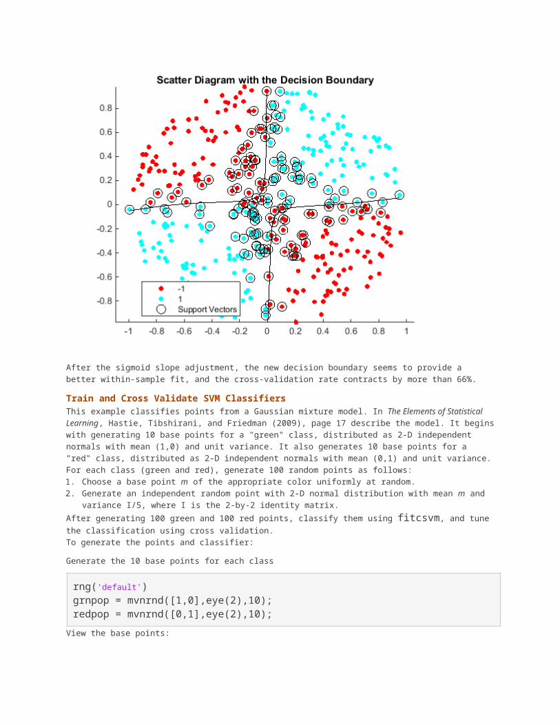
After the sigmoid slope adjustment, the new decision boundary seems to provide a better within-sample fit, and the cross-validation rate contracts by more than 66%.

Train and Cross Validate SVM ClassifiersThis example classifies points from a Gaussian mixture model. In The Elements of Statistical Learning, Hastie, Tibshirani, and Friedman (2009), page 17 describe the model. It beginswith generating 10 base points for a "green" class, distributed as 2-D independent normals with mean (1,0) and unit variance. It also generates 10 base points for a "red" class, distributed as 2-D independent normals with mean (0,1) and unit variance.For each class (green and red), generate 100 random points as follows:1. Choose a base point m of the appropriate color uniformly at random.2. Generate an independent random point with 2-D normal distribution with mean m and

variance I/5, where I is the 2-by-2 identity matrix.After generating 100 green and 100 red points, classify them using fitcsvm, and tune the classification using cross validation.To generate the points and classifier:

Generate the 10 base points for each class

rng('default')grnpop = mvnrnd([1,0],eye(2),10);redpop = mvnrnd([0,1],eye(2),10);

View the base points:

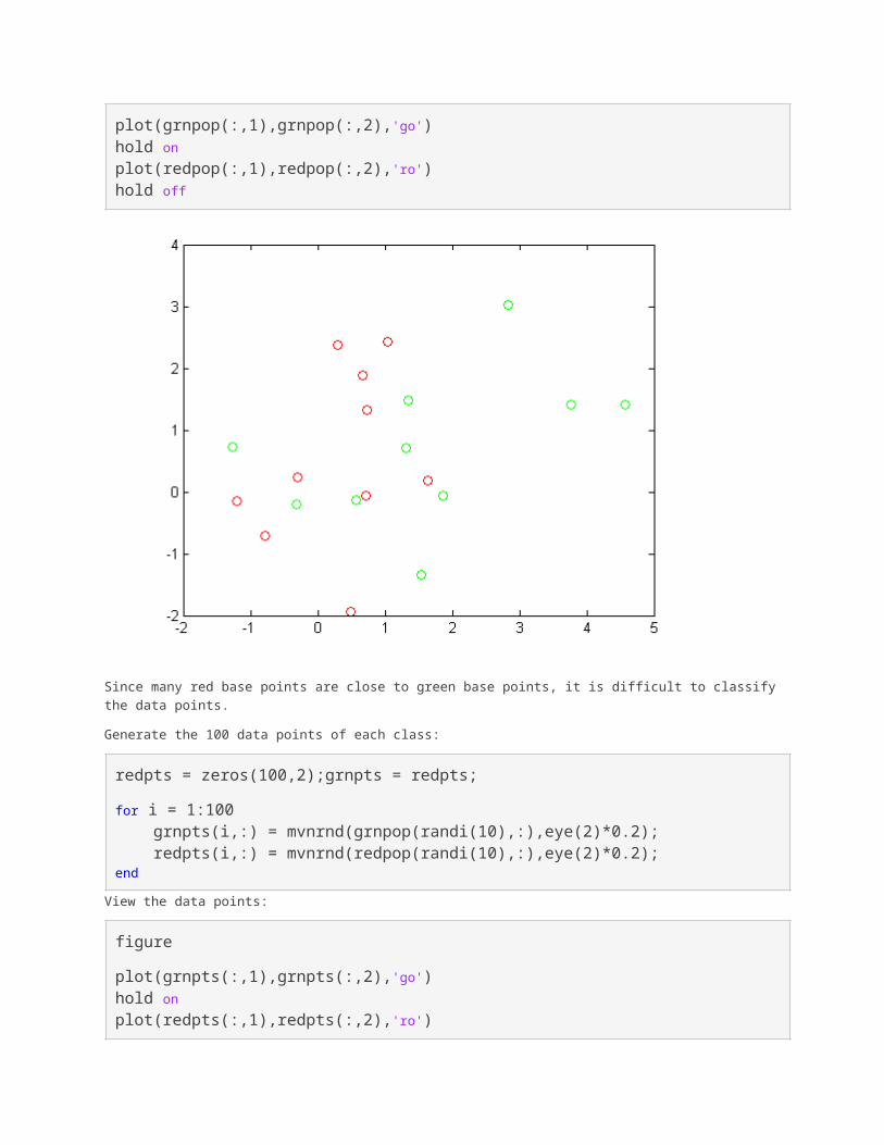
plot(grnpop(:,1),grnpop(:,2),'go')hold onplot(redpop(:,1),redpop(:,2),'ro')hold off

Since many red base points are close to green base points, it is difficult to classifythe data points.

Generate the 100 data points of each class:

redpts = zeros(100,2);grnpts = redpts;

for i = 1:100 grnpts(i,:) = mvnrnd(grnpop(randi(10),:),eye(2)*0.2); redpts(i,:) = mvnrnd(redpop(randi(10),:),eye(2)*0.2);end

View the data points:

figure

plot(grnpts(:,1),grnpts(:,2),'go')hold onplot(redpts(:,1),redpts(:,2),'ro')

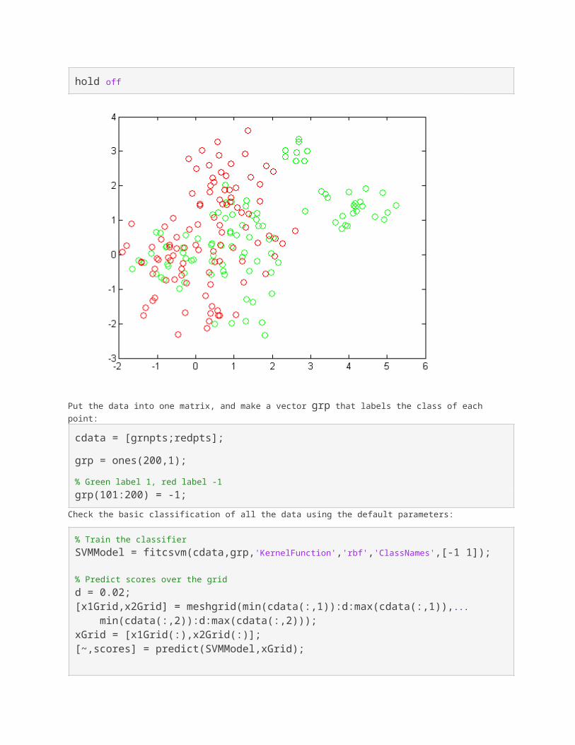
hold off

Put the data into one matrix, and make a vector grp that labels the class of each point:

cdata = [grnpts;redpts];

grp = ones(200,1);% Green label 1, red label -1grp(101:200) = -1;

Check the basic classification of all the data using the default parameters:

% Train the classifierSVMModel = fitcsvm(cdata,grp,'KernelFunction','rbf','ClassNames',[-1 1]);

% Predict scores over the gridd = 0.02;[x1Grid,x2Grid] = meshgrid(min(cdata(:,1)):d:max(cdata(:,1)),... min(cdata(:,2)):d:max(cdata(:,2)));xGrid = [x1Grid(:),x2Grid(:)];[~,scores] = predict(SVMModel,xGrid);

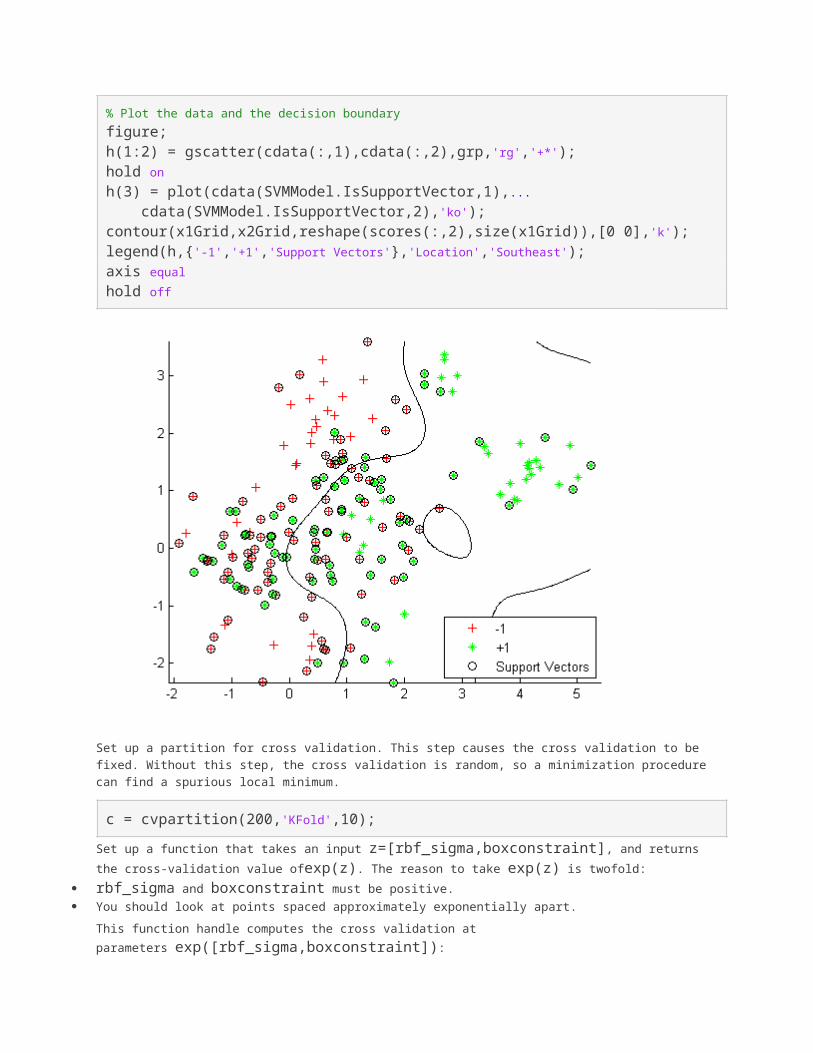
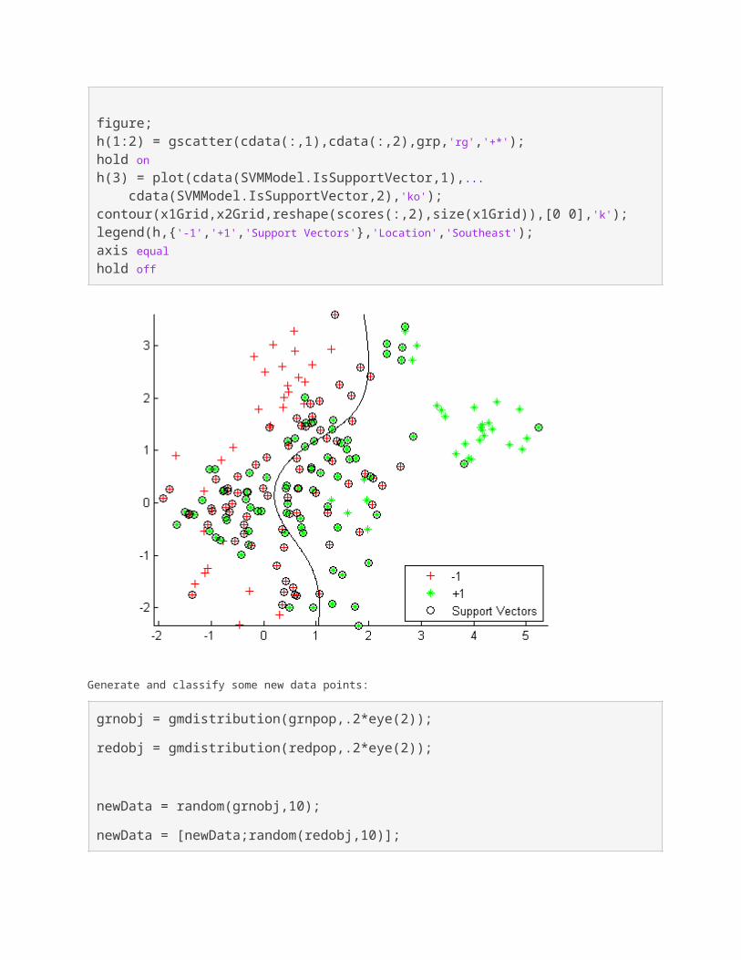
% Plot the data and the decision boundaryfigure;h(1:2) = gscatter(cdata(:,1),cdata(:,2),grp,'rg','+*');hold onh(3) = plot(cdata(SVMModel.IsSupportVector,1),... cdata(SVMModel.IsSupportVector,2),'ko');contour(x1Grid,x2Grid,reshape(scores(:,2),size(x1Grid)),[0 0],'k');legend(h,{'-1','+1','Support Vectors'},'Location','Southeast');axis equalhold off

Set up a partition for cross validation. This step causes the cross validation to be fixed. Without this step, the cross validation is random, so a minimization procedure can find a spurious local minimum.

c = cvpartition(200,'KFold',10);Set up a function that takes an input z=[rbf_sigma,boxconstraint], and returns the cross-validation value ofexp(z). The reason to take exp(z) is twofold:

rbf_sigma and boxconstraint must be positive. You should look at points spaced approximately exponentially apart.

This function handle computes the cross validation at parameters exp([rbf_sigma,boxconstraint]):

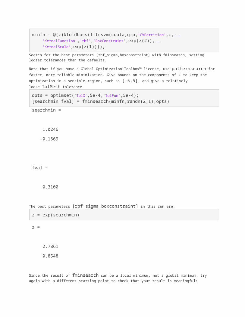
minfn = @(z)kfoldLoss(fitcsvm(cdata,grp,'CVPartition',c,... 'KernelFunction','rbf','BoxConstraint',exp(z(2)),... 'KernelScale',exp(z(1))));

Search for the best parameters [rbf_sigma,boxconstraint] with fminsearch, setting looser tolerances than the defaults.

Note that if you have a Global Optimization Toolbox™ license, use patternsearch forfaster, more reliable minimization. Give bounds on the components of z to keep the optimization in a sensible region, such as [-5,5], and give a relatively loose TolMesh tolerance.opts = optimset('TolX',5e-4,'TolFun',5e-4);[searchmin fval] = fminsearch(minfn,randn(2,1),opts)searchmin =

1.0246

-0.1569

fval =

0.3100

The best parameters [rbf_sigma;boxconstraint] in this run are:z = exp(searchmin)

z =

2.7861

0.8548

Since the result of fminsearch can be a local minimum, not a global minimum, try again with a different starting point to check that your result is meaningful:

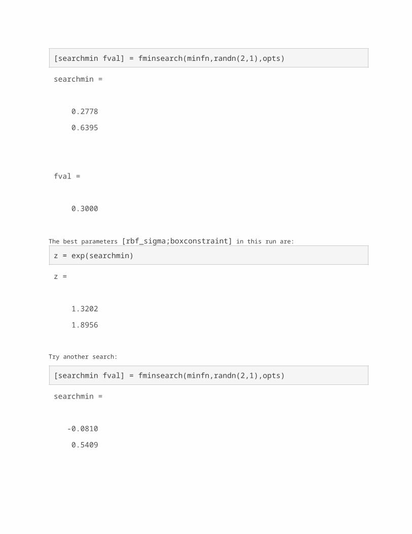
[searchmin fval] = fminsearch(minfn,randn(2,1),opts)

searchmin =

0.2778

0.6395

fval =

0.3000

The best parameters [rbf_sigma;boxconstraint] in this run are:z = exp(searchmin)

z =

1.3202

1.8956

Try another search:

[searchmin fval] = fminsearch(minfn,randn(2,1),opts)

searchmin =

-0.0810

0.5409

fval =

0.3200

The best parameters [rbf_sigma;boxconstraint] in this run are:z = exp(searchmin)

z =

0.9222

1.7175

The suface seems to have many local minima. Try a 20 random sets of random, initial values, and choose the set corresponding to the lowest fval.m = 20;

fval = zeros(m,1);

z = zeros(m,2);

for j = 1:m; [searchmin fval(j)] = fminsearch(minfn,randn(2,1),opts); z(j,:) = exp(searchmin);end

z = z(fval == min(fval),:)z =

1.9301 0.7507

Use the z parameters to train a new SVM classifier:SVMModel = fitcsvm(cdata,grp,'KernelFunction','rbf',... 'KernelScale',z(1),'BoxConstraint',z(2));[~,scores] = predict(SVMModel,xGrid);

figure;h(1:2) = gscatter(cdata(:,1),cdata(:,2),grp,'rg','+*');hold onh(3) = plot(cdata(SVMModel.IsSupportVector,1),... cdata(SVMModel.IsSupportVector,2),'ko');contour(x1Grid,x2Grid,reshape(scores(:,2),size(x1Grid)),[0 0],'k');legend(h,{'-1','+1','Support Vectors'},'Location','Southeast');axis equalhold off

Generate and classify some new data points:

grnobj = gmdistribution(grnpop,.2*eye(2));

redobj = gmdistribution(redpop,.2*eye(2));

newData = random(grnobj,10);

newData = [newData;random(redobj,10)];

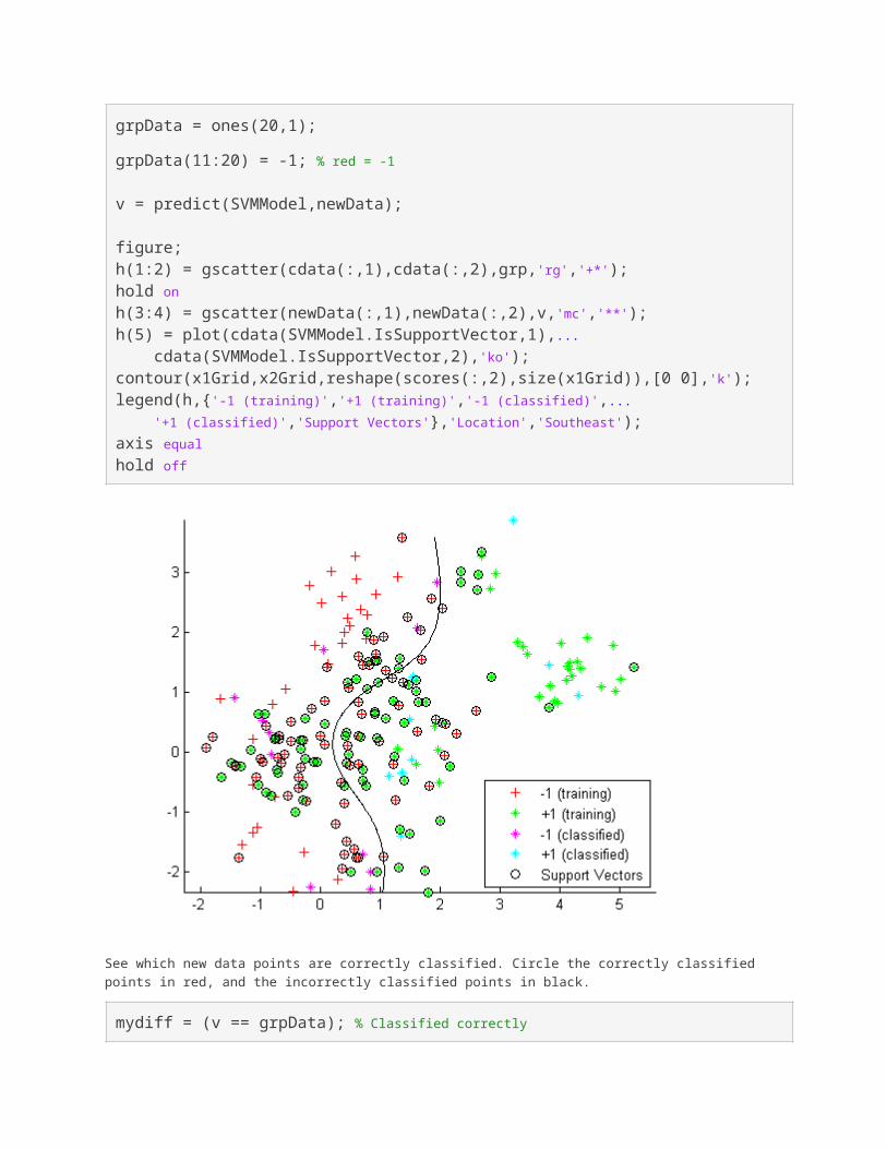
grpData = ones(20,1);

grpData(11:20) = -1; % red = -1

v = predict(SVMModel,newData);

figure;h(1:2) = gscatter(cdata(:,1),cdata(:,2),grp,'rg','+*');hold onh(3:4) = gscatter(newData(:,1),newData(:,2),v,'mc','**');h(5) = plot(cdata(SVMModel.IsSupportVector,1),... cdata(SVMModel.IsSupportVector,2),'ko');contour(x1Grid,x2Grid,reshape(scores(:,2),size(x1Grid)),[0 0],'k');legend(h,{'-1 (training)','+1 (training)','-1 (classified)',... '+1 (classified)','Support Vectors'},'Location','Southeast');axis equalhold off

See which new data points are correctly classified. Circle the correctly classified points in red, and the incorrectly classified points in black.

mydiff = (v == grpData); % Classified correctly

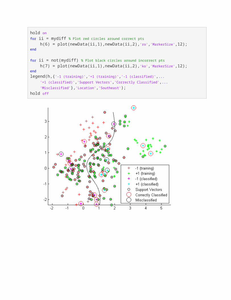
hold onfor ii = mydiff % Plot red circles around correct pts h(6) = plot(newData(ii,1),newData(ii,2),'ro','MarkerSize',12);end

for ii = not(mydiff) % Plot black circles around incorrect pts h(7) = plot(newData(ii,1),newData(ii,2),'ko','MarkerSize',12);endlegend(h,{'-1 (training)','+1 (training)','-1 (classified)',... '+1 (classified)','Support Vectors','Correctly Classified',... 'Misclassified'},'Location','Southeast');hold off