sustainable firewood supply in the murray-darling basin
TRANSCRIPT

Sustainable firewood supply in the Murray-Darling Basin David Freudenberger E. Margaret Cawsey Jacqui Stol PW West
Final Report November 2004 For Australian Department of Environment & Heritage

Enquiries should be addressed to:
Dr David Freudenberger CSIRO Sustainable Ecosystems GPO Box 284 Canberra ACT 2601. [email protected]
Citation: Freudenberger D, Cawsey, EM, Stol, J & West, PW (2004). Sustainable firewood supply in the Murray-Darling Basin. CSIRO: Canberra.
Important Notice
© Copyright Commonwealth Scientific and Industrial Research Organisation (‘CSIRO’) Australia 2005
All rights are reserved and no part of this publication covered by copyright may be reproduced or copied in any form or by any means except with the written permission of CSIRO.
The results and analyses contained in this Report are based on a number of technical, circumstantial or otherwise specified assumptions and parameters. The user must make its own assessment of the suitability for its use of the information or material contained in or generated from the Report. To the extent permitted by law, CSIRO excludes all liability to any party for expenses, losses, damages and costs arising directly or indirectly from using this Report.
Use of this Report
The use of this Report is subject to the terms on which it was prepared by CSIRO. In particular, the Report may only be used for the following purposes.
� Extracts of the Report distributed for these purposes must clearly note that the extract is part of a larger Report prepared by CSIRO for the Client.
� The Report must not be used as a means of endorsement without the prior written consent of CSIRO.
� The name, trade mark or logo of CSIRO must not be used without the prior written consent of CSIRO.

Sustainable firewood supply in the Murray-Darling Basin
Executive Summary CSIRO Sustainable Ecosystems was engaged by the Commonwealth Department of Environment and Heritage (then Environment Australia) to:
• Develop regional exploitation criteria for sustainable harvesting of firewood from woodland and forest communities in the Murray-Darling Basin, based on three scenarios for future harvesting of firewood.
• Identify the location and sustainable yield of firewood from those woodland and forest communities in the Murray-Darling Basin that meet the exploitation criteria of each scenario.
• Analyse the possible ecological impacts of the harvesting scenarios, particularly the green-wood scenario.
This research project is one outcome of the National Approach to Firewood Collection and Use (ANZECC 2001; http://www.deh.gov.au/land/publications/firewood-ris/index.html). In consultation with a broad range of stakeholders, three harvesting scenarios were developed and analysed for their capacity to meet the current demand for firewood of 2.25 million tonnes per year from the Murray-Darling Basin: Scenario 1. Dead-wood; Continued reliance on firewood harvested from standing and fallen dead timber from native forests on privately held land. We estimated that the maximum sustainable yield of dead timber from the 12.3 million hectares of private forests in the Murray-Darling Basin is 10 million tonnes per year, about four times greater than current demand. Our modelling suggested that only 3 million hectares of private forests would be required to meet existing demand through the exclusive harvesting of dead timber (coarse woody debris). However, a reliance on dead timber for firewood would continue to deplete levels of coarse woody debris to an average of 3 tonnes per hectare, far less than the average 20 tonnes per hectare that would remain were there no firewood harvesting of dead timber. We estimated that 1.5 billion tonnes of coarse woody debris has already been lost in the Murray-Darling Basin through clearing. This has greatly reduced habitat availability for the wide range of species reliant on such habitat, and has impaired ecosystem processes and landscape function. Our modelling suggests that there is plenty of scope to manage the intensity of harvest from coarse woody debris. If firewood harvesting of dead timber is to continue, then highly cleared areas of the Murray Darling Basin should be excluded from further harvesting. We suggest that harvesting should only occur in those regions with an extensive forest cover. Scenario 2. Green-wood; Firewood harvests of live trees thinned from existing stands of native forests and woodlands on privately held land We estimated that there are 9.8 million hectares of private forest in the Murray-Darling Basin suitable for harvesting of live thinnings for firewood from managed forests, providing a sustainable maximum yield of 2.3 million tonnes per year. The results from our field surveys indicated that an exclusive harvest of live trees, if properly managed, would eventually create mixed age stands and allow for substantial accumulation of coarse woody debris (15-20 tonnes per hectare). This accumulation should have significant benefits for biodiversity conservation and maintenance of landscape function. Survey results also indicated that thinning can open forest canopies and stimulate the establishment of a greater density and diversity of shrubs, grasses, forbs and orchids.

Sustainable firewood supply in the Murray-Darling Basin
Scenario 3. Plantations; Firewood harvests from plantations of native hardwoods on privately held, presently unforested land. We estimated that, if the most productive sites along the eastern and southern boundaries of the Murray-Darling Basin were used for plantations, a total of just over 0.2 million hectares of plantations, grown on 10 year rotations, would be required to meet the current demands for firewood from the Basin. If planting was restricted to the less productive areas of the Murray-Darling Basin and on soils at high risk of salinisation from agriculture, a total of about 0.6 million hectares of plantations, grown on a 20 year rotation, would be required. If plantings were restricted to such sites, then 29,000 ha would have to be established annually for 20 years to achieve the final estate size required to wholly meet current firewood demand. There is limited prospect for growing commercially viable plantations solely for firewood unless growers receive additional income streams from other timber products or from environmental services such as biodiversity habitat, salinity mitigation and/or carbon sequestration. This project explored alternatives to the current reliance on standing dead and fallen timber as a source of firewood. A reliance on dead timber for firewood will continue to threaten biodiversity, particularly in forest stands closest to markets and within highly cleared landscapes. There is a need to further explore and implement firewood sources other than dead timber. Our modelling and field surveys showed that other sources of firewood include the thinning of live trees from well managed native forests and as one of many products and services that can be provided by an expansion of hardwood plantations within the Murray-Darling Basin.
Sustainable firewood supply in the Murray -Darling Basin
i
Table of Contents 1 Overview and recommendations ........................................................................................1
1.1 Introduction.........................................................................................................................1
1.2 Objectives ...........................................................................................................................1
1.3 Approach ............................................................................................................................2
1.4 Outputs................................................................................................................................2
1.5 Outcomes ...........................................................................................................................3
1.5.1 Dead-wood scenario .................................................................................................3
1.5.2 Green-wood Scenario...............................................................................................5
1.5.3 The plantation scenario ............................................................................................6
1.5.4 Ecological impacts ....................................................................................................6
1.6 Implications for Management and Policy.......................................................................7
1.6.1 Dead-wood scenario .................................................................................................7
1.6.2 Green-wood scenario ...............................................................................................8
1.6.3 Plantation scenario....................................................................................................8
1.7 Recommendations ............................................................................................................9
1.8 Conclusions ........................................................................................................................9
2 Firewood from the Murray-Darling Basin; context and issues.................................11
2.1 Context ..............................................................................................................................11
2.2 Objectives .........................................................................................................................12
2.3 Primary outcomes ...........................................................................................................12
2.4 Project Approach.............................................................................................................13
2.5 Background ......................................................................................................................13
2.5.1 Key Findings from Driscoll et al.(2000) ................................................................13
2.5.2 Comparisons of key findings to other firewood estimates ................................14
2.5.3 Relevance to the current project ...........................................................................16
2.6 Workshop..........................................................................................................................16
2.7 Definition of sustainable harvesting..............................................................................17
2.7.1 A scenario approach to sustainability ..................................................................18
2.8 Report Structure ..............................................................................................................18
3 The Exploitation Criteria .....................................................................................................19
3.1 Overall exploitation criteria ............................................................................................19
3.2 The dead-wood scenario................................................................................................20
3.3 The green-wood scenario ..............................................................................................21
3.4 The plantation scenario ..................................................................................................23
3.5 Application of the exploitation criteria ..........................................................................24
Sustainable firewood supply in the Murray -Darling Basin
ii
4 The Geographic Information System...............................................................................25
4.1 Coordinate system ..........................................................................................................25
4.2 Data ...................................................................................................................................26
4.2.1 Data sources ............................................................................................................26
4.2.2 Data limitations ........................................................................................................27
4.3 The application of the exploitation criteria in the GIS ................................................32
4.3.1 The overall exploitation criteria; methods............................................................33
4.3.2 The overall exploitation criteria; results ...............................................................33
4.3.3 The dead-wood scenario; methods ......................................................................33
4.3.4 The dead-wood scenario; results..........................................................................34
4.3.5 The green-wood scenario; methods.....................................................................35
4.3.6 The green-wood scenario; results ........................................................................42
4.3.7 The plantation scenario; methods ........................................................................46
4.3.8 The plantation scenario; results ............................................................................48
5 Model review and forest mensuration data for model development and validation .................................................................................................................................54
5.1 Introduction.......................................................................................................................54
5.2 Review of existing models and forest data ..................................................................54
5.3 White Cypress Pine Model ............................................................................................55
5.4 Data from known age forests ........................................................................................57
5.5 Forest and woodland types............................................................................................58
5.5.1 Defining the forests of the MDB............................................................................58
5.5.2 Descriptions of the forests and woodlands in the MDB ....................................59
5.6 Field sampling design.....................................................................................................61
5.6.1 Net primary productivity..........................................................................................61
5.6.2 Stand age .................................................................................................................61
5.6.3 Position on slope .....................................................................................................62
5.7 Field sampling methods .................................................................................................62
5.7.1 Live tree measurements.........................................................................................63
5.7.2 Coarse woody debris ..............................................................................................64
5.7.3 Ecological data ........................................................................................................64
5.8 Summary Data .................................................................................................................64
6 Growth and yield models ....................................................................................................66
6.1 Summary...........................................................................................................................66
6.2 Introduction.......................................................................................................................66
6.3 Data ...................................................................................................................................67

Sustainable firewood supply in the Murray -Darling Basin
iii
6.3.1 Stand measurements..............................................................................................67
6.3.2 Stand stem wood biomass.....................................................................................67
6.3.3 Coarse woody debris stand biomass ...................................................................67
6.4 Model for stand stem wood biomass growth ..............................................................68
6.4.1 Approach ..................................................................................................................68
6.4.2 Site productive capacity .........................................................................................68
6.4.3 Stand density ...........................................................................................................69
6.4.4 Fitted model..............................................................................................................71
6.4.5 Predicting growth at young ages ..........................................................................72
6.5 Model to predict coarse woody debris biomass .........................................................73
6.6 Growth and yield model..................................................................................................74
6.6.1 Undisturbed stands .................................................................................................74
6.6.2 Thinned stands ........................................................................................................76
6.6.3 Firewood harvests ...................................................................................................78
6.7 Testing and applying the model ....................................................................................78
6.8 Growth and firewood yield of mallee forests ...............................................................81
6.9 Model Applications ..........................................................................................................82
7 The dead-wood scenario.....................................................................................................83
7.1 Summary...........................................................................................................................83
7.2 Introduction.......................................................................................................................83
7.3 Sustainable yield prediction...........................................................................................84
7.4 Forest area and stratification.........................................................................................84
7.5 Firewood harvest management regimes .....................................................................86
7.6 Long-term firewood yields ..............................................................................................87
7.6.1 Method of determining yields ................................................................................87
7.6.2 Woody debris remaining after firewood harvest .................................................88
7.6.3 Firewood harvest yields..........................................................................................89
7.7 Sustainable firewood supply over the next 100 years ...............................................90
7.7.1 Mathematical programming system .....................................................................92
7.7.2 Sustainable firewood supply..................................................................................94
7.7.3 Residual woody debris ...........................................................................................95
7.8 Discussion and conclusions ..........................................................................................96
8 The green-wood scenario ...................................................................................................98
8.1 Summary...........................................................................................................................98
8.2 Introduction.......................................................................................................................98
8.3 Forest area and stratification.........................................................................................98

Sustainable firewood supply in the Murray -Darling Basin
iv
8.4 Management regimes .................................................................................................. 100
8.4.1 Mallee forest.......................................................................................................... 100
8.4.2 Non-mallee forests ............................................................................................... 101
8.5 Sustainable firewood supply over the next 100 years ............................................ 105
8.5.1 Firewood supply with standard management regimes................................... 105
8.5.2 Sustainable firewood supply............................................................................... 106
8.5.3 Residual woody debris ........................................................................................ 107
8.6 Discussion ..................................................................................................................... 108
9 Case studies on the potential ecological impacts of firewood harvesting ........ 110
9.1 Introduction.................................................................................................................... 110
9.2 Australian research into ecological impacts ............................................................. 111
9.2.1 Estimation of amounts of coarse woody debris............................................... 111
9.2.2 Terrestrial vertebrate and invertebrate diversity and coarse woody debris 112
9.2.3 Ecosystem function and coarse woody debris ................................................ 113
9.3 Case studies for ecological impacts .......................................................................... 113
9.3.1 Measurements of sustainability.......................................................................... 114
9.3.2 Data management................................................................................................ 115
9.4 Description of study area ............................................................................................ 115
9.5 Description of case study sites................................................................................... 118
9.5.1 Murrumbateman ................................................................................................... 118
9.5.2 Frogmore ............................................................................................................... 122
9.5.3 Bungendore ........................................................................................................... 124
9.5.4 Bredbo.................................................................................................................... 127
9.6 Sampling Methodology................................................................................................ 132
9.6.1 Birds........................................................................................................................ 133
9.6.2 Small ground-dwelling mammals ....................................................................... 133
9.6.3 Plants...................................................................................................................... 133
9.6.4 Coarse woody debris ........................................................................................... 133
9.6.5 Regeneration......................................................................................................... 134
9.6.6 Landscape Function Analysis............................................................................. 134
9.7 Analysis methods ......................................................................................................... 135
9.7.2 Birds........................................................................................................................ 137
9.7.3 Small ground-dwelling mammals ....................................................................... 139
9.7.4 Plants...................................................................................................................... 139
9.7.5 Coarse woody debris ........................................................................................... 139
9.7.6 Regeneration......................................................................................................... 140

Sustainable firewood supply in the Murray -Darling Basin
v
9.7.7 Landscape function analysis .............................................................................. 140
9.7.8 Forest/habitat variables ....................................................................................... 140
9.8 Analysis results ............................................................................................................. 141
9.8.1 Birds........................................................................................................................ 141
9.8.2 Small ground-dwelling mammals ....................................................................... 144
9.8.3 Plants...................................................................................................................... 144
9.8.4 Coarse woody debris ........................................................................................... 146
9.8.5 Regeneration......................................................................................................... 147
9.8.6 Landscape Function Analysis............................................................................. 148
9.8.7 Forestry/habitat variables.................................................................................... 149
9.9 Discussion ..................................................................................................................... 150
9.9.1 Birds........................................................................................................................ 151
9.9.2 Small ground-dwelling mammals ....................................................................... 154
9.9.3 Plants...................................................................................................................... 156
9.9.4 Coarse Woody Debris ......................................................................................... 157
9.9.5 Regeneration......................................................................................................... 159
9.9.6 Landscape Function Analysis............................................................................. 160
9.10 Further silvicultural management considerations for biodiversity......................... 161
9.10.1 Variability of forestry attributes within dry sclerophyll forest.......................... 161
9.10.2 Forest stands and the self-thinning rule ........................................................... 161
9.11 Conclusions ................................................................................................................... 162
10 Native hardwood plantation scenario........................................................................... 165
10.1 Summary........................................................................................................................ 165
10.2 Introduction.................................................................................................................... 165
10.3 Growth and yield model............................................................................................... 167
10.4 Estimating plantation firewood yields in the Murray-Darling Basin ...................... 169
10.4.1 Site productive capacity ...................................................................................... 169
10.4.2 Relating site index to net primary productivity index ...................................... 169
10.4.3 Predicting firewood yields from Eucalyptus globulus plantations ................. 172
10.5 Plantation areas required to supply firewood from the Murray-Darling Basin .... 174
10.6 Discussion and conclusions ....................................................................................... 176
11 Management and Policy Implications........................................................................... 178
11.1 Objectives revisited ...................................................................................................... 178
11.2 Outcomes of scenario analysis .................................................................................. 179
11.2.1 The dead-wood scenario..................................................................................... 179
11.2.2 The green-wood scenario ................................................................................... 180

Sustainable firewood supply in the Murray -Darling Basin
vi
11.2.3 The plantation scenario ....................................................................................... 182
11.3 Environmental impacts ................................................................................................ 184
11.3.1 The dead-wood scenario..................................................................................... 184
11.3.2 The green-wood scenario ................................................................................... 185
11.3.3 The plantation scenario ....................................................................................... 187
11.4 Combination of strategies ........................................................................................... 188
11.5 Achievements against objectives............................................................................... 188
12 Acknowledgements........................................................................................................... 189
13 References........................................................................................................................... 191
14 Appendices.......................................................................................................................... 203

Sustainable firewood supply in the Murray -Darling Basin
1
1 Overview and recommendations
1.1 Introduction Australian households burn between 4.5 to 5.5 million tonnes of firewood per year. With the addition of firewood for industrial use, this figure rises to 6-7 million tonnes (ANZECC 2001). The majority of this firewood is harvested by small businesses and individuals, from dead standing and fallen timber on privately held native eucalypts forests (Driscoll et al. 2000). The ecological sustainability of this large and extensive harvest of native vegetation is largely unknown.
In order to address the ecological sustainability of firewood harvesting, a Firewood Taskforce was formed, under the auspices of the former Standing Committee on Environmental Protection (SCEP) and Standing Committee on Conservation (SCC). The Taskforce had State and Commonwealth representatives, including participation from CSIRO. The Taskforce developed a National Approach to Firewood Collection and Use in Australia endorsed by The Australian and New Zealand Environment and Conservation Council (ANZECC 2001). The first of the six broad strategies of the document is to Improve the information base. Actions under Strategy 1 include:
• Determine the impacts of different firewood collection practices in regional forest and woodland ecosystems;
• Determine the impact of firewood collection on biodiversity in particular regional ecosystems, and develop management guidelines.
CSIRO Sustainable Ecosystems was commissioned by the Department of Environment and Heritage (formally Environment Australia), with funding from the Natural Heritage Trust, to address these two actions. Specifically, CSIRO was commissioned to address the following knowledge gaps identified in Strategy 1 of the National Approach document:
• What are the rates of accumulation of fallen timber, and sustainable rates at which to harvest it?
• What are the amounts, availability, and economics of alternative firewood sources? • Guidelines for calculating a sustained yield of firewood. • Data are required on the dead and live wood component of vegetation communities used for
firewood collection and reconciled with firewood collection levels. • Assessment of the rate of natural regeneration and tree mortality in vegetation communities
subject to firewood collection. • A model is needed to guide the sustainable harvest of timber resources. • Is firewood collection likely to cause a decline in biodiversity in particular ecosystems?
CSIRO focused its study on estimating the amounts, availability and potential environmental impact of harvesting firewood from different sources. The study was limited to analysing firewood sources within the Murray Darling Basin (MDB), an area in which 2-2.5 millions tonnes of firewood is harvested per year from private land and in a generally unregulated manner (Driscoll et al. 2000).
1.2 Objectives The key objectives of the project were to:
• Develop regional exploitation criteria for sustainable harvesting of firewood from woodland and forest communities in the MDB, based on three scenarios for future harvesting of firewood.

Sustainable firewood supply in the Murray -Darling Basin
2
• Identify the location and sustainable yield of firewood from those woodland and forest communities in the MDB that meet the exploitation criteria of each scenario.
• Analyse the possible ecological impacts of the harvesting scenarios, particularly the green-wood scenario.
1.3 Approach The analysis of the sustainability of firewood supply in the Murray-Darling Basin (MDB) was conducted using a scenario approach. In consultation with a broad range of stakeholders, three harvesting scenarios were developed:
1. Dead-wood – Continued reliance on firewood harvested from standing and fallen dead timber from native forests on privately held land;
2. Green-wood – Firewood harvests of live trees thinned from existing stands of native forests and woodlands on privately held land;
3. Plantations – Firewood harvests from plantations of native hardwoods on privately held, presently unforested land.
The area of native forest required to meet current firewood demand from private land in the MDB was estimated using a forest growth and yield model, constructed specifically for this project, based on data from fieldwork across previously unsurveyed lower rainfall forests, and running the model on data derived from geographic information system (GIS) datasets of forest and non-forest cover in the MDB. This provided the spatial context to enable the most current forest cover data to be used to estimate the number of hectares of any forest type available for firewood harvest, subject to a rigorously defined set of exploitation criteria. The potential environmental impact, particularly of the green-wood scenario, was examined by ecological surveys of low rainfall forests thinned of live trees. State Forests were excluded from the scenarios as firewood harvest from these are regulated through a system of licensing, permits and fees.
1.4 Outputs
Analysis of Firewood Harvesting Scenarios
We present the results of analyses of the spatial extent and yield of firewood based on the three broad types of harvest: maintenance of the status quo - the dead-wood scenario, the green-wood scenario, the plantation scenario. Detailed exploitation criteria were developed to determine where in the MDB each scenario might be applied (Section 3).
Geographical Information Database
We constructed a GIS database (Section 4), based on a grid dataset representing broad woodland or forest vegetation types, within which the exploitation criteria were applied for the three harvesting scenarios. Implicit in the GIS was the location of potential sources of firewood within broad vegetation types defined by the National Forest Inventory (2003). This enabled the three harvesting scenarios to be spatially explicit, based on the most current forest cover data available for the MDB. This information was not sufficient to reliably assess forest density and age so estimates were based on our assessments.
Forest Growth and Yield Model
We developed a new stand-based, empirical growth and yield model for native species (mallee and non-mallee) for forests and woodlands in the MDB (Section 6). The development of this model required extensive collection of data on stand age, stand wood volume and amounts of coarse woody debris across a broad productivity gradient (Section 5). The field data contributed to the

Sustainable firewood supply in the Murray -Darling Basin
3
characterisation of the low rainfall forests and woodland of the MDB (Section 5). The model predicted yields from non-mallee forests, utilising existing measures of site productive capacity (maximum annual net primary production of plants). A separate growth and yield model was developed for mallee forests from published data, to predict potential firewood yield from harvesting mallee. The area of plantation required to meet curent firewood demand from the MDB was estimated using an already existing plantation growth and yield model and linking it to our GIS datasets.
Prediction of potential firewood supply
The model (Section 6) and data from the GIS (Section 4) were used to provide long-term predictions of the firewood supply available from the three harvesting scenarios (Sections 7, 8 and 10). The GIS provided estimates of the current spatial extent of native forests, or land suitable for eucalypt plantations, available to meet the sustainable yield from each scenario.
Potential ecological impacts
Wildlife, soil surface condition, habitat complexity and plant and animal survey data were collected from the few privately managed native eucalypt forests in MDB in which timber had been thinned and harvested for a range of purposes. The data were used to suggest the possible ecological impacts of harvesting firewood from thinning live trees, the green-wood scenario rather than removal of dead trees, the dead-wood scenario. The ecological impacts of removal of coarse woody debris were also evaluated (Section 9).
1.5 Outcomes
1.5.1 Dead-wood scenario Approach
Harvest regimes were based on standard accepted forestry management practices intended to maintain both firewood supply and sufficient coarse woody debris for biodiversity. This approach uses i) a growth and yield model to predict firewood on a stand basis, ii) an estimate of forest type and productivity, iii) selection of an appropriate management regime and iv) combining the above for an estimate of the long term sustainable supply of coarse woody debris on an annual basis.
Harvestable area
The area considered for the dead-wood scenario is defined by the exploitation criteria: exclusion of the 8.2 million hectares of woody cover further than 500 kilometres from the capital cities that access firewood from the MDB; exclusion of the 1.2 million hectares of mallee forests, which are unsuitable for harvest of dead timber (mallee is considered for the green-wood scenario); exclusion of firewood sourced from publicly owned land. The rationale for these exploitation criteria are presented in Section 3.
Firewood supply
The analysis for the dead-wood scenario (Section 7) estimated that 12.3 million hectares of privately held land in the MDB is potentially available for harvest of standing and fallen dead timber (dead-wood scenario). An appropriate firewood harvest regime for eligible forests could involve about 30 harvests of coarse woody debris (dead timber) over the lifetime of any forest stand, at intervals of 5-10 years, and with the first harvest occurring when a stand is 20-25 years of age. It was estimated that, over the next 100 years, the maximum annual supply of firewood from the MDB under this scenario would average 10 million tonnes per year, with a deviation from this amount in any year of no more than 1.1 million tonnes.

Sustainable firewood supply in the Murray -Darling Basin
4
Key firewood supply issues
This is far more than the present harvest from the MDB, currently estimated to be between 2-2.5 million tonnes per year (Section 2). As little as 3 million hectares of the eligible forest area could be sufficient to meet the existing demand. If the maximum of 10 million oven dry tonnes per year of firewood was harvested, the long-term average amount of coarse woody debris which would remain in the forest after firewood harvesting would be 3 tonnes per hectare, far less than the average 20 tonnes per hectare that would remain were there no firewood harvesting.
Biodiversity implications
This loss of coarse woody debris reduces the availability of habitat for biodiversity and the material required for the ecosystem processes which contribute to sustainable landscape function. A summary of these ecological implications can be found in Section 1.5.4.
1.5.2 Green-wood Scenario Approach
An estimate was made of the maximum and long-term sustainable supply of firewood which might be obtained from the privately owned, native forests of the MDB for the green-wood scenario, under which firewood is obtained only by felling live trees and no coarse woody debris is removed as firewood. The general approach taken for the green-wood scenario follows that of the dead wood scenario.
Separate firewood harvesting regimes were developed for mallee and non-mallee forests. For mallee forests, the regime involved clear- fell harvesting on a 50 year rotation, with regeneration by coppice. For non-mallee, the regime involved “flexible selection” management, with two or three thinnings over the life-time of a stand and with 50% of the standing tree basal area removed at each thinning. Management based on flexible selection should encourage maintenance of forest stands which contain a wide range of tree sizes and ages, consistent with contemporary community expectations for native forest management.
Harvestable area
It was estimated that there are 9.8 million hectares (1.1 M ha mallee and 8.7 M ha non-mallee) of forest in the MDB suitable for harvesting under this scenario. This estimate of available forest was based on the following exploitation criteria: exclusion of forest cover more than 500 kilometres from capital cities; forests on public land; forests within 50 metres of rivers; forests on slopes greater than 15o; forests with less than 30% cover across a 10 square kilometre “window”; and patches of forest less than 100 hectares in size. The ecological and economic rationale for these exploitation criteria are presented in Section 3.
Key firewood supply issues
The model predicted that, over the next 100 years, the sustainable maximum annual supply of firewood from the MDB under the green-wood scenario would average 2.3 million tonnes per year, with a deviation in any year of no more than 0.2 million tonnes. About 22% of this supply would come from mallee forests and the remainder from non-mallee. This level of supply is about the same as the amount of firewood harvested presently from the MDB, which is estimated to be 2-2.5 million tonnes per year.
Biodiversity implications
Because the green-wood scenario does not involve removal of woody debris from the forest (Figure 1.3), it was considered that the green-wood approach to firewood harvest in the MDB should have significant benefits for biodiversity conservation and maintenance of landscape function.

Sustainable firewood supply in the Murray -Darling Basin
5
1.5.3 The plantation scenario Approach
For this scenario, we estimated the minimum area of plantation forests in the MDB needed to provide a long-term, sustainable annual supply of 2.25 million tonnes of firewood, wholly replacing the supply obtained presently from the native forests of the MDB. Estimates were made using a generic growth and yield model system for Eucalyptus globulus plantations.
Key Firewood Supply Issues
It was estimated that if the most productive sites along the eastern and southern boundaries of the MDB were used for plantations, a total of just over 0.2 million hectares of plantations, grown on 10 year rotations, would be required. If plantations were restricted to the less productive areas of lower rainfall (<900 mm yr-1), or to areas where land clearing for agriculture has been particularly intensive, just under 0.35 million hectares of plantations, grown on 11 year rotations, would be required. If planting was restricted to the less productive areas of the MDB, on soils at high risk of salinisation from agriculture, a total of about 0.6 million hectares of plantations, grown on a 20 year rotation, would be required.
Implications
Plantations established solely for firewood are likely to be economically unsustainable. It is more likely that firewood would be a secondary product from plantations. Multi-purpose plantation areas larger than the minima specified above are likely to be required to economically provide the total firewood supply required from the MDB. It appears that there is limited prospect for growing commercially viable plantations which have firewood as their principal product, unless growers receive substantial subsidies, either directly or indirectly, through payments for the environmental benefits that accrue, through mechanisms such as salinity, biodiversity or carbon credits. The practicalities of plantation development in the drier regions of Australia are still in early development, so uptake is likely to be slow.
1.5.4 Ecological impacts We developed a sampling protocol to quantify the ecological impacts of harvesting firewood of both live and dead timber. We applied this protocol to 19 sites selected from four privately owned properties located within a 100 kilometre radius of Canberra, upon which various harvesting regimes had been practiced over the past 50 years or so. We were only able to find one property with some pre-thinning ecological data. Thus we were unable to make any scientifically rigorous analysis of the impact of forest thinning for firewood. However, we were able to use our survey results to suggest some of the likely ecological impacts of harvesting of live trees compared to harvesting of dead timber from the dry sclerophyll forest of the Southern Tablelands of NSW (Section 9).
We found that the different vegetation communities characterised as “dry sclerophyll forest” contain a rich diversity of flora and fauna species, which have historically been poorly surveyed. They have been periodically disturbed, particularly by ring-barking during the late 1800’s and early 1900’s. Older ring-barked sites were typified by dense, even-aged stands of trees, with limited regeneration, few old growth trees and low habitat complexity, including limited shrub and ground cover. Little active management of these forest stands have occurred subsequently.
Bird species richness across the full range of dry sclerophyll forest types was high, although older ringbarked sites had limited habitat structure. As a consequence, bird species richness tended to be lower at these sites in comparison with sites which have undergone more recent harvesting

Sustainable firewood supply in the Murray -Darling Basin
6
disturbances. For example, bird species richness and abundances at younger pulled/chained and bulldozed sites were generally greater than at the older ringbarked or control sites.
Plant species richness within densely stocked sites was relatively low. Plant species richness after harvesting is likely to increase only slowly. Regeneration of trees after harvesting treatments was significantly related to treatment type; thinned sites had the highest regeneration by coppicing, pulled/chained sites had regeneration, primarily from seed.
The species richness and abundance of small ground dwelling mammals was low across all surveyed sites reflecting the low nutrient status of these forests. Other research indicates that these small mammals favour more structurally complex sites, with dense understorey, particularly along drainage lines, which are areas currently exempt from harvesting under forestry practice guidelines.
Coarse woody debris loads were between 0.3 and 48 tonnes per hectare. Loads under 10 t ha-1 were considered depleted, 10-30 t ha-1 at the lower end of “average” and = 30 t ha-1 were higher than “average”. The type of harvest (chaining, bulldozing, or ringbarking) was a significant predictor of coarse woody debris loads. Management history was more influential than other environmental factors in determining coarse woody debris loads.
Landscape function analysis indicated that thinned and pulled/chained sites were relatively functional. However, there has been some loss of infiltration and nutrient cycling where thinning and coarse woody debris removal or bulldozing were the methods of harvest.
Surveyed forest stands varied considerably in terms of basal areas, stems per hectare, diameters and management history. Fifty to one hundred year old, even-age stands are those likely to be closest to maximum density, have the fewest habitat values, and are potentially suitable for harvesting by thinning methods, such as chaining in narrow strips, which maximise residual loads of coarse woody debris and stimulate regeneration.
1.6 Implications for Management and Policy
1.6.1 Dead-wood scenario Our estimate that the maximum sustainable yield of coarse woody debris from the MDB private forests is about four times greater than current demand indicates that there is reasonable scope to manage the intensity of harvest from coarse woody debris. There are at least two broad options; the intensity of harvest could be reduced from any one stand, or large areas could be excluded from coarse woody debris harvesting. We recommend that highly cleared areas of the MDB be excluded from further harvesting of standing and fallen dead timber. Our model estimates that about 1.5 billion tonnes of coarse woody debris has already been lost through clearing. The continued removal of coarse woody debris is of conservation concern, not because any particular patch of woodland or forest has been depleted, but because so much has been lost over all of the landscapes of the MDB since European settlement, through extensive clearing and agricultural development. Fallen and dead timber is a renewable resource only while the forest remains. Much of it is gone, particularly in the most productive areas of the MDB, with the most fertile soils and highest rainfall. Clearly there is a need to conserve what little coarse woody debris is left in these highly cleared regions of the MDB. The load of coarse woody debris in any one remnant is of secondary importance. Any load of coarse woody debris is a scarce resource in a highly cleared region. We argue that there is scope for continuing the firewood harvest of coarse woody debris in regions with an extensive forest cover, but not in regions where clearing, as well as firewood removal, has greatly reduced this important component of forests and woodlands.
This project has developed the modelling capability to analyse the yield of firewood and residual levels of coarse woody debris from any combination of alternative management regimes. We only

Sustainable firewood supply in the Murray -Darling Basin
7
modelled a few simple options. Other regimes and guidelines need to be developed by land managers and state agencies that are responsible for legislation regulating timber harvesting.
1.6.2 Green-wood scenario We suggest that it is feasible to meet a long term demand for firewood exclusively by thinning live trees only in non-mallee forests and clear- felling mallee forest. In doing so we considered suitable only those forests away from major water courses, on shallow slopes less than 15°, and from forests patches of at least 100 hectares that occur in regions with at least a 30% forest cover. An exclusive harvest of live trees in non-mallee forests would eventually create mixed age stands and allow for substantial accumulation of coarse woody debris. Averaged across the entire modelled area, loads of woody debris in non-mallee forests would vary between 15-20 tonnes per hectare over the next 100 years. This would result in 5-7 times greater post-harvesting loads of coarse woody debris than under the dead-wood scenario, which on average left only 3 tonnes per hectare of woody debris after harvest of dead standing and fallen timber. Mallee forests contain little coarse woody debris whether harvested or not.
We suggest that the environmental impact of forest thinning for firewood can be minimised if the thinning operation leads to greater structural complexity. Thinning of forests can increase the structural complexity of forest if it leads to tree regeneration, which in time will create mixed-age stands. Thinning can also increase structural complexity if it leads to greater loads of coarse woody debris left after the thinning operation and if opening of the forest canopy stimulates the establishment of a greater density and diversity of shrubs, grasses, forbs and orchids.
1.6.3 Plantation scenario On the most productive sites for eucalypt plantation forestry in the MDB, it was estimated that 21,000 hectares of plantations would have to be established annually for 10 years to reach the final estate size of 0.21 million hectares needed to wholly replace firewood obtained from native forests in the MDB. If plantings were restricted to sites at risk of soil salinisation, 29,000 ha would have to be established annually for 20 years to achieve the final estate size required. Planting rates of this magnitude constitute an appreciable proportion of the 80,000 hectares per year of new plantations required to achieve the objectives of the 2020 vision for Australian forest plantations.
To initiate and manage plantation programs of the size required for firewood production across the vast area of the MDB and amongst the many private land owners would be a very difficult undertaking. Perhaps the best that might be achieved over the next ten years is the establishment of some plantations, on sites across a range of conditions represented by the various options considered by our project. This might ultimately achieve a total plantation area sufficient to partly replace the firewood supply presently taken from native forests in the MDB, particularly if firewood was a secondary product, i.e. from thinnings.
1.7 Recommendations Recommendation 1. Commercial harvesting of firewood from fallen and standing dead timber
should be phased out in those regions of the MDB where coarse woody debris is highly depleted, particularly in the cropping zone.
Recommendation 2. Firewood could be sourced from thinnings of live trees in densely stocked regrowth forest if harvesting was done under defined exploitation criteria and improved harvesting guidelines (see Recommendation 7).
Recommendation 3. Active and sustained marketing of firewood from densely stocked regrowth forests (e.g. stringy barks) is required if the demand for firewood from coarse

Sustainable firewood supply in the Murray -Darling Basin
8
woody debris (dead wood) from traditionally preferred species (e.g. Red Gum/Box mix) is to be reduced.
Recommendation 4. Active and sustained marketing of firewood sourced from plantations is required to assist in the reduction of demand for firewood from coarse woody debris (dead wood).
Recommendation 5. Long term and rigorous research is needed that experimentally manipulates levels of coarse woody debris in a diversity of vegetation types in order to quantify the environmental impacts of commercial scale removal of fallen and standing dead timber on a range of taxa and ecosystem processes.
Recommendation 6. Within regions where harvest of dead timber could continue, guidelines and regulations are needed to create “refugia” free of dead timber harvesting.
Recommendation 7. Scientifically-defensible harvesting guidelines need to be developed which promote regeneration, improve forest structure and maintains landscape function, in order to improve the management of low rainfall forest stands.
Recommendation 8. A combination of strategies should be modeled then adopted to reduce the impact of firewood harvesting. A combined strategy includes excluding the harvest of coarse woody debris from areas where such a harvest is deemed to be ecologically unsustainable; thinning live trees from regions with extensive regrowth; and investing from hardwood plantations which supply firewood as a secondary product.
1.8 Conclusions The heavily-cleared areas of the MDB, where only fragmentary forest remains, are particularly at risk of loss of biodiversity and landscape function if harvest of dead-wood continues within them.
Four times the existing annual demand (about 2.5 million tonnes per year) for firewood from the MDB could be met from intensively harvesting coarse woody debris from only 3 million of the available 12 million hectares of non-mallee forests. Alternatively, a larger area of these forests could be harvested less intensively, ensuring the retention of sufficient coarse woody debris to maintain biodiversity and landscape function.
The supply of firewood which could obtained by from the harvest of live trees from mallee and non-mallee forests is about equal to the current demand. The stands of non-mallee forests most appropriate to a green-wood harvesting approach are also the stands most likely to benefit ecologically from harvesting, as the preferred methods of thinning encourage regeneration and increase in habitat complexity, which are likely to in turn encourage maintenance of landscape function and species diversity.
Small ground-dwelling mammals occur at low density in these forests, reflecting the dryness and low soil fertility. The ecological sustainability of the forests would be best served by the exclusion of wood harvesting from riparian areas which provide the best habitats for these animals.
Approximately 200,000 hectares of plantation, grown on a 10 year rotation, would have to be established in the MDB to meet the present demand for firewood from the MDB. However, plantation forestry is unlikely to be economical where plantations are established principally for firewood production. However, firewood could be a useful by-product from plantations, as they become more generally established in the MDB, over the next 10-20 years. Firewood from plantation sources would gradually supplement the levels of firewood available from the harvesting of live trees in MDB to a level which would easily meet the future demand.

Sustainable firewood supply in the Murray -Darling Basin
9
There is considerable opportunity to sustainably obtain firewood from the privately-owned forests in the MDB through the harvest of live trees, by-products from plantation forestry and limited continued collection of coarse woody debris. Diversification of industry in this way should have benefits in maintaining biodiversity and landscape function, that is, maintaining ecological sustainability. However, substantial planning and the introduction of government regulation will be necessary to achieve this.

Sustainable firewood supply in the Murray -Darling Basin
10
2 Firewood from the Murray-Darling Basin; context and issues
J.M. Stol and D.O. Freudenberger
2.1 Context The Australian and New Zealand Environment and Conservation Council (ANZECC) have issued the document: A National Approach to Firewood Collection and Use in Australia (ANZECC 2001). The national approach was developed by the Joint Standing Committee on Environmental Protection (SCEP) and Standing Committee on Conservation (SCC) Taskforce on Firewood, which has State and Commonwealth representatives, including participation from CSIRO. The first of the six broad strategies of the document is to “Improve the information base”. Table 1.1 summarises the actions from Strategy 1.
Table 1.1 Summary of actions from Strategy 1 in a A National Approach to Firewood Collection and Use in Australia (ANZECC 2001)
Action Appropriate Jurisdiction
Suggested Timeframe
Expected outcomes
1. Determine where and how much firewood is being collected.
All States, Territories, CSIRO and Commonwealth.
2001-2002 Better targeting of education and on-ground conservation efforts.
2. Determine the impacts of different firewood collection practices in regional forest and woodland ecosystems.
All States, Territories, CSIRO, universities, firewood industry and Commonwealth.
2001 and ongoing Improved ability to maintain the firewood industry without over harvesting the resource.
3. Determine the impact of firewood collection on biodiversity in particular regional ecosystems, and develop management guidelines.
All States, Territories, CSIRO, universities, and Commonwealth.
Ongoing Identification of species at risk from firewood collection. Ecosystem specific management prescriptions to prevent species' decline and extinctions of dead wood dependent species.
In order to address this strategy, Environment Australia provided funding for a number of research projects. CSIRO Sustainable Ecosystems (CSE) (Driscoll, Milkovits and Freudenberger 2000) was commissioned by Environment Australia to address the first action. Through a review of existing literature, canvassing state agencies, and surveys of firewood suppliers and Australian households estimates were made on the amounts, sources, preferred species for firewood and identified the regions in which firewood is most likely to affect biodiversity at a regional scale.
Actions 2 and 3 have been addressed by the current project entitled: Sustainable Firewood Supply in the Murray-Darling Basin. The project was conducted by CSE to address the following research gaps/questions identified by Strategy 1 (ANZECC 2001):
• what are the rates of accumulation of fallen timber, and sustainable rates at which to harvest it;
• what are the amounts, availability, and economics of alternative firewood sources; • a guideline is required for calculating a sustained yield of firewood;

Sustainable firewood supply in the Murray -Darling Basin
11
• data is required on the dead and live wood component of vegetation communities used for firewood collection and reconciled with firewood collection levels;
• the rate of natural regeneration and tree mortality in vegetation communities subject to firewood collection requires assessment;
• primary productivity of the native forest and woodland ecosystem is a key driver for sustainability;
• a model is developed to guide the sustainable harvest of timber resources; and • whether firewood collection is likely to cause a decline in biodiversity in particular
ecosystems
This report also contributes to Strategy 5 (ANZECC 2001) i.e. “Develop a sustainable firewood industry, encouraging plantations, sustainable management of native forest and use of residues”. This project investigates the sustainability of harvesting in native forests and presents estimates of the minimum area of plantation forests required to supply firewood assuming that there will be no harvesting from native forests.
2.2 Objectives The key objectives of the project were to:
• Develop regional exploitation criteria for sustainable harvesting of firewood from woodland and forest communities in the Murray-Darling Basin (MDB).
• Identify the location, sustainable yield of firewood from those woodland and forest communities in the Basin that meet the exploitation criteria.
The project undertook six steps to achieving these objectives: 1. Developed three future firewood harvesting scenarios; 2. Developed specific exploitation criteria for each scenario; 3. Applied the exploitation criteria using a Geographic Information System (GIS) to develop a
spatially explicit database developed for the forests and woodlands of the MDB; 4. Collected field data across the MDB to provide data for a forest growth and yield model, a
volume function and evaluation of ecological impacts of firewood harvesting; 5. Developed a forest growth and yield model specific to the MDB lower rainfall areas; and 6. Applied existing models to estimate the area and location of native hardwood plantations
necessary to meet the existing demand.
2.3 Primary outcomes The primary outputs of the project were identified as:
1. A GIS database capable of applying exploitation criteria for three scenarios for firewood harvesting based on a grid dataset representing broad woodland or fo rest vegetation types on private lands;
2. Location of the source of firewood (implicit in the GIS datasets); 3. Location of the area of each broad forest type which is eligible for harvesting; 4. Data and model for forest growth and yield in the MDB.
5. The predicted sustainable yield of firewood from each scenario compared to current demand;
6. The predicted yield of firewood from each broad forest type; 7. The potential ecological impacts of harvesting regimes based on case study sites; and

Sustainable firewood supply in the Murray -Darling Basin
12
8. The area of native hardwood plantations that would need to be established as an alternative source of firewood in the MDB.
2.4 Project Approach The ultimate aim of the project was to ascertain the potential supply of firewood from three harvesting scenarios and the potential ecological impacts associated with each. The approach used a combination of available literature and scientific expertise, data gathered through fieldwork across the MDB, a new model system for forest growth and yields for lower rainfall forests and woodlands developed from the field data and a GIS developed to provide data on the areas of the MDB which met the requirements of the exploitation criteria for each harvesting scenario.
2.5 Background In November 2000 CSIRO Sustainable Ecosystems (Driscoll, Milkovits and Freudenberger 2000) were commissioned by Environment Australia to report on the “Impact and Use of Firewood in Australia”. The Driscoll et al.(2000) report built upon earlier reports (FTSUT 1989, Bush et al.1999).
A number of key knowledge gaps and a research strategy were identified by Driscoll et al.(2000). The objectives of this project have their origins in the recommendations of the report of Driscoll et al.(2000) but address the actions identified in the National Approach to Firewood Collection and Use in Australia (20001) document.
2.5.1 Key Findings from Driscoll et al.(2000) Australian households burn between 4.5 to 5.5 million tonnes of firewood per year. With the addition of firewood for industrial use, this figure rises to between 6 – 7 million tonnes. The four most commonly burned tree species are River Red Gum (Eucalyptus camaldulensis), Jarrah (Eucalyptus marginata), Red Box (Eucalyptus polyanthemos), Yellow Box (Eucalyptus melliodora) and Ironbark (Eucalyptus sideroxylon).
Driscoll et al.(2000) estimated that 84% of firewood for household use is collected from private lands and that only 9.5% of firewood is collected from State Forests. The remaining firewood was classified as coming from either crown land, such as Travelling Stock Reserves and roadside reserves, or “other” ie. unknown. An important finding was that approximately half of the household firewood was collected by residents rather than purchased and this firewood was primarily fallen timber gathered on private land. The remaining households who purchase timber do so from small suppliers and friends. Established wood merchants only account for around a quarter of these purchased firewood loads.
Driscoll et al.(2000) identified that inland forests and woodlands in lower rainfall zones, i.e. in areas such as the MDB, were most threatened by firewood collection. This is because the most heavily utilised firewood species originate from the Basin, they have slow growth rates due to generally low net primary productivity (NPP) and have been extensively cleared.
2.5.2 Comparisons of key findings to other firewood estimates There have been only two previous examinations of national firewood use in Australia; FTSUT (1989) and ABARE (Bush et al.1999). Table 2.1 shows that the estimates of firewood use from both FTSUT and ABARE are similar to those of Driscoll et al. (2000).

Sustainable firewood supply in the Murray -Darling Basin
13
Table 2.1 Millions of tonnes of firewood estimated by separate national reports. The ABARE data includes industrial firewood use.
FTSUT 1988
estimate
ABARE 1987-88 estimate
FTSUT 2000
forecast
ABARE 2000-01 forecast
Driscoll et al.(2000)
household
Driscoll et al.(2000) plus
industrial
4.38 5.75 4.25 – 6.61 6.85 4.52 – 5.54 6 - 7
Figure 2.1 presents a flowchart showing the derivation of firewood from various sources after Driscoll et al.(2000).
Figure 2.1 Flowchart showing the derivation of the percentages of firewood from various sources from Driscoll et al.(2000).
As part of the firewood certification system, industry workshops run by the Australian Timber Industry Certification Group (ATICG) recently provided some key results. Queensland, NSW and WA representatives state that the Driscoll estimates are too high and that the real figures for firewood consumption in these areas are between 14% and 25% of those figures.
It appears that ATICG have provided estimates based only on firewood supplied by firewood merchants. However, as detailed in Driscoll et al.(2000), only 50% of the firewood consumed is bought as opposed to collected, and of the 50% purchased, only around 25% of firewood is purchased from established wood merchants who advertise in the Yellow Pages or have business premises. Thus any estimate based only upon the figures supplied by firewood merchants is likely to significantly underestimate the actual amount of firewood sourced from the MDB.
One workshop participant/firewood merchant estimated the Armidale firewood market at 1,500 tonnes per annum. It would appear this is a significant underestimation. Julian Wall, from the University of New England, undertook a intensive research project including interviews with
Total household firewood
50% collected
50% bought
84% from private land
26% from established wood merchants
60+% from unregulated small suppliers
10% from friends
Source known by location only: 72% from low rainfall
plant communities
6.7% roadside & other
76% collect fallen timber, 18% standing
dead trees
Unknown source
9.5% state forests

Sustainable firewood supply in the Murray -Darling Basin
14
households and firewood merchants. In Armidale during 1994 he estimated that 17,940 tonnes were consumed within the urban area and 13,000 tonnes in the surrounding rural areas.
2.5.3 Relevance to the current project
Why the Murray Darling Basin?
Driscoll et al.(2000) indicated that the vegetation communities most threatened by firewood collection are the dry forests and woodlands in Victoria, NSW, South Australia, Tasmania and Queensland. Although there have been no assessments in Queensland, the indications are that the southern Brigalow belt could be depleted. The key species harvested for firewood occur in particular on the western slopes and plains of NSW and in the Victorian and NSW Riverina in the Box-Ironbark woodlands. These woodlands and forests have been extensively cleared for agriculture. The Yellow Box/Red Gum Grassy Woodland which was previously extensive in the intensive landuse zone has been declared a threatened ecological community. Additionally the site productive capacity of these regions is generally low, which means that the length of time required for regeneration and growth of these communities is longer than in areas of high productivity (see Section 6).
Private tenure or Crown land?
The findings from Driscoll et al. (2000) indicated that the firewood harvest from state forests is already highly regulated by the responsible agencies. Further, it comprises less than 10% of the total supply. NSW State Forests, the Victorian Department of Sustainability and Environment, Queensland Department of Primary Industries and Forestry SA each have a system of permits, fees and licences which must be purchased by those wishing to collect firewood in their precincts. It is important to note here that this type of firewood collection is limited to coarse woody debris on the forest floor and is therefore relevant to the first scenario presented in this project i.e. the “dead-wood” scenario (Section 3.2 and Section 7).
Because collection of firewood from state forests is so highly controlled they have not been considered within the scope of this project. If firewood harvesting continues under the first two scenarios presented in this project, i.e. the “dead-wood” scenario and the “green-wood” scenario (Section 3.3 and Section 8), it is the remaining native forests and woodlands on private lands which will continue to carry the impact of future demand for firewood from Australian native forests in the MDB. Therefore private lands in the MDB were identified as the particular focus for this project.
2.6 Workshop A workshop was held at the commencement of the project, in February 2002. Its objective was to scope the project’s approach, focus and design with stakeholders and obtain inputs on appropriate exploitation criteria. Twenty-one participants from land management agencies attended the workshop. These were from the NSW Department of Land and Water Conservation, Victorian Department of Natural Resources and Environment, NSW State Forests, NSW National Parks and Wildlife Service, CSIRO Forestry and Forest Products as well as the Australian Greenhouse Office, Environment Australia, Australian National University, a private fuelwood company and CSIRO Sustainable Ecosystems.
Workshop discussions were focused on decision rules for the sustainable harvesting of firewood at different scales and a number of issues emerged:
• Definitions of sustainability; • Time and scale; • Benchmarks and biodiversity surrogates;

Sustainable firewood supply in the Murray -Darling Basin
15
• Remnant size; • Accreditation rules; • Policies, markets and people; and • Harvesting and forest and woodland ecology.
There were a series of common themes throughout discussion of the above issues. The themes were: • Planning: lack of planning and regulation in the firewood industry; • Accreditation: research can contribute by setting benchmarks; • Education: misinformation is common; • Technological developments and their impacts on the firewood industry; • State of current knowledge on environmental impacts and existing data; and • Need for a number of scenarios to address issues of firewood supply.
The workshop provided a useful range of industry and expert contribution to the key issues at a range of scales. The full report from the workshop can be found in Appendix 1.
2.7 Definition of sustainable harvesting Our preferred definition for sustainable harvesting of firewood, developed in part through the workshop process, is: the economic maximum sustained yield which does not impair the compositional, structural and functional attributes of the landscape rather than a narrower definition based on the concept of maximum sustained yield ie. removal of firewood at a rate no greater than the replacement (growth) rate.
The compositional attributes of the landscape include retention of all native species and minimisation of the risk of exotic species invasion. Structural attributes include maintenance of adequate patch size, heterogeneous age structure and diverse understorey including fallen timber and provision of hollow logs. Functional attributes of the landscape include maintenance of adequate nutrient cycling and hydrological balance and minimisation of erosion. A broad definition of sustainability includes inter-generational equity, that is, maintenance of site values and opportunity for future options for use.
An unsustainable firewood harvest is one that is: • Uneconomic; • Unplanned; • Extracts firewood at a rate greater than it re-generates; • Threatens species and ecological communities; • Results in long-term clearing; • Reduces the heterogeneity of age structure within a stand; • Reduces critical habitat such as understorey shrubs, hollows and fallen timber; • Increases erosion, accelerates nutrient loss and increases the risk of salinity; and • Reduces future values or options for use
2.7.1 A scenario approach to sustainability Definitions of sustainable harvesting will differ amongst any group of stakeholders. Some may argue that the current harvesting regime, which is reliant on standing and fallen dead wood is sustainable. Others may argue that firewood could possibly be sourced sustainably from managed native forests and woodlands. A third option might be that only firewood sourced from plantations is sustainable.

Sustainable firewood supply in the Murray -Darling Basin
16
Our study examined each of these three supply strategies, or scenarios, as described in the next section. We hope these scenarios provide a basis for developing policies, regulations and management systems to reduce the impact and improve the sustainability of firewood harvesting in the MDB.
2.8 Report Structure Section 3 details the first step of this project: the development of the exploitation criteria which defined the areas of forests and woodlands of the MDB which would be eligible for harvesting under each scenario.
Section 4 describes the GIS data and methods used to produce the data (the areas of land which met the requirements of the exploitation criteria for each of the scenarios) for analyses.
Section 5 details the process of the collection the field data across the MDB. These data were used to develop a growth and yield model system for the forests and woodlands of the MDB, described in Section 6.
The results of the modelling gave us the information on the amounts of firewood which might sustainably be harvested under each scenario. Section 7 addresses the first scenario; the “dead-wood” or “status quo” scenario. Section 8 addresses the “green-wood” or “sustainable harvesting of existing native forests” scenario. Section 10 addresses the plantation scenario.
Further field data were collected to assess the ecological impacts of firewood harvesting under the green-wood scenario. The ecological impacts of The green-wood scenario are discussed in Section 9.
Section 11 provides a discussion and draws together the conclusions derived by the project.
Section 12 provides acknowledgements to the lengthy list of those who assisted and/or advised us on the methods, approaches and the carriage of the project. The references for all sections of the report have been compiled in Section 13.
The 11 Appendices accompanying this report are grouped at the end of Section 14.

Sustainable firewood supply in the Murray -Darling Basin
17
3 The Exploitation Criteria E.M. Cawsey, D.O. Freudenberger and J.M. Stol
This study examined the potential firewood yield, extent of harvesting and potential environmental impacts of three different harvesting scenarios:
1. The “dead-wood” scenario: this scenario represented the status quo of the current harvesting approach i.e. continued reliance on standing and fallen dead wood;
2. The “green-wood”: scenario: this scenario addressed the supply of firewood from selective harvesting of live native non-mallee forests and clear- felling of vegetation in mallee forests; and
3. The plantation scenario: this scenario addressed the supply of firewood from native hardwood plantations.
These scenarios, and the exploitation criteria (ECs) that drive them, are described in this section. The exploitation criteria were defined with direct reference to the context and objectives of the project (Section 2). Spatially explicit exploitation criteria were used to limit our study area to specific geographic locations, in order to exclude areas from harvesting for a range of reasons, explained under each scenario heading.
The first step was to develop exploitation criteria for the study area as a whole i.e. explicitly define the fundamental geographic context for the project and the broad focus area within it. When that had been achieved, the exploitation criteria for each scenario were developed.
3.1 Overall exploitation criteria The overall project exploitation criteria served to define the study area and limit the analyses to only those areas in the study area relevant to the project objectives. The following exploitation criteria applied to all three Scenarios.
EC 1 Defined the boundaries of the study area. All scenarios were based on a single study area so the results for each scenario would be comparable. The study area was defined as the whole MDB.
EC 2 Addressed the top level constraint of economic feasibility, imposed by distance to markets. This criterion constrains the collection of firewood only to those parts of the MDB within an economically feasible distance from the major population centres in and around the MDB. Driscoll et al.(2000) concluded that the majority of firewood burned in the major capital cities (Adelaide, Brisbane, Canberra, Melbourne, Sydney) comes from a mean maximum distance of 450 km from those cities. Firewood burned in the smaller population centres is more likely to come from the local area. Therefore, taking a conservative approach, parts of the MDB which are further than 500km from any capital city are likely to be of minimal importance for firewood production and harvesting and were not included in any analyses conducted by this project.
EC 3 Focused on private lands only. Firewood supply from public lands is actively regulated by the relevant agencies (see Section 2.5.3) and was not the subject of this project. Further, most firewood comes from privately managed land (Driscoll et al. 2000 and Figure 2.1). All land not leasehold or freehold was excluded from further analysis.

Sustainable firewood supply in the Murray -Darling Basin
18
Table 3.1 describes the overall exploitation criteria which define the study area as a whole and the areas of interest within it, referencing by number the original datasets relevant to each (see Appendix 2, page 1 and Appendix 3, Section 1).
Table 3.1. Overall project exploitation criteria linked to the relevant datasets (see Appendix 2, page 1 and Appendix 3, Section 1).
Exploitation Criteria Assumptions Rationale Dataset
1 The Boundary of the Murray-Darling Basin (MDB) limits the whole study area.
The MDB supplies the majority of the firewood for the capital cities and for the towns in the Basin.
Driscoll et al.(2000). 1
2 Only consider areas within 500km of a capital city.
Collection of firewood is not economical at any further distance from a major population centre.
Regional centres take their supply from the same area.
Driscoll et al.(2000) Table 2.2.5, Fig. 2.2.1
Driscoll et al.(2000)
4
3 Private land only (exclude State Forests, National Parks, crown lands etc.)
1. The majority of firewood comes from private lands.
2. 70% of purchased firewood (35% overall) comes from unregulated small operators. Of this, the majority is collected from private land; see Figure 3.1.
3. States' estimations that only a small percentage of firewood comes from public lands.
1. Driscoll et al.(2000) pages 11, 23 24; 70% plus of firewood is sourced from private lands, and 30% from public lands; see Figure 2.1.
2. Emerging state Firewood Action Plans will throw the burden back to legal collection from private lands.
3. Victorian Firewood Strategy Discussion Paper May 2002, and Neagle (1994).
2
3.2 The dead-wood scenario The dead-wood scenario examined the consequences of continuing a "business as usual" approach to firewood harvesting. It assumed that dead standing and fallen timber would continue to be collected from all native woody vegetation remnants from the lands defined by exploitation criteria 1-5. The objectives of the dead-wood scenario were:
1. To elucidate the regional exploitation criteria which are the current drivers for the harvest of firewood from native open forests and woodlands based on the extraction of all standing or fallen dead trees likely to be available over the next 10-50 years.
2. To identify location, yield and regeneration potential of standing or fallen dead timber from the native open forests and woodlands covered by the exploitation criteria.
The dead-wood scenario built upon the overall exploitation criteria (Section 3.1, exploitation criteria 1-3), with two additional exploitation criteria.

Sustainable firewood supply in the Murray -Darling Basin
19
(The numbering of the exploitation criteria continues from the previous list.) EC 4 Focused on land covered by native forests and woodlands and native hardwood
plantations. All land not having woody cover was excluded from further analysis.
EC 5 Focused only on naturally occurring native woody remnants so all plantations were excluded from this scenario.
Table 3.2 describes the exploitation criteria for the dead-wood scenario, showing the relevant dataset (see Appendix 2, page 1 and Appendix 3, Section 1).
Table 3.2. The dead-wood scenario exploitation criteria linked to the relevant dataset (see Appendix 2, page 1 and Appendix 3, Section 1).
Exploitation Criteria Assumptions Rationale Dataset
4 All gridcells assigned to native hardwood vegetation types within the study area.
1. Historically box woodlands are the preferred source for firewood.
2. With the continuing reduction in box woodlands, other forest types will increasingly be sourced for firewood.
1. Driscoll et al.(2000)
2. National Land and Water Audit for percent area of box woodlands cleared; anecdotal evidence.
2
5 Exclude land already put down to private plantations
Firewood is not currently a major product from plantations.
These lands will be examined in the plantation scenario.
2
3.3 The green-wood scenario The green-wood scenario assumed that the codes of practice currently being developed by the Commonwealth and the States will be put into place, so that only firewood harvested from native forests and woodlands managed under forestry best practices and ecologically sustainable practices will be accepted into the market place. The objectives of the green-wood scenario were:
1. To develop regional exploitation criteria for the sustainable harvesting of a standing crop of native forest/woodland (e.g. thinning of green trees).
2. Identify location, sustainable yield and regeneration potential of green tree firewood from the native open forests and woodlands which meet the exploitation criteria.
The green-wood scenario included exploitation criteria 1-5 (Sections 3.1 and 3.2), with four additional exploitation criteria. The exploitation criteria for the green-wood scenario were based on a set of criteria which apply best management practices employed by the various State forestry agencies (exploitation criteria 6 and 7) and two additional exploitation criteria (exploitation criteria 8 and 9) which addressed ecological sustainability.
(The numbering of the exploitation criteria continues from the previous list.) EC 6 Focused on best management practices for forestry which exclude riparian zones
from disturbance.
EC 7 Focused on best management practices for forestry which exclude steep slopes = 15° from harvesting.
EC 8 Addressed ecological sustainability with regard to the percentage of the landscape which has woody cover.

Sustainable firewood supply in the Murray -Darling Basin
20
EC 9 Addressed ecological sustainability with regard to the maximum size of remnants/patches which might be considered for harvesting.
Table 3.3 describes the exploitation criteria for the green-wood scenario, showing the datasets relevant to each(see Appendix 2, page 1 and Appendix 3, Section 1).
Table 3.3. The green-wood scenario exploitation criteria linked to the relevant datasets (see Appendix 2, page 1 and Appendix 3, Section 1).
Exploitation Criteria Assumptions Rationale Datasets
6 Exclude areas 50m either side of streams and rivers.
The risk of ecological damage is too high in riparian zones.
NSW State Forest Ecologically Sustainable Forest Management Plans: “Broad riparian corridors with high value for wildlife conservation”.
5
7 Exclude slopes = 15° . Too expensive/difficult to harvest on steep slopes.
Soil erosion hazard
NSW State Forests Ecologically Sustainable Forest Management Plans; Victorian Ecologically Sustainable Development policy, National Forest Policy Statement (1995) signed by all states and territories.
3
8 Exclude parts of the study area where woody cover = 30% of the land area.
Harvesting from areas where woody cover = 30% is not likely to be ecologically sustainable.
Bennett and Ford (1997) 10% cover is a minimum to prevent loss of birds.
Andren’s (1994) review of case studies reports 30% in most landscapes.
Reid (1999, 2000) Declining Woodland Birds: decliners drop out where native cover is <30% of the landscape.
McIntyre et al.(2000) minimum 30% woodland cover to maintain ecological sustainability on grazed properties
1, 2, 4
9 Exclude remnants < 100 ha in area.
It is not likely to be ecologically sustainable to harvest from remnants smaller than 100 ha.
Certain remnants may not be able to be harvested sustainably for ecological reasons; Watson et al.(2001): remnants < 100 ha do not support the same composition or diversity of woodland birds as those larger than 100 ha.
1, 2, 4

Sustainable firewood supply in the Murray -Darling Basin
21
3.4 The plantation scenario The plantation scenario examined the potential contributions of firewood which could be provided from native hardwood plantations in the MDB and focused on areas of the MDB which might be suitable for plantation forestry. The objectives of the plantation scenario were:
1. To develop regional exploitation criteria for the sustainable harvest of firewood from native plantation forests.
2. Identify location and potential yield of firewood from existing plantations in the Basin. Additionally, estimate the extra area required to supply all demand for firewood from plantation sources and estimate the time before the firewood from these areas would become ava ilable. We compared the projected quantities needed versus what could be available over time from the establishment of plantations.
The plantation scenario employed the overall exploitation criteria 1-3 (Section 3.2) and also the best forestry management practices employed in the green-wood scenario (Section 3.3, exploitation criteria 6-7), plus three additional exploitation criteria.
(The numbering of the exploitation criteria continues from the previous list.) EC 10 Focused only on non-forested areas of the MDB.
EC 11 Focused only on land with an elevation < 650 metres.
EC 12 Focused only on land with an net primary productivity index of at least 5 t ha-1 yr-1.
Table 3.4 describes the exploitation criterion for the plantation scenario, showing the relevant datasets(see Appendix 2, page 1 and Appendix 3, Section 1).
Table 3.4. The plantation scenario exploitation criteria linked to the relevant datasets (see Appendix 2, page 1 and Appendix 3, Section 1).
Exploitation Criterion Assumptions Rationale Dataset 10 Include gridcells with
“non-native” vegetation cover.
land with non-native vegetation may be eligible for plantations.
2, 4
11 Exclude areas where the elevation ≥ 650m
Multiple benefit plantations are needed to reduce dryland salinity and provide wood for a variety of purposes.
Plantations in high rainfall zones (i.e. ≥ 650m) can reduce the yield or flow of fresh water (Vertessy et al. 2003)
3
12 Only include land with an NPP index of at least 5 t ha-1 yr-1
It is considered that sites with a productive capacity lower than this would not be viable for plantation establishment (see Section 10.5)
Plantations grown in areas with a net primary productivity index < 5 t ha-1 yr-1 would take many decades to produce an harvestable quantity of firewood.
6
3.5 Application of the exploitation criteria The spatial exploitation criteria were applied within the geographic information system (GIS) constructed for the project. This process is described in the next section (Section 4). The growth and yield model which used the data resulting from the application of the exploitation criteria is described in Section 6. The estimates of firewood yield for each of the three scenarios are described

Sustainable firewood supply in the Murray -Darling Basin
22
in Section 7 (the dead-wood scenario), Section 8 (the green-wood scenario) and Section 10 (the plantation scenario).

Sustainable firewood supply in the Murray -Darling Basin
23
4 The Geographic Information System E.M. Cawsey
This Section describes the methodology, data, design, processing and stratification used in the project GIS. The project GIS was implemented on a Sun Sparc Ultra-10 running the SunOS 5.8 operating system, using ArcInfo™ version 8.2 for UNIX, and on a personal computer running the Microsoft Windows 2000 operating system, using ArcGIS™ Version 8.1 modules ArcMap™, ArcCatalog™, ArcTools™ and Spatial Analyst™ under an Arcview™ licence type.
4.1 Coordinate system The first requirement before implementing the GIS was to choose a coordinate system for all of the spatial data used and produced by the project. After discussion with Paul Nanninga of the Murray Darling Basin Commission (MDBC) the project co-ordinate system, spheroid and datum have been set to the following:
Lamberts Conformal Conic False_Easting: 0.000000 False_Northing: 0.000000 Central_Meridian: 146.000000 Standard_Parallel_1: -34.500000 Standard_Parallel_2: -28.500000 Latitude_Of_Origin: -31.500000 Spheroid: GRS1980 Datum: GDA1994
The Lamberts Conformal Conic is preferred by the MDBC (Paul Nanninga pers. comm.). Lamberts Conformal Conic is a good compromise projection because it deals with angles very well, it is good at calculating areas and it is good at calculating distances. The other option considered, i.e. Albers Equal Area, is excellent for calculation of areas but not as appropriate for distances or angles. For this project both distance and area were important. Our main concern was to ensure relative areas were calculated accurately across the MDB. The results of a comparison of the two projections, by projecting the MDB boundary (Dataset 1, Appendix 3 Section 1.1) from its original UTM Zone 55 projection to both Lamberts and Albers (using the parameters shown above for each projection) are summarised in Table 4.1.
Table 4.1 Results of a comparison of area and perimeter of the MDB, between the projection Lamberts Conformal Conic (Lamberts) and Albers Equal Area (Albers).
Area (ha) Perimeter (km)
Albers Lamberts difference %diff Albers Lamberts difference %diff
105,806,621 105,849,681 43060 0.04% 7,559 7,569 9.9 0.06%
The differences between the projections were insignificant, so we chose to use the projection preferred by the MDBC, namely the Lamberts Conformal Conic projection as described above. All original GIS data datasets were converted to this projection.
4.2 Data After the exploitation criteria had been developed (Section 3), the next step was to design a preliminary data processing flowchart, the final version of which can be found in Appendix 2. The detail of the flowchart was developed in an iterative process throughout the life of the project, however in its preliminary form, it allowed for the identification of the datasets which were

Sustainable firewood supply in the Murray -Darling Basin
24
required. It was not within the ambit of this project to develop the original spatial datasets to meet the objectives, so we relied upon data which were readily available from Government and other sources (Appendix 3 Section 1 and this report Section 4.2.1). The methods employed to find data included literature searches, web searches and seeking advice from experts.
4.2.1 Data sources The success of the project hinged upon finding adequate data upon which the exploitation criteria could be applied. Spatial data used for the project needed to be as consistent as possible across the whole study area, to allow comparability across the whole MDB. It was also important to understand the assumptions and limitations implicit in the data. All data have associated limitations, so where choices between datasets existed, the most recent datasets with the most explicit data items and lineages were chosen.
Availability, resolution and consistency of data vary widely. Many datasets were reviewed and rejected as unsuitable for a variety of reasons, ranging from difficulties in obtaining them, time penalties required to process them to a usable state and data inadequacies, e.g. poor coverage, unsuitable resolution, missing projection information, missing metadata.
The quality and availability of data substantially constrained the project to what could be done rather than what might be considered optimal. The major data availability requirements which could not be met consistently across the whole area of the MDB were:
1. data on the distribution of all species suitable for firewood harvesting; 2. data on the distribution of threatened species; 3. data for cultural and historic sites; 4. data allowing spatial assessment of the quality of firewood; i.e. species distributions; 5. data allowing spatial assessment of the age classes of native stands; 6. data allowing spatial assessment of habitat condition; and 7. data allowing spatial assessment of ecological impacts e.g. regeneration potential.
Vegetation species distribution maps at the appropriate detail, scale and consistency do not exist for the whole study area. Neither are there consistent datasets documenting the distribution of threatened species.
Certain areas should be excluded from harvesting through forestry best management practices on the basis of cultural and aesthetic importance or because of the presence of rare and threatened species. We could find no consistent data covering the whole of the MDB to allow us to apply any of these constraints.
Firewood “quality” depends on the tree species in question. Again the lack of specific spatial information for all or any native species and/or communities extant in the MDB did not allow spatial elucidation of firewood quality.
There are no spatial data on the age of native remnants. The project has developed a method of assigning age class using data from the field case studies (Sections 5 and 6).
Habitat “condition”, however it is defined, depends on the disturbance history of each patch of native vegetation and such data do not exist across the MDB.
Regeneration potential depends in part on the condition of each stand. As we could not spatially represent condition, we used data from field case studies to assess the results from the growth and yield modelling (Sections 5 and 6). Data on the regeneration of the dominant potential firewood species from each of the field study sites across the MDB are more fully discussed in Section 9 (Ecological impacts of the green-wood scenario). However, regeneration potential also depends on the climate, substrate and vegetation composition of each patch and also on the existence of a

Sustainable firewood supply in the Murray -Darling Basin
25
sufficient body of knowledge to provide reliable growth curve and carbon cycling response data (Section 6).
Table 4.2 lists the original datasets which provided all source data for the project, and the exploitation criteria to which they pertain. The descriptions and metadata sources for each original dataset are provided in Appendix 3 Section 1.
Table 4.2 The original data datasets used for the project.
Original Dataset Source Exploitation Criteria
1. MDB Boundary Basin- in-a-Box; Murray-Darling Basin Commission
1
2. Woody cover in broad forest types associated with tenure
National Forest Inventory, Bureau of Rural Sciences
3, 4, 5, 8, 9, 10
3. Urban Areas Geoscience Australia 2
4. Digital Elevation Model Geoscience Australia 6, 11
5. Water courses Geoscience Australia 7
Three additional datasets provided data necessary for the growth and yield analyses of the scenarios. Table 4.3 shows these datasets. The metadata sources for these are provided in Appendix 3 Section 1.
Table 4.3 The additional datasets and the scenarios to which they pertained
Dataset Source Scenario
6. Net Primary Productivity Dr Damien Barrett, CSIRO Plant Industry
All
7. Salinity Risk National Land and Water Resources Audit
Plantation scenario Option 4
8. Soil depth, nutrient and water holding capacity data
MDBSIS, CSIRO Land and Water
Plantation scenario.
All data for this project were produced from these eight basic datasets.
4.2.2 Data limitations The most crucial data requirements were forest cover, land tenure and net primary productivity (NPP) datasets and it was particularly necessary to understand the limitations inherent in each. We needed the first to provide us with the actual cover of woody/non-woody vegetation in broad forest types, the second was required to distinguish private from publicly owned land, and the third was required to allow us to stratify areas of different forest types by the net primary productivity index, for the modelling of sustainable firewood yield.
Forest type and tenure
The National Forest Inventory (NFI), Bureau of Rural Sciences (BRS), provided us with the National Forest Inventory 2003 Forest by Tenure dataset (Dataset 2, Appendix 2 and Appendix 3 Section 1.2) for use in this project. This dataset had land cover and tenure data updated in 2003 from data provided by State agencies, and it provided both the woody/non-woody cover classified into NFI forest types, and the tenure data for the project. The dataset came with accompanying

Sustainable firewood supply in the Murray -Darling Basin
26
lookup tables for crown cover classes, height classes and forest formation classes. The details and metadata of this dataset can be found in Appendix 3 Section 1.2.
The NFI 2003 dataset was the most recent and consistent example of its kind, covering the whole of the MDB, and as such it was the best existing dataset available, and was used for the project. However it was constructed from a variety of datasets from different sources and with different attributes, scales and currency dates. As such, the NFI 2003 dataset suffers from the usual caveats with regard to consistency and compatibility. The methods of dealing with issues of consistency and compatibility were explicitly addressed by the NFI in the production of the dataset (see the metadata). The limitations imposed by the dataset on estimating firewood are documented in the following paragraphs. The resolution of this dataset, i.e. 100 metre gridcells, dictated the resolution of the project GIS. It should be noted that the cell size of 100m is not necessarily representative of the scale of all of the input datasets used in its construction, but rather this is the minimum mapping unit.
The resolution of the NFI 2003 dataset constrained the project to ignore all woodland patches smaller than 100 x 100m, or 1 hectare. Again, the scale of the original mapping may not necessarily have captured all areas of this size . The NFI has no minimum mapping unit, however the smallest unit captured would be dependent on the scale of the mapping. With this caveat in mind, we considered that the harvesting of firewood for general sale from isolated patches smaller than 1 hectare was likely not to be economically feasible, although private-owner wood collection from such sites may be significant.
The hierarchy of precedence for the data used for each Australian State is described in the metadata for the NFI 2003 dataset. The issue for this project was to separate privately tenured land classified as non-forest or non-woodland from the forest or woodland areas which could be treated as a source of firewood from private lands. The NFI 2003 dataset classified the land into various forest types (Table 4.4). Map 1 (Appendix 4) shows the geographic distribution of the classes in Table 4.4.
Table 4.4 The forest type classification for the gridcells of the MDB.
Forest Type Area (ha) % Area a “blank” 35 0.00%Acacia a 3,523,742 3.33%Callitris a 1,499,895 1.42%Casuarina a 1,100,900 1.04%Eucalypt Low Open Forest a 72,596 0.07%Eucalypt Low Woodland a 216,652 0.20%Eucalypt Mallee Open Forest a 24,809 0.02%Eucalypt Mallee Woodland a 2,591,844 2.45%Eucalypt Medium Open Forest a 14,050,898 13.28%Eucalypt Medium Woodland a 6,037,171 5.70%Eucalypt Tall Open Forest a 1,198,042 1.13%Eucalypt Tall Woodland a 35,231 0.03%Hardwood Plantation a 1,642 0.00%Melaleuca 77,665 0.07%No Data 27,105,353 25.61%Non Forest 47,436,345 44.82%Other 451,894 0.43%

Sustainable firewood supply in the Murray -Darling Basin
27
Forest Type Area (ha) % Area a Rainforest 51,966 0.05%Softwood Plantation a 351,164 0.33%Unknown Plantation a 2,116 0.00%Total area of the MDB 105,829,960 100.00%Total area non-firewood 75,123,258 70.98%Potentially eligible woody gridcells a 30,706,702 29.02%
a forest types initially assessed to be potentially eligible woody gridcells for the scenarios.
The community descriptions for the forest types in Table 4.4 are provided in Section 5.5.3, Table 5.1. The implications of these forest types, with regard to the selection of field sites and the collection of forest mensuration data for the growth and yield model (Section 6), are addressed in Section 5.
It was possible to classify woodlands and forests, according to the NFI classifications above, into the “mallee” and “non-mallee” classifications required for the growth and yield model (Section 6). The forest type “blank” (i.e. no classification provided), consisting only of 35 gridcells, was excluded from the analysis. Also, we excluded the forest types “melaleuca”, “rainforest”, “softwood plantation” and “unknown plantation” as they contribute little to either firewood harvesting (the dead-wood and green-wood scenarios) or to land which might potentially be available for hardwood plantation (the plantation scenario) because they constitute areas with native vegetation cover.
The “no data” category covers a large part of the study area. Information from the NFI confirmed that this category is equivalent to “non-forest”. We chose to treat it as combined non-woody vegetation and urban land cover, i.e. a virtual equivalent to the “non-forest” category.
The “non-forest” category was treated as non-woody vegetation which might be potentially suitable for plantation. The limitation of this approach was that native grasslands were included in the “non-forest” classification. The implications of this are discussed below.
The “other forest” forest type category included minor forest types, such as banksia and leptospermum, mixed forest types and unknown forest types, all of which meet the NFI definition of forest i.e. “an area dominated by trees with a height of greater than 2 metres and crown cover ≥ 20%”. After consideration it was decided to exclude the “other” forest type from further analyses because most of the area was unlikely to be either suitable for firewood harvesting or available for future plantation, and small in total extent (0.43% of the MDB).
A more serious issue relates to the actual definition of “forest” adopted by the NFI. The NFI used the definition of forest from the National Forest Policy Statement (NFPS), i.e. having a crown cover of 20%. All States/Territories provide forest mapping using this definition. The cover is classified into three classes; woodland (20-50%), open (51-80% and closed (81-100%). Section 5 addresses the issue of definitions of “forest” and “woodland” in more detail.
From Table 4.4 it can be seen that there are no closed forests in the MDB, that is, no forest with a crown cover classification greater than 80%. However, there are likely to be areas of the MDB where there is woody vegetation with a crown cover < 20%, and these have been classified as “non-forest” in the NFI 2003 dataset. These areas, which otherwise might contribute to the harvesting of firewood, do not contribute to the dataset. This has caused some under-prediction of the sustainable supply of firewood from the dead-wood and the green-wood scenarios, although how much we cannot easily estimate.
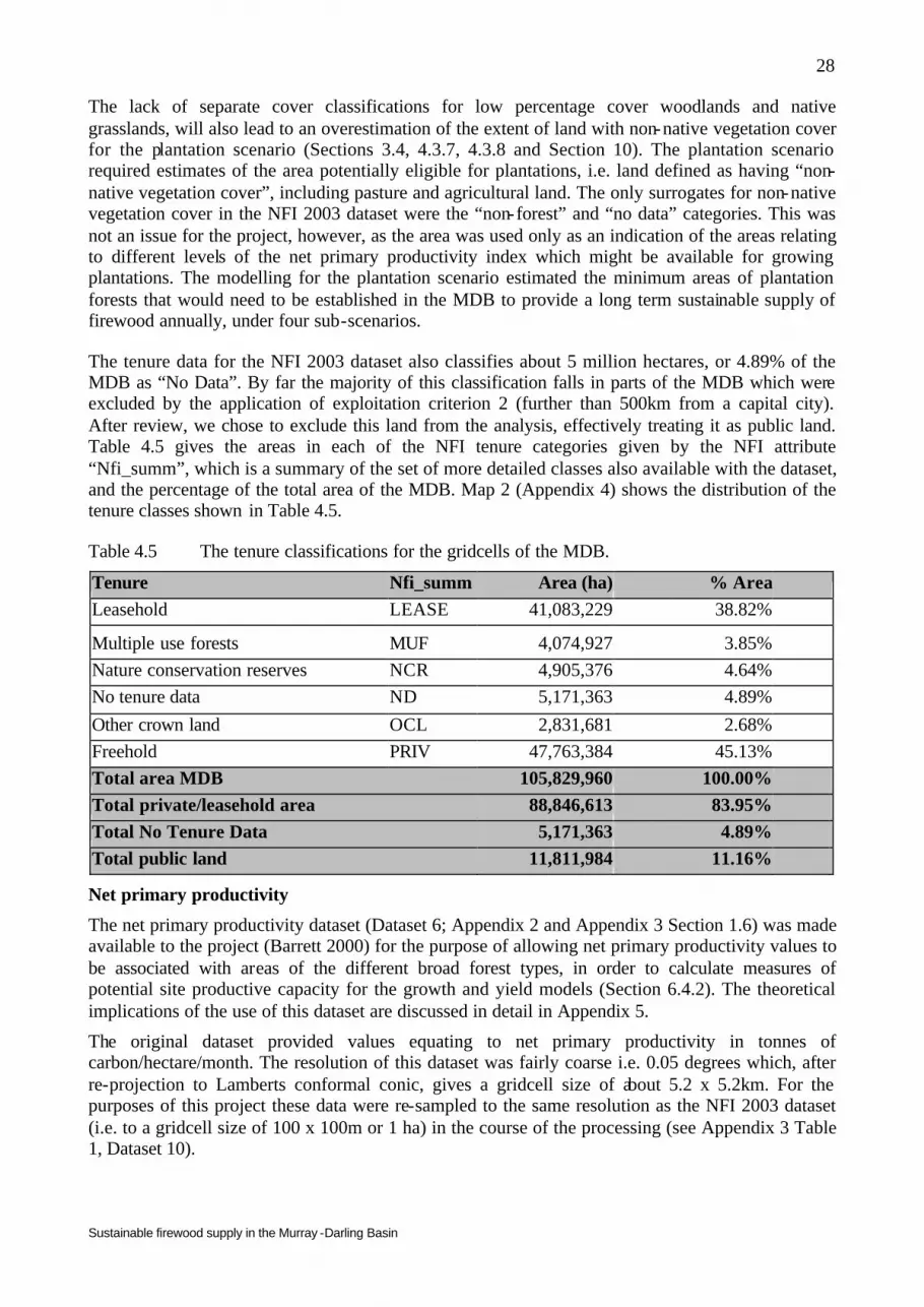
Sustainable firewood supply in the Murray -Darling Basin
28
The lack of separate cover classifications for low percentage cover woodlands and native grasslands, will also lead to an overestimation of the extent of land with non-native vegetation cover for the plantation scenario (Sections 3.4, 4.3.7, 4.3.8 and Section 10). The plantation scenario required estimates of the area potentially eligible for plantations, i.e. land defined as having “non-native vegetation cover”, including pasture and agricultural land. The only surrogates for non-native vegetation cover in the NFI 2003 dataset were the “non-forest” and “no data” categories. This was not an issue for the project, however, as the area was used only as an indication of the areas relating to different levels of the net primary productivity index which might be available for growing plantations. The modelling for the plantation scenario estimated the minimum areas of plantation forests that would need to be established in the MDB to provide a long term sustainable supply of firewood annually, under four sub-scenarios.
The tenure data for the NFI 2003 dataset also classifies about 5 million hectares, or 4.89% of the MDB as “No Data”. By far the majority of this classification falls in parts of the MDB which were excluded by the application of exploitation criterion 2 (further than 500km from a capital city). After review, we chose to exclude this land from the analysis, effectively treating it as public land. Table 4.5 gives the areas in each of the NFI tenure categories given by the NFI attribute “Nfi_summ”, which is a summary of the set of more detailed classes also available with the dataset, and the percentage of the total area of the MDB. Map 2 (Appendix 4) shows the distribution of the tenure classes shown in Table 4.5.
Table 4.5 The tenure classifications for the gridcells of the MDB.
Tenure Nfi_summ Area (ha) % Area Leasehold LEASE 41,083,229 38.82%
Multiple use forests MUF 4,074,927 3.85% Nature conservation reserves NCR 4,905,376 4.64% No tenure data ND 5,171,363 4.89% Other crown land OCL 2,831,681 2.68% Freehold PRIV 47,763,384 45.13% Total area MDB 105,829,960 100.00% Total private/leasehold area 88,846,613 83.95% Total No Tenure Data 5,171,363 4.89% Total public land 11,811,984 11.16%
Net primary productivity
The net primary productivity dataset (Dataset 6; Appendix 2 and Appendix 3 Section 1.6) was made available to the project (Barrett 2000) for the purpose of allowing net primary productivity values to be associated with areas of the different broad forest types, in order to calculate measures of potential site productive capacity for the growth and yield models (Section 6.4.2). The theoretical implications of the use of this dataset are discussed in detail in Appendix 5.
The original dataset provided values equating to net primary productivity in tonnes of carbon/hectare/month. The resolution of this dataset was fairly coarse i.e. 0.05 degrees which, after re-projection to Lamberts conformal conic, gives a gridcell size of about 5.2 x 5.2km. For the purposes of this project these data were re-sampled to the same resolution as the NFI 2003 dataset (i.e. to a gridcell size of 100 x 100m or 1 ha) in the course of the processing (see Appendix 3 Table 1, Dataset 10).

Sustainable firewood supply in the Murray -Darling Basin
29
Another limitation of the net primary productivity dataset was that there were 174,641 hectares of “NoData” values inside the MDB. These coincided with several large lakes for which the Barrett data did not provide net primary productivity estimates. The coarse resolution of the dataset caused the loss of woody gridcells abutting the lakes when the grid was used to stratify the scenario data for modelling. We did not attempt to extrapolate into these “NoData” areas. The results would have been dubious and the effort required to do so was considerable. The area lost in terms of woody gridcells amounted to only 0.02% of the woody gridcells available, and the area of non-forest lost amounted to 0.11% of the possible area, so the effects of the loss on the final results was negligible. Appendix 6, Tables 8-16 document the actual loss of area to lakes for each scenario.
The processing of the net primary productivity data
Section 6 addresses the development of the model system used in this project predict sustainable yield from each scenario. The data inputs for the model system for each scenario were area of eligible land by broad forest type by net primary productivity class, where “class” could be equated to a net primary productivity index value. The net primary productivity index (Sections 6, 7, 8 and 10) is the midpoint of each class interval, in tonnes of biomass/hectare/year (t ha-1 yr-1).
The original net primary productivity dataset (Dataset 6) was processed to a net primary productivity classification dataset (see Appendix 3 Table 1 Dataset 16 bioclas69 for the details) with 69 classes of net primary productivity, class interval of 0.2 t ha-1 yr-1. Appendix 3 Table 1 Dataset 16 describes the processing in detail and the flowchart (Appendix 2) illustrates the process. Map 3 (Appendix 4) shows the geographic distribution of net primary productivity in classes of 1 t ha-1 yr-1. Dataset 16 was used for the stratification of the data from the scenarios to produce the data for the model system. Figure 4.1 shows the breakdown of the area of the MDB by net primary productivity index.
0
1000
2000
3000
4000
5000
6000
7000
8000
0.3
0.9
1.5
2.1
2.7
3.3
3.9
4.5
5.1
5.7
6.3
6.9
7.5
8.1
8.7
9.3
9.9
10.5
11.1
11.7
12.3
12.9
13.5
Thousands
NPP Index (tonnes biomass/ha/year)
area
in h
ecta
res
Figure 4.1 The area of the Murray-Darling Basin by net primary productivity index.
From Figure 4.1 it can be seen that the highest productivity values for the net primary productivity index comprise the smallest area (ie. the eastern and higher rainfall areas) of the MDB and that the majority of the MDB falls in areas of lowest productivity (i.e. in the west).
Sustainable firewood supply in the Murray -Darling Basin
30
4.3 The application of the exploitation criteria in the GIS
This Section provides a general description of the methods for the application of the exploitation criteria to the eight original datasets used for the project. Thirteen key output datasets (Datasets 9-21 inclusive) and the stratified data for modelling were produced from these eight datasets.
Appendix 2 provides the data processing flowchart, including some important interim datasets, beginning with the eight original datasets and culminating in the production of Datasets 9-21. Appendix 2, Boxes 1, 2 and 3 present the details of the methods used to produce the stratified datasets for the estimations of yield from the three scenarios.
Appendix 3 Table 1 provides the dataset identification for Datasets 9-21 and the detailed steps in the processing lineage for each. The information in Appendix 3 Table 1 should allow critical assessment and replication of the methods used in this project. Note that unless otherwise stated, all grids used in the grid calculations to produce the data for the model system were matched to the cell alignment and resolution defined by the National Forest Inventory 2003 dataset (Dataset 2).
Appendix 4 contains the maps which illustrate the geographic implications of the methods, exploitation criteria and scenarios.
Appendix 6 (file Appendix_5.pdf, which will be found on the CD accompanying the final version of this draft report) shows, in a series of tables adapted from the value attribute tables of the relevant GIS datasets, the sequence of changes in area as the exploitation criteria were applied, and the data produced for the yield estimations for each scenario.
4.3.1 The overall exploitation criteria; methods The application of the overall exploitation criteria (Section 3.1) required the availability of original datasets to delineate the boundary of the MDB (exploitation criterion 1, Dataset 1), to limit its extent by distance from the major capital cities (EC2, Dataset 4) and to include only private land (exploitation criteria 3, Dataset 2). The processing methods for the datasets for each criterion were as follows:
EC 1 The MDB boundary Shapefile (Dataset 1) was projected to the project coordinate system and the resulting Shapefile converted to a grid (Dataset 9). The Shapefile was used in some processing of subsequent datasets, but its main use was for the production of the maps for this report. The grid was used to clip other data grids to the extent of the study area, while also setting the resolution of the project GIS.
EC 2 The Shapefile of the urban areas of Australia (Dataset 4) was used to produce a “masking” grid (Dataset 14) which coded as “NoData” all areas beyond 500km of the major capital cities which take firewood from the MDB (Adelaide, Melbourne, Canberra, Sydney, Brisbane).
EC 3 The NFI 2003 dataset (Dataset 2) was clipped to the extent of the MDB (interim dataset mdbften) and reclassified on the basis of the “Nfi-summ” attribute to produce a grid which classified all land previously classified as “private” or “leasehold” to a value of “1” and the rest to “NoData” (interim dataset ftenure).
No map calculations were required to apply the overall exploitation criteria at this point in the processing. The datasets for the overall exploitation criteria were employed in a logical sequence according to the processing flowchart (Appendix 2), documented in the Sections 4.3.3 - 4.3.8.

Sustainable firewood supply in the Murray -Darling Basin
31
4.3.2 The overall exploitation criteria; results There were 88,846,613 hectares of private and leasehold tenure in the MDB. Map 4 (Appendix 4) shows the datasets for the overall exploitation criteria.
4.3.3 The dead-wood scenario; methods The exploitation criteria for this scenario were exploitation criteria 4-5, which are described in Section 3.2. The processing methods for the dataset for exploitation criterion 4 were as follows:
EC 4 The interim dataset mdbften (produced for exploitation criterion 3, see previous Section) was reclassified on the basis of the forest type attribute “For_Type”, and all public tenure was removed. The results were reclassified to give Dataset 10, i.e. all private land in the MDB designated as native hardwood forest types. The forest type breakdown was: 1 = mallee, 2 = non-mallee, 3 = plantation, because the model system (Section 6) deals only with forest types of “mallee” and “non-mallee”, and to allow separation of existing plantations from subsequent analyses.
The stratified data for the dead-wood scenario were then produced. Firstly, exploitation criteria 1-4 were applied simultaneously (Appendix 2, Box 1, Step 1). The resulting dataset was then stratified by net primary productivity class (Appendix 2, Box 1, Step 2). The stratification method is illustrated by Table 4.6.
Table 4.6 The stratification method, illustrated with net primary productivity classes 1-12 and forest types 1 (mallee) and 2 (non-mallee).
NPP class value Forest type value Grid calculation
(NPP class * 10) + Forest type Stratified grid
value 2 1 (2*10) + 1 21 3 1 (3*10) + 1 31 4 1 (4*10) + 1 41 5 1 (5*10) + 1 51 6 1 (6*10) + 1 61 7 1 (7*10) + 1 71 8 1 (8*10) + 1 81 9 1 (9*10) + 1 91 10 1 (10*10) + 1 101 11 1 (11*10) + 1 111 12 1 (12*10) + 1 121 1 2 (1*10) + 2 12 2 2 (2*10) + 2 22 3 2 (3*10) + 2 32 4 2 (4*10) + 2 42 5 2 (5*10) + 2 52 6 2 (6*10) + 2 62 7 2 (7*10) + 2 72 8 2 (8*10) + 2 82 9 2 (9*10) + 2 92 10 2 (10*10) + 2 102 11 2 (11*10) + 2 112 12 2 (12*10) + 2 122

Sustainable firewood supply in the Murray -Darling Basin
32
The value attribute table was imported into a relational database, where the stratified grid value was broken down into the separate net primary productivity and forest type components (see Table 4.6) and the net primary productivity classes equated with their net primary productivity index values for the stratified dataset. The stratified dataset provided the area of each forest type (mallee, non-mallee and plantation) by net primary productivity class and index.
EC 5 All that was required to apply exploitation criterion 5 was to exclude the plantation data from the stratified dataset.
4.3.4 The dead-wood scenario; results
Appendix 6, Tables 1 and 2a,b,c and Table 6 show the cumulative changes in areas of forest types as exploitation criteria 1-4 were applied.
Map 5 (Appendix 4) shows the geographic distribution of the broad forest types after application of exploitation criteria 1, 3 and 4. Map 6 (Appendix 4) shows the geographic distribution of the broad forest types after the application of exploitation criterion 2 (within 500km of capital cities), i.e. the area available for the dead-wood scenario. Table 4.7 shows the forest type by area for the dead-wood scenario.
Table 4.7. Areas by forest type of woody-covered land in the MDB, within 500km of capital cities. The mallee and non-mallee forest types provide the eligible areas for the dead-wood scenario. The plantation area was removed by exploitation criterion 5.
Forest type Area (ha) %Area
Mallee a a 1,230,552 9.11%
Non-mallee a a 12,281,388 90.89%
Plantation 1,536 0.01%
Total private hardwood cover within 500km of Capital Cities 13,511,940 100.00%
Total beyond 500km from Capital Cities 8,203,255 b 26.71%
Total private hardwood cove in the MDB 21,715,195 b 70.72%
Potentially eligible woody gridcells 30,706,702a Eligible area for the dead-wood scenario. b Expressed as a percentage of the initial area assessed as potentially eligible
woody gridcells for the whole area (Table 4.4 and the last row of this Table).
The stratified data for the dead-wood scenario can be found in Appendix 6, Table 8, which shows the net primary productivity class. The net primary productivity class can be related to the net primary productivity index value through Appendix 6 Table 7 Dataset 16. Section 7 describes the use of the stratified data to predict the sustainable yield for the dead-wood scenario.
4.3.5 The green-wood scenario; methods Exploitation criteria 6-7 were based on forestry “best management practice” criteria. Exploitation criteria 8-9 were “ecological sustainability” criteria, in that they applied criteria for ecological sustainability for firewood harvesting. They are described in Section 3.3.
Exploitation criteria 6 and 7 were the simplest to apply. They required the availability of adequate original datasets to allow the exclusion of all areas of the MDB which were within 50 metres of a

Sustainable firewood supply in the Murray -Darling Basin
33
designated river (exploitation criterion 6, Dataset 5) and the exclusion of all areas of the MDB with a slope ≥ 15° (exploitation criterion 7, Dataset 3).
The processing methods for the dataset for exploitation criterion 4 were as follows:
EC 6 The Shapefile of the watercourses of Australia (Dataset 5) was used to produce a “masking” grid (Dataset 15) which coded as “NoData” all areas within 50m of the perennial watercourses and other watercourses designated as “rivers”.
EC 7 The 11 tiles of the 9 Second DEM (Dataset 3) were stitched together, and projected to the project coordinate system (interim dataset basedemlam). Surface analysis was applied to produce a percent slope dataset, which was reclassified such that all areas with a slope < 15° were coded as “1”, and all with a slope ≥ 15° were coded as “NoData.” (Dataset 12).
The production of the datasets for exploitation criteria 8 and 9 were conceptually more complex, which was reflected in the processing.
Exploitation Criterion 8; the “30% cover rule”
Exploitation criterion 8 excluded all parts of the landscape with <30% woody cover from firewood harvesting. Andren (1994), Reid (1999, 2000) and McIntyre et al.(2000) all support the conclusion that landscapes with < 30% cover are ecologically unsustainable. The aim of the green-wood scenario was to assess the sustainable yield of firewood harvested in an ecologically sustainable manner.
This raised the question of how to calculate the percent woody cover, on a landscape basis, for any gridcell. The GIS ArcInfo™ neighbourhood statistic “Focalsum” provided the basis for the approach. The Focalsum focuses on the gridcell at the centre of a window of user-defined dimensions and calculates the sum of the data values of all gridcells within the window, and assigns the sum as a value to the central gridcell. For our purpose, all gridcells which have woody cover were classified with the same value e.g. “1” and the rest designated “NoData” and have no value i.e. no woody cover. Therefore, in this case, the Focalsum is equivalent to the count of the number of woody gridcells inside the window. The window is moved progressively over the whole dataset, so that each gridcell in turn becomes the centre of the focus. Figure 4.2 illustrates the results of a focal sum calculation for two window sizes.
a) b) c)
5 5 2
Figure 4.2. Calculation of the Focalsum of a gridcell. The shaded gridcells have woody cover, i.e. a value = “1”, and the clear gridcells are “NoData” gridcells (no woody cover). For Figures 4.2a and 4.2b the Focalsum = 5. For Figure 4.2c the Focalsum is 2.
Percent cover for each gridcell is then calculated by dividing the Focalsum of each gridcell by the total number of gridcells in the window, and multiplying the result by 100. Figure 4.3 shows the results of this calculation for the same gridcells illustrated in Figure 4.2.

Sustainable firewood supply in the Murray -Darling Basin
34
a) b) c)
56% 20% 22%
Figure 4.3. Percent woody cover values calculated from Figure 4.2.
The Focalsum method, if applied only to the gridcells within the boundary of the MDB, was likely to cause the unnecessary loss of gridcells at the edges. Woody cover does not stop at the boundary of a study area. An isolated woody gridcell at the very edge could well be in part of the landscape which, if areas outside the MDB were included in the calculation, would be calculated to have ≥ 30% cover.
The solution was to expand the size of the total land area eligible for the green-wood scenario by at least one half of a possible window size. Areas within 500km of capital cities but outside the boundaries of the MDB were removed from the original Dataset 14 (citymask) to give a new version of Dataset 14 (citymdb). We then expanded the boundary of citymdb by 200 gridcells. Map 7 (Appendix 4) illustrates this process.
It can be seen from Map 7 that there are a few points where the very edge of the MDB boundary either touch or come closer than 200 gridcells to the edges of the expanded grid. This occurred on the land-sea interface i.e. at the Murray mouth, and where Dataset 2, the NFI 2003 dataset was originally clipped to encompass the boundaries of the MDB (see interim dataset ftenlam, Appendix 3 Table 1 Dataset 10 point 2). The expanded grid could not extend beyond the edge which marks the boundary (including “NoData” values) of the dataset which defines the area within 500km of the capital cities (see Map 7).
This situation was reviewed and it was thought that we would lose few if any gridcells to this edge effect, because for the 30% cover rule we calculated the Focalsum and percent cover values tenure-blind and woody forest-type-blind, in the sense that all woody cover, including melaleuca, all plantations and rainforest, on all land tenures, was included as forest cover. This assumption was checked after calculating percent cover, and we could find no gridcells which were lost to the process through an edge effect.
The next step was to clip the interim forest/tenure grid (ftenlam) to the extent of the expanded grid and reclassify such that all gridcells with woody cover, regardless of tenure or woody forest type, had a value = “1" and the rest "NoData”, producing the forest cover grid (cov30mask) upon which the Focalsum method was run.
It is immediately evident from Figure 4.3 that the size of the window crucially effects the percent woody cover value which will be obtained for each gridcell. Therefore it was important to choose an ecologically relevant window size for calculating the Focalsum and percent woody cover. This issue has been addressed by Andren (1994), Reid (1999, 2000), Bennett and Ford (1997) and Barrett et al.(2003). Andren (1994) used a window size of 100 “units”, without specifying the size of the unit. Barrett et al. chose the window size for bird sampling as 10 minutes of latitude by 10 minutes of longitude. For the approximate centre of the MDB, a window of this dimension gives a

Sustainable firewood supply in the Murray -Darling Basin
35
window size in metres of (0.1667 x 5237.381)/0.05 = 17,461.4283 m2 or 304km2. With a gridcell resolution of 100 metres, this equates to a window size of about 170 x 170 gridcells or 289km2.
We ran a test on a small part of the forest cover grid (see Map 7, Appendix 4), using three different window sizes, i.e. window sizes of 50 x 50 gridcells, 100 x 100 gridcells and 170 x 170 gridcells respectively. It was immediately obvious that at a window size of 50 x 50 gridcells, the effect was patchy, with small, isolated remnants in otherwise heavily cleared areas achieving a percent cover value ≥ 30% and small cleared areas within the more heavily wooded parts of the landscape were calculated to have <30% cover (Map 8, Appendix 4). At a window size of 100 x 100 gridcells,
clearly defined corridors contained the larger remnants within the generally cleared areas and the smaller isolated remnants were calculated to have <30% cover, while smaller cleared areas within heavily wooded landscapes achieved percent cover values ≥ 30% (Map 9, Appendix 4). At a window size of 170 x 170 gridcells the corridors began to break down, as large remnants in the generally cleared areas were calculated to have <30% cover and large cleared areas within the heavily wooded landscape began to be classified with ≥ 30% cover (Map 10 Appendix 4).
Computation time became an issue at window sizes greater than 100 x 100 gridcells. We estimated that a window size of 170 x 170 gridcells would give a minium computation time of around 5 days on a dedicated PC, as the effect of increase in size of the window is not linear. For 100 x 100 gridcells a total of 10,000 calculations per gridcell for the 335,226,112 gridcells of the grid (including all “NoData” gridcells). For 170 x 170 gridcells, there would be 28,900 calculations per gridcell.
There exists no scientifically tested method of choosing window size and this should be addressed elsewhere. Taking into account the practical issues of computation time, we chose to take a compromise, between too many very small patches and too few very large and disconnected patches. The window size for the exploitation criterion 8 was set at 100 x 100 gridcells.
The Focalsum calculation was performed on the forest cover grid. The computation time was 29.25 hours on a dedicated PC with half a gigabyte of RAM.
The percent cover dataset (interim dataset precov30, Appendix 3 Dataset 17, point 5) was calculated from the Focalsum grid, and reclassified so that every value > 29 became “1”, and the rest became “NoData” which provided a mask of all gridcells which obeyed the 30% cover rule i.e. met the constraints of exploitation criterion 8. However, the Focalsum method also gave percent cover values to gridcells which were previously non-woody cells i.e. “NoData” gridcells. Therefore the reclassified percent cover grid was masked by the original forest cover grid upon which the Focalsum had been performed. This simultaneously removed all non-woody gridcells which obeyed the 30% cover rule and all woody gridcells which didn't obey the 30% cover rule, producing a grid of woody cover gridcells for which percent woody cover over the landscape was ≥ 30%.
Exploitation Criterion 9; the “100 hectare rule”
The exploitation criterion 9 dataset was produced from the dataset produced for EC8. The rationale was that we wished to identify patches of native hardwood which occupied landscapes with a percent woody cover ≥ 30% and were at least 100 hectares in size.
The method used to identify woody patches with an area ≥ 100 hectares was adapted from the method developed by Briggs et al.(unpublished).
When defining contiguous areas of forest/woodland which have an area ≥ 100 hectares, it is not sensible to exclude a gridcell which is separated only by the width of a single gridcell from a larger remnant. It was considered desirable that gridcells be treated as connected to gridcells from which

Sustainable firewood supply in the Murray -Darling Basin
36
they were only one gridcell distant, including diagonally. Figure 4.4 illustrates possible configurations of woody gridcells in the 30% cover grid. Each gridcell is 100 x 100 metres.
1
1
1 1 1
1 1 1
1 1 1 1
1
1 1 1
Figure 4.4 Example configuration of woody gridcells. Woody gridcells with cover ≥ 30% are shaded grey, and have a value = “1”. The blank gridcells are non-woody and have no value.
The Briggs et al.(in preparation) method commenced with the calculation of a grid of Euclidean distances between the centres of all gridcells to the centre of the nearest woody gridcell. Figure 4.5 illustrates the results of the distance calculation. The value in each cell is the distance from the nearest woody gridcell, calculated from the example in Figure 4.4. For woody gridcells the distance is zero.
100 141.4 200 300 300 200 100 0
0 100 200 200 200 200 141.4 100
100 141.4 100 100 100 141.4 200 200
200 100 0 0 0 100 200 300
100 100 0 0 0 100 200 300
0 100 0 0 0 100 141.4 200
100 100 100 100 100 0 100 200
0 0 0 100 141.4 100 141.4 200
Figure 4.5 Euclidean distances from the woody gridcells (shaded grey).
The next step in the method was to reclassify the distance grid such that all gridcells with a distance of 100m or less from another woody gridcell are distinguished from all others. This coded all gridcells which fall within 100m of a woody gridcell to “1” and the rest “NoData”. Figure 4.6 illustrates the result of the reclassification of the grid from Figure 4.4.

Sustainable firewood supply in the Murray -Darling Basin
37
1 1 1
1 1 1
1 1 1 1
1 1 1 1 1
1 1 1 1 1 1
1 1 1 1 1 1
1 1 1 1 1 1 1
1 1 1 1
Figure 4.6 Gridcells which are within 100 metres of a woody gridcell. The darker shading indicates a woody gridcell. The lighter shading shows a non-woody gridcell which is within 100 metres of a woody gridcell. The blank gridcells are non-woody and further than 100m from the nearest woody gridcell.
The configuration in Figure 4.6 allowed each gridcell to be allocated to a particular region, using the ArcInfo™ “Regiongroup” function. This function assigns each gridcell to a uniquely numbered region, based on the patterns of contiguity. The method allows gridcells which adjoin on the diagonal to be treated as contiguous. Figure 4.7 illustrates the results of calculating Regiongroup on the grid from Figure 4.7.
2 1 1
2 2 1
2 2 2 2
2 2 2 2 2
2 2 2 2 2 2
2 2 2 2 2 2
2 2 2 2 2 2 2
2 2 2 2
Figure 4.7 The results of the Regiongroup calculation on the grid from Figure 4.5. The value in each gridcell is the region number.
The next step was to remove the non-woody gridcells, i.e. those with the paler grey shade in Figure 4.7, leaving only woody gridcells for the remaining calculations. The method was simply to multiply the 30% cover grid with the grid from the previous step, which gives the result shown in Figure 4.8.

Sustainable firewood supply in the Murray -Darling Basin
38
1
2
2 2 2
2 2 2
2 2 2 2
2
2 2 2
Figure 4.8 The woody gridcells classified into regions. Woody gridcells with cover ≥ 30% are shaded grey. The value in each gridcell is the region number. The blank cells are non-woody.
The regionalised grid illustrated in Figure 4.8 allowed the calculation of the area of each uniquely numbered region. The ArcInfo™ “Zonalarea” method gives each gridcell a value equal to the total number of gridcells in the region to which the gridcell belongs, multiplied by the gridcell area. Figure 4.9 illustrates the results of this calculation for the grid in Figure 4.8, assuming a cell size of 100 x 100 metres. The value is given in hectares in the figure, although the results from the actual calculation are in square metres.
1
15
15 15 15
15 15 15
15 15 15 15
15
15 15 15
Figure 4.9 The results of the Zonalarea calculation, showing the area (in hectares) of the region each woody gridcell (grey) belongs to. The blank gridcells are non-woody. This method allows adjacent woody gridcells to be included into a “single” remnant.
From Figure 4.9 it can be seen that the value for each gridcell gives the area of the region to which it was allocated. We reclassified this grid such that all cells which had an area of < 999,999 m2 became “NoData”, and all others, i.e. those with an area ≥ 1,000,000 m2 (or 100 gridcells, i.e. 100 hectares) were classified = “1”.
This dataset (Dataset 17) contained only those woody gridcells which met all the previous constraints (exploitation criteria 1-7) and were in areas of the landscape with ≥ 30% woody cover (exploitation criterion 8) and belonged to remnants with an area ≥ 100 hectares (exploitation criterion 9). Note that this dataset covered the expanded area.

Sustainable firewood supply in the Murray -Darling Basin
39
Stratified data for the green-wood scenario
The stratified data for the green-wood scenario were then produced. Firstly exploitation criterion 6 (distance from rivers, Appendix 2, Box 2, Step 1), then exploitation criterion 7 (slope, Appendix 2, Box 2, Step 2), then exploitation criteria 8 and 9 (Appendix 2, Box 2, Step 3). The resulting dataset was then stratified by net primary productivity class (Appendix 2, Box 2, Step 4). The stratification method is illustrated by Table 4.6. The value attribute table for the stratified grid (scen2) was imported into a relational database, where the stratified grid value was broken down into the separate net primary productivity and forest type components (see Table 4.6) and the stratified dataset was produced. The stratified data gave the area of each forest type (mallee, non-mallee) by net primary productivity class.
4.3.6 The green-wood scenario; results The results of the green-wood scenario are described in sequence, as the different exploitation criteria were applied. This demonstrates the cumulative changes in area of each forest type as each exploitation criterion takes effect.
Map 11 (Appendix 4) shows the combined effects of exploitation criterion 6 (excluding land < 50 metres from a river) and exploitation criterion 7 (excluding land where slope ≥ 15°) on the geographic distribution of the forest types. The effect of exploitation criterion 6 is very difficult to see at the scale of the map because of the relatively small number of woody gridcells removed. Table 4.8 shows the effects of exploitation criterion 6 on the available areas of each forest type.
Table 4.8. Areas by forest type after exclusion of areas <50 metres from rivers (exploitation criterion 6).
Forest type Area (ha)
%Area
Mallee 1,230,528 9.12%
Non-mallee 12,264,636 90.88%
Total ≥ 50m from rivers 13,495,164 100.00% Total < 50m from rivers 16,776 a 0.05% Total 13,511,940 a 44.00% Potentially eligible woody gridcells 30,706,702
a Expressed as a percentage of the initial area assessed as potentially eligible woody gridcells for the whole area (Table 4.4 and the last row of this Table).
Table 4.9 shows the cumulative effects of exploitation criterion 7 on the eligible areas of each forest type.

Sustainable firewood supply in the Murray -Darling Basin
40
Table 4.9 Areas by forest type after exclusion of land with slope ≥ 15° (exploitation criterion 7).
Forest type Area (ha) %Area
Mallee 1,230,401 9.20%
Non-mallee 12,146,445 90.80%
Total <15° slope 13,376,846 100.00%
Total ≥ 15° slope 118,318 a 0.39%
Total ≥ 50m from rivers 13,495,164 a 43.95%
Potentially eligible woody gridcells 30,706,702 a Expressed as a percentage of the initial area assessed as potentially eligible
woody gridcells for the whole area (Table 4.4 and the last row of this Table).
Map 12 (Appendix 4) shows the effect of exploitation criterion 8 (the 30% cover rule). Table 4.10 shows the cumulative effects of EC8, applied after exploitation criteria 6 and 7, on the eligible areas of each forest type.
Table 4.10 Areas by forest type after the exclusion of land which does not obey the 30% cover rule (exploitation criterion 8).
Forest type Area (ha) %Area
Mallee 1,070,422 10.74%
Non-mallee 8,899,204 89.26%
total ≥ 30% cover 9,969,626 100.00%
total < 30% cover 3,407,220 a 11.10%
total <15° slope 13,376,846 a 43.56%
potentially eligible woody gridcells 30,706,702 a Expressed as a percentage of the initial area assessed as potentially eligible
woody gridcells for the whole area (Table 4.4 and the last row of this Table).
Appendix 4 Map 13 shows the effect of the application of EC9 to the cumulative results of all previous exploitation criteria. This map represents the final geographic distribution of the eligible gridcells by forest type for the green-wood scenario. Table 4.11 shows the cumulative effects of EC9 on the eligible areas of each forest type.

Sustainable firewood supply in the Murray -Darling Basin
41
Table 4.11 Areas by forest type after the exclusion of land which does not obey the 100 hectare rule (exploitation criterion 9).
Forest type Area (ha) %Area
Mallee 1,065,414 10.88%
Non-mallee 8,729,998 89.12%
the green-wood scenario eligible area 9,795,412 100.00%
< 100ha 174,214 a 0.57%
total ≥ 30% cover 9,969,626 a 32.47%
potentially eligible woody gridcells 30,706,702 a Expressed as a percentage of the initial area assessed as potentially eligible
woody gridcells for the whole area (Table 4.4 and the last row of this Table).
In total, 4,196,420 hectares (i.e. gridcells) were removed by exploitation criteria 6-9. Most of the area, 3,329,182 hectares, was excluded by the 30% cover rule (exploitation criterion 8) alone, with only 169,652 hectares excluded by the 100 hectare rule (exploitation criterion 9). Table 4.12 documents the area lost to exploitation criterion’s 8-9 by forest type. Map 14 (Appendix 4) shows the geographic distribution and forest types of the excluded area.
Table 4.12 Areas of the forest types removed by the application of both the 30% cover rule (exploitation criterion 8) and the 100 hectare rule (exploitation criterion 9).
Forest type Area (ha)
%Area
Mallee 164,987 0.54%
Non-mallee 3,416,447 11.13%
area removed by exploitation criteria 8 and 9 3,581,434 a 11.66%
area before exploitation criteria 8 and 9 13,376,846 a 43.56%
potentially eligible woody gridcells 30,706,702
a Expressed as a percentage of the initial area assessed as potentially eligible woody gridcells for the whole area (Table 4.4 and the last row of this Table).
The distribution of the area of the mallee forest type excluded by exploitation criteria 8 and 9, stratified by net primary productivity index, is shown in Figure 4.10. From Figure 4.10 it can be seen that the mallee forest type occurs in the net primary productivity index range of 0.4 - 9.8 t ha-1 yr-1 (net primary productivity classes 2 - 48), and is concentrated in the lower productivity areas, i.e. in the net primary productivity index range of 0.4 and 2.0 t ha-1 yr-1 (net primary productivity classes 2 - 9). The majority of the area of mallee excluded by exploitation criteria 8 and 9 fell in the net primary productivity index range of 0.4 - 2.0 t ha-1 yr-1, amounting to an area of 122,643 hectares, or 74.5% of the total area of mallee excluded. Our understanding of the original distribution of mallee in the MDB indicates that the mallee forest type is still represented across the breadth of its original pre-1750 range, although it has been significantly cleared. Figure 4.10 is still likely to show the environmental preference of the mallee forest type, in terms of net primary productivity, i.e. in the lower rainfall, lower productivity areas of the MDB.

Sustainable firewood supply in the Murray -Darling Basin
42
0
50
100
150
200
250
300
350
4000.
3
0.7
1.1
1.5
1.9
2.3
2.7
3.1
3.5
3.9
4.3
4.7
5.1
5.5
5.9
6.3
6.9
8.3
9.7
Thousands
NPP index (tonnes biomass/ha/year)
area
in h
ecta
res
area ECs 6 & 7
area removed by ECs 8 & 9
Figure 4.10 Area of mallee forest type removed by exploitation criteria 8-9 stratified by net
primary productivity index.
The distribution of the area of the non-mallee forest type excluded by exploitation criteria 8 and 9, stratified by net primary productivity index is shown in Figure 4.11. From Figure 4.11 it can be seen that the non-mallee forest type is much more widely distributed than the mallee forest type, occupying the entire range of net primary productivity i.e. between 0.2 and 14.0 t ha-1 yr-1 (net primary productivity classes 1 - 69). What remains of the non-mallee forest type peaks in the net primary productivity index range 2.2 - 4.8 t ha-1 yr-1 (net primary productivity classes 11 - 23) with a long diminishing tail towards the higher productivity values. The majority of the area of non-mallee excluded by exploitation criteria 8 and 9 fell in the net primary productivity index range 2.2 - 4.8 t ha-1 yr-1, a pattern comparable to the distribution of the entire area of the MDB (see Figure 4.1).
0
200
400
600
800
1000
1200
0.3
0.9
1.5
2.1
2.7
3.3
3.9
4.5
5.1
5.7
6.3
6.9
7.5
8.1
8.7
9.3
9.9
10.5
11.1
11.7
12.3
12.9
Thousands
NPP index (tonnes biomass/ha/year)
area
in h
ecta
res
area ECs 6 & 7
area removed by ECs 8 & 9

Sustainable firewood supply in the Murray -Darling Basin
43
Figure 4.11 Area of non-mallee forest type removed by exploitation criteria 8-9 stratified by net primary productivity index.
The stratified data for the green-wood scenario can be found in Appendix 6, Table 9, which shows the net primary productivity class. The net primary productivity class can be related to the net primary productivity index value through Appendix 6, Table 7, Dataset 16.
4.3.7 The plantation scenario; methods The plantation scenario focused on the areas of the MDB assessed as having non-native vegetation, i.e. on those parts of the landscape which were not addressed by Scenarios 1 and 2. It also employed exploitation criteria 1,2, 3 (Section 3.1) and exploitation criteria 6 and 7 (Section 3.3) and 2 new exploitation criteria, exploitation criteria 10-11 (Section 3.4).
The datasets for exploitation criteria 1, 2, 3, 6 and 7 were already available (Datasets 12, 14, 15 and interim dataset ftenure, Section 4.3.1, exploitation criterion 3, and Appendix 3 Table 1 Dataset 10, point 4).
Exploitation criterion 10 required the urban areas dataset (Dataset 4) and the mdbften dataset (interim dataset Section 4.3.2 from exploitation criterion 4). Exploitation criterion 11 required the dataset basedemlam (interim dataset Section 4.3.5, exploitation criterion 7). The processing methods for the datasets for exploitation criteria 10 and 11 are described below.
EC 10 The mdbften dataset was reclassified on the basis of the forest type attribute to produce a non-native vegetation grid, which held data on the “non-forest” and “no data” forest types for all land tenures (Table 4.4). The urban area Shapefile (Dataset 4) was processed to exclude all urban areas from the non-native vegetation grid.
EC 11 Dataset 13 (elt650) was calculated from the basedemlam dataset such that all areas ≥ 650 metres were classified to “NoData”, and all areas < 650m were = “1”. This excluded high water-yield areas from plantation development.
The stratified data for the plantation scenario were then produced. Firstly exploitation criteria 1 and 2 (within the MDB and within 500km of Capital Cities) were applied (Appendix 2, Box 3 Step 1). Next exploitation criterion 6 (distance from rivers, Appendix 2, Box 3, Step 3), then exploitation criterion 7 (slope, Appendix 2, Box 3, Step 3) followed by exploitation criterion 11 (elevation, Appendix 2, Box 3, Step 4, producing the dataset (cs3layer).
Option 1 Plantations established in the most productive regions of the MDB
The cs3layer dataset was then stratified by net primary productivity class, giving the dataset scen3op1 (Appendix 2, Box 3, Step 5). The stratification method is similar to that illustrated by Table 4.6, except there was only one “forest type” class i.e. non-native vegetation cover, which made things much simpler because the resulting value was the net primary productivity class value. The value attribute table for the stratified grid was imported into a relational database and the stratified dataset produced. The stratified data gave the area of non-native vegetation by net primary productivity class.
The scen3op1 dataset represents the baseline for all data for the plantation scenario. the plantation scenario was considered under four “Options”. Additional constraints were applied to Options 2 -4.
EC 12 The stratified dataset was limited by excluding all data with an net primary productivity index of at < 5 t ha-1 yr-1 (sub-economic productivity).

Sustainable firewood supply in the Murray -Darling Basin
44
Option 2 Plantations established in the most productive regions of the MDB where annual rainfall averages < 900mm
The DEM (Dataset 4, basedem) was used to produce a grid of annual mean rainfall values though ANUCLIM module ESOCLIM (Hutchinson et al.1999). The annual mean rainfall grid was projected to the project coordinate system, clipped to the extent of Dataset 14 (citymdb), and reclassified to give Dataset 19 (rainclass) with three rainfall classes: 1. < 600 mm; 2. 600 - 900 mm; and 3. > 900 mm. The range of annual mean rainfall values for this grid was from 196mm to 2792 mm.
The reclassified rainfall dataset was then used to stratify the data for the plantation scenario, giving the dataset scen3op2 (Appendix 2, Box 3, Step 6). The stratification method is illustrated by Table 4.6. The value attribute table for the stratified grid (scen3op2) was imported into a relational database, where the stratified grid value was broken down into the separate net primary productivity and rainfall class and the stratified dataset produced.
EC 12 The stratified dataset was limited by excluding all data with a net primary productivity index of < 5 t ha-1 yr-1 (sub-economic productivity).
Option 3 Plantations established in regions of the MDB where native woody cover is <30% (priority areas for revegetation).
This option required the ability to determine all non-native vegetation cover gridcells which occurred in areas of the MDB with a percent woody cover of < 30%. The interim dataset precov30, a by-product in the production of Dataset 17 for exploitation criterion 8 (Section 4.3.5, exploitation criterion 8) provided a starting point for this, as it identified all gridcells (woody or non-woody) which had a percent cover ≥ 30%. The value attributes for this dataset were reclassified so that all gridcells with > 30% cover became “NoData” and all “NoData” gridcells i.e. gridcells which either had a percent cover < 30% or were true “NoData” gridcells, became “1”, giving Dataset 18 (covlt3op).
The stratified data for the plantation scenario Option 3 (scen3op3) were produced by multiplying the baseline plantation scenario dataset (scen3op1) by Dataset 18 (Appendix 2, Box 3, Step 7), simultaneously eliminating all non-native vegetation cover gridcells with a percent cover ≥ 30% and true “NoData” gridcells.
The value attribute table for the grid (scen3op3) was imported into a relational database and the stratified dataset produced. The stratified data gave the area of non-native vegetation by net primary productivity class.
EC 12 The stratified dataset was limited by excluding all data with a net primary productivity index of < 5 t ha-1 yr-1 (sub-economic productivity).
Option 4 Plantations established only in regions of the MDB which are at higher risk of degradation through soil salinisation.
The projection of the Land and Water Audit Salinity Assessment coverage (Dataset 7) was defined as a GDA94 geographic projection (from the metadata see Appendix 3 Section 1.7). This dataset was re-projected to the project coordinate system. We selected all polygons from the coverage where the assessment of salinity risk for the year 2000, that is the attribute ASSESS_2000, was set to "high hazard or risk" and saved the result to a Shapefile. The Shapefile was clipped to the extent of the MDB using the Shapefile version of Dataset 1 (mdblam), and converted to a grid of 100m resolution. This grid was reclassified such that all values (which were the polygon identifiers) were set = “1”, identifying all gridcells where the salinity risk was assessed as high, giving Dataset 20 (sasshigh).

Sustainable firewood supply in the Murray -Darling Basin
45
The stratified data for plantation scenario Option 4 were produced by multiplying the baseline plantation scenario data (scen3op1) with Dataset 20 (Appendix 2, Box 3, Step 8), leaving only non-native vegetation cover gridcells which had been assessed with high salinity risk (scen3op4).
The value attribute table for the grid (scen3op4) was imported into a relational database and the stratified dataset produced. The stratified data gave the area of non-native vegetation by net primary productivity class.
EC 12 The stratified dataset was limited by excluding all data with a net primary productivity index of < 5 t ha-1 yr-1 (sub-economic productivity).
4.3.8 The plantation scenario; results The results of the plantation scenario are described in sequence, showing the cumulative changes of area available to the scenario as each exploitation criterion is applied, and as the 4 Options are applied thereafter.
Map 15 (Appendix 4) shows the geographical distribution of the data for exploitation criterion 10 (gridcells with non-native vegetation cover) on private tenure (exploitation criterion 3) for the whole of the MDB (exploitation criterion 1). Table 4.13 shows the effects of exploitation criterion 10 on the available area of non-native vegetation cover.
Table 4.13 Areas of non-native forest cover in the MDB.
Cover type Area (ha) %Area
Private non-native 66,706,502 89.49%
Public non-native 7,835,196 10.51%
Total non-native cover 74,541,698 100.00%
Map 16 (Appendix 4) shows the geographical distribution of elevation classes in the MDB (exploitation criterion 11). About 7.8 million hectares of the MDB have elevations ≥ 650m.
The results of applying the exploitation criteria for the plantation scenario (Steps 1-8, Appendix 2, Box 3) can be seen in the following sequence of tables.
Table 4.14 shows the results of Step 1, which culminates in the application of exploitation criteria 1-3 and exploitation criterion 10. Map 17 illustrates the resulting geographical distribution of the non-native vegetation cover gridcells.
Table 4.14 Area of non-native vegetation cover after the application of exploitation criteria 1-3 and exploitation criterion 10.
Cover type Area (ha) %Area
Private non-native within 500km of capital cities 51,248,291 76.83%
Beyond 500km 15,458,211 23.17%
Total private non-native in the MDB 66,706,502
Table 4.15 shows the results of Step 2, i.e. the effects of exploitation criterion 6 (exclusion of areas within 50m of rivers). The effect is difficult to see at the scale of the map because of the very small area removed.

Sustainable firewood supply in the Murray -Darling Basin
46
Table 4.15 Area of non-native vegetation cover after exclusion of areas < 50m from rivers (exploitation criterion 6).
Cover type Area (ha) %Area
Private non-native within 500km of capital cities and ≥ 50m from rivers
51,210,235 76.77%
Within 50m of rivers 38,056 a 0.06%
Total private non-native within 500km of capital cities 51,248,291 a 76.83%
Total private non-native in the MDB 66,706,502 a Expressed as a percentage of the total area of private non-native vegetation in the MDB (see
last row of this Table and Table 4.14).
Table 4.16 shows the results of Step 3, i.e. the effects of exploitation criterion 7 (exclusion of areas of the MDB where slope ≥ 15°). Map 18 (Appendix 4) shows the combined effects of exploitation criterion 6 (excluding land < 50 metres from a river) and exploitation criterion 7 on the geographic distribution of the non-native vegetation cover.
Table 4.16 Area of non-native vegetation cover after exclusion of areas where slope ≥ 15° (exploitation criterion 7).
Cover type area (ha) %area
Private non-native within 500km of capital cities and ≥ 50m from rivers and slope < 15°
51,155,036 76.69%
Slope ≥ 15° 55,199 0.08% a
Private non-native within 500km of capital cities and ≥ 50m from rivers
51,210,235 76.77% a
Total private non-native in the MDB 66,706,502 a Expressed as a percentage of the total area of private non-native vegetation in the MDB (see
last row of this Table and Table 4.14).
Table 4.17 shows the results of Step 4, i.e. the effects of exploitation criterion 11, i.e. exclusion of areas where elevation ≥ 650m. Map 19 (Appendix 4) shows the effects of exploitation criterion 11, which is also the final geographic distribution of all potential eligible areas for the plantation scenario, i.e. the areas of privately owned non-native vegetation cover deemed potentially suitable for the establishment of plantations.

Sustainable firewood supply in the Murray -Darling Basin
47
Table 4.17 Area of non-native vegetation cover after exclusion of areas where elevation ≥ 650m (exclude high water-yield areas: exploitation criterion 11).
Cover type area (ha) %area
Private non-native within 500km of capital cities and ≥ 50m from rivers and slope < 15° and elevation < 650m
48,139,840 72.17%
Elevation ≥ 650m 3,015,196 a 4.52%
Private non-native within 500km of capital cities and ≥ 50m from rivers and slope < 15°
51,155,036 a 76.69%
Total private non-native in the MDB 66,706,502 a Expressed as a percentage of the total area of private non-native vegetation in the MDB (see
last row of this Table and Table 4.14).
The data for the plantation scenario, stratified by net primary productivity class, can be found in Appendix 6, Table 10.
Option 1 Plantations established in the most productive regions of the MDB
The stratified data for the plantation scenario Option 1 can be seen in Appendix 6, Table 11, which shows the net primary productivity class. The net primary productivity class can be related to the net primary productivity index value through Appendix 6, Table 7, Dataset 16.
The application of exploitation criterion 12 meant that only the high productivity areas falling into a net primary productivity class of 52 and above (10.4 - 14 t ha-1 yr-1) were considered for the plantation scenario Option 1 (see Section 10.5). Map 20 shows the geographic distribution of the privately owned non-native vegetation cover deemed suitable for plantation under the plantation scenario Option 1. The map classifies the area into the four productivity classes used for the modelling (Section 10.5). Table 4.18 shows the available area in hectares for Option 1 for each productivity class.
Table 4.18 The area of land in hectares for Option 1 by productivity class.
Productivity class Area (ha)
5 - 6.8 t ha-1 yr-1 9,969,348
6.8 - 8.2 t ha-1 yr-1 3,769,333
8.2 - 10.4 t ha-1 yr-1 1,787,664
10.4 - 14 t ha-1 yr-1 277,781
Total area for Option 1 15,804,126
Option 2 Plantations established in the most productive regions of the MDB where annual rainfall averages < 900mm (avoiding areas with the highest water yield)
Map 21 (Appendix 4) shows the distribution of the rainfall classes in the area of the MDB defined by exploitation criterion 2 (within 500km of capital cities). Appendix 6, Table 7, Dataset 19 shows the areas (from Map 21) of each rainfall class. Only 3,551,091 hectares, or 4.57% of the area of the MDB within 500km of capital cities, have an annual mean rainfall > 900mm. This area was excluded from consideration in the plantation scenario Option 2.
The plantation scenario Option 2 data can be seen in Appendix 6, Table 12.
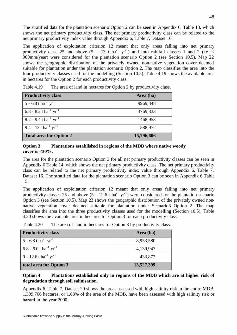
Sustainable firewood supply in the Murray -Darling Basin
48
The stratified data for the plantation scenario Option 2 can be seen in Appendix 6, Table 13, which shows the net primary productivity class. The net primary productivity class can be related to the net primary productivity index value through Appendix 6, Table 7, Dataset 16.
The application of exploitation criterion 12 meant that only areas falling into net primary productivity class 25 and above (5 - 13 t ha-1 yr-1) and into rainfall classes 1 and 2 (i.e. < 900mm/year) were considered for the plantation scenario Option 2 (see Section 10.5). Map 22 shows the geographic distribution of the privately owned non-native vegetation cover deemed suitable for plantation under the plantation scenario Option 2. The map classifies the area into the four productivity classes used for the modelling (Section 10.5). Table 4.19 shows the available area in hectares for the Option 2 for each productivity class.
Table 4.19 The area of land in hectares for Option 2 by productivity class.
Productivity class Area (ha)
5 - 6.8 t ha-1 yr-1 9969,348
6.8 - 8.2 t ha-1 yr-1 3769,333
8.2 - 9.4 t ha-1 yr-1 1468,953
9.4 - 13 t ha-1 yr-1 588,972
Total area for Option 2 15,796,606
Option 3 Plantations established in regions of the MDB where native woody cover is <30%.
The area for the plantation scenario Option 3 for all net primary productivity classes can be seen in Appendix 6 Table 14, which shows the net primary productivity class. The net primary productivity class can be related to the net primary productivity index value through Appendix 6, Table 7, Dataset 16. The stratified data for the plantation scenario Option 3 can be seen in Appendix 6 Table 15.
The application of exploitation criterion 12 meant that only areas falling into net primary productivity classes 25 and above (5 - 12.6 t ha-1 yr-1) were considered for the plantation scenario Option 3 (see Section 10.5). Map 23 shows the geographic distribution of the privately owned non-native vegetation cover deemed suitable for plantation under Scenario3 Option 2. The map classifies the area into the three productivity classes used for the modelling (Section 10.5). Table 4.20 shows the available area in hectares for Option 3 for each productivity class.
Table 4.20 The area of land in hectares for Option 3 by productivity class.
Productivity class Area (ha)
5 - 6.8 t ha-1 yr-1 8,953,580
6.8 - 9.0 t ha-1 yr-1 4,139,947
9 - 12.6 t ha-1 yr-1 433,872
total area for Option 3 13,527,399
Option 4 Plantations established only in regions of the MDB which are at higher risk of degradation through soil salinisation.
Appendix 6, Table 7, Dataset 20 shows the areas assessed with high salinity risk in the entire MDB. 1,309,766 hectares, or 1.68% of the area of the MDB, have been assessed with high salinity risk or hazard in the year 2000.

Sustainable firewood supply in the Murray -Darling Basin
49
The plantation scenario Option 4 data can be seen in Appendix 6, Table 16.
The stratified data for the plantation scenario Option 2 can be seen in Appendix 6, Table 17, which shows the net primary productivity class. The net primary productivity class can be related to the net primary productivity index value through Appendix 6, Table 7, Dataset 16.
The application of exploitation criterion 12 meant that only areas falling into net primary productivity class 25 and above (5 - 13.4 t ha-1 yr-1) were considered for the plantation scenario Option 4 (see Section 10.5). Map 24 shows the geographic distribution of the privately owned non-native vegetation cover deemed suitable for plantation under the plantation scenario Option 4. The map classifies the area into the two productivity classes used for the modelling (Section 10.5). Table 4.21 shows the available area in hectares for Option 4 for each productivity class.
Table 4.21 The area of land in hectares for Option 4 by productivity class.
Productivity class Area (ha)
5 - 6 t ha-1 yr-1 114,927
6 - 13.4 t ha-1 yr-1 763,179
Total area for Option 4 878,106
Sustainable firewood supply in the Murray -Darling Basin
50
5 Model review and forest mensuration data for model development and validation
J.M. Stol, P.W. West and D.O. Freudenberger
5.1 Introduction The key objective of this study was to analyse the long-term sustainability of meeting firewood demand in the Murray-Darling MDB (MDB) from three possible sources: firewood harvested from standing and fallen dead timber (coarse woody debris) termed the “dead-wood scenario” (Section 7), thinning of live trees (“green-wood scenario”; Section 8) and firewood sourced exclusively from plantations (“plantation scenario”; Section 10. Section 3 describes the exploitation criteria for each scenario.
In the previous chapter we described the GIS design and data acquisition, as this was a prerequisite to modelling potential yield of firewood from the three scenarios. In this section we describe the process of searching for appropriate data and models, which had the end result that we were unable to identify an appropriate existing forest growth and yield model or data suitable for predicting long-term firewood supply under the dead-wood and green-wood scenarios in these low rainfall areas. As a consequence we were required to collect suitable forest mensuration data (e.g. basal area, wood volumes and coarse woody debris loads) from known age stands representative of the broad vegetation types subject to harvesting in the MDB, through a specially designed survey process. The methodology for the survey design and field measurements are described in this section.
The results of the stratified surveys were then used to develop a forest growth and yield modelling system which is described in Section 6. A subset of the forest sites surveyed for modelling purposes were also surveyed as case studies for the possible impact of thinning stands under the green-wood scenario and this is described in Section 9.
5.2 Review of existing models and forest data At the commencement of the project, we conducted a comprehensive review of growth data and existing forest growth and yield models which might have been suitable for modelling the potential supply of firewood from forest and woodlands of the MDB. Appendix 7 summarises the information considered. Most growth and yield models presently available were developed for forest species of high commercial value, most of them growing in high rainfall regions outside the MDB. The productivity of the forests in the MDB is generally much lower than that of the tall forests in the higher rainfall areas of coastal and eastern Australia, and as such provide only 5% of Australia’s commercial eucalypt timber (MDBC 2003). There are only four forest types in the MDB which have been used consistently for commercial forest production or firewood:
1. White Cypress Pine (Callitris glaucophylla); the species grows in even- or uneven-aged, closed or open forests, often in mixture with various eucalypt species within the MDB;
2. River Red Gum (Eucalyptus camaldulensis); widespread over the MDB but confined to riparian areas;
3. Ash forests, usually Alpine Ash (Eucalyptus delegatensis); from the higher rainfall and altitude areas of south-east NSW and north-east Victoria; and
4. Mallee woodlands (eg. Eucalyptus socialis, Eucalyptus gracilis, Eucalyptus oleosa subsp. oleosa and Eucalyptus dumosa), confined to the low rainfall regions in the south-west of the MDB.

Sustainable firewood supply in the Murray -Darling Basin
51
Whilst other forest types in the MDB have been used from time to time for firewood or minor wood product production, none has been the subject of a major forest industry and consequently there has been no production model previously developed for these lower rainfall forest types. Of the above four commercially exploited vegetation types that have been modelled in some way, the White Cypress Pine model appeared to have the greatest applicability to the dead-wood and green-wood scenarios, as River Red Gums are a specialised forest type confined to periodically flooded riparian systems along major rivers of the MDB. Its regeneration, growth and yield are dependent on inundation, and hence are not applicable to the vast area of the MDB not on floodplains. Neither was an Alpine Ash model suitable, as this species grows in temperate high rainfall areas which form only a small portion of the south-eastern corner of the MDB. For mallee woodland types, Neagle (1994) published sufficient data to enable us to create a growth and yield model suitable for predicting long-term firewood yield from mallee forests. The mallee model was used in conjunction with estimates from our GIS of the existing areas of mallee in the MDB and is described in Section 8. Initial results suggested that the cypress pine model is inappropriate to predict yields from mallee eucalypts. It is perhaps not surprising that mallee forests display a quite different growth pattern to that of other forest in the MDB as their growth habit differs and they are a more arid species.
As a result of these findings, and because the only forest type within the MDB for which a published and accessible forest growth and yield model has been developed was White Cypress Pine forest (Vanclay 1985), it was felt that the White Cypress Pine model offered the only system available to allow some objective assessment of growth and wood yields from forests of the MDB. It was not known to what extent the growth behaviour of White Cypress Pine forests are typical of the range of forest types that occur in the MDB. Certainly it would be expected that applying a model developed for one species to predict growth and wood yields of the other species in the MDB would lead to at least some bias in estimates of wood yields for the other species. However, no other approach seemed a possibility for the present work without undertaking extensive field work across the MDB.
5.3 White Cypress Pine Model Testing of the White Cypress Pine model system showed that it was not immediately suitable for the purposes of the present work to predict long-term firewood supplies from non-mallee forests and woodlands, so modifications and further development were made to the model to allow its general application for the prediction of firewood quantities available from forests anywhere within the MDB.
Whilst long term wood yields are not that much different, it became obvious during the modelling process that there is a very different pattern of growth between the lower rainfall eucalypts and White Cypress Pine. Some modelling was available from mallee forests of South Australia which suggested that the White Cypress Pine model was inappropriate to apply to those forests and that the differences appeared to be quite substantial. It was perhaps not surprising that preliminary fieldwork data showed that forest and woodland eucalypt species had a much faster growth in the earlier years than the cypress pine model was showing. The consequences were that much more wood was available at the times of thinning in the green-wood scenario and harvest for the dead wood scenario.
Subsequently, as results from the modelling demonstrated (Figures 5.1 and 5.2), it was seen that the available supply of firewood was being significantly underestimated for both dead-wood and green-wood scenarios. Figure 5.1 demonstrates that, for the dead-wood scenario, supply estimated by the modified White Cypress Pine model could not meet the current firewood demands, with an average of only around one million tonnes being available per annum for harvest. This figure should be compared with the results for the dead-wood scenario, estimated using the final model, shown in Figure 7.3.
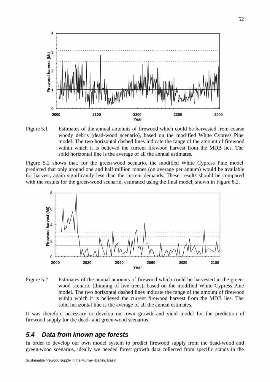
Sustainable firewood supply in the Murray -Darling Basin
52
0
1
2
3
4
2000 2100 2200 2300 2400Year
Fir
ewo
od
har
vest
(M
t)
Figure 5.1 Estimates of the annual amounts of firewood which could be harvested from coarse
woody debris (dead-wood scenario), based on the modified White Cypress Pine model. The two horizontal dashed lines indicate the range of the amount of firewood within which it is believed the current firewood harvest from the MDB lies. The solid horizontal line is the average of all the annual estimates.
Figure 5.2 shows that, for the green-wood scenario, the modified White Cypress Pine model predicted that only around one and half million tonnes (on average per annum) would be available for harvest, again significantly less than the current demands. These results should be compared with the results for the green-wood scenario, estimated using the final model, shown in Figure 8.2.
0
2
4
6
8
2000 2020 2040 2060 2080 2100Year
Fire
woo
d ha
rves
t (M
t)
Figure 5.2 Estimates of the annual amounts of firewood which could be harvested in the green-
wood scenario (thinning of live trees), based on the modified White Cypress Pine model. The two horizontal dashed lines indicate the range of the amount of firewood within which it is believed the current firewood harvest from the MDB lies. The solid horizontal line is the average of all the annual estimates.
It was therefore necessary to develop our own growth and yield model for the prediction of firewood supply for the dead- and green-wood scenarios.
5.4 Data from known age forests In order to develop our own model system to predict firewood supply from the dead-wood and green-wood scenarios, ideally we needed forest growth data collected from specific stands in the

Sustainable firewood supply in the Murray -Darling Basin
53
MDB over many decades. Alternatively, space can be substituted for time; data from many different sites of many different ages would suffice to develop and verify a forest growth and yield model. At the beginning of the project, we undertook a literature review to establish the extent and status of forest mensuration data available for the woodlands and forests of the MDB. The review included web searches, extensive literature searches, telephone and email enquires to a number of regional branches of State Forests NSW; NSW National Parks and Wildlife Service; Department of Conservation and Land Management, Victoria; NSW Department of Infrastructure, Planning and Natural Resources; Greening Australia; CSIRO Forestry and Forest Products; and a variety of statutory and land management agencies e.g. the NSW Office of Private Forestry and private farm forestry groups, individuals and landholders.
Appendix 7 shows a table of the 39 different potential sources of data and models which we initially short- listed from the results of the literature review as being worth further investigation. The potential data sources were tabulated to provide a framework to evaluate the usefulness of each to the project. Once the table was completed, it provided a comprehensive database on author, data source, the type of forestry sampling or modelling, forest yield outputs, growth rates, forest type, tree species and the potential strengths and limitations of that data.
The review found very little data for the MDB, or even within the more productive areas of eastern Australia, that were either accessible or in published format. Where data did exist, there were either problems with data access, or there were large gaps in data collections, or the sample sizes were too small. It was indicative of the limited nature of commercial forestry operations in the MDB that this literature review found no adequate data for developing growth and yields models for woodlands and forests in the MDB.
The greatest limitation was a lack of information on the ages of the remaining stands of forest and woodland in the MDB, at national, regional or even site scales. The State Forests NSW records for ages of harvested sites in the higher productivity forests were the best documented. However, there is very little documentation for stand age at a stand level in the lower productivity areas for species other than White Cypress Pine and River Red Gum. Some information existed for a number of State Forests and National Parks for which detailed historical records had been kept, or significant survey work been undertaken, however the information was not available across the entire range of ne t primary productivity classes extant in the MDB. More consistent and specific data was required for this project.
We also investigated the possibility of deriving age information from dendrochronology, air photograph or satellite image comparisons of specific sites over time, or archival records, but the time required to apply these methodologies was beyond the scope of this project. It was therefore necessary to develop a field sampling program for so that a specific set of forest attributes could be measured and recorded in a consistent and relevant format. The primary requirements were that the methodology was exactly replicated across all sites, that the ages of all sampled stand were known, and that the sampling was stratified to sample the range of forest and woodland types, across a range of ages between 15 and =100 years old and across the range of net primary productivity classes present in the MDB.
Data were required for the development and validation of the coarse woody debris component of the forest growth and yield model (Section 6). Thus an additional objective for the field studies was to obtain estimates of the amounts of coarse woody debris which might be expected to be present in a range of forest and woodland ecosystems, in order to model long-term supplies of coarse woody debris, particularly for the dead-wood scenario.
As was the case for other forest mensuration data, data on amounts of coarse woody debris in forests and woodlands are scarce, although over the last decade there has been increased research into the ability of forests to sequester and store carbon under greenhouse scenarios. There have also been a number of studies, albeit primarily outside of Australia, investigating the role of coarse
Sustainable firewood supply in the Murray -Darling Basin
54
woody debris in ecosystem function. Driscoll et al. (2000) reviewed the Australian scientific literature and found major knowledge gaps in a number of areas, namely the relationships between coarse woody debris levels and vertebrates, invertebrates, fungi and ecosystem processes. The existence of these knowledge gaps has been confirmed by a recent and comprehensive review of coarse woody debris in Australian forest ecosystems (Woldendorp et al. 2002), which concluded that studies addressing the issues of coarse woody debris are rare. See Section 9 for the results of the literature review of coarse woody debris studies in relation to ecological impacts of firewood harvesting.
The field data collected for this project provided the most consistent and available data of forest attributes to characterise many of the forest and woodland types found in the MDB. These attributes include stand basal areas, individual tree as well as stand volumes, number of stems per hectare, species, stand ages, and their associated coarse woody debris loads. The methods used are explicit and readily repeatable.
Data for the majority of the forestry mensuration attributes have not been collected previously in the MDB.
In order to stratify the sample across the range of forest types in the MDB, we first had to define the difference between forests and woodlands, then choose a mapped description of vegetation types that covers all of the MDB. We then broadly sampled at sites of known age across the most relevant vegetation types, stratifying by stand age and net primary productivity..
5.5 Forest and woodland types This project was constrained to categorise the forests and woodlands of the MDB in a manner compatible with the forest and woodland categories used by the spatial data available to the project. The data used by the model system for each scenario (that is, area of forest type, by age, by net primary productivity class) were to be derived from the spatial dataset (Section 4.2.2). Therefore, the data used to develop the growth and yield model had to be based on compatible forest types, and this had to be taken explicitly into account in the selection of sample sites.
5.5.1 Defining the forests of the MDB It is important to be aware of the significant differences between the variety of definitions of “forest” and “woodland” used by different Agencies.
The National Forest Inventory 2003 Forest by Tenure dataset (Section 4.2.2 and Appendix 3 Section 1.2) was used for this project to identify areas of forest and woodland in the MDB. The National Forest Inventory (NFI) is a partnership between the Commonwealth and all State and Territory Governments, with the aim of producing a single, authoritative source of data at the national level. ‘Forests’ and woodlands’ are defined by the NFI as:
“an area, incorporating all living and non-living components, that is dominated by trees having usually a single stem and a mature or potentially mature stand height exceeding 2 metres and with existing or potential crown cover of overstorey strata about equal to or greater than 20 per cent. This definition includes Australia's diverse native forests and plantations, regardless of age. It is also sufficiently broad to encompass areas of trees that are sometimes described as woodlands”
Herewith, we use this broad definition that combines both forests and woodlands into one term called ‘forests’.

Sustainable firewood supply in the Murray -Darling Basin
55
However, the NFT definition of forests is also expressed in three crown cover classes1: woodland (tree crowns cover 20-50 percent of the land area when viewed from above);
1. open forest (51-80 percent crown cover); and 2. closed forest (81-100 percent crown cover). These are mainly rainforest and mangroves
which were not treated as a source of firewood by this project.
There are two other significant sources of definitions for forests and woodlands. The definitions used by the MDB Commission (2003) differ from those used by the NFI in two main respects:
1. mature stand height is 5m; and 2. crown cover is = 30%.
The AUSLIG 1990 Vegetation Atlas of Australian Resources is designed to be more specific at the structural level, defining eight growth forms and four canopy cover classes:
1. open woodland at 0-10% foliage cover; 2. woodland at 10-30%; 3. and open forest above 30% foliage cover; and 4. and closed forest above 30% foliage cover.
The only available dataset at the scale of the entire the MDB was the NFI 2003 dataset, so we were constrained to adopt the NFI classification and definitions for this project.
5.5.2 Descriptions of the forests and woodlands in the MDB Table 5.1 summarises the community descriptions which apply to the forest type categories in the NFI 2003 dataset (also see Table 4.4). These forest types and their descriptions provided the general site descriptions used when considering the selection of the field sites for forest mensuration. The table can also be used to interpret the definitions of forest and woodland types used in the GIS modelling and analysis.
Table 5.1 The community descriptions for the forest and woodland types in the MDB, as defined in the NFI 2003 dataset (also see Table 4.4).
Forest Type Community description
Acacia The most common wattles Acacia spp. in the MDB are Mulga (Acacia aneura) and Brigalow (Acacia harpophylla) woodlands in the drier, north-western areas. Numerous other Acacia species are present in varying densities either as understory or canopy.
Callitris Cypress pines: Callitris species include White Cypress Pine (Callitris glaucophylla) typically either a common component of the central eucalypt woodlands of the MDB or forming extensive stands.
Casuarina Sheoaks (Casuarina and Allocasuarina species) are widely distributed as scattered trees or extensive stands often within the eucalypt forests and woodlands.
Eucalypt Low Open Forest
Most of these forests occur in arid regions in association with Acacia species i.e. Poplar Box (Eucalyptus populnea) and Blackbox (Eucalyptus largiflorens) in western New South Wales, Eucalyptus populnea in southern Queensland, with 21-50% crown cover, <10m tall.
1 Crown cover is determined by estimating or measuring the area of ground covered by tree canopies, ignoring overlap and gaps within individual canopies. A line around the outer edge defines the limits of an individual canopy, and all the area within is treated as “'canopy” irrespective of gaps and overlaps.

Sustainable firewood supply in the Murray -Darling Basin
56
Forest Type Community description
Eucalypt Low Woodland
Most of these forests occur in arid regions in association with Acacia species i.e. Poplar Box (Eucalyptus populnea) and Blackbox (Eucalyptus largiflorens) in western New South Wales, Eucalyptus populnea in southern Queensland, with 50-80% crown cover, <10m tall.
Eucalypt Mallee Open Forest
The more than 100 species of eucalypts with a multistemmed habitat and a vegetation dominated by them, with 51-80% crown cover
Eucalypt Mallee Woodland
The more than 100 species of eucalypts with a multistemmed habitat and a vegetation dominated by them, with 20-50% crown cover
Eucalypt Medium Open Forest
These include dry sclerophyll forests such as those described in detail in Section 9, Murray River Red Gum (Eucalyptus camaldulensis) forests with 50-80% crown cover 11-30m tall.
Eucalypt Medium Woodland
Typical communities include box woodlands with grassy understorey e.g. White Box (Eucalyptus albens) and Yellow Box (Eucalyptus melliodora) woodlands on fertile western slopes of southern New South Wales and Victoria, with 21-50% crown cover, 11-30m tall.
Eucalypt Tall Open Forest
Often referred to as “wet sclerophyll forests”: “wet” occurring only in very south eastern parts of the MDB where rainfall exceeds 1000 mm a year eg. Alpine Ash (Eucalyptus delegatensis) communities, with 50-80% crown cover and >30m tall.
Eucalypt Tall Woodland
Eucalypt forests, with 21-50% crown cover and >30m tall.
Hardwood Plantation Typically eucalypt species suitable for low rainfall areas eg. Spotted Gum (Eucalyptus maculata), Sugar Gum (Eucalyptus cladocalyx), Red Ironbark (Eucalyptus sideroxylon) and Blue Gum (Eucalyptus globulus).
Softwood Plantation Typically Pinus spp. Pinus radiata in higher rainfall areas, other Pinus spp. are being trialled in lower rainfall areas.
Unknown Plantation Unknown Plantation.
5.6 Field sampling design For any particular forest type, a forest growth and yield model predicts how a stand in the forest grows with time and hence the amount of wood available for harvest from it at any stage of its lifetime. Such models take account also of the fact that the productivity of a forest, hence the amount of wood it can yield at any age, depends on the characteristics of the site on which it is growing. The description of the development of the growth and yield model used for the dead-wood and green-wood scenarios is detailed in Section 6. Therefore, it was necessary that the field data collected by this project sampled the range of site productivity capacities and extant in the MDB, and the range of forest age classes.
Consequently, the first step in the design of the sampling strategy was to stratify the MDB into broad primary productivity sub-classes. The second was to stratify by stand age class. The third step was to stratify sites with stands of known age by position on slope, selecting plots and identifying the forest type. Once this had been undertaken, the following data items were collected from the plots for the yield model: stand basal areas, individual tree volumes, stand volumes, number of stems per hectare, species, stand ages, and coarse woody debris loads.
The net primary productivity stratification was carried out using the GIS system (Section 4) to produce maps which could be used in the field to locate areas where sites could be located. The age and position on slope stratifications were conducted in the field during the process of site selection.

Sustainable firewood supply in the Murray -Darling Basin
57
5.6.1 Net primary productivity Four broad net primary productivity classes were chosen for the stratification. Table 4.1 presents these classes in terms of their general geographic area. Map 25 (Appendix 4) shows the geographic distribution of these classes.
Table 4.1 The 4 net primary productivity subclasses used to initially stratify the MDB for field site selection.
Net Primary Productivity (NPP) Class
Net Primary Productivity and oven dry biomass/ha/year Area of the MDB
1 10.6 – 14 Eastern highlands 2 7.2 – 10.6 Eastern tablelands and slopes 3 4.0 – 7.2 Central slopes and plains 4 0.2 – 4.0 Western plains
5.6.2 Stand age After defining an area of the MDB in terms of net primary productivity the next step was to travel into the forest area to specifically locate stands of forest or woodland of known age. Stand “age” in this context is defined as the time since a stand regenerated from bare ground following clearing, destructive wildfire or other natural calamity.
We relied substantially on oral history for the age of the stands selected for sampling. At the stand level i.e. a specific stand of trees which could be sampled, the best source of were private landowners who had a long-term historical connection with the land e.g. a family property, an interest in history or were involved in private farm forestry.
The lack of hard data on age classes meant there is some uncertainty on the ages we have assigned to the stands. If the stand was younger than 70-80 years, we believe that the age is accurate to within year or two. However as stand ages increases, so does the associated degree of uncertainty, increasing to a maximum of 10 years or so. Further, where trees had developed significant hollows and circumference there were no oral or written records to verify ages, so the stand was assigned an age of 100+ years.
Suitability of even aged versus mixed aged stands
A potential sampling site was then assessed further for species composition and its history of disturbance i.e. ringbarking, grazing, fire, fertilising, and harvesting. There were very few sites found to be in a “pristine” condition. The primary disturbances were ringbarking or bulldozing to create cleared pasture, and harvesting for a variety of timber uses, including building, fence posts, mine props and firewood.
The age structure of the dominant overstorey trees was then assessed. For collection of data for the forest growth and yield model an ideal site would consist of an even age stand resulting from one major disturbance event. These conditions were most frequently found in sites less than 30 years old and cleared by bulldozer or clear-felled rather than selectively logged. As a stand age increased, so did the frequency of disturbance events and subsequently there could be up to 1 or 2 other age cohorts present. Potential sampling sites were frequently rejected because disturbance history had resulted in very mixed aged stands.

Sustainable firewood supply in the Murray -Darling Basin
58
5.6.3 Position on slope Topographic position (i.e. position on a slope) is an important explanatory variable for species presence in the landscape but it is also important variable for within species variation as a result of differences in soil characteristics and water availability. Sites on upper slopes tend to have drier shallower soils than those on the lower parts of the slopes. These can influence forest attributes such as tree diameter, volume and height and stand basal area and stocking density as a result of these differences in resource availability. For the initial fieldwork in net primary productivity Class 2, three plots were randomly selected within each site, one each on upper slope, mid slope and lower slope, in order to capture any stand variation characteristics across the slope due to changes. However within net primary productivity Classes 1, 3 and 4 each of these subsequent sites had only 1 plot per site due to time limitations.
5.7 Field sampling methods Forest mensuration is part of the forest inventory process which may be defined as the systematic collection, evaluation and presentation of specific information on forest areas. Generally, detailed observations are only made of a small part of the area and techniques are applied to extrapolate from these limited observation to the whole area of interest (Brack 2000, West 2004). The selection of which measurements and individuals to choose are a fundamental part of forest mensuration. Measurements are made on individual trees, stands (small groups of trees) and forests (groups of stands) and for this report, a unique forest survey method was designed to measure both stand characteristics and individual tree bole taper and volume.
Suitable forest and woodland stands were found on 57 sites and forest mensuration and ecological impact data was collected from a total of 79 stands within the sites. Site ages ranged from 10-150+ years. Each of the four net primary productivity classes contained approximately fifteen sites ranging across these age classes. Sites were located between Tumut/Tumbarumba in the east, to the Bourke/Cobar area in the west on private properties, Travelling Stock Reserves, National Parks and State Forests. Two staff undertook reconnaissance and data collection in the field for approximately 50 days between April and August 2003.
5.7.1 Live tree measurements Once the forest or woodland site of known age had been selected a series of forest mensuration data was collected in order to calculate potential yield of firewood. The stand and forest measurements are summaries derived from specific measurements taken on selected individual trees. So for each forest stand a “point sample” was taken so that the basal area (over bark) of the stand could be determined from a single point, rather than having to establish a plot of known area in which all trees are measured. In most stands, the stem wood volume under bark from ground to tree top was measured for three individual trees included in the point sample. The principles of point sampling underpin the methodology described here and can be found in standards texts on forest measurement practice (e.g. West 2004). Stocking density of the trees can determined also from the point sample. The results from these stand basal areas over bark and stand stocking density of the live trees in each stand are shown in Appendix 8.
In order to calculate stem volume the individual tree height, basal area, tree shape and bark thickness are needed. We used a combination of a Spiegel Relaskop, digital hypsometer (Forestor vertex), transponder and diameter tape. The relaskop was selected because it could be used in the estimation of tree diameter at any point up the tree bole to assist in measuring stem wood volume through centroid sampling technique. The vertex and transponder was used for individual tree heights and distances.

Sustainable firewood supply in the Murray -Darling Basin
59
The relaskop was then used to determine basal area (m² ha-1) and stocking density (tree stems ha-1) for the stand level. Firstly a basal area factor was chosen and the relaskop used to select an average of 15 to 20 trees within the plot to measure their diameter and height. An Excel spreadsheet function was used in cases of uncertainty to determine if the tree was in the sample by using the distance to the tree and its diameter at breast height over bark (DBHOB). If the tree was in the sample its height was determined using the vertex and transponder and its diameter measured at breast height (1.3m) by using a diameter tape. The tree species was recorded and whether it was live or dead. The woody biomass of dead trees were considered part of the coarse woody debris of the stand (see section 5.5.2). Using a hand-held computer, data were entered directly into an Excel spreadsheet with functions which calculated live tree and dead tree stand basal area and stocking density
These standard tables providing known stem volume functions are available from more highly productive forests however these have not yet been deve loped for these lower rainfall forests. Measurements were therefore taken of individual tree stem wood volumes to develop a volume function for these forests. This was undertaken by selecting three trees per plot, with the aim of sampling a wide range of tree sizes and species over all the stands measured. Their stem wood volumes were measured using the “centroid method” (West 2004). This involves measuring the bark thickness at breast height of the tree concerned with a bark gauge and the diameter over bark of the stemat a point high up on the stem, is measured; as prescribed by the centroid method. The Relaskop was used to take such diameter measurements from the ground. Despite its relative simplicity of application, the centroid method generally gives quite precise estimates of stem wood volume of standing trees, with little bias (West 2004). The volume function developed is described in Appendix 9. This function is used to estimate volumes of other trees measured in the point sample from their diameters at breast height over bark and their total heights. Wood densities are included in Appendix 8.
5.7.2 Coarse woody debris Coarse woody debris was defined as all dead standing trees = 5cm DBH and any fallen woody material = 10cm at its mid-point and = 50cm in length. The length and diameter at mid-point of any piece of wood on the ground that fell into this category was measured using a 25x50m plot. The plot was established within the area at which the forestry point sample was made. This is a standard method used for assessing amounts of coarse woody debris in Australian forests (McKenzie et al.2000). As it was measured, each piece of woody debris was assigned to one of three classes:- Class 1 (wood was solid when kicked and lacked cavities, cracks or a hollow pipe), Class 2 (mostly solid when kicked but contained cavities, cracks or a hollow pipe or Class 3 (gave or crushed when kicked).
The volume of any piece of fallen woody debris measured in a ground plot was determined as that of a cylinder, with cross-sectional area determined by the measured diameter of the piece and length equal to the measured length (known as Huber’s fo rmula). This is a standard method used in forestry science to determine volumes of sections of tree stems or branches (West 2004).
To convert those volumes to biomasses, it was assumed that woody debris pieces categorised as Class 1 had suffered negligible decay and their basic density was the same as that used for estimating the live tree stem wood biomass in that stand. Pieces of Class 2 were assumed to have suffered some decay and to have a density equal to 75% of that of undecayed wood. Those of Class 3 were assumed to have a density of 30% of that of undecayed wood. The stand biomasses of each of those classes of woody debris in each stand measured are shown in Appendix 8.
Where standing dead trees were present, they were measured in a point sample and their stand stem wood biomasses estimated from their heights and diameters at breast height in the same way as was

Sustainable firewood supply in the Murray -Darling Basin
60
done for the live trees. The stand stem wood biomasses determined in this way are listed as part of the coarse woody debris of the stand in Appendix 8.
5.7.3 Ecological data In addition to the forest mensuration data, site characteristic data for assessment of ecological impacts e.g. location, aspect, altitude, soil type and depth, slope, geological substrate, vegetation community, topography and site history were recorded for each plot. The ecological data and methods are described in detail in Section 9.
5.8 Summary Data Using the survey design and methodology described here we were able to collect completely new kinds of forestry data for the low rainfall areas in a scientifically rigorous format across carefully stratified sites in the MDB, so that the non-mallee forest model system described in the next section could be based on the most current, consistent and accurate data available. The summary data , for each point sample taken are provided in Appendix 8 tables. Shown in the table are:
1. location, including latitudes and longitudes 2. tree species present 3. wood density of the priciple tree species in the point sampe (based on Ilic et al 2000) 4. stand age 5. net primary productivity index (tonnes ha-1 yr-1), derived from the GIS dataset 6. Basal area over bark (m2 ha-1) 7. Stocking density (stems ha-1) 8. Stem wood biomass (tonnes ha-1) 9. Coarse woody debris (tonnes ha-1) of standing dead trees 10. Coarse woody debris (tonnes ha-1) Decay Class 1 ground debris (solid) 11. Coarse woody debris (tonnes ha-1) Decay Class 2 ground debris (mostly solid) 12. Coarse woody debris (tonnes ha-1) Decay Class 3 ground debris (decayed)
The data are available also in unprocessed form. They have not been documented here due to the large size of the dataset. The raw data provide the detailed measurements of tree heights, tree diameters, species sampled, site description and individual coarse woody debris measurements for each plot. Those data will be made available on request.
The forestry mensuration data were used in the development of the growth and yield model, which is described in Section 6.

Sustainable firewood supply in the Murray -Darling Basin
61
6 Growth and yield models P.W. West
6.1 Summary Forests of the Murray-Darling Basin (MDB) have low productivity by Australian forest standards, principally because the annual rainfall of the Basin is relatively low. The fo rests have been exploited little commercially. Little growth and yield data have been collected from them and few efforts have been made to develop growth and yield models to predict their wood yields. Data on stand stem wood biomass and coarse woody debris biomass, collected from 79 stands of a wide range of non-mallee forest types across the MDB (see Section 5). The data were used to develop a stand-based, empirical growth and yield model to predict firewood harvest yields available from these forests, when live trees are removed from them as thinnings or when coarse woody debris is harvested from time to time during their lifetimes. The model predicts yields in relation to the productive capacity of the site on which a forest is growing; the measure of site productive capacity (maximum annual net primary production of plants growing on a site) had been determined in other work for sites across Australia (Appendix 5). It was found that if the model is used to predict the average stand stem wood biomass of stands of a particular site productive capacity across a wide area of the MDB, the 95% confidence limit about the predicted average would be ±17% of the predicted value. This level of precision was considered appropriate for broad-scale estimation of firewood yields available from the MDB. Using previously published data, a separate growth and yield model was developed to predict firewood yields obtained by clear- felling 20-100 year old mallee eucalypt forests in the MDB.
6.2 Introduction The overall aim of the present project was to determine the sustainable production of firewood possible from the forests of the MDB, firewood obtained either by felling live trees or from the collection of the coarse woody debris present as standing dead trees or fallen from live trees. To do so, it is necessary to predict how much firewood will be available from time to time from the forest at any location in the MDB. In normal forest management practice, such predictions are made using a “forest growth and yield model”. For any particular forest type, such a model predicts how a stand in the forest grows with time and hence the amount of wood available for harvest from it at any stage of its lifetime. Such models take account also of the fact that the productivity of a forest, hence the amount of wood it can yield at any age, depends on the characteristics of the site on which it is growing, particularly the rainfall, temperature and soil fertility. The scope and nature of the growth and yield models developed in the more productive native forests in Australia are summarised by Rayner and Turner (1990a,b).
For the purposes of the present project, field work was undertaken to gather sufficient data on growth and yield of non-mallee forests of the MDB to allow development of a growth and yield model to predict firewood yields from them (see Section 5). This section describes the development of that model. Fortunately, sufficient information was available from the literature to allow growth and yield prediction for mallee forests, without the need to develop a new model system for that forest type; the model system for mallee forests is described also in this section.

Sustainable firewood supply in the Murray -Darling Basin
62
6.3 Data
6.3.1 Stand measurements Section 5 describes the methods used to find suitable stands to provide data on the wood biomasses2 of both live trees and coarse woody debris in forests of the MDB. The sites selected for measurement included a wide range of forest types and ages which had a wide range of productive capacities. Since forests of the MDB include both even- and uneven-aged forest, it is important to recognise that stand “age” in the present context is defined as the time since a stand regenerated from bare ground following clearing, destructive wildfire or other natural calamity.
Data collected from all 79 stands were used to build the growth and yield model for non-mallee forests. A list of the properties, the stand number on each property, their locations and the species present in the measured stands are given in Appendix 8. From the information available about stand age, a specific age was assigned to each stand, usually determined as the mid-point of the period within which it was believed regeneration of the stand occurred from bare ground. The chosen ages are shown in Appendix 8.
6.3.2 Stand stem wood biomass The data collected in the point samples (Section 5.7.1) were used to determine the stand stem wood biomass of live trees in each stand as follows.
Since only diameter at breast height over bark (D, cm) and tree total height (H, m) had been measured for most trees, it was necessary first to deve lop an individual tree stem volume function to allow stem wood volume (V, m3) to be estimated for each tree from its height and diameter. The development of this function used the data from the trees of which the stem wood volume had been measured and is described in Appendix 9. The stem volume function developed was:
V = 0.246x10⁻⁴D1.996H0.947 (6.1)
This function was used, with the tree diameter and height data collected in the point samples, to determine stand stem wood volumes for the live trees of each of the 79 measured stands; West (2004) describes how individual tree volumes determined in a point sample are used to determine a corresponding stand stem wood volume.
These stand wood volume estimates were converted to stand wood biomass estimates, assuming that the basic density (oven-dry weight per unit green volume) of the wood of the trees was that of the most common species in the stand. The basic densities used were obtained from a recent collation of wood densities of Australian trees (Ilic et al.2000). The densities and the live tree stand stem wood biomasses determined for each measured stand are shown in Appendix 8.
6.3.3 Coarse woody debris stand biomass
Coarse woody debris stand biomass includes stem and branch wood of dead standing trees or pieces of fallen wood with length ≥0.5 m and mid-diameter ≥10 cm. Section 5.7.2. describes the methods for measuring and determining the stem volumes of sections of tree stems and branches. The stand stem wood biomasses thus determined are presented as part of the coarse woody debris for each stand in Appendix 8.
2 Throughout this Section, use of the term ‘biomass’ refers to oven-dry biomass.
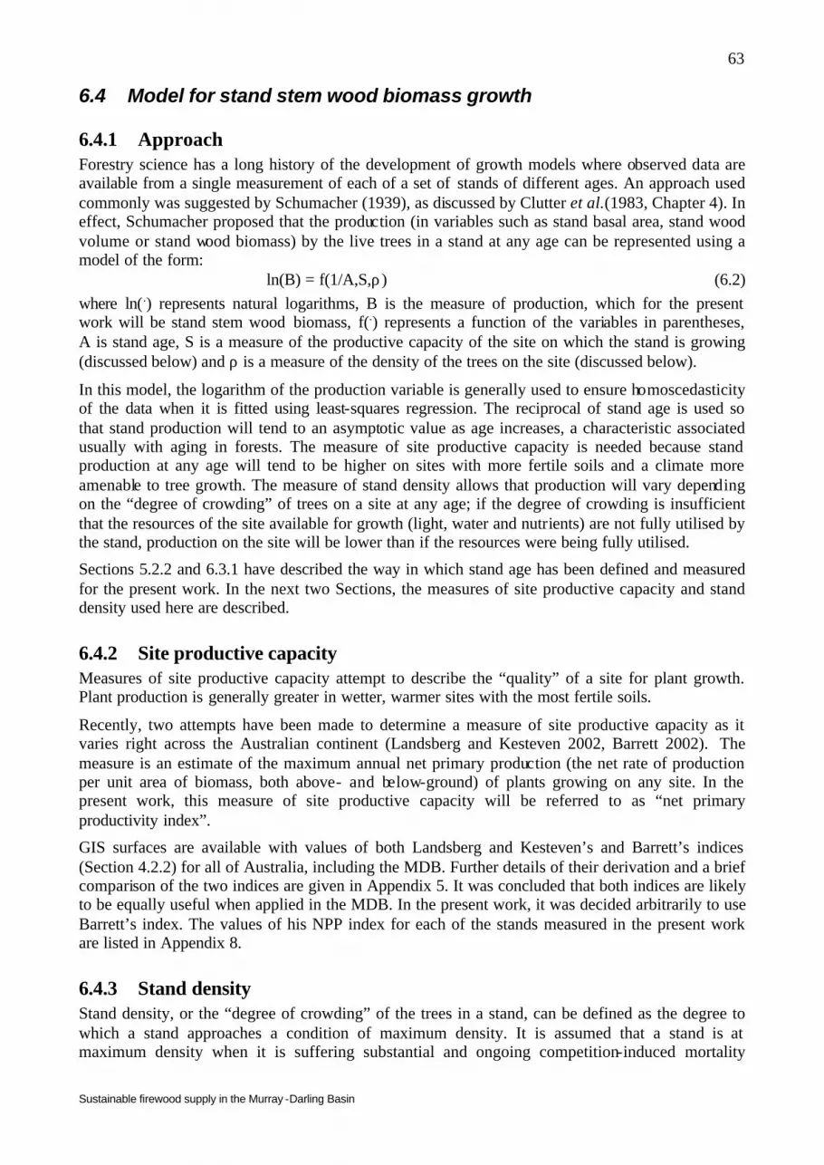
Sustainable firewood supply in the Murray -Darling Basin
63
6.4 Model for stand stem wood biomass growth
6.4.1 Approach Forestry science has a long history of the development of growth models where observed data are available from a single measurement of each of a set of stands of different ages. An approach used commonly was suggested by Schumacher (1939), as discussed by Clutter et al.(1983, Chapter 4). In effect, Schumacher proposed that the production (in variables such as stand basal area, stand wood volume or stand wood biomass) by the live trees in a stand at any age can be represented using a model of the form:
ln(B) = f(1/A,S,ρ) (6.2) where ln(.) represents natural logarithms, B is the measure of production, which for the present work will be stand stem wood biomass, f(.) represents a function of the variables in parentheses, A is stand age, S is a measure of the productive capacity of the site on which the stand is growing (discussed below) and ρ is a measure of the density of the trees on the site (discussed below).
In this model, the logarithm of the production variable is generally used to ensure homoscedasticity of the data when it is fitted using least-squares regression. The reciprocal of stand age is used so that stand production will tend to an asymptotic value as age increases, a characteristic associated usually with aging in forests. The measure of site productive capacity is needed because stand production at any age will tend to be higher on sites with more fertile soils and a climate more amenable to tree growth. The measure of stand density allows that production will vary depending on the “degree of crowding” of trees on a site at any age; if the degree of crowding is insufficient that the resources of the site available for growth (light, water and nutrients) are not fully utilised by the stand, production on the site will be lower than if the resources were being fully utilised.
Sections 5.2.2 and 6.3.1 have described the way in which stand age has been defined and measured for the present work. In the next two Sections, the measures of site productive capacity and stand density used here are described.
6.4.2 Site productive capacity Measures of site productive capacity attempt to describe the “quality” of a site for plant growth. Plant production is generally greater in wetter, warmer sites with the most fertile soils.
Recently, two attempts have been made to determine a measure of site productive capacity as it varies right across the Australian continent (Landsberg and Kesteven 2002, Barrett 2002). The measure is an estimate of the maximum annual net primary production (the net rate of production per unit area of biomass, both above- and below-ground) of plants growing on any site. In the present work, this measure of site productive capacity will be referred to as “net primary productivity index”.
GIS surfaces are available with values of both Landsberg and Kesteven’s and Barrett’s indices (Section 4.2.2) for all of Australia, including the MDB. Further details of their derivation and a brief comparison of the two indices are given in Appendix 5. It was concluded that both indices are likely to be equally useful when applied in the MDB. In the present work, it was decided arbitrarily to use Barrett’s index. The values of his NPP index for each of the stands measured in the present work are listed in Appendix 8.
6.4.3 Stand density Stand density, or the “degree of crowding” of the trees in a stand, can be defined as the degree to which a stand approaches a condition of maximum density. It is assumed that a stand is at maximum density when it is suffering substantial and ongoing competition-induced mortality

Sustainable firewood supply in the Murray -Darling Basin
64
amongst the smaller, suppressed trees in a stand. Substantial work has shown that stands at maximum density conform to what is known as the “power rule of self- thinning”. Under this rule, the relationship between stand biomass (W, g cm-2) of the live plants in a stand (biomass can be expressed as total biomass above- and below-ground, above-ground biomass only or stem biomass only) and stand stocking density (N, stems m-2) can be expressed by the relationship:
W = aNb (6.3) where a and b are parameters and the value of b is close to -0.5.
This rule has been found to hold widely across the plant kingdom, not only for forests, and for both single- and mixed-species plant assemblages.
Weller (1987) has reviewed the validity of this rule. In effect, it sets an upper limit to the circumstances in which plant stands will be found in nature. No stand, of a particular stocking density, will be found with a biomass in excess of that predicted by equation (6.3); if it did have a biomass above that, it would suffer rapid mortality until its stocking density and biomass were reduced to a level such that it did conform to the rule.
This rule is used extensively in forestry science to provide a measure of stand density. If a stand has a biomass Wo (g cm-2) and a stocking density No (stems m-2), then its density (ρ, dimensionless) is defined as its actual stocking density divided by the stocking density it would have if it were at maximum density, that is if it were conforming to equation (6.3). That is, its density is determined as:
ρ = No/[(Wo/a)](1/b) (6.4)
Works such as West (1983), Jack and Long (1996) and Avery and Burkhart (2002) may be consulted to learn how this, and other related stand density measures are derived and used in forestry. Stands with a density of 1 will be at maximum density. Stands with a density below 0.15-0.25 are unlikely to be using fully the resources for growth available at a site (light, water and nutrients) (Jack and Long 1996).
Unfortunately, work in Australia to quantify the power-rule of self- thinning for eucalypt forests generally is limited and none has been done for those of the MDB. Weller (1987) used some limited, published data from eucalypt forests which suggested their behaviour under the rule was somewhat deviant from other forests. However, West (1985) and Hamilton (1988) used more substantial and appropriate data sets from ash eucalypt forests of Victoria and Tasmania to suggest those forests conformed quite reasonably to the rule. West’s results suggest that appropriate parameter values for equation (6.3) for those forests were a=1.22x10⁴ and b=-0.5 (where stand biomass was represented by stem wood biomass and it has been assumed here that basic stem wood density for those forests was 0.502 t m-3).
Figure 6.1 shows a scatter plot of the stand stem wood biomasses against stand stocking densities (transformed as logarithms) for the data collected in the present work for the fo rests of the MDB (Appendix 8). Superimposed upon the diagram are the power-rule of self-thinning for ash eucalypts as determined by West (1985) and lines denoting various stand densities as stands approach the self-thinning line. The two stands which are closest to the self- thinning line were stands 6 and 7 from the property “Maragle”, which is a New South Wales State Forest located in the more productive parts of the MDB on its south-eastern boundary. Those stands were 33 and 20 years old, respectively, and consisted principally of Eucalyptus viminalis and/or Eucalyptus pauciflora. This is a forest type which, whilst not as productive as the ash forests of southern Australia, could generally be expected to grow well and regenerate densely after felling. The fact that at least these stands fell at a position near the self- thinning line for ash eucalypts, in Figure 6.1, suggests that that line has at least some relevance to the forests of the MDB.
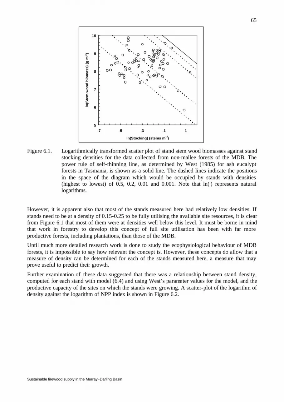
Sustainable firewood supply in the Murray -Darling Basin
65
5
6
7
8
9
10
-7 -5 -3 -1 1
ln(Stocking) (stems m-2)
ln(S
tem
woo
d bi
omas
s) (
g m
-2)
Figure 6.1. Logarithmically transformed scatter plot of stand stem wood biomasses against stand
stocking densities for the data collected from non-mallee forests of the MDB. The power rule of self-thinning line, as determined by West (1985) for ash eucalypt forests in Tasmania, is shown as a solid line. The dashed lines indicate the positions in the space of the diagram which would be occupied by stands with densities (highest to lowest) of 0.5, 0.2, 0.01 and 0.001. Note that ln(.) represents natural logarithms.
However, it is apparent also that most of the stands measured here had relatively low densities. If stands need to be at a density of 0.15-0.25 to be fully utilising the available site resources, it is clear from Figure 6.1 that most of them were at densities well below this level. It must be borne in mind that work in forestry to develop this concept of full site utilisation has been with far more productive forests, including plantations, than those of the MDB.
Until much more detailed research work is done to study the ecophysiological behaviour of MDB forests, it is impossible to say how relevant the concept is. However, these concepts do allow that a measure of density can be determined for each of the stands measured here, a measure that may prove useful to predict their growth.
Further examination of these data suggested that there was a relationship between stand density, computed for each stand with model (6.4) and using West’s parameter values for the model, and the productive capacity of the sites on which the stands were growing. A scatter-plot of the logarithm of density against the logarithm of NPP index is shown in Figure 6.2.

Sustainable firewood supply in the Murray -Darling Basin
66
-9
-7
-5
-3
-1
0.0 0.5 1.0 1.5 2.0 2.5 3.0ln(NPP) (t ha-1 yr-1)
ln(D
ensi
ty)
(dim
ensi
on
less
)
Figure 6.2 Scatter plot of logarithmic transformations of stand density against site
productive capacity (NPP index) for the stands measured in the present work. The solid line shows the ordinary least-squares regression straight line fit to the data.
There appears to be a tendency for stand density to increase with increasing site productive capacity. The ordinary least-squares regression straight line fit to the data was highly significant (p<0.01 at least), but the relationship was only moderately strong (r2=0.34). The fit to the data of the regression is shown on the figure. The model fitted was:
ρ = 0.000181S2.71 (6.5) where S is site productive capacity (NPP index, t ha-1 yr-1). Note that the coefficient value 0.000181 in model (6.5) has been corrected to allow for the bias introduced in back-transforming predictions, from a regression fitted in logarithmic form, to their linear counterparts. In the present work, the bias correction value proposed by Snowdon (1991) was used. This is determined as the mean of the observed values of the dependent variable of the fitted regression divided by the mean of their predicted values from the logarithmic regression, after back-transformation from logarithms.
For the present work, model (6.5) will be used to estimate the average density of forests in the MDB found on sites of a particular productive capacity. For any one stand, it is likely that its density will change with age, but there was no evidence in the data available here that any such trend could be identified. Furthermore, other work has suggested that the intercept of the self-thinning line may change with site productive capacity (e.g. Zeide 1985, Jack and Long 1966), whereas a single value of the intercept has been assumed appropriate for the present work. Considerable research would be necessary to establish in detail a full description of the growth dynamics of the various forest types of the MDB. However, it was felt that for the purposes of the present work, model (6.5) provides at least some opportunity to take account of the very wide range of stand densities that obviously occur in the forests of the MDB and the consequences that may have for their productivity.
6.4.4 Fitted model Given these various considerations, a model was developed to predict stand stem wood biomass at age A (years), BS(A) (t ha-1), in relation to age, site productive capacity (NPP index, S, t ha-1 yr-1) and stand density (ρ, dimensionless as determined using equation 6.4) for the stands measured here. As is evident in Appendix 8, a very wide range of forest types are represented in the data set, none with more than a few observations. This meant that it was impossible to develop separate growth models for different forest types, but only to develop a single growth model which would represent the average behaviour across all non-mallee forest types of the MDB.

Sustainable firewood supply in the Murray -Darling Basin
67
The model developed was based on the functional form shown in equation (6.2). The independent variables considered in fitting the model were 1/A, S, ln(ρ), their squares, their first-order interactions and the squares of those interactions. The model was then fitted, using ordinary least-squares regression, with a forward selection procedure (Draper and Smith 1981) to determine which combination of the independent variables minimised the residual variance of the fitted regression.
The model determined by this procedure (after back-transformation of the dependent variable from logarithms) was
BS(A) = 0.852exp[5.0483-0.1837S+0.0149S2-0.1791ρ’-0.0318(ρ’)2 +0.8195(S/A)2+10.4604(ρ’/A)+13.7934(ρ’/A)2] (6.6)
where ρ’ is the natural logarithm of ρ and the model has been back-transformed from logarithms. Note that the coefficient 0.852 is a bias correction factor, to allow for the back-transformation from logarithms, calculated using the method of Snowdon (1991). The fitted model was statistically significant (p<0.001) with r2=0.79. Scatter plots of the residuals from the regression against the fitted values and the independent variables showed no evidence of any lack of fit to the data.
6.4.5 Predicting growth at young ages The data set used to build model (6.6) contained no data from stands less than 10 years of age and only six observations from stands less than 20 years of age (Appendix 8). Examination of the fit to the data, suggested that predictions of stem wood biomass made with model (6.6) should be considered reliable only for stands 20 years or older.
An approximate model was constructed to allow predictions of stem wood biomass to made between 1 and 19 years of age. It was assumed that the form of the growth curve over that time period in any stand was:
BS(A) = exp(c+d/A) (2 ≤ A ≤ 19) (6.7)
where c and d are parameters.
It was assumed that the stem wood biomass at one year of age of any stand, BS(1) (t ha-1), was 0.01 t ha-1; alteration of this value affects the shape of the growth curve ultimately derived and this value appeared to give a shape consistent with the shape of the curve after 20 years of age described for any stand with model (6.6). Values for the parameters c and d were then determined for any stand as:
d = 0.95 ln[BS(1)/BS(20)] (6.8)
where BS(20) (t ha-1) was the stem wood biomass for the stand concerned predicted from model (6.6), and:
c = ln[BS(1)] - d (6.9)
Determining the values for the parameters of the model in this way ensures that the stem wood biomass which would be predicted with it at 20 years of age is exactly the same as that predicted using model (6.6).
6.5 Model to predict coarse woody debris biomass The total stand biomass of coarse woody debris present, in each of the stands in which debris was measured, was determined by summing the amounts present as dead standing trees and in each of three classes of woody debris measured on the ground (Appendix 8).
Unfortunately, it is likely that there had been removal of coarse woody debris at one time or other from many of the measured stands. The owner may have removed it as firewood or for other purposes, or fire passing through the stand may have burnt the debris present. Of the total 79 stands

Sustainable firewood supply in the Murray -Darling Basin
68
in Appendix 8, coarse woody debris on the ground was measured in only 45 of them. In four of those, no debris was found on the ground. Sufficient was known of the history of the 45 stands that it was felt reasonably certain that there had been no removal of coarse woody debris from 11 of them during their lifetime. Those 11 stands are indicated in Appendix 8.
Figure 6.3 shows a scatter plot of the measured amount of coarse woody debris measured in these stands against the corresponding stem wood biomass of the live trees in the stand.
0
10
20
30
40
50
60
70
80
90
0 50 100 150 200Stem wood biomass (t ha-1)
Deb
ris
biom
ass
(t h
a-1)
Figure 6.3 Scatter plot of the amount of coarse woody debris biomass
measured in non-mallee forest stands in the MDB against the corresponding stem wood biomass of the live trees in the stand. Results are shown for stands from which it was believed coarse woody had not been removed during the lifetime of the stand (l) and for those for which it was uncertain whether or not coarse woody had been removed (O). The solid line shows the fit to the data from the 11 sites thought to have experienced no removal of coarse woody debris.
For the 11 stands in which it was believed that the coarse woody debris was undisturbed, there appears to be a close correlation between the coarse woody debris biomass and the live tree stem wood biomass. This is not surprising; where the live trees in the stand are larger, whether because the forest is older, denser or growing on land of higher site productive capacity, it might reasonably be expected that more coarse woody debris would be present. However, assuming such a straightforward correlation exists, it appears from Figure 6.3 that some of the stands, for which it was uncertain whether or not their coarse woody debris had been disturbed, may in fact have been undisturbed. Also, it appears that some of the stands believed to have been undisturbed may, in fact, have been so.
However, the trends in the data of Figure 6.3 appeared to make it reasonable to assume that, for undisturbed stands, there is a simple correlation between stand coarse woody debris biomass and stand stem wood biomass. This relationship was quantified by fitting a straight- line, least-squares regression relationship passing through the origin, using the data only from the 11 stands it was believed were undisturbed. The fitted relationship was:
BC(A) = 0.437BS(A) (6.10)
where BC(A) (t ha-1) was the stand biomass of coarse woody debris at an age A (years). The fit to the data of this relationship is shown on Figure 6.3.
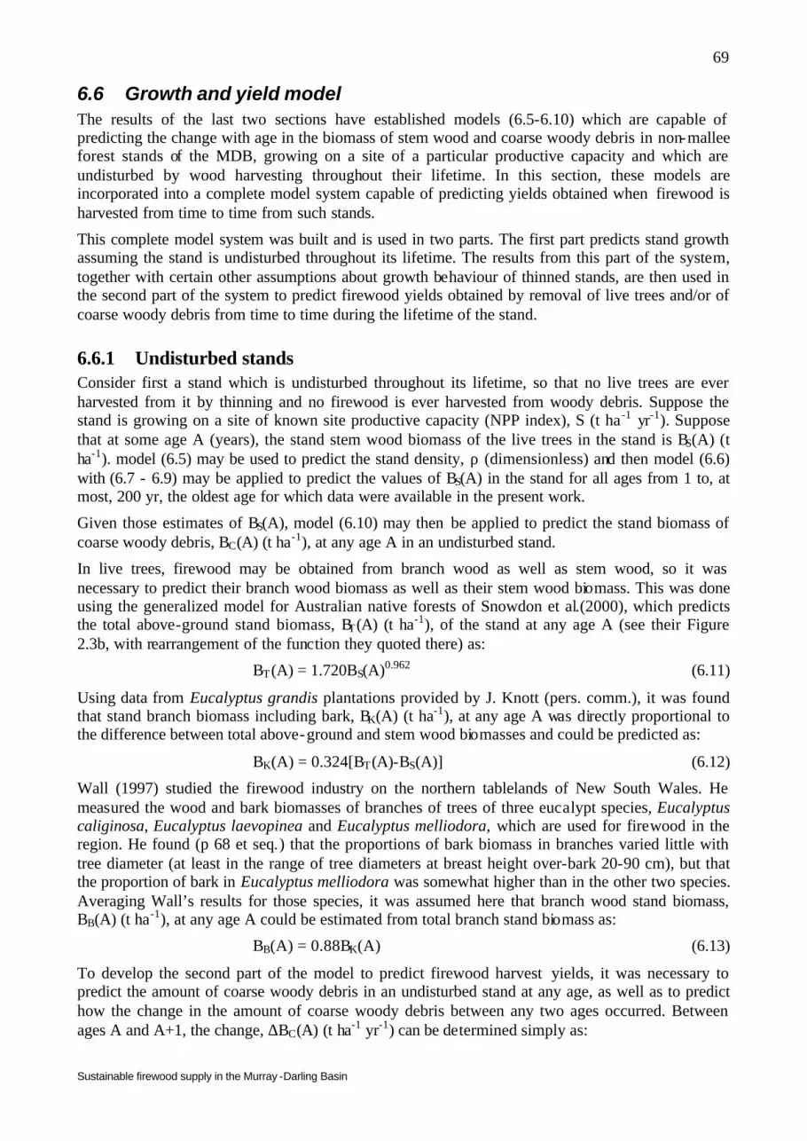
Sustainable firewood supply in the Murray -Darling Basin
69
6.6 Growth and yield model The results of the last two sections have established models (6.5-6.10) which are capable of predicting the change with age in the biomass of stem wood and coarse woody debris in non-mallee forest stands of the MDB, growing on a site of a particular productive capacity and which are undisturbed by wood harvesting throughout their lifetime. In this section, these models are incorporated into a complete model system capable of predicting yields obtained when firewood is harvested from time to time from such stands.
This complete model system was built and is used in two parts. The first part predicts stand growth assuming the stand is undisturbed throughout its lifetime. The results from this part of the system, together with certain other assumptions about growth behaviour of thinned stands, are then used in the second part of the system to predict firewood yields obtained by removal of live trees and/or of coarse woody debris from time to time during the lifetime of the stand.
6.6.1 Undisturbed stands Consider first a stand which is undisturbed throughout its lifetime, so that no live trees are ever harvested from it by thinning and no firewood is ever harvested from woody debris. Suppose the stand is growing on a site of known site productive capacity (NPP index), S (t ha-1 yr-1). Suppose that at some age A (years), the stand stem wood biomass of the live trees in the stand is BS(A) (t ha-1). model (6.5) may be used to predict the stand density, ρ (dimensionless) and then model (6.6) with (6.7 - 6.9) may be applied to predict the values of BS(A) in the stand for all ages from 1 to, at most, 200 yr, the oldest age for which data were available in the present work.
Given those estimates of BS(A), model (6.10) may then be applied to predict the stand biomass of coarse woody debris, BC(A) (t ha-1), at any age A in an undisturbed stand.
In live trees, firewood may be obtained from branch wood as well as stem wood, so it was necessary to predict their branch wood biomass as well as their stem wood biomass. This was done using the generalized model for Australian native forests of Snowdon et al.(2000), which predicts the total above-ground stand biomass, BT(A) (t ha-1), of the stand at any age A (see their Figure 2.3b, with rearrangement of the function they quoted there) as:
BT(A) = 1.720BS(A)0.962 (6.11)
Using data from Eucalyptus grandis plantations provided by J. Knott (pers. comm.), it was found that stand branch biomass including bark, BK(A) (t ha-1), at any age A was directly proportional to the difference between total above-ground and stem wood biomasses and could be predicted as:
BK(A) = 0.324[BT(A)-BS(A)] (6.12)
Wall (1997) studied the firewood industry on the northern tablelands of New South Wales. He measured the wood and bark biomasses of branches of trees of three eucalypt species, Eucalyptus caliginosa, Eucalyptus laevopinea and Eucalyptus melliodora, which are used for firewood in the region. He found (p 68 et seq.) that the proportions of bark biomass in branches varied little with tree diameter (at least in the range of tree diameters at breast height over-bark 20-90 cm), but that the proportion of bark in Eucalyptus melliodora was somewhat higher than in the other two species. Averaging Wall’s results for those species, it was assumed here that branch wood stand biomass, BB(A) (t ha-1), at any age A could be estimated from total branch stand biomass as:
BB(A) = 0.88BK(A) (6.13)
To develop the second part of the model to predict firewood harvest yields, it was necessary to predict the amount of coarse woody debris in an undisturbed stand at any age, as well as to predict how the change in the amount of coarse woody debris between any two ages occurred. Between ages A and A+1, the change, ∆BC(A) (t ha-1 yr-1) can be determined simply as:

Sustainable firewood supply in the Murray -Darling Basin
70
∆BC(A) = BC(A+1) - BC(A) (6.14)
However, this change can be described in more detail by using the model for woody debris change described in equation A1.5 of Barrett (2002), an equation which was part of the overall model system used by Barrett in developing his NPP index for Australia. Barrett’s equation was a differential equation, which predicts the rate of production of woody debris in a stand as:
dqC/dA = qW/τW - qC/τC (6.15)
where A is age (years), qC is the biomass of woody debris (t ha-1), qW is the biomass of wood in the stem and branches of the live trees in the stand (t ha-1), τW is the turn-over time (years) of the wood of the live trees and τC is the time (years) which woody debris takes to decay completely in the stand. Another way of viewing τW is to recognise that its reciprocal represents the proportion per year of the wood of live trees which is lost from the stand as woody debris. Similarly, the reciprocal of τC is the proportion per year of woody debris which is lost from the stand by decay. In Barrett’s model system, woody debris included wood in twigs or whole branches which have fallen from live trees as well as the total amount of stem and branch wood in whole trees which have died and fallen to the ground or have remained standing. It was assumed that model (6.15) applies just as well to the coarse woody debris measured in the present work (stem wood of dead standing trees and fallen wood with length ≥0.5 m and mid-diameter ≥10 cm) as to the entire amount of woody debris which Barrett considered.
In the present work, it was assumed, unlike Barrett, that τW might change with stand age, so that at any age A, the proportion per year of the wood of live trees which is converted to coarse woody debris is [1/τW(A)]. Then, using the same terminology as earlier and rewriting equation (6.15) as a difference, rather than a differential equation, a second expression for the change in the amount of coarse woody debris between age A and A+1 is:
∆BC(A) = [BS(A) +BB(A)]/τW(A) - BC(A)/τC (6.16)
Equating the right hand sides of equations (6.14) and (6.16) and rearranging the results gives:
τW(A) = {BS(A) +BB(A)}/{BC(A+1)-BC(A)[1-1/τC]} (6.17)
Furthermore, the amount of new coarse woody debris added to that already in the stand, between ages A and A+1, ∆BCN(A) (t ha-1 yr-1), is given by the left hand term in the right hand side of (6.16) as:
∆BCN(A) = [BS(A) +BB(A)]/τW(A) (6.18)
Suppose also that the total amount of new coarse woody debris that has been produced by a stand up to any age A is denoted as BCT(A) (t ha-1); the value of this can be determined as:
BCT(A) = ∆BCN(1) + ∆BCN(2) +…..+ ∆BCN(A) (6.19)
Results (6.17 - 6.19) will be used in the second part of the model system.
Barrett (2002) reported in his Table 3 an estimate of the value of τC (it is actually termed τ*C in his
table) for tall forests in Australia of 23 years and for open woodlands of 3 years. However, Mackensen and Bauhus (1999) have reviewed the Australian and world literature on the decay rates in forests of coarse woody debris (defined by them generally as woody material with a diameter of 2.5-10 cm or greater). The values of t0.95 they showed in their Appendix 1, values determined from a wide range of experiments throughout the world where decay rates of woody debris have been studied, can be considered as values of τC appropriate to different forest circumstances.
Mackensen and Bauhus (1999) were unable to draw any conclusions as to what value would be most appropriate generally for τC for Australian forests, or indeed for forests generally around the world. The time taken for woody debris to decay completely in fo rests has been found to vary

Sustainable firewood supply in the Murray -Darling Basin
71
enormously, from perhaps slightly less than one year to several hundred years. The rate of decay varies with the size of the material (small twigs decay much faster than the large stem of a standing dead tree), with the quality of the wood and its natural resistance to decay and with the environmental characteristics of the site, particularly the moisture and temperature regimes which affect the activity of decay micro-organisms.
The results in Mackensen and Bauhus (1999) Appendix 1 for decay rates of large logs and standing trees, material of a size from which firewood might be cut, vary from 20 to >100 years. This suggests that the value of τC=23 years determined by Barrett (2002) for tall forests in Australia generally might be appropriate for use in the present model system. Until experimental data on coarse woody debris rates are collected specifically from the forests of the MDB, it is impossible to determine exactly what value of τC is most appropriate to use in model (6.17).
The second part of the complete model system required consideration of growth behaviour of stands after some trees are removed by thinning, how the amounts of coarse woody debris that remains in stands is affected by removal from time to time of some of it for firewood and what proportion of the wood biomass of live trees or coarse woody debris will actually constitute firewood. These issues are addressed in Sections 6.6.2 and 6.2.3.
6.6.2 Thinned stands To predict the growth behaviour and wood yields from thinned stands, it was assumed that total above-ground biomass production to any age of a thinned stand (that is the above-ground biomass of the live trees in the stand at that age plus the total amount of coarse woody debris that had been produced up to that age plus the total amount of live tree biomass which had been removed from the stand by thinning up to that age) was the same as the total above-ground biomass production of the corresponding unthinned stand to the same age. This assumes that total production by a stand, whether thinned or unthinned, is determined by the resources at the site available for growth (light water and nutrients) and that thinning does not reduce the capability of the stand to use those available resources. West and Osler (1995) have described the biological mechanisms on which this assumption is based. This concept has been developed from research undertaken in plantation and high yield native forests, but remains untested for the rather slower growing forests of the MDB. However, in the absence of any other information for those forests, it seemed a reasonable assumption to make here.
To apply this assumption and develop the second part of the model system, similar terminology will be used to that already established for the first part. However, where a stand is to be thinned during its lifetime, the same symbols will be used as those used for the corresponding unthinned stand, but with the addition of a prime symbol (’) to denote variables which refer to the thinned stand. Thus, the symbol B’S(A) will refer to the stand biomass of the stem wood of the live trees which remain in a thinned stand at age A, whilst if the stand had not been thinned, the corresponding stand biomass would be denoted as BS(A). Suppose also that the total above-ground biomass of all trees which have been removed in all thinnings which have been done in a stand up to age A is denoted as B’Tt(A) (t ha-1).
Using this terminology, the time course of development of a stand which is to be thinned once or several times during its lifetime could be determined as follows. Following the assumption that total production to any age, A (years), by a thinned stand would equal that of the same stand if unthinned to that age, it follows that
B’T(A) + B’Tt(A) + B’CN(A) = BT(A) + BCN(A) (6.20)
and, hence, by rearrangement of (6.20):
B’T(A) = BT(A) + BCT(A) - B’Tt(A) - B’CT(A) (6.21)

Sustainable firewood supply in the Murray -Darling Basin
72
If it is assumed that the stand is unthinned at one year of age, that is BCT(1)=B’CT(1) and B’Tt(1)=0, equation (6.21) provides the basis by which growth of a thinned stand may be determined year by year from one year of age, provided growth of the corresponding unthinned stand has been determined already, using the first part of the model system.
When a thinning occurs at any age, some proportion of the total biomass of the live trees in the stand would be removed from that stand at the thinning. The proportion to be removed would be chosen by the model user. Model (6.11) can then be rearranged and used to predict the stem wood biomasses, from the total above-ground biomasses, of both the trees removed at thinning and the trees remaining. Models (6.12) and (6.13) would then be used to determine branch wood biomasses of both the thinned and remaining trees. The above-ground biomasses removed at thinnings would be accumulated to provide values of B’Tt(A) for use in equation (6.21).
The value of B’CT(A) in (6.21) may be determined using model (6.18) and equation (6.19), but with the corresponding variables for the thinned stand replacing those for the unthinned stand. However, it would be assumed that the rate of production of new coarse woody debris by the remaining trees in the thinned stand is equivalent to that of the live trees in the corresponding unthinned stand so that the value of τW(A) in equation (6.18) for the thinned stand has the same value as that determined for the corresponding unthinned stand.
6.6.3 Firewood harvests To complete the second part of the model system, it remains only to predict the biomass of firewood that could be harvested at any age A, from either the live trees removed at a thinning or from the coarse woody debris that is in the stand at that age.
The stand wood biomass in stems and branches removed from a stand in thinned trees is available simply from the user’s choice of what proportion of the above-ground biomass of the live trees in the stand is removed at any thinning.
For harvests from coarse woody debris, the user needs to make a choice as to what proportion of the biomass of the coarse woody debris in the stand at any particular age is to be removed at the harvest. The amount removed is then subtracted from the total that was in the stand at the time of harvest. If the amount then remaining in the stand at age A is B’C(A), the amount remaining at age A+1 is then determined, using model (6.16), as:
B’C(A+1) = [B’S(A) +B’B(A)]/τW(A) - B’C(A)/τC (6.22)
where the primed terms represent biomass amounts in the stand from which coarse woody debris has been harvested and which may or may not have been thinned; if it had been unthinned then the terms B’S(A) and B’B(A) would have exactly the same values as BS(A) and BB(A) for the unthinned stand.
Not all the biomass of the wood removed from the stand either at thinning or as coarse woody debris will be of a size large enough to be used for firewood. In his study of the firewood industry on the northern tablelands of New South Wales, Wall (1997) found that 82% of the stem and branch wood of trees harvested for firewood was large enough to be sold as firewood. Given this, it was assumed in the present model system that 82% of the biomass of the stem and branch wood of trees removed at thinning or of coarse woody debris which was harvested would actually constitute firewood.
6.7 Testing and applying the model The complete model system has been devised in a way such that it predicts amounts of stand stem wood biomass and coarse woody debris in undisturbed stands consistent with models (6.6) and (6.10), the models derived from the measured data.

Sustainable firewood supply in the Murray -Darling Basin
73
To test the first part of the model system, it was applied to predict live tree stand stem wood and coarse woody debris biomasses in each of the observed stands (Appendix 8) at the ages at which they were measured and assuming they had been undisturbed by thinning or removal of coarse woody debris up to that age. Figure 6.4 shows a scatter plot of the observed stand stem wood biomasses against those predicted by the model.
0
50
100
150
200
0 50 100 150 200Predicted stem wood biomass (t ha-1)
Obs
erve
d st
em w
ood
biom
ass
(t h
a-1)
Figure 6.4 Scatter plot of the observed stand stem wood biomasses in the
measured stands against their values predicted from the first part of the model. The solid line shows where the points would lie if there was exact agreement between the observed and predicted va lues.
There is little indication in the results of Figure 6.4 of any substantial bias in stand stem wood biomass estimation with the model. They do suggest there might be a tendency to underestimate biomasses at high leve ls of biomass, but there were insufficient data available to judge if this was actually so.
Using methods of Reynolds (1984), the information in Figure 6.4 can be used to show that the 95% confidence limit about predictions made with the model of stand stem wood biomass of a single stand in the MDB is ±153% of the predicted value. This is a very low precision of estimate, probably too low to be useful practically. However, if the model is used to predict the average stand stem wood biomass of stands of a particular site productive capacity across a wide area of the MDB, the 95% confidence limit about the predicted average would be ±17% of the predicted value, a far more acceptable precision of estimate. The model was only used to make estimates of average biomass across large areas (Sections 7 and 8).
Figure 6.5 shows a scatter plot of observed against predicted biomasses of coarse woody debris for those stands where coarse woody debris amounts were measured. As discussed earlier, when developing the coarse woody debris model (6.10), it was uncertain for many of the measured stands whether or not there had been disturbance of the coarse woody debris up to their age of measurement. The model assumes no disturbance has occurred. However, comparison of the results of Figure 6.5 with those of Figure 6.3 suggests that the model does make reasonable estimates of coarse woody debris biomasses in undisturbed stands, albeit with possibly a slight tendency to underestimate coarse woody debris amounts in stands with higher amounts of debris. The limitations of these data make it impossible to assess reasonably the precision of those coarse woody debris estimates.

Sustainable firewood supply in the Murray -Darling Basin
74
0
10
20
30
40
50
60
70
80
90
0 10 20 30 40 50 60 70 80 90Predicted debris biomass (t ha-1)
Obs
erve
d de
bris
bio
mas
s (t
ha
-1)
Figure 6.5 Scatter plot of the observed coarse woody debris biomasses in the measured stands
against their values predicted from the model. Results are shown for stands from which it was believed coarse woody had not been removed during the lifetime of the stand (l) and for those for which it was uncertain whether or not coarse woody had been removed (O). The solid line shows where the points would lie if there was exact agreement between the observed and predicted va lues.
Figure 6.6 shows examples of the results obtained when the complete model system is applied in practice. It illustrates how the model predicts the time course deve lopment of firewood biomass in both live tree stems and coarse woody debris in three undisturbed stands of site productive capacities of 2, 9 and 12 t ha-1 yr-1.
0
50
100
150
0 50 100 150 200Age (yr)
Fire
woo
d bi
omas
s (t
ha
-1)
Figure 6.6. Predictions, from the complete model system developed here, for non-mallee forests
of the MDB, of the change with age in the amounts of firewood biomass, in both live trees and coarse woody debris, in undisturbed stands from which no firewood is harvested. Results are shown for stands of NPP index 2 (lowest lines), 9 (middle lines) and 12 (upper lines) (t ha-1 yr-1). For each case, the solid line shows live tree firewood (stem and branch material) and the corresponding dashed line (just above the solid line) shows live tree firewood plus coarse woody debris firewood, so the difference between the two is coarse woody debris firewood.
Sustainable firewood supply in the Murray -Darling Basin
75
Figure 6.7 shows predictions from the model, for a stand of NPP index 12 t ha-1 yr-1, of the firewood biomass remaining both in the live trees in the stand and the coarse woody debris when the stand was thinned by removal of 50% of the live tree above-ground biomass at 55 and 105 years of age and when all available coarse woody debris was harvested from the stand every 10 years between 20 and 150 years of age. The decline in firewood remaining in the stand after each thinning and coarse woody debris harvest is apparent. For this stand, the model estimated that 86 t ha-1 of firewood would have been harvested from the two thinnings and 177 t ha-1 of firewood would have been removed over the 14 coarse woody debris harvests.
0
50
100
150
0 50 100 150 200Age (yr)
Fire
woo
d bi
omas
s (t
ha
-1)
Figure 6.7. Predictions, from the complete model system, of the change with
age in the amounts of firewood biomass remaining in both live trees and coarse woody debris in a stand, of NPP index 12 t ha-1 yr-1, from which firewood was removed by thinning at 55 and 105 years of age and from coarse woody debris every 10 years between 20 and 150 years of age. The solid line shows live tree firewood (stem and branch material) and the dashed line shows live tree firewood plus coarse woody debris firewood, so the difference between the two is residual coarse woody debris firewood.
Because no data were measured here from stands which had been thinned, or for which the history of coarse wood debris removal was known, it is impossib le to test, by formal comparison with observed data, the validity of results such as those shown in Figure 6.7. However, the structure of the complete model system is such that total production of biomass predicted by the model for such a stand is the same as it would be if the stand was unthinned and had no coarse woody debris removed from it at any age.
6.8 Growth and firewood yield of mallee forests Mallee eucalypts have multiple stems which arise at ground level from a large lignotuber. They occur extensively in the drier parts of the MDB (National Forest Inventory 1998, page 49) and generally grow to only 2-10 m in height. Mallee forests in South Australia have been cut regularly for firewood for many years. Some mallee forests in Victoria and NSW are exploited for firewood and charcoal. Their growth habit is so different from that of the other forests of the MDB, that their growth and yield was considered here separately from that of non-mallee forests.
Neagle (1994) reported on the wood yields and management practices used in mallee forests in South Australia. A simple, clear- felling system is used to manage mallee forests for firewood

Sustainable firewood supply in the Murray -Darling Basin
76
production. Regeneration from lignotubers is usually satisfactory following the clear- felling. Clear-felling seems to be restricted generally to stands aged in the range 20-100 years. Figure 6.8 shows a scatter plot of firewood biomass yields for mallee forests in relation to stand age as reported by Neagle (1994). For the present work, it was found that a suitable model system to predict those yields would be:
BF(A) = 8.91 + 0.274A (if A<59) (6.23a)
and:
BF(A) = 25.1 if A≥59 (6.23b)
where BF(A) is stand biomass of firewood (t ha-1) at age A (years). The fit to the data of this model is shown on Figure 6.8.
0
10
20
30
0 20 40 60 80 100Age (yr)
Fir
ewo
od
bio
mas
s (t
ha-1
)
Figure 6.8. Yields of firewood (l) obtained from clear- felling mallee forests
of different ages in South Australia, as reported by Neagle (1994). The fit to the data of model (6.23a,b) is shown also (________).
6.9 Model Applications The application of these models of forest growth and yield to the scenarios is described in subsequent sections of this report. Sections 7 and 8 describes the application of the models to the dead-wood and green-wood scenarios respectively. Section 10 describes the application of a previously published model to predict the areas of the MDB that would need to be put under native hardwood plantation to meet the demand for firewood from the MDB.

Sustainable firewood supply in the Murray -Darling Basin
77
7 The dead-wood scenario P.W. West
7.1 Summary This Section estimates the maximum, long-term sustainable supply of firewood available from the privately owned, native forests of the MDB under a “dead-wood scenario”. This scenario involved firewood harvest only of the coarse woody debris. Such a scenario is relevant only to non-mallee forests of the MDB; where mallee forests are used as a source of firewood it is obtained by felling live trees.
It was estimated there are 12.3 million (M) hectares of non-mallee forest in the MDB suitable for harvesting under the dead-wood scenario. It was considered that an appropriate firewood harvest management regime for these forests would involve about 30 harvests of woody debris over the lifetime of any stand, at intervals of 5-10 years and with the first harvest occurring at 20-25 years of age. Over the next 100 years, it was estimated that the maximum annual sustainable supply of firewood (oven-dry biomass) from the MDB under this scenario would average 10 million tonnes per year (M t yr-1), with a deviation in any year from this amount of no more than 1.1 million tonnes (M t). This is far more than the amount of firewood harvested presently from the MDB, which is believed to be within the range 2-2.5 M t yr-1. It was estimated that as little as 3 M ha of the forests could be sufficient to meet the existing supply. If the maximum 10 M t yr-1 of firewood was harvested, it was estimated that the long-term average amount of woody debris which would remain in the forest after firewood harvesting would be 3 tonnes per hectare (t ha-1), far less than the average 20 t ha-1 it was estimated that would remain if there was no firewood harvesting. This loss of woody debris might have consequences for the biodiversity of the region by reducing the availability of debris for floral, faunal and other ecosystem processes which contribute to sustainable landscape function.
7.2 Introduction Based on information in Driscoll et al.(2000), it may be concluded that 2-2.5 M t yr-1 of firewood3 are supplied annually at present from the privately owned native forests of the MDB (see Section 2, Figure 2.1). It is believed that most of this wood is harvested from the coarse woody debris (defined here as stem and branch wood of dead standing trees and pieces of fallen wood with length ≥0.5 m and mid-diameter ≥10 cm), although principally from fallen materia l rather than from dead standing trees. However, it is believed also that at least some firewood comes at present from felling live trees and some may come from trees removed in land clearing.
Concern was expressed in Driscoll et al’s report that the removal of woody debris from these ecosystems may have important consequences for the biodiversity of the MDB. They suggested (page 3) that “[o]f particular concern are probable effects on ecosystem processes such as nutrient cycling and plant establishment, because of the potential loss of highly specialised species of invertebrates and fungi.” As well, they suggested that loss of woody debris might deprive some faunal species of their necessary habitat.
3 Note that all weights of firewood, coarse woody debris and plant biomass referred to in this report are oven-dry
weights.

Sustainable firewood supply in the Murray -Darling Basin
78
7.3 Sustainable yield prediction The task of a manager responsible for a large area of forest is to determine how it should be managed to ensure a long-term, sustainable supply of the “products” obtained from that forest. The products may vary widely, from the commercial supply of timber to the maintenance of environmental qualities, such as biodiversity. In the context of this Section, the forest to be considered consists of the privately owned, non-mallee, native forests of the MDB and the products to be obtained from it are:
1. firewood, obtained by harvesting coarse woody debris; and 2. the woody debris remaining in the forest as a contributor to the maintenance of biodive rsity.
Turner et al.(2002) summarised the issues faced and the approach generally taken by forest managers to achieve this management task in Australian forests. In general, the approach involves:
a) Development and application of a forest growth and yield model system to predict the amounts of the desired products available from any stand in the forest, at any time in the future, when any particular management regime is applied;
b) Determination of the total area of the forest and stratification of that area by those characteristics which are likely to affect its ability to supply the products (characteristics such as forest type or productive capacity);
c) Choice of a possible set of management regimes which could be applied to any stand in the forest to produce the products; and
d) Prediction of the long-term, sustainable supply of the products available (usually annually) from the entire forest area, under any management regime considered appropriate. This last step involves using the information determined in the three preceding steps. Further, determination of the sustainable supply of products often involves application of a mathematical programming system to determine what areas of which strata of the entire forest area should be managed with which of the possible management regimes which could be applied to any stratum.
This approach was used in the present Section. Section 6 describes the growth and yield model developed by this project to predict both firewood availability from coarse woody debris and the amount of residual woody debris in non-mallee forests of the MDB. The remaining three elements of the approach will be considered in turn below.
7.4 Forest area and stratification The data for the scenario was derived using the GIS described in Section 4. Full details of the information available to this project on the area of privately owned native forests in the MDB and their stratification by the overall exploitation criteria (Section 3.1) are described in Sections 4.3.1 and 4.3.2. The additional exploitation criteria necessary to derive a final stratification of the forest suitable to apply for the dead-wood scenario are described in Section 3.2, and their application to the data to derive the final stratification are detailed in Sections 4.3.3 and 4.3.4. These considerations are summarised below.
The dead-wood scenario applies only to the non-mallee forest of the MDB. Hence, the first step in forest stratification for the dead-wood scenario was to separate mallee and non-mallee forest areas.
Secondly, the dead-wood scenario was confined to native hardwood forests which were not plantations (Section 3.2, exploitation criteria 4 and 5) of the MDB (Section 3.1, exploitation criterion 1) on private land (exploitation criterion 3) located within 500 km of a capital city (Section 3.1, exploitation criterion 2); it was assumed that it was not economically feasible to transport firewood further than this. Using the GIS system described in Section 4, there were found to be 12.3 M ha of such forest (Sections 4.3.3 and 4.3.4, Table 4.7 and Table 7.1).

Sustainable firewood supply in the Murray -Darling Basin
79
Thirdly, this 12.3 M ha of forest was stratified by site productive capacity (Sections 4.3.3 and 4.3.4), as defined by the net primary productivity (NPP) index of Barrett (2002) (expressed as tonnes of plant biomass/hectare/year: t ha-1 yr-1). This index has been described and discussed in detail in Section 6.4 and Appendix 5. The stratification method is described in Section 4.3.3 and the complete stratified dataset is presented in Appendix 6, Table 8. Figure 7.1 shows the distribution of the 12.3 M ha of forest in relation to site productive capacity.
0.0
0.2
0.4
0.6
0.8
1.0
0 2 4 6 8 10 12 14
NPP index (t ha -1 yr-1)
Are
a (M
ha)
Figure 7.1. Distribution of the 12.3 M ha of forest considered eligible for
firewood harvest under the dead-wood scenario in relation to site productive capacity (net primary productivity index). The ranges of the four productivity classes, defined later in this Section, are shown (______), together with their weighted average productive capacities (- - - -) (see Table 7.1).
The fourth step in the stratification was to split the 12.3 M ha of forest into four classes of site productive capacity of roughly equal forest area. It was decided to restrict the number of classes to four principally to reduce the amount of computation necessary subsequently to determine firewood yields from these forests. The weighted average (weighted by the areas within each class of different productive capacities) site productive capacity of each of these four classes was then determined. The results are shown in Table 7.1. The area of those classes and their weighted average productivities are indicated also on Figure 7.1.

Sustainable firewood supply in the Murray -Darling Basin
80
Table 7.1. The site productive capacity classes (based on NPP index) defined here are shown, together with their areas and their weighted average productive capacities For forest eligible for the dead-wood scenario,.
Productivity Class NPP index class
(t ha-1 yr-1) Area
(M ha)
Weighted average NPP index
(t ha-1 yr-1) 1 0.2 - 3.2 2.95 1.9
2 3.2 - 4.0 3.12 3.4
3 4.0 - 6.6 3.09 4.9
4 6.6 - 14.0 3.12 8.3
The sixth and final step in the stratification was to consider the age-class distribution of the forests (age of a stand being defined as the time elapsed since its regeneration from bare ground). Age stratification was necessary to allow application of the growth and yield model. Little information was available to do this reliably. However, it is believed (Turland 2003) that a large proportion of the forests of the MDB regenerated around the turn of the 20th century, when several mild summers occurred following wet winters, coupled with removal of grazing pressure following drought in the 1870s and the rural depression of the 1880s. There was a second period of regeneration in the 1950s following eradication of rabbits. Given this, and from observations by the authors of this report of the forests of the MDB, it was assumed that in 2004, 40% of their area would be aged 50-60 yr, 50% would be 100-120 years and 10% would be 150-178 yr. Further, it was assumed that forest areas were distributed evenly in each annual age-class across these periods.
This stratification process led to subdivision of the 12.3 M ha of forest deemed appropriate to harvest for firewood in the dead-wood scenario into a total of 244 strata. Appendix 10 lists the area of each of those strata. Map 26 (Appendix 4) shows the distribution across the MDB of the 12.3 M ha of non-mallee forests of the MDB deemed suitable for firewood harvest under the dead-wood scenario. The area has been stratified by site productive capacity class as defined in Table 7.1.
7.5 Firewood harvest management regimes Firewood collection from coarse woody debris is a relatively benign harvest practice. It causes only minor site disturbance from vehicle access. It has no effect on the subsequent growth behaviour of the live trees in the forest. However, it does affect the amount of woody debris remaining in the forest for maintenance of biodiversity, which is of concern in the present project.
For the present Section, it was felt, somewhat arbitrarily, that the only constraints which needed to be applied to harvest management for firewood collection from coarse woody debris were:
a) any one harvest in any stand would not be worth undertaking unless it yielded at least 1.5 t ha-1 of firewood; this was considered the minimum amount that it would be worthwhile collecting commercially. Furthermore, it was assumed that as much as possible of the firewood available from coarse woody debris would be removed at any harvest;
b) the first harvest in any stand would usually take place around 20-25 years of age, by which time the stand would be well deve loped;
c) to avoid too frequent intervention in a stand, subsequent ha rvests would be done at intervals of 5-10 years or delayed further until 1.5 t ha-1 of firewood became available; and
d) no harvests would take place after 178 years of age, the age which Barrett (2002) determined was the average life-span of forests of the region.
This will be termed the “standard regime” for firewood harvest from coarse woody debris.

Sustainable firewood supply in the Murray -Darling Basin
81
Using the growth and yield model for non-mallee forests (Section 6), it was found that stands of the weighted average net primary productivity indices for productivity classes 1-4 (Table 7.1) would yield, at most, about 106, 135, 145 and 180 t ha-1 of firewood, respectively, when woody debris was harvested from them over their lifetime using this standard regime. In each case, this involved about 30 harvests over the lifetime of each stand.
7.6 Long-term firewood yields
7.6.1 Method of determining yields Given the considerations of Sections 7.4 and 7.4, attempts were made to estimate the availability of firewood from, and residual amounts of coarse woody debris in the MDB under the dead-wood scenario, in any calendar year from 2004 on. This was done as fo llows:
• Any one of the strata defined in Appendix 10 was considered.
• With the growth and yield model, annual predictions were made of (a) the coarse woody debris firewood yields available per unit area from a stand in that stratum, under any desired firewood harvest management regime; and (b) the amounts of woody debris remaining in the stand at any age. In doing so, it was assumed the stand had a site productive capacity equal to the weighted average site productive capacity for the stratum (Table 7.1). In making these yield predictions, it was assumed that stands in the MDB have an average life-span of 178 years (Barrett 2002), after which they were assumed to be destroyed (perhaps by fire or a violent storm) and then regenerate. Of course, stand destruction and renewal is a chance event and it is not to be expected that any stand will be destroyed and renewed at exactly 178 years of age. To allow for this, the age to which any stand was grown was chosen at random within the range 165-191 yr, a range chosen arbitrarily for the present work.
• Given the age of the stratum in 2004, the firewood harvest yields and residual woody debris amounts per unit area for a stand in that stratum in any calendar year from 2004 on were determined. In doing so, consideration had to be given to the life of a stand beyond the age that it was assumed to be destroyed and regenerated. For example, a stand aged 110 years in 2004 would, if it survived to 178 years of age, be destroyed in 2072 and then regenerate. Where this occurred, it was assumed that the regenerated stand was entering a second “rotation” when it was 1 year of age in 2073. It would then continue to be grown, assuming that the firewood harvest management regime which applied in the first rotation was applied also in the second rotation. The age for destruction of the second rotation was chosen randomly, again in the range 165-191 yr. This process was repeated for as many rotations as desired. It was assumed that any residual woody debris present in a stand at the time of its destruction was lost before its second rotation started.
• It was assumed that the weighted average site productive capacity assigned to the stratum applied to the entire area of that stratum. Firewood yields from coarse woody debris and residual woody debris amounts in any calendar year from 2004 on were determined for the whole stratum by multiplying the unit area stand amounts by the stratum area.
• This process was repeated for all 244 strata and the results were summed across all strata to obtain the total firewood yield and residual woody debris amounts for the entire MDB, in any calendar year from 2004 on.
7.6.2 Woody debris remaining after firewood harvest Given the process described in the preceding section, estimates were made of the amount of coarse woody debris which would remain, over each of the next 400 years, in the 12.3 M ha of the forests

Sustainable firewood supply in the Murray -Darling Basin
82
of the MDB deemed appropriate for the dead-wood scenario, with or without firewood harvest. The upper line in Figure 7.2 shows the results if there was no harvest of firewood and the lower line shows the results if harvests were done using the standard regime defined above. Note that the results are shown as unit area amounts of woody debris, averaged over the entire 12.3 M ha.
0
5
10
15
20
25
2000 2100 2200 2300 2400Year
Woo
dy d
ebri
s (t
ha
-1)
Figure 7.2. Estimates of the amounts of coarse woody debris remaining in the
forest, annually over 2004-2403, averaged over the 12.3 M ha of the MDB considered for firewood harvesting under the dead-wood scenario. The graph shows the results where there was no harvesting of firewood from woody debris (______) and where firewood was harvested using the standard harvest regime described in the text (- - - -).
The results show that, without firewood harvesting, the amount of residual woody debris would vary widely over the next 400 years in a cyclic fashion. The amounts would vary from just over 21 t ha-1 in 2004, to maxima of about 23 t ha-1 in 2053 and 2230 and minima of about 14-15 t ha-1 in 2140 and 2321. The average over the 400 years would be 20 t ha-1. This cyclical rise and fall reflects the assumed distribution of age-classes of the forest of the MDB. Of course, natural or man-induced events over the next 400 years will undoubtedly lead to changes in the distribution of age-classes, with consequent changes in the cycles of the amounts of woody debris remaining in the forest. However, the results illustrate that the uneven age-class distribution of the forests will lead to substantial variation in the availability of woody debris for maintenance of biodiversity and landscape function from time to time in the future.
With firewood harvesting under the standard harvest regime, the results of Figure 7.2 show there would still be a cyclic variation in the amount of woody debris remaining, as was the case without firewood harvest. However, the variation would be much less, from maxima of about 5 t ha-1 to minima of just over 3.5 t ha-1. The average over the 400 years would be 4.4 t ha-1. These results make clear the extent to which the removal of firewood from the entire 12.3 M ha would affect the amount woody debris left in the MDB for the maintenance of biodiversity and landscape function.
It is of interest also that the amounts of woody debris remaining in the forests would differ substantially between the different productivity classes. Table 7.2 illustrates this. It shows estimates of the minimum and maximum values of woody debris which would remain, with and without firewood harvest, at any time over the next 400 years, together with the average over the entire 400 years. The last row of the table shows results averaged across the entire 12.3 M ha of forest and is taken directly from the information in Figure 7.2. Similar results are shown for the areas of forest of

Sustainable firewood supply in the Murray -Darling Basin
83
different productive capacity. The steadily increasing amounts of woody debris present in more productive forest are seen clearly in the table.
Table 7.2. The minimum-average-maximum amounts of coarse woody debris (t ha-1) remaining, without and with firewood harvesting of woody debris, over the next 400 years in the 12.3 M ha of the MDB considered for firewood harvesting under the dead-wood scenario. Results are shown separately for forests of different productivity classes and for the entire forest area.
Productivity class Unharvested Harvested 1 9 - 14 - 17 2 - 3 - 4 2 12 - 18 - 23 3 - 4 - 5 3 14 - 20 - 24 3 - 4 - 6 4 19 - 25 - 29 4 - 6 - 8
All Classes 14 - 20 - 23 4 - 4 - 5
7.6.3 Firewood harvest yields Figure 7.3 shows estimates of the annual harvest of firewood, from the entire 12.3 M ha of forest, under the standard harvest regime. The corresponding (unit area) amounts of woody debris that would remain in the forest after this harvesting were given by the dashed line in Figure 7.2.
0
5
10
15
20
2000 2100 2200 2300 2400Year
Fir
ewo
od
har
vest
(M
t)
Figure 7.3. Estimates of the amounts of firewood which could be harvested
from coarse woody debris, annually over 2004-2403, from the 12.3 M ha of the MDB deemed suitable for firewood harvesting under the dead-wood scenario. The results assume that the entire area was harvested using the standard harvest regime. The two horizontal dashed lines indicate the range of the estimated amount of firewood currently harvested from the MDB. The solid horizontal line is the average of all the annual estimates.
Several things are apparent from Figure 7.3. Firstly, the amount of firewood which could be harvested annually would vary in a cyclic fashion, as a consequence of the uneven age-class distribution of the forests of the MDB. The periods of greater and lesser availability of firewood correspond to the cyclic trends apparent for the residual woody debris shown in Figure 7.3.
Secondly, superimposed on this cyclic change in firewood harvest is a high degree of year-to-year variation in the amount of firewood harvested. This represents chance variation in the years it was chosen that harvests should occur in any one stratum; in deriving these estimates, decisions were made randomly as to which year within the 20-25 years age range the first harvest was made in a

Sustainable firewood supply in the Murray -Darling Basin
84
stand and when within the 5-10 years range each subsequent harvest occurred. Such an irregular supply from year to year would be inappropriate for the firewood industry, which would expect to supply more or less the same amount from year to year. Attempts to determine how the forests of the MDB should be managed to achieve this smoothing of the annual supply are described in the next Section.
Thirdly, it appears there would be no difficulty in supplying the 2-2.5 M t that previous work (Driscoll et al.2000) has suggested is consumed annually at present from the MDB. The average annual supply determined from the data in Figure 7.3 is 10.9 M t yr-1.
7.7 Sustainable firewood supply over the next 100 years The previous section has determined the annual supply of firewood which might be obtained, over the next 400 years, from the MDB under the dead-wood scenario under the standard harvest regime (Figure 7.3).
The results of Figure 7.3 suggest the supply would vary greatly from year to year, for reasons discussed in the previous section. In practical terms, the firewood industry would expect to supply a more or less constant amount of firewood annually from the MDB, to meet customer demand. Furthermore, the previous results were calculated annually for the next 400 years. Again in practical terms, the firewood industry would be unlikely to consider its future this far ahead. As well, social and natural events will inevitably alter substantially the circumstances of the forests of the MDB over a period this long.
With these practical considerations in mind, an attempt was made to determine the maximum, constant annual supply of firewood from the MDB under the dead-wood scenario for the next 100 years. This is still quite a long planning period, but at least it is reasonably foreseeable in human terms; forest managers of the MDB would be likely to reassess the results obtained here from time to time as both the firewood industry changes with time and as the circumstances of the forests of the MDB change. Figure 7.4 shows the results of annual firewood ha rvest yields from the MDB as in Figure 7.3, but only for the next 100 years.
0
5
10
15
20
2000 2020 2040 2060 2080 2100Year
Fir
ewo
od
har
vest
(M
t)
Figure 7.4. Estimates of the amounts of firewood which could be harvested
from woody debris, annually over 2004-2103, of the 12.3 M ha of the MDB considered for firewood harvesting under the dead-wood scenario. The entire area was harvested using the standard harvest regime described earlier in the text. The two horizontal dashed lines indicate the range of the estimated amount of firewood currently harvested from the MDB. The solid horizontal line is the average of all the annual estimates of yield.
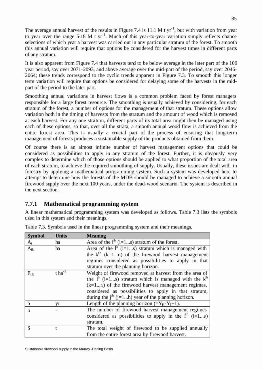
Sustainable firewood supply in the Murray -Darling Basin
85
The average annual harvest of the results in Figure 7.4 is 11.1 M t yr-1, but with variation from year to year over the range 5-18 M t yr-1. Much of this year-to-year variation simply reflects chance selections of which year a harvest was carried out in any particular stratum of the forest. To smooth this annual variation will require that options be considered for the harvest times in different parts of any stratum.
It is also apparent from Figure 7.4 that harvests tend to be below average in the later part of the 100 year period, say over 2071-2093, and above average over the mid-part of the period, say over 2046-2064; these trends correspond to the cyclic trends apparent in Figure 7.3. To smooth this longer term varia tion will require that options be considered for delaying some of the harvests in the mid-part of the period to the later part.
Smoothing annual variations in harvest flows is a common problem faced by forest managers responsible for a large forest resource. The smoothing is usually achieved by considering, for each stratum of the forest, a number of options for the management of that stratum. These options allow variation both in the timing of harvests from the stratum and the amount of wood which is removed at each harvest. For any one stratum, different parts of its total area might then be managed using each of these options, so that, over all the strata, a smooth annual wood flow is achieved from the entire forest area. This is usually a crucial part of the process of ensuring that long-term management of forests produces a sustainable supply of the products obtained from them.
Of course there is an almost infinite number of harvest management options that could be considered as possibilities to apply in any stratum of the forest. Further, it is obviously very complex to determine which of those options should be applied to what proportion of the total area of each stratum, to achieve the required smoothing of supply. Usually, these issues are dealt with in forestry by applying a mathematical programming system. Such a system was developed here to attempt to determine how the forests of the MDB should be managed to achieve a smooth annual firewood supply over the next 100 years, under the dead-wood scenario. The system is described in the next section.
7.7.1 Mathematical programming system A linear mathematical programming system was developed as follows. Table 7.3 lists the symbols used in this system and their meanings.
Table 7.3. Symbols used in the linear programming system and their meanings.
Symbol Units Meaning Ai ha Area of the ith (i=1...s) stratum of the forest. Aik ha Area of the ith (i=1...s) stratum which is managed with
the kth (k=1...ri) of the firewood harvest management regimes considered as possibilities to apply in that stratum over the planning horizon.
Fijk t ha-1 Weight of firewood removed at harvest from the area of the ith (i=1...s) stratum which is managed with the kth (k=1...ri) of the firewood harvest management regimes, considered as possibilities to apply in that stratum, during the jth (j=1...h) year of the planning horizon.
h yr Length of the planning horizon (=YH-YI+1). ri - The number of firewood harvest management regimes
considered as possibilities to apply in the ith (i=1...s) stratum.
S t The total weight of firewood to be supplied annually from the entire forest area by firewood harvest.
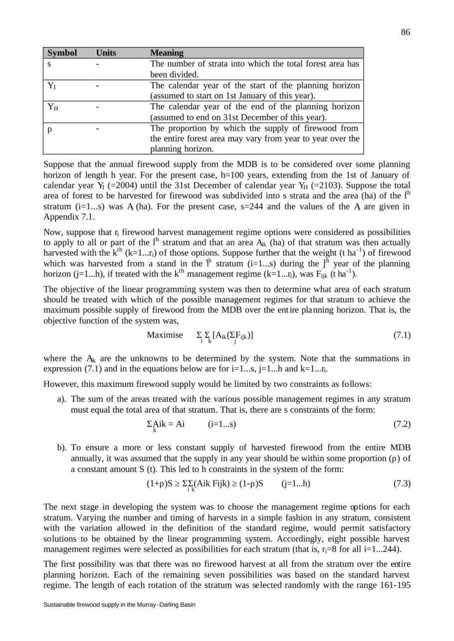
Sustainable firewood supply in the Murray -Darling Basin
86
Symbol Units Meaning s - The number of strata into which the total forest area has
been divided. YI - The calendar year of the start of the planning horizon
(assumed to start on 1st January of this year). YH - The calendar year of the end of the planning horizon
(assumed to end on 31st December of this year). ρ - The proportion by which the supply of firewood from
the entire forest area may vary from year to year over the planning horizon.
Suppose that the annual firewood supply from the MDB is to be considered over some planning horizon of length h year. For the present case, h=100 years, extending from the 1st of January of calendar year YI (=2004) until the 31st December of calendar year YH (=2103). Suppose the total area of forest to be harvested for firewood was subdivided into s strata and the area (ha) of the ith stratum (i=1...s) was Ai (ha). For the present case, s=244 and the values of the Ai are given in Appendix 7.1.
Now, suppose that ri firewood harvest management regime options were considered as possibilities to apply to all or part of the ith stratum and that an area Aik (ha) of that stratum was then actually harvested with the kth (k=1...ri) of those options. Suppose further that the weight (t ha-1) of firewood which was harvested from a stand in the ith stratum (i=1...s) during the jth year of the planning horizon (j=1...h), if treated with the kth management regime (k=1...ri), was Fijk (t ha-1).
The objective of the linear programming system was then to determine what area of each stratum should be treated with which of the possible management regimes for that stratum to achieve the maximum possible supply of firewood from the MDB over the ent ire planning horizon. That is, the objective function of the system was,
Maximise Σ Σ [Aik(ΣFijk)] (7.1) i k j
where the Aik are the unknowns to be determined by the system. Note that the summations in expression (7.1) and in the equations below are for i=1...s, j=1...h and k=1...ri.
However, this maximum firewood supply would be limited by two constraints as follows:
a). The sum of the areas treated with the various possible management regimes in any stratum must equal the total area of that stratum. That is, there are s constraints of the form:
ΣAik = Ai (i=1...s) (7.2) k
b). To ensure a more or less constant supply of harvested firewood from the entire MDB annually, it was assumed that the supply in any year should be within some proportion (ρ) of a constant amount S (t). This led to h constraints in the system of the form:
(1+ρ)S ≥ ΣΣ(Aik Fijk) ≥ (1-ρ)S (j=1...h) (7.3) i k
The next stage in developing the system was to choose the management regime options for each stratum. Varying the number and timing of harvests in a simple fashion in any stratum, consistent with the variation allowed in the definition of the standard regime, would permit satisfactory solutions to be obtained by the linear programming system. Accordingly, eight possible harvest management regimes were selected as possibilities for each stratum (that is, ri=8 for all i=1...244).
The first possibility was that there was no firewood harvest at all from the stratum over the entire planning horizon. Each of the remaining seven possibilities was based on the standard harvest regime. The length of each rotation of the stratum was selected randomly with the range 161-195
Sustainable firewood supply in the Murray -Darling Basin
87
years of age. The age at which the first harvest was done in each rotation was chosen randomly from within the range 20-25 years of age. The number of harvests to be done in each rotation was then chosen randomly within the range 20-40, with no harvest being allowed to occur after 178 years of age if the rotation lasted that long. The harvests were then spaced approximately equally over the chosen harvest period. However, the exact timing of any harvest was chosen randomly within ±1 year of the time of exactly equal spacing of harvests, subject only to delaying any harvest until at least 1.5 t ha-1 of firewood was available from it.
Firewood harvest yields for any of those regimes in any stratum (the Fijk in the linear programming system) were then estimated using the growth and yield model (Section 6). Many more than eight options could have been used in any stratum. The more options available, the more likely it is that the linear programming system will be able to solve the system successfully and determine the maximum possible supply of firewood available from the MDB. However, as more options are considered, the larger becomes the problem to be solved, until the limits of computer resources are reached, in terms of both the amount of memory required and the computation time. For this project, the choice of eight regime options was found to lead to what appeared to be reasonable solutions to the system, with reasonable computing effort. This is not to say that better solutions than those achieved here could not be obtained by enlarging the number of management options available for each stratum.
Solutions to the linear programming system were obtained using the simplex method, as implemented in the MINOS suite of computer programs for solving large, complex mathematical programming problems (Murtagh and Saunders 1978, 1983).
7.7.2 Sustainable firewood supply The linear programming system was applied with a number of different values of S (the annual yield of firewood from the entire MDB) and ρ (the proportion about S by which the yield in any year was permitted to vary). If S is too large, then the MDB may not contain sufficient forest area to yield that amount of wood annually and no solution will exist to the linear programming problem. If ρ is too small, then the linear programming system may be unable to find a solution to achieve that degree of smoothing of the annual supply.
After many runs of the system, it was found that with ρ=0.1 (that is the annual supply did not differ by more than ±10% in any year), a solution to the linear programming system could be obtained only when S was no larger than 9.9 M t yr-1. The annual supply of firewood from the MDB, with this solution, is shown in Figure 7.5. Those results may be compared directly with those of Figure 7.4, where no smoothing of the annual supply was attempted.

Sustainable firewood supply in the Murray -Darling Basin
88
0
5
10
15
20
2000 2020 2040 2060 2080 2100Year
Fir
ewo
od
har
vest
(M
t)
Figure 7.5. Estimates of the maximum amounts of firewood which could be
harvested from woody debris, annually over 2004-2103, of the 12.3 M ha of the MDB deemed suitable for firewood harvesting under the dead-wood scenario. The graph shows the results where the annual firewood supply from the MDB was kept more or less constant from year to year. The two horizontal dashed lines indicate the range of the estimated amount of firewood currently harvested from the MDB. The solid horizontal line is the average of all the annual estimates of yield.
The average annual supply for the results in Figure 7.5 was 10.0 M t yr-1. The smoothing constraints included in the linear programming system ensured that the annual amount never varied outside the range 8.9-10.9 M t yr-1. There is little point in showing here the extremely lengthy details of the solution to the linear programming problem (i.e. the detail of exactly how much of the area of each of the 244 strata should be treated with exactly which harvest management regime). However, the solution found that none of the entire 12.3 M ha would be unharvested and 5.3 M ha would have been part of strata in which more than one of the possible management regimes would need to have been applied to achieve the smoothing of the annual yield. It is of interest also to compare the proportions of the firewood supply derived from forests of different productive capacity classes. Of the annual average of 10.0 M t yr-1, about 1.8, 2.4, 2.6 and 3.2 M t yr-1 were obtained from forest of productivity classes 1-4, respectively.
7.7.3 Residual woody debris Figure 7.6 shows estimates of the unit area amounts of woody debris remaining in the forest, annually over 2004-2103, with the firewood harvesting done to obtain the solution to the linear programming system. Also shown are the results if firewood ha rvesting was done using the standard harvest regime, without smoothing of the annual supply of firewood; these latter results are those for the first 100 years shown in Figure 7.3.

Sustainable firewood supply in the Murray -Darling Basin
89
0
1
2
3
4
5
6
2000 2020 2040 2060 2080 2100Year
Woo
dy d
ebri
s (t
ha
-1)
Figure 7.6. Estimates of the amounts of woody debris remaining in the forest,
annually over 2004-2103, averaged over the 12.3 M ha of the MDB considered for firewood harvesting under the dead-wood scenario. The graph shows the results where the annual firewood supply from the MDB was kept more or less constant from year to (_______) and where firewood was harvested using the standard harvest regime without any smoothing of the annual supply (- - - -).
The average residual woody debris over the 100 years in the data of Figure 7.6 is 3.0 t ha-1 (varying from year to year in the range 2.5-3.7 t ha-1) with smoothing of the annual supply and 4.5 t ha-1 (varying in the range 3.9-5.2 t ha-1) without smoothing. These results suggest that the more regular harvesting involved with the smoothed supply allows less accumulation, on average, of woody debris between harvests. These averages are both far less than the corresponding average of 20 t ha-1 (varying in the range 16-23 t ha-1) for unharvested stands, over the first 100 years of the data shown in Figure 7.3.
7.8 Discussion and conclusions The purpose of the dead-wood scenario was to estimate the maximum, long-term sustainable supply of firewood available from the privately owned, native forests of the MDB. We wished to examine the long-term feasibility of a continued reliance on coarse woody debris as the sole source of firewood to meet the current demand of 2-2.5 M t yr-1 from the MDB. We estimated that the long term supply from coarse woody debris (10 M t yr-1) of far exceeds current demand. However, our model also indicates that harvesting coarse woody debris greatly depletes this important component of forest and woodland ecosystems. If the maximum 10 M t yr-1 of firewood was harvested, we estimated that the long-term average amount of woody debris remaining in forests after firewood harvesting would be 3 t ha-1, far less than the average 20 t ha-1 that would remain if there was no firewood harvesting.
The ecological implications of depleting levels of coarse woody debris are discussed in detail in Section 9. Our model system (Section 6) provides, for the first time, the capability to estimate maximum levels of coarse woody debris expected in the absence of harvesting of any broad vegetation type with any given net productivity potential within the MDB. Estimating potential levels of coarse woody debris is a critical first step in assessing the ecological impacts of harvesting this important component of any forest or woodland.
Because the maximum sustainable supply estimated by our model system is much greater than current demand, it is unnecessary to use the entire 12.3 M ha of forest within 500 km of capital

Sustainable firewood supply in the Murray -Darling Basin
90
cities to obtain the present supply sourced from the MDB. In fact, it was found that the current demand of 2.5 M t yr-1 could be obtained by harvesting only the 3.1 M ha of the most productive forests in the MDB (as defined in Table 7.1 and shown in Figure 7.2). There is clearly potential to exclude large areas of the MDB from harvesting of coarse woody debris while still meeting current demand. Conversely, rather less than all the firewood available at any one harvest could be removed in order to provide the present firewood supply. The policy implications of this dead-wood scenario modelling are discussed further in Section 11.

Sustainable firewood supply in the Murray -Darling Basin
91
8 The green-wood scenario P.W. West
8.1 Summary In this section, an estimate is made of the maximum, long-term sustainable supply of firewood which might be obtained from the privately owned, native forests of the MDB under a “green-wood scenario”, that is, when firewood is obtained only by felling live trees and no woody debris is collected as firewood. It was estimated that there are 9.8 million (M) hectares (ha) (1.1 M ha mallee and 8.2 M ha non-mallee) of forest in the MDB suitable for harvesting under this scenario. Appropriate firewood harvest management regimes were developed for this scenario. For mallee forests, this involved clear- fell harvesting on a 50 year rotation, with regeneration by coppice. For non-mallee, it involved “flexible selection” management, with 2 or 3 thinnings over the life-time of a stand and with 50% of the standing tree basal area being removed at each thinning; such management should encourage maintenance of forest stands which contain a wide range of tree sizes and/or ages, consistent with contemporary community attitudes to native forest management. Over the next 100 years, it was estimated that the maximum, annual, sustainable supply of firewood from the MDB under the green-wood scenario would average 2.3 M oven-dry tonnes per year (t yr-1), with a deviation in any year from this amount of no more than 0.2 M t yr-1. About 22% of this supply would come from mallee forests and the remainder from non-mallee. This level of supply is about the same as the amount of firewood harvested presently from the MDB, which is believed to be within the range 2-2.5 M t yr-1. Because the green-wood scenario does not involve removal of woody debris from the forest, it was considered that this approach to firewood harvest management in the MDB may have benefits for the biodiversity conservation and maintenance of landscape function of the region.
8.2 Introduction
Section 7 considered the sustainable firewood supply from the privately owned native forests of the MDB when firewood was collected only from coarse woody debris, a management strategy termed the “dead-wood” scenario.
This section concerns the supply that would be available under a second management strategy, the “green-wood” scenario. This would involve felling live trees to produce firewood and excludes collection of firewood from woody debris. A principle advantage of such a scenario is that the retention of woody debris in the forest ecosystems of the Basin may have important consequences for the maintenance of its overall biodiversity.
The general approach taken in this section to determine the sustainable firewood supply under the green-wood scenario was the same as that used for the dead-wood scenario (Section 7).
8.3 Forest area and stratification The data for the scenario were derived using the GIS system described in Section 4. Full details of the information available to this project on the area of privately owned native forests in the MDB and their stratification by the relevant exploitation criteria (Section 3.1) are described in Sections 4.3.1 and 4.3.2. The exploitation criteria which apply to the dead-wood scenario also apply to the green-wood scenario, and are described in Section 3.2.
The additional exploitation criteria necessary to derive a final stratification of the forest suitable to apply for the green-wood scenario are described in Section 3.3 and their application to the data to

Sustainable firewood supply in the Murray -Darling Basin
92
derive the final stratification are described in Sections 4.3.5 and 4.3.6. These considerations are summarised below.
As will be discussed later in the section on management regimes, the green-wood scenario applies both to mallee and non-mallee forest of the MDB, for which different growth and yield models were developed in Section 6. Hence, the first step in forest stratification for the green-wood scenario was to separate mallee and non-mallee forests.
Secondly, the green-wood scenario excluded forests inside riparian zones (exploitation criterion 6) and land which sloped 15o or more (exploitation criterion 7). In addition, regions where the landscape was assessed with a percent woody cover < 30% (exploitation criterion 8) and any remnant < 100 hectares in size (exploitation criterion 9) were excluded. Using the GIS system described in Section 4, there were found to be 9.8 M ha of forest suitable for the green-wood scenario; 1.1 M ha of mallee forest and 8.7 M ha of non-mallee (Table 8.1). (Sections 4.3.5 and 4.3.6, Table 4.11 and Table 8.1).
Thirdly, the 9.8 M ha of forest were stratified by site productive capacity, as defined by the net primary productivity (NPP) index of Barrett (2002) (expressed as tonnes of plant biomass ha-1 yr-1)4. This index has been described and discussed in detail in Section 6 and Appendix 5. The stratification method is described in Section 4.3.3 and the complete stratified dataset is presented in Appendix 6, Table 9. Figure 8.1 shows the distribution of both the mallee and non-mallee forests in relation to site productive capacity. For non-mallee forest, the distribution is similar in form to that shown in Figure 7.1 for the dead-wood scenario. Virtually all the mallee forest is located in areas of low productive capacity; 95% of its total area has an net primary productivity index below 2 t ha-1 yr-1.
0.0
0.2
0.4
0.6
0.8
1.0
0 2 4 6 8 10 12 14
NPP index (t ha -1 yr-1)
Are
a (M
ha)
Figure 8.1. Distribution of the 9.8 M ha of forest eligible for use in the green-
wood scenario in relation to site productive capacity (NPP index). The area has been divided into mallee (- - - -) and non-mallee (______) forest. The vertical solid lines delimit the ranges of the four productivity classes (see later) identified for use in applying the green-wood scenario to non-mallee forest and the vertical dashed lines show the weighted average productivities of those classes (Table 8.1).
4 Note that all weights of firewood, coarse woody debris and plant biomass referred to in this section are oven-dry weights.

Sustainable firewood supply in the Murray -Darling Basin
93
As for the dead-wood scenario (Section 7.4), the 8.7 M ha of non-mallee forests were split into four classes of site productive capacity of roughly equal forest area and their weighted average productive capacities determined. The results are shown in Table 8.1 and on Figure 8.1.
Table 8.1. For forest eligible fo r the green-wood scenario, the site productive capacity classes (based on net primary productivity index) defined here for non-mallee forest are shown, together with their areas and their weighted ave rage productive capacities. Results are shown also for mallee forest.
Productivity Class NPP index class
(t ha-1 yr-1) Area
(M ha) Weighted average NPP index
(t ha-1 yr-1) Mallee forest
- 0.4-11.2 1.07 1.2 Non-mallee forest
1 0.2 - 3.2 2.95 1.9 2 3.2 - 4.0 3.12 3.4 3 4.0 - 6.6 3.09 4.9 4 6.6 - 14.0 3.12 8.3
The last step in the stratification for the green-wood scenario was to consider its age-class distribution (age being determined as the time elapsed since the forest regenerated from bare ground). This was done in exactly the same way as described for the dead-wood scenario (Section 7.4), i.e. it was assumed that, in 2004, 40% of forests would be aged 50-60 yr, 50% would be 100-120 years and 10% would be 150-178 years. To what extent this age-class distribution applies to mallee forests is difficult to say. Past harvesting of those forests for firewood will undoubtedly have altered the distribution. However, no other information was available to this project to allow better age stratification of mallee forests.
This stratification process led to subdivision of the 9.8 M ha of forest deemed appropriate for harvest under the green-wood scenario into a total of 305 strata. Appendix 11 lists the areas of each of those strata. Map 27 (Appendix 4) shows the distribution of the forests of the MDB deemed suitable for firewood harvest under the green-wood scenario. The non-mallee forest has been stratified by site productive capacity class as defined in Table 8.1.
8.4 Management regimes
8.4.1 Mallee forest Mallee eucalypt forests have been exploited for firewood production for many years, particularly in South Australia. Sometimes “mallee roots” (the lignotuberous mass at the base of the trees from which coppice arises) have been harvested and sometimes live stems have been harvested.
Neagle (1994) reviewed the silvicultural management practices which have been found to be most appropriate for mallee harvesting in South Australia. He concluded that long term maintenance of the mallee forest ecosystem was best served by a clear-felling harvest of live trees at 50 year intervals, followed by coppice regeneration, which occurs reliably and is generally prolific in these forests, generally leading to production of even-aged regrowth stands.
For the present Section, this was the only silvicultural management system which was considered for the green-wood scenario for mallee forest. It was assumed that all mallee forests were of the same productive capacity. Firewood yields under this system may be predicted using model (6.23) as described in Section 6. The model predicts that a mallee forest yields 23 t ha-1 of firewood if clear- felled at 50 years of age.
Sustainable firewood supply in the Murray -Darling Basin
94
In the age-stratification of mallee eucalypt forests, it was assumed that they are presently all aged 50 years or older. Given this, when firewood yields from mallee forests were estimated in later parts of this section, it was assumed that any one mallee stratum (Appendix 11) would be clear- felled for firewood at a year chosen at random over the next 50 years. This would be the end of the first “rotation” of that stratum. Thereafter, it was assumed that any stratum would be cleared felled in its second and subsequent rotations at intervals chosen randomly in the range 40-60 years. This is termed the “standard” management regime for mallee forests.
8.4.2 Non-mallee forests Non-mallee forests within the MDB have been little used for commercial forestry in the past. Because of this, limited research has been done to identify the silvicultural practices appropriate to ensure either that regeneration after live tree harvesting is adequate or that harvest practices are appropriate to maintain the continued health and biodiversity of the forests. Whilst some work of this nature has been done with the species in the MDB which have been exploited commercially (Callitris glaucophylla, Eucalyptus delegatensis and Eucalyptus camaldulensis), few published reports of this work are available. In his substantial review of the silvicultural practices appropriate for the native eucalypt forests of Australia, Florence (1996) emphasises that most information presently available is based on experience with the more productive native forests of the coastal regions of Australia, not with the woodland forests of the MDB.
The paucity of information means that it is impossible to select specific silvicultural management regimes appropriate to apply to the non-mallee forests of the MDB in the green-wood scenario. Further, given the range of non-mallee forest types which occur in the MDB, it is not to be expected that any single management regime will be appropriate for all of them. Given this, it was felt impossible in the present project to do anything other than establish some basic principles for silvicultural management of the non-mallee forests of the MDB and assume those principles should apply to all of them. Accordingly, it was decided that the following principles should be adhered to in considering silvicultural management of these forests:
a) Silvicultural practice should encourage maintenance of forest stands which contain a wide range of tree sizes and/or ages: in consequence of contemporary community attitudes to forestry practice, clear- felling was considered an inappropriate silvicultural practice, whether or not it is the most appropriate technique to ensure adequate regeneration in any particular forest type. This means that harvest of wood for firewood in the green-wood scenario should involve some form of thinning practice;
b) Any thinning should aim to retain trees of good bole form and with canopy condition which would allow them to respond to the thinning with an acceleration in stem diameter growth rate. Although it is not within the ambit of this project to consider the use of forests of the MDB for wood products other than firewood, it was assumed that silvicultural practices which may lead eventually to production of higher value wood products might have long-term economic advantage;
c) Silvicultural practice should encourage the retention of larger trees (say >60 cm diameter at breast height over bark), since it is these which provide hollows important as faunal habitat, or may grow to a size such that they would do so in the medium term; and
d) Trees to be thinned for firewood should be 15 cm or more in diameter at breast height over bark. Trees smaller than this are unlikely to yield sufficient quantities of firewood to make their felling worthwhile (Wall 1997). This constraint will limit the timing and frequency of thinnings possible from any stand.
Given these principles, it seemed most appropriate that non-mallee forests of the MDB should be managed for the green-wood scenario using a “flexible selection” system of silvicultural

Sustainable firewood supply in the Murray -Darling Basin
95
management (see Florence 1996, p 229). This would maintain, or allow, the development of uneven-aged stands within the forests with a wide range of tree sizes and ages. It would be consistent with a management regime which has the multiple objectives of (a) supplying firewood, (b) encouraging development of trees which might ultimately yield logs of high quality suitable for solid wood products, (c) provision of a diverse habitat to encourage maintenance of biodiversity, and (d) maintaining a permanent forest cover, consistent with community attitudes to native forest management.
In a “flexible selection” regime, the trees selected for harvest at thinning would have diameters at breast height over bark in the range 15-60 cm. Trees with larger stems (>60 cm diameter), which have the potential in the medium term to provide suitable hollows as faunal habitats, would be retained (Gibbons and Lindenmayer 2002). Amongst trees with diameters of 15-60 cm, those with stems suitable for development to logs of high qua lity and with crowns in a condition appropriate to develop vigorously following thinning would be retained; the thinning would be done to provide those trees with sufficient space to encourage their crown development. The timing, intensity and frequency of these thinnings in any stand will be discussed further below. Regeneration in these stands would be expected to be either as coppice or as seedlings from natural seed shed, depending on the biology of any particular forest type.
The biology of some of the forests of the MDB may be such that seedling regeneration will occur adequately only in gaps within the forest. In these cases, it may be necessary to apply a “group selection” silvicultural management regime rather than a “flexible selection” regime. This would involve clear- felling of gaps (perhaps with radii of about 25 m) within the forest to create a matrix of open spaces within which seedlings could develop. Such a regime would not encourage the development of trees to produce high quality logs, although it could be accompanied by selective thinning between the gaps to do so. Insufficient is known at present of the silvicultural requirements of the individual forest types of the MDB to be able to say specifically which types should be managed with either “flexible selection” or with “group selection” under the green-wood scenario. For the remainder of the present Section, only “flexible selection” will be considered.
Insufficient is known of the growth dynamics of forests of the MDB to prescribe with any certainty what ages, intensities and frequencies of “flexible selection” thinning would be most appropriate in these forests. Experience of one forester familiar with them (A. Deane, State Forests NSW, pers. comm.) indicates that the management objectives and silvicultural principles considered here might be appropriate for stands aged in the range 30-120 years, on sites of higher productive capacity. However, no more than three thinnings within this age range would be appropriate. Stands of lower productive capacity might be in appropriate condition when aged 50-150 yr, but no more than one or two thinnings would be feasible. Further, to achieve a worthwhile response in stem diameter growth rate of retained trees, thinning should involve a very substantial opening of the stand with large gaps between the retained trees to allow their future crown expansion.
The next issue was the level of thinning intensity to be applied. Some published work supports the contention that a relatively intensive thinning practice can be appropriate in slow growing Australian native forests. Horne (1990) described experimental work in Callitris glaucophylla forests in the MDB. Twenty six years after thinning 7-year-old dense regeneration (>50,000 stems ha-1) to stocking dens ities as low as 416 stems ha-1, the stand basal areas of the unthinned and thinned stands were generally similar, whilst the average diameter at breast height over bark of the unthinned trees was 4.3 cm and of the thinned trees was 18.1 cm (Horne 1990, Table 2). The heaviest thinning caused some loss of production (less heavily thinned stands had higher basal areas than the most heavily thinned stand), presumably because full occupancy of the site was lost for some years following the thinning (i.e. too few trees remained on the site following the heaviest thinning to use fully the resources which limit tree growth, principally water in these forests). In 2003, when the trees were 46 years old, the authors of this report inspected the thinning experiment.

Sustainable firewood supply in the Murray -Darling Basin
96
The most heavily thinned stands contained well developed and healthy trees, whilst the unthinned controls contained very small trees and substantial mortality was occurring amongst them.
Abbott and Loneragan (1983) examined the growth response to thinning (their experiment D) of 40-year old Eucalyptus marginata, a species which grows in medium-open forests in southwest Western Australia. By observing growth over the succeeding 15 years, they found that removal of 75% of the basal area of the stand at thinning was sufficient to cause some loss of production, presumably due to loss of full site occupancy following thinning. There was no loss of production in stands thinned by removal of 55% of the stand basal area. There was a progressively increased acceleration of stem diameter growth rates as thinning intensity was increased.
Florence (1996, p210-3) describes response to thinning in an east coast, mixed species eucalypt forest of rather higher productivity than forests of the MDB. Of unknown age, but certainly older than 50 years, the stand was very heavily thinned to retain only 25 stems ha-1. Over the next 22 years, the residual stems showed rapid diameter growth and there was vigorous regeneration between the retained trees.
Ellis et al. (1987) studied the response to thinning in multi-aged Eucalyptus delegatensis forests of Tasmania, which had regenerated more than 250 years earlier. These forests are slower growing, more because of cooler temperatures at the higher altitudes at which the species grows than because of low rainfall as in the MDB. Ellis et al. concluded that as much as 87% of the stand basal area would have to be removed from these stands before there was loss of full site occupancy. Thinning was accompanied by a progressively increasing acceleration of stem diameter growth rate as the intensity of thinning increased.
These various results suggest that removal of 50% of the basal area over bark of 30-150 year old stands in the MDB should result in worthwhile acceleration of the stem diameter growth rates of the retained trees. At the same time, this intensity of thinning should not be so great that full occupancy of the site is lost, with a consequent loss of overall production on the site. In the absence of any other information, this thinning intensity was chosen in this section for “flexible selection” silvicultural management in the green-wood scenario.
Given these considerations, Table 8.2 shows thinning regimes which were selected for non-mallee stands for the different productive capacity classes. Hereafter, these are termed the “standard” management regimes for non-mallee forests of the MDB.
Table 8.2. The maximum number of thinnings and the thinning ages which might be appropriate for stands of the non-mallee native forests of the MDB for different site productive capacity classes (Table 8.1). All thinnings would involve removal of 50% of the basal area of the stand at the time of thinning. These are termed the “standard” management regimes for non-mallee forests of the MDB.
Productivity class
Maximum number of thinnings
Age range within which first thinning done (yr)
Delay to each subsequent Thinning (yr)
1 2 50-60 30-60 2 2 50-60 30-60 3 3 30-40 40-45 4 3 30-40 40-45
Table 8.3 shows predictions from the growth and yield model (Section 6) of the firewood yields that might be expected from typical examples of these standard management regimes.

Sustainable firewood supply in the Murray -Darling Basin
97
Table 8.3. For each of the four productivity classes considered in the green-wood scenario for non-mallee forests of the MDB, predictions from the growth and yield model of the amounts of firewood which could be harvested (t ha-1) at various ages (yr) from typical examples of the standard management regimes.
Productivity class 1 2 3 4
Age Firewood Age Firewood Age Firewood Age Firewood 55 11 55 16 35 13 35 21 100 15 100 19 87 20 87 24
129 19 129 22 Total 26 35 52 67
8.5 Sustainable firewood supply over the next 100 years The prediction of the long-term sustainable supply of firewood available from the MDB under the green-wood scenario was done in a similar fashion to that described for the dead-wood scenario (Section 7). The prediction of firewood supply was confined only to the next 100 years, a period considered relevant to long-term industry planning.
8.5.1 Firewood supply with standard management regimes Figure 8.2 shows estimates of the annual harvest of firewood over the period 2004-2103, from the 9.8 M ha of forests deemed appropriate for the harvesting under the green-wood scenario. The results were determined using the standard management regimes, described above, for mallee and non-mallee forests. No attempt was made to smooth the annual supply to a more or less constant amount from year to year.
0
5
10
15
2000 2020 2040 2060 2080 2100Year
Fir
ewo
od
har
vest
(M
t)
Figure 8.2 Estimates of the amounts of firewood which could be harvested
in the green-wood scenario, annually over 2004-2103, of the 9.8 M ha of forest deemed appropriate for that scenario. The results assumed the entire area was harvested using the standard management regimes for mallee and non-mallee forests. The solid horizontal line is the average of all the annual estimates. The two horizontal dashed lines indicate the range of the estimated amount of firewood currently harvested from the MDB.
Figure 8.2 suggests that the annual supply of firewood available during 2004-2014 would be far greater than in later years. This reflects the fact that thinning of non-mallee forest for firewood has not been a common practice in the past. Therefore, when applying the standard management
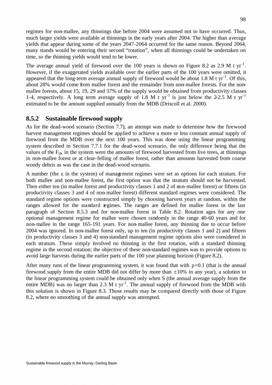
Sustainable firewood supply in the Murray -Darling Basin
98
regimes for non-mallee, any thinnings due before 2004 were assumed not to have occurred. Thus, much larger yields were available at thinnings in the early years after 2004. The higher than average yields that appear during some of the years 2047-2064 occurred for the same reason. Beyond 2064, many stands would be entering their second “rotation”, when all thinnings could be undertaken on time, so the thinning yields would tend to be lower.
The average annual yield of firewood over the 100 years is shown on Figure 8.2 as 2.9 M t yr-1. However, if the exaggerated yields available over the earlier parts of the 100 years were omitted, it appeared that the long-term average annual supply of firewood would be about 1.8 M t yr-1. Of this, about 28% would come from mallee forest and the remainder from non-mallee forests. For the non-mallee forests, about 15, 19, 29 and 37% of the supply would be obtained from productivity classes 1-4, respectively. A long term average supply of 1.8 M t yr-1 is just below the 2-2.5 M t yr-1 estimated to be the amount supplied annually from the MDB (Driscoll et al. 2000).
8.5.2 Sustainable firewood supply As for the dead-wood scenario (Section 7.7), an attempt was made to determine how the firewood harvest management regimes should be applied to achieve a more or less constant annual supply of firewood from the MDB over the next 100 years. This was done using the linear programming system described in Section 7.7.1 for the dead-wood scenario, the only difference being that the values of the Fijk in the system were the amounts of firewood harvested from live trees, at thinnings in non-mallee forest or at clear- felling of mallee forest, rather than amounts harvested from coarse woody debris as was the case in the dead-wood scenario.
A number (the ri in the system) of management regimes were set as options for each stratum. For both mallee and non-mallee forest, the first option was that the stratum should not be harvested. Then either ten (in mallee forest and productivity classes 1 and 2 of non-mallee forest) or fifteen (in productivity classes 3 and 4 of non-mallee forest) different standard regimes were considered. The standard regime options were constructed simply by choosing harvest years at random, within the ranges allowed for the standard regimes. The ranges are defined for mallee forest in the last paragraph of Section 8.5.3 and for non-mallee forest in Table 8.2. Rotation ages for any one optional management regime for mallee were chosen randomly in the range 40-60 years and for non-mallee in the range 165-191 years. For non-mallee forest, any thinning due to occur before 2004 was ignored. In non-mallee forest only, up to ten (in productivity classes 1 and 2) and fifteen (in productivity classes 3 and 4) non-standard management regime options also were considered in each stratum. These simply involved no thinning in the first rotation, with a standard thinning regime in the second rotation; the objective of these non-standard regimes was to provide options to avoid large harvests during the earlier parts of the 100 year planning horizon (Figure 8.2).
After many runs of the linear programming system, it was found that with ρ=0.1 (that is the annual firewood supply from the entire MDB did not differ by more than ±10% in any year), a solution to the linear programming system could be obtained only when S (the annual average supply from the entire MDB) was no larger than 2.3 M t yr-1. The annual supply of firewood from the MDB with this solution is shown in Figure 8.3. Those results may be compared directly with those of Figure 8.2, where no smoothing of the annual supply was attempted.

Sustainable firewood supply in the Murray -Darling Basin
99
0
1
2
3
4
2000 2020 2040 2060 2080 2100Year
Fir
ewo
od
har
vest
(M
t)
Figure 8.3. Estimates of the maximum amounts of firewood which could be
harvested annually over 2004-2103, under the green-wood scenario. The results are for the 9.8 M ha of mallee and non-mallee forests of the MDB deemed appropriate for firewood harvesting under that scenario. The graph shows the results where the annual firewood supply from the MDB was kept more or less constant from year to year. The solid horizontal line is the average of all the annual estimates. The two horizontal dashed lines indicate the range of the estimated amount of firewood currently harvested from the MDB.
The average annual supply for the results shown in Figure 8.3 was 2.3 M t yr-1. The smoothing constraints in the linear programming system ensured that the annual amount never varied outside the range 2.1-2.5 M t yr-1. Of the total annual supply, on average 0.5 M t yr-1 (22%) came from mallee forest and 1.8 M t yr-1 (77%) from non-mallee forest. Of the non-mallee forest supply, 20, 31, 32 and 18% was obtained on average from forest of productivity classes 1-4, respectively.
As with the equivalent results from the dead-wood scenario (Section 7), there is little point in showing here the extremely lengthy details of this solution to the linear programming problem (i.e. the fine detail of exactly how much of the area of each of the 305 strata should be treated with exactly which harvest management regime). However, the results showed that the non-standard regimes would need to be applied in 2.1 M ha (24%) of the non-mallee forest, i.e. that there would be no thinning in the first rotation of that area of those forests to avoid the excessive yields which would otherwise be available because of the lack of thinning in the past (Figure 8.2).
8.5.3 Residual woody debris Figure 8.4 shows the estimates of the unit area amounts of coarse woody debris remaining in the non-mallee forest, annually over 2004-2103, with the firewood harvesting done to obtain the solution to the linear programming system. These results are averaged over the entire 8.7 M ha of the non-mallee forest. Of course no woody debris is removed as firewood in the green-wood scenario. It was assumed that mallee forest has negligible amounts of coarse woody debris of importance for maintenance of biodiversity and landscape function. The cyclic trend apparent in the figure is a consequence of the assumed age-class distribution of forest; the results may be compared with those for unharvested forest in Figure 7.2 for the dead-wood scenario.
Also shown on Figure 8.4 are the amounts of residual coarse woody debris remaining in non-mallee forests harvested to produce a smooth annual supply under the dead-wood scenario, shown in

Sustainable firewood supply in the Murray -Darling Basin
100
Figure 7.6. These results emphasise the extent to which the green-wood scenario ensures the maintenance of coarse woody debris in these forests.
0
5
10
15
20
25
2000 2020 2040 2060 2080 2100Year
Woo
dy d
ebri
s ( (
t ha-
1)
Figure 8.4. Estimates of the unit area amounts of woody debris remaining in
the forest annually over 2004-2103, averaged over the 8.7 M ha of non-mallee forests of the MDB deemed appropriate for firewood harvesting under the green-wood scenario. The solid line shows the results for the green-wood scenario where the annual firewood supply from the MDB was kept more or less constant from year to year. The dashed line shows the (smoothed) results for the dead-wood scenario from Figure 7.6, for the corresponding time period, averaged over the 12.3 M ha of non-mallee forests.
8.6 Discussion It is of interest that the results showed that the annual sustainable yield of firewood from the 8.7 M ha of non-mallee forest would average 0.20 t ha-1 yr-1, whilst that from the 1.1 M ha of mallee forest would be much greater, 0.47 t ha-1 yr-1. This difference occurs despite the fact that mallee forests grow on sites with far lower productive capacity than the non-mallee forests (weighted average productive capacity, as assessed by net primary productivity index, for the 1.1 M ha of mallee forest area was only 1.2 t ha-1 yr-1, whilst that for the 8.7 M ha of non-mallee forest was 4.2 t ha-1 yr-1). The higher yield per unit area from the mallee forests is a consequence of the different management systems used for the two forest types. It was assumed that all the production of mallee forests would be harvested by clear- felling on an average 50 year rotation; the growth and yield model predicted that this will provide a harvest of 23 t ha-1 of firewood every 50 years. By contrast, it was assumed that firewood yields from non-mallee forests were obtained only from thinnings of forests which grow on an average rotation of 178 years. The yields shown for thinning harvests (Table 8.3) will make it clear that the unit area amount of firewood available from mallee forests over any 178 year period is greater than that available from even the highest productivity class of non-mallee forest.
It is unlikely that the maximum annual supply of firewood available from the MDB under the green-wood scenario would ever be achieved in practice. The reasons are similar to those discussed for the dead-wood scenario (Section 7.9). Not all owners of forest will wish that it be used for firewood harvest, it would be impossible to insist that each and every forest property be managed with the particular harvest management regime that is necessary to achieve the maximum yield, supply would be determined on a regional basis rather than over the MDB as a whole and some species are preferred for firewood over others (Driscoll et al. 2000).

Sustainable firewood supply in the Murray -Darling Basin
101
It is of interest that the maximum sustainable yield of firewood estimated under the dead-wood scenario (10 M t yr-1) was far greater than for that under the green-wood scenario (2.3 M t yr-1). Whilst the area available for harvest under the dead-wood scenario (12.3 M ha) was greater than that for the green-wood scenario (9.8 M ha), the greater total yield under the dead-wood scenario is due principally to the much greater unit area yields available from the non-mallee forest under the dead-wood (0.82 t ha-1 yr-1) than the green-wood (0.20 t ha-1 yr-1) scenario. In turn, this reflects largely the harvest management regimes used for the two scenarios. The harvest management regime for the dead-wood scenario involved removal of a very large proportion of the coarse woody debris produced over the lifetime of any stand. Harvests under the green-wood scenario involved only thinning of stands and no clear-felling and hence, removal of only part of the total live tree production over the life-time of a stand.
An advantage of the green- over the dead-wood scenario is the retention of coarse woody debris for maintenance of biodiversity and landscape function. Figure 8.4 provides a comparison of the results of the green-wood scenario and the dead-wood scenario (Figure 7.6). The comparison shows that, from time to time over the next 100 years, 4-8 times as much coarse woody debris would remain in the non-mallee forests of the MDB under the green-wood scenario than under the dead-wood scenario. The amount would vary from time to time under both scenarios in consequence of the existing age-class distribution of the forests of the MDB. The impact of substantially increasing the amount of coarse woody debris is discussed in more detail in the section on the ecological impacts of the green-wood scenario (Section 9).
Comparison of Figure 7.4 (dead-wood scenario) and Figure 8.2 (green-wood scenario) suggests that, in the short-term of perhaps the next 14 years, much greater yields of firewood might be available under the green-wood scenario than the dead-wood. This extra yield would be available because thinning of non-mallee forests has not been normally carried out in the past; in effect, there is a “back- log” of possible thinnings. It would be quite possible to devise a system to allow this additional supply to be made available for a short period and that the supply should then decline over subsequent years to a long-term, sustainable, more or less constant annual supply. This could be important if the firewood industry of the MDB is to be rationalised to reduce eventually the overall supply being obtained from native forests from the MDB; allowing the annual harvest to decline gradually is likely to lead to less social disruption than if it is reduced suddenly to much lower levels. Further management and policy implications of all scenarios are discussed in the concluding section of this report (Section 11).

Sustainable firewood supply in the Murray -Darling Basin
102
9 Case studies on the potential ecological impacts of firewood harvesting
J.M. Stol, D.O. Freudenberger, A. Drew and E.M. Cawsey
9.1 Introduction With regard to firewood harvesting, the term “sustainable” applies not only to economic sustainability, but also to ecological sustainability. The focus on ecological sustainability has come from four main areas: i) The objectives of this project i.e. to develop regional exploitation criteria for sustainable
harvesting of firewood from woodland and forest communities in the Murray-Darling Basin (MDB); see Section 2.2.
ii) The vision statement for the ANZECC National Approach to Firewood Collection and Use in Australia (ANZECC 2001) (NAFCU), which states: firewood collection and use across Australia is managed on an ecologically sustainable basis and in a manner that does not threaten the conservation of flora and fauna of forest and woodland ecosystems…
iii) The first and second objectives of the NAFCU (ANZECC 2001), which are 1. to protect remnant native vegetation, threatened ecosystems and habitat for threatened and declining wildlife species and 2. to encourage ecologically sustainable firewood collection from native forests…
iv) The NAFCU Action Plan, Strategy 1 (ANZECC 2001) which has two particular actions relevant to ecological sustainability (Table 9.1). The Action Plan specifically states that the rate of natural regeneration and tree mortality in vegetation communities subject to firewood collection requires assessment, and that the question of whether firewood collection is likely to cause a decline in biodiversity in particular ecosystems must be addressed.
Table 9.1 NAFCU Action Plan actions relevant to ecological sustainability.
Action Appropriate Jurisdiction Suggested Timeframe
Expected outcomes
Determine the impacts of different firewood collection practices in regional forest and woodland ecosystems.
All States, Territories, CSIRO, universities, firewood industry and Commonwealth.
2001 and ongoing Improved ability to maintain the firewood industry without over harvesting the resource.
Determine the impact of firewood collection on biodiversity in particular regional ecosystems, and develop management guidelines.
All States, Territories, CSIRO, universities, and Commonwealth.
Ongoing Identification of species at risk from firewood collection. Ecosystem specific management prescriptions to prevent species' decline and extinctions of dead wood dependent species.
For these reasons, the approach adopted by this project included the design and testing of case studies intended to assess the potential ecological impacts of firewood harvesting.
9.2 Australian research into ecological impacts Ecological research in Australia is yet to demonstrate comprehensively and quantitatively the impacts of firewood harvesting in lower rainfall woodland and forest ecosystems. Current planning

Sustainable firewood supply in the Murray -Darling Basin
103
documents such as the Victorian Firewood Strategy Discussion Paper (Department of Natural Resources and Environment 2002), Driscoll et al. (2000), and Strategy 1 of ANZECC (2001) rely on a variety of research undertaken usually for purposes other than the assessment of firewood impacts. These three reports provide a summary of literature on the impact of firewood harvesting on coarse woody debris, invertebrates, fungi, birds, mammals, reptiles and flora until 2000/2001.
The most recent reporting on the issue of ecological impacts of current firewood harvesting is provided by the NSW Scientific Committee, established under the NSW Threatened Species Act. In NSW in November 2003 the removal of dead wood and dead trees was declared a Key Threatening Process under Schedule 3 of the NSW Threatened Specie s Conservation Act by the Scientific Committee. There are eleven rationales for the listing, including its contribution to the loss of biodiversity, landscape scale changes from woodland to paddock, removal of fallen logs as habitat, loss of tree hollows as habitat for vertebrates and invertebrates. However of the 32 references for the declaration all but two are based on literature prior to 2000/2001 with focus on the tree hollow literature and its importance as habitat (eg. Gibbons 1999, Gibbons et al. 1996, 1997, 2000, 2002; Lindenmayer et al.1991; Mackowski 1984; Smith and Lindenmayer 1988).
This project undertook an additional literature review to examine the most recent literature and focus particularly on the issues raised by firewood harvesting, as opposed to literature on timber harvesting in the higher rainfall forest types. Our literature review examined the value of coarse woody debris for wildlife and landscape function. It is clear that the ability to estimate the volumes of coarse woody debris produced naturally by various forest types, under a range of climatic conditions, is the first essential step to the quantification of the impacts of firewood harvesting.
9.2.1 Estimation of amounts of coarse woody debris In the northern hemisphere, coarse woody debris has long been accepted as an important structural component of forests and woodlands, and has been relatively well studied. However, in general there has been little focus in the Australian literature on the coarse woody debris component of the forests. This has improved with the establishment of the Australian National Greenhouse Strategy, associated climate and carbon cycling research. One recent effort is a detailed review by Woldendorp et al. (2002), listing 67 Australasian studies which estimate coarse woody debris volume and/or mass in some form. However many of these studies only measured litter (fine twig, leaf and flowering material) as part of research designed for other purposes and, if coarse woody debris was measured, the sites were usually from higher productivity forests or plantations outside of the MDB.
However, from the summary provided by Woldendorp et al. (2002), we do get some estimates of coarse woody debris across the forests and woodlands in Australia. Amounts of coarse woody debris range from an average of 22 tonnes per hectare (t ha-1) in woodlands to 109 t ha-1 in wet forests but, not unexpectedly, there are only 14 coarse woody debris estimates from Australian dry sclerophyll forests. Table 9.2 summarises these results.
Table 9.2 Summary of mean CWD loads from 14 Australian studies in dry sclerophyll forests.
Forest type No. of
estimates
Mean biomass
t ha-1
Standard deviation
t ha-1
Minimum biomass
t ha-1
Maximum biomass
t ha-1 Dry sclerophyll forest 14 50.9 64.4 5.1 221
The average coarse woody debris load from Woldendorp et al. (2000) is higher than found by this project’s field study (Section 9.8.2). This is not unexpected, as there is significant variation about the mean tonnages, i.e. the mean has a large standard deviation and there are large differences between minimum and maximum biomass. Although this makes comparisons difficult, this variation is useful, because it gives a valuable indication of the inherent variation of coarse woody

Sustainable firewood supply in the Murray -Darling Basin
104
debris loads. Also, comparisons may not be particularly useful because 8 of the 14 estimates are from River Red Gum (Eucalyptus camaldulensis) floodplains, where the higher productivity soils and flooding regimes significantly influence the amounts of coarse woody debris.
The most recent literature which includes estimates of coarse woody debris volumes and the impact of experimental manipulation of these loads on terrestrial vertebrate diversity, reports a study by Mac Nally et al. (2000, 2002) in River Red Gum floodplain forests. In these forests, volumes of coarse woody debris varied between 12 and 24 t ha-1, significantly lower than the estimates from Woldendorp et al. (2000). The quantity of coarse woody debris before European settlement was estimated by Mac Nally et al. (2000) at 125 t ha-1.
Our forest mensuration data (Section 6) contributes significantly to the ability to predict maximum coarse woody debris loads in forest stands with a history of little disturbance. We found that for every tonne of stem wood biomass, there is a maximum of 0.4 tonnes of coarse woody debris. Our data and modelling indicates that the maximum expected load of coarse woody debris is a function of site net primary productivity, stand age and disturbance history (Section 6.5 for details).
9.2.2 Terrestrial vertebrate and invertebrate diversity and coarse woody debris
Mac Nally and co-researchers found that terrestrial vertebrate diversity in floodplain forests were significantly influenced by the amount of coarse woody debris. Mac Nally and Horrocks (2002) found higher densities of Yellow Footed Antechinus (Antechinus flavipes) where wood loads exceeded 20 t ha-1. Mac Nally et al. (2002) found that Brown Treecreeper (Climacteris picumnus) densities increased substantially with wood loads greater than 40 t ha-1, although earlier studies (Mac Nally et al. 2000) suggested that bird species diversity overall was unaffected by quantity of coarse woody debris. It is likely that bird species with more specialist requirements, such as the Brown Treecreeper, may be affected more than generalist species, which may account for the seemingly contradictory evidence (Driscoll et al. 2000). With regard to the provision of adequate habitat for specialist species, Mac Nally et al. (2002) suggest an amount of around 40t ha-1 of coarse woody debris as the target for any restoration program. Although this is significantly less than the estimated pre-European settlement of 100t ha-1 it is regarded as a more operationally, socially, and politically feasible target for the next few decades.
Other recent work from the Victorian Firewood Strategy Discussion Paper (DNRE 2002) summarises the impacts of firewood collection and use on invertebrates, fungi, birds, mammals, reptiles and flora. It includes literature not reported in Driscoll et al. (2000), with information on species, including 16 bird and 14 reptile species identified as “at risk”, which occur in areas with high loads of coarse woody debris (9.6 m³ ha-1) and not in areas with low loads (2.6 m³ ha-1).
Another recent experiment (Michael 2003), designed to specifically measure whether faunal habitat was enhanced by coarse woody debris in grazed environments strategically placed fence posts together in ‘log mounds’ to mimic natural accumulations of fallen timber. The study found evidence of seasonal and spatial dependence of usage patterns of new refuge by 8 species, including the Fat-Tailed Dunnart (Sminthopsis crassicaudata) and Curl Snake (Suta suta) in the semi-arid grasslands and woodlands of Terrick Terrick National Park, Victoria.
Forestry studies in Australia have traditionally focused on vertebrates and plants, although invertebrates are now beginning to be incorporated into forestry studies (Andrew et al. 2000). Andrew’s study, based in a commonly harvested coastal forest type (Blackbutt, Eucalyptus pilularis), found a small but significant increase in mean species richness of ants collected from leaf litter adjacent to logs (13 ± 3.5) in comparison to leaf litter collected away from logs (12 ± 2.9). There is yet to be any similar published work in the drier forests, although some work has been

Sustainable firewood supply in the Murray -Darling Basin
105
undertaken through NSW State Forests in the Riverina area (David Leslie, personal communication).
A series of studies over recent years by Grove (2002) found that tree basal area and volume of dead wood can be considered as surrogate indicators of saproxylic (dead wood associated) insect fauna in lowland Australian rainforest. Dead wood generated from old trees and the old trees themselves may provide so much microhabitat that 20% of entire forest insect fauna are associated with it (Grove 2002). Numerous northern hemisphere studies also show these are also important for invertebrate saproxylic diversity (Driscoll et al.2000).
9.2.3 Ecosystem function and coarse woody debris Coarse woody debris contributes to a range of ecosystem functions. These functions are as diverse as providing microhabitat for germination and seedling survival, habitat for vertebrates, fungi, invertebrates and micro-organisms, as well as affecting stream quality, aquatic habitat and nutrient cycling (Woldendorp 2002). Tongway and Hindley (1995) have quantified the contribution of coarse woody debris to ecosystem function in lower rainfall areas, demons trating that fallen live and dead wood strongly influences the retention of soil, water and nutrient resources.
This Section of the report outlines case study surveys specifically designed to investigate the potential ecological impacts of firewood harvesting through its effects on the amounts of coarse woody debris.
9.3 Case studies for ecological impacts The objective for this part of the project was to design and conduct field surveys to collect the data necessary to adequately assess the ecological impacts of firewood harvesting in native forests, with emphasis on the impact of the green-wood harvesting scenario (Section 8), but also incorporating some aspects of the dead-wood scenario (Section 7). A case study approach was adopted because there are few harvested sites for which there are the pre-harvest ecological data needed to rigorously quantify the impact of harvesting treatments.
We developed a sampling protocol to quantify the ecological impacts of harvesting firewood of both live and dead timber. We tested this protocol at 19 sites selected from four privately owned properties, located within the circular study area defined by a 100 kilometre radius from Canberra, on the Southern Tablelands. The properties had been subjected to various harvesting regimes over the past 50 years or so. We used our survey results to hypothesise some of the likely ecological impacts of harvesting of live trees compared to harvesting of dead timber from the dry sclerophyll forest of the Southern Tablelands of NSW. Nowhere else could we find eucalypt forests or woodlands, other than publicly managed Red Gum forests, that had a history of thinning live trees.
9.3.1 Measurements of sustainability The first objective was to select rapid and practical methods for quantifying impact. Thirteen ecological variables were selected for measurement, at 19 forest and woodland sites; with each site being an even aged forest stand of known age and management history. Selected sites had been harvested for firewood by different harvesting techniques (e.g. pulling/chaining or thinning) under the conditions relevant to the green-wood scenario. The sites represent different aged stands of forest harvested or cleared at different times over the last 150 years as well as sites where disturbance was minimal.
The habitat/forestry variables were first defined by Catling et al. (1998) as; vegetative variables such as forest structure that may be altered by human intervention (eg. harvesting, clearing) or by natural disturbance (eg. wildfire). These variables were selected to provide some quantification of

Sustainable firewood supply in the Murray -Darling Basin
106
the impact of firewood harvesting, on the three components of biodiversity, namely compositional, structural and functional (Noss 1990).
1. Compositional impacts of firewood harvesting Habitat changes have been shown to effect species composition and abundance. Birds have been found to be useful indicators of the ecological impacts of some threatening landscape processes, because they respond to changes in habitat variables such as shrub cover and they are mobile and relatively easy to survey (Watson et al.2001). Small mammals can also be useful indicators of the ecological impacts of forest disturbance, if sufficient abundance and species richness data can be obtained. Similarly, the distribution and abundances of plants can change in response to disturbance. This change can be assessed by examining plant species diversity in response to the disturbance in question. Hence, we chose to sample birds, mammals and plant diversity in forest stands affected by various harvesting regimes.
2. Structural impacts of firewood harvesting Changes in the structural composition of vegetation has been shown to be important for modelling and predicting wildlife species diversity and abundance (Catling et al. 1998, Catling et al. 2000, McElhinny 2002). In view of these significant relationships, quantification of habitat structure (habitat complexity) was used to assess another ecological impact of firewood harvesting.
3. Functional impacts of firewood harvesting Changes in landscape function, i.e. changes to the way in which a site retains (or leaks) its soil, nutrient, litter and water resources after disturbances such as harvesting, will have an effect on the long-term ecological condition of a site. The capacity for tree regeneration is essential for sustainable firewood harvesting. Adequate regeneration of canopy trees relies on the ecosystem functioning appropriately, to provide the necessary triggers for germination and subsequent survival of seedlings. The issue of best practice harvesting methods and post harvest treatment to facilitate adequate regeneration have been a longitude-standing issue in both dry and wet sclerophyll forests (Florence 1996).
Landscape Function Analysis (LFA; Tongway and Hindley 1995) was used as a quantitative analysis of the functionality of landscapes which had experienced different levels of firewood harvesting. We also quantified tree regeneration at the 19 case study sites.
9.3.2 Data management A relational database, Firewood (Microsoft® Access 2000), was designed and implemented specifically for the purpose of managing all data collected to assess the potential impacts of firewood harvesting. Appendix 12 provides the documentation for all tables in the database and the relational diagram of the data model.
The case study field data were entered from the field data sheets and notebooks into the database, using specially designed forms. Some of the forest mensuration data originally collected to assist in the development of the growth and yield model (Sections 5 and 6) were also required for the ecological impacts work, so these data were extracted from the spreadsheets (Microsoft® Excel 95) used for the calculation of the forest mensuration variables (Section 5) and entered into the Firewood database using a combination of database forms and digital import methodology.
The relational structure of the database ensured that the data were as error-free as possible and, in concert with powerful features of the relational database software, i.e. the use of combinations of queries, allowed the ready extraction of the data used for the analyses. Many of the tables of information showed in this section were easily compiled in a similar manner.

Sustainable firewood supply in the Murray -Darling Basin
107
9.4 Description of study area The dry forests and woodlands of the Southern Tablelands are typically dominated by Brittle Gum (Eucalyptus mannifera), Scribbly Gum (Eucalyptus rossii) and Red Stringybark (Eucalyptus macroryhncha) on the higher slopes, hills and ridges in ranges of north-south orientation, above the more fertile slopes and plains covered by remnants of the Yellow Box (Eucalyptus melliodora) and Blakely’s Red Gum (Eucalyptus blakelyi) Grassy Box Woodlands. Grasses and mat rushes such as Red Anther Wallaby Grass (Joycea pallida), Wallaby Grasses (Austrodanthonia spp.), Poa and Lomandra spp. are common groundcover. Shrubs species include a range of Acacia, Daviesia, Pultenaea and Hibbertia spp. The soils of these ranges are generally shallow and infertile, derived from an underlying geology of sedimentary or acid volcanic bedrock. The climate is cool and moderately dry, with rainfall averaging around 620mm with little seasonal variation (Semple 1994).
The forests have been extensively modified since European settlement, around the 1830’s. They have been subjected to combinations of selective and broad scale harvesting, clearing and/or grazing, resulting in a matrix of forest types, from virtual monocultures of densely stocked stands, through to diverse open woodland with widely spaced large old trees. A large proportion of the forest is characterised by 80-150 year old regrowth after ringbarking, with high tree stem stocking densities and high basal areas. There are few undisturbed sites. The forest history behind these changes is fairly uniform across the region. Typically, large areas of forest were ringbarked at some stage, to provide open pasture for stock feed. There was extensive harvesting for building materials, fence posts and mine props and, in an effort to produce stock feed or “green pick”, fire regimes changed over time from infrequent high intensity wildfires to be replaced by frequent low intensity burns (Semple 1994).
It has been traditionally accepted that these forests lack a diversity of plant species, due to the long history of clearing, grazing and changes to fire regimes, and that many of these forest stands are, in forestry terms, “overstocked” and degraded ie. have high basal areas, low diversity in tree diameters, little tree growth, have little viable seed present in soil seed banks, minimal understorey and an absence of many palatable grasses (Field and Banks 1999). This view accurately reflects the nature of dense regrowth stands which dominate large areas of these forests.
However, these forest stands exist within a much larger matrix. This matrix consists of a highly diverse landscape of which these “densely stocked” forest stands are only one part. When considered within this broader context, the dry sclerophyll forests can be characterised by high plant and faunal species diversity, within a diverse mosaic of habitat and landscape types. Within the Southern Tablelands region, these forests are intricately associated with sub-alpine and montane communities, box woodlands, grassy box woodlands, natural temperate native grasslands, grassy paddocks, wetlands, rocky outcrops of granite and other geological types, as well as significant aboriginal and cultural sites.
The Picaree Hill Conservation Project Area, which contains the five Murrumbateman case study sites, exemplifies the floral diversity within the dry sclerophyll forest matrix. The area is part of a privately owned fine merino wool sheep property, and can be considered as typical of these dry forests and the matrix of landscapes they exist within. Picaree Hill is characterised by large areas of densely stocked regrowth forest on dry ridges and steeper slopes, interspersed with open valley floors and gentler slopes. It has a broad diversity of native trees, shrubs, grasses and groundcover species resulting from a range of microtopographical features, including soils with varying moisture content, depth and nutrient availability, and a variety of slopes, aspects and elevations. Human management has further superimposed a diverse mosaic of environments ranging from dense patchy regeneration within open grassland, through remnant old trees and areas of older trees with understorey, to open woodland, dams and wetlands and cleared grassy paddocks.

Sustainable firewood supply in the Murray -Darling Basin
108
Greening Australia flora surveys of Picaree Hill in 2003 found a notable diversity of flora (see Table 9.3). A total of 216 species were recorded, with 76 species declining or uncommon and only 27 exotic species (Gould 2003).
Table 9.3 Results from a spring 2003 flora survey of the Murrumbateman site area “Picaree Hill”
Flora Category Number Declining and / or uncommon
Trees 17 0 Shrubs and Heaths 46 22 Forbs 60 22 Lilies and Lomandras 16 9 Orchids 20 19 Ferns 5 3 Grasses 18 1 Rushes and Sedges 7 0 Exotic Species 27 - TOTAL 216 76
This picture contrasts strongly with the widely held perception of the poor floristic value of these dry forests. The perception is perhaps exacerbated by the lack of survey data. Most of these forests have not been intensively surveyed, even within nature reserves, and it is difficult to find references in the literature, so their plant and animal diversity is often underestimated. For example, the Tinderry and Mundoonen Nature Reserves are located closely to the case study sites and share the characteristic dry sclerophyll forest attributes of the case study sites. The Tinderry Nature Reserve Plan of Management (NSW National Parks and Wildlife Service 1998) reports that few fauna surveys have been carried out in the reserve and knowledge of species diversity is limited, while in Mundoonen Nature Reserve Draft Plan of Management (NSW National Parks and Wildlife Service 2003) a key action for faunal management is to undertake fauna survey in the reserve focusing on threatened species.
However, it is now becoming clear that these nature reserves contain a rich diversity of faunal and plant species although mammal abundances are lower than forests to the east ( Newsome and Catling 1979). A number of plant species of regional significance have been recorded there, such as Bossiaea foliosa, Viola caleyana, Argyle Apple (Eucalyptus cinerea) , Hibbertia calycina and a Pultenea species. Faunal assemblages include species of conservation significance such as the koala (Phascolarctos cinereus), the tiger quoll (Dasyurus maculatus), greater long-eared bat (Nyctophilus timoriensis), great pipistrelle (Falsistrellus tasmaniensis), common bent-wing bat (Miniopterus schreibersii) and powerful owl (Ninox strenua) (NSW National Parks and Wildlife Service 2003).
Relatively common native mammals in these forests include the eastern grey kangaroos (Macropus giganteus), red-necked wallaby, (M.rufogriseus), swamp wallaby, (Wallabia bicolor), eastern pygmy possum (Cercartetus nanus), ringtail possum (Pseudocheirus peregrinus), brushtail possum (Trichosurus vulpecula), sugar glider (Petaurus breviceps), echidna (Tachyglossus aculeatus) (NSW National Parks and Wildlife Service 2003).

Sustainable firewood supply in the Murray -Darling Basin
109
In addition, there are several species of small ground dwelling mammals (Table 9.4) which could be expected to be found during site surveys in these types of forests (Peter Catling, personal communication).
Table 9.4 Small ground-dwelling mammals which could be expected to be found in dry sclerophyll forests.
Scientific Name Common Name Antechinus agilis Agile Antechinus Antechinus flavipes Yellow-footed Antechinus Antechinus swainsonii Dusky Antechinus Mus musculus* House Mouse Phascogale tapoatafa Brush-tailed Phascogale Rattus fuscipes Bush Rat Rattus rattus* Black Rat Sminthopsis murina Common Dunnart *exotic species
9.5 Description of case study sites These NSW Southern Tablelands case study sites were selected from within densely stocked forest areas as these represented even aged stands for which an known age could be determined, and which are the sites most likely to be harvested under green-wood scenario. The selected sites are described in detail in this sub-section.
The 19 case study sites were a subset of the field sites already selected as part of the field validation for the forest modelling process. They were located within the mid-range net primary productivity class 7.2-10.6 tonnes/ha/yr, on four privately owned properties, within a 100km radius of Canberra, on the Southern Tablelands. The sites located on the Bungendore property (section 9.5.3) had been aged by the ANU using dendrochronology. Ages for the other sites were assigned based on the knowledge of the property owners. Map 25 (Appendix 4) shows the locations (light green) from which the 19 case study sites were selected.
Note that the scale of the forest/cleared land matrix is vastly different between the Frogmore site (Section 9.5.2) and the Bredbo site (Section 9.5.4). The average size of case study forest stands at Frogmore are between 20 and 100ha. At Bredbo, some of the younger sites are only 5-10ha, whilst the older (>50 years) forest stands cover thousands of hectares. The scales of the Murrumbateman (Section 9.5.1) and Bungendore sites (Section 9.5.3) are more alike, and fall between the scales of Frogmore and Bredbo.
9.5.1 Murrumbateman Murrumbateman is located 40 km northwest of Canberra and 10 km south of Yass. Five sites were selected on “Glen Lee”, 10 km east of Murrumbateman, in dry sclerophyll forest where the age of the stand was known. Sites were in typical vegetation associations for the area, generally on steeper slopes and ridges. All had shallow soils except the “pit prop” site on a valley floor with deeper soils and a higher density of the Broad Leaved Peppermint (Eucalyptus dives).
The history of this family fine-wool property is typical of the case study sites. Settlement in the mid 1800’s was concentrated on the more fertile Yellow Box grassy woodlands and natural grasslands on the plains and lower slopes. During the second half of the century, groups of Chinese contractors were hired to ringbark large areas, for property improvement and to open up pastures. “Sucker bashing” i.e. the removal of coppiced shoots below the ringbarking point using axes, was required to control regrowth. Regrowth from coppiced shoots and regeneration from seed was common, so sucker bashing was a labour intensive process. Low-intensity fires were put through paddocks after clearing to encourage fresh green pasture growth. However, the newly cleared paddocks did not

Sustainable firewood supply in the Murray -Darling Basin
110
prove as productive as landholders had expected and many were eventually left to regrow into the current open forests and woodlands.
The sites are characterised by their general uniformity of vegetation communities. Scribbly Gum (Eucalyptus rossii), Brittle Gum (Eucalyptus mannifera) and Red Stringybark (Eucalyptus macrorhynca) predominate, with other species such as Red Box (Eucalyptus polyanthemos), Yellow Box (Eucalyptus melliodora) and Broad Leaved Peppermint (Eucalyptus dives) occurring where the steeper slopes graduate into gentle, more fertile, valley floors (see Table 9.5). The sites were selected from within uniform densely stocked areas, as theses represent even aged stands for which a known age could be determined and were most likely to be harvested under the green-wood scenario. The sites are all located on Picaree Hill (see also Section 9.4).
Based on comparison of their main vegetation associations, the Murrumbateman sites are most similar to the Bungendore sites (Section 9.5.3). At Frogmore (Section 9.5.2) and Bredbo (Section 9.5.3) those species are also dominant species, however those sites tend to be more diverse. Table 9.5 Forest characteristics of the 5 sites of known age on the Murrumbateman property.
site
Age since
cleared Type of clearing Forest type Site history
LB30yr (Figure 9.1)
30yrs Bulldozed E. macrorhyncha Bulldozed 30 years ago into windrows, grazed in past
LB pit prop (Figure 9.2)
60yrs Ringbarking Harvesting
E.dives E.macrorhyncha E.mannifera
Heavily harvested for mine pit props during WWII, ringbarked also, still grazed
LB 60yr (Figure 9.3)
60yrs Ringbarking E. rossii E. mannifera E. macrorhyncha
Ringbarked approx 60 years ago, not grazed
LB100yrA (Figure 9.4)
100+yrs Ringbarking E. mannifera E. macrorhyncha E. polyanthemos E. melliodora
Ringbarked approximately 100 years ago, selectively logged over that time for fence posts etc, grazed in past
LB100yrB (Figure 9.5)
100+yrs Ringbarking E. rossii E. mannifera E. macrorhyncha
Ringbarked approximately 100 years ago, grazed in past

Sustainable firewood supply in the Murray -Darling Basin
111
Figure 9.1 shows “LB30yr”, which is the youngest Murrumbateman site at 30 years old. The original Eucalyptus rossii and Eucalyptus macroryhncha were bulldozed to ‘improve’ pasture growth. Eucalyptus macrorhyncha regrowth covers this part of the upper slope. The lower slopes have a similar regenerating tree structure but higher shrub cover, typical of a younger regenerating site.
Figure 9.1 LB30yr; the youngest Murrumbateman site at 30 years old.
Figure 9.2 shows The “LB60yr” site, which is approximately 60 years old. The number of tree stems per hectare and stand basal area are reaching a maximum stocking capacity for the site, in terms of resource availability.
Figure 9.2 The LB60yr site; approximately 60 years old.

Sustainable firewood supply in the Murray -Darling Basin
112
Figure 9.3 shows the “LB pit prop” site, which is approximately 60 years old, ringbarked and heavily harvested for mine pit props during and after WWII.
Figure 9.3 The LB pit prop site; approximately 60 years old.
Figure 9.4 shows the “LB100yrA” site which has 100 year-old open forest regrowth after ringbarking. This site is representative of the older forest stands, where tree densities are approaching maximum site capacity, including no shrub layer, and a thick leaf litter.
Figure 9.4 LB100yrA site; 100 year-old open forest regrowth.

Sustainable firewood supply in the Murray -Darling Basin
113
Figure 9.5 shows the “LB100yrB” site which has 100 year old open forest regrowth after ringbarking. Tree densities are again much higher (basal areas and stocking densities) and there is no shrub layer.
Figure 9.5 LB100yrB site 100-year old open forest regrowth.
9.5.2 Frogmore This property is located 50 km north-west of Boorowa and 80 km north of the Murrumbateman sites, via Frogmore. The 3 sites selected on this property were located on the higher, shallower soils, in stands of forest regrowth resulting from ringbarking and bulldozing in the preceding 100 years. Bulldozing was widespread in the region during the 1970’s to clear existing forests and woodlands often previously ringbarked and was undertaken for similar reasons to ringbarking, often in an unsuccessful attempt to improve the availability and abundance of pasture grass for stock grazing.
Vegetation communities are similar to those found at Murrumbateman (Section 9.5.1) but included Mugga Ironbark (Eucalyptus sideroxylon) and Bundy (Eucalyptus goniocalyx), which are typical species of the poorer shallower soils of the region (Table 9.6). The sites differ only in the predominance of 100 year-old stands at Murrumbateman and the presence of an older and more multi-aged stand at Frogmore. Table 9.6 Forest characteristics of the 3 sites of known age on the Frogmore property.
Site name
Age since cleared
Type of clearing Forest type Site history
KK young (Figure 9.6)
30yrs Bulldozing E. goniocalyx E. rossii E. macrorhyncha
Bulldozed into windrows in 1970 (was likely regrowth from ringbarking)
KK medium (Figure 9.7)
60yrs Ringbarked E. macroryncha E. sideroxylon E. rossii
1933 ringbarking of whole site, 1938 "grubbed out" suckers
KK old (Figure 9.8)
100+yrs Ringbarked E.rossii E. macrorhyncha
No records or evidence of clearing, fairly undisturbed - a number of 200+ years trees, although 3 distinct age cohorts present

Sustainable firewood supply in the Murray -Darling Basin
114
Figure 9.6 shows the “KK young” site, the 30 year-old site at Frogmore, which has numerous regenerating Red Stringybark stems and a dense shrub layer. Younger sites have the highest shrub cover and diversity in comparison to the 50 – 100 year sites.
Figure 9.6 KK young site; the 30 year-old site at Frogmore.
Figure 9.7 shows the “KK medium” site which has 60 year-old Red Stringybark in the foreground, Mugga Ironbark (Eucalyptus sideroxylon) with dark bark in the centre, and Scribbly Gum (Eucalyptus rossii), which is the white barked gum at the back of the site.
Figure 9.7 KK medium site; the 60 year-old site at Frogmore.

Sustainable firewood supply in the Murray -Darling Basin
115
Figure 9.8 shows the “KK old” site, which is 100 years+ old. One of the oldest trees, a white Scribbly Gum (Eucalyptus rossii), can be seen at the right of the photograph, amongst the trees of a younger cohort of Scribbly Gums. There is an old Red Stringybark (Eucalyptus macrorhyncha) in the centre.
Figure 9.8 The KK old site; 100 years +.
9.5.3 Bungendore The third property was located near Bungendore, approximately 30 km east of Canberra and 60 km south-east of the Murrumbateman sites, with climatic averages similar to Boorowa. The four sites on this property are located 10 km east of Bungendore on the slopes of the Great Dividing Range amongst Scribbly Gum (Eucalyptus rossii) and Brittle Gum (Eucalyptus mannifera) open forest(Table 9.7).
Table 9.7 Forest characteristics of the 4 sites of known age on the Bungendore property.
Site name
Age since
cleared Type of clearing Forest type Site history
MCno_thin1 (Figure 9.9)
70-100 yrs
Ringbarking E. rossii E. mannifera E.dives
Ringbarked approximately 70-100 years ago, grazed occasionally in past. steep slopes shallow soils
MCthinned1 (Figure 9.10)
70-100 yrs
Selective thinning
E. rossii E. mannifera
Ringbarked approximately 70-100 years ago. Thinned site with reduced site tree basal area and woody debris removed. Steep slopes shallow soils
MCno_thin2 (Figure 9.11)
70-100 yrs
Ringbarking E.mannifera E.dives
Ringbarked approximately 70-100 years ago, grazed occasionally in past not at present. Gentle slopes and deeper soils
MCthinned2 (Figure 9.12)
70-100 yrs
Selective thinning
E. rossii E.mannifera
Ringbarked approximately 70-100 years ago. Thinned site with reduced site tree basal area and woody debris removed. Gentle slopes and deeper soils
A series of experiments have been established on the Bungendore property, by the School of Resources, Environmental and Society, Australian National University, to compare the effects of traditional forest management scenarios, e.g. thinning and burning treatments, on tree growth and

Sustainable firewood supply in the Murray -Darling Basin
116
understorey development in dry open regrowth forest (Field and Banks 1999). The ANU used dendrochronology to age a number of trees and have established the age of the stands at around 80 years. For this project, this places the stands within a 70-100yr age class.
The experiments conducted by the ANU in 1993 included factorial combinations of overstorey thinning, low intensity burns, surface cultivation techniques, direct seeding and grazing exclusion. After and an initial delay of at least two seasons, there was a significant and prolonged response in tree growth in response to thinning and burning, whereas thinning alone produced a short lived tree growth response. There was no increase in understorey plant diversity with any of the experimental treatments (Field and Banks 1999).
For this project, two sites were chosen within the thinned experimental plots on the unburnt controls, and two sites from the grazed, non-thinned original regrowth forest outside of the fenced experimental site.
The treatment for the thinned sites was significantly different to those for all sites on the other Southern Tableland properties, where, if harvesting or clearing had taken place, it was “clearfelling” rather than selective thinning. The thinned sites were also smaller in area than sites on other properties. Note that the thinned plots were not sampled for birds and small mammals because of the small size of the sites and because an analysis including these sites would become confounded by treatment (Section 9.6). However the Bungendore control sites were comparable to the other properties and their sites in terms of vegetation communities, and underlying biophysical data.
Figure 9.9 shows the “MCno_thin1” site, characterised by densely stocked stands of Eucalyptus rossii and Eucalyptus mannifera. The stems have relatively small diameters, of between 155-20 centimetres, typifying remnant regrowth forest. This is an even-aged stand with little species diversity.
Figure 9.9 The MCno_thin1 site; 70-100 years old.

Sustainable firewood supply in the Murray -Darling Basin
117
Figure 9.10 shows the “MCthinned1” site, where basal area was reduced by 60%. Some idea of the original basal area can be gained by comparison to Figure 9.9. Regeneration for coppicing stumps can be seen in the foreground.
Figure 9.10 The MCthinned1 site; 70-100 years old.
Figure 9.11 shows the “MCno_thin2” site, which is a remnant on gentler slopes and deeper soils, with a more diverse regrowth of understorey and canopy species.
Figure 9.11 The MCno_thin2 site; 70-100 years old.

Sustainable firewood supply in the Murray -Darling Basin
118
Figure 9.12 shows the “MCthinned2” site, located only 200 metres from the site shown in Figure 9.11. This site has basal areas reduced by 60% by thinning and burning. The significant regrowth shown in the photograph occurred after an initial delay of two growing seasons.
Figure 9.12 The MCthinned2 site; 70-100 years old.
9.5.4 Bredbo Bredbo is located 35km north of Cooma, NSW, approximately 110 km south of the Murrumbateman sites. It has similar geology, soils and vegetation communities to the northern sites but an average rainfall of only 545mm, in comparison to 620mm. Temperatures are slightly cooler and there are 40 more days on average where the minimum temperatures are =2°C (see Table 9.8)
Table 9.8 Climatic averages of the Bredbo site in comparison to the Frogmore (Boorowa) site (Section 9.5.2), from the Australian Bureau of Meteorology.
Location (met.station)
mean rainfall (mm)
Mean daily max temp ° c
Mean daily min temp ° c
Mean no. days =2° c
Bredbo (Cooma) 545 19.3 4.1 143 Boorowa 613 20.8 6.3 103
All of the Bredbo sites are located in 2 adjoining valleys which are within 2 km of each other and share many site characteristics. Conversely, the history of disturbance for the 2 valleys has been very different.
Table 9.9 describes the vegetation community and site history in terms of these disturbances. Two sites were selected as they had been pulled/chained, which is a harvesting technique using a chain or cable around 15m in length, pulled between two tractors approximately 10m apart. The tractors follow the slope and contour lines parallel to the slope so that as trees are felled they are pulled across the slope. These areas were cleared in 1985-86 under a NSW Department of Land and Water vegetation clearance licence to allow the property owner access to adequate suitable fallen timber for commercial firewood harvesting to supply the ACT region. Timber is selectively harvested by chainsaw, allowed to season, then transported into the ACT to be sold for firewood.

Sustainable firewood supply in the Murray -Darling Basin
119
Table 9.9 Forest characteristics of the 7 sites of known age on the Bredbo property.
Site name
Age since
cleared Type of clearing Forest type Site history
pkd15yr1 control (Figure 9.13)
100yrs Control (ringbarked)
E .rossii E. melliodora E. bridgesiana
Ringbark approx. 100 years ago, possibly 120 or 130 years, grazed in past
pkd15yr1 (Figure 9.14)
15yrs Pulled/ chained
E. macrorhyncha E. bridgesiana E. rubida
Pulled/chained
pkd15yr2 control (Figure 9.15)
100yrs Control, ringbarked
E. macrorhyncha E. bridgesiana E. rubida
Ringbarked approx. 100 years, possibly 120-130 years grazed in past
pkd15yr2 (Figure 9.16)
15yrs Pulled/ chained
E .rossii E. macrorhyncha E. rubida
Pulled/chained and bulldozed
pkd50yr (Figure 9.17)
50yrs Ringbarked E. rossii E. goniocalyx
Ringbarked approx. 50 years ago grazed in past
pkd100yr (Figure 9.18)
100yrs Ringbarked E. macrorhyncha E.rossii, E.melliodora
Ringbarked approx. 100 years ago grazed in past
pkd oldest (Figure 9.19)
100+yrs Control (ringbarked)
E.rossii Only "original" remnant in PKD area. Ages estimated to be =200 years. Site likely to be representative of least disturbed woodland however only approx. 5 ha in area. grazed in past
Figure 9.13 shows, “pkd15yr1” site which has 15 year-old regeneration after harvesting. The main species is Red Stringybark (Eucalyptus macrorhyncha). The photograph shows the typical patchy nature of Red Stringy Bark regeneration, with dense thickets next to open areas. The abundant coarse woody debris and grassy groundcover are significant contributors to high levels of soil, nutrients and water regulation and low resource loss.
Figure 9.13 Site pkd15yr1; 15 year-old Red Stringy Bark regeneration.

Sustainable firewood supply in the Murray -Darling Basin
120
Figure 9.14 shows the = 100 year control site “pkd15yr1 control” is located approximately 500m from Fig. 9. (pkd15yr1) and is representative of Fig. 9. prior to harvesting. Ground cover and plant diversity were amongst the highest recorded across the case study sites.
Figure 9.14 The pkd15yr1 control site; =100 years old.
Figure 9.15 shows the “pkd15yr2” site, which was harvested 15 years ago and is located approximately 2 km from the pkd15yr1 site (Figure 9.13) and the pkd15yr1 control site (Figure 9.14). The same pulled/chained method was used around the site edges, however, as a result of bulldozing in the internal area, regeneration in this site is more patchy, with more exposed soil and a reduced grassy tussock cover.
Figure 9.15 The pkd15yr2 site; harvested 15 years ago by chaining and bulldozing.
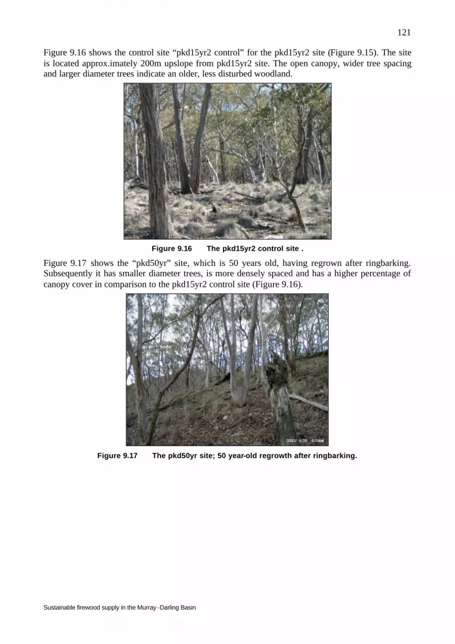
Sustainable firewood supply in the Murray -Darling Basin
121
Figure 9.16 shows the control site “pkd15yr2 control” for the pkd15yr2 site (Figure 9.15). The site is located approx.imately 200m upslope from pkd15yr2 site. The open canopy, wider tree spacing and larger diameter trees indicate an older, less disturbed woodland.
Figure 9.16 The pkd15yr2 control site .
Figure 9.17 shows the “pkd50yr” site, which is 50 years old, having regrown after ringbarking. Subsequently it has smaller diameter trees, is more densely spaced and has a higher percentage of canopy cover in comparison to the pkd15yr2 control site (Figure 9.16).
Figure 9.17 The pkd50yr site; 50 year-old regrowth after ringbarking.

Sustainable firewood supply in the Murray -Darling Basin
122
Figure 9.18 shows the “pkd100yr” site, which is at least 100 years old. All Bredbo sites share the same ‘even aged stand’ characteristics shown here i.e. typically all trees are from the same age cohort with limited age diversity of individual trees.
Figure 9.18 The pkd100yr site; at least 100 years old.
Figure 9.19 shows the “pkd oldest” site. This site was a rare example of a relatively undisturbed forest where no known harvesting or other significant disturbance has occurred. Large old trees with diameters up to 100 cm are well spaced along the slopes, while shrub cover and woody debris increases in abundance higher up the slope.
Figure 9.19 The pkd oldest site; a rare example of a relatively undisturbed forest.
The large number of sites selected from Bredbo property reflect its size and diversity of stand ages. The property has a total area of 2522 ha. Of this, 1500ha is managed native forest, 400ha is used for agriculture and 600 ha for conservation of flora and fauna.
9.6 Sampling Methodology This section describes the sampling methodology used at case study survey sites to investigate the potential ecological impacts on lower rainfall forest and woodland sites of firewood harvesting under the green-wood scenario.
Forestry mensuration, regeneration and coarse woody debris surveys, and bird, small mammal and plant species richness, were undertaken on 19 sites between April and August in 2003. All sites

Sustainable firewood supply in the Murray -Darling Basin
123
were sampled in the same way, except for the Bungendore sites, where bird and small mammal surveys were not undertaken due to size and treatment differences (see Section 9.5.3). Landscape Function Analysis (LFA) was conducted at eight sites on two properties (Bredbo and Bungendore), to investigate potential impacts arising from the two harvesting techniques of thinning and pulling.
9.6.1 Birds Bird surveys were carried out in 1ha plots (50 metres by 200 metres), with one bird plot located at each site. Data on the occurrence (presence/absence) and relative abundance were recorded for each bird species observed. Surveys were conducted during early mornings and late afternoons, no later than three hours after sunrise or earlier than three hours before sunset, to coincide with peak periods of bird activity. Surveys were not conducted during rain, strong wind or fog. Surveys were conducted using a timed walk technique, similar to that described in Fisher (1997), with each 50 metre segment of the transect being traversed in 5 minutes. Thus the entire plot was surveyed in 20 minutes. Each bird plot was surveyed on three separate occasions by experienced CSIRO field ornithologists. All bird surveys were conducted during April 2003.
9.6.2 Small ground-dwelling mammals Small mammals were surveyed over three consecutive nights, using standard Elliot traps. The sampling technique is used extensively to detect most if not all of the small ground dwelling mammals in an area (Catling and Burt 1994, 1995, 1997). Two parallel lines, 10 m apart and each containing 10 Elliott traps (Type A) were placed 7 metres apart and baited with peanut butter and rolled oats. The lines were laid out on the upper slopes of each site. The sma ll mammals captured were identified, weighed, their reproductive condition recorded, marked by cutting a small square of hair from their rump and released at the point of capture. All small mammal surveys were conducted during April 2003, amounting to a total of 60 trap-nights per site trapped.
9.6.3 Plants Section 5.5.1 provides the site descriptions and field sampling methodology for the forest mensuration live tree measurements.
The understorey plant sampling strategy was based on a 10 minute traverse across the regeneration plot described in Section 9.6.4, in lines approximately 5 metres apart. The sampling was done during mid-autumn (April 2003), so the species were characterised by persistent perennials. April 2003 was drier that average, with above-average day-time and night-time temperatures after the 2002-03 drought year. The only significant rainfall over summer was 55 millimetres in February (Bureau of Meteorology 2003). The plant species recorded are therefore considered to under-represent the species richness expected from a spring sampling survey.
Understorey species of grasses, forbs, rushes and shrubs were identified to genus or species level and the foliage cover of ground species and the crown cover of the shrub layer species were estimated, using guidelines from the Australian Soil and Land Survey Field Handbook (McDonald et al.1990).
9.6.4 Coarse woody debris Section 5.5.1 provides the site descriptions and field sampling methodology for the coarse woody debris.
“Coarse woody debris” is elsewhere defined as stem and branch wood of dead standing trees and pieces of fallen wood with length ≥0.5 m and mid-diameter ≥10 cm (Sections 5 and 6). However, for the examination of ecological impacts of firewood harvesting, we have separated the forest floor
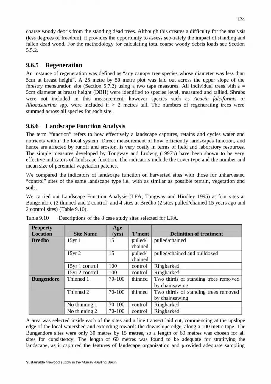
Sustainable firewood supply in the Murray -Darling Basin
124
coarse woody debris from the standing dead trees. Although this creates a difficulty for the analysis (less degrees of freedom), it provides the opportunity to assess separately the impact of standing and fallen dead wood. For the methodology for calculating total coarse woody debris loads see Section 5.5.2.
9.6.5 Regeneration An instance of regeneration was defined as “any canopy tree species whose diameter was less than 5cm at breast height”. A 25 metre by 50 metre plot was laid out across the upper slope of the forestry mensuration site (Section 5.7.2) using a two tape measures. All individual trees with a = 5cm diameter at breast height (DBH) were identified to species level, measured and tallied. Shrubs were not included in this measurement, however species such as Acacia falciformis or Allocasuarina spp. were included if > 2 metres tall. The numbers of regenerating trees were summed across all species for each site.
9.6.6 Landscape Function Analysis The term “function” refers to how effectively a landscape captures, retains and cycles water and nutrients within the local system. Direct measurement of how efficiently landscapes function, and hence are affected by runoff and erosion, is very costly in terms of field and laboratory resources. The simple measures developed by Tongway and Ludwig (1997b) have been shown to be very effective indicators of landscape function. The indicators include the cover type and the number and mean size of perennial vegetation patches.
We compared the indicators of landscape function on harvested sites with those for unharvested “control” sites of the same landscape type i.e. with as similar as possible terrain, vegetation and soils.
We carried out Landscape Function Analysis (LFA; Tongway and Hindley 1995) at four sites at Bungendore (2 thinned and 2 control) and 4 sites at Bredbo (2 sites pulled/chained 15 years ago and 2 control sites) (Table 9.10).
Table 9.10 Descriptions of the 8 case study sites selected for LFA.
Property Location Site Name
Age (yrs) T’ment Definition of treatment
15yr 1 15 pulled/ chained
pulled/chained
15yr 2 15 pulled/ chained
pulled/chained and bulldozed
15yr 1 control 100 control Ringbarked
Bredbo
15yr 2 control 100 control Ringbarked Thinned 1 70-100 thinned Two thirds of standing trees removed
by chainsawing Thinned 2 70-100 thinned Two thirds of standing trees removed
by chainsawing No thinning 1 70-100 control Ringbarked
Bungendore
No thinning 2 70-100 control Ringbarked
A area was selected inside each of the sites and a line transect laid out, commencing at the upslope edge of the local watershed and extending towards the downslope edge, along a 100 metre tape. The Bungendore sites were only 30 metres by 15 metres, so a length of 60 metres was chosen for all sites for consistency. The length of 60 metres was found to be adequate for stratifying the landscape, as it captured the features of landscape organisation and provided adequate sampling

Sustainable firewood supply in the Murray -Darling Basin
125
opportunities for the five replicates required for soil surface condition (SSC) assessments (Tongway and Hindley 1995).
The first step of the LFA process was to assess the organisation of the landscape, by identifying “patch” and “interpatch” areas. Patches are grass tussocks, fine and coarse woody debris, shrubs and trees or a mix of all three. Patches tend to obstruct/halt the flow of water and nutrients, facilitating on-site infiltration and reducing the chances of them leaking from a site. Interpatches may be partially or totally bare. Perennial vegetation may be absent or insufficient to provide any long-term protective soil cover. Interpatches which have been stripped of surface soils or disturbed by harvesting techniques may have stony surfaces. Dysfunctional or “leaky” landscapes have few obstructions (patches), and long fetches (Interpatches) so that surface flows to gain energy and volume, accelerating erosion and losses from the local system (Tongway and Ludwig 1997).
The next step was to assess soil surface features on each of the patch/interpatch types identified in the landscape organisation assessment. Through a stratified, random process, five replicate zones were selected at intervals along the transect line. Each zone type was assessed for the ten soil surface condition indicators as shown in Table 9.11.
Table 9.11 Soil surface features, with their respective process-based interpretations. Protocols for assessment can be found in Tongway and Hindley (1995), pp. 25-32.
Indicator Interpretation 1. Soil cover Assesses vulnerability to rainsplash erosion 2. Basal cover of perennial grass or canopy cover of shrubs and trees
Assesses contribution of root biomass to nutrient cycling processes
3. Litter cover, origin and degree of decomposition Assesses the availability of surface organic matter for decomposition and nutrient cycling.
4. Cryptogam cover An indicator of surface stability, resistance to erosion and nutrient availability
5. Crust broken-ness Assesses loose crusted material available for wind ablation or water erosion
6. Erosion type and severity Assesses the nature and severity of current soil erosion features.
7. Deposited materials Assesses the quantity of alluvial deposits 8. Microtopography Assesses surface roughness for water infiltration and
flow disruption, seed lodgment. 9. Surface resistance to disturbance Assesses likelihood of soil detachment and
mobilisation by mechanical disturbance. 10.Slake test Assesses soil stability/dispersiveness when wet 11.Soil texture An indicator of infiltration rate and water storage.
The LFA vegetation dynamics field sampling was not undertaken, as other field measurements adequately sampled these features.
The resulting data were entered into a Microsoft Excel spreadsheet designed to calculate a series of landscape function indices (Tongway and Hindley 1995, LFA template).
9.7 Analysis methods The analyses aimed to assess the impacts of green-wood scenario harvesting methods, in forests stratified by age classes i.e. time since harvesting, on bird species richness and abundance, small mammal species richness, plant species richness, regeneration, coarse woody debris loads and landscape function. It was not possible to apply generalised linear modelling to the data from each location/property separately, as there were no replicates for each set of site conditions. However, the sites were sufficiently similar (geographic location, soil and geological substrates, management histories, vegetation communities, climatic variables) for their data to be analysed together, and a
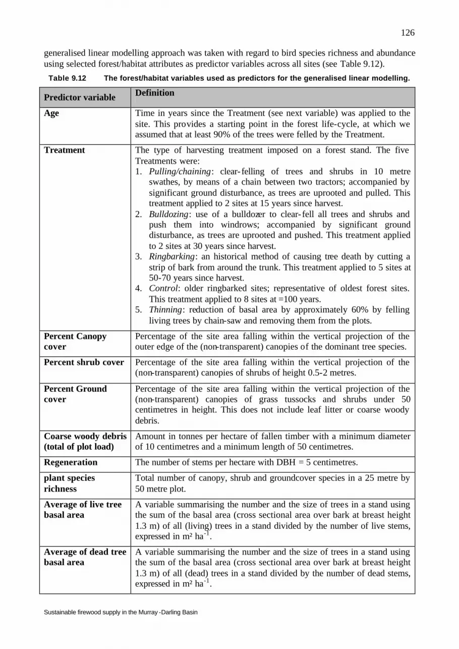
Sustainable firewood supply in the Murray -Darling Basin
126
generalised linear modelling approach was taken with regard to bird species richness and abundance using selected forest/habitat attributes as predictor variables across all sites (see Table 9.12).
Table 9.12 The forest/habitat variables used as predictors for the generalised linear modelling.
Predictor variable Definition
Age Time in years since the Treatment (see next variable) was applied to the site. This provides a starting point in the forest life-cycle, at which we assumed that at least 90% of the trees were felled by the Treatment.
Treatment The type of harvesting treatment imposed on a forest stand. The five Treatments were: 1. Pulling/chaining: clear- felling of trees and shrubs in 10 metre
swathes, by means of a chain between two tractors; accompanied by significant ground disturbance, as trees are uprooted and pulled. This treatment applied to 2 sites at 15 years since harvest.
2. Bulldozing: use of a bulldozer to clear- fell all trees and shrubs and push them into windrows; accompanied by significant ground disturbance, as trees are uprooted and pushed. This treatment applied to 2 sites at 30 years since harvest.
3. Ringbarking: an historical method of causing tree death by cutting a strip of bark from around the trunk. This treatment applied to 5 sites at 50-70 years since harvest.
4. Control: older ringbarked sites; representative of oldest forest sites. This treatment applied to 8 sites at =100 years.
5. Thinning: reduction of basal area by approximately 60% by felling living trees by chain-saw and removing them from the plots.
Percent Canopy cover
Percentage of the site area falling within the vertical projection of the outer edge of the (non-transparent) canopies of the dominant tree species.
Percent shrub cover Percentage of the site area falling within the vertical projection of the (non-transparent) canopies of shrubs of height 0.5-2 metres.
Percent Ground cover
Percentage of the site area falling within the vertical projection of the (non-transparent) canopies of grass tussocks and shrubs under 50 centimetres in height. This does not include leaf litter or coarse woody debris.
Coarse woody debris (total of plot load)
Amount in tonnes per hectare of fallen timber with a minimum diameter of 10 centimetres and a minimum length of 50 centimetres.
Regeneration The number of stems per hectare with DBH = 5 centimetres.
plant species richness
Total number of canopy, shrub and groundcover species in a 25 metre by 50 metre plot.
Average of live tree basal area
A variable summarising the number and the size of trees in a stand using the sum of the basal area (cross sectional area over bark at breast height 1.3 m) of all (living) trees in a stand divided by the number of live stems, expressed in m² ha-1.
Average of dead tree basal area
A variable summarising the number and the size of trees in a stand using the sum of the basal area (cross sectional area over bark at breast height 1.3 m) of all (dead) trees in a stand divided by the number of dead stems, expressed in m² ha-1.

Sustainable firewood supply in the Murray -Darling Basin
127
Predictor variable Definition
Average of live stem stocking density
An index of live tree density (stocking density) = number of live tree stems ha-1.
Average of dead tree stocking density
An index of dead tree density (stocking density) = number of dead tree stems ha-1.
Average of live stem wood volume
Stem wood volume expressed in m³ ha-1. Stand volume is a function of stand height, average tree taper, average bark thickness and average diameter or basal area.
9.7.2 Birds For the analysis the bird species were put into broad “functional” groups, similar to those of Reid (1999). The groups used were: 1. “All bird species” i.e. all species encountered over all of the bird surveys; 2.“Decliner” bird species i.e. species categorised by Reid (1999) as birds which tend to decline in distribution and abundance with disturbance and fragmentation; and 3. “Increaser” bird species i.e. species categorised by Reid (1999) as birds which tend to increase in distribution and abundance with disturbance and fragmentation. Note that only birds actually recorded during the formal 20 minute surveys and observed (heard or seen) actually on a bird survey plot were included in the analyses.
Bird species richness
Generalised linear modelling (GLM); using Genstat Version 6™ was used to investigate the relationships between bird species richness and the predictor variables described in Table 9.12. Each of the bird functional groups was modelled separately. The bird response data consisted of counts i.e. the numbers of species recorded on each survey plot, therefore Poisson error distributions and a logarithmic link function was used in the development of the models (Nicholls 1991, Crawley 1993). All habitat variables were modelled as continuous variables apart from Treatment, which was modelled as a four level factor (see Table 9.12).
The predictor variables were fitted in a forward stepwise fashion (Nicholls, 1991). Variables were retained in the model if the change in residual deviance divided by the change in degrees of freedom was significant at the p ≤ 0.05 level. Variables retained for the final stepwise models (i.e. those which contributed to significant changes in deviance in the model) were reanalysed to develop a final model explaining significant changes in the response variable (species richness).
Where predictor variables were found to be highly correlated only one was used as a predictor in any one model, to avoid issues of colinearity. Table 9.13 shows the correlation matrix, with high correlations between predictors shaded. In each case, the choice of collinear variable was made on the basis of the one which seemed to be the most biologically meaningful. Table 9.13 Correlation matrix for all predictor variables. Shaded cells are those where correlation
is sufficiently high to suggest excluding both variables from being fitted simultaneously in the model to avoid colinearity in the forward stepwise analysis.
Age
Age Class
ID
Basal Area Dead
Basal Area Live
Stem Wood Vol Live
Stock Densty Dead
Stock Densty Live
Canopy Pc
Ground Cover
Pc Plant
sp Regen stems
Shrub Pc
C W D
Age 1.000
Age Class ID 0.824 1.000
Basal Area
0.199 0.441 1.000
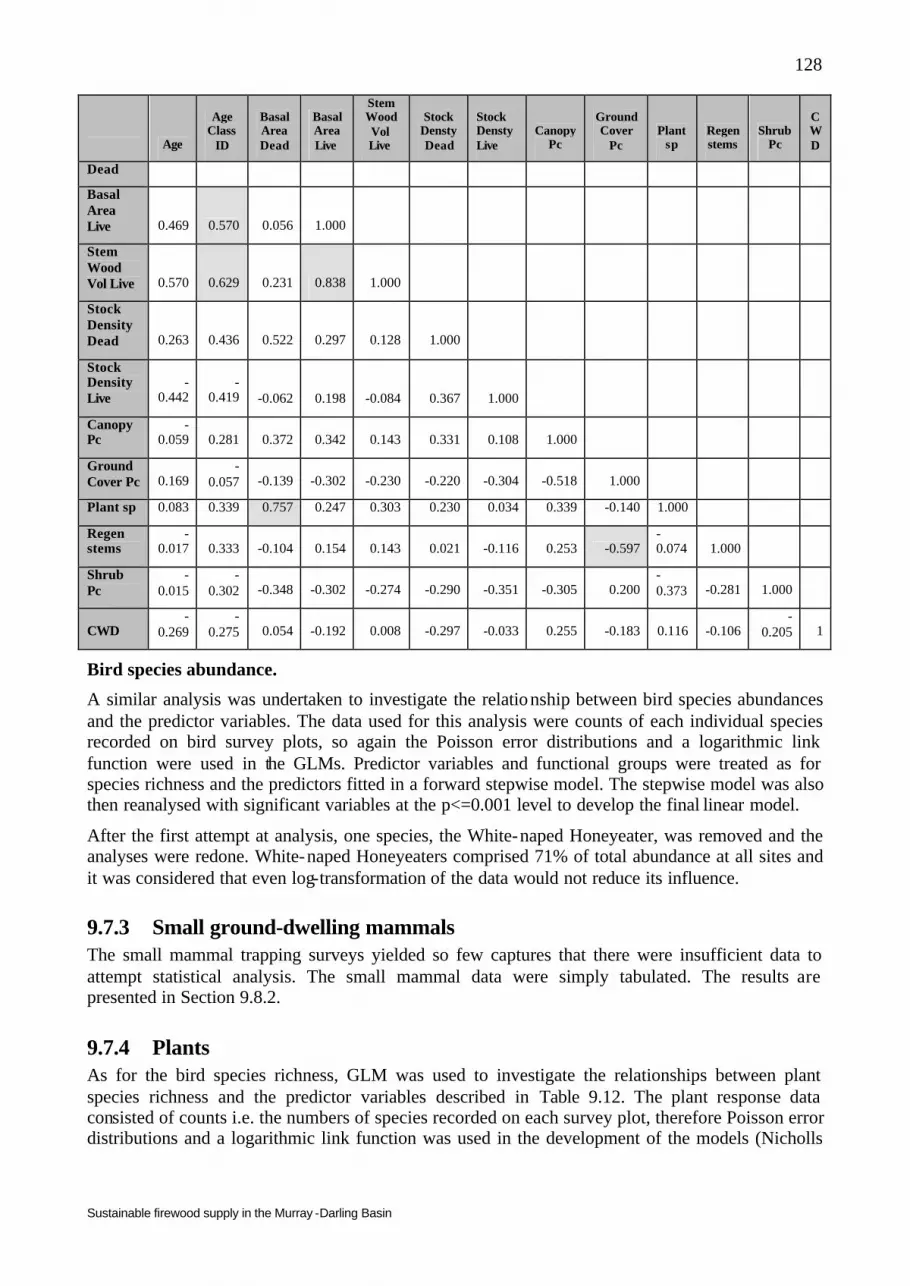
Sustainable firewood supply in the Murray -Darling Basin
128
Age
Age Class
ID
Basal Area Dead
Basal Area Live
Stem Wood Vol Live
Stock Densty Dead
Stock Densty Live
Canopy Pc
Ground Cover
Pc Plant
sp Regen stems
Shrub Pc
C W D
Dead
Basal Area Live 0.469 0.570 0.056 1.000
Stem Wood Vol Live 0.570 0.629 0.231 0.838 1.000
Stock Density Dead 0.263 0.436 0.522 0.297 0.128 1.000
Stock Density Live
-0.442
-0.419 -0.062 0.198 -0.084 0.367 1.000
Canopy Pc
-0.059 0.281 0.372 0.342 0.143 0.331 0.108 1.000
Ground Cover Pc 0.169
-0.057 -0.139 -0.302 -0.230 -0.220 -0.304 -0.518 1.000
Plant sp 0.083 0.339 0.757 0.247 0.303 0.230 0.034 0.339 -0.140 1.000
Regen stems
-0.017 0.333 -0.104 0.154 0.143 0.021 -0.116 0.253 -0.597
-0.074 1.000
Shrub Pc
-0.015
-0.302 -0.348 -0.302 -0.274 -0.290 -0.351 -0.305 0.200
-0.373 -0.281 1.000
CWD -
0.269 -
0.275 0.054 -0.192 0.008 -0.297 -0.033 0.255 -0.183 0.116 -0.106 -
0.205 1
Bird species abundance.
A similar analysis was undertaken to investigate the relationship between bird species abundances and the predictor variables. The data used for this analysis were counts of each individual species recorded on bird survey plots, so again the Poisson error distributions and a logarithmic link function were used in the GLMs. Predictor variables and functional groups were treated as for species richness and the predictors fitted in a forward stepwise model. The stepwise model was also then reanalysed with significant variables at the p<=0.001 level to develop the final linear model.
After the first attempt at analysis, one species, the White-naped Honeyeater, was removed and the analyses were redone. White-naped Honeyeaters comprised 71% of total abundance at all sites and it was considered that even log-transformation of the data would not reduce its influence.
9.7.3 Small ground-dwelling mammals The small mammal trapping surveys yielded so few captures that there were insufficient data to attempt statistical analysis. The small mammal data were simply tabulated. The results are presented in Section 9.8.2.
9.7.4 Plants As for the bird species richness, GLM was used to investigate the relationships between plant species richness and the predictor variables described in Table 9.12. The plant response data consisted of counts i.e. the numbers of species recorded on each survey plot, therefore Poisson error distributions and a logarithmic link function was used in the development of the models (Nicholls

Sustainable firewood supply in the Murray -Darling Basin
129
1991, Crawley 1993). All habitat variables were modelled as continuous variables apart from Treatment, which was modelled as a four level factor (see Table 9.12).
The predictor variables were fitted in a forward stepwise fashion (Nicholls, 1991). Variables were retained in the model if the change in residual deviance divided by the change in degrees of freedom was significant at the p ≤ 0.05 level. Variables retained for the final stepwise models (i.e. those which contributed to significant changes in deviance in the model) were reanalysed to develop a final model explaining significant changes in the response variable (species richness).
Where predictor variables were found to be highly correlated only one was used as a predictor in any one model, to avoid issues of colinearity. Table 9.13 shows the correlation matrix, with high correlations between predictors shaded. In each case, the choice of colinear variable was made on the basis of the one which seemed to be the most biologically meaningful.
9.7.5 Coarse woody debris GLM was used to investigate the relationships between coarse woody debris load and the predictor variables described in Table 9.12. The coarse woody debris response data was modelled as continuous data i.e. amounts of coarse woody debris in t ha-1 on each survey plot, therefore Normal error distributions and an identity link function was used in the development of the models (Nicholls 1991, Crawley 1993). All habitat variables were modelled as continuous variables apart from Treatment, which was modelled as a four level factor (see Table 9.12).
The predictor variables were fitted in a forward stepwise fashion (Nicholls, 1991). Variables were retained in the model if the change in residual deviance divided by the change in degrees of freedom was significant at the p ≤ 0.05 level. Variables retained for the final stepwise models (i.e. those which contributed to significant changes in deviance in the model) were reanalysed to develop a final model explaining significant changes in the response variable (amount of coarse woody debris).
Where predictor variables were found to be highly correlated only one was used as a predictor in any one model, to avoid issues of colinearity. Table 9.13 shows the correlation matrix, with high correlations between predictors shaded. In each case, the choice of colinear variable was made on the basis of the one which seemed to be the most biologically meaningful.
9.7.6 Regeneration GLM was used to investigate the relationships between regeneration and the predictor variables described in Table 9.12. The regeneration response data consisted of counts i.e. the numbers of regenerating stems recorded on each survey plot, therefore Poisson error distributions and a logarithmic link function was used in the development of the models (Nicholls 1991, Crawley 1993). All habitat variables were modelled as continuous variables apart from Treatment, which was modelled as a four level factor (see Table 9.12).
The predictor variables were fitted in a forward stepwise fashion (Nicholls, 1991). Variables were retained in the model if the change in residual deviance divided by the change in degrees of freedom was significant at the p ≤ 0.05 level. Variables retained for the final stepwise models (i.e. those which contributed to significant changes in deviance in the model) were reanalysed to develop a final model explaining significant changes in the response variable (number of regenerating stems).
Where predictor variables were found to be highly correlated only one was used as a predictor in any one model, to avoid issues of colinearity. Table 9.13 shows the correlation matrix, with high correlations between predictors shaded. In each case, the choice of colinear variable was made on the basis of the one which seemed to be the most biologically meaningful.

Sustainable firewood supply in the Murray -Darling Basin
130
9.7.7 Landscape function analysis Landscape Function Analysis describes how a landscape works to capture, retain and use valuable natural resources within the local system (see Section 9.6.6). For analysis we used the standard Microsoft Excel spreadsheet/workbook, developed by Tongway and Hindley (1995), to calculate a series of indices reflecting landscape function. The method is described in Tongway (2003) pages 43-46.
We ran a series of T-tests (Two-Sample Assuming Unequal Variance) to test for any significant differences in the means between the harvested-by-thinning and the control site at Bungendore, and between the harvested-by-pulling/chaining and the control sites at Bredbo. The data analysed were from the five replicates of soil surface condition and the P-value selected was P(T ≤ t) two-tail.
9.7.8 Forest/habitat variables We also used GLMs to model selected forest/habitat variables as response variables, using data from three of the four sites. Bungendore data were not used in the analysis, the “thinned” treatment might confound the results (Section 9.5.3). The treatments for all other sites amounted to a “clear felled” condition, with site characteristics reflecting a known age, whereas this was not the case for the “thinned” sites.
Variables were treated in turn as both response and predictor variables. The variables considered were shrub cover, regeneration, ground cover, plant diversity, coarse woody debris, basal areas, to investigate their relationship with factors such as Treatment and Age and the other forest/habitat variables. The modelling protocols were the same as those detailed in Section 9.7.1, with the difference being that, where the response variables were continuous variables i.e. all except plant species richness, normal error distributions and identity link function were employed (Nicholls 1991, Crawley, 1993).
Each forest/habitat variable was considered at three levels of significance i.e. p ≤ 0.05, p ≤ 0.01 and p ≤ 0.001. Each variable was modelled separately in a forward stepwise fashion (Nicholls, 1991). The colinearity issue was addressed by choosing only the most biologically meaningful of a pair of highly correlated variables (Table 9.13). Forest/habitat variables which contributed to significant changes in deviance in the models were reanalysed to develop final models to explain any significant changes for each response variable.
9.8 Analysis results
9.8.1 Birds The bird functional groups were “all bird species”, “decliner” and “increaser” species (Section 9.7.1). Appendix 13 gives the bird list for the sites, showing overall abundance and functional group. Note that only 4 bird species are classified as decliners and 7 species as increasers.
There were 41 bird species recorded across the 15 sites and a total of 1,865 individual birds observed or heard on the plots (Appendix 13). Abundances varied from only one occurrence of that species for the Australian Owlet-nightjar, Gang gang Cockatoo, Pied Butcherbird, White-throated Gerygone and White-plumed Honeyeater, to 1321 for the White-naped Honeyeater (Appendix 13). The White-naped Honeyeater is migratory in this region and high abundances reflect the birds’ movements in mass migrations from their source area. Abundances on most sites where the White-naped Honeyeater was recorded were up to 66 times higher than the next most abundant species. The next most abundant species were the Striated Thornbill, Spotted Pardalote and Yellow-faced and White-eared Honeyeaters.
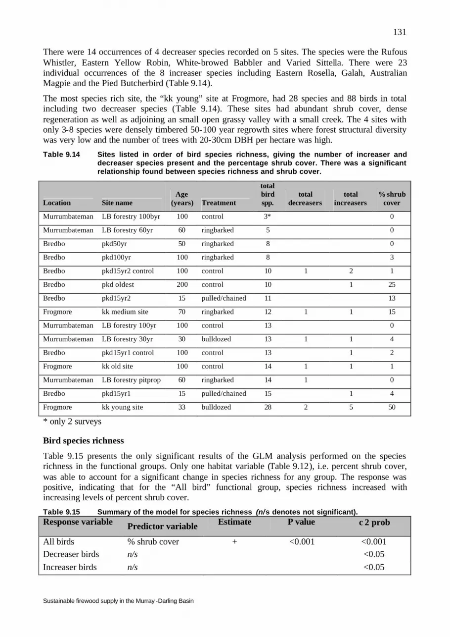
Sustainable firewood supply in the Murray -Darling Basin
131
There were 14 occurrences of 4 decreaser species recorded on 5 sites. The species were the Rufous Whistler, Eastern Yellow Robin, White-browed Babbler and Varied Sittella. There were 23 individual occurrences of the 8 increaser species including Eastern Rosella, Galah, Australian Magpie and the Pied Butcherbird (Table 9.14).
The most species rich site, the “kk young” site at Frogmore, had 28 species and 88 birds in total including two decreaser species (Table 9.14). These sites had abundant shrub cover, dense regeneration as well as adjoining an small open grassy valley with a small creek. The 4 sites with only 3-8 species were densely timbered 50-100 year regrowth sites where forest structural diversity was very low and the number of trees with 20-30cm DBH per hectare was high.
Table 9.14 Sites listed in order of bird species richness, giving the number of increaser and decreaser species present and the percentage shrub cover. There was a significant relationship found between species richness and shrub cover.
Location Site name Age
(years) Treatment
total bird spp.
total decreasers
total increasers
% shrub cover
Murrumbateman LB forestry 100byr 100 control 3* 0
Murrumbateman LB forestry 60yr 60 ringbarked 5 0
Bredbo pkd50yr 50 ringbarked 8 0
Bredbo pkd100yr 100 ringbarked 8 3
Bredbo pkd15yr2 control 100 control 10 1 2 1
Bredbo pkd oldest 200 control 10 1 25
Bredbo pkd15yr2 15 pulled/chained 11 13
Frogmore kk medium site 70 ringbarked 12 1 1 15
Murrumbateman LB forestry 100yr 100 control 13 0
Murrumbateman LB forestry 30yr 30 bulldozed 13 1 1 4
Bredbo pkd15yr1 control 100 control 13 1 2
Frogmore kk old site 100 control 14 1 1 1
Murrumbateman LB forestry pitprop 60 ringbarked 14 1 0
Bredbo pkd15yr1 15 pulled/chained 15 1 4
Frogmore kk young site 33 bulldozed 28 2 5 50
* only 2 surveys
Bird species richness
Table 9.15 presents the only significant results of the GLM analysis performed on the species richness in the functional groups. Only one habitat variable (Table 9.12), i.e. percent shrub cover, was able to account for a significant change in species richness for any group. The response was positive, indicating that for the “All bird” functional group, species richness increased with increasing levels of percent shrub cover.
Table 9.15 Summary of the model for species richness (n/s denotes not significant). Response variable Predictor variable Estimate P value χ2 prob
All birds % shrub cover + <0.001 <0.001 Decreaser birds n/s <0.05 Increaser birds n/s <0.05

Sustainable firewood supply in the Murray -Darling Basin
132
No significant relationships were found between any of the measured habitat variables and “decreaser” or “increaser” species richness, probably due to the low number of occurrences of birds in both functional groups.
The percent shrub cover variable explained 45 % of the observed variation in species richness. The addition of other measured habitat variables did not significantly improve this model. Figure 9.20 illustrates how the predicted number of “All birds” change with changes in % shrub cover.
Figure 9.20 Predicted change in species richness of “All Birds” with increasing percent shrub cover.
Bird species abundance
Table 9.16 presents the only significant results of the GLM analysis performed on the bird abundance in the functional groups, using all species, including the highly abundant White-naped Honeyeater. In order of their contribution to explanation of the total deviance of the model, the significant habitat variables were basal area (live), Treatment and stocking density (live) (Table 9.12). None of the variables were significant for abundance of decreaser or increaser species at the 0.05 level. Table 9.16 Summary of the model for species abundance including the White-naped Honeyeater
(n/s denotes not significant).
Response variable Predictor variable Estimate χ2 prob
All birds basal area (live) Treatment stocking density (live)
- - -
<0.001 <0.001 <0.001
Decreaser birds n/s Increaser birds n/s
Table 9.17 presents the results of the analysis without the White-naped Honeyeater The removal of the honeyeater data caused a change in the habitat variables found to be significant. Stocking density (live) and basal area (live ) were found to be non-significant, replaced by stocking density (dead ) and percent canopy cover.
Table 9.17 Summary of the model for species abundance without the White-naped Honeyeater (n/s denotes not significant).
0
5
10
15
20
25
30
35
0 10 20 30 40 50 60
% shrub cover
spec
ies
richn
ess

Sustainable firewood supply in the Murray -Darling Basin
133
Response variable Predictor variable Estimate χ2 prob
All birds Treatment stocking density (dead) % canopy cover
- + +
<0.001 <0.001 <0.001
Decreaser birds n/s Increaser birds n/s
In both models, Treatment was found to be most significant of the predictor variables. Its significance was not affected by the exclusion of White-naped Honeyeater abundance data. On average, more individual birds were found in the more recently chained and bulldozed sites than in the older ringbarked or control sites (Table 9.18) Table 9.18 Summary of mean abundances for all bird species and for all bird species minus the
White-naped Honeyeater.
Treatment 1 pulled/chained
Treatment 2 bulldozed
Treatment 3 ringbarked
Treatment 4 control
Mean abundance over all bird species
355 68.5 53 129
Mean abundance minus White-naped
Honeyeater
51.5 67 48 32.9
Number of sites 2 2 4 8
9.8.2 Small ground-dwelling mammals Due to the small amount of data from the small mammal surveys, we present the results simply, in tabular form (Table 9.19).
Table 9.19 Small mammal captures by site.
Site Name Common Name Number of individuals kk medium site Yellow-footed Antechinus 2 kk old site Yellow-footed Antechinus 2 kk young site Yellow-footed Antechinus 2 LB forestry 100b yr Agile Antechinus 1 LB forestry 100yr Agile Antechinus 2 LB forestry 60yr Agile Antechinus 2 LB forestry pit prop Agile Antechinus 4 pkd50yr Yellow-footed Antechinus 1
No more than four individuals were found on any site and only two species were detected across all sites. Yellow-footed Antechinus (Antechinus flavipes) was captured on all the Frogmore sites. There was one site (LB forestry 30yr) at Murrumbateman with no captures, 4 sites where the Agile Antechinus (Antechinus agilis) was recorded. For the 7 Bredbo sites there was only one individual captured over 420 trap nights. Table 9.19 does not show the recaptures.
9.8.3 Plants Appendix 14 provides an alphabetic list of all plant species recorded over all case study sites.

Sustainable firewood supply in the Murray -Darling Basin
134
Plant species richness
The plant species richness (all trees, shrubs and groundcover species) at the sites ranged between 3 and 18 species, with a mean of 8 spp ± 3.6. The most common eucalypt species were Eucalyptus rossii and Eucalyptus macrorhyncha, and the most common shrub genera Acacia, Daviesia, and Pultenea. The common groundcover species were grasses and mat rushes such as Joycea pallida, Austrodanthonia spp., Poa spp., Lomandra spp.
Table 9.20 provides a list of the case study sites, in ascending order of plant species richness per plot. Table 9.21 presents the mean species richness per plot for the case study sites, grouped by Treatment.
Table 9.20 The 19 case study sites, presented in ascending order of plant species richness.
Location Site Name Years since
clearing Treatment plant species richness/plot
Bungendore MCthinned1 70-100 thinned 3 Murrumbateman LB forestry 60yr 60 ringbarked 4 Bungendore MCno_thin1 70-100 control 4 Murrumbateman LB forestry 100b yr 100 control 5 Bredbo pkd15yr2 15 pulled/chained 5 Murrumbateman LB forestry 100yr 100 control 5 Bredbo pkd oldest 200 control 6 Bungendore MCthinned2 70-100 thinned 6 Frogmore kk old site 100 control 7 Bredbo pkd15yr2 control 100 control 7 Murrumbateman LB forestry pit prop 60 ringbarked 7 Bungendore MCno_thin2 70-100 control 7 Murrumbateman LB forestry 30yr 30 bulldozed 9 Frogmore kk medium site 70 ringbarked 9 Bredbo pkd15yr1 15 pulled/chained 10 Frogmore kk young site 33 bulldozed 10 Bredbo pkd50yr 50 ringbarked 10 Bredbo pkd100yr 100 ringbarked 14 Bredbo pkd15yr1 control 100 control 18
Table 9.21 Mean plant species richness/plot for the case study sites, grouped by Treatment.
Treatment 1 (pulled/chained)
Treatment 2 (bulldozed)
Treatment 5 (thinned)
Treatment 4 (control)
Treatment 3 (ringbarked)
Mean species richness per plot 7.5 8.5 4.5 7.6 8.8
Number of sites 2 2 2 8 5
Table 9.22 presents the only significant results of the GLM analysis performed on the species richness for the plants. Only two predictor variables (Table 9.12), i.e. Treatment and Regeneration, were able to account for a change in species richness for the plants, and they were only significant at the p < 0.05 level.
Site average species number varied between 4 and 9 (mean = 8.8) with thinned sites containing the lowest diversity and ringbarked sites the highest. Differences between the four treatment s, other than thinned treatment, differ only by one species, and it is likely the significance of this reflects the overall low species diversity across these sites.

Sustainable firewood supply in the Murray -Darling Basin
135
Table 9.22 Summary of model for plant species richness.
Response variable predictor variable P value χ2 prob Plant species richness Treatment
Regeneration 0.047 0.031
0.05 0.05
Shrub and ground cover
Analysis of shrub cover indicated that there was no significant relationship between amount of cover and any of the predictor variables (Table 9.12) although there was a trend suggesting that, with more data, Age might become a significant predictor (Table 9.23).
Analysis of groundcover indicated that there was significant relationship between amount of cover and Regeneration and a trend suggesting Treatment as a predictor (Table 9.23).
Table 9.23 Summary of the models for shrub cover and groundcover.
Response variable Predictor variable Estimate P value χ2 prob Shrub cover (percent) Groundcover (percent)
Age Regeneration Treatment
+- - +
0.059 0.007 0.066
trend <0.01 trend
9.8.4 Coarse woody debris Coarse woody debris loads for the 19 sites varied between 0.3 t/ha and 47 t/ha (Table 9.24) and are presented in order of increasing coarse woody debris load. It can be seen from the table that bulldozed and thinned sites have the lowest coarse woody debris loads while ringbarked, pulled/chained and control sites had the higher coarse woody debris loads. Table 9.24 Site locations, age since clearing. treatment and CWD loads (fallen dead wood only),
been sorted from lowest to highest tonnages per hectare.
Location Age (years) Treatment CWD (t ha-1) Murrumbateman 30 bulldozed 0.3 Bungendore 100 thinned 1.3 Frogmore 33 bulldozed 2.5 Bungendore 100 thinned 2.1 Murrumbateman 100 control 4.6 Bredbo 200 control 8.1 Bungendore 100 control 8.9 Murrumbateman 60 ringbarked 11.2 Murrumbateman 100 control 14.5 Bredbo 100 control 17.0 Murrumbateman 60 ringbarked 21.8 Bredbo 100 ringbarked 22.4 Bungendore 100 control 25.1 Bredbo 50 ringbarked 26.8 Bredbo 100 control 31.0 Frogmore 100 control 35.1 Bredbo 15 pulled/chained 40.1 Bredbo 15 pulled/chained 47.0 Frogmore 70 ringbarked 47.5
Five of the seven sites with less than 10 t ha-1 have had coarse woody debris either physically removed from the site during harvesting (treatment = thinning) or reduced by frequent low intensity

Sustainable firewood supply in the Murray -Darling Basin
136
fires. Sites with more than 30 tonnes per hectare have been either undisturbed for 70-100 years or have accumulated large tonnages through the harvesting method (treatment = chaining). It is therefore not surprising that Treatment was a significant predictor of coarse woody debris load at the p ≤ 0.05 level (Table 9.25) however no other forestry habitat variables were found to be significant.
Table 9.25 Summary of the model for CWD load.
Response variable Predictor variable P value χ2 prob
CWD Treatment 0.023 0.05
The mean coarse woody debris load over all 19 sites is presented in Table 9.26. The table demonstrates that Treatment 2 (bulldozed) and Treatment 5 (thinned) had the lowest coarse woody debris loads, Treatment 3 (ringbarked) and Treatment 4 (control) had medium loads, while Treatment 1 (pulled/chained) had 2-25 times the mean levels of coarse woody debris found at all other Treatments.
Table 9.26 Mean coarse woody debris load at case study sites grouped by Treatment.
Treatment 1 (pulled/chained)
Treatment 2 (bulldozed)
Treatment 4 (control)
Treatment 3 (ringbarked)
Treatment 5 (thinned)
Mean CWD load
(t ha-1) 43.5 1.4 18.25 25.9 1.7
Number of sites
2 2 8 5 2
9.8.5 Regeneration The number of regenerating trees per site ranged from none at all at the oldest site to 144 in one of the 70-100 year Bungendore plots (Table 9.27). The majority of regeneration at two Bungendore sites (MCthinned1, MCthinned2) was coppice from cut stumps, with up to 5 regenerating stems per stump. Table 9.27 Number of regenerating stems of dominant canopy trees (DBH = 5cm) for the 19 study
sites. The sites are presented in ascending order of numbers of regenerating stems.
Location Site Name Age (years) Treatment
no. regenerating stems/plot
no. regenerating stems ha-1
Bredbo pkd oldest 200 control 0 0
Bredbo pkd15yr1 15 pulled/chained 3 24
Murrumbateman LB forestry 100b yr 100 control 6 48
Frogmore kk old site 100 control 7 56
Murrumbateman LB forestry 60yr 60 ringbarked 10 80
Bungendore MCno_thin1 70-100 control 10 80
Bredbo pkd100yr 100 ringbarked 14 112
Bredbo pkd15yr1 control 100 control 15 120
Frogmore kk young site 33 bulldozed 16 128
Murrumbateman LB forestry 30yr 30 bulldozed 17 136
Bredbo pkd50yr 50 ringbarked 17 136
Bredbo pkd15yr2 15 pulled/chained 19 152
Bredbo pkd15yr2 control 100 control 19 152
Murrumbateman LB forestry pit prop 60 ringbarked 23 184
Frogmore kk medium site 70 ringbarked 29 232
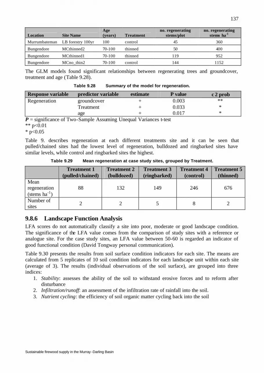
Sustainable firewood supply in the Murray -Darling Basin
137
Location Site Name Age (years) Treatment
no. regenerating stems/plot
no. regenerating stems ha-1
Murrumbateman LB forestry 100yr 100 control 45 360
Bungendore MCthinned2 70-100 thinned 50 400
Bungendore MCthinned1 70-100 thinned 119 952
Bungendore MCno_thin2 70-100 control 144 1152
The GLM models found significant relationships between regenerating trees and groundcover, treatment and age (Table 9.28).
Table 9.28 Summary of the model for regeneration.
Response variable predictor variable estimate P value χ2 prob Regeneration groundcover
Treatment age
+ + +
0.003 0.033 0.017
** * *
P = significance of Two-Sample Assuming Unequal Variances t-test ** p<0.01 * p<0.05
Table 9. describes regeneration at each different treatments site and it can be seen that pulled/chained sites had the lowest level of regeneration, bulldozed and ringbarked sites have similar levels, while control and ringbarked sites the highest.
Table 9.29 Mean regeneration at case study sites, grouped by Treatment.
Treatment 1
(pulled/chained) Treatment 2 (bulldozed)
Treatment 3 (ringbarked)
Treatment 4 (control)
Treatment 5 (thinned)
Mean regeneration (stems ha-1)
88 132 149 246 676
Number of sites 2 2 5 8 2
9.8.6 Landscape Function Analysis LFA scores do not automatically classify a site into poor, moderate or good landscape condition. The significance of the LFA value comes from the comparison of study sites with a reference or analogue site. For the case study sites, an LFA value between 50-60 is regarded an indicator of good functional condition (David Tongway personal communication).
Table 9.30 presents the results from soil surface condition indicators for each site. The means are calculated from 5 replicates of 10 soil condition indicators for each landscape unit within each site (average of 3). The results (individual observations of the soil surface), are grouped into three indices:
1. Stability: assesses the ability of the soil to withstand erosive forces and to reform after disturbance
2. Infiltration/runoff: an assessment of the infiltration rate of rainfall into the soil. 3. Nutrient cycling: the efficiency of soil organic matter cycling back into the soil

Sustainable firewood supply in the Murray -Darling Basin
138
Table 9.30 Summary of the model for LFA soil surface condition indices.
Soil Surface Condition Individual zone contribution to the whole Landscape Values are scored with maximum of 100*
Property/site Treatment Stability Std err
P Infiltration Std err
P Nutrient cycling
Std err
P
pulled/chained 70.9 2.5 51.6 3.4 47.5 3.9 Bredbo 15yr1 control 68.4 3.4 ns 53.7 5.0 ns 49.1 6.9 ns
pulled/chained 65.6 4.4 44.1 4.1 43.0 4.9 Bredbo 15yr 2 control 68.2 2.0 ns 52.4 2.4 ** 49.4 3.2 *
Thinned 65.4 2.9 50.4 3.9 49.7 2.6 Bungendore (MC 1) No thinning 64.1 2.9 ns 59.7 2.8 * 59.3 4.0 **
Thinned 72.2 2.9 55.9 4.3 54.3 6.2 Bungendore (MC 2) No thinning 71.6 1.6 ns 50.8 5.9 ns 50.9 6.7 ns
P = significance of Two-Sample Assuming Unequal Variances t-test ** p<0.01 * p<0.05 ns P>0.05
The model detected no significant differences in soil surface stability, infiltration or nutrient cyc ling found between Bredbo Site 15yr 1 (pulled/chained 15 years ago) and the Bredbo 15yr 1 control (Age =100 years), located 500 metres away.
However we found significant differences in infiltration and nutrient cycling between Bredbo 15yr 2 site (pulled/chained 15 years ago) and the Bredbo 15yr 2 control (Age =100 years), located 200 metres away. The pulled/chained site had lower values for the infiltration index than the control, implying that infiltration of rainfall had not returned to its pre-treatment level.
There were also significant differences in soil surface infiltration and nutrient cycling between Bungendore MCthinned_1 (thinned 10 years ago) and the Bungendore MCno_Thin1 site (70-100 years), located 200m away. The thinned site had lower values than its non-thinned control for infiltration.
There were no significant differences detected in soil surface stability, infiltration or nutrient cycling between Bungendore MCthinned_2 (thinned 10 years ago) and the Bungendore MCno_Thin2 site (70-100 years) located 200m away.
9.8.7 Forestry/habitat variables Modelling of forestry/habitat variables has already been done at a larger scale across the MDB, in the development of a model to predict stem wood volumes (see Section 6). Results of this analysis indicated that, at a stand level, the model has a large standard error i.e. ±153% of predicted level at the 95% confidence limits. However, when the model was used to predict across stands in a wider area in the same NPP class, the standard error was significantly reduced i.e. to ±17% of predicted level at the 95% confidence limits.
In the light of this, it is interesting that the modelling for assessment of ecological impacts of firewood harvesting showed that both treatment and live tree stocking density were significant predictors at the p < 0.05 level of live tree basal area (Table 9.31). Sites which have been bulldozed or pulled/chained, where there are the younger, regenerating stands, have smaller live tree basal areas, frequently between 10-20m², in comparison to older ringbarked or control sites, where live tree basal areas average around 30m², ranging between 20-40m².

Sustainable firewood supply in the Murray -Darling Basin
139
Table 9.31 Summary of the model for live tree basal area.
Response variable predictor variable P value χ2 prob Live tree basal area Treatment
Live tree stocking density 0.030 0.040
0.05 0.05
Table 9. Summary of GLM of individual predictor (forestry/habitat) variables found to be a significant predictor of live tree basal area. ns = P>0.05, * = p<0.05, ** = p<0.01, ***=p<0.001
9.9 Discussion The case studies have created a framework for the investigation of the potential impacts of firewood harvesting through the selection of forest and woodland sites which have forest stands of different ages since they were harvested or cleared over the last 150 years, and which have been harvested using different harvesting methods. The framework also includes two sites where disturbance has been minimal.
The key question is whether this framework is able to provide evidence that firewood harvesting, through clearing or thinning of live trees, has a some significant effect on biodiversity, either positive or negative. Thee case study approach has provided a number of significant relationships between habitat/forestry variables and differently aged and/or harvested sites. It is important to ask whether these results are comparable with the effects of the silvicultural regimes proposed for the green-wood scenario. This issue can be examined through consideration of silvicultural management scenarios and the type of harvesting the dead-wood and green-wood scenario entails.
The green-wood scenario does not imply a simple harvesting formula. Low forest productivity i.e. low commercial productivity, has meant that appropriate sites for investigating the ecological impact of green-wood scenario, i.e. native woodlands and forests with the appropriate harvesting regimes and methods of harvest, are very limited in number. There is also a broad range of forest and woodland types (see Section 8.6) so at this stage the green-wood scenario does not specify long-term silvicultural management regimes for low rainfall-area forests.
For these reasons there are a number of recommended ecological principles which should underpin silvicultural management under the green-wood scenario:
1. Silvicultural practices should encourage the retention of multi-aged stands to provide a diverse mosaic of ecological niches and resources ie. for food, breeding, shelter;
2. Silvicultural practices should encourage retention of larger trees for hollows as wildlife habitat i.e. only thinning trees =15cm DBH; and
3. Silvicultural practices should encourage the maintenance of heterogenous landscape matrix, by using a combination of “flexible selection” harvesting regimes (thinning approximately 50% of the forest stand basal area) and “group selection” harvesting regimes (clear felling of small gaps to create matrix of open spaces).
We found only two sets of experimental sites in NSW older than ten years. One set comprises the Australian National University School of Resources, Environmental and Society experimental sites, established to examine the effects of silvicultural treatments on the growth rates of trees and diversity of the understorey in a dry sclerophyll forest. The other wet was a eucalypt growth and thinning plantation trial, established by NSW State Forests near Parkes, a low rainfall area in forestry terms.
Additionally, it is extremely difficult to find forest stands with a known age since harvesting. It is the exception rather than the rule that any State agencies have any written records, at the stand-specific level of detail, for sites older than 30 years. The process of locating sites of known age is reliant upon locating and talking to private landowners who have a clear knowledge of regeneration and clearing events, on their own properties, over a significant time period.

Sustainable firewood supply in the Murray -Darling Basin
140
Of the 19 case study sites, 2 were pulled/chained, 2 were thinned, 2 were bulldozed, 2 were “undisturbed”, and 11 ringbarked between 50 and =100 years ago. As a group these represented sufficient representation of the range of harvesting and age classes necessary to examine the ecological effects of harvesting under the green-wood scenario, however the actual number of available sites was not sufficient to adequately replicate the forest types, treatments and ages. As a consequence, the types of analyses were severely limited by the lack of adequate data.
Finally, it is important to recognise that all study sites were situated within well forested agricultural areas, where forests and woodlands form between 30 and 80% of each property. Ecological impacts may differ where sites fall in more isolated remnants within an agricultural landscape, surrounded by open paddocks and cropping with occasional remnant trees. This consideration contributes to the rationale for exclusion of remnants with an area < 100 hectares from the estimates of area available for harvesting under the green-wood scenario (exploitation criterion 9, Section 3.3).
9.9.1 Birds
Species richness
Bird species richness has been correlated to a number of habitat variables in forest and woodland remnants in the Southern Tablelands. The structural diversity of a patch, i.e. its canopy cover, density of shrubs, and the amounts of litter and ground cover, has been shown to strongly influence the diversity of bird species in an area (Wiens 1989). For example in the Central Lachlan hill communities, comparable to these Southern Tableland hill communities, increased vegetation cover at heights between 0.5 and 2 m in was related to increased bird diversity (Seddon et al. 2002, in press). The size of the forest or woodland remnant, the habitat complexity score (a ranking of tree, shrub and groundcover cover levels) and the distance to the nearest 10ha woodland remnant significantly influence the number and presence of particular bird species (Watson et al.2001). However in large area forests, the main attributes influencing bird abundance and species are the structure and composition of the vegetation (Ford 1985).
In the case study, between 3 and 28 species were recorded at each site, with 41 species recorded in total. Twelve of the 15 sites had observations ranging between only 8 to 15 bird species. The top 4 species-rich sites were either the youngest, oldest or located on deeper soils along a creek or valley floor. In comparison, the 5 most species-poor sites were the 50 to =100 year-old ringbarked stands, characterised by dense, even-aged stands and located along dry slopes and ridges. The mid-range of species richness was occupied by a combination of older and younger sites.
There are a number of spatial and temporal factors influencing this variation. Species richness for each site will vary according to daily, seasonal and longer term patterns over time, therefore it would be expected that these figures significantly underestimate true species richness compared to what might be recorded from longer term observations. Also, Autumn is not the optimum time for bird surveys, when bird vocalisations are reduced as a result of post-nuptial moulting, so survey observations based on calls are less likely than during the spring breeding season.
However, the positive relationship found between bird species richness and shrub cover is also significant. as up to 10 of the 15 sites had less than 5% shrub cover. The lack of shrub cover will influence species richness and the significant results correlating bird species richness with shrub cover in this study was consistent with previous research.
The lack of a detectable significant response of bird species richness to groundcover, canopy cover, plant diversity and coarse woody debris was surprising. As discussed in Section 9.2, the more structurally complex sites have been related to bird species richness. For example MacNally et al.(2002) found that the densities of wood-dependent Brown Treecreeper increased with higher loads of coarse woody debris. A greater number of occurrences would have enabled more individual species like the Brown Treecreeper to be analysed and modelled.

Sustainable firewood supply in the Murray -Darling Basin
141
However, this result is also consistent with contradictory results from studies examining relationships between coarse woody debris and bird species number (Driscoll et al. 2000). Results may have been different if these site variables were combined to produce a matrix similar to that for habitat complexity scores (ie. a ranking of the value of the habitat based on combining the individual scores). Certainly the habitat complexity index, which combines the percent cover of canopy, shrub, ground, leaf litter and log cover, is a significant predictor of bird species richness in remnant woodlands (Drew et al. 2002; Freudenberger 2001; Watson et al. 2001) and all these variables were present as separate habitat variables in this study.
Bird abundance
The bird survey data was also analysed for bird abundances over all sites. Although birds species richness is traditionally undertaken as the initial analysis, it is also useful to investigate abundance, because both the distribution and abundance of birds are strongly related to landscape variables such as size of a habitat patch and its composition (Watson et al.2001). Glanznig (1995) provided an overview of native vegetation clearance in Australia and its implications for biodiversity and found that numerous studies in many states concluded bird abundances are directly related to the degree of habitat loss and fragmentation. In the Western Australian wheatbelt, 95 of the 195 species of birds recorded have declined in range and/or abundance since the region was developed for agriculture. Most of these losses are due to loss of habitat and fragmentation of the remainder (Saunders and Ingram 1995). Regional loss and decline of bird species has been found in other States such as New South Wales (Barrett et al.1994) and Victoria (Loyn 1986).
More individual birds were found in the younger chained and bulldozed sites than in the older ringbarked or control sites. It is again relevant here to highlight the ecological characteristics of these sites, because of their significance to the ecological impacts of any green-wood harvesting regime. The higher bird abundance sites are the younger sites (15-30 years) with more recent and greater levels of disturbance, and were generally within a landscape with a mosaic of patch types. These patch types ranged between “open” (in between regenerating tree stands) or “dense” (within regenerating stands) and tended to be more structurally complex (see the left hand photograph of Figure 9.21). The older sites (50-100 years) were even-aged stands, whose tree stocking densities were usually approaching the maximum for the site and which were less structurally complex, providing a different level of resources (see the right hand photograph of Figure 9.21). It might therefore be more appropriate to recommend that green-wood harvesting scenarios focus on these 50-100 year old sites.
Figure 9.21 The 15 year-old pulled/chained site (on left) has more structural complexity with fallen
timber and shrubs and greater bird abundances, in comparison to the 100 year-old site (on right), where tree stocking densities are getting to their maximum for the site resources.

Sustainable firewood supply in the Murray -Darling Basin
142
Two other habitat variables were significant in the models: density of dead trees and canopy cover. The basal area of dead trees is significantly correlated to increased plant species richness. It is possible that a higher plant diversity will provide a greater abundance of resources for a bird in terms of structure, food availability and nesting sites. Dead trees can provide nest hollows, if the tree age is sufficient to have allowed hollow development, and provide perches in an open area.
Canopy cover is generally lower at the younger sites, where trees have not yet reached their full site stocking capacity. A significant relationship between bird abundance and canopy cover may again reflect the higher structural complexity in these younger sites with a greater diversity within the patch/interpatch matrix.
Management considerations for birds in dry sclerophyll forests
The implications of shrub cover for different aged stands under the green-wood scenario are important. The basal area of trees was negatively correlated with habitat complexity in the wetter forests of south-eastern New South Wales (Catling and Burt 1995) and our results appear to show the same trend in these drier forests. A mid-aged 50-100 year-old, densely stocked regrowth stand in these forests is less likely to have large areas of shrub cover. The exceptions are areas where site resources are not being completely dominated by the trees e.g. the forest edge, areas of higher fertility soils, or aspects sheltered from solar radiation, winds and temperature extremes. In contrast forest stands with higher shrub covers tend to be the younger highly disturbed sites (ie harvested) and the oldest sites where widely spaced large old trees form a woodland rather than an very dense regrowth forest.
It is also important to consider the natural distribution and abundances of shrubs within the Southern Tableland vegetation communities in terms of forest management. Large areas of the landscape on the lower slopes and plains, with deeper and more fertile soils, were predominately Yellow Box/Red Gum Grassy Box Woodlands. The grass and forb understorey of these woodlands was highly diverse, however shrubs were not a predominant component and their abundances were typified by their patchy occurrences (NSW National Parks and Wildlife Service 2002). These hill communities may have been characterised by a higher shrub component and bird species richness, however large scale changes to forest structure that increase the shrub component are not necessarily desirable. The natural intrinsic variation in the structural component of the vegetation communities indicates that forests with a mosaic of ages, structural and species diversity are the preferred management goal.
It is also clear that for all bird species, large areas of one habitat type or forest age type creates a sub-optimal habitat (Williams et al. 2001). A even-aged, more homogeneous stand has different foraging, nesting, refuges and breeding resources available to forest birds (Wardell-Johnson and Williams 2000) than those provided by more heterogeneous environments. Many 50 to =100 year old sites are characterised by even-aged stands with their corresponding lack of stand structure, whereas the 15-30 year old younger sites are characterised by the patchy nature of their regeneration and a shrub/groundcover layer providing a different level of structural diversity.
Biological and physical edge effects may occur on boundaries between harvested forest stands and have a particular influence on bird distribution and abundance, so are an important consideration in forest planning (Wardell-Johnson and Williams 2000). This study did not specifically address these issues, however they must be considered as influential factors on current and future forest stands. It is likely that the site at Frogmore with the greatest species diversity was impacted by an adjoining small open grassy plain with a permanent creek, and that sites such as 50 year old Bredbo and 60 year old Murrumbateman sites, with only eight bird species, were influenced by their location within very large even-aged stands and not being adjacent to other edge types (see Figure 9.21).
It would be incorrect to surmise that these forests are not important in terms of their biodiversity. On a compositional level, these sites have a level of bird species richness and abundance that is of

Sustainable firewood supply in the Murray -Darling Basin
143
some significance. However, they are likely to the lower diversity end of the scale, compared to other areas of remnant woodland, gullies, open depressions or other forest types present within the dry sclerophyll forest matrix.
9.9.2 Small ground-dwelling mammals The distribution and abundance of small ground-dwelling mammals in south-eastern Australia’s “wet sclerophyll” forests has been intensively researched (Catling and Burt 1994; 1995; 1997, Catling et al. 1998; 2000) and, due to the absence of similar work in the lower rainfall, dry sclerophyll forests, is used to provide a framework for this discussion of small mammals. In brief, these studies found that abundances of small mammals were positively correlated with habitat complexity and although there was a significant relationship to nutrient status (magnesium) of the foliage, the overall nutrient status was not the highly influential factor found for arboreal fauna (Braithwaite 1983, Braithwaite et al. 1983, Braithwaite et al. 1984). Modelling in relation to habitat variables found abundance of Antechinus and Rattus species related strongly to season, and identified their preferences for undisturbed forest, particularly the moist, structurally complex sites with dense understorey and specific eucalypt communities.
Both the Yellow-footed Antechinus (Antechinus flavipes) and the Agile Antechinus (Antechinus agilis) are widespread in a variety of habitats, and so are amongst the most probable of small mammals to be found at the case study sites, with the exception of the exotic house mouse or Rattus spp. It is clear the dryness of the forests contributes to lower overall abundance of small ground dwelling mammal fauna compared to abundances found in the wetter forests (Catling, personal communication.). Generally, the case study areas are characterised by their skeletal soils and low nutrient status and a lower level of mammal diversity. A previous survey of Antechinus spp. in the Southern Tablelands woodlands and forests found low overall densities of only 1-2 individuals ha -1 (Dickman 1980). Where higher densities of Antechinus occurred, they were significantly related to whatever cover is available, ie. gullies, tree-log complexes and logs. These figures correlate closely with the species and the abundances recorded at the Murrumbateman and Frogmore sites during this study. The lack of dense shrubby groundcover, which is positively correlated with increased basal area (Catling et al.2000), would be a major contributor to the low densities of small ground-dwelling mammals. Although the sparseness of the data precluded analysis, numbers were similar across all sites, with the highest abundance recorded in the moister gully.
These findings are reinforced by a parallel CSIRO study being undertaken in the Murrumbateman dry sclerophyll forest where some of the case study sites are located (CSIRO 2003). In that study small mammal surveys using tracking tunnel techniques were undertaken throughout the forest to determine areas of greatest abundances. It found that the wetter gully areas on the lower parts of the slopes had the highest densities in comparison to the drier upper slopes (Steve Henry, personal communication). These findings complement those mentioned in an earlier paragraph from Dickman (1980) and reinforce the appropriateness of current forestry guidelines which exclude drainage lines/gullies from any harvesting, which are obviously vital habitat within these lower rainfall areas. These can be compared in many ways to the value of refugia in semi-arid and arid habitats – an area in which a species or suite of species persist for short periods when large parts of their preferred habitats become uninhabitable because of unsuitable climatic or ecological conditions e.g. drought, flooding or biologically-driven collapses in food supply (Morton et al 1995). In these dry forests drainage lines provide the presence of relatively dependable supplies of moisture and nutrients so may provide refugia for animals dependent upon regular plant production for persistence in the uncertain Australian climate.
It was expected that the Bredbo property, with its extensive landscape mosaic from dense shrubby sites to open forest, would reflect some preferences of small mammals for the sites with higher habitat complexity. However, with only one capture across all sites, the overall abundances were

Sustainable firewood supply in the Murray -Darling Basin
144
extremely low. Low spring abundances have been shown to relate to the unique pattern of reproduction in Antechinus species, where all males die naturally in late winter (Catling et al.1998). However the case study was undertaken during autumn, so it would appear that low abundances were reflecting a generally low nutrient status (Catling, personal communication.) and the effects of the previous drought year.
Based on this research and the study results, in terms of forest management, ground-dwelling mammals seem to represent the remnants of a more diverse fauna which have declined because of extensive clearing, a lack of source-areas to recolonise from, disturbance (fire, grazing and forestry activities), feral predators, forest with generally low nutrient status and lack of structural complexity. A statement from NSW National Parks and Wildlife Service 2003, from the Mundoonen Nature Reserve on koalas may best summarise the potential ecological impacts of harvesting:
Few old growth trees remain. While it is thought that dense thickets of trees may thin naturally over time, there are some indications that in some instances these may become locked by limited nutrients and trees may not grow. Field observations during the koala survey indicate that these dense thickets provide sub-optimal koala habitat. Koala scats were found under trees with a broader cleared area around, potentially for added protection from predators. The management of these regrowth areas may become more active in the future.
The forests sampled during the case study have large areas of “sub-optimal thickets” which support regrowth that is very different from the original forest. Silvicultural management in these areas, such as harvesting for firewood, could benefit the abundance and diversity of ground dwelling mammals if it results in a diverse mosaic of habitats providing a complexity of areas which include dense shrub and groundcover, multi and even aged stands within the dry sclerophyll forest environment. Although abundances will never be comparable to the wetter forests it is possible that, with forest management, densities of Antechinus could reach least 1-2 individuals ha-1 and the same species diversity may be feasible under the green-wood scenario.
9.9.3 Plants Plant species richness could be considered as relatively low with an average of 8 species per site. Thinned sites had the lowest plant diversity across all sites and was almost half the average species number in comparison to all other sites highlighting Field and Banks (1999) comments on low diversity of these sites. However pulled/chained sites and control sites had on average 3 more species, while bulldozed and ringbarked species had on average 4 more plant species. Plant diversity is highest in ringbarked sites, which are actually those traditionally viewed as potentially least diverse. However differences between the four treatments, other than thinned treatment, vary only by one species, and it is likely the trend towards significance in the analysis is only reflecting a difference between ‘extremely low’ and ‘low’ plant diversity and that overall these sites are characterised by low species diversity across these sites. In terms of impacts of firewood harvesting on these sites it is therefore difficult to draw strong relationships to ‘treatment’ and is perhaps more useful to draw some comparisons to other vegetation types within this dry sclerophyll forest matrix, such as those sites at Picaree Hill.
Flora surveys undertaken at Picaree Hill (Gould 2003) found the woodland species richness to be 20-30 species per plot, in comparison to 30-50 species in other areas e.g. open depression, shrubby grassland and cleared woodland. This indicates that these case study sites, with high basal areas, high canopy cover, extensive competition for resources, thick leaf litter and often hydrophobic soils, are at the lower end of the plant diversity spectrum, in comparison to other more diverse sites within close proximity. If firewood harvesting was to be undertaken in these forests these particular type of forest stands, exemplified by the case study sites, are likely to be those most suitable in terms of impacting on plant species diversity although the combined effects of the drought and autumn

Sustainable firewood supply in the Murray -Darling Basin
145
sampling are also likely to be strong contributors to this studies low plant diversity. However, the results also appear to reflect differences in distribution of flora species and species richness across the different areas of forest.
The potential rate of any change in plant diversity should also be considered. As discussed further (Section 9.10.2) these forest stands will self-thin at some stage with subsequent changes to plant diversity. If firewood harvesting is undertaken that “mimicked” this self-thinning process what would be the response of these stands in terms of plant diversity? It may be that the capacity of the sites to respond to changes is relatively slow when the silvicultural treatment is thinning. Plant species richness at sites where the basal area had been reduced by 60% (Fields and Banks 1999) did not increase in the 8 years post-treatment, even at sites where post-harvest treatments such as direct seeding, chisel ploughing and burning were applied. Similar results were found for understorey composition in a dry-to-moist sclerophyll (Eucalyptus sieberi) regrowth forest after thinning 50% of tree basal area (Bauhus et al.1999), where the species richness did not change significantly after six years. Previous work (Bauhus et al.1999) had shown that understorey species are better adapted to larger scale disturbances such as clear- felling and burning, but further research is required on the effects of intensive silviculture on these forest types.
9.9.4 Coarse Woody Debris As well as its importance for ecosystem functioning a site with undisturbed coarse woody debris load often has relatively intact ecological variables such as plant diversity, regeneration and litter cover (see results of the literature review; Section 9.2.1). Undisturbed sites, for example see the left hand photograph in Figure 9.22) are not common and were difficult to locate. In over 70 field sites selected across the MDB we considered only 10 of these sites to be consistent with undisturbed (not harvested) coarse woody debris.
Figure 9.22 The site in the left hand photograph is one of the oldest sites (=100 years-old) in the
case study area. It is relatively undisturbed and has over 35 t ha-1 of coarse woody debris. The right hand photograph shows a regenerating 30 year-old forest stand, with significantly low loads of coarse woody debris measured at 2.5 t ha-1. Both sites are at Frogmore.
After analysis of coarse woody debris with other forestry/habitat variables including birds (Section 9.8.1 and 9.8.7) the only significant predictor of coarse woody debris load was found to be Treatment. However, from the forest growth and yield modelling (Section 6) we know that there is a strong relationship between coarse woody debris load and live tree stem wood biomass, which in turn depends on the Treatment, through what appears to be a simple straight line relationship. This is not unexpected because larger trees have larger limbs and the dead standing trees are larger. This type of result was expected for this analysis.

Sustainable firewood supply in the Murray -Darling Basin
146
This suggests that, regardless of all the other forest variables, the most significant influence in terms of coarse woody debris load present now, is human management history i.e. Treatment, and we can see quite clearly at the site level that there are significant differences between coarse woody debris loads. It is useful to highlight and examine the differences in light of the forest histories of the sites and their treatment over time.
Sites with a fallen coarse woody debris load = 10t/ha
There were seven sites across different properties which had a coarse woody debris load of less than 10 tonnes per hectare. The site names and locations are located in the coarse woody debris Table 9.24. These sites fell into three readily classifiable groups:-
Thinned sites
In the Bungendore sites, which were part of an experiment specifically designed to examine the effects of thinning treatments, all fine and coarse woody debris was removed during the thinning process. A coarse woody debris load of 1-2 t ha-1 represents all coarse woody debris fallen over ta period of 10 years since thinning. For the control sites, where no thinning treatment had been applied, coarse woody debris was 9 and 25 t ha-1 respectively.
Bulldozed sites A typical method of clearing forests and woodlands for pasture during the 1970’s was using a bulldozer to push trees into ‘windrows’ ie bulldozed trees pushed together into rows of stacked wood. The survey plots on the two bulldozed case study sites did not have any windrowed piles and consequently the coarse woody debris consists only of fallen timber from the regeneration, usually very low amounts as trees are in a active growth stage rather than shedding or losing old branches, or small amounts of coarse woody debris left behind after bulldozing.
Sites =100 years old It would be expected that sites of this age would have accumulated at least 20 t ha-1 of coarse woody debris. However, further investigations into site history revealed that selective timber removal for fencing and firewood had occurred, as well as frequent low intensity autumn burns to reduce potential high fuel load build-up which resulted in lower coarse woody debris levels.
Implications for management Coarse woody debris loads less than 10 t ha-1 appear to be well below the level expected for dry sclerophyll forests and, in the absence of any other data we presume this is not at a sufficient level for long term ecological processes, we recommend that harvesting under the dead-wood harvesting scenario is inappropriate where such low loads occur.
Sites with a fallen coarse woody debris load between 10-30 t ha-1
Judging from the field work and coarse woody debris modelling undertaken by this project, it would appear that 10-30 t ha-1 is under-representative of the average coarse woody debris loads for dry sclerophyll forests (see Table 9.24 for site names). However it is difficult to benchmark these figures by comparing them to any of the 15 published dry sclerophyll forest coarse woody debris studies for two reasons summarised here but addressed in specific detail in Section 9.2 . Firstly, the range of values provided by the studies (2-130 t ha-1) is so wide, and secondly, the vegetation communities are not the same across the studies and so may not be comparable.
Another potential area for comparison would be estimated fuel load for sites on closely situated nature reserves; Mundoonen, Brindabella National Park and Tinderry Nature Reserve. However fuel loads have not yet been estimated for these reserves (Jo Calwell, personal communication). Other fuel load estimates, such as that of 54-76 t ha-1 (Cavicchiolo 1991) at the Bungendore property, are based on = 6 millimetre wood diameter, much smaller than the = 10 centimetres used in this study.

Sustainable firewood supply in the Murray -Darling Basin
147
Implications for management Based on the modelling of the relationship between live tree stem wood biomass and coarse woody debris loads (see Section 6, Figure 6.3), the coarse woody debris load predicted for these sites was between 30-70 t ha-1, so the actual figures fall at the extreme lower end of the predicted range. Until comparable data becomes available, it would seem reasonable to assume that the actual coarse woody debris loads are depleted, although they are representative of typical loads currently found in dry sclerophyll forest.
Sites with a fallen coarse woody debris load between 30-40 t ha-1
Of the 5 sites with the highest coarse woody debris loads (see Table 9.24), two were the Bredbo pulled/chained sites, where all standing tree and shrub material were felled in order to harvest firewood, and no windrowing was done. This process left large volumes of coarse woody debris, even after harvesting for firewood.
For the 3 remaining sites, coarse woody debris loads are higher than all the other sites, but fall within the 30-70 t ha-1 range which was predicted by the model and so is likely to reflect the higher live tree stem biomass sites and greater age of these sites.
Implications for management High loads of coarse woody debris suggest that some harvesting under the dead-wood scenario could be considered, and that the harvestable amount would be significantly greater than that available at sites with loads of 10-30 t ha-1.
9.9.5 Regeneration In Section 9.3.1, the importance of regeneration as one indicator of biodiversity (at the functional level) was discussed. This is because regeneration of canopy trees relies upon the appropriate function of specific ecosystem processes which provide specific triggers for germination and the subsequent survival of seedlings. These processes include sufficient seed fall, limited ant predation, some major disturbance (usually fire), appropriate temperatures, adequate moisture, light and some open ground area as thick, undisturbed litter layer reduces the survival of seedlings. The timing of the sequence of the processes is also critical because eucalyptus seed does not survive longer than 6-12 months (Florence 1996). It has also been noted that the Southern Tablelands dry forests are a diverse group and it is unwise to generalise their regeneration requirements (Hamilton and Cowley 1987).
In this project, regeneration of canopy trees was found to be significantly related to the harvesting treatment. Although sites harvested by pulling/chaining had the lowest numbers of =5cm DBH regeneration forestry data reveals that up to 5,000 stems per hectare at these sites are less than 10cm DBH ie. regeneration from 1985. Several factors potentially contribute to regenerative success at sites The treatment pulls/fells whole trees, complete with seed in capsules, directly across the slope onto freshly disturbed soil surfaces created by uprooting the next tree which leaves a deep depression in the soil surface where the tree roots were previously. Microsites provided by these conditions appear to provide ideal conditions for seed fall, seed survival, germination and seedling survival.
That pulling/chaining can have regeneration at these levels contrasts with other studies on regeneration in these forests. Traditionally, cutting the coppice of epicormic shoots which develop on a stump which has been cut close to the ground has been regarded by the forestry literature as the most appropriate method for harvesting dry sclerophyll forests. Certainly the highest levels of regeneration were recorded in thinned sites (Table 9.29). Coppicing is regarded as the characteristic response to cutting of commercially harvested species in these forests, whereas in wet sclerophyll forests, the response is characterised by new seedling regeneration (Jacobs 1955, Florence 1996). Early work by the Forestry and Timber Bureau of Research (Jacobs 1955), on regeneration of

Sustainable firewood supply in the Murray -Darling Basin
148
fuelwood in dry forest at Black Mountain ACT, regarded coppicing as the only appropriate silvicultural techniques for these “poor quality” forests.
There is no doubt about the capacity of these forests to regenerate from coppicing. Both thinned sites at Bungendore had amongst the highest levels of regeneration recorded across the 19 sites, the majority of which was coppice growth from cut stumps. However, forestry research has also showed that the harvesting of coppice shoots was limited, from 2-3 harvests (Jacobs 1955) to a maximum of 4 harvests (Florence 1996), depending on the site and tree species. Therefore, unless there is adequate seedling regeneration, it is unlikely that harvesting coppice alone would be sustainable over the long-term.
9.9.6 Landscape Function Analysis Landscape function analysis (LFA) was selected to assess the functioning of forest ecosystem processes after green-wood harvesting. LFA is based on the theory that landscapes function to capture, concentrate and conserve water and nutrients. Water enters the system as rainfall and is rapidly redistributed as run-off or captured as run-on by landscape patches, reserves or sinks. With runoff, nutrients are also transferred to patches as sediments and litter, where they are assimilated into the biomass of organisms in pulses of growth, then slowly recycled through death and decay (Ludwig and Tongway 1997).
The results of the LFA analysis indicate that for all sites on both properties, harvested by thinning or pulling/chaining, the landscapes are still relatively functional in terms of their stability (their ability to resist erosive force and reform), infiltration (water available for plants) and nutrient cycling (efficient soil organic matter cycling) (Tongway and Hindley personal communication).
However there were conflicting results across the sites and we are unable to definitively ascribe differences in landscape functioning to type of harvest method. In two cases the results supported our contention that landscape functioning was linked to harvest type ie. that pulled/chained sites were more functional than thinned sites. In two cases the analysis did not support it. In these two cases where there was no significant difference between the control and harvested site the reasons may be a) landscape stratification was not sufficiently efficient to capture these differences and/or b) the landscapes were inherently more resilient to start with (greater groundcover, shrubcover, soil depth and flatter slopes and sheltered aspect).
These assessments must be taken in the context of the changed nature of the soils resulting from initial clearing, ringbarking, grazing and frequent fires, which have led to substantial erosion to the upper soil horizons (Fields personal communication) and lack of comparable data prior to ringbarking.
The following sub-section details the results.
Bredbo Pair 1 - pulled/chained sites vs. control Our observations suggested that this method of harvesting caused minimal disturbance to landscape function and that by retaining fallen timber in situ there was minimal leakage of soil and nutrient resources from the site. Subsequent analysis found no significant differences for the soil surface condition indicators of stability, infiltration and nutrients between the first pulled/chained site (15yr 1) and the control (15yr 1 control) . The large volumes of fallen logs, shed bark, leaf and twig materials and largely intact ground cover meant high levels of resources were captured within the sites.
Bredbo Pair 2 - pulled/chained sites vs. control These sites did not follow the above expected trend. There were significant differences between the chained and control site indicating that pulling/chaining at this site had not led to strong resource regulation. Subsequently it was discovered that initial clearing was by chaining but limited to the outside edges of the site. The internal area of the site was cleared by bulldozer with intensive soil

Sustainable firewood supply in the Murray -Darling Basin
149
surface disturbance leading to these significant differences detected between control and harvested sites.
Bungendore Pair 1- pulled/chained sites vs. control Initial observations at Bungendore (MCthinned1) suggested thinned sites were not as functional as control sites. It was hypothesised that as two thirds of the trees had been removed only very limited amounts of residual fine or coarse woody debris remained to provide landscape patches, and site capacity to capture water and nutrients was reduced. This was confirmed when analysis demonstrated significantly reduced functionality for two of the three soil surface condition indicators, i.e. infiltration and nutrient cycling.
Bungendore Pair 2 - pulled/chained sites vs. control However, the LFA on the second thinned site at Bungendore (MCthinned2) found no significant difference between it and the control site (MCno_thin2). In fact, the thinned site had slightly higher function values than the control site. This may be due to insufficient landscape stratification and higher standard errors than normally accepted. However, it also may be due to some inherent resilience to the thinning treatment, conferred by the site’s physical and biological resources. The higher amounts of shrub and groundcover, the deeper and less hydrophobic soils, flatter slopes and protected aspect from solar radiation, winds and temperatures (Semple 1994) may have buffered the site against loss of landscape function after the thinning treatment removed protective canopy and fallen woody debris.
9.10 Further silvicultural management considerations for biodiversity
9.10.1 Variability of forestry attributes within dry sclerophyll forest It would be inappropriate to recommend any firewood harvesting in dry sclerophyll forests without firstly undertaking the appropriate forest mensuration surveys to specifically locate, on a stand basis, those areas with the high stem and basal areas which might provide for both commercially and ecologically sustainable harvesting. The spatial variation in forestry attributes e.g. diameters and stems ha-1, reflect the disturbance history of the forest stands and the varied landscapes they are situated within. The forest types considered most suitable for harvesting will typically be those stands which have been relatively undisturbed for 50 to = 100 years, occurring on the upper exposed slopes. Generally these areas are characterised by dense, even-aged stands, with limited regeneration, other-aged cohorts or older trees. They have substantial canopy cover, low habitat complexity and low levels of shrub and ground cover. The generally low to medium bird, small mammal and plant species richness observed in these sites reflect these attributes.
Forest measurements across these forests indicate that older trees greater than 60cm in diameter tend to be sparsely distributed, with around 1-2 trees ha-1. Although the trees with largest diameters are not necessarily the most suitable as wildlife habitat, as trees with multiple hollows and dead branches in the crown are used more extensively (Gibbons et al. 2002), the probability of hollow development is greater as a tree increases in diameter over time. There also exist trees estimated to have been there since before European settlement, occurring in stands of 1-10 ha. These remnants are often found on upper slopes and ridges, but are uncommon. Retaining old trees in logged forests is critical for wildlife because they reduce the adverse effects of logging, for example on birds (Smith 1985).
9.10.2 Forest stands and the self-thinning rule It is appropriate at this stage to consider the “self-thinning rule”, which describes a density-dependent upper boundary of stand biomass for even-aged stands in a given environment. The upper limit appears to be a result of intraspecific competition for light, water and nutrients. The

Sustainable firewood supply in the Murray -Darling Basin
150
maximum density occurs where a stand undergoes substantial and continuing mortality induced by competition (Bi et al. 2000). Although subject to debate as to when and how maximum density is reached, the assumption is that, after some unknown time, undisturbed forests stands will reach the point where they naturally begin to self- thin. Some indication of the time taken may be gained from native eucalypt forests managed for silviculture in Tasmania, where the point of maximum density is reached somewhere between 80-120 years, and self-thinning will reduce an initial natural regeneration of trees of several thousand trees ha-1 down to 100 trees ha-1. If this timing was similar for the dry sclerophyll forests of the Southern Tablelands, the case study sites in the 50 to =100 year old category should be approaching the maximum density point, where self-thinning will begin to significantly impact on the stem densities. Harvesting in these sites may possibly create a forest stand similar to that after self thinning.
Are these forest sites approaching “maximum density”?
Field and Banks (1999) suggest that typical basal areas of dense regrowth stands at maximum density at the Bungendore site is 36± 2m², although across all case study sites between 30-35m² is common. There are typically between 300 and 3,500 stems per hectare in these areas, with diameters ranging between 20 and 80 centimetres. For these sites, stand basal area could be used as a guideline for harvesting, taking into account that the basal area of a stand of a given age varies with species for a given site and with site for a given species. However, for certain species, the basal area of stands on particular sites may be reasonably constant over a considerable period of the development of the stand, particularly as the stand approaches maturity. In such circumstances, stand basal area is a good measure of the maximum occupancy of the site and thus of stand density. Stand basal area is widely used in the management of even-aged stands for a number of reasons, i.e. it is a practical index of stand density; it is easily measured, it is the natural base for deriving stand volume and volume increment and basal area increment are usually well correlated (Brack 1999).
Estimating the proportion of forest occupied at “maximum density”
The current extent of forest mapping available for spatial analysis is not yet adequate for this level of discrimination without extensive ground truthing. However it is possible to make an approximate estimation from one of the case study sites, Murrumbateman, based on field knowledge of the property. The Picaree Hill Conservation Project Area, an area fenced and mapped with all five Murrumbateman field study sites contained within its boundaries, is 452ha. The areas of native and/or pasture grassland, younger and older forest stands, ie. other than the densely stocked 50-100 year stands, have an area of around 118 ha or 26% of the total area. This result then means approximately 74% of forest area contain densely stocked stands. A neighboring adjoining forest area of 96ha, with densely stocked 50 to =100 year stands, contains approximately 18ha or 19% of forests older than 150 years, leaving around 81% as densely stocked stands. Consequently there are potentially reasonably significant areas of dry sclerophyll forest in this region that could be considered for harvesting under the green-wood and dead-wood scenario.
9.11 Conclusions In Section 8 (green-wood scenario), we suggest that it is feasible to meet a long term demand for firewood exclusively by thinning live trees from only those forests away from major water courses, on shallow slopes less than 15°, and from forests patches at least 100 hectares in size in regions with at least a 30% forest cover. Our modelling suggests that an exclusive harvest of live trees would eventually create mixed age stands and allow for substantial accumulation of coarse woody debris. Averaged across the entire modelled area, loads of woody debris would vary between 15-20 tonnes per hectare over the next 100 years. This would result in 5-7 times greater post-harvesting loads of coarse woody debris than under the dead-wood scenario which on average left only 3 tonnes per hectare of woody debris after harvest of dead standing and fallen timber.

Sustainable firewood supply in the Murray -Darling Basin
151
In this section (9), we sought field evidence to substantiate our green-wood modelling. We sought field sites that demonstrated our modelled expectations that selective harvesting of live trees can be followed by extensive tree regeneration events, can promote mixed age forest structure and can allow for significant accumulation of coarse woody debris.
We succeeded in finding a few case study sites in dry sclerophyll forests on the Southern Tablelands of NSW where live trees have been harvested for a range of products including firewood. The ecological impact of such harvesting depends on the method of live-tree harvest and site characteristics.
We suggest that the impact of harvesting live trees for firewood can be minimised when the harvesting operation leads to greater structural complexity of the forest stand. Harvesting of forests can increase structure when it leads to tree regeneration which in time will create mixed age stands. Selective harvesting can increase structural complexity when it leads to greater loads of coarse woody debris left after the harvesting operation. Patch-scale harvesting of live trees can increase structure when the opening of the forest canopy stimulates the establishment of a greater density and diversity of understorey shrubs, grasses, forbs and orchids.
Our case studies, and many other studies, have shown that there are more wildlife species across a range of taxa in structurally complex forest stands compared to structurally simple forests. For example, our surveys found a greater species richness of woodland birds at sites with higher shrub cover. Our studies, and others, have also shown that structurally complex forests “leak” less water, nutrients and soil than structurally simple forests with little ground cover.
The harvesting of live trees for firewood will have adverse environmental impacts if it perpetuates even aged stands with few old trees with hollows. Harvesting will have adverse impacts if coarse woody debris is also harvested or burned. The effects of harvesting will be adverse if they expose the soil surface to excessive rainfall erosion and prevent the regeneration of trees, shrubs and grasses.
Our case studies suggest that the extensive cover of privately owned dry sclerophyll forests in the upper catchments of the MDB have significant potential for improved management to enhance both biodiversity and commercial values. Few of these forests exhibit “pristine” old growth characteristics. Every case study site exhibited signs of considerable disturbance from various harvesting and partial clearing events over the past 150 years. We suggest that those forest stands that have regenerated from what amounted to clear felling 50-100 years ago, have the greatest potential for patch-scale harvesting of live trees for timber products, including firewood. These medium-age stands are fully stocked and have little structural complexity, particularly little understorey and low levels of coarse woody debris (<10 t h-1). The few old trees remaining in these mostly even-aged stands should be retained for their habitat values, particularly because of the high probability that they have hollows.
The method of harvesting of live trees by pulling/chaining relatively narrow belts of trees along the contour shows potential to allow for regeneration and maintenance of landscape function. We suggest that allowing the fallen green trees to dry (cure) in-situ for a number of years reduces the impact of post-harvest soil disturbance. In-situ drying maximises the amount of timber material lying on the ground and the resulting obstruction of fine-scale movement of soil material and litter, the capture of which provides ideal micro-sites for tree, and under story regeneration.
Further management and policy implications of our findings from these case study surveys are discussed in Section 11.

Sustainable firewood supply in the Murray -Darling Basin
152
10 Native hardwood plantation scenario P.W. West
10.1 Summary This paper estimates the minimum area of plantation forests that would need to be established in the MDB to provide a long-term sustainable supply of 2.25 million tonnes year-1 (M t yr-1) of firewood annually from the MDB to replace wholly the supply obtained presently from native forests. The estimates were made for plantations of Eucalyptus globulus, a species which is considered appropriate for planting in the MDB, which are managed with silvicultural practices consistent with the normal standards considered appropriate today in Australian plantation forestry and growing on sites with reasonably fertile soils. The estimates were made using a publicly available growth and yield model system for Eucalyptus globulus plantations. It was assumed that the plantations are grown exclusively for the production of firewood and would be harvested at an age when 80% of the total stem wood volume of a plantation stand is of a size large enough to produce firewood (that is of logs with a minimum small end diameter under bark of at least 10 cm). It was estimated that if more productive sites, along the eastern and southern boundaries of the MDB, were used for plantations a total of just over 0.2 M ha of plantations would be required, grown on 10 year rotation. If plantations were restricted to less productive areas of lower rainfall (<900 mm yr-1) in the MDB, or to areas where land clearing for agriculture has been particularly intensive, just under 0.35 M ha of plantations would be required, grown on an 11 year rotation. If planting was restricted to the less productive areas of the MDB on soils at high risk of salinisation from agriculture, a total of about 0.6 M ha of plantations would be required, grown on a 20 year rotation. It is considered that the practicalities of plantation establishment in the MDB would make it likely that plantation areas larger than these minima would actually be required to obtain the total firewood supply required from the MDB.
10.2 Introduction Sections 7 and 8 have considered the sustainable firewood supply available from the privately owned native forests of the MDB. The present paper considers the possibility that plantations might be established in the MDB as an alternative source of supply of the 2-2.5 M t yr-1 of firewood5 it is believed are taken annually from the native forests of the MDB at present (determined from Driscoll et al.2000).
In the past, forest plantations for the commercial production of wood have been established in regions of Australia where the annual rainfall is at least 800 mm yr-1 and, to achieve the highest productivity, often above 1000 mm yr-1 (Turnbull and Pryor 1978). Because of the generally lower rainfall of the MDB, there has been little incentive in the past to establish plantations there.
More recently, there has been greater appreciation of the benefits that may arise from plantation establishment, other than simply wood production. Particularly important has been the recognition of their role in assisting in the amelioration of the environmental damage that has been occurring in some regions of Australia through increasing soil salinity; this damage has occurred as soil water tables have risen in consequence of the clearing of native forests and their replacement with shallow-rooted agricultural crops (Lambert and Turner 2000). This has been exacerbated in some areas by excessive irrigation of agricultural crops. The establishment of deeper-rooted, plantation forest crops may assist in rehabilitation of the damaged soil by lowering the water table in affected areas (Marcar and Khanna 1997, Lambert and Turner 2000). Other social, economic and environmental benefits that may flow from plantation establishment include the possibility of crop 5 All firewood weights and plant biomasses referred to here are oven-dry weights.

Sustainable firewood supply in the Murray -Darling Basin
153
diversification for struggling agricultural enterprises, enhancement of biodiversity maintenance in the landscape and contributions to regional development (Gerrand et al.2003).
Recognition of all these benefits of plantation forestry has led in part to development of a government policy in Australia which aims to triple the size of the plantation estate of the country, from about 1 M to 3 M ha, over the period 1997-2020 (Stanton 1999). In the application of this policy, emphasis is being placed on plantation development by the private sector at the small-scale, farm level as well as at a larger scale by major industry (Race 1999). In general, the policy intends that new plantations should be established on land which has been cleared previously for agriculture, rather than replacing any existing native forest with plantation forest.
Because this policy requires that a much larger land area be planted, it has led inevitably to interest in the establishment of plantations both in regions of lower rainfall than have previously been considered appropriate for plantations and in regions where other social and environmental benefits may accrue; the MDB is one such region. However, as work has continued to develop the application of the policy, firewood has been little considered as a principal product to be derived from new plantation areas. In a series of papers from a major conference held in 2002 on “Prospects for Australian Forest Plantations” (Issue 1 of Volume 66 of Australian Forestry), there is virtually no mention of firewood. One paper (Alexandra and Campbell 2003) deplores the fact that the bulk of the approximately 4 M t of domestic firewood burnt annually in Australia (Driscoll et al.2000) derives from native forests and virtually none from plantations. However, Alexandra and Campbell did not consider the practicalities of using plantations for this purpose.
One reason that firewood has been little considered in the context of plantation forestry is that most land-owners see plantations principally as commercial enterprises. Firewood is a low value product, the costs of establishing and managing plantations are high and the time-span of forestry investments is relatively long; it is often difficult to encourage land-owners to grow plantations even for high value wood products (e.g. Race and Curtis 1997, Schirmer et al.2000) and will be even more difficult for a low value product such as firewood. Some firewood would always be available as residue after harvesting more valuable log products from plantations, but the total amount of such wood would be limited. From a commercial point of view, it appears at present that the prospect is limited for growing plantations commercially for firewood as their principal product, unless growers receive substantial subsidies, either directly or indirectly, through payments for the environmental benefits that accrue through mechanisms such as salinity, biodiversity or carbon credits.
There remains considerable research to be done to establish the practicalities of plantation development in the drier regions of Australia. There have been a number of trials undertaken, often in the context of rehabilitation of saline soils, to investigate the growth rates and/or the physiological attributes of various species which might be appropriate for plantation development in these regions, including the MDB (e.g. Biddiscombe et al.1985, Eastham et al.1993, Greenwood et al.1995, Morris et al.1998, Cramer et al.1999, Mazanec 1999a,b, White et al.2000, Dumbrell and McGrath 2003). Other work has examined the processing of wood from plantations in the MDB, although only in the context of sawn wood products and paper pulp, not firewood (Clark et al.1999, Clark and Rawlins 1999, Washusen et al.2000a,b). Some work has investigated the economic feasibility of plantations in the MDB, although only in the context of irrigated plantations for sawn wood or paper pulp (Clark and Rawlins 1999, Sands et al.1999). Irrigation can be expected to increase wood yields substantially and has been considered also in the context of the disposal of sewage waste water in the MDB (Myers et al.1996, 1998). Much work remains to be done to determine definitively which species will be most appropriate and what silvicultural practices are necessary (see Lambert and Turner 2000, Chapter 8) to provide satisfactory growth, appropriate products and adequate environmental benefits in these drier regions of Australia. As well, issues such as the availability of land on which to establish plantations and the intentions of land-owners towards use of their land will need to be addressed.

Sustainable firewood supply in the Murray -Darling Basin
154
It was not the remit of the present project to consider in any detail these practical issues which will need to be addressed before plantations could become major suppliers of firewood from the MDB. Rather, an attempt is made in the present paper to establish a benchmark, by estimating the minimum plantation area wholly dedicated to firewood production, which would be required to supply the amount of firewood it is believed is taken annually at present from the MDB. This benchmark should help to put in context the magnitude of the task that would be faced in replacing wholly the supply of firewood from the native forests of the MDB with plantation grown wood.
10.3 Growth and yield model Fundamental to determination of the area of plantation forests that would be needed in the MDB to supply firewood from it is an estimate of the firewood yields that might be obtained from plantations. There has been insufficient experience of plantation forestry in the MDB to have available enough measured data from forests to answer this question definitively. Fortunately, one plantation forest growth and yield model system has been developed which allows appropriate yield estimates to be made. This system was developed principally for plantations of Eucalyptus globulus, a species which may be appropriate to use for plantations in the MDB as discussed below. The remainder of this Section 10.3 describes this model system.
The system has two parts, a “process-based” model part and an “empirical” model part. Both of these parts will be described briefly below. The “process-based” part is used to predict the productive capacity of a plantation forest, at a particular site, based on the climatic and edaphic characteristics of the site. The measure of productive capacity that the model estimates is the maximum mean annual increment in stem wood volume per unit land area that will occur on the site (mean annual increment is defined as the average annual growth rate to any age). This is very similar to the “net primary productivity index” of Barrett (2000) (Section 4.2.2, Figure 4.1, Section 6, Appendix 4, Map 3 and Appendix 6, Table 7, Dataset 16). The relationship between it and the measure of productive capacity produced by the Eucalyptus globulus plantation model will be discussed below.
The process-based model part, named ProMod, was developed by Battaglia and Sands (1997). It requires as its principal input the leaf area index (one-sided area of leaves per unit ground area) of a plantation stand, at a time after the stand has reached canopy closure and its leaf area index has become stable with time. It requires also, as inputs, information about the environment of the site. Daily weather information is required, in particular, incident solar radiation (MJ m-2 day-1), the sunlit period of the day (sec), maximum and minimum temperatures (oC), rainfall (mm), pan evaporation (mm) and average vapour pressure deficit for the day (Kpa)6. Soil variables required are the soil water storage capacity (mm) between field capacity and wilting point, an indication of whether the soil is well or poorly drained and an index of fertility on five-point scale, 0-4, where 0 represents a fully fertilised site where nutrients do not limit growth and 4 represents low fertility. Battaglia and Sands (1997) discuss in more detail the drainage and soil fertility indices. Subsequently, Battaglia et al.(1998) developed a system which allows prediction of the leaf area index of a stand, for input to ProMod, in relation to the same site environmental factors. The
6 Where daily weather data are not available for a site they may be estimated using a bioclimatic package such as
ANUCLIM (McMahon et al.1996). Often, measured values of daily rainfall (mm) and maximum (Tx) and minimum (Tm) temperatures (oC) are available. The other required daily variables for the site can then be estimated as follows. Daily incident solar radiation anywhere in Australia can be estimated using the monthly daily means given by Hutchinson et al.(1984). These can be interpolated to daily values by assuming a sinusoidal variation of solar radiation over a year. The sunlit period of a day anywhere on earth can be estimated using the method of Barkstrom (1981), the mathematical details of which are too lengthy to give here. Average vapour pressure deficit for a day (D, Kpa), can be estimated using equations of Murray (1967) as follows. Define a function g(T) of temperature (T, o C) as g(T)=0.61078exp[17.269T/(237.3+T)], then D=g(0.606T x+0.394Tn)[1-g(Tn)/g(Tx/2+Tn/2)]. Pan evaporation (E0, mm) can be estimated for Australia, using methods of Fitzpatrick (1963), as E0=1.24+3.98D.

Sustainable firewood supply in the Murray -Darling Basin
155
efficacy of ProMod as a predictor of plantation growth in Australia has been well tested (e.g. Sands et al.2000, Battaglia et al.2002).
ProMod was developed initially for plantations of Eucalyptus globulus, the principal hardwood plantation species which has been planted in temperate southern Australia in recent years. More recently, the model has been developed also for plantations of E. nitens (a species suitable for planting at higher altitudes than those at which Eucalyptus globulus can be grown) and Pinus radiata, the principal softwood plantation species grown in temperate regions of Australia. Neither of those alternative species are particularly relevant to plantation forestry in the MDB, but fortunately Eucalyptus globulus may well be an appropriate species for the MDB (Clarke and Rawlins 1999, Washusen et al.2000a,b). Studies have been done of its wood properties and economic potential in the MDB (Clark et al.1999, Clark and Rawlins 1999, Sands et al.1999, Washusen et al.2000a,b), although not in the context of plantations for firewood production. The calorific value of Eucalyptus globulus wood, at least at three years of age, has been measured as 19.7 MJ kg-1 (Senelwa and Sims 1999).
The process-based model ProMod provides no information about the time-course development of wood production during the life of a plantation stand; it simply provides a measure of the overall productive capacity of the forest. However, the yield of any particular log-size class at any age during the life-span of the plantation can be estimated by combing ProMod with an empirical model system developed by Candy (1997) and Battaglia et al.(1999). Empirical model systems describe growth with functions derived from observed growth behaviour of forests, rather than on the basis of their biological and physiological behaviour, as process-based models attempt to do.
A computer package, called the “Farm Forestry Toolbox”, which incorporates both the process-based and empirical models is available publicly from Private Forests Tasmania, a state government authority concerned with the development of privately owned forests in Tasmania. The package allows prediction of the wood yields of any log-size class specified by the user, at any time during the life of an Eucalyptus globulus plantation, on any site for which the user has available the climatic and weather characteristics required by ProMod. This combined process-based and empirical model will be referred to hereafter as the “Toolbox” model.
10.4 Estimating plantation firewood yields in the Murray-Darling Basin The steps necessary to apply the Toolbox model are described below.
10.4.1 Site productive capacity Environmental circumstances vary widely across the MDB, particularly as rainfall declines from more than 1000 mm yr-1 in the most easterly and southerly parts of the MDB to less than 300 mm yr-1 towards the arid interior of the continent. It is to be expected that plantation productive capacity will tend to decline generally in moving from wetter to drier parts of the MDB. This trend in rainfall across the MDB is reflected generally in the value of Barrett’s net primary productivity (NPP) index. Its value varies from about 12 t ha-1 yr-1 in the wettest parts of the MDB to close to zero in the driest parts (see Map 3, Appendix 4).
The first step in applying the Toolbox model was to attempt to relate the site productive capacity measure used in the Toolbox to Barrett’s net primary productivity index. As mentioned in Sections 4.2.2 and 6, a GIS dataset (Dataset 16) with values of net primary productivity index right across the MDB had been produced. If the net primary productivity index and the Toolbox measure of site productive capacity can be related, it should be possible to use the Toolbox model to predict Eucalyptus globulus plantation growth and yields anywhere in the MDB for which values of net primary productivity index are available.

Sustainable firewood supply in the Murray -Darling Basin
156
In fact, there are two measures of site productive capacity used in the Toolbox. The first (maximum mean annual increment in stem wood volume per unit land area on a site) is determined using the ProMod part of the Toolbox. The second, a measure known in forestry as “site index” and used by the empirical model part of the Toolbox, can be estimated from the site productive capacity estimated from ProMod using equation (1) of Battaglia et al.(1999). Site index is defined in the Toolbox as the average height of the 50 tallest trees ha-1 in a plantation stand at 15 years of age (Candy 1997); the concept of site index as a measure of site productive capacity is described in standard texts on forest measurement (e.g. West 2004).
10.4.2 Relating site index to net primary productivity index To establish the relationship between net primary productivity index and site index, long-term monthly average weather data were obtained for 19 locations across the MDB; these weather data are available publicly from the Australian Bureau of Meteorology web site (http:// www.bom.gov.au). The 19 locations were chosen arbitrarily to cover a wide range of site productive capacities across the MDB. They are listed in Table 10.1, together with values of net primary productivity index for each from Barrett’s GIS surface for the MDB and with long-term average annual weather data for each site as obtained from the Bureau of Meteorology data. The locations cover the MDB from southern Queensland through to Victoria. The wettest location is Creswick, on the extreme southern edge of the MDB, with 1884 mm rain yr-1 and the driest is Kyabram, in northern Victoria, with only 462 mm rain yr-1. The coolest site is Guyra, near the eastern edge of the MDB, in the western slopes of the Great Dividing Range in northern New South Wales (mean annual daily maximum and minimum temperatures of 18 and 5oC respectively), and the warmest is Narrabri, well within the MDB about 150 km west of Guyra (mean annual daily maximum and minimum temperatures of 27 and 12oC respectively). Locations in the generally much drier, more westerly parts of the MDB were not considered for reasons discussed below.
Table 10.1. Location, long-term average annual weather data and NPP index for 19 sites selected arbitrarily in the MDB. The site index of Eucalyptus globulus plantations at each site, as predicted by the Toolbox model, is shown also.
Location
Latitude oS
Longitude oE
Average annual daily
maximum temperature
(oC)
Average annual daily
minimum temperature
(oC)
Annual rainfall (mm)
NPP index (t ha-1 yr-1)
Site index (m)
Armidale 30.52 151.67 20.3 7.1 790 6.9 28.1
Bundarra 30.17 151.07 23.0 7.5 769 7.9 18.3
Carabost State Forest 35.65 147.72 20.0 6.2 1049 9.7 22.8
Castlemaine 37.10 144.20 20.2 6.7 559 7.5 13.1
Coonabarabran 31.27 149.27 23.7 7.4 751 7.7 14.4
Cootamundra 34.64 148.02 22.3 8.5 626 6.9 12.2
Creswick 37.42 143.88 18.0 6.6 1884 8.5 27.7
Gundagai 35.08 148.10 22.3 8.6 714 7.7 16.7
Guyra 30.22 151.67 18.0 5.3 884 9.5 22.6
Kyabram 36.34 145.06 21.3 8.4 462 5.5 8.3
Mudgee 32.60 149.60 23.0 8.3 676 7.1 14.2
Myrtelford 36.57 146.73 21.6 6.5 905 9.7 20.2
Narrabri 30.34 149.75 26.5 11.7 661 4.9 10.6
Stanthorpe 28.66 151.93 21.6 8.8 770 6.7 27.1
Stawell 37.10 142.80 20.1 8.5 534 5.5 14.1
Tenterfield 35.16 147.46 21.3 8.1 856 7.5 31.6

Sustainable firewood supply in the Murray -Darling Basin
157
Location
Latitude oS
Longitude oE
Average annual daily
maximum temperature
(oC)
Average annual daily
minimum temperature
(oC)
Annual rainfall (mm)
NPP index (t ha-1 yr-1)
Site index (m)
Wagga Wagga 32.56 148.95 21.9 9.0 585 6.7 12.5
Wellington 34.83 148.91 24.3 9.3 619 6.3 9.8
Yass 34o 50' 148o 55' 20.6 7.2 651 8.1 16.2
The Toolbox model was applied to these 19 sites to estimate the site index that might be expected of an Eucalyptus globulus plantation growing at each. To do so, the monthly average weather data were converted to daily values, as required by the ProMod part of the Toolbox, by interpolation from their annual trends. Other daily data were determined as described in footnote “b” in the Section 10.3. To apply the Toolbox, it was also necessary to make assumptions about the soil properties at each location. Based on information provided by McKenzie and Hook (1992) (see Appendix 3 Section 1.8 and Table 1, Dataset 21; Maps 28 - 30, Appendix 4), it was assumed that the soils at each site had reasonable drainage that their field capacity for water and soil wilting point were 250 and 90 mm, respectively, giving a soil water holding capacity of 160 mm and that their fertility was generally adequate, so there would be no major growth response by the trees to fertilization. This is not to say it should be assumed that the soils at every location have exactly these properties. Rather, they reflect the circumstances that might generally be accepted as appropriate for plantation establishment and appear consistent with soil properties generally in the MDB. Thus, the results obtained here from the Toolbox should be interpreted as reflecting what might be expected in Eucalyptus globulus plantations which have been established in the MDB on reasonably fertile soils with good water holding capacity.
It should be borne in mind also that it is assumed implicitly in the Toolbox model that appropriate silvicultural practice is applied in any plantation, practice consistent with the standards applied normally in plantation forestry in Australia today. In particular, this means sites will have had appropriate cultivation before planting, browsing by animals (such as kangaroos or possums) will have been controlled, weeds will have been controlled regularly during the first few years of plantation growth until the trees are large enough to shade them out and that some fertilisation may have been done on particularly infertile sites. Such practices may, in effect, influence some of the soil properties that were assumed in applying the Toolbox model to ensure they are appropriate for a plantation forest. If these silvicultural standards are not maintained, wood yields from plantations may be appreciably lower than those reported ultimately in Section 10.5. As discussed in Section 10.2, there must be some doubt about the financial viability of plantations grown in the MDB for a low value product such as firewood; the costs of maintaining proper silvicultural practice in such plantations may limit the possibilities that land-owners will ever plant such plantations in practice, unless integrated with financial returns from the maintenance of other environmental services, such as carbon sequestration and salinity mitigation.
The values for the site index for Eucalyptus globulus plantations, estimated from the Toolbox model, at each of the 19 sites are shown in Table 10.1. Figure10.1 shows a scatter plot of these data against the values of Barrett’s net primary productivity index for each site. It is clear that there is only a moderate relationship between the two site productive capacity measures. To ensure homoscedasticity of the data, they were transformed to logarithms and the relationship between them fitted as a straight line with ordinary least-squares regression. The relationship was statistically significant (p<0.01), but not strong (r2=0.36). After back transformation from logarithms, the fitted relationship was:
S = 1.239PB1.299 (Model 10.1)
where S is stand site index (m) and PB is Barrett’s net primary productivity index (t ha-1 yr-1).

Sustainable firewood supply in the Murray -Darling Basin
158
Note that the value 1.239 in Model 10.1 incorporates the value of the correction factor by which it is necessary to multiply estimates made from a regression equation fitted logarithmically when they are back-transformed from logarithms. In this work, the bias correction factor used was that of Snowdon (1991), which is determined as the mean of the site indices determined with the Toolbox model divided by the mean of their predicted values from the logarithmic regression, after back-transformation from logarithms. The fit to the data of Model 10.1 is shown on Figure 10.1.
5
10
15
20
25
30
35
5 6 7 8 9 10 11NPP index (t ha-1 yr-1)
Site
ind
ex (
m)
Figure 10.1. Scatter plot of values of site index for Eucalyptus globulus
plantations, estimated from the Toolbox model, at each of 19 sites in the MDB against the Barrett (2000) NPP index for each site. The solid line shows the fit to the data of Model 10.1.
It is not surprising that the relationship between the Barrett (2000) net primary productivity index and the estimated site index estimated for Eucalyptus globulus plantations is not very strong. Whilst both indices are derived from process-based models which have similar formulations, there are considerable differences in the way in which the two models were applied. The net primary productivity index was derived for vegetation generally in Australia, not for Eucalyptus globulus plantations specifically, whereas the Toolbox model attempts to describe the specific physiological characteristics of Eucalyptus globulus. Values of net primary productivity index were derived for environmental circumstances averaged across gridcells with a size of approximately 5.2 x 5.2 kilometres, and the weather data used for those areas were obtained by Barrett as predicted values from Australia-wide weather data from the Bureau of Meteorology, whereas the values of site index were derived using data from the specific weather data of particular weather stations. Values for the net primary productivity index were derived using estimates of the average leaf area index of the vegetation which actually occurs across 8 km square areas of Australia, estimates derived from interpretation of satellite imagery, whereas values of site index were derived using specific estimates of the leaf area index of Eucalyptus globulus plantations, at specific weather station sites, using information in the Toolbox model about the specific physiological characteristics of Eucalyptus globulus. Values of net primary productivity index were derived using estimates of soil characteristics at any site obtained as predictions from Australia-wide published data, whereas values of site index were obtained assuming soil at any site was reasonably fertile, well drained and with a water holding capacity of 160 mm. Lastly, in the derivation of net primary productivity index, no assumptions were made about the management practices which have been applied to determine both what vegetation occurs at any site and how that vegetation grew subsequently, whereas values of site index were obtained assuming that a high standard of silvicultural practice had been applied to the Eucalyptus globulus plantation at any particular site.

Sustainable firewood supply in the Murray -Darling Basin
159
Given all this, it was felt for the present work that Model 10.1 could be used to give a reasonable estimate of the productive capacity of an Eucalyptus globulus plantation which might be expected at any site in the MDB for which a value of net primary productivity index is ava ilable.
10.4.3 Predicting firewood yields from Eucalyptus globulus plantations Once the site index of an Eucalyptus globulus plantation was estimated for a site in the MDB using Model 10.1, the empirical part of the Toolbox model was used to predict the time course of wood yields which might be obtained from the plantation over its life-span.
The empirical part of the Toolbox model requires that the user specify the stocking density at establishment of the plantation. Initial stocking density can be expected to affect both the total production of a stand and the average diameter of the trees at any later age. For the present work, it was assumed that stocking density at establishment was 1,111 stems ha-1 (equivalent to a square spacing of about 3 x 3 m). This is a fairly conventional planting density used in forest plantations in Australia. It was chosen here also because it was found that it gave average tree stem diameters at breast height which might be appropriate for firewood plantations at their harvest.
It was assumed also that the diameter under bark at the small end of any firewood log cut from the stem of a tree should be no less than 10 cm; any log with a diameter smaller than this was assumed to be too small for use as firewood. It was assumed also that plantations being grown for firewood would not be thinned at any stage during their life-span; since the value of firewood logs is independent of their diameter (as long as it is above the minimum), it was felt that no advantage would be gained in plantations for firewood through the acceleration of diameter growth rates from thinning. Lastly, it was assumed that the clear- felling harvest of a plantation would occur at the age when at least 80% (a value chosen arbitrarily) of the total stem wood volume of the trees in the plantation was of a size sufficiently large to be used as firewood; in any harvest operation there will be inevitably parts of the stem near the top of the tree have too small a diameter for use as any wood product.
The Toolbox model predicts stem wood volumes. To convert these to weights of firewood, it was assumed that Eucalyptus globulus stems have a basic density of 0.51 t m-3, an average value for young plantation grown Eucalyptus globulus determined by Raymond and MacDonald (1998), as quoted in Ilic et al.(2000).
Given these assumptions, Figure 10.2 shows predictions from the Toolbox model of the time course of development of total stem wood biomass and firewood biomass from plantations of Eucalyptus globulus with site indices of 28.6 and 17.4 m, that is for plantations growing on sites with net primary productivity indices of 11.2 and 7.6 t ha-1 yr-1, respectively (as estimated using Model 10.1). In both cases, results are shown to the age at which firewood biomass first exceeded 80% of total stem biomass. Under the assumption that this should determine rotation age, the results suggest a rotation age of 10 years would be appropriate for the stand of higher productivity and 20 years for that of lower productivity. Corresponding firewood yields at those two ages would be 105 and 78 t ha-1, respectively. The Toolbox model does not report the average diameter of the trees at clear- felling, but does report their “quadratic mean diameter”, which is the diameter at breast height over bark of the tree of average cross-sectional area at breast height over bark, a value often not greatly different from average diameter. For the two examples in Figure10.2, the quadratic mean diameters at clear-felling were predicted as 19 and 18 cm for the higher and lower productivity stands respectively.

Sustainable firewood supply in the Murray -Darling Basin
160
0
20
40
60
80
100
120
0 5 10 15 20Age (yr)
Woo
d bi
omas
s (t
ha
-1)
Figure 10.2. Time course of development of stand stem wood total (______) and
firewood (- - -) biomass for an Eucalyptus globulus plantation of site index 28.6 m (upper two lines) and 17.4 m (lower two lines) as predicted by the Toolbox model.
10.5 Plantation areas required to supply firewood from the Murray-Darling Basin
The application of the firewood yield prediction system developed above now allowed estimates to be made of the minimum areas of Eucalyptus globulus plantations which might be required in the MDB to supply wholly the 2-2.5 M t yr-1 of firewood it is believed are taken annually from the MDB at present (Driscoll et al.2000).
Only land with an net primary productivity index of at least 5 t ha-1 yr-1 was considered. This is the productive capacity at which Model 10.1 predicts the site index of Eucalyptus globulus plantations would be 10 m. This is the lowest productive capacity for which the Toolbox model is able to predict plantation production reliably; it is considered that sites with a productive capacity lower than this would simply be inappropriate for plantation establishment. This constraint limited the sites chosen in Table 10.1 to establish Model 10.1.
For the predictions, four options were considered for the circumstances under which plantations might be established in the MDB (see also Section 4.3.7 and 4.3.8). These were:
Option 1. Plantations are established only in the most productive regions of the MDB, that is along the more easterly and southerly fringes of the MDB. This option should determine the absolute minimum plantation area which might be required to wholly supply the firewood taken presently from the MDB.
Option 2. Plantations are established only in the most productive regions of the MDB where annual rainfall averages less than 900 mm yr-1. This option reflects a desire that water lost from the MDB through evapotranspiration from plantations should not come from the higher rainfall, most productive regions of the MDB. There is presently little risk of environmental degradation through soil salinisation in the more productive regions. As well, those regions supply relatively large quantities of water as run-off to rivers from cleared farm land, water which will reduce river salinity concentrations and

Sustainable firewood supply in the Murray -Darling Basin
161
which would then be available for farm irrigation in drier parts of the MDB (Vertessy et al. 2003).
Option 3. Plantations are established only in regions of the MDB where the general woody landscape cover is less than 30% of the land area. This option reflects a desire to establish trees in areas of the MDB which have suffered more extensive land clearing in the past, areas which are more likely to have suffered loss of floral and faunal biodiversity.
Option 4. Plantations should be established only in regions of the MDB which are at higher risk of environmental degradation through soil salinisation. This option reflects the desire to avoid further degradation of the soils and water of the MDB.
The GIS system available to this project (Section 4) was used to produce the data for the plantation scenario. The exploitation criteria for Scenario 3, which define the land deemed suitable for the establishment of plantations are described in Section 3.4. The GIS data and methods employed to produce the modelling data for the 4 options are described in Section 4.3.7. The resulting data for each option of the Scenario are described in Section 4.3.8.
Maps 20, 22, 23 and 24 (Appendix 4) show the location of privately owned, cleared land in the MDB deemed suitable for plantation establishment under plantation Options 1 - 4 respectively. The land area has been stratified by productive capacity, as assessed by net primary productivity index. The total area of the land of the highest productive capacity class would be sufficient to contain the Eucalyptus globulus plantation area estimated here as necessary to supply 2.25 m t yr-1 of firewood annually from the MDB. Appendix 6, Tables 10, 12, 14 and 16 show the stratified data for Options 1-4 respectively. The stratified data, with a net primary productivity index of at least 5 t ha-1 yr-1, can be found in Appendix 6, Tables 11, 13, 15 and 17 for Options 1-4 respectively.
The results of the application of the firewood yield prediction system for the four options are shown in Table 10.2. They show that the smallest possible area of Eucalyptus globulus plantations that could be established in the MDB to supply the required 2.25 M t yr-1 of firewood annually is 0.21 M ha. As might be expected, this was for plantation Option 1, which assumed the most productive land available in the MDB was used for plantations. Options 2 and 3 gave similar results, 0.33 and 0.35 M ha respectively, but would require larger plantation areas than Option 1 because the land suitable for them is less productive than that for Option 1. Option 4, being on land considerably less productive than the other three, would require by far the largest plantation area (0.58 M ha). The rotation lengths of 10-11 years for Options 1-3 are similar to those generally considered appropriate in Australia for eucalypt plantation forestry for the production of lower value wood products (principally wood chips for paper-making in plantations in southern Australia). The rotation length of 20 years for Option 4 would generally be considered too long to produce a low value forest product; such a rotation length would usually be countenanced only if there were other values, such as environmental benefits, deriving from the plantations.

Sustainable firewood supply in the Murray -Darling Basin
162
Table 10.2. For each of the four plantation options, the sixth column shows estimates of the minimum area of Eucalyptus globulus plantations required in the MDB to supply annually 2.25 M t yr-1 of firewood. The last column shows the area of the most productive regions available for consideration under each option, estimated from the GIS (see Tables 4.18 - 4.21). The weighted average net primary productivity index used to determine these areas is shown, together with the results estimated from the Toolbox model of the rotation age, firewood yield at harvest and the quadratic mean diameter of the trees at harvest.
Plantation option
Weighted average NPP
index (t ha-1 yr-1)
Rotation length
(yr)
Firewood yield
(t ha-1)
Quadratic mean
diameter at harvest (cm)
Plantation area needed to supply
firewood (M ha)
Area of the most productive regions
available for consideration
(M ha) 1 11.2 10 105 19 0.21 0.28 2 9.8 11 75 18 0.33 0.59 3 9.7 11 72 18 0.35 0.43 4 7.6 20 78 18 0.58 0.76
Maps 20, 22, 23 and 24 (Appendix 4) show the regions of the MDB deemed suitable for establishment of plantations under each option respectively. From Table 10.2 it can be seen that the areas of each of the most productive regions, estimated from the GIS (see Tables 4.18 - 4.21), are close to the plantation areas shown for each option. If plantations were established outside those regions, on less productive land, larger plantation areas than those shown in Table 10.2 would be needed to achieve the same annual supply of firewood from the MDB.
10.6 Discussion and conclusions The area of the MDB currently under private hardwood plantation has been estimated by this project at 1,536 ha (Table 4.7). Therefore it would require initiation of a very large plantation program in the MDB, if the firewood supplied presently from native forests is to be replace by plantation grown wood. The results of Table 10.2 suggested that 0.2-0.6 million hectares of plantations would be necessary to achieve this, the final area depending on the choices made as to which of the plantation options 1-4 considered here were preferred.
It should be appreciated that the plantations areas estimated here are the minimum areas necessary for each of the four options. In effect, it was assumed that all the most productive land deemed suitable for plantations under each option would indeed be ava ilable for plantation establishment. This is most unlikely to be so. Many land owners will prefer to continue to use their land for its present agricultural purposes. This would mean that some less productive land would have to used for plantations, with concomitant increases in the plantation area required to meet the firewood supply needed from the MDB.
It was assumed also that plantations are established in the MDB wholly for firewood production. Particularly in more productive areas, it is likely that plantation growers would wish to grow plantations on longer rotations to yield larger, more valuable log sizes for solid wood products. Such plantations might be economically more viable than plantations grown wholly for firewood production. Whilst they would yield firewood as well, from smaller logs cut from near the top of tree stems, the total amount of firewood obtained from them would be much smaller than if the plantations were grown specifically for firewood. This would then require an appreciably greater plantation area to achieve the required firewood supply from the MDB. As discussed in Section 10.1, the financial viability of plantations grown wholly for firewood in the MDB may well rely on some sort of direct or indirect subsidy.

Sustainable firewood supply in the Murray -Darling Basin
163
If plantations are grown in the MDB for firewood, they would start producing firewood only after the end of their first rotation. The results of Table 10.2 suggest that it would be at least 10 years from the start of the plantation program before plantations could replace the firewood supplied presently from native forests and then only if they were established on the most productive land available in the MDB. If they were established on other than the most productive land, it could be up to 20 years before that supply became available.
The plantation areas shown in Table 10.2 are sufficiently large that their achievement would involve a very major plantation program. Even on the most productive sites (Option 1), 21,000 ha of plantations would have to be established annually for 10 years to reach the final estate size of 0.21 M ha. If planting was restricted to sites at risk of soil salinisation (Option 4), 29,000 ha would have to be established annually for 20 years to achieve the final estate size required. Planting rates of this magnitude constitute an appreciable proportion of the 80,000 ha per year of new plantations required to achieve the objectives of the 2020 vision for Australian forest plantations (see Section 10.1); averaged over 1998-2002, the rate of establishment of new plantation areas has been 87,300 ha per year, most of which has been in the more productive, temperate regions of southern Australia (National Forest Inventory 2003).
To initiate and manage plantation programs of the size required for firewood production across the vast area of the MDB and amongst many private land owners would be a very difficult undertaking, particularly if subsidies were needed to encourage the planting. Perhaps the best that might be hoped for is the establishment of some plantations, across a range of sites represented by the various options considered in this work. This might ultimately achieve a total plantation area sufficient to replace partly the firewood supply taken presently from native forests in the MDB, particularly if firewood was a secondary product i.e. from thinnings.

Sustainable firewood supply in the Murray -Darling Basin
164
11 Management and Policy Implications D.O. Freudenberger, J.M. Stol, P.W. West and E.M. Cawsey
11.1 Objectives revisited The aim of this research project was to “Improve the information base”, which is Strategy 1 of the National Approach to Firewood Collection and Use in Australia (ANZECC 2001). Specifically our research addressed the following key information gaps identified in the National Approach document:
1. What are the amounts, availability, and economics of alternative firewood sources? 2. What are the rates of accumulation of fallen timber, and sustainable rates at which to
harvest it? 3. What are the ecological impacts of alternative firewood harvesting regimes?
The project focused on the Murray Darling MDB (MDB) because the majority of firewood supplying the population centres near or within the MDB comes from privately owned forests, in low rainfall areas, which are harvested in a generally unregulated manner (Section 2.5; Driscoll et al. 2000). The communities comprising these forests were identified as being the most threatened because they consist of the most heavily utilised firewood species, they are slower growing than traditionally harvested higher productivity forest communities and have been extensively cleared.
We analysed alternative firewood harvesting regimes by identifying three plausible future sources: continued reliance on dead timber (dead-wood scenario), firewood sourced exclusively from live timber from managed native forests (green-wood scenario), and firewood sourced from plantations of eucalypts grown exclusively for firewood (plantations scenario). We had neither the time nor the resources to consider properly what management regimes are the most appropriate to apply for the green-wood scenario in the various forest types in the MDB; we were able to consider only general management regimes.
The long term quantity and location of firewood harvested under these plausible scenarios were predicted by constructing a forest yield and growth model for low rainfall eucalypts linked to a GIS with the best available coverage of vegetation for the entire MDB. We limited our economic analysis to the broad constraint that it is uneconomic to source firewood beyond 500 kilometres from major markets (eg. capital cities). Our detailed and spatially explicit yield modelling can be used in future for detailed analysis of economic feasibility.
We examined the possible ecological impacts of alternative harvesting regimes, firstly by updating the literature review of Driscoll et al. (2000), then by developing field survey methodology and testing it on 19 sites with a history of different timber harvesting regimes. The case studies allowed us to hypothesise probable impacts of different harvesting regimes under the dead-wood and green-wood scenarios. A scientifically rigorous long term experiment, specifically designed to examine the ecological impacts of different firewood harvesting regimes, was beyond the time and resources of this study. Such an analysis would require harvesting regimes to be carefully replicated, with sufficient pre- and post-treatment data to quantify the differences between seasonal variation and treatment effects. The ecological impacts of plantation forestry were also beyond the resources and time of this two-year project.
11.2 Outcomes of scenario analysis The following sections review and discuss the implications of each of the three scenarios. This is by no means an exhaustive discussion, but rather raises issues that require further deliberation by the wide range of stakeholders involved in the large but highly dispersed firewood harvesting industry in the MDB.

Sustainable firewood supply in the Murray -Darling Basin
165
11.2.1 The dead-wood scenario Our model of sustainable yield, based on spatial data from the project GIS (Section 4), predicted that a continued reliance on dead standing and fallen timber (coarse woody debris) from private native forests and woodlands is entirely feasible. Our model predicted that a long term average annual sustained yield of 10 million tonnes of coarse woody debris and dead standing trees can be harvested from 12.3 million hectares of non-mallee forests within 500 kilometres of the capital cities within or near the MDB. This is about four times the current 2-2.5 million tonnes estimated to be annually harvested from these forests.
However, an exclusive reliance on firewood from coarse woody debris would continue to deplete the residual loads of woody debris left after harvest, which could be done at 5-10 yearly intervals. If the maximum 10 million tonnes per year of firewood was harvested from coarse woody debris, the long-term average amount of woody debris remaining in the forest after harvesting would be 3 tonnes per hectare, far less than the average 20 tonnes per hectare which would remain if there was no harvesting of woody debris.
Our model system assumed implicitly that present loads of coarse woody debris have not been seriously depleted by firewood harvesting in the past. We estimated that there is currently a large surplus of standing and fallen dead timber within the MDB (Fig. 7.3). However, for our forest mensuration studies (Section 5), it was a difficult and time-consuming process to locate forest stands that had little evidence of timber removal. We suggest that coarse woody debris loads are actually well below maximum potential levels in forest stands close to population centres, near roads, on shallow slopes and with forest types that are preferred by firewood markets such as the Yellow Box (Eucalyptus melliodora) woodlands. Forest stands within the MDB with high loads of coarse woody debris are likely to be furthest from population centres, in areas with difficult access and comprised of tree species subject to little demand from firewood markets (e.g. many eucalypt species in dry sclerophyll forests).
If the maximum sustained yield from the MDB private forests approximates our estimate i.e. is about four times greater than current demand, then there exists some flexibility for the management of the intensity of harvest from coarse woody debris. There are at least two broad options; the intensity of harvest can be reduced from any one stand, and/or large areas can be excluded from any harvesting of coarse woody debris. For any given stand, the harvesting rotation can be lengthened to allow for greater accumulation of coarse woody debris before harvesting. Alternatively, the proportion of coarse woody debris harvested at each rotation can be reduced, or a combination of longer rotations and less removal of woody debris at each harvest could be practiced.
Rather than focusing on the management of individual stands, which will be difficult to regulate due to the dispersed nature of firewood harvest on private land, the areas from which firewood can be harvested could be regulated. We modelled the maximum sustained yield of firewood from coarse woody debris from the entire National Forest Inventory (2003) dataset (Appendix 3 Section 1.2) for non-mallee forests and woodlands under private tenure, within 500 kilometres of the capital cities in or near the MDB (12.3 million hectares). One means of regulating the harvest of coarse woody debris would be to apply exploitation criteria such as those we developed for the green-wood scenario (Section 3.3 and 11.2.2).
Another option would be for firewood harvesting to focus on the more productive forests in the MDB. For example, we found that the current demand of 2.5 million tonnes per year could be obtained by harvesting only the 3.1 million hectares of the most productive forests in the MDB (as defined in Table 7.1). This is 9.2 million hectares less than the entire area of the MDB with a cover of non-mallee native forests within the commercially feasible limit of 500 kilometres from capital cities. There is clearly plenty of scope to better manage the harvest of dead timber within the vast area of the MDB with its large variation in potential productivity. There is a need to delineate those

Sustainable firewood supply in the Murray -Darling Basin
166
regions where harvest of fallen and standing timber can continue, and those regions that it should be highly restricted or proscribed.
Recommendation 1. Commercial harvesting of firewood from fallen and standing dead timber should be phased out in those regions of the MDB where coarse woody debris is highly depleted, particularly in the cropping zone.
Our modelling suggests that if the harvest of coarse woody debris cont inues, it can be restricted to the most productive forests above a net primary productivity of = 7-14 tonnes biomass/ha/annum.
This project has developed the modelling capability to analyse the yield of firewood and residual levels of coarse woody debris from any combination of management regimes. Modelling firewood yield and loads of residual coarse woody debris left after a wide range of different management regimes or exploitation criteria was beyond the scope of this project. Additional options for regimes and rules need to be developed by land managers, particularly state agencies responsible for legislation that regulates timber harvesting.
11.2.2 The green-wood scenario The green-wood scenario modelled sustained yields by rotationally harvesting live timber, leaving all dead timber to accumulate as coarse woody debris. For mallee forests this involved clear- fell harvesting on a 50 year rotation, with regeneration by coppice. For non-mallee, it involved “flexible selection” management, with two or three thinnings over the life-time of a stand and with 50% of the standing tree basal area being removed at each thinning. Such management should encourage maintenance of forest stands which contain a wide range of tree sizes and ages, consistent with contemporary community attitudes to native forest management.
Rather than modelling sustained yields from all the privately held MDB forests within a commercially feasible distance of 500 kilometres from capital cities (13.5 M ha), we first applied a series of rules or exploitation criteria to exclude areas of forests deemed particularly sensitive to harvesting disturbances. We excluded harvesting from all forests within 50 metres of rivers which only excluded 16,770 ha of forest, or just 0.05% of the forest cover of the MDB with potential firewood (Table 4.8). In addition, forest cover on slopes greater than 15° were excluded from harvest; our GIS analysis determined that this only excluded 118,000 hectares of forest cover on private tenures (Table 4.9). We then applied the exploitation criteria with the greatest impact: exclusion from harvesting of all forest stands which did not have at least a 30% cover of native forests (the 30% cover rule). This rule excluded 3.4 million hectares of forest, or 25.2% of the total forest cover within 500 kilometres of capital cities. Surprisingly, only an additional 0.17 million hectares of forest was excluded when forest stands < 100 hectares in size were removed from the analyses (the 100 hectare rule); that is the 30% cover rule excluded most patches less than 100 hectares in size before the application of the 100 hectare rule.
Even though our ecologically based exploitation criteria eliminated 3.7 million hectares (or 27%) of the privately managed forests in the MDB within 500 kilometres of capital cities, the remaining 9.8 million hectares of forests on private land appears to be enough to meet current demand of 2-2.5 million tonnes of firewood per year. Our model system estimated that, over the next 100 years, the maximum annual sustainable supply of firewood from the MDB under the green-wood scenario would average 2.3 million tonnes per year, with a deviation no more than 0.2 million tonnes in any year. About 22% of this supply would come from mallee forests and the remainder from non-mallee. Because the green-wood scenario does not involve removal of woody debris from the forests, it was considered that this approach to firewood harvest management in the MDB may have benefits for the conservation of biodiversity and maintenance of landscape function (see Section 11.3).

Sustainable firewood supply in the Murray -Darling Basin
167
We suggest that it is feasible to meet a long term demand for firewood exclusively by thinning live trees from only those forests away from major water courses, on shallow slopes less than 15°, and from forests patches at least 100 hectares in size that have at least a 30% forest cover. An exclusive regulated harvest of live trees would eventually create mixed age stands and allow for substantial accumulation of coarse woody debris. Averaged across the entire modelled area, loads of woody debris would vary between 15-20 tonnes per hectare over the next 100 years. This would result in 5-7 times greater post-harvesting loads of coarse woody debris than under the dead-wood scenario, which on average left only 3 tonnes per hectare of woody debris after harvest of dead standing and fallen timber.
Recommendation 2. Firewood could be sourced from thinnings of live trees in densely stocked regrowth forest if harvesting was done under defined exploitation criteria and improved ha rvesting guidelines (see Recommendation 7).
There is clearly sufficient yield potential to sustainably harvest live trees to meet the current demand for firewood from the MDB, but there are few stand-based guidelines for managing the thinning of live trees from low rainfall forests within the MDB. Most guidelines have been developed for stands with high timber values, grown in high rainfall areas, on highly productive soils (eg. coastal Spotted Gum forests). There are guidelines for managing low rainfall single species Callitris forests on private property and State Forests (Lacey 1973, Knott 1995, Nicholson 1997) but limited guidelines for management of the diverse range of non-mallee eucalypts that dominate the forest cover on private land in the MDB. Guidelines that do exist for dry sclerophyll forest types (Forestry Commission of NSW 1983, Kellas and Hateley 1987, Hamilton and Cowley 1987) are broadly descriptive and, excepting the higher productivity ash forests which have been continually harvested, focused on characterising basic forest processes.
The exploitation criteria developed for the green-wood scenario are a possible basis for regional guidelines. The simple rotation and retention rules built into the growth and yield modelling for the green-wood scenario (2 or 3 thinnings and 50% of the stand basal area removed at each thinning) could also form the basis for stand-scale management guidelines. However, the appropriate scale over which thinning could be feasibly applied with minimal environmental impact needs to be determined. For example should thinning of half the basal area mean that every other tree should be harvested, or should 50% thinning allow for every other 1 hectare block to be clear- felled? In the context used so far it means clearfelling in small blocks. Section 9 of this report examines possible ecological consequences of various thinning regimes practiced by a few private landholders with dry sclerophyll forests on the Southern Tablelands of NSW. There is clearly a need to extend this analysis.
Sustainable harvesting of live trees for firewood is constrained by a few stand based management guidelines. It is also constrained by market acceptance of firewood comprised of thinnings. The traditional firewood market is based on the consumption of slow-growing box species such as iron bark, white box, yellow box and red gums. Market barriers to consumption of other species from more productive forests with a much greater cover (e.g. dry sclerophyll species) need to be reduced.
Recommendation 3. Active and sustained marketing of firewood from densely stocked regrowth forests (e.g. stringy barks) is required if the demand for firewood from coarse woody debris (dead-wood) from traditionally preferred species (e.g. Red Gum/Box mix) is to be reduced.
11.2.3 The plantation scenario A third scenario for meeting the current demand for firewood is to source it from native eucalypt forests. We did not model potential supply from softwood forests as domestic firewood heaters sold in Australia are not licensed to burn softwoods, such as Pinus species.

Sustainable firewood supply in the Murray -Darling Basin
168
Our model system estimated the minimum area of plantation forests that would need to be established in the MDB to provide a long-term sustainable supply of 2.25 million tonnes of firewood annually from the MDB to replace wholly the supply obtained presently from native forests. We estimated that if the most productive regions along the eastern and southern boundaries of the MDB were used for plantations, a total of just over 200,000 hectares of plantations would be required, grown exclusively for firewood on 10 year rotations. If plantations were restricted to less productive areas of lower rainfall (<900 mm yr-1) in the MDB, or to areas where land clearing for agriculture has been particularly intensive, just under 350,000 hectares of plantations would be required, grown on an 11 year rotation. If plantings were restricted to the less productive areas of the MDB on soils at high risk of salinisation from agriculture, a total of about 600,000 hectares of plantations would be required, grown on a 20 year rotation (Section 10).
These estimates were made with models based on plantations of Eucalyptus globulus, a species which is considered appropriate for planting in the higher rainfall regions of the MDB, using a publicly available growth and yield model system for Eucalyptus globulus. It was assumed that the plantations would be grown exclusively for the production of firewood and would be harvested at an age when 80% of the total stem wood volume of a plantation stand is of a size large enough to produce firewood, i.e. logs with a minimum small end diameter under bark of at least 10 cm.
It is unlikely that extensive plantations will be established exclusively for firewood because it is a low value timber product. Commercially viable eucalypt plantations are more likely to need to produce a range of products, including high value saw logs. Firewood may be a commercially viable by-product from plantation thinnings and off-cuts. If firewood becomes a secondary product from plantations, then a much greater area of plantations would be required than our estimates of 0.2-0.6 million hectares grown exclusively for firewood.
Our estimates are also minima because we assumed that trees would be grown on the most productive soils within each of the four options analysed for the plantations scenario (Section 10.5). This is most unlikely to be the case. Many land-owners will prefer to continue to use their best land for its present agricultural purposes. This would mean that some less productive land would have to be used for plantations, with concomitant increases in the plantation area required to meet the firewood supply needed from the MDB.
Even on the most productive sites for plantation forestry in the MDB, 21,000 hectares of plantations would have to be established annually for 10 years to reach the final estate size of 0.21 million hectares. If planting was restricted to sites at risk of soil salinisation, 29,000 ha would have to be established annually for 20 years to achieve the final estate size required. Planting rates of this magnitude constitute an appreciable proportion of the 80,000 hectares per year of new plantations required to achieve the objectives of the 2020 vision for Australian forest plantations (see Section 10.1). High rates of plantation establishment are feasible. The recent rate of establishment of new plantation areas has been 87,300 ha per year, averaged over 1998-2002, most of which has been in the more productive, temperate regions of southern Australia (National Forest Inventory 2003).
To initiate and manage plantation programs of the size required for firewood production across the vast area of the MDB and amongst many private land owners would be a very difficult undertaking, particularly if subsidies were needed to encourage the planting. Perhaps the best that might be achieved over the next ten years is the establishment of some plantations, across a range of sites represented by the various options considered in this work. Current low rainfall tree breeding programs such as ARTLIG (The Australian Low Rainfall Tree Improvement Group) are focusing on the breeding of hardwoods for low rainfall zones of southern Australia and making the appropriate species as available as possible in the short term. This might ultimately achieve a total plantation area sufficient to partly replace the firewood supply presently taken from native forests in the MDB, particularly if firewood was a secondary product, i.e. from thinnings.

Sustainable firewood supply in the Murray -Darling Basin
169
The issue of combining farm forestry plantations and biodiversity conservation is rapidly being promoted as an opportunity for a “win-win” situation for landholders and the environment. Plantation programs which are designed to integrate biodiversity management guidelines have been reasonably well researched and there are a number of accepted farm forestry designs which provide guidelines which address issues such as plantation location in the landscape, tree and shrub diversity and composition, physical complexity and patchiness, and incorporating forestry with remnant vegetation (Dames and Moore 1999, New and England 2002, Salt et al 2003, Race and Freudenberger 2003).
Probably the biggest barrier to sourcing firewood from plantations is lack of market demand for plantation timber. Households have traditionally demanded firewood that is clearly coarse woody debris from slow growing eucalypt species sourced from low rainfall regions of the MDB. A substantial proportion of the firewood sourced from the MDB is harvested by householders themselves, or small semi-commercial harvesters working on a seasonal or casual basis. Shifting demand away from traditionally sourced coarse woody debris in favour of firewood from fast growing plantations is a major challenge. The “Draft Code of Practice for Firewood Merchants” (DEH 2003) which promotes the use of firewood sourced from plantations is a small initial step in developing a significant demand for firewood from plantations.
Recommendation 4. Active and sustained marketing of firewood sourced from plantations is required to assist in the reduction of demand for firewood from coarse woody debris (dead wood).
There is a role for State and Commonwealth agencies to support the marketing of plantation firewood. The commercial firewood industry is too dispersed, informal and poorly coordinated to manage this aspect without support.
11.3 Environmental impacts There is limited data on the potential environmental impact of any of the three harvesting scenarios. Our field work associated with the primary aim of modelling the amounts and locations of alternative supply options did provide some insights into possible impacts and these are summarised below.
11.3.1 The dead-wood scenario The harvesting of coarse woody debris has recently been declared a “threatening process” under the NSW Threatened Species Act. It is our opinion that this listing was based on limited information. We are aware of only a few studies that have directly manipulated (added or removed) levels of coarse woody debris in low rainfall forests in the MDB. In the case of the Mac Nally et al. (2000; 2002) studies, some wildlife species increased in abundance with the addition of coarse woody debris in a flooded Red Gum forest and other species did not. There are very few other studies that have examined the impact of manipulating levels of coarse woody debris across a range of low rainfall forest types.
The research of Mac Nally et al. (2000; 2002), needs to be extended to other vegetation types such as Box and Ironbark woodlands and dry sclerophyll forests. The impact of manipulating levels of coarse woody debris needs to include consideration of the dynamics of the insects dependent on woody debris. In turn, these insects appear to provide critical food resources for many wildlife species, including some woodland birds and reptiles.
Recommendation 5.Long term and rigorous research is needed that experimentally manipulates levels of coarse woody debris in a diversity of vegetation types in order to quantify the environmental impacts of commercial scale remova l of fallen and standing dead timber on a range of taxa and ecosystem processes.

Sustainable firewood supply in the Murray -Darling Basin
170
From an evolutionary and food-web perspective, there are likely to be many species that are dependent on coarse woody debris for all or part of their life cycles, since woody debris has been a component of forest ecosystems for millions of years. However, many species dependent on woody debris are likely to have survived numerous periods of low coarse woody debris loads, since any stand of eucalypt forest has inevitably been burned on many occasions over evolutionary time periods. We know from the effects of contemporary fires that coarse woody debris can be highly depleted after intense burns, but also act as an island for remnant fauna and micro flora which can recolonise an area after low intensity fires (Tolhurst and Flinn 1992)
Thus the issue is not the removal of woody debris at any one small patch or forest stand (e.g. <1 ha), rather the impact of broad scale removal and the duration between removal events. What is clear from even the most superficial examination of forest cover in the MDB, is that the loss of coarse woody debris has been enormous because of the extensive land clearing throughout the most fertile and well-watered regions of the MDB. The current removal of 2-2.5 million tonnes of woody debris per year for firewood pales into insignificance compared to the amount of coarse woody debris lost due to 150 years of clearing. We calculated that there are 74.5 million hectares of non-native forest cover, such as pasture, agricultural land, areas of no forest or no data in the MDB (Table 4.13). Assuming that most of this non-native cover was once primarily forest with some grassland which has since been cleared, and that the average level of coarse woody debris in the absence of removal could be 20 tonnes per hectare (Fig 8.4), then as much as 1.5 billion tonnes of coarse woody debris has been lost due to clearing.
Fallen and dead timber is a renewable resource as long as the forest remains. Much of it is gone, particularly in the most productive areas of the MDB with the most fertile soils and sufficient rainfall for cropping and exotic pasture development. Clearly there is a need to conserve what little coarse woody debris is left in these highly cleared regions of the MDB. Thus the load of coarse woody debris is of secondary importance in any one particular stand within these regions.
We argue that there is scope for continuing the firewood harvest of coarse woody debris in those regions with an extensive forest cover, but not in those regions where clearing as well as firewood removal has greatly reduced this important component of forests and woodlands.
Our model system together with the GIS (which provides the natural resource data layers used by the model system to calculate forest growth and yield), can be used to provide assistance in delineating those regions where continued harvesting of coarse woody debris may be sustainable, and those regions where it is not.
It is proposed that of guidelines are developed that provide an indication of the level of coarse woody debris left after a harvesting rotation, but only in those regions with sufficient forest cover to withstand harvesting. Our field mensuration data (Section 5) provide some preliminary information on the maximum values of coarse woody debris to be expected in forest stands exposed to low levels of disturbance over the past 100 or so years. We found evidence, in the absence of harvesting or other human influences, a linear relationship between live tree biomass and coarse woody debris biomass (Fig. 6.3). This relationship allowed us to predict that there should be about 0.4 tonnes of coarse woody debris for every tonne of live stem wood in those forest stands that have been little disturbed by fire or harvesting. There will inevitably be less coarse woody debris in young stands and in slow-growing stands. In the absence of disturbance, there should be more coarse woody debris in older stands and more productive stands with greater volumes of live trees.
What we don’t yet know is what proportion of the expected load of coarse woody debris can be removed without adverse environmental impacts. Nor do we know at what scale woody debris can be harvested within a region of high forest cover. We need to know if all commercially-useful coarse woody debris should be removed from a 1 hectare stand, 10 hectare stand, or 100 hectare stand, or whether it would be preferable to harvest only half of the available coarse woody debris in any one stand. Maximal harvesting in any one stand and banning harvesting from other stands is

Sustainable firewood supply in the Murray -Darling Basin
171
probably more practicable for both commercial harvesting and regulation. We suggest that coarse woody debris “refugia” (no harvesting) are required within a hierarchy of scales, such as one hectare refugia within 10 hectare harvested blocks, 10 hectare refugia within 100 hectare blocks, and 100 hectare refugia within 1000 hectare blocks. A range of different sizes and numbers of blocks free from harvesting should provide refugia for a wide range of organisms that require both small, medium and large size patches with high levels of coarse woody debris.
Recommendation 6. Within regions where harvest of dead timber could continue, guidelines and regulations are needed to create “refugia” free of dead timber harvesting.
11.3.2 The green-wood scenario We conducted a number of case studies to assess the potential environmental impacts of thinning of live trees in dry sclerophyll forests. We focused on dry sclerophyll forest because it still remains in extensive stands and much of it is under private ownership. We used a case study approach, because each study site had a unique history of disturbance including harvesting of live trees by a range of different means. Our analysis of the survey data can only suggest some of the potential impacts of forest thinning because none of the sites had adequate pre- and post-treatment data.
The insights we gained from these case studies can be summarised as follows: thinning of live trees can enhance biologically diverse habitat if the thinning is done in a way which increases forest structure, stimulates regeneration and maintains essential ecosystem function.
Our surveys, and many others, have quantified much greater habitat values in dry sclerophyll forests and woodlands which have mixed ages of trees, old trees with hollows, and an understorey of shrubs, tussock grasses, fallen timber and litter, i.e. with high structural complexity. Our case studies, and many others, have shown that there are more species across a range of taxa in structurally complex forest stands compared to structurally simple forests. Our studies and others have also shown that structurally complex forests “leak” less water, nutrients and soil than structurally simple forests with little ground cover.
We suggest that the impacts of thinning of forests for firewood can be minimised if the thinning operation leads to greater structural complexity. Thinning of forests can increase forest structure if it leads to tree regeneration which, in time, will create mixed age stands. Thinning can also increase structure if it leads to greater loads of coarse woody debris left after the thinning operation. Thinning can increase structure if opening of the forest canopy stimulates the establishment of a greater density and diversity of shrubs, grasses, forbs and orchids.
Thinning of live trees for firewood will have adverse environmental impacts if it perpetuates even aged stands with few old trees with hollows. Thinning will also have adverse impacts if coarse woody debris is also harvested or burned. Finally, thinning will have adverse effects if it exposes the soil surface to excessive rainfall erosion and prevents the regeneration of trees, shrubs and grasses.
The challenge is to develop thinning regimes that enhance forest structure and landscape functionality, rather than reduce it. Our case studies provide some insights into how thinning operations can improve forest structure, diversity and landscape functionality. We suggest that thinning operations need to achieve three outcomes:
1. Profitable products including firewood are harvested; 2. Significant soil disturbance occurs in the short term; 3. The landscape recovers rapidly from the soil disturbance.
To achieve the first outcome, the scale of harvesting operations needs to be large enough to make efficient use of large scale harvesting equipment. Thinning of individual high value saw logs may be commercially viable, but thinning of individual trees for low value firewood is unlikely to be profitable. Pulling down belts of trees with a chain between two bulldozers (“pulling/chaining”)
Sustainable firewood supply in the Murray -Darling Basin
172
appears to achieve outcomes 1 and 2. Pulling/chaining is a rapid and inexpensive means of getting trees down onto the ground. We and others have hypothesised that soil disturbance is necessary to stimulate regeneration. If this hypothesis proves correct, then pulling/chaining provides the necessary widespread soil surface disturbance.
Outcome 3 can be achieved if the timber is pulled across the slope and if the timber is cured in situ. This is a successful method used at the Bredbo case study site (Section 9). Pulling/chaining at right angles to the slope causes trees to lie across the slope enhancing the capture of litter, fine soil material and seed. Trees that fall down the slope provide much less surface obstruction for capture of fine materials and propagules. Our case study evidence suggests that curing trees in place promotes rapid recovery from soil disturbance. Once cured (a minimum of 2-3 years; P. Davey, personal communication), there will be additional disturbance in sectioning and removing logs, but there appears to be sufficient off cuts remaining (coarse woody debris) to provide the necessary surface obstructions to trap soil and litter material. Our case studies were consistent in showing that if substantial loads of unharvested material are left in place, then outcomes 2 and 3 can be achieved. Bulldozing post-harvest “debris” into windrows appears to be counter-productive as our surveys suggest this practice increases the risk of soil and nutrient loss and retards regeneration, particularly on steep slopes.
Rather than being “debris”, post-harvest coarse woody material is a critical resource for maintaining landscape function and providing “safe” sites for the germination of trees, shrubs and other herbaceous species. Our surveys and others have shown that this post harvest “debris” is also habitat for a wide range of invertebrates and vertebrates.
Again, the question is what is the appropriate scale over which a pulling/chaining style harvest should take place. We need to know the appropriate width of pulled/chained belts and the optimum width of unchained belts left after any one harvesting rotation. The principle of landscape heterogeneity needs to be applied. At some scale, patches of old-growth forest need to remain unharvested to maintain those species dependent on the habitat and resources found only in old-growth stands. At some scale, harvested belts may be beneficial to those species dependent on the dense cover and resources provided where the harvesting regime promotes regeneration.
Recommendation 7. Scientifically-defensible harvesting guidelines need to be developed which promote regeneration, improve forest structure and maintains landscape function, in order to improve the management of low rainfall forest stands.
Our case studies provide some insights for the development of such guidelines that need to be under-pinned by adaptive management research. That is, draft guidelines should be developed and applied and their impact monitored and assessed in a replicated manner.
11.3.3 The plantation scenario The environmental impact of shifting firewood harvesting to plantations is hard to quantity at this point in time. We do anticipate, however, that one of the primary benefits of this shift would be to reduce impacts of harvesting live and dead timber from native remnant forests and woodlands. Secondarily, the difficulties of regulating the highly dispersed harvest of firewood from native forests would be eliminated if all firewood came from plantations. Even if it was economically feasible to exclusively source firewood from plantations, harvests from native forests would need to continue for at least another 20 years. We estimate that there are currently only 1600 hectares of hardwood plantations in the MDB (Table 4.4), far less than the 200-600,000 ha that would be needed to exclusively supply firewood to meet current demand (Section 10).
The conservation values and environmental impacts of plantations themselves are beyond the scope of this report. Again, values and impacts are scale-dependent. If plantations are extensive enough, they can have both positive and negative impacts on catchment hydrology. Plantations can reduce
Sustainable firewood supply in the Murray -Darling Basin
173
the yield of fresh water from high rainfall catchments (Vertessy et al. 2003). Lower water yields may exacerbate down stream salinity because less fresh water is available to dilute saline flows from other sub-catchments. In lower rainfall catchments, plantations have potential to reduce ground water recharge and lower saline water tables (Turner and Lambert 2000). At the scale of an individual stand, Eucalyptus globulus plantations in Western Australia can have greater habitat values than surrounding wheat paddocks, but have fewer habitats and support fewer native species of wildlife than nearby native remnant woodland vegetation (Hobbs et al. 2003)
11.4 Combination of strategies A practical way to reduce the environmental impact of firewood harvesting would be to adopt a combination of strategies. Our research suggests that the current impact of a firewood harvesting regime, which is entirely reliant on dead wood, could be reduced by:
1. The exclusion of dead wood harvesting from highly depleted areas (e.g. extensively cleared regions);
2. Promotion of harvest of live trees from well managed native forests in regions with a high forest cover;
3. Promotion of sourcing of firewood from expanded hardwood plantations.
Our modelling suggests that large areas of fragmented woodlands and forests could be excluded from dead wood harvesting because the current yield of dead wood across the entire forest cover within 500 kilometres of capital cities far exceeds current demand. Some areas have been highly depleted of coarse woody debris, whilst others areas are probably under-exploited. Results from the model suggest that the thinning of live trees can produce large tonnages of firewood, particularly over the next 20 years or so, as there appears to be a significant “backlog” of unthinned forests. Our case studies indicate that thinning can enhance forest structure, landscape function and species diversity if harvesting regimes promote regeneration of trees, shrubs and other herbaceous species. Our model predicts all demand for firewood from the MDB could be met from as little as 200,000 hectares, but this extent of hardwood plantations does not exist, nor is the establishment of plantations exclusively for firewood likely to be economic under current conditions.
Recommendation 8. A combination of strategies should be modeled, then adopted, to reduce the impact of firewood harvesting. A combined strategy includes excluding the harvest of coarse woody debris from areas where such a harvest is deemed to be ecologically unsustainable; thinning live trees from regions with extensive regrowth; and investing from hardwood plantations which supply firewood as a secondary product.
11.5 Achievements against objectives This research project aimed to explore a range of sources and harvesting regimes for the 2-2.5 million tonnes of firewood consumed each year from the MDB. We succeeded in initiating this exploration. We have developed a GIS with sufficient resolution and data layers to provide data for a growth and yield model appropriate for low rainfall forests in the MDB. We have also developed a model system that can explore both the spatial and temporal implications of a variety of harvesting strategies at landscape and regional scales. These are significant accomplishments, particularly given that the forests and woodlands in the MDB are neither static in time nor across space. Our model system was explicitly designed to address the vast spatial and temporal dynamics of the woody cover in the MDB.
Our model system is not precise as it was parameterised on a limited field data set. Even though further validation is required we consider that the outputs from the model system are sufficiently accurate for the analysis of strategic options. Rather than using our system for estimating the growth and yield of any one forest stand it should be used to further explore options to reduce the impact of firewood harvesting in the MDB. We have modelled only a selection of possible options; these

Sustainable firewood supply in the Murray -Darling Basin
174
being harvests exclusively from dead wood, thinnings of live trees and plantations. There is sufficient scope to use our model system to examine the yield and location of harvests from any combination of strategies.

Sustainable firewood supply in the Murray -Darling Basin
175
12 Acknowledgements People Organisation Assistance given
Alex Drew and Mark Clayton CSIRO Sustainable Ecosystems Expert assistance and advice on ecological and forestry surveys
Professor Emeritus Jim Trappe Oregon State University Expert assistance and advice on ecological and forestry surveys
Belinda Allison, Melissa Wood NFI (BRS) Advice and access to data
Peter Catling CSIRO Sustainable Ecosystems Expert assistance with and advice on mammal trapping
Kent Keith, Peter Davies, Lindsay Butt, Sid Mans, Glen Martin,
Landholders Unrestricted and generous availability of their time, hospitality, expert knowledge and properties for forestry and ecological surveys
Ian McLeod and David Spencer Forestry and Forest Products CSIRO
Forestry mensuration equipment and advice
Dr John Fields and Dr John Banks
School of Resources, Environmental and Society, Australian National University
Expert forestry advice and forestry mensuration equipment
Lori Gould Greening Australia Picaree Hill flora data
Warwick Bratby, David Leslie, Gary Millar, Chris Reinhart,
NSW State Forests Expert knowledge, time and access to State Forests
Ian McArthur, Murray Brown and James Gray
Farm Forestry Networks Southern Tablelands and Riverina
Expert assistance for Southern Tablelands, South-west Slopes and Riverina field site locations
Martin Driver, Alan Wilson, Bill Mulham
Natural Resources expert Deniliquin
Expert assistance for Riverina field site locations
Keith Sloane, Anne Sloane, Frank Ryan, Frank Brown, Peter Bradley, Don Gibson, Rona and John Mans, Tony Coote
Landholders Availability of their time, knowledge and properties for forestry surveys
Ernie Smith, Mick Hand, Jo Calwell
NSW NPWS Assistance for Western MDB field site locations
Steve Clipperton Department Agriculture, Trangie
Assistance for Western MDB field site locations
Peter Golding, Geoffrey Dunn BRS Assistance in data search and making data available
Ross Sawtell, Bob Wynne DIPNR Assistance for Western MDB field site locations
Damien Barrett CSIRO Plant Industry Expert advice on Net Primary Productivity and access to data
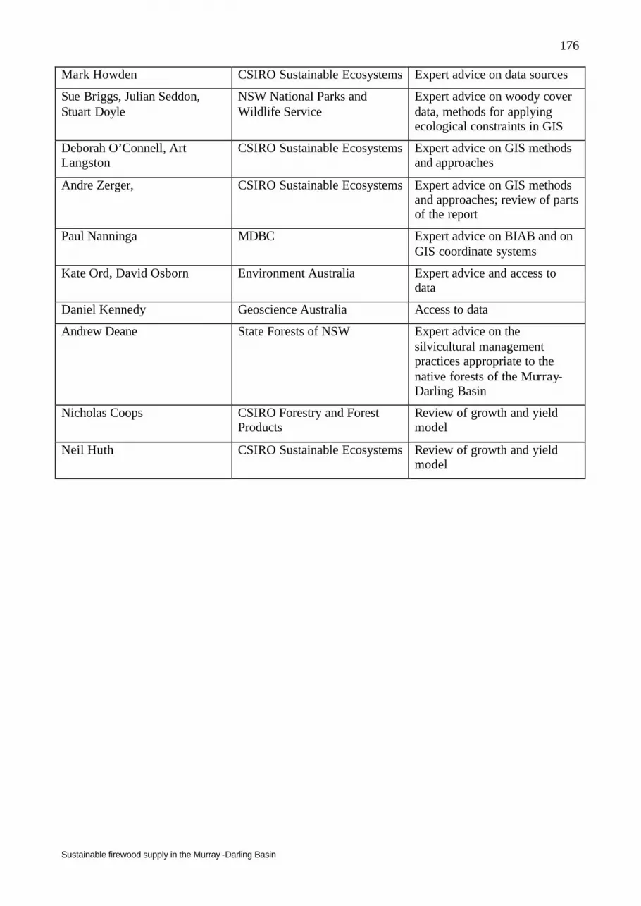
Sustainable firewood supply in the Murray -Darling Basin
176
Mark Howden CSIRO Sustainable Ecosystems Expert advice on data sources
Sue Briggs, Julian Seddon, Stuart Doyle
NSW National Parks and Wildlife Service
Expert advice on woody cover data, methods for applying ecological constraints in GIS
Deborah O’Connell, Art Langston
CSIRO Sustainable Ecosystems Expert advice on GIS methods and approaches
Andre Zerger, CSIRO Sustainable Ecosystems Expert advice on GIS methods and approaches; review of parts of the report
Paul Nanninga MDBC Expert advice on BIAB and on GIS coordinate systems
Kate Ord, David Osborn Environment Australia Expert advice and access to data
Daniel Kennedy Geoscience Australia Access to data
Andrew Deane State Forests of NSW Expert advice on the silvicultural management practices appropriate to the native forests of the Murray-Darling Basin
Nicholas Coops CSIRO Forestry and Forest Products
Review of growth and yield model
Neil Huth CSIRO Sustainable Ecosystems Review of growth and yield model
Sustainable firewood supply in the Murray -Darling Basin
177
13 References Abbott, I. and Loneragan, O. (1983) Response of Jarrah (Eucalyptus marginata) regrowth to
thinning. Aust. For. Res. 13: 217-29.
Alexandra, J. and Campbell, A. (2003) Plantations and sustainability science: the environmental and political settings. Aust. For. 66: 12-19.
Andren, H. (1994) Effects of habitat fragmentation on birds and mammals in landscapes with different proportions of suitable habitat: a review. Oikos 71: 355-366.
Andrew, N., Rodgerson, L. and York, A. (2000) Frequent fuel-reduction burning: the role of logs and associated leaf litter in the conservation of ant biodiversity. Austral Ecology 25(1): 99-107
ANZECC (2001) National Approach to Firewood Collection and Use in Australia. Department of Environment and Heritage, Commonwealth of Australia.
Austin, M.P, Cawsey, E.M., Baker, B.L., Yialeloglou, M.M., Grice, D.J. and Briggs, S.V. (2000) Predicted Vegetation Cover in the Central Lachlan Region. Final Report of the Natural Heritage Trust Project AA 1368.97. CSIRO Wildlife and Ecology, Canberra. www.cse.csiro.au/research/Program2/SL/Lachlan_veg.htm (December 14 2001).
Avery, T.E. and Burkhart, H.E. (2002) Forest Measurements, 5th Ed. McGraw-Hill: New York.
Baalman, E. (2002) Tree volume and taper equations for New South Wales white cypress pine. Unpublished Tech. Note No. 8, Forest Resources Branch, State Forests NSW.
Barkstrom, B. (1981) What time does the sun rise and set? Byte 6(7), 94-114.
Barrett, D.J. (2002) Steady state turnover time of carbon in the Australian terrestrial biosphere. Global Biogeochem. Cycles 16: 1108-1129.
Barrett, G. and Davidson, I. (1999) Community monitoring of woodland habitats - the birds on farms survey. Temperate Eucalypt Woodlands in Australia. Biology, “Conservation, Management and Restoration.” eds. R. J. Hobbs & C. J. Yates. Surrey Beatty & Sons, Chipping Norton, NSW, pp. 382-399.
Barrett, G.W., Ford, H.A. and Recher, H.F. (1994) Conservation of woodland birds in a fragmented rural landscape. Pacific Conservation Biology, 1, 245-256.
Barrett, G., Silcocks A., Barry, S., Cunningham, R. and Poulter, R. (2003) The New Atlas of Australian Birds. Birds Australia (Royal Australasian Ornithologists Union), Melbourne.Barrett, G.W. (2000) Birds on farms: ecological management for agricultural sustainability / by Geoff Barrett. Wingspan, v. 10, no. 4. Suppl. Hawthorn East, Victoria: Birds Australia.
Battaglia, M. and Sands, P. (1997) Modelling site productivity of Eucalyptus globulus in response to climatic and site factors. Aust. J. Plant Physiol. 24, 831-850.
Battaglia, M., Cherry, M.L., Beadle, C.L., Sands, P.J. and Hingston, A. (1998) Prediction of leaf area index in eucalypt plantations: effects of water stress and temperature. Tree Physiol. 18: 521-528.
Battaglia, M., Mummery, D. and Smith, A. (2002) Economic analysis of site survey and production modelling for the selection of plantation areas. For. Ecol. Manage. 162: 185-195.
Battaglia, M., Sands, P.J. and Candy, S.G. (1999) Hybrid growth model to predict tree height and volume growth in young Eucalyptus globulus plantations. For. Ecol. Manage. 120: 193-201.

Sustainable firewood supply in the Murray -Darling Basin
178
Bauhus, J., McElhinny, C.M. and Alcorn, P. (2002) Stand structure and tree growth in uneven-ages spotted gum (Corymbia maculata) forests: some implications for management. Forestry, 75: 451-456.
Bauhus, J.J, Aubin, I., Messier, C. and Connell, M. (1999) Understorey composition and structure in a Eucalyptus sieberi regrowth stand 6 years after thinning and fertilisation. Proc. IFA Conference, Hobart.
Bennett, A.F. (1993) Microhabitat use by the long-nosed potoroo, Potorous tridactylus, and other small mammals in remnant forest vegetation of south-western Victoria. Wildlife Research 20: 267-285.
Bennett, A.F. and Ford, L. A. (1997) Land use, habitat change and the conservation of birds in fragmented rural environments: a landscape perspective from the Northern Plains, Victoria, Australia Pacific Conservation Biology 3: 244-261.
Bennett, A.F., Henein, K. and Merriam, G. (1994) Corridor use and the elements of corridor quality: chipmunks and fencerows in a farmland mosaic. Biological Conservation 68: 155-165.
Bi, H. and Hamilton, F. (1998) Stem volume equations for native tree species in southern New South Wales and Victoria. Aust. For. 61: 275-86.
Bi, H., Wan, G. and Turvey, N.D. (2000) Estimating the self- thinning boundary line as a density-dependent stochastic biomass frontier. Ecology: Vol. 81, No. 6, pp. 1477–1483
Biddiscombe, E.F., Rogers, A.L., Greenwood, E.A.N. and De Boer, E.S. (1985) Growth of tree species near salt seeps, as estimated by leaf area, crown volume and height. Aust. For. Res. 15: 141-154.
Bowman, J.C., Sleep, D., Forbes, G.J. and Edwards, M. (2000) The association of small mammals with coarse woody debris at log and stand scales. Forest Ecology and Management 12:, 119-124.
Brack, C. (1999) School of Forestry and Environmental Science, Australian National University, Canberra, ACT. http://sres.anu.edu.au/associated/mensuration/BrackandWood1998/ DENSITY.HTM (accessed February 2004).
Brack, C (2000) School of Forestry and Environmental Science, Australian National University, Canberra, ACT. http://sres.anu.edu.au/associated/mensuration/forest.htm (accessed February 2004).
Braithwaite, L.W. (1983) Studies on the arboreal marsupial fauna of eucalypt forests being harvested for woodpulp at Eden, N.S.W I. The species and distribution of animals. Australian Wildlife Research 10: 219–229.
Braithwaite, L.W., Dudzinski, M.L., and Turner, J. (1983) Studies on the arboreal marsupial fauna of eucalypt forests being harvested for woodpulp at Eden, N.S.W. II. Relationship between the fauna density, richness and diversity, and measured variables of the habitat. Australian Wildlife Research 10: 231–247.
Braithwaite, L.W., Turner, J. and Kelly, J. (1984) Studies on the arboreal marsupial fauna of eucalypt forests being harvested for woodpulp at Eden, N.S.W. III. Relationships between faunal densities, eucalypt occurrence and foliage nutrients, and soil parent materials. Australian Wildlife Research 11: 41–48.
Briggs, S.V., Doyle, S. and Seddon, J. (unpublished) Areas and numbers of woodland remnants in the wheat/sheep belt of New South Wales.

Sustainable firewood supply in the Murray -Darling Basin
179
Bureau of Meteorology (2003) Media releases for December 2002/January, February, March and April 2003.
Bush, S., Dickson, A., Harman, J.&Anderson, J. (1999) Australian Energy: Market Developments and Projections to 2014-15. Research Report 99.4, Canberra. Australian Bureau of Agriculture and Resource Economics (ABARE).
Candy, S.G. (1997) Growth and yield models for Eucalyptus nitens plantations in Tasmania and New Zealand. Tasforests 9: 167-198.
Catling, P.C. and Burt, R.J. (1994) Studies of the ground dwelling mammals of eucalypt forests in south-eastern New South Wales: the species, their abundance and distribution. Wildl. Res. 21: 219-39.
Catling, P.C. and Burt, R.J. (1995) Studies of the ground dwelling mammals of eucalypt forests in south-eastern New South Wales: the effect of habitat variables on distribution and abundance. Wildl. Res. 22: 271-88.
Catling, P.C. and Burt, R.J. (1997) Studies of the ground dwelling mammals of eucalypt forests in north-eastern New South Wales: the species, their abundance and distribution. Wildl. Res. 24: 1-19
Catling, P.C., Burt, R.J. and Forrester, R.I. (1998) Models of the distribution and abundance of ground-dwelling mammals in the eucalypt forests of south-eastern New South Wales. Wildl. Res. 25: 449-466.
Catling, P.C., Burt, R.J. and Forrester, R.I. (2000) Models of the distribution and abundance of ground-dwelling mammals in the eucalypt forests of north-eastern New South Wales in relation to habitat variables. Wildl. Res. 27: 639-654.
Cavicchiolo, Mark (1991) An investigation into several aspects of the ecological status of the regrowth dry sclerophyll forest at “Mulloon Creek”, a southern tablelands grazing property. Honours Thesis, Dept. Forestry, ANU Canberra.
Clark, N.B. and Rawlins, W.H.M. (1999) Prospects for pulpwood from the Murray Darling Basin. Appita J. 52: 203-212.
Clark, N.B., Read, S.M. and Vinden, P. (1999) Effects of drought and salinity on wood and craft pulps from young plantation eucalypts. Appita J. 52: 93-97.
Clutter, J.L., Fortson, J.C., Pienaar, L.V., Brister, G.H. and Bailey,R.L. (1983) Timber Management. A Quantitative Approach. Wiley: New York.
Cramer, V.A., Thorburn, P.J. and Fraser, G.W. (1999) Transpiration and groundwater uptake from farm forest plots of Casuarina glauca and Eucalyptus camaldulensis in saline areas of southeast Queensland, Australia. Ag. Water Manage. 39: 187-204.
Crawley, M.J.(1993) GLIM for ecologists. Blackwell Scientific Publications, Oxford.
CSIRO (2003) Community Ecology Group, Wildlife, Pests and Diseases Program, CSIRO Sustainable Ecosystems, Gungahlin ACT.
Dames and Moore (1999) Integrating Farm Forestry and Biodiversity. RIRDC Publication No. 99/166. Available from www.rirdc.gov.au/pub/cat/contents.html
Department of Natural Resources and Environment, Victoria. (2002) Victorian Firewood Discussion Paper. May 2002. DNRE Victoria.
Dickman, C.R. (1980) Ecological studies of Antechinus stuartii and Antechinus flavipes (Marsupialia: Dasyuridae) in open forest and woodland habitats. The Australian Zoologist 20: 433-445.

Sustainable firewood supply in the Murray -Darling Basin
180
Draper, N.R. and Smith, H. (1981) Applied Regression Analysis. 2nd Ed. Wiley: New York.
Drew, A., Freudenberger, D. and Briggs, S. (2002) The role of travelling stock routes and other linear remnant vegetation for the conservation of woodland birds in the sheep/wheat zone of central NSW. Canberra: CSIRO Sustainable Ecosystems.
Driscoll, D.A., Milkovits, G. and Freudenberger, D. (2000) Impact and Use of Firewood in Australia. CSIRO Sustainable Ecosystems Report Commissioned by Environment Australia.
Dumbrell, I.C. and McGrath, J.F. (2003) Growth and nutrient relationships of juvenile Pinus pinaster grown on ex-farmland in Western Australia. Aust. For. 66: 137-144.
Eastham, J., Scott, P.R., Steckis, R.A., Barton, A.F.M., Hunter, L.J. and Sudmeyer, R.J. (1993) Survival, growth and productivity of tree species under evaluation for agroforestry to control salinity in the Western Australian wheatbelt. Agroforestry Systems 21: 223-237.
Ellis, R.C., Ratkowsky, D.A., Mattay, J.P. and Rout, A.F. (1987) Growth of Eucalyptus delegatensis following partial harvesting of multi-aged stands. Aust. For. 50: 95-105.
Field, J.B. and Banks, J.C.G. (1999) Effects of silvicultural treatments on growth rates of trees and diversity of understorey in a private dry sclerophyll forest, Southern Tablelands, NSW. Proceedings from the 18th IFA Conference “Practising Forestry Today” October 1999, pp 130-135.
Fisher, A.M. (1997) The distribution and abundance of avifauna in the Bathurst landscape: implications for conservation and land management. Charles Sturt University. PhD Thesis.
Fitzpatrick, E.A. (1963) Estimates of pan evaporation from mean maximum temperature and vapour pressure. J. App. Meteorol. 2: 780-792.
Florence, R.G. (1996) Ecology and silviculture of Australian eucalypt forests. CSIRO Publishing, Melbourne.
Ford, H. (1985) A synthesis of foraging ecology and behaviour of birds in eucalypt forests and woodlands. In: “Birds of Eucalypt Forests and Woodlands”, pp 249-54, Eds A. Keast, H.F. Recher, H. Ford and D. Saunders, Surrey Beatty and Sons and RAOU, NSW.
Forestry Commission of New South Wales (1983) Notes on the silviculture of major NSW forest types. 3. Dry Sclerophyll Ash Types.
Freudenberger, D.O. (2001) Bush for the Birds: Biodiversity enhancement guidelines for the Saltshaker Project, Boorowa, NSW. CSIRO Sustainable Ecosystems, Canberra ACT.
Freudenberger, D.O. and Stol, J.M. (2002) A biodiversity strategy and plan for the Australian Rice Industry. CSIRO Sustainable Ecosystems, Canberra ACT.
FTSUT (1989) Fuelwood Use and Supply in Australia. Forestry Technical Services Pty Ltd and University of Tasmania, Department of Primary Industries and Energy, Canberra.
Gerrand,A., Keenan, R.J., Kanowski, P. and Stanton, R. (2003) Australian forest plantations: an overview of industry, environmental and community issues and benefits. Aust. For. 66: 1-8.
Gibbons, P. (1999) Habitat-tree retention in wood production forests. PhD thesis, Australian National University, Dept. Zoology, Canberra.
Gibbons, P. and Lindenmayer D.B. (2002) “Tree Hollows and Wildlife Conservation in Australia.” CSIRO Publishing, Melbourne.
Gibbons, P. and Lindenmayer, D.B. (1996) Issues associated with the retention of hollow-bearing trees within eucalypt forests managed for wood production. Forest Ecology and Management 83: 245-79.

Sustainable firewood supply in the Murray -Darling Basin
181
Gibbons, P. and Lindenmayer, D.B. (1997) “Conserving hollow-dependent fauna in timber-production forests”, NSW National Parks and Wildlife Service, Hurstville, N.S.W.
Gibbons, P., Lindenmayer, D.B., Barry, S.C. and Tanton, M.T. (2000) Hollow formation in eucalypts from temperate forests in southeastern Australia. Pacific Conservation Biology 6: 218-28.
Gibbons, P., Lindenmayer, D.B., Barry, S.C. and Tanton, M.T. (2002) Hollow selection by vertebrate fauna in forests of southeastern Australia and implications for forest management. Biological Conservation 103: 1–12
Glanznig, A (1995) Native vegetation clearance, habitat loss and biodiversity decline; an overview of recent native vegetation clearance in Australia and its implications for biodiversity. Biodiversity Series. Paper No. 6. Biodiversity Unit, Department of Environment and Heritage, Australia.
Gould, Lori (2003) Flora of Picaree Hill. Unpublished report. Greening Australia ACT and SE Region, Canberra ACT.
Greenwood, E.A.N., Biddiscombe, E.F., Rogers, A.L., Beresford, J.D. and Watson, G.D. (1995) Growth of species in a tree plantation and its influence on salinity and groundwater in the 400 mm rainfall region of south-western Australia. Ag. Water Manage. 28: 231-243.
Grove S. (2002) Tree basal area and dead wood as surrogate indicators of saproxylic insect faunal integrity: a case study from the Australian lowland tropics. Ecological Indicators 1: 171-188.
Hamilton, D.I. and Cowley, N.B. (1987) Southern Tablelands Eucalypts of New South Wales. Forest Management in Australia: Proceedings of the Conference of the Institute of Foresters of Australia, Perth, Western Australia.
Hamilton, F. (1988) Spatial pattern and stand development in even-aged stands with contagious spatial patterns. In: “Modelling Trees, Stands and Forests” Eds. J.W. Leech, R>E> McMurtrie, P.W. West, R.D. Spencer, and B.M. Spencer, Bulletin 5, pp 361-373, School of Forestry, University of Melbourne.
Hobbs, R., Catling, P.C., Wombey, J.C., Clayton, M., Atkins, L. and Reid, A. (2003) Faunal use of Blue Gum (Eucalyptus globulus) plantations in southwestern Australia. Agroforestry Systems 58 (3), pp. 195-212
Horne, R. (1990) Early espacement of wheatfield white cypress pine regeneration: the effect on secondary regeneration, limb size and stand merchantability. Aust. For. 53, 160-7.
Hutchinson, M.F., Booth, T.H., McMahon, J.P. and Nix, H.A. (1984) Estimating monthly mean values of daily total solar radiation for Australia. Solar Energy 32: 277-290.
Hutchinson, M.F., Nix H.A., Houlder, D.J. and McMahon, J.P. (1999) ANUCLIM Version 1.8; A software package for systematic interrogation of climate surface coefficient files, as created by the ANUSPLIN package, for biophysical applications. Centre for Resource and Environmental Studies, Australian National University.
Ilic, J., Boland, D., McDonald, M., Downes, G. and Blakemore, P. (2000) Woody density phase 1 - state of knowledge. National Carbon Accounting System, Tech. Rep. No. 18, Australian Greenhouse Office: Canberra.
Jack, S.B. and Long, J.N. (1996) Linkages between silviculture and ecology: an analysis of density management diagrams. For. Ecol. Manage. 86: 205-220.
Jacobs, M.R. (1955) “Growth Habits of the Eucalypts”. Forestry and Timber Bureau, Commonwealth Govt. Printer, Canberra.

Sustainable firewood supply in the Murray -Darling Basin
182
Johnston, T.N. and Jennings, K.S. (1991) Management of cypress pine forests in Queensland. In Forest Management in Australia (eds F.H. McKinnell, E.R. Hopkins and J.E.D. Fox). Surrey Beatty & Sons in association with Institute of Foresters of Australia.
Kellas, J.D & Hateley, R.F. (1987) Management of dry sclerophyll forests in Victoria; 1. The low elevation mixed species forests. Forest Management in Australia: Proceedings of the Conference of the Institute of Foresters of Australia, Perth, Western Australia.
Knott, J (1995) White cypress pine thinning trials of the Western Region. Research Paper No. 27. Research Division. State Forests of New South Wales. Sydney.
Lambert, M. and Turner, J. (2000) Commercial Forest Plantations on Saline Lands. CSIRO, Melbourne.
Landsberg, J.J. and Kesteven, J. (2002) Spatial estimation of plant productivity. pp 33-50 In Richards,G.P. (Ed) Biomass Estimation: Approaches for Assessment of Stocks and Stock Change. National Carbon Accounting System, Technical Report No. 27. Australian Greenhouse Office: Canberra.
Lacey, C. J. (1973) Silvicultural characteristics of white cypress pine. Forestry Commission of NSW, Research Note No. 26. 51 pp.
Laven, N. and Mac Nally, R. (1998) Association of birds with coarse woody debris in box- ironbark forests of central Victoria. Corella 22: 56-60.
Lindenmayer, D.B., Cunningham, R.B., Tanton, M.T. and Smith, A.P. (1991) Characteristics of hollow-bearing trees occupied by arboreal marsupials in the montane ash forests of the central highlands of Victoria, south-east Australia. Forest Ecology and Management 40: 289-308.
Loyn, R.H. (1986) The 20 minute survey – a simple method for counting birds. Corella 10: 58-64.
Mac Nally, R. and Horrocks, G. (2002) Habitat change and restoration: responses of a forest–floor mammal species to manipulations of fallen timber in floodplain forests. Animal Biodiversity and Conservation 25:1-12
Mac Nally, R., Horrocks, G. and Pettifer, L. (2002) Experimental evidence for potential beneficial effects of fallen timber in forests. Ecological Applications 12: 1588-1594.
Mac Nally, R., Parkinson, A. Horrocks, and Young, M. (2000) Current loads of coarse woody debris on south-eastern Australian floodplains. Report No. R7007. Murray Darling Basin Commission, Natural Resource Management Scheme I and E Program, Riverine Program.
Mac Nally, R., Parkinson, A. Horrocks, G., Conole, L. and Tzaros, C. (2000) Relationship between vertebrate biodiversity and abundance and availability of coarse woody debris on south-east Australian floodplains. Report No. R7007.lll Murray Darling Basin Commission, Natural Resource Management Scheme I and E Program, Riverine Program.
Mac Nally, R., Parkinson, A., Horrocks, G., Conole, L. and Tzaros, C., (2001). Relationships between terrestrial vertebrate diversity, abundance and availability of coarse woody debris on south-eastern Australian floodplains. Biological Conservation 99: 191–205.
Mackensen, J. and Bauhus, J. (1999) The decay of coarse woody debris. National Carbon Accounting System, Technical Report No. 6. Australian Greenhouse Office: Canberra.
Mackowski, C.M. (1984) The ontogeny of hollows in Blackbutt (Eucalyptus pilularis) and its relevance to the management of forests for possums, gliders and timber. In: “Possums and Gliders”, Eds. A.P. Smith and I.D. Hume, pp. 517-25, Surrey Beatty and Sons: Chipping Norton, Sydney.

Sustainable firewood supply in the Murray -Darling Basin
183
Marcar, N.E. and Khanna,P .K. (1997) Reforestation of salt-affected and acid soils. pp 481-525 In Nambiar,E.K.S. and Brown,A.G. (Eds) Management of Soil, Nutrients and Water in Tropical Plantation Forests. ACIAR Monograph No. 43, Canberra.
Mazanec, Z. (1999a) Nine year results from a Eucalyptus camaldulensis Denh. provenance trial in the Wellington catchment of Western Australia. Aust. For. 62: 166-172.
Mazanec, Z. (1999b) Thirteen year results from a Spotted Gum provenance trial in the Wellington catchment of Western Australia. Aust. For. 62: 315-319.
McDonald, R.C., Isbell, R.F., Speight, J.G., Walker, J. and Hopkins, M.S. (1990) Australian Soil and Land Survey Field Handbook. Inkata Press, Melbourne
McElhinny, C (2002) Forest and woodland structure as an index of biodiversity: a review. 80p. (unpublished) NSW NPWS.
McIntyre, S., McIvor, J.G. and MacLeod, N.D. (2000) Principles for sustainable grazing in eucalypt woodlands: Landscape-scale indicators and the search for thresholds. In: Management for Sustainable Ecosystems Eds. P. Hale, A. Petrie, D. Maloney and P. Sattler. Centre for Conservation Biology, University of Queensland, Brisbane.
McKenzie, N. and Hook, J. (1992) Interpretations of the Atlas of Australian Soils. CSIRO Division of Soils, Technical Report 94/1992.
McKenzie, N., Ryan, P., Fogarty, P. and Wood, J. (2000) Sampling, measurement and analytical protocols for carbon estimation in soil, litter and coarse woody debris. National Carbon Accounting System, Technical Report No. 14. Australian Greenhouse Office: Canberra.
McMahon, J.P., Hutchinson, M.F., Nix, H.A. and Ord, K.D. (1996) ANUCLIM Version 1 User’s Guide. CRES, ANU, Canberra.
MDBC (2003) website http://www.mdbc.gov.au/education/encyclopedia/forestry/forestry.htm (February 2004).
Michael, Damian (2003) http://www.csu.edu.au/research/jcentre/project_summaries/JCSummary_DM_Fence%20Posts.pdf (February 2004).
Morton, S.R., Short, J. and Barker R.D. (1995) Refugia for Biological Diversity in Arid and Semi-arid Australia with an Appendix by G.F. Griffin and G. Pearce. Biodiversity Series, Paper No. 4, Biodiversity Unit, Department of Environment and Heritage, Canberra.
Morris, J., Mann, L. and Collopy, J. (1998) Transpiration and canopy conductance in a eucalypt plantation using shallow saline groundwater. Tree Physiol. 18: 547-555.
Murray, F.W. (1967) On the computation of saturation vapour pressure. J. Appl. Meteorol. 6: 203-204.
Murtagh, B.A. and Saunders, M.A. (1978) Large-scale linearly constrained optimization. Mathematical Programming 14: 41-72.
Murtagh, B.A. and Saunders, M.A. (1983) MINOS 5.0 Users Guide. Systems Optimization Laboratory, Department of Operations Research, Stanford University, Tech. Rep. SOL 83-20.
Myers, B.J. Theiveyanathan, S., O'Brien, N.D. and Bond, J.W. (1996) Growth and water-use of Eucalyptus grandis and Pinus radiata plantations irrigated with effluent. Tree Physiol. 16: 211-219.

Sustainable firewood supply in the Murray -Darling Basin
184
Myers, B.J., Benyon, R.G., Theiveyanathan, S., Criddle, R.S., Smith, C.J. and Falkiner, R.A. (1998) Response of effluent- irrigated Eucalyptus grandis and Pinus radiata to salinity and vapour pressure deficits. Tree Physiol. 18: 565-573.
National Forest Inventory (1998) Australia’s State of the Forests Report 1998. Bureau of Rural Sciences: Canberra.
National Forest Inventory. (2003) National plantation inventory annual update - March 2003. Bureau of Rural Sciences: Canberra.
National Forest Policy Statement. (1995) A new focus for Australia's forests. Commonwealth of Australia December 1992, Second Edition 1995.
Neagle, N. (1994) The environmental impact and ecological sustainability of woodcutting in South Australia. Adelaide: Native Vegetation Conservation Section, Dept. of Environment and Natural Resources.
New, B. and England, M. (2002) Farm Forestry: Designing for increased biodiversity. Primary Industries and Natural Resources: South Australia.
Newsome, A.E. and Catling, P.C. (1979) Habitat preferences of vertebrates inhabiting heathlands of coastal, montane and alpine regions of south-east Australia. In "Ecosystems of the World: Volume 9A. Heathlands and related shrublands" Ed. R.L. Specht, pp. 301-16, Elsevier Scientific Publishing Co., Amsterdam.
Nicholls, A.O. (1991) An introduction to statistical modelling using GLIM. In: “Nature Conservation: cost effective biological surveys and data analysis”, Eds. Margules, C.R. and Austin, M.P., pp. 54-63, CSIRO: Melbourne
Nicholson, D. (1997) Managing Cypress Pine on your property. State Forests and North West Catchment Management Committee, NSW. 13 pp.
Noss, R.F. (1990) Indicators for monitoring biodiversity: a hierarchial approach. Conservation Biology 4: 355-364.
NSW National Parks and Wildlife Service (1998) Tinderry Nature Reserve Plan of Management. http://www.nationalparks.nsw.gov.au/PDFs/pom_final_tinderry.pdf (February 2004).
NSW National Parks and Wildlife Service (2002) ID Guidelines for Box-Gum Woodland. http://www.nationalparks.nsw.gov.au/PDFs/box-gum_id_guidelines.pdf (February 2004)
NSW National Parks and Wildlife Service (2003) Mundoonen Nature Reserve Draft Plan of Management. NSW NPWS Report.
Race, D. (1999) Regiona l farm forestry industries: potential dimensions and possible outcomes. Aust. For. 62: 182-192.
Race, D. and Curtis, A. (1997) Socio-economic considerations for regional farm forestry development. Aust. For. 60: 233-239.
Race, D. and Freudenberger, D. (2003) Farm Forestry for Green and Gold: Australian experiences of linking biodiversity to commercial forestry. ANU Forestry & CRC Sustainable Production Forestry and CSIRO Sustainable Ecosystems. ANU and Environment Australia, Canberra.
Raymond, C.A. and MacDonald, A.C. (1998) Where to shoot your pilodyn: within tree variation in basic density in plantations of Eucalyptus globulus and E. nitens in Tasmania. New Forests 15: 205-221.

Sustainable firewood supply in the Murray -Darling Basin
185
Rayner, M.E. and Turner, B.J. (1990a) Growth and yield modelling of Australian eucalypt forests I. Historical development. Aust. For. 53: 224-237.
Rayner, M.E. and Turner, B.J. (1990b) Growth and yield modelling of Australian eucalypt forests II. Future trends. Aust. For. 53: 238-247.
Reid, J.R.W. (1999) Threatened and declining birds in the New south Wales sheep-wheat belt: I. Diagnosis, characteristics and management. Report to the NSW National Parks and Wildlife Service. CSIRO Wildlife and Ecology, Canberra.
Reid, J.R.W. (2000) Threatened and declining birds in the New south Wales sheep-wheat belt: II. Landscape relationships - modelling bird atlas data against vegetation cover. Report to the NSW National Parks and Wildlife Service. CSIRO Wildlife and Ecology, Canberra.
Reynolds, M.R. (1984) Estimating the error in model predictions. For. Sci. 30: 454-469.
Ritman KT (1995) Structural Vegetation Data: a specifications manual for the Murray Darling Basin Project M305. DLWC: NSW.
Salt, D., Hobbs, R. and Lindenmayer, D. (2004). Farm forestry and biodiversity: A guide for farm foresters wanting to improve nature conservation in their plantings. Rural Industries R&D Corporation.
Sands, P., Battaglia, M. and Mummery, D. (2000) Application of process-based models to forest management: experience with PROMOD, a simple plantation productivity model. Tree Physiol. 20: 383-392.
Sands, P., Rawlins,W. and Battaglia, M. (1999) Use of a simple plantation productivity model to study the profitability of irrigated E. globulus. Ecol. Mod. 117: 125-141.
Saunders, D. & Ingram, J.A. (1995) “Birds of Southwestern Australia : an Atlas of Changes in the Distribution and Abundance of Wheatbelt Avifauna”. Surrey Beatty & Sons, Chipping Norton NSW in association with Western Australian Laboratory, CSIRO Division of Wildlife and Ecology.
Schirmer, J., Kanowski, P. and Race, D. (2000) Factors affecting adoption of plantation forestry on farms: implications for forestry development in Australia. Aust. For. 63: 44-51.
Schumacher, F.X. (1939) A new growth curve and its application to timber yield studies. J. For. 37: 619-620.
Seddon, J., Briggs, S. and Doyle, S. (2002) Little River Catchment Biodiversity Assessment: A report for the TARGET project. Canberra: NSW National Parks and Wildlife Service.
Seddon, J., Briggs, S. and Doyle, S. (in press) Relationships between bird species and characteristics of woodland remnants in central New South Wales. Pacific Conservation Biology.
Semple, K.E. (1994) A history of a dry sclerophyll forest stand at Mulloon Creek, Southern Tablelands, NSW. Honours Thesis, Dept. Forestry, ANU, Canberra.
Senelwa, K. and Sims, R.E.H. (1999) Fuel characteristics of short rotation forest biomass. Biomass and Bioenergy 17: 127-140.
Smith, A.P. and Lindenmayer, D.B. (1988) Tree hollow requirements of Leadbeater's possum and other possums and gliders in timber production ash forests of the Victorian central highlands. Australian Wildlife Research 15: 347-62.

Sustainable firewood supply in the Murray -Darling Basin
186
Smith, P. (1985) Woodchip logging and birds near Bega, New South Wales. In: “Birds of Eucalypt Forests and Woodlands”, Eds A. Keast, H.F.Recher, H. Ford and D. Saunders, Surrey Beatty and Sons and RAOU, NSW.
Snowdon, P. (1991) A ratio estimator for bias correction in logarithmic regression. Can. J. For. Res. 21: 720-724.
Snowdon, P., Eamus, D., Gibbons, P., Khanna, P.K., Keith, H., Raison, R.J. and Kirschbaum, M.U.F. (2000) Synthesis of allometrics, review of root biomass and design of future woody sampling strategies. National Carbon Accounting System, Technical Report No. 17, Australian Greenhouse Office: Canberra.
Stanton, R. (1999) Plantations for Australia - the 2020 vision. Int. For. Rev. 1: 189-93.
Tolhurst, K. and Flinn, D. (1992) Ecological impacts of fuel reduction burning in dry sclerophyll forest: first progress report. Research Report No. 349, Forest Reseach Section, Research Development and Assessment Branch, Department of Conservation and Environment, Victoria.
Tongway, D. (2003) Reading the Landscape. A training course in monitoring rangelands by landscape function analysis. CSIRO Sustainable Ecosystems, Canberra.
Tongway, D. and Hindley, N. (1995) Manual for assessment of soil condition in tropical grasslands. CSIRO Australia. ISBN 0 643 05779 X.
Tongway, D. and Hindley, N. (1995) Manual for Soil Condition Assessment of Tropical Grasslands. CSIRO Sustainable Ecosystems, Canberra ACT.
Tongway, D. and Ludwig, J. (1997) The Conservation of Water and Nutrients within Landscapes. In: “Landscape Ecology, Function and Management : Principles from Australia's Rangelands”, Eds. Ludwig, J., Tongway, D., Freudenberger, D., Noble, J., and Hodgkinson. CSIRO Publishing, Canberra
Turland, J.H. (2003) Tree level modelling in western New South Wales; uneven-aged mixed species forests. pp 131-43, Mason,E.G. & Perley,C.J. (Eds) Proc. Aust & NZ Institute of Forestry Conf, Wellington NZ, April 2003.
Turnbull, J.W. and Pryor, L.D. (1978) Choice of species and seed source. pp 6-65 In “Eucalypts for Wood Production.” Eds W.E. Hillis and Brown, A.G., CSIRO: Australia.
Turner, B.J., Chikumbo, O. and Davey, S.M. (2002) Optimisation modelling of sustainable forest management at the regional level: an Australian example. Ecol. Mod. 153: 157-79.
Vanclay, J.K. (1992) Assessing site productivity in tropical moist forest: a review. For. Ecol. Manage. 54: 257-287.
Vanclay, J.K. (1985) A stand growth model for cypress pine. pp 310-332 In Leech, J.W., McMurtrie, R.E., West, P.W., Spencer, R.D. and Spencer, B.M. (Eds) Modelling Trees, Stands and Forests. Bulletin No. 5, School of Forestry, University of Melbourne.
Vertessy, R.A., Zhang, L. and Dawes, W.R. (2003) Plantations, river flows and river salinity. Aust. For. 66: 55-61.
Walker, J. and Hopkins, M.S. (1998) Vegetation. In: “Australian Soil and Land Survey Field Handbook”, Eds. R. C. McDonald, R. F. Isbell, J. R. Speight, J. Walker and M. S. Hopkins, 3rd Edition, Vol. 3, pp. 58–77, Inkata Press, Melbourne.
Wall, J. (1997) Sustainability of the Armidale fuelwood industry on the Northern Tablelands of New South Wales: resource yield, supply, demand and management options. PhD Thesis, University of New England.

Sustainable firewood supply in the Murray -Darling Basin
187
Wardell-Johnson, G.; Williams, M. (2000) Edges and gaps in mature karri forest, south-western Australia: logging effects on bird species abundance and diversity. Forest Ecology and Management 131: 1-21
Washusen, R., Blakemore, P., Northway, R., Vinden, P. and Waugh, G. (2000a) Recovery of dried appearance grade timber from Eucalyptus globulus Labill. grown in plantations in medium rainfall areas of the southern Murray-Darling Basin. Aust. For. 63: 277-283.
Washusen, R., Waugh, G. and Hudson, I. (2000b) Appearance product potential of plantation hardwoods from medium rainfall areas of the southern Murray-Darling Basin. Green product recovery. Aust. For. 63: 66-71.
Watson D.M., Mac Nally, R. and Bennett, A.F. (2000) The avifauna of severely fragmented Buloke Allocasurina luehmanni woodland in western Victoria, Australia. Pacific Conservation Biology 6: 46-60.
Watson, D.M., Freudenberger, D. and Paull, D. (2001) An assessment of the Focal Species Approach for Conserving Birds in Variegated Landscapes in South-eastern Australia. Conservation Biology 15: 1364 - 1373.
Weller, D.E. (1987) A reevaluation of the -3/2 power rule of plant self- thinning. Ecol. Monog. 37: 23-43.
West, P.W. (1983) Comparison of stand density measures in even-aged regrowth eucalypt forest of southern Tasmania. Can. J. For. Res. 13: 22-31.
West, P.W. (1985) Density management diagrams and thinning practice in monoculture. pp 163-168 In Mead, D.J. and Ellis, R.C. (Eds). Proc. Australia and New Zealand Institutes of Foresters Conference, May 1985
West, P.W. (2004) “Tree and Forest Measurement”, Springer: Heidelberg.
West, P.W. and Osler, G.H.R. (1995) Growth response to thinning and its relation to site resources in Eucalyptus regnans. Can. J. For. Res. 25: 69-80.
White, D.A., Turner, N.C. and Galbraith, J.H. (2000) Leaf water relations and stomatal behaviour of four allopatric Eucalyptus species planted in Mediterranean southwestern Australia. Tree Physiology 20: 1157-1165.
Weins, J.A. (1989) “The Ecology of Bird Communities.” Cambridge: Cambridge University Press.
Williams, M.R., Abbott, I., Liddelow, G.L., Vellios, C., Wheeler, I.B. and Mellican, A.E (2001) Recovery of bird populations after clearfelling of tall open eucalypt forest in Western Australia. J. Appl. Ecology 38: 910 - 920
Woldendorp, G., Keenan, R.J. and Ryan, M.F. (2002) Coarse woody debris in Australian forest ecosystems. A Report for the National Greenhouse Strategy, Module 6.6 (Criteria and Indicators of Sustainable Forest Management). Bureau of Rural Sciences, Commonwealth of Australia
Zeide, B. (1985) Tolerance and self- tolerance of trees. For. Ecol. Manage. 13: 149-166.