Sustainability of forestry in Romania Analysis using a dynamic simulation model; a

case for public access to information on natural resources

Thesis Submitted to the Department of Geography

in Partial Fulfillment of the Requirements for the Degree of Master of Philosophy in System Dynamics

Emil Zaharia-Kézdi Supervisor: Prof. Erling Moxnes

12.08.2019 System Dynamics Group

Department of Geography Social Science Faculty

University of Bergen

Table of contents

Abstract 1

1. Introduction 2

2. Methodology and data 4

2.1 Methodology 4 2.2. Data 5

3. Model structure 11

3.1. Area 11 3.2. Age 12 3.3. Volume and density 13 3.4. Growth 16 3.5. Extraction and regeneration 17

4. Model results and analysis 20

4.1. Reproducing historical data for 2012-2018 20 4.2. Base run 24 4.3. Sensitivity analysis within range of uncertainty 25 4.4. Scenario runs 27

5. Discussion 33

5.1. Limitations 33 5.2. Main takeaways 35

5.3. Future research 37

6. Conclusions 38

References 39

Equations

1. Area - integration 11

2. Area - Euler integration 11

3. Age 11

4. Volume and density 14

5. Growth 16

6. Extraction and regeneration 18

Figures

1. Forested area 11

2. Forested area by age group – homogenous stocks 12

3. Forested area by age group – conveyor stocks 13

4. Volume and density 14

5. Growth 16

6. Extraction and regeneration 18

Graphs

1. Forest area by age group – dataset A 7

2. Forest area by age group – dataset B 8

3. Comparison of datasets 8

4. Forest density by age group 9

5. Volume of wood by age group – dataset A 9

6. Volume of wood by age group – dataset B 10

7. Forest density curve 15

8. Forest growth function 17

9. Indicated forest age distribution for 2012 20

10. Indicated loss of wood by age group 20

11. Base run – dataset comparion 24

12. Base run – volume, growth and loss 25

13. Latin Hypercube test – growth 26

14. Latin Hypercube test – volume 27

15. Scenario run – growth and loss 29

16. Scenario run – volume 29

17. Policy run – adapted logging distribution 30

18. Policy run – 100 years 31

19. Policy run – 400 years 31

20. Policy run – 400 years – no area growth 32

Tables

1. Deviation from historical data – forest area by age group 11

2. Deviation from historical data – forest density by age group 12

3. Deviation from historical data – volume of wood by age group 13

4. Deviation from historical data – total loss of volume 14

5. Deviation from historical data – total growth of volume 16

6. Margins of error for uncertainty analysis 18

1

Abstract

There have been ample studies on the sustainability of Romanian forestry from a

qualitative perspective. Quantitative studies on Romania’s forests, however, have

focused on either static analysis, or historical analysis. There have been no quantitative

studies on the sustainability of Romanian forestry from a natural resource management

standpoint. This research addresses the question of whether logging levels in Romania

are sustainable, using a quantified dynamic simulation model. The results show that

current levels of logging would lead to undesirable outcomes in the future, were they to

be held at the same level. It also shows that, the levels of logging determined by actual

forestry policies would be both sustainable, and lead to forest volume growth: a desirable

outcome considering global carbon sequestration goals. The results indicate that early

action to bring logging levels down to the level indicated by policies could have a large

positive impact over the course of the next few decades. The relation between the model

and the underlying data also showcases the importance of open data access on natural

resources. Many parts of the model could be improved with open access to data, and

inconsistencies in the data can more easily be brought to light. Solving these

inconsistencies is important, as smart policies require an adequate understanding of both

the actual state of the forests, as well as the rates of change that affect them.

Keywords: sustainability; forestry; Romanian forests; system dynamics; logging policy.

Acronyms

FAO Food and Agriculture Organization of the United Nations

NFI National Forest Inventory (Inventarul Forestier Național)

INCDS The „Marin Drăcea” National Institute of Research and

Development in Silviculture (Institutul Național de Cercetare-

Dezvoltare în Silvicultură „Marin Drăcea”)

NIS National Institute of Statistics (Institutul Național de Statistică)

NFA National Forest Administration – Romsilva (Regia Națională a

Pădurilor – Romsilva)

2

1. Introduction

The Romanian forestry sector and forest resources are important at both the national and

global level along many dimensions. At the national level, the forestry sector provides

employment and contributes significantly to the economy (Abrudan et al., 2009;

Bouriaud and Marzano, 2014). At the same time, the forests provide essential ecosystem

services, and are critical for carbon sequestration for combatting climate change

(Government of Romania, 2017b). The Carpathians in Romania are of outstanding

importance for nature conservation (Soran et al., 2000; Stăncioiu, Abrudan and Dutca,

2010; Knorn et al., 2012), as Romania still has a lot of old-growth, primary forests that

are important for biodiversity (Biriș and Veen, 2005; Knorn et al., 2013; Munteanu et

al., 2016; Sabatini et al., 2018; Veen et al., 2010).

Though Romania has been confronting issues of forest management since 1895 (Leahu,

2001), it still faces challenges in the sustainable management of its forest resources. The

challenges include the restitution of its forest resources to private owners (Ioras, 2002;

Ioras and Abrudan, 2006; Măntescu and Vasile, 2009; Munteanu et al., 2016; Strîmbu,

Hickey and Strîmbu, 2005), privatisation of the wood industry sector and changes in

market demand of wood products (Ioras and Abrudan, 2006; Nichiforel and Schanz,

2009), the separation of competences across institutions (Abrudan et al. 2009),

communication among many different stakeholders (Dragoi, Popa and Blujdea, 2011),

the establishment of new institutions (Popa, Niță and Hălălișan, 2019), conflicting land

use policies inhibiting afforestation efforts (Stăncioiu, Niță and Lazăr, 2018), illegal

logging (Bouriaud, 2005; Knorn et al., 2012) and corruption (Bouriaud and Marzano,

2014).

The proper management of Romania’s natural forest resources is therefore critical in

order to ensure that the forests can sustainably fulfil their roles in climate and ecosystem

regulation, biodiversity conservation, as well as continue contributing to human welfare.

The National Forest Policy and Strategy, developed in 2000, and revised in 2005, stated

the express policy of ensuring forest management according to the principles of

sustainable management of natural resources (Abrudan et al. 2009). The current National

Forest Strategy 2018-2027 (Romanian Government, 2017b) states that the overall vision

is to have a “forestry industry [that] contributes to the well-being of people in an

economically, socially and environmentally sustainable manner”. Furthermore, the

general objective of the current strategy is “the harmonization of the forest’s functions

with the present and future demands of Romanian society through the sustainable

management of national forestry resources”.

3

Though the legal provisions for sustainable forestry are set in place, there are indications

that the application of these provisions have been far from adequate, both from the

scientific community (Buliga and Nichiforel, 2019; Iojă et al., 2010; Knorn et al., 2013;

Knorn et al., 2012) and from NGO’s and investigative journalists (Agent Green 2018a,

2018b; Cernuta, 2019; Greenpeace 2012a; Greenpeace 2012b). The official values for

the overall level of harvesting are themselves being questioned.

One of the most important tools for the sustainable management of Romania’s forest

resources is the National Forest Inventory – NFI (NFI, 2012b, 2019), for which two

cycles have been completed so far (NFI 2012a, 2018). The NFI is the main data provider

for reporting on indicators of sustainable forest management, under the umbrella of

INCDS. Without it, management decisions at the national level would have no basis.

Cernuta (2019), however, has pointed out some irregularities in the data, from which one

of the conclusions that could be drawn is that the volume of wood available has been

undervalued during the first cycle so that more could be harvested between the first and

second cycles, while giving the appearance of sustainable logging levels. This seems all

the more dangerous, since a yearly report on the state of Romania’s forests (Romanian

Government, 2015) claims the following (paraphrasing):

According to the National Institute of Statistics (NIS) the average volume of wood

harvested yearly, legally, during the period 2008-2014, was 17.9 million cubic meters,

while IFN measurements show that the volume of wood harvested yearly at the national

level during this period was closer to 26.69 million cubic meters.

While studies on Romania’s forestry sector have highlighted obstacles to sustainable

forest management, no study so far has attempted to perform a national-level quantified

analysis of the sustainability of logging levels. Given that government reports, NGO’s,

and investigative journalists all claim higher than allowed levels of logging, the present

research aims to address the following question: Are current levels of logging in Romania

sustainable? The question will be addressed from a natural resource management

perspective, using a quantified dynamic simulation model.

4

2. Methodology and data

2.1 Methodology

Due to a number of factors, such as detail complexity and the dynamic behaviour in the

observed system (e.g. changes in yield, age composition, logging levels), a causal

dynamic simulation model is ideally suited for achieving the aim of gaining a holistic

understanding over the problem (Sterman, 1988). Furthermore, causal dynamic

simulation models are ideal laboratories for exploring the future impacts of current

practices and to test different policies (Axelrod, 1997). The importance of using

simulation modelling for sustainable forest management in particular is also well

established (Peng, 2000; Pretzch, 2010; Shanin, Komarov and Bykhovets, 2012).

A stock and flow model based on the system dynamics methodology has been used for

this research (de Gooyert, 2018; Forrester, 1968; Repenning, 2003; Richardson and Pugh,

1981; Sterman, 2000). Stock and flow models have been used to study a wide range of

environmental/natural resource problems (Cavana and Ford, 2004; Ford, 2010), and they

have been applied to the forestry sector as well (Dudley, 2004a; Dudley, 2004b; Jones,

Seville and Meadows, 2002).

The boundaries of the system will be deemed to be sufficiently encompassing when the

model will sufficiently reproduce the reference mode of behaviour (Barlas, 1996;

Richardon and Pugh, 1981), implying an iterative model-building process. In our case,

the reference mode of behaviour is the timber yield of Romania’s forests.

A literature review has been conducted in order to determine the conceptual relationship

between the system elements within a system dynamics framework (Forrester, 1968;

Richardson and Pugh, 1981; Sterman, 2000). Supplementary interviews have been

conducted with industry specialists in order to fill in the gaps in understanding from

literature with real experience (Bryman and Bell, 2011; Forrester, 1992). Since there are

qualitative data involved as well, a rigorous verification and reporting process must be

applied to both the structure of the model, and the emerging behaviour (Barlas, 1996;

Homer, 2012; Rahmandad and Sterman, 2012; Sterman, 1984, 2000).

5

2.2. Data

Secondary quantitative and qualitative data has been used for the creation of the model

structure and for the representation of the historical behaviour. As mentioned before, the

reference mode in question is the timber yield of Romanian forests. However, there is no

single data series available to represent this value. Yield is estimated at the level of forest

districts when their 10-year forest management plans are created. The silvicultural

systems employed, as well as the maximum logging levels are also determined at the

district level. For the purposes of this research, the aggregation of yield and logging

values of each district would be desirable.

Data at this level of disaggregation, however, is not freely available. Furthermore, not all

forests have forest management plans, while the implementation of the existing plans

most often do not meet many technical and legal requirements (Buliga and Nichiforel,

2019). The values presented also do not account for illegal logging, organized excessive

logging, or for errors in estimation by forestry officials: Bouriaud and Marzano (2014)

point out that officials consistently underestimate both the quantity and the quality of the

wood that is to be sold at auctions.1

Due to these obstacles, I have chosen to instead reconstruct the timber yield of Romania’s

forests from other data available at the national level, namely: forested areas, volume of

standing wood, age composition of forests by area and volume, logging levels and growth

estimates by age group. These data have been taken from FAO (2005, 2010, 2015), NFI

(2012a, 2018), NIS (2019) and the Romanian Government (2006, 2007, 2008, 2009,

2010, 2011, 2012b, 2013, 2014, 2015, 2016, 2017a, 2018).

One measure of the confidence we may have in a model is the degree to which it is able

to reproduce historical data (i.e. the reference mode) (Richardson and Pugh, 1981;

Sterman, 2000). While data on timber yield2 is not publicly available, other historical

data is available with which timber yield may be partially reconstructed. We will

therefore focus on a set of 32 reference modes composed of the other variables used:

1 The reason given for the consistent underestimation by an interviewee during this research is that the

officials often choose the lower bound of their estimation in order to avoid any complaints. 2 Yield is defined as net growth of forests, not including logging.

6

1. Forest area by age group

2. Density of forests by age group

3. Volume of wood by age group – product of the first two

4. Overall wood growth

5. Overall wood loss

The starting year for the model is 2012. Though the reproduction of a reference mode

over a longer time horizon would provide more confidence in the results of the model,

this implies that the reference mode itself should reflect reality. There are four reasons

why the starting year 2012 was selected:

1. Before the first NFI cycle from 2012, the last forest inventory was completed in

1984 (NFI, 2019; Romanian Government, 2012a). The methodology with which

that inventory was achieved is out-dated, and therefore it is difficult to compare

the results of that inventory with the results from NFI.

2. The data available before 2012 is more aggregated, the last age population group

specified being ‚age group 101 and above’ instead of ‚age group 181 and above’.

Extrapolating the data over an almost thirty year period is bound to produce

errors, since there are too many unknowns, such as the age groups where harvest

cuttings have occured in the past. Another challenge with extrapolation is having

to account for shifts between age groups.

3. A number of drastic changes have occurred in the forestry sector over the last

three decades. Since in its current stage the model is limited in its scope, it cannot

represent the structural changes that have occurred in the forestry sector. It is

therefore more accurate to start in 2012, where most of the changes have already

taken place.

4. The ontology of forests within the model includes not only the area and the age,

but also the volume of wood. This data is not publicly available before 2012,

except for the aggregated value of ‘total volume of wood’.

More precise results can therefore be achieved by relying only on the most recent data,

since it is of higher quality, and fewer assumptions have to be made. Though the 2012

cycle of NFI (NFI, 2012a) would provide only one data point, the recently released 2018

cycle of NFI (NFI, 2018) provides the second data point necessary for the reference mode

to be drawn for the period 2012-2018.

7

When analysing forest age distribution, irreconcilable differences were observed

between the data from yearly governmental reports on the one hand, and the data from

NFI on the other.3 Two separate datasets have therefore been developed:

- Dataset A relies primarily on data from the National Forest Inventory, but relies

on yearly governmental reports for forest age distribution data.

- Dataset B relies only on data from the National Forest Inventory.

Two distinct sets of reference modes are thus obtained from the two datasets.4

Graph 1 –Forest area by age group – A. Units in million hectares.

3 Neither the Ministry of Environment, nor NFI has responded to queries about these inconsistencies. 4 Details on how the two sets of reference modes were obtained can be found in Appendix B and C.

0

0.2

0.4

0.6

0.8

1

1.2

1.4

1 to 20 21 to 40 41 to 60 61 to 80 81 to 100 101 to120

121 to140

141 to160

161 to180

181 andabove

Forest area by age group - dataset A

2012 2018

8

Graph 2 – Forest area by age group - B. Units in million hectares.

Graph 3 – Comparison of forest area by age group dataset B to dataset A.

0

0.2

0.4

0.6

0.8

1

1.2

1.4

1.6

1 to 20 21 to 40 41 to 60 61 to 80 81 to 100 101 to120

121 to140

141 to160

161 to180

181 andabove

Forest area by age group - dataset B

2012 2018

-70.00%

-60.00%

-50.00%

-40.00%

-30.00%

-20.00%

-10.00%

0.00%

10.00%

20.00%

30.00%

1 to 20 21 to 40 41 to 60 61 to 80 81 to100

101 to120

121 to140

141 to160

161 to180

181 andabove

Difference between datasets

2012 2018

9

Graph 4 – Forest density. Units in m3/hectares.

Graph 5 – Volume of wood – A. Units in million cubic meters.

0

100

200

300

400

500

600

1 to 20 21 to 40 41 to 60 61 to 80 81 to 100 101 to120

121 to140

141 to160

161 to180

181 andabove

Forest density by age group

2012 2018

0

100000000

200000000

300000000

400000000

500000000

600000000

1 to 20 21 to 40 41 to 60 61 to 80 81 to100

101 to120

121 to140

141 to160

161 to180

181 andabove

Volume of wood by age group - dataset A

2012 2018

10

Graph 6 – Volume of wood – B. Units in million cubic meters.

Carcea and Dissescu (2014), FAO (2012) and Schuck et al. (2002) have been consulted

for the correct understanding and translation of the terminology across Romanian and

English.

0

100

200

300

400

500

600

1 to 20 21 to 40 41 to 60 61 to 80 81 to 100 101 to120

121 to140

141 to160

161 to180

181 andabove

Volume of wood by age group - dataset B

2012 2018

11

3. Model structure

The ontology of forests in the model is limited by the data publicly available. In this

case, it contains the area, the age and the density of the forests.

3.1. Area

Figure 1 – Forested area.

The entire area of forest may be represented as a stock (see above). Growth of forested

areas leads to an increase of the value of the stock, while loss of forested areas leads to a

decrease of the value of the stock. Increase may be due to afforestation, reforestation, or

natural forestland growth through the spreading of seeds (Grebner, Bettinger and Siri,

2013). Loss, on the other hand, may be due to deforestation, natural disasters, or natural

shifts in forest life cycles ((Grebner, Bettinger and Siri, 2013).

Mathematically, we could describe this simple system as:

𝐹𝑎𝑡= ∫ (𝐺𝑎 − 𝐿𝑎)𝑑𝑡 + 𝐹𝑎0

𝑡

𝑡0

Equation 1

Where 𝐹𝑎𝑡 is ‘forested area at time t’, 𝐺𝑎 is the ‘rate of growth of forested area’, 𝐿𝑎 is the

‘rate of loss of forested area’ and 𝐹𝑎0 is the ‘forested area at time 0’. The model computes

the above equation as an Euler integration, and all further equations will be documented

in this manner (Richardson and Pugh, 1981, Sterman, 2000):

𝐹𝑎𝑡= 𝐹𝑎𝑡−1

+ 𝑑𝑡(𝐺𝑎𝑡−1− 𝐿𝑎𝑡−1

) Equation 2

Where dt is now a computational ‘timestep’, and 𝐹𝑎𝑡−1 is the ‘forested area one timestep

before time t’, 𝐺𝑎𝑡−1 is the ‘rate of growth of forested area one timestep before time t’,

and 𝐿𝑎𝑡−1 is the ‘rate of loss of forested area one timestep before time t’. The timestep

12

used in the model is 1/8, meaning that there are eight calculations performed for every

year of the simulation run.

3.2. Age

In order to include the age of the forest in its ontology, the system from figure 1 must be

extended to become an aging chain (Sterman, 2000). As can be seen in figure 2 below,

the stock of forested area has been disaggregated into ten stocks. The first nine stocks

describe age groups of twenty, while the last stock in the aging chain describes all forests

above the age of 180.

Figure 2 – Forested area by age group – homogenous stocks.

One error in this representation is that stocks represent homogenous groups, meaning that

any individual hectare is equally likely to leave the stock at any given time. For our

purposes, however, we need to differentiate the oldest forests from each given stock. One

possible workaround is to have a separate stock for every year, though this would result

conveyor5. As can be seen in the visual representation of the stocks below (figure 3), they

are no longer homogenous, but are divided into ‘slats’. As a unit of forest enters a stock,

it then moves from one slat to the next, taking exactly ‘20 years’ to emerge from the other

side. An exception is the final stock, which does not require heterogeneous

representation, as it is the final stock in the aging chain.

5 See the following link for the documentation on conveyors:

https://www.iseesystems.com/resources/help/v1-8/Default.htm#08-Reference/05-

Computational_Details/Conveyors.htm?Highlight=conveyor

13

Figure 3 – Forested area by age group – conveyor stocks.

Equation 2 still applies in this case, but the meaning of the variables differ slightly: 𝐹𝑎

can represent any given stock in the chain, for instance ‘forested area age 21-40’. In this

case, 𝐺𝑎 represents ‘aging of 20 year old forests’ and 𝐿𝑎 represents ‘aging of 40 year old

forests’. The loss of area from one stock (𝐿𝑎 ) becomes the growth for the next stock

(𝐺𝑎). The rates of change, or flows, may be described in the following manner:

𝐿𝑎𝑡= 𝐹𝑎𝑡−1

[1] Equation 3

Where 𝐿𝑎𝑡 is the ‘loss of forested area at time t’ and 𝐹𝑎𝑡−1

[1] is the ‘stock of forested area

one timestep before time t residing in the first slat’. The number of slats equals the ‘transit

time’ divided by the timestep. In our case, the transit time is the size of the age group,

20, and the timestep is 1/8, meaning that each conveyor contains 160 slats. Whatever

forested area resides in a stock at time t will therefore pass on to the next stock within

160 timesteps.

3.3. Volume and density

By expanding the ontology of the forests to include volume of wood as well, we can track

the evolution of growth and include logging into the model as well. This is achieved

through the implementation of a coflow (Sterman, 2000). As the forest area ages, the

volume of wood belonging to that area flows through an aging chain of its own. The

aging of the volume of wood is defined through the aging of the area itself. The initial

volume of wood in each stock is calculated based on forest density data per age group

from NFI (2012a). The quantity of wood that is carried from one stock to the next is

defined both through the average density of the specific forest age group, as well as the

initial density of the oldest trees from that age group.

14

Figure 4 – Volume and density.

𝐹𝑣𝑡= 𝐹𝑣𝑡−1

+ 𝑑𝑡(𝐺𝑣𝑡−1− 𝐿𝑣𝑡−1

)

𝐿𝑣𝑡= 𝐹𝑑𝑜𝑡

∗ 𝐿𝑎𝑡

𝐹𝑑𝑜𝑡= 𝐹𝑑𝑜0

∗ 𝐹𝑑𝑎𝑡

𝐹𝑑𝑎𝑡=

𝐹𝑣𝑡

𝐹𝑎𝑡

Equation 4

Where 𝐹𝑣𝑡is the ‘volume of wood at time t’, 𝐺𝑣𝑡−1

is the ‘aging of wood from the

previous stock one timestep before time t, 𝐿𝑣𝑡−1 is the ‘aging of wood from current

stock one timestep before time t, 𝐹𝑑𝑜𝑡 is the ‘forest density of oldest trees from current

stock at time t’, 𝐹𝑑𝑜0 is the ‘initial forest density of oldest trees from current stock’, and

𝐹𝑑𝑎𝑡 is the ‘average forest density of the current stock at time t’. The 𝐿𝑣of one stock

becomes the 𝐺𝑣for the next stock. As can be seen from the equations, the density of the

oldest trees changes proportionally to the density of the entire age group. The initial

density is taken from the NFI (2012a), and can be seen in the graph 5 below (smoothed

data is used):

15

Graph 7 – Forest density. Units in m3/ha.

0

100

200

300

400

500

600

0 20 40 60 80 100 120 140 160 180 200

Forest density curve

Raw data Smoothed data

16

3.4. Growth

The volume of wood from each stock in its aging chain changes not only due to the shift

in age distribution of the forest area, but also due to the growth of the forests within each

stock as well. The inclusion of growth results in the system seen in figure 5 below:

Figure 5 – Growth.

The equation for the stock of volume of wood now changes to include forest growth as

well. Additionally, the forest growth is defined by a nonlinear growth function, estimated

based on national-level forest growth data from NFI (2018).

𝐹𝑣𝑡= 𝐹𝑣𝑡−1

+ 𝑑𝑡(𝐹𝑔𝑡−1+ 𝐺𝑣𝑡−1

− 𝐿𝑣𝑡−1)

𝐺𝑓𝑡= 𝑓(𝐹𝑎𝑡

) Equation 5

17

Where 𝐹𝑔𝑡−1 is ‘forest growth one timestep before time t’ and 𝑓(𝐹𝑎𝑡

) is the ‘growth

function of the forested area at time t’. A graphical form of the function can be seen in

graph 6 below.

Graph 8 – Growth function. Units in m3/ha/year.

3.5. Extraction and regeneration

The structure is finalized with the addition of extraction6 and regeneration. Depending

on the silvicultural system employed, the extraction of the wood from the forest may lead

to a reclassification of the forest area in question to the age group 1-207. Forest

regeneration is therefore defined in the model a new growth cycle on an area where

extraction has occurred. All other forest area growth, be it due to afforestation or the

natural spread of forests, is contained as an exogenous variable in ‘Growth of forested

area’8.

6 Extraction contains not only loss of wood through logging, but also through natural means, be they

windfalls, pests or old age. Due to this simplification, the final age group along the aging chain,

namely forests aged 181 and above, cannot grow above a threshhold density derived from the forest

density data from NFI, 2012a. This is in order to avoid situations where the density of the forest grows

to infinity under conditions of low logging levels.. 7 The base value in the model for the fraction of 8 For 2012-2018 historical data has been used. Beyond 2018, the assumption is that the forest area will

continue growing with the average growth rate since 1990.

0

2

4

6

8

10

12

0 20 40 60 80 100 120 140 160 180 200

Growth function

Raw data Smoothed data

18

Figure 6 – Extraction and regeneration.

The final equations for the stocks of forested areas and volumes and wood are:

𝐹𝑣𝑡= 𝐹𝑣𝑡−1

+ 𝑑𝑡(𝐹𝑔𝑡−1− 𝐹𝑒𝑡−1

+ 𝐺𝑣𝑡−1− 𝐿𝑣𝑡−1

)

𝐹𝑎𝑡= 𝐹𝑎𝑡−1

+ 𝑑𝑡(𝐺𝑎𝑡−1− 𝐿𝑎𝑡−1

− 𝐹𝑟𝑡−1)

𝐹𝑟𝑡= 𝐹𝑒𝑡

∗ 𝐹𝑑𝑎𝑡

Equation 6

Where 𝐹𝑒𝑡−1 is the ‘wood extraction one timestep before time t’, and 𝐹𝑟𝑡−1

is

‘regeneration of forested area one timestep before time t’. Exceptions to these equations

19

are the first and last stocks in the aging chain for forested areas. The sum of 𝐹𝑟 from all

stocks is added as an additional inflow to the first stock9. Meanwhile, the last stock

does not feature 𝐿𝑎.

The only policy introduced to the model is to extract wood from older forests when it is

not available in younger forests. Thus, for any amount of wood not available for

extraction from forests aged 1-100, the amount is spread out evenly across forests aged

101 and above. For any amount of wood not available for extraction from forests aged

101-140, the amount is spread out evenly across forests aged 141 and above. And for any

amount of wood not available for extraction from forests aged 141-180, it is to be

extracted from forests aged 181 and above.

9 Though it may seem redundant at first to have 𝐹𝑟 as both an outflow from and an inflow to the stock

‘Forested area age 1-20’, inflows and outflows are treated differently in the case of conveyors. The

inflow is always added to the very last slate (newest element) in the conveyor, while the outflow is

calculated as a percentage leak across all slates.

20

4. Model results and analysis

4.1. Reproducing historical data for 2012-2018

Graph 9 – 2012 forest age distribution indicated by model. Units in hectares on y axis, and years on x axis.

The original data on the age distribution of forest areas in 2012 from Graph 1 and Graph

2 has been first smoothed, and then weighted in such a way as to reproduce as closely as

possible the age distributions in 2018. The resulting age distributions can be seen above.

The overall shapes remain the same, and the absolute values diverge mostly at the two

ends of the spectrum, as was also indicated in Graph 3. There are three substantial peaks

in the curve which have been highlighted. Two of these can be explained by the land-use

changes brought upon by the First and Second World Wars (Munteanu et al., 2016). The

cause for the peak of 40-year-old forests is, however, unclear. Munteanu et al. (2016)

point out that harvesting occurred over much larger territories during the 60’s than during

the 90’s, and the silvicultural systems employed at the time could also have contributed

to a large spike in forest regeneration during the 70’s. This explanation is not entirely

satisfactory, however, since historical data indicates that harvesting levels were higher

0

10000

20000

30000

40000

50000

60000

70000

80000

10

20

30

40

50

60

70

80

90

10

0

11

0

12

0

13

0

14

0

15

0

16

0

17

0

18

0

19

0

20

0

Initial forest area distribution by age

Dataset A Dataset B

End o

f First W

orld

War

End o

f Seco

nd

World

War

Unclear

21

before the second and third peak than before the first peak, yet the first peak is larger

than the second and third peaks. Furthermore, the model run showed a relatively high

deviation from historical data for the age group 1-20 for both datasets. Deviation in one

age group also affects the level of confidence in the accuracy of the results from

neighbouring age groups, as errors bleed from one age group to the next – i.e. solving the

deviation of one group will cause deviation in the next group.

Age group

Dataset A - Smoothed Dataset B - Smoothed

Deviation

in hectares

Percentage

deviation

Deviation

in hectares

Percentage

deviation

1-20 -53272 8.644% -91623 12.783%

21-40 -1636 0.149% -563 0.049%

41-60 -16936 1.281% -7003 0.534%

61-80 -8565 0.684% -790 0.064%

81-100 6648 0.735% 4715 0.532%

101-120 17063 2.697% 33809 5.431%

121-140 60130 19.303% 46082 15.057%

141-160 252 0.187% -185 0.142%

161-180 2273 3.786% 17115 74.852%

181 and above -5958 8.118% -1556 5.568%

Average deviation 17273 4.558% 20344 11.501%

Average deviation – except age group 161-180 20703 4.462%

Table 1 – Deviation from historical data of base run– area by age group in 2018.

Nevertheless, the model was able to replicate the historical data for forest area age

distribution change (See Graph 1 and Graph 2) with a percentage deviation of less than

5%, except for age group 161-180, where there is a percentage deviation. It is, however,

a small deviation in absolute terms, as excluding the age group from the calculation of

the average decreases percentage deviation and increases deviation in absolute terms.

The overall forest area is the same as historical data indicates.

Age group

Dataset A - Smoothed Dataset B - Smoothed

Deviation

in m3/ha

Percentage

deviation

Deviation

in m3/ha

Percentage

deviation

1-20 -8 13.235% -4 6.672%

21-40 -1 0.269% 0.4 0.170%

41-60 4 1.213% -2 0.489%

61-80 3 0.669% 1 0.378%

81-100 -4 0.763% -3 0.674%

101-120 -13 2.683% -20 4.113%

121-140 -84 15.995% -69 13.163%

141-160 -4 0.749% -1 0.256%

161-180 -19 3.587% -227 42.455%

181 and above 47 8.803% 32 6.055%

Average deviation 18 4.797% 36 7.442%

Average deviation – except age group 161-180 15 3.552%

Table 2 – Deviation from historical data of base run– forest density by age group in 2018.

In the case of forest density, the replication of the historical data (See Graph 4) is similar,

as can be seen when comparing Tables 1 and 2. Deviations of over 5% can be seen in age

group 1-20, 121-140, and 181 and above. In the case of dataset B, there is a large

deviation in the case of forest density as well.

22

Age group

Dataset A - Smoothed Dataset B - Smoothed

Deviation in

1000 m3

Percentage

deviation

Deviation in

1000 m3

Percentage

deviation

1-20 -7984 20.735% -8331 18.60%

21-40 -955 0.418% 286 0.12%

41-60 -359 0.084% -4345 1.02%

61-80 -93 0.019% 1525 0.31%

81-100 -141 0.033% -604 0.15%

101-120 -184 0.059% 3365 1.09%

121-140 361 0.221% -141 0.09%

141-160 -420 0.563% -288

0.40%

161-180 20 0.063% 76

0.62%

181 and above -12 0.030% 22 0.15%

Average

deviation

1053 2.222% 1898 2.26%

Table 3 – Deviation from historical data of base run- volume of wood by age group in 2018.

The reproduction of the data for volume shows a different story. Here, only the data for age group 1-20 is

reproduced with a deviation of over 5%, while the rest is close to 0%. This is due to the fact that the

extraction levels were adjusted in such a way as to match the reference mode. This was not possible for

age group 1-20, since even 0 extraction yielded values that were too low.

Overall, there is an average deviation of 5.463% across the 30 reference modes of

behaviour, and only 3.641% when not counting the results of age group 161-180

from dataset B for area and density. This level of historical data reproduction across

30 reference modes is satisfactory in terms of model validation.

Graph 10 – Loss of wood indicated by model. Units in million cubic meters/year.

The historical data on volume has been matched closely with the wood loss values from

Graph 10 above. These values contain both wood extraction through logging, as well as

wood loss through natural means, such as windfalls, pests or old age.

0

1

2

3

4

5

6

7

8

1-20 21-40 41-60 61-80 81-100 100-120 121-140 141-160 161-180 181+

Yearly loss of wood by age group indicated by model

Dataset A Dataset B

23

Interestingly, age the data for age group 141-160 was reproduced with an average

deviation of 0.382%, and the model indicates that these forests have suffered from no

wood loss, either from logging of from natural means. If the allegations from Cernuta,

2019 regarding the tampering of the NFI data are to be believed, perhaps this finding

serves as an indication as to which age groups were tampered with, since it is unlikely

that no logging has occurred within this specific age group.

Table 4 also shows the overall wood loss values for the period 2012-2018, and their

deviation from NFI data, which shows 36.42 million m3/year on average for the period

2012-2018.10

Age group Dataset A - Smoothed Dataset B - Smoothed

Average loss between

2012 and 2018 – in

million m3/year

36.18 34.725

Deviation 7.422% 3.102%

Table 4 – Deviation from historical data on wood loss – average for period 2012-2018.

Finally, model has also been able to replicate overall forest growth for the period 2012-

2018. The growth value indicated by NFI is 54.20 million m3/year.11

Age group Dataset A - Smoothed Dataset B - Smoothed

Average yield between

2012 and 2018 – in

million m3/year

54.84 54.42

Deviation 1.178% 0.053%

Table 5 – Deviation from historical data on wood growth– average for period 2012-2018.

The deviation for dataset A is higher for both overall loss and growth. This is

unsurprising, however, since all of the data for dataset B was based on NFI data, and the

overall loss and yield values come from that same data source. Considering that most of

the historical data for forest area by age group, forest density by age group, forest volume

by age group, as well as the historical data of overall wood loss and growth were

reproduced with a deviation of less than 5%, the indicated future behaviour of the model

can be analysed with a higher degree of confidence.

10 The actual value is 36.42 million, but the NFI uses the international definition for forested areas,

while the Romanian government uses a different definition. Only areas that meet the national

definition are included in the National Forest Fund and managed accordingly. The value of 58.62

million has therefore been adjusted proportionally to the forested area according to the national

definition. See Annex A for detailed explanation of the definitions. 11 See footnote 9 above. Actual value is 58.62 million.

24

4.2.Base run

Graph 11- Base run. Units in million m3/year.

The above graph shows the base run results over a 100 year period for yield. As it can be

seen, the overall trend is the same across both datasets, whether smoothed or not. While

smoothing the dataset may be important for replicating short-term data on age

distributions, the graph shows that it is not important when calculating the long-term

dynamics of overall yield. More importantly, however, it can be seen that growth drops

below loss in every case, should current loss rates continue.

0

10

20

30

40

50

60

70

2012

2020

2030

2040

2050

2060

2070

2080

2090

2100

2112

Base run comparison across datasets

Growth A Growth A - Smoothed Loss A

Growth B Growth B - Smoothed Loss B

25

Graph 12 – Base run. Units in million m3/year on left axis for growth and loss; Billion m3 for volume on right axis.

Results for model run dataset B (raw data).

Over an even longer time horizon, growth will not grow back to higher levels than loss

(Graph 12). Furthermore, since this behaviour leads to overall younger forests, and

therefore less volume of standing wood, and less carbon sequestration (among other

things, such as diminished ecological functions, damaged aesthetic or spiritual values),

the potential impact is quite severe.

4.3. Sensitivity analysis within range of uncertainty

The base run of the model would indicate that the current logging rates are not

sustainable. However, there is uncertainty related to the data on forest area, density, as

well as the growth function. To account for this uncertainty, sensitivity analysis using

Latin Hypercube sampling with 500 runs has been conducted across the range of

uncertainty.12

12 Seed number 44444.

0

0.5

1

1.5

2

2.5

3

3.5

4

0

10

20

30

40

50

60

702

01

2

20

30

20

50

20

70

20

90

21

00

21

30

21

50

21

70

21

90

22

12

Growth, loss and volume

Total growth Total wood loss Total volume of wood

26

The range of uncertainty across the variables is based on the statistical margins of error

reported in NFI (2012a, 2018).

Age group Forest

area

Forest

density

Forest

growth

1-20 4.93% 5.44% 3.22%

21-40 4.16% 2.45% 2.53%

41-60 4.53% 2.09% 2.87%

61-80 4.66% 2.13% 2.34%

81-100 5.37% 2.38% 2.52%

101-120 7.04% 3.11% 2.86%

121-140 10.44% 4.38% 3.97%

141-160 16.89% 7.66% 5.57%

161-180 26.13% 10.21% 6.99%

181+ 26.13% 10.21% 6.99%

Table 6 – Margins of error for variables. Source: NFI (2012a, 2018).

Forest growth

Graph 13 – Latin Hypercube test – dataset B (raw data – not smoothed).

As can be seen in Graph 13, though there is quite some divergence in terms of values at

certain points in time, such as between 2012 and 2062, or 2112 and 2162, the overall

trend remains the same. In fact, towards the end of the model run there is a striking

convergence of values around a single point. The results of the Latin Hypercube test for

the total volume of wood show something similar (Graph 14 below). Though there is

some divergence in the values, the overall trend remains the same for all runs – growth,

then decrease of overall volume.

27

Total volume of wood

Graph 14 – Latin Hypercube test – dataset B (raw data – not smoothed).

The result of the sensitivity runs further reinforces the level of confidence we may have

in the results of the model, as the model overall behaviour of the model is not sensitive

to the statistical margins of error reported in NFI (2012a, 2018).

4.4. Scenario runs

Though the total levels of yearly loss of wood is documented, the actual level of logging

is not publicly available, even though INCDS does have this data within their National

Forest Inventory.

It is difficult to assess how much of the total loss can be attributed to logging without a

significant expansion of the model to separate natural losses from logging. According to

the Romanian Government (2015), the NFI reported findings of logging of 26.69 million

m3/year for the period 2008-2014. Assuming that this rate has held steady for the period

2014-2018, this would mean that 76% of wood loss is attributable to logging, and the rest

is through natural causes.

It is important to mention, however, that the average maximum planned harvest for the

period 2008-2014 was 20.25 million cubic meters per year (Romanian Government,

2009, 2010, 2011, 2012, 2013, 2014, 2015), based on the sum of all forest management

plans. Of the 20.25 maximum planned harvest, an average of 17.8 million cubic meters

were officially reported. This still leaves 8.89 million m3/year of unreported harvesting

during that period. This means that for every cubic meter of wood reported, there is

28

an extra 0.5 cubic meter of unreported wood that is extracted from Romania’s

forests. Cernuta, 2019, estimates that this ratio could have grown as high as 1:1

recently. A few scenario runs are therefore required in order to understand, on the one

hand, the potential outcome of such high logging levels, and on the other hand to

understand the suitability of the actual policies in place – the maximum planned harvest

at the national level.

LOGGING LEVEL LOSS DUE TO NATURAL

CAUSES

TOTAL LOSS

SCENARIO 1 36.5 million m3/year 8 million m3/year 44.5 million m3/year

SCENARIO 2 20.25 million m3/year 8 million m3/year 28.25 million m3/year

The results of the base run have already been shown in section 4.2. The base run implies

a logging level of 26.69 million m3 and loss due to natural causes of 8 million m3/year.

Scenario 1 is the ‘worst case scenario’ and assumes that:

1. The average level of loss due to natural causes will continue to be that from the

period 2012-2018.

2. The average level of reported logging will continue to be that from 2012-2017

(Romanian Government; 2013, 2014, 2015, 2016, 2017a, 2018).

3. In addition, for every m3 of reported logging, there will be m3 of unreported

logging.

Scenario 2 is the ‘best case scenario’ and assumes that:

1. The average level of loss due to natural causes will continue to be that from the

period 2012-2018.

2. The average level of logging will stay at the average of 20.25 million planned

harvest starting.

The results13 from Graph 15 and Graph 16 indicate that high levels of logging lead to a

higher growth level as well, since younger forests grow faster, as shown in the growth

function from Graph 8. However, the increased growth rate is not sufficient to

compensate for the increase logging that takes places, since the overall volume of wood

is much lower in Scenario 1 compared to the base run, and slightly higher in Scenario 2

than in the base run. Furthermore, the higher the level of logging, the sooner the growth

level drops below the loss level. One conclusion to be drawn from this is that the sooner

action is taken to redress logging levels, the greater the impact will be. This is especially

visible when comparing the results for total volume of wood: in the year 2050, Scenario

13 From Dataset B – Smoothed.

29

1 shows 2.5 billion m3, while Scenario 2 shows 3 billion m3. In terms of carbon

sequestration alone, this would mean a difference of 0.5 billion tonnes of CO2.

Considering that the yearly CO2 emissions of Romania have been at around 70 million

tonnes/year lately (Source: UNDS), this implies that the correct implementation of

Romania’s forestry policies could completely neutralize 7 years’ worth of emissions

(current level) by 2050.

Graph 15 – Scenarios: growth and loss. Units in million m3/year.

Graph 16 – Scenarios: volume. Units in billion m3.

0

10

20

30

40

50

60

70

20

12

20

40

20

60

20

80

21

00

21

20

21

40

21

60

21

80

22

00

22

12

Growth and loss across scenarios

Growth: Base run Growth: Scenario 1 Growth: Scenario 2

Loss: base run Loss: Scenario 1 Loss: scenario 2

0

0.5

1

1.5

2

2.5

3

3.5

4

20

12

20

40

20

60

20

80

21

00

21

20

21

40

21

60

21

80

22

00

22

12

Volume across scenarios

Base run Scenario 1 Scenario 2

30

Even though Scenario 2’s loss value is based on the maximum allowable yearly harvest,

the model indicates that not even this level of logging is sustainable, since the volume of

wood will start dropping in the long run, albeit first it will reach higher levels sooner.

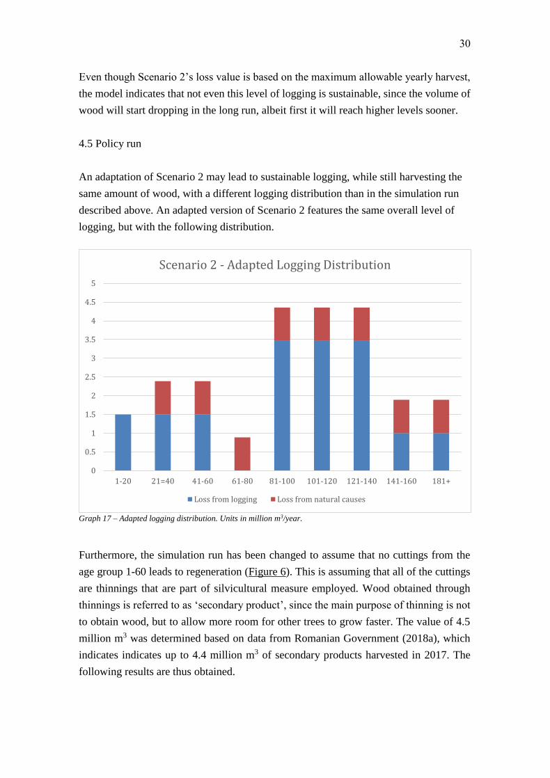
4.5 Policy run

An adaptation of Scenario 2 may lead to sustainable logging, while still harvesting the

same amount of wood, with a different logging distribution than in the simulation run

described above. An adapted version of Scenario 2 features the same overall level of

logging, but with the following distribution.

Graph 17 – Adapted logging distribution. Units in million m3/year.

Furthermore, the simulation run has been changed to assume that no cuttings from the

age group 1-60 leads to regeneration (Figure 6). This is assuming that all of the cuttings

are thinnings that are part of silvicultural measure employed. Wood obtained through

thinnings is referred to as ‘secondary product’, since the main purpose of thinning is not

to obtain wood, but to allow more room for other trees to grow faster. The value of 4.5

million m3 was determined based on data from Romanian Government (2018a), which

indicates indicates up to 4.4 million m3 of secondary products harvested in 2017. The

following results are thus obtained.

0

0.5

1

1.5

2

2.5

3

3.5

4

4.5

5

1-20 21=40 41-60 61-80 81-100 101-120 121-140 141-160 181+

Scenario 2 - Adapted Logging Distribution

Loss from logging Loss from natural causes

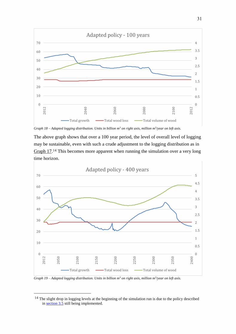
31

Graph 18 – Adapted logging distribution. Units in billion m3 on right axis, million m3/year on left axis.

The above graph shows that over a 100 year period, the level of overall level of logging

may be sustainable, even with such a crude adjustment to the logging distribution as in

Graph 17.14 This becomes more apparent when running the simulation over a very long

time horizon.

Graph 19 – Adapted logging distribution. Units in billion m3 on right axis, million m3/year on left axis.

14 The slight drop in logging levels at the beginning of the simulation run is due to the policy described

in section 3.5 still being implemented.

0

0.5

1

1.5

2

2.5

3

3.5

4

0

10

20

30

40

50

60

702

01

2

20

40

20

60

20

80

21

00

20

12

Adapted policy - 100 years

Total growth Total wood loss Total volume of wood

0

0.5

1

1.5

2

2.5

3

3.5

4

4.5

5

0

10

20

30

40

50

60

70

20

12

20

50

21

00

21

50

22

00

22

50

23

00

23

50

24

00

Adapted policy - 400 years

Total growth Total wood loss Total volume of wood

32

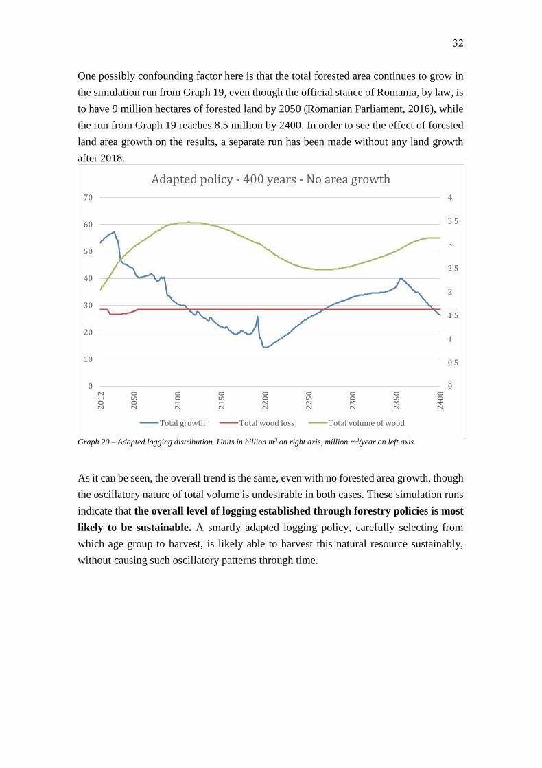
One possibly confounding factor here is that the total forested area continues to grow in

the simulation run from Graph 19, even though the official stance of Romania, by law, is

to have 9 million hectares of forested land by 2050 (Romanian Parliament, 2016), while

the run from Graph 19 reaches 8.5 million by 2400. In order to see the effect of forested

land area growth on the results, a separate run has been made without any land growth

after 2018.

Graph 20 – Adapted logging distribution. Units in billion m3 on right axis, million m3/year on left axis.

As it can be seen, the overall trend is the same, even with no forested area growth, though

the oscillatory nature of total volume is undesirable in both cases. These simulation runs

indicate that the overall level of logging established through forestry policies is most

likely to be sustainable. A smartly adapted logging policy, carefully selecting from

which age group to harvest, is likely able to harvest this natural resource sustainably,

without causing such oscillatory patterns through time.

0

0.5

1

1.5

2

2.5

3

3.5

4

0

10

20

30

40

50

60

70

20

12

20

50

21

00

21

50

22

00

22

50

23

00

23

50

24

00

Adapted policy - 400 years - No area growth

Total growth Total wood loss Total volume of wood

33

5. Discussion

5.1. Limitations

The model used to arrive at the results described in section 4 faces a number of

limitations, and these should be taken into account when considering the results. The

following are the most important limitations identified by the author, though there may

certainly be more:

I. Logging and loss due to natural causes (decay) are not differentiated

Though some estimations have been made in Section 4.4, the model structure does not

differentiate between different types of loss. One reason for this is that precise logging

values are not publicly available, and some guesswork is require, even though, as

previously mentioned, this information is known by INCDS:

The estimation of the total amount of wood harvested from terrains with forest vegetation

is presently based on the yearly statistical reports submitted by forest districts extraction

companies. The measurements performed on the permanent sample surfaces of NFI,

including stumps, will allow for the precise estimation of the quantity of wood harvested

from terrains with forest vegetation. (NFI, 2019)

An even bigger problem caused by this limitation is that the decay rate is static, unlike

the growth rate, which is dynamic and dependent on the age composition of the forests.

The decay rate should also certainly depend at least on the age composition of the forests.

In fact, both the growth and decay rates could further be improved by making them

dependent on forest density as well: higher density slows growth until maximum density

is reached, whereupon growth will equal decay and lead to homeostasis in old-growth

forests – the final successional stage (Grebner, Bettinger and Siry, 2013). While there is

no data on the average decay rate of forests by age group available publicly, the decay

rate could be reconstructed based on research on forest growth dynamics by species in

Romania. To do this, however, the ontology of the forest must be expanded to include

species differentiation as well.

II. Species are not differentiated

While NFI (2012a, 2018) does contain data on species composition, it is impossible to

know the age distribution by species. For example, data on the area and density of beech

forests is available, but the datasets do not specify the age distribution of beech forests

separately, only the total average age distribution of forests. Upon reviewing the

34

measurement methodology of the National Forest Inventory (NFI, 2012b), however, it

becomes apparent that this information too is available to INCDS, or at least could be

calculated based on the disaggregated measurement data.

III. Forest regeneration process not clear

A rough estimate has been made as to how loss of wood affects the age distribution of

forested areas (Section 3.5.). This estimate, however, does not account for the nature of

silvicultural interventions at different age groups (see Section 4.4.). It also does not

account for the differences between the way in which logging and decay processes affect

regeneration processes (though, as mentioned before, logging and decay processes

themselves must first be differentiated).

There are also two assumptions built into the model structure that do not always reflect

reality. Firstly, all forest land begins to regenerate without any delay. While this might

be so in the case of properly executed silvicultural systems, it might not be so in the case

of improperly executed ones, or in the case of illegal logging. Secondly, the model

assumes that all forest land will regenerate, and does not account for the possibility of

soil degradation which would inhibit regeneration. While land use change (and hence,

deforestation), must always be compensated for through an equal or greater amount of

afforestation (Romanian Parliament, 2016), this does no guarantee that all forested areas

that are cleared will regenerate without some sort of additional intervention.

While NFI (2012b) describes the measurement methodology, it does not describe how

the classifications are made based on the measurements. This is important to know when

determining how silvicultural different silvicultural systems actually affect the forest age

classifications of the National Forest Inventory.

IV. The maximum density of forests is not well defined

A rough estimate has been made on the maximum forest density15. The maximum

density, however, should be a result of the growth and decay dynamics of forests.

Improving those aspects of the model structure should help overcome this limitation as

well. Overcoming this limitation is important, as sensitivity analysis included in Annex

D has revealed that model results are sensitive to this parameter, though the overall trend

remains the same.

15 A sensitivity analysis of this parameter has been included in Annex D.

35

V. Private and public land is not differentiated

This limitation is perhaps the least important one at this stage, since ownership does not

affect natural processes. Furthermore, the Forestry Code applies the same stringent rules

upon public and private forest management (Romanian Parliament, 2016). In fact, one of

the complaints from private forest owners is that the Forestry Code is too stringent

(Buliga and Nichiforel, 2019).

VI. All forest areas are open for logging

Some forest areas in Romania are protected to different extents. Logging in such forests

is either restricted or prohibited. In order to more accurately estimate sustainable logging

levels, these forests must be represented separately within the model. The effect of this

limitation on the results of the base run, however, should be limited. Firstly, because of

the many cases of forest disturbances in natural and national parks, and secondly because

of the increased fraction of the implementation of so-called ‘conservation cuttings’.

5.2. Main takeaways

The present research demonstrates, first and foremost, the potential of the use of

simulation models in studying forestry sustainability. System dynamics specifically

allow for the ontology of forests within the model to be adapted to the data available.

Expanding the ontology, however, would allow for more detailed policies to be tested,

rather than the crude ones presented here.

Secondly, the model results indicate that the potential impacts of correctly applying

current forestry policies are significant. It is therefore imperative to correctly assess the

sources of forest loss, and how much each source contributes to the overall loss level. It

can then be determined which courses of action can bring down the overall level of

logging closer to the levels indicated by official policies fastest.

One possible lever is increasing the effectiveness of the Forest Inspectorates. A study by

Popa, Niță and Hălălișan (2019) point out that the effectiveness of new institutions is

affected by the engagement of their employees. Their study indicates that, although the

employees of the recently created Forest Inspectorates have a positive attitude and adopt

positive subjective norms towards performing the required engagement in law

enforcement effort, factors such as unsuitable training, improper planning &

management, unsuitable legislation and even unavailable information limit their

perceived power in performing the required engagement in their work.

36

Another source of excess logging is that officials consistently underestimate both the

quantity and the quality of the wood that is to be sold at auctions (Bouriaud and Marzano,

2014). Romsilva itself states in its management plan for 2016-2020 that one of their main

priorities is the professionalization of their staff, as it has been assessed that many staff

members lack the desired level of training and knowledge. Solving this issue could not

only reduce the level of excess logging, but also prevent economic losses in the long-run.

Another reason for the consistent underestimation, given during an interview for this

research, is that the quantity and quality of wood is measured 13 times in Romania. 16

Once would think that multiple measurements ensure accuracy. What happens instead,

is that responsibility is diluted, and no one is held accountable.

Several authors point out that a necessary policy for sustainable forestry at the national

level is the implementation of financial compensation schemes for owners of protected

areas (Stăncioiu, Abrudan and Dutca, 2010). Though these financial compensation

schemes are part of the Forestry Code (Romanian Parliament, 2016), they have never

been implemented. The implementation of such a policy would lead to a further decrease

of excess logging. Using disaggregated NFI data, one could identify the amount of excess

logging across all protected areas. A cost-benefit analysis can then be made to identify

how to prioritize the implementation of this policy compared to other ones.

Securing funding at the European level for the research of virgin forests, and

guaranteeing their strict protection, would also contribute to a decrease of excess logging.

Such research would prove to be valuable at a global level as well:

The remaining virgin forests of temperate Europe are an inexhaustible source of

ecological information about biodiversity, structure, natural processes and overall

functioning of undisturbed forest ecosystems. Their research will reveal information

which can be used for ecological restoration of man-made forests which are degraded

through intensive forestry practices over the last centuries. - Veen et al. (2010)

The proper conservation of protected areas also faces legislative challenges:

…cuttings in old-growth forests are predominantly in accordance with forest

management plans, legal harvesting activities are obviously responsible for their

diminishment. Protected areas, including recent expansions under the Natura 2000

framework, do not safeguard these forests as originally envisioned. Biodiversity and

16 For comparison’s sake, in Austria it is only measured once.

37

specifically protected area governance continue to face serious challenges with respect

to their ability to safeguard old-growth forests. – Knorn et al. (2013)

Though virgin forest are protected by law, if a local villager were to fell one tree from

that forest for use as firewood, the entire forest is no longer considered to be a virgin

forest by law, and is therefore opened for logging activities.

The third takeaway of this research and its results is the power of data. Had these

aggregated results not been published, the sustainability of Romanian forestry could not

have been quantified even to this extent. Lack of transparency has been a consistent

problem in the Romanian public sector, even until the present day. This research is not

the first one to point out the importance of public access to information.

Lack of information about forest change was also pointed out as worrisome by Knorn et

al. (2012), due to its importance to the conservation of old-growth, primary forests,

biodiversity, and large mammal habitats. Several existing research projects, such as the

one by Munteanu et al. (2016), could be significantly improved with more disaggregated

information. And, as mentioned above, even the Forest Inspectorate suffers from lack of

information.

5.3. Future research

Beyond what has been presented in the ‘Limitations’ section, the present model may

serve as a basis for other future research possibilities as well. One possibility is to include

forestry economics aspects, or ecological function aspects as well. Thus it would be

possible to broaden the research scope beyond the natural resource management

perspective. On the demand side, economic aspects could include firewood demand,

demand for construction material or demand for furniture. On the supply side, economic

aspects could include the way in which species, wood quality, or the diameter of the

felled tree affects the price.

Another possibility is to combine this model with GIS analysis, using Corine Land Cover

data, among others. Combining with GIS analysis would also enable more serious

research into land use change.

Finally, expanding the logging policy section would permit more detailed analysis of the

logging policies that would allow for desirable forest age distribution patterns.

38

6. Conclusions

The question that this thesis addressed using a dynamic simulation model: Are current

levels of logging in Romania sustainable? Though the model indicates that the natural

resources provided by Romania’s forests will not be depleted, the overall yield and

volume of Romania’s forests is set to drop, even under the assumption of continuous

forest area growth. This is the case for both the optimistic and pessimistic assumed levels

of logging.

The model also indicates, however, that current forestry policies, so long as they are

properly implemented, are very likely to be sustainable on the long run, while also

leading to a growing stock of standing wood. This behaviour is the most desirable one,

as it would lead to a fulfilment of economic needs, while also contributing to carbon

sequestration, a higher fulfilment of ecological functions, and biodiversity preservation.

Many parts of the model could be improved with greater access to data concerning the

natural resources of the country. Open access to data on Romania’s forests can lead to

valuable research concerning the effectiveness and sustainability of current and future

natural resource management policies. The use of computer simulation models can aid

in the discovery of inconsistencies in data. Clean and consistent datasets would, in turn,

increase the confidence of public policy-makers in the results of dynamic simulation

models.

Finally, open access to data on natural resources is a question of moral principles. After

all, as Romania’s National Forestry Strategy states: In Romania, this relationship

[between forest and man] is marked by a history filled with moments when "the forest

was a brother to Romanians", as is often described in literature17. (Romanian

Government, 2017b) It is therefore the duty of the Romanian government to not inhibit,

but rather facilitate Romanians to return the favour, and care for the forests.

17 Author’s translation.

39

References

Abrudan, I. V., Marinescu, V., Ionescu, O., Ioras, F., Horodnic, S. A. and Sestras R.

(2009). „Developments in the Romanian forestry and its linkages with other

sectors”. Notulae Botanicae Horti Agrobotanici Cluj-Napoca 37(2):14-21.

Agent Green. (2018a). „Ecologiștii cer Comisiei Europene să intervină pentru salvarea

ariilor protejate din România”. https://www.agentgreen.ro/ecologistii-cer-

comisiei-europene-sa-intervina-pentru-salvarea-ariilor-protejate-din-romania/,

accessed on 08.11.2018.

Agent Green. (2018b). „Scrisoare deschisă adresată președintelui României cu privire

la inventarul forestier național și nivelul exploatărilor forestiere ilegale”.

https://www.agentgreen.ro/scrisoare-deschisa-adresata-presedintelui-romaniei-cu-

privire-la-inventarul-forestier-national-si-nivelul-exploatarilor-forestiere-ilegale/,

accesssed on 28.11.2018.

Axelrod, R. (1997). „Advancing the art of simulation in the social sciences”. In Conte

R., Hegselmann, R. and Terna P. (Eds.) Simulating social phenomena: 21-40.

Barlas, Y. (1996). „Formal aspects of model validity and validation in system

dynamics”. System Dynamics Review 12(3): 183-210.

Biriș, I. and Veen, P. (eds.). (2005) „Inventory and strategy for sustainable management

and protection of virgin forests in Romania. Extended English summary (PIN-

MATRA / 2001 / 018)”. Bucharest: ICAS and KNNV.

Bouriaud, L. (2005). „Causes of Illegal Logging in Central and Eastern Europe”.

Small-Scale Forest Economics. Management and Policy 4(3):269-292.

Bouriaud, L. and Marzano, M. (2014). „Conservation, extraction and corruption: will

sustainable forest management be possible in Romania?”. Pp. 221-240 in Natural

Resource Extraction and Indigenous Livelihoods: Development Challenges in an

Era of Globalization, edited by Gilberthorpe, E. and Hilson, G. New York:

Routledge.

Bryman, A. and Bell, E. (2011). Business research methods (3rd ed.). New York:

Oxford University Press.

Buliga, B. and Nichiforel, L. (2019). „Voluntary forest certification vs. stringent legal

frameworks: Romania as a case study”. Journal of Cleaner Production 207:329-

342.

Carcea, F. and Dissescu R. (2014). „Terminologia Amenajării Pădurilor: Termeni și

definiții în limba română. Echivalențe în germană, engleză, franceză, spaniolă,

italiană, portugheză, maghiară și japoneză”. International Union of Forestry

Research Organizations Secretariat.

Cavana, R. Y. and Ford, A. (2004). „Environmental and resource systems: Editor’s

introduction”. System dynamics review 20: 89-98.

Cernuta, R. (2019). „Inventarul Forestier Național sau despre cum se fură pădurea cu

tabelul Excel”. Declic. http://inventarul-forestier-

declic.strikingly.com/?fbclid=IwAR0KWmgddwQmOSpgJJGq3jaj7vEFdKmEu

GyxmVaUc2Rs29l7OZqcmo2e5bc, accessed on 12.06.2019.

de Gooyert, V. (2018). „Developing dynamic organizational theories; three system

dynamics based research strategies”. Quality & Quantity.

https://doi.org/10.1007/s11135-018-0781-y, accessed on 15.03.2019.

Dragoi, M., Popa, B. and Blujdea, V. (2011). „Improving communication among

stakeholders through ex-post transactional analysis - case study on Romanian

forestry”. Forest Policy and Economics 13(1):16-23.

40

Dudley, R. G. (2004). „A System Dynamics Examination of the Willingness of

Villagers to Engage in Illegal Logging”. Journal of Sustainable Forestry 19:1-3,

31-53.

Dudley, R. G. (2004). „Modeling the effects of a log export ban in Indonesia”. System

Dynamics Review 20(2): 99-116.

Food and Agriculture Organization of the United Nations. (2005). „The Global Forest

Resources Assessment 2005 Country Report Romania”.

http://www.fao.org/tempref/docrep/fao/010/ai940E/ai940E00.pdf, accessed on

07.04.2019.

Food and Agriculture Organization of the United Nations. (2010). „The Global Forest

Resources Assessment 2010 Country Report Romania”.

http://www.fao.org/3/al607E/al607E.pdf, accessed on 07.04.2019.

Food and Agriculture Organization of the United Nations. (2012). „Forest Resources

Assessment Working Paper - FRA 2015 Terms and Definitions”.

http://www.fao.org/3/ap862e/ap862e00.pdf, accessed on 11.04.2019.

Food and Agriculture Organization of the United Nations. (2015). „The Global Forest

Resources Assessment 2015 Country Report Romania”. http://www.fao.org/3/a-

az315e.pdf, accessed on 07.04.2019.

Ford, A. (2010). Modeling the environment (2nd ed.). London: Island Press.

Forrester, J. W. (1968). Principles of systems, Cambridge, MA: Pegasus

Communications.

Forrester, J. W. (1992). „Policies, decisions and information sources for modeling”.

European Journal of Operational Research 59: 42-63.

Grebner, L. D., Bettinger, P. and Siry, J. P. (2013). Introduction to Forestry and

Natural Resources. Waltham, MA: Academic Press.

Greenpeace. (2012a). Tăierile ilegale de arbori în pădurile din România în perioada

2009-2011.

http://www.greenpeace.org/romania/Global/romania/paduri/Despaduririle%20din

%20Romania/Taierile%20ilegale%20de%20arbori%20in%20padurile%20din%2

0Romania%20(2009-2011).pdf, accessed on 01.06.2019.

Greenpeace. (2012b). Evoluția suprafețelor forestiere din România în perioada 2000 –

2011 (Greenpeace Rusia, departamentul GIS).

http://www.greenpeace.org/romania/Global/romania/paduri/Despaduririle%20din

%20Romania/Evolutia%20suprafetelor%20forestiere%20din%20Romania%2020

00-2011.pdf, accessed on 01.06.2019.

Homer, J. B. (2012). „Partial-model testing as a validation tool for system dynamics”.

System Dynamics Review 28: 281-294.

Ioras F. (2002). „Aspects of Romanian forestry: The case for community forest

management in the Piatra Craiului massif”. Forests Trees and Livelihoods 12(4):

297-312.

Ioras F. and Abrudan I. (2006). „The Romanian forestry sector: privatisation facts”.

International Forestry Review 8(3):361-367

Iojă, C. I., Pătroescu, M., Rozylowicz, L., Popescu, V. C., Vergheleț, M., Zotta, M. I.

and Felciuc, M. (2010). „The efficacy of Romania’s protected areas network in

conserving biodiversity”. Biological Conservation 143:2468-2476.

Jones, A., Seville, D. and Meadows, D. (2002). „Resource sustainability in commodity

systems: the sawmill industry in the Northern Forest”. System Dynamics Review

18(2): 171-204.

Knorn, J., Kuemmerle, T., Radeloff, V.C., Keeton, W. S., Gancz, V., Biriș, I., Svoboda,

M., Griffiths, P., Hagatis, A. and Hostert, P. (2013). „Continued loss of old-

41

growth forests in the Romanian Carpathians despite an increasing protected area

network”. Environmental Conservation 40(2):182-193.

Knorn, J., Kuemmerle, T., Radeloff, V. C., Szabo, A., Mindrescu, M., Keeton, W. S.,

Abrudan, I., Griffiths, P., Gancz, V. and Hostert, P. (2012). “Forest restitution and

protected area effectiveness in post-socialist Romania”. Biological Conservation

146:204-212

Leahu, I. (2001). Amenajarea pădurilor. Metode de organizare sistemică, modelare,

fiabilitate, optimizare, conducere și reglare structural-funcțională a

ecosistemelor forestiere. Bucharest: Editura Didactică și Pedagogică

Măntescu, L. and Vasile, M. (2009). „Property reforms in rural Romania and

community-based forests”. Romanian Sociology 7(2):95-113.

Munteanu, C., Nita, M. D., Abrudan, I. V. and Radeloff, V. C. (2016). „Historical

forest management in Romania is imposing strong legacies on contemporary

forests and their management”. Forest Ecology and Management 361:179-193.

National Institute of Statistics. (2019). „Silviculture dataset”.

http://statistici.insse.ro:8077/tempo-online/#/pages/tables/insse-table, accessed on

07.02.2019.

NFI. (2012a). „National Forest Inventory: Forest resources assessment in Romania,

cycle I results”. http://roifn.ro/site/rezultate-ifn-1/, accessed on 07.02.2019.

NFI. (2012b). „Prelucrarea datelor din inventarul forestier național.”

http://roifn.ro/site/wp-content/uploads/2015/04/prelucrarea-datelor-IFN.pdf,

accessed on 07.02.2019.

NFI. (2018). „National Forest Inventory: Forest resources assessment in Romania,

cycle II results”. http://roifn.ro/site/rezultate-ifn-2/, accessed on 07.02.2019.

NFI. (2019). „About IFN”. http://roifn.ro/site/despre-ifn, accessed on 10.06.2019.

Nichiforel, L. and Schanz, H. (2009). „Property rights distribution and entrepreneurial

rent-seeking in Romanian forestry: a perspective of private forest owners”.

European Journal of Forest Research 130:369-381.

Peng, C. (2000). „Understanding the role of forest simulation models in sustainable

forest management”. Environmental Impact Assessment Review, 20: 481-501.

Popa, B., Niță M. D. And Hălălișan, A.F. (2019). „Intentions to engage in forest law

enforcement in Romania: An application of the theory of planned behavior”.

Forest Policy and Economics 100: 33-43

Pretzsch, H. (2010). Forest Dynamics, Growth and Yield: From measurement to model.

Berlin: Springer.

Rahmandad, H. and Sterman, J.D. (2012). „Reporting guidelines for simulation-based

research in social sciences”. System Dynamics Review 28(4): 396-411.

Repenning, N. P. (2003). „Selling system dynamics to (other) social scientists”. System

Dynamics Review 19: 303-327.

Richardson, G. P. and Pugh, Alexander L. III. (1981). Introduction to system dynamics

modeling with dynamo. Waltham: Pegasus Communications.

Romanian Government. (2006). „Raport privind starea pădurilor în România 2005”.

http://www.mmediu.ro/app/webroot/uploads/files/2016-12-

16_Raport_Starea_padurilor_2005.pdf, accessed on 18.02.2019.

Romanian Government. (2007). „Raport privind starea pădurilor în România 2006”.

http://www.mmediu.ro/app/webroot/uploads/files/2016-12-

16_Raport_Starea_padurilor_2006.pdf, accessed on 18.02.2019.

Romanian Government. (2008). „Raport privind starea pădurilor în România 2007”.

http://www.mmediu.ro/app/webroot/uploads/files/2016-12-

16_Raport_Starea_padurilor_2007.pdf, accessed on 18.02.2019.

42

Romanian Government. (2009). „Raport privind starea pădurilor în România 2008”.

http://www.mmediu.ro/app/webroot/uploads/files/2016-12-

16_Raport_Starea_padurilor_2008.pdf, accessed on 18.02.2019.

Romanian Government. (2010). „Raport privind starea pădurilor în România 2009”.

http://www.mmediu.ro/app/webroot/uploads/files/2016-12-

16_Raport_Starea_padurilor_2009.pdf, accessed on 18.02.2019.

Romanian Government. (2011). „Raport privind starea pădurilor în România 2010”.

http://www.mmediu.ro/app/webroot/uploads/files/2016-12-

16_Raport_Starea_padurilor_2010.pdf, accessed on 18.02.2019.

Romanian Government. (2012a). „Analiza funcțională a sectorului mediu și păduri în

România – Vol. 2”. http://sgg.gov.ro/docs/File/UPP/doc/rapoarte-finale-

bm/etapa-

II/MMP_FR_Environment_Water_Forestry_Vol_2_FORESTRY_ROM_FINAL.

pdf, accessed on 14.06.2019.

Romanian Government. (2012b). „Raport privind starea pădurilor în România 2011”.

http://www.mmediu.ro/app/webroot/uploads/files/2016-12-

16_Raport_Starea_padurilor_2011.pdf, accessed on 18.02.2019.

Romanian Government. (2013). „Raport privind starea pădurilor României 2012”.

http://www.mmediu.ro/app/webroot/uploads/files/2016-12-

16_Raport_Starea_padurilor_2012.pdf, accessed on 18.02.2019.

Romanian Government. (2014). „Raport privind starea pădurilor României 2013”.

http://www.mmediu.ro/app/webroot/uploads/files/2016-12-

16_Raport_Starea_padurilor_2013.pdf, accessed on 18.02.2019.

Romanian Government. (2015). „Raport privind starea pădurilor României 2014”.

http://www.mmediu.ro/app/webroot/uploads/files/2016-12-

16_Raport_Starea_padurilor_2014.pdf, accessed on 18.02.2019.

Romanian Government. (2016). „Raport privind starea pădurilor României 2015”.

http://www.mmediu.ro/app/webroot/uploads/files/2016-12-

16_Raport_Starea_padurilor_2015.pdf, accessed on 18.02.2019.

Romanian Government. (2017a). „Raport privind starea pădurilor României 2016”.

http://apepaduri.gov.ro/wp-content/uploads/2014/07/Raport-starea-pădurilor-

2016.pdf, accessed on 18.02.2019.

Romanian Government. (2017b). „Strategia forestieră națională 2018-2027”.

http://www.mmediu.ro/app/webroot/uploads/files/2017-10-

27_Strategia_forestiera_2017.pdf, accessed on 23.01.2019.

Romanian Government. (2018). „Raport privind starea pădurilor României 2017”.

http://apepaduri.gov.ro/wp-content/uploads/2014/07/Starea-pădurilor-în-anul-

2017.pdf, accessed on 18.02.2019.

Romanian Parliament. (2016). „Forestry Code (Law nr. 46/2008) - Republished and

Updated 2016”.

Romsilva. (2016). „Plan de administrare și management pentru perioada august 2016 -

iulie 2020”. http://www.rosilva.ro/files/content/bucuresti/plan de administrare si

management.pdf, accessed on 09.04.2019.

Romsilva. (2017). „Strategia Comercială 2017-2020”.

http://www.rosilva.ro/files/content/bucuresti/Strategia Comerciala 2017-2020.pdf,

accessed on 09.04.2019.

Sabatini, F. M., S. Burrascano, W. S. Keeton, C. Levers, M. Lindner, F. Pötzschner, P.

J. Verkerk, J. Bauhus, E. Buchwald, O. Chaskovsky, N. Debaive, F. Horváth, M.

Garbarino, N. Grigoriadis, F. Lombardi, I. M. Duarte, P. Meyer, R. Midteng, S.

Mikac, M. Mikolas, R. Motta, G. Mozgeris, L. Nunes, M. Panayotov, P. Ódor, A.

43

Ruete, B. Simovski, J. Stillhard, M. Svoboda, J. Szwagrzyk, O.-P. Tikkanen, R.

Volosyanchuk, T. Vrska, T. M. Zlatanov, and T. Kuemmerle. (2018). „Where are

Europe’s last primary forests?”. Diversity and Distributions 24:1426–1439.

Schuck, A., Päivinen, R., Hytönen, T. and Pajari, B. (2002). „Compilation of Forestry

Terms and Definitions”. European Forest Institute Internal Report 6: 1-48

Scriban, R. E., Nichiforel, L., Bouriaud, L. G., Barnoaiea, I., Cosofret, V. C. and

Barbu, C. O. (2019). „Governance of the forest restitution process in Romania:

An application of the DPSIR model”. Forest Policy and Economics 99:55-67.

Shanin, V., Komarov, A. and Bykhovets, S. (2012). „Simulation modelling for

sustainable forest management: a case study”. The 18th Biennial Conference of

International Society for Ecological Modelling. 13:535-549.

Soran, V., Bíró, J., Moldovan, O. and Ardelean, A. (2000). „Conservation of

biodiversity in Romania”. Biodiversity and Conservation 9:1187-1198.

Stăncioiu, P., Abrudan, I. and Dutca I. (2010). „The Natura 2000 ecological network

and forests in Romania: implications on management and administration”.

International Forestry Review 12(1):106-113.

Stăncioiu, P., Niță, M. and Lazăr, G. (2018). „Forestland connectivity in Romania—

Implications for policy and management”. Land Use Policy 76: 487-499.

Sterman, J. D. (1984). „Appropriate summary statistics for evaluating the historical fit

of system dynamics models”. Dynamica 10(2): 51-66.

Sterman, J. D. (1988). “A sceptic’s guide to computer models”. In Grant, L. (Ed.),

Foresight and national decisions: The horseman and the bureaucrat, 133-169.

Lanham: University Press of America.

Sterman, J. D. (2000). Business dynamics: Systems thinking and modeling for a

complex world. Boston: McGraw-Hill.

Strîmbu, B., Hickey, G. and Strîmbu, V. (2005). „Forest conditions and management

under rapid legislation change in Romania”. Forestry Chronicles 81(3):350-358.

Veen, P., Fanta, J., Raev, I., Biriș, I., de Smidt, J. and Maes, B. (2010). „Virgin forests

in Romania and Bulgaria: results of two national inventory projects and their

implications for protection”. Biodiversity and Conservation 19(6):1805-1819.